econometric models of road use, accidents, and road
TRANSCRIPT

TØI report457/1999
Econometric models of road use, accidents, and road investment decisions
Lasse Fridstrøm
Volume II: An econometric model of car ownership, road use, accidents, and their severity (Essay 3)
Copyright @ Institute of Transport Economics, 1999
ISSN 0802-0175 ISBN 82-480-0121-0 Oslo, November 1999

Title: Econometric models of road use, accidents, Tittel: Econometric models of road use, accidents, and and road investment decisions. Volume II road investment decisions. Volume II
Author(s): Lasse Fridstrøm Forfatter(e Lasse Fridstrøm
TØI report 457/1999 TØI rapport 457/1999 Oslo, 1999-11 Oslo: 1999-11 292 pages 292 sider ISBN 82-480-0121-0 ISBN 82-480-0121-0 ISSN 0802-0175 ISSN 0802-0175
Financed by: Finansieringskilde Research Council of Norway (formerly NTNF), Norges Forskningsråd (tidl NTNF), Transportøkonomisk Institute of Transport Economics (TØI) institutt (TØI)
Project: 1523 Road use, accidents, and fuel Prosjekt: 1523 Vegtransport, ulykker og energi consumption
Project manager: Lasse Fridstrøm Prosjektleder: Lasse Fridstrøm Quality manager: Marika Kolbenstvedt Kvalitetsansvarli Marika Kolbenstvedt
Key Emneord: Road accidents; car ownership; car use; regression Bilhold; vegtrafikk; ulykker; regresjonsmodell; elastisiteter analysis; elasticities
Summary: Sammendrag: Using a fairly large cross-section/time-series data Ved hjelp av en økonometrisk modell anslås hvordan de base, covering all provinces of Norway and all månedlige trafikkulykkestallene i norske fylker avhenger av months between January 1973 and December 1994, bl a folkemengde, inntekter, priser, rentenivå, we estimate non-linear (Box-Cox) regression veginvesteringer og -vedlikehold, kollektivtrafikktilbud, equations explaining aggregate car ownership, road dagslys, værforhold, bilbeltebestemmelser, alkohol- use, seat belt use, accident frequency, and accident tilgjengelighet, rapporteringsrutiner, kalenderbegivenheter severity. Explanatory variables used include road og geografiske forhold. Modellen forklarer også bilhold, infrastructure, public transportation level-of-service bilbruk og bilbeltebruk. Faktorer som påvirker disse and fares, population, income, fuel prices, vehicle størrelsene får indirekte også virkning for ulykkestallene. prices, interest level, weather, daylight, seat belt Datamaterialet er månedlige tidsserier for alle norske fylker legislation, access to alcohol, calendar effects, gjennom 22 år (1973-94). Modellen har fått navnet TRULS reporting routines, and geographic characteristics. (TRafikk, ULykker og Skadegrad). The econometric model has received the acronym TRULS.
Language of report: English
The report can be ordered from: Rapporten kan bestilles fra: Institute of Transport Economics, The library Transportøkonomisk institutt, Biblioteket Gaustadalleen 21, NO 0349 Oslo, Norway Gaustadalleen 21, 0349 Oslo Telephone +47 22 57 38 00 - www.toi.no Telefon 22 57 38 00 - www.toi.no
Copyright © Transportøkonomisk institutt, 1999 Denne publikasjonen er vernet i henhold til Åndsverkloven av 1961 Ved gjengivelse av materiale fra publikasjonen, må fullstendig kilde oppgis

An econometric model of car ownership, road use, accidents, and their severity
Contents Preface .............................................................................................................................................................. 1 Acknowledgements ............................................................................................................................................ 3 Chapter 1: Introduction and overview............................................................................................................... 7
1.1. Motivation................................................................................................................ 7 1.2. Scope........................................................................................................................ 7 1.3. Essay outline ............................................................................................................ 8
Chapter 2: General perspective and methodology .......................................................................................... 11 2.1. A widened perspective on road accidents and safety............................................. 11 2.2. TRULS – a model for road use, accidents and their severity ................................ 12
2.2.1. The DRAG family of models ......................................................................... 12 2.2.2. The general structure of TRULS .................................................................... 12
2.3. Choosing the level of aggregation ......................................................................... 15 2.3.1. Errors of aggregation and disaggregation....................................................... 15 2.3.2. Aggregate vs disaggregate demand modeling in transportation..................... 17 2.3.3. The case for moderately aggregate accident models ...................................... 19 2.3.4. An exogenous population of counties and months......................................... 21
2.4. Econometric method .............................................................................................. 24 2.4.1. The issue of functional form........................................................................... 24 2.4.2. The Box-Cox and Box-Tukey transformations .............................................. 24 2.4.3. The BC-GAUHESEQ method of estimation.................................................. 25 2.4.4. Elasticities ...................................................................................................... 25 2.4.5. Dummies and quasi-dummies ........................................................................ 26 2.4.6. A note on alternative methods of estimation .................................................. 28
Chapter 3: The relationship between road use, weather conditions, and fuel sales........................................ 31 3.1. Motivation.............................................................................................................. 31 3.2. Notation ................................................................................................................. 32 3.3. Relating traffic counts to fuel sales........................................................................ 33 3.4. An error theory for traffic counts........................................................................... 38 3.5. Specifying the random disturbance term ............................................................... 40 3.6. Sample ................................................................................................................... 42
3.6.1. Traffic counts ................................................................................................. 42 3.6.2. Fuel sales statistics ......................................................................................... 42 3.6.3. Meteorology ................................................................................................... 44
3.7. Empirical results .................................................................................................... 44 3.7.1. Fuel sales ........................................................................................................ 45 3.7.2. Weather .......................................................................................................... 45 3.7.3. Price variations ............................................................................................... 49 3.7.4. Calendar effects .............................................................................................. 50 3.7.5. Heteroskedasticity .......................................................................................... 52
3.8. Model extrapolation and evaluation....................................................................... 53

Chapter 4: Aggregate car ownership and road use ......................................................................................... 61 4.1. Introduction............................................................................................................ 61 4.2. A partial adjustment model of aggregate, private car ownership...........................62 4.3. Models for overall and heavy vehicle road use......................................................64 4.4. Empirical results ....................................................................................................65
4.4.1. Car ownership partial adjustment ...................................................................65 4.4.2. Effect of car ownership on road use ...............................................................67 4.4.3. Population....................................................................................................... 67 4.4.4. Public transportation supply ...........................................................................68 4.4.5. Income ............................................................................................................ 68 4.4.6. Prices and taxes .............................................................................................. 72 4.4.7. Road infrastructure ......................................................................................... 82 4.4.8. Spatial differences in road supply .................................................................. 86 4.4.9. Weather and seasonality .................................................................................89 4.4.10. Calendar events ............................................................................................ 92 4.4.11. Geographic characteristics............................................................................92 4.4.12. Heteroskedasticity ........................................................................................94 4.4.13. Autocorrelation.............................................................................................96
4.5. Summary and discussion........................................................................................96 Chapter 5: Seat belt use ................................................................................................................................... 99
5.1. Motivation.............................................................................................................. 99 5.2. Seat belt use sample surveys and regulations ......................................................100 5.3. A logit model of seat belt use ..............................................................................100 5.4. Empirical results .................................................................................................. 104 5.5. Imputed seat belt use............................................................................................ 106
Chapter 6: Accidents and their severity......................................................................................................... 109 6.1. Behavioral adaptation ..........................................................................................109
6.1.1. Balder’s death – a mythical example............................................................ 109 6.1.2. The lulling effect – and its generalization ....................................................110 6.1.3. Behavioral adaptation on the road................................................................113 6.1.4. A microeconomic perspective ......................................................................116 6.1.5. Testing for risk compensation ......................................................................125
6.2. Road accidents as an internal and external cost ...................................................127 6.3. Random versus systematic variation in casualty counts ......................................132
6.3.1. The Poisson process ..................................................................................... 135 6.3.2. The generalized Poisson distribution............................................................138
6.4. Testing for spurious correlation in casualty models ............................................140 6.4.1. The overdispersion criterion.........................................................................140 6.4.2. Specialized goodness-of-fit measures for accident models .......................... 141 6.4.3. The casualty subset test ................................................................................ 143
6.5. Accident model specification............................................................................... 146 6.5.1. General ......................................................................................................... 146 6.5.2. Heteroskedasticity ........................................................................................147 6.5.3. Autocorrelation.............................................................................................148
6.6. Severity model specification................................................................................ 148 6.6.1. General ......................................................................................................... 148 6.6.2. Heteroskedasticity ........................................................................................148 6.6.3. Autocorrelation.............................................................................................148

6.7. Empirical results .................................................................................................. 149 6.7.1. Traffic volume and density........................................................................... 150 6.7.2. Motorcycle exposure .................................................................................... 161 6.7.3. Public transportation supply......................................................................... 162 6.7.4. Vehicle stock ................................................................................................ 163 6.7.5. Seat belt and helmet use ............................................................................... 165 6.7.6. Population..................................................................................................... 168 6.7.7. Road infrastructure ....................................................................................... 173 6.7.8. Road maintenance ........................................................................................ 175 6.7.9. Daylight ........................................................................................................ 177 6.7.10. Weather ...................................................................................................... 179 6.7.11. Legislation and reporting routines.............................................................. 183 6.7.12. Access to alcohol........................................................................................ 185 6.7.13. Geographic characteristics.......................................................................... 190 6.7.14. Calendar and trend effects .......................................................................... 191 6.7.15. Autocorrelation........................................................................................... 193 6.7.16. Explanatory power ..................................................................................... 193
Chapter 7: Synthesis...................................................................................................................................... 195 7.1. Calculating compound elasticities in a recursive model structure ....................... 195 7.2. Direct and indirect casualty effects...................................................................... 197
7.2.1. Exposure....................................................................................................... 197 7.2.2. Road infrastructure ....................................................................................... 200 7.2.3. Road maintenance ........................................................................................ 202 7.2.4. Population..................................................................................................... 204 7.2.5. Income .......................................................................................................... 204 7.2.6. Prices and tax rates ....................................................................................... 206 7.2.7. Weather ........................................................................................................ 207 7.2.8. Daylight ........................................................................................................ 210 7.2.9. Seat belts....................................................................................................... 211 7.2.10. Alcohol availability .................................................................................... 213 7.2.11. Calendar effects .......................................................................................... 216 7.2.12. Time trend .................................................................................................. 217
7.3. Suggestions for further research .......................................................................... 219 7.3.1. Methodological improvements ..................................................................... 219 7.3.2. Subject matter issues .................................................................................... 221
Literature....................................................................................................................................................... 225 Appendix A: Estimating Box-Cox accident and severity models with Poisson disturbance variance ........... 237 Appendix B: Supplementary tables................................................................................................................ 245 Appendix C: Variable nomenclature ............................................................................................................. 289


Preface The present volume contains the last part of the author’s dissertation for the dr. polit. degree at the Institute of Economics of the University of Oslo.
In total, the dissertation consists of an introductory overview and three accompanying essays.
The first essay – entitled «The barely revealed preference behind road investment priorities» and co-authored by Rune Elvik – has been published in Public Choice 92: 145-168 (1997).
The second essay – entitled «Measuring the contribution of randomness, exposure, weather, and daylight to the variation in road accident counts» and co-authored by Jan Ifver, Siv Inge-brigtsen, Risto Kulmala and Lars Krogsgård Thomsen – can be found in Accident Analysis and Prevention 27: 1-20 (1995). This paper is based on the report «Explaining the variation in road accident counts», by the same authors, issued by the Nordic Council of Ministers (Nord 1993:35).
Both of these essays are reprinted, together with the introductory overview, in a separate Vol-ume I (TØI report 456/1999).
The third essay – entitled «An econometric model of car ownership, road use, accidents, and their severity» and printed in this Volume II – is by far the largest. Certain parts of this re-search were presented at the 8th World Conference on Transport Research (WCTR) in Ant-werpen in July 1998, at the 9th International Conference «Road Safety in Europe» in Ber-gisch-Gladbach in September 1998, at the conference «The DRAG Approach to Road Safety Modelling» in Paris in November 1998, at the «2nd European Road Research Conference» in Brussels in June 1999, at the 10th International Conference «Traffic Safety on Two Conti-nents» in Malmö in September 1999, in report 402/1998 from the Institute of Transport Eco-nomics (TØI) (in Norwegian), and in a series of articles in the journal Samferdsel (issues 4 through 10, 1998 and 1-2, 1999 – also in Norwegian). Additional documentation is forthcom-ing in the book «Structural Road Accident Models: The International DRAG family», edited by Marc Gaudry and Sylvain Lassarre and published by Elsevier, and in the final report from the COST 329 project («Models for traffic and safety development and interventions») of the European Commission.
Oslo, November 1999 INSTITUTE OF TRANSPORT ECONOMICS
Knut Østmoe Marika Kolbenstvedt Managing Director Head of Department
Copyright @ Institute of Transport Economics, 1999 1

2

Acknowledgements The author is indebted to a large number of people and institutions for their help in complet-ing the present analyses.
First and foremost, thanks are due my colleague Peter Christensen for his help in extracting seemingly endless sets of specified casualty counts from the national register of road acci-dents, and for his fruitful comments and advice at various stages of the research process. Without Peter’s invaluable assistance from an early stage, it is doubtful if this thesis would have ever seen the light.
I was also, in an early phase of the process, greatly helped by Per Christian Svae, who set up and organized the first version of the database for essays 2 and 3, using the dBase IV format.
For our most constructive cooperation during the so-called MBAT project («Metode for Be-skrivelse og Analyse av ulykkesTall»), which forms the basis for essay 2, I am indebted to my Nordic partners Jan Ifver, Risto Kulmala and Lars Krogsgård Thomsen. Thanks are also due to my Norwegian colleagues Siv Ingebrigtsen and Jan Erik Lindjord, who helped perform certain parts of the statistical and numerical calculations for the MBAT project, to Tore Vaaje, who initiated the project, and to the Nordic Council of Ministers, which financed it.
For the analysis underlying essay 1, I was helped by James Odeck and Toril Presttun of the Norwegian Public Roads Administration in obtaining a data set on road investment priorities, by Rune Elvik, Jan Erik Lindjord og Lasse Torgersen in «purging» and preparing the data for analysis, and by Inger Spangen in interpreting and qualifying the results.
This doctoral dissertation would not have been possible without the financial support – which is gratefully acknowledged – of the Royal Norwegian Council for Scientific and Industrial Research (NTNF – now merged into the Research Council of Norway), of the Norwegian Ministry of Transport and Communications, and of my employer – the Institute of Transport Economics (TØI). For the support received through TØI I am indebted to each and every em-ployee, who have accepted to cross-subsidize my research through a large number of years and, on top of that, have offered continual encouragement and advice. Although no one is forgotten, I especially want to thank Torkel Bjørnskau, Rune Elvik, Stein Fosser, Alf Glad, Odd Larsen, Harald Minken, Arne Rideng, and Fridulv Sagberg, for their helpful hints and assistance, Astrid Ødegaard Horrisland and Anne Marie Hvaal for their superb library ser-vices, Svein Johansen and Jack van Domburg for their graphical and printing services, Lars Hansson, Jurg Jacobsen, Tore Lien, Torbjørn Strand Rødvik, and Arne Skogli for their com-puter support services, and Laila Aastorp Andersen, Jannicke Eble, Magel Helness, Trude Rømming, and Unni Wettergreen for their secretarial assistance.
I am generally indebted to my colleagues at the Department of Safety and Environment for our inspiring discussions and exchange of views and for their warm support in my apparently never-ending pursuit of the dr. polit. degree. I am particularly grateful to my Head of Depart-ment Marika Kolbenstvedt, who helped provide the resources and energy needed to give this thesis its final touch.
Certain people outside my Institute have also contributed significantly to the realization of this thesis. Morten Merg of the Road Traffic Information Council («Opplysningsrådet for vegtrafikken») provided machine-readable data on the vehicle stock by county and year. Bjørn Reusch and the Norwegian Petroleum Institute helped provide data on fuel sales by
Copyright @ Institute of Transport Economics, 1999 3

county and month. Finn Harald Amundsen, Kjell Johansen and Lars Bendik Johansen of the Public Roads Administration were most helpful in making available a suitable data set on traffic counts. I am generally grateful to a large number of helpful researchers and employees in the Central Bureau of Statistics (now Statistics Norway), in the Norwegian Social Science and Data Services (NSD), and in the Bank of Norway, who on various occasions have pro-vided the necessary data input and background material for my analyses. I have learnt a lot from the constructive comments and advice offered by Finn Jørgensen of the Bodø Graduate School of Business, and from my cooperation, within the COST 329 action and the OECD Scientific Expert Group RS6 on «Safety Theory, Models, and Research», with Sylvain Las-sarre of the INRETS. I have also benefited greatly from the insights offered, through the AFFORD project for the European Commission, by Erik Verhoef of the Free University of Amsterdam.
Without the software support offered by Francine Dufort and the TRIO team at the Centre de Recherche sur les Transports of the Université de Montréal my analyses would not have been feasible.
Last, but not least, I wish to extend a warm thank you to my advisors Erik Biørn and Marc Gaudry, for their untiring support, encouragement and advice, and for letting me partake of their immense professional competence and patience.
4

- And Eeyore whispered back: «I’m not saying there won’t be an Accident now, mind you. They’re funny things, Accidents. You never have them till you’re having them.»
A. A. Milne (1929): The House at Pooh Corner
Copyright @ Institute of Transport Economics, 1999 5

6

Chapter 1: Introduction and overview
Copyright @ Institute of Transport Economics, 1999 7
Chapter 1: Introduction and overview
1.1. Motivation
Road accidents are a major public health problem.
In the western industrialized societies, few single causes of death – if any – deduct more years from the average citizen’s life than do road accidents.
In addition to the years of life lost, road accidents give rise to immense pain and suffering among human beings and to large economic costs in the form of material damage repairs, medical treatment, and loss of manpower.
Road accidents occur as a result of a potentially very large number of (causal) factors ex-erting their influence at the same location and time.
Accidents are – with few exceptions – unwanted events, frequently even very traumatizing ones. To a large extent, this fact serves to preclude the use of perfectly controlled experi-ments as a means of gaining insights into the causal relationships governing the accident generating process.
There is, however, an abundance of non-experimental data available, in the form of road accident statistics, as well as other social and economic indicators having been observed over a long period of time and for a large number of different geographic units.
The use of econometric models to analyze non-experimental data has been common prac-tice in economics for half a century. There are, however, several reasons why this method would be at least as well suited for accident analysis as it is for economics.
In this essay, therefore, we set out to explain the aggregate number of road accidents and victims by means of recursive econometric model, in which we attempt to include all the most important factors exerting causal influence at the macro level.
As a by-product, we also obtain relationships explaining the variation in certain important intermediate variables, such as car ownership, road use, fuel consumption, and seat belt use.
1.2. Scope
An econometric model of road accidents and victims can, of course, be specified and esti-mated in an infinite number of ways.
This essay is not a comparative methodological study. Our focus is on substantive empiri-cal relationships and on their interpretation. More precisely, the aim is to identify the most important, systematic determinants of road accidents and their severity, assess the functional form of each relationship, and estimate the sign and strength of each partial as-sociation.
Concentrating upon this single, yet quite comprehensive objective, we stick to one, fairly general method of statistical inference, viz the so-called Box-Cox Generalized Autoregres-sive Heteroskedastic Single Equation (BC-GAUHESEQ) technique.

An econometric model of car ownership, road use, accidents, and their severity
8 Copyright @ Institute of Transport Economics, 1999
For the purpose of estimating accident equations, we offer certain developments to this methodology, in which we exploit the assumption that casualty counts are approximately Poisson-distributed. In essence, our procedure is tantamount to applying a variance stabi-lizing transform to the dependent variable, so as to improve on the statistical efficiency as compared to the (misspecified) homoskedastic model.
Alternative methods of estimation include various forms of simultaneous equation meth-ods, or – in the case of casualty counts – (generalized) Poisson regression models esti-mated by (quasi-)maximum likelihood methods. Although quite interesting, a comparison with respect to these alternative methodologies has been beyond the scope of the present study1.
The analysis is based on an aggregate, combined cross-section/time-series data set, consist-ing of monthly observations on the 19 counties (provinces) of Norway. Although the data lend themselves to various forms of panel data modeling, we consistently apply a homoge-neity assumption to the analysis, constraining cross-sectional and temporal effects to be identical. A comparison with respect to less restrictive, panel data methods of estimation has – again – been beyond the scope of the present essay.
1.3. Essay outline
This essay is organized as follows.
In chapter 2, we describe, in somewhat greater detail, the general methodological perspec-tives and history upon which we base our analysis. We discuss the structure of causal macro relations bearing on road use and accidents, and sketch the general structure of the DRAG family of models, to which our TRULS model belongs. We discuss, at some length, the question of choosing an appropriate level of aggregation for the purpose of accident analysis. Finally, the chosen econometric specification, the method of estimation and the software to be used are explained.
A most important explanatory factor to be included in any road accident model is the vol-ume of exposure, i e the amount of entities or units exposed to accident risk. Under con-stant risk, the (expected) number of accidents will – by definition – be proportional to the amount of exposure.
Thus, chapter 3 is concerned with the calculation of total and heavy vehicle traffic volumes by county and month. Based on a subsample of counties and months for which traffic counts are available on certain points of the road network, we are able to impute total and heavy vehicle traffic volumes from observations on fuel sales, weather conditions, fuel hoarding and calendar effects, and the composition of the vehicle stock. These calculated traffic volumes can be extrapolated to the entire cross-section/time-series sample and used in the estimation of road use demand and accident equations.
The estimation of car ownership and road use demand equations is the topic of chapter 4. Aggregate car ownership is modeled as a partial adjustment process, implying that the ag-gregate car stock, when subject to exogenous shocks, adjusts only slowly towards its new long-term equilibrium. Next, short and long term road use demand and Engel curves are
1 For a generalized Poisson regression approach to road casualties, see Fridstrøm et al (1993 or 1995).

Chapter 1: Introduction and overview
Copyright @ Institute of Transport Economics, 1999 9
derived, the long term effects incorporating – by definition – changes affecting car owner-ship equilibrium. Explanatory variables used include road infrastructure, public transporta-tion supply, population, income, fuel prices, vehicle prices, interest level, weather and cli-mate, calendar effects, and geographic characteristics. Separate relations are estimated for overall (total) and heavy vehicle traffic volumes.
Seat belts are probably the single most important safety measure that has been brought to bear on road users in the post-war period. In chapter 5, we present an analysis of seat belt use frequencies, as measured by numerous roadside surveys carried out since 1973. Seat belt use is affected by legislative as well as by financial (penalty) measures. Seat belt use rates imputed from this analysis are used as input into the accident and severity equations.
Chapter 6, on accidents and their severity, is the central chapter of this essay. The first section (6.1) is concerned with the theory of risk compensation (behavioral adaptation) and on whether – and how – it can be tested econometrically. Section 6.2 raises the issue of external versus internal costs of transportation, with particular emphasis on accident costs and on the possible relevance of econometric model results in this respect. In section 6.3, we discuss the distinction between systematic and random variation in casualty counts and on how econometric modeling can provide insights into both. Section 6.4 presents a set of testing criteria, specially designed for accident regression analysis, which provide the ana-lyst with an enhanced opportunity to avoid specification errors due to spurious correlation or omitted variable bias. In section 6.5 and 6.6 and in Appendix A, we present the technical details of the casualty and severity model specifications. Empirical results and interpreta-tion follow in section 6.7, with further details included in Appendix B.
While in chapters 4 and 5 we have described how certain exogenous variables affect vehi-cle ownership, road use and seat belt use, and hence indirectly also the expected number of casualties, in chapter 6 only direct effects on accidents and severity are dealt with. The total impact on casualties is generally a sum of direct and indirect effects. In chapter 7 we attempt to pull all these strings together. By recursive accumulation of the relevant elastic-ities we calculate the total impact of each independent variable on the number of accidents, severe injuries and fatalities. In a final section, we identify a number of areas in which fur-ther research, correcting or extending the analysis presented in this essay, would seem to be fruitful.
In Appendix C we explain the principles of variable naming used throughout the essay.

An econometric model of car ownership, road use, accidents, and their severity
10 Copyright @ Institute of Transport Economics, 1999

Chapter 2: General perspective and methodology
Copyright @ Institute of Transport Economics, 1999 11
Chapter 2: General perspective and methodology
2.1. A widened perspective on road accidents and safety
Road accidents occur as a result of a potentially very large number of (causal) factors ex-erting their influence at the same location and time. It might be fruitful to distinguish be-tween six broad categories of factors influencing accident counts.
First, accident numbers depend on a number of truly autonomous factors, determined out-side the (national) social system, such as the weather, the natural resources, the state of technology, the international price of oil, the population size and structure, etc – in short, factors that can hardly be influenced (except perhaps in the very long term) by any (single) government, no matter how strong the political commitment.
Second, they depend on a number of general socio-economic conditions, some of which are, in practice or in principle, subject to political intervention, although rarely with the primary purpose of promoting road safety, nor – more generally – as an intended part of transportation policy (industrial development, (un)employment, disposable income, con-sumption, taxation, inflation, public education, etc).
At a third level, however, the size and structure of the transportation sector, and the policy directed towards it, obviously have a bearing on accident counts, although usually not in-tended as an element of road safety policy (transport infrastructure, public transportation level-of-service and fares, overall travel demand, modal choice, fuel and vehicle tax rates, size and structure of vehicle pool, driver’s license penetration rates, etc). Most importantly, many of these factors are strongly associated with aggregate exposure, i e with the total volume of activities exposing the members of society to road accident risk.
Fourth, the accident statistics depend, of course, on the system of data collection. Accident underreporting is the rule rather than the exception. Changes in the reporting routines are liable to produce fictitious changes in the accident counts.
Fifth, accidents counts, much like the throws of a die, are strongly influenced by sheer ran-domness, producing literally unexplainable variation. This source of variation is particu-larly prominent in small accident counts. For larger accident counts, the law of large num-bers prevails, producing an astonishing degree of long-run stability, again in striking anal-ogy with the dice game.
Finally, accident counts are susceptible to influence – and, indeed, influenced – by acci-dent countermeasures, i e measures intended to reduce the risk of being involved or in-jured in a road accident, as reckoned per unit of exposure.
Although generally at the center of attention among policy-makers and practitioners in the field of accident prevention, this last source of influence is far from being the only one, and may not even be the most important. To effectively combat road casualties at the so-cietal level, it appears necessary to broaden the perspective on accident prevention, so as to – at the very least – incorporate exposure as an important intermediate variable for policy analysis and intervention.

An econometric model of car ownership, road use, accidents, and their severity
12 Copyright @ Institute of Transport Economics, 1999
2.2. TRULS – a model for road use, accidents and their severity
To understand the process generating accidents on Norwegian roads in such a widened perspective, we have set out to construct the model TRULS.
2.2.1. The DRAG family of models
The TRULS model is a member of a larger family of models, all inspired by the DRAG model for Quebec, and explaining the Demand for Road use, Accidents and their Gravity, whence the acronym DRAG:
• DRAG (Demand Routière, les Accidents et leur Gravité), authored by Gaudry (1984) and further developed by Gaudry et al (1995), covering the state of Quebec.
• SNUS (Straßenverkehrs-Nachfrage, Unfälle und ihre Schwere), authored by Gaudry and Blum (1993), covering Germany.
• DRAG-Stockholm, authored by Tegnér and Loncar-Lucassi (1996), covering the Stockholm county of Sweden.
• TAG (Transports, Accidents, Gravité), authored by Jaeger and Lassarre (1997), cover-ing France
• TRAVAL (TRAffic Volume and Accident Losses), authored by McCarthy (1999), cov-ering California.
• TRULS (TRafikk, ULykker og Skadegrad2), the present author, covering Norway.
An account of all of these models is forthcoming in Gaudry and Lassarre (1999).
The common feature of all members of the DRAG family is an at least three-layer recur-sive structure of explanation, including road use, accident frequency, and severity as sepa-rate equations.
Road use (traffic volume) is not considered an exogeneous factors, but explained by a number of socio-economic, physical and political variables (as suggested by the enumera-tion in section 2.1 above). Accident frequency is modeled depending on road use, the pre-sumably single most important causal factor. Accident severity is modeled as the number of severe injuries or fatalities per accident, i e as the conditional probability of sustaining severe injury given that an accident takes place. The decomposition of the absolute number of fatalities or severe injuries into these two multiplicative parts allows for interesting sub-stantive interpretations, as we shall see later on (chapter 6).
2.2.2. The general structure of TRULS
Some DRAG-type models include additional layers of explanation or prediction. The TRULS model, e g, includes (i) car ownership (chapter 4), (ii) seat belt use (chapter 5), and (iii) a decomposition between light and heavy vehicle road use (chapters 3 and 4), add-ing to the set of econometric equations.
2 «Traffic, Accidents, and Severity», when translated into English.

Chapter 2: General perspective and methodology
Copyright @ Institute of Transport Economics, 1999 13
Also, while most DRAG-type models use the fuel sales as a (rather imperfect) measure of the traffic volume, in TRULS we have constructed (iv) a submodel designed to «purge» the fuel sales figures of most nuisance factors affecting the number of vehicle kilometers driven per unit of fuel sold (chapter 3). These nuisance factors include vehicle fuel econ-omy, aggregate area-wide vehicle mix, weather conditions, and fuel hoarding due to cer-tain calendar events or price fluctuations.
A further point at which the TRULS model differs from other members of the DRAG fam-ily, is by the estimation of (v) separate equations for various subsets of casualties (car occupants, seat belt non-users, pedestrians, heavy vehicle crashes, etc). These equations are meant to shed further light on the causal mechanism governing accidents and severity. In order to avoid, to the largest possible degree, spurious correlation and omitted variable biases, we develop certain casualty subset tests not previously used within the DRAG modeling framework (chapter 6).
Unlike other DRAG family models, the TRULS model starts from an assumption that casualty counts in general follow a (generalized) Poisson distribution. To enhance effi-ciency, in the accident equations we therefore rely on (vi) a disturbance variance specifi-cation approximately consistent with the Poisson law. To this end, we develop a special statistical procedure, termed Iterative Reweighted POisson-SKedastic Maximum Likeli-hood (IRPOSKML), for use within the standard DRAG-type modeling software (Appendix A).
Finally, the TRULS model is the only DRAG-type model so far being based on (vii) pooled cross-section/time-series data. Other models in the DRAG family rely exclusively on time-series. Our data, however, are monthly observations pertaining to all counties (provinces) of Norway.
The structure and interdependencies between endogenous variables in the TRULS model are shown in figure 2.1.
While figure 2.1 contains dependent variables only, in table 2.1 we provide an overview of (broad categories of) independent variables entering the model.
Note that only direct effects are ticked off in this table. In general, the total effect of an independent variable on – say – accident frequency, will be a mixture of direct and indirect effects, as channeled though the recursive system pictured in figure 2.1. For instance, the interest level has a direct effect on car ownership only. However, since car ownership af-fects road use, which in turn affects accidents, interest rates may turn out as an important indirect determinant of road casualties. The tracing of such effects is the very purpose of our recursive, multi-layer modeling approach.
The TRULS model relies on an aggregate, direct demand specification focusing on road use. It does not explain or predict the demand for other modes of transportation. The at-tributes of these modes are, however, to some extent used as explanatory variables, thus capturing certain cross-demand effects between modes.

An econometric model of car ownership, road use, accidents, and their severity
14 Copyright @ Institute of Transport Economics, 1999
Car ownership
Road use - light vehicles - heavy vehicles
Seat belt use - urban areas - rural areas
Victims - fatalities - dangerously injured - severely injured - slightly injured
- car occupants - pedestrians - bicyclists - motorcyclists
Accidents - injury accidents - fatal accidents
Severity - killed per injury accident - severely injured per accident etc
Figure 2.1: Dependent variables in the model TRULS

Chapter 2: General perspective and methodology
Copyright @ Institute of Transport Economics, 1999 15
Table 2.1: Independent variables in the model TRULS
Direct effect upon (dependent variable) Independent variable Car
owner-ship
Ve-hicle kms
Seat belt use
Acci-dents
Vic-tims
Seve-rity
Exposure √ √ √ Infrastructure √ √ √ √ √ Road maintenance √ √ √ Public transportation √ √ √ √ √ Population √ √ √ √ √ Income √ √ Prices √ √ Interest rates √ Taxes √ √ Vehicle characteristics √ √ √ √ √ Daylight √ √ √ √ Weather conditions √ √ √ √ Calendar effects √ √ √ √ Geographic characteristics √ √ √ √ √ √ Legislation √ √ √ √ Fines and penalties √ Access to alcohol √ √ √ Information √ √ Reporting routines √ √ √ Randomness and measure-ment errors
√ √ √ √ √ √
2.3. Choosing the level of aggregation
2.3.1. Errors of aggregation and disaggregation3
Errors of aggregation are a well-known source of bias in behavioral empirical science in general and in econometric analysis in particular.
Robinson (1950) demonstrated that bivariate measures of correlation can vary widely at different levels of aggregation and thus that it is incorrect to make inferences from results on aggregate data to the individual level. This mistake has become known as the «ecologi-cal» or «aggregative» fallacy.
3 This section takes many arguments and formulations from the book by Hannan (1991).

An econometric model of car ownership, road use, accidents, and their severity
16 Copyright @ Institute of Transport Economics, 1999
Perhaps the most well known case in point is Durkheim’s (1951) classical study of suicide rates, which were found to be higher in predominantly protestant districts than in the catholic areas. One cannot conclude that Protestantism causes suicide, since, for what we know, most of the suicides in the protestant districts may have been committed by the few Catholics living there. Only disaggregate data, linking each individual suicide to that per-son’s religion, could help resolve this question.
Theil (1954)4 extended the analysis of aggregation error to the multivariate case, and showed how a regression run on a macro relation defined for an aggregate of decision makers with unequal behavioral parameters will usually provide biased estimates of the corresponding, average individual parameters within the population.
Few authors have addressed the issue of a possible opposite error, that of excessive disag-gregation. Riley (1963:706) suggested, however, that there is an «atomistic» fallacy analo-gous to the aggregative fallacy:
«... if the hypothesis [of interest] refers to a group, an analysis based on individuals can often lead to an atomistic fallacy by obscuring the social processes of interest. This type of fallacy may be avoided by analysis based on groups.»
In an article with the suggestive title «Is aggregation necessarily bad?», Grunfeld and Griliches (1960) raised the issue of a possible disaggregate specification error counterbal-ancing the aggregation bias. They argue that economists generally do not know enough about individual economic behavior to perfectly specify micro relations. Hence, in most disaggregate models there would be a specification error that is more likely to be «evened out» in more aggregate relations. In their own words (Grunfeld and Griliches 1960:1):
«Aggregation of economic variables can, and in fact, frequently does, reduce these specifica-tion errors. Hence aggregation does not only produce an aggregation error, but it may also produce an aggregation gain.»
Grunfeld and Griliches (1960) identified the following conditions under which aggregation seems to improve inferences: (i) heterogeneity of slopes among micro units, (ii) correlation of disturbances across micro units, and (iii) misspecification due to an omitted macro vari-able.
Later studies (Hannan and Burstein 1974) indicate that misspecification of the micro rela-tion alone is not a sufficient condition for aggregation to yield a net gain.
Aigner and Goldfeld (1974) examine the case in which the aggregate relation can be speci-fied with less error-in-variables than the corresponding disaggregate relations. They find that, depending on the heterogeneity of micro coefficients, aggregation may or may not involve a gain in efficiency.
Stoker (1993) reviews the issue of aggregate versus disaggregate econometric specifica-tions, pointing out that the «representative agent» approach, in which a «typical» micro relation is assumed to hold verbatim even at the aggregate level, is generally inadmissible on account of the heterogeneity of individual agents. Aggregate modeling is, however, not generally discouraged, as long as the models are specified in ways consistent with the ag-gregate nature of the data and with the heterogeneity of the underlying micro relations.
4 Alternatively, see Theil (1971:556-562) or Hannan (1991:75-89).

Chapter 2: General perspective and methodology
Copyright @ Institute of Transport Economics, 1999 17
2.3.2. Aggregate vs disaggregate demand modeling in transportation
One might easily draw the conclusion that disaggregate analysis is necessarily the best way to uncover causal relations. This is, however, in our view not so. In many cases the study of existing disaggregate units may not have sufficient scope. We believe this is true of be-havioral science and of transportation demand analysis in general, and of accident analysis in particular.
Modern transportation research is strongly influenced by the paradigm of discrete choice, disaggregate modeling of consumer behavior, as the proper way of understanding transpor-tation demand. Based on a sample of individual travelers or households, route, mode and/or destination choice probabilities are commonly estimated, depending on income, prices, and the level-of-service offered by the available alternatives. By means of the so-called sample enumeration technique, aggregate consumer response parameters, such as direct and cross demand price elasticities, can be calculated for the population in question, with a minimum of aggregation error (Ben-Akiva and Lerman 1985).
But his technique will yield unbiased estimates of the aggregate effects only if (i) individ-ual units behave independently of each other, and – more importantly – (ii) if the popula-tion from which units are sampled is exogenous, i e unaffected by the phenomenon under study. We shall refer to these two assumptions as the problems of aggregate feedback (i) and endogenous populations (ii). In the case of transportation and accident analysis, these assumptions may often fail to be true, for the following reasons.
Aggregate feedback Transportation demand choices are often affected by the degree of access to a scarce public good, such as road space, or by the level-of-service characterizing supply, such as the fre-quency and comfort offered by a bus or subway service. As experienced by the single indi-vidual, both quality aspects will usually depend on the behavior of all other consumers. When many travelers react to the same incentive, such as an improved road or bus service, the attractiveness of the new supply will be modified. A new road may relieve congestion at certain points of the network, while possibly creating new bottlenecks elsewhere. As travelers adapt to the modified supply by choosing a different route, mode or destination, it is conceivable that congestion increases or diminishes even for consumers that would be entirely unaffected by the initial improvement, had it not been for the change in other trav-elers’ behavior. This is particularly true of public mass transportation services, where there are important economies of scale present, tending to generate certain favorable or vicious circles. An increased demand, generating increased revenue, may allow or induce the op-erator to further improve the frequency, network or general level-of-service, which in turn generates new demand, and so on. These aggregate feedback effects, which operate over some time, are rarely captured by traditional disaggregate models, which tend to be based on cross-sectional samples taken at a single point in time.
When disaggregate travel demand models are made to comprise all steps in the chain of transportation choices (route choice, mode choice, destination choice, and trip generation, to follow the traditional four-step taxonomy), and integrated into an appropriate network flow analysis, the above weaknesses of simple disaggregate mode choice models may be greatly reduced, perhaps almost eliminated. A much more fundamental source of error is therefore the possible endogeneity of disaggregate populations.

An econometric model of car ownership, road use, accidents, and their severity
18 Copyright @ Institute of Transport Economics, 1999
Endogenous populations When the population of disaggregate units is not invariant under changes in one or more independent variables, one might say that the population itself is endogenous. In the oppo-site case, the population is exogenous.
Note that population exogeneity is a much more fundamental requirement than the usual condition of exogenous samples (which – by the way – in important cases can be dispensed with, on account of the so-called «choice-based sample theorem», see Manski and Lerman 1977 or Ben-Akiva and Lerman 1985). Not only do we require that the probability of being selected from the population into the sample is unaffected by the variables of interest – the set of elements making up the population itself should also be invariant.
To see how a disaggregate population can be endogenous, consider the example of a new road or railway link, which drastically reduces the time and cost of travel between the city center and a certain, fairly distant suburban area. It is unlikely that the (long term) effect of this new link can be predicted from a sample of respondents drawn from the resident popu-lations in the two areas prior to the development, for the simple reason that the population in the suburb will change, and perhaps grow.
Human populations are affected by migration, which is not necessarily unrelated to trans-portation infrastructure or level-of-service. They are also affected by births and by deaths, some of which may occur on the road, although here the contribution of transportation is unlikely to be more than marginal.
As applied to travel demand modeling, it is fair to say that the endogeneity of resident populations is rarely a pressing problem, except perhaps in the context of long term fore-casting. In most cases the population will be stable enough for all practical purposes, at least in the short and medium term.
If, however, we define the population of interest as consisting only of trips or of travelers in a given, initial situation, the problem may be more serious. Implicitly, one has then de-fined away the possibility that there may be more trips or more travelers as a result of the development considered5. As pointed out by Oum et al (1992:143,154),
«… mode-choice studies produce elasticities between modes but they differ from the [regular Marshallian] demand elasticities discussed earlier in that they do not take into account the ef-fect of a price change on the aggregate volume of traffic. [...] it is necessary to aggregate across individuals in order to derive the regular demand elasticity estimates from discrete choice models. This will, however, widen the confidence intervals of the resulting elasticity estimates since, in addition to the standard errors associated with the parameter estimates, there is also an error of aggregation. More importantly, the statistical distribution of the de-mand elasticity estimates will be difficult, if not impossible to determine, since there are two sources of errors.»
By contrast, aggregate direct demand models provide, when properly specified, elasticity estimates incorporating all mode-choice and aggregate demand generation effects, with sampling distributions derivable from the disturbance variance assumptions made or from asymptotic theory, wherever applicable. Cross demand price effects from competing
5 Alternatively, this may be viewed as another case of neglected aggregate feedback, as applied to the popu-lation of residents.

Chapter 2: General perspective and methodology
Copyright @ Institute of Transport Economics, 1999 19
modes may be estimated provided these prices have been included in the regression model. The same applies to cross demand level-of-service effects.
More intriguing examples of population endogeneity are found when we move into freight transportation analysis. Here, it is not at all obvious what would be the appropriate disag-gregate unit of analysis, as all are, to some extent, elements of endogenous populations. Most obviously, this applies – even in the very short term – to shipments, ton kilometers, and trucking trips. Less obviously, it also applies – in the medium and long term – to freight vehicles, shipper companies, receiving companies, and carrier companies. None of these populations are likely to be unaffected by developments in the transportation sector. A carrier company may go bankrupt, or merge with a competitor, in which case it ceases to exist as an element of the population. A change in relative prices, tax rates or costs may sometimes be sufficient to spark such events.
Perhaps the most obvious examples of population endogeneity apply to accidents. It would not make much sense to analyze a disaggregate population of accidents or victims, for the obvious reason that membership in this population constitutes the very point of interest.
2.3.3. The case for moderately aggregate accident models
The pitfalls of excessive disaggregation are thus particularly manifest in the case of acci-dent analysis.
First, in many cases there is interaction between the different micro units, in such a way that a change occurring to unit i would affect the behavior (or risk) pertaining to unit j. In accident analysis, such cases seem almost ubiquitous. Measures taken at the local or indi-vidual level can easily have the effect of moving risk or exposure to another (disaggregate) unit of observation, such as when a given road is closed to through traffic (other roads will receive more traffic), a car owner replaces a small car by a larger (the larger car may be more dangerous to other road users), or the minimum driving age is increased so as to avoid accidents among inexperienced teen-agers (20-year-olds will end up less experi-enced). This is not to say that such measures are necessarily ineffective. But – owing to cross-individual feedback mechanisms – their net effect can hardly be judged on the basis of disaggregate data.
Among the more striking examples of this is the so-called accident migration phenomenon (Boyle and Wright 1984). In some cases the treatment of accident blackspots may generate more accidents elsewhere in the road network. Boyle and Wright offer the explanation that, with the removal of the blackspot, drivers get subjected to fewer «near-misses», and con-sequently become less aware of the need for attention. In many cases, an equally plausible mechanism could simply be that the speed goes up, not only at the site receiving remedial treatment, but in adjacent parts of the road system as well. Drivers get used to higher qual-ity roads and higher speed. Thus, a before-and-after study of those sites which have been treated would be too limited in scope.
This is so, even if one were able to control for the regression-to-the-mean effect (Hauer, 1980), the third – and perhaps most notorious – source of error in disaggregate accident analysis. Micro units (individuals, vehicles, intersections, road links) are typically selected for treatment or analysis because they exhibit higher than average accident rates by some standard. But since accidents happen at random, there will be variation in the observed accident rates even if the underlying risk and exposure are constant throughout the popula-

An econometric model of car ownership, road use, accidents, and their severity
20 Copyright @ Institute of Transport Economics, 1999
tion. There will be accident clusters due to sheer coincidence. These clusters are unlikely to repeat themselves in the next period of observation. However if such clusters are «treated», the decrease in accidents normally observable in the following period is easily misinterpreted as a treatment effect.
In essence, this error is simply a failure to recognize the fact that accident blackspots con-stitute an endogenous selection. The collection of accident involved micro units may be viewed as an example of data sets with selectivity bias, a topic on which there exists a sub-stantial econometric literature (see Heckman 1977, 1987 and references therein).
In comparison, analyses based on aggregate data sets have the advantage of encompassing – at least potentially – all net system-wide effects. This is true provided the process of de-fining the set of observations bears no relation to the phenomenon under study (i e, the population and sample are exogenous), and provided the units of observation are large enough to absorb (temporal or spatial) accident migration effects. When the units of obser-vation are defined by the calendar and/or a set of predetermined administrative or political boundaries, as is typically the case in aggregate time-series/cross-section data sets, the risk of sample selectivity bias in minimized.
A fourth argument in favor of aggregate analysis exists when the relation studied is in ef-fect of a collective nature. Suppose, returning to the suicide example, that Catholics take their own lives partly because, as a minority, they are persecuted or harassed by the Protes-tants. Would it not be correct to say that Protestantism causes suicide, although the sui-cides actually occur to Catholics?6
As a possible example taken from the field of road safety, one might consider the relation-ship between aggregate alcohol consumption and accidents. It has been shown (Skog 1985) that drinking habits have a strong collective component, so that the population tends to move together up and down the scale of consumption. The incidence of drinking and driv-ing is likely to be strongly correlated with the incidence of drinking. Every alcohol con-sumer – driving or not – contributes to the formation of drinking habits and to their social acceptability or attractiveness. Any increase in aggregate alcohol consumption is therefore of relevance to the issue of drinking and driving. One might ask whether or not this collec-tivity of drinking cultures would speak in favor of an aggregate rather than disaggregate approach to the study of alcohol and traffic safety.
Fortunately, aggregate and disaggregate statistical models are not mutually exclusive (apart from resource constraints). On the contrary – the amount of detailed data contained in the accident reporting forms in use in various countries might provide interesting oppor-tunities to check the validity of aggregate models using not-so-aggregate data.
Suppose, e g, that an aggregate, multivariate time series analysis reveals – not implausibly – a favorable safety effect of seat belts, i e negative partial correlation between road traffic injuries (or deaths) and seat belt use. Suppose, further, that we are able to classify car driv-ers injured in an accident according to their wearing a seat belt or not. The number of in-jured seat belt users should go up as seat belt use increases, while the opposite should be true of non-users. To the extent that these two (partial) relationships cannot be confirmed empirically one must suspect the effect found in the aggregate model to be influenced by spurious correlation. We shall elaborate on this in section 6.4.3 below. 6 The reader, whatever his or her religious affiliation, is advised to take no offense at this purely hypothetical, methodological argument.

Chapter 2: General perspective and methodology
Copyright @ Institute of Transport Economics, 1999 21
A final and – in practice – quite compelling argument in favor of aggregate accident mod-els, is the fact that accidents are (fortunately) rare. To study accident risk by means of dis-aggregate data, a very large sample would usually be necessary, in order for any systematic relationships not to be completely blurred by the comparatively large amount of random variation present (see section 6.3 below).
While the process of aggregation may serve to reduce the relative magnitude of the random variation in casualty counts, measurement errors may increase as individual characteristics are replaced by corresponding group averages. Moreover, less aggregate units usually im-ply that more units of observations can be constructed from the same primary data set.
On the other hand, splitting a given population into very disaggregate units obviously af-fects the feasibility and cost of measurement and observation. It could quickly explode the sample into an almost intractably large data set.
Similar arguments apply to (dis)aggregation over time. To maximize measurement accu-racy, one might want to work with minimal units of time, assessing accidents, casualties, exposure, and risk factors by the day or by the hour, if possible. Even here, however, there is a possible atomistic fallacy present, in that trips may be postponed or advanced – i e, moved between units of time – in response to certain independent variables of interest (such as weather conditions, congestion, etc).
It is therefore an open (and interesting) question what is the «optimal» level of (dis)aggregation for an econometric accident model. One needs to strike a balance between various concerns, including (i) the accuracy and (ii) cost of measurement, (iii) the random noise affecting casualty counts, and (iv) the atomistic and (v) aggregative fallacies of in-ference.
2.3.4. An exogenous population of counties and months
In this study, we have chosen to base the analysis on a sample of moderately large spatial and temporal units, viz the 19 counties (provinces) of Norway, as observed monthly.
Our period of observation extends from January 1973 through December 1994, covering 264 months. There are thus 5 016 (= 264 × 19) units of observation in total, 228 for each calendar year.
A map showing the area covered by each county is given in figure 2.2. Certain key statis-tics are gathered in table 2.2.
The capital county of Oslo is by far the most densely populated. It has the smallest surface and the smallest supply of road kilometers per inhabitant, but the highest population and the highest road network density in relation to its area. The opposite is true, on all points, of the northernmost county of Finnmark.

An econometric model of car ownership, road use, accidents, and their severity
22 Copyright @ Institute of Transport Economics, 1999
Figure 2.2: Administrative map of Norway

Chapter 2: General perspective and methodology
Copyright @ Institute of Transport Economics, 1999 23
Table 2.2: Population, area, car ownership, and public road density in Norwegian coun-ties as of January 1, 1998. County Population Area
(sq kms)Inhabitants per sq km
Passenger cars per
1000 popu-lation
Public road kms per
1000 popu-lation
Public road kms per
100 sq kms
All counties 4 417 599 306 253 14 398 21 30
1. Østfold 243 585 3 889 63 413 15 93
2. Akershus 453 490 4 587 99 444 10 95
3. Oslo 499 693 427 1 170 361 3 304
4. Hedmark 186 118 26 120 7 459 36 25
5. Oppland 182 162 23 827 8 445 31 24
6. Buskerud 232 967 13 856 17 433 17 29
7. Vestfold 208 687 2 140 98 417 12 117
8. Telemark 163 857 14 186 12 422 25 28
9. Aust-Agder 101 152 8 485 12 401 28 33
10. Vest-Agder 152 553 6 817 22 386 25 56
11. Rogaland 364 341 8 553 43 393 15 62
12. Hordaland 428 823 14 962 29 348 15 43
14. Sogn og Fjordane 107 790 17 864 6 380 48 29
15. Møre og Romsdal 241 972 14 596 17 395 27 44
16. Sør-Trøndelag 259 177 17 839 15 394 21 30
17. Nord-Trøndelag 126 785 20 777 6 414 43 26
18. Nordland 239 280 36 302 7 366 37 24
19. Troms 150 288 25 147 6 373 35 21
20. Finnmark 74 879 45 879 2 332 53 9
Source: Statistics Norway (1998)
The counties are, of course, also entirely exogeneous in relation to the phenomena to be studied. With the possible exception of Oslo, they are most probably also large enough (area-wise) to absorb all important accident migration effects and other net system-wide impacts. Yet they are small enough to allow for fairly accurate, representative measure-ments of variables with pronounced spatial variation, such as weather conditions.
There is, however, a potential measurement problem attached to the fact that vehicles or individuals registered to a given county may well perform activity – such as road use, fuel purchases, or work – in other counties. For the most part, we shall assume that these effects tend to cancel each other out between the counties. But in the case of Oslo, a rather sys-tematic error of this kind might be foreseen, although of unknown size and sign. To neu-tralize this error, we shall include a dummy variable for the county of Oslo in all regres-sion equations.

An econometric model of car ownership, road use, accidents, and their severity
24 Copyright @ Institute of Transport Economics, 1999
2.4. Econometric method
2.4.1. The issue of functional form
Gaudry and Wills (1978) have demonstrated how allowing for flexible functional forms in transportation demand relations may significantly alter the subject-matter empirical con-clusions to be drawn, compared to fixed-form model specifications.
Such specifications appear particularly attractive when the analyst has no strong a priori theoretical reason to prefer one functional from to the other. In aggregate demand analysis, this is frequently the case. In accident analysis, it is the rule rather than the exception.
2.4.2. The Box-Cox and Box-Tukey transformations
The Box-Cox transformation (Box and Cox 1964) offers a framework for testing whether, e g, price and income elasticities diminish or increase as the price or income level grows. More generally, one will be able to determine the optimal (best-fit maximum likelihood) form of the relation, as a function of the empirical evidence available.
The Box-Cox transformation is defined by
(2.1) ( ) ( )
( )⎪⎩
⎪⎨⎧
=
>≠−
=.xln
xxx
0if
00 if1
λ
λλ
λ
λ
The parameter λ is generally referred to as the Box-Cox parameter. Different values of this parameter correspond to different curvatures or functional forms for the ( )x λ transforma-tion. For instance, λ = 1 yields a linear relation, λ = 0.5 a square root law, λ = 2 a quad-ratic function, and λ = 3 a cubic function, while λ = 0 and λ = −1 correspond to the loga-rithmic and reciprocal (hyperbolic) functional forms, respectively.
A most remarkable property of the Box-Cox transformation is the fact that it is continuous and differentiable even at λ = 0. It is, however, undefined for non-positive x.
A generalization of the Box-Cox transformation is the Box-Tukey transformation (Tukey 1957):
(2.2) ( )( )( ) ( )
( )⎪⎩
⎪⎨⎧
=+
>+≠−+
=+.axln
axaxax
0if
00 if1
λ
λλ
λ
λ
This function is defined for all ax −> . When there is a need to define a Box-Cox trans-formation on a variable which may take on zero values, the problem may be circumvented by adding a small positive constant a, i e by using the Box-Tukey transformation instead. We shall refer to a as the Box-Tukey constant.

Chapter 2: General perspective and methodology
Copyright @ Institute of Transport Economics, 1999 25
2.4.3. The BC-GAUHESEQ method of estimation
The generalized Box-Cox regression model is defined (for time period t and region r in a pooled cross-section/time-series data set) by
(2.3) y x utr i trii
trxi( ) ( )μ λβ= +∑ ,
where, in principle, each independent variable xtri has its own Box-Cox parameter λ xi and an ordinary regression coefficient β i . Even the dependent variable may, within this framework, be Box-Cox transformed (parameter μ ). All variables xtri and try are, by as-sumption, observable.
In the BC-GAUHESEQ algorithm of the TRIO computer package (Liem et al 1993, Gau-dry et al 1993), this methodology is generalized further, by allowing very general het-eroskedasticity and autocorrelation structures to be specified for the random disturbance term utr , viz
(2.4) u z utr i trii
trzi=
⎛⎝⎜
⎞⎠⎟
⎡
⎣⎢
⎤
⎦⎥ ′∑exp ( )ζ λ
12
(2.5) tr
J
jr,jtjtr uuu ′′+′=′ ∑
=−
1ρ .
Here, the ztrj are variables determining the disturbance variance («heteroskedasticity fac-tors»), the ′utr are homoskedastic, although possibly autocorrelated error terms, and the ′′utr terms represent white noise (independent and normally distributed disturbance terms with equal variances). λ zi , ζ i and ρ j are coefficients to be fixed or estimated.
To fix ideas, consider the special case λ ζzi i= =0 1, , in which the disturbance variance is seen to be proportional to the heteroskedasticity variable ztri .
The BC-GAUHESEQ algorithm computes simultaneous maximum likelihood estimates of all free parameters zixijii ,,,,, λλμρζβ and (for details, the reader is referred to Liem et al 1993). The user may, however, choose to constrain the Box-Cox-parameters to any fixed constant, or impose equality restrictions between any set of Box-Cox parameters.
2.4.4. Elasticities
In the Box-Cox regression model (2.3), the elasticity of [ ]trtr yE≡ω with respect to a vari-able xtri , as defined at each sample point, is given by
(2.6) [ ] ( )[ ] ( )∫ −⋅⋅=⋅≡w
xi
R
trtr
trii
tr
tri
tri
trtritr dwwwyxx
xx;El ϕ
ωβ
ω∂∂ωω μ
λ1 ,

An econometric model of car ownership, road use, accidents, and their severity
26 Copyright @ Institute of Transport Economics, 1999
where ( )⋅ϕ is the (normal) density function of the white noise disturbance term ( ′′utr ) and
wR is its integration domain7.
In the case 0=μ (log transformed dependent variable), formula (2.6) simplifies to
(2.7) [ ] xitriitritr xx;El λβω ⋅= .
When 0≠μ , we can write
(2.8) [ ] ( ) ( )[ ] ( ) μ
λμλ
ωβϕ
ωβω
tr
trii
R
trtr
trtriitritr
xi
w
xixdwwwywyxx;El ⋅≈⋅⋅= ∫ − .
Hence, the elasticity is constant only if λ μxi = = 0 . It is an increasing function of xtri if and only if λ xi > 0 , and an increasing function of [ ]tryE if and only if μ < 0 .
To obtain an overall elasticity for the entire sample or for a subset thereof, the BC-GAUHESEQ algorithm computes elasticities as evaluated at (sub)sample means of xtri and
trω , the latter being derived by substituting the estimates iβ and xiλ for the unknown pa-rameters iβ and xiλ into the formulae for [ ]tryE and [ ]tritr x;El ω .
As a first option, our algorithm computes elasticities based on means calculated over the entire sample used for estimation, i e the set KL ,J,Jt 21 ++= , where J is the highest order of non-zero autocorrelation parameters (see formula 2.5).
Second, one may use means calculated over a subset including the last observations in the sample. We shall exploit this facility to compute elasticites based on sample means for our last year of observation (1994), i e the set 264254253 ,,,t K= .
2.4.5. Dummies and quasi-dummies
When the dependent variable xtri is not continuous, derivatives and elasticities are, strictly speaking, not defined. We shall distinguish two important such cases, viz
(i) (real) dummies, i e variables whose only two possible values are 0 and 1, and
(ii) quasi-dummies, i e non-negative variables with mass point at zero.
We are, even in such cases, interested in deriving an elasticity analogue, which would ex-press the partial effect of xtri on [ ]tryE .
Let n be the total number of observations used for estimation, let +in denote the number of
units with a strictly positive value for xtri , and denote by ⋅⋅ω and ix ⋅⋅ the sample means of
trω and xtri , respectively.
7 When 0≠μ , the integration domain is a fairly complicated function depending, inter alia, on the autocor-relation structure (2.4-2.5), see Liem et al (1993) for mathematical details. Also, note that formula (2.6) is correct only under the assumption that the set of independent variables ( trix ) and the set of heteroskedasticity factors ( trjz ) are disjoint. This assumption will be fulfilled in all of our applications. When it does not hold, certain complications arise (ibid).

Chapter 2: General perspective and methodology
Copyright @ Institute of Transport Economics, 1999 27
Consider the simple case 0=μ . An intuitively reasonable way to go about is to compute
(2.9) [ ] xiii
ii
i
xnnx;El
nn λβω ⋅⋅+⋅⋅⋅⋅+ = ,
i e evaluate the «elasticity» at the sample mean according to formula (2.7), as if xtri were continuous, and inflate this measure by the inverse share of strictly positive observations in the sample. This is tantamount to evaluating the elasticity at the sample mean of strictly positive values only. That is, we compute the marginal effect of xtri on [ ]tryE given that the former is non-zero. The inflated elasticity (2.9) is unaffected by how large a share of the sample for which the mass point of zero applies.
A similar procedure may be defined for the case 0≠μ , using (2.8), rather than (2.7), as the basic elasticity formula substituted into (2.9).
When a Box-Cox-transformation is applied to a quasi-dummy, only positive values are transformed, and unit values are transformed into zeros. To distinguish these values from the original zeros, it is customary (in the BC-GAUHESEQ algorithm) to generate an «as-sociated dummy», taking on the value one for all strictly positive observations. Thus, in the Box-Cox regression model (2.3), the effect of a quasi-dummy is captured by up to three parameters: (i) the general slope coefficient β i , indicating the direction and strength of covariation given that xtri is positive, (ii) the Box-Cox parameter λ xi , expressing curva-ture over the positive range of values, and (iii) the coefficient of the associated dummy, capturing the qualitative difference («threshold») between zero and non-zero values.
If xtri is a real dummy, the Box-Cox transformation is meaningless and will never apply. Here, we have nnx ii
+⋅⋅ = , and formula (2.9) reduces to
(2.10) [ ] iii
x;Elnn βω =⋅⋅⋅⋅+ .
In other words, we define the «elasticity» of a dummy variable as equal to its regression coefficient. It may be viewed as a rough measure of the relative change in the dependent variable when the independent dummy changes from 0 to 1, while all other regressors re-main constant. This is so because, if the dependent variable is log transformed ( 0=μ ), we can write
(2.11) ( )( )
i
i
i
eee
xyExyE
tritr
tritr ββ
β
====
⋅
⋅
0
1
01
iβ+≈ 1 for small iβ .

An econometric model of car ownership, road use, accidents, and their severity
28 Copyright @ Institute of Transport Economics, 1999
2.4.6. A note on alternative methods of estimation
Simultaneous equation methods The BC-GAUHESEQ method of estimation, to be applied in this study, is a limited infor-mation method, in that it does not take into account the possible interdependencies across equations.
In the TRULS model, there are no cross-equation restrictions on the parameters. Moreover, the system is recursive in the sense of forming an upper triangular matrix of coefficients when the equations have been ordered so as to exhibit severity equations on top, followed by accident frequency, seat belt use, road use, and car ownership equations, in that order. If we assume that the disturbance terms are uncorrelated across equations, the system can be consistently estimated by ordinary least squares, and efficiently estimated by appropriate limited information techniques.
This last assumption is, however, not quite innocuous. Certain (groups of) equations are unlikely to exhibit totally uncorrelated disturbances. This applies in particular to the car ownership and road use equations, in which the respective dependent variables are proba-bly subject to many of the same exogenous shocks. Most clearly, it also applies to the ac-cident frequency and severity equations, and more generally to the entire set of casualty equations, which – with few exceptions – are based on the same set of independent vari-ables and would probably be subject to many of the same sources of omitted variable bias, if any.
This suggests Zellner's (1962) «seemingly unrelated regression equations» (SURE) tech-nique as an attractive alternative to the BC-GAUHESEQ procedure used.
The fact that the independent variables of TRULS are very much the same within closely related subsets of equations, and thus are highly correlated across equations, would tend to reduce the inefficiency problem. Another argument in favor of our single equation ap-proach is that it is, in a sense, less sensitive to specification errors. Any error affecting any one of our equations does not carry over to («contaminate») the other ones, as would be the case in a full information estimation procedure8.
Generalized Poisson maximum likelihood There are compelling reasons to think of accidents as the outcome of a (generalized) Pois-son process (see section 6.3 below). For this reason, we exploit the heteroskedasticity facil-ity of the BC-GAUHESEQ procedure to specify (variance-stabilizing) weights consistent with the Poisson law, according to which the variance is equal to the mean.
The BC-GAUHESEQ procedure being a maximum likelihood technique based on nor-mally distributed errors, we do not, however, exploit the information that our dependent variables in the casualty equations are discrete (integer-valued). Nor do we take full ac-count of the fact that the (generalized) Poisson distribution is skewed, especially for small
8 Summers (1965, quoted by Dhrymes 1970:377-380) presents Monte-Carlo experiments for misspecified and correctly specified four-equation models. While in the correctly specified model, full information maxi-mum likelihood (FIML) is clearly superior to ordinary least squares (OLS) (by the root mean square error criterion), the opposite is true in the misspecified model. The limited information maximum likelihood (LIML) and two-stage least squares (2SLS) techniques appear much superior to FIML in the misspecified case, while only marginally inferior in the correctly specified case.
Chapter 2: General perspective and methodology
Copyright @ Institute of Transport Economics, 1999 29
casualty counts, yielding non-negative outcomes with probability one. This loss of infor-mation most probably has a cost in terms of efficiency.
Following the seminal works of Nelder and Wedderburn (1972), McCullagh and Nelder (1983), Gourieroux et al (1984a, b) and Hausman et al (1984), (generalized) Poisson re-gression models have come into widespread use in recent years, as applied to data sets with non-negative integer-valued dependent variables («count data»). One might ask why these methods have not been applied in our study.
The answer is – again – that these methods cannot, with the software available at present, be combined with an algorithm offering simultaneous estimation of multiple Box-Cox pa-rameters and ordinary regression coefficients. Our methodological choice has been to pre-fer the opportunity to estimate flexible functional forms for the systematic partial relation-ships, rather than to ensure a maximally rigorous treatment of the random variation.
Comparing (or integrating) the two approaches represents a rather interesting topic of re-search, one, however, that has been beyond the scope of this study (confer section 7.3.1).
Panel data methods Although various panel data techniques (see, e g, Hsiao 1986) might appear fruitful as ap-plied to our pooled, cross-section/time-series data set, the exploration of such methods has been beyond the scope of our study. Our main focus being on the estimation of non-linear demand and casualty relations, a (simplifying) homogeneity assumption has been imposed on all relationships, meaning that cross-section and time-series effects (intercept, slope, and curvature parameters) are generally constrained to be identical along both dimen-sions9.
The homogeneity assumption is information efficient whenever justified. That is, given that is does not contradict the «true» process having generated the data, it allows us to make maximally powerful inferences regarding the structural relationships. A fixed effects panel data model (corresponding to the inclusion of one intercept term per county) would, in comparison, «drain out» a large part of the variation that could otherwise be used for estimation.
If, on the other hand, the homogeneity assumption is not warranted, serious biases may arise. The comparative study of homogeneous and more or less heterogeneous model for-mulations has – again – been beyond the scope of our study, but constitutes a rather obvi-ous area of continued research.
9 To be precise, the s'λ and s'β of equation (2.3) above never carry the subscript t or r, as they would have done in a model with different intercept, slope or curvature parameters for different time periods or different regions.
An econometric model of car ownership, road use, accidents, and their severity
30 Copyright @ Institute of Transport Economics, 1999

Chapter 3: The relationship between road use, weather conditions, and fuel sales
Copyright @ Institute of Transport Economics, 1999 31
Chapter 3: The relationship between road use, weather conditions, and fuel sales
3.1. Motivation
The most important explanatory factor to be included in any road accident model (indeed, in any risk analysis) is without much doubt exposure, i e a (set of) measure(s) of the amount of entities or units exposed to accident risk. Under constant risk, the (expected) number of accidents will – by definition – be proportional to the amount of exposure.
In the case of road accidents, one can think of various ways to measure exposure. Perhaps the most commonly used measure is the traffic volume, i e the number of vehicle kilome-ters driven on the road network under study.
In our model, therefore, we will put considerable emphasis on the development of reliable and maximally complete measures of exposure.
The volume of traffic supported by the road networks of various Norwegian counties is, however, largely unknown, as is – in fact – the national total.
True, traffic counts are made more or less continuously at selected cross-sections of the road network. Many of the counting devices in current use in Norway are even able to split the traffic between light and heavy vehicles (more precisely between short and long ones, the line of division being drawn at 5.5 meters’ length). The counting stations provide data at a rather detailed level, if desired by the hour, allowing the calculation of fairly disaggre-gate measures of traffic for the given cross-section points.
However, the translation from the hourly (or daily, or monthly) number of vehicles passing a given (set of) point(s) to the number of vehicle kilometers traveled within a given geo-graphic area is a non-trivial one. To make such a translation, one would need information (or assumptions) concerning the representativity of the road links surveyed as applied to the geographic area of interest. Within any larger geographic area, a rather large (and pref-erably random) number of counting points would be needed in order to provide reasonably precise measures of the absolute volume of traffic (as measured in vehicle kilometers) per unit of time.
Such measures, therefore, are generally not available, at least not in the form of time series of any considerable length. What we do have are monthly time series on the average daily number of light and heavy vehicles passing a certain selection of counting points located in various parts of the country. Also, for the year 1994 a complete set of calculated bench-mark data fortunately exists on the number of light and heavy vehicle kilometers traveled in each county (Public Roads Administration 1995).
As our main source of information we will use the very detailed statistics available on the sales of motor vehicle fuel (gasoline and diesel) by county and month.
While there is obviously a very close relationship between fuel sales and traffic volume, this relationship is not perfect, (i) because fuel consumption per vehicle kilometer varies with the road surface conditions, temperature and speed, as well as with the composition of the vehicle pool by type, size and model year, (ii) because fuel, especially diesel, is used for more purposes than road transportation, (iii) because there is a certain lag between fuel

An econometric model of car ownership, road use, accidents, and their severity
32 Copyright @ Institute of Transport Economics, 1999
sales and consumption, and (iv) because fuel need not be sold and consumed within the same geographic area.
By combining data on traffic counts, benchmark traffic volumes, fuel sales, weather condi-tions, vehicle mix and other accessory variables within a rigorous econometric framework, we intend to model all of these relationships and thereby estimate the monthly number of total, light, and heavy vehicle kilometers in each county.
This chapter is outlined as follows. In section 3.2 we develop a rigorous notational frame-work for traffic count data and vehicle kilometers driven per county and month. Relying on this notation, we propose, in section 3.3, a general principle for relating the former to the latter. We then go on to work out the econometric and measurement details of this princi-ple, and define a set of four testable, nested specifications, each of them with relevant and interesting interpretations in relation to certain a priori expectations. These expectations are presented and briefly discussed. In section 3.4 we sketch an error theory for traffic counts, as a basis for specifying, in section 3.5, the random part of our econometric rela-tions. Section 3.6 is a brief characterization of our data set. Empirical results are presented and discussed in section 3.7. In section 3.8, results are extrapolated in space and time and evaluated against nationwide official statistics.
3.2. Notation
Let ctrjsq denote the number of vehicles of type j counted on day s of month t at cross-
section q of county r (j=L for light vehicles, j=H for heavy vehicles, or j=A for all vehicles pooled), let mt denote the number of days in month t, and define
(3.1) TtRrAHLjcm
ctm
s
sqtrj
t
qtrj ,...,2,1;,...,2,1;,,,1
1==== ∑
=
⋅
the average daily number of type j vehicles passing point q during the month, and
(3.2) cn
ctrjr
trjq
q
nr
= ⋅
=∑1
1
,
the average of all the nr counting stations in county r. Furthermore, let v rj+* denote the
(benchmark) number of type j vehicle kilometers traveled in county r throughout 1994, and let
c c mrj srj ss M
+∈
= ∑*
94
denote the corresponding sum of mean monthly traffic counts, M94 denoting the set of all months in 1994. Finally, define the expansion factor
(3.3) *rj
*rj
rj cv
+
+=ξ ,
which translates mean vehicle counts into vehicle kilometers by assuming a constant ratio between the two magnitudes, as applied to a given county r and a given vehicle type j.
Now, to obtain sample estimates of the absolute number of vehicle kilometers traveled each month within each county, we calculate

Chapter 3: The relationship between road use, weather conditions, and fuel sales
Copyright @ Institute of Transport Economics, 1999 33
(3.4) ∑∈
+==
94
*
Msssrj
ttrjrjttrjrjtrj mc
mcvmcv ξ .
3.3. Relating traffic counts to fuel sales
To study the relationships between traffic volume, fuel sales, weather conditions and vehi-cle mix, we now postulate
(3.5) v g d x utrj trj trj ij tri trjij j ij= +∑γ δ λβexp( )( ) .
Here, gtrj is a measure of gasoline sales relevant for vehicle type j, while dtrj is the corre-sponding diesel sales figure. The coefficients γ j and δ j define the (partial) elasticities of type j vehicle kilometers vtrj with respect to the measures gtrj and dtrj , respectively.
The xtri variables represent various «adjustment factors», such as weather, vehicle mix and calendar effects, to be described in greater detail below (section 3.7). Here, suffice it to point out that these variables are, in general, specified as estimable Box-Cox transforma-tions, including the logarithmic ( λ ij = 0 ), linear ( λ ij = 1), or quadratic ( λ ij = 2 ) functions as special cases. Note that if λ ij = 0 , the coefficient10 β ij defines the (partial) elasticity of type j vehicle kilometers vtrj with respect to factor xtri . When λ ij ≠ 0 , this elasticity in non-constant, depending on the initial level of xtri (see section 2.4.4).
Finally, utrj denotes a random disturbance term, assumed to be normally distributed with mean zero and a variance dependent, among other things, on the size and number of traffic counts underlying the dependent variable vtrj (see sections 3.4-3.5 below for details).
In equation (3.5), we specify vehicle kilometers as a function of fuel sales. It might be ar-gued that a more «natural» specification, in line with the direction of causation, would in-volve fuel sales as a dependent variable and vehicle kilometers as an independent variable.
Our specification is guided by the purpose of the analysis, which is to predict (impute) the number of vehicle kilometers from observations on the fuel sales (and on certain auxiliary variables). To obtain such a prediction from a model explaining fuel sales, one would have to invert the relation(s) – a non-trivial task given that there are several, non-linear equa-tions including the same explanatory factors. Moreover, while the traffic counts are obvi-ously subject to sampling and measurement error, for which it is possible to develop a meaningful theory (see section 3.4), the same does not apply to the fuel sales statistics. It is well known that models with measurement error in the independent variables can yield quite inconsistent estimates (Theil 1971:607-615, Johnston 1984:428-435).
We therefore prefer to treat the variable measured with error as our dependent variable, in which case this error can be modeled as part of the disturbance term. Our preferred way of interpreting equation (3.5) is this: The traffic counts represent a sample from the «traffic population» of vehicle kilometers. We expand the sample values so as to reflect (bench- 10 To minimize confusion, we shall consistently refer to the ordinary regression parameters (β, γ, and δ, etc, in this case) as coefficients, while the term parameter is used when referring to Box-Cox parameters (the λs).

An econometric model of car ownership, road use, accidents, and their severity
34 Copyright @ Institute of Transport Economics, 1999
mark) population values, and estimate these expanded traffic counts as functions (i) of cer-tain systematic factors closely related to the traffic population, and (ii) of a random distur-bance term representing the sampling and measurement error. Having estimated the pa-rameters of the systematic factors, we obtain – as the fitted values of the dependent vari-ables – a set of traffic population measures in which the random sampling error has – in principle – been filtered away. In so doing, we have exploited «all» relevant available in-formation on variables indicating the amount of road use and the rate of fuel use per vehi-cle kilometer (fuel efficiency).
It should be noted, however, that the use of traffic counts as representative of the temporal variations in vehicle kilometers is not without pitfalls. In general, the traffic counts reflect the combined effects of variations (i) in the county-wide amount of road use and (ii) in the route and destination choice of motorists. Of these two, we want our estimates to capture only the former. Since, however, the counting stations are generally located along the lar-ger and more important highways rather than at randomly selected points on the network, a possible bias may arise to the extent that route choice and destination choice are influenced by the same factors which determine the overall traffic volume.
Equation (3.5) specifies the number of type j vehicle kilometers as explicable through an essentially multiplicative function of gasoline and diesel sales, along with a set of «adjust-ment factors». Concerning the relationship between traffic volume and fuel sales, we wish to investigate four different specifications:
FC. «Free» model with Constant elasticities between traffic volume vtrj and total fuel sales.
FV. «Free» model with Variable traffic-vs-fuel elasticities, depending on the vehicle mix in each county.
CC. «Constrained» model with Constant elasticities. CV. «Constrained» model with Variable elasticities. By a «constrained» model, we have in mind a relationship in which the the gasoline and diesel «effects», as measured by their respective traffic-vs-fuel elasticities, sum to one, certain other variables being constant. This model assures, ceteris paribus, proportionality between the traffic volume and total fuel sales. In the «free» model, no such constraint is imposed.
The «variable elasticity» model is one in which changes in the county vehicle pool are al-lowed to affect the respective effects of gasoline and diesel, in such a way that, e g, the gasoline variable is more closely associated with heavy vehicle traffic volumes when gaso-line driven vehicles make up a larger share of the heavy vehicle pool. In the «constant elas-ticity» model, (spatial or temporal) differences in the vehicle mix are, in this context, dis-regarded.
To formally describe these different models, we shall need some extra notation. Let ptrDj
denote the stock of diesel driven, class j vehicles registered in county r during month t, and let ptr
Gj be the corresponding stock of gasoline vehicles. Similarly, let qtrDj and qtr
Gj represent the standardized (normal) annual distance traveled for diesel and gasoline driven vehicle of type j. Finally, let f tr
Dj and Gjtrf be indices of fuel consumption per type j vehicle kilome-
ter.

Chapter 3: The relationship between road use, weather conditions, and fuel sales
Copyright @ Institute of Transport Economics, 1999 35
As a matter of convention, we shall let a plus sign replacing a superscript indicate summa-tion over that index, while a dot will indicate the (weighted) average, e g:
(3.6) p p ptrj
trGj
trDj+ = + ,
(3.7) q p q p qp ptr
j trGj
trGj
trDj
trDj
trGj
trDj
⋅ =++
,
(3.8) f p q f p q fp q p qtr
D trDL
trDL
trDL
trDH
trDH
trDH
trDL
trDL
trDH
trDH
⋅ =++
.
Equation (3.6) calculates the total vehicle stock of type j in month t and county r, (3.7) the corresponding mean annual distance traveled, and (3.8) the mean diesel consumption per light or heavy diesel vehicle kilometer.
To shorten notation, we may write
(3.9) s p qtrDj
trDj
trDj=
for the standardized annual number of type j diesel vehicle kilometers, given by the prod-uct of the vehicle stock and the mean distance driven per vehicle.
Now, to distinguish between our four model types, we write, for the diesel sales measure
(3.10) )()()( ⋅++⋅⋅+⋅+ ⋅⎥⎦
⎤⎢⎣
⎡=⋅⎥
⎦
⎤⎢⎣
⎡= D
trDtr
Djtr
Djtr
Djtr
trj
tr
Djtr
Dtr
Dtr
Dtr
Djtr
Djtr
Djtr
Djtr
trj
trj
tr
Djtr
Djtr
trj fsfs
fdln
ss
fqpfqp
fdln
qpqpdln
ηη
)( +⋅+ ⋅⎥⎦
⎤⎢⎣
⎡= D
tr
Djtr
Dtr
trj
tr
Djtr
ss
fdln
ss
η
(j=L, H, A).
Here, dtr denotes the total sales of diesel for road transportation purposes in month t and county r, and η is a dummy parameter set equal to either zero or one. In the variable elas-ticity models (FV and CV), we let η = 1, while in the simpler, constant elasticity models (FC and CC), we set η = 0, meaning that the bracketed term can be ignored.
The bracketed term expresses the diesel vehicle share of type j vehicle traffic volume,
while the fraction s fs f
trDj
trDj
trD
trD+ ⋅ entering the log function after the second equality sign meas-
ures the share of diesel consumption in principle attributable to type j vehicles. For j=A (all vehicles), this fraction reduces to one ( s str
DAtrD= + , f ftr
DAtrD= ⋅ ). We shall refer to
df
ss
tr
trD
trDj
trD⋅ +⋅ as the «diesel sales attributable to type j vehicles, adjusted for fuel economy».
For the gasoline driven vehicles, we have, similarly,
(3.11) ln( ) ln( )g ss
gf
sstrj
trGj
trj
tr
trG
trGj
trG=
⎡
⎣⎢
⎤
⎦⎥ ⋅+ ⋅ +
η
(j=L, H, A).
where gtr denotes the total sales of gasoline for road transportation purposes.

An econometric model of car ownership, road use, accidents, and their severity
36 Copyright @ Institute of Transport Economics, 1999
Note that, although the f, p, q and s measures all carry a full set of temporal and spatial subscripts t and r, the idea is not to exploit data on time-varying vehicle kilometrage within each county. Such data are not available – if they were, this entire exercise would have been redundant. Only the vehicle stock measures (p) will be included in our database with full spatial and temporal variation. The kilometrage variables (q) are standardized figures measured at one point in time and applied uniformly to all time periods, as fixed weights designed to take account of the fact that certain vehicle categories typically do longer an-nual distances than others. Since, however, even these measures will often be computed as weighted averages over various subcategories of light and heavy vehicles, whose relative shares may vary, a certain amount of spatial and temporal variation will be present even in our q measures11.
Substituting (3.10) and (3.11) into (3.5), we have, as our basic econometric equation,
(3.12) ( ) )A,H,Lj(uxss
fd
ss
fgv i trj
)(triij
ss
Dtr
Djtr
Dtr
trss
Gtr
Gjtr
Gtr
trtrj
ij
jjtr
Djtr
jjtr
Gjtr
=∑ +⋅⎥⎦
⎤⎢⎣
⎡⋅⎥
⎦
⎤⎢⎣
⎡⋅=
⋅⎟⎟⎠
⎞⎜⎜⎝
⎛
+⋅
⋅⎟⎟⎠
⎞⎜⎜⎝
⎛
+⋅
++λ
δγ
β
ηη
exp .
11 To be specific, for each type of fuel, nine subcategories of vehicles are used as our basis for computing the p, q, s and f measures: Light vehicles are subdivided into (i) private (passenger) cars, (ii) taxis, (iii) small buses (10-20 seats), and (iv) small vans (under 1 ton’s carrying capacity). Heavy vehicles consist of (v) larger buses (more than 20 seats), and of freight vehicles with a carrying capacity (vi) between 1 and 2 tons, (vii) between 2 and 4 tons, (viii) between 4 and 10 tons, or (ix) above 10 tons (intervals being closed in the lower while open in the upper end).
The distinction between privately owned cars and taxis is made in order to capture the very important differ-ence in annual kilometrage and the fact that, while most taxis were previously gasoline driven, in the 1980’s and early 1990’s a substantial shift towards diesel driven taxis took place. Annual private car kilometrage is estimated, for each county, through the «Survey of Private Motoring 1995» (Weekly Bulletin of Statistics no. 26/1996). For taxi kilometrage, our source of information is the 1992 administrative records of the Director-ate of Customs and Excise, relying on the (until October 1st, 1993) compulsory kilometer tax levied on die-sel driven vehicles, and published in the Transport and Communications Statistics 1994 (NOS C 264, table 110). Even these figures are available by county, and hence vary with our index r.
For other vehicle categories, only national averages are available on annual kilometrage, and used uniformly for all counties. For freight vehicles, we base our estimates on a set of special tabulations made from the 1993 Trucking Survey. This survey also provides information on fuel use per vehicle kilometer, allowing us to form the f indices. For larger buses, estimates on annual kilometrage and fuel consumption are based the 1992 statistics provided by the bus companies, as published in NOS C 264 (table 101 and 103). For the small vans and buses, kilometrage is set equal to that of private cars.
As for fuel consumption per passenger car kilometer, a «theoretical» average, varying in time and space, has been computed on the basis of the age distribution of cars in each county and data on the nominal average per kilometer gasoline consumption of new cars registered in a given year in Norway, as stated by the manu-facturer as applicable under optimal driving conditions. Hence, for light vehicles we take account of the facts (i) that car fuel economy generally has improved over time, and (ii) that the speed of improvement is related to local rates of car population turnover (new car acquisition and scrapping).
The fuel efficiency of small vans is assumed to be equal to that of passenger cars, while small buses are as-sumed to consume 0.1 liter per km, somewhat more than the cars. To enhance comparability between the «theoretical» fuel efficiency of passenger cars and the empirical estimates derived for other vehicle types, cars are assumed to consume, on the average, 10 per cent in excess of their theoretical optimum.
Some of these assumptions may appear rather arbitrary. Note, however, their limited role: to provide reason-able weights for our indices on vehicle mix and fuel efficiency. Any error or inaccuracy present will apply uniformly to all counties and months in the data set and have no more than a marginal effect on the coeffi-cient estimates to be derived.

Chapter 3: The relationship between road use, weather conditions, and fuel sales
Copyright @ Institute of Transport Economics, 1999 37
Here, the exponents of the bracketed terms are interpretable as the elasticities of the traffic volume with respect to the gasoline and diesel sales (respectively), adjusted for fuel econ-omy. Thus, when η = 1, the elasticity of light or heavy vehicle traffic volume with respect to diesel sales is assumed to be proportional to the diesel vehicle share of the light, respec-tively heavy, vehicle pool in the county. In the simpler, constant elasticity models, where η = 0, the elasticity does not depend on the vehicle mix.
In the «free» models, no constraints are put on the sign or size of the traffic-vs-fuel elastic-ities. In the constrained models, on the other hand, we require
(3.13) ss
ss
trGj
trj j
trDj
trj j+ +
⎡
⎣⎢
⎤
⎦⎥ +
⎡
⎣⎢
⎤
⎦⎥ =
η η
γ δ 1,
in other words that the elasticities with respect to gasoline and diesel sales should sum to one, as long as all the «adjustment factors» are kept constant.
For the purpose of estimation, we rewrite equation (3.12) as follows:
(3.14) ( )
( ) )A,H,Lj(uxexpss
fg
ss
fd
uxexpss
fd
ss
fg
ss
fg
vw
i trj)(
triij
ss
Gtr
Gjtr
Gtr
trDtr
Djtr
Dtr
tr
i trj)(
triij
ss
Dtr
Djtr
Dtr
trss
Gtr
Gjtr
Gtr
tr
Gtr
Gjtr
Gtr
tr
trjtrj
ij
jjtr
Djtr
ij
jjtr
Djtr
jjtr
Gjtr
=∑ +⋅⎥⎦
⎤⎢⎣
⎡⋅⋅=
∑ +⋅⎥⎦
⎤⎢⎣
⎡⋅⎥
⎦
⎤⎢⎣
⎡⋅=
⋅≡
⋅⎟⎟⎠
⎞⎜⎜⎝
⎛
+⋅+⋅
⋅⎟⎟⎠
⎞⎜⎜⎝
⎛
+⋅
−⋅⎟⎟⎠
⎞⎜⎜⎝
⎛
+⋅
+⋅
+
++
λδ
λδγ
β
β
η
ηη
1
where the last equality sign follows from (3.13).
In other words, to estimate the constrained model we use, as our dependent variable, the ratio of vehicle kilometrage to the gasoline consumption, corrected for differences in fuel economy. The ratio of diesel to gasoline sales, both corrected for fuel economy effects, becomes the prime independent variable. In the variable elasticity model we raise this ra-tio to the power of the assumed diesel vehicle share of the total vehicle kilometers driven in the county.
In the constrained model, the implication is that, when the county vehicle mix, the weather conditions and the calendar are unaltered, while gasoline and diesel sales both increase by, say, π per cent, the traffic volume grows by the same percentage (π).
This condition should be at least approximately fulfilled even in a «free» model, in order for the model to provide reasonable predictions. In other words, one expects
(3.15) ss
ss
t r jtrGj
trj j
trDj
trj j+ +
⎡
⎣⎢
⎤
⎦⎥ +
⎡
⎣⎢
⎤
⎦⎥ ≈ ∀
η η
γ δ 1 , , ,
reducing to γ δj j+ ≈ 1

An econometric model of car ownership, road use, accidents, and their severity
38 Copyright @ Institute of Transport Economics, 1999
in the constant elasticity model. Assuming that all factors generating variation in the fuel sales per vehicle kilometer have been (correctly) controlled for, one expects proportional-ity between traffic volume and fuel sales.
Moreover, in this model we expect
(3.16) 0 05 1 0 05 1 0 05 1< < < < < < < < < < < <γ δ δ γ δ γH H L L A A. , . , . .
All traffic-vs-fuel elasticities should be strictly positive but smaller than one. For light ve-hicles, the gasoline elasticity should be greater than the diesel elasticity, and vice versa for heavy vehicles, given the fact than most passenger cars run on gasoline, while diesel is the most frequently used fuel for trucks and buses.
In the variable elasticity models, we expect
(3.17) γ δj j j L H A≈ ≈ =1 1, , , , .
Since the differences in fuel economy and in the county vehicle mix is roughly taken ac-count of through the s and f measures, the effect left for each coefficient to be estimated should be one of near-proportionality.
3.4. An error theory for traffic counts
To properly account for the supposedly large random variation affecting the traffic counts ( sq
trjc ) underlying our dependent variables trjv and trjw , we shall need an error theory ad-dressing this issue.
Assume that the number of vehicles passing a given point on the road network within a given time interval follows a Poisson process. This assumption has a long standing within traffic flow analysis, having gained support through a number of theoretical and empirical studies (see, e g, Gerlough and Schuhl 1955, Haight et al 1961, Breiman 1963, and Thedéen 1964).
In other words, we assume
(3.18) ctrjsq ~ ( )κ trj
sq [ ] [ ] ( )K,,,m!me
mcPsqtrjmsq
trjsqtrj 210=
⋅==⇔
−κκ,
κ trjsq being the expected number of class j vehicles passing point q in county r during day s
of month t. It follows that
(3.19) E c ctrjsq
trjsq
trjsq( ) var( )= = κ .
Assuming that counts made on different days and at different points are independent Pois-son variates12, we also have
(3.20) ctrjsq
qs∑∑ ~ ( )κ trj
sq
qs∑∑
12 This assumption is, of course, at best only approximately true. We shall assume that the error arising from this inaccuracy is negligible.

Chapter 3: The relationship between road use, weather conditions, and fuel sales
Copyright @ Institute of Transport Economics, 1999 39
by the invariance-under-summation property of the Poisson distribution (see, e g, Hoel et al 1971). The sum of all traffic counts in a given county and month is also Poisson distrib-uted. Hence,
(3.21) var( ) var( )c m n c m ntrjsq
qst r trj t r trj trj
sq
qs=∑∑ = = ∑∑κ κ
and
(3.22) var( )cm ntrj
trj
t r
=κ
,
where we have defined
(3.23) κ κtrjt r
trjsq
q
n
s
m
m nrt
= ∑∑==
111
,
the expected value of the arithmetic average of all daily traffic counts in county r during month t. Furthermore, using (3.4) and (3.14), we have
(3.24) var( )v mntrj rj t
trj
r
= ξκ2
and
(3.25) var( )wm
gf
ss
ntrjrj t
tr
trG
trGj
trG
trj
r
=
⋅⎡
⎣⎢
⎤
⎦⎥⋅ +
ξ κ2
2 .
In other words, the dependent variable of the free model (3.12) is subject to a random dis-turbance, whose variance is proportional to the mean expected monthly traffic flow and to the square of the expansion factor, while inversely proportional to the number of counting points operating in a given county. In the constrained model (3.14), one also has to divide by the square of the gasoline sales attributable to type j vehicles, adjusted for fuel econ-omy.
To obtain an empirical estimate the error variance following from this theory, one may replace the expected mean daily traffic flow κ trj in formulae (3.24) and (3.25) by its em-
pirical counterpart ctrj , i e by its unbiased estimate.

An econometric model of car ownership, road use, accidents, and their severity
40 Copyright @ Institute of Transport Economics, 1999
3.5. Specifying the random disturbance term
To estimate models (3.12) and (3.14), we take logarithms on both sides of the equations, in which case the models reduce to generalized (Box-Cox) log-linear structures. In this for-mulation, the disturbance term is defined as the difference between the log of the depend-ent variable and the corresponding expected value. Hence, to properly account for the dis-turbance variance attributable to the randomness of traffic counts, one needs to compute
[ ]var ln( )vtrj (or [ ]var ln( )wtrj , respectively).
Note that
(3.26) ln( ) ln( ) ln( ) ln( ) ln( ) ln( ) ln( )v c m c ntrj rj trj t trjsq
qsrj r= + + = ∑∑ + −ξ ξ
and
(3.27) ln( ) ln( ) ln( ) ln( ) lnw c n gf
sstrj trj
sq
qsrj r
tr
trG
trGj
trG= ∑∑ + − − ⋅
⎛⎝⎜
⎞⎠⎟⋅ +ξ .
Assuming that all terms except those involving ctrjsq are non-random and hence have zero
variance, we can write
(3.28) [ ] [ ] [ ]var ln( ) var ln( ) var ln( ) var ln( )v w c m n ctrj trj trjsq
qst r trj= = ∑∑
⎡⎣⎢
⎤⎦⎥
= .
In other words, we need to evaluate the variance of the log of a Poisson variate.
There is no exact, closed-form formula for this variance. Indeed, since there is always a non-zero probability of a Poisson variate taking on the value zero, its log does not even have finite variance.
var[ln(y+a)]
0.001
0.01
0.1
1
10
0.001 0.01 0.1 1 10 100 1000
ω
a=0.01
a=0.1
a=0.5
a=1
Figure 3.1: The variance of ( )ayln + , where y is Poisson distributed with parameter ω .

Chapter 3: The relationship between road use, weather conditions, and fuel sales
Copyright @ Institute of Transport Economics, 1999 41
One may circumvent this problem by working with ln(y+a) rather than ln(y), where y is the Poisson variate and a is a small positive constant (the Box-Tukey constant). Having com-puted the variance of ln(y+a) for a certain range of values of a and [ ]E y , we show the relationship between [ ]var ln( )y a+ and [ ] ω≡yE on a logarithmic scale in figure 3.1.
For values of a above one half, the shape of the curve is remarkably symmetric around its peak, which occurs around 1=ω . For values of ω larger than 10, there appears to be a decreasing, close-to-linear relationship between [ ]{ })ayln(varln + and { }ωln . In fact, for larger ω the Taylor approximation formula
(3.29) [ ] [ ] [ ]yvar)('h)y(hvar 2ω≈
(see, e g, Sverdrup 1973, p 147) is quite accurate, yielding, in the case h y y a( ) ln( )= + ,
(3.30) [ ] 2)a()ayln(var
+≈+
ωω ω1≈ when a>>ω .
The variance of the log of a (large) Poisson variate is approximately equal to the inverse of the Poisson parameter. Hence, for purposes of estimation we use
(3.31) [ ] [ ]var ln( ) var ln( )v wtrj trjtrjsq
qs
= ≈∑∑1κ
and estimate this variance by substituting the observed traffic counts for their theoretical expectation:
(3.32) [ ] [ ]trj
rt
s q
sqtrj
trjtrj cnm
c)wln(rav)vln(rav ===
∑∑1 .
The BC-GAUHESEQ software to be applied allows for the specification of disturbance variance structures of the form (confer equation 2.4 above)
(3.33) trji
)(trjiitrj uzexpu zi ′⎥
⎦
⎤⎢⎣
⎡⎟⎠
⎞⎜⎝
⎛= ∑
21
λζ
where, by assumption, trju′ is a constant variance disturbance term, and the ztrji could be any variables. To represent formula (3.32) within this framework, one may take
(3.34) z m nc
itrjt r
trjz i1 1 10 1 0 1= = = = >, , , .λ ζ ζand for
In addition, to include other possible sources of disturbance (omitted variables, incomplete traffic counts, etc), one may add more variables to the disturbance variance structure, let-ting ζ i ≠ 0 for i=2,3,4. The BC-GAUHESEQ software allows for up to four heteroskedas-ticity variables, although with the potentially cumbersome restriction that they combine in a multiplicative rather than an additive fashion. The reader is referred to section 3.7.5 for more specifics.
An econometric model of car ownership, road use, accidents, and their severity
42 Copyright @ Institute of Transport Economics, 1999
3.6. Sample
3.6.1. Traffic counts
Automated traffic counts are available as recorded on a selection of cross-sections taken from the road network of each county. In principle, the counting procedure records the hourly number of light and heavy vehicles passing, respectively, light vehicles being «de-fined» as being less than 5.5 meters long. From these hourly counts we extract the aggre-gate monthly number of vehicles and calculate the daily average over the month (ADT).
While the data on total vehicles passed are subject to only small inaccuracies13, the split between light and heavy vehicles is of variable reliability and completeness. For traffic counts exhibiting relatively few missing values (or obvious gross errors) concerning the split, the share of heavy vehicles was estimated by means of 12 months’ backwards or for-wards extrapolation. Traffic counts subject to an excessive number of missing values were discarded altogether. Thus, traffic count data were deemed to be of acceptable quality for only 14 (out of 19) counties, each county being represented by two to eight separate road cross-section points14.
These traffic counts cover the period from January 1988 until December 1994, i e an 84-month period, leaving us with a total cross-section/time-series sample of 14×84=1176 units of observation.
3.6.2. Fuel sales statistics
Monthly data are available on the amount of gasoline and diesel delivered in each county, broken down by purchaser category, of which gas stations are one (table 3.1). That is, the figures relate to the deliveries made to the gas stations, rather than to their sales.
Not all diesel sold is used for road transportation. In our calculations, it is assumed that diesel sold through sectors 61 and 62 is used for road transportation in its entirety, while diesel passing through the hands of other purchaser categories is split between various types of use.
As of October 1, 1993, a new road transportation tax scheme came into effect in Norway, increasing the normal price of diesel by some 85 per cent over night as a result of a new surtax. From this date on, only certain uses of diesel are exempt from paying the surtax. This applies to tractors, certain military vehicles, motorized machinery, diplomat cars, buses operating under touring or scheduled passenger transportation government license, as well as any use other than motor vehicle propulsion. These users are allowed to use a specially «marked» diesel, sold without surtax. The mark is a red dye. Any non-authorized user of marked diesel is subject to a heavy fine.
13 In cases in which the equipment has failed during one or more hours, the gap is filled in based on an em-pirical 24-hour profile representative of the cross-section in question. Similarly, when the gap covers an entire day or more, weekly or monthly profiles are used to complete the data series. 14 The following counties had to be left out: Oslo, Telemark, Hordaland, Nord-Trøndelag and Finnmark.

Chapter 3: The relationship between road use, weather conditions, and fuel sales
Copyright @ Institute of Transport Economics, 1999 43
Table 3.1: Classification of gasoline and diesel purchasers. Code Purchaser category
10 Agriculture/forestry 21 Fishing and hunting - fuel dealers22 Fishing and hunting - fuel users31 Mining 32 Petroleum extraction 33 Food manufacturing 34 Pulp and paper industry 35 Chemical industry 36 Mineral industry 38 Other manufacturing industries 39 Power supply 40 Construction 51 Households and household fuel retailers 52 Apartment buildings 53 Office buildings etc (incl hotel, schools, and institutions)61 Gas stations62 Land transportation carriers (incl car repair shops) 64 The Norwegian State Railways (incl their bus services)66 Domestic sea transportation carriers67 International sea transportation carriers69 Air carriers and fuel retailers71 Local government institutions and administration72 Central government institutions and administration73 Defense 81 Other fuel dealers (incl yachting marinas) and motor vehicle retailers 82 Other petroleum users (incl laundries and dry cleaning) 85 Own use by petroleum companies 90 Local oil companies
By far the largest road transportation category exempt from the diesel surtax are the li-censed buses. Almost all of these belong, however, to category 62 (Land transportation carriers), and are hence counted as transportation users in their entirety.
For our purpose, the imposition of such a surtax, essentially splitting the diesel consump-tion between road transportation and other uses, comes in rather handy, in that it allows us to assess, at the county level, what share of the diesel sold through the various sectors in 1994 was actually used for road transportation.
True, a certain amount of fraud is likely to have taken place, in the interest of tax evasion, but by and large the sales of unmarked (fully taxed) diesel should provide of a fairly reli-able clue as to the road transportation share of diesel consumption. For each county and purchaser group15, we have therefore calculated the share of unmarked diesel sold in 1994.
To assess the transportation use of diesel in previous years, we apply the same shares as calculated for 1994. As of this year, a calculated 28 per cent of the diesel not sold through
15 The data allow us to calculate shares varying even by month. A quick inspection of the data reveals, how-ever, that shares vary a lot more by county than by season. Moreover, month to month fluctuations in small sales figures are likely to be strongly influenced by stock variations. In assessing the road transportation share of diesel consumption, we have chosen, therefore, to disregard seasonal variation, calculating one fig-ure for each cell in the cross-tabulation between county and purchaser group.

An econometric model of car ownership, road use, accidents, and their severity
44 Copyright @ Institute of Transport Economics, 1999
gas stations or to transportation firms is used for road transportation purposes. This corre-sponds to a calculated 16 per cent of the total amount of diesel used for road transportation purposes (172 out of 1066 million liters).
3.6.3. Meteorology
Weather conditions are recorded at a sample of meteorological stations and weighed to-gether for each county. Stations were selected in such a way as to be maximally represen-tative of the weather conditions affecting road users in the county, being located close to the county’s «center(s) of gravity» in terms of traffic. Some counties are small enough that the weather records would be only marginally different as between different stations. Here, records from one station are generally sufficient. In the larger counties, however, records from up to six different stations are weighed together to form a set of measures representa-tive of the county.
3.7. Empirical results
Partial estimation results for models (3.12) and (3.14) are shown in tables 3.2 through 3.6. We limit our attention to models explaining (i) overall vehicle kilometers (j=A) or (ii) heavy vehicle kilometers (j=H), the last (light vehicle) category (j=L) being – in principle – residually determinable. Only the overall and heavy vehicle modeling results are needed for the road use and casualty model equations, to be dealt with in chapters 4 and 6 ahead.
In the tables, we generally show elasticities of the dependent variable with respect to each independent variable, as evaluated at the sample means. Since, in models (3.12) and (3.14), the dependent variable will always be log transformed, the elasticity coincides with the regression coefficient estimate if and only if the Box-Cox parameter of the independent variable is zero (see section 2.4.4). This will apply, e g, to all the fuel sales measures, and hence the parameters γ and δ are readily interpretable as elasticities.
In the case of dummy variables, whose code names will be doubly underscored in the ta-bles, the «elasticity» shown is – by definition – equal to the regression coefficient (see sec-tion 2.4.5).
The tables also report t-statistics conditional on (the estimated value of) the Box-Cox pa-rameter16.
In tables 3.3 through 3.6, whenever an independent variable is subject to a Box-Cox trans-formation, a third line indicating LAM (for lambda – λ ) is added to the output for the vari-able in question. Towards the end of each table, the Box-Cox parameter values are given. Box-Cox parameters could be fixed or estimated. In the latter case, the t-statistic for testing against λ = 0 is given.
Each column in the table corresponds to a particular equation estimated.
For a full report on the models, detailing coefficient estimates as well as elasticities, we refer the reader to Appendix B.
16 Whenever the Box-Cox parameter is fixed (or non-existent), the conditional and unconditional t-statistics coincide. In the opposite case, the unconditional t-statistic is not scale invariant.
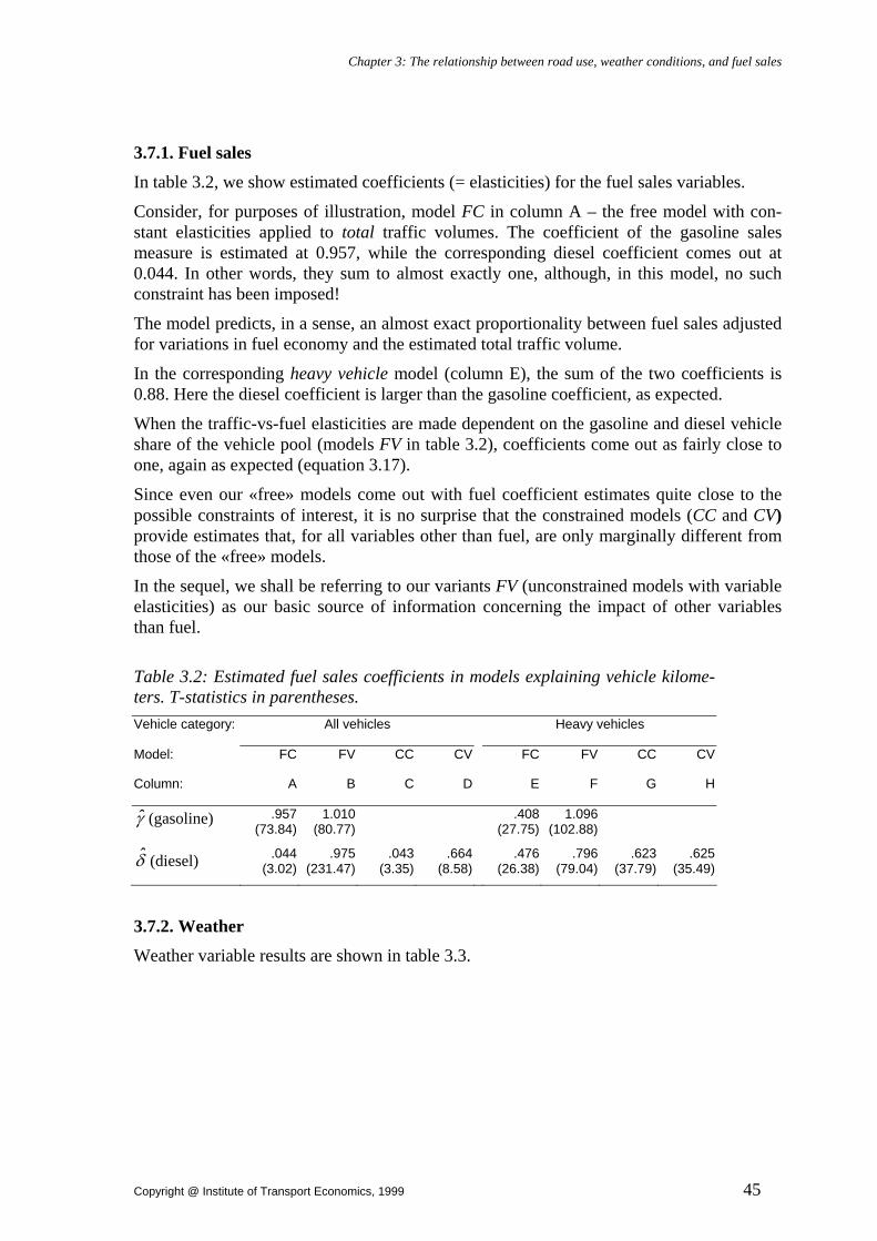
Chapter 3: The relationship between road use, weather conditions, and fuel sales
Copyright @ Institute of Transport Economics, 1999 45
3.7.1. Fuel sales
In table 3.2, we show estimated coefficients (= elasticities) for the fuel sales variables.
Consider, for purposes of illustration, model FC in column A – the free model with con-stant elasticities applied to total traffic volumes. The coefficient of the gasoline sales measure is estimated at 0.957, while the corresponding diesel coefficient comes out at 0.044. In other words, they sum to almost exactly one, although, in this model, no such constraint has been imposed!
The model predicts, in a sense, an almost exact proportionality between fuel sales adjusted for variations in fuel economy and the estimated total traffic volume.
In the corresponding heavy vehicle model (column E), the sum of the two coefficients is 0.88. Here the diesel coefficient is larger than the gasoline coefficient, as expected.
When the traffic-vs-fuel elasticities are made dependent on the gasoline and diesel vehicle share of the vehicle pool (models FV in table 3.2), coefficients come out as fairly close to one, again as expected (equation 3.17).
Since even our «free» models come out with fuel coefficient estimates quite close to the possible constraints of interest, it is no surprise that the constrained models (CC and CV) provide estimates that, for all variables other than fuel, are only marginally different from those of the «free» models.
In the sequel, we shall be referring to our variants FV (unconstrained models with variable elasticities) as our basic source of information concerning the impact of other variables than fuel.
Table 3.2: Estimated fuel sales coefficients in models explaining vehicle kilome-ters. T-statistics in parentheses. Vehicle category: All vehicles Heavy vehicles
Model: FC FV CC CV FC FV CC CV
Column: A B C D E F G H
γ (gasoline) .957 (73.84)
1.010 (80.77)
.408(27.75)
1.096(102.88)
δ (diesel) .044 (3.02)
.975 (231.47)
.043(3.35)
.664(8.58)
.476(26.38)
.796(79.04)
.623 (37.79)
.625 (35.49)
3.7.2. Weather
Weather variable results are shown in table 3.3.

An econometric model of car ownership, road use, accidents, and their severity
46 Copyright @ Institute of Transport Economics, 1999
Table 3.3: Estimated elasticities of vehicle kilometers with respect to weather variables, condi-tional on fuel sales etc, with curvature parameters. T-statistics in parentheses. Vehicle category: All vehicles Heavy vehicles
Model: FC FV CC CV FC FV CC CV
Column: A B C D E F G H
Elasticities evaluated at sample means Days with snowfall cmsnowd1s .000 -.002 .000 .000 -.032 -.037 -.031 -.029during month, (1.65) (-.34) (1.64) (1.78) (-4.79) (-5.57) (-4.20) (-3.98)plus one LAM LAM LAM LAM LAM LAM LAM LAM Difference cmtcold -.127 -.135 -.127 -.143 -.241 -.244 -.252 -.246between 25 degrees (-16.35) (-9.26) (-16.47) (-11.94) (-14.15) (-14.17) (-13.94) (-13.38)C and mean LAM LAM LAM LAM LAM LAM LAM LAMmonthly temperature Curvature parameters LAMBDA(X) cmsnowd1s 7.128 .887 7.115 -3.420 1.123 1.096 1.121 1.169 [1.04] [.18] [1.03] [-.34] [2.33] [2.69] [2.14] [2.06] LAMBDA(X) cmtcold 2.652 2.274 2.648 2.249 1.036 1.031 1.260 1.336 [7.57] [6.18] [7.62] [6.90] [4.09] [4.36] [4.89] [4.88]
TRIO PROJECT: TRULS - an econometric model of road use, accidents and their severityDATE: 97 01 14USER: lef Figure 3.2: Estimated partial relationship between snowfall frequency and fuel use per heavy vehicle km
The left-most column of table 3.3 provides a description of each independent variable. The second column states the variable name, as defined in the TRULS data base17. In the sub-
17 Refer to appendix C for a variable nomenclature to be used throughout this essay.

Chapter 3: The relationship between road use, weather conditions, and fuel sales
Copyright @ Institute of Transport Economics, 1999 47
sequent eight columns (A through H) we report estimates derived under the various models for total and heavy vehicle traffic, respectively.
Somewhat to our surprise, the frequency of snowfall18 during the month has no significant effect on overall fuel use per vehicle kilometer.
This may have to do with lowered (and hence more economical) speed during snow condi-tions, counterbalancing the «initial», energy-increasing effect of snow on the road. It could also reflect a diversion of traffic towards the larger and better maintained roads, which inflates the traffic counts compared to the overall county-wide traffic volume.
For heavy vehicles, however, snowfall does appear to significantly affect fuel economy, with an elasticity of 0.03719. The estimated relationship between snowfall and fuel use per heavy vehicle km is shown in figure 3.220.
A much larger impact is due to temperature variations. Fuel consumption per overall vehi-cle kilometer is an estimated 25 per cent higher when the mean monthly temperature drops to minus 10 degrees C, compared to a (plus) 25 degrees reference point (figure 3.3). As expected, the Box-Cox parameter (on the variable cmtcold) is considerably larger than zero (generally above 2 in the overall vehicle models and 1.0 to 1.3 in the heavy vehicle mod-els), meaning that fuel consumption increases more than proportionately with the cold (as measured in relation to a 25 degrees reference point21).
Fuel consumption per heavy vehicle kilometer is estimated to increase by no less than 40-50 per cent in the coldest periods compared to the warmest (fig 3.4). There is reason to doubt whether this effect is due to vehicle fuel economy alone. More plausibly, we spot the effect of diesel being used for multiple purposes, notably for heating. Although we have attempted to purge the diesel sales statistics of those parts which are not used for road transportation, a certain amount of non-transportation use is apparently left in our fig-ures22.
18 The variable cmsnowd1s is a standardized snowfall frequency measure, defined as 1 30+ ⋅x nt t/ , where xt is the number of days with snowfall during month t and nt is the length of the month (number of days). We add one to the count in order to allow for Box-Cox transformation without creating a threshold between zero and one day of snowfall. 19 Model FV (column F of table 3.3) comes with an elasticity as evaluated at the sample means of –0.037. I e, for given fuel sales, the traffic counts decrease by 0.037 per cent for each per cent increase in the snowfall frequency. To interpret these figures as measures of fuel use per vehicle km, we reverse the sign. 20 The points shown in the TRIO scattergrams are true sample points. That is, not only do they depict the partial relationship estimated, they also – for both variables – indicate the range of variation upon which the relationship has been estimated. 21 This reference point is, of course, arbitrarily chosen. This arbitrariness is, however, mitigated by the fact that we let the data determine the functional form, through Box-Cox transformation. In the sample, the mean monthly temperature ranges from -13 to +20 degrees C (see figure 3.3). 22 Most oil-powered heating installations run perfectly well on automobile diesel. There is, moreover, a certain economic incentive to substitute diesel for heating oil, in that fuel dealers incurring transportation costs exceeding NOK 0.07 per liter automobile diesel are entitled to a NOK 0.07 reimbursement from the Government, under the fuel transportation subsidy scheme for remote areas. This reimbursement does not apply to ordinary heating oil (Bjørn Reusch, Norwegian Institute of Petroleum Studies, personal communica-tion). It is unlikely that we have been able to purge our diesel sales figures of all such occurrences.
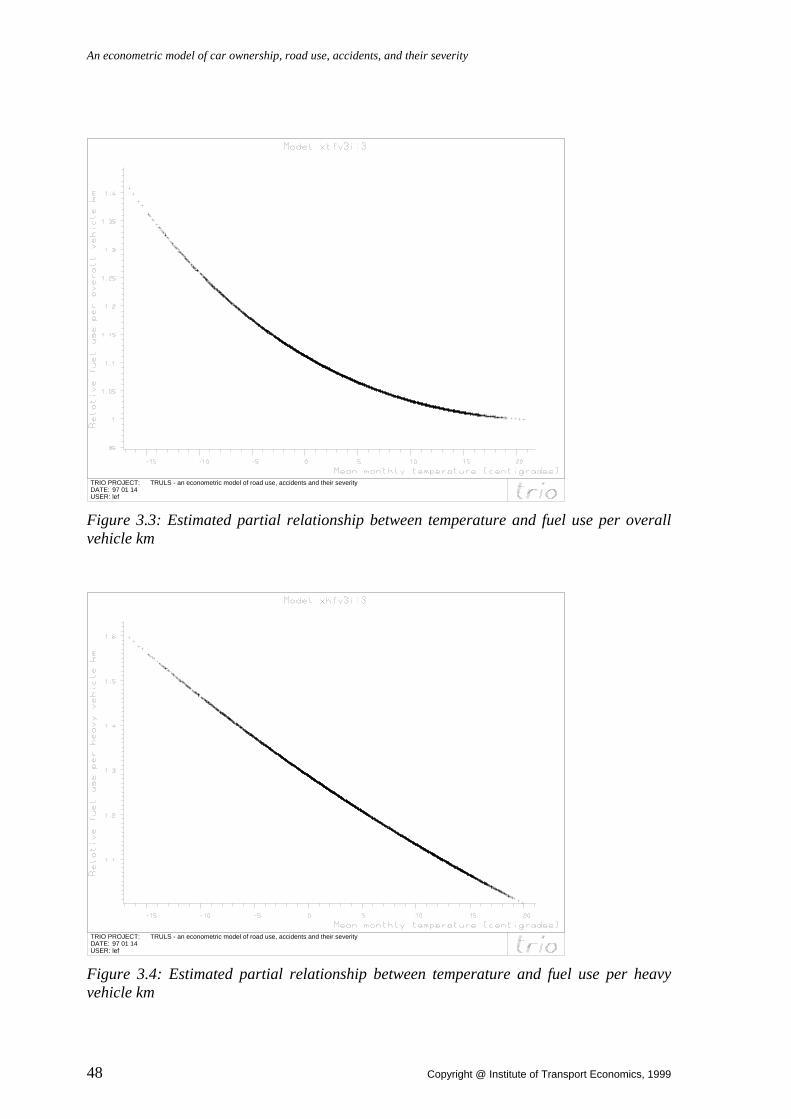
An econometric model of car ownership, road use, accidents, and their severity
48 Copyright @ Institute of Transport Economics, 1999
TRIO PROJECT: TRULS - an econometric model of road use, accidents and their severityDATE: 97 01 14USER: lef Figure 3.3: Estimated partial relationship between temperature and fuel use per overall vehicle km
TRIO PROJECT: TRULS - an econometric model of road use, accidents and their severityDATE: 97 01 14USER: lef Figure 3.4: Estimated partial relationship between temperature and fuel use per heavy vehicle km

Chapter 3: The relationship between road use, weather conditions, and fuel sales
Copyright @ Institute of Transport Economics, 1999 49
This illustrates the importance of modeling the relationship between traffic volume and fuel sales in a fairly thorough way.
3.7.3. Price variations
Certain price variables are included in the model, not to estimate their impact on demand, but in order to control for potential hoarding effects due to price fluctuations. Most impor-tantly, the very pronounced, overnight increase in the diesel price occurring on October 1st, 1993 appears to have spurred massive hoarding during the preceding month, and – supposedly – a correspondingly low sales volume in the month(s) following. Even for gasoline, a certain amount of hoarding due to price fluctuations is likely to take place. Re-call that our fuel statistics are wholesale rather than retail sales data, reflecting the sales of fuel to – not from – the gas stations.
Table 3.4: Estimated elasticities of vehicle kilometers with respect to fuel price ratios, condi-tional on fuel sales etc. T-statistics in parentheses. Vehicle category: All vehicles Heavy vehicles
Model: FC FV CC CV FC FV CC CV
Column: A B C D E F G H
Elasticities evaluated at sample means Diesel price previous epdlag1 -.044 -.071 -.044 -.052 -.126 -.151 -.164 -.132month relative (-1.08) (-1.91) (-1.08) (-1.35) (-1.69) (-2.03) (-2.82) (-2.12)to current month LAM 1 LAM 1 LAM 1 LAM 1 LAM 1 LAM 1 LAM 1 LAM 1 Diesel price epdlead1 -.006 -.103 -.005 -.039 -.244 -.374 -.374 -.270of subsequent (-.14) (-2.89) (-.12) (-.82) (-4.98) (-9.25) (-6.63) (-5.22)month relative LAM 1 LAM 1 LAM 1 LAM 1 LAM 1 LAM 1 LAM 1 LAM 1to current month Gasoline epglag1 -1.336 -1.307 -1.334 -1.326 -1.049 -.999 -1.279 -1.290price previous (-11.92) (-12.08) (-11.97) (-11.97) (-5.45) (-5.29) (-6.90) (-6.75)month relative LAM 1 LAM 1 LAM 1 LAM 1 LAM 1 LAM 1 LAM 1 LAM 1to current month Gasoline price epglead1 -.920 -.732 -.921 -.853 -.671 -.365 -.586 -.779of subsequent (-7.56) (-6.16) (-7.57) (-6.95) (-3.76) (-2.13) (-3.31) (-4.35)month relative LAM 1 LAM 1 LAM 1 LAM 1 LAM 1 LAM 1 LAM 1 LAM 1to current month Ratio of epgswenor1 -.420 -.368 -.421 -.391 -.254 -.178 -.235 -.323Swedish to Norwegian (-3.53) (-3.37) (-3.53) (-3.44) (-1.22) (-.92) (-1.04) (-1.45)price of gasoline, Østfold county Dummy for epkno .051 .055 .051 .063 .124 .124 .114 .121diesel surtax ===== (7.02) (7.97) (7.17) (9.44) (11.53) (11.75) (10.51) (11.06)replacing kilometrage tax Dummy for diesel epkno1 -.045 -.032 -.045 -.041 .064 .093 .101 .065surtax, Østfold county ====== (-1.50) (-1.09) (-1.51) (-1.43) (1.07) (1.59) (1.57) (1.04) Østfold dummy hcounty1 .016 -.043 .016 -.023 -.050 -.118 -.115 -.037 ======== (.91) (-2.85) (.94) (-1.37) (-1.62) (-4.31) (-3.53) (-1.14) Curvature parameters LAMBDA(X) - GROUP 1 LAM 1 .000 .000 .000 .000 .000 .000 .000 .000 FIXED FIXED FIXED FIXED FIXED FIXED FIXED FIXED

An econometric model of car ownership, road use, accidents, and their severity
50 Copyright @ Institute of Transport Economics, 1999
All price variables are entered in logarithmic form (i e, with a zero Box-Cox parameter) and have the expected (usually negative) coefficient sign (table 3.4). Variable epdlag1, e g, reflects the fact that when the diesel price has dropped relative to the previous month (i e, epdlag1>1), a larger fuel sales volume can be expected for a given traffic volume, i e the vehicle kilometrage is smaller, given the fuel sales. Similarly, when the price is (known to be) going up the next month, more fuel is purchased during the current month, for con-sumption at a later stage.
As expected, the diesel price effects (i e, elasticities) are fairly large in the heavy vehicle models, but smaller in the overall vehicle models. For gasoline, the converse is true.
The Swedish price of gasoline affects the ratio of vehicle kilometrage to fuel sales in the main border county (Østfold)23, especially for light vehicles. When the price in Sweden is lower than in Norway, a certain amount of the gasoline consumed in Østfold is purchased abroad.
Simultaneously with the introduction of a diesel surtax (from October 1993), the diesel vehicle kilometer tax in force up until then was abolished, thus counteracting the effect of more expensive fuel. To capture the possible effects of this legislative measure we intro-duce two dummy variables, one main effect term (epkno) and one interaction term (epkno1) allowing for an added effect specific to Østfold county. The main effect is significant in the overall vehicle models as well as in the heavy vehicle models. Apparently, the diesel surtax is associated with increased heavy vehicle kilometrage in relation to fuel sales, sup-posedly because diesel may still be purchased at a lower price in Sweden, in which case the road user avoids both the kilometer tax and the diesel surtax. Note that for heavy vehi-cles, this effect is estimated to be 50 to 100 per cent higher in Østfold than in the rest of the country, although the interaction term for Østfold is, in general, statistically insignificant. The models generally suggest an about 12 to 13 per cent drop in diesel sales per heavy vehicle kilometer after the diesel tax reform (more than 20 per cent in Østfold).
All models also include a general dummy for Østfold county (hcounty1), in order to adjust the scale for variables defined exclusively for this county.
3.7.4. Calendar effects
Since fuel need not be sold and consumed during the same month, it might be important to control for certain calendar effects, especially those related to the Easter week – a major holiday season in Norway. Unusual amounts of traffic, flowing out of the larger cities, are generated on Friday and Saturday before Palm Sunday, while the main inflow takes place on Easter Sunday and Monday. Most of these traffic flows take place on the main roads covered by traffic counts, possible inflating the traffic counts as compared to the county-wide amount of road use.
This traffic pattern has unforeseeable effects on the time relation between (wholesale) fuel sales and consumption, especially as the Easter week moves back and forth between the calendar months of March and April. On the one hand, one may expect the gas stations to stock up maximally before the Easter week. On the other hand, any unusually large con-
23 The variable epgswenor1 is set equal to 1 for every county except Østfold, i e the effect of the Swedish gasoline price applies only to this one county.

Chapter 3: The relationship between road use, weather conditions, and fuel sales
Copyright @ Institute of Transport Economics, 1999 51
sumer demand for fuel is likely to be reflected in wholesale figures for the subsequent pe-riod, as the gas stations take steps to replenish their stocks.
Table 3.5: Estimated calendar effects on vehicle kilometers, conditional on fuel sales etc. T-statistics in parentheses. Vehicle category: All vehicles Heavy vehicles
Model: FC FV CC CV FC FV CC CV
Column: A B C D E F G H
«Elasticities» Dummy for ekee .002 .009 .002 .010 .038 .046 .047 .042end of Easter ==== (.07) (.26) (.07) (.31) (.90) (1.01) (1.09) (.99) Dummy for end ekee3 -.004 -.004 -.004 -.011 -.087 -.086 -.077 -.088of Easter in March ===== (-.08) (-.08) (-.08) (-.23) (-1.44) (-1.41) (-1.31) (-1.48) Dummy for start ekes -.084 -.071 -.084 -.076 -.044 -.028 -.047 -.054of Easter week ==== (-3.49) (-2.74) (-3.49) (-2.94) (-1.19) (-.69) (-1.30) (-1.51) Dummy for start ekes3 .023 .020 .023 .018 -.034 -.037 -.017 -.021of Easter in March ===== (.71) (.57) (.70) (.51) (-.67) (-.70) (-.35) (-.43) March ekm3 .022 .022 .022 .019 .038 .034 .031 .035 ==== (1.61) (1.53) (1.61) (1.41) (1.52) (1.32) (1.36) (1.51) April ekm4 .041 .038 .041 .032 -.008 -.015 -.006 -.006 ==== (1.38) (1.28) (1.38) (1.12) (-.23) (-.39) (-.16) (-.17)
To control for these effects, whose sign we do not venture to conjecture on a priori grounds, we include a set of six dummy variables, capturing the start and end of Easter (defined as Saturday before Palm Sunday, and Easter Monday, respectively), the months of March and April, as well as interaction terms between these two sets.
In the heavy vehicle models, these dummies are generally not significant, as might be ex-pected since the holiday season does not entail any increased activity within commercial freight – rather the contrary (table 3.5).
In the overall vehicle models, the end-of-Easter dummies are insignificant, while the start of Easter appears to boost the fuel sales in relation to the traffic volume by some 7 to 8 per cent (negative24 coefficient on variable ekes). The effect is smaller, however, when Easter starts in March (add up the coefficients of ekes and ekes3). Also, in general, the fuel sales in April appear to be some 4 per cent lower than what corresponds to the traffic counts (variable ekm4), suggesting that the gas stations do, indeed, usually stock up before Easter.
24 Recall that the dependent variable measures vehicle kilometers, in relation to fuel sales, so that a negative coefficient is consistent with increased fuel use per unit of traffic.

An econometric model of car ownership, road use, accidents, and their severity
52 Copyright @ Institute of Transport Economics, 1999
3.7.5. Heteroskedasticity
In table 3.6, we report our assumptions and estimation results concerning the disturbance variance structure.
Table 3.6: Estimated heteroskedasticity structure in models explaining traffic volumes from fuel sales etc. Coefficient assumptions and estimation results, with t-statistics in parentheses. Vehicle category: All vehicles Heavy vehicles
Model: FC FV CC CV FC FV CC CV
Column: A B C D E F G H
Coefficients (ζ) Inverse cectinv 1.000 1.000 1.000 1.000 total number of FIXED FIXED FIXED FIXED vehicles LAM 1 LAM 1 LAM 1 LAM 1 counted during month Inverse total cechinv 1.000 1.000 1.000 1.000number of heavy FIXED FIXED FIXED FIXEDvehicles LAM 1 LAM 1 LAM 1 LAM 1counted during month Number of ekvhis .056 .049 .057 .053 .050 .055 .039 .037vacation days, (5.20) (4.76) (5.21) (5.04) (5.18) (6.41) (4.39) (4.11)including LAM 2 LAM 2 LAM 2 LAM 2 LAM 2 LAM 2 LAM 2 LAM 2summer vacation Inverse share cecndashinv -.095 .063 -.094 .057 .444 .617 .228 .170of available (-.56) (.36) (-.56) (.33) (2.51) (3.64) (1.30) (.98)traffic count LAM 1 LAM 1 LAM 1 LAM 1 LAM 1 LAM 1 LAM 1 LAM 1days during month Exponential of cksouthsumr 1.738 1.730 1.741 1.651 dummy for July (2.00) (2.30) (2.00) (2.21) in the two LAM 1 LAM 1 LAM 1 LAM 1 southernmost counties Exponential of cexpout1 3.396 3.574 3.471 3.399dummy for (.00) (.00) (.00) (.00)outlier LAM 1 LAM 1 LAM 1 Curvature parameters LAMBDA(Z) - GROUP 1 LAM 1 .000 .000 .000 .000 .000 .000 .000 .000 FIXED FIXED FIXED FIXED FIXED FIXED FIXED FIXED LAMBDA(Z) - GROUP 2 LAM 2 1.000 1.000 1.000 1.000 1.000 1.000 1.000 1.000 FIXED FIXED FIXED FIXED FIXED FIXED FIXED FIXED
The first two variables in the table (cectinv and cechinv) correspond to m nc
t r
trA
and m nc
t r
trH
,
respectively, as entered in equation (3.32); these have their coefficients constrained to one and their Box-Cox parameters fixed at zero, in accordance with our error theory set out above (sections 3.4-3.5).
Four heteroskedasticity variables have been specified in addition to these. The variable ekvhis measures the number of common vacation days during the month25, as the holiday season tends to inflate the traffic volume in certain (resort) counties, while depressing it in other ones, generating a considerably increased disturbance variance. The Box-Cox pa- 25 As vacation days, we count all Saturdays, Sunday, fixed and moving holidays, as well as ordinary work-ing days during which large parts of the labor force are actually on vacation or exempt from work (Christmas and New Year’s Eve, entire Easter week). In July, three weeks of general staff holiday is counted as well, bringing the number of vacation days in July in any year to at least 25.

Chapter 3: The relationship between road use, weather conditions, and fuel sales
Copyright @ Institute of Transport Economics, 1999 53
rameter of this variable is set at one (in accordance with preliminary tests), while the coef-ficient (ζ ) is freely estimated, coming out highly significant (p-value < 0.0001) and with the expected (positive) sign.
Our fourth heteroskedasticity variable (cecndashinv) is defined as the inverse of the number of days for which traffic counts have been available in the county. When, for some reason, no traffic count is put out for a given day26, a total daily traffic flow figure is imputed based on empirically estimated time profiles, taking account of calendar and seasonal ef-fects. This variable measures the extent to which data have been «reconstructed», being hence subject to extraordinary measurement error.
The fifth and sixth variables (cksouthsumr and cexpout1) are the only heteroskedasticity factors which are based on ad hoc data inspection rather than on a priori theoretical con-siderations.
An informal look at the residuals for the overall vehicle model reveals a small group of outliers restricted, in space and time, to the month of July in the two southernmost coun-ties. While the fuel sales exhibit a visible peak during the vacation time in these popular seaside resort areas, somehow this peak is not captured by the available traffic counts.
In the heavy vehicle model, there is one very pronounced outlier, viz. Akershus county in December 1988. To prevent this outlier, presumably due to a gross measurement error, from exerting excessive influence on the parameter estimates, we specify a heteroskedas-ticity dummy, allowing the variance to be (according to the estimates) about 36 (= 5743.e ) times higher for this one observation than for the rest of the sample, and its weight in the estimation correspondingly lower.
3.8. Model extrapolation and evaluation
The aim of our submodels relating traffic counts to fuel sales, weather, calendar, and fuel price fluctuations is to be able to impute reliable measures of exposure (i e, traffic vol-umes) at a fairly disaggregate level (i e, county and month), for input into the econometric accident model to be estimated (chapters 4 through 6 below). Not only do we intend to impute values for all units of observation in our traffic count subsample – we need to ex-trapolate values, temporally (15 years backwards in time) as well as spatially (from 14 to 19 counties), so as to cover all Norwegian counties over the period 1973-1994.
26 A traffic count day is considered missing if the counting equipment has been out of operation for more than one hour during the (24-hour) day.

An econometric model of car ownership, road use, accidents, and their severity
54 Copyright @ Institute of Transport Economics, 1999
TRIO PROJECT: TRULS - an econometric model of road use, accidents and their severityDATE: 97 01 14USER: lef Figure 3.5: Scattergram between imputed overall traffic volumes and total transportation fuel sales. Model FV, 19 counties, 1973-94.
TRIO PROJECT: TRULS - an econometric model of road use, accidents and their severityDATE: 97 01 14USER: lef Figure 3.6: Scattergram between imputed heavy vehicle traffic volumes and gasoline sales. Model FV, 19 counties, 1973-94.

Chapter 3: The relationship between road use, weather conditions, and fuel sales
Copyright @ Institute of Transport Economics, 1999 55
TRIO PROJECT: TRULS - an econometric model of road use, accidents and their severityDATE: 97 01 14USER: lef Figure 3.7: Scattergram between imputed heavy vehicle traffic volumes and transportation diesel sales. Model FV, 19 counties, 1973-94.
TRIO PROJECT: TRULS - an econometric model of road use, accidents and their severityDATE: 97 01 14USER: lef Figure 3.8: Scattergram between imputed heavy vehicle share of traffic and diesel share of transportation fuel sales. Models FV, 19 counties, 1973-94.

An econometric model of car ownership, road use, accidents, and their severity
56 Copyright @ Institute of Transport Economics, 1999
Imputed values are, of course, derived by plugging the estimated coefficients and parame-ters into equations (3.12) and (3.14), respectively. Essentially, these relations can now be viewed as weighted (geometric) sums of the relevant gasoline and diesel sales figures, cor-rected for certain factors that have been shown to affect the ratio of vehicle kilometrage to fuel sales.
In figures 3.5 to 3.8 we present scattergrams illustrating the covariation – or lack thereof – between «crude» fuel sales statistics and imputed traffic volumes, as extrapolated to the entire, 19-county, 1973-94 sample. Imputed overall traffic volumes correlate strongly with the gasoline sales, although the relationship is far from exact (fig 3.5). Heavy vehicle traf-fic volumes appear to correlate more strongly with gasoline sales than with diesel sales (figs 3.6 and 3.7). The correlation between the heavy vehicles’ share of the traffic volume and the diesel share of the total fuel sales is comparatively weak (fig 3.8). The less than perfect correlation appearing may be thought to illustrate the potentially enhanced infor-mation content in our imputed model estimates as compared to uncorrected fuel sales re-cords.
How well do our imputed values predict? Unfortunately, there are no statistics against which they can be judged, by county and month; if there were, this entire excercise would, of course, have been redundant.
There are, however, public statistics available on nationwide, annual road use. To check our figures against these, we have summed the imputed traffic volumes across all counties and across all months in each year.
In figure 3.9, we compare the absolute, overall traffic volumes imputed for each year with the statistics compiled by Rideng (1996). These figures, being based on the official Trans-port and Communications Statistics published by Statistics Norway (see, e g, NOS C 264 and previous issues) and on calculations made at the Institute of Transport Economics, include all motorized, domestic road transportation. Transport volumes generated by im-port or export are, in other words, not included, not even that part of the journey which takes place on Norwegian territory. Our figures, on the other hand, include – in principle – all kilometrage done on Norwegian soil.
In view of these definitional discrepancies, the correspondence between Rideng’s figures and ours appears quite adequate. In terms of relative figures, the two sources come rather close (figure 3.11).
Unlike official statistics, however, our figures clearly pick up the downturn following the first energy crisis in 1973, the strong business cycle upsurge in the late 1980’s and the re-cession in the early 1990’s.
As we extrapolate backwards from 1988, the gap between our four alternative models is seen to widen. This should come as no surprise.
In figure 3.10, we show imputed heavy vehicle traffic compared to official statistics on domestic vehicle kilometers driven by vans, trucks, and scheduled buses. In the latter fig-ures, light freight vehicles are included, while our figures include only vehicles with more than one ton’s carrying capacity or at least 20 passenger seats. The main source of official road freight statistics are the quinquennial trucking surveys, which have been carried out in 1963, -68, -73, -78, -83, and -88, and annually from 1993. For intermediate years, statistics are generally compiled through some kind of interpolation.

Chapter 3: The relationship between road use, weather conditions, and fuel sales
Copyright @ Institute of Transport Economics, 1999 57
The trucking surveys indicate a downward trend in road freight transportation between the survey years of 1978 and 1983. Mainly because of this, a large gap arises between our ag-gregate, imputed heavy vehicle traffic volumes and official statistics (fig 3.10). As reck-oned over the entire 1973 to 1994 period, however, the total heavy vehicle traffic growth is of the same order of magnitude according to both sources (fig 3.12).
Figure 3.9: Total national traffic volumes , as estimated by four models and by public statistics
14000
16000
18000
20000
22000
24000
26000
28000
30000
32000
1973 1978 1983 1988 1993
Year
Mill veh kms
Overall model CC
Overall model CV
Overall model FC
Overall model FV
Domestic vehicle kms, according to Rideng(1996)
Figure 3.10: National, heavy vehicle traffic volumes, as estimated by four models and by public statistics
1500
2000
2500
3000
3500
4000
4500
1973 1978 1983 1988 1993
Year
Mill veh kms
Heavy vehicle model CC
Heavy vehicle model CV
Heavy vehicle model FC
Heavy vehicle model FV
Domestic bus and freight vehicle kms,according to Rideng (1996)
Each trucking survey is based on a probability sample of trucks and vans drawn from the vehicle register of the Public Roads Administration, however with non-response rates gen-erally exceeding 40 per cent (NOS A 796, NOS B 136, NOS B 636, NOS B 974).
An additional source of statistical information bearing on heavy vehicle road use is the Directorate of Customs and Excise, which, up until October 1, 1993, was charged with levying a kilometer tax on most diesel driven vehicles (buses representing the most impor-tant exception). The administrative records kept for this purpose made it possible to com-
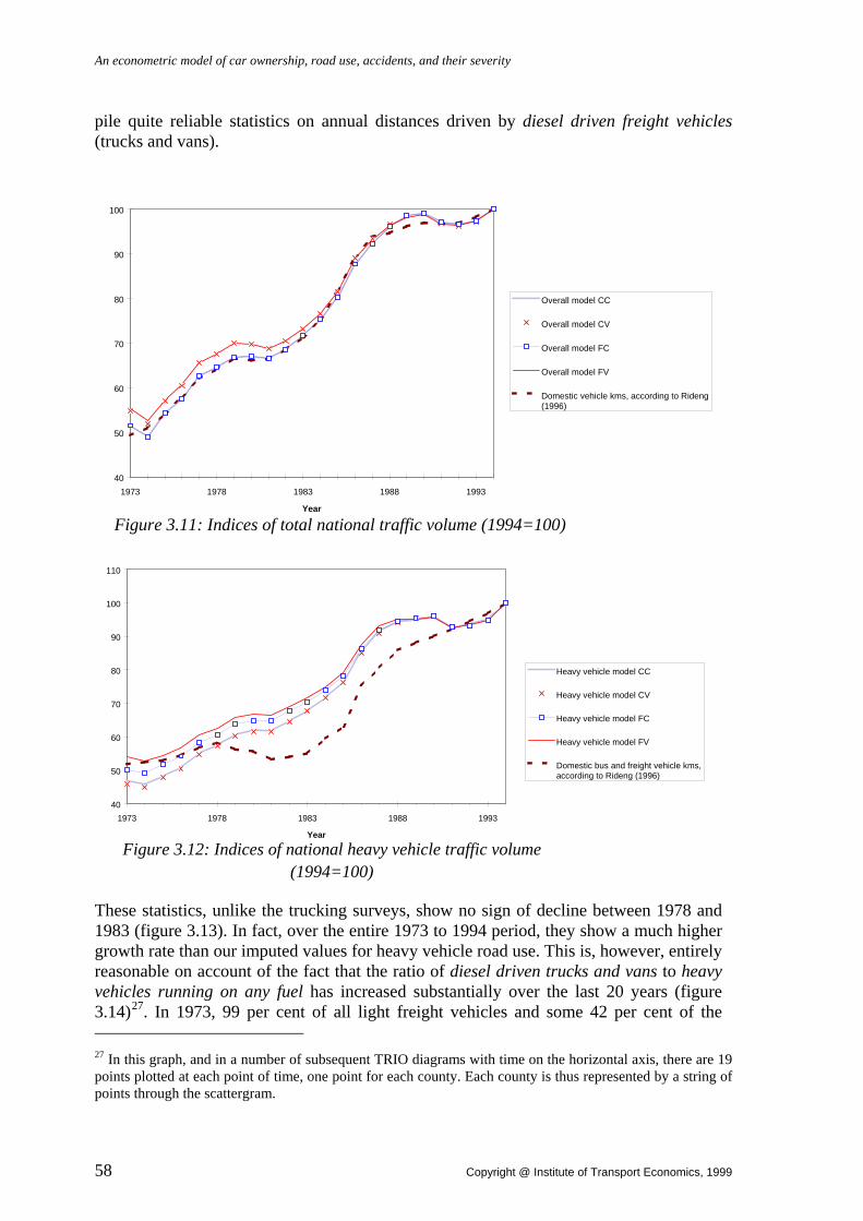
An econometric model of car ownership, road use, accidents, and their severity
58 Copyright @ Institute of Transport Economics, 1999
pile quite reliable statistics on annual distances driven by diesel driven freight vehicles (trucks and vans).
Figure 3.11: Indices of total national traffic volume (1994=100)
40
50
60
70
80
90
100
1973 1978 1983 1988 1993
Year
Overall model CC
Overall model CV
Overall model FC
Overall model FV
Domestic vehicle kms, according to Rideng(1996)
Figure 3.12: Indices of national heavy vehicle traffic volume (1994=100)
40
50
60
70
80
90
100
110
1973 1978 1983 1988 1993
Year
Heavy vehicle model CC
Heavy vehicle model CV
Heavy vehicle model FC
Heavy vehicle model FV
Domestic bus and freight vehicle kms,according to Rideng (1996)
These statistics, unlike the trucking surveys, show no sign of decline between 1978 and 1983 (figure 3.13). In fact, over the entire 1973 to 1994 period, they show a much higher growth rate than our imputed values for heavy vehicle road use. This is, however, entirely reasonable on account of the fact that the ratio of diesel driven trucks and vans to heavy vehicles running on any fuel has increased substantially over the last 20 years (figure 3.14)27. In 1973, 99 per cent of all light freight vehicles and some 42 per cent of the 27 In this graph, and in a number of subsequent TRIO diagrams with time on the horizontal axis, there are 19 points plotted at each point of time, one point for each county. Each county is thus represented by a string of points through the scattergram.

Chapter 3: The relationship between road use, weather conditions, and fuel sales
Copyright @ Institute of Transport Economics, 1999 59
heavy freight vehicles were running on gasoline (Opplysningsrådet for biltrafikken 1974). In 1994, by contrast, these shares had dropped to 58 and 31 per cent, respectively (Opplysningsrådet for veitrafikken 1995).
Figure 3.13: Indices of national heavy vehicle traffic volume and of diesel freight vehicle kilometrage (1994=100)
20
30
40
50
60
70
80
90
100
110
1973 1978 1983 1988 1993
Year
Heavy vehicle model CC Heavy vehicle model CV Heavy vehicle model FC Heavy vehicle model FV Diesel freight vehicle kms
TRIO PROJECT: TRULS - an econometric model of road use, accidents and their severityDATE: 97 01 14USER: lef Figure 3.14: Ratio of diesel freight vehicles to all heavy vehicles. 19 counties, 1973-94.
We conclude that our imputed values for overall and heavy vehicles traffic volumes appear by no means unreasonable in the light of alternative statistical sources. In fact, our figures may seem to represent a major improvement compared to hitherto existing statistical in-formation on road use. Not only are we able to provide, for the first time, absolute vehicle

An econometric model of car ownership, road use, accidents, and their severity
60 Copyright @ Institute of Transport Economics, 1999
kilometer measures fully cross-classified by county, month and vehicle class. Even at the aggregate (nationwide, annual) level, we suspect our figures to be rather more reliable than previously available data.
There are reassuringly small differences between our four model variants. None of the four can be said to match official statistics unambiguously better than the other ones.
For the purpose of the analyses to follow, we shall choose the imputed values from the unconstrained, variable elasticity models (FV) as our standard measures of motor vehicle exposure. These models incorporate a maximum of information and provide a clearly supe-rior explanatory power compared to the constant elasticity models (FC) (by the log-likelihood reported in Appendix B). Without having been subjected to constraints, their fuel coefficients are also quite reasonable in view of a priori expectations.

Chapter 4: Aggregate car ownership and road use
Copyright @ Institute of Transport Economics, 1999 61
Chapter 4: Aggregate car ownership and road use
4.1. Introduction
In this chapter, we set out of examine how aggregate car ownership and road use demand depend on key economic and socio-demographic variables, such as income, interest rates, and travel costs, and implicitly also on certain important policy variables such as fuel and vehicle taxes.
Transportation demand elasticities have been the subject of extensive research, at least for passenger transport (see, e g, the excellent survey articles by Oum et al (1992) and by Goodwin (1992), and references therein)28. But the elasticity estimates derived are quite disparate, depending on data, functional specification, degree of aggregation, etc. Some researchers (Goodwin 1977, Blaise 1980, Gately 1992, Dargay 1993) suggest that con-sumer response may not be symmetric in regard to rising or falling prices («hysteresis»), demand being less elastic as the price (of fuel) falls than when it rises.
Few – if any – studies allow for the possibility that (aggregate) demand elasticities may not be constant over the observed range of price (or income) variation. We can, however, see no theoretical reason why they should be. Even under the (unfounded) assumption that demand elasticities with respect to the total cost of transport should be constant, there is every reason to think of the elasticity with respect to the fuel price component as variable. A higher fuel price is associated with a higher fuel cost share. If only for this reason, fuel price elasticities should be increasing (in absolute value) with the initial fuel price level. This applies to commercial freight as well as to private travel. Even in the latter case, fuel is but one of the (generalized) costs of travel incurred, other distance-dependent compo-nents being travel time, discomfort, risk, insurance, vehicle maintenance, etc.
Oum et al (1992:153) argue cogently that «Different functional forms can result in widely different elasticity estimates, even with the same set of data. ... The problem is long neglected by researchers and transport practitioners. Typically, an ad hoc demand specification is used and little attention is directed towards test-ing the specification against an alternative. With the advances in econometric theory and computing technology, we think that specification testing should become an integral part of empirical transport demand research in the future.»
Being in complete agreement with this argument, we are in a position to specify and assess estimably non-linear demand relations, using the Box-Cox regression modeling technique. We will therefore be able, not only to test various specifications against each other, but also to determine the optimal (best fit maximum likelihood) form of the relation, as a func-tion of the empirical evidence available.
Our suspicion is that such (Box-Cox) relations might be entirely sufficient to explain the apparent asymmetry («hysteresis») of road user response. Large price reductions tend to shift the market equilibrium into the inelastic range, while substantially increasing prices imply a movement into the highly elastic range. The theoretical and empirical insight into (the possible curvature of) these relations may have important policy implications. 28 A closely related issue is the demand for transportation fuel, on which there also exist numerous studies, see e g Dahl and Sterner (1991a, b), Franzén and Sterner (1995), Gately (1990, 1992), Greene (1992), Dahl (1995), and Johansson and Schipper (1997).

An econometric model of car ownership, road use, accidents, and their severity
Copyright @ Institute of Transport Economics, 1999 62
Another recommendation made by Oum et al (1992) is this: «It is well known that demand becomes more elastic in the long run because users are better able to adjust to price changes. The distinction between long-run and short-run, however, is quite arbitrary in most transport demand studies. More carefully structured long-run studies are needed to integrate location choice and asset ownership decisions with transport de-mand.»
While localization effects are well beyond the scope of our study, we do intend to explic-itly model asset (i e, car) ownership, using a partial adjustment approach, so as to be able to derive short term as well as long (or at least medium) term demand effects.
4.2. A partial adjustment model of aggregate, private car ownership
A most important determinant of individual travel demand and mode choice is household car ownership (Nielsen and Vibe 1989). Many travel demand models use car ownership as a key explanatory factor.
Car ownership is, however, in our perspective hardly an exogenous variable, and should not be treated as such. Indeed, in recent microeconometric work it has become customary to model car ownership and use as jointly dependent (simultaneous) choice variables (de Jong 1990, Ramjerdi and Rand 1992a). Within this framework, the variable cost of car use helps explain the decision to own a car, and the fixed cost of car ownership helps explain the annual distance traveled by car, in other words its use.
We view this modeling perspective as an entirely sound and fairly realistic description of household decision making. A higher fuel price makes it less attractive for households to possess an (additional) car. And a higher purchasing price of cars makes it less probable that a randomly selected traveler would have a car available for use, when needed.
A vehicle population is an inert matter, much like a human population, although with gen-erally higher rates of turnover and shorter life expectancy. Individual car owners may sell their car, in response to large and abrupt changes in wealth or relative prices, but this op-tion hardly exists for the Norwegian car owner population as an aggregate. Given the very high level of purchase tax imposed on automobiles in Norway, used cars can be sold abroad only at very substantial losses. Thus, the only important downward adjustment mechanism operating at the macro level is scrapping, something which also involves heavy losses unless the car is old enough to have lost most of its market value. Hence, in the ag-gregate, car owners can be expected to adjust only slowly to changes in economic vari-ables.
In view of this inertia, we choose to specify our car ownership equation as a partial ad-justment model of the following form:
(4.1) tri
)(triCi
)(tr e~x~C~ Ci += ∑ λμ β
(4.2) [ ] tr)(
r,t)(
tr)(
r,t)(
tr eCC~CC +−⋅=− −−μμμμ γ 1212 .
Here, ~Ctr denotes the equilibrium («desired», «optimal») level of aggregate car ownership in country r at month t, given the independent factors xtri (i=1,2,....), which are assumed to include all relevant prices and other exogenous determinants. The observed (actual) num-

Chapter 4: Aggregate car ownership and road use
Copyright @ Institute of Transport Economics, 1999 63
ber of cars registered Ctr is assumed to adjust to the equilibrium level at a rate determined by the partial adjustment coefficient γ and the difference between this year’s optimal level and last year’s actual level (both of which may be Box-Cox transformed). tre~ and tre are random disturbance terms.
The equilibrium number of cars ~Ctr is, of course, unobservable. Thus, in order to estimate this model, we need to solve (4.1)-(4.2) for the observable variable Ctr . Rearranging (4.2) and substituting in for ~Ctr , we obtain
(4.3) ( ) trtr)(
trii
Ci)(
r,t)(
tr ee~x~CC Ci +⋅+⋅+⋅−= ∑− γβγγ λμμ121
( ) tr)(
trii
Ci)(
r,t uxC Ci ++⋅−= ∑−λμ βγ 121 (say),
where we have defined trtrtr ee~u +⋅= γ and the directly estimable coefficients β γ βCi Ci= ⋅~
. Given estimates of 1− γ and β Ci , it is a trivial matter to compute indirect estimates of the
structural coefficients ~β Ci .
As applied to a cross-section/time-series data set like ours, where the dependent variable is an absolute rather than a relative measure, such as the aggregate number of cars Ctr or the aggregate number of vehicle kilometers ~vtrj (see section 4.3 below), some caution must be exercized in constraining or relaxing the dependent variable Box-Cox parameter ( μ ). Un-less μ = 0 , the elasticity is going to depend on the size of county r, as reflected in the ag-gregate measure Ctr or ~vtrj (confer section 2.4.4).
Such an implication appears neither reasonable nor theoretically sound. Hence, in all our car ownership and road use demand equations, we shall fix the dependent variable Box-Cox parameter at zero. In other words, we always apply a logarithmic transformation to the dependent variable. Essentially, this means that car ownership or road use are modeled as multiplicative functions of the right-hand side regressors.
In an autoregressive model like (4.3), standard methods of estimation are not necessarily unbiased, since the lagged variable ~
,Ct r−12 depends on last year’s disturbance terms and is hence random. Ordinary least squares estimation can only yield consistent estimates if the errors are serially uncorrelated, and even then only under certain (weak) conditions (Theil 1971:412). On the other hand, Malinvaud (1970:559) points out that the presence of ex-ogenous variables in the equation (such as our xtrj ) tends to greatly reduce the size of the asymptotic bias, even if the errors should be correlated. Johnston (1984) advocates the use of an iterative Cochran-Orcutt procedure in combination with a first-round instrumental variable estimator, since the Cochran-Orcutt procedure itself may yield inconsistent esti-mates unless a consistent starting point has been provided (Betancourt and Kelejian 1981). Hatanaka (1974) has devised a consistent two-step, estimator also based on a first-round instrumental variable procedure (see, e g, Greene 1993:436 for a brief account).
Such an analysis has been beyond the scope of this study, and would hardly be feasible unless we gave up on our ambition to estimate certain Box-Cox transforms rather than to assume a given functional form. We shall therefore proceed to estimate equation (4.3) as it

An econometric model of car ownership, road use, accidents, and their severity
Copyright @ Institute of Transport Economics, 1999 64
stands, however with a keen eye on the autocorrelation structure. Recall that our BC-GAUHESEQ software allows us to specify disturbance structures of the form
(2.4) tri
)(triitr uzexpu zi ′⎥
⎦
⎤⎢⎣
⎡⎟⎠
⎞⎜⎝
⎛= ∑
21
λζ
(2.5) ′ = ′ + ′′−=
∑u u utr j t j rj
J
trρ ,1
,
where the triz are heteroskedasticity factors, the ′utr are homoskedastic, although possibly autocorrelated error terms, and the ′′utr terms represent white noise. ζ i , ziλ and ρ j are coefficients to be fixed or estimated.
We shall exploit this structure in two ways. First, we specify a 12th order autocorrelation term, as given by (2.5), by allowing ρ12 0≠ , while setting ρ j j= ∀ ≠0 12 .
Second, since aggregate car ownership is actually measured only once a year (as of Janu-ary 1st), all other observations in our data base being interpolated values between January stocks, we shall define a triz variable such that all «artificial» (interpolated) observations receive virtually no weight in the estimation (see section 4.4.12 for details).
As for the set of independent variables used, we refer the reader to section 4.4, in which all variables and their estimated effects are presented.
4.3. Models for overall and heavy vehicle road use
To estimate the demand for road use, we specify a standard Box-Cox regression model of the form
(4.4) ~( ) ( )v x utrj ij trii
trjj ijμ λβ= +∑ ,
where the dependent variable ~vtrj is the traffic volume calculated from equation (3.5) of chapter 3 (j = A, H for overall and heavy vehicle traffic volumes, respectively).
Again, the error terms may be heteroskedastic and/or autocorrelated, according to the for-mulation (2.4)-(2.5). For the road use equations, we specify first and second order autocor-relation terms, i e letting 01 ≠ρ and 02 ≠ρ , but 20 >∀= jjρ .
In the overall road use model (j=A), the first independent variable ( xtr1 ) is aggregate car ownership per capita. As for the other independent variables, we refer the reader to sec-tions 4.4.3-4.4.12.

Chapter 4: Aggregate car ownership and road use
Copyright @ Institute of Transport Economics, 1999 65
4.4. Empirical results
Estimation results for our partial adjustment car ownership model, as well as for the road use demand models, are summarized in tables 4.1 to 4.8, the format of which is like tables 3.3 through 3.6, with one addition: Elasticities (of the dependent with respect to the inde-pendent variables) are presented, as evaluated not only at the overall sample means (line 1 of each «cell»), but also at the subsample means for 1994, our last year observation (line 2). These differ because the estimated relationships are not generally log-linear.
In column A of tables 4.1-4.8, we present short-term elasticities and (conditional) t-statistics for the car ownership submodel. That is, the tables generally show elasticities computed as
(4.5) [ ] Ciˆ
triCitritr xˆx;CEl λβ=
and evaluated at the (sub)sample means.
Long term (equilibrium) elasticities could be obtained by replacing the short-term coeffi-cient Ciβ by its equilibrium counterpart γββ CiCi
~= :
(4.6) [ ] Ciˆ
triCitritr x~x;CElˆ
λβγ
=1 .
In column B, we show short-term elasticity estimates for overall road use demand (total vehicle kilometers). In this case, «short-term» means «ignoring changes in equilibrium car ownership». For an overview of compound elasticities, incorporating short- and long-term, direct and indirect effects, we refer the reader to Chapter 7.
To properly understand and estimate the effect of, e g, income and prices on road use de-mand, one should either (i) estimate a two-equation system explaining car ownership as well as use, or (ii) estimate a reduced form equation for road use, in which only exogenous determinants appear.
Of these two, we prefer the former. For a maximum of insight, we are, however, also going to display – in column C – a pseudo-reduced form of the model consisting of columns A and B. It differs from column B only in that the car ownership variable has been left out of the regression. Its coefficients may be roughly interpreted as partial effects on road use, given that aggregate car ownership is not assumed constant.
Finally, in column D, the heavy vehicle road use demand model is shown.
4.4.1. Car ownership partial adjustment
The partial adjusted coefficient of the car ownership model comes out at about 0.122 ( γ−1 = 0.878, the coefficient of variable cvrcarsl12 in table 4.1). This essentially means that, to obtain long-run (equilibrium) effects, all coefficients and elasticities derived from the same model must be multiplied by 8.2 (=1/0.122). Only about one eighth of the desired adjustment in car ownership seems to take place within one year from a given exogenous shock.
The autocorrelation parameter is estimated at –0.129, in other words a negative but only moderately large value. It is significantly different from zero by the t-test. Thus we cannot,

An econometric model of car ownership, road use, accidents, and their severity
Copyright @ Institute of Transport Economics, 1999 66
unfortunately, discard the possibility of a certain bias being present in our estimate of γ . Also, note that a small bias in the estimable «parameter» 1− γ translates into a relatively large bias in the partial adjustment parameter γ , inflating (or deflating) all long-term (equilibrium) elasticities calculable from the car ownership model. Any results concerning the equilibrium demand for cars, to be detailed below, are therefore rather uncertain and should be interpreted with considerable caution.
Table 4.1: Estimated elasticities etc with respect to vehicle ownership, demogra-phic indicators and public transportation supply. T-statistics in parentheses. Dependent variable: Aggregate
car owner-ship
Total vehicle kilometers
Total vehicle kilometers
(reduced form)
Heavy vehi-cle kilome-
ters
Column: A B C D Elasticities evaluated at the 1974-94 means (1st line) and at the 1994 means (2nd line) -------- Vehicles -------- Number of automobiles cvrcarsl12 .878 registered .878 12 months back (434.45) LAM 4 Passenger cvrcarsp .936 cars per capita .982 (31.20) LAM ---------- Population ---------- Population density cdpopdnsty .109 .907 .754 1.174 (inhabitants per sq .109 .907 .754 1.174 km) (54.40) (41.75) (20.54) (8.14) LAM 4 LAM 4 LAM 4 LAM 4 Unemployment rate cderate -.021 -.018 -.082 (per -.021 -.018 -.082 cent of working (-5.50) (-3.33) (-14.97) age population) LAM 4 LAM 4 LAM 4 ---------------------------- Public transportation supply ---------------------------- Density of dtabus -.058 .017 public bus service -.062 .018 (annual veh kms (-3.03) (.53) per km public road) Density of dtarail -.005 -.095 -.023 subway and streetcar ------- -.009 -.181 -.044 service (annual (-3.94) (-.80) (-.11) car kms per km rd)
Curvature parameters LAMBDA(Y) - GROUP 4 LAM 4 .000 .000 .000 .000 FIXED FIXED FIXED FIXED LAMBDA(X) cvrcarsp .284 [3.93]

Chapter 4: Aggregate car ownership and road use
Copyright @ Institute of Transport Economics, 1999 67
4.4.2. Effect of car ownership on road use
As expected, aggregate car ownership has a very strong and significant effect on aggregate road use (t-values around 30, see column B of table 4.1). Our best-fit elasticity estimate is 0.936, as evaluated at the overall sample means (1974-94). In other words, road use in-creases almost proportionately with aggregate car ownership.
The Box-Cox parameter of car ownership in this model is estimated at 0.284, representing a curvature about midway between the square root and the logarithmic transformation. The elasticity of road use with respect to aggregate car ownership appears to be slightly in-creasing with the initial level of car ownership.
4.4.3. Population
The elasticity of car ownership and use with respect to the size of the population is of the order of 0.9. In other words, road use demand increases somewhat less than proportion-ately with the population, whose variation, in our data set, is mainly cross-sectional. Note that, although population density is the variable entering the model, its coefficient is also interpretable as the effect of population per se, on account of our multiplicative decompo-sition encompassing income, population and geographic size (see footnote 38 below).
TRIO PROJECT: TRULS - an econometric model of road use, accidents and their severityDATE: 97 02 21USER: lef Figure 4.1: Registered unemployment. Per cent of working age population. 19 counties 1973-94
The elasticity of heavy vehicle road use demand with respect to population size is larger than one, although not significantly so (column D). In other words, densely populated ar-

An econometric model of car ownership, road use, accidents, and their severity
Copyright @ Institute of Transport Economics, 1999 68
eas may seem to attract a little more than their «proportionate» share of the heavy vehicle traffic.
The unemployment rate has a clearly depressive effect on road use, especially for heavy vehicles. Its sample variation across time is shown in figure 4.1. (There are 19 data points per month, one for each county.)
4.4.4. Public transportation supply
There appears to be only weak (and rather uncertain) cross-demand effects on car use from public transportation supply, as measured by the density of bus (dtabus) and sub-way/streetcar (dtarail) services per km public road. The latter also seems to affect car own-ership, while the former initially came out with a counterintuitive sign and was dropped from the car ownership equation.
Note, however, that the subway/streetcar service is zero in all counties except in Oslo and Sør-Trøndelag (city of Trondheim), and almost negligibly small in Sør-Trøndelag com-pared to Oslo. Even the bus supply is markedly larger in Oslo than in all other counties. Thus, most of the variation in these variables is cross-sectional rather than temporal. The effects estimated may therefore be subject to certain biases originating from omitted vari-ables with a stable regional pattern of variation. One important such variable is parking facilities, the lack of which represents a major constraint on car ownership and use in Oslo, but hardly in any other county.
4.4.5. Income
Statistics on disposable household income are, unfortunately, not available in the form of county level time series. As a relevant proxy we choose to use real gross earned personal income, i e gross income earned by the working population, not including capital gains or other non-work revenue (figure 4.2). In principle, profits earned by self-employed persons are included only in so far as they are considered as returns to labor rather than to capital. The income figures are «real» in the sense of being deflated by the consumer price index, and «gross» in the sense that, for wage earners, tax deductible expenses are not deducted, as in «net income» statistics. Hence, our measure is invariant with respect changes in the tax deductibility of certain costs (such as travel expenses) and in the volume of tax-deductible private expenditure (such as interest payments)29.
29 The Norwegian language equivalent of our «gross earned personal income» is «pensjonsgivende inntekt» («pensionable income»), i e remuneration from work earned by persons aged 17-69.
To obtain monthly income data from annual flows, we divide by 12, in order to form the moving average over the last 12 months. Thus, December income data always equal the income earned during the past calen-dar year, while for other months our income figures are weighted averages of the income flows pertaining to the previous and current years.

Chapter 4: Aggregate car ownership and road use
Copyright @ Institute of Transport Economics, 1999 69
TRIO PROJECT: TRULS - an econometric model of road use, accidents and their severityDATE: 97 02 21USER: lef Figure 4.2: Real gross earned personal income per capita. 19 counties 1973-94
TRIO PROJECT: TRULS - an econometric model of road use, accidents and their severityDATE: 97 02 21USER: lef Figure 4.3: Real taxable net corporate income per capita. 19 counties 1973-94

An econometric model of car ownership, road use, accidents, and their severity
Copyright @ Institute of Transport Economics, 1999 70
Table 4.2: Estimated elasticities etc with respect to income measures. T-statistics in parentheses. Dependent variable: Aggregate
car owner-ship
Total vehicle kilometers
Total vehicle kilometers
(reduced form)
Heavy vehi-cle kilome-
ters
Column: A B C D Elasticities evaluated at the 1974-94 means (1st line) and at the 1994 means (2nd line) ------ Income ------ Gross earned personal crtgrosspc .149 .382 1.080 .931 income per .144 .449 1.074 .809 capita (kNOK 1995) (79.55) (7.74) (16.08) (4.43) LAM 1 LAM 1 LAM 1 LAM 1 Taxable net corporate crtnetcpc .000 .027 .060 -.001 income per .000 .075 .058 -.000 capita (kNOK 1995) (1.42) (6.85) (5.75) (-.04) LAM 1 LAM 1 LAM 1 LAM 1
Curvature parameters LAMBDA(X) - GROUP 1 LAM 1 -.226 1.069 -.037 -.939 [-5.87] [5.54] [-.24] [-.94]
As a rather imperfect proxy for the activity level of the corporate sector, we use the real taxable net corporate income per capita (figure 4.3). This measure is «net» in the sense of representing corporate profits net of all legally deductible costs, hence it does depend on tax legislation and on changes therein. Since expanding levels of activity also tend to mean expanding volumes of corporate expenditure, the association between activity and net in-come levels need not be very strong30.
The long-term (personal) income elasticity of (equilibrium) demand for cars is estimated at approximately 1.2 (=0.149/0.122, see column A of table 4.2) as evaluated at the sample means. The Box-Cox parameter on income is estimated at –0.226, yielding slightly de-creasing income elasticities.
In figure 4.4, we show the imputed Engel curve31 for aggregate equilibrium car ownership in a sample county (Oslo). The curve shows the hypothetical relationship between aggre-gate equilibrium car ownership and per capita income, assuming that all other independent variables (including population) in the car ownership equation remain constant.
By model construction, the shape of the Engel curve is the same for all counties, but their levels shift in response to all other independent variables than income. Note that the almost linear shape is not imposed by the model, but follows from the unconstrained Box-Cox parameter estimated.
30 In Norwegian, «net corporate income» corresponds to «nettoinntekt for etterskuddspliktige skattytere». Profits earned by personally owned companies are not included. 31 While Engel curves usually show how expenditure varies with income, our curves are cast in terms of physical units of traffic (vehicle kilometers). This amounts to assuming that the (generalized) unit cost borne by car owners or road users is kept constant.

Chapter 4: Aggregate car ownership and road use
Copyright @ Institute of Transport Economics, 1999 71
TRIO PROJECT: TRULS - an econometric model of road use, accidents and their severityDATE: 97 02 26USER: lef Figure 4.4: Engel curve for equilibrium car ownership in Oslo.
TRIO PROJECT: TRULS - an econometric model of road use, accidents and their severityDATE: 97 02 21USER: lef Figure 4.5: Short term and long term Engel curves for aggregate road use.
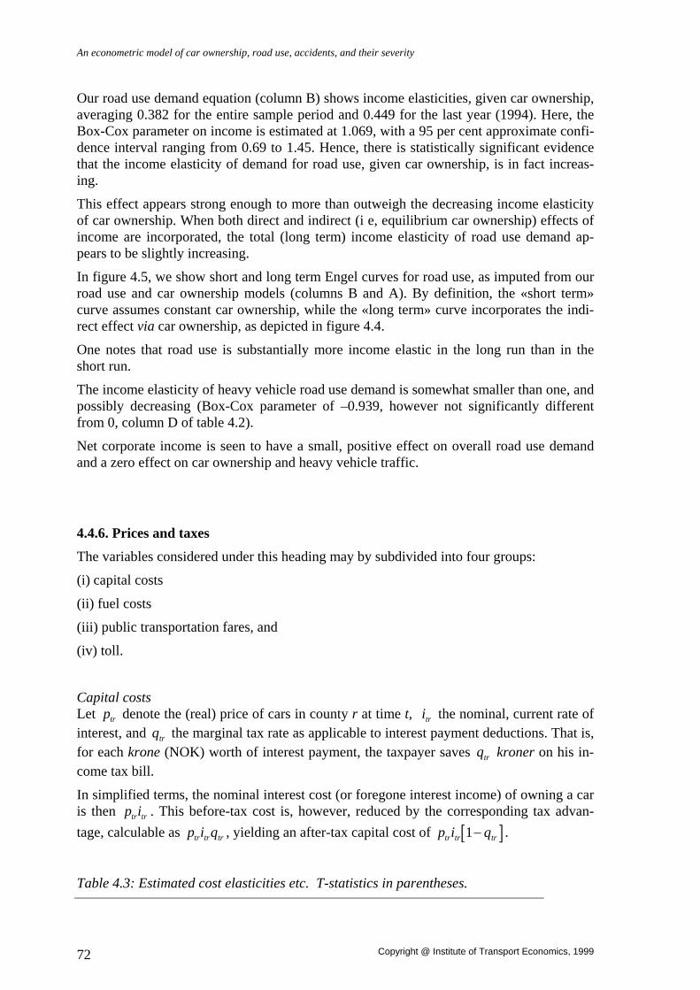
An econometric model of car ownership, road use, accidents, and their severity
Copyright @ Institute of Transport Economics, 1999 72
Our road use demand equation (column B) shows income elasticities, given car ownership, averaging 0.382 for the entire sample period and 0.449 for the last year (1994). Here, the Box-Cox parameter on income is estimated at 1.069, with a 95 per cent approximate confi-dence interval ranging from 0.69 to 1.45. Hence, there is statistically significant evidence that the income elasticity of demand for road use, given car ownership, is in fact increas-ing.
This effect appears strong enough to more than outweigh the decreasing income elasticity of car ownership. When both direct and indirect (i e, equilibrium car ownership) effects of income are incorporated, the total (long term) income elasticity of road use demand ap-pears to be slightly increasing.
In figure 4.5, we show short and long term Engel curves for road use, as imputed from our road use and car ownership models (columns B and A). By definition, the «short term» curve assumes constant car ownership, while the «long term» curve incorporates the indi-rect effect via car ownership, as depicted in figure 4.4.
One notes that road use is substantially more income elastic in the long run than in the short run.
The income elasticity of heavy vehicle road use demand is somewhat smaller than one, and possibly decreasing (Box-Cox parameter of –0.939, however not significantly different from 0, column D of table 4.2).
Net corporate income is seen to have a small, positive effect on overall road use demand and a zero effect on car ownership and heavy vehicle traffic.
4.4.6. Prices and taxes
The variables considered under this heading may by subdivided into four groups:
(i) capital costs
(ii) fuel costs
(iii) public transportation fares, and
(iv) toll.
Capital costs Let ptr denote the (real) price of cars in county r at time t, itr the nominal, current rate of interest, and qtr the marginal tax rate as applicable to interest payment deductions. That is, for each krone (NOK) worth of interest payment, the taxpayer saves qtr kroner on his in-come tax bill.
In simplified terms, the nominal interest cost (or foregone interest income) of owning a car is then p itr tr . This before-tax cost is, however, reduced by the corresponding tax advan-tage, calculable as p i qtr tr tr , yielding an after-tax capital cost of [ ]p i qtr tr tr1− .
Table 4.3: Estimated cost elasticities etc. T-statistics in parentheses.

Chapter 4: Aggregate car ownership and road use
Copyright @ Institute of Transport Economics, 1999 73
Dependent variable: Aggregate car owner-
ship
Total vehicle kilometers
Total vehicle kilometers
(reduced form)
Heavy vehi-cle kilome-
ters
Column: A B C D Elasticities evaluated at the 1974-94 means (1st line) and at the 1994 means (2nd line) ------------- Capital costs ------------- Nominal interest epcncc -.064 cost of -.048 cars before tax (-46.18) Tax advantage cpcncctx .057 corresponding .021 to car (72.28) ownership interest cost ---------- Fuel costs ---------- Real price epg95r -.017 of 95 octane -.018 gasoline (NOK (-9.47) 1995 per liter) Mean fuel cost per cpgaar -.151 -.221 gasoline -.112 -.171 vehicle km (NOK 95) (-12.72) (-10.89) LAM 2 LAM 2 Weighted cpdaarrelv -.184 .138 ratio of diesel to -.238 .178 gasoline mean (-8.72) (4.83) vehicle km cost Variable km cpdahr -.668 cost for heavy -.665 diesel vehicles (-12.52) (fuel + tax, NOK 95) LAM 2 Weighted cpgahrrelv -.373 ratio of gasoline -.329 to diesel heavy (-7.39) vehicle km cost Ratio of cpdrelhsea .786 non-road diesel price .798 to heavy diesel (18.38) vehicle km cost LAM --------------------------- Public transportation fares --------------------------- Real subway and cppswir .010 tramway fares .010 (=1 outside Oslo) (9.60) ---- Toll ---- Cordon toll ring in cptollring -.005 -.003 .020 .078 operation in ---------- -.005 -.003 .020 .078 largest city (dummy) (-7.27) (-.14) (.54) (1.11) Curvature parameters LAMBDA(X) - GROUP 2 LAM 2 8.324 7.099 -.316 [4.70] [4.24] [-.69] [4.13] [3.64] [-2.88] LAMBDA(X) cpdrelhsea 6.099 [9.88] [8.26]
Up until 1991, marginal tax rates on net income (and hence on income deductions) varied greatly depending in the income bracket. In the 1970s, the highest marginal tax rate was around 70 per cent. Since 1992, however, an almost uniform tax rate of 28 per cent applies to interest payment deductions. A somewhat lowered tax rate applies to taxpayers resident in the northernmost municipalities (all municipalities in the county of Finnmark and some in northern Troms) (Statistics Norway 1994).

An econometric model of car ownership, road use, accidents, and their severity
Copyright @ Institute of Transport Economics, 1999 74
As our ptr measure, we use, uniformly for all counties r, the consumer price subindex for private car purchases, deflated by the general consumer price index, i e a real price index for private cars (see Central Bureau of Statistics 1991). The interest level itr is measured in terms of the average per annum rate of interest on private loans, again uniformly for all counties (source: Bank of Norway) (see figure 4.6).
Since we lack information on the average tax advantage in effect for the population of each county, we use (as qtr ) the maximum marginal tax rate applicable under the current tax law (figure 4.7), and specify the before-tax nominal interest cost p itr tr and the corresponding (maximal) tax advantage p i qtr tr tr as separate independent variables in the car ownership submodel, i e with separately estimable coefficients. We expect a negative elasticity with respect to the before-tax cost term and a positive one for the tax advantage term, the latter being smaller than the former in absolute value (since many consumers do not pay the maximal marginal tax rate) and decreasing over time (as the marginal tax rate).
These a priori expectations are fully met, as shown in table 4.3. The (equilibrium) elastic-ity with respect to interest cost before tax (epcncc) is estimated at –0.53 (= – 0.064/0.122), as evaluated at the sample means, decreasing to –0.39 in 1994. The tax advantage elasticity (variable cpcncctx) is estimated at 0.47 (=0.057/0.122) on the average, decreasing to 0.17 in 1994.
The general impression is that equilibrium car ownership demand is relatively elastic with respect to the interest level and the tax deduction rate. This relationship is demonstrated in figure 4.8. Here, the upper part shows (January values of) of the ratio between estimated equilibrium car ownership, defined by
(4.7) γβββ λμ ˆˆ~,x~C~ CiCii
)ˆ(triCi
)(tr
Ci == ∑ where ,
and the observed car stock Ctr . The lower part depicts the after tax interest cost of car ownership [ ]p i qtr tr tr1− . One notes a rather clear negative covariation between the two measures. In the 1970s and early -80s, when the after-tax rate of interest was low, the car stock was consistently «too low» compared to the equilibrium level, generating brisk de-mand for new cars. As the recession set in and after tax interest rates soared in the late 1980s and early -90s, the car stock became «too large» for the current capital cost, leading to several years of depressed market for automobiles. From 1994 on, however, capital costs have gone down, boosting the demand for cars.32
32 Our model is, of course, a simplification. Depreciation and capital gains are disregarded, as is also the possible effect of inflation. Attempts to use real rather than nominal interest rates in the capital cost measure, or to include the rate of inflation as a separate variable, gave, however, nonsense results. The econometric evidence is thus that consumers act in response to the larger interest payment cash flows associated with a higher nominal rate of interest, rather than to the real cost of capital. More in-depth studies would be of in-terest here, to verify or refute that Norwegian consumers are subject to some degree of «money illusion».

Chapter 4: Aggregate car ownership and road use
Copyright @ Institute of Transport Economics, 1999 75
TRIO PROJECT: TRULS - an econometric model of road use, accidents and their severityDATE: 97 02 20USER: lef Figure 4.6: Components of car ownership interest cost before tax: real price index for cars (upper part) and average rate of interest on private loans (lower part).
TRIO PROJECT: TRULS - an econometric model of road use, accidents and their severityDATE: 97 02 21USER: lef Figure 4.7: Components of nominal interest cost of car ownership: interest cost before tax (upper part) and highest marginal tax rate on interest payment deductions (lower part)

An econometric model of car ownership, road use, accidents, and their severity
Copyright @ Institute of Transport Economics, 1999 76
TRIO PROJECT: TRULS - an econometric model of road use, accidents and their severityDATE: 97 02 21USER: lef Figure 4.8: Disequilibrium in aggregate car ownership demand: ratio of equilibrium to actual car stock (upper part) and nominal interest cost of car ownership after tax (lower part).
Fuel costs The price of gasoline (epg95r) affects equilibrium car ownership by an elasticity estimated at –0.14 (= – 0.017/0.122), translating into an indirect effect on road use of approximately –0.13. The direct effect of general fuel costs (cpgaar) (figure 4.9)33 on road use is estimated at –0.151, as an average elasticity for the entire sample period, however decreasing to –0.112 in 1994. Thus the total long-run fuel cost demand elasticity is calculable at –0.24 (= – 0.13 – 0.112) as of 1994. Interestingly, the indirect effect (through car ownership) is lar-ger than the direct (short-term) effect, which assumes constant car ownership.
A strongly non-linear effect of fuel costs is evident from the Box-Cox parameter estimate: 8.32. The fuel cost elasticity of demand for road use increases with the cost level. This result is not unreasonable in view of the fact that, for private as well as for commercial road users, fuel represents a higher cost share the higher its price.
33 The fuel cost has a certain spatial variation because of differences in the composition of the county vehi-cle pool.

Chapter 4: Aggregate car ownership and road use
Copyright @ Institute of Transport Economics, 1999 77
TRIO PROJECT: TRULS - an econometric model of road use, accidents and their severityDATE: 97 01 19USER: LEF Figure 4.9: Gasoline fuel cost development. 19 counties 1973-94
TRIO PROJECT: TRULS - an econometric model of road use, accidents and their severityDATE: 97 02 22USER: lef
Figure 4.10: Development of fuel and tax cost for heavy diesel vehicles. 19 counties 1973-94

An econometric model of car ownership, road use, accidents, and their severity
Copyright @ Institute of Transport Economics, 1999 78
TRIO PROJECT: TRULS - an econometric model of road use, accidents and their severityDATE: 97 02 26USER: lef Figure 4.11: Short term and long term road use demand curves as of January 1974. Real price of fuel versus aggregate road use.
TRIO PROJECT: TRULS - an econometric model of road use, accidents and their severityDATE: 97 02 26USER: lef Figure 4.12: Short term and long term road use demand curves as of December 1994. Real price of fuel versus aggregate road use.

Chapter 4: Aggregate car ownership and road use
Copyright @ Institute of Transport Economics, 1999 79
In figures 4.11 and 4.12, we show imputed short and long term demand curves for road use. By analogy to the Engel curves (figure 4.5 above), the «short term» is identified with a constant stock of cars, while in the «long term» aggregate car ownership is assumed to adjust to its equilibrium level.
Again, the model shows a markedly more elastic demand in the long run than in the short. Note, however, that in this case there is a long term adjustment mechanism not taken ac-count of in the model: higher fuel prices represent an incentive to own, use and manufac-ture more fuel economic vehicles. This means that in the long run, aggregate road use de-mand would be slightly less elastic than depicted by figures 4.11 and 4.12.
TRIO PROJECT: TRULS - an econometric model of road use, accidents and their severityDATE: 97 02 26USER: lef Figure 4.13: Development of mean fuel consumption per four-wheeled gasoline vehicle kilometer.
Demand becomes very much more elastic as the price of fuel goes up. At the lower fuel price levels, short run demand is relatively inelastic. It may seem that, for a given stock of cars, there are limits to the amount of car travel undertaken, possibly because the stock of cars is nearing its maximum practical rate of utilization. When the size of the vehicle stock is allowed to adjust to the low fuel price, road use demand is seen to be considerably more elastic.
In figure 4.11, the mean fuel consumption per vehicle kilometer is assumed constant, and equal to the rate calculated for Oslo in January 1974. When the same diagram is drawn for December 1994, the last month in our data set (figure 4.12), clearly steeper demand curves emerge, on account of the improved fuel economy of more recently manufactured cars, but also because gasoline driven heavy vehicles have become much fewer (figure 4.13). The road use demand curve shifts down to its more inelastic range as technology develops in a more fuel efficient direction.

An econometric model of car ownership, road use, accidents, and their severity
Copyright @ Institute of Transport Economics, 1999 80
Note that these demand curves are drawn on the assumption that diesel and gasoline prices (as well as kilometer tax rates, if applicable) all change in the same proportion. Hence, we estimate a general fuel cost elasticity of demand rather than a specific gasoline price effect.
Diesel vehicle fuel cost is another important determinant of road use demand. We capture this effect by means of a variable (cpdaarrelv) expressing the ratio between of the stipulated mean km costs of diesel and gasoline driven vehicles, respectively, weighted by their «nominal annual kilometrage». To be precise, we use as our variable
(4.8) ( )
( )s ks k
s fs f
trDA
trDA
trGA
trGA
trDA
trDA
tD
trA
trGA
trGA
tG
⋅⋅
=⋅ +
⋅
π τ
π,
where ktrGA and ktr
DA are the km costs of gasoline and diesel vehicles, respectively, depen-ding on the (real) prices of gasoline and diesel π t
G andπ tD , and on the average (real) kilo-
meter tax τ trA paid by diesel vehicles. The s and f measures are nominal annual kilometrage
and mean fuel consumption per vehicle km, as defined by formulae (3.6-3.9) of Chapter 3.
On account of this specification, the coefficient of the gasoline fuel cost variable ktrGA
(=cpgaar) has an interpretation as the effect of a general increase in fuel (and kilometer tax) costs, affecting diesel and gasoline vehicles in the same proportion, so that the ratio between their costs remains constant. The added effect of diesel vehicle kilometer costs
increasing more than gasoline vehicle fuel costs is captured by the term s ks k
trDA
trDA
trGA
trGA
⋅⋅
(=cpdaarrelv).
This effect is negative (as expected), quite significant and surprisingly large (elasticity –0.184 over 1973-94). It has been increasing (in absolute value) over time on account of a larger diesel vehicle share of the traffic volume.
For heavy vehicle traffic, we use the kilometer cost of diesel vehicles (cpdahr, figure 4.10) rather than gasoline costs as our main price variable. The elasticity is estimated at –0.668, and slightly decreasing (in absolute value) with the price level (Box-Cox parameter of –0.316).
To account for the cost of operating the heavy gasoline vehicles, we use, by analogy to the relative measure (4.8), the weighted ratio of heavy gasoline vehicle fuel cost to that of heavy diesel vehicles (cpdahrrelv)34:
(4.9) ( )
( )s ks k
s fs f
trGH
trGH
trDH
trDH
trGH
trGH
tG
trDH
trDH
tD
trH
⋅⋅
=⋅
⋅ +
π
π τ
This cost term has an estimated demand elasticity of –0.373, as evaluated at the means for 1973-94. Thus, gasoline prices appear to have a non-negligible influence even on heavy vehicle road use.
As a final fuel cost variable relevant to heavy vehicle road use demand, we use the ratio of the diesel price paid by users outside the road sector to the diesel/tax cost incurred by truckers (cpdrelhsea, figure 4.14). The idea is to capture variations in the competitive ad-
34 Superscript H denotes sum or average across heavy vehicles only rather than across all vehicles.

Chapter 4: Aggregate car ownership and road use
Copyright @ Institute of Transport Economics, 1999 81
vantage of the sea mode relative to road freight carriers35. Changes in the diesel price af-fects not only the input costs of truck companies, but also those of its competitors. In fact, the fuel cost share is typically much larger within the (domestic) shipping trade than for road carriers. Hence sea carriers stand to gain more from a fuel price reduction than do truckers. A lowered diesel price would not necessarily enhance profitability within the road freight sector.
Indeed, our estimate shows a very clear and statistically significant cross-demand effect of this kind. It has the expected (positive) sign.
TRIO PROJECT: TRULS - an econometric model of road use, accidents and their severityDATE: 97 02 02USER: lef Figure 4.14: Ratio of diesel price paid by non-road users to the mean heavy diesel vehicle fuel and tax cost per kilometer. 19 counties 1973-94.
Public transportation fares In an exploratory model version, we included price indices for various public transporta-tion modes of travel, such as subway/streetcar, bus, and airplanes, in an attempt to estimate cross-price elasticities of demand for car travel.
These coefficients generally come out with counterintuitive (i e, negative) effects. We con-clude that the cross-price elasticities are practically zero, as has also been shown in previ-ous studies (Ramjerdi and Rand 1992a, Fridstrøm and Rand 1993), and reestimate the model without most of the cross-demand fare variables.
35 In Norway, ships represent some 77 per cent of the domestic freight ton kilometers carried, versus 19 per cent being hauled by road and only 4 per cent by rail (Rideng 1996:49). Although for many commodities and market segments substitutability between modes is low, a certain cross demand effect must be expected if only in view of the very large aggregate market share held by the sea mode.

An econometric model of car ownership, road use, accidents, and their severity
Copyright @ Institute of Transport Economics, 1999 82
Public transit fares in Oslo (cppswir) may, however, seem to have a small positive effect on car ownership.
Toll Cordon toll rings were introduced in Bergen (Hordaland county) in the beginning of Janu-ary 1986, in Oslo in mid-January 1990, and in Trondheim (Sør-Trøndelag) in mid-October 1991. A (quasi-)dummy36 variable (cptollring) captures whether or not a toll ring is in op-eration in the county’s largest city in a given month. The Oslo toll ring is also assumed to affect the surrounding county of Akershus, from which a large number of people commute every day.
Contrary to common beliefs, the political aim of the Norwegian toll rings is not traffic re-straint in congested areas. Their sole purpose is to raise funds for infrastructure investment. In other words, the strategy has been to relieve congestion through enhanced supply rather than by restraining demand.
The toll rings per se do not seem to have had any significant effect on road use in the af-fected areas. Equilibrium car ownership, on the other hand, appears to drop by an esti-mated 4 per cent (=0.005/0.122) as a result of a toll ring being introduced. However, as mentioned in section 4.4.7 below, these results must be interpreted with some extra cau-tion, since important road infrastructure improvements tend to coincide in time with the toll ring introduction, making it difficult to identify the separate effects of price and quality on demand.
4.4.7. Road infrastructure
A 10 per cent increase in the road capital, as measured by the accumulated investment ex-penditure37, can be expected to increase long-run, aggregate car ownership by about 1.7 per cent (short-term elasticity of about 0.021, to be divided by =γ 0.122, see table 4.4). The effect is highly significant, but should be interpreted with some extra caution, as the road capital has developed very steadily over time (fig 4.15). This variable is thus liable to pick up any close-to-linear trend effect not captured by our other regressors.
36 When the toll ring is in operation only part of the month, the variable is the defined as the share of days during which the toll ring is in effect. 37 Data on the stock of road capital have been obtained in the following way. Benchmark values for the year 1980 were obtained from the national accounts. Based on the annual accounts of the Public Roads Admini-stration, we obtain real annual investment expenditure and add these flows to the 1980 benchmark values, in order to obtain cumulative figures for the subsequent years. Similarly, to compute stock data for the years prior to 1980, we subtract the investment flows occurring during earlier years. Annual expenditure flows are translated into monthly flows simply by dividing by 12.
No allowance is made for capital depreciation. In a manner of speaking, therefore, we assume that the amount of road maintenance being done is just about sufficient to keep existing roads from losing their value.
In the econometric models, we use the capital stock lagged 24 months, since in a majority of cases, a new or improved road is not put into operation until several years after the first investment takes place.
Our data refer to national and county road capital only, i e municipal and private roads are not taken into account. Except for the county of Oslo, these minor roads represent only a small share of the traffic volume.

Chapter 4: Aggregate car ownership and road use
Copyright @ Institute of Transport Economics, 1999 83
TRIO PROJECT: TRULS - an econometric model of road use, accidents and their severityDATE: 97 02 03USER: lef Figure 4.15: Real capital invested in national and county roads, by county.
In the road use demand equations, we decompose the road capital effect into one part in-terpretable as improvements of the existing road network (capital invested per km road length), and one part measuring road network extension (road length relative to the 1980 situation). Both variables are transformed logarithmically (fixing their λ at zero), so that this formulation is in fact a generalization equivalent to an absolute road capital measure only in the case of equality between the two coefficients38.
38 More generally, multiplicative decompositions like this are used in various parts of the model. For in-stance, the road capital term, xtr1
1β , say, is «decomposed» into
4
321
130
30
20
20
2
2
11
ββββ
βr
r
r
r
tr
tr
trtr x
xx
xx
xxx ⋅⎥
⎦
⎤⎢⎣
⎡⋅⎥
⎦
⎤⎢⎣
⎡⋅⎥
⎦
⎤⎢⎣
⎡→ ,
where 1trx is aggregate road capital in county r in month t, 2trx is the length of public roads, 20rx is the length of roads as of 1980, and x r0 3 is the size of the county, as measured in square kilometers. Thus, β 1 measures the effect of capital per km road, β 2 the effect of road extension over time, β 3 the effect of road network density differing between counties, while β 4 is the size effect. In tables 4.4, 4.5 and 4.7, these ef-fects correspond to variables cictprkml24r, cils12t, ailrddnsty, and hoarea, respectively. Note that if β β β β1 2 3 4= = = , all effects except the first cancel out. In all other cases, the decomposition represents a
generalization compared to a model including only 11
βtrx . Also, note that this formulation is only a reparame-
trization of a model in which xtr1 , xtr 2 , and x r0 3 are entered directly – one, however, with a potentially smaller multicollinearity, since there is only one variable capturing variations in size between the counties.

An econometric model of car ownership, road use, accidents, and their severity
Copyright @ Institute of Transport Economics, 1999 84
Table 4.4: Estimated elasticities etc with respect to road infrastructure vari-ables. T-statistics in parentheses. Dependent variable: Aggregate car
ownershipTotal vehicle
kilometersTotal vehicle
kilometers (reduced
form)
Heavy vehi-cle kilome-
ters
Column: A B C D Elasticities evaluated at the 1974-94 means (1st line) and at the 1994 means (2nd line) ------------------- Road infrastructure ------------------- County and national cictl24 .021 road capital, .021 lagged 24 months (36.24) LAM 4 Real fixed capital cictprkml24r -.012 .023 -.032 invested pr km county -.012 .023 -.032 or national road, (-.97) (1.07) (-.38) lagged 24 months LAM 4 LAM 4 LAM 4 Length of cils12t .085 .063 -.207 national and county .085 .063 -.207 roads relative (1.04) (.44) (-.44) to 1980 situation LAM 4 LAM 4 LAM 4 Major infrastructure cisaker -.006 -.011 -.183 improvements ------- -.008 -.016 -.261 affecting Akershus (-.22) (-.25) (-1.67) Major infrastructure cisbergen .038 -.007 -.008 improvements in Bergen --------- .051 -.009 -.011 (1.56) (-.15) (-.07) Major infrastructure cisoslo -.166 -.156 -.188 improvements in Oslo ------- -.276 -.258 -.311 (-4.03) (-2.42) (-2.21) Oslo: the Oslo tunnel cisoslo4 -.024 .113 .080 -.078 ("Fjellinjen") in -------- -.024 .114 .081 -.078 operation (-11.09) (2.70) (1.10) (-.41) Major infrastructure cistroms .035 .059 -.005 improvements in Tromsø -------- .037 .063 -.006 (1.43) (1.55) (-.05) Major infrastructure cistrond .010 .027 -.067 improvements -------- .012 .032 -.079 in Trondheim (.49) (.75) (-.71)
Curvature parameters LAMBDA(X) - GROUP 4 LAM 4 .000 .000 .000 .000 FIXED FIXED FIXED FIXED
The effect of road quality on overall road use demand, given car ownership (column B), is ambiguous, different model formulations providing different sign effects, none of them significant. When car ownership is not controlled for (column C), a small positive (but still insignificant) effect appears (t-value of 1.07, elasticity of 0.023). It seems that although
Similarly, income is specified by means of a three-layer decomposition, obtained by letting xtr1 be aggre-
gate gross personal income, xtr 2 the population size, and 30rx the size of the county surface.

Chapter 4: Aggregate car ownership and road use
Copyright @ Institute of Transport Economics, 1999 85
improvements in the road network have only negligible short-term effects on car use, the long run effect may be to render automobile ownership somewhat more attractive and en-hance the competitiveness of the car mode.
In addition to the general measures of road capital and length, we include a set of special-ized road infrastructure (quasi-)dummies, capturing the rather important infrastructure improvements that have taken place over the last decade in the largest cities. These im-provements are generally financed by the cordon toll rings operating in Oslo, Bergen and Trondheim, or, in the case of Tromsø, by a local fuel tax. Since the introduction of the cor-don toll ring usually coincides more or less accurately with the inauguration of the first major road improvement39, the separate effects of enhanced supply and increased cost are difficult to identify econometrically. This is why, rather than specifying one dummy vari-able for each significant new road section inaugurated, we count the number of such im-provements and include their number in the model.40 (A general toll ring variable is also included in the model, as pointed out in section 4.4.6 above.) Another complication is the likely measurement error inherent in our calculated measures of road use demand (the de-pendent variable), due to the fuel-saving effect of relieved congestion.
By and large, therefore, the sign of these infrastructure effects are a priori uncertain. One notes that they are also generally insignificant by the t-test, with a few exceptions. The number of major infrastructure improvements in Oslo (cisoslo) comes out with a signifi-cant negative sign. This is the likely effect of improved fuel economy owing to relieved congestion. Since the county of Oslo was not represented in the subsample used to derive traffic volumes from fuel sales, we have not been able to neutralize this effect in our data. Hence the traffic generation effect of the Oslo road investment program is unfortunately indeterminate, as far as our analyses can tell. In terms of aggregate fuel consumption and CO2 emissions, however, our results suggest that, in general, the fuel economy effect must have more than offset the traffic generation effect of the Oslo road development plan, at least in the short term.
The important «Oslo tunnel», however, whose extra effect is captured by a separate dummy (cisoslo4), appears to have had a traffic generating effect exceeding any fuel eco-nomic effect.
For heavy vehicles (column D), the Oslo road development plan appears to have had an unambiguously favorable environmental effect, at least within the time perspective covered by our data set (both cisoslo and cisoslo4 have negative coefficients).
In Hordaland county, the road improvement program in Bergen may seem to have had a certain traffic generating effect, large enough to outweigh any fuel economy effect, al-though the uncertainty surrounding these estimates is considerable. Given that the city of Bergen gathers less than half the county population, very large effects are unlikely to be visible at the county level.
39 This is true, in particular, of the single most important infrastructure improvement in Oslo, the Oslo tunnel. 40 A certain amount of arbitrariness is, of course, unavoidable, when one decides what particular road im-provements are to be included in the count. Only projects with a rather noticeable effect on travel times are considered. For Oslo, e g, we count the Vålerengen tunnel northbound and southbound, the Oslo tunnel («Fjellinjen»), the «Ibsen ring» tunnels, the Granfos tunnel, the freeway intersection at Vestbanen, and the Sinsen-Storo freeway development. By far the most important of these, the Oslo tunnel, is in addition ac-counted for by a separate dummy (cisoslo4).

An econometric model of car ownership, road use, accidents, and their severity
Copyright @ Institute of Transport Economics, 1999 86
4.4.8. Spatial differences in road supply
The car ownership and road use demand equations also include a set of variables capturing physical road infrastructure characteristics as measured at the county level in 1977-80. The idea behind these variables is twofold.
First, it seems reasonable to assume that the quality of road supply in a given county would have an impact on travel demand and mode choice within the general population. Im-proved accessibility by road would reduce the disutility of making a trip and enhance the probability that the car (or bus) mode would be preferred.
Unfortunately, no data are available on changes in the regional, physical road characteris-tics over time. We have, however, been able to exploit a comprehensive data base assem-bled by Muskaug (1985), in which the national road network in each county was examined and statistics compiled, not only on the share of road kilometers falling in certain catego-ries as of 1980, but also on the share of vehicle kilometers driven, during 1977-80, on na-tional roads with differing characteristics.
These data offer information on the quality of road supply, as it differs between the coun-ties, at a given point of time. Since these county level characteristics are liable to change only quite slowly, they may be expected, in conjunction with the road capital measures mentioned above, to capture a fairly large part of the relevant variation in road supply over our entire cross-section/time-series sample.
Since, however, there is only spatial and no temporal variation present in these measures, there can be no more 18 variables of this kind (in addition to the constant term) until the space of regional variation (as between the 19 counties) is completely spanned, and the model becomes perfectly collinear.
The second role played by these variables is thus one of possibly neutralizing any meas-urement error with a systematic regional pattern of variation. An important potential source of error of this kind lies in the benchmark data on vehicle kilometers traveled in 1994 (the v rj+
* of equation 3.3), used to inflate our traffic counts from vehicles passed to vehicle kilometers driven countywide. Any error affecting these benchmark values would have translated into our calculated traffic volumes, i e into the dependent variable of our road use submodels.
Because of this potentially double role played by the regional road supply variables, the signs of their coefficients are not entirely predictable. With few exceptions, however, they come out as one would expect from the perspective that they represent regional supply side characteristics, i e with a positive sign.

Chapter 4: Aggregate car ownership and road use
Copyright @ Institute of Transport Economics, 1999 87
Table 4.5: Estimated elasticities etc with respect to spatial road infrastructure measures. T-statistics in parentheses. Dependent variable: Aggregate car
ownershipTotal vehicle
kilometersTotal vehicle
kilometers (reduced
form)
Heavy vehicle kilometers
Column: A B C D Elasticities --------------------------- Road standard as of 1977-80 --------------------------- Density of ailrddnsty .006 -.224 -.119 -.217 public road network (5.49) (-9.71) (-2.90) (-1.33) as of Jan 1, LAM 4 LAM 4 LAM 4 LAM 4 1980 (kms per sq km) Share of aisaccess1 .088 .402 1.633 2.150 national road traffic (26.99) (5.39) (15.55) (4.60) in non-urban LAM 4 LAM 4 LAM 4 LAM 4 environment in 1977-80 Of which on aisaccess2 -.126 -.578 -1.287 -.523 roads with moderate (-27.30) (-6.07) (-8.15) (-.77) frequency of access LAM 4 LAM 4 LAM 4 LAM 4 points (<16 per km) Of which on aisaccess3 -.057 1.004 1.203 -1.528 roads with low (-19.48) (14.16) (9.73) (-2.42) frequency of access LAM 4 LAM 4 LAM 4 LAM 4 points (<11 per km) Of which on aisaccess4 -.147 -.205 -1.070 -2.206 roads with minimal (-46.39) (-2.74) (-9.15) (-4.54) frequency of access LAM 4 LAM 4 LAM 4 LAM 4 points (<6 per km) Weighted aisslwm .173 1.689 4.883 3.003 average speed limit (18.63) (7.63) (14.30) (2.02) on national LAM 4 LAM 4 LAM 4 LAM 4 roads during 1977-80 Share of aiswiderds .013 .054 .718 1.261 national road traffic (10.32) (1.64) (14.15) (5.86) on roads wider LAM 4 LAM 4 LAM 4 LAM 4 than 6 m in 1977-80 Of which on aiswiderrds -.022 .130 .216 -.409 roads wider than 7 m (-30.55) (8.56) (8.24) (-2.63) LAM 4 LAM 4 LAM 4 LAM 4 Of which on aiswxpress .007 -.067 .126 .771 expressways (7.16) (-2.69) (2.86) (3.90) LAM 4 LAM 4 LAM 4 LAM 4
Curvature parameters LAMBDA(X) - GROUP 4 LAM 4 .000 .000 .000 .000 FIXED FIXED FIXED FIXED
Furthermore, it should be noted that the interpretation of these variables as supply charac-teristics is not entirely self-evident. It may be argued that the quantity and quality of roads in a given county is as much a function of road use demand as a measure of exogenous supply: roads are generally built or improved where needed. This would result in a positive partial correlation between road use and road quality, even if there were no feed-back from road supply to demand. Hence we are faced with a classical simultaneity problem.
Against this view it might objected that the available research evidence on the Norwegian road investment decision process points almost unanimously in the opposite diection:

An econometric model of car ownership, road use, accidents, and their severity
Copyright @ Institute of Transport Economics, 1999 88
Within each county, as well as between counties, there appears to be almost no association between the relative benefits derived from competing road investment projects and the respective priorities assigned to them (Elvik 1993 and 1995, Fridstrøm and Elvik 1997, Nyborg and Spangen 1996, Odeck 1991 and 1996). Similar results have been found for Sweden (Jansson and Nilsson 1989, Nilsson 1991).
Now, although very weak associations can be found between benefit and priority setting among the road projects formally considered for implementation, it seems reasonable to assume that the set of projects that are at all put up for consideration is not entirely without regard to road user needs, as perceived by the regional road authorities. Thus, we cannot, on the basis of the abovementioned research, quite rule out the possibility that road use demand does have a long term effect on our «supply» characteristics. The coefficient esti-mates reported in table 4.5 must, therefore, be interpreted with some caution.
Road network density A counterintuitive, negative effect on road use demand is estimated for the density of the public road network (road kilometers per square kilometer county surface - ailrddnsty). By and large, a larger supply of roads, as measured by the density, seems to be associated with a smaller calculated traffic volume. One possible explanation lies in the fact counties with a dense network also tend to have a land use pattern generally generating shorter commuter and service trips, possibly also more bicyclist or walking trips in place of the car mode.
Density of cross-roads and access points The aisaccess variables shown in table 4.5 capture the degree to which the traffic flow on the main (i e, national) roads is not disturbed by traffic to or from interfering roads, drive-ways, or other access points. Thus, the larger the share of traffic taking place in a non-urban environment (aisaccess1), the more competitive is the car mode and the more road use is generated. This effect is particularly large for heavy vehicle traffic (column D of table 4.5).
Outside the urban areas, the frequency of cross-roads and access points has a more am-biguous effect on road use demand (variables aisaccess2 to -4)41.
Average speed limits An interesting effect is revealed by the aisslwm variable - the weighted average speed limit on national roads (i e, weighted by the vehicle kilometers affected). The higher the speed limit, the more competitive is the car mode and the more traffic is generated. A one percent increase in the mean speed limit is associated with an estimated 1.7 per cent increase in road use, given car ownership (column B of table 4.5), and a full 4.9 per cent traffic incre-ment when the car ownership is allowed to change as well (column C).
Alternatively, relying on the «structural model coefficients»42, one may note that the elas-ticity of speed limits on (equilibrium) car ownership is estimated at approximately 1.4
41 Note that all of these variables are entered logarithmically, and in the form of a multiplicative decomposi-tion, such that, if all coefficients were equal, all except the share of the traffic volume taking place on roads with minimal frequency of access points would cancel out.

Chapter 4: Aggregate car ownership and road use
Copyright @ Institute of Transport Economics, 1999 89
(=0.173/0.122, column A), translating into an 1.2 per cent increase in road use when mul-tiplied by the elasticity of road use with respect to car ownership (0.936). This effect must be added to the partial effect of speed limits, given car ownership (column B), resulting in a compound elasticity of (1.7+1.2=) 2.9 per cent.
For heavy vehicle traffic (column D), the speed limit elasticity is estimated at 3.0, i e very similar to the overall effect implicit in the «structural model».
Certain qualifications are in order. First, speed has an effect not only on road use demand, but also on fuel consumption per vehicle kilometer. Given that our dependent variable is essentially an adjusted measure of fuel sales, there is a potential bias involved here. Its sign and size are, however, largely unforeseeable, as they depend on a complex mixture of fac-tors such as (deviations from) fuel-economic speed, traffic congestion and road geometry effects. Recall, secondly, that equilibrium car ownership effects may be subject to a certain bias.
Notwithstanding these objections, there seem to be fairly strong econometric indications that faster roads have the effect of encouraging car ownership and use.
Road width Road use demand appears to be higher in counties with generally wider roads. With two exceptions, all three coefficients have come out positive in all our equations. Note, how-ever, that we cannot unequivocally interpret this as a pure effect of shifts in supply.
4.4.9. Weather and seasonality
Daylight and weather variables are included in our road use models with the double pur-pose of (i) capturing regular seasonal variations and (ii) estimating the immediate effect of weather conditions on road use demand. By the former, we have in mind recurrent patterns of social and economic activity conditioned by the calendar season, while the latter is meant to represent short-term deviations from this cyclical pattern owing to day-to-day meteorological variations.
One cannot, of course, expect to be able to separate these two types of effect with any de-gree of accuracy. To a large extent, seasonality is due precisely to variations in the (nor-mal) weather conditions.
To express seasonality, we use the number of minutes of daylight per day (bnd) and the mean monthly temperature in Oslo (emts00a). The former varies in identical ways through-out each year, but differently in the respective counties. In the northernmost counties, day-light varies from 0 to 24 hours (1440 minutes) per day over the year. By the temperature measure, we intend to capture a seaonality component common to all regions, applying to all counties the temperature recorded in Oslo.
42 Recall that one may regard columns A and B as a structural, two-equation model, and equation C as a reduced form model, in which car ownership has been eliminated as endogenous. These two models consti-tute alternative ways to assess partial effects, when aggregate car ownership is not to be assumed constant.

An econometric model of car ownership, road use, accidents, and their severity
Copyright @ Institute of Transport Economics, 1999 90
Table 4.6: Estimated elasticities etc with respect to daylight and weather vari-ables. T-statistics in parentheses. Dependent variable: Aggregate car
ownershipTotal vehicle
kilometersTotal vehicle
kilometers (reduced
form)
Heavy vehi-cle kilome-
ters
Column: A B C D Elasticities evaluated at the 1974-94 means (1st line) and at the 1994 means (2nd line) -------- Daylight -------- Minutes of bnd .141 .148 .097 daylight per day --- .141 .148 .096 (23.24) (21.58) (15.94) ------- Weather ------- Mean monthly emts00a .068 .067 .047 temperature in .069 .068 .048 Oslo (centigrades) (19.61) (18.12) (14.61) Days with snowfall cmsnowd1s -.025 -.024 -.067 during month, plus one -.025 -.025 -.069 (-8.99) (-8.63) (-28.21) LAM 3 LAM 3 LAM 3 Per cent of snow days cmsnowlotsh .000 .001 .009 with large ----------- .000 .001 .009 snowfall (>5 mms) (.08) (.42) (5.31) LAM 3 LAM 3 LAM 3 Days with frost cmtfrostd1s .010 .012 -.008 during month, .009 .011 -.008 plus one (2.46) (3.03) (-2.62) LAM 3 LAM 3 LAM 3
Curvature parameters LAMBDA(X) - GROUP 3 LAM 3 .591 .544 .445 [3.36] [3.17] [8.92] [-2.33] [-2.66] [-11.13]
These two seasonal indicators turn out highly significant and with the expected sign (table 4.6). Activity levels increase under favorable daylight and weather conditions.
More ambiguous results are found for our remaining three meteorological variables. Snow-fall (cmsnowd1s) tends to depress the traffic volume, although not drastically. We estimate an elasticity of approximately –0.025 between overall traffic volumes and the monthly number of days with snowfall, and about –0.07 for heavy vehicle traffic. Other things be-ing equal, the overall traffic volume is reduced by an estimated 5 per cent in a month con-taining 10 days of snowfall, compared to a snowfree month43. Snowfall is a rather common event in Norway, occurring in more than half the months/counties represented in our data set (figure 4.16).
43 This effect is calculable as follows: ( )[ ]λβ λ /xexp 1−⋅ = 0.95, where we have used β = – 0.0091993, λ = 0.591 (see table B.2 of Appendix B), and x = cmsnowd1s = 11. We add one day to the count of snow days in order to be able to form the Box-Cox transformation without introducing a qualitative shift between zero and one day of snowfall.

Chapter 4: Aggregate car ownership and road use
Copyright @ Institute of Transport Economics, 1999 91
We attempt to estimate the potential extraordinary effect of markedly adverse weather con-ditions by a secondary snowfall variable (cmsnowlotsh) defined as the per cent of snowy days with a large snowfall (more than 5 mms in water form). This variable is, however, not significant, except for heavy vehicle traffic, where its coefficient is positive, but quite small.
Frost, i e the frequency of days with minimum temperatures dropping below 0 °C (cmtfrostd1s), does not seem to depress traffic volumes. Its coefficient estimate is positive, but rather imprecise. The effect, if any, is quite small.
TRIO PROJECT: TRULS - an econometric model of road use, accidents and their severityDATE: 97 01 14USER: lef Figure 4.16: Histogram of snowfall frequency in data set44.
The shape of the relationship between weather variables and the log of the traffic volume is estimated at something close to the square root transformation, the Box-Cox parameter estimate being 0.591 in the overall traffic model and 0.445 in the heavy vehicle traffic model. Both are significantly different from 0 (the logarithmic form) as well as from 1 (the linear form). As one would expect, the elasticity with respect to weather variables in-creases with the initial level of, e g, snowfall frequency: a change from 5 to 10 days of snowfall has a larger impact than a change from 1 to 2, although not 5 times as large.
44 Each bar of the histogram covers two days on the snowfall count scale, except for the left-most bar, which represents the number of months/counties with zero days of snowfall.

An econometric model of car ownership, road use, accidents, and their severity
Copyright @ Institute of Transport Economics, 1999 92
4.4.10. Calendar events
Under this heading we enter a few variables expressing calendar variations, such as the length of the month (ekd), vacationing (ekvhsh), beginning and end of Easter (ekes, ekee), and a dummy for December (ekm12), capturing the effect of the Christmas shopping sea-son. Their coefficients are all highly significant and show the expected sign.
Longer months have larger traffic volumes, although the relationship is somewhat less than proportional. In general, less traffic is generated during the holiday seasons. Easter begin-ning or end, however, tends to inflate traveling by road by some 5 per cent. The Christmas season boosts traffic by an estimated 28 per cent (= e0.248–1), compared to a hypothetical «normal» month with a similar number of holidays.
Certain studies have shown strikingly reduced accident rates during spectacular media events, notably during the Gulf war in January-February 1990. Indeed, it has been hy-pothesized that more American lives may have been saved on the roads due to this war than were lost on the battleground, most probably because people reduced their exposure in order to follow the events on television.
To capture any such effect, we include a variable (ezgulfwar) defined as the number of days of Gulf war during the month. It is, of course, zero for all months prior to January 1990 or after February 1990. Its coefficient is negative, as expected, but small, and significant only in the heavy vehicle traffic model.
4.4.11. Geographic characteristics
Larger counties generate more traffic, although the relationship is somewhat underpropor-tional (variable hoarea, elasticity 0.825, column B of table 4.7). Note that population den-sity is also included in the model, so that this elasticity has an interpretation as the effect of population and geographic size increasing proportionately. The population density elastic-ity was estimated at 0.907 (see section 4.4.3). For a given population, the effect of ex-tended geographic size is thus calculable at –0.082 (= 0.825 – 0.907) for overall traffic volumes and at –0.299 (= 0.875 – 1.174) for heavy vehicle traffic. In other words, it is not true that sparse populations generate more road transportation per capita than densely populated regions, as one might expect in view of the generally longer distances to be overcome in the more peripheral districts.

Chapter 4: Aggregate car ownership and road use
Copyright @ Institute of Transport Economics, 1999 93
Table 4.7: Estimated effects of calendar events, geography etc. T-statistics in parentheses. Dependent variable: Aggregate car
ownershipTotal vehicle
kilometersTotal vehicle
kilometers (reduced
form)
Heavy vehi-cle kilome-
ters
Column: A B C D «Elasticities» -------- Calendar -------- Length of month (days) ekd .697 .710 .475 (18.59) (18.62) (12.66) LAM 4 LAM 4 LAM 4 Dummy for ekee .048 .054 .011 end of Easter ==== (10.83) (12.95) (2.82) Dummy for ekes .055 .052 .027 start of Easter week ==== (12.04) (12.32) (7.25) December (dummy) ekm12 .248 .245 .160 ===== (41.40) (41.75) (34.52) Share of vacation and ekvhsh -.290 -.298 -.279 holidays during month (-38.80) (-40.57) (-44.56) (excl summer vacation) LAM 4 LAM 4 LAM 4 Days of Gulf war ezgulfwar -.017 -.022 -.051 --------- (-1.36) (-1.75) (-4.20) --------- Geography --------- Østfold hcounty1 .045 .031 .416 ======== (3.67) (1.36) (3.96) Oslo hcounty3 .702 .751 .486 ======== (3.60) (2.23) (1.51) Kms mainland hseaccess1 -.008 -.105 coastline per 1000 (-48.08) (-4.20) sq kms surface LAM 4 LAM 4 County hoarea .101 .825 .727 .875 surface area (sq kms) (56.95) (83.79) (44.80) (9.62) LAM 4 LAM 4 LAM 4 LAM 4
Curvature parameters LAMBDA(Y) - GROUP 4 LAM 4 .000 .000 .000 .000 FIXED FIXED FIXED FIXED
Equilibrium car ownership appears to grow more than proportionately with population size, but is practically unaffected by geographic size per se, for a given population (elastic-ity –0.066 = (0.101 – 0.109)/0.122).
The competitive advantage of road transportation with respect to other modes may be thought to depend on certain natural geographic conditions, such as access to the sea and/or topographical obstacles to road construction or use. In some Norwegian counties, fiords and inlets represent important barriers to traveling by road, while at the same time facilitating alternative seaway transportation. We attempt to capture these effects by means of a proxy (hseaccess1), entered into the car ownership and heavy vehicle traffic models,

An econometric model of car ownership, road use, accidents, and their severity
Copyright @ Institute of Transport Economics, 1999 94
and defined as the length of the (mainland) coastline in relation to the surface area (kms per square km). For the two landlocked counties (Hedmark and Oppland), this variable is zero.
Its coefficient is significant in both models and has the expected negative sign. A ten per cent longer coastline is associated with a 1.2 per cent smaller heavy vehicle traffic volume, presumably because of enhanced competition from the sea mode and/or more costly trans-portation by road.
Equilibrium car ownership also appears to be slightly smaller in counties with a longer shoreline (elasticity –0.065 = –0.008/0.122).
A large dummy coefficient is estimated for the county of Oslo (hcounty3). Note, however, that this variable does not have any subject matter interpretation, since it only serves to neutralize a number of measurement inconsistencies affecting certain independent vari-ables, notably the road infrastructure variables. Here, data are generally missing for the capital county and set at some arbitrary value in the data base45.
The dummy coefficient for Østfold county (hcounty1), however, is interpretable as the ef-fect of being the main county of transit for international road transportation. This effect is estimated at about 5 per cent (= e0.045 – 1) for the total traffic volume and a full 52 per cent (= e0.486 – 1) for heavy vehicle traffic. Since the heavy vehicle traffic share in Østfold hov-ers between 12 and 20 per cent, the entire effect on total traffic appears to be due to the added freight transportation activity.
4.4.12. Heteroskedasticity
In the car ownership model, we have included a heteroskedasticity variable (exjanuaryxp) defined by
ztrz
11 1( )λ = for January, otherwise ztr
z1
1 0( )λ = ,
with coefficient
ζ ζ1 10 0 1= − = ∀ >, i i
(confer equation 2.4, repeated in section 4.2 above).
This is tantamount to multiplying the variance of all observations other than those for January by a factor of 2202610 =e , thereby allowing them virtually no weight in the esti-mation. We do this because aggregate car ownership is actually measured only once a year (as of January 1st), all other observations in our data base being «artificial» values, inter-polated between January stocks.
In the road use models, we specify a heteroskedasticity structure depending on two exoge-nous variables – distance of dependent variable extrapolation (ekxtrapltxp) and the number of vacation days (ekvhis).
45 The county of Oslo consists of only one municipality. There are therefore no county roads, only national and municipal roads. Also, unlike all the other counties, municipal roads in Oslo carry a major share of the traffic volumes (more than 50 per cent), rendering statistics on national road infrastrucure and traffic less relevant than for the other counties.

Chapter 4: Aggregate car ownership and road use
Copyright @ Institute of Transport Economics, 1999 95
Table 4.8: Disturbance (co)variance structure in car ownership and road use equations. Coefficient assumptions and estimation results, with t-statistics in pa-rentheses. Dependent variable: Aggregate car
ownershipTotal vehicle
kilometersTotal vehicle
kilometers (reduced
form)
Heavy vehicle kilometers
Column: A B C D ζ coefficients Exponential of ekjanuaryxp -10.0 dummy for January FIXED LAM Exponential of ekxtrapltxp .590 .640 .521 extrapolating (11.40) (11.72) (12.21) distance from fuel LAM LAM LAM use submodel sample Number of ekvhis .097 .083 .027 vacation days, (31.17) (27.90) (8.55) including LAM LAM LAM summer vacation
Curvature parameters ( ziλ ) LAMBDA(Z) ekjanuaryxp .000 FIXED LAMBDA(Z) ekxtrapltxp .000 .000 .000 FIXED FIXED FIXED LAMBDA(Z) ekvhis 1.000 1.000 1.000 FIXED FIXED FIXED
Autocorrelation parameters ( jρ )
1st order 1ρ .336 .463 .526 (23.96) (33.68) (45.47)
2nd order 2ρ .106 .262 .458 (7.12) (18.83) (39.77)
12th order 12ρ -.129 (-22.29)
Recall that our independent variables in the road use models are calculated values based on a subsample of traffic counts, fuel sales etc covering the period 1988-94 (see chapter 3). For all years prior to 1988, the calculated values are, in a sense, constructed by (backward) extrapolation. The imprecision affecting these extrapolated values may be expected to in-crease with the distance of extrapolation, as is also suggested by figure 3.9 to 3.12 of chap-ter 3, which show a widening gap between alternative model versions as we move back-wards in time from 1988.
Since we have no a priori knowledge of the rate at which this imprecision would increase with the distance of extrapolation, we exploit the data and the BC-GAUHESEQ software to estimate it. The estimated coefficient (ζ 1 in equation 2.4) has the expected (positive)

An econometric model of car ownership, road use, accidents, and their severity
Copyright @ Institute of Transport Economics, 1999 96
sign and a numerical value implying that a 40 to 45 per cent lower weight is assigned to the first observations (January 1973), compared to the period 1988-9446.
Vacation times are assumed to affect the road use model variance for the same reasons as stated in section 3.7.5 above. In some counties, the influx of tourist serves to inflate the traffic volume, while in other counties this effect is more than offset by reduced business activity and out-of-county vacationing.
The vacation variable is also highly significant with the expected positive sign. Its coeffi-cient value implies that, by and large, observations from July receive only about 20 per cent of the weight assigned to months not affected by holidays.
4.4.13. Autocorrelation
In the road use models, we allow 1st and 2nd order autocorrelation terms to be estimated. They all come out positive and strongly significant, particularly in the heavy vehicle road use model, where they sum to almost one (table 4.8).
In the car ownership model, the autocorrelation parameter is negative (see section 4.4.1 above)
4.5. Summary and discussion
We have estimated aggregate car ownership and road use demand functions using a proce-dure allowing for estimably non-linear relationships between the dependent and several independent variables. We use a combined cross-section/time-series data set covering all 19 Norwegian counties and all months from 1973 through 1994.
A salient finding relates to the key role played by the car ownership variable. Unless one explicitly models the demand for cars, one is not likely to capture some of the most impor-tant behavioral relations bearing on road use demand. This is so because many variables having small, short-term effects on road use given car ownership, turn out to have large, long-term effects on (equilibrium) car ownership itself. These variables include interest rates, tax rates, fuel prices, and road infrastructure quality.
Road use tends to increase more or less in proportion with car ownership. There is little sign of increased car ownership leading to reduced distance traveled per car. Thus, any policy aimed at influencing road use demand would seem to be misguided in ignoring car ownership effects. Even if road use should be the main target variable, say from an envi-ronmental point of view, some of the more efficient policy measures would probably be directed at car ownership rather than use.
46 Technically, the ekxtrapltxp variable is defined as [ ]t)tt,(maxexpztr −+= 101 and its Box-Cox parameter as 01 =zλ , where 180=t is the number of months from January 1973 ( 1=t ) until January 1988 ( 181=t ).
For 1=t – our first month of observation – we have, in the overall traffic model, ( )[ ] 118018011 == explnz )(
trzλ
and ( )( ) 8015902011
1 .ezexp .tr
z ==λζ , i e an 80 per cent inflated standard deviation, corresponding to a relative weight of 0.55=1/1.80. (The exponential and logarithmic transformations canceling each other out may seem unnecessary, but are used in order to avoid numerical overflow in the algorithm.)

Chapter 4: Aggregate car ownership and road use
Copyright @ Institute of Transport Economics, 1999 97
The Box-Cox regression modeling approach reveals strongly non-linear quantity-price relationships but almost linear Engel functions. The fuel price elasticity of demand is small (in absolute value) at the lower end of the price spectrum, but quite high in the upper range. The impact of, e g, fuel taxes would, therefore, increase far more than proportion-ately with the level of taxation imposed.
The long term income elasticity of demand for road use appears to be somewhat larger than one, and apparently increasing with the income level. This finding may seem to have important and rather discouraging implications with respect to the goal of sustainable mo-bility. There is no sign of aggregate road use growth tapering off as the economy continues to grow – rather the contrary.
Certain qualifications are, however, in order, especially as regards the car ownership par-tial adjustment model, which undoubtedly could be improved upon. Our method of estima-tion is not necessarily consistent, and a small error in the estimation of 1− γ translates into a relatively large bias affecting the estimate γ . Experimentation shows that this estimate is rather sensitive to even moderate changes in the set of regressors. However, the equilib-
rium effect parameters γββ ˆˆ~CiCi = seem much more robust that its respective components
γ and Ciβ . These two tend to move in the same direction under varying model specifica-tions, leaving the ratio and hence the equilibrium elasticities more or less unaffected.
The rather large discrepancy imputed, for most sample points, between equilibrium and actual car ownership (up to 70 per cent according to figure 4.8) may suggest that the partial adjustment parameter is, indeed, underestimated. Moreover, the fact that this discrepancy is almost invariably positive suggests that a more sophisticated, asymmetric adjustment mechanism might be more appropriate. There may seem to be much less compelling rea-sons why the car stock cannot momentarily adjust itself upwards than downwards. Cars may be bought, but not easily sold, abroad. Thus, a switching modeling approach, distin-guishing between positive and negative disequilibrium regimes, and implying faster up-wards than downwards adjustment, might turn out to be more realistic.
In general, since all our estimation results rely on a homogeneity assumption regarding the respective effects of spatial versus temporal variation, our conclusions hinge on the appro-priateness of this assumption. For variables whose sample variation is predominantly cross-sectional, particular caution should be observed when extrapolating effects over time.
Alternative estimation methods or modeling techniques have, however, been beyond the scope of this study.

An econometric model of car ownership, road use, accidents, and their severity
Copyright @ Institute of Transport Economics, 1999 98

Chapter 5: Seat belt use
Copyright @ Institute of Transport Economics, 1999 99
Chapter 5: Seat belt use
5.1. Motivation
Seat belts are perhaps the single most important road safety measure introduced in indus-trialized societies in the postwar period. Studies suggest that seat belts may cut the injury or death risk by some 50 per cent, perhaps even more (Elvik et al 1989).
In Norway, seat belt use (among car drivers) has risen from around 20-30 per cent in the early 1970s to about 80 per cent in the 1990s, according to roadside surveys (Fosser 1995). This large increase may be thought to have had a considerable effect on the road casualty toll, explaining, perhaps, in large part the downward casualty trend observed in the 1970s and -80s.
In this chapter, we present a pair of submodels predicting urban and rural seat belt use, respectively, as functions of relevant exogenous variables. The motivation for these sub-models is threefold.
First, seat belt use is not an exogenous variable with respect to the accident generating pro-cess. At the micro level, wearing a seat belt or not is a choice made by the individual driver or passenger, depending on a multitude of factors, many of which may also have separate, direct effects on risk (such as road surface conditions or geometry, vehicle crashworthi-ness, or driver experience). Seat belt use is an important behavioral variable, and it is en-tirely possible that car occupants may use seat belt wearing as one of their instruments of behavioral adjustment (risk compensation), for instance by relaxing their seat belt use in situations perceived as less risky (see section 6.1 below). We would like to estimate such relationships rather than including observed seat belt use as an (erroneously assumed) ex-ogenous factor in our accident submodels.
Second, seat belt wearing is to a large extent conditioned by truly exogenous, politically determined laws and regulations, the effects of which we would like to estimate, as these represent highly policy relevant pieces of information.
Third, seat belt use is not generally an observed variable (at the level of county and month during 1973-1994), although a fairly large number of roadside sample surveys exist, split-ting the car drivers passing a given point on a certain day between seat belt users and non-users (Fosser 1978, 1979, 1990 and 1995). However, these estimates are subject to random sampling error and also, as applied to our countywide, monthly units of observations, to an incalculable systematic error originating from the non-random sampling of roadside survey points. Fortunately, these survey points remain fixed from one survey to the other, so that the temporal variation in estimated seat belt use frequency is not, in the same way as its level, affected by the process of survey point determination.
By fitting a model to this incomplete set of observations and then imputing values for all units of observations in our cross-section/time-series data set, we obtain a fairly well-founded set of measures on seat belt use by county and month, in which sampling errors have been «smoothed out» and the structural information on exogenous laws and regula-tions has been exploited and incorporated.

An econometric model of car ownership, road use, accidents, and their severity
Copyright @ Institute of Transport Economics, 1999 100
5.2. Seat belt use sample surveys and regulations
Road side surveys of seat belt use have been conducted more or less regularly since 1973, quite frequenly in the 1970s, but no more than annually since 1981. Surveys are made at fourteen predetermined points of the road network, seven of which are located in built-up areas (henceforth referred to as «urban» surveys), while the remaining seven are done in a «rural» (i e, non built-up) environment. The following eight counties are represented in the sample: Oslo (urban survey only), Akerhus (rural survey only), Hedmark, Vestfold, Vest-Agder, Hordaland, Sør-Trøndelag, and Troms.
The crude seat belt use frequencies observed in these surveys are shown in figures 5.1 and 5.2, in which the most important laws and regulations applying are indicated by vertical lines. Since January 1st, 1971, front seat belt installation has been mandatory in all new cars. Thus, seat belt installation has gradually penetrated into the car stock at a rate deter-mined by new car acquisitions and scrapping (figure 5.347). From September 1975, seat belt use has been mandatory for car drivers and front seat passengers above the age of 15, when riding in a car equipped with belts. Since October 1979, car drivers and front seat passengers not wearing a seat belt have been subject to a ticket fine, the (nominal) value of which was set at NOK 200 at its introduction, increased to NOK 300 in January 1987 and to NOK 500 in March 1993. Its real value has, however, generally not increased over time. Brisk inflation during the 1980s served to reduce the real value of the ticket by almost 50 per cent between 1979 and 1987 (figure 5.4).
One notes from figures 5.1 and 5.2 that the seat belt use has increased in two big leaps: one when seat belt use became mandatory, and another when non-use first became subject to a penalty. Interestingly, the latter leap appears to have been bigger than the former. There are, however, clear signs of decreasing seat belt use in the nearest periods following the two big leaps.
One also notes that urban seat belt use is generally much inferior to rural seat belt use, es-pecially in the earliest part of the period.
5.3. A logit model of seat belt use
We shall estimate the relationships between seat belt use and exogenous regulations etc using a Box-Cox logit model of the form
(5.1) )R,Uj(uxS
SlnL trj
i
)(triij
trj
trjtrj
ij =+=⎟⎟⎠
⎞⎜⎜⎝
⎛
−≡ ∑ λβ
1
47 From 1992 on, we assume all cars are to have front seat belts installed. Our data source does not keep track of vehicle age for more than 20 years, hence from 1992 on we are unable to calculate the (small) per-centage of cars older than 1971.

Chapter 5: Seat belt use
Copyright @ Institute of Transport Economics, 1999 101
TRIO PROJECT: TRULS - an econometric model of road use, accidents and their severityDATE: 97 03 01USER: lef Figure 5.1: Urban seat belt use survey results
TRIO PROJECT: TRULS - an econometric model of road use, accidents and their severityDATE: 97 03 01USER: lef Figure 5.2: Rural seat belt use survey results

An econometric model of car ownership, road use, accidents, and their severity
Copyright @ Institute of Transport Economics, 1999 102
TRIO PROJECT: TRULS - an econometric model of road use, accidents and their severityDATE: 97 01 20USER: lef Figure 5.3: Front seat belt penetration rates 1973-94 in 19 counties
TRIO PROJECT: TRULS - an econometric model of road use, accidents and their severityDATE: 97 01 20USER: lef Figure 5.4: Real value of ticket fine for not wearing seat belt

Chapter 5: Seat belt use
Copyright @ Institute of Transport Economics, 1999 103
where StrU and StrR are the observed urban and rural seat belt use shares, as estimated in the sample surveys, Ltrj are the corresponding log-odds, xtrj are exogenous variables, λ ij are Box-Cox parameters, β ij are coefficients and the utrj are heteroskedastic error terms.
When the elasticities calculated within this model are to be interpreted, one must keep in mind that the dependent variable has been defined, not as a belt use share, but in terms of its log-odds. To be specific, we have
(5.2) [ ]El L x xLtrj tri ij
tri
trj
ij
; = βλ
and
(5.3) [ ] ( ) [ ]El S x SS
SEl L xtrj tri trj
trj
trjtrj tri; ln ;= −
−
⎛
⎝⎜
⎞
⎠⎟ ⋅1
1
(5.4) ( )= − ⋅ ⋅1 S xtrj ij triijβ λ
That is, to obtain the elasticity of the seat belt share with respect to some independent vari-able xtri , one has to multiply the log-odds elasticities shown in table 5.1 ( [ ]= El L xtrj tri; ) by one minus the belt use share and by its log-odds. At the 50 per cent rate of seat belt use, these factors reduce to one half, meaning that the log-odds elasticity is interpretable as twice the elasticity of belt use share with respect to the independent variable. As the level of seat belt use increases (towards 100 per cent), elasticities are bound to decline.
As for the error terms, it can be shown (see, e g, Fridstrøm 1980:41) that the log-odds of a binomial share ( Strj , say) has an approximate variance given by
(5.5) ( )var lnS
S n S S n S Strj
trj trj trj trj trj trj trj11 1 1
111−
⎛
⎝⎜
⎞
⎠⎟
⎧⎨⎪
⎩⎪
⎫⎬⎪
⎭⎪≈ +
−
⎡
⎣⎢⎢
⎤
⎦⎥⎥
=−
where ntrj denotes the number of binomial trials (in our case: the survey sample size), and
(5.6) [ ]S E Strj trj=
is the expected value under random sampling, i e the share of – in this case – seat belt users in the population at time t in county r. One may estimate this variance using the sample shares in lieu of the unknown population values, i e by
(5.7) ( ) ( )trjtrjtrjtrj
trjtrj SSnS
Slnravurav
−≈
⎪⎭
⎪⎬⎫
⎪⎩
⎪⎨⎧
⎟⎟⎠
⎞⎜⎜⎝
⎛
−=
11
1,
which is the heteroskedasticity specification chosen for our seat belt use model48. Inciden-tally, the optimal weights
48 In some cases, the sample size data trjn are missing, in which case we use the average sample size re-corded for the survey point in question, as reckoned over all sample surveys taken. Since the survey points are geographically fixed and all surveys have been done in roughly the same way (counting all cars passing

An econometric model of car ownership, road use, accidents, and their severity
Copyright @ Institute of Transport Economics, 1999 104
(5.8) ( )[ ] ( )trjtrjtrjtrj SSnurav −=− 121
corresponding to this heteroskedasticity structure coincide with the weights implicit in the socalled minimum logit chi-square estimator developed by Berkson (1944, 1953, 1955) (see also Bishop et al 1975:355).
5.4. Empirical results
Estimation results are shown in table 5.1. The submodel for urban seat belt use is shown in the left data column and the rural submodel in the right. For each independent variable, we report the log-odds elasticity as evaluated at the overall (1973-94) sample means, the log-odds elasticity as evaluated at sample means in 1994, and the conditional t-statistic. Box-Cox parameters are reported at the end of the table.
All independent variables are highly significant and their coefficients have the expected sign.
The percentage of cars having front seat belts installed (cvsbfrontpc) has an obvious effect on seat belt use. In terms of elasticities, the effect is much stronger in the urban setting than in the rural, but this is so only on account of the lower initial level of use in the built-up areas. The Box-Cox parameters put on this variable are estimated at 0.035 in the urban submodel and at –0.345 in the rural case, suggesting logarithmic or even more strongly downward bending relationships.
The law requiring drivers to wear seat belts whenever installed (eldbelt1) also has a very clear effect, adding 0.46 and 0.64 to the urban and rural seat belt use log-odds, respec-tively.
The real value of the penalty for not wearing a seat belt when required by law (esfbeltr) has an estimated log-odds elasticity, as of 1994, of 1.43 in the urban case and 0.52 in the rural case. Given an approximate, initial level of urban seat belt use of 70 per cent, a ten per cent increase in the fine level would, according to this model, lead to an about 2.5 percentage point increase in urban seat belt use (from 70 to 72.5, by formula 5.3). The elasticity is, however, decreasing with the initial fine level (urban/rural Box-Cox parameters of –0.485 and –1.272, respectively)49.
on an ordinary workday between 8 a m and 4 p m), the sample sizes turn out to be comparatively stable from one time point to the next, but differ considerably between survey locations.
Technically, we also exploit the BC-GAUHESEQ heteroskedasticity facility to practically weed out the ob-servations for which no sample surveys exist, setting the variances of these observations at e10=22026. Road-side seat belt surveys are available for about 350 out of our 5016 sample points. For the remaining part of the sample, artificial seat belt use data have been constructed by averaging over all counties and interpolating between survey dates. On account of the very large «variance» imposed for these data points, they have, however, negligible effects on our parameter estimates. 49 In the model, the ticket variable has an «associated dummy», defined equal to one whenever the fine is strictly positive (i e, from October 1979). On account of this dummy, the Box-Cox transformation is not constrained to pass through the point (1, 0) (0 being the Box-Cox transformation of 1, for any Box-Cox pa-rameter), and the curvature is estimated on the basis of the strictly positive values only. Put otherwise, the level of seat belt use observed prior to the introduction of a penalty affects neither the slope nor the curva-ture, only the associated dummy coefficient.

Chapter 5: Seat belt use
Copyright @ Institute of Transport Economics, 1999 105
Table 5.1: Estimated elasticities etc in seat belt use mod-els. T-statistics in parentheses. Dependent variable: Urban seat belt
use log-odds
Rural seat belt use
log-odds «Elasticities» evaluated at 1973-94 sample meanse (1st line) and at 1994 means (2nd line) -------- Vehicles -------- Per cent of cars with cvsbfrontpc 2.662 .302 mandatory front 1.489 .223 seat belts installed (129.35) (48.60) LAM LAM -------------------- Legislative measures -------------------- Seat belt use eldbelt1 .892 .463 mandatory for ======== .495 .373 driver and adult (47.73) (71.94) front seat passenger ----------------------------------------- Financial safety incentives and penalties ----------------------------------------- Real value of esfbeltr 5.150 2.178 ticket fine for -------- 1.431 .515 not wearing (120.11) (113.26) seat belt (NOK 1995) LAM LAM Dummy for esfbeltr -101.656 -1407.639 ticket fine ======== -56.364 -1131.413 in existence (-117.72) (-113.21) ------------------- Publicity campaigns ------------------- Ongoing road safety ezibipe1 .416 .045 campaign ======== .000 .000 through 1974 and 1975 (32.33) (8.16)
Curvature parameters LAMBDA(X) cvsbfrontpc .035 -.345 [1.28] [-4.76] LAMBDA(X) esfbeltr -.485 -1.272 [-5.34] [-10.21]
The falling real value of the ticket seems to a large extent to explain the apparently declin-ing seat belt use rates through the early 1980s.
Our final independent variable (the dummy ezibipe1) is meant to capture the effect of the widespread publicity surrounding the enaction of mandatory seat belt use in 1975. Exten-sive publicity campaigns and a vivid public debate took place, in which even opponents to the seat belt legislation argued adamantly in favor of belt use, in the hope that increased voluntary seat belt wearing might convince politicians that legislative measures were un-necesary. Once the law had come into effect, publicity diminished, and so – apparently – did seat belt use.

An econometric model of car ownership, road use, accidents, and their severity
Copyright @ Institute of Transport Economics, 1999 106
TRIO PROJECT: TRULS - an econometric model of road use, accidents and their severityDATE: 97 01 31USER: lef Figure 5.5. Imputed county-wide mean rates of seat belt use. 19 counties 1973-94
5.5. Imputed seat belt use
To derive an overall (urban-rural) seat belt use rate for each county and month, we proceed as follows. Let ar denote the share of vehicle kilometers taking place in built-up («urban»)
areas, as recorded in county r during 1977-80, and let trUS and trRS denote the fitted val-ues obtained by plugging the estimates of β ij and λ ij into equation (5.1) and solving for Strj . The mean rate of seat belt use in county r during month t (cbbeltuse) is calculated as
(5.9) ( ) trRrtrUrtrA SaSaS −+= 1 .
Hence, for every county, imputed urban and rural seat belt rates are weighed together in a particular way throughout the observation period. In Oslo, all traffic is assumed to take place within built-up areas, implying considerably lower imputed seat belt use rates than in the other counties. The mean, county-wide imputed seat belt use rates are shown in figure 5.5.
At the outset of this research, our ambition had been to estimate, not only the effects of legislative measures, but also the possible effects of various risk or safety factors, for which the road users might be suspected to compensate by wearing (or not wearing) their seat belt. Unfortunately, our data did not turn out to be sufficiently accurate or disaggre-gate for such an exercise. Efforts to link the observed seat belt use rate to monthly weather conditions, county-wide traffic density measures or road infrastructure variables gave only quite inconsistent and unstable results. This should come as no surprise, since the condi-
Chapter 5: Seat belt use
Copyright @ Institute of Transport Economics, 1999 107
tions prevailing at the exact time and location of the survey need not resemble the average value observed for the county or month in question.
Our imputed rate of county-wide seat belt use summarizes the information available on legislative measures aimed at seat belt use and on the effectiveness of these measures. In view of this, it seems fairly reasonable to treat it, in our subsequent modeling of accident and casualty rates, as an exogenously determined factor. It should not be interpreted as a measure of how actual seat belt use adapts to short term changes in the traffic environment.

An econometric model of car ownership, road use, accidents, and their severity
Copyright @ Institute of Transport Economics, 1999 108

Chapter 6: Accidents and their severity
Copyright @ Institute of Transport Economics, 1999 109
Chapter 6: Accidents and their severity
Road accidents represent tremendous losses to society in general and to the individuals most directly affected in particular. Enhanced knowledge of the accident generating mechanisms operating at the societal level might help improve the effectiveness of the fight against these losses. In this chapter we direct attention to the determinants of road accident frequency and severity.
The chapter is organized as follows.
In section 6.1, we review and discuss, from various facets, the rather important issue of risk compensation (behavioral adaptation), perhaps the most intriguing matter of discus-sion within contemporary road accident research and within safety regulatory policy in general. It is a topic to which the application of microeconomic theory and/or econometric analysis may add important insights. The understanding of risk compensation mechanisms is essential to the assessment of casualty countermeasure effectiveness in general and to the interpretation of econometric model results in particular.
In section 6.2, we review some arguments and issues relating to accidents as seen as an external or internal cost of road use. Such issues are of some relevance to our analysis since some of the econometric estimates to be derived have a direct bearing on the accident externality issue.
Section 6.3 is concerned with the distinction between systematic and random variation in casualty counts and with the various ways to specify either component in an econometric model.
In section 6.4, we present various informal tests, applicable to econometric casualty mod-els, which may be useful in checking for possible omitted variable bias and spurious corre-lation.
The chosen econometric specification is described in sections 6.5 and 6.6, and the empiri-cal results in section 6.7.
6.1. Behavioral adaptation
To fix ideas, while paying respect to chronology, we shall start our discussion of behav-ioral adaptation by a small digression back into Norse mythology50.
6.1.1. Balder’s death – a mythical example
Among all the Æsir (gods) living in Asgard, the home of Norse gods, Balder was the most fair-haired, handsome, and beloved. Everyone would praise him for his wiseness, gentle-ness, and eloquence.
One night, however, Balder had a bad dream, in which his life appeared to be threatened, although in ways he was unable to grasp. To his father, Odin, the highest of all gods, this 50 See, e g, Hveberg (1962) for more detailed account.

An econometric model of car ownership, road use, accidents, and their severity
110 Copyright @ Institute of Transport Economics, 1999
seemed like such a bad omen that he decided to gather all the Æsir in council, to see if there was any way that they could spare Balder of all evil. Frigg, the mother of all things, proposed to make all things swear an oath that they would not harm Balder. All Æsir agreed to this ingenious plan, and Frigg soon went around to all things – fire and water, iron and ores, stone and earth, trees and plants, animals and birds, poison and venom, sick-ness and serpents – so they could take the oath.
As a result of this, Balder’s brothers and the other Æsir noticed that Balder would never since get stung by a needle, cut by a knife, or bruised by a rock. In fact, they realized they were free to throw stones at him, shoot arrows at him, or use any kind of weapon against him; he would never get harmed. So they made it a sport to let him serve as a target for their arrows, thrilled by the fact that he was invulnerable.
Only Loki, the cunning and malicious, secret contender of the Æsir, was not amused by this. Jealous of Balder’s immense popularity, he pondered how he might be able to hurt him, or perhaps even do away with him.
Disguised as an old woman, Loki went to see Frigg, telling her that the Æsir were all doing their best to kill Balder. But Frigg reassured the old woman that neither weapons nor trees would do Balder any harm, because she had bound them all by oath.
The old woman asked if it was really true that everything had vowed to protect Balder. «To be honest», Frigg said, «there is one tiny twig growing west of Valhall, it is called the mis-tletoe51, and I thought it too young to swear any oath.»
Having heard this, Loki went out to find and cut down the mistletoe, which was easily rec-ognizable with its light green leaves and waxy white berries. He sharpened the twig into an arrowhead, attached it to a spear in place of its iron point, and went to where the Æsir were playing their games with Balder.
Balder’s brother Hod was standing outermost in the ring of men, because he was blind and could not participate in the game. Loki went over to him and said: «You must do as the others, and pay Balder the same homage as they do. Now I will show you where he is standing. Take this spear and throw at him.» Hod so did and hit Balder right in the heart with the mistletoe spearhead.
Balder fell dead to the ground, leaving the Æsir numb with grief and fury. It was the great-est disaster that had ever occurred in Asgard.
6.1.2. The lulling effect – and its generalization
A couple of thousand years after the origination of this myth, what caused the death of Balder has become known as the «lulling effect».
Having been lulled into the belief that nothing could possibly do him harm, the Æsir em-barked on a practice that they would have known to be extremely risky, had it not been for the «measure» taken by Frigg. They adapted their behavior so as to exploit the safety pre-caution, not for safety, but for fun. As a result of this trade-off, Balder ended up being in more immediate danger than he would ever have been in the absence of any initial precau-tion. 51 Viscum album, an evergreen parasitical shrub growing in the top of linden, birch, rowan, willow, maple, and certain other trees.

Chapter 6: Accidents and their severity
Copyright @ Institute of Transport Economics, 1999 111
Thus, a «lulling effect» may occur whenever a precaution leaves decision-makers with a strengthened faith in the built-in safety of a product, a procedure, or an environment. In extreme cases, the lulling effect may be strong enough to override the effect of the initial safety precaution, leaving decision-makers and their dependants with a larger overall final risk than they would otherwise have been exposed to.
The most disastrous and spectacular example of a lulling effect ever to take place in the real world probably occurred on the night between April 14 and 15, 1912. The technologi-cal precautions taken to make the Titanic «unsinkable» ended up costing 1 502 lives, mainly because humans perceived the ship as even safer than it really was, and took advan-tage of this «safety».
The size of the Titanic disaster may be attributed to the fact that lulling effects were oper-ating at virtually every level of decision. The shipowners and shipyard did not find it nec-essary to equip this «unsinkable» ship with lifeboats for more than 1 178 of the 2 207 pas-sengers and crew on board, nor did the British regulatory authorities. The captain did not find it necessary to change course or slow down so as to avoid barging into the ice of which he had received multiple warnings. The passengers were incredulous about the need to abandon the ship and quite reluctant to do so when they were first told to – the first life-boats being lowered less than half-full. The crew of the most nearby ship, who observed the emergency rockets and were in a position to save everybody, were unable to imagine that the Titanic was actually calling for help (Lord 1984).
The lulling effect may be seen as a special case of a more general phenomenon known as risk compensation, or behavioral adaptation.
In a narrow sense, risk compensation occurs when a decision maker perceives some exo-genously determined increase in risk taking place, and changes his behavior so as to coun-teract, to a smaller or larger extent, this initial risk increase by an enhanced safety effort.
In a broader sense, one may refer to risk compensation, or behavioral adaptation, as the decision-maker’s response to any exogenous change in risk, positive or negative, i e re-gardless of the direction of initial change. In the sequel, we shall be using the term risk compensation in this broader sense.
Within this conceptual framework, the lulling effect may be understood as a case of adap-tation to a negative (i e, favorable) initial change in risk, in other words to an initial safety improvement.
Viscusi (1984), who seems to have coined the term «lulling effect», provides evidence relating to child-resistant packaging on drug containers. In 1972, the US Food and Drug Administration imposed a protective bottlecap requirement on aspirin and certain other drugs. This technological (engineering) approach to safety will work provided children’s exposure to hazardous products does not increase, in other words if the precautionary be-havior of parents (and children) does not change.
But it does. Protective caps may tempt parents to exercise less care in storing medicines, leaving them on the bathroom shelf, or even at the living-room table, rather than in a locked-up safety cabinet. At worst, such carelessness may spill over to other drug contain-ers as well, even those not equipped with child-resistant packaging. Moreover, if protective bottlecaps turn out difficult to open even for grownups, chances are that some of the con-tainers will simply be left open, or not properly closed. In all of these cases, human behav-

An econometric model of car ownership, road use, accidents, and their severity
112 Copyright @ Institute of Transport Economics, 1999
ior is seen to adapt in such a way as to reduce, perhaps even reverse, the effect of the initial safety precaution.
Thus, in general, there are at least three different mechanisms by which technological safety measures may become counterproductive, or at least inefficient. First, if the safety measure is misperceived as more efficient initially than it really is, consumers may reduce their own precautionary efforts to an extent producing increased final risk. More generally, even correctly perceived risk reductions may induce the consumer to choose another mix of goods or activities, thus «spending» (part of) the safety enhancement to obtain another advantage. Second, if the engineering measure requires some extra effort, cost or discom-fort from the consumer in order to be effective, some consumers may abandon its use. Third, if there are indivisibilities in the consumer’s actions, regulating one product or ac-tivity may affect the safety of other ones, in potentially unfavorable ways.
Behavioral adaptation is a quite general phenomenon, indeed a pervasive fact of life. Tell-ing examples can be found in the most diverse fields and disciplines, including medicine, biology, politics, and finance.
Recent reports from the US Center for Disease Control and Prevention suggest that light cigarettes may be at least as harmful as stronger ones, (i) since smokers tend to inhale more deeply in order to get the same nicotine jolt, and (ii) because the daily consumption of cigarettes tends to increase52.
The widespread use of sunscreen lotion may increase the incidence of melanoma skin can-cers, because it allows users to spend more time in the sun, without receiving nature's warning signal, which is a burn53.
Since the discovery of penicillin, an increasing number of bacteria have developed strains that are resistant to various kinds of antibiotics, posing a new challenge to their (would-be) victims and to the medical science. Adapting to an increasingly hostile medical and physiological environment, penicillin-resistant mutants are much more likely to survive and propagate, being the «fittest» among the lot of germs.
The recognition of this behavioral adaptation process is starting to have a bearing on the recommended prescription practice of physicians. While helpful in the combat of bacterial infections initially, the escalated use of antibiotics may leave patients and physicians with a significantly less efficient medical technology at the end of the day.
More generally, the entire Darwinist theory of evolution may be seen as one big example of behavioral adaptation at the genetic level. The species themselves adapt to (changes in) their exogenously given environment in ways that, in the long run, counteract the initial hazards met.
The New York Stock Exchange has introduced «circuit breaker» rules to calm down trad-ing in the event of an imminent stock market crash. Trading is suspended for half an hour if the Dow Jones industrial average drops 350 points, and for one hour if the index loses 550 points during a single day54. But if stockbrokers foresee the circuit breaker kicking in,
52 Dagbladet, November 17, 1997. 53 ABCNews, February 17, 1998; Dagbladet, February 23, 1998 54 CNNfn, November 24, 1997 and December 4, 1998.

Chapter 6: Accidents and their severity
Copyright @ Institute of Transport Economics, 1999 113
and intensify their efforts to sell out before it becomes too late, the circuit breaker rules may actually be counterproductive.
The cold war in the 1950s and -60s may have remained cold because of the ominous pros-pect of a «nuclear exchange». An escalated military confrontation between any two nuclear powers offers the most disastrous prospects for both parties, conceivably leading both of them to minimize the risk of such confrontation.
6.1.3. Behavioral adaptation on the road
Although a quite general phenomenon, behavioral adaptation has received comparatively little attention outside the field of road accident prevention. Within this area of application, however, the scientific literature is quite voluminous.
Few studies have aroused more debate than the seminal paper by Peltzman (1975), who concluded that the vehicle safety design standards promulgated by the US National High-way and Traffic Safety Administration had done nothing to reduce the highway death rate. These regulations, which were imposed during the 1960s, required that new cars be equipped with (i) seat belts for all occupants, (ii) energy-absorbing steering column, (iii) penetration-resistant windshield, (iv) dual braking system, and (v) padded instrument panel.
Peltzman (1975) regressed road fatalities on a set of variables assumed to affect risky driv-ing over the preregulatory period 1947-65, used this regression to predict traffic death rates for the postregulatory period 1966-73, and then compared the actual and predicted death rates. He found that while car occupant death rates had decreased by nearly 10 per cent, non-occupant death rates were up by some 30 per cent, leaving the overall death rates largely unaffected. Peltzman’s interpretation was that drivers had reacted to the regulation by substituting «driving intensity» for safety. Although this behavioral adaptation was not large enough to completely offset the initial (engineering) effect on car occupant safety, it adversely affected pedestrians, who had not benefitted from any initial safety improve-ment.
At about the same time, a similar but even more radical hypothesis, developed from a psy-chological angle, was put forward by Wilde (1972, 1975, 1982). According to his theory of risk homeostasis, the road user endeavors to maintain a constant (target) level of risk per unit of time. A subjectively perceived initial increase in risk (or safety) will always induce the road user to adjust his behavior in such a way as to keep the final risk at the target level, i e constant. In other words, not only does risk compensation always occur, it is also 100 per cent effective, in the sense of exactly neutralizing any extraneous changes in sub-jective risk.
If this is true, it follows that all policy measures aimed at reducing the accident rate are bound to fail, unless they (i) attack the target level of risk, i e make the road users want another risk level, or (ii) are not (fully) perceived by the road users.
The studies by Peltzman and Wilde enhanced interest in the risk compensation issue and were followed by an extensive multidisciplinary literature55.
55 See, e g, Joksch (1977), Näätänen and Summala (1976), Rumar et al (1976), O’Neill (1977), Robertson (1977a-b, 1981, 1984), Blomquist (1977, 1986), Lindgren and Stuart (1980), Orr (1982, 1984), Crandall and Graham (1984), Graham (1984), Graham and Garber (1984), Zlatoper (1984, 1987, 1989), Evans (1985),
An econometric model of car ownership, road use, accidents, and their severity
114 Copyright @ Institute of Transport Economics, 1999
In relation to the dominant road safety paradigm of the time, according to which the solu-tions were to be sought mostly in engineering and legislative measures directed towards vehicles, road users and road systems, the notion of more or less complete risk compensa-tion was a rather contentious one. If it were true that virtually all technological safety measures and restrictive legislation are ineffective on account of behavioral response from the road users, all past and future effort and expenditure invested in such a policy would be wasted from a safety point of view56. Moreover, under the new paradigm of behavioral adaptation, the engineering profession would cease to be the key discipline of safety re-search and policy, leaving the ground instead to social scientists and specialists on human factors.
Thus, the vested interests in this matter affect most groups and institutions involved with transportation, including the road users, the automobile industry, the public roads admini-stration, the legislative and regulatory authorities, and even the scientific community.
Although no general agreement has yet been reached on the prevalence of behavioral adap-tation, most scientists and planners today agree that risk compensation does occur under certain circumstances, although not necessarily in such a way as to keep the risk level ex-actly constant. Janssen and Tenkink (1988) show that the risk homeostasis hypothesis is consistent with utility maximization only under very restrictive assumptions.
Risa (1992, 1994) makes the paradoxical observation that certain, well established accident countermeasures make use of the behavioral adaptation mechanism in order to achieve a given safety goal. Such is, e g, the case of road bumps designed to force down the speed of motor vehicles. Unless drivers adapt their behavior in the way foreseen by planners, i e by reduced speed, road bumps are liable to increase the number of casualties, since drivers may lose control of the vehicle and/or have their passengers jolted around inside the vehi-cle. Thus in this case, planners obviously believe in behavioral response. It seems hard to defend the position that in other cases, such response can generally be disregarded.
At present, the scientific challenge consists in understanding under what circumstances offsetting behavior can be expected to occur, and in assessing its magnitude and effect on casualties.
A widespread view among safety researchers (see, e g, Lund and O’Neill 1986) is that road user behavior is much more likely to adapt to accident reducing measures than to injury (severity) reducing measures. While the former kind of measure has a postulated effect on the probability (frequency) of accidents, the latter kind works by reducing the loss given that an accident occurs.
Dual or antilock breaking systems, studded tires, and drinking-and-driving regulations are examples of accident countermeasures. Seat belts, air bags, energy-absorbing steering col-umn, and padded instrument panels, on the other hand, represent common injury (severity) countermeasures.
Janssen and Tenkink (1988), OECD (1990), Risa (1992, 1994), Jørgensen (1993), Jørgensen and Polak (1993). 56 From an economic viewpoint, however, the safety measures are by no means wasted, if they allow con-sumers to trade an initial safety benefit for something even more valuable in terms of their own utility func-tion.

Chapter 6: Accidents and their severity
Copyright @ Institute of Transport Economics, 1999 115
Bjørnskau (1994) formulates a number of hypotheses bearing on the possible behavioral adaptation to accident and severity reducing factors, respectively. Some of these can be summarized as follows:
A. The larger the initial (engineering) effect, the stronger the behavioral response.
B. Road users expecting large material losses in the event of an accident will to a lesser extent respond to severity reducing measures.
C. Car drivers adapt to severity reducing measures to a lesser extent than do bicyclists or pedestrians.
D. Road users’ perception of the risk and cost of material damage and injury accidents, respectively, in the initial situation57 does not affect the size of the behavioral response to an accident reducing measure.
Hypothesis A states the relatively obvious conjecture that large changes in risk matter more than small ones. Hence they are also, other things being equal, more liable to produce large behavioral reactions.
Hypothesis B is based on the assumption that, in order to compensate for a severity reduc-ing measure, the road user will have to behave in such a way as to increase the accident probability58. Such a behavior may be thought of as less tempting the higher the material cost of an accident, since these costs are normally not reduced through the severity coun-termeasure. Thus, the «cost of adaptation» may become quite high in terms of (uncondi-tionally) expected loss.
Hypothesis C can be seen as a corollary to hypothesis B. According to this line of reason-ing, bicyclists may be expected to compensate for the use of helmets, since their material «stakes» are quite low, whereas car drivers should not be expected to adapt to the presence of seat belts or air bags.
Another set of possible corollaries to B is this:
E. Drivers of expensive cars adapt to severity reducing measures to a lesser extent than do drivers of less expensive cars.
F. Drivers without collision coverage adapt to severity reducing measures to a lesser ex-tent than do drivers with such insurance.
In support of hypothesis D, Bjørnskau (1994) argues that, irrespective of the initial risk level, road users will always be able to adjust their behavior in such a way as to keep the final accident probability constant.
We shall have a closer look at these hypotheses once we have established a formalized microeconomic framework.
57 I e, prior to the accident countermeasure. 58 This assumption is not necessarily true. It is conceivable that road users may compensate in ways affect-ing severity only, for instance by failing to put on the seat belt when the car is equipped with air bags. In most cases, however, the instrument of behavioral adaptation will affect the accident probability (increased speed, reduced attention, less defensive driving).
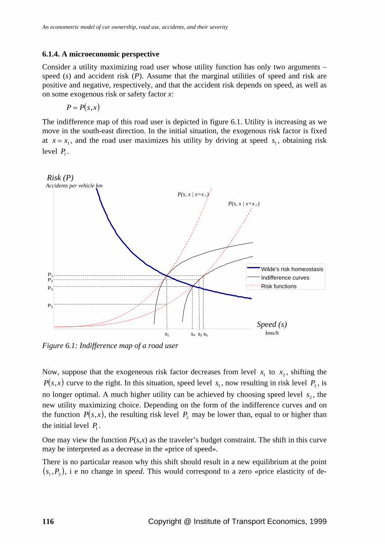
An econometric model of car ownership, road use, accidents, and their severity
116 Copyright @ Institute of Transport Economics, 1999
6.1.4. A microeconomic perspective
Consider a utility maximizing road user whose utility function has only two arguments – speed (s) and accident risk (P). Assume that the marginal utilities of speed and risk are positive and negative, respectively, and that the accident risk depends on speed, as well as on some exogenous risk or safety factor x:
( )x,sPP =
The indifference map of this road user is depicted in figure 6.1. Utility is increasing as we move in the south-east direction. In the initial situation, the exogenous risk factor is fixed at 1xx = , and the road user maximizes his utility by driving at speed 1s , obtaining risk level 1P .
Speed (s)kms/h
Risk (P)
Wilde's risk homeostasisIndifference curvesRisk functions
P1P2
P3
P4
s1 s2s4
P(s, x | x=x 1 )P(s, x | x=x 2 )
Accidents per vehicle km
s5
Figure 6.1: Indifference map of a road user
Now, suppose that the exogeneous risk factor decreases from level 1x to 2x , shifting the ( )x,sP curve to the right. In this situation, speed level 1s , now resulting in risk level 3P , is
no longer optimal. A much higher utility can be achieved by choosing speed level 2s , the new utility maximizing choice. Depending on the form of the indifference curves and on the function ( )x,sP , the resulting risk level 2P may be lower than, equal to or higher than the initial level 1P .
One may view the function P(s,x) as the traveler’s budget constraint. The shift in this curve may be interpreted as a decrease in the «price of speed».
There is no particular reason why this shift should result in a new equilibrium at the point ( )31 P,s , i e no change in speed. This would correspond to a zero «price elasticity of de-

Chapter 6: Accidents and their severity
Copyright @ Institute of Transport Economics, 1999 117
mand for speed». Only in such a case would the final (equilibrium) effect equal the initial (engineering) effect 31 PP − .
Nor is there any reason to expect the risk to remain constant (i e, 12 PP = ), as would be predicted under a certain, «weak» version of the risk homeostasis hypothesis. According to this tenet, the traveler would endeavor to keep the expected number of accidents, as reck-oned per trip or per kilometer traveled, unchanged. He would then choose to increase his speed s to the exact point ( 5ss = , say) where ( ) ( )112 x,sPx,sP = . This case would corre-spond to a «speed price elasticity» of exactly –1.
In Wilde’s «strong» version of the risk homeostasis hypothesis, the risk is constant per unit of time rather than per unit of distance traveled. This would imply that the product of risk (as defined per trip or kilometer) and speed is a constant, and hence that the new equilib-rium ( 4ss = , say) would be defined by ( ) ( )111244 x,sPsx,sPs = . As indicated in figure 6.1, the individual’s risk P would always move along a descending hyperbolic function of s ,
defined by sPsP 11= .
This hypothesis is «stronger» than the claim 21 PP = (constant risk per kilometer) in the following sense. Not only would a policy measure to bring down speed be ineffective (leave the accident count unchanged), it would – with probability one – be directly coun-terproductive, because the number of accidents would increase in proportion with the time spent on the road. According to this tenet, the number of accidents goes down because the speed goes up.
To the economist, this hypothesis makes as little sense as the «weak» version of risk ho-meostasis. As seen in a microeconomic perspective, the extent to which risk compensation occurs depends on the indifference map of the road user. It is therefore, in essence, an em-pirical question. There is no a priori reason why the «price elasticity of demand for speed» would be either exactly 0 or exactly –1.
A formal economic model of road user behavior
The above diagrammatic discussion is a simplification, inter alia because it does not con-sider the size of the loss incurred in the event of an accident, only the accident probability. The distinction between these two components may provide rather interesting and impor-tant insights. To see this, we shall need a more formalized mathematical apparatus59.
Consider a utility maximizing road user with a resource constraint I (say). As before, let s denote speed and x some exogenously determined risk factor60. Also, denote by ( )D s x, the 59 Our approach is based to a large extent on the formulation put forward by Blomquist (1986), but attempts to carry this analysis a few steps further. 60 More generally, one might think of s as a vector of (endogenous) road user choice variables and x as a vector of exogenous risk factors. For purposes of exposition we shall, however, treat s and x as scalar vari-ables.
Alternatively, one may interpret s as (the reciprocal of) a general behavioral variable, such as «driver safety effort» (time, inconvenience, attention, energy, and money), in line with Blomquist (1986), or «care», in line with Risa (1994). In such a case, however, the assumptions (6.5)-(6.6) become harder to defend: reduced attention does not necessarily increase the loss given that an accident takes place.

An econometric model of car ownership, road use, accidents, and their severity
118 Copyright @ Institute of Transport Economics, 1999
disutility cost incurred by making a trip, by ( )P s x, the probability of being involved in an accident, and by ( )L s x, the expected loss incurred given that an accident takes place. As-sume that D, P and L are all twice differentiable, with first and second derivatives obeying
(6.1) ( ) ( )DD s x
sD
D s xxs x≡ < ≡ =
∂∂
∂∂
,,
,,0 0
(6.2) ( )D DD s xx ssx xs= ≡ =
∂∂ ∂
2
0,
,
(6.3) ( ) ( )PP s x
sP
P s xxs x≡ > ≡ >
∂∂
∂∂
,,
,,0 0
(6.4) ( )P PP s xx ssx xs= ≡ >
∂∂ ∂
2
0,
,
(6.5) ( ) ( )LL s x
sL
L s xxs x≡ > ≡ >
∂∂
∂∂
,,
,,0 0
(6.6) ( )L LL s xx ssx xs= ≡ >
∂∂ ∂
2
0,
.
The disutility cost is a decreasing function of speed61, but assumed independent of the risk factor, whose entire effect is channeled through the accident frequency and loss functions (6.1). The accident frequency and loss functions are assumed to be increasing functions of speed, and a given change in the risk factor is assumed to have a larger effect on accidents and loss the higher the speed level (6.3-6.6).
Let U 0 denote the utility drawn from making a certain trip, given that an accident does not occur, let U1 denote the utility given that an accident does occur, and assume that the road user endeavors to maximize the linearly separable function
(6.7) ( ) [ ] [ ]V s x E U U, var≡ + ⋅υ ,
where
(6.8)
( ) ( )[ ] ( )( )[ ] ( )[ ] ( ) ( ) ( )[ ]( ) ( ) ( )
E U P s x U P s x U
P s x I D s x P s x I D s x L s x
I D s x P s x L s x
= − ⋅ + ⋅
= − ⋅ − + ⋅ − −
= − − ⋅
1
10 1, ,
, , , , ,
, , ,
and, with the help of some algebra,
61 In many economic models, a much more restrictive assumption is used, namely that the (disutility) cost is proportional to the reciprocal of speed (1/s), as if travel time spent is the only element affecting road user preference (beside risk). We believe, however, that, in view of the relatively marginal time savings that result from a more aggressive style of driving, this perspective is much too narrow to explain risk taking behavior on the road. We therefore allow for the possibility that speed per se has a direct effect on utility, as it affects not only the travel time but also the boredom, enjoyment or excitement experienced by the driver.

Chapter 6: Accidents and their severity
Copyright @ Institute of Transport Economics, 1999 119
(6.9)
( ) ( ) ( )[ ]( )[ ] ( ) ( )[ ] ( ){ }
( ) ( )[ ] ( )[ ] .x,sLx,sPx,sP
Ux,sPUx,sPUx,sPUx,sP
UEUEUvar
2
210
21
20
22
1
11
⋅−⋅=
⋅+⋅−−⋅+⋅−=
−=
One may interpret the (negative of the) parameter υ of equation (6.7) as the marginal rate of substitution between expected utility and its variance. In the special case υ = 0 , the road user is risk neutral, maximizing expected utility. Risk averters are characterized by υ < 0 , and risk lovers byυ > 0 62.
The first order condition for maximum is given by
(6.10) ( ) ( ) ( )[ ]VV s x
sD P L PL P L P L LP Ps s s s s s≡ = − − − + − + − =
∂∂
υ, 2 1 2 2 1 0
and the second order condition by
(6.11) ( )
VV s x
sss ≡ <∂
∂
2
2 0,
.
Differentiating (6.10), we have, by the implicit function theorem,
(6.12) ( ) ( )V ds V dxV s x
sds
V s xx
dxss sxs s+ ≡ + =
∂∂
∂∂
, ,0 ,
and hence the behavioral response to a marginal change in the exogenous safety factor is given by
(6.13)
( )
( )dsdx
VV
V s xx
V s xs
sx
ss
s
s
= − = −
∂∂
∂∂
,
,.
62 This is but one among several possible definitions of risk aversion, and one that has been severely criti-cized (Borch 1969). More commonly, an individual is said to be risk averse if the utility function is concave (Arrow 1970, Rotschild and Stiglitz 1970, 1971, Diamond and Stiglitz 1974). Analyses within this tradition usually take account of only the first moment of the uncertain outcome (expected utility).
We believe, however, with Allais (1953, 1984, 1987), that in order to understand individual risk taking be-havior, it is paramount to consider more than just the first moment. In our mean-variance approach, a clear distinction is implicit between those individuals who are particularly anxious to avoid large losses L (the «risk averters»), as opposed to those who are only concerned with the mean (unconditionally expected) loss PL. This approach can be seen as a special case of Allais’ (1987) formulation, according to which even higher order moments than the second belong in the preference function. The third moment (skewness) would, e g, capture the difference between a lottery, where the loss is bounded, and a car trip, in which the gain is bounded, explaining why risk averse individuals may still want to participate in a lottery. Allais (1987) refers to the case υ < 0 as an individual’s «propensity for security», while υ = 0 corresponds to «Bernoullian behavior» and υ > 0 to «propensity for risk». In his words, «... the neo-Bernoullian formulation reduces to considering the mathematical expectation of cardinal utility alone, neglecting its dispersion about the average. In so doing, it neglects what may be considered as the specific element of risk». Most individu-als, he suggests, have «a preference for security in the neighborhood of certainty when dealing with sums that are large in relation to the subject’s capital». We believe the prospect of losing life or health in a road accident fits this description rather well.

An econometric model of car ownership, road use, accidents, and their severity
120 Copyright @ Institute of Transport Economics, 1999
Note that the denominator of this expression is negative by the second order condition (6.11), so that the sign of the response is identical to that of Vsx .
The two second-order derivatives are calculable as
(6.14) [ ]( ) [ ] ( ){ }2222 212214
2
LPPPLLLPPLLPL
PLLPLPDV
ssssssss
ssssssssss
−−++−++
−−−−=
υ
and
(6.15) [ ]( ) [ ] ( ){ }22 2122122 LPPPPLLLLPPLLPLLPL
PLLPLPLPDV
xsxssxxssxsx
sxsxxssxsxsx
−−++−+++
−−−−−=
υ
from which it is understandable why the risk aversion (or risk-loving) case ( 0≠υ ) has received comparatively little attention in the literature.
The risk neutrality case
In the risk neutrality case ( )υ = 0 , on the other hand, these expressions simplify to
(6.16) V D P L P L PLss ss ss s s ss= − − − −2
and
(6.17) V D P L P L P L PLsx sx sx s x x s sx= − − − − − .
By assumptions (6.1) through (6.6), all terms in (6.17) are non-positive, with at least two ( −P Ls x and − P Ls s ) being strictly negative, yielding a negative second derivative Vsx . Hence, by (6.13), any increase (dx) in the exogenous risk factor x will induce a behavioral response (ds) in the form of diminished speed s.
What happens to the accident risk and the loss per accident when a change in exogenous safety takes place? To see this, use (6.13), (6.16), (6.17), and the implicit function rule to derive
(6.18) dPdx
P P dsdx
P D P L P L P L PLD P L P L PL
Px s xsx sx s x x s sx
ss ss s s sss= + = −
− − − − −− − − −
⋅2
and
(6.19) dLdx
L L dsdx
L D P L P L P L PLD P L P L PL
Lx s xsx sx s x x s sx
ss ss s s sss= + = −
− − − − −− − − −
⋅2
.
As in the above diagrammatic exercise, we note that there is no a priori reason why these expressions should come out at exactly zero, except by sheer coincidence. Nor are the final equilibrium effects ever equal to the initial exogenous changes induced.
Hence, under the utility maximization model defined by assumptions (6.1)-(6.7), behav-ioral response to exogenous risk or safety factors is the rule rather than the exception. On the other hand, there is no reason why the size of the response would be such as to exactly offset the initial change.
In analyzing behavioral response to safety measures, an important distinction is often made between accident countermeasures, aimed at reducing the probability P, and severity coun-

Chapter 6: Accidents and their severity
Copyright @ Institute of Transport Economics, 1999 121
termeasures, designed to protect the road user in the event of an accident, i e reducing the loss variable L.
To fix ideas, one might identify a pure accident countermeasure by a situation in which Px > 0 and Lx = 0 (and hence L L Lxx sx xs= = = 0 ), while a pure severity countermeasure is characterized by P P P Px xx sx xs= = = = 0 and Lx > 0 63. It then follows from (6.13), (6.18) and (6.19) that, for an accident countermeasure,
(6.20) dsdx
D P L P LD P L P L PL
sx sx x s
ss ss s s ss
= −− − −
− − − −<
20,
(6.21) dPdx
P D P L P LD P L P L PL
P Pxsx sx x s
ss ss s s sss x= −
− − −− − − −
⋅ <2
and
(6.22) dLdx
D P L P LD P L P L PL
Lsx sx x s
ss ss s s sss= −
− − −− − − −
⋅ <2
0 ,
while for a severity countermeasure, we have
(6.23) dsdx
D P L PLD P L P L PL
sx s x sx
ss ss s s ss
= −− − −
− − − −<
20,
(6.24) dPdx
D P L PLD P L P L PL
Psx s x sx
ss ss s s sss= −
− − −− − − −
⋅ <2
0
and
(6.25) dLdx
L D P L PLD P L P L PL
L Lxsx s x sx
ss ss s s sss x= −
− − −− − − −
⋅ <2
.
A pure accident countermeasure has an indeterminate sign effect on accident probability, in that the behavioral response may or may not be large enough to offset the exogenous risk reduction. It does, however, have a (smaller or larger) adverse effect on severity, since in this case, there is no exogenous effect at work, only an endogenous behavioral adapta-tion working in the opposite direction.
By the same token, a pure severity countermeasure has an indeterminate effect on severity, but a necessarily adverse effect on accident probability.
Within this formalism, there is, contrary to Bjørnskau’s hypotheses (see section 6.1.3 above), apparently complete symmetry between accident and severity countermeasure in terms of their effects on either variable (P or L) or on behavioral adaptation in general. Accident countermeasures appear to affect severity in equilibrium in precisely the same way as severity countermeasures affect the accident probability in equilibrium.
To evaluate the assertions made by Bjørnskau, we need, however, to consider the form of the functions ( )P s x, and ( )L s x, . Let ( )L s xm , and ( )L s xb , denote the (conditionally ex-pected) material and bodily damage suffered, respectively, and hence
63 Since we have chosen to interpret x as a risk factor, a safety measure must be thought of as an event char-acterized by decreasing x.

An econometric model of car ownership, road use, accidents, and their severity
122 Copyright @ Institute of Transport Economics, 1999
(6.26) ( ) ( ) ( )L s x L s x L s xm b, , ,= + .
Consider a severity reducing measure such that
(6.27) ( ) ( ) ( )LL s x
sL
L s xx
L LL s x
x ssm
m
xm
m
xsm
sxm
m
≡ > ≡ = ⇒ ≡ ≡ =∂
∂∂
∂∂
∂ ∂,
,,
,,
0 0 02
(6.28) ( ) ( )LL s x
sL
L s xxs
bb
xb
b
≡ > ≡ >∂
∂∂
∂,
,,
0 0 ,
i e, the risk factor x (which is inversely related to the severity countermeasure) is assumed to have no effect on material loss, only on bodily injury.
In this case, equations (6.13)/(6.23) become, in view of (6.2),
(6.29) ( )dsdx
P L PLV
P L PLD P L L P L PL
s xb
sxb
ss
s xb
sxb
ss ssm b
s s ss
= −− −
= −− −
− − + − −<
20 .
To examine Bjørnskau’s hypothesis B, rewrite the level of material loss as
(6.30) ( ) ( )L s x L L s xm m m, ,= +0 1 ,
where Lm0 is an additive shift parameter not depending on s or x. Differentiating (6.29) with respect to Lm0 we obtain
(6.31) ( ) ( )
( )[ ]∂
∂
dsdxL
P P L PLV
P P L PL
D P L L P L PLm
ss s xb
sxb
ss
ss s xb
sxb
ss ssm b
s s ss
⎛⎝⎜
⎞⎠⎟
=+
=+
+ + + +0 2 2
2.
A sufficient condition for this derivative to be positive, and hence for the behavioral re-sponse to decrease (in absolute value) with the initial level of expected material loss, is that the inequalities (6.3), (6.28), and
(6.32) P L Lss sxb
xsb> ≡ >0 0,
hold, in other words that the accident probability is a convex, increasing function of speed, that the loss due to bodily injury also increases with speed, and that even the partial initial effect of the severity countermeasure increases with speed.
These assumptions seem by no means unrealistic in view of the fact that the stopping dis-tance as well as the impact energy in the event of a collision is roughly proportional to the square of the speed.
Hence, our formal analysis may be seen, under certain plausible assumptions, to lend sup-port to the hypothesis that road users expecting larger material losses in the event of an accident, to a lesser extent will adapt their behavior in response to severity reducing (or increasing) factors.
However, the behavioral response is unlikely to vanish completely. For this to happen, one must have
(6.33) P L PLs xb
sxb+ = 0 ,
a rather implausible condition in view of the above discussion.

Chapter 6: Accidents and their severity
Copyright @ Institute of Transport Economics, 1999 123
Turning to Bjørnskau’s hypothesis D, that the initial level of accident risk or severity does not affect the behavioral response to pure accident reducing measures, we have (compare (6.20-6.21))
(6.34) ( )
( )dsdx
P L P LV
P L L L P LD P L L L P L PL
sx x s
ss
sxm m b
x s
ss ssm m b
s s ss
= −− −
= −− + + −
− − + + − −
0 1
0 1 2
Differentiating (6.34), we obtain
(6.35) [ ][ ]
∂
∂
dsdxL
P V P P L P LV
D P P P L PP L P P LD P L P L PLm
sx ss ss sx x s
ss
ss sx s sx s sx ss x ss s
ss ss s s ss
⎛⎝⎜
⎞⎠⎟
=+ +
=− − − +
+ + +0 2 22
2,
the sign of which is theoretically indeterminate, since the term P Vsx ss is negative while [ ]P P L P Lss sx x s+ is positive. Thus, if a shift in the loss function fails to affect the extent of
behavioral response, it does so only because two opposite effects happen to cancel each other out.
To examine the effect of a higher initial accident probability, one may define, by analogy to (6.30), an additive shift parameter for accident risk P 0 , independent of s and x:
(6.36) ( ) ( )P s x P P s x, ,≡ +0 1 .
One may interpret P 0 as a minimum level of risk, unavoidable by the road user no matter how he chooses to behave or what countermeasures are in effect.
Again, by differentiating (6.34), we have
(6.37) [ ] [ ][ ]
∂
∂
dsdxP
L P L P LV
L P L P LD P L P L PL
ss sx x s
ss
ss sx x s
ss ss s s ss
⎛⎝⎜
⎞⎠⎟
=+
=+
+ + +0 2 22,
a presumably positive magnitude, suggesting that the behavioral response is smaller (in absolute value) the higher the initial accident probability.
However, the assumption of an additive shift in risk, not affecting the derivatives P P P Ps x ss sx, , ,and , is a rather counterintuitive one. More realistically, a shift in accident risk is multiplicative, affecting the accident risk at all speed levels, and hence all deriva-tives, by the same proportionality factor. In this case all terms entering (6.34), except Dss , will change proportionately. Formally, define the generalized accident probability function
(6.38) ( ) ( )P s x z zP s x Ps
zP Px
zP Ps
zP Ps x
zPs x ss sx' , , , ' , ' , ' , '= ⇒ = = = =
∂∂
∂∂
∂∂
∂∂ ∂
2
2
2
where we have introduced a third risk factor z, assumed to be multiplicatively separable from s and x. Replacing P by P' in (6.34) and differentiating, we obtain
(6.39) [ ]∂
∂
dsdxz
D P L P LV
ss sx x s
ss
⎛⎝⎜
⎞⎠⎟
=− +
2 .

An econometric model of car ownership, road use, accidents, and their severity
124 Copyright @ Institute of Transport Economics, 1999
In other words, the behavioral response is independent of the accident risk level only if the disutility cost of traveling is a linear function of speed, so that its second derivative Dss vanishes.
In the more realistic case, where the disutility cost is inversely proportional to speed (con-fer footnote 61), for instance
(6.40) ( )D s x s D s D ss ss, ( )= > ⇒ = − ⇒ = >− − −α α α α1 2 30 2 0 ,
the derivative (6.39) is seen to be negative, implying that the size of the behavioral re-sponse increases (in absolute value) with the general level of risk.
Thus, there is an important distinction to be made between (i) additive shifts in risk, which affect the intercept of the risk function but not its slope, and (ii) multiplicative shifts, which have the opposite effects. Behavioral response is hampered by the former, but fur-thered by the latter.
According to this model, it is not in general true that the extent of behavioral response is independent of the the initial risk level or conditionally expected loss. Such a condition will apply (approximately) only if the overall risk level is extremely low throughout the range of behavioral choice (a multiplicative shift factor approaching zero) or if, irrespec-tive of road user behavior, the risk is extremely high (a large, positive additive shift). Es-sentially, these are situations in which the road user can do little, either way, to influence his risk.
The risk aversion case
Recall that the above results have been proven for the risk neutrality case only.
To examine whether some of these results can be generalized to the risk aversion (or risk loving) case, we differentiate (6.14) and (6.15) with respect to the risk aversion parameter υ . Upon rearranging terms, one obtains
( ) [ ]( ) [ ] ( ) ⎥⎦
⎤⎢⎣
⎡⎟⎟⎠
⎞⎜⎜⎝
⎛+−+−++−+=
Ls
Pssssssssss
ss PPLLPPLLLPPLLPLV.ε
ε∂υ
∂2
121212212416 22
[ ]( ) [ ] ( ) ⎥⎦
⎤⎢⎣
⎡⎟⎟⎠
⎞⎜⎜⎝
⎛+−+−++−+=
Ls
Psxsxssxsxsx
sx PPLLPPLLLLPPLLPLVε
ε∂υ
∂2
121212212(6.42) 2 ,
where we have defined the elasticities of P and L with respect to speed s:
(6.43) ε εPs s Ls sP sP
L sL
= =, .
Under the assumptions (6.1)-(6.6), (6.32) and
Lss > 0 ,
all terms in (6.41) and (6.42) are positive, except possibly the last one, which depends on the ratio between the two elasticities. For small accident probabilities P, even the last term
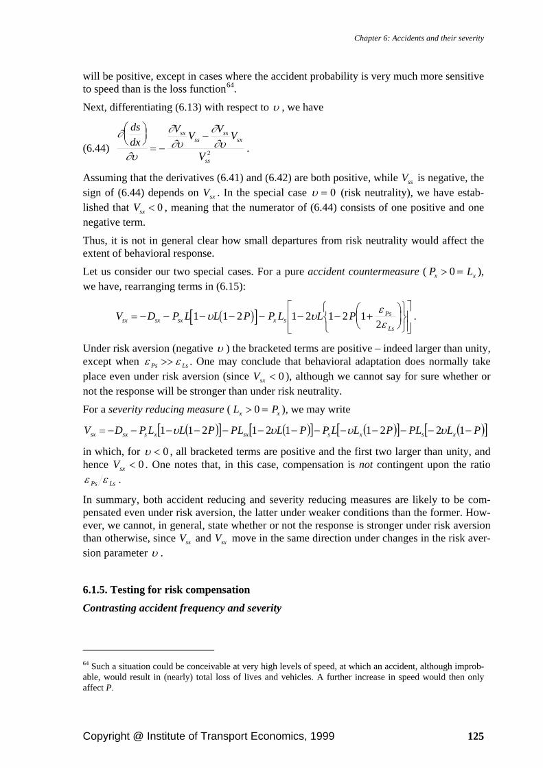
Chapter 6: Accidents and their severity
Copyright @ Institute of Transport Economics, 1999 125
will be positive, except in cases where the accident probability is very much more sensitive to speed than is the loss function64.
Next, differentiating (6.13) with respect to υ , we have
(6.44) ∂
∂υ
∂∂υ
∂∂υ
dsdx
V V V V
V
sxss
sssx
ss
⎛⎝⎜
⎞⎠⎟
= −−
2 .
Assuming that the derivatives (6.41) and (6.42) are both positive, while Vss is negative, the sign of (6.44) depends on Vsx . In the special case υ = 0 (risk neutrality), we have estab-lished that Vsx < 0 , meaning that the numerator of (6.44) consists of one positive and one negative term.
Thus, it is not in general clear how small departures from risk neutrality would affect the extent of behavioral response.
Let us consider our two special cases. For a pure accident countermeasure ( P Lx x> =0 ), we have, rearranging terms in (6.15):
( )[ ]V D P L L P P L L Psx sx sx x sPs
Ls
= − − − − − − − +⎛⎝⎜
⎞⎠⎟
⎧⎨⎩
⎫⎬⎭
⎡
⎣⎢⎢
⎤
⎦⎥⎥
1 1 2 1 2 1 2 12
υ υ εε
.
Under risk aversion (negative υ ) the bracketed terms are positive – indeed larger than unity, except when ε εPs Ls>> . One may conclude that behavioral adaptation does normally take place even under risk aversion (since Vsx < 0 ), although we cannot say for sure whether or not the response will be stronger than under risk neutrality.
For a severity reducing measure ( L Px x> =0 ), we may write
( )[ ] ( )[ ] ( )[ ] ( )[ ]PLPLPLLPPLPLPLLPDV xsxssxxssxsx −−−−−−−−−−−−−= 1221121211 υυυυ
in which, for υ < 0 , all bracketed terms are positive and the first two larger than unity, and hence Vsx < 0 . One notes that, in this case, compensation is not contingent upon the ratio ε εPs Ls .
In summary, both accident reducing and severity reducing measures are likely to be com-pensated even under risk aversion, the latter under weaker conditions than the former. How-ever, we cannot, in general, state whether or not the response is stronger under risk aversion than otherwise, since Vss and Vsx move in the same direction under changes in the risk aver-sion parameter υ .
6.1.5. Testing for risk compensation
Contrasting accident frequency and severity
64 Such a situation could be conceivable at very high levels of speed, at which an accident, although improb-able, would result in (nearly) total loss of lives and vehicles. A further increase in speed would then only affect P.

An econometric model of car ownership, road use, accidents, and their severity
126 Copyright @ Institute of Transport Economics, 1999
The results derived in section 6.1.4 provide us, in principle, with an interesting opportunity to reveal whether risk compensation does take place in practice. Whenever a severity coun-termeasure is subject to risk compensation through a change in speed, an increase in acci-dent frequency may be expected. And vice versa: whenever an accident countermeasure is compensated for, an increase in severity should be observable.
Thus, whenever an independent variable has an opposite sign effect on the two dependent variables (frequency and severity), it appears reasonable to conclude that we are faced with a risk or safety factor whose effect is somehow subject to compensation. Accident coun-termeasures presumably lower the accident frequency, but, if compensation takes place, severity is increased. Severity countermeasures, on the other hand, usually reduce severity, while possibly enhancing the accident frequency65.
To obtain an empirical test in line with this principle, we propose to use the number of in-jury accidents (given exposure and other explanatory variables) as an indicator of accident frequency, while we use the number of serious (or fatal) injuries per injury accident as an indicator of accident severity.
Now, it should be noted that a testing procedure based on these statistics has some rather important shortcomings, as seen in relation to the purpose of revealing risk compensation. These shortcomings are twofold.
First, a much more reliable set of indicators could be obtained if data were available on material damage accidents as well. In Norway, they are not. Only accidents causing (non-negligible) bodily injury are subject to mandatory police reporting and hence covered by the official road accident statistics. This is unfortunate because severity countermeasures may be expected to affect, not only the number of fatal and serious injuries, but also the number of slight injuries and of injury accidents altogether, shifting some of these into the «material damage» or «negligible injury» category, and hence beyond the scope of acci-dent statistics. We shall refer to this phenomenon as the problem of reporting drift.
Increased seat belt use, for instance, while obviously reducing the number of fatalities, shifting some of these cases into the «serious injury» or perhaps even into the «slight in-jury» category, also has the effect of reducing many injury accidents to material damage accidents. The latter effect is likely to be much larger than the former, as measured by the absolute number of cases, and it is impossible to tell a priori which effect will be larger in relative terms.
It is, in other words, not obvious that a severity countermeasure will reduce the number of fatalities (or serious injuries) by a larger percentage than the number of recorded injury accidents. Hence, an efficient severity countermeasure does not necessarily translate into a decreasing severity indicator, as defined by the number of fatal (or serious) injuries per injury accident.
A second problem is accident underreporting. It is well known that, although all accidents with (non-negligible) injuries are, in principle, subject to reporting, the actual reporting incidence may be as low as fifty per cent (Borger et al 1995, Nedland and Lie 1986), as evaluated for injury road accidents in general.
65 When the degree of risk compensation exceeds 100 per cent, both indicators (accident frequency and se-verity) may move in the «counterintuitive» direction.

Chapter 6: Accidents and their severity
Copyright @ Institute of Transport Economics, 1999 127
Underreporting is more pronounced for some accident categories than for other ones. In general, the incidence of reporting increases with the level of severity. Fatal accidents may be assumed to have a 100 per cent reporting incidence (perhaps even higher, to the extent that suicides are recorded as accidents). For less serious accidents and injuries, reporting is notoriously incomplete.
Thus, even if we were justified in disregarding the problem of reporting drift, there would still be at least two ways to interpret a partial relationship between accident frequency and some explanatory factor (x, say): (i) x has an effect on the frequency of injury accidents, or (ii) x has an effect on the probability that an injury accident be reported to the police.
A risk (increasing) factor negatively correlated with reporting incidence will tend to inflate the severity quotient, by deflating its denominator. This will lead to overestimation of the effect on severity, but underestimation of the effect on injury (accident) frequency.
In view of these shortcomings, we shall have to interpret with great caution any indication that a risk or safety factor has opposite effects on accident frequency and severity, respec-tively. Such results would have to be qualified in light of the plausibility of a reporting drift or an underreporting effect correlated with the substantive effect on accident or sever-ity rates. In some cases, such correlation will appear quite likely, while in other cases its existence may seem rather far-fetched.
Contrasting road user or accident categories
A second opportunity for testing for behavioral adaptation lies in the comparison of acci-dent frequencies between disjoint road user groups. If an initial safety improvement bene-fitting, say, car drivers is compensated, one might expect an adverse effect on other road user categories, to the extent that these are involved in bipartite or multipartite accidents with automobiles.
In essence, this was the rationale behind Peltzman’s (1975) controversial assertions (see section 6.1.3 above).
Estimating separate injury frequency equations for various road user groups and types of accidents, we shall endeavor to shed light on the possibility of behavioral adaptation, as well as on other issues relevant to the interpretation of accident frequency and severity modeling results. A more general framework for such testing and comparison is provided in section 6.4.3 below.
6.2. Road accidents as an internal and external cost
It is widely recognized that road transportation is an activity characterized, at least occa-sionally, by large external costs. Such externalities may include accidents, environmental effects, congestion, and road wear.
An externality (external cost) is an adverse (side-)effect of production or consumption that is not considered by the decision-maker. More precisely, one might say that66
66 Our formulation builds on Verhoef (1996), who in turn relies on Mishan (1971) and Baumol and Oates (1988).

An econometric model of car ownership, road use, accidents, and their severity
128 Copyright @ Institute of Transport Economics, 1999
an external effect exists when an agent’s utility (or production) function contains a real (i e, non-pecuniary) variable, whose actual value depends on the behavior of an-other agent, who does not take this effect of his behavior into account in his decision making process.
Note that, according to this definition, externalities operate at the disaggregate level. That is, for an externality to be present, it is sufficient that there is a cross effect between two individual decision-makers. Even if both individuals happen to be, e g, motorists, so that the cross effect is – in a sense – internal to the club of road users, we are faced with an externality in the relevant economic sense.
The issue of road accident externalities has been the subject of several important studies in recent years67. A common theoretical finding resulting from these studies is that the exter-nal accident cost of road use is a function of the marginal relationship between road use and accidents, as expressed, for instance, by the elasticity.
However, very few studies provide well-founded empirical evidence as to the (range of) value(s) of this elasticity. In the words of Newbery (1988:171),
«The key element in determining the accident externality cost is […] the relationship between traffic flow and accident rates, where the evidence is sketchy, to say the least.»
Our intention is to help fill this gap, (i) by suggesting a suitable econometric method of analysis, and (ii) by applying this method to our unusually rich spatio-temporal data set covering 19 Norwegian counties (provinces) over 264 months. Our exposition is generally in line with standard theory, as formulated e g by Verhoef (1996), Maddison et al (1996) or Jansson (1994), however with certain modifications and extensions so as to encompass the mixed (heterogeneous) traffic case.
Assume that there are two types of traffic68 on the network, say light and heavy vehicle traffic, and denote by Lv , Hv , and HLA vvv += the number of light, heavy, and overall vehicle kilometers driven, respectively, during a given time period. Let ( )HL vv=v be the vector of light and heavy vehicle traffic volumes, let ( )vc denote the generalized (private) unit cost of road use at traffic volumes Lv and Hv , and let ( )vb denote the corresponding cost borne by other people than the road user himself. Denoting by ( )vK the total (aggre-gate) cost of road use, we can write
(6.45) ( ) )(cv)(bv)(kvK AAA vvvv ⋅+⋅=⋅= ,
where ( )vk is the average unit cost per overall vehicle kilometer.
The private (internal) cost ( )vc consists of out-of-pocket expenditure, such as fuel, main-tenance, and vehicle depreciation, in addition to a range of non-monetary costs, of which time costs are usually the most important. A certain part of the accident cost is – one might assume – also borne by the road user in private, in the form of personal economic and physical risk. 67 See, e g, Lave (1987), Newbery (1988), Jones-Lee (1990), Vitaliano and Held (1991), Jansson (1994), Elvik (1994), Persson and Ödegaard (1995), Mayeres et al (1996), European Commission (1996), Maddison et al (1996), Jansson and Lindberg (1998), and Christensen et al (1998). 68 Our derivation generalizes verbatim to the case with an arbitrary number of separate traffic categories.

Chapter 6: Accidents and their severity
Copyright @ Institute of Transport Economics, 1999 129
The social (external) cost component ( )vb includes road wear and maintenance, environ-mental effects (noise, gas emissions, dust and dirt, barrier effects, etc), as well as those parts of the accident costs which are not inflicted upon – or taken into account by69 – the individual road user himself. These costs comprise medical costs, vehicle repair costs and loss of manpower paid for by the insurance company70 or the social security system, as well as grief, pain, and suffering inflicted upon the road user’s family, friends, passengers and accident counterparts.
Furthermore, denoting by ( ) ( ) ( )vvv jjj c,b,k and the overall, external and internal unit cost of using a type j vehicle, we can write
( ) ( ) ( )( )
( )( )
.v
cvc,
v
bvb,
vkv
kj j
j jj
j j
j jj
i i
i ii
∑∑
∑∑
∑∑ ===
vv
vv
vv
Note that the functions ( ) ( ) ( )vvv jjj c,b,k and depend not only on jv , but also on ( )ijvi ≠ , and vice versa. Both vehicle categories make use of the same network, involving each other in accidents as well as in congestion.
Differentiating (6.45), we obtain the marginal total cost of road use with respect to traffic category j:
( ) ( ) ( )j
AKj
jA
j vvk
vkvk
vK ε⋅=
∂∂
⋅+=∂∂ vvv ,
where we have defined the elasticity of the total aggregate cost of road use with respect to type j vehicle kilometers
( )( )
( )( )( )
( )( ) ⎥
⎥⎦
⎤
⎢⎢⎣
⎡+
∂∂
=∂
∂=
∂∂
≡A
jj
jA
j
j
Aj
j
Kj v
vkv
vk
kvv
vkv
Kv
vK
vv
vv
vvε .
At the margin, the external cost of using a type j vehicle is given by the difference between the total marginal cost and the average private cost taken into account by the individual decision-maker:
69 Some researchers contend that for most drivers, the perceived ex ante accident cost (i e, the risk) is zero. On account of this, Turvey (1973), quoted by Jansson (1994), argues that it would not be unreasonable to consider even the driver’s own expected accident cost as external. Moreover, the loss of life and health usu-ally inflicts mental pain and suffering also on the victim’s family and friends. Even this cost is external to the extent that the driver does not consider it when making his decisions. 70 Although the part covered by the insurance company is internal to the club of motorists, it is clearly a marginal external cost from the perspective of the individual, decision-making road user, at least in the short term. Contrary to what is often maintained, automobile insurance serves – at the margin – to externalize a cost that would otherwise have been internal, although the extent to which this is the case depends on the precise decision considered. For the choice of behavior on the road, there is an obvious incentive to take more risk if the cost of accidents is partly covered by an insurance company – a genuine moral hazard prob-lem. Even for the decision to drive a marginal kilometer, (part of) the ex ante accident cost is normally exter-nalized from the decision-making individual, because insurance premiums typically take the form of (step-wise) fixed costs per vehicle. To correct this inefficiency, Litman (1998, 1999) advocates a distance-based vehicle insurance scheme.
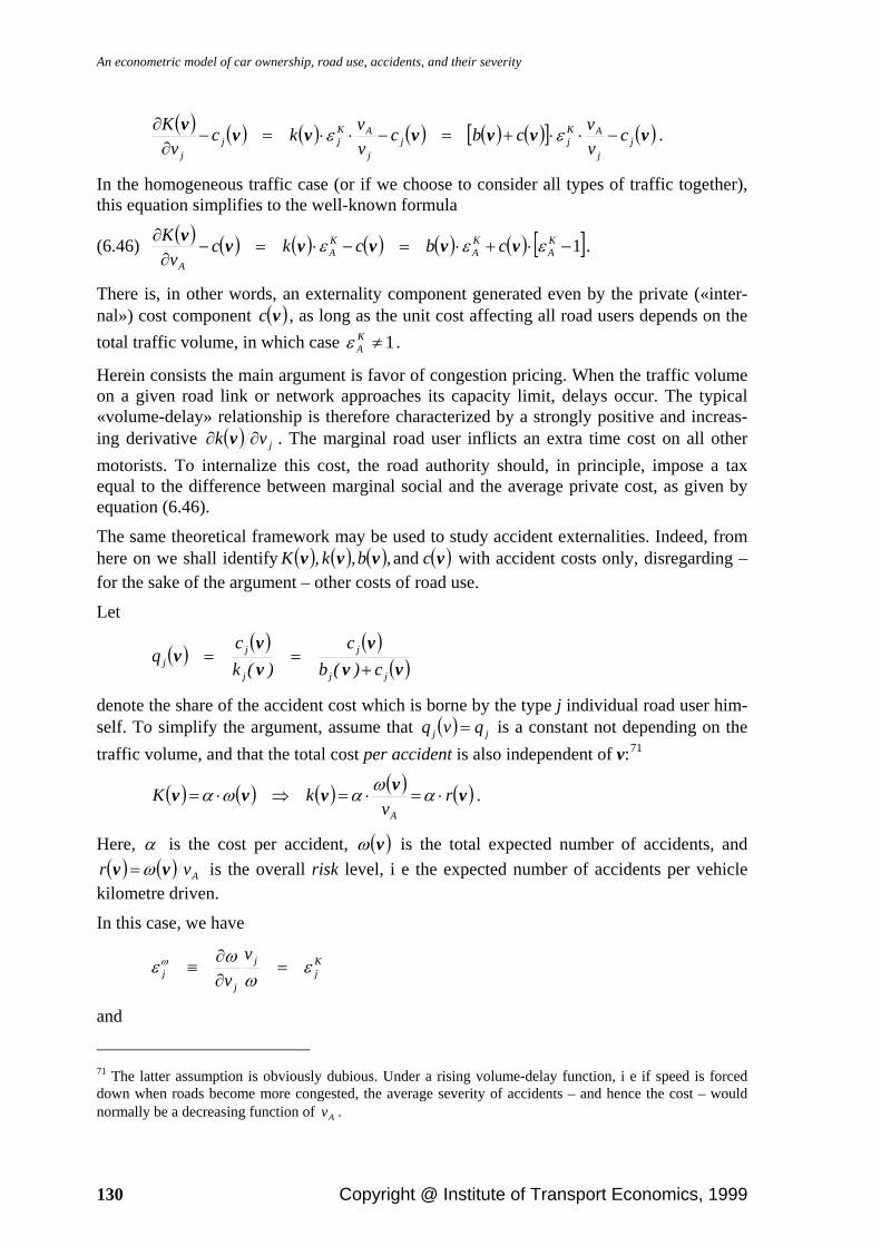
An econometric model of car ownership, road use, accidents, and their severity
130 Copyright @ Institute of Transport Economics, 1999
( ) ( ) ( ) ( ) ( ) ( )[ ] ( )vvvvvvvj
j
AKjj
j
AKjj
j
cvvcbc
vvkc
vK
−⋅⋅+=−⋅⋅=−∂
∂ εε .
In the homogeneous traffic case (or if we choose to consider all types of traffic together), this equation simplifies to the well-known formula
(6.46) ( ) ( ) ( ) ( ) ( ) ( ) [ ]1−⋅+⋅=−⋅=−∂
∂ KA
KA
KA
A
cbckcv
K εεε vvvvvv .
There is, in other words, an externality component generated even by the private («inter-nal») cost component ( )vc , as long as the unit cost affecting all road users depends on the total traffic volume, in which case 1≠K
Aε .
Herein consists the main argument is favor of congestion pricing. When the traffic volume on a given road link or network approaches its capacity limit, delays occur. The typical «volume-delay» relationship is therefore characterized by a strongly positive and increas-ing derivative ( ) jvk ∂∂ v . The marginal road user inflicts an extra time cost on all other motorists. To internalize this cost, the road authority should, in principle, impose a tax equal to the difference between marginal social and the average private cost, as given by equation (6.46).
The same theoretical framework may be used to study accident externalities. Indeed, from here on we shall identify ( ) ( ) ( ) ( )vvvv c,b,k,K and with accident costs only, disregarding – for the sake of the argument – other costs of road use.
Let
( ) ( ) ( )( )vv
vvv
vjj
j
j
jj c)(b
c)(k
cq
+==
denote the share of the accident cost which is borne by the type j individual road user him-self. To simplify the argument, assume that ( ) jj qvq = is a constant not depending on the traffic volume, and that the total cost per accident is also independent of v:71
( ) ( ) ( ) ( ) ( )vvvvv rv
kKA
⋅=⋅=⇒⋅= αωαωα .
Here, α is the cost per accident, ( )vω is the total expected number of accidents, and ( ) ( ) Avr vv ω= is the overall risk level, i e the expected number of accidents per vehicle
kilometre driven.
In this case, we have
Kj
j
jj
vv
εω
ωε ω =∂∂
≡
and
71 The latter assumption is obviously dubious. Under a rising volume-delay function, i e if speed is forced down when roads become more congested, the average severity of accidents – and hence the cost – would normally be a decreasing function of Av .

Chapter 6: Accidents and their severity
Copyright @ Institute of Transport Economics, 1999 131
( )( ) A
jj
A
j
j
Aj
j
rj v
vv
vvv
rv
vr
−=∂
∂=
∂∂
≡ ωεω
ωε
where ωε j and rjε , respectively, are the overall accident and risk elasticities with respect to
traffic category j.
Under these assumptions, we may write the marginal external accident cost as
(6.47)
( ) ( ) ( ) ( ) ( ) ( )( )
( ) ( )( ) ,
kk
qvvr
kk
qvvkc
vvkc
vK
jj
j
Arj
jj
j
Ajj
j
Ajj
j
⎥⎥⎦
⎤
⎢⎢⎣
⎡−+⋅⋅=
⎥⎥⎦
⎤
⎢⎢⎣
⎡−⋅=−⋅=−
∂∂
vv
v
vv
vvvvv
1εα
εε ωω
reducing to
(6.48) ( ) ( ) ( ) ( ) ( ) [ ] ( ) [ ]ArAAAA
A
qrqkckcv
K−+⋅⋅=−⋅=−⋅=−
∂∂ 1εαεε ωω vvvvvv
in the homogeneous traffic case.
The sign and size of the accident externality depends crucially on the risk elasticity with respect to the traffic volume. For all types of traffic considered together, this elasticity is equal to the elasticity of accidents with respect to traffic, minus one. It is, in other words, positive if and only if the number of accidents increases more than proportionately with the number of vehicle kilometers.
There is a positive external accident cost generated by the marginal representative road user only in so far as his own share ( )Aq of the average accident cost is smaller than the accident elasticitiy.
For a particular traffic category j, the relevant parameters are the partial accident elasticity ( ωε j ) weighted by the inverse traffic share ( jA vv ), and the internal share of accident costs ( jq ) adjusted to reflect the higher or lower cost of accidents ( jk ) involving type j vehicles compared to the overall mean cost per accident Ak (formula 6.47).
Since, in an «unsaturated» traffic environment, the number of possible two-party conflict situations may be thought to increase in relation to the square of the number of vehicles on the road, one might imagine that the accident elasticity ( ωε A ) would be larger than one in the early phase of the automobile era:
( ) 122 =⇒=⇒∝ rAAAv εεω ωv .
For such a case, Newbery (1988) points out that there would be an externality involved which would be at least equal to the total cost of the accident. (If 1<Aq , the externality would be even larger than the total cost of the accident.)
As roads become crowded, however, traffic density is bound to affect driving behavior, notably speed, thus forcing down the number of conflict situations, or at least the severity of their outcome. Where on this curve are we? This is an empirical question that can only be resolved by means of appropriate econometric analysis, allowing for explicitly and es-timably non-linear relationships.
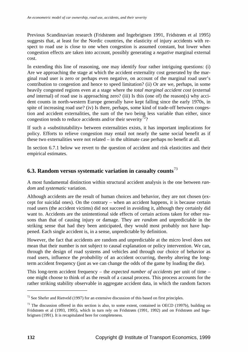
An econometric model of car ownership, road use, accidents, and their severity
132 Copyright @ Institute of Transport Economics, 1999
Previous Scandinavian research (Fridstrøm and Ingebrigtsen 1991, Fridstrøm et al 1995) suggests that, at least for the Nordic countries, the elasticity of injury accidents with re-spect to road use is close to one when congestion is assumed constant, but lower when congestion effects are taken into account, possibly generating a negative marginal external cost.
In extending this line of reasoning, one may identify four rather intriguing questions: (i) Are we approaching the stage at which the accident externality cost generated by the mar-ginal road user is zero or perhaps even negative, on account of the marginal road user’s contribution to congestion and hence to speed limitation? (ii) Or are we, perhaps, in some heavily congested regions even at a stage where the total marginal accident cost (external and internal) of road use is approaching zero? (iii) Is this (one of) the reason(s) why acci-dent counts in north-western Europe generally have kept falling since the early 1970s, in spite of increasing road use? (iv) Is there, perhaps, some kind of trade-off between conges-tion and accident externalities, the sum of the two being less variable than either, since congestion tends to reduce accidents and/or their severity72?
If such a «substitutability» between externalities exists, it has important implications for policy. Efforts to relieve congestion may entail not nearly the same social benefit as if these two externalities were not related – in the ultimate case perhaps no benefit at all.
In section 6.7.1 below we revert to the question of accident and risk elasticities and their empirical estimates.
6.3. Random versus systematic variation in casualty counts73
A most fundamental distinction within structural accident analysis is the one between ran-dom and systematic variation.
Although accidents are the result of human choices and behavior, they are not chosen (ex-cept for suicidal ones). On the contrary – when an accident happens, it is because certain road users (the accident victims) did not succeed in avoiding it, although they certainly did want to. Accidents are the unintentional side effects of certain actions taken for other rea-sons than that of causing injury or damage. They are random and unpredictable in the striking sense that had they been anticipated, they would most probably not have hap-pened. Each single accident is, in a sense, unpredictable by definition.
However, the fact that accidents are random and unpredictable at the micro level does not mean that their number is not subject to causal explanation or policy intervention. We can, through the design of road systems and vehicles and through our choice of behavior as road users, influence the probability of an accident occurring, thereby altering the long-term accident frequency (just as we can change the odds of the game by loading the die).
This long-term accident frequency – the expected number of accidents per unit of time – one might choose to think of as the result of a causal process. This process accounts for the rather striking stability observable in aggregate accident data, in which the random factors 72 See Shefer and Rietveld (1997) for an extensive discussion of this based on first principles. 73 The discussion offered in this section is also, to some extent, contained in OECD (1997b), building on Fridstrøm et al (1993, 1995), which in turn rely on Fridstrøm (1991, 1992) and on Fridstrøm and Inge-brigtsen (1991). It is recapitulated here for completeness.

Chapter 6: Accidents and their severity
Copyright @ Institute of Transport Economics, 1999 133
(«noise», «disturbance») having a decisive effect at the micro level, are «evened out» by virtue of the law of large numbers. The causal process determines the expected number of accidents, as a function of all the factors making up the causal set (the causes).
To be specific, let ω tr denote the expected number of accidents occurring during period t at location74 r. The expected number of accidents is, of course, not a constant – it varies with location and time, i e with r and t. We shall refer to this variation, attributable to the various causal factors, as systematic. Unlike the random or pure chance variation, the sys-tematic variation can – in principle – be influenced and controlled. Only the systematic variation is of interest from a policy point of view.
Let [ ]'....xx trtrtr 21=x denote the set of causal factors determining ω tr , i e
[ ] ( )trtrtrtr fyE xx ==ω ,
where ytr denotes the observed (factual) number of accidents at time t in location r, and ( )trf x is some (regression) function of the causal factors. Then, trivially,
( ) trtrtr ufy += x ,
where the tru are disturbance terms defined as the difference between observed and ex-pected accident counts.
With this notation, one might decompose the total variation in accident numbers into ran-dom and systematic as follows (Miaou 1995):
( ) ( )[ ] ( )[ ]var var vary E y E ytr tr tr tr tr= +x x
Here, the first term corresponds to the random variation (normal spread in ytr , given the systematic factors xtr ), and the second term to the systematic variation (spread between the respective, expected numbers of accidents ω tr )75.
Now, to understand the process producing accident numbers ytr , one must (i) acquire in-formation or make an assumption concerning the general functional form f, (ii) determine the set of explanatory (independent) factors xtr , and (iii) estimate the parameters entering the function f( xtr ). In so doing, it usually helps (iv) to have a good notion even of the na-ture of the probability distribution governing the random variation ytr tr−ω , since the rela-tive efficiency of the respective, candidate estimation techniques is likely to depend cru-cially on the distributional characteristics of this random «disturbance» term.
As for items (i) and (ii), little can be said a priori about the relative merits of different model specifications in general. Suffice to mention that the expected number of accidents is necessarily a non-negative (or strictly positive) number, although possibly a very small one. In many applications (especially when working with small accident counts), it might
74 By location, we have in mind any kind of spatially delimited entity, e g a road stretch, an intersection, an area, or even an entire country. By the same token, the time period considered might be of any length. 75 In this expression, we envision x and y as (vector) variables generated by a stable, simultaneous multivari-ate random process. The moments of the conditional expectation and variance of y are calculable by integra-tion over the range of x.

An econometric model of car ownership, road use, accidents, and their severity
134 Copyright @ Institute of Transport Economics, 1999
be a good idea to build this information explicitly into the model, by specifying a func-tional form f which cannot take on negative values, e g
ω β βtr
x xi
e ei trii i tri= ∑ = ∏ ,
or, equivalently,
(6.49) ( ) trii
itr xln ∑= βω ,
meaning that the log of the expected number of accidents is a linear function of a parame-ter vector ( β β1 2, , ... ), measuring the effects of the respective, systematic explanatory fac-tors ( ...,x,x trtr 21 ). In this (log-linear regression) model, the relationship between the inde-pendent and dependent variables is essentially multiplicative in character, an intuitively appealing property in most accident modeling applications. Under the assumption of (probabilistic) independence, the probability ABP (say) of the joint event BA ∩ is equal to the product of the marginal probabilities AP and BP (say), rather than to their sum.
This log-linear formulation may be viewed as one member of wider class of models, e g the so-called generalized linear models, first described by Nelder and Wedderburn (1972), and later developed by McCullagh and Nelder (1983):
( ) ∑=i
triitr xh βω .
Here, h is commonly referred to as the link function. The expected value of the dependent variable is linked to a linear regression term by means of some general, monotonic func-tion.
An, in a sense, even more general formulation is given by the Box-Cox regression model76
(2.3) ( ) ( )y x utr ii
tri triμ λβ= +∑ ,
in which utr is a random disturbance term with zero expectation. In this model, dependent as well as independent variables are, in principle, specified as Box-Cox transformations with unknown, estimable shape parameters and in which, ideally, all parameters ( μ , λ i , and β i , i = 1 2, ,...) are estimated simultaneously. Thus, the data are allowed to determine not only the coefficients, but also the optimal functional form of certain relationships (within the Box-Cox family of monotonic transforms). This formulation may appear par-ticularly attractive when, for one or more regressors, there exists little theoretical guidance in support of one functional form or the other.
In the above Box-Cox regression model, the link function is the Box-Cox transformation with parameter μ . In the special case 0=μ , this link function coincides with the loga-rithmic transformation.
As for items (iii) and (iv), concerning the structure of the random variation and its conse-quence in terms of estimation, much stronger a priori assumptions may seem to be justi-fied. Forceful arguments can be found in support of the assertion that accident counts must
76 Confer sections 2.4.2-3 of chapter 2 above.

Chapter 6: Accidents and their severity
Copyright @ Institute of Transport Economics, 1999 135
follow the Poisson probability law. To see this, we shall make a brief digression into the theory of stochastic processes.
6.3.1. The Poisson process77
At first, we shall need a few definitions.
A stochastic process ( ){ }Tt,tY ∈ is a family of random variables. For each t contained in the index set T, ( )tY is a random variable. The index t is often interpreted as time, in which case ( )tY represents the state of the process at time t. The set of possible values of ( )tY is called the state space of the process.
A continuous time stochastic process is said to have independent increments if, for all choices nt...ttt <<<< 210 , the random variables
( ) ( ) ( ) ( ) ( ) ( )11201 −−−− nn tYtY,...,tYtY,tYtY
are mutually independent. The process is said to have stationary independent increments if, for all Tt,t ∈21 and 0>s , the variables ( ) ( )stYstY +−+ 12 and ( ) ( )12 tYtY − have the same distribution.
The stochastic process ( ){ }0≥t,tY is said to be a counting process if ( )tY represents the total number of events which have occurred up to time t.
A particularly important counting process is the Poisson process, defined by
(6.50.a) ( ) 00 =Y ,
(6.50.b) ( ){ }0≥t,tY has stationary independent increments,
(6.50.c) ( )[ ] ( )totYP =≥ 2 , and
(6.50.d) ( )[ ] ( )tottYP +== λ1 ,
where we have made use of the notation ( )to defined as follows: A function f is said to be ( )to if
( ) 00
=→ t
tflimt
.
Assumption (6.50.a) can be seen as an innocuous normalization rule. Assumptions (6.50.b-d) may, in plain language, be interpreted as follows:
i. The time of recurrence of an event is unaffected by past occurrences.
ii. The distribution of the number of events depends only on the length of the time for which we observe the process. For time intervals (s) of identical lengths, the event counts have identical distributions.
iii. The probability of exactly one event, divided by the length of the time period, tends towards a stable, positive parameter λ , which is called the rate or intensity of the pro-cess.
77 This exposition relies on Ross (1970), Bickel and Doksum (1977), and Haight (1967).

An econometric model of car ownership, road use, accidents, and their severity
136 Copyright @ Institute of Transport Economics, 1999
iv. The chance of any occurrence in a given period goes to 0 as the period shrinks, and having only one occurrence becomes far more likely than multiple occurrences. For this reason, the Poisson process has been referred to as the law of rare events.
It can be shown (see, e g, Ross 1970) that, for any process fulfilling these conditions, the number of events occurring during any interval of length t (say) has a Poisson distribu-tion78 with mean tλ . That is, for all 0≥t,s
(6.51) ( ) ( )[ ] ( )K,,,m,
!metmsYstYP
tm
210=⋅
==−+−λλ .
It follows that
(6.52) ( )[ ] ttYE λ= ,
i e the expected number of events is proportional to the length of the time period and to the rate of the process λ .
A bit simplified, one might say that, for any stationary counting process characterized by rare, mutually independent events, the number of events occurring during a time period of arbitrary length t follows the Poisson distribution with parameter tλω = , λ being the rate of the process.
This property is, of course, the reason why the process characterized by assumptions (6.50a-d) is called a Poisson process.
Note, however, that the Poisson distribution is in no way part of these same assumptions. It is a remarkable, non-trivial mathematical fact that the Poisson distribution follows from these assumptions79.
A well-known example of a process fitting this description is the disintegration of radioac-tive isotopes. The atom decays by emitting neutrons at a given rate. The number of atoms disintegrating during a certain period is Poisson distributed.
It is impossible to tell when a specified atom will decay, but since all atoms are equal and the rate of decay is stable, we can predict with fairly large accuracy how many atoms will decay during a specified period. This is an example of what Salmon (1984) has referred to as an «irreducibly statistical law» – a causal law that includes an inevitable, objectively random component. No matter how much we learn about the radioactive substance, we would never be able to predict the behavior of each elementary particle. Only their aggre-gate behavior is knowable, and this only up to a certain (statistical) margin of error.
Another example of a process fitting the above description is – and this should come as no surprise – accident counts.80
78 Named after Poisson (1837, 1841). 79 Alternatively, one might have taken (6.50.a-b) and (6.51) as the set of assumptions and derived (6.50.c-d) as implications. The latter relations are, in other words, both necessary and sufficient conditions for a Pois-son process (Ross 1970:13-14). 80 The first scientist to make a connection between empirical phenomena and the theoretical probability distribution derived by Poisson (1837, 1841) was Ladislaus von Bortkiewicz, who discovered that the Pois-son distribution offered a perfect fit to the frequency of death by horse-kick in the Prussian army (Bort-kewitsch 1898).

Chapter 6: Accidents and their severity
Copyright @ Institute of Transport Economics, 1999 137
By striking analogy to the decaying radioactive isotope, accidents are also random and unpredictable at the micro level. Had the accident been anticipated, it would not have hap-pened. Each single accident is, therefore, in a sense unpredictable by definition. Thus, even accident counts may seem to be governed by an «irreducibly statistical law», according to which single events occur at random intervals, but with an almost constant overall fre-quency in the long run. Although the single event is all but impossible to predict, the col-lection of such events behaves in a perfectly predictable way, amenable to description by means of precise mathematical-statistical relationships. There is reason to think that this principle applies to traffic accidents as it does to quantum physics, or to the (repeated) toss of a die.
Now, road users and road conditions are not, like the atoms of an isotope, all equal. At first sight, therefore, the stationarity part of condition (6.50.b) above may seem like a rather unrealistic assumption as applied to accidents, since it requires that the accident rate be constant over time. Even this condition is, however, for all practical purposes, an innocu-ous one. This is so on account of the convenient invariance-under-summation property of the Poisson distribution: any sum of independent Poisson variates is itself Poisson distrib-uted, with parameter equal to the sum of the underlying, individual parameters (Hoel et al 1971:75-76). Thus all we need to assume is that, through some very short time interval (say, a minute, second, or fraction thereof), the accident rate can be considered constant, and that events occurring during disjoint time intervals are probabilistically independent. In such a case the number of events occurring during a given period t (week, month, or year) will, indeed, be Poisson distributed.
In fact, the conditions (6.50.a-d) may be generalized so as to describe the non-homogeneous Poisson process, in which the rate of the process may vary continuously over time, yet giving rise to Poisson distributed event counts. In the non-homogenous Poisson process, the intensity is a function of time (t), and the mean of the resulting Pois-son variable is found by integration over the range of the intensity function:
(6.53) ( )[ ] ( )∫=t
dsstYE0
λ .
The crucial condition left to be fulfilled, in order for the Poisson distribution to apply, is the independence part of criterion (6.50.b). Even this condition is, however, less restrictive than it may seem. It does not mean that accident counts should not be autocorrelated over time. If the underlying accident intensity ( )tλ depends on systematic explanatory factors showing some degree of stability across consecutive time periods (a rather plausible as-
Bortkiewicz' observation represented an extremely original and innovative idea for his time. The relationship between probability theory and statistics, which is now seen as so obvious that teachers may have difficulty explaining the difference to their students, had not yet been recognized as a general principle applying to all probability distributions. It was, however, known that the normal distribution and the law of large numbers could be applied in this way. The elegance and usefulness of these mathematical results, associated with some of the most illustrious and prestigious mathematicians of all times (Gauss, Laplace, and others), had created a research paradigm in which almost all attention was focused on large sample theory. Against this background, the title of Bortkiewicz' book – «The law of small numbers» – was an intriguing one.
It was, however, not very accurate. We now know that the Poisson probability model is equally valid for large event counts, although the limiting distribution of the Poisson is the normal, so that in this case the distinction between the two distributions becomes immaterial (see Haight 1967, or Johnson and Kotz 1969).

An econometric model of car ownership, road use, accidents, and their severity
138 Copyright @ Institute of Transport Economics, 1999
sumption), changes in ( )tλ will occur slowly and gradually, and this «inertia» will be re-flected in the observed accident counts as well. Only the random part of the observed variation is, according to the Poisson process, uncorrelated across time.
The fact that an accident has just taken place does not increase the probability of another one occurring within the next few seconds, minutes, hours, or days. Nor does it reduce it. It may, however, well be that the systematic factors influencing ( )tλ in period 10 ttt << , take on similar values in the next period 21 ttt << , thus increasing the accident probability in both periods. Such a phenomenon will manifest itself in the form of autocorrelated em-pirical accident counts. It does not contradict the assumption of probabilistically independ-ent81 accident counts or events82.
6.3.2. The generalized Poisson distribution
There are thus rather compelling arguments in favor of treating accident counts as a sample generated by the Poisson probability law, given by the formula
(6.54) [ ]!memyP
trmtr
tr
ωω −⋅==
where trω denotes the expected number of accidents during period t in area r, while try is the corresponding, actual number of accidents.
In terms of analysis, the Poisson assumption has a number of useful and interesting impli-cations (Fridstrøm et al 1995). Most importantly, the variance of a Poisson variable equals its expected value, both being equal to the Poisson parameter – ω tr . Having estimated the expected value – relying, e g, on a regression specification like (6.49) above – one also knows how much random variation is to be expected around that expected value.
Assume, for the sake of the argument, that we have somehow acquired complete and cor-rect knowledge of all the factors xtr causing systematic variation, and of all their coeffi-cients β i . In other words, the expected number of accidents ω tr – i e, all there is to know about the accident generating process – is known. Could we then predict the accident num-ber with certainty? The answer is no: there would still be an unavoidable amount of purely random variation left, the variance of which would be given – precisely – by ω tr . The residual variation should never be smaller than this, or else one must conclude that part of
81 We use the term probabilistically independent precisely to avoid confusion with respect to the two other meanings of the term «independent», that of functional independence (a uniformly zero partial derivative between two variables) and that of independent (exogenous) variables in a regression model. 82 It might be argued that in certain cases, one cannot rule out the possibility that accident events may be probabilistically dependent. This occurs, e g, (i) when the decision makers (the road users, the road authori-ties, the car manufacturers etc) learn from an accident and change their behavior so as to avoid repetitions, or (ii) when an accident disrupts the traffic flow and thereby increases the risk of another one. In the statistical literature, this case is sometimes referred to as «true contagion» (see section 6.3.2 below). Unless, however, we are working with very disaggregate accident counts – pertaining to, say, individual drivers, vehicles, road links, or intersections – it is unlikely that such effects would represent more than an almost negligible devia-tion from the independence assumption. Moreover, to the extent that behavior is changed in ways affecting risk, this would be reflected in the intensity of the Poisson process and – ideally – captured by the systematic factors included in the model.

Chapter 6: Accidents and their severity
Copyright @ Institute of Transport Economics, 1999 139
the purely random variation has been misinterpreted as systematic, and erroneously attrib-uted to one or more causal factors83.
In practice one is seldom in the fortunate situation that all risk factors have been correctly identified and their coefficients most accurately estimated, so that the expected number of accidents is virtually known. A generalization of the Poisson probability model, and a sometimes more realistic regression model, is obtained when one assumes that the Poisson parameter tω is itself random, and drawn from a gamma distribution with shape parameter ξ (say). In this case the observed number of accidents can be shown (Greenwood and Yule 1920, Eggenberger and Pólya 1923, Gourieroux et al 1984 a, b) to follow a negative binomial distribution with expected value [ ]E tr trω ϖ= (say) and variance
(6.55) [ ]σ ϖ θϖtr tr tr2 1= ⋅ + ,
where θ ξ= 1 .
In the negative binomial distribution, the variance thus generally exceeds the mean. In the special case θ = 0 , the gamma distribution is degenerate, and we are back to the simple Poisson distribution, in which the variance equals the mean. We shall refer to θ as the «overdispersion parameter», and to models in which θ > 0 as «overdispersed». In such a model, the amount of unexplained variation is larger than the normal amount of random disturbance in a perfectly specified Poisson model, meaning, in fact, that not all the noise is purely random. The model does not explain all the systematic variation, but lumps part of it together with the random disturbance term.
The above line of arguments constitutes what could be termed the epistemic (subjective) reason for overdispersion. We recognize our lack of (complete) knowledge and specify the model accordingly, as when utility is treated as «observationally random», i e as random as seen from the viewpoint of the analyst (Ben-Akiva and Lerman 1985:55-57).
More fundamentally, ontic84 (objective) overdispersion may exist if the events are not probabilistically independent, such as accident victims, of which there may be several in a single accident. This fact tends to inflate the variance more than the expected value. In victim count models one should therefore never expect zero overdispersion.
83 American planners, politicians and scientists deliberately seek to avoid the term «accidents», replacing it by «crashes», on the grounds that the former tends to evoke the connotation of sheer randomness or bad luck, thereby neglecting the role of responsible, causal agents. In our view, however, the connotation of random-ness is an entirely relevant one, as there is hardly, within the realm of social science, any phenomenon com-ing closer than road accidents to being truly (objectively) random in character. Moreover, randomness does not in any way contradict causation. As should be clear from the above discussion, random and systematic (causal) influences coexist. Being aware of the random component and of the need to separate it from the systematic part adds to our understanding, to our analytical opportunities, and hence ultimately to our knowl-edge on efficient accident countermeasures. We shall therefore, in this essay, continue to use the term «acci-dents», though definitely without implying that no one or nothing is to blame for them. 84 Ontology is the theory of what really exists, i e of how the world really is, as opposed to what it looks like. Epistemology is the theory of knowledge, i e of how and whether we can learn or know about the real world. While ontic laws are, in a sense, true by definition, epistemic laws are just expressions of what we presently believe. The ontic law may exist even if its epistemic counterpart does not (the case of ignorance), or vice versa (the case of false theories).

An econometric model of car ownership, road use, accidents, and their severity
140 Copyright @ Institute of Transport Economics, 1999
This distinction between epistemic and ontic overdispersion is reflected in the two alterna-tive derivations first offered for the negative binomial distribution. As noted by Feller (1943), quoted by Cameron and Trivedi (1998), these differed in a rather interesting way.
Greenwood and Yule (1920) based their derivation on an assumption of unobserved popu-lation heterogeneity, adjusting the statistical procedure so as to take explicit account of the analyst’s less than perfect knowledge of the true expected values. This rationale is clearly epistemic: one does not question the underlying probability model, only our ability to learn about it.
Eggenberger and Pólya (1923), on the other hand, derived the very same distribution from an assumption of «true contagion», meaning that the occurrence of one event tends to in-crease the probability of another, as when counting disease cases during an epidemic. In this case, one relaxes the independence assumption of the underlying stochastic process, based on a belief that such independence is inconsistent with reality. This rationale is ontic in nature.
As applied to accident victims, the «true contagion» assumption is obviously more realistic than the independence assumption. The fact that there is one victim increases the probabil-ity of another one.
When considering certain subsets of victims, however, deviations from the independence assumption may in some cases be so small as to be practically negligible. For instance, very few accidents involve more than one pedestrian or bicyclist. Hence, a good model for pedestrian and/or bicyclist injury victims should normally exhibit very little overdisper-sion. Bus or car accidents, in contrast, often involve more than one injury victim. Models explaining bus or car occupant injuries will therefore inevitably be overdispersed.
6.4. Testing for spurious correlation in casualty models
6.4.1. The overdispersion criterion
The overdispersion parameter can be used to test whether or not our independent variables explain all the explainable (systematic) variation, i e if there is residual variation left in the model over and above the amount that should be there in a perfectly specified and esti-mated Poisson model.
Certain software packages for count data regression (i e, models for non-negative, integer-valued dependent variables) provide direct maximum likelihood estimates and standard errors for the overdispersion parameter, as defined explicitly within the generalized Pois-son (negative binomial) modeling framework. For a theoretical overview and general maximum likelihood algorithm we refer the reader to the LIMDEP software manual (Greene 1995). When other methods than negative binomial maximum likelihood (like, e g, a pure Poisson or standard (log)linear regression model) are used to derive the estimates, the overdispersion parameter is still calculable by means of more indirect procedures. Kulmala (1995:33-34) shows how this can be done based on any set of fitted values jω (say) and residuals )n,...,,j(u j 21= in a sample of size n:

Chapter 6: Accidents and their severity
Copyright @ Institute of Transport Economics, 1999 141
(6.56) ( )∑
∑
=
=
−== n
iii
n
ii
ˆun
ˆn
ˆˆ
1
2
1
2
1
11
ω
ω
θξ .
Recall that (near-)zero overdispersion can only be expected when the events analyzed are probabilistically independent. Fridstrøm et al (1993, 1995) illustrate this point by estimat-ing negative binomial models for fatal accidents and fatalities (i e, death victims), respec-tively, using identical sets of independent variables. While in the fatal accidents models for Norway and Sweden, the overdispersion parameter is estimated at 0.03 (for both coun-tries), in the corresponding fatality models it comes out at 0.157 for Norway and 0.123 for Sweden. The fact that the fatality models have higher overdispersion than the accident models does not (necessarily) indicate that the former have inferior explanatory power.
Even if the overdispersion is found to be (almost) zero, it does not follow that the analyst has found all the true causal factors and correctly calculated their effects. The generalized Poisson formulation is no guarantee against spurious correlation being interpreted as causal, only against too much correlation being interpreted that way. In principle, two quite distinct sets of alleged causal factors could provide equally good and apparently complete explanations, as judged by the overdispersion criterion.
6.4.2. Specialized goodness-of-fit measures for accident models
Fridstrøm et al (1993, 1995) demonstrate how one can construct goodness-of-fit measures for accident models, which take account of the fact that casualty counts inevitably contain a certain amount of purely random, unexplainable variation.
The coefficient of determination for systematic variation Consider the well-known (squared) multiple correlation coefficient
(6.57) ( )
( )( )∑ ∑
∑ ∑∑ ∑∑ ∑
∑ ∑−
−−=
−−=
t r tr
t r trt r tr
t r tr
t r tr
yyuyy
yyu
R 2
22
2
22
ˆˆ1
where tru are the residuals and y is the sample average of all casualty counts try .
If ytr is Poisson distributed with mean (and variance) trω (say), conditional on the inde-pendent variables, then the expected value of 2
tru is equal to the variance of ytr , which in turn equals ω tr (assuming no specification error). Thus, the total squared residual variation will have an expected value, correcting for the degrees of freedom, given by
[ ] ∑ ∑∑ ∑ −=
t r trt r tr nknuE ω2 ,
where n is the sample size and k is the number of estimated parameters.
A consistent (and usually very precise) estimate of ∑ ∑t r trω is the sum of the fitted val-
ues ∑ ∑t r try . This means that even in the perfectly specified accident model (in which all relevant variables have been included and all parameters have been estimated virtually

An econometric model of car ownership, road use, accidents, and their severity
142 Copyright @ Institute of Transport Economics, 1999
without error), an observable upper bound on the coefficient of determination 2R is given by
(6.58) ( )∑ ∑
∑ ∑−
−
−=t r tr
t r tr
yy
yn
kn
P 22 1 .
Given this bound85, an intuitively appealing procedure would be to always judge the ex-planatory power of an accident model in relation to the maximally obtainable goodness-of-fit, by computing
(6.59) ( )
( )∑ ∑ ∑ ∑∑ ∑∑ ∑
−−−
−−==
t r t r trtr
t r trt r trP
yn
knyy
uyyPRR
2
22
2
22 .
Note that this measure differs from (6.57) only in that the normal amount of pure random variation has been subtracted from the total sample variation appearing in the denominator. To obtain a relevant measure of the model’s power to explain systematic variation, we «purge» the overall sample variance of its inevitable random component.
One might therefore refer to 2PR as the coefficient of determination (R square) for system-
atic variation. A model explaining virtually all systematic variation should have an 2PR
approaching one. In an overfitted model, we would have 12 >PR .
The Freeman-Tukey goodness-of fit statistic for systematic variation Another goodness-of-fit measure proposed by Fridstrøm et al (1993, 1995) is based on the so-called Freeman-Tukey residuals.
Freeman and Tukey (1950) suggested the following variance stabilizing transformation of a Poisson variable ytr with mean ω tr :
f y ytr tr tr= + +1 .
It turns out that this statistic has an approximate normal distribution with mean
φ ωtr tr= +4 1
and unit variance. In other words, the Freeman-Tukey deviates
e ftr tr tr= − φ
have an approximate, standard normal distribution. The corresponding residuals are given by
(6.60) 1ˆ41ˆ +−++= trtrtrtr yye ω .
By analogy to the standard multiple correlation coefficient ( 2R ), a natural goodness-of-fit measure based on the Freeman-Tukey residuals is given by
85 We refer to 2P as a «bound» not in the strict mathematical sense, but in the sense of an optimal (target) value – a prescriptive benchmark, so to speak. As noted below, an overfitted model would exhibit 22 PR > .

Chapter 6: Accidents and their severity
Copyright @ Institute of Transport Economics, 1999 143
(6.61) ( )( )
( )∑ ∑∑ ∑∑ ∑
∑ ∑∑ ∑
−
−−=
−−=
t r tr
t r trt r tr
t r tr
t r trFT
ff
eff
ff
eR 2
22
2
22 1
where f is the sample average of f tr across all t and r.
Since the Freeman-Tukey deviates have unit variance, the sum of squared Freeman-Tukey residuals in a Poisson model with zero overdispersion tends in probability to n k− . Hence the optimal fit is given by
(6.62) ( )
P n kf f
FT
trrt
221= −
−
−∑∑.
By analogy to the 2PR measure discussed above, one may define the Freeman-Tukey good-
ness-of-fit statistic for systematic variation:
(6.63) ( )
( )∑ ∑∑ ∑∑ ∑
+−−
−−==
t r tr
t r trt r tr
FT
FTPFT
knff
effPRR 2
22
2
22 ˆ
.
This last measure may be viewed as superior to the simple 2PR measure because it is based
on a variance stabilizing transformation. It therefore implicitly attaches equal weights to equal amounts of information (as measured by the reciprocal of the standard deviation), and is hence more efficient (under the Poisson assumption)86. Moreover, it also to a large extent corrects for the skewness characterizing the Poisson distribution as compared to the normal.
6.4.3. The casualty subset test
Omitted variable bias is an important source of error in any econometric study. Whenever a regressor is correlated with the collection of explanatory variables not included in the model, the effect due to the excluded variables tends to be ascribed to the included one, inflating (or deflating) the coefficient of the latter. Any statistically significant effect found may thus, in principle, be due either (i) to a true causal relationship or (ii) to some kind of spurious correlation, or, indeed, to a combination of the two.
The number of factors influencing casualty counts is notoriously quite large. It is incon-ceivable that any econometric model would encompass all of them. Some factors are quite general, potentially influencing the frequency of (virtually) all types of accidents or vic-tims, while other factors may be assumed to affect only certain subsets of casualties. To exploit our a priori knowledge of such relationships we introduce the following:
Definition 6.1: Casualty subset tests. Let A, B, C and D denote four sets of casualties (ac-cidents or victims) such that
86 It may be argued that a much simpler variance stabilizing transformation may be obtained by weighing each observation by the inverse square root of the expected accident count, as estimated by the fitted value (i e, by try1 ). However this procedure, which is tantamount to computing the Pearson chi-square statistic, is not recommended, for reasons explained by Fridstrøm et al (1993, 1995).

An econometric model of car ownership, road use, accidents, and their severity
144 Copyright @ Institute of Transport Economics, 1999
(6.64) ADCBDCDBCB =∪∪∅=∩=∩=∩ and , i e B, C and D are disjoint, exhaustive subsets of A, not all of them necessarily non-empty. Let
(6.65) ( )Y E yA Ax x≡ , ( )Y E yB Bx x≡ , ( )Y E yC Cx x≡ and ( )Y E yD Dx x≡
denote the expected number of each type of casualties, conditional on a set of independ-ent variables [ ]x = x x1 2 .... ' . Also, denote by
(6.66) ε ∂∂Ai
A
i
i
A
Yx
xY
≡ x
x
, ε ∂∂Bi
B
i
i
B
Yx
xY
≡ x
x
, ε ∂∂Ci
C
i
i
C
Yx
xY
≡ x
x
and ε ∂∂Di
D
i
i
D
Yx
xY
≡ x
x
the partial elasticities of YAx , YBx , YCx , and YDx with respect to some element xi of x. Note that, by definition,
(6.67) ε ε ε εAi Bi B Ci C Di Ds s s= + +x x x , where
(6.68) s YYB
B
Ax
x
x
≡ ≥ 0 , s YYC
C
Ax
x
x
≡ ≥ 0 and s YYD
D
Ax
x
x
≡ ≥ 0
denote the share of casualties belonging to subsets B, C, and D, respectively.
Suppose that D = ∅ and that we want to test a hypothesis of the form
(6.69) H Bi Ai Ci1 0+ > > =: ε ε ε or (6.70) CiAiBi:H εεε =<<− 01 in other words that xi has a larger positive (negative) effect on the number of casualties within subset B, a smaller positive (negative) effect on the total number of casualties (set A), and a zero effect on casualties of type C.
Let DiCiBiAi ˆ,ˆˆ,ˆ εεεε and, denote empirical sample estimates corresponding to the theo-retical elasticities DiCiBiAi ,,, εεεε and , respectively.
The hypothesis H1
+ (or H1− ) is said to pass the affirmative casualty subset test as ap-
plied to B versus A if and only if
(6.71) )case(in0)Hcase(in0 11−+ <<>> Hˆˆorˆˆ AiBiAiBi εεεε .

Chapter 6: Accidents and their severity
Copyright @ Institute of Transport Economics, 1999 145
It is said to pass the complement casualty subset test as applied to B versus C if and only if
(6.72) )case(in0)case(in0 11
−+ ≈<≈> HˆˆorHˆˆ CiBiCiBi εεεε . Alternatively, assume that C = ∅ and consider the hypotheses
(6.73) DiBi:H εε >>+ 02 or (6.74) DiBi:H εε <<− 02 Hypothesis H2
+ (or H2− ) is said to pass the converse (opposite) casualty subset test as
applied to B versus D if and only if
(6.75) )Hcase(in0)Hcase(in0 -2
+2 DiBiDiBi ˆˆorˆˆ εεεε <<>> .
The logic of these tests is illustrated by the following examples.
Example 6.1: Let A denote the set of all road users injured, B the set of car occupants in-jured, C the set of non-occupants injured. D is an empty subset. Also, let xi denote the rate of seat belt non-use. Clearly, in this case one expects hypothesis H1
+ to hold. If the total number of road victims goes up as a result of reduced seat belt use (increased non-use), one should – ceteris paribus – be able to observe a stronger (relative) effect on car occupants (B) than on road injuries in general (A). This is the affirmative casualty subset test, confirming the impact of the safety measure by narrowing in on its target group. One should, however, not see any effect of seat belt (non-)use on bicyclist and pedes-trian injuries (C) – unless, of course, car drivers adapt in the way maintained by Peltz-man (1975), exposing non-occupants to higher risk. This is the complement casualty subset test, comparing the effect on the target group to the effect on its complement sub-set.
Example 6.2: Let A denote the set of car occupants injured, B the set of car occupants in-
jured while wearing a seat belt, and D the set of car occupants injured while not wear-ing a seat belt. C is empty. As in the previous example, let xi denote the rate of seat belt non-use. In this case one expects hypothesis H2
− to hold: increased seat belt non-use should be positively related to the number of non-users injured, but negatively related to the number of seat belt users injured, simply because of the exposure effects. This is the converse (or opposite) casualty subset test, checking if the risk factor in question has the expected converse (opposite) effect on a suitably defined subset of the casualties. More seat belt use should – ceteris paribus – mean more seat belt users injured, even if the in-jury risk is much lower than in the non-user group.

An econometric model of car ownership, road use, accidents, and their severity
146 Copyright @ Institute of Transport Economics, 1999
At this stage the reader may want to ask what is the point of «testing» such entirely trivial relationships. It is this:
If our seat belt variable does not pass the complement casualty subset test as applied to car occupants versus non-occupants, but shows, e g, a clearly significant, positive partial elas-ticity of non-occupant injuries with respect to seat belt non-use, there is reason to suspect omitted variable bias, probably inflating the effect of the seat belt variable on its target group (car occupant injuries) as well.
An even stronger indication of such bias is conveyed if our hypothesis fails to pass the converse casualty subset test as applied to seat belt users versus non-users.
One may note that our casualty subset tests are not set up as formal statistical significance tests. Only point estimates are compared, and pragmatic conclusions are drawn on the basis of their relative magnitudes. This is so because in most practical applications, one would not possess the relevant covariance estimates needed to perform, e g, the asymptotic Wald test. Nor would comparable likelihood statistics be available, since casualty subset tests are generally based on separate, identical regressions explaining different dependent variables.
Only when a single elasticity is to be tested against a zero (or constant) alternative will we have enough information to perform a significance test.
In some cases, however, the zero alternative (in the complement casualty subset test) must be regarded as only approximate, such as when a risk or safety factor has a diluted effect even outside its main «target group». This will rarely apply to severity reducing (or in-creasing) factors, but quite frequently to accident reducing (or increasing) variables, since the latter will have spillover effects to other road user groups involved in bipartite or mul-tipartite accidents. For instance, measures to reduce the accident risk of young drivers have a primary effect (if any) on this particular age group, but presumably also a diluted effect on the average risk experienced by other road users. In this case, therefore, one should not expect the effect observable within the complement subset to be exactly zero.
6.5. Accident model specification
6.5.1. General
The general form of our accident frequency and casualty count equations is this:
(6.76) ( ) tri
)(triitr uxayln xi +=+ ∑ λβ .
Here, try denotes the number of accidents or victims (of some kind) occurring in county r during month t. trix are independent variables, with Box-Cox parameters xiλ and regres-sion coefficients iβ . tru are random disturbances, and a is the Box-Tukey constant. In general, we set a = 0.1.
Thus, the dependent variable is Box-Tukey transformed, although with a Box-Cox parame-ter set to zero, yielding a logarithmic functional form87. The independent variables may, in principle, all be Box-Cox-transformed, although the Box-Cox parameters need not all be different from each other.
87 Refer back to the discussion in sections 2.4.2-3 and 6.3.

Chapter 6: Accidents and their severity
Copyright @ Institute of Transport Economics, 1999 147
6.5.2. Heteroskedasticity
Recall (from section 2.4.3) that the BC-GAUHESEQ estimation method allows for fairly flexible disturbance term formulations within the general structure
(2.4) u z utr i trii
trzi=
⎛⎝⎜
⎞⎠⎟
⎡
⎣⎢
⎤
⎦⎥ ′∑exp ( )ζ λ
12
(2.5) ′ = ′ + ′′−=
∑u u utr j t j rj
J
trρ ,1
.
Here, the ′utr are homoskedastic, although possibly autocorrelated error terms, and the ′′utr terms represent white noise (independent and normally distributed disturbance terms with equal variances). The ztrj are variables determining the disturbance variance («heteroske-dasticity factors»), and λ zi , ζ i and ρ j are coefficients to be fixed or estimated. How should all of these be specified?
As argued in section 6.3, casualty counts may be assumed to follow a (generalized) Pois-son distribution. This means that the model (6.76) is indeed heteroskedastic, and in a quite particular way:
(6.77) [ ])ayln(var)uvar( trtr += ,
where try is – by assumption – (approximately) Poisson distributed.
We therefore need to evaluate the variance of the log of a Poisson variable with a small (Box-Tukey) constant added.
Recall that this is precisely the problem discussed in section 3.5. There, however, we were dealing with rather large Poisson variates, so large that the approximation
(6.78) [ ] [ ][ ]{ } [ ] [ ] ayE
yEayEyE)ayln(var tr
trtr
trtr >>≈
+≈+ when1
2
would be very accurate.
For smaller accident counts, however, [ ])ayln(var tr + is not a linear function of the recip-rocal of [ ]tryE . It is not even monotonic, as demonstrated by figure 3.1 in chapter 3.
Since – to our knowledge – there exists no closed formed formula linking [ ])ayln(var tr + to [ ]tryE , we proceeded to construct a numerical approximation.
The details of this exercise, and of the resulting Iterative Reweighted POisson-SKedastic Maximum Likelihood (IRPOSKML) estimation procedure, are given in Appendix A. All casualty equations in the TRULS model are estimated by means of the IRPOSKML proce-dure.

An econometric model of car ownership, road use, accidents, and their severity
148 Copyright @ Institute of Transport Economics, 1999
6.5.3. Autocorrelation
In TRULS, all casualty equations are specified with 1st and 12th order temporal autocorre-lation terms, i e by setting { }1210 ,jj ∉∀=ρ in the general formula (2.5) above. In other words, we set
(6.79) trr,tr,ttr uuuu ′′+′+′=′ −− 121211 ρρ .
We allow, in other words – for each county – for autocorrelation with respect to the fore-going month, as well as with respect to the same month in the foregoing year.
A zero spatial autocorrelation (between counties r) is assumed throughout.
6.6. Severity model specification
6.6.1. General
The general form of our severity equations is this:
(6.80) ( )
tri
)(trii
tr
tr uxayah
xi +=⎥⎦
⎤⎢⎣
⎡++ ∑ λ
μ
β .
Here, try denotes the number of injury accidents in county r during month t, while trh is the number of victims of a certain severity (road user killed, dangerously injured, or se-verely injured, respectively). Note that in this case, the dependent variable Box-Cox pa-rameter ( μ ) is unconstrained, and estimated along with all the other model parameters.
Thus, the number of victims of a given severity is explained by means of a recursive, two-step model. We first estimate the number of injury accidents (equation 6.76), and then the number of victims per injury accident (equation 6.80). The absolute number of victims is calculable by multiplication of the two.
An important advantage of this multiplicative decomposition is that it allows us to shed light on the possible risk compensation mechanisms present. As pointed out in section 6.1.5 above, such behavioral adaptation may be assumed to manifest itself in the form of differently signed partial effects in the accident and severity equations, respectively.
6.6.2. Heteroskedasticity
Severity ratios are subject to heteroskedastic random disturbances, as are single casualty counts. In this case, however, the issue is somewhat more complex, in that we are dealing with a ratio of two random variables, transformed by a general Box-Cox function.
Again, we develop an iterative, heteroskedastic estimation procedure using the information that both casualty counts are approximately Poisson distributed. The details of this proce-dure are described in section A.2 of Appendix A.
6.6.3. Autocorrelation
As in the case of accident frequency regressions, all severity equations are specified with 1st and 12th order temporal autocorrelation terms.

Chapter 6: Accidents and their severity
Copyright @ Institute of Transport Economics, 1999 149
6.7. Empirical results
Empirical results on injury accidents and on their victims and severity are shown in tables 6.1-6.15.
For each model version and each independent variable, the tables show elasticities as evaluated at the overall (1974-94) sample means (first line) and at the subsample means for 1994 (second line), as well as (conditional) t-statistics for testing the β coefficient against zero (third line). The fourth line (if any) indicates whether a Box-Cox-transformation has been applied to the independent variable in question. The relevant Box-Cox parameter es-timates are shown at the bottom of each table.
For complete model results, including the β coefficient estimates, we refer the reader to table B.3 of Appendix B.
Recall that variable names that are underscored once indicate «quasi-dummies», for which the elasticities are averaged over positive values only. Real dummies are marked by double underscoring; here, the «elasticity» is (roughly) interpretable as the relative change in the dependent variable produced when the dummy changes from zero to one.
Table 6.1: Estimated casualty elasticities etc with respect to exposure and traffic density. T-statistics in parentheses. Dependent variable: Injury
accidentsCar
occupants injured
MC occu-pants
injured
Bicyclists injured
Pede-strians injured
Severely injured per accident
Dange-rously
injured per accident
Mortality (fatalities per acci-
dent)
Column: A B C D E F G H
Elasticities evaluated at overall sample means (1st line) and at 1994 subsample means (2nd line) -------- Exposure -------- Total vehicle cevxtfv3i .911 .962 .749 1.079 1.109 .098 -.206 -.142 kms driven (1000) .911 .962 .749 1.079 1.109 .122 -.231 -.150 (28.26) (26.24) (11.66) (12.06) (14.07) (2.52) (-2.03) (-1.31) LAM 4 LAM 4 LAM 4 LAM 4 LAM 4 LAM 4 LAM 4 LAM 4 Heavy vehicle cevhvysh .149 -.146 .476 .529 .105 .013 -.171 -.037 share of .149 -.146 .476 .529 .105 .016 -.192 -.039 traffic volume (2.65) (-1.89) (3.94) (2.92) (.80) (.15) (-.83) (-.17) LAM 4 LAM 4 LAM 4 LAM 4 LAM 4 LAM 4 LAM 4 LAM 4 Warm days cevmcw1 .024 .001 .196 .239 .032 .006 -.021 -.029 times ratio of MC .026 .001 .208 .254 .034 .008 -.025 -.033 to 4-wheel (4.80) (.08) (8.72) (8.99) (3.29) (.66) (-1.02) (-1.31) light vehicle pool LAM LAM LAM LAM LAM LAM LAM LAM --------------- Traffic density --------------- Traffic chsdense -.415 -.310 .008 -.655 -.971 .140 .515 .587 density (1000 monthly -.414 -.319 .012 -.604 -.972 .176 .589 .642 vehicle kms (-11.02) (-5.59) (2.82) (-8.58) (-10.66) (2.46) (3.40) (3.70) driven per road km) LAM LAM LAM LAM LAM LAM LAM LAM ---------------------------- Public transportation supply ---------------------------- Density of dtabus .243 .189 .409 .138 .764 .018 -.019 -.185 public bus service .243 .189 .409 .139 .764 .022 -.022 -.196

An econometric model of car ownership, road use, accidents, and their severity
150 Copyright @ Institute of Transport Economics, 1999
(annual veh kms (8.02) (5.00) (6.72) (1.93) (10.86) (.48) (-.21) (-1.86) per km public road) LAM 4 LAM 4 LAM 4 LAM 4 LAM 4 LAM 4 LAM 4 LAM 4 Density of dtarail .216 -.046 -.176 .729 .727 -.145 -.801 -.700 subway and streetcar ------- .366 -.078 -.297 1.232 1.229 -.307 -1.473 -1.254 service (annual (3.05) (-.56) (-1.20) (3.92) (5.47) (-1.71) (-4.03) (-3.32) car kms per km rd) LAM 4 LAM 4 LAM 4 LAM 4 LAM 4 LAM 4 LAM 4 LAM 4
Curvature parameters Dependent variable MU .000 .000 .000 .000 .000 .547 .436 .350 Box-Cox parameter FIXED FIXED FIXED FIXED FIXED [45.10] [27.75] [21.94] LAMBDA(X) - GROUP 4 LAM 4 .000 .000 .000 .000 .000 FIXED FIXED FIXED FIXED FIXED LAMBDA(X) chsdense -.013 .226 2.668 -.613 .014 .036 .190 .247 [-.17] [1.63] [.95] [-4.10] [.22] [.10] [.84] [1.17] LAMBDA(X) cevmcw1 -.230 -.230 -.230 -.230 -.230 -.230 -.230 -.230 FIXED FIXED FIXED FIXED FIXED FIXED FIXED FIXED
Eight different regression equations are shown in the table. In column A, we report our main, general model of injury accidents. In columns B through E, we use, by and large, the same set of independent variables to explain the number of injuries among car occupants, motorcycle occupants, bicyclists, and pedestrians, respectively88. In columns F through H, we show severity regressions, starting with the number of severely injured (or worse) per injury accident («severity 2», column F). In column G, we analyze the number of danger-ous (or fatal) injuries («severity 3») per injury accident, while the last column (H) repre-sents «mortality», i e ratio of fatalities (road users killed) to injury accidents. Thus, sever-ity is measured and analyzed at three different levels89.
6.7.1. Traffic volume and density
Main results The main model (column A) shows an accident elasticity with respect to the overall traffic volume (variable cevxtfv3i) of 0.911, with an approximate (95 per cent) confidence interval ranging from to 0.848 to 0.974. In other words, the injury accident toll appears to increase slightly less than proportionately with the overall traffic volume.
Note, however, that this elasticity is interpretable as the partial effect given a constant mix between light and heavy vehicle traffic (cevhvysh), and given a constant traffic density90
88 Unless otherwise stated, we shall be using the terms «motorcycle» and «MC» in a broad sense, encompass-ing all motorized, two-wheel vehicles, mopeds included. Also we shall be using the term «injuries» meaning «(the number of) injury victims», and the word «casualties» in a generic sense, covering «accidents and/or their victims». 89 The fourth possible level, «severity 1», would be defined as all (light and severe) injuries divided by the number of accidents. Since, however, only injury accidents are recorded in our data base, the relation be-tween these two variables is almost tautological. Note that, to minimize the problem of reporting drift (see section 6.1.5), severity categories are defined cumulatively. We always count, at a given severity level, also the even more severe cases sustained: «dangerous injuries» include the fatal, «severe injuries» include the dangerous and fatal. By the same token, «injury» accidents include the fatal ones, car occupants «injured» is shorthand for «killed or injured», and similarly for the other road victim categories. 90 We use the term «traffic density» in a sense different from the normal usage in traffic flow analysis. In this essay, «traffic density» means «vehicle kilometers per kilometer road per month». Our «density» measure is thus interpretable as 30 times the «average daily traffic (ADT) characterizing the county», i e as the monthly traffic flow as averaged over «all points» on the county’s network. The terms «traffic volume» and «road

Chapter 6: Accidents and their severity
Copyright @ Institute of Transport Economics, 1999 151
(chsdense). It would, in other words, apply only in the hypothetical case in which the road network is extended at a rate corresponding to the traffic growth, so that the ratio of vehi-cle kilometers to road kilometers remains unchanged.
For the opposite and more realistic case, where the road network does not change, one has to add up the elasticities of traffic volume and traffic density. The latter comes out with an average value of –0.415. Thus an accident elasticity averaging approximately 0.50 (= 0.911 – 0.415) over our entire sample is derived.
An increase in traffic density tends, in other words, to dampen the (otherwise near-proportionate) effect of larger traffic volumes, as measured in vehicle kilometers. We sus-pect this dampening effect to be due, at least in part, to the fact that speed is forced down in denser traffic, so that accidents, if they occur, are less likely to produce bodily injury.
We are, at any rate, far from the quadratic functional relationship between accidents and vehicle kilometers that would follow from an abstract mathematical calculation of the number of possible conflict situations.
Obviously, such a quadratic law would only by reasonable as applied to accidents involv-ing more than one vehicle. For single vehicle or pedestrian accidents, a different and less steeply rising curve should be expected. To provide insight into these relationships, addi-tional casualty subset models were estimated (table 6.2).
In column A of table 6.2, we show exposure effects from a model for multiple vehicle in-jury accidents, while column B is a model for single vehicle injury accidents91.
Table 6.2: Casualty subset models for multiple vs single vehicle accidents and for accidents with or without heavy vehicles. Selected results. Dependent variable: Multiple vehi-
cle injury accidents
Single vehicle injury
accidents
Injury acci-dents involving heavy vehicles
Injury acci-dents
not involving heavy vehicles
Column: A B C D
Elasticities evaluated at overall sample means , with t-statistics in parentheses -------- Exposure -------- Total vehicle cevxtfv3i 1.032 .804 1.345 .937 kms done (1000) (24.71) (15.95) (13.66) (22.30) Heavy vehicle cevhvysh .347 -.209 .688 -.033 share of (4.61) (-2.18) (3.35) (-.46) traffic volume Warm days cevmcw1 .025 .029 -.019 .036 times ratio of MC (3.47) (3.12) (-1.14) (5.11) to 4-wheel light vehicle pool --------------- Traffic density ---------------
use», on the other hand, are used synonymously with «the number of vehicle kilometers (per county and month)». Thus the traffic volume is equal to the traffic density times the length of the county network. 91 Note that pedestrian accidents are not included in any of the two categories. Accidents involving one mov-ing and one parked vehicle, as well as accidents involving animals, are, however, included in the «single vehicle accident» category.

An econometric model of car ownership, road use, accidents, and their severity
152 Copyright @ Institute of Transport Economics, 1999
Traffic chsdense -.324 -.325 -1.009 -.496 density (1000 monthly (-6.88) (-5.30) (-8.72) (-9.53) vehicle kms done per road km) ---------------------------- Public transportation supply ---------------------------- Density of dtabus .108 .307 .649 .082 public bus service (2.66) (6.50) (6.63) (1.77) (annual veh kms per km public road) Density of dtarail .283 -.202 .683 .184 subway and streetcar ------- (3.39) (-1.89) (4.05) (2.32) service (annual car kms per km rd) ------- Weather ------- Average snow depth cmds3a .032 -.174 .065 -.073 during month (cms) ------ (2.82) (-11.49) (2.22) (-6.21) Dummy for positive cmds3a -.121 -.033 -.197 -.069 average snow depth ====== (-6.35) (-1.51) (-3.64) (-3.66)
Consider column A of table 6.2. Multiple vehicle accidents appear to increase at a rate almost exactly equal to the traffic growth, when the dampening effect of traffic density is disregarded. When this effect is taken into account, the (net) elasticity is estimated at 0.71 (= 1.032 – 0.324), compared to 0.50 for all injury accidents and to 0.48 ( = 0.804 – 0.325) for single vehicle accidents (column B).
The model for pedestrian injuries is shown in column E of table 6.1. For pedestrian vic-tims, the elasticity with respect to vehicle kilometers is estimated at 1.109 when the road network is extended at the rate of traffic growth, but only at 0.138 (= 1.109 – 0.971) when the road network is unaltered.
The pedestrian accident elasticity thus almost vanishes when we take account of increasing density. Note, however, that this result is contingent upon a constant public transit supply. It turns out that a major part of the pedestrian exposure effect is captured by this variable (see section 6.7.3 below).
The aggregate motor vehicle exposure effects found in the main model may thus – roughly speaking – be viewed as a mix of three rather different tendencies. When the road network is unaltered, pedestrian and single vehicle accidents tend to increase at a rate less than half the rate of traffic growth, while multiple vehicle accidents apparently increase at a rate somewhat closer to proportionality.
It may seem that all types of accidents are subject to a dampening effect due to density, but that multiple vehicle accidents are also to some extent influenced by the quadratic rise in potential conflict situations. Empirically we can observe only the net effect of these mechanisms.
Table 6.1 also shows results pertaining to car occupants and bicyclists (columns B and D). These exhibit exposure elasticities similar to those derived in the main (injury accidents) model. Motorcyclists (column C) may seem to have somewhat higher elasticities, the den-sity effect being practically nil92.
92 It should be noted, however, that the exposure coefficients derived for two-wheelers are unreliable, as they turn out to be quite sensitive to our choice of Box-Tukey constant, much smaller coefficient estimates result-
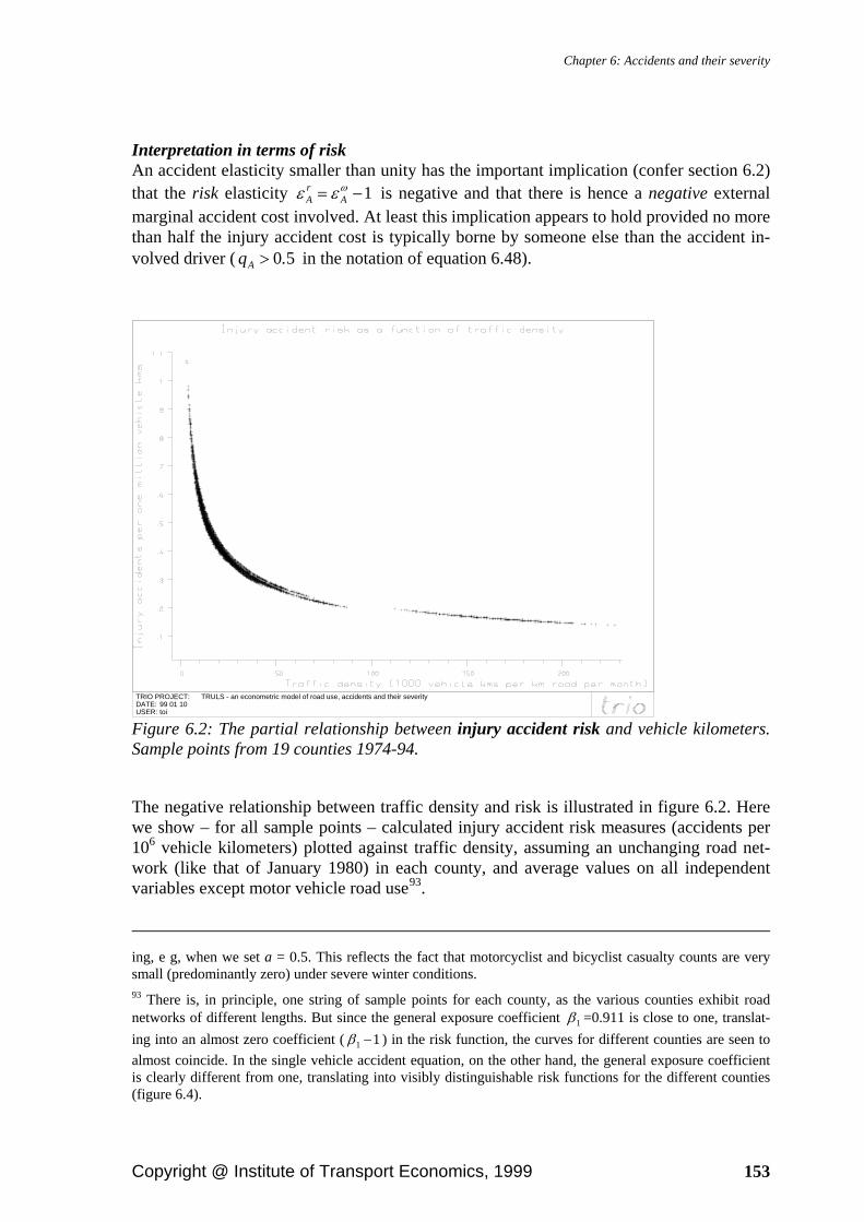
Chapter 6: Accidents and their severity
Copyright @ Institute of Transport Economics, 1999 153
Interpretation in terms of risk An accident elasticity smaller than unity has the important implication (confer section 6.2) that the risk elasticity 1−= ωεε A
rA is negative and that there is hence a negative external
marginal accident cost involved. At least this implication appears to hold provided no more than half the injury accident cost is typically borne by someone else than the accident in-volved driver ( 50.qA > in the notation of equation 6.48).
TRIO PROJECT: TRULS - an econometric model of road use, accidents and their severityDATE: 99 01 10USER: toi Figure 6.2: The partial relationship between injury accident risk and vehicle kilometers. Sample points from 19 counties 1974-94.
The negative relationship between traffic density and risk is illustrated in figure 6.2. Here we show – for all sample points – calculated injury accident risk measures (accidents per 106 vehicle kilometers) plotted against traffic density, assuming an unchanging road net-work (like that of January 1980) in each county, and average values on all independent variables except motor vehicle road use93.
ing, e g, when we set a = 0.5. This reflects the fact that motorcyclist and bicyclist casualty counts are very small (predominantly zero) under severe winter conditions. 93 There is, in principle, one string of sample points for each county, as the various counties exhibit road networks of different lengths. But since the general exposure coefficient 1β =0.911 is close to one, translat-ing into an almost zero coefficient ( 11 −β ) in the risk function, the curves for different counties are seen to almost coincide. In the single vehicle accident equation, on the other hand, the general exposure coefficient is clearly different from one, translating into visibly distinguishable risk functions for the different counties (figure 6.4).

An econometric model of car ownership, road use, accidents, and their severity
154 Copyright @ Institute of Transport Economics, 1999
The imputed risk varies by a factor of about seven between the highest and lowest density observations in the sample.
Similarly shaped relationships apply even to the subset of multiple vehicle accidents caus-ing personal injury (figure 6.3), although here the risk varies by a factor of less than four within the sample. For single vehicle accidents, on the other hand, the risk is almost nine times higher at the lower end of the density range than in the upper end (figure 6.4).
TRIO PROJECT: TRULS - an econometric model of road use, accidents and their severityDATE: 99 01 10USER: toi Figure 6.3: The partial relationship between multiple vehicle injury accident risk and vehicle kilometers. Sample points from 19 counties 1974-94.

Chapter 6: Accidents and their severity
Copyright @ Institute of Transport Economics, 1999 155
TRIO PROJECT: TRULS - an econometric model of road use, accidents and their severityDATE: 99 01 10USER: toi Figure 6.4: The partial relationship between single vehicle injury accident risk and vehi-cle kilometers. Sample points from 19 counties 1974-94. Heavy vehicle traffic The heavy vehicle share of the traffic volume (cevhvysh) appears to affect the injury acci-dent frequency unfavorably, with an elasticity of 0.149 (table 6.1, column A). Heavy vehi-cles are apparently more (injury) accident prone than light vehicles.
Interestingly, the heavy vehicle traffic share has a moderately negative (i e, favorable) and barely significant effect on car occupant injuries, but a very strong positive (unfavorable) effect on two-wheeler injuries, the elasticity exceeding 0.4 for motorcyclists as well as for bicyclists (table 6.1, columns C-D).
Also, the heavy vehicle share has a much stronger than average impact on multiple vehicle injury accidents, while the effect on single vehicle accidents is much less significant, and besides negative (table 6.2, columns A-B).
Columns C-D of table 6.2 represent casualty subset tests for the heavy vehicle effect on accident frequency. Column C is a model for injury accidents involving truck or bus. This model comes out with an elasticity estimate of 0.688. Column D is a corresponding model for injury accidents not involving a truck or bus. Here, the corresponding elasticity esti-mate is 0330.− , and not significant94.
Thus, the heavy vehicle exposure measure passes the affirmative casualty subset test (see section 6.4.3) as applied to accidents involving truck or bus versus all injury accidents. It
94 Data on injury accidents by type of vehicles involved are available (to us) only for the subsample period 1973-86. Hence certain variables which do not vary within this subsample (such as dummies for legislative changes taking place during 1987-94) had to be dropped. Otherwise the set of regressors is identical to the set used in our main model.

An econometric model of car ownership, road use, accidents, and their severity
156 Copyright @ Institute of Transport Economics, 1999
also passes the complement casualty subset test as applied to accidents involving truck or bus versus those not involving such vehicles.
We conclude that our calculated measure of heavy vehicle exposure does seem to represent well what it is supposed to capture, and that the heavy vehicle effect estimated in the main model is most probably not due to spurious correlation.
Accident elasticities
We have discussed the relationship between traffic density and risk in terms of elasticities as evaluated at the sample means.
In our model, however, the accident elasticity is not in general constant. To be precise, the model is specified as follows:
(6.86) ( ) ( )( )
( )tr
itrii
tr
trA
trA
trHtrAtr ux
lv~
v~v~lnv~lnayln i ++⎟⎟
⎠
⎞⎜⎜⎝
⎛+⎟⎟
⎠
⎞⎜⎜⎝
⎛+=+ ∑
>3321
3
λλ
ββββ ,
where ytr denotes the number of accidents or victims of some kind, a (= 0.1) is the Box-Tukey constant, trAv~ is the overall traffic volume (vehicle kilometers driven), as derived in chapter 3 above, trHv~ is the corresponding heavy vehicle traffic volume, ltr is the length of the (public) road network, xtri (i>3) denote all the other independent variables of the model, utr is the random disturbance term, β i are coefficients, and λ i are Box-Cox pa-rameters.
1β is the general exposure (traffic volume) coefficient, 2β is the coefficient for the share of heavy vehicles, while 3β measures the separate effect of traffic density, given the traffic volume (vehicle kilometers).
Assume, for the sake of argument, that the heavy vehicle share of the traffic volume ( )trAtrH v~v~ or the length of the road network ( )ltr does not change. In such a case, we can write the elasticity of [ ]trtr yE≡ω with respect to the traffic volume95 ( trAv~ ) as
(6.87) 3
31
λω ββε
ωω
⎟⎟⎠
⎞⎜⎜⎝
⎛+=≡
∂∂
tr
trAtrA
tr
trA
trA
tr
lv~v~
v~,
in keeping with the notation introduced in section 6.2 above.
This elasticity depends, in other words, on the traffic density, and on no other variables. In figure 6.5, therefore, we show accident elasticities as evaluated at each sample point and plotted against traffic density. Separate curves are shown for (i) injury accidents in total, as well as for the three disjoint subsets (ii) multiple vehicle accidents, (iii) single vehicle ac-cidents, and (iv) pedestrian casualties.
One notes that all elasticities are between 0 and 1, not only on the average, but for each and every observation in the sample. Also, one notes that the multiple vehicle accident
95 In deriving these elasticities we disregard the small Box-Tukey constant. To correct for this inaccuracy, one should multiply all elasticities by ( ) ωω a+ , ω being the expected number of accidents or casualties.

Chapter 6: Accidents and their severity
Copyright @ Institute of Transport Economics, 1999 157
elasticity is higher than the general injury accident elasticity throughout the range of our sample, and that the opposite is true of the pedestrian injuries elasticity.
The elasticity is a decreasing function of the traffic density if and only if
(6.88) ( ) 01
33
3
<⎟⎟⎠
⎞⎜⎜⎝
⎛=
−λω
λβ∂
∂ε
tr
trA
trtrA
A
lv~
lv~,
i e if and only if β 3 and λ 3 have opposite signs.
In the main (injury accidents) model, the traffic density coefficient is estimated at 43503 .ˆ −=β (–0.512, –0.357) and its Box-Cox parameter at 01303 .ˆ −=λ (–0.163, 0.137)
(95 per cent confidence intervals in parentheses). We cannot, therefore, reject the hypothe-sis that λ 3 0= and hence that the overall injury accident elasticity is unaffected by the traffic density.
The same is true even for pedestrian casualties and for multiple vehicle accidents. In nei-ther case is the Box-Cox parameter λ 3 significantly different from zero (confidence inter-vals from –0.110 to 0.139 and from –0.456 to 0.126, respectively).
Thus the apparently rising tendency of the multiple vehicle accident elasticity should be interpreted with caution, as the slope is – in a sense – not significantly different from zero.
For single vehicle accidents, however, the elasticity is seen to decline significantly with traffic density. Here, the Box-Cox parameter λ 3 is estimated at 0.408, with confidence interval ranging from 0.075 to 0.741.
TRIO PROJECT: TRULS - an econometric model of road use, accidents and their severityDATE: 99 01 11USER: toi Figure 6.5: Accident elasticities evaluated at sample points, plotted against traffic density.

An econometric model of car ownership, road use, accidents, and their severity
158 Copyright @ Institute of Transport Economics, 1999
At this point, let us relax the assumption that the mix between light and heavy vehicles is constant, and compute elasticity formulae with respect to either type of vehicles. Noting that
trHtrLtrA v~v~v~ +≡ ,
where trLv~ is the number of light vehicle kilometres driven96, we have, after some algebra,
(6.89) trA
trL
tr
trAtrL
tr
trL
trL
tr
v~v~
lv~v~
v~⋅
⎥⎥⎦
⎤
⎢⎢⎣
⎡⎟⎟⎠
⎞⎜⎜⎝
⎛+−=≡
∂∂ 3
321
λω βββε
ωω
and
(6.90) trA
trH
tr
trA
trH
trLtrH
tr
trH
trH
tr
v~v~
lv~
v~v~v~
v~⋅
⎥⎥⎦
⎤
⎢⎢⎣
⎡⎟⎟⎠
⎞⎜⎜⎝
⎛++=≡
∂∂ 3
321
λω βββε
ωω .
The terms outside the brackets are the vehicle categories’ respective «market» (traffic) shares. The elasticities depend on these shares in a multiplicative fashion, as is commonly also found in travel demand analysis.
Combining these formulae with equation (6.47) of section 6.2, we note that the traffic shares cancel out, leaving us with the terms inside the brackets as the most relevant meas-ures in relation to externality assessments.
Externality assessments
In table 6.3, we show imputed injury accident elasticities with respect to overall, light and heavy vehicle traffic volumes (by formulae 6.87, 6.89 and 6.90), as well as the measures
( )trjtrAtrj v~v~ωε entering the accident externality formula (6.47). Minimal, mean and maxi-mum values, as resulting from evaluating the elasticities at each sample point, are shown.
Table 6.3: Estimated measures of partial association between injury accidents and overall, light vehicle and heavy vehicle road use. Minimal, mean and maximal sample point values.
Elasticity Inverse traffic share times elasticity Traffic category
Minimum Mean Maximum Minimum Mean Maximum
Total vehicle kilometers 0.484 0.494 0.506 0.484 0.494 0.506
Light vehicle kilometers 0.248 0.291 0.361 0.335 0.345 0.357
Heavy vehicle kilometers 0.181 0.202 0.236 0.909 1.321 1.974
These elasticities do not vary a lot across the sample. The sample point elasticities with respect to light vehicle road use cluster between 0.25 and 0.36, with a mean of 0.291. With respect to heavy vehicle traffic, the imputed elasticities range from 0.18 to 0.24, with a sample mean of 0.202. 96 Light vehicles are defined as all vehicles with less than 20 passenger seats or less than 1 ton’s carrying capacity.

Chapter 6: Accidents and their severity
Copyright @ Institute of Transport Economics, 1999 159
The elasticity is, in other words, consistently lower with respect to heavy vehicle road use than for light vehicles. This is, however, primarily due to the heavy vehicles’ much smaller traffic share. In our sample, the light vehicle traffic volume is, on the average, six times larger than the heavy vehicle road use.
When correcting for the unequal traffic shares, we note that the marginal accident effect of heavy vehicle traffic is 3.8 times larger than for light vehicles. Heavy vehicles are thus, in a sense, about four times more dangerous than light ones.
Owing to the pronounced variation in traffic mix across space and time, the marginal acci-dent effect of heavy vehicles is more than twice as strong at its sample maximum com-pared to its minimum value.
According to these estimates, there is a positive external injury accident cost generated by the marginal representative road user only in so far as the share of the accident cost borne by the individual road user himself is smaller than 0.5 (see equation 6.48). In the opposite case, there is an external benefit involved97.
For light vehicle users, the analogous mean «threshold» point is 0.34, and for heavy vehi-cles 1.32.
There is reason to believe that the share of the accident cost borne by the heavy vehicle operator is relatively small, and hence that there is a positive external accident cost linked to the marginal heavy vehicle kilometre. Assuming that, statistically speaking, the heavy vehicle operator sustains a private loss per kilometre amounting to no more than 32 per cent of the average unit cost of accidents, his road use typically gives rise to a positive marginal external accident cost which is at least as large as the mean total cost of an acci-dent.
For light vehicle users, the sign of the externality is more questionable. Depending on the values attached to personal pain and suffering or to the loss of life or limb, and on the dis-tribution of casualties between single vehicle accidents, unprotected road users, and multi-ple vehicle crashes, one might arrive at different conclusions. It is not obvious that
( ) ( )vv kkq LL is smaller than one third (= appr 0.34), but if it is, this would probably be due, inter alia, to the fact that significant parts of the accidents costs are usually covered by private and social insurance. There is therefore, in our view, a potential positive exter-nal accident cost involved even for private car users, not in spite of automobile insurance, but because of it.
Since, however, the measure ( ) ( )vv kkq LL cannot possibly drop below zero, the external part of the marginal light vehicle accident cost is unlikely to be very large. It cannot, based on our estimates, exceed one third of the total accident cost on the average.
For a definite conclusion in this matter, research is needed to estimate the quantities α , jq and ( )vjk and their possible dependence on the traffic volume.
One might want to ask to what extent these results could be generalized outside our sam-ple. In general, the traffic density in Norway is relatively low by international standards. In 97 Recall that we have made the simplifying assumption that the average loss incurred during an accident is independent of the traffic density. If, however, speed is forced down in denser traffic, it seems reasonable to assume that this loss is a negative function of density. Taking account of this would pull our externality esti-mate even further in the direction of a marginal benefit.

An econometric model of car ownership, road use, accidents, and their severity
160 Copyright @ Institute of Transport Economics, 1999
our data set, only the county of Oslo exhibits traffic density levels above 90 000 vehicles per month, corresponding to an ADT of some 3 000 vehicles as averaged over all road links in the network. The maximum density represented in the sample corresponds to an ADT of approximately 7 000 vehicles.
Note that these figures are not comparable to the traffic flow on given road links, as they are interpretable as averages for all road links within an extended geographic area. Still we suspect that in most urbanized districts of, e g, Western Europe, the level of traffic density would often extend far beyond the values found in our Norwegian sample. A similar em-pirical analysis based on data from these regions would be necessary in order to assess whether the negative relationship between risk and density would hold even at the high rates of road use characterizing the densely populated regions of Europe.
Judging by the analysis presented herein, it is not true, as is often maintained, that the ac-cident risk is largely independent of the traffic volume. Nor is it true that the risk elasticity with respect to road use is positive. This elasticity appears to be close to zero when con-gestion is assumed constant, but distinctly smaller than zero when congestion (traffic den-sity) effects are taken into account, conceivably generating a negative marginal external cost, at least for private car users.
Severity An intriguing set of results are derived in the severity submodels. Previous studies (Frid-strøm and Ingebrigtsen 1991, Fridstrøm et al 1995) have shown lower elasticities with re-spect to exposure for fatal accidents then for injury accidents, and stronger traffic density effects. Our severity equations, however, suggest otherwise. The elasticity of fatalities with respect to traffic volume is calculable by summing the relevant partial elasticities from the injury accident and mortality equations, i e as 0.769 (= 0.911 – 0.142) under constant traf-fic density, and as 0.941 (= 0.759 – 0.415 + 0.587) under constant road length.
Thus, traffic density appears to have an increasing effect on severity. This is true of all three severity measures, although none of the three effects are statistically significant.
We cannot rule out methodological errors as one possible interpretation here. These errors are potentially threefold.
First, when speed is forced down in denser traffic, it is quite conceivable that fewer acci-dents end up causing injury, and that the relative reduction in injury accidents is stronger than the decline in fatalities («reporting drift»).
Second, if the reporting incidence for injury accidents is negatively correlated with traffic density, a negative bias is caused in the accident equation and a positive one in the mortal-ity equation, affecting the density coefficient estimates.
Third, regressions based on small casualty counts turn out to be sensitive to the choice of the Box-Tukey constant (a), especially as regards the exposure coefficients. This problem carries over to the mortality and «severity 3» equations.
Further analysis would be in order at this point (see section 7.3.1).

Chapter 6: Accidents and their severity
Copyright @ Institute of Transport Economics, 1999 161
6.7.2. Motorcycle exposure
Exposure must be understood as a multidimensional causal agent. Light and heavy vehicle kilometers are the two components discussed so far. A third important road user group is the motorcyclists. No statistics exist, however, on MC exposure by county and month. We have therefore constructed a proxy variable (cevmcw1), described as «warm days times ratio of MC to 4-wheel light vehicle pool», assumed to capture the essence of the cross-section/time-series variation in motorcycle exposure. It takes account of the weather condi-tions as well as of the size of the motorcycle stock relative to the car pool. To be precise, it is defined by
(6.91) ( ) ( ) ( )
xxx
pptr
trW
t M
tr
tr4
2
4
0 23
430 1λ =
+⎡
⎣⎢
⎤
⎦⎥
⋅
+
+
− .
where xtrW is the number of days with maximum temperature above 10 °C in month t in county r, xt M⋅ is the length of the month (in days), ptr
+2 is the number of motorcycles and mopeds registered, and ptr
+4 is the number of light 4-wheel vehicles. The best-fit Box-Cox parameter λ 4 0 23= − . was estimated from a very simple, intermediate model, in which the number of motorcyclists injured was regressed on the total traffic volume and on the xtr4 (= cevmcw1) measure only. We keep this Box-Cox parameter fixed in all our accident (and severity) models.
The variation in ( )xtr44λ is depicted in figure 6.6. One notes a strongly seasonal pattern of
variation, MC exposure being almost zero during the winter months, at least in the north-ernmost counties.
TRIO PROJECT: TRULS - an econometric model of road use, accidents and their severityDATE: 97 11 10USER: toi Figure 6.6: Motorcycle exposure proxy variable. 19 counties 1973-94.

An econometric model of car ownership, road use, accidents, and their severity
162 Copyright @ Institute of Transport Economics, 1999
MC exposure is seen to have a small, but clearly significant effect on the injury accident frequency (table 6.1, column A). A complement casualty subset test is obtained by com-paring a model for MC victims (column C) to, e g, a model for car occupant injuries (col-umn B). The former effect is about eight times stronger than the general effect, and highly significant, while the latter effect is zero, as expected. We conclude that our MC exposure proxy does capture what it is supposed to capture, and little less.
Bicyclist exposure is even harder to assess than motorcycle exposure, since there is no register of bicycle ownership, let alone regional time-series on their use. It appears, how-ever, that our MC exposure proxy also acts a fairly good measure of bicyclist exposure, coming out with an even larger and more significant effect in the bicyclist injuries model (column D) than in the MC model. This result is by no means unreasonable, since the same climatic and meteorological conditions favoring MC ownership and use would obviously also make bicycling more attractive.
6.7.3. Public transportation supply
Pedestrians are the fifth road user group with an exposure whose size we would like to know and control for.
Pedestrian exposure probably exhibits less seasonal variation than bicyclist and MC expo-sure. To the extent that walking and bicycling act as substitute modes, one might even imagine opposite patterns of seasonal variation between the two. Casual observation from the Norwegian travel environment suggests, however, a markedly higher pedestrian expo-sure during summer than in winter.
To account for pedestrian exposure, we must rely entirely on indirect measures. Public transportation supply typically generates pedestrian access and egress trips. To capture these effects we include the density of bus and (sub)urban rail services (annual vehicle kilometers per kilometer public road - dtabus and dtarail) as separate exposure measures. These variables obviously also capture the exposure represented by the buses and street-cars themselves, although bus exposure is, in principle, already accounted for by the heavy vehicle traffic share variable.
In addition, it should be kept in mind that certain other independent variables are also li-able to capture, to some extent, variations in pedestrian exposure. This applies to road network density (cilrdspc, see section 6.7.7), population density (cdpopdnsty, section 6.7.6), as well as all daylight and weather variables (sections 6.7.9 and 6.7.10),
The density of bus services affects injury accidents in general by an elasticity of 0.243 (ta-ble 6.1, column A). The effect is clearly significant. Even for this exposure component, confidence is strengthened through a casualty subset test, obtained by comparing the pe-destrian casualties model (elasticity 0.764, column G) to the car occupant injuries model (elasticity 0.189, column B), or to the overall accident model.
Similar effects are found for public transportation by rail (streetcar or subway)98. The es-timated elasticity of car occupant injuries with respect to light rail supply is, however,
98 This variable is a «quasi-dummy», being equal to zero for all counties except two. The elasticities shown are averaged over units with strictly positive values only.

Chapter 6: Accidents and their severity
Copyright @ Institute of Transport Economics, 1999 163
negative and insignificant. This is an entirely reasonable result in view of the fact that the greater part of the rail transport (the suburban subways) is confined to tracks completely separated from the road network.
A rather important lesson to be learnt from these analyses is that, in a wide perspective, public transportation is not without risk. A one per cent uniform growth in bus and rail supply is apt to increase pedestrian accidents by some 0.8 per cent. Even bicyclist acci-dents appear to be strongly affected by public transportation supply (table 6.1, column D), presumably because many commuters use the bicycle as an access/egress mode.
6.7.4. Vehicle stock
It is frequently argued that old cars are dangerous. Vehicle crashworthiness has improved greatly over the last few decades, making it likely that a recently manufactured car would mean a lower injury accident risk compared to an earlier model. Moreover, the technical condition of cars tends to deteriorate with their age. There is, in other words, a potential «car cohort effect» as well as a «pure age effect».
However, the frequently observed positive bivariate correlation between vehicle age and accident rate may well be due to the fact that the younger and less wealthy drivers tend to drive the cheaper and older cars. Novice drivers have a markedly higher risk than the more experienced ones.
Table 6.4: Estimated casualty elasticities etc with respect to vehicle characteristics, seat belt use and helmet use. T-statistics in parentheses. Dependent variable: Injury
accidentsCar
occupants injured
MC occu-pants
injured
Bicyclists injured
Pede-strians injured
Severely injured per accident
Dange-rously
injured per accident
Mortality (fatalities per acci-
dent)
Column: A B C D E F G H
Elasticities evaluated at overall sample means (1st line) and at 1994 subsample means (2nd line) -------- Vehicles -------- Passenger cvrcarsp .068 .239 .116 -.030 .025 .206 .070 cars per capita .058 .204 .099 -.026 .027 .208 .063 (.98) (2.12) (.63) (-.24) (.33) (1.08) (.36) LAM LAM LAM LAM LAM LAM LAM Mean age of passenger cvrta1 .172 .172 -.345 1.765 -.344 .188 -.498 -.639 cars .172 .172 -.345 1.765 -.344 .235 -.558 -.677 registered in county (1.56) (1.27) (-1.47) (5.96) (-1.58) (1.35) (-1.57) (-1.89) LAM 4 LAM 4 LAM 4 LAM 4 LAM 4 LAM 4 LAM 4 LAM 4 ------------------ Road user behavior ------------------ Calculated cbbeltnonw .092 .167 -.016 -.057 -.075 county-wide share .235 .302 -.044 -.115 -.174 of drivers not (5.91) (7.15) (-.72) (-.91) (-1.31) wearing seat belt LAM LAM LAM LAM LAM Imputed MC cbhnonw -.144 helmet non-use rate -.036 (-4.86)
Curvature parameters Dependent variable MU .000 .000 .000 .000 .000 .547 .436 .350 Box-Cox parameter FIXED FIXED FIXED FIXED FIXED [45.10] [27.75] [21.94]

An econometric model of car ownership, road use, accidents, and their severity
164 Copyright @ Institute of Transport Economics, 1999
LAMBDA(X) - GROUP 4 LAM 4 .000 .000 .000 .000 .000 .000 .000 .000 FIXED FIXED FIXED FIXED FIXED FIXED FIXED FIXED LAMBDA(X) cvrcarsp -1.000 -1.000 -1.000 -1.000 -1.000 -1.000 -1.000 FIXED FIXED FIXED FIXED FIXED FIXED FIXED LAMBDA(X) cbbeltnonw -1.204 -.757 -1.000 -1.000 -1.000 [-2.00] [-1.60] FIXED FIXED FIXED
Indeed, in a very large and well controlled experimental study on the effects of periodic motor vehicle inspection (Fosser 1992), it was found that the technical deterioration of cars did not have any influence on their accident rates. Two explanations were offered: «Either the technical defects do not affect vehicle performance in ways that are important to safe
driving, or drivers compensate for known technical defects by driving more carefully.» In another large-scale, disaggregate analysis (Fosser and Christensen 1998), it was found that older cars are involved in significantly fewer accidents than new cars, when the annual driving distance and the owner’s age, gender and province of residence were controlled for. Such a partial relationship was found for material damage accidents as well as for in-jury accidents. The authors suggest risk compensation (offsetting behavior) as their main explanation: Newer, «safer» and more comfortable cars are generally driven less defen-sively than old cars.
In our model, no statistically significant effect was found of the mean age of the automo-bile stock (table 6.4). Some support is found for the risk compensation hypothesis, in that the coefficient in the mortality equation, although barely significant, has the opposite sign compared to the accident equation. If drivers compensate for the age of the car by going more slowly, this is precisely the coefficient pattern to be expected (confer sections 6.1.4-6.1.5).
TRIO PROJECT: TRULS - an econometric model of road use, accidents and their severityDATE: 97 05 09USER: lef

Chapter 6: Accidents and their severity
Copyright @ Institute of Transport Economics, 1999 165
Figure 6.7: Sample variation in the mean age of cars. 19 counties 1973-94.
Now, the fact that no significant effect is estimated for injury accidents in general (or for car occupant injuries, column B of table 6.1) does not prove, of course, that the effect is zero (or smaller). It could be due to insufficient variation in the sample, something that widens the confidence interval and reduces the power of any test.
However, such an explanation hardly seems justified. There is, in fact, ample cross-sectional as well as temporal variation in our car age variable, as demonstrated by figure 6.7. The mean age of the automobile pool varies from about 5 to almost 11 years within the sample. It has been increasing in all counties between 1986 and 1994.
In our exploratory model, we also tested two more vehicle stock attributes for significance: the percentage of cars with mandatory rear seat belts installed, and the percentage obliged to use daytime running lights. Both were, however, dropped following casualty subset tests. Rear seat belts became mandatory on all cars from 1984 on, and has since penetrated into the car population at a rate depending on scrapping and new car acquisition. This vari-able did show a significant negative effect on injury accidents in general. However, the effect was larger for pedestrian and bicyclist casualties than for car occupants, and larger for grown-ups than for children – quite contrary to expectations under a casualty subset perspective.
Automatic daytime running lights have been mandatory equipment on all new cars since 1985. Since 1987, all cars have been obliged to use daytime running lights, whether or not an automatic switch-on device has been installed. This variable was blatantly insignificant in the exploratory model, and with counterintuitive signs as applied to nighttime and day-time accidents separately99.
In the models for car occupant, motorcyclist, bicyclist and pedestrian injuries (columns B-D of table 6.1), we also include the number of passenger cars per capita (cvrcarsp) as an independent variable, with a Box-Cox parameter fixed at minus one. This is tantamount to relating the injury count to the reciprocal of the car ownership rate, i e to the number of inhabitants per car, which may be viewed as a proxy for the car occupancy rate.
The injury count may be thought to vary with the car occupancy rate because the higher this rate, the more persons are exposed to risk per vehicle kilometer traveled. One might also envisage a certain exposure effect for bicyclists and pedestrians, in that these modes of travel become relatively less attractive as the availability of cars increases.
The variable is, however, significant only for motorcyclists. It generally comes out with a counterintuitive sign.
6.7.5. Seat belt and helmet use
Seat belt use has a clear safety effect. When the proportion of drivers not wearing a belt increases by 10 per cent (from the level imputed for 1994), injury accidents in general in-
99 If daytime running lights did have any effect, one should find a negative coefficient for daytime accidents and a zero coefficient for nighttime events, by a complement casualty subset test. We found, however, rather the opposite pattern: positive for daytime events and negative for nighttime.

An econometric model of car ownership, road use, accidents, and their severity
166 Copyright @ Institute of Transport Economics, 1999
crease by about 2.4 per cent. Car occupant injuries increase more, by 3.0 per cent, as ex-pected from an affirmative casualty subset test (confer example 6.1 of section 6.4.3).
A more powerful, converse casualty subset test for the effect of seat belt use is reported in table 6.5. Since 1977, the accident report forms include information as to whether or not car occupants were wearing a seat belt at the time of the crash. Thus, in column A, we show partial result from a model explaining the number of car occupants injured while wearing a belt. In column B, we have regressed the number of car occupants injured while not wearing a belt on the same independent variable. For comparison, we have reestimated the models for all car occupant injuries and for all injury accidents on the 1977-94 sub-sample (columns C and D, respectively).
Unless the seat belt effect found in the main model is due to spurious correlation, we ex-pect to find a negative elasticity in column A, a positive one in column C, and an even lar-ger, positive one in column B. Seat belt non-use should decrease the number of injuries among seat belt wearers, while a larger than average increase should be found among non-wearers (example 6.2 of section 6.4.3 above).
This is exactly what our converse casualty subset test reveals, all coefficients being highly significant with the expected relative size and sign.
Table 6.5: Casualty subset models for seat belt users vs non-users. 1977-94 sub-sample. Selected results. Dependent variable: Car occupants
injured while wearing belt
Car occupants injured while
not wearing belt
Car occupants injured in total
Injury acci-dents in total
Column: A B C D
Elasticities evaluated at sample means, with t-statistics in parentheses Calculated cbbeltnonw -.082 .380 .194 .118 county-wide share (-4.04) (10.91) (6.97) (5.99) of drivers not wearing seat belt
There is no significant tendency, according to our estimates, for bicyclist and pedestrian injuries to decrease with the rate of non-use, as implied by Peltzman (1975). These coeffi-cients came out as close to zero and were hence dropped from the bicyclist and pedestrian injury submodels.
For motorcyclists, we include a measure of nationwide helmet use, calculated from a sum-mary regression of helmet survey results on legislative dummies. This variable has the counterintuitive sign, as do the relevant legislative dummies when entered directly into the casualty model. There is, in other words, no sign that increased helmet use, or the legisla-tion meant to promote it, has had any casualty reducing effect – rather the contrary. These results are consistent with nationwide aggregate statistics on motorcyclist injuries before and after the helmet use legislation in Norway, but contrary to international findings, which tend to show clearly injury reducing effects of MC helmet use (Elvik et al 1997 and references therein).

Chapter 6: Accidents and their severity
Copyright @ Institute of Transport Economics, 1999 167
It is interesting to note that our empirical results concerning seat belt and helmet use are quite consistent with Bjørnskau’s hypotheses B-C (see section 6.1.4). Car drivers, who stand to suffer large material losses in the event of an accident, do not seem to compensate for seat belt use. For motorcyclists, on the other hand, the balance between expectable ma-terial and bodily damage is quite different. Hence it is quite conceivable that these do com-pensate for helmet use, increasing the overall accident risk, as has been suggested by cer-tain studies on bicycle helmets (Vulcan et al 1992, Cameron et al 1994, Robinson 1996).
For seat belt non-use, a Box-Cox parameter of –1.204 is estimated in the injury accidents model, while in the car occupant injuries model the Box-Cox parameter estimate is –0.757. These negative curvature parameters imply – rather reasonably – that the elasticity of seat-belt non-use is tapering off as the rate of non-use approaches 100 per cent. In the severity models, only very imprecise estimates could be obtained for this Box-Cox pa-rameter, whence it was fixed at –1.
The imputed partial relationship between injury accidents and seat belt use is depicted in figure 6.8. The relationship is curving more steeply downwards as the rate of seat belt use approaches 100 per cent. This result is probably a reflection of the fact that in two-vehicle collisions, the probability that at least one driver sustains injury is determined, roughly speaking, by a quadratic function of the seat belt use rate100.
100 Let p denote the probability that an accident involved, seat-belt wearing car driver sustains injury, and assume, for the sake of the argument, that the corresponding probability for seat-belt non-users can be set to 1. If accident involved drivers are a random sample of the driver population, the probability that any one driver is injured, given that there is an accident, is calculable as ( ) pss +−1 , where s is the proportion using seat belts. The complement probability is ( ) ( )pspss −=−−− 111 , and hence the probability that, in a two-
vehicle accident, at least one driver is injured is given by ( ) ( )sfps ≡−− 22 11 (say). This function has nega-tive first and second order derivatives, like the curve shown in figure 6.8. Taking account also of accidents that involve no more than one vehicle will shift the curve and the first order derivative, but affect the second order derivative only by a proportionality factor.

An econometric model of car ownership, road use, accidents, and their severity
168 Copyright @ Institute of Transport Economics, 1999
TRIO PROJECT: TRULS - an econometric model of road use, accidents and their severityDATE: 99 02 09USER: toi Figure 6.8: Partial relationship between injury accidents and seat belt use.
A 90 per cent rate of seat belt use is seen to be consistent, ceteris paribus, with an ap-proximately 20 per cent lower incidence of injury accidents, compared to the situation when no one is using the belt. For car occupant injuries, we find a corresponding 30 per cent decrease from the lowest to the highest observed level of seat belt use. These results are well in line with previous research, which suggest a 23 to 33 per cent decrease in injury risk for a seat belt wearing driver compared to a non-user (Elvik et al 1997:413).
More disturbing is the finding that seat belt non-use seems to have a negative effect on severity (table 6.4), implying that seat belts are more effective in preventing slight injuries than in counteracting the more severe ones. This result is contrary to the great bulk of pre-vious research (ibid). Further studies would be in order at this point (see section 7.3.2).
6.7.6. Population
Demographic structure
Changes in the demographic structure represent a potentially powerful source of variation in aggregate accident counts. Young drivers have a markedly higher accident risk than the middle-aged. Their share of the driving population might therefore be an important deter-minant. Even elderly drivers have a clearly augmented risk compared, e g, to drivers in their forties (Bjørnskau 1993, Fridstrøm 1996).

Chapter 6: Accidents and their severity
Copyright @ Institute of Transport Economics, 1999 169
To take account of these effects, we calculated the share of young persons (aged 18-24) in the adult population (above 18), and, as a further decomposition, the share of these who were only 18-19 years old. These variables were included in our exploratory model101.
Much to our surprise, these variables came out with entirely counterintuitive, negative co-efficients. Casualty subset tests carried out by comparing models for younger and older accident involved car drivers gave equally counterintuitive results. We concluded that these effects must be due to omitted variable bias of some kind and decided to drop the age variables from the main model102.
Kindergartens
Another population variable whose effect we would like to assess is the share of preschool children attending daycare centers (nursery homes, kindergartens). Norwegian children start school at the age of seven (at six since 1997). Up until rather recently, only a minority of preschool children used to be enrolled in daycare centers. Our conjecture is that such enrollment helps keep children away from of the streets and hence lowers their overall risk of being involved in an accident. On the other hand, transportation to and from the daycare center might expose the children to a certain road accident risk, not incurred at home.
The daycare center enrollment variable came out significant and had the expected negative sign in the exploratory model. It did, however, not pass our affirmative casualty subset test, effectuated by running separate regressions for 0-6-year-old road victims and for those above 7. True, a larger than average effect was found for preschool children. But a signifi-cant, obviously spurious effect was found even for older road users, not affected by the daycare centers. Such a confounding effect is not very surprising given the relatively mo-notonous growth in daycare center enrollment that has taken place in the sample period.
In conclusion, there appears to be a certain safety effect of daycare center enrollment. However, the spurious component attached to this variable is too large to justify its inclu-sion in our main model.
Table 6.6: Estimated casualty elasticities etc with respect to socio-demographic variables. T-statistics in parentheses. Dependent variable: Injury
accidentsCar
occupants injured
MC occu-pants
injured
Bicyclists injured
Pede-strians injured
Severely injured per accident
Dange-rously
injured per accident
Mortality (fatalities per acci-
dent)
Column: A B C D E F G H
101 Ideally, the share of car drivers (or of car driver kilometers traveled) belonging to certain age groups, and/or the share of novice drivers in the total car driver population, would have been entered into the model. Such data have, however, not been available at the level of county and month. Most individuals acquire their driving licenses before the age of 20, so that our measures should represent a set of rather good proxies for the true variables of interest. 102 Even more sophisticated demographic variables were also tried, such as a «demographic risk index» cal-culated by weighing together all age groups in the population with their corresponding «road accident health risk» (i e, the frequency of injury road accidents per year of living). All our demographic variables came, however, out with counterintuitive effects.

An econometric model of car ownership, road use, accidents, and their severity
170 Copyright @ Institute of Transport Economics, 1999
Elasticities evaluated at overall sample means (1st line) and at 1994 subsample means (2nd line) ---------- Population ---------- Population density cdpopdnsty .068 .020 .151 .033 .066 -.104 -.194 -.178 (inhabitants per sq .068 .020 .151 .033 .066 -.131 -.218 -.189 km) (2.91) (.63) (3.13) (.46) (1.16) (-3.34) (-2.94) (-2.66) LAM 4 LAM 4 LAM 4 LAM 4 LAM 4 LAM 4 LAM 4 LAM 4 Unemployment rate cderate -.024 -.032 .019 .023 -.044 -.029 -.033 .021 (per cent of -.024 -.032 .019 .023 -.044 -.037 -.037 .022 working age (-2.34) (-2.27) (.94) (.83) (-2.06) (-2.04) (-.93) (.58) population) LAM 4 LAM 4 LAM 4 LAM 4 LAM 4 LAM 4 LAM 4 LAM 4 Women cdpregrate2 .181 .115 .472 .004 -.071 -.073 -.225 -.267 pregnant in first .181 .115 .472 .004 -.071 -.091 -.253 -.283 quarter per (3.38) (1.64) (4.21) (.03) (-.61) (-.99) (-1.28) (-1.45) 1000 women 18-44 LAM 4 LAM 4 LAM 4 LAM 4 LAM 4 LAM 4 LAM 4 LAM 4
Curvature parameters Dependent variable MU .000 .000 .000 .000 .000 .547 .436 .350 Box-Cox parameter FIXED FIXED FIXED FIXED FIXED [45.10] [27.75] [21.94] LAMBDA(X) - GROUP 4 LAM 4 .000 .000 .000 .000 .000 .000 .000 .000 FIXED FIXED FIXED FIXED FIXED FIXED FIXED FIXED
Population size
The size (or density) of population103 has a small effect on casualties, over and above the exposure effects expressed by vehicle kilometers and public transportation supply (table 6.6). For car occupant injuries the effect is insignificant and very small, but for pedestrian injuries a somewhat larger (although still insignificant) effect can be traced. This might reflect a higher pedestrian exposure in densely populated areas. Interestingly, severity ap-pears to decrease significantly with population density, possibly reflecting the lower aver-age speed typical of the more urbanized environments.
Unemployment
Several studies have shown a negative partial correlation between accident frequency and unemployment. The causal mechanisms behind this relationship are not well understood. One possible explanation might be that during a recession, time becomes less valuable and hence road users tend to go less fast and adopt a generally less aggressive style of driving. Another conjecture is that the exposure due to young (and less wealthy) drivers may be particularly sensitive to business cycle fluctuations. Hence the share of less proficient driv-ers may tend to decrease during periods of low unemployment.
The unemployment variable (cderate) comes out with a significant negative effect in the main model. Although the effect is small, it turns out to be quite robust under changes in the model specification. Recall, again, that exposure is already controlled for.
Pregnancy
103 Since the area covered by a given county is constant, the elasticities with respect to population size and density coincide.

Chapter 6: Accidents and their severity
Copyright @ Institute of Transport Economics, 1999 171
Our final population variable is the share of women in childbearing age that are pregnant in the first quarter (cdpregrate2, figure 6.9)104.
In the DRAG-1 model for Quebec, population pregnancy rates were found to have a strong influence on aggregate accident counts. Gaudry (1984) tentatively attributes this finding to the very strong alterations in the hormonal balance occurring during pregnancy.
This conclusion has since been severely criticized as an overly bold interpretation of a sim-ple partial correlation found in an aggregate time series, which could, in principle, be due to any kind of confounding effect or omitted variable bias. Since pregnancy is basically an attribute of the individual rather than of the road user population as a collective entity, any partial correlation between pregnancy and risk would have to be established at the disag-gregate (individual) level in order to be judged reliable (confer the discussion in section 2.3.1 above).
Such a disaggregate analysis has been beyond the scope of our study. We are, however, in a position to perform somewhat less aggregate analyses than the ones made by Gaudry (1984), in the form of carefully designed casualty subset tests. These tests are shown graphically in figure 6.10.
TRIO PROJECT: TRULS - an econometric model of road use, accidents and their severityDATE: 97 05 10USER: lef Figure 6.9: First quarter pregnancy rates. 19 counties 1973-94.
104 This variable was calculated by summing up childbirths 6 to 8 months ahead, and then dividing this sum by the number of women aged 18-44. Pregnancies ending in (induced) abortion are hence not taken into account, but these represent no more than 20 per cent of the pregnancies and are unlikely to systematically distort the figures.

An econometric model of car ownership, road use, accidents, and their severity
172 Copyright @ Institute of Transport Economics, 1999
-0.2 -0.1 0 0.1 0.2 0.3 0.4 0.5 0.6
Total injury accidents
Total car occupants killedor injured
Accident involved femalecar drivers aged 18-40
Killed and injured cardrivers except women 18-
40
Elasticity with respect to pregnancy rate Figure 6.10: Estimated effects of pregnancy on four casualty subsets, with 95 per cent approximate confidence intervals. 1977-1994 subsample.
In the main model, the first quarter105 pregnancy rate comes out with an elasticity of 0.18 and a t-ratio of 3.38, i e quite significant, as evaluated over the total sample 1973-94. For the 1977-1994 subsample, these statistics are just marginally larger (0.21 and 3.66). When we regress the number of accident involved (injured or non-injured) female car drivers aged 18-40 on the same variables, we obtain an elasticity of no less than 0.31, while in the complementary model for killed or injured car drivers except females aged 18-40, a zero effect (0.045) is found.
Thus, the pregnancy variables passes the affirmative casualty subset test as applied to acci-dent involved female drivers in the relevant age (versus all car occupant injuries), as well as the complement casualty subset test as applied to all car drivers except those potentially affected by pregnancy.
These tests, aggregate as they are, still do not represent conclusive evidence as to the pos-sibly increased accident risk during pregnancy. We do not know if the increased accident frequency among female car drivers in childbearing aged is actually due to pregnant or to non-pregnant women. But the fact that no similar risk increase is found for the collection of all other road users is apt to strengthen our suspicion of an effect not being due to spuri-ous correlation.
Women pregnant in the first quarter typically represent only two per cent of the female population in childbearing age (figure 6.9), and an even smaller share of the total car driver pool. Yet a ten per cent increase (say, from 2.0 to 2.2 per cent) in the pregnancy rate is estimated to cause a more than 3 per cent increase in the mean accident frequency of all female drivers aged 18-40. Taken at face value, our estimates therefore suggest a tremen- 105 We limit our attention to pregnancies in the first quarter because in later stages of pregnancy, women may be expected to reduce their mobility, at least as car drivers. Thus there is a likely exposure effect present, blurring any effect on risk.

Chapter 6: Accidents and their severity
Copyright @ Institute of Transport Economics, 1999 173
dously increased risk among pregnant drivers. Given the uncertainty surrounding the method of analysis, we do not venture to calculate how large an increase is implied.
We do suggest, however, that further research be done on the subject, preferably relying on disaggregate data.
6.7.7. Road infrastructure
Seven variables characterizing the quantity and quality of road infrastructure are included in the accident model. Few of them are significant, but all come out with positive signs, suggesting that the road infrastructure improvements made have tended, in general, to in-crease the accident frequency rather than reduce it. Recall that the indirect effects through increased exposure are not incorporated in these estimates, since exposure is controlled for elsewhere in the model. In table 6.7, only direct effects are shown.
In the general case, the supply of roads is decomposed into two variables, of which one (cilrdspc) represents the length of public roads per inhabitant,106 while the other (cictprkml24r) measures the real fixed capital invested per kilometer national or county road (lagged two years).
An extended road network appears to be associated with a somewhat smaller overall acci-dent frequency, the elasticity being estimated at –0.189 in the main model. Note, however, that the variation in the road length variable is almost exclusively cross-sectional, so that this variable is liable to pick up systematic differences between the counties that may be correlated with road density and not accounted for elsewhere in the model.
Casualty subset tests appear, however, to yield reassuring results concerning the adequacy of the road length variable. Larger road space is a characteristic of the more sparsely popu-lated counties, in which the slow modes (walking and bicycling) are much less attractive and hence represent a smaller exposure. Thus, for pedestrian and bicyclist injuries, the elasticities with respect to road length are –0.53 and –0.93, respectively, versus (an insig-nificant) –0.031 for car occupant injuries.
Table 6.7: Estimated casualty elasticities etc with respect to road infrastructure variables. T-statistics in parentheses. Dependent variable: Injury
accidentsCar
occupants injured
MC occu-pants
injured
Bicyclists injured
Pede-strians injured
Severely injured per accident
Dange-rously
injured per accident
Mortality (fatalities per acci-
dent)
Column: A B C D E F G H
Elasticities evaluated at overall sample means (1st line) and at 1994 subsample means (2nd line) ------------------- Road infrastructure ------------------- Real fixed capital cictprkml24r .035 -.095 .139 .062 .046 -.079 .006 -.055 invested pr km county .035 -.095 .139 .062 .046 -.098 .007 -.058 or national road, (.90) (-2.34) (1.83) (.52) (.51) (-1.80) (.05) (-.47) lagged 24 months LAM 4 LAM 4 LAM 4 LAM 4 LAM 4 LAM 4 LAM 4 LAM 4 Public road cilrdspc -.189 -.031 .170 -.933 -.527 .224 .294 .329 kms per inhabitant -.189 -.031 .170 -.933 -.527 .280 .330 .348
106 Recall that the number of inhabitants is controlled for (section 6.7.6).

An econometric model of car ownership, road use, accidents, and their severity
174 Copyright @ Institute of Transport Economics, 1999
(-2.51) (-.32) (1.21) (-4.48) (-2.99) (2.26) (1.25) (1.30) LAM 4 LAM 4 LAM 4 LAM 4 LAM 4 LAM 4 LAM 4 LAM 4 Major infrastructure cisbergen -.001 .039 .120 -.031 -.044 -.037 .110 -.044 improvements in Bergen --------- -.001 .052 .160 -.042 -.058 -.061 .164 -.062 (-.03) (.93) (1.50) (-.33) (-.72) (-.80) (1.03) (-.38) Major infrastructure cisoslo .021 .068 -.423 .428 .163 .145 -.051 -.412 improvements in Oslo ------- .035 .113 -.701 .709 .269 .300 -.095 -.724 (.43) (.97) (-2.50) (2.90) (1.87) (1.58) (-.23) (-1.74) Oslo: the Oslo tunnel cisoslo4 .045 .087 .180 .016 -.057 .007 -.054 .158 ("Fjellinjen") in -------- .046 .088 .182 .016 -.058 .009 -.062 .169 operation (.80) (.98) (.95) (.09) (-.70) (.07) (-.20) (.56) Major infrastructure cistroms .167 .264 -.165 -.179 .056 -.037 .083 .129 improvements in Tromso -------- .177 .280 -.175 -.190 .060 -.049 .099 .145 (2.62) (3.98) (-.84) (-.85) (.14) (-.36) (.38) (.50) Major infrastructure cistrond .003 -.094 -.299 .436 .223 -.059 -.079 -.127 improvements -------- .003 -.110 -.352 .513 .263 -.087 -.105 -.159 in Trondheim (.06) (-1.84) (-2.02) (3.61) (2.24) (-1.15) (-.83) (-1.10)
Curvature parameters Dependent variable MU .000 .000 .000 .000 .000 .547 .436 .350 Box-Cox parameter FIXED FIXED FIXED FIXED FIXED [45.10] [27.75] [21.94] LAMBDA(X) - GROUP 4 LAM 4 .000 .000 .000 .000 .000 .000 .000 .000 FIXED FIXED FIXED FIXED FIXED FIXED FIXED FIXED
Despite the decline in pedestrian and bicyclist casualties, extended road length seems to imply an increase in severity, as if drivers take advantage of the situation to increase the speed. The net effect of road length on fatalities is calculable as (an elasticity of) +0.140 (=0.329–0.189), the accident and severity effects having opposite signs.
Improvements in road quality, as opposed to quantity, appear to have quite small effects, if any. A 10 per cent boost in the road capital is estimated to produce a 0.35 per cent increase in accidents, given exposure. The effect is thus quite small, and besides not statistically different from zero. Moreover, it should be noted that the effect of road capital is sensitive to alternative ways of including the time factor, a negative (and just barely significant) elasticity (of minus 0.1) being found when the linear trend term is dropped from the model (see section 6.7.14 below). The fact that the road capital evolves quite steadily over time (see figure 4.15) makes it difficult to separate its effect from that of a general linear risk trend, if present.
Another word of caution is in order as well. The fact that no or – at best – only small risk reducing effects have been found for road capital enhancements in general, does not mean that certain types of road improvements may not be efficient accident countermeasures. What it does mean is that, given the way that road investment funds have been allocated over the last few decades in Norway, they have not – by and large – made a large contribu-tion to safety. This is not very surprising in view of the fact that accident costs have been shown to play a rather insignificant role in the choice between candidate road investment projects (Fridstrøm and Elvik 1997).
In addition to the general measures of road length and capital, we include (quasi-)dummies capturing the major infrastructure improvements in four cities (Oslo, Bergen, Trondheim and Tromsø). All coefficients are positive in the main injury accidents model, but only the one for Troms county is significant. Note, however, that the large, congestion relieving infrastructure improvements represented by these variables may have noticeably shifted the relationship between fuel use and traffic volume. Thus, the positive coefficients found

Chapter 6: Accidents and their severity
Copyright @ Institute of Transport Economics, 1999 175
might simply reflect an increase in exposure rather than in risk, our fuel-based, calculated measure of vehicle kilometers being subject to underestimation during later years. This is particularly true for Oslo, where the infrastructure improvements have affected a rather large share of the county traffic.
6.7.8. Road maintenance
Three measures of road maintenance activity are included in the model.
The effect of winter maintenance efforts is represented by an interaction variable (cimtsnowmain) calculated as the product of snowy days and the winter maintenance inten-sity. The latter figure is in turn calculated as the real annual winter maintenance expendi-ture spent per kilometer (county or national) road and per annual millimeter of snowfall107. Since the snowfall variable is also included in the model (see section 6.7.10 below), the interaction variable measures the additional effect of winter maintenance, over and above the sheer effect of snow. To the extent that winter maintenance improves safety, its ex-pected sign is negative, unless risk compensation prevails.
It is, however, not significantly different from zero (table 6.8).
Table 6.8: Estimated casualty elasticities etc with respect to road maintenance expenditure. T-statistics in parentheses. Dependent variable: Injury
accidentsCar
occupants injured
MC occu-pants
injured
Bicyclists injured
Pede-strians injured
Severely injured per accident
Dange-rously
injured per accident
Mortality (fatalities per acci-
dent)
Column: A B C D E F G H
Elasticities evaluated at overall sample means (1st line) and at 1994 subsample means (2nd line) ---------------- Road maintenance ---------------- Snowfall cimtsnowmain -.007 .002 .029 .056 -.011 .008 -.011 -.018 interaction with ------------ -.007 .002 .028 .054 -.010 .009 -.012 -.018 winter (-.94) (.24) (1.56) (3.51) (-.69) (.79) (-.43) (-.65) maintenance intensity Expenditure on road cimroadmarks -.050 -.003 -.179 -.182 -.047 .055 -.172 -.040 marks, signposting ------------ -.068 -.004 -.246 -.250 -.064 .095 -.257 -.058 etc per km national (-2.87) (-.15) (-4.94) (-3.54) (-1.31) (2.51) (-2.04) (-.69) or county road LAM LAM LAM LAM LAM LAM LAM Dummy for positive cimroadmarks .125 .059 .153 -.140 -.013 -.085 .031 expenditure measured ============ .125 .059 .153 -.140 -.013 -.107 .033 for signposting etc (2.84) (.80) (1.15) (-.87) (-.18) (-1.29) (.18) Expenditure on cimmisc .054 .181 -.117 .036 -.179 .045 .347 .137 miscellaneous road ------- .045 .150 -.098 .030 -.149 .047 .346 .120 maintenance per km (1.40) (3.90) (-1.50) (.30) (-2.16) (.90) (2.50) (1.14) national or county road
Curvature parameters Dependent variable MU .000 .000 .000 .000 .000 .547 .436 .350 Box-Cox parameter FIXED FIXED FIXED FIXED FIXED [45.10] [27.75] [21.94] LAMBDA(X) cimroadmarks 1.000 1.000 1.000 1.000 1.000 1.000 1.000 FIXED FIXED FIXED FIXED FIXED FIXED FIXED
107 The fact that only annual data exist on this represents an obvious source of measurement error and a rea-son not to expect very precise coefficient estimates.

An econometric model of car ownership, road use, accidents, and their severity
176 Copyright @ Institute of Transport Economics, 1999
Road marking and signposting etc is another, potentially safety relevant type of mainte-nance included in the model. Accumulated real expenditure per kilometer (county or na-tional) road over the last 12 months (cimroadmarks) is used as a measure of this activity. This variable has a significant accident reducing effect, apparently due to an improvement in motorcycle safety108.
Finally, we include a summary measure of all road maintenance activities other than win-ter maintenance and road marking (cimmisc). This expenditure item is not significant in the main model, and but clearly significant in the car occupant injuries model, although with an unexpected positive sign, suggesting risk compensation on the part of car drivers.
108 Statistics on road marking expenditure etc are unavailable for Oslo county and for all counties prior to 1977. In these cases the variable has been set to zero. We attempt to neutralize this measurement error by means of an associated dummy variable, set to one whenever the expenditure measure is non-zero.

Chapter 6: Accidents and their severity
Copyright @ Institute of Transport Economics, 1999 177
6.7.9. Daylight
In Norway, there is an unusual degree of variability in the amount of daylight. In the north-ernmost counties, the length of the day varies from 0 to 24 hours over the calendar year. Even in Oslo, the day is only 6 hours long in mid-December.
In the model, the lack of daylight during various parts of the day is represented by four variables (table 6.9). These represent the lack of daylight during the typical rush hours (7 to 9 a m and 3 to 5 p m), during the most general working hours (9 a m to 3 p m), and dur-ing the evening (5 to 11 p m). We distinguish between these components because exposure levels vary strongly over the day. In addition, one variable captures the length of the twi-light period109.
The evening and rush hour (lack of) daylight variables are clearly significant and have the expected, positive sign, while the working hour daylight and the twilight variables are in-significant in the main model.
Table 6.9: Estimated casualty elasticities etc with respect to daylight. T-statistics in parentheses.Dependent variable: Injury
accidentsCar
occupants injured
MC occu-pants
injured
Bicyclists injured
Pede-strians injured
Severely injured per accident
Dange-rously
injured per accident
Mortality (fatalities per acci-
dent)
Column: A B C D E F G H
Elasticities evaluated at overall sample means (1st line) and at 1994 subsample means (2nd line) -------- Daylight -------- Minutes of bnt -.003 .004 .000 -.096 -.080 -.007 -.000 -.001 Twilight per day --- -.003 .004 .000 -.096 -.080 -.009 -.000 -.001 (-.40) (.84) (.04) (-2.98) (-3.01) (-.59) (-.02) (-.22) LAM 5 LAM 5 LAM 5 LAM 5 LAM 5 LAM 5 LAM 5 LAM 5 Minutes without cnn .093 .106 -.105 -.077 .421 -.023 .041 .042 Daylight --- .087 .094 -.093 -.073 .399 -.029 .044 .038 Between 5 and 11 p m (5.54) (6.31) (-3.56) (-1.35) (12.74) (-2.22) (.91) (1.31) LAM 5 LAM 5 LAM 5 LAM 5 LAM 5 LAM 5 LAM 5 LAM 5 Minutes without cnr .022 .004 -.013 -.059 .112 .049 .017 .002 Daylight 7-9 a m --- .022 .004 -.013 -.059 .111 .060 .019 .002 And 3-5 p m (4.60) (3.29) (-4.57) (-2.40) (7.32) (2.68) (2.54) (2.93) LAM 5 LAM 5 LAM 5 LAM 5 LAM 5 LAM 5 LAM 5 LAM 5 Minutes without cnw -.000 -.000 .000 .002 .007 -.023 -.000 .000 Daylight --- -.000 -.000 .000 .002 .007 -.029 -.000 .000 Between 9 a m (-1.39) (-4.35) (2.70) (1.81) (3.04) (-.62) (-.02) (.44) And 3 p m LAM 5 LAM 5 LAM 5 LAM 5 LAM 5 LAM 5 LAM 5 LAM 5
Curvature parameters Dependent variable MU .000 .000 .000 .000 .000 .547 .436 .350 Box-Cox parameter FIXED FIXED FIXED FIXED FIXED [45.10] [27.75] [21.94] LAMBDA(X) - GROUP 5 LAM 5 2.320 3.876 4.038 2.000 1.829 .249 3.212 5.305 [3.04] [3.03] [2.49] FIXED [5.73] [.73] [1.16] [1.46]
109 The «daylight» period is defined as the number of minutes per day during which the sun is above the horizontal plane, at midmonth at a selected county «midpoint». The twilight period is the time during which the sun is between 0 and 6 degrees below the horizontal plane. Note that, thus defined, the twilight period forms part of the theoretical night, i e it is included in the period without daylight.

An econometric model of car ownership, road use, accidents, and their severity
178 Copyright @ Institute of Transport Economics, 1999
TRIO PROJECT: TRULS - an econometric model of road use, accidents and their severityDATE: 99 01 29USER: toi Figure 6.11: Partial relationship between monthly injury accident frequency and (lack of) daylight in the evening.
TRIO PROJECT: TRULS - an econometric model of road use, accidents and their severityDATE: 99 01 29USER: toi Figure 6.12: Partial relationship between monthly injury accident frequency and (lack of) daylight during rush hour periods.

Chapter 6: Accidents and their severity
Copyright @ Institute of Transport Economics, 1999 179
The estimated partial relationship between injury accidents and evening daylight is de-picted in figure 6.11. One notes that, ceteris paribus, the expected number of accidents is 12 per cent higher when there is no daylight at all between 5 and 11 p m, as compared – for instance – to a midsummer’s day in central Norway (Trondheim), when the sun does not set till after 11 p m110.
In figure 6.12, the corresponding relationship with respect to rush hour daylight is shown (the rush hour period being defined as 7 to 9 a m and 3 to 5 p m). Here, the maximal dif-ferential effect (between zero and full daylight) is seen to amount to some 11 per cent.
Note that these two effects accumulate. In comparing, e g, the months of December and June in central Norway, the imputed accident increase on account of daylight variation is calculable as approximately 1.232 (= 1.12×1.11), i e a 23 per cent higher monthly accident frequency, other things (notably exposure and weather conditions) being equal.
The (common) Box-Cox parameter for all daylight variables is estimated at 2.32, whence the upward-bending (convex) shape of the relationships.
Severity effects, whenever significant, generally have the same sign as the corresponding accident frequency effects. Clearly, darkness represents a risk factor to road users, to which they do not adapt to any considerable degree. Pedestrians are seen to be particularly vulnerable to this risk factor.
The effect of twilight is a priori indeterminate in the general model, since it would tend to capture two opposite effects. On the one hand, twilight reduces the period of absolute darkness, whereby a negative (i e, favorable) partial effect on accident frequency would be expected, when daylight/darkness is otherwise controlled for. On the other hand, the twi-light variable is strongly correlated with the prevalence of low sun in the morning and af-ternoon, possibly impairing the vision of car drivers, whereby a positive (unfavorable) ef-fect on accidents might be expected.
A pattern of variation entirely consistent with these tendencies can be seen in the road user subset models. Bicyclists and pedestrians appear to benefit from the twilight period more than they lose on account of the low sun, while the opposite appears to be true of car occu-pants, although the latter effect is statistically insignificant.
6.7.10. Weather
Weather conditions are described through seven different variables, two of which concern temperature, one represents rainfall, while four variables describe the various aspects of snowfall111.
110 Recall that the dependent variable is monthly injury accidents in total, regardless of time-of-day. If we assume that, say, one quarter of the exposure (vehicle kilometers driven) takes place in the evening (5 to 11 p m), a 12 per cent higher accident frequency is consistent, roughly speaking, with a 48 per cent increase in risk, as reckoned per kilometer driven between 5 and 11 p m. 111 Rather than measuring the monthly amount of precipitation (in, e g, millimeters) or the mean monthly temperature, we count the days during which traffic is affected by rainfall, snowfall or low temperature. We add one day to all these counts in order not to create an artifical break between zero and one day when the variables are Box-Cox-transformed. Finally, since the months have unequal length, we standardize the meas-ures by dividing the day count by the length of the month (in days) and then multiplying by 30 (as in formula (6.91) above). One common Box-Cox parameter («lambda group 3») is usually defined for these weather
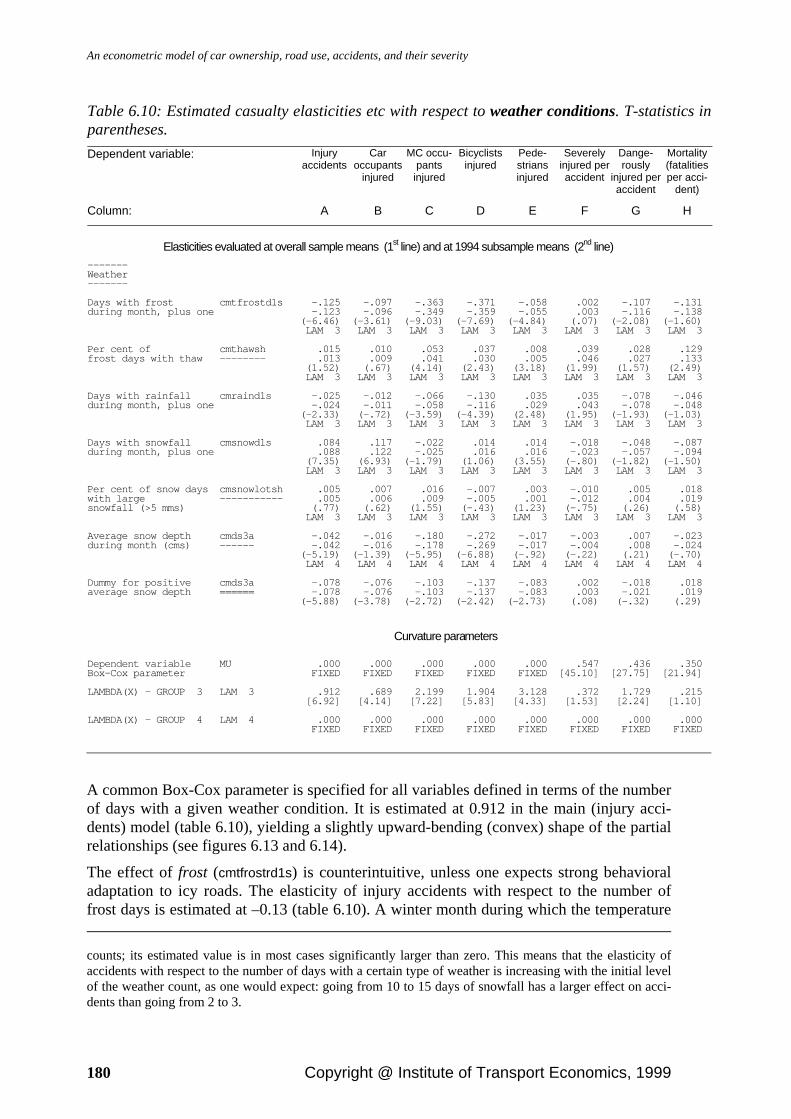
An econometric model of car ownership, road use, accidents, and their severity
180 Copyright @ Institute of Transport Economics, 1999
Table 6.10: Estimated casualty elasticities etc with respect to weather conditions. T-statistics in parentheses. Dependent variable: Injury
accidentsCar
occupants injured
MC occu-pants
injured
Bicyclists injured
Pede-strians injured
Severely injured per accident
Dange-rously
injured per accident
Mortality (fatalities per acci-
dent)
Column: A B C D E F G H
Elasticities evaluated at overall sample means (1st line) and at 1994 subsample means (2nd line) ------- Weather ------- Days with frost cmtfrostd1s -.125 -.097 -.363 -.371 -.058 .002 -.107 -.131 during month, plus one -.123 -.096 -.349 -.359 -.055 .003 -.116 -.138 (-6.46) (-3.61) (-9.03) (-7.69) (-4.84) (.07) (-2.08) (-1.60) LAM 3 LAM 3 LAM 3 LAM 3 LAM 3 LAM 3 LAM 3 LAM 3 Per cent of cmthawsh .015 .010 .053 .037 .008 .039 .028 .129 frost days with thaw -------- .013 .009 .041 .030 .005 .046 .027 .133 (1.52) (.67) (4.14) (2.43) (3.18) (1.99) (1.57) (2.49) LAM 3 LAM 3 LAM 3 LAM 3 LAM 3 LAM 3 LAM 3 LAM 3 Days with rainfall cmraind1s -.025 -.012 -.066 -.130 .035 .035 -.078 -.046 during month, plus one -.024 -.011 -.058 -.116 .029 .043 -.078 -.048 (-2.33) (-.72) (-3.59) (-4.39) (2.48) (1.95) (-1.93) (-1.03) LAM 3 LAM 3 LAM 3 LAM 3 LAM 3 LAM 3 LAM 3 LAM 3 Days with snowfall cmsnowd1s .084 .117 -.022 .014 .014 -.018 -.048 -.087 during month, plus one .088 .122 -.025 .016 .016 -.023 -.057 -.094 (7.35) (6.93) (-1.79) (1.06) (3.55) (-.80) (-1.82) (-1.50) LAM 3 LAM 3 LAM 3 LAM 3 LAM 3 LAM 3 LAM 3 LAM 3 Per cent of snow days cmsnowlotsh .005 .007 .016 -.007 .003 -.010 .005 .018 with large ----------- .005 .006 .009 -.005 .001 -.012 .004 .019 snowfall (>5 mms) (.77) (.62) (1.55) (-.43) (1.23) (-.75) (.26) (.58) LAM 3 LAM 3 LAM 3 LAM 3 LAM 3 LAM 3 LAM 3 LAM 3 Average snow depth cmds3a -.042 -.016 -.180 -.272 -.017 -.003 .007 -.023 during month (cms) ------ -.042 -.016 -.178 -.269 -.017 -.004 .008 -.024 (-5.19) (-1.39) (-5.95) (-6.88) (-.92) (-.22) (.21) (-.70) LAM 4 LAM 4 LAM 4 LAM 4 LAM 4 LAM 4 LAM 4 LAM 4 Dummy for positive cmds3a -.078 -.076 -.103 -.137 -.083 .002 -.018 .018 average snow depth ====== -.078 -.076 -.103 -.137 -.083 .003 -.021 .019 (-5.88) (-3.78) (-2.72) (-2.42) (-2.73) (.08) (-.32) (.29)
Curvature parameters Dependent variable MU .000 .000 .000 .000 .000 .547 .436 .350 Box-Cox parameter FIXED FIXED FIXED FIXED FIXED [45.10] [27.75] [21.94] LAMBDA(X) - GROUP 3 LAM 3 .912 .689 2.199 1.904 3.128 .372 1.729 .215 [6.92] [4.14] [7.22] [5.83] [4.33] [1.53] [2.24] [1.10] LAMBDA(X) - GROUP 4 LAM 4 .000 .000 .000 .000 .000 .000 .000 .000 FIXED FIXED FIXED FIXED FIXED FIXED FIXED FIXED
A common Box-Cox parameter is specified for all variables defined in terms of the number of days with a given weather condition. It is estimated at 0.912 in the main (injury acci-dents) model (table 6.10), yielding a slightly upward-bending (convex) shape of the partial relationships (see figures 6.13 and 6.14).
The effect of frost (cmtfrostrd1s) is counterintuitive, unless one expects strong behavioral adaptation to icy roads. The elasticity of injury accidents with respect to the number of frost days is estimated at –0.13 (table 6.10). A winter month during which the temperature counts; its estimated value is in most cases significantly larger than zero. This means that the elasticity of accidents with respect to the number of days with a certain type of weather is increasing with the initial level of the weather count, as one would expect: going from 10 to 15 days of snowfall has a larger effect on acci-dents than going from 2 to 3.

Chapter 6: Accidents and their severity
Copyright @ Institute of Transport Economics, 1999 181
drops below zero on every single day is, ceteris paribus, associated with a 25 per cent lower injury accident toll than a summer month without frost (figure 6.13).
TRIO PROJECT: TRULS - an econometric model of road use, accidents and their severityDATE: 99 01 29USER: toi Figure 6.13: Partial relationship between monthly injury accident frequency and the num-ber of days with frost.
The mortality effect, although not significant, also has the negative sign, suggesting that icy road are compensated for to an extent more than necessary to offset the initial effect on injury accident risk.
Comparing the two-wheeler injuries models to the pedestrian and car occupant injuries models, one notes, however, a much stronger, negative effect for bicyclist and motorcy-clists. This suggests that part of the effect found in the main model may be due to a reduc-tion in two-wheeler exposure, not entirely controlled for through our MC exposure proxy. Yet, it is interesting to note that even for car occupants, the estimated effect is negative, and clearly significant.
When the temperature drops below freezing at night, but rises above 0 °C during the day, certain particularly hazardous road surface conditions may arise. If snow melts during the day, wetting the road surface and forming a cap of ice at night, road users risk being sur-prised by some extremely slippery patches of a road surface that generally appears clear and dry, suitable for considerable speed. To take account of this effect we include, as a second aspect of temperature, the percentage of frost days during which the maximum tem-perature is above freezing (cmthawsh).
This variable generally has the expected positive sign, although its effect is not significant in the main model, or in the car occupant injuries model. It does, however, have a signifi-cant effect on mortality.

An econometric model of car ownership, road use, accidents, and their severity
182 Copyright @ Institute of Transport Economics, 1999
Rainfall (cmraind1s) has a seemingly negative (i e, favorable) effect on the accident count. Again, however, it appears that the effect is mainly due to reduced exposure among the unprotected road users, especially bicyclists. For car occupants, the effect is virtually zero.
TRIO PROJECT: TRULS - an econometric model of road use, accidents and their severityDATE: 99 01 29USER: toi Figure 6.14: Partial relationship between monthly injury accident frequency and the num-ber of days with snowfall.
Snowfall (cmsnowd1s) generally means more accidents112. In the main model, the elasticity is estimated at 0.084, significant at a very low level. The imputed maximal differential effect of snowfall (between zero and 30 days per month) is appr 45 per cent (figure 6.14). The monthly number of injury accidents may be expected to grow by about 1.5 per cent for each additional day of snowfall.
Note – again – that these partial effects apply ceteris paribus, i e given, for instance, a cer-tain number of frost days. When comparing winter to summer conditions, a mixture of these two (as well as other) effects will determine the end effect on risk, snowfall pulling the casualty frequency upwards while an opposite effect is apparently due to frost113. The snowfall effect is particularly strong for car occupants, for whom the injuries elasticity is
112 This results contradicts the findings of Fridstrøm et al (1995), who found a net negative (favorable) effect of snowfall on injury accidents. In this study, however, crude gasoline sales were used as the only measure of exposure. When account is taken of the fact that the amount of exposure per liter fuel decreases in winter, the negative partial effect is turned into a positive one. 113 The correlation between snowfall and frost days in our data set is 0.86 as calculated for the original (un-transformed) variables, and 0.76 as calculated for the Box-Cox transformed variables entering the model. In spite of this fairly strong correlation, we are able to derive separate partial effects for both variables, with reasonably high precision.

Chapter 6: Accidents and their severity
Copyright @ Institute of Transport Economics, 1999 183
estimated at about 0.12. Snowfall also has a positive effect on pedestrian and bicyclist inju-ries, although the latter is insignificant.
Interestingly, the severity effect of snowfall is negative, i e opposite to the accident fre-quency effect, and almost equally large in absolute value (elasticity 0870.− ). This suggest that even here, behavioral adaptation does take place, and to a degree almost exactly suffi-cient to offset the initial increase in fatality risk.
Does it matter how much snow is falling? One might imagine that heavy snowfall creates a particularly risky traffic situation. To answer this we added a variable (cmsnowlotsh) de-fined as the percentage of snowfall days during which the precipitation exceeds 5 millime-ters (in water form). This effect, too, is generally positive, although too small to be statisti-cally significant.
Another consequence of heavy snowfall is the formation of snowdrifts along the roadside. These snowdrifts may serve to reduce the frequency of single vehicle injury accidents, as they prevent cars from leaving the road and/or dampen the shock whenever a car is stray-ing aside (Brorsson et al 1988). A certain layer of snow also serves to reflect light and hence to strongly enhance visibility at night. On the other hand, snowdrifts tend to limit the road space and may thus increase the risk of head-on collisions, as when cars are thrown back into the road after hitting the snowdrift.
To take account of these effects, we include two snow depth variables in the model: one is a dummy which is one whenever the mean monthly snow depth is strictly positive, in which case night time visibility is enhanced. The other (cmds3a) is defined as the average monthly snow depth in centimeters, logarithmically transformed.
Both are highly significant and have the expected negative sign in the main model. More-over, the casualty subset model results are consistent with the causal mechanisms sug-gested above. The visibility dummy is negative and significant for all road user groups and for all accident types. The continuous snow depth factor is also negative for all road user groups. Interestingly, this variable has a very much larger (negative) effect on single vehi-cle accidents than on injury accidents in general. Multiple vehicle accidents, on the other hand, are not reduced by snow depth, rather the contrary, and accidents involving heavy vehicles, requiring more road space, increase significantly as the snow drifts grow (refer back to table 6.2).
In the exploratory model, we included a fifth snowfall variable, a dummy set equal to one when a snowfall occurs during the month, but not during the two previous months. It was meant to capture the effect of the first (surprising) snowfall during the winter season, an event regularly creating massive traffic problems and numerous material damage acci-dents. Its effect on injury accidents being, however, practically nil, it was dropped from the main model.
6.7.11. Legislation and reporting routines
On January 1st, 1977, a new and more complete set of road accident reporting forms and routines were introduced. The dummy capturing this change (eur77) suggests that the re-corded number of injury accidents is thereby inflated by some 10 per cent (e0.091 ≈ 1.10, table 6.11).

An econometric model of car ownership, road use, accidents, and their severity
184 Copyright @ Institute of Transport Economics, 1999
Table 6.11: Estimated casualty «elasticities» etc with respect to changes in legislation and re-porting routines. T-statistics in parentheses. Dependent variable: Injury
accidentsCar
occupants injured
MC occu-pants
injured
Bicyclists injured
Pede-strians injured
Severely injured per accident
Dange-rously
injured per accident
Mortality (fatalities per acci-
dent)
Column: A B C D E F G H
«Elasticities» evaluated at overall sample means (1st line) and at 1994 subsample means (2nd line) New eur77 .091 .184 -.210 .574 -.003 -.293 -.292 accident reporting ----- .091 .184 -.210 .574 -.003 -.367 -.309 routines from (2.66) (2.87) (-1.54) (4.33) (-.07) (-5.48) (-1.97) January 1, 1977 New highway code and eldhwycode2 -.108 -.126 -.083 -.006 -.141 -.008 -.010 .094 reporting routines =========== -.108 -.126 -.083 -.006 -.141 -.010 -.012 .100 from October 1, 1978 (-5.95) (-4.53) (-1.89) (-.10) (-4.18) (-.28) (-.16) (1.29)
Curvature parameters Dependent variable MU .000 .000 .000 .000 .000 .547 .436 .350 Box-Cox parameter FIXED FIXED FIXED FIXED FIXED [45.10] [27.75] [21.94]
In the exploratory model, we included eight different variables capturing various legisla-tive changes potentially affecting road safety. Seven of these were statistically insignificant or came out with nonsensical signs.
The only legislative variable with a clear effect on accidents was the dummy capturing the new highway code and reporting routines in effect from October 1st, 1978 (eldhwycode2). From this date one, an estimated 10 per cent decrease (e-0.108 = 0.90) in the accident count is effectuated. The greater part of this effect is most probably due to the change in report-ing routines rather than to the (relatively minor) amendments to the highway code. Accord-ing to the new routines, road accidents with only «insignificant» personal injury are no longer subject to mandatory police reporting.
Among the legislative changes not found to significantly affect the accident count, we find
(i) the abolition, on September 15, 1988, of mandatory jail punishment for drinking and driving offenses. After this date, heavy fines rather than jail punishment are imposed on drivers in the lower ranges of blood alcohol content.
(ii) the legal warrant, effective from June 25, 1981, for routine roadside alcohol control on the part of the police. Prior to this date, the police was not allowed to test drivers for blood alcohol content unless there was «reason to suspect» the driver for such an of-fense.
(iii) the enactment, on October 1, 1988, of mandatory seat belt use for all car occupants regardless of age. Children were required to use appropriate child safety equipment. Previously, the seat belt legislation did not affect persons below the age of 15.
(iv) the enactment, on April 1, 1977, of mandatory helmet use for motorcyclists. Although it did have a clear effect on helmet use, this legislative measure has not had economet-rically discernible effects on the injury accident frequency in Norway in general, nor on the MC accidents in particular (see section 6.7.5 above).
(v) three variables capturing the gradually stricter legislation on rest and service hours among bus and truck drivers. In the 1970s, this legislation affected only Norwegian

Chapter 6: Accidents and their severity
Copyright @ Institute of Transport Economics, 1999 185
vehicles with a total weight exceeding 16 tons. In December 1981, its enforcement was strengthened through the mandatory installation of certified tachographs in all vehi-cles covered by the regulations. In July 1987, the European agreement on rest and ser-vice hours in international road transport (AETR) came into effect in Norway. Fi-nally, in January 1994, the EEA (European Economic Area) agreement came into ef-fect, extending the rest and service hours regulations to all domestic and international transport by buses and trucks above 3.5 tons of (total) weight. None of the variables capturing these three legislative extensions or reinforcements had, however, signifi-cantly negative coefficients – indeed, the second one came out clearly positive114.
It should be emphasized that these negative results by no means imply that the above legis-lative measures are necessarily without effects on safety. It only means that, given the amount of systematic and random variation present in our sample, the effects – if any – are not large enough to be revealed in our aggregate econometric model.
6.7.12. Access to alcohol
Access to alcohol is more severely regulated in Norway than in most other western indus-trialized countries. Wine and liquor are sold only from state monopoly stores, generally found only in larger townships, and even beer sales are subject to licensing by the munici-pal assembly. Restaurants also need a state or municipal license in order to serve alcoholic beverage.
More than half the counties have less than one outlet per 3 000 square kilometers (figure 6.15)115. Even beer sales have been heavily restricted in some counties, although more so in the 1970s and early -80s than at present. A few municipalities116 still maintain an abso-lute ban on any kind of alcoholic beverage being served or sold.
114 The potential impact of these regulations would depend on the amount of heavy vehicle traffic in relation to the total amount of road use. The variables were therefore defined as interaction terms between the respec-tive legislative dummies and our calculated heavy vehicle share of the traffic volume (cevhvysh). 115 In this diagram, the vertical axis is a count of units of observations, 264 units corresponding to one county through 22 years (1973-94). Recall that the entire sample consists of 5 016 observations. 116 The municipality is a much smaller administrative unit than the county, there being approximately 450 municipalities in Norway. No county is without beer outlets, but until 1991, the county of Sogn and Fjor-dane, with a population of more than 100 000 and a surface of 18 634 square kms, was without a single wine/liquor store.

An econometric model of car ownership, road use, accidents, and their severity
186 Copyright @ Institute of Transport Economics, 1999
TRIO PROJECT: TRULS - an econometric model of road use, accidents and their severityDATE: 97 06 12USER: toi Figure 6.15: Histogram of wine/liquor store density by county, excl Oslo. 1973-94.
TRIO PROJECT: TRULS - an econometric model of road use, accidents and their severityDATE: 97 08 05USER: toi Figure 6.16: Density of alcohol outlets in the counties 1973-94.

Chapter 6: Accidents and their severity
Copyright @ Institute of Transport Economics, 1999 187
There are, in other words, large regional differences in terms of access to alcohol. Since the late 1980s, however, a certain «leveling out» has taken place, making the access to alcohol more similar between the counties, and generating a certain amount of time-series variation as well (figure 6.16).
In the TRULS model we decompose the availability of various forms of alcohol into six variables, three of which relate to outlets (i e, shops), while the remaining three concern (bars and) restaurants.
As for shops, our first variable (dxloutletspc) is defined as the total number of outlets per 1000 inhabitants. A second variable (dxloutstrong) measures the percentage of outlets al-lowed to sell beverage stronger than lager beer (4.5 per cent alcohol by volume), while the third (dxloutliqsh) is defined as the percentage of these, in turn, that are wine/liquor stores.
Since 1993, the last measure has been uniformly 100 per cent, while the number of outlets for strong beer (or stronger, i e above 4.5 per cent alcohol) has fallen drastically (figure 6.17), since strong beer is no longer allowed to be sold outside the state monopoly (wine/liquor) stores.
Thus there is a very pronounced jump in most regional time-series between December 1992 and January 1993. If access to strong beer has a bearing on road safety, there is every possibility to detect the effect econometrically.
TRIO PROJECT: TRULS - an econometric model of road use, accidents and their severityDATE: 97 08 05USER: toi Figure 6.17: Density of outlets for strong beer, wine or liquor in the counties 1973-94.
Restaurant licensing is another way of limiting public access to alcohol. Here, too, the TRULS model specification relies on a three-part multiplicative decomposition: The main variable (dxlrstalcpc) expresses the number of bars and restaurants licensed to serve (some kind of) alcoholic beverage, per 1000 population, the second variable (dxlrestlwsh) meas-

An econometric model of car ownership, road use, accidents, and their severity
188 Copyright @ Institute of Transport Economics, 1999
ures the percentage of these which are allowed to serve wine (or stronger), while the third (dxlrestliqsh) measures the percentage of these, in turn, that are also allowed to serve liquor.
Access to alcohol in terms of restaurant licenses has generally been increasing over our period of observation, especially since the mid-80s (figure 6.18). This is true in particular of wine/liquor licenses. There is ample cross-sectional as well as time-series variation in these measures.
Table 6.12: Estimated casualty elasticities etc with respect to access to alcohol. T-statistics in parentheses. Dependent variable: Injury
accidentsCar
occupants injured
MC occu-pants
injured
Bicyclists injured
Pede-strians injured
Severely injured per accident
Dange-rously
injured per accident
Mortality (fatalities per acci-
dent)
Column: A B C D E F G H
Elasticities evaluated at overall sample means (1st line) and at 1994 subsample means (2nd line) ----- Shops ----- Alcohol outlets dxloutletspc .088 -.020 .181 .052 -.023 -.041 .118 .131 per 1000 population .082 -.021 .179 .049 -.018 -.052 .116 .116 (3.44) (-3.88) (4.15) (.61) (-1.18) (-2.50) (3.44) (3.07) LAM LAM LAM LAM LAM LAM LAM LAM Per cent dxloutstrong .025 -.034 .098 .037 .088 .006 .023 -.006 alcohol outlets .025 -.034 .098 .037 .088 .007 .026 -.006 selling strong (2.70) (-3.09) (4.62) (1.72) (4.73) (.56) (1.02) (-.24) beer, wine or liquor LAM 4 LAM 4 LAM 4 LAM 4 LAM 4 LAM 4 LAM 4 LAM 4 Per cent wine/liqour dxloutliqsh .041 -.012 .086 .049 .094 -.004 .007 -.034 stores of outlets .041 -.012 .086 .049 .094 -.005 .008 -.036 for strong alcoholic (4.43) (-1.13) (3.89) (2.14) (5.47) (-.37) (.33) (-1.43) beverage LAM 4 LAM 4 LAM 4 LAM 4 LAM 4 LAM 4 LAM 4 LAM 4 -------------------- Bars and restaurants -------------------- Restaurants dxlrstalcpc -.016 .075 -.093 -.343 -.005 .038 -.157 -.126 licensed to -.006 .090 -.049 -.319 -.001 .063 -.176 -.098 serve alcohol (-6.41) (2.51) (-6.88) (-5.50) (-4.67) (1.19) (-1.84) (-2.29) per 1000 population LAM LAM LAM LAM LAM LAM LAM LAM Per cent of licensed dxlrestlwsh -.205 -.154 -.173 -.390 -.259 .158 -.129 -.079 restaurants with -.205 -.154 -.173 -.390 -.259 .197 -.145 -.084 wine/liquor license (-3.42) (-2.04) (-1.30) (-2.11) (-2.04) (2.12) (-.65) (-.38) LAM 4 LAM 4 LAM 4 LAM 4 LAM 4 LAM 4 LAM 4 LAM 4 Per cent of dxlrestliqsh .020 -.017 .080 .020 -.001 -.049 -.059 -.070 wine/liquour .020 -.017 .080 .020 -.001 -.061 -.067 -.075 licenses (1.22) (-.82) (1.96) (.36) (-.02) (-2.06) (-.94) (-1.26) including liquor LAM 4 LAM 4 LAM 4 LAM 4 LAM 4 LAM 4 LAM 4 LAM 4
Curvature parameters Dependent variable MU .000 .000 .000 .000 .000 .547 .436 .350 Box-Cox parameter FIXED FIXED FIXED FIXED FIXED [45.10] [27.75] [21.94] LAMBDA(X) dxloutletspc 1.437 -.772 .174 1.000 4.277 -.101 3.762 3.312 [2.29] [-1.73] [.58] FIXED [.80] [-.16] [2.62] [2.41] LAMBDA(X) dxlrstalcpc -2.527 .464 -1.553 -.176 -3.939 .702 -.005 -.769 [-2.87] [.77] [-2.84] [-.73] [-2.49] [.52] [-.01] [-.96] LAMBDA(X) - GROUP 4 LAM 4 .000 .000 .000 .000 .000 .000 .000 .000 FIXED FIXED FIXED FIXED FIXED FIXED FIXED FIXED
In the main (injury accidents) model, all three variables characterizing the density of alco-hol outlets have significant positive coefficients (table 6.12). The elasticity of accidents with respect to alcohol outlets in general is estimated at 0.088, as a 1973-94 average. With
Chapter 6: Accidents and their severity
Copyright @ Institute of Transport Economics, 1999 189
respect to outlets for strong beer (or stronger alcohol), a small but significantly positive elasticity of 0.025 is found, while wine/liquor stores yield an elasticity of 0.041, given the total number of alcohol outlets117. There is thus a consistent pattern of influence, in that all types of alcohol outlets appear to increase the accident frequency, and more so the stronger the alcohol sold.
Severity also appears to increase significantly with the total number of alcohol outlets. The elasticity of fatalities with respect to alcohol stores is calculable as 0.219 (= 0.088 + 0.131). The strength of alcohol sold does not, however, have any significant impact on severity.
TRIO PROJECT: TRULS - an econometric model of road use, accidents and their severityDATE: 97 08 05USER: toi Figure 6.18: Density of restaurants licensed to serve alcohol. 19 counties 1973-94.
This strikingly consistent pattern of influence becomes rather more mixed when we exam-ine the results for different road user groups. The number of car occupant injuries seem to be negatively related to alcohol outlet density, and more so the stronger the type of alcohol. For MC occupant injuries the effects are consistently positive, while for bicyclists and pe-destrians an accident increasing effect is found only for the stronger types of alcohol.
The strict Norwegian legislation against drinking and driving represents a strong incentive for car drivers to conceal their accident whenever under the influence, even in the event of
117 The variable dxloutstrong measures the extra impact of more outlets for strong alcohol, conditional on the total number of alcohol outlets, in other words the effect of replacing an ordinary beer outlet by a shop al-lowed to sell strong beer. Similarly, dxloutliqsh represents the extra effect of liquor stores, conditional on the number of weak and strong beer outlets. The unconditional effects would be calculable as a certain weighted sum of the respective conditional elasticities, the weights being determined by the ratios between different kinds of alcohol outlets.

An econometric model of car ownership, road use, accidents, and their severity
190 Copyright @ Institute of Transport Economics, 1999
(slight) injury. It is therefore quite possible that the reporting incidence for single vehicle accidents is negatively correlated with the incidence of alcohol-impaired driving. In prin-ciple, this could in part explain the negative elasticities of car occupant injuries with re-spect to alcohol outlet density factors. A complement casualty subset test as applied to sin-gle vehicle versus multiple vehicle accidents fails, however, to reveal any pattern consis-tent with such an explanation.
Another possible explanation of the discrepancy between the effects on injury accidents and car occupant injuries, respectively, is that car occupancy rates may be negatively re-lated to alcohol-impaired driving, in other words that drunk drivers tend to be alone in their cars. Most people would hesitate to ride with a visibly impaired driver, and the driver him-self has a clear incentive not to reveal his condition to any other person.
Yet another set of surprising results pertain to the variables measuring the density of bars and restaurants licensed to serve various types of alcohol (dxlrstalcpc, dxlrestlwsh, and dxlrestliqsh). These factors appear to be negatively related to accident frequency and sever-ity. Thus, to the extent that such licenses have any bearing on the incidence of impaired driving, it would appear that drivers compensate for it, to an extent more than sufficient to offset the initial effect.
Such effective compensation is unlikely to take place except possibly at rather moderate levels of blood alcohol concentration (BAC)118. Restaurant guests may, however, be less likely to obtain very high levels of blood alcohol content than are persons consuming alco-hol in private. This could help explain the discrepancy between the effects of alcohol out-lets and restaurants.
Casualty subset tests would have been useful in order to rule out possible spurious correla-tion or omitted variable bias. It is difficult, however, to identify subsets that would be clearly more (or less) affected by this risk factor than the average.
In the exploratory model, certain other alcohol availability variables were tested as well. These include a variable measuring the extent to which liquor stores have been closed due to strike, and a dummy capturing the abolition of self-service sale of strong beer. Neither variable was significant.
In summary, the alcohol availability variables convey a rather mixed picture and one that suggests the need for more in-depth analysis, including, if possible, the important interven-ing variables of alcohol consumption, drinking-and-driving incidence, and/or speed. There are relatively clear indications, however, that the density of outlets is positively associated with road accident risk and severity.
6.7.13. Geographic characteristics
The models include a dummy for the county of Oslo. This dummy serves to neutralize the effect of certain independent variables being unobservable (and hence set to zero) for Oslo, and is thus without any substantive interpretation.
118 Such a mechanism could, in principle, explain the celebrated «Grand Rapids Dip», i e the apparent below-baseline risk, reported by Borkenstein et al (1964), for the 0.01 to 0.04 % BAC interval. This study has, however, been severely criticized on methodological grounds (see, e g, Allsop 1966, Hurst et al 1994).

Chapter 6: Accidents and their severity
Copyright @ Institute of Transport Economics, 1999 191
Table 6.13: Estimated casualty «elasticities» etc with respect to geographic variables and cal-endar events. T-statistics in parentheses. Dependent variable: Injury
accidentsCar
occupants injured
MC occu-pants
injured
Bicyclists injured
Pede-strians injured
Severely injured per accident
Dange-rously
injured per accident
Mortality (fatalities per acci-
dent)
Column: A B C D E F G H
«Elasticities» evaluated at overall sample means (1st line) and at 1994 subsample means (2nd line) --------- Geography --------- Oslo hcounty3 -.160 .471 -1.321 -1.609 -1.036 .247 .509 .593 ======== -.160 .471 -1.321 -1.609 -1.036 .309 .571 .628 (-1.31) (2.94) (-4.86) (-4.36) (-3.78) (1.52) (1.51) (1.46) -------- Calendar -------- Dummy for ekes .023 .081 -.055 -.156 -.038 .024 .043 .098 start of Easter week ==== .023 .081 -.055 -.156 -.038 .030 .048 .104 (1.34) (3.26) (-.89) (-1.95) (-.69) (.71) (.55) (1.13) Dummy for ekee -.132 -.152 -.070 -.054 -.171 -.010 .023 .007 end of Easter ==== -.132 -.152 -.070 -.054 -.171 -.013 .026 .007 (-7.45) (-5.75) (-1.26) (-.62) (-3.11) (-.30) (.31) (.08) Years ektrend -.361 .124 -1.822 -1.975 -1.099 -1.677 -.132 .012 passed since 1945 -.454 .156 -2.295 -2.488 -1.384 -2.640 -.179 .015 (-1.79) (.46) (-4.34) (-3.17) (-2.58) (-6.20) (-.18) (.02) Share of ekvhsh -.014 -.016 .104 .037 .007 .007 -.041 -.090 vacation and holidays -.014 -.016 .103 .037 .007 .009 -.045 -.095 during month (-.61) (-.47) (1.77) (.45) (.15) (.22) (-.43) (-.84) (excl summer vacation)
Curvature parameters Dependent variable MU .000 .000 .000 .000 .000 .547 .436 .350 Box-Cox parameter FIXED FIXED FIXED FIXED FIXED [45.10] [27.75] [21.94]
6.7.14. Calendar and trend effects
The strongest concentration of traffic on a single day in Norway probably occurs at Easter end, i e Easter Monday, when large parts of the population return home after the holiday. The dummy capturing (the month containing) this event (ekee) shows a significantly nega-tive effect on accidents. It appears that the injury accident toll during this month is about 12 per cent lower than it would normally be, given the exposure volume (table 6.13). This must probably be understood in terms of the restraint forced upon the drivers on unusually congested roads.
The traffic volumes generated by Easter start (ekes) are less concentrated and may some-times divide themselves between the months of March and April. Here, the effect is insig-nificant in the main (injury accidents) model and positive in the car occupant injuries model.
Apart from the Easter traffic, holidays per se (ekvhsh) do not seem to have any effect on the accident frequency, given exposure.
Our final and most important calendar variable is the linear119 trend term (ektrend), defined as years passed (or parts thereof) since 1945. It is highly significant and negative. As of
119 We specify this term as «linear», since this is the only formulation that leaves all model parameters (ex-cept the constant term) invariant with respect to the (quite arbitrary) choice of calendar reference point.

An econometric model of car ownership, road use, accidents, and their severity
192 Copyright @ Institute of Transport Economics, 1999
1994, the injury accident frequency is estimated to fall by some 0.9 per cent annually, when all (our) other independent variables are kept constant120.
Interpreting this trend effect is a challenge. Its coefficient is not robust against changes in the model specification, being particularly sensitive to the inclusion (or not) of variables developing almost monotonously over time, such as road infrastructure, traffic density, and mean age of vehicles. In principle, it would capture, although crudely, all risk or safety developments not otherwise taken account of in the model. Obviously, there are a number of such omitted factors – suffice it to mention vehicle crashworthiness, targeted infrastruc-ture improvements, driver education and experience, general police surveillance, vehicle inspection, pedestrian and bicyclist exposure, demographic structure, or speed limits and other traffic regulations. Some of these variables typically evolve gradually and steadily over time, more or less in parallel between the various counties. The net effect of all such developments would, in principle, be captured by the trend term. Previous analyses have come up with a trend effect (over 1973-86) of minus 1.9 per cent annually (Fridstrøm et al 1995), however without taking account of other independent variables than reporting, weather and daylight.
Note, however, that the entire trend effect appears to be due to pedestrians and two-wheelers. For these, the trend effect is estimated at minus 2 to 5 per cent annually, while for car occupant injuries the trend variable is positive and statistically insignificant. This speaks against vehicle crashworthiness or inspection as prime explanatory factors. Indeed, the results suggest that car occupants have benefitted from few safety enhancements other than those explicitly included in our model, of which seat belt use is probably the pre-dominant single factor. The unprotected road users, on the other hand, have either reduced their exposure or witnessed a major improvement in their safety, or both.
One might argue that time itself is never an explanatory factor, that only the events occur-ring in time are justifiably understood as true causal agents, and hence that a trend term like this does not belong in a properly specified econometric model. It turns out, however, that without a trend term capturing autonomous safety improvements taking place over time, certain independent variables come out with entirely implausible coefficients, sug-gesting strong omitted variable bias.
One possible interpretation of the trend effect is learning. Road users, teachers, policemen, manufacturers, engineers, planners and politicians all gradually accumulate knowledge and experience on how to avoid and mitigate casualties. For this reason, risk levels are very much higher in the early stages of the automobile age than in a «mature» motorized soci-ety, and very much higher in most developing countries than in the western industrialized world.
According to this tenet, the risk level might be thought of as a function of the hitherto ac-quired driving experience in the road user population. To test the explanatory power of
Since, however, the dependent variable is log transformed, the «linear» trend is really an exponentially de-creasing (or increasing) curve in terms of accidents. 120 As of 1994 the trend elasticity is calculable at –0.454 for injury accidents. Since the trend variable is de-fined as years passed since 1945, a one per cent increase in this variable corresponds (as of 1994) to a time lapse of almost half a year. Thus the trend elasticitiy is consistent with a 0.9 per cent risk reduction per an-num.

Chapter 6: Accidents and their severity
Copyright @ Institute of Transport Economics, 1999 193
such a hypothesis, we replaced the trend term by an estimate of the accumulated aggregate vehicle kilometers driven in the county since 1945 121.
Although this variable, unlike the trend term, contains cross-sectional variation in addition to the monotonous temporal growth, it possesses markedly poorer explanatory power. There appears to be something more to the trend effect than just the accumulation of ag-gregate experience. When both variables are included, the experience term becomes insig-nificant and acquires a counterintuitive sign.
6.7.15. Autocorrelation
The 1st and 12th order autocorrelation parameters come out clearly significant and positive in all models except in the severity equations (table 6.14). Thus, it appears important to allow for an autocorrelation structure of the disturbances.
Table 6.14: Estimated autocorrelation parameters in casualty equations. T-statistics in paren-theses. Dependent variable: Injury
accidentsCar
occupants injured
MC occu-pants
injured
Bicyclists injured
Pede-strians injured
Severely injured per accident
Dange-rously
injured per accident
Mortality (fatalities per acci-
dent)
Column: A B C D E F G H
Autocorrelation parameters ( jρ )
1st order 1ρ .192 .099 .135 .066 .058 .027 -.009 .011 (13.62) (6.79) (9.51) (4.66) (3.68) (1.85) (-.55) (.75)
12th order 12ρ .234 .126 .081 .130 .110 .035 .010 .018 (15.74) (8.34) (5.49) (8.71) (7.81) (2.31) (.64) (1.18)
6.7.16. Explanatory power
How well do our casualty models fit? In table 6.15 we report various goodness-of-fit meas-ures, including the overdispersion parameters and the ordinary and Freeman-Tukey coeffi-cients of determination for total and systematic variation (see section 6.4.2 for definitions).
Note that for fatalities, dangerously injured and severely injured, we report the goodness-of-fit obtained by combining the accident frequency and severity equations. For each de-gree of severity, we compare the observed number of victims with a predicted value, which is obtained by multiplying – for each sample point – the (estimated) expected number of accidents by the expected severity. The number of parameters (k) is given by the sum of the parameters in the accident frequency and severity equations.
Table 6.15: Goodness-of-fit measures for casualty models
Casualty count n k θ 2R 2P 2PR 2
FTR 2FTP 2
PFTR
121 Vehicle kilometers driven before 1945 may be disregarded without large error, as these represent, in total, less than one year’s traffic volume as of 1973.

An econometric model of car ownership, road use, accidents, and their severity
194 Copyright @ Institute of Transport Economics, 1999
Injury accidents 4788 57 0.014 0.864 0.918 0.941 0.861 0.912 0.944
Car occupants injured 4788 58 0.049 0.686 0.895 0.767 0.697 0.896 0.778
MC occupants injured 4788 57 0.054 0.712 0.818 0.870 0.698 0.829 0.842
Bicyclists injured 4788 54 0.058 0.677 0.779 0.869 0.629 0.771 0.816
Pedestrians injured 4788 56 0.028 0.783 0.839 0.934 0.671 0.788 0.851
Severely injured 4788 115 0.061 0.621 0.798 0.779 0.623 0.776 0.803
Dangerously injured 4104 112 0.133 0.259 0.496 0.522 0.257 0.466 0.553
Fatalities 4788 115 0.161 0.172 0.387 0.443 0.166 0.328 0.506
The accident frequency model explains 86 per cent of the total variation, by the ordinary 2R measure (formula 6.57 in section 6.4.2 above), and a full 94 per cent of the explainable
systematic variation, as judged by 2PR (formula 6.59). A maximally obtainable fit in this
model would correspond to an 2R of 0.92 (= 2P , formula 6.58).
An almost identical picture is revealed by the corresponding Freeman-Tukey goodness-of-fit measures (formulae 6.61 to 6.63).
The accident frequency model has a very small overdispersion: θ = 0.014, by formula (6.56). In the models explaining victim counts by road user category, the overdispersion is somewhat higher, as expected, and the goodness-of-fit somewhat lower. These models explain between 77 and 93 per cent of the systematic variation.
The comparatively small overdispersion found in the pedestrian injuries model probably reflects the fact that few accidents involve more than one pedestrian. Hence these events come very close to being probabilistically independent.
The combined models explaining victims by degree of severity typically exhibit poorer goodness-of-fit – only around 50 per cent explained systematic variation for the most se-vere injuries. This is, however, primarily a reflection of the non-independence of severe injury events, as witnessed by the overdispersion parameter: θ = 0.161 for fatalities and θ = 0.133 for dangerous injuries.
As judged by the ordinary 2R measure, the fit is down to 17 per cent in the fatalities model. But on account of the small casualty counts being analyzed, the maximally obtain-able fit, assuming independent events, is only about 39 per cent (= 2P ). For probabilisti-cally dependent events, such as fatalities, the limit is even lower.

Chapter 7: Synthesis
Copyright @ Institute of Transport Economics, 1999 195
Chapter 7: Synthesis
In the previous chapters, we have presented a recursive chain of analyses attempting to explain – in that order – car ownership, road use, seat belt use, accident frequency, and accident severity.
Road use and seat belt use are important input variables in the accident frequency and se-verity relations. Car ownership is, in turn, a most important determinant of aggregate road use. Thus, a number of independent variables entering the car ownership, road use or seat belt use equations are implicitly assumed to affect accident frequency and severity indi-rectly, through their influence on the antecedent links in the recursive chain. Some of these independent variables enter the accident frequency and severity equations as well, adding a direct to the indirect effect.
The principal aim of this final chapter is, therefore, to sum up and describe all these direct and indirect effects, so as to obtain a maximally complete picture of the major factors af-fecting road casualties at the aggregate (macro) level. We do this by recursive accumula-tion of the relevant elasticities, as evaluated at the subsample means for our last year of observation – 1994. We shall start by setting out the formal algebra behind these calcula-tions.
7.1. Calculating compound elasticities in a recursive model structure
Consider a general recursive structure of relationships given by
(7.1) ( ) ( )zgxzx == ,,fy ,
where ( ) ( ) ( ) ( )( )'g...gg'x...xx mm zzzx 2121 == and ( )'z...zz n21=z are differentiable vec-tor variables with partial derivatives denoted by
(7.2) ( ) ( ) ( ) ( )n,...,,j;m,...,,igz
g,fz
,f,fx
,fij
j
izj
jxi
i
2121 ==≡∂
∂≡
∂⋅∂
≡∂
⋅∂ zzx .
Define the partial elasticities
(7.3) yxf i
xifxi≡ε ,
(7.4) yz
f jzjfz j
≡ε
(7.5) i
jijzx x
zg
ji≡ε ,
and the compound elasticity
(7.6) ( )( )yz
z,f j
jyz j ∂
∂≡
zzgε .
To express the last of these elasticities in terms of the three first, note that

An econometric model of car ownership, road use, accidents, and their severity
196 Copyright @ Institute of Transport Economics, 1999
(7.7)
( )( ) ( ) ( )
( ) ,zy
zy
zx
xy
fgfz
,fzx
x,f
z,f
jfz
n
izxfx
jfz
n
i j
izx
ifx
zjij
n
ixi
jj
in
i ij
jjiijjii ⎥⎦
⎤⎢⎣
⎡+=+
⎥⎥⎦
⎤
⎢⎢⎣
⎡⋅=
+=∂
⋅∂+∂∂
∂⋅∂=
∂∂
∑∑
∑∑
==
==
εεεεεε11
11
zxzzg
where the third equality sign follows from (7.3)-(7.5). Substituting (7.7) into (7.6), we have the general recursive elasticity formula
(7.8) ( )n,...,,jjjiij fzzx
m
ifxyz 21
1
=+= ∑=
εεεε ,
where the last term represents the direct effect of jz on y, while the terms inside the sum-mation sign correspond to the various indirect effects.
Note that this formula is valid irrespective of the functional forms f and g.
To fix ideas, let y represent injury accidents, x the right-hand side variables in the injury accident equation, and z the right-hand side variables in the road use equation. Let the first element of x, 1x say, represent road use (vehicle kilometers), and assume
(7.9) ( ) jiz
ggj
iij ∀>∀≡
∂∂
= and10z .
i e only the first element of vector x is functionally dependent on z.
In this case, formula (7.8) simplifies to
(7.10) jjj fzzxfxyz εεεε +=
11.
That is, the elasticity of accident frequency with respect to jz is composed of two parts. An indirect effect is given by the elasticity of accidents with respect to road use, times the elasticity of road use with respect to jz . In addition, a direct effect is determined by the partial derivative of y with respect to jz , as estimated in the accident frequency equation.
By induction, this argument can be extended to any number of links in the recursive chain of relations, so as to, e g, also take account of indirect car ownership effects, or – at the other end of the chain – severity effects122.
As for severity, a most useful type of inference can be made by letting, e g, y denote the
number of fatalities, 1x the number of injury accidents, 1
2 xyx = the mortality ratio, and z
the (common) vector of exogenous variables. Here,
(7.11) 21xxy = , 12121
===yxx
fxfx εε ,
and hence, by (7.8),
122 Recall that our recursive model structure consists of relations explaining (i) car ownership, (ii) vehicle kilometers, (iii) seat belt use, (iv) injury accidents, (v) injury victims, and (vi) severity.

Chapter 7: Synthesis
Copyright @ Institute of Transport Economics, 1999 197
(7.12) jjj zxzxyz 21
εεε += ,
i e, the elasticity of fatalities with respect to any exogenous variable jz is calculable sim-ply by summation of the corresponding elasticities in the accident frequency and mortality equations. Again, note that this formula applies without regard to the form of the functions
( ) ( )zz 2211 and gxgx == .
7.2. Direct and indirect casualty effects
In figures 7.1 through 7.25 we show calculated elasticities with respect to various inde-pendent variables. Partial elasticities are evaluated at the means across all 228 sample points observed in 1994, as already displayed in the tables of chapters 4 through 6 (see section 2.4.4 for an account of the methodology). Compound elasticities, including all relevant direct and indirect effects, are then computed from the mean partial elasticities in accordance with formula (7.8)123. That is, whenever applicable, the effect channeled through increased (or decreased) car ownership is included in the road use elasticity, the effect coming through increased road use is included in the accident elasticity, and the ef-fect on accident frequency is included in the fatalities elasticity.
The values shown in figures 7.1-7.25 are point estimates. They should be interpreted with some caution, as the diagrams provide no information on standard errors or confidence intervals, or on whether the effects shown are significantly different from zero. For such information, the reader is referred to the tables of Appendix B, or to the discussion in chap-ters 4 through 6.
7.2.1. Exposure
In figure 7.1, we show estimated partial elasticities with respect to various components of exposure.
The injury accident frequency has an elasticity of 0.911 with respect to the total volume of motor vehicle road use (vehicle kilometers). That is, injury accidents increase almost in proportion to the traffic volume, other things being equal. Fatalities appear to increase somewhat less than proportionately, viz. by an elasticity of 0.761.
This elasticity applies, however, only on the condition that the traffic density, defined as vehicle kilometers driven per kilometer road length, is kept constant. In other words, the elasticities with respect to traffic volume implicitly assume that the road network is being extended at a rate corresponding exactly to the traffic growth, so that the ratio of vehicle kilometers to road kilometers remains unchanged.
In the opposite and more realistic case, where the road network does not change, an aver-age accident elasticity of approximately 0.50 (= 0.911 – 0.414) is calculable for 1994. An increase in traffic density tends, in other words, to dampen the (otherwise near-proportionate) effect of larger traffic volumes, as measured in vehicle kilometers.
123 An Excel spreadsheet was used to do all the calculations, based on a TRIO output table of mean direct elasticities as of 1994.

An econometric model of car ownership, road use, accidents, and their severity
198 Copyright @ Institute of Transport Economics, 1999
0.000
0.000
0.000
0.000
-0.062
-0.253
0.911
-0.414
0.149
0.026
0.212
0.240
1.033
-0.238
0.165
0.034
0.216
-0.144
0.680
0.175
-0.043
0.001
0.168
-1.339
0.761
0.228
0.110
-0.007
-0.014
-1.143
-1.6 -1.4 -1.2 -1.0 -0.8 -0.6 -0.4 -0.2 0.0 0.2 0.4 0.6 0.8 1.0 1.2
Motor vehiclekilometers
Traffic density (vehkms pr km road)
Heavy vehicle trafficshare
MC exposure (proxy)
Bus service density
Streetcar/subwaydensity
Elasticity
FatalitiesDangerously injuredSeverely injuredInjury accidentsTraffic volume
Figure 7.1: Exposure elasticities as of 1994. Accidents and victims by severity.
Heavy vehicles124 are more dangerous than private cars. The larger the heavy vehicle share of the traffic volume, the higher the injury accident frequency. However, fatalities and dan-
124 I e, vehicles with more than 1 ton’s carrying capacity or more than 20 passenger seats.

Chapter 7: Synthesis
Copyright @ Institute of Transport Economics, 1999 199
gerous (i e, very severe) injuries increase less than the accident frequency, meaning that the average severity (persons severely injured per injury accident) does not increase. This may reflect the fact the truck driver himself is well protected and usually escapes the acci-dent without (severe) injuries. Heavy vehicles appear to be particularly dangerous to two-wheelers, while car occupant injuries become less frequent when a large share of the traffic does not consist of private cars (figure 7.2).
0.000
0.000
0.000
0.000
-0.062
-0.253
0.911
-0.414
0.149
0.026
0.212
0.240
0.962
-0.319
-0.146
0.001
0.149
-0.245
0.749
0.012
0.476
0.208
0.362
-0.505
1.079
-0.604
0.529
0.254
0.110
1.104
1.109
-0.972
0.105
0.034
0.756
1.196
-1.0 -0.5 0.0 0.5 1.0 1.5
Motor vehiclekilometers
Traffic density(veh kms pr km
road)
Heavy vehicletraffic share
MC exposure(proxy)
Bus servicedensity
Streetcar/subwaydensity
Elasticity
Pedestrians injuredBicyclists injuredMC occupants injuredCar occupants injuredInjury accidentsTraffic volume
Figure 7.2: Exposure elasticities as of 1994. Injury accidents and victims by road user category.

An econometric model of car ownership, road use, accidents, and their severity
200 Copyright @ Institute of Transport Economics, 1999
Motorcycle exposure has a clear effect on motorcycle accidents but, on account of its small share of the exposure, a quite modest effect on the overall accident frequency125.
Enhanced public transportation services tend to reduce the use of private cars and hence the total number of vehicle kilometers. A one per cent increase in the density of bus service lowers the overall traffic volume by an estimated 0.062 per cent. However, this is not suf-ficient to offset the exposure effect of the bus service: injury accidents increase by 0.212 per cent, i e by 0.264 (= 0.212 + 0.062) per cent as reckoned per vehicle kilometer (figure 7.1). This effect is due primarily to more pedestrians being injured, presumably on their way to or from the bus stop, but even car occupants and two-wheelers are exposed to a somewhat higher risk owing to the bus service (figure 7.2).
Similar and even stronger effects are found for public transportation by rail (streetcar or subway). Obviously, this kind of service does not entail increased risk or exposure for mo-torized road users, only for bicyclists and pedestrians.
7.2.2. Road infrastructure
The calculated effects of improved or extended road networks are exhibited in figures 7.3 and 7.4. The effects shown in these and the following graphs are all interpretable as long-term (equilibrium) effects, i e they incorporate effects due to changes in (optimal) car own-ership. Also, it is assumed throughout that the heavy vehicles represent a constant share of the total traffic volume.
For analytical purposes, we decompose the supply of road infrastructure into two parts: (i) the length of the public road network (in kilometers per county), and (ii) the accumulated real investment expenditure per kilometer (national or county) road. We interpret the first component as a measure of size, while the second one may be understood as an economic measure of road quality126.
An added supply of roads appears to generally increase the accident toll. This is true for (size) enlargements as well as for (quality) improvements.
The great bulk of this effect can be traced back to the fact that road use demand responds to shifts in supply. An extended or improved road network reduces the cost of travel by car and hence increases the demand for cars and road use.
The risk level (accidents or casualties per vehicle kilometer) is not very strongly affected, although there is a tendency for casualties to increase slightly more than proportionately with the traffic volume, when new roads are added to the network. The main reason for this is that a decrease in density (increase in road space) tends to augment the risk.
125 The «elasticity» computed for motorcycle exposure should not be interpreted literally, since the independ-ent variable used is only a proxy, which appears to capture bicyclist exposure as well. 126 This measure is, of course, far from perfect, since property values and topographical conditions differ sharply between the counties, affecting the costs of road construction.

Chapter 7: Synthesis
Copyright @ Institute of Transport Economics, 1999 201
0.172
0.172
0.157
0.254
0.113
0.351
0.066
0.536
0.212
0.219
0.143
0.193
0.0 0.1 0.2 0.3 0.4 0.5 0.6
Capital invested pr kmroad
Road length (kms)
Elasticity
FatalitiesDangerously injuredSeverely injuredInjury accidentsTraffic volumeCar ownership
Figure 7.3: Road infrastructure elasticities as of 1994. Accidents and victims by severity.
0.172
0.172
0.157
0.254
0.113
0.351
0.016
0.461
0.294
0.386
0.154
-0.191
0.063
0.475
-0.3 -0.2 -0.1 0.0 0.1 0.2 0.3 0.4 0.5 0.6
Capital invested pr kmroad
Road length (kms)
Elasticity
Pedestrians injuredBicyclists injuredMC occupants injuredCar occupants injuredInjury accidentsTraffic volumeCar ownership
Figure 7.4: Road infrastructure elasticities as of 1994. Injury accidents and victims by road user category.
It should be noted, though, that the estimated partial effects of road infrastructure are gen-erally not (very) significant (except the effect on car ownership). The uncertainty sur-rounding these elasticities is therefore considerable. Our confidence in these results is, however, strengthened by the relatively consistent and unambiguous pattern emerging.

An econometric model of car ownership, road use, accidents, and their severity
202 Copyright @ Institute of Transport Economics, 1999
With one exception, all the elasticities shown in figures 7.3 and 7.4 are positive. The fact that bicyclist injuries tend to decrease with the length of the road network may simply be a cross-sectional exposure effect: The supply of road kilometers per inhabitant is larger in more sparsely populated counties, where distances are generally large and slow modes of travel comparatively unattractive.
Another word of caution is in order as well. One cannot draw the conclusion that every road investment, be it for extension or improvement, increases the accident toll. Certain types of road improvements or alterations are undoubtedly effective accident countermea-sures (see Elvik et al 1997:149-242). What the TRULS model results do suggest, however, is that, given the way that road investment expenditures have been allocated over our pe-riod of observation (1973-94) in Norway, they have not – by and large – contributed to a smaller accident toll, nor to a significantly reduced risk as reckoned per unit of traffic. Their main effect has been to facilitate an increase in mobility.
This finding is not very surprising in the light of recent knowledge on the road investment decision process. The respective benefits accruing from competing investment projects have little influence on the allocation of funds (Odeck 1991 and 1996, Elvik 1993 and 1995, Nyborg and Spangen 1996). The weight attached to safety benefits is particularly small (Fridstrøm and Elvik 1997).
7.2.3. Road maintenance
In figure 7.5 and 7.6 we show estimated road maintenance expenditure elasticities.
0.000
0.000
0.000
0.000
0.000
0.000
-0.007
-0.068
0.045
0.002
0.027
0.092
-0.019
-0.325
0.391
-0.025
-0.126
0.165
-0.4 -0.3 -0.2 -0.1 0.0 0.1 0.2 0.3 0.4 0.5
Winter maintenenceexpenditure
Road markingexpenditure
Misc. maintenanceexpenditure
Elasticity
FatalitiesDangerously injuredSeverely injuredInjury accidentsTraffic volumeCar ownership
Figure 7.5: Road maintenance elasticities as of 1994. Accidents and victims by severity.
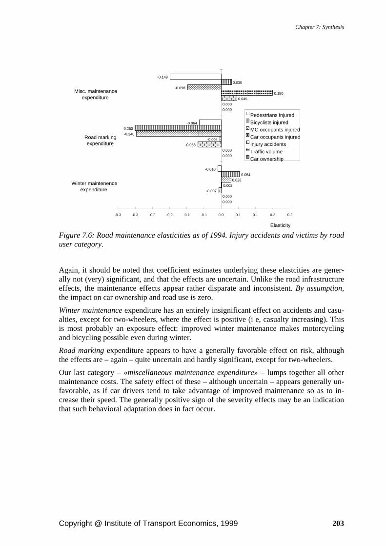
Chapter 7: Synthesis
Copyright @ Institute of Transport Economics, 1999 203
0.000
0.000
0.000
0.000
0.000
0.000
-0.007
-0.068
0.045
0.002
-0.004
0.150
0.028
-0.246
-0.098
0.054
-0.250
0.030
-0.010
-0.064
-0.149
-0.3 -0.3 -0.2 -0.2 -0.1 -0.1 0.0 0.1 0.1 0.2 0.2
Winter maintenenceexpenditure
Road markingexpenditure
Misc. maintenanceexpenditure
Elasticity
Pedestrians injuredBicyclists injuredMC occupants injuredCar occupants injuredInjury accidentsTraffic volumeCar ownership
Figure 7.6: Road maintenance elasticities as of 1994. Injury accidents and victims by road user category.
Again, it should be noted that coefficient estimates underlying these elastcities are gener-ally not (very) significant, and that the effects are uncertain. Unlike the road infrastructure effects, the maintenance effects appear rather disparate and inconsistent. By assumption, the impact on car ownership and road use is zero.
Winter maintenance expenditure has an entirely insignificant effect on accidents and casu-alties, except for two-wheelers, where the effect is positive (i e, casualty increasing). This is most probably an exposure effect: improved winter maintenance makes motorcycling and bicycling possible even during winter.
Road marking expenditure appears to have a generally favorable effect on risk, although the effects are – again – quite uncertain and hardly significant, except for two-wheelers.
Our last category – «miscellaneous maintenance expenditure» – lumps together all other maintenance costs. The safety effect of these – although uncertain – appears generally un-favorable, as if car drivers tend to take advantage of improved maintenance so as to in-crease their speed. The generally positive sign of the severity effects may be an indication that such behavioral adaptation does in fact occur.

An econometric model of car ownership, road use, accidents, and their severity
204 Copyright @ Institute of Transport Economics, 1999
7.2.4. Population
Car ownership and road use increase near-proportionately with the size (or density) of the population, other things127 being equal. Accident and casualties increase less than road use, owing to the traffic density effect (figure 7.7).
Unemployment has a small, but highly significant, negative effect on road use, and an ad-ditional, barely significant effect on casualties.
The rate of (first quarter) pregnancy has a clearly significant, unfavorable effect on the injury accident frequency, but not on the number of very serious or fatal injuries.
0.000
0.893
0.000
-0.021
0.802
0.000
-0.034
0.656
0.181
-0.078
0.481
0.090
-0.079
0.373
-0.072
-0.023
0.507
-0.102
-0.2 0.0 0.2 0.4 0.6 0.8 1.0
Unemployment
Population density
1st quarter pregnancyrate
Elasticity
FatalitiesDangerously injuredSeverely injuredInjury accidentsTraffic volumeCar ownership
Figure 7.7: Population elasticities as of 1994. Accidents and victims by severity.
7.2.5. Income
Figures 7.8 and 7.9 show income elasticities for car ownership, road use, accident fre-quency and victims. The graphs are drawn under the assumption of a constant road net-work, so that traffic density increases at a rate identical to the vehicle kilometer growth.
The (private) income elasticity of aggregate, long-term (equilibrium) car ownership is es-timated at more than one (1.18). For aggregate road use (and hence also for fatalities and very serious injuries), the long-term income elasticity is estimated at no less than 1.61 as of 1994. The short-term income elasticity of road use (assuming constant car ownership) can be inferred as the difference between the former two, i e at appr 0.43 (= 1.61 – 1.18).
127 To be specific, the road network, public transportation supply, price levels and per capita income are assumed constant, but car ownership and road use are not.

Chapter 7: Synthesis
Copyright @ Institute of Transport Economics, 1999 205
1.180
0.000
1.608
0.075
0.799
0.037
1.341
0.061
1.620
0.064
1.665
0.074
0.0 0.2 0.4 0.6 0.8 1.0 1.2 1.4 1.6 1.8
Personal income
Corporate income
Elasticity
FatalitiesDangerously injuredSeverely injuredInjury accidentsTraffic volumeCar ownership
Figure 7.8: Income elasticities as of 1994. Accidents and victims by severity.
1.180
0.000
1.608
0.075
0.799
0.037
1.102
0.048
1.465
0.057
0.881
0.036
0.190
0.010
0.0 0.2 0.4 0.6 0.8 1.0 1.2 1.4 1.6 1.8
Personal income
Corporate income
Elasticity
Pedestrians injuredBicyclists injuredMC occupants injuredCar occupants injuredInjury accidentsTraffic volumeCar ownership
Figure 7.9: Income elasticities as of 1994. Injury accidents and victims by road user cate-gory.
A rising income level has a much smaller effect on pedestrian and bicyclist injuries than on car and motorcycle accidents (figure 7.9).
Corporate income has an almost negligible effect on road use as well as on accidents.

An econometric model of car ownership, road use, accidents, and their severity
206 Copyright @ Institute of Transport Economics, 1999
-0.393
0.172
-0.148
0.082
-0.386
0.169
-0.257
0.080
-0.192
0.084
-0.128
0.040
-0.324
0.142
-0.213
0.068
-0.412
0.180
-0.250
0.086
-0.407
0.178
-0.263
0.085
-0.5 -0.4 -0.3 -0.2 -0.1 0.0 0.1 0.2 0.3
Interest cost of cars
Tax advantage of carownership interest cost
Fuel price
Subway/streetcar fares
Elasticity
FatalitiesDangerously injuredSeverely injuredInjury accidentsTraffic volumeCar ownership
Figure 7.10: Price elasticities as of 1994. Accidents and victims by severity.
-0.393
0.172
-0.148
0.082
-0.386
0.169
-0.257
0.080
-0.192
0.084
-0.128
0.040
-0.271
0.119
-0.174
0.057
-0.374
0.164
-0.226
0.078
-0.222
0.097
-0.137
0.046
-0.043
0.019
-0.031
0.009
-0.5 -0.4 -0.3 -0.2 -0.1 0.0 0.1 0.2 0.3
Interest cost of cars
Tax advantage of carownership interest cost
Fuel price
Subway/streetcar fares
Elasticity
Pedestrians injuredBicyclists injuredMC occupants injuredCar occupants injuredInjury accidentsTraffic volumeCar ownership
Figure 7.11: Price elasticities as of 1994. Injury accidents and victims by road user cate-gory.
7.2.6. Prices and tax rates
Price elasticities are shown on figure 7.10 and 7.11.

Chapter 7: Synthesis
Copyright @ Institute of Transport Economics, 1999 207
A most important price variable (under Norwegian conditions) is the current rate of inter-est, which strongly affects the equilibrium car ownership and hence road use, accidents and fatalities. For car ownership and road use, as well as for fatalities and very severe injuries, its elasticity is estimated at close to –0.4.
The tax advantage due to interest payment deductibility works in the opposite direction, dampening the effect of increased interest rates.
The fuel price elasticity as of 1994 is estimated at –0.257 for overall road use (vehicle kilometers). More than half of this effect (–0.148) is due to reduced (equilibrium) car own-ership. Some households no longer find it worthwhile to keep a(n extra) car when its use becomes too expensive.
In the short run, when car ownership is constant, the price elasticity is only –0.109 (= –0.257 + 0.148). Note, however, that the fuel price elasticity increases strongly with the initial price level (see chapter 4).
Obviously, the fuel price effects on road use translates into similar effects on traffic casual-ties.
Public transportation fares have a modest, but clearly significant cross-price effect on mo-tor vehicle road use and hence also on accidents and fatalities, although not for pedestrians. Fatalities may be expected to increase by 0.085 per cent for each per cent increase in the streetcar/subway fares.
7.2.7. Weather
Weather conditions have a marked impact on accident risk, although the direction of ef-fects may in some cases seem surprising (figures 7.12 and 7.13).
In Norway, accidents become less frequent when the ground is covered by snow. We be-lieve this is due to the fact that a certain layer of snow serves to reflect light and hence strongly enhances visibility at night. The risk reduction is larger the deeper the snow is. This is probably a snowdrift effect. The formation of snowdrifts along the roadside serves to reduce the frequency of single vehicle injury accidents, as they prevent cars from leav-ing the road and/or dampen the shock whenever a car is straying aside (Brorsson et al 1988). On the other hand, snowdrifts tend to limit the road space and may thus increase the risk of head-on collisions, as when cars are thrown back into the road after hitting the snowdrift.
During days with snowfall, however, the accident frequency goes up. At the same time, severity is reduced sufficiently to more than offset the increase in accident frequency, at least as far as fatalities are concerned. This is most probably a risk compensation effect: motorists reduce their speed on slippery surface, perhaps not quite enough to keep the in-jury accident frequency constant, but certainly enough to strongly reduce the consequence once an accident does occur.
Does it matter how much snow is falling? One might imagine that heavy snowfall creates a particularly risky traffic situation. The variable «heavy snowfall» is defined as the percent-age of snowfall days during which the precipitation exceeds 5 millimeters (in water form). This effect, too, is generally positive for all road user groups, although too small to be sta-tistically significant.

An econometric model of car ownership, road use, accidents, and their severity
208 Copyright @ Institute of Transport Economics, 1999
0.000
0.000
0.000
-0.025
0.000
0.009
0.000
-0.078
-0.042
-0.024
0.076
0.005
-0.119
0.013
-0.073
-0.044
0.015
0.055
-0.009
-0.110
0.056
-0.099
-0.034
-0.102
0.010
0.009
-0.231
0.040
-0.059
-0.066
-0.072
-0.031
0.024
-0.252
0.146
-0.30 -0.25 -0.20 -0.15 -0.10 -0.05 0.00 0.05 0.10 0.15 0.20
Mean snowdepth > 0
Snow depth(cms)
Days with rainfall
Days withsnowfall
Heavy snowfall(per cent)
Days with frost
Ice-cap risk (percent frost days
with thaw)
Elasticity
FatalitiesDangerously injuredSeverely injuredInjury accidentsTraffic volume
Figure 7.12: Weather effects as of 1994. Accidents and victims by severity.
An even clearer example of behavioral adaptation is seen in the frost variable. The monthly number of days with temperatures dropping below zero has a negative (i e, favorable) ef-fect on the accident toll, especially on the most severe injuries.

Chapter 7: Synthesis
Copyright @ Institute of Transport Economics, 1999 209
0.000
0.000
0.000
-0.025
0.000
0.009
0.000
-0.078
-0.042
-0.024
0.076
0.005
-0.119
0.013
-0.076
-0.016
-0.011
0.106
0.006
-0.090
0.009
-0.103
-0.178
-0.058
-0.044
0.009
-0.342
0.041
-0.137
-0.269
-0.116
0.004
-0.005
-0.355
0.030
-0.083
-0.017
0.029
0.013
0.001
-0.054
0.005
-0.4 -0.3 -0.2 -0.1 0.0 0.1 0.2
Mean snowdepth > 0
Snow depth(cms)
Days withrainfall
Days withsnowfall
Heavy snowfall(per cent)
Days with frost
Ice-cap risk (percent frost days
with thaw)
Elasticity
Pedestrians injuredBicyclists injuredMC occupants injuredCar occupants injuredInjury accidentsTraffic volume
Figure 7.13: Weather effects as of 1994. Injury accidents and victims by road user cate-gory.
Comparing the two-wheeler injury models to the pedestrian and car occupant injury mod-els, one notes, however, a much stronger, negative effect for bicyclist and motorcyclists. This suggests that part of the frost effect found in the main model may be due to a reduc-tion in two-wheeler exposure, not entirely controlled for through our MC exposure proxy. Yet, it is interesting to note that even for car occupants, the estimated effect is negative.
When the temperature drops below freezing at night, but rises above 0 °C during the day, certain particularly hazardous road surface conditions may arise. If snow melts during the
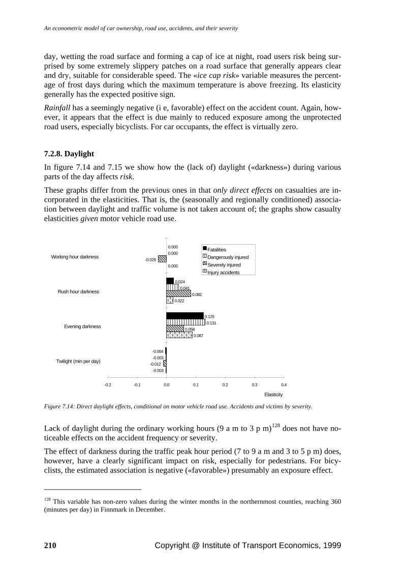
An econometric model of car ownership, road use, accidents, and their severity
210 Copyright @ Institute of Transport Economics, 1999
day, wetting the road surface and forming a cap of ice at night, road users risk being sur-prised by some extremely slippery patches on a road surface that generally appears clear and dry, suitable for considerable speed. The «ice cap risk» variable measures the percent-age of frost days during which the maximum temperature is above freezing. Its elasticity generally has the expected positive sign.
Rainfall has a seemingly negative (i e, favorable) effect on the accident count. Again, how-ever, it appears that the effect is due mainly to reduced exposure among the unprotected road users, especially bicyclists. For car occupants, the effect is virtually zero.
7.2.8. Daylight
In figure 7.14 and 7.15 we show how the (lack of) daylight («darkness») during various parts of the day affects risk.
These graphs differ from the previous ones in that only direct effects on casualties are in-corporated in the elasticities. That is, the (seasonally and regionally conditioned) associa-tion between daylight and traffic volume is not taken account of; the graphs show casualty elasticities given motor vehicle road use.
-0.003
0.087
0.022
0.000
-0.012
0.058
0.082
-0.029
-0.003
0.131
0.041
0.000
-0.004
0.125
0.024
0.000
-0.2 -0.1 0.0 0.1 0.2 0.3 0.4
Twilight (min per day)
Evening darkness
Rush hour darkness
Working hour darkness
Elasticity
FatalitiesDangerously injuredSeverely injuredInjury accidents
Figure 7.14: Direct daylight effects, conditional on motor vehicle road use. Accidents and victims by severity.
Lack of daylight during the ordinary working hours (9 a m to 3 p m)128 does not have no-ticeable effects on the accident frequency or severity.
The effect of darkness during the traffic peak hour period (7 to 9 a m and 3 to 5 p m) does, however, have a clearly significant impact on risk, especially for pedestrians. For bicy-clists, the estimated association is negative («favorable») presumably an exposure effect.
128 This variable has non-zero values during the winter months in the northernmost counties, reaching 360 (minutes per day) in Finnmark in December.

Chapter 7: Synthesis
Copyright @ Institute of Transport Economics, 1999 211
An even stronger effect is due to dark evenings (5 to 11 p m). Again, the largest risk in-crease applies to pedestrians, while two-wheelers are probably subject to reduced exposure and hence also to a lower accident toll. Car occupant injuries are significantly more fre-quent when the evenings are dark.
The length of the twilight period does not, in general, have any significant impact on casu-alty rates, except for bicyclists and pedestrians. Here the effect is negative (favorable), when the amount of daylight is controlled for.
-0.003
0.087
0.022
0.000
0.004
0.094
0.004
0.000
0.000
-0.093
-0.013
0.000
-0.096
-0.073
-0.059
0.002
-0.080
0.399
0.111
0.007
-0.2 -0.1 0.0 0.1 0.2 0.3 0.4
Twilight (min per day)
Evening darkness
Rush hour darkness
Working hourdarkness
Elasticity
Pedestrians injuredBicyclists injuredMC occupants injuredCar occupants injuredInjury accidents
Figure 7.15: Direct daylight effects, conditional on motor vehicle road use. Injury acci-dents and victims by road user category.
7.2.9. Seat belts
Seat belts are an effective injury countermeasure (figure 7.16). A 10 per cent increase in the number of car drivers not wearing the belt (from – say – the 12 per cent rate estimated in 1994, to 13.2 per cent) will increase the number of car occupant injuries by some 3 per cent and the number of fatalities by some 0.6 per cent. It appears that seat belts are more effective in preventing less severe injuries than in saving lives.

An econometric model of car ownership, road use, accidents, and their severity
212 Copyright @ Institute of Transport Economics, 1999
0.302
0.235
0.191
0.12
0.061
0.00 0.05 0.10 0.15 0.20 0.25 0.30 0.35
Non-use of seat belt
Elasticity
FatalitiesDangerously injuredSeverely injuredInjury accidentsCar occupants injured
Figure 7.16: Seat belt effects as of 1994.
0.131
-0.283
-0.220
-0.179
-0.112
-0.057
-0.4 -0.3 -0.2 -0.1 0.0 0.1 0.2
Real value of ticket fornot wearing belt
Elasticity
FatalitiesDangerously injuredSeverely injuredInjury accidentsCar occupants injuredSeat belt use
Figure 7.17: Seat belt ticket elasticities as of 1994.
In the TRULS model, we find no sign that seat belts give rise to behavioral adaptation on the part of car drivers, in such a way as to represent an increased hazard to pedestrians, as was once suggested by Peltzman (1975).
By combining the elasticities found in the seat belt model (chapter 5) with the elasticities shown in figure 7.16, we are able to calculate the estimated effect of increasing the (real value of the) ticket fine for not wearing a safety belt. This ticket runs at NOK 500 as of 1994.
A 10 per cent increase in this fine corresponds, as of 1994, to a 1.3 per cent increase in the rate of seat belt use, i e from 88 to 89.2 per cent. This corresponds to an almost 10 per cent

Chapter 7: Synthesis
Copyright @ Institute of Transport Economics, 1999 213
decrease in the rate of non-use (from 12 to 10.8 per cent), which translates into a 2.8 per cent decrease in the number of car occupant injuries and a 2.2 per cent reduction in the total number of injury accidents (figure 7.17).
The gradual reduction of the real value of the ticket due to inflation will, by assumption, have opposite effects.
7.2.10. Alcohol availability
Access to alcohol is more severely regulated in Norway than in most other western indus-trialized countries. Wine and liquor are sold only from state monopoly stores, generally found only in larger townships, and even beer sales are subject to licensing by the munici-pal assembly. Bars and restaurants also need a central or local government license in order to serve alcoholic beverage.
More than half the counties have less than one alcohol outlet (shop) per 3 000 square kilo-meters. Even beer sales have been heavily restricted in some counties, although more so in the 1970s and early -80s than at present. A few municipalities still maintain an absolute ban on any kind of alcoholic beverage being served or sold.
In the TRULS model we decompose the availability of various forms of alcohol into six parts.
One («alcohol outlets») measures the total number of shops per 1000 inhabitants. A second one («strong beer outlets – share») measures the percentage of shops allowed to sell bev-erage stronger than lager beer (4.5 per cent alcohol by volume). A third variable («hard liquor outlets – share») measures the percentage of these, in turn, that are wine/liquor stores.
A similar decomposition is applied to (bars and) restaurants. General availability is meas-ured in terms of «restaurants licensed to serve alcohol» per 1000 population. Secondly, we measure the share of these that are allowed to serve wine or liquor – i e, not only beer («wine/liquor licenses – share»). Thirdly, we measure the share of these, in turn, which may serve liquor («hard liquor licenses – share»).
In figure 7.18, the alcohol outlet effects come out strikingly consistent, yielding positive casualty elasticities for every degree of severity, with respect to every type of alcohol. Judged by these estimates, the restrictive Norwegian alcohol policy has helped prevent a certain number of road accidents and fatalities. By assumption, alcohol availability does not affect car ownership or road use.
When the effects are partitioned between different road user groups, the picture becomes more mixed (figure 7.19). Apparently, an increase in the availability of alcohol has an im-pact on pedestrian, bicyclist and motorcyclist injuries, but not on car occupant injuries.
Another set of surprising results relates to the density of restaurants with a license to serve alcohol. In general, the effects of restaurant density are negative (figures 7.20 and 7.21). This is true in particular of wine restaurants (as opposed to beer gardens etc), suggesting that only the latter category – if any – represents a problem in relation to road safety.

An econometric model of car ownership, road use, accidents, and their severity
214 Copyright @ Institute of Transport Economics, 1999
0.082
0.025
0.041
0.048
0.036
0.04
0.198
0.051
0.049
0.198
0.019
0.005
0 0.05 0.1 0.15 0.2 0.25
Alcohol outlets
Strong beer outlets(share)
Hard liquor outlets (share)
Elasticity
FatalitiesDangerously injuredSeverely injuredInjury accidents
Figure 7.18: Alcohol availability effects as of 1994. Outlets. Accidents and victims by se-verity.
0.082
0.025
0.041
-0.021
-0.034
-0.012
0.179
0.098
0.086
0.049
0.037
0.049
-0.018
0.088
0.094
-0.05 0 0.05 0.1 0.15 0.2
Alcohol outlets
Strong beer outlets(share)
Hard liquor outlets(share)
Elasticity
Pedestrians injuredBicyclists injuredMC occupants injuredCar occupants injuredInjury accidents
Figure 7.19: Alcohol availability effects as of 1994. Outlets. Injury accidents and victims by road user category.
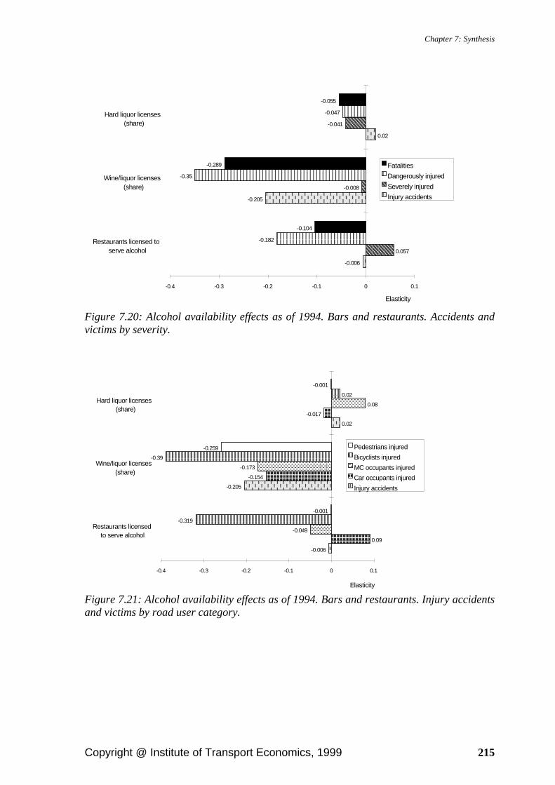
Chapter 7: Synthesis
Copyright @ Institute of Transport Economics, 1999 215
-0.006
-0.205
0.02
0.057
-0.008
-0.041
-0.182
-0.35
-0.047
-0.104
-0.289
-0.055
-0.4 -0.3 -0.2 -0.1 0 0.1
Restaurants licensed toserve alcohol
Wine/liquor licenses(share)
Hard liquor licenses(share)
Elasticity
FatalitiesDangerously injuredSeverely injuredInjury accidents
Figure 7.20: Alcohol availability effects as of 1994. Bars and restaurants. Accidents and victims by severity.
-0.006
-0.205
0.02
0.09
-0.154
-0.017
-0.049
-0.173
0.08
-0.319
-0.39
0.02
-0.001
-0.259
-0.001
-0.4 -0.3 -0.2 -0.1 0 0.1
Restaurants licensedto serve alcohol
Wine/liquor licenses(share)
Hard liquor licenses(share)
Elasticity
Pedestrians injuredBicyclists injuredMC occupants injuredCar occupants injuredInjury accidents
Figure 7.21: Alcohol availability effects as of 1994. Bars and restaurants. Injury accidents and victims by road user category.

An econometric model of car ownership, road use, accidents, and their severity
216 Copyright @ Institute of Transport Economics, 1999
7.2.11. Calendar effects
The calendar per se has a certain impact on human activity and hence also on road casual-ties. This is shown in figures 7.22 and 7.23129.
The Easter holiday has a pronounced traffic generating effect, by around 5 per cent (on a monthly basis) at the onset as well as at Easter end. Injury accidents increase at about the same rate as the traffic at Easter start, and fatalities go up by almost 20 per cent.
Behind these overall accident statistics lie a 12 per cent increase in car occupant injuries and a clear decrease in two-wheeler and pedestrian injuries. Few people walk or bike to their Easter resort.
At Easter end, the congestion is apparently so heavy that fewer injury accidents and fatali-ties occur than should «normally» follow from the (increased) exposure.
The extra activity generated during the month of December translates into an about 25 per cent higher traffic volume and an almost equally large increase in fatalities.
Holidays and vacation («leisure days») dampen the overall (domestic) mobility and hence also the number of road casualties. The number of days in a given month («length of month») also has an obvious effect – not forgotten in the TRULS model – on total vehicle kilometers and their accident toll.
0.697
0.048
0.055
0.248
-0.290
0.346
-0.108
0.050
0.123
-0.158
0.554
-0.107
0.097
0.197
-0.236
0.596
-0.065
0.118
0.212
-0.307
0.689
-0.078
0.181
0.245
-0.396
-0.6 -0.4 -0.2 0.0 0.2 0.4 0.6 0.8
Length of month
Easter end
Easter start
December
Leisure days (share)
"Elasticity"
FatalitiesDangerously injuredSeverely injuredInjury accidentsTraffic volume
Figure 7.22: Calendar effects as of 1994. Accidents and victims by severity.
129 Note that in these diagrams, the effects shown for December, Easter start and Easter end are not elastic-ities in the traditional sense, but (approximate) relative changes associated with the respective dummy vari-ables. For instance, injury accidents are about 5 per cent (= e0.050 – 1) more frequent during a month compris-ing the start of Easter, other independent variables being equal (see section 2.4.5).

Chapter 7: Synthesis
Copyright @ Institute of Transport Economics, 1999 217
0.697
0.048
0.055
0.248
-0.290
0.346
-0.108
0.050
0.123
-0.158
0.448
-0.121
0.116
0.159
-0.202
0.530
-0.033
-0.013
0.189
-0.118
0.331
-0.031
-0.130
0.118
-0.101
0.095
-0.164
-0.030
0.034
-0.033
-0.4 -0.2 0.0 0.2 0.4 0.6 0.8
Length of month
Easter end
Easter start
December
Leisure days (share)
"Elasticity"
Pedestrians injuredBicyclists injuredMC occupants injuredCar occupants injuredInjury accidentsTraffic volume
Figure 7.23: Calendar effects as of 1994. Injury accidents and victims by road user cate-gory.
7.2.12. Time trend
The injury accident equation comes out with a highly significant time trend effect. As of 1994 the trend elasticity is calculable at –0.454 for injury accidents (fig 7.24). Note, how-ever, that the trend variable is defined as years passed since 1945, so that a one per cent increase in this variable corresponds (as of 1994) to a time lapse of almost half a year. Thus the interpretation of this elasticity is that there is an autonomous safety improvement taking place over time, which – at present – tends to reduce the number of injury accidents by approximately 0.5 per cent every six months.
For fatalities, an almost equally strong trend effect is estimated, while for the number of severe injuries the effect appears to be more than six times stronger.
An interesting insight is gained when the trend effect is differentiated between road user groups (fig 7.25). Here, one notes that there is no independent trend effect for car occupant injuries (the small positive effect shown is statistically insignificant). The reduction in car occupant risk that has taken place during 1973-94 is, in other words, fully explained by the independent variables of the model. A most important single factor here is no doubt the escalated use of seat belts.
For two-wheelers and pedestrians, however, the trend effects are all the stronger. Bicyclist injuries decrease by no less than 5 per cent annually, other independent variables being equal, and pedestrian injuries by almost 3 per cent. It should be understood that large parts of these effects might be due to reduced (relative) exposure, not captured in the TRULS model. As the slower modes represent a steadily reduced part of total kilometers traveled, the frequency of accidents involving these modes – as reckoned per motor vehicle kilome-ter – naturally becomes lower.

An econometric model of car ownership, road use, accidents, and their severity
218 Copyright @ Institute of Transport Economics, 1999
-0.454
-3.094
-0.633
-0.439
-3.5 -3.0 -2.5 -2.0 -1.5 -1.0 -0.5 0.0
Trend (years passedsince 1945)
Elasticity
FatalitiesDangerously injuredSeverely injuredInjury accidents
Figure 7.24: Trend effects as of 1994. Accidents and victims by severity.
-0.454
0.156
-2.295
-2.488
-1.384
-3.0 -2.5 -2.0 -1.5 -1.0 -0.5 0.0 0.5
Trend (years passed since1945)
Elasticity
Pedestrians injuredBicyclists injuredMC occupants injuredCar occupants injuredInjury accidents
Figure 7.25: Trend effects as of 1994. Injury accidents and victims by road user category.

Chapter 7: Synthesis
Copyright @ Institute of Transport Economics, 1999 219
7.3. Suggestions for further research
The TRULS modeling exercise, although a rather comprehensive research endeavor, still leaves a large number of questions unanswered. In some cases, the TRULS model results give rise to entirely new questions and ideas, which may deserve the subsequent attention of researchers.
Some of the possible enhancements and extensions are primarily methodological, while others concern the subject matter empirical relationships. These two areas are, of course, to some extent interrelated.
7.3.1. Methodological improvements
As noted in section 2.4, the examination and application of competing econometric meth-ods have been beyond the scope of this study. There are, however, several points where the exploration of alternative methods would be of great interest.
Generalized Poisson maximum likelihood A most important improvement would be the development and application of (generalized) Poisson maximum likelihood algorithms for casualty models with Box-Cox transforma-tions on the independent variables. In our IRPOSKML130 procedure, the basic distribu-tional assumption is one of normally distributed disturbances. This assumption is obvi-ously not very realistic as applied to data sets containing small casualty counts.
As a second best solution, one might proceed to reestimate the casualty equations of the TRULS model by (generalized) Poisson maximum likelihood, transforming the independ-ent variables with fixed Box-Cox parameters as already estimated by IRPOSKML. In a sense, this amounts to adding another, final step to the IRPOSKML procedure – one, how-ever, that cannot (at present) be performed by means of the TRIO algorithm.
It is not known to what extent our IRPOSKML estimates can be expected to differ from true Poisson (or negative binomial) maximum likelihood estimates. A comparative study of these two techniques would be of great interest.
The forced addition of a small (Box-Tukey) constant to all counts introduces an unfortu-nate degree of arbitrariness into the IRPOSKML procedure. There are indications that cer-tain coefficients, especially those concerning exposure and traffic density, may be sensitive to the choice of Box-Tukey constant, when the casualty counts are small. An investigation into these matters would be of interest.
Simultaneous equation estimation In order to make use of the Box-Cox regression technique, we have had no choice but to estimate one equation at a time. There are, however, obvious arguments in favor of a si-multaneous equation estimation approach, since certain (groups of) equations are unlikely to exhibit uncorrelated disturbances. This applies in particular to the car ownership and road use equations, in which the respective dependent variables are probably subject to
130 Iterative Reweighted POisson-SKedastic Maximum Likelihood, see Appendix A.

An econometric model of car ownership, road use, accidents, and their severity
220 Copyright @ Institute of Transport Economics, 1999
many of the same exogenous shocks. Most clearly, it also applies to the accident frequency and severity equations, and more generally to the entire set of casualty equations, which – with few exceptions – are based on the same set of independent variables and may be ex-pected to vary in response to many of the same exogenous shocks.
A reestimation by means simultaneous equation or block-recursive methods, using – again – fixed Box-Cox parameters as estimated in TRULS, would be of considerable methodo-logical – and perhaps also substantive – interest.
Panel data methods The panel structure of our data set has not been exploited. We have assumed throughout that cross-sectional and time-series effects are identical. This procedure is information ef-ficient given that the homogeneity assumption is justified. In the opposite case, it can lead to quite misleading results.
The examination of this homogeneity assumption, and the possible reestimation of the model by means panel data methods, constitute another highly interesting follow-up study. Hausman et al (1984) have shown how specialized Poisson or negative binomial models, with fixed or random effects, may be estimated on count data with a panel structure.
With the exception of the car ownership submodel, and a few lagged variables concerning road infrastructure, our approach in the TRULS model has generally been one of static econometric relations. Panel data may, on the other hand, lend themselves to various kinds of dynamic model specifications. We would like to warn, however, against casualty model specifications in which the accident count is made to depend on previous realizations of itself. Such a model seems incompatible with the hypothesis of probabilistically independ-ent events underlying the (generalized) Poisson disturbance distribution.
The car ownership equation As noted in section 4.5, the car ownership equation can probably be improved upon.
Our method of estimation does not take account of the fact that autocorrelation in a model with lagged endogenous variables introduces bias into the ordinary regression estimates, and even into the Cochran-Orcutt procedure. Hatanaka (1974) has suggested a method by which consistent and efficient estimates can be obtained for the partial adjustment model. It would be interesting to reestimate the car ownership model by means of this procedure, using fixed Box-Cox parameters, and compare the results to the BC-GAUHESEQ esti-mates.
The symmetry of adjustment assumed for the car ownership model is another point where alternative approaches might be of interest. Using a switching model approach (Maddala 1986), it should be possible to estimate a model in which the car stock adjusts more slowly downwards than upwards. We suspect that such a model may prove more realistic under Norwegian market conditions.
The power of significance testing: a pseudo Monte Carlo study At an exploratory stage, a number of variables capturing legislative and other accident countermeasures were introduced into the accident frequency model, however without

Chapter 7: Synthesis
Copyright @ Institute of Transport Economics, 1999 221
yielding statistically significant or reasonably robust131 coefficient estimates. Most of these variables were therefore not retained in the final version of the model.
The question arises as to how large an impact a risk or safety factor needs to have, and how much variation there needs to be in the data set, in order for an econometrically discernible (statistically significant) effect to emerge.
There is, in other words, a need to investigate the power of significance testing in econo-metric accident models. When can we confidently conclude that a given independent vari-able, whose coefficient does not come out significant, is in fact without effect? How does the power depend (i) on the sample size, (ii) on the average size of the casualty counts, (iii) on the true regression coefficient, (iv) on the variation present in the data set, and (v) on the collinearity with other independent variables?
We are in a position to propose an unusually realistic (pseudo) Monte Carlo experiment to shed light on these questions. The expected number of casualties at each sample point, as estimated in our model, may serve as a set of authentic benchmark values. A random sample of synthetic casualty counts may be generated using the Poisson (or negative bino-mial) distribution with parameters given by the benchmark values, and a new set of pa-rameters may be estimated. Next, another random sample should be generated, in which some independent variable has been subject to certain modifications, or a new risk factor has been introduced, with known effects on the expected number of casualties. Another set of estimates will be derived based on this new data set.
This exercise may be repeated so as to cover a wide range of cases along the dimensions (i) through (v) above. The sample size may be varied by using all of or just a random subset of the real sample, or by generating several random observations for each benchmark value. The size of the casualty counts may be varied realistically by comparing, e g, injury acci-dents to fatalities, or artificially by multiplying all benchmark values by a given factor. The variation in a given explanatory factor may be conveniently summarized in terms of the first four moments. And the collinearity with respect to other independent variables is summarized in the eigenvalue iλ (say) of the matrix XX' ( X being the matrix of inde-
pendent variables) and in the conditional indices imax λλ (Gaudry et al 1993, Liem et al 1993).
In an extended Monte Carlo experiment, one might even consider (vi) competing methods of estimation. How do, e g, the standard BC-GAUHESEQ, the IRPOSKML, the Poisson ML, and the negative binomial ML methods compare in terms of testing power?
7.3.2. Subject matter issues
Among the substantive questions raised or neglected by the TRULS model, the most im-portant are, in our view, (i) the unknown effects on material damage accidents and hence – strictly speaking – on severity, (ii) the surprising effect of traffic density on accident sever-ity and hence on fatalities, (iii) the strong but somewhat ambiguous effects of alcohol availability, (iv) the remarkable effect of pregnancy rates, and – last but not least – (v) the
131 Robust in the sense of yielding similar(ly signed) estimates under small changes in the model specifica-tion.

An econometric model of car ownership, road use, accidents, and their severity
222 Copyright @ Institute of Transport Economics, 1999
role of unobserved intermediate, behavioral variables such as speed and alcohol consump-tion. Many of these issues are interrelated.
An econometric study of speed choice, its determinants and consequences Material damage accidents are not subject to mandatory police reporting and therefore not included in our accident counts. This means that our «severity» measures are subject to an annoying source of error referred to (in section 6.1.5) as «reporting drift». This in turn has the unfortunate consequence that certain, potentially powerful tests for risk compensation, in which one compares (the signs of) the corresponding effects on accident frequency and severity, become rather elusive.
A second limitation to the study of risk compensation is the lack of data on key behavioral instruments, notably on speed. As long as we cannot observe the variation in this crucial intermediate variable, assertions about behavioral adjustment remain largely unsubstanti-ated.
Recent enhancements to the stock of relevant statistical data may pave the ground for an analysis that overcomes both of these obstacles. Since the late 1980s, the Norwegian Pub-lic Roads Administration has been automatically recording speed at a fairly large number of cross sections on the national road network. Measurements are available on average speed by the hour. In some cases even hourly fractiles can be extracted. These data should be detailed enough to capture, e g, how speed varies with the density of traffic, or with temporal changes in weather and daylight.
The major insurance companies cooperate to compile a publicly accessible data base («TRAST») comprising material damage as well as injury accident records. This data base may provide the information necessary to calculate reliable severity indicators, or – more generally – to analyze and compare accident frequencies by degree of severity in a consis-tent and dependable way.
By combining these two sources with the data set already compiled for TRULS, and possi-bly some other extensions, a most interesting, follow-up econometric study would be fea-sible.
Traffic density and severity Contrary to the TRULS model, previous Scandinavian research (Fridstrøm and Inge-brigtsen 1991, Fridstrøm et al 1995) has suggested that severity is a decreasing function of traffic density. Such a mechanism would be consistent with the hypothesis that speed is forced down in denser traffic, and thus help explain the negative density effect found even for the less severe injury accidents.
As our first priority we would examine the possible role of the probability model and method of estimation. As pointed out in the previous section, very small accident counts may call for another set of techniques than BC-GAUHESEQ/IRPOSKML, notably a (gen-eralized) Poisson maximum likelihood approach. Moreover, the IRPOSKML procedure may be sensitive to the specification of the (arbitrary) Box-Tukey constant. This applies in particular to the exposure and density coefficients.
Until the surprising effects of traffic density on severity have been confirmed by count data methods of estimation, we recommend that these results be interpreted with considerable
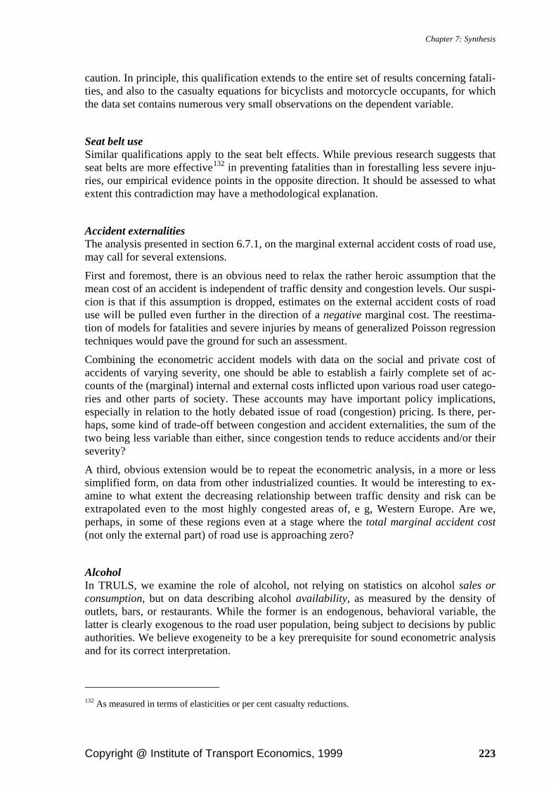
Chapter 7: Synthesis
Copyright @ Institute of Transport Economics, 1999 223
caution. In principle, this qualification extends to the entire set of results concerning fatali-ties, and also to the casualty equations for bicyclists and motorcycle occupants, for which the data set contains numerous very small observations on the dependent variable.
Seat belt use Similar qualifications apply to the seat belt effects. While previous research suggests that seat belts are more effective132 in preventing fatalities than in forestalling less severe inju-ries, our empirical evidence points in the opposite direction. It should be assessed to what extent this contradiction may have a methodological explanation.
Accident externalities The analysis presented in section 6.7.1, on the marginal external accident costs of road use, may call for several extensions.
First and foremost, there is an obvious need to relax the rather heroic assumption that the mean cost of an accident is independent of traffic density and congestion levels. Our suspi-cion is that if this assumption is dropped, estimates on the external accident costs of road use will be pulled even further in the direction of a negative marginal cost. The reestima-tion of models for fatalities and severe injuries by means of generalized Poisson regression techniques would pave the ground for such an assessment.
Combining the econometric accident models with data on the social and private cost of accidents of varying severity, one should be able to establish a fairly complete set of ac-counts of the (marginal) internal and external costs inflicted upon various road user catego-ries and other parts of society. These accounts may have important policy implications, especially in relation to the hotly debated issue of road (congestion) pricing. Is there, per-haps, some kind of trade-off between congestion and accident externalities, the sum of the two being less variable than either, since congestion tends to reduce accidents and/or their severity?
A third, obvious extension would be to repeat the econometric analysis, in a more or less simplified form, on data from other industrialized counties. It would be interesting to ex-amine to what extent the decreasing relationship between traffic density and risk can be extrapolated even to the most highly congested areas of, e g, Western Europe. Are we, perhaps, in some of these regions even at a stage where the total marginal accident cost (not only the external part) of road use is approaching zero?
Alcohol In TRULS, we examine the role of alcohol, not relying on statistics on alcohol sales or consumption, but on data describing alcohol availability, as measured by the density of outlets, bars, or restaurants. While the former is an endogenous, behavioral variable, the latter is clearly exogenous to the road user population, being subject to decisions by public authorities. We believe exogeneity to be a key prerequisite for sound econometric analysis and for its correct interpretation.
132 As measured in terms of elasticities or per cent casualty reductions.

An econometric model of car ownership, road use, accidents, and their severity
224 Copyright @ Institute of Transport Economics, 1999
The other side of this coin is that – again – we miss out on a key intermediate, behavioral variable. Until one has established the empirical link between alcohol availability and con-sumption, and between consumption and the incidence of alcohol impaired driving, the assumed causal chain of effects is unsubstantiated.
An econometric analysis directed at these relationships would be highly interesting, but is hampered by the notorious unreliability of alcohol sales data as indicators of consumption. Moreover, very few data exist on the incidence of alcohol impaired driving. Specialized techniques might, however, be applied, to account for such «latent» variables as legal and illegal home production and import. Induced exposure techniques, based on blood tests taken from a sample of accident involved drivers, might help establish the link between aggregate consumption, alcohol impaired driving, and accident risk.
The alcohol availability effects found in our pooled cross-section/time-series data set might be influenced by certain omitted factors varying primarily along the regional axis. Counties with a high density of alcohol outlets generally also exhibit a high degree of ur-banization and high densities of traffic, roads, public transportation, and population. One might argue that since all of these density measures are included in the model, the presence of an omitted variable bias is far from obvious. Yet a reanalysis of the alcohol effects based on panel data methods would be highly desirable.
Pregnancy The estimated effect of pregnancy is such as to elicit more questions than answers. The casualty subset tests come out quite clearly in support of the claim that the effect is not due to some kind of spurious correlation or ecological fallacy. Yet the aggregate relationship can hardly be relied upon until substantiated by disaggregate analysis.
Literature
Copyright @ Institute of Transport Economics, 1999 225
Literature
Aigner D J & Goldfeld S M (1974) : Estimation and prediction from aggregate data when aggregates are measured more accurately than their components. Econometrica 42 :113-134.
Allais M (1953): Le comportement de l’homme rationnel devant le risque: critique des postulats et axiomes de l’Ecole Américaine. Econometrica 21:503-546.
Allais M (1979): The so-called Allais paradox and rational decisions under uncertainty. In: Allais M & Hagen O (eds): Expected utility hypotheses and the Allais paradox. Reidel, Dordrecht.
Allais M (1984): The foundations of the theory of utility and risk. In: Hagen O & Wenstøp F (eds): Progress in decision theory. Reidel, Dordrecht.
Allais M (1987): Allais paradox. Pp 80-82 in: Eatwell J, Milgate M & Newman P (eds) The new Palgrave: a dictionary of economics.. Vol 1. The Macmillan Press Ltd, Lon-don.
Allsop R E (1966): Alcohol and road accidents. A discussion of the Grand Rapids study. RRL Report no 6, Road Research Laboratory, Harmondsworth.
Arrow K J (1970): Essays in the theory of risk-bearing. North-Holland, Amsterdam. Baumol W J & Oates W E (1988): The theory of environmental policy. 2nd edition. Cam-
bridge University Press, Cambridge, Mass. Ben-Akiva M (1973): Structure of passenger travel demand models. PhD dissertation, De-
partment of Civil Engineering, MIT, Cambridge, Mass. Ben-Akiva M and Lerman S R (1985): Discrete choice analysis: theory and application to
travel demand. MIT Press, Cambridge, Mass. Berkson J (1944): Application of the logistic function to bioassay. Journal of the American
Statistical Association 39:357-65 Berkson J (1953): A statistically precise and relatively simple method of estimating the
bioassay with quantal response, based on the logistic function. Journal of the American Statistical Association 48:565-599
Berkson J (1955): Maximum likelihood and minimum X2 estimates of the logistic function. Journal of the American Statistical Association 50: 130-162
Betancourt R & Kelejian H (1981): Lagged endogenous variables and the Cochrane-Orcutt procedure. Econometrica 49:1073-1078.
Bickel P J & Doksum K A (1977): Mathematical statistics: basic ideas and selected topics. San Francisco, Holden-Day.
Bishop Y M M, Fienberg S E & Holland P W (1975): Discrete multivariate analysis: the-ory and practice. MIT Press, Cambridge, Mass.
Bjørnskau T (1993): Risiko i vegtrafikken 1991/92. Report 216, Institute of Transport Eco-nomics, Oslo.
Bjørnskau T (1994): Hypoteser om atferdstilpasning (risikokompensasjon). Working paper TST/0512/1994, Institute of Transport Economics, Oslo.
Bjørnskau T & Fosser S (1996): Bilisters atferdstilpasning til innføring av vegbelysning. Report 332, Institute of Transport Economics, Oslo.
Blaise J H (1980): Hysteresis in travel demand. Transportation Planning and Technology 6(2).
Blomquist G (1977): The economics of safety and seat belt usage. Journal of Safety Re-search 9:179-189

An econometric model of car ownership, road use, accidents, and their severity
Copyright @ Institute of Transport Economics, 1999 226
Blomquist G (1986): A utility maximizing model of driver traffic safety behavior. Accident Analysis & Prevention 18:371-375
Blum U C H, Bolduc D & Gaudry M (1990): From correlation to distributed contiguites: a family of AR-C-D autocorrelation processes. Publication 734, Centre de Recherche sur les Transports (CRT), Université de Montréal
Borch K (1969): A note on uncertainty and indifference curves. Review of Economic Stud-ies 36:1-4.
Borkenstein R F, Crowther R F Schumate R P, Ziel W B & Zylman R (1964): The role of the drinking driver in traffic accidents. Department of Police Administration, Indiana University.
Borger A, Fosser S, Ingebrigtsen S & Sætermo I-A (1995): Underrapportering av trafikku-lykker. Report 318, Institute of Transport Economics, Oslo
Bortkewitsch L von (1898): Das Gesetz der kleinen Zahlen. B G Teubner, Leipzig. Box G E P & Cox D R (1964): An analysis of transformations. Journal of the Royal Statis-
tical Sociey B 26:211-243. Box G E P & Jenkins G H (1976): Time series analysis: Forecasting and control. Holden-
Day, San Francisco Boyle A J & Wright C C (1984): Accident ’migration’ after remedial treatment at accident
blackspots. Traffic Engineering + Control 25:260-267. Breiman L (1963): The Poisson tendency in traffic distribution. Annals of Mathematical
Statistics 34:308-311 Brorsson B, Ifver J & Rydgren H (1988): Injuries from single vehicle crashes and snow
depth. Accident Analysis & Prevention 20:367-377. Broughton J (1995): The identification of casualty trends using quadratic splines. Paper
prepared for COST 329, Transport Research Laboratory, UK. Brännäs K & Johansson P (1992): Time series count data regression. Umeå Economic
Studies no 289, University of Umeå. Cameron A C & Trivedi P K (1986): Econometric models based on count data: comparison
and applications of some estimators and tests. Journal of Applied Econometrics 1:29-53.
Cameron A C & Trivedi P K (1998): Regression analysis of count data. Econometric So-ciety Monographs no 30. Cambridge University Press, Cambridge.
Cameron M H, Vulcan A P, Finch C F & Newstead S V (1994): Mandatory bicycle helmet use following a decade of helmet promotion in Victoria, Australia - an evaluation. Acci-dent Analysis & Prevention 26:325-337.
Central Bureau of Statistics (1991): Konsumprisindeksen. Report 91/8, Central Bureau of Statistics, Oslo.
Christensen P, Beaumont H, Dunkerley C, Lindberg G, Otterström T, Gynther L, Rothen-gatter W & Doll C (1998): Internalisation of externalities: Appendix. Deliverable 7, version 1.2 from the PETS project (ST-96-SC.172), European Commision/Leeds Uni-versity (ITS).
Coase R H (1960): The problem of social cost. Journal of Law and Economics 3:1-44. Crandall R & Graham J D (1984): Automobile safety regulation and offsetting behavior:
some new empirical estimates. American Economic Review 74:328-331. Dahl C (1995): Demand for transportation fuels: A survey of demand elasticities and their
components. Journal of Energy Literature 1:3-27. Dahl C & Sterner T (1991a): Analysing gasoline demand elasticities: a survey. Energy
Economics 13:203-210.

Literature
Copyright @ Institute of Transport Economics, 1999 227
Dahl C & Sterner T (1991b): A survey of econometric gasoline demand elasticities. Inter-national Journal of Energy Systems 11:53-76.
Dargay J M (1993): Demand elasticities: a comment. Journal of Transport Economics and Policy 27:87-90.
Dhrymes P J (1970): Econometrics: statistical foundations and applications. Harper & Row, New York.
Domencich T & McFadden D (1975): Urban travel demand – a behavioral analysis. North-Holland, Amsterdam.
Dupuit J (1844): On the measurement of the utility of public works. In: Murphy D (ed): Transport. Penguin, London.
Diamond P A & Stiglitz J E (1970): Increases in risk and in risk aversion. Journal of Eco-nomic Theory 8:337-360.
Durkheim E (1951): Suicide. Free Press, Glencoe, Ill. Eggenberger F & Pólya G (1923): Über die Statistik verketteter Vorgänge. Zeitschrift für
angewandte Mathematik und Mechanik 1:279-289. Elvik R (1993): Hvor rasjonell er trafikksikkerhetspolitikken? Report 175, Institute of
Transport Economics, Oslo. Elvik R (1994): The external costs of traffic injury: definition, estimation, and possibilities
for internalization. Accident Analysis & Prevention 26:719-732. Elvik R (1995): Explaining the distribution between state funds for national road invest-
ments between counties in Norway: Engineering standards or vote trading? Public Choice 85:371-388.
Elvik R, Vaa T & Østvik E (1989): Trafikksikkerhetshåndbok: oversikt over virkninger. kostnader og offentlige ansvarsforhold for 84 trafikksikkerhetstiltak. Institute of Trans-port Economics, Oslo.
Elvik R, Mysen A B & Vaa T (1997): Trafikksikkerhetshåndbok: oversikt over virkninger. kostnader og offentlige ansvarsforhold for 124 trafikksikkerhetstiltak. Institute of Transport Economics, Oslo.
European Commision (1996): Towards fair and efficient pricing in transport. Bulletin of the European Union, Supplement 2/96.
Evans L (1985): Human behavior feedback and traffic safety. Human Factors 27:555-576. Feller W (1943): On a general class of ‘contagious’ distributions. Annals of mathematical
Statistics 14:389-400. Fosser S (1978): Bruk av bilbelter og hjelmer i Norge 1973-77. Institute of Transport Eco-
nomics, Oslo. Fosser S (1979): Bilbelte- og hjelmbruk i april 1979. Working report 463, Institute of
Transport Economics, Oslo. Fosser S (1990): Bilbelte- og hjelmbruk fra 1973 til 1990. Working report 943, Institute of
Transport Economics, Oslo. Fosser S (1995): Bilbelte- og hjelmbruk fra 1973 til 1993. Working report 996, Institute of
Transport Economics, Oslo. Fosser S (1992): An experimental evaluation of the effects of periodic motor vehicle in-
spection on accident rates. Accident Analysis & Prevention 24:599-612. Fosser S & Christensen P (1998): Bilers alder og ulykkesrisiko. Report 386, Institute of
Transport Economics, Oslo. Fosser S, Sagberg F & Sætermo I-A (1996): Atferdstilpasning til kollisjonsputer og blok-
keringsfrie bremser. Report 335, Institute of Transport Economics, Oslo.

An econometric model of car ownership, road use, accidents, and their severity
Copyright @ Institute of Transport Economics, 1999 228
Franzén M & Sterner T (1995): Long-run demand elasticities for gasoline. Pp 106-120 in: Barker T, Ekins P & Johnstone N (eds): Global warming and energy demand. Rout-ledge, London.
Freeman M F & Tukey J W (1950): Transformations related to the angular and the square root. Annals of Mathematical Statistics 21:607-611.
Fridstrøm L (1980): Linear and log-linear qualitative response models. Report 80/26, Central Bureau of Statistics, Oslo.
Fridstrøm L (1991): In favor of aggregate econometric accident models. Paper presented at the 6th International Conference on Travel Behavior, Quebec, May 22-24,1991.
Fridstrøm L (1992): Causality – is it all in your mind? An inquiry into the definition and measurement of causal relations. Pp 103-123 in: Ljones O, Moen B & Østby L (eds): Mennesker og modeller – livsløp og kryssløp. Social and Economic Studies 78, Central Bureau of Statistics, Oslo.
Fridstrøm L (1996): Prognoser for trafikkulykkene. Working report 1027, Institute of Transport Economics, Oslo.
Fridstrøm L (1997): Perspektiv på trafikkulykkene. Working report 1067, Institute of Transport Economics, Oslo.
Fridstrøm L & Elvik R (1997): The barely revealed preference behind road investment priorities. Public Choice 92:145-168.
Fridstrøm L, Ifver J, Ingebrigtsen S, Kulmala R & Thomsen L K (1993): Explaining the variation in road accident counts. Report Nord 1993:35, Nordic Council of Ministers, Copenhagen/Oslo.
Fridstrøm L, Ifver J, Ingebrigtsen S, Kulmala R & Thomsen L K (1995): Measuring the contribution of randomness, exposure, weather and daylight to the variation in road ac-cident counts. Accident Analysis & Prevention 27:1-20.
Fridstrøm L & Ingebrigtsen S (1991): An aggregate accident model based on pooled, re-gional time-series data. Accident Analysis & Prevention 23:363-378.
Fridstrøm L & Rand L (1992): Markedet for lange reiser i Norge. Report 220, Institute of Transport Economics, Oslo
Gately D (1990): The U.S. demand for highway travel and motor fuel. The Energy Journal 11(3):59-72.
Gately D (1992): Imperfect price-reversibility of U.S. gasoline demand: asymmetric res-ponses to price increases and declines. The Energy Journal 13(4):179-207.
Gaudry M (1984): DRAG, un modèle de la Demande Routière, des Accidents et de leur Gravité, appliqué au Québec de 1956 à 1982. Publication 359, Centre de Recherche sur les Transports (CRT), Université de Montréal
Gaudry M & Blum U (1993): Une présentation brève du modèle SNUS-1 (Straßen-verkehrs-Nachfrage, Unfälle und ihre Schwere). Modélisation de l'insécurité routière. Collection Transport et Communication no 47:37-44, Paradigme, Caen.
Gaudry M, Duclos L-P, Dufort F & Liem T (1993): TRIO Reference Manual, Version 1.0. Publication 903, Centre de Recherche sur les Transports (CRT), Université de Montréal
Gaudry M, Fournier F & Simard R (1995): DRAG-2, un modèle économétrique appliqué au kilometrage, aux accidents et à leur gravité au Québec: Synthèse des résultats. Société de l’assurance automobile du Québec
Gaudry M, Jara-Díaz S R & Ortúzar J de D (1989): Urban travel demand: the impact of Box-Cox transformations with nonspherical residual errors. Transportation Research B 23:151-158.
Gaudry M & Lassarre S (eds) (1999): Structural Road Accident Models: The International DRAG Family. Elsevier (forthcoming)

Literature
Copyright @ Institute of Transport Economics, 1999 229
Gaudry M, Mandel B & Rothengatter W (1994): Introducing spatial competition through an autoregressive contiguous distributed (AR-C-D) process in intercity generation-distribution models within a quasi-direct format (QDF). Publication 971, Centre de Recherche sur les Transports (CRT), Université de Montréal
Gaudry M & Wills M I (1978): Estimating the functional form of travel demand models. Transportation Research 12:257-289.
Gerlough D L & Schuhl A (1955): Poisson and Traffic. The Eno Foundation, Saugatuck, Connecticut
Goodwin P B (1977): Habit and hysteresis in mode choice. Urban Studies 14:95-98. Goodwin P B (1992): A review of new demand elasticities with special reference to short
and long run effects of price changes. Journal of Transport Economics and Policy 26:155-169.
Gourieroux C, Monfort A & Trognon A (1984a): Pseudo maximum likelihood methods: theory. Econometrica 52:681-700.
Gourieroux C, Monfort A & Trognon A (1984b): Pseudo maximum likelihood methods: application to Poisson models. Econometrica 52:701-720.
Graham J D (1984): Technology, behavior and safety: An empirical study of automobile occupant-protection regulation. Policy Sciences 17 :141-151
Graham J D & Garber S (1984): Evaluating the effects of automobile safety regulation. Journal of Policy Analysis and Management 3:206-224.
Greene D L (1992): Vehicle use and fuel economy: how big is the “rebound” effect? The Energy Journal 13(1):117-143.
Greene W H (1993): Econometric analysis. 2nd edition. Prentice Hall, New York. Greene W H (1995): LIMDEP Version 7.0: User’s Manual. Econometric Software Inc,
Bellport NY Greenwood M & Yule G U (1920): An enquiry into the nature of frequency distributions to
multiple happenings, with particular reference to the occurrence of multiple attacks of disease or repeated accidents. Journal of the Royal Statistical Society A 83:255-279.
Grunfeld Y & Griliches Z (1960): Is aggregation necessarily bad? Review of Economics and Statistics 42:1-13.
Haight F A (1967): Handbook of the Poisson distribution. Wiley, New York. Haight F A, Whisler B F & Mosher W W (1961): New statistical method for describing
highway distribution of cars. Highway Research Board Proceedings 40, 557-564 Hannan M T (1991): Aggregation and disaggregation in the social sciences. Revised edi-
tion. Lexington Books, Lexington, Mass. Hannan M T & Burstein L (1991): Estimation from grouped observations. American So-
ciological Review 39:374-392. Hatanaka T (1974): An efficient two-step estimator for the dynamic adjustment model with
autocorrelated errors. Journal of Econometrics 2:199-220 Hauer E (1980): Bias-by-selection: overestimation of the effectiveness of safety counter-
measures caused by the process of selection for treatment. Accident Analysis & Preven-tion 12:113-117.
Hausman J, Hall B H & Griliches Z (1984): Econometric models for count data with an application to the patents-R&D relationship. Econometrica 52(4):909-938.
Heckman J (1977): Sample selection bias as a specification error. Econometrica 47:153-162.
Heckman J (1987): Selection bias and self-selection. Pp 287-297 in: Eatwell J, Milgate M & Newman P (eds) The new Palgrave: a dictionary of economics.. Vol 4. The Macmil-lan Press Ltd, London.

An econometric model of car ownership, road use, accidents, and their severity
Copyright @ Institute of Transport Economics, 1999 230
Hoel P G, Port S C & Stone C J (1971): Introduction to probability theory. Houghton Mif-flin, Boston
Hsiao C (1986): Analysis of panel data. Econometric Society Monographs no 11, Cam-bridge University Press, Cambridge
Hurst P M, Harte D & Frith W J (1994): The Grand Rapids dip revisited. Accident Analysis & Prevention 26:647-654.
Hveberg H (1962): Of gods and giants: Norse mythology. Tanum, Oslo. Jaeger L & Lassarre S (1997): Pour une modélisation de l’évolution de l’insécurité
routière. Estimation du kilométrage mensuel en France de 1957 à 1993: méthodologie et résultats. Rapport DERA no 9709, Convention DRAST/INRETS, Strasbourg/Paris.
Jansson J O & Nilsson J-E (1989): Spelar samhällsekonomiske kalkyler någon verklig roll i vägväsendet? Ekonomisk Debatt no 2:8595.
Janssen W H & Tenkink E (1988): Considerations on speed selection and risk homeostasis in driving. Accident Analysis & Prevention 20:137-142.
Jansson J O (1994): Accident externality charges. Journal of Transport Economics and Policy 28:31-43.
Jansson J O & Lindberg G (1998): Summary of transport pricing principles. Deliverable 2, version 3 from the PETS project (ST-96-SC.172), European Commision/Leeds Univer-sity (ITS).
Johansson O & Schipper L (1997): Measuring the long-run fuel demand of cars. Journal of Transport Economics and Policy 31:277-292.
Johnson N L & Kotz S (1969): Discrete distributions. Wiley, New York. Johnston J (1984): Econometric methods. Third edition. McGraw-Hill, Singapore Joksch H C (1977): Critique of Sam Peltzman’s study - the effects of automobile safety
regulation. Accident Analysis & Prevention 8:129-137. Joksch H C (1984): The relation between motor vehicle accident deaths and economic
Jong G de(1990): An indirect utility model of car ownership and private car use. Euro-pean Economic Review 34:971-985
Jones-Lee M W (1990): The value of transport safety. Oxford Review of Economic Policy 6:39-60.
Jong G de (1990): An indirect utility model of car ownership and private car use. Euro-pean Economic Review 34:971-985.
Jørgensen F (1993): Measuring car drivers’ skill - an economists view. Accident Analysis & Prevention 25:555-559.
Jørgensen F & Polak J (1993): The effect of personal characteristics on drivers’ speed se-lection: an economic approach. Journal of Transport Economics and Policy 27:237-251.
Knight F H (1924): Some fallacies in the interpretation of social cost. Quarterly Journal of Economics 38:582-606.
Kulmala R (1995): Safety at rural three- and four-arm junctions. Development and applica-tion of accident prediction models. VTT Publications 233, Technical Research Centre of Finland, Espoo
Lave L B (1987): Injury as externality: an economic perspective of trauma. Accident Analysis & Prevention 19:29-37
Liem T, Dagenais M & Gaudry M (1993): LEVEL: the L-1.4 program for BC-GAUHESEQ regression - Box-Cox Generalized AUtoregressive HEteroskedastic Sin-gle EQuation models. Publication 510, Centre de recherche sur les transports, Université de Montréal.

Literature
Copyright @ Institute of Transport Economics, 1999 231
Liem T & Gaudry M (1990): The L-2.0 program for BC-DAUHESEQ regressions - Box-Cox Directed AUtoregressive HEteroskedastic Single EQuation models. Publication 972, Centre de Recherche sur les Transports (CRT), Université de Montréal.
Lindgren B & Stuart C (1980): The effects of traffic safety regulation in Sweden. Journal of Political Economy 88:412-427.
Litman T (1998): Distance-based vehicle insurance: A practical strategy for more optimal vehicle pricing. Victoria Transport Policy Institute, Victoria (British Columbia).
Litman T (1999): Mileage-based vehicle insurance: Feasibility, costs and benefits. Victoria Transport Policy Institute, Victoria (British Columbia).
Lord W (1984): A night to remember. Illustrated edition, Penguin Books Ltd, Har-monsworth.
Lund A K & O’Neill B (1986): Perceived risk and driving behavior. Accident Analysis & Prevention 18:367-370.
Maddala G S (1986): Disequilibrium, self-selection, and switching models. Pp 1633-1688 in: Griliches Z & Intriligator M D (eds): Handbook of Econometrics. Volume III. North-Holland, Amsterdam.
Maddison D, Pearce D, Johansson O, Calthrop E, Litman T & Verhoef E (1996): The true costs of transport. Earthscan Publications Ltd, London.
Malinvaud E (1970): Statistical methods of econometrics.. Second revised edition. North-Holland/American Elsevier, Amsterdam/New York.
Manski C & Lerman S R (1977): The estimation of choice probabilities from choice-based samples. Econometrica 45:1977-1988.
Manski C & McFadden D (eds) (1981): Structural analysis of discrete data with econo-metric applications. MIT Press, Cambridge, Mass.
Maycock G & Hall R D (1984): Accidents at 4-arm roundabouts. TRRL Laboratory Report 1120, Transport and Road Research Laboratory; Crowthorne, Berkshire
Mayeres I, Ochelen S & Proost S (1996): The marginal external costs of urban transport. Transportation Research D 1:111-130.
McCarthy P (1999): TRAVAL-1: A Model for California. In: Gaudry & Lassarre (1999): Structural Road Accident Models: The International DRAG Family. Elsevier (forthcom-ing)
McCullagh P & Nelder J (1983): Generalized linear models. Chapman and Hall, New York McFadden D (1974): Conditional logit analysis of qualitative choice behavior. Pp 105-142
in Zarembka P (ed): Frontiers in econometrics. Academic Press, New York. McFadden D (1975): The revealed preferences of a government bureaucracy: theory. Bell
Journal of Economics 6:401-416. McFadden D (1976): The revealed preferences of a government bureaucracy: empirical
evidence. Bell Journal of Economics 7:55-72. McFadden D (1978): Modelling the choice of residential location. Pp 75-96 in Karlquist A
et al (eds): Spatial interaction theory and residential location. North-Holland, Amster-dam.
McFadden D (1981): Econometric models of probabilistic choice. Pp 198-272 in Manski C F & McFadden D (eds): Structural analysis of discrete data with econometric applica-tions. MIT Press, Cambridge, Mass.
Miaou S-P (1995): Measuring the goodness-of-fit of accident prediction models. Publica-tion no FHWA-RD-95-DRAFT, US Department of Transportation, Federal Highway Administration, Washington DC

An econometric model of car ownership, road use, accidents, and their severity
Copyright @ Institute of Transport Economics, 1999 232
Miaou S-P, Hu P S, Wright T, Davis S C & Rathi A K (1992): Relationships between truck accidents and highway geometric design: a Poisson regression approach. Transportation Research Record 1376:10-18.
Milne A A (1929): The house at Pooh Corner. 3rd edition, Methuen, London Mishan E J (1971): The postwar literature on externalities: an interpretative essay. Journal
of Economic Literature 9:1-28. Muskaug R (1985): Risiko på norske riksveger. Institute of Transport Economics, Oslo Näätänen R & Summala H (1976): Road user behaviour and traffic accidents. North-
Holland, Amsterdam. Nash C (1997): Transport externalities: does monetary valuation make sense? Pp 232-254
in: de Rus & Nash (eds) (1997). Nedland K T & Lie T (1986): Offisiell statistikk over vegtrafikkulykker er ufullstendig og
skjev. Note 786, Institute of Transport Economics, Oslo Nelder J A & Wedderburn R W M (1972): Generalized linear models. Journal of the Royal
Statistical Society A 135:370-384. Newbery D (1988): Road user charges in Britain. Economic Journal 98 (Conference
1988):161-176. Nielsen G & Vibe N (1989): Drivkrefter bak trafikkutviklingen i byene. Report 44, Institute
of Transport Economics, Oslo Nilsson J-E (1991): Investment decisions in a public bureaucracy: A case study of Swedish
road planning practices. Journal of Transport Economics and Policy 25:163-175 NOS A 796: Lastebiltransport 1973. Oslo: Statistisk sentralbyrå NOS B 136: Lastebiltransport 1978. Oslo: Statistisk sentralbyrå NOS B 636: Lastebiltransport 1983. Oslo: Statistisk sentralbyrå NOS B 974: Lastebiltransport 1988. Oslo: Statistisk sentralbyrå NOS C 264: Samferdselsstatistikk 1994. Oslo: Statistisk sentralbyrå Nyborg K & Spangen I (1996): Politiske beslutninger om investeringer i veger. Working
Report 1026, Institute of Transport Economics, Oslo Odeck J (1991): Om nytte-kostnadsanalysenes plass i beslutningsprosessen i vegsektoren.
Sosialøkonomen no 3:10-15 Odeck J (1996): Ranking of regional road investment in Norway: Does socioeconomic
analysis matter? Transportation 23:123-140 OECD (1990): Behavioural adaptations to changes in the road transport system. Organi-
sation for Economic Cooperation and Development, Paris OECD (1997a): Road safety principles and models. Report IRRD no 888815, Organisation
for Economic Cooperation and Development, Paris. OECD (1997b): Road safety principles and models: review of descriptive, predictive, risk
and accident consequence models. Report IRRD no 892483 (OCDE/GD(97)153), Or-ganisation for Economic Cooperation and Development, Paris.
O’Neill B (1977): A decision-theory model of danger compensation. Accident Analysis & Prevention 9:157-165.
Oppe S (1989): Macroscopic models for traffic and traffic safety. Accident Analysis & Pre-vention 21:225-232.
Opplysningsrådet for biltrafikken (1974): Bil- og veistatistikk 1974. Oslo: Grøndahl & Søn Opplysningsrådet for veitrafikken (1995): Bil- og veistatistikk 1995. Oslo: Falch Hurtig-
trykk Orr L D (1982): Incentives and efficiency in automobile safety regulation. Quarterly Re-
view of Economics and Business 22:43-65.

Literature
Copyright @ Institute of Transport Economics, 1999 233
Orr L D (1984): The effectiveness of automobile safety regulation: Evidence from the FARS data. American Journal of Public Health 74:1384-1389.
Oum T H, Waters W G & Yong J-S (1992): Concepts of price elasticities of transport de-mand and recent empirical estimates. Journal of Transport Economics and Policy 26:139-154.
Partyka S C (1984): Simple models of fatality trends using employment and population data. Accident Analysis & Prevention 16:211-222.
Partyka S (1991): Simple models of fatality trends revisited seven years later. Accident Analysis & Prevention 23:423-430.
Peltzman S C (1975): The effects of automobile safety regulation. Journal of Political Economy 83:677-725.
Peltzman S (1977): A reply. Journal of Economic Issues 11:672-678. Persson U & Ödegaard K (1995): External cost estimates of road traffic accidents: an in-
ternational comparison. Journal of Transport Economics and Policy 29:291-304. Pigou A C (1920): The economics of welfare. Macmillan, London. Poisson S D (1837): Recherches sur la probabilité des jugements en matière criminelle et
en matière civile, précédées des règles générales du calcul des probabilités. Bachelier, Paris.
Poisson S D (1841): Lehrbuch der Wahrscheinlichkeitsrechnung und deren wichtigsten Anwendungen. Meyer, Braunschweig.
Public Roads Administration (1995): Prognoser for NVVP 1998-2007. Veileder 4. Norsk veg- og vegtrafikkplan 1998-2007, Statens Vegvesen/Vegdirektoratet, Oslo.
Ramjerdi F & Rand L (1992a): The national model system for private travel. Report 150, Institute of Transport Economics, Oslo.
Ramjerdi F & Rand L (1992b): The Norwegain climate policy and the passenger transport sector: an application of the national model system for private travel. Report 152, Insti-tute of Transport Economics, Oslo.
Recht J L (1965): Multiple regression study of the effects of safety activities on the traffic accident problem. National Safety Council, Chicago.
Rideng A (1996): Transportytelser i Norge 1946-1995. Report 331, Institute of Transport Economics, Oslo.
Riley M W (1963): Sociological Research. I. A case approach. Harcourt, Brace & World, New York.
Risa A (1992): Public regulation of private accident risk: the moral hazard of technological improvements. Journal of Regulatory Economics 4:335-346.
Risa A (1994): Adverse incentives from improved technology: traffic safety regulation in Norway. Southern Economic Journal 60:844-857.
Robertson L S (1977a): A critical analysis of Peltzman’s ‘the effects of automobile safety regulation’. Journal of Economic Issues 11:587-600.
Robertson L S (1977b): Rejoinder to Peltzman. Journal of Economic Issues 11:679-683. Robertson L S (1981): Automobile safety regulation and death reductions in the United
States. American Journal of Public Health 71:818-822. Robertson L S (1984): Automobile safety regulation: rebuttal and new data. American
Journal of Public Health 74:1390-1394. Robinson D L (1996): Head injuries and bicycle helmet laws. Accident Analysis & Preven-
tion 28:463-475. Robinson W S (1950): Ecological correlations and the behavior of individuals. American
Sociological Review 15:351-357.

An econometric model of car ownership, road use, accidents, and their severity
Copyright @ Institute of Transport Economics, 1999 234
Ross S M (1970): Applied probability models with optimization applications. Holden-Day, San Francisco.
Rotschild M & Stiglitz J E (1970): Increasing risk: I. A definition. Journal of Economic Theory 2:225-243.
Rotschild M & Stiglitz J E (1970): Increasing risk II: Its economic consequences. Journal of Economic Theory 3:66-84.
Rumar K, Berggrund U, Jernberg P & Ytterbom U (1976): Driver reaction to a technical safety measure - studded tires. Human Factors 18:443-454.
Rus G de & Nash C (eds) (1997): Recent developments in transport economics. Ashgate Publishing Ltd, Aldershot.
Sagberg F, Fosser S & Sætermo I-A (1997): In investigation of behavioural adapatation to airbags and antilock brakes among taxi drivers. Accident Analysis & Prevention 29:293-302.
Salmon W C (1984): Scientific explanation and the causal structure of the world. Prince-ton University Press, Princeton.
Shefer D & Rietveld P (1997): Congestion and safety on highways: towards an analytical model. Urban Studies 34:679-692.
Skog O-J (1985): The collectivity of drinking cultures. British Journal of Addiction 80:83-99.
Smeed R J (1949): Some statistical aspects of road safety research. Journal of the Royal Statistical Society A 112:1-34.
Smeed R J (1974): The frequency of road accidents. Zeitschrift für Verkehrssicherheit, 20:95-108 & 151:159.
Summers R (1965): A capital intensive approach to the small sample properties of various simultaneous estimators. Econometrica 33:1-41.
Sverdrup E (1973): Lov og tilfeldighet. Bind I. 2nd edition, Universitetsforlaget, Oslo. Statistics Norway (1994): Skatter og overføringer til private: Historisk oversikt over satser
mv. Årene 1975-1994. Report 94/21, Statistics Norway, Oslo. Statistics Norway (1998): Statistical Yearbook of Norway 1998. NOS C 477, Statistics
Norway, Oslo. Stoker T M (1993): Empirical approaches to the problem of aggregation over individuals.
Journal of Economic Literature 31:1827-1874. Tegnér G & Loncar-Lucassi V (1996): Tidsseriemodeller över trafik- och
olycksutvecklingen. Transek AB, Stockholm. Thedéen T (1964): A note on the Poisson tendency in traffic distribution. Annals of
Mathematical Statistics 35:1823-24. Theil H (1954): Linear aggregation of economic relations. North-Holland, Amsterdam. Theil H (1969): A multinomial extension of the linear logit model. International Economic
Review 10:251-259. Theil H (1971): Principles of econometrics. Wiley, New York Train K (1986): Qualitative choice analysis: Theory, econometrics and an application to
automobile demand. MIT Press, Cambridge, Mass. Tukey J W (1957): On the comparative anatomy of transformations. Annals of
Mathematical Statistics 28:602-632. Turvey R (1973): Vägtrafikanternas kostnadsansvar. Svenska Vägföreningen, Stockholm. Vaa T, Christensen P & Ragnøy A (1995): Politiets fartskontroller: Virkning på fart og
subjektiv oppdagelserisiko ved ulike overvåkingsnivåer. Report 301, Institute of Trans-port Economics, Oslo.

Literature
Copyright @ Institute of Transport Economics, 1999 235
Verhoef E (1996): The economics of regulating road transport. Edward Elgar, Chelten-ham.
Verhoef E, Nijkamp P & Rietveld P (1995): Second-best regulation of road transport ex-ternalities. Journal of Transport Economics and Policy 29:147-167.
Vickrey W (1968): Automobile accidents, tort law, externalities, and insurance: an econo-mist’s critique. Journal of Law and Contemporary Problems, pp 464-484.
Viscusi W K (1984): The lulling effect: the impact of child resistant packaging on aspirin and analgesic ingestions. AEA Papers and Proceedings 74(2):324-327.
Vitaliano D F & Held J (1991): Road accident external effects: an empirical assessment. Applied Economics 23:373-378.
Vulcan A P, Cameron M H & Watson W L (1992): Mandatory bicycle helmet use: experi-ence in Victoria, Australia. World Journal of Surgery 16:389-397.
Wilde G J S (1972): General survey of efficiency and effectiveness of road safety cam-paigns: achievements and challenges. Proceedings of the International Congress on the Occasion of the 40th Anniversary of the Dutch Road Safety Association, The Hague.
Wilde G J S (1975): Road user behaviour and traffic safety: toward a rational strategy of accident prevention. Paper presented at the Annual Convention of the Dutch Road Safety League, Amsterdam.
Wilde G J S (1982): The theory of risk homeostasis: Implications for safety and health. Risk Analysis 2(4):209-225.
Williams H C W L (1977): On the formation of travel demand models and economic evaluation measures of user benefit. Environment and Planning 9:285-344.
Winkelmann R & Zimmermann K F (1992): Recursive probability estimators for count data. Münchener Wirtschaftwissenschaftliche Beiträge 92-04, Volkswirtschaftliche Fa-kultät, Ludwig-Maximilians-Universität, München. Presented at the EC2 conference «Econométrie des Modèles de Durée, de Comptage et de Transition», Paris, December 10-11, 1992.
Yang H & Huang H-J (1998): Principle of marginal-cost pricing: how does it work in a general road network. Transportation Research A 32:45-54.
Zeger S L (1988): A regression model for time series counts. Biometrika 75:621-629. Zellner (1962): An efficient method of estimating seemingly unrelated regressions and
tests of aggregation bias. Journal of the American Statistical Association 57:348-368. Zlatoper T J (1984): Regression analysis of time series data on motor vehicle deaths in the
United States. Journal of Transport Economics and Policy 18:263-274. Zlatoper T J (1987): Factors affecting motor vehicle deaths in the USA: some cross-
sectional evidence. Applied Economics 19:753-761. Zlatoper T J (1989): Models explaining motor vehicle death rates in the United States. Ac-
cident Analysis & Prevention 21:125-154. Zlatoper T J (1991): Determinants of motor vehicle deaths in the United States: a cross-
sectional analysis. Accident Analysis & Prevention 23:431-436.


Appendix A
Copyright @ Institute of Transport Economics, 1999 237
Appendix A: Estimating Box-Cox accident and severity models with Poisson disturbance variance A.1. Accident model specification The general form of our accident frequency and casualty count equations is this:
(A.1) ( ) tri
)(triitr uxayln xi +=+ ∑ λβ .
Here, try denotes the number of accidents or victims (of some kind) occurring in county r during month t. trix are independent variables, with Box-Cox parameters xiλ and regression coefficients iβ . tru are random disturbances, and a is the so-called Box-Tukey constant1. In general, we set a = 0.1.
Thus, the dependent variable is Box-Tukey transformed, although with a Box-Cox parameter set to zero, yielding a logarithmic functional form. The independent variables may, in princi-ple, all be Box-Cox-transformed, although the Box-Cox parameters need not all be different from each other.
As argued in section 6.3, casualty counts may be assumed to follow a (generalized) Poisson distribution. This means that the model (A.1) is heteroskedastic, and in a quite particular way:
(A.2) [ ])ayln(var)uvar( trtr += ,
where try is – by assumption – Poisson distributed.
We therefore need to evaluate the variance of the log of a Poisson variable with a small (Box-Tukey) constant added.
For large Poisson variates, one can invoke the Taylor approximation formula
(A.3) [ ] [ ][ ]{ } [ ] [ ] ayE
yEayEyE)ayln(var tr
trtr
trtr >>≈
+≈+ when1
2 .
For smaller accident counts, however, [ ])ayln(var tr + is not a linear function of the recipro-cal of [ ]tryE . It is not even monotonic (see figure 3.1).
Since – to our knowledge – there exists no exact, closed-formed formula linking [ ])ayln(var tr + to [ ]tryE , we proceeded to construct a numerical approximation. The results
of this exercise are summarized in figure A.1 and table A.1.
1 The reader is referred to section 2.4.2 or to Box and Cox (1964), Tukey (1957), and Gaudry and Wills (1977) for a more complete account of the Box-Cox and Box-Tukey transformations.

An econometric model of car ownership, road use, accidents, and their severity
Copyright @ Institute of Transport Economics, 1999 238
TRIO PROJECT: TRULS - an econometric model of road use, accidents and their severityDATE: 99 04 13USER: toi Figure A.1: Alternative approximations to [ ])ayln(var + , when y~ (ω ).
Curve A shows the exact relationship between [ ])ayln(var + and [ ]yE≡ω , for ω values given by
(A.4) 5016321where002506 ,...,,,ie i. == ⋅+−ω
i e for ω values ranging from 0024806 .e =− to 692546 =.e , in equal logarithmic steps2.
Curve B is the approximation given by the first equality sign of (A.3). Note that this «ap-proximation» is very bad – indeed, outright misleading – for any value of ω less than 10 (cor-responding to an index i < 3321).
C and D are numerical approximations estimated by fitting functions to a sample of observa-tions (given by A.4) on the exact relationship (curve A). Curve C uses the entire sample up to
314=ω ; as one can see, this approximation is not too accurate over the middle range of ω values. Curve D, however, is estimated without using the very smallest observations, and pro-vides a quite satisfactory fit in the middle range. Both approximations have the form
(A.5) ( ) ( ) ( ) ( )( )⎥⎦
⎤⎢⎣
⎡++++= ∑
−=
3
3
1002
100110
21
k
kkeelnexpf ωαγγωβωβω
λωωλ
i e, there are 13 parameters estimated, including the constant 0α and the two Box-Cox pa-rameters 1λ and 2λ .
2 A small GAUSS program was written to compute the exact points defining curve A.

Appendix A
Copyright @ Institute of Transport Economics, 1999 239
Table A.1: Approximations to ( )[ ]10.ylnvar + , when y~ (ω ). ==================================================================== I. BETA CURVE = C D VARIANT = qpls01 qpls01 (COND. T-STATISTIC) VERSION = 12 10 DEP.VAR. = qpvar01 qpvar01 ==================================================================== ----------------------------------------------- Artificial data describing Poisson distribution ----------------------------------------------- ln(omega) (i e, beta0 .137595E+01 -.900662E+01 logarithm of (301.99) (-210.74) Poisson parameter) Box-Cox beta1 -.998650E+02 .212181E+02 transformed (-261.07) (154.64) Poisson parameter LAM LAM Exponential gamma1 -.146792E+01 -.786153E+00 of Poisson (-16.10) (-81.69) parameter divided by 100 Box-Cox transformed gamma2 .111817E+03 .547438E+02 exponential (142.96) (161.95) of omega/100 LAM LAM Cubic inverse of alpha-3 .542707E-07 .130388E-01 Poisson parameter (25.51) (66.32) Squared inverse alpha-2 -.407530E-04 -.438190E+00 of Poisson parameter (-29.95) (-86.60) Inverse of alpha-1 .108554E-01 .138182E+02 Poisson parameter (40.71) (129.52) REGRESSION CONSTANT alpha0 -.963134E+02 -.126669E+02 (-221.44) (-119.67) Poisson alpha1 .972405E+02 .174562E+00 parameter (omega) (262.69) (219.46) Squared alpha2 -.402538E-02 -.616178E-03 Poisson parameter (-351.77) (-212.39) Cube of alpha3 .476936E-05 .138938E-05 Poisson parameter (62.28) (137.96) ==================================================================== II. PARAMETERS (COND. T-STATISTIC) ==================================================================== ------------------------------------------------------------------ BOX-COX TRANSFORMATIONS: UNCOND: [T-STATISTIC=0] / [T-STATISTIC=1] ------------------------------------------------------------------ LAMBDA(Y) zero .000 .000 FIXED FIXED LAMBDA(X) lambda1 .993 -.663 [68.86] [-21.32] [-.50] [-53.47] LAMBDA(X) lambda2 -3.667 -6.526 [-104.28] [-231.14] [-132.72] [-266.56] ==================================================================== III.GENERAL STATISTICS CURVE = C D ==================================================================== LOG-LIKELIHOOD 16531.490 13585.346 PSEUDO-R2 : - (E) .994 .999 - (L) 1.000 1.000 - (E) ADJUSTED FOR D.F. .994 .999 - (L) ADJUSTED FOR D.F. 1.000 1.000 SAMPLE : - NUMBER OF OBSERVATIONS 4700 3201 - FIRST OBSERVATION 1 1500 - LAST OBSERVATION 4700 4700 NUMBER OF ESTIMATED PARAMETERS : . BETAS 11 11 . BOX-COX 2 2 ====================================================================

An econometric model of car ownership, road use, accidents, and their severity
Copyright @ Institute of Transport Economics, 1999 240
TRIO PROJECT: TRULS - an econometric model of road use, accidents and their severityDATE: 97 12 10USER: toi Figure A.2: Calculated disturbance variance in the injury accident equation, plotted against the estimated expected number of injury accidents.
To estimate a casualty equation like (A.1), we therefore proceed as follows.
1. A first-round set of estimates 1iβ and 1
xiλ are computed based on a homoskedasticity as-sumption within the general BC-GAUHESEQ estimation procedure of Liem et al (1993).
Fitted values 1try are calculated by the formula axˆexpy
i
)ˆ(triitr
xi −⎥⎦
⎤⎢⎣
⎡= ∑
111 λβ . These estimates
are then plugged into the variance approximation C or D3 (of figure A.1), to form a set of variance estimates 1
trσ (say) for the Box-Tukey transformations )ayln( tr + , valid under the Poisson assumption.
2. A second round of estimation is run, this time with heteroskedastic disturbances, obtained by specifying 10and10 1
111 >∀==== iz,ˆz,, tritrtrz σζλ in the BC-GAUHESEQ het-
eroskedasticity formula: u z utr i trii
trzi=
⎛⎝⎜
⎞⎠⎟
⎡
⎣⎢
⎤
⎦⎥ ′∑exp ( )ζ λ
12
, where the tr'u are homoskedastic. A
3 For casualty counts with expected values ranging below 0.1, we use the more robust approximation C. In other cases, we use the (locally) more accurate function D.

Appendix A
Copyright @ Institute of Transport Economics, 1999 241
new set of fitted values 2try is thus obtained, and a new set of variance estimates calcu-
lated.
3. etc. The process is repeated until convergence.
It turns out that three to four iterations are usually sufficient for convergence.
We refer to this procedure as the Iterative Reweighted POisson-SKedastic Maximum Likeli-hood (IRPOSKML) method4.
TRIO PROJECT: TRULS - an econometric model of road use, accidents and their severityDATE: 97 12 10USER: toi Figure A.3: Calculated disturbance variance in an equation explaining fatalities, plotted against the estimated expected number of fatalities.
In figures A.2 and A.3, we show – as an illustration – final round sample values for the dis-turbance variance in equations explaining injury accidents and fatalities, respectively. One notes that in the injury accident model, the variance varies by a factor of at least 10 across the sample, a clear indication that our weighting procedure is worthwhile.
In the fatalities equation, the variance varies non-monotonically, owing to the rather small expected values found. These values are such as to question the appropriateness of a model with (approximately) normal disturbance terms. For this and other reasons, we prefer to esti-mate the number of fatalities in a two-step fashion, combining the injury accident equation with an equation explaining the number of fatalities per injury accident (severity).
4 The «ML» part of the acronym is due to the fact that the basic BC-GAUHESEQ algorithm is a maximum like-lihood method based on normally distributed disturbances. The main principle of the IRPOSKML procedure could, however, be applied to any program capable of weighted least-squares regression analysis.

An econometric model of car ownership, road use, accidents, and their severity
Copyright @ Institute of Transport Economics, 1999 242
A.2. Severity model specification The general form of our severity equations is this:
(A.6) ( )
tri
)(trii
tr
tr uxayah
xi +=⎥⎦
⎤⎢⎣
⎡++ ∑ λ
μ
β .
Here, try denotes the number of injury accidents in county r during month t, while trh is the number of victims of a certain severity (road user killed, dangerously injured, or severely in-jured, respectively). Note that in this case, the dependent variable Box-Cox parameter (μ ) is unconstrained, and estimated along with all the other model parameters.
Severity ratios are subject to heteroskedastic random disturbances, as are single casualty counts. In this case, however, the issue is somewhat more complex, in that we are dealing with a ratio of two random variables, transformed by a general Box-Cox function.
Sverdrup (1973:147) shows how the variance of an arbitrary differentiable function ( )21 x,xgY = of two random variables 1x and 2x can be approximated by means a first order
Taylor expansion ( 'Y , say) around the means ( 1χ and 2χ , say):
(A.7) ( ) ( ) ( )21
2
121 χχ
χχχχ ,gx,g'YY
iiii ∂
∂−+=≈ ∑
=
⇓
(A.8) ( ) ( ) ( ) ( )2121
2
1
2
2 x,xcovggxvarg'YvarYvar ii i χχχ ∂
∂∂∂
+⎟⎟⎠
⎞⎜⎜⎝
⎛∂∂
=≈ ∑=
,
where we use i
gχ∂∂ as shorthand for ( ) ix
iii
x,xgx ∀=∂∂
χ21 .
Letting ( )( )
trtr hx,yx,axaxx,xg ==⎥⎦
⎤⎢⎣
⎡++
= 122
121 and
μ
, we have
(A.9) ( ) ( ) μμ ωηη
−− ++=∂∂ aag
trtrtr
1
(A.10) ( ) ( ) 1−−++−=∂∂ μμ ωηω
aagtrtr
tr
where we have defined [ ]trtr hE≡η and [ ]trtr yE≡ω .
Substituting these expressions into (A.8), we have
(A.11) ( )
≈⎥⎥⎦
⎤
⎢⎢⎣
⎡⎟⎟⎠
⎞⎜⎜⎝
⎛++
μ
ayahvar
tr
tr ( ) ( ) ( ) ( )trtrhytrtr yvarhvaraa ρωη μμ 12122 −−− ++−
( ) ( ) ( ) ( ) ( ) ( )trtrtrtrtrtr yvaraahvaraa 222222 −−−− ++++++ μμμμ ωηωη

Appendix A
Copyright @ Institute of Transport Economics, 1999 243
( ) ( ) trtrhytrtr aa ωηρωη μμ 12122 −−− ++−=
( ) ( ) ( ) ( ) trtrtrtrtrtr aaaa ωωηηωη μμμμ 222222 −−−− ++++++
where ( )( ) ( )trtr
trtrhy yvarhvar
y,hcov≡ρ is the correlation coefficient between trh and try , and the last
equality sign follows from the Poisson assumptions ( ) ( )trtrtr hvarhE =≡η and ( ) ( )trtrtr yvaryE =≡ω .
To estimate a severity equation like (A.6), we proceed as follows.
1. A set of separate casualty equations for try and trh are estimated (by the IRPOSKML pro-
cedure above), fitted vales try are calculated by the formula axˆexpyi
)ˆ(triitr
xi −⎥⎦
⎤⎢⎣
⎡= ∑
11 λβ ,
and similarly for trh .
2. The residuals trtrytr yyu −= and trtr
htr hhu −= are calculated, and an estimate of the prob-
abilistic correlation5 between the two variables is calculated as ( )( )
( ){ } ( ){ }∑ ∑∑ ∑∑ ∑
−−
−−=
t ryy
trt rhh
tr
t ryy
trhh
trhy
uuuu
uuuuˆ
22ρ , where hu and yu are the means of the re-
spective residuals.
3. Substituting trh for trη , try for trω , and hyρ for hyρ in (A.11), and choosing a starting
value 0μ (= 0, say) for μ , we calculate a first-round set of disturbance variance estimates ( )
⎥⎥
⎦
⎤
⎢⎢
⎣
⎡⎟⎟⎠
⎞⎜⎜⎝
⎛++
=
0
1
μ
tr
trtr ay
ahravz for the severity ratio.
4. Using this variance estimate, we estimate a first-round heteroskedastic severity model on equation (A.6), deriving, inter alia, a first-round estimate of μ ( 1μ , say).
5. Step 4 is repeated, with 1μ instead of 0μ plugged into (A.11), and so on until conver-gence.
Note that in this procedure, only the dependent variable Box-Cox parameter μ is iterated upon. The statistics hytrtr ˆ,y,h ρand are calculated only once.
Again, three to four iterations turn out to be sufficient for convergence.
In our data set, the residual correlation coefficients hyρ come out as follows: 0.1613 between injury accidents and fatalities, 0.2132 between injury accidents and dangerous injuries, and 0.4388 between injury accidents and severe injuries.
5 We are interested in the random part of the covariation only, corresponding, in principle, to the residuals. The systematic sample covariation is very much larger than the random covariation, since the independent factors affect victims and accidents in much the same way.

An econometric model of car ownership, road use, accidents, and their severity
Copyright @ Institute of Transport Economics, 1999 244
In figure A.4, we show the calculated disturbance variance of the mortality model (fatalities per injury accidents), plotted against the expected number of injury accidents. Clearly, the variance is a decreasing function of the «base» number of accidents, by which the fatality count is divided. The larger the base, the smaller the relative scope for purely random varia-tion. Since, however, there are two random variables at work, the relationship is not exact.
Here, too, the variance is seen to vary across the sample by a factor of more than 10.
TRIO PROJECT: TRULS - an econometric model of road use, accidents and their severityDATE: 97 12 10USER: toi Figure A.4: Calculated disturbance variance in mortality equation, plotted against estimated expected number of injury accidents.

Appendix B.
Copyright @ Institute of Transport Economics, 1999 245
Appendix B. Supplementary tables In this appendix, we present complete results for all regression equations used in the text.
General format The tables follow the so-called TABLEX format of the TRIO software for BC-GAUHESEQ estimation. Each table consists of three sections.
In section I, we report estimated regression coefficients ( iβ ), their corresponding elasticities and t-statistics. The coefficients of the heteroskedasticity structure ( iζ ) are also reported here.
Section II contains the estimated (or fixed) Box-Cox parameters (μ , xiλ and ziλ ) and the autocorrelation parameters ( jρ ).
In section III, we report certain general statistics, such as the log-likelihood, the sample size and the number of parameters estimated, along with certain goodness-of-fit measures.
Each table consist of two text columns and up to ten data columns. The first text column is a brief, plain language description of each independent variable. The second column exhibits the code name of this variable, as defined in the TRULS data base (see Appendix C).
The data columns are labeled A, B, …. and so on. There is one data column for each regres-sion equation.
In each section head, we find eight or more lines of text providing information on the respec-tive regression equations. The labels A, B, …. are shown in the first line. The below three lines contain code names and numbers identifying the regression model variant and the de-pendent variable; these codes are included for unambiguous reference only and are of no in-terest to the reader. An abbreviated, plain language characterization of the dependent variable is, however, printed on line 6 and below of the table head.
Section I: regression coefficients, elasticities and t-statistics. In the top left-hand corner of each section, the contents of the table are indicated.
Section I generally exhibits (i) regression coefficients ( iβ ), (ii) elasticities, and (iii) condi-tional1 t-statistics.
Elasticities may be evaluated at the overall sample means and/or at the means calculated over a certain subsample towards the end of the observation period (such as the last year). The reader is referred to sections 2.4.4-5 for details.
1 The t-statistics are conditional on the values of the Box-Cox parameters. It turns out that in a Box-Cox regres-sion model, the unconditional t-statistics are not scale invariant and hence of limited interest. When there is no Box-Cox parameter estimated for the independent variable in question (nor for the dependent variable), the con-ditional and unconditional t-statistics coincide.

An econometric model of car ownership, road use, accidents, and their severity
Copyright @ Institute of Transport Economics, 1999 246
As a last item corresponding to each independent variable, we indicate – in the data column – (iv) whether this variable has been Box-Cox transformed, in which case the code «LAM» or «LAM i» ( K,,,i 321= ) will appear.
To find the actual value of the Box-Cox parameter, the reader will have to refer to section II and there look up the variable code name or the text «LAMBDA (X) - GROUP i». All variables in «group i» share a common Box-Cox parameter. The Box-Cox groups are, in other words, a way of forcing equality constraints on certain subsets of the Box-Cox parameters.
Our database keeps track of each variable’s range of variation, in particular whether the vari-able is non-negative with a mass point at zero (quasi-dummy) or dichotomous (real dummy). In the regression output tables, the code names of quasi-dummies and real dummies are un-derscored once and twice, respectively. This information is necessary for the correct interpre-tation of the «elasticities» shown in the tables. The «elasticity» of a dummy or quasi-dummy is computed by means of the same formula as if it were a continuous variable, but the averag-ing is done over positive values only (see section 2.4.5 for details).
The associated dummies of Box-Cox transformed quasi-dummies (see section 2.4.5) and the regression constant are shown as the last group of β regression coefficients.
Towards the very end of section I, the heteroskedasticity variables and their coefficients ( iζ ) are shown.
Section II: Box-Cox and autocorrelation parameters In section II, we report fixed or estimated Box-Cox parameters.
For estimated Box-Cox parameters, we show, in addition to the point estimate (1st line), t-statistics for testing against 0=λ (2nd line) and against 1=λ (3rd line).
The Box-Cox parameters pertaining to the heteroskedasticity structure are reported first. Next, those of the dependent and independent (explanatory) variables are shown.
The third part of section II contains the autocorrelation parameters ( jρ = «RHO 19×j». The parameter «RHO 19» is, in fact, a first order temporal autocorrelation parameter, since our sample is sorted first by year, then by month, and finally by county, of which there are 19. Similarly, «RHO228» is a 12th-order temporal autocorrelation term, as there are 228 observa-tions for each year (19 counties × 12 months).
Section III: goodness-of-fit and general statistics In section III, we report, first, the log-likelihood value, and then a set of four goodness-of-fit statistics defined as follows (see Liem at al 1993 for details):
(B.1) ( )[ ]
[ ]∑∑∑∑
−
−−=
t rtr
t rtrtr
Eyy
yEyR
2
2
2 1
(B.2) ( ) n*LR 2
02 1 ΛΛ−=

Appendix B.
Copyright @ Institute of Transport Economics, 1999 247
(B.3) ( )22 111 EE Rkn
nR −−−
−=
(B.4) ( )22 111 LL Rkn
nR −−−
−=
Here, ( )tryE denotes the estimated expected value of the dependent variable, y is the sample average, n is the sample size, k is the total number of parameters estimated, *Λ the maxi-mized likelihood of the model, and 0Λ is the likelihood in a model with only a constant term.
The measure (B.1) is based on the fitted values of the model, while (B.2) is based on the like-lihood ratio. In the standard homoskedastic linear regression model, where there are no curva-ture, autocorrelation or heteroskedasticity parameters, these two coincide. In the general Box-Cox regression model, they do not.
(B.3) and (B.4) are the corresponding measures adjusted for the degrees of freedom.
Note that, for the casualty equations reported in table B.3, more specialized and relevant goodness-of-fit measures are defined in sections 6.4.1-2 of Chapter 6. Their empirical values are reported in 6.7.16.
Section III also provides information on the sample used for estimation and on the various types of parameters estimated.
Table B.1: Models relating road use to fuel sales, vehicle mix, weather conditions, fuel price fluctuations, and calendar events. The first table reports the full results of the models discussed in Chapter 3, in which we relate variations in vehicle kilometers, as reflected by the traffic counts, to fuel sales, vehicle mix, weather conditions, fuel price fluctuations, and calendar events.
The sample used for these models includes only 14 counties and monthly data from 1988 through 1994. The elasticities shown are evaluated at the overall sample mean.
Table B.2: Car ownership, road use and belt use equations
Table B.2 contains equations for the aggregate car ownership, overall road use, heavy vehicle road use, and urban and rural seat belt use. Column C contains a pseudo-reduced form of the overall road use model; it differs from column B only in that the car ownership variable has been dropped.
Note that in the seat belt use equations, the dependent variable is the log-odds of the seat belt use rate. When interpreting the elasticities, one should keep this in mind (see section 5.3).
In tables B.2 through B.4, we show two sets of elasticities. The first are evaluated at the over-all sample means, while the second are evaluated at the means calculated for the last year of observation.

An econometric model of car ownership, road use, accidents, and their severity
Copyright @ Institute of Transport Economics, 1999 248
Table B.3: Accidents, casualties and severity equations Table B.3 exhibits the results of our equations explaining the number of injury accidents and victims, as well as their severity.
Column G («Dangerously injured per accident») is based on a reduced sample (1977-94), since this category did not exist in the accident reporting routines until January 1, 1977.
Table B.4: Casualty subset models
In table B.4, we provide full results for the most important casualty subset equations esti-mated. The concept and ideas behind our casualty subset tests are explained in section 6.4.3.
Column A and B contain models explaining accidents with and without heavy vehicles in-volved, respectively. The sample available for these models extends from 1973 through 1986 only.
Columns C and D show models explaining single and multiple vehicle accidents, respectively. Here, a full sample (1973-94) is available.
Columns G and H compare models for accident involved female car drivers aged 18-40 and for injured car drivers other than females 18-40. In column I and J, we show models for car drivers injured with or without their seat belt snatched on, respectively.
All of these four models are based on a reduced sample (1977-94). For comparison, therefore, we also show, in columns E and F, the general injury accidents and car occupant injuries models, as reestimated on the same reduced sample.

Copyright @ Institute of Transport Economics, 1999 249

Copyright @ Institute of Transport Economics, 1999 250
Table B.1: Models relating road use to fuel sales, vehicle mix, weather conditions, fuel price fluctuations, and calendar events. ============================================================================================================================================= I. BETA COLUMN = A B C D E F G H ELASTICITY 1988-94 VARIANT = xtff3i xtfv3i xtcf3i xtcv3i xhff3i xhfv3i xhcf3i xhcv3i (COND. T-STATISTIC) VERSION = 3 3 3 3 3 3 3 3 DEP.VAR. = cevvtra cevvtra cevwtra cevwtra cevvtrh cevvtrh cevwtrh cevwtrh Overall Overall Overall Overall Heavy Heavy Heavy Heavy vehicle kms vehicle kms vehicle kms vehicle kms vehicle kms vehicle kms vehicle kms vehicle kms MODEL = FF FV CF CV FF FV CF CV ============================================================================================================================================= -------------------- Fuel and vehicle mix -------------------- Diesel sales cfdtraeta0 .438118E-01 adjusted for .044 overall (3.02) diesel fuel economy LAM 1 Adjusted cfdtraeta1 .101017E+01 diesel sales to 1.010 the overall (80.77) diesel km-age share LAM 1 Adjusted diesel sales cfdtrheta0 .475715E+00 attributable to .476 heavy vehicles (26.38) LAM 1 Adjusted heavy cfdtrheta1 .795975E+00 vehicle diesel .796 sales to the hvy (79.04) diesel km-age share LAM 1 Gasoline cfgtraeta0 .956918E+00 sales adjusted .957 for overall (73.84) gas fuel economy LAM 1 Adjusted cfgtraeta1 .975162E+00 gasoline sales to the .975 weighted overall (231.47) gas km-age share LAM 1 Adjusted cfgtrheta0 .408118E+00 gasoline sales .408 attributable (27.75) to heavy vehicles LAM 1 Adjusted cfgtrheta1 .109595E+01 heavy vehicle gas 1.096 sales to the (102.88) heavy gas km-age share LAM 1

Copyright @ Institute of Transport Economics, 1999 251
Ratio of cfqtraeta0 .429255E-01 diesel to gasoline .043 sales, adjusted (3.35) for fuel economy LAM 1 Adj ratio of cfqtraeta1 .664348E+00 diesel to gas sales .664 to the overall (8.58) diesel km-age shar LAM 1 Ratio of heavy cfqtrheta0 .623277E+00 veh diesel to gas .623 sales adjusted for (37.79) fuel economy LAM 1 Adj ratio of cfqtrheta1 .625387E+00 hvy veh diesel to .625 gas sales, to the (35.49) hvy dsl km-age share LAM 1 ------- Weather ------- Days with snowfall cmsnowd1s .203905E-09 -.473800E-03 .210959E-09 .461060E-01 -.563321E-02 -.685700E-02 -.545436E-02 -.471711E-02 during month, plus one .000 -.002 .000 .000 -.032 -.037 -.031 -.029 (1.65) (-.34) (1.64) (1.78) (-4.79) (-5.57) (-4.20) (-3.98) LAM LAM LAM LAM LAM LAM LAM LAM Difference cmtcold -.504744E-04 -.163111E-03 -.511346E-04 -.187132E-03 -.113104E-01 -.116186E-01 -.609165E-02 -.474545E-02 between 25 degrees -.127 -.135 -.127 -.143 -.241 -.244 -.252 -.246 C and mean (-16.35) (-9.26) (-16.47) (-11.94) (-14.15) (-14.17) (-13.94) (-13.38) monthly temperature LAM LAM LAM LAM LAM LAM LAM LAM ------ Prices ------ Diesel price previous epdlag1 -.443097E-01 -.711628E-01 -.440396E-01 -.524873E-01 -.126036E+00 -.151480E+00 -.163696E+00 -.132425E+00 month relative -.044 -.071 -.044 -.052 -.126 -.151 -.164 -.132 to current month (-1.08) (-1.91) (-1.08) (-1.35) (-1.69) (-2.03) (-2.82) (-2.12) LAM 1 LAM 1 LAM 1 LAM 1 LAM 1 LAM 1 LAM 1 LAM 1 Diesel price epdlead1 -.622286E-02 -.102774E+00 -.530588E-02 -.394847E-01 -.243551E+00 -.374071E+00 -.374159E+00 -.270066E+00 of subsequent -.006 -.103 -.005 -.039 -.244 -.374 -.374 -.270 month reltive (-.14) (-2.89) (-.12) (-.82) (-4.98) (-9.25) (-6.63) (-5.22) to current month LAM 1 LAM 1 LAM 1 LAM 1 LAM 1 LAM 1 LAM 1 LAM 1 Gasoline epglag1 -.133569E+01 -.130663E+01 -.133434E+01 -.132566E+01 -.104915E+01 -.999022E+00 -.127895E+01 -.128974E+01 price previous -1.336 -1.307 -1.334 -1.326 -1.049 -.999 -1.279 -1.290 month relative (-11.92) (-12.08) (-11.97) (-11.97) (-5.45) (-5.29) (-6.90) (-6.75) to current month LAM 1 LAM 1 LAM 1 LAM 1 LAM 1 LAM 1 LAM 1 LAM 1 Gasoline price epglead1 -.919815E+00 -.731663E+00 -.920546E+00 -.853396E+00 -.671178E+00 -.365268E+00 -.585668E+00 -.779093E+00 of subsequent -.920 -.732 -.921 -.853 -.671 -.365 -.586 -.779 month relative (-7.56) (-6.16) (-7.57) (-6.95) (-3.76) (-2.13) (-3.31) (-4.35) to current month LAM 1 LAM 1 LAM 1 LAM 1 LAM 1 LAM 1 LAM 1 LAM 1

Copyright @ Institute of Transport Economics, 1999 252
Table B.1 (continued) ============================================================================================================================================= I. BETA COLUMN = A B C D E F G H ELASTICITY 1988-94 VARIANT = xtff3i xtfv3i xtcf3i xtcv3i xhff3i xhfv3i xhcf3i xhcv3i (COND. T-STATISTIC) VERSION = 3 3 3 3 3 3 3 3 DEP.VAR. = cevvtra cevvtra cevwtra cevwtra cevvtrh cevvtrh cevwtrh cevwtrh Overall Overall Overall Overall Heavy Heavy Heavy Heavy vehicle kms vehicle kms vehicle kms vehicle kms vehicle kms vehicle kms vehicle kms vehicle kms MODEL = FF FV CF CV FF FV CF CV ============================================================================================================================================= ------ Prices continued ------ Ratio of epgswenor1 -.423122E+00 -.370457E+00 -.423311E+00 -.393671E+00 -.255930E+00 -.179286E+00 -.236107E+00 -.324964E+00 Swedish to Norwegian -.420 -.368 -.421 -.391 -.254 -.178 -.235 -.323 price of gasoline, (-3.53) (-3.37) (-3.53) (-3.44) (-1.22) (-.92) (-1.04) (-1.45) Østfold county Dummy for diesel epkno .509089E-01 .553838E-01 .510839E-01 .631433E-01 .123667E+00 .124366E+00 .113874E+00 .120802E+00 surtax replacing ===== .051 .055 .051 .063 .124 .124 .114 .121 kilometrage tax (7.02) (7.97) (7.17) (9.44) (11.53) (11.75) (10.51) (11.06) (from Oct 1, 1993) Dummy for diesel epkno1 -.450735E-01 -.318540E-01 -.453271E-01 -.408332E-01 .641117E-01 .931549E-01 .101470E+00 .652462E-01 surtax, Østfold county ====== -.045 -.032 -.045 -.041 .064 .093 .101 .065 (-1.50) (-1.09) (-1.51) (-1.43) (1.07) (1.59) (1.57) (1.04) -------- Calendar -------- Dummy for ekee .224771E-02 .884739E-02 .221663E-02 .996095E-02 .375403E-01 .456411E-01 .471071E-01 .420548E-01 end of Easter ==== .002 .009 .002 .010 .038 .046 .047 .042 (.07) (.26) (.07) (.31) (.90) (1.01) (1.09) (.99) Dummy for end ekee3 -.371146E-02 -.396867E-02 -.378879E-02 -.111265E-01 -.873803E-01 -.862447E-01 -.774098E-01 -.876955E-01 of Easter in March ===== -.004 -.004 -.004 -.011 -.087 -.086 -.077 -.088 (-.08) (-.08) (-.08) (-.23) (-1.44) (-1.41) (-1.31) (-1.48) Dummy for start ekes -.837513E-01 -.712703E-01 -.836795E-01 -.757102E-01 -.437880E-01 -.275060E-01 -.474303E-01 -.540016E-01 of Easter week ==== -.084 -.071 -.084 -.076 -.044 -.028 -.047 -.054 (-3.49) (-2.74) (-3.49) (-2.94) (-1.19) (-.69) (-1.30) (-1.51) Dummy for start ekes3 .234144E-01 .202099E-01 .232324E-01 .179256E-01 -.335000E-01 -.372205E-01 -.171149E-01 -.208130E-01 of Easter in March ===== .023 .020 .023 .018 -.034 -.037 -.017 -.021 (.71) (.57) (.70) (.51) (-.67) (-.70) (-.35) (-.43) March ekm3 .222756E-01 .218109E-01 .223464E-01 .192586E-01 .377520E-01 .344601E-01 .312059E-01 .346542E-01 ==== .022 .022 .022 .019 .038 .034 .031 .035 (1.61) (1.53) (1.61) (1.41) (1.52) (1.32) (1.36) (1.51)

Copyright @ Institute of Transport Economics, 1999 253
April ekm4 .411516E-01 .384449E-01 .410958E-01 .319601E-01 -.847024E-02 -.154394E-01 -.595801E-02 -.602356E-02 ==== .041 .038 .041 .032 -.008 -.015 -.006 -.006 (1.38) (1.28) (1.38) (1.12) (-.23) (-.39) (-.16) (-.17) --------- Geography --------- Østfold hcounty1 .156233E-01 -.425203E-01 .159412E-01 -.228939E-01 -.497135E-01 -.117983E+00 -.114955E+00 -.373143E-01 ======== .016 -.043 .016 -.023 -.050 -.118 -.115 -.037 (.91) (-2.85) (.94) (-1.37) (-1.62) (-4.31) (-3.53) (-1.14) --------------------------------------------------------------------------------------------------------------------------------------------- REGRESSION CONSTANT CONSTANT .666176E+00 .105411E+01 .673398E+00 .753080E+00 .257431E+01 .249378E+01 .139150E+01 .162605E+01 - - - - - - - - (5.18) (8.64) (5.56) (6.50) (11.09) (11.59) (6.09) (7.18) ---------------------------- HETEROSKEDASTICITY STRUCTURE ---------------------------- ZETA COEFFICIENTS ----------------- Exponential of cksouthsumr .173801E+01 .172961E+01 .174129E+01 .165139E+01 dummy for July .016 .015 .016 .015 in the two (2.00) (2.30) (2.00) (2.21) southernmost counties LAM LAM LAM LAM Number of ekvhis .565064E-01 .494312E-01 .565111E-01 .530331E-01 .486922E-01 .549260E-01 .394819E-01 .371949E-01 vacation days, .006 .005 .006 .005 .012 .013 .010 .010 including (5.20) (4.76) (5.21) (5.04) (5.18) (6.41) (4.39) (4.11) summer vacation LAM LAM LAM LAM LAM LAM LAM LAM Inverse share cecndashinv -.953217E-01 .631882E-01 -.944557E-01 .565674E-01 .444499E+00 .617085E+00 .228043E+00 .169808E+00 of available -.001 .001 -.001 .001 .010 .013 .005 .004 traffic count (-.56) (.36) (-.56) (.33) (2.51) (3.64) (1.30) (.98) days during month LAM LAM LAM LAM LAM LAM LAM LAM Inverse cectinv .100000E+01 .100000E+01 .100000E+01 .100000E+01 total number of .009 .009 .009 .009 vehicles (.00) (.00) (.00) (.00) counted during month LAM LAM LAM LAM Exponential of cexpout1 .339597E+01 .357351E+01 .347063E+01 .339884E+01 dummy for outlier .074 .076 .079 .078 (.00) (.00) (.00) (.00) LAM LAM LAM LAM Inverse total cechinv .100000E+01 .100000E+01 .100000E+01 .100000E+01 number of heavy .022 .021 .023 .023 vehicles (.00) (.00) (.00) (.00) counted during month LAM LAM LAM LAM

Copyright @ Institute of Transport Economics, 1999 254
Table B.1 (continued) ============================================================================================================================================= II. PARAMETERS COLUMN = A B C D E F G H VARIANT = xtff3i xtfv3i xtcf3i xtcv3i xhff3i xhfv3i xhcf3i xhcv3i (COND. T-STATISTIC) VERSION = 3 3 3 3 3 3 3 3 DEP.VAR. = cevvtra cevvtra cevwtra cevwtra cevvtrh cevvtrh cevwtrh cevwtrh Overall Overall Overall Overall Heavy Heavy Heavy Heavy vehicle kms vehicle kms vehicle kms vehicle kms vehicle kms vehicle kms vehicle kms vehicle kms MODEL = FF FV CF CV FF FV CF CV ============================================================================================================================================= ---------------------------- HETEROSKEDASTICITY STRUCTURE ---------------------------- BOX-COX TRANSFORMATIONS: UNCOND: [T-STATISTIC=0] / [T-STATISTIC=1] ------------------------------------------------------------------ LAMBDA(Z) cksouthsumr .000 .000 .000 .000 FIXED FIXED FIXED FIXED LAMBDA(Z) ekvhis 1.000 1.000 1.000 1.000 1.000 1.000 1.000 1.000 FIXED FIXED FIXED FIXED FIXED FIXED FIXED FIXED LAMBDA(Z) cecndashinv .000 .000 .000 .000 .000 .000 .000 .000 FIXED FIXED FIXED FIXED FIXED FIXED FIXED FIXED LAMBDA(Z) cectinv .000 .000 .000 .000 FIXED FIXED FIXED FIXED LAMBDA(Z) cexpout1 .000 .000 .000 .000 FIXED FIXED FIXED FIXED LAMBDA(Z) cechinv .000 .000 .000 .000 FIXED FIXED FIXED FIXED ------------------------------------------------------------------ BOX-COX TRANSFORMATIONS: UNCOND: [T-STATISTIC=0] / [T-STATISTIC=1] ------------------------------------------------------------------ LAMBDA(Y) cevvtra .000 .000 FIXED FIXED LAMBDA(Y) cevwtra .000 .000 FIXED FIXED LAMBDA(Y) cevvtrh .000 .000 FIXED FIXED

Copyright @ Institute of Transport Economics, 1999 255
LAMBDA(Y) cevwtrh .000 .000 FIXED FIXED LAMBDA(X) cmtcold 2.652 2.274 2.648 2.249 1.036 1.031 1.260 1.336 [7.57] [6.18] [7.62] [6.90] [4.09] [4.36] [4.89] [4.88] [4.72] [3.46] [4.74] [3.83] [.14] [.13] [1.01] [1.23] LAMBDA(X) cmsnowd1s 7.128 .887 7.115 -3.420 1.123 1.096 1.121 1.169 [1.04] [.18] [1.03] [-.34] [2.33] [2.69] [2.14] [2.06] [.89] [-.02] [.89] [-.45] [.25] [.23] [.23] [.30] LAMBDA(X) - GROUP 1 LAM 1 .000 .000 .000 .000 .000 .000 .000 .000 FIXED FIXED FIXED FIXED FIXED FIXED FIXED FIXED ============================================================================================================================================= III.GENERAL STATISTICS COLUMN = A B C D E F G H ============================================================================================================================================= LOG-LIKELIHOOD -12717.478 -12662.900 825.764 861.011 -10986.758 -10949.356 -1728.910 -1740.536 PSEUDO-R2 : - (E) .948 .953 .291 .296 .852 .854 .613 .592 - (L) .955 .959 .267 .309 .875 .883 .567 .558 - (E) ADJUSTED FOR D.F. .947 .953 .278 .282 .849 .851 .605 .584 - (L) ADJUSTED FOR D.F. .954 .958 .253 .296 .873 .881 .558 .550 SAMPLE : - NUMBER OF OBSERVATIONS 1176 1176 1176 1176 1176 1176 1176 1176 - FIRST OBSERVATION 1 1 1 1 1 1 1 1 - LAST OBSERVATION 1176 1176 1176 1176 1176 1176 1176 1176 NUMBER OF ESTIMATED PARAMETERS : - FIXED PART : . BETAS 19 19 18 18 19 19 18 18 . BOX-COX 2 2 2 2 2 2 2 2 . ASSOCIATED DUMMIES 0 0 0 0 0 0 0 0 - AUTOCORRELATION 0 0 0 0 0 0 0 0 - HETEROSKEDASTICITY : . ZETAS 4 4 4 4 4 4 4 4 . BOX-COX 0 0 0 0 0 0 0 0 . ASSOCIATED DUMMIES 0 0 0 0 0 0 0 0 =============================================================================================================================================

Copyright @ Institute of Transport Economics, 1999 256
Table B.2: Car ownership, road use and belt use equations =================================================================================================================== I. BETA COLUMN = A B C D E F ELASTICITY 1973(74)-94 VARIANT = vcow21j etwc22g etxc22g ehvy22g belturb beltrur ELASTICITY 1994 VERSION = 3 12 4 5 0 0 (COND. T-STATISTIC) DEP.VAR. = cvrcars cevxtfv3i cevxtfv3i cevxhfv3i cbbor1ln cbbor2ln Aggregate Total Total Heavy Urban seat Rural seat car vehicle kms vehicle kms vehicle kms belt use belt use ownership driven driven driven log-odds log-odds =================================================================================================================== -------- Vehicles -------- Passenger cars cvrcarsl12 .878207E+00 registered .878 12 months back .878 (434.45) LAM 4 Passenger cvrcarsp .129217E+01 cars per capita .936 .982 (31.20) LAM Per cent of cars with cvsbfrontpc .117992E+01 .186508E+01 mandatory front 2.662 .302 seat belts installed 1.489 .223 (129.35) (48.60) LAM LAM ---------------------------- Public transportation supply ---------------------------- Density of dtabus -.120609E-04 .354074E-05 public bus service -.058 .017 (annual veh kms -.062 .018 per km public road) (-3.03) (.53) Density of dtarail -.605262E-06 -.117880E-04 -.288497E-05 subway and streetcar ------- -.005 -.095 -.023 service (annual -.009 -.181 -.044 car kms per km rd) (-3.94) (-.80) (-.11)

Copyright @ Institute of Transport Economics, 1999 257
--------------------------- Road standard as of 1977-80 --------------------------- Density of ailrddnsty .619924E-02 -.223872E+00 -.119027E+00 -.217338E+00 public road network .006 -.224 -.119 -.217 as of Jan 1, .006 -.224 -.119 -.217 1980 (kms per sq km) (5.49) (-9.71) (-2.90) (-1.33) LAM 4 LAM 4 LAM 4 LAM 4 Weighted aisslwm .173340E+00 .168928E+01 .488270E+01 .300278E+01 average speed limit .173 1.689 4.883 3.003 on national .173 1.689 4.883 3.003 roads during 1977-80 (18.63) (7.63) (14.30) (2.02) LAM 4 LAM 4 LAM 4 LAM 4 Share of aisaccess1 .875861E-01 .401917E+00 .163258E+01 .215031E+01 national road traffic .088 .402 1.633 2.150 in non-urban .088 .402 1.633 2.150 environment in 1977-80 (26.99) (5.39) (15.55) (4.60) LAM 4 LAM 4 LAM 4 LAM 4 Of which on aisaccess2 -.125915E+00 -.578114E+00 -.128748E+01 -.522573E+00 roads with moderate -.126 -.578 -1.287 -.523 frequency of -.126 -.578 -1.287 -.523 access points (-27.30) (-6.07) (-8.15) (-.77) (<16 per km) LAM 4 LAM 4 LAM 4 LAM 4 Of which on aisaccess3 -.571201E-01 .100387E+01 .120345E+01 -.152777E+01 roads with low -.057 1.004 1.203 -1.528 frequency of access -.057 1.004 1.203 -1.528 points (<11 per km) (-19.48) (14.16) (9.73) (-2.42) LAM 4 LAM 4 LAM 4 LAM 4 Of which on aisaccess4 -.146926E+00 -.204516E+00 -.106960E+01 -.220649E+01 roads with minimal -.147 -.205 -1.070 -2.206 frequency of -.147 -.205 -1.070 -2.206 access points (-46.39) (-2.74) (-9.15) (-4.54) (<6 per km) LAM 4 LAM 4 LAM 4 LAM 4 Share of aiswiderds .127953E-01 .543459E-01 .717729E+00 .126121E+01 national road traffic .013 .054 .718 1.261 on roads wider .013 .054 .718 1.261 than 6 m in 1977-80 (10.32) (1.64) (14.15) (5.86) LAM 4 LAM 4 LAM 4 LAM 4 Of which on aiswiderrds -.220342E-01 .129907E+00 .216487E+00 -.409036E+00 roads wider than 7 m -.022 .130 .216 -.409 -.022 .130 .216 -.409 (-30.55) (8.56) (8.24) (-2.63) LAM 4 LAM 4 LAM 4 LAM 4 Of which on aiswxpress .725806E-02 -.665950E-01 .126366E+00 .771021E+00 expressways .007 -.067 .126 .771 .007 -.067 .126 .771 (7.16) (-2.69) (2.86) (3.90) LAM 4 LAM 4 LAM 4 LAM 4

Copyright @ Institute of Transport Economics, 1999 258
Table B.2 (continued) =================================================================================================================== I. BETA COLUMN = A B C D E F ELASTICITY 1973(74)-94 VARIANT = vcow21j etwc22g etxc22g ehvy22g belturb beltrur ELASTICITY 1994 VERSION = 3 12 4 5 0 0 (COND. T-STATISTIC) DEP.VAR. = cvrcars cevxtfv3i cevxtfv3i cevxhfv3i cbbor1ln cbbor2ln Aggregate Total Total Heavy Urban seat Rural seat car vehicle kms vehicle kms vehicle kms belt use belt use ownership driven driven driven log-odds log-odds =================================================================================================================== ------------------- Road infrastructure ------------------- County and national cictl24 .209679E-01 road capital, .021 lagged 24 months .021 (36.24) LAM 4 Real fixed cictprkml24r -.115058E-01 .230410E-01 -.322227E-01 capital invested pr -.012 .023 -.032 km county or -.012 .023 -.032 nat'l road, lagged 24 (-.97) (1.07) (-.38) months LAM 4 LAM 4 LAM 4 Length of cils12t .847812E-01 .630583E-01 -.207022E+00 national and county .085 .063 -.207 roads relative .085 .063 -.207 to 1980 situation (1.04) (.44) (-.44) LAM 4 LAM 4 LAM 4 Major infrastructure cisaker -.407549E-02 -.785473E-02 -.130332E+00 improvements ------- -.006 -.011 -.183 affecting Akershus -.008 -.016 -.261 (-.22) (-.25) (-1.67) Major infrastructure cisbergen .172569E-01 -.296240E-02 -.354588E-02 improvements in Bergen --------- .038 -.007 -.008 .051 -.009 -.011 (1.56) (-.15) (-.07) Major infrastructure cisoslo -.484390E-01 -.453621E-01 -.546584E-01 improvements in Oslo ------- -.166 -.156 -.188 -.276 -.258 -.311 (-4.03) (-2.42) (-2.21) Oslo: the Oslo tunnel cisoslo4 -.239591E-01 .114407E+00 .807217E-01 -.782295E-01 ("Fjellinjen") in -------- -.024 .113 .080 -.078 operation -.024 .114 .081 -.078 (-11.09) (2.70) (1.10) (-.41)
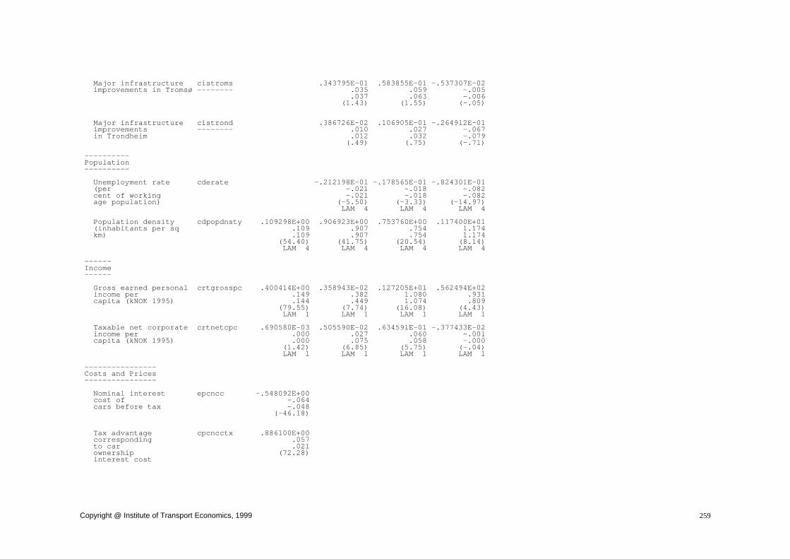
Copyright @ Institute of Transport Economics, 1999 259
Major infrastructure cistroms .343795E-01 .583855E-01 -.537307E-02 improvements in Tromsø -------- .035 .059 -.005 .037 .063 -.006 (1.43) (1.55) (-.05) Major infrastructure cistrond .386726E-02 .106905E-01 -.264912E-01 improvements -------- .010 .027 -.067 in Trondheim .012 .032 -.079 (.49) (.75) (-.71) ---------- Population ---------- Unemployment rate cderate -.212198E-01 -.178565E-01 -.824301E-01 (per -.021 -.018 -.082 cent of working -.021 -.018 -.082 age population) (-5.50) (-3.33) (-14.97) LAM 4 LAM 4 LAM 4 Population density cdpopdnsty .109298E+00 .906923E+00 .753760E+00 .117400E+01 (inhabitants per sq .109 .907 .754 1.174 km) .109 .907 .754 1.174 (54.40) (41.75) (20.54) (8.14) LAM 4 LAM 4 LAM 4 LAM 4 ------ Income ------ Gross earned personal crtgrosspc .400414E+00 .358943E-02 .127205E+01 .562494E+02 income per .149 .382 1.080 .931 capita (kNOK 1995) .144 .449 1.074 .809 (79.55) (7.74) (16.08) (4.43) LAM 1 LAM 1 LAM 1 LAM 1 Taxable net corporate crtnetcpc .690580E-03 .505590E-02 .634591E-01 -.377433E-02 income per .000 .027 .060 -.001 capita (kNOK 1995) .000 .075 .058 -.000 (1.42) (6.85) (5.75) (-.04) LAM 1 LAM 1 LAM 1 LAM 1 ---------------- Costs and Prices ---------------- Nominal interest epcncc -.548092E+00 cost of -.064 cars before tax -.048 (-46.18) Tax advantage cpcncctx .886100E+00 corresponding .057 to car .021 ownership (72.28) interest cost

Copyright @ Institute of Transport Economics, 1999 260
Table B.2 (continued) =================================================================================================================== I. BETA COLUMN = A B C D E F ELASTICITY 1973(74)-94 VARIANT = vcow21j etwc22g etxc22g ehvy22g belturb beltrur ELASTICITY 1994 VERSION = 3 12 4 5 0 0 (COND. T-STATISTIC) DEP.VAR. = cvrcars cevxtfv3i cevxtfv3i cevxhfv3i cbbor1ln cbbor2ln Aggregate Total Total Heavy Urban seat Rural seat car vehicle kms vehicle kms vehicle kms belt use belt use ownership driven driven driven log-odds log-odds =================================================================================================================== ---------------- Costs and Prices continued ---------------- Mean fuel cost per cpgaar -.174650E+01 -.177807E+01 gasoline -.151 -.221 vehicle km (NOK 95) -.112 -.171 (-12.72) (-10.89) LAM 2 LAM 2 Variable km cpdahr -.805392E+00 cost for heavy -.668 diesel vehicles -.665 (fuel + tax, NOK 95) (-12.52) LAM 2 Real price epg95r -.224448E-02 of 95 octane -.017 gasoline (NOK -.018 1995 per liter) (-9.47) Weighted cpdaarrelv -.567936E+00 .423899E+00 ratio of diesel to -.184 .138 gasoline mean -.238 .178 vehicle km cost (-8.72) (4.83) Weighted cpgahrrelv -.269914E+01 ratio of gasoline -.373 to diesel heavy -.329 vehicle km cost (-7.39) Ratio of cpdrelhsea .148140E-01 non-road diesel price .786 to heavy diesel .798 vehicle km cost (18.38) LAM Real subway and cppswir .931507E-02 tramway fares .010 (1 outside Oslo) .010 (9.60) Cordon toll ring in cptollring -.496692E-02 -.284188E-02 .199614E-01 .779555E-01 operation in ---------- -.005 -.003 .020 .078 largest city (dummy) -.005 -.003 .020 .078 (-7.27) (-.14) (.54) (1.11)

Copyright @ Institute of Transport Economics, 1999 261
-------- Daylight -------- Minutes of bnd .185761E-03 .194440E-03 .127001E-03 daylight per day --- .141 .148 .097 .141 .148 .096 (23.24) (21.58) (15.94) ------- Weather ------- Days with snowfall cmsnowd1s -.919935E-02 -.976648E-02 -.318722E-01 during month, plus one -.025 -.024 -.067 -.025 -.025 -.069 (-8.99) (-8.63) (-28.21) LAM 3 LAM 3 LAM 3 Per cent of snow days cmsnowlotsh .165339E-04 .956515E-04 .132173E-02 with large ----------- .000 .001 .009 snowfall (>5 mms) .000 .001 .009 (.08) (.42) (5.31) LAM 3 LAM 3 LAM 3 Days with frost cmtfrostd1s .215550E-02 .292948E-02 -.261396E-02 during month, plus one .010 .012 -.008 .009 .011 -.008 (2.46) (3.03) (-2.62) LAM 3 LAM 3 LAM 3 Mean monthly emts00a .982085E-02 .964414E-02 .687836E-02 temperature in .068 .067 .047 Oslo (centigrades) .069 .068 .048 (19.61) (18.12) (14.61) -------------------- Legislative measures -------------------- Seat belt use eldbelt1 .459966E+00 .636055E+00 mandatory for ======== .892 .463 driver and adult .495 .373 front seat passenger (47.73) (71.94) ----------------------------------------- Financial safety incentives and penalties ----------------------------------------- Real value of esfbeltr .274387E+02 .245983E+04 ticket fine for -------- 5.150 2.178 not wearing 1.431 .515 seat belt (NOK 1995) (120.11) (113.26) LAM LAM

Copyright @ Institute of Transport Economics, 1999 262
Table B.2 (continued) =================================================================================================================== I. BETA COLUMN = A B C D E F ELASTICITY 1973(74)-94 VARIANT = vcow21j etwc22g etxc22g ehvy22g belturb beltrur ELASTICITY 1994 VERSION = 3 12 4 5 0 0 (COND. T-STATISTIC) DEP.VAR. = cvrcars cevxtfv3i cevxtfv3i cevxhfv3i cbbor1ln cbbor2ln Aggregate Total Total Heavy Urban seat Rural seat car vehicle kms vehicle kms vehicle kms belt use belt use ownership driven driven driven log-odds log-odds =================================================================================================================== --------- Publicity --------- Ongoing road safety ezibipe1 .214664E+00 .618187E-01 campaign ======== .416 .045 through 1974 and 1975 .000 .000 (32.33) (8.16) Days of Gulf war ezgulfwar -.871597E-03 -.111795E-02 -.253249E-02 --------- -.017 -.022 -.051 .000 .000 .000 (-1.36) (-1.75) (-4.20) --------- Geography --------- Østfold hcounty1 .454753E-01 .310797E-01 .416147E+00 ======== .045 .031 .416 .045 .031 .416 (3.67) (1.36) (3.96) Oslo hcounty3 .702247E+00 .751192E+00 .485984E+00 ======== .702 .751 .486 .702 .751 .486 (3.60) (2.23) (1.51) Kms hseaccess1 -.797036E-02 -.105141E+00 mainland coastline -.008 -.105 per 1000 sq -.008 -.105 kms surface (-48.08) (-4.20) LAM 4 LAM 4 County hoarea .100549E+00 .825278E+00 .727112E+00 .874958E+00 surface area (sq kms) .101 .825 .727 .875 .101 .825 .727 .875 (56.95) (83.79) (44.80) (9.62) LAM 4 LAM 4 LAM 4 LAM 4

Copyright @ Institute of Transport Economics, 1999 263
-------- Calendar -------- Length of month (days) ekd .697099E+00 .710039E+00 .475373E+00 .697 .710 .475 .697 .710 .475 (18.59) (18.62) (12.66) LAM 4 LAM 4 LAM 4 Dummy for ekee .481568E-01 .540637E-01 .107941E-01 end of Easter ==== .048 .054 .011 .048 .054 .011 (10.83) (12.95) (2.82) Dummy for ekes .545667E-01 .522898E-01 .269191E-01 start of Easter week ==== .055 .052 .027 .055 .052 .027 (12.04) (12.32) (7.25) December ekm12 .247900E+00 .245173E+00 .160419E+00 ===== .248 .245 .160 .248 .245 .160 (41.40) (41.75) (34.52) Share of ekvhsh -.289897E+00 -.298022E+00 -.278775E+00 vacation and holidays -.290 -.298 -.279 during month -.290 -.298 -.279 (excl summer vacation) (-38.80) (-40.57) (-44.56) LAM 4 LAM 4 LAM 4 ------------------------ ASSOCIATED DUMMIES GROUP ------------------------ Real value of esfbeltr -.524228E+02 -.193184E+04 ticket fine for ======== -101.656 -1407.639 not wearing -56.364 -1131.413 seat belt (NOK 1995) (-117.72) (-113.21) ------------------------------------------------------------------------------------------------------------------- REGRESSION CONSTANT CONSTANT -.193962E+01 -.831529E+01 -.269360E+02 -.750153E+02 -.628540E+01 -.398434E+01 - - - - - - - - - - - - (-38.62) (-8.75) (-17.75) (-5.07) (-179.34) (-49.46)

Copyright @ Institute of Transport Economics, 1999 264
Table B.2 (continued) =================================================================================================================== I. BETA COLUMN = A B C D E F ELASTICITY 1973(74)-94 VARIANT = vcow21j etwc22g etxc22g ehvy22g belturb beltrur ELASTICITY 1994 VERSION = 3 12 4 5 0 0 (COND. T-STATISTIC) DEP.VAR. = cvrcars cevxtfv3i cevxtfv3i cevxhfv3i cbbor1ln cbbor2ln Aggregate Total Total Heavy Urban seat Rural seat car vehicle kms vehicle kms vehicle kms belt use belt use ownership driven driven driven log-odds log-odds =================================================================================================================== ---------------------------- HETEROSKEDASTICITY STRUCTURE ---------------------------- ZETA COEFFICIENTS ----------------- Exp of ekjanuaryxp -.100000E+02 dummy for January -1.148 -1.145 (.00) LAM Exponential of ekxtrapltxp .590171E+00 .639637E+00 .520914E+00 extrapolating -.189 -.298 -.511 distance from fuel -.191 -.315 -.478 use submodel sample (11.40) (11.72) (12.21) LAM LAM LAM Number of ekvhis .967131E-01 .833924E-01 .274302E-01 vacation days, -.349 -.438 -.303 including -.349 -.458 -.281 summer vacation (31.17) (27.90) (8.55) LAM LAM LAM Variance cbbv1 .100000E+01 estimate for urban -15.126 seat belt use -.292 log-odds ratio (.00) LAM Variance cbbv2 .100000E+01 estimate for rural -215.858 seat belt use -.159 log-odds ratio (.00) LAM

Copyright @ Institute of Transport Economics, 1999 265
=================================================================================================================== II. PARAMETERS (COND. T-STATISTIC) =================================================================================================================== ---------------------------- HETEROSKEDASTICITY STRUCTURE ---------------------------- BOX-COX TRANSFORMATIONS: UNCOND: [T-STATISTIC=0] / [T-STATISTIC=1] ------------------------------------------------------------------ LAMBDA(Z) ekjanuaryxp .000 FIXED LAMBDA(Z) ekxtrapltxp .000 .000 .000 FIXED FIXED FIXED LAMBDA(Z) ekvhis 1.000 1.000 1.000 FIXED FIXED FIXED LAMBDA(Z) cbbv1 .000 FIXED LAMBDA(Z) cbbv2 .000 FIXED ------------------------------------------------------------------ BOX-COX TRANSFORMATIONS: UNCOND: [T-STATISTIC=0] / [T-STATISTIC=1] ------------------------------------------------------------------ LAMBDA(Y) - GROUP 4 LAM 4 .000 .000 .000 .000 FIXED FIXED FIXED FIXED LAMBDA(X) cvrcarsp .284 [3.93] [-9.92] LAMBDA(X) cpdrelhsea 6.099 [9.88] [8.26] LAMBDA(X) cvsbfrontpc .035 -.345 [1.28] [-4.76] [-35.54] [-18.58] LAMBDA(X) esfbeltr -.485 -1.272 [-5.34] [-10.21] [-16.34] [-18.23]

Copyright @ Institute of Transport Economics, 1999 266
Table B.2 (continued) =================================================================================================================== II. PARAMETERS COLUMN = A B C D E F VARIANT = vcow21j etwc22g etxc22g ehvy22g belturb beltrur VERSION = 3 12 4 5 0 0 (COND. T-STATISTIC) DEP.VAR. = cvrcars cevxtfv3i cevxtfv3i cevxhfv3i cbbor1ln cbbor2ln Aggregate Total Total Heavy Urban seat Rural seat car vehicle kms vehicle kms vehicle kms belt use belt use ownership driven driven driven log-odds log-odds =================================================================================================================== ------------------------------------------------------------------ BOX-COX TRANSFORMATIONS: UNCOND: [T-STATISTIC=0] / [T-STATISTIC=1] continued ------------------------------------------------------------------ LAMBDA(X) - GROUP 1 LAM 1 -.226 1.069 -.037 -.939 [-5.87] [5.54] [-.24] [-.94] [-31.79] [.36] [-6.78] [-1.94] LAMBDA(X) - GROUP 2 LAM 2 8.324 7.099 -.316 [4.70] [4.24] [-.69] [4.13] [3.64] [-2.88] LAMBDA(X) - GROUP 3 LAM 3 .591 .544 .445 [3.36] [3.17] [8.92] [-2.33] [-2.66] [-11.13] LAMBDA(X) - GROUP 4 LAM 4 .000 .000 .000 .000 FIXED FIXED FIXED FIXED --------------- AUTOCORRELATION --------------- ORDER 19 RHO 19 .336 .463 .526 (23.96) (33.68) (45.47) ORDER 38 RHO 38 .106 .262 .458 (7.12) (18.83) (39.77) ORDER228 RHO228 -.129 (-22.29)

Copyright @ Institute of Transport Economics, 1999 267
=================================================================================================================== III.GENERAL STATISTICS COLUMN = A B C D E F VARIANT = vcow21j etwc22g etxc22g ehvy22g belturb beltrur VERSION = 3 12 4 5 0 0 DEP.VAR. = cvrcars cevxtfv3i cevxtfv3i cevxhfv3i cbbor1ln cbbor2ln Aggregate Total Total Heavy Urban seat Rural seat car vehicle kms vehicle kms vehicle kms belt use belt use ownership driven driven driven log-odds log-odds =================================================================================================================== LOG-LIKELIHOOD -57051.992 -50855.484 -51134.667 -41416.687 -15118.593 -13672.125 PSEUDO-R2 : - (E) .024 .970 .970 .978 .900 .884 - (L) .097 .986 .984 .984 - - - (E) ADJUSTED FOR D.F. .019 .970 .970 .978 .900 .884 - (L) ADJUSTED FOR D.F. .092 .986 .984 .984 - - SAMPLE : - NUMBER OF OBSERVATIONS 4788 4978 4978 4978 5016 5016 - FIRST OBSERVATION 229 39 39 39 1 1 - LAST OBSERVATION 5016 5016 5016 5016 5016 5016 NUMBER OF ESTIMATED PARAMETERS : - FIXED PART : . BETAS 24 42 41 41 6 6 . BOX-COX 1 4 3 4 2 2 . ASSOCIATED DUMMIES 0 0 0 0 1 1 - AUTOCORRELATION 1 2 2 2 0 0 - HETEROSKEDASTICITY : . ZETAS 1 2 2 2 1 1 . BOX-COX 0 0 0 0 0 0 . ASSOCIATED DUMMIES 0 0 0 0 0 0 ===================================================================================================================

Copyright @ Institute of Transport Economics, 1999 268
Table B.3: Accidents, casualties and severity equations ============================================================================================================================================= I. BETA COLUMN = A B C D E F G H ELASTICITY 1974(77)-94 VARIANT = aah023x avc023x avm023x avb023x avp023x ass023x asd123x asf023x ELASTICITY 1994 VERSION = 5 5 6 5 5 4 3 3 (COND. T-STATISTIC) DEP.VAR. = caas0bt01 cavg1bt01 cavg3bt01 cavg6bt01 cavg5bt01 cass casd casf Injury Car Motorcycle Bicyclists Pedestrians Severely Dangerously Fatalities accidents occupants occupants injured injured injured per injured per per injured injured accident accident accident ============================================================================================================================================= -------- Exposure -------- Total vehicle cevxtfv3i .911155E+00 .961683E+00 .748861E+00 .107909E+01 .110865E+01 .486516E-01 -.615528E-01 -.473502E-01 kms driven (1000) .911 .962 .749 1.079 1.109 .098 -.206 -.142 .911 .962 .749 1.079 1.109 .122 -.231 -.150 (28.26) (26.24) (11.66) (12.06) (14.07) (2.52) (-2.03) (-1.31) LAM 4 LAM 4 LAM 4 LAM 4 LAM 4 LAM 4 LAM 4 LAM 4 Heavy vehicle cevhvysh .148937E+00 -.145525E+00 .475976E+00 .529401E+00 .105285E+00 .650806E-02 -.511220E-01 -.123028E-01 share of .149 -.146 .476 .529 .105 .013 -.171 -.037 traffic volume .149 -.146 .476 .529 .105 .016 -.192 -.039 (2.65) (-1.89) (3.94) (2.92) (.80) (.15) (-.83) (-.17) LAM 4 LAM 4 LAM 4 LAM 4 LAM 4 LAM 4 LAM 4 LAM 4 Warm days cevmcw1 .273896E-01 .703985E-03 .220011E+00 .268249E+00 .362610E-01 .319322E-02 -.698448E-02 -.108701E-01 times ratio of MC .024 .001 .196 .239 .032 .006 -.021 -.029 to 4-wheel .026 .001 .208 .254 .034 .008 -.025 -.033 light vehicle pool (4.80) (.08) (8.72) (8.99) (3.29) (.66) (-1.02) (-1.31) LAM LAM LAM LAM LAM LAM LAM LAM --------------- Traffic density --------------- Traffic chsdense -.434501E+00 -.143805E+00 .927969E-06 -.527104E+01 -.926939E+00 .617744E-01 .804088E-01 .845883E-01 density (1000 monthly -.415 -.310 .008 -.655 -.971 .140 .515 .587 vehicle kms -.414 -.319 .012 -.604 -.972 .176 .589 .642 driven per road km) (-11.02) (-5.59) (2.82) (-8.58) (-10.66) (2.46) (3.40) (3.70) LAM LAM LAM LAM LAM LAM LAM LAM ---------------------------- Public transportation supply ---------------------------- Density of dtabus .243311E+00 .189173E+00 .409284E+00 .138500E+00 .764088E+00 .884384E-02 -.574363E-02 -.616533E-01 public bus service .243 .189 .409 .138 .764 .018 -.019 -.185 (annual veh kms .243 .189 .409 .139 .764 .022 -.022 -.196 per km public road) (8.02) (5.00) (6.72) (1.93) (10.86) (.48) (-.21) (-1.86) LAM 4 LAM 4 LAM 4 LAM 4 LAM 4 LAM 4 LAM 4 LAM 4 Density of dtarail .192635E-01 -.412291E-02 -.156669E-01 .649136E-01 .647613E-01 -.645415E-02 -.207237E-01 -.208035E-01 subway and streetcar ------- .216 -.046 -.176 .729 .727 -.145 -.801 -.700 service (annual .366 -.078 -.297 1.232 1.229 -.307 -1.473 -1.254 car kms per km rd) (3.05) (-.56) (-1.20) (3.92) (5.47) (-1.71) (-4.03) (-3.32) LAM 4 LAM 4 LAM 4 LAM 4 LAM 4 LAM 4 LAM 4 LAM 4

Copyright @ Institute of Transport Economics, 1999 269
-------- Vehicles -------- Passenger cvrcarsp .220558E-01 .777450E-01 .378437E-01 -.971616E-02 .403909E-02 .210939E-01 .757680E-02 cars per capita .068 .239 .116 -.030 .025 .206 .070 .058 .204 .099 -.026 .027 .208 .063 (.98) (2.12) (.63) (-.24) (.33) (1.08) (.36) LAM LAM LAM LAM LAM LAM LAM Mean age of passenger cvrta1 .172085E+00 .171989E+00 -.345489E+00 .176501E+01 -.344140E+00 .935141E-01 -.149027E+00 -.212994E+00 cars .172 .172 -.345 1.765 -.344 .188 -.498 -.639 registered in county .172 .172 -.345 1.765 -.344 .235 -.558 -.677 (1.56) (1.27) (-1.47) (5.96) (-1.58) (1.35) (-1.57) (-1.89) LAM 4 LAM 4 LAM 4 LAM 4 LAM 4 LAM 4 LAM 4 LAM 4 ------------------ Road user behavior ------------------ Calculated cbbeltnonw .179661E-01 .600650E-01 -.210088E-02 -.362021E-02 -.648496E-02 county-wide share .092 .167 -.016 -.057 -.075 of drivers not .235 .302 -.044 -.115 -.174 wearing seat belt (5.91) (7.15) (-.72) (-.91) (-1.31) LAM LAM LAM LAM LAM Imputed MC cbhnonw -.150099E+01 helmet non-use rate -.144 -.036 (-4.86) ------------------- Road infrastructure ------------------- Public road cilrdspc -.188511E+00 -.308852E-01 .170091E+00 -.933076E+00 -.526717E+00 .111592E+00 .881361E-01 .109577E+00 kms per inhabitant -.189 -.031 .170 -.933 -.527 .224 .294 .329 -.189 -.031 .170 -.933 -.527 .280 .330 .348 (-2.51) (-.32) (1.21) (-4.48) (-2.99) (2.26) (1.25) (1.30) LAM 4 LAM 4 LAM 4 LAM 4 LAM 4 LAM 4 LAM 4 LAM 4 Real fixed cictprkml24r .348968E-01 -.948406E-01 .138521E+00 .617653E-01 .456976E-01 -.391550E-01 .174928E-02 -.182087E-01 capital invested pr .035 -.095 .139 .062 .046 -.079 .006 -.055 km county or .035 -.095 .139 .062 .046 -.098 .007 -.058 nat'l road, lagged 24 (.90) (-2.34) (1.83) (.52) (.51) (-1.80) (.05) (-.47) months LAM 4 LAM 4 LAM 4 LAM 4 LAM 4 LAM 4 LAM 4 LAM 4 Major infrastructure cisbergen -.491128E-03 .174155E-01 .537249E-01 -.140496E-01 -.196540E-01 -.819524E-02 .147510E-01 -.656006E-02 improvements in Bergen --------- -.001 .039 .120 -.031 -.044 -.037 .110 -.044 -.001 .052 .160 -.042 -.058 -.061 .164 -.062 (-.03) (.93) (1.50) (-.33) (-.72) (-.80) (1.03) (-.38) Major infrastructure cisoslo .617984E-02 .198615E-01 -.123206E+00 .124610E+00 .473437E-01 .210538E-01 -.446303E-02 -.400388E-01 improvements in Oslo ------- .021 .068 -.423 .428 .163 .145 -.051 -.412 .035 .113 -.701 .709 .269 .300 -.095 -.724 (.43) (.97) (-2.50) (2.90) (1.87) (1.58) (-.23) (-1.74)

Copyright @ Institute of Transport Economics, 1999 270
Table B.3 (continued) ============================================================================================================================================= I. BETA COLUMN = A B C D E F G H ELASTICITY 1974(77)-94 VARIANT = aah023x avc023x avm023x avb023x avp023x ass023x asd123x asf023x ELASTICITY 1994 VERSION = 5 5 6 5 5 4 3 3 (COND. T-STATISTIC) DEP.VAR. = caas0bt01 cavg1bt01 cavg3bt01 cavg6bt01 cavg5bt01 cass casd casf Injury Car Motorcycle Bicyclists Pedestrians Severely Dangerously Fatalities accidents occupants occupants injured injured injured per injured per per injured injured accident accident accident ============================================================================================================================================= ------------------- Road infrastructure continued ------------------- Oslo: the Oslo tunnel cisoslo4 .459149E-01 .875399E-01 .181637E+00 .157216E-01 -.576921E-01 .351639E-02 -.164618E-01 .531405E-01 ("Fjellinjen") in -------- .045 .087 .180 .016 -.057 .007 -.054 .158 operation .046 .088 .182 .016 -.058 .009 -.062 .169 (.80) (.98) (.95) (.09) (-.70) (.07) (-.20) (.56) Major infrastructure cistroms .164006E+00 .259937E+00 -.162604E+00 -.176462E+00 .554186E-01 -.182506E-01 .244540E-01 .423080E-01 improvements in Tromsø -------- .167 .264 -.165 -.179 .056 -.037 .083 .129 .177 .280 -.175 -.190 .060 -.049 .099 .145 (2.62) (3.98) (-.84) (-.85) (.14) (-.36) (.38) (.50) Major infrastructure cistrond .993404E-03 -.367121E-01 -.117394E+00 .171138E+00 .877024E-01 -.115755E-01 -.931689E-02 -.166345E-01 improvements -------- .003 -.094 -.299 .436 .223 -.059 -.079 -.127 in Trondheim .003 -.110 -.352 .513 .263 -.087 -.105 -.159 (.06) (-1.84) (-2.02) (3.61) (2.24) (-1.15) (-.83) (-1.10) ---------------- Road maintenance ---------------- Snowfall cimtsnowmain -.493625E+00 .155027E+00 .206632E+01 .394834E+01 -.773872E+00 .275582E+00 -.227732E+00 -.425268E+00 interaction with ------------ -.007 .002 .029 .056 -.011 .008 -.011 -.018 winter -.007 .002 .028 .054 -.010 .009 -.012 -.018 maintenance intensity (-.94) (.24) (1.56) (3.51) (-.69) (.79) (-.43) (-.65) Expenditure cimroadmarks -.130024E-01 -.842064E-03 -.469325E-01 -.475709E-01 -.122152E-01 .719083E-02 -.112551E-01 -.349019E-02 on road marks, ------------ -.050 -.003 -.179 -.182 -.047 .055 -.172 -.040 signposting etc -.068 -.004 -.246 -.250 -.064 .095 -.257 -.058 per km nat'l or (-2.87) (-.15) (-4.94) (-3.54) (-1.31) (2.51) (-2.04) (-.69) county road LAM LAM LAM LAM LAM LAM LAM Expenditure on cimmisc .235966E-02 .790054E-02 -.513296E-02 .156098E-02 -.784132E-02 .983849E-03 .485967E-02 .199159E-02 miscellaneous ------- .054 .181 -.117 .036 -.179 .045 .347 .137 road maintenance .045 .150 -.098 .030 -.149 .047 .346 .120 per km nat'l or (1.40) (3.90) (-1.50) (.30) (-2.16) (.90) (2.50) (1.14) county road

Copyright @ Institute of Transport Economics, 1999 271
---------- Population ---------- Unemployment rate cderate -.238049E-01 -.320392E-01 .191220E-01 .229945E-01 -.442348E-01 -.145893E-01 -.991800E-02 .698746E-02 (per -.024 -.032 .019 .023 -.044 -.029 -.033 .021 cent of working -.024 -.032 .019 .023 -.044 -.037 -.037 .022 age population) (-2.34) (-2.27) (.94) (.83) (-2.06) (-2.04) (-.93) (.58) LAM 4 LAM 4 LAM 4 LAM 4 LAM 4 LAM 4 LAM 4 LAM 4 Population density cdpopdnsty .677007E-01 .200300E-01 .150727E+00 .331766E-01 .660012E-01 -.520854E-01 -.581636E-01 -.593827E-01 (inhabitants per sq .068 .020 .151 .033 .066 -.104 -.194 -.178 km) .068 .020 .151 .033 .066 -.131 -.218 -.189 (2.91) (.63) (3.13) (.46) (1.16) (-3.34) (-2.94) (-2.66) LAM 4 LAM 4 LAM 4 LAM 4 LAM 4 LAM 4 LAM 4 LAM 4 Women cdpregrate2 .180509E+00 .114598E+00 .471991E+00 .383799E-02 -.714103E-01 -.364256E-01 -.674646E-01 -.890234E-01 pregnant in first .181 .115 .472 .004 -.071 -.073 -.225 -.267 quarter per .181 .115 .472 .004 -.071 -.091 -.253 -.283 1000 women 18-44 (3.38) (1.64) (4.21) (.03) (-.61) (-.99) (-1.28) (-1.45) LAM 4 LAM 4 LAM 4 LAM 4 LAM 4 LAM 4 LAM 4 LAM 4 -------- Daylight -------- Minutes of bnt -.247308E-06 .493875E-09 .161068E-10 -.257521E-04 -.433655E-04 -.133184E-02 -.152816E-09 -.121967E-12 twilight per day --- -.003 .004 .000 -.096 -.080 -.007 -.000 -.001 -.003 .004 .000 -.096 -.080 -.009 -.000 -.001 (-.40) (.84) (.04) (-2.98) (-3.01) (-.59) (-.02) (-.22) LAM 5 LAM 5 LAM 5 LAM 5 LAM 5 LAM 5 LAM 5 LAM 5 Minutes without cnn .314268E-06 .798095E-10 -.331073E-10 -.146592E-05 .201310E-04 -.284756E-02 .350578E-09 .468984E-14 daylight --- .093 .106 -.105 -.077 .421 -.023 .041 .042 between 5 and 11 p m .087 .094 -.093 -.073 .399 -.029 .044 .038 (5.54) (6.31) (-3.56) (-1.35) (12.74) (-2.22) (.91) (1.31) LAM 5 LAM 5 LAM 5 LAM 5 LAM 5 LAM 5 LAM 5 LAM 5 Minutes without cnr .723576E-06 .226460E-09 -.422732E-09 -.713221E-05 .269997E-04 .353585E-02 .456469E-08 .118014E-12 daylight 7-9 --- .022 .004 -.013 -.059 .112 .049 .017 .002 a m and 3-5 p m .022 .004 -.013 -.059 .111 .060 .019 .002 (4.60) (3.29) (-4.57) (-2.40) (7.32) (2.68) (2.54) (2.93) LAM 5 LAM 5 LAM 5 LAM 5 LAM 5 LAM 5 LAM 5 LAM 5 Minutes without cnw -.225145E-06 -.140030E-09 .556948E-10 .293229E-05 .123971E-04 -.119593E-02 -.183994E-10 .457413E-14 daylight --- -.000 -.000 .000 .002 .007 -.023 -.000 .000 between 9 a m -.000 -.000 .000 .002 .007 -.029 -.000 .000 and 3 p m (-1.39) (-4.35) (2.70) (1.81) (3.04) (-.62) (-.02) (.44) LAM 5 LAM 5 LAM 5 LAM 5 LAM 5 LAM 5 LAM 5 LAM 5 ------- Weather ------- Average snow depth cmds3a -.240838E-01 -.903330E-02 -.102184E+00 -.154926E+00 -.983287E-02 -.857632E-03 .125181E-02 -.438811E-02 during month (cms) ------ -.042 -.016 -.180 -.272 -.017 -.003 .007 -.023 -.042 -.016 -.178 -.269 -.017 -.004 .008 -.024 (-5.19) (-1.39) (-5.95) (-6.88) (-.92) (-.22) (.21) (-.70) LAM 4 LAM 4 LAM 4 LAM 4 LAM 4 LAM 4 LAM 4 LAM 4
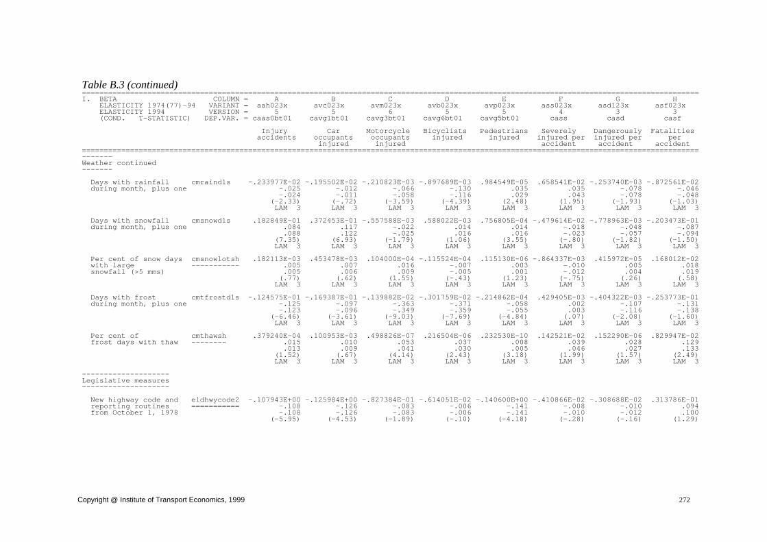
Copyright @ Institute of Transport Economics, 1999 272
Table B.3 (continued) ============================================================================================================================================= I. BETA COLUMN = A B C D E F G H ELASTICITY 1974(77)-94 VARIANT = aah023x avc023x avm023x avb023x avp023x ass023x asd123x asf023x ELASTICITY 1994 VERSION = 5 5 6 5 5 4 3 3 (COND. T-STATISTIC) DEP.VAR. = caas0bt01 cavg1bt01 cavg3bt01 cavg6bt01 cavg5bt01 cass casd casf Injury Car Motorcycle Bicyclists Pedestrians Severely Dangerously Fatalities accidents occupants occupants injured injured injured per injured per per injured injured accident accident accident ============================================================================================================================================= ------- Weather continued ------- Days with rainfall cmraind1s -.233977E-02 -.195502E-02 -.210823E-03 -.897689E-03 .984549E-05 .658541E-02 -.253740E-03 -.872561E-02 during month, plus one -.025 -.012 -.066 -.130 .035 .035 -.078 -.046 -.024 -.011 -.058 -.116 .029 .043 -.078 -.048 (-2.33) (-.72) (-3.59) (-4.39) (2.48) (1.95) (-1.93) (-1.03) LAM 3 LAM 3 LAM 3 LAM 3 LAM 3 LAM 3 LAM 3 LAM 3 Days with snowfall cmsnowd1s .182849E-01 .372453E-01 -.557588E-03 .588022E-03 .756805E-04 -.479614E-02 -.778963E-03 -.203473E-01 during month, plus one .084 .117 -.022 .014 .014 -.018 -.048 -.087 .088 .122 -.025 .016 .016 -.023 -.057 -.094 (7.35) (6.93) (-1.79) (1.06) (3.55) (-.80) (-1.82) (-1.50) LAM 3 LAM 3 LAM 3 LAM 3 LAM 3 LAM 3 LAM 3 LAM 3 Per cent of snow days cmsnowlotsh .182113E-03 .453478E-03 .104000E-04 -.115524E-04 .115130E-06 -.864337E-03 .415972E-05 .168012E-02 with large ----------- .005 .007 .016 -.007 .003 -.010 .005 .018 snowfall (>5 mms) .005 .006 .009 -.005 .001 -.012 .004 .019 (.77) (.62) (1.55) (-.43) (1.23) (-.75) (.26) (.58) LAM 3 LAM 3 LAM 3 LAM 3 LAM 3 LAM 3 LAM 3 LAM 3 Days with frost cmtfrostd1s -.124575E-01 -.169387E-01 -.139882E-02 -.301759E-02 -.214862E-04 .429405E-03 -.404322E-03 -.253773E-01 during month, plus one -.125 -.097 -.363 -.371 -.058 .002 -.107 -.131 -.123 -.096 -.349 -.359 -.055 .003 -.116 -.138 (-6.46) (-3.61) (-9.03) (-7.69) (-4.84) (.07) (-2.08) (-1.60) LAM 3 LAM 3 LAM 3 LAM 3 LAM 3 LAM 3 LAM 3 LAM 3 Per cent of cmthawsh .379240E-04 .100953E-03 .498826E-07 .216504E-06 .232530E-10 .142521E-02 .152290E-06 .829947E-02 frost days with thaw -------- .015 .010 .053 .037 .008 .039 .028 .129 .013 .009 .041 .030 .005 .046 .027 .133 (1.52) (.67) (4.14) (2.43) (3.18) (1.99) (1.57) (2.49) LAM 3 LAM 3 LAM 3 LAM 3 LAM 3 LAM 3 LAM 3 LAM 3 -------------------- Legislative measures -------------------- New highway code and eldhwycode2 -.107943E+00 -.125984E+00 -.827384E-01 -.614051E-02 -.140600E+00 -.410866E-02 -.308688E-02 .313786E-01 reporting routines =========== -.108 -.126 -.083 -.006 -.141 -.008 -.010 .094 from October 1, 1978 -.108 -.126 -.083 -.006 -.141 -.010 -.012 .100 (-5.95) (-4.53) (-1.89) (-.10) (-4.18) (-.28) (-.16) (1.29)

Copyright @ Institute of Transport Economics, 1999 273
----------------- Access to alcohol ----------------- Alcohol outlets dxloutletspc .658396E-01 -.236591E-01 .174606E+00 .424714E-01 -.959841E-02 -.211072E-01 .177637E-01 .222676E-01 per 1000 population .088 -.020 .181 .052 -.023 -.041 .118 .131 .082 -.021 .179 .049 -.018 -.052 .116 .116 (3.44) (-3.88) (4.15) (.61) (-1.18) (-2.50) (3.44) (3.07) LAM LAM LAM LAM LAM LAM LAM LAM Per cent dxloutstrong .246444E-01 -.336192E-01 .983682E-01 .372209E-01 .877902E-01 .282249E-02 .698103E-02 -.187031E-02 alcohol outlets .025 -.034 .098 .037 .088 .006 .023 -.006 selling strong .025 -.034 .098 .037 .088 .007 .026 -.006 beer, wine or liquor (2.70) (-3.09) (4.62) (1.72) (4.73) (.56) (1.02) (-.24) LAM 4 LAM 4 LAM 4 LAM 4 LAM 4 LAM 4 LAM 4 LAM 4 Per cent dxloutliqsh .411379E-01 -.122530E-01 .862403E-01 .487602E-01 .944929E-01 -.189033E-02 .219686E-02 -.112931E-01 wine/liquor store of .041 -.012 .086 .049 .094 -.004 .007 -.034 outlets for .041 -.012 .086 .049 .094 -.005 .008 -.036 strong (4.43) (-1.13) (3.89) (2.14) (5.47) (-.37) (.33) (-1.43) alcoholic beverag LAM 4 LAM 4 LAM 4 LAM 4 LAM 4 LAM 4 LAM 4 LAM 4 Restaurants dxlrstalcpc -.108951E-01 .806137E-01 -.719131E-01 -.333006E+00 -.258898E-02 .210889E-01 -.470928E-01 -.369629E-01 licensed to -.016 .075 -.093 -.343 -.005 .038 -.157 -.126 serve alcohol -.006 .090 -.049 -.319 -.001 .063 -.176 -.098 per 1000 population (-6.41) (2.51) (-6.88) (-5.50) (-4.67) (1.19) (-1.84) (-2.29) LAM LAM LAM LAM LAM LAM LAM LAM Per cent of licensed dxlrestlwsh -.204775E+00 -.154473E+00 -.172775E+00 -.389620E+00 -.259114E+00 .785531E-01 -.386878E-01 -.263627E-01 restaurants with -.205 -.154 -.173 -.390 -.259 .158 -.129 -.079 wine/liquor license -.205 -.154 -.173 -.390 -.259 .197 -.145 -.084 (-3.42) (-2.04) (-1.30) (-2.11) (-2.04) (2.12) (-.65) (-.38) LAM 4 LAM 4 LAM 4 LAM 4 LAM 4 LAM 4 LAM 4 LAM 4 Per cent of dxlrestliqsh .201514E-01 -.173668E-01 .800540E-01 .197989E-01 -.757450E-03 -.243753E-01 -.178112E-01 -.234620E-01 wine/liquour .020 -.017 .080 .020 -.001 -.049 -.059 -.070 licenses .020 -.017 .080 .020 -.001 -.061 -.067 -.075 including liquor (1.22) (-.82) (1.96) (.36) (-.02) (-2.06) (-.94) (-1.26) LAM 4 LAM 4 LAM 4 LAM 4 LAM 4 LAM 4 LAM 4 LAM 4 --------------------------- Accident reporting routines --------------------------- New eur77 .909561E-01 .183751E+00 -.210120E+00 .573770E+00 -.318269E-02 -.146272E+00 -.973054E-01 accident reporting ----- .091 .184 -.210 .574 -.003 -.293 -.292 routines from .091 .184 -.210 .574 -.003 -.367 -.309 January 1, 1977 (2.66) (2.87) (-1.54) (4.33) (-.07) (-5.48) (-1.97) --------- Geography --------- Oslo hcounty3 -.159978E+00 .470809E+00 -.132115E+01 -.160928E+01 -.103622E+01 .123123E+00 .152361E+00 .197736E+00 ======== -.160 .471 -1.321 -1.609 -1.036 .247 .509 .593 -.160 .471 -1.321 -1.609 -1.036 .309 .571 .628 (-1.31) (2.94) (-4.86) (-4.36) (-3.78) (1.52) (1.51) (1.46)
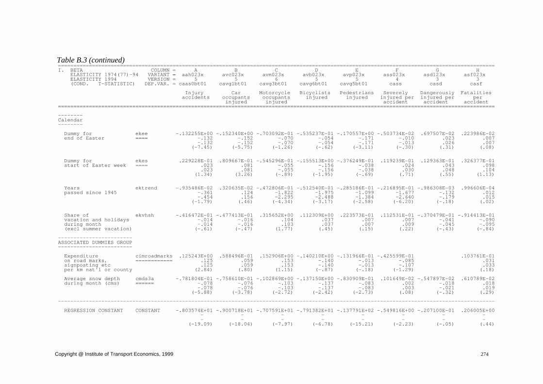
Copyright @ Institute of Transport Economics, 1999 274
Table B.3 (continued) ============================================================================================================================================= I. BETA COLUMN = A B C D E F G H ELASTICITY 1974(77)-94 VARIANT = aah023x avc023x avm023x avb023x avp023x ass023x asd123x asf023x ELASTICITY 1994 VERSION = 5 5 6 5 5 4 3 3 (COND. T-STATISTIC) DEP.VAR. = caas0bt01 cavg1bt01 cavg3bt01 cavg6bt01 cavg5bt01 cass casd casf Injury Car Motorcycle Bicyclists Pedestrians Severely Dangerously Fatalities accidents occupants occupants injured injured injured per injured per per injured injured accident accident accident ============================================================================================================================================= -------- Calendar -------- Dummy for ekee -.132255E+00 -.152340E+00 -.703092E-01 -.535237E-01 -.170557E+00 -.503734E-02 .697507E-02 .223986E-02 end of Easter ==== -.132 -.152 -.070 -.054 -.171 -.010 .023 .007 -.132 -.152 -.070 -.054 -.171 -.013 .026 .007 (-7.45) (-5.75) (-1.26) (-.62) (-3.11) (-.30) (.31) (.08) Dummy for ekes .229228E-01 .809667E-01 -.545296E-01 -.155513E+00 -.376249E-01 .119239E-01 .129363E-01 .326377E-01 start of Easter week ==== .023 .081 -.055 -.156 -.038 .024 .043 .098 .023 .081 -.055 -.156 -.038 .030 .048 .104 (1.34) (3.26) (-.89) (-1.95) (-.69) (.71) (.55) (1.13) Years ektrend -.935486E-02 .320635E-02 -.472806E-01 -.512540E-01 -.285186E-01 -.216895E-01 -.986308E-03 .996606E-04 passed since 1945 -.361 .124 -1.822 -1.975 -1.099 -1.677 -.132 .012 -.454 .156 -2.295 -2.488 -1.384 -2.640 -.179 .015 (-1.79) (.46) (-4.34) (-3.17) (-2.58) (-6.20) (-.18) (.02) Share of ekvhsh -.416472E-01 -.477413E-01 .315652E+00 .112309E+00 .223573E-01 .112531E-01 -.370479E-01 -.914413E-01 vacation and holidays -.014 -.016 .104 .037 .007 .007 -.041 -.090 during month -.014 -.016 .103 .037 .007 .009 -.045 -.095 (excl summer vacation) (-.61) (-.47) (1.77) (.45) (.15) (.22) (-.43) (-.84) ------------------------ ASSOCIATED DUMMIES GROUP ------------------------ Expenditure cimroadmarks .125243E+00 .588496E-01 .152906E+00 -.140210E+00 -.131966E-01 -.425599E-01 .103761E-01 on road marks, ============ .125 .059 .153 -.140 -.013 -.085 .031 signposting etc .125 .059 .153 -.140 -.013 -.107 .033 per km nat'l or county (2.84) (.80) (1.15) (-.87) (-.18) (-1.29) (.18) Average snow depth cmds3a -.781804E-01 -.758610E-01 -.102869E+00 -.137150E+00 -.830909E-01 .101649E-02 -.547897E-02 .610789E-02 during month (cms) ====== -.078 -.076 -.103 -.137 -.083 .002 -.018 .018 -.078 -.076 -.103 -.137 -.083 .003 -.021 .019 (-5.88) (-3.78) (-2.72) (-2.42) (-2.73) (.08) (-.32) (.29) --------------------------------------------------------------------------------------------------------------------------------------------- REGRESSION CONSTANT CONSTANT -.803574E+01 -.900718E+01 -.707591E+01 -.791382E+01 -.137791E+02 -.549816E+00 -.207100E-01 .206005E+00 - - - - - - - - - - - - - - - - (-19.09) (-18.04) (-7.97) (-6.78) (-15.21) (-2.23) (-.05) (.44)

Copyright @ Institute of Transport Economics, 1999 275
---------------------------- HETEROSKEDASTICITY STRUCTURE ---------------------------- ZETA COEFFICIENTS ----------------- var[ln(y+0.1)] as maah023x_4vu .100000E+01 estimated by .030 model aah023x_4 .021 (.00) LAM 4 var[ln(y+0.1)] as mavc023x_4vu .100000E+01 estimated by .063 model avc023x_4 .070 (.00) LAM 4 var[ln(y+0.1)] as mavm023x_5wu .100000E+01 estimated by .481 model avm023x_5 .523 (.00) LAM 4 var[ln(y+0.1)] as mavb023x_4wu .100000E+01 estimated by .597 model avb023x_4 .627 (.00) LAM 4 var[ln(y+0.1)] as mavp023x_4vu .100000E+01 estimated by .375 model avp023x_4 .489 (.00) LAM 4 Calculated mass023x_2 .100000E+01 variance of .042 2nd degree .069 log-severity ratio (.00) LAM 4 Calculated masd123x_2 .100000E+01 variance of .272 3rd degree .355 log-severity ratio (.00) LAM 4 Calculated variance masf023x_2 .100000E+01 of log-mortality ratio .417 .505 (.00) LAM 4

Copyright @ Institute of Transport Economics, 1999 276
Table B.3 (continued) ============================================================================================================================================= II. PARAMETERS COLUMN = A B C D E F G H VARIANT = aah023x avc023x avm023x avb023x avp023x ass023x asd123x asf023x VERSION = 5 5 6 5 5 4 3 3 (COND. T-STATISTIC) DEP.VAR. = caas0bt01 cavg1bt01 cavg3bt01 cavg6bt01 cavg5bt01 cass casd casf Injury Car Motorcycle Bicyclists Pedestrians Severely Dangerously Fatalities accidents occupants occupants injured injured injured per injured per per injured injured accident accident accident ============================================================================================================================================= ---------------------------- HETEROSKEDASTICITY STRUCTURE ---------------------------- BOX-COX TRANSFORMATIONS: UNCOND: [T-STATISTIC=0] / [T-STATISTIC=1] ------------------------------------------------------------------ LAMBDA(Z) - GROUP 4 LAM 4 .000 .000 .000 .000 .000 .000 .000 .000 FIXED FIXED FIXED FIXED FIXED FIXED FIXED FIXED ------------------------------------------------------------------ BOX-COX TRANSFORMATIONS: UNCOND: [T-STATISTIC=0] / [T-STATISTIC=1] ------------------------------------------------------------------ LAMBDA(Y) cass .547 [45.10] [-37.33] LAMBDA(Y) casd .436 [27.75] [-35.95] LAMBDA(Y) casf .350 [21.94] [-40.69] LAMBDA(Y) - GROUP 4 LAM 4 .000 .000 .000 .000 .000 FIXED FIXED FIXED FIXED FIXED LAMBDA(X) cbbeltnonw -1.204 -.757 -1.000 -1.000 -1.000 [-2.00] [-1.60] FIXED FIXED FIXED [-3.66] [-3.72] LAMBDA(X) chsdense -.013 .226 2.668 -.613 .014 .036 .190 .247 [-.17] [1.63] [.95] [-4.10] [.22] [.10] [.84] [1.17] [-12.96] [-5.59] [.59] [-10.79] [-15.99] [-2.64] [-3.60] [-3.58] LAMBDA(X) dxloutletspc 1.437 -.772 .174 1.000 4.277 -.101 3.762 3.312 [2.29] [-1.73] [.58] FIXED [.80] [-.16] [2.62] [2.41] [.70] [-3.98] [-2.72] [.62] [-1.75] [1.92] [1.68] LAMBDA(X) dxlrstalcpc -2.527 .464 -1.553 -.176 -3.939 .702 -.005 -.769 [-2.87] [.77] [-2.84] [-.73] [-2.49] [.52] [-.01] [-.96] [-4.01] [-.89] [-4.68] [-4.85] [-3.12] [-.22] [-1.60] [-2.22] LAMBDA(X) cimroadmarks 1.000 1.000 1.000 1.000 1.000 1.000 1.000 FIXED FIXED FIXED FIXED FIXED FIXED FIXED

Copyright @ Institute of Transport Economics, 1999 277
LAMBDA(X) cevmcw1 -.230 -.230 -.230 -.230 -.230 -.230 -.230 -.230 FIXED FIXED FIXED FIXED FIXED FIXED FIXED FIXED LAMBDA(X) cvrcarsp -1.000 -1.000 -1.000 -1.000 -1.000 -1.000 -1.000 FIXED FIXED FIXED FIXED FIXED FIXED FIXED LAMBDA(X) - GROUP 3 LAM 3 .912 .689 2.199 1.904 3.128 .372 1.729 .215 [6.92] [4.14] [7.22] [5.83] [4.33] [1.53] [2.24] [1.10] [-.66] [-1.87] [3.94] [2.77] [2.94] [-2.59] [.94] [-4.01] LAMBDA(X) - GROUP 4 LAM 4 .000 .000 .000 .000 .000 .000 .000 .000 FIXED FIXED FIXED FIXED FIXED FIXED FIXED FIXED LAMBDA(X) - GROUP 5 LAM 5 2.320 3.876 4.038 2.000 1.829 .249 3.212 5.305 [3.04] [3.03] [2.49] FIXED [5.73] [.73] [1.16] [1.46] [1.73] [2.25] [1.87] [2.60] [-2.20] [.80] [1.18] --------------- AUTOCORRELATION --------------- ORDER 19 RHO 19 .192 .099 .135 .066 .058 .027 -.009 .011 (13.62) (6.79) (9.51) (4.66) (3.68) (1.85) (-.55) (.75) ORDER228 RHO228 .234 .126 .081 .130 .110 .035 .010 .018 (15.74) (8.34) (5.49) (8.71) (7.81) (2.31) (.64) (1.18) ============================================================================================================================================= III.GENERAL STATISTICS ============================================================================================================================================= LOG-LIKELIHOOD -16240.622 -17461.730 -10836.959 -9104.780 -11824.320 3907.508 6571.212 9294.841 PSEUDO-R2 : - (E) .864 .686 .712 .677 .783 .378 .108 .115 - (L) .886 .724 .858 .877 .814 .573 .544 .660 - (E) ADJUSTED FOR D.F. .862 .683 .708 .674 .781 .370 .096 .104 - (L) ADJUSTED FOR D.F. .885 .720 .857 .876 .812 .568 .538 .656 SAMPLE : - NUMBER OF OBSERVATIONS 4788 4788 4788 4788 4788 4788 4104 4788 - FIRST OBSERVATION 229 229 229 229 229 229 913 229 - LAST OBSERVATION 5016 5016 5016 5016 5016 5016 5016 5016 NUMBER OF ESTIMATED PARAMETERS : - FIXED PART : . BETAS 47 48 48 47 47 48 46 48 . BOX-COX 6 6 5 3 5 6 6 6 . ASSOCIATED DUMMIES 2 2 2 2 2 2 1 2 - AUTOCORRELATION 2 2 2 2 2 2 2 2 - HETEROSKEDASTICITY : . ZETAS 1 1 1 1 1 1 1 1 . BOX-COX 0 0 0 0 0 0 0 0 . ASSOCIATED DUMMIES 0 0 0 0 0 0 0 0 =============================================================================================================================================
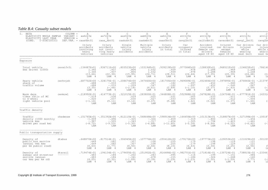
Copyright @ Institute of Transport Economics, 1999 278
Table B.4: Casualty subset models =================================================================================================================================================================== I. BETA COLUMN = A B C D E F G H I J ELASTICITY WHOLE SAMPLE VARIANT = aa6223x aa7223x aas023x aam023x aah123x avc123x avc123p avc123n avc123u avc123 ELASTICITY LAST YEAR VERSION = 5 5 5 5 5 5 5 5 5 5 (COND. T-STATISTIC) DEP.VAR. = caas6bt01 caas_6bt01 caaksbt01 caakmbt01 caas0bt01 cavg1bt01 caifcdbt01 cavxcdbt01 cavg1_2bt01 cavg2bt Injury Injury Single Multiple Injury Car Accident Injured Car drivers Car driv accidents accidents vehicle vehicle accidents occupants involved car drivers injured injure involving not invol- injury injury in total injured female car except while while n heavy ving heavy accidents accidents in total drivers females wearing wearin vehicles vehicles aged 18-40 aged 18-40 seat belt seat be =================================================================================================================================================================== -------- Exposure -------- Total vehicle cevxtfv3i .134487E+01 .936711E+00 .803523E+00 .103194E+01 .939219E+00 .977584E+00 .128830E+01 .968521E+00 .124825E+01 .786148 kms driven (1000) 1.345 .937 .804 1.032 .939 .978 1.288 .969 1.248 1.345 .937 .804 1.032 .939 .978 1.288 .969 1.248 (13.66) (22.30) (15.95) (24.71) (28.51) (24.44) (17.35) (20.39) (24.68) (14 LAM 4 LAM 4 LAM 4 LAM 4 LAM 4 LAM 4 LAM 4 LAM 4 LAM 4 LA Heavy vehicle cevhvysh .687702E+00 -.328175E-01 -.208674E+00 .347460E+00 .181705E+00 -.969089E-01 .452484E+00 -.397895E-01 .670840E-01 -.213797 share of .688 -.033 -.209 .347 .182 -.097 .452 -.040 .067 - traffic volume .688 -.033 -.209 .347 .182 -.097 .452 -.040 .067 - (3.35) (-.46) (-2.18) (4.61) (2.89) (-1.10) (3.37) (-.43) (.59) (-1 LAM 4 LAM 4 LAM 4 LAM 4 LAM 4 LAM 4 LAM 4 LAM 4 LAM 4 LA Warm days cevmcw1 -.218992E-01 .414773E-01 .321015E-01 .283800E-01 .344808E-01 .552988E-02 .367828E-01 .124704E-01 -.677781E-02 .143316 times ratio of MC -.019 .036 .029 .025 .031 .005 .033 .011 -.006 to 4-wheel -.020 .037 .030 .027 .033 .005 .035 .012 -.006 light vehicle pool (-1.14) (5.11) (3.12) (3.47) (5.48) (.62) (3.02) (1.37) (-.64) (1 LAM LAM LAM LAM LAM LAM LAM LAM LAM --------------- Traffic density --------------- Traffic chsdense -.151765E+01 -.351392E+00 -.812110E-01 -.568648E+00 -.598914E+00 -.164456E+00 -.101313E+01 -.318807E+00 -.327198E+00 -.100187 density (1000 monthly -1.009 -.496 -.325 -.324 -.459 -.319 -.800 -.419 -.456 - vehicle kms -.987 -.505 -.343 -.317 -.456 -.325 -.794 -.423 -.461 - driven per road km) (-8.72) (-9.53) (-5.30) (-6.88) (-11.80) (-5.34) (-8.94) (-6.52) (-6.42) (-3 LAM LAM LAM LAM LAM LAM LAM LAM LAM ---------------------------- Public transportation supply ---------------------------- Density of dtabus .648870E+00 .817514E-01 .306945E+00 .107776E+00 .255412E+00 .179172E+00 .197773E+00 .129053E+00 .121029E+00 .301209 public bus service .649 .082 .307 .108 .255 .179 .198 .129 .121 (annual veh kms .649 .082 .307 .108 .255 .179 .198 .129 .121 per km public road) (6.63) (1.77) (6.50) (2.66) (8.15) (4.43) (3.34) (3.25) (2.56) (5 LAM 4 LAM 4 LAM 4 LAM 4 LAM 4 LAM 4 LAM 4 LAM 4 LAM 4 LA Density of dtarail .719474E-01 .194134E-01 -.179655E-01 .251902E-01 .816486E-02 -.982701E-02 .171816E-01 -.130724E-01 .738815E-02 -.233463 subway and streetcar ------- .683 .184 -.202 .283 .095 -.114 .199 -.151 .086 - service (annual .683 .184 -.341 .478 .155 -.186 .326 -.248 .140 - car kms per km rd) (4.05) (2.32) (-1.89) (3.39) (1.29) (-1.23) (1.30) (-1.59) (.77) (-2 LAM 4 LAM 4 LAM 4 LAM 4 LAM 4 LAM 4 LAM 4 LAM 4 LAM 4 LA
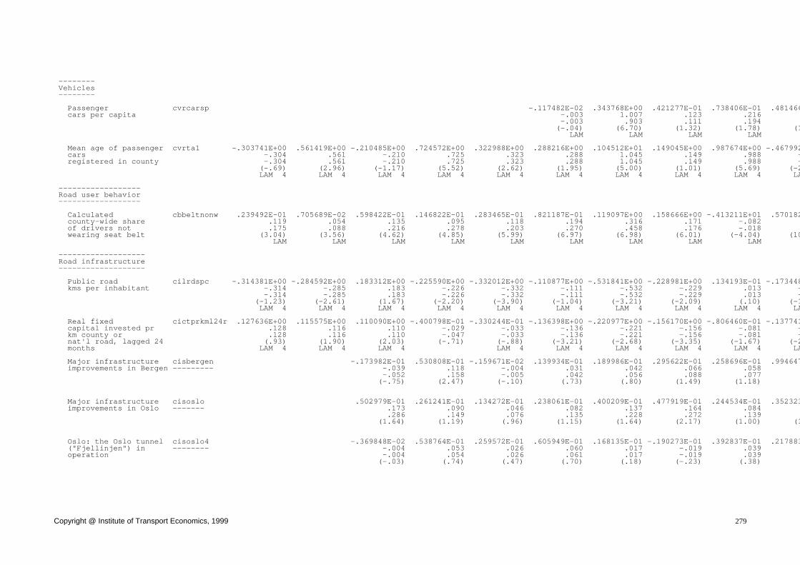
Copyright @ Institute of Transport Economics, 1999 279
-------- Vehicles -------- Passenger cvrcarsp -.117482E-02 .343768E+00 .421277E-01 .738406E-01 .481466 cars per capita -.003 1.007 .123 .216 -.003 .903 .111 .194 (-.04) (6.70) (1.32) (1.78) (1 LAM LAM LAM LAM Mean age of passenger cvrta1 -.303741E+00 .561419E+00 -.210485E+00 .724572E+00 .322988E+00 .288216E+00 .104512E+01 .149045E+00 .987674E+00 -.467992 cars -.304 .561 -.210 .725 .323 .288 1.045 .149 .988 - registered in county -.304 .561 -.210 .725 .323 .288 1.045 .149 .988 - (-.69) (2.96) (-1.17) (5.52) (2.62) (1.95) (5.00) (1.01) (5.69) (-2 LAM 4 LAM 4 LAM 4 LAM 4 LAM 4 LAM 4 LAM 4 LAM 4 LAM 4 LA ------------------ Road user behavior ------------------ Calculated cbbeltnonw .239492E-01 .705689E-02 .598422E-01 .146822E-01 .283465E-01 .821187E-01 .119097E+00 .158666E+00 -.413211E+01 .570182 county-wide share .119 .054 .135 .095 .118 .194 .316 .171 -.082 of drivers not .175 .088 .216 .278 .203 .270 .458 .176 -.018 wearing seat belt (3.04) (3.56) (4.62) (4.85) (5.99) (6.97) (6.98) (6.01) (-4.04) (10 LAM LAM LAM LAM LAM LAM LAM LAM LAM ------------------- Road infrastructure ------------------- Public road cilrdspc -.314381E+00 -.284592E+00 .183312E+00 -.225590E+00 -.332012E+00 -.110877E+00 -.531841E+00 -.228981E+00 .134193E-01 -.173448 kms per inhabitant -.314 -.285 .183 -.226 -.332 -.111 -.532 -.229 .013 - -.314 -.285 .183 -.226 -.332 -.111 -.532 -.229 .013 - (-1.23) (-2.61) (1.67) (-2.20) (-3.90) (-1.04) (-3.21) (-2.09) (.10) (-1 LAM 4 LAM 4 LAM 4 LAM 4 LAM 4 LAM 4 LAM 4 LAM 4 LAM 4 LA Real fixed cictprkml24r .127636E+00 .115575E+00 .110090E+00 -.400798E-01 -.330244E-01 -.136398E+00 -.220977E+00 -.156170E+00 -.806460E-01 -.137741 capital invested pr .128 .116 .110 -.029 -.033 -.136 -.221 -.156 -.081 - km county or .128 .116 .110 -.047 -.033 -.136 -.221 -.156 -.081 - nat'l road, lagged 24 (.93) (1.90) (2.03) (-.71) (-.88) (-3.21) (-2.68) (-3.35) (-1.67) (-2 months LAM 4 LAM 4 LAM 4 LAM 4 LAM 4 LAM 4 LAM 4 LAM 4 LA Major infrastructure cisbergen -.173982E-01 .530808E-01 -.159671E-02 .139934E-01 .189986E-01 .295622E-01 .258696E-01 .994647 improvements in Bergen --------- -.039 .118 -.004 .031 .042 .066 .058 -.052 .158 -.005 .042 .056 .088 .077 (-.75) (2.47) (-.10) (.73) (.80) (1.49) (1.18) ( Major infrastructure cisoslo .502979E-01 .261241E-01 .134272E-01 .238061E-01 .400209E-01 .477919E-01 .244534E-01 .352323 improvements in Oslo ------- .173 .090 .046 .082 .137 .164 .084 .286 .149 .076 .135 .228 .272 .139 (1.64) (1.19) (.96) (1.15) (1.64) (2.17) (1.00) (1 Oslo: the Oslo tunnel cisoslo4 -.369848E-02 .538764E-01 .259572E-01 .605949E-01 .168135E-01 -.190273E-01 .392837E-01 .217883 ("Fjellinjen") in -------- -.004 .053 .026 .060 .017 -.019 .039 operation -.004 .054 .026 .061 .017 -.019 .039 (-.03) (.74) (.47) (.70) (.18) (-.23) (.38) (

Copyright @ Institute of Transport Economics, 1999 280
Table B.4 (continued) =================================================================================================================================================================== I. BETA COLUMN = A B C D E F G H I J ELASTICITY WHOLE SAMPLE VARIANT = aa6223x aa7223x aas023x aam023x aah123x avc123x avc123p avc123n avc123u avc123 ELASTICITY LAST YEAR VERSION = 5 5 5 5 5 5 5 5 5 5 (COND. T-STATISTIC) DEP.VAR. = caas6bt01 caas_6bt01 caaksbt01 caakmbt01 caas0bt01 cavg1bt01 caifcdbt01 cavxcdbt01 cavg1_2bt01 cavg2bt Injury Injury Single Multiple Injury Car Accident Injured Car drivers Car driv accidents accidents vehicle vehicle accidents occupants involved car drivers injured injure involving not invol- injury injury in total injured female car except while while n heavy ving heavy accidents accidents in total drivers females wearing wearin vehicles vehicles aged 18-40 aged 18-40 seat belt seat be =================================================================================================================================================================== ------------------- Road infrastructure continued ------------------- Major infrastructure cistroms .295479E+00 .134311E+00 .162106E+00 .264429E+00 .200154E+00 .312870E+00 .196310E+00 .337028 improvements in Tromsø -------- .300 .136 .165 .269 .203 .318 .199 .319 .145 .175 .285 .216 .337 .212 (3.09) (1.62) (2.78) (4.13) (2.20) (3.93) (3.31) (3 Major infrastructure cistrond -.485058E-01 .885620E-02 -.157361E-01 -.506180E-01 .989338E-02 -.383602E-01 -.458038E-01 -.576942 improvements -------- -.124 .023 -.040 -.129 .025 -.098 -.117 - in Trondheim -.146 .027 -.047 -.152 .030 -.115 -.137 - (-1.94) (.49) (-1.01) (-2.60) (.45) (-2.15) (-2.56) (-1 ---------------- Road maintenance ---------------- Snowfall cimtsnowmain .171011E+01 -.227916E+01 -.728060E+00 .113418E+01 -.409627E+00 -.141872E-01 .173057E+01 -.136033E+00 .138638E+01 -.872708 interaction with ------------ .025 -.034 -.010 .016 -.006 -.000 .024 -.002 .020 - winter .024 -.032 -.010 .015 -.006 -.000 .023 -.002 .019 - maintenance intensity (1.18) (-3.04) (-.66) (1.82) (-.73) (-.02) (2.07) (-.18) (1.67) (- Expenditure cimroadmarks -.809489E-02 -.121691E-01 -.835227E-02 -.206928E-01 -.158703E-01 -.344634E-02 .616327E-02 -.395860E-02 .959461E-02 -.205878 on road marks, ------------ -.025 -.038 -.032 -.079 -.059 -.013 .023 -.015 .044 - signposting etc -.028 -.042 -.044 -.109 -.082 -.018 .032 -.021 .058 - per km nat'l or (-.59) (-1.82) (-1.23) (-3.03) (-2.51) (-.43) (.50) (-.48) (1.03) (-2 county road LAM LAM LAM LAM LAM LAM LAM LAM Expenditure on cimmisc .554189E-02 -.478996E-02 .308810E-02 .294734E-02 .452261E-02 .108432E-01 .489233E-02 .109907E-01 .775157E-02 .137337 miscellaneous ------- .135 -.116 .071 .067 .097 .232 .105 .235 .166 road maintenance .123 -.106 .059 .056 .086 .206 .093 .209 .147 per km nat'l or (1.09) (-2.13) (1.19) (1.44) (2.05) (3.73) (1.04) (3.75) (2.23) (3 county road ---------- Population ---------- Unemployment rate cderate -.178275E-01 -.439133E-01 -.883392E-01 -.172781E-02 -.148547E-01 -.173943E-01 .171765E-02 -.374093E-01 .676259E-01 -.526306 (per -.018 -.044 -.088 -.002 -.015 -.017 .002 -.037 .068 - cent of working -.018 -.044 -.088 -.002 -.015 -.017 .002 -.037 .068 - age population) (-.55) (-3.42) (-5.16) (-.13) (-1.27) (-1.11) (.08) (-2.32) (3.46) (-2 LAM 4 LAM 4 LAM 4 LAM 4 LAM 4 LAM 4 LAM 4 LAM 4 LAM 4 LA

Copyright @ Institute of Transport Economics, 1999 281
Population density cdpopdnsty .205226E+00 .120198E+00 .866618E-02 .132833E+00 .256776E-01 -.293638E-02 .104113E+00 .251233E-01 .722954E-01 -.592540 (inhabitants per sq .205 .120 .009 .133 .026 -.003 .104 .025 .072 - km) .205 .120 .009 .133 .026 -.003 .104 .025 .072 - (2.58) (3.02) (.24) (4.76) (.98) (-.09) (1.87) (.71) (1.89) (-1 LAM 4 LAM 4 LAM 4 LAM 4 LAM 4 LAM 4 LAM 4 LAM 4 LAM 4 LA Women cdpregrate2 .801921E+00 .320579E+00 -.620299E-01 .236233E+00 .209576E+00 .153798E+00 .305005E+00 .450509E-01 .230424E+00 .464622 pregnant in first .802 .321 -.062 .236 .210 .154 .305 .045 .230 quarter per .802 .321 -.062 .236 .210 .154 .305 .045 .230 1000 women 18-44 (4.29) (4.39) (-.76) (3.58) (3.66) (1.99) (2.63) (.57) (2.52) ( LAM 4 LAM 4 LAM 4 LAM 4 LAM 4 LAM 4 LAM 4 LAM 4 LAM 4 LA -------- Daylight -------- Minutes of bnt -.121769E-04 -.175857E-06 .583805E-22 .276557E-02 -.201522E-06 .917918E-08 -.137421E-05 .779195E-05 .202287E-07 .202871 twilight per day --- -.045 -.010 .000 .002 -.004 .008 -.032 .015 .003 -.045 -.010 .000 .002 -.004 .008 -.032 .015 .003 (-1.29) (-1.04) (.62) (.20) (-.46) (1.19) (-1.76) (.92) (.25) ( LAM 5 LAM 5 LAM 5 LAM 5 LAM 5 LAM 5 LAM 5 LAM 5 LAM 5 LA Minutes without cnn .150283E-05 .509120E-07 .445225E-25 .326573E-01 .184675E-06 .152140E-08 .169718E-06 .745050E-05 .199896E-07 .324945 daylight --- .082 .106 .014 .020 .084 .105 .099 .160 .107 between 5 and 11 p m .074 .093 .010 .021 .081 .099 .094 .155 .102 (1.57) (4.84) (5.75) (4.42) (5.05) (5.51) (3.32) (6.14) (3.98) (5 LAM 5 LAM 5 LAM 5 LAM 5 LAM 5 LAM 5 LAM 5 LAM 5 LAM 5 LA Minutes without cnr .663605E-05 .116918E-06 .313223E-23 -.952406E-02 .574323E-06 .507190E-08 .674447E-06 .918133E-05 .827649E-07 .744129 daylight 7-9 --- .055 .015 .000 -.016 .024 .009 .034 .039 .022 a m and 3-5 p m .054 .015 .000 -.016 .024 .009 .034 .039 .022 (2.68) (3.03) (4.20) (-1.59) (5.33) (4.33) (3.80) (3.78) (5.15) (2 LAM 5 LAM 5 LAM 5 LAM 5 LAM 5 LAM 5 LAM 5 LAM 5 LAM 5 LA Minutes without cnw -.666126E-05 -.156566E-07 -.112265E-24 .607185E-02 -.125134E-06 -.269975E-08 -.169616E-06 -.112923E-04 -.330834E-07 -.502378 daylight --- -.006 -.000 -.000 .024 -.000 -.000 -.000 -.006 -.000 - between 9 a m -.006 -.000 -.000 .024 -.000 -.000 -.000 -.006 -.000 - and 3 p m (-2.41) (-.46) (-2.51) (.76) (-1.15) (-4.02) (-.84) (-3.39) (-2.98) (-2 LAM 5 LAM 5 LAM 5 LAM 5 LAM 5 LAM 5 LAM 5 LAM 5 LAM 5 LA ------- Weather ------- Average snow depth cmds3a .377501E-01 -.419049E-01 -.987336E-01 .183489E-01 -.212670E-01 -.320363E-02 .238380E-01 -.418968E-02 .177224E-01 -.179969 during month (cms) ------ .065 -.073 -.174 .032 -.037 -.006 .042 -.007 .031 - .067 -.074 -.172 .032 -.037 -.006 .041 -.007 .031 - (2.22) (-6.21) (-11.49) (2.82) (-4.15) (-.45) (2.10) (-.56) (2.03) (-1 LAM 4 LAM 4 LAM 4 LAM 4 LAM 4 LAM 4 LAM 4 LAM 4 LAM 4 LA Days with rainfall cmraind1s .266809E-04 -.331654E-03 -.533942E-03 -.420693E-05 -.339461E-02 -.185209E-02 .300645E-02 -.175404E-02 .193113E-02 -.608443 during month, plus one .001 -.011 -.090 -.000 -.032 -.010 .051 -.006 .008 - .001 -.012 -.079 -.000 -.030 -.010 .048 -.006 .008 - (.03) (-.74) (-5.73) (-.00) (-2.75) (-.58) (2.23) (-.34) (.41) (-1 LAM 3 LAM 3 LAM 3 LAM 3 LAM 3 LAM 3 LAM 3 LAM 3 LAM 3 LA Days with snowfall cmsnowd1s .532071E-02 .708646E-02 -.608164E-03 .334719E-01 .214620E-01 .432444E-01 .162005E-01 .489373E-01 .565497E-01 .353742 during month, plus one .058 .071 -.016 .105 .090 .129 .100 .106 .142 .057 .070 -.018 .109 .093 .132 .104 .108 .146 (2.15) (5.32) (-1.29) (6.30) (7.02) (6.79) (4.48) (5.11) (6.06) (4 LAM 3 LAM 3 LAM 3 LAM 3 LAM 3 LAM 3 LAM 3 LAM 3 LAM 3 LA

Copyright @ Institute of Transport Economics, 1999 282
Table B.4 (continued) ==================================================================================================================================================================== I. BETA COLUMN = A B C D E F G H I J ELASTICITY WHOLE SAMPLE VARIANT = aa6223x aa7223x aas023x aam023x aah123x avc123x avc123p avc123n avc123u avc123 ELASTICITY LAST YEAR VERSION = 5 5 5 5 5 5 5 5 5 5 (COND. T-STATISTIC) DEP.VAR. = caas6bt01 caas_6bt01 caaksbt01 caakmbt01 caas0bt01 cavg1bt01 caifcdbt01 cavxcdbt01 cavg1_2bt01 cavg2bt Injury Injury Single Multiple Injury Car Accident Injured Car drivers Car driv accidents accidents vehicle vehicle accidents occupants involved car drivers injured injure involving not invol- injury injury in total injured female car except while while n heavy ving heavy accidents accidents in total drivers females wearing wearin vehicles vehicles aged 18-40 aged 18-40 seat belt seat be =================================================================================================================================================================== ------- Weather continued ------- Per cent of snow days cmsnowlotsh -.983559E-06 -.588513E-04 .529568E-05 -.508248E-03 .405685E-03 .118516E-02 .578718E-03 .284402E-02 .277406E-02 .318465 with large ----------- -.000 -.008 .004 -.008 .010 .015 .028 .021 .027 snowfall (>5 mms) -.000 -.008 .002 -.007 .009 .014 .023 .021 .026 (-.01) (-.86) (.55) (-.73) (1.32) (1.34) (1.73) (1.75) (1.78) ( LAM 3 LAM 3 LAM 3 LAM 3 LAM 3 LAM 3 LAM 3 LAM 3 LAM 3 LA Days with frost cmtfrostd1s .136265E-02 -.365543E-02 -.150592E-02 -.980207E-02 -.149128E-01 -.194822E-01 -.307792E-02 -.170109E-01 -.237262E-01 -.219956 during month, plus one .050 -.117 -.213 -.056 -.129 -.100 -.047 -.055 -.095 - .049 -.117 -.206 -.055 -.126 -.099 -.046 -.054 -.094 - (.85) (-4.69) (-8.50) (-2.22) (-6.18) (-3.59) (-1.24) (-1.88) (-2.79) (-3 LAM 3 LAM 3 LAM 3 LAM 3 LAM 3 LAM 3 LAM 3 LAM 3 LAM 3 LA Per cent of cmthawsh -.312103E-06 .257567E-05 .209223E-06 -.484478E-03 .298764E-04 .110261E-03 .563207E-06 -.101022E-02 .356945E-04 .160283 frost days with thaw -------- -.003 .015 .051 -.046 .008 .008 .001 -.024 .001 -.002 .015 .040 -.042 .007 .008 .001 -.023 .001 (-.12) (1.56) (6.16) (-3.14) (.76) (.54) (.03) (-1.40) (.07) ( LAM 3 LAM 3 LAM 3 LAM 3 LAM 3 LAM 3 LAM 3 LAM 3 LAM 3 LA -------------------- Legislative measures -------------------- New highway code and eldhwycode2 -.437431E-01 -.146661E+00 -.194501E-01 -.108581E+00 -.974212E-01 -.111401E+00 -.850452E-01 -.161927E+00 .714019E-01 -.133124 reporting routines =========== -.044 -.147 -.019 -.109 -.097 -.111 -.085 -.162 .071 - from October 1, 1978 -.044 -.147 -.019 -.109 -.097 -.111 -.085 -.162 .071 - (-.83) (-6.12) (-.64) (-4.45) (-5.61) (-3.87) (-1.67) (-5.45) (1.38) (-4 ----------------- Access to alcohol ----------------- Alcohol outlets dxloutletspc .339880E+00 .568177E-02 .128998E-01 .639402E-04 .545077E-01 -.137285E-01 -.148106E-01 -.296910E-03 -.305455E-01 -.978975 per 1000 population .414 .006 .018 .000 .061 -.011 -.032 -.001 -.026 - .433 .006 .016 .000 .060 -.011 -.028 -.001 -.027 - (4.44) (.20) (.50) (3.44) (2.40) (-3.54) (-1.55) (-.80) (-2.96) (-2 LAM LAM LAM LAM LAM LAM LAM LAM LAM Per cent dxloutstrong -.166465E-01 .558770E-01 .183672E-01 .474214E-02 .835460E-02 -.460835E-01 -.714111E-02 -.177537E-01 -.188556E-01 -.570797 alcohol outlets -.017 .056 .018 .005 .008 -.046 -.007 -.018 -.019 - selling strong -.017 .056 .018 .005 .008 -.046 -.007 -.018 -.019 - beer, wine or liquor (-.64) (4.25) (1.38) (.44) (.82) (-3.93) (-.29) (-1.32) (-1.16) (-3 LAM 4 LAM 4 LAM 4 LAM 4 LAM 4 LAM 4 LAM 4 LAM 4 LAM 4 LA

Copyright @ Institute of Transport Economics, 1999 283
Per cent dxloutliqsh .622246E-01 .658551E-01 .331707E-01 .180420E-01 .232736E-01 -.270135E-01 .134478E-01 -.531213E-02 -.438732E-01 -.181338 wine/liquor stores .062 .066 .033 .018 .023 -.027 .013 -.005 -.044 - of outlets for .062 .066 .033 .018 .023 -.027 .013 -.005 -.044 - strong (2.25) (4.89) (2.44) (1.68) (2.22) (-2.30) (.57) (-.41) (-2.69) (-1 alcoholic beverage LAM 4 LAM 4 LAM 4 LAM 4 LAM 4 LAM 4 LAM 4 LAM 4 LAM 4 LA Restaurants dxlrstalcpc -.539019E-01 .210319E+00 .452655E-01 -.262968E-02 -.837285E-02 .794329E-01 .239706E-01 .100550E+00 .174818E+00 -.106411 licensed to -.002 .124 .035 -.005 -.011 .078 .022 .095 .175 - serve alcohol -.011 .164 .067 -.001 -.005 .083 .029 .113 .175 - per 1000 population (-4.26) (4.31) (1.32) (-5.50) (-4.42) (2.38) (.47) (2.71) (4.62) (- LAM LAM LAM LAM LAM LAM LAM LAM LAM Per cent of licensed dxlrestlwsh -.622820E-01 .114292E-01 -.249022E+00 -.201662E+00 -.122539E+00 -.784577E-01 .471669E-01 -.227523E+00 .579641E-01 -.157373 restaurants with -.062 .011 -.249 -.202 -.123 -.078 .047 -.228 .058 - wine/liquor license -.062 .011 -.249 -.202 -.123 -.078 .047 -.228 .058 - (-.44) (.15) (-2.76) (-2.64) (-1.84) (-.86) (.43) (-2.52) (.54) (-1 LAM 4 LAM 4 LAM 4 LAM 4 LAM 4 LAM 4 LAM 4 LAM 4 LAM 4 LA Per cent of dxlrestliqsh .438171E-01 .302122E-01 .130595E-01 -.113664E-01 -.179756E-01 -.803034E-01 -.108999E+00 -.721082E-01 -.844253E-01 -.965886 wine/liquour .044 .030 .013 -.011 -.018 -.080 -.109 -.072 -.084 - licenses .044 .030 .013 -.011 -.018 -.080 -.109 -.072 -.084 - including liquor (.78) (1.26) (.42) (-.50) (-.90) (-2.86) (-3.06) (-2.43) (-2.44) (-2 LAM 4 LAM 4 LAM 4 LAM 4 LAM 4 LAM 4 LAM 4 LAM 4 LAM 4 LA --------------------------- Accident reporting routines --------------------------- New eur77 .294969E-01 .107640E+00 .177627E+00 .185441E+00 accident reporting ----- .029 .108 .178 .185 routines from .029 .108 .178 .185 January 1, 1977 (.40) (2.73) (1.98) (3.65) --------- Geography --------- Oslo hcounty3 -.130945E+01 -.377634E+00 .198009E+00 -.434717E+00 -.190638E+00 .503418E+00 -.270116E+00 .486995E+00 .687319E+00 .262959 ======== -1.309 -.378 .198 -.435 -.191 .503 -.270 .487 .687 -1.309 -.378 .198 -.435 -.191 .503 -.270 .487 .687 (-3.27) (-2.07) (.91) (-3.17) (-1.73) (3.49) (-1.16) (3.31) (4.20) (1 -------- Calendar -------- Dummy for ekee -.166339E+00 -.153696E+00 -.117907E+00 -.149843E+00 -.137669E+00 -.147491E+00 -.207560E+00 -.115457E+00 -.144590E+00 -.145869 end of Easter ==== -.166 -.154 -.118 -.150 -.138 -.147 -.208 -.115 -.145 - -.166 -.154 -.118 -.150 -.138 -.147 -.208 -.115 -.145 - (-1.99) (-4.80) (-3.55) (-6.09) (-7.43) (-5.39) (-5.03) (-3.79) (-4.21) (-4 Dummy for ekes .605840E-02 .491733E-01 .231642E-01 .325038E-01 .292697E-01 .883601E-01 .939637E-01 .896534E-01 .974650E-01 .779328 start of Easter week ==== .006 .049 .023 .033 .029 .088 .094 .090 .097 .006 .049 .023 .033 .029 .088 .094 .090 .097 (.08) (1.68) (.69) (1.37) (1.67) (3.52) (2.21) (3.30) (3.09) (2

Copyright @ Institute of Transport Economics, 1999 284
Table B.4 (continued) =================================================================================================================================================================== I. BETA COLUMN = A B C D E F G H I J ELASTICITY WHOLE SAMPLE VARIANT = aa6223x aa7223x aas023x aam023x aah123x avc123x avc123p avc123n avc123u avc123 ELASTICITY LAST YEAR VERSION = 5 5 5 5 5 5 5 5 5 5 (COND. T-STATISTIC) DEP.VAR. = caas6bt01 caas_6bt01 caaksbt01 caakmbt01 caas0bt01 cavg1bt01 caifcdbt01 cavxcdbt01 cavg1_2bt01 cavg2bt Injury Injury Single Multiple Injury Car Accident Injured Car drivers Car driv accidents accidents vehicle vehicle accidents occupants involved car drivers injured injure involving not invol- injury injury in total injured female car except while while n heavy ving heavy accidents accidents in total drivers females wearing wearin vehicles vehicles aged 18-40 aged 18-40 seat belt seat be =================================================================================================================================================================== -------- Calendar continued -------- Years ektrend -.173192E-01 -.172815E-01 -.438408E-03 -.176734E-01 -.113216E-01 .333595E-02 -.605120E-02 .181048E-01 -.171770E-01 .741286 passed since 1945 -.598 -.597 -.017 -.681 -.453 .134 -.242 .725 -.688 -.702 -.701 -.021 -.858 -.550 .162 -.294 .879 -.834 (-1.01) (-2.10) (-.05) (-2.85) (-2.03) (.41) (-.53) (2.18) (-1.77) ( Share of ekvhsh -.269761E+00 .177104E+00 .822429E-01 -.148509E+00 -.101051E+00 -.114898E+00 -.181486E-02 -.282349E+00 -.230426E+00 -.260195 vacation and holidays -.088 .058 .027 -.049 -.033 -.038 -.001 -.093 -.076 - during month -.088 .058 .027 -.048 -.033 -.037 -.001 -.092 -.075 - (excl summer vacation) (-1.13) (1.72) (.65) (-1.61) (-1.37) (-1.09) (-.01) (-2.51) (-1.82) (- ------------------------ ASSOCIATED DUMMIES GROUP ------------------------ Expenditure cimroadmarks .145962E+00 .508146E-01 -.642985E-01 .118926E+00 on road marks, ============ .146 .051 -.064 .119 signposting etc per km .146 .051 -.064 .119 nat'l or county road (1.41) (.99) (-.64) (1.89) Average snow depth cmds3a -.197173E+00 -.688902E-01 -.331593E-01 -.121423E+00 -.765247E-01 -.829165E-01 -.975499E-01 -.919964E-01 -.150919E+00 -.359236 during month (cms) ====== -.197 -.069 -.033 -.121 -.077 -.083 -.098 -.092 -.151 - -.197 -.069 -.033 -.121 -.077 -.083 -.098 -.092 -.151 - (-3.64) (-3.66) (-1.51) (-6.35) (-5.20) (-3.77) (-3.08) (-3.84) (-5.47) (-1 ------------------------------------------------------------------------------------------------------------------------------------------------------------------- REGRESSION CONSTANT CONSTANT -.171659E+02 -.966177E+01 -.676212E+01 -.975345E+01 -.875050E+01 -.946154E+01 -.151508E+02 -.906173E+01 -.151588E+02 -.663428 - - - - - - - - - - - - - - - - - - (-13.97) (-17.03) (-10.58) (-18.59) (-18.03) (-16.13) (-15.54) (-14.85) (-17.56) (-9

Copyright @ Institute of Transport Economics, 1999 285
---------------------------- HETEROSKEDASTICITY STRUCTURE ---------------------------- ZETA COEFFICIENTS ----------------- var[ln(y+0.1)] as maa6223x_4wu .100000E+01 estimated by .330 model aa6223x_4 .304 (.00) LAM 4 var[ln(y+0.1)] as maa7223x_4vu .100000E+01 estimated by .038 model aa7223x_4 .015 (.00) LAM 4 var[ln(y+0.1)] as maas023x_4wu .100000E+01 estimated by .144 model aas023x_4 .189 (.00) LAM 4 var[ln(y+0.1)] as maam023x_4vu .100000E+01 estimated by .071 model aam023x_4 .022 (.00) LAM 4 var[ln(y+0.1)] as maah123x_4vu .100000E+01 estimated by .029 model aah123x_4 .054 (.00) LAM 4 var[ln(y+0.1)] as mavc123x_4vu .100000E+01 estimated by .060 model avc123x_4 .075 (.00) LAM 4 var[ln(y+0.1)] as mavc123p_4wu .100000E+01 estimated by .252 model avc123p_4 .179 (.00) LAM 4 var[ln(y+0.1)] as mavc123n_4wu .100000E+01 estimated by .086 model avc123n_4 .087 (.00) LAM 4 var[ln(y+0.1)] as mavc123u_4wu .100000E+01 estimated by .143 model avc123u_4 .064 (.00) LAM 4 var[ln(y+0.1)] as mavc123v_4wu .100000 estimated by model avc123v_4 (

Copyright @ Institute of Transport Economics, 1999 286
Table B.4 (continued) ==================================================================================================================================================================== II. PARAMETERS COLUMN = A B C D E F G H I J VARIANT = aa6223x aa7223x aas023x aam023x aah123x avc123x avc123p avc123n avc123u avc123 VERSION = 5 5 5 5 5 5 5 5 5 5 (COND. T-STATISTIC) DEP.VAR. = caas6bt01 caas_6bt01 caaksbt01 caakmbt01 caas0bt01 cavg1bt01 caifcdbt01 cavxcdbt01 cavg1_2bt01 cavg2bt Injury Injury Single Multiple Injury Car Accident Injured Car drivers Car driv accidents accidents vehicle vehicle accidents occupants involved car drivers injured injure involving not invol- injury injury in total injured female car except while while n heavy ving heavy accidents accidents in total drivers females wearing wearin vehicles vehicles aged 18-40 aged 18-40 seat belt seat be =================================================================================================================================================================== --------------------------- HETEROSKEDASTICITY STRUCTURE ---------------------------- BOX-COX TRANSFORMATIONS: UNCOND: [T-STATISTIC=0] / [T-STATISTIC=1] ------------------------------------------------------------------ LAMBDA(Z) - GROUP 4 LAM 4 .000 .000 .000 .000 .000 .000 .000 .000 .000 FIXED FIXED FIXED FIXED FIXED FIXED FIXED FIXED FIXED F ------------------------------------------------------------------ BOX-COX TRANSFORMATIONS: UNCOND: [T-STATISTIC=0] / [T-STATISTIC=1] ------------------------------------------------------------------ LAMBDA(Y) - GROUP 4 LAM 4 .000 .000 .000 .000 .000 .000 .000 .000 .000 FIXED FIXED FIXED FIXED FIXED FIXED FIXED FIXED FIXED F LAMBDA(X) cbbeltnonw -1.389 -1.765 -.602 -1.379 -.922 -.558 -.632 -.050 2.537 [-.94] [-.97] [-.84] [-1.96] [-1.58] [-1.09] [-1.36] [-.09] [3.31] [ [-1.62] [-1.51] [-2.23] [-3.38] [-3.30] [-3.03] [-3.52] [-1.95] [2.01] [-2 LAMBDA(X) chsdense -.123 .104 .408 -.165 -.077 .193 -.069 .080 .097 [-1.27] [1.23] [2.40] [-1.11] [-.99] [1.31] [-.76] [.65] [.71] [1 [-11.56] [-10.62] [-3.49] [-7.80] [-13.82] [-5.48] [-11.83] [-7.46] [-6.63] [-3 LAMBDA(X) dxloutletspc .976 .388 1.630 10.000 .603 -1.269 4.215 7.486 -.844 -1 [3.36] [.06] [.37] [2.15] [1.00] [-1.16] [.99] [.48] [-.95] [- [-.08] [-.09] [.14] [1.94] [-.66] [-2.08] [.76] [.42] [-2.08] [-1 LAMBDA(X) dxlrstalcpc 8.742 1.349 1.652 -3.672 -2.496 .178 .851 .484 .008 [1.72] [1.71] [.74] [-2.45] [-2.00] [.30] [.21] [.86] [.02] [ [1.53] [.44] [.29] [-3.11] [-2.81] [-1.38] [-.04] [-.92] [-3.20] [- LAMBDA(X) cimroadmarks 1.000 1.000 1.000 1.000 1.000 1.000 1.000 1.000 FIXED FIXED FIXED FIXED FIXED FIXED FIXED FIXED LAMBDA(X) cevmcw1 -.230 -.230 -.230 -.230 -.230 -.230 -.230 -.230 -.230 - FIXED FIXED FIXED FIXED FIXED FIXED FIXED FIXED FIXED F LAMBDA(X) cvrcarsp -1.000 -1.000 -1.000 -1.000 -1 FIXED FIXED FIXED FIXED F

Copyright @ Institute of Transport Economics, 1999 287
LAMBDA(X) - GROUP 3 LAM 3 1.400 1.350 1.959 .687 .852 .648 1.082 .462 .549 [1.45] [5.27] [7.77] [4.27] [6.87] [4.11] [2.84] [2.77] [3.23] [3 [.41] [1.37] [3.81] [-1.95] [-1.20] [-2.23] [.21] [-3.23] [-2.65] [-1 LAMBDA(X) - GROUP 4 LAM 4 .000 .000 .000 .000 .000 .000 .000 .000 .000 FIXED FIXED FIXED FIXED FIXED FIXED FIXED FIXED FIXED F LAMBDA(X) - GROUP 5 LAM 5 2.000 2.672 9.997 -.100 2.405 3.336 2.450 1.839 2.862 3 FIXED [2.51] [2.87] [-.40] [3.00] [2.88] [2.44] [3.53] [2.91] [2 [1.57] [2.58] [-4.45] [1.76] [2.02] [1.44] [1.61] [1.90] [1 --------------- AUTOCORRELATION --------------- ORDER 19 RHO 19 .065 .174 .129 .159 .161 .091 .067 .071 .081 (3.75) (9.48) (8.67) (10.92) (10.61) (5.75) (4.74) (4.59) (5.15) (6 ORDER228 RHO228 .066 .216 .119 .187 .220 .110 .059 .096 .084 (3.53) (11.28) (7.81) (12.86) (13.54) (6.60) (3.67) (5.70) (5.19) (4 =================================================================================================================================================================== III.GENERAL STATISTICS =================================================================================================================================================================== LOG-LIKELIHOOD -6867.950 -9861.533 -13172.231 -14638.588 -13878.542 -14965.330 -10420.007 -12018.758 -12666.024 -13392 PSEUDO-R2 : - (E) .612 .849 .620 .815 .866 .694 .633 .693 .701 - (L) .614 .870 .626 .843 .889 .729 .657 .727 .741 - (E) ADJUSTED FOR D.F. .605 .847 .616 .813 .864 .690 .628 .689 .697 - (L) ADJUSTED FOR D.F. .608 .868 .621 .841 .888 .726 .653 .724 .738 SAMPLE : - NUMBER OF OBSERVATIONS 2964 2964 4788 4788 4104 4104 4104 4104 4104 - FIRST OBSERVATION 229 229 229 229 913 913 913 913 913 - LAST OBSERVATION 3192 3192 5016 5016 5016 5016 5016 5016 5016 NUMBER OF ESTIMATED PARAMETERS : - FIXED PART : . BETAS 42 42 47 47 45 46 46 46 46 . BOX-COX 5 6 6 6 6 6 6 6 6 . ASSOCIATED DUMMIES 2 2 2 2 1 1 1 1 1 - AUTOCORRELATION 2 2 2 2 2 2 2 2 2 - HETEROSKEDASTICITY : . ZETAS 1 1 1 1 1 1 1 1 1 . BOX-COX 0 0 0 0 0 0 0 0 0 . ASSOCIATED DUMMIES 0 0 0 0 0 0 0 0 0 ===================================================================================================================================================================

Copyright @ Institute of Transport Economics, 1999 288

Appendix C.
Copyright @ Institute of Transport Economics, 1999 289
Appendix C. Variable nomenclature The variables in the TRULS database follow a standard nomenclature, according to which the three first letters indicate the level of aggregation and the variable group and subgroup.
1st letter: level of spatial and temporal aggregation The reader can tell from the first letter of the variable code name at what level of spatial and temporal aggregation the measurement has been made. The following codes are used.
A. Measurement as of 1980 or 1977-80, by county.
B. Measurement by county and calendar month; uniform data for all years.
C. Measurement by county, year and month.
D. Measurement by county and year.
E. Measurement by year and month; national totals or averages.
F. Measurement by year; national totals or averages.
G. Miscellaneous units of aggregation
H. Measurement by county; invariant across time.
Variables with full cross-sectional and time-series variation, i e by county, year and month, have code names starting with a C. Most variables are of this kind. This group also includes variables constructed by interpolation between annual stock measurements, by splitting an-nual flows into monthly flows and/or by formation of moving averages, etc.
When measurements vary by month but not by year, the code B is used (e g daylight).
Code D is used when measurements are made only once a year but applied uniformly to all months (e g, alcohol licenses).
Code E applies to variables with full time-series but no cross-sectional variation (e g interest rates).
Code F represents variables with annual but no monthly or cross-sectional variation.
Code H is used for measurements that cannot vary over time. There is, however, full cross-sectional variation between counties (e g, length of a county’s coastline).
Code A is used for variables that are measured only once, although the phenomenon described does vary over time (e g, regional road standard as measured in 1980). As for code H, there is full cross-sectional variation between counties.
Code G is a rest category assembling all other principles of aggregation.

An econometric model of car ownership, road use, accidents, and their severity
290 Copyright @ Institute of Transport Economics, 1999
2nd and 3rd letters: variable group and subgroup The second and third letters refer to different variable groups, in accordance with the follow-ing.
A. Accidents and victims AA. Injury accidents AF. Fatal accidents AI. Accident involved road users AK. Fatalities AS. Severity AV. Persons killed or injured B. Road user behavior BB. Seat belt use BH. Helmet use BS. Speed C. Law enforcement and control CR. Radar control CT. Vehicle inspection D. Demography DA. Abortions DB. Births DD. Divorces DE. (Un)employment DP. Population size E. Exposure EB. Bus kilometers EC. Traffic counts EM. Person kilometers EP. Passenger kilometers by bus ER. Passengers transported by bus EV. Vehicle kilometers EX. Outlier/gross error F. Fuel sales and consumption FD. Diesel FG. Gasoline FQ. Ratio of diesel to gasoline G. Fuel consuming activity outside the road sector GA. Agriculture GC. Construction GF. Fisheries GM. Manufacturing industry GS. Forestry GY. Pleasure yachts H. Traffic density HS. Vehicle kilometers per road kilometer I. Infrastructure IC. Real fixed capital II. Investment expenditure

Appendix C.
Copyright @ Institute of Transport Economics, 1999 291
IL. Road length IM. Maintenance IS. Road standard J. Car repair shops JE. Employment JN. Number of establishments JS. Sales volume K. Calendar KD. Number of days in month KE. Easter KH. Number of Sundays and holidays in month KJ. January KM. Month KP. Number of isolated workdays between holidays KS. Summer KT. Trend KV. Vacation/holiday KW. Number of workdays KX. Temporal extrapolation L. Legislation LD. Dummies for legislative changes LH. Speed limits M. Meteorology MD. Snow depth MR. Precipitation in the form of rain MS. Precipitation in the form of snow MT. Temperature N. Daylight ND. Total amount of daylight NN. Daylight 5 - 11 p m NR. Daylight 7-9 a m and 3 - 5 p m NS. Daylight savings time NT. Twilight NU. Time of sunrise NW. Daylight 9 a m - 3 p m P. Prices PA. Alcohol PC. Automobiles PD. Diesel PG. Gasoline PI. Insurance premiums PK. Kilometer tax PM. Automobile maintenance PP. Public transportation PT. Toll and ferry charges PX. Price- and cost indices Q. Industry QC. Trade

An econometric model of car ownership, road use, accidents, and their severity
292 Copyright @ Institute of Transport Economics, 1999
QT. Tourism QM. Manufacturing R. Income RP. Operating surplus RT. Taxable income S. Sanctions and penalties SF. Fine level SN. Fines and sentences T. Public transportation supply TA. Supply TC. Capacity TF. Frequency U. Accident reporting UB. Underreporting UR. Reporting routines V. Vehicles VI. Risk index VR. Registered vehicles VS. Seat belt installation W. Drivers WI. Risk index WN. New licenses WS. License holders X. Alcohol XC. Consumption XH. Home production XI. Import XL. Restaurant licenses XS. Sales XT. Trade leaks (border-crossing sales) Z. Information/publicity ZG. Media events ZI.. Safety campaigns 4th and following letters: detailed identification Letters 4 through 12 are used for unambiguous identification of variables within each group.
For instance, the variable cmtcold is a measure of «coldness», defined as the «difference be-tween 25 degrees C and the mean monthly temperature». One can tell from the first letter that it is a variable with full spatial and temporal variation.
The variable epg95r measures the «real price of 95 octane gasoline in NOK 1995 per liter». Here, the first letter indicates that the same price is applied to all counties, i e there is no spa-tial variation in the data.

Appendix C.