vol. 179, no. 3 the american naturalist march 2012

Ecological Specialization in Fossil Mammals

Explains Cope’s Rule

P. Raia,1,* F. Carotenuto,1 F. Passaro,1 D. Fulgione,2 and M. Fortelius3

1. Dipartimento di Scienze della Terra, Universita degli Studi Federico II, Largo San Marcellino 10, 80138 Napoli, Italy;2. Dipartimento di Biologia Strutturale e Funzionale, Universita degli Studi Federico II, via Cinthia 4–Monte Sant’Angelo Edificio 7,80126 Napoli, Italy; 3. Department of Geosciences and Geography, University of Helsinki, P.O. Box 64, 00014 Helsinki, Finland; andInstitute of Biotechnology, University of Helsinki, P.O. Box 56, 00014 Helsinki, Finland

Submitted May 3, 2011; Accepted October 25, 2011; Electronically published January 19, 2012

Online enhancement: appendix. Dryad data: http://dx.doi.org/10.5061/dryad.8bn8431n.

abstract: Cope’s rule is the trend toward increasing body size ina lineage over geological time. The rule has been explained either aspassive diffusion away from a small initial body size or as an activetrend upheld by the ecological and evolutionary advantages that largebody size confers. An explicit and phylogenetically informed analysisof body size evolution in Cenozoic mammals shows that body sizeincreases significantly in most inclusive clades. This increase occursthrough temporal substitution of incumbent species by larger-sizedclose relatives within the clades. These late-appearing species havesmaller spatial and temporal ranges and are rarer than the incum-bents they replace, traits that are typical of ecological specialists.Cope’s rule, accordingly, appears to derive mainly from increasingecological specialization and clade-level niche expansion rather thanfrom active selection for larger size. However, overlain on a net trendtoward average size increase, significant pulses in origination of large-sized species are concentrated in periods of global cooling. Thesepulses plausibly record direct selection for larger body size accordingto Bergmann’s rule, which thus appears to be independent of butconcomitant with Cope’s.

Keywords: Cope’s rule, Bergmann’s rule, mammals, ecological spe-cialization, range size, body size.

Introduction

Of the many empirical “laws” of evolution tentatively at-tributed to E. D. Cope (Simpson 1953; Rensch 1954; butsee Polly 1998), the one known today as Cope’s rule positsa trend toward increasing body size in a lineage over geo-logical time (Cope 1887). This rule has received mixedsupport in the scientific literature. Among terrestrial ver-tebrates, it has been shown to apply to fossil mammals(Stanley 1973; Alroy 1998; Finarelli 2007) and to Mesozoicreptiles (Hone and Benton 2007). Besides these supportive

* Corresponding author; e-mail: pasquale.raia@unina.it.

Am. Nat. 2012. Vol. 179, pp. 328–337. � 2012 by The University of Chicago.

0003-0147/2012/17903-53013$15.00. All rights reserved.

DOI: 10.1086/664081

cases, mixed or inconclusive evidence comes from studiespertaining to the earliest ruminants (Gingerich 1974), earlyamniotes (Laurin 2004), Mesozoic birds (Butler and Go-swami 2008; Hone et al. 2008), and extant mammals(Clauset and Erwin 2008; Monroe and Bokma 2010).

As Cope’s rule represents a large-scale evolutionarytrend, two sorts of opposing explanations could be ad-vanced for it: it is either generated by a passive mechanismor driven by selection (McShea 1994; Wagner 1996). Inthe particular context of Cope’s rule, a “passive drive”hypothesis depicts body size evolution as diffusion awayfrom a lower boundary of minimum size (Stanley 1973;Gould 1988; Clauset and Erwin 2008). As such, an increasein variance and mean body size through time is expectedto occur within lineages (Gould 1988). For instance, pas-sive drive assumes from empirical observation the exis-tence of a 2-g lower limit to body size in mammals (Clausetand Erwin 2008). Because of that limit, evolution wouldhave been constrained to produce more large-sized thansmall-sized species (Stanley 1973; Clauset and Erwin2008).

In contrast, the “active drive” hypothesis seeks the com-petitive advantages of being large as the causation behindCope’s rule (Kingsolver and Pfennig 2004; Hone and Ben-ton 2005). Active drive presumes that larger sizes are pref-erentially favored because large size confers ecological ad-vantages over smaller competitors (e.g., better resourceprovisioning, larger niche breadth, larger range size, andincreased longevity), provided that these advantages arenot offset by the corresponding disadvantages of beinglarge (such as longer generation time and higher absoluteenergy requirement) and assuming that they translate intohigher evolutionary fitness for clades of large-sized or-ganisms (Brown and Sibly 2006).

Unfortunately, explicit tests of active drive at the mac-roevolutionary level have to date been exceedingly rareand mostly confined to invertebrates (Arnold et al. 1995;

Ecology of Cope’s Rule 329

Novack-Gottshall and Lanier 2008). Those studies haveused traits such as size-related survival of major pertur-bations (Arnold et al. 1995), size-biased origination andextinction dynamics, and species duration (Novack-Gottshall and Lanier 2008) to test the active drive hy-pothesis. Here we provide the first, to our knowledge,explicit and phylogenetically informed test for active drivein body size evolution in mammals. We compiled a spe-cies-level tree ( ) of extinct large mammals livingn p 554during the Cenozoic by expanding on published phylog-enies introduced in Meloro et al. (2008), Raia (2010), andRaia et al. (2010; see the appendix, available online, fordetails). The smallest species in the tree is the Miocenemustelid Plesiomeles pusilla, estimated to be 200 g in size.The largest species is the late Miocene Deinotheriumgiganteum, a giant (≈11,000 kg) proboscidean. The averagebody size in our data set is 71.8 kg, and the median is69.0 kg. Using this phylogenetic tree, we tested whetherCope’s rule applied. We then contrasted the body sizes,range sizes, commonness, and stratigraphic duration ofspecies to their phylogenetically closest relatives after col-lating species in the chronological order of appearance inthe fossil record. For active drive to apply, we presumethat species should be substituted in time by larger, morecommon, geographically more widespread, and longer-lived relatives. Whereas range size and commonness areobvious signs of the ecological “success” of a species, phy-letic longevity is herein assumed to represent the naturaloutcome of this success in evolutionary time (Wilson 1987;Jablonski and Hunt 2006).

Material and Methods

Species Data and Geostatistics

A description of and the methods used to construct thephylogenetic tree are available from Dryad (http://dx.doi.org/10.5061/dryad.8bn8431n). We compiled a da-tabase of occurrences of mammals as provided by the Pa-leobiology Database (http://www.paleodb.org) and theNeogene of the Old World Database (http://www.helsinki.fi/science/now/). Our data set includes 554 ex-tinct species that are distributed worldwide and that coverthe time interval from circa 60 Ma to the recent. Thestratigraphic duration of each species was computed as thedifference in million years between the species’ first andlast occurrence in the fossil record. Extinct species’ bodysizes either were taken from the source databases or pub-lished papers or are estimates based on regressions of in-dividual bone measurements versus known body size(equations in Damuth and MacFadden 1990).

We first detected the actual position of all fossil localitiesby using their paleocoordinates. The Paleobiology Data-

base provides the correct position of a specific fossil localityrelated to its measured age. For the remaining localities,we computed the paleolatitudes and paleolongitudes byusing PointTracker software (http://www.scotese.com).

The fossil record was divided into temporal intervals(time bins) of 1 million years (myr) long and then 2 myrlong. Both temporal resolutions were used for the analyses.Only the results for the 1-myr temporal resolution arereported here. The results for the 2-myr temporal reso-lution are available in the appendix.

Each species covers temporally a set of consecutiven ≥ 1time bins. In reference to the time bins where they occur,species are heretofore indicated either as “first occurring”in the oldest time bin they cover or as “incumbent” foreach younger time bin.

Using ESRI ArcGis 9.3, we computed the range sizes(km2) of species by considering the minimum convex poly-gon (MCP) identified by localities’ geographic distribu-tions in each time bin. The data were then projected inthe Mollweide equal area projection. The areas of MCPscomputed in this way could not be used as the species’range sizes because they include seas and portions of lakesthat could overestimate the real range size of the taxa. Toovercome this problem, in ESRI ArcGis 9.3 we drew twodifferent sea shapefiles (one for the Miocene and anotherfor the Pleistocene/Recent time periods) by removing age-specific world maps of the Reconstructed Shapefile Library(http://www.scotese.com) from a rectangular polygonspreading from �180 and �180 decimal degrees in lon-gitude and from �90 and �90 degrees in latitude. In thisway, the areas of polygons were computed after removingthe portions occupied by water bodies from the MCPs.Although this procedure for computing range size in ex-tinct species is now becoming routine in the paleobio-logical literature (Lyons 2003, 2005; Carotenuto et al. 2010;Heim and Peters 2011; Raia et al. 2011), it inevitably some-what misestimates actual range sizes because the fossil rec-ord is discontinuous and time bins are unevenly repre-sented. In this case this is not a problem, however, sincewe compared range sizes of different species in the sametime bin, using one and the same sample of the fossilrecord for each pairwise comparison (see below). Speciescommonness was computed as the ratio of the number ofoccurrences of each species to the number of total fossillocalities in a specific time bin (Jernvall and Fortelius 2004;Raia et al. 2006; Carotenuto et al. 2010).

Testing whether Cope’s Rule Applies

To investigate whether the data support Cope’s rule, wefirst calculated the median body size per time bin. Second,for each time bin i we recorded which species have theirfirst occurrence in the fossil record in i. We then tested

330 The American Naturalist

whether these first-occurring species tended to be largerthan the median body size of the species present in theprevious time bin ( ). We did this by contrasting thei � 1observed proportion of “large” (greater than the medianbody size in ) first-occurring species to a null modeli � 1of unbiased first occurrences of either large or small speciesby means of a likelihood ratio test, as described in Finarelli(2007). This test assumes that the unbiased proportion offirst-occurring species being either smaller or larger thanthe median body size of the species in the previous timebin is 0.5 and then assesses significant deviations from thisproportion by means of binomial likelihood calculation(Finarelli 2007).

This same procedure was applied to extinction (last oc-currences in the fossil record). We also calculated the cor-relation between body size and first-appearance age foreach species within clades, which by Cope’s rule shouldbe negative.

It has been noted that for Cope’s rule to apply, bodysize within lineages should not increase on average only;the smallest size should increase as well (Jablonski 1997;Brown and Sibly 2006). Therefore, we computed the nettrend of both the minimum and the maximum body sizefor 43 clades included in the tree, corresponding to tax-onomic orders or families, to see whether both the min-imum and the maximum body size per clade increasedthrough time.

Relationship between Diversification Rate and Body Size

If diversification rate scales positively with body size,Cope’s rule would be explained by the faster pace of orig-ination of large-sized versus small-sized species, regardlessof whether large body size confers higher evolutionaryfitness. Estimating the change in diversification rate in aphylogeny of living species could be problematic (Quentaland Marshall 2010; Losos 2011), especially because living-species phylogenies do not consider past extinction (Ra-bosky 2010; Tarver and Donoghue 2011). Fossil phylog-enies consider past extinction. Phylogenetically explicitmethods for computing rates from fossil phylogenies arebecoming available (Ezard and Purvis 2009; Liow et al.2010). We computed speciation and extinction rates withintime bins by using the package paleoPhylo (Ezard andPurvis 2009) in R, as follows: within a given time bin, thenumber of speciation events is the number of branchesthat bifurcate into daughter branches that cross the youn-ger but not the older time boundary of the bin. Similarly,extinctions are the number of branches crossing the olderbut not the younger time boundary, thus representingbranches that terminate within the time bin without givingbirth to daughter branches. Dividing these speciation andextinction numbers for the sum branch lengths that fall

within the bin gives the speciation l and extinction m rates(i.e., the number of events per unit of time; Ezard andPurvis 2009). The difference is the diversificationl � m

rate within the time bin. Diversification rates were cor-related with the mean body size of the species that livedin that time bin. If size-related change in diversificationrate drives Cope’s rule, then as body size increases in timethe diversification rate should increase as well.

The Mechanisms behind Cope’s Rule

After determining whether Cope’s rule applies to our data,we tested the active drive hypothesis by comparing thebody size, range size, commonness, and stratigraphic du-ration of each first-occurring species in a given time binwith its phylogenetically closest relative living in that timebin that was already present in the previous one (i.e., thespecies taken for comparison is not also first occurringbut incumbent). The closest phylogenetic relative is heredefined as the species having the smallest patristic distance(the shortest distance of summed branch lengths separat-ing two species in the tree, down to the most recent com-mon ancestor for the pair) to the first-occurring species.This choice is justified by guild competition theory, whichindicates that a species’ fiercest competitors are very likelyits closest relatives, to the extent that guilds are often de-fined on taxonomic grounds (e.g., the mustelid guild andthe canid guild) and intraguild competition often drivescharacter displacement (Dayan and Simberloff 2005).

For active drive to apply, body size, range size, com-monness, and stratigraphic duration of the first-occurringspecies should be higher, on average, than those of theirincumbent competitors. Range size and occupancy trajec-tories tend to have an unimodal course over a species’existence (Jernvall and Fortelius 2004; Foote et al. 2007;Carotenuto et al. 2010). As such, per-time-bin measuresof these variables could be misleading (e.g., comparing aspecies on the ascending phase of its trajectory to a speciesat its peak). For this reason, pairwise comparisons of rangesizes and occupancies were performed by using both thelifetime range and the occupancy for each species and thencomputing these variables per time bin.

Our record is composed of 554 species, four of themoccurring in the first time bin, 61–62 Ma. For each of the550 remaining species first occurring in the record in agiven time bin, there is a single pairwise comparison toan incumbent species. Among them, we selected speciespairs whose geographic ranges overlap or at least toucheach other, taking geographic overlap as minimum evi-dence of potential competition between the two species.By applying this criterion, we selected 325 pairwise com-parisons out of 550. By applying the 2-myr temporal res-olution, 400 pairwise comparisons were valid. By com-

Ecology of Cope’s Rule 331

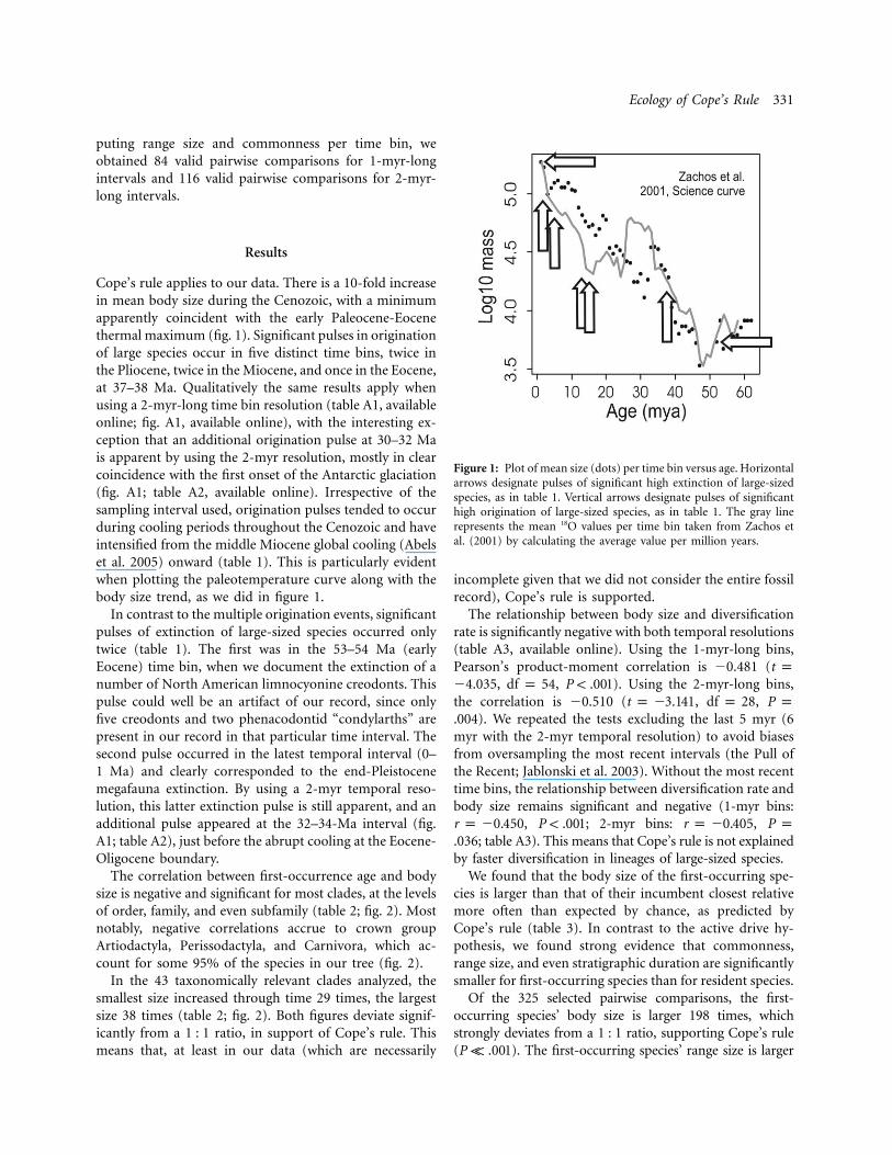
Figure 1: Plot of mean size (dots) per time bin versus age. Horizontalarrows designate pulses of significant high extinction of large-sizedspecies, as in table 1. Vertical arrows designate pulses of significanthigh origination of large-sized species, as in table 1. The gray linerepresents the mean 18O values per time bin taken from Zachos etal. (2001) by calculating the average value per million years.

puting range size and commonness per time bin, weobtained 84 valid pairwise comparisons for 1-myr-longintervals and 116 valid pairwise comparisons for 2-myr-long intervals.

Results

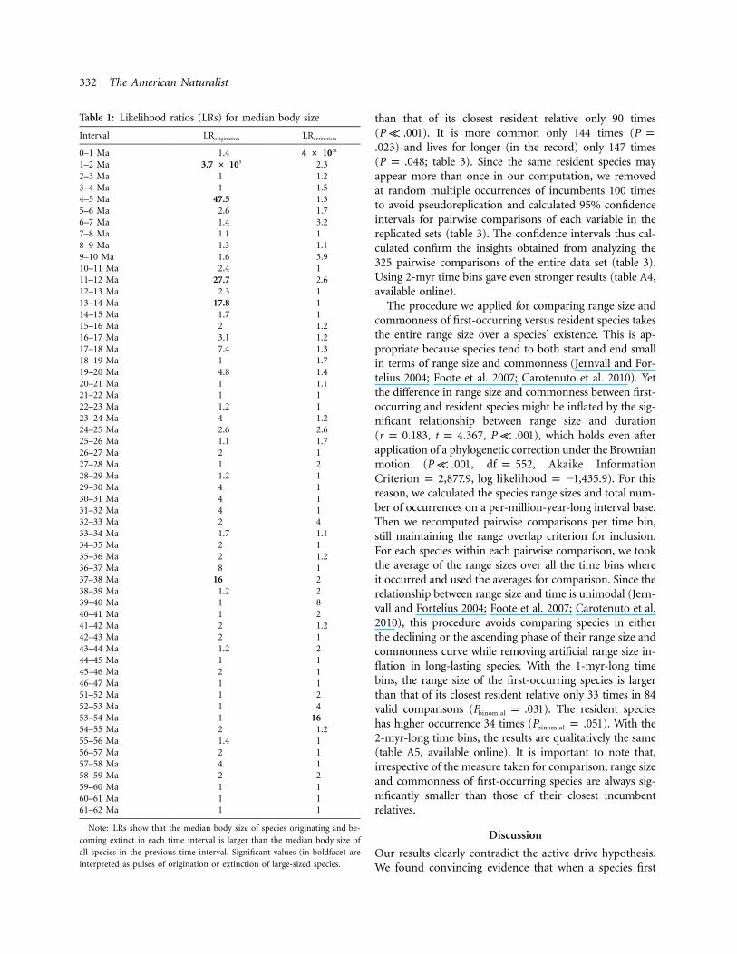
Cope’s rule applies to our data. There is a 10-fold increasein mean body size during the Cenozoic, with a minimumapparently coincident with the early Paleocene-Eocenethermal maximum (fig. 1). Significant pulses in originationof large species occur in five distinct time bins, twice inthe Pliocene, twice in the Miocene, and once in the Eocene,at 37–38 Ma. Qualitatively the same results apply whenusing a 2-myr-long time bin resolution (table A1, availableonline; fig. A1, available online), with the interesting ex-ception that an additional origination pulse at 30–32 Mais apparent by using the 2-myr resolution, mostly in clearcoincidence with the first onset of the Antarctic glaciation(fig. A1; table A2, available online). Irrespective of thesampling interval used, origination pulses tended to occurduring cooling periods throughout the Cenozoic and haveintensified from the middle Miocene global cooling (Abelset al. 2005) onward (table 1). This is particularly evidentwhen plotting the paleotemperature curve along with thebody size trend, as we did in figure 1.

In contrast to the multiple origination events, significantpulses of extinction of large-sized species occurred onlytwice (table 1). The first was in the 53–54 Ma (earlyEocene) time bin, when we document the extinction of anumber of North American limnocyonine creodonts. Thispulse could well be an artifact of our record, since onlyfive creodonts and two phenacodontid “condylarths” arepresent in our record in that particular time interval. Thesecond pulse occurred in the latest temporal interval (0–1 Ma) and clearly corresponded to the end-Pleistocenemegafauna extinction. By using a 2-myr temporal reso-lution, this latter extinction pulse is still apparent, and anadditional pulse appeared at the 32–34-Ma interval (fig.A1; table A2), just before the abrupt cooling at the Eocene-Oligocene boundary.

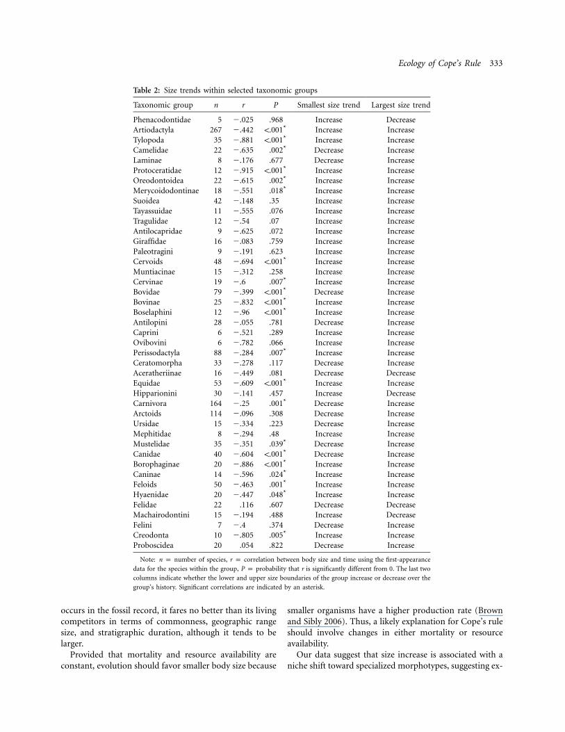
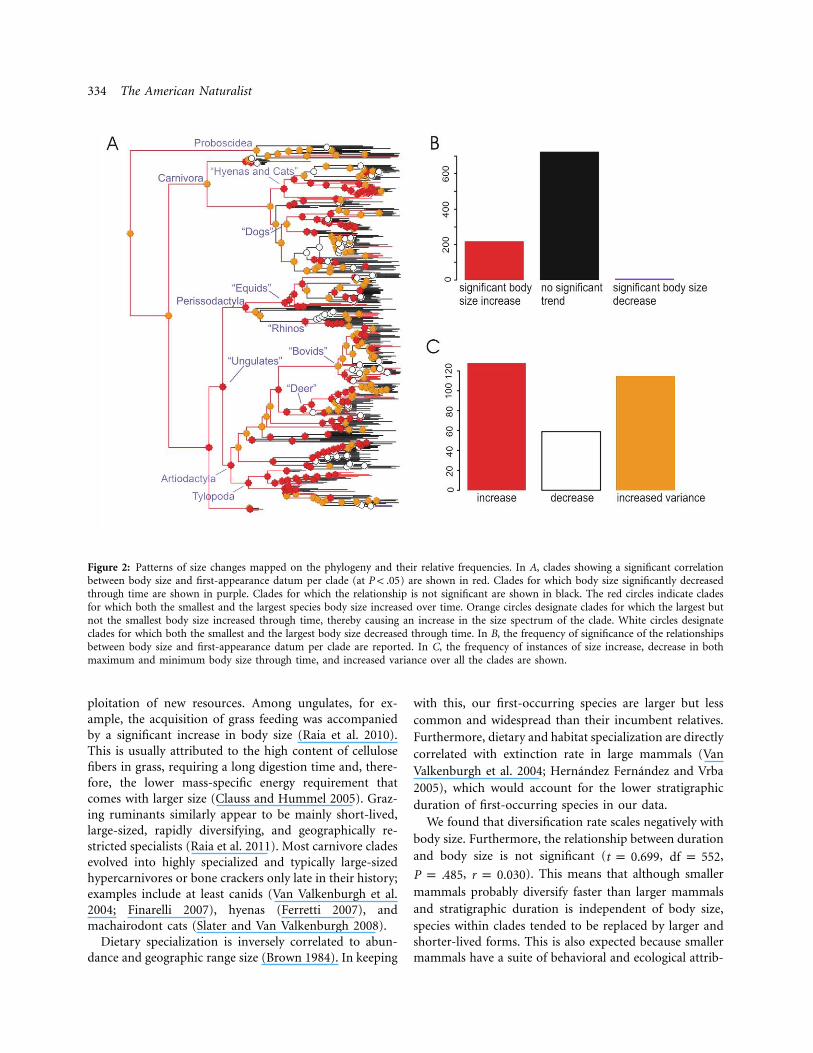
The correlation between first-occurrence age and bodysize is negative and significant for most clades, at the levelsof order, family, and even subfamily (table 2; fig. 2). Mostnotably, negative correlations accrue to crown groupArtiodactyla, Perissodactyla, and Carnivora, which ac-count for some 95% of the species in our tree (fig. 2).

In the 43 taxonomically relevant clades analyzed, thesmallest size increased through time 29 times, the largestsize 38 times (table 2; fig. 2). Both figures deviate signif-icantly from a 1 : 1 ratio, in support of Cope’s rule. Thismeans that, at least in our data (which are necessarily

incomplete given that we did not consider the entire fossilrecord), Cope’s rule is supported.

The relationship between body size and diversificationrate is significantly negative with both temporal resolutions(table A3, available online). Using the 1-myr-long bins,Pearson’s product-moment correlation is �0.481 (t p

, , ). Using the 2-myr-long bins,�4.035 df p 54 P ! .001the correlation is �0.510 ( , ,t p �3.141 df p 28 P p

). We repeated the tests excluding the last 5 myr (6.004myr with the 2-myr temporal resolution) to avoid biasesfrom oversampling the most recent intervals (the Pull ofthe Recent; Jablonski et al. 2003). Without the most recenttime bins, the relationship between diversification rate andbody size remains significant and negative (1-myr bins:

, ; 2-myr bins: ,r p �0.450 P ! .001 r p �0.405 P p; table A3). This means that Cope’s rule is not explained.036

by faster diversification in lineages of large-sized species.We found that the body size of the first-occurring spe-

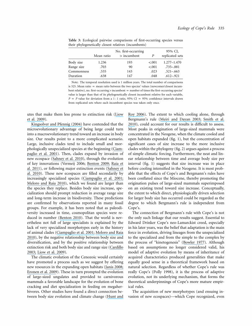
cies is larger than that of their incumbent closest relativemore often than expected by chance, as predicted byCope’s rule (table 3). In contrast to the active drive hy-pothesis, we found strong evidence that commonness,range size, and even stratigraphic duration are significantlysmaller for first-occurring species than for resident species.

Of the 325 selected pairwise comparisons, the first-occurring species’ body size is larger 198 times, whichstrongly deviates from a 1 : 1 ratio, supporting Cope’s rule( ). The first-occurring species’ range size is largerP K .001

332 The American Naturalist

Table 1: Likelihood ratios (LRs) for median body size

Interval LRorigination LRextinction

0–1 Ma 1.4 4 # 1031

1–2 Ma 3.7 # 105 2.32–3 Ma 1 1.23–4 Ma 1 1.54–5 Ma 47.5 1.35–6 Ma 2.6 1.76–7 Ma 1.4 3.27–8 Ma 1.1 18–9 Ma 1.3 1.19–10 Ma 1.6 3.910–11 Ma 2.4 111–12 Ma 27.7 2.612–13 Ma 2.3 113–14 Ma 17.8 114–15 Ma 1.7 115–16 Ma 2 1.216–17 Ma 3.1 1.217–18 Ma 7.4 1.318–19 Ma 1 1.719–20 Ma 4.8 1.420–21 Ma 1 1.121–22 Ma 1 122–23 Ma 1.2 123–24 Ma 4 1.224–25 Ma 2.6 2.625–26 Ma 1.1 1.726–27 Ma 2 127–28 Ma 1 228–29 Ma 1.2 129–30 Ma 4 130–31 Ma 4 131–32 Ma 4 132–33 Ma 2 433–34 Ma 1.7 1.134–35 Ma 2 135–36 Ma 2 1.236–37 Ma 8 137–38 Ma 16 238–39 Ma 1.2 239–40 Ma 1 840–41 Ma 1 241–42 Ma 2 1.242–43 Ma 2 143–44 Ma 1.2 244–45 Ma 1 145–46 Ma 2 146–47 Ma 1 151–52 Ma 1 252–53 Ma 1 453–54 Ma 1 1654–55 Ma 2 1.255–56 Ma 1.4 156–57 Ma 2 157–58 Ma 4 158–59 Ma 2 259–60 Ma 1 160–61 Ma 1 161–62 Ma 1 1

Note: LRs show that the median body size of species originating and be-

coming extinct in each time interval is larger than the median body size of

all species in the previous time interval. Significant values (in boldface) are

interpreted as pulses of origination or extinction of large-sized species.

than that of its closest resident relative only 90 times( ). It is more common only 144 times (P K .001 P p

) and lives for longer (in the record) only 147 times.023( ; table 3). Since the same resident species mayP p .048appear more than once in our computation, we removedat random multiple occurrences of incumbents 100 timesto avoid pseudoreplication and calculated 95% confidenceintervals for pairwise comparisons of each variable in thereplicated sets (table 3). The confidence intervals thus cal-culated confirm the insights obtained from analyzing the325 pairwise comparisons of the entire data set (table 3).Using 2-myr time bins gave even stronger results (table A4,available online).

The procedure we applied for comparing range size andcommonness of first-occurring versus resident species takesthe entire range size over a species’ existence. This is ap-propriate because species tend to both start and end smallin terms of range size and commonness (Jernvall and For-telius 2004; Foote et al. 2007; Carotenuto et al. 2010). Yetthe difference in range size and commonness between first-occurring and resident species might be inflated by the sig-nificant relationship between range size and duration( , , ), which holds even afterr p 0.183 t p 4.367 P K .001application of a phylogenetic correction under the Brownianmotion ( , ,P K .001 df p 552 Akaike Information

, ). For thisCriterion p 2,877.9 log likelihood p �1,435.9reason, we calculated the species range sizes and total num-ber of occurrences on a per-million-year-long interval base.Then we recomputed pairwise comparisons per time bin,still maintaining the range overlap criterion for inclusion.For each species within each pairwise comparison, we tookthe average of the range sizes over all the time bins whereit occurred and used the averages for comparison. Since therelationship between range size and time is unimodal (Jern-vall and Fortelius 2004; Foote et al. 2007; Carotenuto et al.2010), this procedure avoids comparing species in eitherthe declining or the ascending phase of their range size andcommonness curve while removing artificial range size in-flation in long-lasting species. With the 1-myr-long timebins, the range size of the first-occurring species is largerthan that of its closest resident relative only 33 times in 84valid comparisons ( ). The resident speciesP p .031binomial

has higher occurrence 34 times ( ). With theP p .051binomial

2-myr-long time bins, the results are qualitatively the same(table A5, available online). It is important to note that,irrespective of the measure taken for comparison, range sizeand commonness of first-occurring species are always sig-nificantly smaller than those of their closest incumbentrelatives.

Discussion

Our results clearly contradict the active drive hypothesis.We found convincing evidence that when a species first

Ecology of Cope’s Rule 333

Table 2: Size trends within selected taxonomic groups

Taxonomic group n r P Smallest size trend Largest size trend

Phenacodontidae 5 �.025 .968 Increase DecreaseArtiodactyla 267 �.442 !.001* Increase IncreaseTylopoda 35 �.881 !.001* Increase IncreaseCamelidae 22 �.635 .002* Decrease IncreaseLaminae 8 �.176 .677 Decrease IncreaseProtoceratidae 12 �.915 !.001* Increase IncreaseOreodontoidea 22 �.615 .002* Increase IncreaseMerycoidodontinae 18 �.551 .018* Increase IncreaseSuoidea 42 �.148 .35 Increase IncreaseTayassuidae 11 �.555 .076 Increase IncreaseTragulidae 12 �.54 .07 Increase IncreaseAntilocapridae 9 �.625 .072 Increase IncreaseGiraffidae 16 �.083 .759 Increase IncreasePaleotragini 9 �.191 .623 Increase IncreaseCervoids 48 �.694 !.001* Increase IncreaseMuntiacinae 15 �.312 .258 Increase IncreaseCervinae 19 �.6 .007* Increase IncreaseBovidae 79 �.399 !.001* Decrease IncreaseBovinae 25 �.832 !.001* Increase IncreaseBoselaphini 12 �.96 !.001* Increase IncreaseAntilopini 28 �.055 .781 Decrease IncreaseCaprini 6 �.521 .289 Increase IncreaseOvibovini 6 �.782 .066 Increase IncreasePerissodactyla 88 �.284 .007* Increase IncreaseCeratomorpha 33 �.278 .117 Decrease IncreaseAceratheriinae 16 �.449 .081 Decrease DecreaseEquidae 53 �.609 !.001* Increase IncreaseHipparionini 30 �.141 .457 Increase DecreaseCarnivora 164 �.25 .001* Decrease IncreaseArctoids 114 �.096 .308 Decrease IncreaseUrsidae 15 �.334 .223 Decrease IncreaseMephitidae 8 �.294 .48 Increase IncreaseMustelidae 35 �.351 .039* Decrease IncreaseCanidae 40 �.604 !.001* Decrease IncreaseBorophaginae 20 �.886 !.001* Increase IncreaseCaninae 14 �.596 .024* Increase IncreaseFeloids 50 �.463 .001* Increase IncreaseHyaenidae 20 �.447 .048* Increase IncreaseFelidae 22 .116 .607 Decrease DecreaseMachairodontini 15 �.194 .488 Increase DecreaseFelini 7 �.4 .374 Decrease IncreaseCreodonta 10 �.805 .005* Increase IncreaseProboscidea 20 .054 .822 Decrease Increase

Note: n p number of species, r p correlation between body size and time using the first-appearance

data for the species within the group, P p probability that r is significantly different from 0. The last two

columns indicate whether the lower and upper size boundaries of the group increase or decrease over the

group’s history. Significant correlations are indicated by an asterisk.

occurs in the fossil record, it fares no better than its livingcompetitors in terms of commonness, geographic rangesize, and stratigraphic duration, although it tends to belarger.

Provided that mortality and resource availability areconstant, evolution should favor smaller body size because

smaller organisms have a higher production rate (Brownand Sibly 2006). Thus, a likely explanation for Cope’s ruleshould involve changes in either mortality or resourceavailability.

Our data suggest that size increase is associated with aniche shift toward specialized morphotypes, suggesting ex-

334 The American Naturalist

Figure 2: Patterns of size changes mapped on the phylogeny and their relative frequencies. In A, clades showing a significant correlationbetween body size and first-appearance datum per clade (at ) are shown in red. Clades for which body size significantly decreasedP ! .05through time are shown in purple. Clades for which the relationship is not significant are shown in black. The red circles indicate cladesfor which both the smallest and the largest species body size increased over time. Orange circles designate clades for which the largest butnot the smallest body size increased through time, thereby causing an increase in the size spectrum of the clade. White circles designateclades for which both the smallest and the largest body size decreased through time. In B, the frequency of significance of the relationshipsbetween body size and first-appearance datum per clade are reported. In C, the frequency of instances of size increase, decrease in bothmaximum and minimum body size through time, and increased variance over all the clades are shown.

ploitation of new resources. Among ungulates, for ex-ample, the acquisition of grass feeding was accompaniedby a significant increase in body size (Raia et al. 2010).This is usually attributed to the high content of cellulosefibers in grass, requiring a long digestion time and, there-fore, the lower mass-specific energy requirement thatcomes with larger size (Clauss and Hummel 2005). Graz-ing ruminants similarly appear to be mainly short-lived,large-sized, rapidly diversifying, and geographically re-stricted specialists (Raia et al. 2011). Most carnivore cladesevolved into highly specialized and typically large-sizedhypercarnivores or bone crackers only late in their history;examples include at least canids (Van Valkenburgh et al.2004; Finarelli 2007), hyenas (Ferretti 2007), andmachairodont cats (Slater and Van Valkenburgh 2008).

Dietary specialization is inversely correlated to abun-dance and geographic range size (Brown 1984). In keeping

with this, our first-occurring species are larger but lesscommon and widespread than their incumbent relatives.Furthermore, dietary and habitat specialization are directlycorrelated with extinction rate in large mammals (VanValkenburgh et al. 2004; Hernandez Fernandez and Vrba2005), which would account for the lower stratigraphicduration of first-occurring species in our data.

We found that diversification rate scales negatively withbody size. Furthermore, the relationship between durationand body size is not significant ( , ,t p 0.699 df p 552

, ). This means that although smallerP p .485 r p 0.030mammals probably diversify faster than larger mammalsand stratigraphic duration is independent of body size,species within clades tended to be replaced by larger andshorter-lived forms. This is also expected because smallermammals have a suite of behavioral and ecological attrib-

Ecology of Cope’s Rule 335

Table 3: Ecological pairwise comparisons of first-occurring species versustheir phylogenetically closest relatives (incumbents)

Mean ratioNo. first-occurring

1 incumbent P95% CI,

replicated sets

Body size 1.236 193 !.001 1.277–1.470Range size .703 90 !.001 .735–.881Commonness .535 143 .023 .521–.663Duration .638 147 .048 .612–.921

Note: The temporal resolution used is 1 million years. The total number of comparisons

is 325. Mean ratio p mean ratio between the two species’ values (newcomer/closest incum-

bent relative), no. first-occurring 1 incumbent p number of times the first-occurring species’

value is larger than that of its phylogenetically closest incumbent relative for each variable,

P p P value for deviation from a 1 : 1 ratio, 95% CI p 95% confidence intervals drawn

from replicated sets where each incumbent species was taken only once.

utes that make them less prone to extinction risk (Liowet al. 2009).

Kingsolver and Pfennig (2004) have contended that themicroevolutionary advantage of being large could turninto a macroevolutionary trend toward an increase in bodysize. Our results point to a more complicated scenario.Large, inclusive clades tend to include small and mor-phologically unspecialized species at the beginning (Ciam-paglio et al. 2001). Then, clades expand by invasion ofnew ecospace (Sahney et al. 2010), through the evolutionof key innovations (Vermeij 2006; Benton 2009; Raia etal. 2011), or following major extinction events (Sahney etal. 2010). These new ecospaces are filled secondarily byincreasingly specialized species (Ciampaglio et al. 2001;Meloro and Raia 2010), which we found are larger thanthe species they replace. Besides body size increase, spe-cialization should prompt reduction in average range sizeand long-term increase in biodiversity. These predictionsare confirmed by observations reported in many fossilgroups. For example, it has been noted that as paleodi-versity increased in time, cosmopolitan species were re-duced in number (Benton 2010). That the world is nev-ertheless not full of large specialists is explained by thelack of very specialized morphotypes early in the historyof animal clades (Ciampaglio et al. 2001; Meloro and Raia2010), by the negative relationship between body size anddiversification, and by the positive relationship betweenextinction risk and both body size and range size (Cardillo2003; Liow et al. 2009).

The climatic evolution of the Cenozoic would certainlyhave promoted a process such as we suggest by offeringnew resources in the expanding open habitats (Janis 2008;Eronen et al. 2009). These in turn prompted the evolutionof large-sized ungulates and provided to carnivorousmammals a favorable landscape for the evolution of bonecracking and diet specialization in feeding on megaher-bivores. Other studies have found a direct connection be-tween body size evolution and climate change (Hunt and

Roy 2006). The extent to which cooling alone, throughBergmann’s rule (Meiri and Dayan 2003; Smith et al.2010), could account for our results is difficult to assess.Most peaks in origination of large-sized mammals wereconcentrated in the Neogene, when the climate cooled andopen habitats expanded (fig. 1), but the concentration ofsignificant cases of size increase to the more inclusiveclades within the phylogeny (fig. 2) argues against a processof simple climatic forcing. Furthermore, the neat and lin-ear relationship between time and average body size perinterval (fig. 1) suggests that size increase was in placebefore cooling intensified in the Neogene. It is most prob-able that the effects of Cope’s and Bergmann’s rules havebeen conflated since the Miocene, thereby promoting theorigination pulses of large-sized mammals superimposedon an existing trend toward size increase. Conceptually,the extent to which direct, physiologically driven selectionfor larger body size has occurred could be regarded as thedegree to which Bergmann’s rule is independent fromCope’s.

The connection of Bergmann’s rule with Cope’s is notthe only such linkage that our results suggest. Essential toEdward Drinker Cope’s neo-Lamarckist creed, especiallyin his later years, was the belief that adaptation is the mainforce in evolution, driving lineages from the unspecializedto the specialized and from the simple to the complex bythe process of “kinetogenesis” (Bowler 1977). Althoughbased on assumptions no longer considered valid, hismodel of adaptive evolution by means of inheritance ofacquired characteristics produced generalities that makeequally good sense in a theoretical framework based onnatural selection. Regardless of whether Cope’s rule wasreally Cope’s (Polly 1998), it is the process of adaptiveevolution, not its underlying mechanism, that forms thetheoretical underpinnings of Cope’s more mature empir-ical rules.

The acquisition of new morphotypes (and ensuing in-vasion of new ecospaces)—which Cope recognized, even

336 The American Naturalist

without having the morphotype concept at hand—can, ina contemporary framework, be comfortably attributed tothe exploration of new resources and habitats by special-ized forms. The early dominance in evolving clades ofunspecialized small-sized forms and the subsequent nicheexpansion provided by new specialized morphotypes oflarger size appears to us to be the most likely fundamentaldriver of Cope’s rule of size increase in mammals.

Acknowledgments

We are grateful to A. Gentry, who kindly helped us incorrecting the taxonomy of bovids in the tree and gave usimportant insights as to the phylogenetic position of someclades. We are grateful to Neogene of the Old World Da-tabase contributors for their continuous support andwork. S. Meiri, C. Meloro, and P. Piras discussed with ussome of the issues we dealt with in this article. M. Benton,D. Polly, and one anonymous referee reviewed the man-uscript and provided fundamental advice to improve itsquality. This study grew out of a study visit by P.R. toHelsinki, which was supported by a grant (to M.F.) fromthe Academy of Finland.

Literature Cited

Abels, H. A., F. J. Hilgen, W. Krijgsman, R. W. Kruk, I. Raffi, E.Turco, and W. J. Zachariasse. 2005. Long-period orbital controlon middle Miocene global cooling: integrated stratigraphy andastronomical tuning of the Blue Clay Formation on Malta.Paleoceanography 20:PA4012.

Alroy, J. 1998. Cope’s rule and the dynamics of body mass evolutionin North American mammals. Science 280:731–734.

Arnold, A. J., D. C. Kelly, and W. C. Parker. 1995. Causality andCope’s rule: evidence from the planktonic foraminifera. Journalof Paleontology 69:203–210.

Benton, M. J. 2009. The Red Queen and the Court Jester: speciesdiversity and the role of biotic and abiotic factors through time.Science 323:728–732.

———. 2010. The origins of modern biodiversity on land. Philo-sophical Transactions of the Royal Society B: Biological Sciences365:3667–3679.

Bowler, P. J. 1977. Edward Drinker Cope and the changing structureof evolutionary theory. Isis 68:249–265.

Brown, J. H. 1984. On the relationship between abundance and dis-tribution of species. American Naturalist 124:255–279.

Brown, J. H., and R. M. Sibly. 2006. Life-history evolution under aproduction constraint. Proceedings of the National Academy ofSciences of the USA 103:17595–17599.

Butler, R., and A. Goswami. 2008. Body size evolution in Mesozoicbirds: little evidence for Cope’s rule. Journal of Evolutionary Bi-ology 21:1673–1682.

Cardillo, M. 2003. Biological determinants of extinction risk: whyare smaller species less vulnerable? Animal Conservation 6:63–69.

Carotenuto, F., C. Barbera, and P. Raia. 2010. Occupancy, range size

and phylogeny in Eurasian Pliocene to recent large mammals.Paleobiology 36:399–414.

Ciampaglio, C. N., M. Kemp, and D. W. McShea. 2001. Detectingchanges in morphospace occupation patterns in the fossil record:characterization and analysis of measures of disparity. Paleobiology27:695–715.

Clauset, A., and D. Erwin. 2008. The evolution and distribution ofspecies body size. Science 321:399–401.

Clauss, M., and J. Hummel. 2005. The digestive performance ofmammalian herbivores: why big may not be that much better.Mammal Reviews 35:174–187.

Cope, E. 1887. The origin of the fittest. Appleton, New York.Damuth, J., and B. J. MacFadden. 1990. Body size in mammalian

paleobiology. Cambridge University Press, Cambridge.Dayan, T., and D. Simberloff. 2005. Ecological and community-wide

character displacement: the next generation. Ecology Letters 8:875–894.

Eronen, J. T., M. M. Ataabadi, A. Micheels, A. Karme, R. L. Bernor,and M. Fortelius. 2009. Distribution history and climatic controlsof the Late Miocene Pikermian chronofauna. Proceedings of theNational Academy of Sciences of the USA 106:11867–11871.

Ezard, T., and A. Purvis. 2009. paleoPhylo: biodiversity analyses ina paleontological and phylogenetic context. R package version 1.0-97/r127.

Ferretti, M. P. 2007. Evolution of bone-cracking adaptations inhyaenids (Mammalia, Carnivora). Swiss Journal of Geosciences100:41–52.

Finarelli, J. A. 2007. Mechanisms behind active trends in body sizeevolution of the Canidae (Carnivora: Mammalia). American Nat-uralist 170:876–885.

Foote, M., J. S. Crampton, A. G. Beu, B. A. Marshall, R. A. Cooper,P. A. Maxwell, and I. Matcham. 2007. Rise and fall of speciesoccupancy in Cenozoic marine mollusks. Science 318:1131–1134.

Gingerich, P. 1974. Stratigraphic record of early Eocene Hyopsodusand the geometry of mammalian phylogeny. Nature 248:107–109.

Gould, S. J. 1988. Trends as changes in variance: a new slant on bodysize evolution. Journal of Paleontology 62:319–329.

Heim, N. A., and S. E. Peters. 2011. Regional environmental breadthpredicts geographic range and longevity in fossil marine genera.PLoS ONE 6(5):e18946.

Hernandez Fernandez, M., and E. S. Vrba. 2005. Macroevolutionaryprocesses and biomic specialization: testing the resource-use hy-pothesis. Evolutionary Ecology 19:199–219.

Hone, D. W. E., and M. Benton. 2005. The evolution of large size:how does Cope’s rule work? Trends in Ecology & Evolution 20:4–6.

———. 2007. Cope’s rule in the Pterosauria, and differing percep-tions of Cope’s rule at different taxonomic levels. Journal of Evo-lutionary Biology 20:1164–1170.

Hone, D. W. E., G. J. Dyke, M. Haden, and M. Benton. 2008. Bodysize evolution in Mesozoic birds. Journal of Evolutionary Biology21:618–624.

Hunt, G., and K. Roy. 2006. Climate change, body size evolution,and Cope’s rule in deep-sea ostracodes. Proceedings of the Na-tional Academy of Sciences of the USA 103:1347–1352.

Jablonski, D. 1997. Body-size evolution in Cretaceous mollusks andthe status of Cope’s rule. Nature 385:250–252.

Jablonski, D., and G. Hunt. 2006. Larval ecology, geographic range,and species survivorship in Cretaceous mollusks: organismic versusspecies-level explanations. American Naturalist 168:556–564.

Ecology of Cope’s Rule 337

Jablonski, D., K. Roy, J. W. Valentine, R. M. Price, and P. S. Anderson.2003. The impact of the Pull of the Recent on the history of marinediversity. Science 300:1133–1135.

Janis, C. M. 2008. An evolutionary history of browsing and grazingungulates. Pages 21–45 in I. J. Gordon and H. H. T. Prins, eds.The ecology of browsing and grazing. Springer, Berlin.

Jernvall, J., and M. Fortelius. 2004. Maintenance of trophic structurein fossil mammal communities: site occupancy and taxon resil-ience. American Naturalist 164:614–624.

Kingsolver, J., and D. Pfennig. 2004. Individual-level selection as acause of Cope’s rule of phyletic size increase. Evolution 58:1608–1612.

Laurin, M. 2004. The evolution of body size, Cope’s rule and theorigin of amniotes. Systematic Biology 53:594–622.

Liow, L. H., M. Fortelius, K. Lintulaakso, H. Mannila, and N. C.Stenseth. 2009. Lower extinction risk in sleep-or-hide mammals.American Naturalist 173:264–272.

Liow, L. H., T. B. Quental, and C. R. Marshall. 2010. When candecreasing diversification rates be detected with molecular phy-logenies and the fossil record? Systematic Biology 59:646–659.

Losos, J. B. 2011. Seeing the forest for the trees: the limitations ofphylogenies in comparative biology. American Naturalist 177:709–727.

Lyons, K. S. 2003. A quantitative assessment of the rate of rangeshifts of Pleistocene mammals. Journal of Mammalogy 84:385–402.

———. 2005. A quantitative model for assessing community dy-namics of Pleistocene mammals. American Naturalist 165:E168–E185.

McShea, D. W. 1994. Mechanisms of large-scale evolutionary trends.Evolution 48:1747–1763.

Meiri, S., and T. Dayan. 2003. On the validity of Bergmann’s rule.Journal of Biogeography 30:331–351.

Meloro, C., and P. Raia. 2010. Cats and dogs down the tree: thetempo and mode of evolution in the lower carnassial of fossil andliving Carnivora. Evolutionary Biology 37:177–186.

Meloro, C., P. Raia, P. Piras, C. Barbera, and P. O’Higgins. 2008. Theshape of the mandibular corpus in large fissiped carnivores: al-lometry, function and phylogeny. Zoological Journal of the Lin-nean Society 154:832–845.

Monroe, M. J., and F. Bokma. 2010. Little evidence for Cope’s rulefrom Bayesian phylogenetic analysis of extant mammals. Journalof Evolutionary Biology 23:2017–2021.

Novack-Gottshall, P. M., and M. A. Lanier. 2008. Scale-dependenceof Cope’s rule in body size evolution of Paleozoic brachiopods.Proceedings of the National Academy of Sciences of the USA 105:5430–5434.

Polly, P. D. 1998. Cope’s rule. Science 282:50–51.

Quental, T. B., and C. R. Marshall. 2010. Diversity dynamics: mo-lecular phylogenies need the fossil record. Trends in Ecology &Evolution 25:434–441.

Rabosky, D. L. 2010. Extinction rates should not be estimated frommolecular phylogenies. Evolution 64:1816–1824.

Raia, P. 2010. Phylogenetic community assembly over time in Eur-asian Plio-Pleistocene mammals. Palaios 25:327–338.

Raia, P., C. Meloro, A. Loy, and C. Barbera. 2006. Species occupancyand its course in the past: macroecological patterns in extinctcommunities. Evolutionary Ecology Research 8:181–194.

Raia, P., F. Carotenuto, C. Meloro, P. Piras, and D. Pushkina. 2010.The shape of contention: adaptation, history, and contingency inungulate mandibles. Evolution 64:1489–1503.

Raia, P., F. Carotenuto, J. T. Eronen, and M. Fortelius. 2011. Longerin the tooth, shorter in the record? the evolutionary correlates ofhypsodonty in Neogene ruminants. Proceedings of the Royal So-ciety B: Biological Sciences 278:3474–3481.

Rensch, B. 1954. Neuere Probleme der Abstammungslehre. Ferdi-nand Enke, Stuttgart.

Simpson, G. G. 1953. The major features of evolution. ColumbiaUniversity Press, New York.

Slater, G. J., and B. Van Valkenburgh. 2008. Long in the tooth: evo-lution of sabertooth cat cranial shape. Paleobiology 34:403–419.

Smith, F. A., A. G. Boyer, J. H. Brown, D. P. Costa, T. Dayan, S. K.M. Ernest, A. R. Evans, et al. 2010. The evolution of maximumbody size of terrestrial mammals. Science 330:1216–1219.

Sahney, S., M. J. Benton, and P. A. Ferry. 2010. Links between globaltaxonomic diversity, ecological diversity, and the expansion of ver-tebrates on land. Biology Letters 6:544–547.

Stanley, S. 1973. An explanation for Cope’s rule. Evolution 27:1–26.Tarver, J. E., and P. J. C. Donoghue. 2011. The trouble with topology:

phylogenies without fossils provide a revisionist perspective of evo-lutionary history in topological analyses of diversity. SystematicBiology 60:700–712.

Van Valkenburgh, B., X. Wang, and J. Damuth. 2004. Cope’s rule,hypercarnivory, and extinction in North American canids. Science306:101–104.

Vermeij, G. J. 2006. Nature: an economic history. Princeton Uni-versity Press, Princeton, NJ.

Wagner, P. J. 1996. Contrasting the underlying patterns of activetrends in morphologic evolution. Evolution 50:990–1007.

Wilson, E. O. 1987. Causes of ecological success: the case of the ants.Journal of Animal Ecology 56:1–9.

Zachos, J., M. Pagani, L. Sloan, E. Thomas, and K. Billups. 2001.Trends, rhythms, and aberrations in global climate 65 Ma to pres-ent. Science 292:686–693.

Associate Editor: Susan KaliszEditor: Mark A. McPeek