dynamics of complex systems chapter 4

420

# 29412 Cust: AddisonWesley Au: Bar-Yam Pg. No. 420Title: Dynamics Complex Systems Short / Normal / Long

4Protein Folding I:Size Scaling of Time

Conceptual Outline

The simplest question about dynamics—how long does a process take?—becomes particularly relevant when the time may be so long that the process cannothappen at all. A fundamental problem associated with the dynamics of protein fold-ing is understanding how a system of many interacting elements can reach a desiredstructure in a reasonable time. In this chapter, we discuss the parallel-processingidea for resolving this problem; kinetic pathways will be considered in the next chap-ter. Parallel processing and interdependence are at odds and must be balanced in thedesign of complex systems.

We use finite-size Ising type models to explore the nature of interactionsthat can allow a system to relax in a time that grows less than exponentially in the sizeof the system. These models illustrate various ways to realize the parallel-processingidea.

The simplest idealization of parallel processing is the case of completelyindependent spins. We discuss a two-spin model as a first example of how such asystem relaxes.

Various homogeneous models illustrate some of the properties that enablesystems to relax in a time that grows no more than a power law in the system size.These include ideal parallel processing, and nucleation and growth of a stable statefrom a metastable state. The models also illustrate cases where exponential growthin the relaxation time can prevent systems from relaxing.

Inhomogeneous models extend the range of possibilities for interaction ar-chitectures that still allow a reasonable relaxation time. Among these are space andtime partitioning and preselected initial conditions. However, inhomogeneous long-range interactions generally lead to an exponential growth of relaxation time withsystem size.

❚ 4 . 5 ❚

❚ 4 . 4 ❚

❚ 4 . 3 ❚

❚ 4 . 2 ❚

❚ 4 . 1 ❚

04adBARYAM_29412 3/10/02 10:37 AM Page 420

The Protein-Folding Problem

One of the simplest questions we can ask about the dynamics of a complex system is,How long does a process take? In some cases this question presumes that we have anunderstanding of the initial and final state of the process. In other cases we are look-ing for a characteristic time scale of dynamic change. For a complex system,a partic-ular process may not occur in any reasonable amount of time. The time that a dy-namic process takes is of central importance when a system has an identifiablefunction or purpose. We will consider this in the context of proteins, for which thisquestion is a fundamental issue in understanding molecular function in biologicalcells.

We begin by describing the structure of proteins, starting from their “primarystructure.” Proteins are molecules formed out of long chains of, typically, twenty dif-ferent kinds of amino acids. Amino acids can exist as separate molecules in water, butare constructed so that they can be covalently bonded in a linear chain by removal ofone water molecule per bond (Fig. 4.1.1). In general,molecules formed as long chainsof molecular units are called polymers. Proteins,RNA and DNA,as well as other typesof biological molecules (e.g., polysaccharides) are polymers. In biological cells, pro-teins are formed in a linear chain by transcription from RNA templates that are them-selves t ranscribed from DNA. The sequence of amino acids forming the protein iscalled its primary structure (Fig. 4.1.2). The active form of proteins (more specifically

4.1

Th e p ro t e i n - f o l d i n g p ro b l e m 421


Rn-1

C

O

C N

H

H

n-1C

O

C N

H

HRn

nC

O

C N

H

HRn+1

n+1

NH2-CHR-COOH

C

O

C N

H

HR

H

H

O

H-(NH-CHR-CO)N-OH

Figure 4.1.1 Illustration of the atomiccomposition of an amino acid. The usualnotation for carbon (C), oxygen (O), ni-trogen (N) and hydrogen (H) is used. Rstands for a radical that is generally ahydrocarbon chain and may contain hy-drocarbon rings. It is different for eachof the distinct amino acids, and is thedifference between them. The bottomfigure is a chain of amino acids formedby removing a single water moleculeand bonding one nitrogen to the car-bon of the next amino acid. Thesequence of amino acids is theprimary structure of the pro-tein (see Fig. 4.1.2). ❚

04adBARYAM_29412 3/10/02 10:37 AM Page 421

422 P ro te i n Fo l d i ng I


MVRITQLLGIRLFRLEGWEVTLA

RIEIEADLDKLILVGAMMRGREN

LTMKFAFVDLFAMLELDTGMALL

NNKRLADDDESHQTWTYEEEQPK

PKEEISDEQQEHNNAREMSEKQA

GIRYEALYSNLFRPMFSLEGEDM

QAVADIIQIYGVIDTTWEEFLDM

QHGADGLDYRYNPDRHLGELTLA

QLQLKEKTSSGKYDNWYSLPFIA

AITGVRPMWSATLSLLEEDJTWL

VRLMLDTTRGEQOASATLQQLER

EGGKLRLSGRLYSFMESDVSCQG

FCRAQILQAIKKGLFIPEQSKEK

VGKNQFLYRLVDGRTQSPLIER

TYEFLAQEPKLYTIARPMMDRK

GQASIHALQASASVSLKTTERV

PARLSCNVNAAIFNFAALLDQV

CRGFTYEKLNNLFTDEATHNYS

LHLDIGELVINYSPMREQAIGA

VI

MDSLVLLLERRKGEMVSDEE

LAITNYRVLIEGPRLPRVKELE

AASDWDKGSAHNEESI

MTGEVR

GVTQKARSQNEHIIQAKRLRRM

ATFLNHWRDNAQKGTANFERPQ

GFHADLQAFPESDPLVVTFLEK

STTLLKNRPHRRLASRNLPAPG

GNLLKAKFAVVVLTGDQRYYSQ

KKGKTCITLFTFALRLLDVVRS

TALEPNRVKEGEYKGIFMYGFH

RADLSVYVVKEKLKYHSMMILL

––––––––––––––––––––––

Common Amino AcidsName Notation Name NotationGlycine (gly, G) Cysteine (cys, C)Alanine (ala, A) Methionine (met, M)Valine (val, V) Asparagine (asn, N)Leucine (leu, L) Glutamine (gln, Q)Isoleucine (ile, I) Aspartic acid (asp, D)Phenylalanine (phe, F) Glutamic acid (glu, E)Tyrosine (tyr, Y) Lysine (lys, K)Tryptophan (trp, W) Arginine (arg, R)Serine (ser, S) Histidine (his, H)Threonine (thr, T) Proline (pro, P)

Figure 4.1.2 Amino acid sequence of the protein acetylcholinesterase — its primary struc-ture. A list of common amino acids and their commonly used three-letter and one-letter no-tation is attached. ❚

04adBARYAM_29412 3/10/02 10:37 AM Page 422

Th e p ro t e i n - fo l d i n g p ro b l e m 423


globular proteins) is, however, a tightly bound three-dimensional (3-d) structure(Fig. 4.1.3) with active sites on the surface. The active sites serve enzymatic roles,con-trolling chemical reactions in the cell. The transformation of the linear protein chainto the enzymatically active 3-d structure is known as protein folding. The 3-d struc-ture arises because of additional bonding between the amino acids of the chain. Thesebonds are characteristically weaker than the covalent bonds along the chain.They in-clude hydrogen bonds, van der Waals bonds and a few covalent sulfur-sulfur(disulfide) bonds. The relative weakness of the bonds responsible for the 3-d struc-ture makes the distinction between the primary and 3-d structure meaningful.

The 3-d structure of proteins can be further analyzed in terms of secondary, ter-tiary and,sometimes, quaternary structure. These describe levels of spatial organiza-tion between individual amino acids and the complete 3-d structure.A plot of the pro-tein chain backbone in space (Fig. 4.1.3 (b)) generally reveals two kinds of amino acid

(a)

(b)

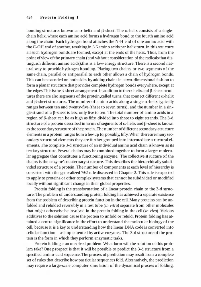
F i g u re 4 . 1 . 3 T h re e -dimensional structure ofthe protein acetylchol-inesterase. The top pic-ture is constructed usingspace-filling balls thatschematically portray theelectron density of eachatom. The bottom illus-tration is a simplified ver-sion showing only thebackbone of the protein.Helical segments ( -he-lices) and regions of par-allel chains ( -sheets)are visible. They are illus-trated as ribbons to dis-tinguish them from theconnecting regions of thechain (turns). The -he-lices, -sheets and turnsconstitute the secondarystructure of the protein.(Rendered on a Macintoshusing RasMol [developedby Roger Sayle] and aNational Institutes ofHealth protein databank(PDB) file) ❚

04adBARYAM_29412 3/10/02 10:37 AM 23

bonding structures known as -helix and -sheet. The -helix consists of a single-chain helix, where each amino acid forms a hydrogen bond to the fourth amino acidalong the chain. Each hydrogen bond attaches the N-H end of one amino acid withthe C-OH end of another, resulting in 3.6 amino acids per helix turn. In this structureall such hydrogen bonds are formed, except at the ends of the helix. Thus, from thepoint of view of the primary chain (and without consideration of the radicals that dis-tinguish different amino acids),this is a low-energy structure. There is a second nat-ural way to provide hydrogen bonding. Placing two chains, or two segments of thesame chain, parallel or antiparallel to each other allows a chain of hydrogen bonds.This can be extended on both sides by adding chains in a two-dimensional fashion toform a planar structure that provides complete hydrogen bonds everywhere, except atthe edges.This is the -sheet arrangement. In addition to the -helix and -sheet struc-tu res there are also segm ents of the pro tei n ,c a ll ed tu rn s , that con n ect different - h elixand -sheet structures. The number of amino acids along a single -helix typicallyranges between ten and twenty-five (three to seven turns), and the number in a sin-gle strand of a -sheet is less, only five to ten. The total number of amino acids in aregion of -sheet can be as high as fifty, divided into three to eight strands. The 3-dstructure of a protein described in terms of segments of -helix and -sheet is knownas the secon d a ry stru ctu re of the pro tei n . The nu m ber of d i f ferent secon d a ry - s tru ctureelements in a protein ranges from a few up to, possibly, fifty. When there are many sec-ondary structural elements they are further grouped into intermediate structural el-ements. The complete 3-d structure of an individual amino acid chain is known as itstertiary structure. Several chains may be combined together to form a larger molecu-lar aggregate that constitutes a functioning enzyme. The collective structure of thechains is the enzyme’s quaternary structure. This describes the hierarchically subdi-vided structure of a protein. The number of components at each level of hierarchy isconsistent with the generalized 7±2 rule discussed in Chapter 2. This rule is expectedto apply to proteins or other complex systems that cannot be subdivided or modifiedlocally without significant change in their global properties.

Protein folding is the transformation of a linear protein chain to the 3-d struc-ture. The problem of understanding protein folding has achieved a separate existencefrom the problem of describing protein function in the cell. Many proteins can be un-folded and refolded reversibly in a test tube (in vitro) separate from other moleculesthat might otherwise be involved in the protein folding in the cell (in vivo). Variousadditives to the solution cause the protein to unfold or refold. Protein folding has at-tained a central significance in the effort to understand the molecular biology of thecell, because it is a key to understanding how the linear DNA code is converted intocellular function—as implemented by active enzymes. The 3-d structure of the pro-tein is the form in which they perform enzymatic tasks.

Protein folding is an unsolved problem. What form will the solution of this prob-lem take? One prospect is that it will be possible to predict the 3-d structure from aspecified amino-acid sequence. The process of prediction may result from a completeset of rules that describe how par ticular sequences fold. Alternatively, the predictionmay require a large-scale computer simulation of the dynamical process of folding.

424 P ro t e i n Fo l d i ng I


04adBARYAM_29412 3/10/02 10:37 AM Page 424

Most researchers studying protein folding are concerned with determining or pre-dicting the 3-d structure without describing the dynamics. Our concern is with thedynamics in a generalized context that applies to many complex systems.

From early on in the discussion of the protein-folding problem, it has been pos-sible to separate from the explicit protein-folding problem an implicit problem thatbegs for a fundamental resolution. How, in principle, can protein folding occur?Consider a system composed of elements, where each element may be found in anyof several states.A complete specification of the state of all the elements describes theconformation of the system. The number of possible conformations of the systemgrows exponentially with the number of elements. We require the system to reach aunique conformation—the folded structure. We may presume for now that the foldedstructure is the lowest energy conformation of the system. The amount of time nec-essary for the system to explore all possible conformations to find the lowest-energyone grows exponentially with system size. As discussed in the following paragraphs,this is impossible. Therefore we ask, How does a protein know where to go in the spaceof conformations to reach the folded structure?

We can adopt some very rough approximations to estimate how much time itwould take for a system to explore all possible conformations, when the number ofconformations grows exponentially with system size. Let us assume that there are 2N

conformations, where N is the size of the system—e.g.,the number of amino acids ina protein. Assume further that the system spends only one atomic oscillation time ineach conformation before moving on to the next one. This is a low estimate,so ourresult will be a reasonable lower bound on the exploration time.An atomic oscillationtime in a material is approximately 10−12 sec. We should increase this by at least an or-der of magnitude, because we are talking about a whole amino acid moving ratherthan a single atom. Our conclusions, however, won’t be sensitive to this distinction.The time to relax would be 2N10−12 sec,if we assume optimistically that each possiblestate is visited exactly once before the right arrangement is found.

A protein folds in, of order, 1 second. For conformation space exploration towork, we would have to rest rict the number of amino acids to be smaller than thatgiven by the equation:

2N10−12 sec = 1 sec (4.1.1)

or N = 40. Real proteins are formed from chains that typically have 100 to 1000 aminoacids. Even if we were to just double our limit from 40 to 80 amino acids, we wouldhave a conformation exploration time of 1012 seconds or 32,000 years. The many or-ders of magnitude that separate a reasonable result from this simple estimate suggeststhat there must be something fundamentally wrong with our way of thinking aboutthe problem as an exploration of possible conformations.Figuring out what is a rea-sonable picture,and providing justification for it,is the fundamental protein-foldingproblem.

The fundamental protein-folding problem applies to other complex systems aswell.A complex system always has a large set of possible conformations. The dynam-ics of a complex system takes it from one type of conformation to another type of

Th e p ro t e i n - f o l d i n g p ro b l e m 425


04adBARYAM_29412 3/10/02 10:37 AM Page 425

conformation. By the argument presented above, the dynamics cannot explore allpossible conformations in order to reach the final conformation. This applies to thedynamics of self-organization, adaptation or function. We can consider neural net-works (Chapters 2 and 3) as a second example. Three relevant dynamic processes arethe dynamics by which the neural network is formed during physiological develop-ment,the dynamics by which it adapts (is trained,learns) and the dynamics by whichit responds to external information. All of these cause the neural network to attain oneof a small set of conformations,selected from all of the possible conformations of thesystem. This implies that it does not explore all alternatives before realizing its finalform. Similar constraints apply to the dynamics of other complex systems.

Because the fundamental protein-folding problem exists on a very general level,it is reasonable to look at generic models to identify where a solution might exist. Twoconcepts have been articulated as responsible for the success of biological proteinfolding—parallel processing and kinetic pathways. The concept of parallel processingsuggests, quite reasonably, that more than one process of exploration may be done atonce. This can occur ifand only ifthe processes are in some sense independent. If par-allel processing works then, naively speaking, each amino acid can do its own explo-ration and the process will take very little time. In contrast to this picture,the idea ofkinetic pathways suggests that a protein starts from a class of conformations that nat-urally falls down in energy directly toward the folded structure. There are large barri-ers to other conformations and there is no complete phase space exploration. In thispicture there is no need for the folded structure to be the lowest energy conforma-tion—it just has to be the lowest among the accessible conformations.One way to en-visage this is as water flowing through a riverbed, confined by river banks, rather thanexploring all possible routes to the sea.

Our objective is to add to these ideas some concrete analysis of simple modelsthat provide an understanding of how parallel processing and kinetic pathways maywork. In this chapter we discuss the concept of parallel processing, or independent re-laxation, by developing a series of simple models. Section 4.2 describes the approxi-mations that will be used. Section 4.3 describes a decoupled two-variable model. Themain discussion is divided into homogeneous models in Section 4.4 and inhomoge-neous models in Section 4.5.In the next chapter we discuss the kinetic aspects of poly-mer collapse from an expanded to a compact structure as a first test of how kineticsmay play a role in protein folding. It is to be expected that the evolving biology of or-ganisms will take advantage of all possible “tricks” that enable proteins to fold in ac-ceptable time. Therefore it is likely that both parallel processing and kinetic effects doplay a role.By understanding the possible generic scenarios that enable rapid folding,we are likely to gain insight into the mechanisms that are actually used.

As we discuss various models of parallel processing we should keep in mind thatwe are not concerned with arbitrary physical systems, but rather with complex sys-tems. As discussed in S ection 1.3, a complex system is indivisible, its parts are inter-dependent. In the case of proteins this means that the complete primary structure—the sequence of amino acids—is important in determining its 3-d structure. The 3-dstructure is sometimes, but not always,affected by changing a single amino acid. It is



04adBARYAM_29412 3/10/02 10:37 AM Page 426

likely to be affected by changing two of them. The resulting modifications of the 3-dstructure are not localized at the position of the changed amino acids. Both the lackof effect of changing one amino acid,and the various effects of changing more aminoacids suggest that the 3-d structure is determined by a strong coupling between theamino acids, rather than b eing solely a local effect. These observations should limitthe applicability of parallel processing, because such a structural interdependence im-plies that the dynamics of the protein cannot be separated into completely indepen-dent parts. Thus, we recognize that the complexity of the system does not naturallylead to an assumption of parallel processing. It is this conflict of the desire to enablerapid dynamics through independence, with the need to promote interdependence,which makes the question of time scale interesting. There is a natural connection be-tween this discussion and the discussion of substructure in Chapter 2. There weshowed how functional interdependence arose from a balance between strong andweak interactions in a hierarchy of subsystems. This balance can also be relevant tothe problem of achieving essentially parallel yet interdependent dynamics.

Before proceeding, we restate the formal protein-folding problem in a concretefashion:the objective is to demonstrate that protein folding is consistent with a modelwhere the basic scaling of the relaxation time is reduced from an exponential increaseas a function of system size, to no more than a power-law increase. As can be readilyverified, for 1000 amino acids, the relaxation time of a system where ∼ N z is not afundamental problem when z < 4. Our discussion of various models in this chaptersuggests a framework in which a detailed understanding of the parallel minimizationof different coordinates can be further developed. Each model is analyzed to obtainthe scaling of the dynamic relaxation (folding) time with the size of the system (chainlength).

Introduction to the Models

We will study the time scale of relaxation dynamics of various model systems as con-ceptual prototypes of protein folding. Our analysis of the models will make use of theformalism and concepts of Section 1.4 and Section 1.6.A review is recommended. Weassume that relaxation to equilibrium is complete and that the desired folded struc-ture is the energy minimum (ground state) over the conformation space. The con-formation of the protein chain is described by a set of variables {si} that are the localrelative coordinates of amino acids—specifically dihedral angles (Fig. 4.2.1). Thesevariables, which are continuous variables, have two or more discrete values at whichthey attain a local minimum in energy. The local minima are separated by energy bar-riers. Formal results do not depend in an essential way on the number of local min-ima for each variable. Thus, it is assumed that each variable si is a two-state system(Section 1.4), where the two local minima are denoted by si = ±1.

A model of protein folding using binary variables to describe the protein confor-mation is not as farfetched as it may sound.On the other hand, one should not be con-vinced that it is the true protein-folding problem. Protein conformational changes doarise largely from changes in the dihedral angles between bonds (Fig. 4.2.1). The

4.2

I n t r od uc t i o n to t he m ode l s 427


04adBARYAM_29412 3/10/02 10:37 AM Page 427

energy required to change the dihedral angle is small enough to be affected by the sec-ondary bonding between amino acids. This energy is much smaller than the energyrequired to change bond lengths,which are very rigid,or bond-to-bond angles, whichare less rigid than bond lengths but more rigid than dihedral angles. As shown inFig. 4.2.1, there are two dihedral angles that specify the relative amino acid coordi-nates. The values taken by the dihedral angles vary along the amino acid chain. Theyare different for different amino acids, and different for the same amino acid in dif-ferent locations.

It is revealing to plot the distribution of dihedral angles found in proteins. Thescatter plot in Fig. 4.2.2 shows that the values of the dihedral angles cluster aroundtwo pairs of values. The plot suggests that it is possible,as a first approximation, to de-fine the conformation of the protein by which cluster a particular amino acid belongsto. It might be suggested that the binary model is correct, by claiming that the vari-able si only indicates that a particular pair of dihedral angles is closer to one of the twoaggregation points. However, this is not strictly correct, since it is conceivable that aprotein conformation can change significantly without changing any of the binaryvariables defined in this way.

For our purposes, we will consider a specification of the variables {si} to be acomplete description of the conformation of the protein, except for the irrelevant ro-

428 P ro t e in F o l d i ng I


C

O

C N

H

HR

H

H

O

Figure 4.2.1 Illustration of the dihedral angles and These coordinates are largely re-sponsible for the variation in protein chain conformation. Changing a single dihedral angleis achieved by rotating all of the protein from one end up to a selected backbone atom. Thispart of the protein is rotated around the bond that goes from the selected atom to the nextalong the chain. The rotation does not affect bond lengths or bond-to-bond angles. It doesaffect the relative orientation of the two bonds on either side of the bond that is the rota-tion axis. ❚

04adBARYAM_29412 3/10/02 10:37 AM Page 428

tational and translational degrees of freedom of the whole protein. The potential en-ergy, E({si}), of the protein is a function of the values of all the variables. By redefin-ing the variables si → − si , when necessary, we let the minimum energy conformationbe si = −1. Furthermore, for most of the discussion, we assume that the unfolded ini-tial state consists of all si = +1. We could also assume that the unfolded conformationis one of many possible disordered states obtained by randomly picking si = ±1. Thefolding would then be a disorder-to-order transition.

The potential energy of the system E({si}) models the actual physical energy aris-ing from atomic interactions, or, more properly, from the interaction between elec-trons and nuclei, where the nuclear positions are assumed to be fixed and the elec-trons are treated quantum mechanically. The potential energy is assumed to beevaluated at the particular conformation specified by {si}. It is the potential energyrather than the total energy, because the kinetic energy of atomic motion is not in-cluded. Since a protein is in a water environment at non-zero temperature, the

I n t r o duc t i on t o t h e m o de l s 429


-180

-135

-90

-45

0

45

90

135

180

-180 -135 -90 -45 0 45 90 135 180φ(degrees)

ψ(d

egre

es)

Figure 4.2.2 Scatter plot of the dihedral angle coordinates (Fig. 4.2.1) of each amino acidfound along the protein acetylcholinesterase (Figs. 4.1.2–4.1.3). This is called aRamachandran plot. The coordinates are seen to cluster in two groups. The clustering sug-gests that it is reasonable to represent the coordinates of the protein using binary variablesthat specify which of the two clusters a particular dihedral angle pair is found in. The two co-ordinates correspond to -helix and -sheet regions of the protein. The more widely scatteredpoints typically correspond to the amino acid glycine which has a hydrogen atom as a radi-cal and therefore has fewer constraints on its conformation. (Angles were obtained from aPDB file using MolView [developed by Thomas J. Smith]) ❚

04adBARYAM_29412 3/10/02 10:37 AM Page 429

potential energy is actually the free energy of the protein after various positions of wa-ter molecules are averaged over. Nevertheless, for protein folding the energy is closelyrelated to the physical energy. This is unlike the energy analog that was used inChapter 2 for the attractor neural network, which was not directly related to the phys-ical energy of the system.

In addition to the energy of the system, E({si}),there is also a relaxation time i

for each variable, si . The relaxation time is governed by the energy barrier EBi of eachtwo-state system—the barrier to switch between values of si . The value of EBi may varyfrom variable to variable,and depend on the values of the other variables {sj }j≠i . Themodel we have constructed is quite similar to the Ising model discussed in Section 1.6.The primary difference is the distinct relaxation times for each coordinate. Unlessotherwise specified, we will make the assumption that the time for a single variable toflip is small. Specifically, the relaxation times will be assumed to be bounded by asmall time that does not change with the size of the system. In this case the model isessentially the same as an Ising model with kinetics that do not take into account thevariation in relaxation time between different coordinates. In specific cases we willaddress the impact of variation in the relaxation times. However, when there is a sys-tematic violation of the assumption that relaxation times are bounded, the behavioris dominated by the largest barriers or the slowest kinetic processes and a different ap-proach is necessary. Violation of this assumption is what causes the models we areabout to discuss not to apply to glasses (Section 1.4), or other quenched systems. Insuch systems a variable describing the local structure does not have a small relaxationtime. The assumption of a short single-variable relaxation time is equivalent to as-suming a temperature well above the two-state freezing transition.

Our general discussion of protein folding thus consists of assigning a model forthe energy function E({si }) and the dynamics { i} for the transition from si = +1 tosi = −1. In this general prescription there is no assumed arrangement of variables inspace, or the dimensionality of the space in which the variables are located. We will,however, specialize to fixed spatial arrays of variables in a space of a par ticular di-mension in many of the models. It may seem natural to assume that the variables {si}occupy a space which is either one-dimensional because of the chain structure orthree-dimensional because of the 3-d structure of the eventual protein. Typically, weuse the dimensionality of space to distinguish between local interactions and long-range interactions. Neither one nor three dimensions is actually correct because of themany possible interactions that can occur between amino acids when the chain dy-namically rearranges itself in space. In this chapter, however, our generic approachsuggests that we should not be overly concerned with this problem.

We limit ourselves to considering an expansion of the energy up to interactionsbetween pairs of variables.

(4.2.1)

Included is a local preference field hi determined by local properties of the system(e.g., the structure of individual amino acids), and the pairwise interactions Jij .

E({si}) = − hisi∑ − Jij sis j∑



04adBARYAM_29412 3/10/02 10:37 AM Page 430

Higher-order interactions between three or more variables may be included and canbe important. However, the formal discussion of the scaling of relaxation is wellserved by keeping only these terms. Before proceeding we note that our assumptionsimply ∑hi < 0. This follows from the condition that the energy of the initial unfoldedstate is higher than the energy of the final folded state:

(4.2.2)

Thu s , in the lower en er gy state si tends to have the same sign as hi . We wi ll adopt them a gn etic term i n o l ogy of the Ising model in our discussions (Secti on 1.6). The va ri-a bles si a re call ed spins, the para m eters hi a re local va lues of the ex ternal fiel d , the in-teracti ons are ferrom a gn etic if Jij > 0 or anti ferrom a gn etic if Jij < 0 . Two spins wi ll besaid to be align ed if t h ey have the same sign . No te that this does not imply that the ac-tual micro s copic coord i n a tes are the same, s i n ce they have been redef i n ed so that thel owest en er gy state corre s ponds to si = −1 . In s te ad this means that they are ei t h er bo t hin the initial or both in the final state . Wh en conven i ent for sen ten ce stru ctu re we useU P (↑) and DOW N (↓) to refer to si =+1 and si =−1 re s pectively. The folding tra n s i ti onbet ween {si =+1} and {si =−1 } ,f rom U P to DOW N, is a gen era l i z a ti on of the discussionof f i rs t - order tra n s i ti ons in Secti on 1.6. The pri m a ry differen ces are that we are inter-e s ted in finite - s i zed sys tems (sys tems wh ere we do not assume the therm odynamic limitof N → ∞) and we discuss a ri ch er va ri ety of m odel s , not just the ferrom a gn et .

In this chapter we restrict ourselves to considering the scaling of the relaxationtime, (N),in these Ising type models. However, it should be understood that similarIsing models have been used to construct predictive models for the secondary struc-ture of proteins. The approach to developing predictive models begins by relating thestate of the spins si directly to the secondary structure. The two choices for dihedralangles generally correspond to -helix and -sheet. Thus we can choose si =+1 to cor-respond to -helix,and si =−1 to -sheet. To build an Ising type model that describesthe formation of secondary structure,the local fields, hi , would be chosen based uponpropensities of specific amino acids to be part of -helix and -sheet structures. Anamino acid found more frequently in -helices would be assigned a positive value ofhi . The greater the bias in probability, the larger the value of hi . Conversely, for aminoacids found more frequently in -sheet structures, hi would be negative. The cooper-ative nature of the and structures would be represented by ferromagnetic inter-actions Jij between near neighbors. Then the minimum energy conformation for aparticular primary structure would serve as a prediction of the secondary structure.A chain segment that is consistently UP or DOWN would be -helix or -sheet re-spectively. A chain that alternates between UP and DOWN would be a turn. Variousmodels of this kind have been developed. These efforts to build predictive models havemet with some, but thus far limited, success. In order to expand this kind of model toinclude the tertiary structure there would be a need to include interactions of and

structures in three dimensions. Once the minimum energy conformation is deter-mined,this model can be converted to a relaxation time model similar to the ones wewill discuss, by redefining all of the spins so that si = −1 in the folded state.

E({si = +1}) − E({si = −1}) = −2 hi∑ > 0

I n t r od uc t i o n to t he m ode l s 431


04adBARYAM_29412 3/10/02 10:37 AM Page 431

Parallel Processing in a Two-Spin Model

Our primary objective in this chapter is to elucidate the concept of parallel process-ing in relaxation kinetics. Parallel processing describes the kinetics of independent oressentially independent relaxation processes. To illustrate this concept in some detailwe consider a simple case of two completely independent spins—two independentsystems placed side by side. The pair of spins start in a high energy state identified as(1,1), or s1 = s2 = 1. The low-energy state is (–1,–1), or s1 = s2 = −1. The system hasfour possible states: (1,1), (1,–1), (–1, 1) and (–1, –1).

We can consider the relaxation of the two-spin system (Fig. 4.3.1) as consistingof hops between the four points (1, 1), (1, –1), (–1,1), and (–1, –1) in a two-dimensional plane. Or we can think about these four points as lying on a ring that isessentially one-dimensional, with periodic boundary conditions.Starting from (1,1)there are two possible paths that might be taken by a particular system relaxing to(–1,–1),if we neglect the back transitions. The two paths are (1,1)→(1,–1)→( –1, –1)and (1,1)→(–1,1)→(–1,–1). What about the possibility of both spins hopping atonce (1,1)→(–1,–1)? This is not what is meant by parallel processing. It is a separateprocess,called a coherent transition. The coherent transition is unlikely unless it is en-hanced by a lower barrier (lower ) specifically for this process along the direct pathfrom (1 ,1) to (–1,–1). In par ticular, the coherent process is unlikely when the twospins are independent. When they are independent,each spin goes over its own bar-rier without any coupling to the motion of the other. The time spent going over thebarrier is small compared to the relaxation time Thus it is not likely that both willgo over at exactly the same time.

There are several ways to describe mathematically the relaxation of the two-spinsystem.One approach is to use the independence of the two systems to write the prob-ability of each of the four states as a product of the probabilities of each spin:

P(s1, s2;t) = P(s1; t)P(s2; t) (4.3.1)

The Master equation which describes the time evolution of the probability can besolved directly by using the solution for each of the two spins separately. We havesolved the Master equation for the time evolution of the probability of a two state (onespin) system in Section 1.4. The probability of the spin in state s decays or grows ex-ponentially with the time constant :

P(s ;t) = (P(s;0) − P(s ;∞))e−t / + P(s;∞) (4.3.2)

which is the same as Eq.(1.4.45). The solution of the two-spin Master equation is justthe product of the solution of each spin separately:

P(s1, s2; t) = P(s1; t)P(s2;t) (4.3.3)

For simplicity, it is assumed that the relaxation constant is the same for both. Thisequation applies to each of the four possible states. If the energy difference between

= [P(s1;0)e−t / + (1− e−t / )P(s1; ∞)][P(s2; 0 )e−t / + (1− e−t / )P(s2;∞)]

4.3



04adBARYAM_29412 3/10/02 10:37 AM Page 432

Pa r a l l e l p r o c e s s i n g i n a two - s p in mo d e l 433


(1,1)

(1,-1)

(-1,1)

(-1,-1)

E

Figure 4.3.1 Illustration of a four-state (two-spin) system formed out of two independenttwo-state systems. The two-dimensional energy is shown on the upper left. The coordinatesof the local energy minima are shown on the right. Below, a schematic energy of the systemis shown on a one-dimensional plot, where the horizontal axis goes around the square in thecoordinate space of the top right figure. ❚

the UP state and the DOWN state of each spin is sufficiently large,essentially all mem-bers of the ensemble will reach the (–1, –1) state. We can determine how long thistakes by looking at the probability of the final state:

(4.3.4)

where we have used the initial and final values: P(−1;0) = 0, P(−1;∞) ≈ 1. Note that akey part of this analysis is that we don’t care about the probability of the intermedi-ate states. We only care about the time it takes the system to reach its final state. Whendoes the system arrive at its final state? A convenient way to define the relaxation timeof this system is to recognize that in a conventional exponential convergence, is the

P(−1,−1;t) = [(1− e−t / )P(−1;∞)][(1 − e−t / )P(−1;∞)] ≈ (1− e− t / )2

04adBARYAM_29412 3/10/02 10:37 AM Page 433

time at which the system has a probability of only e−1 of being anywhere else.Applying this condition here we can obtain the relaxation time, (2), of two indepen-dent spins from:

(4.3.5)

or

(4.3.6)

which is slightly larger than .A plot of P(−1,−1; t) is compared to P(−1;t) in Fig. 4.3.2.Why is the relaxation time longer for two systems? It is longer because we have to

wait until the spin that takes the longest time relaxes. Both of the spins relax with thesame time constant . However, statistically, one will take a little less time and theother a little more time. It is the longest time that is the limiting one for the relaxationof the two-spin system.

Where do we see the effect of parallel processing? In this case it is expressed bythe statement that we can take either one of the two paths and get to the minimumenergy conformation. If we take the path (1,1)→(1,–1)→(–1,–1), we don’t have tomake a transition to the state (–1, 1) in order to see if it is lower in energy. In the two-spin system we have to visit three out of four conformations to get to the minimumenergy conformation. If we add more spins, however, this advantage becomes muchmore significant.

There may be confusion on one important point. The ability to independently re-lax different coordinates means that the energies of the system for different states arecorrelated. For example, in the two-spin system, the energies satisfy the relationship

E(1,1) − E(1,−1) = E(−1,1) − E(−1, −1) (4.3.7)

If we were to assume instead that each of the four energies, E(±1, ±1),can be speci-fied independently, energy minimization would immediately require a complete ex-ploration of all conformations. Independence of the energies of different conforma-tions for a system of N spins would require the impossible exploration of all phase

(2) = [− ln(1 − (1− e−1)1 / 2)] = 1.585

1 − P(−1,−1; (2)) = e−1 ≈ 1− (1− e− ( 2 ) / )2



0 0.5 1 1.5 2 2.5 3

0.2

0.4

0.6

0.8

1.0

two spins

one spin

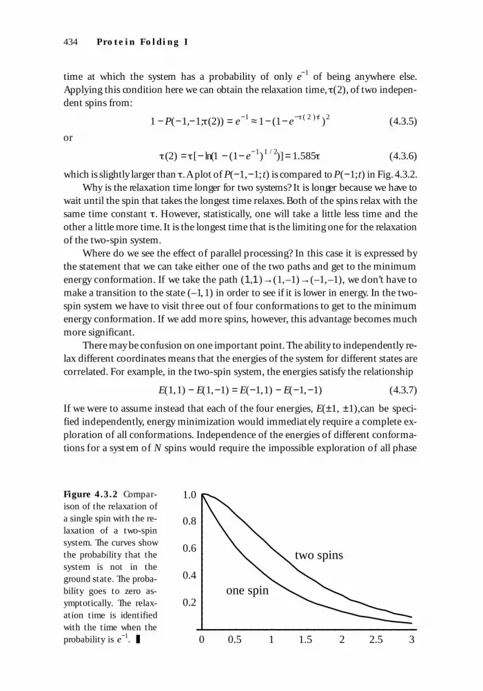
F i g u re 4 . 3 . 2 C o m p a r-ison of the relaxation ofa single spin with the re-laxation of a two-spinsystem. The curves showthe probability that thesystem is not in theground state. The proba-bility goes to zero as-ymptotically. The relax-ation time is identifiedwith the time when theprobability is e−1. ❚

04adBARYAM_29412 3/10/02 10:37 AM Page 434

space. It is the existence of correlations in the energies of different conformations thatenables parallel processing to work.

Homogeneous Systems

The models we will consider for a system of N relaxing spins {si} naturally divide intohomogeneous models and inhomogeneous models. For homogeneous models atransformation can be made that maps any spin si onto any other spin sj , where thetransformation preserves the form of the energ y. Specifically, it preserves the localfields and the interactions between spins.A homogeneous model is loosely analogousto assuming that all amino acids are the same. Such a polymer is called a homopoly-mer. Boundary conditions may break the t ransformation symmetry, but their effectcan still be considered in the context of homogeneous models. In contrast, an inho-mogeneous model is analogous to a heteropolymer where amino acids along thechain are not all the same. Inhomogeneities are incorporated in the models by vary-ing local fields, relaxation times or interactions between spins in a specified way, or byassuming they arise from a specified type of quenched stochastic variable.

In the homogeneous case, all sites are equivalent, and thus the local fields hi inEq. (4.2.1) must all be the same. However, the interactions may not all be the same.For example, there may be nearest-neighbor interactions, and different second-neighbor interactions. We indicate that the interaction depends only on the relativelocation of the spins by the notation Ji−j :

(4.4.1)

Ji − j is symmetric in i − j and each pair i, j appears only once in the sum. Eq. (4.2.2)implies that h is negative.A further simplification would be to consider each spin tointeract only with z neighbors with equal interaction strength J . This would be theconventional ferromagnet or antiferromagnet discussed in Section 1.6. When it isconvenient we will use this simpler model to illustrate properties of the more generalcase. In the following sections, we systematically describe the relaxation in a numberof model homogeneous systems. The results of our investigations of the scaling be-havior of the relaxation time are summarized in Table 4.4.1.Each of the models illus-trates a concept relevant to our understanding of relaxation in complex systems. Thistable can be referred to as the analysis proceeds.

4.4.1 DecoupledThe simplest homogeneous model is the decoupled case, where all spins are indepen-dent. Starting from Eq. (4.4.1) we have:

(4.4.2)

This is the N spin analog of the two-spin system we considered in Section 4.3. The en-ergetics are the same as the noninteracting Ising model. However, our interest here isto understand the dependence of kinetics on the number of spins N. The dynamics

E = −h∑ si

E({si }) = −h∑ s i − ∑ J i− js is j

4.4

Homo g eneo us s y s t e m s 435


04adBARYAM_29412 3/10/02 10:37 AM Page 435

are defined by the individual two-state systems, where a barrier controls the relaxationrate. Relaxation is described by the exponential decay of the probability that each spinis +1.

We have to distinguish between two possible cases. When we analyzed the two-spin case we assumed that essentially all members of the ensemble reach the uniquestate where al l si = −1. We have to check this assumption more carefully now. Theprobability that a par ticular spin is in the +1 state in equilibrium is given by the ex-pression (Eq. (1.4.14)):

(4.4.3)

where E+ = −2h is the (positive) energy difference between si = +1 and si = −1. If wehave N spins, the average number that are +1 in equilibrium is

(4.4.4)

Because N can be large , we do not immed i a tely assume that this nu m ber is negl i gi bl e .However, we wi ll assume that in equ i l i brium a large majori ty of spins are DOW N. This istrue on ly wh en E+> >k T and e−E+ /k T < < 1 . In this case we can approx i m a te Eq . (4.4.4) as:

(4.4.5)

There are now two distinct possibilities depending on whether N+ is less than orgreater than one. If N+ is less than one, all of the spins are DOWN in the final state. IfN+ is greater than one,almost all, but not all, of the spins are DOWN in the final state.

In the first case,N + << 1, we proceed as with the two-spin system to consider thegrowth of the probability of the final state:

(4.4.6)Defining the relaxation time as for the two-spin case we have:

(4.4.7)1 − P({si = −1}; (N )) = e−1 ≈1 − (1 − e− (N )/ )N

P({si = −1}; t ) = [P(si = −1;0)e− t / + (1 − e−t / )P(si = −1;∞)]i

∏ = (1 − e−t / )N

N+ = Ne− E+ / kT

N+ = Ne− E+ / kT /(1 + e− E+ / kT )

P(+1;∞) = e− E+ / kT /(1+ e− E+ / kT )



Model Scaling

Decoupled model O(ln(N );1)Essentially decoupled model O(ln(N );1)Nucleation and growth—with neutral boundaries O(aN (d−1)/d

;N −1;ln(N );1)—with nucleating boundaries O(N 1/d; ln(N);1)

Boundary-imposed ground state O(N 2/d)Long-range interactions O(ln(N );aN 2

)

Table 4.4.1 Summary of scaling behavior of the relaxation time of the homogeneous modelsdiscussed in Section 4.4. The notation indicates the different scaling regimes from smaller tolarger systems. ❚

04adBARYAM_29412 3/10/02 10:37 AM Page 436

or

(4.4.8)

For large N we expand this using a1/N ∼ 1 + (1 / N)ln(a) to obtain

(4.4.9)

Neglecting the constant term, we have the result that the time scales logarithmicallywith the size of the system (N) ∼ ln(N). We see the tremendous advantage of paral-lel processing, where the relaxation time grows only logarithmically with system sizerather than exponentially.

In the second case, N >> N+ >> 1, we cannot determine the relaxation time fromthe probability of a particular final state of the system. There is no unique final state.Instead, we have to consider the growth of the probability of the set of systems thatare most likely—the equilibrium ensemble with N+ spins si = +1. We can guess thescaling of the relaxation time from the divisibility of the system into independentgroups of spins. Since we have to wait only until a particular fraction of spins relax,and this fraction does not change with the size of the system,the relaxation time mustbe independent of the system size or (N) ∼ 1. We can show this explicitly by writingthe fraction of the remaining UP spins as:

(4.4.10)

where we use the assumption that e−E+/ kT<<1. We must now set a criterion for the re-laxation time (N).A reasonable criterion is to set (N) to be the time when there arenot many more than the equilibrium number of excited spins,say (1 + e−1) times asmany:

(4.4.11)

This implies that:

(4.4.12)

or

(4.4.13)

This rel a x a ti on time is indepen dent of the size of the sys tem or (N) ∼ 1 ; we name it ∞.The (N) ∼ 1 scaling we found for this case is lower than the logarithmic scaling.

We must understand more ful ly when it applies. In order for N+ (Eq. (4.4.5)) to begreater than 1, we must have:

N > e+E+ /kT (4.4.14)

(N ) = (E+ / kT + 1) ≡ ∞

N e− (N )/ + e− E+ / kT[ ] = (1 + e−1)Ne− E+ / kT

N+ ( (N)) = (1 + e−1)N+ (∞)

N+ (t ) =i

∑ P(si = 1;t) = [P(si = +1;0)e− t / + (1 − e−t / )P(si = +1;∞)]i∑

= N e−t / + (1− e −t / )e− E+ / kT[ ] ≈ N e−t / + e− E+ / kT[ ]

(N ) ~ [− ln(1− (1+ (1/ N )ln(1 − e−1)))] = [− ln(−(1/ N )ln(1− e−1))]

= [ln(N) − ln(− ln(1− e−1))] = [ln( N) + 0.7794]

(N ) = [−ln(1− (1− e−1)1/ N )]

Ho mog en eou s sy s t e m s 437


04adBARYAM_29412 3/10/02 10:37 AM Page 437

Thus N must be large in order for N+ to be greater than 1.It may seem surprising thatfor larger systems the scaling is lower than for smaller systems. The behavior of thescaling is illustrated schematically in Fig. 4.4.1 (see Question 4.4.1).

There is another way to estimate the relaxation time for very large systems, ∞.Weuse the smaller system relaxation Eq.(4.4.9) at the point where we crossover into theregime of Eq.(4.4.14) by setting N = e+E+ / kT. Because the relaxation time is a contin-uous function of N, at the crossover point it should give an estimate of ∞. This givesa similar result to that of Eq. (4.4.13):

(4.4.15)

Question 4.4.1 Combine the analysis of both cases N+ << 1 and N+ >> 1by setting an appropriate value of N+( (N)) that can hold in both cases.

Use this to draw a plot like Fig. 4.4.1.

Solution 4.4.1 The time evo luti on of N+(t) is de s c ri bed by Eq . (4.4.10) forei t h er case N+ < < 1 and N+ > > 1 . The difficulty is that wh en N+ > > 1 , t h eprocess stops wh en N+(t) becomes less than 1, and there is no more rel a x a ti on

∞ ~ [E+ /kT + 0.7794]



0

2

4

6

8

10

12

14

1 10 102

(N)/

ln(N)+0.7794

N

E+/kT+1

E+/kT+0.7794

103 104 105

Figure 4.4.1 Relaxation time (N) of N independent spins as a function of N. For systemsthat are small enough, so that relaxation is to a unique ground state, the relaxation timegrows logarithmically with the size of the system. For larger systems, there are always someexcited spins, and the relaxation time does not change with system size. This is the thermo-dynamic limit. The different approximations are described in the text. A unified treatment inQuestion 4.4.1 gives the solid curve. In the illustrated example, the crossover occurs for asystem with about 150 independent spins. This number is given by eE+ /kT so it varies expo-nentially with the energy difference between the two states of each spin. ❚

04adBARYAM_29412 3/10/02 10:37 AM Page 438

to be don e . For this case we would like to iden tify the rel a x a ti on time as thetime wh en there is less than one spin not U P. So we rep l ace Eq . (4.4.11) by

where Nr is a constant we can choose which is less than 1. When N+ >> 1,thefirst term will dominate and we will have the same result as Eq. (4.4.13),when N+ << 1 the second term will dominate. Eq. (4.4.16) leads instead ofEq. (4.4.13) to:

(N) = ln(N / Nr + e−1N+)) (4.4.17)

When N+ << 1 this reduces to:

(N) = (ln(N) − ln(Nr)) (4.4.18)

which is identical to Eq. (4.4.9) if we identify

(4.4.19)

which shows that our original definition of the relaxation time is equivalentto our new definition if we use this value for the average number of residualunrelaxed spins.

The plot in Fig. 4.4.1 was constructed using a value of E+ /kT = 5 andEqs. (4.4.9), (4.4.13), (4.4.15) and (4.4.17). ❚

The behavior for large systems satisfying Eq.(4.4.13) is just the thermodynamiclimit where intrinsic properties, including relaxation times, become independent ofthe system size. In this independent spin model, the relaxation time grows logarith-mically in system size until the thermodynamic limit is reached, and then its behav-ior crosses over to the thermodynamic behavior and becomes constant. To summa-rize the two regimes, we will label the scaling behavior of the independent system asO(ln(N);1) (the O is read “order”).

While the scaling of the relaxation time in the thermodynamic limit is as low aspossible, and therefore attractive in principle for the protein-folding problem, thereis an unattractive feature—that the equilibrium state of the system is not unique.This violates the assumption we have made that the eventual folded structure of aprotein is well defined and precisely given by {si = −1}. However, in recent years ithas been found that a small set of conformations that differ slightly from each otherconstitute the equilibrium protein structure. In the context of this model, the exis-tence of an equilibrium ensemble of the protein suggests that the protein is just atthe edge of the thermodynamic regime. In the homogeneous model there is no dis-tinction between different spins, and all are equally likely to be excited to theirhigher energy state. In the protein it is likely that the ensemble is more selective. Foressentially all models we will investigate, for large enough systems,a finite fraction ofspins must be thermally excited to a higher energy state. The crossover size dependsexponentially on the characteristic energy required for an excited state to occur. Thisenergy is just E+ in the independent spin model. Because the fraction of excited

Nr = − ln(1− e−1) = 0.4587 ≈ .5

N+ ( (N)) = (1 + e−1)N+ (∞) + Nr



04adBARYAM_29412 3/10/02 10:37 AM Page 439

states also depends exponentially on the temperature, the structure of proteins is af-fected by physical body temperature. This is one of the ways in which protein func-tion is affected by the temperature.

Either the logarithmic or the constant scaling of the independent spin model, ifcorrect,is more than adequate to account for the rapid folding of proteins.Of coursewe know that amino acids interact with each other. The interaction is necessary forinterdependence in the system. Is it possible to generalize this model to include someinteractions and still retain the same scaling? The answer is yes,but the necessary lim-itations on the interactions between amino acids are still not very satisfactory.

4.4.2 Essentially decoupledThe decoupled model can be generalized without significantly affecting the scaling,by allowing limited interactions that do not affect the relaxation of any spins. Toachieve this we must guarantee that at all times the energy of the spin si is lower whenit is DOWN than when it is UP. For a protein, this corresponds to a case where eachamino acid has a certain low-energy state regardless of the protein conformation. Wespecialize the discussion to nearest-neighbor interactions between each spin and zneighbors—a ferromagnetic or antiferromagnetic Ising model. We also assume thesame relaxation time applies to all spins at all times. The more general case is de-ferred to Question 4.4.2.

When there are interactions,the change in energy upon flipping a particular spinsi from UP to DOWN is dependent on the condition of the other spins {sj}j ≠ i . We writethe change as:

(4.4.20)

The latter expression is for homogeneous systems. For only nearest-neighbor interac-tions in both ferromagnet and antiferromagnet cases

(4.4.21)

where the sum is over the z nearest neighbors of si . Note that this expression dependson the state of the neighboring spins,not on the state of si . For the spins to relax es-sentially independently, we require that the minimum possible value of Eq. (4.4.21)

E+min = −2h − 2z |J | (4.4.22)

is greater than zero. To satisfy these requirements we must have

|h|>z|J | (4.4.23)

which means that the local field |h| is stronger than the interactions. When it is con-venient we will also assume that E+min >>kT, so that the energy difference between UP

and DOWN states is larger than the thermal energy.The ferromagnetic case J > 0 is the same as the kinetics of a first-order transition

(Section 1.6) when the local field is so large that nucleation is not needed and eachspin can relax separately. Remembering that h < 0,the value of E+i starts from its min-

E+i ({sj}j ≠i ) = −2h − 2J s jnn∑

E +i({s j } j≠i ) = E(s i = +1,{s j }j ≠i ) − E(si = −1,{s j } j≠i ) = −2h −2 J i− jj≠i∑ s j



04adBARYAM_29412 3/10/02 10:37 AM Page 440

imum value when all of the spins (neighbors of si) are UP, sj =+1. E+i then increases asthe system relaxes until it reaches its maximum value everywhere when all the spins(neighbors of si) are DOWN, sj = −1 (see Fig. 4.4.2). This means that initially the inter-actions fight relaxation to the ground state,because they are promoting the alignmentof the spins that are UP. However, each spin still relaxes DOWN. The final state with allspins DOWN is self-reinforcing, since the interactions raise the energy of isolated UP

spins. This inhibits the excitation of individual spins and reduces the probability thatthe system is out of the ground state. Thus, ferromagnetic interactions lead to what iscalled a cooperative ground state. In a cooperative ground state,interactions raise theenergy cost of, and thus inhibit, individual elements from switching to a higher en-ergy state.This property appears to be characteristic of proteins in their 3-d structure.Various interactions between amino acids act cooperatively to lower the conforma-tion energy and reduce the likelihood of excited states.

In order to consider the relaxation time in this model, we again consider twocases depending upon the equilibrium number of UP spins, N+. The situation is morecomplicated than the decoupled model because the eventual equilibrium N+ is notnecessarily the target N+ during the relaxation. We can say that the effective N+(E+) as

Homog en eou s s y s t e m s 441


E+

(# of neighbors=+1)-(# of neighbors=-1)

J>0J<0

E+min0

-z z0

–2h

Figure 4.4.2 Illustration, for the essentially decoupled model, of the value of the single-spinenergy E+ as a function of the number of its neighbors (out of a total of z) that are UP andDOWN. At the right all of the neighbors are UP, and at the left all of the neighbors are DOWN.E+ measures the energy preference of the spin to be DOWN. E+ is always positive in the es-sentially decoupled model. The relaxation process to the ground state takes the system fromright to left. For a ferromagnet, J > 0, the change reinforces the energy preference for thespin to be DOWN. For the antiferromagnet, J < 0, the change weakens the energy preferencefor the spin to be DOWN. Implications for the time scale of relaxation are described in thetext. ❚

04adBARYAM_29412 3/10/02 10:37 AM Page 441

given by Eq. (4.4.5) changes over time. Because E+ starts out small, it may not beenough to guarantee that all spins will be DOWN in the final state. But the increase inE+ may be sufficient to guarantee that all spins will be DOWN at the end.

The situation is simplest if there is complete relaxation toward the ground stateat all times. This means:

(4.4.24)

In this case, the relaxation time scaling is bounded by the scaling of the decoupledmodel. We can show this by going back to the equation for the dynamics of a singlerelaxing two-state system, as written in Eq. (1.4.43):

(4.4.25)

The difficulty in solving this equation is that P(1;∞) (Eq. (4.4.3)) is no longer a con-stant. It varies between spins and over time because it depends on the value of E+.Nevertheless, Eq. (4.4.25) is valid at any particular moment with the instantaneousvalue of P(1;∞). When Eq.(4.4.24) holds, P(1;∞)<1/N is always negligible comparedto P(1; t), even when all the spins are relaxed, so we can simplify Eq. (4.4.24) to be:

(4.4.26)

This equation is completely independent of E+. It is therefore the same as for the de-coupled model. We can integrate to obtain:

P(1;t) = e−t / (4.4.27)

Thus each spin relaxes as a decoupled system,and so does the whole system with a re-laxation time scaling of O(ln(N)).

When Eq. (4.4.24) is not true, the difficulty is that we can no longer neglectP(1;∞) in Eq. (4.4.25). This means that while the spins are relaxing, they are not re-laxing to the equilibrium probability. There are two possibilities. The first is that theequilibrium state of the system includes a small fraction of excited spins. Since thefraction of the excited spins does not change with system size,the relaxation time doesnot change with system size and is O(1).

The other possibility is that initially the relaxation allows a small fraction of spinsto be excited. Then as the relaxation proceeds, the energy differences E+i({sj }j ≠ i) in-crease. This increase in energy differences then causes all of the spins to relax. Howdoes the scaling behave in this case? Since each of the spins relaxes independently, inO(1) time all except a small fraction N will relax. The remaining fraction consists ofspins that are in no particular relationship to each other; they are therefore indepen-dent because the range of the interaction is short. Thus,they relax in O(ln( N)) timeto the ground state.The total relaxation time would be the sum of a constant term anda logarithmic term that we could write as O(ln( N)+1), which is not greater thanO(ln(N)). This concludes the discussion of the ferromagnetic case.

For the antiferromagnetic case, the situation is actually simpler. Since J < 0, re-membering that h < 0,the value of E+ starts from its maximum value when all sj =+1,and reaches its minimum value when all sj =−1 (see Fig. 4.4.2). Thus N+(E+) is largestin the ground state.Once again,if there is a nonzero fraction of spins at the end that

˙ P (1; t) = −P(1; t )/

˙ P (1; t) = (P(1; ∞) − P(1; t ) ) /

N < e+ E+ min / kT



04adBARYAM_29412 3/10/02 10:37 AM Page 442

are UP then the relaxation must be independent of system size, O(1). If there are noresidual UP spins in equilibrium,then in Eq.(4.4.25) P(1;∞)<1/N always,and the re-laxation reduces directly to the independent case O(ln(N)).

The ferromagnetic case is essentially different from the antiferromagnetic casebecause we can continue to consider stronger values of the ferromagnetic interactionwithout changing the ground state. However, if we consider stronger antiferromag-netic interactions,the ground state will consist of alternating UP and DOWN spins andthis is inconsistent with our assumptions (we would have redefined the spin vari-ables). Thus,nearest-neighbor antiferromagnetic interactions,as long as they do notlead to an antiferromagnetic ground state, do not affect the relaxation behavior.

When there are spin-spin interactions, we would also expect the relaxation times

i to be affected by the interactions. The relaxation time depends on the barrier to re-laxation, EBi , as shown in the energy curve of the two-state system Fig. 1.4.1. Whenthe energy difference E+ is higher, we might expect that the barrier to relaxation of thetwo-state system will become lower. This would be the case if we raise E+ without rais-ing the energy at the top of the barrier. On the other hand,if the energy surface is mul-tiplied by a uniform factor to increase E+, then the barrier would increase. These dif-ferences in the barrier show up in the relaxation times i . In the former case therelaxation is faster, and in the latter case the relaxation is slower. For the nearest-neighbor Ising model, there would be only a few different relaxation times corre-sponding to the different possible states of the neighboring spins.We can place a limiton the relaxation time (N) of the whole system by replacing all the different spin re-laxation times with the maximum possible spin relaxation time. As far as the scalingof (N) with system size,this will have no effect. The scaling remains the same as inthe noninteracting case, O(ln(N);1).

Question 4.4.2 Consider the more general case of a homogeneous modelwith interactions that may include more than just nearest-neighbor in-

teractions. Restricting the interactions not to affect the minimum energy ofa spin,argue that the relaxation time scaling of the system is the same as thedecoupled model. Assume that the interactions have a limited range and thesystem size is much larger than the range of the interactions.

Solution 4.4.2 As in Eq. (4.4.20), the change in energy on flipping a par-ticular spin is dependent on the conditions of the other spins {sj}j ≠ i .

(4.4.28)

We assume that E+i({sj}j ≠ i ) is always positive. Moreover, for relaxation to oc-cur, the energy difference must be greater than kT. Thus the energy must bebounded by a minimum energy E+min satisfying:

E+i({sj}j ≠ i) > E+min >> kT (4.4.29)

This implies that the interactions do not change the lowest energy state ofeach spin si . For the energy of Eq. (4.4.1), E+min can be written

E +i({s j } j≠i ) = −2h − 2 Ji −jj ≠i∑ s j



04adBARYAM_29412 3/10/02 10:37 AM Page 443

(4.4.30)

Interactions may also affect the relaxation time of each spin i{sj}j ≠ i, so wealso assume that relaxation times are bounded to be less than a relaxationtime max .

We assume that the parameters max and E+min do not change with sys-tem size. This will be satisfied, for example,if the interactions have a limitedrange and the system size is larger than the range of the interactions.

Together, the assumption of a bound on the energy differences and abound on the relaxation times suggest that the equilibration time is boundedby that of a system of decoupled spins with −2h = E+min and = max. Thereis one catch. We have to consider again the possibility of incomplete relax-ation to the ground state. The scenario follows the same possibilities as thenearest-neighbor model. The situation is simplest if there is complete relax-ation to the ground state at all times. This means:

(4.4.31)

which is a more stringent condition than Eq.(4.4.29). In this case the boundon (N) is straightforward because each spin is relaxing to the ground statefaster than in the original case. Again using Eq. (1.4.43):

(4.4.32)

This equation applies at any particular moment, with the time-dependentvalues of P(1;∞; t) and (t), where the time dependence of these quantities isexplicitly written. Since P(1;∞;t) is always negligible compared to P(1; t),when Eq. (4.4.31) applies, this is

(4.4.33)

We can integrate to obtain:

(4.4.34)

The inequality follows from the assumption that the relaxation time of eachspin is always smaller than max. Each spin relaxes faster than the decoupledsystem,and so does the whole system. The scaling behavior O(ln(N)) of thedecoupled system is a bound for the increase in the relaxation time of thecoupled system.

When Eq. (4.4.31) is not true, we can no longer neglect P(1;∞;t) inEq.(4.4.32). This means that while the spins are relaxing faster, they are notrelaxing to the equilibrium probability. There are two possibilities. The firstis that the equilibrium state of the system includes a small fraction of excitedspins. Since the range of the interactions is smaller than the system size, the

P(1;t) = e− dt

(t)0

t

∫< e −t / max

˙ P (1; t) = −P(1; t )/ (t )

˙ P (1; t) = (P(1; ∞;t ) − P(1; t) ) / (t)

N < e+ E+ min / kT

E+ min = −2h − 2 | Ji− jj ≠i∑ |

444 P r o t e in F o l d i ng I


04adBARYAM_29412 3/10/02 10:37 AM Page 444

fraction of the excited spins does not change with system size and the relax-ation time does not change with system size.The other possibility is that ini-tially the values of E+i({sj}j ≠ i) do not satisfy Eq.(4.4.31) and so allow a smallfraction of spins to be excited. Then as the relaxation proceeds, the energydifferences E+i ({sj}j ≠ i) increase. This increase in energy differences thencauses all of the spins to relax. The relaxation time will not be larger thanO(ln(N)) as long as E+min >> kT (Eq.(4.4.29)) holds. Because of this condi-tion,each of the spins will almost always relax,and in O(1) time all except asmall fraction N will relax. The remaining fraction consists of spins that arein no particular relationship to each other; they are therefore independent,because the range of the interaction is short, and will relax in at mostO(ln( N )) time to the ground state. The total relaxation time would be thesum of a constant term and a logarithmic term that we could write asO(ln( N )+1), which is not greater than O(ln(N )). ❚

We have treated carefully the decoupled and the almost decoupled models todistinguish b etween O(ln(N )) and O(1) scaling. One reason to devote such atten-tion to these simple models is that they are the ideal case of parallel processing. Itshould be understood, however, that the difference between O(ln(N )) and O(1)scaling is not usually significant. For 1000 amino acids in a protein, the difference isonly a factor of 7, which is not significant if the individual amino acid relaxationtime is microscopic.

One of the points that we learned about interactions from the almost decoupledmodel is that the ferromagnetic interactions J > 0 cause the most problem for relax-ation. This is because they reinforce the initial state before the effect of the field h actsto change the conformation. In the almost decoupled model, however, the field hdominates the interactions J. In the next model this is not the case.

The almost decoupled model is not satisfactory in describing protein folding be-cause the interactions between amino acids can affect which conformation they arein. The next model allows this possibility. The result is a new scaling of the relaxationwith system size, but only under particular circumstances.

4.4.3 Nucleation and growth: relaxation by driven diffusionThe next homogenous model results from assuming that the interactions are strongenough to affect the minimum energy conformation for a particular spin:

E+min < 0 (4.4.35)

From Eqs.(4.4.20) and (4.4.21) we see that this implies that the total value of the in-teractions exceeds the local preference as determined by the field h. Eventually, it is hthat ensures that all of the spins are DOWN in the ground state. However, initiallywhen all of the spins are UP, due to the interactions the spins have their lowest energyUP rather than DOWN. During relaxation, when some are UP and some are DOWN, aparticular spin may have its lowest energy either UP or DOWN. The effect of both theexternal field and the interactions together leads to an effective field, h + ∑

j

Ji−j sj , thatdetermines the preference for the spin orientation at a particular time.



04adBARYAM_29412 3/10/02 10:37 AM Page 445

The simplest model that illustrates this case is the Ising ferromagnet in a d-dimensional space (Section 1.6). The interactions are all positive,and the spins tryto align with each other. Initially the local preference is for the spins to remain UP; theglobal minimum of energy is for all of the spins to be DOWN. The resolution of thisproblem occurs when enough of the spins in a particular region flip DOWN usingthermal energy, to create a critical nucleus. A critical nucleus is a cluster o f DOWN

spins that is sufficiently large so that further growth of the cluster lowers the energyof the system. This happens when the energy lowering from flipping additional spinsis larger than the increase in boundary energy between the DOWN cluster and the UP

surrounding region.Once a critical nucleus forms in an infinite system,the region ofdown spins grows until it encounters other such regions and merges with them toform the equilibrium state. In a finite system there may be only one critical nucleusthat is formed, and it grows until it consumes the whole system.

The nucleation and growth model of first-order transitions is valid for quite ar-bitrary interactions when there are two phases, one which is metastable and onewhich is stable,if there is a well-defined boundary between them when they occur sideby side. This applies to a large class of models with finite length interactions. For ex-ample, there could be positive nearest-neighbor interactions and negative second-neighbor interactions. As long as the identity of the g round state is not disturbed,varying the interactions affects the value of the boundary energy, but not the overallbehavior of the metastable region or the stable region. We do not consider here thecase where the boundaries become poorly defined. In our models, the metastablephase consists of UP spins and the stable phase consists of DOWN spins.A system withonly nearest-neighbor antiferromagnetic interactions on a bipartite lattice is not in-cluded in this section. For J < 0 on a bipartite lattice, when Eq.(4.4.35) is satisfied,theground state is antiferromagnetic (alternating si = ±1),and we would have redefinedthe spins to take this into consideration.

The dynamics of relaxation for nucleation and growth are controlled by the rateof nucleation and by the rate of diffusion of the boundary between the two phases.Because of the energy difference of the two phases,a flat boundary between them willmove at constant velocity toward the metastable phase,converting UP spins to DOWN

spins. This process is essentially that of driven diffusion down a washboard potentialas illustrated in Fig . 1.4.5. The velocity of the boundary, v, can be measured in unitsof interspin separation per unit time.

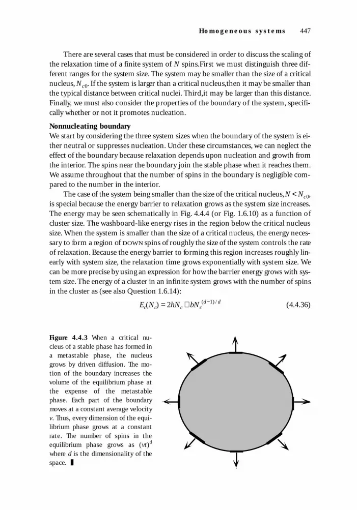
During relaxation, once a critical nucleus of the stable phase forms, it grows bydriven diffusion and by merging with other clusters. The number of spins in a partic-ular region of the stable phase grows with time as (vt)d. This rate of growth occurs be-cause the region of the stable phase grows uniformly in all directions with velocity v.Every part of the boundary diffuses like a flat boundary (Fig. 4.4.3). This follows ourassumption that the boundary is well defined. There are two parts to this assumption.The first is that the thickness of the boundary is small compared to the size of the crit-ical nucleus. The second is that it becomes smooth, not rough, over time. When theseassumptions are satisfied, the stable region expands with velocity v in all directions.



04adBARYAM_29412 3/10/02 10:37 AM Page 446

There are several cases that must be considered in order to discuss the scaling ofthe relaxation time of a finite system of N spins.First we must distinguish three dif-ferent ranges for the system size. The system may be smaller than the size of a criticalnucleus, Nc 0. If the system is larger than a critical nucleus,then it may be smaller thanthe typical distance between critical nuclei. Third,it may be larger than this distance.Finally, we must also consider the properties of the boundary of the system, specifi-cally whether or not it promotes nucleation.

Nonnucleating boundaryWe start by considering the three system sizes when the boundary of the system is ei-ther neutral or suppresses nucleation. Under these circumstances, we can neglect theeffect of the boundary because relaxation depends upon nucleation and growth fromthe interior. The spins near the boundary join the stable phase when it reaches them.We assume throughout that the number of spins in the boundary is negligible com-pared to the number in the interior.

The case of the system being smaller than the size of the critical nucleus,N < Nc 0,is special because the energy barrier to relaxation grows as the system size increases.The energy may be seen schematically in Fig. 4.4.4 (or Fig. 1.6.10) as a function ofcluster size. The washboard-like energy rises in the region below the critical nucleussize. When the system is smaller than the size of a critical nucleus, the energy neces-sary to form a region of DOWN spins of roughly the size of the system controls the rateof relaxation. Because the energy barrier to forming this region increases roughly lin-early with system size, the relaxation time grows exponentially with system size. Wecan be more precise by using an expression for how the barrier energy grows with sys-tem size. The energy of a cluster in an infinite system grows with the number of spinsin the cluster as (see also Question 1.6.14):

Ec(Nc) = 2hNc + bNc(d −1) / d (4.4.36)



Figure 4.4.3 When a critical nu-cleus of a stable phase has formed ina metastable phase, the nucleusgrows by driven diffusion. The mo-tion of the boundary increases thevolume of the equilibrium phase atthe expense of the metastablephase. Each part of the boundarymoves at a constant average velocityv. Thus, every dimension of the equi-librium phase grows at a constantrate. The number of spins in theequilibrium phase grows as (vt)d

where d is the dimensionality of thespace. ❚

04adBARYAM_29412 3/10/02 10:37 AM Page 447

The first term is the bulk energy of the DOWN spins in the cluster as compared tometastable UP spins. The second term is the boundary energy, where b is a measure ofthe boundary energy per unit length. This expression is reasonable if the critical nu-cleus is large compared to the boundary width—the boundary is well defined. Thecritical nucleus for an infinite system is determined by the maximum value of Ec(Nc).This is obtained setting its derivative with respect to Nc to zero. Aside from a factor of(d − 1)/d, this means that both terms are equal in magnitude for the critical nucleus.If the system is smaller than the critical nucleus size, then the boundary energy mustdominate the bulk energy of a cluster for all possible cluster sizes. Thus for a systemwith N < Nc 0 we can neglect the first term in Ec(Nc), leaving us with the energyEc(Nc) ≈ bNc

(d−1) / d.For a system with N < Nc 0 that has periodic boundary conditions,the boundary

of a cluster grows only as long as the cluster contains less than one-half of the spins inthe system. Beyond this point, the boundary of the cluster shrinks. So the maximumcluster energy is reached when Nc is N /2. This is still true for a fixed boundary if theboundary is neutral. The relevant cluster may be identified by bisecting the systemwith UP spins on one side and DOWN spins on the other. If the boundary suppressesnucleation, then the maximum value of Nc may be greater than N / 2, but it is notlarger than N. As long as the maximum value of Nc is proportional to N, the resultsgiven below are essentially unaffected.



E

0

EB(N)

N/2 N

Ec(Nc)

N c0

Figure 4.4.4 Schematic illustration of the energy of a cluster of DOWN spins in a metastablebackground of UP spins as a function of the number of spins in the cluster Nc. The corruga-tion of the line indicates the energy barrier as each spin flips from UP to DOWN. The dashedline illustrates the energy Ec(Nc) of the cluster in an infinite system. The energy increases un-til it reaches the size of a critical nucleus Nc0 and decreases thereafter as the cluster growsto become the stable phase. The solid line indicates the energy in a finite system of sizeN < Nc0. In this case the maximum energy, which is the barrier to relaxation, is located in thevicinity of N/2, as indicated. ❚

04adBARYAM_29412 3/10/02 10:37 AM Page 448

The cluster energy we have calculated is the energy at the bottom of a particularwell in Fig. 4.4.4. It does not include the height of the corrugation EB0 which is the en-ergy barrier to flipping a single spin. The energy barrier for nucleation in the systemwith N < Nc 0 is thus given by

EB(N) = Ec(N / 2) + EB0 = b(N /2)(d −1) / d + EB0 (4.4.37)

The relaxation time is given approximately by the probability that the system willreach this barrier energy, as given by a Boltzmann factor of the energy. More specifi-cally, it is given by Eq. (1.4.44), which gives the relaxation of a two-state system withthe same barrier (we neglect the back transition rate):

(4.4.38)

This shows the exponential dependence of the relaxation time on system size in thissmall system limit when N < Nc 0. We note that we have neglected to consider the manypossible ways there are to form a cluster of a particular size, which may also affect thescaling of the relaxation time.

The existence of a region of exponential growth of the relaxation time should beunderstood in a context where we compare the nucleation time with the observationtime. If the nucleation time is long compared to the observation time, we would notexpect to see relaxation to the ground state.

If the size of the system is much larger than the size of a critical nucleus, N >> Nc 0,we can consider each nucleus to be essentially a point object of no size,when it forms.A nucleus forms at a particular site according to a local relaxation process with a timeconstant we denote c 0—the nucleation time. The nuclei then grow, as discussed pre-viously, with a constant velocity v in each direction. During the relaxation we eitherhave one or many nuclei that form.Only one nucleus forms when the typical time forforming a nucleus in the system is longer than the time a single nucleus takes to con-sume the whole system. As soon as one nucleus forms, its growth is so rapid that noother nuclei form during the time it grows to the size of the whole system(Fig. 4.4.5(a)). The relaxation time is determined by the time that passes until the firstnucleation event occurs in the system. For larger systems,the number of possible nu-cleation sites increases in direct proportion to N. Thus the time till the first nucleationevent decreases, and the relaxation time actually decreases with system size. We willderive the result that (N) ~ N −1. To determine when this scaling applies we must findexpressions for the nucleation time, and the time a nucleus takes to grow to the sizeof the system. Independent nuclei can form on every Nc 0 sites. The typical time toform a critical nucleus anywhere in the system, c N , where c N << c 0, is the time ittakes any one of the possible N /Nc 0 sites to form a single critical nucleus:

(4.4.39)

expanding the exponential using cN / c 0 << 1 gives

(4.4.40)cN = c0 Nc0 / N

(N / Nc0)e− cN / c0 = N / Nc0 −1

(N ) = −1e EB (N )/ kT = −1e(E B0 +bN(d −1)/ d

/ 2( d−1)/ d

)/ kT = ebN(d−1)/ d

/ 2(d−1)/ d

/ kT



04adBARYAM_29412 3/10/02 10:37 AM Page 449

This result says that the time to form a single nucleus is inversely proportional to thesize of the system. The time for a single nucleus to grow to the size of the system, v ,is given by

(4.4.41)

or

(4.4.42)

We are neglecting numerical factors that reflect different possible locations the nu-cleus may form and their relationship to the boundary of the system.

The condition that a single nucleus will form cN v is given by combining Eq.(4.4.40) and Eq. (4.4.41) to obtain

(4.4.43)

where we have also repeated our assumption that the size of the system is larger thanthe critical nucleus. Eq.(4.4.43) describes the bounds on the system size so that onlyone nucleus is important. Under these circumstances the relaxation time actually de-creases with system size, because as the size of the system increases so do the oppor-tunities for forming critical nuclei. The relaxation time is given by the sum of the nu-

(v c 0Nc 0 )d /(d+1) > N >> Nc 0

v = N 1/ d / v

(v v )d= N



(a)

(b)

(c)

F i g u re 4 . 4 . 5 S e v e ra lcases of the relaxation ofsystems by driven diffu-sion are illustrated. Seethe text for a detailed dis-cussion. In (a) the systemis larger than the size of acritical nucleus but smallenough so that only onenucleation event occurs inthe system. The boundaryis nonnucleating. In (b)the system is large enoughso that several nucleationevents occur during the re-laxation; the boundary isnonnucleating. In (c) theboundary nucleates theequilibrium phase. ❚

04adBARYAM_29412 3/10/02 10:37 AM Page 450

cleation time and the time for consumption of the whole system. The latter has beenassumed to be small compared to the former:

(4.4.44)

Thus the scaling of the relaxation time is O(N −1).

If the system is large enough so that more than one nucleation event occurs(Fig. 4.4.5(b)),then different regions of the material may be treated as essentially de-coupled. We expect from the analysis of independent systems that the scaling of therelaxation time is logarithmic.A more detailed analysis given as Question 4.4.3 showsthe scaling is O(ln(N)1/(d +1)). While the analysis in Question 4.4.3 has interesting fea-tures, the difference between this and O(1) or O(ln(N)) scaling is unlikely to be sig-nificant.Finally, as with the independent spin model,the relaxation time is indepen-dent of N if N+ is greater than 1. For convenience we assume that this occurs after thetransition between the regime o f Fig. 4.4.5(a) and Fig. 4.4.5(b), i.e., for systems inwhich there are many nucleation events.

Question 4.4.3 Calculate the scaling of the relaxation time when thereare many nuclei formed in a system with N spins with boundaries that

do not affect the nucleation. Assume that all spins are DOWN at the end ofthe relaxation. Numerical factors that do not affect the dependence of (N)on N may be neglected.

Solution 4.4.3 Nucleation sites occur randomly through the system andthen grow and merge together. In order to find the time at which the wholesystem will become DOWN, we calculate the probability that a spin at a par-ticular site will remain UP. A particular spin si is UP at time t only if there hasbeen no nucleation event in its vicinity that would have grown enough toreach its site.

The probability that no critical nucleus formed at a position rj with re-spect to the site si until the time t is given by the probability of a two-statesystem with a time constant c 0 remaining in its high energy state or

e−t / c0 (4.4.45)

If we are looking at the spin si at time t , we must ask whether there wasformed a nucleus at a distance r away prior to t ′=t − rj /v . If the nucleusformed before t ′ then the nucleus would arrive before time t at the site si . Themaximum distance that can affect the spin si is rmax = min(vt,R), whereR∝N 1/d is the size of the system. When there are many nuclei in the system,then each nucleus is much smaller than the system and R >> vt, so thatrmax = vt. The probability that no nucleus formed within this radius at anearly enough time is given by:

(4.4.46)

rj

rmax

∏ e−( t− rj / v )/ c0 = e

− (t− rj / v) / c 0∑

(N ) = cN + v ≈ cN = c0N c0 / N



04adBARYAM_29412 3/10/02 10:37 AM Page 451

where the product and the sum are over all possible nucleation sites withina distance rmax.

The sum can be directly evaluated to give:

(4.4.47)

where we divided by the volume of a nucleation site and neglected constants.The number of sites that remain UP is given by N times Eq.(4.4.46) with Eq.(4.4.47) substituted in:

(4.4.48)

The coefficient accounts for the numerical prefactors we have neglected.Requiring that this is a number less than 1 when t = (N) gives the relaxationtime (N) ~ ln(N)1/(d+1) as indicated in the text.

If we consider this same derivation but do not substitute for rmax in Eq.(4.4.47) then we arrive at the expression:

(4.4.49)

and

(4.4.50)

This more general expression also contains the behavior when we have onlyone nucleation event. We can recover this case by substituting a constantvalue of rmax = R∝N 1/d. Then the time dependence of N+ is given by thesimple exponential dependence with the relaxation constant (N) =

c 0Nc 0 / r dmax∝1/N. ❚

Nucleating boundaryIf the boundary of the system promotes nucleation,the nucleus formed at the bound-ary will increase by driven diffusion. If there are no other nucleation events(Fig. 4.4.5(c)) then the relaxation-time scales as (N)~ N 1/d. Since the critical nucleusforms at the boundary, the system does not have to be larger than a critical nucleusfor this to occur. If the system is large enough so that there are many nucleationevents,then the behavior of the boundary is irrelevant and the same scaling found be-fore applies.

We have found an anomaly in the intermediate regime characterized byEq. (4.4.43). In this regime the relaxation time of a system with a nonnucleatingboundary decreases, while that with a nucleating boundary increases. It should be un-derstood that for the same microscopic parameters (except at the boundaries),the re-laxation time is longer in the former case than in the latter.

N + = Ne− (t −(d d+1)rmax /v)rmaxd

/( c0 N c0 )

(t −rj /v)j

∑ ∝1

N c 0(t − r /v)r d−1dr

0

rmax

∫ ∝(t − (d d + 1)rmax /v)rmaxd / N c0

N + = Ne− (v t )d +1

/(v c 0N c 0 )

(t −rj /v)j

∑ ∝1

N c 0(t − r /v)r d−1dr

0

rmax =vt

∫ ∝(vt)d +1 /(vN c0)



04adBARYAM_29412 3/10/02 10:37 AM Page 452

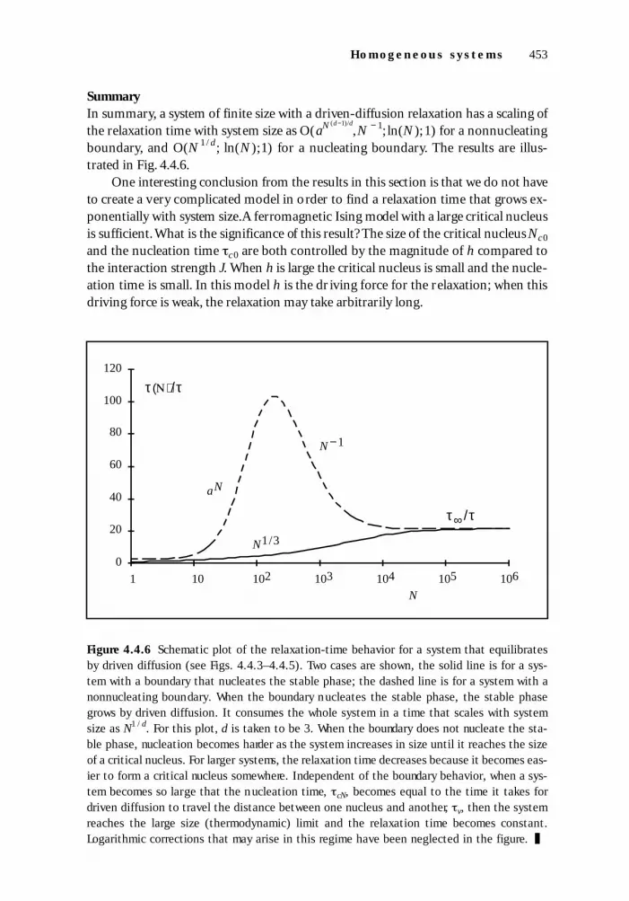
SummaryIn summary, a system of finite size with a driven-diffusion relaxation has a scaling ofthe relaxation time with system size as O(aN (d−1)/d

,N − 1; ln(N); 1) for a nonnucleatingboundary, and O(N 1 / d; ln(N);1) for a nucleating boundary. The results are illus-trated in Fig. 4.4.6.

One interesting conclusion from the results in this section is that we do not haveto create a very complicated model in order to find a relaxation time that grows ex-ponentially with system size.A ferromagnetic Ising model with a large critical nucleusis sufficient. What is the significance of this result? The size of the critical nucleus Nc 0

and the nucleation time c 0 are both controlled by the magnitude of h compared tothe interaction strength J. When h is large the critical nucleus is small and the nucle-ation time is small. In this model h is the driving force for the relaxation; when thisdriving force is weak, the relaxation may take arbitrarily long.



0

20

40

60

80

100

120

102

τ( )/τ

103 104 105 1061 10N

N −1

aN

N1/3

τ∞ /τ

Figure 4.4.6 Schematic plot of the relaxation-time behavior for a system that equilibratesby driven diffusion (see Figs. 4.4.3–4.4.5). Two cases are shown, the solid line is for a sys-tem with a boundary that nucleates the stable phase; the dashed line is for a system with anonnucleating boundary. When the boundary nucleates the stable phase, the stable phasegrows by driven diffusion. It consumes the whole system in a time that scales with systemsize as N1 /d. For this plot, d is taken to be 3. When the boundary does not nucleate the sta-ble phase, nucleation becomes harder as the system increases in size until it reaches the sizeof a critical nucleus. For larger systems, the relaxation time decreases because it becomes eas-ier to form a critical nucleus somewhere. Independent of the boundary behavior, when a sys-tem becomes so large that the nucleation time, cN, becomes equal to the time it takes fordriven diffusion to travel the distance between one nucleus and another, v, then the systemreaches the large size (thermodynamic) limit and the relaxation time becomes constant.Logarithmic corrections that may arise in this regime have been neglected in the figure. ❚

04adBARYAM_29412 3/10/02 10:37 AM Page 453

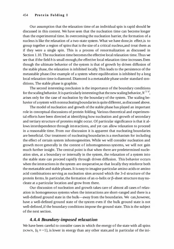
Our assumption that the relaxation time of an individual spin is rapid should bediscussed in this context. We have seen that the nucleation time can become longerthan the experimental time. In overcoming the nucleation barrier, the formation of anucleus is like the relaxation of a two-state system. What we have done,in effect,is togroup together a region of spins that is the size of a critical nucleus,and treat them asif they were a single spin. This is a process of renormalization as discussed inSection 1.10. The nucleation time becomes the effective local relaxation time.Thus wesee that if the field h is small enough,the effective local relaxation time increases.Eventhough the ultimate behavior of the system is that of growth by driven diffusion ofthe stable phase, the relaxation is inhibited locally. This leads to the persistence of themetastable phase.One example of a system where equilibration is inhibited by a longlocal relaxation time is diamond. Diamond is a metastable phase under standard con-ditions. The stable phase is graphite.

The second intere s ting con clu s i on is the import a n ce of the bo u n d a ry con d i ti on sfor the scaling beh avi or. It is parti c u l a rly intere s ting that the new scaling beh avi or,N 1/ d,a rises on ly for the case of nu cl e a ti on by the bo u n d a ry of the sys tem . The scaling be-h avi or of a sys tem with non nu cl e a ting bo u n d a ries is qu i te differen t , as discussed above .

The model of nucleation and growth of the stable phase has played an importantrole in conceptual discussions of protein folding. Various theoretical and experimen-tal efforts have been directed at identifying how nucleation and growth of secondaryand tertiary structure of proteins might occur. Of particular significance is that it al-lows interdependence through interactions, and yet can allow relaxation to proceedin a reasonable time. From our discussion it is apparent that nucleating boundariesare beneficial. Our treatment of nucleating boundaries is a mechanism for includingthe effect of certain system inhomogeneities. While we will consider nucleation andgrowth more generally in the context o f inhomogeneous systems, we will not gainmuch further insight. The central point is that when there are predetermined nucle-ation sites, at a boundary or internally in the system, the relaxation of a system intothe stable state can proceed rapidly through driven diffusion. This behavior occurswhen the interactions in the system are cooperative,so that locally they reinforce boththe metastable and stable phases. It is easy to imagine particular amino acids or aminoacid combinations serving as nucleation sites around which the 3-d structure of theprotein forms. In particular, the formation of an -helix or -sheet structure may nu-cleate at a particular location and grow from there.

Our discussion of nucleation and growth takes care of almost all cases of relax-ation in homogeneous systems when the interactions are short-ranged and there is awell-defined ground state in the bulk—away from the boundaries. We can,however,have a well-defined ground state of the system even if the bulk ground state is notwell-defined,if the boundary conditions impose the ground state. This is the subjectof the next section.

4.4.4 Boundary-imposed relaxationWe have been careful to consider cases in which the energy of the state with all spinsDOWN, {si = −1}, is lower in energy than any other state,and in particular of the ini-



04adBARYAM_29412 3/10/02 10:37 AM Page 454

tial state with all spins UP, {si = +1}. In a system with ferromagnetic interactions,if theenergies of the initial and final states are equal, then there are two ground states. Inthe homogeneous model this is the case where h = 0. In general, the existence of twoground states is counter to our assumptions about relaxation to a unique groundstate. However, we can still have a unique ground state if the boundaries impose si = −1. Such boundaries mean that the ground state is uniquely determined to be{si = −1}, even though h = 0.

In the absence of additional nucleation events, such a system would equilibrateby inward diffusion of the interface between the UP interior and the DOWN border, asin Fig . 4.4.5(c). There is no bulk driving force that locally causes the UP region toshrink. The only driving force is the interface energy (surface tension) that causes theinterface to shrink. We can treat the system as performing a driven random walk inthe number of UP spins. However, we must treat each part of the boundary as mov-ing essentially independently. The rate of change of the average number of UP spinsN+(t) is given by the boundary velocity times the boundary length:

(4.4.51)

The velocity of a driven random walk is (from Eq. (1.4.58) and (1.4.60))

(4.4.52)

From Fig. 1.4.5 we can see that (∆E+ − ∆E−) is the energy difference between steps. Asingle step changes the number of UP spins by one, so

(4.4.53)

where E(N+(t)) ∝ N+(t)(d −1) /d is the average surface energy for a cluster with N+(t) UP

spins. Since the single-step energy difference decreases with the number of UP spins,we can assume it is small compared to kT. We can then expand the exponential insidethe parenthesis in Eq.(4.4.52) and substitute the resulting expression for the velocityinto Eq. (4.4.51) to obtain

(4.4.54)

The negative sign is consistent with the decreasing size of the region of UP spins. Weintegrate Eq.(4.4.54) to find the dependence of the relaxation time on the size of thesystem:

(4.4.55)

The final expression is valid even in one dimension, where the boundary executes arandom walk because there is no local preference of the boundary to move in one di-rection or the other and (N) ∝ N 2.

(N ) ∝ −N

0

∫ N+ (t) (2 −d) /d dN+ (t) = N 2/ d

dN+ (t)

dt≈ −

a

kTe −∆E + / kT (∆E + − ∆E− )N +(t)(d−1)/ d ∝ −N + (t)−(d−2)/d

(∆E + − ∆E− ) = E(N +(t)) − E(N +(t) −1) ≈

dE(N +(t))

d(N +(t))∝N +(t)−1/ d

v = a (e − ∆E+ /kT − e −∆E− /kT ) = a e −∆E + /kT(1 −e (∆E +− ∆E− )/kT )

dN+ (t)

dt∝vN +(t)(d−1)/ d



04adBARYAM_29412 3/10/02 10:37 AM Page 455

In this discussion we have ignored the possible effect of the nucleation of regionsof DOWN spins away from the boundary of the system.One way to understand this isto note that the size of a critical nucleus is infinite when h = 0. Nucleation may onlychange the relaxation behavior when the interface between UP and DOWN spins is notwell-defined. Otherwise, nucleation does not help the relaxation, since any region ofDOWN spins inside the region of UP spins will shrink. Thus, for the case where theboundary determines the ground state, the relaxation is O(N 2/d).

It is also possible to consider the case where h is positive and the bulk preferenceis to have all of the spins UP. However, the boundary imposes all si =−1,and the com-petition between the bulk and boundary energies still results in all of the spins in theground state being DOWN. This occurs for systems where h is much smaller than J > 0,so that the influence of the boundary can extend throughout the system. The energyat the interface is bN+(t)d /d + 1 where b ∝ J is a local measure of the boundary energy.The bulk energy is −2hN+(t)d. The latter must be smaller in magnitude than the for-mer. As N+(t) becomes smaller, the bulk energy becomes still smaller compared to theinterface energy. Thus we can neglect the bulk energy in calculating the relaxationtime, which scales with N as if h = 0.

4.4.5 Long-range interactionsWhen interactions have a range comparable to the system size,the possibility of defin-ing interior and exterior to a domain does not generally exist. If we assume a long-range ferromagnetic interaction between spins so that Jij = J, for all i and j, the energyof the system is

(4.4.56)

There is a difficulty with this expression because the energy is no longer extensive(proportional to N) since the second term grows as N 2 when all the spins are aligned.As discussed in Section 1.6, for many calculations the long-range interactions arescaled to decrease with system size, J ~ 1 /N, so that the energy is extensive. However,it is not obvious that this scaling should be used for finite systems. If we keep h and Jfixed as the system size increases,then,as shown below, one term or the other domi-nates in the energy expression.

We can solve Eq. (4.4.56) directly by defining the collective variable

(4.4.57)

Substituting this into the energy gives:

(4.4.58)

The term NJ /2 , wh i ch is indepen dent of M, accounts for the missing i = j terms inEq .( 4 . 4 . 5 6 ) . It does not affect any of the re sults and can be negl ected . Adding the en tro-pic con tri buti on from Secti on 1.6 to obtain the free en er gy as a functi on of M we obt a i n

E({si}) = −hM − 12 JM 2 + NJ / 2

M = sii

∑

E({si}) = −h sii

∑ − J 12 sis j

i≠ j∑



04adBARYAM_29412 3/10/02 10:37 AM Page 456

(4.4.59)

(4.4.60)

The exact substitution of the collective variable M for the many variables si indicatesthat this system reduces to a single-variable system. The maximum value of M in-creases linearly with N. In the following we show self-consistently that M itself growslinearly with N, and obtain the relaxation-time scaling.

Assuming that M grows linearly with N, the first and third terms in the free en-ergy grow linearly with N. The second term 1

2 JM 2, describing interactions, grows qua-dratically with N. For small enough N the interaction term will be insignificant com-pared to the other terms, and the system will become essentially decoupled. For adecoupled system M must grow linearly with N. The relaxation time is also the sameas the relaxation time of a decoupled system.

For N larger than a certain value,the terms that are linear in N become negligi-ble. Only the interaction term is important. All of the spins must be either UP orDOWN in order to minimize the free energy. This also implies M grows linearly withN. There is a small energy difference between UP and DOWN that is controlled by thevalue of h. However, to switch between them the system must pass through a confor-mation where half of the spins are UP and half are DOWN. The energy barrier,F(M = 0) − F(M = N) = JM 2 /2,scales as N 2. Because the barrier grows as N 2 the re-laxation time grows as eN 2

. Thus the system is frozen into one state or the other. Wecan still consider raising the temperature high enough to cause the system to flip overthe barrier. In this case, however, the difference in energy between UP and DOWN isnot enough to force the system into the lower energy state.

Including the small system regime, where the long-range interactions are not rel-evant, and the large system regime, gives a relaxation-time scaling of O(ln(N),eN 2

).We see that even simple models with long-range interactions have a relaxation timethat scales exponentially with system size. Another conclusion from this section is thatin the presence of long-range interactions, the relaxation-time scaling does not de-crease as the system size increases. This behavior was characteristic of systems thathave short-range interactions.

It is interesting to consider what would happen if we scale the interactionsJ ~ 1/N. Since all the energies are now extensive, the free-energy barrier would growlinearly in the size of the system and the relaxation time would grow exponentiallywith the size of the system.Starting from all of the spins UP, the system would rapidlyrelax to a metastable state consisting of most of the spins UP and a fraction of DOWN

spins as determined by the local minimum of the free energy. This relaxation is fastand does not scale with the system size.However, to flip to the ground state with mostof the spins DOWN would require an O(eN) relaxation time.

We could also consider decaying interactions of the form

(4.4.61)

(4.4.62)J(x) ∝ x p

E({si }) = −h∑ s i − ∑ J(|ri −rj |)s is j

s0 (x) = k{ln(2) − 12 (1+ x)ln(1 + x) + (1 − x)ln(1 − x)}

F(M) = −hM − 12 JM 2 − TNs0(M / N)



04adBARYAM_29412 3/10/02 10:37 AM Page 457

For p <−1 this is essentially the same as short-range interactions, where there is a well-defined boundary and driven diffusion relaxation. For p > 1 this is essentially the sameas long-range interactions with exponential relaxation time. p = 1 is a crossover casethat we do not address here.

Inhomogeneous Systems

In the general inhomogeneous case, each spin has its own preference for orientationUP or DOWN, determined by its local field, hi , which may be positive or negative. Thispreference may also be overruled by the interactions with other spins. We begin,how-ever, by reconsidering the decoupled or essential ly decoupled model for inhomoge-neous local fields and relaxation times.

4.5.1 Decoupled model—barrier and energy difference variation

There are two ways in which inhomogeneity affects the decoupled model. Both thespin relaxation time, i , and the energy difference E+i = −2hi , may vary between spins.Analogous to Eq. (4.4.10), the average number of UP spins is given by:

(4.5.1)

For a distribution of relaxation times P( ) this can be written as:

(4.5.2)

We are assuming that P( ) does not depend on the number of spins N. The relaxationtime of the system is defined so that all spins relax to their ground state. It might seemnatural to define the system relaxation time (N) as before by Eq. (4.4.11) orEq. (4.4.16):

(4.5.3)

However, allowing an additional factor of e −1 spins that are unrelaxed can cause prob-lems in the inhomogeneous model that were not present in the homogeneous case.When there is only one microscopic relaxation time,the existence of nonequilibriumresidual UP spins can be considered as a small perturbation on the structure, if theyare a smaller fraction of spins than the equilibrium UP spins. There is no special iden-tity to the spins that have not yet relaxed. In the present case, however, the spins withlongest relaxation times are the last to relax. It is best not to assume that the structureof the system is relaxed when there are specific spins that have not relaxed. This leadsus to adopt a more stringent condition on relaxation by leaving out the e−1 i nEq .( 4 . 5 . 3 ) , N+( (N)) = N+(∞) + Nr . Combining this with Eq. (4.5.2) we have:

(4.5.4) N r = N d P( )∫ e − (N )/

N+ ( (N)) = (1 + e−1)N+ (∞) + Nr

N+ (t ) = N d P( )∫ e−t / + N+ (∞)

N+ (t ) =i

∑ P(si = −1;t) ≈i

∑ e−t / i + e−E +i / kT[ ] =i

∑ e−t / i + N+ (∞)

4.5



04adBARYAM_29412 3/10/02 10:37 AM Page 458

where Nr is a number that should be less than one, or for definiteness we can takeNr ≈ 0.5, as in Eq. (4.4.19).

One way to understand Eq.(4.5.4) is to let all of the spins except one have a re-laxation time 1. The last one has a relaxation time of 2. We ask how does the relax-ation time of the final spin affect the relaxation time of the whole system. The relax-ation of the spins with 1 is given by the usual relaxation time of a system of N spins(Eq. (4.4.17)). If the relaxation time of the final spin is shorter than this, it does notaffect the system relaxation time. If it is longer, then the system relaxation time will bedetermined by 2. Thus spins with long relaxation times,almost as long as the relax-ation of the whole system,can exist and not effect the relaxation time of the system.The conclusion is more general than the decoupled model.A realization of this in pro-tein folding is the amino acid proline. Experimental studies indicate that proline hastwo conformations that correspond to cis and trans isomers. The conversion of oneform to the other has been found to limit the time of folding of particular proteins.We note that the temperature at which the folding is done can play a role in the rela-tive importance of a single long relaxation time as compared to the relaxation of therest of the system. When a single relaxation time is large in comparison to the relax-ation of other spins,it becomes proportionately even larger as temperature is lowered(Question 4.5.1). The existence of the long proline relaxation time is consistent witha rule of thumb that nature takes advantage of all possibilities. Since it is possible forsuch a long relaxation time to exist, it does.

Question 4.5.1 Assume all of the spins in a system except one have a re-laxation time of 1 and the last one has a relaxation time of 2. Show that

if the last spin has the same relaxation time as the rest of the spins together,at a particular temperature,then it is slower at lower temperatures and fasterat higher temperatures.

Solution 4.5.1 The key point is that the relaxation times depend exponen-tially on the temperature and the large relaxation time will change morerapidly with temperature than the smaller one. The ratio of relaxation timesof individual spins as a function of temperature is given by:

(4.5.5)

where EB1 and EB2 are the barrier energies for the respective relaxationprocesses. In order for the relaxation time of the last spin to be relevant wemust have EB2 > EB1. As a function of temperature,the ratio increases expo-nentially with decreasing temperature:

(4.5.6)

where T0 is a reference temperature.We are interested in comparing the relaxation time of N − 1 ≈ N spins

whose individual relaxation time is 1(T), with the relaxation of one spin

2 (T ) / 1 (T ) = 2 (T0 )/ 1(T0)( )T0 T

2 (T ) / 1 (T ) = e−E B2 / kT / e−E B1 / kT = e−(EB2 −E B1) /kT

I n ho mog en eou s sy s t e m s 459


04adBARYAM_29412 3/10/02 10:37 AM Page 459

whose individual relaxation time is 2(T). Thus we are concerned with thequantity:

(4.5.7)

where we write 1(T,N), as the relaxation time of N spins whose individualrelaxation time is 1. We have used the expression for this relaxation time ob-tained from the decoupled spin model of Section 4.4.1. This is not essential;as discussed below the result really only depends on having 2(T0)/ 1(T0)>> 1.

Since we are given that the last spin has the same relaxation time asthe rest of the spins together at the reference temperature T0 , i.e.,

2(T0)/ 1(T0,N) = 1 evaluating Eq. (4.5.7) at T = T0 we have that:

(4.5.8)

Considering this relaxation time ratio as an expression for ln(N), we substi-tute Eq. (4.5.8) and Eq. (4.5.6) into Eq. (4.5.7) to find that:

(4.5.9)

which implies the desired result.For T > T0 this ratio is less than one,and forT < T0 this ratio is greater than one.

For the decoupled mo del, because the relaxation time increases onlyslowly with the number of spins,the ratio of the relaxation times in Eq.(4.5.8)is not very large, so that the temperature dependence of the ratio of relax-ation times will also not be strong, even though it is exponential. However,Eq. (4.5.9) is more general. We can understand this by allowing the rest ofthe system to interact, except for the individual spin.Our conclusions holdas long as the relaxation of the interacting spins depends on a large numberof hops over barriers. These interacting spins give rise to a relaxation time

1(T, N) that depends on the number of spins as some function of N. Theconsequence in the above equations would only be to replace ln(N) with thisfunction of N. Eq. (4.5.9) would be unaffected. The ratio of individual spinrelaxation times at a reference temperature, ( 2(T0)/ 1(T0)), could even bedetermined empirically. Moreover, if a single barrier has a relaxation time ofthe same duration as the rest of the protein, the conclusion is immediate.Since microscopic relaxation times of a single degree of freedom can be assmall as 10−10 seconds,and that of the protein is of order 1 second,the ratiobetween the two relaxation times is large and Eq.(4.5.9) would imply a rapiddependence of the relaxation time ratio with temperature. ❚

The more general case of an arbitrary distribution of individual spin relaxationtimes P( ) in Eq.(4.5.4) can lead to arbitrary scaling of the total relaxation time withthe number of spins. Intuitively, there appears to be a problem with this statement,since the spins are independent. How can the relaxation time grow arbitrarily if we

2 (T ) / 1 (T, N ) = 2 (T0 ) / 1(T0 )( )(T0 T )−1

2(T0 ) / 1(T0 )( ) = ln(N )

2 (T ) / 1 (T, N ) ≈ 2 (T )/( 1(T)ln( N ))



04adBARYAM_29412 3/10/02 10:37 AM Page 460

only, say, double the system size? The reason that the relaxation time can grow arbi-trarily is that when we increase the system size,there is a greater chance for spins withlonger relaxation times to occur. It is the addition of spins in the tail of the distribu-tion of probabilities P( ) that controls the scaling of the relaxation time of the system.However, if we only have a few different relaxation times corresponding to a limitednumber of types of amino acids,then increasing the system size cannot change the re-laxation time more than logarithmically with the system size.Thus,if the distributionof spin relaxation barriers is relatively narrow or is composed of a number N of nar-row dist ributions, where N << N, then we will still have the characteristic scalingO(ln(N ); 1). This will be assumed for the remaining inhomogeneous models.

From Eq . (4.5.4) we see that va ri a ti ons in E+i , while keeping i f i xed , do not affectthe scaling of the rel a x a ti on time in the deco u p l ed model . If we retu rn to a con s i dera-ti on of the basic properties of rel a x a ti on there are two points that imply this con clu-s i on . The first is the ef fect of E+i on the rel a x a ti on ra te of an indivi dual spin. The re-l a x a ti on ra te of an indivi dual spin can be affected on ly if the differen ce in en er gybet ween the two states becomes very small . Even in this case, the ch a n ge can be at mosta factor of 2 (see Eq .( 1 . 4 . 4 4 ) ) . A factor of 2 is not parti c u l a rly important wh en we con-s i der rel a x a ti on - time scaling. The second point is that in gen eral we do not all ow theva lue of E+i to become very small because of our assu m pti on that almost all of the spinsrelax to their ground state . Thus the impact of va ri a ti ons in E+i should be negl i gi bl e .

Our discussion in this secti on of the ef fect of va ri a ti ons in i and E+i is valid alsoin the case of the essen ti a lly deco u p l ed model , wh ere interacti ons are all owed bet weenspins as long as the interacti ons do not affect wh i ch of the states of a particular spin isthe lowest en er gy. In ad d i ti on to all owing va ri a ti ons in i and E+i , we can also all ow in-h om ogen eous interacti ons bet ween spins. In Secti on 4.4.2, in the hom ogen eous case,it was natu ral to assume that the para m eters m a x and E+m i n do not ch a n ge with sys tems i ze . In the inhom ogen eous case this assu m pti on is less natu ra l . However, on ce this as-su m pti on is made , the arguments pre s en ted in Questi on 4.4.2 proceed as before .

More significant for our interests is that the inhomogeneous case provides newmodels that retain the same relaxation-time scaling as the decoupled model.Specifically, it is possible for interactions to affect the minimum energy conformationof particular spins without changing the relaxation-time scaling. This is the topic ofthe next section.

4.5.2 Space and time partition (decoration of the decoupled model)

The next inhomogeneous model includes interactions that change the minimum en-ergy state of particular spins. In the homogeneous case this led immediately to mod-els with relaxation controlled by nucleation and growth. In the inhomogeneous casethere is a richer analysis.Our first objective is to construct a generalization of the de-coupled model that still relaxes with the same scaling. This can happen because, evenif a few spins start out with their local equilibrium being UP, as long as the other spinshave their equilibrium as DOWN the few spins will relax DOWN once the rest have. Wecan generalize this systematically. The idea that we will develop in this section is that

In h omog en eou s s ys t e m s 461


04adBARYAM_29412 3/10/02 10:37 AM Page 461

an inhomogeneous system may be constructed so that it can be partitioned in spaceand time. The partitioning results in a finite collection of subsystems. We can thenrelate the relaxation of the whole system to the relaxation of each of the subsystems,and to the behavior of the subsystems as N increases. Partitioning the system in spaceand time is closely related to the discussion of subnetworks in Chapter 2. Partitioningin space is directly related to the discussion of subdivision in attractor networks, whilepartitioning in time is more loosely analogous to the discussion of feedforwardnetworks.

It is useful to consider again the conceptual framework of renormalization dis-cussed in Section 1.10. In essence the subsystems that we will construct are decoupledrelaxing variables. They act like individual spins in a decoupled model. We can thinkabout renormalizing the system by grouping together all of the spins in each subsys-tem.Each subsystem is then replaced by a single spin, with a relaxation time equal tothe relaxation time of the original subsystem. The result of the renormalization is adecoupled system of spins. Another way to think about this is to invert the process ofrenormalization. This inverse process is called decoration. Starting from the d ecou-pled model, we decorate it by replacing each spin with a subsystem formed out ofmany spins.

Space partitioning is the separation of the whole system into subsystems. We im-pose a much more stringent form of separation than that in Chapter 2. Within eachsubsystem the values of the spins may affect each other’s minimum energy state butthey do not affect the minimum energy state of spins in other subsystems. This doesnot mean that there are no interactions between spins in different subsystems, onlythat they are not strong enough to matter. The whole system then relaxes accordingto the combination of relaxation times of each subsystem combined as in the decou-pled case, specifically Eq. (4.5.4). However, the distribution of relaxation times P( )may now depend directly upon N.

As N increases, either the number of subsystems or the size of subsystemsgrows. If the size of the subsystems does not grow with N, the internal behavior ofeach subsystem does not affect the scaling of the relaxation time of the whole sys-tem. The relaxation of the system depends only on the distribution of relaxationtimes of the subsystems, exactly as Eq.(4.5.4) describes the relaxation in terms of in-dividual spins. If the number of subsystems does not change and the subsystemsgrow linearly with N, then the relaxation-time scaling of the whole system followsthe relaxation-time scaling of the subsystem with the longest relaxation time. Unlessspecial circumstances apply, this would correspond to the highest scaling. There areother possible ways for the growth of the system with N to be distributed betweensubsystem growth and growth of the number of subsystems. They can be analyzedin a similar manner.

Time partitioning implies that some spins know their equilibrium conformationfrom the start. When they are equilibrated,their effect on the remainder causes someof the remaining spins to relax. Then a third set of spins relax. The dynamics is like arow of dominoes. This can be illustrated first by considering only two subsystems. Let



04adBARYAM_29412 3/10/02 10:37 AM Page 462

(4.5.10)

Thus, W2 is the set of si such that E+i({sj}j ≠ i ) can be negative. If all si in W2 are insome sense independent of each other, then the relaxation of the system will stillscale as O(ln(N);1). This is because the spins in W1 relax first, then the spins in W2

relax. The condition of independence of spins in W2 that we ne ed to impose has todo with which spins can affect the sign of their energy E+i({sj}j ≠ i). Specifically, thespins whose state can affect the sign of E+i({sj}j ≠ i) must all be in W1, not W2. Thisimplies that only relatively weak interactions exist between two spins in W2. If this istrue, then consider all spins in W1. These spins satisfy the conditions of the essen-tially independent model, so their relaxation takes at most O(ln(N);1) time. Oncethese have flipped DOWN, the remaining UP spins, all of which must be in W2, aredecoupled and therefore must satisfy E+i ({sj}j ≠ i)>0. Since they satisfy the conditionsof the essentially independent model, they also relax in O(ln(N); 1). The total relax-ation is (at most) the sum of these relaxation times and so is also O(ln(N);1). Insummary, the relaxation scaling does not depend on spins that prefer to be UP forsome arrangements of their neighbors, if none of their neighbors have this propertyat the same time as they do.

The partitioning of the system into two subsystems that relax sequentially canbe generalized to a finite number of subsystems. If the spins of a system can bepartitioned into a finite set of subsystems {Wk}, such that for a spin si of setWk , E+i({sj}j ≠ i)>0 when all the sj = −1 in sets W1,. ..,Wk−1, then the system relaxes inO(ln(N);1). This follows because the subsystems relax sequentially, each inO(ln(N);1).One may think about the subsystems as illustrated in Fig. 4.5.1.Each suc-cessive circle denotes the boundary of a subsystem. The smallest region relaxes first,followed by the next larger one. The scaling O(ln(N);1) for the whole system followsfrom the scaling of each subsystem in O(ln(N);1), when the number of subsystems isassumed to be independent of N. It is also possible to construct models where thenumber of subsystems grows with N. For specific assumptions about how the num-ber of subsystems changes with N, the relaxation-time scaling can be determined.

A better way to describe the partitioned model uses a concept of the neighbor-hood of a spin. (The definition of “neighborhood” used in this section does not sat-isfy the conditions necessary to give a topology on the space.) For statistical fields,the physical distance is not particularly significant; it is the magnitude of the inter-action between spins that determines the effective proximity. For the nearest-neighbor Ising models in Section 1.6, we determine interactions by using a spatialarrangement of spins and assign equal interactions to the nearest neighbors. For acubic lattice, the number of nearest neighbors is directly related to the dimensional-ity (z = 2d). Other lattices give different numbers of neighbors. More generally, wecan define the neighbors of a spin si as the spins sj that can change the minimum en-ergy state of the spin si .

W2 = {s i min(E+ i({s j } j≠i ))≤ 0}

W1 = {s i min(E +i ({s j} j≠i )) > 0}

I n ho mog en eou s sy s t e m s 463


04adBARYAM_29412 3/10/02 10:37 AM Page 463

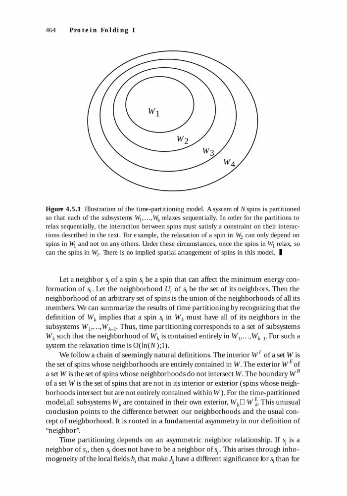
Let a neighbor sj of a spin si be a spin that can affect the minimum energy con-formation of si . Let the neighborhood Ui of si be the set of its neighbors. Then theneighborhood of an arbitrary set of spins is the union of the neighborhoods of all itsmembers. We can summarize the results of time partitioning by recognizing that thedefinition of Wk implies that a spin si in Wk must have all of its neighbors in thesubsystems W1,. . .,Wk–1. Thus, time partitioning corresponds to a set of subsystemsWk such that the neighborhood of Wk is contained entirely in W1,. . .,Wk–1. For such asystem the relaxation time is O(ln(N);1).

We follow a chain of seemingly natural definitions. The interior W I of a set W isthe set of spins whose neighborhoods are entirely contained in W. The exterior W E ofa set W is the set of spins whose neighborhoods do not intersect W. The boundary W B

of a set W is the set of spins that are not in its interior or exterior (spins whose neigh-borhoods intersect but are not entirely contained withinW ). For the time-partitionedmodel,all subsystems Wk are contained in their own exterior, Wk⊂ W k

E. This unusualconclusion points to the difference between our neighborhoods and the usual con-cept of neighborhood. It is rooted in a fundamental asymmetry in our definition of“neighbor”.

Time partitioning depends on an asymmetric neighbor relationship. If sj is aneighbor of si, then si does not have to be a neighbor of sj . This arises through inho-mogeneity of the local fields hi that make Jij have a different significance for si than for



W1

W2W3

W4

Figure 4.5.1 Illustration of the time-partitioning model. A system of N spins is partitionedso that each of the subsystems W1,…,Wk relaxes sequentially. In order for the partitions torelax sequentially, the interaction between spins must satisfy a constraint on their interac-tions described in the text. For example, the relaxation of a spin in W2 can only depend onspins in W1 and not on any others. Under these circumstances, once the spins in W1 relax, socan the spins in W2. There is no implied spatial arrangement of spins in this model. ❚

04adBARYAM_29412 3/10/02 10:37 AM Page 464

sj . The spins with the largest values of hi tend to be in Wk with lower values of k. A spinin W1 must have a large enough hi so that it dominates all of the interactions and thereare no spins in its neighborhood.

The definition of “neighborhoods” enables us also to summarize space parti-tioning. The partitioning of space corresponds to a partitioning of the system intodisjoint neighborhoods. The neighborhood of each subsystem does not intersect anyother subsystem. Thus,in this case, we can say that each subsystem is the same set ofspins as its own interior. Space partitioning can result from both inhomogeneous in-teractions and fields.

The model of decorated independent relaxation with both spatial and temporalsubsystems is attractive as a model of the relaxation in protein folding. The existenceof secondary structure, with limitations on the size of secondary-structure elements,suggests that secondary-structure elements may form first. Moreover, each of themmay form essential ly independently of the others. This would correspond to spacepartitioning. Each set of coordinates that change and cause the formation of a partic-ular secondary-structure element would be a single subsystem. All of these togetherwould be included in the same time partition. Then there is a second stage of relax-ation that forms the tertiary structure. The coordinates that control the formation ofthe tertiary structure would constitute the second time partition. It is possible, how-ever, and even likely, that during the second stage in which tertiary structure isformed, some of the secondary structure also changes.

4.5.3 Nucleation and growth in inhomogeneous fieldsDiffusive equilibration can be generalized to the inhomogeneous case. General con-clusions can be reached by relatively simple considerations;a complete analysis is dif-ficult. Nucleation and growth is a model that applies when nucleation is a relativelyrare event, so that only one critical nucleus forms in a large region. After the criticalnucleus is formed, the region of the stable phase grows by driven diffusion of theboundary between the stable and metastable phases. In order to have a diffusive in-homogeneous system,the interactions between spins Jij must be important comparedto the variation in the local field, hi , and the interactions must be essentially local anduniform. Inhomogeneities tend to enhance nucleation and inhibit diffusion of theboundaries between stable and metastable phases.Thus,increasing the inhomogene-ity tends to reduce the relevance of nucleation and growth. We will discuss morespecifically the effect of variations in hi and Jij , and then the effect of inhomogeneityin general, on the scaling of the relaxation time.

Inhomogeneities of the local fields hi cause variations in the local strength ofpreference for the stable and metastable phases. Regions that have a larger averagenegative hi will tend to nucleate before regions of a smaller average negative hi. Sincethe problem is to form a nucleus somewhere, in contrast to the rare nucleation in ahomogeneous system, this variation increases the rate of nucleation. The eff ect ofvariation in hi on diffusion of a boundary between stable and metastable phases oc-curs through local variation in the driving force. Sites that have a larger than averagenegative hi tend to increase the boundary velocity v, while sites of lower than average



04adBARYAM_29412 3/10/02 10:37 AM 5

negative hi tend to decrease the boundary velocity. The boundary must sweep throughevery site. Moreover, there is no bound on how long the boundary can be delayed,sothe sites that slow it tend to trap it. Thus, on average the velocity is reduced.

Inhomogeneities of the interactions Jij cause similar variations in nucleation anddiffusion. Smaller values of Jij make nucleation easier and the boundary diffusionslower. Conversely, larger values of Jij make nucleation harder and the boundarydiffusion faster. Since nucleation can occur anywhere while diffusion must sweepthrough everywhere, again the nucleation rate is increased while the diffusion rate isreduced.

For the case of nonnucleating boundaries,the effect on relaxation time is partic-ularly significant. The time necessary to form a critical nucleus is apparent in therelaxation-time scaling behavior as a peak in Fig. 4.4.6. With the introduction of in-homogeneities, the peak will decrease in height. For the case of nucleating bound-aries,the relaxation time is controlled by the diffusion rate and so the relaxation timewill increase. For both cases,the transition to the thermodynamic limit, where the re-laxation time is independent of N, will occur at smaller system sizes. This occurs be-cause the increasing nucleation rate and decreasing diffusion rate causes the typicalsize to which one nucleus grows—which is the size of independently relaxing parts ofthe system—to decrease.

Another consideration in the discussion of diffusive relaxation in inhomoge-neous fields is the structure of the boundary. In the presence of inhomogeneities,themoving boundary becomes rougher due to the inhomogeneities that slow and speedits motion. As long as the bulk energy dominates the boundary energy, it will remainsmooth;however, when the variation in boundary energy becomes large enough,theboundary will become rough and the dynamic behavior of the system will change.Since we have limited ourselves to considering smooth boundaries, our discussiondoes not apply to this regime.

As briefly discussed in Section 4.4.3, the model of diffusion in variable fields islikely to be of relevance to understanding the local properties of protein folding in thenucleation and growth of the secondary structure. If this applies locally to each of thesegments of secondary structure separately, then the scaling of this relaxation is notnecessarily relevant to the folding as a whole. However, it is relevant to our under-standing of the local kinetics by which secondary structural elements are formed.

4.5.4 Spin glassThere have been some efforts to describe the problem of protein folding in terms of aspin glass model and spin glass dynamics. Spin glasses are treated using models thathave long-range random interactions between all spins (Section 1.6.6):

(4.5.11)

The difficulty with this model is that many of the properties of spin glasses do not ap-ply to proteins.Spin glasses have many degenerate ground states,the number of whichgrows with the size of the system. This means that there is no unique conformation

E[{si}] = −1

2NJ ij sis j

ij∑



04adBARYAM_29412 3/10/02 10:37 AM Page 466

that can be identified with the folded state of the protein. Choose any conformation,the system will spend much more time in dramatically different conformations be-cause of the essential degeneracy of ground states. Moreover, the barriers betweenlow-lying states also grow with the size of the system. Thus, the relaxation time be-tween any of the low-lying states grows exponentially with system size. Even the con-cept of equilibration must be redefined for a low temperature spin glass, since trueequilibration is not possible. What is possible is a descent into one of the many low-lying energy states. If we model a particular set of interactions Jij as being specified bythe primary structure of a protein, there would be no correlation between low-lyingstates reached by different proteins with the same primary structure. This is in directcontrast to protein folding, where a unique (functional) structure of the protein mustbe reached.

Despite the great discrepancy between the phenomenology of spin glasses andthe protein-folding problem,there are reasons for considering this model. The use ofa spin glass model for protein folding is based on the understanding that many pos-sible bonding arrangements between amino acids are possible. For a sufficiently longchain there are many compact conformations of the chain where different bondingarrangements are found. There is always an inherent frustration in the competitionbetween different possible bonding arrangements of the amino acids. This frustra-tion is similar to the frustration that is found in a spin glass. Because of this, in thevery long chain limit, the spin glass model should become relevant. In this limit thefrustration and multiple ground states are likely to be the correct description of thechain.

However, as discussed in Section 4.4.5, even when there are long-range interac-tions, the local fields, hi, can be more important than the interactions, Jij , for smallenough systems. In an inhomogeneous system we can expand the term “local field” toinclude the effect of local interactions:

(4.5.12)

where the second sum describes the near-neighbor interactions and the third de-scribes the long-range interactions. Long-range interactions that give rise to frustra-tion may not dominate over local interactions. There are many different energies inthe problem of protein folding. The analog of local interactions in Eq.(4.5.12) are theinteractions between amino acids near each other along the chain, not interactionsthat are local in space. Hydrogen bonding between different parts of the chain, eventhough it is local in space,can give rise to frustration. Note that the -helix structureis constructed entirely out of short-range interactions, while the -sheet structure isformed out of a combination of short-range and long-range interactions.

There is a difference between bonding between different parts of the amino acidchain and long-range interactions in an Ising model. Although there are many possi-ble hydrogen bond interactions between amino acids,these interactions are quite re-stricted. The number of amino acids that can interact with a particular amino acid atany one time is limited. Moreover, the chain structure restricts which combinations

E({si }) = − hi si∑ −1

2J ij sis j

<ij>∑ −

1

2′ J ijs is j

ij∑



04adBARYAM_29412 3/10/02 10:37 AM Page 467

of amino acids can interact at one time. These limitations do not eliminate the prob-lem of frustration for very long chains. They do, however, increase the chain length atwhich crossover occurs,from the regime in which local interactions dominate, to theregime in which long-range interactions dominate. It is the latter regime which is acandidate for the spin glass model.

Our discussion implies that pro teins are fundamen t a lly re s tri cted in thei rl en g t h , and that a tre a tm ent of t h eir dynamics should inclu de this finite len g t hre s tri cti on . From ex peri m ent we know that each el em ent of the secon d a ry stru c-tu re has a limited nu m ber of amino ac i d s , and the nu m ber of s econ d a ry - s tru c-tu re el em ents in the pro tein is also limited . These ob s erved limitati ons on pro tei ns i ze are con s i s tent with our discussion of the rel a tive import a n ce of l ocal fiel d sand lon g - ra n ge interacti on s .S tru ctu ral fru s tra ti on due to lon g - ra n ge interacti on smust limit the size of pro teins to the regime in wh i ch local fiel d s , or more gen er-a lly local interacti on en er gi e s , a re import a n t . It should be assu m ed that pro tei n sex tend up to their maximal po s s i ble size . Thu s , the largest pro teins are likely to beat the cro s s over point wh en both short - ra n ge and lon g - ra n ge interacti ons com-pete . This com peti ti on should then play an important role in the rel a x a ti on - ti m es c a l i n g.

The assumption of frustration in the long-range interactions appears to be theopposite of the cooperative bonding that has been found in proteins. Cooperativebonding is equivalent to long-range ferromagnetic interactions that enhance the sta-bility of the ground state.Frustration implies that different bonds are competing witheach other. It is possible to argue that the low-energy states of the spin glass representcooperative action of many bonds and therefore constitute cooperative bonding. Onthe other hand, proteins are engineered, so that we would expect that bonds are de-signed to reinforce each other and cooperatively lower the energy of the folded stateto increase its stability. This is unlike the random spin glass model. This notion of en-gineered cooperativity leads us to consider the engineered spin glass, which is moretypically used as a model of neural network memory.

4.5.5 Engineered spin glass—neural networkNeural networks (Chapter 2) have been modeled as engineered spin glass systems (theattractor network) where energy minima of the system are specified. This might beconsidered to be analogous to the engineering of the 3-d structure of a folded proteinby selection of the amino acid sequence. In the attractor network, the interactions Jij

determine the minimum energy states. In our discussion of protein folding in thischapter, it is largely the local fields hi that determine the minimum energy state.Oneof the differences is that the attractor network cannot have a unique ground state—the inverse of a state has the same energy.

The simplest way to model the engineered spin glass is through the Mattis model(Question 1.6.12). In this model a particular state is determined to be a ground stateusing only interactions Jij and no local fields hi. We can redefine all of the spins in theground state to be si = −1. Then the Mattis model is equivalent to the long-range fer-romagnetic Ising model with no external field, h = 0,and all Jij = J. Since it is the in-



04adBARYAM_29412 3/10/02 10:37 AM Page 468

teractions that determine the ground state, both si = −1 and its inverse si = +1 areground states.

Under these circumstances we cannot consider the folding transition to be fromsi = +1 to si = −1. We can recognize, however, that the essential point of this model isto consider the impact of the initial conditions. We therefore abandon our insistenceon starting from a state where all of the spins are UP. The system will relax to the de-sired ground state if the initial conditions are favorable, specifically, if more of thespins in the initial state are DOWN than are UP.

One way to think about this is to look at the transition in terms of changing sud-denly the interaction parameters. Indeed, this is a physically meaningful analogy,since the actual folding of proteins is achieved by changing the interaction energies ofthe real system. Fig. 4.5.2 illustrates several different transitions on a phase diagramof the ferromagnet that includes both the interaction J and the field h. The transitionwe have been considering thus far in this chapter is the transition across the first-ordertransition boundary shown as (A). In this section we are considering the disorder-to-order transition that is represented by (B). As long as there are a majority of DOWN



kT

h

(A)

(B)

(C)

Figure 4.5.2 Illustration of transitions in a ferromagnetic Ising model that start with differ-ent initial conditions. The transitions, indicated by arrows, are superimposed on the Isingmodel phase diagram. The final state in each case corresponds to having all spins DOWN. (A)is a first-order transition starting from all spins UP. (B) and (C) both start from a largely ran-dom arrangement of spins but (B) starts from a majority of DOWN spins. (C) starts from a ma-jority of UP spins. ❚

04adBARYAM_29412 3/10/02 10:37 AM Page 469

spins in the initial state,there is no need for the process of nucleation and growth tooccur. The relaxation is local, and the system reduces to the decoupled model.

We can generalize the Mattis model to the attractor neural network models dis-cussed in Chapter 2. In these models, there may be more than one energy minimum.As with the random spin glass,an arbitrary initial condition leads to any one of theselow-energy states. Therefore, we cannot talk about a unique folded state in equilib-rium. However, there is a difference in this case. The neural network can be designedto have only a limited number of low-energy states. Each energy state has a basin ofattraction that consists of all of the states of the system that will naturally fall towardthe low-energy state. The basin of attraction of a particular minimum energy stateconsists of initial states that have more than a certain overlap with the minimum en-ergy state.Within this basin of attraction,the dynamics that updates the spins reachesthe ground state in a finite number of steps. This can be seen to be equivalent to thetime-partitioned decoupled model (Section 4.5.2). The spins that flip in a particularupdate correspond to a particular subsystem. The time scale for relaxation is againO(ln(N);1).

To make use of the neural network model for protein folding, we can choose aninitial conformation that has a finite fraction of spins overlapping with the desiredground state. There is a lesson to be learned from this model regarding the impor-tance of the initial conformation in protein folding. Recently there have been sugges-tions that the initial conformation is not arbitrary, but instead assumes one of a re-stricted family of conformations that are either partially folded or are related in someway to the eventual folded conformation. This would be consistent with the conceptof a basin of attraction. The introduction of a limited phase space exploration, wherethe protein does not explore all possible conformations but is restricted from the be-ginning to the basin of attraction of the folded conformation,also brings us to the sec-ond mechanism for reducing the relaxation time—kinetic effects. We will discuss ki-netic effects more generally in the next chapter.

The attractor neural network model may also be useful for understanding morecomplex protein dynamics than just protein folding. Proteins act as enzymes.However, their enzymatic efficiency may be influenced by chemical or other influ-ences that control their function.One mechanism for this control is a change in con-formation that affects the active enzymatic site. Thus a protein may respond to a va-riety of controlling influences by changing its conformation. This suggests that theremay be two or more well-defined folded conformations that are each relevant underparticular external conditions. If a change in conformation due to a particular exter-nal influence is maintained for some time after the external influence is removed,thena description of the protein in terms of multiple minimum energy conformationsmay become useful.

Missing from attractor neural networks is the incorporation of propagativestructures, specifically, interactions that can support driven diffusion or diffusion.Thus, the equilibration of neural network spin glass systems corresponds to the de-coupled model and not to any of the models that include driven diffusion or diffu-sion. The absence of propagative structures is not realistic either for protein folding



04adBARYAM_29412 3/10/02 10:37 AM Page 470

or for the general description of neural networks. Feedforward networks are a simpleapproach to incorporating propagation in neural networks. More complex propaga-tive structures are likely both in proteins and the brain.

Conclusions

In this chapter we have considered a variety of models that display a range of scalingbehavior of the relaxation time with system size. There are diverse individual featuresof these models that can be related to properties observed in protein-folding experi-ments. The models also provide some insight into the nature of the relaxation timeand its relationship to inter-amino-acid interactions. All of these models,however, aremissing the chain structure and its relaxation in space. When a chain is spread out inspace,there is an inherent scaling of the relaxation time with chain length, due to thetravel time of amino acids through the space before they can bond with other aminoacids. In the following chapter we show that this travel time leads to a characteristicrelaxation time that scales approximately as N 2 for an expanded chain.

While the models in this chapter are general enough that they cannot be used di-rectly as models of the kinetics of protein folding, this investigation does allow us torelate our findings to other complex systems. There are some general conclusions thatcan be made. First, it is not difficult to design models that cannot relax in any rea-sonable time. Long-range interactions,in particular, lead to exponential scaling of therelaxation time. A weak driving force for the transition may also cause problems.There are, however, systematic approaches to interactions that give rise to relaxationin a time that scales as a low power of the size of the system.One approach is parti-tioning in space and time; another is diffusion or driven diffusion of boundaries; athird is predisposing the system by its initial state; a fourth is dominance of local in-teractions. All of these are likely to occur in protein folding as well as in the dynamicsof other complex systems. It should be apparent that creating a complex system whereinteractions cause interdependence and yet allow dynamics to proceed in a reasonabletime requires a careful design. Complex systems have specific properties that are notgeneric to physical systems. The issues of how complex systems arise will be discussedin Chapter 6.

4.6

C o n c l u s i o n s 471


04adBARYAM_29412 3/10/02 10:37 AM Page 471

dynamics of complex systems chapter 4

Documents