dynamics and control of a suspended atn vehicle
TRANSCRIPT
San Jose State University San Jose State University
SJSU ScholarWorks SJSU ScholarWorks
Master's Theses Master's Theses and Graduate Research
Summer 2016
Dynamics and Control of A Suspended ATN Vehicle Dynamics and Control of A Suspended ATN Vehicle
Wade Patterson Brown San Jose State University
Follow this and additional works at: https://scholarworks.sjsu.edu/etd_theses
Recommended Citation Recommended Citation Brown, Wade Patterson, "Dynamics and Control of A Suspended ATN Vehicle" (2016). Master's Theses. 4717. DOI: https://doi.org/10.31979/etd.6dek-z87t https://scholarworks.sjsu.edu/etd_theses/4717
This Thesis is brought to you for free and open access by the Master's Theses and Graduate Research at SJSU ScholarWorks. It has been accepted for inclusion in Master's Theses by an authorized administrator of SJSU ScholarWorks. For more information, please contact [email protected].
DYNAMICS AND CONTROL OF A SUSPENDED ATN VEHICLE
A Thesis
Presented to
The Faculty of the Department of Mechanical Engineering
San José State University
In Partial Fulfillment
of the Requirements for the Degree
Master of Science
by
Wade P. Brown
August 2016

c© 2016
Wade P. Brown
ALL RIGHTS RESERVED
The Designated Thesis Committee Approves the Thesis Titled
DYNAMICS AND CONTROL OF A SUSPENDED ATN VEHICLE
by
Wade P. Brown
APPROVED FOR THE DEPARTMENT OF MECHANICAL ENGINEERING
SAN JOSÉ STATE UNIVERSITY
August 2016
Dr. Burford Furman Department of Mechanical Engineering
Dr. Ping Hsu Department of Electrical Engineering
David Levinson Space Systems Loral
ABSTRACT
DYNAMICS AND CONTROL OF A SUSPENDED ATN VEHICLE
by Wade P. Brown
In order to enhance the research into Automation Transit Network (ATN) systems
performed by the Spartan Superway team, a simulation environment and controller is
developed for a suspended ATN vehicle. The equations of motion are derived for a
suspended ATN vehicle constrained to move on a circular guideway (referred to as the
Planar System) and for an ATN vehicle constrained to move on a guideway of arbitrary
geometry (referred to as the General System). Additionally, a controller using feedback
linearization is designed that tracks the position of the ATN for a conditioned displacement
profile and minimizes the lateral acceleration experienced by the passenger. A literature
review is first performed that covers the background of ATN systems and other important
concepts important to vehicle control. The equations of motion for both the Planar System
and General System are derived by the use of hand calculations and the MotionGenesis
application. MotionGenesis is also used for the geometric calculations to allow for the
interpolation of the arbitrary geometry guideway, the formation of the displacement
profile, and the formation of the wind profile. SIMULINK is used to form the simulation
environment built from the theoretical work and run validation simulations. Using a
circular guideway with a radius of 100 m, it is found that there is negligible deviation
between simulations of the Planar System and simulations of the General System. A
controller is successfully implemented on the Planar System using feedback linearization
with dynamics derived from both the Planar System and General System. Finally, there is
a proof-of-concept test of the dynamics of an ATN vehicle on an Euler spiral guideway.

DEDICATION
This thesis is dedicated in loving memory of my grandmother Virginia Patterson,
whose love and support in my youth made my future possible.
v
ACKNOWLEDGEMENTS
I would like to thank my committee members Dr. Burford Furman, Dr. Ping Hsu,
and David Levinson for volunteering their time to provide guidance and mentorship for
this thesis. I would also like to thank Ron Swenson of INIST for sponsoring the Spartan
Superway project to which my thesis contributes and Bengt Gustafsson of Beamways AB
for taking time to answer my questions regarding how to assign physical values to my
mathematical idealizations to ensure a realistic simulation.
vi
TABLE OF CONTENTS
LIST OF TABLES . . . . . . . . . . . . . . . . . . . . . . . . . . . . . . . . . . . . . . . . . . . . . . . . . . . . . x
LIST OF FIGURES . . . . . . . . . . . . . . . . . . . . . . . . . . . . . . . . . . . . . . . . . . . . . . . . . . . . xi
1 INTRODUCTION . . . . . . . . . . . . . . . . . . . . . . . . . . . . . . . . . . . . . . . . . . . . . . . . . . . 1
1.1 Introduction to the Automated Transit Network Concept . . . . . . . . . . 1
1.2 Literature Review . . . . . . . . . . . . . . . . . . . . . . . . . . . . . . . 4
1.2.1 Introduction to the Literature Review . . . . . . . . . . . . . . . . 4
1.2.2 ATN System Background with Respect to Control Research Appli-
cations . . . . . . . . . . . . . . . . . . . . . . . . . . . . . . . . 5
1.2.3 Vectus Review . . . . . . . . . . . . . . . . . . . . . . . . . . . . 10
1.2.4 GM Open Guideway Vehicle Research . . . . . . . . . . . . . . . 13
1.2.5 Optimal Sample-Data Control of PRT Vehicles . . . . . . . . . . . 15
1.2.6 Optimal Cruise Control of Heavy-Haul Trains Equipped with Elec-
tronically Controlled Pneumatic Brake Systems . . . . . . . . . . . 23
1.2.7 Robust Sampled-Data Cruise Control Scheduling of High Speed
Train . . . . . . . . . . . . . . . . . . . . . . . . . . . . . . . . . 28
1.2.8 Suspension Control for Conventional Trains . . . . . . . . . . . . . 32
2 OBJECTIVE . . . . . . . . . . . . . . . . . . . . . . . . . . . . . . . . . . . . . . . . . . . . . . . . . . . . . . . . 35
3 METHODOLOGY . . . . . . . . . . . . . . . . . . . . . . . . . . . . . . . . . . . . . . . . . . . . . . . . . . . 38
3.1 Dynamical System Idealization . . . . . . . . . . . . . . . . . . . . . . . . 38
3.2 Forming the Equations of Motion and Validation Simulations . . . . . . . . 39
3.3 Numerically Defined Unit Vectors . . . . . . . . . . . . . . . . . . . . . . 39
3.4 Designing the Controller . . . . . . . . . . . . . . . . . . . . . . . . . . . 39
vii
4 ATN VEHICLE DYNAMICS. . . . . . . . . . . . . . . . . . . . . . . . . . . . . . . . . . . . . . . . . . . 40
4.1 Planar System - Manual Derivation . . . . . . . . . . . . . . . . . . . . . . 40
4.2 General System - Theoretical Overview . . . . . . . . . . . . . . . . . . . 55
4.3 MotionGenesis Overview . . . . . . . . . . . . . . . . . . . . . . . . . . . 61
4.3.1 Planar System - Derivation with MotionGenesis . . . . . . . . . . . 62
4.3.2 General System - Working with Spatial Derivatives . . . . . . . . . 68
5 ATN VEHICLE SIMULATION . . . . . . . . . . . . . . . . . . . . . . . . . . . . . . . . . . . . . . . . . 72
5.1 Displacement Profile Calculation . . . . . . . . . . . . . . . . . . . . . . . 72
5.2 Angle Setpoint Calculation . . . . . . . . . . . . . . . . . . . . . . . . . . 75
5.3 Wind Force Calculation . . . . . . . . . . . . . . . . . . . . . . . . . . . . 78
5.4 Non-Linear Friction Force . . . . . . . . . . . . . . . . . . . . . . . . . . 80
5.5 Feedback Linearization . . . . . . . . . . . . . . . . . . . . . . . . . . . . 82
5.6 P Control - Pole Placement . . . . . . . . . . . . . . . . . . . . . . . . . . 84
6 RESULTS AND DISCUSSION . . . . . . . . . . . . . . . . . . . . . . . . . . . . . . . . . . . . . . . . . 86
6.1 Results Introduction . . . . . . . . . . . . . . . . . . . . . . . . . . . . . . 86
6.2 Planar System - Comparison Study . . . . . . . . . . . . . . . . . . . . . . 87
6.3 General System - Numerical Unit Vector Analysis . . . . . . . . . . . . . . 93
6.4 General System - Comparison Study . . . . . . . . . . . . . . . . . . . . . 97
6.5 Planar System - Controlled Plant . . . . . . . . . . . . . . . . . . . . . . . 100
6.6 Planar System - No Vehicle Angle Control . . . . . . . . . . . . . . . . . . 109
6.7 Planar System - Controlled Plant w/ Feedback Linearization from General
System Dynamics . . . . . . . . . . . . . . . . . . . . . . . . . . . . . . . 112
6.8 General System - Euler Spiral Example . . . . . . . . . . . . . . . . . . . 120
7 CONCLUSION AND RECOMMENDATIONS FOR FUTHER RESEARCH. . . . . 128
REFERENCES . . . . . . . . . . . . . . . . . . . . . . . . . . . . . . . . . . . . . . . . . . . . . . . . . . . . . . . . 130
viii
APPENDIX
A Appendix A: MotionGenesis Scripts . . . . . . . . . . . . . . . . . . . . . . . . . . . . . . . . . . . . . 132
A.1 Planar System Equations of Motion Derivation . . . . . . . . . . . . . . . 132
A.2 General System Equations of Motion Derivation . . . . . . . . . . . . . . . 133
A.3 General System - Unit Vector Coefficient Calculation . . . . . . . . . . . . 135
B Appendix B: SIMULINK MODEL - PLANAR SYSTEM . . . . . . . . . . . . . . . . . . . . 137
C Appendix C: SIMULINK MODEL - GENERAL SYSTEM. . . . . . . . . . . . . . . . . . . 138
ix
LIST OF TABLES
1 Table of VECTUS Performance Data . . . . . . . . . . . . . . . . . . . . . 12
2 Performance Parameters of Optimally Controlled PRT Vehicle . . . . . . . 20
3 S Unit Vectors Relation - Planar System . . . . . . . . . . . . . . . . . . . 42
4 A Unit Vectors Relation - Planar System . . . . . . . . . . . . . . . . . . . 45
5 Planar System - Partial Velocities and Partial Angular Velocities . . . . . . 51
6 S Unit Vectors Relation - General System . . . . . . . . . . . . . . . . . . 57
7 Guideway Geometry - 100m Circle Example . . . . . . . . . . . . . . . . . 61
8 Non-Linear Friction Model Coefficients . . . . . . . . . . . . . . . . . . . 81
9 Comparison Study - Parameters . . . . . . . . . . . . . . . . . . . . . . . 88
10 Planar System - Comparison Study - Initial Conditions . . . . . . . . . . . 88
11 Comparison Study - Constant Bogie Force . . . . . . . . . . . . . . . . . . 92
12 General System - Comparison Study - Constant Bogie Force . . . . . . . . 99
13 Planar System - Controlled Plant - Parameters . . . . . . . . . . . . . . . . 101
14 Planar System - Controlled Plant - Initial Conditions . . . . . . . . . . . . 101
15 Planar System - Controlled Plant - Displacement Profile . . . . . . . . . . . 102
16 Planar System - Controlled Plant - Performance . . . . . . . . . . . . . . . 108
17 Planar System - General System Controller - Performance . . . . . . . . . 119
18 General System - Euler Spiral - Parameters . . . . . . . . . . . . . . . . . 124
19 General System - Euler Spiral - Initial Conditions . . . . . . . . . . . . . . 124
x
LIST OF FIGURES
1 Beamways ATN System . . . . . . . . . . . . . . . . . . . . . . . . . . . 3
2 Acceleration Profile Example . . . . . . . . . . . . . . . . . . . . . . . . . 6
3 ATN Vehicle Comparison . . . . . . . . . . . . . . . . . . . . . . . . . . . 8
4 Headway Diagram . . . . . . . . . . . . . . . . . . . . . . . . . . . . . . 9
5 Offline Station Example . . . . . . . . . . . . . . . . . . . . . . . . . . . . 10
6 The Vectus Test Track . . . . . . . . . . . . . . . . . . . . . . . . . . . . . 11
7 Vectus PRT Constant Voltage/Frequency Test . . . . . . . . . . . . . . . . 12
8 Vectus Dynamic Response Test . . . . . . . . . . . . . . . . . . . . . . . . 13
9 GM Transmode Chassis . . . . . . . . . . . . . . . . . . . . . . . . . . . . 14
10 Slot Advance Acceleration Profile . . . . . . . . . . . . . . . . . . . . . . 20
11 Constant Velocity ATN Vehicle Response . . . . . . . . . . . . . . . . . . 21
12 Slot Advance Acceleration of ATN Vehicle . . . . . . . . . . . . . . . . . 22
13 Sampling Time for a Slot Advance Simulation . . . . . . . . . . . . . . . . 22
14 Heavy Haul Trains without Fencing . . . . . . . . . . . . . . . . . . . . . 25
15 Heavy Haul Trains with Fencing . . . . . . . . . . . . . . . . . . . . . . . 25
16 Open Loop Control of Heavy Haul Trains . . . . . . . . . . . . . . . . . . 26
17 Feedback Control with Generic Tuning Parameters . . . . . . . . . . . . . 27
18 Model of High Speed Passenger Train . . . . . . . . . . . . . . . . . . . . 28
19 Velocty Input of Robust High Speed Passenger Train Controller . . . . . . 30
20 Relative Displacement of Robust High Speed Passenger Train Controller . . 31
21 Velocity of Robust High Speed Passenger Train Controller . . . . . . . . . 32
22 Tilting Train Diagram . . . . . . . . . . . . . . . . . . . . . . . . . . . . . 33
23 Planar System - Kinematics Overview . . . . . . . . . . . . . . . . . . . . 41
24 Planar System - Frame s . . . . . . . . . . . . . . . . . . . . . . . . . . . 42
xi
25 Planar System - Frame A . . . . . . . . . . . . . . . . . . . . . . . . . . . 45
26 Planar System - Bogie Free Body Diagram . . . . . . . . . . . . . . . . . . 48
27 Planar System - BC External Torques . . . . . . . . . . . . . . . . . . . . . 49
28 Planar System - Vehicle Body Free Body Diagram . . . . . . . . . . . . . . 50
29 General System - Kinematics Overview . . . . . . . . . . . . . . . . . . . 56
30 Displacement Profile Example . . . . . . . . . . . . . . . . . . . . . . . . 74
31 Passenger Free Body Diagram . . . . . . . . . . . . . . . . . . . . . . . . 76
32 Wind Profile Example . . . . . . . . . . . . . . . . . . . . . . . . . . . . . 79
33 Vehicle Arm Angle Non-Linear Friction . . . . . . . . . . . . . . . . . . . 81
34 Planar System - Bogie Position and Velocity - Reference . . . . . . . . . . 89
35 Planar System - Vehicle Angular Displacement and Vehicle Angular Ve-
locity - Reference . . . . . . . . . . . . . . . . . . . . . . . . . . . . . . . 90
36 Planar System - Comparison Study - Bogie Position and Velocity Error . . . 91
37 Planar System - Comparison Study - Vehicle Angular Position and Velocity
Error . . . . . . . . . . . . . . . . . . . . . . . . . . . . . . . . . . . . . . 92
38 General System - Determinant Error of Rotation Matrix . . . . . . . . . . . 94
39 General System - Element Error of Rotation Matrix . . . . . . . . . . . . . 95
40 General System - Unit Vector Error . . . . . . . . . . . . . . . . . . . . . . 97
41 General System - Comparison Study - Bogie States . . . . . . . . . . . . . 98
42 General System - Comparison Study - Vehicle Angle States . . . . . . . . . 99
43 General System - Comparison Study - Unit Vector Error . . . . . . . . . . 100
44 Planar System - Controlled Plant - Bogie States . . . . . . . . . . . . . . . 102
45 Planar System - Controlled Plant - Vehicle Angle States . . . . . . . . . . . 103
46 Planar System - Controlled Plant - Error . . . . . . . . . . . . . . . . . . . 104
47 Planar System - Controlled Plant - Bogie Performance . . . . . . . . . . . 105
xii
48 Planar System - Controlled Plant - Vehicle Angle Performance . . . . . . . 106
49 Planar System - Controlled Plant - Reaction Forces . . . . . . . . . . . . . 107
50 Planar System - Controlled Plant - Power Consumption . . . . . . . . . . . 108
51 Planar System - No Angle Control - Bogie States . . . . . . . . . . . . . . 110
52 Planar System - No Angle Control - Vehicle Angle States . . . . . . . . . . 111
53 Planar System - No Angle Control - Reaction Forces . . . . . . . . . . . . 112
54 Planar System - General System Controller - Bogie States . . . . . . . . . . 113
55 Planar System - General System Controller - Vehicle Angle States . . . . . 114
56 Planar System - General System Controller - Tracking Error . . . . . . . . 115
57 Planar System - General System Controller - Bogie Performance . . . . . . 116
58 Planar System - General System Controller - Vehicle Angle Performance . . 117
59 Planar System - General System Controller - Reaction Forces . . . . . . . . 118
60 Planar System - General System Controller - Power Consumption . . . . . 119
61 General System - Euler Spiral . . . . . . . . . . . . . . . . . . . . . . . . 121
62 General System - Euler Spiral - Geometry Analysis 1 . . . . . . . . . . . . 122
63 General System - Euler Spiral - Geometry Analysis 2 . . . . . . . . . . . . 123
64 General System - Euler Spiral - Bogie States . . . . . . . . . . . . . . . . . 125
65 General System - Euler Spiral - Vehicle Angle States . . . . . . . . . . . . 126
66 General System - Euler Spiral - Curvature Analysis . . . . . . . . . . . . . 127
67 SIMULINK Model - Planar System . . . . . . . . . . . . . . . . . . . . . 137
68 SIMULINK Model - General System . . . . . . . . . . . . . . . . . . . . . 138
xiii
CHAPTER 1
INTRODUCTION
1.1 Introduction to the Automated Transit Network Concept
During the 20th century, the reliance on the use of automobiles expanded with the
creation of new highway systems throughout the rural and urban centers of the country.
This increased reliance on automobiles allowed the average citizen a previously
unparalleled degree of convenience in personal transportation. However, as the 20th
century came to a close, it became apparent that cities depending only highway networks
were victims of unforeseen negative externalities. Chief among these was the problem of
traffic congestion, which could turn a nominally short commute into hours, as well as the
long term problem of air pollution. While an obvious solution would be investment in
public transportation, traditional public transportation is nominally slower and less
convenient than automobiles. An attractive middle ground solution, which was originally
developed in the mid 20th century, is an Automated Transit Network or ATN. An ATN is a
network of exclusive guideways, typically elevated, on which a fleet of small vehicles are
allowed to move. The vehicles can move on the guideway with a captive bogie, where the
vehicle can only move tangent to the guideway (similar to conventional rail vehicles), or
be vehicles on an open paved surface. The vehicles are all controlled autonomously and
have no set time-table. Thus, the vehicles will travel directly from the point of origin to
the desired destination of the passengers. This system of networked vehicles retains the
advantages of traditional train systems, such as reducing congestion and being powered by
the electric grid (which can utilize renewable energy) while vastly decreasing the amount
of time required for an individual commuter to reach his or her destination. In addition,
the exclusive guideway network, which is typically above grade, enhances safety by
1
ensuring that the vehicle remains segregated from pedestrian and bicycle traffic. There are
currently five public transportation systems around the world that qualify as ATN systems
which are in service and carry passengers (Furman, Fabian, Ellis, Muller, & Swenson,
2014). These five systems are in the following locations:
• The Morgantown PRT at West Virginia University
• The Parkshuttle Rivium metro-feeder outside Rotterdam (1999)
• The Masdar City PRT in Abu Dhabi (2010)
• The Terminal 5 Shuttle at London Heathrow Airport (2011)
• The Nature Park Shuttle in Suncheon Bay, South Korea (2014)
Of these five systems, the technology behind the ATN at Sunceheon Bay in South Korea
(which was developed by the company Vectus PRT) is investigated in the Literature
Review of this thesis.
However, this novel form of public transportation has unique engineering
challenges. These challenges include the structural design of the vehicle and guideway,
the energy source and power consumption of the ATN vehicles, the control of the
individual ATN vehicles, and the routing method for the entire network. This thesis will
focus primarily on the control of the individual vehicle. This thesis will specifically
present a controller for a suspended ATN vehicle using a captive bogie design that tracks
position and minimizes centripetal acceleration. The general vehicle and system design is
being referenced from work done by Beamways AB (B. Gustafsson, 2014) and the INIST
sponsored Spartan Superway research (Furman, 2016). Beamways AB, a design firm in
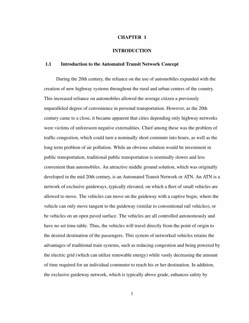
Sweden, is designing an ATN system using a suspended vehicle. See Figure 1 for an
example of the Beamways AB vehicle.
2
Figure 1. An artistic representation of what the Beamways ATN system will look like.Property of Beamways AB. Reprinted with permission.
Spartan Superways, an engineering team comprised of undergraduate and graduate
students at San José State University, is developing the technology using concepts original
to Beamways. As this thesis is being developed under the guidance of the INIST
sponsored Spartan Superway project, the vehicle parameters are similar to the designs
developed by members of the Spartan Superway team. The research in this thesis will
investigate a novel method for the vehicle to simultaneously track position and maintain
rider comfort using state control. To simplify the vehicle dynamics, the bogie is
considered to be a point mass which can track its position on a straight or curved
guideway and the suspended vehicle is considered to be a point mass which is suspended
from the bogie mass by means of a rigid rod. The rod is allowed to tilt normal to the
direction of the guideway. This simplification ignores the complicated internal dynamics
of the vehicle suspension which is still under development. Additionally, a simplified
model is easier to validate.
The following chapter describes a review of the literature focusing in three areas.
The first is a background of the existing ATN design literature and includes a case study of
a full scale model system. This information is obtained from relevant textbooks and
3
whitepapers. Next a review of historical research in ATN control is conducted which gives
a background in developing classical and state control algorithms. Finally a review of the
modern control techniques used for conventional rail vehicles is presented. While these
vehicles are much heavier and larger than the ATN vehicles being analyzed and the
research can be specific to a certain rail line or particular rail vehicle, there are similarities
in the dynamics and control between conventional train vehicles and ATN vehicles. These
papers are referenced for controller design strategies as the field of rail vehicle control is
mature compared to ATN control. These three sources will allow for the development of a
thesis that attempts to solve a historically defined problem with modern tools.
1.2 Literature Review
1.2.1 Introduction to the Literature Review
The first section of the literature review gives an introduction to the terminology and
concepts of ATN systems. Special emphasis is placed on how each of the concepts relates
to controller research. The second section reviews research specific to ATN systems. This
includes a case study of the commercially developed Vectus ATN system, an open
guideway vehicle tested by GM, and a study researching full state control of an idealized
ATN vehicle. As discussed earlier, the dynamical behavior of an ATN vehicle is similar to
the dynamical behavior of a conventional railway vehicle. Therefore, a useful resource for
ATN vehicle control to investigate research modern control of conventional railway
vehicles. Three different research projects are reviewed, one in the position and velocity
control of a high speed train with multiple cars, one in the position and velocity control of
a freight train, and one paper in the implementation of a passenger train that uses tilting
for active suspension.
4
1.2.2 ATN System Background with Respect to Control Research Applications
There is a desire to understand existing research performed in the past on the
control of ATN vehicles. The body of research in ATN typically uses a standardized
performance criteria for system analysis and vehicle control. Additionally, some of the
terminology the literature uses is in the context of urban planning or system design rather
than control engineering. Therefore, there is a need to understand the physical meaning of
the terminology used in ATN literature.
Passenger comfort and transit time are conflicting ATN vehicle controller
performance criteria. At a system level, the two variables that govern both of these criteria
are the acceleration and jerk of the pod car. The acceleration (a) is the second time
derivative of the position of the vehicle. The jerk (J) is defined as the time derivative of
acceleration or the third time derivative of vehicle’s position. The acceleration and jerk of
the vehicle may not exceed given values at any point in time during motion. The exact
value depends the regulations governing the ATN system as well as other factors (such as
if the passengers are standing or sitting) (Anderson, 1978). At a system level, the
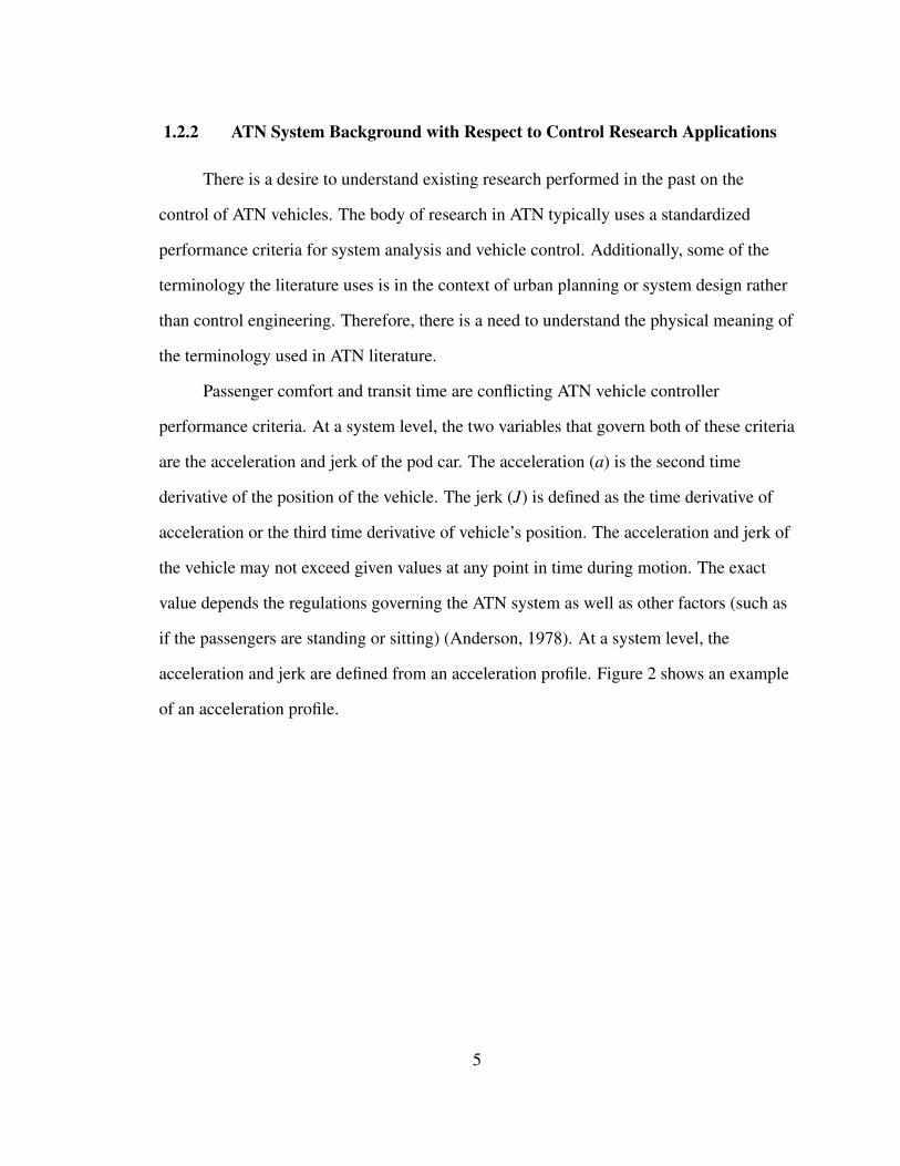
acceleration and jerk are defined from an acceleration profile. Figure 2 shows an example
of an acceleration profile.
5
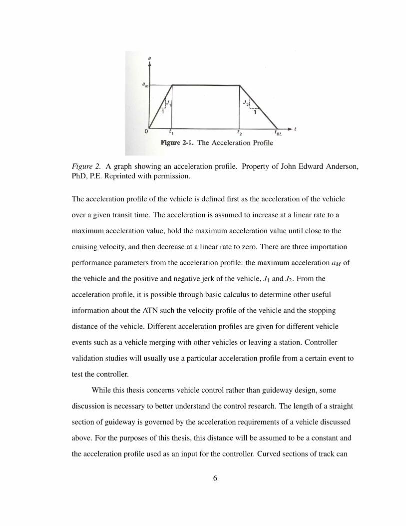
Figure 2. A graph showing an acceleration profile. Property of John Edward Anderson,PhD, P.E. Reprinted with permission.
The acceleration profile of the vehicle is defined first as the acceleration of the vehicle
over a given transit time. The acceleration is assumed to increase at a linear rate to a
maximum acceleration value, hold the maximum acceleration value until close to the
cruising velocity, and then decrease at a linear rate to zero. There are three importation
performance parameters from the acceleration profile: the maximum acceleration aM of
the vehicle and the positive and negative jerk of the vehicle, J1 and J2. From the
acceleration profile, it is possible through basic calculus to determine other useful
information about the ATN such the velocity profile of the vehicle and the stopping
distance of the vehicle. Different acceleration profiles are given for different vehicle
events such as a vehicle merging with other vehicles or leaving a station. Controller
validation studies will usually use a particular acceleration profile from a certain event to
test the controller.
While this thesis concerns vehicle control rather than guideway design, some
discussion is necessary to better understand the control research. The length of a straight
section of guideway is governed by the acceleration requirements of a vehicle discussed
above. For the purposes of this thesis, this distance will be assumed to be a constant and
the acceleration profile used as an input for the controller. Curved sections of track can
6
either be circular arcs or spiral segments. Additionally, curved segments of track can
exploit the super elevation principle. Super elevation (also referred in conventional rail
literature as “canting") is the concept of tilting the ATN vehicle during travel. This allows
for a reduction in the centrifugal force on the passengers in the vehicle. This allows for
either a higher speed around a given radius in the guideway or for the radius to be reduced.
Either the guideway can be tilted or the vehicle body can be tilted to achieve this effect.
Equation 1 (Anderson, 1978) estimates the reduction in centrifugal force.
an = g tanφ + e≈ g(φ + e) (1)
e is the elevated angle of the guideway and φ is the angle between the acceleration due to
gravity (g) and the normal to the floor of the vehicle. The centripetal acceleration an is the
acceleration vector from the vehicle body pointing to the center of the guideway arc. This
concept is important to understanding the difference between supported and suspended
captive bogie ATN vehicles.
The core of an ATN system is the vehicle which carries passengers between
destinations. The two main types of vehicles are captive bogie ATN vehicle, such as the
Vectus ATN system, and ATN vehicles for open guideways, such as the ULTra PRT ATN
system and the experimental GM ATN system (Muller, 2009). The open guideway vehicle
is where the vehicle is allowed to move freely on a guideway and must control for its
longitudinal and lateral position on the guideway. The captive bogie ATN vehicle is where
the vehicle has a bogie fixed to the track and can only move tangentially to the track.
Additionally a captive bogie ATN vehicle may be Support-Vehicle-System type vehicle
(otherwise known as a supported vehicle) or a Hanging-Vehicle-System type vehicle
(otherwise known as a suspended vehicle) (Anderson, 2013). Figure 3 shows a
comparison between each vehicle type. On the left is a supported vehicle and on the right
7
is a suspended vehicle. d represents the chord length on a curved section of guideway.
The symbols Fc and w represent the centrifugal force and weight respectively. h is the
distance of the center of mass on the supported vehicle to the guideway. h1 is the distance
from the suspended vehicle center of mass to the revolute joint of the suspended vehicle
and h2 is the distance from the revolute joint to the guideway.
Figure 3. A comparison of a suspended vehicle (right) and a simply supported vehicle(left). Property of John Edward Anderson, PhD, P.E. Reprinted with permission.
The supported vehicles have simpler construction than the suspended vehicles, however,
supported vehicles must have a tilted guideway in order to take advantage of the
super-elevation principle. Suspended vehicles can exploit the super-elevation principle by
means of the vehicle body tilting inward. Lastly, for any type of vehicle, there can be
point-following and car-following vehicle control schemes (Kornhauser, Lion, McEvaddy,
& Garrard, 1974). Point following vehicles are given a position reference to a point
moving along the guideway with a given acceleration profile. The reference for car
following vehicles is based on the position of adjacent vehicles (Kornhauser et al., 1974).
For both types of control, the reference value is decided from either a central computer
(referred to as synchronous control) or by each vehicle (referred to as asynchronous
control).
An important concept for rating an ATN system, as well as measuring performance
of a position tracking algorithm, is minimum headway. Headway is the time it takes a
trailing vehicle to be in the same position as the leading vehicle (Anderson, 1978) and has
8
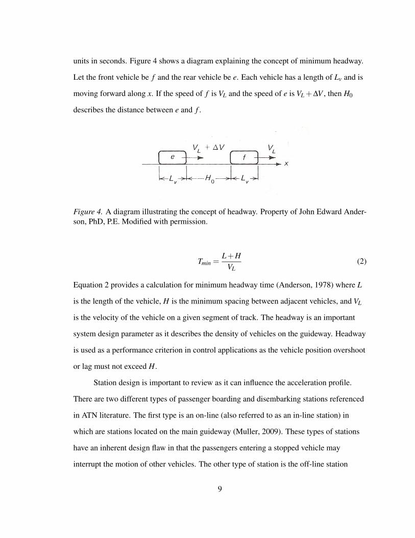
units in seconds. Figure 4 shows a diagram explaining the concept of minimum headway.
Let the front vehicle be f and the rear vehicle be e. Each vehicle has a length of Lv and is
moving forward along x. If the speed of f is VL and the speed of e is VL +∆V , then H0
describes the distance between e and f .
Figure 4. A diagram illustrating the concept of headway. Property of John Edward Ander-son, PhD, P.E. Modified with permission.
Tmin =L+H
VL(2)
Equation 2 provides a calculation for minimum headway time (Anderson, 1978) where L
is the length of the vehicle, H is the minimum spacing between adjacent vehicles, and VL
is the velocity of the vehicle on a given segment of track. The headway is an important
system design parameter as it describes the density of vehicles on the guideway. Headway
is used as a performance criterion in control applications as the vehicle position overshoot
or lag must not exceed H.
Station design is important to review as it can influence the acceleration profile.
There are two different types of passenger boarding and disembarking stations referenced
in ATN literature. The first type is an on-line (also referred to as an in-line station) in
which are stations located on the main guideway (Muller, 2009). These types of stations
have an inherent design flaw in that the passengers entering a stopped vehicle may
interrupt the motion of other vehicles. The other type of station is the off-line station
9
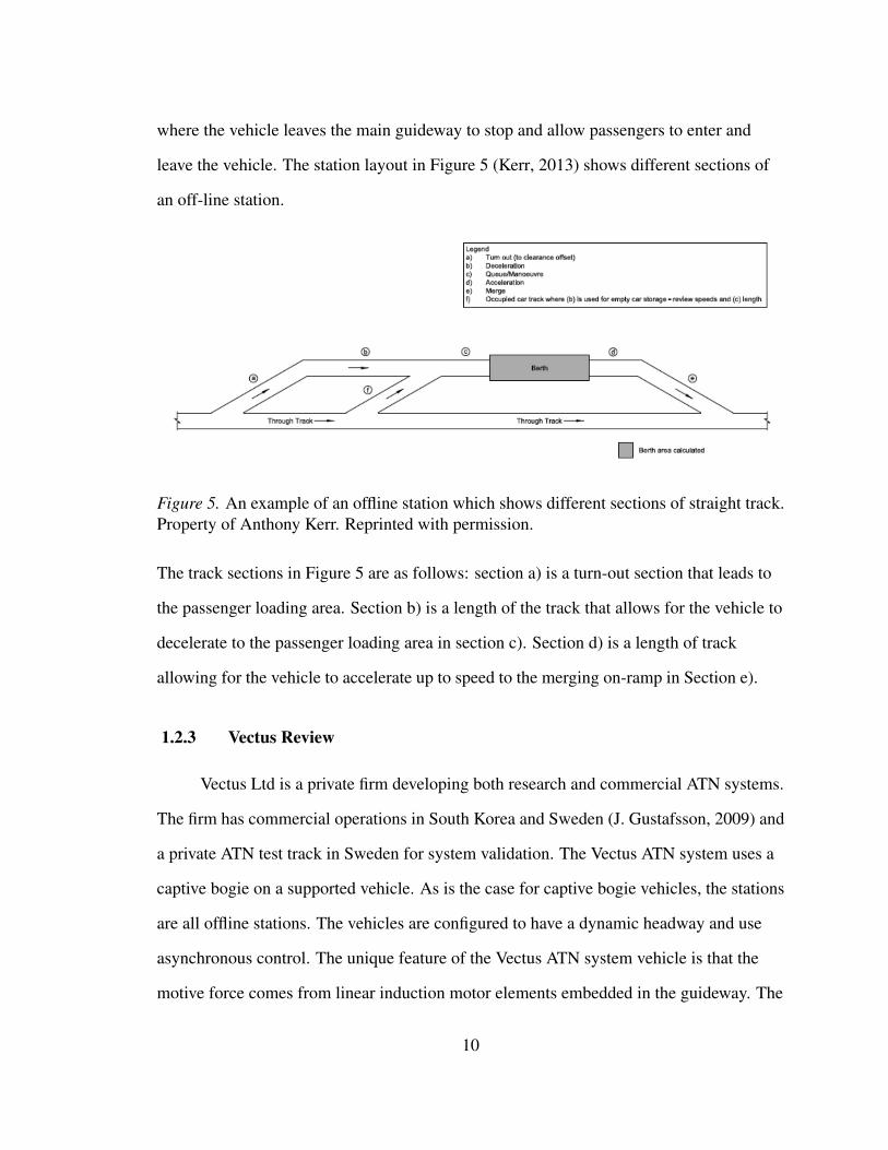
where the vehicle leaves the main guideway to stop and allow passengers to enter and
leave the vehicle. The station layout in Figure 5 (Kerr, 2013) shows different sections of
an off-line station.
Figure 5. An example of an offline station which shows different sections of straight track.Property of Anthony Kerr. Reprinted with permission.
The track sections in Figure 5 are as follows: section a) is a turn-out section that leads to
the passenger loading area. Section b) is a length of the track that allows for the vehicle to
decelerate to the passenger loading area in section c). Section d) is a length of track
allowing for the vehicle to accelerate up to speed to the merging on-ramp in Section e).
1.2.3 Vectus Review
Vectus Ltd is a private firm developing both research and commercial ATN systems.
The firm has commercial operations in South Korea and Sweden (J. Gustafsson, 2009) and
a private ATN test track in Sweden for system validation. The Vectus ATN system uses a
captive bogie on a supported vehicle. As is the case for captive bogie vehicles, the stations
are all offline stations. The vehicles are configured to have a dynamic headway and use
asynchronous control. The unique feature of the Vectus ATN system vehicle is that the
motive force comes from linear induction motor elements embedded in the guideway. The
10
linear motors embedded in the guideway have the advantage of giving constant propulsive
force to the vehicle as well as allowing for variation in the amount of propulsive force by
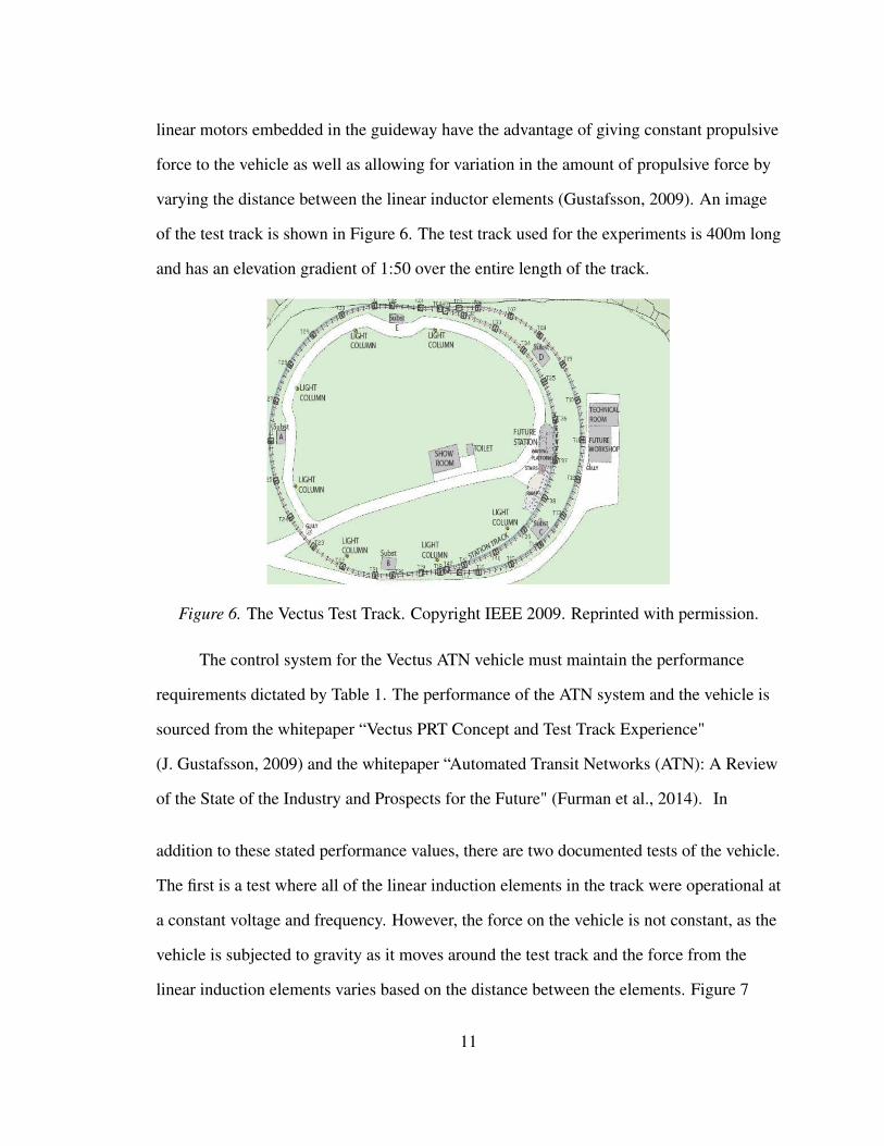
varying the distance between the linear inductor elements (Gustafsson, 2009). An image
of the test track is shown in Figure 6. The test track used for the experiments is 400m long
and has an elevation gradient of 1:50 over the entire length of the track.
Figure 6. The Vectus Test Track. Copyright IEEE 2009. Reprinted with permission.
The control system for the Vectus ATN vehicle must maintain the performance
requirements dictated by Table 1. The performance of the ATN system and the vehicle is
sourced from the whitepaper “Vectus PRT Concept and Test Track Experience"
(J. Gustafsson, 2009) and the whitepaper “Automated Transit Networks (ATN): A Review
of the State of the Industry and Prospects for the Future" (Furman et al., 2014). In
addition to these stated performance values, there are two documented tests of the vehicle.
The first is a test where all of the linear induction elements in the track were operational at
a constant voltage and frequency. However, the force on the vehicle is not constant, as the
vehicle is subjected to gravity as it moves around the test track and the force from the
linear induction elements varies based on the distance between the elements. Figure 7
11
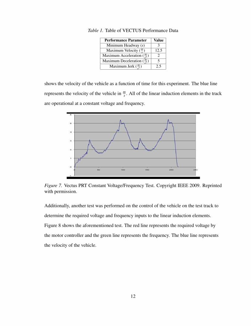
Table 1. Table of VECTUS Performance Data
Performance Parameter ValueMinimum Headway (s) 3Maximum Velocity ( m
s ) 12.5Maximum Acceleration ( m
s2 ) 2Maximum Deceleration ( m
s2 ) 5Maximum Jerk ( m
s3 ) 2.5
shows the velocity of the vehicle as a function of time for this experiment. The blue line
represents the velocity of the vehicle in ms . All of the linear induction elements in the track
are operational at a constant voltage and frequency.
Figure 7. Vectus PRT Constant Voltage/Frequency Test. Copyright IEEE 2009. Reprintedwith permission.
Additionally, another test was performed on the control of the vehicle on the test track to
determine the required voltage and frequency inputs to the linear induction elements.
Figure 8 shows the aforementioned test. The red line represents the required voltage by
the motor controller and the green line represents the frequency. The blue line represents
the velocity of the vehicle.
12
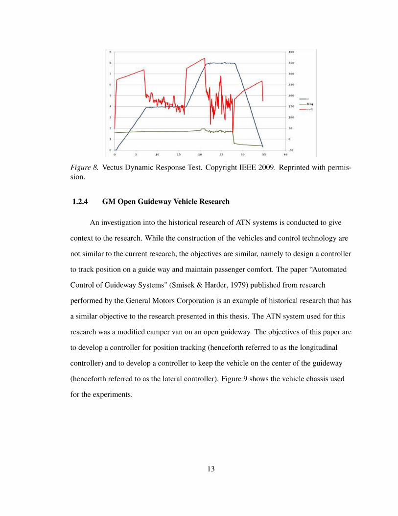
Figure 8. Vectus Dynamic Response Test. Copyright IEEE 2009. Reprinted with permis-sion.
1.2.4 GM Open Guideway Vehicle Research
An investigation into the historical research of ATN systems is conducted to give
context to the research. While the construction of the vehicles and control technology are
not similar to the current research, the objectives are similar, namely to design a controller
to track position on a guide way and maintain passenger comfort. The paper “Automated
Control of Guideway Systems" (Smisek & Harder, 1979) published from research
performed by the General Motors Corporation is an example of historical research that has
a similar objective to the research presented in this thesis. The ATN system used for this
research was a modified camper van on an open guideway. The objectives of this paper are
to develop a controller for position tracking (henceforth referred to as the longitudinal
controller) and to develop a controller to keep the vehicle on the center of the guideway
(henceforth referred to as the lateral controller). Figure 9 shows the vehicle chassis used
for the experiments.
13
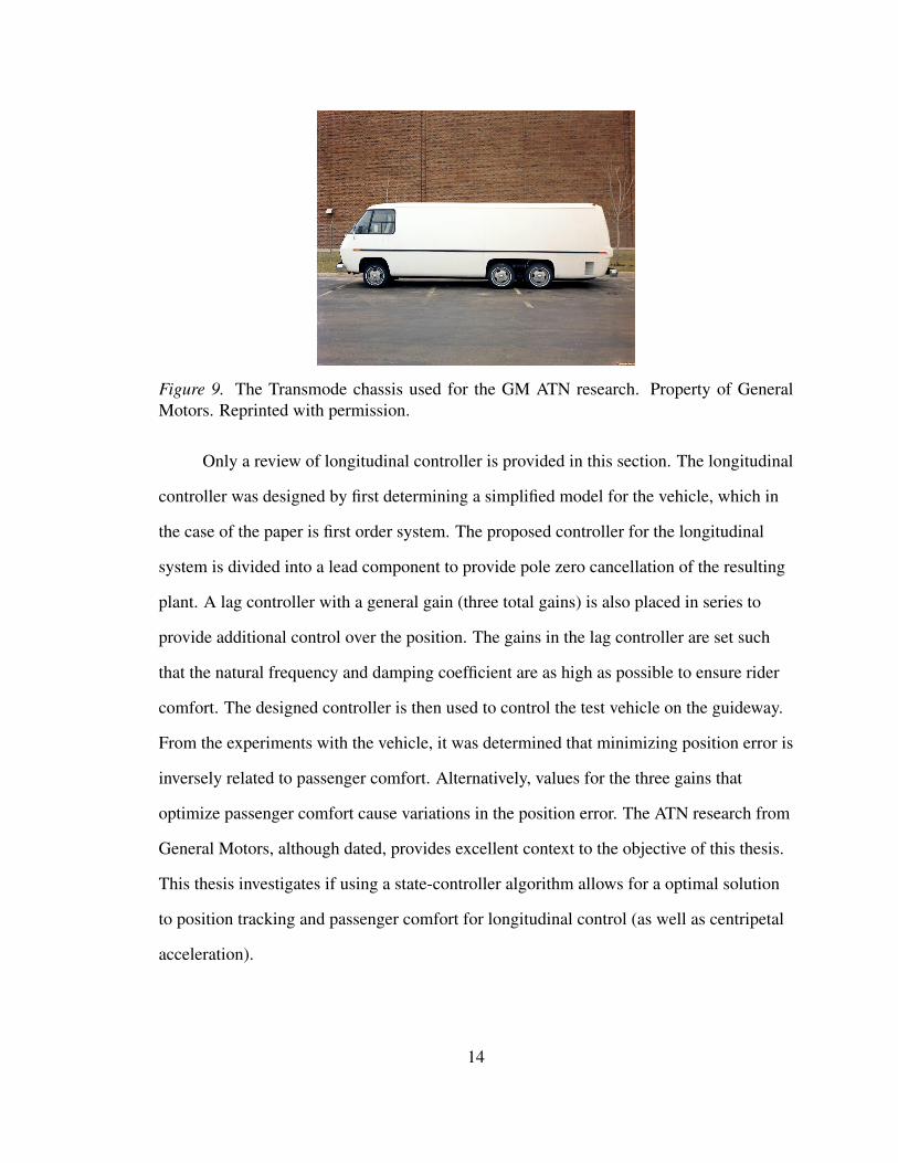
Figure 9. The Transmode chassis used for the GM ATN research. Property of GeneralMotors. Reprinted with permission.
Only a review of longitudinal controller is provided in this section. The longitudinal
controller was designed by first determining a simplified model for the vehicle, which in
the case of the paper is first order system. The proposed controller for the longitudinal
system is divided into a lead component to provide pole zero cancellation of the resulting
plant. A lag controller with a general gain (three total gains) is also placed in series to
provide additional control over the position. The gains in the lag controller are set such
that the natural frequency and damping coefficient are as high as possible to ensure rider
comfort. The designed controller is then used to control the test vehicle on the guideway.
From the experiments with the vehicle, it was determined that minimizing position error is
inversely related to passenger comfort. Alternatively, values for the three gains that
optimize passenger comfort cause variations in the position error. The ATN research from
General Motors, although dated, provides excellent context to the objective of this thesis.
This thesis investigates if using a state-controller algorithm allows for a optimal solution
to position tracking and passenger comfort for longitudinal control (as well as centripetal
acceleration).
14
1.2.5 Optimal Sample-Data Control of PRT Vehicles
The research paper titled “Optimal State Control of PRT Vehicles" (Kornhauser
et al., 1974) demonstrates how to control a highly idealized ATN vehicle using state
control techniques. The state control is formulated in discrete time and subjected to
random noise to better provide for more realistic simulations. This paper treats the ATN as
a point moving on a straight section of guideway. The equation of motion of the ATN are
not derived, but given as
Mv =−FD +F−FM−Mgsinθ (3)
The ATN system in Equation 3 is idealized as a particle of mass M that moves along a
straight guideway at velocity v. The forces on the vehicle are the propulsive force F , the
rolling resistance FM, the weight from the vehicle due to a sloped guideway and a drag
force FD. The definition of FD in Equation 3 is
FD =CD(v+ vW )2 (4)
The drag force is a function of the drag coefficient CD and sum of v and the wind velocity
vW . The unique development used in order to provide jerk control is to model F as a first
order system which has the form of
F =−1τ
F +Ki (5)
Where τ is a time constant, i is the control input to the motor, and K is the gain to the
input. Given expressions for the motion of the ATN vehicle and the definitions of FD and
F , Equation 3 is reformulated using the error, e, between the ATN vehicle position and the
15
desired position, xc. The expression for e is
x = e+ xc (6)
Substituting from Equation 6 into Equation 3 produces
Me =−CD(e+ xc + vw)2 +F−Mgsinθ −Mxc−FM (7)
The next step is to create a non-dimensional form of the equations of motion. This is
performed by first choosing a non-dimensional form for each of the terms in the equations
of motion.
y =eH
(8)
The position error e is divided by minimum headway spacing between each ATN vehicle.
σ =tT
(9)
The elapsed time, t, is divided by the minimum headway time T (Refer to Equation 2).
T =HvN
(10)
In turn, the minimum headway time T is defined as the minimum headway spacing
divided by the nominal cruising velocity, vN .
w =vW
vN(11)
16
The non-dimensional wind velocity is vW divided by vN .
f =T F
MvN(12)
The non-dimensional force is a function of T , the force on the ATN vehicle F , M, and vN .
v∗ =T 2KiMvn
(13)
The non-dimensional input is defined as a function of the square of T ,the motor input
signal i and its gain K (which has units of kg ms3 ), M, and vN .
ddt
= Td
dσ(14)
Finally, a non-dimensional form of the time derivative is needed, which is found from the
derivative of Equation 9. Using the non-dimension forms in Equations 8 through 14 with
Equation 7 and then solving for y yields
y =−CD
M(y+ yc +w)2 + f − T gsinθ
vN− yc−
FMTMvN
(15)
Using the non-dimension forms in Equations 8 through 14 with Equation 5 yields
f =−Tτ
f + v∗ (16)
17
Linearization of Equation 15 is performed by finding the derivative of Equation 15 with
respect to y and evaluating at vN . This operation yields
y =−2CDH
M(w+1)y+ f −d
d =T gsinθ
vn+
FMTvN
+CDH
M(w+1)2
(17)
The continuous state space model is formed from Equation 17 as
x(t) =
y
y
y
f
A =
0 1 0 0
0 0 1 0
0 0 −2CDHM 1
0 0 0 −Tτ
B =
0
0
0
1
u = v
x(t) = Ax(t)+Bu
(18)
The state space model is then converted to discrete time
x(k+1) = Φx(k)+Du(k) (19)
The discrete plant matrix, Φ, is defined as
Φ = eAT (20)
Likewise, the control matrix is defined as
D =∫ T
0eAT Bdt (21)
18
The resulting discrete time state space model is used with the LQR algorithm which has
the form
J = limN→∞
∫ NT
0
[x′(τ)Qx(τ)+u′(τ)Ru(τ)
]dτ (22)
The LQR algorithm uses the state vector x and control input u from Equation 19. The
weights for the error and control energy are Q and R respectively.
The resulting state model was experimented with in simulations for varying
acceleration profiles and events that can occur during normal operation. The purpose of
the simulations is to determine the effects of varying the sample time, testing the effects of
random wind gusts, and the effect of noise on the performance of the controller.
Additionally, three different vehicle acceleration profiles were tested. The first is the
vehicle running at nominal mainline velocity (an acceleration profile of zero), the second
is an acceleration profile for an slot-advance event, and the third is an acceleration profile
for a vehicle leaving an offline station.
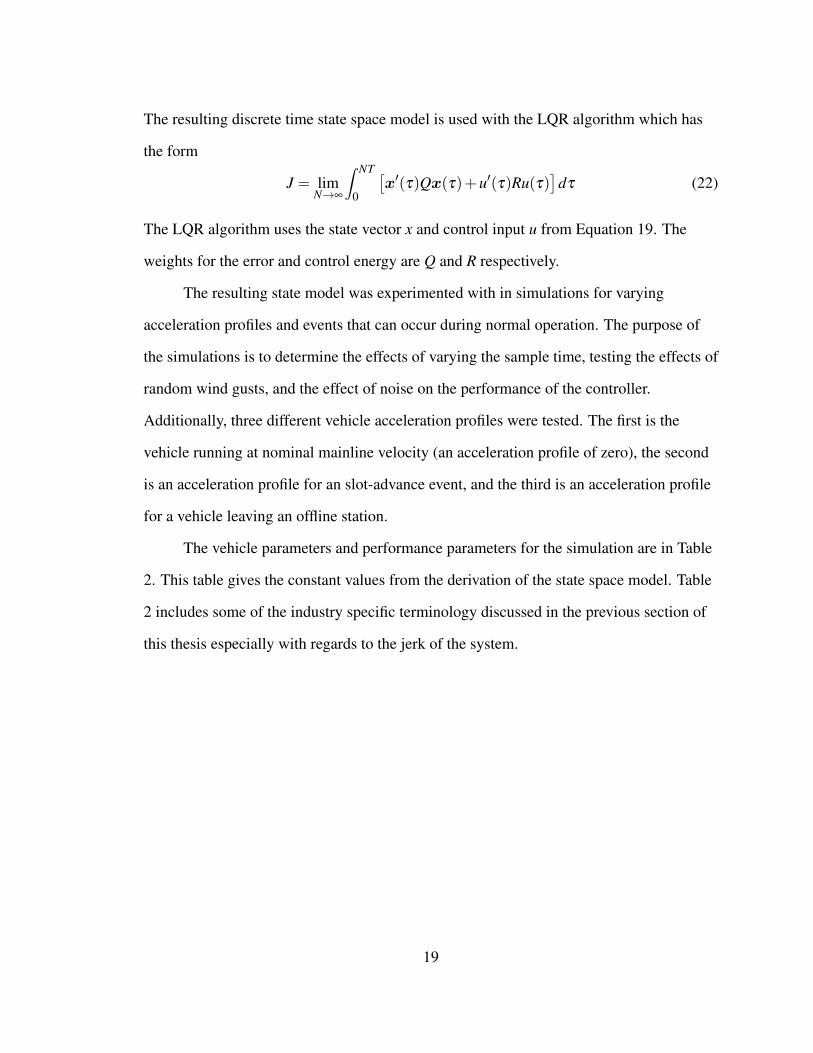
The vehicle parameters and performance parameters for the simulation are in Table
2. This table gives the constant values from the derivation of the state space model. Table
2 includes some of the industry specific terminology discussed in the previous section of
this thesis especially with regards to the jerk of the system.
19
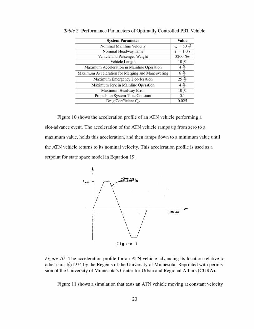
Table 2. Performance Parameters of Optimally Controlled PRT Vehicle
System Parameter ValueNominal Mainline Velocity vN = 50 f t
sNominal Headway Time T = 1.0 s
Vehicle and Passenger Weight 3200 lbsVehicle Length 10 f t
Maximum Acceleration in Mainline Operation 4 f ts2
Maximum Acceleration for Merging and Maneuvering 6 f ts2
Maximum Emergency Deceleration 25 f ts2
Maximum Jerk in Mainline Operation 4 f ts2
Maximum Headway Error 10 f tPropulsion System Time Constant 0.1
Drag Coefficient CD 0.025
Figure 10 shows the acceleration profile of an ATN vehicle performing a
slot-advance event. The acceleration of the ATN vehicle ramps up from zero to a
maximum value, holds this acceleration, and then ramps down to a minimum value until
the ATN vehicle returns to its nominal velocity. This acceleration profile is used as a
setpoint for state space model in Equation 19.
Figure 10. The acceleration profile for an ATN vehicle advancing its location relative toother cars, c©1974 by the Regents of the University of Minnesota. Reprinted with permis-sion of the University of Minnesota’s Center for Urban and Regional Affairs (CURA).
Figure 11 shows a simulation that tests an ATN vehicle moving at constant velocity
20
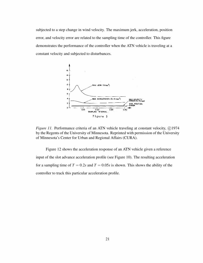
subjected to a step change in wind velocity. The maximum jerk, acceleration, position
error, and velocity error are related to the sampling time of the controller. This figure
demonstrates the performance of the controller when the ATN vehicle is traveling at a
constant velocity and subjected to disturbances.
Figure 11. Performance criteria of an ATN vehicle traveling at constant velocity, c©1974by the Regents of the University of Minnesota. Reprinted with permission of the Universityof Minnesota’s Center for Urban and Regional Affairs (CURA).
Figure 12 shows the acceleration response of an ATN vehicle given a reference
input of the slot advance acceleration profile (see Figure 10). The resulting acceleration
for a sampling time of T = 0.2s and T = 0.05s is shown. This shows the ability of the
controller to track this particular acceleration profile.
21
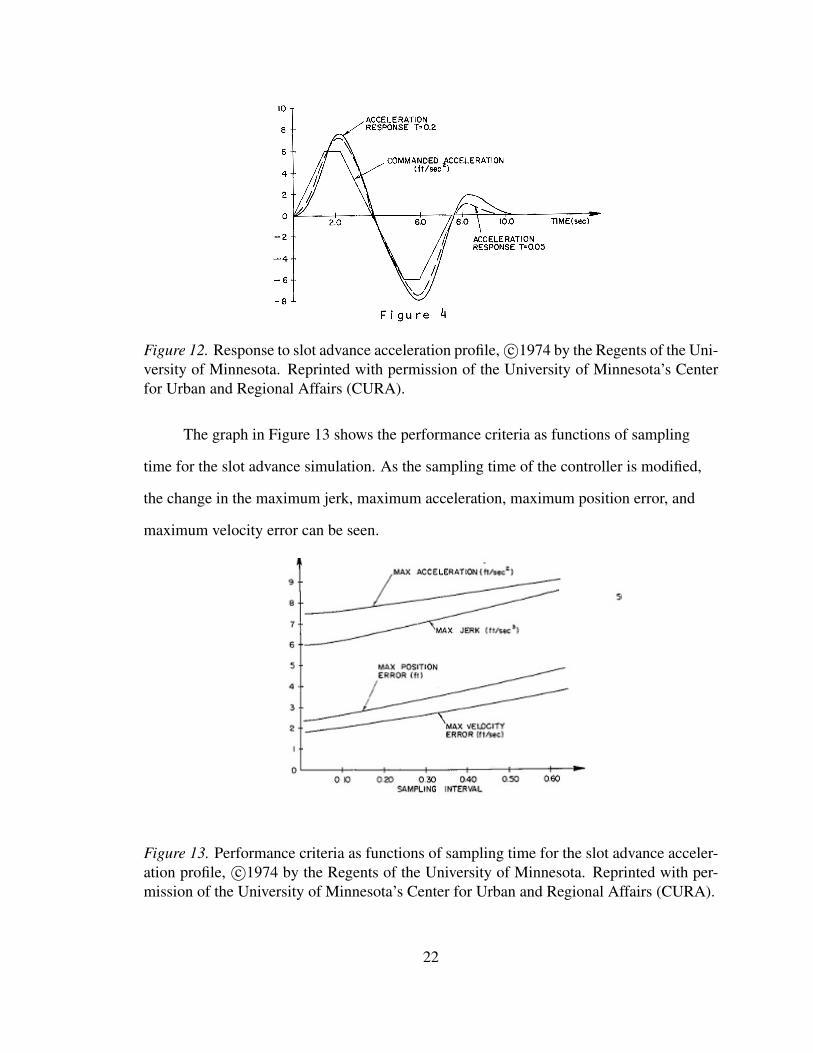
Figure 12. Response to slot advance acceleration profile, c©1974 by the Regents of the Uni-versity of Minnesota. Reprinted with permission of the University of Minnesota’s Centerfor Urban and Regional Affairs (CURA).
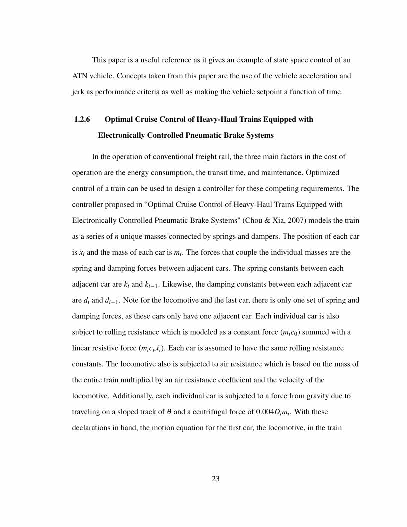
The graph in Figure 13 shows the performance criteria as functions of sampling
time for the slot advance simulation. As the sampling time of the controller is modified,
the change in the maximum jerk, maximum acceleration, maximum position error, and
maximum velocity error can be seen.
Figure 13. Performance criteria as functions of sampling time for the slot advance acceler-ation profile, c©1974 by the Regents of the University of Minnesota. Reprinted with per-mission of the University of Minnesota’s Center for Urban and Regional Affairs (CURA).
22
This paper is a useful reference as it gives an example of state space control of an
ATN vehicle. Concepts taken from this paper are the use of the vehicle acceleration and
jerk as performance criteria as well as making the vehicle setpoint a function of time.
1.2.6 Optimal Cruise Control of Heavy-Haul Trains Equipped with
Electronically Controlled Pneumatic Brake Systems
In the operation of conventional freight rail, the three main factors in the cost of
operation are the energy consumption, the transit time, and maintenance. Optimized
control of a train can be used to design a controller for these competing requirements. The
controller proposed in “Optimal Cruise Control of Heavy-Haul Trains Equipped with
Electronically Controlled Pneumatic Brake Systems" (Chou & Xia, 2007) models the train
as a series of n unique masses connected by springs and dampers. The position of each car
is xi and the mass of each car is mi. The forces that couple the individual masses are the
spring and damping forces between adjacent cars. The spring constants between each
adjacent car are ki and ki−1. Likewise, the damping constants between each adjacent car
are di and di−1. Note for the locomotive and the last car, there is only one set of spring and
damping forces, as these cars only have one adjacent car. Each individual car is also
subject to rolling resistance which is modeled as a constant force (mic0) summed with a
linear resistive force (micvxi). Each car is assumed to have the same rolling resistance
constants. The locomotive also is subjected to air resistance which is based on the mass of
the entire train multiplied by an air resistance coefficient and the velocity of the
locomotive. Additionally, each individual car is subjected to a force from gravity due to
traveling on a sloped track of θ and a centrifugal force of 0.004Dimi. With these
declarations in hand, the motion equation for the first car, the locomotive, in the train
23
(i = 1) is
m1x1 = u1− k1(x1− x2)−d1(x1− x2)
− (c0 + cvx1)m1− cax21
(n
∑i=1
mi
)−9.98sinθ1m1−0.004D1m1
(23)
The motion equation for the last car (i = n) is
mnxn = un− kn−1(xn− xn−1)−dn−1(xn− xn−1)
− (c0 + cvxn)mn−9.98sinθnmn−0.004Dnmn
(24)
The system of equations for all other cars are
mixi = ui− ki(xi− xi+1)− ki−1(xi− xi−1)−di(xi− xi+1)−di−1(xi− xi−1)
− (c0 + cvxi)mi−9.98sinθimi−0.004Dimi
(25)
The input force of u1 in Equation 23 can be positive or negative. The input forces ui and
un in Equations 25 and 24 can only be negative as individual cars are not powered.
A state space model formed from Equations 23, 25 and 24 allows for each
individual car to have its own control signal. In practice, this is not realizable as the signal
bandwidth does not support individual control of up to 200 individual train cars over the
speeds at which the train travels. The current industry standard is to have one control
signal for the locomotive group and one for all of the other cars. This is potentially
inefficient as it is possible on certain grades that in the case of decelerating the train
system, the brakes would be applied to a car going uphill. The paper introduces the
concept of “fencing", which is to have several control inputs based on the expected forces
on the train. The number of control groups is calculated every sampling period based on
the expected forces from the variations in slope and curvature of the track. If the change in
24
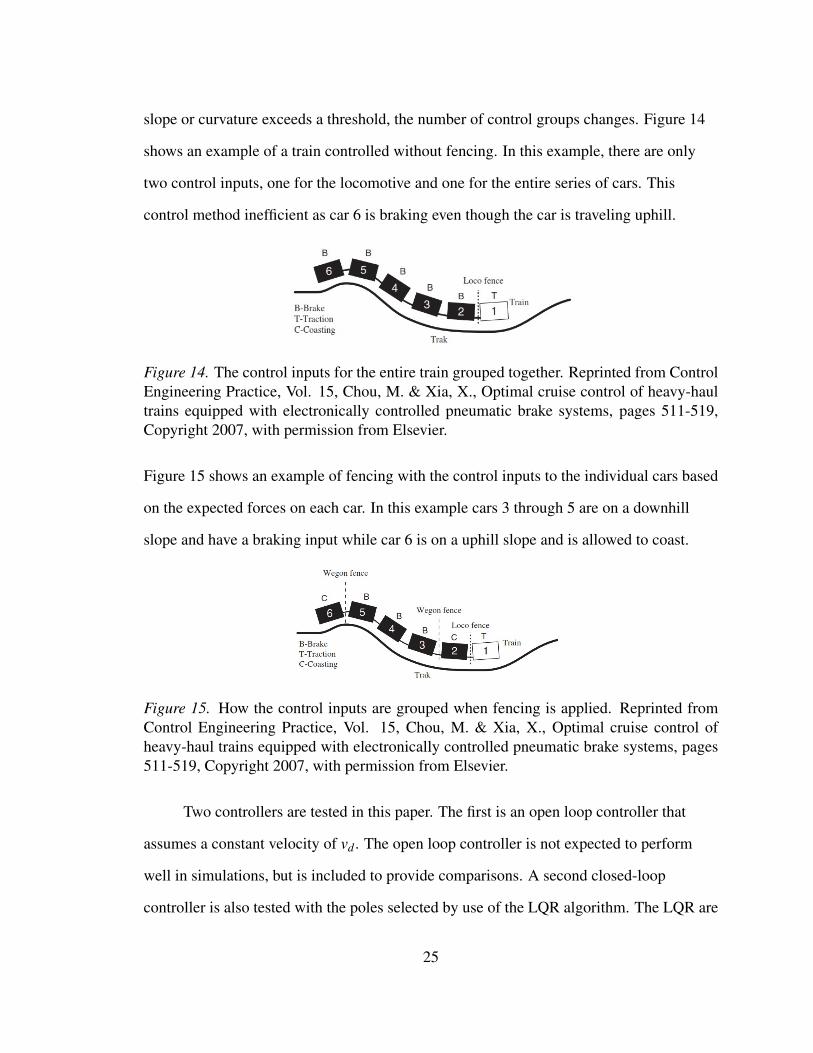
slope or curvature exceeds a threshold, the number of control groups changes. Figure 14
shows an example of a train controlled without fencing. In this example, there are only
two control inputs, one for the locomotive and one for the entire series of cars. This
control method inefficient as car 6 is braking even though the car is traveling uphill.
Figure 14. The control inputs for the entire train grouped together. Reprinted from ControlEngineering Practice, Vol. 15, Chou, M. & Xia, X., Optimal cruise control of heavy-haultrains equipped with electronically controlled pneumatic brake systems, pages 511-519,Copyright 2007, with permission from Elsevier.
Figure 15 shows an example of fencing with the control inputs to the individual cars based
on the expected forces on each car. In this example cars 3 through 5 are on a downhill
slope and have a braking input while car 6 is on a uphill slope and is allowed to coast.
Figure 15. How the control inputs are grouped when fencing is applied. Reprinted fromControl Engineering Practice, Vol. 15, Chou, M. & Xia, X., Optimal cruise control ofheavy-haul trains equipped with electronically controlled pneumatic brake systems, pages511-519, Copyright 2007, with permission from Elsevier.
Two controllers are tested in this paper. The first is an open loop controller that
assumes a constant velocity of vd . The open loop controller is not expected to perform
well in simulations, but is included to provide comparisons. A second closed-loop
controller is also tested with the poles selected by use of the LQR algorithm. The LQR are
25
decided based on the in-train force, the fuel consumption, and the traveling time to the
control input.
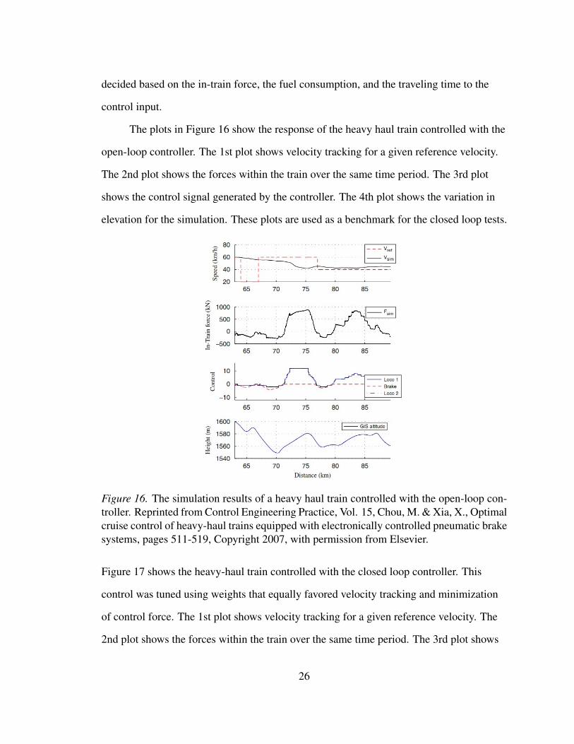
The plots in Figure 16 show the response of the heavy haul train controlled with the
open-loop controller. The 1st plot shows velocity tracking for a given reference velocity.
The 2nd plot shows the forces within the train over the same time period. The 3rd plot
shows the control signal generated by the controller. The 4th plot shows the variation in
elevation for the simulation. These plots are used as a benchmark for the closed loop tests.
Figure 16. The simulation results of a heavy haul train controlled with the open-loop con-troller. Reprinted from Control Engineering Practice, Vol. 15, Chou, M. & Xia, X., Optimalcruise control of heavy-haul trains equipped with electronically controlled pneumatic brakesystems, pages 511-519, Copyright 2007, with permission from Elsevier.
Figure 17 shows the heavy-haul train controlled with the closed loop controller. This
control was tuned using weights that equally favored velocity tracking and minimization
of control force. The 1st plot shows velocity tracking for a given reference velocity. The
2nd plot shows the forces within the train over the same time period. The 3rd plot shows
26
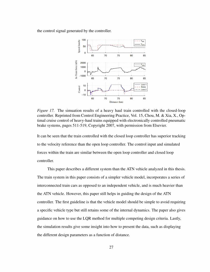
the control signal generated by the controller.
Figure 17. The simuation results of a heavy haul train controlled with the closed-loopcontroller. Reprinted from Control Engineering Practice, Vol. 15, Chou, M. & Xia, X., Op-timal cruise control of heavy-haul trains equipped with electronically controlled pneumaticbrake systems, pages 511-519, Copyright 2007, with permission from Elsevier.
It can be seen that the train controlled with the closed loop controller has superior tracking
to the velocity reference than the open loop controller. The control input and simulated
forces within the train are similar between the open loop controller and closed loop
controller.
This paper describes a different system than the ATN vehicle analyzed in this thesis.
The train system in this paper consists of a simpler vehicle model, incorporates a series of
interconnected train cars as opposed to an independent vehicle, and is much heavier than
the ATN vehicle. However, this paper still helps in guiding the design of the ATN
controller. The first guideline is that the vehicle model should be simple to avoid requiring
a specific vehicle type but still retains some of the internal dynamics. The paper also gives
guidance on how to use the LQR method for multiple competing design criteria. Lastly,
the simulation results give some insight into how to present the data, such as displaying
the different design parameters as a function of distance.
27
1.2.7 Robust Sampled-Data Cruise Control Scheduling of High Speed Train
Another paper that discusses control of conventional trains is “Robust
Sampled-Data Cruise Control Scheduling of High Speed Train" (Li, Yang, Li, & Gao,
2014). In this paper, the train system is treated as a series of n masses connected by a
spring. In addition, there are also force terms for rolling resistance, air resistance, and
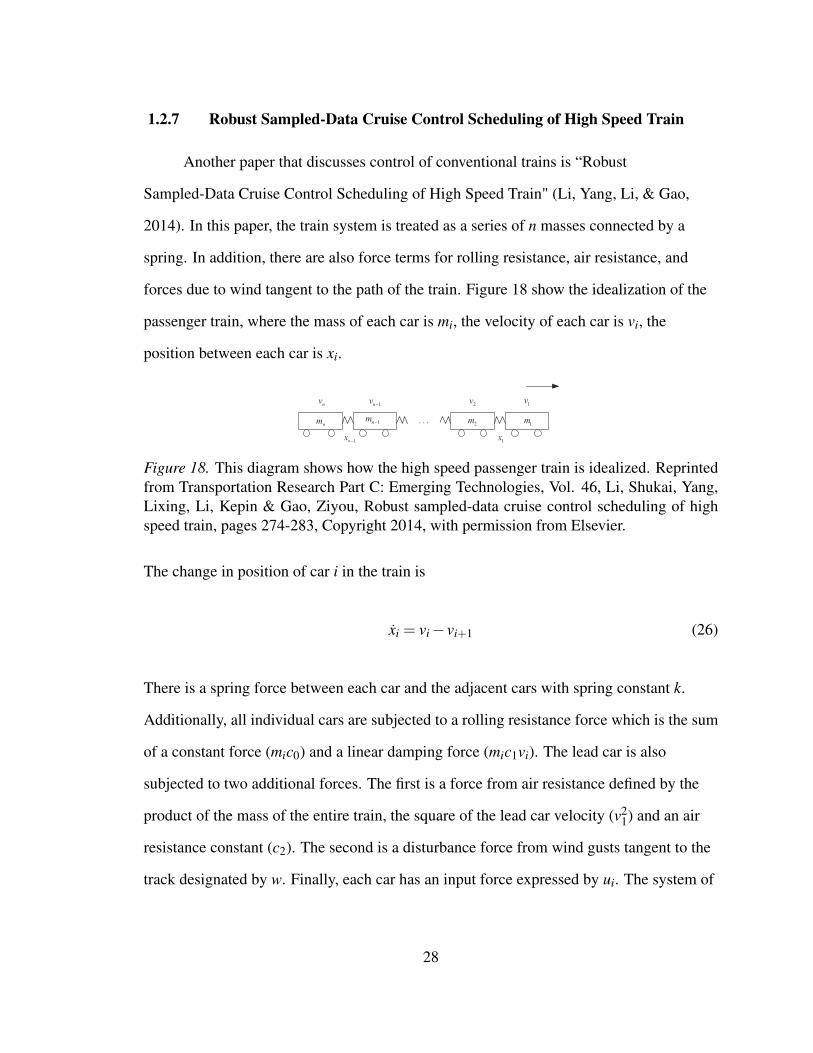
forces due to wind tangent to the path of the train. Figure 18 show the idealization of the
passenger train, where the mass of each car is mi, the velocity of each car is vi, the
position between each car is xi.
Figure 18. This diagram shows how the high speed passenger train is idealized. Reprintedfrom Transportation Research Part C: Emerging Technologies, Vol. 46, Li, Shukai, Yang,Lixing, Li, Kepin & Gao, Ziyou, Robust sampled-data cruise control scheduling of highspeed train, pages 274-283, Copyright 2014, with permission from Elsevier.
The change in position of car i in the train is
xi = vi− vi+1 (26)
There is a spring force between each car and the adjacent cars with spring constant k.
Additionally, all individual cars are subjected to a rolling resistance force which is the sum
of a constant force (mic0) and a linear damping force (mic1vi). The lead car is also
subjected to two additional forces. The first is a force from air resistance defined by the
product of the mass of the entire train, the square of the lead car velocity (v21) and an air
resistance constant (c2). The second is a disturbance force from wind gusts tangent to the
track designated by w. Finally, each car has an input force expressed by ui. The system of
28
equations for the lead car (the locomotive) is
m1v1(t) = u1− kx1− (c0 + c1v1)m1
− c2
(n
∑i=1
mi
)v2
1 +w(27)
The system of equations for the end car is
mnvn(t) = un + kxn−1
− (c0 + c1vn)mn
(28)
The system of equations for all other cars is
mivi(t) = ui + kxi−1− kxi
− (c0 + c1vi)mi
(29)
A continuous state space model is formed from Equations 26, 27, 29, and 28. The
proposed form of the controller is
u(t) = K1x(t)+K2v(t) (30)
The continuous controller in Equation 30 is transformed into discrete form using a zero
order hold. The discrete controller is
u(t) = u(tk) = K1x(tk)+K2v(tk) tk−1≤ t < tk (31)
Lyapunov stability theory is used to choose the gains of K1 and K2.
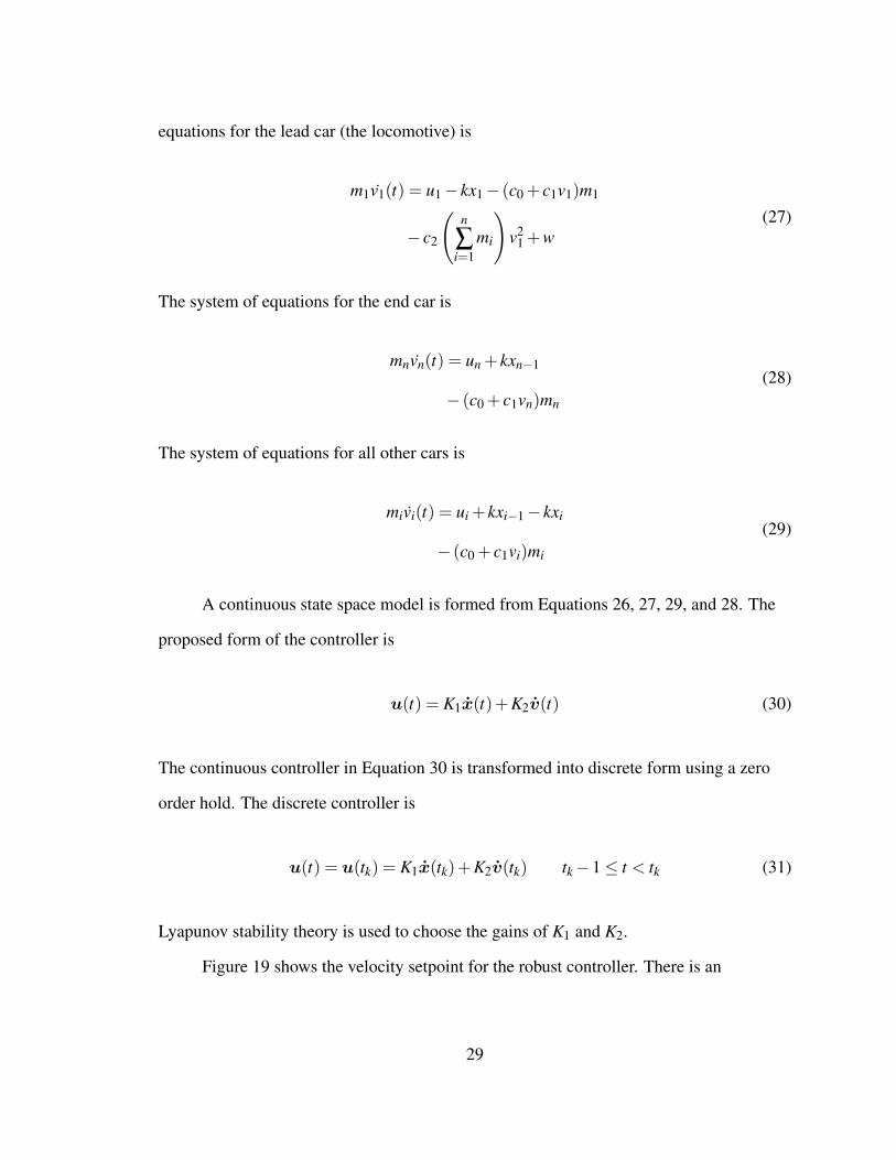
Figure 19 shows the velocity setpoint for the robust controller. There is an
29
acceleration period to the first cruising velocity followed by the short deceleration period
to the second cruising velocity.
Figure 19. The velocity setpoint for the lead car in a high speed passenger train. Reprintedfrom Transportation Research Part C: Emerging Technologies, Vol. 46, Li, Shukai, Yang,Lixing, Li, Kepin & Gao, Ziyou, Robust sampled-data cruise control scheduling of highspeed train, pages 274-283, Copyright 2014, with permission from Elsevier.
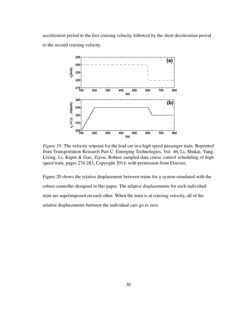
Figure 20 shows the relative displacement between trains for a system simulated with the
robust controller designed in this paper. The relative displacements for each individual
train are superimposed on each other. When the train is at cruising velocity, all of the
relative displacements between the individual cars go to zero.
30
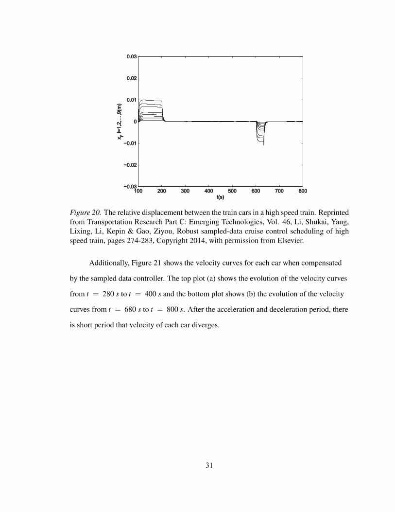
Figure 20. The relative displacement between the train cars in a high speed train. Reprintedfrom Transportation Research Part C: Emerging Technologies, Vol. 46, Li, Shukai, Yang,Lixing, Li, Kepin & Gao, Ziyou, Robust sampled-data cruise control scheduling of highspeed train, pages 274-283, Copyright 2014, with permission from Elsevier.
Additionally, Figure 21 shows the velocity curves for each car when compensated
by the sampled data controller. The top plot (a) shows the evolution of the velocity curves
from t = 280 s to t = 400 s and the bottom plot shows (b) the evolution of the velocity
curves from t = 680 s to t = 800 s. After the acceleration and deceleration period, there
is short period that velocity of each car diverges.
31
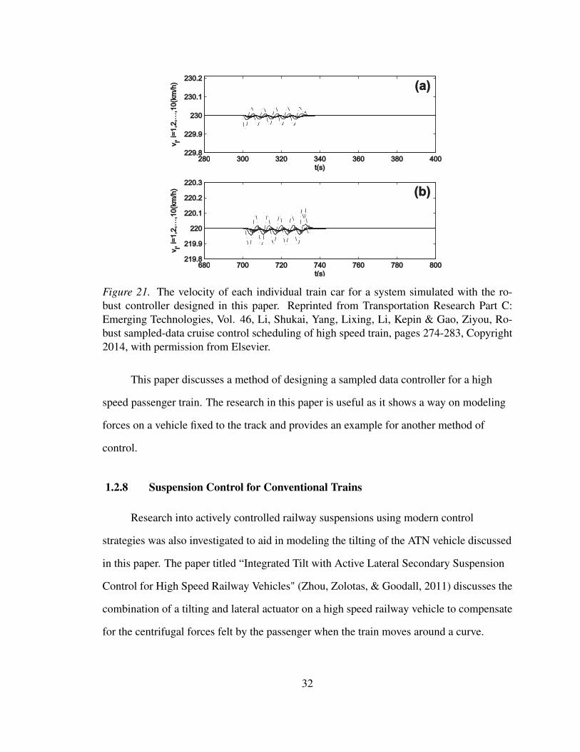
Figure 21. The velocity of each individual train car for a system simulated with the ro-bust controller designed in this paper. Reprinted from Transportation Research Part C:Emerging Technologies, Vol. 46, Li, Shukai, Yang, Lixing, Li, Kepin & Gao, Ziyou, Ro-bust sampled-data cruise control scheduling of high speed train, pages 274-283, Copyright2014, with permission from Elsevier.
This paper discusses a method of designing a sampled data controller for a high
speed passenger train. The research in this paper is useful as it shows a way on modeling
forces on a vehicle fixed to the track and provides an example for another method of
control.
1.2.8 Suspension Control for Conventional Trains
Research into actively controlled railway suspensions using modern control
strategies was also investigated to aid in modeling the tilting of the ATN vehicle discussed
in this paper. The paper titled “Integrated Tilt with Active Lateral Secondary Suspension
Control for High Speed Railway Vehicles" (Zhou, Zolotas, & Goodall, 2011) discusses the
combination of a tilting and lateral actuator on a high speed railway vehicle to compensate
for the centrifugal forces felt by the passenger when the train moves around a curve.
32
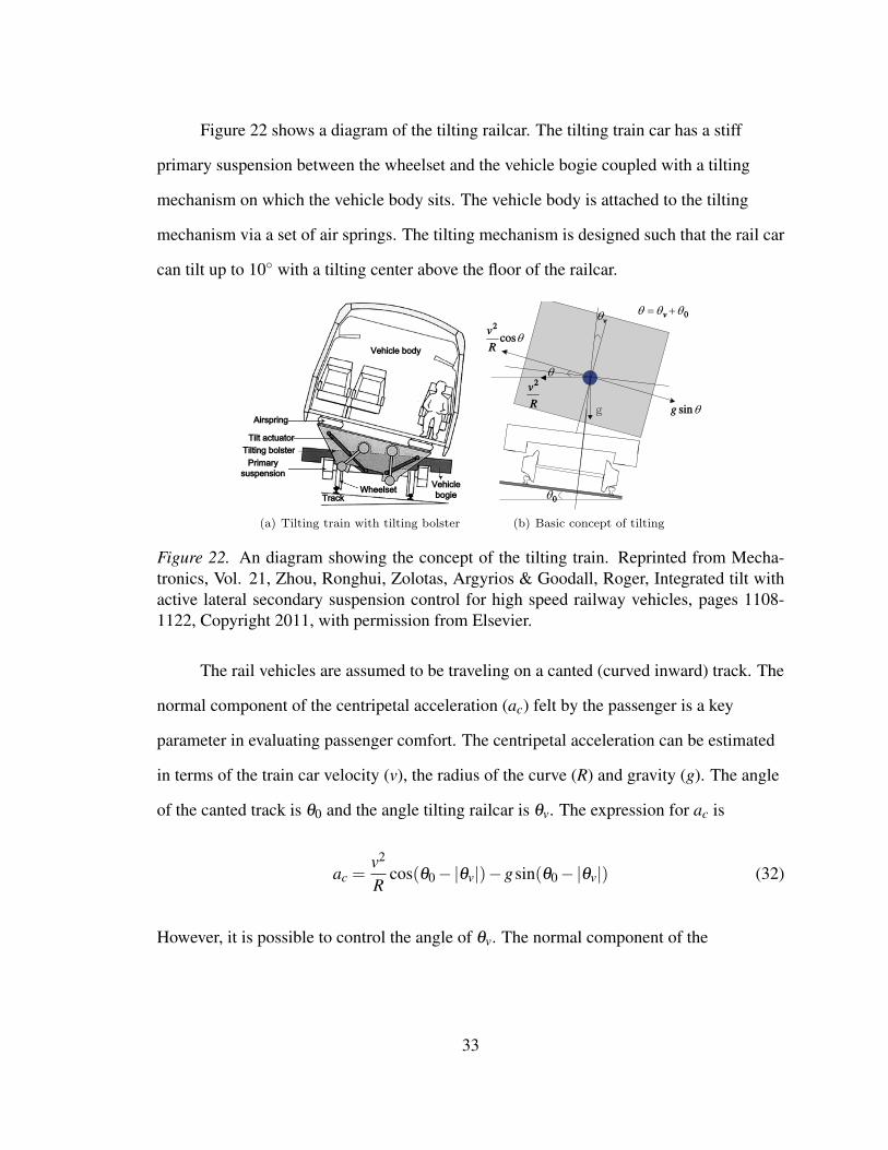
Figure 22 shows a diagram of the tilting railcar. The tilting train car has a stiff
primary suspension between the wheelset and the vehicle bogie coupled with a tilting
mechanism on which the vehicle body sits. The vehicle body is attached to the tilting
mechanism via a set of air springs. The tilting mechanism is designed such that the rail car
can tilt up to 10◦ with a tilting center above the floor of the railcar.
Figure 22. An diagram showing the concept of the tilting train. Reprinted from Mecha-tronics, Vol. 21, Zhou, Ronghui, Zolotas, Argyrios & Goodall, Roger, Integrated tilt withactive lateral secondary suspension control for high speed railway vehicles, pages 1108-1122, Copyright 2011, with permission from Elsevier.
The rail vehicles are assumed to be traveling on a canted (curved inward) track. The
normal component of the centripetal acceleration (ac) felt by the passenger is a key
parameter in evaluating passenger comfort. The centripetal acceleration can be estimated
in terms of the train car velocity (v), the radius of the curve (R) and gravity (g). The angle
of the canted track is θ0 and the angle tilting railcar is θv. The expression for ac is
ac =v2
Rcos(θ0−|θv|)−gsin(θ0−|θv|) (32)
However, it is possible to control the angle of θv. The normal component of the
33
centrifugal acceleration for a train with controlled tilting can be estimated by
ac =v2
Rcos(θ0−|θv|)−gsin(θ0 + |θv|) (33)
The angle θv in Equation 33 can be controlled to have the component from gravity cancel
the component from the centripetal acceleration of the railcar to minimize the acceleration
felt by the passengers.
The simplest control method is referred to as “nulling" and measures the lateral
acceleration and uses Equation 33 to determine to the setpoint angle of the tilting actuator.
However, this control method was found unsuitable for commercial usage as the coupling
between the roll dynamics and lateral dynamics of the rail car caused motion sickness in
the passengers. An alternative control method of “precedence control" which determines a
tilt command from the bogie acceleration. This control method avoids negative effects of
the coupled lateral dynamics. This controller is too complicated for the research this thesis
as the proposed model does not incorporate lateral dynamics of the bogie or the vehicle.
However, while the paper dismissed the use of “nulling" to control the tilting actuator as a
suitable strategy, the concept is ideal for the control of the ATN vehicle in the thesis. The
vehicle being analyzed in this thesis does not have sufficient complexity in the idealization
to have lateral dynamics, so the “nulling" control method is a useful initial approach.
34
CHAPTER 2
OBJECTIVE
The primary objective of this research is to deliver a SIMULINK model for a
controlled idealized ATN vehicle with an active suspension element. While there is
existing research being performed on multiple ATN vehicles in the Spartan Superway
team, there has been a lack of a dedicated research into a control algorithm for the vehicle.
In addition, most of the literature on controller design investigates supported ATN
vehicles as opposed to the suspended design being researched by the Spartan Superway
team. The controller in the SIMULINK model is a point-following controller and the
controller’s performance is judged by the maximum acceleration and jerk experienced by
the vehicle, as well as the error between the vehicle and its desired position. The desired
end-users for this simulation environment and controller are future engineering design
teams on the Spartan Superway project. It is intended that the design teams are able to
integrate the controller in a SIMULINK application interfaced with a microprocessor (e.g.
Arduino) to control a test vehicle as well as use the SIMULINK model to test their own
design. The research is split into three different overlapping sections: the formulation of
the equations of motion for the ATN vehicle, the design of the SIMULINK model and
controller, and the analysis of the results of simulations to validate the research objectives.
The formulation of the equations of motion for the ATN vehicle is performed first as
these equations govern the controller design and the validation simulations. Because of
the complexity of real world systems coupled with the fact that there is no final design for
the suspended ATN vehicle, a simple idealization is utilized. For the first idealization
(henceforth referred to as the Planar System), the ATN vehicle is simplified to two point
masses, one representing the bogie of the ATN vehicle and one representing the center of
mass of the vehicle body. Between the point mass representing the bogie and the vehicle
35
body, there is an arm that is allowed to rotate perpendicular to the guideway. In the Planar
System, it is assumed that the bogie point mass is constrained to move on a circular arc.
The equations of motion for the Planar System are derived by hand and by MotionGenesis.
The second idealization (henceforth referred to as the General System) is the same as the
Planar System with the exception that the bogie point mass is constrained to move on a
numerically defined arbitrary curve in space. The equations of motion of the General
System are based on numerically interpolated unit vectors calculated from the guideway
geometry. Both systems are subjected to a propulsive force from the bogie, a stabilizing
force on the vehicle body, friction forces and air resistance, as well as a disturbance force
from wind gusts. Approximate values for all of the parameters are obtained by a
combination of communication with Bengt Gustafsson, the director of Beamways AB,
referencing existing designs, and using information from the literature review.
The resulting equations of motion are used to design a state-space controller using
feedback linearization and the pole placement method to determine both the propulsive
and stabilizing force mentioned above. The goal of the controller is to track the position of
the ATN vehicle on the guideway with minimal error at the highest possible velocity while
simultaneously ensuring that the acceleration and jerk in motion tangent and normal to the
guideway remain below the targeted levels. There is a controller for both the Planar
System and the General System.
In order to validate both the equations of motion and the resulting controller, there
are multiple simulations on a virtual test track with a 100 meter radius. The first set of
simulations compares the hand derived and computer derived equations of motion for the
Planar System for a vehicle with constant velocity subjected to a disturbance force. The
next set of simulations validates the numerical method of determining the numerical unit
vectors of the General System. Next, the equations of motions for the general system are
36
compared to the hand derived equations under the same initial conditions and subjected to
the same forces as the Planar System comparison study.
A set of simulations is performed to analyze the state space controller derived from
the dynamics of the Planar System. This set of simulations uses three different sets of
closed loop poles for the bogie and one set of closed loop poles for the angle position.
Then a controller defined from the dynamics of the General System is used to control the
output of a plant defined by the dynamics of the Planar System. This set of simulations
shows the viability of using numerically defined guideway geometry to control the output
of a suspended ATN vehicle.
The last set of simulations demonstrates the dynamics of an ATN vehicle on a
guideway shaped like an Euler spiral. An Euler spiral is a curve in which the curvature is
linearly related to the displacement along the curve. This geometry is used in transit
engineering and demonstrates the ability of the General System to simulate complex
guideway geometry.
37
CHAPTER 3
METHODOLOGY
3.1 Dynamical System Idealization
In order to construct the equations of motion for the ATN vehicle, a suitable
idealization must be made and numerical values must be assigned to the associated
parameters. The process for assigning these values is a combination of communications
with consultants from Beamway, referencing selected resources from the literature review,
and using engineering data from other sectors of the Spartan Superway team. The relevant
parameters for the rigid idealization are the radius of the curve, the mass of the bogie point
mass, the mass of the vehicle body point mass, the length of the pendulum arm between
the bogie point mass and vehicle body point mass, the coefficient of viscous damping on
the rotating ATN vehicle body, the coefficient for rolling resistance, and the coefficient for
air resistance. The mass values have been discussed in a cited communication with a
consultant from Beamways AB, the length of the pendulum arm is found by using the
maximum angle deflection in the “The Tradeoff Between Supported vs. Hanging
Vehicles" (Anderson, 2013) and from the geometry from a CAD model of a proposed
cabin created by visiting Swedish students to the Spartan Superway design center during
the summer of 2015. The rolling resistance is based on the weight and wheel diameter
from the Beamways AB design. The air resistance is based on the drag coefficient of a
half sphere and the profile area from a CAD model designed by Swedish students
interning for a summer with the Spartan Superway team. The exact equations and process
for determining these values are listed in the theoretical work section and the exact values
used in the simulations are detailed in the Results section.
38
3.2 Forming the Equations of Motion and Validation Simulations
For the Planar System, the equations of motion are formed by hand and by using the
computer algebra software MotionGenesis (Mitiguy, 2015). This software is also used for
other complex symbolic calculations. Once the equations of motion have been
determined, MATLAB code for the equations is used to create SIMULINK blocks. These
SIMULINK blocks are then used for validation simulations in order to determine that the
simulated dynamical system behaves as expected. The General System follows the same
steps; however, the equations of motion are derived only with MotionGenesis.
3.3 Numerically Defined Unit Vectors
A dataset containing the guideway geometry that has path displacement as an
independent variable and the X, Y, and Z positions in an inertial frame as the dependent
variables is generated. This dataset is used in conjunction with the MATLAB Curve
Fitting toolbox to fit 5th order splines for each function of X, Y, and Z to the path
displacement. The resulting splines are used to generate a dataset of the geometric
information of the General System as a function of path displacement. This dataset of
geometric information is used in interpolation blocks in the SIMULINK models.
3.4 Designing the Controller
Once the equations of motion have been validated, a controller is designed for both
the Planar and General Systems. The controller is formed by creating a state space model
around the desired setpoints and then using the pole placement algorithm in the MATLAB
Control System toolbox to find the gains of the system. The controller is implemented in
SIMULINK along with the SIMULINK model of the dynamical system for validation
purposes.
39
CHAPTER 4
ATN VEHICLE DYNAMICS
As this research involves designing a control algorithm for the suspended ATN
vehicle, the research must begin by a formulation of the equations of motion. Two ATN
systems are studied, the first system being an idealized ATN vehicle constrained to move
on an arc (the “Planar System") in which the equations of motion are manually derived
using Kane’s method and derived again using MotionGenesis. Both of these sections are
explicit in detail in order to provide a tutorial. The second system is the same ATN
suspended vehicle on an arbitrary curve in space that is defined through numerical values
(the “General System"). The equations of motion for the General System are derived only
with MotionGenesis, but the mathematical theory behind the concepts of the model is
discussed.
4.1 Planar System - Manual Derivation
While the final goal of this research is a controller that is based on the dynamics of
the General System, it is advantageous to first solve for the equations of motion for the
Planar System to provide a hand calculated comparison to the MotionGenesis derived
equations. The kinematics and the expressions for the forces of the Planar System are
formulated and the equations of motion are then derived using Kane’s Method in terms of
two generalized speeds.
In Figure 23, let Nx, Ny, and Nz form a right-handed set of mutually
perpendicular unit vectors fixed in an inertial frame N. The guideway geometry is
assumed to be an arc of radius r0 with center N0 that is fixed in the plane formed by Nx
and Ny. Let B be a particle of mass mB which is allowed to freely move along the arc for
40
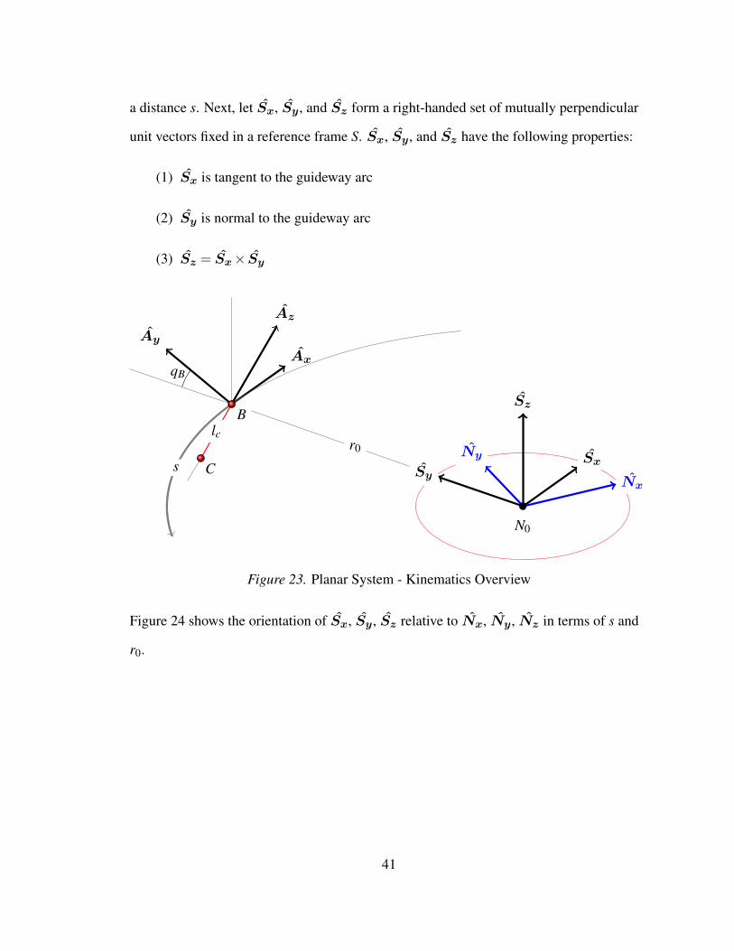
a distance s. Next, let Sx, Sy, and Sz form a right-handed set of mutually perpendicular
unit vectors fixed in a reference frame S. Sx, Sy, and Sz have the following properties:
(1) Sx is tangent to the guideway arc
(2) Sy is normal to the guideway arc
(3) Sz = Sx× Sy
Ax
Az
r0
Ay
Sz
Sy
SxNy
Nx
qB
B
C
lc
s
N0
Figure 23. Planar System - Kinematics Overview
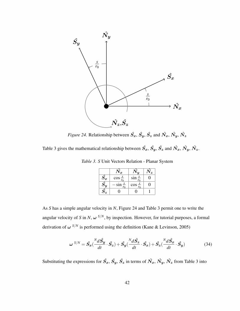
Figure 24 shows the orientation of Sx, Sy, Sz relative to Nx, Ny, Nz in terms of s and
r0.
41
Nz,Sz
Nx
Ny
Sx
Sy
sr0
sr0
Figure 24. Relationship between Sx, Sy, Sz and Nx, Ny, Nz
Table 3 gives the mathematical relationship between Sx, Sy, Sz and Nx, Ny, Nz.
Table 3. S Unit Vectors Relation - Planar System
Nx Ny Nz
Sx cos sr0
sin sr0
0Sy −sin s
r0cos s
r00
Sz 0 0 1
As S has a simple angular velocity in N, Figure 24 and Table 3 permit one to write the
angular velocity of S in N, ω S/N , by inspection. However, for tutorial purposes, a formal
derivation of ω S/N is performed using the definition (Kane & Levinson, 2005)
ω S/N = Sx(NdSy
dt· Sz)+ Sy(
NdSz
dt· Sx)+ Sz(
NdSx
dt· Sy) (34)
Substituting the expressions for Sx, Sy, Sz in terms of Nx, Ny, Nz from Table 3 into
42
Equation 34 and evaluating the derivatives produces
ω S/N = Sz
(sr0
(−sin
sr0Nx+ cos
sr0Ny
)·(−sin
sr0Nx+ cos
sr0Ny
))(35)
The dot product in Equation 35 is evaluated to give ω S/N as
ω S/N =sr0Sz (36)
Moving on to the kinematics of B, the position vector from rB N0 to B, is found by
inspection of Figure 23 as
rB = r0Sy (37)
The velocity of B in N, v B/N , is given by:
v B/N =SddtrB +ω S/N×rB (38)
Substituting from Equations 36 and 37 into Equation 38 gives
v B/N = 0+sr0Sz× r0Sz (39)
Evaluating the cross product in Equation 39 yields
v B/N = s(−Sx) (40)
The acceleration of B in N, a B/N , is given by
a B/N =SddtvB/N +ω B/N×v B/N (41)
43
Substituting from Equations 36 and 40 into Equation 41 yields
a B/N = s(−Sx)+sr0(−Sx)×
sr0Sz (42)
Evaluating the cross product in Equation 42 produces
a B/N =−sSx−s2
r0Sy (43)
Now that an expression for a B/N is in hand, analysis of the kinematics of the suspended
vehicle can begin. Additional hardware components must be taken into account to
represent a suspended ATN vehicle. Referring to Figure 23, let C be a particle of mass mC
that represents the vehicle cabin. Let C be constrained to B by means of massless rod BC
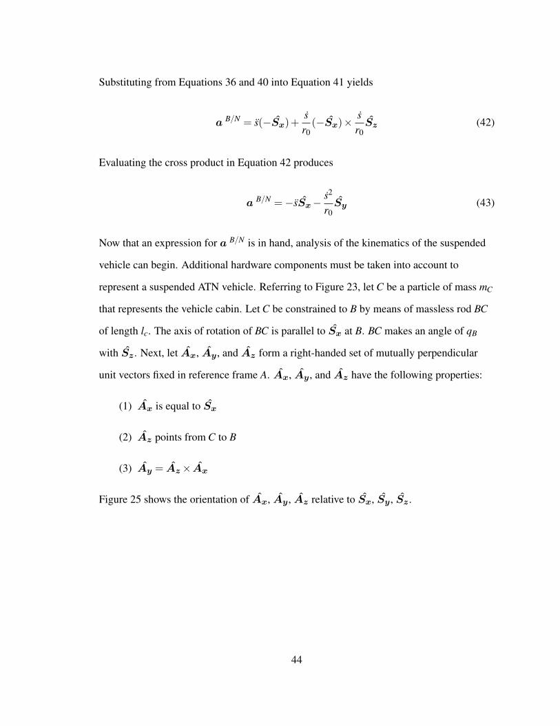
of length lc. The axis of rotation of BC is parallel to Sx at B. BC makes an angle of qB
with Sz. Next, let Ax, Ay, and Az form a right-handed set of mutually perpendicular
unit vectors fixed in reference frame A. Ax, Ay, and Az have the following properties:
(1) Ax is equal to Sx
(2) Az points from C to B
(3) Ay = Az× Ax
Figure 25 shows the orientation of Ax, Ay, Az relative to Sx, Sy, Sz.
44
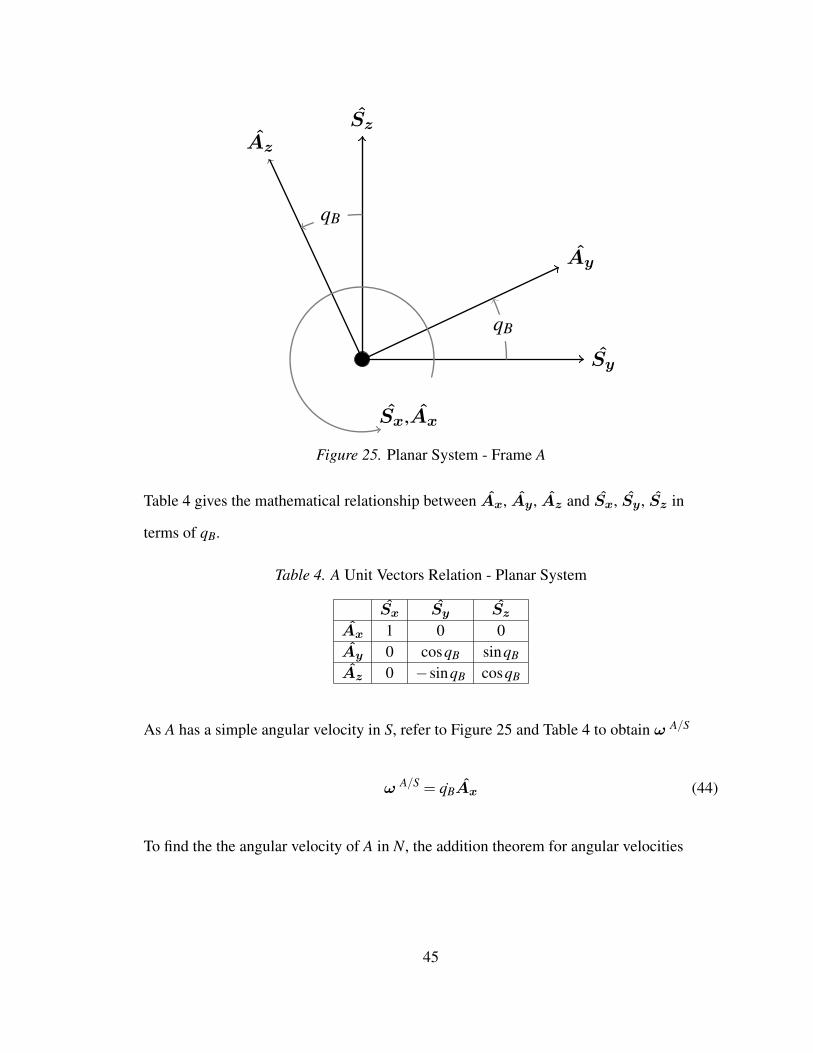
Sx,Ax
Sy
Sz
Ay
Az
qB
qB
Figure 25. Planar System - Frame A
Table 4 gives the mathematical relationship between Ax, Ay, Az and Sx, Sy, Sz in
terms of qB.
Table 4. A Unit Vectors Relation - Planar System
Sx Sy Sz
Ax 1 0 0Ay 0 cosqB sinqB
Az 0 −sinqB cosqB
As A has a simple angular velocity in S, refer to Figure 25 and Table 4 to obtain ω A/S
ω A/S = qBAx (44)
To find the the angular velocity of A in N, the addition theorem for angular velocities
45
(Kane & Levinson, 2005) can be utilized which yields
ω A/N = ω A/S +ω S/N (45)
Substituting from Equations 44 and 36 into Equation 45 produces
ω A/N = qBAx+sr0Sz (46)
Refer to Figure 23 to obtain the position vector r′C from B to C by inspection
r′C =−lCAz (47)
The position vector from N0 to C is found by adding Equations 47 and 37
rC = r0Sy− lCAz (48)
The velocity of C in N, v C/N , is
v C/N =NddtrB−
Nddt
lCAz (49)
Substituting from Equation 37 into Equation 49 and evaluating the derivatives yields
v C/N =−s(
1+lcr0
sinqB
)Sx+ qBlcAy (50)
The acceleration of C in N, a C/N , is defined as
a C/N =Nddtv C/N (51)
46
Substituting from Equation 50 into Equation 51 and evaluating the derivative yields
a C/N =
Sx
[−s(
1+lcr0
sinqB
)−2sqB
lcr0
cosqB
]+Sy
[− s2
ro
(1+
lcr0
sinqB
)]+Ay [qBlc]
+Az
[qB
2lc]
(52)
Now that expressions for a B/N and a C/N are in hand, the next step is to establish
expressions for the external forces and torques on the system. Figure 26 is a free body
diagram for B. FP is the propulsion force on the bogie from the wheels on the guideway
and acts in the Sx direction. FR is a resistive force that acts in the ˆ−Sx direction and is
defined as
FR = c0 + c1s+ c2s2 (53)
Equation 53 is referred to as the Davis equation and is used in research performed in
conventional train simulations (Li et al., 2014). The value of FR is the sum of a constant
force, a linear damping force (to model rolling resistance), and a damping force
proportional to the square of the speed (to model air resistance). FW is the force on the
ATN Vehicle from wind gusts and is considered a disturbance on the system. Because the
wind gusts are possible in any direction, FW acts in the direction of the independent unit
vector W . Also present is the force due to the weight of the bogie, mBg which acts in the
Sz direction. Additionally, the weight and motion of C is expressed by Rv which acts in
the −Az direction. Lastly, there are the reaction forces Ry and N which act in the Sy and
47
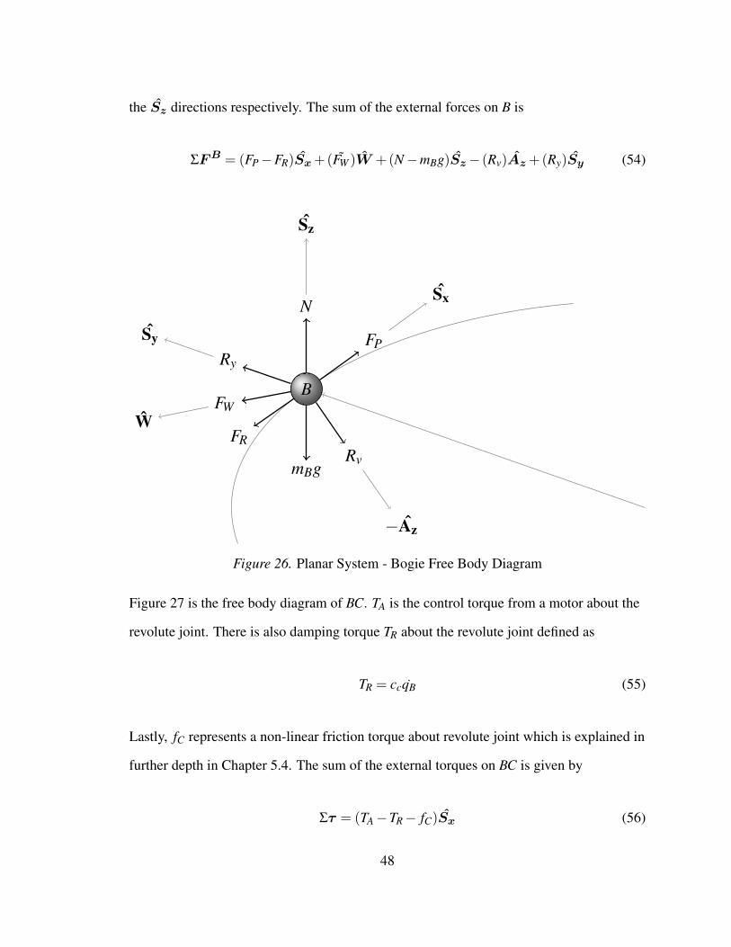
the Sz directions respectively. The sum of the external forces on B is
ΣFB = (FP−FR)Sx+(FW )W +(N−mBg)Sz− (Rv)Az+(Ry)Sy (54)
mBg
N
FP
FR
FWW
Rv
Sz
Sy
Sx
−Az
Ry
B
Figure 26. Planar System - Bogie Free Body Diagram
Figure 27 is the free body diagram of BC. TA is the control torque from a motor about the
revolute joint. There is also damping torque TR about the revolute joint defined as
TR = ccqB (55)
Lastly, fC represents a non-linear friction torque about revolute joint which is explained in
further depth in Chapter 5.4. The sum of the external torques on BC is given by
Στ = (TA−TR− fC)Sx (56)
48
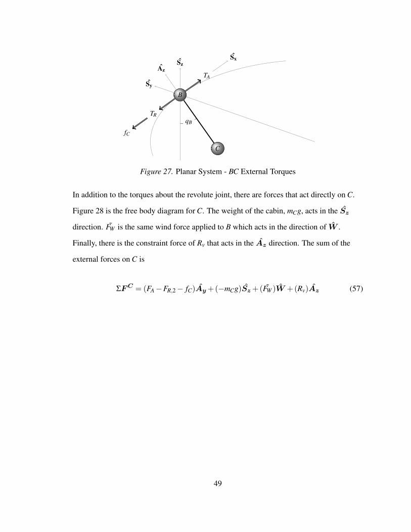
TA
TR
fC
Sz
Sy
Sx
Az
C
B
qB
Figure 27. Planar System - BC External Torques
In addition to the torques about the revolute joint, there are forces that act directly on C.
Figure 28 is the free body diagram for C. The weight of the cabin, mCg, acts in the Sz
direction. FW is the same wind force applied to B which acts in the direction of W .
Finally, there is the constraint force of Rv that acts in the Az direction. The sum of the
external forces on C is
ΣFC = (FA−FR,2− fC)Ay+(−mCg)Sz+(FW )W +(Rv)Az (57)
49
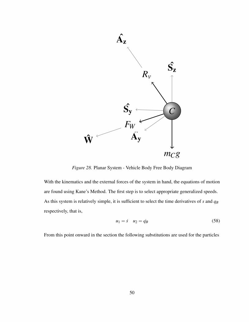
mCg
Sz
Ay
FW
W
Rv
Sy
Az
C
Figure 28. Planar System - Vehicle Body Free Body Diagram
With the kinematics and the external forces of the system in hand, the equations of motion
are found using Kane’s Method. The first step is to select appropriate generalized speeds.
As this system is relatively simple, it is sufficient to select the time derivatives of s and qB
respectively, that is,
u1 = s u2 = qB (58)
From this point onward in the section the following substitutions are used for the particles
50
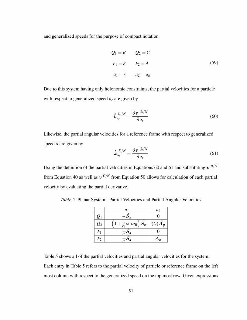
and generalized speeds for the purpose of compact notation
Q1 = B Q2 =C
F1 = S F2 = A
u1 = s u2 = qB
(59)
Due to this system having only holonomic constraints, the partial velocities for a particle
with respect to generalized speed ur are given by
ˆvQi/N
ur=
∂v Qi/N
∂ur(60)
Likewise, the partial angular velocities for a reference frame with respect to generalized
speed a are given by
ˆωFi/N
ur=
∂v Qi/N
∂ur(61)
Using the definition of the partial velocities in Equations 60 and 61 and substituting v B/N
from Equation 40 as well as v C/N from Equation 50 allows for calculation of each partial
velocity by evaluating the partial derivative.
Table 5. Planar System - Partial Velocities and Partial Angular Velocities
u1 u2
Q1 −Sx 0
Q2 −(
1+ lcr0
sinqB
)Sx (lc)Ay
F11r0Sz 0
F21r0Sz Ax
Table 5 shows all of the partial velocities and partial angular velocities for the system.
Each entry in Table 5 refers to the partial velocity of particle or reference frame on the left
most column with respect to the generalized speed on the top most row. Given expressions
51
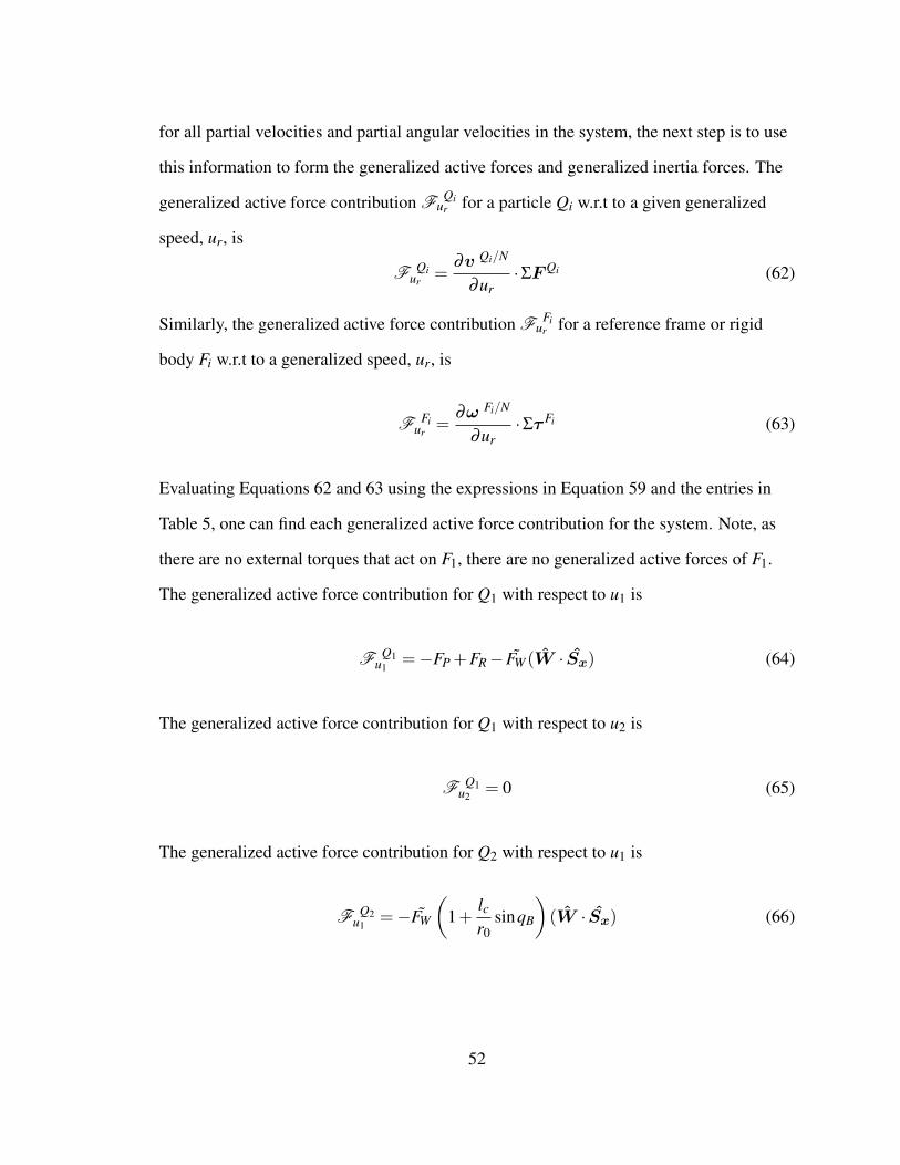
for all partial velocities and partial angular velocities in the system, the next step is to use
this information to form the generalized active forces and generalized inertia forces. The
generalized active force contribution F Qiur for a particle Qi w.r.t to a given generalized
speed, ur, is
F Qiur
=∂v Qi/N
∂ur·ΣFQi (62)
Similarly, the generalized active force contribution F Fiur for a reference frame or rigid
body Fi w.r.t to a generalized speed, ur, is
F Fiur
=∂ω Fi/N
∂ur·ΣτFi (63)
Evaluating Equations 62 and 63 using the expressions in Equation 59 and the entries in
Table 5, one can find each generalized active force contribution for the system. Note, as
there are no external torques that act on F1, there are no generalized active forces of F1.
The generalized active force contribution for Q1 with respect to u1 is
F Q1u1
=−FP +FR− FW (W · Sx) (64)
The generalized active force contribution for Q1 with respect to u2 is
F Q1u2
= 0 (65)
The generalized active force contribution for Q2 with respect to u1 is
F Q2u1
=−FW
(1+
lcr0
sinqB
)(W · Sx) (66)
52
The generalized active force contribution for Q2 with respect to u2 is
F Q2u2
= (FW (W · Ay) )lc−mglc sinqB (67)
The generalized active force contribution for F2 with respect to u1 is
F F2u1
= 0 (68)
The generalized active force contribution for F2 with respect to u2 is
F F2u2
= TA−TR− fC (69)
With the generalized active forces in hand, the next step is find the generalized inertia
forces of the system. The generalized inertia force contribution F ∗ Qiur for particle Qi with
respect to a generalized speed, ur, is
F ∗ Qiur
=∂v Qi/N
∂ur·mQia
Qi/N (70)
As the only rotating components in this system are inertia-less reference frames, there are
no generalized inertia forces of the rotating components of the system. The generalized
inertia force contribution for Q1 with respect to u1 is
F ∗ Q1u1
= mBs (71)
The generalized inertia force contribution for Q1 with respect to u2 is
F ∗ Q1u2
= 0 (72)
53
The generalized inertia force contribution for Q2 with respect to u1 is
F ∗ Q2u1
= mC
[(1+
lcr0
sinqB
)(s(
1+lcr0
sinqB
)−2sqB
lcr0
cosqB
)](73)
The generalized inertia force contribution for Q2 with respect to u2 are
F ∗ Q2u1
= mC
[l2c qB + cosqB
(− s2
ro
(1+
lcr0
sinqB
))](74)
The next step is to express Kane’s Equations for each generalized speed in terms of the
generalized active and generalized inertia forces. Kane’s Equations with respect to s (u1)
are2
∑i=1
F Qiu1
=2
∑i=1
F ∗ Qiu1
(75)
Likewise, Kane’s Equations with respect to qB (u2) are
2
∑i=1
F Qiu2
=2
∑i=1
F ∗ Qiu2
(76)
To find the equations of motion for s, substitute the generalized active forces in Equations
64 and 66 and the generalized inertia forces in Equations 71 and 73 into Equation 75
which gives
−FP +FR− FW
[1+(
1+lcr0
sinqB
)](W · Sx) =
mBs+mC
[(1+
lcr0
sinqB
)(s(
1+lcr0
sinqB
)−2sqB
lcr0
cosqB
)] (77)
54
Solving for s yields
s =−(−FP +FR1−Z0 + fB) +2lCmC cosqB
(1+ lc
r0sinqB
)qBsr0
)mB +mC
(1+ lC
r0sinqB
)2 (78)
Where Z0 is
Z0 = FW
[1+(
1+lcr0
sinqB
)](W · Sx) (79)
To find the equations of motion for qB, substitute the generalized active forces in
Equations 65, 67, and 69 as well as the generalized inertia forces in Equations 72 and 74
into Equation 76 which gives
TA−TR− fC +(FW (W · Ay) )lc−mglc sinqB
= mC
[l2c qB + cosqB
(− s2
ro
(1+
lcr0
sinqB
))] (80)
Solving for qB yields
qB =TA−TR− fC
m2ClC
+FW (W · Ay)
mClC+ cosqB
(r0
lC+ sinqB
)s2
r20− g
lCsinqB (81)
4.2 General System - Theoretical Overview
In the General System, the ATN vehicle is constrained to move on an arbitrary
curve in space. The advantage of such a constraint is that an ATN vehicle can be
simulated over any possible guideway geometry. Only MotionGenesis is used to
formulate the equations of motion for the General System. Additionally, an overview of
the system and mathematical operation are provided rather than an explicit derivation of
the exact equations.
55
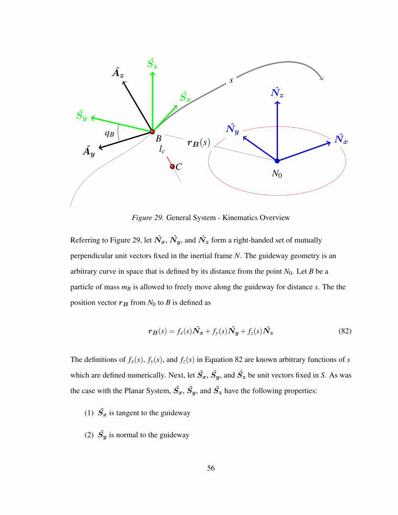
sAz
rB(s)Ay
Nz
Sz
Sy
Sx
NyNxB
C
qB
lc
N0
Figure 29. General System - Kinematics Overview
Referring to Figure 29, let Nx, Ny, and Nz form a right-handed set of mutually
perpendicular unit vectors fixed in the inertial frame N. The guideway geometry is an
arbitrary curve in space that is defined by its distance from the point N0. Let B be a
particle of mass mB is allowed to freely move along the guideway for distance s. The the
position vector rB from N0 to B is defined as
rB(s) = fx(s)Nx+ fy(s)Ny+ fz(s)Nz (82)
The definitions of fx(s), fy(s), and fz(s) in Equation 82 are known arbitrary functions of s
which are defined numerically. Next, let Sx, Sy, and Sz be unit vectors fixed in S. As was
the case with the Planar System, Sx, Sy, and Sz have the following properties:
(1) Sx is tangent to the guideway
(2) Sy is normal to the guideway
56
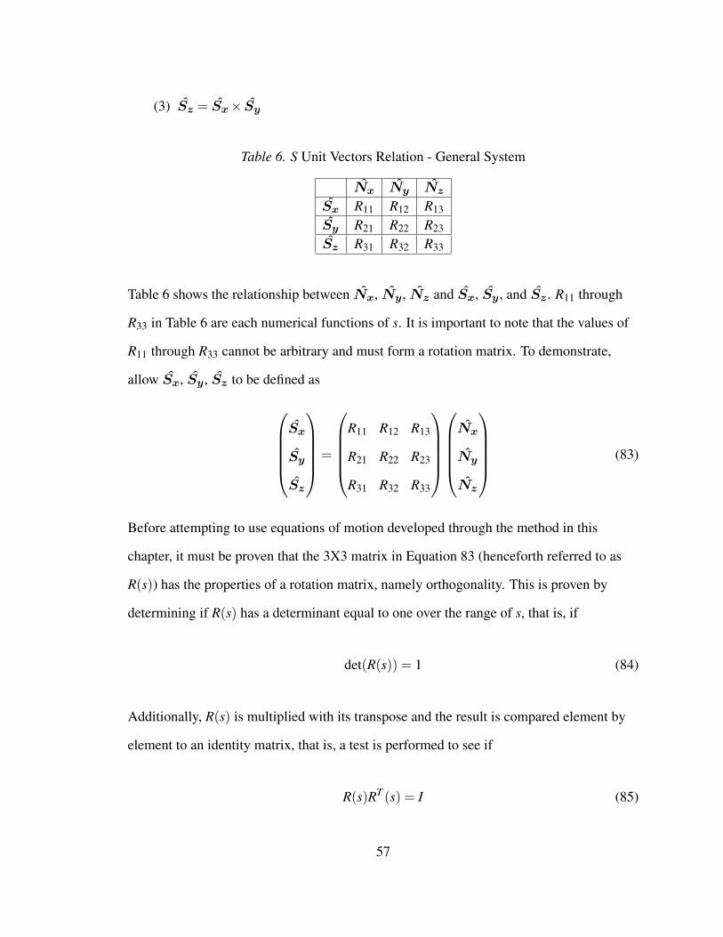
(3) Sz = Sx× Sy
Table 6. S Unit Vectors Relation - General System
Nx Ny Nz
Sx R11 R12 R13
Sy R21 R22 R23
Sz R31 R32 R33
Table 6 shows the relationship between Nx, Ny, Nz and Sx, Sy, and Sz. R11 through
R33 in Table 6 are each numerical functions of s. It is important to note that the values of
R11 through R33 cannot be arbitrary and must form a rotation matrix. To demonstrate,
allow Sx, Sy, Sz to be defined as
Sx
Sy
Sz
=
R11 R12 R13
R21 R22 R23
R31 R32 R33
Nx
Ny
Nz
(83)
Before attempting to use equations of motion developed through the method in this
chapter, it must be proven that the 3X3 matrix in Equation 83 (henceforth referred to as
R(s)) has the properties of a rotation matrix, namely orthogonality. This is proven by
determining if R(s) has a determinant equal to one over the range of s, that is, if
det(R(s)) = 1 (84)
Additionally, R(s) is multiplied with its transpose and the result is compared element by
element to an identity matrix, that is, a test is performed to see if
R(s)RT (s) = I (85)
57
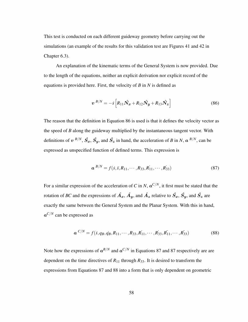
This test is conducted on each different guideway geometry before carrying out the
simulations (an example of the results for this validation test are Figures 41 and 42 in
Chapter 6.3).
An explanation of the kinematic terms of the General System is now provided. Due
to the length of the equations, neither an explicit derivation nor explicit record of the
equations is provided here. First, the velocity of B in N is defined as
v B/N =−s[R11Nx+R12Ny+R13Nz
](86)
The reason that the definition in Equation 86 is used is that it defines the velocity vector as
the speed of B along the guideway multiplied by the instantaneous tangent vector. With
definitions of v B/N , Sx, Sy, and Sz in hand, the acceleration of B in N, a B/N , can be
expressed as unspecified function of defined terms. This expression is
a B/N = f (s, s,R11, · · · ,R33, ˙R11, · · · , ˙R33) (87)
For a similar expression of the acceleration of C in N, aC/N , it first must be stated that the
rotation of BC and the expressions of Ax, Ay, and Az relative to Sx, Sy, and Sz are
exactly the same between the General System and the Planar System. With this in hand,
aC/N can be expressed as
a C/N = f (s,qB, qB,R11, · · · ,R33, ˙R11, · · · , ˙R33, ¨R11, · · · , ¨R33) (88)
Note how the expressions of aB/N and aC/N in Equations 87 and 87 respectively are are
dependent on the time directives of R11 through R33. It is desired to transform the
expressions from Equations 87 and 88 into a form that is only dependent on geometric
58
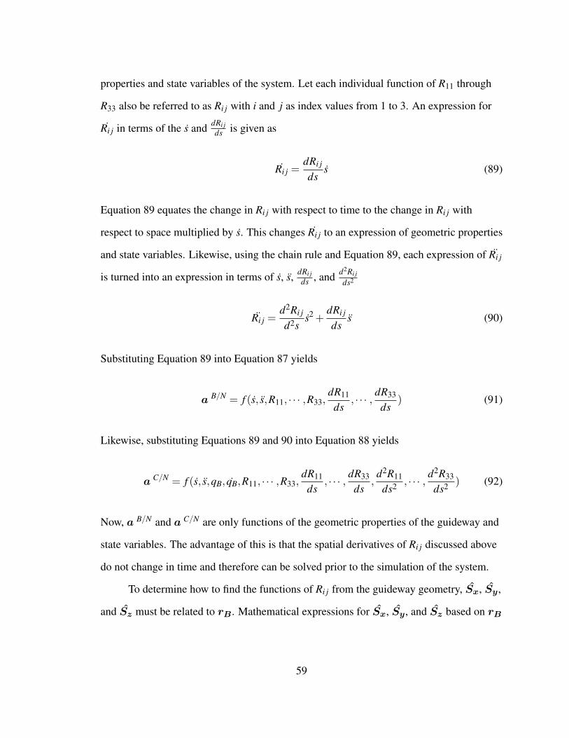
properties and state variables of the system. Let each individual function of R11 through
R33 also be referred to as Ri j with i and j as index values from 1 to 3. An expression for
Ri j in terms of the s and dRi jds is given as
Ri j =dRi j
dss (89)
Equation 89 equates the change in Ri j with respect to time to the change in Ri j with
respect to space multiplied by s. This changes Ri j to an expression of geometric properties
and state variables. Likewise, using the chain rule and Equation 89, each expression of Ri j
is turned into an expression in terms of s, s, dRi jds , and d2Ri j
ds2
Ri j =d2Ri j
d2ss2 +
dRi j
dss (90)
Substituting Equation 89 into Equation 87 yields
a B/N = f (s, s,R11, · · · ,R33,dR11
ds, · · · , dR33
ds) (91)
Likewise, substituting Equations 89 and 90 into Equation 88 yields
a C/N = f (s, s,qB, qB,R11, · · · ,R33,dR11
ds, · · · , dR33
ds,d2R11
ds2 , · · · , d2R33
ds2 ) (92)
Now, a B/N and a C/N are only functions of the geometric properties of the guideway and
state variables. The advantage of this is that the spatial derivatives of Ri j discussed above
do not change in time and therefore can be solved prior to the simulation of the system.
To determine how to find the functions of Ri j from the guideway geometry, Sx, Sy,
and Sz must be related to rB . Mathematical expressions for Sx, Sy, and Sz based on rB
59
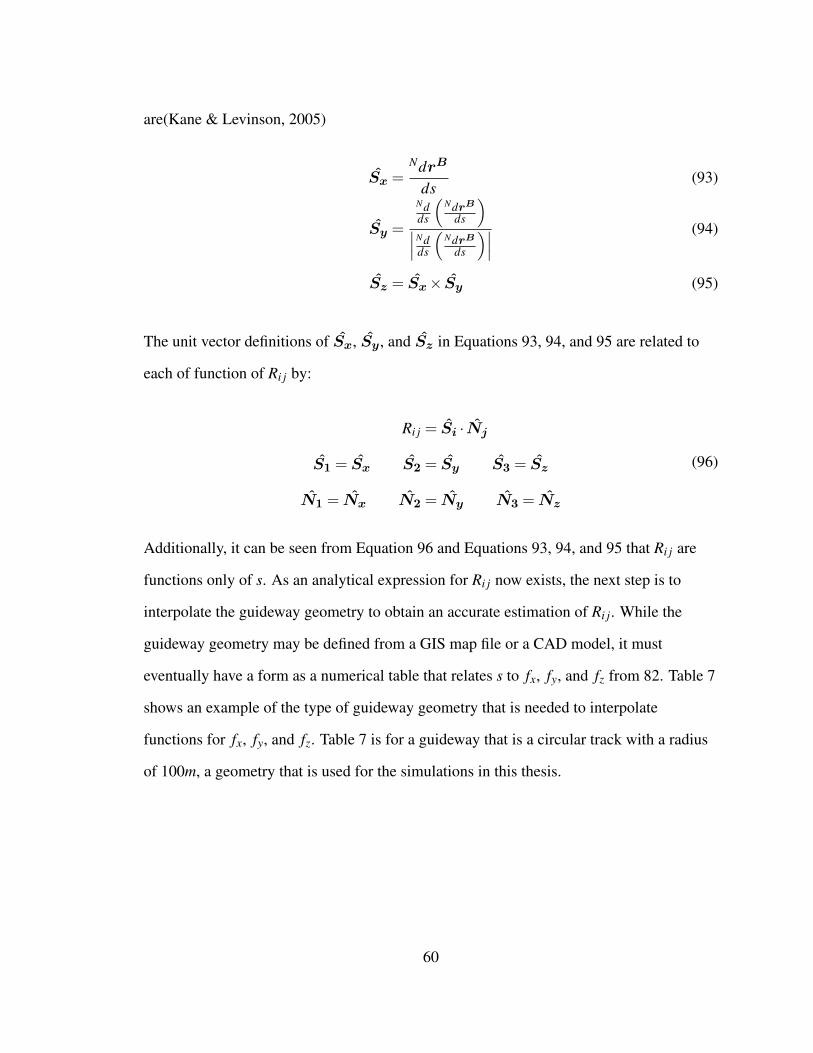
are(Kane & Levinson, 2005)
Sx =NdrB
ds(93)
Sy =
Ndds
(NdrB
ds
)∣∣∣Nd
ds
(NdrB
ds
)∣∣∣ (94)
Sz = Sx× Sy (95)
The unit vector definitions of Sx, Sy, and Sz in Equations 93, 94, and 95 are related to
each of function of Ri j by:
Ri j = Si ·Nj
S1 = Sx S2 = Sy S3 = Sz
N1 = Nx N2 = Ny N3 = Nz
(96)
Additionally, it can be seen from Equation 96 and Equations 93, 94, and 95 that Ri j are
functions only of s. As an analytical expression for Ri j now exists, the next step is to
interpolate the guideway geometry to obtain an accurate estimation of Ri j. While the
guideway geometry may be defined from a GIS map file or a CAD model, it must
eventually have a form as a numerical table that relates s to fx, fy, and fz from 82. Table 7
shows an example of the type of guideway geometry that is needed to interpolate
functions for fx, fy, and fz. Table 7 is for a guideway that is a circular track with a radius
of 100m, a geometry that is used for the simulations in this thesis.
60
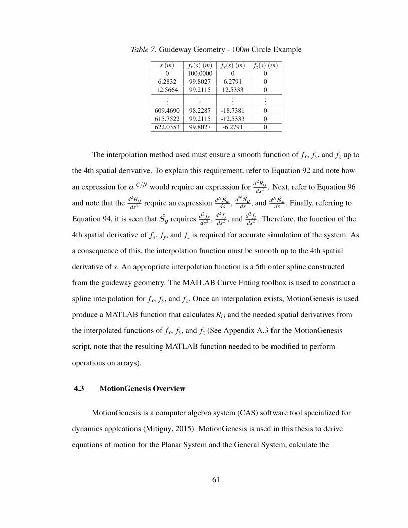
Table 7. Guideway Geometry - 100m Circle Example
s (m) fx(s) (m) fy(s) (m) fz(s) (m)0 100.0000 0 0
6.2832 99.8027 6.2791 012.5664 99.2115 12.5333 0
......
......
609.4690 98.2287 -18.7381 0615.7522 99.2115 -12.5333 0622.0353 99.8027 -6.2791 0
The interpolation method used must ensure a smooth function of fx, fy, and fz up to
the 4th spatial derivative. To explain this requirement, refer to Equation 92 and note how
an expression for a C/N would require an expression for d2Ri jds2 . Next, refer to Equation 96
and note that the d2Ri jds2 require an expression dNSx
ds , dNSy
ds , and dNSzds . Finally, referring to
Equation 94, it is seen that Sy requires d2 fxds2 , d2 fy
ds2 , and d2 fzds2 . Therefore, the function of the
4th spatial derivative of fx, fy, and fz is required for accurate simulation of the system. As
a consequence of this, the interpolation function must be smooth up to the 4th spatial
derivative of s. An appropriate interpolation function is a 5th order spline constructed
from the guideway geometry. The MATLAB Curve Fitting toolbox is used to construct a
spline interpolation for fx, fy, and fz. Once an interpolation exists, MotionGenesis is used
produce a MATLAB function that calculates Ri j and the needed spatial derivatives from
the interpolated functions of fx, fy, and fz (See Appendix A.3 for the MotionGenesis
script, note that the resulting MATLAB function needed to be modified to perform
operations on arrays).
4.3 MotionGenesis Overview
MotionGenesis is a computer algebra system (CAS) software tool specialized for
dynamics applcations (Mitiguy, 2015). MotionGenesis is used in this thesis to derive
equations of motion for the Planar System and the General System, calculate the
61
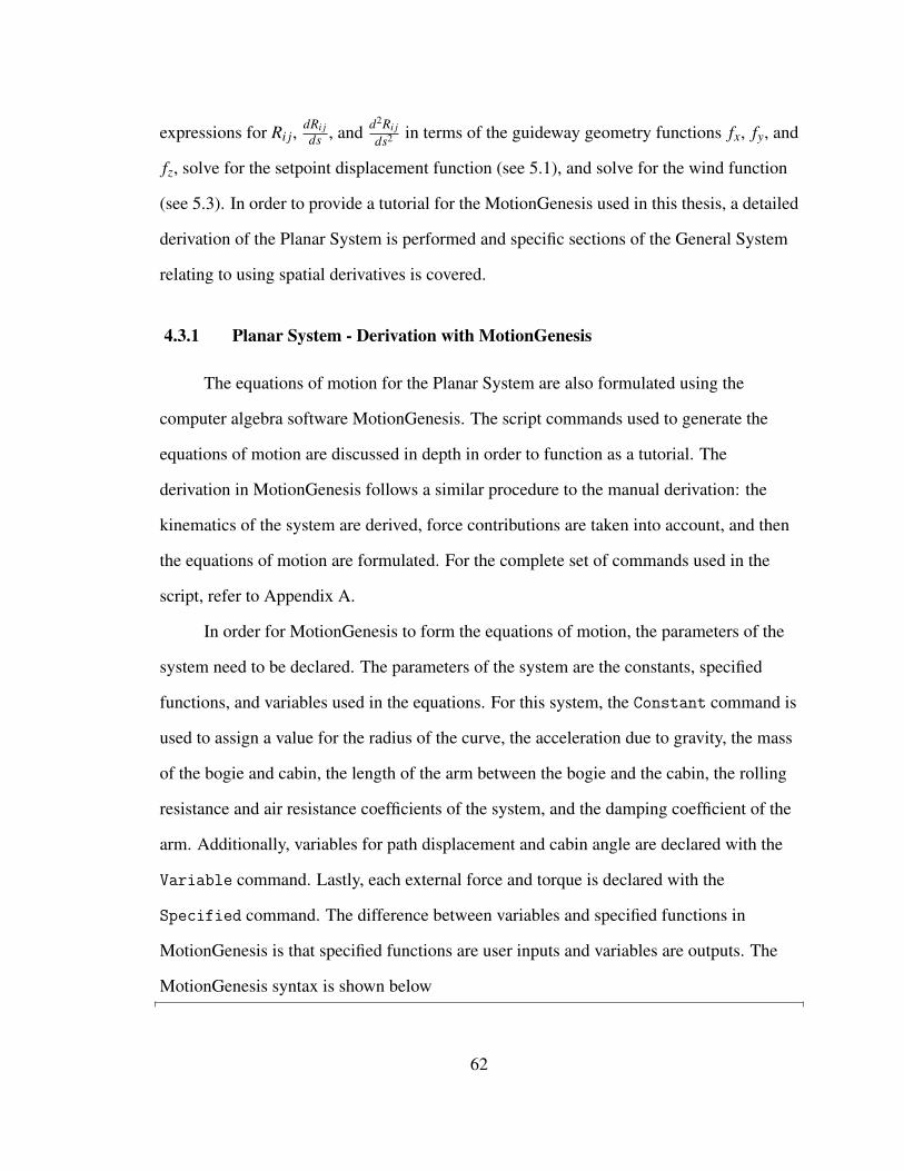
expressions for Ri j,dRi jds , and d2Ri j
ds2 in terms of the guideway geometry functions fx, fy, and
fz, solve for the setpoint displacement function (see 5.1), and solve for the wind function
(see 5.3). In order to provide a tutorial for the MotionGenesis used in this thesis, a detailed
derivation of the Planar System is performed and specific sections of the General System
relating to using spatial derivatives is covered.
4.3.1 Planar System - Derivation with MotionGenesis
The equations of motion for the Planar System are also formulated using the
computer algebra software MotionGenesis. The script commands used to generate the
equations of motion are discussed in depth in order to function as a tutorial. The
derivation in MotionGenesis follows a similar procedure to the manual derivation: the
kinematics of the system are derived, force contributions are taken into account, and then
the equations of motion are formulated. For the complete set of commands used in the
script, refer to Appendix A.
In order for MotionGenesis to form the equations of motion, the parameters of the
system need to be declared. The parameters of the system are the constants, specified
functions, and variables used in the equations. For this system, the Constant command is
used to assign a value for the radius of the curve, the acceleration due to gravity, the mass
of the bogie and cabin, the length of the arm between the bogie and the cabin, the rolling
resistance and air resistance coefficients of the system, and the damping coefficient of the
arm. Additionally, variables for path displacement and cabin angle are declared with the
Variable command. Lastly, each external force and torque is declared with the
Specified command. The difference between variables and specified functions in
MotionGenesis is that specified functions are user inputs and variables are outputs. The
MotionGenesis syntax is shown below
62
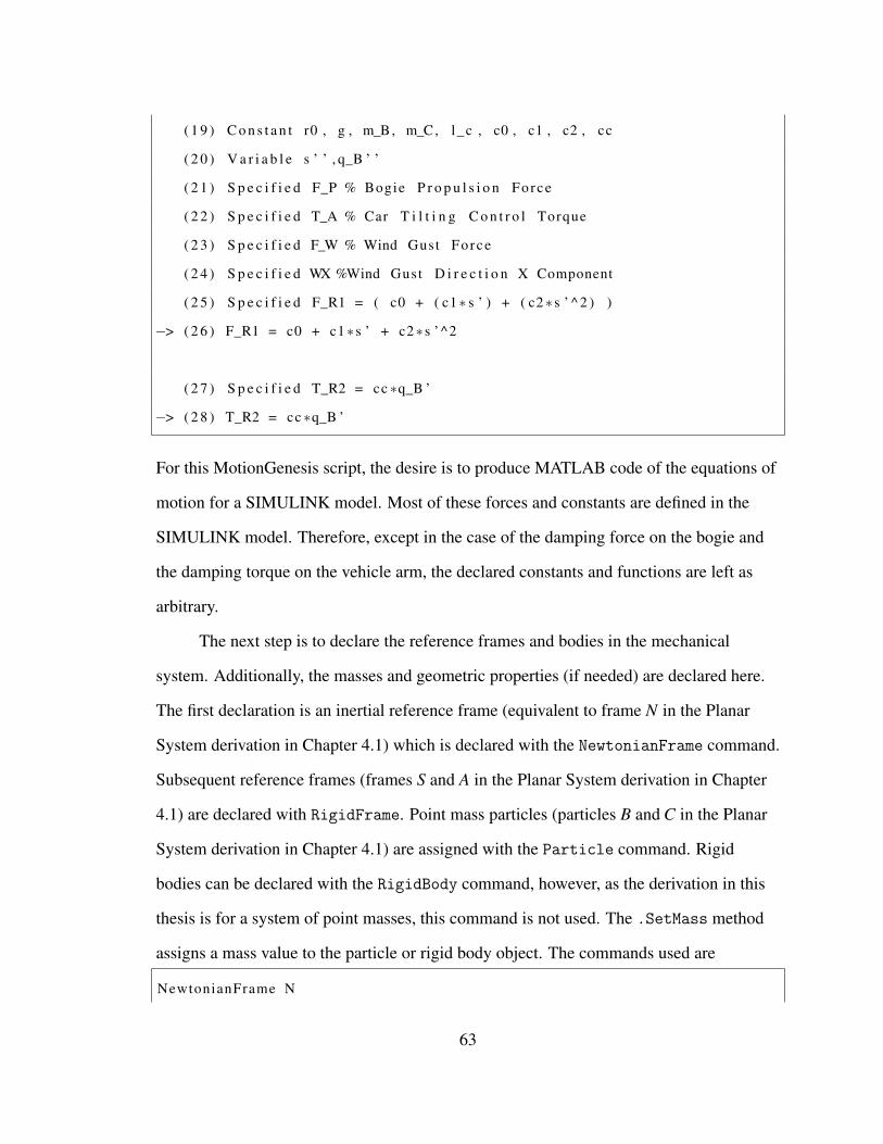
( 1 9 ) C o n s t a n t r0 , g , m_B, m_C, l_c , c0 , c1 , c2 , cc
( 2 0 ) V a r i a b l e s ’ ’ , q_B ’ ’
( 2 1 ) S p e c i f i e d F_P % Bogie P r o p u l s i o n Force
( 2 2 ) S p e c i f i e d T_A % Car T i l t i n g C o n t r o l Torque
( 2 3 ) S p e c i f i e d F_W % Wind Gust Force
( 2 4 ) S p e c i f i e d WX %Wind Gust D i r e c t i o n X Component
( 2 5 ) S p e c i f i e d F_R1 = ( c0 + ( c1∗ s ’ ) + ( c2∗ s ’ ^ 2 ) )
−> ( 2 6 ) F_R1 = c0 + c1∗ s ’ + c2∗ s ’ ^2
( 2 7 ) S p e c i f i e d T_R2 = cc ∗q_B ’
−> ( 2 8 ) T_R2 = cc ∗q_B ’
For this MotionGenesis script, the desire is to produce MATLAB code of the equations of
motion for a SIMULINK model. Most of these forces and constants are defined in the
SIMULINK model. Therefore, except in the case of the damping force on the bogie and
the damping torque on the vehicle arm, the declared constants and functions are left as
arbitrary.
The next step is to declare the reference frames and bodies in the mechanical
system. Additionally, the masses and geometric properties (if needed) are declared here.
The first declaration is an inertial reference frame (equivalent to frame N in the Planar
System derivation in Chapter 4.1) which is declared with the NewtonianFrame command.
Subsequent reference frames (frames S and A in the Planar System derivation in Chapter
4.1) are declared with RigidFrame. Point mass particles (particles B and C in the Planar
System derivation in Chapter 4.1) are assigned with the Particle command. Rigid
bodies can be declared with the RigidBody command, however, as the derivation in this
thesis is for a system of point masses, this command is not used. The .SetMass method
assigns a mass value to the particle or rigid body object. The commands used are
NewtonianFrame N
63
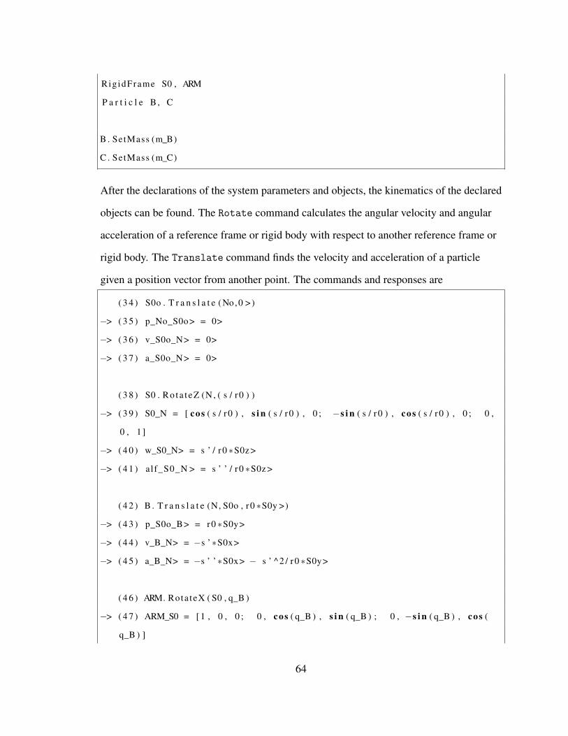
RigidFrame S0 , ARM
P a r t i c l e B , C
B . SetMass (m_B)
C . SetMass (m_C)
After the declarations of the system parameters and objects, the kinematics of the declared
objects can be found. The Rotate command calculates the angular velocity and angular
acceleration of a reference frame or rigid body with respect to another reference frame or
rigid body. The Translate command finds the velocity and acceleration of a particle
given a position vector from another point. The commands and responses are
( 3 4 ) S0o . T r a n s l a t e ( No,0 > )
−> ( 3 5 ) p_No_S0o> = 0>
−> ( 3 6 ) v_S0o_N> = 0>
−> ( 3 7 ) a_S0o_N> = 0>
( 3 8 ) S0 . Ro ta t eZ (N , ( s / r0 ) )
−> ( 3 9 ) S0_N = [ cos ( s / r0 ) , s i n ( s / r0 ) , 0 ; −s i n ( s / r0 ) , cos ( s / r0 ) , 0 ; 0 ,
0 , 1 ]
−> ( 4 0 ) w_S0_N> = s ’ / r0 ∗S0z >
−> ( 4 1 ) alf_S0_N > = s ’ ’ / r0 ∗S0z >
( 4 2 ) B . T r a n s l a t e (N, S0o , r0 ∗S0y >)
−> ( 4 3 ) p_S0o_B> = r0 ∗S0y>
−> ( 4 4 ) v_B_N> = −s ’∗S0x>
−> ( 4 5 ) a_B_N> = −s ’ ’∗S0x> − s ’ ^ 2 / r0 ∗S0y>
( 4 6 ) ARM. Rota teX ( S0 , q_B )
−> ( 4 7 ) ARM_S0 = [ 1 , 0 , 0 ; 0 , cos ( q_B ) , s i n ( q_B ) ; 0 , −s i n ( q_B ) , cos (
q_B ) ]
64
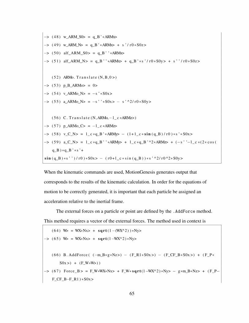
−> ( 4 8 ) w_ARM_S0> = q_B ’∗ARMx>
−> ( 4 9 ) w_ARM_N> = q_B ’∗ARMx> + s ’ / r0 ∗S0z >
−> ( 5 0 ) alf_ARM_S0> = q_B ’ ’∗ARMx>
−> ( 5 1 ) alf_ARM_N> = q_B ’ ’∗ARMx> + q_B ’∗ s ’ / r0 ∗S0y> + s ’ ’ / r0 ∗S0z >
( 5 2 ) ARMo. T r a n s l a t e (N, B,0 > )
−> ( 5 3 ) p_B_ARMo> = 0>
−> ( 5 4 ) v_ARMo_N> = −s ’∗S0x>
−> ( 5 5 ) a_ARMo_N> = −s ’ ’∗S0x> − s ’ ^ 2 / r0 ∗S0y>
( 5 6 ) C . T r a n s l a t e (N,ARMo,− l _ c ∗ARMz>)
−> ( 5 7 ) p_ARMo_C> = − l _ c ∗ARMz>
−> ( 5 8 ) v_C_N> = l _ c ∗q_B ’∗ARMy> − (1+ l _ c ∗ s i n ( q_B ) / r0 ) ∗ s ’∗ S0x>
−> ( 5 9 ) a_C_N> = l _ c ∗q_B ’ ’∗ARMy> + l _ c ∗q_B ’ ^2∗ARMz> + (−s ’ ’− l _ c ∗ (2∗ cos (
q_B ) ∗q_B ’∗ s ’+
s i n ( q_B ) ∗ s ’ ’ ) / r0 ) ∗S0x> − ( r0 + l _ c ∗ s i n ( q_B ) ) ∗ s ’ ^ 2 / r0 ^2∗S0y>
When the kinematic commands are used, MotionGenesis generates output that
corresponds to the results of the kinematic calculation. In order for the equations of
motion to be correctly generated, it is important that each particle be assigned an
acceleration relative to the inertial frame.
The external forces on a particle or point are defined by the .AddForce method.
This method requires a vector of the external forces. The method used in context is
( 6 4 ) W> = WX∗Nx> + s q r t (1−(WX^2) ) ∗Ny>
−> ( 6 5 ) W> = WX∗Nx> + s q r t (1−WX^2) ∗Ny>
( 6 6 ) B . AddForce ( (−m_B∗g∗Nz>) − ( F_R1∗S0x >) − ( F_CF_B∗S0x >) + ( F_P∗
S0x >) + (F_W∗W>) )
−> ( 6 7 ) Force_B > = F_W∗WX∗Nx> + F_W∗ s q r t (1−WX^2) ∗Ny> − g∗m_B∗Nz> + ( F_P−
F_CF_B−F_R1 ) ∗S0x>
65
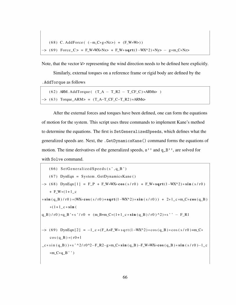
( 6 8 ) C . AddForce ( (−m_C∗g∗Nz>) + (F_W∗W>) )
−> ( 6 9 ) Force_C > = F_W∗WX∗Nx> + F_W∗ s q r t (1−WX^2) ∗Ny> − g∗m_C∗Nz>
Note, that the vector W> representing the wind direction needs to be defined here explicitly.
Similarly, external torques on a reference frame or rigid body are defined by the
.AddTorque as follows
( 6 2 ) ARM. AddTorque ( (T_A − T_R2 − T_CF_C ) ∗ARMx> )
−> ( 6 3 ) Torque_ARM> = ( T_A−T_CF_C−T_R2 ) ∗ARMx>
After the external forces and torques have been defined, one can form the equations
of motion for the system. This script uses three commands to implement Kane’s method
to determine the equations. The first is SetGeneralizedSpeeds, which defines what the
generalized speeds are. Next, the .GetDynamicsKane() command forms the equations of
motion. The time derivatives of the generalized speeds, s’’ and q_B’’, are solved for
with Solve command.
( 6 6 ) S e t G e n e r a l i z e d S p e e d s ( s ’ , q_B ’ )
( 6 7 ) DynEqn = System . GetDynamicsKane ( )
−> ( 6 8 ) DynEqn [ 1 ] = F_P + F_W∗WX∗ cos ( s / r0 ) + F_W∗ s q r t (1−WX^2) ∗ s i n ( s / r0 )
+ F_W∗ (1+ l _ c
∗ s i n ( q_B ) / r0 ) ∗ (WX∗ cos ( s / r0 ) + s q r t (1−WX^2) ∗ s i n ( s / r0 ) ) + 2∗ l _ c ∗m_C∗ cos ( q_B )
∗ (1+ l _ c ∗ s i n (
q_B ) / r0 ) ∗q_B ’∗ s ’ / r0 + (m_B+m_C∗ (1+ l _ c ∗ s i n ( q_B ) / r0 ) ^2 ) ∗ s ’ ’ − F_R1
−> ( 6 9 ) DynEqn [ 2 ] = − l _ c ∗ ( F_A+F_W∗ s q r t (1−WX^2) ∗ cos ( q_B ) ∗ cos ( s / r0 ) +m_C∗
cos ( q_B ) ∗ ( r0 + l
_c∗ s i n ( q_B ) ) ∗ s ’ ^ 2 / r0 ^2−F_R2−g∗m_C∗ s i n ( q_B )−F_W∗WX∗ cos ( q_B ) ∗ s i n ( s / r0 )− l _ c
∗m_C∗q_B ’ ’ )
66
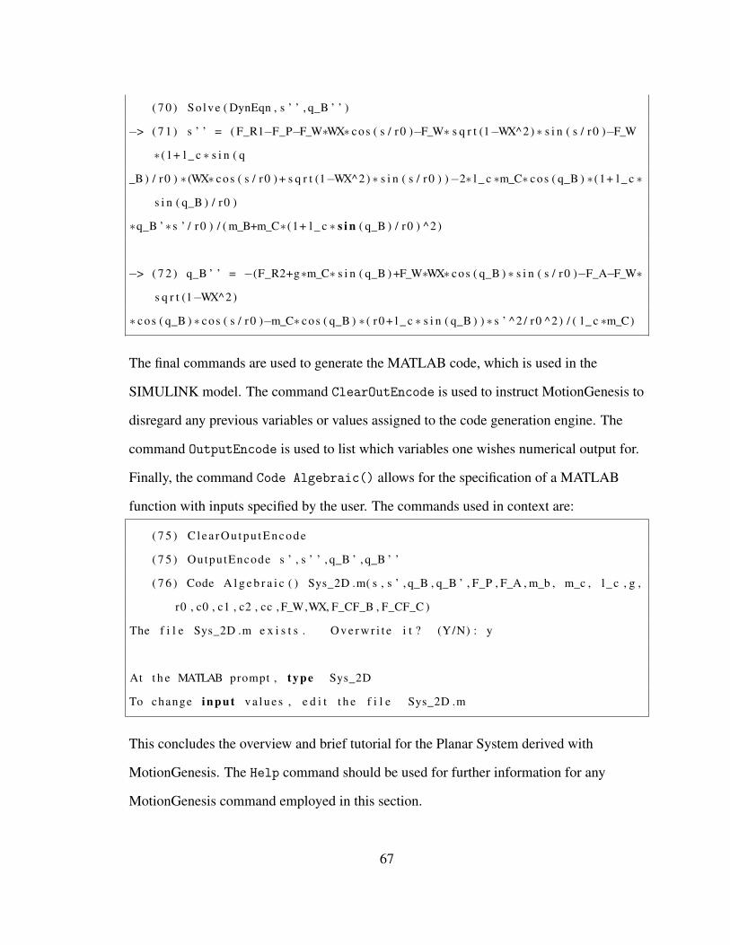
( 7 0 ) So lve ( DynEqn , s ’ ’ , q_B ’ ’ )
−> ( 7 1 ) s ’ ’ = ( F_R1−F_P−F_W∗WX∗ cos ( s / r0 )−F_W∗ s q r t (1−WX^2) ∗ s i n ( s / r0 )−F_W
∗ (1+ l _ c ∗ s i n ( q
_B ) / r0 ) ∗ (WX∗ cos ( s / r0 ) + s q r t (1−WX^2) ∗ s i n ( s / r0 ) )−2∗ l _ c ∗m_C∗ cos ( q_B ) ∗ (1+ l _ c ∗
s i n ( q_B ) / r0 )
∗q_B ’∗ s ’ / r0 ) / ( m_B+m_C∗ (1+ l _ c ∗ s i n ( q_B ) / r0 ) ^2 )
−> ( 7 2 ) q_B ’ ’ = −(F_R2+g∗m_C∗ s i n ( q_B ) +F_W∗WX∗ cos ( q_B ) ∗ s i n ( s / r0 )−F_A−F_W∗
s q r t (1−WX^2)
∗ cos ( q_B ) ∗ cos ( s / r0 )−m_C∗ cos ( q_B ) ∗ ( r0 + l _ c ∗ s i n ( q_B ) ) ∗ s ’ ^ 2 / r0 ^2 ) / ( l _ c ∗m_C)
The final commands are used to generate the MATLAB code, which is used in the
SIMULINK model. The command ClearOutEncode is used to instruct MotionGenesis to
disregard any previous variables or values assigned to the code generation engine. The
command OutputEncode is used to list which variables one wishes numerical output for.
Finally, the command Code Algebraic() allows for the specification of a MATLAB
function with inputs specified by the user. The commands used in context are:
( 7 5 ) C le a r Ou t pu tEn co de
( 7 5 ) OutputEncode s ’ , s ’ ’ , q_B ’ , q_B ’ ’
( 7 6 ) Code A l g e b r a i c ( ) Sys_2D .m( s , s ’ , q_B , q_B ’ , F_P , F_A , m_b , m_c , l_c , g ,
r0 , c0 , c1 , c2 , cc , F_W,WX, F_CF_B , F_CF_C )
The f i l e Sys_2D .m e x i s t s . O v e r w r i t e i t ? (Y/N) : y
At t h e MATLAB prompt , type Sys_2D
To change input v a l u e s , e d i t t h e f i l e Sys_2D .m
This concludes the overview and brief tutorial for the Planar System derived with
MotionGenesis. The Help command should be used for further information for any
MotionGenesis command employed in this section.
67
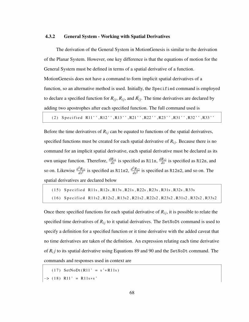
4.3.2 General System - Working with Spatial Derivatives
The derivation of the General System in MotionGenesis is similar to the derivation
of the Planar System. However, one key difference is that the equations of motion for the
General System must be defined in terms of a spatial derivative of a function.
MotionGenesis does not have a command to form implicit spatial derivatives of a
function, so an alternative method is used. Initially, the Specified command is employed
to declare a specified function for Ri j, Ri j, and Ri j. The time derivatives are declared by
adding two apostrophes after each specified function. The full command used is
( 2 ) S p e c i f i e d R11 ’ ’ , R12 ’ ’ , R13 ’ ’ , R21 ’ ’ , R22 ’ ’ , R23 ’ ’ , R31 ’ ’ , R32 ’ ’ , R33 ’ ’
Before the time derivatives of Ri j can be equated to functions of the spatial derivatives,
specified functions must be created for each spatial derivative of Ri j. Because there is no
command for an implicit spatial derivative, each spatial derivative must be declared as its
own unique function. Therefore, dR11ds is specified as R11s, dR12
ds is specified as R12s, and
so on. Likewise d2R11ds2 is specified as R11s2, d2R12
ds2 is specified as R12s2, and so on. The
spatial derivatives are declared below
( 1 5 ) S p e c i f i e d R11s , R12s , R13s , R21s , R22s , R23s , R31s , R32s , R33s
( 1 6 ) S p e c i f i e d R11s2 , R12s2 , R13s2 , R21s2 , R22s2 , R23s2 , R31s2 , R32s2 , R33s2
Once there specified functions for each spatial derivative of Ri j, it is possible to relate the
specified time derivatives of Ri j to it spatial derivatives. The SetNoDt command is used to
specify a definition for a specified function or it time derivative with the added caveat that
no time derivatives are taken of the definition. An expression relating each time derivative
of Ri j to its spatial derivative using Equations 89 and 90 and the SetNoDt command. The
commands and responses used in context are
( 1 7 ) SetNoDt ( R11 ’ = s ’∗R11s )
−> ( 1 8 ) R11 ’ = R11s∗ s ’
68
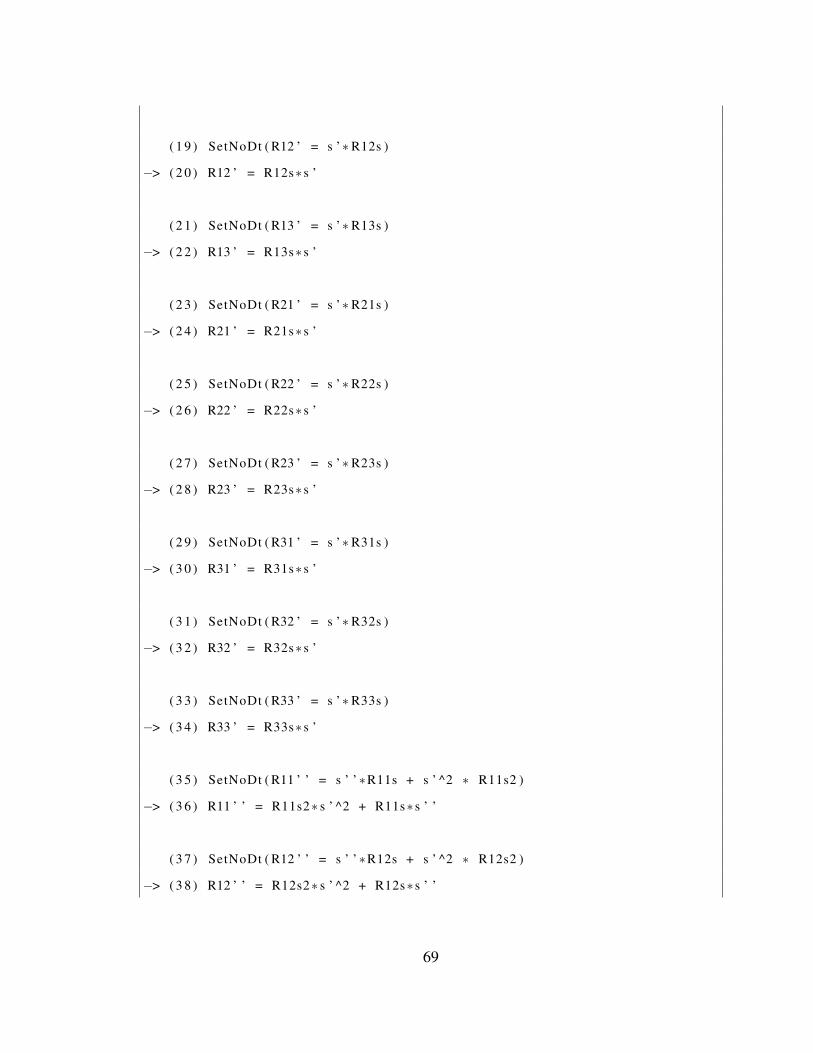
( 1 9 ) SetNoDt ( R12 ’ = s ’∗R12s )
−> ( 2 0 ) R12 ’ = R12s∗ s ’
( 2 1 ) SetNoDt ( R13 ’ = s ’∗R13s )
−> ( 2 2 ) R13 ’ = R13s∗ s ’
( 2 3 ) SetNoDt ( R21 ’ = s ’∗R21s )
−> ( 2 4 ) R21 ’ = R21s∗ s ’
( 2 5 ) SetNoDt ( R22 ’ = s ’∗R22s )
−> ( 2 6 ) R22 ’ = R22s∗ s ’
( 2 7 ) SetNoDt ( R23 ’ = s ’∗R23s )
−> ( 2 8 ) R23 ’ = R23s∗ s ’
( 2 9 ) SetNoDt ( R31 ’ = s ’∗R31s )
−> ( 3 0 ) R31 ’ = R31s∗ s ’
( 3 1 ) SetNoDt ( R32 ’ = s ’∗R32s )
−> ( 3 2 ) R32 ’ = R32s∗ s ’
( 3 3 ) SetNoDt ( R33 ’ = s ’∗R33s )
−> ( 3 4 ) R33 ’ = R33s∗ s ’
( 3 5 ) SetNoDt ( R11 ’ ’ = s ’ ’∗R11s + s ’ ^2 ∗ R11s2 )
−> ( 3 6 ) R11 ’ ’ = R11s2∗ s ’ ^2 + R11s∗ s ’ ’
( 3 7 ) SetNoDt ( R12 ’ ’ = s ’ ’∗R12s + s ’ ^2 ∗ R12s2 )
−> ( 3 8 ) R12 ’ ’ = R12s2∗ s ’ ^2 + R12s∗ s ’ ’
69
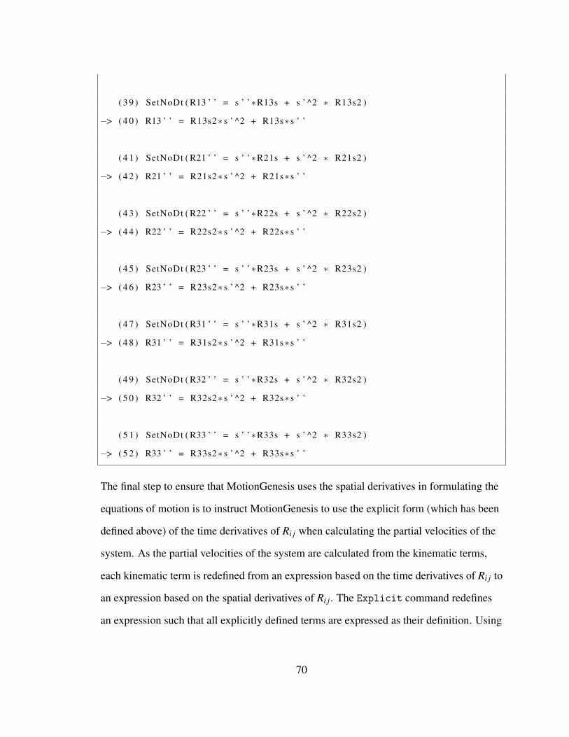
( 3 9 ) SetNoDt ( R13 ’ ’ = s ’ ’∗R13s + s ’ ^2 ∗ R13s2 )
−> ( 4 0 ) R13 ’ ’ = R13s2∗ s ’ ^2 + R13s∗ s ’ ’
( 4 1 ) SetNoDt ( R21 ’ ’ = s ’ ’∗R21s + s ’ ^2 ∗ R21s2 )
−> ( 4 2 ) R21 ’ ’ = R21s2∗ s ’ ^2 + R21s∗ s ’ ’
( 4 3 ) SetNoDt ( R22 ’ ’ = s ’ ’∗R22s + s ’ ^2 ∗ R22s2 )
−> ( 4 4 ) R22 ’ ’ = R22s2∗ s ’ ^2 + R22s∗ s ’ ’
( 4 5 ) SetNoDt ( R23 ’ ’ = s ’ ’∗R23s + s ’ ^2 ∗ R23s2 )
−> ( 4 6 ) R23 ’ ’ = R23s2∗ s ’ ^2 + R23s∗ s ’ ’
( 4 7 ) SetNoDt ( R31 ’ ’ = s ’ ’∗R31s + s ’ ^2 ∗ R31s2 )
−> ( 4 8 ) R31 ’ ’ = R31s2∗ s ’ ^2 + R31s∗ s ’ ’
( 4 9 ) SetNoDt ( R32 ’ ’ = s ’ ’∗R32s + s ’ ^2 ∗ R32s2 )
−> ( 5 0 ) R32 ’ ’ = R32s2∗ s ’ ^2 + R32s∗ s ’ ’
( 5 1 ) SetNoDt ( R33 ’ ’ = s ’ ’∗R33s + s ’ ^2 ∗ R33s2 )
−> ( 5 2 ) R33 ’ ’ = R33s2∗ s ’ ^2 + R33s∗ s ’ ’
The final step to ensure that MotionGenesis uses the spatial derivatives in formulating the
equations of motion is to instruct MotionGenesis to use the explicit form (which has been
defined above) of the time derivatives of Ri j when calculating the partial velocities of the
system. As the partial velocities of the system are calculated from the kinematic terms,
each kinematic term is redefined from an expression based on the time derivatives of Ri j to
an expression based on the spatial derivatives of Ri j. The Explicit command redefines
an expression such that all explicitly defined terms are expressed as their definition. Using
70
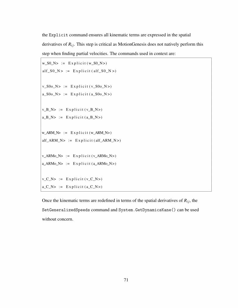
the Explicit command ensures all kinematic terms are expressed in the spatial
derivatives of Ri j. This step is critical as MotionGenesis does not natively perform this
step when finding partial velocities. The commands used in context are:
w_S0_N> := E x p l i c i t ( w_S0_N >)
alf_S0_N > := E x p l i c i t ( alf_S0_N >)
v_S0o_N> := E x p l i c i t ( v_S0o_N >)
a_S0o_N> := E x p l i c i t ( a_S0o_N >)
v_B_N> := E x p l i c i t ( v_B_N >)
a_B_N> := E x p l i c i t ( a_B_N >)
w_ARM_N> := E x p l i c i t (w_ARM_N>)
alf_ARM_N> := E x p l i c i t ( alf_ARM_N >)
v_ARMo_N> := E x p l i c i t (v_ARMo_N>)
a_ARMo_N> := E x p l i c i t ( a_ARMo_N>)
v_C_N> := E x p l i c i t ( v_C_N >)
a_C_N> := E x p l i c i t ( a_C_N >)
Once the kinematic terms are redefined in terms of the spatial derivatives of Ri j, the
SetGeneralizedSpeeds command and System.GetDynamicsKane() can be used
without concern.
71
CHAPTER 5
ATN VEHICLE SIMULATION
For the ATN vehicle simulation and control research, a SIMULINK model is
constructed using the equations of motion derived in the previous chapter as the plant and
a controller designed using the Control Systems Toolbox in MATLAB. The plant
dynamics use a MATLAB function block in SIMULINK that uses code generated by the
MotionGenesis script in Appendix A.1. The controller is implemented in SIMULINK
blocks outside of the plant. The controller uses feedback linearization to negate the
nonlinear dynamics of the plant and decouple the dynamics of the bogie and the vehicle
angle. Additionally, proportional control is applied to the error of the bogie position and to
the error of the angular position of the vehicle body. This controller tracks the position of
the ATN vehicle and minimizes the centrifugal force on the passenger. The setpoints for
both the displacement and the angular position are calculated in SIMULINK blocks
separate from the plant and the controller. Additionally, there are two blocks that calculate
system dynamics outside of the MATLAB function block: the force due to wind gusts and
the non-linear friction force.
5.1 Displacement Profile Calculation
The controller for the ATN vehicle requires that the vehicle be able to track a
position on a guideway with restrictions on the maximum velocity, acceleration, and jerk.
If a constant position setpoint is used with a P controller, then the velocity, acceleration,
and jerk are governed completely by the location of the closed loop poles. A simple
method of ensuring that the controller output meets the design criteria is to have the
setpoint of the ATN vehicle be a displacement profile that meets the required conditions.
The displacement profile chosen for this is the piecewise function s0(t) comprised of the
72
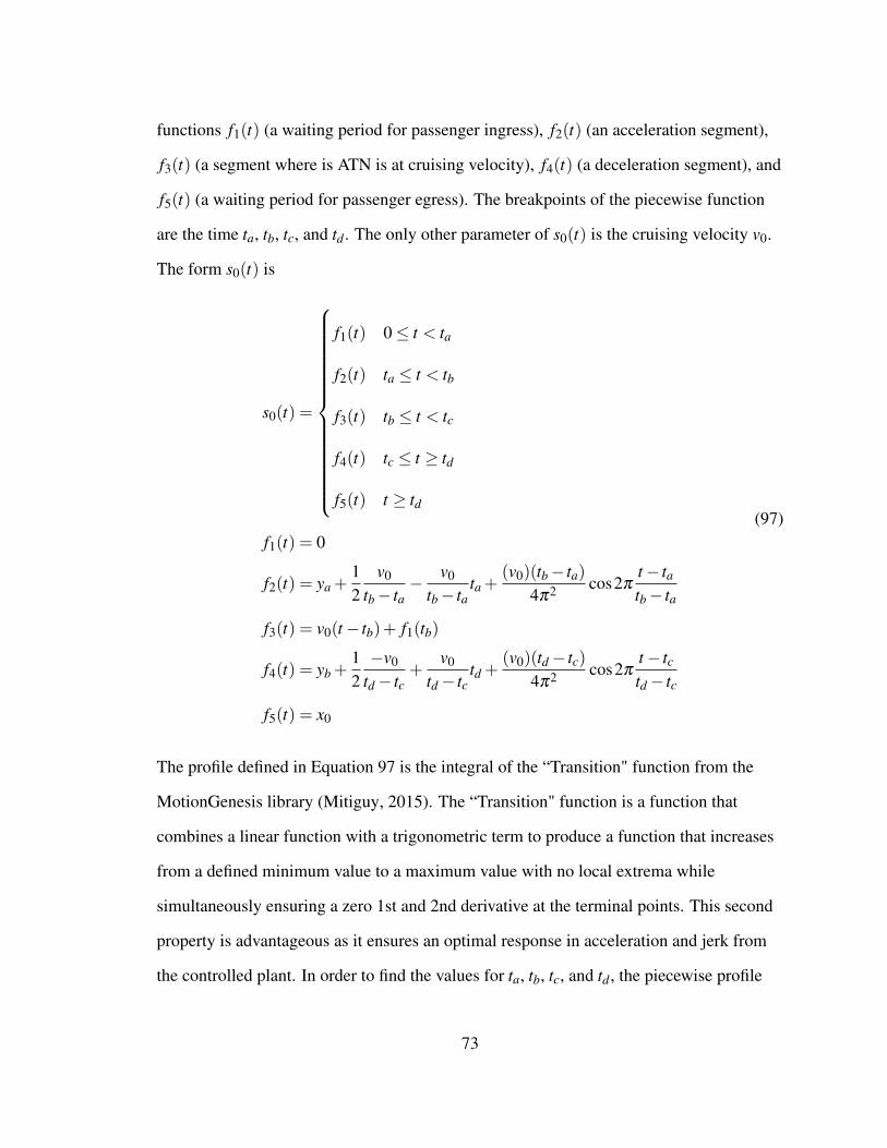
functions f1(t) (a waiting period for passenger ingress), f2(t) (an acceleration segment),
f3(t) (a segment where is ATN is at cruising velocity), f4(t) (a deceleration segment), and
f5(t) (a waiting period for passenger egress). The breakpoints of the piecewise function
are the time ta, tb, tc, and td . The only other parameter of s0(t) is the cruising velocity v0.
The form s0(t) is
s0(t) =
f1(t) 0≤ t < ta
f2(t) ta ≤ t < tb
f3(t) tb ≤ t < tc
f4(t) tc ≤ t ≥ td
f5(t) t ≥ td
f1(t) = 0
f2(t) = ya +12
v0
tb− ta− v0
tb− tata +
(v0)(tb− ta)4π2 cos2π
t− tatb− ta
f3(t) = v0(t− tb)+ f1(tb)
f4(t) = yb +12−v0
td− tc+
v0
td− tctd +
(v0)(td− tc)4π2 cos2π
t− tctd− tc
f5(t) = x0
(97)
The profile defined in Equation 97 is the integral of the “Transition" function from the
MotionGenesis library (Mitiguy, 2015). The “Transition" function is a function that
combines a linear function with a trigonometric term to produce a function that increases
from a defined minimum value to a maximum value with no local extrema while
simultaneously ensuring a zero 1st and 2nd derivative at the terminal points. This second
property is advantageous as it ensures an optimal response in acceleration and jerk from
the controlled plant. In order to find the values for ta, tb, tc, and td , the piecewise profile
73
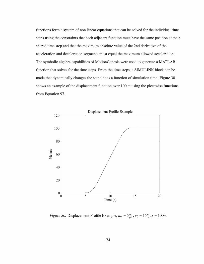
functions form a system of non-linear equations that can be solved for the individual time
steps using the constraints that each adjacent function must have the same position at their
shared time step and that the maximum absolute value of the 2nd derivative of the
acceleration and deceleration segments must equal the maximum allowed acceleration.
The symbolic algebra capabilities of MotionGenesis were used to generate a MATLAB
function that solves for the time steps. From the time steps, a SIMULINK block can be
made that dynamically changes the setpoint as a function of simulation time. Figure 30
shows an example of the displacement function over 100 m using the piecewise functions
from Equation 97.
0 5 10 15 200
20
40
60
80
100
120Displacement Profile Example
Time (s)
Met
ers
Figure 30. Displacement Profile Example, am = 5 ms2 , v0 = 15m
s , x = 100m
74
5.2 Angle Setpoint Calculation
The setpoint for the angular position qB of the suspended vehicle is not determined
by an externally defined setpoint, but rather from velocity of the ATN bogie. Using the
mechanics of suspended ATN vehicles (Anderson, 1978) and control of tilting high speed
trains (Zhou et al., 2011), a simple method of determining the angular value to minimize
the reaction forces on the passenger is developed. This method is based on the derivation
of the equations of motion for the Planar System and is used without modification with the
General System. Refer to Chapter 4.1 for the definition of the terms used for the
derivation of the angle setpoint formula.
The development of the angle setpoint formula is based on the reaction forces felt
by the passenger relative to A.
• A force that acts in the Ax direction pushes the passenger against the rear face of
the seat or throws the passenger forward from the seat.
• A force that acts in the Ay direction pushes the passenger to either side of the
seat.
• A force that acts in the Az direction pushes the passenger against the cushion of
the seat or lifts the passenger from the seat.
Forces on the passenger in the direction of Ax cannot be compensated by rotation of the
vehicle body and therefore warrant no further discussion or analysis. It is shown that there
is a trade between forces in the directions of Ay and Az. Figure 31 shows a free body for
an ATN passenger at steady cruising velocity and constant vehicle angle.
75
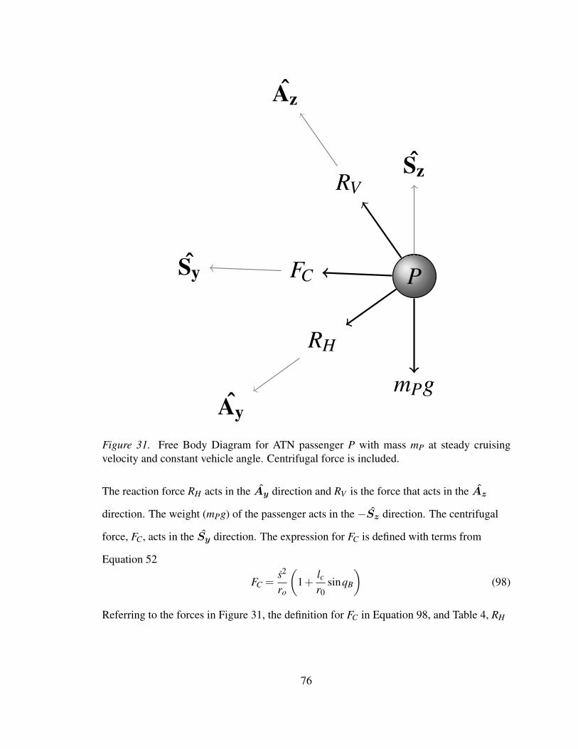
mPg
Sz
Ay
RV
Sy
Az
RH
FC P
Figure 31. Free Body Diagram for ATN passenger P with mass mP at steady cruisingvelocity and constant vehicle angle. Centrifugal force is included.
The reaction force RH acts in the Ay direction and RV is the force that acts in the Az
direction. The weight (mPg) of the passenger acts in the −Sz direction. The centrifugal
force, FC, acts in the Sy direction. The expression for FC is defined with terms from
Equation 52
FC =s2
ro
(1+
lcr0
sinqB
)(98)
Referring to the forces in Figure 31, the definition for FC in Equation 98, and Table 4, RH
76
at steady cruising velocity and constant vehicle angle is
RH =−mPs2
r0
(1+
lcr0
sinqB
)cosqB +mPgsinqB (99)
Likewise, the expression for RV at steady cruising velocity and constant vehicle angle is
RV = mPsr0
(1+
lcr0
sinqB
)sinqB +mPgcosqB (100)
As the length of the vehicle body arm is usually much less than the radius of the curve, it
safe to neglect the lcr0
term in Equation 99, which simplifies RH to
RH =−mPs2
r0cosqB +mPgsinqB (101)
From an ergonomics standpoint, forces that act in the Az direction are preferable over
forces that act in the Ay direction. Therefore, the vehicle angle setpoint is defined by the
value qB that results when RH is zero. Setting RH to 0 in Equation 101 gives
mPsr0
cosqB = mPgsinqB (102)
Solving for qB in Equation 102 gives
qB = atans2
gr(103)
Although the angle setpoint formula is defined for a guideway that is an arc of constant
radius, the same setpoint for qB is used for any possible guideway geometries. Therefore,
77
a useful alternative expression for qB, which is in terms of a varying curvature, κ , is
qB = atans2κ
g(104)
With κ defined as the inverse of the radius (Weisstein, 2016b) at a given path length.
κ =1
r(s)(105)
As this thesis investigates the control of vehicles over a numerically defined guideway, it
is convenient to express the angle setpoint formula as the form in Equation 104. This is
because the numerical guideway may have straight segments which have an effective
infinite radius.
5.3 Wind Force Calculation
The magnitude and direction of the wind force are controlled by MATLAB
functions embedded in the SIMULINK program. The wind force needs to be an
intermittent force that ramps up to a maximum force value and then ramps back down to
zero. The 1st and 2nd derivatives of function governing wind force must be zero. The
piecewise function FM is created to model the wind force as a zero force segment, a ramp
up period, a ramp down period, and another zero force segment. The maximum force of
FM is FW and FM acts in the W direction. The ramp up and ramp down sections of FM
are modeled by the “Transition" function from MotionGenesis. The two time steps are ta
78
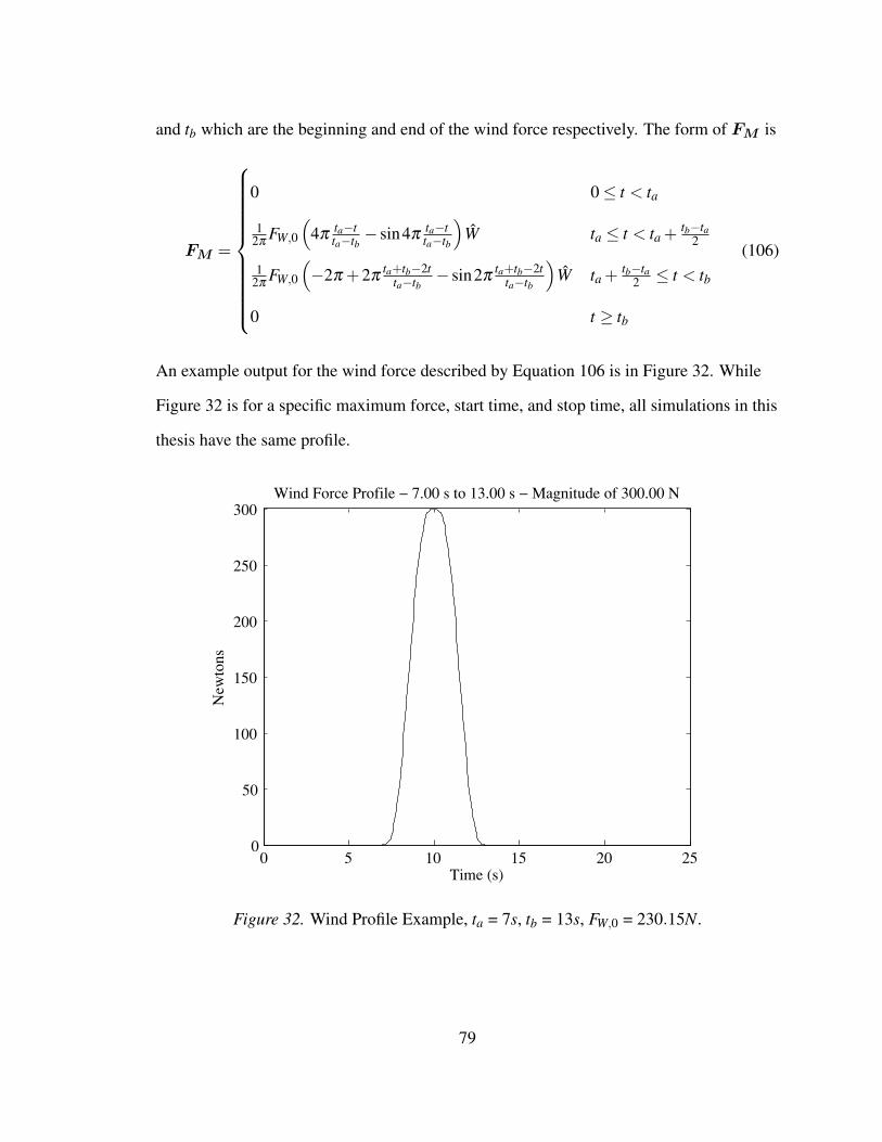
and tb which are the beginning and end of the wind force respectively. The form of FM is
FM =
0 0≤ t < ta
12π
FW,0
(4π
ta−tta−tb− sin4π
ta−tta−tb
)W ta ≤ t < ta +
tb−ta2
12π
FW,0
(−2π +2π
ta+tb−2tta−tb
− sin2πta+tb−2t
ta−tb
)W ta +
tb−ta2 ≤ t < tb
0 t ≥ tb
(106)
An example output for the wind force described by Equation 106 is in Figure 32. While
Figure 32 is for a specific maximum force, start time, and stop time, all simulations in this
thesis have the same profile.
0 5 10 15 20 250
50
100
150
200
250
300Wind Force Profile − 7.00 s to 13.00 s − Magnitude of 300.00 N
Time (s)
New
tons
Figure 32. Wind Profile Example, ta = 7s, tb = 13s, FW,0 = 230.15N.
79
5.4 Non-Linear Friction Force
The nonlinear friction force refers to combined effect of static friction and the
Stribeck effect(Makkar, Dixon, Sawyer, & Hu, 2005). The Stribeck effect is when the
coefficient of friction decreases from the static coefficient to the kinetic coefficient. These
frictional forces involve discontinuities and thus can be difficult to model in a simulation
as the discontinuities represent situations where the time derivative goes to infinity. A
solution is to use a mathematical model comprised of hyperbolic tangent functions to
replicate the discontinuous behavior. The coefficient of friction modeled with hyperbolic
tangent functions (Makkar et al., 2005) is
f (x) = γ1(tanhγ2x− tanhγ3x)+ γ4 tanhγ5x+ γ6x (107)
The mathematical model in Equation 107 is dependent on the velocity, x, and the
constants γ1, γ2, γ3, γ4, γ5, and γ6. It should be noted that γ6 represents vicious friction and
is set to zero in the simulations as viscous friction is defined by other forces in the
equations of motion. Table 8 shows the constants used for the coefficient of friction model
for the suspended vehicle body. The constants for the coefficient of friction of the bogie
are not included due the discontinuous nature of the non-linear friction causing
discontinuities in the acceleration of the bogie. These acceleration discontinuities in the
motion of the bogie result in unrealistic jerk results of the bogie. The velocity of the bogie
does not cross zero and the effect of the nonlinear friction forces is only prevalent in the
beginning of the simulation. Therefore, it is acceptable to discount the nonlinear friction
effects of the bogie. The values of γ1, γ2, γ3, γ4, and γ5 are defined from the design
guidelines in the paper “A New Continuously Differentiable Friction Model for Control
Systems Design" (Makkar et al., 2005) and accepted static and kinetic friction coefficients
80
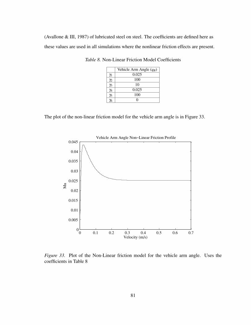
(Avallone & III, 1987) of lubricated steel on steel. The coefficients are defined here as
these values are used in all simulations where the nonlinear friction effects are present.
Table 8. Non-Linear Friction Model Coefficients
Vehicle Arm Angle (qB)γ1 0.025γ2 100γ3 10γ4 0.025γ5 100γ6 0
The plot of the non-linear friction model for the vehicle arm angle is in Figure 33.
0 0.1 0.2 0.3 0.4 0.5 0.6 0.70
0.005
0.01
0.015
0.02
0.025
0.03
0.035
0.04
0.045Vehicle Arm Angle Non−Linear Friction Profile
Velocity (m/s)
Mu
Figure 33. Plot of the Non-Linear friction model for the vehicle arm angle. Uses thecoefficients in Table 8
81
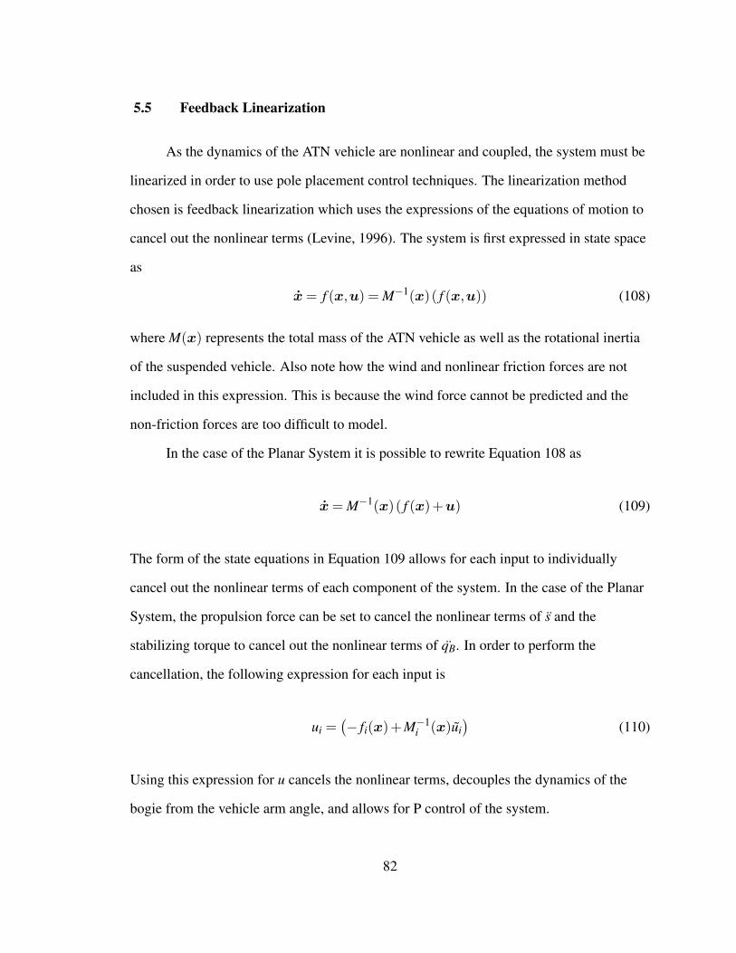
5.5 Feedback Linearization
As the dynamics of the ATN vehicle are nonlinear and coupled, the system must be
linearized in order to use pole placement control techniques. The linearization method
chosen is feedback linearization which uses the expressions of the equations of motion to
cancel out the nonlinear terms (Levine, 1996). The system is first expressed in state space
as
x= f (x,u) = M−1(x)( f (x,u)) (108)
where M(x) represents the total mass of the ATN vehicle as well as the rotational inertia
of the suspended vehicle. Also note how the wind and nonlinear friction forces are not
included in this expression. This is because the wind force cannot be predicted and the
non-friction forces are too difficult to model.
In the case of the Planar System it is possible to rewrite Equation 108 as
x= M−1(x)( f (x)+u) (109)
The form of the state equations in Equation 109 allows for each input to individually
cancel out the nonlinear terms of each component of the system. In the case of the Planar
System, the propulsion force can be set to cancel the nonlinear terms of s and the
stabilizing torque to cancel out the nonlinear terms of qB. In order to perform the
cancellation, the following expression for each input is
ui =(− fi(x)+M−1
i (x)ui)
(110)
Using this expression for u cancels the nonlinear terms, decouples the dynamics of the
bogie from the vehicle arm angle, and allows for P control of the system.
82
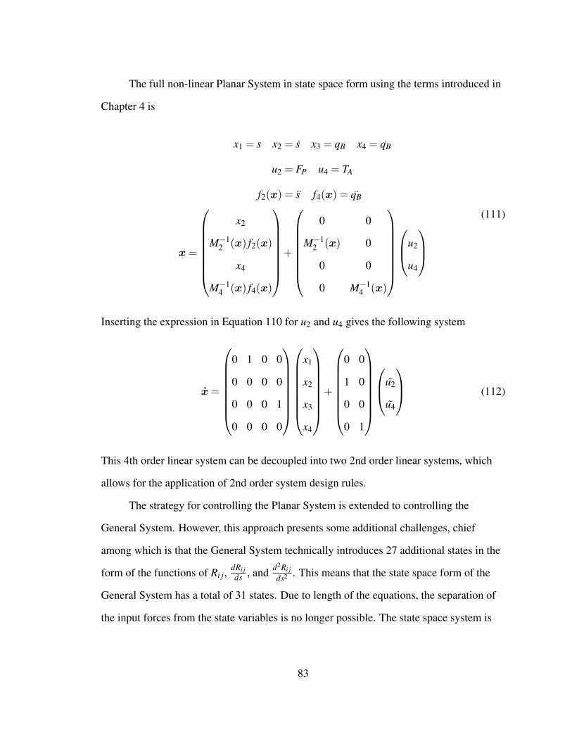
The full non-linear Planar System in state space form using the terms introduced in
Chapter 4 is
x1 = s x2 = s x3 = qB x4 = qB
u2 = FP u4 = TA
f2(x) = s f4(x) = qB
x=
x2
M−12 (x) f2(x)
x4
M−14 (x) f4(x)
+
0 0
M−12 (x) 0
0 0
0 M−14 (x)
u2
u4
(111)
Inserting the expression in Equation 110 for u2 and u4 gives the following system
x=
0 1 0 0
0 0 0 0
0 0 0 1
0 0 0 0
x1
x2
x3
x4
+
0 0
1 0
0 0
0 1
u2
u4
(112)
This 4th order linear system can be decoupled into two 2nd order linear systems, which
allows for the application of 2nd order system design rules.
The strategy for controlling the Planar System is extended to controlling the
General System. However, this approach presents some additional challenges, chief
among which is that the General System technically introduces 27 additional states in the
form of the functions of Ri j,dRi jds , and d2Ri j
ds2 . This means that the state space form of the
General System has a total of 31 states. Due to length of the equations, the separation of
the input forces from the state variables is no longer possible. The state space system is
83
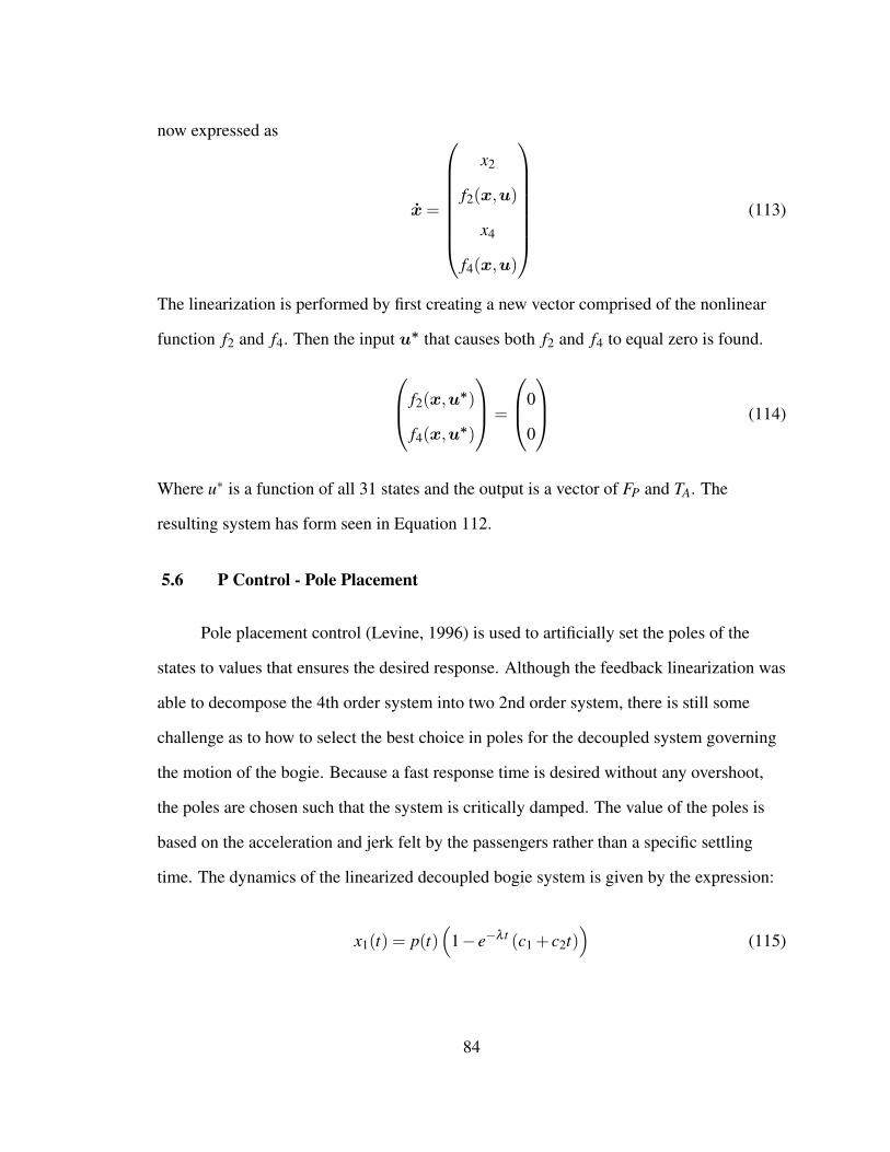
now expressed as
x=
x2
f2(x,u)
x4
f4(x,u)
(113)
The linearization is performed by first creating a new vector comprised of the nonlinear
function f2 and f4. Then the input u∗ that causes both f2 and f4 to equal zero is found.
f2(x,u∗)
f4(x,u∗)
=
0
0
(114)
Where u∗ is a function of all 31 states and the output is a vector of FP and TA. The
resulting system has form seen in Equation 112.
5.6 P Control - Pole Placement
Pole placement control (Levine, 1996) is used to artificially set the poles of the
states to values that ensures the desired response. Although the feedback linearization was
able to decompose the 4th order system into two 2nd order system, there is still some
challenge as to how to select the best choice in poles for the decoupled system governing
the motion of the bogie. Because a fast response time is desired without any overshoot,
the poles are chosen such that the system is critically damped. The value of the poles is
based on the acceleration and jerk felt by the passengers rather than a specific settling
time. The dynamics of the linearized decoupled bogie system is given by the expression:
x1(t) = p(t)(
1− e−λ t (c1 + c2t))
(115)
84
From Equation 115, it can be seen that poles further along the left hand plane cause the
displacement to better adhere to the displacement setpoint profile. However, poles further
on the left hand plane have a higher initial acceleration and jerk that may exceed comfort
levels. While there are methods of optimally choosing the poles (such as the LQR), the
use of that technique is beyond the scope of this thesis. Therefore, multiple selections of
the values of the poles were selected for the bogie system and multiple simulations were
run for each selection. The same pole placement strategy is used to control the vehicle
body angle based on the setpoint defined in Chapter 5.2. However, only a single set of
poles for this controller are tested.
85
CHAPTER 6
RESULTS AND DISCUSSION
6.1 Results Introduction
The results of this thesis are from SIMULINK simulations of the system described
in this thesis. The following simulations are conducted to validate the theoretical work in
this thesis:
• A simulation that compares the MotionGenesis derived equations for a Planar
System with hand derived equations for the Planar System.
• A geometry analysis on the General System for circular guideway with a 100 m
radius
• A simulation that compares the MotionGenesis derived equations for a General
System with hand derived equations for the Planar System.
• A simulation that experiments with a controller derived from the Planar System
dynamics to control a plant derived from the Planar System Dynamics.
• A simulation that experiments with a controller derived from the General System
dynamics to control a plant derived from the Planar System Dynamics.
• A geometry analysis and dynamics simulation of a spiral guideway using the
General System
The purpose of these simulations is to provide a proof-of-concept for the ideas discussed
in this thesis. The primary goal is to prove the suitability of the General System for
dynamical simulation and for control applications. Additional conclusions drawn from
these studies are discussed but not explored further.
86
A variable step differential equation solver (ode45) is used for the simulations. In
order to allow for the replication of these simulation, the SIMULINK solver parameters
are provided below:
• Absolute Tolerance = 1E−4
• Relative Tolerance = 1E−4
• Minimum Step Size = 1E−4
• Maximum Step Size = 1E−3
• Initial Step Size = 1E−4
• Maximum Consecutive Minimum Steps = 10
The solver parameters are deliberately kept coarse to reduce the simulation time and to
provide a worst-case example of the performance of the dynamical models presented here.
Experimentation with additional solver parameters is outside the scope of this research.
6.2 Planar System - Comparison Study
The first simulation tests the generated MATLAB code from MotionGenesis against
the manually derived Equation 78 and Equation 81. A set of simulations is run for each
system in which an ATN vehicle with no damping or external forces given an initial bogie
velocity of 50 ms and be subjected to a 500 N wind force from 100 s to 200 s using the
wind profile in Equation 106. Each simulation has a running time of 300 s.
87
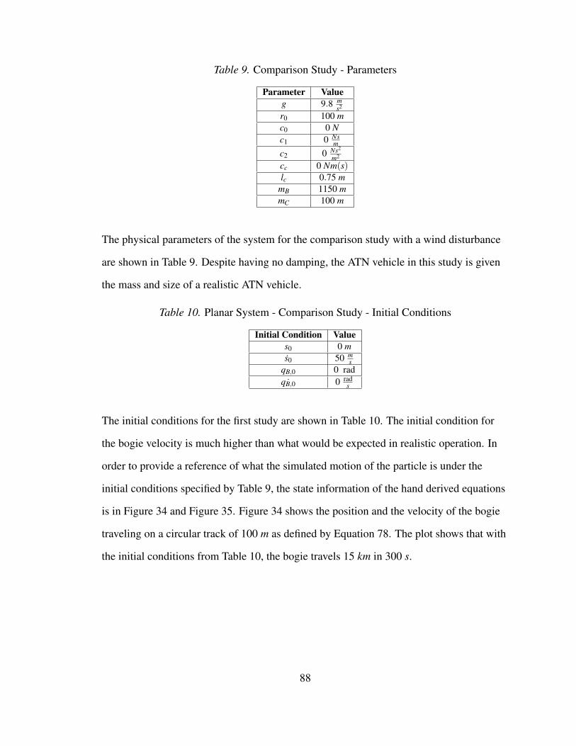
Table 9. Comparison Study - Parameters
Parameter Valueg 9.8 m
s2
r0 100 mc0 0 Nc1 0 Ns
m
c2 0 Ns2
m2
cc 0 Nm(s)lc 0.75 m
mB 1150 mmC 100 m
The physical parameters of the system for the comparison study with a wind disturbance
are shown in Table 9. Despite having no damping, the ATN vehicle in this study is given
the mass and size of a realistic ATN vehicle.
Table 10. Planar System - Comparison Study - Initial Conditions
Initial Condition Values0 0 ms0 50 m
sqB,0 0 rad
˙qB,0 0 rads
The initial conditions for the first study are shown in Table 10. The initial condition for
the bogie velocity is much higher than what would be expected in realistic operation. In
order to provide a reference of what the simulated motion of the particle is under the
initial conditions specified by Table 9, the state information of the hand derived equations
is in Figure 34 and Figure 35. Figure 34 shows the position and the velocity of the bogie
traveling on a circular track of 100 m as defined by Equation 78. The plot shows that with
the initial conditions from Table 10, the bogie travels 15 km in 300 s.
88
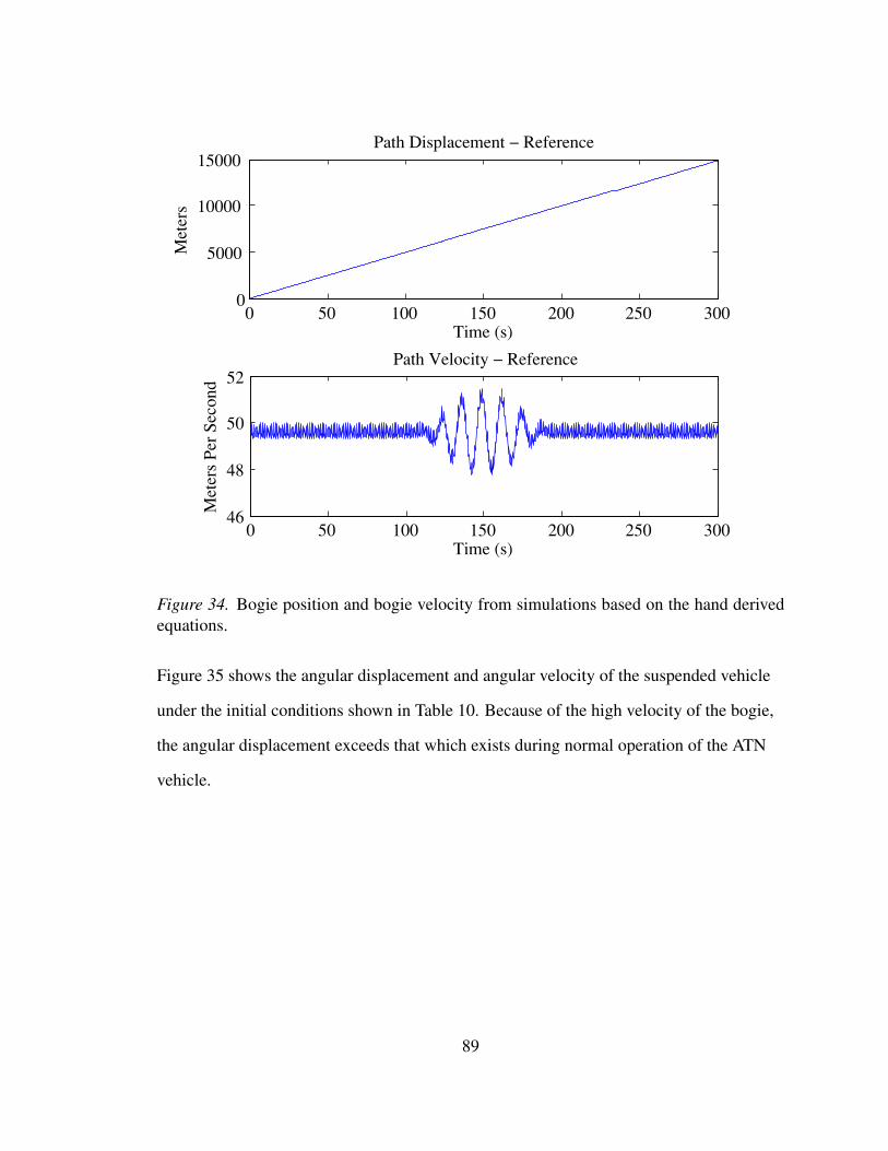
0 50 100 150 200 250 3000
5000
10000
15000Path Displacement − Reference
Time (s)
Met
ers
0 50 100 150 200 250 30046
48
50
52Path Velocity − Reference
Time (s)
Met
ers
Per
Seco
nd
Figure 34. Bogie position and bogie velocity from simulations based on the hand derivedequations.
Figure 35 shows the angular displacement and angular velocity of the suspended vehicle
under the initial conditions shown in Table 10. Because of the high velocity of the bogie,
the angular displacement exceeds that which exists during normal operation of the ATN
vehicle.
89
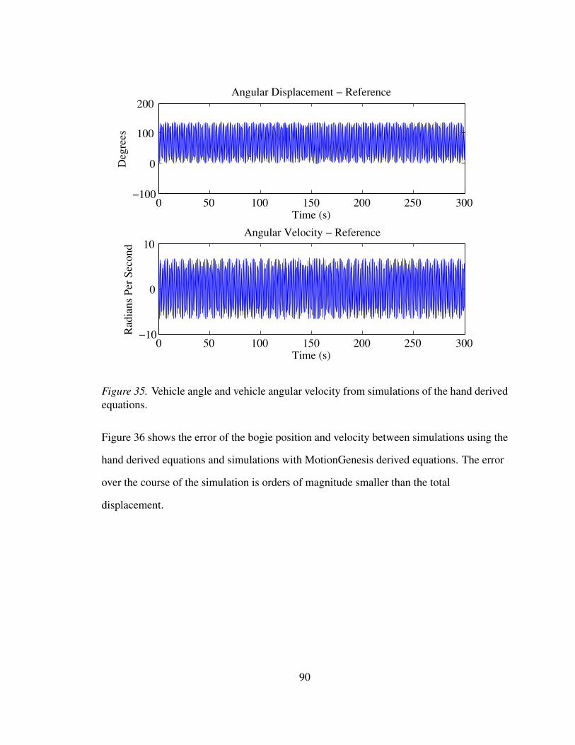
0 50 100 150 200 250 300−100
0
100
200Angular Displacement − Reference
Time (s)
Deg
rees
0 50 100 150 200 250 300−10
0
10Angular Velocity − Reference
Time (s)
Rad
ians
Per
Sec
ond
Figure 35. Vehicle angle and vehicle angular velocity from simulations of the hand derivedequations.
Figure 36 shows the error of the bogie position and velocity between simulations using the
hand derived equations and simulations with MotionGenesis derived equations. The error
over the course of the simulation is orders of magnitude smaller than the total
displacement.
90
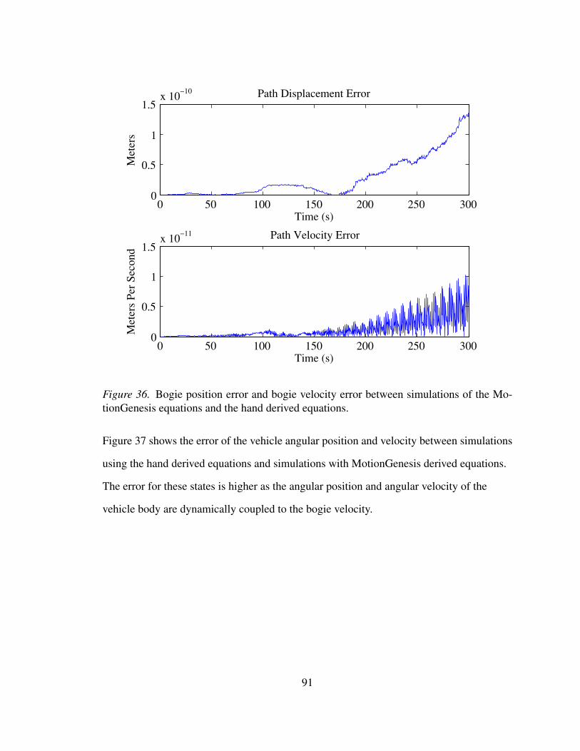
0 50 100 150 200 250 3000
0.5
1
1.5x 10
−10 Path Displacement Error
Time (s)
Met
ers
0 50 100 150 200 250 3000
0.5
1
1.5x 10
−11 Path Velocity Error
Time (s)
Met
ers
Per
Seco
nd
Figure 36. Bogie position error and bogie velocity error between simulations of the Mo-tionGenesis equations and the hand derived equations.
Figure 37 shows the error of the vehicle angular position and velocity between simulations
using the hand derived equations and simulations with MotionGenesis derived equations.
The error for these states is higher as the angular position and angular velocity of the
vehicle body are dynamically coupled to the bogie velocity.
91
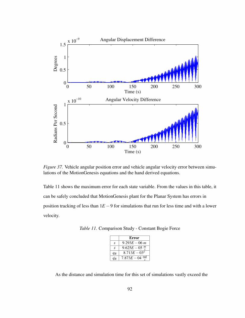
0 50 100 150 200 250 3000
0.5
1
1.5x 10
−9 Angular Displacement Difference
Time (s)
Deg
rees
0 50 100 150 200 250 3000
0.5
1x 10
−10 Angular Velocity Difference
Time (s)
Rad
ians
Per
Sec
ond
Figure 37. Vehicle angular position error and vehicle angular velocity error between simu-lations of the MotionGenesis equations and the hand derived equations.
Table 11 shows the maximum error for each state variable. From the values in this table, it
can be safely concluded that MotionGenesis plant for the Planar System has errors in
position tracking of less than 1E−9 for simulations that run for less time and with a lower
velocity.
Table 11. Comparison Study - Constant Bogie Force
Errors 9.293E−06 ms 9.625E−05 m
sqB 8.713E−03o
qB 7.873E−04 rads
As the distance and simulation time for this set of simulations vastly exceed the
92
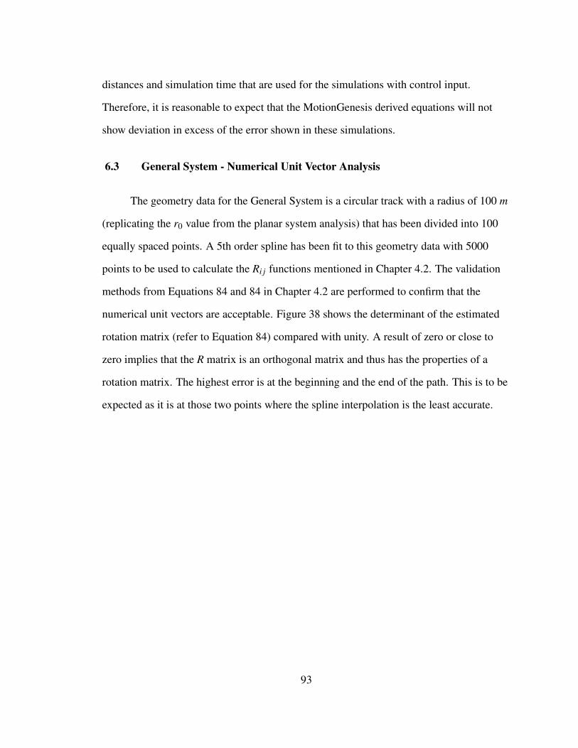
distances and simulation time that are used for the simulations with control input.
Therefore, it is reasonable to expect that the MotionGenesis derived equations will not
show deviation in excess of the error shown in these simulations.
6.3 General System - Numerical Unit Vector Analysis
The geometry data for the General System is a circular track with a radius of 100 m
(replicating the r0 value from the planar system analysis) that has been divided into 100
equally spaced points. A 5th order spline has been fit to this geometry data with 5000
points to be used to calculate the Ri j functions mentioned in Chapter 4.2. The validation
methods from Equations 84 and 84 in Chapter 4.2 are performed to confirm that the
numerical unit vectors are acceptable. Figure 38 shows the determinant of the estimated
rotation matrix (refer to Equation 84) compared with unity. A result of zero or close to
zero implies that the R matrix is an orthogonal matrix and thus has the properties of a
rotation matrix. The highest error is at the beginning and the end of the path. This is to be
expected as it is at those two points where the spline interpolation is the least accurate.
93
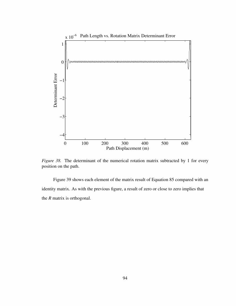
0 100 200 300 400 500 600
−4
−3
−2
−1
0
1
x 10−6 Path Length vs. Rotation Matrix Determinant Error
Path Displacement (m)
Det
erm
inan
t Err
or
Figure 38. The determinant of the numerical rotation matrix subtracted by 1 for everyposition on the path.
Figure 39 shows each element of the matrix result of Equation 85 compared with an
identity matrix. As with the previous figure, a result of zero or close to zero implies that
the R matrix is orthogonal.
94
0 100 200 300 400 500 600
−1
0
1
x 10−4 Path Length vs. Orthogonality Error
Path Displacement (m)
Indi
vidu
al E
lem
ent E
rror
R(1,1)R(1,2)R(1,3)R(2,1)R(2,2)R(2,3)R(3,1)R(3,2)R(3,3)
Figure 39. Each individual element of the numerical rotation matrix multiplied by its trans-pose and subtracted by an identity matrix for every position on the path.
Figures 38 and 39 show that the numerical rotation matrix produced by the MATLAB
code has the properties that define a rotation matrix.
With regards to the error, the maximum determinant error is on the order of 10E−6
and the maximum error of the product of the numerical rotation matrix multiplied by its
transpose is on the order of 10E−4. With regards to the order of magnitude of the error, it
is difficult to determine the threshold for acceptability. A sensitivity analysis of the error
of the numerical rotation matrix with respect to the error of the General System simulation
in SIMULINK is outside the scope of this thesis. However, the determinant error seen in
Figure 38 can be compared to the simulation error in the General System comparison
study in the next section to establish rough estimate of the sensitivity. An additional test is
95
to determine if values of Sx, Sy, and Sz for a circular guideway determined by the
method prescribed in Chapter 4.2 match Sx, Sy, and Sz as specified in Table 3. This test
is additional to the validation tests described in Chapter 4.2. To test this, first let Sx, Sy,
and Sz determined by the method prescribed in Chapter 4.2 be expressed as ˆSx, ˆSy, and
ˆSz. Then calculate one minus the dot product of ˆSx and Sx
Sx Error = 1−|(R11, R12, R13) · (coss/r0, sins/r0, 0)| (116)
Then, calculate one minus the dot product of ˆSy and Sy for all values of s
Sy Error = 1−|(R21, R22, R23) · (−sins/r0, coss/r0, 0)| (117)
Finally, calculate one minus the dot product of ˆSz and Sz for all values of s
Sz Error = 1−|(R31, R32, R33) · ( 0, 0, 1)| (118)
If the results of Equations 116, 117, and 118 are equal or close to zero for all values of s,
then ˆSx, ˆSy, and ˆSz can be assumed to be parallel to Sx, Sy, and Sz. Figure 40 shows
the results of Equations 116, 117, and 118 for s for a vehicle traveling from 0 m to
15072 m (24 laps) for a circular guideway with a radius of 100 m. This distance traveled is
higher than the circumference of the circular guideway to test if consecutive laps traveled
affect the unit vector value. From Figure 40, it is seen that the dot product error is on the
order of 10E−6 over 24 laps. Of note is the observation that the maximum error occurs at
the beginning and the end of each lap which corresponds to the beginning and the end of
each dataset, where the spline interpolation is the least accurate.
96
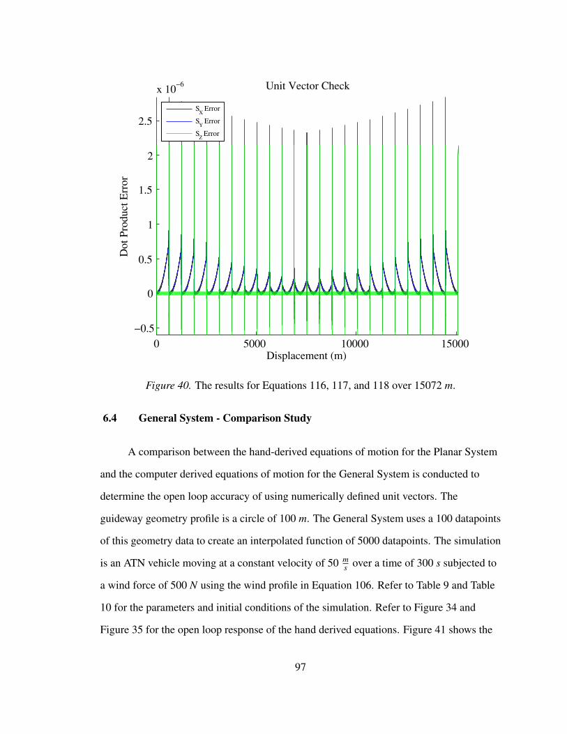
0 5000 10000 15000−0.5
0
0.5
1
1.5
2
2.5
x 10−6 Unit Vector Check
Displacement (m)
Dot
Pro
duct
Err
or
S
X Error
SY Error
SZ Error
Figure 40. The results for Equations 116, 117, and 118 over 15072 m.
6.4 General System - Comparison Study
A comparison between the hand-derived equations of motion for the Planar System
and the computer derived equations of motion for the General System is conducted to
determine the open loop accuracy of using numerically defined unit vectors. The
guideway geometry profile is a circle of 100 m. The General System uses a 100 datapoints
of this geometry data to create an interpolated function of 5000 datapoints. The simulation
is an ATN vehicle moving at a constant velocity of 50 ms over a time of 300 s subjected to
a wind force of 500 N using the wind profile in Equation 106. Refer to Table 9 and Table
10 for the parameters and initial conditions of the simulation. Refer to Figure 34 and
Figure 35 for the open loop response of the hand derived equations. Figure 41 shows the
97
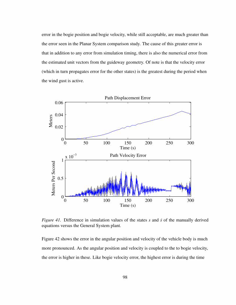
error in the bogie position and bogie velocity, while still acceptable, are much greater than
the error seen in the Planar System comparison study. The cause of this greater error is
that in addition to any error from simulation timing, there is also the numerical error from
the estimated unit vectors from the guideway geometry. Of note is that the velocity error
(which in turn propagates error for the other states) is the greatest during the period when
the wind gust is active.
0 50 100 150 200 250 3000
0.02
0.04
0.06Path Displacement Error
Time (s)
Met
ers
0 50 100 150 200 250 3000
0.5
1x 10
−3 Path Velocity Error
Time (s)
Met
ers
Per
Seco
nd
Figure 41. Difference in simulation values of the states s and s of the manually derivedequations versus the General System plant.
Figure 42 shows the error in the angular position and velocity of the vehicle body is much
more pronounced. As the angular position and velocity is coupled to the to bogie velocity,
the error is higher in these. Like bogie velocity error, the highest error is during the time
98
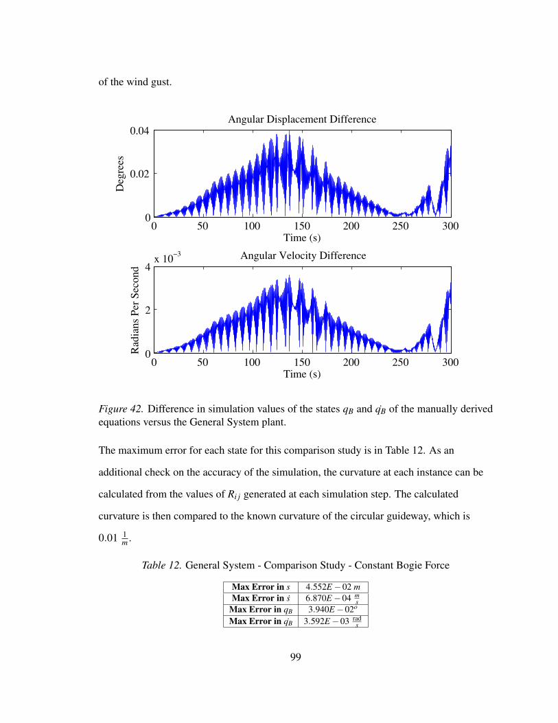
of the wind gust.
0 50 100 150 200 250 3000
0.02
0.04Angular Displacement Difference
Time (s)
Deg
rees
0 50 100 150 200 250 3000
2
4x 10
−3 Angular Velocity Difference
Time (s)
Rad
ians
Per
Sec
ond
Figure 42. Difference in simulation values of the states qB and qB of the manually derivedequations versus the General System plant.
The maximum error for each state for this comparison study is in Table 12. As an
additional check on the accuracy of the simulation, the curvature at each instance can be
calculated from the values of Ri j generated at each simulation step. The calculated
curvature is then compared to the known curvature of the circular guideway, which is
0.01 1m .
Table 12. General System - Comparison Study - Constant Bogie Force
Max Error in s 4.552E−02 mMax Error in s 6.870E−04 m
sMax Error in qB 3.940E−02o
Max Error in qB 3.592E−03 rads
99
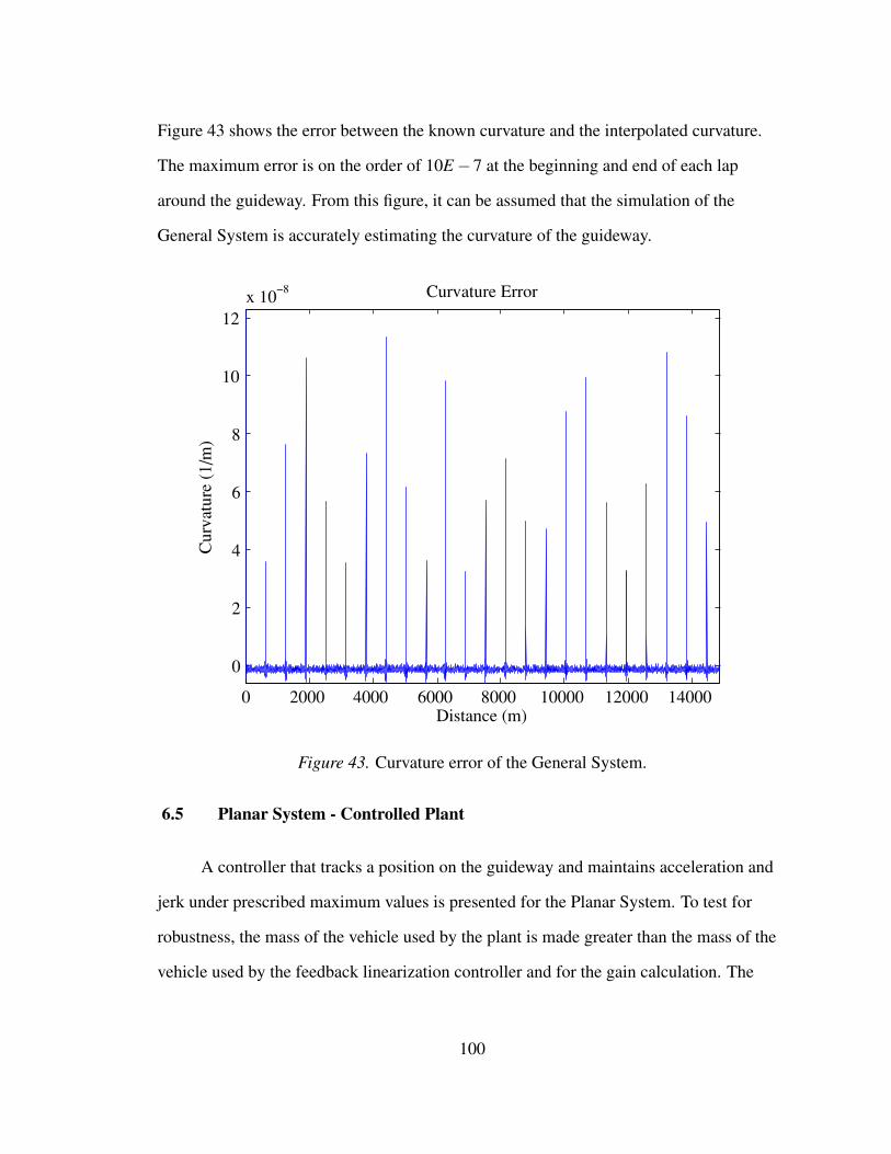
Figure 43 shows the error between the known curvature and the interpolated curvature.
The maximum error is on the order of 10E−7 at the beginning and end of each lap
around the guideway. From this figure, it can be assumed that the simulation of the
General System is accurately estimating the curvature of the guideway.
0 2000 4000 6000 8000 10000 12000 14000
0
2
4
6
8
10
12x 10
−8 Curvature Error
Distance (m)
Cur
vatu
re (
1/m
)
Figure 43. Curvature error of the General System.
6.5 Planar System - Controlled Plant
A controller that tracks a position on the guideway and maintains acceleration and
jerk under prescribed maximum values is presented for the Planar System. To test for
robustness, the mass of the vehicle used by the plant is made greater than the mass of the
vehicle used by the feedback linearization controller and for the gain calculation. The
100
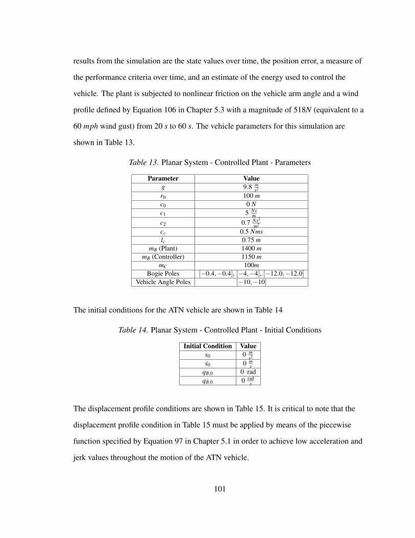
results from the simulation are the state values over time, the position error, a measure of
the performance criteria over time, and an estimate of the energy used to control the
vehicle. The plant is subjected to nonlinear friction on the vehicle arm angle and a wind
profile defined by Equation 106 in Chapter 5.3 with a magnitude of 518N (equivalent to a
60 mph wind gust) from 20 s to 60 s. The vehicle parameters for this simulation are
shown in Table 13.
Table 13. Planar System - Controlled Plant - Parameters
Parameter Valueg 9.8 m
s2
r0 100 mc0 0 Nc1 5 Ns
m
c2 0.7 Ns2
m2
cc 0.5 Nmslc 0.75 m
mB (Plant) 1400 mmB (Controller) 1150 m
mC 100mBogie Poles [−0.4,−0.4], [−4,−4], [−12.0,−12.0]
Vehicle Angle Poles [−10,−10]
The initial conditions for the ATN vehicle are shown in Table 14
Table 14. Planar System - Controlled Plant - Initial Conditions
Initial Condition Values0 0 m
s2
s0 0 ms
qB,0 0 rad˙qB,0 0 rad
s
The displacement profile conditions are shown in Table 15. It is critical to note that the
displacement profile condition in Table 15 must be applied by means of the piecewise
function specified by Equation 97 in Chapter 5.1 in order to achieve low acceleration and
jerk values throughout the motion of the ATN vehicle.
101
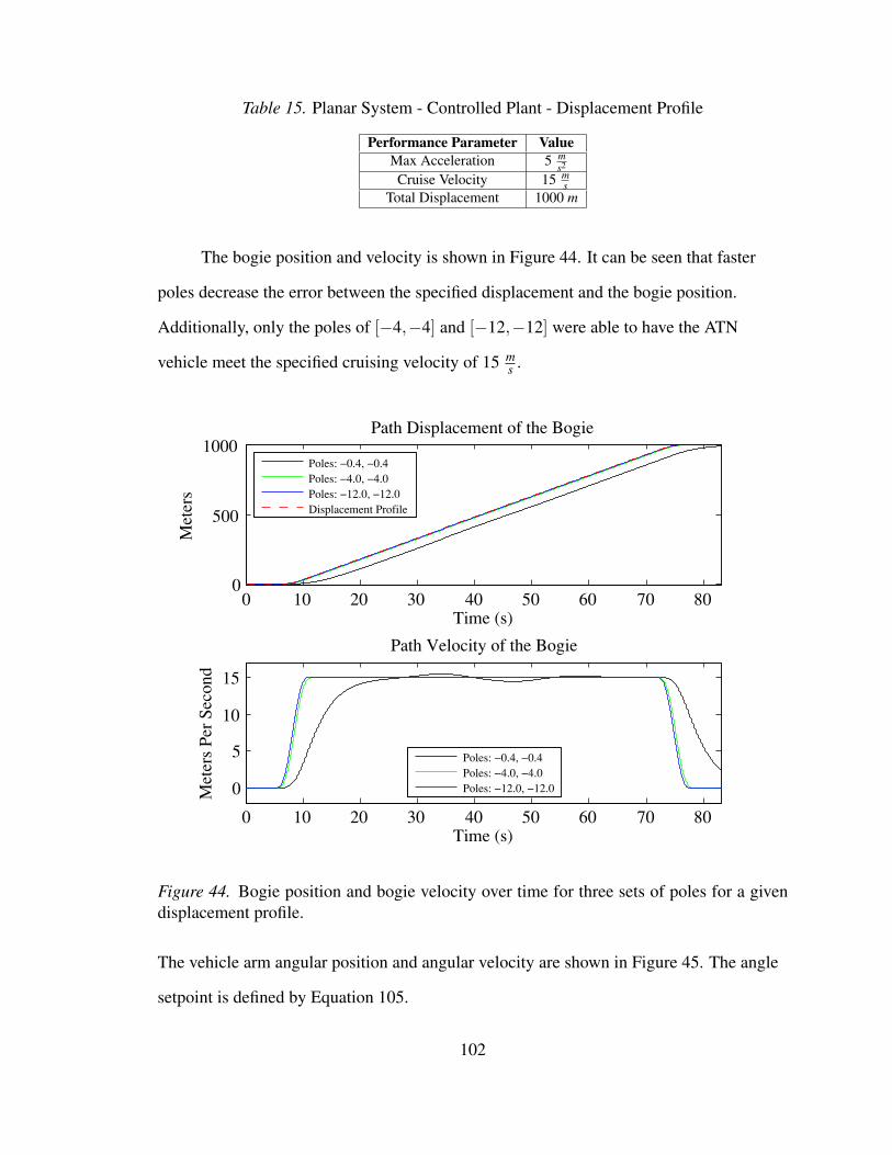
Table 15. Planar System - Controlled Plant - Displacement Profile
Performance Parameter ValueMax Acceleration 5 m
s2
Cruise Velocity 15 ms
Total Displacement 1000 m
The bogie position and velocity is shown in Figure 44. It can be seen that faster
poles decrease the error between the specified displacement and the bogie position.
Additionally, only the poles of [−4,−4] and [−12,−12] were able to have the ATN
vehicle meet the specified cruising velocity of 15 ms .
0 10 20 30 40 50 60 70 800
500
1000Path Displacement of the Bogie
Time (s)
Met
ers
Poles: −0.4, −0.4Poles: −4.0, −4.0Poles: −12.0, −12.0Displacement Profile
0 10 20 30 40 50 60 70 80
0
5
10
15
Path Velocity of the Bogie
Time (s)
Met
ers
Per
Seco
nd
Poles: −0.4, −0.4Poles: −4.0, −4.0Poles: −12.0, −12.0
Figure 44. Bogie position and bogie velocity over time for three sets of poles for a givendisplacement profile.
The vehicle arm angular position and angular velocity are shown in Figure 45. The angle
setpoint is defined by Equation 105.
102
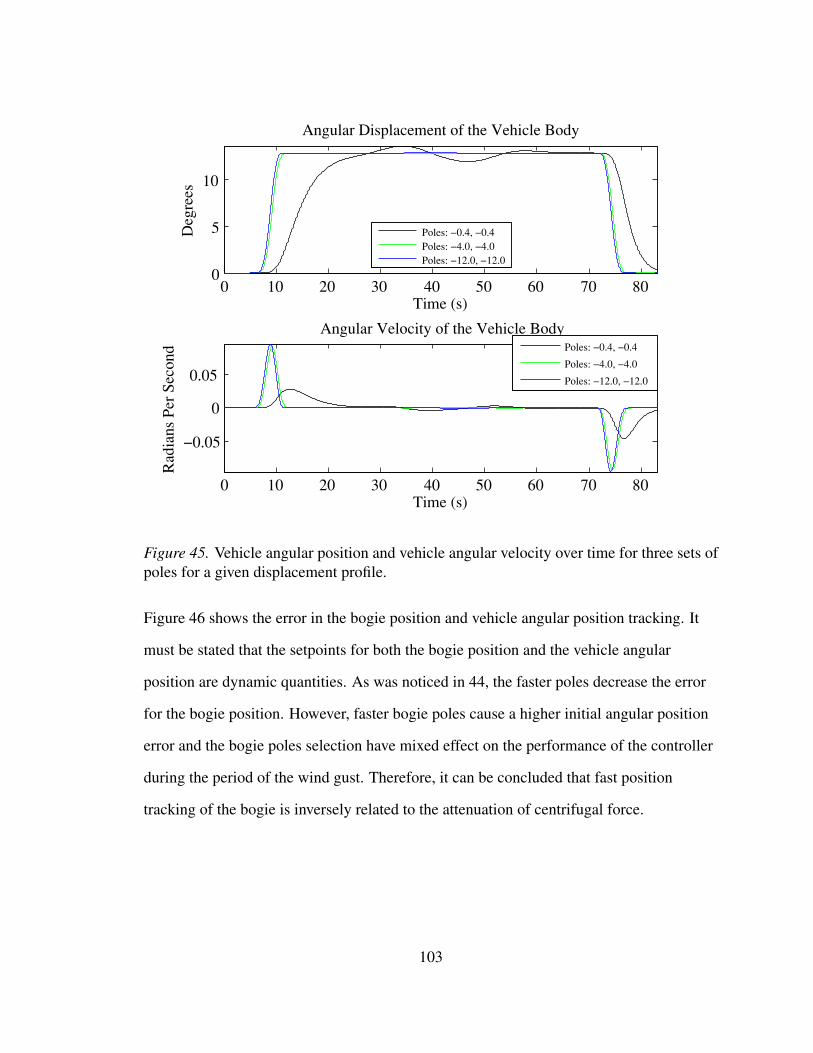
0 10 20 30 40 50 60 70 800
5
10
Angular Displacement of the Vehicle Body
Time (s)
Deg
rees
Poles: −0.4, −0.4Poles: −4.0, −4.0Poles: −12.0, −12.0
0 10 20 30 40 50 60 70 80
−0.05
0
0.05
Angular Velocity of the Vehicle Body
Time (s)
Rad
ians
Per
Sec
ond
Poles: −0.4, −0.4
Poles: −4.0, −4.0
Poles: −12.0, −12.0
Figure 45. Vehicle angular position and vehicle angular velocity over time for three sets ofpoles for a given displacement profile.
Figure 46 shows the error in the bogie position and vehicle angular position tracking. It
must be stated that the setpoints for both the bogie position and the vehicle angular
position are dynamic quantities. As was noticed in 44, the faster poles decrease the error
for the bogie position. However, faster bogie poles cause a higher initial angular position
error and the bogie poles selection have mixed effect on the performance of the controller
during the period of the wind gust. Therefore, it can be concluded that fast position
tracking of the bogie is inversely related to the attenuation of centrifugal force.
103
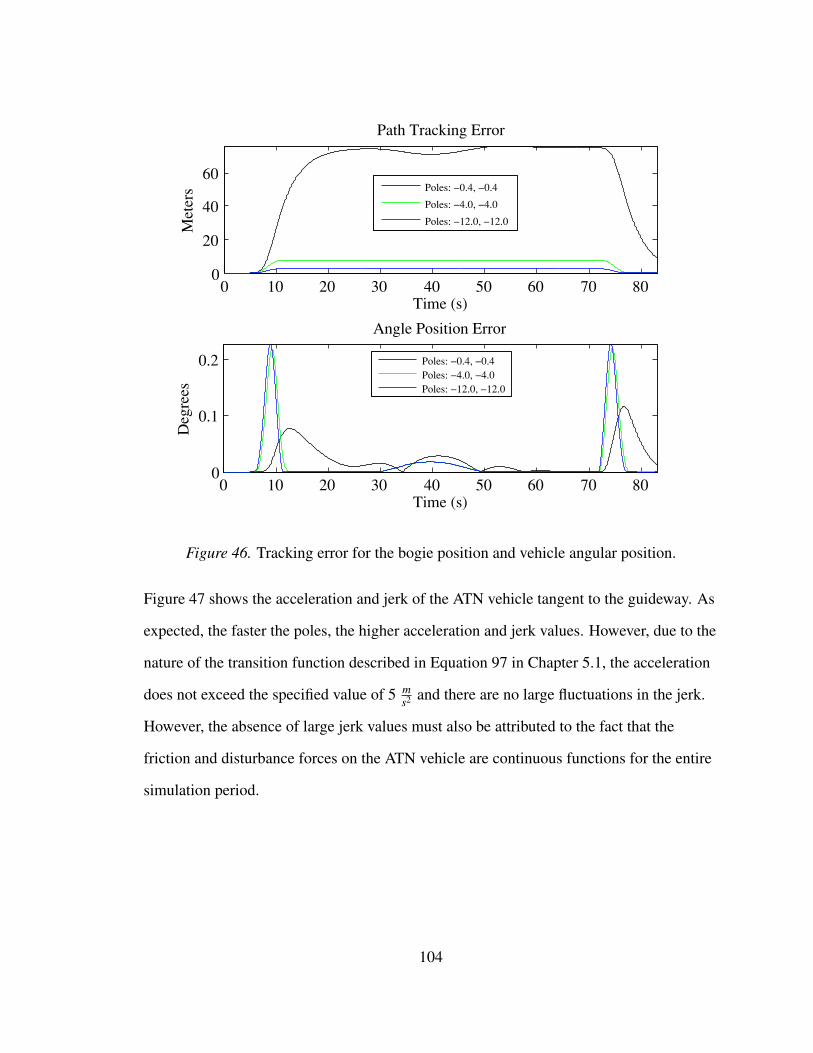
0 10 20 30 40 50 60 70 800
20
40
60
Path Tracking Error
Time (s)
Met
ers
Poles: −0.4, −0.4
Poles: −4.0, −4.0
Poles: −12.0, −12.0
0 10 20 30 40 50 60 70 800
0.1
0.2
Angle Position Error
Time (s)
Deg
rees
Poles: −0.4, −0.4Poles: −4.0, −4.0Poles: −12.0, −12.0
Figure 46. Tracking error for the bogie position and vehicle angular position.
Figure 47 shows the acceleration and jerk of the ATN vehicle tangent to the guideway. As
expected, the faster the poles, the higher acceleration and jerk values. However, due to the
nature of the transition function described in Equation 97 in Chapter 5.1, the acceleration
does not exceed the specified value of 5 ms2 and there are no large fluctuations in the jerk.
However, the absence of large jerk values must also be attributed to the fact that the
friction and disturbance forces on the ATN vehicle are continuous functions for the entire
simulation period.
104
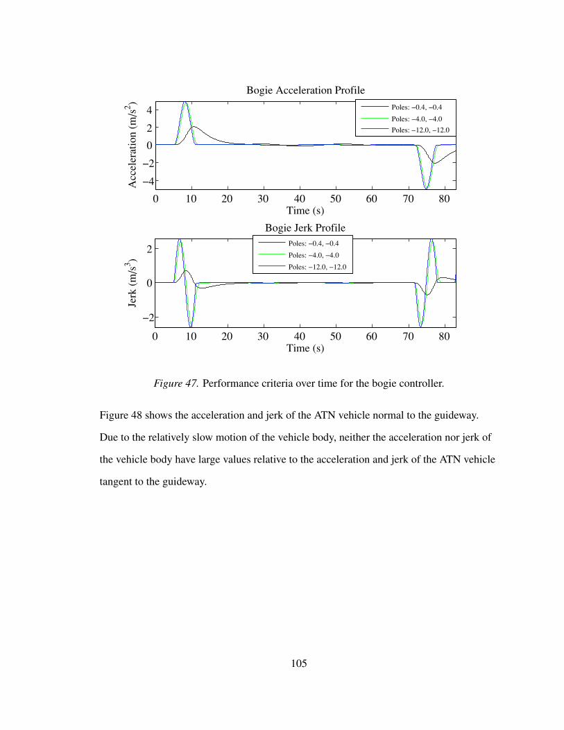
0 10 20 30 40 50 60 70 80
−4
−2
0
2
4
Bogie Acceleration Profile
Time (s)
Acc
eler
atio
n (m
/s2 )
Poles: −0.4, −0.4
Poles: −4.0, −4.0
Poles: −12.0, −12.0
0 10 20 30 40 50 60 70 80
−2
0
2
Bogie Jerk Profile
Time (s)
Jerk
(m
/s3 )
Poles: −0.4, −0.4
Poles: −4.0, −4.0
Poles: −12.0, −12.0
Figure 47. Performance criteria over time for the bogie controller.
Figure 48 shows the acceleration and jerk of the ATN vehicle normal to the guideway.
Due to the relatively slow motion of the vehicle body, neither the acceleration nor jerk of
the vehicle body have large values relative to the acceleration and jerk of the ATN vehicle
tangent to the guideway.
105
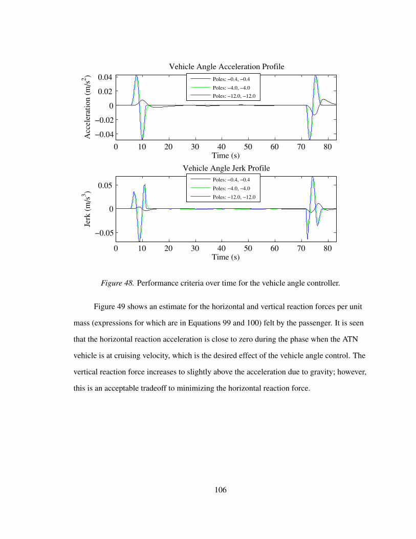
0 10 20 30 40 50 60 70 80
−0.04
−0.02
0
0.02
0.04Vehicle Angle Acceleration Profile
Time (s)
Acc
eler
atio
n (m
/s2 )
Poles: −0.4, −0.4
Poles: −4.0, −4.0
Poles: −12.0, −12.0
0 10 20 30 40 50 60 70 80
−0.05
0
0.05
Vehicle Angle Jerk Profile
Time (s)
Jerk
(m
/s3 )
Poles: −0.4, −0.4
Poles: −4.0, −4.0
Poles: −12.0, −12.0
Figure 48. Performance criteria over time for the vehicle angle controller.
Figure 49 shows an estimate for the horizontal and vertical reaction forces per unit
mass (expressions for which are in Equations 99 and 100) felt by the passenger. It is seen
that the horizontal reaction acceleration is close to zero during the phase when the ATN
vehicle is at cruising velocity, which is the desired effect of the vehicle angle control. The
vertical reaction force increases to slightly above the acceleration due to gravity; however,
this is an acceptable tradeoff to minimizing the horizontal reaction force.
106
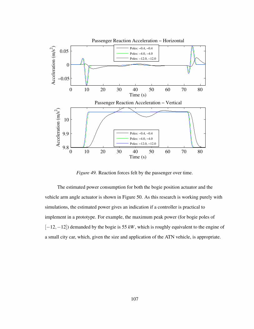
0 10 20 30 40 50 60 70 80
−0.05
0
0.05
Passenger Reaction Acceleration − Horizontal
Time (s)
Acc
eler
atio
n (m
/s2 )
Poles: −0.4, −0.4
Poles: −4.0, −4.0
Poles: −12.0, −12.0
0 10 20 30 40 50 60 70 809.8
9.9
10
Passenger Reaction Acceleration − Vertical
Time (s)
Acc
eler
atio
n (m
/s2 )
Poles: −0.4, −0.4
Poles: −4.0, −4.0
Poles: −12.0, −12.0
Figure 49. Reaction forces felt by the passenger over time.
The estimated power consumption for both the bogie position actuator and the
vehicle arm angle actuator is shown in Figure 50. As this research is working purely with
simulations, the estimated power gives an indication if a controller is practical to
implement in a prototype. For example, the maximum peak power (for bogie poles of
[−12,−12]) demanded by the bogie is 55 kW , which is roughly equivalent to the engine of
a small city car, which, given the size and application of the ATN vehicle, is appropriate.
107
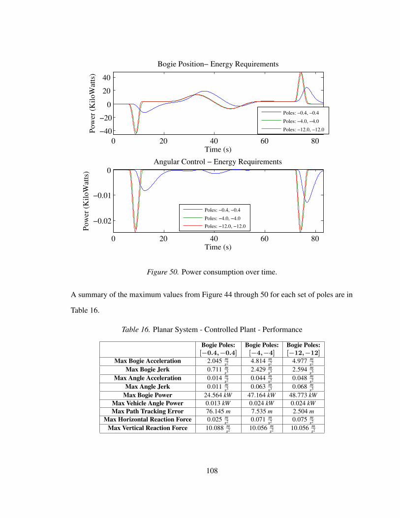
0 20 40 60 80−40
−20
0
20
40
Bogie Position− Energy Requirements
Time (s)
Pow
er (
Kilo
Wat
ts)
Poles: −0.4, −0.4
Poles: −4.0, −4.0
Poles: −12.0, −12.0
0 20 40 60 80
−0.02
−0.01
0Angular Control − Energy Requirements
Time (s)
Pow
er (
Kilo
Wat
ts)
Poles: −0.4, −0.4
Poles: −4.0, −4.0
Poles: −12.0, −12.0
Figure 50. Power consumption over time.
A summary of the maximum values from Figure 44 through 50 for each set of poles are in
Table 16.
Table 16. Planar System - Controlled Plant - Performance
Bogie Poles: Bogie Poles: Bogie Poles:[−0.4,−0.4] [−4,−4] [−12,−12]
Max Bogie Acceleration 2.045 ms2 4.814 m
s2 4.977 ms2
Max Bogie Jerk 0.711 ms3 2.429 m
s3 2.594 ms3
Max Angle Acceleration 0.014 ms2 0.044 m
s2 0.048 ms2
Max Angle Jerk 0.011 ms3 0.063 m
s3 0.068 ms3
Max Bogie Power 24.564 kW 47.164 kW 48.773 kWMax Vehicle Angle Power 0.013 kW 0.024 kW 0.024 kWMax Path Tracking Error 76.145 m 7.535 m 2.504 m
Max Horizontal Reaction Force 0.025 ms2 0.071 m
s2 0.075 ms2
Max Vertical Reaction Force 10.088 ms2 10.056 m
s2 10.056 ms2
108
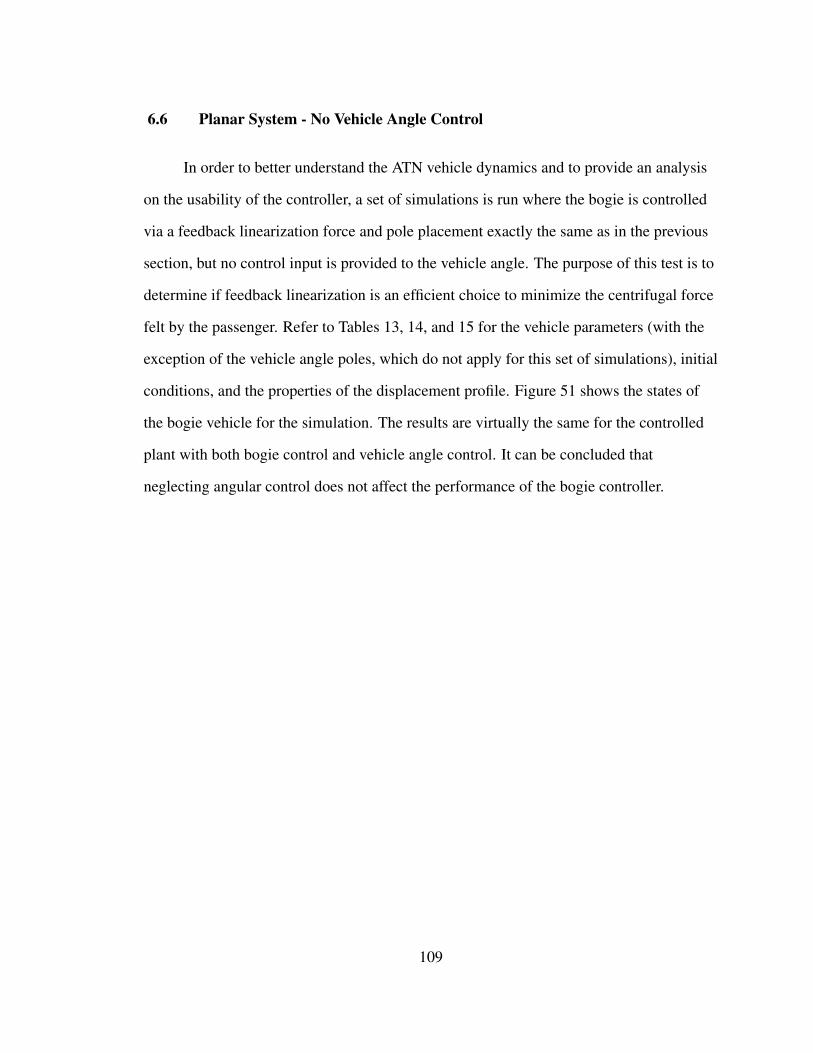
6.6 Planar System - No Vehicle Angle Control
In order to better understand the ATN vehicle dynamics and to provide an analysis
on the usability of the controller, a set of simulations is run where the bogie is controlled
via a feedback linearization force and pole placement exactly the same as in the previous
section, but no control input is provided to the vehicle angle. The purpose of this test is to
determine if feedback linearization is an efficient choice to minimize the centrifugal force
felt by the passenger. Refer to Tables 13, 14, and 15 for the vehicle parameters (with the
exception of the vehicle angle poles, which do not apply for this set of simulations), initial
conditions, and the properties of the displacement profile. Figure 51 shows the states of
the bogie vehicle for the simulation. The results are virtually the same for the controlled
plant with both bogie control and vehicle angle control. It can be concluded that
neglecting angular control does not affect the performance of the bogie controller.
109
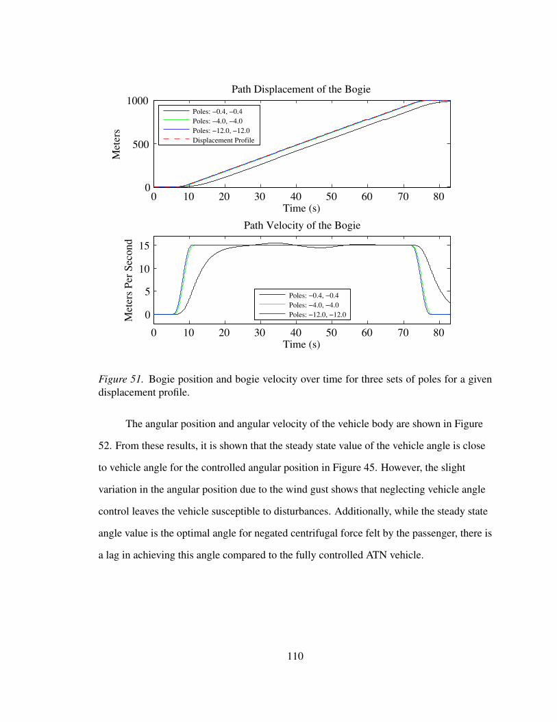
0 10 20 30 40 50 60 70 800
500
1000Path Displacement of the Bogie
Time (s)
Met
ers
Poles: −0.4, −0.4Poles: −4.0, −4.0Poles: −12.0, −12.0Displacement Profile
0 10 20 30 40 50 60 70 80
0
5
10
15
Path Velocity of the Bogie
Time (s)
Met
ers
Per
Seco
nd
Poles: −0.4, −0.4Poles: −4.0, −4.0Poles: −12.0, −12.0
Figure 51. Bogie position and bogie velocity over time for three sets of poles for a givendisplacement profile.
The angular position and angular velocity of the vehicle body are shown in Figure
52. From these results, it is shown that the steady state value of the vehicle angle is close
to vehicle angle for the controlled angular position in Figure 45. However, the slight
variation in the angular position due to the wind gust shows that neglecting vehicle angle
control leaves the vehicle susceptible to disturbances. Additionally, while the steady state
angle value is the optimal angle for negated centrifugal force felt by the passenger, there is
a lag in achieving this angle compared to the fully controlled ATN vehicle.
110
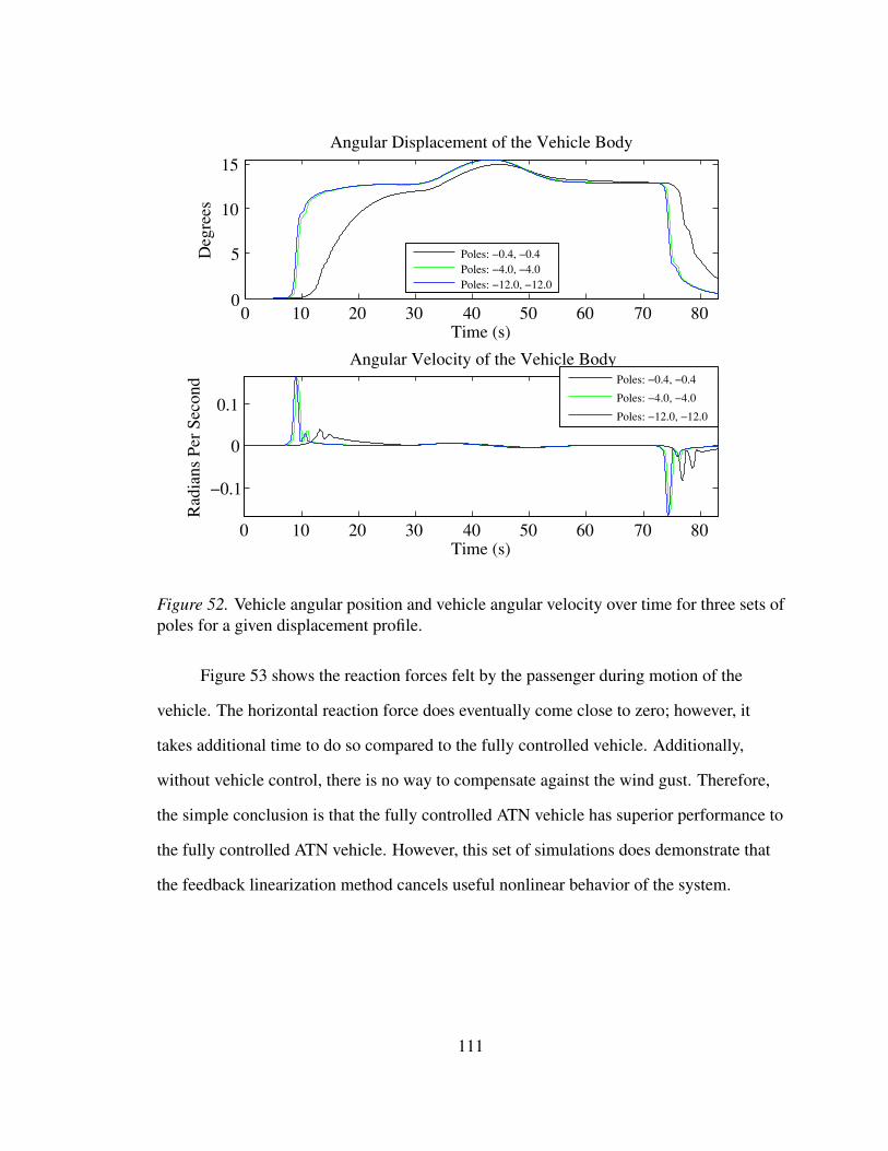
0 10 20 30 40 50 60 70 800
5
10
15Angular Displacement of the Vehicle Body
Time (s)
Deg
rees
Poles: −0.4, −0.4Poles: −4.0, −4.0Poles: −12.0, −12.0
0 10 20 30 40 50 60 70 80
−0.1
0
0.1
Angular Velocity of the Vehicle Body
Time (s)
Rad
ians
Per
Sec
ond
Poles: −0.4, −0.4
Poles: −4.0, −4.0
Poles: −12.0, −12.0
Figure 52. Vehicle angular position and vehicle angular velocity over time for three sets ofpoles for a given displacement profile.
Figure 53 shows the reaction forces felt by the passenger during motion of the
vehicle. The horizontal reaction force does eventually come close to zero; however, it
takes additional time to do so compared to the fully controlled vehicle. Additionally,
without vehicle control, there is no way to compensate against the wind gust. Therefore,
the simple conclusion is that the fully controlled ATN vehicle has superior performance to
the fully controlled ATN vehicle. However, this set of simulations does demonstrate that
the feedback linearization method cancels useful nonlinear behavior of the system.
111
0 10 20 30 40 50 60 70 80−0.4
−0.2
0
0.2
0.4
Passenger Reaction Acceleration − Horizontal
Time (s)
Acc
eler
atio
n (m
/s2 )
Poles: −0.4, −0.4
Poles: −4.0, −4.0
Poles: −12.0, −12.0
0 10 20 30 40 50 60 70 809.8
9.9
10
Passenger Reaction Acceleration − Vertical
Time (s)
Acc
eler
atio
n (m
/s2 )
Poles: −0.4, −0.4
Poles: −4.0, −4.0
Poles: −12.0, −12.0
Figure 53. Reaction forces felt by the passenger over time.
6.7 Planar System - Controlled Plant w/ Feedback Linearization from General
System Dynamics
A set of simulations of a plant that is defined by the equations of motion of the
Planar System and controlled with a feedback linearization controller defined by the
equations of motion of the General System is performed. Refer to Tables 13, 14, and 15
for the system parameters, initial conditions, and displacement profile. The same wind
force of 518 N from 20 s to 60 s is applied and the vehicle arm angle is subjected to
nonlinear friction. This simulation is of considerable interest as it represents the goal of
using a guideway defined by geometry to control an ATN vehicle. The bogie position and
velocity is shown in Figure 54. As with the previous study, it can be seen that faster poles
112
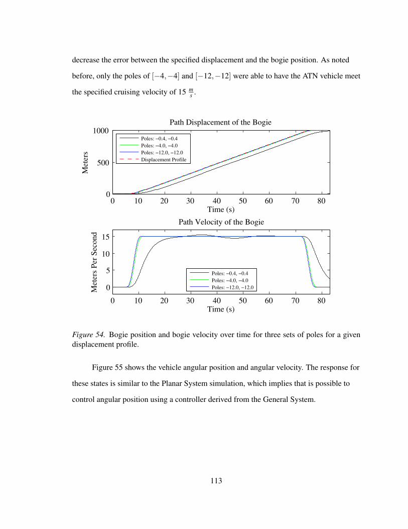
decrease the error between the specified displacement and the bogie position. As noted
before, only the poles of [−4,−4] and [−12,−12] were able to have the ATN vehicle meet
the specified cruising velocity of 15 ms .
0 10 20 30 40 50 60 70 800
500
1000Path Displacement of the Bogie
Time (s)
Met
ers
Poles: −0.4, −0.4Poles: −4.0, −4.0Poles: −12.0, −12.0Displacement Profile
0 10 20 30 40 50 60 70 80
0
5
10
15
Path Velocity of the Bogie
Time (s)
Met
ers
Per
Seco
nd
Poles: −0.4, −0.4Poles: −4.0, −4.0Poles: −12.0, −12.0
Figure 54. Bogie position and bogie velocity over time for three sets of poles for a givendisplacement profile.
Figure 55 shows the vehicle angular position and angular velocity. The response for
these states is similar to the Planar System simulation, which implies that is possible to
control angular position using a controller derived from the General System.
113
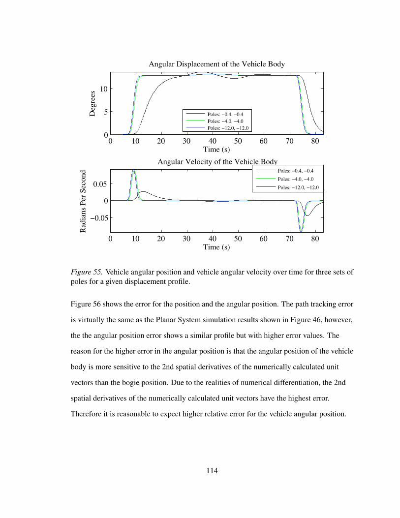
0 10 20 30 40 50 60 70 800
5
10
Angular Displacement of the Vehicle Body
Time (s)
Deg
rees
Poles: −0.4, −0.4Poles: −4.0, −4.0Poles: −12.0, −12.0
0 10 20 30 40 50 60 70 80
−0.05
0
0.05
Angular Velocity of the Vehicle Body
Time (s)
Rad
ians
Per
Sec
ond
Poles: −0.4, −0.4
Poles: −4.0, −4.0
Poles: −12.0, −12.0
Figure 55. Vehicle angular position and vehicle angular velocity over time for three sets ofpoles for a given displacement profile.
Figure 56 shows the error for the position and the angular position. The path tracking error
is virtually the same as the Planar System simulation results shown in Figure 46, however,
the the angular position error shows a similar profile but with higher error values. The
reason for the higher error in the angular position is that the angular position of the vehicle
body is more sensitive to the 2nd spatial derivatives of the numerically calculated unit
vectors than the bogie position. Due to the realities of numerical differentiation, the 2nd
spatial derivatives of the numerically calculated unit vectors have the highest error.
Therefore it is reasonable to expect higher relative error for the vehicle angular position.
114
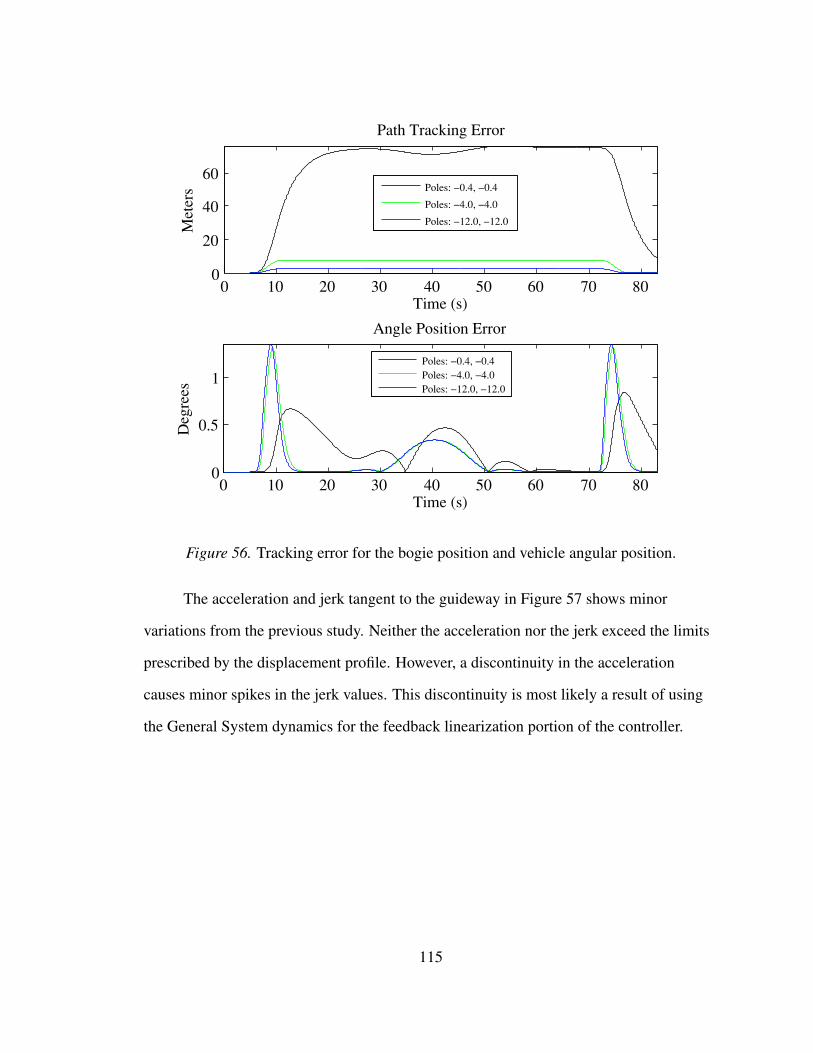
0 10 20 30 40 50 60 70 800
20
40
60
Path Tracking Error
Time (s)
Met
ers
Poles: −0.4, −0.4
Poles: −4.0, −4.0
Poles: −12.0, −12.0
0 10 20 30 40 50 60 70 800
0.5
1
Angle Position Error
Time (s)
Deg
rees
Poles: −0.4, −0.4Poles: −4.0, −4.0Poles: −12.0, −12.0
Figure 56. Tracking error for the bogie position and vehicle angular position.
The acceleration and jerk tangent to the guideway in Figure 57 shows minor
variations from the previous study. Neither the acceleration nor the jerk exceed the limits
prescribed by the displacement profile. However, a discontinuity in the acceleration
causes minor spikes in the jerk values. This discontinuity is most likely a result of using
the General System dynamics for the feedback linearization portion of the controller.
115
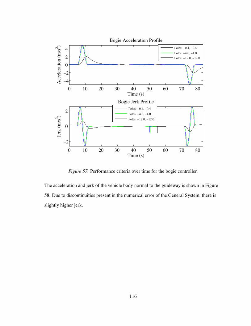
0 10 20 30 40 50 60 70 80
−4
−2
0
2
4
Bogie Acceleration Profile
Time (s)
Acc
eler
atio
n (m
/s2 )
Poles: −0.4, −0.4
Poles: −4.0, −4.0
Poles: −12.0, −12.0
0 10 20 30 40 50 60 70 80
−2
0
2
Bogie Jerk Profile
Time (s)
Jerk
(m
/s3 )
Poles: −0.4, −0.4
Poles: −4.0, −4.0
Poles: −12.0, −12.0
Figure 57. Performance criteria over time for the bogie controller.
The acceleration and jerk of the vehicle body normal to the guideway is shown in Figure
58. Due to discontinuities present in the numerical error of the General System, there is
slightly higher jerk.
116
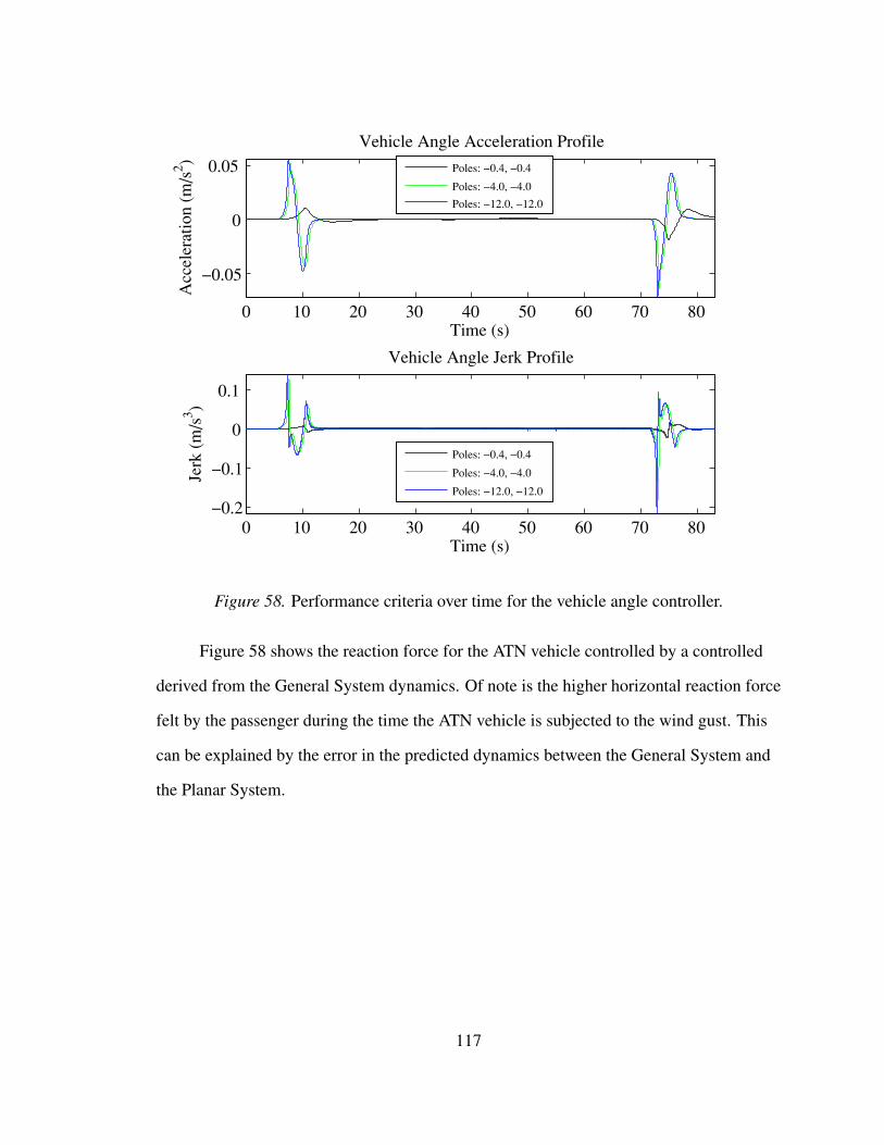
0 10 20 30 40 50 60 70 80
−0.05
0
0.05
Vehicle Angle Acceleration Profile
Time (s)
Acc
eler
atio
n (m
/s2 )
Poles: −0.4, −0.4
Poles: −4.0, −4.0
Poles: −12.0, −12.0
0 10 20 30 40 50 60 70 80−0.2
−0.1
0
0.1
Vehicle Angle Jerk Profile
Time (s)
Jerk
(m
/s3 )
Poles: −0.4, −0.4
Poles: −4.0, −4.0
Poles: −12.0, −12.0
Figure 58. Performance criteria over time for the vehicle angle controller.
Figure 58 shows the reaction force for the ATN vehicle controlled by a controlled
derived from the General System dynamics. Of note is the higher horizontal reaction force
felt by the passenger during the time the ATN vehicle is subjected to the wind gust. This
can be explained by the error in the predicted dynamics between the General System and
the Planar System.
117
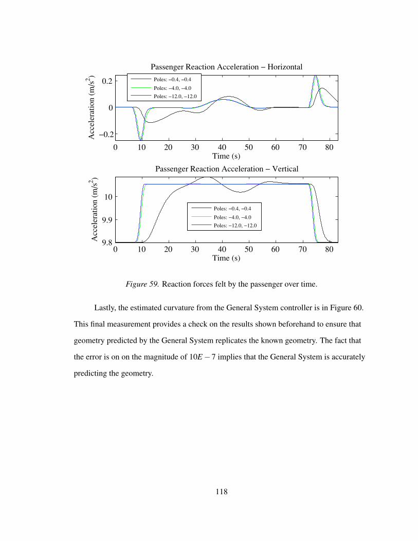
0 10 20 30 40 50 60 70 80
−0.2
0
0.2
Passenger Reaction Acceleration − Horizontal
Time (s)
Acc
eler
atio
n (m
/s2 )
Poles: −0.4, −0.4
Poles: −4.0, −4.0
Poles: −12.0, −12.0
0 10 20 30 40 50 60 70 809.8
9.9
10
Passenger Reaction Acceleration − Vertical
Time (s)
Acc
eler
atio
n (m
/s2 )
Poles: −0.4, −0.4
Poles: −4.0, −4.0
Poles: −12.0, −12.0
Figure 59. Reaction forces felt by the passenger over time.
Lastly, the estimated curvature from the General System controller is in Figure 60.
This final measurement provides a check on the results shown beforehand to ensure that
geometry predicted by the General System replicates the known geometry. The fact that
the error is on on the magnitude of 10E−7 implies that the General System is accurately
predicting the geometry.
118
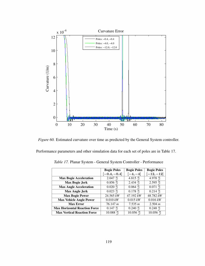
0 10 20 30 40 50 60 70 80
0
2
4
6
8
10
12x 10
−8 Curvature Error
Time (s)
Cur
vatu
re (
1/m
)
Poles: −0.4, −0.4
Poles: −4.0, −4.0
Poles: −12.0, −12.0
Figure 60. Estimated curvature over time as predicted by the General System controller.
Performance parameters and other simulation data for each set of poles are in Table 17.
Table 17. Planar System - General System Controller - Performance
Bogie Poles Bogie Poles Bogie Poles[−0.4,−0.4] [−4,−4] [−12,−12]
Max Bogie Acceleration 2.047 ms2 4.815 m
s2 4.978 ms2
Max Bogie Jerk 0.856 ms3 2.434 m
s3 2.595 ms3
Max Angle Acceleration 0.020 ms2 0.064 m
s2 0.071 ms2
Max Angle Jerk 0.023 ms3 0.178 m
s3 0.214 ms3
Max Bogie Power 24.565 kW 47.192 kW 48.782 kWMax Vehicle Angle Power 0.010 kW 0.015 kW 0.016 kW
Max Error 76.147 m 7.535 m 2.504 mMax Horizontal Reaction Force 0.147 m
s2 0.240 ms2 0.248 m
s2
Max Vertical Reaction Force 10.088 ms2 10.056 m
s2 10.056 ms2
119
6.8 General System - Euler Spiral Example
The validation of the General System involved simulations of a simple geometry.
However, the appeal of the General System is that the dynamics constrained to any
numerically defined geometry can be simulated. Therefore, an example of a different
geometry is simulation without comparison to hand derived models. The purpose of this is
to showcase the method developed in this thesis for a different, more complex guideway
geometry. The guideway geometry chosen is that of an Euler Spiral in which a point of the
guideway at position s in inertial frame N is defined as
r = cosA12
πs2Nx+ sinA12
πs2Ny+(0)Nz (119)
Euler spirals are important concepts in ATN research as portions of such spirals are used
to transition between straight and curved segments of the guideway. A unique property of
the Euler spiral is that the curvature changes linearly with distance. Figure 61 shows an
Euler spiral based on Equation 119 with a coefficient of A = 2.5E−5 (Weisstein,
2016a). The vehicle begins travel at green circle on the plot where there the curvature is at
a minimum and travels to the red X where the curvature is greatest.
120
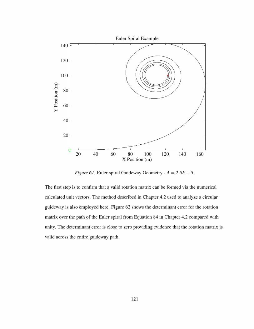
20 40 60 80 100 120 140 160
20
40
60
80
100
120
140
Euler Spiral Example
X Position (m)
Y P
ositi
on (
m)
Figure 61. Euler spiral Guideway Geometry - A = 2.5E−5.
The first step is to confirm that a valid rotation matrix can be formed via the numerical
calculated unit vectors. The method described in Chapter 4.2 used to analyze a circular
guideway is also employed here. Figure 62 shows the determinant error for the rotation
matrix over the path of the Euler spiral from Equation 84 in Chapter 4.2 compared with
unity. The determinant error is close to zero providing evidence that the rotation matrix is
valid across the entire guideway path.
121
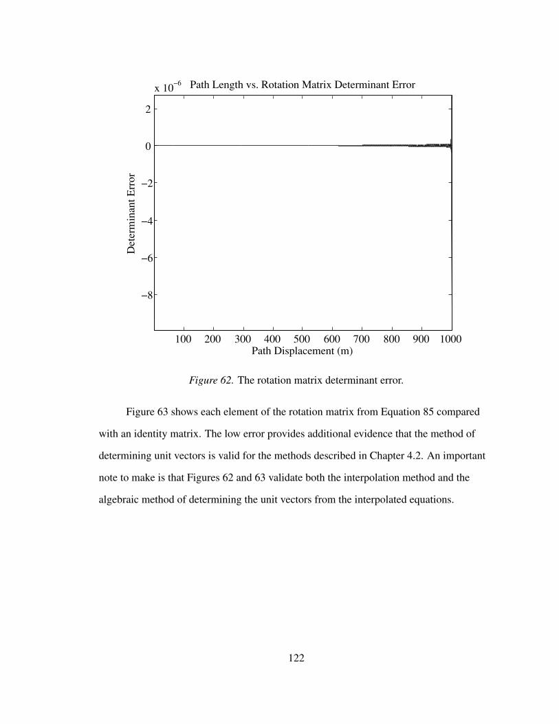
100 200 300 400 500 600 700 800 900 1000
−8
−6
−4
−2
0
2
x 10−6 Path Length vs. Rotation Matrix Determinant Error
Path Displacement (m)
Det
erm
inan
t Err
or
Figure 62. The rotation matrix determinant error.
Figure 63 shows each element of the rotation matrix from Equation 85 compared
with an identity matrix. The low error provides additional evidence that the method of
determining unit vectors is valid for the methods described in Chapter 4.2. An important
note to make is that Figures 62 and 63 validate both the interpolation method and the
algebraic method of determining the unit vectors from the interpolated equations.
122
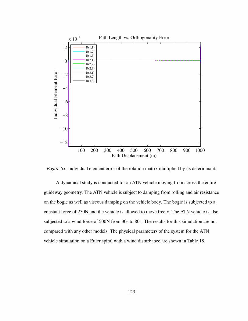
100 200 300 400 500 600 700 800 900 1000
−12
−10
−8
−6
−4
−2
0
2
x 10−4 Path Length vs. Orthogonality Error
Path Displacement (m)
Indi
vidu
al E
lem
ent E
rror
R(1,1)R(1,2)R(1,3)R(2,1)R(2,2)R(2,3)R(3,1)R(3,2)R(3,3)
Figure 63. Individual element error of the rotation matrix multiplied by its determinant.
A dynamical study is conducted for an ATN vehicle moving from across the entire
guideway geometry. The ATN vehicle is subject to damping from rolling and air resistance
on the bogie as well as viscous damping on the vehicle body. The bogie is subjected to a
constant force of 250N and the vehicle is allowed to move freely. The ATN vehicle is also
subjected to a wind force of 500N from 30s to 80s. The results for this simulation are not
compared with any other models. The physical parameters of the system for the ATN
vehicle simulation on a Euler spiral with a wind disturbance are shown in Table 18.
123
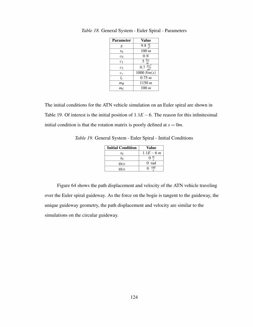
Table 18. General System - Euler Spiral - Parameters
Parameter Valueg 9.8 m
s2
r0 100 mc0 0 Nc1 5 Ns
m
c2 0.7 Ns2
m2
cc 1000 Nm(s)lc 0.75 m
mB 1150 mmC 100 m
The initial conditions for the ATN vehicle simulation on an Euler spiral are shown in
Table 19. Of interest is the initial position of 1.1E−6. The reason for this infinitesimal
initial condition is that the rotation matrix is poorly defined at s = 0m.
Table 19. General System - Euler Spiral - Initial Conditions
Initial Condition Values0 1.1E−6 ms0 0 m
sqB,0 0 rad
˙qB,0 0 rads
Figure 64 shows the path displacement and velocity of the ATN vehicle traveling
over the Euler spiral guideway. As the force on the bogie is tangent to the guideway, the
unique guideway geometry, the path displacement and velocity are similar to the
simulations on the circular guideway.
124
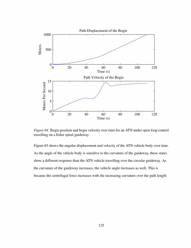
0 20 40 60 80 100 1200
500
1000Path Displacement of the Bogie
Time (s)
Met
ers
0 20 40 60 80 100 1200
5
10
15Path Velocity of the Bogie
Time (s)
Met
ers
Per
Seco
nd
Figure 64. Bogie position and bogie velocity over time for an ATN under open loop controltravelling on a Euler spiral guideway.
Figure 65 shows the angular displacement and velocity of the ATN vehicle body over time.
As the angle of the vehicle body is sensitive to the curvature of the guideway, these states
show a different response than the ATN vehicle travelling over the circular guideway. As
the curvature of the guideway increases, the vehicle angle increases as well. This is
because the centrifugal force increases with the increasing curvature over the path length.
125
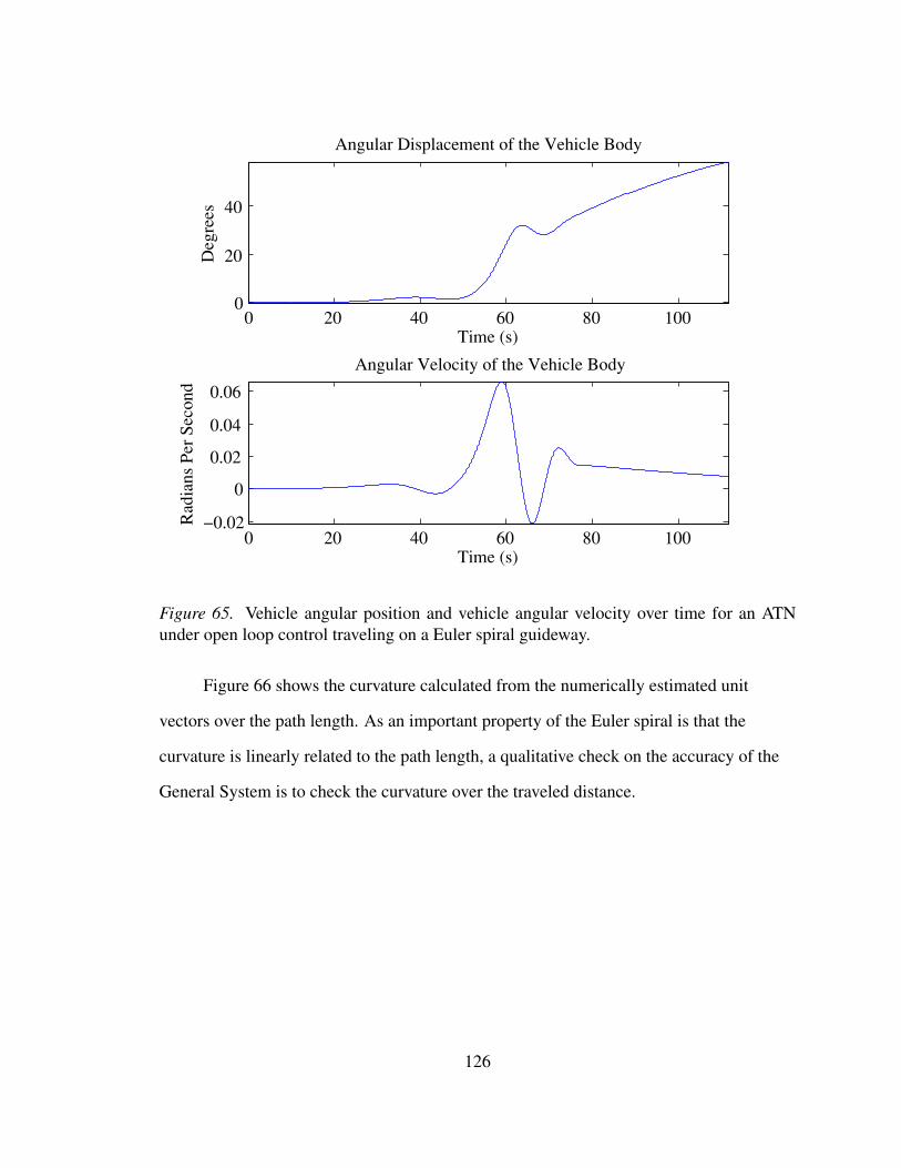
0 20 40 60 80 1000
20
40
Angular Displacement of the Vehicle Body
Time (s)
Deg
rees
0 20 40 60 80 100−0.02
0
0.02
0.04
0.06
Angular Velocity of the Vehicle Body
Time (s)
Rad
ians
Per
Sec
ond
Figure 65. Vehicle angular position and vehicle angular velocity over time for an ATNunder open loop control traveling on a Euler spiral guideway.
Figure 66 shows the curvature calculated from the numerically estimated unit
vectors over the path length. As an important property of the Euler spiral is that the
curvature is linearly related to the path length, a qualitative check on the accuracy of the
General System is to check the curvature over the traveled distance.
126
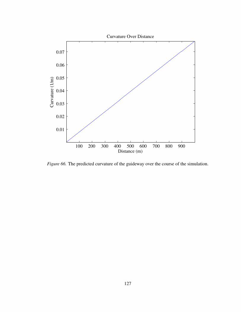
100 200 300 400 500 600 700 800 900
0.01
0.02
0.03
0.04
0.05
0.06
0.07
Curvature Over Distance
Distance (m)
Cur
vatu
re (
1/m
)
Figure 66. The predicted curvature of the guideway over the course of the simulation.
127
CHAPTER 7
CONCLUSION AND RECOMMENDATIONS FOR FUTHER RESEARCH
From the simulation data in the comparison studies, it is seen that the General
System is able to accurately simulate the dynamics of a suspended ATN vehicle. While
there is some increased error in the simulation output between the General System
dynamics and the Planar System dynamics, the error is orders of magnitude less than the
maximum displacement. Additionally, another useful conclusion is that feedback
linearization is possible using dynamics derived from the General System. This is an
important conclusion as it means that a controller can be given numerical data from CAD
or GIS to control a physical or prototype ATN vehicle. However, one consideration that
the comparison studies and other simulation do not fully address is the limitations of the
General System with regards to guideway geometry. An expected goal of the General
System is to be able to simulate the dynamics on any numerically defined guideway. The
two guideway geometries studied for this thesis are a circular guideway and an Euler
spiral guideway. The geometry of these two guideways were interpolated with a 5th order
spline. From the interpolated spline, a rotation matrix over the entire length of the
guideway was formed. However, both of these guideways were continuous and did not
contain any straight segments. Because some guideways of interest may have straight
segments, these segments may have singularities due to an undefined unit normal vector.
Therefore, the interpolation method of a 5th order spline may not be suitable for those
particular guideway geometries. However, the tools to determine the rotation matrix over
the guideway path can be used to to verify a particular interpolation method.
Future work for this research falls into three areas: increasing the complexity of the
ATN idealization, increasing complexity of the features of the simulation environment,
and researching the interpolation method of the numerical guideway data used for the
128
General System. Adding complexity to this idealization involves adding passive
suspension components and determining if the vibrations cause the feedback linearization
method to fail. Additional simulation environment features that increase the realism and
provide a better engineering tool include discrete time sampling and measurement noise.
Finally, new interpolation methods besides 5th order polynomial splines can be tried. This
research should be performed in parallel with sensitivity studies to investigate the effect
on granularity of the numerical guideway data and the accuracy of the simulation.
129
REFERENCES
Anderson, J. E. (1978). Transit system theory (1st ed.). Lexington, MA: Lexington Books.
Anderson, J. E. (2013). The tradeoff between supported vehicles vs. hanging vehicles.Retrieved from http://www.inist.org/Library/2013.Anderson.Tradeoff%20between%20Supported%20vs%20Hanging%20Vehicles.pdf
Avallone, E. A. & III, T. B. (Eds.). (1987). Marks’ standard handbook for mechanicalengineers (9th). New York: McGraw-Hill Book Company.
Chou, M. & Xia, X. (2007, May). Optimal cruise control of heavy-haul trains equippedwith electronically controlled pneumatic brake systems. Control EngineeringPractice, 15, 511–519. doi:10.1016/j.conengprac.2006.09.007
Furman, B. (2016, January). Innovating automated transit technology with students.Retrieved from http://www.inist.org/Library/2015-12.Furman.Innovating%20Automated%20Transit%20Technology%20with%20Students.ATRA-Pulse.pdf
Furman, B., Fabian, L., Ellis, S., Muller, P., & Swenson, R. (2014, September). Automatedtransit networks (atn): a review of the state of the industry and prospects for thefuture (MTI Report No. CA-MTI-14-1227). San Jose, CA: Mineta TransportationInstitute, San Jose State University.
Gustafsson, B. (2014). Automatic transit networks explained. Retrieved fromhttp://www.inist.org/Library/2014-01-27.Beamways%20Gustafsson.ATN%20Explained.pptx
Gustafsson, J. (2009, November). Vectus - intelligent transport. Proceedings of the IEEE,97, 1856–1863. doi:10.1109/JPROC.2009.2030242
Kane, T. R. & Levinson, D. A. (2005). Dynamics: theory and applications. Ithaca, NY:The Internet-First University Press.
Kerr, T. (2013). Prt stations. Retrieved fromhttp://www.advancedtransit.org/wp-content/uploads/2011/08/PRT-Stations.pdf
Kornhauser, A. L., Lion, P. M., McEvaddy, P. J., & Garrard, W. L. (1974). Optimalsample-data control of prt vehicles. In Personal rapid transit ii. progress - problems- potential (pp. 359–365).
Levine, W. S. (Ed.). (1996). The control handbook (1st). Boca Raton, FL: CRC Press, Inc.
130
Li, S., Yang, L., Li, K., & Gao, Z. (2014, September). Robust sampled-data cruise controlscheduling of high speed train. Transportation Research Part C: EmergingTechnologies, 46, 274–283. doi:10.1016/j.trc.2014.06.004
Makkar, C., Dixon, W. E., Sawyer, W. G., & Hu, G. (2005, July). A new continuouslydifferentiable friction model for control systems design. In Proceedings, 2005ieee/asme international conference on advanced intelligent mechatronics.(pp. 600–605). doi:10.1109/AIM.2005.1511048
Mitiguy, P. (2015). Motiongenesis kane (version 5.7) [computer software]. Menlo Park,CA.
Muller, P. J. (2009). Open-guideway personal rapid transit station options. Retrieved fromhttp://www.inist.org/Library/2009.Muller.PRT%20Stations.APM09.pdf
Smisek, R. R. & Harder, G. A. (1979, March). Automated control of guideway transitvehicles. In Vehicular technology conference, 1979. 29th ieee (Vol. 29, pp. 57–64).doi:10.1109/VTC.1979.1622665
Weisstein, E. W. (2016a). Cornu spiral. Retrieved fromhttp://mathworld.wolfram.com/CornuSpiral.html
Weisstein, E. W. (2016b). Curvature. Retrieved fromhttp://mathworld.wolfram.com/Curvature.html
Zhou, R., Zolotas, A., & Goodall, R. (2011, September). Integrated tilt with active lateralsecondary suspension control for high speed railway vehicles. Mechatronics, 21(6),1108–1122. doi:10.1016/j.mechatronics.2011.07.001
131
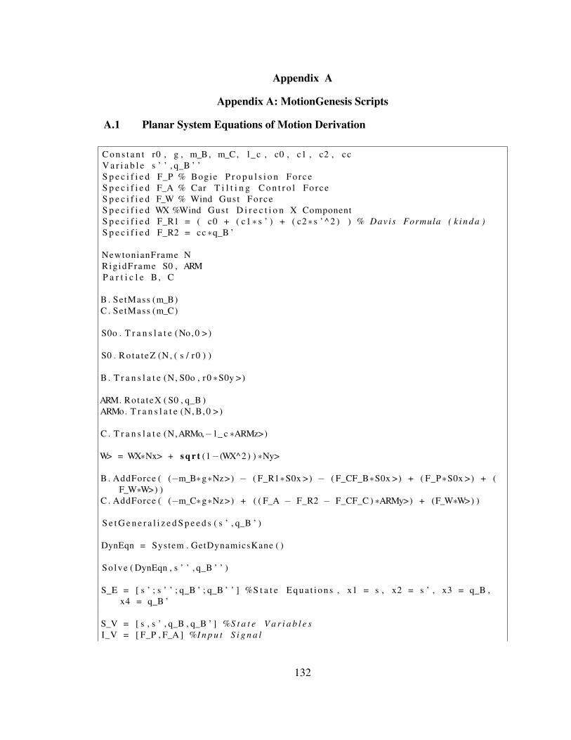
Appendix A
Appendix A: MotionGenesis Scripts
A.1 Planar System Equations of Motion Derivation
C o n s t a n t r0 , g , m_B, m_C, l_c , c0 , c1 , c2 , ccV a r i a b l e s ’ ’ , q_B ’ ’S p e c i f i e d F_P % Bogie P r o p u l s i o n ForceS p e c i f i e d F_A % Car T i l t i n g C o n t r o l ForceS p e c i f i e d F_W % Wind Gust ForceS p e c i f i e d WX %Wind Gust D i r e c t i o n X ComponentS p e c i f i e d F_R1 = ( c0 + ( c1∗ s ’ ) + ( c2∗ s ’ ^ 2 ) ) % Davis Formula ( k i n d a )S p e c i f i e d F_R2 = cc ∗q_B ’
NewtonianFrame NRigidFrame S0 , ARMP a r t i c l e B , C
B . SetMass (m_B)C . SetMass (m_C)
S0o . T r a n s l a t e ( No,0 > )
S0 . Ro ta t eZ (N , ( s / r0 ) )
B . T r a n s l a t e (N, S0o , r0 ∗S0y >)
ARM. Rota teX ( S0 , q_B )ARMo. T r a n s l a t e (N, B, 0 >)
C . T r a n s l a t e (N,ARMo,− l _ c ∗ARMz>)
W> = WX∗Nx> + s q r t (1−(WX^2) ) ∗Ny>
B . AddForce ( (−m_B∗g∗Nz>) − ( F_R1∗S0x >) − ( F_CF_B∗S0x >) + ( F_P∗S0x >) + (F_W∗W>) )
C . AddForce ( (−m_C∗g∗Nz>) + ( ( F_A − F_R2 − F_CF_C ) ∗ARMy>) + (F_W∗W>) )
S e t G e n e r a l i z e d S p e e d s ( s ’ , q_B ’ )
DynEqn = System . GetDynamicsKane ( )
So lve ( DynEqn , s ’ ’ , q_B ’ ’ )
S_E = [ s ’ ; s ’ ’ ; q_B ’ ; q_B ’ ’ ] %S t a t e E q u a t i o n s , x1 = s , x2 = s ’ , x3 = q_B ,x4 = q_B ’
S_V = [ s , s ’ , q_B , q_B ’ ] %S t a t e V a r i a b l e sI_V = [ F_P , F_A ] %I n p u t S i g n a l
132
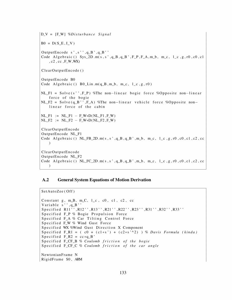
D_V = [F_W] %D i s t u r b a n c e S i g n a l
B0 = D( S_E , I_V )
OutputEncode s ’ , s ’ ’ , q_B ’ , q_B ’ ’Code A l g e b r a i c ( ) Sys_2D .m( s , s ’ , q_B , q_B ’ , F_P , F_A , m_b , m_c , l_c , g , r0 , c0 , c1
, c2 , cc , F_W,WX)
Cl ea rOu tp u tE nc ode ( )
OutputEncode B0Code A l g e b r a i c ( ) B0_Lin .m( q_B , m_b , m_c , l_c , g , r0 )
NL_F1 = So lve ( s ’ ’ , F_P ) %The non− l i n e a r b o g i e f o r c e %O p p o s i t e non− l i n e a rf o r c e o f t h e b o g i e
NL_F2 = So lve ( q_B ’ ’ ,F_A ) %The non− l i n e a r v e h i c l e f o r c e %O p p o s i t e non−l i n e a r f o r c e o f t h e c a b i n
NL_F1 := NL_F1 − F_W∗D( NL_F1 ,F_W)NL_F2 := NL_F2 − F_W∗D( NL_F2 ,F_W)
Cl ea rOu tp u tE nc odeOutputEncode NL_F1Code A l g e b r a i c ( ) NL_FB_2D .m( s , s ’ , q_B , q_B ’ , m_b , m_c , l_c , g , r0 , c0 , c1 , c2 , cc
)
C l ea rOu tp u tE nc odeOutputEncode NL_F2Code A l g e b r a i c ( ) NL_FC_2D .m( s , s ’ , q_B , q_B ’ , m_b , m_c , l_c , g , r0 , c0 , c1 , c2 , cc
)
A.2 General System Equations of Motion Derivation
SetAutoZee ( Off )
C o n s t a n t g , m_B, m_C, l_c , c0 , c1 , c2 , ccV a r i a b l e s ’ ’ , q_B ’ ’S p e c i f i e d R11 ’ ’ , R12 ’ ’ , R13 ’ ’ , R21 ’ ’ , R22 ’ ’ , R23 ’ ’ , R31 ’ ’ , R32 ’ ’ , R33 ’ ’S p e c i f i e d F_P % Bogie P r o p u l s i o n ForceS p e c i f i e d F_A % Car T i l t i n g C o n t r o l ForceS p e c i f i e d F_W % Wind Gust ForceS p e c i f i e d WX %Wind Gust D i r e c t i o n X ComponentS p e c i f i e d F_R1 = ( c0 + ( c1∗ s ’ ) + ( c2∗ s ’ ^ 2 ) ) % Davis Formula ( k i n d a )S p e c i f i e d F_R2 = cc ∗q_B ’S p e c i f i e d F_CF_B % Coulomb f r i c t i o n o f t h e b o g i eS p e c i f i e d F_CF_C % Coulomb f r i c t i o n o f t h e car a n g l e
NewtonianFrame NRigidFrame S0 , ARM
133
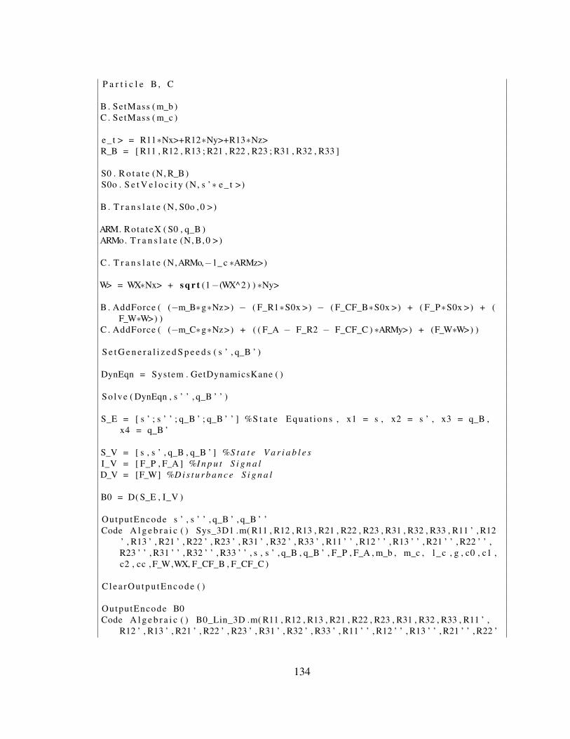
P a r t i c l e B , C
B . SetMass ( m_b )C . SetMass ( m_c )
e_ t > = R11∗Nx>+R12∗Ny>+R13∗Nz>R_B = [ R11 , R12 , R13 ; R21 , R22 , R23 ; R31 , R32 , R33 ]
S0 . R o t a t e (N, R_B)S0o . S e t V e l o c i t y (N, s ’∗ e_ t >)
B . T r a n s l a t e (N, S0o , 0 > )
ARM. Rota teX ( S0 , q_B )ARMo. T r a n s l a t e (N, B, 0 >)
C . T r a n s l a t e (N,ARMo,− l _ c ∗ARMz>)
W> = WX∗Nx> + s q r t (1−(WX^2) ) ∗Ny>
B . AddForce ( (−m_B∗g∗Nz>) − ( F_R1∗S0x >) − ( F_CF_B∗S0x >) + ( F_P∗S0x >) + (F_W∗W>) )
C . AddForce ( (−m_C∗g∗Nz>) + ( ( F_A − F_R2 − F_CF_C ) ∗ARMy>) + (F_W∗W>) )
S e t G e n e r a l i z e d S p e e d s ( s ’ , q_B ’ )
DynEqn = System . GetDynamicsKane ( )
So lve ( DynEqn , s ’ ’ , q_B ’ ’ )
S_E = [ s ’ ; s ’ ’ ; q_B ’ ; q_B ’ ’ ] %S t a t e E q u a t i o n s , x1 = s , x2 = s ’ , x3 = q_B ,x4 = q_B ’
S_V = [ s , s ’ , q_B , q_B ’ ] %S t a t e V a r i a b l e sI_V = [ F_P , F_A ] %I n p u t S i g n a lD_V = [F_W] %D i s t u r b a n c e S i g n a l
B0 = D( S_E , I_V )
OutputEncode s ’ , s ’ ’ , q_B ’ , q_B ’ ’Code A l g e b r a i c ( ) Sys_3D1 .m( R11 , R12 , R13 , R21 , R22 , R23 , R31 , R32 , R33 , R11 ’ , R12
’ , R13 ’ , R21 ’ , R22 ’ , R23 ’ , R31 ’ , R32 ’ , R33 ’ , R11 ’ ’ , R12 ’ ’ , R13 ’ ’ , R21 ’ ’ , R22 ’ ’ ,R23 ’ ’ , R31 ’ ’ , R32 ’ ’ , R33 ’ ’ , s , s ’ , q_B , q_B ’ , F_P , F_A , m_b , m_c , l_c , g , c0 , c1 ,c2 , cc , F_W,WX, F_CF_B , F_CF_C )
Cl ea rOu tp u tE nc ode ( )
OutputEncode B0Code A l g e b r a i c ( ) B0_Lin_3D .m( R11 , R12 , R13 , R21 , R22 , R23 , R31 , R32 , R33 , R11 ’ ,
R12 ’ , R13 ’ , R21 ’ , R22 ’ , R23 ’ , R31 ’ , R32 ’ , R33 ’ , R11 ’ ’ , R12 ’ ’ , R13 ’ ’ , R21 ’ ’ , R22 ’
134
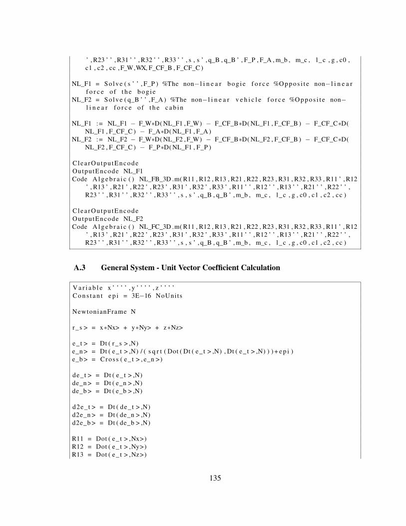
’ , R23 ’ ’ , R31 ’ ’ , R32 ’ ’ , R33 ’ ’ , s , s ’ , q_B , q_B ’ , F_P , F_A , m_b , m_c , l_c , g , c0 ,c1 , c2 , cc , F_W,WX, F_CF_B , F_CF_C )
NL_F1 = So lve ( s ’ ’ , F_P ) %The non− l i n e a r b o g i e f o r c e %O p p o s i t e non− l i n e a rf o r c e o f t h e b o g i e
NL_F2 = So lve ( q_B ’ ’ ,F_A ) %The non− l i n e a r v e h i c l e f o r c e %O p p o s i t e non−l i n e a r f o r c e o f t h e c a b i n
NL_F1 := NL_F1 − F_W∗D( NL_F1 ,F_W) − F_CF_B∗D( NL_F1 , F_CF_B ) − F_CF_C∗D(NL_F1 , F_CF_C ) − F_A∗D( NL_F1 , F_A )
NL_F2 := NL_F2 − F_W∗D( NL_F2 ,F_W) − F_CF_B∗D( NL_F2 , F_CF_B ) − F_CF_C∗D(NL_F2 , F_CF_C ) − F_P∗D( NL_F1 , F_P )
C l ea rOu tp u tE nc odeOutputEncode NL_F1Code A l g e b r a i c ( ) NL_FB_3D .m( R11 , R12 , R13 , R21 , R22 , R23 , R31 , R32 , R33 , R11 ’ , R12
’ , R13 ’ , R21 ’ , R22 ’ , R23 ’ , R31 ’ , R32 ’ , R33 ’ , R11 ’ ’ , R12 ’ ’ , R13 ’ ’ , R21 ’ ’ , R22 ’ ’ ,R23 ’ ’ , R31 ’ ’ , R32 ’ ’ , R33 ’ ’ , s , s ’ , q_B , q_B ’ , m_b , m_c , l_c , g , c0 , c1 , c2 , cc )
C l ea rOu tp u tE nc odeOutputEncode NL_F2Code A l g e b r a i c ( ) NL_FC_3D .m( R11 , R12 , R13 , R21 , R22 , R23 , R31 , R32 , R33 , R11 ’ , R12
’ , R13 ’ , R21 ’ , R22 ’ , R23 ’ , R31 ’ , R32 ’ , R33 ’ , R11 ’ ’ , R12 ’ ’ , R13 ’ ’ , R21 ’ ’ , R22 ’ ’ ,R23 ’ ’ , R31 ’ ’ , R32 ’ ’ , R33 ’ ’ , s , s ’ , q_B , q_B ’ , m_b , m_c , l_c , g , c0 , c1 , c2 , cc )
A.3 General System - Unit Vector Coefficient Calculation
V a r i a b l e x ’ ’ ’ ’ , y ’ ’ ’ ’ , z ’ ’ ’ ’C o n s t a n t e p i = 3E−16 NoUnits
NewtonianFrame N
r_s > = x∗Nx> + y∗Ny> + z∗Nz>
e_t > = Dt ( r_s > ,N)e_n > = Dt ( e_ t > ,N) / ( s q r t ( Dot ( Dt ( e_ t > ,N) , Dt ( e_ t > ,N) ) ) + e p i )e_b > = Cross ( e_ t > , e_n >)
de_t > = Dt ( e_ t > ,N)de_n > = Dt ( e_n > ,N)de_b > = Dt ( e_b > ,N)
d2e_t > = Dt ( de_ t > ,N)d2e_n > = Dt ( de_n > ,N)d2e_b > = Dt ( de_b > ,N)
R11 = Dot ( e_ t > ,Nx>)R12 = Dot ( e_ t > ,Ny>)R13 = Dot ( e_ t > ,Nz>)
135
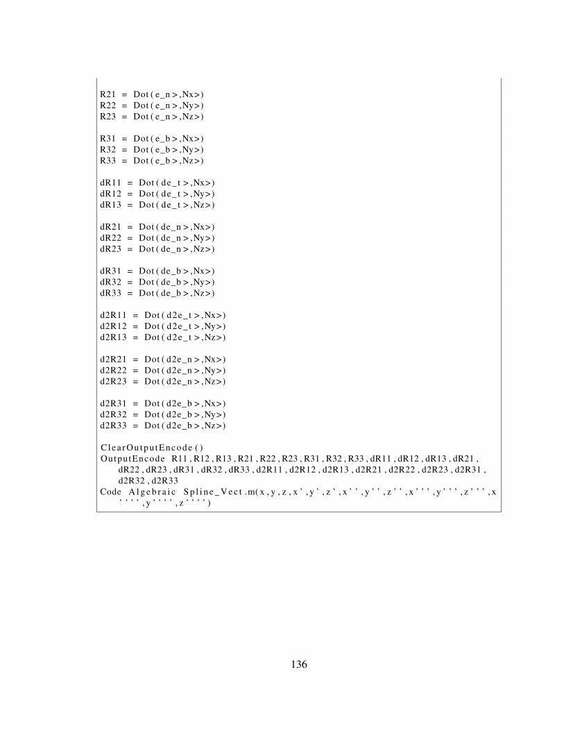
R21 = Dot ( e_n > ,Nx>)R22 = Dot ( e_n > ,Ny>)R23 = Dot ( e_n > ,Nz>)
R31 = Dot ( e_b > ,Nx>)R32 = Dot ( e_b > ,Ny>)R33 = Dot ( e_b > ,Nz>)
dR11 = Dot ( de_ t > ,Nx>)dR12 = Dot ( de_ t > ,Ny>)dR13 = Dot ( de_ t > ,Nz>)
dR21 = Dot ( de_n > ,Nx>)dR22 = Dot ( de_n > ,Ny>)dR23 = Dot ( de_n > ,Nz>)
dR31 = Dot ( de_b > ,Nx>)dR32 = Dot ( de_b > ,Ny>)dR33 = Dot ( de_b > ,Nz>)
d2R11 = Dot ( d2e_t > ,Nx>)d2R12 = Dot ( d2e_t > ,Ny>)d2R13 = Dot ( d2e_t > ,Nz>)
d2R21 = Dot ( d2e_n > ,Nx>)d2R22 = Dot ( d2e_n > ,Ny>)d2R23 = Dot ( d2e_n > ,Nz>)
d2R31 = Dot ( d2e_b > ,Nx>)d2R32 = Dot ( d2e_b > ,Ny>)d2R33 = Dot ( d2e_b > ,Nz>)
C l ea rOu tp u tE nc ode ( )OutputEncode R11 , R12 , R13 , R21 , R22 , R23 , R31 , R32 , R33 , dR11 , dR12 , dR13 , dR21 ,
dR22 , dR23 , dR31 , dR32 , dR33 , d2R11 , d2R12 , d2R13 , d2R21 , d2R22 , d2R23 , d2R31 ,d2R32 , d2R33
Code A l g e b r a i c S p l i n e _ V e c t .m( x , y , z , x ’ , y ’ , z ’ , x ’ ’ , y ’ ’ , z ’ ’ , x ’ ’ ’ , y ’ ’ ’ , z ’ ’ ’ , x’ ’ ’ ’ , y ’ ’ ’ ’ , z ’ ’ ’ ’ )
136
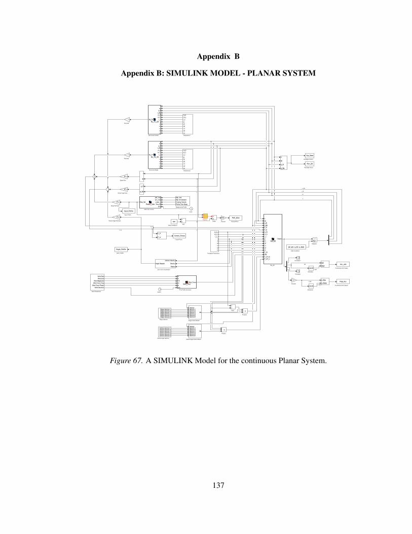
Appendix B
Appendix B: SIMULINK MODEL - PLANAR SYSTEM
Figure 67. A SIMULINK Model for the continuous Planar System.
137
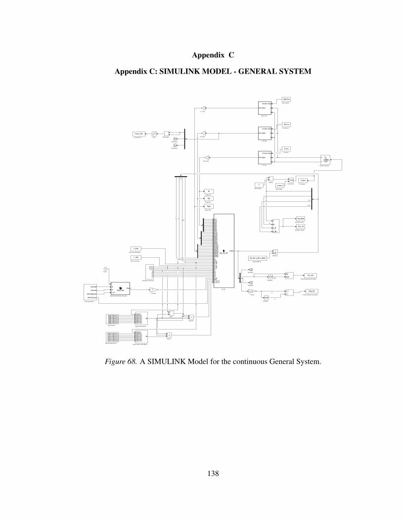
Appendix C
Appendix C: SIMULINK MODEL - GENERAL SYSTEM
Figure 68. A SIMULINK Model for the continuous General System.
138