dynamic spare part control
TRANSCRIPT

Dynamic spare part control
for performance-based service contracts
- J.W. van den Bussche -


University of Twente
March, 2019
Enschede, The Netherlands
Faculty
Behavioural Management and Social Sciences
Study programme Industrial Engineering and Management MSc
Specialisation Production and Logistics Management
Dynamic spare part control for performance-based service contracts
Master thesis of Jasper W. van den Bussche BSc
University supervisors
Company supervisors
Dr. M.C van der Heijden
Associate Professor
Contact: [email protected]
Dr. E. Topan
Assistant Professor
Contact: [email protected]
Ir. R.M. Ypma
Logistic Engineer
Thales Nederland B.V., Hengelo
Ir. J.C. Bolhaar
Workpackage Manager
Thales Nederland B.V., Hengelo


Thales | University of Twente v
Preface
To great satisfaction, I may announce that my final work as a student lays in front of you. This report
describes the graduation research I did on the subject of after-sales logistics at Thales Nederland B.V
which enabled me to accomplish the master’s programme Industrial Engineering and Management. The
choice for this study followed from my interest in understanding and improving production and logistic
processes with associated complexities. My interest in this industry is to a large extent the result of
gathered experience during the bachelor’s programme Industrial Engineering and Management, in which
I obtained the bachelor’s degree 2.5 years ago. After six months of working in the company of my former
graduation research and travelling through Southeast Asia, it was time to start the masters.
Thanks to Matthieu van der Heijden from the University of Twente, I could apply for the assignment at
Thales which allowed me to start on time with the graduation research. Due to the concept of
performance-based service logistics, Thales is interested in having a method to dynamically update
failure rate estimates and adapt spare part stock levels accordingly, so that is what this research is
about. The topic caught my attention during courses given by Matthieu, thus it was a logical step to ask
him for an interesting assignment.
I hereby want to thank Matthieu again for being my first supervisor and providing me with extensive,
critical and valuable feedback along the way which certainly contributed in bringing this research to a
higher academic level. I would also like to thank my second supervisor Engin Topan for the constructive
feedback to further improve this thesis.
A special thanks goes to my company supervisor Rindert Ypma for giving me the opportunity to do the
graduation research at Thales and sharing practical knowledge and experiences to guide me through the
process. I have experienced our conservations as truly useful for the progress of the research and
appreciate the time efforts being made. I want to thank Jord Bolhaar for taking over the job as
supervisor from Rindert during his holiday and being a good sparring partner with helpful suggestions
from both a practical and academic perspective. In addition, I thank all my colleagues at Thales for the
nice social interactions during work and lunch time.
Lastly, I would like to express my gratitude to my family and friends for their support during all years of
studying. Besides that I felt supported by them, they helped me in having a healthy work-life balance.
Although a nice and instructive period of studying has come to an end, a new period with new challenges
will come soon. Enjoy reading this report!
Jasper van den Bussche
Hengelo, March 2019

Thales | University of Twente vi

Thales | University of Twente vii
Management summary
Thales Nederland B.V. is mainly involved in naval defence systems, among others radar systems. A quite
new concept within Thales is the offering of after-sales services in combination with a performance-based
service contract. The Dutch defence organization has agreed to make use of the services for six radar
systems. The corresponding service contracts state that Thales is responsible for meeting a supply or
system availability of 90% per year, otherwise a penalty applies. To be able to meet the requirement,
Thales needs to set up a supply chain network for the handling of spare parts and execution of repair,
production and new buy processes in case of LRU (Line-Replaceable Unit) failures in the system.
The required spare part stock levels are, among others, dependent on the part failure rates. The main
group of parts in the radar systems can be classified as electronic components. Thales predicts the failure
rates under the well-founded assumption in the literature that the failure rates of electronic components
remain constant during their lifecycle. Given the estimates, the initial spare part stock levels would be
determined. As operational failure data will be gathered in the coming years, failure rate estimates could
be updated to correct for unknown differences between the initial estimates and the actual failure rates.
Stock level interventions can be performed accordingly to better align them with reality and reduce the
risk of backorders and penalties. Goal of this research study is to find a method or protocol to do so.
Based on literature, the Bayesian estimation (explained in Section 3.3) seems to be suitable for Thales to
update failure rate estimates. A new estimate of the failure rate is based on both the initial engineering
estimate and operational failure data from the installed base. The Bayesian estimation is well-known for
its applicability in situations with little data. The amount of data to be gathered in the coming years at
Thales is expected to be low, due to a relatively small installed base (6 systems) and relatively low
failure rates, so this strengthens the preference for the Bayesian estimation. Parameters of the model can
be configured to be more sensitive or less sensitive to failure data in the estimation process.
Given the random nature of electronic failures and variability in the corresponding failure data, applying
the Bayesian estimation as a foundation for stock level interventions (dynamic approach) is not without
risks. Dependent on the amount of failures (demand) and data coming in, the accuracy of the estimates
can be low. This leads to the risk of anticipating on the updated estimate and increasing the stock level
by ordering parts even though the actual failure rate is lower, equal or just slightly higher than initially
estimated. The opposite also applies, meaning a risk of decreasing the stock level even though the actual
failure rate is equal or higher than initially estimated. Additionally, even if the actual failure rate is
higher than initially estimated, this does not necessarily mean that potential penalty cost savings
outweigh costs associated with increasing the stock level. Therefore, it might be wise to be less sensitive
to failure data in the estimation process (higher Bayesian weight factor) to lower the beforementioned
risks. A drawback is however a slower adaptation process to the actual failure rate, meaning a longer
exposure to higher penalty risks if the actual failure rate is higher than initially estimated.
The main focus of the research is on the trade-off between stock level intervention costs and potential
penalty savings during the term of the service contract (15 years). A simulation study has been executed
to experiment with different Bayesian settings while considering different part characteristics, i.e., part
price; expected average demand during lead time; and gap between initially estimated and actual failure

Thales | University of Twente viii
rate. The static approach, in which no failure rate and stock level updates take place, has been included
in the experiments as well. Furthermore, given lead times of one year at Thales, stocking issues can
already arise during the first years of practice before the first stock level intervention could have been
implemented. Hence, a balance needs to be sought between (possibly adapted) initial stock levels to start
the contract and data collection with, and the start time of the Bayesian estimation followed by dynamic
stock level interventions. The next findings emerged from the simulation study:
Thresholds of estimated average part demand (failures) during lead time apply before potential
penalty cost savings outweigh the costs for dynamic stock level interventions. For parts with
prices of €1.000, €50.000, €100.000 this is respectively: 0.020, 0.774, 2.406 failures per year.
Dynamic approach can be applied to save initial stock investment without significantly higher
average probability of penalty per year.
Required responsiveness to data and initial stock level have negative correlation.
For relatively high demand parts (initial estimate of at least 2.406 failures on average per year):
starting Bayesian estimation (possibly followed by stock level interventions) within the first year
can increase the part availability (in % of time per year) in second year with at most 18%.
For expensive parts (€50.000 and €100.000), it is not cost-efficient to increase initial stock levels
in advance given the uncertainty about the actual failure rate.
Based on the simulation study, we recommend Thales the following:
Apply Bayesian estimation for updating failure rates as a foundation for dynamic stock level
interventions but use appropriate thresholds for estimated average part demand during lead
time. Below the thresholds, apply a static approach.
Rely more heavily on initial estimates, i.e., less sensitive to data, if part price is relatively high
(€50.000 and €100.000) and/or if estimated average failures per year is relatively low (≤ 0.475).
Only increase initial stock levels in advance for relatively cheap parts.
Respond quickly to failure data, after 3 or 4 failures, if initial stock level has not been increased
and initial estimate of failure rate is relatively high (≥ 2.406 failures per year).
For parts with an initial estimate of failure rate lower than 2.406 failures per year, wait at least
one year of time before updating failure rates (with Bayesian estimation) and possibly stock
levels. Also, include current level of stock on hand in decision to increase stock level or not.
For relatively cheap parts with increased initial stock levels, wait at least one year of time and
until a certain number of failures have occurred before updating failure rates and stock levels.
For relatively expensive parts (€50.000 and €100.000) with relatively high estimated average
demand (≥ 2.406), consider other stock level interventions, e.g., putting SRUs on stock or fast
repairs. However, only 2% of parts in radar system at Thales have expected demand of ≥ 2.406.
Develop procedures for operational decisions in the periods between tactical stock level
interventions and for fast repairs to shorten lead times.

Thales | University of Twente ix
Table of contents
Preface ............................................................................................................................................................. v
Management summary .................................................................................................................................. vii
Abbreviations and definitions ........................................................................................................................ xi
1. Research introduction ................................................................................................................................. 1
1.1 Thales Group and Thales Nederland B.V............................................................................................ 1
1.2 Problem context .................................................................................................................................... 1
1.3 Research goal ........................................................................................................................................ 3
1.4 Research scope ...................................................................................................................................... 4
1.5 Research questions ................................................................................................................................ 5
1.6 Methodology.......................................................................................................................................... 6
1.7 Outline of the report ............................................................................................................................. 7
2. Business description .................................................................................................................................... 8
2.1 Background radar systems ................................................................................................................... 8
2.2 Initial stock level determination ......................................................................................................... 10
2.3 Simulation based scenario analysis..................................................................................................... 14
2.4 Conclusion ........................................................................................................................................... 15
3. Literature review ....................................................................................................................................... 16
3.1 Failure characteristics ......................................................................................................................... 16
3.2 Comparing failure rate updating models............................................................................................ 18
3.3 Bayesian estimation ............................................................................................................................ 20
3.4 Dynamic stock level interventions...................................................................................................... 22
3.5 Dynamic inventory control policy ...................................................................................................... 23
3.6 Conclusion ........................................................................................................................................... 24
4. Applying Bayesian estimation .................................................................................................................. 25
4.1 Setting prior parameters ..................................................................................................................... 25
4.2 Consequence of Bayesian estimation .................................................................................................. 27
4.3 Conclusion ........................................................................................................................................... 28
5. Impact and risks dynamic stock level interventions ................................................................................ 29
5.1 Research approach .............................................................................................................................. 29
5.2 Results and findings ............................................................................................................................ 33
5.3 Conclusion ........................................................................................................................................... 35

Thales | University of Twente x
6. Simulation model ...................................................................................................................................... 36
6.1 Simulation model design ..................................................................................................................... 36
6.2 Scenarios to examine .......................................................................................................................... 40
6.3 Experimental design ........................................................................................................................... 42
6.4 Conclusion ........................................................................................................................................... 44
7. Simulation results ..................................................................................................................................... 45
7.1 Bayesian setting experiments ............................................................................................................. 45
7.2 Initial stock level experiments ............................................................................................................ 48
7.3 Conclusion ........................................................................................................................................... 52
8. Benchmarking and extensions .................................................................................................................. 53
8.1 Benchmarking ..................................................................................................................................... 53
8.2 Conservative order policy ................................................................................................................... 54
8.3 Shortening lead times ......................................................................................................................... 56
8.4 Conclusion ........................................................................................................................................... 58
9. Implementation plan ................................................................................................................................. 59
10. Conclusions and recommendations ......................................................................................................... 61
10.1 Conclusions........................................................................................................................................ 61
10.2 Recommendations ............................................................................................................................. 62
10.3 Limitations research .......................................................................................................................... 62
10.4 Recommendations for further research ............................................................................................. 63
References ...................................................................................................................................................... 64
Appendix A: VARI-METRIC.......................................................................................................................... i
Appendix B: Literature review methodology ................................................................................................. ii
Appendix C: Failure rate updating models ................................................................................................... iv
Appendix D: Demand range per stock level................................................................................................. vii
Appendix E: Proposed stock levels Bayesian estimation – risks ................................................................ viii
Appendix F: Technical details Plant Simulation model .............................................................................. xii
Appendix G: Sequential procedure – number of replications ...................................................................... xv
Appendix H: Paired-t test – configuration comparison .............................................................................. xvi
Appendix I: Experiment results – Bayesian settings ................................................................................. xvii
Appendix J: Experiment results – initial stock levels (worst-case) .......................................................... xxvi
Appendix K: Experiment settings – initial stock levels .......................................................................... xxviii
Appendix L: Experiment results – initial stock levels .............................................................................. xxix

Thales | University of Twente xi
Abbreviations and definitions
The underlined phrases in the report refer to one of the alphabetically ordered definitions in the list
below:
Common Random Numbers (CRN): variance reduction technique which applies when two or
more alternative configurations (of a system) would be compared. It synchronizes the random
number streams such that the same random number stream is being used for the same
replication across different configurations/experiments.
Configuration: an arrangement of elements in a particular form or combination. Used in
simulation experiments to describe one situation given a unique combination of variable and
experimental factors.
Economies of scale: proportionate saving in costs gained by an increased level of output.
Enterprise Resource Planning (ERP): Business process management software that allows an
organization to use a system of integrated applications to manage the business and automate
many tasks related to technology, services and human resources.
Fill rate: fraction of customer demand that is met through immediate stock availability, without
lost sales or backorders.
Full factorial: a full factorial experiment is an experiment whose design consist of two or more
factors, each with discrete levels, and whose experimental units take on all possible combinations
of these levels across all factors.
Mean-Time-Between-Failure (MTBF): the predicted average elapsed time between inherent
failures of an electronic or mechanical system.
Obsolete: part is no longer produced or used; out of date.
Original Equipment Manufacturer (OEM): a company that produces parts to be sold under
another company’s brand.
Poisson process: a model for a series of discrete events where the average time between events is
known, but the exact timing of events is random. A Poisson process meets the following criteria:
events are independent of each other, the average events per period is constant and two events
cannot occur at the same time. The Poisson distribution gives the probabilities of events.
Product Lifecycle Management: the process of managing the entire lifecycle of a product from
initiation, through engineering design and manufacturing, to service and disposal of
manufactured products.
Risk pooling effect: demand variability is reduced if one aggregates demand across locations
because it becomes more likely that high demand from one customer will be offset by low demand
from another. This reduction in variability makes it possible to reduce safety stock and therefore
average inventory levels.
Total Cost of Ownership (TCO): estimate of all direct and indirect costs associated with an
asset or acquisition over its entire lifecycle.

Thales | University of Twente xii

1. Research introduction
Thales | University of Twente 1
1. Research introduction
In Section 1.1 of this chapter we introduce the company Thales in which the research will be conducted.
Section 1.2 addresses the context of the problem addressed by the logistics department within Thales. In
Section 1.3 and 1.4 we formulate the goal and respectively the scope of the research. Thereafter, the
research questions will be defined that need to be answered to be able to solve the problem. We conclude
the chapter with the methodology, in Section 1.6, and an outline of the report in Section 1.7.
1.1 Thales Group and Thales Nederland B.V.
Thales Group is a French multinational company that designs, builds and maintains electrical systems
and provides relating services for the aerospace, space, defence, transportation and security markets. Its
revenue is roughly 15 billion euros of which 675 million euros is being invested in Research and
Development. Thales Group is active in 56 countries, employing around 65000 employees worldwide.
(Thales Group, 2018).
Thales Nederland B.V. is a Dutch subsidiary of the international Thales Group and is involved primarily
in naval defence systems. Thales Nederland B.V. specializes in designing, producing and maintaining
professional electronics for defence and security applications, such as radar and communication systems.
She employs about 3000 people of which 1500 are located in the headquarters in Hengelo. To give an
impression of the size, the worth of sales is roughly 500 million euros on a yearly basis (Thales
Netherlands, 2018).
1.2 Problem context
In this section, we describe the context of a problem encountered in the logistics department at Thales
Nederland B.V. The research study discussed in this report would enable Thales to deal with the
problem context.
1.2.1 Radar systems
One of the various types of products Thales Nederland B.V. offers, is naval radar systems. Radar is an
acronym for “radio detection and ranging” and is used to detect the position and/or movement of
objects by means of radio waves. Among others, the following objects can be detected: aircrafts, ships,
spacecrafts, guided missiles, motor vehicles and weather formations. Radar systems are mainly sold to
national governments as the naval forces and belonging necessary equipment are owned by them. Due to
this, Thales is currently doing business with more than 50 navies all around the world.
1.2.2 Performance-based service contracts
Besides designing, producing and selling radar systems, Thales also offers after-sales services for
maintaining and repairing the radars. These services, of which the sales volume is growing during recent
years, are related to a performance-based service contract agreed with the customer. Within the
contract, it is stated either what fraction of time the radar system should work properly or what fraction
of time the required spare parts should be available in stock to repair a non-operational radar system.
Thales is responsible for meeting the agreed performance standard and therefore has increased
responsibility over their supply chain performance. Inventories of spare parts are needed throughout the

1. Research introduction
Thales | University of Twente 2
entire supply chain network to be able to repair failed radar systems within limited amount of time. In
case Thales could not achieve the performance level as agreed upon, they may expect substantially high
penalty costs.
To determine spare part stock levels required for meeting the performance level, the logic as depicted in
Figure 1 is being used. Input for this calculation is ERP data and Product Lifecycle Management data.
The ERP data consists of the replenishment lead times of the spare parts and the costs. The
replenishment lead times can influence the stock levels because the higher the lead time for sending a
spare part from a central depot to the customer where the part is needed, the sooner it pays off to place
stock close by the customer, even though that might diminish the gains of the risk pooling effect. The
cost price of the spare parts has impact on the stock levels since the cheaper a spare part the more
attractive it becomes to place parts nearby the customer. The probability of getting penalty costs caused
by a failure of a relatively cheap part should be minimized as much as possible, even though the stock
levels may be somewhat higher leading to higher inventory costs. Product Lifecycle Management data
consists of expectations about how a certain radar system will be used and how it will behave during its
lifecycle. Based on the data, the failure rate of the system and underlying parts will be predicted forming
an important indicator of how much stock is required. The higher the expected failure rate, the higher
the required stock levels and the sooner it becomes cost-efficient to place stock close to the customer,
again despite ruling out possible risk pooling advantages.
Figure 1 Logic of the system to calculate and adapt stock levels
After applying initial stock levels in the supply chain network, operational data can be gathered.
Moreover, the logistic performance can be observed, and it can be concluded whether the performance is
in line with the required one. Data about the failures of parts may give information whether the
expected failure rates are correctly predicted or not. Based on the obtained information, the failure rates
might be adjusted leading to different stock levels. The failure data of Thales becomes more voluminous
but is not systematically included in their estimations, calculations and decision making yet. Therefore,
Thales seeks a way to frequently estimate the failure rates and increase their reliability by making use of
operational failure data which gives Thales the opportunity to dynamically adapt the stock levels in the
supply chain network accordingly.
Product Lifecycle Management data, e.g.:- Planned usage of systems- Planned redesigns- Required logistic performance- Expected failure rate
ERP data, e.g.:- Costs- Planned lead times
Calculation required stock levels
Actual stock levels
Operational data (observed logistic
performance)
Operational data, e.g.:- Failure logs- Usage of systems
Adapt expected failure rate
Adapt stock levels

1. Research introduction
Thales | University of Twente 3
Core problem: inventory control does not incorporate operational failure data
to create reliable estimates of the failure rates and to enable stock level
interventions in a dynamic fashion.
By anticipating on failure data, the failure rates can better reflect reality, i.e., the failure rates are more
in line with the actual failure behaviour of the parts, and upcoming issues like understocking or
overstocking can be identified early, such that preventive actions can take place. Thales would be able to
save penalty and inventory cost by narrowing the gap between the required and its actual supply chain
network performance. Furthermore, by analysing the expected and the observed failure rates, causes of
potential differences can be identified. Feedback can thereafter be given to the designers of the different
parts to improve the design and lower the probability of having failures in the future.
1.3 Research goal
The focus of this research and report lays on designing a protocol to dynamically adapt stock levels after
the predicted failure rates are being assessed by means of operational failure data.
Since the failure data can indicate risks of understocking or overstocking, it might be wise to adapt the
failure rates as they form an essential input for stock level calculations. The research should give
guidance in decisions whether to adapt the failure rates, and if so, when and how to adapt them. If there
is little or only unreliable failure data available for parts, it might be wise not to use the data at all.
Even if there is much data for certain spare parts, there may exist a trend in it reflecting different life
cycle phases. A portion of the data would become useless as it does not belong to the current life cycle
phase. This complicates the situation and probably affect the procedures for adapting failure rates.
Besides adapting the failure rates when the failure data gives reason to assume risks of under or
overstocking, there are interventions to consider on the tactical level. If there is understocking predicted,
purchasing new parts to increase the stock level could solve the problem although high lead times and/or
costs may apply. If there is overstocking predicted, the redundant stock can be removed from the
location, but this is only a good intervention if the estimated failure rate from the data is reliable.
Another intervention to consider is adapting initial stock levels of the spare parts.
As it is not preferable for Thales to perform stock level interventions very often, the number of stock
interventions should be kept to a minimum. Not only do the logistic movements require time, money and
effort, but it also may mean that the cycle of stock interventions could be shorter than the
replenishment lead time of specific parts. Consequently, the last stock interventions would not have been
applied in practice before next interventions should take place.
In conclusion, to help Thales coping with dilemmas as mentioned before, the main deliverable of this
research is a decision and support model that clarifies how to deal with the operational failure data and
what (preventive) actions to take in case of under or overstocking risks. Since parts can have different
risk and failure characteristics, different rules to adapt the stock levels may apply.

1. Research introduction
Thales | University of Twente 4
1.4 Research scope
In this section we clarify what is in and beyond the scope of this research. Given the limited amount of
time available for executing the research, it is necessary to set some boundaries.
Level-Of-Repair Analysis (LORA) is outside the scope. The LORA model determines where to
repair, move or discard the parts or modules of the radar system within the supply chain network while
considering trade-offs between equipment, transportation and discarding costs. Thales has performed a
LORA and foresees no gains in changing the current situation. The LORA is therefore out of scope of
this project. Most repairs are being done at Thales in Hengelo to make use of economies of scale. Since
the equipment needed for the repairs is expensive, it is unlikely from a financial perspective that
repairing elsewhere and giving up the economies of scale would outperform the current situation.
We focus on performance-based contracted radar systems. Although Thales also sells radar
systems without a performance-based service contract, the focus of this research lays on the radar
systems with such contracts. Thales has increased responsibility over the supply chain performance for
these radar systems and, due to this, it becomes relevant anticipating on failure data. Given the fact
that service contracts are growing in volume and predicted to sustain their growth in the future, it is
greatly needed to prepare for this and incorporate failure data in the business processes at Thales. Up to
now, 6 radar systems are related to a performance-based service contract and will get the attention
during the research.
Cheap parts are beyond the scope. For cheap parts it is inexpensive to set the stock to a level
leading to a chance of understocking close to zero. Logically, the more expensive parts have the greatest
influence on the supply chain network and thus will be focused on during the research.
The only variable to consider is the failure rate. Although several inputs are in place for
calculating the stock levels, only the failure rates are considered as non-deterministic during this
research. For the other inputs like replenishment lead time and costs it may be assumed that they are
deterministic and resemble reality close enough. Therefore, regarding this research, only the failure rates
may be adapted based on the operational failure data.
Root cause analysis beyond scope of this research. If necessary, observed differences between
expected and measured failure rates will be passed on to specific departments for further investigation. A
thorough root cause analysis about the differences for an explanation of their existence is beyond the
scope of this research. The specific departments are more experienced in performing analyses like this
and do have more knowledge about the design of the parts and corresponding failure risks.
Only tactical decisions are addressed in this research. To restrict the amount of decisions to
consider and focus on the ones having the greatest influence on the supply chain network in the mid to
long term, only the tactical decisions are within the scope of this research. The short-term operational
decisions, e.g., the processes to build up or reduce the stock levels, do not belong to the responsibility of
the logistics department at Thales and are therefore left out of consideration. Although the distinction
between operational and tactical decisions can be vague and equivocal, the expected impact of the
decision on the mid to long term would determine whether to consider it as an operational or a tactical
decision.

1. Research introduction
Thales | University of Twente 5
1.5 Research questions
To achieve the goal of this research and improve the problem context at Thales, the following main
research question need to be answered:
“How can Thales use the operational failure data to (dynamically) update
failure rate estimates and adapt stock levels accordingly?”
On the way to find an answer to the main research question, several sub-questions are denoted below:
RQ 1: “How does the current supply chain network set up function at Thales?”
To get an understanding of the current situation at Thales, it is important to be informed on the supply
chain network of Thales, on what models and procedures stock level determinations are based, what the
content of the existing service contracts is, and which considerations or actions are in place whenever
failure data indicates incorrectly estimated failure rates.
RQ 2: “What is known in the literature about failure behaviour of parts, models to modify the failure
rate and the tactical stock level interventions that may follow?”
The problem can be made easier manageable by dividing the spare parts in groups with identical failure
characteristics. Questions arise what may be viewed as similar failure behaviour, so the literature might
help. The literature might also contribute in choosing a suitable model to base the failure rate
modifications on. Lastly, interventions in case of risks to under or overstocking would be investigated.
RQ 3: “How to apply the failure rate updating model to make it suitable for the situation at Thales?”
After choosing model(s) for estimating and updating the failure rates, we can investigate how to apply
the model in an appropriate way. To do so, we need to know which parameters of the model can already
be set and which parameters require further research before deciding on its value.
RQ 4: “What is the potential impact of using a dynamic approach and what are risks?
Given different part characteristics, it is not necessarily the case that a dynamic approach would always
be preferred. Therefore, we do research to what extent the chosen dynamic model can improve the
situation and under which circumstances. Furthermore, we focus on the underlying risks when using the
model, i.e., incorrect decisions due to high variation in demand and unreliable updated estimates.
RQ 5: “What is the most suitable setting of the updating model and which other decision rules can be
designed to link a failure rate update to stock level interventions?”
As a follow-up on previous research question, we like to know the best settings of the model for those
parts for which the model would be beneficial. Additionally, more variants of the updating model and
other decision rules to link an updated failure rate to stock level interventions might be applicable.
RQ 6: “How can the decision model be implemented at Thales to improve the problem context?”
After designing the decision and support model, it needs to be implemented in practice. An
implementation plan should highlight the most important aspects to consider from both a theoretical
and a practical perspective to successfully implement the suggested recommendations.

1. Research introduction
Thales | University of Twente 6
1.6 Methodology
For every research question, we shortly explain the methodology providing us with the ability to find
satisfactory answers to them. It is important to note that the methodology describes how things are
planned to be done and minor changes may apply during the execution of the research project whenever
new knowledge or information gives reason for that. The research questions are connected to chapters of
the remaining report. Figure 2 depicts the outline of the report.
With the first research question (chapter 2) we aim to get to know the current situation at Thales. To
find the necessary information, several interviews should take place with people at Thales given their
experience and knowledge about the radar system parts and belonging service contracts. They probably
have files with background information which they can hand over to us.
The second research question (chapter 3) focuses on the literature. To be able to answer the question,
scientific articles need to be collected and analysed. To find relevant literature, the (online) Scopus
library will be used which covers a broad spectrum of subjects. Comparing the collected information and
deducing conclusions relevant for the situation at Thales will be done in the form of desk research.
For the third research question (chapter 4), the chosen model from the literature needs to be applied in
practice. To do so, it should be investigated which parameters to set. Logically, the research will mainly
be done in the form of desk research. However, whenever questions come up, either an employee at
Thales or the supervisor at the University of Twente can probably help.
The fourth research question (chapter 5) is about assessing the impact of the chosen model compared
with a static situation in which no stock level interventions would take place. It is planned to answer the
research question with the help of an Excel model. Suitable assumptions will be made in collaboration
with employees at Thales given their practical knowledge.
The fifth research question (chapter 6, 7 and 8) concerns the experimentation phase. To perform
experiments we need a simulation model, either the Simlox model already being used at Thales, or one
set up by ourselves. This decision will be made on the fly when more information is known from earlier
research questions. Supervisors at the University of Twente and Thales may help during this process.
Lastly, the sixth research question (chapter 9) has a focus on implementation of the designed decision
model. To highlight the most important aspects in an implementation plan, the logistics department at
Thales will be approached to gain knowledge about what is needed to successfully implement the model.
Moreover, the literature might deliver some valuable input as well.

1. Research introduction
Thales | University of Twente 7
1.7 Outline of the report
Figure 2 shows the outline of the remaining report. The research questions as stated in Section 1.5 will
be handled one by one in separate chapters of the report. The conclusions and recommendations will be
presented in the last chapter of the report.
Figure 2 Outline of the report
Ch. 2• Business description (RQ 1)
Ch. 3• Literature review (RQ 2)
Ch. 4• Applying Bayesian estimation (RQ 3)
Ch. 5• Impact and risks dynamic stock level interventions (RQ 4)
Ch. 6• Simulation model (RQ 5)
Ch. 7• Simulation results (RQ 5)
Ch. 8• Benchmarking and extensions (RQ 5)
Ch. 9 • Implementation plan (RQ 6)
Ch. 10• Conlusions and recommendations

2. Business description
Thales | University of Twente 8
2. Business description
In Section 2.1 we will give background information about the radar systems this research is about.
Section 2.2 describes the current processes and procedures relevant for determining the initial stock
levels in Thales’ supply chain network to support the after-sales services for radar systems. In Section
2.3 the simulation model will be explained which is being used within Thales for scenario analyses. In
Section 2.4 we shortly summarize the chapter and draw conclusions about our findings.
2.1 Background radar systems
First, we will give some background information about the radar systems before going into detail about
the processes concerning the stock level determinations for the spare parts. As mentioned in the previous
chapter, the research relates to the radar systems being sold with after-sales service and corresponding
performance-based service contract. This allows the customer to reduce the total cost of ownership by
outsourcing the responsibility for the maintenance and repairs to Thales.
Currently, six radar systems have been sold to the Dutch defence organization. The first conversations
regarding the requirements of the radar systems, the service and the content of the contract already
started in 2011. Up to today, the radar systems are not operational at the intended place yet. This gives
an impression of the period it takes before a radar system, which must satisfy the requirements and
desired functionalities given by the customer, is fully operational and achieving its intended goals. The
systems are customer-specific which negatively impacts the amount of time needed for designing,
building, testing and maintaining them. Besides, Thales needs to work in accordance with regulations
and legislation given by the Dutch national government because of its close collaboration with the
national defence organization. It is expected that the first radar system would be installed at the
customer at the end of 2019. The other systems would follow shortly after, but strict deadlines could not
be set. Till that time, they are somewhere in the process of designing, building, testing or storing.
Although the systems are not at the customer yet, they already deliver some failure data. Given the
complexity of the system, parts or components can break down during the production, assembling or
testing phase. However, a distinction should be made between failures caused by design or production
mistakes and failures caused by (proper) use of the system. Only the latter type of failures is interesting
for estimating the failure rate during usage at the customer. As the six radar systems are subdivided into
four respectively two of the same type both belonging to a different customer and service contract, the
two types of systems will be discussed separately.
2.1.1 Naval radar systems
Four out of the six radar systems are of the same type and are meant for the Dutch navy. Each system
will be placed on a ship owned by the navy (from now on: frigate), although not simultaneously. As the
four frigates switch functioning roles per year in a four-year cycle, there is another ship in maintenance
every year when the installation of the radar system also will take place. Consequently, the service
contracts of the four systems all have different starting dates. Furthermore, the cycle means that the
usage of the radar systems will vary in intensity over the years. Logically, the usage is the most intensive
during years in which the frigate is assigned to safety missions. The service contract belonging to the
four naval radar systems is based on a service level of 90% supply availability of spare parts per year,

2. Business description
Thales | University of Twente 9
i.e., a failed system is waiting for spares at most 10% of the time based on calendar hours (under the
condition that the system is used for a predefined maximum number of operational hours per year). The
clock starts ticking when the incident is reported and stops when the right spare part to solve the
problem has been delivered at the naval base in Den Helder. As the navy has its own maintenance
organization with personnel, the navy performs the maintenance and repair activities themselves. Thales
is responsible only for the availability of spare parts. The level of 90% availability per year is given by
the navy and is a very common percentage used within several defence organizations. Important to note
is that an availability of (close to) 100% is practically not reachable when costs play a role.
2.1.2 Air force radar systems
Two out of the six radar systems are meant for the Dutch air force and are slightly different from the
naval systems. The air force radar systems have an extra component on top of the radar, namely an
interrogator. This interrogator can distinguish whether an identified plane is from the enemy or not. The
two search radars will be installed on land at two different places in the Netherlands to search for
(un)known objects in the air. Now, the two systems are still on the company site of Thales in Hengelo.
One of the reasons for this is the fact that there is no permit yet for the construction of the towers to
place the systems on. Nevertheless, they can be tested, and some failure data can be gathered in order to
check the reliability of the parts and improve the design whenever necessary. The failure data can reflect
the failure behaviour of parts in the long term but may also include infant mortality failures. Strictly
spoken, Thales Nederland B.V. is not allowed to build air force systems as the division for that kind of
systems is in France. However, an exception has been made for systems meant for its own government.
As the air force radar systems will be more easily accessible than the naval radar systems, the service
contract is quite different. Although the service level of 90% per year remains the same, it is based on an
operational availability, i.e., a radar system may stand still at most 10% of the time. Since the radars
will run every day of the year for 24 hours, the running hours are theoretically the same as the calendar
hours. Regarding the operational availability, the clock stops ticking when the failed radar system is
fully operational again instead of when the spare part has been delivered which is the case with supply
availability. Concerning the unreachable 100% availability as mentioned in the previous Section 2.1.1,
the same holds here.
See Figures 3 and 4 for the Naval respectively the Air Force radar system.
Figure 3 Naval radar system Figure 4 Air force radar system

2. Business description
Thales | University of Twente 10
2.2 Initial stock level determination
Referring back to Figure 1, the processes for determining the initial stock levels and the stock level
interventions based on failure data are interrelated. However, the latter process does not exist yet in
practice at Thales. Therefore, the focus of this research lays on developing a method to handle the failure
data and allow for (dynamic) stock level interventions. To understand the context in which this new
process should take place, we describe how the initial stock levels are being established.
2.2.1 Opus 10 software
Thales makes use of Opus 10 software to determine initial stock levels. The underlying model of Opus 10
is VARI-METRIC (Sherbrooke, 1986), an extension of the theoretical METRIC (Multi-Echelon
Technique for Recoverable Item Control) model published by Sherbrooke (1968). For an explanation of
the principle of VARI-METRIC, see Appendix A. We refer to the book for the exact formulations of the
model. VARI-METRIC calculates the required stock levels of spare parts for which on average in the
long term a certain supply availability can be reached against minimized inventory costs, i.e., for
different periods in time the availability can be higher or lower as long as the average meets the target.
Although the VARI-METRIC calculations are based on a supply availability, Opus 10 has some
extensions to include the operational availability as well.
Logically, the model requires, besides the costs of the parts, input before inventory options can be
weighed against each other. The list below addresses the required input. The terms LRU and SRU stand
for Line Replaceable Unit respectively Shop Replaceable Unit.
Expected LRU failures (used interchangeably with: demand) at the customer
Mean repair throughput time of item at certain location
o Provided that all SRUs required for LRU repair are available
Order-and-ship time from (intermediate/central) depot to operating site of customer
Fraction LRU failures found to be caused by certain SRU at customer
Fraction of item demand at certain location that can be repaired there
In the next section we explain how Thales deals with the required input as listed before.
2.2.2 Expected LRU failures
To determine the expected LRU demand and indirectly the demand of SRUs at Thales, both the
expected failure rate of the LRUs and the number of operating hours of the radar systems is relevant.
The higher the expected failure rate and the higher the hours of use at the customer, the more failures
you may expect leading to a higher expected demand. Consequently, more demand means higher
required stock levels. Important to note, the number of identical LRUs in the system proportionally
increases the expected demand.
Operating hours radar systems
The running hours of the air force radar systems differ from those of the naval systems. The air force
systems are meant to run 24/7 while the usage of the naval systems depends on whether it is on a
mission or not. In the latter case, it is stated in the service contract how many hours the system will be
used at most per frigate per year. This number is based on historical data and holds for every system on
a frigate per year. Given the similarity between the four systems on four different frigates, the hours not
being used by one system in one year may be divided over the others as long as it does not exceed a

2. Business description
Thales | University of Twente 11
certain maximum number. The hours stated in the contract cannot be changed as the contract is fixed
over a period of 15 years. To prevent Thales from acting on wrong incentives, every year Thales can get
a penalty for underperformance and a compensation for previously obtained penalties in case of
overperformance.
Initial estimate of the failure rate
As there is barely operational failure data available yet, an estimate of the failure rate, i.e., number of
failures per unit of time, is relevant in determining the demand for spare parts. A failure is recognized as
a failure when the performance of a part deviates from the specified function. First initial estimates of
the SRU failure rates need to be determined since these can be combined, based on the break-down
structure of the LRU into several SRUs, to end up with initial estimates of the LRU. The initial estimate
of the SRU is derived from the expected impact of thermal, mechanical, electrical and chemical processes
that the part may encounter during the life cycle. To determine the impact, reliability design handbooks
are being used consisting of many tables with guidelines about relations between for instance pressure,
vibration and/or temperature on the number of failures. The tables are based on worldwide historical
research and experience.
As the failure rates are predictions, operational failure data creates the possibility to make the
predictions more accurate and let them better describe the situation at Thales. However, the operational
failure data already gathered during the process is not voluminous and/or reliable enough yet for
estimating the failure rates in the long term since it may reflect infant mortalities. Another reason for
the lack of available operational data until now is the fact that Thales has never offered performance-
based services before. Although the collection of operational data could have been started sooner for
other services and parts, there was no incentive to do so as Thales was not responsible for the customer’s
supply chain. Additionally, customers are hesitant with releasing (causes of) failure information about
their radar systems because of the confidential nature of the product. As Thales has supplied spare parts
to customers anyway, there is some data about those transactions. However, the data is not suitable for
estimating the failure rate because it does not contain information about causes of failures and whether
it is a failure or just an order to increase the stock level. The latter may be related to budget spending at
the end of the year. If Thales suspects certain failure rates of parts from not being representative to the
actual failure behaviour, it can be requested to start up a process to gather field feedback. However, this
is not common practice and expensive.
Thales assumes a constant failure rate during the useful life period of an equipment’s life. Thales does
not incorporate infant mortalities in calculating the failure rates as it is not representative for the
failures in the long term. Infant mortalities should not influence the spare part stock levels since it may
be assumed that the mistakes are caught during the testing phase and eliminated before it is installed at
the customer. Mechanical parts may have wear-out failures after a certain period of use which also
rejects the constant failure rate assumption. Thales deals with this by replacing the part in question at
the point in time for which it is expected that 10% of the parts have been failed. In reliability
engineering this point in time is called the L10 life expectancy value.
To calculate the expected number of LRU failures during a period of time, Thales has moved from the
MIL-HDBK-217F reliability engineering model (Defense, 1995) to the RIAC-HDBK-217PLUS reliability
engineering model (RIAC, 2006). The difference in the formulas is as follows:

2. Business description
Thales | University of Twente 12
217F: 𝑁𝑓 = (𝜆𝑜)𝑂 (2.1)
217PLUS: 𝑁𝑓 = (𝜆𝑜 − 𝜆𝑐)𝑂 + 𝜆𝑐𝐶 (2.2)
Where: Nf = expected number of failures
C = calendar hours
O = operational hours or running hours
λo = failure rate when LRU is operational
λc = failure rate when LRU is dormant
The 217PLUS model calculates non-operating failure rates in addition to operating failure rates based on
the expected impact of thermal, mechanical, electrical and chemical processes during the life cycle. As
mentioned before, reliability handbooks are being used for this. For new systems and parts with little
foreknowledge, the failure rate of a similar part will be chosen.
Since the environment in which the radar systems will be used is unique, together with the fact that
there is a lot of customization requested by customers, the reliability of the failure rates could be
disputed (see Goel & Graves, 2007; Gu & Pecht, 2007). Moreover, it is assumed that all stresses are
known which does not have to be the case. Also, the customer orders are relatively small leading to the
fact that the impact of the risk pooling effect in stock levels is minor, i.e., great variability in actual
demand is usual and foreseen. Besides uncertainty in the initial estimate itself, there is no clue about the
difference between the initial estimate and the actual performance because no failure data could have
been gathered before. The following factors might increase the gap:
Radar systems have different functions with separate failure rates due to intensity differences. It
has been estimated how many hours the radar systems are operational in each function, but
there is uncertainty if it corresponds with the actual values.
It might be the case that there exists variability in actual field performance between different
(production) batches of the same parts.
By considering all the variability and uncertainty factors, Thales assumes that the actual failure rate (in
the field) does not exceed three times the value of the initial estimate of the failure rate. In exceptional
cases where it seems to exceed three times the initial estimate, it is believed to be a production or design
fault. Consequently, a root cause analysis and possibly a redesign process takes place.
The 217PLUS failure rate prediction might be stated in failures per million calendar hours, not the
traditional failures per million operating hours in 217F. Nevertheless, the 217PLUS prediction based on
calendar hours can be converted to a prediction based on operating hours to make comparisons to a
217F prediction (Nicholls, 2009). Conversion might be necessary given that Thales makes use of three
channels to collect parts:
Commercial off the shelves (COTS): standard parts outsourced to an external supplier. The
supplier gives an expected failure rate but for Thales it might be unclear how it has been
determined. Furthermore, it can be given in different forms, for example 217F.
Built-to-Spec: parts outsourced to an external supplier but according to specifications given by
Thales. Usually the most recent 217PLUS model would be used for calculating the failure rate.
In-house production: parts produced by and within Thales. Concerns mainly electronic parts like
PCBs (Printed Circuit Boards). The expected failure rate will be calculated according 217PLUS.

2. Business description
Thales | University of Twente 13
Sometimes the calculation or supplier gives the Mean-Time-Between-Failure (MTBF) based on
operational hours. The next equations show the relation between failure rate and MTBF:
𝐹𝑎𝑖𝑙𝑢𝑟𝑒 𝑟𝑎𝑡𝑒 (𝜆) = 1/𝑀𝑇𝐵𝐹 (2.3)
𝑀𝑇𝐵𝐹 = 𝑜𝑝𝑒𝑟𝑎𝑡𝑖𝑜𝑛𝑎𝑙 ℎ𝑜𝑢𝑟𝑠/𝑛𝑢𝑚𝑏𝑒𝑟 𝑜𝑓 𝑓𝑎𝑖𝑙𝑢𝑟𝑒𝑠 (2.4)
MTBF is the average elapsed time between one failure to another, excluding the repair time, and is a
basic measure of a system’s reliability. A common misconception is that it is equivalent to a lower bound
of the length of period before failure (Torell & Avelar, 2011).
Given the uncertainty in failure rates and MTBFs, the operational data should improve the predictions.
This research focuses on developing a method for this. Important to note is that we focus in this research
on failure rates from a logistical instead of a reliability perspective. In the logistical perspective, for
instance, human errors will be considered as they are relevant for the stock levels, but they are not
relevant for reliability measures. Although other input factors which will be shortly discussed in the next
sections also show some uncertainties, they are not part of this research due to time considerations.
2.2.3 Lead times
LRUs are being repaired at Thales or the Original Equipment Manufacturer (from now on: OEM). The
lead times, i.e., the time it takes to replenish stock after a failure by repairing or producing a part, are
estimated and put into the VARI-METRIC model. Most lead times at Thales are around one year.
There are difficulties in estimating the lead times precisely while considering the variability. Especially
when Thales is dependent on the OEM and its workload, lead times can greatly vary and may become
unreliable. Thales works with (updated) lead times given by the supplier but logically this is a rather
conservatively chosen lead time to cover themselves. By including those lead times in the VARI-
METRIC model, the stock levels can be higher than necessary if the lead times appear to be shorter.
As some parts are not bought or repaired frequently, the corresponding lead times registered in the
system may be outdated. For these instances, the supplier should be asked to give an updated lead time.
The purchasing department at Thales does this sort of reviews on a yearly basis but not all (spare) parts
related to the radar systems with performance-based service contract are included in this review cycle.
Hence, we suggest Thales to check if all lead times still represent reality. For relatively cheap parts the
lead time with its variability has less impact on the VARI-METRIC model since those parts fall under
the all-time buy policy, i.e., parts will be bought in advance for the whole duration of the contract.
2.2.4 Repair fractions
The last two input factors of the VARI-METRIC model are: the fraction of item demand at a certain
location that can be repaired there, and the fraction of failures caused by the different SRUs. Regarding
the first fraction, it is assumed that the LRUs and SRUs can almost always be successfully repaired.
Therefore, we do no further research to this fraction. The fractions of LRU failures caused by different
SRUs are not relevant for this research since mainly LRUs are put on stock at Thales and only LRUs
will deliver operational failure data.

2. Business description
Thales | University of Twente 14
2.3 Simulation based scenario analysis
Before implementing the stock levels as have been calculated by VARI-METRIC, Thales simulates the
situation in practice to keep track of multiple performance indicators simultaneously and become aware
of the consequences in the long term. To explain this further, we describe what VARI-METRIC does not
consider and how Thales copes with this by means of the simulation model in Simlox.
2.3.1 Limitations of the VARI-METRIC model
Since VARI-METRIC is a mathematical optimization model and works with fixed steady-state numbers
as input, it does not consider the range of stochastic values they can assume. Furthermore, VARI-
METRIC calculates the minimal stock levels to reach on average the (operational/supply) availability
target in the long term without taking care of the variance in the interval availabilities. At Thales, the
availability performance will be reviewed on a yearly basis, so the length of the interval is one year. To
illustrate the problem, nine years performing for 100% and one year performing for 0% is totally
different, and not preferable for the customer, from 10 years performing around 90%.
Additionally, as the availability target is 90%, the probability area of underperforming and getting a
penalty is greater than the area of over performing and getting a reward. Hence, Thales would tend to
increase the stock levels arising from VARI-METRIC to countervail this negative effect. Since the VARI-
METRIC model works on system level, a possible outcome might be not to stock certain underlying
parts at all. In that case, Thales increases the stock to at least one to reduce the risk of getting a penalty
after only one failure that can practically happen any time. Consequently, the average performance level
in the long term would be somewhat higher than 90%. As a remark, Thales can only be rewarded for
over performance if there was a penalty before, i.e., the reward functions as a compensation for earlier
paid penalties rather than increasing the profit for delivering the services.
2.3.2 Complementary simulation model
To manage the complications mentioned before, Thales makes use of a simulation model (Simlox) to
simulate years of practice to consider different realistic scenarios and discover the expected penalties.
The VARI-METRIC output, namely initial stock levels, is input for the simulation model. By generating
failures according to a statistical theoretical distribution, a range of values will be generated with an
average being the same as the fixed number in VARI-METRIC. By keeping track of the penalty costs,
Thales can set a target for internal use regarding how much penalty costs she is willing to accept. Given
that it is not possible to predict all arbitrary events and prevent them from happening, it is not realistic
aiming for zero penalty costs when cost boundaries are in place. The stock levels can be manually
modified until the penalty performance level can be met according to the simulation model. During the
simulation runs the mission profiles of the frigates are simulated as well to incorporate the variation of
use intensities of the radar systems. Opposed to VARI-METRIC, the simulation model is not an
optimization model and should be used as a complementary tool for scenario analyses.
Additional benefit of the simulation model is the great visibility of the supply and availability
performance on both system and part level. This holds for the performance in the long but also the short
term and makes it possible to test and compare different inventory policies and interventions to learn
what may work best in the practical, modelled, situation. Simulation can be of good use during this
research for experimental and validation purposes as we are aiming for a method to do stock level
interventions that will work well in terms of spare part supply availability in the short and long term.

2. Business description
Thales | University of Twente 15
2.4 Conclusion
In this chapter answers have been found to the first research question. We have learned that Thales has
signed performance-based service contracts for naval and air force radar systems based on a supply
respectively operational availability target of 90%. The required stock levels are determined with the
software Opus 10 with VARI-METRIC as underlying model. It is discussed how Thales deals with the
necessary input factors. One of those input factors is the failure rate, on which will be focused during
this research. To create more reliable estimates of the failure rate, operational failure data will be
gathered. Dynamic stock level interventions can be done according to updates of the failure rate, but the
process to do so is still unknown.
Given that VARI-METRIC does not consider all relevant key performance indicators, the practical
situation is modelled with a simulation model. This simulation model may be useful during this research
for experimental and validation purposes.
As Thales assumes constant failure rates during the useful life of parts, we are interested in whether this
assumption is appropriate and would be supported in the literature for the categories of parts in the
radar system. Therefore, we perform a literature review in the next chapter. Furthermore, since we need
to develop a method to deal with incoming failure data, we will consult the literature to discover and
compare existing failure rate updating models. Lastly, we want to know which stock level interventions
may be possible and how these interventions could be applied in a dynamic inventory control setting.

3. Literature review
Thales | University of Twente 16
3. Literature review
It is wise to consult the literature to prevent doing research in something which has already been
discovered by other researchers. We first search for confirmation of the assumptions being done by
Thales (Section 3.1). In Section 3.2 and 3.3, we explore existing models for updating failure rate
predictions and explain the model of our choice. Sections 3.4 and 3.5 focus on finding possible stock level
interventions and policies. We will conclude and summarize the chapter in Section 3.6.
3.1 Failure characteristics
In this research, we want to focus on the categories of parts with the highest influence on the supply
chain. Given the break-down structure of the radar systems corresponding to a performance-based
service contract, most parts can be classified as electronic parts, e.g., PCBs. The second largest category
of parts is mechanical parts.
The literature might help to predict the failure behaviour of the two categories. Knowing about the
failure behaviour is necessary before developing a method to update the failure rate. For details about
the methodology of finding the scientific articles, see Appendix B.
3.1.1 Bathtub curve
According to the military handbook (Defense,
1998), the ‘’Bathtub curve’’ in Figure 5 shows a
typical time versus failure rate curve for equipment
in general which, over the years, has become widely
accepted by the reliability community. It has
proven to be appropriate for electronic equipment
and mechanical systems, but it is questioned though
whether modern electronic equipment, which have
no short term wear out mechanism, even enters the
third zone.
The characteristic pattern of the bathtub curve is a period of decreasing failure rate followed by a period
of constant failure rate followed by a period of increasing failure rate:
The first period is known as the ‘’burn-in’’ or infant mortality period which is characterized by
an initially high failure rate. This is normally the result of poor design, the use of substandard
components, or lack of adequate controls in the manufacturing process. Generally, the
equipment is released for actual use only when it has passed through this period.
The second period is the useful life period and is characterized by an essentially constant failure
rate. It is dominated by failures that result from strictly random or chance causes and cannot be
eliminated by for example preventive maintenance practices. The period is usually the longest
one of the three.
The third period is the wear out period and is characterized by failures because of equipment
deterioration due to age or use. The only way to prevent failures due to wear out is to repair or
replace the deteriorating component before it fails.
Figure 5 Bathtub curve

3. Literature review
Thales | University of Twente 17
3.1.2 Mechanical versus electronic parts
According to the literature (Defense, 1998; Nelson, 1989; Engel, 1993; Pecht & Nash, 1994), mechanical
components are exposed to wear out failure behaviour which can compromise system performance,
regardless of how well they are made. This corresponds to the third period of the ‘’bathtub curve’’.
Replacement would be necessary to prevent failures to occur (Xie, Tang, & Goh, 2002). However, there
is not a widely acceptable definition for the change point when the replacement should take place, and
hence the method to estimate the change point can be different (Jiang, 2013).
Another way of looking at wear-out parts is that the probability distribution of time to the next failure
does not decrease uniformly like the exponential, which can be used for constant failure rates. Instead
there is a peak value to the right of the origin as in distributions such as the Gamma, Weibull, or log
normal (Sherbrooke, 2004).
Electronic components, on the other hand, probably have constant failure rates and are not exposed to
wear out failure behavior. Failures occur at a fairly constant rate within the entire population; therefore,
it can be treated as a homogeneous population of components having constant failure rates (Holcomb &
North, 1985). Holcomb and North also state that wear
out of electronic components will probably not occur
during a forty-year service life. There are also critics
that consider the constant failure rate assumption as
incorrect. They state that the failure rate decreases
over time, perhaps even approaching zero (Watson,
1992). In that case, the ‘’bathtub curve’’ has become a
‘’Roller coaster curve’’, see Figure 6. However, many reliability experts take issue with this complaint
and claim that all causes of failure should be included since the equipment does not discriminate between
causes. ‘’When all causes are considered, the recorded constant failure rate may well represent actual in-
field performance’’ (Watson, 1992). An underlying assumption considered to be valid in the 217F and
217PLUS models is the randomness of failures for electronic components, i.e., failures are independent
and do not depend on time. It is typically invoked to describe failures due to temporally random external
causes. These external causes include repair blunders, equipment accidents, inadequate failure reporting,
mixed operational environmental conditions, human error and so on. The totality of these effects
conspired to produce time-independent ‘’random’’ failures and an approximately constant failure rate
during its useful life (Wong, 1991).
If the failures can be described as ‘’random’’ with a constant failure rate, the occurrence of these random
failures can be considered as a Poisson process, in which the number of failures during any specified time
period is identically and individually independent distributed (Sherbrooke, 2004). The (state)
probabilities can be calculated by the Poisson-distribution. Given the Poisson-distribution, the
exponential distribution is applicable for the mean waiting time till the next failure.
Given the knowledge from the literature, we conclude that the process to frequently update the failure
rate would be different and more complex for mechanical parts compared to electronic parts. For this
reason, together with the fact that radar systems consist mainly of electronic parts, this category would
be focused on during the research.
Figure 6 Roller coaster curve

3. Literature review
Thales | University of Twente 18
3.2 Comparing failure rate updating models
Now we know the failure characteristics, we can search and compare existing models to modify the initial
estimate of the failure rate in accordance with gathered failure data. Since spare parts demand for the
South Korean Navy exhibits non-normal characteristics (Moon, Hicks, & Simpson, 2012), it is likely the
same is true for the Dutch navy. Demand that has low average values (slow moving demand) or highly
variable volumes (erratic demand), is known as non-normal characteristics (Boylan, Syntetos, &
Karakostas, 2008). The non-normal characteristics of spare parts demand make forecasting difficult
(Syntetos & Boylan, 2005).
The models found capable of dealing with non-normal demand characteristics have been compared to
each other: exponential smoothing, (weighted) moving average, Croston’s forecast, baseline method,
Bayesian estimation and maximum likelihood estimation. See Section 3.3 for details of the Bayesian
estimation, see Appendix C for details of the other models. The Bayesian Estimate differentiates itself
from the others as it explicitly incorporates the initial engineering estimate.
Willemain et al. (1994) and Johnston & Boylan (1996) proved that Croston’s forecast is robustly
superior to exponential smoothing and moving average for non-normal data and it is the recommended
method in inventory control textbooks (Willemain, Smart, & Schwarz, 2004). However, Syntetos and
Boylan (2005) showed that the forecast for the next period is biased. Additional drawbacks include the
lack of independent smoothing parameters for demand size and interval size, and the assumption that
demand size and demand interval are independent (which is generally too strong). As a remark, it relies
heavily on operational data since it does not incorporate initial estimates. The same holds for moving
average and exponential smoothing. In the absence of any data, the baseline method could be applied.
An extensive case study performed by Bergman, Noble, McGarvey & Bradley (2017) compared the
performance of two methods: the baseline method and the Bayesian method plotted against the
engineering estimate. The two forecasting methods are compared to observed demand using four
accuracy metrics: mean absolute deviation (MAD), mean absolute percentage error (MAPE), the ratio of
MAD to mean and the root mean squared error (RMSE). Furthermore, the three forecasting methods’
impact on inventory stock levels and costs are compared. Lastly, the study compares the three methods’
impact on supply chain performance by means of a simulation study. The Bayesian approach has been
used to overcome difficulties with limited empirical data and the case study validates that this method
indeed performs well and even superior to the other methods for parts that have limited data. In
addition, it supports the use of the Bayesian method for high demand parts most of the time. The
baseline method and the Bayesian method both outperform engineering estimates, and over time, both
the baseline method and the Bayesian method result in similar performance. However, the Bayesian
method significantly outperforms the baseline method in the first few years of data collection because it
incorporates the experience of early demands. Thus, learning from demand immediately is important.
Therefore, the Bayesian method is especially recommended when data is limited available, which is the
case for new programs where most of parts experience low demand.
To give a visualization of the performance in terms of fill rate of the three methods, see Figure 7.

3. Literature review
Thales | University of Twente 19
Figure 7 Fill rate performance of three forecasting methods (Bergman et al, 2017)
To add on this, Aronis, Magou, Dekker & Tagars (2004) utilized a Bayesian approach to compare
forecasts for electronic equipment spare parts demands versus other approaches. They found that the
Bayesian approach resulted in lower stock levels at a 95% service level.
The literature contains relatively little discussion about models for demand that is very low in volume,
although interestingly Johnston and Boylan (1996) indicate that a simple Poisson process might suffice
for slow movers. This claim directs towards using the Bayesian approach or Maximum Likelihood
estimation given the underlying assumption of the Poisson distribution to describe the demand
behaviour. A possible disadvantage of the Maximum Likelihood estimation is that it does not include
initial estimates.
3.2.1 Choice of model
Now we know the available models to deal with different characteristics of the failure data, we can
decide which model to apply at Thales.
According to the information gained from the scientific articles about prediction and forecasting models
we can link the several possible characteristics of the failure data to the models that seems to be most
applicable for estimating the amount of failures in the future using operational failure data. When it
comes to non-normal demand, which may be expected at Thales, the Croston’s forecast seems applicable.
However, it does not incorporate initial estimates. Moreover, it is believed that the existing initial
estimate is of some value at Thales, especially in the absence of (much) operational failure data. The
Bayesian estimation does incorporate initial estimates and can, according to a literature study, not only
deal with non-normal and low demand but also high demand. Furthermore, it is based on the underlying
assumption that demand is of random nature and follows a Poisson process. Therefore, the Bayesian
estimation will be chosen as failure rate updating model.
In the next section, Section 3.3, we explain the Bayesian estimation more in detail.
3. Literature review
Thales | University of Twente 20
3.3 Bayesian estimation
‘’There are two sources of hard data: data collected at a facility – ‘’plant-specific’’ – and data reported
by industry – ‘’generic’’ data. Although both provide you with some estimates, neither could produce
representative equipment failure frequencies. This is because plant specific data is statistically invalid
due to a short duration of data collection or limited population of equipment. Generic data, on the other
hand, does not reflect the characteristic and conditions of the plant that the equipment is operated
under. There is another way, which is often known as data augmentation, which is performed using the
Bayesian methodology. In this approach we use the generic data as a priori and plant specific data as an
evidence (likelihood) to obtain posterior.’’ (Shafaghi, 2008).
According to (Shafaghi, 2008), in failure rate estimations often generic data is used as the basis for the
priori distribution. Evidence is based on the historical data and its statistics collected at a specific
facility. Note that the evidence must be independent of the prior. The likelihood function is defined by
the Poisson distribution, which is an appropriate distribution for random variables that involve counts or
events per unit time, such as number of failures during the useful life of parts. The conjugate family of
prior distributions for Poisson data is the family of gamma distributions. The meaning of the conjugate
family is that the gamma distribution and the event/failure data can be combined to result in another
gamma distribution. In the context of the Bayesian methodology, the uncertainty about the initial
estimate may be treated by assigning it to a prior probability distribution, to be updated as a posterior
distribution on the basis of new observations (failures) (Aronis, Magou, & Dekker, 2004). When we
choose the gamma distribution for the prior and updating it by failure observations during a certain
period, then the posterior distribution is also constructed by the gamma distribution. The gamma
distribution for the prior is characterized as follows:
𝐺𝑎𝑚𝑚𝑎 𝑝𝑟𝑖𝑜𝑟 (𝜆|𝛼, 𝛽) =𝛽𝛼𝜆𝛼−1𝑒−𝜆𝛽
(𝛼−1)! (3.1)
In which 𝛼 and 𝛽 are the scale respectively the shape factor and 𝜆 is the failure rate. The mean of the
prior Gamma is 𝛼 / 𝛽 and the variance is 𝛼 / 𝛽 2 and the mode is (𝛼 -1)/ 𝛽. Based on an initial
(engineering) estimate of the failure rate, 𝛼 and 𝛽 can be derived. But specifying the unknown
parameters is a critical and subjective part of the Bayesian approach because two equations are needed
to define 𝛼 and 𝛽 and these equations can be specified in several alternative ways (Aronis, Magou, &
Dekker, 2004). In the first equation either the mean or the mode of the prior Gamma distribution can be
set equal to the initial estimate of 𝜆0. The second equation may come from expert’s experience, e.g., in
95% of the cases the actual failure rate does not exceed twice the originally estimated failure rate:
𝑃 (𝜆 ≤ 2𝜆0) = 0.95 → ∫ 𝛽𝛼𝜆𝛼−1𝑒−𝜆𝛽
(𝛼−1)!
2𝜆0
0 𝑑𝜆 = 0.95 (3.2)
After the observation of n failures in t operating hours, updating the parameters is done through:

3. Literature review
Thales | University of Twente 21
𝛼′(𝑝𝑜𝑠𝑡𝑒𝑟𝑖𝑜𝑟) = 𝛼 + 𝑛 (3.3)
𝛽′(𝑝𝑜𝑠𝑡𝑒𝑟𝑖𝑜𝑟) = 𝛽 + 𝑡 (3.4)
𝜆′(𝑝𝑜𝑠𝑡𝑒𝑟𝑖𝑜𝑟) =𝛼+𝑛
𝛽+𝑡=
𝛼′
𝛽′ (3.5)
Thus, updating the parameters is rather simple. Figure 8 gives
a graphical illustration of how the Bayesian methodology
operates on the prior distribution (Sherbrooke, 2004). If the
observed value x exceeds the prior mean, the posterior
distribution is shifted up toward larger failure rates with a
mean that exceeds the prior mean. But, the posterior mean is
less than the observed value x. The other way around also
holds. ‘’In the large majority of cases a better estimate would
have been to use the initial estimates and modify them with
Bayes, giving progressively more weight to the observed data’’
(Sherbrooke, 2004).
Previous research has noted that the prior importance in the posterior diminishes quickly with actual
failure data (e.g., Aronis, Magou, Dekker & Tagaras (2004); Bergman, Noble, McGarvey & Bradley
(2017)). This is a very encouraging finding, because it suggests that the effect of the only arbitrary part
of the Bayesian approach, namely specification of 𝛼 and 𝛽, diminishes quickly with incoming failure
data. However, if there is little data to update the prior, a weight w might be applied to prior
parameters to prevent great variation in estimations. The weight parameter is defined to allow managers
to incorporate their initial relative confidence in the engineering estimates for different parts. In this case
equation 3.5 changes to:
𝜆′(𝑝𝑜𝑠𝑡𝑒𝑟𝑖𝑜𝑟) =𝛼∗𝑤+𝑛
𝛽∗𝑤+𝑡 (3.6)
The setting of the prior parameters and the application of the Bayesian model will gain further attention
during this research and will be discussed in Chapter 4 of this report.
Figure 8 Bayes’ procedure

3. Literature review
Thales | University of Twente 22
3.4 Dynamic stock level interventions
If the failure data indicates an exposure to under or overstocking, an intervention may be needed to
adapt the spare part stock levels. Several interventions are possible (Van Houtum & Kranenburg, 2015):
1. Decrease stock level: a decrease of the stock level for a consumable part means that one part less
is procured in the near future. Sometimes it is possible to deliver parts back to the original
supplier, but one may then receive a lower price back than the original price for which the part
was bought. A decrease of the stock level for a repairable part may lead to less or postponed
repairs in the near future.
2. Increase stock level: an increase of the stock level for a consumable part means that one part
more is procured in the near future. It should be noted that the purchasing lead time applies
here. An increase of the stock level for an in-house produced part implies one part more in the
production process in the near future.
3. Increase or decrease stock level for another part: if the availability performance is on multi-item
level instead of on single-item level, it might be that VARI-METRIC places another part on
stock as for which the risk of understocking or overstocking applies as it may have a greater
impact on the overall system availability.
4. Decrease repair and/or purchasing lead time to be more responsive: this can be done by
increasing the stock level of SRUs to decrease the chance of waiting time for SRUs to perform a
repair of the LRU. This intervention might especially be interesting for parts with high failure
rates and long lead times leading to high stock levels. Another option is to perform a fast repair
against higher costs.
5. Adapt initial stock levels : due to lead times, it takes time before an intervention following from a
failure rate update is being implemented. In the meantime, inventory problems can already be
encountered. Therefore, it might be necessary or desired to adapt initial stock levels in advance.
Regarding intervention 1, Thales would not proactively decrease stock levels because of the uniqueness of
parts; they cannot be used outside the pool of six radar systems with service contract. Instead, repair of
the next failed LRU will be postponed until an increase of the stock level is desired later in time.
Intervention 3 is based on the compensation principle, like in VARI-METRIC, that the availability of
one part can compensate for another under the condition that the system level target can be reached.
This is however counterintuitive and since every LRU can cause severe downtime due to insufficient
stock levels and equal, long lead times, we decide to value all LRUs the same and leave the
compensation principle out of consideration. The initial stock levels can be held accountable for 90%
system availability, so every LRU with a failure rate higher than estimated leads to an increased risk of
underperformance and getting a penalty. Hence, intervention 3 will not be considered.
Concerning point 4, SRUs can put to stock to be more responsive. Other options include a fast repair or
production but the current (execution of the) procedures at Thales are not reliable enough to consider
them as tactical interventions. Until now, it belongs more to operational interventions. Therefore, and
because intervention 4 is mainly interesting for parts with relatively high failure rates, it will not get the
main attention during this research. Nevertheless, we come back to it in Chapter 8 in Section 8.3.
To conclude, we continue the research by considering interventions 1, 2 and 5.

3. Literature review
Thales | University of Twente 23
3.5 Dynamic inventory control policy
According to Van Houtum & Kranenburg (2015), in general one-for-one replenishments will make sense
for parts that have high inventory holding costs and/or low demand rates. For less expensive parts,
however, it may be appropriate to order a fixed batch size Q when the stock level drops below a certain
reorder point s, and thus to follow an (s,Q)-policy instead of a base stock policy. For relatively cheap
parts, it can even be decided to perform an all-time buy which is actually an extreme form of the (s,Q)-
policy. Here, inventory of spare parts will be bought for the whole duration of the contract. At Thales,
this policy would be followed for parts with prices below €1.000. Although the (s,Q)-policy is less
dynamic in nature than the one-for-one policy, the failure data can play an important role to optimize
the reorder point and the batch size. Nevertheless, this research is about relatively expensive electronic
equipment which is characterized by low failure rates, so the one-for-one replenishment policy makes
sense and will only be considered here. It concerns parts with prices of at least €1.000.
By using the Bayesian estimation, the operational failure data leads to a new estimation of the failure
rate or MTBF as is shown with equations 3.5 and 3.6. However, the question arises how to use the new
estimates to determine the required stock levels. Aronis et al (2004), propose a method to do so which is
based on the compound Gamma-Poisson probability function (is: negative binomial probability function)
for the number of failures k during the replenishment lead time L, see equation 3.7. 𝛼 and 𝛽 are the
prior parameters of the Gamma distribution. The demand during lead time is 𝜆𝑛𝐿 in which 𝜆 is the
failure rate and 𝑛 the number of parts installed in the field.
𝑃(𝑘|𝛼, 𝛽) = ∫(𝜆𝑛𝐿)𝑘𝑒−𝜆𝑛𝐿
𝑘!
𝛽𝛼𝜆𝛼−1𝑒−𝜆𝛽
(𝛼−1)! 𝑑𝜆
∞
0 (3.7)
The required base stock level is the lowest stock level S that provides at least the required service level
p. Hence, S is the lowest value that satisfies the next inequality:
∑ ∫(𝜆𝑛𝐿)𝑘𝑒−𝜆𝑛𝐿
𝑘!
𝛽𝛼𝜆𝛼−1𝑒−𝜆𝛽
(𝛼−1)! 𝑑𝜆 ≥ 𝑝
∞
0𝑆−1𝑘=0 (3.8)
To apply the method (which will be discussed further in Chapter 5), initial values of the unknown
parameters 𝛼, 𝛽 of the prior Gamma-distribution must be specified. This would be main topic of the
next chapter.

3. Literature review
Thales | University of Twente 24
3.6 Conclusion
There are two types of parts distinguished at Thales, electronic and mechanical parts. We could learn
from the literature about the failure behaviour of these types of parts. Generally, the ‘’bathtub’’ curve
applies to failure behaviour of the parts except that for electronic parts the wear out phase may be
considered as non-existent. Mechanical parts are characterized by wear out and an increasing failure rate
after its useful life. Unfortunately, it is rather difficult to find the right moments in time when the
transition between phases takes place. For sake of simplicity, this research will focus on the most
important category: electronic parts with constant failure rates.
After comparing different failure rate updating models, it became clear that the Bayesian estimation
would be the most suitable one for Thales. This method can deal with different demand characteristics
that may be expected at Thales and explicitly incorporates the initial estimate which may be the best
estimate on hand in the absence of (much) operational data.
We discussed several stock level interventions that may follow a failure rate update. The interventions to
work further with are: increase stock level, decrease stock level and adapt initial stock level. The
literature proposes a method to link failure rate estimates to stock level interventions that will be used
from Chapter 5 on. First, the prior parameters of the Bayesian estimation will be explained and set in
Chapter 4.

4. Applying Bayesian estimation
Thales | University of Twente 25
4. Applying Bayesian estimation
In the first section of this chapter, we explain the prior parameters of the Bayesian estimation and the
impact they have on the estimation of the failure rate. Section 4.2 focuses on the consequence of an
updated failure rate with the Bayesian estimation. We conclude the chapter by summarizing our findings
and giving the direction in which the research will be continued.
4.1 Setting prior parameters
To apply the Bayesian estimation and update the failure rate, we need to determine the Gamma prior
parameters 𝛼, 𝛽 and the weight factor of the initial estimate (w in equation 3.6). The prior is a starting
point in which no operational data is included yet. Before diving further into the parameters, we first
show that the estimated failure rate is an unbiased estimator of the unknown, actual failure rate:
𝐸[�̅�] =1
n∗ 𝐸[∑ 𝑋𝑖
𝑛𝑖=1 ] =
1
n[∑ 𝜆𝑖
𝑛𝑖=1 ] =
1
𝑛∗ 𝑛𝜆 = 𝜆 (4.1)
In equation 4.1, 𝐸[�̅�] is the mean number of observed failures, 𝑋𝑖 is the number of observed failures
during a certain review period 𝑖 and 𝑛 is the total number of periods. The review periods in which the
number of failures is being observed need to be independent. At Thales, the review period would be a
year due to dependencies in number of failures during periods shorter than one year. The �̂�, the sample
standard deviation, and 𝜎, the actual unknown standard deviation, differ a factor 1/√𝑛 meaning that
the sample standard deviation is half the actual standard deviation after 4 review periods.
4.1.1 Parameters: α and β
To set the prior parameters, we can make use of the next equation in which 𝜆0 is the initial estimate of
the failure rate:
𝛼
𝛽= 𝜆0 (4.2)
As there is no operational data in the beginning, we consider the initial estimate as true. Based on
equation 4.2, we conclude that 𝛽 =𝛼
𝜆0. As 𝜆0 is known and given in advance, we need to determine 𝛼 to
find 𝛽 simultaneously. The Gamma parameter 𝛼 is a shape parameter of the probability distribution.
If we consider an estimated failure rate of the Poisson distribution, the probability density and the
coefficient of variation is given by: 𝜆0−0.5. The coefficient of variation is the ratio of the standard
deviation divided by the mean. As there is little to no information about the reliability of the initial
estimate (see Goel & Graves, 2007; Gu & Pecht, 2007), the only assumption that can be made in this
point in time is: 𝐸(𝜆) = 𝜆0. This means that the Gamma prior density could be constrained by 𝜆0−0.5 to
represent the same boundaries for the variance. The form is a limit of the Gamma density with 𝛼 = 0.5.
Therefore, it might be wise to set 𝛼 = 0.5. In the literature, this is called a constrained noninformative
prior (Atwood, 1994). If 𝛼 = 0.5 then 𝜆0 =0.5
𝛽→ 𝛽 = 0.5/𝜆0. The prior distribution may be thought of as

4. Applying Bayesian estimation
Thales | University of Twente 26
equivalent to half a failure in time 0.5 ∗ 𝑀𝑇𝐵𝐹. The constrained noninformative prior distribution is
constructed to have little influence on the posterior distribution, other than that its mean value is
specified. We can modify the prior distribution even after setting the α and differentiate between
different part characteristics with the weight factor of the initial estimate (w in equation 3.6). Hence, we
set α to 0.5 and discuss the weight factor in the next section.
In the Gamma distribution with the parameters as explained before, the probability 𝑃(𝜆 ≤ 3 ∗ 𝜆0) is
equal to approximately 99%. Since Thales assumes it is exceptional that the unknown, actual estimate
exceeds three times the value of the initial estimate, it is in line with their claim.
4.1.2 Parameter: weight factor initial estimate
Given the uncertainty and variability factors within Thales and the disputable reliability of the failure
rate prediction methods MIL-HDBK-217F and RIAC 217PLUS (see Goel & Graves, 2007; Gu & Pecht,
2007), it could be argued that the initial reliability engineering estimate of the failure rate is of low
value. Hence, it makes sense to use the operational failure data in estimating the failure rate, also
because the data includes human errors which is not included in the initial reliability estimate but is
relevant for logistic purposes.
Regardless the weight factor of the initial estimate in the Bayesian procedure (w in equation 3.6), the
estimation relies more heavily on the operational data as more data becomes available. The weight factor
has, in addition to the prior parameter 𝛼 that has just been set, influence on the speed of this process.
As can be seen in Figures 9 and 10, especially in the beginning of the data collection and/or with limited
amount of observed failures, the broad chi-squared confidence intervals reflect the high risk of relying
heavily on the data. As an approximation, at least 3 and 15 failures for the upper respectively the lower
bound are needed before the bounds on the mean time between failures start becoming flat. It should be
noted that 100 parts observed for 20 operating hours yield the same number of accumulated test hours
as 10 parts for 200 hours.
Figure 9 Χ2 upper bound on the mean (RMQSI, 2016) Figure 10 Χ2 lower bound on the mean (RMQSI, 2016)
Figure 11 illustrates an example of the influence of the weight factor on the updated MTBF given a
fixed initial estimate of the MTBF. A weight factor of for example 3 means that more than 3 review
periods, in which the amount of failures are observed, are needed to put more confidence in the failure
data than in the initial engineering estimate.

4. Applying Bayesian estimation
Thales | University of Twente 27
Figure 11 Influence of the weight factor on estimation MTBF
The following conclusions can be drawn:
The higher the weight factor, the less sensitive of operational failure data and the less relative
deviation of the newly estimated MTBF compared to the initial one.
If the weight factor is 1 and the observed failures during a certain period is 0, the increase of the
MTBF is equal to the number of operating hours in the period.
To give an example of the last finding, if the initial MTBF estimate is 10.000 hours and the period in
which no failures occur consist of 17.520 operating hours (2 years), the updated MTBF is 27.520 hours
even though the chance of having 0 failures in that period is only 17%. The lower the failure rate and/or
the number of parts in the system, the higher the chance of underestimating the number of failures.
Therefore, together with the fact that Thales wants to minimize the number of stock interventions, we
tend to aim for a weight factor higher than 1 for that kind of parts. However, more research would be
needed to decide on this. We explain this further in the next section.
4.2 Consequence of Bayesian estimation
In the previous section the weight factor of the initial estimate could not be set yet. Different weight
factors lead to different estimations of the failure rate and therefore possibly different stock level
interventions. To be able to compare weight factors against each other and choose what factor to use, we
need to get insight in the consequences of using them. The consequences depend on the stock level
interventions that would be linked to a failure rate estimate. As became clear in Section 3.4, we focus on
the following stock level interventions: increase stock level, decrease stock level and/or adapt the initial
stock level. The first two can be linked to failure rate updates, the latter is independent from that as the
data collection has not yet started at that point in time.
Although different weight factors may be applied for parts with different estimated failure rates, it is not
necessarily the case that the Bayesian estimation would lead to only accurate estimates and “right” stock
level interventions if they are based on those estimates. Hence, we dive further into the risks of updating
failure rates with the Bayesian estimation, possibly followed by stock level interventions, in the next
chapter (Chapter 5).

4. Applying Bayesian estimation
Thales | University of Twente 28
4.3 Conclusion
It became clear that at least 3 failures would be necessary to get a narrow upper confidence bound of the
MTBF, i.e., lower bound of the failure rate. This means that for parts with a low failure rate/high
MTBF it can take a long time before the operational data can deliver reliable estimates. Relying on
unreliable data can give great fluctuations in the failure rate estimates and stock levels if the estimate
would be used to intervene in these levels. This effect can be reduced by relying more heavily on the
initial estimate, this is where the Bayesian weight factor comes into play.
As it is not necessarily the case that a rather dynamic situation (adapt stock levels based on Bayesian
estimation) is better than a static situation (maintain initial stock level) in terms of probabilities of
backorders and penalties, we try to find out in the next chapter what the impact is of using a dynamic
approach compared to a static approach and where risks lay. We do this for different part characteristics
and for Bayesian weight factors of 1 to 4. To measure the consequence of updated failure rate estimates,
the stock level interventions to consider is to either increase or decrease the stock level based on the
update. Concluding from this chapter, we set the alpha parameter to 0.5 such that the prior Gamma
distribution is constrained by the variability of the initial estimate.
After assessing the risks of using the Bayesian estimation and comparing it with a static situation in the
next chapter (Chapter 5), we continue the research with simulation experiments to determine the
Bayesian weight factors that should be used, after how much time or failures the Bayesian estimation
should be started and whether it makes sense to adapt initial stock level in advance even before
operational data comes in.

5. Impact and risks dynamic stock level interventions
Thales | University of Twente 29
5. Impact and risks dynamic stock level interventions
When there is little or no failure data available, it can be risky to let failure rate estimates form the
foundation of dynamic stock level interventions. In this chapter, we do research on the impact and risks
that go together with this. In Section 5.1, we explain the research approach in detail. Section 5.2
addresses the results. In Section 5.3 we draw conclusions and discuss about how to continue.
5.1 Research approach
In this section, we discuss the approach to investigate the impact and risks of a dynamic situation, in
which the Bayesian estimation would be used, compared to a static situation, in which no data would be
used. We measure the impact and risks with the sum of probabilities of getting out of stock (and risking
a penalty) over 15 years, which is the duration of the service contracts. Concluding from chapter 3, the
failures/demand arrive according to a Poisson process.
5.1.1 Demand variation
Only LRUs and no SRUs are put on stock at Thales, so we only consider LRU demand. There are parts
with different characteristics within Thales, it concerns the characteristics as listed below. Together they
form the number of failures/demands during the replenishment lead time.
MTBF/failure rate of LRU in hours
Running hours radar system
Number of identical parts per radar system
Number of radar systems
Lead time (repair, production, purchase)
For sake of simplicity, we will only consider uncertainty in the failure rate, and consequently the average
demand during lead time. The running hours, number of parts in system, number of systems and lead
time will be set respectively to: 8760 hours per year, 1, 1 and 1 year. The magnitude of demand during
lead time and a certain stock level together determine the Poisson probability of no backorders (equation
5.1). 𝑁𝑡 is number of failures during lead time 𝑡, 𝑠 is stock level and 𝜆𝑡 is estimated demand during 𝑡 .
𝑃(𝑁𝑡 = 𝑠) =(𝜆𝑡)𝑠
𝑠!𝑒−𝜆𝑡 (5.1)
5.1.2 Availability target
To calculate the minimum required stock level with equation 5.1 and estimations of the failure rate and
average demand during lead time, we set a target for the supply availability (= probability of no
backorders during lead time). This is in line with the method as explained in Section 3.5 proposed by
Aronis et al (2004). As we work on part level and leave out the compensation principle, we strive for the
same availability for every type of LRU. We let 𝑥 denote the unknown target availability per type of
LRU. Provided that the radars consist of 248 different LRUs, the system availability is 𝑥248 (redundancy
out of scope). Setting this value to 0.90, which is the system target availability as stated in the contract,
we find the target availability per LRU: 0.999575. We do not differentiate between operational and
supply availability because the repair times are very small compared with the replenishment lead times.
LRU demand during lead time
= (running hours in lead time/MTBF) *
number identical parts per system * number
of systems

5. Impact and risks dynamic stock level interventions
Thales | University of Twente 30
Although VARI-METRIC results in different targets for different LRUs, the target as just calculated can
be viewed as an average. The minimum required stock level to reach the availability target can be found
with the Poisson distribution, in which 𝜆𝑡 is the (estimated) LRU demand during lead time (see equation
5.1). The lowest stock level 𝑠 in equation 5.1 that meets the target is the minimum required stock level.
5.1.3 Factor 3 difference between initial and actual failure rate
It is unclear whether the initial estimate of the failure rate and demand is correct and, if it is not, how
much it deviates from the actual value. From a logistical perspective, the worst-case scenario occurs if
the failure rate is 3 times higher than estimated while the initial stock level is based on the initial
estimate. It might be even higher than a factor 3, but then a root cause analysis (and possibly a redesign
of the part) takes place. It is no longer the responsibility of logistics then. To check the highest possible
impact and risks of a dynamic situation with stock level interventions compared to a static situation in
which the initial stock level would be maintained, we work with a factor 3 difference. We only consider
the failure rate as not fixed, so the demand during lead time also is a factor 3 higher than estimated.
5.1.4 Demand ranges
Given that demand is a continuous variable and the minimum required stock level a discrete variable,
each stock level applies for a certain demand range. The ranges depend on the availability target as
mentioned in Section 5.1.2. See Appendix D for the demand ranges per stock level according to the
availability target of 0.999575. The required stock level of 2 starts at a demand of 0.03. Due to the
conservative risk averse approach of Thales to put at least 1 part on stock for every type of LRU
because any part can fail at any time, we do not consider demand below 0.01. It makes no sense to
dynamically update the failure rate and stock level as the required stock level would remain 1 even if the
failure rate is a factor 3 higher. For the other demand ranges listed in Appendix D, we check which ones
apply at Thales. As a result, 9 (expected) demand ranges and related initial stock levels can be seen in
Table 1. For ease of reading the remaining report, we number the demand ranges by 1 to 9.
Range number Demand range Initial stock level
1 0.010-0.029 1
2 0.030-0.141 2
3 0.142-0.339 3
4 0.340-0.609 4
5 0.610-0.937 5
6 0.938-1.311 6
7 2.170-2.641 9
8 4.194-4.747 13
9 8.977-9.610 21
Table 1 Nine demand ranges encountered at Thales with corresponding initial stock levels
As the initial stock levels are based on initial estimates of the failure rates and demand, one can imagine
that the initial stock levels would not be enough if the failure rate, and therefore demand, appears to be
three times higher than initially estimated.
In a dynamic situation in which the Bayesian estimation is being used to update the failure rate, it is
possible that the updated failure rate is lower than the initial estimate even though the actual, unknown
failure rate is higher. If the same availability target would be used, the proposed stock level intervention

5. Impact and risks dynamic stock level interventions
Thales | University of Twente 31
following from the update could be to decrease the (initially estimated) stock level. We call this:
“incorrectly decreasing”. The opposite is also possible, meaning that the ‘’proposed’’ stock level is even
higher than the required/desired stock level based on the demand multiplied by 3. We call this: ‘’overly
increasing”. We consider both concepts as risks of the Bayesian estimation. Therefore, to get an idea of
the highest risks that may be encountered, we work further with the lowest and highest value for the
demand in the beforementioned ranges in the worst-case scenario that the failure rate (and demand) is
three times higher (Section 5.1.3). Logically, demand low in the range gives the highest risk of
incorrectly decreasing, demand high in the range the highest risk of overly increasing. Consequences of
these “wrong” decisions is a higher penalty risk respectively unnecessary part/order cost.
5.1.5 Excel model: dynamic versus static inventory control approach
Before going into detail about the Excel model to compare the dynamic with the static approach, we
first give a schematic overview of the previous sections to clarify the process steps to find the minimum
required stock level given an estimate of the failure rate (Figure 12). The difference between the dynamic
and static approach becomes visible as well.
Figure 12 Schematic overview of the process in a dynamic and a static approach
The process to assess the impact and risks of a dynamic approach and compare it with a static situation,
is depicted in Figure 13.
Figure 13 Diagram of the research process
Static approach
Dynamic approach: Bayesian estimation
Initial estimate failure rate/MTBF
Initial estimate of demand during lead
timeInitial stock level
Availability target
No update of estimate MTBF
Keep initial stock level during
contract
No update of estimated demand
Update estimate of MTBF by Bayesian
estimation
Update estimate of demand during lead
time
Calculate required stock level
(new proposed stock level)
Poisson distribution
Apply new stock level
Start
End
Failures in practice
Failures in practice
End
Estimated MTBF and demand
Actual demand (=3 * estimated)
Static or dynamic?
Initial stock level
Desired stock level
Initial stock level ≠ desired stock level
Static, keep initial stock level
Dynamic, update MTBF dependent on
observed failures
Sum % of backorder (over 15 years)
Sum % of backorder (over 15 years)
Compare!
% of ending up with certain stock level
Input
Input

5. Impact and risks dynamic stock level interventions
Thales | University of Twente 32
The failures can be modelled with the Poisson distribution such that it can be calculated in Excel what
the probability is of observing X failures in years 1-15. To represent the risk that may be encountered in
the situation at Thales, we model three times more failures than estimated while the initial stock level is
based on the estimated demand/failures. If the Bayesian estimation (with different weight factors) would
be applied to update the MTBF/failure rate, the expected demand during lead time and required stock
level can be derived accordingly. If the ‘’proposed’’ stock level after applying the Bayesian estimation
would be followed, different stock levels can be ended up with, each with a certain probability.
Consequently, we multiply the probabilities of having certain stock levels with the probabilities of having
backorders corresponding to those stock levels and summon over 15 years. The sum can be compared
with the sum in a static situation to expose the potential impact and risks of the dynamic situation.
5.1.6 Assumptions
For simplification purposes, some assumptions have been made in the model:
No mission profiles. It is expected that on average the workload of the frigates is equal and
independent per year regardless the exact mission profiles. This is because they switch roles
every year in a cycle of four years. Therefore, we do not model the missions specifically.
Lead time of 1 year for increasing stock because the repair, production and purchase lead time is
1 year. Although Thales will not proactively decrease the stock level but will postpone the repair
of the next failed LRU, the time of the next failure cannot be deduced from the Excel model.
Hence, for decreasing the stock level, the lead time of 0 would apply. For the worst-case scenario
considered in this chapter it is not required to model this principle exactly. In the next chapters,
when more scenarios would be considered, we model this more precisely.
Review period of 1 year. Updating the failure rate after a certain amount of time can be
considered as a time-driven approach. The time between review periods is 1 year and is chosen
because years can be considered as independent when it comes to number of failures, due to
workload levelling of the frigates. Moreover, it is planned to do tactical stock interventions and
(exceptional) problems that arise within each year would be solved by means of operational
processes, e.g., fast repair. The event-driven approach, i.e., updating after a certain number of
observed failures, would get attention in next chapters as well. For now, to get insight in the
potential impact and risks of the Bayesian estimation, the time-driven approach suffices.
Running hours of 8760 per year. The number of observed failures, so the demand, decrease or
increase proportionally with the running hours. Although the systems on frigates may have
fewer running hours, we work further with 8760 running hours per year for this research.
The probability of backorders has been calculated per year since the review period is 1 year and
the stock level in a certain year is fixed over a whole year. Given the independency of failures
(characteristic of Poisson process), the static situation encounters the same probability every
year. Thus, the probability can be multiplied by 15 to get the requested sum.
The Bayesian weight factors for the initial estimate to consider in the model are 1 to 4. Later in
the report, we determine the most suitable weight factors to use for different parts and
experiment with even higher weight factors.

5. Impact and risks dynamic stock level interventions
Thales | University of Twente 33
5.2 Results and findings
Now we have explained the approach, we elaborate on the results and findings. The results are
summarized in Table 2. The demand ranges and corresponding results are listed in ascending order.
Probability of backorder: summation over 15 years (worst-case scenario)
Range
number
Demand range
(high and low in range)
Static Dynamic (Bayesian estimation)
w=1 w=2 w=3 w=4
1 Lowest in range: 0.010
Highest in range: 0.029
0.66%
5.36%
0.65%
3.21%
0.66%
3.21%
0.66%
3.21%
0.66%
3.21%
2 Lowest in range: 0.030
Highest in range: 0.141
0.17%
13.83%
2.98%
4.25%
2.99%
4.50%
2.99%
4.61%
2.99%
4.72%
3 Lowest in range: 0.142
Highest in range: 0.339
1.47%
30.07%
2.87%
6.87%
3.01%
6.80%
3.12%
7.02%
3.20%
7.30%
4 Lowest in range: 0.340
Highest in range: 0.609
5.96%
57.59%
4.12%
11.88%
4.07%
10.96%
4.30%
11.23%
4.53%
11.47%
5 Lowest in range: 0.610
Highest in range: 0.937
16.77%
99.11%
6.56%
17.57%
5.64%
17.03%
5.91%
17.30%
5.86%
17.70%
6 Lowest in range: 0.938
Highest in range: 1.311
37.48%
155.72%
9.18%
23.75%
8.64%
24.52%
8.91%
25.00%
8.72%
25.50%
7 Lowest in range: 2.170
Highest in range: 2.641
185.21%
410.80%
28.10%
58.25%
28.59%
58.80%
29.09%
59.52%
29.93%
60.31%
8 Lowest in range: 4.194
Highest in range: 4.747
571.66%
841.29%
79.53%
115.62%
80.23%
116.18%
80.82%
116.93%
81.43%
117.54%
9 Lowest in range: 8.977
Highest in range: 9.610
1280.25%
1378.29%
173.85%
186.91%
174.43%
187.42%
175.07%
188.08%
175.75%
188.70%
Table 2 Sum of probabilities of backorder over 15 years for static and dynamic situation
5.2.1 Findings per demand range
Below we discuss the findings per demand range. For the graphs depicting the probabilities we talk
about, see Appendix E. In the next section, we discuss the findings in a more generic way.
When the demand is low in range 1, there is no difference between a static and dynamic situation. When
high in the range, the probability of backorders could be reduced by the dynamic approach, but this
would cost money to increase the stock level. The probabilities that the Bayesian estimation would lead
to a failure rate update corresponding with a lower stock level than the initial stock level (incorrectly
decreasing) or higher than the desired stock level (overly increasing) are close to zero.
When the demand is low in range 2, there is a high probability for 15 years that the proposed stock level
(is: calculated required stock level after updating the failure rate with the Bayesian estimation) is lower
than the initial stock level, regardless the weight factor. In year 1, the chance is even 90%. This explains
the increased risk of having backorders compared with the static situation. When high in the range,
there is a reasonable chance of overly increasing when the Bayesian estimation would be applied with
weight factor 1. It fluctuates around 6%. This declares the lower number in the table for weight factor 1.
When the demand is low in range 3, the probability of incorrectly decreasing is 65% in year 1. In
addition, if Bayes’ weight factor is 1, there is a chance of overly increasing (±6%). When high in the
range, the chance of overly increasing is even higher (±12%), although it is below the 6% per year for
weight factors 2, 3 and 4.

5. Impact and risks dynamic stock level interventions
Thales | University of Twente 34
When the demand is low in range 4, the dynamic approach gives an improvement compared to the static
situation. This is mainly because the chance of incorrectly decreasing is lower than for smaller demand
ranges (35% in year 1). When high in the range, the probability of incorrectly decreasing is still 16% if a
weight factor of 1 would be used and close to zero for other weights. This explains the higher number for
weight factor 1 in the table. There is a reasonable chance of overly increasing for all weight factors.
When the demand is low in range 5, the probability that the proposed stock level following from the
Bayesian estimation would be lower than the initial stock level is 16% in year 1, regardless the weight
factor. When high in the range, the chance of incorrectly decreasing is still 6% in year 1 for weight
factors 1, 2 and 3. For weight factor 4 the chance can be considered as zero. The chances of overly
increasing have risen again compared with lower demand ranges.
When the demand is low in range 6, the probability of incorrectly decreasing when using the Bayesian
estimation is 6% in year 1, regardless the weight factor. When high in the range, this chance has fallen
to 2%. The probability of overly increasing is reasonable for both levels in the range and for all weight
factors. Again, they are higher than for lower demand ranges.
For the demand ranges 7, 8 and 9, we see the same kind of risk profile as sketched for demand range
number 6. Probabilities of incorrectly decreasing become lower, probabilities of overly increasing become
higher. For demand range 8 and 9, the chance of incorrectly decreasing can be considered as zero.
5.2.2 General findings
The dynamic approach seems to have a large potential, which is increasing with the demand, to reduce
the risk of having backorders (and penalties) over 15 years if the demand would be three times higher
than estimated. The value of the weight factor seems to have little impact and decreases with demand,
but it should be noted that we only considered the extreme values in the ranges. The difference between
weight factors could be more visible when considering all values in the range. In general, the higher the
weight factor the narrower the range of possible stock levels and the lower the number of interventions
but the slower the adaptation process. As every intervention would cost money, there is a trade-off
between costs and risk reduction. Therefore, in the next chapter we do further research in this trade-off.
For demand ranges 1, 2 and 3 it may be disputed whether it makes sense to apply a dynamic approach,
given that the impact is relatively low. Furthermore, the chance of incorrectly decreasing the stock level
is high for demand ranges 2 and 3. Therefore, when the demand is low in those ranges, the probability of
having backorders is higher than in a static situation. As can be seen in the graphs in Appendix E, the
probability can be reduced by collecting data for years before updating the failure rate and stock level.
The probabilities of overly increasing are relatively low.
For demand ranges 4, 5 and 6 it seems that weight factor 2 gives the lowest probability of having
backorders. However, given the small relative differences between the weight factors, it should still be
checked if the differences between the risk reduction is worth the money by taking the number of stock
level interventions and costs into account. Given the reasonable chances of incorrectly decreasing
(Appendix E), it can be decided to wait a few years before using the data and updating the failure rate.
For demand ranges 7, 8 and 9 the dynamic approach has its highest gain potential when it comes to risk
reduction of getting backorders. It seems that weight factor 1 would deliver the lowest probability of

5. Impact and risks dynamic stock level interventions
Thales | University of Twente 35
having backorders. Downside, although not dependent on weight factor, is the relatively high risk of
overly increasing with the consequence of buying too much (expensive) parts. As this risk also exists for
the other weight factors, although a little lower, there is a trade-off that should gain further attention.
Concluding, it seems that the weight factor has more impact when the demand is relatively low and
should be set higher to lower risks compared to higher demand.
5.3 Conclusion
In this chapter we considered the worst-case scenario that the demand for a part is three times higher
than estimated due to more failures. If that happens, the initial stock level would be insufficient leading
to an increased risk of having backorders. Consequently, the probability that Thales needs to pay a
penalty becomes higher. As the penalties are high, we were interested in whether and to what extent a
dynamic approach (by updating failure rates with the Bayesian estimation) can improve the situation by
reducing the probability of having backorders.
We modelled the situation in Excel and got a view of the impact and risks of using the dynamic
approach versus the static approach (initial stock level is maintained). Based on the findings, it might be
disputable to use a dynamic approach for low demand parts due to the risk of incorrectly decreasing the
stock level and the relatively low gain potential in terms of backorder reduction. For high demand the
opposite applies. For demand in the midranges, there is still a substantial gain potential but important
to note is the reasonable chance of incorrectly decreasing the stock level. To lower this risk, start
updating after a few years seems logical. Hence, this would be investigated in the next chapters.
As we need to consider the number of interventions and costs to give guidelines how much risk could be
accepted, the research will be continued in this direction in the next chapters. Furthermore, as we only
considered one scenario in this chapter, we aim to test other scenarios as well. Lastly, the Excel model
does not generate failures, but only works with the probabilities of failures, such that we have not
simulated the actual situation yet. For example, the number of failures in a year and the moment of
time of these failures affect the stock on hand, the number of backorders and the down time. To find a
method that works in practice, we simulate the situation with a simulation model in the next chapters.
The interventions to examine are no longer either to increase or to decrease the stock level following
from the Bayesian estimation but also adapting the initial stock level comes into play. Before
experimenting, we first need to design the simulation model in the next chapter (Chapter 6).

6. Simulation model
Thales | University of Twente 36
6. Simulation model
In this chapter we explain the design of the simulation model in Section 6.1, and the scenarios to
examine in Section 6.2. In Section 6.3, the experimental design for testing the scenarios will be
discussed. We conclude the chapter by summarizing the findings and clarifying how to work further.
6.1 Simulation model design
Continuing on the research approach of previous chapter, we design, build, test and use a simulation
model to perform scenario analyses. The whole process will be illustrated in the next sections. The
scenarios to examine and the experimental design will be discussed afterwards.
6.1.1 Plant Simulation
First the simulation software to use needs to be determined. Although there is a professional scenario-
based simulation tool within Thales, as explained in Section 2.3.2, it does not include the functionality of
determining and implementing decisions in a dynamic fashion. In other words, it is not efficiently
possible to use the results of the simulation to base new decisions on and continue the simulation. Due to
this, and the flexibility to program functionalities yourself, we have emigrated to the discrete event
simulation software from Siemens, namely Plant Simulation. Plant Simulation is developed for
modelling, simulating, analysing, visualizing and optimizing production systems and processes, the flow
of materials and logistic operations. After building the model, it is possible to efficiently experiment with
scenarios. The license to get access to the software can be gathered via the University of Twente.
6.1.2 Details of the model
Figure 14 depicts the process as modelled in Plant Simulation. As soon as the simulation starts, the
initial spare part stock level would be determined which is based on the initial estimate of the failure
rate and average demand during lead time. In the model, failures (exponential interarrival times) will be
generated according to the initial estimate of average demand multiplied by a certain failure rate factor
to mimic a situation in which the failure rate (and demand) is different from the initial estimate. The
failure rate factors to consider will be explained in Section 6.2. The model starts empty and the
simulation length is 15 years which is the duration of the service contracts. Although the model is not in
the steady-state in the beginning we do not use a warm-up period before storing statistics, simply
because the steady-state has not been reached at Thales in the beginning either. If the dynamic approach
would be applied, the Bayesian estimation will be triggered at the end of each year (time-driven). Later,
in Chapter 7, we also experiment with an event-driven Bayesian estimation, i.e., triggered by failures.
The dynamic decision logic in the model is as follows: failure rates will be updated with the Bayesian
Estimation followed by a new estimation of the average demand during lead time. Given the newly
estimated demand, the required stock level can be calculated according to the ‘’static’’ availability target
of 0.999575. Then, the stock level would be kept the same or would be either increased or decreased. In
this chapter and chapter 7, we work further with the decision logic as explained above. In chapter 8, we
experiment with a more sophisticated decision rule to determine whether to order parts or not.
The uniqueness of parts lead to the fact that they cannot be used for other radar systems than the 6
systems with service contract. Also, due to safety and confidentiality regulations, they cannot be sold to

6. Simulation model
Thales | University of Twente 37
third parties. Hence, the stock level would not proactively be decreased. Instead, the policy would be to
do nothing until the next failure. After the next failure, the LRU would be stored and not repaired to
save repair costs. When later in time an increase of the stock level is desired, it will first be checked if
there are failed LRUs stored which can be repaired to (partly) fulfil the desired intervention. The
remaining number of desired parts would be ordered, i.e., produced in-house or purchased.
As will be mentioned again in Section 6.2, we also consider non-repairable, discardable units (from now
on: DUs) in the scenario analyses. We slightly modify the model for these relatively cheap parts. As it is
not cost-efficient to repair the parts after replacement at the customer, they will be discarded, and new
ones will be bought or produced with a lead time of 1 year. Hence, repair costs do not apply anymore. If
a stock level reduction is desired, next failed parts would be discarded without ordering a new one.
Compared to repairable parts (from now on: LRUs), it is not an option to place failed DUs in storage.
For the technical details of the model, see Appendix F.
Figure 14 Process flowchart of the model in Plant Simulation
6.1.3 Assumptions
In the simulation model, the next assumptions apply for simplification purposes:
Replenishment lead times (repair, production and purchase lead time) are considered as
deterministic and are set to 8760 hours (1 year).
Interarrival times of failures are exponentially distributed.
If there is system downtime, the failure generation is paused.
Process flowchart Plant Simulation model
Operational field Thales Hengelo
Increase sto
ck level and
stock o
n h
and
Mo
del
led
sys
tem
Bayesian estimation (dynamic)InputGenerating failures
Place spare part in radar system
Downtime until next repair has been
completed
Spare part on stock to replace
failed one?
Repair shop: lead time 1 year
Update failure rate(Bayesian
estimation)
Difference current and
required stock level?
Keep current stock level
Availability target
Calculate average demand during lead time and required
stock level
End of contract?(after 15 years)
Increase or decrease stock
level?
Check failed LRU storage and send to
repair shop: lead time 1 year
Order new parts if necessary: lead
time 1 year
Poisson distr.
No
NoYes
Increase stock level
Yes
Updaten failure rate and stock
levels?
Pick spare part from shelf
Determine initial stock level with
estimated average demand during lead
time
Yes
Estimated average demand In lead time multiplied by
failure rate factor
No
Keep initial stock level
No
Stock level decrease
proposed?
Yes
Is it LRU or DU?
Increase stock on hand
Discard, order new one: lead time 1
year
Failed LRU storage
Yes
Discard, no order for new one
DU
Is it LRU or DU?No
LRU
Decrease stock level
LRU DU
Related
Increase stock level
Exponential distribution
End simulation
Review period every yearStart simulation
Next part failure in operational system

6. Simulation model
Thales | University of Twente 38
Capacity of the repair shop (at Thales) may be considered as unlimited.
Review period Bayesian updating is 1 year. Each year a stock level intervention may take place.
If failed LRUs have been stored to decrease the stock level, they can be repaired to increase the
stock level in a later Bayesian update. If the desired stock level intervention is smaller or equal
to the number of stored parts, no new parts would be ordered.
Stock holding costs are calculated at the end of each year. If the stock level changes during or
at the end of the year, it only affects the costs of next, coming year.
Stock holding costs are also being charged during the repair process.
No stock holding costs if failed LRU is in storage as the part has lost most of its value. If part
will be repaired later, holding costs apply if repair starts.
Fixed order costs only apply for orders for new parts in case of increasing stock levels.
Penalty costs occur if part availability is below availability target. Penalty costs are higher if
availability is lower according to the formula that will be discussed in Section 6.2.5.
Repair and holding costs per year are approximated by fractions of the part (purchasing) price,
0.25 respectively 0.10. The part price, order costs and penalty costs are considered to remain
constant during the years and are estimated by means of expert opinions within Thales.
The inventory investment for the initial stock adds up to the total costs.
Although parts can become obsolete, this phenomenon is out of scope of this research. The
salvage value of parts in stock at the end of the life cycle is considered zero.
6.1.4 Verification and validation model
Verification is the process of checking whether the model meets the specified requirements. This process
should take place before using the model for experimental purposes. We compared the model in Plant
Simulation with the Simlox model that is being used within Thales with the following arbitrary input:
Input model (no use of Bayesian estimation):
Estimated demand 2
Actual demand 6 (based on failure rate factor of 3, i.e., 3 times more demand)
Availability target 99,9575%
Initial stock level 8 (based on estimated demand)
# replications 1000
Run length 15 years
Table 3 Model input data for verification purposes
The results of the model in Plant Simulation and Simlox are as follows:
KPIs Plant Simulation Simlox
Availability % 92,67% 92,78%
Fill rate % 88,43 % 88,42%
Average waiting hours 112,28 hours 113,33 hours
# fails in 15 years 83,63 83,30
# repairs in 15 years 78,05 77,74
Table 4 Comparison of Plant Simulation model and Simlox model
We can hereby conclude that the values for the key performance indicators (from now on: KPIs) of the
Plant Simulation model are close to the Simlox model. The KPI results of the Simlox model are within
the 95% confidence bounds of the Plant Simulation model. Therefore, we cannot consider the results as

6. Simulation model
Thales | University of Twente 39
significantly different. Additionally, we run the Plant Simulation model for 1500 years with 1000
replications but now with a failure rate factor of 1. The resulting availability is 99,9816%. Based on the
manual calculation we expected a steady-state availability of 99,9763%. The difference is 0,005%, the so-
called measurement error. Verification of the Bayesian estimation has been done by running the model,
manually calculate the decisions and compare them with the decisions the model makes itself. The
decisions are in line, so it may be assumed that it is implemented correctly.
Model validation is the process of checking the accuracy of the model’s representation of the actual
system. As there is little to no data from practice, validation of the model should be done by logic
reasoning. We do so by experimenting with some input values of the model and try to link remarkable
outcomes to things that may happen in practice. For example, if we generate more failures than
anticipated on there should be more downtime and the availability of the system should decrease.
Mechanisms like this seem to work in the model, so we view the model as validated.
Given all results, we consider the Plant Simulation model as proper to use for experimentation.
6.1.5 Number of replications
The required number of simulation replications follows from obtaining a specified precision that is aimed
for a certain KPI. The method to find the required number of replications is the “Sequential procedure”
(Law, 2006). The details of using this procedure can be found in Appendix G. We choose to apply the
method for the KPI: ‘’number of failures in 15 years’’ since this variable exhibits the greatest relative
variability, such that the resulting number of replications is certainly enough for the other KPIs given
the specified precision. In statistics, a confidence interval of 95% is commonly used so we work with the
same. As the number of replications may differ per demand range, we vary the initial (estimated)
demand. The following numbers of replications (rounded up) should be used:
Demand: Number of replications:
<= 0.5 1000
> 0.5 and <= 1 500
> 1 and <= 2 250
> 2 125
Table 5 Number of replications for simulation runs
We differentiate between four ranges of demand to reduce the simulation/computation time.
6.1.6 Key Performance Indicators
Before using the model, we need to decide the key performance indicators to base conclusions on. All
KPIs are measured over 15 years (duration service contracts) of (simulation) time per replication.
One KPI to keep track of is total costs which consists of other costs: inventory investment, holding
costs, penalty costs (or savings), order costs and repair costs.
Second KPI is the average part availability per year, which correlates with the system downtime.
Third KPI is the probability of penalty per year, i.e., number of years with penalty divided by 15.
In our model, a penalty applies if the part availability in a year is below the availability target.
Fourth KPI is the number of new parts ordered, which correlates with the likelihood that a stock
level increase is followed by a decrease meaning contradictory interventions in different points in time.

6. Simulation model
Thales | University of Twente 40
6.2 Scenarios to examine
This section addresses the scenario analyses to examine to deal with the trade-off between the costs of
stock level interventions and the corresponding risk reduction of getting penalties.
6.2.1 Unknown difference between initial and actual failure rate
In the previous chapter the unknown difference between the initially estimated and actual failure rate
was assumed to be a factor three. By considering other variables constant, this gives demand three times
higher than initially estimated. Although this worst-case scenario gave a good impression of the ultimate
risks and impact of the Bayesian estimation, the difference can be smaller or opposite in direction in
practice. The number of possible scenarios is infinite, so we work further with a limited set of scenarios
as mentioned in Table 6. It reflects the range that might be encountered in practice at Thales. A failure
rate factor of 1 means that the initially estimated and actual failure rate are equal.
Failure rate factor: difference between initial and actual failure rate (and demand):
1/3 1/2 1 2 3
Table 6 Factors of difference between the initial and actual failure rate
The demand ranges, on which the factor will be applied, remain the same as mentioned in Table 1. From
now on, the demand value in the middle of each range would be used for experimentation. We do not
consider both the highest and lowest value in each demand range anymore, as we did in previous
chapter, to facilitate the ease of comparisons. We no longer focus on only the “extreme” scenarios but
are interested in the more rigid ones also, i.e., stock level interventions would be proposed less quickly.
6.2.2 Bayesian weight factor
In the previous chapter, we could not get enough certainty to set the weight factor for different demand
ranges. Thus, it will be part of the scenario analyses and we vary the Bayesian weight factor from 1 to 4.
It is expected that the use of higher weight factors, i.e., slower adaptation to the data, would not be
preferred over a static approach. We will decide on the fly if we experiment further with higher factors.
Bayesian weight factor initial estimate:
1 2 3 4
Table 7 Bayesian weight factors to experiment with
6.2.3 Delay Bayesian estimation updates
According to previous chapter, it might be risk-reducing to wait a few years before using the data,
updating the failure rate and perform stock interventions accordingly. This may be interesting mainly for
low-range and mid-range demand. The maximum delay time to consider is 13 years with steps of 1 year.
Longer delays would not make sense as the lead time is 1 year, and the contract duration is 15 years.
Time of starting Bayesian estimation (end of years):
1 2 3 4 5 6 7 8 9 10 11 12 13
Table 8 Points in time when Bayesian estimation may start
6.2.4 Stock level interventions
The stock level intervention that could follow a Bayesian failure rate update is to either increase or
decrease the stock level. Of course, keeping the same stock level is also an option. Increasing the stock
level corresponds with repairing, purchasing or producing a part and a lead time of 1 year applies.

6. Simulation model
Thales | University of Twente 41
For decreasing the stock level, the story is slightly different as mentioned in Section 6.1.2. As there
already can occur stocking issues before an order could have been arrived, an intervention in advance or
in the first year of practice might be necessary. Those interventions include: adapting the initial stock
level, start even before the end of the first year with the Bayesian updating or a combination of both.
6.2.5 Cost components
Every risk reduction comes at a price, so to make inferences about how much risk reduction is worth the
money, the main cost components are defined in Table 9. Some were already mentioned in Section 6.1.3.
Cost components
Penalty costs (yearly)
x: part availability (per year)
y: availability target (= 0.999575)
If x ≤ 0.9 €500.000
If 0.9 < x < y €500.000 * [(y-x)/(y-0.9)]
If x ≥ y €0
Part price To be specified in Table 10
Repair costs 25% of part price per repair
Holding costs 10% of part price per year per part (on stock or in repair)
Order costs €5.000 per order for new parts
Table 9 Cost components to consider
The maximum penalty costs considered in this research (for supply or operational availability lower than
a fraction of 0.9 of time in a year), are €500.000. Although defined on system level, it would also be
charged in case of a part availability performing at least as poorly. For availabilities of at least the target
(0.999575), no penalty costs will be charged in the model. For part availabilities between the 0.9 and the
target, the formula in the table above has been determined by approximation to transform penalty costs
on system level to part level. If the part availability is below the target a penalty would be charged in
our model because it already increases the risk of getting the full penalty on system level. This effect
might be compensated in practice by parts performing above its target, but it is unknown if and for
which parts this will occur. In the remaining of this report, we talk about penalties on part level.
Repair costs and holding costs per year are approximately 25% respectively 10% of the part price (to be
specified later in this section). The costs to order new parts, i.e., increasing stock level, are expected to
be fixed and around €5.000 and emanate from administrative and communication processes. The amount
does not depend on the size of the order or the part price. In this way, a method with many relatively
small stock level changes will become less attractive. There are no costs for a stock level decrease as
LRU repairs will be postponed and holding costs do not apply because the part has lost its value.
Since there exists variation in costs for parts, and because other cost components depend on the part
price, the part price would be varied (Table 10). At Thales, €50.000 is approximately the average part
price, €100.000 is approximately the average of most expensive parts and €1.000 is the lowest price for
which no all-time buy takes place (Section 3.5). The latter is about discardable, non-repairable parts.
Part price:
€1.000 (DU) €50.000 (LRU) €100.000 (LRU)
Table 10 Part prices to consider
One can claim that the stock investment would be smoothened out over years, but this is not really the
case at Thales. Parts are not interchangeable with other systems and may become obsolete.

6. Simulation model
Thales | University of Twente 42
6.3 Experimental design
As mentioned before, for every demand range we take the value in the middle to perform the scenario
analyses on. Table 11 shows the demand input values to be used as initial demand. Before the scenario
analyses can be performed with the model, the experimental design needs to be defined.
Number range: Demand ranges: Input value:
1 0.010-0.029 0.020
2 0.030-0.141 0.086
3 0.142-0.339 0.241
4 0.340-0.609 0.475
5 0.610-0.937 0.774
6 0.938-1.311 1.125
7 2.170-2.641 2.406
8 4.194-4.747 4.471
9 8.977-9.610 9.294
Table 11 Demand input values for experimentation
6.3.1 First round of experiments: Bayesian settings
Table 12 depicts an overview of the experimental setup of the first round of experiments.
Experimental setup: Bayesian settings
Cases Description
Static
Dynamic (Bayesian estimation)
Maintain initial stock level
Update failure rate and either increase or decrease stock level
Fixed input variables Value
Estimated demand
Availability target
Cost components
Value in middle of each 9 demand ranges, see Table 11
0.999575, based on 248 LRUs
All cost components except part price, see Table 10
Non-fixed input variables Values
Failure rate factor
Part price
1/3; 1/2; 1; 2; 3
€1.000, €50.000 and €100.000
Experimental variables Values
Bayes’ weight factor
Bayes’ start time (end of year)
1; 2; 3; 4
1; 2; 3; 4; 5; 6; 7; 8; 9; 10; 11; 12; 13
Table 12 Experimental setup, first round of experiments
We first perform experiments in a full factorial design regarding the following variables: failure rate
factor, the weight factor of the initial estimate, the delay time before starting the Bayesian estimation
and the part price. We do this for every demand range and let the Bayesian estimation decide the stock
level interventions to either increase or decrease the stock level. Goal of the experiments is to find the
most suitable settings of the Bayesian estimation (weight factor and start time) for parts with different
characteristics. Regarding the availability target, we use the target based on 248 LRUs. This target may
be viewed as too strong, but that would not be a drawback for this round of experiments because if the
Bayesian settings function properly for this target, they certainly work for the other, weaker availability
target. Additionally, we include experiments without doing stock level interventions according to the
Bayesian estimation, i.e., the static approach.

6. Simulation model
Thales | University of Twente 43
Main KPI to compare the results of configurations on is total costs. This KPI includes all cost
components such that it can be concluded when the costs for stock level interventions outweighs the
savings in penalty costs. In this way we can determine when the Bayesian estimation improves the
situation and, if so, which Bayesian setting leads to the most cost-efficient part availability while
minimizing the number of interventions.
To compare whether differences between configurations are significant, the statistical paired-t test (Law,
2006) would be used, see Appendix H for the details. It can deal with correlation between samples, but it
requires equal sizes of samples. It is commonly used in simulation studies due to common random
numbers and the ability to control the number of replications.
6.3.2 Second round of experiments: adapt initial stock levels
As it is expected that stocking issues may arise even before the first stock level intervention could have
been applied in practice if the failure rate is higher than estimated, further experimentation might give
insights in whether to increase the initial stock level or not. There is another option to start Bayesian
updating sooner than at the end of the first year. Of course, a combination of both is possible as well.
Table 13 depicts the experimental setup of the second round of experiments.
Experimental setup: adapt initial stock levels
Cases Description
Adapt initial stock level
Dynamic (Bayesian estimation)
Increase initial stock level before start of contract with customer
Update failure rate and either increase or decrease stock level
Fixed input variables Value
Estimated demand
Availability target
Cost components
Bayes’ weight factor
Value in middle of each 9 demand ranges, see Table 11
0.999575, based on 248 LRUs
All cost components except part price, see Table 10
As found in previous experiments (first round of experiments)
Non-fixed input variables Values
Failure rate factor
Part price
1/3; 1/2; 1; 2; 3
€1.000, €50.000 and €100.000
Experimental variables Values
Initial stock level
Bayes’ start time
Increase initial stock level: see Appendix K
After specified number of observed failures: see Appendix K
Table 13 Experimental setup, second round of experiments
We perform a second round of experiments in a full factorial design while applying the Bayesian weight
factors as already found in previous experiments. If we have found in previous experiments that the
Bayesian estimation should be started later than at the end of the first year for certain demand ranges,
we will only consider initial stock level adaptations as there is apparently no need to start updating
sooner. In the experiments, we vary the start time of the Bayesian estimation by relating it to a number
of observed failures (event-driven). This depends on the demand range so see Appendix K for the levels
to consider. The variation of the initial stock level can be seen in Appendix K as well. We explain the
details in Section 7.2.
Main KPI to compare results of the configurations on is total costs such that trade-off between initial
stock investment and penalty costs can be addressed. To compare whether differences are significant, the
statistical paired-t test (Law, 2006) would be used, see Appendix H for the details.

6. Simulation model
Thales | University of Twente 44
6.3.3 Additional experiments
To further develop the application of the Bayesian estimation, additional experiments would be done.
The simulation model should be changed accordingly to support the intended experiments. As the most
promising search areas for extensions and variants of decisions rules follows from the first two round of
experiments, the additional experiments will be designed on the fly when intermediate results are known.
We will come back to this in Chapter 8.
6.4 Conclusion
In this chapter, we designed and built a simulation model in Plant Simulation to be used for
experimental purposes. Plant Simulation is a discrete event simulation software program developed by
Siemens and provides us with the ability to understand what might happen in practice at Thales. The
scenarios to experiment with are related to the following variables: estimated demand during lead time,
failure rate factors, Bayesian weight factors, Bayesian delay times and part prices. Regarding the latter,
the cheapest replaceable parts (€1.000) to consider can be classified as discardable units (DUs). The two
highest price classes in this research are €50.000 and €100.000. Parts in these price classes can be
classified as repairable units (LRUs).
In the next chapter (Chapter 7), we will show the results of the first two rounds of experiments. The
first round will focus on the settings of the Bayesian estimation, i.e., the Bayesian weight factors and
delay times. The second round will elaborate on the outcomes by addressing the issue whether to adapt
the initial stock levels in advance and whether to start updating failure rates and stock levels before the
end of the first year. In Chapter 8, we benchmark the Bayesian estimation against another model. Also,
we aim to find a more sophisticated decision rule for increasing stock levels, i.e., ordering new parts.

7. Simulation results
Thales | University of Twente 45
7. Simulation results
In this chapter the results of the simulation experiments will be shown and discussed. As we perform the
experiments in two successive rounds, the results of the experiments will be discussed in Section 7.1
respectively 7.2. We conclude the chapter in Section 7.3 by summarizing and discussing our findings.
7.1 Bayesian setting experiments
The first round of experiments relates to the setting of the Bayesian estimation. The results of the
experiments will be discussed below. Detailed results can be found in Appendix I.
7.1.1 Experiment results
For the three price classes, nine demand ranges and five failure rate factors, we experiment with different
weight factors and start times of the Bayesian estimation. We include the static approach in the
experiments to compare with the dynamic approach (by applying Bayesian estimation). We are
interested in the configurations that lay within the 95 % confidence interval of the mean total costs of
the cheapest configuration. See Appendix I for extensive results per demand range and failure rate factor.
To summarize, the static approach belongs to the most cost-efficient configurations for the cases
mentioned in Table 14, i.e., penalty savings do not significantly outweigh the costs for dynamic stock
level interventions. For the other cases, the dynamic approach is significantly less expensive due to less
penalties. For parts of €1.000, €50.000 and €100.000 this is at most respectively -77%, -12% and -5%.
Part price Demand ranges Failure rate factors
€1.000 1-31 ≤ 2
€1.000 1-21 ≤ 3
€50.000 1-7 ≤ 2
€50.000 1-4 ≤ 3
€100.000 1-9 ≤ 2
€100.000 1-6 & 8-92 ≤ 3 1Although for these ranges the static approach is cost-efficient, we would recommend the dynamic approach as it
does not significantly increase costs but slightly increases the availability if the failure rate is higher than estimated.
2 The static approach appears to be cost-efficient for ranges 8 and 9, but this is caused by the fact that it is cheaper
to accept many penalties than to prevent this by stock level interventions. As this is not desirable for the customer
and Thales, we would recommend the Bayesian Estimation even though the total costs are significantly higher.
Table 14 Instances for which the static approach appears to be cost-efficient
If the failure rate is lower than estimated (actual demand turns out to be less), savings in repair and
holding costs can be achieved by applying the dynamic approach. However, in general the savings are
not necessary when it comes to penalty risks and smaller than the net savings, i.e., penalty savings
deducted by part, order and holding cost, if the failure rate and actual demand is higher than estimated.
As there is no clue about the difference between the estimated and actual failure rate in practice, we
work further with the average KPI results over the five failure rate factors. We determine the
configurations leading to the lowest average total cost over 15 years over all failure rate factors to
recommend on the most cost-efficient configuration for every price class and demand range. Table 15
lists the recommended spare part control policy per demand range and price part and the resulting

7. Simulation results
Thales | University of Twente 46
confidence intervals (from now on: CI) of the mean availability per year (in % of time) and mean
probability of penalty per year (below target availability of 0.999575). The CIs are based on the ultimate
worst-case scenario that the failure rate is three times higher than estimated.
Experiment results (Bayesian settings) over all failure rate factors:
Demand
range:
Part
price:
Recommended stock policy
CI worst-case
part availability
in % of time
CI worst-case
probability
penalty
1: 0.020 €1.000
€50.000
€100.000
Bayes: all settings possible
Static approach
Static approach
[99.8495; 99.9364]
[99.7952; 99.9042]
[99.7952; 99.9042]
[0.0021; 0.0045]
[0.0030; 0.0060]
[0.0030; 0.0060]
2: 0.086 €1.000
€50.000
€100.000
Bayes: weight = 3, start: end year 1
Static approach
Static approach
[99.8563; 99.9240]
[99.7824; 99.8747]
[99.7824; 99.8747]
[0.0034; 0.0062]
[0.0051; 0.0084]
[0.0051; 0.0084]
3: 0.241 €1.000
€50.000
€100.000
Bayes: weight = 3, start: end year 1
Static approach
Static approach
[99.7638; 99.8520]
[99.3437; 99.5109]
[99.3437; 99.5109]
[0.0071; 0.0106]
[0.0219; 0.0281]
[0.0219; 0.0281]
4: 0.475 €1.000
€50.000
€100.000
Bayes: weight = 2, start: end year 1
Static approach
Static approach
[99.7155; 99.8064]
[98.7595; 98.9740]
[98.7595; 98.9740]
[0.0103; 0.0141]
[0.0505; 0.0594]
[0.0505; 0.0594]
5: 0.774 €1.000
€50.000
€100.000
Bayes: weight = 1, start: end year 1
Bayes: weight = 4, start: end year 11
Static approach
[99.5384; 99.6550]
[99.4337; 99.5612]
[97.7032; 97.9749]
[0.0173; 0.0221]
[0.0245; 0.0303]
[0.1046; 0.1166]
6: 1.125 €1.000
€50.000
€100.000
Bayes: weight = 1, start: end year 1
Bayes: weight = 4, start: end year 11
Static approach
[99.4910; 99.6101]
[99.4285; 99.5488]
[96.4229; 96.7471]
[0.0211; 0.0263]
[0.0267; 0.0325]
[0.1723; 0.1865]
7: 2.406 €1.000
€50.000
€100.000
Bayes: weight = 1, start: end year 1
Bayes: weight = 4, start: end year 1
Bayes: weight = 4, start: end year 1
[98.9043; 99.0510]
[98.8575; 99.0033]
[98.8575; 99.0033]
[0.0557; 0.0623]
[0.0600; 0.0667]
[0.0600; 0.0667]
8: 4.471 €1.000
€50.000
€100.000
Bayes: weight = 1, start: end year 1
Bayes: weight = 4, start: end year 1
Bayes: weight = 4, start: end year 1
[98.0405; 98.2035]
[97.9928; 98.1550]
[97.9928; 98.1550]
[0.0934; 0.0993]
[0.0975; 0.1035]
[0.0975; 0.1035]
9: 9.294 €1.000
€50.000
€100.000
Bayes: weight = 1, start: end year 1
Bayes: weight = 4, start: end year 1
Bayes: weight = 4, start: end year 1
[96.6686; 96.8147]
[96.6510; 96.7950]
[96.6510; 96.7950]
[0.1313; 0.1347]
[0.1367; 0.1373]
[0.1367; 0.1373] 1It might be argued to start one or two years later because of minimal differences in total costs and worst-case
probability of penalties (still below 0.05). Nevertheless, we work further with the numbers stated in the table.
Table 15 Summary findings of the experiments over all failure rate factors per demand range and part price
According to Table 15, the higher the part price the higher the demand should be to let dynamic stock
interventions/investments outweigh the penalty reduction. Figures 15-17 show the impact of the
Bayesian approach compared to the static approach in terms of average total costs over all failure rate
factors. It confirms the findings from Chapter 5 that the impact in risk reduction, and therefore costs, is
minor for low demand ranges but grows with demand. Furthermore, the impact is especially great for
cheap parts (DUs), which declares the relatively low weight factors in Table 15. Logically, the risk of
getting a penalty should be minimized. We also experimented with higher weight factors (6 and 8) but
this gave no significantly lower costs or higher availabilities. The worst-case availabilities decrease

7. Simulation results
Thales | University of Twente 47
rapidly for relatively high demand. Main cause is the period of two years before the first order of parts
could have been arrived. Therefore, in the next section we investigate whether it is a good idea to
increase the initial stock levels in advance and/or start updating failure rates and stock levels sooner.
Figure 15 Average total costs per demand range (part price is €1.000)
Figure 16 Average total costs per demand range (part price is €50.000)
Figure 17 Average total costs per demand range (part price is €100.000)
€ -€ 200.000 € 400.000 € 600.000 € 800.000
€ 1.000.000 € 1.200.000 € 1.400.000 € 1.600.000 € 1.800.000 € 2.000.000 € 2.200.000
Sta
tic
Bay
es
Sta
tic
Bay
es
Sta
tic
Bay
es
Sta
tic
Bay
es
Sta
tic
Bay
es
Sta
tic
Bay
es
Sta
tic
Bay
es
Sta
tic
Bay
es
Sta
tic
Bay
es
1 2 3 4 5 6 7 8 9
Aver
age
tota
l co
sts
Demand ranges:
Average total costs per demand range (part price: €1.000)
€ -€ 500.000
€ 1.000.000 € 1.500.000 € 2.000.000 € 2.500.000 € 3.000.000 € 3.500.000 € 4.000.000 € 4.500.000 € 5.000.000 € 5.500.000 € 6.000.000 € 6.500.000 € 7.000.000
Sta
tic
Bay
es
Sta
tic
Bay
es
Sta
tic
Bay
es
Sta
tic
Bay
es
Sta
tic
Bay
es
Sta
tic
Bay
es
Sta
tic
Bay
es
Sta
tic
Bay
es
Sta
tic
Bay
es
1 2 3 4 5 6 7 8 9
Aver
age
tota
l co
sts
Demand ranges:
Average total costs per demand range (part price: €50.000)
€ -€ 1.000.000 € 2.000.000 € 3.000.000 € 4.000.000 € 5.000.000 € 6.000.000 € 7.000.000 € 8.000.000 € 9.000.000
€ 10.000.000 € 11.000.000 € 12.000.000
Sta
tic
Bay
es
Sta
tic
Bay
es
Sta
tic
Bay
es
Sta
tic
Bay
es
Sta
tic
Bay
es
Sta
tic
Bay
es
Sta
tic
Bay
es
Sta
tic
Bay
es
Sta
tic
Bay
es
1 2 3 4 5 6 7 8 9
Aver
age
tota
l co
sts
Demand ranges:
Average total costs per demand range (part price: €100.000)

7. Simulation results
Thales | University of Twente 48
7.2 Initial stock level experiments
As a follow-up on previous section, Figure 18 shows the expected availabilities in the first two years of
practice for the nine demand ranges in the worst-case scenario that the failure rate is three times higher
than initially estimated. The availabilities do not depend on whether the static or dynamic approach has
been applied as the first Bayesian review took place at the end of year 1 and the lead time for new parts
is one year. It might be interesting though, especially for the relatively high demand ranges, to start
updating the failure rate and stock level sooner than at the end of the first year and/or to increase the
initial stock level in advance. Therefore, this would be experimented in this section. Before showing the
results, first some details of the experiments will be mentioned.
Figure 18 Availabilities in first two years in worst-case scenario (failure rate factor is 3)
7.2.1 Details of the experiments
As a starting point, we use the Bayesian weights as listed in Table 15 and do not perform experiments
for those price classes and demand ranges for which a static approach had been recommended. It
concerns demand ranges 1-4 for the price class of €50.000 and demand ranges 1-6 for the price class of
€100.000. For those ranges, there is no need to dynamically intervene in the stock levels or adapt initial
stock levels in advance due to relatively low demand and high part prices. For the remaining demand
ranges, updating before the end of year 1 or adapting initial stock levels can make sense so we include
them in the experiments.
The reason to increase the initial stock level and/or start sooner with the Bayesian estimation would be
caused by the desire to be able to handle a worst-case scenario in which the failure rate is three times
higher than estimated. Hence, we run initial experiments with a failure rate factor of 3 to see how much
the initial stock level may be increased at most in a cost-efficient way, i.e., the additional initial stock
investment earns itself back by having lower penalty risks. The results can be seen in Appendix J. If
Thales wants to be risk averse, Thales should increase the initial stock levels to one of the numbers
mentioned in the tables. Based on the outcomes, we choose “upper bounds” of initial stock levels to
consider in the main experiments of this section in which all failure rates factors will be taken into
account. See Appendix K for these “upper bounds”. Without any prior knowledge about the deviation of
the estimated and the actual failure rate, it is wise to include all failure rate factors in the experiments.
1 2 3 4 5 6 7 8 9
Availability year 1 99,909 99,925 99,848 99,674 99,312 99,028 96,633 90,525 77,024
Availability year 2 99,877 99,834 99,329 98,727 97,472 96,142 89,794 82,442 74,836
60,000%
65,000%
70,000%
75,000%
80,000%
85,000%
90,000%
95,000%
100,000%
Avai
lability %
Demand ranges
Average worst-case availability in year 1 and 2
Availability year 1
Availability year 2

7. Simulation results
Thales | University of Twente 49
In the experiments, the Bayesian estimation would be started after a specified number of observed
failures (event-driven) as we want to know how quick Thales needs to respond if more failures occur
than estimated. The number of failures that can be observed depends on the demand range. See
Appendix K for the details of the experiment settings. We assume that if the Bayesian estimation would
be started after a certain number of failures a new update and stock level intervention may take place
after one of the next failures at least one year later in time. Updating more often is risky when it comes
to tactical decisions because it cannot be guaranteed that periods shorter than one year are independent
in terms of workload of the frigates and expected number of failures.
We run the experiments in a full factorial design such that every combination would be tested. Again,
we differentiate between the nine demand ranges and three price classes. The run length of the
experiments is 15 years. This is wisely chosen because a decision in the first year of practice influences
the decisions and KPI results for the other 14 years as well.
7.2.2 Experiment results
The tables in Appendix L show the results of the experiments per demand range and price class. The
configurations mentioned in the tables are the most cost-efficient on average over all failure rate factors,
i.e., the mean of the total costs lays within the 95% confidence interval of the cheapest configuration.
From the tables, we choose the configuration with the lowest initial stock level to save initial stock
investment since the uncertainty about the actual failure rates is the highest when there is no data yet.
When it comes to the most suitable start time of the Bayesian estimation, for every demand range and
price class there can be found a start time with the lowest expected average probability of getting a
penalty per year. Starting sooner or later leads to undesired, higher probabilities of penalties. The start
time represents the trade-off between estimate reliability and response time. Together with the results
from previous section, we end up with recommended stock policies for every price class and demand
range, see Table 16.
We shortly elaborate on some general findings:
Do not update after having observed only one failure due to unreliability of the estimate.
Relative penalty risk and cost reduction of 1 part extra on initial stock decreases with demand.
Absolute penalty risk and cost reduction of 1 part extra on initial stock increases with demand.
The Bayesian estimation can be applied to save initial stock investment without significantly
higher probability of having penalties.
The initial stock level and required responsiveness to the data have negative correlation. From
risk perspective: the higher the initial stock level, the later you may start the Bayesian
estimation. Otherwise speed/time/responsiveness in adaptation process regarding the actual
failure rate (and corresponding required stock levels) more important.
The higher the demand, the lower the impact of starting the Bayesian estimation one failure
sooner or later due to shorter time periods between those failures.
Increasing initial stock levels is mainly interesting for relatively cheap parts. For relatively
expensive parts, it is not cost-efficient to increase initial stock levels given the uncertainty about
the actual failure rate. As a result the Bayesian estimation should start within the first year.

7. Simulation results
Thales | University of Twente 50
Experiment results (initial stock levels + Bayesian settings) over all failure rate factors:
Demand
range:
Part
price:
Initial
stock
level:
Recommended stock policy
1: 0.020 €1.000
€50.000
€100.000
1
1
1
Initial stock +1, no dynamic updates and interventions
Static approach, no stock level interventions
Static approach, no stock level interventions
2: 0.086 €1.000
€50.000
€100.000
2
2
2
Initial stock +1, no dynamic updates and interventions
Static approach, no stock level interventions
Static approach, no stock level interventions
3: 0.241 €1.000
€50.000
€100.000
3
3
3
Initial stock +1, Bayesian estimation(w=3) after 3 failures or 1 year
Static approach, no stock level interventions
Static approach, no stock level interventions
4: 0.475 €1.000
€50.000
€100.000
4
4
4
Initial stock +2, no dynamic updates and interventions
Static approach, no stock level interventions
Static approach, no stock level interventions
5: 0.774 €1.000
€50.000
€100.000
5
5
5
Initial stock +3, no dynamic updates and interventions
Initial stock +0, Bayesian estimation(w=4) after 2 failures or 1 year
Static approach, no stock level interventions
6: 1.125 €1.000
€50.000
€100.000
6
6
6
Initial stock +3, Bayesian estimation(w=1) after 5 failures or 1 year
Initial stock +0, Bayesian estimation(w=4) after 3 failures or 1 year
Static approach, no stock level interventions
7: 2.406 €1.000
€50.000
€100.000
9
9
9
Initial stock +5, Bayesian estimation(w=1) after 5 failures or 1 year
Initial stock +0, Bayesian estimation(w=4) after 3 failures or 1 year
Initial stock +0, Bayesian estimation(w=4) after 3 failures or 1 year
8: 4.471 €1.000
€50.000
€100.000
13
13
13
Initial stock +7, Bayesian estimation(w=1) after 10 failures or 1 year
Initial stock +0, Bayesian estimation(w=4) after 3 failures or 1 year
Initial stock +0, Bayesian estimation(w=4) after 3 failures or 1 year
9: 9.294 €1.000
€50.000
€100.000
21
21
21
Initial stock +14, Bayesian estimation(w=1) after 5 failures or 1 year
Initial stock +0, Bayesian estimation(w=4) after 4 failures or 1 year
Initial stock +1, no dynamic updates and interventions1 1It is cheaper to accept many penalties than to perform dynamic stock level interventions. As this is not desired for
the customer due to low service performance, we suggest other tactical interventions at the end of this section.
Table 16 Summary of the experiment results over all failure rate factors per demand range and part price
To conclude whether the time-driven (previous section) or event-driven (this section) approach should be
followed for the Bayesian estimation, we set the chosen (possibly increased) initial stock levels as fixed
and run experiments with both approaches. We compare the two approaches on the mean of the next
KPIs: total costs, probability (from now on: Prob.) of penalty in year 2 and number of ordered new
parts. Starting with DUs, we draw the following conclusions:
Event-driven versus time-driven approach: DUs (€1.000)
Demand range Total costs Prob. penalty year 2 Number of new parts
3, 6, 7 and 8 No significant difference
for all failure rate factors
No significant difference
for all failure rate factors
Significantly ↓ for all
failure rate factors (event)
9 No significant difference
for all failure rate factors
No significant difference
for all failure rate factors
Significantly ↓ if failure
rate factor ≥ 1 (time)
Table 17 Time-driven versus event-driven approach for DUs

7. Simulation results
Thales | University of Twente 51
According to Table 17, there is no major difference between the two approaches. Evidently, there is no
need to intervene in the stock levels within the first year. The initial stock levels are increased so
responsiveness is less crucial. As the time-driven approach is most convenient to work with in practice,
we suggest applying this approach and only ordering new parts after the number of observed failures as
stated in the table has passed. This combination of a time and event-driven approach provides the
ability to take advantage of both. The event-driven aspect mitigates the risk of ordering parts while the
failure rate is equal or lower than initially estimated. Especially for low demand parts, it is risky to
decide on stock level interventions after one year due to lack of (reliability in the) data.
For LRUs (both price classes) the next conclusions apply:
Event-driven versus time-driven approach: LRUs (€50.000 & €100.000)
Demand range Total costs Prob. penalty year 2 Number of new parts
5 & 6 Significantly ↓* if failure
rate factor ≤ 1 (time)
No significant difference
for all failure rate factors
No significant difference for
all failure rate factors
7 Significantly ↓* if failure
rate factor ≤ 1 (time)
Significantly ↓ if failure
rate factor = 3 (event)
No significant difference for
all failure rate factors
8 & 9 Significantly ↓ if failure
rate factor ≤ 1 (time)
Significantly ↓ if failure
rate factor ≥ 2 (event)
Significantly ↓ if failure
rate factor ≤ 1 (time)
*Although minimal, i.e., confidence intervals almost overlap, and decreases with the failure rate factor
Table 18 Time-driven versus event-driven approach for LRUs
According to Table 18, it seems logical to apply the time-driven approach for demand ranges 5 and 6.
Minimal, but significant, (repair and holding) cost savings can be achieved because repairs can be
postponed sooner in time if the failure rate appears to be smaller than estimated. For demand range 7,
the same holds but the availability in year 2 (in % of time) can be increased roughly from 89% to 94% in
the worst-case scenario (failure rate factor 3) with an event-driven approach. For demand ranges 8 and
9, this is even from 82% to 92% respectively from to 74% to 92%. Also, when the failure rate factor is 2,
it goes roughly from 96% to 98% respectively from 92% to 96%. Hence, the event-driven approach is
mainly interesting for high demand parts to ensure a quick response and significantly increase the
availability of the second year. However, the negative side-effect is a less reliable failure rate estimate
leading to more ‘’wrong’’ decisions if the failure rate factor ≤ 1, i.e., more ordered parts when it is not
needed. This is the price Thales needs to pay if the initial stock level should be kept as low as possible
and will not be increased in advance. To conclude, we suggest applying the event-driven approach from
demand range 7 on. At Thales, only 2% of the parts in the radar system belong to those demand ranges.
By using the recommended stock policies, the mean worst-case availabilities in year 2 are as follows:
Mean worst-case availabilities in year 2:
Demand range
Part price 1 2 3 4 5 6 7 8 9
€1.000 100% 99.99% 99.93% 99.95% 99.94% 99.79% 99.54% 98.53% 97.75%
€50.000 99.88% 99.83% 99.33% 98.73% 97.47% 96.14% 94.11% 92.21% 91.79%
€100.000 99.88% 99.83% 99.33% 98.73% 97.47% 96.14% 94.11% 92.21% 77.23%
Table 19 Expected availabilities in year 2 in the worst-case scenario (failure rate factor = 3)
To account for higher availabilities, Thales should either increase the initial stock levels or emigrate to
other interventions, e.g., shortening lead times by fast repairs/production or putting SRUs on stock.

7. Simulation results
Thales | University of Twente 52
7.3 Conclusion
Based on the experiment results discussed in this chapter, we can conclude the following:
When the application of a dynamic stock policy, by using the Bayesian estimation, starts
becoming more cost-efficient (due to penalty reduction) than a static approach depends on
estimated demand, the difference between estimated and actual failure rate and the part price.
The higher the estimated demand during lead time, the higher the failure rate factor and the
lower the part price, the sooner it pays off to apply a dynamic approach by using the Bayesian
estimation as a foundation for failure rate updates.
Higher weight factors, e.g., 3 or 4, should be given to parts with relatively low estimated
demand (demand ranges 1-4) and to relatively expensive parts (€50.000 and €100.000).
Bayesian updating becomes less sensitive to the weight factor when demand is higher.
Minor impact of starting the Bayesian estimation one year later than at the end of the first year
for low demand ranges (range numbers 1-6).
Major impact of starting the Bayesian estimation sooner than at the end of the first year for
high demand ranges (range numbers 7-9). Impact on availability (in % of time per year) in year
2 is at most +18% and occurs for demand range 9.
Higher initial stock levels lead to lower required responsiveness to failure data and vice versa.
It is mainly interesting to increase initial stock levels for relatively cheap parts to lower the risk
of penalties effective immediately at the start of the contract. Dynamically updating the failure
rate and stock levels further reduces the risk if demand will be higher than estimated.
Event-driven approach mainly relevant for relatively high demand parts (demand ranges 7, 8
and 9 in this report) to enable responsiveness if failure rate is higher than initially estimated.
However, at Thales the percentage of parts in these ranges is rather small, i.e., roughly 2%.
Given long lead times and high uncertainty about the actual failure rate, stocking issues can still
occur despite using the recommended cost-efficient tactical stock policies. Operational decisions
and processes should be in place to ‘’survive’’ the periods between tactical decisions.
As stated in Table 19, the higher the demand the worse the availabilities can get in the worst-case
scenario (during all years of practice). To account for higher availabilities, it is not cost-efficient to
(further) increase initial stock levels or start even sooner with the Bayesian estimation according to our
model. Instead, Thales might spend its money on other interventions, e.g., SRUs on stock or fast repairs.
We based the most suitable settings of the Bayesian estimation on the lowest average costs over all
failure rate factors as there is no clue about how much the actual situation deviates from the estimation.
However, if it is believed during the years that certain factors are more likely, the Bayesian setting can
be changed accordingly by consulting the tables and figures in this chapter and the appendices.
Until now, updating failure rates with the Bayesian estimation was the foundation for dynamic stock
level interventions. The Bayesian estimation is unique in combining the initial estimate and operational
data to reduce fluctuations in the updates. It is unclear however if the situation would be worse, and if
so how much, when the initial estimate would not be included in the estimation. Therefore, we do
research on this in Chapter 8. In addition, a more sophisticated decision rule for ordering new parts will
be investigated and we do further research on another tactical intervention: shortening lead times.

8. Benchmarking and extensions
Thales | University of Twente 53
8. Benchmarking and extensions
In Section 8.1 we benchmark the Bayesian estimation against another model. In Section 8.2, an
extension would be addressed regarding a more sophisticated order policy. Section 8.3 focuses on lead
time shortening. The results and findings will be summarized at the end of the chapter in Section 8.4.
8.1 Benchmarking
Although our choice for the Bayesian estimation as a foundation for stock level interventions is
supported in the literature and seems to be particularly applicable in the situation to be encountered at
Thales, it is unknown if and how much another model would perform worse. Until now, we considered an
approach without using failure data (static), and an approach unique in combining the failure data with
the initial estimate (Bayesian estimation). Another approach could be to only use the failure data for
failure rate updates. According to Efron & Morris (1977), the obvious first choice of an estimator for one
unknown mean to be estimated is the average of the data related to that mean. For the failure rate
estimation of Poisson failures, this would come down to the Maximum Likelihood Estimation (MLE) as
explained in Appendix C.5. The input factors for MLE are the same as for Bayesian estimation, namely
the number of observed failures and the achieved running hours of the system. Hence, we benchmark the
Bayesian estimation against MLE to discover if it indeed adds value to include the initial estimate.
For a fair comparison, we use Table 16 as starting point and run additional experiments with the use of
MLE instead of Bayesian estimation. We set the (adapted) initial stock levels as fixed as we only want
to let the reliability of the failure rate estimates influence our conclusions. We consider the number of
failures after which the estimation should start as an experimental variable because the ones listed in
Table 16 are configured specifically on the Bayesian estimation. The number of failures after which the
MLE should start is the one with the lowest expected average probability of penalty per year. After
running the experiments and analysing results, we come to the conclusions as listed in Table 20 and 21.
Bayesian estimation versus MLE: DUs (€1.000)
Demand range Mean total costs Mean prob. penalty Mean # new parts
3, 6, 7 and 8 No significant difference
for all failure rate factors
No significant difference
for all failure rate factors
Significantly ↑* if failure
rate factor ≥ 2 (MLE)
9 No significant difference
for all failure rate factors
No significant difference
for all failure rate factors
Significantly ↑* if failure
rate factor = 3 (MLE)
*Although minimal, i.e., 95% confidence intervals almost overlap
Table 20 Bayesian estimation versus MLE for DUs
Bayesian estimation versus MLE: LRUs (€50.000 & €100.000)
Demand range Mean total costs Mean prob. penalty Mean # new parts
5, 6 and 7 Significantly ↑ if failure
rate factor ≥ 0.5 (MLE)
Significantly ↓* if failure
rate factor = 3 (MLE)
Significantly ↑ if failure
rate factor ≥ 0.5 (MLE)
8 Significantly ↑ if failure
rate factor ≥ 1 (MLE)
Significantly ↓* if failure
rate factor = 3 (MLE)
Significantly ↑ if failure
rate factor ≥ 0.5 (MLE)
9 Significantly ↑ if failure
rate factor ≥ 2 (MLE)
Significantly ↓* if failure
rate factor = 3 (MLE)
Significantly ↑ if failure
rate factor ≥ 1 (MLE)
*Although minimal, i.e., 95% confidence intervals almost overlap
Table 21 Bayesian estimation versus MLE for LRUs

8. Benchmarking and extensions
Thales | University of Twente 54
According to Table 20, differences in total costs and probability of penalties between the models are not
significant for DUs. Only the number of ordered new parts is slightly higher with MLE if the failure rate
is higher than estimated. Due to the low price of parts, it has no significant impact on the costs. The
great similarity between the models can be declared by relatively low Bayesian weight factors given to
DUs, i.e., sensitive to failure data like MLE. Also, the risk of penalties is already low due to raised initial
stock levels. The chance of ordering extra parts has been decreased by this.
For LRUs in both price classes (Table 21) total costs are significantly higher with MLE, although the
number of failure rate factors for which this applies decreases with demand. Main cause is a higher
number of ordered parts without having any or much impact on the probability of penalties. This effect
of MLE diminishes with demand, i.e., more data, as estimates become more reliable.
Concluding, the chance of overestimating the failure rate is higher with MLE, leading to (on average) a
higher number of ordered parts without significant savings in penalty risks and costs. However, when
using the Bayesian estimation, more small orders will take place instead of fewer orders bigger in size.
8.2 Conservative order policy
Up to now, we based all dynamic stock level interventions on the outcome of the Bayesian estimation,
i.e., the updated failure rate estimate. In this section, we try to understand whether it could be wise to
include more information before deciding to increase the stock level. Being more conservative in ordering
parts might help to reduce the risk of buying parts when the actual failure rate is (almost) the same as
initially estimated or even lower. This risk belongs to the use of failure data due to variability.
8.2.1 Decision rules
An indication of whether the period until the next Bayesian update, which is the same as the lead time
(one year), can be survived in terms of part supply is the current stock on hand (excluding repair
pipeline). During the years, this might be used in the decision process such that the stock level would
only be increased if the current stock on hand is below a predefined limit. This might save costs for
ordered new (expensive) parts. The following predefined limits/decision rules will be experimented with:
Order limit: initially estimated demand during lead time multiplied by 0.5, 1, 2 or 3.
Order limit: updated demand during lead time, based on Bayesian failure rate estimate.
For experimentation, the recommended stock policies as mentioned in Table 16 would be used. We focus
on LRUs and not on DUs because of the large impact on costs. According to previous chapter, demand
ranges 5 and 6 would be approached with a time-driven Bayesian estimation and demand ranges 7, 8
and 9 with an event-driven Bayesian estimation. Confidence intervals (95%) of the mean of the next
KPIs determine whether the rule improves the situation with no additional rule: total costs, probability
of penalty per year and number of ordered parts. Results will be discussed in section 8.2.2.
Additionally, to reach the same conservative effect it could make sense to use higher Bayesian weight
factors in case of an event-driven approach since we only experimented with weight factors in the first
experimentation round in which the earliest start time of the Bayesian estimation was at the end of year
1. With an event-driven approach this start time can be within the first year. Although the impact is
expected to be low, we experiment with Bayesian weight factors 5, 6, 7 & 8 to be certain about this.

8. Benchmarking and extensions
Thales | University of Twente 55
8.2.2 Experiment results
Here we discuss the decision rules with desired conservative effect without negative side-effects, i.e.,
significantly lower number of ordered parts with no significantly higher costs and/or average probability
of penalty per year. The different demand ranges and failure rate factors will be distinguished.
This next rule gives the best results, shown in Table 22, for LRUs in demand ranges 5 & 6 (time-driven):
Only increase the stock level if the current stock on hand is at most twice the initially estimated demand
during lead time (based on the initially estimated failure rate).
Decision rule for conservatively ordering: LRUs (€50.000 & €100.000)
Demand range Mean total costs Mean prob. penalty Mean # new parts
5 & 6
(time-driven)
Significantly ↓ if failure
rate factor ≤ 1
No significant difference
for all failure rate factors
Significantly ↓* for all
failure rate factors
*Although minimal, i.e., 95% confidence intervals almost overlap
Table 22 Experiment results concerning conservatively ordering
According to Table 22, costs can be saved by using the rule due to a lower risk of ordering (unnecessary)
parts in case the actual failure rate and demand is equal to or lower than initially estimated.
Furthermore, the rule can be applied without having a significantly higher probability of penalty per
year for all failure rate factors. Evidently, even if the failure rate is higher than expected, the demand
during the replenishment lead time is quite low such that a more conservative order policy would not
affect the risk of getting penalties. Therefore, the current stock on hand can give a good indication
whether it is required to increase the stock level.
For LRUs in demand ranges 7, 8 and 9 (event-driven approach), the decision rules cannot reach the
same effect without having higher penalty risks. The best rule found is the next one:
Only increase the stock level if the current stock on hand is at most the updated estimated demand
during lead time (based on the most recently updated failure rate).
By applying the rule, the total costs and number of ordered parts are significantly lower for failure rate
factors below or equal to 1. However, the average probability of penalty per year is significantly higher
for failure rate factors 2 and 3. Hence, the rule only works well if there is certainty that the actual failure
rate is less than twice as high as initially estimated. Apparently, the demand during lead time becomes
too high, and the next repair completion time is too late, if the failure rate is higher than initially
estimated to prevent the conservative order policy from negatively affecting the risk of penalties.
It might be considered to use a Bayesian weight factor of 5 for parts in demand ranges 7, 8 and 9 as it
slightly, but not significantly reduces the number of ordered parts for all failure rate factors, and
therefore the chance of ordering parts when the failure rate is lower than estimated. It has no significant
impact on total costs and average probability of penalty per year. Higher weight factors continue to
lower the number of ordered parts, but this comes with a slightly, but significantly, higher average
probability of penalty per year for failure rates twice or three times as high as initially estimated.

8. Benchmarking and extensions
Thales | University of Twente 56
8.3 Shortening lead times
Until now, we only considered deterministic replenishment lead times of one year for repair, production
and new-buy processes. In practice at Thales, however, they can be shorter although it depends on the
supplier(s) of (sub)parts. To see the impact of shorter lead times, and because lead time shortening was
suggested as an interesting intervention at the end of Section 7.2, we consider lead times of half a year in
this section. By keeping the rest of our model unchanged, it means that the initially estimated average
demand per year would be divided by two leading to lower initial stock levels. It also affects the dynamic
updates of estimated demand during lead time (i.e. half a year). For sake of simplicity, the periods
between Bayesian reviews remain one year and the running time of the model remains 15 years.
For experimentation, the stock policies as listed in Table 16 would be used. Only the LRUs will be
included in the experiments as the availabilities of DUs are already relatively high due to increased
initial stock levels such that lead time shortening would have a minor impact. Again, for demand ranges
5 & 6 and demand ranges 7, 8 & 9 a time-driven respectively an event-driven approach would be
followed for the Bayesian estimation. Moreover, the additional rule concerning a conservative order
policy mentioned in Section 8.2 would be applied for demand ranges 5 & 6. With the mentioned settings,
we compare three cases on average availabilities per year in the worst-case scenario that the initially
estimated failure rate is three times higher in practice. The three cases are: original situation with lead
times of 1 year; situation with lead times of 0.5 year; and situation in which another intervention takes
place, namely to add an extra LRU to initial stock. See Figure 19 and 20 for the results from the model.
Figure 19 Average worst-case availability per year for LRU of €50.000
Figure 20 Average worst-case availability per year for LRU of €100.000
95,00%
96,00%
97,00%
98,00%
99,00%
100,00%
1 2 3 4 5 6 7 8 9
Avai
lability in %
of tim
e/yea
r
Demand ranges
Average availability worst-case scenario (LRU €50.000)
Lead time 1 year Lead time 0,5 year Extra part initial stock
95,00%
96,00%
97,00%
98,00%
99,00%
100,00%
1 2 3 4 5 6 7 8
Avai
lability in %
of tim
e/yea
r
Demand ranges
Average availability worst-case scenario (LRU €100.000)
Lead time 1 year Lead time 0,5 year Extra part initial stock
70,00%72,00%74,00%76,00%78,00%80,00%82,00%84,00%86,00%
9

8. Benchmarking and extensions
Thales | University of Twente 57
The differences between the two figures can be declared by different stock policies (see Table 16)
followed for the two price classes. The static approach had been used for demand ranges 1-4 respectively
demand ranges 1-6 for the price classes €50.000 and €100.000. Furthermore, the relatively low part
availability for demand range 9 in Figure 20 can be explained by the stock policy to only increase the
initial stock level with one without any dynamic stock level interventions during the years.
As can be seen in the figures, the positive impact of shorter lead times in comparison with increasing the
initial stock level with one is high for relatively high demand parts (demand ranges 7, 8 and 9).
Certainly more than one part should be added to initial stock, or dynamically added to stock, to reach a
similar effect. Therefore, it seems interesting for Thales to shorten lead times for high demand and
expensive parts. Of course, it depends on the associated costs if it is cost-efficient to do so, i.e., potential
(additional) penalty and stocking cost savings outweigh the costs for securing shorter lead times. Also,
dependent on those costs, it might be relevant for lower demand ranges as well. The costs for securing
shorter lead times depend on, e.g., the number of SRUs in the LRU and the failure rates and prices; or
the additional costs to speed up repair and/or production processes at Thales or the OEM. Although we
do not have insights in the costs, we recommend Thales to determine those to enable experimentation
with shortening lead times as a tactical intervention, whether or not in combination with dynamic failure
rate and stock level updates. Nevertheless, we do have insight in (initial) LRU stock savings if the lead
times can be shortened to half a year. We elaborate and compare the three cases as mentioned before.
Initial stock levels per demand range for three cases:
Demand range
Cases 1 2 3 4 5 6 7 8 9
Lead time 1 year 1 2 3 4 5 6 9 13 21
Lead time 0.5 year 1 2 2 3 4 4 6 9 13
Extra part on initial stock 2 3 4 5 6 7 10 14 22
Table 23 Initial stock levels per demand range for three cases
As can be seen in Table 23, 2 or more LRUs on initial stock can be saved due to lead time shortening
from demand range 6 on. In addition, if lead time shortening would be executed in combination with
dynamic stock level interventions, fewer parts needs to be (dynamically) ordered which saves costs
during the years of practice. To get an idea, see Figure 21 in which we calculated the average number of
ordered new parts over all failure rate factors. We selected the demand ranges in which LRUs would be
ordered given the stock policies as listed in Table 16. With the information it has been indicated how
many LRUs (and money) can be directly saved with, and could be spent on, shortening lead times.
Figure 21 Average of new parts (dynamically) ordered over all failure rate factors
1,11 1,61
3,29
5,38
9,75
0,411,12
2,12,89
5,62
0,61 1,07
2,71
4,77
9,14
0123456789
10
5 6 7 8 9
Num
ber
new
par
ts
Demand ranges
Average of new parts ordered over all failure rate factors
Lead time 1 year Lead time 0,5 year Extra part initial stock

8. Benchmarking and extensions
Thales | University of Twente 58
8.4 Conclusion
After benchmarking the Bayesian estimation against MLE it became clear that the chance of
overestimating the failure rate is higher with MLE (which is sensitive to failure data) due to a small
amount of data in the first years, i.e., low demand parts. If stock level interventions would be based on
the estimates, MLE leads to fewer but bigger orders compared to the Bayesian estimation. As a result,
the chance of increasing the stock level to a level higher than strictly necessary is greater. Nevertheless,
the negative effect of MLE decreases with demand and with possible increments of the initial stock level.
Besides using the updates from the Bayesian estimation to perform stock level interventions, we
experimented with additional rules/order limits to decide whether the stock level should be increased or
not. The next order limit came out as successful for LRUs in demand ranges 5 & 6:
Only increase the stock level if the current stock on hand is at most twice the initially estimated demand
during lead time (based on the initially estimated failure rate).
By applying the rule, fewer parts would be ordered without significantly higher penalty risks per year.
For LRUs in higher demand ranges, this is no longer the case as the penalty risk is significantly higher.
To conclude, we gave insights in the impact and potential LRU stock (investment) savings if lead times
would be shortened. Shortening lead times as a tactical intervention appears to be especially relevant for
expensive parts (LRUs of €50.000 and €100.000) with relatively high estimated average demand/failures
per year (≥ 2.406).

9. Implementation plan
Thales | University of Twente 59
9. Implementation plan
In this chapter, we shortly discuss the most important aspects that enables Thales to successfully
implement the tactical decision model and lower the chance of getting a penalty in the future. Moreover,
the implementation plan contributes in creating an environment in which continuous improvement would
be encouraged.
Validate input factors VARI-METRIC. As discussed in Chapter 2, the VARI-METRIC model that
underlies the OPUS10 software for initial stock level calculations requires several input factors, e.g.,
initial estimates of failure rates, replenishment lead times and part prices. Uncertainty in estimates
makes the outcome of the model less reliable and less representative for the situation that may be
encountered in practice. Therefore, the input factors should be thoughtfully estimated to mitigate the
risk of having inaccurate initial stock levels to start the service contracts with. With this is mind we
suggest Thales to verify the estimates of input factors once again.
Prepare action plan(s). To enable updates of the failure rate estimates and stock level interventions
accordingly, it is wise to have some procedures in place for all departments involved in the supply chain.
This concerns procedures for information sharing, communication, administration, finance, production
planning, logistics, etcetera. It may be hoped for that stock level interventions would not often be
necessary, but the consequence is that the processes to follow will not become routine. Due to proper
preparation, possible barriers in the required processes can be encountered and removed in advance. In
addition, as time plays an important role in service contracts, preparation can speed up the processes.
Do not let nonrepresentative data influence estimations of failure rates. The failure data forms
the basis for tactical stock level decisions, but it may contain failures not representative for ‘’random’’
failures in the long term. For example, failures caused by design or production mistakes may be
considered as exceptional cases. These failures should not be included in the estimation of the failure
rates unless strong suspicions of those failures happening more often in the future. We suggest Thales to
think how to assess this in a structured way. However, data can always be “polluted” regardless all the
efforts being done to prevent this.
Initiate multidisciplinary review cycles. Meet with stakeholders, e.g., logistic engineers, purchasers,
supply chain engineers, contract managers and reliability engineers, on a regular basis to discuss whether
the parameters of the Bayesian estimation still seem appropriate given the new information and what to
do with the newly updated failure rates when it comes to the stock levels. Regarding the latter, decisions
should be made by combining data from an integral perspective. Review cycles create the possibility of
discussing (upcoming) problems and anticipate on them on time. By doing this in a multidisciplinary
setting, the chance of missing important information and making wrong choices would be reduced.
Keep track of urgent matters. Although the tactical decision model aims to minimize the probability
of getting a penalty in a cost-efficient way, it can still happen that a penalty would be expected on a
short-term basis. This can be caused by many unforeseen circumstances, e.g., design or production
mistakes, outdated (spare) parts and supply disruption of parts. In situations like this, quick
(operational) decisions are required because the quicker the problem would be discovered, defined and
discussed the lower the risk of backorders and penalties. A possible intervention to undertake could be to

9. Implementation plan
Thales | University of Twente 60
speed up the repair or production process. To facilitate quick decisions, the prepared action plan(s) and
procedures might come into play.
Create awareness and willingness throughout the supply chain. To properly and efficiently
follow all beforementioned steps, there must be a sense of importance amongst the employees throughout
the entire supply chain. They should be motivated to work as a team, help each other whenever that
seems necessary and aim for improvement. To achieve this, Thales should clearly explain and emphasize
the goal of providing performance-based after-sales services and the (new) challenges this may bring.

10. Conclusions and recommendations
Thales | University of Twente 61
10. Conclusions and recommendations
In this chapter we first elaborate on the conclusions of our research in Section 10.1. In Section 10.2 we
will discuss recommendations enabling Thales to improve the problem context now and in the future.
Section 10.3 addresses the limitations of this research. We conclude the chapter in Section 10.4 by giving
recommendations for further research on the same topic as our research.
10.1 Conclusions
In this thesis we have tried to answer the research question:
“How can Thales use the operational failure data to (dynamically) update
failure rate estimates and adapt spare part stock levels accordingly?”
From the literature it became clear that the failure rate of electronic parts can be considered as constant
during its useful life and the occurrence of failures is ‘’random’’ according to the Poisson distribution.
The Bayesian estimation came out as most suitable failure rate updating model. This model is unique in
combining the initial estimate of the failure rate with failure data and is well-known for its applicability
to situations with little data, which is also the case at Thales. However, given the variability in the data
and the unknown gap between the initial estimate and actual failure rate, the accuracy of the estimates
can be low. To reduce fluctuations in the updates (less sensitive to data), a weight factor could be given
to the initial estimate, but the adaptation to the actual failure rate would be slower.
If the updated estimates form the foundation for stock level interventions, a slower adaptation process
means a longer exposure to higher risks of backorders and penalties if the actual failure rate is higher
than initially estimated. A simulation study has been executed to address the trade-off between stock
level intervention costs and potential penalty savings. We conclude the following:
Thresholds of estimated average part demand (failures) during lead time apply before potential
penalty cost savings outweigh the costs for dynamic stock level interventions. For parts of
€1.000, €50.000, €100.000 this is respectively: 0.020, 0.774, 2.406 failures per year.
Dynamic stock level interventions provide the opportunity to save initial stock investment
without significantly higher average probability of penalty per year.
For cheap parts (€1.000 in this report) it is cost-efficient to increase the initial stock levels in
advance when there is no data yet.
For expensive parts (€50.000 and €100.000 in this report), it is not cost-efficient to increase
initial stock levels in advance given the uncertainty about the actual failure rate.
For relatively high demand parts (initially estimated average of at least 2.406 failures per year):
starting Bayesian estimation (possibly followed by stock level interventions) within the first year
can increase the part availability (in % of time/year) in second year with at most 18%.
For parts with initially estimated average demand below 2.406 failures per year: number of
(dynamically) ordered parts to increase stock level can be reduced without significantly higher
penalty risks by including current level of stock on hand in decision process.

10. Conclusions and recommendations
Thales | University of Twente 62
10.2 Recommendations
We recommend Thales the following:
Apply Bayesian estimation for updating failure rates as a foundation for dynamic stock level
interventions but use appropriate thresholds for initially estimated average part demand during
lead time. Below the thresholds, apply a static approach.
Rely more heavily on initial estimates, i.e., less sensitive to data, if part price is relatively high
(€50.000 and €100.000) and/or if estimated average failures per year is relatively low (≤ 0.475).
Only increase initial stock levels in advance for relatively cheap parts (in this report: €1.000).
Respond quickly to failure data, after 3 or 4 failures, if initial stock level has not been increased
and initially estimated failure rate is relatively high (≥ 2.406 failures per year).
For parts with initially estimated failure rate lower than 2.406 failures per year, wait at least
one year of time before updating failure rates (with Bayesian estimation) and possibly stock
levels. Also, include current level of stock on hand in decision to increase stock level or not.
For relatively cheap parts with increased initial stock levels, wait at least one year of time and
until a certain number of failures have occurred before updating failure rates and stock levels.
To complement the use of our tactical model in practice, we refer to the research of Sleiderink (2015) for
guidelines concerning tactical decisions about the allocation of spare parts in a performance-based service
logistics setting. Moreover, Sleiderink recommends to rather spend resources on shortening replenishment
lead times than reducing the failure rates since the lead times have more influence on expected penalty
costs. Van Zwam (2010) also claims that it pays off to invest in lead time reduction. Based on our
experiments results, we find it especially useful for expensive parts with relatively high initially estimated
failure rates (≥ 2.406 failures per year), although it concerns only 2% of parts in the system. One way to
reduce lead times is proposed by Van Zwam, namely the allocation of cheaper subcomponents, i.e.,
SRUs, in the supply chain network. Another option is to speed up repair, production and/or new buy
processes. It saves (initial) LRU stock investment and increases responsiveness. We suggest Thales to
investigate the (economic) feasibility of both options to shorten lead times and mitigate penalty risks.
10.3 Limitations research
Main reasons for some limitations of this research are directly related to simplification activities and time
constraints. Simplification of the situation needed to take place to make the problem manageable. Time
constraints can be dedicated to the research requirements defined by the University of Twente. We
shortly discuss the limitations in this section.
Provided there is little to no representative actual failure data yet, the possibilities for testing and
validating the model were limited and could not have been exploited.
We only considered the main cost components and part prices in this research and our simulation model,
which have been approximated based on expert opinions. Nevertheless, we belief the main cost
components represent reality close enough to make the model valuable.
Only a limited amount of available information namely: failure rates; stock levels; and current stock on
hand, have been included in the decision whether to order parts or not.

10. Conclusions and recommendations
Thales | University of Twente 63
Based on the literature, the Bayesian estimation as used in this report seems most suitable for the
problem encountered at Thales. However, other updating models could have been investigated more
intensively to learn about its behaviour and applicability. Additionally, this might bring up ideas to
combine different models to benefit from the best of everything.
10.4 Recommendations for further research
First recommendation for further research is to check (and modify) assumptions being made in this
research. Also, other or more assumptions can be tested to understand the impact on the decision model.
As the initial stock levels are based on a system availability of 90%, and because the parts deliver
operational data separately, they all can cause severe downtime leading to penalties. Therefore, we have
chosen to value all parts the same and worked on part level instead of system level. In addition, working
on system level could mean that stock levels will be increased for other parts than for which the failure
data indicates a higher failure rate than initially estimated. This is counterintuitive and does not
mitigate the existing risk for the part that fails more often. Nevertheless, the performance of the radar
systems at the customer would be reviewed on system level, so it might be interesting to do further
research in the application of the Bayesian estimation on system level meaning that more than one
availability target and (minor) risk pooling effects would be considered.
Parts with wear out characteristics show an increasing failure rate at the end of or after its useful life.
There are two options to deal with this. The first one is to replace the part even before the wear out
period begins. It is however difficult to find the right point in time to do so. Further research might give
insight what the optimal point of replacement would be. The second option is to gather operational data
and keep track of the (increasing) failure rate. As the failure rate updating model would be different
from the one used in this research, further research should be done to conclude how to use the data,
which updating model to apply and how to adapt the stock levels accordingly.
In this research we focused on the demand encountered at Thales. To make the decision model wider
applicable, e.g., in other companies and industries, it would be worthwhile to investigate more and larger
demand ranges. Greater demand can be caused by more systems in the field and/or higher failure rates.
We have considered the Bayesian estimation and MLE as updating models, but other variants of the
model and/or other models might be better suitable for (slightly) different situations within and across
companies. To create solutions for a wide range of companies and industries, it might be interesting to
investigate which model(s) to use, and how to use, in different realistic situations and companies.
For the highest demand ranges considered in this research, the initial stock levels should be greatly
increased otherwise the chance of getting a penalty in the first two years of practice is quite high. Due to
uncertainty about the failure rate (estimate), it is not cost-efficient (especially for expensive parts) to do
so. Another option is to shorten lead times by putting SRUs on stock or executing fast repairs.
Experiments gave indeed promising results. Further research might give insights to what extent dynamic
stock level interventions and shortening lead times should be used as tactical interventions
simultaneously. Moreover, it might give knowledge about the best practical ways, e.g. SRUs on stock or
fast repair/production, to achieve shorter lead times in different situations.

References
Thales | University of Twente 64
References
Aronis, K., Magou, I., & Dekker, R. &. (2004). Inventory control of spare parts using a Bayesian
approach: A case study. European Journal of Operational Research 154, 730-739.
Atwood, C. (1994). Constrained Noninformative Priors. Idaho National Engineering Laboratory, 1-24.
Bergman, J., Noble, J., McGarvey, R., & Bradley, R. (2017). A Bayesian approach to demand
forecasting for new equipment programs. Robotics and Computer- Integrated Manufacturing 47,
17-21.
Boylan, J., Syntetos, A., & Karakostas, G. (2008). Classification for forecasting and stock control: a case
study. Journal of the Operational Research Society, 473-481.
Croston, J. (1972). Forecasting and Stock Control for Intermittent Demands. Operational Research
Quarterly, Vol 23, No 3, 289-303.
Defense, D. o. (1995). Military Handbook - Reliability Prediction of Elektronic Equipment. United States
of America.
Defense, D. o. (1998). In Military Handbook - Electronic Reliability Design Handbook (p. 5.28). United
States of America.
Efron, B., & Morris, C. (1977, May). Stein's Paradox in Statistics. Scientific American, 119-127.
Engel, P. (1993). Failure Models for Mechanical Wear Modes & Mechanisms. IEEE Transactions on
reliability, vol 42, no 2, 262-267.
Goel, A., & Graves, R. (2007). Assessing the assumptions used in reliability prediction modeling.
Electronics Systemintegration Technology Conference , 1143-1148.
Gu, J., & Pecht, M. (2007). Predicting the reliability of electronic products. Proceedings of the
Electronic Packaging Technology Conference.
Holcomb, D., & North, J. (1985). An Infant Mortality and Long-Term Failure Rate Model for Electronic
Equipment. AT&T Technical Journal.
Jiang, R. (2013). Two Methods to Estimate the Change Points of a Bathtub Curve. International
Journal of Performability Engineering, Vol 9, No 5, 569-579.
Johnston, F., & Boylan, J. (1996). Forecasting for items with intermittent demand. Journal of the
Operational Research Society 47, 113-121.
Johnston, F., & Boylan, J. (1996). Forecasting with intermittent demand. Journal of the Operational
Research Society 47, 113-121.
Law, A. (2006). Output data analysis for a single system. In Simulation Modeling and Analysis (pp. 500-
504). Chennai: McGraw Hill Eduation.

References
Thales | University of Twente 65
Mes, M. (2017). Simulation Modelling using Practical Examples: A Plant Simulation Tutorial. Enschede:
University of Twente.
Moon, S., Hicks, C., & Simpson, A. (2012). The development of a hierarchical forecasting method for
predicting spare parts demand in the South Korean Navy - A case study. International Journal
Production Economics 140, 794-802.
Myung, J. (2003). Tutorial on maximum likelihood estimation. Journal of Mathematical Psychology 47,
90-100.
Nelson, J. (1989). Reliability Models for Mechanical Equipment. Proceedings Annual Reliability and
Maintainability Symposium, 146-153.
Nicholls, D. (2009). Converting a RIAC 217 PLUS reliability prediction calendar hour-based failure rate
to an operating hour-based failure rate. The Journal of the Reliability Information Analysis
Center, 1.
Pecht, M., & Nash, F. (1994). Predicting the Reliability of Electronic Equipment. Proceedings of the
IEEE, 992-1004.
RIAC. (2006). Handbook of 217PLUS Reliability Prediction Models. Utica, NY: Reliability Information
Analysis Center.
RMQSI. (2016, January 5). Confidence Bounds on the Mean Time Between Failure for a Time-
Truncated Test. Retrieved from RMQSI Knowledge Center: https://www.rmqsi.org/confidence-
bounds-on-the-mean-time-between-failure-mtbf-for-a-time-truncated-test/
Shafaghi, A. (2008). Equipment failure rate updating - Bayesian estimation. Journal of Hazardous
Materials, 87-91.
Sherbrooke, C. (1968). METRIC: A Multi-Echelon Technique for Recoverable Item Control. In
Operations Research 16 (pp. 122-141).
Sherbrooke, C. (1986). In VARI-METRIC: Improved Approximations for Multi-Indenture, Multi-Echelon
Availability Models (pp. 311-319). Operations Research 34.
Sherbrooke, C. (2004). Optimal inventory modeling of systems - Multi-echlelon techniques. Boston:
Kluwer Academic Publishers.
Sleiderink, W. (2015). Reducing penalty costs in performance-based service contracts. Enschede:
University of Twente.
Syntetos, A., & Boylan, J. (2005). The accuracy of intermittent demand estimates. International Journal
of Forecasting 21, 303-314.
Thales Group. (2018). Retrieved from Thales Group: www.thalesgroup.com
Thales Netherlands. (2018). Retrieved from Thales Netherlands:
www.thalesgroup.com/en/countries/europe/netherlands

References
Thales | University of Twente 66
Torell, W., & Avelar, V. (2011). Mean Time Between Failure: Explanation and Standards. White Paper
Library, 1-10.
Van Houtum, G., & Kranenburg, B. (2015). Basic Multi-Item, Single-Location Inventory Model. In G.
Van Houtum, & B. Kranenborg, Spare Parts Inventory Control Under System Availability
Constraints (pp. 11-49). New York: Springer US.
Van Zwam, M. (2010). Tactical decisions to improve service contract performance. Enschede: University
of Twente.
Watson, G. (1992). MIL reliability: a new approach. IEEE Spectrum, 46-49.
Willemain, T., Smart, C., & Schwarz, H. (2004). A new approach to forecasting intermittent demand for
service parts inventories. International Journal of Forecasting 20, 375-387.
Willemain, T., Smart, C., Shockor, J., & DeSautels, P. (1994). Forecasting intermittent demand in
manufacturing: a comparative evaluation of Croston's method. International Journal of
Forecasting 10, 529-538.
Wong, K. (1991). The physical bases for the roller-coaster hazard rate curve for electronics. Quality &
Reliability Engineering International, vol 7, 489.
Xie, M., Tang, Y., & Goh, T. (2002). A modified Weibull extension with bathtub-shaped failure rate
function. Reliability Engineering and System Safety 76, 279-285.
Yager, R. (2013). Exponential smoothing with credibility weighted observations. Information Sciences
252, 96-105.

Appendix A: VARI-METRIC
Thales | University of Twente i
Appendix A: VARI-METRIC
The underlying theoretical model for calculating the spare part stock levels is VARI-METRIC
(Sherbrooke C. , 1986), an extension of the theoretical METRIC (Multi-Echelon Technique for
Recoverable Item Control) model published by (Sherbrooke C. , 1968). As an addition to METRIC,
VARI-METRIC takes also the multi-indenture problem into account. Figure A.1 and A.2 illustrate the
multi-indenture respectively the multi-echelon concept. Without getting too much into detail as we refer
to the book for the exact formulations of the model, we shortly explain the principle of the model below.
VARI-METRIC is an inventory optimization model for allocating LRUs (Line-Replaceable Units), SRUs
(Shop-Replaceable Units) and components to different stages/echelons in the supply chain, e.g., retailers
and central depot, in order to reach a specific supply availability while staying within budget
constraints. When the customer experiences a failed product, the product can be repaired by replacing
the LRU. The LRU will then be discarded or repaired. For repairing the LRU it might be necessary to
replace a sub-item, the SRU. It gets even more complex if the SRU is also being repaired which might
consist of other components as well. Depending on the decisions what to repair and where to install the
necessary equipment for the repairs, which is managed by the LORA model, spare parts would be
allocated such that repairs of LRUs and/or SRUs would be possible while still being able to meet the
agreed supply availability. There are two important trade-offs that play a role: inventory more upstream
(further from the customer) in the supply chain leads to longer response times but can profit from risk
pooling advantages and more inventory of spare parts can reduce the risk of having backorders (and
waiting time) but is more expensive in terms of money.
To determine how much stock of spare parts is needed at what place in the supply chain, VARI-
METRIC iteratively increases the total stock level by checking all the options and choosing the most
cost-efficient one. Most cost-efficient means the biggest increment in the supply availability for 1 unit of
money, or in other words, decline in total expected backorders divided by the spare part cost price. No
more stock will be added if either the target supply availability or the budget constraint has been
reached.
Logically, the model requires, besides the costs of the parts, some input before the options can be
weighed against each other. This list can be seen in Section 2.2.1 of the report.
Figure A.2 Multi-echelon concept Figure A.1 Multi-indenture concept

Appendix B: Literature review methodology
Thales | University of Twente ii
Appendix B: Literature review methodology
For collecting the articles during the literature review, mainly Scopus is being used. Scopus is the world’s
largest abstract and citation database of peer-reviewed literature, including scientific journals, books and
conference proceedings.
The articles consulted during the literature review are listed below. To ensure to only use reliable articles
of sufficient quality, we keep track of the number of citations, the field-weighted citation impact ratio
and the year of origin. The field-weighted citation impact ratio is the ratio of the total citations actually
received by the denominator’s output, and the total citations that would be expected based on the
average of the subject field. Thus, a ratio of at least one is preferable. Articles published more than ten
years ago without either more than zero citations or a field-weighted citation impact ratio of at least one
is excluded from the literature review as there is no indication these articles contributed to the literature
and, hence, it may be disputed whether they are of good quality.
Article # Citations Year
An infant mortality and long-term failure
rate model for electronic equipment.
16 1985
MIL reliability: A new approach 22 1992
Predicting the reliability of Electronic
equipment
69 1994
Reliability Models for Mechanical
Equipment
9 1989
A modified Weibull extension with
bathtub-shaped failure rate function
212 2002
Failure Models for Mechanical Wear
Modes & Mechanisms
33 1993
Two methods to estimate the change
points of a bathtub curve
3 2013
Specification of change points of failure
rate or intensity function: a non-
parametric approach
3 (2.64) * 2012
The development of a hierarchical
forecasting method for predicting spare
parts demand in the South Korean Navy
– A caste study
24 (5.97) * 2012
A Bayesian approach to demand
forecasting for new equipment programs
3 (1.36) * 2017
Equipment failure rate updating –
Bayesian estimation
11 2008
Inventory control of spare parts using a
Bayesian approach: A case study
73 (1.49) * 2004
Tutorial on maximum likelihood
estimation
552 (4.35) * 2003
Exponential smoothing with credibility
weighted observations
15 (1.42) * 2013
* The field-weighted citation impact ratio is stated between the brackets whenever existent
Table B.1 Summary of main articles literature review

Appendix B: Literature review methodology
Thales | University of Twente iii
Article # Citations Year
A new approach to forecasting
intermittent demand for service parts
inventories.
161 (7.78) * 2004
Forecasting and stock control for
intermittent demands
288 1972
Forecasting intermittent demand in
manufacturing: a comparative evaluation
of Croston’s method
126 1994
The accuracy of intermittent demand
estimates
157 (9.82) * 2005
Forecasting for items with intermittent
demand
114 (2.11) * 1996
* The field-weighted citation impact ratio is stated between the brackets whenever existent
Table B.1 Summary of main articles literature review
To give an idea of the process to arrive at the articles, the table below shows the search keywords, the
time frame in which is searched and the number of gathered articles.
Search key words Years # Results
Electronic AND equipment AND failures 1960-present
7295
Reliability AND prediction AND
electronic AND equipment
1960-present 585
Predicting AND reliability AND
electronic AND equipment
1960-present 122
Reliability AND models AND mechanical
AND equipment
1960-present 1283
Bathtub AND failure AND rate AND
curve
1960-present 191
Wear AND mechanical AND systems 1960-present 27
Wear AND bathtub 1960-present 42
Change AND points AND bathtub 1960-present 44
Spare AND parts AND demand AND
navy
1960-present 8
Updating AND failure AND rate AND
model
1960-present 145
Demand AND forecasting AND Bayesian 1960-present 30
Inventory AND control AND Bayesian
AND approach
1960-present 84
Tutorial AND maximum AND likelihood
AND estimation
1960-present 63
Time AND series AND exponential AND
smoothing
1960-present 1002
Forecasting AND intermittent AND
demand
1960-present 300
Table B.2 The search keywords during literature review

Appendix C: Failure rate updating models
Thales | University of Twente iv
Appendix C: Failure rate updating models
The compared failure rate updating model are discussed below.
C.1 Exponential smoothing
The exponential smoothing forecast uses the amount of actual failures during period t and the forecast
for period t to predict the amount of failures in period t+1. The revised level of the estimate is a
weighted average of the observed value of the level and the old estimate of the level.
𝑥𝑡+1 = (1 − 𝛼)𝑥𝑡 + 𝛼𝑑𝑡 (1)
In the formula above d is the amount of failed LRUs derived from the operational failure data. The
smoothing constant 𝛼 has a value somewhere between 0 and 1. The closer the value to zero, the smaller
the weight of the most recently observations. A higher value for 𝛼 means that the forecast is more
responsive to recent observations. As becomes clear, this method does not make use of initial estimates
and there should be sufficient operational data available to get reliable estimates of the failure rates.
If the observations within a dataset should not be valued the same because they may have different
importances or credibility, the method of Yager (2013) could be used in which the observations can have
different importance weights in the smoothing process.
C.2 (Weighted) moving average
The moving average forecast is the mean of the previous N time periods t:
𝑥𝑡+1 =1
𝑁 ∑ 𝑑𝑡−𝑁+𝑖
𝑁𝑖=1 (2)
In the formula above d is the amount of failed LRUs derived from the operational failure data. The
method does not make use of initial estimates and there should be sufficient operational data available to
get reliable estimates of the failure rates. By setting N higher, the range becomes greater which means
that the moving average becomes less responsive to the most recently observations. The weighted
moving average gives a weighted average of the previous N periods t, where the weighting decreases with
each previous period.
C.3. Croston’s forecast
Accurate forecasting of failures/demand is important in inventory control, but the intermittent nature of
demand, i.e., random demand with a large proportion of zero values, makes forecasting especially
difficult for service parts (Willemain, Smart, & Schwarz, 2004). Exponential smoothing and weighted
moving average have been recognized as appropriate forecasting methods for non-normal demand (Moon,
Hicks, & Simpson, 2012) but Croston (1972) has shown that Croston’s forecast works even better,
especially if there are period with zero demands. Croston proposes to update the demand size and the

Appendix C: Failure rate updating models
Thales | University of Twente v
demand interval separately using exponential smoothing. Updates are only carried out in periods with
positive demands. Croston’s forecasting method works as follows:
�̂�𝑡+1 = {�̂�𝑡 𝑖𝑓 𝑑𝑡 = 0(1 − 𝛼)�̂�𝑡 + 𝛼𝑑𝑡 𝑖𝑓 𝑑𝑡 > 0
(3)
�̂�𝑡+1 = {�̂�𝑡 𝑖𝑓 𝑑𝑡 = 0
(1 − 𝛽)�̂�𝑡 + 𝛽𝑘𝑡 𝑖𝑓 𝑑𝑡 > 0 (4)
𝑥𝑡+1 =�̂�𝑡+1
�̂�𝑡+1 (5)
Where 𝛼 and 𝛽 are both between 0 and 1. The method does not include initial estimates.
C.4. Baseline Method
The baseline method (Bergman, Noble, McGarvey, & Bradley, 2017) uses engineering estimates to
forecast demand for spare parts in the future. Once the engineering estimates are determined, managers
decide when the demand estimates transition from an engineering estimate to observed demand.
Transitioning to actual demand can be triggered by for example:
accumulation of a certain amount of operating hours
accumulation of a certain amount of failures/demand
Of course, there are many variants of the transitioning rule. Once parts transition to observed demand,
exponential smoothing and causal factors are utilized to calculate the forecast. As the baseline method
assumes that past data represents future demand, it does not handle forecasting low demand well. The
same holds for the other mentioned methods so far. Nevertheless, this method includes the initial
estimate which may be assumed to be more reliable than estimates based on little operational data.
C.5. Maximum Likelihood estimation
‘’Maximum Likelihood estimation (MLE) is a preferred method of parameter estimation in statistics and
is an indispensable tool for many statistical modeling techniques, in particular in non-linear modeling
with non-normal data. MLE requires no or minimal distributional assumptions, is useful for obtaining a
descriptive measure for summarizing observed data, but it has no basis for testing hypotheses or
constructing confidence intervals.’’ (Myung, 2003).
The principle of MLE, originally developed by R.A. Fisher in the 1920s, states that MLE is a method to
seek the probability distribution that makes the observed data most likely. When the Poisson
distribution best describes the behavior of (random) failures, the probability of n observed failures over t
operational hours given a certain failure rate (initial estimate) is:
𝑃(𝑛|𝜆, 𝑡) = 𝑃𝑜𝑖𝑠𝑠𝑜𝑛(𝜆𝑡) = (𝜆 ∗ 𝑡)𝑛 ∗𝑒−(𝜆∗𝑡)
𝑛! (6)

Appendix C: Failure rate updating models
Thales | University of Twente vi
To find the failure rate that gives the highest probability of observing n failures over t operational hours,
formula 3.6 need to be differentiated:
𝑃𝑜𝑖𝑠𝑠𝑜𝑛(𝜆𝑡)′ = 0 → 𝜆 =𝑛
𝑡= 𝜆∗ (7)
The newly estimated failure rate is 𝜆∗ and as becomes clear by the formula the initial estimate is ignored
in the new estimate. Hence, in case the initial estimates are not believed to have much value, the
Maximum Likelihood estimation can be a good choice to prevent these estimates from being incorporated
in failure rate updates.

Appendix D: Demand range per stock level
Thales | University of Twente vii
Appendix D: Demand range per stock level
The demand range for each stock level is listed below. It is based on a (target) probability of 0.999575
(derived from 248 LRUs) of having no backorders during the replenishment lead time (8760 hours).
Stock level Demand Stock level Demand
1 0,010 41 23,000
2 0,030 42 23,700
3 0,142 43 24,500
4 0,340 44 25,200
5 0,610 45 26,000
6 0,938 46 26,700
7 1,312 47 27,500
8 1,724 48 28,200
9 2,170 49 29,000
10 2,642 50 29,800
11 3,139 51 30,500
12 3,657 52 31,300
13 4,194 53 32,100
14 4,748 54 32,800
15 5,316 55 33,600
16 5,898 56 34,400
17 6,493 57 35,200
18 7,099 58 36,000
19 7,715 59 36,700
20 8,341 60 37,500
21 8,977 61 38,300
22 9,620 62 39,100
23 10,272 63 39,900
24 10,930 64 40,700
25 11,596 65 41,500
26 12,268 66 42,300
27 12,946 67 43,100
28 13,700 68 43,900
29 14,400 69 44,700
30 15,100 70 45,500
31 15,800 71 46,300
32 16,500 72 47,100
33 17,200 73 47,900
34 17,900 74 48,700
35 18,600 75 49,500
36 19,300 76 50,300
37 20,100 77 51,100
38 20,800 78 51,900
39 21,500 79 52,700
40 22,300 80 53,500

Appendix E: Proposed stock levels Bayesian estimation – risks
Thales | University of Twente viii
0%
2%
4%
6%
8%
10%
12%
14%
16%
1 2 3 4 5 6 7 8 9 10 11 12 13 14 15Review periods (years)
% proposed stock level > desired stock level
Weight factor 1 Weight factor 2
Weight factor 3 Weight factor 4
Figure E.6 High in demand range 3
Appendix E: Proposed stock levels Bayesian estimation – risks
See below graphs per demand range about the behaviour of proposed stock levels by the Bayesian
estimation if the actual failure rate would be three times higher than the estimated one. There has been
focused on the risks that the Bayesian estimation would propose a stock level that is either lower than
the initial stock level or higher than the desired stock level (according to availability target of
99,9575%). We call this “incorrectly decreasing” respectively “overly increasing”.
Figure E.1 Low in demand range 2
Figure E.3 Low in demand range 3
0%
20%
40%
60%
80%
100%
1 2 3 4 5 6 7 8 9 10 11 12 13 14 15
Review periods (years)
% proposed stock level < initial stock level
Weight factor 1 Weight factor 2
Weight factor 3 Weight factor 4
0%
10%
20%
30%
40%
50%
60%
70%
1 2 3 4 5 6 7 8 9 10 11 12 13 14 15
Review periods (years)
% proposed stock level < initial stock level
Weight factor 1 Weight factor 2
Weight factor 3 Weight factor 4
0%
2%
4%
6%
8%
10%
1 2 3 4 5 6 7 8 9 10 11 12 13 14 15
Review periods (years)
% proposed stock level > desired stock level
Weight factor 1 Weight factor 2
Weight factor 3 Weight factor 4
Figure E.2 High in demand range 2
Figure E.4 Low in demand range 3
0%
1%
2%
3%
4%
5%
1 2 3 4 5 6 7 8 9 10 11 12 13 14 15
Review periods (years)
% proposed stock level < initial stock level
Weight factor 1 Weight factor 2
Weight factor 3 Weight factor 4
0%1%2%3%4%5%6%7%8%9%
1 2 3 4 5 6 7 8 9 10 11 12 13 14 15
Review periods (years)
% proposed stock level > desired stock level
Weight factor 1 Weight factor 2
Weight factor 3 Weight factor 4
Figure E.5 High in demand range 3

Appendix E: Proposed stock levels Bayesian estimation – risks
Thales | University of Twente ix
Figure E.7 Low in demand range 4
Figure E.9 High in demand range 4
Figure E.11 Low in demand range 5
Figure E.13 High in demand range 5 Figure E.14 High in demand range 5
0%
10%
20%
30%
40%
1 2 3 4 5 6 7 8 9 10 11 12 13 14 15Review periods (years)
% proposed stock level < initial stock level
Weight factor 1 Weight factor 2
Weight factor 3 Weight factor 4
0%
5%
10%
15%
20%
1 2 3 4 5 6 7 8 9 10 11 12 13 14 15Review periods (years)
% proposed stock level < initial stock level
Weight factor 1 Weight factor 2
Weight factor 3 Weight factor 4
0%
5%
10%
15%
20%
1 2 3 4 5 6 7 8 9 10 11 12 13 14 15Review periods (years)
% proposed stock level < initial stock level
Weight factor 1 Weight factor 2
Weight factor 3 Weight factor 4
0%
2%
4%
6%
8%
1 2 3 4 5 6 7 8 9 10 11 12 13 14 15Review periods (years)
% proposed stock level < initial stock level
Weight factor 1 Weight factor 2
Weight factor 3 Weight factor 4
0%
5%
10%
15%
20%
1 2 3 4 5 6 7 8 9 10 11 12 13 14 15Review periods (years)
% proposed stock level > desired stock level
Weight factor 1 Weight factor 2
Weight factor 3 Weight factor 4
Figure E.8 Low in demand range 4
0%
5%
10%
15%
20%
25%
1 2 3 4 5 6 7 8 9 10 11 12 13 14 15Review periods (years)
% proposed stock level > desired stock level
Weight factor 1 Weight factor 2
Weight factor 3 Weight factor 4
0%
5%
10%
15%
20%
25%
1 2 3 4 5 6 7 8 9 10 11 12 13 14 15Review periods (years)
% proposed stock level > desired stock level
Weight factor 1 Weight factor 2
Weight factor 3 Weight factor 4
Figure E.10 High in demand range 4
Figure E.12 Low in demand range 5
0%
5%
10%
15%
20%
25%
30%
1 2 3 4 5 6 7 8 9 10 11 12 13 14 15Review periods (years)
% proposed stock level > desired stock level
Weight factor 1 Weight factor 2
Weight factor 3 Weight factor 4

Appendix E: Proposed stock levels Bayesian estimation – risks
Thales | University of Twente x
Figure E.15 Low in demand range 6
Figure E.17 High in demand range 6
Figure E.19 Low in demand range 7
Figure E.21 High in demand range 7 Figure E.22 High in demand range 7
0%
2%
4%
6%
8%
1 2 3 4 5 6 7 8 9 10 11 12 13 14 15Review periods (years)
% proposed stock level < initial stock level
Weight factor 1 Weight factor 2
Weight factor 3 Weight factor 4
0%
1%
1%
2%
2%
3%
1 2 3 4 5 6 7 8 9 10 11 12 13 14 15Review periods (years)
% proposed stock level < initial stock level
Weight factor 1 Weight factor 2Weight factor 3 Weight factor 4
0%
1%
2%
3%
4%
5%
1 2 3 4 5 6 7 8 9 10 11 12 13 14 15Review periods (years)
% proposed stock level < initial stock level
Weight factor 1 Weight factor 2
Weight factor 3 Weight factor 4
0%
1%
1%
2%
2%
1 2 3 4 5 6 7 8 9 10 11 12 13 14 15Review periods (years)
% proposed stock level < initial stock level
Weight factor 1 Weight factor 2
Weight factor 3 Weight factor 4
0%
5%
10%
15%
20%
25%
30%
1 2 3 4 5 6 7 8 9 10 11 12 13 14 15Review periods (years)
% proposed stock level > desired stock level
Weight factor 1 Weight factor 2
Weight factor 3 Weight factor 4
Figure E.16 Low in demand range 6
0%
5%
10%
15%
20%
25%
30%
35%
1 2 3 4 5 6 7 8 9 10 11 12 13 14 15Review periods (years)
% proposed stock level > desired stock level
Weight factor 1 Weight factor 2
Weight factor 3 Weight factor 4
Figure E.18 High in demand range 6
0%
5%
10%
15%
20%
25%
30%
1 2 3 4 5 6 7 8 9 10 11 12 13 14 15Review periods (years)
% proposed stock level > desired stock level
Weight factor 1 Weight factor 2
Weight factor 3 Weight factor 4
Figure E.20 Low in demand range 7
0%
10%
20%
30%
40%
1 2 3 4 5 6 7 8 9 10 11 12 13 14 15Review periods (years)
% proposed stock level > desired stock level
Weight factor 1 Weight factor 2
Weight factor 3 Weight factor 4

Appendix E: Proposed stock levels Bayesian estimation – risks
Thales | University of Twente xi
Figure E.23 Low in demand range 8
Figure E.25 Low in demand range 9
0%
10%
20%
30%
40%
50%
1 2 3 4 5 6 7 8 9 10 11 12 13 14 15Review periods (years)
% proposed stock level > desired stock level
Weight factor 1 Weight factor 2
Weight factor 3 Weight factor 4
0%
10%
20%
30%
40%
1 2 3 4 5 6 7 8 9 10 11 12 13 14 15Review periods (years)
% proposed stock level > desired stock level
Weight factor 1 Weight factor 2
Weight factor 3 Weight factor 4
0%
10%
20%
30%
40%
50%
1 2 3 4 5 6 7 8 9 10 11 12 13 14 15Review periods (years)
% proposed stock level > desired stock level
Weight factor 1 Weight factor 2
Weight factor 3 Weight factor 4
Figure E.24 High in demand range 8
0%
10%
20%
30%
40%
50%
1 2 3 4 5 6 7 8 9 10 11 12 13 14 15Review periods (years)
% proposed stock level > desired stock level
Weight factor 1 Weight factor 2
Weight factor 3 Weight factor 4
Figure E.26 High in demand range 9

Appendix F: Technical details Plant Simulation model
Thales | University of Twente xii
Appendix F: Technical details Plant Simulation model
In Plant Simulation, the model is largely built up with methods and tables. The programming code is
placed in the methods and is needed to let the right things happen at the right point in (simulation)
time. All the data and (intermediate) results are stored in tables. The ExperimentManager takes care of
running the specified experiments. It changes the stream of random numbers for every replication, but
uses common random numbers across different experiments, such that they can be fairly compared. For
sake of simplicity and running speed, only the failures are actual entities in the model. The exact
movements of spare parts are not simulated as they can be deduced from the occurrence of failures. The
model is built on two frames, one for the simulation of failures and one is being used as a control
dashboard. The initial settings, experimental variables and results can be modified and observed on the
dashboard. Figure F.1 depicts how the dashboard in Plant Simulation looks like. For more technical
details of the model, i.e., logic flowcharts of the methods, see Figures F.2 – F.9. More information about
the functions, features, debugging, procedures and algorithms of Plant Simulation can be found in the
Plant Simulation manual (Mes, 2017).
Figure F.1 Dashboard of the model in Plant Simulation
Figure F.2 Logic flowchart of “Init” method, called at start of simulation
Set availability norm to 0.999575
YesSet initial stock level
given the norm
Set failure rate factor, actual
demand and desired stock level
according to norm
Set estimated demand given initial estimate failure rate
Set CurrentDay = 1Set CurrentYear = 1
Set cost components
Start simulation
End

Appendix F: Technical details Plant Simulation model
Thales | University of Twente xiii
Figure F.3 Logic flowchart of “ArriveFail” method, called when failure occurs
Figure F.4 Logic flowchart of “DecreaseByDiscard” method, only applied in DU model
Figure F.5 Logic flowchart of “RepairLate” method, only applied in LRU model
Figure F.6 Logic flowchart of “RepairedPart” method, called after each repair or production process
Increase failure identifier (IdNo)
with 1
Set failure identifier (IdNo)
Decrease counter for stock on hand
with 1
Backorder?Store statistics
(IdNo, failure time, backorder)
Store downtime start time
No
Yes
Lower stock level (Bayesian)?
Set destination to: ‘’Repair/production
shop’’No
Increase counter for stored, not-repaired
parts
Set destination to: “Storage”
Yes
Call DecreaseByDiscard
Is it LRU?
Yes
No
Failure End
Negative mutation (Bayes)?
Increase counter “DecreaseByDiscard”
with 1
Mutation accomplished?
No
Yes Yes
No
Set destination to “exit”
ArriveFail End
Is >= 1 part in store waiting?
Repair shopIncrease counter
“IncreasedByRepair” with 1
Mutation accomplished?
No
Yes Yes
No
Positive mutation (Bayes) End
Decrease counter in repair or production
by 1
Is there downtime going
on?
Stop current downtime clock and
store statisticsYes
No
Fulfil backorder or increase counter
stock on hand
New part or part repaired End

Appendix F: Technical details Plant Simulation model
Thales | University of Twente xiv
Figure F.7 Logic flowchart of “StatisticsYear” method, called at the end of each year
Figure F.8 Logic flowchart of “CalculationBayes” method, called at the end of each year (time-driven)
During the initial stock experimentation phase the whole process got triggered by failures (event-driven)
and not by time (time-driven). The logic of the model used for this phase is depicted below.
Figure F.9 Logic flowchart of model used for second round of experiments: adapting initial stock levels
Store counter of the year
Downtime period finished?
Is downtime period still going
on?No
Store length of period
Yes
Is availability of last year under
target?
Store that penalty would be charged
for this yearYes
No
Running hours:8760 - period(s) of
downtimeNo
Store length of period
Yes
End of year
End
Register number of year and observed
failures
Downtime period(s) earlier in simulation?
Running hours =current time
Running hours:Current time –
downtime period(s)
YesNo
New stock mutation (Bayes)?
No
Mutation to increase stock
level?
ArriveFail. Next failed parts to
storage
Is Bayes switched on?
Is year number >= Delay Bayes?
Yes
Yes
No
NoYes
No
Was there stock mutation last
year?
Update stock level
Yes No
Are failed parts stored?
RepairLate
YesCreate new order for part(s). Lead
time 1 year
Yes
No
Desired increase > parts in storage?
Yes
No
EndYear
End
Call CalculationBayes
May Bayes start now?
Adapt initial stock level?
Update failure counter
Yes
Use of Bayesian Estimation?
Update initial stock level
Yes
No
Yes
No
Start simulation
Failure
End

Appendix G: Sequential procedure – number of replications
Thales | University of Twente xv
Appendix G: Sequential procedure – number of replications
Here the sequential procedure (Law, 2006) will be explained and performed. With the sequential
procedure it is possible to calculate the required number of replications (separate simulation runs) to
achieve a specified precision for a chosen KPI. The more replications, the more certain one can be about
the mean value of the KPI and the narrower the confidence interval. In statistics it is common to work
with a confidence interval of 95%, i.e., the significance level (α) is 5%. We take the number of failures
during 15 years as KPI since it represents the greatest relative variability, so the required number of
replications that will be found is certainly enough for other KPIs with less variability. The procedure is
as follows:
1. Start: make n0 ≥ 2 replications and set n=n0.
n0 is an initial number of replications.
2. Calculate �̂�𝑛, 𝑆𝑛2 and the confidence interval half-width:
𝛿(𝑛, 𝛼) = 𝑡𝑛−1,1−𝛼
2 √𝑆𝑛
2/𝑛
�̂�𝑛 is the average over all replications n. 𝑆𝑛2 is the variance over all replications n.
3. If 𝛿(𝑛, 𝛼)/�̂�𝑛 ≤ 𝛾′, then STOP. The confidence interval is then:
[�̂�𝑛 − 𝛿(𝑛, 𝛼), �̂�𝑛 + 𝛿(𝑛, 𝛼)]
𝛾′ = 𝛾/(1 − 𝛾) and is the estimated relative error.
Else:
Set n = n + 1
Make additional replication and go to step 2.
In our case, the required number of replications is at least 1000 for demand till 0.5, 500 for demand till
1, 250 for demand till 2 and 125 for demand till 3. Thus, we work further with the mentioned numbers of
replications for the experiments in Plant Simulation.

Appendix H: Paired-t test – configuration comparison
Thales | University of Twente xvi
Appendix H: Paired-t test – configuration comparison
The paired-t test (Law, 2006) is a statistical approach to compare the performance of two configurations
both being measured in separate experiments. The paired-t test requires that the sample sizes, i.e., the
number of observations per experiment, are equal. Although other approaches require independence
between samples, the paired-t test might be applied for correlated samples. In simulation studies, the
paired-t test is commonly used due to common random numbers and the ability to control the number of
observations. Therefore, it is also incorporated in the software Plant Simulation. The paired-t test will be
explained in detail below:
Define 𝑊𝑗 = 𝑋𝑗 − 𝑌𝑗 in which 𝑋𝑗 is the value of the chosen KPI in replication j and 𝑌𝑗 is the value of the
chosen KPI in replication j. 𝑊𝑗 is the difference between the values in replication j. n is the total number
of performed replications.
The confidence interval would be constructed for �̂� =1
𝑛∗ ∑ 𝑊𝑗
𝑛𝑗=1 . The confidence interval is then:
�̂� ± 𝑡𝑛−1,1−𝛼
2∗ √𝑣𝑎𝑟 [�̂�] with:
𝑣𝑎𝑟 [�̂�] =1
𝑛∗ 𝑣𝑎𝑟[𝑊] =
1
𝑛(𝑛−1)∗ ∑ [𝑊𝑗 − 𝑊]̂2𝑛
𝑗=1
For α we choose 0.05 such that the result is a 95% confidence interval which is commonly used in the
statistical field.
Differences between two samples, i.e., two configurations, are significant if zero does not lie in the
confidence interval.

Appendix I: Experiment results – Bayesian settings
Thales | University of Twente xvii
Appendix I: Experiment results – Bayesian settings
Below the results of scenarios will be discussed per demand range in ascending order. The simulation
running time was 15 years. The tables show the configurations that lay within the 95 % confidence
interval (abbreviated: conf. limits) of the mean total costs of the cheapest configuration. If “No” is stated
in the column “Bayes?” in the table, it concerns the static approach. Comparing KPI values of different
configurations is done by means of the statistical paired-t test (Appendix H).
Demand range 1: 0.020 – Configurations* leading to lowest costs
€1.000 €50.000 €100.000
Failure
factor
Bayes
weight
Bayes
delay
Bayes? Bayes
weight
Bayes
delay
Bayes? Bayes
weight
Bayes
delay
Bayes?
1/3 All All Yes/No -
3
4
-
9-13
1-13
No
Yes
Yes
- - No
1/2 All All Yes/No -
3
4
-
10-13
1-13
No
Yes
Yes
- - No
1 All All Yes/No -
3
4
-
10-13
1-13
No
Yes
Yes
- - No
2 All All Yes/No -
3
4
-
10-13
1-13
No
Yes
Yes
- - No
3 All All Yes/No -
3
4
-
10-13
1-13
No
Yes
Yes
- - No
* Within the confidence interval of the cheapest configuration
Table I.1 Demand range 1, results of the experiments
Demand range 1: as can be seen in Table I.1, the lowest costs can be reached without making use of the
Bayesian estimation for the two highest price classes. This confirms the findings from chapter 5 where it
became clear that the potential gains in terms of risk/penalty reduction are minimal even in the most
extreme cases. For cheap parts, there are no significant differences in cost and availability between the
Bayesian dynamic and the static approach. Even if the parts are cheap and the failure rate is two or
three times as high as estimated, the risk reduction achieved by the Bayesian estimation does not
outweigh the costs for the interventions and new parts. However, as there are many parts with demand
somewhere in this demand range at Thales, it may be decided to use the Bayesian estimation for cheap
parts as this does not significantly increase the costs but can slightly increase the availability if the
failure rate is higher than estimated.
Hence, we would recommend using the Bayesian estimation only for cheap parts in this demand range.
According to the table, the setting of the Bayesian estimation does not matter.
For the other price classes, we recommend not to use the Bayesian estimation and just stick to the initial
stock level for the whole duration of the contract. The risk of backorders, and possibly penalties, is and
remains low even if the failure rate is higher than estimated. Therefore, to reduce the risk of making
wrong decisions based on (unreliable) data, the situation should be managed with a static approach.

Appendix I: Experiment results – Bayesian settings
Thales | University of Twente xviii
Demand range 2: 0.086 – Configurations* leading to lowest costs
€1.000 €50.000 €100.000
Failure
factor
Bayes
weight
Bayes
delay
Bayes? Bayes
weight
Bayes
delay
Bayes? Bayes
weight
Bayes
delay
Bayes?
1/3 -
2
3
4
-
10-13
8-13
1-13
No
Yes
Yes
Yes
-
1
2
3
4
-
12-13
10-13
8-13
1-13
No
Yes
Yes
Yes
Yes
-
1
2
3
4
-
12-13
10-13
8-13
1-13
No
Yes
Yes
Yes
Yes
1/2 -
3
4
-
8-13
6-13
No
Yes
Yes
-
1
2
3
4
-
12-13
10-13
8-13
6-13
No
Yes
Yes
Yes
Yes
-
1
2
3
4
-
12-13
10-13
8-13
6-13
No
Yes
Yes
Yes
Yes
1 -
1
2
3
4
-
12-13
10-13
1-13
1-13
No
Yes
Yes
Yes
Yes
-
4
-
13
No
Yes
-
4
-
13
No
Yes
2 All All Yes/No - - No - - No
3 All All Yes/No - - No - - No
* Within the confidence interval of the cheapest configuration
Table I.2 Demand range 2, results of the experiments
Demand range 2: looking in the table above, the same story as for demand range 1 applies. Again, this
confirms the findings from the Excel model in chapter 5 stating that the potential gains of the Bayesian
estimation are minimal. As the impact of using the Bayesian estimation is limited, we would recommend
using the dynamic approach only for cheap parts. According to the table, the influence of the settings is
little but a weight factor of 3 or 4 seems to be most suitable to lower the number of interventions as
much as possible. For the other price classes, we would recommend using a static approach to save
efforts, costs and risks belonging to the usage of operational failure data for stock level interventions (the
static approach is most-efficient for all failure rate factors)
€1.000: Bayesian estimation with weight factor = 3, start end of year 1
Potential relative reduction in costs compared to static: 5%. Not significant.
€50.000: Static approach
€100.000: Static approach

Appendix I: Experiment results – Bayesian settings
Thales | University of Twente xix
Demand range 3: 0.241 – Configurations* leading to lowest costs
€1.000 €50.000 €100.000
Failure
factor
Bayes
weight
Bayes
delay
Bayes? Bayes
weight
Bayes
delay
Bayes? Bayes
weight
Bayes
delay
Bayes?
1/3 - - No
1
2
3
4
6-12
5-12
8-12
10-12
Yes
Yes
Yes
Yes
1
2
3
4
6-12
5-12
8-12
10-12
Yes
Yes
Yes
Yes
1/2 - - No -
1
2
3
4
-
9-13
6-13
8-13
7-13
No
Yes
Yes
Yes
Yes
-
1
2
3
4
-
7-13
5-13
8-13
7-13
No
Yes
Yes
Yes
Yes
1 -
2-4
-
1-13
No
Yes
- - No - - No
2 All All Yes/No - - No - - No
3 1
2-4
1-6
1-5
Yes
Yes
- - No - - No
* Within the confidence interval of the cheapest configuration
Table I.3 Demand range 3, results of the experiments
Demand range 3: from the table above, we can conclude that if the failure rate is equal or greater than
half of the estimation, the static approach seems most appropriate for parts of €50.000 or more. Only if
the failure rate is a third of what was initially estimated, some savings can be achieved by applying the
Bayesian estimation. However, the savings are small and if we determine the average total costs over all
failure rate factors for all configurations, the static approach is most cost-efficient.
For cheap parts of €1.000, the static approach works fine for failure rate factors of at most 2 as the
potential penalty savings do not significantly outweigh the costs for dynamic stock level interventions.
For factors of 1 or higher, the Bayesian estimation performs equally well or slightly better. That is also
the reason why the Bayesian estimation with weight factor 3 (starting at the end of year 1) scores the
highest when we determine the average total costs over all failure rate factors. Therefore, we would
recommend the next configurations for each part class in this demand range:
€1.000: Bayesian estimation with weight factor = 3, start end of year 1
Potential relative reduction in costs compared to static: 32%
€50.000: Static approach
€100.000: Static approach

Appendix I: Experiment results – Bayesian settings
Thales | University of Twente xx
Demand range 4: 0.475 – Configurations* leading to lowest costs
€1.000 €50.000 €100.000
Failure
factor
Bayes
weight
Bayes
delay
Bayes? Bayes
weight
Bayes
delay
Bayes? Bayes
weight
Bayes
delay
Bayes?
1/3 -
1
2
3
4
-
10-13
9-13
9-13
9-13
No
Yes
Yes
Yes
Yes
1
2
3
4-6
2-6
3-5
Yes
Yes
Yes
1
2
3
4
4-6
2-6
3-4
3-4
Yes
Yes
Yes
Yes
1/2 -
1
2
3-4
-
12-13
12-13
10-13
No
Yes
Yes
1
2
3-4
4-10
2-10
3-9
Yes
Yes
Yes
1
2
3-4
4-9
2-9
3-8
Yes
Yes
Yes
1 -
1-2
3-4
-
10-13
7-13
No
Yes
Yes
- - No - - No
2
1-3
4
1-8
1-7
Yes
Yes
- - No - - No
3
1
2
3
4
1-3
1-3
1-2
1-2
Yes
Yes
Yes
Yes
-
2
3
4
-
1-4
1-5
1-6
No
Yes
Yes
Yes
- - No
* Within the confidence interval of the cheapest configuration
Table I.4 Demand range 4, results of the experiments
Demand range 4: preferably, there should be one configuration that would be most cost-efficient for all
failure rate factors as it is unknown what factor represents best the actual situation, i.e., there is no clue
(yet) about the difference of the initial estimate with the actual, unknown failure rate. Looking in the
table, the Bayesian estimation can be cost-efficient for most of the failure rate factors but if the failure
rate is equal or higher than initially estimated, the static approach is not significantly worse for the two
highest price classes. Explanation for this is that the savings in penalty costs by using a dynamic
approach does not outweigh the costs for ordering and maintaining new parts.
To decide on the most cost-efficient configuration, we calculated the average of the total costs over all
failure rate factors. The next settings came out as the most cost-efficient ones:
€1.000: Bayesian estimation with weight factor = 2, start end of year 1
Potential relative reduction in costs compared to static: 50%
€50.000: Static approach (compared with best Bayesian setting: weight = 4, start: end of year 4)
€100.000: Static approach (compared with best Bayesian setting: weight = 4, start: end of year 13)
The settings can be found back in the table above so besides that they are cost-efficient measured over
all failure rate factors, they are for (most of) the factors separately as well. As a remark, the impact on
costs of a higher failure rate than estimated is greater than a smaller failure rate than estimated.

Appendix I: Experiment results – Bayesian settings
Thales | University of Twente xxi
Demand range 5: 0.774 – Configurations* leading to lowest costs
€1.000 €50.000 €100.000
Failure
factor
Bayes
weight
Bayes
delay
Bayes? Bayes
weight
Bayes
delay
Bayes? Bayes
weight
Bayes
delay
Bayes?
1/3 -
1
2
3
4
-
4-13
4-13
3-13
3-13
No
Yes
Yes
Yes
Yes
1
2
3
4
1-5
1-5
1-4
1-3
Yes
Yes
Yes
Yes
1
2
3
4
1-5
1-4
1-4
1-3
Yes
Yes
Yes
Yes
1/2 -
1
2
3
4
-
10-13
10-13
10-13
11-13
No
Yes
Yes
Yes
Yes
1
2
3
4
3-7
1-6
1-7
1-6
Yes
Yes
Yes
Yes
1
2
3
4
2-7
1-7
1-6
1-6
Yes
Yes
Yes
Yes
1 -
1
2
3
4
-
8-13
8-13
5-13
4-13
No
Yes
Yes
Yes
Yes
-
1
-
13
No
Yes
- - No
2 1-4 1-8 Yes - - No - - No
3 1
2
3
4
1-3
1-3
1-2
1-2
Yes
Yes
Yes
Yes
1
2
3
4
1-2
1-3
1-3
1-4
Yes
Yes
Yes
Yes
- - No
* Within the confidence interval of the cheapest configuration
Table I.5 Demand range 5, results of the experiments
Demand range 5: according to Table I.5, for failure rates higher than estimated, it depends on the part
price whether it pays off to apply the Bayesian estimation. To get the most cost-efficient configuration
for all failure rate factors, we calculated the average total costs over all factors for every configuration.
The next settings came out which we also recommend being applied:
€1.000: Bayesian estimation with weight factor = 1, start end of year 1
Potential relative reduction in costs compared to static: 60%
€50.000: Bayesian estimation with weight factor = 4, start end of year 1
Potential relative reduction in costs compared to static: 1.5%
€100.000: Static approach (compared with best Bayesian setting: weight = 4, start: end of year 2)
The configurations make sense when looking at the table. For the most expensive parts, it is still not
cost-efficient to deviate from a static approach. The costs of dynamic stock level interventions do not
significantly outweigh the penalty savings. Furthermore, the dynamic approach brings the risk of buying
parts when it is not necessary, e.g., if the failure rate factor is 1.

Appendix I: Experiment results – Bayesian settings
Thales | University of Twente xxii
Demand range 6: 1.125 – Configurations* leading to lowest costs
€1.000 €50.000 €100.000
Failure
factor
Bayes
weight
Bayes
delay
Bayes? Bayes
weight
Bayes
delay
Bayes? Bayes
weight
Bayes
delay
Bayes?
1/3 1-2
3-4
5-13
3-13
Yes
Yes
1-2
3-4
1-4
1-3
Yes
Yes
1-2
3-4
1-4
1-3
Yes
Yes
1/2 All All Yes/No 1-4 1-7 Yes 1-4 1-6 Yes
1 -
1
2
3
4
-
6-13
5-13
5-13
5-13
No
Yes
Yes
Yes
Yes
-
1
2
3
4
-
11-13
11-13
12-13
9-13
No
Yes
Yes
Yes
Yes
-
1
2
3
4
-
13
13
13
11-13
No
Yes
Yes
Yes
Yes
2
1-2
3-4
1-5
1-4
Yes
Yes
- - No - - No
3
1
2
3
1-2
1
1
Yes
Yes
Yes
1
2
3
4
1-2
1-3
1-3
1-3
Yes
Yes
Yes
Yes
-
3
4
-
1-2
1-3
No
Yes
Yes
* Within the confidence interval of the cheapest configuration
Table I.6 Demand range 6, results of the experiments
Demand range 6: if the actual failure rate and demand is equal or at most twice as high as initially
estimated, the static approach would be best to use for parts of €50.000 or more. For parts of €100.000
the static approach is even in the list of cheapest configurations in case the failure rate is three times
higher than estimated. For cheap parts, it certainly pays off to use the Bayesian estimation regardless
the difference between estimated and actual failure rate.
Given that the difference between the estimated and actual failure rate is unknown, we calculated the
average total costs over all failure rate factors and come to the next settings:
€1.000: Bayesian estimation with weight factor = 1, start end of year 1
Potential relative reduction in costs compared to static: 68%
€50.000: Bayesian estimation with weight factor = 4, start end of year 1
Potential relative reduction in costs compared to static: 6%
€100.000: Static approach (compared with best Bayesian setting: weight = 4, start: end of year 1 or 2)
The settings above are listed in the table above as well. Without a clue about the difference between the
actual and estimated failure rate, a balanced and cost-efficient solution can be achieved with these
settings. In addition, compared with lower demand ranges, the potential cost reduction has been
increased again.

Appendix I: Experiment results – Bayesian settings
Thales | University of Twente xxiii
Demand range 7: 2.406 – Configurations* leading to lowest costs
€1.000 €50.000 €100.000
Failure
factor
Bayes
weight
Bayes
delay
Bayes? Bayes
weight
Bayes
delay
Bayes? Bayes
weight
Bayes
delay
Bayes?
1/3 1-2
3-4
1-12
1-12
Yes
Yes
1-2
3-4
1-3
1-3
Yes
Yes
1-2
3-4
1-3
1-2
Yes
Yes
1/2 All All Yes/No 1
2-4
1-5
1-5
Yes
Yes
1
2-4
1-5
1-4
Yes
Yes
1 All All Yes/No -
1-2
3-4
-
6-13
5-13
No
Yes
Yes
- - No
2
1-4
1-4
Yes
-
1-4
-
1-12
No
Yes
- - No
3 1
2
3
4
1
1
1
1
Yes
Yes
Yes
Yes
1
2
3
4
1
1
1-2
1-2
Yes
Yes
Yes
Yes
1
2
3
4
1
1-2
1-2
1-3
Yes
Yes
Yes
Yes
* Within the confidence interval of the cheapest configuration
Table I.7 Demand range 7, results of the experiments
Demand range 7: interesting to conclude from the table above is that it is no longer cost-efficient to
prefer a static approach above the Bayesian estimation for any of the failure rate factors for part prices
till €50.000. To give an idea of the impact, with a static approach the probability of getting a penalty
would be 44.48% in case of a factor of 3. Moreover, for the first time the static approach is no longer
cost-efficient if the failure rate factor is 3 and the part price is €100.000. Only if the failure rate is equal
or at most twice as high as initially estimated, the static approach would be preferred from an economic
perspective. The configurations leading to the most cost-efficient spare part control policy when
considering all failure rate factors are as follows:
€1.000: Bayesian estimation with weight factor = 1, start end of year 1
Potential relative reduction in costs compared to static: 74%
€50.000: Bayesian estimation with weight factor = 4, start end of year 1
Potential relative reduction in costs compared to static: 13%
€100.000: Bayesian estimation with weight factor = 4, start end of year 1
Potential relative reduction in costs compared to static: 1.3%
The potential reduction has been increased again.

Appendix I: Experiment results – Bayesian settings
Thales | University of Twente xxiv
Demand range 8: 4.471 – Configurations* leading to lowest costs
€1.000 €50.000 €100.000
Failure
factor
Bayes
weight
Bayes
delay
Bayes? Bayes
weight
Bayes
delay
Bayes? Bayes
weight
Bayes
delay
Bayes?
1/3 1-2
3
4
1-11
1-11
1-11
Yes
Yes
Yes
1-2
3
4
1-2
1-2
1
Yes
Yes
Yes
1-2
3
4
1-2
1
1
Yes
Yes
Yes
1/2 -
1
2
3-4
-
5-13
2-13
2-13
No
Yes
Yes
Yes
1
2
3-4
1-5
1-5
1-4
Yes
Yes
Yes
1
2
3-4
1-4
1-4
1-3
Yes
Yes
Yes
1 -
1
2-3
4
-
3-13
3-13
2-13
No
Yes
Yes
Yes
-
1
2-3
4
-
6-13
5-13
5-13
No
Yes
Yes
Yes
-
1
2-3
4
-
6-13
6-13
6-13
No
Yes
Yes
Yes
2
1-2
3-4
1-2
1-2
Yes
Yes
1-2
3-4
1-4
1-5
Yes
Yes
- - No
3
1
2-3
4
1
1
1
Yes
Yes
Yes
1
2-3
4
1
1
1
Yes
Yes
Yes
-
1
2-3
4
-
1
1-2
1-3
No
Yes
Yes
Yes
* Within the confidence interval of the cheapest configuration
Table I.8 Demand range 8, results of the experiments
Demand range 8: as can be seen in the table, there is less differentiation between weight factors
compared to smaller demand ranges, i.e., the data has become voluminous such that the influence of the
initial estimate is small anyway regardless the weight factor. Consequently, the static approach is
present in the tables to a lesser extent for higher demand ranges. The negative impact of sticking to a
static approach becomes larger with higher demand ranges, especially if the actual failure rate is three
times higher than estimated. Although the settings of the Bayesian estimation are less influential, we
determine the most cost-efficient configurations in this demand range for different part prices. The
calculation is based on the average total costs over all failure rate factors.
€1.000: Bayesian estimation with weight factor = 1, start end of year 1
Potential relative reduction in costs compared to static: 75%
€50.000: Bayesian estimation with weight factor = 4, start end of year 1
Potential relative reduction in costs compared to static: 15%
€100.000: Bayesian estimation with weight factor = 4, start end of year 1
Potential relative reduction in costs compared to static: 2%
The potential cost reduction has been increased again, although less strongly as before. This might be
caused by many downtime periods and penalties which cannot be prevented by tactical decisions in
relation with relatively long lead times.

Appendix I: Experiment results – Bayesian settings
Thales | University of Twente xxv
Demand range 9: 9.294 – Configurations* leading to lowest costs
€1.000 €50.000 €100.000
Failure
factor
Bayes
weight
Bayes
delay
Bayes? Bayes
weight
Bayes
delay
Bayes? Bayes
weight
Bayes
delay
Bayes?
1/3 1
2
3
4
2-11
2-11
1-11
1-11
Yes
Yes
Yes
Yes
1
2
3
4
1-2
1-2
1-2
1-2
Yes
Yes
Yes
Yes
1
2
3
4
1-2
1-2
1
1
Yes
Yes
Yes
Yes
1/2 1-4 1-13 Yes 1-4 1-2 Yes 1-4 1-2 Yes
1 -
1-3
4
-
4-13
4-13
No
Yes
Yes
-
1-3
4
-
6-13
6-13
No
Yes
Yes
-
1-3
4
-
6-13
5-13
No
Yes
Yes
2 1-4 1 Yes 1-4 1-2 Yes - - No
3
1-3
4
1
1
Yes
Yes
1-3
4
1
1-2
Yes
Yes
- - No
* Within the confidence interval of the cheapest configuration
Table I.9 Demand range 9, results of the experiments
Demand range 9: According the data in the table, it is even for cheap parts no longer cost-efficient to
apply a static approach if the failure rate is lower than estimated. This can be explained by a substantial
amount of savings in repair and holding costs. For the two highest price classes, this occurred already
from demand range 4 on.
Remarkable to observe in the table above is that the Bayesian estimation is no longer cost-efficient if the
failure rate is three times higher than estimated and the part price is €100.000. Apparently, it is cheaper
to accept many penalties due to low availabilities than trying to prevent them by applying the Bayesian
estimation. Nevertheless, since this is all but desirable for Thales and its customers, we would
recommend applying the Bayesian estimation even though the higher costs. We recommend the next
settings for the Bayesian estimation based on the average total costs over all failure rate factors:
€1.000: Bayesian estimation with weight factor = 1, start end of year 1
Potential relative reduction in costs compared to static: 74%
€50.000: Bayesian estimation with weight factor = 4, start end of year 1
Potential relative reduction in costs compared to static: 10%
€100.000: Bayesian estimation with weight factor = 4, start end of year 1
Potential relative reduction in costs compared to static: -2.6% (negative reduction)

Appendix J: Experiment results – initial stock levels (worst-case)
Thales | University of Twente xxvi
Appendix J: Experiment results – initial stock levels (worst-case)
Below we discuss the results of the experiments per price class and demand range if the failure rate
factor is 3. The tables list the most cost-efficient configurations given the trade-off between penalty costs
and initial stock investment. The most cost-efficient configurations lay within the confidence interval of
the mean of the total costs of the cheapest configuration. We first show the results for the price class of
€1.000. For this price class, the Bayesian estimation would be recommended from demand range 1 on.
Thereafter, we show the results for the price classes €50.000 and €100.000. The Bayesian estimation
would be recommended from demand range 5 respectively 7 on.
Demand range 1-9: – Configuration leading to lowest costs*
Part price: €1.000 (DU)
Demand
range
Failure
rate factor
Adapt initial
stock?
Initial stock plus
parts:
Use
Bayes?
Start updating
from failure:
1 3 Yes
Yes
1 + 1
1 + 1
No
Yes
Does not apply here
1
2 3 Yes
Yes
2 + 1 or 2
2 + 1 or 2
No
Yes
Does not apply here
1
3 3 Yes
Yes
3 + 2 or 3
3 + 2 or 3
No
Yes
Does not apply here
1
4 3 Yes
Yes
4 + 3 or 4
4 + 3 or 4
No
Yes
Does not apply here
1
5 3 Yes
Yes
5 + 4 or 5
5 + 4 or 5
No
Yes
Does not apply here
1 or 2
6 3 Yes
Yes
6 + 5 or 6
6 + 4, 5 or 6
No
Yes
Does not apply here
1, 2 or 3
7 3 Yes
Yes
9 + 8, 9 or 10
9 + 7, 8, 9 or 10
No
Yes
Does not apply here
1, 2, 3, 4, 5, 6 or 7
8 3 Yes
Yes
Yes
Yes
13 + 13, 14 or 15
13 + 12, 13, 14 or 15
13 + 11
13 + 10
No
Yes
Yes
Yes
Does not apply here
1-12
1-7
1-5
9 3 Yes
Yes
21 + 18, 19 or 20
21 + 17
Yes
Yes
1-21
1-4
* Within the confidence interval of the cheapest configuration
Table J.1 Experiment results for the price class of €1.000
Demand range 5-9: – Configurations* leading to lowest costs
Part price: €50.000 (LRU)
Demand
range
Failure
rate factor
Adapt
initial stock?
Initial stock
plus parts:
Use
Bayes?
Start updating
from failure:
5 3 Yes 5 + 1 or 2 No Does not apply here
6 3 Yes 6 + 2, 3 or 4 No Does not apply here
7 3 Yes 9 + 4-7 No Does not apply here
8 3 Yes 13 + 7-11 No Does not apply here
9 3 Yes 21 + 15-20 No Does not apply here
* Within the confidence interval of the cheapest configuration
Table J.2 Experiment results for the price class of €50.000
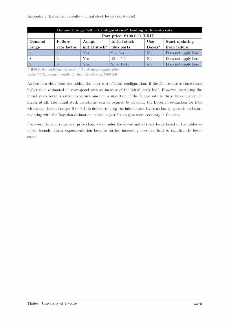
Appendix J: Experiment results – initial stock levels (worst-case)
Thales | University of Twente xxvii
Demand range 7-9: – Configurations* leading to lowest costs
Part price: €100.000 (LRU)
Demand
range
Failure
rate factor
Adapt
initial stock?
Initial stock
plus parts:
Use
Bayes?
Start updating
from failure:
7 3 Yes 9 + 3-5 No Does not apply here
8 3 Yes 13 + 5-9 No Does not apply here
9 3 Yes 21 + 13-15 No Does not apply here
* Within the confidence interval of the cheapest configuration
Table J.3 Experiment results for the price class of €100.000
As becomes clear from the tables, the most cost-efficient configurations if the failure rate is three times
higher than estimated all correspond with an increase of the initial stock level. However, increasing the
initial stock level is rather expensive since it is uncertain if the failure rate is three times higher, or
higher at all. The initial stock investment can be reduced by applying the Bayesian estimation for DUs
within the demand ranges 6 to 9. It is desired to keep the initial stock levels as low as possible and start
updating with the Bayesian estimation as late as possible to gain more certainty in the data.
For every demand range and price class, we consider the lowest initial stock levels listed in the tables as
upper bounds during experimentation because further increasing does not lead to significantly lower
costs.

Appendix K: Experiment settings – initial stock levels
Thales | University of Twente xxviii
Appendix K: Experiment settings – initial stock levels
Table K.1 below clarifies how much the initial stock level would be varied per demand range and price
class in the experiments. The upper level of the initial stock level is based on the experiment results
shown in Appendix J. The failure rate factor was 3 such that the upper levels represent the ‘’stock
buffer’’ that would be needed in a worst-case scenario. However, without foreknowledge whether the
failure rate is a factor 3 higher, or even higher at all, it might be wise to consider al failure rate factors.
That is what this experimentation is about.
Table K.2 lists the Bayesian start times to consider. Again, it depends on the demand range. As the
numbers of observed failures in certain years depend of the failure rate factor, we decide to derive the
latest/upper bound start times from the mean number of observed failures after 14 years (rounded down)
if the failure rate is 1. This means that if the failure rate is 3, this number would be encountered sooner.
If the failure rate factor is 1/3, there is no updating at all in 15 years. For this experimental variable, we
do not differentiate between the price classes.
Range
number
Demand
(year)
Initial
stock level
Initial stock
level variation
(part: €1.000)
Initial stock level
variation
(part: €50.000)
Initial stock level
variation
(part: €100.000)
1 0.02 1 0 to + 1 * *
2 0.086 2 0 to + 1 * *
3 0.241 3 0 to + 2 * *
4 0.475 4 0 to + 3 * *
5 0.774 5 0 to + 4 0 to + 1 *
6 1.125 6 0 to + 4 0 to + 2 *
7 2.406 9 0 to + 7 0 to + 4 0 to + 3
8 4.471 13 0 to + 10 0 to + 7 0 to + 5
9 9.294 21 0 to + 17 0 to + 15 0 to + 13
* Static approach had been recommended so would not be included in this experimentation phase
Table K.1 Experiment settings regarding initial stock level variation
Range
number
Demand
(year)
Mean # observed fails after year 14
if failure rate factor = 1
Start time Bayes variation
(after observed # of fails)
1 0.02 0.28 1
2 0.086 1.204 1, or 2
3 0.241 3.374 1, 2 or 3
4 0.475 6.65 1, 2… or 6
5 0.774 10.836 1, 2… or 10
6 1.125 15.57 1, 2… or 15
7 2.406 33.684 1, 2… or 71
8 4.471 62.594 1, 2… or 121
9 9.294 130.116 1, 2… or 211
1Level of variation during experimentation not based on mean number of observed failures after 14 years, but on the
mean number of observed failures after year 1 if the failure rate factor is 3. Waiting longer is not desired as the
availability in year 1 and year 2 would be dramatic such that the 90% system availability cannot be reached. The
Bayesian estimation must be applied within the first year then. Only increasing initial stock is not desired either.
Table K.2 Experiment settings regarding start time of Bayesian estimation

Appendix L: Experiment results – initial stock levels
Thales | University of Twente xxix
Appendix L: Experiment results – initial stock levels
The tables show the results of the experiments per demand range and price class. The configurations
mentioned in the tables are the most cost-efficient on average over all failure rate factors, i.e., the mean
of the total costs lays within the 95% confidence interval of the cheapest configuration.
Demand range 1-9: – Configurations* leading to lowest costs (all failure rate factors)
Part price: €1.000 (DU)
Demand
range
Adapt initial
stock?
Initial stock plus
extra part(s):
Use Bayesian
estimation?
Start updating
from failure:
1 Yes 1 + 1 Yes/No All
2 Yes 2 + 1 or 2 Yes/No All
3 Yes
Yes
Yes
3 + 1
3 + 1
3 + 2
No
Yes
No
Does not apply here
2-3
Does not apply here
4 Yes 4 + 2 or 3 No Does not apply here
5 Yes 5 + 3 or 4 No Does not apply here
6 Yes
Yes
Yes
6 + 4
6 + 4
6 + 3
No
Yes
Yes
Does not apply here
3-10
5-10
7 Yes
Yes
9 + 6 or 7
9 + 5, 6 or 7
No
Yes
Does not apply here
3-7
8 Yes
Yes
Yes
Yes
No
13 + 7
13 + 8
13 + 9
13 + 10
13 + 10
Yes
Yes
Yes
Yes
No
9-12
4-12
3-12
2-12
Does not apply here
9 Yes 21 + 14-17 Yes 4-21
* Within confidence interval of the cheapest configuration
Table L.1 Experiment results for the price class of €1.000
Demand range 5-9: – Configurations* leading to lowest costs (all failure rate factors)
Part price: €50.000 (LRU)
Demand
range
Adapt initial
stock?
Initial stock plus
extra part(s):
Use Bayesian
estimation?
Start updating
after failure:
5 No
Yes
5 + 0
5 + 1
Yes
No
1-10
Does not apply here
6 No 6 + 0 Yes 1-10
7 No
Yes
9 + 0
9 + 1
Yes
Yes
1-7
1-7
8 No
Yes
13 + 0
13 + 1
Yes
Yes
1-9
1-7
9 No
Yes
Yes
Yes
21 + 0
21 + 1
21 + 2
21 + 3
Yes
Yes
Yes
Yes
1-20
1-15
1-10
2-4
* Within confidence interval of the cheapest configuration
Table L.2 Experiment results for the price class of €50.000

Appendix L: Experiment results – initial stock levels
Thales | University of Twente xxx
Demand range 7-9: – Configurations* leading to lowest costs (all failure rate factors)
Part price: €100.000 (LRU)
Demand
range
Adapt initial
stock?
Initial stock plus
extra part(s):
Use Bayesian
estimation?
Start updating
after failure:
7 No
Yes
9 + 0
9 + 1
Yes
No
1-7
Does not apply here
8 No
Yes
Yes
13 + 0
13 + 1
13 + 1
Yes
No
Yes
1-12
Does not apply here
1-5
9 Yes 21 + 1 No Does not apply here
* Within confidence interval of the cheapest configuration
Table L.3 Experiment results for the price class of €100.000
Concluding from the tables, only increasing initial stock level without applying the Bayesian estimation
is mainly interesting for cheap parts (DUs). For these parts, you want to minimize the risk of getting
backorders and penalties as much as possible. Nevertheless, from demand range 6 on, savings in initial
stock investment can be made by applying the Bayesian estimation during the term of the service
contract. For the two highest price classes, it certainly makes sense to apply the Bayesian estimation to
save (expensive) initial stock investment without knowing whether the failure rate is even higher than
initially estimated. For some ranges, you do not even have to add initial stock.
