dynamic binding in a neural network for shape recognition
TRANSCRIPT
Psychological Review1992. Vol. 99, No. 3, 480-517
Copyright 1992 by the American Psychological Association, Inc.0033-295X/92/S3.00
Dynamic Binding in a Neural Network for Shape Recognition
John E. Hummel and Irving BiedermanUniversity of Minnesota, Twin Cities
Given a single view of an object, humans can readily recognize that object from other views thatpreserve the parts in the original view. Empirical evidence suggests that this capacity reflects theactivation of a viewpoint-invariant structural description specifying the object's parts and therelations among them. This article presents a neural network that generates such a description.Structural description is made possible through a solution to the dynamic binding problem: Tempo-rary conjunctions of attributes (parts and relations) are represented by synchronized oscillatoryactivity among independent units representing those attributes. Specifically, the model usessynchrony (a) to parse images into their constituent parts, (b) to bind together the attributes of apart, and (c) to bind the relations to the parts to which they apply. Because it conjoins independentunits temporarily, dynamic binding allows tremendous economy of representation and permits therepresentation to reflect the attribute structure of the shapes represented.
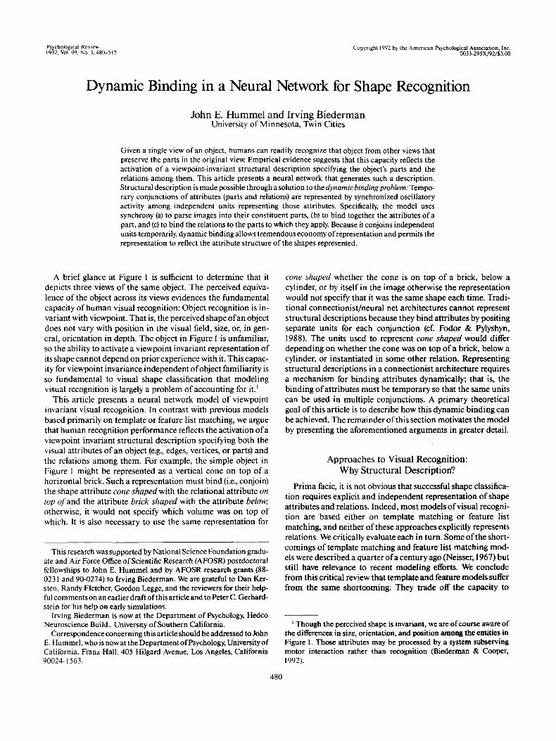
A brief glance at Figure 1 is sufficient to determine that itdepicts three views of the same object. The perceived equiva-lence of the object across its views evidences the fundamentalcapacity of human visual recognition: Object recognition is in-variant with viewpoint. That is, the perceived shape of an objectdoes not vary with position in the visual field, size, or, in gen-eral, orientation in depth. The object in Figure 1 is unfamiliar,so the ability to activate a viewpoint invariant representation ofits shape cannot depend on prior experience with it. This capac-ity for viewpoint invariance independent of object familiarity isso fundamental to visual shape classification that modelingvisual recognition is largely a problem of accounting for it.1
This article presents a neural network model of viewpointinvariant visual recognition. In contrast with previous modelsbased primarily on template or feature list matching, we arguethat human recognition performance reflects the activation of aviewpoint invariant structural description specifying both thevisual attributes of an object (e.g., edges, vertices, or parts) andthe relations among them. For example, the simple object inFigure 1 might be represented as a vertical cone on top of ahorizontal brick. Such a representation must bind (i.e., conjoin)the shape attribute cone shaped with the relational attribute ontop of and the attribute brick shaped with the attribute below;otherwise, it would not specify which volume was on top ofwhich. It is also necessary to use the same representation for
This research was supported by National Science Foundation gradu-ate and Air Force Office of Scientific Research (AFOSR) postdoctoralfellowships to John E. Hummel and by AFOSR research grants (88-0231 and 90-0274) to Irving Biederman. We are grateful to Dan Ker-sten, Randy Fletcher, Gordon Legge, and the reviewers for their help-ful comments on an earlier draft of this article and to Peter C. Gerhard-stein for his help on early simulations.
Irving Biederman is now at the Department of Psychology, HedcoNeuroscience Build., University of Southern California.
Correspondence concerning this article should be addressed to JohnE. Hummel, who is now at the Department of Psychology, University ofCalifornia, Franz Hall, 405 Hilgard Avenue, Los Angeles, California90024-1563.
cone shaped whether the cone is on top of a brick, below acylinder, or by itself in the image otherwise the representationwould not specify that it was the same shape each time. Tradi-tional connectionist/neural net architectures cannot representstructural descriptions because they bind attributes by positingseparate units for each conjunction (cf. Fodor & Pylyshyn,1988). The units used to represent cone shaped would differdepending on whether the cone was on top of a brick, below acylinder, or instantiated in some other relation. Representingstructural descriptions in a connectionist architecture requiresa mechanism for binding attributes dynamically; that is, thebinding of attributes must be temporary so that the same unitscan be used in multiple conjunctions. A primary theoreticalgoal of this article is to describe how this dynamic binding canbe achieved. The remainder of this section motivates the modelby presenting the aforementioned arguments in greater detail.
Approaches to Visual Recognition:Why Structural Description?
Prima facie, it is not obvious that successful shape classifica-tion requires explicit and independent representation of shapeattributes and relations. Indeed, most models of visual recogni-tion are based either on template matching or feature listmatching, and neither of these approaches explicitly representsrelations. We critically evaluate each in turn. Some of the short-comings of template matching and feature list matching mod-els were described a quarter of a century ago (Neisser, 1967) butstill have relevance to recent modeling efforts. We concludefrom this critical review that template and feature models sufferfrom the same shortcoming: They trade off the capacity to
1 Though the perceived shape is invariant, we are of course aware ofthe differences in size, orientation, and position among the entities inFigure 1. Those attributes may be processed by a system subservingmotor interaction rather than recognition (Biederman & Cooper,1992).
480
NEURAL NETWORK FOR SHAPE RECOGNITION 481
Figure 1. This object is readily detectable as constant across the threeviews despite its being unfamiliar.
represent attribute structures with the capacity to represent re-lations.
Template Matching
Template matching models operate by comparing an incom-ing image (perhaps after filtering, noise reduction, etc.) againsta template, a representation of a specific view of an object. Toachieve viewpoint invariant recognition, a template modelmust either (a) store a very large number of views (templates) foreach known object or (b) store a small number of views (or 3-Dmodels) for each object and match them against incomingimages by means of transformations such as translation, scal-ing, and rotation. Recognition succeeds when a template isfound that fits the image within a tolerable range of error. Tem-plate models have three main properties: (a) The fit between astimulus and a template is based on the extent to which activeand inactive points2 in the image spatially correspond to activeand inactive points in the template; (b) a template is used torepresent an entire view of an object, spatial relations amongpoints in the object coded implicitly as spatial relations amongpoints in the template; and (c) viewpoint invariance is a func-tion of object classification. Different views of an object areseen as equivalent when they access the same object label (i.e.,either by matching the same template or by matching differenttemplates with pointers to the same object label).
Template matching currently enjoys considerable popularityin computer vision (e.g., Edelman & Poggio, 1990; Lowe, 1987;Ullman, 1989). These models can recognize objects under dif-ferent viewpoints, and some can even find objects in clutteredscenes. However, they evidence severe shortcomings as modelsof human recognition. First, recall that template matching suc-ceeds or fails according to the number of points that mismatchbetween an image and a stored template and therefore predictslittle effect of where the mismatch occurs. (An exception to thisgeneralization can be found in alignment models, such as thoseof Ullman, 1989, and Lowe, 1987. If enough critical alignment
points are deleted from an image—in Oilman's model, threeare required to compute an alignment—the alignment processwill fail. However, provided alignment can be achieved, thedegree of match is proportional to the number of correspond-ing points.) Counter to this prediction, Biederman (1987b)showed that human recognition performance varied greatly de-pending on the locus of contour deletion. Similarly, Biedermanand Cooper (199 Ib) showed that an image formed by removinghalf the vertices and edges from each of an object's parts (Figure2a) visually primed3 its complement (the image formed fromthe deleted contour, Figure 2b) as much as it primed itself, butan image formed by deleting half of the parts (Figure 2c) did notvisually prime its complement at all (Figure 2d). Thus, visualpriming was predicted by the number of parts shared by twoimages, not by the amount of contour.
Second, template models handle image transformations suchas translation, rotation, expansion, and compression by apply-ing an equivalent transformation to the template. Presumably,such transformations would require time. However, Biedermanand Cooper (1992) showed no loss in the magnitude of visualpriming for naming object images that differed in position,size, or mirror image reflection from their original presenta-tion. Similarly, Gerhardstein and Biederman (1991) showed noloss in visual priming for objects rotated in depth (up to partsocclusion).
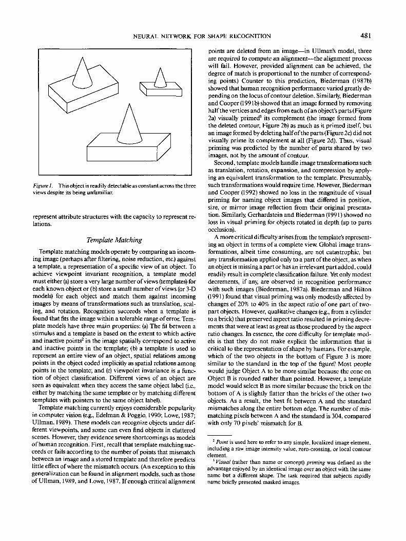
A more critical difficulty arises from the template's represent-ing an object in terms of a complete view. Global image trans-formations, albeit time consuming, are not catastrophic, butany transformation applied only to a part of the object, as whenan object is missing a part or has an irrelevant part added, couldreadily result in complete classification failure. Yet only modestdecrements, if any, are observed in recognition performancewith such images (Biederman, 1987a). Biederman and Hilton(1991) found that visual priming was only modestly affected bychanges of 20% to 40% in the aspect ratio of one part of two-part objects. However, qualitative changes (e.g., from a cylinderto a brick) that preserved aspect ratio resulted in priming decre-ments that were at least as great as those produced by the aspectratio changes. In essence, the core difficulty for template mod-els is that they do not make explicit the information that iscritical to the representation of shape by humans. For example,which of the two objects in the bottom of Figure 3 is moresimilar to the standard in the top of the figure? Most peoplewould judge Object A to be more similar because the cone onObject B is rounded rather than pointed. However, a templatemodel would select B as more similar because the brick on thebottom of A is slightly flatter than the bricks of the other twoobjects. As a result, the best fit between A and the standardmismatches along the entire bottom edge. The number of mis-matching pixels between A and the standard is 304, comparedwith only 70 pixels' mismatch for B.
2 Point is used here to refer to any simple, localized image element,including a raw image intensity value, zero-crossing, or local contourelement.
3 Visual (rather than name or concept) priming was defined as theadvantage enjoyed by an identical image over an object with the samename but a different shape. The task required that subjects rapidlyname briefly presented masked images.
482 JOHN E. HUMMEL AND IRVING BIEDERMAN
a.
Figure 2. Examples of contour-deleted images used in the Bieder-man and Cooper (1991 b) priming experiments, (a: An image of a pianoas it might appear in the first block of the experiment in which half theimage contour was removed from each of the piano's parts by remov-ing every other edge and vertex. Long edges were treated as two seg-ments, b: The complement to Panel a formed from the contours re-moved from Panel a. c: An image of a piano as it might appear in thefirst block of trials in the experiment in which half the parts weredeleted from the piano, d: The complement to Panel c formed from theparts deleted from Panel c. From "Priming Contour-Deleted Images:Evidence for Intermediate Representations in Visual Object Recogni-tion" by I. Biederman & E. E. Cooper, 1991, Cognitive Psychology, 23,Figures 1 and 4, pp. 397, 403. Copyright 1991 by Academic Press.Adapted by permission.)
Another difficulty with templates—one that has been partic-ularly influential in the computer vision community—is theircapacity to scale with large numbers of objects. In particular,the critical alignment features used to select candidate tem-plates in Ullman's (1989) and Lowe's (1987) models may bedifficult to obtain when large numbers of templates must bestored and differentiated. Finally, a fundamental difficultywith template matching as a theory of human recognition isthat a template model must have a stored representation of anobject before it can classify two views of it as equivalent. Assuch, template models cannot account for viewpoint invariancein unfamiliar objects. Pinker (1986) presented several otherproblems with template models.
The difficulties with template models result largely fromtheir insensitivity to attribute structures. Because the template'sunit of analysis is a complete view of an object, it fails to explic-itly represent the individual attributes that define the object'sshape. The visual similarity between different images is lost inthe classification process. An alternative approach to recog-nition, motivated largely by this shortcoming, is featurematching.
Feature Matching
Feature matching models extract diagnostic features from animage and use those as the basis for recognition (e.g., Hinton,
1981; Hummel, Biederman, Gerhardstein, & Hilton, 1988;Lindsay & Norman, 1977; Selfridge, 1959; Selfridge & Neisser,1960). These models differ from template models on each ofthe three main properties listed previously: (a) Rather thanoperating on pixels, feature matching operates on higher orderimage attributes such as parts, surfaces, contours, or vertices;(b) rather than classifying images all at once, feature modelsdescribe images in terms of multiple independent attributes;and (c) visual equivalence consists of deriving an equivalent setof visual features, not necessarily accessing the same final ob-ject representation. Feature matching is not subject to the sameshortcomings as template matching. Feature matching modelscan differentially weight different classes of image features, forexample, by giving more weight to vertices than contour mid-segments; they can deal with transformations at the level ofparts of an image; and they can respond in an equivalent man-ner to different views of novel objects.
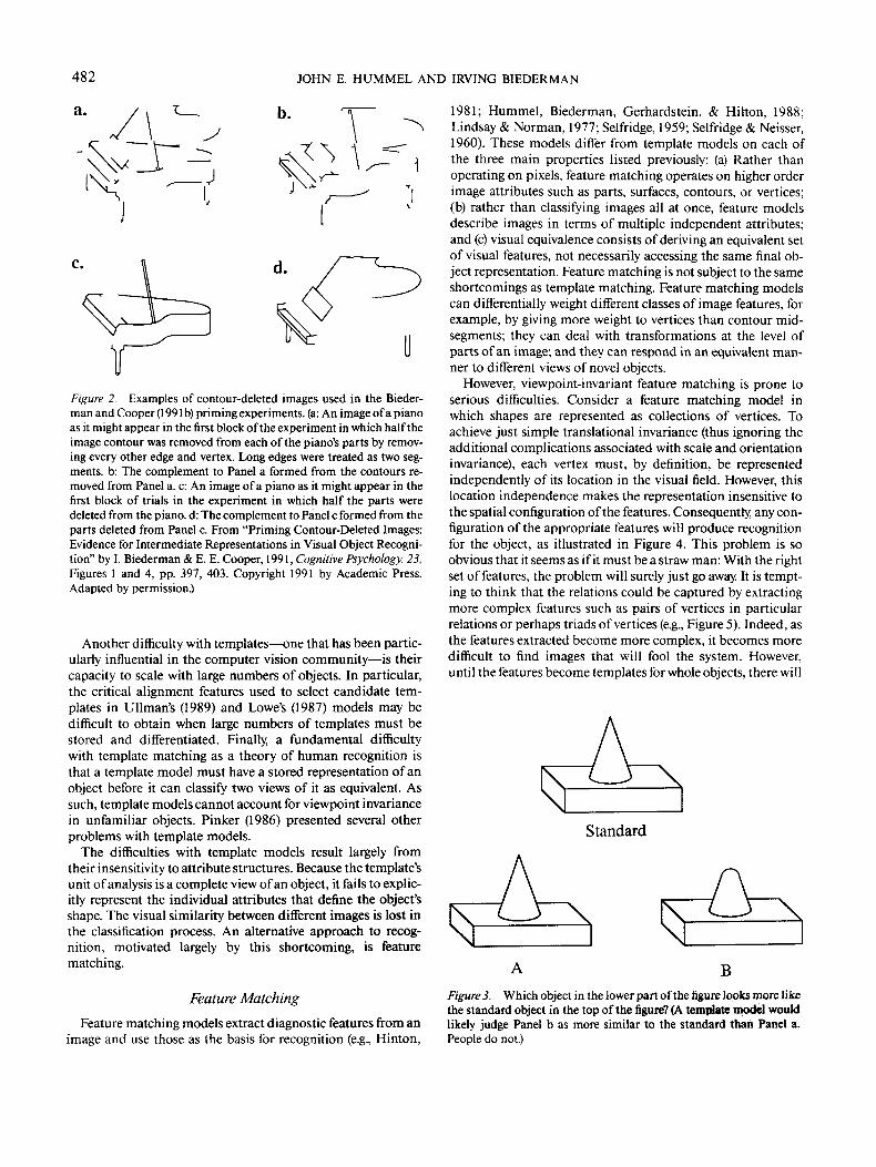
However, viewpoint-invariant feature matching is prone toserious difficulties. Consider a feature matching model inwhich shapes are represented as collections of vertices. Toachieve just simple translational invariance (thus ignoring theadditional complications associated with scale and orientationinvariance), each vertex must, by definition, be representedindependently of its location in the visual field. However, thislocation independence makes the representation insensitive tothe spatial configuration of the features. Consequently, any con-figuration of the appropriate features will produce recognitionfor the object, as illustrated in Figure 4. This problem is soobvious that it seems as if it must be a straw man: With the rightset of features, the problem will surely just go away. It is tempt-ing to think that the relations could be captured by extractingmore complex features such as pairs of vertices in particularrelations or perhaps triads of vertices (e.g., Figure 5). Indeed, asthe features extracted become more complex, it becomes moredifficult to find images that will fool the system. However,until the features become templates for whole objects, there will
Standard
A BFigure 3. Which object in the lower part of the figure looks more likethe standard object in the top of the figure? (A template model wouldlikely judge Panel b as more similar to the standard than Panel a.People do not.)
NEURAL NETWORK FOR SHAPE RECOGNITION 483
Image TranslationallyInvariant Features
Memory
Curved L vertex
Arrow vertexObjectLabel
Curved L vertex
Arrow vertex ObjectLabel
Fork vertex
Figure 4. Illustration of illusory recognition with translationally in-variant feature list matching on the basis of vertices. (Both imagescontain the same vertices and will therefore produce recognition forthe object.)
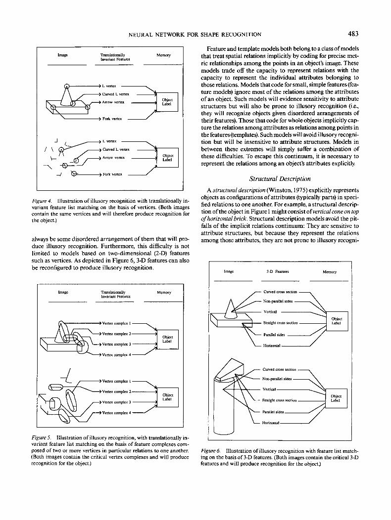
always be some disordered arrangement of them that will pro-duce illusory recognition. Furthermore, this difficulty is notlimited to models based on two-dimensional (2-D) featuressuch as vertices. As depicted in Figure 6, 3-D features can alsobe reconfigured to produce illusory recognition.
Image TranslationallyInvariant Features
^ Vertex complex 1 -
Vertex complex 2 -
Vertex complex 3 -
Vertex complex 4 -
Memory
ObjectLabel
Vertex complex 1
Vertex complex 2
Vertex complex 3
Vertex complex 4
Figure 5. Illustration of illusory recognition, with translationally in-variant feature list matching on the basis of feature complexes com-posed of two or more vertices in particular relations to one another.(Both images contain the critical vertex complexes and will producerecognition for the object.)
Feature and template models both belong to a class of modelsthat treat spatial relations implicitly by coding for precise met-ric relationships among the points in an object's image. Thesemodels trade off the capacity to represent relations with thecapacity to represent the individual attributes belonging tothose relations. Models that code for small, simple features (fea-ture models) ignore most of the relations among the attributesof an object. Such models will evidence sensitivity to attributestructures but will also be prone to illusory recognition (i.e.,they will recognize objects given disordered arrangements oftheir features). Those that code for whole objects implicitly cap-ture the relations among attributes as relations among points inthe features (templates). Such models will avoid illusory recogni-tion but will be insensitive to attribute structures. Models inbetween these extremes will simply suffer a combination ofthese difficulties. To escape this continuum, it is necessary torepresent the relations among an object's attributes explicitly.
Structural Description
A structural description (Winston, 1975) explicitly representsobjects as configurations of attributes (typically parts) in speci-fied relations to one another. For example, a structural descrip-tion of the object in Figure 1 might consist of vertical cone on topof horizontal brick. Structural description models avoid the pit-falls of the implicit relations continuum: They are sensitive toattribute structures, but because they represent the relationsamong those attributes, they are not prone to illusory recogni-
Image 3-D Features
Curved cross section
Non-parallel sides —
Vertical
Memory
Straight cross section
Parallel sides
Horizontal —
Curved cross section -
Non-parallel sides -
Vertical
Straight cross section -
Parallel sides
Horizontal
Figure 6. Illustration of illusory recognition with feature list match-ing on the basis of 3-D features. (Both images contain the critical 3-Dfeatures and will produce recognition for the object.)
484 JOHN E. HUMMEL AND IRVING BIEDERMAN
tion. These models can also provide a natural account of thefundamental characteristics of human recognition. Providedthe elements of the structural description are invariant withviewpoint, recognition on the basis of that description will alsobe invariant with viewpoint. Provided the description can beactivated bottom up on the basis of information in the 2-Dimage, the luxury of viewpoint invariance will be enjoyed forunfamiliar objects as well as familiar ones.
Proposing that object recognition operates on the basis ofviewpoint-invariant structural descriptions allows us to under-stand phenomena that extant template and feature theoriescannot handle. However, it is necessary to address how thevisual system could possibly derive a structural description inthe first place. This article presents an explicit theory, imple-mented as a connectionist network, of the processes and repre-sentations implicated in the derivation of viewpoint-invariantstructural descriptions for object recognition. The point of de-parture for this effort is Biederman's (1987b) theory of recogni-tion by components (RBC). RBC states that objects are recog-nized as configurations of simple, primitive volumes calledgeons in specified relations with one another. Geons are recog-nized from 2-D viewpoint-invariant4 properties of image con-tours such as whether a contour is straight or curved, whether apair of contours is parallel or nonparallel, and what type ofvertex is produced where contours coterminate. The geons de-rived from these 2-D contrasts are defined in terms of view-point-invariant 3-D contrasts such as whether the cross-sectionis straight (like that of a brick or a pyramid) or curved (like thatof a cylinder or a cone) and whether the sides are parallel (likethose of a brick) or nonparallel (like those of a wedge).
Whereas a template representation necessarily commits thetheorist to a coordinate space, 2-D or 3-D, the structural de-scription theory proposed here does not. This is important tonote because structural descriptions have been criticized forassuming a metrically specified representation in a 3-D object-centered coordinate space. Failing to find evidence for 3-D in-variant recognition for some unfamiliar objects, such as crum-pled paper (Rock & DiVita, 1987), bent wires (Edelman &Weinshall, 1991; Rock & DiVita, 1987), and rectilinear arrange-ments of bricks (Tarr & Pinker, 1989), some researchers haverejected structural description theories in favor of representa-tions based on multiple 2-D views. But the wholesale rejectionof structural descriptions on the basis of such data is un-warranted. RBC (and the implementation proposed here) pre-dict these results. Because a collection of similarly bent wires,for example, tend not to activate distinctive viewpoint-invariantstructural descriptions that allow one wire to be distinguishedfrom the other wires in the experiment, such objects should bedifficult to recognize from an arbitrary viewpoint.
ute conjunctions (Feldman, 1982; Feldman & Ballard, 1982;Hinton, McClelland, & Rumelhart, 1986; Sejnowski, 1986;Smolensky, 1987; von der Malsburg, 1981). Recall that a struc-tural description of the nonsense object in Figure 1 must spec-ify that vertical and on top o/are bound with cone shaped,whereas horizontal and below are bound with brick shaped. Thisproblem is directly analogous to the problem encountered bythe feature matching models: Given that some set of attributesis present in the system's input, how can it represent whetherthey are in the proper configuration to define a given object?
The predominant class of solutions to this problem is con-junctive coding (Hinton et al., 1986) and its relatives, such astensor product coding (Smolensky, 1987), and the interunits ofFeldman's (1982) dynamic connections network. A conjunctiverepresentation anticipates attribute conjunctions and allocatesa separate unit or pattern for each. For example, a conjunctiverepresentation for the previously mentioned shape attributeswould posit one pattern for vertical cone on top of and com-pletely separate patterns for horizontal cone on top of, horizontalcone below, and so forth. A fully local conjunctive representation(i.e., one in which each conjunction is coded by a single unit) canprovide an unambiguous solution to the binding problem: Onthe basis of which units are active, it is possible to know exactlyhow the attributes are conjoined in the system's input. Verticalcone on top of horizontal brick and vertical brick on top of horizon-tal cone would activate nonoverlapping sets of units. However,local conjunctive representations suffer a number of shortcom-ings.
The most apparent difficulty with local conjunctive represen-tations is the number of units they require: The size of such arepresentation grows exponentially with the number of attrib-ute dimensions to be represented (e.g., 10 dimensions, each with5 values would require 510 units). As such, the number of unitsrequired to represent the universe of possible conjunctions canbe prohibitive for complex representations. Moreover, the unitshave to be specified in advance, and most of them will go un-used most of the time. However, from the perspective of repre-senting structural descriptions, the most serious problem withlocal conjunctive representations is their insensitivity to attrib-ute structures. Like a template, a local conjunctive unit re-sponds to a specific conjunction of attributes in an all-or-nonefashion, with different conjunctions activating different units.The similarity in shape between, say, a cone that is on top ofsomething and a cone that is beneath something is lost in such arepresentation.
These difficulties with local conjunctive representations willnot come as a surprise to many readers. In defense of conjunc-tive coding, one may reasonably protest that a fully local con-junctive representation represents the worst case, both in terms
Connectionist Representation and StructuralDescription: The Binding Problem
Given a line drawing of an object, the goal of the currentmodel is to activate a viewpoint-invariant structural descrip-tion5 of the object and then use that description as the basis forrecognition. Structural descriptions are particularly challeng-ing to represent in connectionist architectures because of thebinding problem. Binding refers to the representation of attrib-
4 The term viewpoint invariant as used here refers to the tendency ofthe image feature's classification to remain unchanged under changesin viewpoint. For instance, the degree of curvature associated with theimage of the rim of a cup will change as the cup is rotated in depthrelative to the viewer. However, the fact that edge is curved rather thanstraight will remain unchanged in all but a few accidental views of thecup.
5 Henceforth, it is assumed that the elements of the structural de-scription are geons and their relations.
NEURAL NETWORK FOR SHAPE RECOGNITION 485
of the number of units required and in terms of the loss ofattribute structures. Both these problems can be attenuated con-siderably by using coarse coding and other techniques for dis-tributing the representation of an entity over several units (Feld-man, 1982; Hinton et al., 1986; Smolensky, 1987). However, inthe absence of a technique for representing attribute bindings,distributed representations are subject to cross talk (i.e., mutualinterference among independent patterns), the likelihood ofwhich increases with the extent of distribution. Specifically,when multiple entities are represented simultaneously, the likeli-hood that the units representing one entity will be confusedwith the units representing another grows with the proportionof the network used to represent each entity, von der Malsburg(1987) referred to this familiar manifestation of the bindingproblem as the superposition catastrophe. Thus, the costs of aconjunctive representation can be reduced by using a distrib-uted representation, but without alternative provisions for bind-ing the benefits are also reduced.
This tradeoff between unambiguous binding and distributedrepresentation is the connectionist's version of the implicit rela-tions continuum. In this case, however, the relations that arecoded implicitly (i.e., in the responses of conjunctive units) arebinding relations. Escaping this continuum requires a way torepresent bindings dynamically. That is, we need a way to tem-porarily and explicitly bind independent units when the attrib-utes for which they code occur in conjunction.
Recently, there has been considerable interest in the use oftemporal synchrony as a potential solution to this problem. Thebasic idea, proposed as early as 1974 by Peter Milner (Milner,1974), is that conjunctions of attributes can be represented bysynchronizing the outputs of the units (or cells) representingthose attributes. To represent that Attribute A is bound to At-tribute B and Attribute C to Attribute D, the cells for A and Bfire in synchrony, the cells for C and D fire in synchrony, and theAB set fires out of synchrony with the CD set. This suggestionhas since been presented more formally by von der Malsburg(1981, 1987) and many others (Abeles, 1982; Atiya & Baldi,1989; Baldi & Meir, 1990; Crick, 1984; Crick & Koch, 1990;Eckhorn et al., 1988; Eckhorn, Reitboeck, Arndt, & Dicke,1990; Gray et al, 1989; Gray & Singer, 1989; Grossberg &Somers, 1991; Hummel & Biederman, 1990a; Shastri & Ajjana-gadde, 1990; Strong & Whitehead, 1989; Wang, Buhmann, &von der Malsburg, 1991).
Dynamic binding has particularly important implicationsfor the task of structural description because it makes it possi-ble to bind the elements of a distributed representation. What iscritical about the use of synchrony in this capacity is that itprovides a degree of freedom whereby multiple independentcells can specify that the attributes to which they respond arecurrently bound. In principle, any variable could serve this pur-pose (e.g., Lange & Dyer, 1989, used signature activations), sothe use of synchrony, per se, is not theoretically critical. Tem-poral synchrony simply seems a natural choice because it is easyto establish, easy to exploit, and neurologically plausible.
This article presents an original proposal for exploitingsynchrony to bind shape and relation attributes into structuraldescriptions. Specialized connections in the model's first twolayers parse images into geons by synchronizing the oscillatoryoutputs of cells representing local image features (edges and
vertices): Cells oscillate in phase if they represent features of thesame geon and out of phase if they represent features of sepa-rate geons. These phase relations are preserved throughout thenetwork and bind cells representing the attributes of geons andthe relations among them. The bound attributes and relationsconstitute a simple viewpoint-invariant structural descriptionof an object. The model's highest layers use this description as abasis for object recognition.
The model described here is broad in scope, and we havemade only modest attempts to optimize any of its individualcomponents. Rather, the primary theoretical statement con-cerns the general nature of the representations and processesimplicated in the activation of viewpoint-invariant structuraldescriptions for real-time object recognition. We have designedthese representations and processes to have a transparentneural analogy, but we make no claims as to their strict neuralrealism.
A Neural Net Model of Shape Recognition
Overview
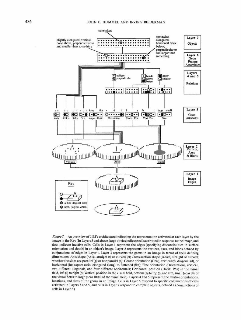
The model (JIM; John and Irv's model) is a seven-layer con-nectionist network that takes as input a representation of a linedrawing of an object (specifying discontinuities in surface orien-tation and depth) and, as output, activates a unit representingthe identity of the object. The model achieves viewpoint invar-iance in that the same output unit will respond to an objectregardless of where its image appears in the visual field, the sizeof the image, and the orientation in depth from which the ob-ject is depicted. An overview of the model's architecture isshown in Figure 7. JIM's first layer (LI) is a mosaic of orienta-tion-tuned cells with overlapping receptive fields. The secondlayer (L2) is a mosaic of cells that respond to vertices, 2-D axesof symmetry, and oriented, elongated blobs of activity. Cells inLI and L2 group themselves into sets describing geons bysynchronizing oscillations in their outputs.
Cells in L3 respond to attributes of complete geons, each cellrepresenting a single value on a single dimension over which thegeons can vary. For example, the shape of a geon's major axis(straight or curved) is represented in one bank of cells, and thegeon's location is represented in another, thereby allowing therepresentation of the geon's axis to remain unchanged when thegeon is moved in the visual field. The fourth and fifth layers(L4 and L5) determine the relations among the geons in animage. The L4-L5 module receives input from L3 cells repre-senting the metric properties of geons (location in the visualfield, size, and orientation). Once active, units representing rela-tions are bound to the geons they describe by the same phaselocking that binds image features together for geon recognition.The output of L3 and L5 together constitute a structural de-scription of an object in terms of its geons and their relations.This representation is invariant with scale, translation, and ori-entation in depth.
The model's sixth layer (L6) takes its input from both thethird and fifth layers. On a single time slice (ts), the input to L6is a pattern of activation describing one geon and its relations tothe other geons in the image (a geon feature assembly). Each cellin L6 responds to a particular geon feature assembly. The cells
486 JOHN E. HUMMEL AND IRVING BIEDERMAN
nuke plant
slightly elongated, verticalcone above, perpendicular toand smaller than something
somewhatelongated,horizontal brickbelow,
/perpendicular toand larger than
• • »O *f* something» • • • • • • • • • • • • • • • • •£• • °
largersmaller
s c s c p n v d h long luit v
Layer 7
Objects
Layer 6Geon
FeatureAssemblies
Layers4 and 5
Relations
Axis X-Scn Sides Orn. Aspect Rnlio Orientation Horiz. Pos. Vert. Pos. Size
either (logical OR)
both (logical AND)
Figure 7. An overview of JIM's architecture indicating the representation activated at each layer by theimage in the Key. (In Layers 3 and above, large circles indicate cells activated in response to the image, anddots indicate inactive cells. Cells in Layer 1 represent the edges (specifying discontinuities in surfaceorientation and depth) in an object's image. Layer 2 represents the vertices, axes, and blobs denned byconjunctions of edges in Layer 1. Layer 3 represents the geons in an image in terms of their definingdimensions: Axis shape (Axis), straight (s) or curved (c); Cross-section shape (X-Scn) straight or curved;whether the sides are parallel (p) or nonparallel (n); Coarse orientation (Orn.), vertical (v), diagonal (d), orhorizontal (h); aspect ratio, elongated (long) to flattened (flat); Fine orientation (Orientation), vertical,two different diagonals, and four different horizontals; Horizontal position (Horiz. Pos.) in the visualfield, left (1) to right (r); Vertical position in the visual field, bottom (b) to top (t); and size, small (near 0% ofthe visual field) to large (near 100% of the visual field). Layers 4 and 5 represent the relative orientations,locations, and sizes of the geons in an image. Cells in Layer 6 respond to specific conjunctions of cellsactivated in Layers 3 and 5, and cells in Layer 7 respond to complete objects, defined as conjunctions ofcells in Layer 6.)
NEURAL NETWORK FOR SHAPE RECOGNITION 487
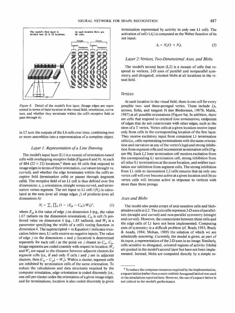
The model's first layer is At each location there aredivided into 22 X 22 locations. 48 cells.
Segment SegmentTermination T Termination
Figure 8. Detail of the model's first layer. (Image edges are repre-sented in terms of their location in the visual field, orientation, curva-ture, and whether they terminate within the cell's receptive field orpass through it.)
in L7 sum the outputs of the L6 cells over time, combining twoor more assemblies into a representation of a complete object.
Layer 1: Representation of a Line Drawing
The model's input layer (LI) is a mosaic of orientation-tunedcells with overlapping receptive fields (Figures 8 and 9). At eachof 484 (22 X 22) locations,6 there are 48 cells that respond toimage edges in terms of their orientation, curvature (straight vs.curved), and whether the edge terminates within the cell's re-ceptive field (termination cells) or passes through (segmentcells). The receptive field of an LI cell is thus defined over fivedimensions: x, y, orientation, straight versus curved, and termi-nation versus segment. The net input to LI cell i (Nt) is calcu-lated as the sum (over all image edges j) of products (over alldimensions k):
- \Ejk-cik\/wk)\ (1)where Ejk is the value of edge j on dimension k (e.g., the value1.67 radians on the dimension orientation), Cik is cell ;'s pre-ferred value on dimension k (e.g., 1.85 radians), and Wk is aparameter specifying the width of a cell's tuning function indimension k. The superscripted + in Equation 1 indicates trun-cation below zero; LI cells receive no negative inputs. The valueof edge j on the dimensions x and y (location) is determinedseparately for each cell / as the point on j closest to Cix, Ciy.Image segments are coded coarsely with respect to location: Wx
and Wy are equal to the distance between adjacent clusters forsegment cells (i.e., if and only if cells i and j are in adjacentclusters, then \Cix - Cjx\ = Wx). Within a cluster, segment cellsare inhibited by termination cells of the same orientation. Toreduce the calculations and data structures required by thecomputer simulation, edge orientation is coded discretely (i.e.,one cell per cluster codes the orientation of a given image edge),and for terminations, location is also coded discretely (a given
termination represented by activity in only one LI cell). Theactivation of cell / (A,) is computed as the Weber function of itsnet input:
A, = NJ(l + N,). (2)
Layer 2: Vertices, Two-Dimensional Axes, and Blobs
The model's second layer (L2) is a mosaic of cells that re-spond to vertices, 2-D axes of parallel and nonparallel sym-metry, and elongated, oriented blobs at all locations in the vi-sual field.
Vertices
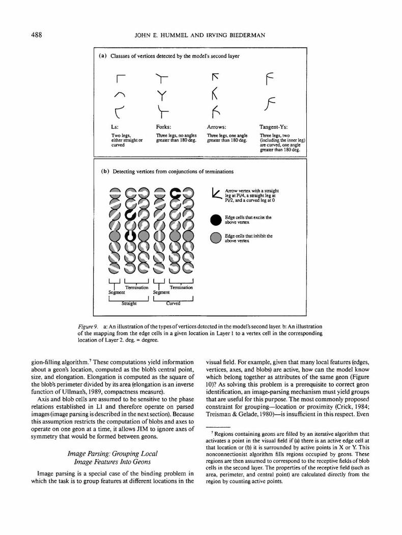
At each location in the visual field, there is one cell for everypossible two- and three-pronged vertex. These include Ls,arrows, forks, and tangent 7s (see Biederman, 1987b; Malik,1987) at all possible orientations (Figure 9a). In addition, thereare cells that respond to oriented lone terminations, endpointsof edges that do not coterminate with other edges, such as thestem of a T vertex. Vertex cells at a given location receive inputonly from cells in the corresponding location of the first layer.They receive excitatory input from consistent LI terminationcells (i.e., cells representing terminations with the same orienta-tion and curvature as any of the vertex's legs) and strong inhibi-tion from segment cells and inconsistent termination cells (Fig-ure 9b). Each L2 lone termination cell receives excitation fromthe corresponding LI termination cell, strong inhibition fromall other LI terminations at the same location, and neither exci-tation nor inhibition from segment cells. The strong inhibitionfrom LI cells to inconsistent L2 cells ensures that (a) only onevertex cell will ever become active at a given location and (b) novertex cells will become active in response to vertices withmore than three prongs.
Axes and Blobs
The model also posits arrays of axis-sensitive cells and blob-sensitive cells in L2. The axis cells represent 2-D axes of parallel-ism (straight and curved) and non-parallel symmetry (straightand curved). However, the connections between these cells andthe edge cells of LI have not been implemented. Computingaxes of symmetry is a difficult problem (cf. Brady, 1983; Brady& Asada, 1984; Mohan, 1989) the solution of which we areadmittedly assuming. Currently, the model is given, as part ofits input, a representation of the 2-D axes in an image. Similarly,cells sensitive to elongated, oriented regions of activity (blobs)are posited in the model's second layer but have not been imple-mented. Instead, blobs are computed directly by a simple re-
6 To reduce the computer resources required by the implementation,a square lattice (rather than a more realistic hexagonal lattice) was usedin the simulations reported here. However, the use of a square lattice isnot critical to the model's performance.
488 JOHN E. HUMMEL AND IRVING BIEDERMAN
(a) Classses of vertices detected by the model's second layer
r
Ls:
Two legs,either straight orcurved
VYV
Forks: Arrows: Tangent-Ys:
Three legs, no angles Three legs, one angle Three legs, twogreater than 180 deg. greater than 180 deg. (including the inner leg)
are curved, one anglegreater than 180 deg.
(b) Detecting vertices from conjunctions of terminations
k. Arrow vertex with a straightleg at Pi/4, a straight leg atPi/2, and a curved leg at 0
Edge cells that excite theabove vertex
O Edge cells that inhibit theabove vertex
Termination | TerminationSegment Segment
I I I IStraight Curved
Figure 9. a: An illustration of the types of vertices detected in the model's second layer, b: An illustrationof the mapping from the edge cells in a given location in Layer 1 to a vertex cell in the correspondinglocation of Layer 2. deg. = degree.
gion-filling algorithm.7 These computations yield informationabout a geon's location, computed as the blob's central point,size, and elongation. Elongation is computed as the square ofthe blob's perimeter divided by its area (elongation is an inversefunction of Ullman's, 1989, compactness measure).
Axis and blob cells are assumed to be sensitive to the phaserelations established in LI and therefore operate on parsedimages (image parsing is described in the next section). Becausethis assumption restricts the computation of blobs and axes tooperate on one geon at a time, it allows JIM to ignore axes ofsymmetry that would be formed between geons.
Image Parsing: Grouping LocalImage features Into Geons
Image parsing is a special case of the binding problem inwhich the task is to group features at different locations in the
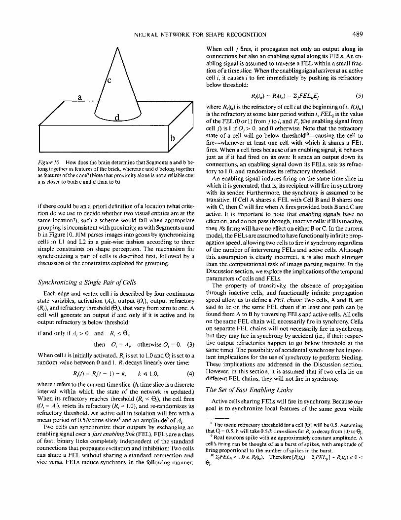
visual field. For example, given that many local features (edges,vertices, axes, and blobs) are active, how can the model knowwhich belong together as attributes of the same geon (Figure10)? As solving this problem is a prerequisite to correct geonidentification, an image-parsing mechanism must yield groupsthat are useful for this purpose. The most commonly proposedconstraint for grouping—location or proximity (Crick, 1984;Treisman & Gelade, 1980)—is insufficient in this respect. Even
7 Regions containing geons are filled by an iterative algorithm thatactivates a point in the visual field if (a) there is an active edge cell atthat location or (b) it is surrounded by active points in X or Y Thisnonconnectionist algorithm fills regions occupied by geons. Theseregions are then assumed to correspond to the receptive fields of blobcells in the second layer. The properties of the receptive field (such asarea, perimeter, and central point) are calculated directly from theregion by counting active points.
NEURAL NETWORK FOR SHAPE RECOGNITION 489
Figure 10. How does the brain determine that Segments a and b be-long together as features of the brick, whereas c and d belong togetheras features of the cone? (Note that proximity alone is not a reliable cue:a is closer to both c and d than to b.)
if there could be an a priori definition of a location (what crite-rion do we use to decide whether two visual entities are at thesame location?), such a scheme would fail when appropriategrouping is inconsistent with proximity, as with Segments a andb in Figure 10. JIM parses images into geons by synchronizingcells in LI and L2 in a pair-wise fashion according to threesimple constraints on shape perception. The mechanism forsynchronizing a pair of cells is described first, followed by adiscussion of the constraints exploited for grouping.
Synchronizing a Single Pair of Cells
Each edge and vertex cell /' is described by four continuousstate variables, activation (A,), output (0,), output refractory(/?,), and refractory threshold (0,), that vary from zero to one. Acell will generate an output if and only if it is active and itsoutput refractory is below threshold:
if and only if A{ > 0 and G,,
then Ot = A,, otherwise 0, = 0. (3)
When cell i is initially activated, Rt is set to 1 .0 and 6, is set to arandom value between 0 and 1 . /?, decays linearly over time:
R,{t) = R,{t - I) - k, (4)
where / refers to the current time slice. (A time slice is a discreteinterval within which the state of the network is updated.)When its refractory reaches threshold (Rt < 6,), the cell fires(Ot = A,), resets its refractory (Rt = 1.0), and re-randomizes itsrefractory threshold. An active cell in isolation will fire with amean period of 0.5/A: time slices8 and an amplitude9 of At.
Two cells can synchronize their outputs by exchanging anenabling signal over a fast enabling link (PEL). FELs are a classof fast, binary links completely independent of the standardconnections that propagate excitation and inhibition: Two cellscan share a FEL without sharing a standard connection andvice versa. FELs induce synchrony in the following manner:
When cell j fires, it propagates not only an output along itsconnections but also an enabling signal along its FELs. An en-abling signal is assumed to traverse a FEL within a small frac-tion of a time slice. When the enabling signal arrives at an activecell /, it causes i to fire immediately by pushing its refractorybelow threshold:
,(Q = R,(Q - (5)
where Rt(t0) is the refractory of cell / at the beginning oft, -/?,(<„)is the refractory at some later period within /, FELtj is the valueof the FEL (0 or 1) from j to /, and E, (the enabling signal fromcell j ) is 1 if Oj > 0, and 0 otherwise. Note that the refractorystate of a cell will go below threshold10—causing the cell tofire—whenever at least one cell with which it shares a FELfires. When a cell fires because of an enabling signal, it behavesjust as if it had fired on its own: It sends an output down itsconnections, an enabling signal down its FELs, sets its refrac-tory to 1.0, and randomizes its refractory threshold.
An enabling signal induces firing on the same time slice inwhich it is generated; that is, its recipient will fire in synchronywith its sender. Furthermore, the synchrony is assumed to betransitive. If Cell A shares a FEL with Cell B and B shares onewith C, then C will fire when A fires provided both B and C areactive. It is important to note that enabling signals have noeffect on, and do not pass through, inactive cells: if B is inactive,then As firing will have no effect on either B or C. In the currentmodel, the FELs are assumed to have functionally infinite prop-agation speed, allowing two cells to fire in synchrony regardlessof the number of intervening FELs and active cells. Althoughthis assumption is clearly incorrect, it is also much strongerthan the computational task of image parsing requires. In theDiscussion section, we explore the implications of the temporalparameters of cells and FELs.
The property of transitivity, the absence of propagationthrough inactive cells, and functionally infinite propagationspeed allow us to define a FEL chain: Two cells, A and B, aresaid to lie on the same FEL chain if at least one path can befound from A to B by traversing FELs and active cells. All cellson the same FEL chain will necessarily fire in synchrony. Cellson separate FEL chains will not necessarily fire in synchrony,but they may fire in synchrony by accident (i.e., if their respec-tive output refractories happen to go below threshold at thesame time). The possibility of accidental synchrony has impor-tant implications for the use of synchrony to perform binding.These implications are addressed in the Discussion section.However, in this section, it is assumed that if two cells lie ondifferent FEL chains, they will not fire in synchrony.
The Set of Fast Enabling Links
Active cells sharing FELs will fire in synchrony. Because ourgoal is to synchronize local features of the same geon while
8 The mean refractory threshold for a cell (9,) will be 0.5. Assumingthat 6, = 0.5, it will take 0.5/A: time slices for R, to decay from 1.0 to 6,.
9 Real neurons spike with an approximately constant amplitude. Acell's firing can be thought of as a burst of spikes, with amplitude offiring proportional to the number of spikes in the burst.
10 VjFELtj > 1.0 > Rfa). Therefore [/},&) - 2/EAy 1 = *,-(O ̂ 0 <9,.
490 JOHN E. HUMMEL AND IRVING BIEDERMAN
keeping separate geons out of synchrony, a PEL should onlyconnect two cells if the features they represent are likely tobelong to the same geon. A pair of cells will share a PEL if andonly if that pair satisfies one of the following three conditions:
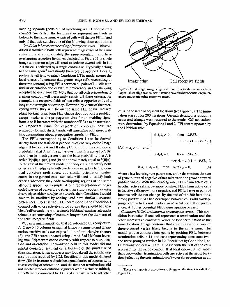
Condition I: Local coarse coding of image contours. This con-dition is satisfied if both cells represent image edges of the samecurvature and approximately the same orientation and haveoverlapping receptive fields. As depicted in Figure 11, a singleimage contour (or edge) will tend to activate several cells in LI.All the cells activated by a single contour will typically belongto the same geon11 and should therefore be grouped. Locally,such cells will tend to satisfy Condition I. The model groups thelocal pieces of a contour (i.e., groups edge cells responding tothe same contour) using FELs between all pairs of LI cells withsimilar orientation and curvature preferences and overlappingreceptive fields (Figure 12). Note that not all cells responding toa given contour will necessarily satisfy all these criteria; forexample, the receptive fields of two cells at opposite ends of along contour might not overlap. However, by virtue of the inter-vening units, they will lie on the same PEL chain. Indirectphase locking using long PEL chains does not pose a problemexcept insofar as the propagation time for an enabling signalfrom A to B increases with the number of FELs to be traversed.An important issue for exploration concerns how thesynchrony for such distant units will generalize with more real-istic assumptions about propagation speeds for FELs.
The FELs corresponding to Condition I can be derivedstrictly from the statistical properties of coarsely coded imageedges. If two cells A and B satisfy Condition I, the conditionalprobability that A will be active given that B is active [p(A|B)]should (a) be much greater than the base probability that A isactive [P(A|B) > p(A)] and (b) be approximately equal to P(B|A).In the case of the present model, the only cells that satisfy bothcriteria are LI edge cells with overlapping receptive fields, iden-tical curvature preferences, and similar orientation prefer-ences. In the general case, two cells will tend to satisfy bothcriteria whenever they code overlapping regions of the sameattribute space. For example, if our representation of edgescoded degree of curvature (rather than simply coding an edgediscretely as either straight or curved), then Condition I wouldhave to be modified by adding "and have similar curvaturepreferences." Because the FELs corresponding to Condition Iconnect cells whose activity should covary, they should be capa-ble of self-organizing with a simple Hebbian learning rule and astimulus set consisting of contours longer than the diameter ofthe cells' receptive fields.
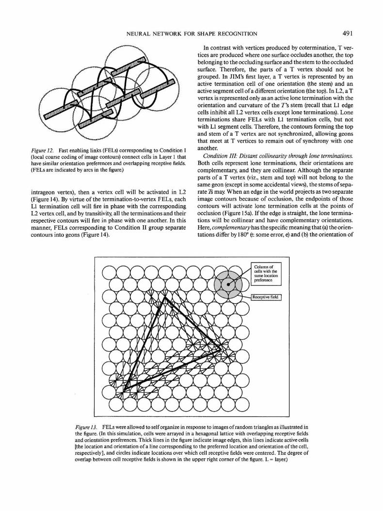
We ran a small simulation that corroborated this conjecture.A12-row X10-column hexagonal lattice of segment- and termi-nation-sensitive cells was exposed to random triangles (Figure13), and FELs were updated using a modified Hebbian learn-ing rule. Edges were coded coarsely, with respect to both loca-tion and orientation. Termination cells in this model did notinhibit consistent segment cells. Because of the small size ofthis simulation, it was not necessary to make all the simplifyingassumptions required by JIM. Specifically, this model differedfrom JIM in its more realistic hexagonal lattice of edge cells, itscoarse coding of orientation, and the fact that terminations didnot inhibit same-orientation segments within a cluster. Initially,a/I cells were connected by FELs of strength zero to all other
Image edge Cell receptive fields
Figure 11. A single image edge will tend to activate several cells inLayer 1. (Locally, these cells will tend to have similar orientation prefer-ences and overlapping receptive fields.)
cells in the same or adjacent locations (see Figure 1 3). The simu-lation was run for 200 iterations. On each iteration, a randomlygenerated triangle was presented to the model. Cell activationswere determined by Equations 1 and 2. FELs were updated bythe Hebbian rule:
if At + Aj > 0, and
j > 0,
j = 0,
then
then
- \FELU\
j + Aj = 0,
= -Vr(Ai
then
Aj)(l - \FELV\),
= 0, (6)
where v is a learning rate parameter, and r determines the rateof growth toward negative values relative to the growth towardpositive values. With this learning rule, FELs from active cellsto other active cells grow more positive, FELs from active cellsto inactive cells grow more negative, and FELs between pairs ofinactive cells do not change. By the end of the 200 iterations,strong positive FELs had developed between cells with overlap-ping receptive fields and identical or adjacent orientation prefer-ences. All other potential FELs were negative or zero.
Condition II: Cotermination in an intrageon vertex. This con-dition is satisfied if one cell represents a termination and theother represents a consistent vertex or lone termination at thesame location. Image contours that coterminate in a two- orthree-pronged vertex likely belong to the same geon. Themodel groups contours into geons by positing FELs betweentermination cells in LI and cells representing consistent two-and three-pronged vertices in L2. Recall that by Condition I, anLI termination cell will fire in phase with the rest of the cellsrepresenting the same contour. If at least one — but not morethan two — other termination cells are active at the same loca-tion (reflecting the cotermination of two or three contours in an
1' There are important exceptions to this generalization as evident inFigure 19.
NEURAL NETWORK FOR SHAPE RECOGNITION 491
Figure 12. Fast enabling links (FELs) corresponding to Condition I(local coarse coding of image contours) connect cells in Layer 1 thathave similar orientation preferences and overlapping receptive fields.(FELs are indicated by arcs in the figure.)
intrageon vertex), then a vertex cell will be activated in L2(Figure 14). By virtue of the termination-to-vertex FELs, eachLI termination cell will fire in phase with the correspondingL2 vertex cell, and by transitivity, all the terminations and theirrespective contours will fire in phase with one another. In thismanner, FELs corresponding to Condition II group separatecontours into geons (Figure 14).
In contrast with vertices produced by cotermination, T ver-tices are produced where one surface occludes another, the topbelonging to the occluding surface and the stem to the occludedsurface. Therefore, the parts of a T vertex should not begrouped. In JIM's first layer, a T vertex is represented by anactive termination cell of one orientation (the stem) and anactive segment cell of a different orientation (the top). In L2, a Tvertex is represented only as an active lone termination with theorientation and curvature of the 7"s stem (recall that LI edgecells inhibit all L2 vertex cells except lone terminations). Loneterminations share FELs with LI termination cells, but notwith LI segment cells. Therefore, the contours forming the topand stem of a T vertex are not synchronized, allowing geonsthat meet at T vertices to remain out of synchrony with oneanother.
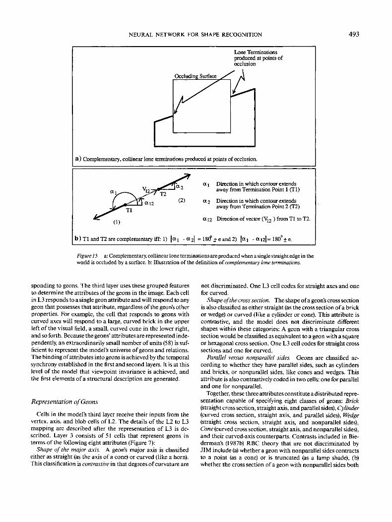
Condition HI: Distant collinearity through lone terminations.Both cells represent lone terminations, their orientations arecomplementary, and they are collinear. Although the separateparts of a T vertex (viz., stem and top) will not belong to thesame geon (except in some accidental views), the stems of sepa-rate 7s may. When an edge in the world projects as two separateimage contours because of occlusion, the endpoints of thosecontours will activate lone termination cells at the points ofocclusion (Figure 15a). If the edge is straight, the lone termina-tions will be collinear and have complementary orientations.Here, complementary has the specific meaning that (a) the orien-tations differ by 180° (t some error, e) and (b) the orientation of
Figure 13. FELs were allowed to self organize in response to images of random triangles as illustrated inthe figure. (In this simulation, cells were arrayed in a hexagonal lattice with overlapping receptive fieldsand orientation preferences. Thick lines in the figure indicate image edges, thin lines indicate active cells[the location and orientation of a line corresponding to the preferred location and orientation of the cell,respectively], and circles indicate locations over which cell receptive fields were centered. The degree ofoverlap between cell receptive fields is shown in the upper right corner of the figure. L = layer.)
492 JOHN E. HUMMEL AND IRVING BIEDERMAN
Active L2vertex cell
Active LIterminationcells
Image
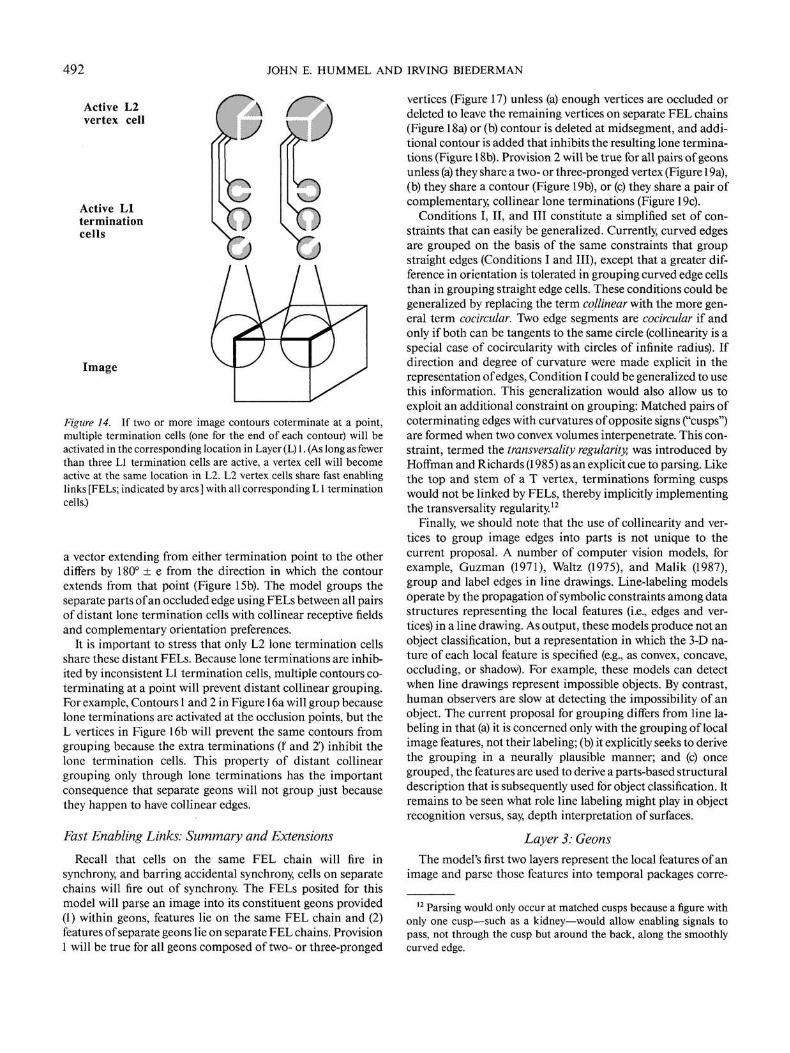
Figure 14. If two or more image contours coterminate at a point,multiple termination cells (one for the end of each contour) will beactivated in the corresponding location in Layer (L) 1. (As long as fewerthan three LI termination cells are active, a vertex cell will becomeactive at the same location in L2. L2 vertex cells share fast enablinglinks [FELs; indicated by arcs] with all corresponding L1 terminationcells.)
a vector extending from either termination point to the otherdiffers by 180° ± e from the direction in which the contourextends from that point (Figure 15b). The model groups theseparate parts of an occluded edge using FELs between all pairsof distant lone termination cells with collinear receptive fieldsand complementary orientation preferences.
It is important to stress that only L2 lone termination cellsshare these distant FELs. Because lone terminations are inhib-ited by inconsistent LI termination cells, multiple contours co-terminating at a point will prevent distant collinear grouping.For example, Contours 1 and 2 in Figure 16a will group becauselone terminations are activated at the occlusion points, but theL vertices in Figure 16b will prevent the same contours fromgrouping because the extra terminations (!' and 2') inhibit thelone termination cells. This property of distant collineargrouping only through lone terminations has the importantconsequence that separate geons will not group just becausethey happen to have collinear edges.
Fast Enabling Links: Summary and Extensions
Recall that cells on the same FEL chain will fire insynchrony, and barring accidental synchrony, cells on separatechains will fire out of synchrony. The FELs posited for thismodel will parse an image into its constituent geons provided(1) within geons, features lie on the same FEL chain and (2)features of separate geons lie on separate FEL chains. Provision1 will be true for all geons composed of two- or three-pronged
vertices (Figure 17) unless (a) enough vertices are occluded ordeleted to leave the remaining vertices on separate FEL chains(Figure 18a) or (b) contour is deleted at midsegment, and addi-tional contour is added that inhibits the resulting lone termina-tions (Figure 18b). Provision 2 will be true for all pairs of geonsunless (a) they share a two- or three-pronged vertex (Figure 19a),(b) they share a contour (Figure 19b), or (c) they share a pair ofcomplementary, collinear lone terminations (Figure 19c).
Conditions I, II, and III constitute a simplified set of con-straints that can easily be generalized. Currently, curved edgesare grouped on the basis of the same constraints that groupstraight edges (Conditions I and III), except that a greater dif-ference in orientation is tolerated in grouping curved edge cellsthan in grouping straight edge cells. These conditions could begeneralized by replacing the term collinear with the more gen-eral term cocircular. Two edge segments are cocircular if andonly if both can be tangents to the same circle (collinearity is aspecial case of cocircularity with circles of infinite radius). Ifdirection and degree of curvature were made explicit in therepresentation of edges, Condition I could be generalized to usethis information. This generalization would also allow us toexploit an additional constraint on grouping: Matched pairs ofcoterminating edges with curvatures of opposite signs ("cusps")are formed when two convex volumes interpenetrate. This con-straint, termed the transversality regularity, was introduced byHoffman and Richards (1985) as an explicit cue to parsing. Likethe top and stem of a T vertex, terminations forming cuspswould not be linked by FELs, thereby implicitly implementingthe transversality regularity.12
Finally, we should note that the use of collinearity and ver-tices to group image edges into parts is not unique to thecurrent proposal. A number of computer vision models, forexample, Guzman (1971), Waltz (1975), and Malik (1987),group and label edges in line drawings. Line-labeling modelsoperate by the propagation of symbolic constraints among datastructures representing the local features (i.e., edges and ver-tices) in a line drawing. As output, these models produce not anobject classification, but a representation in which the 3-D na-ture of each local feature is specified (e.g., as convex, concave,occluding, or shadow). For example, these models can detectwhen line drawings represent impossible objects. By contrast,human observers are slow at detecting the impossibility of anobject. The current proposal for grouping differs from line la-beling in that (a) it is concerned only with the grouping of localimage features, not their labeling; (b) it explicitly seeks to derivethe grouping in a neurally plausible manner; and (c) oncegrouped, the features are used to derive a parts-based structuraldescription that is subsequently used for object classification. Itremains to be seen what role line labeling might play in objectrecognition versus, say, depth interpretation of surfaces.
Layer 3: GeonsThe model's first two layers represent the local features of an
image and parse those features into temporal packages corre-
12 Parsing would only occur at matched cusps because a figure withonly one cusp—such as a kidney—would allow enabling signals topass, not through the cusp but around the back, along the smoothlycurved edge.
NEURAL NETWORK FOR SHAPE RECOGNITION 493
Lone Terminationsproduced at points ofocclusion
Occluding Surface
a) Complementary, collinear lone terminations produced at points of occlusion.
a i Direction in which contour extendsaway from Termination Point 1 (Tl)
a 2 Direction in which contour extendsaway from Termination Point 2 (T2)
a 12 Direction of vector (V12 ) from Tl to T2.
b)Tl and T2 are complementary iff: 1) \a^ - a2| = 18(f + e and2) (aj - a.n\- 180°±e.
Figure 15. a: Complementary, collinear lone terminations are produced when a single straight edge in theworld is occluded by a surface, b: Illustration of the definition of complementary lone terminations.
spending to geons. The third layer uses these grouped featuresto determine the attributes of the geons in the image. Each cellin L3 responds to a single geon attribute and will respond to anygeon that possesses that attribute, regardless of the geon's otherproperties. For example, the cell that responds to geons withcurved axes will respond to a large, curved brick in the upperleft of the visual field, a small, curved cone in the lower right,and so forth. Because the geons' attributes are represented inde-pendently, an extraordinarily small number of units (58) is suf-ficient to represent the model's universe of geons and relations.The binding of attributes into geons is achieved by the temporalsynchrony established in the first and second layers. It is at thislevel of the model that viewpoint invariance is achieved, andthe first elements of a structural description are generated.
Representation of Geons
Cells in the model's third layer receive their inputs from thevertex, axis, and blob cells of L2. The details of the L2 to L3mapping are described after the representation of L3 is de-scribed. Layer 3 consists of 51 cells that represent geons interms of the following eight attributes (Figure 7):
Shape of the major axis. A geon's major axis is classifiedeither as straight (as the axis of a cone) or curved (like a horn).This classification is contrastive in that degrees of curvature are
not discriminated. One L3 cell codes for straight axes and onefor curved.
Shape of the cross section. The shape of a geon's cross sectionis also classified as either straight (as the cross section of a brickor wedge) or curved (like a cylinder or cone). This attribute iscontrastive, and the model does not discriminate differentshapes within these categories: A geon with a triangular crosssection would be classified as equivalent to a geon with a squareor hexagonal cross section. One L3 cell codes for straight crosssections and one for curved.
Parallel versus nonparallel sides. Geons are classified ac-cording to whether they have parallel sides, such as cylindersand bricks, or nonparallel sides, like cones and wedges. Thisattribute is also contrastively coded in two cells: one for paralleland one for nonparallel.
Together, these three attributes constitute a distributed repre-sentation capable of specifying eight classes of geons: Brick(straight cross section, straight axis, and parallel sides), Cylinder(curved cross section, straight axis, and parallel sides), Wedge(straight cross section, straight axis, and nonparallel sides),Cone (curved cross section, straight axis, and nonparallel sides),and their curved-axis counterparts. Contrasts included in Bie-derman's (1987b) RBC theory that are not discriminated byJIM include (a) whether a geon with nonparallel sides contractsto a point (as a cone) or is truncated (as a lamp shade), (b)whether the cross section of a geon with nonparallel sides both
494 JOHN E. HUMMEL AND IRVING BIEDERMAN
2 i
Image
(a) (b)
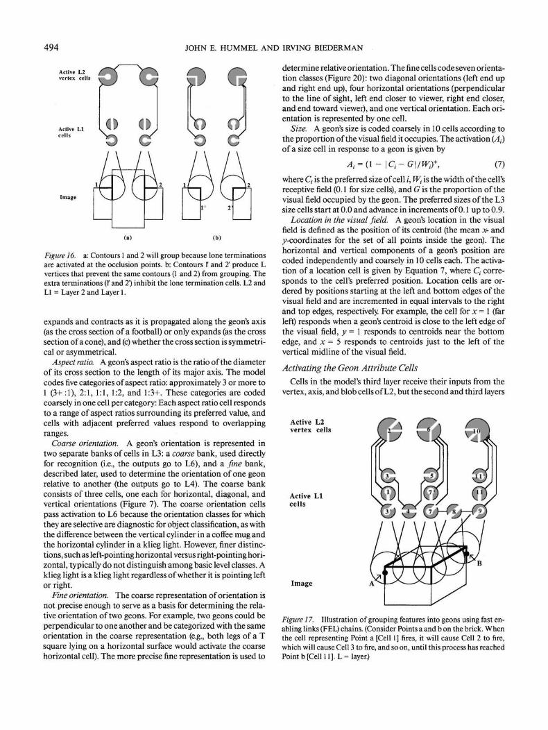
Figure 16. a: Contours 1 and 2 will group because lone terminationsare activated at the occlusion points, b: Contours 1' and 2' produce Lvertices that prevent the same contours (1 and 2) from grouping. Theextra terminations (!' and 2') inhibit the lone termination cells. L2 andLI = Layer 2 and Layer 1.
expands and contracts as it is propagated along the geon's axis(as the cross section of a football) or only expands (as the crosssection of a cone), and (c) whether the cross section is symmetri-cal or asymmetrical.
Aspect ratio. A geon's aspect ratio is the ratio of the diameterof its cross section to the length of its major axis. The modelcodes five categories of aspect ratio: approximately 3 or more to1 (3+:l), 2:1, 1:1, 1:2, and 1:3+. These categories are codedcoarsely in one cell per category: Each aspect ratio cell respondsto a range of aspect ratios surrounding its preferred value, andcells with adjacent preferred values respond to overlappingranges.
Coarse orientation. A geon's orientation is represented intwo separate banks of cells in L3: a coarse bank, used directlyfor recognition (i.e., the outputs go to L6), and a fine bank,described later, used to determine the orientation of one geonrelative to another (the outputs go to L4). The coarse bankconsists of three cells, one each for horizontal, diagonal, andvertical orientations (Figure 7). The coarse orientation cellspass activation to L6 because the orientation classes for whichthey are selective are diagnostic for object classification, as withthe difference between the vertical cylinder in a coffee mug andthe horizontal cylinder in a klieg light. However, finer distinc-tions, such as left-pointing horizontal versus right-pointing hori-zontal, typically do not distinguish among basic level classes. Aklieg light is a klieg light regardless of whether it is pointing leftor right.
Fine orientation. The coarse representation of orientation isnot precise enough to serve as a basis for determining the rela-tive orientation of two geons. For example, two geons could beperpendicular to one another and be categorized with the sameorientation in the coarse representation (e.g., both legs of a Tsquare lying on a horizontal surface would activate the coarsehorizontal cell). The more precise fine representation is used to
determine relative orientation. The fine cells code seven orienta-tion classes (Figure 20): two diagonal orientations (left end upand right end up), four horizontal orientations (perpendicularto the line of sight, left end closer to viewer, right end closer,and end toward viewer), and one vertical orientation. Each ori-entation is represented by one cell.
Size. A geon's size is coded coarsely in 10 cells according tothe proportion of the visual field it occupies. The activation (At)of a size cell in response to a geon is given by
= (l- \Ci-G\/Wi)+, (7)
where C, is the preferred size of cell i, Wt is the width of the cell'sreceptive field (0.1 for size cells), and G is the proportion of thevisual field occupied by the geon. The preferred sizes of the L3size cells start at 0.0 and advance in increments of 0.1 up to 0.9.
Location in the visual field. A geon's location in the visualfield is defined as the position of its centroid (the mean x- and^-coordinates for the set of all points inside the geon). Thehorizontal and vertical components of a geon's position arecoded independently and coarsely in 10 cells each. The activa-tion of a location cell is given by Equation 7, where C, corre-sponds to the cell's preferred position. Location cells are or-dered by positions starting at the left and bottom edges of thevisual field and are incremented in equal intervals to the rightand top edges, respectively. For example, the cell for x = 1 (farleft) responds when a geon's centroid is close to the left edge ofthe visual field, y = 1 responds to centroids near the bottomedge, and x = 5 responds to centroids just to the left of thevertical midline of the visual field.
Activating the Geon Attribute Cells
Cells in the model's third layer receive their inputs from thevertex, axis, and blob cells of L2, but the second and third layers
Active L2vertex cells
Active LIcells
Image
Figure 17. Illustration of grouping features into geons using fast en-abling links (PEL) chains. (Consider Points a and b on the brick. Whenthe cell representing Point a [Cell 1] fires, it will cause Cell 2 to fire,which will cause Cell 3 to fire, and so on, until this process has reachedPoint b [Cell 11]. L= layer.)
NEURAL NETWORK FOR SHAPE RECOGNITION 495
a) Recoverable Nonrecoverable
b) Recoverable Nonrecoverable
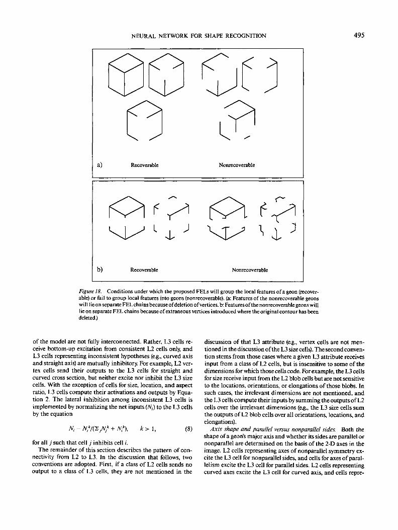
Figure 18. Conditions under which the proposed FELs will group the local features of a geon (recover-able) or fail to group local features into geons (nonrecoverable). (a: Features of the nonrecoverable geonswill lie on separate FEL chains because of deletion of vertices, b: Features of the nonrecoverable geons willlie on separate FEL chains because of extraneous vertices introduced where the original contour has beendeleted.)
of the model are not fully interconnected. Rather, L3 cells re-ceive bottom-up excitation from consistent L2 cells only, andL3 cells representing inconsistent hypotheses (e.g., curved axisand straight axis) are mutually inhibitory. For example, L2 ver-tex cells send their outputs to the L3 cells for straight andcurved cross section, but neither excite nor inhibit the L3 sizecells. With the exception of cells for size, location, and aspectratio, L3 cells compute their activations and outputs by Equa-tion 2. The lateral inhibition among inconsistent L3 cells isimplemented by normalizing the net inputs (N,) to the L3 cellsby the equation
N, = + N/0), k > 1, (8)
for all j such that cell j inhibits cell /.The remainder of this section describes the pattern of con-
nectivity from L2 to L3. In the discussion that follows, twoconventions are adopted. First, if a class of L2 cells sends nooutput to a class of L3 cells, they are not mentioned in the
discussion of that L3 attribute (e.g., vertex cells are not men-tioned in the discussion of the L3 size cells). The second conven-tion stems from those cases where a given L3 attribute receivesinput from a class of L2 cells, but is insensitive to some of thedimensions for which those cells code. For example, the L3 cellsfor size receive input from the L2 blob cells but are not sensitiveto the locations, orientations, or elongations of those blobs. Insuch cases, the irrelevant dimensions are not mentioned, andthe L3 cells compute their inputs by summing the outputs of L2cells over the irrelevant dimensions (e.g., the L3 size cells sumthe outputs of L2 blob cells over all orientations, locations, andelongations).
Axis shape and parallel versus nonparallel sides. Both theshape of a geon's major axis and whether its sides are parallel ornonparallel are determined on the basis of the 2-D axes in theimage. L2 cells representing axes of nonparallel symmetry ex-cite the L3 cell for nonparallel sides, and cells for axes of paral-lelism excite the L3 cell for parallel sides. L2 cells representingcurved axes excite the L3 cell for curved axis, and cells repre-
496 JOHN E. HUMMEL AND IRVING BIEDERMAN
senting straight axes excite L3's straight axis cell. The parallel-sides and non-parallel-sides cells are mutually inhibitory, as arethe straight-axis and curved-axis cells.
Cross section. Whether a geon's cross section is straight orcurved is determined on the basis of the vertices active in L2.Tangent-Y vertices and L vertices with at least one curved legexcite the L3 curved-cross-section cell. Forks and arrows excitethe straight cross section cell. Straight cross section and curvedcross section cells are mutually inhibitory. This mapping is sum-marized in Figure 21.
Size and location. L3 cells representing geon size and loca-tion take their input from the blobs derived in L2. Recall that ablob represents a region of the visual field with a particularlocation, size, orientation, and elongation. It is assumed thateach blob cell excites a set of L3 size and location cells consis-tent with its receptive field properties. The receptive field prop-erties of the size and location cells were described earlier; theirinputs (G in Equation 7) come from the blob computations. It isassumed that the term (1 — \Ct - G\/Wt)
+ is equal to the connec-tion weight to an L3 size or location cell from an active blobcell. For example, as shown in Figure 22, a given blob mightrespond to a region of activity just left and above the middle ofthe visual field, elongated slightly, oriented at or around II/4(45°) and occupying between 10% and 15% of the visual field. Inthe L3 location bank, this blob will strongly excite x = 5 andmore weakly excite x = 4, and it will strongly excite y = 5 and
a) Separable Nonseparable
b) Separable
c) Separable Nonseparable
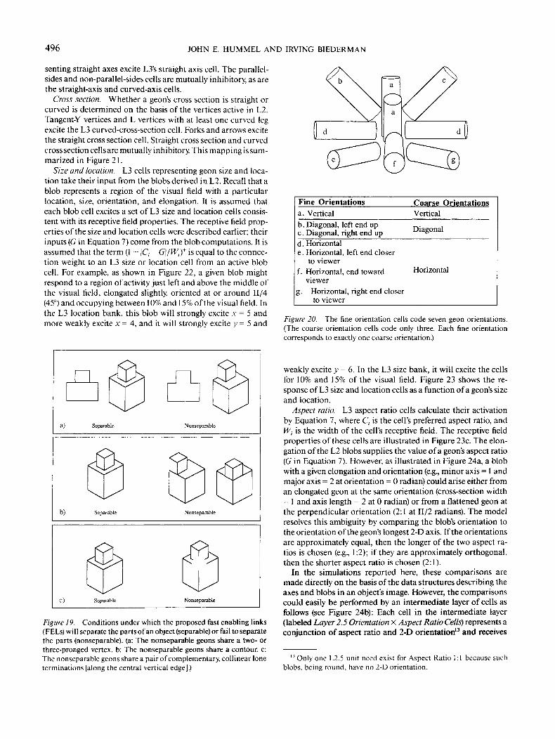
Figure 19. Conditions under which the proposed fast enabling links(FELs) will separate the parts of an object (separable) or fail to separatethe parts (nonseparable). (a: The nonseparable geons share a two- orthree-pronged vertex, b: The nonseparable geons share a contour, c:The nonseparable geons share a pair of complementary, collinear loneterminations [along the central vertical edge].)
Fine Orientationsa. Verticalb. Diagonal, left end upc. Diagonal, right end upd. Horizontale. Horizontal, left end closer
to viewerf. Horizontal, end toward
viewerg. Horizontal, right end closer
to viewer
Coarse OrientationsVertical
Diagonal
Horizontal
Figure 20. The fine orientation cells code seven geon orientations.(The coarse orientation cells code only three. Each fine orientationcorresponds to exactly one coarse orientation.)
weakly excite y = 6. In the L3 size bank, it will excite the cellsfor 10% and 15% of the visual field. Figure 23 shows the re-sponse of L3 size and location cells as a function of a geon's sizeand location.
Aspect ratio. L3 aspect ratio cells calculate their activationby Equation 7, where C, is the cell's preferred aspect ratio, andWt is the width of the cell's receptive field. The receptive fieldproperties of these cells are illustrated in Figure 23c. The elon-gation of the L2 blobs supplies the value of a geon's aspect ratio(G in Equation 7). However, as illustrated in Figure 24a, a blobwith a given elongation and orientation (e.g., minor axis = 1 andmajor axis = 2 at orientation = 0 radian) could arise either froman elongated geon at the same orientation (cross-section width= 1 and axis length = 2 at 0 radian) or from a flattened geon atthe perpendicular orientation (2:1 at H/2 radians). The modelresolves this ambiguity by comparing the blob's orientation tothe orientation of the geon's longest 2-D axis. If the orientationsare approximately equal, then the longer of the two aspect ra-tios is chosen (e.g., 1:2); if they are approximately orthogonal,then the shorter aspect ratio is chosen (2:1).
In the simulations reported here, these comparisons aremade directly on the basis of the data structures describing theaxes and blobs in an object's image. However, the comparisonscould easily be performed by an intermediate layer of cells asfollows (see Figure 24b): Each cell in the intermediate layer(labeled Layer 2.5 Orientation X Aspect Ratio Cells) represents aconjunction of aspect ratio and 2-D orientation13 and receives
13 Only one L2.5 unit need exist for Aspect Ratio 1:1 because suchblobs, being round, have no 2-D orientation.
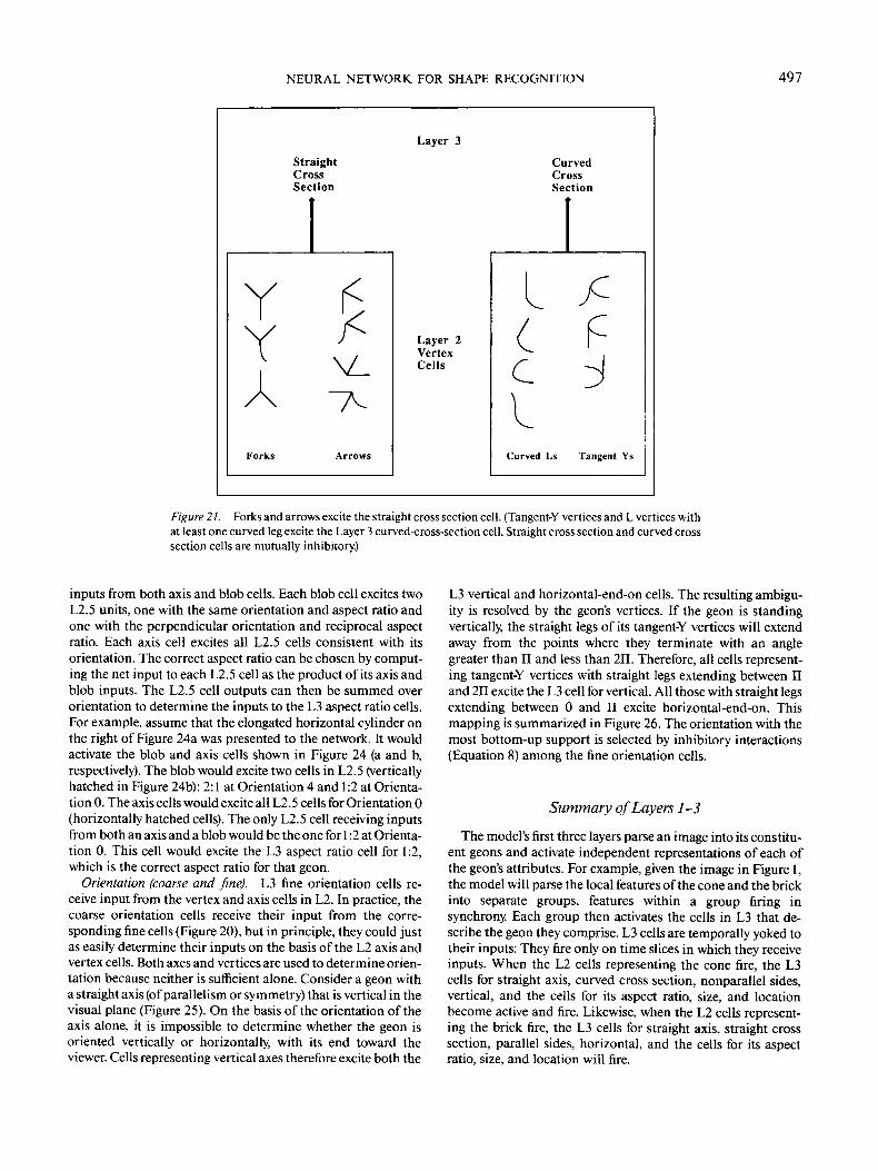
NEURAL NETWORK FOR SHAPE RECOGNITION 497
Layer 3
StraightCrossSection
CurvedCrossSection
Y
Forks Arrows
Layer 2VertexCells
Lc
Curved Ls Tangent Ys
Figure 21. Forks and arrows excite the straight cross section cell. (Tangent-Y vertices and L vertices withat least one curved leg excite the Layer 3 curved-cross-section cell. Straight cross section and curved crosssection cells are mutually inhibitory.)
inputs from both axis and blob cells. Each blob cell excites twoL2.5 units, one with the same orientation and aspect ratio andone with the perpendicular orientation and reciprocal aspectratio. Each axis cell excites all L2.5 cells consistent with itsorientation. The correct aspect ratio can be chosen by comput-ing the net input to each L2.5 cell as the product of its axis andblob inputs. The L2.5 cell outputs can then be summed overorientation to determine the inputs to the L3 aspect ratio cells.For example, assume that the elongated horizontal cylinder onthe right of Figure 24a was presented to the network. It wouldactivate the blob and axis cells shown in Figure 24 (a and b,respectively). The blob would excite two cells in L2.5 (verticallyhatched in Figure 24b): 2:1 at Orientation 4 and 1:2 at Orienta-tion 0. The axis cells would excite all L2.5 cells for Orientation 0(horizontally hatched cells). The only L2.5 cell receiving inputsfrom both an axis and a blob would be the one for 1:2 at Orienta-tion 0. This cell would excite the L3 aspect ratio cell for 1:2,which is the correct aspect ratio for that geon.
Orientation (coarse and fine). L3 fine orientation cells re-ceive input from the vertex and axis cells in L2. In practice, thecoarse orientation cells receive their input from the corre-sponding fine cells (Figure 20), but in principle, they could justas easily determine their inputs on the basis of the L2 axis andvertex cells. Both axes and vertices are used to determine orien-tation because neither is sufficient alone. Consider a geon witha straight axis (of parallelism or symmetry) that is vertical in thevisual plane (Figure 25). On the basis of the orientation of theaxis alone, it is impossible to determine whether the geon isoriented vertically or horizontally, with its end toward theviewer. Cells representing vertical axes therefore excite both the
L3 vertical and horizontal-end-on cells. The resulting ambigu-ity is resolved by the geon's vertices. If the geon is standingvertically, the straight legs of its tangent-Y vertices will extendaway from the points where they terminate with an anglegreater than II and less than 211. Therefore, all cells represent-ing tangent-Y vertices with straight legs extending between IIand 211 excite the L3 cell for vertical. All those with straight legsextending between 0 and II excite horizontal-end-on. Thismapping is summarized in Figure 26. The orientation with themost bottom-up support is selected by inhibitory interactions(Equation 8) among the fine orientation cells.
Summary of Layers 1-3
The model's first three layers parse an image into its constitu-ent geons and activate independent representations of each ofthe geon's attributes. For example, given the image in Figure 1,the model will parse the local features of the cone and the brickinto separate groups, features within a group firing insynchrony. Each group then activates the cells in L3 that de-scribe the geon they comprise. L3 cells are temporally yoked totheir inputs: They fire only on time slices in which they receiveinputs. When the L2 cells representing the cone fire, the L3cells for straight axis, curved cross section, nonparallel sides,vertical, and the cells for its aspect ratio, size, and locationbecome active and fire. Likewise, when the L2 cells represent-ing the brick fire, the L3 cells for straight axis, straight crosssection, parallel sides, horizontal, and the cells for its aspectratio, size, and location will fire.
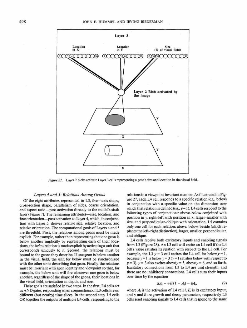
498 JOHN E. HUMMEL AND IRVING BIEDERMAN
Layer 2 Blob activated bythe image
Figure 22. Layer 2 blobs activate Layer 3 cells representing a geon's size and location in the visual field.
Layers 4 and 5: Relations Among GeonsOf the eight attributes represented in L3, five—axis shape,
cross-section shape, parallelism of sides, coarse orientation,and aspect ratio—pass activation directly to the model's sixthlayer (Figure 7). The remaining attributes—size, location, andfine orientation—pass activation to Layer 4, which, in conjunc-tion with Layer 5, derives relative size, relative location, andrelative orientation. The computational goals of Layers 4 and 5are threefold. First, the relations among geons must be madeexplicit. For example, rather than representing that one geon isbelow another implicitly by representing each of their loca-tions, the below relation is made explicit by activating a unit thatcorresponds uniquely to it. Second, the relations must bebound to the geons they describe. If one geon is below anotherin the visual field, the unit for below must be synchronizedwith the other units describing that geon. Finally, the relationsmust be invariant with geon identity and viewpoint so that, forexample, the below unit will fire whenever one geon is belowanother, regardless of the shape of the geons, their locations inthe visual field, orientation in depth, and size.
These goals are satisfied in two steps. In the first, L4 cells actas AND gates, responding when conjunctions of L3 cells fire ondifferent (but nearby) time slices. In the second step, L5 cellsOR together the outputs of multiple L4 cells, responding to the
relations in a viewpoint-invariant manner. As illustrated in Fig-ure 27, each L4 cell responds to a specific relation (e.g., below)in conjunction with a specific value on the dimension overwhich that relation is defined (e.g., y = I). L4 cells respond to thefollowing types of conjunctions: above-below conjoined withposition in y, right-left with position in x, larger-smaller withsize, and perpendicular-oblique with orientation. L5 containsonly one cell for each relation: above, below, beside (which re-places the left-right distinction), larger, smaller, perpendicular,and oblique.
L4 cells receive both excitatory inputs and enabling signalsfrom L3 (Figure 28). An L3 cell will excite an L4 cell if the L4cell's value satisfies its relation with respect to the L3 cell. Forexample, the L3 y = 3 cell excites the L4 cell for below|j; = 1,because y = 1 is below y = 3 (y = 1 satisfies below with respect toy = 3). y = 3 also excites above|y = 5, above\y = 6, and so forth.Excitatory connections from L3 to L4 are unit strength, andthere are no inhibitory connections. L4 cells sum their inputsover time by the equation
where A, is the activation of L4 cell i, Et is its excitatory input,and 7 and d are growth and decay parameters, respectively. L3cells send enabling signals to L4 cells that respond to the same
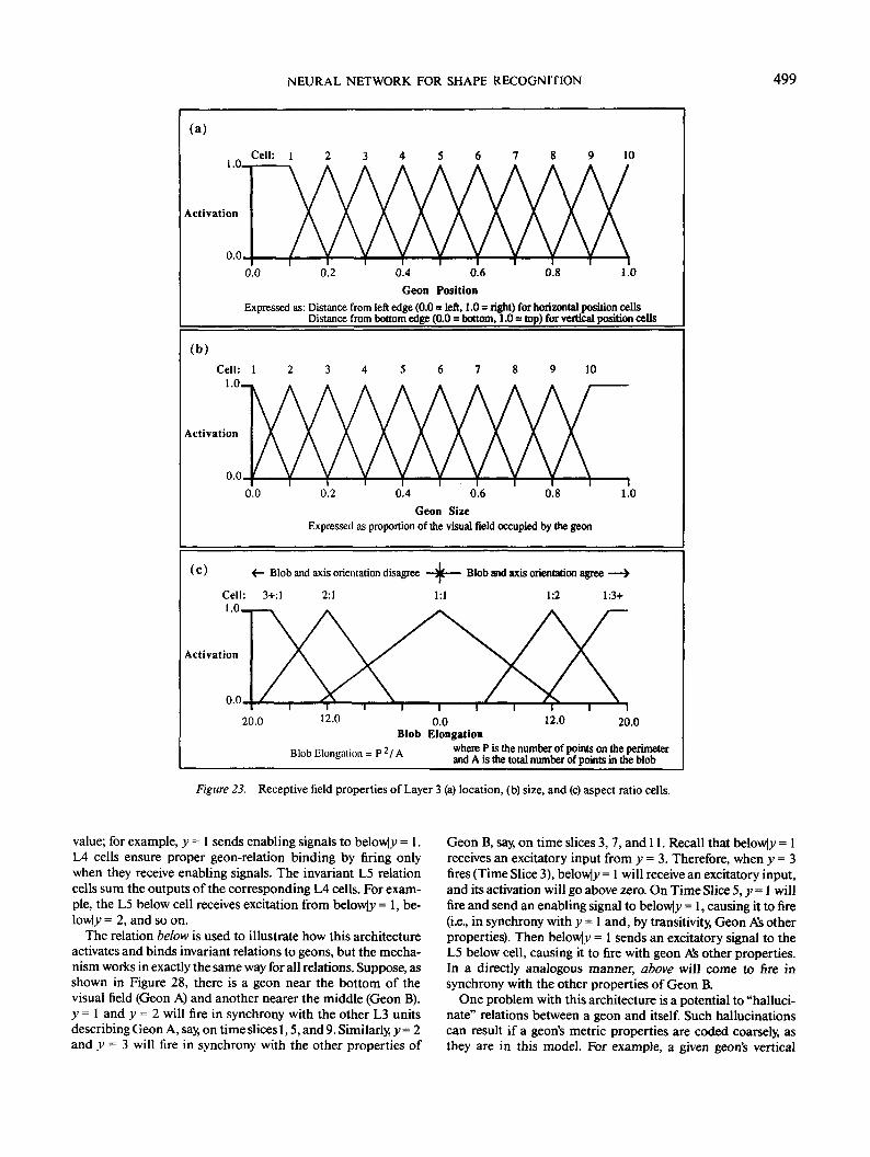
NEURAL NETWORK FOR SHAPE RECOGNITION 499
(a)
Cell: 1
Activation
0.0 0.4 0.6Geon Position
0.8 1.0
Expressed as: Distance from left edge (0.0 = left, 1.0 = right) for horizontal position cellsDistance from bottom edge (0.0 = bottom, 1.0 = top) for vertical position cells
(b)
Activation
0.2 0.80.4 0.6Geon Size
Expressed as proportion of the visual field occupied by the geon
1.0
(C)
Cell: 3+:l1.0
<- Blob and axis orientation disagree —*— Blob and axis orientation agree —>
2:1 1:1 1:2 1:3+
Activation
20.0 12.0 20.00.0Blob Elongation
Blob Elongation - P 2/ A where P K ** number of points on the perimeterBlob faiongation - P / A and A is the total number of points in the blob
Figure 23. Receptive field properties of Layer 3 (a) location, (b) size, and (c) aspect ratio cells.
value; for example, y = 1 sends enabling signals to below|y = 1.L4 cells ensure proper geon-relation binding by firing onlywhen they receive enabling signals. The invariant L5 relationcells sum the outputs of the corresponding L4 cells. For exam-ple, the L5 below cell receives excitation from below|>> = 1, be-lowly = 2, and so on.
The relation below is used to illustrate how this architectureactivates and binds invariant relations to geons, but the mecha-nism works in exactly the same way for all relations. Suppose, asshown in Figure 28, there is a geon near the bottom of thevisual field (Geon A) and another nearer the middle (Geon B).y = 1 and y = 2 will fire in synchrony with the other L3 unitsdescribing Geon A, say, on time slices 1,5, and 9. Similarly, y = 2and y = 3 will fire in synchrony with the other properties of
Geon B, say, on time slices 3,7, and 11. Recall that below|_y = 1receives an excitatory input from y = 3. Therefore, when y = 3fires (Time Slice 3), below]}* = 1 will receive an excitatory input,and its activation will go above zero. On Time Slice 5, y = 1 willfire and send an enabling signal to below|y = 1, causing it to fire(i.e., in synchrony with y - 1 and, by transitivity, Geon As otherproperties). Then below|_y = 1 sends an excitatory signal to theL5 below cell, causing it to fire with geon As other properties.In a directly analogous manner, above will come to fire insynchrony with the other properties of Geon B.
One problem with this architecture is a potential to "halluci-nate" relations between a geon and itself. Such hallucinationscan result if a geon's metric properties are coded coarsely, asthey are in this model. For example, a given geon's vertical
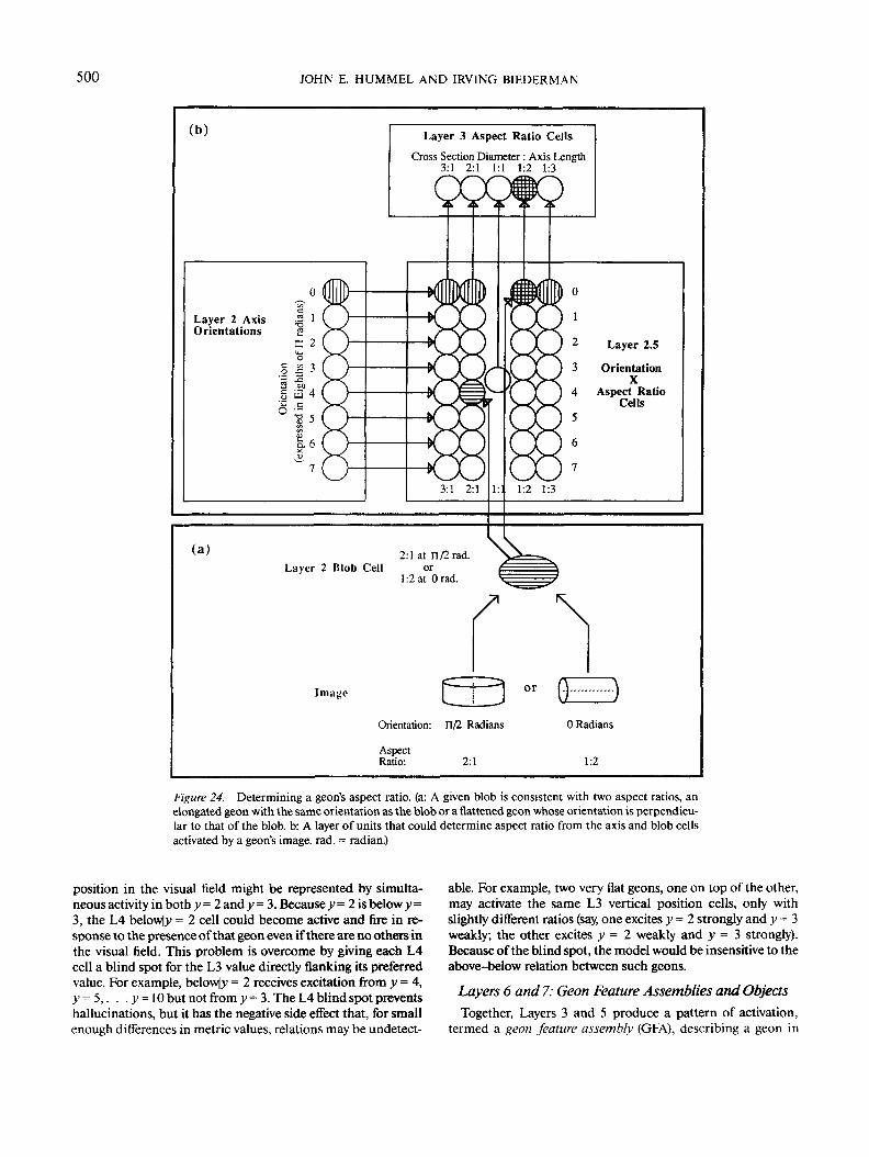
500 JOHN E. HUMMEL AND IRVING BIEDERMAN
(b) Layer 3 Aspect Ratio Cells
Cross Section Diameter : Axis Length3:1 2:1 1:1 1:2 1:3
OrientationX
Aspect RatioCells
(a)Layer 2 Blob Cell
2:1 at n/2rad.or
1:2 at Orad.
\
Imayc or
Orientation: n/2 Radians
2:1AspectRatio:
0 Radians
1:2
Figure 24. Determining a geon's aspect ratio, (a: A given blob is consistent with two aspect ratios, anelongated geon with the same orientation as the blob or a flattened geon whose orientation is perpendicu-lar to that of the blob, b: A layer of units that could determine aspect ratio from the axis and blob cellsactivated by a geon's image, rad. = radian.)
position in the visual field might be represented by simulta-neous activity in both y = 2 and y = 3. Because y = 2 is below y=3, the L4 belowly = 2 cell could become active and fire in re-sponse to the presence of that geon even if there are no others inthe visual field. This problem is overcome by giving each L4cell a blind spot for the L3 value directly flanking its preferredvalue. For example, belowly = 2 receives excitation from y = 4,y=5,. . . y= 10 but not from y- 3. The L4 blind spot preventshallucinations, but it has the negative side effect that, for smallenough differences in metric values, relations may be undetect-
able. For example, two very flat geons, one on top of the other,may activate the same L3 vertical position cells, only withslightly different ratios (say, one excites y=2 strongly and y = 3weakly; the other excites y = 2 weakly and y = 3 strongly).Because of the blind spot, the model would be insensitive to theabove-below relation between such geons.
Layers 6 and 7: Geon Feature Assemblies and Objects
Together, Layers 3 and 5 produce a pattern of activation,termed a geon feature assembly (GFA), describing a geon in
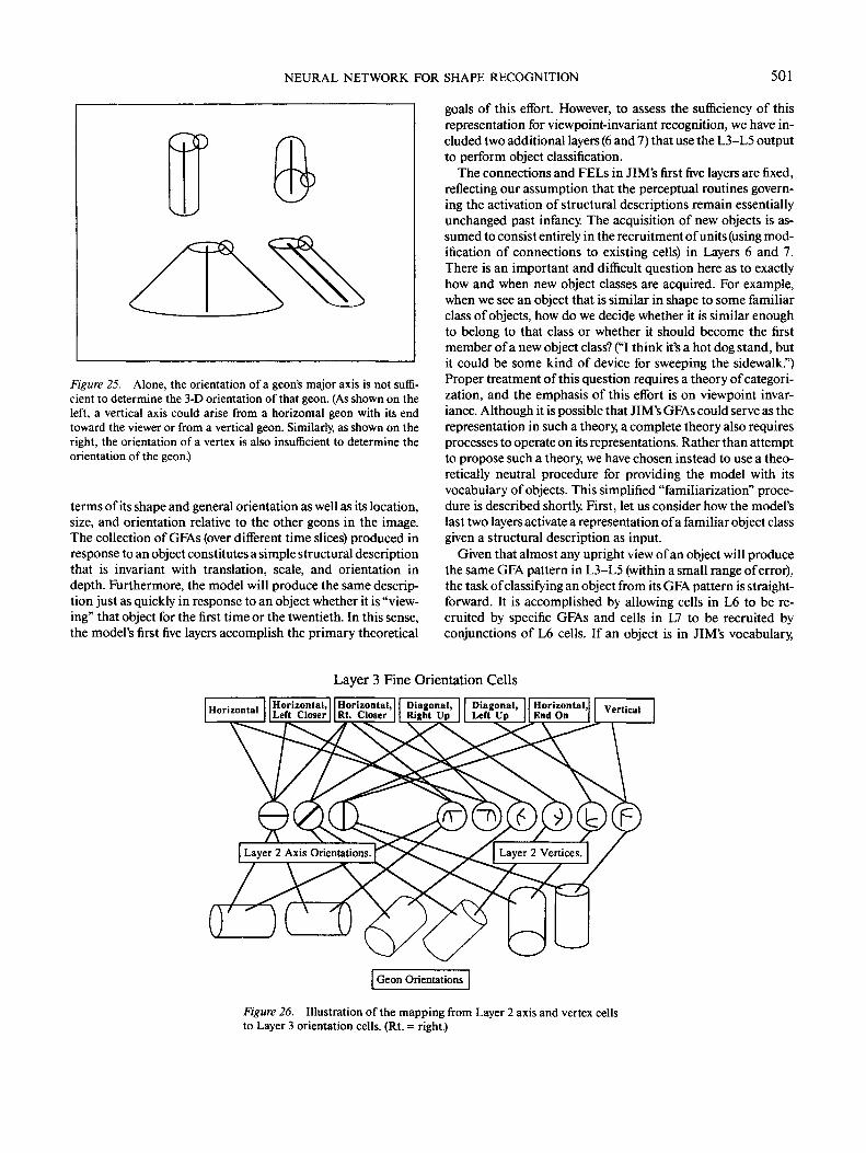
NEURAL NETWORK FOR SHAPE RECOGNITION 501
Figure 25. Alone, the orientation of a geon's major axis is not suffi-cient to determine the 3-D orientation of that geon. (As shown on theleft, a vertical axis could arise from a horizontal geon with its endtoward the viewer or from a vertical geon. Similarly, as shown on theright, the orientation of a vertex is also insufficient to determine theorientation of the geon.)
terms of its shape and general orientation as well as its location,size, and orientation relative to the other geons in the image.The collection of GFAs (over different time slices) produced inresponse to an object constitutes a simple structural descriptionthat is invariant with translation, scale, and orientation indepth. Furthermore, the model will produce the same descrip-tion just as quickly in response to an object whether it is "view-ing" that object for the first time or the twentieth. In this sense,the model's first five layers accomplish the primary theoretical
goals of this effort. However, to assess the sufficiency of thisrepresentation for viewpoint-invariant recognition, we have in-cluded two additional layers (6 and 7) that use the L3-L5 outputto perform object classification.
The connections and FELs in JIM's first five layers are fixed,reflecting our assumption that the perceptual routines govern-ing the activation of structural descriptions remain essentiallyunchanged past infancy. The acquisition of new objects is as-sumed to consist entirely in the recruitment of units (using mod-ification of connections to existing cells) in Layers 6 and 7.There is an important and difficult question here as to exactlyhow and when new object classes are acquired. For example,when we see an object that is similar in shape to some familiarclass of objects, how do we decide whether it is similar enoughto belong to that class or whether it should become the firstmember of a new object class? ("I think it's a hot dog stand, butit could be some kind of device for sweeping the sidewalk.")Proper treatment of this question requires a theory of categori-zation, and the emphasis of this effort is on viewpoint invar-iance. Although it is possible that JIM's GFAs could serve as therepresentation in such a theory, a complete theory also requiresprocesses to operate on its representations. Rather than attemptto propose such a theory, we have chosen instead to use a theo-retically neutral procedure for providing the model with itsvocabulary of objects. This simplified "familiarization" proce-dure is described shortly. First, let us consider how the model'slast two layers activate a representation of a familiar object classgiven a structural description as input.
Given that almost any upright view of an object will producethe same GFA pattern in L3-L5 (within a small range of error),the task of classifying an object from its GFA pattern is straight-forward. It is accomplished by allowing cells in L6 to be re-cruited by specific GFAs and cells in L7 to be recruited byconjunctions of L6 cells. If an object is in JIM's vocabulary,
Layer 3 Fine Orientation Cells
Horizontal Horizontal,Left Closer
Horizontal,Rt. Closer
Diagonal,Right Up
Diagonal,Left Up
Horizontal,End On Vertical
Figure 26. Illustration of the mapping from Layer 2 axis and vertex cellsto Layer 3 orientation cells. (Rt. = right.)
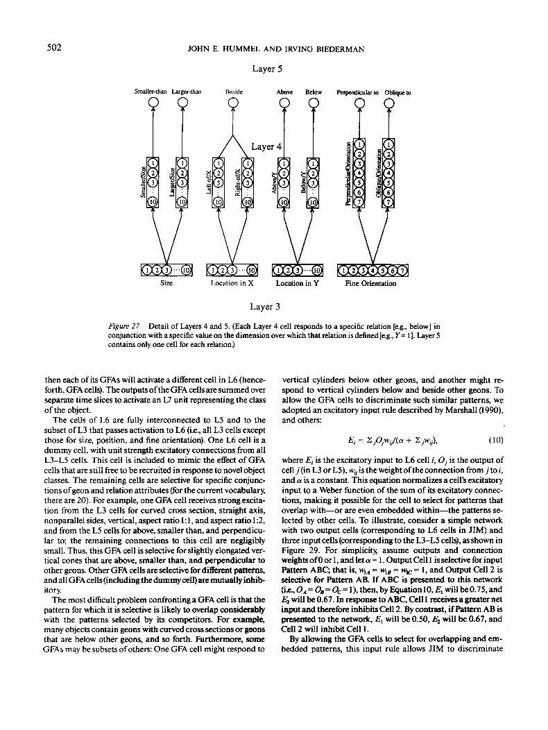
502 JOHN E. HUMMEL AND IRVING BIEDERMAN
Layer 5
Smaller-than Larger-than
o oBeside
OAbove Below
O OPerpendicular to Oblique to
O O
Size Location in X Location in Y Fine Orientation
Layer 3
Figure 27. Detail of Layers 4 and 5. (Each Layer 4 cell responds to a specific relation [e.g., below] inconjunction with a specific value on the dimension over which that relation is defined [e.g., Y=l]. Layer 5contains only one cell for each relation.)
then each of its GFAs will activate a different cell in L6 (hence-forth, GFA cells). The outputs of the GFA cells are summed overseparate time slices to activate an L7 unit representing the classof the object.
The cells of L6 are fully interconnected to L5 and to thesubset of L3 that passes activation to L6 (i.e., all L3 cells exceptthose for size, position, and fine orientation). One L6 cell is adummy cell, with unit strength excitatory connections from allL3-L5 cells. This cell is included to mimic the effect of GFAcells that are still free to be recruited in response to novel objectclasses. The remaining cells are selective for specific conjunc-tions of geon and relation attributes (for the current vocabulary,there are 20). For example, one GFA cell receives strong excita-tion from the L3 cells for curved cross section, straight axis,nonparallel sides, vertical, aspect ratio 1:1, and aspect ratio 1:2,and from the L5 cells for above, smaller than, and perpendicu-lar to; the remaining connections to this cell are negligiblysmall. Thus, this GFA cell is selective for slightly elongated ver-tical cones that are above, smaller than, and perpendicular toother geons. Other GFA cells are selective for different patterns,and all GFA cells (including the dummy cell) are mutually inhib-itory.
The most difficult problem confronting a GFA cell is that thepattern for which it is selective is likely to overlap considerablywith the patterns selected by its competitors. For example,many objects contain geons with curved cross sections or geonsthat are below other geons, and so forth. Furthermore, someGFAs may be subsets of others: One GFA cell might respond to
vertical cylinders below other geons, and another might re-spond to vertical cylinders below and beside other geons. Toallow the GFA cells to discriminate such similar patterns, weadopted an excitatory input rule described by Marshall (1990),and others:
E, = + (10)
where £, is the excitatory input to L6 cell /', Os is the output ofcell j (in L3 or L5), wtj is the weight of the connection from j to /,and a is a constant. This equation normalizes a cell's excitatoryinput to a Weber function of the sum of its excitatory connec-tions, making it possible for the cell to select for patterns thatoverlap with—or are even embedded within—the patterns se-lected by other cells. To illustrate, consider a simple networkwith two output cells (corresponding to L6 cells in JIM) andthree input cells (corresponding to the L3-L5 cells), as shown inFigure 29. For simplicity, assume outputs and connectionweights of 0 or 1, and let a = 1. Output Cell 1 is selective for inputPattern ABC; that is, wlA = wlB = w,c = 1, and Output Cell 2 isselective for Pattern AB. If ABC is presented to this network(i.e, OA = OB = Oc= 1), then, by Equation 10, £", will be 0.75, andEI will be 0.67. In response to ABC, Cell 1 receives a greater netinput and therefore inhibits Cell 2. By contrast, if Pattern AB ispresented to the network, £, will be 0.50, £j will be 0.67, andCell 2 will inhibit Cell 1.
By allowing the GFA cells to select for overlapping and em-bedded patterns, this input rule allows JIM to discriminate
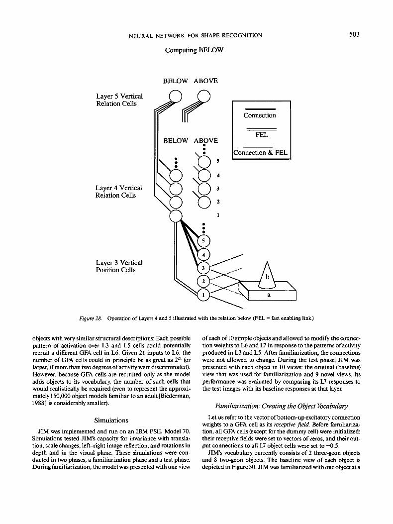
NEURAL NETWORK FOR SHAPE RECOGNITION
Computing BELOW
503
BELOW ABOVE
Layer 5 VerticalRelation Cells
Layer 4 VerticalRelation Cells
Layer 3 VerticalPosition Cells
Figure 28. Operation of Layers 4 and 5 illustrated with the relation below. (PEL = fast enabling link.)
objects with very similar structural descriptions: Each possiblepattern of activation over L3 and L5 cells could potentiallyrecruit a different GFA cell in L6. Given 21 inputs to L6, thenumber of GFA cells could in principle be as great as 221 (orlarger, if more than two degrees of activity were discriminated).However, because GFA cells are recruited only as the modeladds objects to its vocabulary, the number of such cells thatwould realistically be required (even to represent the approxi-mately 150,000 object models familiar to an adult [Biederman,1988] is considerably smaller).
Simulations
JIM was implemented and run on an IBM PSII, Model 70.Simulations tested JIM's capacity for invariance with transla-tion, scale changes, left-right image reflection, and rotations indepth and in the visual plane. These simulations were con-ducted in two phases, a familiarization phase and a test phase.During familiarization, the model was presented with one view
of each of 10 simple objects and allowed to modify the connec-tion weights to L6 and L7 in response to the patterns of activityproduced in L3 and L5. After familiarization, the connectionswere not allowed to change. During the test phase, JIM waspresented with each object in 10 views: the original (baseline)view that was used for familiarization and 9 novel views. Itsperformance was evaluated by comparing its L7 responses tothe test images with its baseline responses at that layer.
Familiarization: Creating the Object Vocabulary
Let us refer to the vector of bottom-up excitatory connectionweights to a GFA cell as its receptive field. Before familiariza-tion, all GFA cells (except for the dummy cell) were initialized:their receptive fields were set to vectors of zeros, and their out-put connections to all L7 object cells were set to —0.5.
JIM's vocabulary currently consists of 2 three-geon objectsand 8 two-geon objects. The baseline view of each object isdepicted in Figure 30. JIM was familiarized with one object at a
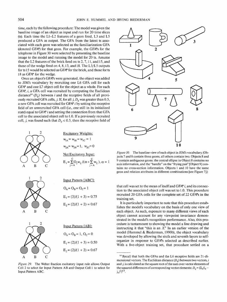
504 JOHN E. HUMMEL AND IRVING BIEDERMAN
time, each by the following procedure: The model was given thebaseline image of an object as input and run for 20 time slices(ts). Each time the L1-L2 features of a geon fired, L3 and L5produced a GFA as output. The GFA from the latest ts asso-ciated with each geon was selected as the familiarization GFA(denoted GFA*) for that geon. For example, the GFA*s for thetelephone in Figure 30 were selected by presenting the baselineimage to the model and running the model for 20 ts. Assumethat the L2 features of the brick fired on ts 2, 7,11, and 15, andthose of the wedge fired on 4, 8,13, and 18. The L3/L5 outputsfor ts 15 would be selected as GFA* for the brick, and those for ts18 as GFA* for the wedge.
Once an object's GFA*s were generated, the object was addedto JIM's vocabulary by recruiting one L6 GFA cell for eachGFA* and one L7 object cell for the object as a whole. For eachGFA*, i, a GFA cell was recruited by computing the Euclideandistance14 (Z),-,) between i and the receptive fields of all previ-ously recruited GFA cells, j. If, for all j, Dtj was greater than 0.5,a new GFA cell was recruited for GFA* i by setting the receptivefield of an unrecruited GFA cell (i.e., one still in its initializedstate) equal to GFA*; and setting the connection from that GFAcell to the associated object cell to 1.0. If a previously recruitedcell, y, was found such that Dtj < 0.5, then the receptive field of
Excitatory Weights:W IA = W IB = W IC = !
W2A= W2B= 1> W2C=°
Net Excitatory Input:
Ej = A j = A
A B C
Input Pattern FABC1:
0A= 0B= Oc= 1
E 1 =(3) / ( l+3) = 0.75
E2=(2)/(l +2) = 0.67
Input Pattern [AB1:
0 A =0 B =1,0 C =0
E1=(2)/(l +3) = 0.50
E2=(2)/(l +2) = 0.67
Figure 29. The Weber fraction excitatory input rule allows OutputCell 2 to select for Input Pattern AB and Output Cell 1 to select forInput Pattern ABC.
Figure 30. The baseline view of each object in JIM's vocabulary. (Ob-jects 7 and 8 contain three geons, all others contain two. Objects 8 and9 contain ambiguous geons: the central ellipse in Object 8 contains noaxis information, and the "handle" on the "frying pan" [Object 9] con-tains no cross-section information. Objects 1 and 10 have the samegeon and relation attributes in different combinations [see Figure 7].)
that cell was set to the mean of itself and GFA* /', and its connec-tion to the associated object cell was set to 1.0. This procedurerecruited 20 GFA cells for the complete set of 22 GFA*s in thetraining set.
It is particularly important to note that this procedure estab-lishes the model's vocabulary on the basis of only one view ofeach object. As such, exposure to many different views of eachobject cannot account for any viewpoint invariance demon-strated in the model's recognition performance. Also, this pro-cedure is tantamount to showing the model a line drawing andinstructing it that "this is an X? In an earlier version of themodel (Hummel & Biederman, 1990b), the object vocabularywas developed by allowing the sixth and seventh layers to self-organize in response to GFA*s selected as described earlier.With a five-object training set, that procedure settled on a
14 Recall that both the GFAs and the L6 receptive fields are 21-di-mensional vectors. The Euclidean distance (D,y) between two vectors, iand j, is calculated as the square root of the sum over vector elements ofthe squared differences of corresponding vector elements: Dff = (2t(it -
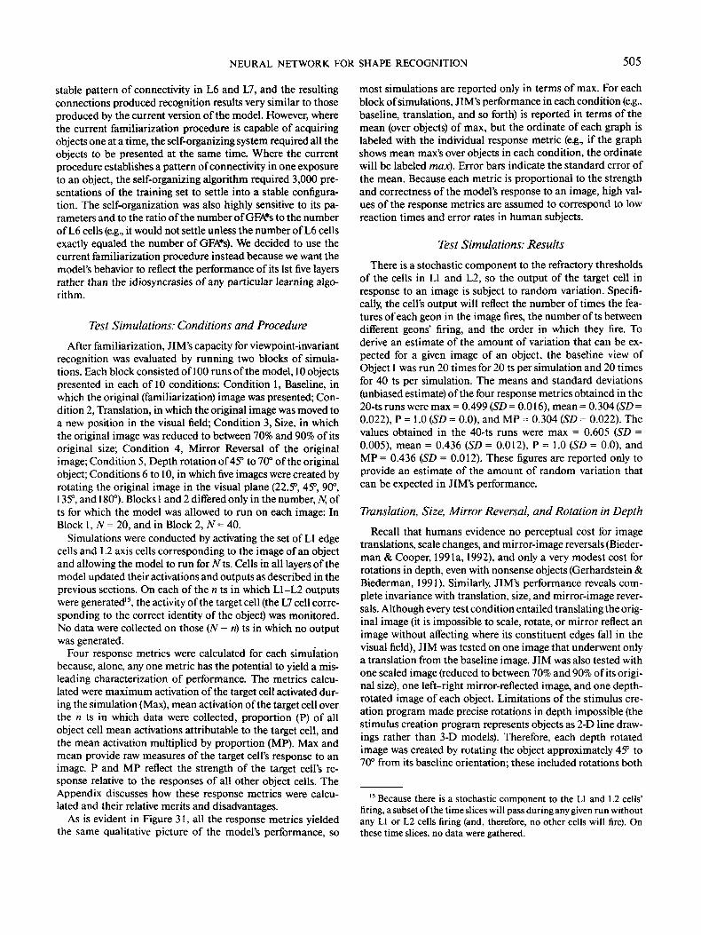
NEURAL NETWORK FOR SHAPE RECOGNITION 505
stable pattern of connectivity in L6 and L7, and the resultingconnections produced recognition results very similar to thoseproduced by the current version of the model. However, wherethe current familiarization procedure is capable of acquiringobjects one at a time, the self-organizing system required all theobjects to be presented at the same time. Where the currentprocedure establishes a pattern of connectivity in one exposureto an object, the self-organizing algorithm required 3,000 pre-sentations of the training set to settle into a stable configura-tion. The self-organization was also highly sensitive to its pa-rameters and to the ratio of the number of GFA*s to the numberof L6 cells (e.g, it would not settle unless the number of L6 cellsexactly equaled the number of GFA*s). We decided to use thecurrent familiarization procedure instead because we want themodel's behavior to reflect the performance of its 1st five layersrather than the idiosyncrasies of any particular learning algo-rithm.
Test Simulations: Conditions and Procedure
After familiarization, JIM's capacity for viewpoint-invariantrecognition was evaluated by running two blocks of simula-tions. Each block consisted of 100 runs of the model, 10 objectspresented in each of 10 conditions: Condition 1, Baseline, inwhich the original (familiarization) image was presented; Con-dition 2, Translation, in which the original image was moved toa new position in the visual field; Condition 3, Size, in whichthe original image was reduced to between 70% and 90% of itsoriginal size; Condition 4, Mirror Reversal of the originalimage; Condition 5, Depth rotation of 45° to 70° of the originalobject; Conditions 6 to 10, in which five images were created byrotating the original image in the visual plane (22.5°, 45°, 90°,135°, and 180°). Blocks 1 and 2 differed only in the number, N, ofts for which the model was allowed to run on each image: InBlock l,N=20, and in Block 2,N = 40.
Simulations were conducted by activating the set of LI edgecells and L2 axis cells corresponding to the image of an objectand allowing the model to run for TVts. Cells in all layers of themodel updated their activations and outputs as described in theprevious sections. On each of the n ts in which L1-L2 outputswere generated15, the activity of the target cell (the L7 cell corre-sponding to the correct identity of the object) was monitored.No data were collected on those (N — ri) ts in which no outputwas generated.
Four response metrics were calculated for each simulationbecause, alone, any one metric has the potential to yield a mis-leading characterization of performance. The metrics calcu-lated were maximum activation of the target cell activated dur-ing the simulation (Max), mean activation of the target cell overthe n ts in which data were collected, proportion (P) of allobject cell mean activations attributable to the target cell, andthe mean activation multiplied by proportion (MP). Max andmean provide raw measures of the target cell's response to animage. P and MP reflect the strength of the target cell's re-sponse relative to the responses of all other object cells. TheAppendix discusses how these response metrics were calcu-lated and their relative merits and disadvantages.
As is evident in Figure 31, all the response metrics yieldedthe same qualitative picture of the model's performance, so
most simulations are reported only in terms of max. For eachblock of simulations, JIM's performance in each condition (e.g.,baseline, translation, and so forth) is reported in terms of themean (over objects) of max, but the ordinate of each graph islabeled with the individual response metric (e.g., if the graphshows mean max's over objects in each condition, the ordinatewill be labeled max). Error bars indicate the standard error ofthe mean. Because each metric is proportional to the strengthand correctness of the model's response to an image, high val-ues of the response metrics are assumed to correspond to lowreaction times and error rates in human subjects.
Test Simulations: Results
There is a stochastic component to the refractory thresholdsof the cells in LI and L2, so the output of the target cell inresponse to an image is subject to random variation. Specifi-cally, the cell's output will reflect the number of times the fea-tures of each geon in the image fires, the number of ts betweendifferent geons' firing, and the order in which they fire. Toderive an estimate of the amount of variation that can be ex-pected for a given image of an object, the baseline view ofObject 1 was run 20 times for 20 ts per simulation and 20 timesfor 40 ts per simulation. The means and standard deviations(unbiased estimate) of the four response metrics obtained in the20-ts runs were max = 0.499 (SD = 0.016), mean = 0.304 (SD =0.022), P = 1.0 (SD = 0.0), and MP = 0.304 (SD = 0.022). Thevalues obtained in the 40-ts runs were max = 0.605 (SD =0.005), mean = 0.436 (SD = 0.012), P = 1.0 (SD = 0.0), andMP= 0.436 (SD = 0.012). These figures are reported only toprovide an estimate of the amount of random variation thatcan be expected in JIM's performance.
Translation, Size, Mirror Reversal, and Rotation in Depth
Recall that humans evidence no perceptual cost for imagetranslations, scale changes, and mirror-image reversals (Bieder-man & Cooper, 199la, 1992), and only a very modest cost forrotations in depth, even with nonsense objects (Gerhardstein &Biederman, 1991). Similarly, JIM's performance reveals com-plete invariance with translation, size, and mirror-image rever-sals. Although every test condition entailed translating the orig-inal image (it is impossible to scale, rotate, or mirror reflect animage without affecting where its constituent edges fall in thevisual field), JIM was tested on one image that underwent onlya translation from the baseline image. JIM was also tested withone scaled image (reduced to between 70% and 90% of its origi-nal size), one left-right mirror-reflected image, and one depth-rotated image of each object. Limitations of the stimulus cre-ation program made precise rotations in depth impossible (thestimulus creation program represents objects as 2-D line draw-ings rather than 3-D models). Therefore, each depth rotatedimage was created by rotating the object approximately 45° to70° from its baseline orientation; these included rotations both
15 Because there is a stochastic component to the LI and L2 cells'firing, a subset of the time slices will pass during any given run withoutany LI or L2 cells firing (and, therefore, no other cells will fire). Onthese time slices, no data were gathered.
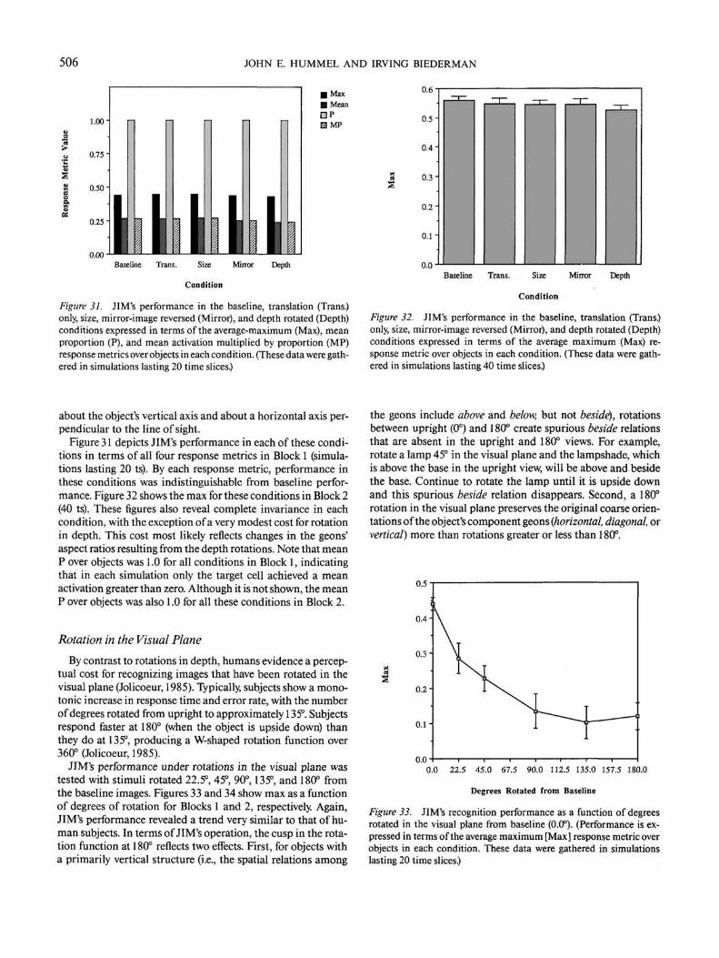
506 JOHN E. HUMMEL AND IRVING BIEDERMAN
•s
g.s«
i.oo-
0.75-
0.50-
0.25-
0.00 I ll
MaxMean
BMP
0.6
Baseline Trans. Size Mirror Depth
Condition
Figure 31. JIM's performance in the baseline, translation (Trans.)only, size, mirror-image reversed (Mirror), and depth rotated (Depth)conditions expressed in terms of the average-maximum (Max), meanproportion (P), and mean activation multiplied by proportion (MP)response metrics over objects in each condition. (These data were gath-ered in simulations lasting 20 time slices.)
0.5-
0.4-
0.3-
0.2
0.1
0.0Baseline Trans. Size Mirror Depth
Condition
Figure 32. JIM's performance in the baseline, translation (Trans.)only, size, mirror-image reversed (Mirror), and depth rotated (Depth)conditions expressed in terms of the average maximum (Max) re-sponse metric over objects in each condition. (These data were gath-ered in simulations lasting 40 time slices.)
about the object's vertical axis and about a horizontal axis per-pendicular to the line of sight.
Figure 31 depicts JIM's performance in each of these condi-tions in terms of all four response metrics in Block 1 (simula-tions lasting 20 ts). By each response metric, performance inthese conditions was indistinguishable from baseline perfor-mance. Figure 32 shows the max for these conditions in Block 2(40 ts). These figures also reveal complete invariance in eachcondition, with the exception of a very modest cost for rotationin depth. This cost most likely reflects changes in the geons'aspect ratios resulting from the depth rotations. Note that meanP over objects was 1.0 for all conditions in Block 1, indicatingthat in each simulation only the target cell achieved a meanactivation greater than zero. Although it is not shown, the meanP over objects was also 1.0 for all these conditions in Block 2.
Rotation in the Visual Plane
By contrast to rotations in depth, humans evidence a percep-tual cost for recognizing images that have been rotated in thevisual plane (Jolicoeur, 1985). Typically, subjects show a mono-tonic increase in response time and error rate, with the numberof degrees rotated from upright to approximately 135°. Subjectsrespond faster at 180° (when the object is upside down) thanthey do at 135°, producing a W-shaped rotation function over360° (Jolicoeur, 1985).
JIM's performance under rotations in the visual plane wastested with stimuli rotated 22.5°, 45°, 90°, 135°, and 180° fromthe baseline images. Figures 33 and 34 show max as a functionof degrees of rotation for Blocks 1 and 2, respectively. Again,JIM's performance revealed a trend very similar to that of hu-man subjects. In terms of JIM's operation, the cusp in the rota-tion function at 180° reflects two effects. First, for objects witha primarily vertical structure (i.e., the spatial relations among
the geons include above and below, but not beside), rotationsbetween upright (0°) and 180° create spurious beside relationsthat are absent in the upright and 180° views. For example,rotate a lamp 45° in the visual plane and the lampshade, whichis above the base in the upright view, will be above and besidethe base. Continue to rotate the lamp until it is upside downand this spurious beside relation disappears. Second, a 180°rotation in the visual plane preserves the original coarse orien-tations of the object's component geons (horizontal, diagonal, orvertical) more than rotations greater or less than 180°.
22.5 45.0 67.5 90.0 112.5 135.0 157.5 180.0
Degrees Rotated from Baseline
Figure 33. JIM's recognition performance as a function of degreesrotated in the visual plane from baseline (0.0°). (Performance is ex-pressed in terms of the average maximum [Max] response metric overobjects in each condition. These data were gathered in simulationslasting 20 time slices.)
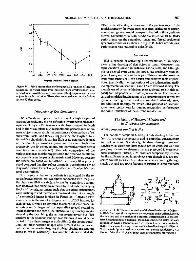
NEURAL NETWORK FOR SHAPE RECOGNITION 507
22.5 45.0 67.5 90.0 112.5 135.0 157.5 180.0
Degrees Rotated from Baseline
Figure 34. JIM's recognition performance as a function of degreesrotated in the visual plane from baseline (0.0°). (Performance is ex-pressed in terms of the average maximum [Max] response metric overobjects in each condition. These data were gathered in simulationslasting 40 time slices.)
Discussion of Test Simulations
The simulations reported earlier reveal a high degree oftranslation, scale, and mirror-reflection invariance in JIM's rec-ognition of objects. Performance with objects rotated in depthand in the visual plane also resembles the performance of hu-man subjects under similar circumstances. Comparison of re-sults from Block 1 and Block 2 suggests that the length of timefor which a simulation is run has little or no qualitative impacton the model's performance (mean and max were higher onaverage for the 40 ts simulations, but the relative values acrossconditions were unaffected). Similarly, comparison of thevarious response metrics suggests that the observed results arenot dependent on the particular metric used. However, becausethe results are based on simulations with only 10 objects, itcould be argued that they reflect the model's use of some sort ofdiagnostic feature for each object, rather than the objects' struc-tural descriptions.
This diagnostic feature hypothesis is challenged by the re-sults of two additional test conditions conducted with images ofthe objects in JIM's vocabulary. In the first condition, a scram-bled image of each object was created by randomly rearrangingblocks of the original image such that the edges' orientationswere unchanged and the vertices remained intact. An exampleof a scrambled image is given in Figure 35. If JIM's perfor-mance reflects the use of a diagnostic list of 2-D features foreach object, it would be expected to achieve at least moderateactivation in the target cell corresponding to each scrambledimage (although the axes of parallelism and symmetry are de-stroyed by the scrambling, the vertices are preserved), but if it issensitive to the relations among these features, it would be ex-pected to treat these images as unfamiliar. In the second condi-tion, the intact baseline images were presented to the model,but the binding mechanism was disabled, forcing the separategeons to fire in synchrony. This condition demonstrated the
effect of accidental synchrony on JIM's performance; if themodel's capacity for image parsing is truly critical to its perfor-mance, recognition would be expected to fail in this conditionas well. Simulations in both conditions lasted for 40 ts. JIM'sperformance on the scrambled image and forced accidentalsynchrony conditions is shown in Figure 36. In both conditions,performance was reduced to noise levels.
Discussion
JIM is capable of activating a representation of an objectgiven a line drawing of that object as input. Moreover, thatrepresentation is invariant with translation, scale, and left-rightmirror reversal even when the model has previously been ex-posed to only one view of the object. This section discusses theimportant aspects of JIM's design and explores their implica-tions. Specifically, the implications of the independent attrib-ute representation used in L3 and L5 are reviewed shortly. Themodel's use of dynamic binding plays a pivotal role in this ca-pacity for independent attribute representations. The theoreti-cal and empirical implications of using temporal synchrony fordynamic binding is discussed in some detail. Also addressedare additional findings for which JIM provides an account,some novel predictions for human recognition performance,and some limitations of the current architecture.
The Nature of Temporal Binding andIts Empirical Consequences
What Temporal Binding Is Not
The notion of temporal binding is only starting to becomefamiliar to most psychologists, and its empirical consequencesare not obvious. Specifically, binding through temporalsynchrony as described here should not be confused with thegrouping of stimulus elements that are presented in close tem-poral contiguity. Indeed, JIM produces temporal asynchronyfor the different geons in an object even though they are pre-sented simultaneously. The confusion between binding throughsynchrony and grouping features presented in close temporal
» / V)
Figure 35. Left: The representation of the baseline image of Object 1in JIM's first layer. (Line segments correspond to active cells in Layer 1,the location and orientation of a segment corresponding to the pre-ferred location and orientation of the cell, respectively. Circles indicatelocations in Layer 2 containing active vertex (or lone termination) cells.Right: The scrambled image version of the baseline image for Object 1.Vertices and edge orientations are preserved, but the positions of 2 X 2blocks of the 22 X 22 cluster input layer are randomly rearranged.)
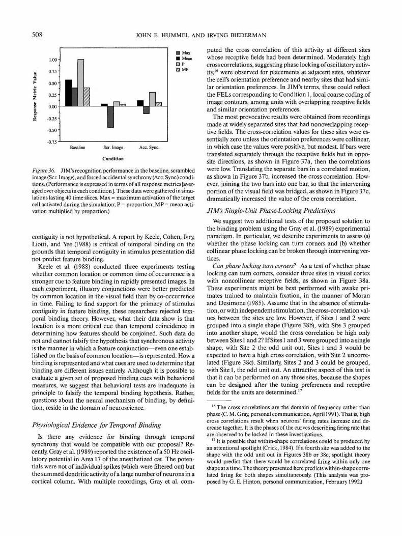
508 JOHN E. HUMMEL AND IRVING BIEDERMAN
-0.75Baseline Scr. Image
Condition
Ace. Sync.
Figure 36. JIM's recognition performance in the baseline, scrambledimage (Scr. Image), and forced accidental synchrony (Ace. Sync.) condi-tions. (Performance is expressed in terms of all response metrics [aver-aged over objects in each condition]. These data were gathered in simu-lations lasting 40 time slices. Max = maximum activation of the targetcell activated during the simulation; P = proportion; MP = mean acti-vation multiplied by proportion.)
contiguity is not hypothetical. A report by Keele, Cohen, Ivry,Liotti, and Yee (1988) is critical of temporal binding on thegrounds that temporal contiguity in stimulus presentation didnot predict feature binding.
Keele et al. (1988) conducted three experiments testingwhether common location or common time of occurrence is astronger cue to feature binding in rapidly presented images. Ineach experiment, illusory conjunctions were better predictedby common location in the visual field than by co-occurrencein time. Failing to find support for the primacy of stimuluscontiguity in feature binding, these researchers rejected tem-poral binding theory. However, what their data show is thatlocation is a more critical cue than temporal coincidence indetermining how features should be conjoined. Such data donot and cannot falsify the hypothesis that synchronous activityis the manner in which a feature conjunction—even one estab-lished on the basis of common location—is represented. How abinding is represented and what cues are used to determine thatbinding are different issues entirely. Although it is possible toevaluate a given set of proposed binding cues with behavioralmeasures, we suggest that behavioral tests are inadequate inprinciple to falsify the temporal binding hypothesis. Rather,questions about the neural mechanism of binding, by defini-tion, reside in the domain of neuroscience.
Physiological Evidence for Temporal Binding
Is there any evidence for binding through temporalsynchrony that would be compatible with our proposal? Re-cently, Gray et al. (1989) reported the existence of a 50 Hz oscil-latory potential in Area 17 of the anesthetized cat. The poten-tials were not of individual spikes (which were filtered out) butthe summed dendritic activity of a large number of neurons in acortical column. With multiple recordings, Gray et al. com-
puted the cross correlation of this activity at different siteswhose receptive fields had been determined. Moderately highcross correlations, suggesting phase locking of oscillatory activ-ity,16 were observed for placements at adjacent sites, whateverthe cell's orientation preference and nearby sites that had simi-lar orientation preferences. In JIM's terms, these could reflectthe FELs corresponding to Condition 1, local coarse coding ofimage contours, among units with overlapping receptive fieldsand similar orientation preferences.
The most provocative results were obtained from recordingsmade at widely separated sites that had nonoverlapping recep-tive fields. The cross-correlation values for these sites were es-sentially zero unless the orientation preferences were collinear,in which case the values were positive, but modest. If bars weretranslated separately through the receptive fields but in oppo-site directions, as shown in Figure 37a, then the correlationswere low. Translating the separate bars in a correlated motion,as shown in Figure 37b, increased the cross correlation. How-ever, joining the two bars into one bar, so that the interveningportion of the visual field was bridged, as shown in Figure 37c,dramatically increased the value of the cross correlation.
JIM's Single-Unit Phase-Locking Predictions
We suggest two additional tests of the proposed solution tothe binding problem using the Gray et al. (1989) experimentalparadigm. In particular, we describe experiments to assess (a)whether the phase locking can turn corners and (b) whethercollinear phase locking can be broken through intervening ver-tices.
Can phase locking turn comers? As a test of whether phaselocking can turn corners, consider three sites in visual cortexwith noncollinear receptive fields, as shown in Figure 38a.These experiments might be best performed with awake pri-mates trained to maintain fixation, in the manner of Moranand Desimone (1985). Assume that in the absence of stimula-tion, or with independent stimulation, the cross-correlation val-ues between the sites are low. However, if Sites 1 and 2 weregrouped into a single shape (Figure 38b), with Site 3 groupedinto another shape, would the cross correlation be high onlybetween Sites 1 and 2? If Sites 1 and 3 were grouped into a singleshape, with Site 2 the odd unit out, Sites 1 and 3 would beexpected to have a high cross correlation, with Site 2 uncorre-lated (Figure 38c). Similarly, Sites 2 and 3 could be grouped,with Site 1, the odd unit out. An attractive aspect of this test isthat it can be performed on any three sites, because the shapescan be designed after the tuning preferences and receptivefields for the units are determined.17
16 The cross correlations are the domain of frequency rather thanphase (C. M. Gray, personal communication, April 1991). That is, highcross correlations result when neurons' firing rates increase and de-crease together. It is the phases of the curves describing firing rate thatare observed to be locked in these investigations.
17 It is possible that within-shape correlations could be produced byan attentional spotlight (Crick, 1984). If a fourth site was added to theshape with the odd unit out in Figures 38b or 38c, spotlight theorywould predict that there would be correlated firing within only oneshape at a time. The theory presented here predicts within-shape corre-lated firing for both shapes simultaneously. (This analysis was pro-posed by G. E. Hinton, personal communication, February 1992.)
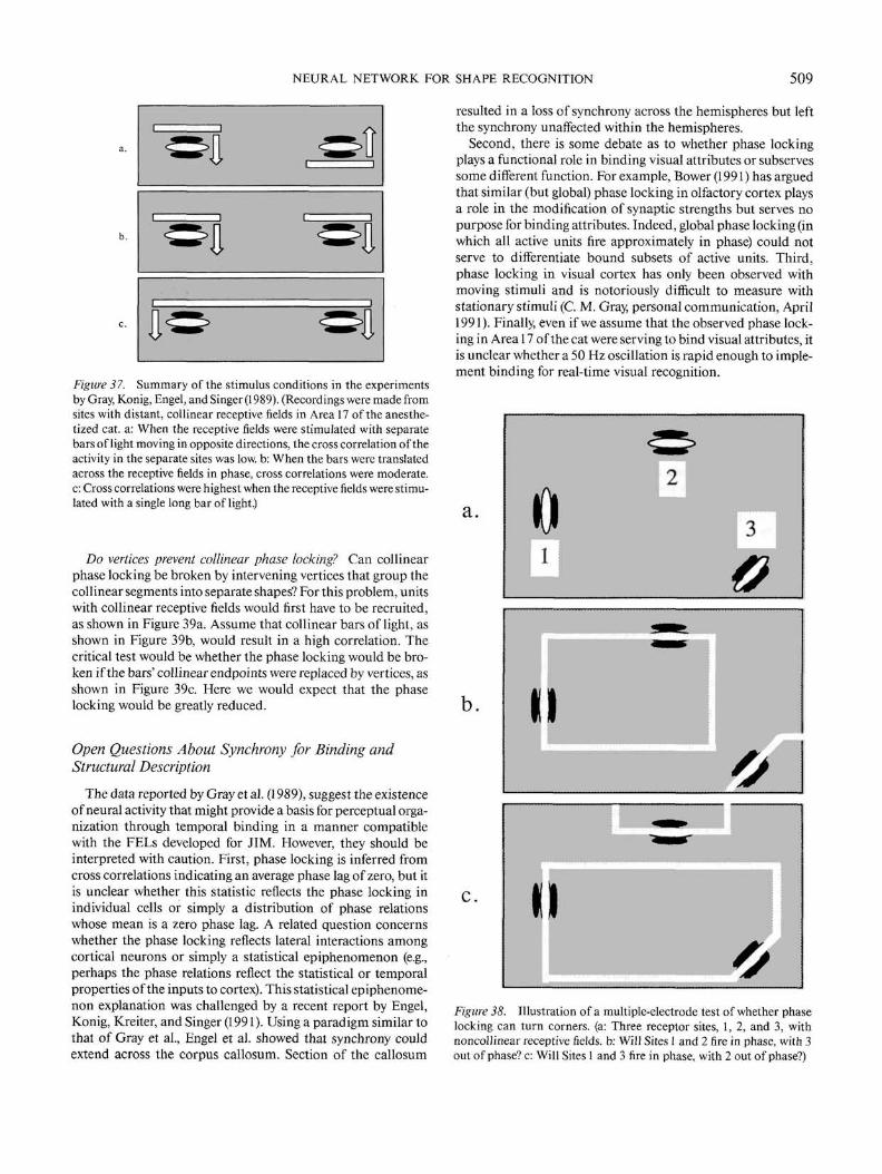
NEURAL NETWORK FOR SHAPE RECOGNITION 509
Figure 37. Summary of the stimulus conditions in the experimentsby Gray, Konig, Engel, and Singer (1989). (Recordings were made fromsites with distant, collinear receptive fields in Area 17 of the anesthe-tized cat. a: When the receptive fields were stimulated with separatebars of light moving in opposite directions, the cross correlation of theactivity in the separate sites was low. b: When the bars were translatedacross the receptive fields in phase, cross correlations were moderate,c: Cross correlations were highest when the receptive fields were stimu-lated with a single long bar of light.)
Do vertices prevent collinear phase locking? Can collinearphase locking be broken by intervening vertices that group thecollinear segments into separate shapes? For this problem, unitswith collinear receptive fields would first have to be recruited,as shown in Figure 39a. Assume that collinear bars of light, asshown in Figure 39b, would result in a high correlation. Thecritical test would be whether the phase locking would be bro-ken if the bars' collinear endpoints were replaced by vertices, asshown in Figure 39c. Here we would expect that the phaselocking would be greatly reduced.
Open Questions About Synchrony for Binding andStructural Description
The data reported by Gray et al. (1989), suggest the existenceof neural activity that might provide a basis for perceptual orga-nization through temporal binding in a manner compatiblewith the FELs developed for JIM. However, they should beinterpreted with caution. First, phase locking is inferred fromcross correlations indicating an average phase lag of zero, but itis unclear whether this statistic reflects the phase locking inindividual cells or simply a distribution of phase relationswhose mean is a zero phase lag. A related question concernswhether the phase locking reflects lateral interactions amongcortical neurons or simply a statistical epiphenomenon (e.g.,perhaps the phase relations reflect the statistical or temporalproperties of the inputs to cortex). This statistical epiphenome-non explanation was challenged by a recent report by Engel,Konig, Kreiter, and Singer (1991). Using a paradigm similar tothat of Gray et al., Engel et al. showed that synchrony couldextend across the corpus callosum. Section of the callosum
resulted in a loss of synchrony across the hemispheres but leftthe synchrony unaffected within the hemispheres.
Second, there is some debate as to whether phase lockingplays a functional role in binding visual attributes or subservessome different function. For example, Bower (1991) has arguedthat similar (but global) phase locking in olfactory cortex playsa role in the modification of synaptic strengths but serves nopurpose for binding attributes. Indeed, global phase locking (inwhich all active units fire approximately in phase) could notserve to differentiate bound subsets of active units. Third,phase locking in visual cortex has only been observed withmoving stimuli and is notoriously difficult to measure withstationary stimuli (C. M. Gray, personal communication, April1991). Finally, even if we assume that the observed phase lock-ing in Area 17 of the cat were serving to bind visual attributes, itis unclear whether a 50 Hz oscillation is rapid enough to imple-ment binding for real-time visual recognition.
a.
b.
c.
Figure 38. Illustration of a multiple-electrode test of whether phaselocking can turn corners, (a: Three receptor sites, 1, 2, and 3, withnoncollinear receptive fields, b: Will Sites 1 and 2 fire in phase, with 3out of phase? c: Will Sites 1 and 3 fire in phase, with 2 out of phase?)
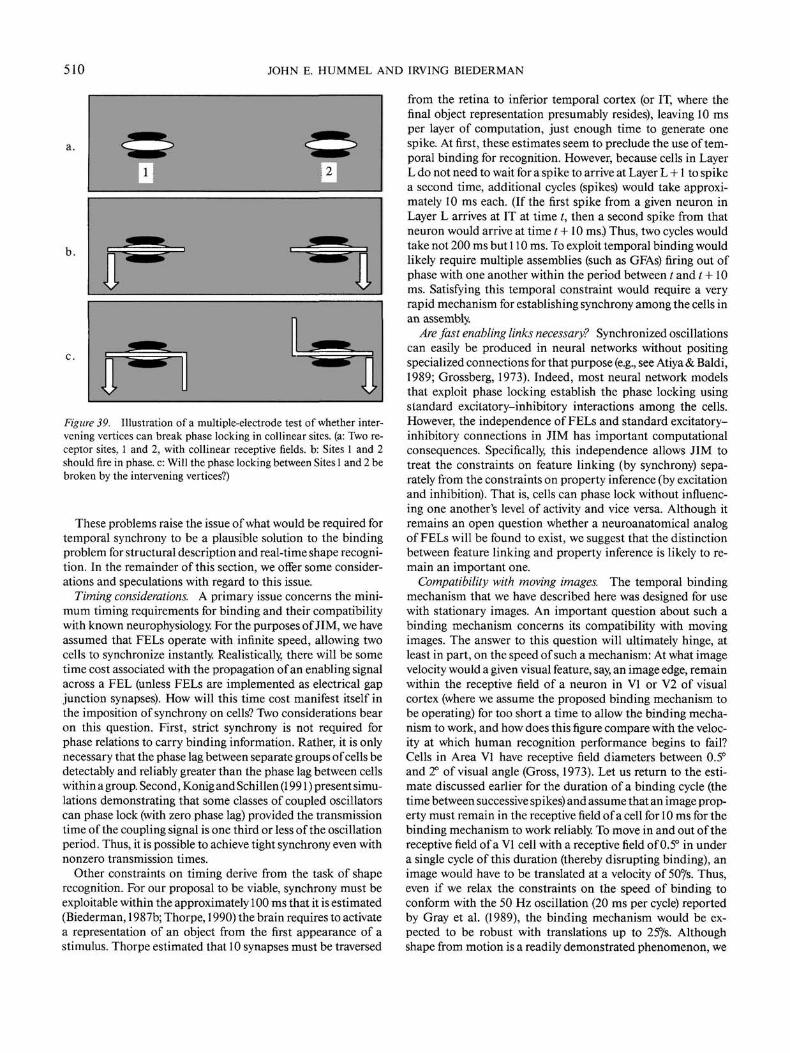
510 JOHN E. HUMMEL AND IRVING BIEDERMAN
a.
b.
12
Figure 39. Illustration of a multiple-electrode test of whether inter-vening vertices can break phase locking in collinear sites, (a: Two re-ceptor sites, 1 and 2, with collinear receptive fields, b: Sites 1 and 2should fire in phase, c: Will the phase locking between Sites 1 and 2 bebroken by the intervening vertices?)
These problems raise the issue of what would be required fortemporal synchrony to be a plausible solution to the bindingproblem for structural description and real-time shape recogni-tion. In the remainder of this section, we offer some consider-ations and speculations with regard to this issue.
Timing considerations. A primary issue concerns the mini-mum timing requirements for binding and their compatibilitywith known neurophysiology. For the purposes of JIM, we haveassumed that FELs operate with infinite speed, allowing twocells to synchronize instantly. Realistically, there will be sometime cost associated with the propagation of an enabling signalacross a FEL (unless FELs are implemented as electrical gapjunction synapses). How will this time cost manifest itself inthe imposition of synchrony on cells? Two considerations bearon this question. First, strict synchrony is not required forphase relations to carry binding information. Rather, it is onlynecessary that the phase lag between separate groups of cells bedetectably and reliably greater than the phase lag between cellswithin a group. Second, Konig and Schillen (1991) present simu-lations demonstrating that some classes of coupled oscillatorscan phase lock (with zero phase lag) provided the transmissiontime of the coupling signal is one third or less of the oscillationperiod. Thus, it is possible to achieve tight synchrony even withnonzero transmission times.
Other constraints on timing derive from the task of shaperecognition. For our proposal to be viable, synchrony must beexploitable within the approximately 100 ms that it is estimated(Biederman, 1987b; Thorpe, 1990) the brain requires to activatea representation of an object from the first appearance of astimulus. Thorpe estimated that 10 synapses must be traversed
from the retina to inferior temporal cortex (or IT, where thefinal object representation presumably resides), leaving 10 msper layer of computation, just enough time to generate onespike. At first, these estimates seem to preclude the use of tem-poral binding for recognition. However, because cells in LayerL do not need to wait for a spike to arrive at Layer L +1 to spikea second time, additional cycles (spikes) would take approxi-mately 10 ms each. (If the first spike from a given neuron inLayer L arrives at IT at time t, then a second spike from thatneuron would arrive at time t + 10 ms.) Thus, two cycles wouldtake not 200 ms but 110 ms. To exploit temporal binding wouldlikely require multiple assemblies (such as GFAs) firing out ofphase with one another within the period between / and t + 10ms. Satisfying this temporal constraint would require a veryrapid mechanism for establishing synchrony among the cells inan assembly.
Are fast enabling links necessary? Synchronized oscillationscan easily be produced in neural networks without positingspecialized connections for that purpose (e.g., see Atiya & Baldi,1989; Grossberg, 1973). Indeed, most neural network modelsthat exploit phase locking establish the phase locking usingstandard excitatory-inhibitory interactions among the cells.However, the independence of FELs and standard excitatory-inhibitory connections in JIM has important computationalconsequences. Specifically, this independence allows JIM totreat the constraints on feature linking (by synchrony) sepa-rately from the constraints on property inference (by excitationand inhibition). That is, cells can phase lock without influenc-ing one another's level of activity and vice versa. Although itremains an open question whether a neuroanatomical analogof FELs will be found to exist, we suggest that the distinctionbetween feature linking and property inference is likely to re-main an important one.
Compatibility with moving images. The temporal bindingmechanism that we have described here was designed for usewith stationary images. An important question about such abinding mechanism concerns its compatibility with movingimages. The answer to this question will ultimately hinge, atleast in part, on the speed of such a mechanism: At what imagevelocity would a given visual feature, say, an image edge, remainwithin the receptive field of a neuron in VI or V2 of visualcortex (where we assume the proposed binding mechanism tobe operating) for too short a time to allow the binding mecha-nism to work, and how does this figure compare with the veloc-ity at which human recognition performance begins to fail?Cells in Area VI have receptive field diameters between 0.5°and 2° of visual angle (Gross, 1973). Let us return to the esti-mate discussed earlier for the duration of a binding cycle (thetime between successive spikes) and assume that an image prop-erty must remain in the receptive field of a cell for 10 ms for thebinding mechanism to work reliably. To move in and out of thereceptive field of a VI cell with a receptive field of 0.5° in undera single cycle of this duration (thereby disrupting binding), animage would have to be translated at a velocity of 507s. Thus,even if we relax the constraints on the speed of binding toconform with the 50 Hz oscillation (20 ms per cycle) reportedby Gray et al. (1989), the binding mechanism would be ex-pected to be robust with translations up to 25°/s. Althoughshape from motion is a readily demonstrated phenomenon, we
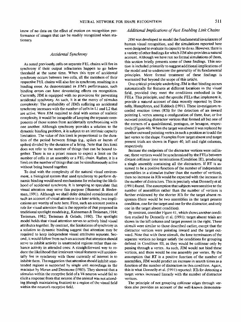
NEURAL NETWORK FOR SHAPE RECOGNITION 511
know of no data on the effect of motion on recognition per-formance of images that can be readily recognized when sta-tionary.
Accidental Synchrony
As noted previously, cells on separate PEL chains will fire insynchrony if their output refractories happen to go belowthreshold at the same time. When this type of accidentalsynchrony occurs between two cells, all the members of theirrespective PEL chains will also fire in synchrony, resulting in abinding error. As demonstrated in JIM's performance, suchbinding errors can have devastating effects on recognition.Currently, JIM is equipped with no provisions for preventingaccidental synchrony. As such, it is at the mercy of stimuluscomplexity: The probability of JIM's suffering an accidentalsynchrony increases with the number of cells in LI and L2 thatare active. Were JIM required to deal with scenes of realisticcomplexity, it would be incapable of keeping the separate com-ponents of those scenes from accidentally synchronizing withone another. Although synchrony provides a solution to thedynamic binding problem, it is subject to an intrinsic capacitylimitation. The value of this limit is proportional to the dura-tion of the period between firings (e.g., spikes or bursts ofspikes) divided by the duration of a firing. Note that this limitdoes not refer to the number of things that can be bound to-gether. There is no a priori reason to expect a limit on thenumber of cells in an assembly or a PEL chain. Rather, it is alimit on the number of things that can be simultaneously activewithout being bound together.
To deal with the complexity of the natural visual environ-ment, a biological system that used synchrony to perform dy-namic binding would need mechanisms for reducing the likeli-hood of accidental synchrony. It is tempting to speculate thatvisual attention may serve this purpose (Hummel & Bieder-man, 1991). Although we shall defer detailed consideration ofsuch an account of visual attention to a later article, two impli-cations are worthy of note here. First, such an account posits arole for visual attention that is the opposite of that proposed intraditional spotlight models (e.g., Kahneman & Treisman, 1984;Treisman, 1982; Treisman & Gelade, 1980). The spotlightmodel holds that visual attention serves to actively bind visualattributes together. By contrast, the limitations of synchrony asa solution to dynamic binding suggest that attention may berequired to keep independent visual attributes separate. Sec-ond, it would follow from such an account that attention shouldserve to inhibit activity in unattended regions rather than en-hance activity in attended ones: A straightforward way to re-duce the likelihood that irrelevant visual features will acciden-tally fire in synchrony with those currently of interest is toinhibit them. The suggestion that attention should inhibit unat-tended regions is supported by single unit recordings in themacaque by Moran and Desimone (1985). They showed that astimulus within the receptive field of a V4 neuron would fail toelicit a response from that neuron if the animal was not attend-ing (though maintaining fixation) to a region of the visual fieldwithin the neuron's receptive field.
Additional Implications of Fast Enabling Link Chains
JIM was developed to model the fundamental invariances ofhuman visual recognition, and the simulations reported herewere designed to evaluate its capacity to do so. However, there isa variety of other findings for which JIM also provides a naturalaccount. Although we have run no formal simulations of them,this section briefly presents some of these findings. This sec-tion is included primarily to suggest additional implications ofthe model and to underscore the generality of its fundamentalprinciples. More formal treatment of these findings iswarranted but beyond the scope of this article.
One critical principle underlying JIM is that binding occursautomatically for features at different locations in the visualfield, provided they meet the conditions embodied in theFELs. This principle, and the specific FELs that implement it,provide a natural account of data recently reported by Don-nelly, Humphreys, and Riddoch (1991). These investigators re-corded reaction times (RTs) for the detection of an inwardpointing L vertex among a configuration of three, four, or fiveoutward pointing distractor vertices that formed all but one ofthe corners of a quadrilateral, pentagon, or hexagon, respec-tively (Figure 40). When the target was absent it was replaced byanother outward pointing vertex in such a position as to add thelast vertex to the shape. Examples from target absent and targetpresent trials are shown in Figure 40, left and right columns,respectively.
Because the endpoints of the distractor vertices were collin-ear, these vertices would be synchronized by the FELs betweendistant collinear lone terminations (Condition III), producinga single assembly containing all the distractors. If RT is as-sumed to be a positive function of the number of independentassemblies in a stimulus (rather than the number of vertices),then no increase in RTs would be expected with the increase inthe number of distractors. This is precisely what Donnelly et al.(1991) found. The assumption that subjects were sensitive to thenumber of assemblies rather than the number of vertices isfurther evidenced by the shorter RTs for the target absent re-sponses (there would be two assemblies in the target presentcondition, one for the target and one for the distractor, and onlyone in the target absent condition).
By contrast, consider Figure 41, which shows another condi-tion studied by Donnelly et al. (1991); target absent trials areshown in the left column and target present in the right. Thesestimuli were similar to those described earlier, except that thedistractor vertices were pointing inward and the target out-ward. Note that with these stimuli, the lone terminators of theseparate vertices no longer satisfy the conditions for groupingdefined in Condition III, as they would be collinear only bypassing through a vertex. As such, JIM would not bind thesevertices, and there would be one assembly per vertex. By theassumption that RT is a positive function of the number ofassemblies, JIM would predict an increase in search times as afunction of the number of distractors in this condition. Again,this is what Donnelly et al. (1991) reported: RTs for detecting atarget vertex increased linearly with the number of distractorvertices.
The principle of not grouping collinear edges through ver-tices also provides an account of the well-known demonstra-
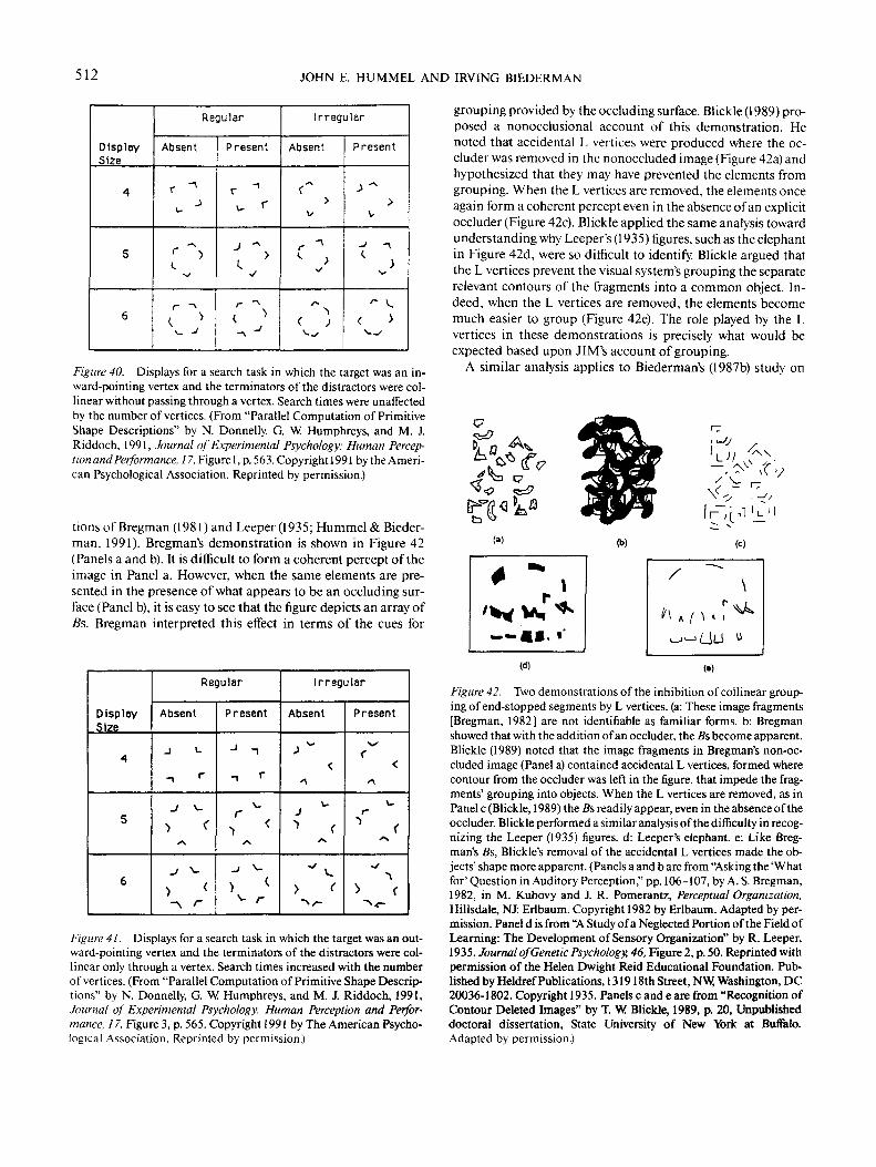
512 JOHN E. HUMMEL AND IRVING BIEDERMAN
DisplaySize
4
5
6
Regular
Absent
r n
1
Oi.
N/
r -v
c >s. -/
Present
r n
v r
J^>V
r -^
< ^
Irregular
Absent
r >V
r •*<• >
V
y^
>
< ;W
Present
> ̂>
V-
-i -\
sr
^ V.
< >> — >
Figure 40. Displays for a search task in which the target was an in-ward-pointing vertex and the terminators of the distractors were col-linear without passing through a vertex. Search times were unaffectedby the number of vertices. (From "Parallel Computation of PrimitiveShape Descriptions" by N. Donnelly, G. W Humphreys, and M. J.Riddoch, 1991, Journal of Experimental Psychology: Human Percep-tion and Performance, 17, Figure 1, p. 563. Copyright 1991 by the Ameri-can Psychological Association. Reprinted by permission.)
tions of Bregman (1981) and Leeper (1935; Hummel & Bieder-man, 1991). Bregman's demonstration is shown in Figure 42(Panels a and b). It is difficult to form a coherent percept of theimage in Panel a. However, when the same elements are pre-sented in the presence of what appears to be an occluding sur-face (Panel b), it is easy to see that the figure depicts an array ofBs. Bregman interpreted this effect in terms of the cues for
DisplaySize
4
5
6
Regular
Absent
J U
_ r
j \-
) '
^
./ *>-
-v /-
Present
-> -i
n r
r•) *
/N
_, X.
^ (^- r
Irregular
Absent
j N-
^
X.Ji (
s*
^ ^. (
^-
Present
•*r
-
-A
Ur
<~
^V ^
^Figure 41. Displays for a search task in which the target was an out-ward-pointing vertex and the terminators of the distractors were col-linear only through a vertex. Search times increased with the numberof vertices. (From "Parallel Computation of Primitive Shape Descrip-tions" by N. Donnelly, G. W Humphreys, and M. J. Riddoch, 1991,Journal of Experimental Psychology: Human Perception and Perfor-mance, 17, Figure3, p. 565. Copyright 1991 by The American Psycho-logical Association. Reprinted by permission.)
grouping provided by the occluding surface. Blickle (1989) pro-posed a nonocclusional account of this demonstration. Henoted that accidental L vertices were produced where the oc-cluder was removed in the nonoccluded image (Figure 42a) andhypothesized that they may have prevented the elements fromgrouping. When the L vertices are removed, the elements onceagain form a coherent percept even in the absence of an explicitoccluder (Figure 42c). Blickle applied the same analysis towardunderstanding why Leeper's (1935) figures, such as the elephantin Figure 42d, were so difficult to identify. Blickle argued thatthe L vertices prevent the visual system's grouping the separaterelevant contours of the fragments into a common object. In-deed, when the L vertices are removed, the elements becomemuch easier to group (Figure 42e). The role played by the Lvertices in these demonstrations is precisely what would beexpected based upon JIM's account of grouping.
A similar analysis applies to Biederman's (1987b) study on
(a)
4
/^^J^VW
r
ft*.
\
r(d)
(b) (c)
Figure 42. Two demonstrations of the inhibition of collinear group-ing of end-stopped segments by L vertices, (a: These image fragments[Bregman, 1982] are not identifiable as familiar forms, b: Bregmanshowed that with the addition of an occluder, the Bs become apparent.Blickle (1989) noted that the image fragments in Bregman's non-oc-cluded image (Panel a) contained accidental L vertices, formed wherecontour from the occluder was left in the figure, that impede the frag-ments' grouping into objects. When the L vertices are removed, as inPanel c (Blickle, 1989) the Bs readily appear, even in the absence of theoccluder. Blickle performed a similar analysis of the difficulty in recog-nizing the Leeper (1935) figures, d: Leeper's elephant, e: Like Breg-man's Bs, Blickle's removal of the accidental L vertices made the ob-jects' shape more apparent. (Panels a and b are from "Asking the 'Whatfor" Question in Auditory Perception," pp. 106-107, by A. S. Bregman,1982, in M. Kubovy and J. R. Pomerantz, Perceptual Organization,Hillsdale, NJ: Erlbaum. Copyright 1982 by Erlbaum. Adapted by per-mission. Panel d is from "A Study of a Neglected Portion of the Field ofLearning: The Development of Sensory Organization" by R. Leeper,1935, Journal of Genetic Psychology, 46, Figure 2, p. 50. Reprinted withpermission of the Helen Dwight Reid Educational Foundation. Pub-lished by Heldref Publications, 131918th Street, N W, Washington, DC20036-1802. Copyright 1935. Panels c and e are from "Recognition ofContour Deleted Images" by T. W Blickle, 1989, p. 20, Unpublisheddoctoral dissertation, State University of New York at Buffalo.Adapted by permission.)
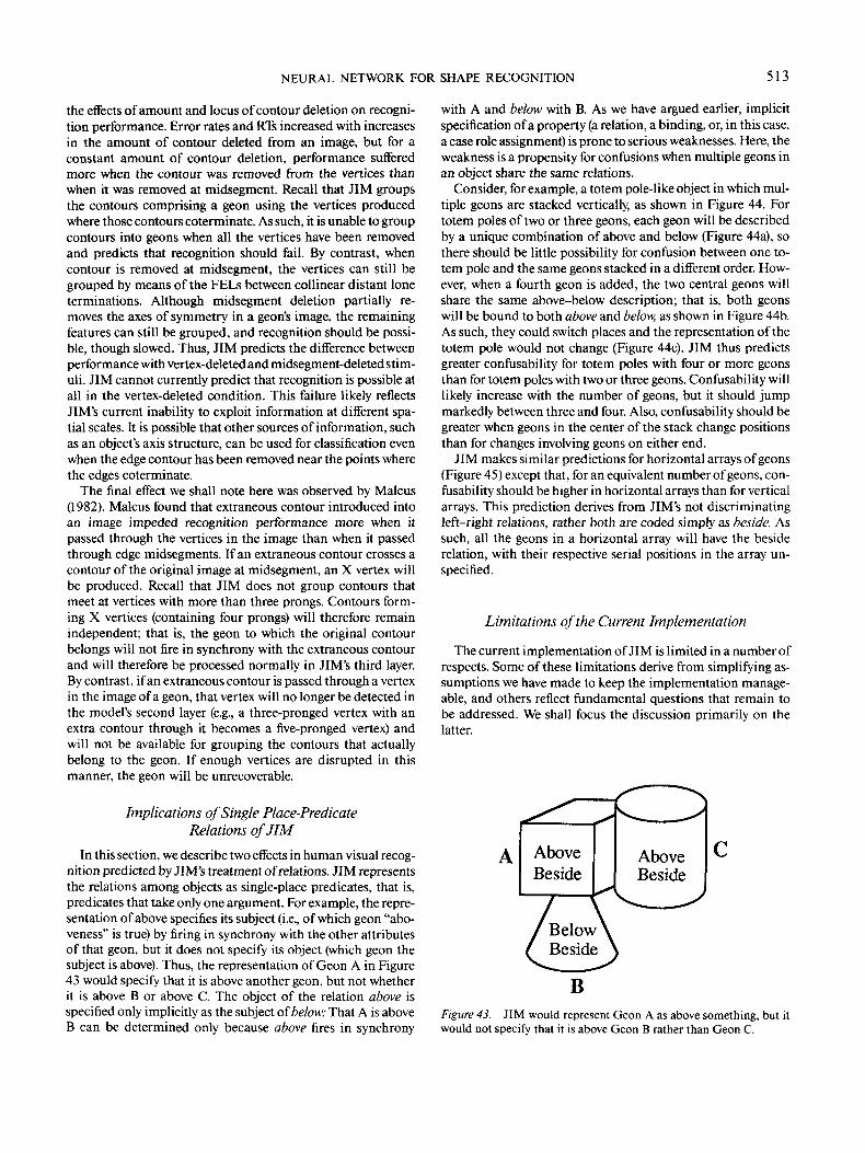
NEURAL NETWORK FOR SHAPE RECOGNITION 513
the effects of amount and locus of contour deletion on recogni-tion performance. Error rates and RTs increased with increasesin the amount of contour deleted from an image, but for aconstant amount of contour deletion, performance sufferedmore when the contour was removed from the vertices thanwhen it was removed at midsegment. Recall that JIM groupsthe contours comprising a geon using the vertices producedwhere those contours coterminate. As such, it is unable to groupcontours into geons when all the vertices have been removedand predicts that recognition should fail. By contrast, whencontour is removed at midsegment, the vertices can still begrouped by means of the FELs between collinear distant loneterminations. Although midsegment deletion partially re-moves the axes of symmetry in a geon's image, the remainingfeatures can still be grouped, and recognition should be possi-ble, though slowed. Thus, JIM predicts the difference betweenperformance with vertex-deleted and midsegment-deleted stim-uli. JIM cannot currently predict that recognition is possible atall in the vertex-deleted condition. This failure likely reflectsJIM's current inability to exploit information at different spa-tial scales. It is possible that other sources of information, suchas an object's axis structure, can be used for classification evenwhen the edge contour has been removed near the points wherethe edges coterminate.
The final effect we shall note here was observed by Malcus(1982). Malcus found that extraneous contour introduced intoan image impeded recognition performance more when itpassed through the vertices in the image than when it passedthrough edge midsegments. If an extraneous contour crosses acontour of the original image at midsegment, an X vertex willbe produced. Recall that JIM does not group contours thatmeet at vertices with more than three prongs. Contours form-ing X vertices (containing four prongs) will therefore remainindependent; that is, the geon to which the original contourbelongs will not fire in synchrony with the extraneous contourand will therefore be processed normally in JIM's third layer.By contrast, if an extraneous contour is passed through a vertexin the image of a geon, that vertex will no longer be detected inthe model's second layer (e.g., a three-pronged vertex with anextra contour through it becomes a five-pronged vertex) andwill not be available for grouping the contours that actuallybelong to the geon. If enough vertices are disrupted in thismanner, the geon will be unrecoverable.
Implications of Single Place-PredicateRelations of JIM
In this section, we describe two effects in human visual recog-nition predicted by JIM's treatment of relations. JIM representsthe relations among objects as single-place predicates, that is,predicates that take only one argument. For example, the repre-sentation of above specifies its subject (i.e., of which geon "abo-veness" is true) by firing in synchrony with the other attributesof that geon, but it does not specify its object (which geon thesubject is above). Thus, the representation of Geon A in Figure43 would specify that it is above another geon, but not whetherit is above B or above C. The object of the relation above isspecified only implicitly as the subject of below: That A is aboveB can be determined only because above fires in synchrony
with A and below with B. As we have argued earlier, implicitspecification of a property (a relation, a binding, or, in this case,a case role assignment) is prone to serious weaknesses. Here, theweakness is a propensity for confusions when multiple geons inan object share the same relations.
Consider, for example, a totem pole-like object in which mul-tiple geons are stacked vertically, as shown in Figure 44. Fortotem poles of two or three geons, each geon will be describedby a unique combination of above and below (Figure 44a), sothere should be little possibility for confusion between one to-tem pole and the same geons stacked in a different order. How-ever, when a fourth geon is added, the two central geons willshare the same above-below description; that is, both geonswill be bound to both above and below, as shown in Figure 44b.As such, they could switch places and the representation of thetotem pole would not change (Figure 44c). JIM thus predictsgreater confusability for totem poles with four or more geonsthan for totem poles with two or three geons. Confusability willlikely increase with the number of geons, but it should jumpmarkedly between three and four. Also, confusability should begreater when geons in the center of the stack change positionsthan for changes involving geons on either end.
JIM makes similar predictions for horizontal arrays of geons(Figure 45) except that, for an equivalent number of geons, con-fusability should be higher in horizontal arrays than for verticalarrays. This prediction derives from JIM's not discriminatingleft-right relations, rather both are coded simply as beside. Assuch, all the geons in a horizontal array will have the besiderelation, with their respective serial positions in the array un-specified.
Limitations of the Current Implementation
The current implementation of JIM is limited in a number ofrespects. Some of these limitations derive from simplifying as-sumptions we have made to keep the implementation manage-able, and others reflect fundamental questions that remain tobe addressed. We shall focus the discussion primarily on thelatter.
Figure 43. JIM would represent Geon A as above something, but itwould not specify that it is above Geon B rather than Geon C.
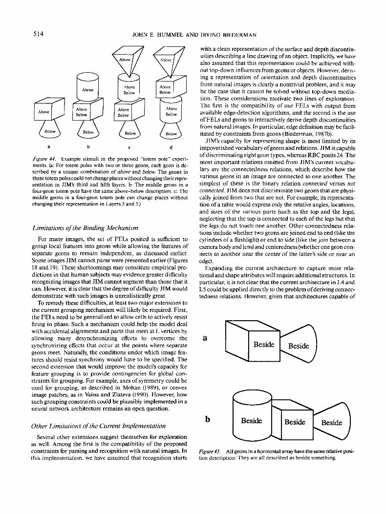
514 JOHN E. HUMMEL AND IRVING BIEDERMAN
Figure 44. Example stimuli in the proposed "totem pole" experi-ments, (a: For totem poles with two or three geons, each geon is de-scribed by a unique combination of above and below. The geons inthese totem poles could not change places without changing their repre-sentation in JIM's third and fifth layers, b: The middle geons in afour-geon totem pole have the same above-below description, c: Themiddle geons in a four-geon totem pole can change places withoutchanging their representation in Layers 3 and 5.)
Limitations of the Binding Mechanism
For many images, the set of FELs posited is sufficient togroup local features into geons while allowing the features ofseparate geons to remain independent, as discussed earlier.Some images JIM cannot parse were presented earlier (Figures18 and 19). These shortcomings may constitute empirical pre-dictions in that human subjects may evidence greater difficultyrecognizing images that JIM cannot segment than those that itcan. However, it is clear that the degree of difficulty JIM woulddemonstrate with such images is unrealistically great.
To remedy these difficulties, at least two major extensions tothe current grouping mechanism will likely be required. First,the FELs need to be generalized to allow cells to actively resistfiring in phase. Such a mechanism could help the model dealwith accidental alignments and parts that meet at L vertices byallowing many desynchronizing effects to overcome thesynchronizing effects that occur at the points where separategeons meet. Naturally, the conditions under which image fea-tures should resist synchrony would have to be specified. Thesecond extension that would improve the model's capacity forfeature grouping is to provide contingencies for global con-straints for grouping. For example, axes of symmetry could beused for grouping, as described in Mohan (1989), or conveximage patches, as in Vaina and Zlateva (1990). However, howsuch grouping constraints could be plausibly implemented in aneural network architecture remains an open question.
Other Limitations of the Current Implementation
Several other extensions suggest themselves for explorationas well. Among the first is the compatibility of the proposedconstraints for parsing and recognition with natural images. Inthis implementation, we have assumed that recognition starts
with a clean representation of the surface and depth discontin-uities describing a line drawing of an object. Implicitly, we havealso assumed that this representation could be achieved with-out top-down influences from geons or objects. However, deriv-ing a representation of orientation and depth discontinuitiesfrom natural images is clearly a nontrivial problem, and it maybe the case that it cannot be solved without top-down media-tion. These considerations motivate two lines of exploration.The first is the compatibility of our FELs with output fromavailable edge-detection algorithms, and the second is the useof FELs and geons to interactively derive depth discontinuitiesfrom natural images. In particular, edge definition may be facil-itated by constraints from geons (Biederman, 1987b).
JIM's capacity for representing shape is most limited by itsimpoverished vocabulary of geons and relations. JIM is capableof discriminating eight geon types, whereas RBC posits 24. Themost important relations omitted from JIM's current vocabu-lary are the connectedness relations, which describe how thevarious geons in an image are connected to one another. Thesimplest of these is the binary relation connected versus notconnected. JIM does not discriminate two geons that are physi-cally joined from two that are not. For example, its representa-tion of a table would express only the relative angles, locations,and sizes of the various parts (such as the top and the legs),neglecting that the top is connected to each of the legs but thatthe legs do not touch one another. Other connectedness rela-tions include whether two geons are joined end to end (like thecylinders of a flashlight) or end to side (like the join between acamera body and lens) and centeredness (whether one geon con-nects to another near the center of the latter's side or near anedge).
Expanding the current architecture to capture more rela-tional and shape attributes will require additional structures. Inparticular, it is not clear that the current architecture in L4 andL5 could be applied directly to the problem of deriving connec-tedness relations. However, given that architectures capable of
Beside
Figure 45. All geons in a horizontal array have the same relative posi-tion description: They are all described as beside something.
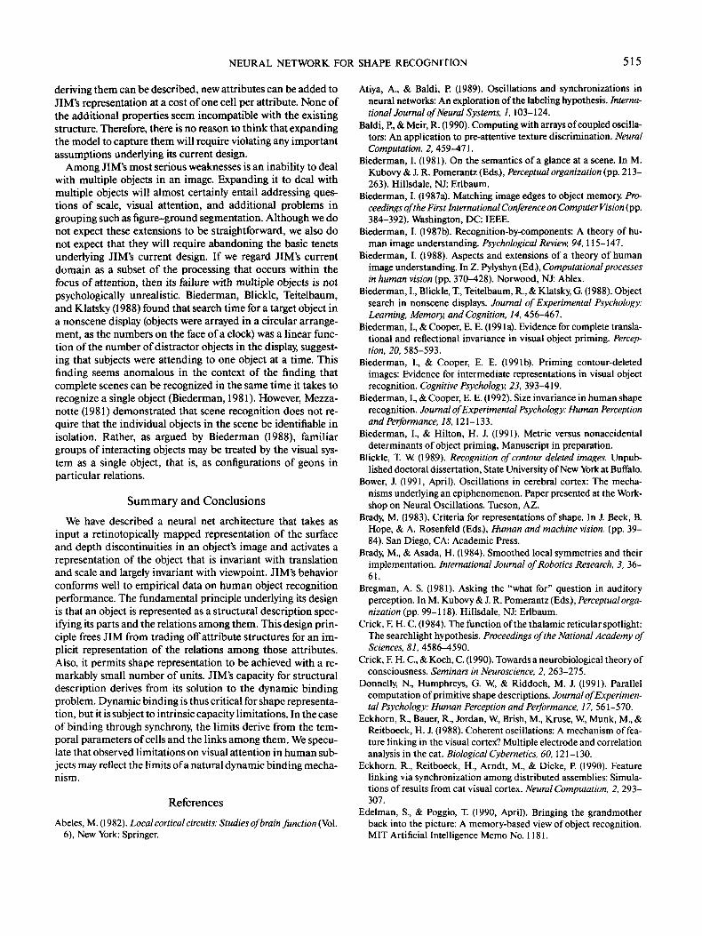
NEURAL NETWORK FOR SHAPE RECOGNITION 515
deriving them can be described, new attributes can be added toJIM's representation at a cost of one cell per attribute. None ofthe additional properties seem incompatible with the existingstructure. Therefore, there is no reason to think that expandingthe model to capture them will require violating any importantassumptions underlying its current design.
Among JIM's most serious weaknesses is an inability to dealwith multiple objects in an image. Expanding it to deal withmultiple objects will almost certainly entail addressing ques-tions of scale, visual attention, and additional problems ingrouping such as figure-ground segmentation. Although we donot expect these extensions to be straightforward, we also donot expect that they will require abandoning the basic tenetsunderlying JIM's current design. If we regard JIM's currentdomain as a subset of the processing that occurs within thefocus of attention, then its failure with multiple objects is notpsychologically unrealistic. Biederman, Blickle, Teitelbaum,and Klatsky (1988) found that search time for a target object ina nonscene display (objects were arrayed in a circular arrange-ment, as the numbers on the face of a clock) was a linear func-tion of the number of distractor objects in the display, suggest-ing that subjects were attending to one object at a time. Thisfinding seems anomalous in the context of the finding thatcomplete scenes can be recognized in the same time it takes torecognize a single object (Biederman, 1981). However, Mezza-notte (1981) demonstrated that scene recognition does not re-quire that the individual objects in the scene be identifiable inisolation. Rather, as argued by Biederman (1988), familiargroups of interacting objects may be treated by the visual sys-tem as a single object, that is, as configurations of geons inparticular relations.
Summary and Conclusions
We have described a neural net architecture that takes asinput a retinotopically mapped representation of the surfaceand depth discontinuities in an object's image and activates arepresentation of the object that is invariant with translationand scale and largely invariant with viewpoint. JIM's behaviorconforms well to empirical data on human object recognitionperformance. The fundamental principle underlying its designis that an object is represented as a structural description spec-ifying its parts and the relations among them. This design prin-ciple frees JIM from trading off attribute structures for an im-plicit representation of the relations among those attributes.Also, it permits shape representation to be achieved with a re-markably small number of units. JIM's capacity for structuraldescription derives from its solution to the dynamic bindingproblem. Dynamic binding is thus critical for shape representa-tion, but it is subject to intrinsic capacity limitations. In the caseof binding through synchrony, the limits derive from the tem-poral parameters of cells and the links among them. We specu-late that observed limitations on visual attention in human sub-jects may reflect the limits of a natural dynamic binding mecha-nism.
References
Abeles, M. (1982). Local cortical circuits: Studies of brain function (Vol.6), New York: Springer.
Atiya, A., & Baldi, P. (1989). Oscillations and synchronizations inneural networks: An exploration of the labeling hypothesis. Interna-tional Journal of Neural Systems, 1,103-124.
Baldi, P., & Meir, R. (1990). Computing with arrays of coupled oscilla-tors: An application to pre-attentive texture discrimination. NeuralComputation, 2, 459-471.
Biederman, I. (1981). On the semantics of a glance at a scene. In M.Kubovy & J. R. Pomerantz (Eds.), Perceptual organization (pp. 213-263). Hillsdale, NJ: Erlbaum.
Biederman, I. (1987a). Matching image edges to object memory. Pro-ceedings of the First International Conference on Computer Vision (pp.384-392). Washington, DC: IEEE.
Biederman, I. (1987b). Recognition-by-components: A theory of hu-man image understanding. Psychological Review, 94,115-147.
Biederman, I. (1988). Aspects and extensions of a theory of humanimage understanding. In Z. Pylyshyn (Ed.), Computational processesin human vision (pp. 370-428). Norwood, NJ: Ablex.
Biederman, I., Blickle, T., Teitelbaum, R., & Klatsky, G. (1988). Objectsearch in nonscene displays. Journal of Experimental Psychology:Learning, Memory, and Cognition, 14, 456-467.
Biederman, I., & Cooper, E. E. (199 la). Evidence for complete transla-tional and reflectional invariance in visual object priming. Percep-tion, 20, 585-593.
Biederman, I., & Cooper, E. E. (1991b). Priming contour-deletedimages: Evidence for intermediate representations in visual objectrecognition. Cognitive Psychology, 23, 393-419.
Biederman, I., & Cooper, E. E. (1992). Size invariance in human shaperecognition. Journal of Experimental Psychology: Human Perceptionand Performance, 18,121-133.
Biederman, I., & Hilton, H. J. (1991). Metric versus nonaccidentaldeterminants of object priming, Manuscript in preparation.
Blickle, T. W (1989). Recognition of contour deleted images. Unpub-lished doctoral dissertation, State University of New York at Buffalo.
Bower, J. (1991, April). Oscillations in cerebral cortex: The mecha-nisms underlying an epiphenomenon. Paper presented at the Work-shop on Neural Oscillations. Tucson, AZ.
Brady, M. (1983). Criteria for representations of shape. In J. Beck, B.Hope, & A. Rosenfeld (Eds.), Human and machine vision, (pp. 39-84). San Diego, CA: Academic Press.
Brady, M., & Asada, H. (1984). Smoothed local symmetries and theirimplementation. International Journal of Robotics Research, 3, 36-61.
Bregman, A. S. (1981). Asking the "what for" question in auditoryperception. In M. Kubovy & J. R. Pomerantz (Eds.), Perceptual orga-nization (pp. 99-118). Hillsdale, NJ: Erlbaum.
Crick, F. H. C. (1984). The function of the thalamic reticular spotlight:The searchlight hypothesis. Proceedings of the National Academy ofSciences, 81, 4586-4590.
Crick, F. H. C., & Koch, C. (1990). Towards a neurobiological theory ofconsciousness. Seminars in Neuroscience, 2, 263-275.
Donnelly, N., Humphreys, G. W, & Riddoch, M. J. (1991). Parallelcomputation of primitive shape descriptions. Journal of Experimen-tal Psychology: Human Perception and Performance, 17, 561-570.
Eckhorn, R., Bauer, R., Jordan, W, Brish, M., Kruse, W, Munk, M., &Reitboeck, H. J. (1988). Coherent oscillations: A mechanism of fea-ture linking in the visual cortex? Multiple electrode and correlationanalysis in the cat. Biological Cybernetics, 60,121-130.
Eckhorn, R., Reitboeck, H., Arndt, M., & Dicke, P. (1990). Featurelinking via synchronization among distributed assemblies: Simula-tions of results from cat visual cortex. Neural Computation, 2, 293-307.
Edelman, S., & Poggio, T. (1990, April). Bringing the grandmotherback into the picture: A memory-based view of object recognition.MIT Artificial Intelligence Memo No. 1181.
516 JOHN E. HUMMEL AND IRVING BIEDERMAN
Edelman, S., & Weinshall, D. (1991). A self-organizing multiple-viewrepresentation of 3D objects. Biological Cybernetics, 64, 209-219.
Engel, A. K., Konig, P., Kreiter, A. K., & Singer, W (1991). Interhemi-spheric synchronization of oscillatory neuronal responses in cat vi-sual cortex. Science, 252,1177-1179.
Feldman, J. A. (1982). Dynamic connections in neural networks. Bio-logical Cybernetics, 46, 27-39.
Feldman, J. A., & Ballard, D. H. (1982). Connectionist models andtheir properties. Cognitive Science, 6, 205-254.
Fodor, J. A., & Pylyshyn, Z. W (1988). Connectionism and cognitivearchitecture: A critical analysis. Cognition, 28, 1-71.
Gerhardstein, P. C, & Biederman, I. (1991, May). Priming depth-ro-tated object images: Evidence for 3D invariance. Paper presented atthe Meeting of the Association for Research in Vision and Ophthal-mology, Sarasota, FL.
Gray, C. M., Konig, P., Engel, A. E., & Singer, W (1989). Oscillatoryresponses in cat visual cortex exhibit inter-column synchronizationwhich reflects global stimulus properties. Nature, 338, 334-337.
Gray, C. M., & Singer, W (1989). Stimulus specific neuronal oscilla-tions in orientation columns of cat visual cortex. Proceedings of theNational Academy of Sciences, 86, 1698-1702.
Gross, C. G. (1973). Visual functions of inferotemporal cortex. In R.Jung (Ed.), Handbook of sensory physiology: Vol. VlI/3. Central pro-cessing of information. Part B. Visual centers in the brain, (pp. 451-482). Berlin: Springer-Verlag.
Grossberg, S. (1973). Contour enhancement, short-term memory, andconstancies in reverberating neural networks. Studies in AppliedMathematics, 52, 217-257.
Grossberg, S., & Somers, D. (1991). Synchronized oscillations duringcooperative feature linking in a cortical model of visual perception.Neural Networks, 4, 453-466.
Guzman, A.(1971). Analysis of curved line drawings using context andglobal information. Machine Intelligence, 6, 325-375. Edinburgh,Scotland: Edinburgh Press.
Hinton, G. E. (1981). A parallel computation that assigns canonicalobject-based frames of reference. Proceedings of the 7th InternationalJoint Conference on Artificial Intelligence. Symposium conducted atthe University of British Columbia, Vancouver, British Columbia,Canada.
Hinton, G. E., McClelland, J. L., & Rumelhart, D. E. (1986). Distrib-uted representations. In D. E. Rumelhart, J. L. McClelland, and thePOP Research Group, Parallel distributed processing: Explorationsin the microstructure of cognition. Volume J: Foundations (pp. 77-109). Cambridge, MA: MIT Press/Bradford Books.
Hoffman, D. D, & Richards, W A. (1985). Parts of recognition. Cogni-tion, 18, 65-96.
Hummel, J. E., & Biederman, I. (1990a). Dynamic binding: A basis forthe representation of shape by neural networks. In M. P. Palmarini,Proceedings of the 12lh Annual Conference of the Cognitive ScienceSociety (pp. 614-621). Hillsdale, NJ: Erlbaum.
Hummel, J. E., & Biederman, I. (1990b, November). Binding invariantshape descriptors for object recognition: A neural net implementation.Paper presented at the 21st Annual Meeting of the PsychonomicsSociety, New Orleans, LA.
Hummel, J. E., & Biederman, I. (1991, May). Binding by phase lockedneural activity: Implications for a theory of visual attention. Paperpresented at the Annual Meeting of the Association for Research inVision and Ophthalmology, Sarasota, FL.
Hummel, J. E., Biederman, I., Gerhardstein, P. C, & Hilton, H. J.(1988). From image edges to geons: A connectionist approach. In D.Touretsky, G. Hinton, & T. Sejnowski (Eds.), Proceedings of the 1988Connectionist Models Summer School (pp. 462-471), San Mateo,CA: Morgan Kaufman.
Jolicoeur, P. (1985). The time to name disoriented natural objects.Memory <& Cognition, 13. 289-303.
Kahneman, D, & Treisman, A. (1984). Changing views of attentionand automaticity. In R. Parasuraman, R. Davies, & J. Beatty (Eds.),Varieties of attention (pp. 29-62). San Diego, CA: Academic Press.
Keele, S. W, Cohen, A., Ivry, R., Liotti, M., & Yee, P. (1988). Test of atemporal theory of attentional binding. Journal of Experimental Psy-chology: Human Perception and Performance, 14, 444-452.
Konig, P., & Schillen, T. B. (1991). Stimulus-dependent assembly for-mation of oscillatory responses: I. Synchronization. Neural Compu-tation, 3, 167-178.
Lange. T, & Dyer, M. (1989). High-level inferencing in a connectionistneural network. (Tech. Rep. No. UCLA-AI-89-12), Los Angeles: Uni-versity of California, Computer Science Department.
Leeper, R. (1935). A study of a neglected portion of the field of learn-ing: The development of sensory organization. Journal of GeneticPsychology, 46,41-15.
Lindsay, P. H., & Norman, D. A. (1977). Human information processing:An introduction to psychology (2nd ed.). San Diego, CA: AcademicPress.
Lowe, D. G. (1987). The viewpoint consistency constraint. Interna-tional Journal of Computer Vision, 1, 57-72.
Malcus, L. (1982). Contour formation, segmentation, and semantic ac-cess in scene and object perception. Unpublished doctoral disserta-tion, State University of New York at Buffalo.
Malik, J. (1987). Interpreting line drawings of curved objects. Interna-tional Journal of Computer Vision, 1, 73-103.
Marshall, J. A. (1990). A self-organizing scale-sensitive neural net-work. Proceedings of the International Joint Conference on NeuralNetworks, 3, 649-654.
Mezzanotte, R. J. (1981). Accessing visual schemata: Mechanisms in-voking world knowledge in the identification of objects in scenes, Un-published doctoral dissertation, State University of New York at Buf-falo, Department of Psychology.
Milner, P. M. (1974). A model for visual shape recognition. Psychologi-cal Review, 81, 521-535.
Mohan, R. (1989). Perceptual organization for computer vision. Unpub-lished doctoral dissertation, University of Southern California, De-partment of Computer Science.
Moran, J., & Desimone, R. (1985). Selective attention gates visual pro-cessing in the extrastriate cortex. Science, 229, 782-784.
Neisser, U (1967). Cognitive psychology. New York: Appleton-Century-Crofts.
Pinker, S. (1986). Visual cognition: An introduction. In S. Pinker (Ed.),Visual cognition (pp. 1-63). Cambridge, MA: MIT Press.
Rock, I., & DiVita, J. (1987). A case of viewer-centered perception.Cognitive Psychology, 19, 280-293.
Sejnowski, T. J. (1986). Open questions about computation in cerebralcortex. In J. L. McClelland, & D. E. Rumelhart. (Eds.), Parallel dis-tributed processing: Explorations in the microstructure of cognition(pp. 372-389). Cambridge, MA: MIT Press.
Selfridge, O. G. (1959). Pandemonium: A paradigm for learning. Sym-posium on the Mechanism of Thought Processes. London: Her Ma-jesty's Stationery Office.
Selfridge, O. G., & Neisser, U. (1960). Pattern recognition by machine.Scientific American, 203, 60-68.
Shastri, L., & Ajjanagadde, V (1990). From simple associations to sys-tematic reasoning: A connectionist representation of rules, variablesand dynamic bindings (Tech. Rep. No. MS-CIS-90-05). Philadel-phia: University of Pennsylvania, Department of Computer and In-formation Sciences.
Smolensky, P. (1987). On variable binding and the representation of sym-bolic structures in connectionist systems (Internal Rep. No. CU-CS-355-87). Boulder, CO: University of Colorado, Department of Com-puter Science & Institute of Cognitive Science.
Strong, G. W, & Whitehead, B. A. (1989). A solution to the tag-assign-
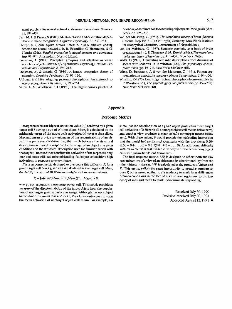
NEURAL NETWORK FOR SHAPE RECOGNITION 517
ment problem for neural networks. Behavioral and Brain Sciences,72,381-433.
Tarr, M. J., & Pinker, S. (1989). Mental rotation and orientation depen-dence in shape recognition. Cognitive Psychology, 21, 233-283.
Thorpe, S. (1990). Spike arrival times: A highly efficient codingscheme for neural networks. In R. Eckmiller, G. Hartmann, & G.Hauske (Eds.), Parallel processing in neural systems and computers(pp. 91-94). Amsterdam: North-Holland.
Treisman, A. (1982). Perceptual grouping and attention in visualsearch for objects. Journal of Experimental Psychology: Human Per-ception and Performance, 8,194-214.
Treisman, A., & Gelade, G. (1980). A feature integration theory ofattention. Cognitive Psychology, 12, 97-136.
Oilman, S. (1989). Aligning pictorial descriptions: An approach toobject recognition. Cognition, 32,193-254.
Vaina, L. M., & Zlateva, S. D. (1990). The largest convex patches: A
boundary-based method for obtaining object parts. Biological Cyber-netics, 62, 225-236.
von der Malsburg, C. (1981). The correlation theory of brain function(Internal Rep. No. 81-2). Gottingen, Germany: Max-Plank-Institutefor Biophysical Chemistry, Department of Neurobiology.
von der Malsburg, C. (1987). Synaptic plasticity as a basis of brainorganization. In J. P. Chaneaux & M. Konishi (Eds.), The neural andmolecular bases of learning (pp. 411-432). New York: Wiley.
Waltz, D. (1975). Generating semantic descriptions from drawings ofscenes with shadows. In P. Winston (Ed.), The psychology of com-puter vision (pp. 19-91). New 'York: McGraw-Hill.
Wang, D, Buhmann, J., & von der Malsburg, C. (1991). Pattern seg-mentation in associative memory. Neural Computation, 2, 94-106.
Winston, P. (1975). Learning structural descriptions from examples. InP. Winston (Ed.), The psychology of computer vision (pp. 157-209).New York: McGraw-Hill.
Appendix
Response Metrics
MaXj represents the highest activation value (A,) achieved by a giventarget cell i during a run of N time slices. Mean, is calculated as thearithmetic mean of the target cell's activation (A,) over n time slices.Max and mean provide raw estimates of the recognizability of an ob-ject in a particular condition (i.e., the match between the structuraldescription activated in response to the image of an object in a givencondition and the structural description used for familiarization withthat object). Because they consider the activation of the target cell only,max and mean will tend to be misleading if all object cells achieve highactivations in response to every image.
P is a response metric designed to overcome this difficulty. P, for agiven target cell / on a given run is calculated as the target cell Meant
divided by the sum of all above-zero object cell mean activations:
Pi = [Mean,l(Mean, + 2jMeanJ)]+, j > 0,
where j corresponds to a nontarget object cell. This metric provides ameasure of the discriminability of the target object from the popula-tion of nontargets given a particular image. Although it is not subjectto the same criticism as max and mean, P is a less sensitive metric whenthe mean activation of nontarget object cells is low. For example, as-
sume that the baseline view of a given object produces a mean targetcell activation of 0.50 (with all nontarget object cell means below zero),and another view produces a mean of 0.01 (nontarget means belowzero). With these values, P would provide the misleading impressionthat the model had performed identically with the two views: 0.50/(0.50+ 0 + . . .0) = 0.01/(0.01 + 0 + . . . 0). An additional difficultywith P as a metric is that it is sensitive only to differences among objectcells with mean activations above zero.
The final response metric, MP, is designed to reflect both the rawrecognizability of a view of an object and its discriminability from theother objects in the set. MP, is calculated as the product of Mean, andP,. This metric suffers the same insensitivity to negative numbers asdoes P, but is prone neither to /"'s tendency to mask large differencesbetween conditions in the face of inactive nontargets, nor to the ten-dency of max and mean to mask indiscriminate responding.
Received July 30,1990Revision received July 30,1991
Accepted August 12,1991