does regionalism hinder multilateralism: a case study of india
TRANSCRIPT

Discussion Papers in Economics
Does Regionalism Hinder Multilateralism: A Case Study of India.
Manoj Pant and Amit Sadhukhan
Revised, November, 2008.
Discussion Paper 09-03
Centre for International Trade and Development
School of International Studies
Jawaharlal Nehru University
India

Does Regionalism Hinder Multilateralism:
A Case Study of India.
Manoj Pant and Amit Sadhukhan*
September, 2008.
(This paper is forthcoming in Journal of Economic Integration, June, 2009)
ABSTRACT
Today many developing countries fear that regional movements in other parts of the world will adversely impact their trade as regionalism overtakes multilateralism. The response has been that most of them are trying to get into one regional bloc or the other via regional trade arrangements (RTAs). In this paper we have investigated how India as a non-member country is affected by formation of RTAs like ASEAN, EU, NAFTA, and MERCOSUR..Controlling for non-RTA factors that influence exports, we find that. India’s exports to these RTAs seem to be affected not by the formation of these RTAs per se but by demand side factors.
Key Words: Regional Trade Arrangements, Regionalism, Multilateralism, Non
Member Countries, External Trade Creation, Trade Diversion.
JEL Listing: F15, F51
* The authors are Professor and Ph.D. student, respectively at the Centre for
International Trade and Development, School of International Studies, Jawaharlal Nehru
University, India.
Address for correspondence:
Prof. Manoj Pant, Centre for International Trade and Development, School of
International Studies, Jawaharlal Nehru University, New Delhi – 110067, India.
Fax/Telephone: +91-011-26741288,
E-mail: [email protected] , [email protected]

3
I. Introduction1
As is now well known, Article XXIV of GATT was formulated with the objective
of promoting regional free trade arrangements (RTAs) or, at least, not excluding
countries which were already part of existing preferential trade arrangements. Examples
like Benelux and the European Economic Community come readily to mind. Since these
are obvious violations of the MFN clause underlying GATT, some exception to allow for
such arrangements was necessary. However the stipulation in Article XXIV that members
of such RTAs could not raise their tariffs above pre-RTA levels ensured that
multilateralism could proceed apace.
The logic of Article XXIV must then lie in the international political economy of
trade liberalisation. As the theory of second best tells us (see, for example, Lipsey and
Lancaster (1956-57), Lipsey (1957), Meade (1955)) it is not possible to argue that limited
free trade is better than no trade though both are inferior to multilateral free trade. In
other words, the case for Article XXIV must rest on the ground that a series of smaller
regional movements may pave the way for multilateral free trade. More importantly, for
many countries RTAs are a method of locking in free trade policy reforms which are
difficult to sell politically at the multilateral level. To that extent, it can be argued that
regionalism helps multilateralism rather than act as a stumbling block.
The welfare arguments of RTAs rest on Viner’s well known distinction between
trade creating and trade diverting custom unions (see, Viner, 1950). More generally, if
1 We are grateful to two anonymous referees whose suggestions greatly improved the original version of this paper. The errors of course remain ours.

4
efficiency driven trade creation within an RTA is larger than similar trade diverted from
the non-RTA countries (who face a tariff disadvantage vis a vis the RTA member
countries) then an RTA could be welfare increasing for the RTA as a whole. This itself is
questioned by some authors (see, Lipsey, 1958). In any case, the welfare arguments in the
Viner tradition are obviously a function of the tariff levels: the higher the tariff levels in
the world prior to the RTA the greater the likely Vinerian benefits of an RTA (see,
Bhagwati and Panagariya, 1996).
Yet, the history of RTAs reveals something different. The highest tariffs on world
trade were in the period 1950-75 with world tariffs dropping in most of the developed
countries after 1980 or so (see, Bhagwati, 1992). In fact, by 1990, world tariffs were
lower than ever before in the period after the Great Depression. Hence, one should have
seen most RTA agreements taking place during the period of high tariffs. In fact, the
explosion of RTAs came after 1990 or so and during the build up to the Uruguay round
(UR) agreement of 1995. According to the World Bank report on ‘Global Economic
Prospects’ (2005), around 230 new RTAs have been notified to WTO since 1990 to late
2004.. What is even more interesting is that over seventy percent of these RTAs involved
some developing country and nearly 40 percent of global trade is taking place between
partners. Many developing countries were members of more than one RTA and some
RTAs involved only developing countries.
It must be remembered that prior to the UR, the ‘non-reciprocity clause’ made it
unnecessary for developing countries to worry about tariff negotiations under the GATT.
The non-reciprocity clause, introduced as a concession to the less developed countries
(LDCs) during the Tokyo round of trade negotiations in the late 1970s, exempted LDCs

5
from offering reciprocal tariff cuts in response to tariff cuts effected by the developed
countries (DCs). However, the ‘single undertaking’ of the UR ended this reciprocity. This
clause, introduced during the UR negotiations of 1995, required that a country signatory
to any agreement was automatically committed to all agreements signed under the WTO
irrespective of whether that country was signatory to all or only specific agreements.(for
some details see, Pant, 2002). The consequence was that after 1995, a country could not
unilaterally opt out of tariff cutting agreements and had to make some offers during trade
negotiations.
The proliferation of the RTAs after 1990 could thus be a defensive response to
multilateralism. However, in LDCs in particular with very high tariff levels, tariff cuts as
part of multilateral agreements could be difficult to sell politically. On the other hand,
tariff cuts negotiated among similar countries in RTAs could be easier to sell politically
and be a preparation for impending multilateralism. It is a common article of faith in
developing countries that reciprocal tariff cut agreements with other developing countries
does not arouse the same political passions as similar agreements with DCs.
. While the political logic for the spate of RTAs after 1990 is not difficult to
understand, it has also been argued that RTAs are a defensive economic response to
exclusion from other markets. This has, for example, been the justification for India
negotiating a whole spate of RTAs in the last few years. This therefore begs the question
whether an RTA necessarily implies trade exclusion to non-member countries and hence
necessitates a counter RTA. Existing literature has mainly looked at the issue of the
welfare gains to members of an RTA after formation of a regional grouping. What is

6
however less studied is what impact an RTA has on the trade of non-member countries.
This is the question that this paper seeks to address.
This paper is organized as follows. The next section presents a brief overview of
the developments of the principal RTAs which impact on India’s trade and India’s own
initiatives in this regard. Section III deals with a brief literature review of the economic
impacts of an RTA. This is followed in Section IV by a discussion of the methodology
used in our analysis, data sources and our main results. Finally, some concluding
observations are given in Section V.
II. Overview of RTAs.
Like many other developing countries, India too has been negotiating RTAs with a large
number of developing countries and trading blocs. A broad overview of the various RTAs
India has contracted or is in the process of contracting is given in Appendix A. An
inspection of Appendix A indicates that the operating RTAs cover most of India’s trading
partners in South and South East Asia, Europe, Latin America and North America.
However, as India has been a late starter in this regard, it is also clear that the only RTA
actually in operation for some time is the bilateral agreement concluded with Sri Lanka.
Of the rest, only the RTA with ASEAN has seen closure this year with implementation to
begin from 2009. The SAFTA is now in operation but it accounts for only a small part
(around 5 percent in the year 2006-07) of India’s total exports. The other operative RTA
is the CECA with Singapore which was quickly concluded mainly because investment
and services are of importance to India while Singapore does not have a significant
manufacturing base. Thus Singapore’s principal exports to India of Machinery and

7
Transport Equipment accounted for only about 5 percent of India’s imports of these items
in 2006.
However, for our study what is more important is how the formation of an RTA
would impact India’s exports if India remained outside of that RTA. For our study we
have looked at four RTAs: ASEAN, MERCOSUR, NAFTA and EU. Table 1 gives us
regional share of India’s total exports. The share of India’s total exports to these four
regions was around 40 percent of its total exports to the world in the year 1985, going
upto around 55 and 49 percent in the years 1995 and 2006, respectively. As nearly a half
of India’s total exports go to these four regions, so any policy changes like formation of
RTAs in these regions might have some impact not only on India’s exports to these
regions but also India’s total exports to the world. Among the four regions, EU and
NAFTA accounted for 37.7 percent and 39 percent respectively of India’s total exports in
the year 1985 and 2005. That means among the four regions, EU and NAFTA are India’s
major export destinations. For ASEAN the share of India’s total exports increased
significantly from 2.51 percent to 10.11 percent between 1985 and 2005. For
MERCOSUR the share is not significant but among four member countries, Brazil had a
share of around 70 and 83 percent of India’s exports to MERCOSUR in the year 1985
and 2006 respectively. This implies that Brazil alone accounts for a majority of
MERCOSUR’s imports from India.
Table 1: Share (%) of India’s total exports to different regions.
Region Year ���� 1985 1995 2006 ASEAN 2.51 8.61 9.97 NAFTA 19.37 18.5 16.23 EU 18.33 27.47 21.21 MERCOSUR 0.04 0.45 1.36 Total 40.26 55.04 48.78

8
In addition, each has been in operation for some time allowing us to assess the impact
on India in an econometric model. Finally, the RTAs range from simple Free Trade
Agreements (FTAs) like ASEAN and NAFTA to the full economic integration of the EU
which has progressed from a customs union to an economic union of member countries
and hence constitutes the most integrated form any RTA could take. The details of these
four RTAs are given in Appendix B.
III. Literature review.
As we have already noted earlier, the theoretical literature on RTAs has largely
concentrated on the gains or losses to member countries. Thus, Viner (1950) initiated the
concepts of ‘trade creation’ and ‘trade diversion’ to describe the welfare implication of an
RTA. In Vinerian framework a union is assumed to be small in terms of its share in world
trade and unable to impact on international terms of trade through trade creation and trade
diversion effects of an RTA formation. Therefore formation of an RTA cannot affect the
rest of the world’s welfare. This implies a non-member countries’ welfare is unaffected
by the formation of an RTA. Later Meade (1955) extended the Vinerian logic in a more
general equilibrium framework allowing for changes in international terms of trade.
Viner argued that trade creation is welfare improving where as trade diversion is welfare
reducing. The net result thus remains an empirical question. However, it was argued by
Gehrels (1956-57) that the static Vinerian welfare gains or losses do not allow for the
possibilities of consumption changes after formation of an RTA. Latter Lipsey (1957),
Kirman (1973), Johnson (1974, 1975) elaborated further whether trade diverting customs
union may be welfare improving or not for the member countries. In another study which
deals more specifically with the welfare of non-member countries, Kemp and Wan

9
(1976) showed that under special circumstances there exist a common external tariff for
an RTA which keeps the non-members’ welfare unchanged and hence increases world
welfare unambiguously. Developments in the new theories of trade after 1975 led to new
possibilities for welfare gains and losses based on trade in differentiated goods and
monopolistic competition. The implication of these considerations has been discussed by
Krugman (1979, 1980), Helpman and Krugman (1985).
Corden (1972) incorporated economies of scale into customs union theory. The
formation of an RTA may affect non-member countries through supply side
improvements. These supply side effects could favourably impact non-member countries
via price changes and/or provision of new product varieties. There are some additional
possible gains to non-member countries. For example, mutual recognition of standards
reduces directly the fixed cost of entering the union’s market, and this cost saving may
give benefit to non-member firms as well as member firms. In one study, Smith and
Venables (1991) suggested that a reduction of these fixed costs may directly lead to an
increase in the market share of non-member firms to the union. However, the theoretical
literature has in general concentrated on the impact of RTAs on the welfare of member
countries.
Since the theoretical literature is largely inconclusive about the welfare gains of
RTAs, a large member of authors have tried to empirically test some of the propositions
that have emerged in the theoretical literature. However, here too most of the literature
has concentrated on measuring the static gains and losses to member countries. ( see, for
example, Aitken (1973), Balassa (1967), Cernat (2001), Coulibali (2007), Kandogan
(2008), Winters and Chang (2000), Yeats (1997)). Some studies which measure the

10
effects of an RTA formation on non-member countries are Cernat, L (2001), Chang and
Winters (2002), Winters (1997), Winters and Chang (2000).
To our knowledge there are no studies which capture the effects of an RTA on India’s
welfare in a case where India is non-member for that RTA. Again there exist a few
studies which tried to look at the welfare implication of an RTA in the case where India
is a member country. Kelegama and Mukherji (2007) and Joshi, V. (2008) have tried to
see the effect of India-Sri Lanka Free Trade Agreement on the intra-regional trade and
accordingly the trade creation and trade diversion effects of the formation of India-
Sri Lanka Free Trade Agreement (ISLFTA). Kelegama and Mukherji (op. cit.) studied
trade creation and trade diversion of India-Sri Lanka Free Trade Agreement on the basis
of bilateral trade flows under different categories of products. Sector wise imports and
exports figures were compared for pre and post India-Sri Lanka Free Trade Agreement.
Joshi, V. (op. cit.) studied trade creation or trade diversion of India-Sri Lanka Free Trade
Agreement base on method used recently by Romalis (2005). In this case Joshi tried to
measure trade creation and trade diversion effects of India-Sri Lanka Free Trade
Agreement based on comparing the ISLFTA members’ imports of products from the
control countries (165 countries grouped together as control country which are non-
members of ISLFTA) with China’s imports of the same products from these control
countries. Some studies on SAFTA are mainly based on measuring ex-post intra-regional
trade and ex-ante comparative advantage in the SAFTA region.
IV. Measuring the Impact of RTAs on India.
While most of the empirical studies measure the effects of RTAs using volume of trade
as a proxy for welfare; some of the studies measure the impacts on terms of trade and

11
prices. In our study we are going to employ the first methodology, that is, to measure the
effects on volume of trade resulting from any RTA formation.
In our study, we are going to investigate the issue of how India as a non-member country
has been affected by the formation of RTAs like ASEAN, EU, NAFTA, and
MERCOSUR. As already noted, the rationale behind considering these four RTAs is that
India’s exports to these four regions comprise nearly half of India’s total exports to the
world in 2006 and these four unions are among the major RTAs which have been under
implementation for some time.
In this study we are going to use two different methodologies; firstly, the rather simplistic
Balassa (1967) methodology measuring ex-post ‘income elasticities of demand for
imports’2, where imports from India by each of the ASEAN, EU, NAFTA, and
MERCOSUR are taken for pre and post-integration periods and, secondly, estimating a
modified gravity model to capture the impacts of the formation of these RTAs on India’s
exports to the various regions. In the gravity model we are able to control for the effect of
non-RTA factors on India’s exports. This last factor is the obvious shortcoming of the
Balassa approach.
This rather simple approach rests on calculation of an RTA’s income elasticities of
import demand for some ‘reasonable’ period before and after the formation of an RTA.
The application to our study gives us the following definition:
th
j th
Compound growth rate of Import from India by j region.Income Elasticity
Compound growth rate of GDP of j region.=
Where j = {ASEAN, NAFTA, EU, MERCOSUR}
2This is typically Balassa’s ‘income elasticity of demand for extra-area import’ (see Balassa, 1967, pp. 5)

12
Compound growth rate of both imports and GDP have been calculated for pre-integration
and post-integration periods separately. Each period has been defined as seven years. The
year of effective implementation of each of ASEAN, EU, NAFTA, and MERCOSUR has
been taken as the ‘benchmark’ year that separates the two estimating periods for each
region. This is shown in Table 2.
Table 2: Pre-integration and post-integration periods for different RTAs
RTA
Year of RTA Formation or Benchmark Year
Pre-Integration Period
Post-Integration Period
ASEAN 1992 1985 to1991 1992 to1998 NAFTA 1994 1987 to 1993 1994 to 2000 EU 1993 1986 to 1992 1993 to 1999 MERCOSUR 1991 1984 to 1990 1991 to 1997
Now the Balassa hypothesis is that if the post-integration ‘income elasticity’ increases
(decreases) for region j that means jth region’s imports from India had increased
(decreased) due to external trade creation resulting from formation of jth region.
Consequently, the formation of the RTA is considered favourable (unfavourable) to
India. The Balassa methodology assumes that income elasticities of demand for imports
would have remained unchanged in the absence of RTA formation. This assumption is
reasonable if the pre and post integration periods are not too long. We have done the
exercise at the aggregate level and for ten broad disaggregated commodity categories
based on Standard International Trade Classification (SITC Rev.1). Analysis based on
commodity categories gives us commodity specific trade diversion or external trade
creation resulting from any RTA formation.

13
Modified Gravity Model Approach:
The use of the gravity model in investigating the welfare impact of RTAs is now well
known. (see, Greenaway and Milner, 2002 ). However, as we have noted, our focus in
this paper is on measuring the impact of various RTAs on a non-member country, India.
In addition, our focus is on India’s exports to theses regions rather than all bilateral trade
pairs as in usual gravity model applications. Hence, in the second methodology we have
used a modified gravity model to measure the impact of any RTA on India’s exports to
that region controlling for other variables which have some impacts on India’s exports.
Our purpose of using the gravity model is to overcome an obvious shortcoming of the
Balassa approach; it does not allow us to ‘control’ for non-RTA factors which affect
India’s exports to these regions. Our first modification to the gravity model implies
dropping the distance variable. Since our focus is on time series rather than cross
sectional data (as in most gravity model studies) the distance variable is irrelevant.
Second, rather than working with log variables we have defined variables in ratio form
which serves the same purpose of reducing the impact of extreme values in our
estimation.
The regression equation obtained for our ‘modified’ gravity model is as follows:
1 2 3 4( )( )
( ) ( )
j jjit It it
t itWt Wt Wt
X GDP GDPRTA t u
X GDP GDPα β β β β
+−+ +
= + + + + +
-------------- (A)
Where, j is any one region among ASEAN, EU, NAFTA, MERCOSUR, �: is one of the
member country of jth RTA, t: time period in year comprises both pre-integration and

14
post-integration periods, W: World, I: India, jitX : Exports from India to ith country of jth
region in the year t, W tX : Exports from India to the world in the year t, ItGDP : India’s
GDP in the year t, WtGDP : World’s GDP in the year t, jitGDP : GDP of country � in region
j, jtRTA : This is dummy variable for RTA. It takes values 1 for the years in post-
integration period, and values 0 for the years in pre-integration period, and finally
:itu Normally distributed random error term which captures other influences on X .
We have normalised the figures for exports and GDPs taking ratios to world totals.
This normalization helps us to reduce the severity of multicollinearity within these
variables. These variables have standard economic interpretations.
Dependent variable:
ji t
W t
XX
: The share of India’s exports to ith country of jth region to its total exports to the
world in the year t. This term captures the ith country’s imports from non-member India
where ith country is a member of region j or in other words this is an extra-area import by
ith country of jth region.
Independent variables:
It
Wt
GDPGDP
: Share of India’s GDP to the world GDP. This term captures India’s economic
capacity to export. This is typically a supply side argument that as any country’s GDP
increases it is potentially more capable of increasing its production base and therefore
exports. So, this variable should have a positive impact on India’s exports.

15
jit
Wt
GDPGDP
: Share of ith country’s GDP to the world GDP. This variable gives a demand side
specification. As any country’s GDP increases then demand for imports should increase.
So this value should also have a positive impact on India’s exports.
jtRTA : This is a dummy variable for RTA, which captures the effect of jth region’s RTA
formation on India’s exports. If the impact of this variable is negative (positive) on
India’s exports, that implies a trade diversion (trade creation) for India resulting from the
formation of the jth RTA.. Clearly trade diversion harms India’s exports, whereas
external trade creation benefits India’s exports.
t: t is the time trend so that �4 measures the trend effect on share of India’s exports to ith
country of jth region to its total exports to the world.
As our aim is to investigate the region specific RTA effect on India’s exports we have to
estimate the above mentioned gravity equation (A) for each of regions separately.
For ASEAN and EU we have taken the major member countries from each RTA
for regression analysis since in the case of other countries we either do not have available
data for whole period and/or India’s exports to these countries are negligible. For
NAFTA and MERCOSUR, we have data for the whole period for every member country.
The member countries which have been taken to estimate the gravity model for ASEAN
are Indonesia, Malaysia, Singapore, and Thailand. For EU, gravity equation has been
estimated considering the following countries; United Kingdom, Netherlands, Germany,
France, Belgium, and Italy. For NAFTA and MERCOSUR we have data for all the
members of each RTA.

16
The data sources our study are United Nation’s COMTRADE database for all kinds
(aggregate level and 1 digit commodity classifications level SITC Rev.1) of trade data.
For GDP data for all countries and for all regions we have used International Monetary
Fund’s World Economic Outlook Database for October, 2007.
Model Estimation
It is first necessary to look at the major commodities imported by each RTA from India.
The details are shown in Appendix C. If a commodity category holds a significant share
of total imports from India by a region, then trade diversion effect or external trade
creation effect on this commodity is much more important to the policy makers than in
the case of a commodity which has a negligible share. We have used this information to
identify those commodities where sectoral results for our estimation have been generated.
Using the methodology outlined in Section IV we have calculated Balassa’s
income elasticities of import demand for the four regions both for the pre and post-
integration periods. This is shown in Table 3 below. From an inspection of Table 3, it is
clear that ASEAN’s post-integration income elasticity declined to 1.98 from pre-
integration income elasticity 3.63. For rest of the regions post-integration income
elasticities increased, for EU it increased to 2.28 from 1.53, for NAFTA it increased
slightly to 2.08 from 1.64, and for MERCOSUR the income elasticity increased to 3.7
from 2.86.

17
Table 3: Income elasticities of demand for imports from India by different
regions.
Region Pre-Integration Income Elasticity
Post-Integration Income Elasticity
ASEAN 3.63 (1985-1991) 1.98 (1992-1998) NAFTA 1.64 (1987-1993) 2.08 (1994-2000) EU 1.53 (1986-1992) 2.28 (1993-1999) MERCOSUR 2.86 (1984-1990) 3.70 (1991-1997)
Note: Range of years of each period in parenthesis.
The income elasticities at aggregate level clearly show a decline for ASEAN, which
indicates there was a possible trade diversion effect of ASEAN on India’s exports. This
implies India’s exports to ASEAN were adversely affected in the post-integration period
of ASEAN. For EU, NAFTA, and MERCOSUR the income elasticities increased, thus
implying an external trade creation in the post-integration periods of these RTAs. So
India would have been better off due to external trade creation effects.
In Table 4 we present income elasticities of imports calculated at a disaggregated
commodity level. We have seen in Table 4 that for ASEAN, food and live animals, crude
materials & inedible except fuels, chemicals & related products, manufactured goods
classified chiefly by material, and machinery and transport equipment (i.e. Product codes:
0, 2, 5, 6, and 7) are the major exportable commodities with a share of more than 90
percent of India’s total exports to this region. From Table 4, we see that post-integration
income elasticities had declined for all these major products. Hence there seems to have
been trade diversion effects on all major commodities exported from India to ASEAN.
This result is consistent with our previous estimated income elasticities at the aggregate
level. Note that there are some commodity categories like beverage and live animals,
animal & vegetable oils, fates & waxes, and miscellaneous manufactured article for

18
which income elasticities increased which imply that for these products there was
external trade creation in ASEAN.
In case of EU we considered food and live animals, manufactured goods classified
chiefly by material, and miscellaneous manufactured articles (Product Codes: 0, 6, and 8)
accounting for more than 80 percent of India’s total exports to this region. From Table 4,
it is clear that for all these commodities post-integration elasticities declined. But at the
aggregate level the overall income elasticity had increased. So our commodity wise break
up of income elasticity give results which contradict what we obtained at the aggregate
level. We think more useful conclusions can be reached if the data are appropriately
disaggregated.
Next, for NAFTA food and live animals, manufactured goods classified chiefly
by material, and miscellaneous manufactured articles (Product Codes: 0, 6, and 8) are the
major export commodities with a share of more than 80 percent of India’s total exports to
this region. It should be noted that product code 6 accounted for almost fifty percent of
India’s total exports to NAFTA. For this product income elasticity increased to 5.29 from
4.98. For the other two products, namely, product codes: 0 and 8, income elasticities
declined. Hence no unambiguous trade creation or trade diversion can be inferred.
Finally, for MERCOSUR, Product Codes: 2, 5, 6, 7, and 8 accounted for more
than 90 percent of India’s exports to this region. Inspection of Table 4 indicates some
mixed results. We see that for product code 2 and 7, income elasticities increased and for
product codes 5, 6, and 8 income elasticities declined in the post integration period.
Hence no unambiguous trade creation or trade diversion can be inferred.

19
Table 4: Commodity wise Income elasticities of demand for imports from India by ASEAN, EU, NAFTA, and
MERCOSUR.
ASEAN EU NAFTA MERCOSUR
Commodity Code (SITC Rev 1) Commodity
Pre-integration (1985-1991)
Post-integration (1992-1998)
Pre-integration (1986-1992)
Post-integration (1993-1999)
Pre-integration (1987-1993)
Post-integration (1994-2000)
Pre-integration (1984-1990)
Post-integration (1994-1997)
0 Food and live animals 7.53 -0.31 8.05 1.74 4.11 3.73 18.55 -1.23 1 Beverages and tobacco 8.17 14.09 8.62 7.35 12.19 18.13 NA NA
2 Crude materials, inedible except fuels 8.48 -1.38 7.16 3.09 -0.45 5.98 -0.69 18.54
3 Mineral fuels, lubricants and related materials NA -7.61 NA -2.24 NA 60.31 NA NA
4 Animal and vegetable oils, fates and waxes -10.47 17.84 14.22 7.81 63 6.34 NA NA
5 Chemicals and related products 11.74 5.08 20.37 5.74 17.34 7.78 34.85 12.61
6
Manufactured goods classified chiefly by material 8.2 -0.26 11.07 2.84 4.98 5.3 10.95 9.78
7 Machinery and transport equipment 6.07 0.97 19.5 7.42 14.11 8.36 4.68 9.9
8 Miscellaneous manufactured articles 7.95 9.67 13.1 2.91 8.25 5.27 12.47 9.39
9
Commodities and transactions not classified elsewhere in the SITC 16.69 11.9 28.6 5.26 4.61 6.87 31.49 12.6

20
As already mentioned, the Balassa methodology using income elasticities does
not control for non-RTA factors that impact trade. In addition, our earlier results show
that the conclusion are ambiguous and vary from commodity to commodity. We have
tried to control for non-RTA factors using the regression model given in equation A.
The current data available for pre and post integration phases gives us a limited
number of data points. One way to enlarge our data set and obtain a comprehensive
estimation of A is to estimate our model for all RTAs taken together. However, such a
panel data estimation will need to test for both country and region specific effects. The
issue is whether there are country and /or region specific peculiarities which justify
estimation of a fixed or random effect model ( see, Cheng and Wall (2005)). The results
of our estimation are shown in Table 5 below. Column 1 in the Table 5 shows the pooled
cross-section regression results vis a vis the ‘random-effect’ panel estimation results in
column 2 and 3 for all RTAs taken together.

21
Table 5: Panel Estimation of Modified Gravity Equation
Dependent variable: j
it
Wt
XX
Independent
variable
(1)
Pooled Cross-
Section
Regression
(2)
Random Effects Panel
Regression on the Cross
Section of 17 Countries
Over 10 Years (5 Years
pre-RTA and 5 Years
Post RTA)
(3)
Random Effects Panel
Regression on the Cross
Section of 4 Regions
Over 10 Years (5 Years
pre-RTA and 5 Years
Post RTA)
Constant .013 .008 .018
It
Wt
GDPGDP
-489 -.116 -.838
jit
Wt
GDPGDP
.702** .69** .698**
jtRTA .0004 .003 .003
t -.00008 -.0004 -.001
R Squared .874
Within = 0.078
Between = 0.907
Overall = 0.878
Within = 0.873
Between = 0.92
Overall = 0.878
F (4, 216)
= 374.03**
Wald chi2 (4)
= 166.88**
Wald chi2(4)
= 1186.43**
Number of
Observations 221 170 170
Hausman Fixed
Ho: difference in
coefficients not systematic.
chi2(4) = 0.00
Prob>chi2 = 1.000
Ho: difference in
coefficients not
systematic.
chi2(4) = 2.11
Prob>chi2 = 0.716
Note: ** denote significance at 5 percent level.

22
In estimating the results given in Table 5 we have confirmed that the Hausmann test
statistic indicates that there is no heterogeneity among the countries or regions and hence
the random effects model is appropriate. The two panel regressions in Columns 2 and 3
have been run to test for both counry and region specific fixed effects. As the last row of
table 5 indicates, there are no region or country specific effects. .
Inspection of Table 5 clearly indicates that the formation of the RTAs themselves has had
no impact on India’s exports to these regions: the coefficient of the RTA dummy variable
is statistically insignificant. In fact the only variable that significantly impact India’s
exports to these regions is the demand factor represented by the GDP of a partner country
of any RTA. In Table 5, the coefficient of the variable j
it
Wt
GDPGDP
is positive and statistically
significant. In other words, what drives India’s exports is how a country’s GDP’s behaves
rather than whether or not a country is part of any RTA. Our results also show that there
are no significant supply constraints on India’s exports.
However, it is also useful to estimate equation A as an ordinary least squares
regression (OLS) separately for each RTA to see how demand expansion has impacted
India’s exports in these regions. Since the coefficient of j
it
Wt
GDPGDP
in Table 5 is a weighted
average of that for the various regions it could hide some regional/country specific
differences. The final results of our estimation are shown in Table 6 below.
In Table 6, equation A is estimated for each region separately using standard
OLS techniques based on pooled cross section data.

23
Table 6: OLS Estimation of Modified Gravity Equations
Dependent variable: j
it
Wt
XX
Independent
variable
(1)
ASEAN
(2)
EU
(3)
NAFTA
(4)
MERCOSUR
Constant 0.031** .034* -.032 -.002**
It
Wt
GDPGDP
-1.183 -.679 2.402 .139*
jit
Wt
GDPGDP
-2.153** .398** .752** .077**
jtRTA 0.003 -.001 .007 .0004
t 0.0007 -.00006 -.001 .0001**
Adjusted R squared 0.43 .23 .95 .72
F statistics
F (4, 43)
= 10.15**
F (4, 79)
= 7.28**
F (4, 28)
= 169.8**
F (4, 51)
= 37.65**
Number of
observation 48 84 33 56
Note: *, ** denote significance at 10 percent and 5 percent levels respectively.
From the estimation results we can draw the following findings specified for each
region:

24
It is interesting to note that for ASEAN, the coefficient of j
it
Wt
GDPGDP
has a statistically
significant negative sign which means as ASEAN’s GDP relative to world GDP
increased then its imports from India decreased. This result is consistent with another
study3 where ASEAN’s extra-regional imports decreased in the post-integration period. If
we compare the results of Balassa’s income elasticity approach with our modified gravity
model, for ASEAN, then we can argue that the decrease in income elasticity of ASEAN
might be because of negative effect of j
it
Wt
GDPGDP
(demand constraints) rather than trade
diversion due to formation of ASEAN. Our results thus indicate that India’s exports are
losing competitiveness in the ASEAN market. In the absence of price information, we
could infer that Indian exports are considered inferior goods in the ASEAN markets so
that their demand falls with income. However, further study on price competiveness is
essential for any firm conclusions.
As can be seen from columns (2) to (4) of Table 6 for EU, NAFTA, and MERCOSUR
the same variable, that is, j
it
Wt
GDPGDP
has a significantly positive sign. This implies that as
the GDPs of these regions relative to world GDP increased, India’s exports to these
regions increased. This is quite reasonable to us as a demand side argument that as
importer country’s GDP increases then it increases imports from all sources. This is a
kind of income effect.
In general, as can be seen from columns (1) to (4) of Table 6 none of the RTA dummies
are statistically significant. This implies that for all the regions, formation of an RTA, per
3 Cernat, Lucian (2001), ‘Assessing Regional Trade Arrangements: are South-South RTAs more Trade Diverting’, Policy Issues in International Trade and Commodities Study Series, No. 16. pp.9.

25
se, had no impact on India’s exports. This conclusion has already been seen in the results
of panel estimation shown in Table 5.
The coefficients of It
Wt
GDPGDP
, which measures the impact of India’s GDP relative to world
GDP on India’s exports to these regions, is seen to be positive and statistically significant
only for MERCOSUR. This seems to indicate that exports to these countries, being of
recent origin are supply constrained and determined by availability of an export surplus
unlike in the case of traditional markets like the US, EU or ASEAN where supply lines
are already in place.
V. Conclusion.
Particularly in the last decade, there has been a proliferation of RTAs globally.
Many of these are in fact among the developing countries themselves. It may be argued
that developing countries are contracting these RTAs in order to avoid any trade
exclusion effects of existing RTAs. It has thus been inferred that these RTAs are a
hindrance to trade multilateralism. On the other hand, tariff reductions in RTAs may be
politically easier to conclude and this could be a useful method of locking in tariff
reductions in later multilateral negotiations. In addition, getting into some RTA or the
other may make it politically easier to negotiate at the multilateral level.
This paper looks at these issues using India as a case study. India has been slower
than other developing countries in contracting RTAs but has been doing so vigorously in
the last few years. The issue is to what extent have existing RTAs affected India’s
exports? Have the exclusion effects of major RTAs on India been strong enough to
require some defensive response by India? Here the issue is to what extent India’s exports
to its major trade partners have been affected by the formation of RTAs per se. In other
26
words, has the formation of RTAs like ASEAN, NAFTA, EU and MERCOSUR had a
negative impact on India’s exports to any region or is the impact due to supply and/or
demand factors unrelated to the RTA formation?
Using the a regression model to isolate the impact of an RTA per se, we observe
that India, as a non-member of ASEAN, EU, NAFTA, and MERCOSUR, is not impacted
by any RTA formation per se. India’s exportability to ASEAN seems to be impacted
mainly by demand constraints. Thus in the case of all the RTAs except ASEAN, India’s
exports increased in the post RTA period due to the demand effect of increasing GDPs in
the member countries. The negative income effect in case of ASEAN, is probably related
to either the nature of commodity exported and/or lower price competitiveness of India’s
exports. However our present study is not designed to investigate these issues. In
addition, our regression results also indicate that supply side positive impacts are only
observed in the case of MERCOSUR. In conclusion, the defensive response of India to
RTA formation in other parts of the world do not seen warranted at least on economic
grounds. In addition, if India’s example is looked at, it would be seen that RTAs have not
been the stumbling block to multilateralism as often feared. We suggest a more detailed
study of this at a disaggregated commodity levels and also expansion of the model to
allow for possible terms of trade effects.

27
28
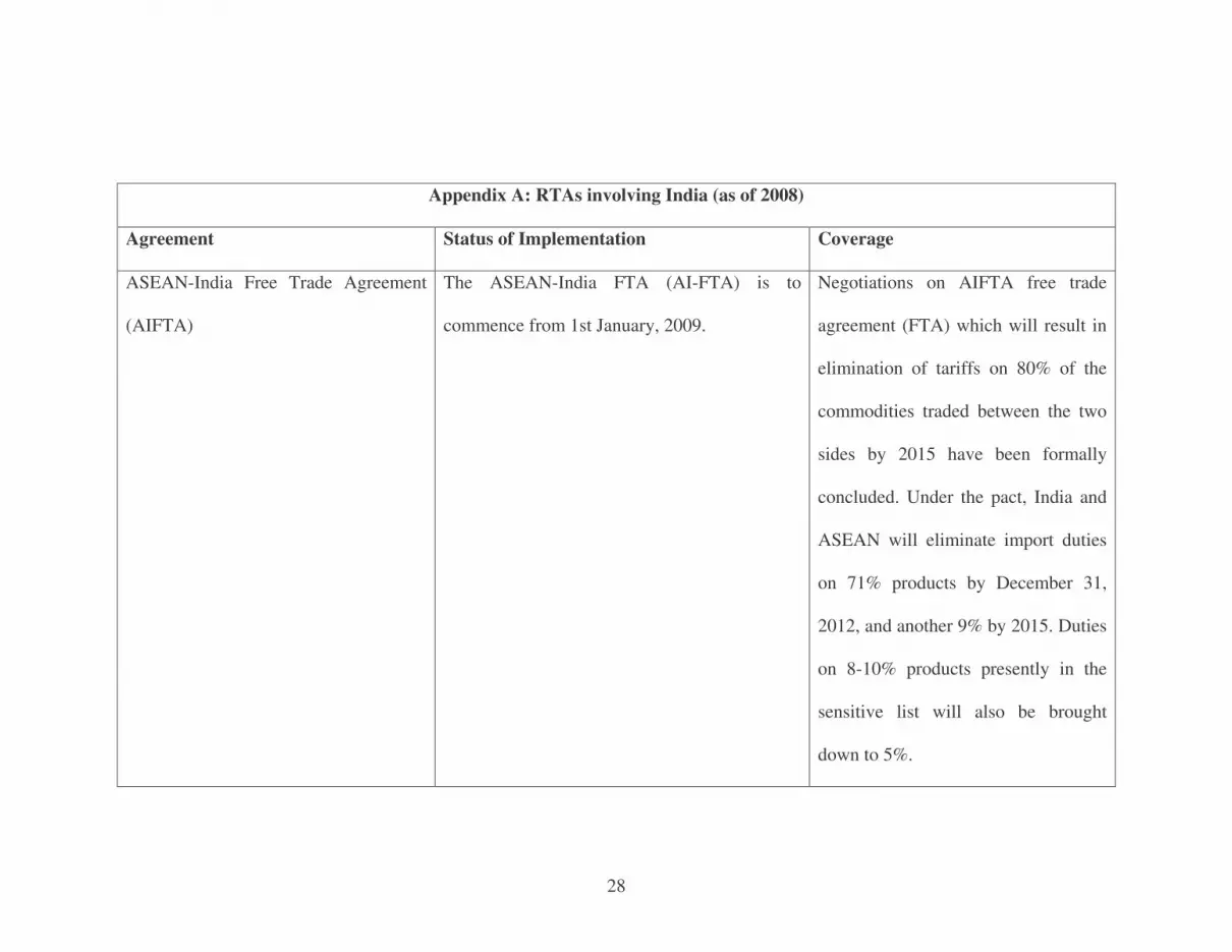
Appendix A: RTAs involving India (as of 2008)
Agreement Status of Implementation Coverage
ASEAN-India Free Trade Agreement
(AIFTA)
The ASEAN-India FTA (AI-FTA) is to
commence from 1st January, 2009.
Negotiations on AIFTA free trade
agreement (FTA) which will result in
elimination of tariffs on 80% of the
commodities traded between the two
sides by 2015 have been formally
concluded. Under the pact, India and
ASEAN will eliminate import duties
on 71% products by December 31,
2012, and another 9% by 2015. Duties
on 8-10% products presently in the
sensitive list will also be brought
down to 5%.

29
India-Singapore Comprehensive
Economic Cooperation Agreement
(CECA).
The CECA has become operational with effect
from 1st August, 2005.
Joint Study Group identifies areas of
increased economic engagement
between two countries. These areas
are FTA in goods, services, and
investment.
Framework Agreement for establishing
Free Trade between India and Thailand.
The tariff concessions on 82 items of EHS list
began in 2004. The tariffs on these items would
become zero for both sides on 1st September,
2006. FTA in goods would commence from
March, 2005. However, due to difference of
opinion on certain issues, this deadline could
not be met.
The Framework Agreement covers
FTA in Goods, Services, Investment
and Areas of Economic Cooperation.
Preferential Trade Agreement (PTA)
between India and Chile.
The PTA has been signed in 2006.The PTA has
come into force in India from November 2007.
India has offered to provide fixed
tariff preferences ranging from 10% to
50% on 178 tariff lines at the 8 digit

30
level to Chile; the latter have offered
a similar range of tariff preferences on
296 tariff lines at the 8 digit level. The
products covered in the mutual offers
account for more than 90 percent of
the value of total bilateral trade.
The Bay of Bengal Initiative for Multi-
Sectoral Technical and Economic
Cooperation (BIMSTEC) was launched
in December 1997 and has membership
of Bangladesh, India, Myanmar, Sri
Lanka, Thailand, Bhutan, and Nepal.
The negotiations are at an advanced stage on
FTA in goods which is scheduled to be
implemented from 1st July, 2006. The
negotiations on the Agreement on Services &
Investment have also commenced.
Six areas were identified for
cooperation in BIMST-EC, namely,
trade and investment, technology,
transportation and communication,
energy, tourism and fisheries.
Agreement on South Asia Free Trade
Area (SAFTA). The members are India,
Pakistan, Sri Lanka, Bangladesh, Nepal,
SAFTA has come into force from 1st January,
2006. Tariff reductions will take place at
different rates for the least developed members
The agreement had exclusive
coverage of trade in goods and
provided for gradual concessions on

31
Bhutan, and Maldives. Afghanistan is
slated to join the SAFTA in January
2008.
(LDMs) namely Bangladesh, Nepal, Bhutan
and Maldives as against the non-least
developed members (NLDMs) namely India,
Pakistan and Sri Lanka.
tariffs and non-tariff measures in
various stages. In two years NLDMs
will reduce tariffs from the existing
levels to a maximum of 20 per cent
while LDMs will bring them down to
30%. In 5 years NLDMs will bring
down tariffs from 20% to 0-5%, while
LDMs will do so in 8 years.
India-Sri Lanka Free Trade Agreement. Bilateral trade between India and Sri Lanka is
regulated by India-Sri Lanka Free Trade
Agreement (ISFTA) signed in December 1998
and operational with effect from March 2000.
Now, both sides are negotiating on not
only trade in goods but also on trade
in services and Economic
Cooperation.

32
Appendix B: Major RTAs for which India is a Non-Member
Agreement and Economic
Characteristics of the RTA
Status of Implementation Coverage
Association of South-East Asian
Nations (ASEAN):
As on 2005, ASEAN’s combined GDP
was 893 billion US dollar, its intra-
regional imports were 142 billion US
dollar and extra-regional imports were
441 billion US dollar. ASEAN’s import
from India was 10.4 billion dollar in
2005 and India’s export to ASEAN
region was 10.11 percent of India’s total
ASEAN initiated its free trade
agreement called ASEAN Free Trade
Area (AFTA) in 1992. It is now
working as a free trade area among ten
member countries.
As on January 1, 2005, tariffs on almost 99
percent of the products in the inclusion list of
the ASEAN-6 (Brunei Darussalam, Indonesia,
Malaysia, the Philippines, Singapore, and
Thailand) have been reduced to no more than 5
percent. More than 60 percent of these
products have zero tariffs. The average tariff
for ASEAN-6 has been brought down from
more than 12 percent when AFTA started to 2
in 2005. The average Common Effective

33
export to the world.
Preferential Tariff (CEPT) tariff rates for
products in the inclusion list is approximately
2.7% in 2003, down from about 12.76% in
1993 at the start of the tariff reduction program.
Within the CEPT mechanism tariffs on goods
traded within the ASEAN region should meet a
40% ASEAN content requirement and expected
to be reduced to 0 to 5% by the year 2002/2003
(2006 for Vietnam, 2008 for Laos and
Myanmar, and 2010 for Cambodia).
Southern Common Market
(MERCOSUR):
As on 2005, MERCOSUR’s combined
GDP was 1.08 trillion US dollar, its
The CECA has become operational
with effect from 1st August, 2005. On
January 1, 1995, MERCOSUR
designated itself as a customs union by
For MERCOSUR CET covers 85 percent of
traded goods. In 1999, most trade between
Brazil and Argentina became duty-free under
the intra-MERCOSUR duty phase out schedule.

34
intra-regional imports were 22 billion
US dollar and extra-regional imports
were 94 billion US dollar.
MERCOSUR’s import from India was
1.3 billion dollar in 2005 and India’s
export to MERCOSUR was 1.3 percent
of India’s total export to the world.
establishing a common external tariff
(CET).
In 1999, most trade between Brazil and
Argentina became duty-free under the intra-
MERCOSUR duty phase out schedule. In case
of rules of origin the value content should be
more than 40 percent of the free of board
(FOB) export value of the final product and it
must be produced within any of the member
states.
North American Free Trade
Agreement (NAFTA):
As on 2005, NAFTA’s combined GDP
was 14.3 trillion US dollar, its intra-
regional imports were 809 billion US
dollar and extra-regional imports were
1510 billion US dollar. NAFTA’s
Implementation of the North
American Free Trade Agreement
(NAFTA) began on Jan. 1, 1994 and
will complete in 2008.
Under NAFTA, tariffs on qualifying goods
traded within the NAFTA countries became
duty free from January, 1998. The tariffs on
virtually all originating goods traded between
have been eliminated by 2003.

35
import from India was 18.9 billion
dollar in 2005 and India’s export to
NAFTA region was 18.2 percent of
India’s total export to the world.
European Union:
As on 2005, EU’s combined GDP was
13.6 trillion US dollar, its intra-regional
imports were 2503 billion US dollar and
extra-regional imports were 1535 billion
US dollar. EU’s import from India was
22.5 billion dollar in 2005 and India’s
export to EU was 21.78 percent of
India’s total export to the world.
The PTA has been signed in 2006. The
PTA has come into force in India from
November 2007.
India has offered to provide fixed tariff
preferences ranging from 10% to 50% on 178
tariff lines at the 8 digit level to Chile; the latter
have offered us a similar range of tariff
preferences on 296 tariff lines at the 8 digit
level. The products covered in the mutual offers
account for more than 90 percent of the value
of total bilateral trade.

36
Appendix C: Shares (%) of different commodity groups in total imports from India by ASEAN, EU, NAFTA, and
MERCOSUR.
Commodity ASEAN EU NAFTA MERCOSUR
1985 1991 1998 1986 1992 1999 1987 1993 2000 1984 1990 1997
0 Food and live animals 29.28 27.6 24.45 15.41 11.25 9.38 10.24 8.43 6.81 0.56 0.84 0.96
1 Beverages and tobacco 0.37 0.39 0.79 1.55 1.18 0.91 0.03 0.05 0.16 NA NA 0.21
2
Crude materials, inedible
except fuels 6.24 6.91 3.82 5.02 3.41 3.58 4.23 2.25 2.11 19.15 1.97 4.55
3
Mineral fuels, lubricants and
related materials NA 0.02 0.26 NA 0.06 0.07 NA 0.09 0.02 NA NA NA
4
Animal and vegetable oils,
fates and waxes 2.42 0.03 0.49 0.44 0.52 1.19 0.01 0.5 0.38 NA NA 2.68
5
Chemicals and related
products 6.08 11.32 16.93 3.79 7.02 9.43 1.96 4.89 6.38 9.05 66.74 38.13
6
Manufactured goods
classified chiefly by material 32.49 34.32 29.76 43.06 40.03 37.11 53.79 47.95 42.7 22.93 13.67 18.53

37
7
Machinery and transport
equipment 18.14 13.26 12.19 2.32 4.04 7.18 2.07 4.02 6.2 38.92 9.61 20.84
8
Miscellaneous manufactured
articles 4.59 4.65 8.8 27.66 30.08 28.1 24.14 28.78 31.64 9.29 6.73 13.14
9
Commodities and
transactions not classified
elsewhere in the SITC 0.4 1.5 2.5 0.75 2.42 3.06 3.53 3.04 3.6 0.07 0.4 0.96

38
References
Aitken, N.D. (1973) The Effects of the EEC and EFTA on European Trade: A Temporal
Cross-Section Analysis, The American Economic Review, Vol. 63, No. 5: 881-892.
Balassa, B. (1967) Trade Creation and Trade Diversion in the European Common
Market, The Economic Journal, Vol. 77, No. 305: 1-21.
Baldwin, R. and A. J. Venables. (1995) Regional Economic Integration, Grossman, G. M.
and K. Rogoff (eds), Handbook of International Economics, Elsevier, Vol. III. Chapter
39.
Batra, A. (2004) India’s Global Trade Potential: The Gravity Model Approach, Working
Paper No. 151, Indian Council for Research on International Economic Relations.
Bhagwati, J. (1971), Trade Diverting Customs Unions and Welfare Improvement: A
Clarification, Economic Journal, Chapter 63.
Bhagwati, J. (1992) Regionalism versus multilateralism, The World Economy, 15 (5):
535-556.
Bhagwati, J. and A. Panagariya. (1996) Preferential trading areas and multilateralism-
strangers, friends, or foes? J. Bhagwati and A. Panagariya. (eds.), The economics of
preferential trade agreements, Washington, D.C. The AEI Press.
Carrere, C (2004) Revisiting the Effects of Regional Trade Agreements on Trade flows
with Proper Specification of the Gravity Model, European Economic Review, 50. pp:
223-247.
Cernat, L. (2001) Assessing Regional Trade Arrangements: are South-South RTAs more
Trade Diverting, Policy Issues in International Trade and Commodities Study Series, No.
16.

39
Chang, W. and A. Winters. (2002) How Regional Blocs Affect Excluded Countries: The
Price Effects of MERCOSUR, The American Economic Review, Vol. 92, No. 4: 889-904.
Cheng, I-Hui and H. J. Wall (2005) Controlling for Heterogeneity in Gravity Models of
Trade and Integration, Federal Reserve Bank of St. Louis Review, 87(1). pp.49-63.
Cordon, M. W. (1972) Economies of Scale and Customs Union Theory, Journal of
Political Economy, 80: 456-475.
Coulibaly, S. (2007) Evaluating the Trade Effect of Developing Regional Trade
Agreements: A Semi-parametric Approach, World Bank Policy Research Working Paper
4200, World Bank.
DeRosa, D. A., (2007) Regional Integration Arrangements: static Economic Theory,
Quantitative Findings, and Policy Guidelines, Policy Research Working Paper, No. 2007,
World Bank.
Feenstra, R.C. (2004) Advanced International Trade, Theory and Evidence, Princeton
and Oxford, Princeton University Press.
Gehrels, F. (1956-1957), “Customs Union from a Single-Country Viewpoint”, The
Review of Economic Studies, Vol. 24, No. 1: 61-64.
Greenaway, D. and C, Milner. (2002) Regionalism and Gravity, Scottish Journal of
Political Economy, Vol. 49, No. 5: 574-585.
Helpman, E and P. Krugman. (1985) Market Structure and Foreign Trade: Increasing
Returns, Imperfect Competition, and the International Economy, Chambridge,
Massachusetts, The MIT Press.
Johnson, H. G. (1974) Trade Diverting Customs Union: A comments, Economic Journal,
Vol. 84, No. 335: 618-621.

40
Johnson, H. G. (1975) A note on Welfare–Increasing Trade Diversion, Canadian Journal
of Economics and Political Science, Vol. 8, No. 1: 117-123.
Joshi, Vivek. (2008) An Econometric Analysis of India Sri Lanka Free Trade Agreement,
Master in International Studies (MIS) Dissertation, Geneva, University of Geneva.
Jovanovic, M. N. (2006) The Economics of International Integration, Northampton, MA,
USA: Edward Elgar.
Kalbasi, H. (2001) The Gravity Model and Global Trade Flows, Paper in the Conference
of EcoMod, Washington DC.
Kandogan, Y. (2008) Consistent Estimates of Regional Blocs’ Trade Effects” Review of
International Economics, 16(2): 301-314.
Kelegama, S. and I. N. Mukherji (2007) India-Sri Lanka Bilateral Free Trade Agreement:
Six Years Performance and Beyond, RIS Discussion Paper, No. 119, Research and
Information System for Developing Countries, New Delhi.
Kemp, M., and H.Y. Wan. (1976) An elementary proposition concerning the formation of
customs union, Journal of International Economics, 6 (1): 95-97.
Kirman, A. P. (1973) Trade Diverting Customs Union and Welfare Improvement: A
Comment, Economic Journal, Vol. 83, No. 331: 890-893.
Krenin, M. E. (1961) Effect of Tariff Changes on the Prices and Volume of Imports, The
American Economic Review, Vol. 51, No. 3: 310-324.
Krugman, P. (1979) Increasing Returns, Monopolistic Competition, and International
Trade, Journal of International Economics, Vol. 9, No. 4: 469-479.
Krugman, P. (1980) Scale Economies, Product differentiation, and the Pattern of Trade,
The American Economic Review, Vol. 70: 950-959.

41
Lipsey, R. G. and K. J. Lancaster (1956-57) The General Theory of Second Best, Review
of Economic Studies, 24, pp. 33-49.
Lipsey, R. G. (1957) The Theory of Customs Union: Trade Diversion and Welfare,
Economica, Vol. 24, No. 93: 40-46.
Lipsey, R. G. (1957) Mr. Gehrels on Customs Union, The Review of Economic Studies,
Vol.24, No. 3: 211-214.
Lipsey, R. G. (1960) The Theory of Customs Union: A General Survey, The Economic
Journal, Vol. 70, No. 279: 496-513.
Meade, J.E. (1955) The theory of customs unions. Amsterdam, North-Holland.
Ohyama, M. (1972) Trade and welfare in general equilibrium, Keio Economic Studies, 9:
37-73.
Pant, M. (2002) Millennium Round of Trade Negotiations: A Developing Country
Perspective’, Journal of International Studies, July-Sept,2002, pp. 213-226, Sage
Publications, India..
Santos-Paulino, A. and A. P. Thirlwall, (2004) The Impact of Trade Liberalization on
Exports, Imports and the Balance of Payments of Developing Countries, The Economic
Journal, 114: F50-F72.
Schiff, M. (1996) Small is beautiful: Preferential trade agreements and the impact of
country size, market share, efficiency, and trade policy, Policy Research Working Paper
No. 1668. International Trade Division, the World Bank, Washington, D.C.
Smith, A. and A. J. Venables (1991) Economic integration and market access, European
Economic Review, 35: 388-395.

42
Tinbergen, J. (1962) An Analysis of World Trade Flows: in Shaping the World Economy,
Jan Tinbergen (ed.), New York, the Twentieth Century Fund.
Poyhonen, P, (1963) A Tentative Model for the Volume of Trade between Countries,
Weltwirtschaftliches Archiv 90.
Rahman, M. M. (2003) A Panel Data Analysis of Bangladesh’s Trade: The Gravity
Model Approach, University of Sydney.
Viner, J. (1950) The customs union issue. New York: Carnegie Endowment for
International Peace.
Winters, L. A. (1997) Regionalism and the Rest of the World: Theory and Estimates of
the Effects of European Integration, Review of International Economics, Special
supplement: 134-147.
Winters, L. A. (1997) Regionalism and the Rest of the World: The Irrelevance of the
Kemp-Wan Theorem, Oxford Economics Papers, 49(2): 228-234.
Winters, L. A. and W. Chang. (2000) Regional integration and import Prices: an
empirical investigation, Journal of International Economics, 51: 363-377.
Yeats, A. (1997) Does Mercosur’s Trade Performance Raise Concerns about the effects
of Regional Trade Arrangements? Policy Research Working Paper, 1729, World Bank.