does money matter in inflation forecasting?
TRANSCRIPT

Research Division Federal Reserve Bank of St. Louis Working Paper Series
Does Money Matter in Inflation Forecasting?
Jane M. Binner
Peter Tino Jonathan Tepper
Richard G. Anderson Barry Jones
and Graham Kendall
Working Paper 2009-030B
http://research.stlouisfed.org/wp/2009/2009-030.pdf
June 2009 Revised May 2010
FEDERAL RESERVE BANK OF ST. LOUIS Research Division
P.O. Box 442 St. Louis, MO 63166
______________________________________________________________________________________
The views expressed are those of the individual authors and do not necessarily reflect official positions of the Federal Reserve Bank of St. Louis, the Federal Reserve System, or the Board of Governors.
Federal Reserve Bank of St. Louis Working Papers are preliminary materials circulated to stimulate discussion and critical comment. References in publications to Federal Reserve Bank of St. Louis Working Papers (other than an acknowledgment that the writer has had access to unpublished material) should be cleared with the author or authors.

1
Does Money Matter in Inflation Forecasting?
JM Binner 1 P Tino 2 J Tepper 3 R Anderson4 B Jones 5 G Kendall 6 1 Aston University, Birmingham, UK
2 University of Birmingham, Birmingham, UK 3 Nottingham Trent University, Nottingham, UK
4 Federal Reserve Bank of St. Louis, USA and Aston University UK 5 State University of New York, Binghamton, USA
6 University of Nottingham, Nottingham, UK
April 2010
Abstract
This paper provides the most fully comprehensive evidence to date on whether or not monetary aggregates are valuable for forecasting US inflation in the early to mid 2000s. We explore a wide range of different definitions of money, including different methods of aggregation and different collections of included monetary assets. In our forecasting experiment we use two non-linear techniques, namely, recurrent neural networks and kernel recursive least squares regression - techniques that are new to macroeconomics. Recurrent neural networks operate with potentially unbounded input memory, while the kernel regression technique is a finite memory predictor. The two methodologies compete to find the best fitting US inflation forecasting models and are then compared to forecasts from a naive random walk model. The best models were non-linear autoregressive models based on kernel methods. Our findings do not provide much support for the usefulness of monetary aggregates in forecasting inflation. Beyond its economic findings, our study is in the tradition of physicists’ long-standing interest in the interconnections among statistical mechanics, neural networks, and related nonparametric statistical methods, and suggests potential avenues of extension for such studies.
Keywords: Inflation, Monetary Aggregates, Recurrent Neural Networks, Kernel Methods. JEL Codes: E31, E41, E47, E51.
Opinions e xpressed herein a re no t necessarily t hose of t he F ederal R eserve B ank of S t. L ouis or t he
Federal R eserve S ystem. Anderson and J ones t hank the S chool of B usiness, A ston U niversity, f or its
support a nd hospitality as vi sitors while c onducting t his research. Anderson a lso t hanks t he R esearch
Department of the Federal Reserve Bank of Minneapolis for its hospitality as a visitor while conducting
parts of this research.

2
1. Introduction
It is a widely held belief among macroeconomists that there exists a long-run relationship
between the growth rate of the money supply and the growth rate of prices (i.e., inflation). This belief
forms the foundation for monetary policymaking at the world’s central banks, and hence is extraordinarily
important for the conduct of public policy. Its importance makes it one of the most commonly tested
hypotheses in economics. Yet, the mechanism through which money affects an economy’s overall,
average price level is necessarily complex – as complex as the economies themselves. The mechanism
almost surely is not linear, and the short-run dynamics may disguise the long-run relationship, confusing
tests of the relationship. Linkages need not be univariate, and fluctuations in other variables (including the
growth rate of productivity, and international economic conditions) may affect the near- and medium-
term correspondence between money growth and inflation. Such interactions raise the possibility that the
correspondence may be both nonlinear and time-varying, perhaps with complexity beyond capture in
parametric frameworks. In a recent paper, Bachmeier, Leelahanon, and Li (2007), for example, soundly
reject both linear autoregressive (univariate) and vector-autoregressive (multivariate) models.
If indeed there exists a dynamic, long-run relationship between the money supply and increases in
prices, then it is a reasonable proposition that the near-term growth of the money supply might have
predictive power for inflation. This study explores that relationship. In this paper, we investigate a wide
range of measures of the money supply (i.e., monetary aggregates) for the United States, and evaluate
their usefulness as leading indicators for inflation in the early to mid 2000s. We derive inflation forecasts
using two nonlinear techniques with varying degrees of input memory, namely, recurrent neural network
operating with potentially unbounded input memory, and a kernel regression technique with finite input
memory.
In addition to the economic analysis, our study contributes to physicists’ long-standing interest in
the interconnections among statistical mechanics, neural networks, and related nonparametric statistical
methods. A number of the statistical issues addressed in this paper are similar to those addressed in
3
econophysics. Consider the problem of linear vs nonlinear models. Galluccio et al. (1998), Laloux et al.
(1999), Plerou et al. (1999) and Plerou et al. (2002), for example, study correlations among returns on
different stocks by applying random matrix theory to the stock-returns cross-correlation matrix. This
approach imposes a linear model on the statistical linkages among the entities under consideration (e.g.
stock returns, monetary aggregates, inflation); the assumed linearity is a limitation of the approach despite
the approach being `model-free’ to the degree that the correlation measure is a model-free quantity. Our
analysis proceeds in a nonlinear, model-based fashion to consider possible linkages among future
inflation, past inflation, interest rates, and monetary aggregates. We assume, specifically, that the
structure of such relationships can be explained through two classes of non-linear models: one with
infinite and the other with finite input memory. In addition to importance in their own right, our findings
suggest possibilities for generalizations and extensions of previous econophysics financial-market studies
that have used the correlation- or mutual information based method. 1
In this regard, our study adopts the
argument made by Plerou et al (2000) that “In economics, one often starts with a model and tests what the
data can say about the model. The physics approach to this field differs in that it starts in the spirit of
experimental physics where one tries to uncover the empirical laws which one later models.” Saito
(2007), for example, studies the possibility of using a neural network to statistically learn an economic
time series—but his network validation was performed using data generated by a model developed in
econophysics rather than observed data. Finally, we note that our methodology also lies within the
discipline of computational intelligence, a topic of interest to many physicists. Chen, Jain and Tai (2006),
for example, illustrate the application of computational intelligence in many fields, including computer
science, engineering, psychology and, especially, physics.
1. A generalization to admit non-linear relationships might be achieved by considering information theoretic measures such as multivariate mutual information.

4
2. Monetary Aggregates and Monetary Policymaking
Policymakers worldwide seek to foster economic conditions of robust economic activity and low,
stable rates of inflation. In that regard, it is important to identify indicators of macroeconomic conditions
that will alert policy makers to impending inflationary pressures sufficiently early to allow the necessary
actions to be taken to control and remedy the problem. Equally important, such indicators must not falsely
signal future increases in inflation that cause policymakers to slow the pace of economic output in vain
efforts to temper inflation. Given the widely held belief in the existence of a long-run relationship
between money and prices, monetary aggregates would seem to hold much promise as indicator variables
for central banks. The European Central Bank (ECB), for example, employs a “two pillared” approach,
which includes monetary analysis. Specifically, ECB (2003) states that “…the [President’s Introductory]
statement will [after identifying short to medium-term risks to price stability] proceed to monetary
analysis to assess medium to long-term trends in inflation in view of the close relationship between
money and prices over extended horizons.” Evidence to date has not provided strong support for the
proposition that monetary aggregates assist forecasting inflation for the United States; see, for example,
Stock and Watson (1999a, 2007).2
Recently, some economists have issued cautionary notes on the importance of money. See, for
examples, Nelson (2002), Nelson (2003) and Leeper and Rouch (2003). In particular, Carlstrom and
Fuerst (2004) state “…we think the current de-emphasis on the role of money may have gone too far. It is
Moreover, as noted by Federal Reserve Board chairman Ben
Bernanke, monetary aggregates have not played a central role in the formulation of US monetary policy,
since 1982. He further states (Bernanke, 2006): “Why have monetary aggregates not been more
influential in U.S. monetary policymaking, despite the strong theoretical presumption that money growth
should be linked to growth in nominal aggregates and to inflation? In practice, the difficulty has been that,
in the United States, deregulation, financial innovation, and other factors have led to recurrent instability
in the relationships between various monetary aggregates and other nominal variables.”
2 Stock and Watson (2007) also conclude that most “real” economic variables, including real GDP, are not helpful in predicting future inflation.

5
important to think seriously about the role of money and how money affects optimal policy.” In a similar
vein, the Governor of the Bank of England Mervyn King (2002) stated “My own belief is that the absence
of money in the standard models which economists use will cause problems in future, and that there will
be profitable developments from future research into the way in which money affects risk premia and
economic behavior more generally. Money, I conjecture, will regain an important place in the
conversation of economists.”
Linkages between money and inflation have become increasingly important during the recent
financial crisis as in a number of countries, the instrument of monetary policy has shifted towards the
quantity of money and away from overnight interest rates (for example, Bank Rate in the U.K.; the federal
funds rate in the United States). A complicating factor in this debate is that money measurement is a
complex problem. There are two key questions. First, which monetary assets are to be included in a
particular aggregate? And, second, how are these assets to be aggregated together?
Economists generally classify a financial asset as “money” if it is medium-of-exchange (that is,
may be used for the purchase or sale of goods and services without being converted into any other form),
or if the asset may be converted into medium of exchange at almost any time, and at low cost. This
classification scheme admits a wide range of candidate assets. The most obvious is currency. “Narrow”
monetary aggregates include currency and bank deposits transferable by cheque. Somewhat broader
aggregates include the assets of narrow aggregates but, in addition, assets that are not medium of
exchange but have little or no cost of conversion into medium of exchange; in the United States, these
include savings deposits and shares in money market mutual fund. “Broad” monetary aggregates, in
addition, include assets with higher conversion costs into medium of exchange; many of these assets have
contractual fixed terms to maturity and financial penalties for withdrawal prior to contract expiration.
Among these are small-denomination time deposits. Typically, the assets in narrow aggregates earn zero,
or relatively low, interest rates. Broader aggregates, in contrast, include a wide range of assets with higher
returns, such as money market mutual funds.

6
This study considers a number monetary aggregates for the United States, defined in Appendix 1.
We investigate the forecasting performance of both Divisia and simple sum monetary aggregates at
various levels of aggregation ranging from narrow to broad. For comparison purposes, we also explore
several interest rate variables. Our forecasting experiments with Divisia monetary aggregates build on
several recent papers including Schunk (2001), Drake and Mills (2005), Elger et al. (2006) and Bachmeier
et al. (2007), but are novel in several aspects, discussed below.
We consider a wide range of money aggregates because the choice among the aggregates is far
from clear-cut: both the definitions and roles of monetary aggregates in U.S. policymaking have changed
through time, largely in response to financial innovation and deregulation. Prior to 1980, both academic
researchers and policymakers focused on M1, containing currency and checkable deposits. Following
significant deregulation in 1980, attention shifted toward the broader M2 monetary aggregate (Simpson,
1980; Moore, Porter and Small, 1990). Yet, the initial stability of its demand (at least, in linear parametric
models) proved ephemeral: Subsequent studies traced its instability to innovations that changed the
behavior of small-denomination time deposits (Carlson, Hoffman, Keene and Rasche, 2000). During both
the 1970s and 1980s, the repeated introduction of new substitute financial products caused some analysts
to explore the “MZM” aggregate, consisting of currency plus those financial assets issued by banks and
money market mutual funds that could be converted to checkable deposits without cost (that is, all
financial assets with “zero maturity”). Duca and VanHoose (2004) state that one response to the
instability of M2 demand, at least by researchers if not policymakers, was a renewed focus on MZM,
motivated by the assertion that the instability of M2 demand largely was due to heightened substitution
between small time deposits and shares in bond-type mutual funds—yet, demand for MZM also
encountered instability in the early 2000’s. By the mid-1990s, the Federal Reserve largely had abandoned
monetary aggregates as an important policy guide. In 1994, the policymaking Federal Open Market
Committee began announcing its policy objective to the public after each meeting solely in terms of a
desired level of the federal funds rate; in 2001 the Committee ceased publishing annual monitoring ranges
for growth of monetary aggregates.

7
We note that the M1 monetary aggregate used in this study differs from the M1 aggregate
published by the Federal Reserve’s Board of Governors on its H.6 statistical release. We add to the
published M1 the amount of transaction deposits that banks are allowed, under Federal Reserve
regulations, to report as saving deposits. The latter reclassification of deposits is referred to as “retail
deposit sweeping” (Anderson and Rasche, 2001; Jones et al., 2005). Hence, our M1 aggregate
corresponds to the “M1RS” aggregate as defined by Dutkowsky et al. (2006). Data are obtained from the
web site of the Federal Reserve Bank of St. Louis (research.stlouisfed.org).
In addition to the uncertainty regarding which financial assets to include within a monetary
aggregate, a second measurement issue arises: How should the selected financial assets be aggregated
together? There are two candidate methods of aggregation. First, the monetary aggregates (including M1,
MZM, M2 and M3) published by the Board of Governors of the Federal Reserve System (Washington,
D.C.) are constructed by simple summation; that is adding together the amounts of assets as different as
currency, saving deposits, time deposits with fixed maturities, and money market mutual fund shares. But
a second, alternative method of aggregation is suggested by the economic theory of index numbers. The
use of Divisia index number formulae for construction of monetary aggregates was proposed by Barnett
(1980, 1982). Because such monetary aggregates draw on both statistical index number and consumer
demand theory, they are theoretically preferable to monetary aggregates built by simple summation.
Further, Divisia aggregates admit time-variation in liquidity properties of the components of a monetary
aggregate by causing the weight of each component within the aggregate to depend on both its
expenditure share relative to the other components of the monetary aggregate and on its user cost.3
3 We note that Divisia indexes are correctly defined in continuous time. The most common discrete time approximation is the Törnqvist-Theil (TT) index (Törnqvist, 1936;] Theil, 1967), a chained superlative index (Diewert, 1974, 1976). Barnett et al. (1992) and Anderson et al. (1997a) provide surveys of the relevant literature, whilst Drake et al. (1997) review the construction of Divisia indices and associated problems.
(The
Divisia economic index numbers provide parameter- and estimation-free approximations of aggregator functions and are therefore independent of the researcher’s choice of theoretical and empirical model. The quality of an index number is dependent on how well it tracks the unknown aggregator function. Since the Divisia index is directly derived from the utility maximization problem it can track the unknown underlying aggregator function exactly. The continuous time Divisia index is directly derived from the rational individuals (current period) blockwise weakly

8
growth rate of the overall Divisia index is calculated as the weighted average of the growth rates of its
components, where the weights are each asset’s share in the total expenditure on all monetary assets.)
Typically, currency and non-interest bearing deposits receive the highest weight because they are highly
liquid assets and (correspondingly) have high user costs (in terms of interest foregone). Interest-bearing
time deposits by contrast pay a relatively high rate of interest and, hence, have a smaller expenditure
share and a lower weight than might be expected from their relative size. Economic theory suggests that
Divisia monetary aggregates should be more closely related to the overall level of liquidity and total
spending in the economy than are conventional monetary aggregates.
Despite their grounding in index number theory, measurement issues arise with Divisia monetary
aggregate measures. As previously noted, the growth rate of a Divisia monetary aggregate equals the sum
of the expenditure share-weighted growth rates of its component assets. Measures of these expenditure
shares depends on measures of the opportunity cost of the monetary assets, defined as the spread between
the monetary assets’ own rates of return and the rate of return on a “benchmark” asset that does not
provide any monetary services in the current period (that is, using the asset to purchase goods or services
during the current period is infeasible). In practice, choice of a benchmark rate is uncertain and the choice
affects the properties of the aggregate; see, for example, Hancock (2005). Drake and Mills (2005) suggest
that the relatively poor forecasting performance of Divisia M2 in their study may be due to the choice of
benchmark rate used by the Federal Reserve Bank of St. Louis in its construction. Hence, a first novel
feature of our study is that we investigate how the choice of benchmark rate affects the forecasting
performance of Divisia aggregates over a range of different levels of aggregation. We discuss the details
surrounding this issue in the next section. A second novel aspect of the paper lies in our use of nonlinear
techniques to examine the recent experience of inflation in the U.S4
separable sub-utility function over monetary assets. Hulten (1973) has shown that the Divisia line integral is path independent under weak separability.
. Our previous experience in inflation
4 A number of recent studies of inflation and inflation uncertainty have appeared in the literature including Berument and Dincer (2005) and Berument and Yuksel (2007).
9
forecasting using state of the art approaches gives us confidence to believe that significant advances in
macroeconomic forecasting and policymaking are possible using techniques such as those employed in
this paper. As in our earlier work (Binner et al., 2005a), results achieved using artificial intelligence
techniques (i.e., Neural Networks and Kernal Methods) are compared with those using a baseline naïve
predictor.
3. Data and Forecasting Framework
Two aspects of the data must be discussed: the choice of an inflation measure and the choice of a
monetary aggregate. The choices are substantive because we cannot pre-test for invariance (with respect
to the measure of money and inflation) of the nonlinear and potentially time-varying relationships that
connect a specific monetary aggregate and an inflation measure.
Choice of Inflation Measure
A number of inflation measures are available for the United States, including the chain-price
index for gross domestic product, the chain-price index for personal consumption expenditures both
including and omitting food and energy, the implicit price deflator for gross domestic product, and several
variants of the consumer price index for urban workers and wage earners (CPI-U and CPI-W). The CPI-U
is perhaps the best known among households and businesses. Although the Federal Reserve’s
policymaking Federal Open Market Committee monitors the chain-price index for personal consumption
expenditures omitting food and energy (“core PCE price index”) on the belief that it best measures the
underlying inflation trend affected by monetary policy, the Committee’s underlying concern, as
summarized by a former Federal Reserve governor, is the path of headline CPI inflation: “I have no
qualm in stating that controlling headline inflation, not core inflation, is—along with maintaining
maximum sustainable employment—the ultimate aim of monetary policy.” (Mishkin, 2007) Similarly,
inflation-targeting central banks worldwide focus on the behavior of headline CPI measures, regardless of
their intermediate price index targets (Mishkin and Schmidt-Hebbel, 2001). Annual cost-of-living
adjustments for Social Security recipients, as well as federal government and military retirees, are based

10
on the CPI-U, as are annual adjustments of federal income tax brackets and the payments to holders of the
Treasury’s inflation-protected (indexed) bonds.
In its construction, the CPI-U is a compromise between rapid evolution of expenditure weights so
as to accurately track changing consumer expenditure patterns and the more sluggish adjustment required
to measure cost-of-living changes relative to a set of base-period reference expenditure shares. In the
event, CPI-U expenditure weights are updated every two years, based on consumer surveys. At finer
levels of disaggregation, goods and services are aggregated using geometric means so as to minimize
substitution bias; at more aggregate levels, aggregation is via Laspeyres formulas so as to avoid
understating the impact of rising prices on households’ cost of living. The CPI has a careful process for
quality adjustment, partially based on hedonics that seeks to include inevitable changes in available goods
and services. Housing is treated via a rental equivalence approach that both collects actual spending
through the Consumer Expenditure Survey and market data regarding the rental prices of apartments and
houses. Greenlees and McClelland (2008) provide an accessible discussion of these and other issues.
An alternative index used in some studies, and also available monthly, is the chain-price index for
PCE. This index is closely related to the CPI in that both indexes are built from the same underlying price
and quantity data furnished by the U.S. Bureau of the Census, and both in their current versions measure
the user cost of housing services consumed by households rather than the purchase prices of houses,
utility services, etc. Yet, there are substantive differences between the indexes, including the formula used
for upper-level aggregation (the CPI uses a Laspeyres formula, the PCE chain-price index uses a Fisher-
Ideal superlative formula), the weights (the CPI uses weights from a monthly consumer expenditure
survey, the PCE index uses weights from monthly business surveys including the survey of retail sales),
the updating of the weights (CPI weights are updated every two years, PCE index weights are updated
each year based on a ratio of the preceding two years), quality adjustments (mandated changes due to
safety or environmental concerns generally appear as price increases in the CPI but as quality adjustments
in the PCE index), and scope (the CPI includes only out-of-pocket payments by consumers, while the
PCE includes payments made by firms on behalf of employees). For the period considered in this study

11
(1960-2005), the two indexes behave similarly: average monthly year-over-year inflation measured by the
CPI-U and PCE index is 4.3 percent and 3.8 percent, respectively, and the differences between the
measure in almost all months is less than 1 percent except for periods in 1979-1981 when CPI inflation
exceeded 10 percent due to elevated mortgage interest rates. In empirical studies, use of the PCE price
index is not obviously to be preferred to the CPI. Clark (1999) argues that the CPI is preferable because
the data are more timely and better quality. Although his analysis is a decade old, it seems the situation
has changed little since (McCully et al., 2007; Garner et al., 2006).
Price indexes at lower frequencies also are available but we do not consider them in this study.5
The chain-price index for GDP is available quarterly, but with a longer lag than the CPI; the first
observation for a quarter is published late in the third month following the end of the measured quarter,
revised values are published late in each of the following two months, and a further value is published the
following year. Its delayed availability and tendency to be revised make the GDP price index less
informative to policymakers and infrequently used in contracts. The GDP price index both contains items
excluded from the CPI and includes additional items. Excluded items include prices of used consumer
goods and prices of imported goods. Many of the included items are intermediate products, including
consumer goods in distribution and producers’ durable equipment and structures. Changes in such prices
are only weakly linked to changes in consumer goods’ prices and the cost of living.6
Inflation in this paper is measured monthly as the year over year percentage change in the CPI-U.
We prefer the CPI due its wide-spread publ ic recognition and timely data availability. In the interests of
brevity, we do not explore alternative measures here but leave them as a subject of future research.
5Nakamura (2005), for example, studies the quarterly GDP implicit deflator. 6 Nakamura (2008) concludes that variation in retail prices arises primarily from retail-level demand and supply shocks rather than manufacturer-level price fluctuations.

12
Monetary Aggregates
We consider in this study sixteen alternative monetary aggregates, varying in terms of the
monetary assets included in each aggregate and the method of aggregation.
First, we consider four different groupings of monetary assets: M1, which consists of currency,
demand deposits, and other checkable deposits; MZM, which consists of all M1 assets plus savings
deposits, including money market deposit accounts (MMDA) and retail-type money market mutual funds;
M2, which consists of MZM assets plus small-denomination time deposits; and M3, which consists of M2
assets plus institutional-type money market mutual funds, repurchase agreements, Eurodollar accounts,
and large denomination time deposits.
Second, we consider monetary aggregates built with different aggregation methods. We obtained
simple sum and Divisia monetary aggregates for each of the four levels of aggregation (M1, MZM, M2,
and M3) from online databases maintained by the Federal Reserve Bank of St Louis; see Anderson et al.
(1997b). In addition, we obtained the Divisia monetary aggregates built by Elger et al. (2006) at the same
four levels of aggregation (M1, MZM, M2, and M3). These aggregates differ from those constructed in
St. Louis primarily in two respects: choice of the benchmark rate that is used in measurement of assets’
opportunity costs and the imputed own rate of return on noninterest-bearing bank deposits. Elger et al.
(2006) choose the benchmark rate as the upper envelope of the returns in M3, that is, in each time period
the benchmark rate is measured as the maximum own-interest rate on the assets included in the M3 level
of aggregation; the St. Louis aggregates are based on an upper envelope that includes a long-term bond
rate (the Baa rate) that, in practice, is selected as the benchmark rate in the majority of time periods. In
addition, Elger et al. (2006) set to zero the own-rate of return on non-interest bearing demand deposits,
while the St. Louis indexes include an implicit return. (There are additional differences between the
aggregates not discussed here; see Elger et al., 2006, pp. 432-3). Finally, as a check for robustness, we
construct an additional set of Divisia aggregates that follow the construction method of Elger et al. (2006)
except that the Baa corporate bond rate is included in the upper envelope selection process for the
benchmark rate.

13
Finally, we also considered in our study the inflation forecasting potential of both a short- and a
long-term interest rate: specifically, the bond-equivalent yield on three-month Treasury bills and the yield
to maturity on Baa corporate bonds. We allowed each model the freedom, if it wished, to include these
rates alongside or instead of the chosen measures of money, or to omit the interest rates altogether. Each
model was permitted to select lags and/or orders of differencing of each variable as it wished. By
permitting the model to choose among such transformations, we also implicitly include the slope of a
yield curve in our model, a variable that some previous studies have concluded has predictive power for
inflation (Estrella, 2005; Ang et al, 2006). In no case did the inclusion of interest rates improve a model’s
performance.
4. Methodologies
In our experiments, two artificial intelligence forecasting techniques—recurrent neural networks
and kernel recursive least squares—compete to predict the year-over-year inflation rate that will prevail 6
months in the future. For each technique, we begin with a competition in which a large number of models
are fit to the training dataset; we retain the four best models for each technique judged on their
performance on the hold-out validation dataset. Next, we compare the forecasting performance of the four
models (and their flat ensembles) for out-of-sample forecasting on the test set. Of the 541 data points
available, the first 433 were used for training (model fitting), (January 1960 - February 1997), the next 50
data points were used for validation, (March 1997 – April 2001) and the next 46 data points were used for
forecasting (May 2001 – February 2005). We also consider a “naïve” random walk model for comparison.
Neural network and kernel techniques are able to approximate a wide family of linear and nonlinear data
transformations, and hence are robust to the order of integration of explanatory variables (Moody, 1995;
Zhang, Patuwo and Hu, 1998; Giles, Lawrence and Tsoi, 2001). The input data series, i.e. the right hand
side explanatory variables for our experiments, in the jargon of time-series econometrics, are allowed to
be of differing “orders of integration.” This is addressed further below.
14
The ability of artificial intelligence techniques to approximate linear and nonlinear
transformations of the data may be illustrated by considering the least squares regression problem.
Consider choosing a vector of fixed parameters, β so as to solve ( )2
1
ˆmint
t ti
y yβ
=
−∑ where y denotes the
dependent variable; ( )1,..., Kx xx = denotes a vector of explanatory variables 1,...,k K= ; ( )y xβ φ= ⋅ ;
and ( )1( ) ( ),..., ( )Jx x xφ φ φ ′= is a fixed, finite dimensional mapping defined over the explanatory
variables. Linear least squares regression defines ( )j kx xφ = for all ,j k∀ . Regressions with differences
of the explanatory variables are denoted ( )j kx xφ = ∆ ; regressions with interaction effects are denoted,
1 2( )j k kx x xφ = ⋅ , 1 2k k≠ , for some j; and regression-based specification error tests are denoted
2( )j kx xφ = or 3( )j kx xφ = for some j (typically, j > K). Our techniques admit all of these and others.
Kernel regression methods, for example, may be written as 1
ˆ ( , )J
t j jj
y k xβ=
≡ ∑ x where { } 1
J
j jx
= are the
training data points and the ( , )k ⋅ ⋅ are positive-definite (nonlinear) kernel functions; see Schölkopf and
Smola (2002) or Engel, Mannor and Meir (2004). Some authors, e.g. Andrews (1995) have labelled these
nonparametric kernel estimators of semi parametric models.
An earlier investigation is Dorsey (2000): “We use an artificial neural network [ANN]to exp lore
the explanatory power of a variety of measures of a single variable that is certainly related to inflation and
money… the ANN can approximate any Borel measurable function to any degree of desired accuracy …
in other words, the ANN can provide a completely flexible mapping that can approximate highly
nonlinear functions to any degree of desired accuracy as long as a sufficient number of hidden nodes are
included.” Dorsey considers inflation to be an unknown function of k recent levels of the money stock ,
( )1 2, ,...t t t t k tF M M Mπ ξ− − −= + . The function F( ) is unknown. His methods are capable of suggesting
that the preferred F( ) is linear in levels

15
1
( )k
t i t i ti
F Mπ α ξ−=
= = +∑ ,
or in first differences
1
( )k
t i t i ti
F Mπ β ξ−=
= = ∆ +∑
(where 1t i t i t iM M M− − − −∆ = − ), or linear in a combination of levels and differences, or nonlinear.
Note, in particular, that the flexibility of neural network and kernel methods obviates the need to
determine in advance, for example, the order of integration of the explanatory variables. As in Dorsey
(2000), when provided with the levels of the “explanatory” variables, these techniques are sufficiently
powerful to explore transformations of those variables. Our methods are robust to issues such as the order
of integration of the variables and the risk of accepting “spurious regressions.”
The power of neural network approximations, for example, is summarized in the well-known
theorem of Hornik et al (1989) that says, essentially, that a neural network can approximate all probability
density functions supported compactly on the real numbers. This version is from Judd (1998), p. 245-6:
Theorem: Let G be a continuous function, :G R R→ , such that either (1) ( )G x dx∞
−∞∫ is finite and
nonzero and G is pL for 1 p≤ < ∞ or (2) G is a squashing function [ ]: 0,1G R → ; that is, G is nondecreasing, lim ( ) 1x G x→∞ = , and lim ( ) 0x G x→∞ = . Define the set of all possible single hidden-layer feedforward neural networks, using G as the hidden layer activation function:
( ) ( )1
: | ( ) ; , ; , 0; 1,2,...m
n n j j n jj j j j
jG g R R g x G w x b b R w R w mβ β
=
= → = ⋅ + ∈ ∈ ≠ =
∑ ∑ .
Then, for all 0ε > , probability measures µ , and compact sets nK R⊂ , there is a ( )ng G∈Σ such
that su p ( ) ( )x K
f x g x ε∈
− ≤ and ( ) ( )K
f x g x dµ ε− ≤∫ .

16
Multi-recurrent Neural Networks
Recurrent neural networks (RNNs) are typically adaptations of the traditional feed-forward multi-
layered perceptron (FF-MLP) trained with gradient-descent learning algorithms (see Pearlmutter, 1995,
and Rumelhart et al., 1986). This class of RNN extends the FF-MLP architecture to include recurrent
connections that allow network activations to feedback as inputs to units within the same or preceding
layer(s). Such internal memories enable the RNN to construct dynamic internal representations of
temporal order and dependencies which may exist within the data. Units that receive feedback values are
often referred to as context or state units. Also, assuming non-linear activation functions are used, the
universal function approximation properties of FF-MLPs naturally extends to RNNs. These properties
have led to wide appeal of RNNs for modeling time-series data, Moshiri, et al. (1999); Tenti (1996);
Ulbricht (1994); Binner et al. (2004); Jordan (1986).7
We build upon our previous successes with RNNs, (Binner et al., 2004, 2006) for modeling
financial time-series data and extend our RNN models to a subset of RNNs referred to as multi-recurrent
networks (MRNs) (Ulbricht, 1994; Dorffner, 1996). The MRN architecture combines several types of
feedback and delay to form a state-based model whose state transitions are modeled as an extended non-
linear auto-regressive moving average (ARMA) process (Dorffner, 1996). The architecture employs three
levels of feedback allowing recurrent connections from: (i) the output layer back to the input layer, as
found in Jordan networks (Dorffner, 1996); (ii) the hidden layer back to the input layer, as found in
Elman’s (1990) simple recurrent networks (SRNs) and, finally, (iii) from the context units within the input
layer back to themselves (self-recurrent links).
As described in Section 2, the external input vector consists of between one to four input
variables representing combinations of previous inflation rates, one of the measures of money and zero,
one or two of the interest rate measures. We do not permit recurrent or self-recurrent connections from
7 Previous studies have found little forecasting improvement from feed-forward networks. Stock and Watson (1999b) hypothesize that recurrent networks might do better.

17
external input units. We extend each allowable feedback by additional banks of context units (memory
banks) on the input layer. The number of additional memory banks relates directly to the degree of
granularity at which past and current information is integrated and stored. Following Ulbricht (1994), we
use ϕ memory banks where 4ϕ = as past experience has shown that moving beyond this does not lead
to enhanced performance. Rather, it is the number of units within each bank that is pivotal to the
performance of the network and that is determined on the validation set. The MRN architecture is shown
in figure 1 and can be expressed generally as:
c x W Wˆ( ) ( ( ( ), ( ), ( )), ( ))f gy t g f t t t tτ+ = (1)
where ˆ( )y t τ+ denotes the predicted value of inflation (the target for is ( )y t τ+ where τ=6 for our
purposes and refers to the value of inflation 6 months ahead); c( )t (the context vector) is the
concatenation of the previous hidden state vector with four delays of varying strength and summation of
elements of previous output vector with four delays of varying strength; x( )t is the external vector of
input variables; W ( )f t is the weight matrix connecting the input layer to the hidden layer, W ( )g t is the
weight matrix connecting the hidden layer to the output layer and, finally, vector function f and function
g return the activation vectors from the hidden and output layers, respectively. We apply the hyperbolic
tangent function to the inner products performed for f and the binary sigmoid function to the inner
products performed for g. We also use an internal output unit to provide an estimate, ˆ( )t +ε τ , for the
noise term ( )t +ε τ where ˆ ˆ( ) ( ) ( )t + y t + y t +ε τ τ τ= − . For the inner products associated with ˆ( )t +ε τ
we use the identity function for g.

18
Figure 1. Architecture for the Multi-recurrent Network.
After a number of preliminary experiments to determine the most useful information to feedback
from the output layer, it was clearly evident that feeding back the target value, ( )y t +τ , produces superior
models (with respect to performance on the validation set) compared to feeding back either the predicted
forecast, ˆ( )y t +τ , or the estimated noise value, ˆ( )t +ε τ . This method, however, is unrealistic as, for the
current prediction task, the target values would not be available for use during estimation. It was therefore
decided to assess whether we could estimate the target, for feedback purposes, by simply summing the
predicted forecast with the estimated noise value to form an internal target, ˆ'( )y t +τ . This consistently
produced superior models (with respect to performance on the validation set) compared to those which
fed back either the predicted forecast or the estimated noise term and was therefore selected as the
information to feedback from the output layer. As shown in figure 1, we return ˆ'( )y t +τ as the network’s
prediction value.
H
Previous
C Extern
Previ
I l
External
∑
)(tfW
)(ˆ τ+ty )(ˆ τε +t
)('ˆ τ+ty
)(tgW
)(tx)(tc
)('ˆ τ+ty
)(th

19
The context vector, c( )t , represents an internal memory of varying rigidity – that is some context
units will represent information from very recent time steps and thus change rapidly whilst others will
represent information further back in time and change much more slowly. To achieve this, the unit values
fed back from the hidden and output layers are combined, to varying degrees, with their respective
context units, c ( )i t , in the input layer (as determined by the weighting values applied to their recurrent
links). The influence of the previous context unit values are determined by the weighting values applied
to the self-recurrent links. When the weighting on the recurrent links are greater than those on the self-
recurrent links then more flexible memories are formed storing more recent information at the expense of
historical information stored in the context units. Conversely, if the weighting values on the self-recurrent
links are greater than those on the recurrent links then more rigid memories are formed since more
historical information is preserved in the context units at the expense of the more recent information being
fed back from subsequent layers. This can be generally expressed as follows:
( ) ( ( ) ( ) )i j j i ic t = f a t - 1 v + c t - 1 z (2)
where ic (t) refers to context unit i at time t; ja (t - 1) denotes either an internal output target value or a
hidden unit activation value at time t-1; jv refers to the connection strength of the recurrent link from ja
to ic where 1
jv jϕ
= where 1,2,...,j ϕ= ; ( 1)ic t − refers to context unit i at time t-1; and finally iz refers
to the connection strength of the self-recurrent link for ic where 1
iz iϕ
= where 1,2,...,i ϕ= . The
number of hidden units, and thus size of the recurrent layer, is a significant hyper-parameter for this
model and is determined by performance on the validation set.
We use back propagation-through-time (Werbos, 1990; Williams and Peng, 1990), an efficient
gradient-descent learning algorithm for training RNNs. Input data were scaled to zero mean and unit
variance. To facilitate convergent learning, the ‘search and converge’ learning rate schedule as defined by
Darken et al. (1992) was used for all training experiments with an initial learning rate, 0η of 0.0054.

20
This provides an effective time varying learning rate that guarantees convergence of stochastic
approximation algorithms and has proven effective for temporal domains (Lawrence et al., 2000). The
momentum term is fixed at 0.95 due to the low learning rates. To identify the onset of over-fitting during
training we use the decline in performance on the hold-out validation set as the basis for terminating the
training process. We generate independent training sequences directly from the time-series using a time
window, whose lag size is determined by performance on the validation set. The MRN context units are
initialized to known values at the beginning of each sequence of data and each element within a sequence
is processed sequentially by the network. Although this restricts the MRN to behaving as a finite memory
model and also means that the MRN must first learn to ignore the first context values of each sequence, it
allows for efficient randomized learning.
Although such RNNs and variants thereof have enjoyed some success for time-series problem
domains we tread with cautious optimism. Due to the additional recurrency, such models inherently
contain large degrees of freedom (weights) which may require many training cases to constrain. Also,
gradient descent-based learning algorithms are notoriously difficult at finding the optimum solution the
architecture is theoretically capable of representing (Bengio et al., 1994; Sharkey et al., 2000).
Kernel-based Regression Techniques
Kernel methods (sometimes known as “kernel machines”) are a popular class of learning
algorithms based on a simple idea: it is possible to produce non-linear versions of traditional linear
learning techniques by formulating them in a (so-called) feature space H (as opposed to working directly
in the input space X where the inputs come from). Given a kernel function K: X×X→R (satisfying
Mercer conditions), there exists a Hilbert space H where K acts as a dot product. In kernel machines, the
feature space associated with kernel K is such a Hilbert space H. Now, because many linear learning
algorithms can be written purely in terms of dot products of inputs, it is easy to formulate their non-linear
versions using the “kernel trick”: simply substitute dot products of inputs by dot products of images of
inputs in H, which can be calculated directly using the kernel function K. Kernel machines were shown in

21
numerous studies to be able to achieve competitive state-of-art performances. There is one prominent
problem with kernel machines though: they typically scale rather unfavorably with the number of training
examples, as this is directly related to the number of degrees of freedom. Numerous approaches for
achieving sparsity of kernel machines have been suggested. For more information on kernel machines we
refer the interested reader to Engel et al. (2004).
Kernel machines have shown great promise in financial forecasting (Haykin, 1999; Kim, 2003;
Wang and Zu, 2008). In this paper, we use the “kernelized” version of the linear recursive least
squares technique, termed Kernel Recursive Least Squares (KRLS) (Engel et al., 2004). This
particular approach is an example of a kernel machine with on-line constructive sparsification
methodology. Loosely speaking, a training input is allowed to enter construction of the kernel machine
only if its image in the feature space H cannot be “approximately” represented as a linear combination of
images in H of previously admitted training inputs. This makes sense, since there is no non linearity in the
model formulation once we transform the inputs into the feature space H. Of course, the resulting model
will be non-linear, because the mapping of inputs to their images in H is nonlinear. The amount of
tolerance in allowing the image in H of the currently considered input not to lie exactly in the linear
subspace spanned by images in H of the previously admitted training inputs is quantified by a parameter
ν >0. The greater the value of parameter, ν, the more sparse will be the resulting model. On top of this
methodology, a kernel based version of the recursive least squares algorithm operates, enabling it to solve
efficiently in a recursive manner nonlinear least squares prediction tasks.
The input vector ( )1 2( ) , ,..., Lx t x x x= at time step t consists of lagged inputs for the most recent
previous L periods and , 1,2,...,jx j L= denotes the value of the input variable at time 1t - j + . The
resulting (trained) model returns for each input x( )t a real valued output x( ( ))f t R∈ (predicted
inflation rate at time t τ+ ) that takes the typical form of a kernel regression machine:
τ=
+ = =∑x x x1
ˆ( ) ( ( )) ({ } ( ))N
ji
i
y t f t w K , t (3)

22
where N is the number of admitted training inputs { }jx , 1,2,...,j N= , and ( )...Κ is the kernel
function. Given the set of training input-output pairs { },j jx y , 1,2,...,j M= ,and due to the model
sparsity, N is typically (much) smaller than the number of training inputs M. We used spherical
Gaussian kernels, defined as:
x - x
x,x2
2
'( ') exp( )
2K
κ= − (4)
where 0κ > determines the kernel width (KW) and 2 is the squared Euclidean norm in the input
space X. Small kernel widths κ yield more “flexible” models (that are more prone to possible over fitting
of training data).
Given the training data, the collinearity threshold, ν, and the kernel width, the KRLS returns a
(potentially) sparse model that can be tested on the hold-out validation set. The most appropriate values
for ν and κ are given by the best performing model on the validation set.
We also considered Kernel Partial Least Squares (KPLS) (Rosipal and Trejo, 2001). This is a
kernelized version of the Partial Least Squares technique. Again, spherical Gaussian kernels were used.
Kernel width as well as the number of latent factors were set on the validation set.
Naïve model - Random walk hypothesis
Our baseline Naïve predictor operates as follows: if the prediction horizon is τ months (in our
case τ=6), predict that in τ months we will observe the current inflation rate ( )y t . In other words, we
predict that the inflation rate at time t τ+ will be ( )y t , i.e., ( ) ( )y t y tτ+ = . This model corresponds to
the random walk (RW) hypothesis with moves governed by a symmetrical zero-mean density function,
and thus measures “the degree to which the efficient market hypothesis applies.”

23
5. Results
Before reporting results of individual prediction techniques, we briefly describe performance
measures that form the basis of our model evaluation and comparison.
Performance measures
The actual and predicted inflation rates at time t are denoted ( )y t and ˆ( )y t respectively.
Given a sample of T test times 1 2, ,..., Tt t t , we calculate the root mean square error (RMSE) of the
model predictions
2
1
1 ˆ( ( ) ( ))T
n nn
RMSE y t y tT =
= −∑ (5)
However, it may be difficult to appreciate the value of RMSE for model M on its own.
Therefore, we also report the rate (in percent) of improvement in RMSE of the tested model M
with respect to the baseline random walk (RW) assumption:
( ) ( )( )
( )RMSE RW RMSE MIORW M
RMSE M−
= (6)
where RMSE(M) and RMSE(RW) are the RMSE of the model M and RW baseline, respectively.
Negative values of IORW(M) indicate the case where model predictions are worse than baseline
prediction capabilities.
Multi-recurrent neural networks
To determine the combination of allowable input variables which have the most influence on
predicted inflation values, a simple selection scheme was followed. First, experiments with only past
inflation rates were performed. Past inflation rates are naturally used in all other input variable
combinations. Second, experiments with one or both of the interest rate measures (TB, Baa) were
performed. Finally, to determine the influence of money measures, a measure of money was included as
an input variable with zero, one or both of the interest rates. For each of the above variable combinations,
24
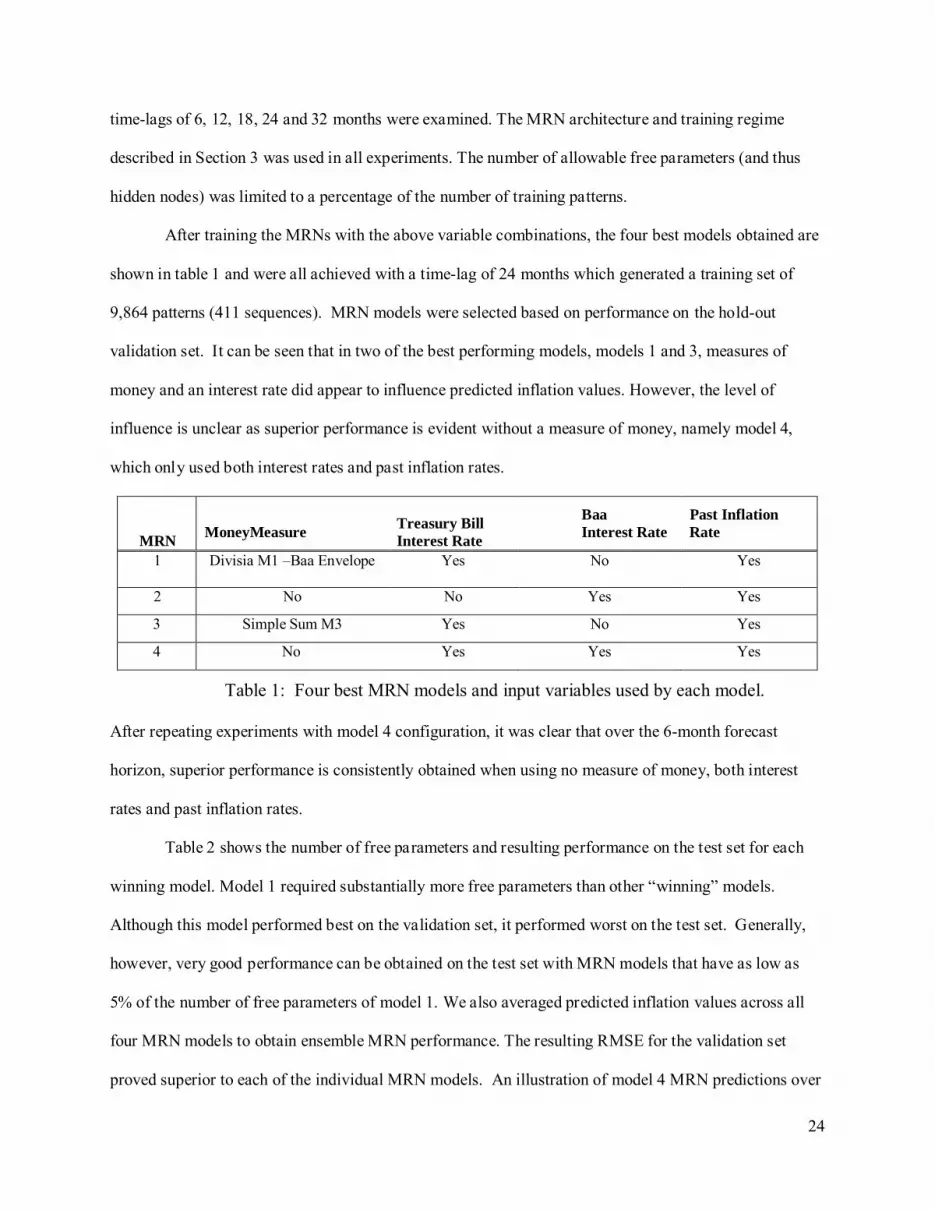
time-lags of 6, 12, 18, 24 and 32 months were examined. The MRN architecture and training regime
described in Section 3 was used in all experiments. The number of allowable free parameters (and thus
hidden nodes) was limited to a percentage of the number of training patterns.
After training the MRNs with the above variable combinations, the four best models obtained are
shown in table 1 and were all achieved with a time-lag of 24 months which generated a training set of
9,864 patterns (411 sequences). MRN models were selected based on performance on the hold-out
validation set. It can be seen that in two of the best performing models, models 1 and 3, measures of
money and an interest rate did appear to influence predicted inflation values. However, the level of
influence is unclear as superior performance is evident without a measure of money, namely model 4,
which only used both interest rates and past inflation rates.
MRN
MoneyMeasure
Treasury Bill Interest Rate
Baa Interest Rate
Past Inflation Rate
1 Divisia M1 –Baa Envelope Yes No Yes
2 No No Yes Yes
3 Simple Sum M3 Yes No Yes
4 No Yes Yes Yes
Table 1: Four best MRN models and input variables used by each model.
After repeating experiments with model 4 configuration, it was clear that over the 6-month forecast
horizon, superior performance is consistently obtained when using no measure of money, both interest
rates and past inflation rates.
Table 2 shows the number of free parameters and resulting performance on the test set for each
winning model. Model 1 required substantially more free parameters than other “winning” models.
Although this model performed best on the validation set, it performed worst on the test set. Generally,
however, very good performance can be obtained on the test set with MRN models that have as low as
5% of the number of free parameters of model 1. We also averaged predicted inflation values across all
four MRN models to obtain ensemble MRN performance. The resulting RMSE for the validation set
proved superior to each of the individual MRN models. An illustration of model 4 MRN predictions over

25
the test period is presented in figure 2. The solid and dashed lines correspond to the real and predicted
inflation rates respectively.
MRN Number of Hidden Layers Number of Parameters RMSE
1 25 2,752 0.0072 2 5 147 0.0077 3 10 502 0.0070 4 10 502 0.0064
Ensemble n/a n/a 0.0065
Table 2: Number of hidden layers, parameters and RMSE on test set for the four best RNN models.
Figure 2: The best predicted inflation rates by the MRN.
MRN Method, for US Inflation Rate
1.0%
1.5%
2.0%
2.5%
3.0%
3.5%
4.0%
4.5%
5.0%
1 5 9 13 17 21 25 29 33 37 41 45
Time (Test Sample) May 2001- Feb 2005
Year over year growth rate
Observed inflation Predicted inflation
Kernel machines
In general, over the 6-month forecast horizon performance of KRLS and KPLS were comparable;
for brevity only results for KRLS are reported. The best performing KRLS model candidates on
validation set were consistently (non-linear) autoregressive models on inflation rates alone (see table 3).

26
Input data was normalized to zero mean and unit standard deviation (the mean and variance are
determined on the training set alone). As table 4 shows, the best 4 candidates from the KRLS model
class used lags of 10 and 12 months. The kernel width κ varied between 1.2 and 1.5 and the
collinearity threshold ν ranged between 0.21 and 0.28.
KRLS
Money
Measure
Treasury Bill Interest Rate
Baa Interest
Rate
Lagged Inflation Rate
1 No No No Yes 2 No No No Yes 3 No No No Yes 4 No No No Yes
Table 3: Four best Kernel models and input variables used by each model.
KRLS Inflation Rate Lag
KW ν RMSE
1 12 1.2 0.27 0.0050 2 10 1.2 0.27 0.0053 3 10 1.2 0.28 0.0057 4 10 1.5 0.21 0.0082
Ensble n/a n/a n/a 0.0055
Table 4: Model structure and test set performance of the best four Kernel recursive least squares models.
The rather limited range of values of structural parameters for the KRLS class indicates that a
stable regime within which the KRLS class yields a satisfying performance on the given problem. It
seems that having historical monthly inflation rates roughly a year into the past and a spherical kernel of
width slightly larger than standard deviation of input data, with modest model sparsity induced by
0.27v ≅ yields the best performance. An illustration of KRLS predictions over the test period is
presented in figure 3. The solid and dashed lines correspond to the real and predicted inflation rates,
respectively.

27
KRLS Method, for US Inflation Rate
1.0%
1.5%
2.0%
2.5%
3.0%
3.5%
4.0%
1 5 9 13 17 21 25 29 33 37 41 45
Time (Test Sample) May 2001 – Feb 2005
Year over year growth rate
Observed inflation Predicted inflation
Figure 3: The best predicted inflation rates by the KRLS.
Model comparison
A summary of results showing the best fitting model for each approach are reported in table 5.
The kernel based regression provides the biggest improvement (43.4%) over the random walk, with the
recurrent neural network in second place.
MRN KRLS Model 4 1 RMSE 0.0064 0.0050 IORW 27.5 43.4
Money? No No Table 5: Results summary
Our early indications suggest that the kernel method appears to implement a more efficient
feature extraction method that is well suited to the problem. It appears that using the “kernelized” version
of the linear least squares technique provides an effective mechanism for constructing efficient feature
domains well suited to the task of prediction. One key difference between the two techniques employed in
this paper is the treatment of the input variables. The kernel based regression methods treat the inputs as

28
inherently static, whilst the recurrent neural networks treat the inputs as dynamic due to the internal state
memory being formed and fed back at each time step.
Since the validation and test sets are only samples, the performance of the best model on the test
set may overestimate the typical performance one would expect from the corresponding model class. The
average performance of the few best performing models, however, gives an indication of the expected
performance, if sound model selection techniques are used. The average IORW measures of the best four
models were 19.9% and 29.7% for the MRN and KRLS model classes respectively. This gives a strong
positive indication of the predictive capacity of the model classes considered in this inflation prediction
task.
With respect to the question ‘does money matter?’ simple sum money and a Divisia money
constructed using the upper envelope approach are among the best performing models in the MRN model
class. Nevertheless, the best model in that class did not contain any money but did contain interest rates.
Overall the best models are the nonlinear autoregressive models based on kernel methods. It is felt that
further improvements in the construction of the money supply might help to obtain improvements in the
inflation forecasting performance of the monetary aggregates.
We also considered all the monetary aggregates together as 16-dimesional input time series based
on which the future inflation rate was predicted. To base the prediction on the dominant factors (in the
variance maximization sense) in the 16 monetary aggregates, we decomposed the 16-dimensional input
series using Principal Component Analysis (PCA)8
8 We thank an anonymous reviewer for this suggestion
. We discovered that when using PCA to reduce the
signal dimensionality, similar large-scale trends in the monetary aggregates tend to mask the time-
conditional differences between them that, however, may be crucial for inflation prediction. There was
only a single dominant eigenvalue of the monetary aggregates covariance matrix, corresponding to the
eigenvector of roughly equal terms across all 16 monetary aggregates. Projection onto this eigenvector
roughly corresponds to computing the mean of the 16 monetary aggregates. Hence, PCA performed

29
smoothing of the monetary aggregates into a single average aggregate. Predictions based on such average
aggregate were comparable to (or worse than) predictions based on the individual monetary aggregates.
This approach, commonly termed Principal Component Regression (PCR), is known to be suboptimal
when only concentrating on dominant eigen-directions (Jolliffe, 1982). We tried various combinations of
the major component with the minor ones (or minor components only), but the performance did not
improve9
6. Discussion, Conclusions and Future Work
.
Our findings provide the most comprehensive evidence to date that neither the aggregation
method nor level of aggregation has a significant impact on the performance of our model, in contrast to
the results reported by Schunk (2001). To the contrary, our results lend more support to the conclusion
that the use of monetary aggregates lead, at most, to marginal improvements in forecasting inflation and
are of limited value in that context. With continual innovation in financial markets, the impact on the
measurement of monetary aggregates will continue to present problems in the form of monetary control.
Aggregates that have been adjusted to take account of financial innovations and the riskiness of the assets,
along the lines proposed recently by Barnett and Wu (2005), have the potential to make a valuable
contribution to the future development of monetary policy and is likely to be a fruitful area for future
research. Having established the preferred monetary aggregate construct for forecasting purposes, a next
vital question to ask is how best to incorporate our chosen aggregate into a composite leading indicator of
inflation for detecting early warning signs of upturns and downturns in inflation, along the lines outlined
in Binner et al. (1999, 2005b) and Binner and Wattam (2003). The construction of a composite leading
9 We a lso t ried to b reak down t he do minance o f t he l arge-scale co mmon trend in monetary a ggregates ( in comparison to their smaller scale profiles) by differencing the monetary aggregates and repeating the PCR approach on s uch de -trended data. The m odels pr edicted the change i n i nflation rate 6 months ah ead, and the p redicted difference was then a dded to the cur rent i nflation rate. E ven t hough the cl ear do minance o f t he a veraging eigenvector was weakened, the prediction performance did not improve.

30
indicator of US inflation along with a detailed timing classification of the cycles is recommended for
future study.
How should we interpret our finding that monetary aggregates are not helpful in forecasting US
inflation? There are several possible explanations for these findings. As Stock and Watson (2007) point
out, beginning in the mid-1980s inflation has become more difficult to forecast; in the sense that it has
become more difficult for an inflation forecaster to provide value added relative to a univariate model.
This is not unique to monetary aggregates, but is a more general phenomenon (Atkeson and Ohanian,
2001). Another explanation, more specific to money, is that monetary aggregates may be less informative
when inflation is low and stable than during periods of high and volatile inflation. The reason is that one
can think of money demand shocks as noise that obscures the signal from the monetary aggregates. Thus,
in periods when inflation and money growth are both subdued, the signal to noise ratio of the monetary
aggregates is likely to be low (Estrella and Mishkin, 1997).
The “market is efficient” in the sense that it is difficult to beat the naïve RW model. The IORW
measure is best suited for our purposes, because rather than worrying about the precise RMSE values, we
should be concerned about by how much we can beat the rather obvious RW strategy. In other
experiments (not reported here) we found that the longer the prediction horizon, the harder it is to
accurately predict the inflation rate. It seems that inclusion of historical inflation rates alone works quite
well for the KRLS model class. We may speculate that the value of money is implicitly represented in the
inflation rates and thus their explicit inclusion as input variables does not help, rather, it can actually
make things worse because of the under sampling problems.
The validation set is just a sample; therefore we cannot rely solely on picking the best model on
the validation set. Slightly worse models on the validation set may be slightly better on the test set.
Therefore we constructed flat ensembles of several best performing models on the validation set. We
tested such ensembles on the test set but their performance was inferior to that of the single winner picked
on the validation set.

31
We also noted an interesting fact that the IORW measures did not change drastically with
increasing prediction horizon. This indicates that for longer prediction horizons, it is more difficult to
predict the inflation rates, but the naïve model is less suited as well, so things cancel out.
The class of recurrent neural networks used for this problem domain appeared to have offered
some advantages over simple recurrent networks. Although the additional feedback connections used
increases the complexity of the model, the improvement in performance appears to outweigh the negative
effect of increased number of parameters. Also, the success of the MRNs is largely dependent on the
hyper-parameters used, most of which have to be empirically established. There is no universal rule to
determine the level and nature of recurrent and self-recurrent connections. A key problem with the
approach taken is the use of gradient-descent based learning algorithms. The problems with back-
propagation through time, for example, are well documented Bengio et al. (1994) and Haykin (1999).
Bengio et al. (1994) in particular has shown that the error gradient vanishes exponentially for dependent
observations that are separated by intervening non-related observations, where greater number of
intervening observations yields poorer generalization performance. Although the MRN offers
modifications to the architecture which may alleviate some of the problems posed by gradient-descent
learning methods (i.e., through the formation of sluggish state-spaces), we will also investigate other
learning algorithms that are better able to find solutions the architecture is theoretically capable of
representing (see Siegelmann and Sontag, 1991; Gers et al., 2001; Jaeger and Haas, 2004).
In the case of the kernel based regression method, further investigation is required to understand
and improve the stability of the model with respect to the addition of further input variables (e.g.,
measures of money). It may be that other compound measures of money may be more useful however this
is likely to be model dependent. Further investigation into controlling model complexity (e.g.,
determining the number of kernels) may provide additional improvement and insight into the efficacy of
this approach to inflation forecasting. This will require more sophisticated versions of cross-validation
than the one employed in this paper.

32
Future work will need to address the problem of why the kernel models break down when
measures of money are added. It seems that this issue is related to over fitting. When we tried using
money alone, we could (after some work) get an excellent fit on the training set, but the models were
inferior on the validation (and test) set. In other words, the learnt relationships by KRLS between past
measures of money and future inflation were not representing anything real. Indeed, we experimented
with another class of non-linear predictors, namely evolutionary neural networks Yao (1999), Stanley and
Miikkulainen (2002) (results not reported here). This framework can produce powerful predictors, but
controlling complexity in the evolutionary setting becomes more challenging. Most models tended to over
fit the training sample, leading to inaccurate out-of-sample forecasts.
We noted that, using KRLS, a good fit on the training set was obtained more naturally and easily
when only past inflation rates were considered. This would suggest that, conditional on the kernel
machine class used, there is little mutual information between past bulk measures of money and future
inflation. Of course, future work will need to validate or refute this hypothesis.

33
References
[1] Anderson, R. and R. Rasche (2001). “Retail sweep programs and bank reserves: 1994–1999”. Federal Reserve Bank of St. Louis Review, 83, 51–72.
[2] Anderson, R., B. Jones and T. Nesmith (1997a). “Monetary aggregation theory and statistical index numbers.” Federal Reserve Bank of St. Louis Review, 79, 31-51.
[3] Anderson, R., B. Jones and T. Nesmith (1997b). “Building new monetary services indexes: concepts, data, and methods.” Federal Reserve Bank of St. Louis Review, 79, 53–82.
[4] Andreeski, C. and P. Vasant (2009). “Comparative Analysis on Time Series with included Structural Break.” In Power Control and Optimization: Proceedings of the Second Global Conference on Power Control and Optimization. American Institute of Physics Conference Proceedings series, 1159(1), 2009.
[5] Andrews, D. (1994). “Asymptotics for Semi-parametric econometric models via stochastic equicontinuity.” Econometrica. 62, 43-72.
[6] Andrews, D. (1995). “Nonparametric Kernel Estimation for Semiparametric Models.” Econometric Theory, 11, 560-596.
[7] Ang, A., M. Piazzesi, and M. Wei (2006). “What does the yield curve tell us about GDP growth?” Journal of Econometrics, 131(1-2), 359-403.
[8] Atkeson, A. and L. Ohanian. (2001). “Are Phillips curves useful for forecasting inflation?” Federal Reserve Bank of Minneapolis Quarterly Review, 25(1), 2-11.
[9] Bachmeier, L., S. Leelahanon and Q. Li (2007). “Money growth and inflation in the United States.” Macroeconomic Dynamics, 11, 113 – 127.
[10] Barnett, W.A. (1980) “Economic Monetary Aggregates: An Application of Index Number and Aggregation Theory.” Journal of Econometrics, 14(1), 11-48.
[11] Barnett, W.A. (1982). “The optimal level of monetary aggregation.” Journal of Money, Credit and Banking, 14 (4), 687-710.
[12] Barnett, W.A., D. Fisher and A. Serletis (1992). “Consumer theory and the demand for money.” Journal of Economic Literature, 30, 86-119.
[13] Barnett, W.A. and S. Wu (2005). “On user costs of risky monetary assets.” Annals of Finance, 1(1), 35-50.
[14] Bengio, Y., P. Simard and P. Frasconi (1994). “Learning long-term dependencies with gradient descent is difficult.” IEEE Transactions on Neural Networks, 5(2), 157 -166.
[15] Bernanke, B. (2006). “Monetary aggregates and monetary policy at the Federal Reserve: A historical perspective.” Remarks at the fourth ECB central banking conference, Frankfurt, Germany, November 10, 2006. Board of Governors of the Federal Reserve System, Washington, D.C.
[16] Berument, H. and N. Dincer. (2005). “Inflation and inflation uncertainty in the G-7 countries.” Physica A: Statistical Mechanics and its Applications, 348, 371-379.
[17] Berument H. and E. Yuksel. (2007). “Effects of adopting inflation targeting regimes on inflation variability.” Physica A: Statistical Mechanics and its Applications, 375. 265-273.
[18] Bierens, Hans J. (1983). “Uniform consistency of kernel estimators of a regression function under generalized conditions.” Journal of the American Statistical Association. 78 (383). 699-707.
[19] Binner, J., A. Gazely and G. Kendall (2005a). “Evaluating the performance of a EuroDivisia index using artificial intelligence techniques.” 4th International Conference on Computational Intelligence in Economics and Finance, 871-874.
[20] Binner J., R. Bissoondeeal, and A. Mullineux (2005b). “A Composite Leading Indicator of the Inflation Cycle for the Euro Area.” Applied Economics, 37, 1257-1266.
[21] Binner, J., A. Fielding and A. Mullineux (1999). “Divisia money in a composite leading indicator of inflation” Applied Economics, 31, 1021–1031.
[22] Binner, J, T. Elger, B. Nilsson and J. Tepper (2004). “Tools for non-linear time series forecasting in economics: an empirical comparison of regime switching vector autoregressive models and recurrent neural networks.”Advances in Econometrics: applications of artificial intelligence in finance and economics, 19, 71-91, Elsevier Science Ltd.

34
[23] Binner, J., G. Kendall and A. Gazely (2004). “Evolving neural networks with evolutionary strategies: A new application to Divisia money.” Advances in Econometrics: applications of artificial intelligence in finance and economics, 19, 127-143, Elsevier Science Ltd.
[24] Binner, J., T. Elger, B. Nilsson and J. Tepper (2006). “Predictable non-linearities in U.S. inflation.” Economic Letters, 93 (3), 323 – 328.
[25] Binner, J., and S. Wattam (2003). “A new composite leading indicator of inflation for the UK: a Kalman filter approach.” Global Business and Economics Review, 5(2), 242-264.
[26] Carlson, J., D. Hoffman, B. Keene, and R. Rasche (2000). “Results of a study of the stability of cointegrating relations comprised of broad monetary aggregates.” Journal of Monetary Economics, 46(2), 345-383.
[27] Carlstrom, C. and T. Fuerst (2004) “Thinking about monetary policy without money.” International Finance, 7 (2), 325-347.
[28] Chen, S., L. Jani, and C. Tai (2006) Computational Economics: A Perspective from Computational Intelligence. Idea Publishing Group, Hershey PA, USA.
[29] Clark, Todd. (1999). “A Comparison of the CPI and PCE Price Index,” Federal Reserve Bank of Kansas City Economic Review. Third Quarter, 15-29.
[30] Darken, C., J. Chang, and J. Moody, J (1992). “Learning rate schedules for faster stochastic gradient search.” in Proceedings of the IEEE Workshop on Neural Networks for Signal Processing 2, IEEE Press.
[31] Diewert, E. (1974). “Intertemporal consumer theory and the demand for durables.” Econometrica, 42(3), 497 – 516.
[32] Diewert, E. (1976). “Exact and superlative index numbers.” Journal of Econometrics, 4(2), 115-145. [33] Dorffner, G. (1996). “Neural networks for time series processing.” Neural Network World, 6(4) 447–
468. [34] Dorsey, R. (2000). “Neural Networks with Divisia Money: Better Forecasts of Future Inflation.” in
M. Belongia and J. M. Binner, eds., Divisia Monetary Aggregation: Theory and Practice. Palgrave. [35] Drake. L., A.W. Mullineux and J. Agung (1997). “One Divisia money for Europe.” Applied
Economics, 29, 775-786. [36] Drake, L., and T. Mills (2005). “A new empirically weighted monetary aggregate for the United
States.” Economic Inquiry, 43, 138-157. [37] Duca, J. (2000). “Financial technology shocks and the case of the missing M2.” Journal of Money,
Credit, and Banking, 32(4), 820–39. [38] Duca, J., and D. VanHoose, (2004). “Recent developments in understanding the demand for money.”
Journal of Economics and Business, 56, 247–272. [39] Dutkowsky, D., B. Cynamon, and B. Jones. (2006). “U.S. Narrow Money for the Twenty-First
Century.” Economic Inquiry, 44(1), 142-152. [40] Elger, T., B. Jones, and B. Nilsson (2006). “Forecasting with monetary aggregates: recent evidence
for the United States.” Journal of Economics and Business, 15, 428-446. [41] Elman J. (1990). “Finding structure in time.” Cognitive Science, 14, 179-211. [42] Engel Y., S. Mannor and R. Meir (2004). “The kernel recursive least-squares algorithm.” IEEE
Transactions on Signal Processing, 52 (8), 2275-2285. [43] Estrella, Arturo. (2005). “Why Does the Yield Curve Predict Output and Inflation?” Economic
Journal. 115(505), 722-744. [44] Estrella, A., and F. Mishkin (1997). “Is there a role for monetary aggregates in the conduct of
monetary policy?” Journal of Monetary Economics, 40, 279-304. [45] European Central Bank (2003). “The outcome of the ECB’s evaluation of its monetary policy
strategy.” ECB Monthly Bulletin, June, 87-102. [46] Galluccio, S., J-P. Bouchaud, and M. Potters (1998). “Rational decisions, random matrices and spin
glasses.” Physica A: Statistical and Theoretical Physics 259 (3-4), 449-456. [47] Garner, T., G. Janini, W. Passero, L. Paszkiewicz, and M. Vendermia. (2006). “The CE and the
PCE: A Comparison.” Monthly Labor Review, 129(9), 20-46. September. [48] Gers, F., D. Eck, and J. Schmidhuber (2001). “Applying LSTM to Time Series Predictable Through
Time-Window Approaches.” International Conference on Artificial Neural Networks, Vienna, Austria, pp. 669-675.

35
[49] Giles, C., S. Lawrence, and A. Tsoi. (2001). “Noisy Time Series Prediction using Recurrent Neural Networks and Grammatical Inference.” Machine Learning. 44, 161-183.
[50] Greene, William H. (2008). Econometric Analysis, 6th ed. Pearson-Prentice Hall. [51] Greenlees, J. S. and R. B. McClelland (2008). “Addressing Misconceptions About the Consumer
Price Index.” Monthly Labor Review, 131(8), 3-19. August. [52] Hancock, M. (2005). “Divisia money.” Bank of England Quarterly Bulletin, 45 (1), 39-46. [53] Haykin, S. (1999) Neural networks: A comprehensive foundation. 2nd edition, Prentice Hall, Upper
Saddle River, NJ. [54] Hornik, K., M. Stinchcombe and H. White (1989). “Multi-layer feedforward networks are universal
approximators.” Neural Networks, 2, 359-366. [55] Hulten, C. (1973). “Divisia Index Numbers.” Econometrica 41(6) 1017-25. [56] Jaeger, H., and H. Haas (2004). “Harnessing Nonlinearity: Predicting Chaotic Systems and Saving
Energy in Wireless Communication.” Science 2, 304(5667) 78 – 80. [57] Jolliffe, I.T. (1982). “A note on the Use of Principal Components in Regression”. Journal of the
Royal Statistical Society, Series C, 31(2), 300-303. [58] Jones, B., D. Dutkowsky, and T. Elger (2005). “Sweep Programs and Optimal Monetary
Aggregation.” Journal of Banking and Finance, 29(2), 483-508. [59] Jordan M. (1990). “Attractor dynamics and parallelism in a connectionist sequential machine.” in
Diederich, J., ed., Artificial Neural Networks: Concept-learning. 112-127. IEEE Press, Piscataway NJ. Also, Proceedings of the 8th Annual Conference of the Cognitive Science Society, 1986, 531-545.
[60] Judd, K. (1998). Numerical Methods in Economics. MIT Press. [61] Kim K. (2003). “Financial time series forecasting using support vector machines.” Neurocomputing,
55 (1-2), 307-319. [62] King, M. (2002). “No money, no inflation – the role of money in the economy.” Bank of England
Quarterly Bulletin, Summer, 162-177. [63] Laloux, L., P. Cizeau, J.-P. Bouchaud and M. Potters (1999). “Noise Dressing of Financial
Correlation Matrices.” Physical Review Letters, 83 (7) 1467-1470. [64] Lawrence, S., C.Giles, and S. Fong (2000) “Natural language grammatical inference with recurrent
neural networks.” IEEE Transactions on Knowledge and Data Engineering, 12(1), 126-140. [65] Leeper, E. and J. Rouch (2003). “Putting ‘M’ back in monetary policy”. Journal of Money, Credit
and Banking, 35, 1217-1256. [66] Li, Q. and J. S. Racine (2007). Nonparametric Econometrics: Theory and Practice. Princeton
University Press. [67] McCully, C., B. Moyer, and K. Stewart. (2007). “A Reconciliation Between the Consumer Price
Index and the Personal Consumption Expenditures Price Index,” mimeo, Bureau of Labor Statistics, September 2007.
[68] Michalewicz, Z and D. Fogel (2000). How to solve it. Springer-Verlag. ISBN 3-540-66061-5 [69] Mishkin, F. and K. Schmidt-Hebbel (2001). "One Decade of Inflation Targeting in the World:
What Do We Know and What Do We Need to Know?" in N. Loayza and R. Soto, eds., Inflation Targeting: Design, Performance, Challenges. Santiago: Central Bank of Chile, pp. 117-219.
[70] Mishkin, F. (2007). “Headline versus Core Inflation in the Conduct of Monetary Policy.” Speech presented at the Business Cycles, International Transmission and Macroeconomic Policies Conference, HEC Montreal, Montreal, October. Board of Governors of the Federal Reserve System, Washington, D.C.
[71] Moody, J. (1995). “Economic Forecasting: Challenges and Neural Network Solutions”. Paper presented at the International Symposium on Artificial Neural Networks, Hsinchu, Taiwan, December 1995.
[72] Moore, G., R. Porter, and D. Small (1990). “Modeling the Disaggregated Demands for M2 and M1: The U.S. Experience in the 1980s”, in P. Hooper, K. Johnson, D. Kohn, D. Lindsey., R. Porter and R Tryon ( eds.), Financial Sectors in Open Economies: Empirical Analysis and Policy Issues. Board of Governors of the Federal Reserve System, Washington, D.C. pp. 21-105.
[73] Moshiri, S., N.E. Cameron, and D. Scuse (1999). “Static, dynamic and hybrid neural networks in forecasting inflation”. Computational Economics, 14, 219-235.
36
[74] Nakamura, E. (2005). “Forecasting Inflation using a neural network.” Economics Letters, 86. 373-378.
[75] Nakamura, E. (2008). “Pass-through in Retail and Wholesale.”American Economic Review 98(2), 430-437.
[76] Nelson, E. (2002). “Direct effects of base money on aggregate demand: theory and evidence”. Journal of Monetary Economics, 49(4), 687–708.
[77] Nelson, E. (2003). “The future of monetary aggregates in monetary policy analysis.” Journal of Monetary Economics, 50(5), 1029–59.
[78] Pearlmutter, B. A. (1995). “Gradient calculations for dynamic recurrent neural networks: a survey”. IEEE Transactions on Neural Networks, 6(5), 1212-1228.
[79] Plerou, V., P. Gopikrishnan, B. Rosenow, L.A.Nunes Amaral and H.Eugene Stanley (1999). “Universal and Nonuniversal Properties of Cross Correlations in Financial Time Series.” Physical Review Letters, 83(7), 1471-1474.
[80] Plerou, V., P. Gopikrishnan, B. Rosenow, L. A.Nunes Amaral, and H. Eugene Stanley (2000). “Econophysics: financial time series from a statistical physics point of view.” Physica A: Statistical Mechanics and its Applications, 279 (1-4), 443-456.
[81] Plerou, V, P. Gopikrishnan, B. Rosenow, L. A. Nunes Amaral, T. Guhr, H.E. Stanley (2002). “Random matrix approach to cross correlations in financial data.” Physical. Review E. 65(6).
[82] Rosipal, R. and L.J. Trejo (2002). “Kernel partial least squares regression in reproducing kernel hilbert space.” Journal of Machine Learning Research, 2, 97-123.
[83] Rumelhart, D., G. Hinton and R. Williams (1986). “Learning internal representations by error propagation” in: Parallel distributed processing, Explorations in the microstructure of cognition, Vol. 1, pp. 318-362. Princeton University Press.
[84] Saito, S. (2007). “Verification of Possibility of Forecasting Economical Time Series Using Neural Network and Digital Filter.” Third International Conference on Natural Computation, vol 3, pp. 381-388.
[85] Schölkopf, B. and Smola, A. (2002). Learning With Kernels. MIT Press. [86] Schunk, D. (2001). “The relative forecasting performance of the Divisia and simple sum monetary
aggregates.” Journal of Money, Credit, and Banking, 33, 272–283. [87] Sharkey, N., A. Sharkey, and S. Jackson (2000). “Are SRN’s sufficient for modeling language
acquisition?” in: P. Broeder and J. Murre, Models of language acquisition: inductive and deductive approaches. Oxford University Press. pp. 33-54.
[88] Siegelmann, H. T., and E. D. Sontag (1991). “Turing computability with neural nets”. Applied Mathematics Letters, 4, 77-80.
[89] Simpson, T. (1980). “The Redefined Monetary Aggregates.” Federal Reserve Bulletin. February. pp. 97-114.
[90] Stanley, K. and R. Miikkulainen (2002). “Evolution of neural networks through augmenting topologies.” Evolutionary Computation, 10, 99–127
[91] Stock, J., and M. Watson (1999a) “Forecasting inflation.”Journal of Monetary Economics, 44, 293–335.
[92] Stock, J. and M.Watson. (1999b). “A comparison of linear and non-linear univariate models for forecasting macroeconomic time series.” in R. Engle and H. White, eds., Cointegration, Causality and Forecasting: A Festschrift in honor of Clive Granger. Oxford University Press.
[93] Stock, J. and M. Watson (2007). “Why has U.S. inflation become harder to forecast?” Journal of Money, Credit, and Banking, 39, 3-33.
[94] Tenti, P. (1996). “Forecasting foreign exchange rates using recurrent neural networks.” Applied Artificial Intelligence 10, 567-581.
[95] Theil, H. (1967) Economics and Information Theory, Chapter 5, Amsterdam: North-Holland. [96] Törnqvist, L. (1936). “The Bank of Finland's consumption price index.” Bank of Finland Bulletin,10,
1-8. [97] Ulbricht, C. (1994). “Multi-Recurrent networks for traffic forecasting”. Proceedings of the Twelfth
National Conference in Artificial Intelligence, AAAI Press/MIT Press, Cambridge, MA 883-888. [98] Wang, L. and J. Zhu (2010). “Financial market forecasting using a two-step kernel learning method
for the support vector regression.” Annals of Operations Research, 174, 103-120.

37
[99] Werbos, P. J. (1990). “Backpropagation through time: What it does and how to do it.” in Proceedings of IEEE Special Issue on Neural Networks, vol 78, 1550-1560.
[100] Williams, R. J. and J. Peng (1990). “An efficient gradient-based algorithm for on-line training of recurrent network trajectories.” Neural Computation, 2, 490-501.
[101] Yao, X. (1999) Evolving artificial neural networks. Proceedings of the IEEE, 87(9) 1423-1447. [102] Zhang, G., B. Patuwo, and M. Hu (1998). “Forecasting with artificial neural networks: the state of
the art.” International Journal of Forecasting. 14, 35-62.

38
Appendix 1 US Monetary Aggregates
Definition Source / Construction
M1 St Louis Federal Reserve Bank, Fred database, USA M2 St Louis Federal Reserve Bank, Fred database, USA MZM St Louis Federal Reserve Bank, Fred database, USA M3 St Louis Federal Reserve Bank, Fred database, USA Divisia (MSI) M1 St Louis Federal Reserve Bank, Fred database, USA Divisia (MSI) M2 St Louis Federal Reserve Bank, Fred database, USA Divisia (MSI) MZM St Louis Federal Reserve Bank, Fred database, USA Divisia (MSI) M3 St Louis Federal Reserve Bank, Fred database, USA Divisia (MSI) M1 Upper Envelope Benchmark Rate Divisia (MSI) M2 Upper Envelope Benchmark Rate Divisia (MSI) MZM Upper Envelope Benchmark Rate Divisia (MSI) M3 Upper Envelope Benchmark Rate Divisia (MSI) M1 Baa Benchmark Rate Divisia (MSI) M2 Baa Benchmark Rate Divisia (MSI) MZM Baa Benchmark Rate Divisia (MSI) M3 Baa Benchmark Rate