does mixing tree species enhance stand resistance against natural hazards? a case study for spruce

Forest Ecology and Management 267 (2012) 284–296

Contents lists available at SciVerse ScienceDirect

Forest Ecology and Management

journal homepage: www.elsevier .com/ locate/ foreco

Does mixing tree species enhance stand resistance against natural hazards? Acase study for spruce

Verena C. Griess a,⇑, Ricardo Acevedo a, Fabian Härtl a, Kai Staupendahl b,1, Thomas Knoke a

a Institute of Forest Management, Center of Life and Food Sciences Weihenstephan, Technische Universität München, Hans-Carl-von-Carlowitz-Platz 2, 85354 Freising, Germanyb Department of Forest Economics and Forest Management, Georg-August-University Göttingen, Büsgenweg 3, 37077 Göttingen, Germany

a r t i c l e i n f o a b s t r a c t

Article history:Received 21 April 2011Received in revised form 16 November 2011Accepted 17 November 2011Available online 8 January 2012

Keywords:Mixed species standSurvival analysisRiskForest managementForest damage surveyWeibull

0378-1127/$ - see front matter � 2011 Elsevier B.V. Adoi:10.1016/j.foreco.2011.11.035

⇑ Corresponding author. Tel.: +49 8161 71 4699; faE-mail addresses: [email protected]

forst.wzw.tum.de (R. Acevedo), [email protected] (K. Staupendahl), [email protected] (

1 Current address: ARGUS Forstplanung, Büsgenweg

In this study, survival of spruce (Picea abies [L.] Karst.) trees in mixed- and mono-species stands was ana-lyzed using the database of Rhineland-Palatinate’s forest damage survey (FDS). The influence of speciesmixture on tree survival probability was analyzed using data from 9864 trees, of which 2866 spruce treeshave been analysed in detail. Data was collected on 495 research plots in a series of continuous measure-ments taken since 1984.

For estimating survival probability, the Kaplan–Meier method was applied to achieve a firstoverview about possible effects. The analysis was then extended using Accelerated Failure Time (AFT)models to estimate the parameters of a Weibull function, used to describe survival times. The resultingmodels were used to simultaneously analyze the effects of intensity of mixture (represented by Shannon–Weaver-Index and, alternatively, by species proportion), time since harvest and site characteristics.

Results obtained indicate positive effects of species mixture on resistance of spruce trees: survivalprobabilities increase with increasing intensity of mixture, regardless whether mixture is characterisedby Shannon–Weaver-Index or species proportion.

Spruce trees in monocultures on average site conditions will reach age 100 with a probability of 80%.Spruce trees growing in a moderately mixed stand (average Shannon–Weaver-Index 0.4) show a slightincrease in survival probability to a 83% probability of reaching age 100 whilst spruce trees in a morediverse stand (average Shannon–Weaver-Index 1.2) have a 97% probability of reaching age 100. Anadmixture of 50% thus leads to an increase in survival probability of 17 percentage points. Site variableseven show a stronger impact on survival than tree species mixture. From these variables wet soils had thestrongest negative influence on spruce survival, while orographic conditions of saddles, anticlines, val-leys, trenches or dells showed the strongest positive influence on survival. However, the strongest influ-ence on spruce survival was recent harvest activity. The more time had passed since the harvestoperation, the less likely residual trees were to succumb to stresses.

� 2011 Elsevier B.V. All rights reserved.

1. Introduction

The use of simple models for the evaluation of management op-tions in ecosystem management is very common amongst econo-mists (Armstrong, 2007). However, many of the models used sufferfrom a lack of biological accuracy (Bulte and van Kooten, 1999),which originates from their deterministic nature, as well as fromtheir focus on single-species situations (Knoke and Seifert, 2008).Modelling deterministically means to implicitly provide the exis-tence of genuine information about the future and ignore the numer-ous uncertainties in forest management (Palma and Nelson, 2010).

ll rights reserved.

x: +49 8161 71 4545.e (V.C. Griess), acevedo@

um.de (F. Härtl), kstaupe@T. Knoke).5, 37077 Göttingen, Germany.

This practice may lead to very optimistic financial assessmentsof economically-optimised silvicultural decisions (Lucas andAndres, 1978; Möhring, 1986; Knoke et al., 2008), which in turnprecludes the possibility of integration of the precautionary ap-proach into economic modelling (Figge and Hahn, 2004; Knokeand Mosandl, 2004; Knoke and Moog, 2005; Weber-Blaschke etal., 2005 or Krysiak, 2006). However, precaution is a centralcomponent of modern sustainability concepts (Hahn and Knoke,2010), and becomes particularly important if climate change sce-narios are to be considered.

This lack of biological accuracy as described is particularly truefor the modelling of mixed-species stands. Here, models often notonly ignore relevant factors like a possible compensation of finan-cial risks between tree species (Clasen et al., 2011; Knoke andWurm, 2006), they also regularly exclude the ecological effects ofmixing tree species and the resulting biophysical consequences(Knoke et al., 2008; Pretzsch, 2009).

http://dx.doi.org/10.1016/j.foreco.2011.11.035

mailto:[email protected]

mailto:acevedo@ forst.wzw.tum.de

mailto:acevedo@ forst.wzw.tum.de


mailto:kstaupe@ gwdg.de

mailto:kstaupe@ gwdg.de


http://dx.doi.org/10.1016/j.foreco.2011.11.035

http://www.sciencedirect.com/science/journal/03781127

http://www.elsevier.com/locate/foreco

V.C. Griess et al. / Forest Ecology and Management 267 (2012) 284–296 285

One of the key factors influencing forest dynamics is tree mor-tality. Survival research thus aims at understanding how and whytree mortality occurs (Sims et al., 2009). Highly reliable estimatesof tree survival are an essential basis for management decisionsin forestry, such as choice of tree species or optimum timing ofharvest operations. Various mechanisms for considering survivalrates to inform forest management schedules and forest develop-ment scenarios do exist, but most of them are, once again, limitedto the use in mono-species stands (Gadow, 2000).

Within the scope of the on-going discussion regarding the conse-quences of climate change for forests and forestry, the call for mixed-species stands is getting louder. However, since Gayer (1886) ex-pressed support for the establishment of mixed-species stands,not much has changed, at least in Germany (Beinhofer, 2009), exceptin stands younger than 20 years (Knoke et al., 2008). This is surpris-ing, since ample evidence exists to show that mixed-species standsare highly resistant to biotic and abiotic hazards (Griess and Knoke,2011). This evidence is not new. As early as 1828, Cotta highlightedthe fact that in mixed-species stands neither insects nor storm canlead to such considerable damages as those that occur in mono-species stands. However, adequate curves to model survival of treespecies in mixed stands on a quantitative basis are still lacking. Eventhough valuable research regarding the influence of mixture onresistance has been carried out in the past, the results obtained can-not be implemented into economic modelling directly. This is trueeither because survival curves are missing from these results – asin the studies by Schmid-Haas and Bachofen (1991), Mayer et al.(2005) or Schütz et al. (2006), or due to the fact that the effect of mix-ture cannot be supported with statistical evidence. König (1995), forexample, delivered survival curves that are based on data consider-ing only areas of 0.49 hectares or larger, which leads to extremelyoptimistic results.

This situation explains the necessity to carry out additional sin-gle-tree-based analysis of mixture effects that deliver quantitativeresults, such as the work reported here.

Large uncertainties exist about the nature and extent of advanc-ing climate change. Information about survival probabilities inmono- and mixed-species stands can improve the possibility thatfuture climate developments can be mitigated to ensure forestmanagement objectives can still be met (Gadow, 2000). Thoughit is difficult to reliably estimate the frequency and intensity of ex-treme weather events and insect calamities, it is likely that forestdisturbances will occur more often than in the past (Kölling etal., 2010). Under these changing conditions, it seems prudent toenhance the adaptive ability of forests by encouraging a mixtureof tree species (v. Lüpke, 2009). Therefore differences in survivalprobabilities in mono-species and mixed-species stands need tobe taken into account.

Given the above, the following research question will beaddressed here:

Are survival probabilities in mixed-species stands different fromthose in mono-species stands?

According to the approach by Staupendahl and Zucchini (2011),who presented a method to derive survival functions from damagesurvey data by means of survival analysis, our first step in answer-ing this question is an analysis of the long term data available fromthe Rhineland-Palatinate forest damage survey.

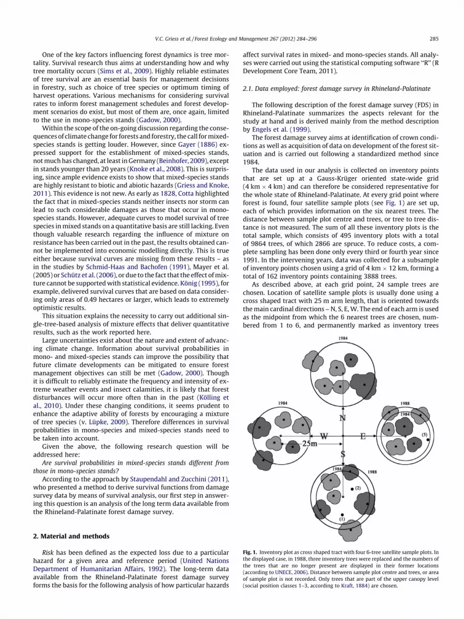
Fig. 1. Inventory plot as cross shaped tract with four 6-tree satellite sample plots. Inthe displayed case, in 1988, three inventory trees were replaced and the numbers ofthe trees that are no longer present are displayed in their former locations(according to UNECE, 2006). Distance between sample plot centre and trees, or areaof sample plot is not recorded. Only trees that are part of the upper canopy level(social position classes 1–3, according to Kraft, 1884) are chosen.

2. Material and methods

Risk has been defined as the expected loss due to a particularhazard for a given area and reference period (United NationsDepartment of Humanitarian Affairs, 1992). The long-term dataavailable from the Rhineland-Palatinate forest damage surveyforms the basis for the following analysis of how particular hazards

affect survival rates in mixed- and mono-species stands. All analy-ses were carried out using the statistical computing software ‘‘R’’ (RDevelopment Core Team, 2011).

2.1. Data employed: forest damage survey in Rhineland-Palatinate

The following description of the forest damage survey (FDS) inRhineland-Palatinate summarizes the aspects relevant for thestudy at hand and is derived mainly from the method descriptionby Engels et al. (1999).

The forest damage survey aims at identification of crown condi-tions as well as acquisition of data on development of the forest sit-uation and is carried out following a standardized method since1984.

The data used in our analysis is collected on inventory pointsthat are set up at a Gauss-Krüger oriented state-wide grid(4 km � 4 km) and can therefore be considered representative forthe whole state of Rhineland-Palatinate. At every grid point whereforest is found, four satellite sample plots (see Fig. 1) are set up,each of which provides information on the six nearest trees. Thedistance between sample plot centre and trees, or tree to tree dis-tance is not measured. The sum of all these inventory plots is thetotal sample, which consists of 495 inventory plots with a totalof 9864 trees, of which 2866 are spruce. To reduce costs, a com-plete sampling has been done only every third or fourth year since1991. In the intervening years, data was collected for a subsampleof inventory points chosen using a grid of 4 km � 12 km, forming atotal of 162 inventory points containing 3888 trees.

As described above, at each grid point, 24 sample trees arechosen. Location of satellite sample plots is usually done using across shaped tract with 25 m arm length, that is oriented towardsthe main cardinal directions – N, S, E, W. The end of each arm is usedas the midpoint from which the 6 nearest trees are chosen, num-bered from 1 to 6, and permanently marked as inventory trees

286 V.C. Griess et al. / Forest Ecology and Management 267 (2012) 284–296

(Fig. 1). If one or more of the four ends of each arm are located out-side a forest stand, the described distributional pattern may be chan-ged, e.g. by shortening arm lengths or by displacing the midpoints.

If no adequate distribution of the satellite points within the for-est stand is possible using the above method, or if crown assess-ment is impeded due to extremely dense stands, six trees withwell visible crowns are chosen at each of four points within a100 m square plot.

For both inventory methods, only trees that are part of theupper canopy level (social position classes 1–3 according to Kraft(1884)) are chosen. The groups of the tree classification systemaccording to Kraft (1884) are explained in Table 1.

Each tree is explicitly identifiable by grid point and tree numberand is retained as long as possible within future samples. However,the forest stands holding inventory points are still under regularuse. If sample trees are thinned or fail due to damage by windthrow or snow break between sampling periods, they are replacedin the inventory at the next sampling date with the next nearesttree to the midpoint.

Dead trees that are still standing remain in the sample until thecrown loses all brushwood. All newly selected trees must be atleast co-dominant, and are numbered 7, 8, 9, etc. To ensure a con-sistent traceability of tree replacements, the original tree numberassigned in 1984 is kept in the data set and updated with the dateand reason for its replacement. If a complete inventory plot isthinned, or fails due to large-scale wind throw, etc., it is kept asa fail patch. As soon as a new stand is formed at this location,the plot is reintegrated into the inventory. If the forest is clearedor transformed into a different type of land use, the inventory plotsare permanently removed from the sample.

2.2. Data on forest damage

The FDS database was used to obtain data regarding tree dam-age or failure times in order to derive survival probabilities forspruce in mixed and mono-species stands. Beginning in 1994, thedevelopment of all inventory trees was observed and the statusof each tree was documented at each sampling date. As the causeof tree failure was documented only for years 1994 and later, ear-lier years could not be considered in our analysis. Therefore it is,for example, not possible to gain information about the impact ofthe storms Vivian and Wiebke, which occurred in 1990.

2.3. Dependent and independent variables

The terms independent and dependent variable are used to dif-ferentiate between two types of variables being considered,separating them into those present at the start of a process and

Table 1Social tree position classes of the inventoried trees according to Kraft (1884).

Code Status Inventoried

Groups for the tree classification system according to Kraft (1884)1 Predominant trees, invariably having a strong well-

developed crownYes

2 Dominant trees, forming the main crop with relativelywell-developed crowns

Yes

3 Co-dominant trees. Crowns still normally developed(according to class 2) but relatively small and confined

Yes

4 Suppressed trees. Crowns more or less rudimentaryeither suppressed from all sides or developed on onlyone side

(a) more or less without cover(b) already fully covered

No

5 Completely overtopped trees(a) viable crown(b) crown dying or already dead

No

those being induced by it, where the latter are dependent on theformer.

Our study focuses on the survival of trees; therefore the cate-gorical status variable describing whether a tree is still alive andmore or less undamaged is used in combination with the tree’sage to derive our dependent variable – the survival probability ofa tree. Trees which have a status code of 1, 3 or 4 (see Table 2), eachof which describe death or heavy damage due to calamity or windthrow, are considered damaged to the extent that they are no long-er part of the productive stand, and are therefore treated as dead.

Within the framework of the FDS, data on several other vari-ables have also been collected. These variables consist mainly ofinformation defining site characteristics that are widely consideredto be important determining factors in a particular stand’s suscep-tibility to wind throw or insect damage. They can be consideredindependent variables, as they influence our dependent variable– the survival times of the trees in our sample. All analyzed inde-pendent variables are displayed in Table 3.

2.4. Water supply

The FDS data on water supply was recorded as seven levelsranging from ‘‘wet’’ to ‘‘dry’’. For the purposes of our analysis, theseseven levels were reduced to four – combining some of the initiallypossible states to create larger groups with the following values:moist, mesic moist, dry or periodically wet.

2.5. Nutrient supply

Information on nutrient supply was obtained from the forestmanagement plan and is represented by the values poor, goodand rich.

2.6. Orographic conditions

The orographic conditions describe the slope at every site. Thesix possible values are: plain or plateau, anticline or saddle, tophillside, mean hillside, lower hillside, and valley, trench or dell.

2.7. Soil depth and structure

The FDS database contains a rough description of the soils forevery forest stand, which was obtained from the forest manage-ment plan. The data on soil used in our analysis is taken directlyfrom this information.

2.8. Gradient, aspect (NS/EW), altitude

In the basic FDS data, the eight cardinal points (N, NE, E, etc.) weretransformed into the metric variables NS and EW. By calculating the

Table 2Possible states of the inventory trees within our sample and overview over data. SD,standard deviation of age.

Code Status N Mean age[years]

SD

Spruce complete data set0 Existing 1748 70.2 26.11 Existing, but substantially damaged 39 45.6 24.52 Existing, but changed to kraft classes 4

or 526 48.8 13.7

3 Existing, but died off or thrown 88 67.5 21.84 Nonexistent due to calamity 281 71.6 28.35 Nonexistent due to planned thinning

or harvest401 53.7 24.9

6 Nonexistent due to unknown reasons 283 44.3 30.8

Total 2866

Table 3Independent variables.

Variable Specification

X1 Water supply 1 – moist2 – mesic moist3 – mesic dry4 – periodically wet

X2 Nutrientsupply

1 – poor2 – medium3 – rich

X3 Orographicconditions

1 – plain, plateau2 – anticline, saddle4 – hillsides, combining top hillside (3), mean hillside(4) and lower hillside (5)6 – valley, trench, dell

X4 Soil depth 1 – shallow2 – fairly shallow3 – deep

X5 Soil structure 1 – free of stones2 – rocky3 – sk (>75% parts > 2 mm)

X6 Altitude Average height above sea levelX7 Gradient Non dimensional number [1,�1]X8 NS-aspect Cosine of the aspect (NS gradient)X9 EW-aspect Sine of the aspect (EW gradient)X10 Mixture

(Shannon)1 – H0 = 02–0 > H0 < 13–1 6 H0

– X10 depending on the chosen model –X10 Mixture

(spruce ratio)1 – Spruce ratio 680%2 – Spruce ration >80% <100%3 – Spruce ratio 100%

X11 Type ofmixture

0 – unmixed1 – single tree2 – in troops3 – area wise

X12 Standstructure

0 – single level1 – multi level

X13 Canopyclosure

1 – tight2 – loose3 – no canopy closure

X14 Time sinceharvest

1 – <3 years2–3 – 6 years3 – >6 years


cosine of the exposition possible values are a range that can be usedto display a gradient regarding the hazard from north to south,whilst EW (calculated as sine of the exposition) displays an east westgradient. The altitude defines the height above sea level of a stand.

2.9. Mixture

Information regarding whether or not each inventory point waslocated in a mixed forest stand was available from the forest man-agement plan for that site. The types of mixture are non-mixed,single-tree mixture, in troops and large blocks. As these plansmay not describe the situation for every tree adequately, wecalculated the numerical Shannon Index for each tree to label themixture (see Section 2.14).

2.10. Stand structure

Stand structure describes the distribution of trees by speciesand size within a stand. Possible parameter values are single- ormulti-level stand structure.

2.11. Canopy closure

Information regarding the crown density was collected by visu-ally assessing the canopy closure.

2.12. Time since harvest

The variable ‘‘time since harvest’’ was derived from the infor-mation available for each of the inventory points regarding the lastyear a thinning or harvest was carried out.

2.13. Vertical structure

Within the FDS, a description of the vertical structure for everyforest stand was carried out. The according data is taken directlyfrom this information.

Due to the large number of variables available (Table 3), thevariables to be considered in our analysis had to be determinedbased on their relative importance in influencing the dependentvariable. This was done following a method by Glomb (2007)(see Section 3.2).

2.14. Quantification of mixture

To determine whether or not a certain tree is situated in amixed- or mono-species situation, several options are available.First, the information delivered within the forest management plancan be used. Second, mixture or abundance can be calculated usingvarious calculative models or diversity indices.

One very prominent and well-known Entropy Index to measurediversity is the Shannon Index. As previously described, at eachinventory point, 24 trees were recorded. Using this information aShannon Index (Shannon and Weaver, 1949) can be assigned forevery tree in every plot. This Index is based on the entropy conceptdefined as follows:

The Shannon Index H0 of a population consisting of N individu-als from S different species, of which ni belong to a species.

H0 ¼ �Xi¼1

s

pi � ln pi ð1Þ

pi ¼ni

N;

where pi is the frequency proportion each species i holds of the totalN.

The Shannon Index was chosen over the information given inthe management plan, because the specific mixture at each indi-vidual inventory plot may differ from the situation described forthe complete stand in the management plan documentation. Fur-thermore, the calculated Shannon Index value can also be usedas a measure of the intensity of the mixture which can be usefullater in describing the relative effect of mixture on survivalprobability.

The Shannon Index values used to define the intensity of mix-ture are displayed in Table 4. The number of classes and the rangeof index values included in each class were determined by theactual frequency distribution of index values in the sample.

For a stand belonging to our first type of stands – ‘‘Mono speciesstands’’ – only stands made up of one single tree species were in-cluded. The second stand type ‘‘Mixed stand a’’ includes severalpossible species mixtures. The average Shannon Index of 0.4 cho-sen for mixed stands, for example, describes a stand made up oftwo species, of which species one is represented by 83% of thetrees, and a second species by 17%. A Shannon Index value of 1.2describes a stand that is, for example, made up of four species, ofwhich the first represents 50%, the second 25%, the third 17% andthe fourth 8% of the total trees.

Each average Shannon Index value thus represents a variety ofpossible species mixtures in a forest stand. Because the results ofour study are intended for practical integration into future models,in addition to determining mixture by calculating the Shannon In-

Table 4Overview of classes of Shannon Index values used to describe mixtures, and the stands they represent.

Stand type Shannon Index [H0] Average H0 Exemplary stand represented by H0

Spruce Species 2 Species 3 Species 4

Mono-species stand H0 = 0 0 100% – – –Mixed-stand a 0 < H0 < 1 0.4 83% 17% – –Mixed-stand b 1 6 H0 1.2 50% 25% 17% 8%


dex, the proportion of spruce at each inventory plot was also calcu-lated and evaluated (see below). These proportions are thought tobe more easily interpreted than Shannon Index values by practitio-ners in the field.

2.15. Kaplan–Meier survival analysis

Key aspect for each survival analysis is the distribution of thenonnegative variable T that describes the distribution of points intime when an incidence occurs. In our case T describes the age ofa tree at the time of its death or failure, while t describes a certainrealization of T (Staupendahl and Zucchini, 2011). The distributionof T can be described with the density function f(t), the distributionfunction F(t), the hazard function h(t) or the Survival function S(t).

To get an overview of possible effects of tree species mixture onstand resistance, first a survival analysis was performed using thewell-known Kaplan–Meier method (Kaplan and Meier, 1958) forspruce trees in both mixed- and mono-species stands. Here alltrees with a Shannon Index of H > 0 (mixed stand a + mixed standb) are considered to be growing in a mixed stand.

Kaplan–Meier survival analysis, also known as Kaplan–Meierestimator, is a method of generating plots of survival or hazardfunctions for event-history data. It is a monotone, decreasing,right-continuous step function with jumps at each observed eventtime (Plante, 2009). The main idea of this method is that timeintervals are defined by events and not set prior to the calculation(Ziegler et al., 2007). A new time interval will be defined by anevent – in our case, the failure or death of a tree.

The Kaplan–Meier estimator is the nonparametric maximumlikelihood estimate of S(t) (Therneau, 1999). It is a product of theform:

SðtÞ ¼Yti�t

ni � di

ni; ð2Þ

where S(t) is the estimated survival probability for any particularone of the t time periods, ni is the number of subjects at risk atthe beginning of time period ti, and di represents the number of sub-jects who die during time period ti.

By taking trees that experienced no event from the study, wewould be losing all information regarding how long they actuallysurvived before the event occurred. Kaplan and Meier (1958) real-ized that any attempt to save this information would involve a cer-tain amount of bias, because subjects who become unavailableduring a given time period are counted among those who survivethrough the end of that period, but then deleted from the numberwho are at risk for the next time period. Therefore they stated that:

‘‘These conventions may be paraphrased by saying that deathsrecorded as of an age t are treated as if they occurred slightlybefore t, and losses recorded as of an age t are treated as occur-ring slightly after t. In this way the fudging is kept conceptual,systematic, and automatic’’. (Kaplan and Meier 1958, pp. 461.)

For our purposes, Kaplan–Meier analysis is applied to deliver afirst overview of the survival probabilities of spruce trees in mixedand mono species stands.

2.16. Weibull distribution

Using the Kaplan–Meier survival function, the survival proba-bility was interpreted subject to time (age). To evaluate the sur-vival probability depending on other parameters as well,Accelerated Failure Time (AFT) models are one possible solution.

The Weibull distribution (Weibull, 1951) is a flexible model forthe analysis of survival data that is often used to form parametricmodels (see Kouba, 2002; Holecy and Hanewinkel, 2006; Staupen-dahl and Zucchini, 2011), as it is described by only two parametersbut can still display various distributions very flexibly. Analysisbased on Weibull distribution may represent both Accelerated Fail-ure Time (AFT) and Proportional Hazards (PH) models. The Weibulldistribution is the only family of distributions with this property(Lambert et al., 2004). The results of fitting a Weibull model cantherefore be interpreted in either framework (Kay and Kinnersley,2002). For use in an AFT model, a distribution must have a param-eterization that includes a scale parameter. The logarithm of thescale parameter is then modelled as a linear function of the covar-iates. As the name suggests, Accelerated Failure Time (AFT) modelsassume that the explanatory variable decelerates or accelerates thelifetime of an individual. The explanatory variable thereforechanges the time scale compared to the situation in which allcovariates are 0.

The survival function for t > 0 following Glomb (2007) is

SðtÞ ¼ exp � tb

� �a� �; ð3Þ

where b is the scale- and a the shape-parameter. The shape param-eter a > 0 allows the display of increasing (a > 1), decreasing (a < 1)or constant (a = 1) hazard rates, which can thus be interpreted aseither age-related risks, such as wind throw or snow break, or asrisks that are not related to age. The shape parameter therefore de-scribes the kind of risk and can be easily interpreted (Staupendahland Zucchini, 2011).

As previously stated, the FDS database contains information onthe date of failure (death) for only some of the trees. For all otherswe know only that they were alive when last seen, which meansthat the age at death is still unknown. This constraint can be over-come by the use of censoring models (see Crawley, 2009). Censor-ing without constant hazard can be modelled with parametricmodels (e.g. Weibull) or non-parametric techniques (e.g. Cox Pro-portional hazard). In R parametric survival regression models arefitted using the ‘survreg’ function (Crawley, 2009), which is a loca-tion-scale model for an arbitrary transformation of the time vari-able. In our case a log transformation was employed, leading toan Accelerated Failure Time model.

The assumed probability distribution governing the ‘event age’variable then was Weibull, parameterized in a general location-scale family following Therneau (2010), with

survreg’s scale ¼ 1=ðWeibull distribution shapeÞandsurvreg’s intercept ¼ log ðWeibull distribution scaleÞ:

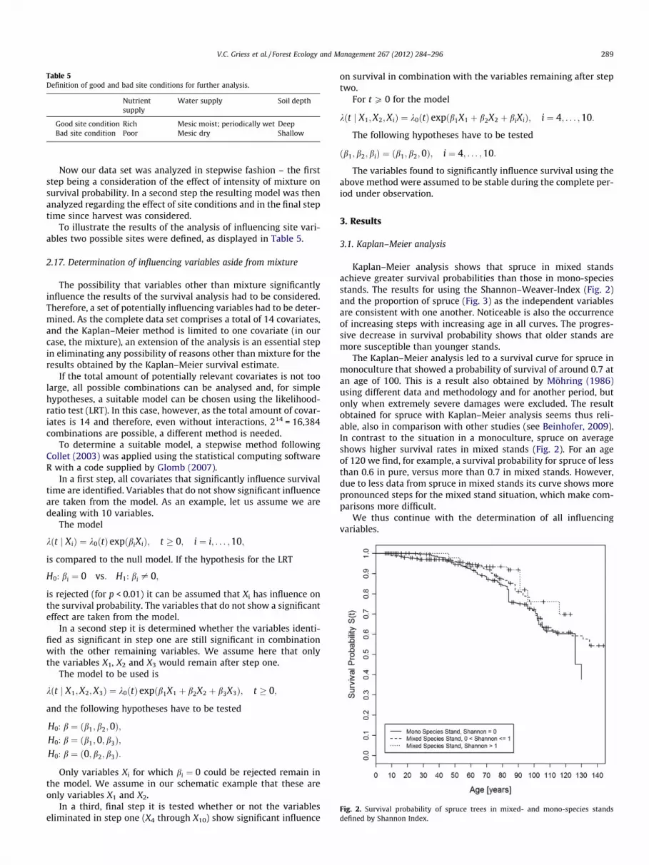
Table 5Definition of good and bad site conditions for further analysis.

Nutrientsupply

Water supply Soil depth

Good site condition Rich Mesic moist; periodically wet DeepBad site condition Poor Mesic dry Shallow

Fig. 2. Survival probability of spruce trees in mixed- and mono-species standsdefined by Shannon Index.


Now our data set was analyzed in stepwise fashion – the firststep being a consideration of the effect of intensity of mixture onsurvival probability. In a second step the resulting model was thenanalyzed regarding the effect of site conditions and in the final steptime since harvest was considered.

To illustrate the results of the analysis of influencing site vari-ables two possible sites were defined, as displayed in Table 5.

2.17. Determination of influencing variables aside from mixture

The possibility that variables other than mixture significantlyinfluence the results of the survival analysis had to be considered.Therefore, a set of potentially influencing variables had to be deter-mined. As the complete data set comprises a total of 14 covariates,and the Kaplan–Meier method is limited to one covariate (in ourcase, the mixture), an extension of the analysis is an essential stepin eliminating any possibility of reasons other than mixture for theresults obtained by the Kaplan–Meier survival estimate.

If the total amount of potentially relevant covariates is not toolarge, all possible combinations can be analysed and, for simplehypotheses, a suitable model can be chosen using the likelihood-ratio test (LRT). In this case, however, as the total amount of covar-iates is 14 and therefore, even without interactions, 214 = 16,384combinations are possible, a different method is needed.

To determine a suitable model, a stepwise method followingCollet (2003) was applied using the statistical computing softwareR with a code supplied by Glomb (2007).

In a first step, all covariates that significantly influence survivaltime are identified. Variables that do not show significant influenceare taken from the model. As an example, let us assume we aredealing with 10 variables.

The model

kðt j XiÞ ¼ k0ðtÞ expðbiXiÞ; t � 0; i ¼ i; . . . ;10;

is compared to the null model. If the hypothesis for the LRT

H0: bi ¼ 0 vs: H1: bi – 0;

is rejected (for p < 0.01) it can be assumed that Xi has influence onthe survival probability. The variables that do not show a significanteffect are taken from the model.

In a second step it is determined whether the variables identi-fied as significant in step one are still significant in combinationwith the other remaining variables. We assume here that onlythe variables X1, X2 and X3 would remain after step one.

The model to be used is

kðt j X1;X2;X3Þ ¼ k0ðtÞ expðb1X1 þ b2X2 þ b3X3Þ; t � 0;

and the following hypotheses have to be tested

H0: b ¼ ðb1;b2;0Þ;H0: b ¼ ðb1;0;b3Þ;H0: b ¼ ð0;b2;b3Þ:

Only variables Xi for which bi ¼ 0 could be rejected remain inthe model. We assume in our schematic example that these areonly variables X1 and X2.

In a third, final step it is tested whether or not the variableseliminated in step one (X4 through X10) show significant influence

on survival in combination with the variables remaining after steptwo.

For t P 0 for the model

kðt j X1;X2;XiÞ ¼ k0ðtÞ expðb1X1 þ b2X2 þ biXiÞ; i ¼ 4; . . . ;10:

The following hypotheses have to be tested

ðb1;b2;biÞ ¼ ðb1;b2;0Þ; i ¼ 4; . . . ;10:

The variables found to significantly influence survival using theabove method were assumed to be stable during the complete per-iod under observation.

3. Results

3.1. Kaplan–Meier analysis

Kaplan–Meier analysis shows that spruce in mixed standsachieve greater survival probabilities than those in mono-speciesstands. The results for using the Shannon–Weaver-Index (Fig. 2)and the proportion of spruce (Fig. 3) as the independent variablesare consistent with one another. Noticeable is also the occurrenceof increasing steps with increasing age in all curves. The progres-sive decrease in survival probability shows that older stands aremore susceptible than younger stands.

The Kaplan–Meier analysis led to a survival curve for spruce inmonoculture that showed a probability of survival of around 0.7 atan age of 100. This is a result also obtained by Möhring (1986)using different data and methodology and for another period, butonly when extremely severe damages were excluded. The resultobtained for spruce with Kaplan–Meier analysis seems thus reli-able, also in comparison with other studies (see Beinhofer, 2009).In contrast to the situation in a monoculture, spruce on averageshows higher survival rates in mixed stands (Fig. 2). For an ageof 120 we find, for example, a survival probability for spruce of lessthan 0.6 in pure, versus more than 0.7 in mixed stands. However,due to less data from spruce in mixed stands its curve shows morepronounced steps for the mixed stand situation, which make com-parisons more difficult.

We thus continue with the determination of all influencingvariables.

Fig. 3. Survival probability of spruce trees in mixed- and mono-species standsdefined by spruce ratio.

Table 7Regression coefficients of factors influencing the survival analysis with Weibulldistribution, for a mixture defined by Shannon (Model A). SE, standard error; p, errorprobability.

Model A: Shannon Coefficient SE z p

(Intercept) 4.3058 0.0529 81.384 0.0000Nutrient supply 1 0.1746 0.0576 3033 2.42E-03Nutrient supply 3 �0.4462 0.0660 �6761 1.37E-11Type of mixture 1 0.1992 0.0674 2957 3.11E-03Type of mixture 2 �0.0409 0.0548 �0747 4.55E-01Type of mixture 3 �0.0525 0.0472 �1111 2.66E-01Water supply 1 �0.6229 0.0579 �10.760 5.29E-27Water supply 3 �0.2290 0.0472 �4851 1.23E-06Water supply 4 �0.0839 0.0903 �0929 3.53E-01Orographic conditions 2 0.6133 0.1257 4880 1.06E-06Orographic conditions 4 0.3593 0.0413 8691 3.60E-18Orographic conditions 6 0.8414 0.1708 4926 8.41E-07Soil depths 1 0.2548 0.0563 4523 6.09E-06Soil depths 3 0.0056 0.0516 0108 9.14E-01Soil structure 1 0.0278 0.0413 0674 5.00E-01Soil structure 3 0.2785 0.1000 2786 5.34E-03Shannon 1 0.0485 0.0406 1194 2.32E-01Shannon 2 0.5380 0.1938 2777 5.49E-03NS. Expos �0.3083 0.0274 �11.242 2.52658E-29EW. Expos �0.1054 0.0329 �3208 1.34E-03Time_Since_Harvest 2 0.3222 0.0438 7354 1.93E-13Time_Since_Harvest 3 0.3832 0.0435 8818 1.16E-18Stand structure 1 0.0363 0.0514 0707 4.80E-01Log(scale) �1.3553 0.0456 �29.741 2.27E-194


3.2. Determination of influencing variables

After gaining an overview of possible effects of tree species mix-ture on stand resistance, by a first survival analysis using the Kap-lan–Meier method (Kaplan and Meier, 1958), we applied the multi-step analysis following Glomb (2007) described above to identifythe other variables that might possibly influence our model. Re-sults are displayed in Table 6.

The intensity or meaning of the influence of these variables wasnot assessed in this step, but will later be evaluated in detail usingthe Weibull distribution (see ‘coefficients’ in Table 7, section ‘Anal-ysis based on Weibull distribution’). However this step allows us toeliminate certain, less influential variables from the model.

To insure reliable results, those sets of data for which one ormore of the variables contained no significant information (p-va-lue > 0.05) or only very few observations were excluded from theanalysis. Examples are the variables ‘‘Altitude’’, ‘‘Gradient’’ or ‘‘Can-opy closure’’.

3.3. Analysis based on Weibull distribution

3.3.1. Mixture determined by Shannon IndexConcordant to the Kaplan–Meier-analysis, the Weibull based

analysis of survival time of spruce trees showed a significant posi-tive influence of mixture on the survival probabilities of spruce.Fig. 4 shows the survival functions for the three classes of the

Table 6Variables influencing the survival model.

VariableX1 Water supplyX2 Nutrient supplyX3 Orographic conditionsX4 Soil depthX5 Soil structureX8 NS-aspectX9 EW-aspectX10 Mixture (Shannon or spruce

ratio)X11 Type of mixtureX12 Stand structureX14 Time since harvest

Shannon–Weaver-Index according to Table 4, with constant valuesfor all other covariables, which are the reference values repre-sented by the overall intercept for this particular case (Model A:average nutrient and water supply, fairly shallow soil, a plain oro-graphic condition and single level stand structure). To representaverage site conditions, the parameter value of orographic condi-tion 4 (hillsides) was added for all following graphs. To representthe influence of all times since harvest, all three parameter valueswere included for all graphs accordingly. In model A the intensityof mixture was defined by means of the Shannon–Weaver-Indexaccording to Table 4. As seen in Fig. 4, the survival probabilitiesof spruce increase with increasing intensity of mixture. Detailedresults are displayed in Table 8. In this case, spruce trees in

Fig. 4. Survival of spruce trees in mixed and mono species stands, defined byShannon Index.

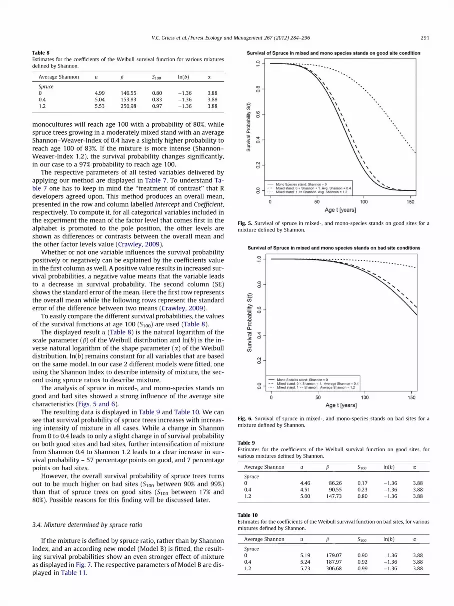
Table 8Estimates for the coefficients of the Weibull survival function for various mixturesdefined by Shannon.

Average Shannon u b S100 ln(b) a

Spruce0 4.99 146.55 0.80 �1.36 3.880.4 5.04 153.83 0.83 �1.36 3.881.2 5.53 250.98 0.97 �1.36 3.88

Fig. 5. Survival of spruce in mixed-, and mono-species stands on good sites for amixture defined by Shannon.

Fig. 6. Survival of spruce in mixed-, and mono-species stands on bad sites for amixture defined by Shannon.

Table 9Estimates for the coefficients of the Weibull survival function on good sites, forvarious mixtures defined by Shannon.


Spruce0 4.46 86.26 0.17 �1.36 3.880.4 4.51 90.55 0.23 �1.36 3.881.2 5.00 147.73 0.80 �1.36 3.88


monocultures will reach age 100 with a probability of 80%, whilespruce trees growing in a moderately mixed stand with an averageShannon–Weaver-Index of 0.4 have a slightly higher probability toreach age 100 of 83%. If the mixture is more intense (Shannon–Weaver-Index 1.2), the survival probability changes significantly,in our case to a 97% probability to reach age 100.

The respective parameters of all tested variables delivered byapplying our method are displayed in Table 7. To understand Ta-ble 7 one has to keep in mind the ‘‘treatment of contrast’’ that Rdevelopers agreed upon. This method produces an overall mean,presented in the row and column labelled Intercept and Coefficient,respectively. To compute it, for all categorical variables included inthe experiment the mean of the factor level that comes first in thealphabet is promoted to the pole position, the other levels areshown as differences or contrasts between the overall mean andthe other factor levels value (Crawley, 2009).

Whether or not one variable influences the survival probabilitypositively or negatively can be explained by the coefficients valuein the first column as well. A positive value results in increased sur-vival probabilities, a negative value means that the variable leadsto a decrease in survival probability. The second column (SE)shows the standard error of the mean. Here the first row representsthe overall mean while the following rows represent the standarderror of the difference between two means (Crawley, 2009).

To easily compare the different survival probabilities, the valuesof the survival functions at age 100 (S100) are used (Table 8).

The displayed result u (Table 8) is the natural logarithm of thescale parameter (b) of the Weibull distribution and ln(b) is the in-verse natural logarithm of the shape parameter (a) of the Weibulldistribution. ln(b) remains constant for all variables that are basedon the same model. In our case 2 different models were fitted, oneusing the Shannon Index to describe intensity of mixture, the sec-ond using spruce ratios to describe mixture.

The analysis of spruce in mixed-, and mono-species stands ongood and bad sites showed a strong influence of the average sitecharacteristics (Figs. 5 and 6).

The resulting data is displayed in Table 9 and Table 10. We cansee that survival probability of spruce trees increases with increas-ing intensity of mixture in all cases. While a change in Shannonfrom 0 to 0.4 leads to only a slight change in of survival probabilityon both good sites and bad sites, further intensification of mixturefrom Shannon 0.4 to Shannon 1.2 leads to a clear increase in sur-vival probability – 57 percentage points on good, and 7 percentagepoints on bad sites.

However, the overall survival probability of spruce trees turnsout to be much higher on bad sites (S100 between 90% and 99%)than that of spruce trees on good sites (S100 between 17% and80%). Possible reasons for this finding will be discussed later.

Table 10Estimates for the coefficients of the Weibull survival function on bad sites, for variousmixtures defined by Shannon.


Spruce0 5.19 179.07 0.90 �1.36 3.880.4 5.24 187.97 0.92 �1.36 3.881.2 5.73 306.68 0.99 �1.36 3.88

3.4. Mixture determined by spruce ratio

If the mixture is defined by spruce ratio, rather than by ShannonIndex, and an according new model (Model B) is fitted, the result-ing survival probabilities show an even stronger effect of mixtureas displayed in Fig. 7. The respective parameters of Model B are dis-played in Table 11.

Table 11Regression coefficients of factors influencing the survival analysis with Weibulldistribution, for a mixture defined by Spruce ratio (Model B). SE, standard error, p,error probability.

Model B: Spruce ratio Coefficient SE z p

(Intercept) 4.6342 0.1007 46.013 0.0000Nutrient supply 1 0.2016 0.0530 3803 1.43E-04Nutrient supply 3 �0.4320 0.0654 �6606 3.94E-11Type of mixture 1 0.1377 0.0667 2066 3.88E-02Type of mixture 2 �0.0180 0.0528 �0341 7.33E-01Type of mixture 3 �0.0698 0.0461 �1514 1.30E-01Water supply 1 �0.6468 0.0549 �11.773 5.37E-32Water supply 3 �0.2127 0.0459 �4637 3.53E-06Water supply 4 �0.1083 0.0889 �1218 2.23E-01Orographic conditions 2 0.5210 0.1271 4101 4.12E-05Orographic conditions 4 0.3580 0.0400 8944 3.76E-19Orographic conditions 6 0.8622 0.1680 5131 2.88E-07Soil depths 1 0.2279 0.0563 4046 5.21E-05Soil depths 3 �0.0158 0.0524 �0302 7.63E-01Soil structure 1 0.0225 0.0424 0530 5.96E-01Soil structure 3 0.0981 0.1004 0977 3.29E-01Spruce ratio 2 �0.1923 0.1001 �1921 5.48E-02Spruce ratio 3 �0.3309 0.0865 �3824 1.32E-04NS. Expos �0.2958 0.0264 �11.189 4.59939E-29EW. Expos �0.1219 0.0329 �3706 2.10E-04Time_Since_Harvest 2 0.3234 0.0431 7500 6.39E-14Time_Since_Harvest 3 0.3792 0.0427 8880 6.71E-19Stand structure 1 0.0401 0.0522 0768 4.42E-01Log(scale) �1.3695 0.0457 �29.957 3.61E-197


The three categories of spruce ratio to be analysed were chosenbased on the actual frequency distribution of spruce trees in mixedstands. The actual distribution for the two mixed categories is dis-played in Figs. 8 and 9.

The values of the survival functions at age 100 (S100) are dis-played in Table 12. Combined with the shape parameter a, that al-lows the display of increasing (a > 1), decreasing (a < 1) or constant(a = 1) hazard rates, S100 allows an easy interpretation of the sur-vival function.

As displayed in Table 12, the survival probabilities of spruce in-crease with increasing proportion of admixed tree species. Undersimilar site conditions given for the results displayed in Fig. 4,spruce trees growing in monocultures will reach age 100 with aprobability of 80%, whilst spruce trees growing in almost purestands (average admixture 7%) experience an increase of 8%. Ifthe mixture is, however, more intense, the survival probability in-creases further, in our case to a 94% probability of reaching age100. An admixture of around 50% thus leads to an increase in sur-vival probability of 5 percentage points.

The analysis of mixture based on spruce proportions on goodand bad sites showed a strong influence of the average site charac-teristics (Tables 13 and 14) as was the case in the analysis deter-mining mixture using the Shannon Index.

The overall survival probability of spruce trees turned out to bemuch higher on bad sites (S100 between 91% and 97%) than that ofspruce trees on good sites (S100 between only 15% and 60%) usingmodel B as well.

3.5. Analysis in consideration of elapsed time since last harvest

The analysis regarding time since harvest was based on ModelA. It showed a strong influence on spruce survival. Survival proba-bility was drastically higher in stands in which harvest operationswere carried out in the distant past than on those stands whereharvest operations were carried out just recently (see Fig. 10).

To find out whether or not harvest operations had an evenstronger influence on survival than site quality and/or mixture,analyses using a combination of all variables were carried out(see Tables 15–17).

Fig. 7. Survival of spruce trees in mixed and mono species stands, defined by spruceratio.

Fig. 8. Frequency distribution of spruce trees in the group >0 <80% spruceproportion.

Fig. 9. Frequency distribution of spruce trees in the group 81–99% spruceproportion.

As displayed in Fig. 10 the survival probability of spruce in-creases with increasing distance in time to the last harvest opera-tion. Spruce trees growing in monocultures will reach age 100 withthe smallest probability, irrespective of site conditions, while

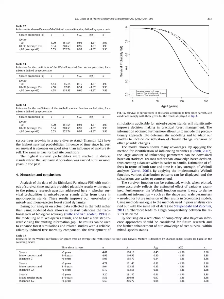
Table 12Estimates for the coefficients of the Weibull survival function, defined by spruce ratio.

Spruce proportion [%] u b S100 ln(b) a

Spruce100 5.20 181.54 0.91 �1.37 3.9381–99 (average 93) 5.34 208.53 0.95 �1.37 3.93680 (average 49) 5.53 252.74 0.97 �1.37 3.93

Table 13Estimates for the coefficients of the Weibull survival function on good sites, for amixture defined by spruce ratio.



Table 14Estimates for the coefficients of the Weibull survival function on bad sites, for amixture defined by spruce ratio.



Fig. 10. Survival of spruce trees in all stands, according to time since harvest. Siteconditions comply with those given for the results displayed in Fig. 4.


spruce trees growing in a more diverse stand (Shannon 1.2) havethe highest survival probabilities. Influence of time since harveston survival is stronger on good sites than influence of mixture it-self. The same is true for bad site conditions.

The highest survival probabilities were reached in diversestands where the last harvest operation was carried out 6 or moreyears in the past.

4. Discussion and conclusions

Analysis of the data of the Rhineland Palatinate FDS with meth-ods of survival time analysis provided plausible results with regardto the primary research question addressed here – whether sur-vival probabilities in mixed-species stands differ from those inmono-species stands. These results improve our knowledge ofmixed- and mono-species forest stand dynamics.

Basing our analysis on actual data collected in the field ratherthan using modelled data allows us to start balancing the tradi-tional lack of biological accuracy (Bulte and van Kooten, 1999) inthe modelling of mixed-species stands, and to take a first step to-ward closing the existing information gap. The results can be usedto enhance forest simulations and related studies with a reliable,calamity induced tree mortality component. The development of

Table 15Estimates for the Weibull coefficients for spruce trees on average sites with respect to taccording model.

Time since harvest u

Spruce <3 years 4.67Mono species stand 3–6 years 4.99(Shannon 0) >6 years 5.05

Spruce <3 years 4.71Mono species stand 3–6 years 5.04(Shannon 0.4) >6 years 5.10

Spruce <3 years 5.20Mixed species stand 3–6 years 5.53(Shannon 1.2) >6 years 5.59

simulations applicable for mixed-species stands will significantlyimprove decision making in practical forest management. Theinformation obtained furthermore allows us to include the precau-tionary approach into deterministic modelling and to adapt ourmodels to include consideration of climate change scenarios orother possible changes.

The model chosen shows many advantages. By applying themethod for identification of influencing variables (Glomb, 2007),the large amount of influencing parameters can be downsizedbased on statistical reasons rather than knowledge-based decision,thus creating a dataset which is easier to handle. Estimation of ef-fects in terms of both rate and time is a key strength of Weibullanalyses (Carrol, 2003). By applying the implementable Weibullfunction, various distribution patterns can be displayed, and thecalculations are easier to comprehend.

The survivor function can be estimated, which, when plotted,more accurately reflects the estimated effect of variables exam-ined. Furthermore, the Weibull function makes it easy to derivesignificant information – such as the shape and scale parameters– needed for future inclusion of the results in (economic) models.Using methods analogue to the methods used in prior analysis car-ried out with the same set of data (see Staupendahl and Zucchini,2011) furthermore leads to a high comparability between the re-sults delivered.

By focusing on a reduction of complexity, also Bayesian infer-ence approaches should be considered for future research andthe further enhancement of our knowledge of tree survival withinmixed-species stands.

ime since harvest. Mixture is described by Shannon-Index; results are based on the

b S100 ln(b) a

106.18 0.45 �1.36 3.88146.55 0.80 �1.36 3.88155.77 0.84 �1.36 3.88

111.46 0.52 �1.36 3.88153.83 0.83 �1.36 3.88163.51 0.86 �1.36 3.88

181.85 0.91 �1.36 3.88250.98 0.97 �1.36 3.88266.77 0.98 �1.36 3.88

Table 16Estimates for the Weibull coefficients for spruce trees on good site conditions with respect to time since harvest. Mixture is described by Shannon Index; results are based on theaccording model.

Time since harvest u b S100 ln(b) a

Spruce <3 years 4.14 62.50 0.00 �1.36 3.88Mono species stand 3–6 years 4.46 86.26 0.17 �1.36 3.88(Shannon 0) >6 years 4.52 91.68 0.25 �1.36 3.88

Spruce <3 years 4.18 65.60 0.01 �1.36 3.88Mono species stand 3–6 years 4.51 90.55 0.23 �1.36 3.88(Shannon 0.4) >6 years 4.57 96.24 0.31 �1.36 3.88

Spruce <3 years 4.67 107.03 0.46 �1.36 3.88Mixed species stand 3–6 years 5.00 147.73 0.80 �1.36 3.88(Shannon 1.2) >6 years 5.06 157.02 0.84 �1.36 3.88

Table 17Estimates for the Weibull coefficients for spruce trees on bad site conditions with respect to time since harvest. Mixture is described by Shannon Index, results are based on theaccording model.

Time since harvest u b S100 ln(b) a

Spruce <3 years 4.87 129.74 0.69 �1.36 3.88Mono species stand 3–6 years 5.19 179.07 0.90 �1.36 3.88(Shannon 0) >6 years 5.25 190.33 0.92 �1.36 3.88

Spruce <3 years 4.91 136.19 0.74 �1.36 3.88Mono species stand 3–6 years 5.24 187.97 0.92 �1.36 3.88(Shannon 0.4) >6 years 5.30 199.79 0.93 �1.36 3.88

Spruce <3 years 5.40 222.20 0.96 �1.36 3.88Mixed species stand 3–6 years 5.73 306.68 0.99 �1.36 3.88(Shannon 1.2) >6 years 5.79 325.97 0.99 �1.36 3.88


While the use of the Shannon Index may be a more complicatedway to define the intensity of mixture than the spruce proportion,both approaches are reasonable. The Shannon Index is the mostuniversal measure of entropy in most natural sciences. This aloneis reason enough to select the Shannon Index to describe diversitymeasures (Jost, 2006). On the other hand, using a ratio or propor-tion of a certain species to describe mixture allows a direct com-parison with other common mixtures as well as direct use of theresults by a practitioner, who will most likely find the ratios easierto interpret. The differences in the results obtained using the twomethods is likely a result of the variation in the categories whichwere formed due to the amount of data available. For the futureit will be important to find the tipping point in the sense of a min-imum required admixture in spruce stands in order to achieve im-proved survival rates.

The decrease of survival probabilities in steps is, in part, due tothe fact that calamities that happened in the far past can only beidentified as such by the inventory personnel if they occurredarea-wise. Single damaged trees that have been removed as partof a harvest of healthy trees that led to a continuous decrease ofsurvival probability are hard to identify as such without additionalinformation. Besides a resulting systematic overestimation of thesurvival probability, this enlarges the discrete spaces of theKaplan–Meier function and complicates the adaption of a paramet-ric model (Staupendahl and Zucchini, 2011).

The results obtained in this paper however show an enhancedresistance against natural hazards for spruce trees in mixed stands,and therefore lend support the theory that short-term benefitsachieved by the homogenization of ecosystems and the accordingloss of biodiversity are overshadowed by the consequent reductionin the ability of forest stands to cope with natural risks. This resultis consistent with findings by Griess and Knoke (2011), Pretzsch(2009), König (1995), Rau (1995), Winterhoff et al. (1995), Kennel(1965) and many others. Spruce trees can develop broader crownswhen growing in mixture with deciduous trees, as they are able tocontinue to accumulate needle biomass, while broadleaves are los-

ing their leaves (Schütz et al., 2006). Furthermore and possibly ofgreater importance, is the experience of practitioners that showsthat beech trees or other broadleaves may be able to temper thependulum effects of wind during a storm, preventing the standfrom reaching critical amplitude. However, the latter effect re-mains largely uninvestigated. Regarding insect calamities it isobvious that in a mixed species stands antagonists of commonpests will be more likely to find suitable habitat than in monocul-tures. Furthermore mass reproduction of insect pests in single spe-cies stands is more likely to occur due to the clustering of foodsources.

Still, the biological processes behind these results require fur-ther discussion and research.

The potential for elevated mortality of trees following harvestoperations is a critical concern for forest managers. Our study dem-onstrates the strong importance of time elapsed since harvestoperations on tree mortality, while also showing that these influ-ences are far smaller in mixed species stands than in monocultures.However, the results need to be interpreted carefully, since theunderlying recordings regarding the last harvest operation carriedout are partially uncertain. Other studies dealing with the subjectof post-harvest tree failure have shown that intensity of thinning(Albrecht, 2009) or proximity to skid trails or to the edge of a standare important predictors both of wind throw and standing death(see Thorpe et al., 2008). The data used here was not sufficient toinvestigate these assumptions, as no information regarding inten-sity of thinning, tree-to-tree distance, or change in basal area with-in a certain neighbourhood was available. To more fully investigatethe reasons for an increase in post-harvest mortality, collection ofappropriate data should be considered for further inventories.

If site quality is taken into account, it might come as a surprisethat higher nutrient availability leads to lower survival probabilities.But, under very good site conditions, trees will be taller than those ofsimilar age on poorer sites, making the lever for storm and wind lar-ger (Staupendahl and Zucchini, 2011). Furthermore the soils on goodsites may not necessitate such a strong formation and anchoring of


roots as required on poorer sites, leading to a higher susceptibilitytowards wind throw (Griess and Knoke, 2011).

Similar results have been published by Schelhaas et al. (2003),who were able to prove a high risk on deep soils with a good avail-ability of nutrients. König (1995) pointed out similar results forwaterlogged sites as well. Deep soils are often characterized by awash-out that again leads to a hardening of the subsoil. This aggre-gation lowers the water permeability, and in case of strong precip-itation, complete saturation is quickly reached. The susceptibilitytowards wind throw is then drastically increased, which has beenaffirmed by (Schmidt et al., 2010).

However, as not only wind throw, but other calamities are beingconsidered within our study, results are only applicable under theassumption that, in large part, damage is caused by wind throw,and that these damages are usually followed by bark beetle calam-ities, thus leading to an increase in total risk (Hanewinkel et al.,2008). Our survival analysis concentrates only on calamity-in-duced mortality, although in reality interactions between treeresistance against biotic or abiotic stress factors and competitionmust also be assumed. Within our analysis only trees that are par-ticipating in the upper canopy level – and are therefore less likelyto suffer from competition – are taken into account. Backgroundmortality due to self-thinning therefore has no direct influenceon the results. With respect to decision models a further distinc-tion is required between mortality caused by calamities and thatcaused by competition, whereas the latter depends on shade toler-ance and density of tree species.

Regarding possible analysis of other tree species, it has to bepointed out that in most cases the data set available was too smallto get reliable results. This drawback could easily be solved by add-ing data from other according inventories, especially as the two ap-proaches for the determination of mixture described here, as wellas the method itself, are easily expandable with FDS data fromother German states or even survival data from other countries.This would not only allow us to gain comparable information forother relevant species – such as beech – or other site conditionsin the future, but would also strengthen the reliability of the re-sults we present here. A disadvantage in the otherwise very appli-cable FDS data is that within the annual inventories which werecarried out, no diameters were taken. This makes it hard to analysesurvival in mixed stands with respect to species area rather thannumber of stems and leads to an underestimation of the amountof deciduous trees necessary for a positive influence on survival.For future inventories the measurement of diameters should there-fore be added as a standard.

Furthermore, the sampling method applied in the FDS inventory– even though widely used in forest inventory systems all over Eur-ope – causes some major drawbacks. Within the framework of n-tree sampling following Prodan (1965) a constant number ofinventory trees is measured at each inventory spot, for examplethe six trees closest to the centre of the inventory spot. The area re-ferred to therefore varies among the inventory points and is sub-ject to the distance between the trees furthest away from eachinventory point centre. A high variance between the sampled dataof the inventory points is caused by the relatively small number ofinventory trees. Furthermore, concerns regarding the existence ofan unbiased estimator for stem number within this particular plotdesign do exist (Kleinn and vilcko, 2006). Still, n-tree sampling iswidely used as it is currently the only method allowing collectionof large-scale information on the vitality of forests at the nationallevel at reasonable costs (ICP Forests, 2009). In our case some ofthese problems are irrelevant, as no area reference is necessaryfor the applied analysis. Still it has to be kept in mind that a biasmay occur due to under- or overestimation of certain species orage classes caused by a possibly lumped distribution of trees with-in our sample.

In terms of increasing the reliability and significance of the re-sults obtained, the FDS data of other German states and equivalentdata from other countries should be analyzed with respect to mix-ture as well. Besides delivering the according survival functions,this would also enable an economic inclusion of production risksinto models and prognosis.

This could for example be done by enhancing approaches likethe ones by Rößiger et al. (2011) or Clasen et al. (2011) by im-proved empirical survival probabilities.

Acknowledgements

The authors thank the Forest Research Institute Rheinland-Pfalz(FVA) for their exceptional cooperativeness, particularly Mr. Fried-rich Engels for his support. The authors also wish to thank Mrs.Laura Carlson for the language editing of the manuscript, Mr. Dipl.Stat. Andreas Böck (TUM Stat) for help regarding the analysis andtwo anonymous reviewers for valuable suggestions. Furthermore,the author gratefully acknowledges the support of TUM GraduateSchools Thematic Graduate Center at the Technische UniversitätMünchen.

The presented study is part of the project ‘‘Bioeconomic model-ling and optimization of forest stands: towards silvicultural eco-nomics’’ KN 586/7-1 funded by the German Research Foundation.

References

Albrecht, A., 2009. Sturmschadensanalysen langfristiger WaldwachstumskundlicherVersuchsflächendaten in Baden-Württemberg. Freiburg (Breisgau)(Schriftenreihe Freiburger Forstliche Forschung, 42.

Armstrong, C.W., 2007. A note on the ecological-economic modelling of marinereserves in fisheries. Ecological Economics 62, 242–250.

Beinhofer, B., 2009. Zur Anwendung der Portfoliotheorie in der Forstwissenschaft –Finanzielle Optimierungsansätze zur Bewertung von Diversifikationseffekten,Thesis, Technische Universität München.

Bulte, E.H., van Kooten, G.C., 1999. Metapopulation dynamics and stochasticbioeconomic modeling. Ecological Economics 30, 293–299.

Carroll, K.J., 2003. On the use and utility of the Weibull model in the analysis ofsurvival data. Controlled Clinical Trials 24 (6) (Suppl.), 682–701.

Clasen, C., Griess, V.C., Knoke, T., 2011. Financial consequences of losing admixedtree species: a new approach to value increased financial risks by ungulatebrowsing. Forest Policy and Economics 13, 503–511.

Collet, D., 2003. Modelling Survival Data in Medical Research, second ed. Chapman& Hall, Boca Raton, FL.

Cotta, H., 1828. Anweisung zum Waldbau, Carl Heinrich Edmund von Berg.Crawley, M., 2009. The R Book. Ed. John Wiley & Sons Ltd.Engels, F., Block, J., Wunn, U., 1999. Methodenbeschreibung – Terrestrische

Waldschadenserhebung (TWE) in Rheinland-Pfalz.Figge, F., Hahn, T., 2004. Sustainable value added-measuring corporate

contributions to sustainability beyond eco-efficiency. Ecological Economics 48(2), 173–187.

Gadow, K.v., 2000. Evaluating risk in forest planning models. Silva Fennica 34 (2),181–191.

Gayer, K., 1886. Der gemischte Wald: seine Begründung und Pflege, insbesonderedurch Horst- und Gruppenwirtschaft. Paul Parey, Berlin.

Glomb, P., 2007. Statistische Modelle und Methoden in der Analyse vonLebenszeitdaten, Diploma Thesis. Carl von Ossietzky Universität, Oldenburg.Institut für Mathematik.

Griess, V.C., Knoke, T., 2011. Growth performance, wind-throw, and insects: meta-analyses of parameters influencing performance of mixed-species stands inboreal and northern temperate biomes. Can. J. For. Res. 41, 1141–1159.

Hahn, A., Knoke, T., 2010. Sustainable development and sustainable forestry:analogies, differences, and the role of flexibility. Eur. J. For. Res. 129, 787–801.

Hanewinkel, M., Breidenbach, J., Neeff, T., Kublin, E., 2008. Seventy-seven years ofnatural disturbances in a mountain forest area – the influence of storm, snow,and insect damage analysed with a long-term time series. Canadian Journal ofForest Research 38, 2249–2261.

Holecy, J., Hanewinkel, M., 2006. A forest management risk insurance model and itsapplication to coniferous stands in southwest Germany. Forest Policy andEconomics 8 (2), 161–174.

International Co-operative Programme on Assessment and Monitoring of AirPollution Effects on Forests operating under the UNECE Convention on Long-range Transboundary Air Pollution, 2009. Results of the Forest ConditionSurvey: National Report Germany. ICP (Results of the Forest Condition Survey).Available from: <http://www.icp-forests.org/pdf/NatRepGermany2009.pdf>.

Jost, L., 2006. Entropy and diversity. OIKOS 113, 2.Kaplan, E.L., Meier, P., 1958. Nonparametric estimation from incomplete

observations. Journal of the American Statistical Association 53 (282), 457–481.

http://www.icp-forests.org/pdf/NatRepGermany2009.pdf


Kay, R., Kinnersley, N., 2002. On the use of the accelerated failure time model as analternative to the proportional hazards model in the treatment of time to eventdata: a case study in influenza. Drug Information Journal 3, 571–579.

Kennel, R., 1965. Untersuchungen über die Leistung von Fichte und Buche im Rein-und Mischbestand, Teil I. Allgemeine Forst- und Jagdzeitung 136, 149–161.

Kleinn, C., Vilcko, F., 2006. A new empirical approach for estimation in k-treesampling. Forest Ecology and Management 237 (1–3) (Suppl.), 522–533.

Knoke, T., Mosandl, R., 2004. Integration ökonomischer, ökologischer und sozialerAnsprüche: Zur Sicherung einer umfassenden Nachhaltigkeit im Zuge derForstbetriebsplanung. Forst und Holz 59 (11), 535–539.

Knoke, T., Moog, M., 2005. Timber harvesting versus forest reserves-producer pricesfor open-use areas in German beech forests (Fagus sylvatica L.). EcologicalEconomics 52 (1), 97–110.

Knoke, T., Wurm, J., 2006. Mixed forests and a flexible harvest policy: a problem forconventional risk analysis? European Journal of Forest Research 125 (3), 303–315.

Knoke, T., Seifert, T., 2008. Integrating selected ecological effects of mixed Europeanbeech – Norway spruce stands in bioeconomic modelling. Ecological Modelling210 (4), 487–498.

Knoke, T., Ammer, C., Stimm, B., Mosandl, R., 2008. Admixing broadleaved toconiferous tree species: a review on yield, ecological stability and economics.European Journal of Forest Research 127 (2), 89–101.

Kölling, C., Beinhofer, B., Hahn, A., Knoke, T., 2010. Wie soll die Forstwirtschaft aufneue Risiken im Klimawandel reagieren? Allg. Forst Z. Waldwirtsch.Umweltvorsorge 65, 18–22.

König, A., 1995. Sturmgefährdung von Beständen im Altersklassenwald – EinErklärungs– und Prognosemodell. Frankfurt am Main. J.D. Sauerländer’s Verlag.

Kouba, J., 2002. Das Leben des Waldes und seine Lebensunsicherheit.Forstwissenschaftliches Centralblatt 121 (4), 211–228.

Kraft, G., 1884. Beiträge zur Lehre von den Durchforstungen, Schlagstellungen undLichtungshieben. Klindworths, Hannover.

Krysiak, F.C., 2006. Entropy, limits to growth, and the prospects for weaksustainability. Ecological Economics 58 (1), 182–191.

Lambert, P., Collett, D., Kimber, A., Johnson, R., 2004. Parametric accelerated failuretime models with random effects and an application to kidney transplantsurvival. Statistics in Medicine 23 (20), 3177–3192.

Lucas, G., Andres, B., 1978. Mathematische Grundlagen zur Anwendung vonÜbergangswahrscheinlichkeiten bei der Strukturregelung im Walde. Techn.Univ. Dresden, Tharandt.

Lüpke, B.v., 2009. Überlegungen zu Baumartenwahl und Verjüngungsverfahren beifortschreitender Klimaänderung in Deutschland. Forstarchiv 80 (3), 67–75.

Mayer, P., Brang, P., Dobertin, M., Hallenbarter, D., Renaud, J.P., Zimmermann,L.W.S., 2005. Forest storm damage is more frequent on acidic soils. Annals ofForest Science (62) (Suppl.), 303–311.

Möhring, B., 1986. Dynamische Betriebsklassensimulation – Ein Hilfsmittel für dieWaldschadensbewertung und Entscheidungsfindung im Forstbetrieb.Selbstverlag (Ber. Forschungsztr. Waldökosys., 20), Göttingen.

Palma, C.D., Nelson, J.D., 2010. Bi-objective multi-period planning with uncertainweights: a robust optimization approach. European Journal of Forest Research129 (6), 1081–1091.

Plante, J.F., 2009. About an adaptively weighted Kaplan–Meier estimate. LifetimeData Analysis 15, 295–315.

Pretzsch, H., 2009. Forest Dynamics Growth and Yield. A Review Analysis of thePresent State and Perspective. Springer, Berlin, Heidelberg.

Prodan, M., 1965. Holzmesslehre. Frankfurt am Main: Sauerländer. 644 p. Availablefrom:<http://www.portal.hebis.de/jsp/customers/hebis/trefferlisten/documenthead.jsp?database=ROOT:Verbuende@BVB$2&position=0&timeout=10&tab=katalog>.

Rau, H., 1995. Die Sturmschäden im Virngrund (Nordostwürttemberg) von 1870 bis1990 – eine waldbaugeschichtliche und standortskundliche Untersuchung.Mitteilungen der Forstlichen Versuchs- und Forschungsanstalt Baden-Württemberg., 188.

Roßiger, J., Griess, V.C., Knoke, T., 2011. May risk aversion lead to near-naturalforestry? A simulation study. Forestry.

Schelhaas, M.J., Nabuurs, G.J., Schuck, A., 2003. Natural disturbances in the Europeanforests in the 19th and 20th centuries. Global Change Biology 9 (11), 1620–1633.

Schmid-Haas, P., Bachofen, H., 1991. Die Sturmgefährdung von Einzelbäumen undBeständen. Schweizerische Zeitschrift für Forstwesen 142 (6), 477–504.

Schmidt, M., Hanewinkel, M., Kaendler, G., Kublin, E., Kohnle, U., 2010. Aninventory-based approach for modeling single-tree storm damage –experiences with the winter storm of 1999 in southwestern Germany.Canadian Journal of Forest Research 40 (8), 1636–1652.

Schütz, J.-P., Götz, M., Schmid, W., Mandallaz, D., 2006. Vulnerability of spruce(Picea abies) and beech (Fagus sylvatica) forest stands to storms andconsequences for silviculture. European Journal of Forest Research 125 (3),261–302.

Shannon, C.E, Weaver, W., 1949. The Mathematical Theory of Communication. TheUniversity of Illinois Press, Urbana, 117pp.

Sims, A., Kiviste, A., Hordo, M., Laarman, D., Gadow, K.v., 2009. Estimating treesurvival: a study based on the Estonian Forest Research Plots Network. AnnalesBotanici Fennici 46 (4), 336–352.

Staupendahl, K., Zucchini, W., 2011. Schätzung von Überlebensfunktionen derHauptbaumarten auf der Basis von Zeitreihendaten der Rheinland-PfälzischenWaldzustandserhebung. Allg. Forst- u. Jagdztg 182, 129–145.

Therneau, T.M., 1999. A Package for Survival Analysis in R. Mayo Clinic Foundation.Therneau, T.M., 2010. Survival analysis, including penalised likelihood. R package

‘survival’. Available from: <http://cran.r-project.org/web/packages/survival/survival.pdf>.

Thorpe, H.C., Thomas, S.C., Caspersen, J.P., 2008. Tree mortality following partialharvests is determined by skidding proximity. Ecological Applications 18 (7)(Suppl), 1652–1663.

UNECE, I.C.P. Forests, 2006. Manual on methods and criteria for harmonisedsampling, assessment, monitoring and analysis of the effects of air pollution onforests. Coordinating Centre, Federal Research Centre for Forestry, Hamburg.

United Nations Department of Humanitarian Affairs, 1992. Internationally agreedglossary of basic terms related to disaster management, Geneva.

Weber-Blaschke, G., Mosandl, R., Faulstich, M., 2005. History and mandate ofsustainability: from local forestry to global policy. In: Wilderer, P.A. et al. (Eds.)(Hg.), Global Sustainability, Bd., Wiley.

Weibull, W., 1951. A statistical distribution function of wide. Journal of AppliedMechanics 18, 293–297.

Winterhoff, B., Schönfelder, E., Heiligmann-Brauer, G., 1995. Sturmschäden desFrühjahrs 1990 in Hessen. Hessische Landesanstalt für Forsteinrichtung,Waldforschung und Waldökologie Forschungsberichte, 20.

Ziegler, A., Lange, S., Bender, R., 2007. Survival analysis: properties and Kaplan–Meier method. Deutsche Medizinische Wochenschrift 132, 36–38.

http://www.portal.hebis.de/jsp/customers/hebis/trefferlisten/documenthead.jsp?database=ROOT:Verbuende@BVB$2&position=0&timeout=10&tab=katalog



http://cran.r-project.org/web/packages/survival/survival.pdf

http://cran.r-project.org/web/packages/survival/survival.pdf

does mixing tree species enhance stand resistance against natural hazards? a case study for spruce

Documents