does immigration affect the phillips curve? some evidence for spain

Samuel Bentolila, Juan J. Doladoand Juan F. Jimeno

DOES IMMIGRATION AFFECT THE PHILLIPS CURVE?SOME EVIDENCE FOR SPAIN

2008

Documentos de Trabajo N.º 0814

DOES IMMIGRATION AFFECT THE PHILLIPS CURVE? SOME EVIDENCE

FOR SPAIN

DOES IMMIGRATION AFFECT THE PHILLIPS CURVE?

SOME EVIDENCE FOR SPAIN (*)

Samuel Bentolila

CEMFI

Juan J. Dolado

UNIVERSIDAD CARLOS III DE MADRID

Juan F. Jimeno

BANCO DE ESPAÑA

(*) The first author is also affiliated with CEPR and CESifo; the second and third, with CEPR and IZA. We are grateful to Javier Andrés, Olivier Blanchard, Alex Cukierman, Harris Dellas, Jordi Galí, Steve Nickell, and participants in the June2007 Kiel Institute for the World Economy conference on "The Phillips Curve and the Natural Rate of Unemployment", inthe MadMac at CEMFI, and in seminars at the Swiss National Bank and the University of Bern for helpful comments.Corresponding author: Samuel Bentolila, CEMFI, Casado del Alisal 5, 28014 Madrid; e-mail: [email protected].

Documentos de Trabajo. N.º 0814

2008

The Working Paper Series seeks to disseminate original research in economics and finance. All papers have been anonymously refereed. By publishing these papers, the Banco de España aims to contribute to economic analysis and, in particular, to knowledge of the Spanish economy and its international environment. The opinions and analyses in the Working Paper Series are the responsibility of the authors and, therefore, do not necessarily coincide with those of the Banco de España or the Eurosystem. The Banco de España disseminates its main reports and most of its publications via the INTERNET at the following website: http://www.bde.es. Reproduction for educational and non-commercial purposes is permitted provided that the source is acknowledged. © BANCO DE ESPAÑA, Madrid, 2008 ISSN: 0213-2710 (print) ISSN: 1579-8666 (on line) Depósito legal: M. 33372-2008 Unidad de Publicaciones, Banco de España

Abstract

The Phillips curve has flattened in Spain over 1995-2006: unemployment has fallen by 15

percentage points, with roughly constant inflation. This change has been more pronounced

than elsewhere. We argue that this stems from the immigration boom in Spain over this

period. We show that the New Keynesian Phillips curve is shifted by immigration if natives'

and immigrants' labor supply or bargaining power differ. Estimation of the curve for Spain

indicates that the fall in unemployment since 1995 would have led to an annual increase in

inflation of 2.5 percentage points if it had not been largely offset by immigration.

Keywords: Phillips curve, immigration.

JEL Codes: E31, J64.

1 Introduction

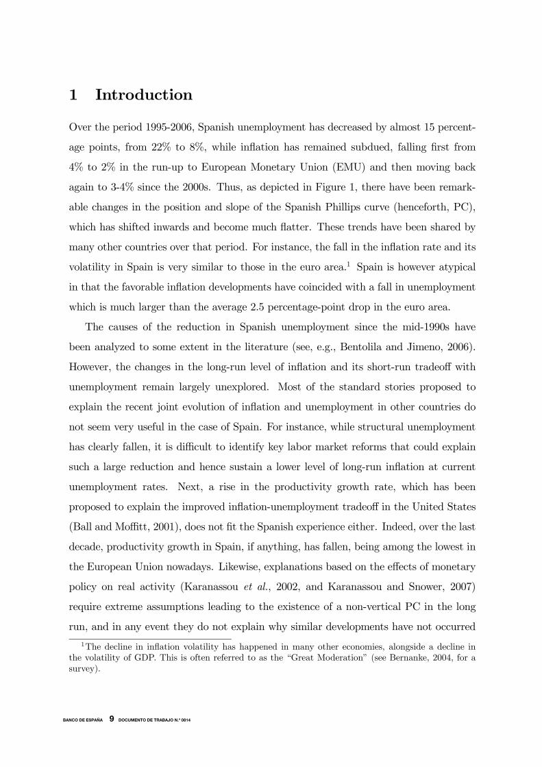
Over the period 1995-2006, Spanish unemployment has decreased by almost 15 percent-

age points, from 22% to 8%, while inflation has remained subdued, falling first from

4% to 2% in the run-up to European Monetary Union (EMU) and then moving back

again to 3-4% since the 2000s. Thus, as depicted in Figure 1, there have been remark-

able changes in the position and slope of the Spanish Phillips curve (henceforth, PC),

which has shifted inwards and become much flatter. These trends have been shared by

many other countries over that period. For instance, the fall in the inflation rate and its

volatility in Spain is very similar to those in the euro area.1 Spain is however atypical

in that the favorable inflation developments have coincided with a fall in unemployment

which is much larger than the average 2.5 percentage-point drop in the euro area.

The causes of the reduction in Spanish unemployment since the mid-1990s have

been analyzed to some extent in the literature (see, e.g., Bentolila and Jimeno, 2006).

However, the changes in the long-run level of inflation and its short-run tradeoff with

unemployment remain largely unexplored. Most of the standard stories proposed to

explain the recent joint evolution of inflation and unemployment in other countries do

not seem very useful in the case of Spain. For instance, while structural unemployment

has clearly fallen, it is difficult to identify key labor market reforms that could explain

such a large reduction and hence sustain a lower level of long-run inflation at current

unemployment rates. Next, a rise in the productivity growth rate, which has been

proposed to explain the improved inflation-unemployment tradeoff in the United States

(Ball and Moffitt, 2001), does not fit the Spanish experience either. Indeed, over the last

decade, productivity growth in Spain, if anything, has fallen, being among the lowest in

the European Union nowadays. Likewise, explanations based on the effects of monetary

policy on real activity (Karanassou et al., 2002, and Karanassou and Snower, 2007)

require extreme assumptions leading to the existence of a non-vertical PC in the long

run, and in any event they do not explain why similar developments have not occurred

1The decline in inflation volatility has happened in many other economies, alongside a decline inthe volatility of GDP. This is often referred to as the “Great Moderation” (see Bernanke, 2004, for asurvey).

1BANCO DE ESPAÑA 9 DOCUMENTO DE TRABAJO N.º 0814

1981

19851990

1994

1997

2006

0

2

4

6

8

10

12

14

8 10 12 14 16 18 20 22 24

Unemployment rate (%)

Infla

tion

rate

(%)

Figure 1: Inflation and unemployment in Spain, 1980-2006

in other European countries. It has also been argued that the opening of both the trade

and the capital account lead to a flattening of the PC (Razin and Loungani, 2007),

although other authors point out that if globalization increases competition and, hence,

makes wages and prices more flexible, the PC ought to become steeper, not flatter.2

Moreover, although trade openness has noticeably increased since the early 1990s, it

seems doubtful that it could sustain low inflation on its own, in the face of such a large

reduction in unemployment. Finally, EMU could have contributed to the flattening of

the PC, as low inflation expectations became better anchored. Still, why inflation did

not surge with the large reduction in unemployment is puzzling.

Recent studies on the inflation rate and its tradeoff with unemployment in Spain

have taken three different approaches. First, the sources of the Spanish persistent pos-

itive inflation differential vis-à-vis the rest of the Euro area have been analyzed within

calibrated dynamic stochastic general equilibrium models. This type of studies con-

cludes that the differential could be explained either by demand shocks biased towards

2See Ball (2006). Further discussion is found in Rogoff (2003) and Bean (2006).


non-tradable goods combined with real wage rigidities (López-Salido et al., 2005) or by

fluctuations in productivity growth in the tradable sector (Rabanal, 2006). Secondly,

as mentioned above, there is research on the possibility of a non-zero unemployment-

inflation tradeoff in the long-run Spanish PC, which focuses on the interaction between

money growth and nominal frictions by estimating reduced form inflation equations

(Karanassou et al., 2002). Lastly, and closer to our work, Galí and López-Salido (2001)

estimate a New Keynesian PC (NKPC) for the Spanish economy during the disinflation

period (1980-1998). They show that it fits the data quite well, though with a relatively

high degree of inflation persistence, and that the price of imported intermediate goods

and labor market frictions are the key factors driving the dynamics of marginal costs,

which determine inflation jointly with inflation expectations.

None of these studies, however, addresses a recent fundamental change affecting the

Spanish labor market, namely the immigration boom that has taken place since the

mid-1990s. The proportions of foreigners in the Spanish population and labor force were

both around 1% in 1995, while in 2006 they reached around 10% and 14%, respectively.

As we will discuss later, there have been very large waves of immigrants, specially since

2000, coming mainly from Latin America, North Africa, and Eastern Europe.

In this paper we aim at filling this gap by analyzing the consequences of immigration

for the joint behavior of unemployment and inflation. So far this topic has drawn little

attention in the literature on the PC. To our knowledge, only two recent papers tackle

it directly. On the one hand, Razin and Binyamini (2007) show that immigration and

outmigration raise the elasticities of labor supply and labor demand inducing a flat-

ter PC. On the other hand, Engler (2007) finds a similar result, albeit this time via

temporary outmigration of natives. Our approach differs from theirs in that we stress

other labor-market channels through which immigration can affect inflation determina-

tion. To the extent that wages are differently determined for natives and immigrants

—for instance if immigrants are less well represented by labor unions than natives— or

insofar as the marginal rate of substitution between consumption and leisure is different

for each group —immigrants tend to be more mobile and more willing to take low-paid

jobs than natives— expected marginal costs can fall as immigration increases. Through


these effects, we embed immigration into an otherwise standard NKPC with real wage

sluggishness, as proposed recently by Blanchard and Galí (2007). In this way, we derive

microfounded inflation equations that are estimated and used to account for the impact

of the immigration boom on the recent evolution of the Spanish PC.

The rest of the paper is structured as follows. In Section 2 we review in more detail

several hypotheses used in the literature to explain the changes in the PC in most major

economies, and discuss whether they fit the evidence for Spain. In Section 3 we document

the changes in the Spanish labor market since the mid-1990s, focusing on immigration.

In Section 4 we derive an NKPC when the labor market is composed of two worker types,

namely immigrants and natives. In Section 5 we discuss the results from estimating the

NKPC with immigration for Spain since the early 1980s. Section 6 contains evidence

about how our proposed NKPC performs at the industry level, given that immigration

is highly concentrated on some industries. Section 7 concludes. Two Appendices gather

some analytical derivations and a description of the data.

2 The joint fall of inflation and unemployment

The recent evolution of inflation and unemployment in Spain brings out three stylized

features: a reduction in inflationary expectations, a large fall in the structural unem-

ployment rate or NAIRU, and a flatter PC. While the fall in inflationary expectations is

clearly due to the change in the monetary policy regime in the late 1990s brought forth

by EMU, the factors behind the other two changes are less evident.

According to some estimates, the NAIRU has fallen from about 15% in 1996 to 9% in

2006 (Izquierdo and Regil, 2006). This is remarkable, as structural policy indicators do

not exhibit important changes. For instance, the “reform intensity indicator” of Brandt

et al. (2005) for 1994-2004 ranks Spain in the 24th position out of 30 OECD countries.

In fact, considering all institutions usually regarded as relevant in explaining structural

unemployment —tax wedge, employment protection legislation (EPL), unemployment

benefits, wage setting and industrial relations, working-time flexibility, incentives for la-

bor market participation, and product market regulation— Spain only shows noticeable


0

5

10

15

20

25

1980 1983 1986 1989 1992 1995 1998 2001 2004-4

-2

0

2

4

6

8

Unemployment rate (%) Labor productivity grow th (%) TFP grow th (%)

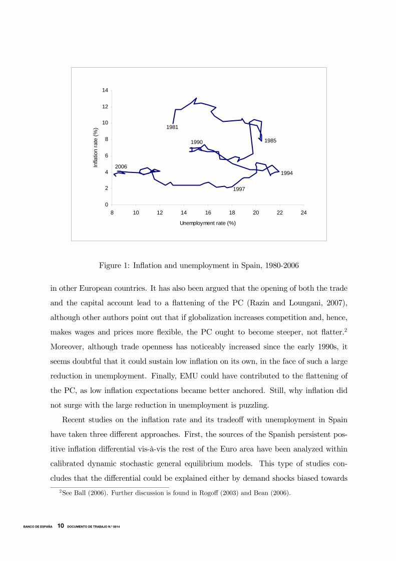
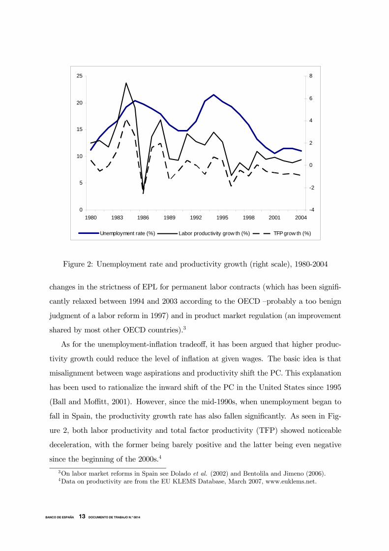
Figure 2: Unemployment rate and productivity growth (right scale), 1980-2004

changes in the strictness of EPL for permanent labor contracts (which has been signifi-

cantly relaxed between 1994 and 2003 according to the OECD —probably a too benign

judgment of a labor reform in 1997) and in product market regulation (an improvement

shared by most other OECD countries).3

As for the unemployment-inflation tradeoff, it has been argued that higher produc-

tivity growth could reduce the level of inflation at given wages. The basic idea is that

misalignment between wage aspirations and productivity shift the PC. This explanation

has been used to rationalize the inward shift of the PC in the United States since 1995

(Ball and Moffitt, 2001). However, since the mid-1990s, when unemployment began to

fall in Spain, the productivity growth rate has also fallen significantly. As seen in Fig-

ure 2, both labor productivity and total factor productivity (TFP) showed noticeable

deceleration, with the former being barely positive and the latter being even negative

since the beginning of the 2000s.4

3On labor market reforms in Spain see Dolado et al. (2002) and Bentolila and Jimeno (2006).4Data on productivity are from the EU KLEMS Database, March 2007, www.euklems.net.


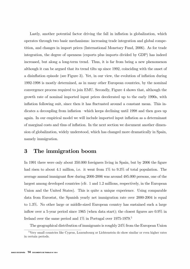
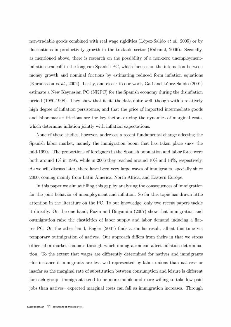
Lastly, another potential factor driving the fall in inflation is globalization, which

operates through two basic mechanisms: increasing trade integration and global compe-

tition, and changes in import prices (International Monetary Fund, 2006). As for trade

integration, the degree of openness (exports plus imports divided by GDP) has indeed

increased, but along a long-term trend. Thus, it is far from being a new phenomenon

although it can be argued that its trend tilts up since 1992, coinciding with the onset of

a disinflation episode (see Figure 3). Yet, in our view, the evolution of inflation during

1992-1998 is mostly determined, as in many other European countries, by the nominal

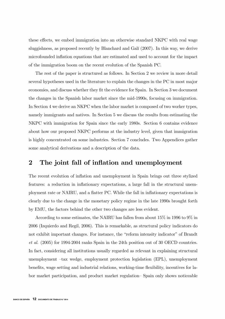
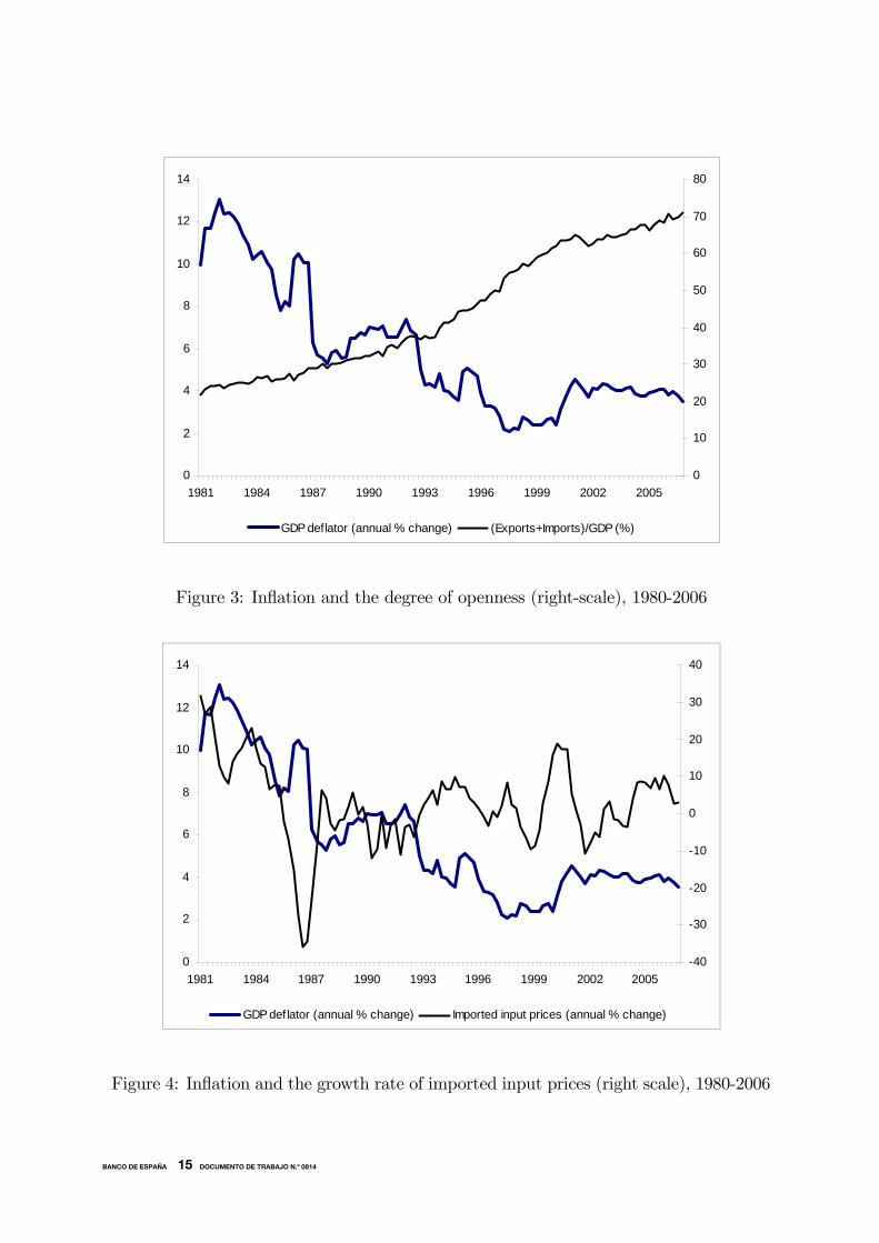
convergence process required to join EMU. Secondly, Figure 4 shows that, although the

growth rate of nominal imported input prices decelerated up to the early 1990s, with

inflation following suit, since then it has fluctuated around a constant mean. This in-

dicates a decoupling from inflation —which keeps declining until 1998 and then goes up

again. In our empirical model we will include imported input inflation as a determinant

of marginal costs and thus of inflation. In the next section we document another dimen-

sion of globalization, widely understood, which has changed more dramatically in Spain,

namely immigration.

3 The immigration boom

In 1991 there were only about 350.000 foreigners living in Spain, but by 2006 the figure

had risen to about 4.1 million, i.e. it went from 1% to 9.3% of total population. The

average annual immigrant flow during 2000-2006 was around 485.000 persons, one of the

largest among developed countries (cfr. 1 and 1.2 millions, respectively, in the European

Union and the United States). This is quite a unique experience. Using comparable

data from Eurostat, the Spanish yearly net immigration rate over 2000-2004 is equal

to 1.3%. No other large or middle-sized European country has sustained such a large

inflow over a 5-year period since 1965 (when data start); the closest figures are 0.9% in

Ireland over the same period and 1% in Portugal over 1975-1979.5

The geographical distribution of immigrants is roughly 24% from the European Union

5Very small countries like Cyprus, Luxembourg or Lichtenstein do show similar or even higher ratesin certain periods.


0

2

4

6

8

10

12

14

1981 1984 1987 1990 1993 1996 1999 2002 20050

10

20

30

40

50

60

70

80

GDP deflator (annual % change) (Exports+Imports)/GDP (%)

Figure 3: Inflation and the degree of openness (right-scale), 1980-2006

0

2

4

6

8

10

12

14

1981 1984 1987 1990 1993 1996 1999 2002 2005-40

-30

-20

-10

0

10

20

30

40

GDP deflator (annual % change) Imported input prices (annual % change)

Figure 4: Inflation and the growth rate of imported input prices (right scale), 1980-2006


and 76% from the rest of the world (34% from South America, 20% from Africa, 13%

from Eastern Europe, 5% from Asia, and 4% from other areas).6 Immigrants are over-

represented, vis-à-vis natives, in agriculture (7.4% vs. 5.6% in 2000-2006) and construc-

tion (17.8% vs. 11.5%), and under-represented in industry and services (though they

show high shares in some service industries, like home services, and hotels and catering).

For the most representative group of immigrants over the period 1996-2006, namely those

aged 20-45 years old from Eastern Europe, Africa, and Latin America, Fernández and

Ortega (2007) report that immigrants have slightly less schooling than natives (10.08

vs. 10.35 years, although those from Africa show a significantly lower figure, 7.5 years).

Nevertheless, 39% of them take jobs for which they are overqualified, vis-à-vis 17% of

natives.7

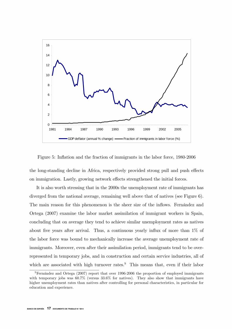
As seen in Figure 5, immigration flows started to increase around 1996 and acceler-

ated from 2000. Why did it happen precisely at those periods? Mostly due to prosperity.

The latest Spanish economic boom began in the second half of 1995. Then, in the 2000s,

Spain sustained high growth while many other European countries had low growth or

stagnation. Since 1995 Spanish GDP growth has surpassed the euro area average by

1.3% per year while the differential in Spanish employment growth has been a stag-

gering 2.9%, implying that Spain has created 48% of all new net jobs in the euro area

(OECD Economic Outlook database, June 2007). More specifically, the large fall in real

interest rates following the adoption of the euro favored industries with long and large

investments, like construction, which are intensive in unskilled labor. The progressive

rise in female labor force participation8 also increased the demand for household ser-

vices which migrants were ready to provide at low wages. Additionally, although there

has not been an active policy geared towards attracting immigrants, several amnesties

have granted legal residence to illegal immigrants (1996, 2000/2001, and 2005). These

forces, alongside the crises in several Latin American countries in the early 2000s and

6For a more detailed account of the stylised facts of immigration in Spain see Carrasco et al. (2007),and Dolado and Vázquez (2007).

7A worker is considered to be overeducated when his/her level of education is above the mean plusone standard deviation in his/her occupational category.

8For example, the participation rate of native females aged 24 to 54 years old rose from 57.5% in1996 to 67.8% in 2004.


0

2

4

6

8

10

12

14

16

1981 1984 1987 1990 1993 1996 1999 2002 2005

GDP deflator (annual % change) Fraction of immigrants in labor force (%)

Figure 5: Inflation and the fraction of immigrants in the labor force, 1980-2006

the long-standing decline in Africa, respectively provided strong pull and push effects

on immigration. Lastly, growing network effects strengthened the initial forces.

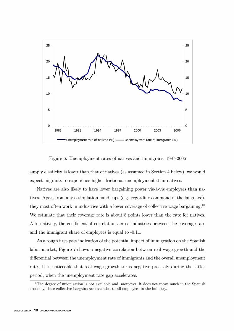
It is also worth stressing that in the 2000s the unemployment rate of immigrants has

diverged from the national average, remaining well above that of natives (see Figure 6).

The main reason for this phenomenon is the sheer size of the inflows. Fernández and

Ortega (2007) examine the labor market assimilation of immigrant workers in Spain,

concluding that on average they tend to achieve similar unemployment rates as natives

about five years after arrival. Thus, a continuous yearly influx of more than 1% of

the labor force was bound to mechanically increase the average unemployment rate of

immigrants. Moreover, even after their assimilation period, immigrants tend to be over-

represented in temporary jobs, and in construction and certain service industries, all of

which are associated with high turnover rates.9 This means that, even if their labor

9Fernández and Ortega (2007) report that over 1996-2006 the proportion of employed immigrantswith temporary jobs was 60.7% (versus 33.6% for natives). They also show that immigrants havehigher unemployment rates than natives after controlling for personal characteristics, in particular foreducation and experience.


0

5

10

15

20

25

1988 1991 1994 1997 2000 2003 20060

5

10

15

20

25

Unemployment rate of natives (%) Unemployment rate of immigrants (%)

Figure 6: Unemployment rates of natives and immigrans, 1987-2006

supply elasticity is lower than that of natives (as assumed in Section 4 below), we would

expect migrants to experience higher frictional unemployment than natives.

Natives are also likely to have lower bargaining power vis-à-vis employers than na-

tives. Apart from any assimilation handicaps (e.g. regarding command of the language),

they most often work in industries with a lower coverage of collective wage bargaining.10

We estimate that their coverage rate is about 8 points lower than the rate for natives.

Alternatively, the coefficient of correlation across industries between the coverage rate

and the immigrant share of employees is equal to -0.11.

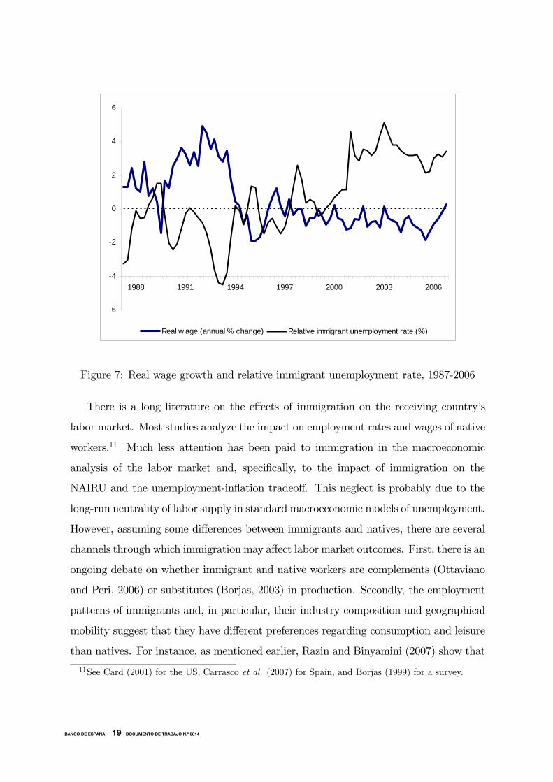
As a rough first-pass indication of the potential impact of immigration on the Spanish

labor market, Figure 7 shows a negative correlation between real wage growth and the

differential between the unemployment rate of immigrants and the overall unemployment

rate. It is noticeable that real wage growth turns negative precisely during the latter

period, when the unemployment rate gap accelerates.

10The degree of unionization is not available and, moreover, it does not mean much in the Spanisheconomy, since collective bargains are extended to all employees in the industry.


-6

-4

-2

0

2

4

6

1988 1991 1994 1997 2000 2003 2006

Real w age (annual % change) Relative immigrant unemployment rate (%)

Figure 7: Real wage growth and relative immigrant unemployment rate, 1987-2006

There is a long literature on the effects of immigration on the receiving country’s

labor market. Most studies analyze the impact on employment rates and wages of native

workers.11 Much less attention has been paid to immigration in the macroeconomic

analysis of the labor market and, specifically, to the impact of immigration on the

NAIRU and the unemployment-inflation tradeoff. This neglect is probably due to the

long-run neutrality of labor supply in standard macroeconomic models of unemployment.

However, assuming some differences between immigrants and natives, there are several

channels through which immigration may affect labor market outcomes. First, there is an

ongoing debate on whether immigrant and native workers are complements (Ottaviano

and Peri, 2006) or substitutes (Borjas, 2003) in production. Secondly, the employment

patterns of immigrants and, in particular, their industry composition and geographical

mobility suggest that they have different preferences regarding consumption and leisure

than natives. For instance, as mentioned earlier, Razin and Binyamini (2007) show that

11See Card (2001) for the US, Carrasco et al. (2007) for Spain, and Borjas (1999) for a survey.


immigration alters the elasticities of labor supply and labor demand, inducing a flatter

PC. Lastly, it is also likely that immigrants have a lower bargaining power than natives in

noncompetitive labor markets. Hence, a rise in the immigration flow increases the labor

intensity of production, changes the elasticity of labor supply, and decreases the markup

of wages over the marginal rate of substitution between consumption and leisure. In the

next section, we explicitly model how these three effects interact to change the PC.

4 An NKPC accounting for immigration

In this section we extend the standard analysis of the NKPC to take into account het-

erogeneity across two types of workers with different characteristics, namely immigrants

and natives. We first present the setup of the model and then solve for equilibrium with

real wage rigidity and monopoly power.

4.1 Model setup

As is standard in the literature on the NKPC, we start by assuming an economy with a

continuum of monopolistically competitive firms, each producing a differentiated product

(Q) and facing an isoelastic demand with price elasticity > 1. The production function

is constant returns to scale (CRS) Cobb-Douglas with two inputs, labor (N) and raw

materials (M). For simplicity, as in Blanchard and Galí (2007) (hereafter BG), we ignore

capital in the following analysis, so that Q should be interpreted stricto sensu as final

output net of capital compensation. The main novelty here with respect to most models

in this literature is the assumption that the labor input consists of two components, to

be interpreted as native (N1) and immigrant workers (N2). Since both types of workers

are bound to be imperfect substitutes, we aggregate them into the single labor-input

index (N) through a CES function. Hence,

Qt = N1−αt Mα

t (1)

Nρt = δ1N

ρ1t + δ2N

ρ2t , (2)


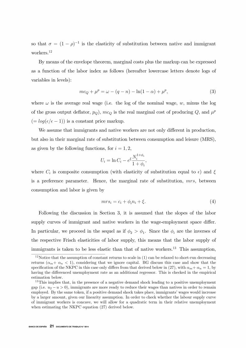
so that σ = (1 − ρ)−1 is the elasticity of substitution between native and immigrant

workers.12

By means of the envelope theorem, marginal costs plus the markup can be expressed

as a function of the labor index as follows (hereafter lowercase letters denote logs of

variables in levels):

mcQ + µp = ω − (q − n)− ln(1− α) + µp, (3)

where ω is the average real wage (i.e. the log of the nominal wage, w, minus the log

of the gross output deflator, pQ), mcQ is the real marginal cost of producing Q, and µp

(= log( / − 1)) is a constant price markup.We assume that immigrants and native workers are not only different in production,

but also in their marginal rate of substitution between consumption and leisure (MRS),

as given by the following functions, for i = 1, 2,

Ui = lnCi − eξN1+φii

1 + φi,

where Ci is composite consumption (with elasticity of substitution equal to ) and ξ

is a preference parameter. Hence, the marginal rate of substitution, mrs, between

consumption and labor is given by

mrsi = ci + φini + ξ. (4)

Following the discussion in Section 3, it is assumed that the slopes of the labor

supply curves of immigrant and native workers in the wage-employment space differ.

In particular, we proceed in the sequel as if φ2 > φ1. Since the φi are the inverses of

the respective Frisch elasticities of labor supply, this means that the labor supply of

immigrants is taken to be less elastic than that of native workers.13 This assumption,12Notice that the assumption of constant returns to scale in (1) can be relaxed to short-run decreasing

returns (αm+ αn < 1), considering that we ignore capital. BG discuss this case and show that thespecification of the NKPC in this case only differs from that derived below in (27), with αm+ αn = 1, byhaving the differenced unemployment rate as an additional regressor. This is checked in the empiricalestimation below.13This implies that, in the presence of a negative demand shock leading to a positive unemployment

gap (i.e. u2− u > 0), immigrants are more ready to reduce their wages than natives in order to remainemployed. By the same token, if a positive demand shock takes place, immigrants’ wages would increaseby a larger amount, given our linearity assumption. In order to check whether the labour supply curveof immigrant workers is concave, we will allow for a quadratic term in their relative unemploymentwhen estimating the NKPC equation (27) derived below.


however, can be tested later in the empirical section.

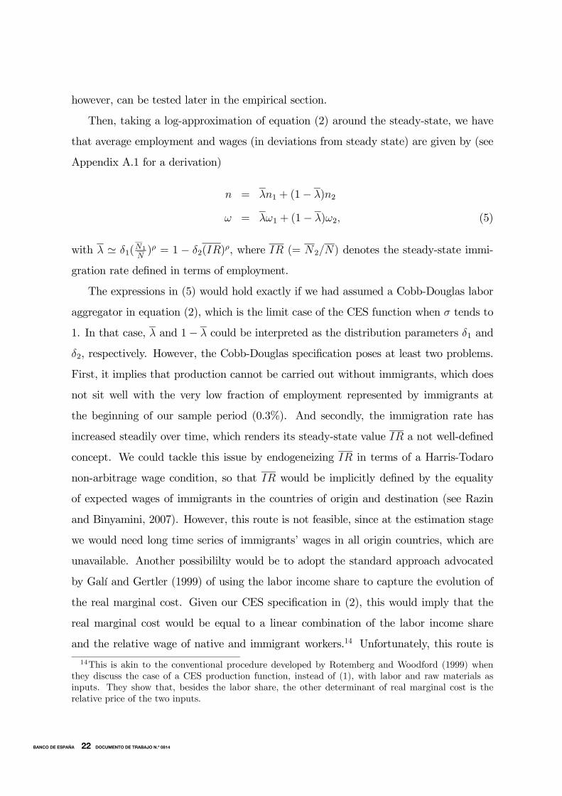
Then, taking a log-approximation of equation (2) around the steady-state, we have

that average employment and wages (in deviations from steady state) are given by (see

Appendix A.1 for a derivation)

n = λn1 + (1− λ)n2

ω = λω1 + (1− λ)ω2, (5)

with λ ' δ1(N1

N)ρ = 1 − δ2(IR)

ρ, where IR (= N2/N) denotes the steady-state immi-

gration rate defined in terms of employment.

The expressions in (5) would hold exactly if we had assumed a Cobb-Douglas labor

aggregator in equation (2), which is the limit case of the CES function when σ tends to

1. In that case, λ and 1− λ could be interpreted as the distribution parameters δ1 and

δ2, respectively. However, the Cobb-Douglas specification poses at least two problems.

First, it implies that production cannot be carried out without immigrants, which does

not sit well with the very low fraction of employment represented by immigrants at

the beginning of our sample period (0.3%). And secondly, the immigration rate has

increased steadily over time, which renders its steady-state value IR a not well-defined

concept. We could tackle this issue by endogeneizing IR in terms of a Harris-Todaro

non-arbitrage wage condition, so that IR would be implicitly defined by the equality

of expected wages of immigrants in the countries of origin and destination (see Razin

and Binyamini, 2007). However, this route is not feasible, since at the estimation stage

we would need long time series of immigrants’ wages in all origin countries, which are

unavailable. Another possibililty would be to adopt the standard approach advocated

by Galí and Gertler (1999) of using the labor income share to capture the evolution of

the real marginal cost. Given our CES specification in (2), this would imply that the

real marginal cost would be equal to a linear combination of the labor income share

and the relative wage of native and immigrant workers.14 Unfortunately, this route is

14This is akin to the conventional procedure developed by Rotemberg and Woodford (1999) whenthey discuss the case of a CES production function, instead of (1), with labor and raw materials asinputs. They show that, besides the labor share, the other determinant of real marginal cost is therelative price of the two inputs.


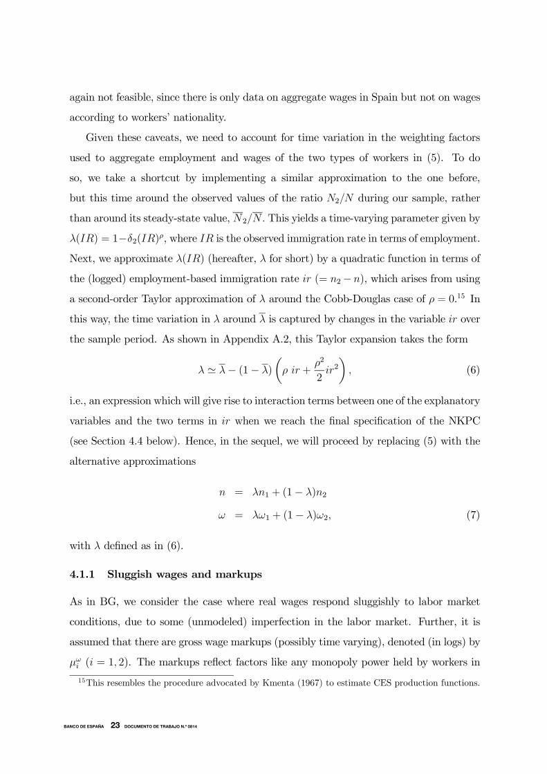
again not feasible, since there is only data on aggregate wages in Spain but not on wages

according to workers’ nationality.

Given these caveats, we need to account for time variation in the weighting factors

used to aggregate employment and wages of the two types of workers in (5). To do

so, we take a shortcut by implementing a similar approximation to the one before,

but this time around the observed values of the ratio N2/N during our sample, rather

than around its steady-state value, N2/N. This yields a time-varying parameter given by

λ(IR) = 1−δ2(IR)ρ, where IR is the observed immigration rate in terms of employment.Next, we approximate λ(IR) (hereafter, λ for short) by a quadratic function in terms of

the (logged) employment-based immigration rate ir (= n2−n), which arises from using

a second-order Taylor approximation of λ around the Cobb-Douglas case of ρ = 0.15 In

this way, the time variation in λ around λ is captured by changes in the variable ir over

the sample period. As shown in Appendix A.2, this Taylor expansion takes the form

λ ' λ− (1− λ)

µρ ir +

ρ2

2ir2¶, (6)

i.e., an expression which will give rise to interaction terms between one of the explanatory

variables and the two terms in ir when we reach the final specification of the NKPC

(see Section 4.4 below). Hence, in the sequel, we will proceed by replacing (5) with the

alternative approximations

n = λn1 + (1− λ)n2

ω = λω1 + (1− λ)ω2, (7)

with λ defined as in (6).

4.1.1 Sluggish wages and markups

As in BG, we consider the case where real wages respond sluggishly to labor market

conditions, due to some (unmodeled) imperfection in the labor market. Further, it is

assumed that there are gross wage markups (possibly time varying), denoted (in logs) by

µωi (i = 1, 2). The markups reflect factors like any monopoly power held by workers in

15This resembles the procedure advocated by Kmenta (1967) to estimate CES production functions.


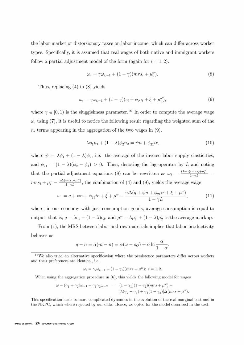
the labor market or distorsionary taxes on labor income, which can differ across worker

types. Specifically, it is assumed that real wages of both native and immigrant workers

follow a partial adjustment model of the form (again for i = 1, 2):

ωi = γωi,−1 + (1− γ)(mrsi + µωi ). (8)

Thus, replacing (4) in (8) yields

ωi = γωi,−1 + (1− γ)(ci + φini + ξ + µωi ), (9)

where γ ∈ [0, 1) is the sluggishness parameter.16 In order to compute the average wageω, using (7), it is useful to notice the following result regarding the weighted sum of the

ni terms appearing in the aggregation of the two wages in (9),

λφ1n1 + (1− λ)φ2n2 = ψn+ φ21ir, (10)

where ψ = λφ1 + (1 − λ)φ2, i.e. the average of the inverse labor supply elasticities,

and φ21 = (1 − λ)(φ2 − φ1) > 0. Then, denoting the lag operator by L and noting

that the partial adjustment equations (8) can be rewritten as ωi =(1−γ)(mrsi+µωi )

1−γL =

mrsi + µωi − γ∆(mrsi+µωi )

1−γL , the combination of (4) and (9), yields the average wage

ω = q + ψn+ φ21ir + ξ + µω − γ∆(q + ψn+ φ21ir + ξ + µω)

1− γL, (11)

where, in our economy with just consumption goods, average consumption is equal to

output, that is, q = λc1 + (1− λ)c2, and µω = λµω1 + (1− λ)µω2 is the average markup.

From (1), the MRS between labor and raw materials implies that labor productivity

behaves as

q − n = α(m− n) = α(ω − sQ) + α lnα

1− α,

16We also tried an alternative specification where the persistence parameters differ across workersand their preferences are identical, i.e.,

ωi = γiωi,−1 + (1− γi)(mrs+ µω); i = 1, 2.

When using the aggregation procedure in (6), this yields the following model for wages

ω − (γ1 + γ2)ω−1 + γ1γ2ω−2 = (1− γ1)(1− γ2)(mrs+ µω) +

[λ(γ2 − γ1) + γ1(1− γ2)]∆(mrs+ µω).

This specification leads to more complicated dynamics in the evolution of the real marginal cost and inthe NKPC, which where rejected by our data. Hence, we opted for the model described in the text.


where sQ is the real price of raw materials (i.e., the log of its nominal price, pm, minus

pQ). Thereby, substituting this expression into (11), yields an equation describing the

dynamic evolution of real wages from the workers’ side:

ω = Γω−1 +1− Γ

1− α[α ln

α

1− α+ (1 + ψ)n+ φ21ir + ξ − αsQ + µω], (12)

with Γ = γ1−α+γα < 1.

4.2 First-best equilibrium

The next step is to derive the first-best price equilibrium in this economy. This corre-

sponds to the case where prices and wages are flexible (γ = 0), and labor and goods

markets are perfectly competitive, i.e. µω = µp = 0. In such an equilibrium, from the

firms’ side, the real aggregate wage would be equal to the marginal product of labor

(mpn), that is, ω = mpn = q− n+ ln(1−α). Similarly, from the workers’ side, the real

wage would be equal to the marginal rate of substitution, that is, ω = q+ψn+φ21ir+ξ.

Therefore, equating both expressions and labeling the first-best equilibrium value of a

generic variable x by xF , we have that the employment of natives and immigrants in

this equilibrium satisfy the following condition

(1 + ψ) nF + φ21irF= ln(1− α)− ξ. (13)

4.3 Equilibrium with real wage rigidities and monopoly power

Going back to our economy with labor market frictions and monopolistic power in the

goods and labor markets, substitution of (13) into (12) yields the evolution of the wage-

setting from the workers’ side,

ω = Γω−1 +1− Γ

1− α[α lnα+ (1− α) ln(1− α)− αsQ + µω + (1 + ψ)en+ φ21eir], (14)

where en (= n − nF ) and eir (= ir − irF) are the deviations of n and ir from their

corresponding first-best equilibrium values.

From the firms’ side we have thatmcQ+µp = ω−mpn+µp. Then, inserting (14) into

this expression and using (1) yields the following equation describing the corresponding


dynamic evolution of the real marginal cost of gross output

(1−ΓL)(mcQ+µp) =(1− Γ)(1 + ψ)

1− αeq+(1−Γ)φ21eir+αΓ∆sQ+(1−Γ)(µω+µp), (15)

where eq = q − qF .

4.4 Unemployment and immigration in the marginal cost

In order to express (15) in terms of observables, namely the unemployment (u) and

immigration rates, we follow BG in assuming that the (logged) labor supplies ( i) and

the relative labor supply of immigrants vis-à-vis natives (irl = 2 − 1) are implicitly

defined by:

ω = q + ψ + φ21irl + ξ + µω. (16)

That is, and irl measure the notional quantities of labor that native and immigrant

workers would like to supply given their current wage, marginal utility of income, and

steady-state wage markup, µω. Hence, from the firms’ side, substitution of (16) into (3),

yields

mcQ + µp = (1 + ψ) − ( − n) + ξ − ln(1− α) + φ21irl + µω + µp. (17)

Next, making use of the standard approximation u ' − n, noticing that irl =

(irl − irF) + ir

F, and recalling the first-best equilibrium condition (13), implies that

(17) can be rewritten as

mcQ + µp =1 + ψ

1− αeq + ψu+ φ21(irl − ir

F) + µω + µp. (18)

Hence, solving for (1+ψ)eq/(1−α) in (18) and replacing it in (15), yields the followingequation describing the evolution of mcQ+ µp in terms of observables

∆(mcQ + µp) = −1− Γ

Γ[ψu+ φ21(u2 − u)− eµω] + α∆sQ, (19)

where eµw = µω−µω, and use has been made of the result that irl− ir = ( 2− )− (n2−n) ' u2 − u, i.e. the difference between the unemployment rate of immigrants and the

aggregate unemployment rate.


4.4.1 Interaction terms with immigration

The next step is to notice that parameters ψ and φ21 depend on the time-varying weight

λ, derived in (6). Thus we need to express equation (19) in terms of constant parameters.

To do so, it is useful to notice that, since ψ = φ1+(1−λ)(φ2−φ1) = φ1+φ21, the linear

combination of unemployment rates given by ψu+ φ21(u2− u) in (19), can be rewritten

as follows (see Appendix A.2)

ψu+ φ21(u2 − u) = ψu+ φ21(u2 − u) + ρφ21u2ir +ρ2

2φ21u2ir

2, (20)

where ψ = φ1+φ21 and φ21 = (1−λ)(φ2−φ1), with λ interpreted as in (5). Substitutionof (20) into (19) yields an alternative specification of (19) in terms of constant rather

than changing parameters, in which two new interaction terms of u2 with ir and ir2

appear, namely

∆(mcQ+µp) = −1− Γ

Γ[ψu+φ21(u2− u)+ ρφ21u2ir+

ρ2

2φ21u2ir

2− eµω] +α∆sQ. (21)

Finally, deviations of the wage markup from its steady-state value, i.e. eµw 6= 0,

would also alter the marginal cost (see Galí et al., 2001, for a discussion). As explained

in Appendix A.3, in a right-to-manage model of wage determination by firms and unions,

among other alternatives, a labor supply shift due to immigration can be captured by a

rise in u2 − u —since it is likely that immigrants will take longer than natives in finding

a job— which, in turn, could be interpreted as implying a fall in eµw. For simplicity, weassume a linear relationship of the form eµw = −ν(u2 − u), so that (21) becomes:

∆(mcQ+µp) = −1− Γ

Γ[ψu+(φ21+ ν)(u2−u)+ρφ21u2ir+

ρ2

2φ21u2ir

2] +α∆sQ. (22)

Notice that the term in u2−u plus the two interaction terms in u2 and ir are the newvariables that our model adds to the specification proposed by BG in a similar model

where immigration is ignored. The intuition behind these effects is as follows. First,

insofar as the unemployment rate of immigrants is higher than the unemployment rate of

natives, this will induce a reduction in the marginal cost both via lower wages —because

immigrants have a less elastic labor supply than natives—17 and through a reduction17Think of a negative labor demand shift: wages fall more the less elastic is labor supply. Here the

shift is one that reduces immigrants’ employment more than natives’.


in the wage markup set by unions. Further, in our model the interaction terms give

rise to the convenient property that these effects of the u2 − u gap depend on the size

of the immigration rate in the economy: the higher is the immigration rate the larger

will be the reduction in inflation brought about by the unemployment rate differential.

Alternatively, these effects on the marginal cost will more sizeable in economies with

large immigration rates than in those with low immigration.

4.4.2 Gross output and GDP deflators

Before turning to the final specification of NKPC equation, a final issue to be addressed

is that, according to our interpretation of Q in (1), equation (22) yields the determinants

of the marginal cost of producing gross output, rather than value added (GDP). Since a

time series of the gross output deflator, pQ, is not available for Spain (only nominal gross

output at current prices is available), we need to reinterpret (22) in terms of the GDP

deflator, p, which is the series we will use in the empirical section below to construct

the inflation rate in the NKPC. The assumption of a Cobb-Douglas production function

in (1) implies separability between raw materials and the labor input used to produce

GDP. Hence, it follows that ∆(mcQ + µp) = ∆(mc+ µp), where mc is the real marginal

cost of producing GDP. Consequently, the only variable in the right-hand-side of (22)

that needs to be changed is the real price of raw materials, sQ, which was deflated by

pQ. To replace pQ by p in this real price, we make use of the fact the former price index

is implicitly defined by pQ = (1− χ)p+ χpm or pQ = p+ χsm, where s = pm − p and χ

is the share of the value of imports in nominal gross output, as reported in the national

accounts. Hence, the changes in sQ and s are related by

∆sQ = ∆s− (∆pQ −∆p) = ∆s− χ(∆pm −∆p) = (1− χ)∆s. (23)

Substitution of (23) into (22) yields the final specification of the real marginal cost

of producing GDP

∆(mc+µp) = −1− Γ

Γ[ψu+(φ21+ν)(u2−u)+ρφ21u2ir+

ρ2

2φ21u2ir

2]+α(1−χ)∆s. (24)

Notice that there is a difference between the shares of raw materials α and χ. As

argued above, we have that χ = PmM/PQQ, whereas, denoting capital compensation


by rK, α = PmM/(PQQ− rK), since capital has been ignored as an input of Q in (1).

Therefore, χ < α. In any case, the coefficient on ∆s in the above equation is positive

since α(1− χ) > 0.

An important feature of (23) is that the marginal cost of producing GDP has a unit

root as long as 0 < Γ < 1, i.e. 0 < γ < 1. As will be shown below, this implies that the

NKPC has the appealing property that inflation is in the long run independent of real

factors, which only influence the change in inflation. As explained in Appendix A.4, the

insight behind this property is the presence of real rigidities, either in wages (as in the

present model) or in the price-setting rule.

4.5 Alternative specifications of the NKPC

Having derived the evolution of the real marginal cost, the last step is to obtain an

NKPC linking it to inflation. For that, we use the two well-known alternatives proposed

by Galí and Gertler (1999): the forward-looking model (FNPC) and the hybrid (i.e., a

combination of forward and backward-looking price-setters) model (HNPC). These two

specifications are given (introducing time subscripts), respectively by

πt = βEtπt+1 + κf(mct + µp) (25)

πt =βθ

τEtπt+1 +

ς

τπt−1 +

κhτ(mct + µp), (26)

where πt (≡ pt−pt−1) is the inflation rate in period t, Etπt+1 is the (rational) expectation

of inflation in t+1 conditional on all information available up to t, κf = (1−βθ)(1−θ)/θ,κh = (1− ς)(1− βθ)(1− θ), and τ = θ + ς[1− θ(1− β)]. In these expressions, β is the

discount rate, 1− θ is the probability that firms are allowed to optimally reset prices in

period t according to Calvo’s (1983) model, and ς is the proportion of firms which use

the simple backward-looking rule of thumb proposed by Galí and Gertler (1999).18

Substituting (22) into (25) and (26) yields the two specifications of the NKPC with

immigration that we estimate below. The forward-looking PC with immigration (FN-

18As discussed in Appendix A.4 a similar NKPC can be derived using Rotemberg’s (1982) quadraticadjustment cost model of changing prices.


PCI) is

πt = ψf1Etπt+1 + ψf

2πt−1 −(1− Γ)κf(1 + β)Γ

[ψut + (φ21 + ν)(u2t − ut)

+ρφ21u2tirt +ρ2

2φ21u2tir

2t ] +

α(1− χ)κf1 + β

∆st, (27)

with ψf1 = β/(1+β) and ψf

2 = 1/(1+β). Hence, everything else equal, (27) establishes a

tradeoff between the change in inflation, ∆π, and the unemployment rate, u. It is worth

noticing that in this specification both the intercept and the slope (with respect to ut)

of the standard PC are shifted by the presence of immigrants. In effect, in the absence

of immigration (i.e. φ21 = ν = 0, λ = 1), the slope of the PC in the (∆π, u) plane will

be −κf (1−Γ)Γ(1+β)

φ1, since ψ = φ1 when φ21 = 0, as in BG. By contrast, with immigration, for

given values of u2 and ir, the slope becomes −κf (1−Γ)Γ(1+β)

¡ψ − φ21 − ν

¢= −κf (1−Γ)

Γ(1+β)(φ1 − ν)

so that the PC is flatter than in the previous case. Likewise, with immigration the

intercept shifts downwards by −κf (1−Γ)Γ(1+β)

[¡φ21 − ν

¢u2t + ρφ21u2tirt +

ρ2

2φ21u2tirt

2]. Notice

that both changes are therefore in line with the evolution of the Spanish PC during the

last decade or so, as shown in Figure 1.

The hybrid PC with immigration (HNPCI), in turn, becomes:

πt = ψh1Etπt+1 + ψh

2πt−1 + ψh3πt−2 −

τ(1− Γ)κh(τ + βθ)Γ

[ψut + (φ21 + ν)(u2t − ut)

+ρφ21u2tirt +ρ2

2φ21u2tir

2t ] +

ατ(1− χ)κhτ + βθ

∆st, (28)

with ψh1 = βθ/(τ+βθ), ψh

2 = (τ+ς)/(τ+βθ), and ψh3 = −ς/(τ+βθ). Thus, ψh

1+ψh2+ψ

h3 =

1, so that, as before, the NKPC is vertical in the long run.

Inspection of (27) shows that this specification leads to the presence of forward and

backward components of inflation in the NKPCwithout having to rely on the existence of

firms which use a simple backward-looking rule of thumb to set prices. By contrast, when

this type of firms is considered in (28), the backward component of inflation has two lags,

the first one with a positive coefficient and the second one with a negative coefficient.

These implications will be used to discriminate between the two specifications of the

NKPC.

Given the long-run neutrality property, we can define the concept of fundamental

change of inflation, ∆π∗t , along the lines of Galí and Gertler (1999) and Galí et al.


(2001), to then integrate forwards this variable in order to calculate the fundamental

level of inflation, π∗t . In what follows we illustrate this procedure with the FNPCI

specification, since the approach for the HNPCI is similar but more cumbersome. First,

by iterating (27) forward, we obtain

∆π∗t = (1 + β)∞Xj=0

βjEtbxt+j | zt, (29)

where in our empirical application, zt = [bxt, bxt−1, bxt−2, πt, πt−1, πt−2] andbxt = −(1− Γ)κf

(1 + β)Γ[ψut + (φ21 + ν)(u2t − ut)

+ρφ21u2tirt +ρ2

2φ21u2tir

2t ] +

α(1− χ)κf1 + β

∆st.

Next, we construct bxt using the coefficients in our estimated FNPCI and, to computeforecasts of its future values, we run a second-order vector autoregression of the bivariate

system formed by ∆πt and bxt. Letting A denote the companion matrix of the VAR(1)

representation of zt, we have that Etbxt+j | zt = e01Ajzt, where e1 is a vector with 1 in

its first position and zeros elsewhere. Hence:

∆π∗t = (1 + β)e01(I − βA)−1zt, (30)

using the standard result that Σ∞j=0βjAj = (I − βA)−1 for a matrix A with eigenvalues

less that unity.

5 Empirical results

In this section we present our estimates of the model. We estimate first the forward-

looking specification in equation (27):

Et[πt−α1πt+1−α2πt−1−α3ut−α4(u2t− ut)−α5u2tirt−α6u2tir2t −α7∆st] Zt (31)

by the Generalized Method of Moments (GMM), using a set of instruments, Zt, consist-

ing of a constant and, as is standard in the literature (see e.g. Galí et al., 2003), four

lags of the following variables: the inflation rate (πt), the relative unemployment rate

of immigrants (u2t − ut), the log share of immigrants in employment (irt), the inflation


rate of imported inputs (∆st) —which proxies for the total intermediate input prices that

appear in the model—, and the labor income share. We also include two lags of the

following variables: cyclical output (with the trend estimated with the Hodrick-Prescott

filter using a parameter of 1,600) and of an index of the degree of globalization of the

Spanish economy.19 Detailed definitions of all variables appear in Appendix B. The data

start in 1980:1 but given the lead and lags involved, our effective estimation period is

1982:1-2006:3. There is no data on the split of the labor force between natives and immi-

grants before 1987:2, which forces us to assume that they had the same unemployment

rate through that date. However, this is not an important limitation since during that

period immigration only represented 0.3% of the labor force on average.

Column (1) in Table 1 presents the estimated coefficients in the unrestricted specifi-

cation of equation (27). All coefficients are statistically significant and have the expected

signs. In particular, the relative immigrant unemployment rate and the interactions of

the immigrants’ unemployment rate with their (logged) share in employment and its

square all have negative effects on inflation, as predicted by the model. In other words,

the negative signs on these estimated coefficients indicate that our claim that immigrants

have a lower labor supply elastiticy than natives (φ21 > 0) is strongly supported by the

data. The unrestricted value of the discount rate β implied by the coefficient on lagged

inflation is 0.972, which is higher and more realistic than those found in the literature.

For instance, Galí et al. (2003) find values between 0.84 and 0.92 for the euro area, and

Galí and López-Salido (2001) between 0.75 and 0.85 for Spain over the period 1990-1998.

To check whether this model is appropriate, we perform several tests of our proposed

specification in (27) against the most relevant modelling alternatives that were discussed

before, namely: (i) constant vs. decreasing returns to scale in (1) (see footnote 11), (ii)

a linear vs. a concave shape of immigrant workers’ labor supply (see footnote 12), and

(iii) the unemployment rate gap against the labor force differential as the determinant

of the wage markup (see Appendix A.3). As regards (i), following BG (Appendix 3),

we included the first differences of ut and u2t − ut as additional regressors in (27) and

19The higher the degree of globalization, the higher should be the immigrant flow, e.g. attracted byforeign investment.


tested for the joint significance of their coefficients; this yielded a p-value of 0.132 in the

corresponding χ2(2) test, so that we are not able to reject the null of constant returns

to scale. With regard to (ii), a quadratic term in u2t−ut was added; again its estimated

coefficient was not statistically significant (t-ratio=1.35).20 Finally, regarding (iii), we

added the relative labor force, 2t− t, to the list of regressors, obtaing once more a non-

significant effect (t-ratio=1.13). In view of these results, we keep (27) as our preferred

unrestricted model, which we use for testing the remaining restrictions implied by the

underlying structural parameters.

In Column (1), the sum of the coefficients on future and lagged inflation is very close

to unity, as implied by the model. A Wald test of this null hypothesis yields a p-value of

0.22. Thus we impose this restriction to gain efficiency, with a value for the coefficient

on lagged inflation of 0.490, implying a value for β of 0.961. Column (2) shows the

restricted estimates, which are very similar to those in Column (1). This set of results

allows us to account for the flattening of the standard PC (i.e. the slope of inflation

vis-à-vis unemployment) by the presence of the new term in the relative unemployment

rate of immigrants. The slope falls from -0.112 to -0.032, so that the PC becomes

significantly flatter. We also saw in Figure 1 that there were shifts in the intercept of

the PC. If we take the stable PC traced for the period before the rise in immigration that

is apparent in the graph, i.e. from 1990:1 to 1994:1, and compare its intercept to that

of the subsequent stable locus, from say 1998:4 to 2006:4, we find that it shifts by 0.44

percentage points, due to the introduction of the three immigrantion-related variables.21

20As pointed out earlier, immigrant workers in Spain tend to achieve similar unemployment rates asnatives five years after arrival. Thus, lack of concavity in the relative unemployment may mean higherinflation pressure in the future. However, as also mentioned, even after their assimilation period, immi-grants tend to be over-represented in temporary and low-skilled jobs, for which they are overqualified.This may reduce inflationary pressure since the real unit labor costs associated to these jobs are lower.21Computed as the difference across averages over those two periods of the magnitude: bα4u2t +bα5u2tirt + bα6u2tir2t .


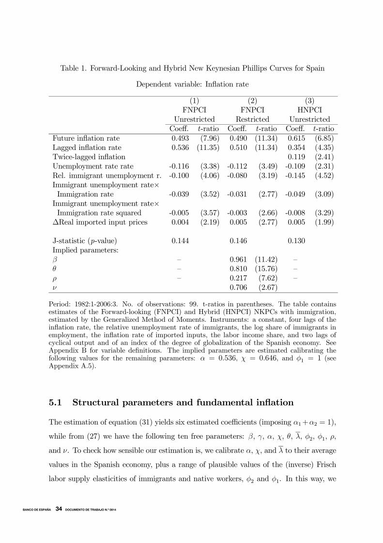
Table 1. Forward-Looking and Hybrid New Keynesian Phillips Curves for Spain

Dependent variable: Inflation rate

(1) (2) (3)FNPCI FNPCI HNPCI

Unrestricted Restricted UnrestrictedCoeff. t-ratio Coeff. t-ratio Coeff. t-ratio

Future inflation rate 0.493 (7.96) 0.490 (11.34) 0.615 (6.85)Lagged inflation rate 0.536 (11.35) 0.510 (11.34) 0.354 (4.35)Twice-lagged inflation 0.119 (2.41)Unemployment rate rate -0.116 (3.38) -0.112 (3.49) -0.109 (2.31)Rel. immigrant unemployment r. -0.100 (4.06) -0.080 (3.19) -0.145 (4.52)Immigrant unemployment rate×Immigration rate -0.039 (3.52) -0.031 (2.77) -0.049 (3.09)Immigrant unemployment rate×Immigration rate squared -0.005 (3.57) -0.003 (2.66) -0.008 (3.29)

∆Real imported input prices 0.004 (2.19) 0.005 (2.77) 0.005 (1.99)

J-statistic (p-value) 0.144 0.146 0.130Implied parameters:β — 0.961 (11.42) —θ — 0.810 (15.76) —ρ — 0.217 (7.62) —ν 0.706 (2.67)

Period: 1982:1-2006:3. No. of observations: 99. t-ratios in parentheses. The table containsestimates of the Forward-looking (FNPCI) and Hybrid (HNPCI) NKPCs with immigration,estimated by the Generalized Method of Moments. Instruments: a constant, four lags of theinflation rate, the relative unemployment rate of immigrants, the log share of immigrants inemployment, the inflation rate of imported inputs, the labor income share, and two lags ofcyclical output and of an index of the degree of globalization of the Spanish economy. SeeAppendix B for variable definitions. The implied parameters are estimated calibrating thefollowing values for the remaining parameters: α = 0.536, χ = 0.646, and φ1 = 1 (seeAppendix A.5).

5.1 Structural parameters and fundamental inflation

The estimation of equation (31) yields six estimated coefficients (imposing α1+α2 = 1),

while from (27) we have the following ten free parameters: β, γ, α, χ, θ, λ, φ2, φ1, ρ,

and ν. To check how sensible our estimation is, we calibrate α, χ, and λ to their average

values in the Spanish economy, plus a range of plausible values of the (inverse) Frisch

labor supply elasticities of immigrants and native workers, φ2 and φ1. In this way, we


are able to identify some of the underlying structural parameters: β, θ, ρ, and ν (see

Appendix A.4 for details).22 We obtain a value for θ, the fraction of firms that keep

their prices unchanged per quarter, of 0.810, which is in line with the estimates of Galí

et al. (2003) for the Euro area (from 0.78 to 0.87) and of Galí and López-Salido (2001)

for Spain (from 0.84 to 0.91). Our quarterly estimate of θ implies that the average time

over which a price is fixed, given by 1/(1− θ), is 1.3 years. This is close to the survey

evidence about the price-setting behavior of Spanish firms at the end of our sample

period (2003-2004) reported in Fabiani et al. (2006), according to which the average

duration of unchanged prices in Spain is one year.

As for the remaining parameters, we obtain an elasticity of substitution between

native and immigrant workers of σ = 1.277 (ρ = 0.217), which implies that they are

gross substitutes but not too far from the Cobb-Douglas case (σ = 1). Under the

plausible assumption that φ1 is unity, the implied estimate of the effect of immigration

on the wage markup is ν ' 0.7, being rather robust to a wide range of larger values ofφ2, so that for each percentage point increase in immigration the wage markup decreases

by about 0.7 percentage points. We do not have any other empirical evidence in the

literature to check how sensible this finding is, though it agrees with the fact that the

growth of real wages has been slightly negative since the mid-1990s, as shown in Figure

7, when the Spanish economy entered a long expansion which still lasts today.

In order to check how the model explains the evolution of inflation, we estimate the

fundamental inflation rate as described in Section 4. To compute forecasts of a single

right-hand side variable determining inflation we use the coefficients presented in column

(2) of Table 1. We then run a second-order vector autoregression of inflation changes

and the deviations of xt from its sample mean, and then apply equation (30), which is

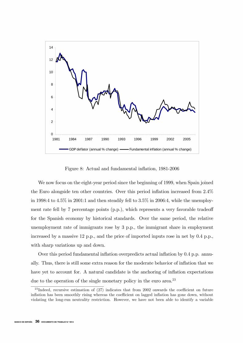
integrated forward. As can be observed, the resulting fundamental inflation, shown in

Figure 8, tracks observed inflation surprisingly well.

22Notice that an estimate of the real wage sluggishness, γ, cannot be directly identified from (27).However, an indirect estimate can be recovered from the coefficient of the lagged dependent variable,ωt−1, when estimating by GMM the partial adjustment model for the real wage in (12), with four lagsof the regressors as instruments. This yields bΓ = 0.713 (t-ratio=12.56). Hence, using Γ = γ

1−α+γα withthe calibrated value for α = 0.536 (see Appendix A.4), we get bγ = 0.535 (t-ratio=7.43).


0

2

4

6

8

10

12

14

1981 1984 1987 1990 1993 1996 1999 2002 2005

GDP deflator (annual % change) Fundamental inf lation (annual % change)

Figure 8: Actual and fundamental inflation, 1981-2006

We now focus on the eight-year period since the beginning of 1999, when Spain joined

the Euro alongside ten other countries. Over this period inflation increased from 2.4%

in 1998:4 to 4.5% in 2001:1 and then steadily fell to 3.5% in 2006:4, while the unemploy-

ment rate fell by 7 percentage points (p.p.), which represents a very favorable tradeoff

for the Spanish economy by historical standards. Over the same period, the relative

unemployment rate of immigrants rose by 3 p.p., the immigrant share in employment

increased by a massive 12 p.p., and the price of imported inputs rose in net by 0.4 p.p.,

with sharp variations up and down.

Over this period fundamental inflation overpredicts actual inflation by 0.4 p.p. annu-

ally. Thus, there is still some extra reason for the moderate behavior of inflation that we

have yet to account for. A natural candidate is the anchoring of inflation expectations

due to the operation of the single monetary policy in the euro area.23

23Indeed, recursive estimation of (27) indicates that from 2002 onwards the coefficient on futureinflation has been smoothly rising whereas the coefficient on lagged inflation has gone down, withoutviolating the long-run neutrality restriction. However, we have not been able to identify a variable


To compute their contribution to fundamental inflation, we shut out in turn the

unemployment rate, the three terms in the immigrant’s unemployment rate, and the im-

ported input inflation rate in the equation determining the fundamental inflation rate.

The results from this exercise are quite revealing. Rescaling by the average observed in-

flation rate of 3.9% per year, we find that without the contribution of the unemployment

rate, inflation would have been 2.5 p.p. lower annually, whereas without the compos-

ite contribution of the immigrant unemployment terms inflation would have been 2.2

p.p. higher on average every year. Thus, over this particular period, about 85% of the

increase in inflation derived from the reduction in the average unemployment rate was

compensated by the effects of the increase of the unemployment rate of immigrants and

their share in employment. Conversely, the contribution of imported input prices to

inflation has been marginal relative to the effect of immigration.

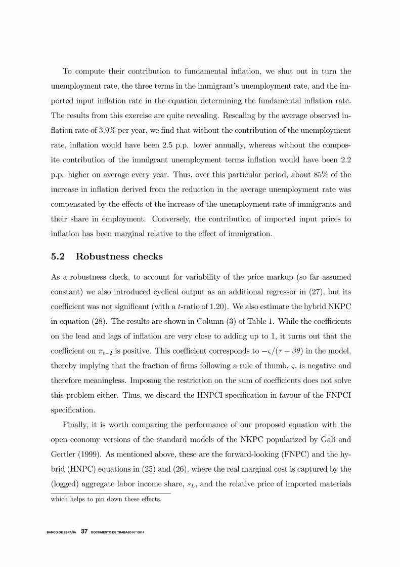
5.2 Robustness checks

As a robustness check, to account for variability of the price markup (so far assumed

constant) we also introduced cyclical output as an additional regressor in (27), but its

coefficient was not significant (with a t-ratio of 1.20). We also estimate the hybrid NKPC

in equation (28). The results are shown in Column (3) of Table 1. While the coefficients

on the lead and lags of inflation are very close to adding up to 1, it turns out that the

coefficient on πt−2 is positive. This coefficient corresponds to −ς/(τ + βθ) in the model,

thereby implying that the fraction of firms following a rule of thumb, ς, is negative and

therefore meaningless. Imposing the restriction on the sum of coefficients does not solve

this problem either. Thus, we discard the HNPCI specification in favour of the FNPCI

specification.

Finally, it is worth comparing the performance of our proposed equation with the

open economy versions of the standard models of the NKPC popularized by Galí and

Gertler (1999). As mentioned above, these are the forward-looking (FNPC) and the hy-

brid (HNPC) equations in (25) and (26), where the real marginal cost is captured by the

(logged) aggregate labor income share, sL, and the relative price of imported materials

which helps to pin down these effects.


and labor, that is: mc = sL + ξ(pm − w). As discussed in Rotemberg and Woodford

(1999), the parameter ξ is zero when the production function is Cobb-Douglas whereas,

using instead a CES specification, it is positive when the elasticity of substitution be-

tween labor and intermediate goods is above unity, as is often found in the literature.

These equations were applied by Galí and López-Salido (2001) to estimate the NKPC

for Spain over 1980-1998, yielding a good fit and sensible estimates of the underlying

structural parameters that we also found with our dataset. Since their estimation period

ends before immigration surged, it is interesting to check how these models perform up

to the end of our sample period, 2006:3. Estimating by GMM with their instrument set

yields, for the FNPC:24

πt= 1.050 Etπt+1 — 0.037 sLt + 0.004 (pmt − wt)(31.10) (3.31) (1.65)

(32)

and for the HNPC:

πt= 0.410 Etπt+1 + 0.629 πt−1 + 0.010 sLt — 0.004 (pmt − wt)(9.41) (17.12) (1.69) (4.23)

(33)

where t-ratios are reported in parentheses. In both regressions, the implied value of

β is above unity, violating the restriction that both the coefficient on Etπt+1 (i.e., β)

in (25) and the sum of the coefficients on Etπt+1 and πt−1 (i.e., (βθ + ζ)/τ) in (26)

should be smaller than 1. Moreover, the estimated coefficient on sLt is negative and

significant in (31) and positive but nonsignificant in (32), while the coefficient on the

relative price changes sign across the two specifications. These results turn out to be

robust to imposing a value of β in a plausible range between, say, 0.90 and 1. For

example, for β = 0.99, we get, for the FNPC:

πt= 0.99 Etπt+1 — 0.029 sLt + 0.007 (pmt − wt)(−) (2.92) (5.88)

(34)

and for the HNPC:

πt= 0.358 Etπt+1 + 0.639 πt−1 + 0.004 sLt — 0.002 (pmt − wt)(9.98) (9.98) (0.76) (2.40)

(35)

24The instruments set includes a constant plus four lags of price and wage inflation, relative prices,detrended output, and the labor share.


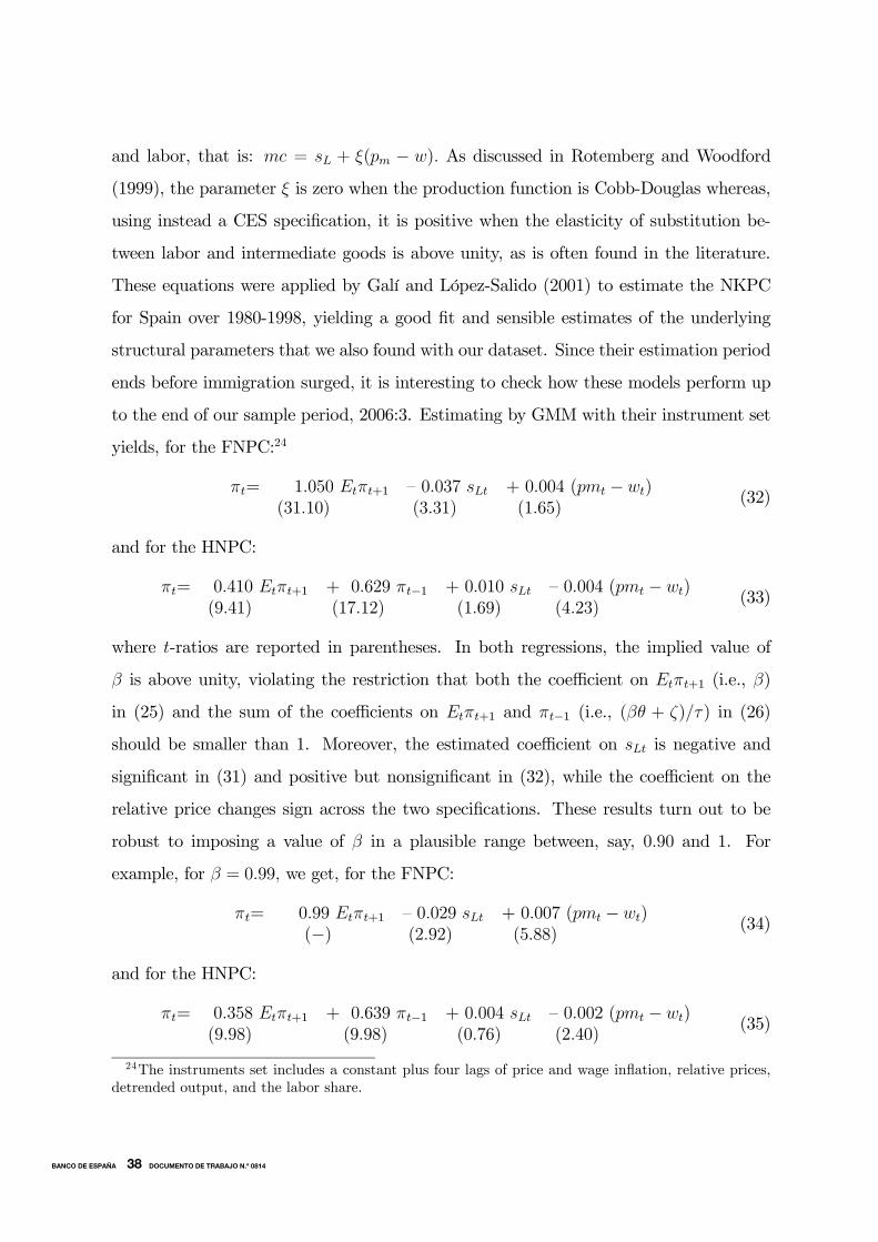
Therefore, applying the standard models of the NKPC —which ignore differences

between the preferences of immigrants and native workers— does not work once the

sample is extended to include the immigration boom in the Spanish labor market, which

provides some further support to our approach.

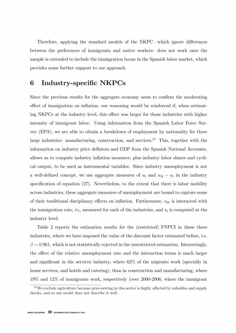
6 Industry-specific NKPCs

Since the previous results for the aggregate economy seem to confirm the moderating

effect of immigration on inflation, our reasoning would be reinforced if, when estimat-

ing NKPCs at the industry level, this effect was larger for those industries with higher

intensity of immigrant labor. Using information from the Spanish Labor Force Sur-

vey (EPA), we are able to obtain a breakdown of employment by nationality for three

large industries: manufacturing, construction, and services.25 This, together with the

information on industry price deflators and GDP from the Spanish National Accounts,

allows us to compute industry inflation measures, plus industry labor shares and cycli-

cal output, to be used as instrumental variables. Since industry unemployment is not

a well-defined concept, we use aggregate measures of ut and u2t − ut in the industry

specification of equation (27). Nevertheless, to the extent that there is labor mobility

across industries, these aggregate measures of unemployment are bound to capture some

of their traditional disciplinary effects on inflation. Furthermore, u2t is interacted with

the immigration rate, irt, measured for each of the industries, and st is computed at the

industry level.

Table 2 reports the estimation results for the (restricted) FNPCI in these three

industries, where we have imposed the value of the discount factor estimated before, i.e.

β = 0.961, which is not statistically rejected in the unrestricted estimation. Interestingly,

the effect of the relative unemployment rate and the interaction terms is much larger

and significant in the services industry, where 62% of the migrants work (specially in

home services, and hotels and catering), than in construction and manufacturing, where

19% and 12% of immigrants work, respectively (over 2000-2006, where the immigrant

25We exclude agriculture because price-setting in this sector is highly affected by subsidies and supplyshocks, and so our model does not describe it well.


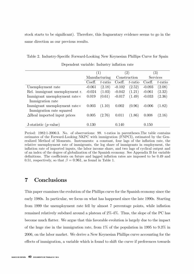
stock starts to be significant). Therefore, this fragmentary evidence seems to go in the

same direction as our previous results.

Table 2. Industry-Specific Forward-Looking New Keynesian Phillips Curve for Spain

Dependent variable: Industry inflation rate

(1) (2) (3)Manufacturing Construction ServicesCoeff. t-ratio Coeff. t-ratio Coeff. t-ratio

Unemployment rate -0.061 (2.18) -0.102 (2.52) -0.093 (2.08)Rel. immigrant unemployment r. -0.024 (1.03) -0.042 (1.21) -0.061 (2.32)Immigrant unemployment rate× 0.019 (0.61) -0.017 (1.49) -0.033 (2.36)Immigration rateImmigrant unemployment rate× 0.003 (1.10) 0.002 (0.96) -0.006 (1.82)Immigration rate squared

∆Real imported input prices 0.005 (2.76) 0.011 (1.86) 0.008 (2.16)

J-statistic (p-value) 0.130 0.140 0.150

Period: 1982:1-2006:3. No. of observations: 99. t-ratios in parentheses.The table containsestimates of the Forward-Looking NKPC with immigration (FNPCI), estimated by the Gen-eralized Method of Moments. Instruments: a constant, four lags of the inflation rate, therelative unemployment rate of immigrants, the log share of immigrants in employment, theinflation rate of imported inputs, the labor income share, and two lags of cyclical output andof an index of the degree of globalization of the Spanish economy. See Appendix B for variabledefinitions. The coefficients on future and lagged inflation rates are imposed to be 0.49 and0.51, respectively, so that β = 0.961, as found in Table 1.

7 Conclusions

This paper examines the evolution of the Phillips curve for the Spanish economy since the

early 1980s. In particular, we focus on what has happened since the late 1990s. Starting

from 1999 the unemployment rate fell by almost 7 percentage points, while inflation

remained relatively subdued around a plateau of 2%-4%. Thus, the slope of the PC has

become much flatter. We argue that this favorable evolution is largely due to the impact

of the huge rise in the immigration rate, from 1% of the population in 1995 to 9.3% in

2006, on the labor market. We derive a New Keynesian Phillips curve accounting for the

effects of immigration, a variable which is found to shift the curve if preferences towards


labor supply or the bargaining power of immigrants and natives differ. In particular,

we find that the relative unemployment rate of immigrants with respect to the national

unemployment rate and the interaction of the immigrant unemployment rate with their

share in employment, in levels and squared, enters the PC, so that both its intercept

and slope is shifted by the presence of immigration.

By estimating our NKPC model with quarterly data for Spain over the period 1982-

2006, we are able to confirm that the variables in which the immigrant unemployment

rate enters are significant determinants of the PC and that conventional models of the

NKPC which treat labor as an homogeneous input do not fit the data well. We also

find that while the fall in the average unemployment rate over the last 8 years caused

the inflation rate to increase by 2.5 percentage points per year, the surge in immigra-

tion accounts for an offsetting 2.2 percentage-point drop in the inflation rate per year.

Finally, we also estimate industry-specific PCs, finding that the impact of the relative

immigrant unemployment rate is larger for the industries with a higher share of immi-

grant employment. These effects may decay over time, as immigrants integrate and their

labor supply behavior becomes closer to that of natives, but it is too soon to detect such

evolution in the case of Spain.

In this respect, the effect of immigration on inflation is good news for central banks.

Yet, as Bean (2006) argues, the flattening of the PC is rather more of a mixed blessing

since, on the one hand, it implies that demand shocks and policy mistakes will not show

up in large movements of inflation but, on the other, if inflation remains above target,

a deeper slowdown or increasing immigration flows will be needed to bring it down.


A Appendix A. Some derivations

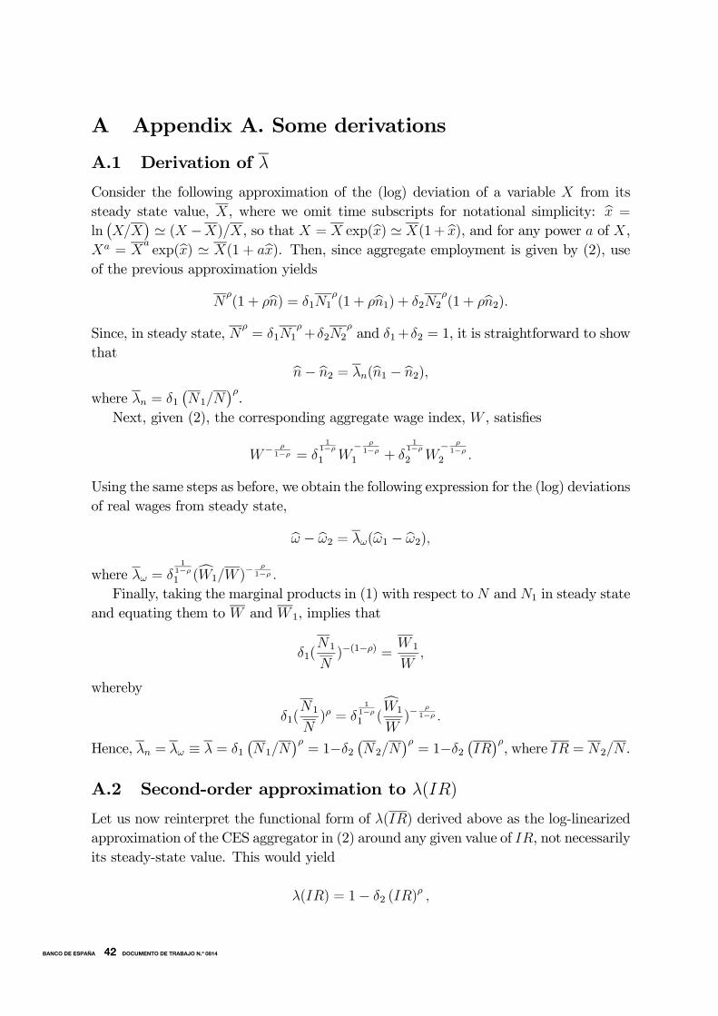
A.1 Derivation of λ

Consider the following approximation of the (log) deviation of a variable X from itssteady state value, X, where we omit time subscripts for notational simplicity: bx =ln¡X/X

¢ ' (X −X)/X, so that X = X exp(bx) ' X(1 + bx), and for any power a of X,Xa = X

aexp(bx) ' X(1 + abx). Then, since aggregate employment is given by (2), use

of the previous approximation yields

Nρ(1 + ρbn) = δ1N1

ρ(1 + ρbn1) + δ2N2

ρ(1 + ρbn2).

Since, in steady state, Nρ= δ1N1

ρ+δ2N2

ρand δ1+δ2 = 1, it is straightforward to show

that bn− bn2 = λn(bn1 − bn2),where λn = δ1

¡N1/N

¢ρ.

Next, given (2), the corresponding aggregate wage index, W , satisfies

W− ρ1−ρ = δ

11−ρ1 W

− ρ1−ρ

1 + δ1

1−ρ2 W

− ρ1−ρ

2 .

Using the same steps as before, we obtain the following expression for the (log) deviationsof real wages from steady state,

bω − bω2 = λω(bω1 − bω2),where λω = δ

11−ρ1 (cW1/W )

− ρ1−ρ .

Finally, taking the marginal products in (1) with respect to N and N1 in steady stateand equating them to W and W 1, implies that

δ1(N1

N)−(1−ρ) =

W 1

W,

whereby

δ1(N1

N)ρ = δ

11−ρ1 (

cW1

W)−

ρ1−ρ .

Hence, λn = λω ≡ λ = δ1¡N1/N

¢ρ= 1−δ2

¡N2/N

¢ρ= 1−δ2

¡IR¢ρ, where IR = N2/N .

A.2 Second-order approximation to λ(IR)

Let us now reinterpret the functional form of λ(IR) derived above as the log-linearizedapproximation of the CES aggregator in (2) around any given value of IR, not necessarilyits steady-state value. This would yield

λ(IR) = 1− δ2 (IR)ρ ,


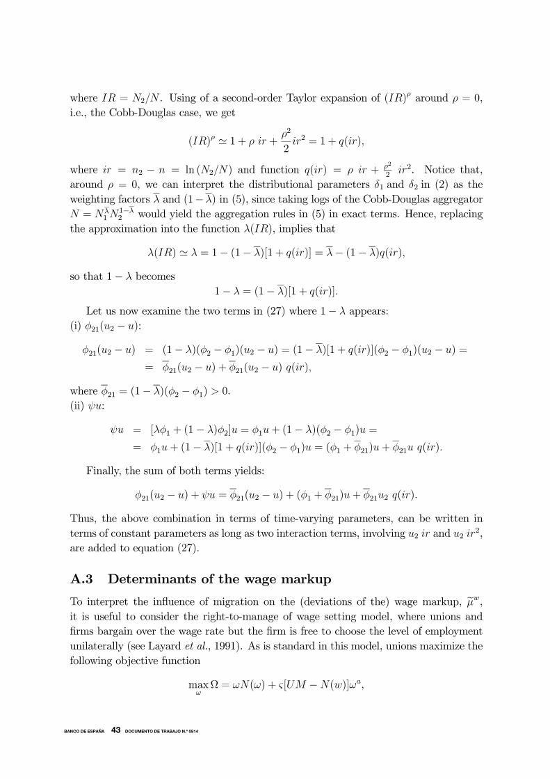
where IR = N2/N . Using of a second-order Taylor expansion of (IR)ρ around ρ = 0,

i.e., the Cobb-Douglas case, we get

(IR)ρ ' 1 + ρ ir +ρ2

2ir2 = 1 + q(ir),

where ir = n2 − n = ln (N2/N) and function q(ir) = ρ ir + ρ2

2ir2. Notice that,

around ρ = 0, we can interpret the distributional parameters δ1 and δ2 in (2) as theweighting factors λ and (1−λ) in (5), since taking logs of the Cobb-Douglas aggregatorN = Nλ

1N1−λ2 would yield the aggregation rules in (5) in exact terms. Hence, replacing

the approximation into the function λ(IR), implies that

λ(IR) ' λ = 1− (1− λ)[1 + q(ir)] = λ− (1− λ)q(ir),

so that 1− λ becomes1− λ = (1− λ)[1 + q(ir)].

Let us now examine the two terms in (27) where 1− λ appears:(i) φ21(u2 − u):

φ21(u2 − u) = (1− λ)(φ2 − φ1)(u2 − u) = (1− λ)[1 + q(ir)](φ2 − φ1)(u2 − u) =

= φ21(u2 − u) + φ21(u2 − u) q(ir),

where φ21 = (1− λ)(φ2 − φ1) > 0.(ii) ψu:

ψu = [λφ1 + (1− λ)φ2]u = φ1u+ (1− λ)(φ2 − φ1)u =

= φ1u+ (1− λ)[1 + q(ir)](φ2 − φ1)u = (φ1 + φ21)u+ φ21u q(ir).

Finally, the sum of both terms yields:

φ21(u2 − u) + ψu = φ21(u2 − u) + (φ1 + φ21)u+ φ21u2 q(ir).

Thus, the above combination in terms of time-varying parameters, can be written interms of constant parameters as long as two interaction terms, involving u2 ir and u2 ir2,are added to equation (27).

A.3 Determinants of the wage markup

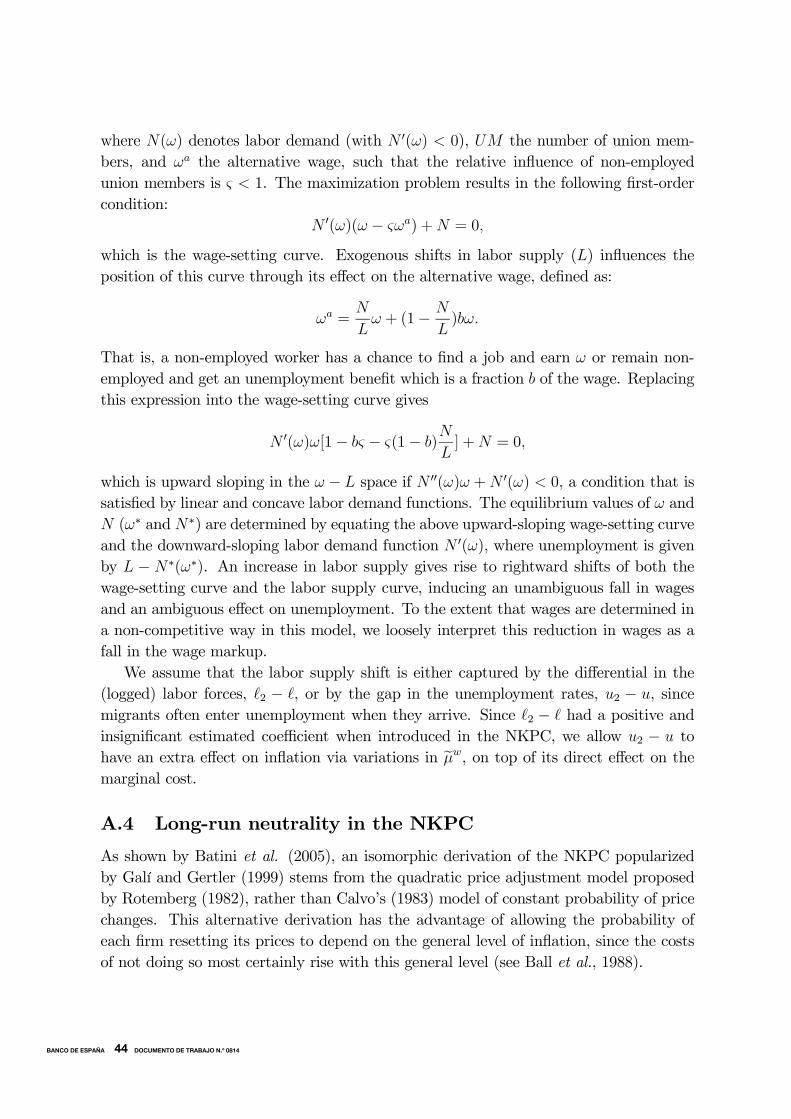
To interpret the influence of migration on the (deviations of the) wage markup, eµw,it is useful to consider the right-to-manage of wage setting model, where unions andfirms bargain over the wage rate but the firm is free to choose the level of employmentunilaterally (see Layard et al., 1991). As is standard in this model, unions maximize thefollowing objective function

maxω

Ω = ωN(ω) + ς[UM −N(w)]ωa,


where N(ω) denotes labor demand (with N 0(ω) < 0), UM the number of union mem-bers, and ωa the alternative wage, such that the relative influence of non-employedunion members is ς < 1. The maximization problem results in the following first-ordercondition:

N 0(ω)(ω − ςωa) +N = 0,

which is the wage-setting curve. Exogenous shifts in labor supply (L) influences theposition of this curve through its effect on the alternative wage, defined as:

ωa =N

Lω + (1− N

L)bω.

That is, a non-employed worker has a chance to find a job and earn ω or remain non-employed and get an unemployment benefit which is a fraction b of the wage. Replacingthis expression into the wage-setting curve gives

N 0(ω)ω[1− bς − ς(1− b)N

L] +N = 0,

which is upward sloping in the ω − L space if N 00(ω)ω +N 0(ω) < 0, a condition that issatisfied by linear and concave labor demand functions. The equilibrium values of ω andN (ω∗ and N∗) are determined by equating the above upward-sloping wage-setting curveand the downward-sloping labor demand function N 0(ω), where unemployment is givenby L − N∗(ω∗). An increase in labor supply gives rise to rightward shifts of both thewage-setting curve and the labor supply curve, inducing an unambiguous fall in wagesand an ambiguous effect on unemployment. To the extent that wages are determined ina non-competitive way in this model, we loosely interpret this reduction in wages as afall in the wage markup.We assume that the labor supply shift is either captured by the differential in the

(logged) labor forces, 2 − , or by the gap in the unemployment rates, u2 − u, sincemigrants often enter unemployment when they arrive. Since 2 − had a positive andinsignificant estimated coefficient when introduced in the NKPC, we allow u2 − u tohave an extra effect on inflation via variations in eµw, on top of its direct effect on themarginal cost.

A.4 Long-run neutrality in the NKPC

As shown by Batini et al. (2005), an isomorphic derivation of the NKPC popularizedby Galí and Gertler (1999) stems from the quadratic price adjustment model proposedby Rotemberg (1982), rather than Calvo’s (1983) model of constant probability of pricechanges. This alternative derivation has the advantage of allowing the probability ofeach firm resetting its prices to depend on the general level of inflation, since the costsof not doing so most certainly rise with this general level (see Ball et al., 1988).


Let us consider the firm’s problem as choosing a price path that solves

minpt+s

∞Xs=0

βsEt

½1

2(pt+s − p∗t+s)

2 − b

2(pt+s − pt+s−1 − cπat+s−1)

2

¾,

where the optimal price is p∗t+s = µp + mcnt+s, with mcn being the nominal marginalcost, πa denotes the general level of inflation (taken as given by the firm), and b > 0

and 0 ≤ c ≤ 1 are parameters in the loss function. When c = 1, price adjustmentcosts fully depend on the deviations from the general level of inflation . Notice thatthe quadratic adjustment cost term in price changes implies that the higher is πat+s−1the more beneficial is for firms to reset prices more frequently. The Euler equation (inperiod t) of the above minimization yields

βbEtpt+1 − (1− b(1 + β))pt + bpt−1 = −bpt,where bpt = p∗t + cbπat−1 − βcbπat .

The standard solution to this Euler equation is

pt = µ1pt−1 + (1− µ1)(1− βµ1)bpt

1− βµ1L−1 ,

where L−1 is the forward operator (e.g. L−sxt = Etxt+s) and µ1 is the unique stableroot of βbµ2 − [1 − b(1 + β)]µ + b = 0. If we now subtract from the previous solutionthe following identity

pt−1 ≡ µ1pt−1 + (1− µ1)(1− βµ1)pt−1

1− βµ1,

we obtain a new solution in terms of firm’s price inflation, πt (= pt − pt−1)

πt = (1− µ1)(1− βµ1)mc+ pt + cbπat−1 − βcbπat

1− βµ1L−1 − pt−1

1− βµ1,

where use has been made of mcnt = mct + pt. Then, since in equilibrium all firms areidentical (so that π = πa), straightforward algebra leads to the following NKPC:

πt =β

1 + βcEtπt+1 +

c

1 + βcπt−1 +

(1− µ1)(1− βµ1)

µ1(1 + βc)mct.

If 0 < c < 1, this NKPC corresponds to the hybrid case of Galí and Gertler (1999)where we find that in the long-run steady state, πt = Etπt+1 = πt−1, there is a non-zerorelationship between inflation and the real marginal cost, i.e., π = (1−µ1)(1−βµ1)

µ1(1−β)(1−c) mc.If c = 0, the NKPC is equivalent to the forward-looking case of Galí and Gertler

(1999), such that

πt = βEtπt+1 +(1− µ1)(1− βµ1)

µ1mct,


where again, there is a long-run tradeoff given by π = (1−µ1)(1−βµ1)µ1(1−β) mc.

Finally, if c = 1, the NKPC becomes

πt =β

1 + βEtπt+1 +

1

1 + βπt−1 +

(1− µ1)(1− βµ1)

µ1(1 + β)mct,

so that inflation is independent of the real marginal cost in the long run, although itinfluences the change in inflation, i.e., ∆π = (1−µ1)(1−βµ1)

µ1(1−β) mc.As discussed in Section 4.5, an alternative way of obtaining long-run neutrality in

the NKPC is to assume real wage sluggishness.

A.5 Calibration of the parameters

As mentioned in the main text, the estimation of equation (31) yields 6 estimated co-efficients (imposing that α1 + α2 = 1), while from (27) we have the following 10 freeparameters: β, γ, α, χ, θ, λ, φ2, φ1, ν, and ρ. Thus, we can only attempt to identifya subset of the structural parameters. As shown below, through calibration of α, χ, λ,and the (average) labor supply elasticity of natives, φ1, we are able to identify β, θ, ρ,and ν. The identification procedure for each of these structural parameters involves thevalues of the restricted coefficients reported in Table 1 (Column 2) and, in each case, itcan be summarized as follows:(i) β, from the estimated coefficient on Etπ+1, bψf

1 , which is equal to 0.490 (t-ratio=11.34). Hence, since ψf

1 =β1+β, the delta method yields bβ = 0.961 (t-ratio=

11.42).(ii) θ, from the estimated coefficient of ∆st which is

α(1−χ)κf(1+β)

= 0.005 (t-ratio=2.77),

with κf =(1−βθ)(1−θ)

θ, using calibrated values for α and χ, and the estimated value of β

obtained in (i). It is easy to check that this yields a quadratic function in θ. If we takeα = 0.536 and χ = 0.646 —computed as the average shares of imported intermediateinputs in gross output (α) and in gross output net of capital compensation (χ) in theSpanish economy over the period 1980-2003 according to the EU KLEMS database(www.euklems.net)— plus bβ = 0.961, this yields bθ = 0.810 (t-ratio=15.76), whereas theother root in the quadratic function is larger than unity. For this value of θ, we also getbκf = 0.0517 (t-ratio=4.07).(iii) ρ, from the ratio between the estimated coefficients on the interaction terms

u2ir2 and u2ir. In effect, from (27), this ratio yields bρ = 20.0033

0.0307= 0.217 (t-ratio=7.62).

Hence, the estimated elasticity of substitution in (2) is given by bσ = 11−0.217 = 1.277

(t-ratio=35.47).(iv) ν, from the ratio of the estimated coefficients on u and u2 − u. This ratio

yields ψ

φ21+ν= φ1+(1−λ)(φ2−φ1)

(1−λ)(φ2−φ1)+ν= 1.4. From equations (1) and (2), with δ1 + δ2 = 1, we

have that dQdN1

= dQdN

dNdNρ δ1ρN

ρ−11 = W1

PQand dQ

dN2= dQ

dNdNdNρ (1 − δ1)ρN

ρ−12 = W2

PQ, so that

(N1N2)ρ−1 = W1

W2, where respective markup terms would multiply the wage terms under


imperfect competition. If we assume that in steady state N1N2= N1/N

N2/N= 0.97

0.03= 32.33,

taking ρ = 0.217, we would have that δ11−δ10.06576 =

W1

W2. Now, to obtain a value for δ1we

need to assume some value for the relative wage (or relative wage plus markup). Let ustake three alternatives: (a) W1/W2 = 1 ⇒ δ1 = 0.938, (b) W1/W2 = 1.3 ⇒ δ1 = 0.952,and (c) W1/W2 = 1.5 ⇒ δ1 = 0.958. Thus, since λ = δ1(

N1N)ρ = δ1 (0.97)

0.217, we have:(a) λ = 0.932, (b) λ = 0.946, and (c) λ = 0.952.We also need to make some assumption regarding the (inverse) Frisch labor supply

elasticities. If we take a value of 1 for native workers, so that φ1 = 1, as is assumed inmost of the literature on NKPCs (see, e.g., Galí et al., 2001, and BG), and a value ofφ2 = 2, from the above ratio, ψ

φ21+ν= 1.4, we get: (a) bν = 0.695, (b) bν = 0.698, and

(c) bν = 0.701. Alternatively, if we assume use φ2 = 4, we obtain: (a) bν = 0.658, (b)bν = 0.668, and (c) bν = 0.672. Thus the value given in the text, bν ' 0.7, is quite robust.


B Appendix B. Variable definitions and sources

Nominal and Real GDP. GDP from Spanish National Accounts produced by InstitutoNacional de Estadística (INE, www.ine.es) Base 1995, linked forward to Base 2000 at1995:1 using growth rates. Data are seasonally adjusted and adjusted for calendar effectsby INE.Inflation. Change in GDP deflator from Spanish National Accounts by INE. Computedas quarterly change in nominal GDP minus quarterly change in real GDP.Employment and unemployment for immigrants and natives. From the Spanish LaborForce Survey (Encuesta de Población Activa) by INE, linking 1976, 1987, 2001, and 2005definitions. Data correspond to full-time equivalent jobs. Seasonally adjusted by INE.Workers with double nationality are considered as immigrants throughout the sample.There is no data on immigrants before 1987:2, so we assume that they have the sameunemployment rate as natives through that quarter. Seasonally adjusted using ProgramTSW.Imported input prices. Price index for imported intermediate inputs from Ministerio deEconomía y Hacienda, SERSIE Database (www.meh.es).Labor share. Remuneration of employees multiplied by the ratio of employment toemployees and divided by nominal GDP. This entails assuming that the self-employedearn the same labor income as employees.Nominal wage. Remuneration of employees divided by the number of employees. Thelatter is constructed following the same procedure as for total employment.Degree of openness. Real imports plus exports divided by real GDP from INE. Sameprocedures as for real GDP.Index of globalization. This index measures economic globalization, including both ac-tual flows (trade, foreign direct investment, portfolio investment, and income paymentsto foreigners) and restrictions (hidden import barriers, mean tariff rate, taxes on inter-national trade, and capital account restrictions). Source: Swiss Institute for BusinessCycle Research (globalization.kof.ethz.ch), see Dreher (2006).


ReferencesBALL, L. (2006). Has Globalization Changed Inflation?, NBER Working Paper No.

12687.

BALL, L., N. G. MANKIW and D. ROMER (1988). “The New Keynesian Economicsand the Output-Inflation Trade-Off”, Brookings Papers on Economic Activity, 1,pp. 1-65.

BALL, L., and R. MOFFITT (2001). Productivity Growth and the Phillips Curve,mimeo.

BATINI, N., B. JACKSON and S. NICKELL (2005). “An Open Economy New PhillipsCurve for the UK”, Journal of Monetary Economics, 52, pp. 1061-1071

BEAN, C. (2006). “Globalisation and Inflation”, Bank of England Quarterly Bulletin,Q4, pp. 468-475.

BENTOLILA, S., and J. F. JIMENO (2006). “Spanish Unemployment: The End ofthe Wild Ride?”, in Martin Werding (ed.), Structural Unemployment in WesternEurope. Reasons and Remedies, MIT Press, Cambridge, MA.

BERNANKE, B. S. (2004). The Great Moderation, Speech at the meetings of theEastern Economic Association.

BLANCHARD, O., and J. GALÍ (2007).”Real Wage Rigidities and the New KeynesianModel”, Journal of Money, Credit, and Banking, forthcoming.

BORJAS, G. (1999). “The Economic Analysis of Immigration”, in O. Ashenfelter andD. Card (eds.), Handbook of Labour Economics,Vol. 3A, North Holland.

— (2003). “The Labor Demand Curve is Downward Sloping: Reexamining the Impactof Immigration on the Labor Market”, Quarterly Journal of Economics, 118, pp.1335-1370.

BRANDT, N., J.-M. BURNIAUX and R. DUVAL (2005). Assessing the OECD JobsStrategy: Past Development and Reforms, OECD Economics Department WorkingPaper No. 429.

CALVO, G. (1983). “Staggered Prices in a Utility Maximizing Framework”, Journalof Monetary Economics, 12, pp. 383-398.

CARD, D. (2001). “Immigrants Inflows, Native Outflows, and the Local Labour MarketImpacts of Higher Immigration”, Journal of Labor Economics, 19, pp. 22-64.

CARRASCO, R., J. F. JIMENO and C. ORTEGA (2007). “The Effect of Immigrationon the Labor Market Performance of Native-Born Workers: Some Evidence forSpain”, Journal of Population Economics, forthcoming.


DOLADO, J., C. GARCÍA-SERRANO and J. F. JIMENO (2002). “Drawing Lessonfrom the Boom of Temporary Jobs in Spain”, Economic Journal, 112, pp. 270-295.

DOLADO, J., and P. VÁZQUEZ (2007). “Los Efectos Económicos y las Políticas deInmigración: Panorámica y Reflexiones”, in J. Dolado and P. Vázquez (eds.), En-sayos sobre los Efectos Económicos de la Inmigración en España, FEDEA, Madrid.

DREHER, A. (2006). “Does Globalization Affect Growth? Evidence from a New Indexof Globalization”, Applied Economics, 38, pp. 1091-1110.

ENGLER, P. (2007). Gains from Migration in a New-Keynesian Framework, mimeo,Free University of Berlin.

FABIANI, S. et al. (2006). “What Firms’ Surveys Tell Us about Price-Setting Behaviorin the Euro Area”, International Journal of Central Banking, 2, pp. 3-47.

FERNÁNDEZ, C., and C. ORTEGA (2007). “Labour Market Assimilation of Im-migrants in Spain: Employment at the Expense of Bad-Job Matches?”, SpanishEconomic Review, forthcoming.

GALÍ, J., and M. GERTLER (1999). “Inflation Dynamics: A Structural EconometricAnalysis”, Journal of Monetary Economics, 44, pp. 195-222.

GALÍ, J., M. GERTLER and J. D. LÓPEZ-SALIDO (2001). “European InflationDynamics”, European Economic Review, 45, pp. 1237-1279.

— (2003). “Erratum to ’European Inflation Dynamics”, European Economic Review,47, pp. 759-760.

GALÍ, J., and J. D. LÓPEZ-SALIDO (2001). “A New Phillips Curve for Spain”,BIS Papers 3: Empirical studies of structural changes and inflation, Bank forInternational Settlements, Basel.

INTERNATIONAL MONETARY FUND (2006). “How Has Globalization AffectedInflation?”, World Economic Outlook, Spring, pp. 97-134.

IZQUIERDO, M., and A.V. REGIL (2006). “Actualización de las estimaciones dela tasa de desempleo estructural de la economía española”, Boletín Económico,September, Banco de España.

KARANASSOU, M., H. SALA and D. J. SNOWER (2002). Long-Run Inflation-Unemployment Dynamics: The Spanish Phillips Curve and Economic Policy, IZADiscussion Paper 645.

KARANASSOU, M., and D. J. SNOWER (2007). Inflation Persistence and the PhillipsCurve Revisited, IZA Discussion Paper 2600.

KMENTA, J (1967). “On Estimation of the CES Production Function”, InternationalEconomic Review, 8, pp. 180-189.


LAYARD, R., S. NICKELL and R. JACKMAN (1991). Unemployment. Macroeco-nomics and the Labor Market, Oxford University Press, Oxford.

LÓPEZ-SALIDO, J. D., F. RESTOY and J. VALLÉS (2005). “Inflation Differentialsin EMU: The Spanish Case”, Moneda y Crédito, 220.

OTTAVIANO, G., and G. PERI (2006). Rethinking the Effects of Immigration onWages, NBER Working Paper No. 12497.

RABANAL, P. (2006). Explaining Inflation Differentials Between Spain and the Euroarea, Working Paper No. 2, December, La Caixa.

RAZIN, A., and A. BINYAMINI (2007). Flattening of the Short-run Trade-off betweenInflation and Domestic Activity: The Analytics of the Effects of Globalization,mimeo, Tel Aviv University.

RAZIN, A., and P. LOUNGANI (2007). “Globalization and Equilibrium Inflation-Output Tradeoffs”, NBER International Seminar on Macroeconomics 2005, Cam-bridge, MA: NBER, forthcoming.

ROGOFF, K. (2003). “Globalization and Global Disinflation, in Federal Reserve Bankof Kansas City”,Monetary Policy and Uncertainty: Adapting to a Changing Econ-omy, pp. 77-112.

ROTEMBERG, J. (1982). “Sticky Prices in the United States”, Journal of PoliticalEconomy, 90, pp. 1187-1211.

ROTEMBERG, J., and M. WOODFORD (1999). “The Cyclical Behavior of Prices andCosts”, in J. B. Taylor and M. Woodford (eds.), Handbook of Macroeconomics, Vol.1B, Amsterdam: North Holland.


BANCO DE ESPAÑA PUBLICATIONS

WORKING PAPERS1

0701 PRAVEEN KUJAL AND JUAN RUIZ: Cost effectiveness of R&D and strategic trade policy.

0702 MARÍA J. NIETO AND LARRY D. WALL: Preconditions for a successful implementation of supervisors’ prompt

corrective action: Is there a case for a banking standard in the EU?

0703 PHILIP VERMEULEN, DANIEL DIAS, MAARTEN DOSSCHE, ERWAN GAUTIER, IGNACIO HERNANDO,

ROBERTO SABBATINI AND HARALD STAHL: Price setting in the euro area: Some stylised facts from individual

producer price data.

0704 ROBERTO BLANCO AND FERNANDO RESTOY: Have real interest rates really fallen that much in Spain?

0705 OLYMPIA BOVER AND JUAN F. JIMENO: House prices and employment reallocation: International evidence.

0706 ENRIQUE ALBEROLA AND JOSÉ M.ª SERENA: Global financial integration, monetary policy and reserve

accumulation. Assessing the limits in emerging economies.

0707 ÁNGEL LEÓN, JAVIER MENCÍA AND ENRIQUE SENTANA: Parametric properties of semi-nonparametric

distributions, with applications to option valuation.

0708 ENRIQUE ALBEROLA AND DANIEL NAVIA: Equilibrium exchange rates in the new EU members: external

imbalances vs. real convergence.

0709 GABRIEL JIMÉNEZ AND JAVIER MENCÍA: Modelling the distribution of credit losses with observable and latent

factors.

0710 JAVIER ANDRÉS, RAFAEL DOMÉNECH AND ANTONIO FATÁS: The stabilizing role of government size.

0711 ALFREDO MARTÍN-OLIVER, VICENTE SALAS-FUMÁS AND JESÚS SAURINA: Measurement of capital stock

and input services of Spanish banks.

0712 JESÚS SAURINA AND CARLOS TRUCHARTE: An assessment of Basel II procyclicality in mortgage portfolios.

0713 JOSÉ MANUEL CAMPA AND IGNACIO HERNANDO: The reaction by industry insiders to M&As in the European

financial industry.

0714 MARIO IZQUIERDO, JUAN F. JIMENO AND JUAN A. ROJAS: On the aggregate effects of immigration in Spain.

0715 FABIO CANOVA AND LUCA SALA: Back to square one: identification issues in DSGE models.

0716 FERNANDO NIETO: The determinants of household credit in Spain.

0717 EVA ORTEGA, PABLO BURRIEL, JOSÉ LUIS FERNÁNDEZ, EVA FERRAZ AND SAMUEL HURTADO: Update of

the quarterly model of the Bank of Spain. (The Spanish original of this publication has the same number.)

0718 JAVIER ANDRÉS AND FERNANDO RESTOY: Macroeconomic modelling in EMU: how relevant is the change in regime?

0719 FABIO CANOVA, DAVID LÓPEZ-SALIDO AND CLAUDIO MICHELACCI: The labor market effects of technology

shocks.

0720 JUAN M. RUIZ AND JOSEP M. VILARRUBIA: The wise use of dummies in gravity models: Export potentials in

the Euromed region.

0721 CLAUDIA CANALS, XAVIER GABAIX, JOSEP M. VILARRUBIA AND DAVID WEINSTEIN: Trade patterns, trade

balances and idiosyncratic shocks.

0722 MARTÍN VALLCORBA AND JAVIER DELGADO: Determinantes de la morosidad bancaria en una economía

dolarizada. El caso uruguayo.

0723 ANTÓN NÁKOV AND ANDREA PESCATORI: Inflation-output gap trade-off with a dominant oil supplier.

0724 JUAN AYUSO, JUAN F. JIMENO AND ERNESTO VILLANUEVA: The effects of the introduction of tax incentives

on retirement savings.

0725 DONATO MASCIANDARO, MARÍA J. NIETO AND HENRIETTE PRAST: Financial governance of banking supervision.

0726 LUIS GUTIÉRREZ DE ROZAS: Testing for competition in the Spanish banking industry: The Panzar-Rosse

approach revisited.

0727 LUCÍA CUADRO SÁEZ, MARCEL FRATZSCHER AND CHRISTIAN THIMANN: The transmission of emerging

market shocks to global equity markets.

0728 AGUSTÍN MARAVALL AND ANA DEL RÍO: Temporal aggregation, systematic sampling, and the

Hodrick-Prescott filter.

0729 LUIS J. ÁLVAREZ: What do micro price data tell us on the validity of the New Keynesian Phillips Curve?

0730 ALFREDO MARTÍN-OLIVER AND VICENTE SALAS-FUMÁS: How do intangible assets create economic value?

An application to banks.

1. Previously published Working Papers are listed in the Banco de España publications catalogue.

0731 REBECA JIMÉNEZ-RODRÍGUEZ: The industrial impact of oil price shocks: Evidence from the industries of six

OECD countries.

0732 PILAR CUADRADO, AITOR LACUESTA, JOSÉ MARÍA MARTÍNEZ AND EDUARDO PÉREZ: El futuro de la tasa

de actividad española: un enfoque generacional.

0733 PALOMA ACEVEDO, ENRIQUE ALBEROLA AND CARMEN BROTO: Local debt expansion… vulnerability

reduction? An assessment for six crises-prone countries.

0734 PEDRO ALBARRÁN, RAQUEL CARRASCO AND MAITE MARTÍNEZ-GRANADO: Inequality for wage earners and

self-employed: Evidence from panel data.

0735 ANTÓN NÁKOV AND ANDREA PESCATORI: Oil and the Great Moderation.

0736 MICHIEL VAN LEUVENSTEIJN, JACOB A. BIKKER, ADRIAN VAN RIXTEL AND CHRISTOFFER KOK-

SØRENSEN: A new approach to measuring competition in the loan markets of the euro area.

0737 MARIO GARCÍA-FERREIRA AND ERNESTO VILLANUEVA: Employment risk and household formation: Evidence

from differences in firing costs.

0738 LAURA HOSPIDO: Modelling heterogeneity and dynamics in the volatility of individual wages.

0739 PALOMA LÓPEZ-GARCÍA, SERGIO PUENTE AND ÁNGEL LUIS GÓMEZ: Firm productivity dynamics in Spain.

0740 ALFREDO MARTÍN-OLIVER AND VICENTE SALAS-FUMÁS: The output and profit contribution of information

technology and advertising investments in banks.

0741 ÓSCAR ARCE: Price determinacy under non-Ricardian fiscal strategies.

0801 ENRIQUE BENITO: Size, growth and bank dynamics.

0802 RICARDO GIMENO AND JOSÉ MANUEL MARQUÉS: Uncertainty and the price of risk in a nominal convergence

process.

0803 ISABEL ARGIMÓN AND PABLO HERNÁNDEZ DE COS: Los determinantes de los saldos presupuestarios de las

Comunidades Autónomas.

0804 OLYMPIA BOVER: Wealth inequality and household structure: US vs. Spain.

0805 JAVIER ANDRÉS, J. DAVID LÓPEZ-SALIDO AND EDWARD NELSON: Money and the natural rate of interest:

structural estimates for the United States and the euro area.

0806 CARLOS THOMAS: Search frictions, real rigidities and inflation dynamics.

0807 MAXIMO CAMACHO AND GABRIEL PEREZ-QUIROS: Introducing the EURO-STING: Short Term INdicator of

Euro Area Growth.

0808 RUBÉN SEGURA-CAYUELA AND JOSEP M. VILARRUBIA: The effect of foreign service on trade volumes and

trade partners.

0809 AITOR ERCE: A structural model of sovereign debt issuance: assessing the role of financial factors.

0810 ALICIA GARCÍA-HERRERO AND JUAN M. RUIZ: Do trade and financial linkages foster business cycle

synchronization in a small economy?

0811 RUBÉN SEGURA-CAYUELA AND JOSEP M. VILARRUBIA: Uncertainty and entry into export markets.

0812 CARMEN BROTO AND ESTHER RUIZ: Testing for conditional heteroscedasticity in the components of inflation.

0813 JUAN J. DOLADO, MARCEL JANSEN AND JUAN F. JIMENO: On the job search in a model with heterogeneous

jobs and workers.

0814 SAMUEL BENTOLILA, JUAN J. DOLADO AND JUAN F. JIMENO: Does immigration affect the Phillips curve?

Some evidence for Spain.

Unidad de PublicacionesAlcalá, 522; 28027 Madrid

Telephone +34 91 338 6363. Fax +34 91 338 6488e-mail: [email protected]

www.bde.es

does immigration affect the phillips curve? some evidence for spain

Documents