1  

 

 

Do Private Firms Perform Better than Public Firms? 

SerkanAkguc*,JongmooJayChoi#,andSuk‐JoongKim^

Thisversion:August2015

Abstract

Thispaperexaminesthefinancialperformanceoflistedpublicfirmsvs.unlistedprivatefirmsintheU.K.overtheperiod2003‐2012.Weestablishastylizedfactthatprivatefirmstypicallyoutperformpublicfirms.Thisfindingisrobustinvariousmodelsettings,usingalternativematchingsamples,differentdefinitionsofperformance,changesinownershipstatus,andtheendogeneityofafirm’slistingdecision.Wethenidentifyandtestthreechannelsthatexplainhigherperformanceofprivatefirms,andtwo“counter”channelsthatfavorpublicfirms.First,privatefirmsaremoreefficientoperationallythanpublicfirmsduetomanagerialflexibility.Second,theR&Dintensityishigherforprivatethanpublicfirms,indicatinglongertimehorizon.Third,privatefirmshavehighercontrollingownership,whichreducesagencycost.Consideringcounterchannels,wefindthatthebasicresultisindependentofliquidityorfinancialresourcesastheoperatingprofitabilityishigherforprivatefirmsthanpublicfirmswhentheybotharefinanciallyconstrained.

Keywords:privatefirm,publicfirm,corporateownership,exchangelisting,operatingprofit,firmperformance

JELCodes:G32,G34

   

                                                            *Department of Finance, Temple University, Fox School of Business, Philadelphia, PA 19122, United States, email:serkan.akguc@temple.edu.  # DepartmentofFinance,TempleUniversity,FoxSchoolofBusiness,Philadelphia,PA19122,UnitedStates.Email:jjchoi@temple.edu. 

^CorrespondingAuthor,DisciplineofFinance,TheUniversityofSydneyBusinessSchool,TheUniversityofSydney,NSW,2006,Australia.Email:sukjoong.kim@sydney.edu.au.TheauthorsgreatlyacknowledgethecommentsandsuggestionsonanearlierdraftfromlateMichaelMcKenzie,whowasatUniversityofSydneyprior tomoving toUniversityofLiverpool.Additionalcommentswerereceived fromRonAnderson,RonMasulis,LalithaNaveen,OlegRytchkov,andparticipantsatseminarsatUniversityofSydney,TempleUniversity,2014MidwestFinanceAssociation,and2014AcademyofInternationalBusiness. 

2  

I. Introduction   

While publicly‐held  listed companies  (“public  firms”)  typically constitute the majority of  investors’ equity 

investment holdings, they represent only a small fraction of all firms in the economy. For example, in our sample of 

U.K.  industrial  firms  from  the Orbis  database,  only  about  2%  of  all  firms  are  public  firms.1  Not  only  are  there 

substantially more privately‐held unlisted firms (“private firms”) than public firms, but their economic significance is 

also greater. Asker, Farre‐Mensa and Ljungqvist (2014) estimate that private firms accounted for about 69% of private 

sector employment, 59% of sales and 49% of aggregate pre‐tax profits  in  the U.S.  In our Orbis database of U.K. 

companies, private firms account for 70% of total corporate assets, 65% of total sales, and 59% of after‐tax corporate 

profits in 2010. 

The purpose of this paper  is to  investigate the existence and nature of systematic differences  in financial 

performance between private and public  industrial  firms  in  the U.K. and  to examine channels  that  influence  the 

relative performance. The basic characteristics of U.K. firms and capital markets are similar to those of U.S. in many 

respects  including ownership and governance, corporate finance,  legal tradition, and so forth. As such, this paper 

may be viewed as contributing to an emerging literature that uses newly available datasets to identify differences 

between public and private firms in the Anglo‐American world. Gao, Harford and Li (2013) study U.S. firms and find 

that public firms hold about twice as much cash as private firms. Asker, Farre‐Mensa and Ljungqvist (2014) find that 

public firms invest less and are also less responsive to changes in investment opportunities than private firms in the 

U.S. For U.K. firms, Ball and Shivakumar (2005) find that the quality of financial reporting by private firms is lower 

than public firms even though they face equivalent regulations on auditing, accounting standards and taxes. These 

differences in the quality of information may help explain the findings on U.K. firms by Brav (2009) and Saunders and 

Steffen (2011) that private firms face significantly higher financing costs than public firms due to their higher reliance 

on debt and private capital. On the other hand, Michaely and Roberts (2012) report that public firms pay relatively 

higher dividends and tend to smooth dividends more than private firms in the U.K. While some of these studies have 

implications for firm performance, we are not aware of any comprehensive, economy‐wide study of the performance 

of private vs. public U.K. firms.2 

                                                            1Whenthecompleteuniverseoffirmsareconsidered(BureauvanDijkOrbisdatabase,26Sep2013edition),98.3%ofallfirmsintheUK(281,608of286,479firms)or99.2%ofallfirmsintheUS(1,943,181outof1,959,180firms)areunlistedprivatefirms.2 WebecameawareofanaccountingworkingpaperbyAllee,BadertscherandYohn(2013)thatshowsthatlowerfutureprofitabilityofpublicthanprivatefirmsisdrivenbylowerfutureprofitmargins;wefindthisfindingabitcircularinnatureasitonlyexplainstheconnectionbetweenthetwofuturerelativeprofitabilityvariables.TheearliercontributionbyKe,Petroni,andSafieddine(1999)usesaverysmallsampleofpublicandprivateU.S.insurancecompanies,toshowthattheoperatingprofitabilityofpublicandprivatefirmsarenotsignificantlydifferentfromeachother.Wearenotawareofanyresearchthatsystematicallyinvestigatestherelativecontemporaneousprofitabilityofprivateversuspublicfirmsinacomprehensiveway. 

3  

In this paper, we establish a stylized fact on the relative financial performance of private vs. public industrial 

firms and investigate several channels through which this may come about. A study of the relative performance of 

private and public firms is worthwhile because the extant literature on public vs. private ownership points to several 

potential advantages of public ownership. An  implication of  the  literature on  initial public offering  (IPO)    (e.g., a 

survey article by Roell (1996)) is that public firms have advantages over private firms in accessing capital (Pagano, 

Panetta and Zingales (1998), Saunders and Steffen (2011)), and in resultant capacity to invest in profitable projects. 

Gao, Lemmon and Li (2013) compared executive pays in U.S. public and private firms and found that remuneration 

in public firms is more sensitive to firm performance. Public firms also enjoy more prestige and reputation, which 

may help them attract profitable businesses and talented employees. 

However, private firms may also have advantages over public firms as well. For instance, private firms face 

less agency costs (Gao, Harford, and Li (2013), and Akguc and Choi (2014)), as well as avoid listing costs, and may not 

have  to disclose  strategic  information  (Brau and Fawcett  (2006) and Farre‐Mensa  (2014)). Graham, Harvey, and 

Rajgopal (2005) document a survey result that the majority of the Chief Financial Officers of public firms would not 

take on a positive NPV project if it would lead them to miss quarterly earnings targets. If so, private firms may be 

able to make decisions in the long‐term interest of the firm, free from pressures of short‐term market reactions or 

analyst earnings forecasts. Asker, Farre‐Mensa and Ljungqvist (2014) find that private firms invest more than public 

firms in the U.S. and are more responsive to investment opportunities, which they attribute to managerial myopia of 

public‐firm managers. Additionally, given controlled ownership structure, private firms may have a lower agency cost, 

and may even have a greater incentive, as Bhide (1993) argues, to engage in close monitoring of management than 

public firm shareholders as they typically do not have an easy option to exit. This implies that management may be 

more proactive in making decisions to enhance longer‐term firm performance in private firms more than in public 

firms.3 

In sum, private firms (a) may have a potential advantage in management flexibility, (b) may have a longer 

investment time horizon than public firms, and (c) may have a lower agency cost including no listing costs and not 

having to release sensitive strategic information. On the other hand, public firms have advantage in liquidity due to 

better access to capital markets. In addition, public firms may have better reputation and visibility than private firms. 

Assessment of the net effect is an empirical issue. 

                                                            3 Admati and Pfleider (2009) argue that shareholder activism or the threat of the “Wall Street walk” can have a disciplining impact on managers of public firms. The latter refers to a situation whereby major institutional shareholders sell stocks whose performance is below expectations, resulting  in further fall  in share prices. However, the management  is acutely aware of this threat and can take action to prevent this from happening. We do not consider this “activist” channel  in this paper, except to note that private firms would be far  less vulnerable to such threat. 

4  

Our empirical results show that private firms typically have higher operating profitability than public firms. 

In univariate analysis, an average private firm has a higher ROA than an average public firm by 3.9% in unmatched 

full  sample,  by  3.0%  in  industry  and  size‐matched  sample,  and  by  4.0%  in  propensity  score matched  sample. 

(Comparable differences  in ROE are 17.7%, 16.2%, and 15.7%, in respective samples). In multivariate analysis, the 

difference  in  ROA  range  from  4.4%  in  unmatched  sample,  and  2.3%  in  matched  sample  (14.9%  and  10.3%, 

respectively, in ROE). These findings are robust to alternative definitions of operating performance as well as the use 

of median difference rather than the mean difference. We also find that private firms add to their profitability more 

than public firms each year on average.   

The choice of public vs. private  firms, however, may not be exogenous and may create an  identification 

problem if the factors that affect profitability also affect the firm’s organizational choice. To deal with this potential 

endogeneity issue, we use an instrumental variables approach. Following Saunders and Steffen (2011), we use the 

geographic distance between a firm’s headquarter and London as an instrument. We find that firms located closer 

to London are more likely to be publicly listed. The two‐stage least squares estimation shows that an average private 

firm is 7.4% more profitable (measured in ROAs) than an average public firm, lending further support to our main 

finding  and  alleviating  concerns  over  endogeneity.  A  separate  two‐stage  analysis  based  on  the  Heckman  self‐

selection bias test adds to the robustness of the result.  

As a further robustness test, we look at a subsample of firms that conducted IPOs during our sample period. 

This setup allows us to compare a firm’s operating performance before an IPO (i.e., the firm is private) and after an 

IPO (i.e., the firm  is public). We find that mean and median operating profitability  is higher before an  IPO, which 

supports our main findings, and is consistent with the findings in the literature that performance declines after IPO 

(e.g., Pagano, Panetta, Zingales, 1998, Pastor, Taylor and Veronesi 2009).  

Having  established  that  private  firms,  on  average,  perform  better  than  public  firms, we  now  consider 

channels through which that may come out. We examine three possible channels and two “counter” channels that 

favor public firms. First, we investigate whether private firms are more operationally efficient than public firms due 

to managerial flexibility. Second, we examine whether private firms invest in more R&D relative to total assets than 

public  firms  because  of  their  longer  time  horizon.  Third, we  consider whether  private  ownership  structure  is 

advantageous because of a  lower agency cost. As “counter” channels, we also examine whether the above result 

stands because of apparent advantage of public firms in terms of liquidity and reputation.  

First,  unencombered  by  pressures  of  short‐term  market  pressures  and  analyst  earnings  targets,  the 

management of private  firms may be  freer  to push  for higher operational efficiency and productivity,  leading  to 

5  

higher profitability. We find such result and attribute the difference in operating profitability party to private firms’ 

higher operating efficiency. Such inference is supported by our finding that the private firms are nimbler to respond 

to market opportunities and challenges as evidenced by having higher asset turnover rates, lower collection period 

and  faster payment to suppliers. Specifically,  in multivariate analysis, we show that average tangible  fixed assets 

turnover for private firms is 26.8% higher than that of average public firms in unmatched sample (and 16.4% in the 

matched sample). Also, In unmatched (matched) sample, it takes 31.1% (43.3%) less time for an average private firm 

to collect its credit account and 37.1% (41.1%) less time to pay its suppliers than an average private firm. 

Second, we find that the R&D investment lowers contemporaneous firm profitability, but less so for private 

firms. When we look at the effect of total R&D investments relative to total assets in the past three years (i.e., R&D 

stock) on current profitability, we again find that the reduction in profitability is less for private firms than it is for 

public firms,  implying that the value of R&D  is higher for private firms. We also  investigate whether economically 

significant R&D  investment  increases affect future operating performance differently for public and private firms. 

We  find  that operating performance  for private  firms  is higher  than  for public  firms one  and  two  years  after  a 

significant R&D investment increase. These results are consistent with Asker et al. (2014) that public firms invest less 

and are  less responsive to changes  in  investment opportunities compared to private firms, suggesting that public 

firms may suffer from managerial myopia. Also, given the informational asymmetry of R&D, the internalization theory 

(Buckley (2009)) suggests that the value of R&D investment accrued through internal market may be greater than its 

value in open market, implying that the higher internal value of R&D may lead to higher R&D intensity for private 

firms than public firms. 

Third, regarding the effect of ownership controls on profitability, we find that 81.5 % of all private firm‐year 

observations have at least one dominant shareholder whose ownership is at least 50%, while this ratio is only 9.8% 

for public  firm‐year observations. However, 67.7% of all public firm‐year observations have shareholders with no 

more than 25% ownership in the company, while it is only 3.6% for private firms. Clearly, the majority of private firms 

have a controlling owner while public firms often have dispersed ownership. To address the impacts of controlling 

ownership, we split the sample into three groups based on ownership percentages: (a) no shareholder owns more 

than 25%, (b) at least one shareholder owns more than 25% but no shareholder holds more than 50%, and (c) one 

shareholder owns more than 50% of all shares outstanding. In each ownership group, we again find that private firms 

are more profitable than public firms. The differences are more pronounced in controlling ownership sample (i.e., 

6  

case c) than it is in a dispersed ownership sample (i.e., case a). This is consistent with the benefit of private firms due 

to lower agency cost compared to public firms.4 

We also consider two “counter” channels that favor public firms. As a rule, we expect public firms to be more 

liquid or have more  financial  resources  than private  firms because of access  to public capital markets. Following 

Hadlock and Pierce (2010), we classify all firms as financially constrained or unconstrained and find that the difference 

in  operating  profitability  of  private  and  public  firms  is  even  higher  when  both  types  of  firms  are  financially 

constrained.5 It  is noteworthy that the higher operational efficiency of private  firms  is not at the expense of  less 

liquidity or more volatility. We show that private firms have higher liquidity and more operating profit available per 

dollar of interest paid compared to an average public firm. Cash flow volatility is also lower for an average private 

firm although private firms on average have higher debt ratios.6 Even though the unit employee cost is somewhat 

higher, private firms have significantly higher labor productivity measured by profit or revenue per employee than 

comparable public firms. Additionaly, we find that the basic stylized fact remains when we consider reputation of 

firms.  

In sum, private firms are more profitable than public firms in the UK. We attribute this to superior operational 

efficiency and  labor productivity of private firms despite higher debt ratios, inferior access to capital markets and 

lower reputational considerations. compared to public firms, 

The rest of the paper proceeds as follows. In section II, we discuss data and provide summary statistics. In 

section III, we establish a stylized fact that private firms outperform public firms under various modelling and data 

assumptions.  In  section  IV, we  examine  the  channels  that  influence  the  relative  firm  performance.    Section  V 

concludes. 

 

 

 

 

                                                            4 Anderson and Reeb (2003) make a similar point with respect to family ownership and firm performance in the U.S. However, they only use listed public firms controlled by family, not private firms. Because of the lack of data on family‐owned private vs. public firms in U.K., we leave this to future work. 5TheKaplanandZingales (1997) index,as introduced inLamont,Polk, andSaa‐Requejo (2001), isacommonmeasureof financialconstraints used in the literature.However,we cannot calculate it for private firms as theKZ index includes a firm’s stock price,unavailableforprivatefirms..  6Interestinglycontraryto the findingofAskeratal. (2013)forU.S. firms,ouranalysisofU.K. firmsindicatesthatpublic firmshavegreaterinvestmentproclivityrelativetototalassetsthanprivatefirms.Astowhatexplainsthisdifference,weleaveittofuturework.

7  

II. Data Description and Univariate Analysis    IIa. Sample construction  

The main data for this study is sourced from ORBIS, which provides information for over 100 million publicly 

listed and privately held firms across 207 countries.7 To construct our dataset, we start with all firms located in the 

United Kingdom from 2003 to 2012. We exclude small companies that are not required for external audit. As this 

requirement changed over time, we drop  firms with an annual operating  income of  less than £1 million (or total 

assets of less than £1.4 million) in 2003, less than £5.6 million in operating income (or £2.8 million in assets) during 

2004‐2007, and less than £6.5 million in operating income (or £3.26 million in assets) during 2008‐2012, pursuant to 

external audit requirement (http://www.bis.gov.uk/files/file50491.pdf). Following Brav (2009), we include the following 

types of incorporated entities as “private” unlisted firms: private limited, public not quoted, public quoted OFEX (off 

exchange), public alternative investment market (AIM) and public quoted. We only consider industrial firms excluding 

financial firms (SIC codes between 6000 and 6999) and regulated utilities companies (SIC codes between 4900 and 

4949). We also exclude firm‐year observations with inconsistent financial information (e.g. negative assets, revenue, 

debt, etc.) and any observation for which basic accounting identities are not satisfied. Furthermore, we require at 

least three years of observations to be available for each firm.  

The Orbis database classifies a firm as public or private based on the firms’ latest legal status. In order to 

correctly classify a firm as public or private over time, we search for all key dates and identify those that underwent 

changes in status: 325 initial public offerings and 151 delistings from the stock market during our sample period. We 

then  reclassify  a  firm  as  public  or  private  based  on  these  key  dates. 8  To  correctly  account  for  differences  in 

profitability and efficiency between public and private firms, we exclude firm‐year observations related to IPOs and 

delistings in our main analysis and examine these cases separately.  

The initial sample consisted of 287,052 unique public and private firms during 2003‐2012. After applying the 

above  screening  and updating  the  firm  status  as discussed,  the  final  sample was  reduced  to 319,096  firm‐year 

observations or 39,437 unique firms, consisting of 312,356 private firm observations (or 38,699 unique private firms) 

and  6,740  public  firm  observations  (or  799  unique  public  firms). 9  Table  1  presents  a  summary  of  firm‐year 

observations by  industry  in the dataset.  It  is striking to note that 98% of all observations represent private firms, 

while only 2%  represent public  firms. Using  the Fama‐French 48  industry  classification  scheme,  three  industries 

                                                            7Fordetaileddescriptionofthedatabase,seeorbis.bvdinfo.com.Asthedatabaseiscontinuallyupdated,thenumberofobservationswillchangeovertime.ThedatainthisstudywasdownloadedonOctober,2013.8Forexample,ifafirmdidanIPOin2007,andithasfinancialinformationfrom2003to2012,Orbisclassifiesthisfirmaspublicinallyearssincemostrecentstatusispublic.Wereclassifythisfirmasprivatefor2003‐2006andpublicfor2007‐2012.9NumbersdonotexactlyaddupduetothefirmsthatchangedtheirownershipstatusbyIPOsanddelistings.Theeffectsoftrackingfirmownershipchangeswillbeexaminedlaterinthepaper. 

8  

(business services, wholesale, construction) have the highest frequency (with 19.9%, 17.2%, and 11.6%, respectively) 

of total firm observations.   

[Insert Table 1 about here] 

In addition to the full sample of raw firm data, we also assemble a smaller matched sample of public and 

private firms. That  is, for each year,  individual public firms are matched to a private firms based on two‐digit SIC 

industry code and asset  size. To ensure a close match, we  follow Asker, Farre‐Mensa and Ljungqvist  (2014) and 

impose the restriction that  

max{Total Asset (public), Total Asset(private)} / min{(Total Asset (public), Total Asset(private)}  <  2.10  

The quality of the matches produced by this process can be seen in Figure 1. Panel A presents a plot of the 

distribution of  total assets  (in natural  logarithm)  for  the  full  sample of public and private  firms and  the overlap 

between two distributions  is  limited. Public firms have a higher average total asset as expected and private firms 

show much narrower distribution around a lower average total asset. Panel B shows firm size distribution of matched 

sample based on 2‐digit SIC code. As we match with replacement, the matched sample (based on 2‐digit SIC) has 

6,455  private  firm‐year  observations  representing  4,209  distinct  private  firms,  and  6,455  public  firm‐year 

observations  from 785 distinct public  firms. We  conduct  the Wilcoxon‐Mann‐Whitney  test  to  check  if  there  is a 

statistically significant difference  in  the matched sample between  the underlying distributions of  total assets  for 

public firms and total assets for private firms. The null hypothesis of no difference between private and public firms 

is not rejected at the 5% level for matched samples (Panel B) indicating comparability of private and public firms. For 

a  full  raw  firm sample, however,  the null  is strongly  rejected confirming  the significant difference  in distribution 

between the two firm types as shown in Panel A. We also conduct a propensity score matching for robustness later 

and the results are qualitatively the same.    

[Insert Figure 1 about here] 

IIb. Descriptive Statistics: Firm Characteristics 

For each firm‐year observation in the sample, a wide range of firm‐specific accounting and financial data are 

obtained from the Orbis database.  Appendix A provides detailed definitions of these variables. All monetary variables 

are expressed in British pound (£) and are in constant 2012 prices in millions of pounds. All ratios are scaled by the 

book value of total assets unless otherwise noted and all continuous variables (except for number of employees, and 

                                                            10 Weobtainverysimilarresultswhenweimposeamorerestrictiveupperboundof1.5.

9  

number of branches) are winsorized at the 2.5% level in each tail to reduce the effect of outliers. Following Bates,

KahleandStulz(2009),wenormalizedleverageratiosbetween 0 and 1 after winsorization.  

Table 2 provides summary statistics for various firm characteristics for public and private firms for the full 

raw sample (Panel A) and for the matched sample (Panel B). The tests of equality of means (and medians) in Panel A 

reveal the heterogeneity of public and private firms. In the full sample, public firms are much larger in total assets, 

revenue and employment, and also older than private firms. For instance, the average public firm is around 31 years 

old and has 6,942 employees, the average private firm is around 25 years old and has only 353 employees. In the 

industry and size matched sample, the differences in means and medians of total assets between public and private 

firms become statistically insignificant (and in either the mean or median test for revenue, firm age and number of 

branches). It is noteworthy that even In the matched sample, private firms hold higher ratios of current asset to total 

asset (63.7%) than public firms (48.6%) while public firms have higher fixed asset ratios (51.4%) than public firms 

(36.3%). In fact, net working capital ratio is higher for private firms (9.9%) than public firms (1%), indicating potentially 

greater liquidity as well as operating efficiency. However, public firms hold more cash (15.7%) on average than private 

firms (10.6%), consistent with the findings of Gao, Harford and Li (2013), Farre‐Mensa (2014), and Akguc and Choi 

(2014). As reported by Brav (2009), private firms have higher debt ratios than public firms and rely more on short 

term debt. 

[Insert Table 2 about here] 

Table 3 provides pairwise correlations among the key variables for the full sample (Panel A) and the matched 

sample (Panel B). In general, estimated correlations are quite low, the highest one is 0.31 in the full sample and 0.55 

in the matched sample, involving the relation between market share and the log of total asset.  

[Insert Table 3 about here] 

IIc. Univariate Analysis of Relative Firm Performance  

Table 4 presents six dimensions of firm performance indicators in both means and medians for public and 

private firms for full unmatched (Panel A) and for matched samples (Panel B). Firm performances are assessed by six 

dimensions  of  30  financial  and  economic  firm‐specific  variables:  profitability,  efficiency,  productivity,  structural 

ratios, growth, and volatility. The unmatched and matched samples, however, give virtually an identical qualitative 

picture of public vs. private firm performances. Actually, the mean difference tests for public and private firms are 

exactly identical in the two panels qualitatively, although there are minor differences in medians (3 out of 30 variables 

differ in significance levels, albeit of same signs). We focus on discussing the results in the matched sample (Panel B).  

[Insert Table 4 about here] 

10  

The most striking feature in the matched sample is that private firms are more profitable than public firms 

consistently, and  the differences are  statistically  significant at 1%. The mean ROA  (return on assets), defined as 

EBITDA (earnings before interest, taxes, depreciation and amortization) scaled by the book value of assets, is 10.3% 

for private firms as opposed to 8.7% for public firms. When EBIT (earnings before interest and taxes) is used, the ROA 

is 6.3% vs. 3.3%, respectively; using net income, it is 5.2% for private firms and 0.7% for public firms. The ROE (return 

on equity) is much higher than ROA for both, but the same relative performance of private and public firms remains: 

44.7%  for private  firms  and 24.5%  for public  firms  in  terms of  EBITDA,  and 26.6%  and 10.4%  in  terms of  EBIT, 

respectively. The mean ROE based on net income is 17.4% for private firms vs. 2.6% for public firms. These are further 

reinforced by sales statistics normalized to equity: for every pound (£) of equity, private firms generate, on average, 

£8.52 in sales for private firms as compared with only £3.45 for public firms. Similarly, for every £ of operating sales 

revenue generated, there is cash flow of £0.109 available for private firms vs. only £0.008 for public firms.11  

We also examine the evolution of four definitions of operating profitability over time in Figure 2. As expected, 

the negative impact of the 2008‐09 crisis is evident, but interestingly its impacts last longer in listed public firms than 

unlisted  private  firms  due  to  the  importance  of market  propagation  of  shocks  during  the  crisis.  The  superior 

performance of private vs. public firms in both ROA and ROE remains throughout the period. 

[Insert Figure 2 about here] 

Profitability  is driven by  efficiency  and productivity.  The  efficiency  ratios  indicate  that private  firms,  on 

average, are more efficient than comparable public firms (Panel B of Table 4). Specifically, asset efficiency measured 

by tangible fixed asset turnover ratio is higher for private firms than public firms: private firms on average generate 

£46.96  of  operating  revenue  per  tangible  fixed  asset  compared  to  £22.42  for  public  firms.  Similarly,  inventory 

turnover  is much higher  for private  firms  than public  firms. Private  firms are also more efficient  in collection of 

receivables and in payment of their accounts. For an average private firm, it takes 46 days to collect receivables as 

opposed to 54 days for public for public firms, and it takes 28 days to pay suppliers for private firms vs. 39 days for 

public firms. Finally, the interest coverage of operating profit is much higher for private firms (27.9) than public firms 

(19.5).  

Private firms also fare better in terms of productivity. Both profit and revenue per employee are much higher 

for private firms than public firms, across all three measures of profitability used. In our matched sample, EBIT per 

                                                            11 The relative performance is less clear in medians though since the effects of firm size in assets still remain to some effect even in the firm size‐industry‐matched sample due to the disparity in the number of private vs. public firms. For instance, public firms have higher ROA than private firms while the reverse is true in ROE. We will investigate this further later by conducting propensity score matching and in the context of multivariate analysis. 

11  

employee  is £50,000  for private  firms as opposed  to only £4,000  for public  firms;  in  terms of EBITDA,  the  labor 

productivity is £52,000 vs. £17,000, respectively (and 50,000 vs. 0 in net income). Revenue per employee is £591,000 

for private firms compared to £179,000 for public firms. On the other side of coin, the average cost of an employee 

for each dollar of revenue generated is less for private firms (£0.23) than it is for public firms (£0.31). This is shown 

up in higher cost per employee (e.g., compensation) for private firms (£43,000) than it is for public firms (£38,000), 

as well as in higher equity ownership per employee for private firms (£574,000) than for public firms (£178,000). 

As for structural ratios, it is surprising to see that private firms have higher liquidity ratios. Specifically, the 

current ratio (current assets to current liabilities) is 2.72 for private firms compared to 1.97 for public firms. Similarly, 

the liquidity ratio calculated as (current assets – inventory)/current liabilities) is 2.11 for private firms and 1.64 for 

public firms.  As expected, the leverage ratios are higher for private firms (higher debt‐to‐equity and lower equity to 

asset ratios). 

Despite higher operating profitability and higher efficiency, the average sales growth for private firms (11.7%) 

is substantially lower than that of public firms (19.4%). Private firms also have lower average employee growth (4%) 

than public  firms  (9.8%).  Private  and public  firms  also  show differences  in  terms of  investment  in  fixed  assets. 

Michaely  and Roberts  (2012) define  capital  investment  as  growth  in  fixed  assets  from  time  t  to  t‐1. Using  this 

definition, fixed assets of private firms in our matched  sample grow on average 14.6% a year compared to 27.3% for 

public  firms  (11.2% vs. 25.3%  respectively  in  raw sample).12 Asker, Farre‐Mensa and Ljungqvist  (2014), however, 

define investment as the annual increase in gross fixed assets from time to t to t‐1 scaled by beginning of year total 

assets (i.e., gross investment). Using this definition, we see that gross investment for private firms in our matched 

(raw) sample is on average 3% (1.7%) a year compared to 9.2% (8.8%) for public firms. These findings contrast with 

those reported in Asker et al. (2014), who report that private firms on average invest substantially more (nearly 10%) 

than observably similar public firms (4%). Thus, our results support the point by Michaely and Roberts (2012) that, 

while the U.S. and the U.K. economic environments are similar in many respects, the investment behavior of average 

public and private firms in these two countries can be different and the lessons in one country do not necessarily 

apply to another.  

As for volatility, the results are mixed. Private firms have higher earnings volatility (35.6%) than do public 

firms (25.8%), but operating cash flow volatility (calculated as the standard deviation of cash flow from operations) 

                                                            12MichaelyandRoberts(2012)useasampleofpublicandprivatefirmsinU.K.from1993to2002.Fixedassetsofpublicfirmsintheirfullsamplegrowonaverage37%ayearcomparedto18%forprivatefirms.

12  

for an average private firm (7.5%) is less than that of public firms (9.4%). In order to ascertain the role of volatility in 

performance, we examine volatility‐adjusted earnings performance in the next section on multivariate analysis. 

Overall, the univariate analysis presented in this section shows that, for both the full sample and the industry‐

size matched sample, private firms on average are more profitable than public firms. Private firms are also more 

operationally efficient and productive, but with ambiguous structural and volatility results relative to public firms. 

Private  firms,  however,  seem  to  have  lower  growth  rates  than  public  firms.  These  preliminary  findings will  be 

examined  further  in multivariate  context, with  an  eye  toward  establishing  a  stylized  fact  regarding  the  relative 

performance of private vs. public firms as well as examining channels that produce such results. 

 III. Multivariate Analysis of Public vs. Private Firm Performance 

In this section, we estimate the relative profitability of public and private firms under varying modeling assumptions 

and data. In section IV, we will then assess the viability of several channels that could bring about such results.  

IIIa. The relative profitability of public and private firms: A baseline model 

We first estimate a baseline model of relative firm performance that takes the form: 

Profitabilityit = β0 + β1Publici+β2 Ln(Total assets)it + β3 Ln(Asset turnover)it       (1) 

          + β 4 (Market share)it + β5 (Sales growth)it  

        + β6 Ln(Firm age)it + β7 (Firm risk)it + β8 (Leverage)it +  β9 Ln(Unit employee cost)it  

      + β10  Ln(Number of branches)it + industry dummies + year dummies + εit 

 where Profitability is an accounting‐based measure of firm performance such as return on assets (EBIT/total assets, 

or Net income/total assets), or return on equity (EBIT/shareholders’ equity, or Net income/shareholders’ equity). We 

are  limited to using accounting measures of performance because market‐based performance  is not avialable for 

private firms. A key variable of interest is Public, which is a dummy that takes the value of one if the firm is publicly 

listed and zero otherwise. The model is supplemented by other firm‐specific variables  including controls. Ln(Asset 

turnover)  is the natural  logarithm of tangible asset turnover, calculated as operating revenue divided by average 

tangible fixed assets during the year. Market share is firm’s market share in sales at the 2‐digit SIC level (operating 

revenue over total 2‐digit SIC level operating revenue). Sales growth is the percentage increase in operating revenue 

from time t‐1 to time t. Ln(Firm age) is the natural logarithm of one plus years since firm’s founding. Firm risk is the 

coefficient of variation in sales, calculated as the standard deviation of sales in the past 5 years over mean of sales in 

13  

the past 5 years (requiring at least 3 years of data to be available). Leverage is total debt over total assets. Ln(Unit 

employee  cost)  is  the  natural  logarithm  of  total  cost  of  employees  divided  by  total  employees.  Ln(Number  of 

branches) is the natural logarithm of one plus the number of branches a firm has. 

We  estimate  equation  (1)  using  the  pooled OLS  approach with  industry  and  year  dummies  and  cluster 

standard errors at the firm level, which allows for serial correlation within firm clusters. Table 5 presents a summary 

of the estimation results for unmatched and industry‐firm size matched samples. The public firm dummy is negative 

and  significant  in  all  specifications  for  both  samples,  indicating  that  private  firms  outperform  public  firms.  The 

coefficients indicate that private firms on average have higher ROA than public firms by 4.4‐5.6% and higher ROE by 

12.7‐14.9%  in the raw  full sample, depending on whether EBIT or Net  income  is used  for return;  in the matched 

sample, the net performance of private vs. public firms is 2.3‐4% in ROA and 6.7‐10.3% in ROE. Similar to Brav (2009), 

the performance difference is larger for ROE measures, which might be traceable to higher debt‐to‐equity ratios of 

private firms as seen in Table 4. The control variables show the expected signs: the profitability is positively related 

to the log of total asset, sales growth and asset turnover, and negatively to firm risk, leverage, and unit employee 

cost for most measures of profitability.  

[Insert Table 5 about here] 

As a robustness check, we also used two additional definitions of operating profitability, EBIT margin and Net 

income margin. The results are reported in Appendix B and the public firm dummy again has a significantly negative 

coefficient, supporting our main finding that private firms are on average more profitable than public firms. We also 

estimate  equation  1  for  public  and  private  firms  separately  and  test whether  coefficients  in  two  samples  are 

statistically different from each other using a Chow test. The results are presented in Appendix B and in most cases, 

the hypothesis of equal coefficients across the public and private firm samples is rejected.  

 

IIIb. Changes‐in‐variables model  

In the baseline model, we are only able to control for observable factors. If any unobservable factor (e.g., 

firm culture) affects the choice of being public and profitability, then the coefficient estimate  for the public  firm 

dummy will  be  inconsistent  and  biased. We  address  this  problem  in  two ways:  errors‐in‐variables model  and 

endogeneity estimation. In this subsection, we conduct the former and estimate the following changes‐in‐variables 

model to account for the impact of unobservable firm characteristics on firm profitability (we do the latter in the next 

subsection): 

ΔProfitabilityit = β0 + β1Publici+β2 ΔLn(Total assets)it + β3 ΔLn(Asset turnover)it       (2) 

14  

+ β4  Δ (Market share)it + β5 Δ (Sales growth)it  + β6 Ln(Firm age)it + β7 (Firm risk)it  

+ β8 Δ (Leverage)it +  β9 ΔLn(Unit employee cost)it  + β10  Ln(Number. of branches)it  

+ industry dummies + year dummies + εit 

where Δ indicates change from time t‐1 to time t. The estimation results are presented in Table 6 for both unmatched 

and matched samples. The coefficient for the public firm dummy is negative and significant in all specifications and 

samples, indicating that an average private firm adds to its profitability each year more than an average public firm. 

The adjusted R2 ranges from 6.9% to 23.8%, which are fairly high for a model in which changes are specified. These 

findings provide further support for the finding of private firms being relatively more profitable.  

[Insert Table 6 about here] 

IIIc. Endogeneity of firm ownership  

Another potential issue in the presence of unobserables is concern on endogeneity. That is, one might raise 

the  concern  that  some  unobservable  firm‐specific  factors  might  affect  profitability  and  firm’s  listing  decision 

simultaneously. In order to address this endogeneity concern, we use the two‐stage instrumental variable approach, 

performing the Durbin‐Wu‐Hausman test of the public firm dummy for endogeneity. We also conduct Heckman’s 

(1979) two‐stage method to correct for sample selection bias to further alleviate the endogeneity concern.  

Following Saunders and Steffen (2011), we use the distance between firm’s headquarters and London, the 

financial center of the U.K. as an instrument.13 A justification is that this instrument is correlated with a firm’s public 

ownership  status  (i.e., we  expect  that  firms  that  are  closer  to  London  are more  likely  to be  listed)  and  affects 

profitability only  through  the  firm’s decision on ownership status. To  this end, we use Google maps  to measure 

driving  distance  to  compute  the  “distance  to  London.”  Firms  in  our  sample  are  located  in  1,193  distinct  cities 

throughout the U.K. and the average distance of these cities from London is 177.12 miles (or 3 hours 12 minutes by 

car). When we consider all observations in our sample, an average private firm is 119.78 miles and an average public 

firm is 83.26 miles away from London. An alternative measure of distance is the physical distance between London 

and the  location of each firm calculated using  longitudes and  latitudes as normally used  in the gravity models of 

financial flows literature. Our measure is an improvement since we consider ‘driving distance’ instead of the shortest 

physical distance which may not be practical for traveling in most cases. 

                                                            13SaundersandSteffen(2011)studythedifferenceinborrowingcostsbetweenpubliclytradedandprivatelyheldfirmsinU.K.Inorderto separate the extent to which loan spreads are driven by economic differences between private and public firms, not by anunobservablefirmspecificfactors,theyusethedistanceofafirm’sheadquarterstoLondon’scapitalmarketsasanexogenousvariationinfirm’spublic/privatechoice.

15  

We adopt a two‐stage instrumental variable (IV) approach. In the first stage, we estimate a probit model of 

a firm’s choice of an organizational form (i.e., public or private) as a function of the instrumental variable (distance 

between firm’s location and London) and lagged values (at the beginning of year t) of firm characteristics that affect 

firm’s organizational form, as controls. We use the predicted probability from the first stage probit model as data in 

the second stage as a proxy for the public  firm dummy, and also  in calculating  lambda  in Heckman’s  (1979) self‐

selection model. Estimation  results  for  first stage probit are presented  in column 1 of Table 7. The second‐stage 

results from the instrumental variable estimation and from the Heckman selection model are shown in column 2 and 

3, respectively. 

[Insert Table 7 about here] 

As expected, the coefficient for the distance to London is negative and statistically significant at 1% in the 

first stage. That  is, firms  located closer to London are found to be more  likely to be public. The coefficient  is also 

economically significant: the marginal effect for “distance to London” variable is  

‐0.0038 (holding all other variables at their mean values), meaning that as the distance to London goes down by 1 

mile, the probability of being Public goes up by 0.38%. In the second stage, the coefficient for the predicted Public 

firm dummy is ‐0.074 and highly significant (and higher in magnitude than –0.044 in column 1 of Table 5). This again 

provides support for our main finding that private firms on average are more profitable than public firms, holding all 

else constant.14 If the public firm dummy  is not exogenous, then the 2SLS would be more efficient than OLS. The 

Durbin‐Wu‐Hausman  test  rejects  the null hypothesis  that  the public  firm dummy  is exogenous at 1%  (p‐value of 

nearly zero) and confirm that the public dummy is in fact endogenous.15 

We also use Heckman’s (1979) two‐stage method to control for bias due to self‐selection of firms that choose 

to be publicly listed. The result in column 3 of Table 7 shows the public firm dummy that is negative and statistically 

significant at 1%; after correction for selection bias, the value of coefficient at 0.148 in absolute value is higher than 

that in Table 5. The coefficient of lambda itself, the correction for selection bias, is positive and significant at 1%.16 

                                                            14 In unreported analysis, we also repeat the second stage regression for other definitions of profitability and find that the coefficients for the predicted Public dummy are ‐0.084, ‐0.138, and ‐0.189 for ROA net income, ROE EBIT, and ROE net income, respectively. 15We follow themethodology by Gourieroux,Monfort, Renault and Trognon (1987) to calculate the test statistics forDurbin‐Wu‐Hausmantest.First,weruntheprobitmodelinthefirstcolumnofTable7andsavethepredictedvalues(p_hat).Then,wecalculate

generalized residuals using the formula: . .

. . . .. . , where p.d.f and c.d.f are the probability

distribution function and cumulative distribution function of N(0,1). Finally, we add this generalized residual to the second stageregressionandtestforitssignificance.16  We  follow  Campa  and  Kedia  (2002)  to  calculate  sample‐correction  variable  lambda.  ∝ ∝ ∝ ∝

, Ф

1 Ф

0. .  

16  

Thus, compared to our baseline estimation in Table 5, the correction for selection bias by Heckman two‐stage method 

actually strengthens our main finding that profitability is higher for private firms than public firms. 

IIId. Propensity score matching 

To further allay any sample selection concerns, we also match firms based on propensity scores. Figure 3 

provides a histogram of the propensity scores for the unmatched full sample and a propensity score matched sample 

based on the nearest neighbor with replacement. Propensity scores come from a probit model, where dependent 

variable is the zero‐one Public firm dummy. Explanatory variables included are Ln(Total assets), sales growth, Ln(Firm 

age),  industry dummy, year dummy, and constant.17 In contrast to  large differences  in propensity scores between 

private and public  firms  in the unmatched  full sample  (Panel A), their propensity scores  in the propensity score‐

matched sample are far more comparable (Panel B). Since we match with replacement, the matched sample has 

4,184 private  firm‐year observations  (3,480 distinct private  firms)  and  4,184 public  firm‐year observations  (704 

distinct public  firms). Table 8 presents mean differences  in various definitions of operating profitability between 

public firms and propensity score‐matched private firms. An average private firm is from 4%‐5.1% more profitable 

than public firms  in ROA and 15.7%‐17.8% more profitable  in ROE.   These results confirm our baseline findings  in 

Table 5 that private firms are on average more profitable than public firms: we are keeping the industry‐size matching 

in the basic empirical section because of loss of observations due to additional data requirement and because the 

results are virtually identical.  

[Insert Figure 3 and Table 8 about here] 

IIIe. Median Regressions 

The multivariate  regression analysis discussed above was about  the mean differences of performance of 

public vs. private firms. To address the median differences as another measure of relative performance, we now 

estimate baseline profitability model (Table 5) by median regression using least absolute deviation method for the 

unmatched full sample. One advantage of this method is that coefficient estimates are not affected by extreme values 

at each tail.18 Estimation results in Table 9 show that the coefficient estimate for the public firm dummy is negative 

                                                            Ф .   are the density and cumulative distribution functions of the standard normal, respectively. Z is a vector of controls. Predicted values from 

first stage probit are used to calculate sample‐correction variables λ1 and λ2. In the second stage, we estimate the cash model as specified 

above, including λ as sample‐correction variable.  

 17Wealsocomputedpropensityscoresusinganextensivemodel,whichincludesLn(Assetturnover),marketshare,firmrisk,leverage,Ln(Unitemployeecost),andLn(Numberofbranches)asadditionalexplanatoryvariablesinthefirststage,Thematchedsamplebasedonthisprobitmodelhas2,809privatefirm‐yearobservationsand2,809publicfirm‐yearobservations.Privatefirmsarestillonaverage4.4%to15.5%moreprofitablethancomparablepublicfirms,dependingonwhetherROAorROEareused.18Noethatwealreadywinsorizedeachvariableat2.5%ateachtailtoreducetheeffectofoutliers,somedianregressionsbyleastabsolutedeviationmethodwouldserveasadditionalrobustness.

17  

and statistically significant across all specifications. The median profitability is 0.6% (for ROA EBIT) to 5.1% (for ROE 

net income) higher for private firms compared to public firms. This result supports our earlier least squares method 

findings for the means and again serves to confirm that private firms are more profitable than public firms. 

   [Insert Table 9 about here]   

IIIf. Changes in Ownership Status 

An additional  issue  is  that  firms’ ownership  status may have been  changed due  to  IPOs or delisting. To 

address this concern, we first focus on a sample of 325 firms that conducted an  IPO during our sample period of 

2003‐2012. These firms effectively experienced a transition in ownership from private to public and Figure 4 presents 

the mean (Panel A) and median (Panel B) operating profitability for this restricted sample. We define time zero as 

the year of the IPO, time t‐1 a year before IPO, and so forth. We see that both mean and median profitability before 

IPO (i.e., when firm is private) is higher compared to years after IPO (i.e., when firm is public). This is consistent with 

the findings  in the  IPO  literature (e.g., Jain and Kini,1994; Pagano, Panetta and Zingales, 1998; Pastor, Taylor and 

Veronesi, 2009) and further supports our main finding that private firms perform better than public firms.  

[Insert Figure 4 about here] 

  In Table 10, we examine the performance difference between public and private firms for two subsamples 

of firms: firms that underwent changes in ownership status due to IPOs or deletions during 2003‐2012 and firms 

without any changes in ownership status. Our basic result that private firms have higher profitability than public 

firms remains true in both subsamples. However, it is interesting to note that the performance difference between 

private and public firms is higher for firms that did not change their ownership status compared to firms that did. 

Apparently, the cost of ownership change is more adverse for public than private firms.   

[Insert Table 10 about here] 

 

IV. Channnels of Influence for Relative Firm Performance 

Having established a stylized fact that unlisted private firms perform better than listed pubic firms under a variety of 

different model  and data  assumptions, we now  examine  three  channels  through with  superior performance of 

private firms can come about, and a “counter” channel that favors public firms. We first summarize channels most 

of which were discussed thus far and examine their viability empirically.  

IVa. A Summary of Channels 

As discussed above, we identify the following three channels that provide performance advantages to private firms 

over public ones and test their empirical viability: (1) operational efficiency due to managerial flexibility, (2) higher 

18  

level and value of R&D due to long time horizon, and (3) lower agency cost due to controlled ownership. We 

consider two “counter” channels that may favor public firms over private ones: (1) liquidity or financial resources 

due to access to public capital market, and (2) reputation advantages of public firms.   

 

Channel  1  (Operational  efficiency)  –  Private  firms  are more  efficient  operationally  than  public  firms  due  to 

managerial flexibility. 

Factors that affect profitability manifest itself in a range of metrics that capture various dimensions of the business. 

For example, managerial flexibility of private firms suggests that private firms may have freedom in pushing for higher 

operational efficiency and productivity over time than public firms in terms of asset turnover, collection of receivables 

and labor productivity.  

 

Channel 2 (R&D) – Private firms have a higher R&D intensity than public firms due to longer time horizon.  

Free  from pressures  to produce quarterly earnings and other market  scrutiny,  the management of private  firms 

arguably may have a longer time horizon than public firms, leading to more commitments to R&D and other long‐

term projects. Then it is plausible that private firms invest more and are more responsive to changes in investment 

opportunities compared to comparable public firms. The difference in investment between public and private firms 

is more apparent in industries where stock prices are particularly sensitive to current earnings, suggesting that public 

firms may suffer from managerial myopia (e.g., Asker, Farre‐Mensa, Ljungqvist, 2014). In addition, the internalization 

theory (Buckley and Casson, 1976) suggests that the value of R&D accrued internally may be greater than its value in 

the markets. This implies that the R&D can bring in more valuation for private firms than public firms. 

 

Channels 3 (Ownership control) – Private firms have lower agency cost than public firms due to ownership control. 

As a rule, private firms would higher  level of ownership controls, which  lowers agency cost (Jensen and Meckling 

(1976)) and increases firm performance ceteris paribus. In emerging market countries with inadequate institutional 

development, private expropriation by corporate insiders is possible (Shleifer and Vishny (1997)). However, in Anglo‐

Saxon countries such as U.K. or U.S. with well‐developed governance and institutional infrastructure, such possibility 

would be less of an issue.   

 

We now consider a “counter” channel that gives advantages to public firms over private firms, The overall 

performance effect of these counter channels as opposed to three channels above that favor private firms should be 

determined empirically. Identification of these channels, however, help us focus on the role of different ways that 

influence the relative performance of private vs. public firms. 

19  

 

Counter‐Channel (Liquidity or financial resources) – Public firms are less constrained financially than private firms 

due to access to public capital markets.  

We expect public firms to be more liquid or have more financial resources than private firms because of access to 

public capital markets. The acquisition of same level of financial resources is generally not possible for unlisted 

private firms due to limited access to public capital markets, or inimitable in the sense of resource dependency 

theory (Pfeffer and Salancik (1978)).  

 

IVb. Channel 1: Operational efficiency 

Empirical investigation of Channel 1 is conducted in two steps. First, the relative efficiency of public and 

private firms is estimated by the following operational efficiency model. Second, the predicted efficiency output for 

fixed asset tunover from this estimation rather than actual values is then used in the baseline profitability model of 

Table 5. This two‐step approach addresses potential concerns relating to simultaneity between fixed asset turnover 

and profitability. 

 

Log(Efficiencyit) = β0 + β1Publici + β2 Ln(Total assets)i(t‐1) + β4 Ln(Capital intensity)i(t‐1)            (3) 

                  + Β5 (Market share)i(t‐1) + β6 (Sales growth)i(t‐1)   + β7 Ln(Firm age)it  

                  + β8 (Firm risk)it  + β9 (Leverage)i(t‐1) + industry dummies + year dummies + εit 

where  log(Efficiency)  is  the natural  logarithm of  an  accounting‐based measure of operational efficiency  such  as 

tangible fixed asset turnover, inventory turnover, collection period, and credit period. This is a baseline model for 

operational efficiency. An additional independent variable beyond Table 5 is Ln(Capital intensity), which is the natural 

logarithm  of  firm’s  capital  stock  over  total  employment.  The  estimation  results  in  Table  11  confirm  the  earlier 

univariate finding that private firms on average are more operationally efficient than public firms. The public firm 

dummy is negative and significant for fixed asset and inventory turnovers in both unmatched and matched samples, 

implying that an average private firms are more efficient  in turning over their fixed assets or  inventory. For asset 

turnover, the estimated coefficient for the public firm dummy is ‐0.312 for unmatched sample (and ‐0.179 for the 

matched sample), which means that the average tangible fixed asset turnover  is 26.8% (16.4%) higher for private 

firms than public firms.19 Moreover, the public firm dummy is positive and highly significant for collection period and 

credit period regressions, meaning that it takes less time for an average private firm to collect its accounts or pay its 

                                                            19Givennaturallogspecification,26.8%=e‐0.312–1,and16.4%=e‐0.179–1.Similaradjustmentisappliedforeconomicinterpretationsofothercoefficientsoflogvariablesaswell.

20  

suppliers,  compared  to an average public  firm.  In other words,  in unmatched  (matched)  sample,  it  takes 31.1% 

(43.3%)  less time for an average private firm to collect  its credit account and 37.1% (41.1%) more time to pay  its 

suppliers than an average public firm, again pointing to the relative operational efficiency of private vs. public firms.  

[Insert Table 11 about here] 

Panel B of Table 11 uses the predicted values of fixed asset turnover ratios from Panel A and re‐estimates 

four variants of ROA and ROE equations of the baseline profitability models in Table 5.  We replace the actual fixed 

asset turnover ratios by their predicted values from the panel of unmatched and matched sample in Panel A. We find 

that the public firm dummy is still negative and statistically significant at 1%, underscoring our basic hypothesis that 

private firms are relatively more profitable. We attribute this to managerial flexibility of private firms vs. public firms. 

IVc. Channel 2: R&D  

To test channel 2 that the superior performance of private firms relative to public firms is due to higher R&D 

intensity stemming  from  longer time horizon of private  firms’ management, we estimate the  following empirical 

model: 

 

Profitabilityit = β0 + β1Publici+β2 (R&D)it + β3(R&D )*Publicit           (4) 

         +  β4 Ln(Total assets)it + β5 Ln(Asset turnover)it + β6 (Market share)it + β7 (Sales growth)it  

        + β8 Ln(Firm age)it + β9 (Firm risk)it  + β10 (Leverage)it +  β11 Ln(Unit employee cost)it  

      + β12 Ln(Number of branches)it  + industry dummies + year dummies + εit 

The results for this model are summarized in Table 12, using a R&D flow measure (current R&D expenditures 

scaled by total assets)  in Panel A, and a R&D stock (sum of R&D expenditures  in the past 3 years, scaled by total 

assets) as well as total intangible assets scaled by total assets in Panel B. In both Panel A and B, the R&D variables are 

statistically insignificant. However, a variable of interest here is the interactive term between R&D and public firm 

dummy as we are focusing on R&D as a moderating variable that may influence the relative performance of private 

vs.  public  firms.  In  fact,  in  both  Panels A  and  B,  the  interaction  term,  R&D*Public,  is  negative  and  statistically 

significant, suggesting that the reduction in contemporaneous profitability due to R&D expenditure is less for private 

firms than it is for public firms. Asker, et al. (2014) show that private firms invest more long‐term investments relative 

to  total assets  than public  firms  in U.S. due  to  their  longer  term orientation. Applied  to multinational corporate 

network, the  internalization theory (Buckley and Casson, 1976) suggests that the value of R&D accrued  internally 

may be greater than its value in the markets; if so, the informational value of R&D is higher for private firms than 

21  

public firms. The present results are consistent with both of these theories, suggesting the role of R&D as a moderator 

of influencing relative firm performance.20  

Eberhart, Maxwell, and Siddique (2004) examine firms which unexpectedly increased their R&D spending, 

that  is, R&D  is a  shock.   The  results  show positive abnormal operating performance.  In Panel C, we  investigate 

whether economically  significant  increases  in R&D affect  future operating performance differently  for public vs. 

private firms. Following their (whose?) work, we construct a subsample of firm data  in which we only retain firm‐

year observations when the R&D to assets and R&D to sales are at least 5 % (i.e., R&D is a significant expense) and 

the increase in the R&D to asset ratio from prior year is at least 5 % (i.e. R&D increase is significant). The results show 

that the average ROA or ROE for private firms is higher than that of public firms a year after following R&D increase 

for the subsample of firms with “significant” R&D increases (i.e., at least 5% of total assets). Moreover, the average 

profitability remains higher for private firms two years after a significant R&D increase. This finding again supports 

Channel 2 that R&D is an intermediary that produces higher earnings performance of private firms relative to public 

firms.   

[Insert Table 12 about here] 

IVd. Channel 3: Ownership control  

In this section, we investigate the role of controlling vs. dispersed ownership structure on private vs. public 

firm profitability. As Figure 5 shows, most private firms  in fact have a controlling ownership structure while most 

public firms have dispersed ownership structure in our U.K. firm sample. In 81.54% of private firm‐year observations, 

there is a known controlling owner, holding more than 50% of the shares, whereas only 9.83% of public‐firm year 

observations have a known controlling owner. On the other hand, only 3.63% of private firm‐year observations is 

characterized by dispersed ownership (no owner has more than 25% of the shares), whereas 67.76% of the public 

firm‐year observations are characterized by dispersed ownership. If we accept a notion that ownership concentration 

ceteris paribus implies a lower agency cost including costs of conflict resolution (Jensen and Meckling (1976)), as well 

as the saving of listing fees and disclosure of strategic information (Farre‐Mensa (2014)), this may give private firms 

an important advantage, leading to better performance of private firms relative to public firms. 

[Insert Figure 5 about here] 

To control for sample selection concerns on ownership, we split the sample into three categories: (a) firms 

in which no shareholder owns more than 25% of the shares; (b) firms in which there is at least one shareholder with 

more than 25% of the shares but no shareholder with more than 50% ownership; and, (c) firms in which there is an 

                                                            20 We also included intangibles and interaction with public firm dummy instead of R&D. The results are somewhat weaker than the ones with R&D but are consistent with our main results. 

22  

identifiable shareholder holding more than 50% of the shares. This classification allows us to control for the effect of 

ownership  differences  among  public  and  private  firms.  In  Table  13,  we  present  mean  differences  of  various 

definitions  of  profitability  between  public  and  private  firms  by  ownership  category.  In  each  of  the  ownership 

categories, we still find that private firms are more profitable than public firms for all four definitions of earnings 

performance. The differences are more notable in controlling ownership sample (i.e., when both public and private 

firms have a controlling owner) than it is in dispersed ownership sample (i.e., when no shareholder owns more than 

25% of total shares).  

[Insert Table 13 about here] 

IVe. Counter‐Channel: Liquidity and financial resources 

Pagano, Panetta and Zingales (1998) and Saunders and Steffen (2011) suggest that public firms may have 

greater access  to  capital markets  in general and  to equity market  in particular. To  investigate  the  link between 

financial resources due to capital market access and profitability, we estimate the following empirical model where 

financial constraint and its interaction with public firm dummy is added to the baseline profitability model in Table 

5: 

 

Profitabilityit = β0 + β1Publici+ β2Constrainedit + β3Publici*FinancialConstraintit                           (5) 

        +  β4 Ln(Total assets)it + β5 Ln(Asset turnover)it  + β 6 (Market share)it + β7 (Sales growth)it     

    + β8 Ln(Firm age)it + β9 (Firm risk)it  + β10 (Leverage)it +  β11 Ln(Unit employee cost)it  

   + β12  Ln(Number of branches)it + industry dummies + year dummies + εit 

Constrained is a dummy variable that takes the value of one if a firm is financially constrained and zero otherwise. 

We use SA (size‐age)  index proposed by Hadlock and Pierce (2010) to classify a  firm as  financially constrained or 

unconstrained. We  could  not  use  the  Kaplan  and  Zingales  (1997) measure  of  financial  constraint  due  to  the 

unavailability of market price data for private firms. Specifically, the SA index is calculated as (‐0.737*(Firm size)) + 

(0.043*(Firm size)2) – (0.040*(Firm age)), where firm size is log of inflation‐adjusted (to 2012) book assets, and Firm 

age is number of years since incorporation. The SA index is calculated for each firm at the beginning of the year and 

is used  to place  firms with  index values  in  the  top  (bottom)  tercile within  the year cohort  in  the constrained or 

unconstrained category.21 This classification system means that, in unmatched raw firm sample, 70.84% or all public 

                                                            21Firmsizeiswinsorizedat2.5%atthebottomand2.85billionBritishPoundatthetop.(HadlockandPiercewinsorizesizeat4.5billion2004‐constant US dollars at the top.).We convert $4.5billion into 2012 British Pound (equals 2.92billion) by using the historicalexchangerateandCPI.Ageiswinsorizedat37yearsatthetop.

23  

firm‐year observations  in  the  sample or 32.52% of  all private  firm observations  are  classified  as unconstrained; 

10.53% of public firms or 33.83% of private firms are constrained; and 18.63% of public firms  or 33.65% of private 

firms are neither financially constrained or unconstrained. In the size‐industry matched firm sample, however, the 

breakdowns of public and private firm observations are more comparable for each category: 69.63% of public firms 

or 73.56% of private firms are unconstrained, 10.93% of public firms or 9.44% of private firms are constrained, and 

19.44% or publics or 17.00% of privates are classified neither constrained nor unconstrained.  

Table 14 presents the estimation results for equation (5) and the public firm dummy is found to be negative 

and statistically significant in six out of eight models. We interpret this as further evidence in support of our finding 

that private firms are on average more profitable than public firms. The financial constraint dummy is positive and 

significant for all regressions in both unmatched and matched samples, meaning that financially constrained firms 

(both Public and Private) are more profitable than unconstrained firms in terms of profitability ratios. One 

argument is that the positive coefficient may reflect the fact that financially constrained firms tend to be smaller 

and younger firms (in the raw sample), which may also be more profitable firms. Another argument is that 

financially constrained firms are forced to consider only high positive NPV projects than they may otherwise do, 

which leads to higher profitability ratios, although their aggregate profits would be much lower. The negative and 

significant coefficient for the interaction variable between financial constraint and public firm dummy implies that 

the average profitability is even lower for constrained public firms than constrained private firms. All in all, our 

main finding that private firms perform better than public firms holds even when we consider financial constraint. 

[Insert Table 14 about here] 

 

V. Conclusion 

Almost the entirety of empirical finance research has been about publicly listed firms. Although private firms 

are predominant both in numbers and their role in an economy (e.g., jobs, assets), a lack of data has traditionally 

hampered  investigative  efforts. With  the  recent  introduction  of  private  firm  databases,  there  is  a  burgeoning 

literature of private vs. public firms regarding a specific corporate finance issue such as dividend or investment policy. 

Still the basic underlying question of how (and why) private firms perform relative to comparable public firms remains 

an open issue. In this paper, we fill this gap and present a comprehensive analysis of private and public UK firms using 

a rich dataset from ORBIS covering the period 2003‐2012. Specifically, we establish a stylized fact that private firms 

outperform public firms under various model and data assumptions. We then  investigate three channels through 

which this result favoring private firms may come about – operational efficiency, R&D investments, and ownership 

controls, as well as a “counter” channel that favors public firms – financial resources due to market access. First, we 

show  that  private  firms  perform  better  than  public  firms  due  to  greater  operational  efficiency  stemming  from 

24  

managerial flexibility. Second, we show that the superior performance of private vs. public firms is due to higher R&D 

investment due to longer time horizon.  Third, we report that an increase in controlling ownership ceteris paribus 

increases firm performance, and more so for private firms than public firms. Regarding the two “counter”‐channels, 

we find that average operating profitability of public firms is even lower than that of private firms when both types 

of  firms are  financially constrained. Finally, our stylized  fact  remains unchanged when we consider  the effect of 

corporate reputation and visibility which favor public firms.  

   

References 

Adams, R., Almeida, H., Ferreira, D., 2009. Understanding the relationship between founder CEOs and firm performance. Journal of Empirical Finance 16, 136‐150.  Adams, R.B., Almeida, H., Ferreira, D., 2005. Powerful CEOs and their impact on corporate performance. Review of Financial Studies 18, 1403‐1432.  Adams, R.B., Ferreira, D., 2009. Women in the boardroom and their impact on governance and performance. Journal of Financial Economics 94, 291‐309.  Admati, A R., Pfleiderer, P., 2009. The “Wall Street Walk” and shareholder activism: Exit as a form of voice. Review of Financial Studies 22, 2645‐2685.   Agrawal, A., Jaffe, J.F., Mandelker, G.N., 1992. The post‐merger performance of acquiring firms – a reexamination of an anomaly. Journal of Finance 47, 1605‐1621.  Akguc, S., Choi, J., 2014. Cash holdings of public and private firms: Evidence from Europe, Temple University Working 

Paper. 

Allee, K., Badertscher, B. and Yohn. T., 2013. Private  versus public  corporate ownership:  Implications  for  future 

profitability. Working Paper.  

Anderson, R. C. and Reeb, D. M., 2003. Fouding‐family ownership and firm performance: Evidence from the S&P 500, 

Journal of Finance 58, 1301‐1327. 

Asker, J. W, Farre‐Mensa, J., Ljungqvist, A., 2014. Comparing the  investment behavior of public and private firms. 

Review of Financial Studies, forthcoming.  

Badertscher, B., Shroff, N., White, H. D., 2013. Externalities of public  firm presence: Evidence  from private  firms’ 

investment decisions. Journal of Financial Economics 109, 682‐706. 

Ball, R. and Shivakumar, L., 2005. Earnings quality  in UK private  firms – comparative  loss  recognition  timeliness. Journal of Accounting & Economics 39, 83‐128.  

25  

Bebchuk, L., Cohen, A., Ferrell, A., 2009. What matters in corporate governance? Review of Financial Studies 22, 783‐827  Bekaert, G., Harvey, C., Lundblad, C., Siegel, S., 2013. The European Union, the Euro, and equity market integration. 

Journal of Financial Economics 109, 583‐603. 

 

Bhagat, S., Bolton, B., 2013. Director ownership, governance, and performance. Journal of Financial and Quantitative Analysis 48, 105‐135.  Bhide, A., 1993. The hidden costs of stock market liquidity. Journal of Financial Economics 34, 31‐ 51.  

Billett, M. T., Xue, H., 2007. The takeover deterrent effect of open market share repurchases. Journal of Finance 62, 

1827‐1850.  

 

Brav, Omer, 2009. Access to capital, capital structure, and the funding of the firm, Journal of Finance 64, 263‐208. 

 

Brau, J. C., Fawcett, S. E., 2006. Initial public offerings: An analysis of theory and practice. Journal of Finance 59, 399‐

436. 

 

Buckley, P. J., 2009. The  internalization theory of multinational enterprise: A review of the progress of a research 

agenda after 30 years. Journal of International Business Studies 40, 1563‐1580. 

 

Dennis, D.K., McConnell, J.J., 1986. Corporate mergers and security returns. Journal of Financial Economics 16, 143‐187.  Faccio, M., McConnell, J.J., Stolin, D., 2006. Returns to acquirers of listed and unlisted targets. Journal  of Financial and Quantitative Analysis 41, 197‐220.  

Farre‐Mensa, J., 2014. Why are most firms privately held? New York University and Harvard Business School, Working 

Paper. 

 

Gao, H., Lemmon, M., Li, K. 2013. Shareholder monitoring and CEO pay‐performance sensitivity: New evidence from privately‐held firms. Working Paper.  Gao, H., Harford,  J.,  Li,  K.,  2013. Determinants  of  corporate  cash  policy:  Insights  from  private  firms.  Journal  of Financial Economics 60, 187–243.  Gao, H., Harford, J., Li, K., 2013. Corporate governance and CEO turnover: Insights from private firms. Working Paper.  Giroud, X., Mueller, H.M., 2010. Does corporate governance matter in competitive industries?  Journal of Financial Economics 95, 312‐331.  Giroud, X., Mueller, H.M., 2011. Corporate governance, product market competition, and equity  prices. Journal of Finance 66, 563‐600.  

26  

Gourieroux, C., Monfort, A., Renault, E., Trognon. A.,1987. Generalized residuals. Journal of Econometrics 34, 5‐32.  Graham, J.R., Harvey, C.R., Rajgopal, S., 2005. The economic implications of corporate financial reporting. Journal of Accounting and Economics 40, 3‐73.  Hadlock, C. J., Pierce, J. R., 2010. New evidence on measuring  financial constraints: moving beyond the KZ  index. Review of Financial Studies 23, 1909‐1940.   Healy, P.M., Palepu, K.G., Ruback, R.S., 1992. Does corporate performance improver after mergers?. Journal of Financial Economics 31, 135‐175  Heckman, James. 1979. Sample selection bias as specification error, Econometrica 47, 153–161.  Hodrick, L. S., 1999. Does stock price elasticity affect corporate financial decisions? Journal of  Financial Economics 52, 225–256.  

Jain, B.A., Kini, O., 1994. The post‐issue operating performance of IPO firms. Journal of Finance 49,  1699‐1726.  Jensen, M., Meckling, W., 1976. Theory of  the  firm, managerial behavior, agency costs and ownership structure. Journal of Financial Economics 4, 305‐360.  Kaplan, S., 1989. The effects of management buyouts on operating performance and value. Journal  of Financial Economics 24, 217‐254.  Kaplan, S., Zingales, L., 1997. Do investment‐cash flow sensitivities provide useful measures of financing constraints. Quarterly Journal of Economics 112, 169‐215.  Ke, B., Petroni, K.,  Safieddine, A., 1999. Ownership concentration and sensitivity of executive pay to accounting performance measures: Evidence from publicly and privately‐held insurance  companies. Journal of Accounting and Economics 28, 185‐209.  Lamont, O., Polk, C., Saa‐Requejo, J., 2001. Financial constraints and stock returns. Review of  Financial Studies 14, 529‐554.  Maksimovic, V., Phillips, G., Yang, L. 2013. Private and public merger waves. Journal of Finance 68, 2177‐2217.  

 

Michaely, R., Roberts, M. R.  , 2011. Corporate dividend policies: Lessons  from private  firms, Review of Financial 

Studies 25, 711‐746. 

 

Moeller, S.B., Schlingemann, F.P., Stulz, R.M., 2005. Wealth destruction on a massive scale? A study  of acquiring‐firm returns in the recent merger wave. Journal of Finance 60, 757‐782.  Pagano, M., Panetta, F., Zingales, L., 1998. Why do companies go public? An empirical analysis. Journal of Finance 53, 27‐64.  Pastor, L., Taylor, L.A., Veronesi, P., 2009. Entrepreneurial learning, the IPO decision, and the post‐ IPO drop in firm profitability. Review of Financial Studies 22, 3005‐3046. 

27  

 Pfeffer, J. and Salancik, G. R., 1978. The External Control of Organization: A Resource Dependence Perspective, New York: Harper and Row.  

Pinkowitz, L., Stulz, R., Williamson, R., 2013. Is there a US high cash holdings puzzle after the financial crisis? Ohio 

State University Fisher College of Business Working Paper. 

 Saunders, A. and Steffen, S., 2011. The costs of being private: Evidence from the loan market, Review of Financial Studies 24, 4091‐4122.  Shleifer, A. and Vishny, R., 1997. A survey of corporate governance, Journal of Finance 52, 737‐783.     

28  

Table 1:Distribution of Sample Firms by Industry This table presents the distribution of public and private firms  in the U.K. for 2003‐2012 using Fama‐French  industry classifications. Source: Bureau van Dijk’s Orbis database.  

Fama and French industry classification  Public  firms  %  Private  firms  %    Total  % 

1 Agriculture  69  0.022% 4,558  1.428%    4,627  1.450% 2 Food products  103  0.032% 6,519  2.043%    6,622  2.075% 3 Candy and soda  39  0.012% 603  0.189%    642  0.201% 4 Beer & liquor  80  0.025% 918  0.288%    998  0.313% 5 Tobacco products  90  0.028% 20  0.006%    110  0.034% 6 Recreation  39  0.012% 601  0.188%    640  0.201% 7 Entertainment  152  0.048% 7,074  2.217%    7,226  2.265% 8 Printing and publishing  171  0.054% 4,873  1.527%    5,044  1.581% 9 Consumer goods  146 0.046% 3,025 0.948%    3,171 0.994%10 Apparel  105  0.033% 1,339  0.420%    1,444  0.453% 11 Healthcare  66  0.021% 4,460  1.398%    4,526  1.418% 12 Medical equipment  76  0.024% 1,043  0.327%    1,119  0.351% 13 Pharmaceutical products  163  0.051% 1,484  0.465%    1,647  0.516% 14 Chemicals  163  0.051% 3,985  1.249%    4,148  1.300% 15 Rubber and plastic products  107  0.034% 3,683  1.154%    3,790  1.188% 16 Textiles  35  0.011% 1,722  0.540%    1,757  0.551% 17 Construction materials  174  0.055% 12,246  3.838%    12,420  3.892% 18 Construction  285  0.089% 36,756  11.519%    37,041  11.608%19 Steel works, etc.  49  0.015% 2,218  0.695%    2,267  0.710% 20 Fabricated products  0  0.000% 478  0.150%    478  0.150% 21 Machinery  181  0.057% 7,095  2.223%    7,276  2.280% 22 Electrical equipment  44  0.014% 1,277  0.400%    1,321  0.414% 23 Automobiles and trucks  73 0.023% 3,861 1.210%    3,934 1.233%24 Aircraft  30  0.009% 481  0.151%    511  0.160% 25 Shipbuilding, railroad equipment  0  0.000% 292  0.092%    292  0.092% 26 Defense  0  0.000% 98  0.031%    98  0.031% 27 Precious metals  153  0.048% 109  0.034%    262  0.082% 28 Non‐metallic and ind. metal mining  159 0.050% 1,182 0.370%    1,341 0.420%29 Coal  48  0.015% 105  0.033%    153  0.048% 30 Petroleum and natural Gas  289  0.091% 3,295  1.033%    3,584  1.123% 32 Communication  311  0.097% 3,768  1.181%    4,079  1.278% 33 Personal services  94  0.029% 16,148  5.061%    16,242  5.090% 34 Business services  1,673  0.524% 61,897  19.398%    63,570  19.922%35 Computers  81  0.025% 841  0.264%    922  0.289% 36 Electronic equipment  354  0.111% 3,801  1.191%    4,155  1.302% 37 Measuring and control equipment  70  0.022% 184  0.058%    254  0.080% 38 Business supplies  83  0.026% 2,061  0.646%    2,144  0.672% 39 Shipping containers  30  0.009% 1,873  0.587%    1,903  0.596% 40 Transportation  191  0.060% 17,413  5.457%    17,604  5.517% 41Wholesale  307  0.096% 54,645  17.125%    54,952  17.221%42 Retail  288  0.090% 13,797  4.324%    14,085  4.414% 43 Restaurants, hotels, motels  174  0.055% 9,037  2.832%    9,211  2.887% 48 Other  85  0.027% 11,511  3.607%    11,596  3.634% 

All industries (N)  6,740  2.112% 312,356  97.888%     319,096 100% 

29  

Table 2: Descriptive Statistics on Firm Characteristics This table presents descriptive statistics for raw sample of public and private firms in U.K. from 2003 to 2012 obtained from Bureau van Dijk’s Orbis database. See Appendix A for detailed variable descriptions. All monetary values are expressed in 2012 constant price, in million British pound. All continuous variables are winsorized at 2.5% at each tail to reduce the impact of outliers. ***, **, * represent significance at 1%, 5% and 10% levels, respectively. 

 Panel A: Descriptive statistics – raw sample ?what is asset intensity? Is this in the variable definition? ?make sure all variables are exact throught out the paper? 

   Public firms     Private firms          

   N  mean  median sd    N  mean  median  sd   Difference in means 

Difference in medians 

Total assets 6433 919.4 81.4 2,345.6 312189 36.6  8.2 84.8 882.8*** 73.2***Revenue 6377 871.5 78.2 2,248.9 249853 44.5  15.3 81.6 827.0*** 62.9***Fixed asset 6433 0.523 0.535 0.241 312189 0.279  0.189 0.274 0.245*** 0.346***Intangible asset  6418 0.227 0.151 0.226 285046 0.027  0.000 0.077 0.201*** 0.151***Tangible fixed asset  6420 0.227 0.142 0.231 291267 0.229  0.131 0.247 ‐0.002 0.011***Current asset  6433 0.477 0.465 0.241 312189 0.721  0.811 0.274 ‐0.245*** ‐0.346***Inventory 6429 0.086 0.036 0.106 303906 0.138  0.065 0.173 ‐0.052*** ‐0.029***Accounts receivable  6433 0.153 0.132 0.125 308492 0.197  0.150 0.198 ‐0.044*** ‐0.018***Cash and equivalents  6326 0.150 0.095 0.160 283431 0.140  0.069 0.172 0.010*** 0.026***Cash flow 6361 0.066 0.083 0.125 251227 0.096  0.081 0.094 ‐0.030*** 0.002**Accounts payable  6433 0.102 0.076 0.088 305236 0.132  0.079 0.148 ‐0.030*** ‐0.003*Short‐term debt  6422 0.043 0.013 0.071 302910 0.160  0.075 0.206 ‐0.117*** ‐0.062***Long‐term debt  6098 0.113 0.057 0.140 227908 0.107  0.011 0.184 0.006*** 0.047***Total debt 6087 0.157 0.124 0.155 224862 0.250  0.187 0.241 ‐0.093*** ‐0.063***Working capital  6433 0.161 0.128 0.221 312181 0.243  0.207 0.293 ‐0.082*** ‐0.079***Net working capital  6326 0.008 ‐0.006 0.163 283429 0.091  0.073 0.272 ‐0.083*** ‐0.079***Capital Intensity  6285 0.033 0.006 0.080 241560 0.018  0.001 0.052 0.015*** 0.005***Asset intensity  6325 21.593 6.984 35.062 229223 82.898  12.765 205.648 ‐61.306*** ‐5.781***Market share  6377 0.002 0.000 0.005 249853 0.000  0.000 0.000 0.002*** 0.000***Firm risk  5028 0.306 0.214 0.274 175901 0.224  0.163 0.194 0.081*** 0.050***R&D 2579 0.055 0.020 0.085 6860 0.045  0.017 0.071 0.010*** 0.003***Number of employees  6285 6942 484 28987 241841 353  85 2656 6,588.7*** 399.0***Firm age 6377 31.149 17.000 33.000 312151 24.953  19.000 20.965 6.2*** ‐2.00***Number of branches  6433 13.715 1.000 65.502 312189 2.553  0.000 21.906 11.2*** 1.00***

30  

Table 2: Descriptive Statistics (Continued)  Panel B: Descriptive statistics – matched sample ?add a sentence about the matching method? 

   Public firms    Private firms          

   N  Mean  median  sd    N  mean  median  sd    Difference in means 

Difference  in medians 

Total assets 6455  554.8 70.2 1,297.9 6455 521.4  70.7 1,199.7 33.5 ‐0.5Revenue 6389  522.4 64.4 1,213.9 5981 348.3  60.7 816.0 174.1*** 3.7Fixed asset 6455  0.514 0.522 0.244 6455 0.363  0.304 0.302 0.150*** 0.218***Intangible fixed asset  6433  0.227 0.149 0.228 6000 0.057  0.000 0.128 0.170*** 0.149***Tangible fixed asset  6437  0.222 0.134 0.231 6103 0.228  0.126 0.251 ‐0.006 0.007***Current asset 6455  0.486 0.478 0.244 6455 0.637  0.696 0.302 ‐0.150*** ‐0.218***Inventory 6451  0.085 0.030 0.106 6299 0.100  0.031 0.140 ‐0.015*** ‐0.001***Accounts receivable  6455  0.157 0.136 0.127 6407 0.142  0.089 0.156 0.015*** 0.047***Cash and equivalents  6338  0.157 0.099 0.167 5740 0.106  0.046 0.143 0.051*** 0.054***Cash flow 6380  0.062 0.081 0.130 5616 0.090  0.076 0.096 ‐0.028*** 0.005***Accounts payable  6455  0.102 0.076 0.089 6346 0.089  0.049 0.110 0.013*** 0.027***Short‐term debt 6444  0.042 0.012 0.072 6320 0.200  0.104 0.234 ‐0.157*** ‐0.092***Long‐term debt 6086  0.111 0.050 0.141 5252 0.133  0.013 0.210 ‐0.022*** 0.036***Total debt 6075  0.154 0.118 0.157 5188 0.315  0.265 0.259 ‐0.161*** ‐0.147***Working capital 6455  0.169 0.134 0.226 6455 0.209  0.179 0.312 ‐0.040*** ‐0.045***Net working capital  6338  0.010 ‐0.006 0.164 5740 0.099  0.077 0.291 ‐0.089*** ‐0.083***Capital Intensity 6297  0.032 0.006 0.075 5470 0.112  0.002 0.391 ‐0.080*** 0.003***Asset intensity 6337  22.592 7.363 36.583 5472 49.906  7.973 127.630 ‐27.314*** ‐0.609***Market share 6389  0.0011 0.0001 0.002 5981 0.0008  0.0001 0.002 0.0003*** 0.000Firm risk  4894  0.309 0.215 0.277 4407 0.244  0.168 0.227 0.065*** 0.047***R&D 2474  0.058 0.022 0.087 424 0.033  0.013 0.056 0.025*** 0.009***Number of employees  6297  5164 425 24229 5482 2933  248 13322 2,231.0*** 177.5***Firm age 6403  29.625 16.000 32.293 6451 28.992  21.000 25.858 0.6 ‐5.00***Number of branches  6455  13.304 1.000 65.132 6455 14.970  0.000 71.376 ‐1.7 1.00***

 

   

31  

Table 3: Data Correlation Matrix 

Panel A: Pairwise correlation matrix – raw sample

   1  2  3  4  5  6  7  8  9 

1   Public  1                 

2   Ln(Total assets)  0.2245*  1               

3   Ln(Asset tunover)  ‐0.0587*  ‐0.2165*  1             

4   Market share  0.3341*  0.3174*  ‐0.0471*  1           

5   Sales growth  0.0511*  0.0420*  0.0873*  0.0121*  1         

6   Ln(Firm age)  0.0050*  0.1104*  ‐0.1113*  0.0430*  ‐0.1434*  1       

7   Firm risk  0.0680*  0.0353*  0.0986*  ‐0.0258*  0.2336*  ‐0.2149*  1     

8  Leverage  ‐0.0624*  0.2910*  ‐0.2122*  ‐0.0052*  0.0199*  ‐0.1360*  0.0839*  1   

9   Ln(Unit employee cost)  0.0117*  0.1199*  0.3359*  ‐0.0134*  0.0790*  ‐0.0497*  0.2012*  ‐0.0868*  1 

10 Ln(Number of branches)  0.0990*  0.3057*  ‐0.0889*  0.1683*  ‐0.0350*  0.2178*  ‐0.0953*  0.0357*  ‐0.1476* 

Panel B: Pairwise correlation matrix – matched sample

   1  2  3  4  5  6  7  8  9 

1   Public  1                 

2   Ln(Total assets)  0.0042  1               

3   Ln(Asset tunover)  ‐0.0371*  ‐0.2239*  1             

4   Market share  0.0690*  0.5469*  ‐0.0817*  1           

5   Sales growth  0.0877*  ‐0.0426*  0.0246*  ‐0.0588*  1         

6   Ln(Firm age)  ‐0.0738*  0.2017*  ‐0.0629*  0.1473*  ‐0.2153*  1       

7   Firm risk  0.1265*  ‐0.1393*  ‐0.0416*  ‐0.1690*  0.4193*  ‐0.3259*  1     

8  Leverage  ‐0.3568*  0.2803*  ‐0.1807*  0.0823*  ‐0.0329*  ‐0.0332*  ‐0.0746*  1   

9   Ln(Unit employee cost)  ‐0.0992*  ‐0.0288*  0.2755*  ‐0.1661*  0.0390*  ‐0.0841*  0.1337*  ‐0.0348*  1 

10 Ln(Number of branches)  0.0353*  0.4197*  ‐0.1078*  0.3647*  ‐0.1015*  0.2992*  ‐0.2185*  0.0875*  ‐0.2479* 

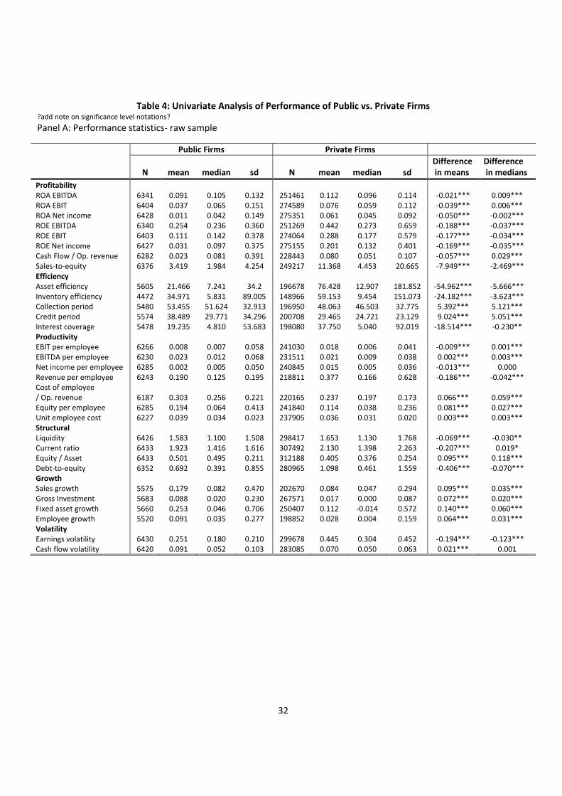
32  

Table 4: Univariate Analysis of Performance of Public vs. Private Firms ?add note on significance level notations? 

Panel A: Performance statistics‐ raw sample  

   Public Firms  Private Firms   

   N  mean  median  sd  N  mean  median  sd Difference in means 

Difference in medians 

Profitability                      ROA EBITDA  6341  0.091  0.105  0.132  251461  0.112  0.096  0.114  ‐0.021***  0.009*** ROA EBIT  6404  0.037  0.065  0.151  274589  0.076  0.059  0.112  ‐0.039***  0.006*** ROA Net income  6428  0.011  0.042  0.149  275351  0.061  0.045  0.092  ‐0.050***  ‐0.002*** ROE EBITDA  6340  0.254  0.236  0.360  251269  0.442  0.273  0.659  ‐0.188***  ‐0.037*** ROE EBIT  6403  0.111  0.142  0.378  274064  0.288  0.177  0.579  ‐0.177***  ‐0.034*** ROE Net income  6427  0.031  0.097  0.375  275155  0.201  0.132  0.401  ‐0.169***  ‐0.035*** Cash Flow / Op. revenue  6282  0.023  0.081  0.391  228443  0.080  0.051  0.107  ‐0.057***  0.029*** Sales‐to‐equity  6376  3.419  1.984  4.254  249217  11.368  4.453  20.665  ‐7.949***  ‐2.469*** Efficiency                     Asset efficiency  5605  21.466  7.241  34.2  196678  76.428  12.907  181.852  ‐54.962***  ‐5.666*** Inventory efficiency  4472  34.971  5.831  89.005  148966  59.153  9.454  151.073  ‐24.182***  ‐3.623*** Collection period  5480  53.455  51.624  32.913 196950 48.063 46.503 32.775  5.392*** 5.121***Credit period  5574  38.489  29.771  34.296 200708 29.465 24.721 23.129  9.024*** 5.051***Interest coverage  5478  19.235  4.810  53.683  198080  37.750  5.040  92.019  ‐18.514***  ‐0.230** Productivity                     EBIT per employee  6266  0.008  0.007  0.058  241030  0.018  0.006  0.041  ‐0.009***  0.001*** EBITDA per employee  6230  0.023  0.012  0.068  231511  0.021  0.009  0.038  0.002***  0.003*** Net income per employee  6285  0.002  0.005  0.050  240845  0.015  0.005  0.036  ‐0.013***  0.000 Revenue per employee  6243  0.190  0.125  0.195  218811  0.377  0.166  0.628  ‐0.186***  ‐0.042*** Cost of employee  / Op. revenue  6187  0.303  0.256  0.221  220165  0.237  0.197  0.173  0.066***  0.059*** Equity per employee  6285  0.194  0.064  0.413  241840  0.114  0.038  0.236  0.081***  0.027*** Unit employee cost  6227  0.039  0.034  0.023  237905  0.036  0.031  0.020  0.003***  0.003*** Structural                      Liquidity  6426  1.583  1.100  1.508  298417  1.653  1.130  1.768  ‐0.069***  ‐0.030** Current ratio  6433  1.923  1.416  1.616  307492  2.130  1.398  2.263  ‐0.207***  0.019* Equity / Asset  6433  0.501  0.495  0.211  312188  0.405  0.376  0.254  0.095***  0.118*** Debt‐to‐equity  6352  0.692  0.391  0.855  280965  1.098  0.461  1.559  ‐0.406***  ‐0.070*** Growth                      Sales growth  5575  0.179  0.082  0.470  202670  0.084  0.047  0.294  0.095***  0.035*** Gross Investment  5683  0.088  0.020  0.230  267571  0.017  0.000  0.087  0.072***  0.020*** Fixed asset growth  5660  0.253  0.046  0.706  250407  0.112  ‐0.014  0.572  0.140***  0.060*** Employee growth  5520  0.091  0.035  0.277  198852  0.028  0.004  0.159  0.064***  0.031*** Volatility                     Earnings volatility  6430  0.251  0.180  0.210  299678  0.445  0.304  0.452  ‐0.194***  ‐0.123*** Cash flow volatility  6420  0.091  0.052  0.103  283085  0.070  0.050  0.063  0.021***  0.001 

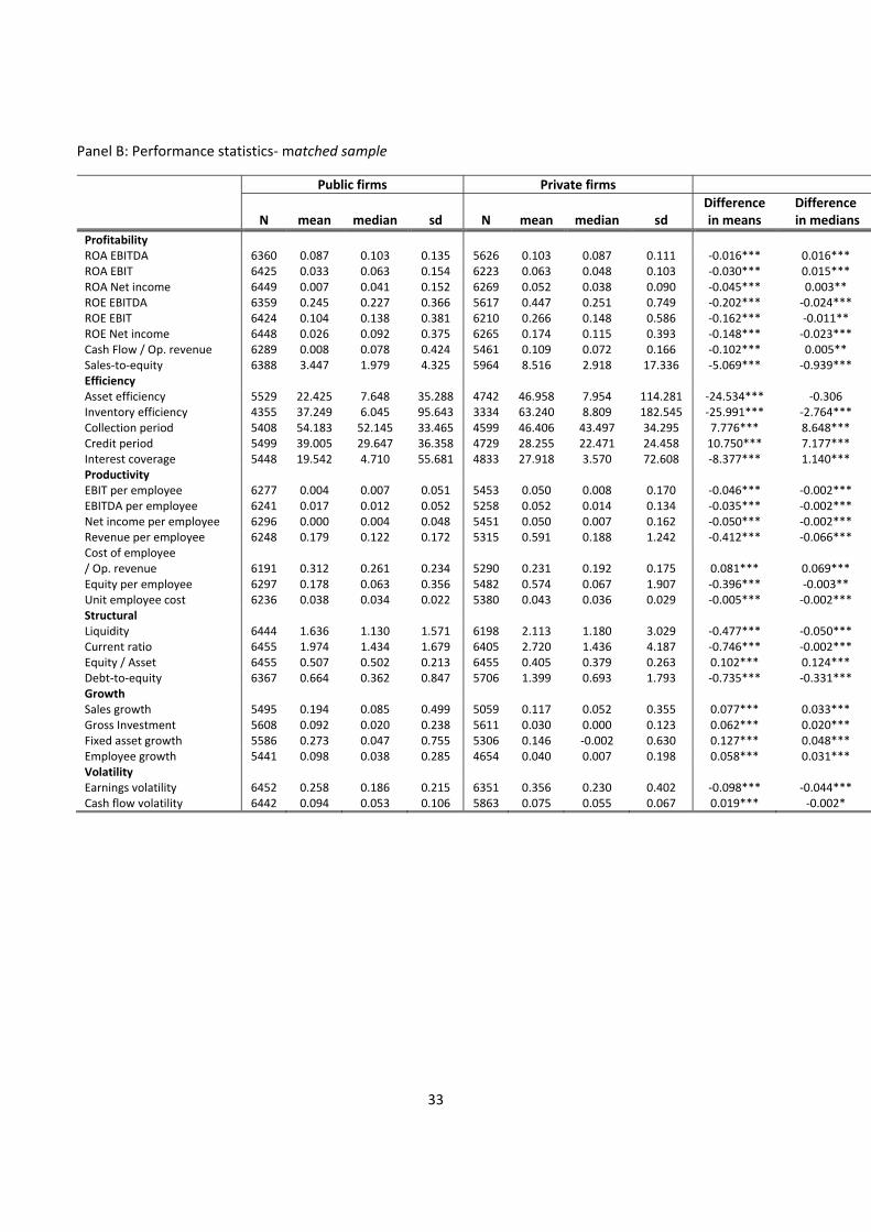
33  

Panel B: Performance statistics‐ matched sample  

  Public firms Private firms    

   N  mean  median  sd  N  mean  median  sd Differencein means 

Difference in medians 

Profitability                      ROA EBITDA  6360  0.087  0.103  0.135  5626  0.103  0.087  0.111  ‐0.016***  0.016*** ROA EBIT  6425  0.033  0.063  0.154  6223  0.063  0.048  0.103  ‐0.030***  0.015*** ROA Net income  6449  0.007  0.041  0.152  6269  0.052  0.038  0.090  ‐0.045***  0.003** ROE EBITDA  6359  0.245  0.227  0.366  5617  0.447  0.251  0.749  ‐0.202***  ‐0.024*** ROE EBIT  6424  0.104  0.138  0.381  6210  0.266  0.148  0.586  ‐0.162***  ‐0.011** ROE Net income  6448  0.026  0.092  0.375  6265  0.174  0.115  0.393  ‐0.148***  ‐0.023*** Cash Flow / Op. revenue  6289  0.008  0.078  0.424  5461  0.109  0.072  0.166  ‐0.102***  0.005** Sales‐to‐equity  6388  3.447  1.979  4.325  5964  8.516  2.918  17.336  ‐5.069***  ‐0.939*** Efficiency                     Asset efficiency  5529  22.425  7.648  35.288  4742  46.958  7.954  114.281  ‐24.534***  ‐0.306 Inventory efficiency  4355  37.249  6.045  95.643  3334  63.240  8.809  182.545  ‐25.991***  ‐2.764*** Collection period  5408  54.183  52.145  33.465  4599  46.406  43.497  34.295  7.776***  8.648*** Credit period  5499  39.005  29.647 36.358 4729 28.255 22.471 24.458  10.750*** 7.177***Interest coverage  5448  19.542  4.710 55.681 4833 27.918 3.570 72.608  ‐8.377*** 1.140***Productivity     EBIT per employee  6277  0.004  0.007  0.051  5453  0.050  0.008  0.170  ‐0.046***  ‐0.002*** EBITDA per employee  6241  0.017  0.012  0.052  5258  0.052  0.014  0.134  ‐0.035***  ‐0.002*** Net income per employee  6296  0.000  0.004  0.048  5451  0.050  0.007  0.162  ‐0.050***  ‐0.002*** Revenue per employee  6248  0.179  0.122  0.172  5315  0.591  0.188  1.242  ‐0.412***  ‐0.066*** Cost of employee  / Op. revenue  6191  0.312  0.261  0.234  5290  0.231  0.192  0.175  0.081***  0.069*** Equity per employee  6297  0.178  0.063  0.356  5482  0.574  0.067  1.907  ‐0.396***  ‐0.003** Unit employee cost  6236  0.038  0.034  0.022  5380  0.043  0.036  0.029  ‐0.005***  ‐0.002*** Structural                      Liquidity  6444  1.636  1.130  1.571  6198  2.113  1.180  3.029  ‐0.477***  ‐0.050*** Current ratio  6455  1.974  1.434  1.679  6405  2.720  1.436  4.187  ‐0.746***  ‐0.002*** Equity / Asset  6455  0.507  0.502  0.213  6455  0.405  0.379  0.263  0.102***  0.124*** Debt‐to‐equity  6367  0.664  0.362  0.847  5706  1.399  0.693  1.793  ‐0.735***  ‐0.331*** Growth                      Sales growth  5495  0.194  0.085  0.499  5059  0.117  0.052  0.355  0.077***  0.033*** Gross Investment  5608  0.092  0.020  0.238  5611  0.030  0.000  0.123  0.062***  0.020*** Fixed asset growth  5586  0.273  0.047  0.755  5306  0.146  ‐0.002  0.630  0.127***  0.048*** Employee growth  5441  0.098  0.038  0.285  4654  0.040  0.007  0.198  0.058***  0.031*** Volatility                     Earnings volatility  6452  0.258  0.186  0.215  6351  0.356  0.230  0.402  ‐0.098***  ‐0.044*** Cash flow volatility  6442  0.094  0.053  0.106  5863  0.075  0.055  0.067  0.019***  ‐0.002* 

 

   

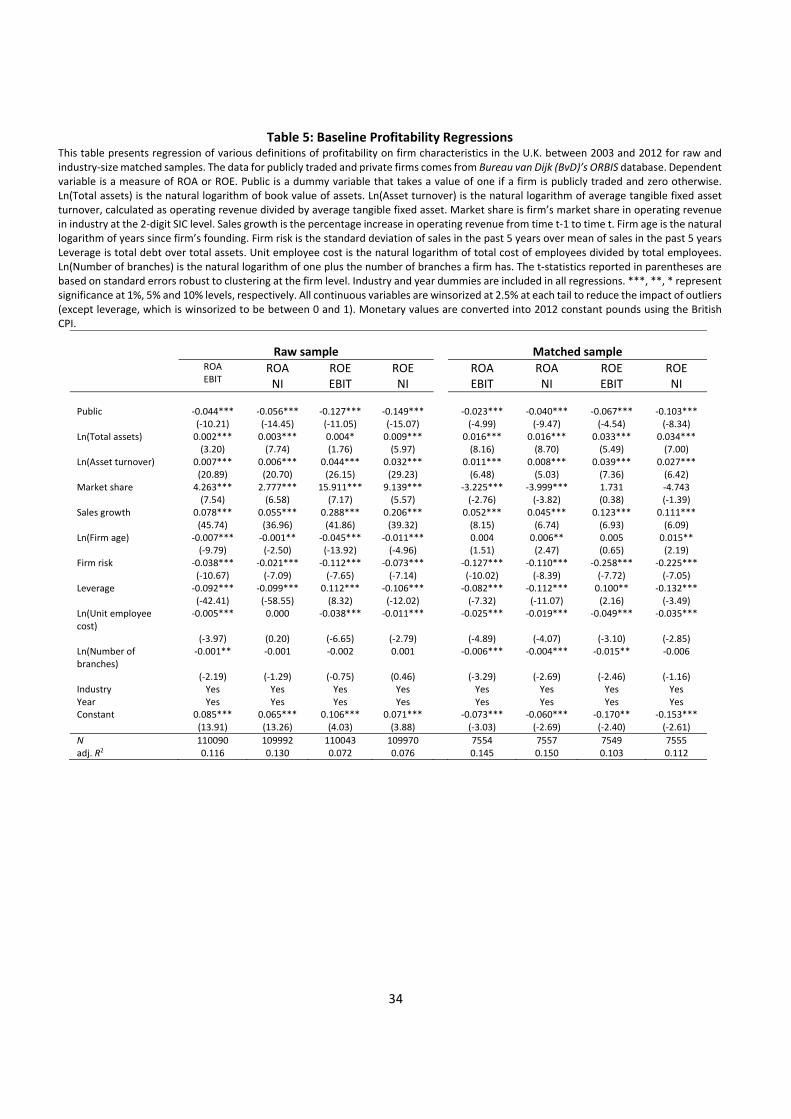
34  

Table 5: Baseline Profitability Regressions This table presents regression of various definitions of profitability on firm characteristics in the U.K. between 2003 and 2012 for raw and industry‐size matched samples. The data for publicly traded and private firms comes from Bureau van Dijk (BvD)’s ORBIS database. Dependent variable  is a measure of ROA or ROE. Public  is a dummy variable that takes a value of one  if a firm  is publicly traded and zero otherwise. Ln(Total assets) is the natural logarithm of book value of assets. Ln(Asset turnover) is the natural logarithm of average tangible fixed asset turnover, calculated as operating revenue divided by average tangible fixed asset. Market share is firm’s market share in operating revenue in industry at the 2‐digit SIC level. Sales growth is the percentage increase in operating revenue from time t‐1 to time t. Firm age is the natural logarithm of years since firm’s founding. Firm risk is the standard deviation of sales in the past 5 years over mean of sales in the past 5 years Leverage is total debt over total assets. Unit employee cost is the natural logarithm of total cost of employees divided by total employees. Ln(Number of branches) is the natural logarithm of one plus the number of branches a firm has. The t‐statistics reported in parentheses are based on standard errors robust to clustering at the firm level. Industry and year dummies are included in all regressions. ***, **, * represent significance at 1%, 5% and 10% levels, respectively. All continuous variables are winsorized at 2.5% at each tail to reduce the impact of outliers (except leverage, which is winsorized to be between 0 and 1). Monetary values are converted into 2012 constant pounds using the British CPI.  

                     Raw sample Matched sample   ROA 

EBIT ROA NI 

ROEEBIT 

ROENI 

ROAEBIT 

ROANI 

ROE EBIT 

ROENI 

       Public  ‐0.044***  ‐0.056***  ‐0.127***  ‐0.149***    ‐0.023***  ‐0.040***  ‐0.067***  ‐0.103***   (‐10.21)  (‐14.45)  (‐11.05) (‐15.07) (‐4.99) (‐9.47)  (‐4.54)  (‐8.34)Ln(Total assets)  0.002***  0.003***  0.004*  0.009***    0.016***  0.016***  0.033***  0.034***   (3.20)  (7.74)  (1.76) (5.97) (8.16) (8.70) (5.49)  (7.00)Ln(Asset turnover)  0.007***  0.006***  0.044***  0.032***    0.011***  0.008***  0.039***  0.027***   (20.89)  (20.70)  (26.15) (29.23) (6.48) (5.03) (7.36)  (6.42)Market share  4.263***  2.777***  15.911***  9.139***    ‐3.225***  ‐3.999***  1.731  ‐4.743   (7.54)  (6.58)  (7.17) (5.57) (‐2.76) (‐3.82)  (0.38)  (‐1.39)Sales growth  0.078***  0.055***  0.288***  0.206***    0.052***  0.045***  0.123***  0.111***   (45.74)  (36.96)  (41.86) (39.32) (8.15) (6.74) (6.93)  (6.09)Ln(Firm age)  ‐0.007***  ‐0.001**  ‐0.045***  ‐0.011***    0.004  0.006**  0.005  0.015**   (‐9.79)  (‐2.50)  (‐13.92) (‐4.96) (1.51) (2.47) (0.65)  (2.19)Firm risk  ‐0.038***  ‐0.021***  ‐0.112***  ‐0.073***    ‐0.127***  ‐0.110***  ‐0.258***  ‐0.225***   (‐10.67)  (‐7.09)  (‐7.65) (‐7.14) (‐10.02) (‐8.39)  (‐7.72)  (‐7.05)Leverage  ‐0.092***  ‐0.099***  0.112***  ‐0.106***    ‐0.082***  ‐0.112***  0.100**  ‐0.132***   (‐42.41)  (‐58.55)  (8.32)  (‐12.02)    (‐7.32)  (‐11.07)  (2.16)  (‐3.49) Ln(Unit employee cost) 

‐0.005*** 0.000  ‐0.038*** ‐0.011*** ‐0.025*** ‐0.019***  ‐0.049***  ‐0.035***

  (‐3.97)  (0.20)  (‐6.65) (‐2.79) (‐4.89) (‐4.07)  (‐3.10)  (‐2.85)Ln(Number of branches) 

‐0.001**  ‐0.001  ‐0.002  0.001    ‐0.006***  ‐0.004***  ‐0.015**  ‐0.006 

  (‐2.19)  (‐1.29)  (‐0.75)  (0.46)    (‐3.29)  (‐2.69)  (‐2.46)  (‐1.16) Industry   Yes  Yes  Yes Yes Yes Yes Yes  YesYear   Yes  Yes  Yes  Yes    Yes  Yes  Yes  Yes Constant  0.085***  0.065***  0.106*** 0.071*** ‐0.073*** ‐0.060***  ‐0.170**  ‐0.153***  (13.91)  (13.26)  (4.03)  (3.88)    (‐3.03)  (‐2.69)  (‐2.40)  (‐2.61) 

N  110090  109992  110043 109970 7554 7557 7549  7555adj. R2  0.116  0.130  0.072  0.076    0.145  0.150  0.103  0.112 

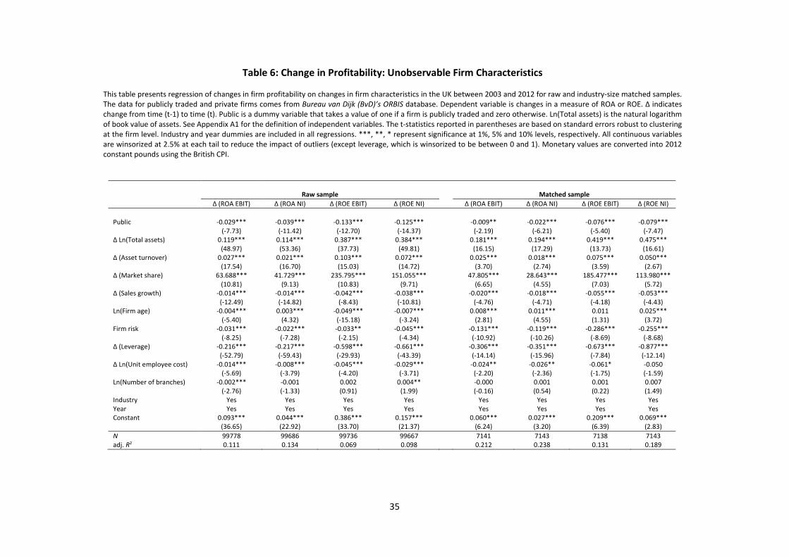
35  

Table 6: Change in Profitability: Unobservable Firm Characteristics  This table presents regression of changes in firm profitability on changes in firm characteristics in the UK between 2003 and 2012 for raw and industry‐size matched samples. The data for publicly traded and private firms comes from Bureau van Dijk (BvD)’s ORBIS database. Dependent variable is changes in a measure of ROA or ROE. ∆ indicates change from time (t‐1) to time (t). Public is a dummy variable that takes a value of one if a firm is publicly traded and zero otherwise. Ln(Total assets) is the natural logarithm of book value of assets. See Appendix A1 for the definition of independent variables. The t‐statistics reported in parentheses are based on standard errors robust to clustering at the firm level. Industry and year dummies are included in all regressions. ***, **, * represent significance at 1%, 5% and 10% levels, respectively. All continuous variables are winsorized at 2.5% at each tail to reduce the impact of outliers (except leverage, which is winsorized to be between 0 and 1). Monetary values are converted into 2012 constant pounds using the British CPI.   

                     Raw sample   Matched sample

  ∆ (ROA EBIT) ∆ (ROA NI) ∆ (ROE EBIT) ∆ (ROE NI)   ∆ (ROA EBIT) ∆ (ROA NI) ∆ (ROE EBIT) ∆ (ROE NI)

                   Public ‐0.029*** ‐0.039*** ‐0.133*** ‐0.125***   ‐0.009** ‐0.022*** ‐0.076*** ‐0.079***  (‐7.73)  (‐11.42)  (‐12.70)  (‐14.37)    (‐2.19)  (‐6.21)  (‐5.40)  (‐7.47) ∆ Ln(Total assets)  0.119*** 0.114*** 0.387*** 0.384***   0.181*** 0.194*** 0.419*** 0.475***  (48.97)  (53.36)  (37.73)  (49.81)    (16.15)  (17.29)  (13.73)  (16.61) ∆ (Asset turnover)  0.027*** 0.021*** 0.103*** 0.072***   0.025*** 0.018*** 0.075*** 0.050***  (17.54)  (16.70)  (15.03)  (14.72)    (3.70)  (2.74)  (3.59)  (2.67) ∆ (Market share) 63.688*** 41.729*** 235.795*** 151.055***   47.805*** 28.643*** 185.477*** 113.980***  (10.81)  (9.13)  (10.83)  (9.71)    (6.65)  (4.55)  (7.03)  (5.72) ∆ (Sales growth) ‐0.014*** ‐0.014*** ‐0.042*** ‐0.038***   ‐0.020*** ‐0.018*** ‐0.055*** ‐0.053***  (‐12.49)  (‐14.82)  (‐8.43)  (‐10.81)    (‐4.76)  (‐4.71)  (‐4.18)  (‐4.43) Ln(Firm age) ‐0.004*** 0.003*** ‐0.049*** ‐0.007***   0.008*** 0.011*** 0.011 0.025***  (‐5.40)  (4.32)  (‐15.18)  (‐3.24)    (2.81)  (4.55)  (1.31)  (3.72) Firm risk ‐0.031*** ‐0.022*** ‐0.033** ‐0.045***   ‐0.131*** ‐0.119*** ‐0.286*** ‐0.255***  (‐8.25)  (‐7.28)  (‐2.15)  (‐4.34)    (‐10.92)  (‐10.26)  (‐8.69)  (‐8.68) ∆ (Leverage)  ‐0.216***  ‐0.217***  ‐0.598***  ‐0.661***    ‐0.306***  ‐0.351***  ‐0.673***  ‐0.877***   (‐52.79) (‐59.43) (‐29.93) (‐43.39)   (‐14.14) (‐15.96) (‐7.84) (‐12.14)∆ Ln(Unit employee cost)  ‐0.014***  ‐0.008***  ‐0.045***  ‐0.029***    ‐0.024**  ‐0.026**  ‐0.061*  ‐0.050   (‐5.69) (‐3.79) (‐4.20) (‐3.71)   (‐2.20) (‐2.36) (‐1.75) (‐1.59)Ln(Number of branches)  ‐0.002***  ‐0.001  0.002  0.004**    ‐0.000  0.001  0.001  0.007   (‐2.76) (‐1.33) (0.91) (1.99)   (‐0.16) (0.54) (0.22) (1.49)Industry   Yes  Yes  Yes  Yes    Yes  Yes  Yes  Yes Year  Yes Yes Yes Yes   Yes Yes Yes YesConstant  0.093***  0.044***  0.386***  0.157***    0.060***  0.027***  0.209***  0.069***   (36.65) (22.92) (33.70) (21.37)   (6.24) (3.20) (6.39) (2.83)

N  99778  99686  99736  99667    7141  7143  7138  7143 adj. R2 0.111 0.134 0.069 0.098   0.212 0.238 0.131 0.189

 

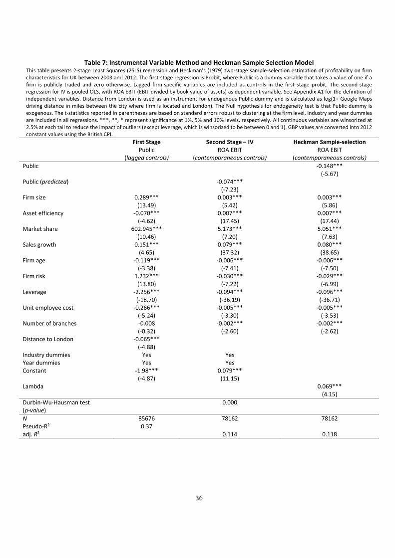
36  

Table 7: Instrumental Variable Method and Heckman Sample Selection Model This table presents 2‐stage Least Squares (2SLS) regression and Heckman’s (1979) two‐stage sample‐selection estimation of profitability on firm characteristics for UK between 2003 and 2012. The first‐stage regression is Probit, where Public is a dummy variable that takes a value of one if a firm  is  publicly  traded  and  zero  otherwise.  Lagged  firm‐specific  variables  are  included  as  controls  in  the  first  stage  probit.  The  second‐stage regression for IV is pooled OLS, with ROA EBIT (EBIT divided by book value of assets) as dependent variable. See Appendix A1 for the definition of independent variables. Distance from London  is used as an  instrument  for endogenous Public dummy and  is calculated as  log(1+ Google Maps driving distance  in miles between the city where firm  is  located and London). The Null hypothesis for endogeneity test  is that Public dummy  is exogenous. The t‐statistics reported in parentheses are based on standard errors robust to clustering at the firm level. Industry and year dummies are included in all regressions. ***, **, * represent significance at 1%, 5% and 10% levels, respectively. All continuous variables are winsorized at 2.5% at each tail to reduce the impact of outliers (except leverage, which is winsorized to be between 0 and 1). GBP values are converted into 2012 constant values using the British CPI.  

  First Stage  Second Stage – IV Heckman Sample‐selection  Public  ROA EBIT ROA EBIT  (lagged controls) (contemporaneous controls) (contemporaneous controls)

Public    ‐0.148***    (‐5.67)Public (predicted)    ‐0.074***    (‐7.23)Firm size  0.289***  0.003*** 0.003***  (13.49)  (5.42) (5.86)Asset efficiency  ‐0.070***  0.007*** 0.007***  (‐4.62)  (17.45) (17.44)Market share  602.945***  5.173*** 5.051***  (10.46)  (7.20) (7.63)Sales growth  0.151***  0.079*** 0.080***  (4.65)  (37.32) (38.65)Firm age  ‐0.119***  ‐0.006*** ‐0.006***  (‐3.38)  (‐7.41) (‐7.50)Firm risk  1.232***  ‐0.030*** ‐0.029***  (13.80)  (‐7.22) (‐6.99)Leverage  ‐2.256***  ‐0.094*** ‐0.096***  (‐18.70)  (‐36.19) (‐36.71)Unit employee cost  ‐0.266***  ‐0.005*** ‐0.005***  (‐5.24)  (‐3.30) (‐3.53)Number of branches  ‐0.008  ‐0.002*** ‐0.002***  (‐0.32)  (‐2.60) (‐2.62)Distance to London  ‐0.065***   (‐4.88) Industry dummies  Yes  YesYear dummies  Yes  YesConstant  ‐1.98***  0.079***  (‐4.87)  (11.15)Lambda    0.069***    (4.15)

Durbin‐Wu‐Hausman test     0.000(p‐value)   

N  85676  78162 78162Pseudo‐R2  0.37 adj. R2    0.114 0.118

    

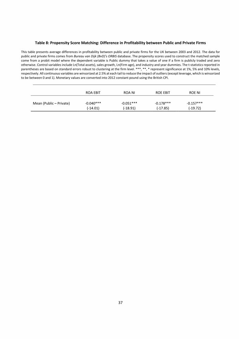
37  

 

Table 8: Propensity Score Matching: Difference in Profitability between Public and Private Firms  This table presents average differences in profitability between public and private firms for the UK between 2003 and 2012. The data for public and private firms comes from Bureau van Dijk (BvD)’s ORBIS database. The propensity scores used to construct the matched sample come from a probit model where the dependent variable  is Public dummy that takes a value of one  if a firm  is publicly traded and zero otherwise. Control variables include Ln(Total assets), sales growth, Ln(Firm age), and industry and year dummies. The t‐statistics reported in parentheses are based on standard errors robust to clustering at the firm level. ***, **, * represent significance at 1%, 5% and 10% levels, respectively. All continuous variables are winsorized at 2.5% at each tail to reduce the impact of outliers (except leverage, which is winsorized to be between 0 and 1). Monetary values are converted into 2012 constant pound using the British CPI.  

         

   

           ROA EBIT ROA NI ROE EBIT  ROE NI

     

Mean (Public – Private)  ‐0.040*** ‐0.051*** ‐0.178***  ‐0.157***

  (‐14.01) (‐18.91) (‐17.85)  (‐19.72)

         

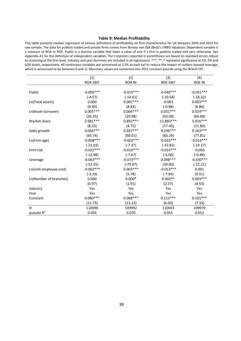
38  

Table 9: Median Profitability This table presents median regression of various definitions of profitability on firm characteristics for UK between 2003 and 2012 for raw sample. The data for publicly traded and private firms comes from Bureau van Dijk (BvD)’s ORBIS database. Dependent variable is a measure of ROA or ROE. Public  is a dummy variable that takes a value of one  if a firm  is publicly traded and zero otherwise. See Appendix A1 for the definition of independent variables. The t‐statistics reported in parentheses are based on standard errors robust to clustering at the firm level. Industry and year dummies are included in all regressions. ***, **, * represent significance at 1%, 5% and 10% levels, respectively. All continuous variables are winsorized at 2.5% at each tail to reduce the impact of outliers (except leverage, which is winsorized to be between 0 and 1). Monetary values are converted into 2012 constant pounds using the British CPI.   

  (1)  (2) (3)  (4)  ROA EBIT  ROA NI ROE EBIT  ROE NI

   Public  ‐0.006*** ‐0.015*** ‐0.040***  ‐0.051***  (‐4.57)  (‐14.61) (‐10.54)  (‐18.32)Ln(Total assets)  0.000  0.001*** ‐0.001  0.003***  (0.99)  (8.83) (‐0.98)  (6.80)Ln(Asset turnover)  0.005***  0.004*** 0.031***  0.024***  (26.35)  (29.98) (63.04)  (66.68)Market share  2.081***  0.892*** 11.883***  5.916***  (8.33)  (4.75) (17.40)  (11.80)Sales growth  0.068***  0.047*** 0.236***  0.163***  (65.74)  (60.01) (83.29)  (77.81)Ln(Firm age)  ‐0.008*** ‐0.002*** ‐0.033***  ‐0.014***  (‐21.03)  (‐7.37) (‐32.82)  (‐19.27)Firm risk  ‐0.022*** ‐0.010*** ‐0.023***  ‐0.003  (‐12.98)  (‐7.47) (‐5.00)  (‐0.88)Leverage  ‐0.063*** ‐0.073*** 0.098***  ‐0.030***  (‐52.55)  (‐79.97) (30.00)  (‐12.21)Ln(Unit employee cost)  ‐0.002*** 0.003*** ‐0.013***  0.001  (‐3.19)  (5.78) (‐7.84)  (0.51)Ln(Number of branches)  0.000  0.000* 0.002**  0.003***  (0.97)  (1.91) (2.37)  (4.53)Industry   Yes  Yes Yes  YesYear   Yes  Yes Yes  YesConstant  0.080***  0.068*** 0.112***  0.101***  (11.75)  (13.15) (6.03)  (7.33)

N  110090  109992 110043  109970pseudo R2  0.056  0.070 0.055  0.052

  

   

39  

Table 10: Changes in Ownership Status  

This table presents operating profitability for public and private firms for the UK between 2003 and 2012. We differentiate between firms that 

are public or private throughout the sample period, and those who did IPO or delisted from stock exchange.  

 

   Firms  with no change in ownership status during 2003‐2012 

Firms that conducted IPO or delisted from stock exchange during 2003‐2012      

   Public  Private  Difference     Public  Private  Difference 

ROA EBIT  0.045  0.076  ‐0.031***    0.015  0.035  ‐0.021*** 

ROA NI  0.019  0.061  ‐0.042***    ‐0.011  0.045  ‐0.056*** 

ROE EBIT  0.131  0.289  ‐0.157***    0.051  0.075  ‐0.024*** 

ROE NI  0.051  0.201  ‐0.150***     ‐0.023  0.076  ‐0.098*** 

 

   

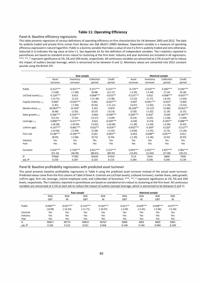
40  

Table 11: Operating Efficiency Panel A: Baseline efficiency regressions This table presents regression of various definitions of operating efficiency on firm characteristics for UK between 2003 and 2012. The data for publicly traded and private firms comes from Bureau van Dijk (BvD)’s ORBIS database. Dependent variable  is a measure of operating efficiency expressed in natural logarithm. Public is a dummy variable that takes a value of one if a firm is publicly traded and zero otherwise. Subscript (t‐1) indicates the lag value at time t‐1. See Appendix A1 for the definition of independent variables. The t‐statistics reported in parentheses are based on standard errors robust to clustering at the firm level. Industry and year dummies are included in all regressions. ***, **, * represent significance at 1%, 5% and 10% levels, respectively. All continuous variables are winsorized at 2.5% at each tail to reduce the  impact of outliers (except  leverage, which  is winsorized to be between 0 and 1). Monetary values are converted  into 2012 constant pounds using the British CPI.  

 

                       Raw sample Matched sample

  Asset turnover 

Inventory turnover 

Collection  period 

Credit  period 

    Asset turnover 

Inventory turnover 

Collection  period 

Credit  period 

                     Public  ‐0.312*** ‐0.451***  0.271*** 0.315*** ‐0.179** ‐0.410***  0.360*** 0.344***  (‐5.68)  (‐7.68)  (8.48)  (11.17)      (‐2.24)  (‐5.44)  (7.14)  (9.18) Ln(Total assets) (t‐1)  ‐0.118*** 0.013  ‐0.068*** ‐0.013** ‐0.125*** 0.032  ‐0.098*** ‐0.033***  (‐13.71)  (1.51)  (‐11.30)  (‐2.48)      (‐5.22)  (1.17)  (‐6.35)  (‐2.65) Capital intensity (t‐1)  0.006*  ‐0.024***  0.001 ‐0.022*** ‐0.007 ‐0.041***  ‐0.015* ‐0.003  (1.81)  (‐7.40)  (0.35)  (‐11.11)      (‐0.47)  (‐2.92)  (‐1.70)  (‐0.41) Market share (t‐1)  69.064*** 14.392*  3.162 ‐0.874 36.228** ‐15.123  12.881 10.815**  (6.96)  (1.92)  (0.57)  (‐0.23)      (2.50)  (‐1.02)  (1.19)  (2.15) Sales growth (t‐1)  0.266*** 0.159***  ‐0.002 ‐0.038*** 0.260*** 0.102*  ‐0.039 ‐0.140***  (12.21)  (7.54)  (‐0.17)  (‐3.09)      (5.24)  (1.65)  (‐1.06)  (‐3.84) Leverage (t‐1)  ‐0.898*** ‐0.471***  ‐0.021 ‐0.439*** ‐0.240 ‐0.276  ‐0.205** 0.488***  (‐18.28)  (‐10.03)  (‐0.62)  (‐16.04)      (‐1.38)  (‐1.44)  (‐2.04)  (5.43) Ln(Firm age)  ‐0.147*** ‐0.081***  0.022** ‐0.019** ‐0.932*** ‐0.359*  0.220* ‐0.217**  (‐10.56)  (‐5.99)  (2.38)  (‐2.42)      (‐4.69)  (‐1.91)  (1.72)  (‐2.26) Firm risk  0.538*** ‐0.194***  0.031 0.093** ‐0.053 ‐0.098**  0.057** 0.011  (8.05)  (‐2.86)  (0.71)  (2.54)      (‐1.29)  (‐2.36)  (2.01)  (0.55) Industry   Yes  Yes  Yes Yes Yes Yes  Yes YesYear   Yes  Yes  Yes Yes Yes Yes  Yes Yes                     Constant  3.355*** 2.718***  3.651*** 3.157*** 3.059*** 2.555***  3.497*** 2.981***  (55.10)  (46.09)  (86.81)  (89.93)      (14.85)  (12.84)  (27.06)  (30.31) 

N  97960  77393  95434  97353      7114  5554  6899  7030 adj. R2  0.259  0.287  0.235 0.114 0.284 0.246  0.295 0.139

 

Panel B: Baseline profitability regressions with predicted asset turnover This panel presents baseline profitability  regressions  in Table 4 using  the predicted asset  turnover  instead of  the actual asset  turnover. Predicted values come from the first column of Table 9 Panel A. Controls are Ln(Total assets), Ln(Asset turnover), market share, sales growth, Ln(Firm age), firm risk, leverage, Ln(Unit employee cost), and Ln(Number of branches). ***, **, * represent significance at 1%, 5% and 10% levels, respectively. The t‐statistics reported in parentheses are based on standard errors robust to clustering at the firm level. All continuous variables are winsorized at 2.5% at each tail to reduce the impact of outliers (except leverage, which is winsorized to be between 0 and 1).                      Raw sample Matched sample 

  ROA  EBIT 

ROA  NI 

ROE  EBIT 

ROE  NI 

  ROA  EBIT 

ROA  NI 

ROE  EBIT 

ROE  NI 

       Public  ‐0.040***  ‐0.057***  ‐0.142***  ‐0.164***    ‐0.011**  ‐0.028***  ‐0.048***  ‐0.077***   (‐8.99)  (‐14.24)  (‐11.71) (‐16.07) (‐2.04) (‐5.45)  (‐2.96)  (‐5.26)Controls  Yes  Yes  Yes  Yes    Yes  Yes  Yes  Yes Industry   Yes  Yes  Yes Yes Yes Yes  Yes  YesYear   Yes  Yes  Yes  Yes    Yes  Yes  Yes  Yes 

N  90817  90774  90810 90767 6890 6901  6890  6901adj. R2  0.105  0.122  0.051  0.058    0.140  0.149  0.094  0.109 

  

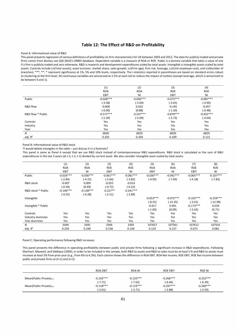
41  

Table 12: The Effect of R&D on Profitability  Panel A: Informational value of R&D This panel presents regression of various definitions of profitability on firm characteristics for UK between 2003 and 2012. The data for publicly traded and private firms comes from Bureau van Dijk (BvD)’s ORBIS database. Dependent variable is a measure of ROA or ROE. Public is a dummy variable that takes a value of one if a firm is publicly traded and zero otherwise. R&D is research and development expenditures scaled by total assets. Intangible is intangible assets scaled by total assets. Controls include Ln(Total assets), asset turnover, market share, sales growth, Ln(Firm age), firm risk, leverage, Ln(Unit employee cost), and Ln(Number of branches). ***, **, * represent significance at 1%, 5% and 10% levels, respectively. The t‐statistics reported in parentheses are based on standard errors robust to clustering at the firm level. All continuous variables are winsorized at 2.5% at each tail to reduce the impact of outliers (except leverage, which is winsorized to be between 0 and 1).  

  (1)  (2)  (3)  (4)   ROA 

EBIT ROA NI 

ROE  EBIT 

ROE NI 

Public  ‐0.028*** ‐0.036*** ‐0.073***  ‐0.087***  (‐3.58)  (‐5.04)  (‐3.65)  (‐4.90) R&D flow  ‐0.000 0.032 ‐0.195  ‐0.057  (‐0.00)  (0.88)  (‐1.30)  (‐0.48) R&D flow * Public  ‐0.577*** ‐0.537*** ‐0.879***  ‐0.925***  (‐5.39)  (‐5.09)  (‐3.73)  (‐4.04) Controls  Yes Yes Yes  YesIndustry   Yes  Yes  Yes  Yes Year   Yes Yes Yes  Yes

N  6830  6829  6830  6829 adj. R2  0.202 0.204 0.109  0.115

 Panel B: Informational value of R&D stock ?I would delete intangiles in the table – just discuss it in a footnote? This panel  is  same as Panel A except  that we use R&D  stock  instead of contemporaneous R&D expenditures. R&D  stock  is  calculated as  the  sum of R&D expenditures in the last 3 years (at t‐3, t‐2, t‐1) divided by current asset. We also consider intangible asset scaled by total assets.  

  (1)  (2)  (3) (4) (5) (6)  (7)  (8)  ROA  

EBIT ROA  NI 

ROE  EBIT 

ROE  NI 

ROA  EBIT 

ROA  NI 

ROE  EBIT 

ROE  NI 

Public  ‐0.026***  ‐0.036***  ‐0.061***  ‐0.081***  ‐0.030***  ‐0.042***  ‐0.065***  ‐0.107***   (‐2.84) (‐4.15)  (‐2.64) (‐3.82) (‐4.93) (‐7.69)  (‐4.18) (‐7.83)R&D stock  ‐0.007  0.009  ‐0.055  ‐0.014           (‐0.34) (0.49)  (‐0.72) (‐0.22)    R&D stock * Public  ‐0.146***  ‐0.138***  ‐0.227**  ‐0.241***           (‐4.55) (‐4.28)  (‐2.51) (‐2.89)    Intangible           ‐0.053***  ‐0.075***  ‐0.105***  ‐0.259***       (‐8.55) (‐15.45)  (‐3.41) (‐12.98)Intangible * Public          ‐0.017  0.001  ‐0.173***  0.029       (‐1.00) (0.09)  (‐3.43) (0.71)Controls  Yes  Yes  Yes  Yes  Yes  Yes  Yes  Yes Industry dummies  Yes  Yes  Yes Yes Yes Yes  Yes YesYear dummies  Yes  Yes  Yes  Yes  Yes  Yes  Yes  Yes 

N  3394  3395  3394 3395 107657 107561  107612 107541Adj. R2  0.259  0.240  0.158  0.149  0.119  0.137  0.073  0.081 

    Panel C: Operating performance following R&D increases  This panel presents the difference in operating profitability between public and private firms following a significant increase in R&D expenditures. Following Eberhart, Maxwell, and Siddique (2004), in order to be included in the sample, both R&D to assets and R&D to sales must be at least 5 % and R&D to assets must increase at least 5% from prior year (e.g., from 6% to 6.3%). Each column shows the difference in ROA EBIT, ROA Net income, ROE EBIT, ROE Net income between public and private firms at (t+1) and (t+2).  

   

           ROA EBIT ROA NI ROE EBIT  ROE NI

   Mean(Public‐Private)t+1  ‐0.142***  ‐0.133***  ‐0.266***  ‐0.252***   (‐7.71) (‐7.62) (‐6.46)  (‐6.39)Mean(Public‐Private)t+2  ‐0.118***  ‐0.119***  ‐0.297***  ‐0.260***   (‐3.61) (‐3.71) (‐3.88)  (‐3.59)

42  

Table 13:  Mean Profitability by Percentage of Ownership  

This table shows operating profitability for public and private firms for different shareholder ownership brackets.   

   Ownership (0%, 25%]     Ownership (25%, 50%]     Ownership (50%, 100%] 

   Public  Private  Difference     Public  Private  Difference     Public  Private  Difference 

ROA EBIT  0.040  0.058  ‐0.018***    0.029  0.075  ‐0.047***    0.030  0.077  ‐0.046*** 

ROA net income  0.014  0.046  ‐0.032***    0.003  0.055  ‐0.053***    0.004  0.063  ‐0.059*** 

ROE EBIT  0.125  0.208  ‐0.082***    0.075  0.280  ‐0.205***    0.089  0.293  ‐0.204*** 

ROE net income  0.047  0.136  ‐0.089***     ‐0.007  0.174  ‐0.181***     0.008  0.208  ‐0.200*** 

 

    

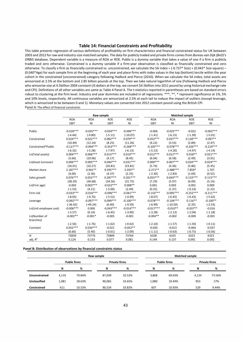
43  

Table 14: Financial Constraints and Profitability This table presents regression of various definitions of profitability on firm characteristics and financial constrained status for UK between 2003 and 2012 for raw and industry‐size matched samples. The data for publicly traded and private firms comes from Bureau van Dijk (BvD)’s ORBIS database. Dependent variable is a measure of ROA or ROE. Public is a dummy variable that takes a value of one if a firm is publicly traded and  zero otherwise. Constrained  is a dummy variable  if a  firm‐year observation  is  classified as  financially constrained and  zero otherwise. To classify a firm as financially constrained vs. unconstrained, we calculate the SA index = (‐0.737* Size) + (0.043* Size‐square) – (0.040*Age) for each sample firm at the beginning of each year and place firms with index values in the top (bottom) tercile within the year cohort in the constrained (unconstrained) category following Hadlock and Pierce (2010). When we calculate the SA index, total assets are winsorized at 2.5% at the bottom and 2.85 billion pounds at the top. Then we take natural logarithm of size (Following Hadlock and Pierce who winsorize size at 4.5billion 2004 constant US dollars at the top, we convert $4.5billion into 2011 pound by using historical exchange rate and CPI). Definitions of all other variables are same as Table 4 Panel A. The t‐statistics reported in parentheses are based on standard errors robust to clustering at the firm level. Industry and year dummies are included in all regressions. ***, **, * represent significance at 1%, 5% and 10% levels, respectively. All continuous variables are winsorized at 2.5% at each tail to reduce the impact of outliers (except leverage, which is winsorized to be between 0 and 1). Monetary values are converted into 2012 constant pound using the British CPI.  Panel A: The effect of financial constraints 

         Raw sample    Matched sample 

  ROA  EBIT 

ROA  NI 

ROE  EBIT 

ROE  NI 

  ROA  EBIT 

ROA  NI 

ROE  EBIT 

ROE  NI 

                   Public  ‐0.018***  ‐0.035***  ‐0.059*** ‐0.096*** ‐0.006 ‐0.025***  ‐0.022  ‐0.063***  (‐4.44)  (‐9.80)  (‐5.11)  (‐10.07)    (‐1.41)  (‐6.15)  (‐1.39)  (‐5.01) Constrained  0.024***  0.022***  0.082*** 0.079*** 0.053*** 0.037***  0.158***  0.097**  (10.49)  (12.24)  (8.25)  (11.26)    (4.22)  (3.53)  (2.89)  (2.47) Constrained*Public  ‐0.117***  ‐0.094***  ‐0.353*** ‐0.268*** ‐0.105*** ‐0.078***  ‐0.326***  ‐0.219***  (‐6.32)  (‐5.28)  (‐7.97)  (‐6.13)    (‐5.13)  (‐4.20)  (‐4.97)  (‐4.14) Ln(Total assets)  0.004***  0.006***  0.013*** 0.019*** 0.012*** 0.012***  0.018**  0.021***  (5.66)  (10.06)  (4.17)  (8.45)    (6.04)  (6.58)  (2.49)  (3.91) Ln(Asset turnover)  0.006***  0.005***  0.040*** 0.031*** 0.009*** 0.007***  0.034***  0.024***  (16.01)  (16.27)  (20.81)  (23.81)    (5.74)  (4.36)  (5.86)  (5.45) Market share  2.187***  0.941**  9.595***  3.593**    ‐2.271**  ‐2.488***  7.859*  1.707   (4.00)  (2.36)  (4.37) (2.25) (‐2.30) (‐2.83)  (1.69)  (0.52)Sales growth  0.076***  0.052***  0.287***  0.201***    0.055***  0.044***  0.133***  0.115***   (38.29)  (30.68)  (34.56) (31.75) (7.29) (5.97)  (6.09)  (5.14)Ln(Firm age)  ‐0.002  0.003***  ‐0.022***  0.008**    0.001  0.003  ‐0.001  0.009   (‐1.53)  (4.21)  (‐5.00) (2.49) (0.25) (1.37)  (‐0.14)  (1.22)Firm risk  ‐0.033***  ‐0.016***  ‐0.096***  ‐0.061***    ‐0.116***  ‐0.095***  ‐0.252***  ‐0.211***   (‐8.05)  (‐4.70)  (‐5.52) (‐4.99) (‐8.07) (‐6.45)  (‐6.43)  (‐5.62)Leverage  ‐0.092***  ‐0.097***  0.099***  ‐0.100***    ‐0.078***  ‐0.104***  0.116**  ‐0.100**   (‐36.42)  (‐49.24)  (6.40) (‐9.59) (‐6.99) (‐10.50)  (2.35)  (‐2.53)Ln(Unit employee cost)  ‐0.006***  0.000  ‐0.043***  ‐0.014***    ‐0.017***  ‐0.010**  ‐0.037**  ‐0.016   (‐3.57)  (0.16)  (‐6.45) (‐3.00) (‐3.28) (‐2.13)  (‐2.04)  (‐1.18)Ln(Number of branches) 

‐0.002**  ‐0.001*  ‐0.005  ‐0.001    ‐0.004**  ‐0.002  ‐0.009  ‐0.001 

  (‐2.56)  (‐1.76)  (‐1.62)  (‐0.62)    (‐2.10)  (‐1.57)  (‐1.50)  (‐0.11) Constant  0.052***  0.034***  ‐0.021 ‐0.052** ‐0.026 ‐0.013  ‐0.064  ‐0.037  (6.66)  (5.40)  (‐0.61)  (‐2.09)    (‐1.11)  (‐0.63)  (‐0.75)  (‐0.56) 

N  73839  73776  73809 73764 6328 6325  6323  6323adj. R2  0.124  0.133  0.077  0.081    0.144  0.137  0.091  0.092 

 Panel B: Distribution of observations by financial constraints status 

   Raw sample     Matched sample 

   Public firms     Private firms    Public firms     Private firms 

   N  %    N  %    N  %    N  % 

Unconstrained  4,110  70.84%    87,039  32.52%    3,868  69.63%    4,124  73.56% 

Unclassified  1,081  18.63%    90,065  33.65%    1,080  19.44%    953  17% 

Constrained  611  10.53%     90,534  33.83%     607  10.93%     529  9.44% 

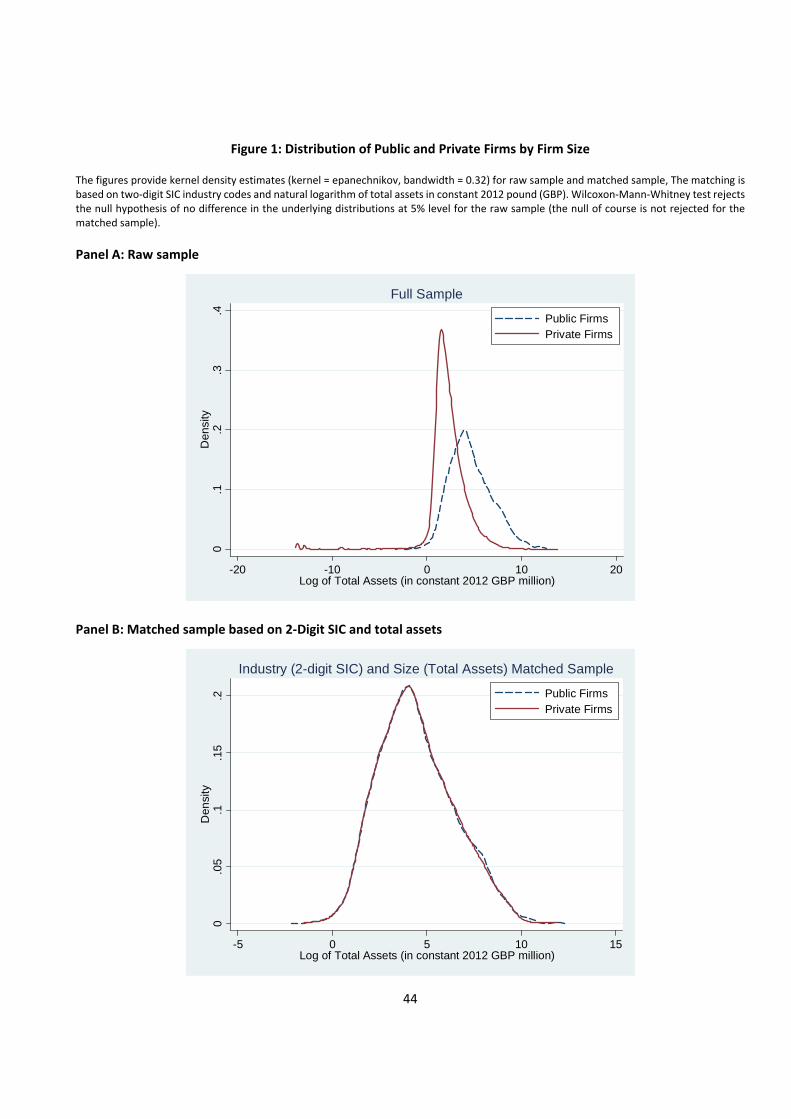
44  

Figure 1: Distribution of Public and Private Firms by Firm Size 

The figures provide kernel density estimates (kernel = epanechnikov, bandwidth = 0.32) for raw sample and matched sample, The matching is based on two‐digit SIC industry codes and natural logarithm of total assets in constant 2012 pound (GBP). Wilcoxon‐Mann‐Whitney test rejects the null hypothesis of no difference in the underlying distributions at 5% level for the raw sample (the null of course is not rejected for the matched sample).  

 

Panel A: Raw sample 

 

Panel B: Matched sample based on 2‐Digit SIC and total assets 

 

0.1

.2.3

.4D

ensi

ty

-20 -10 0 10 20Log of Total Assets (in constant 2012 GBP million)

Public FirmsPrivate Firms

Full Sample

0.0

5.1

.15

.2D

ensi

ty

-5 0 5 10 15Log of Total Assets (in constant 2012 GBP million)

Public FirmsPrivate Firms

Industry (2-digit SIC) and Size (Total Assets) Matched Sample

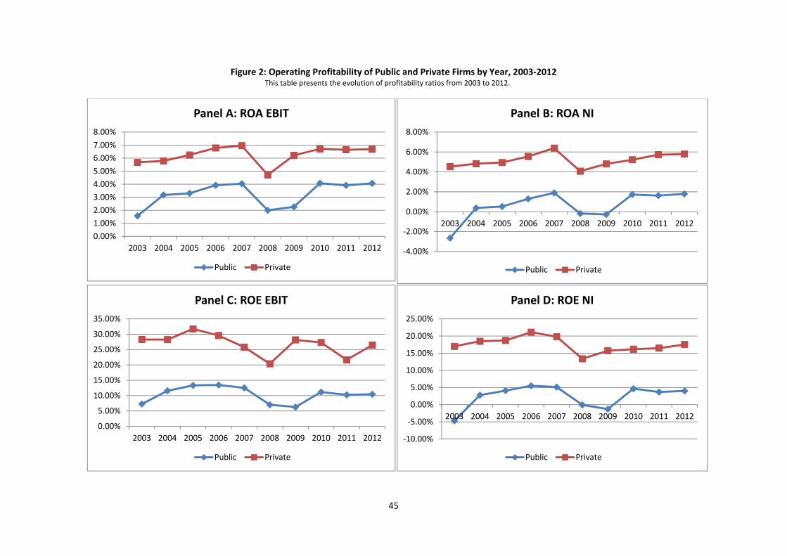
45  

Figure 2: Operating Profitability of Public and Private Firms by Year, 2003‐2012 This table presents the evolution of profitability ratios from 2003 to 2012. 

0.00%

1.00%

2.00%

3.00%

4.00%

5.00%

6.00%

7.00%

8.00%

2003 2004 2005 2006 2007 2008 2009 2010 2011 2012

Panel A: ROA EBIT

Public Private

‐4.00%

‐2.00%

0.00%

2.00%

4.00%

6.00%

8.00%

2003 2004 2005 2006 2007 2008 2009 2010 2011 2012

Panel B: ROA NI

Public Private

0.00%

5.00%

10.00%

15.00%

20.00%

25.00%

30.00%

35.00%

2003 2004 2005 2006 2007 2008 2009 2010 2011 2012

Panel C: ROE EBIT

Public Private

‐10.00%

‐5.00%

0.00%

5.00%

10.00%

15.00%

20.00%

25.00%

2003 2004 2005 2006 2007 2008 2009 2010 2011 2012

Panel D: ROE NI

Public Private

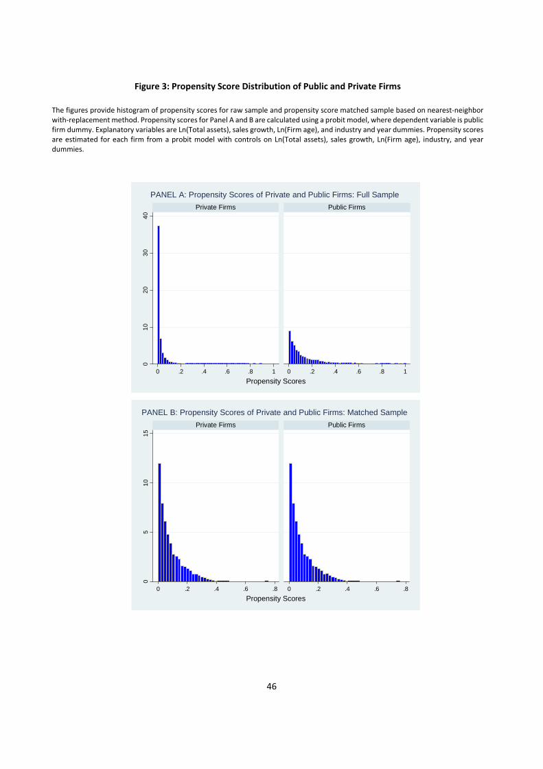
46  

Figure 3: Propensity Score Distribution of Public and Private Firms 

  The figures provide histogram of propensity scores for raw sample and propensity score matched sample based on nearest‐neighbor with‐replacement method. Propensity scores for Panel A and B are calculated using a probit model, where dependent variable is public firm dummy. Explanatory variables are Ln(Total assets), sales growth, Ln(Firm age), and industry and year dummies. Propensity scores are estimated  for each  firm  from a probit model with controls on Ln(Total assets), sales growth, Ln(Firm age),  industry, and year dummies. 

  

 

 

01

02

03

04

0

0 .2 .4 .6 .8 1 0 .2 .4 .6 .8 1

Private Firms Public Firms

Propensity Scores

PANEL A: Propensity Scores of Private and Public Firms: Full Sample

05

10

15

0 .2 .4 .6 .8 0 .2 .4 .6 .8

Private Firms Public Firms

Propensity Scores

PANEL B: Propensity Scores of Private and Public Firms: Matched Sample

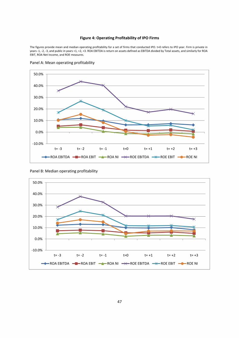
47  

Figure 4: Operating Profitability of IPO Firms 

The figures provide mean and median operating profitability for a set of firms that conducted IPO. t=0 refers to IPO year. Firm is private in years ‐1, ‐2, ‐3, and public in years +1, +2, +3. ROA EBITDA is return on assets defined as EBITDA divided by Total assets, and similarly for ROA EBIT, ROA Net Income, and ROE measures.   

Panel A: Mean operating profitability 

 

Panel B: Median operating profitability 

 

   

‐10.0%

0.0%

10.0%

20.0%

30.0%

40.0%

50.0%

t= ‐3 t= ‐2 t= ‐1 t=0 t= +1 t= +2 t= +3

ROA EBITDA ROA EBIT ROA NI ROE EBITDA ROE EBIT ROE NI

‐10.0%

0.0%

10.0%

20.0%

30.0%

40.0%

50.0%

t= ‐3 t= ‐2 t= ‐1 t=0 t= +1 t= +2 t= +3

ROA EBITDA ROA EBIT ROA NI ROE EBITDA ROE EBIT ROE NI

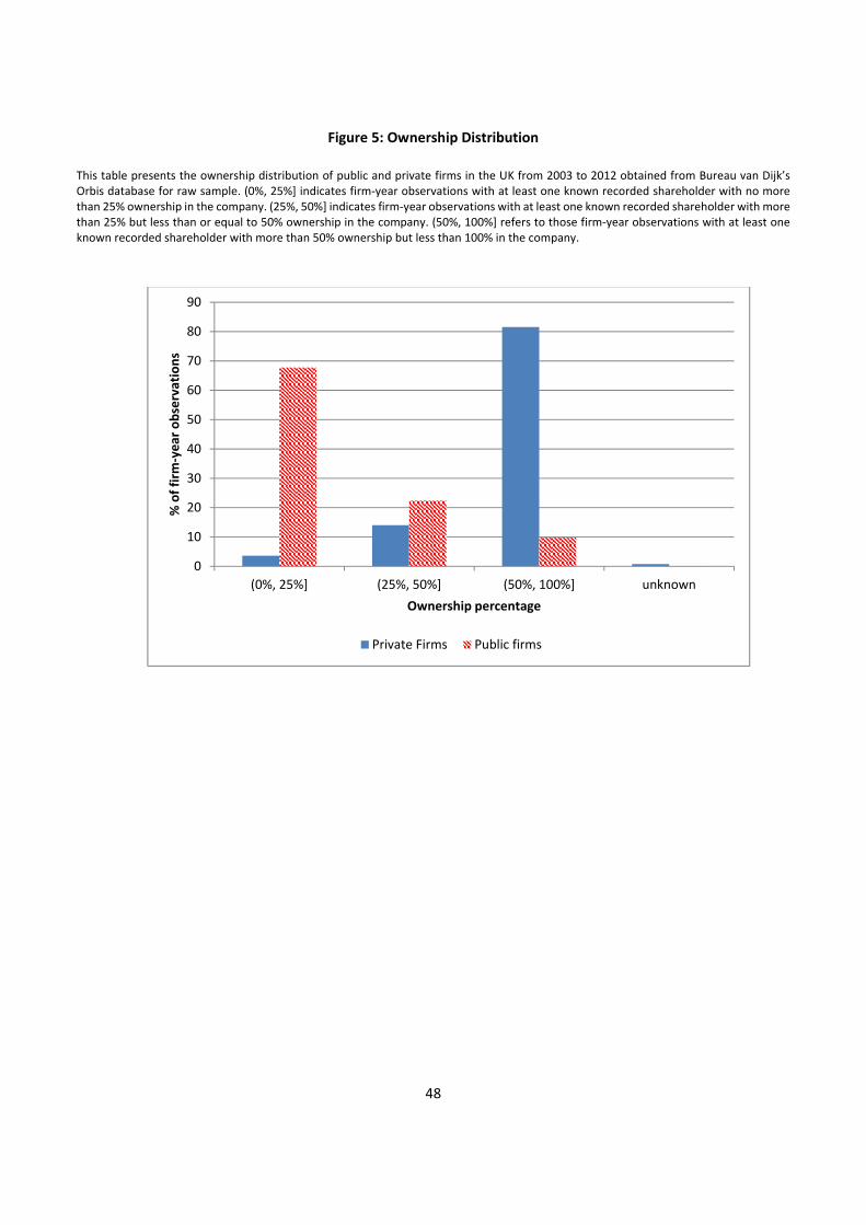
48  

Figure 5: Ownership Distribution 

 This table presents the ownership distribution of public and private firms in the UK from 2003 to 2012 obtained from Bureau van Dijk’s Orbis database for raw sample. (0%, 25%] indicates firm‐year observations with at least one known recorded shareholder with no more than 25% ownership in the company. (25%, 50%] indicates firm‐year observations with at least one known recorded shareholder with more than 25% but less than or equal to 50% ownership in the company. (50%, 100%] refers to those firm‐year observations with at least one known recorded shareholder with more than 50% ownership but less than 100% in the company.    

 

  

 

0

10

20

30

40

50

60

70

80

90

(0%, 25%] (25%, 50%] (50%, 100%] unknown

% of firm

‐year observations

Ownership percentage

Private Firms Public firms

49  

Appendix A: Variable Definitions 

General  

Public  A dummy variable that takes a value of one if the firm is public and zero otherwise. 

Total assets  Book value of total assets in constant 2011 GBP million. 

Revenue  Total operating revenues (Net sales + Other operating revenues+ Stock variations). The figures do not include VAT. Local differences may occur regarding excises taxes and similar obligatory payments for specific market of tobacco and alcoholic beverage industries. Values are in constant 2011 GBP million. 

Fixed asset  Total amount (after depreciation) of non‐current assets (Intangible assets + Tangible assets + Other fixed assets) scaled by total assets 

Intangible asset  All intangible assets such as formation expenses, research expenses, goodwill, development expenses and all other expenses with a long term effect  scaled by total assets 

Tangible fixed asset  All tangible assets such as buildings, machinery, etc. scaled by total assets 

Current asset  Total amount of current assets (Inventory + Accounts receivable + Other current asset)  scaled by total assets 

Inventory  Total inventories (raw materials +in progress + finished goods)   scaled by total assets 

Accounts receivable  Trade receivables from clients and customers   scaled by total assets 

Cash and equivalents  Detail of the Other current assets =Only the amount of cash at bank and in hand of the company  scaled by total assets   

Cash flow  Operating cash flows  scaled by total assets 

Accounts payable  Debts to suppliers and contractors  scaled by total assets 

Long‐term debt  Long term financial debts (e.g., to credit institutions (loans and credits), bonds)  scaled by total assets 

Short‐term debt  Short term financial debts (e.g., to credit institutions + part of Long term financial debts payable within the year, bonds, etc.)   scaled by total assets 

Total debt  (Long‐term debt +Short‐term debt)  scaled by total assets 

Working capital  Indicates how much capital is used by day to day activities= Inventory + Accounts Receivable –Accounts Payable  scaled by total assets 

Net working capital  Working capital – cash and equivalents  scaled by total assets 

Capital Intensity  Firm’s capital stock / total employment 

Market Share  Firm’s market share at the 2‐digit SIC level (operating revenue / total 2‐digit SIC level operating revenue) 

Firm Risk  Standard deviation of sales in the past 5 years / mean of sales in the past 5 years. At least 3 years of data is required for each firm to calculate this ratio.  

R&D   Total amount of expenses on research and development activities  scaled by total assets 

Number of employees  Number of employees  

Firm age  Years since firm’s founding 

Number of branches  Number of branches  

Profitability  

ROA EBITDA  EBITDA  scaled by total assets 

ROA EBIT  EBIT  scaled by total assets 

ROA (NI/TA)  Net income scaled by total assets 

50  

ROE EBITDA  EBITDA  scaled by shareholders’ funds 

ROE EBIT  EBIT  scaled by shareholders’ funds 

ROE Net income  Net income  scaled by shareholders’ funds 

EBIT margin  EBIT  scaled by operating revenue 

Net income margin  Net Income  scaled by operating Revenue 

Cash flow / Op. revenue  Cash flow  scaled by operating revenue 

Sales‐to‐equity  Operating revenue divided by  equity 

Efficiency  

Asset efficiency  Average tangible fixed asset turnover = Operating revenue divided by average tangible fixed assets (average tangible fixed asset is calculated as tangible fixed asset at the beginning of year and end of year divided by 2) 

Inventory turnover  Operating revenue / inventory 

Collection period  (Average accounts receivable / Operating revenue) * 360 . Average accounts receivable is calculated as accounts receivable at the beginning of year and end of year divided by 2. 

Credit period  (Average accounts payable / Operating revenue) * 360. Average accounts payable is calculated as accounts payable at the beginning of year and end of year divided by 2. 

Interest coverage  Operating profit / Interest paid 

Structural ratios  

Liquidity  (Current asset – Inventory) / Current liabilities 

Current ratio  Current asset / Current liabilities 

Equity/Asset  Total shareholder’s equity / total assets 

Debt‐to‐equity  ((Non‐current liabilities + Long‐term debt) / Equity)  

Productivity  

EBIT per employee  EBIT divided by number of employees on payroll 

EBITDA per employee  EBITDA divided by number of employees on payroll 

Net income per employee  Net income  divided by number of employees on payroll 

Revenue  per employee  Revenue  divided by number of employees on payroll 

Cost of employee/revenue  Total cost of employees divided by operating revenue 

Equity per employee  Total Equity  divided by number of employees on payroll 

Unit employee cost  Total cost of employees divided by total employees 

Growth  

Sales growth  Growth in operating revenue from time t‐1 to time t 

Gross investment  Change in total fixed assets from (t‐1) to (t) scaled by beginning of year total assets 

Fixed asset growth  (Fixed asset(t)‐ Fixed asset(t‐1))/ Fixed asset(t‐1) 

Employee growth  (Number of employees(t) ‐  Number of employees (t‐1)) /  Number of employees (t‐1) 

Volatility  

Earnings volatility  Standard deviation of operating revenue to asset ratio for all available observations for each firm 

Cash flow volatility  Standard deviation of cash flow for each firm for all available observations 

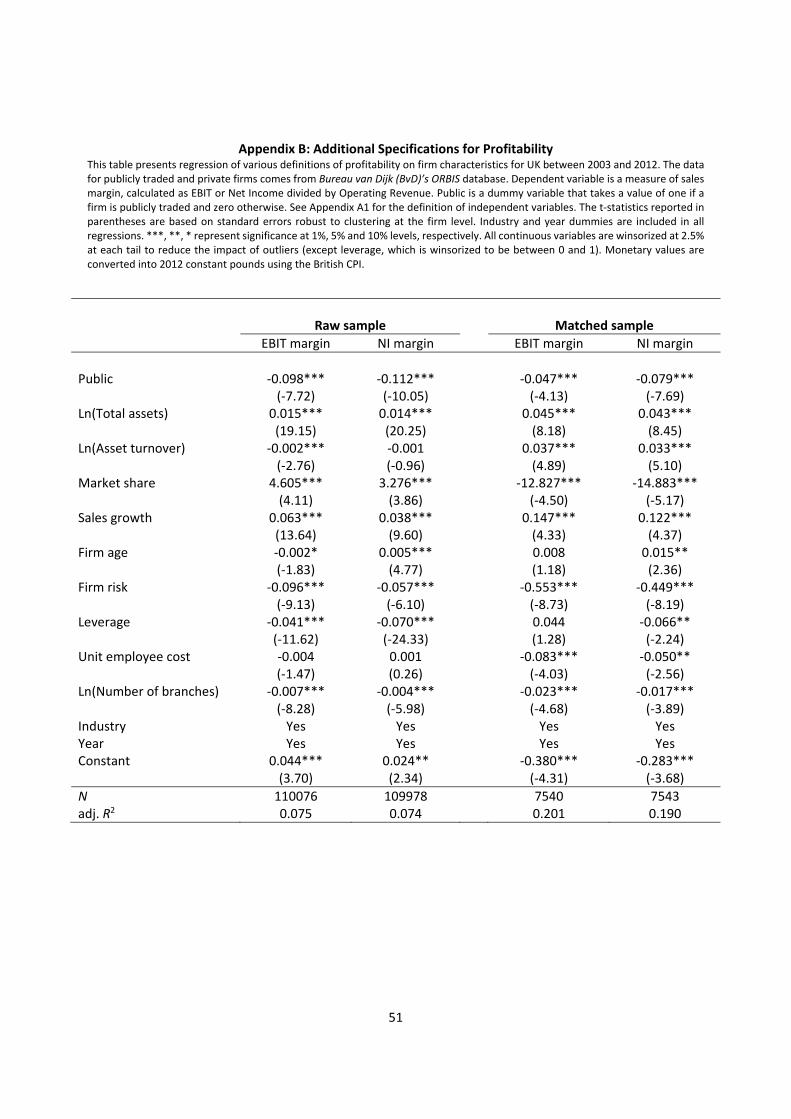
51  

Appendix B: Additional Specifications for Profitability This table presents regression of various definitions of profitability on firm characteristics for UK between 2003 and 2012. The data for publicly traded and private firms comes from Bureau van Dijk (BvD)’s ORBIS database. Dependent variable is a measure of sales margin, calculated as EBIT or Net Income divided by Operating Revenue. Public is a dummy variable that takes a value of one if a firm is publicly traded and zero otherwise. See Appendix A1 for the definition of independent variables. The t‐statistics reported in parentheses are based on standard errors robust  to clustering at  the  firm  level.  Industry and year dummies are  included  in all regressions. ***, **, * represent significance at 1%, 5% and 10% levels, respectively. All continuous variables are winsorized at 2.5% at each tail to reduce the impact of outliers (except leverage, which  is winsorized to be between 0 and 1). Monetary values are converted into 2012 constant pounds using the British CPI.   

             Raw sample Matched sample 

  EBIT margin  NI margin    EBIT margin  NI margin 

           Public  ‐0.098***  ‐0.112*** ‐0.047***  ‐0.079***  (‐7.72)  (‐10.05)    (‐4.13)  (‐7.69) Ln(Total assets)  0.015***  0.014***    0.045***  0.043***   (19.15)  (20.25)    (8.18)  (8.45) Ln(Asset turnover)  ‐0.002***  ‐0.001    0.037***  0.033***   (‐2.76)  (‐0.96)    (4.89)  (5.10) Market share  4.605***  3.276***    ‐12.827***  ‐14.883***   (4.11)  (3.86)    (‐4.50)  (‐5.17) Sales growth  0.063***  0.038***    0.147***  0.122***   (13.64)  (9.60)    (4.33)  (4.37) Firm age  ‐0.002*  0.005***    0.008  0.015**   (‐1.83)  (4.77)    (1.18)  (2.36) Firm risk  ‐0.096***  ‐0.057***    ‐0.553***  ‐0.449***   (‐9.13)  (‐6.10)    (‐8.73)  (‐8.19) Leverage  ‐0.041***  ‐0.070***    0.044  ‐0.066**   (‐11.62)  (‐24.33)    (1.28)  (‐2.24) Unit employee cost  ‐0.004  0.001    ‐0.083***  ‐0.050**   (‐1.47)  (0.26)    (‐4.03)  (‐2.56) Ln(Number of branches)  ‐0.007***  ‐0.004***    ‐0.023***  ‐0.017***   (‐8.28)  (‐5.98)    (‐4.68)  (‐3.89) Industry   Yes  Yes Yes YesYear   Yes  Yes    Yes  Yes Constant  0.044***  0.024**    ‐0.380***  ‐0.283***   (3.70)  (2.34)    (‐4.31)  (‐3.68) 

N  110076  109978    7540  7543 adj. R2  0.075  0.074    0.201  0.190 

 

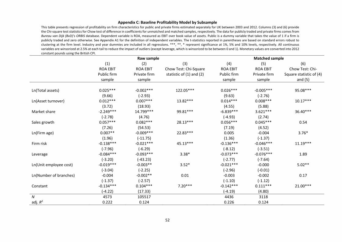
52  

Appendix C: Baseline Profitability Model by Subsample This table presents regression of profitability on firm characteristics for public and private firms estimated separately for UK between 2003 and 2012. Columns (3) and (6) provide the Chi‐square test statistics for Chow test of difference in coefficients for unmatched and matched samples, respectively. The data for publicly traded and private firms comes from Bureau van Dijk (BvD)’s ORBIS database. Dependent variable is ROA, measured as EBIT over book value of assets. Public is a dummy variable that takes the value of 1 if a firm is publicly traded and zero otherwise. See Appendix A1 for the definition of independent variables. The t‐statistics reported in parentheses are based on standard errors robust to clustering at the firm  level.  Industry and year dummies are  included  in all regressions. ***, **, * represent significance at 1%, 5% and 10%  levels, respectively. All continuous variables are winsorized at 2.5% at each tail to reduce the impact of outliers (except leverage, which is winsorized to be between 0 and 1). Monetary values are converted into 2012 constant pounds using the British CPI.  

  Raw sample    Matched sample   (1) (2) (3)  (4) (5) (6)   ROA EBIT 

Public firm sample 

ROA EBIT Private firm sample 

Chow Test: Chi‐Square statistic of (1) and (2) 

  ROA EBIT Public firm  sample 

ROA EBIT Private firm sample 

Chow Test: Chi‐Square statistic of (4) 

and (5) 

               Ln(Total assets)  0.025***  ‐0.002***  122.05***    0.026***  ‐0.005***  95.08***   (9.66)  (‐2.93)      (9.63)  (‐2.76)   Ln(Asset turnover)  0.012***  0.007***  13.82***    0.014***  0.008***  10.17***   (3.72)  (18.93)      (4.55)  (5.88)   Market share  ‐2.249***  14.799***  99.81***    ‐6.839***  3.621***  36.40***   (‐2.78)  (4.76)      (‐4.93)  (2.74)   Sales growth  0.057***  0.082***  28.13***    0.056***  0.045***  0.54   (7.26) (54.53) (7.19) (4.52)  Ln(Firm age)  0.007**  ‐0.009***  22.83***    0.005  ‐0.004  3.76*   (1.96)  (‐11.75)      (1.36)  (‐1.37)   Firm risk  ‐0.138***  ‐0.021***  45.13***    ‐0.136***  ‐0.046***  11.19***   (‐7.96)  (‐6.29)      (‐8.12)  (‐3.51)   Leverage  ‐0.084***  ‐0.093***  3.38*    ‐0.073***  ‐0.076***  1.89   (‐3.20)  (‐43.23)      (‐2.77)  (‐7.64)   Ln(Unit employee cost)  ‐0.019***  ‐0.003**  3.52*    ‐0.021***  ‐0.000  5.02**   (‐3.04)  (‐2.25)      (‐2.96)  (‐0.01)   Ln(Number of branches)  ‐0.004  ‐0.002**  0.01    ‐0.003  ‐0.002  0.17   (‐1.37)  (‐2.57)      (‐1.10)  (‐1.12)   Constant  ‐0.134***  0.104***  7.20***    ‐0.142***  0.111***  21.00***   (‐4.22)  (17.33)      (‐4.19)  (4.80)   

N  4573  105517      4436  3118   adj. R2  0.222  0.124      0.226  0.124