distributional dimension of educational access and
TRANSCRIPT
189
Lawrence Kwaku Ado-Kofie
Distributional Dimension of Educational Access and Attainment in Ghana
A thesis submitted to The University of Manchester for the degree of
Doctor of Philosophy (PhD) in the Faculty of Humanities
2014
School of Environment, Education and Development (SEED)
Institute for Development Policy and Management (IDPM)
2
Table of Contents
List of Tables.............................................................................................................................. 5
List of Acronyms and Abbreviations ......................................................................................... 7
Abstract ...................................................................................................................................... 9
Declaration and Copyright Statement ...................................................................................... 10
Acknowledgement.................................................................................................................... 11
Dedication ................................................................................................................................ 12
Chapter 1 ................................................................................................................................ 13
Introduction ............................................................................................................................ 13
1.1 Background ........................................................................................................................ 13
1.2 Why Ghana as a case study ................................................................................................ 13
1.3 Significance and contributions of the study ....................................................................... 16
1.4 Equal educational access matters for growth and poverty reduction ................................. 17
1.5 Research objectives and questions ..................................................................................... 20
1.5.1 Research objectives ................................................................................................... 20
1.5.2 Research questions .................................................................................................... 20
1.6 Structure of the thesis ......................................................................................................... 21
Chapter 2 ................................................................................................................................ 22
Background and context of the study ................................................................................... 22
2.1 Introduction ........................................................................................................................ 22
2.2 Country overview ............................................................................................................... 22
2.3 Education provision and inequality in educational outcomes ............................................ 24
2.4 Access to education in Sub-Saharan Africa context .......................................................... 25
2.5 Education policy and trends in educational outcomes in Ghana........................................ 27
2.5.1 Education sector reforms and policy interventions ................................................... 27
2.5.2 Trends in educational outcomes ................................................................................ 30
2.6 Conclusions ........................................................................................................................ 34
Chapter 3 ................................................................................................................................ 36
Economic growth, income and non-income inequality and conceptual framework ........ 36
3.1 Introduction ........................................................................................................................ 36
3.2 Economic growth, inequality and non-income poverty ..................................................... 36
3.3 Focus on non-income inequality and poverty .................................................................... 40
3.4 Progress in educational outcomes ...................................................................................... 43
3.5 Socioeconomic inequality in educational outcomes .......................................................... 45
3.6 Socioeconomic determinants of educational outcomes ..................................................... 49
3.6.1 Children’s demographic characteristics .................................................................... 49
3.6.2 Household wealth ...................................................................................................... 50
3.6.3 Household composition/size ..................................................................................... 52
3.6.4 Residency and location effects .................................................................................. 57
3.6.5 Distance to school, quality and availability of schools ............................................. 58
3.7 Theoretical framework ....................................................................................................... 60
3.8 Data, descriptive statistics and variable definition ............................................................. 62
3.8.1 Data source: justification and details ........................................................................ 62
3
3.8.2 Why GDHS datasets are used instead of GLSS datasets .......................................... 63
3.8.3 Computation of wealth index .................................................................................... 67
3.8.4 Variables for the analysis .......................................................................................... 69
3.9 Conclusions ........................................................................................................................ 75
Chapter 4 ................................................................................................................................ 78
Socioeconomic determinants of educational access and attainment in Ghana ................ 78
4.1 Introduction ........................................................................................................................ 78
4.2 School attendance and completion ..................................................................................... 80
4.2.1 Distribution of educational access by socioeconomic status .................................... 81
4.2.2 Distribution of educational attainment by socioeconomic status .............................. 84
4.3 Multivariate regression framework .................................................................................... 88
4.3.1 Binary probit model .................................................................................................. 88
4.3.2 Empirical specification.............................................................................................. 89
4.3.3 Endogeneity concern ................................................................................................. 90
4.4 Regression results and discussions .................................................................................... 93
4.4.1 Primary and secondary attendance ............................................................................ 93
4.4.2 Primary and secondary completion ......................................................................... 103
4.4.3 Robustness check .................................................................................................... 112
4.5 Policy lessons ................................................................................................................... 113
4.6 Conclusions ...................................................................................................................... 114
Chapter 5 .............................................................................................................................. 116
Educational outcomes of males and females by wealth distribution in Ghana .............. 116
5.1 Introduction ...................................................................................................................... 116
5.2 Educational access and attainment by gender .................................................................. 119
5.2.1 Validity check .......................................................................................................... 119
5.2.2 Gender inequality in educational outcomes among the poor and the non-poor ....... 121
5.3 Regression results and discussions .................................................................................. 129
5.3.1 Inequality in primary and secondary school attendance .......................................... 129
5.3.2 Inequality in primary and secondary school completion ......................................... 135
5.3.3 Robustness check ..................................................................................................... 140
5.4 Policy perspective ............................................................................................................ 141
5.5 Conclusions ...................................................................................................................... 142
Appendix A5: t-test of difference in means of male and female educational outcomes ........ 144
Chapter 6 .............................................................................................................................. 146
Socioeconomic inequality in educational access and attainment in Ghana .................... 146
6.1. Introduction ..................................................................................................................... 146
6.2 Models .............................................................................................................................. 147
6.2.1 Measuring education inequality .................................................................................... 147
6.3 Concentration Index ......................................................................................................... 148
6.3.1 Concentration index approach.................................................................................. 150
6.3.2 Empirical specification............................................................................................. 151
6.3.4 Decomposition of inequality and its evolution over time ........................................ 152
6.3.5 Non-linear regression model .................................................................................... 155
4
6.4 Results and discussions .................................................................................................... 158
6.4.1 Sources of inequality in primary education access .................................................. 160
6.4.2 Sources of inequality in secondary education access ............................................... 171
6.4.3 Sources of inequality in primary education attainment............................................ 180
6.4.4 Sources of inequality in secondary education attainment ........................................ 188
6.5 Conclusions ...................................................................................................................... 198
Appendix A6: Marginal effect and contributions of explanatory variables... ........................ 201
Chapter 7 .............................................................................................................................. 205
Summary and Conclusions .................................................................................................. 205
7.1 Introduction ...................................................................................................................... 205
7.2 Summary .......................................................................................................................... 205
7.3 Major contributions to the literature ................................................................................ 211
7.4 Policy implications ........................................................................................................... 211
7.5 Limitations ....................................................................................................................... 214
7.6 Further research ................................................................................................................ 215
References .............................................................................................................................. 216
Word count 77,708 (main text and footnotes)
5
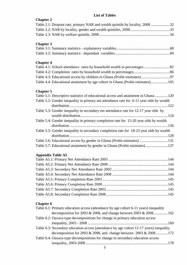
List of Tables
Chapter 2
Table 2.1: Dropout rate, primary NAR and wealth quintile by locality, 2008 .................... 32
Table 2.2: NAR by locality, gender and wealth quintiles, 2008 .......................................... 33
Table 2.3: NAR by welfare quintile, 2008 ........................................................................... 34
Chapter 3
Table 3.1: Summary statistics - explanatory variables......................................................... 68
Table 3.2: Summary statistics - dependant variables .......................................................... 69
Chapter 4
Table 4.1: School attendance rates by household wealth in percentages ............................ 82
Table 4.2: Completion rates by household wealth in percentages ...................................... 86
Table 4.3: Educational access by children in Ghana (Probit estimates) .............................. 97
Table 4.4: Educational attainment by age cohort in Ghana (Probit estimates) .................. 105
Chapter 5
Table 5.1: Descriptive statistics of educational access and attainment in Ghana .............. 120
Table 5.2: Gender inequality in primary net attendance rate for 6-11 year olds by wealth
distribution ........................................................................................................ 122
Table 5.3: Gender inequality in secondary net attendance rate for 12-17 year olds by
wealth distribution ............................................................................................. 124
Table 5.4: Gender inequality in primary completion rate for 15-20 year olds by wealth
distribution ........................................................................................................ 126
Table 5.5: Gender inequality in secondary completion rate for 18-23 year olds by wealth
distribution ........................................................................................................ 128
Table 5.6: Educational access by gender in Ghana (Probit estimates) .............................. 131
Table 5.7: Educational attainment by gender in Ghana (Probit estimates) ........................ 137
Appendix Table A5
Table A5.1: Primary Net Attendance Rate 2003 ............................................................... 144
Table A5.2: Primary Net Attendance Rate 2008 ............................................................... 144
Table A5.3: Secondary Net Attendance Rate 2003 ........................................................... 144
Table A5.4: Secondary Net Attendance Rate 2008 ........................................................... 144
Table A5.5: Primary Completion Rate 2003 ..................................................................... 145
Table A5.6: Primary Completion Rate 2008 ..................................................................... 145
Table A5.7: Secondary Completion Rate 2003.................................................................. 145
Table A5.8: Secondary Completion Rate 2008.................................................................. 145
Chapter 6
Table 6.1: Primary education access (attendance by age cohort 6-11 years) inequality
decomposition for 2003 & 2008, and change between 2003 & 2008 ............... 162
Table 6.2: Oaxaca-type decompositions for change in primary education access
inequality, 2003 - 2008 ..................................................................................... 169
Table 6.3: Secondary education access (attendance by age cohort 12-17 years) inequality
decomposition for 2003 & 2008, and change between 2003 & 2008 ............. 172
Table 6.4: Oaxaca-type decompositions for change in secondary education access
inequality, 2003-2008 ....................................................................................... 178
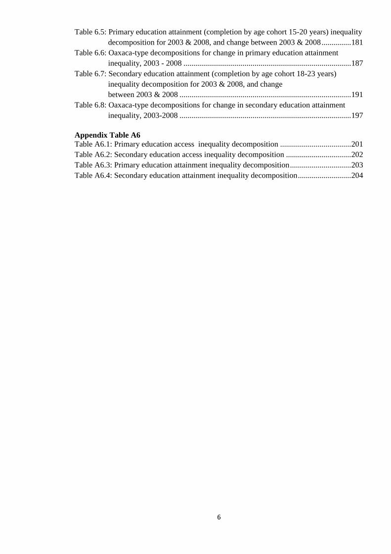
6
Table 6.5: Primary education attainment (completion by age cohort 15-20 years) inequality
decomposition for 2003 & 2008, and change between 2003 & 2008 ............... 181
Table 6.6: Oaxaca-type decompositions for change in primary education attainment
inequality, 2003 - 2008 ..................................................................................... 187
Table 6.7: Secondary education attainment (completion by age cohort 18-23 years)
inequality decomposition for 2003 & 2008, and change
between 2003 & 2008 ....................................................................................... 191
Table 6.8: Oaxaca-type decompositions for change in secondary education attainment
inequality, 2003-2008 ....................................................................................... 197
Appendix Table A6
Table A6.1: Primary education access inequality decomposition .................................... 201
Table A6.2: Secondary education access inequality decomposition ................................. 202
Table A6.3: Primary education attainment inequality decomposition ............................... 203
Table A6.4: Secondary education attainment inequality decomposition ........................... 204
7
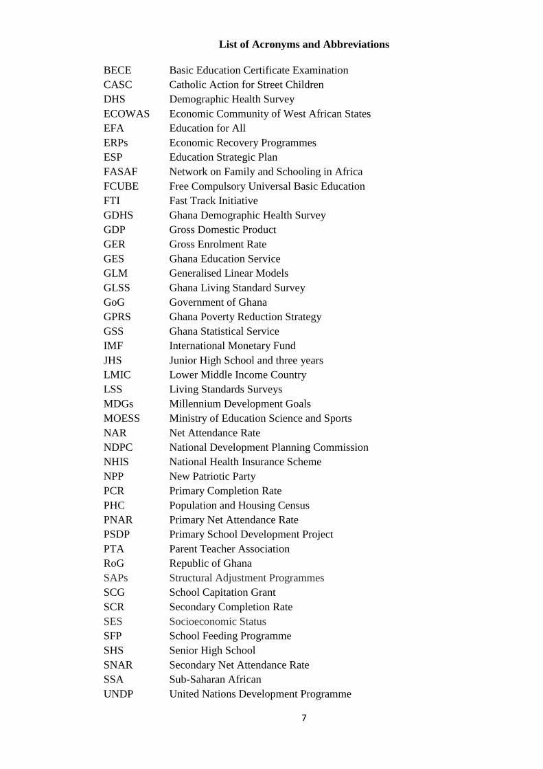
List of Acronyms and Abbreviations
BECE Basic Education Certificate Examination
CASC Catholic Action for Street Children
DHS Demographic Health Survey
ECOWAS Economic Community of West African States
EFA Education for All
ERPs Economic Recovery Programmes
ESP Education Strategic Plan
FASAF Network on Family and Schooling in Africa
FCUBE Free Compulsory Universal Basic Education
FTI Fast Track Initiative
GDHS Ghana Demographic Health Survey
GDP Gross Domestic Product
GER Gross Enrolment Rate
GES Ghana Education Service
GLM Generalised Linear Models
GLSS Ghana Living Standard Survey
GoG Government of Ghana
GPRS Ghana Poverty Reduction Strategy
GSS Ghana Statistical Service
IMF International Monetary Fund
JHS Junior High School and three years
LMIC Lower Middle Income Country
LSS Living Standards Surveys
MDGs Millennium Development Goals
MOESS Ministry of Education Science and Sports
NAR Net Attendance Rate
NDPC National Development Planning Commission
NHIS National Health Insurance Scheme
NPP New Patriotic Party
PCR Primary Completion Rate
PHC Population and Housing Census
PNAR Primary Net Attendance Rate
PSDP Primary School Development Project
PTA Parent Teacher Association
RoG Republic of Ghana
SAPs Structural Adjustment Programmes
SCG School Capitation Grant
SCR Secondary Completion Rate
SES Socioeconomic Status
SFP School Feeding Programme
SHS Senior High School
SNAR Secondary Net Attendance Rate
SSA Sub-Saharan African
UNDP United Nations Development Programme

8
UNESCO United Nations Education, Scientific and Cultural Organization
UNICEF United Nations Children’s Fund
UPE Universal Primary Education
WASSCE West African Senior School Certificate Examination
WEF World Education Forum
WHO World Health Organization
9
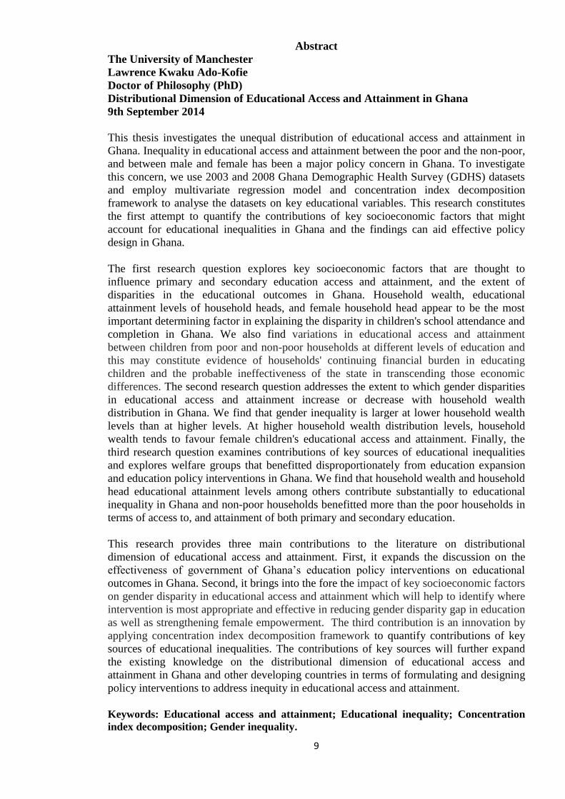
Abstract
The University of Manchester
Lawrence Kwaku Ado-Kofie
Doctor of Philosophy (PhD)
Distributional Dimension of Educational Access and Attainment in Ghana
9th September 2014
This thesis investigates the unequal distribution of educational access and attainment in
Ghana. Inequality in educational access and attainment between the poor and the non-poor,
and between male and female has been a major policy concern in Ghana. To investigate
this concern, we use 2003 and 2008 Ghana Demographic Health Survey (GDHS) datasets
and employ multivariate regression model and concentration index decomposition
framework to analyse the datasets on key educational variables. This research constitutes
the first attempt to quantify the contributions of key socioeconomic factors that might
account for educational inequalities in Ghana and the findings can aid effective policy
design in Ghana.
The first research question explores key socioeconomic factors that are thought to
influence primary and secondary education access and attainment, and the extent of
disparities in the educational outcomes in Ghana. Household wealth, educational
attainment levels of household heads, and female household head appear to be the most
important determining factor in explaining the disparity in children's school attendance and
completion in Ghana. We also find variations in educational access and attainment
between children from poor and non-poor households at different levels of education and
this may constitute evidence of households' continuing financial burden in educating
children and the probable ineffectiveness of the state in transcending those economic
differences. The second research question addresses the extent to which gender disparities
in educational access and attainment increase or decrease with household wealth
distribution in Ghana. We find that gender inequality is larger at lower household wealth
levels than at higher levels. At higher household wealth distribution levels, household
wealth tends to favour female children's educational access and attainment. Finally, the
third research question examines contributions of key sources of educational inequalities
and explores welfare groups that benefitted disproportionately from education expansion
and education policy interventions in Ghana. We find that household wealth and household
head educational attainment levels among others contribute substantially to educational
inequality in Ghana and non-poor households benefitted more than the poor households in
terms of access to, and attainment of both primary and secondary education.
This research provides three main contributions to the literature on distributional
dimension of educational access and attainment. First, it expands the discussion on the
effectiveness of government of Ghana’s education policy interventions on educational
outcomes in Ghana. Second, it brings into the fore the impact of key socioeconomic factors
on gender disparity in educational access and attainment which will help to identify where
intervention is most appropriate and effective in reducing gender disparity gap in education
as well as strengthening female empowerment. The third contribution is an innovation by
applying concentration index decomposition framework to quantify contributions of key
sources of educational inequalities. The contributions of key sources will further expand
the existing knowledge on the distributional dimension of educational access and
attainment in Ghana and other developing countries in terms of formulating and designing
policy interventions to address inequity in educational access and attainment.
Keywords: Educational access and attainment; Educational inequality; Concentration
index decomposition; Gender inequality.
10
Declaration and Copyright Statement
Declaration
I, Lawrence Kwaku Ado-Kofie, hereby declare that no portion of the work referred to in
the thesis has been submitted in support of an application for another degree or
qualification of this or any other university or other institute of learning.
Copyright Statement
(i) The author of this thesis (including any appendices and/or schedules to this
thesis) owns certain copyright or related rights in it (the “Copyright”) and he
has given The University of Manchester certain rights to use such Copyright,
including for administrative purposes.
(ii) Copies of this thesis, either in full or in extracts and whether in hard or
electronic copy, may be made only in accordance with the Copyright, Designs
and Patents Act 1988 (as amended) and regulations issued under it or, where
appropriate, in accordance with licensing agreements which the University has
from time to time. This page must form part of any such copies made.
(iii) The ownership of certain Copyright, patents, designs, trademarks and other
intellectual property (the “Intellectual Property”) and any reproductions of
copyright works in the thesis, for example graphs and tables (“Reproductions”),
which may be described in this thesis, may not be owned by the author and may
be owned by third parties. Such Intellectual Property and Reproductions cannot
and must not be made available for use without the prior written permission of
the owner(s) of the relevant Intellectual Property and/or Reproductions.
(iv) Further information on the conditions under which disclosure, publication and
commercialisation of this thesis, the Copyright and any Intellectual Property
and/or Reproductions described in it may take place is available in the
University IP Policy
(see http://documents.manchester.ac.uk/DocuInfo.aspx?DocID=487), in any
relevant Thesis restriction declarations deposited in the University Library, The
University Library’s regulations
(see http://www.manchester.ac.uk/library/aboutus/regulations) and in The
University’s policy on Presentation of Theses.

11
Acknowledgement
My foremost thanks go to the Almighty God for His unfailing love, sustenance and grace
for the successful completion of my entire study. This work would not have achieved its
standard without the constructive comments, suggestions and encouragement that I have
received from several people without of course, holding them responsible for any
deficiencies that may remain in this thesis.
I am particularly indebted to my supervisors Dr David Lawson and Dr Ralitza Dimova for
their constructive comments, priceless suggestions and advice and above all the time and
energy they put into reading the draft copies of this thesis which have made this work to be
completed in time. I also want to specially thank Dr David Lawson for his financial
assistant in times of financial difficulties that I faced as self-financing student during the
course of this study. Dr Lawson and Dr Dimova, I say every support I received from you is
highly appreciated and will never be forgotten. To our Senior PGR administrator, Miss
Monique Brown, I owe you a lot for your administrative support, especially during those
difficult times when quick and positive administrative responses were much needed. Your
performance is second to none, even at the shortest notice of my requests.
I also owe a great debt of gratitude to my lovely wife, Mrs Naa Dede Ado-Kofie. She has
been and will always be the backbone of my accomplishments. She has worked day and
night in providing financial support for my studies and for the maintenance of the family.
Her encouragements, patience, faith in me and above all her love have given me the
strength and determination to go through this long and arduous academic journey of my
life. Without her support and understanding during my years of study in the UK, especially
the PhD programme, it would have been extremely difficult if not impossible for me to
undertake and complete the PhD programme within the 3 years as a self-financing student
with two children.
I also like to appreciate the prayer supports and encouragement from my brethren in
Calvary Hephzibah Full Gospel Church, Manchester. Special appreciation goes to my
pastors Dr Emmanuel Olatoye and Dr Mrs Shade Olatoye for their prayer supports over the
years, and especially for this PhD programme. To the entire church, I say God bless you all.
Indeed, my thanks also go to all my friends and colleagues in the PhD community at IDPM
and Economics, especially; Dr Justice Bawole, Hamza Bukari, Adams Yakubu Adama,
Alma Kudebayeva and Eleni Sifaki for their supports and inspirations during the
challenging and great moments we shared together as PhD candidates. Hamza Bukari, you
have been more than just a friend and a colleague and I appreciate all your supports,
networking and encouragements. To Dr Justice Bawole, I say thanks for your special
support during those difficult times when my laptop which contained one whole year of my
PhD work was stolen in the department.
To everyone who has supported either directly or indirectly, has my heartfelt gratitude.
May God bless you all!
12
Dedication
This thesis is dedicated to:
My lovely wife, Mrs Naa Dede Ado-Kofie, and my lovely children, Master
Winston and Miss Winielle Ado-Kofie.
The loving memory of my Dad (Mr Abraham Ado-Kofie) and Grandma (Ms
Martha Afezukeh) who, though had no formal education, knew the value of
investing in education and invested substantially in my education.
13
Chapter 1
Introduction
1.1 Background
There is general recognition of the importance of education in socioeconomic development
of countries, especially the developing countries. As a result, the role of human capital in
socioeconomic development has been widely recognised in the various developing
countries studies (Appleton 1995; Appleton et al. 1996; Lloyd and Blanc 1996; Lavy 1996;
Filmer and Pritchett 1999a & 1999b; Lewin 2007 & 2009; Lewin and Akyeampong 2009;
Mani et al. 2009; Harttgen et al. 2010; Harttgen and Klasen 2012). A major trend that
emerges in all these studies is that educational access and attainments are relatively low
and there are observed disparities in educational outcomes between: the poor and non-poor;
and males and females, even at the basic education levels.
Inequality in educational distribution and low educational outcomes has been one of the
top priorities in many poor developing countries where various education policy initiatives
have been evolved in the last two decades to meet Education for All (EFA) goals. The
2000 EFA Conference and the 2000 UN Millennium Summit affirmed low levels of
educational outcomes and educational inequalities in developing countries (UNESCO 2000,
2002a, 2002b & 2008; UN 2000) . Consequently, EFA goals 2 and 5 which are in harmony
with Millennium Development Goals (MDGs) 2 and 3 were set to address the gaps in
educational outcomes in the developing countries. These goals have been incorporated into
educational policies being evolved by governments in developing countries, including
Ghana.
1.2 Why Ghana as a case study
Ghana is seen as one of the role models for Sub-Saharan African (SSA) countries by her
development partners (Bogetic 2007; Coulombe and Wodon 2007; Coulombe and McKay
2007) about the country’s economic performance following successful implementation of
the World Bank and IMF’s various economic programmes (i.e. ERPs, SAPs, and GPRS
etc.). During much of the 1990s and 2000s, Ghana had one of the strongest growth rates
and falling incidence of poverty amongst the SSA countries (Bogetic 2007). In comparison
with many other SSA countries, Ghana’s economic growth performance in the past two
decades has been relatively good.
14
In addition, Ghana is one of the few SSA countries for which EFA and MDGs on universal
access to primary education and gender equality in access to education, and the reduction
of absolute poverty by half by 2015 targets were believed to be within reach (World Bank
2011a, 2011b & 2013; NDPC et al. 2012). The assumption that these targets lie within
reach was based on the relatively good economic performance and reduction in absolute
poverty in Ghana. Since 2000, the education sector in Ghana has experienced substantial
expansion at all levels of education with primary school enrolment ratio around 90%
(World Bank 2004; Akyeampong et al. 2007; NDPC et al. 2010). In addition, Ghana has
recorded one of the strongest and steady GDP growth rates and falling incidence of poverty
amongst the SSA countries (Bogetic 2007; World Bank 2014). The average GDP growth
rate for Ghana since 2000 is around 6.5% with respectable 9th
position in the average GDP
rating of SSA countries (World Bank 2014).
Moreover, currently available data indicate that the share of the population below the
poverty line decreased from 39.5% in 1998/99 to 28.5% in 2005/06 (Ghana Statistical
Service 2000 & 2007). Some researchers described Ghana’s poverty reduction
performance as probably the best record in the whole of SSA over the last two decades
(Coulombe and Wodon 2007). According to Coulombe and Wodon (2007) and World
Bank (2014) online database the absolute number of the poor (consumption based: $1.25 a
day) decreased from 7.2 million in 1998/99 to 6.3 million in 2005/06. However, it has also
been argued that the economic growth benefitted the non-poor disproportionately and if
the growth had benefitted the poor and the non-poor households equally, the poverty
reduction goal would have been achieved (Coulombe and McKay 2007).
Consequently, the impact of the differential distribution of economic growth on poverty
reduction and education expansion present considerable challenges for equitable
distribution of education provision in Ghana, especially to meet EFA and Millennium
Development education related goals. It is worth noting that the steady economic growth
rate, educational expansion and declining absolute poverty in Ghana do not necessarily
imply equity in educational access and attainment and equality of opportunity. Since
economic growth alone cannot guarantee equitable distribution of education, it became
imperative for the government of Ghana (GoG) to increase access to basic education
through a number of international initiatives including EFA Fast Track Initiative (FTI) and
national policy interventions.
15
Throughout the last decade, some policy interventions were carried out in Ghana to
reinforce education initiatives (stipulated in 1987 education reforms, 1992 Constitution,
and Vision 2020) that have been aimed at widening education participation and reducing
cost barriers which have consistently limited educational access for the poor households.
Among the policy interventions are; the construction and rehabilitation of classrooms,
Capitation Grant (CG), School Feeding Programme (SFP), and enforcement of laws that
support the implementation of Free Compulsory Universal Basic Education (FCUBE)
(World Bank 2004; NDPC et al. 2010 & 2012).
Although the FCUBE policy was outlined in 1995 in accordance with the constitution of
the Fourth Republic of Ghana, with the aim to achieve Universal Primary Education (UPE)
by 2005, it was not until the year 2000 when laws that support the implementation of
FCUBE were fully enforced (NDPC et al. 2010). The FCUBE also sought to improve girls’
enrolment and has generally succeeded in achieving this target (Ministry of Education
Science and Sports 2006a). However, as the name suggests Free Compulsory Universal
Basic Education on the contrary was never totally free. It has cost sharing principles that
went with it. Fees and levies such as; Parent Teacher Association (PTA) contributions,
sports fees, and other school activities fees were still being charged under the FCUBE
programme until the year 2004. In effect, these fees represent a regressive taxation on poor
households which affected the enrolment and excluded children from poor households
(Akyeampong et al. 2007; Akyeampong 2009) who are very sensitive to fees, even when
these fees are small. These fees were thought to be negatively impacting on school
attendance of children at the basic level and undermining the GoG’s EFA initiatives.
The government, therefore, decided to implement SCG in 2005 and SFP in 2006 to
increase access to education and maintain, especially the poor children in school.1 In 2008,
the GoG disbursed a total amount of GH¢15 million as payment of SCG to pupils in all
public schools in addition to subsidising the conduct of Basic Education Certificate
Examination (BECE) amounting to over GH¢4 million (NDPC et al. 2010).2 The SFP is
also aimed at increasing school enrolment, retention, attendance, and reduction in
malnutrition among children. It was expanded to cover 596,089 pupils nationwide in 2008,
up from 408,989 in 2007 to help ease the burden on households (NDPC et al. 2010).
1 The School Capitation Grant (SCG) is a form of grant given to all public basic schools in Ghana. It covers
tuition fees and all other forms of fees and levies previously charged under FCUBE. It is an additional
initiative to abolish all forms of fees in basic education and makes school enrolment and attendance at public
basic schools totally free to all households irrespective of income levels (Akyeampong, K. 2011). 2 At the time, GH¢1.00 was equivalent to US$1.00
16
In 2005/06 academic year, there was high increase in school enrolment when a school
capitation grant of GH¢3.00 (equivalent to US$3 at the time) per enrolled child was
introduced. The enrolment in Grade 1 increased by 20%, for the first time ever, but was not
sustained in the following years (Ministry of Education Science and Sports 2008). This
shows that the SCG may not be enough to increase and sustain high enrolments through
into higher grades. Most importantly, the policy intervention does not specifically target
the poor households who need the grant most, but instead spreads the grant for all
households, irrespective of income and socioeconomic status (SES). Although, the broad
education policy objective of the GoG is to ensure that all Ghanaian children, irrespective
of their household income levels, SES and gender have access to and attain at least the
basic level of quality education (Republic of Ghana 1997), this objective is yet to be
achieved (Republic of Ghana 1997 & 2003; Akyeampong et al. 2007; Sackey 2007; Ghana
Statistical Service et al. 2004 & 2009; Rolleston 2009; Nguyen and Wodon 2014;
Nordensvard 2014). However, the key question is whether the poor households have been
able to benefit from these policy interventions (FCUBE, SCG, and SFP) and the
educational expansions in general.
1.3 Significance and contributions of the study
There is now strong support for reducing all forms of inequality including educational
inequalities. For example, in a letter to Dr Homi Kharas, lead author and executive
secretary of the secretariat supporting the High-Level Panel of Eminent Persons on the
Post-2015 Development Agenda, ninety economists, academics, and development experts
urged that reduction in inequality in the post-2015 development agenda be made a priority.
This thesis lends support to the suggestions of the ninety economists, academics, and
development experts. These experts recognised that “While the MDGs did spur some
progress in human development in the last two decades, there is evidence of growing gaps
in terms of income, education, health, nutrition and many other areas that impede the
fulfilment of human rights and wellbeing” (Pickett et al. 2013:1). They, therefore, urged
that reduction in inequality in the post-2015 development agenda be made a priority.
This study informs the literature on inequalities in educational access and attainment in
three fronts. It expands the discussion on the effectiveness of government of Ghana’s
education policy interventions on educational outcomes in Ghana and constitutes the first
attempt to analyse educational outcomes by household wealth distribution using household
data before and after the government's education policy intervention implementation period.
17
In terms of gender inequality debates, it contributes to an enhanced understanding of the
impact of key socioeconomic factors on gender inequality in educational access and
attainment which will invariably help to identify where intervention is most appropriate
and effective in reducing gender inequality gap in education as well as strengthening
female empowerment. Finally, the third contribution is an innovation, by applying
concentration index decomposition framework (widely used in health economics) to
quantify both the absolute and relative contributions of key sources of educational
inequalities (through regression analysis). This application also allows us to explore which
income groups benefitted disproportionately from education provision, which the
traditional methods (reviewed in Chapter 3, sub-section 3.7.1.2) failed to achieve. Again, it
contributes to the literature by distinguishing between the elasticity differences and
inequality differences of socioeconomic determinants of educational inequalities. In other
words, we are able to determine for the first time whether the impacts (i.e. elasticities)
differences of the socioeconomic factors on educational inequality are more important than
the inequality differences between households or vice versa. This distinction is important
for policy direction. This is because policymakers will see whether equitable distribution
of educational opportunities will be preferable to redistribution of existing assets or
incomes or vice versa.
For example, in Ghana we find that the elasticity differences of the key socioeconomic
determinants of educational outcomes are greater than the inequality differences. In other
words, the impacts of the socioeconomic factors on educational inequality are more
important than the inequality differences between households. Thus, reducing educational
inequalities in Ghana seems more a matter of reducing these elasticities (impacts) through
appropriate education-related policies than a matter of income redistribution. The
implication of this finding for policy direction is that an equitable distribution of
educational opportunities will be preferable to a redistribution of existing assets or incomes.
This is a new finding and contributes to the literature on educational inequalities by
providing policy direction and implementation.
1.4 Equal educational access matters for growth and poverty reduction
Why do we have to bother about the distribution of education and its implications for
inequality? The distribution of education matters and unequal distribution of education
tends to have negative impact on per capita income in most countries (Lopez et al. 1998).
Thus, the way in which education is distributed will have profound impact on the
18
distribution of income, the nature of economic growth and poverty reduction. Therefore,
understanding the trends and impacts of inequalities in educational access and attainment is
particularly important because government policy can address them than in the case of
reducing income poverty. It has been shown in the empirical literature that attainment of
higher education, equal distribution of education and public spending, have contributed
significantly to the equalisation of income distribution (Gregorio and Lee 2002). On the
other hand, inequality in educational attainment increases income inequality and restrict
socioeconomic mobility and if we are concern about economic growth, poverty reduction
and equality of opportunity then we should care about inequality in educational access and
attainment of children today. Thus, the distributional dimension of education is extremely
important for both welfare consideration and for production (Corak 2013). Furthermore,
inequalities in educational access and attainment are considered as the primary determinant
of inequalities in income and opportunity. As Doyle and Stiglitz (2014:9) stated “one of
the most pernicious forms of inequality relates to inequality of opportunity, reflected in a
lack of socioeconomic mobility, condemning those born into the bottom of the economic
pyramid to almost surely remain there”. Thus, the lack of socioeconomic mobility of those
at the bottom of income distribution may be largely attributed to inequalities in educational
outcomes and opportunities. The educational outcomes of children reflect a series of
factors such; as the prevailing socioeconomic inequalities to which they are exposed to (e.g.
access to good schools), household socioeconomic status (SES) and public policy on
education (Corak 2013). Thus, household resources and the degree of inequality in access
to education can determine the return to the education children receive. For example,
inequality in educational access and attainment can skew opportunity and lower
intergenerational mobility for the poor households (ibid).
It is also important to note that inequality in education will lead to income inequality that
heightens the income consequences of innate differences between individuals, changes
opportunities, and incentives which put some households in position to support their
children’s achievement independent of talent (Corak 2013). Thus, those with relatively
little or no formal education are less positioned to participate in economic growth. A
reduction in inequalities in educational access and attainment will lead to reduction in
education poverty and as a result, increase economic growth. For example, it has been
shown that reduced inequality in educational access contributes to significant reductions in
education poverty (Sahn and Younger 2006). Therefore, equal distribution of educational
access at least at both primary and secondary school levels, irrespective of household
19
income levels, will serve as a ‘ladder’ for children born into the bottom economic pyramid
to ‘climb up’ and acquire the necessary skills that will help them to partake in
opportunities that economic growth might present to them to increase their socioeconomic
mobility. In addition, not only will access to education for all increase the individuals’
productivity but also the total productivity of the country will increase with and the long
run effect being economic growth and poverty reduction, ceteris paribus.
In terms of distribution of education and its implications for inequality in Ghana, there is
little information on what actually happened during the last decade in terms of educational
outcomes along disparities in wealth distribution versus educational outcomes of the poor
households in Ghana. Thus, the study provides new insights into the directions of
distributional changes in educational outcomes along wealth distributions, sources of
educational inequalities, and the impact of policy interventions using pre-and-post policy
intervention household surveys.
Specifically, the study investigates: (i) the socioeconomic determinants of educational
access and attainment; (ii) inequalities in educational outcomes of males and females by
wealth distribution; and (iii) sources of socioeconomic inequality and contributions of the
sources in educational access and attainment inequality in Ghana. In general, the outcome
of the distribution of educational access and attainment in Ghana provides important policy
evaluations and directions. Such policy evaluations include: whether GoG’s intended pro-
poor education policy intervention has significantly reduced the impact of household
income on schooling outcomes, especially at primary education level for the income poor
households; how gender differentials in educational outcomes by wealth distribution have
changed; and whether poor households have benefited disproportionately in terms of
educational outcomes from the steady economic growth, educational expansions and the
education policy interventions. Thus, the impact of past policies on households such as
children from poor households educational outcomes, become visible so that lessons from
the past can be incorporated into the design of new policies and programmes.
20
1.5 Research objectives and questions
The research aims to investigate the effect of wealth distribution and education policy
interventions on education distribution and inequalities in educational access and
attainment in Ghana.
1.5.1 Research objectives
The specific objectives the study aims to achieve include the following:
i. To measure the socioeconomic determinants of educational access and attainment
of school-age children and young adults from poor households compared with
those from non-poor households.
ii. To estimate gender disparities in educational outcomes by wealth distribution and
to explore how gender differentials have changed at different points of educational
access and attainment in response to income levels.
iii. To estimate both absolute and relative contributions of key determinants of
socioeconomic inequality in educational access and attainment, and to explore who
benefitted disproportionately from the economic growth, education expansion and
policy interventions in Ghana.
1.5.2 Research questions
Specifically, the study seeks answers to the following questions:
i. What key socioeconomic factors influence primary and secondary education access
and attainment, and what is the extent of disparities in the educational outcomes?
ii. To what extent do gender disparities in educational access and attainment increase
or decrease with household wealth distribution, and what is the change in gender
differentials at different points of educational access and attainment in response to
income levels?
iii. What are the absolute and relative contributions of socioeconomic factors to
inequality in educational access and attainment in Ghana and which income groups
benefitted disproportionately from educational access, attainment and educational
policy interventions in Ghana?
21
These are some of the questions this thesis sets out to investigate for education provision
and distribution in Ghana. Answers to these questions will provide policy lessons and to
shed more lights on educational inequalities, especially at primary education level before
and after the implementation of education policy interventions in Ghana.
1.6 Structure of the thesis
The rest of the thesis is organised as follows. Chapter 2 provides the background and
context of the study. The chapter explores economic performance trend in Ghana and
relates it to education provision and educational disparities in Ghana. We then discuss
education reforms and their impacts on access to, and attainment of education in Ghana.
This is followed by Chapter 3 which explores the impact of economic growth on income
and wealth distribution, non-income poverty and socioeconomic inequality in education.
The chapter also details both the theoretical and empirical evidence on the demand aspect
of education, the distribution of education, and inequality in educational access and
attainment in developing countries. It also discusses the conceptual framework and models
of the study. Chapter 4 provides the empirical findings and discussions of socioeconomic
determinants of educational access and attainment in Ghana. In Chapter 5, we estimate
gender disparities in educational outcomes by household wealth distribution and explore
the results for policy implications. The determination of sources of educational inequalities
in educational outcomes is carried out in Chapter 6. In the same chapter, we estimate both
the absolute and relative contributions of each determinant of educational inequality to the
total inequality in educational access and attainment by households in Ghana. Finally,
Chapter 7 provides the summary, conclusions and policy implications of the study.
22
Chapter 2
Background and context of the study
2.1 Introduction
This chapter explores how the general economic performance of Ghana and education
policy intervention relates to educational outcomes in the country. Specific discussions
include: the country’s economic performance; education distribution and educational
inequality; education policy and trends in educational outcomes. These overviews,
therefore, set the scope and direction for further discussions and analysis in the subsequent
chapters.
2.2 Country overview
Ghana is situated on the west coast of Africa and has a land area of 238,533 square
kilometres with total population of about 24.7 million (Ghana Statistical Service 2012).
The country is divided into ten administrative regions and 170 decentralized administrative
districts. The population density increased from 79 persons per square kilometre in 2000 to
103 persons per square kilometre in 2010 (Ghana Statistical Service 2012 & 2013). The
increase in population density implies more pressure on education provision, existing
school facilities and other resources in the country.
Ghana’s economy is ranked the 85th largest in the world with a total GDP of US$40.7
billion and a per capita GDP of US$1,605 in 2012 and 9th position in the average GDP
rating of SSA countries (World Bank 2014). In the ECOWAS sub-region, Ghana’s
economy ranks second and accounts for 10.3% of the total GDP of the sub-region, with
Nigeria taken the first position in the sub-region.3 Ghana’s economic growth has been quite
strong and steady, especially over the past two decades after pursuing IMF and World
Bank Economic Recovery Programmes (ERPs) in 1983 (Appiah et al. 2000).4
Consequently, between 1984 and 2010, Ghana recorded an annual average growth rate of
about 5.2 % and became a Lower Middle Income Country (LMIC) after a rebasing of its
national accounts in 2010 with a change in the base year from 1993 to 2006 (Ghana
Statistical Service 2010 & 2011; Moss and Majerowicz 2012). The rebasing pushed the
country’s annual average growth rate to 8.3% between 2007 and 2012 (World Bank 2013).
In 2011, the country commenced commercial production of oil. This development
3 Nigeria alone accounts for 66.2% of total GDP of all the 15 ECOWAS countries.
4 The ERPs was followed by Structural Adjustment Programmes (SAPs) including the Programme of Actions
to Mitigate the Social Costs of Adjustment (PAMSCAD) from 1986 to 1991 which the country believed was
bound to change the pattern of growth, income distribution and reduce the level of poverty.
23
contributed 5.4% (oil-GDP) to the 15.0% real GDP growth in 2011, with the country been
ranked as one of the six fasters growing economies in the world in 2011 (World Bank 2013;
Ghana Statistical Service 2014). .
In terms of education, over 2.3 million households in Ghana (representing 42.8% of total
number of households) are disadvantaged in access to primary education (Ghana Statistical
Service 2013a). For example, the 2010 Population and Housing Census (PHC) summary
report reveals that 23.4% of the Ghanaian population (i.e. 5,299,884) has never been to
school. Out of this number, 9.1% of males and 14.3% of female have never attended
school depicting a marked difference between the males and females in favour of the males.
The 2010 PHC summary report also shows that 39.5% of the population were attending
school and 37.1% have attended school. The proportion of the population which has never
attended school in the rural area is about 33.1% compared to 14.2% in the urban areas
(Ghana Statistical Service 2012). Furthermore, 2010 PHC summary statistics indicates that
28.5% of the 15.2 million working age population in 2010 had no formal education, while
48% had only basic education. Beyond basic education level, approximately 21% and 3%
had secondary and university education, respectively (Ghana Statistical Service 2012).
These statistics, however, represent an improvement in education and human capital
development over the past two decades. For instance, 1991/92 GLSS shows that about 40%
of the working age population had never been to school while 54% had some basic
education with the remaining 6% accounting for secondary education and tertiary
education (Ghana Statistical Service 1995).
Notwithstanding, the adult literacy rate (percentage of people aged 15 and above)
increased from 57.9% in 2000 to 71.5% in 2010, while the youth literacy rate (percentage
of people aged 15-24) also increased from 70.7% in 2000 to 85.7% in 2010. For female
and male adult population, 49.8% and 66.4% respectively were literate in 2000 and this has
also increased to 65.3% and 78.3% respectively in 2010. For the youth, the literacy is
relatively higher in both 2000 and 2010 compared to the adults. The literacy rate for female
and male youth increased from 65.5% and 75.9% in 2000 to 83.2% and 88.3% in 2010,
respectively (World Bank 2014). Compared with the 2000 census data, the level of literacy
has increased tremendously and this may be attributed to the GoG’s efforts to meet the
MDGs 2 and 3 by 2015 by implementing education policy interventions (Republic of
Ghana 1997 & 2003; NDPC et al. 2010).
24
2.3 Education provision and inequality in educational outcomes
Progress in educational access and attainment depends not only on GDP growth rates and
personal incomes of the households but also government policies. In the development
community, there is an assumption that public expenditure on education is the prime policy
instrument for achieving desired educational outcomes (Roberts 2003). Thus, progress in
educational inequality and poverty reduction requires policies that address both the
demand-side and supply-side constraints of education.
In Ghana, the provision of classroom blocks, textbooks, and trained teachers tend to ease
supply-side constraints to education (World Bank 2004). On the other hand, the main
factors on the demand-side which affect poor households include; household income and
the opportunity cost of sending children to school. It is argued that one of the reasons why
children from poor households in Ghana do not attend school is that their parents cannot
afford the cost of sending the children to school (Osei et al. 2009). In response to make
education accessible, especially at the basic levels to all households, the GoG implemented
various educational policies (i.e. FTI, FCUBE, SCG, and SFP discussed in both Chapters 1
and 2) in order to mitigate demand-side constraints and to increase educational access to all
children.
In terms of inequality in education, Filmer and Pritchett (1999b) emphasise the pronounced
effects of poverty and gender on primary school completion rates. In Ghana, the
distribution of education (enrolments, financing or attainments) suggests that there is
inequality in educational outcomes, and this is also strongly related to income poverty and
gender (Ghana Statistical Service et al. 2009; Akyeampong et al. 2007; World Bank 2004).
Ghana 2008 Demographic and Health Survey dataset (Ghana Statistical Service et al. 2009)
also reveals that children from poor households have lower school enrolment and
attendance rates, and they are more likely to drop out in the course of the primary cycle,
than the children from non-poor households. This suggests that in Ghana, income
inequality and educational inequality are closely linked. This also confirms the findings of
Filmer and Pritchett (1999b) who have also extracted evidence from Demographic Health
Surveys (DHS) in 35 countries including West African countries. The authors show that
the dropout rates for the poor are consistently higher than for the non-poor households.
The situation as regards girls’ education is more nuanced. In Ghana, girls are educationally
disadvantaged compared to boys in most of the regions, with lower enrolment and
completion rates (Sackey 2007). However, once enrolled, girls have as good, if not better,
25
chance of completing primary education as boys (ICF Macro 2010; Akyeampong et al.
2007). Since public policy on education can impact on educational outcomes, Section 2.5
examines the extent to which education policy interventions in Ghana impact on
educational access and attainment of households in Ghana.
2.4 Access to education in Sub-Saharan Africa context
When reviewing the theory and empirical research on educational access and attainment in
SSA, several themes emerge that are relevant to the Ghanaian context. In SSA, there are
policies implemented towards achieving Education for All (EFA). Policies have been
implemented to: increase equity in educational access and attainment; reduce or eliminate
gender inequality in education; and in scaling-up of resources for basic education.
However, achieving EFA is very challenging, particularly in Africa where most of the
world’s out-of-school children live (UNESCO 2008). Although available statistics show
that there are 11 million more SSA children in school in 2012 compared to 2000, 32
million have never been in school as of 2012 (World Bank 2014). Indeed, the World Bank
has predicted that by 2015 three out of four of the world’s out of school children will live
in Africa (World Bank 2002).
Resource constraints have been identified as one of the most prevalent obstacles for
achieving EFA goals (UNESCO 2007; USAID 2007; Yamada 2005). In SSA, households
provide a significant share of overall education expenditures since the world made
commitments to strive to achieve Education for All in 1990 and renewed in 2000 (World
Bank 2004). For example, a survey conducted in 2004 found that in Zambia, parents paid
50% to 75% of total primary education spending and the average household expenditure
for public primary school in Malawi was nearly 80% (World Bank 2004). At the household
level, income has been identified as a major barrier that prevents many children from
accessing and completing quality basic education in Africa (Lloyd and Blanc 1996; Filmer
and Pritchett 1999b; Deininger 2003; Okumu et al. 2008). Especially, in SSA countries
where poverty imposes difficult choices on households about how many and which
children to send to school, and for how long (Kattan 2006). Thus, lack of household
economic resources creates inequality in educational outcomes between the poor and the
noon-poor and also between female and male children of school-age. For example, in 1992,
the proportion of children in Uganda who were not enrolled in school due to costs related
reasons was estimated at 71% (Kattan 2006; Deininger 2003). The Zambia’s Central
26
Statistics Office also estimated that at least 45% of children who dropped out of school did
so because they could not pay school fees (Kattan 2006).
Studies in Ghana have also shown that high cost of schooling is often the most frequent
reason cited for non-attendance in basic schools (Akyeampong et al. 2007; Sackey 2007).
In Ghana, the cost of providing food, clothing, school levies and registration costs have
been identified as the three largest expenditure items facing households (Akyeampong et al.
2007). Thus, Akyeampong et al. (2007) have argued that parents in Ghana who face
education affordability constraints, normally give preference to male child education over
the female child.
Inequality in educational access and attainment and gender inequality in educational
outcomes in SSA have be linked mostly to household resource constraints (Lloyd and
Blanc 1996; Filmer and Pritchett 1999b; Deininger 2003; World Bank 2004; Akyeampong
et al. 2007; Sackey 2007). Consequently, interventions aimed at eliminating school fees
especially at the basic education level have been adopted by some SSA countries as one of
the key policy interventions for influencing education outcomes (USAID 2007). Malawi
represents one of the first countries to adopt the policy of school fees abolition and
Madagascar introduced school grants in school year 2002-03 as part of the abolition of
school fees. Grants were given to both public and private schools, and were used to finance
a limited amount of education supplies and small repairs (Fredriksen 2007). In Tanzania,
capitation as well as school development grants for primary education were introduced
under a World Bank-supported programme in 2002. Other countries in Africa that
abolished school fees in the 2000s in attempt to make basic education more accessible and
equitable include; Lesotho, Kenya, Mozambique, Tanzania, Cameroon and Zambia (Al-
Samarrai 2006; Kattan 2006).
The effect of abolishing school fees was immediate. Countries that have implemented
policies to eliminate school fees and other indirect education costs saw an increase in total
enrolment in the year following the abolition. Malawi abolished fees in 1994 and as a
result, enrolments increased by 49%; Uganda abolished fees in 1996 and experienced 68%
increase in enrolments (Kattan 2006); and Ghana abolished school fees for basic education
in 2004 and recorded an increase in enrolment ratio from 93.7% to 95.2% in in 2004/5
(Ministry of Education Science and Sports 2010; NDPC et al. 2010). In 2001, Tanzania
abolished school fees and the result was a rapid increase of 33% primary enrolment in
2002. The most important effect of the policy is that these enrolment figures mostly
27
represent the enrolment rates among the disadvantaged children which experienced rapid
increases and thereby widening access to education, especially for children from poor
households (Kattan 2006).
2.5 Education policy and trends in educational outcomes in Ghana
2.5.1 Education sector reforms and policy interventions
The current education system in Ghana takes its roots from the 1974 educational reforms
which introduced the idea of thirteen years of pre-tertiary education consisting of: six years
primary school; three years Junior High School (JHS); and three years Senior High School
(SHS). However, for the purpose of the thesis, the discussion will focus on education
reforms starting from 1987 to date.
The 1987 education reform sets out measures to improve access to basic education, equity
in the education sector, improve quality and efficiency. The reform sets the following
objectives and introduced new structures among others:
i. To expand and make access more equitable at all levels of education;
ii. To contain and partially recover costs and to enhance sector management and
budgeting procedures.
According to Akyeampong et al. (2007), the reform was designed to enable all products of
the primary school to have access to a higher level of general academic training to address
the inequity in the old education system.5 An assessment of 1987 reform indicates that the
reform has improved access and quality of basic education mostly in terms of investment.6
However, Akyeampong et al. (2007) argue that although the reform has made an impact on
educational performance in Ghana, many educational performance indicators suggest that
there is still more to do if the EFA goals and MDGs 2 and 3 are to be achieved and
sustained.
In line with the objectives of the 1987 reform, FCUBE was introduced in 1996 to fix the
weaknesses in the 1987 reform. The aim of the FCUBE was to achieve Universal Primary
5 The old system consists of 6 years primary school, 4 years middle school and 5 years lower secondary
school and 2 years upper secondary school (six from) with cost sharing principle at levels of education. 6 Over US$500 million of donor funding had been injected into Ghana’s education sector by 2003 (see
Akyeampong et al., 2007). Funding from the World Bank, from 1986 to 1994 was used for school
infrastructure development and rehabilitation, teacher training instructional materials etc. in primary and JHS.
The DFID, USAID, and the European Union also supported various aspects of the reforms (World Bank,
2004).
28
Education (UPE) by 2005. However, it is now clear that this target has been missed and
Ghana is yet to achieve UPE. The implementation of the FCUBE was supposed to increase
school participation at the basic education level by reducing the cost of basic education
paid by families or households. The policy initiative was supported by the World Bank
Primary School Development Project (PSDP). The areas of activity of the PSDP were;
policy and management (which includes reducing student fees and levies inter alia), and
investment in physical infrastructure (i.e. construction of classrooms, construction of head
teachers’ housing, and provision of roofing sheets) (World Bank 2004). The World Bank’s
assessment of the reforms in 1987 and 1995 indicates that educational access and quality in
Ghana have generally improved. The number of schools increased from 12,997 in 1980 to
18,374 in 2000, basic school enrolment rates increased since the beginning of the reforms
by over 10% points, and there was improvement in attendance rates in public basic schools
(World Bank 2004).
However, a study by Akyeampong et al. (2007) shows that there are still difficulties in
reaching a significant proportion of children who do not enrol at all. In particular, the study
claims that gains made in enrolment have been difficult to sustain throughout the nine year
basic education cycle (primary and JHS) in Ghana. In the World Bank’s evaluation report
on the reforms, the Bank admits that, improving quality and quantity of education
infrastructure is an important strategy but is not by itself adequate, and that more needs to
be done to ensure equitable access to quality basic education (World Bank 2004).
It was also argued that under the FCUBE the basic school enrolment rates in Ghana were
high compared to some other African countries, yet a persistent number of school-age
children (6-11 year olds) remained out of school (Adamu-Issah et al. 2007; Akyeampong et
al. 2007). Despite the policy of fee-free tuition in basic schools, many districts charged
levies as a means of raising funds, for example, for school repairs, cultural and sporting
activities (Akyeampong 2009). One of the main arguments put forward by the critics of the
FCUBE for the failure to increase educational access and achievement of UPE by 2005 in
Ghana was that many school-age children did not attend school because their parents could
not afford to pay the levies charged by the schools (Adamu-Issah et al. 2007; Akyeampong
et al. 2007; Akyeampong 2009). The levies had the effect of deterring many families or
households, particularly the poor, from sending their children, especially girls, to school
(Akyeampong 2009).
29
In order to rectify the failures of FCUBE and to increase access to basic education in
Ghana and to meet the EFA goals and MDGs for education, and the national targets
established in the 2003-2015 Education Strategic Plan (ESP), the GoG took a bold step by
abolishing all fees and implemented SCG and SFP (Republic of Ghana 2003; Ministry of
Education Science and Sports 2005; NDPC et al. 2010). In 2004, the government of Ghana
came out with a White Paper on education reforms. The White Paper Reform outlines a
portfolio of reforms and objectives spanning the entire education sector, (Ministry of
Education Science and Sports 2005) which were implemented in 2007 and have major
targets identified for 2015 and 2020 (Ministry of Education Science and Sports 2005 &
2008). The key objectives of the White Paper Reform are twofold: Firstly, to build upon
the ESP commitments and to ensure that all children are provided with the foundation of
high quality free basic education; and secondly to ensure that second cycle or secondary
education is more inclusive and appropriate to the needs of young people and the demands
in the Ghanaian economy (Ministry of Education Science and Sports 2005).
2.5.1.1 School capitation grant
Another policy which was introduced as part of education sector reforms in Ghana to
increase basic education participation and to meet EFA goals and MDGs 2 and 3 is the
SCG which we briefly touched on in Chapter 1 of the thesis. The SCG is a demand-side
basic education financing initiative implemented in 2005 for school operating budgets for
primary schools and JHS. It was first introduced in 2004 in 40 districts as a pilot scheme
and later extended to 53 districts designated as deprived. In 2005, the SCG policy
intervention was extended nationwide and initial evidence indicated that its introduction
had led to substantial increases in enrolment (Ministry of Education Science and Sports
2006a & 2006b).7 The aim of SCG is to realise equitable and universal access to basic
education in Ghana by; increasing student enrolment in basic schools and removing the
financial barrier to enrolling in schools, while also compensating schools for any loss of
revenue schools face by eliminating student levies formally charged. When SCG initiative
was introduced, every public school received an amount of GH¢ (Ghanaian Cedis)
equivalent of US$3.00 per pupil or student enrolled per year. In 2005, however, the actual
unit cost for a child in a public primary school was about US$72.00 (Ministry of Education
Science and Sports 2006b). Clearly, as a percentage of unit cost per primary school child,
the US$3.00 was insignificant. However, available published information on SCG shows
that, each school now receives on average US$6 per enrolled child (Akyeampong 2011).
7 The introduction of SCG led to about 17% additional increase in enrolment at the basic education level.
30
Akyeampong et al. (2007) argue that although the total capitation budget may be high, it
has done little to raise the unit cost for a primary school child and by implication the
quality of education that a child receives. In spite of the inadequacy of the SCG to cover
unit cost per child, there is evidence that primary school enrolment has increased
significantly as a result of the capitation grants and the removal of all remaining fees and
levies (Ministry of Education Science and Sports 2006a & 2006b; Adamu-Issah et al.
2007). Progress has also been reported in terms of achieving gender parity through a
significant increase in girls’ enrolment and general trends in the education sector (like the
enrolment ratios, transition rates, retention in school and completion rates, and gender and
geographic disparities) (Adamu-Issah et al. 2007).
On the other hand, Osei et al. (2009) employ an econometric estimation model to assess
how SCG affects; gross enrolment rates at the JHS level, the pass rates for the national
examinations at the JHS level, and the gap in the examination performance of boys and
girls. The authors find that SCG have not had any significant effect on the key education
outcomes in Ghana. The World Bank (2011a) report on education in Ghana also indicates
that while basic education enrolment increases in the first year as a result of SCG,
increasing dropouts and limits in learning outcomes counterbalanced the effect of the SCG
on net enrolment. The report further indicates that the effect of SCG on school attendance
in deprived districts was not significant given the high level dropout rates. As highlighted
by Akyeampong et al. (2007), the provision of SCG is based on a single allocative formula
determined at national level. As a result, it is rational to wonder how pro-poor is SCG if
districts with acute poverty and are socioeconomically disadvantaged receive the same
amount of SCG per child as non-poor districts?
2.5.2 Trends in educational outcomes
In Ghana, the number of primary schools rose from 16,903 in 2006/07 to 17,315 in
2007/08, while gross enrolment ratio increased from 93.7% to 95.2% over the same period
after the SCG and free school programmes were implemented in 2004/5 (Ministry of
Education Science and Sports 2010; NDPC et al. 2010). In terms of gender parity,
especially at primary and junior high school levels, there is indication that Ghana is on
track in achieving both targets, although primary level parity has stagnated at 0.96 since
2006/07, while parity at the JHS decreased slightly from 0.99 in 2006/07 to 0.98 in
2007/08 (NDPC et al. 2010). However, in order to gain a better understanding of
educational outcomes in Ghana with respect to access to primary and secondary education,
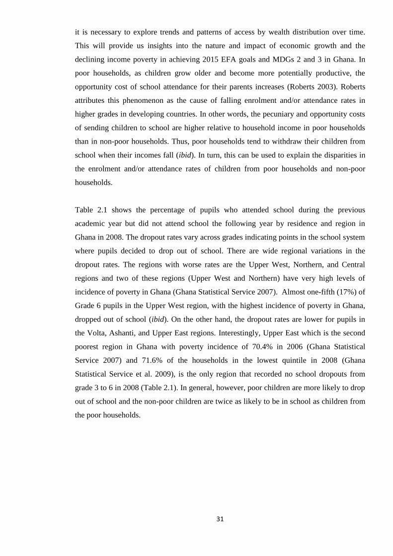
31
it is necessary to explore trends and patterns of access by wealth distribution over time.
This will provide us insights into the nature and impact of economic growth and the
declining income poverty in achieving 2015 EFA goals and MDGs 2 and 3 in Ghana. In
poor households, as children grow older and become more potentially productive, the
opportunity cost of school attendance for their parents increases (Roberts 2003). Roberts
attributes this phenomenon as the cause of falling enrolment and/or attendance rates in
higher grades in developing countries. In other words, the pecuniary and opportunity costs
of sending children to school are higher relative to household income in poor households
than in non-poor households. Thus, poor households tend to withdraw their children from
school when their incomes fall (ibid). In turn, this can be used to explain the disparities in
the enrolment and/or attendance rates of children from poor households and non-poor
households.
Table 2.1 shows the percentage of pupils who attended school during the previous
academic year but did not attend school the following year by residence and region in
Ghana in 2008. The dropout rates vary across grades indicating points in the school system
where pupils decided to drop out of school. There are wide regional variations in the
dropout rates. The regions with worse rates are the Upper West, Northern, and Central
regions and two of these regions (Upper West and Northern) have very high levels of
incidence of poverty in Ghana (Ghana Statistical Service 2007). Almost one-fifth (17%) of
Grade 6 pupils in the Upper West region, with the highest incidence of poverty in Ghana,
dropped out of school (ibid). On the other hand, the dropout rates are lower for pupils in
the Volta, Ashanti, and Upper East regions. Interestingly, Upper East which is the second
poorest region in Ghana with poverty incidence of 70.4% in 2006 (Ghana Statistical
Service 2007) and 71.6% of the households in the lowest quintile in 2008 (Ghana
Statistical Service et al. 2009), is the only region that recorded no school dropouts from
grade 3 to 6 in 2008 (Table 2.1). In general, however, poor children are more likely to drop
out of school and the non-poor children are twice as likely to be in school as children from
the poor households.
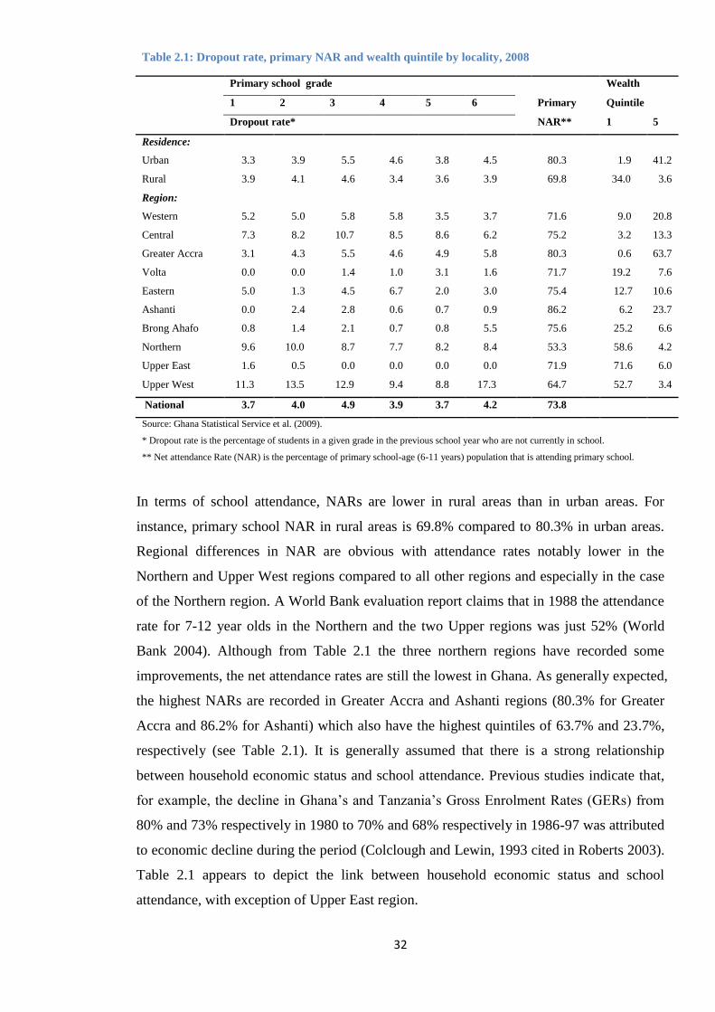
32
Table 2.1: Dropout rate, primary NAR and wealth quintile by locality, 2008
Primary school grade
Wealth
1 2 3 4 5 6
Primary
Quintile
Dropout rate* NAR** 1 5
Residence:
Urban 3.3 3.9 5.5 4.6 3.8 4.5
80.3
1.9 41.2
Rural 3.9 4.1 4.6 3.4 3.6 3.9
69.8
34.0 3.6
Region:
Western 5.2 5.0 5.8 5.8 3.5 3.7
71.6
9.0 20.8
Central 7.3 8.2 10.7 8.5 8.6 6.2
75.2
3.2 13.3
Greater Accra 3.1 4.3 5.5 4.6 4.9 5.8
80.3
0.6 63.7
Volta 0.0 0.0 1.4 1.0 3.1 1.6
71.7
19.2 7.6
Eastern 5.0 1.3 4.5 6.7 2.0 3.0
75.4
12.7 10.6
Ashanti 0.0 2.4 2.8 0.6 0.7 0.9
86.2
6.2 23.7
Brong Ahafo 0.8 1.4 2.1 0.7 0.8 5.5
75.6
25.2 6.6
Northern 9.6 10.0 8.7 7.7 8.2 8.4
53.3
58.6 4.2
Upper East 1.6 0.5 0.0 0.0 0.0 0.0
71.9
71.6 6.0
Upper West 11.3 13.5 12.9 9.4 8.8 17.3
64.7
52.7 3.4
National 3.7 4.0 4.9 3.9 3.7 4.2
73.8
Source: Ghana Statistical Service et al. (2009).
* Dropout rate is the percentage of students in a given grade in the previous school year who are not currently in school.
** Net attendance Rate (NAR) is the percentage of primary school-age (6-11 years) population that is attending primary school.
In terms of school attendance, NARs are lower in rural areas than in urban areas. For
instance, primary school NAR in rural areas is 69.8% compared to 80.3% in urban areas.
Regional differences in NAR are obvious with attendance rates notably lower in the
Northern and Upper West regions compared to all other regions and especially in the case
of the Northern region. A World Bank evaluation report claims that in 1988 the attendance
rate for 7-12 year olds in the Northern and the two Upper regions was just 52% (World
Bank 2004). Although from Table 2.1 the three northern regions have recorded some
improvements, the net attendance rates are still the lowest in Ghana. As generally expected,
the highest NARs are recorded in Greater Accra and Ashanti regions (80.3% for Greater
Accra and 86.2% for Ashanti) which also have the highest quintiles of 63.7% and 23.7%,
respectively (see Table 2.1). It is generally assumed that there is a strong relationship
between household economic status and school attendance. Previous studies indicate that,
for example, the decline in Ghana’s and Tanzania’s Gross Enrolment Rates (GERs) from
80% and 73% respectively in 1980 to 70% and 68% respectively in 1986-97 was attributed
to economic decline during the period (Colclough and Lewin, 1993 cited in Roberts 2003).
Table 2.1 appears to depict the link between household economic status and school
attendance, with exception of Upper East region.
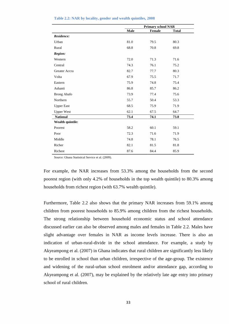
33
Table 2.2: NAR by locality, gender and wealth quintiles, 2008
Primary school NAR
Male Female Total
Residence:
Urban 81.0 79.5 80.3
Rural 68.8 70.8 69.8
Region:
Western 72.0 71.3 71.6
Central 74.3 76.1 75.2
Greater Accra 82.7 77.7 80.3
Volta 67.9 75.5 71.7
Eastern 75.9 74.8 75.4
Ashanti 86.8 85.7 86.2
Brong Ahafo 73.9 77.4 75.6
Northern 55.7 50.4 53.3
Upper East 68.5 75.9 71.9
Upper West 62.1 67.5 64.7
National 73.4 74.1 73.8
Wealth quintile:
Poorest 58.2 60.1 59.1
Poor 72.3 71.6 71.9
Middle 74.8 78.1 76.5
Richer 82.1 81.5 81.8
Richest 87.6 84.4 85.9
Source: Ghana Statistical Service et al. (2009).
For example, the NAR increases from 53.3% among the households from the second
poorest region (with only 4.2% of households in the top wealth quintile) to 80.3% among
households from richest region (with 63.7% wealth quintile).
Furthermore, Table 2.2 also shows that the primary NAR increases from 59.1% among
children from poorest households to 85.9% among children from the richest households.
The strong relationship between household economic status and school attendance
discussed earlier can also be observed among males and females in Table 2.2. Males have
slight advantage over females in NAR as income levels increase. There is also an
indication of urban-rural-divide in the school attendance. For example, a study by
Akyeampong et al. (2007) in Ghana indicates that rural children are significantly less likely
to be enrolled in school than urban children, irrespective of the age-group. The existence
and widening of the rural-urban school enrolment and/or attendance gap, according to
Akyeampong et al. (2007), may be explained by the relatively late age entry into primary
school of rural children.
34
Table 2.3: NAR by welfare quintile, 2008
Quintile
Primary
NAR Secondary
NAR
Wealth quintile:
Poorest 59.1
22.2
Poor 71.9
34.9
Middle 76.5
41.7
Richer 81.8
51.3
Richest 85.9
60.7
Source: Ghana Statistical Service et al (2009)
In terms of wealth distribution, children from poor households have lower primary and
secondary NARs compared to children from non-poor households in Ghana (Table 2.3).
For example, primary NAR for children from poor households are significantly lower
compared to children from the rich households. The situation is even worse at the
secondary level where the gap between the poor and the non-poor widens. Although it is
believed that there is high return to education at this level, the poor continue to be deprived
of secondary education in Ghana (Ghana Statistical Service et al. 2004 & 2009; Rolleston
2009 & 2011).
Referring to Table 2.1 earlier indicates that as children progress through the grades, their
number drops consistently in the regions, except Upper East region. It remains to be seen
whether the economic growth and education policy interventions change the attendance
and attainment trends significantly. Additionally, the improvement in GER identified is
insufficient for assessing the real impacts of household wealth distribution in conjunction
with education sector reforms on progress in educational access and attainment. What is
required is a study that takes into account children’s socioeconomic background in
conjunction with education reforms and policy interventions in Ghana to fully understand
who enrols, attends and has a better chance of completing successfully basic education and
beyond.
2.6 Conclusions
In summary, it appears Ghana has made some gains in terms of economic growth, poverty
reduction, and especially educational outcomes after the education reforms and policy
interventions. These findings are consistent with other empirical studies and reports on
economic growth, poverty reduction, and improvements in educational outcomes in Ghana
(Coulombe and McKay 2007; Coulombe and Wodon 2007; Adjasi and Osei 2007;
Akyeampong et al. 2007; Ghana Statistical Service 2007, 2008, 2010 & 2011; Adamu-
35
Issah et al. 2007; Sackey 2007; Rolleston 2011; NDPC et al. 2010; Ministry of Education
Science and Sports 2008; World Bank 2011a, 2013 and 2014). For example, Akyeampong
et al. (2007) have also shown that from 1998 to 2003, Gross Enrolment Rates (GERs) for
all levels of pre-tertiary education have remained at a near constant level, only rising
slightly in 2004. Furthermore, gross enrolment ratio increased from 93.7% to 95.2%
between 2006/07 and 2007/08 academic year after the SCG and Free School Feeding
programmes were implemented during the mid 2000 (Ministry of Education Science and
Sports 2010; NDPC et al. 2010).
However, the review of Ghana’s economic growth, education sector reforms, and trends in
educational outcomes suggest that there are still questions that remained to be answered
about educational access and attainment in Ghana. This is in spite of the country’s good
economic performance (i.e. steady GDP growth rate) and education policy interventions.
The next chapter reviews both the theoretical and empirical literature on economic growth,
income and wealth distribution, non-income poverty and socioeconomic inequality,
determinants of educational access and attainments in a broader perspective. It also
outlines the conceptual framework of the study. The essence is not only to support the
framework of the study but also to identify the niche where the study can contribute to in
the literature.
36
Chapter 3
Economic growth, income and non-income inequality and conceptual framework
3.1 Introduction
This chapter discusses theoretical and empirical literature of the thesis on wealth
distribution, income and non-income inequality, non-income poverty, and socioeconomic
determinants of educational access and attainments. Section 3.2 provides a review of the
impacts of economic growth on income inequality and non-income inequality and poverty,
while Section 3.3 highlights why it is important to focus on non-income inequality and
poverty. Section 3.4 discusses progress in education in the context of EFA goals 2 and 5.
We review socioeconomic inequality in educational access and attainments in Section 3.5.
The evidence of what determines and contributes to educational access and attainment
inequalities are reviewed in Section 3.6. The conceptual framework and the data for
empirical analysis form the second part of this chapter and are discussed in Sections 3.7
and 3.8, respectively. Section 3.9 concludes the chapter.
3.2 Economic growth, inequality and non-income poverty
It is widely accepted that economic growth is a necessary condition for sustainable poverty
reduction. Thus, in order to understand how economic growth can impact on poverty
reduction, Ravallion (2001) advocates for more microeconomic approach to the analysis of
growth policies and poverty. Some studies demonstrate that economic growth benefits the
poor in most developing countries in which substantial growth has taken place (Deininger
and Squire 1998; Ravallion 1996; Roemer and Gugerty 1997; Ravallion and Chen 2003).
Indeed, economic growth appears to be one of the best ways to reduce poverty. In fact,
countries which experienced rapid economic growth over the past years, such as Hong
Kong, Korea, Malaysia, and Indonesia, saw their per capita incomes of the bottom 20%
and 40% of the population grow significantly (Roemer and Gugerty 1997). Consequently,
one may say that income growth could promote the growth of non-income dimensions of
well-being (e.g. education and health) through non-income variables which may correlate
with average incomes.
From capability expansion point of view, economic growth can expand capabilities directly.
Drèze and Sen (1991) suggest that as average incomes increase, the population has greater
access to relevant non-income dimensions of well-being such as; basic education, and
healthcare among others. This implies that all capabilities can expand with economic
growth, thus promoting human capital development. Drèze and Sen (1991) also argue that
37
non-income poverty outcomes can be improved appreciably if income inequality and
poverty are reduced, reflecting a tendency for economic growth to lead to lower absolute
poverty reduction. Furthermore, they suggest that progress in non-income dimensions of
poverty can be achieved through public social services. In theory, public social spending
on essential non-income dimensions of well-being (education and health) can lead to
improved progress in capability outcomes. By implication, growth matters in reducing
non-income poverty if it is used to finance suitable public social services. In this regards
too, economic growth has the tendency to lead to better provision of public social services.
There are a number of studies on the relationship between economic growth and income
poverty (Grimm et al. 2002; Kakwani and Son 2008; Ravallion and Chen 2003; Gravelle
2003; Greeley 1994; Kakwani 1997; Lopez 2004; Dollar and Kraay 2002; Ravallion and
Chen 1997; Christiaensen et al. 2002; Adam and Page 2001). However, only few studies
(Klasen 2008; Grosse et al. 2008; Gunther and Klasen 2009; Christiaensen et al. 2003;
Harttgen et al. 2010) have specifically analysed the impacts of economic growth on non-
income poverty. In particular, Klasen (2008) and Grosse et al. (2008) apply a pro-poor
growth framework developed by Ravallion and Chen (2003) to measure the impacts of
economic growth on education, health and nutrition. The authors analyse the distributional
pattern of improvements of these non-income dimensions of poverty and from the study, it
emerges that there is no perfect overlap of income poor and of non-income poor
households in Bolivia. They also observe that the poor have not benefited
disproportionately from improvements in the non-income dimensions as a result of the
increased growth rates. The findings reveal that relative economic growth does not
automatically mean that the poor catch up with the non-poor in absolute terms. This
supports the view that improving income situation of households does not automatically
guarantee improving non-income situation of the poor, such as access to education and
healthcare among others (Klasen 2000; Grimm et al. 2002).
In Africa, Christiaensen et al. (2003) examine economic growth, trends in poverty, and
economic policies in eight SSA countries during the 1990s using household data. Out of
the eight countries studied, four countries (Ethiopia, Ghana, Mauritania, and Uganda)
experienced economic growth, with improvements in their human development indicators
to different degrees. Improvements in primary school enrolment in Ethiopia, Ghana,
Mauritania, and Uganda were recorded. But, the other four countries (Madagascar, Nigeria,
Zambia, and Zimbabwe) that experienced stagnation and decline in growth, suffered a
38
decline in living standards. Surprisingly, primary school enrolment improved in
Madagascar, Nigeria, and Zimbabwe in spite of the stagnation or decline in their annual
economic growth rates. Also child mal-nutrition improved in Zimbabwe during an episode
of deteriorating economic situation (Christiaensen et al. 2003). The authors note that it is
quite possible through public policy intervention to increase primary school enrolment
rates even if economic growth rate is not rising. However, the question still remains
whether the increase in primary school enrolment rate is sustainable without economic
growth.
Furthermore, other evidence suggest that economic growth may remain stagnant but
welfare may rise due to improvements in non-income dimensions of poverty as in the case
of some Latin America countries (World Bank 2006; Sahn and Younger 2006). On the
other hand, Adam and Page (2001) observe that there is no clear relationship between a
reduction in monetary poverty and an improvement in non-income dimensions of poverty.
Thus, a country for example, may have a high rate of monetary poverty alongside a high
rate of education, and vice versa. Cardozo and Grosse (2009) analyse how the distribution
of education and health changed between two periods in Colombia and discover that while
income and expenditures fluctuated according to economic growth, the selected non-
income indicators had only minor changes. Furthermore, they also observe that while
income and expenditures decreased for all income percentiles, and relatively more for the
non-poor, the non-income dimensions of well-being stagnated and remained unequally
distributed.
From development economics literature, it has generally been argued that the nature of the
impact of economic growth on inequality and poverty will depend on numerous factors,
such as the initial distributional conditions (i.e. inequality and average income levels), the
type of growth experienced, the functioning of markets, and the ability of the poor to
partake in the growth process (Alesina and Rodrik 1994). One reason for the initial
distributional condition is that inequality may be potentially bad for growth (Alesina and
Rodrik 1994; Deininger and Squire 1998). The assumption is that high inequality may
make poverty fall slower for a given level of economic growth. Consequently, inequality
may further breeds relative deprivation, economic isolation and social exclusion (Duclos
2009). Furthermore, there is a general notion that even in periods of relatively good
economic performance, the poor are being left behind due to the high level of income
inequality (De Janvry and Sadoulet 2000). Likewise, economic stagnation is also
39
particularly harsh for the poor because of the prevailing inequality (Kanbur and Lustig
1999) and as a result, worsening inequality will impede efforts to reduce non-income
poverty.
There are often concerns about high degree of income inequality in developing countries
contributing to the perpetuation of persistent poverty. However, a study conducted by Sahn
and Younger (2006) in six Latin American (Bolivia, Brazil, Colombia, Guatemala,
Nicaragua and Peru) shows that although these countries experienced high income
inequality, this was not the case in terms of education and health inequalities. Interestingly,
the authors observe declines in inequality of the selected non-income dimensions of
poverty. In addition, they discover that increases in mean levels of education and health
have contributed to substantial declines in education and health poverty in the six Latin
American countries, even as income poverty has remained stagnant or declined only
modestly. For example, in most of the six countries studied, inequality in education
outcomes reduced substantially. In Peru, the education Gini decreased from 0.388 to 0.270
between 1986 and 2000. In Guatemala, the decline was from 0.63 to 0.53 between 1987
and 1999, while in Brazil it was from 0.40 to 0.34 over a ten-year period. However, in
Nicaragua there was no decline in education inequality.
Furthermore, in terms of economic growth and human capital development, some believe
that inequalities brought about as a result of market-oriented reforms may be good in one
aspect and bad in other. Chaudhuri and Ravallion (2006) used market-oriented reforms in
China and India to demonstrate both the good and bad aspects inequalities. The authors
argue that “patterns of social exclusion, unequal opportunities for enhancing human capital,
lack of access to credit and insurance among others, can conspire to fuel rising inequality
and prevent certain segments of the population from making transition out of low
productivity activities” (Chaudhuri and Ravallion 2006:17). They refer to these inequalities
as ‘bad inequalities’ which according to the authors are entrenched in market failures and
governance failures that can prevent the individuals from connecting to markets and limit
investment in human capital. Normally, it is poor people who tend to be most constrained
in financing investments in human capital (Aghion et al. 1999; Filmer and Pritchett 1999a
& 1999b; Filmer 2005; World Bank 2005).
Conversely, there is also an argument that inequalities are good for growth when there is
“rising returns to schooling and increasing dispersion of wages, because they reflect freer
40
labour markets with increased incentives for work and skill acquisition” (Chaudhuri and
Ravallion 2006:18). Nevertheless, Chaudhuri and Ravallion also note that inequalities in
human capital are bad because they retard poverty reduction through growth in developing
countries. Thus, those with relatively little schooling are less positioned to participate in
economic growth. The bad aspect of inequalities which Chaudhuri and Ravallion (2006)
argued, arise from differences in endowments that are the results of both supply-side
governmental and demand-side market failures.
3.3 Focus on non-income inequality and poverty
While non-income indicators of inequality and poverty have recently received more and
more attention in the concept and measurement of multidimensional poverty (Bourguignon
and Chakravarty 2003; Alkire and Santos 2010; Ray and Sinha 2011; Harttgen and Klasen
2012), they have not been fully incorporated in the country level policy analysis. This
inadequacy has been recognised and advocated for, among other categorisations of
inequality, to be focused on in the post-2015 development framework (Doyle and Stiglitz
2014).
Non-income inequality and poverty happens when people do not have access to affordable
social and physical services such as education, healthcare, and sanitation (Grosse et al.
2008; Harttgen et al. 2010; Sen 1985). Consequently, lack of these non-income dimensions
of well-being limits the poor people’s capabilities to take advantage of opportunities that
may be unleashed by economic growth.8 For example, lack of schooling is now considered
as a very important constraint on prospects of people escaping poverty in developing
countries (Chaudhuri and Ravallion 2006). Yet most assessments of poverty levels and
progress towards the MDGs have focused primarily on the income poverty target (Grimm
et al. 2002; Kakwani and Son 2008; Ravallion and Chen 2003; Gravelle 2003; Greeley
1994; Kakwani 1997; Lopez 2004; Dollar and Kraay 2002;Ravallion and Chen 1997).
Predictions that most countries are on track for achieving the poverty goals by 2015 are
generally based on income poverty assessments. Out of 134 countries assessed by the
World Bank on progress towards achieving the MDGs, only 34 countries (24%) were on
track to achieve non-income target (World Bank 2006). The World Bank further shows
that many countries, excluding several countries in SSA, will achieve the MDG in income
8
The key indicators usually used for measuring non-income inequality and poverty include: school
enrolment, attendance and completion rates, and years of schooling for education dimension; child mortality,
nutrition, vaccination, and maternal health for health dimension; drinking water, sanitation, electricity, and
cooking fuel for standard of living dimension .
41
poverty target but less than 25% will achieve the non-income poverty targets. This means
that achieving income poverty goals do not necessarily mean that non-income inequality
and poverty goals will be achieved. Thus, income and non-income poverty goals could be
given equal weighting when it comes to poverty reduction policies.
Furthermore, if we conceptualise well-being from a capability perspective (Sen 1985),
income is but one means to generate capabilities such as the ability to be healthy, well-
educated, housed, integrated, etc. (Klasen 2000). Klasen, therefore, argues that it would be
preferable to study well-being outcomes directly by analysing non-income dimensions of
poverty. In both theoretical and empirical literature, it is known that improvements of non-
income dimensions are not a natural by-product of economic growth (Sen 1998; Klasen
2000; Ravallion 2001; Grimm et al. 2002; Sahn and Younger 2006; World Bank 2006).
Furthermore, Adam and Page (2001) also assert that the international community is
increasingly sensitive to other non-monetary aspects of poverty such as education, life
expectancy and health, in addition to its monetary side. They compare the performances
recorded for each indicator in several countries in the Middle East and North Africa, and
find that there is no clear relationship between a reduction in monetary poverty (as a result
of economic growth) and an improvement in other welfare indicators. Thus, to understand
how the poor can benefit from economic growth, there is the need to identify and analyse
non-income dimensions of inequality and poverty that directly measure the capabilities of
individuals and households.
Although we cannot deny the fact that income is an important measure of well-being, it
does not capture all aspects of well-being (Sen 1985; Bourguignon and Chakravarty 2003;
Alkire and Santos 2010; Ray and Sinha 2011; Harttgen and Klasen 2012). The idea that
income is an inadequate measure of well-being is now widely accepted in theory. Yet in
empirical studies of inequality, the emphasis is mostly on income. Defining inequality and
poverty in terms of non-income dimensions of well-being has the added advantage that we
measure and analyse outcomes such as education and health at the individual level rather
than household level (Sahn and Younger 2006; Klasen 2008; Grosse et al. 2008; Gunther
and Klasen 2009).
Furthermore, recognising and analysing inequalities in non-income dimensions of well-
being such as education is of particular importance in designing relevant public policy in
addressing inequality issues, more so than in the case of reducing income inequality (Sahn
42
and Younger 2006). Inequality reduces income growth for the poor, but not for the rich
(Deininger and Squire 1998). Thus, for any pro-poor pattern of growth to be effective in
reducing non-income inequality and poverty, policies are required to address non-income
inequality, just as effective pro-poor growth depends on initial inequality in income
poverty measurement discussed earlier. Evidence show that investment in early childhood
development, for example, will promote equality of opportunity, and efficient public
spending on the basic social services such as; education, health, and infrastructure that
reach the poor is vital for pro-poor growth (Sahn and Younger 2006). However, in many
developing countries, public spending is not efficient and benefits the non-poor
disproportionately (Wilhelm and Fiestas 2005 ).
By decomposing changes in education and health inequalities into shifts in the mean and
changes in the distribution of education and health, Sahn and Younger (2006) show that
reduced inequality in these dimensions has contributed to significant reductions in
education poverty, and to a lesser extent, health poverty. The findings are very different
with respect to findings from income inequality literature. A possible reason from the
literature with regards to the findings may be explained in terms of differences in the
evolution of income and other indicators of inequality reflecting the fact that the
underlying factors that determine income inequality are different from those that contribute
to education and health inequality. Generally, income inequality can be explained by: the
nature of the labour market; the role of non-earned incomes, (including remittances from
overseas workers); the distribution of productive assets; and the differential returns to
human capital (Sahn and Younger 2007). In contrast, non-income dimensions of inequality
(e.g. education, and health inequalities) largely reflect public provision of basic services
and social infrastructure (Wilhelm and Fiestas 2005 ; Sahn and Younger 2006).
Consequently, the availability and access to the institutions providing the public services
may have relationship to the underlying distribution of incomes (Sahn and Younger 2007).
Thus, progress in the provision of public services, focus of public spending and the
distribution of non-income dimensions of well-being could be the explanation why
inequality in education and health could decline concurrent with improvements in the level
of non-income poverty despite worsening income inequality and stagnant or worsening
levels of income poverty (Sahn and Younger 2006). This suggests that reduction in non-
income inequality and poverty is possible even in economically challenged environments.
For example, Lloyd and Hewett (2009) observe that SSA countries have been able to
43
achieve relatively high primary school completion and/or low gender inequality in
education despite relatively low levels of economic growth. However, they also recognise
the fact that other factors such as donor expenditures on primary education and job
opportunities after completion of school among others contribute to reducing education
inequality between the poor and the non-poor in most of the countries.
Sahn and Younger (2007) also examine how non-income dimensions of poverty (education
and health) and inequality in education and health changed over time in twenty three
African countries covering a period of 15-20 years. They observe limited progress in the
African countries improving health and education outcomes in contrast with results from
Latin America study. With regards to education, the authors discover that education
poverty has declined and likewise for inequality in the vast majority of cases. However,
health inequality measure shows that while there were few instances of reduced inequality,
there was little evidence of success in improving equality of outcomes (ibid). In all,
findings about the distributional impact of economic growth on income and non-income
inequality and poverty in the literature are mixed.
3.4 Progress in educational outcomes
The world conference on Education for All (EFA), adopted in 1990 the World Declaration
on EFA. This was in response to the high promise of education and the large gaps in
educational access persisting in many developing countries (UNESCO 2008). Despite the
declaration that everyone has a right to a full cycle of basic education, developing
countries continue to lack progress in access to education (Harttgen et al. 2010).
Consequently, in the year 2000, World Education Forum (WEF) adopted a new framework
for action containing six EFA goals.9 These goals directly emphasise the importance of
education for human development and are to be reached until the year 2015 to overcome
the persisting insufficient progress in access to, and attainment of education in the
developing countries.
In 2008, UNESCO report shows that most developing countries have made progress
towards the EFA goals set in Dakar in 2000. The report shows that the net attendance rate
in primary education has increased from 79% in 1991 to 86% in 2005 in developing
9The six EFA goals adopted in the years 2000 are: the expansion of early childhood care and education, the
achievement of universal primary education, the development of learning opportunities for youth and adults,
the spread of literacy, the achievement of gender parity and gender equality in education, and improvements
in education quality.
44
countries. In particular, faster progress has been made between 1999 and 2005 than
between 1991 and 1999. For example, participation in primary education increased in SSA
from 54% in 1991 to 57% in 1999 and 70% in 2005 (UNESCO 2008).
According to UNESCO, the educational progress averages (especially those relating SSA
countries) hide specific country progress in reaching the EFA goals by the year 2015.
While some countries may be making progress towards achieving the EFA goals, others
may be lagging far behind (UNESCO 2008). Moreover, wide disparities in educational
progress remain between the poor and non-poor, and males and females (Harttgen et al.
2010). There are also evidence of significant within country differences in access to
education and in educational attainment of children, especially between urban and rural
areas (UNESCO 2008). Thus, progress in meeting the EFA goals is more likely to depend
on individual country’s economic growth and policies relating to reducing existing
inequalities in educational access.
In order to meet EFA goals in conjunction with MDGs 2 and 3, there has been substantial
expansion in education provisions in developing countries in recent years. However, the
question still remains if the expansion in education facilities and enrolments has reduced
existing inequalities in educational access and attainment in developing countries. Harttgen
et al. (2010) analyse differences in improvements in the access to the education system and
in educational outcomes across welfare distribution between countries and also by gender
in 37 developing countries. From the analysis, it emerges that there are drastic inequalities
in educational attendance across the wealth distributions in all the 37 countries. In SSA,
for example, Berthélemy (2006) finds that education policies are biased against the poor.
Berthélemy argues that on average, the policies favour the non-poor because the policies
are concentrated on improvements in secondary and tertiary education and only little
attention is paid to improvements in primary education access and attendance by the poor
households.
Consequently, the main channels by which overall economic growth can promote
education, as suggested by Anand and Ravallion (1993), is by lessening the extent of
poverty which constrains families in their ability to send their children to school, and by
increasing public educational investments which leads to greater schooling access and
better quality education. It is hypothesed that a pro-poor progress in education combine
with a focused public spending in education sector is expected to contribute to declining
45
inequality and poverty in education, even in an environment of stagnant or worsening
levels of income poverty (Sahn and Younger 2007; Filmer and Pritchett 1999b).
Nevertheless, sustained economic growth and poverty reduction can result in higher levels
of household resources. Thereby, allowing higher investments by households in their
children’s education because parents are less dependent on their children’s labour
(Harttgen et al. 2010). On the other hand, existing inequality and poverty may be worsened
through poor education. For instance, it has been shown that poverty significantly reduces
the likelihood of school attendance and attainments (Smits et al. 2007).
3.5 Socioeconomic inequality in educational outcomes
Human capital is widely recognised as essential for economic and human development.
The distribution of education matters and unequal distribution of education tends to have a
negative impact on per capita income in most countries (Lopez et al. 1998). On educational
inequality, World Bank (1995) points out that the issue of equity affects several
overlapping disadvantaged groups including the poor, street children and children in the
workforce. The World Bank stresses that the different access that the poor and the non-
poor children, boys, and girls have to the education system should not be ignored because
it contributes to inequality gap among these group of people later in life. For example,
Gopal and Salim (1998) argue that low levels of female education lead to legal illiteracy,
creating a severe constraint to effective implementation of equitable legal provisions. Thus,
the way in which education is distributed will have profound impact on the distribution of
income, the nature of economic growth, and poverty reduction. Therefore, understanding
the trends and impacts of educational inequalities is particularly important because public
policy can relatively address them than in the case of reducing income inequality.
Filmer and Pritchett (2001) examine socioeconomic inequalities in educational outcomes
in India and discover a large school enrolment differences which they attributed to income
inequality that varies widely across India states between the poor and the non-poor. On
average, the non-poor Indian child is 31% point more likely to be enrolled than a poor
child. According to Filmer and Pritchett (1999b), very low primary school attainment by
children from poor households is usually driven by the patterns of enrolment and dropout
among the poor households. They suggest that the patterns of enrolment and dropout of the
poor tend to follow regional patterns observed in a cross-country study of school enrolment
and educational attainment by household wealth in 35 countries. In Western and Central
Africa, they observe low enrolment and high dropout rates resulting in more than 40% of
46
children from poor households never able to complete Grade 1, and only one in four
completed Grade 5.
High enrolment and late dropout rates were recorded for Eastern and Southern African
countries, while low enrolment and low dropout rates were also recorded for South Asian
countries. In Colombia and Peru (Latin America) for instance, the larger percentage
shortfall in achieving universal primary or basic education completion was attributable to
children from the poorest households (Filmer and Pritchett 1999b). In many developing
countries, it is evidenced that the bulk of the deficit from achieving universal primary
education comes from the poor (Filmer and Pritchett 1999b; Filmer 2000) .
Furthermore, Filmer and Pritchett (1999b) discover that in most of the 35 countries
examined, children from households at the top 20% of the wealth index stayed in school
longer than children from households who occupied either the middle 40% or the bottom
40% of the wealth index. In addition, children from the middle 40% of the wealth index
had a higher school retention rate than those in the bottom 40% of the wealth index. In
most countries, the poor (bottom 40% of the wealth index) did not complete primary
school. The studies by Filmer and Pritchett in 1999 and 2001 reveal that household wealth
inequality is associated with low level of educational attainment, low median grade
completion, and high school dropout. In other words, household wealth is positively
associated with children’s enrolment, and inequalities in education outcomes are derived
mainly from household wealth. Montgomery and Hewett (2005) also investigate the effects
of living standards and relative poverty on children’s schooling in urban and rural areas of
Senegal. Their findings show that the living standards in urban areas exert substantial
influence on children’s education. The effect of living standards is, however, weaker in the
rural areas of the country. However, the authors note that income growth alone is unlikely
to close the schooling gap between urban and rural areas, and between boys and girls.
In Ghana, many children fail to continue and complete their basic education programme. In
2008, about a third (32.3%) of children who enrolled in Junior High School dropped out in
the final year of JHS (Ministry of Education Science and Sports 2008), despite the fact that
at the basic education level (primary school and JHS) education is free. According to 2010
PHC report, 23.4% of Ghanaians have never attended school (Ghana Statistical Service
2013a). With respect to education equity; educational access, standards and achievement
varied widely in the country, especially between urban and rural areas, and the poor and
47
non-poor households (Ghana Statistical Service 2008). Other research conducted in Ghana
reveal that educational access and attainment disparities exist based on socioeconomic
groups and gender (Sutherland-Addy 2002; Palmer 2006; Tuwor and Sossou 2008).
Sackey (2007) also analyses school attendance for school-age children within the context
of parental education and household resources using Ghana Living standards Survey
(cross-sectional household data) in 1992 and 1999. The study reveals that household
resources play an important role in the education of children in Ghana, and children from
wealthy households tend to achieve higher rates of school attendance both in 1992 and
1999 household surveys.
Besides, the distribution of education in Ghana suggests that there is inequality in
education which is linked to income poverty and gender (Ghana Statistical Service et al.
2009; Akyeampong et al. 2007; World Bank 2004). For example, Ghana Statistical Service
et al. (2009) also reveal that children from poor households have lower school enrolment
and attendance rates, and they are more likely to drop out in the course of the primary
cycle, than the children from non-poor households. This confirmed earlier findings by
Filmer and Pritchett (1999b) which shows that the dropout rates for the poor are
consistently higher than for the non-poor.
A study by Deininger (2003) evaluates the impact of Universal Primary Education
programme in 1997 which aimed at reducing the cost of primary education in Uganda. The
study shows that before the UPE in 1992, household income significantly increased the
probability of primary and secondary school attendance of children from non-poor but not
the poor households. By 1999, increases in primary school attendance were recorded for
both the poor and non-poor children, and inequalities in attendance related to income and
gender were reduced substantially. The implementation of the UPE programme in Uganda
led to reduction in the cost of primary education but not secondary education to households.
Consequently, the inequality concern at the secondary education level still remains
(Deininger 2003), indicating that household income or wealth distribution may be the key
factor contributing to the inequalities in educational access and attainment in Uganda.
On a cross country level, enrolments in education and associated years of schooling have
expanded substantially in developing countries in recent years (Harttgen et al. 2010) . But
to what extent has this expansion in enrolments reduced existing inequalities in educational
access and achievements in individual countries? Evidence of improvements in access to
48
education system and in educational outcomes across the welfare distribution between and
within countries, and also by gender for 37 countries show drastic inequalities in
educational attendance across wealth distributions (Harttgen et al. 2010). The study shows
that inequality in attendance declines with rising average attendance, while inequality in
completion rates or number of years of schooling increases with rising completion rates.
From a gender perspective, gender inequality in education may come about as a result of
schooling investments which may differ by gender when rates of returns on children
education to parents are gender-specific (Alderman and King 1998). In addition,
differences in cost streams of educating children may differ when direct costs such as fees
and expenses for uniforms are gender-specific. Another reason put forward for gender
inequality in educational access and attainment is when access to education differs by
gender and when the opportunity cost of a school-age child’s time varies by gender (ibid).
Such costs may lead to differences in rates of investment in children’s education and if, for
example, poor parents believe that the costs of educating female child is high with low
returns (especially in developing country setting) then this will lead to gender inequality in
educational outcomes, ceteris paribus. Consequently, resource constraints can exacerbate
gender inequality in education, due to credit constraints and patterns of preferences as
incomes change (Alderman and Gertler 1997).
Furthermore, parental empathy and expected future transfers (remittances) from children to
their parents may differ by gender. There is a general assumption in developing country
setting that boys are able to send remittances to their parents when they start working
compared to girls. For example, Garg and Morduch (1998:473) explain that in many
households, ‘women move out of the family when they marry, while men stay within the
household with their wives’. As a result, parents are more likely to receive more returns on
investing in male children’s education than investing in female children’s education.
Empirically, the extent of inequality among girls in primary school attendance and
completion rates according to socioeconomic status, is found to be substantially greater
than for boys (Lloyd and Hewett 2009). In Ghana, the picture as regards girls’ education is
more nuanced. Girls are educationally deprived compared to boys in most of the
administrative regions in Ghana, with lower enrolment and completion rates. However,
once enrolled, girls have as good if not better chance of completing primary education as
boys (ICF Macro 2010; Akyeampong et al. 2007). These findings are consistent with
49
Sackey (2007) who also finds that although school attainment has improved for both boys
and girls between 1992 and 1999 survey periods, generally the likelihood of girls attending
school is relatively lower than that of boys. However, from Sackey's empirical analysis,
there appear to be a general tendency for the attendance rates of girls to rise faster than that
of boys, suggesting a narrowing of the gender gap in primary education in Ghana. It also
appears that for male and female children, the impact of household resources on school
attendance has reduced from 1992 to 1999 survey periods (Sackey 2007).
A study by Holmes (2003) also shows that girls receive less education than boys. The
reason for this disparity is attributed to both economic and social-cultural reasons. Homes
further argues that the opportunity cost of sending female children to school in rural areas,
where girls are married quite early, is high because benefits of their schooling will not
accrue to their parental household. This supports the general belief that gender inequalities
in school enrolment and completion are magnified even among the children from poor
households. This may, in turn, have serious consequences for girl-child education in terms
of access to schools of reasonable quality.
3.6 Socioeconomic determinants of educational outcomes
There are many factors described in the literature as determinants of educational enrolment,
attendance, and attainments based on specific settings of the studies. However the major
factors that are often cited to explain the observed trend in educational enrolment,
attendance, and attainment of children are: the age and gender of children; household
resources; educational status of household heads or parents, household composition and/or
size; availability and quality of schools; distance to school; and location effects among
others.
3.6.1 Children’s demographic characteristics
A child's age is considered as a good predictor of education attainment in the empirical
literature (Holmes 2003). Age is relevant because it is related to learning abilities, and
whether or not a child starts his or her education on time. Hanushek and Lavy (1994),
Jimerson et al. (2000), and Farmer et al. (2003) highlight a child's age as one of the main
determinants of a child's school enrolment, completion, and dropout rates among other
characteristics (i.e. gender, IQ and cognitive skills, academic achievement, nutritional and
health). In addition, Psacharopoulos and Arriagada (1986) also suggest that the opportunity
cost for spending time in school can be considered to be dependent on the age of the child,
and the demand for schooling will necessarily be dependent on the child's age.
50
The gender of a child is also important in determining the chances of the child's school
attendance and attainment especially in developing countries context, ceteris paribus, for
several reasons. Households commonly prefer to invest in boys’ rather than girls’
education. The main reason for this gender discrimination according to Oxaal (1997) is the
low perceived returns to schooling for girls because they usually leave their natal home
when they marry. Lloyd and Gage-Brandon (1994) find that dropout rates were
significantly greater for girls, and their educational attainment levels were also lower than
that of boys in Ghana, especially when there were younger siblings in the household. Girls’
school attendance also depends on opportunity costs generated by providing child care for
younger siblings (Lewin 2009).
3.6.2 Household wealth
Household income and assets are among the main household characteristics identified in
the literature that impact on school enrolment, attendance and completion rates (Bredie and
Beeharry 1998; Hanushek and Lavy 1994; Sathar and Lloyd 1994). Household income has
been shown to be important determinant of children’s school enrolment and educational
attainment, particularly in settings where households face tight liquidity constraints caused
by the lack of insurance and limited possibilities to smooth consumption through credits or
savings (Becker and Tomes 1986). Thus, the magnitude of family income may be
influential in educational choices households make. For example, if families are credit
constrained, current income may influence a family’s capacity to invest in children's
education (Jacoby 1994; Lillard and Kilburn 1995; Filmer 2005).
From human capital theory framework and dwelling on the sources of variation in
household financial resources, children are perceived as an investment. Consequently,
parents acting in a rational manner will invest resources in their children in such a way as
to maximise the probability of future payoffs (Becker 1975). However, the extent to which
children can be sponsored in their schooling engagements depends in part on household
assets and the number of claimants in the family entitled to (Steelman and Powell 1991).
Theoretically, if poor households are credit constraint and imperfect credit markets
conditions prevail, these conditions can preclude poor households from making profitable
but indivisible investments, such as investing in children's education (Becker and Tomes
1986). Becker and Tomes point out that parents’ concern for the economic capabilities and
success of their children prompts them to invest resources in the children's education,
51
health and motivation. According to the authors, these expenditures influence the human
capital and earnings of children later in life.
It is also expected that the greater the total resources of a household, the greater will be the
demand for child schooling, and hence the likelihood that a child will attend school, ceteris
paribus. The implications of this assumption for the poor households are low demand for
education and increased inequality in the education outcomes between the poor and the
rich households. However, if government spends generously on education and provides
universal access to primary education, in particular, the cost of education to households
will fall (Lloyd and Blanc 1996). This may in turn reduce socioeconomic inequalities in
educational participation by poor households. On the other hand, if access is limited and
schooling is costly, households' financial support for their children’s education will be
critical (ibid).
In the empirical literature, there are evidence indicating the impacts of household resources
on school attendance and attainments. In developing countries contexts, it is well
established that household economic resources are key determinants of children's school
enrolment and attainment (Canagarajah and Coulombe 1997; Filmer and Pritchett 1999b).
Bredie and Beeharry (1998) have also shown that the likelihood of children dropping out
of school depends on the level of opportunity costs incurred by parents. A study by
Hanushek and Lavy (1994) indicates that children with greater opportunities to earn
income are likely to be taken out of school and involved in work if parents need additional
income. Sackey (2007) also finds that household resources play an important role in the
education of children in Ghana, and children from rich households tend to achieve higher
rates of school attendance both in 1992 and 1999 household surveys.
Other studies have found that children’s school enrolment and attainments are associated
with socioeconomic status of households (Psacharopoulos and Arriagada 1986; Sathar and
Lloyd 1994; Lloyd and Blanc 1996; Gage et al. 1997; Buchmann and Hannum 2001). For
example, Lloyd and Blanc (1996) have also confirmed that the household living standard is
strongly associated with the likelihood that children of school-age will be enrolled in a
school and that they will have completed school. It is important to note that households'
access to financial resources have direct implications for children's welfare and education
attainment, ceteris paribus. This, in turn, makes children's access to education positively
associated with household wealth (Patrinos and Psacharopoulos 1997). These studies
52
demonstrate that household wealth is a key determinant of a household’s ability to invest in
children's education, and as a result, it can lead to inequality in educational outcomes of
children. However, none of the studies has estimated absolute and relative contributions of
household income or wealth to inequalities in educational outcomes of households.
3.6.3 Household composition/size
Household size can be considered as a determining factor when it comes to the decision of
whether or not to enrol a child in school. The assumption is that the larger the family, the
lower the probability of a child attending school. This assumption could be based on the
premise that larger families spread their financial and human resources thinly compared to
smaller households (Sathar and Lloyd 1994; Sandefur et al. 2006). Also, the presence of
very young children (age 0-5years) in the household in the context of developing countries
can increase the time needed for childcare and this can affect school attendance and
completion of school-aged children (Sathar and Lloyd 1994). This responsibility is often
shared between adults and older children which may affect the older children's school
attendance and completion (Lloyd and Blanc 1996).
In the empirical literature, the effects of the presence of young children and school-age
children on educational outcomes have been documented and have been mostly negative,
especially in developing country settings. Lloyd and Blanc (1996) assessment of children’s
schooling in SSA identifies the possible effect of other children’s presence on schooling
possibilities of any given child. Using Kenya, Tanzania, Cameroon, Niger, Malawi,
Namibia and Zambia as case studies, they observe that the presence of young children
decreases the likelihood of school attendance of the older children in the household,
especially among girls. In Ghana, Sackey (2007) finds that the presence of younger
siblings, relative to older ones, tends to reduce the probability of school attendance. Sackey
further points out that the reduction in the probability of schooling by virtue of having
younger siblings is higher for girls than for boys and attributes the findings to the socio-
cultural norms and practices on gender roles in Ghanaian households.
In addition, the presence of more school-age children in the household may also put more
pressure on household resources, thereby affecting children's school attendance and
completion rates negatively. This effect has been observed by Butcher and Case (1994) in
their study on sibling composition and educational attainment. The study shows that where
parents are faced with borrowing constraints, the presence of one child may alter the
53
opportunity cost of investing in the education of another. In theory, households who intend
to maximise investment in their children’s education, but are limited in their ability to
borrow will stop short of investing until the rate of return to each child’s education is equal
to the market rate of interest (Becker 1975). In such situations, children with the highest
perceived marginal return to education will receive the most education. For example,
where there are both boys and girls in a household competing for limited resources, boys
are more likely to receive more education than girls because of low perceived returns to
schooling for girls. This tendency can result in a gender gap in education, as long as
parents or households tend to put a higher premium on the education of boys.
In Botswana, Chernichovsky (1985) finds negative impact of younger children and positive
impact of school-aged children on the schooling outcomes of the older children in the
family. Contrary to the notion of the quality-quantity trade-off, the author discovers that in
Botswana, “the larger the number of school-aged children in the household, the greater the
probability that they are enrolled in school and the higher the levels of education”
(Chernichovsky 1985:328). This finding is supported with the argument that due to
diminishing returns to labour, parents may choose to allocate roles to their children and as
a result, some children work and others attend school.
For the effects of household size or family size on educational outcomes, there are mixed
findings. The findings of studies in developed countries show a negative relationship
between family size and educational outcomes (Blake 1981; Downey 1995). Similar results
were also found in Thailand (Knodel et al. 1990) and Malaysia (Pong 1997; Parish and
Willis 1993). On the other hand, studies in SSA have shown that cultural differences may
mitigate the adverse effects of large families on children's schooling (Lloyd and Gage-
Brandon 1994; Chernichovsky 1985; Lloyd and Blanc 1996). Knodel and Wongsith (1991)
explain that the extent of the negative effect of large families is dependent on the cultural
and socioeconomic setting. Other researchers have also found that in Kenya, Botswana and
Israel, the extended family can improve the educational opportunities of children from
large families (Gomes 1984; Chernichovsky 1985; Shavit and Pierce 1991). For instance,
Shavit and Pierce (1991) find that in Israel, Muslims utilise a large kinship network beyond
the nuclear family, which alleviates the resource constraints associated with having more
children. On the contrary, for the Israeli Jews who do not have strong extended family ties,
the association between their household size and educational outcomes of their children
was negative.
54
Furthermore, Patrinos and Psacharopoulos (1997) also explore the negative association
between household size and educational outcomes of children from a different angle and
suggest that the negative relationship could be linked to the preferences of parents. They
explain that parents with a preference for larger families generally see less need to educate
their children. Thus, the negative relationship between house size and children’s
educational attainment may be the result of parental preferences and resource constraints.
The number of economically active household members (aged between 18 and 64 years)
has also been used as a determinant of schooling access and attainment in the empirical
literature. It has been shown that the variable may have a positive or negative impact on
the chances of children's education. A study by Okumu et al. (2008) on socioeconomic
determinants of primary school dropout in Uganda shows that as the proportion of the
economically active members of household increases, the likelihood of primary school
dropout increases, other factors held unchanged. The authors argue that the inverse
relationship found in their study implies that a good number of the economically active
household members were actually unproductive (i.e. unemployed). They further suggest
that the effect squeezes out the households resources, thereby increasing households’
dependence burden. On the other hand, it also implies that the presence of large proportion
of economically active household members who are economically productive (i.e.
employed) is highly likely to impact positively on children's education, all other things
being equal.
Household head’s or parents’ educational level is one of the key factors used to determine
the socioeconomic status of households. In considering the determinants of children’s
educational choices, Haveman and Wolfe (1995) argue that the most fundamental
economic factor is the human capital of parents and that household head or parental
education reflects a sort of intergenerational transmission of socioeconomic status. The
authors find that a mother’s education tends to be more closely related to the child’s
schooling attainment than does the father’s. Lillard and Willis (1994), also note that the
effect of parents’ education on that of their children is one of the key factors in any
consideration of the intergenerational transmission of human capital and economic
wellbeing within households or families. Most studies have found a positive association
between household head’s or parents’ education and children's educational outcomes. The
empirical studies that have found positive relationship between educational level of
household heads or parents and children's educational outcomes include: Glewwe and
Jacoby (1994) and Oliver (1995) for Ghana; Tansel (1997) for Côte d’Ivoire and Ghana;
55
Glick and Sahn (2000) for Guinea; Sathar and Lloyd (1994) for Pakistan; and Tansel (2002)
for Turkey. More recent studies by Rolleston (2011) and Sackey (2007) on the
determinants of educational access using ordered probit regression analysis show that
higher levels of parental education tend to reduce the probability of children dropping out
of school in Ghana.
Similarly, Behrman et al. (1999) and Swada and Lokshin (1999) also report a consistently
positive and significant coefficient of father’s and mother’s education at all levels of
education except at secondary school level. From the literature, it is been proving that the
children of more educated parents are more likely to be enrolled and more likely to
progress further through school (Sathar and Lloyd 1994). However, Holmes (2003) shows
that this impact differs by gender, and that the education of the father increases the
expected level of school retention of boys and that of the mother’s enhances the
educational attainment of girls.
For mothers, it has also been shown that the positive impact of their education on their
children could perhaps be attributed to the fact that educated mothers reduce the time spent
doing household chores while increasing the time spent with their children than their
uneducated counterparts (Pong 1996). Pong further argues that educated mothers are more
effective in helping their children in academic work and in doing so they are able to
monitor and supervise their children’s academic progress. In addition, educated fathers are
also interested in the academic progress of their children and willing to spend more time
helping their children in academic problems. The findings of Leclercq (2001) indicate that
educated parents are more aware of the possible returns to their children's education and
they are more likely to have access to information that will help their children to engage
into relatively human capital intensive activities yielding high returns to education.
Furthermore, a study by Lloyd and Blanc (1996) on children's schooling in SSA shows that
the education of the household head is one of the important factors in determining whether
or not children attend school and how rapidly children who are enrolled progress in their
educational attainments. The authors compare education effects for children who live in
households headed by a person with no schooling, with 1-6 years of schooling and with 7
or more years and discover that the more educated the household head is, the more likely a
child living in the household will be attending school and if the child ever attended, will
have completed at least Grade 4. In Botswana, Chernichovsky (1985) also finds that the
56
educational level of the household head has the greatest impact on whether or not a child
was enrolled in school. In all, there is strong indication from the literature that the
academic attainment of household head or parents enhances educational attendance and
attainments of children.
The effects of the gender of household head on household's socioeconomic status and the
subsequent impacts on educational outcomes of children have been documented both in
developed and developing countries, and the findings have been mixed. Studies conducted
in the United States of America (McLanahan 1985; Pong and Ju 2000) have found
increased likelihood of poverty and poor educational outcomes among children who reside
in female-headed and single-parent households. Studies in SSA that have determined the
effects of the gender of household head on children's welfare and education outcomes
include; Lloyd and Gage-Brandon (1993), Lloyd and Blanc (1996), Lloyd and Desai
(1992), Bhalotra and Heady (2003), Holmes (2003), and Kabeer (2003) among others.
Generally, women's vulnerability to poverty is assumed to be based on women having less
education and because they are normally discriminated against when it comes to access to
resources. Research by Lloyd and Gage-Brandon (1993) in Ghana has shown that there has
been a rise in the proportion of households headed by women, accompanied by an increase
in the proportion of poverty among women. Women household heads' vulnerability to
poverty in Ghana is further highlighted by the study conducted by Catholic Action for
Street Children (CASC) and UNICEF (Beauchemin 1999). The studies show that in Ghana,
female-headed households face economic marginalisation, especially in rural areas where
agricultural productivity is low and employment opportunities are scarce. Consequently,
these effects could have detrimental impacts on the education of children who reside in
households headed by females who face these difficulties. A study by Bhalotra and Heady
(2003) also confirms that in rural Ghana, the rate of school attendance was lower in
female-headed households.
However, in other African contexts, female-headed households appear to be linked with
greater educational participation for children. Lloyd and Blanc (1996) analyse the effects
of the gender of household head on children’s schooling in seven countries in SSA. They
use female-headed household variable to test for the "effect on children's educational
progress of having a woman in the position of authority and resource control within their
residential household, as opposed to having a man in that position" (Lloyd and Blanc
57
1996:281). They discover that despite higher rates of poverty, children in female-headed
households were more likely to enrol and complete at least Grade 4 than were children in
male-headed households. The authors argue that a child could have more education and
welfare if the child’s mother has greater access and command over household resources.
The authors conclude: “female household heads are more likely to invest resources,
including time, money and emotional support, in facilitating the education of children
living in their household” (Lloyd and Blanc 1996:288). Along the same line, it has been
observed that female-headed households, and mothers who have more decision making
power, tend to make decisions in favour of children's education. It has also been argued
that when female decision making power is combined with higher maternal education
levels, children are more likely to be enrolled in school and progress through their
education (Holmes 2003; Kabeer 2003). In short, female household head can have either
positive or negative impacts on children's education both in developed and developing
countries.
3.6.4 Residency and location effects
From the empirical literature, it has been shown that children’s attendance levels vary
considerably among schools, and are often low in rural areas, especially during the farming
season and on occasions such as market days. In Ghana, Sackey (2007) finds locality
differences with respect to children’s school attendance and attainment which posed a
worrying concern over the inequality in educational outcomes between the urban and rural
areas in Ghana. According to Sackey, children residing in rural areas are more likely to
drop out of school, and when they do attend school, they are more likely to have lower
educational attainments than children in urban areas. The Ghana Statistical Service et al.
(2004 & 2009) reports also show higher school attendance and completion rates for urban
areas than rural areas, as well as higher attendance and completion rates for southern
regions than for the northern regions.
Francis et al. (1998) also analyse the effects of residency on school enrolment, attendance
and retention in Nigeria and find disparities based on where school children live. In
Uganda, a study by Okumu et al. (2008) reveals regional imbalances in children's school
enrolments, particularly with respect to female pupils. The authors show that the
probability of a child dropping out from primary school reduces as one moves from rural to
urban areas. They attribute the disparity in school enrolments to easier access to schools in
urban areas as compared to rural areas. In India, Jayachandran (2002) finds a negative
58
impact of urbanisation on school attendance rate of both boys and girls based on a single
period analysis. However, his trend analysis between in 1981 and 1991 reveals little
evidence of any systematic association between school attendance rate and urbanisation.
Region specific effects on school attendance in India were found to have positive effects
on school attendance. However, Jayachandran concludes that attendance rates in the
Southern regions are higher than the attendance rates in Northern and Western regions for
both boys and girls. These findings show that residency and location factors can influence
school attendance and attainments of school children.
3.6.5 Distance to school, quality and availability of schools
School quantity, quality and distance to school variables also play an important role in
school attendance and completion rates (Hanushek and Lavy 1994; World Bank 2004;
Woldehanna et al. 2005). It has been argued that poor school quality may discourage
households from educating their children. For example, in Egypt Hanushek and Lavy
(1994) find that school quality influences students’ dropout decisions, and students
attending higher quality schools tend to stay in school longer and complete higher grades.
The lack of availability of schools, and proximity to schools in any given community, were
found to be negatively associated with school attendance rate (World Bank 2004; Okumu
et al. 2008). It has also been shown that long distances to schools increase the opportunity
costs of children's school attendance by reducing the potential number of hours of work a
child might do at school (Tilak 1989; Glewwe 1999). In addition, long distance to school
also potentially reduces children's ability to learn if they are tired after a long walk to
school (ibid).
Furthermore, Okumu et al. (2008) also find that the likelihood of a pupil dropping out of
primary school increases with increase in the distance a pupil travels to school. Thus,
school children who have to travel long distances to school are more likely to drop out of
school and this was generally evident and significant in rural areas but not for urban
households. Again, the authors attribute the phenomenon to the easier access to schools in
urban areas as compared to rural areas. However, Schaffner (2004) argues that distance
from school plays a smaller intrinsic role in determining whether the child ever attended
school than it plays in the determination of current enrolment.
The available data from the GDHS which is used for this study, however, limit the analysis
of household-level determinants of the supply-side of school attendance and completion.
59
Data on school characteristics are not available in DHS dataset and as a result, it is not
possible to test how school quality and household’s distance from the nearest school affect
the schooling decision of households and the educational outcomes of the children. Similar
studies using DHS dataset have all recognised these limitations. In order to reduce the
effect of these limitations on schooling outcomes, rural residency is used as a proxy for
distance to school and availability of schools (Harttgen et al. 2010; Huebler 2008; Lloyd
and Blanc 1996). However, Woldehanna et al. (2005:7) suggest that “the number of
schools available in the community, the level of education of the teachers, the pupil:
teacher ratio, and the availability of books, desks, blackboards, water and toilets” could be
used as proxy for school quality.
Based on the review of both theoretical and empirical literature, we now turn to the second
part of this chapter (i.e. next section) where we outlined and discuss the theoretical
framework and data for the study.

60
3.7 Theoretical framework
In an economics model where education is treated as a pure investment (Schultz 1960;
Becker 1975 & 1991), and if households are perfectly linked across generations and credit
markets are perfect, then investment in and returns to education will be equally distributed
across individuals (Filmer 2005). With such a model, Filmer argues, it would imply that
investments in education will not be related to a household’s present financial wealth or a
child’s gender. However, in reality investment in children’s education could differ by
household wealth and other variables. Consequently, if investment in children’s education
could differ by household wealth, and if children’s education is valued as a consumption
(Schultz 1960), then demand for children’s education will increase with increases in
household income or wealth and vice versa (Filmer 2005).
From human capital development theory, it follows that if there are credit constraints and
households are not able to borrow for investment in their children’s education then only the
rich households who have ready cash will be able to afford the education expenses.
Furthermore, if rich households are able to borrow at cheaper rates than poor households,
then investments in education will be higher among the rich than the poor households
(Becker 1975; Lazear 1980). Thus, inequalities in human resource development are often
linked to credit market failures on the demand-side but also reflecting supply-side where
there are also governmental failures in service delivery (Chaudhuri and Ravallion 2006).
For example, in Peru, Jacoby (1994) finds that poor households are more credit constrained
than rich households. Therefore, if the theory holds as in the case of Peru, this could lead to
differences in educational access and attainment of school-age children, particularly when
the analysis is based on socioeconomic status.
It is also important to note that since acquisition of education is a significant and
indivisible investment, poverty can constitute an impediment to acquiring education due to
credit constraints (Banerjee 2000). Another reason why poor children do not attend and
complete school is that poor households cannot afford the cost of education if the cost of
schooling is too high or the household income is too low (Bonnet 1993; Jensen and Nielsen
1997). The cost of education would be high if either the direct or the indirect costs of
education are large which could deter poor households from sending their children to
school. The direct costs include school fees, books, uniforms and the distance to school
and indirect costs are forgone income of the child while going to school. Thus, the
opportunity cost of poor households increases as the children get older and this usually
impacts on school attendance and completion at both primary and secondary school levels.
61
Consequently, in absence of public finance for education and lack of credit, the quantity
and quality of education available to school-age children will be entirely dependent on
children’s household income levels or the ability of parents to pay the cost of educating
their children (Dutta et al. 1999).
Although human capital is widely recognised as essential for economic growth and human
development, the way in which education is distributed will have a profound impact on the
distribution of income and the nature of growth. As already noted, credit market
imperfections can preclude poor households from making profitable but indivisible
investments in education of their children (Becker 1975; Lazear 1980). If the acquisition of
education requires a cash outlay that exceeds the household budget, children from poor
households or families would thus, be excluded from the acquisition of education
(Deininger 2003). Thus, credit market imperfections can lead to inter-generational
persistence of inequality (Aghion and Bolton 1997; Aghion et al. 1999; Banerjee and
Newman 1993). As a result, government support to the acquisition of human capital, either
through free compulsory basic education (Eckstein and Zilcha 1994) or through income
redistribution (Aghion et al. 1999) has been part of policy interventions in many poor
developing countries to enhance equity in educational outcomes. This has been evidenced
in many education attainment policy evolved in many developing countries as a response
to EFA goals in conjunction with MDGs 2 and 3.
It is also important to note that, not only economic factors but also socio-cultural factors
are expected to be important when considering children’s school attendance and attainment.
Among the important socio-cultural variables are the gender of the child, the gender of the
household head, marriage, and the family relation to the household head. The education
and the occupation of the head of the household influence school attendance and
attainment for both economic and socio-cultural reasons. Furthermore, it is important to
keep in mind that some determinants of school attendance and attainment in developing
countries may be non-measurable. Such determinants include; norms, traditions and beliefs.
These non-measurable determinants assumed to be captured by household-specific error
components in the empirical analysis (Jensen and Nielsen 1997).
The next section discusses the data sources and justification for the data used for the
empirical analysis. It also presents the summary statistics and discusses the variables for
the empirical analysis in Chapter 4, 5 and 6 of the thesis.
62
3.8 Data, descriptive statistics and variable definition
3.8.1 Data source: justification and details
There are two main types of surveys (administrative data / school based surveys and
household surveys) that can be used to analyse educational outcomes of school children
and young adults. The main examples of sources of household surveys include Living
Standards Surveys (LSS) and Demographic Health Surveys (DHS). In Ghana, all the three
sources of data; Administrative Data / School Based Surveys, Ghana Living Standards
Surveys (GLSS) and Ghana Demographic Health Surveys (GDHS) are available and can
be used for educational outcome analysis. However, in order to achieve the main
objectives of this research, GDHS is used for the empirical analysis. The justification for
using the GDHS and the details of the datasets are discussed below.
Limitations of Administrative Data / School Based Surveys
Administrative data or school based surveys are based on school reporting at the beginning
of the school year. Typically, enrolment ratios are based on the numbers of children
enrolled in school and the school-age population is normally estimated from national
censuses and/or vital statistics. Consequently, these datasets provide limited information on
the individual characteristics of pupils or students (such as age, sex and residence), and
little information on the characteristics of their households. The datasets focus primarily on
children who attend school and there is no information on the individual characteristics and
family backgrounds of children who do not attend school. Furthermore, some children will
have enrolled in school without ever actually attending, and other children will have
dropped out of school during the school year. In addition, the accuracy of the population
estimate and the completeness of school level data can affect the calculation of
participation ratios from administrative data (FASAF et al. 2004). Another limitation of
administrative data or school based surveys is the question of reliability of data when the
data is reported by government or public schools, particularly when resource allocation
from the government is tied to enrolment. According to (FASAF et al. 2004:10), “schools
may report higher enrolment figures in order to obtain greater resources, producing
distortions in the estimates of student enrolments”.
Household surveys
Both GLSS and GDHS datasets contain data on enrolment and/or school attendance among
a representative sample of children. Therefore, data on children’s school enrolment, school
attendance and school completion can then be analysed according to household and child
63
characteristics. For example, the percentages of school-age children attending school and
children who have completed school in a given year can be compared by urban-rural
residence, household wealth, sex, and other characteristics critical for decision-making. In
addition, GLSS and GDHS datasets also provide data on adult educational attainment and
literacy skills. These surveys provide national-level sources of data on adult educational
attainment and allow comparisons by different household characteristics.
With regards to the limitations of administrative data or school based surveys, the
completeness of the census enumeration and the sample design for the household survey
may also affect the accuracy of estimates produced by censuses and surveys. Thus, many
factors may contribute to variations in estimates of enrolment and attendance ratios and
this may affect the empirical analysis based on the household surveys.
3.8.2 Why GDHS datasets are used instead of GLSS datasets
GLSS 4 and 5 (1998/99 & 2005/06) is another potential source that could have been used
for the empirical analysis of the thesis. Although, the datasets contain more information on
education indicators and there are data on household consumption expenditure compared
to GDHS datasets, the available GLSS datasets (GLSS 4 and 5) will not be appropriate in
answering the research questions. In other words, GLSS 4 and 5 could not provide the
information needed to answer the research questions to achieve the objective of the
thesis.10 Therefore, the empirical analysis in Chapters 4, 5 and 6 are carried out based on
2003 GDHS and 2008 GDHS. The 2003 GDHS is used as pre-policy period and 2008 is
used as post-policy period to capture any impacts of government of Ghana’s intended pro-
poor education policy interventions implemented in 2004/5 through households’ SES on
educational outcomes of children in Ghana.
Details of GDHS datasets
The datasets contain information about household wealth, education, age, gender,
household head and relationship to the head of household for each member of the
residential unit. Information on education include; school participation, educational
attainment among household members and literacy among adults. For example, the surveys
collect data for all household members who are primary school-age, secondary school-age,
10
One of the main aims of the research is to capture any impacts of government of Ghana’s intended pro-
poor education policy interventions implemented in 2004/5 through households’ SES on educational
outcomes of children in Ghana.
64
or older. In addition, GDHS includes a household questionnaire, which collects data on
household characteristics and location. It is also important to note that the samples used for
our empirical models include all households with children in the relevant age ranges.
School attendance and completion are calculated based on the questions included in the
survey. For our school attendance variable, a household head is asked whether or not a
child of primary school-age (6-11 years) is currently in school, which was interpreted as
whether or not the child was attending school, and not merely enrolled. If a child of
primary school-age currently attends primary school, the response is coded 1 otherwise 0.
In terms of secondary school attendance, a household head is asked whether a child of
secondary school-age (12-17 years) is currently attending secondary school. If a child of
secondary school-age currently attends secondary school, the response is coded 1
otherwise 0. For school completion, information on 15 year olds and over was collected on
the level of education attained. The questions asked were; what is the highest level of
school attended and what is the highest grade completed at that level? Thus, attendance,
net attendance rate and school completion are calculated from the basic questions included
in the DHS. The derivation of net attendance and completion measures which is similar to
procedure used by (Harttgen et al. 2010) are discussed on page 71 to 73. Thus, it is
possible to combine information on schooling, and residence with more traditional
household data on age, gender, household headship, and household socioeconomic status
for children of school-age in order to analyse some of the key determinants of children's
educational access and attainment in Ghana. These variables are useful for evaluating and
informing policy decisions on educational access and attainment and have been used by
other researchers to evaluate educational outcomes in other developing countries (Filmer
and Pritchett 1999b & 2001; Harttgen et al. 2010).
We also recognised the fact that DHS datasets are usually based on sampling frames
available from the most recent national censuses. Therefore, there may be a problem of
selective representation of secondary completion based on age cohort 18-23 year. The
reason being that the two datasets are based on 2000 Ghana Population and Housing
Census sample frame. We, therefore, recognised the fact that the 18-23 year olds may have
left home and the sample may have become increasingly selective. Taking this limitation
of the DHS datasets, we recognise a potential for selection bias and thus, the need for
caution in interpreting the results for secondary school completion. However, we also
know from the questionnaire that household heads were asked to list names of all usual
65
residents of the household, including the household head himself or herself and guests who
stayed in the household the night before the interview. It is also important to note that these
datasets are reliable and comparable because they are based on the same sample frame
(2000 Ghana Population and Housing Census). Therefore, the effect of selective
representation of secondary completion on the empirical analysis is likely to be minimised.
The empirical analysis in Chapters 4, 5 and 6 is based on 2003 and 2008 Ghana
Demographic Health Surveys (GDHS) datasets. The 2003 and 2008 survey periods are
chosen to indirectly capture the impact of the government of Ghana’s education policy
(discussed in Chapter 2) on educational outcomes of households through the households’
socioeconomic status. Although data on the policy and programmes were not directly
collected in the GDHS datasets, by using the 2003 GDHS dataset as pre-policy and 2008
GDHS dataset as a post-policy implementation periods, it is possible to explain any
indirect impacts of the policy interventions on households’ financial burden of enrolling
and maintaining their children in school. The GDHS which are independent cross-section
surveys employ stratified and clustered sampling methods to collect data on households in
Ghana. The survey design (two-stage sample) is based on the Ghana 2000 Population and
Housing Census to produce estimates for key indicators at national level, as well as for
each of the ten regions in Ghana (Ghana Statistical Service et al. 2004 & 2009). The 2003
survey has a sample size of 6,251 households (containing 26,601 members) and 2008
survey has 11,778 households (containing 46,536 members). Each survey covers 412
clusters (sample points) throughout Ghana.
The two surveys are also comparable and are nationally representative samples of
households in Ghana. Although the sample size in 2008 is almost as twice as the sample
size in 2003, the sample means of the two datasets are relatively comparable (see Table
3.1). The comparability of the two surveys has enabled us to undertake trend analysis
between 2003 and 2008 to capture any indirect impact of the intended pro-poor education
policy and interventions implemented in 2004/05 by the government of Ghana on
households’ SES and educational access and attainment of children. For example, Nguyen
and Wodon (2014) also use the 2003 and 2008 GDHS datasets to conduct trend analysis of
gender gap in educational attainment in Ghana. Thus, this research is not the first to use the
2003 and 2008 GDHS datasets for trend analysis.
Although Demographic Health Surveys do not collect information on household income
and consumption expenditure, the 2003 and 2008 surveys contain household welfare asset
66
index generated from information on household assets to cater for income or consumption
expenditure data using statistical technique of principal component analysis (MEASURE
DHS+ 2013). The wealth index is used extensively in the literature as a proxy for
household income or consumption expenditure (Filmer and Pritchett 1999b; Lloyd and
Blanc 1996; Sahn and Stifel 2003; Wagstaff et al. 2003; Klasen 2008; Harttgen et al. 2010;
Bbaale and Buyinza 2013). Filmer and Pritchett (1999b & 2001) have shown, that wealth
indices are comparable with current consumption expenditures and, moreover, are better
than traditional consumption expenditure indices in predicting school enrolment.
Whereas measures of income or consumption expenditure only reflect a household’s
economic environment at a particular point in time, wealth on the other hand reflects
lifetime earnings and purchasing power, as well as the economic environment in which a
child develops (Holmes 2003; Lloyd and Blanc 1996; Filmer and Pritchett 1999b;
Leibowitz 1974). Wagstaff and Watanabe (2003) also compare measured inequality in
wasting and stunting for 19 countries and find that for most countries the choice between
consumption and the asset index as the welfare measure makes little difference to the
measured degree of socioeconomic inequality in malnutrition. The wealth index is,
therefore, robust enough to be used as a proxy for household income or consumption
expenditure to examine the relationship between a household wealth and children’s
educational outcomes. Therefore, we have chosen wealth index to rank households into
their socioeconomic status in this study.
The effect of household wealth variable is very important in determining the educational
access and attainment of children. For example, if households are credit constrained,
current income may influence a household’s capacity to invest in children's education
(Jacoby 1994;Lillard and Kilburn 1995). Thus, household wealth is used to proxy the
permanent income available for education outlays. It is, therefore, relevant to include
wealth when examining the relationship between household background and children’s
educational outcomes. This is because, in addition to the direct impact of wealth on a
household’s economic well-being, wealth could affect households’ expectations of their
children and the level of educational resources and cultural capital that is available to the
children (Orr 2003). In other words, wealth or income influences the decision of parents to
invest in their children’s education (Becker 1975)
67
3.8.3 Computation of wealth index
As DHS do not collect data on income or expenditure, we have used an alternative (asset-
based) approach used by other researchers (Filmer and Pritchett 2001; Sahn and Stifel
2003) to define the socio-economic status of a household. We, therefore, construct an
aggregated uni-dimensional index over the range of different dichotomous variables of
household assets capturing housing durables and information on the housing quality, water
source, toilet types, cooking fuel and others that indicate the material status or welfare of
the household. Following MEASURE DHS+ (2013) and Harttgen et al. (2010), we
compute the wealth index as follows:
𝐴𝑖 = �̃�1𝑎𝑖1 + ⋯ + �̃�𝑛𝑎𝑖𝑛 3.1
Where 𝐴𝑖 is the wealth index, �̃� are the respective weights for each asset that are to be
estimated and the 𝑎𝑖𝑛′𝑠 refer to the respective asset of the household i recorded as
dichotomous variables in the DHS datasets. For the estimation of the weights and the
aggregation of the index, we use Principal Component Analysis proposed by Filmer and
Pritchett (2001).11 The components for the asset index computation include dichotomous
variables on asset holdings in a household. These household assets include: land owned,
bicycle, motorbike, car, truck, tractor, motorised boats, horse or cart, electric
generator/inverter, computer, radio, TV, phone / mobile phone, video recorder/player,
refrigerator, sewing machine, and washing machine, (capturing household durables); type
of floor material, type of wall material, type of toilet, and type or source of drinking water
and type of cooking fuel, (capturing the housing quality). Based on these variables, the
wealth index was computed for each individual, weighted by the household size household
(MEASURE DHS+ 2013) using STATA/SE 11 software. After the derivation of the
aggregated wealth index, we then derive the welfare distribution and classify population
welfare subgroups using quintiles as the segmentation dimension. Where, quintile 1
corresponds to the poorest household and quintile 5 to the richest household, respectively.
The results from the computation of the wealth index were the same as the ones provided
in the DHS datasets. Consequently, the descriptive and econometric analysis of educational
access and attainment in Ghana primarily rely on this welfare distribution.
The summary statistics of the selected variables from the 2003 and 2008 GDHS datasets
for the empirical analysis are shown in Table 3.1 on the next page.
11 Another way to estimate the weights for the assets to derive the aggregated index is a Factor Analysis (FA)
used by Sahn and Stifel (2003). Both PCA and FA estimation methods provide similar results.
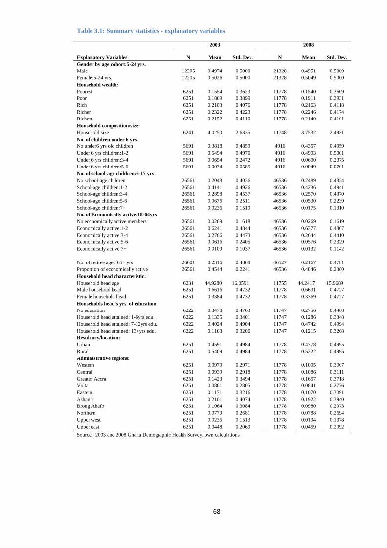
68
Table 3.1: Summary statistics - explanatory variables
2003 2008
Explanatory Variables
N
Mean
Std. Dev.
N
Mean
Std. Dev.
Gender by age cohort:5-24 yrs.
Male 12205 0.4974 0.5000
21328 0.4951 0.5000
Female:5-24 yrs. 12205 0.5026 0.5000
21328 0.5049 0.5000
Household wealth:
Poorest 6251 0.1554 0.3623
11778 0.1540 0.3609
Poor 6251 0.1869 0.3899
11778 0.1911 0.3931
Rich 6251 0.2103 0.4076
11778 0.2163 0.4118
Richer 6251 0.2322 0.4223
11778 0.2246 0.4174
Richest 6251 0.2152 0.4110
11778 0.2140 0.4101
Household composition/size:
Household size 6241 4.0250 2.6335
11748 3.7532 2.4931
No. of children under 6 yrs.
No under6 yrs old children 5691 0.3818 0.4859
4916 0.4357 0.4959
Under 6 yrs children:1-2 5691 0.5494 0.4976
4916 0.4993 0.5001
Under 6 yrs children:3-4 5691 0.0654 0.2472
4916 0.0600 0.2375
Under 6 yrs children:5-6 5691 0.0034 0.0585
4916 0.0049 0.0701
No. of school-age children:6-17 yrs
No school-age children 26561 0.2048 0.4036
46536 0.2489 0.4324
School-age children:1-2 26561 0.4141 0.4926
46536 0.4236 0.4941
School-age children:3-4 26561 0.2898 0.4537
46536 0.2570 0.4370
School-age children:5-6 26561 0.0676 0.2511
46536 0.0530 0.2239
School-age children:7+ 26561 0.0236 0.1519
46536 0.0175 0.1310
No. of Economically active:18-64yrs
No economically active members 26561 0.0269 0.1618
46536 0.0269 0.1619
Economically active:1-2 26561 0.6241 0.4844
46536 0.6377 0.4807
Economically active:3-4 26561 0.2766 0.4473
46536 0.2644 0.4410
Economically active:5-6 26561 0.0616 0.2405
46536 0.0576 0.2329
Economically active:7+ 26561 0.0109 0.1037
46536 0.0132 0.1142
No. of retiree aged 65+ yrs 26601 0.2316 0.4868
46527 0.2167 0.4781
Proportion of economically active 26561 0.4544 0.2241
46536 0.4846 0.2380
Household head characteristic:
Household head age 6231 44.9280 16.0591
11755 44.2417 15.9689
Male household head 6251 0.6616 0.4732
11778 0.6631 0.4727
Female household head 6251 0.3384 0.4732
11778 0.3369 0.4727
Households head's yrs. of education
No education 6222 0.3478 0.4763
11747 0.2756 0.4468
Household head attained: 1-6yrs edu. 6222 0.1335 0.3401
11747 0.1286 0.3348
Household head attained: 7-12yrs edu. 6222 0.4024 0.4904
11747 0.4742 0.4994
Household head attained: 13+yrs edu. 6222 0.1163 0.3206
11747 0.1215 0.3268
Residency/location:
Urban 6251 0.4591 0.4984
11778 0.4778 0.4995
Rural 6251 0.5409 0.4984
11778 0.5222 0.4995
Administrative regions:
Western 6251 0.0979 0.2971
11778 0.1005 0.3007
Central 6251 0.0939 0.2918
11778 0.1086 0.3111
Greater Accra 6251 0.1423 0.3494
11778 0.1657 0.3718
Volta 6251 0.0861 0.2805
11778 0.0841 0.2776
Eastern 6251 0.1171 0.3216
11778 0.1070 0.3091
Ashanti 6251 0.2101 0.4074
11778 0.1922 0.3940
Brong Ahafo 6251 0.1064 0.3084
11778 0.0980 0.2973
Northern 6251 0.0779 0.2681
11778 0.0788 0.2694
Upper west 6251 0.0235 0.1513
11778 0.0194 0.1378
Upper east 6251 0.0448 0.2069
11778 0.0459 0.2092
Source: 2003 and 2008 Ghana Demographic Health Survey, own calculations
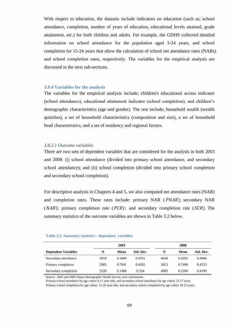
69
With respect to education, the datasets include indicators on education (such as; school
attendance, completion, number of years of education, educational levels attained, grade
attainment, etc.) for both children and adults. For example, the GDHS collected detailed
information on school attendance for the population aged 3-24 years, and school
completion for 15-24 years that allow the calculation of school net attendance rates (NARs)
and school completion rates, respectively. The variables for the empirical analysis are
discussed in the next sub-sections.
3.8.4 Variables for the analysis
The variables for the empirical analysis include; children's educational access indicator
(school attendance), educational attainment indicator (school completion), and children’s
demographic characteristics (age and gender). The rest include; household wealth (wealth
quintiles), a set of household characteristics (composition and size), a set of household
head characteristics, and a set of residency and regional factors.
3.8.2.1 Outcome variables
There are two sets of dependent variables that are considered for the analysis in both 2003
and 2008: (i) school attendance (divided into primary school attendance, and secondary
school attendance); and (ii) school completion (divided into primary school completion
and secondary school completion).
For descriptive analysis in Chapters 4 and 5, we also computed net attendance rates (NAR)
and completion rates. These rates include: primary NAR ( 𝑃𝑁𝐴𝑅); secondary NAR
( 𝑁𝐴𝑅); primary completion rate ( 𝑃𝐶𝑅) ; and secondary completion rate ( 𝑆𝐶𝑅). The
summary statistics of the outcome variables are shown in Table 3.2 below.
Table 3.2: Summary statistics - dependant variables
2003
2008
Dependent Variables N Mean Std. Dev.
N Mean Std. Dev.
Secondary attendance 3918 0.3469 0.4761
6658 0.4262 0.4946
Primary completion 2985 0.7041 0.4565
5813 0.7496 0.4333
Secondary completion 2526 0.1468 0.354
4983 0.2284 0.4199
Source: 2003 and 2008 Ghana Demographic Health Survey, own calculations.
Primary school attendance by age cohort 6-11 year olds, and secondary school attendance by age cohort 12-17 years
Primary school completion by age cohort, 15-20 year olds, and secondary school completion by age cohort 18-23 years.
70
Why School attendance / NAR and Completion/ Completion rates?
The school attendance / NAR and completion rate analysis help to examine school systems
(Harttgen et al. 2010). For example, NAR reveals whether school children start school on
time, and the completion rate estimates the progress of school children through the
education system as expected. Lower rates indicate weak internal inefficiencies in a given
education system (Harttgen et al. 2010). These education indicators are normally used to
measure the capacity and performance of education system in relation to national education
goals and plans, and to determine future development policies (FASAF et al. 2004;
Harttgen et al. 2010). The indicators also show the extent of children’s participation in
primary and secondary education among children of primary and secondary school-age
(FASAF et al. 2002 & 2004).
Therefore, these education indicators not only allow us to examine the internal efficiencies
in the Ghanaian education system but also to capture changes in the educational access,
and attainment at a point in time and over a period of time. More importantly, analysing
differences in school attendance and completion before and after the GoG’s education
policy intervention periods in the distribution of access and attainment of education by
income groups could guide government policy on pro-poor education interventions in
Ghana.
School attendance
The school attendance is one of the indicators of educational access and we are using this
indicator other than enrolment to capture access to education by households. The reason
not to use the enrolment indicator is that it measures initial enrolment and not a regular
attendance. In other words, attending school is not necessarily the same as being enrolled
in school. Children may be recorded in school enrolment records and yet not actually be
attending school (FASAF et al. 2004). Roberts (2003) also notes that in some Latin
America countries where primary education cycles are unusually long, a quarter of the
children who enrolled in Grade 1 dropped out of primary school. Thus, school attendance
is considered to be more relevant indicator of educational participation or access and is
preferred to enrolment (Jayachandran 2002; Ghana Statistical Service et al. 2004 & 2009;
Harttgen et al. 2010). For example, in the context of Ghanaian education system, access to
basic education is defined as the ability of children to progress through the basic education
cycle without repetition or dropping out (Chao and Alper 1998). This means enrolling in
primary school at age six and completing six years of primary education, and three years of
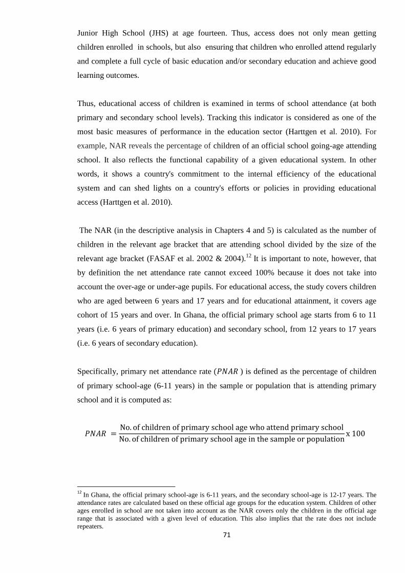
71
Junior High School (JHS) at age fourteen. Thus, access does not only mean getting
children enrolled in schools, but also ensuring that children who enrolled attend regularly
and complete a full cycle of basic education and/or secondary education and achieve good
learning outcomes.
Thus, educational access of children is examined in terms of school attendance (at both
primary and secondary school levels). Tracking this indicator is considered as one of the
most basic measures of performance in the education sector (Harttgen et al. 2010). For
example, NAR reveals the percentage of children of an official school going-age attending
school. It also reflects the functional capability of a given educational system. In other
words, it shows a country's commitment to the internal efficiency of the educational
system and can shed lights on a country's efforts or policies in providing educational
access (Harttgen et al. 2010).
The NAR (in the descriptive analysis in Chapters 4 and 5) is calculated as the number of
children in the relevant age bracket that are attending school divided by the size of the
relevant age bracket (FASAF et al. 2002 & 2004).12
It is important to note, however, that
by definition the net attendance rate cannot exceed 100% because it does not take into
account the over-age or under-age pupils. For educational access, the study covers children
who are aged between 6 years and 17 years and for educational attainment, it covers age
cohort of 15 years and over. In Ghana, the official primary school age starts from 6 to 11
years (i.e. 6 years of primary education) and secondary school, from 12 years to 17 years
(i.e. 6 years of secondary education).
Specifically, primary net attendance rate (𝑃𝑁𝐴𝑅 ) is defined as the percentage of children
of primary school-age (6-11 years) in the sample or population that is attending primary
school and it is computed as:
𝑃𝑁𝐴𝑅 =No. of children of primary school age who attend primary school
No. of children of primary school age in the sample or populationx 100
12
In Ghana, the official primary school-age is 6-11 years, and the secondary school-age is 12-17 years. The
attendance rates are calculated based on these official age groups for the education system. Children of other
ages enrolled in school are not taken into account as the NAR covers only the children in the official age
range that is associated with a given level of education. This also implies that the rate does not include
repeaters.
72
The secondary net attendance rate ( 𝑆𝑁𝐴𝑅 ) measures the percentage of children of
secondary school-age (12-17 years) in the sample or population that is attending secondary
school and it is computed as:
𝑆𝑁𝐴𝑅 =No. of children of secondary school age who attend secondary school
No. of children of secondary school age in the sample or populationx100
A high NAR is only possible if the education system has the capacity to educate all
children in the relevant age bracket and allow them to enter and progress through the
school system according to their age (Harttgen et al. 2010). Thus, net attendance rate can
be used as an indicator of functional capability of an educational system.
School Completion
To examine education attainment, there are usually two main indicators used in the
literature; average years of schooling completed, and school completion or completion
rates (Sahn and Younger 2006; Klasen 2008; Gunther and Klasen 2009; Harttgen et al.
2010; Harttgen and Klasen 2012; Thomas et al. 2001). However, in order to examine
education attainment of children across the household wealth distribution in Ghana, we are
using school completion which is in line with UNESCO and World Bank choice of
education attainment indicator (World Bank 2002). For example, UNESCO (2002a &
2002b) and World Bank (2002) use primary completion rate as their preferred measure of
progress towards the MDG 2 target13
.
The World Bank (2002) defines school completion rate as the proportion of the total
number of pupils (students) successfully completing or graduating from the last year of
primary (secondary) school in a given year to the total number of children of official
graduation age in the population . In other words, the completion rate is an indicator of
educational attainment and it measures the percentage level of primary or secondary school
completion rate among children who completed the last grade of primary or secondary
school. Completion rate monitors education system coverage and student progression, and
it is also intended to monitor school system quality and measure human capital formation
(FASAF et al. 2002 & 2004; Thomas et al. 2001; UNESCO 2002a & 2002b; Harttgen et al.
2010; World Bank 2002) .
13
UNESCO suggests inter alia, that all primary school-age children should be enrolled and should be able to
complete primary school, but not necessarily on time.
73
School completion is extremely important both socially and economically for school
children, as well as the for a country's education system. The indicator can reveal how
successful children from different income groups are in reaching educational milestone
(Lloyd and Blanc 1996; Lloyd and Hewett 2009; Harttgen et al. 2010). By UNESCO
(2002a & 2002b) definition, the 𝑃𝐶𝑅 is the percentage of children age 15 years and older
in the sample or population who completed primary school or have attended a higher grade.
Also, the 𝑆𝐶𝑅 measures the percentage of adults age 20 years and older in the sample or
population who completed secondary school or have attended a higher grade (FASAF et al.
2002 & 2004).
Following UNESCO (2002a & 2002b), FASAF et al. (2002 & 2004), Harttgen et al.
(2010), and considering the number of years between the survey periods (2003 and 2008),
we restrict the sample to a specific cohort of young adults aged 15-20 years for the
computation of primary school completion, and 18-23 years for the computation of
secondary school completion to monitor changes in the educational attainment over time.
The range equates the number of years between the Demographic Health Surveys.
Harttgen et al. (2010) also use similar range to calculate completion rates for 37
developing countries using DHS datasets.
Specifically, the school completion rates at both primary and secondary school levels are
computed as follows; where 𝑃𝐶𝑅 is primary completion rate, 𝑆𝐶𝑅 is the secondary
completion rate.
𝑃𝐶𝑅 = No. of adults age 15 − 20 years who completed primary school
No. of adults age 15 − 20 years in the sample or population x 100
𝑆𝐶𝑅 = No. of adults age 18 − 23 years who completed secondary school
No. of adults age 18 − 23 years in the sample or population x 100
It is important to note that both the primary and secondary completion rates can only be
high if most children of the age cohort enter primary and secondary school at the official
school-age and complete according to their age (Harttgen et al. 2010).
74
3.8.2.2 Explanatory variables
An understanding of the factors which influence educational access and attainment would
enable policy makers to adopt strategies to improve the allocation of resources, with the
objectives of increasing school attendance and completion rates, and reducing inequality in
attendance and attainment, simultaneously. For example, assessing the effects of factors
that are time-varying and analysing current attendance decision will allow us to relate
current school choices to socioeconomic aspects of the household such as; household
wealth or income and household structure (Glick and Sahn 2000). Thus, the sources of
educational disparities in children’s educational outcomes are expected to come from a
series of; demographic, household, residency, regional, and school characteristics.
However, since the DHS datasets do not contain information on school characteristics, the
focus in this study is on the effects of household SES and other individual factors on
educational outcomes.
The theoretical and empirical literature reviews in this chapter provide some guidance for
the selection of variables to be included in the model for the analysis of school attendance
and completion at both primary and secondary school levels in Ghana. For example,
Schultz (1999) identifies three key socioeconomic determinants of household demand for
schooling; public expenditure on education, education of the parents, and wealth of the
family. Consequently, the resources available to children of primary and secondary school-
age through their household are likely to be strongly associated with the likelihood that
they will be currently attending school and that they will have completed primary school at
age 11, and secondary school by age 17. These resources include: household wealth or
standard of living (measured by households' SES - wealth quintiles); the presence of very
young children in the household (under-six year olds); the presence of other school-age
children (6-17 year olds) who can share in household tasks; economically active adults,
and the education attainment levels of the household head (Lloyd and Blanc 1996; Filmer
and Pritchett 1999b & 2001; Roberts 2003; Lloyd and Hewett 2009; Montgomery and
Hewett 2005; Bredie and Beeharry 1998; Butcher and Case 1994; Okumu et al. 2008;
Lillard and Willis 1994; Haveman and Wolfe 1995). For example, the presence of young
siblings may alter the allocation of time among schooling, household work and other uses.
In addition, including the number of siblings under-six years old in the analysis could also
show how schooling access and attainment are affected by “fertility shocks” (Glick and
Sahn 2000).
75
The explanatory variables included in the analysis are grouped into; pupil/student level
characteristics, SES of households, a set of household level variables, a set of household
head variables, and a set of residency and regional factors. Consequently, our regression
analysis includes the following determinants: children's gender; household SES (wealth
quintiles as a proxy of income levels); household composition/size (number of household
members under-six years old, 6-17 years old, economically active adults, proportion of
economically active members, and retirees); gender of the household head; education level
attained by the household head (primary, secondary, and higher); and dummies for
residency and regional location (to capture the effects of location-related disparities).
Distance to and/or availability of schools and quality of schools are other variables that
could also contribute to socioeconomic inequality in educational outcomes (Hanushek and
Lavy 1994; World Bank 2004; Woldehanna et al. 2005; Schaffner 2004). However, data on
school characteristics are not available in DHS datasets and as a result it is not possible to
include these variables in the analysis to see how they impact on educational disparities in
Ghana. Instead we use urban/rural dummy variable to proxy for availability of schools.
3.9 Conclusions
From the literature review on socioeconomic inequality in education and determinants of
educational outcomes, there is no indication that any of the empirical studies reviewed has
estimated and decomposed the contributions of the various determinants discussed. Yet,
knowing the proportion of the contribution of each determinant to the total inequality in
educational access and attainment is important when designing policy interventions. Thus,
one of the main objectives of the thesis (stated in Chapter 1) is to estimate and decompose
the contributions of these determinants to educational inequalities to bridge the gap in
knowledge and to contribute to the literature. Such contribution to the literature will have
relevant policy implications for policy makers. This is because policy makers will be able
to see both the absolute and relative contributions of key sources of inequality in
educational outcomes in Ghana. By identifying the key sources and their contributions to
educational inequalities, policy interventions could be tailored to deal with some of the
root causes of educational inequality in Ghana.
Furthermore, it emerges that there is broad agreement that income is an inadequate
measure of welfare, and economic growth is a necessary condition but not a sufficient
condition for poverty reduction in developing countries. From capability expansion point
of view, economic growth can expand capabilities directly. In addition, as average incomes
76
increase, the population has greater access to relevant non-income dimensions of well-
being such as basic education and healthcare among others. This implies that all
capabilities can expand with economic growth, thus promoting human capital development.
Some studies demonstrate that economic growth benefits the poor in most developing
countries in which substantial growth has taken place. Others suggest that income growth
could promote non-income dimensions of well-being (e.g. education and health) through
non-income variables which may correlate with average incomes. Consequently, the main
channels through which overall economic growth can promote education (as argued in the
literature) is by: (i) lessening the extent of income poverty which constraints households in
their ability to send children to school; and (ii) increasing public educational investments
which lead to greater school access and better quality education (Anand and Ravallion
1993). It has also been suggested that if progress in education is combined with a focused
public spending in education sector, it will lead to declining inequality and poverty
reduction in education, even in an environment of stagnant or worsening levels of income
poverty (Sahn and Younger 2006 & 2007; Filmer and Pritchett 1999b).
However, evidence gathered in the review suggest that there are socioeconomic
inequalities in educational outcomes across developing countries, and that the attainment
of MDGs 2 and 3 is in doubt in most developing countries, especially in SSA countries.
Household resources emerged as the key contributing factor in educational inequalities and
poverty. From a gender perspective, the extent of inequality among girls in primary school
attendance and completion rates according to SES, is found to be substantially greater than
for boys (Lloyd and Hewett 2009; Harttgen et al. 2010).
Furthermore, where educational inequalities are analysed and discussed, the focus is
mainly on primary education, and less attention is been directed towards secondary
education where returns to education can be high. However, for children from poor
households to partake in the benefits of economic growth and to break the poverty-cycles
in their households, they will need to progress to higher levels of education to acquire the
necessary skills needed for the job market and for life. This is where the secondary
education comes to the fore. However, in most developing countries including Ghana,
secondary education is not free. The question then is how will children from poor
households acquire the necessary skills if they cannot afford secondary education? Will
primary or basic education alone be enough to provide the skills children need to succeed
77
in life? Consequently, Chapters 4, 5 and 6 attempt to give us empirical insights into some
of the gaps identified in the literature review alongside the aims and the objectives of the
thesis.
78
Chapter 4
Socioeconomic determinants of educational access and attainment in Ghana
4.1 Introduction
Persistent differences in educational access and attainment of school-age children due to
socioeconomic status has long been a serious education policy concern in Ghana
(Akyeampong et al. 2007; Chowa et al. 2013). This is in spite of the fact that the education
sector in Ghana has experienced substantial expansion during the last two decades at all
levels (World Bank 2004; Akyeampong et al. 2007; NDPC et al. 2010), with primary
school enrolment ratio around 90% and poverty levels having been reduced from 51.7% in
1991/92 to 28.5% in 2005 (Ghana Statistical Service 2007). Such concerns have been
generally recognised in developing countries in MDG 2 (UN 2000). In an attempt to
address these concerns, the Government of Ghana (GoG) has engaged in the construction
and rehabilitation of more classroom blocks, supply of textbooks, and trained teachers to
ease supply-side constraints to education provision in Ghana (World Bank, 2004).
On the other hand, the main factors on the demand side which affect households, especially
the poor include; household income and the opportunity cost of sending children to school
(Roberts 2003). It has also been argued that one of the reasons why children from poor
households in Ghana do not attend school is that their parents cannot afford the cost of
sending them to school (Osei et al. 2009). However, throughout the last decade or more,
increases in access to basic education in Ghana has been strengthened through a number of
international initiatives; EFA – Fast Track Initiative, and national education policy
interventions were carried out to reinforce the attainment of UPE in particular (NDPC et al.
2010). The national policy interventions include; FCUBE, SCG, and SFP which we have
discussed in Chapter 2. These policy interventions were intended to mitigate demand-side
constraints and to increase educational access to poor children. For instance; SCG is
expected to positively affect the quantity of education provided (measured in terms of
enrolment rates), and SFP is also aimed at increasing school enrolment, retention,
attendance, and reduction in malnutrition among children. The increased educational
resources, holding everything else constant, should increase the probability that all school-
age children attend and complete at least primary education. However, many Ghanaian
children fail to continue and complete their basic education programme. In 2008, about a
third (32.3%) of children who enrolled in JHS dropped out in the final year of JHS
(Ministry of Education Science and Sports 2008). According to Ghana Statistical Service
(2008) report, 30% of Ghanaians have never attended school. Furthermore, educational
79
access, standards, and attainments vary widely in the country, especially between urban
and rural areas, and the poor and non-poor households (Ghana Statistical Service 2008).
Other studies conducted in Ghana also reveal that educational access and attainment
disparities exist (Sutherland-Addy 2002; Palmer 2006; Tuwor and Sossou 2008).
It is against this background that this chapter explores what might be considered the
‘demand-side’ of educational outcomes in Ghana. The aim is to estimate and explain the
disparity in educational outcomes of children aged 6-17 years old as a response to key
socioeconomic factors which might have been responsible for the differences in
educational outcomes. Measuring socioeconomic determinants and their impacts on
educational access and attainment is very important in assessing an educational system.
However, more interesting for policy purpose is to try to explain the impacts of key
socioeconomic factors on school attendance, and school completion (at both primary and
secondary school levels). Therefore, the contribution of this chapter is to estimate and
explain the impacts of key socioeconomic factors on the educational outcomes in Ghana
before and after the GoG’s education policy interventions implemented in 2004/05
discussed in Chapter 2. The research in this chapter constitutes the only first attempt to
specifically analyse the impact of GoG’s education policy interventions through household
wealth distribution on educational access and attainment using household level data before
and after the policy implementation period. Thus, the findings could aid future policy
directions.
Consequently, we employ descriptive analysis to understand the trend of the distribution of
educational outcomes in Ghana by income groups, and also multivariate probit regression
model relevant to investigating the concerns discussed earlier. The first concerns variations
in socioeconomic determinants of educational outcomes at a point in time and over a
period of time. For descriptive analysis, we also examine the net attendance and
completion rates to allow us to measure the internal efficiency (Harttgen et al. 2010) of the
education system in Ghana. For regression analysis, probabilities of school attendance and
completion may presumably reflect variations in determinants of education service
utilisation (e.g. access to education, opportunity cost, household income, other household
level factors, residency and regional location effects etc.)
80
The empirical questions we seek to address are:
i. What key household socioeconomic factors influence educational access and
attainment in Ghana?
ii. To what extent has GoG’s education policy interventions and educational
expansion reduced the differences in educational access and attainment at primary
school level?
iii. What is the extent of the disparity in access to, and attainment of secondary
education?14
The remainder of the chapter is structured as follows. In Section 4.2 we examine
descriptive statistics on the distribution of educational access and attainment by household
wealth in Ghana to determine the level of disparity in educational outcomes between the
poor and the non-poor households. For more robust analysis, we employ a binary probit
regression model focusing on variations in parameters to be estimated and their effect on
the dependent variables (school attendance and attainment) in Section 4.3. The regression
results are presented and discussed in Section 4.4. Section 4.5 discusses policy lessons of
the results, while Sections 4.6 concludes the chapter.
4.2 School attendance and completion
Before we proceed to the descriptive analysis of the distribution of educational access and
attainment by socioeconomic status, it important to put into perspective the descriptive
statistics of the net attendance rate and completion rate for the household population in
Ghana presented in Tables 4.1 and 4.2. In 2003 and 2008, about 61% and 74% respectively,
of children aged 6-11 years who should be attending primary school, attended primary
school. At the secondary level, about 35% and 43% of children aged 12-17 years who
should be attending secondary school, attended secondary school in 2003 and 2008,
respectively. For completion rates at primary school level, about 70% and 75% of the age
cohort, 15-20 years who should have completed primary school, completed primary school
in 2003 and 2008, respectively. At the secondary level, the completion rates for the age
cohort, 18-23 years were very low. The statistics show that about 15% and 23% of the age
cohort who should have completed secondary school, completed secondary school in 2003
and 2008, respectively.
14
At secondary school level, there are no policy interventions to mitigate the cost of secondary education
borne by household, compared to pro-poor education policy interventions at the basic education level.
81
4.2.1 Distribution of educational access by socioeconomic status
This sub-section presents an illustrative overview of the distribution of children’s
educational access and attainment by household wealth quintiles in Ghana. It also
discusses the disparities between the poor and the non-poor households’ educational
outcomes. In essence, the section provides descriptive statistics on the distribution of
educational access in Ghana among income groups. The descriptive statistics are presented
in terms of welfare distribution and demographic background characteristics of households.
Table 4.1 shows net attendance rates (NARs) in 2003 (8 years after the implementation of
FCUBE), and 2008 (8 years after the enforcement of laws that support the implementation
of FCUBE, and 3 years after the implementation of SCG and SFP). The changes in NAR
between the two periods are positive for the country and also for the income groups. The
changes in primary and secondary NAR for the country between 2003 and 2008 are 13.3%
and 7.9%, respectively. This means that educational access at both levels of education has
increased. More importantly, all income groups have also recorded increased access,
especially the poor at the primary school level. The rising attendance rate could be
explained in terms of the general improvement in the standards of living of the average
Ghanaian over the years. For instance, Ghana has reduced its incidence of poverty levels
by almost half between 1991 and 2006. The share of the population below the poverty line
decreased from 51.7% in 1991/92 to 39.5% in 1998/99 and 28.5% in 2005/06 (Ghana
Statistical Service 2000 & 2007). According to Coulombe and Wodon (2007), the absolute
number of the poor also decreased from 7.9 million in 1991/92 to 7.2 million in 1998/99
and 6.2 million in 2005/06.
Table 4.1 also depicts household wealth quintiles, wealth quintile means, as well as wealth
quintile ratios. The quintile ratio of fifth to first is a direct indicator of inequality between
the richest and the poorest population subgroup. The NAR at the primary school level
between 2003 and 2008, without taking into consideration the household wealth, shows
that female NAR increased by 14.5% compared to 12.2% achieved by the male children.
Although, the NAR (59.7%) for females in 2003 was lower than the NAR (61.2%) for
males, in 2008 the NAR (74.2%) for females was slightly higher than that of the males
(73.4%).
There is an indication that more female children have gained access to primary education
from 2003 to 2008 than male children within the same period. Therefore, gender inequality
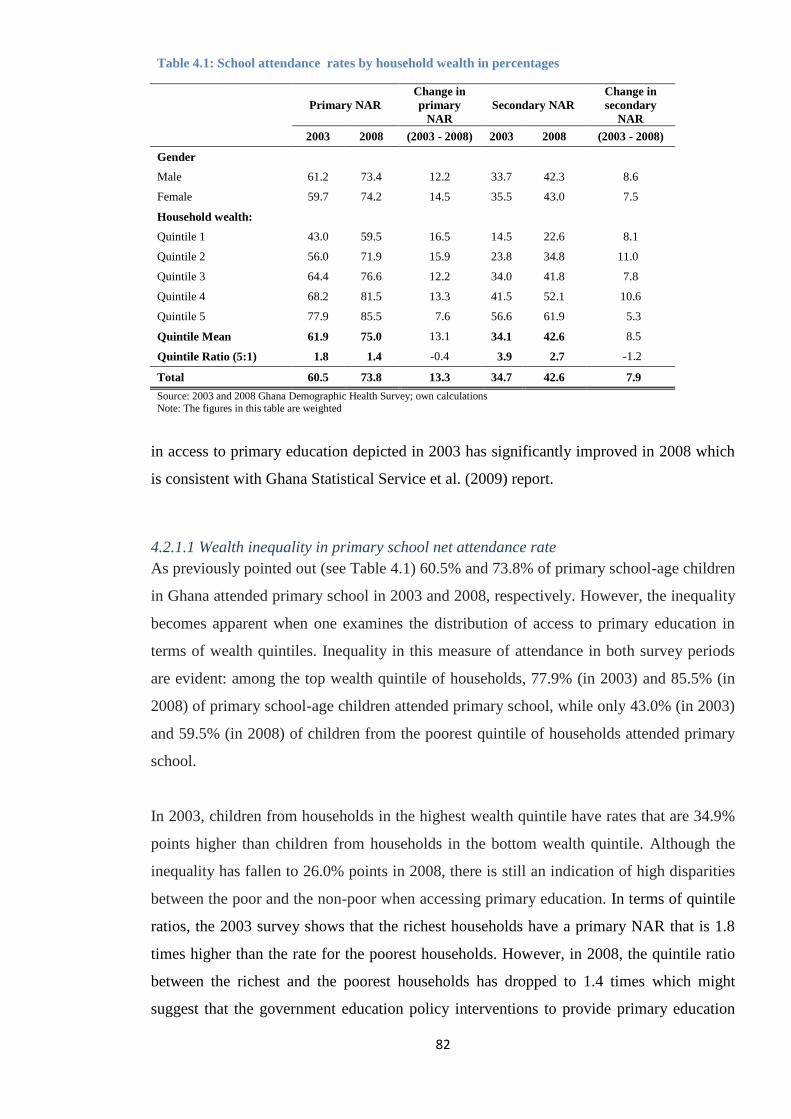
82
Table 4.1: School attendance rates by household wealth in percentages
Primary NAR
Change in
primary
NAR
Secondary NAR
Change in
secondary
NAR
2003 2008 (2003 - 2008) 2003 2008 (2003 - 2008)
Gender
Male 61.2 73.4 12.2 33.7 42.3 8.6
Female 59.7 74.2 14.5 35.5 43.0 7.5
Household wealth:
Quintile 1 43.0 59.5 16.5 14.5 22.6 8.1
Quintile 2 56.0 71.9 15.9 23.8 34.8 11.0
Quintile 3 64.4 76.6 12.2 34.0 41.8 7.8
Quintile 4 68.2 81.5 13.3 41.5 52.1 10.6
Quintile 5 77.9 85.5 7.6 56.6 61.9 5.3
Quintile Mean 61.9 75.0 13.1 34.1 42.6 8.5
Quintile Ratio (5:1) 1.8 1.4 -0.4 3.9 2.7 -1.2
Total 60.5 73.8 13.3 34.7 42.6 7.9
Source: 2003 and 2008 Ghana Demographic Health Survey; own calculations
Note: The figures in this table are weighted
in access to primary education depicted in 2003 has significantly improved in 2008 which
is consistent with Ghana Statistical Service et al. (2009) report.
4.2.1.1 Wealth inequality in primary school net attendance rate
As previously pointed out (see Table 4.1) 60.5% and 73.8% of primary school-age children
in Ghana attended primary school in 2003 and 2008, respectively. However, the inequality
becomes apparent when one examines the distribution of access to primary education in
terms of wealth quintiles. Inequality in this measure of attendance in both survey periods
are evident: among the top wealth quintile of households, 77.9% (in 2003) and 85.5% (in
2008) of primary school-age children attended primary school, while only 43.0% (in 2003)
and 59.5% (in 2008) of children from the poorest quintile of households attended primary
school.
In 2003, children from households in the highest wealth quintile have rates that are 34.9%
points higher than children from households in the bottom wealth quintile. Although the
inequality has fallen to 26.0% points in 2008, there is still an indication of high disparities
between the poor and the non-poor when accessing primary education. In terms of quintile
ratios, the 2003 survey shows that the richest households have a primary NAR that is 1.8
times higher than the rate for the poorest households. However, in 2008, the quintile ratio
between the richest and the poorest households has dropped to 1.4 times which might
suggest that the government education policy interventions to provide primary education
83
access to all, coupled with steady economic growth performance discussed in Chapter 2
might have had some effects on these ratios.
The fall in the quintile ratio (i.e. fall in inequality in primary NAR) between the two
periods can be seen in terms of the increase in the primary NAR of the poorest from 43.0%
in 2003 to 59.5% in 2008 (an increase of 16.3%), compared to an increase of 7.6% points
in the primary NAR of the richest households between 2003 and 2008. The quintile mean
for primary NAR has also improved by 13.1% points between the two periods (61.9% in
2003 and 75.0% in 2008).
4.2.1.2 Wealth inequality in secondary school net attendance rate
The analysis of the NAR in secondary education can yield some insights into the progress
of educational inequality as a result of expanding access to education in Ghana. Secondary
NAR shows more marked income or wealth inequalities in access to education beyond
primary education level. The NAR is 42.1% points higher for children from households in
the top wealth quintile than children from households in the bottom wealth quintile in 2003.
Although in 2008 the rate has reduced to 39.3% points, the inequality still remains high.
In Table 4.1, 34.7% and 42.6% of secondary school age children in Ghana attended
secondary school in 2003 and 2008, respectively. The inequality in the secondary NAR in
both survey periods is more evident than that of the primary school net attendance rate.
Consequently, among the top wealth quintile households, 56.6% (in 2003) and 61.9% (in
2008) of children attended secondary school, while only 14.5% (in 2003) and 22.6% (in
2008) of children from the bottom wealth quintile of households attended secondary school.
Although, there has been an improvement of 8.1% points (from 2003 to 2008) in the
secondary NAR for the poorest households compared to 5.3% within the same period for
richest households, the quintile ratio is still high. In 2003, the richest households have
secondary NAR that is 3.9 times higher than the rate for the poorest households. Even
though in 2008 the quintile ratio between the richest and the poorest households has
dropped to 2.7 times, the inequality between the richest and the poorest households is still
high compared to the ratios for primary NARs. The quintile mean for secondary NAR has
also improved by 8.5% points between the two periods (34.1% in 2003 and 42.6% in 2008).
What is interesting to note is that educational inequality between the richest and the
poorest households increases with lower mean levels of NARs (see Table 4.1). There seem
84
to be different worlds when one considers the distribution of access to secondary education
between welfare groups.
In Ghana, secondary education is not free and this might partially explain why the
secondary NARs are very low for the poor than the non-poor households. One suggestion
is that NARs for secondary schools are generally low in low and middle income countries
due to the fact that many of these countries have moved towards universal primary
education but lack the resources to promote secondary education (Porta et al. 2011). At
household levels it is also suggested that in poor households, as children grow older and
become more potentially productive the opportunity cost of school attendance for their
parents increases (Roberts 2003; Holmes 2003; Lloyd and Blanc 1996). For example,
Roberts (2003) attributes this phenomenon as one of the causes of falling attendance rates
in higher grades or levels. In other words, the pecuniary and opportunity costs of sending
children to school are higher relative to household income in poor households than in non-
poor households. In turn, this could be used to explain the disparity in the attendance rates
of the children from poorest households and the richest households. According to Roberts
(2003), poor households tend to withdraw their children from school when their incomes
fall. Furthermore, lower access to secondary education may compel children from poor
households to enter the labour force too early and with a lower level of education than they
may need. The transmission mechanism is that the low level of education as a result of low
access to secondary education will lead to low level of skills and productivity which will
not be enough to avoid a generational poverty, all other things being equal.
4.2.2 Distribution of educational attainment by socioeconomic status
The educational attainment is measured by school completion rate and it is extremely
important both socially and economically for pupils, students, as well as for a country's
education system (Harttgen et al. 2010). Primary and secondary completion rates are
indicators of primary and secondary school attainments of children aged 15-20 years and
18-23 years, respectively. The indicator can reveal how successful children from different
income groups are in reaching critical educational milestone (Lloyd and Blanc 1996;
Harttgen et al. 2010). Again, because we are interested in the effects of the government of
Ghana’s education policy and programmes (SCG, SFP, and FCUBE), the school
completion rate serves as one of the key education indicators to be examined. It may shed
some lights on the distribution of educational attainment in Ghana. Table 4.2 shows the
primary and secondary school completion rates.
85
The completion rates are examined with respect to wealth quintile to determine the
inequalities between the poor and the non-poor households at both primary and secondary
education levels. The changes in school completion rates between the two periods are
positive for the country as a whole and also for the income groups. The change in primary
and secondary completion rates for the country between 2003 and 2008 are 4.6% and 8.1%,
respectively. The positive change in the rates means that educational attainment at both
levels of education for the age cohorts has increased. In comparison, at the primary school
level, it seems there is more improvement at access level than the attainment level. It is
also worth to note that, all income groups have recorded increased attainment between
2003 and 2008, especially the rich at the secondary school level. The increase in secondary
school attainment by the rich may be due to the fact that secondary education is not free
and therefore, the children from poor households might have struggled to complete
secondary education.
4.2.2.1 Wealth inequality in primary school completion rate
The inequalities in primary completion rate in 2003 are glaring, although on average 67.9%
of children from all the welfare groups completed primary education in 2003. The
completion rate of children from households in the top wealth quintile is 47.5% points
higher than for children from the bottom wealth quintile. In other words, the children from
the top quintile households have 2.2 times more completion rate than children from the
bottom quintile households. In 2008, it appears there is no significant improvement in the
inequality in completion rate of children from the poorest and richest households.
4.2.2.2 Wealth inequality in secondary school completion rate
Generally, the secondary attendance rates in most developing countries are significantly
lower than primary attendance rates (Porta et al. 2011), and Ghana is not an exception as
indicated in Table 4.1. Consequently, the secondary completion rates are more likely to be
lower than the primary completion rates (see Table 4.2 below).
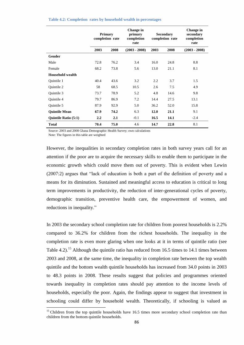
86
Table 4.2: Completion rates by household wealth in percentages
Primary
completion rate
Change in
primary
completion
rate
Secondary
completion rate
Change in
secondary
completion
rate
2003 2008 (2003 - 2008) 2003 2008 (2003 - 2008)
Gender
Male 72.8 76.2 3.4 16.0 24.8 8.8
Female 68.2 73.8 5.6 13.0 21.1 8.1
Household wealth
Quintile 1 40.4 43.6 3.2 2.2 3.7 1.5
Quintile 2 58 68.5 10.5 2.6 7.5 4.9
Quintile 3 73.7 78.9 5.2 4.8 14.6 9.8
Quintile 4 79.7 86.9 7.2 14.4 27.5 13.1
Quintile 5 87.9 92.9 5.0 36.2 52.0 15.8
Quintile Mean 67.9 74.2 6.3 12.0 21.1 9.1
Quintile Ratio (5:1) 2.2 2.1 -0.1 16.5 14.1 -2.4
Total 70.4 75.0 4.6 14.7 22.8 8.1
Source: 2003 and 2008 Ghana Demographic Health Survey; own calculations
Note: The figures in this table are weighted
However, the inequalities in secondary completion rates in both survey years call for an
attention if the poor are to acquire the necessary skills to enable them to participate in the
economic growth which could move them out of poverty. This is evident when Lewin
(2007:2) argues that “lack of education is both a part of the definition of poverty and a
means for its diminution. Sustained and meaningful access to education is critical to long
term improvements in productivity, the reduction of inter-generational cycles of poverty,
demographic transition, preventive health care, the empowerment of women, and
reductions in inequality.”
In 2003 the secondary school completion rate for children from poorest households is 2.2%
compared to 36.2% for children from the richest households. The inequality in the
completion rate is even more glaring when one looks at it in terms of quintile ratio (see
Table 4.2).15
Although the quintile ratio has reduced from 16.5 times to 14.1 times between
2003 and 2008, at the same time, the inequality in completion rate between the top wealth
quintile and the bottom wealth quintile households has increased from 34.0 points in 2003
to 48.3 points in 2008. These results suggest that policies and programmes oriented
towards inequality in completion rates should pay attention to the income levels of
households, especially the poor. Again, the findings appear to suggest that investment in
schooling could differ by household wealth. Theoretically, if schooling is valued as
15 Children from the top quintile households have 16.5 times more secondary school completion rate than
children from the bottom quintile households.
87
consumption (i.e. normal good) then demand for it will increase with increases in
household income or wealth.
In addition, if there are credit constraints (where poor households are not able to borrow
for investments in education) then only those with access to ready-cash or credit facilities
(the non-poor) will be able to afford the education costs (Becker 1975; Lazear 1980).
From the literature it is evident that poorer households are more credit constrained than
richer households (Jacoby 1994; Rose 2000). Moreover, if there are credit facilities
available for both the poor and the non-poor and the non-poor households are able to
borrow at cheaper rates than the poor households, then investments in education will still
be higher among the rich than the poor (Becker 1975; Lazear 1980). Besides, if non-poor
households are able to make complementary investments, such as additional tutoring
(which the poor cannot afford) then the efficiency of schooling and school completion rate
will be higher for the rich households than the poor households (Filmer 2005). Such
conditions and constraints may explain some of the huge inequalities in secondary
completion rate between the poor and the non-poor households in Ghana. This finding is
consistent with both the theoretical underpinnings and the empirical findings of Jacoby
(1994) and Rose (2000).
The results from Tables 4.2 and 4.3 suggest that there is a direct relationship between
schooling outcomes and household wealth or income. The relationship is explored further
using binary probit regression model in Sections 4.3 and 4.4, including some other
covariates.
88
4.3 Multivariate regression framework
The descriptive analysis in Section 4.2 suggests that household wealth could be the main
underlying factor for disparities in educational access and attainment by households in
Ghana. However, household wealth may not necessarily be the only factor and there may
be other factors that may equally affect educational outcomes in Ghana. For robustness of
the analysis, we employ probit regression model to analyse the factors that are likely
impact on whether a child i from household j attends school or not, and if the child
attended school whether the child completed a given educational level or not.
The empirical specification of the regression model (Equation 4.1) are used for analysing
‘Socioeconomic determinants of educational access and attainment’ in this chapter and
also for modelling ‘Disparity in educational outcomes of males and females within the
welfare groups’ in Chapter 5.
4.3.1 Binary probit model
Policy makers would be interested in the importance of the effects of the various factors
thought to be socioeconomic determinants of educational access and attainment in Ghana,
since that would give some idea of policy direction. Therefore, one of the convenient ways
of considering educational differences between households (in terms of access and
attainment) is to apply a probit regression analysis in which the educational access and/or
attainment is related to the equity group (i.e. households) of the individual i; i = 1; ...,N
(Tansel 2002; Deininger 2003; Filmer 2005; Sackey 2007; Okumu et al. 2008; Bbaale and
Buyinza 2013; Filmer and Pritchett 2001) . Thus, to explain variations in school attendance
and completion at both primary and secondary school levels, a reduced educational
production-type probit regression model used by Filmer and other authors referenced
above is adapted to estimate factors that might affect educational outcomes of households
in Ghana. The model for the pupil/student’s attendance and completion is specified to be a
non-linear function of: a vector of characteristics of pupil/student level variable of
household j, Gij; the income or wealth quintile of the household j the child belongs to, Wij;
a vector of household characteristics/composition of child level variables of household j,
Hcij; a vector of household head characteristics of child variables, Hhij; educational
attainment level of household head, HhEdij, and dummy variables for where household j is
located, Rij.
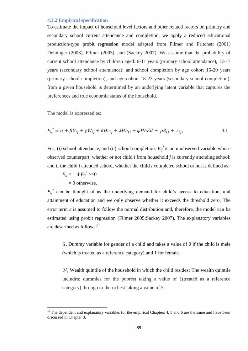
89
4.3.2 Empirical specification
To estimate the impact of household level factors and other related factors on primary and
secondary school current attendance and completion, we apply a reduced educational
production-type probit regression model adapted from Filmer and Pritchett (2001)
Deininger (2003), Filmer (2005), and (Sackey 2007). We assume that the probability of
current school attendance by children aged: 6-11 years (primary school attendance), 12-17
years (secondary school attendance); and school completion by age cohort 15-20 years
(primary school completion), and age cohort 18-23 years (secondary school completion),
from a given household is determined by an underlying latent variable that captures the
preferences and true economic status of the household.
The model is expressed as:
Eij* = 𝛼 + 𝛽𝐺𝑖𝑗 + 𝛾𝑊𝑖𝑗 + 𝛿𝐻𝑐𝑖𝑗 + 𝐻ℎ𝑖𝑗 + 𝜑𝐻ℎ𝐸𝑑 + 𝜌𝑅𝑖𝑗 + ε𝑖𝑗 , 4.1
For; (i) school attendance, and (ii) school completion: Eij* is an unobserved variable whose
observed counterpart, whether or not child i from household j is currently attending school;
and if the child i attended school, whether the child i completed school or not is defined as:
Eij = 1 if Eij* >=0
= 0 otherwise.
Eij* can be thought of as the underlying demand for child’s access to education, and
attainment of education and we only observe whether it exceeds the threshold zero. The
error term is assumed to follow the normal distribution and, therefore, the model can be
estimated using probit regression (Filmer 2005;Sackey 2007). The explanatory variables
are described as follows:16
𝐺, Dummy variable for gender of a child and takes a value of 0 if the child is male
(which is treated as a reference category) and 1 for female.
𝑊, Wealth quintile of the household in which the child resides: The wealth quintile
includes; dummies for the poorest taking a value of 1(treated as a reference
category) through to the richest taking a value of 5.
16
The dependent and explanatory variables for the empirical Chapters 4, 5 and 6 are the same and have been
discussed in Chapter 3.
90
𝐻𝑐 , Vector of household composition/size: Household size; number of children
under 6 years old; number of children of school-age from 6-17 year olds; and
number of economically active members of household, retirees; and proportion of
economically active household members.
𝐻ℎ, Vector of household head characteristics which include: Age of household
head in years; a dummy variable for the gender of the household head, and takes a
value of 0 if household head is male (treated as a reference category) and 1 for
female.
𝐻ℎ𝐸𝑑, Education levels of household head – primary, secondary, and higher (no
education is treated as the reference category)
𝑅, Dummy variables for urban/rural (value of 0 for urban and 1 for rural) and
regional effects (Western = 1, Central = 2, Greater Accra = 3, Volta = 4, Eastern =5,
Ashanti = 6, Brong Ahafo = 7, Northern = 8, and Upper East = 9. Urban and Upper
West are the reference categories and are, therefore, treated as the omitted
categories. The Upper West region is the poorest region in Ghana (Ghana Statistical
Service et al. 2004 & 2009).
The different elements of the coefficient vector β, , , , , and , provide an estimate of
the impact of the socioeconomic determinants on the probability of educational access
(school attendance) and educational attainment (school completion) of school-age children
(6-17 year olds). Equation 4.1 is estimated at both primary and secondary school levels in
2003 and 2008. In other words, for the jth element of explanatory variables, the
corresponding elements of the coefficients (β, , , , , and ) denote the impact of
particular characteristic or determinant on the probability of school attendance and
completion in 2003 and 2008.
4.3.3 Endogeneity concern
Household wealth
Total income of household is likely to be endogenous to the household education decisions
(participation and attainment). To avoid this bias, often non labour income and wealth
information of the household is used as a proxy for permanent income (Roberts 2003).
From the literature, household permanent income is one of the most controversial variables.
This is because it is not clear whether it should be treated as endogenous or exogenous.
91
Generally it is assumed that the household expenditure is an endogenous variable and as a
result, they are instrumented by an indicator of household wealth based on the ownership
of assets (Burchi 2009). Thus, household wealth can be treated as exogenous under the
assumption that it is the result of unearned income (ibid). Although the wealth index based
on assets' ownership (available in the DHS surveys) seems to better reflect permanent
income (Roberts 2003), the assumption has some shortcomings. For example, household
wealth may not be the result of unearned income. According to (Strauss and Thomas
1995:1900) "non-labour income is the return to assets built up with previous labour
earnings". In this regard, the wealth index may be considered as a poor instrument for
household expenditures (Strauss and Thomas 1995). Unfortunately, the DHS datasets do
not contain information on household consumption expenditures, but only on assets owned
by the households which is aggregated into an indicator of wealth referred to as wealth
index.
Both Filmer and Pritchett (2001) and Sahn and Stifel (2003) show that asset index (i.e.
wealth index) can be used as an instrument for expenditures. For example, Sahn and Stifel
(2003: 485) note that “even when expenditure data are available, analysts may prefer to use
the asset index as an explanatory variable or as a means of mapping a metric in permanent
income space to other living standards and capabilities”. Filmer and Pritchett (2001) use
wealth index as an instrument for household wealth to estimate the household wealth
effects on the probability of being in school, for children aged 6-14 years in India using
probit regression. They compared the impact of wealth index with the log of consumption
expenditures per adjusted household size on school enrolment and find that the results
were qualitatively similar. Although the authors note that asset index will be imperfect
proxy for long-run household economic status (wealth), they also argue that the
measurement errors will not be correlated perfectly. They, therefore, suggest that wealth
index can be used as an instrument for household wealth. Furthermore, Filmer and
Pritchett (2001:125) argue that “using assets as instruments for household per capita
expenditures is most likely the more effective way of extracting the maximum amount of
information from household data while reducing the impact of measurement error”. For
example, the authors support their argument by comparing results based on DHS datasets
from India, Indonesia, and Pakistan which show that the “results are consistent with the
presence of less measurement error in the asset index than in consumption expenditures as
a proxy for long-run wealth in predicting educational outcomes” (Filmer and Pritchett 2001:
128).
92
Other studies that use DHS data in analysing the effect of wealth index on schooling
outcomes include; Lloyd and Blanc (1996), Filmer (2000), and Bbaale and Buyinza (2013).
All these studies did not use instrumental variable identification method to instrument for
household wealth but use wealth index (wealth quintile) as an instrument for household
wealth in their regression analysis.
For those studies that use other forms of household survey that contain information on
income or expenditure component have all used log of household expenditure as an
instrument for household expenditure. 17 We could not use this method because DHS
datasets do not contain information on neither income nor consumption expenditure. Even
when the log consumption expenditure is used an instrument for long-run wealth in
predicting educational outcomes, Filmer and Pritchett (2001) argue that household wealth
index has less measurement error than the log consumption expenditure.
Since it is very difficult to find more reliable instruments for wealth, the analysis in
Chapters 4, 5 and 6 could not report the estimations together with Rivers and Vuong (1988)
or wu-Hausman test for endogeneity. Nevertheless, the estimations and results in Chapters
4, 5 and 6 are consistent with other empirical studies that use household wealth (i.e. wealth
index) as a proxy for permanent income without controlling the index via instrumental
variable (Lloyd and Blanc 1996; Filmer and Pritchett 1999a, 1999b & 2001; Filmer 2000
& 2005; Burchi 2009; Bbaale and Buyinza 2013). Thus, by following these authors the
wealth index in Equations 4.1is treated as exogenous variable.
Fertility (number of children)
It is commonly believed that households with more children are less likely to send them to
school, although evidence in the empirical literature reviewed in Chapter 3 is mixed. There
is also a concern that fertility could be endogenous to household decisions and, therefore,
unobserved shifts in changes in costs of education might lead a household to have more or
less children (Maitra and Ray 2002). For example, parents may not send their children to
school either because of a lack of resources or a high relative price of education. However,
Jensen and Nielsen (1997), Ray (2000), Maitra and Ray (2002), and Ravallion and Wodon
(2000) treat the number of children in their empirical models of schooling outcomes of
children as exogenous variables. For example, Maitra and Ray (2002:52) observe that
17
Examples of the instrument include: log expenditure per adult (Glick and Sahn 2000); log per adult total
expenditure (Tasel 1997); log per capita expense (Deininger 2003); log of expenditure per capita (Sackey
2007); log of household welfare (Rolleston 2009 & 2011); log per real total expenditure (Ogundari and
Abdulai 2014).
93
“household composition, generally, does not exert a significant impact on the child’s
schooling/employment decision and where it does, it is through the number of adults rather
than the number of children in the household”. Following other researchers (Jensen and
Nielsen 1997; Ray 2000; Maitra and Ray 2002; Ravallion and Wodon 2000), the number
of children is treated as exogenous variable in our empirical specifications.
4.4 Regression results and discussions
We present and discuss the results pertaining to school attendance at both primary and
secondary school levels in sub-section 4.4.1, while results of primary and secondary school
completion are presented and discussed in sub-section 4.4.2. A positive (negative) and
statistically significant marginal effect in the regression indicates that the relevant
determinant enhances (decreases) the probability of educational access (attendance) and
educational attainment (completion).
4.4.1 Primary and secondary attendance
It is important to note that although the descriptive analysis has given us some insights into
educational distribution by household wealth, the NARs and/or completion rates do not tell
us the factors that contribute to whether a child attends school or not. Thus, the results of
the determinants of school attendance reported in Table 4.3 supplement the descriptive
analysis in Section 4.2. To facilitate the interpretation of the regression results, the
marginal effects of household wealth together with other socioeconomic factors on school
attendance at both primary and secondary levels in 2003 and 2008 are shown together with
the corresponding z-values. Furthermore, it is worth noting that the probabilities are
evaluated at the means of the variables included in the regression. In addition, the
relationship specified by the probit model is non-linear and the effect is estimated for an
‘average’ child in the sample. The estimate of the marginal effects is to guide (Filmer 2000)
us to what the effect is for a child from a given household with an average characteristics
in Ghana. The likelihood rate 2 test, (Pr >
2) result shows that the model is well fit. The
predicted probability for primary school attendance increased from 58.8% in 2003 to 73.4%
in 2008. At the secondary school level, predicted probability for attendance also increased
from 29.6% in 2003 to 38.8% in 2008.
94
Household wealth distribution
The wealth quintiles in the regression analysis are constructed as dummy variables. For
example, poorest, poor, rich, richer, and richest dummy variables equal to one if the child
is from a poorest, poor, rich, richer and richest wealth groups or households, respectively
(the poorest group is the reference group). The marginal effects correspond to the change
in the percentage probability of a child attending school (primary or secondary) and
completing school (primary or secondary) as a result of a change in the dummy variable
(i.e. the quintiles) from zero to one holding all other variables in the equation at their
sample mean.
The results from the multivariate regression analysis (depicted in Table 4.3) confirm the
hypothesis that household wealth or income available to school children has strong impact
on the educational outcomes of children. The estimated marginal effect of household
wealth distribution has the expected signs and is highly significant across all the welfare
groups in 2003 and 2008 for both primary and secondary school attendance. The result
confirms the positive impact of household wealth on school attendance which is line with
the literature (Patrinos and Psacharopoulos 1997; Sathar and Lloyd 1994; Lloyd and Blanc
1996; Buchmann and Hannum 2001; Okumu et al. 2008; Sackey 2007; Deininger 2003;
Holmes 2003).
The marginal effect of moving from the second quintile (poor household) to the fifth
quintile (richest household) increases the probability of primary school attendance for
primary school-age children from 7.2 to 24.0 percentage points in 2003 (Table 4.3). On the
other hand, the marginal effect of being in the poor household increases the probability of
primary school attendance of children in the poor household by only 7.2 percentage points
compared to all other welfare groups in the same year. In other words, the margin effect of
the welfare distribution on primary school attendance is larger in the richest households
and decreases as one moves down the welfare distribution to the poorest households in
Ghana.
Comparing the difference between the impact of household wealth distribution on primary
school attendance of children from poor and richest households, shows that the marginal
effect of household wealth on primary school attendance of children from the richest
households is over three times more than that of the poor in 2003 (i.e. 0.240 vs. 0.072).
However, in 2008 the estimated marginal effect of household wealth on primary school
95
attendance for all welfare groups has fallen compared to 2003. The fall in the impact of
household wealth distribution on primary school attendance of poor children (a reduction
of 1.4%) is fairly negligible compared to that of children from the richest households (a
reduction of 10.0%). These results indicate that there are still disparities between the poor
and the non-poor when accessing primary education in Ghana, in spite of the intended pro-
poor education policy interventions being pursued in Ghana (NDPC et al. 2010).
Furthermore, the effect of the distribution of household wealth on primary school
attendance between the poor and the richest households has reduced from 3.3 times in
2003 (i.e. 0.240 vs. 0.072) to 2.4 times in 2008 (i.e. 0.058 vs. 0.140). The fall in the impact
of household wealth distribution on the primary school attendance could be explained in
terms of increased government expenditure on education in Ghana (World Bank 2004)
coupled with other education policies (NDPC et al. 2010) to meet MDG 2 by 2015
discussed in Chapter 2. The fall in the marginal effect of household wealth of the richest
households on primary school attendance (from 24% to 14%) supports the suggestion that
if government spends generously on education and provides free universal access to
primary schools of reasonable quality, the financial support of households will have less
impact on primary school attendance (Lloyd and Blanc 1996). However, the marginal
effect of the household wealth of the poor on primary school attendance failed to improve
significantly between the two periods (7.2% in 2003 and 5.8% in 2008). For example, the
education policy interventions implemented in Ghana (NDPC et al. 2010) were intended to
reduce the cost of basic education to households.18
Although, the impact of the policies
may have appeared to benefit the rich households by reducing their financial burden on
primary school attendance in 2008 (see Table 4.3), the policies on the other hand appeared
to have no significant change in the impact of household wealth on the probability of
primary school attendance of children from the poor households between 2003 and 2008.
In general, the indirect impacts of the government of Ghana's educational policies might
have helped to reduce the financial burden of primary education to parents which is
consistent with the findings of Akyeampong et al. (2007) in Ghana and Deininger (2003)
in Uganda. However, from Table 4.3, there is an indication that the poor have recorded
only 1.4% point change in the effect of household wealth on primary school attendance,
18
Although data on these policies and programmes are not collected in the GDHS datasets, by using the 2003
GDHS dataset as pre-policy and 2008 GDHS dataset as a post-policy implementation periods, it is possible to
explain any indirect impacts of the policies and programmes on households’ financial burden of enrolling and
maintaining their children in school, ceteris paribus.
96
but the non-poor have recorded a minimum of 5.6% points to a maximum of 10.0% fall in
their household wealth impact on primary school attendance. With this evidence, it seems
the policies have at least to date, not been able to generate significant pro-poor progress in
access to primary education in Ghana. The impact of household wealth on access to
secondary education (i.e. secondary school attendance) is also positive and highly
statistically significant across the wealth distribution depicted in Table 4.3 below.
Again, the marginal effect of moving from the second quintile (poor household) to the fifth
quintile (richest household) increases the probability of secondary school attendance of
children from 7.9 to 31.3 percentage points in 2003 (Table 4.3). Thus, as one moves up the
welfare distribution from the poor households to the richest households, the margin effect
of welfare distribution increases the probability of secondary school attendance of the
children in the welfare groups.
In 2008, the marginal effect of being in the poor household increases the probability of
primary school attendance of children in the poor household by only 9.4 percentage points
in relation other welfare groups or households (an improvement of 1.5% points from 2003).
In comparison with children from the richest households, the marginal effect increases the
probability of secondary school attendance of children (from the richest household) by
26.0 percentage points.
The differentials in the access to secondary education between the poor and the richest
households have, however, reduced from about 23% points in 2003 to about 17% points in
2008. Although there is still large disparity between access to secondary education by
children from poor and the richest households, one could consider the reduction in the
disparity as a significant improvement in the distribution of access to education between
2003 and 2008. This is in the recognition of the fact that in Ghana secondary education is
not free.19
19
In theory, tuition fees in secondary school is supposed to be free in Ghana, however, in practice parents
pay material costs, transportation, boarding and lodging costs (Gyimah-Brempong, K. & Asiedu, E. 2014:6).
This put the cost of accessing and attaining secondary education beyond the reach of the majority (i.e.
children poor households).
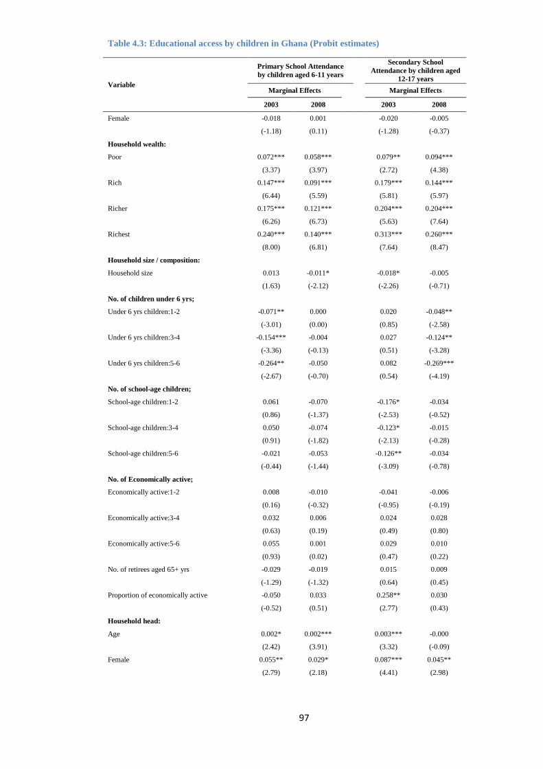
97
Table 4.3: Educational access by children in Ghana (Probit estimates)
Variable
Primary School Attendance
by children aged 6-11 years
Secondary School
Attendance by children aged
12-17 years
Marginal Effects
Marginal Effects
2003 2008 2003 2008
Female -0.018 0.001
-0.020 -0.005
(-1.18) (0.11)
(-1.28) (-0.37)
Household wealth:
Poor 0.072*** 0.058***
0.079** 0.094***
(3.37) (3.97)
(2.72) (4.38)
Rich 0.147*** 0.091***
0.179*** 0.144***
(6.44) (5.59)
(5.81) (5.97)
Richer 0.175*** 0.121***
0.204*** 0.204***
(6.26) (6.73)
(5.63) (7.64)
Richest 0.240*** 0.140***
0.313*** 0.260***
(8.00) (6.81)
(7.64) (8.47)
Household size / composition:
Household size 0.013 -0.011*
-0.018* -0.005
(1.63) (-2.12)
(-2.26) (-0.71)
No. of children under 6 yrs;
Under 6 yrs children:1-2 -0.071** 0.000
0.020 -0.048**
(-3.01) (0.00)
(0.85) (-2.58)
Under 6 yrs children:3-4 -0.154*** -0.004
0.027 -0.124**
(-3.36) (-0.13)
(0.51) (-3.28)
Under 6 yrs children:5-6 -0.264** -0.050
0.082 -0.269***
(-2.67) (-0.70)
(0.54) (-4.19)
No. of school-age children;
School-age children:1-2 0.061 -0.070
-0.176* -0.034
(0.86) (-1.37)
(-2.53) (-0.52)
School-age children:3-4 0.050 -0.074
-0.123* -0.015
(0.91) (-1.82)
(-2.13) (-0.28)
School-age children:5-6 -0.021 -0.053
-0.126** -0.034
(-0.44) (-1.44)
(-3.09) (-0.78)
No. of Economically active;
Economically active:1-2 0.008 -0.010
-0.041 -0.006
(0.16) (-0.32)
(-0.95) (-0.19)
Economically active:3-4 0.032 0.006
0.024 0.028
(0.63) (0.19)
(0.49) (0.80)
Economically active:5-6 0.055 0.001
0.029 0.010
(0.93) (0.02)
(0.47) (0.22)
No. of retirees aged 65+ yrs -0.029 -0.019
0.015 0.009
(-1.29) (-1.32)
(0.64) (0.45)
Proportion of economically active -0.050 0.033
0.258** 0.030
(-0.52) (0.51)
(2.77) (0.43)
Household head:
Age 0.002* 0.002***
0.003*** -0.000
(2.42) (3.91)
(3.32) (-0.09)
Female 0.055** 0.029*
0.087*** 0.045**
(2.79) (2.18)
(4.41) (2.98)
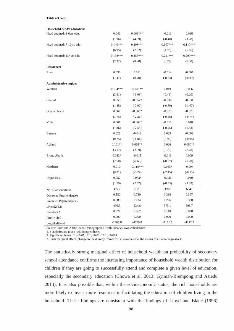
98
Table 4.3 cont.:
Household head's education:
Head attained: 1-6yrs edu. 0.046 0.068***
-0.011 0.038
(1.96) (4.59)
(-0.40) (1.78)
Head attained: 7-12yrs edu. 0.140*** 0.108***
0.107*** 0.110***
(6.95) (7.92)
(4.73) (6.16)
Head attained: 13+yrs edu. 0.198*** 0.153***
0.221*** 0.209***
(7.32) (8.90)
(6.72) (8.00)
Residence:
Rural 0.036 0.011
-0.014 -0.007
(1.47) (0.70)
(-0.63) (-0.39)
Administrative region:
Western 0.134*** -0.081**
0.019 0.006
(3.91) (-3.03)
(0.46) (0.20)
Central 0.058 -0.057*
-0.036 -0.034
(1.48) (-2.02)
(-0.89) (-1.07)
Greater Accra 0.067 -0.065*
-0.015 -0.023
(1.75) (-2.21)
(-0.38) (-0.74)
Volta 0.067 -0.068*
-0.010 0.010
(1.86) (-2.55)
(-0.25) (0.33)
Eastern 0.028 -0.048
0.039 -0.002
(0.75) (-1.84)
(0.95) (-0.08)
Ashanti 0.101** 0.065**
0.026 0.080**
(3.17) (2.99)
(0.70) (2.78)
Brong Ahafo 0.082* -0.015
-0.013 0.009
(2.50) (-0.60)
(-0.37) (0.28)
Northern 0.010 -0.118***
-0.085* -0.004
(0.31) (-5.24)
(-2.45) (-0.15)
Upper East 0.052 0.053*
-0.036 0.040
(1.59) (2.57) (-0.93) (1.33)
No. of observations 4725 7826
3897 6640
Observed Pr(attendance) 0.580 0.720
0.319 0.397
Predicted Pr(attendance) 0.588 0.734
0.296 0.388
LR chi2(33) 496.3 624.6
575.1 698.7
Pseudo R2 0.077 0.067
0.118 0.078
Prob > chi2 0.000 0.000
0.000 0.000
Log likelihood -2965.8 -4329.8 -2151.5 -4112.5
Source: 2003 and 2008 Ghana Demographic Health Surveys; own calculations
1. z statistics are given within parentheses
2. Significant levels: * p<0.05, ** p<0.01, *** p<0.001
3. Each marginal effect (change in the dummy from 0 to 1) is evaluated at the means of all other regressors.
The statistically strong marginal effect of household wealth on probability of secondary
school attendance confirms the increasing importance of household wealth distribution for
children if they are going to successfully attend and complete a given level of education,
especially the secondary education (Chowa et al. 2013; Gyimah-Brempong and Asiedu
2014). It is also possible that, within the socioeconomic status, the rich households are
more likely to invest more resources in facilitating the education of children living in the
household. These findings are consistent with the findings of Lloyd and Blanc (1996)
99
Patrinos and Psacharopoulos (1997) Deininger (2003), Sackey (2007), and Harttgen et al.
(2010). These studies demonstrate that household wealth is a key determinant of a
household’s ability to invest in children's education and as a result, it can lead to inequality
in educational outcomes between children from poor and the non-poor households.
Our results demonstrate that the effect wealth distribution on educational access is still far
from resolved, especially at secondary school level. Even with significant improvements in
supply-side factors; increase in the overall number and geographical distribution of schools,
more resources being allocated to teacher and administrative capacity-building, and greater
community-school interaction mechanisms (World Bank 2004), our findings indicate that
aggregate household wealth is still an important barrier to children’s schooling in Ghana.
Household composition/size
The average household size in Ghana in 2003 and 2008 is 4.0 and 3.8 persons, respectively
(Table 3.1 in Chapter 3; and Ghana Statistical Service et al. 2004 & 2009). The impact of
household size on primary school attendance is negative with weak statistical significance
in 2008. At the secondary level, the impact is also negative with weak statistical
significance in 2003 (Table 4.3). The negative marginal effect of household size (although
statistically weak) which reduces the probability of both primary and secondary school
attendance, could be dependent on socioeconomic setting of the households (Knodel et al.
1990;Knodel and Wongsith 1991). For example, poor households normally tend to have
more children with associated household resource constraints. In other words, larger
families tend to spread their financial and human resources thinly compared to smaller
households thereby negatively affecting the schooling outcomes of the children (Sathar and
Lloyd 1994; Sandefur et al. 2006). Thus, if the average Ghanaian household size is
constraint with economic resources to maintain their children in school, then this could
justify the negative impact of the household size on the educational outcomes of the
children, ceteris paribus. The negative association between the household size and school
attendance is not surprising, since 28.5% of Ghanaians are below the poverty line (Ghana
Statistical Service 2007) with consumption based inequality of 39.4% based on currently
available data (Coulombe and Wodon 2007).
This negative association between household size and educational outcomes has also been
found in both developed (Blake 1981 & 1989; Downey 1995) and developing (Knodel et al.
1990; Parish and Willis 1993; Pong 1997; Patrinos and Psacharopoulos 1997) countries.
100
For example, Patrinos and Psacharopoulos (1997) explore the negative association between
household size and educational outcomes of children from a different angle and suggest
that parents with a preference for larger families generally see less need to educate their
children. Thus, the negative relationship between household size and children’s
educational attainment may be the result of parental preferences and household resource
constraints.
In terms of household composition, the number of children under-six years old in a
household has a negative impact on both primary and secondary attendance. However, the
marginal effect is only statistically significant in 2003 and 2008 for primary school
attendance and secondary school attendance, respectively. At the primary school level, a
household size containing a minimum of 1 to 2 and a maximum of 5 to 6 under-six year
olds reduces the probability of primary school attendance of school-age children by 7.1%
to 26.4%. Also at the secondary school level, the trend is similar. For example, a household
size containing a minimum of 1 to 2 and a maximum of 5 to 6 under-six year olds reduces
the probability of secondary school attendance of school-age children by 4.8% and 26.9%,
respectively (see Table 4.3). At both levels of education, the increasing number of very
young children (i.e. age 0-5 years) in the household negatively affects the probability of
educational access (i.e. school attendance) of school-age children in the household. These
findings are consistent with the findings of Sathar and Lloyd (1994), Lloyd and Blanc
(1996), and (Sackey 2007). In Kenya, Tanzania, Cameroon, Niger, Malawi, Namibia and
Zambia, Lloyd and Blanc (1996) observe that the presence of young children decreases the
likelihood of school attendance of the older children in the household. Sackey (2007) also
observes that in Ghana, the presence of younger siblings, relative to older ones, tends to
reduce the probability of school attendance. Furthermore, the results depicted in Table 4.3
confirm the a priori expectation that with increases in the family size, school-age children
are kept back at home to tend to various domestic chores. For example, school children
from poor households in particular, will be needed more at home to carry out various
household chores and to mind the younger siblings as the family size increases, thereby
negatively affecting the likelihood of school attendance (Lloyd and Blanc 1996).
The impact of the number of economically active household members and retirees on the
probability of both primary and secondary school attendance in 2003 and 2008 are
insignificant. However, the impact of the proportion of economically active household
members on school attendance is positive and statistically significant only in 2003 at the
101
secondary school level (Table 4.3). As per the earlier discussions in Chapter 3, the positive
marginal effect implies that the proportion of economically active household members is
likely to be economically productive (employed), thereby contributing to households
resources available to maintain children in school. In effect, the positive impact frees out
the households resources, thereby reducing households’ dependence burden. This finding
corroborates the findings of Okumu et al. (2008). The authors find that as the proportion
of the economically active members of household increases, the likelihood of primary
school dropout increases. They argue that the results of the study imply that a good number
of the economically active household members were actually unproductive. Thus, if the
likelihood of school dropout had decreased, it would have meant that the proportion of the
economically active household members was actually employed.
Household head characteristics/background
Households headed by females have statistically significant positive marginal effect on
both primary and secondary school attendance in 2003 and 2008. At the primary school
level, female household head increases the probability of primary school attendance of
children by 5.5% and 2.9% points in 2003 and 2008, respectively, when the marginal effect
of female household head increases by one percentage point (Table 4.3). This implies that
on average, the probability of children from households headed by female, attending
primary school is higher compared with the probability of primary school attendance of
children from households headed by males over the two survey periods. At the secondary
school level, the trend is similar. The probability of secondary school attendance increases
by 8.7% and 4.5% points in 2003 and 2008, respectively when the marginal effect of
female household head increases by one percentage point (Table 4.3). This also means that
the probability of secondary school attendance of children from households headed by
female are higher than the probability of secondary school attendance of children from
households headed by males over the two survey periods.
These findings appear to show that female household heads are more likely to invest in
resources; including time, money, and emotional support in facilitating the education of
children living in their household as suggested by Lloyd and Blanc (1996). The positive
and strong impact of female household head on the likelihood of children’s educational
access, could also be attributed to the importance of women empowerment that allows
them in taking key decisions, especially in favour of children’s welfare. The finding is
consistent with other empirical studies indicating that female household heads spend a
102
larger percentage of the household budget on children than the male household heads do
(Lloyd and Gage-Brandon 1994; Lloyd and Blanc 1996; Bruce J et al. 1995; Bruce Judith
and Lloyd 1996; Bbaale and Buyinza 2013; Gyimah-Brempong and Asiedu 2014).
The marginal effect of household head’s educational attainment (secondary and higher
levels of education) is positive and highly statistically significant in both 2003 and 2008.
The impact of household heads with primary education level on children’s school
attendance in both 2003 and 2008 is only statistically significant at primary school level
(Table 4.3). The educational level effect is compared for children who live in households
headed by person with no schooling with households with educated heads. It is also
important to note that the marginal effect of household heads’ educational level increases
the probability of primary school attendance of children from 4.6% to 19.8% points. Thus,
as the level of education attained by household head increases from primary level to higher
level, the probability of school attendance also increases. Similar trend is also observed in
2008 for primary school attendance.
At the secondary school level, the marginal effect of household head educational
attainment (secondary and higher levels) relative to no schooling significantly increases the
probability of children attending school in both 2003 and 2008. Thus, the higher the level
of household heads’ or parents’ schooling the more favourable are the child’s educational
access, all other things being equal. Consequently, children of household heads or parents
with no formal education or low level of educational attainment are more likely to face low
educational prospects while those who live in the households with parents or household
heads with at least secondary education attainment, have better educational prospects. An
important policy lesson may be derived from this analysis. For example, household head’s
educational attainment at lower level (primary or no education) tends to reduce the
probability of children’s school attendance. Conversely, household head’s educational
attainment at a higher level (secondary or higher) tends to increase the probability of
children’s school attendance.
The finding confirms the a priori condition discussed in Chapter 3 that the more educated
the household head is, the more likely that a child of school-age living in the household
will be attending school currently. Our results probably reflect the desire of more educated
household heads to ensure the education of their own children as well as the children of
other relatives within the household for whom they (household heads) feel some
103
responsibility. The results depicted in Table 4.3 also corroborate most studies that have
found a positive association between household head’s or parents’ education and children's
educational outcomes (Jacoby 1994; Haveman and Wolfe 1995; Lillard and Willis 1994;
Sathar and Lloyd 1994; Oliver 1995; Tansel 1997; Glick and Sahn 2000; Tansel 2002).
More recent studies by Sackey (2007) and Rolleston (2011) in Ghana, and Bbaale and
Buyinza (2013) in Uganda on the determinants of educational access using ordered probit
regression analysis also find that higher levels of parental education tend to reduce the
probability of children dropping out of school.
Residency /location
The regional impact on primary school attendance is only significant in both 2003 and
2008 in two regions: Western, and Ashanti regions. In 2003, these regions including the
Brong Ahafo region had statistically significant positive marginal effect on primary school
attendance. Interestingly, however, in 2008 Western, Central, Greater Accra, Volta, and
Northern regions have also recorded statistically significant negative effect (some with
weak effect) on primary school attendance. The implication is that in 2008, the probability
of primary school attendance reduces with a percentage increase in marginal effect of the
regions concerned. At the secondary school level, only Ashanti region has a statistically
significant marginal effect with positive impact on the school attendance in 2008. On the
other, the probability of secondary school attendance by children in Northern region
reduces by 8.5% point. Since most of the regional effects on educational access are
statistically insignificant, our trend analysis between in 2003 and 2008 reveals little
evidence of any systematic regional effect on school attendance in Ghana.
4.4.2 Primary and secondary completion
For educational attainment, we analyse if a given age cohort who attended school has
completed a given level of education or not. Table 4.4 depicts the marginal effects and
predicted probabilities of the key explanatory variables on school completion by age
cohorts at both primary and secondary levels in 2003 and 2008. The likelihood rate 2 test,
(Pr > 2) result shows that the model is well fit. The predicted probability for primary
school completion by age cohort 15-20 years increased from 69.9% in 2003 to 75.3% in
2008. At the secondary school level, predicted probability for secondary education
completion by age cohort 18-23 years increased from 9.9% in 2003 to 17.5% in 2008. It is
worth mentioning that secondary attainment rates (i.e. completion rates) are quite low in
Ghana compared to primary school completion rates. For example, the summary statistics
104
(in Table 4.2) show primary completion rates of 70.4% and 75.0% for the age cohort, 15-
20 years in 2003 and 2008, respectively. At the secondary level, the completion rates for
the age cohort, 18-23 years are very low. The statistics show that about 15% and 23% of
the age cohort completed secondary school in 2003 and 2008, respectively which is
consistent with the predicted probability for 2003 and 2008.
Table 4.4 below presents the results from probit estimation relating education attainment of:
(i) age cohort 15-20 years (primary school completion); and (ii) age cohort 18-23 years
(secondary school completion) and household wealth together with other socioeconomic
factors. The marginal effect of female student is negative and statistically significant at
both primary and secondary school levels in 2003 and 2008. This implies that the
probability of female children completing primary and secondary school among Ghanaian
households is lower compared to the male children (reference category). In 2003, the
probability of female children completing primary education was 9.7% points lower than
that of the male children. Although, by 2008 the probability has improved to 3.5% it is still
lower than the probability of male children completing primary education.
At the secondary level, the disparity in completing secondary education between male and
female children is smaller, though the marginal effect is statistically weak. Although, the
marginal effect of female children indicates that female children have lower probability of
completing both primary and secondary education compared to male children, the gender
inequality gap appears to be narrower at the secondary school level between the two survey
periods. This shows that there have been some improvements in school completion rate,
though the females are still lagging behind.
These findings are consistent with the findings of Sackey (2007). Sackey who also finds
that although school attainment has improved for both boys and girls between 1992 and
1999 survey periods generally, the likelihood of girls completing school is relatively lower
than that of boys. The gender disparity in educational attainment has also been found by;
Lloyd and Gage-Brandon (1994), Oxaal (1997), Holmes (2003), Lewin (2009), and Lloyd
and Hewett (2009). Lloyd and Gage-Brandon find that dropout rates were significantly
greater for girls, and their educational attainment levels were also lower than those of boys
in Ghana, especially when there were younger siblings in the household.
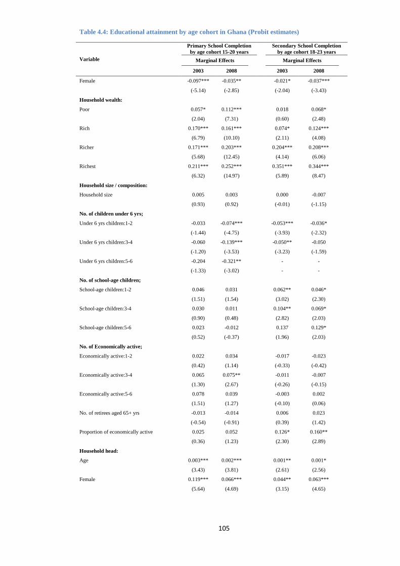
105
Table 4.4: Educational attainment by age cohort in Ghana (Probit estimates)
Variable
Primary School Completion
by age cohort 15-20 years
Secondary School Completion
by age cohort 18-23 years
Marginal Effects
Marginal Effects
2003 2008 2003 2008
Female -0.097*** -0.035**
-0.021* -0.037***
(-5.14) (-2.85)
(-2.04) (-3.43)
Household wealth:
Poor 0.057* 0.112***
0.018 0.068*
(2.04) (7.31)
(0.60) (2.48)
Rich 0.170*** 0.161***
0.074* 0.124***
(6.79) (10.10)
(2.11) (4.08)
Richer 0.171*** 0.203***
0.204*** 0.208***
(5.68) (12.45)
(4.14) (6.06)
Richest 0.211*** 0.252***
0.351*** 0.344***
(6.32) (14.97)
(5.89) (8.47)
Household size / composition:
Household size 0.005 0.003
0.000 -0.007
(0.93) (0.92)
(-0.01) (-1.15)
No. of children under 6 yrs;
Under 6 yrs children:1-2 -0.033 -0.074***
-0.053*** -0.036*
(-1.44) (-4.75)
(-3.93) (-2.32)
Under 6 yrs children:3-4 -0.060 -0.139***
-0.050** -0.050
(-1.20) (-3.53)
(-3.23) (-1.59)
Under 6 yrs children:5-6 -0.204 -0.321**
- -
(-1.33) (-3.02)
- -
No. of school-age children;
School-age children:1-2 0.046 0.031
0.062** 0.046*
(1.51) (1.54)
(3.02) (2.30)
School-age children:3-4 0.030 0.011
0.104** 0.069*
(0.90) (0.48)
(2.82) (2.03)
School-age children:5-6 0.023 -0.012
0.137 0.129*
(0.52) (-0.37)
(1.96) (2.03)
No. of Economically active;
Economically active:1-2 0.022 0.034
-0.017 -0.023
(0.42) (1.14)
(-0.33) (-0.42)
Economically active:3-4 0.065 0.075**
-0.011 -0.007
(1.30) (2.67)
(-0.26) (-0.15)
Economically active:5-6 0.078 0.039
-0.003 0.002
(1.51) (1.27)
(-0.10) (0.06)
No. of retirees aged 65+ yrs -0.013 -0.014
0.006 0.023
(-0.54) (-0.91)
(0.39) (1.42)
Proportion of economically active 0.025 0.052
0.126* 0.160**
(0.36) (1.23)
(2.30) (2.89)
Household head:
Age 0.003*** 0.002***
0.001** 0.001*
(3.43) (3.81)
(2.61) (2.56)
Female 0.119*** 0.066***
0.044** 0.063***
(5.64) (4.69)
(3.15) (4.65)
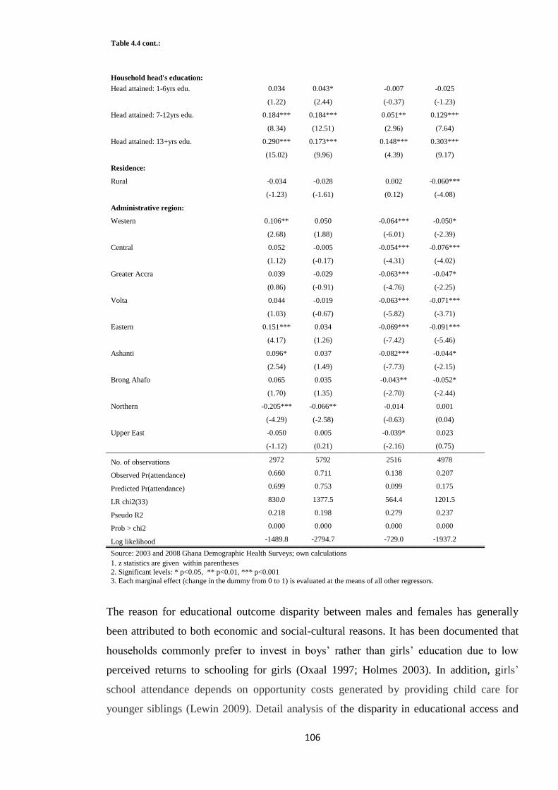
106
Table 4.4 cont.:
Household head's education:
Head attained: 1-6yrs edu. 0.034 0.043*
-0.007 -0.025
(1.22) (2.44)
(-0.37) (-1.23)
Head attained: 7-12yrs edu. 0.184*** 0.184***
0.051** 0.129***
(8.34) (12.51)
(2.96) (7.64)
Head attained: 13+yrs edu. 0.290*** 0.173***
0.148*** 0.303***
(15.02) (9.96)
(4.39) (9.17)
Residence:
Rural -0.034 -0.028
0.002 -0.060***
(-1.23) (-1.61)
(0.12) (-4.08)
Administrative region:
Western 0.106** 0.050
-0.064*** -0.050*
(2.68) (1.88)
(-6.01) (-2.39)
Central 0.052 -0.005
-0.054*** -0.076***
(1.12) (-0.17)
(-4.31) (-4.02)
Greater Accra 0.039 -0.029
-0.063*** -0.047*
(0.86) (-0.91)
(-4.76) (-2.25)
Volta 0.044 -0.019
-0.063*** -0.071***
(1.03) (-0.67)
(-5.82) (-3.71)
Eastern 0.151*** 0.034
-0.069*** -0.091***
(4.17) (1.26)
(-7.42) (-5.46)
Ashanti 0.096* 0.037
-0.082*** -0.044*
(2.54) (1.49)
(-7.73) (-2.15)
Brong Ahafo 0.065 0.035
-0.043** -0.052*
(1.70) (1.35)
(-2.70) (-2.44)
Northern -0.205*** -0.066**
-0.014 0.001
(-4.29) (-2.58)
(-0.63) (0.04)
Upper East -0.050 0.005
-0.039* 0.023
(-1.12) (0.21) (-2.16) (0.75)
No. of observations 2972 5792
2516 4978
Observed Pr(attendance) 0.660 0.711
0.138 0.207
Predicted Pr(attendance) 0.699 0.753
0.099 0.175
LR chi2(33) 830.0 1377.5
564.4 1201.5
Pseudo R2 0.218 0.198
0.279 0.237
Prob > chi2 0.000 0.000
0.000 0.000
Log likelihood -1489.8 -2794.7 -729.0 -1937.2
Source: 2003 and 2008 Ghana Demographic Health Surveys; own calculations
1. z statistics are given within parentheses
2. Significant levels: * p<0.05, ** p<0.01, *** p<0.001
3. Each marginal effect (change in the dummy from 0 to 1) is evaluated at the means of all other regressors.
The reason for educational outcome disparity between males and females has generally
been attributed to both economic and social-cultural reasons. It has been documented that
households commonly prefer to invest in boys’ rather than girls’ education due to low
perceived returns to schooling for girls (Oxaal 1997; Holmes 2003). In addition, girls’
school attendance depends on opportunity costs generated by providing child care for
younger siblings (Lewin 2009). Detail analysis of the disparity in educational access and
107
attainment of males and females by welfare distribution is explored in Chapter 5 to
determine the socioeconomic factors that might be contributing to the low educational
outcomes of females revealed by the result in Table 4.4.
Household wealth distribution
The results in Table 4.4 also confirm the significance of household wealth as key
explanatory variable for education attainment (school completion) as well as the poverty
hypothesis (Hanushek and Lavy 1994; Sathar and Lloyd 1994; Jacoby 1994; Lloyd and
Blanc 1996; Bredie and Beeharry 1998; Filmer and Pritchett 1999b). The marginal effect
of household wealth on the probability of educational attainment depicted in Table 4.4
across the wealth distribution is positive and statistically significant except at secondary
school level in 2003. Household wealth increases the probability of school completion for
all welfare groups. However, the effect is larger for rich households than the poor
households. For example, the marginal effect of moving from the second quintile (poor
household) to the fifth quintile (richest household) increases the probability of primary
school completion for primary school-age children from 5.7 to 21.0 percentage points in
2003 and from 11.2 to 25.2 percentage points in 2008 (Table 4.4).
The marginal effect shows that children from the richest households are more likely to
complete primary education than children from the poor households in both survey years.
Although, the impact of household wealth distribution on primary school completion has
increased the probability of primary school completion for both the poor and the non-poor,
the disparity between the poor and the richest remains between the two survey periods. The
disparity in the vertical comparison (the bottom and top wealth quintiles) should be of
great concern if children from poor households are to catch up with the children from
richest households in terms of educational attainment and to progress from primary to
secondary education level. Although, the government of Ghana’s education policy
interventions appear to have had some indirect positive impact on access to primary
education (through reducing the financial burden of poor households enrolling their
children in primary school, depicted in Table 4.3 in 2008), the primary school completion
appears to be more dependent on household wealth levels or wealth distribution in 2008.
The effects at primary school level have direct impact on secondary school access and
completion. These effects feed through to the secondary level, especially for less affluent
households. At the secondary level, the marginal effect of household wealth on the
108
probability of secondary education attainment for all income groups is positive and
statistically significant in 2003 and 2008, except for the poor households in 2003. Children
from the richest households are (4.7 times in 2003 and 2.8 times in 2008) more likely to
complete secondary education than children from rich or households in the middle of the
wealth distribution. The strong and large impacts of household wealth or household wealth
distribution on secondary school completion depicted in Table 4.4 is a testament to the fact
that in Ghana, secondary education is not free (Gyimah-Brempong and Asiedu 2014) and
only few Ghanaians can afford the high cost of secondary education. The result from Table
4.4 corroborates the findings of Sackey (2007) and Gyimah-Brempong and Asiedu (2014)
which show that household resources play an important role in the education of children in
Ghana. Sackey also finds that children from rich households tend to achieve higher rates of
school attendance both in 1992 and 1999 household surveys. Other studies also confirm
that children’s schooling outcomes are associated with socioeconomic status of households
(Psacharopoulos and Arriagada 1986; Sathar and Lloyd 1994; Lloyd and Blanc 1996; Gage
et al. 1997; Buchmann and Hannum 2001; Patrinos and Psacharopoulos 1997). For
example, Lloyd and Blanc (1996) have also confirmed the strong association between
household living standard and the likelihood that children of school-age will be enrolled in
a school and that they will have completed school. Our findings are consistent with these
studies that demonstrate household wealth as a key socioeconomic determinant of a
household’s ability to invest in children's education, and the resultant disparity in
educational outcomes of children from poor and non-poor households.
Household composition/size
As expected (based on literature review), the number of children under-six year olds has a
negative impact on both primary and secondary completion. At the primary school level,
the marginal effect is only statistically significant in 2008. The number of under-six year
olds reduces the probability of primary school attainment (completion) by a minimum of
7.4% points to a maximum of 32.1% points (see Table 4.4). The impact of the number of
under-six year old children on secondary school completion is also negative and
statistically significant in 2003. A household with 1 to 2 and 3 to 4 under-six year olds
reduces the probability of secondary school attainment by 5.3% and 5.0% points,
respectively. Our results corroborate other research findings which demonstrate that the
presence of very young children in the household can increase the time needed for
childcare and this can affect school attendance and completion rates of school children
(Sathar and Lloyd 1994; Sackey 2007; Psacharopoulos and Arriagada 1989). For example,
109
Lloyd and Blanc (1996) find that school-age children are kept back at home to carry out
various household chores and mind the younger siblings as the family size increases,
thereby negatively affecting school completion rate of female children. In Ghana, Sackey
(2007) also observes that the presence of younger siblings, relative to older ones, tends to
reduce the probability of school completion rates.
The marginal effect of the number of school-age children in the household on the
probability of primary school completion is statistically insignificant. At the secondary
level, the marginal effect of the number of school-age children increases the probability of
secondary school completion from 6.2% to 10.4% points in 2003 and from 4.6% to 12.9%
points in 2008. Even though, this finding corroborates the findings of Chernichovsky
(1985), the evidence depicted in Table 4.4 is very weak to suggest that the number of
school-age children in Ghanaian households increases the probability of secondary
education attainment.
The marginal effect of the proportion of economically active household members is
positive and statistically significant only at the secondary school level. The positive impact
implies that the proportion of economically active household members is likely to be
economically productive (employed), thereby contributing to household resources to
support children to achieve educational outcomes (school completion). In effect, the
positive impact frees out the households resources by reducing households’ dependency
burden. This finding corroborates the findings of Okumu et al. (2008). The authors find
that as the proportion of the economically active members of household increases, the
likelihood of school dropout increases. They argue that their findings imply that the
proportion of the economically active household members was actually unproductive.
Household head characteristics
Female household head has positive and strong statistical significant marginal effect on
primary and secondary education attainment in both 2003 and 2008. In 2003 and 2008, the
impact of female household head increases the probability of primary school completion
by 11.9% and 6.6% points, respectively higher than that of the male household head (i.e.
reference category). At the secondary level also, the marginal effect of female household
head increases the probability of secondary school completion by 4.4% in 2003 and 6.3%
in 2008 compared to the secondary education attainment by children from households
headed by male. This finding is consistent with the earlier results for school attendance and
110
other studies documenting the impact of female headed households on children educational
outcomes. It has been found that female household heads spend a larger percentage of the
household budget on children than the male household heads do (Lloyd and Gage-Brandon
1994; Lloyd and Blanc 1996; Bruce Judith and Lloyd 1996). The finding also confirms the
argument of having a woman in the position of authority and resource control within the
household, as opposed to having a man in that position, is more likely to impact positively
on children's educational access and attainment (Lloyd and Blanc 1996). For example,
Gyimah-Brempong and Asiedu (2014) find that remittances received by female household
head in Ghana increases the probability of educational access and attainment of children
compared to their male counterparts. These reasons might have contributed to the positive
and strong statistical significant marginal effect of female household head on the
probability of children’s school completion rate in Ghana.
The marginal effect of household head’s educational attainment (secondary and higher
levels) is positive and highly statistically significant in both 2003 and 2008 (Table 4.4).
The educational level effect is compared for children who live in households headed by
person with no schooling with households with educated heads. It is also important to note
that the marginal effect of household heads’ educational attainment increases the
probability of primary school completion of children from 18.4% to 29.0% points. Thus, as
the level of education attained by household head increases, the probability of school
completion also increases. However, in 2008 there is a slight change in the probability of
primary school completion (Table 4.4).
At the secondary school level, the marginal effect of household head educational
attainment (secondary and higher levels) relative to no schooling significantly increases the
probability of secondary school completion in both 2003 and 2008. Thus, the higher the
level of household head's or parents’ schooling the more favourable is a child’s educational
attainment, all other things being equal. Consequently, children of household heads or
parents with no formal education or low level of educational attainment are more likely to
face low educational prospects while those who live in the households with parents or
household heads with at least secondary education attainment have better educational
prospects of completing secondary education.
These results are consistent with school attendance results discussed earlier in Table 4.3.
Moreover, the results obtained from Tables 4.3 and 4.4 probably reflect the desire of
111
educated household heads or parents to ensure the education of their own children as well
as the children of other relatives within the household for whom they feel some
responsibility. The results depicted in Table 4.4 corroborate most studies that have found a
positive association between household head’s or parents’ education and children's
educational outcomes (Jacoby 1994; Haveman and Wolfe 1995; Lillard and Willis 1994;
Sathar and Lloyd 1994; Oliver 1995; Tansel 1997; Glick and Sahn 2000; Tansel 2002;
Rolleston 2011). For example, Sackey (2007) finds that higher levels of parental education
tend to reduce the probability of children dropping out of school in Ghana, which
corroborates our findings.
Residency /location
The negative marginal effect of residency in rural area is only statistically significant in
2008 at secondary school level (Table 4.4). This implies that the probability of children
completing secondary school in rural areas is lower than those in the urban areas. Although
the rural effect on primary completion (in both 2003 and 2008) and secondary school
completion in 2003 was statistically insignificant, the statistically significant effect in 2008
at the secondary school level corroborates the findings of Sackey (2007), and Ghana
Statistical Service et al. (2004 & 2009). Sackey (2007) observes locality differences with
respect to children’s school attendance and attainment. According to Sackey, children
residing in rural areas in Ghana are more likely to drop out of school, and when they do
attend school, they are more likely to have lower educational attainments than children in
urban areas. The Ghana Statistical Service et al. (2004 & 2009) reports also reveal higher
completion rates for urban areas than rural areas. These consistent findings (including ours)
pose a worrying concern over the disparity in educational attainments between the urban
and rural areas in Ghana.
The regional effect on primary school completion is positive and statistically significant in;
Western, Eastern, and Ashanti regions in 2003 but not in 2008. The Northern region
records negative and statistically significant marginal effect on primary school completion
in both 2003 and 2008 (Table 4.4). While the probability of primary school completion
increases from 9.6% to 15.1% points in the three southern regions (Western, Eastern, and
Ashanti), that of the Northern region reduces by 20.5% points in 2003. The result to some
extent highlights the old North-South divide inequality debate in Ghana. In the northern
part of Ghana where poverty levels are higher than any part of the country (Ghana
Statistical Service 2000; Ghana Statistical Service 2007; Ghana Statistical Service et al.
112
2009), the primary completion rates are significantly lower than other regions in southern
part of the country.
At the secondary level, the regional effect reduces the probability of secondary education
attainment which is statistically significant in eight regions in 2003 and seven regions in
2008 with reference to Upper West region (Table 4.4). In 2003, the probability of
secondary school completion reduces by 3.9% points in Upper East region to 8.2% points
in Ashanti region. A similar trend is observed in 2008, where the probability of secondary
school completion reduces by a minimum of 4.4% points to a maximum of 9.1% points.
On average, the probability of secondary education attainment in most regions has
worsened in 2008. Furthermore, there are disparities in the magnitude of the regional
effect on the probability of educational attainment in the various regions. The findings are
consistent with the GSS report (Ghana Statistical Service et al. 2009) which shows that
there are wide regional variations in dropout rates in Ghana.
4.4.3 Robustness check
We check the robustness of our results to the choice of explanatory variables by estimating
the model (Equation 4.1) with dummy variables for: religion (no religion, Christianity,
Muslim, and Traditional religion); ethnicity (Akan, Ga/Dangme, Ewe, Guan,
Mole/Dagbani, Grussi, Gruma, and Hausa/Mande) and resource control (household
spending) which could impact schooling outcomes. We estimated different combinations
of these variables with the final model variables and also by replacing some of the
variables in the final estimated model by these variables. However, the estimated results
from these combinations with respect to these variables were highly insignificant. For
example, as a proxy for household resource control, we replaced female household dummy
variable by household spending (husband alone, wife alone, husband and wife). The results
were highly statistically insignificant and did not change the stability of the final results
reported in Tables 4.3 and 4.4. For example, the largest deviation of the alternative
estimates compared to the main specification is about 7%. The largest change in estimates
across all specifications is about 9%. To the extent that the estimates are stable, they
provide confidence in the plausibility of the results and the validity of the identification of
the regression model.
In addition, we also used the linktest to check our final model. The idea behind linktest is
that if the model is properly specified, one should not be able to find any additional
113
predictors that are statistically significant except by chance (Pregibon 1980). None of the
linktest result (hatsq) is statistically significant.20 The link test reveals no problems with
our specification since the prediction squared does not have explanatory power. Although,
the linktest indicates that there is no problem of misspecifications, we check our model
against the theories of determinants of educational inequality to make sure that our model
is valid based on the theoretical underpinnings of educational inequality reviewed in
Chapter 3.
4.5 Policy lessons
An important policy lessons may be derived from this analysis. Household wealth and
educational attainment of the household head appear to be the key factors in determining
children's access to education, and educational attainment in Ghana. For example, the
educational access and attainment in Ghana are more likely to benefit children from rich
households more than children from the poor households. Consequently, the efforts of the
government of Ghana towards achieving universal access to primary education by 2015
have not yet seem to overcome the advantage of children who live in relatively well-off
households. Moreover, household head’s educational attainment at lower level (primary
education) tends to reduce the probability of children’s school attendance. Conversely,
household head’s educational attainment at higher levels (secondary or higher levels) tends
to increase the probability of children’s school attendance and completion. This finding
implies that for more favourable children’s educational outcomes for the future generations,
the government of Ghana should aim at policies that strengthen educating children beyond
basic education level.
Furthermore, the findings from the fore-going multivariate probit regression analysis
vindicate the importance of household wealth distribution in particular, and household
heads educational attainment in children's educational access and attainment in Ghana.
Although, the government of Ghana has spent a lot of resources (World Bank 2004; NDPC
et al. 2010) providing universal access to basic education, household financial support
appears to be critical, especially at the secondary school level where schooling can be very
20
Primary school attendance, hatsq: p = 0.920 in 2003 and p = 0.071 in 2008
Primary school completion, hatsq: p = 0.128 in 2003 and p = 0.280 in 2008
Secondary school attendance, hatsq: p = 0.137 in 2003 and p = 0.568 in 2008
Secondary school completion, hatsq: p = 0.384 in 2003 and p = 0.800 in 2008
Where = .05 (significance level)
114
costly to children from poor households. Therefore, designing education interventions at
the secondary school level that are focused on economically disadvantaged groups will be
an excellent positive discrimination mechanism. Alternatively, expanding free universal
education to secondary level could improve educational outcomes in Ghana. This would
allow children from poor households who cannot afford secondary education to continue
with schooling after the basic education levels. Thus, investing in education and making
educational access available to all households up to secondary school level irrespective of
income levels of households could be a solution to reducing income and educational
inequalities, and poverty reduction in Ghana.
4.6 Conclusions
We have explored socioeconomic determinants of educational outcomes in Ghana using
both descriptive analysis and multivariate regression framework to capture and explain the
impact of the GoG’s education policy interventions implemented in 2004/05 through
household wealth distribution on educational access and attainment of children in Ghana.
We estimated the impacts of key socioeconomic factors on both primary and secondary
school access (probability of attendance) and attainment (probability of completing school
by age cohorts) to explain educational disparities in Ghana before and after the GoG’s
education policy interventions. The key household socioeconomic factors that influence
educational access and attainment have been identified, the extent of disparity in
educational outcomes at both primary and secondary school levels between 2003 and 2008
examined, and policy implications highlighted.
The results of the analysis confirm the significance of household wealth as an important
explanatory variable in addition to other covariates in estimating the persistent disparities
in educational access and attainment of school-age children in Ghana. Especially, at the
secondary school level, the disparity between the poor and the non-poor with respect to
access and attainment should be of a great concern in terms of the magnitude of the impact.
The household wealth appears to be the most important determining factor in explaining
the disparity in children's school attendance and completion. This is evident throughout the
multivariate regression analysis, both in terms of strong statistical significance and in terms
of the magnitude of the overall impact on children's educational access and attainment.
The variations in educational access and attainment between children from poor and non-
poor households at different levels of education may constitute an evidence of households'
115
continuing financial burden in educating children and the probable ineffectiveness of the
state (the government of Ghana) in transcending those economic differences. The
particularly strong marginal effect of household wealth on children educational outcomes
confirms the increasing importance of household wealth distribution for children if they are
going to successfully progress from grade to grade and from level to level in the Ghanaian
education system. It also appears that, within the socioeconomic status, the rich households
are more likely to invest more resources in facilitating the education of their children than
the poor households. The descriptive statistics in Tables 4.1 and 4.2 also show that there is
huge disparity in net attendance rate between primary and secondary school levels. The
primary net attendance rate is almost doubled the secondary net attendance rate. The
completion rate at secondary school level compared to primary school level is even more
worrying. For example, about 70% and 75% primary completion rates were recorded for
age cohort 15-20 in 2003 and 2008 respectively, compared to about 15% and 23%
secondary completion rates for age cohort 18-23 in the same periods.
The findings also indicate a positive and strong statistically significant marginal effect of
female household head on the probability of school attendance and completion. The
marginal effect suggests that there is a direct link between the impact of households headed
by female and educational outcomes of children. This finding also illustrates the crucial
role played by women in educating children. Specially so when they are in the position of
authority and resource control as these increase their say in the intra-household decision
making process as well as in the society at large (Lloyd and Blanc 1996). This finding
corroborates the findings of Lloyd and Gage-Brandon (1994), Lloyd and Blanc (1996), and
Bbaale and Buyinza (2013).
However, this chapter has not been able to shed light on the impacts of socioeconomic
factors on gender disparities in the educational outcomes. To address this, the next chapter
explores socioeconomic factors that might have contributed to the low education
attainments depicted in Table 4.4 and the possible policy lessons for policy makers and the
Ghanaian education system as a whole.
116
Chapter 5
Educational outcomes of males and females by wealth distribution in Ghana
5.1 Introduction
Disparities in educational outcomes between males and females in low-income developing
countries is well established in the literature (Appleton et al. 1996 ; Alderman and King
1998; Glick and Sahn 2000; Filmer 2000 & 2005; Appleton 1995) and remain policy
concern in many developing countries. These inequalities have important implications for
the development of the developing countries (World Bank 2001 & 2011) and have been
recognised in a letter to Dr Homi Kharas, lead author and executive secretary of the
secretariat supporting the High-Level Panel of Eminent Persons on the Post-2015
Development Agenda.21
The letter further stresses that the post-2015 development
framework must aim to reduce the inequality gaps within countries, including gender
inequalities.
The importance of gender equality in educational attainment cannot be over-emphasised
enough. There is strong gender equity rational for equalising schooling for both female and
male children. This is because education can empower women and improve their welfare
by increasing the economic opportunities available to them and also by possibly increasing
their bargaining power within the household. “Education represents an important life
opportunity for both women and men, and a vital social and economic resource for
societies. Gender inequality in education constructs, and in turn, is constructed by
inequalities between women and men in other spheres that intersect with education”
(Subrahmanian 2003:9). As a result, gender inequality in education is likely to have
negative knock-on effects in other dimensions of gender inequality. For example, gender
inequality in educational outcomes can perpetuate gender inequality in future labour
market outcomes and socioeconomic status (Filmer 2005) which in turn can negatively
impact on female empowerment. In addition, World Bank (1995) also stresses that the
different access that boys and girls have to the education system should not be ignored
because it contributes to inequality gap between them later in life. Gopal and Salim (1998)
also argue that low levels of female education lead to legal illiteracy, creating a severe
constraint to effective implementation of equitable legal provisions. Thus, equal access to
educational opportunities can be seen as one of the effective means to empower women,
21
In the letter ninety economists, academics, and development experts suggest that the post-2015
development framework should include a top-level goal to reduce inequalities, including gender inequalities
in particular (Pickett et al. 2013).
117
especially in low and poor income countries. Therefore, understanding the trends and
impacts of gender inequalities in educational access and attainment is particularly
important because public policy can relatively address them than in the case of reducing
income inequality.
In Ghana, educational inequality constitutes one area of policy concern (Nordensvard 2014;
Nguyen and Wodon 2014; Sackey 2007). This concern has been consistent with the
discussions in Chapter 2. Our empirical analysis in Chapter 4 shows that there are
educational inequalities in Ghana, despite GoG’s education policy intervention efforts
(discussed in Chapter 2). While educational outcomes have increased substantially in
recent decades for the population as a whole, some groups of Ghanaian continue to
experience poorer educational outcomes (Nguyen and Wodon 2014). Although the country
has a reputation for having an exemplary education policy on paper with free education for
everyone at the basic level, many have argued that the education reform policies have
failed to deliver the expected results (Nordensvard 2014; NDPC et al. 2010 & 2012; Osei
et al. 2009; Akyeampong et al. 2007 & 2009). For example, the National Development
Planning Commission (NDPC) and the United Nations (NDPC et al. 2012) have
acknowledged that there is inequality between females and males, especially in educational
attainments in Ghana. Also, a decomposition analysis by Nguyen and Wodon (2014)
shows that 6.6% more males start primary education in Ghana than females, and the gender
inequality increases with the increasing education level. However, the authors did not
account for factors that might explain the estimated gender disparities. Apart from Nguyen
and Wodon (2014), there are a couple of recent studies (Rolleston 2009; Sackey 2007) that
have used household surveys to analyse inequality in educational outcomes in Ghana.
Rolleston (2009) uses 1991/92, 1998/99 and 2005/06 Ghana living standards surveys
(GLSS3, GLSS4, and GLSS5, respectively) to analyse educational outcomes in Ghana.
The author identifies seven exclusion zones of educational access and uses regression
framework to explore the inequality in educational outcomes, yet the analysis is not gender
specific. Even though a study by Sackey (2007) on determinants of school attendance and
attainment in Ghana is gender specific, the study does not cover the start of the
enforcement period of FCUBE (2000), and the implementation periods of SCG and SFP
118
(2004/05) to give us any insights into the impact of the policy interventions on gender
inequalities in educational outcomes in Ghana.22
It has also been argued that even in countries with relatively small gender gap, the gaps in
educational outcomes between the rich and the poor can be very large (Filmer 2000). This
chapter, therefore, estimates the impact of household wealth distribution on gender
inequalities in: educational access by males and females of school-age; and educational
attainment of age cohorts using GDHS 2003 and GDHS 2008 datasets. The analysis is
done with respect to GoG’s educational policy and programmes discussed in Chapter 2.
This chapter also aims to highlight the importance of household wealth distribution and its
impact on gender gap in educational outcomes for policy direction in Ghana.
The main empirical question we attempt to answer in this chapter is, to what extent do
disparities in educational outcomes of males and females increase or decrease with
household wealth distribution? However, if the GoG’s education policy interventions
impacted positively on poor households’ income levels then household wealth distribution
may not be important in explaining disparities in educational outcomes of male and female
children. In addition, investigating whether inequalities in educational outcomes of male
and female children are focused within the poor households will be especially important
for targeting policy interventions. Furthermore, improved understanding of the impact of
key socioeconomic factors on inequality in educational access and attainment of males and
females will help to identify where intervention is most appropriate and effective in
reducing inequality gap in educational outcomes of males and females. This is because
inequality in educational outcomes which affects female children today, for example, could
perpetuate gender inequality in future with its dire consequences for female empowerment,
especially in developing countries.
The remainder of this chapter is organised as follows. Section 5.2 discusses the descriptive
results based on the datasets discussed in Chapter 3. Section 5.3 presents and discusses the
regression results based on empirical specification of regression model (Equation 4.1)
discussed in Chapter 4. Section 5.4 discusses policy lessons of the results, while Section
5.5 concludes the chapter.
22
The reason is that Sackey’s study uses GLSS3 and GLSS4 datasets (1991/92 and 1998/99, respectively) to
analyse the determinants of school attendance and attainment and these datasets were collected before the
above policies were implemented and, therefore, could not capture the effects of the policy interventions.
119
5.2 Educational access and attainment by gender
Most models of human capital investments by parents have been formulated in terms of
household utility function. This is because resource constraints can affect parental
investment in the human capital of children, due to credit constraints and to patterns of
preferences as household incomes change. Garg and Morduch (1998), assert that as long as
the human capital of children is valued intrinsically and treated like a normal good, rising
income will lead to rising human capital and in turn, reduces gender inequalities.
Furthermore, Garg and Morduch (1996) also show that whether or not inequality in
investments of children’s education increase or decrease with income, the inequality may
be sensitive to the curvature in the returns to investments in education. Therefore, if it is
assumed that returns in education are higher for male children, gender disparities in
educational outcomes will be affected by both the relative rates of the decline of marginal
returns and whether resource constraints are binding (Garg and Morduch 1996 & 1998), so
that parents cannot set marginal returns of investment equal to their costs.
One other aspect of Garg and Morduch model of human capital investment is inequality
aversion. Since inequality aversion is important in the model, it implies that the
composition of siblings also determines schooling choices. Consequently, at low household
income levels and due to competition for resources between male and female children, a
male child with all sisters will have higher education investments than one with only
brothers. The inequality between male and female children’s education is, however,
predicted to dissipate with increase in income levels. Thus, gender inequality in
educational access and attainment can decline with increase household incomes (Garg and
Morduch 1996 & 1998). These theoretical underpinnings, therefore, guide both the
descriptive and regression analysis of this chapter.
5.2.1 Validity check
It is generally argued that more boys attend and complete school compared to girls in
Ghana. However, it is important to know whether the difference in educational outcomes
of male and female children in Ghana is significant. We, therefore, carried out a test of
difference in means of male and female educational outcomes. The results reported in
Appendix A5 indicate that the difference in mean educational outcomes of male and
female children is statistically significant at; primary school completion in both 2003 and
2008, and secondary completion level in 2008.
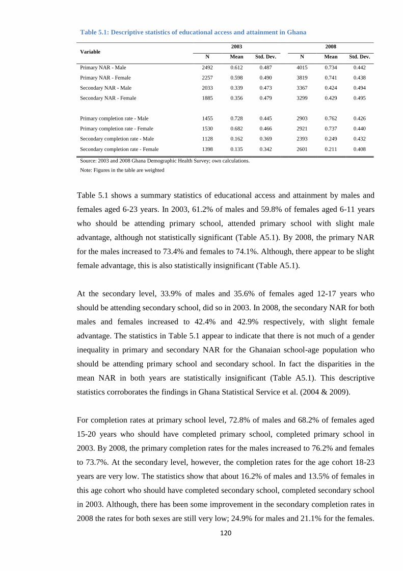
120
Table 5.1: Descriptive statistics of educational access and attainment in Ghana
Variable 2003
2008
N Mean Std. Dev. N Mean Std. Dev.
Primary NAR - Male 2492 0.612 0.487
4015 0.734 0.442
Primary NAR - Female 2257 0.598 0.490
3819 0.741 0.438
Secondary NAR - Male 2033 0.339 0.473
3367 0.424 0.494
Secondary NAR - Female 1885 0.356 0.479
3299 0.429 0.495
Primary completion rate - Male 1455 0.728 0.445
2903 0.762 0.426
Primary completion rate - Female 1530 0.682 0.466
2921 0.737 0.440
Secondary completion rate - Male 1128 0.162 0.369
2393 0.249 0.432
Secondary completion rate - Female 1398 0.135 0.342
2601 0.211 0.408
Source: 2003 and 2008 Ghana Demographic Health Survey; own calculations.
Note: Figures in the table are weighted
Table 5.1 shows a summary statistics of educational access and attainment by males and
females aged 6-23 years. In 2003, 61.2% of males and 59.8% of females aged 6-11 years
who should be attending primary school, attended primary school with slight male
advantage, although not statistically significant (Table A5.1). By 2008, the primary NAR
for the males increased to 73.4% and females to 74.1%. Although, there appear to be slight
female advantage, this is also statistically insignificant (Table A5.1).
At the secondary level, 33.9% of males and 35.6% of females aged 12-17 years who
should be attending secondary school, did so in 2003. In 2008, the secondary NAR for both
males and females increased to 42.4% and 42.9% respectively, with slight female
advantage. The statistics in Table 5.1 appear to indicate that there is not much of a gender
inequality in primary and secondary NAR for the Ghanaian school-age population who
should be attending primary school and secondary school. In fact the disparities in the
mean NAR in both years are statistically insignificant (Table A5.1). This descriptive
statistics corroborates the findings in Ghana Statistical Service et al. (2004 & 2009).
For completion rates at primary school level, 72.8% of males and 68.2% of females aged
15-20 years who should have completed primary school, completed primary school in
2003. By 2008, the primary completion rates for the males increased to 76.2% and females
to 73.7%. At the secondary level, however, the completion rates for the age cohort 18-23
years are very low. The statistics show that about 16.2% of males and 13.5% of females in
this age cohort who should have completed secondary school, completed secondary school
in 2003. Although, there has been some improvement in the secondary completion rates in
2008 the rates for both sexes are still very low; 24.9% for males and 21.1% for the females.
121
At both the primary and secondary school levels, it appears that males have slight
advantage in educational attainment over the females. These disparities are statistically
significant (Table A5.8) and consistent with the findings in Nguyen and Wodon (2014).
5.2.2 Gender inequality in educational outcomes among the poor and the non-poor
The descriptive statistics depicted by Tables 5.2 to 5.5 highlight the extent of gender
inequality in educational access and attainment by the distribution of household wealth at a
point in time and over a period of time (2003, 2008, and between 2003 and 2008). The
inequality is discussed at two main levels: (i) gender inequality in educational access; and
(ii) gender inequality in educational attainment. The gender inequality in educational
access is determined by primary school NAR of 6-11 year olds and secondary school NAR
of 12-17 year olds. At the attainment level, the gender inequality is determined by primary
completion rate by age cohort 15-20 year olds, and secondary completion rate by age
cohort 18-23 year olds. These classifications for the analysis have been discussed and
cross-referenced in Chapter 3. Tables 5.2 to 5.5 report: NAR and completion rates of males
and females by household wealth; gender gaps; and gender parity ratios for the selected
age cohorts. The descriptive statistics are summary measures that capture the share of both
the males and females who attended and completed primary and secondary school in 2003
and 2008 survey years.
5.2.2.1 Gender inequality in primary NAR by household wealth
Table 5.2 shows that among the top wealth quintile households; 78.9% of male and 77.0%
of female children of primary school-age who should be attending primary school did so in
2003, and 87.6% of male and 84.4% of female children who should be attending primary
school in 2008, did attend. The results indicate an increasing trend of inequality in access
to primary education between male and female children of primary school-age from the
richest households in favour of the males (1.9% points in 2003 and 3.2% points in 2008).
Among the bottom wealth quintile households; 43.7% of males and 41.9% of females of
primary school-age who should be attending primary school did so in 2003, and 58.2% of
males and 60.1% of females of primary school-age who should be attending primary
school did attend in 2008. There is an indication of slight gender gap in access to primary
education in favour of the males (1.8%) in 2003 which is almost equal to the size of the
gender gap shown in the top wealth quintile households in 2003.
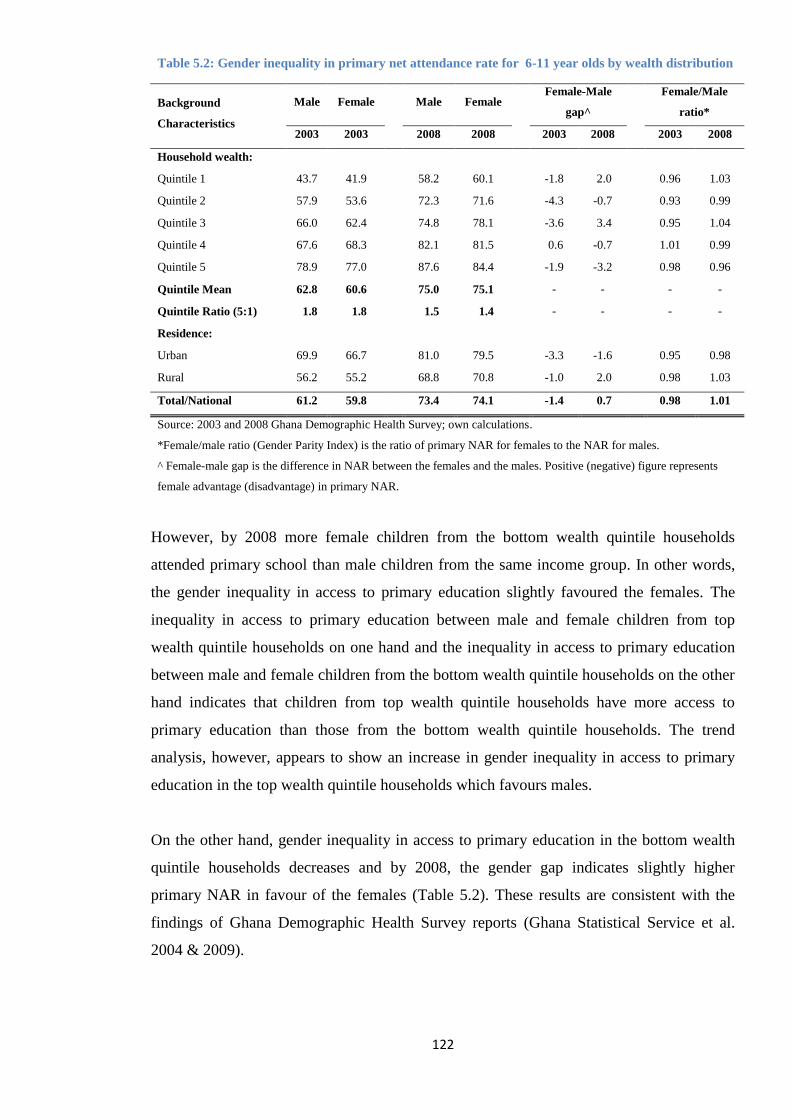
122
Table 5.2: Gender inequality in primary net attendance rate for 6-11 year olds by wealth distribution
Background
Characteristics
Male Female
Male Female
Female-Male
gap^
Female/Male
ratio*
2003 2003
2008 2008
2003 2008
2003 2008
Household wealth:
Quintile 1 43.7 41.9
58.2 60.1
-1.8 2.0
0.96 1.03
Quintile 2 57.9 53.6
72.3 71.6
-4.3 -0.7
0.93 0.99
Quintile 3 66.0 62.4
74.8 78.1
-3.6 3.4
0.95 1.04
Quintile 4 67.6 68.3
82.1 81.5
0.6 -0.7
1.01 0.99
Quintile 5 78.9 77.0
87.6 84.4
-1.9 -3.2
0.98 0.96
Quintile Mean 62.8 60.6 75.0 75.1 - - - -
Quintile Ratio (5:1) 1.8 1.8 1.5 1.4 - - - -
Residence:
Urban 69.9 66.7
81.0 79.5
-3.3 -1.6
0.95 0.98
Rural 56.2 55.2
68.8 70.8
-1.0 2.0
0.98 1.03
Total/National 61.2 59.8 73.4 74.1 -1.4 0.7 0.98 1.01
Source: 2003 and 2008 Ghana Demographic Health Survey; own calculations.
*Female/male ratio (Gender Parity Index) is the ratio of primary NAR for females to the NAR for males.
^ Female-male gap is the difference in NAR between the females and the males. Positive (negative) figure represents
female advantage (disadvantage) in primary NAR.
However, by 2008 more female children from the bottom wealth quintile households
attended primary school than male children from the same income group. In other words,
the gender inequality in access to primary education slightly favoured the females. The
inequality in access to primary education between male and female children from top
wealth quintile households on one hand and the inequality in access to primary education
between male and female children from the bottom wealth quintile households on the other
hand indicates that children from top wealth quintile households have more access to
primary education than those from the bottom wealth quintile households. The trend
analysis, however, appears to show an increase in gender inequality in access to primary
education in the top wealth quintile households which favours males.
On the other hand, gender inequality in access to primary education in the bottom wealth
quintile households decreases and by 2008, the gender gap indicates slightly higher
primary NAR in favour of the females (Table 5.2). These results are consistent with the
findings of Ghana Demographic Health Survey reports (Ghana Statistical Service et al.
2004 & 2009).
123
Furthermore, the wealth quintile mean of primary NAR for females has also improved by
14.5% between the two periods (60.6% in 2003 and 75.1% in 2008) compared to that of
the males of 12.2% within the same survey periods (62.8% in 2003 and 75.0% in 2008).
The wealth quintile ratio estimates the inequality between the richest and the poorest
households. The ratio shows that both male and female children from the richest
households have 1.8 times more primary NAR (i.e. more access to primary education) than
those from the poorest households in 2003. Although the wealth quintile ratios are still
high in 2008, there has been a slight improvement in primary NAR of females than males
from poorest households (Table 5.2).
In terms of the distributional effect of household wealth on gender inequality in access to
primary education, the NAR at the primary education level did not reveal much
educational inequality between male and female children from top wealth quintile
households compared to male and female children from the bottom wealth quintile
households. However, there appears to be more gender inequality in the primary NAR at
the top wealth quintile at the advantage of the males than at the bottom wealth quintile
level. In Table 5.2, more female children from the poorest households appear to have
attended primary school than male children from the poorest households in 2008 which is
consistent with the findings of Ghana Statistical Service et al. (2009). However, the results
generally appear to indicate that there is not much of a gender inequality in primary NAR
determined by household wealth distribution for the Ghanaian primary school-age
population who should be attending primary school. This descriptive analysis seems to
suggest that the FCUBE, SCG and SFP policy interventions might have reduced the
financial burden of the poor households of maintaining both male and female children in
school.
5.2.2.2 Gender inequality in secondary NAR by household wealth
Generally, the secondary attendance rates in most developing countries are significantly
lower than primary attendance rates (Porta et al. 2011). In Ghana, the secondary NAR is
just above 50% lower than the primary NAR (see Tables 5.2 and 5.3). In terms of gender
and wealth distribution, among the top wealth quintile households; 57.0% of the male
children and 56.5% of female children of secondary school-age who should be attending
secondary school did so in 2003, and 62.8% of male children and 59.1% of female children
of secondary school-age who should be attending secondary school were in school in 2008.
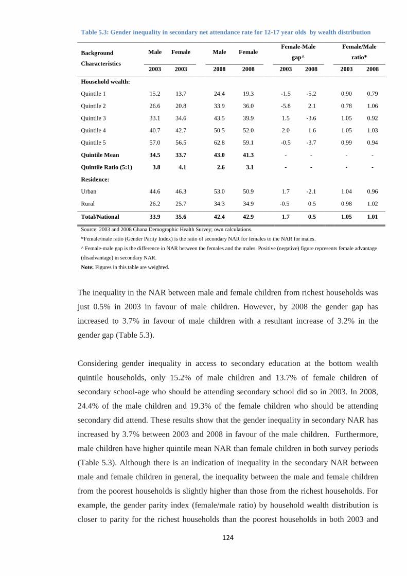
124
Table 5.3: Gender inequality in secondary net attendance rate for 12-17 year olds by wealth distribution
Background
Characteristics
Male Female
Male Female
Female-Male
gap^
Female/Male
ratio*
2003 2003
2008 2008
2003 2008
2003 2008
Household wealth:
Quintile 1 15.2 13.7
24.4 19.3
-1.5 -5.2
0.90 0.79
Quintile 2 26.6 20.8
33.9 36.0
-5.8 2.1
0.78 1.06
Quintile 3 33.1 34.6
43.5 39.9
1.5 -3.6
1.05 0.92
Quintile 4 40.7 42.7
50.5 52.0
2.0 1.6
1.05 1.03
Quintile 5 57.0 56.5
62.8 59.1
-0.5 -3.7
0.99 0.94
Quintile Mean 34.5 33.7 43.0 41.3 - - - -
Quintile Ratio (5:1) 3.8 4.1 2.6 3.1 - - - -
Residence:
Urban 44.6 46.3
53.0 50.9
1.7 -2.1
1.04 0.96
Rural 26.2 25.7
34.3 34.9
-0.5 0.5
0.98 1.02
Total/National 33.9 35.6
42.4 42.9
1.7 0.5
1.05 1.01
Source: 2003 and 2008 Ghana Demographic Health Survey; own calculations.
*Female/male ratio (Gender Parity Index) is the ratio of secondary NAR for females to the NAR for males.
^ Female-male gap is the difference in NAR between the females and the males. Positive (negative) figure represents female advantage
(disadvantage) in secondary NAR.
Note: Figures in this table are weighted.
The inequality in the NAR between male and female children from richest households was
just 0.5% in 2003 in favour of male children. However, by 2008 the gender gap has
increased to 3.7% in favour of male children with a resultant increase of 3.2% in the
gender gap (Table 5.3).
Considering gender inequality in access to secondary education at the bottom wealth
quintile households, only 15.2% of male children and 13.7% of female children of
secondary school-age who should be attending secondary school did so in 2003. In 2008,
24.4% of the male children and 19.3% of the female children who should be attending
secondary did attend. These results show that the gender inequality in secondary NAR has
increased by 3.7% between 2003 and 2008 in favour of the male children. Furthermore,
male children have higher quintile mean NAR than female children in both survey periods
(Table 5.3). Although there is an indication of inequality in the secondary NAR between
male and female children in general, the inequality between the male and female children
from the poorest households is slightly higher than those from the richest households. For
example, the gender parity index (female/male ratio) by household wealth distribution is
closer to parity for the richest households than the poorest households in both 2003 and
125
2008. It is also worth noting that even though the gender gap in the NAR increases and
gender parity index of the NAR decreases at both the top and bottom wealth quintile levels
in 2008, the inequality in access to secondary education is more pronounced in the poorest
households. Also, the wealth quintile ratios show that the inequality between the female
children from the richest and the poorest households are marginally higher than the
inequality between the male children from the richest and the poorest households.
In summary, household wealth distribution appears not to account for gender inequality in
primary NAR between the richest and the poorest households. However, there is an
indication that at the secondary education level, household wealth distribution appears to
have increased the gender inequality in secondary NAR of the poorest households than the
richest households in Ghana. Furthermore, it is worth noting that without taking into
account household wealth distribution, there is no discernible gender inequality in primary
and secondary NARs for the Ghanaian primary and secondary school-age who should be
attending school (see Tables 5.2 and 5.3). These findings are consistent with the findings
in Ghana Statistical Service et al. (2004 & 2009) reports.
5.2.2.3 Gender inequality in primary school completion by household wealth distribution
Among the top wealth quintile households, the primary completion rate is 91.6% and 85.3%
for male and female children respectively, with 6.3% inequality gap in favour of male
children and 0.93 gender parity index in 2003. In 2008, the completion rates increased to
96.0% for male children and 90.0% for the female children with corresponding 5.8%
inequality gap in favour of male children and 0.94 gender parity index. These results
appear to show that even in the richest households, male children do have slight advantage
in primary school attainment. Table 5.4 shows that about 6.0% more male than female
children completed primary education in both 2003 and 2008 based on household wealth
distribution in Ghana.
In terms of wealth distribution at the bottom 20% of the population, the completion rates
for both male and female children in this income group is less than 50% of the completion
rates for the male and female children from top wealth quintile households in 2003 and
2008. Table 5.4 also shows that among the bottom wealth quintile households, the primary
completion rate is 44.4% and 35.9% for male and female children respectively, with 8.5%
gender gap and 0.81 gender parity index in 2003.
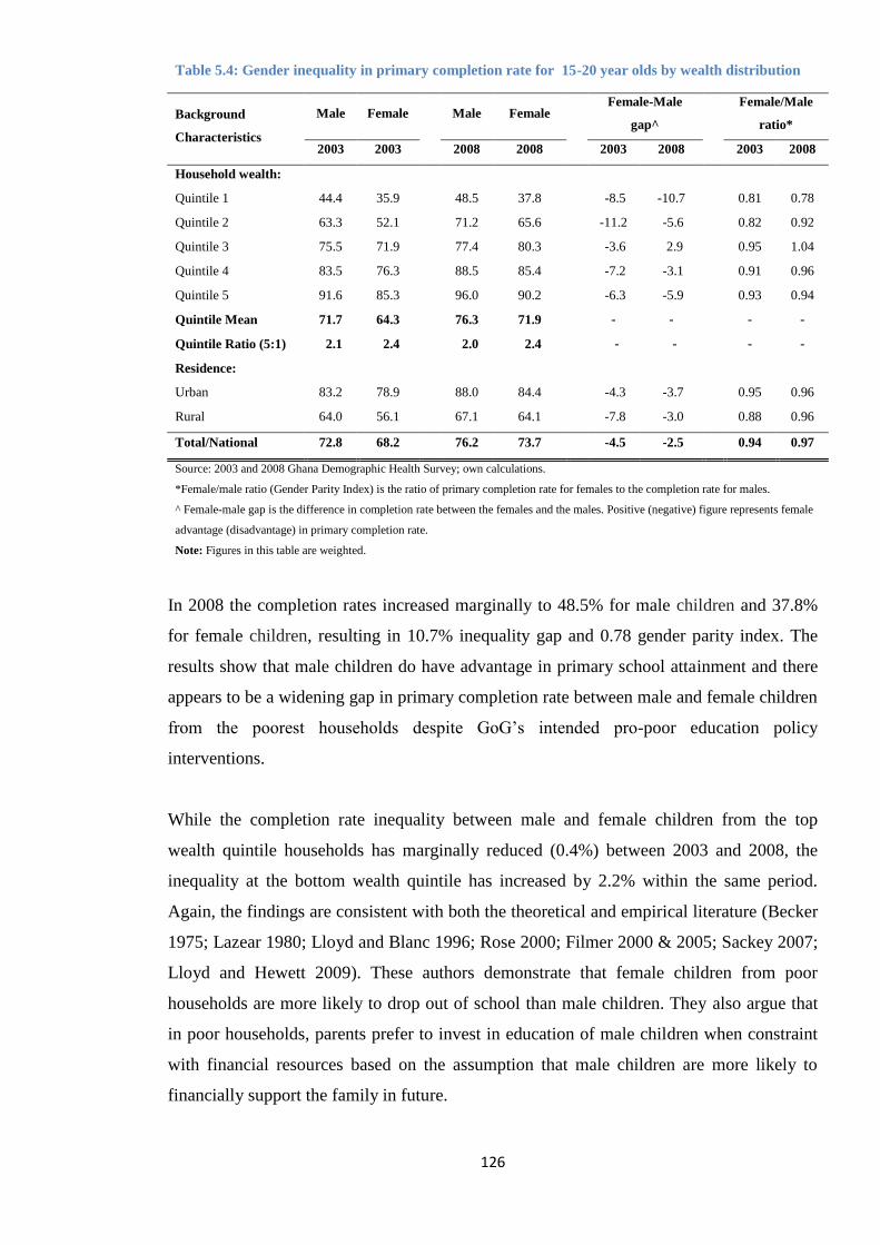
126
Table 5.4: Gender inequality in primary completion rate for 15-20 year olds by wealth distribution
Background
Characteristics
Male Female
Male Female
Female-Male
gap^
Female/Male
ratio*
2003 2003
2008 2008
2003 2008
2003 2008
Household wealth:
Quintile 1 44.4 35.9
48.5 37.8
-8.5 -10.7
0.81 0.78
Quintile 2 63.3 52.1
71.2 65.6
-11.2 -5.6
0.82 0.92
Quintile 3 75.5 71.9
77.4 80.3
-3.6 2.9
0.95 1.04
Quintile 4 83.5 76.3
88.5 85.4
-7.2 -3.1
0.91 0.96
Quintile 5 91.6 85.3
96.0 90.2
-6.3 -5.9
0.93 0.94
Quintile Mean 71.7 64.3 76.3 71.9 - - - -
Quintile Ratio (5:1) 2.1 2.4 2.0 2.4 - - - -
Residence:
Urban 83.2 78.9
88.0 84.4
-4.3 -3.7
0.95 0.96
Rural 64.0 56.1
67.1 64.1
-7.8 -3.0
0.88 0.96
Total/National 72.8 68.2
76.2 73.7
-4.5 -2.5
0.94 0.97
Source: 2003 and 2008 Ghana Demographic Health Survey; own calculations.
*Female/male ratio (Gender Parity Index) is the ratio of primary completion rate for females to the completion rate for males.
^ Female-male gap is the difference in completion rate between the females and the males. Positive (negative) figure represents female
advantage (disadvantage) in primary completion rate.
Note: Figures in this table are weighted.
In 2008 the completion rates increased marginally to 48.5% for male children and 37.8%
for female children, resulting in 10.7% inequality gap and 0.78 gender parity index. The
results show that male children do have advantage in primary school attainment and there
appears to be a widening gap in primary completion rate between male and female children
from the poorest households despite GoG’s intended pro-poor education policy
interventions.
While the completion rate inequality between male and female children from the top
wealth quintile households has marginally reduced (0.4%) between 2003 and 2008, the
inequality at the bottom wealth quintile has increased by 2.2% within the same period.
Again, the findings are consistent with both the theoretical and empirical literature (Becker
1975; Lazear 1980; Lloyd and Blanc 1996; Rose 2000; Filmer 2000 & 2005; Sackey 2007;
Lloyd and Hewett 2009). These authors demonstrate that female children from poor
households are more likely to drop out of school than male children. They also argue that
in poor households, parents prefer to invest in education of male children when constraint
with financial resources based on the assumption that male children are more likely to
financially support the family in future.
127
5.2.2.4 Gender inequality in secondary school completion by wealth distribution
Secondary completion rates for both male and female children by income groups are very
low compared to primary completion rates in Ghana (see Tables 5.4 and 5.5). Among the
top wealth quintile households, the secondary completion rate is 39.7% and 33.7% for
male and female children respectively, in 2003. In 2008 the completion rates have
significantly increased to; 54.3% for male children, and 50.0% for female children. Thus,
the gender gap in secondary education attainment has reduced from 6.0% in 2003 to 4.3%
in 2008 and gender parity index has also increased from 0.85 in 2003 to 0.92 points in
2008 (Table 5.5).
It is not surprising to see from Table 5.5 that the secondary school completion rates for
both male and female children from the bottom wealth quintiles households are
significantly very low compared to the secondary completion rates for male and female
children from the top wealth quintiles. Again, it is important to emphasise that secondary
education is not free in Ghana and there are no education policy interventions to reduce the
education cost borne by households or parents. In effect, this might have affected the
completion rates for both male and female children from the lowest income groups in the
country. The completion rate for female children from poorest households increased from
just 1.0% in 2003 to 1.9% in 2008 and for male children from the same income group, the
rate increased from 3.5% in 2003 to 5.4% in 2008. Although the gender gaps appear to be
smaller, the gender parity index of 0.29 and 0.34 points respectively, in 2003 and 2008
shows the magnitude of gender inequality in secondary education attainment at the bottom
level of wealth distribution in Ghana (Table 5.5). The gender inequality in secondary
education attainment exhibited at bottom level of wealth distribution could perpetuate
gender inequality in future labour market outcomes and socioeconomic status of the poor
households (Filmer 2005). This may also result in intergenerational poverty cycle of the
poor households. The findings at the secondary education level are extremely important for
policy targeting if the GoG is to achieve poverty reduction target stipulated in Vision 2020
and Ghana Poverty Reduction Strategy (Republic of Ghana 1997 & 2003).
Furthermore, the results in Table 5.4 and 5.5 corroborate the findings of (Holmes 2003;
Lloyd and Hewett 2009). The authors find that the extent of inequality among female
children in school attendance and completion rates according to socioeconomic status is
found to be substantially greater than for male children.
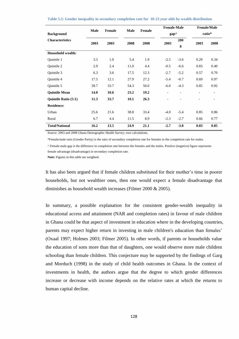
128
Table 5.5: Gender inequality in secondary completion rate for 18-23 year olds by wealth distribution
Background
Characteristics
Male Female
Male Female
Female-Male
gap^
Female/Male
ratio*
2003 2003
2008 2008
2003 200
8 2003 2008
Household wealth:
Quintile 1 3.5 1.0
5.4 1.9
-2.5 -3.6
0.29 0.34
Quintile 2 2.9 2.4
11.0 4.4
-0.5 -6.6
0.83 0.40
Quintile 3 6.3 3.6
17.5 12.3
-2.7 -5.2
0.57 0.70
Quintile 4 17.5 12.1
27.9 27.2
-5.4 -0.7
0.69 0.97
Quintile 5 39.7 33.7
54.3 50.0
-6.0 -4.3
0.85 0.92
Quintile Mean 14.0 10.6 23.2 19.2 - - - -
Quintile Ratio (5:1) 11.3 33.7 10.1 26.3 - - - -
Residence:
Urban 25.6 21.6
38.8 33.4
-4.0 -5.4
0.85 0.86
Rural 6.7 4.4
11.5 8.9
-2.3 -2.7
0.66 0.77
Total/National 16.2 13.5
24.9 21.1
-2.7 -3.8
0.83 0.85
Source: 2003 and 2008 Ghana Demographic Health Survey; own calculations.
*Female/male ratio (Gender Parity) is the ratio of secondary completion rate for females to the completion rate for males.
^ Female-male gap is the difference in completion rate between the females and the males. Positive (negative) figure represents
female advantage (disadvantage) in secondary completion rate.
Note: Figures in this table are weighted.
It has also been argued that if female children substituted for their mother’s time in poorer
households, but not wealthier ones, then one would expect a female disadvantage that
diminishes as household wealth increases (Filmer 2000 & 2005).
In summary, a possible explanation for the consistent gender-wealth inequality in
educational access and attainment (NAR and completion rates) in favour of male children
in Ghana could be that aspect of investment in education where in the developing countries,
parents may expect higher return in investing in male children's education than females’
(Oxaal 1997; Holmes 2003; Filmer 2005). In other words, if parents or households value
the education of sons more than that of daughters, one would observe more male children
schooling than female children. This conjecture may be supported by the findings of Garg
and Morduch (1998) in the study of child health outcomes in Ghana. In the context of
investments in health, the authors argue that the degree to which gender differences
increase or decrease with income depends on the relative rates at which the returns to
human capital decline.
129
However, the question as to whether the household wealth distribution is enough to explain
these wealth-related inequalities in educational access and attainment of male and female
children at both primary and secondary school levels in Ghana is further explored using
regression analysis in Sections 5.3 and 5.4.
5. 3 Regression results and discussions
The regression model specified in Chapter 4 sub-section 4.3.2 is re-estimated separately for
male and female so that the impact of all covariates is allowed to differ by gender of the
school-age children. These estimates are represented in Tables 5.6 and 5.7. We present and
discuss the regression results pertaining to school attendance and completion at both
primary and secondary school levels. The results in Tables 5.6 and 5.7 are obtained by
estimating Equation 4.1 in Chapter 4 separately for males and females using STATA/SE
11 software. A positive (negative) and statistically significant marginal effect indicates that
the relevant determinant enhances (decreases) the probability of educational access
(attendance) and educational attainment (completion).
5.3.1 Inequality in primary and secondary school attendance
The results of the determinants of disparity in educational access of males and females are
shown by marginal effects together with the corresponding z-values in parentheses. These
results are based on the binary probit estimation of current school attendance of male and
female children aged 6-11 years and 12-17 years old in Table 5.6. The likelihood ratio 2
test shows that the model is well fit. The predicted probability for primary school
attendance increased from 59.3% in 2003 to 72.9% in 2008 for male children. For female
children, the predicted probability for primary school attendance increased from 58.3% in
2003 to 74.0% in 2008. At the secondary school level, the predicted probabilities for male
and female children are very low in both 2003 and 2008 compared to primary school
attendance results. The predicted probabilities for secondary school attendance were 28.6%
in 2003 and 38.0% in 2008 for the male children, and 30.4% in 2003 and 39.5% in 2008
for the female children. The results at both primary and secondary school levels support
the results from the descriptive analysis in Section 5.2 based on Tables 5.2 and 5.3.
5.3.1.1 Access to primary education
Table 5.6 shows that household wealth is a significant determinant of inequality in school
attendance for both male and female children in Ghana. The impact of household wealth is
positive and statistically significant at all levels of wealth distribution on primary school
130
attendance of male children in both 2003 and 2008. For female children, the impact of
household wealth is also statistically significant at all levels of wealth distribution except at
the second quintile level (i.e. poor) in both 2003 and 2008. In 2003, the impact of
household wealth on primary school attendance of children from rich households appears
to be higher for female than male children. The marginal effect of moving from the third
quintile (middle welfare group) to the fifth quintile (richest household) increases the
probability of female primary school attendance from 14.0 to 25.6 percentage points
compared to 15.1% to 22.5% for male children in 2003 (Table 5.6). The results shows that
the marginal effect of household wealth distribution on female children’s primary school
attendance on average is about 1.3 times larger than for the male children. This finding is
consistent with the findings of Sackey (2007). The finding also supports the suggestion that
the larger wealth effect for girls from rich households can be explained in terms of
financial capability of wealthy households to hire help for childcare and other household
work, thereby reducing female children’s domestic tasks (Appleton 1995; Glick and Sahn
2000).
Furthermore, Glick and Sahn (2000:82) also argue that "increases in household income
will disproportionately benefit girls’ schooling because they relax the time constraints that
girls face". Another theoretical explanation offered in the literature is that in the rich
households, there is a relaxation of credit constraints with increased household income that
enables rich households to undertake less remunerative investments in female children's
schooling while poor households can only afford to educate male children (Glick and Sahn
2000).
In case of children from poor households (second and third quintiles), the impact of
household wealth on primary school attendance is higher for male than for female children.
For example, the marginal impact of household wealth on primary attendance is 1.1 times
(i.e. 0.151 vs. 0.140) larger for male than for female children. This result again supports
the findings of Appleton (1995) and Glick and Sahn (2000). The results from Table 5.6
may imply that poor households could not afford to hire help for childcare and other
household work to reduce female children’s domestic tasks. Consequently, female children
from poor households are disadvantaged in school attendance compared to those from rich
households. The positive marginal effect of household wealth distribution on both male
and female children’s primary school attendance is much reduced in 2008 compared to
2003.
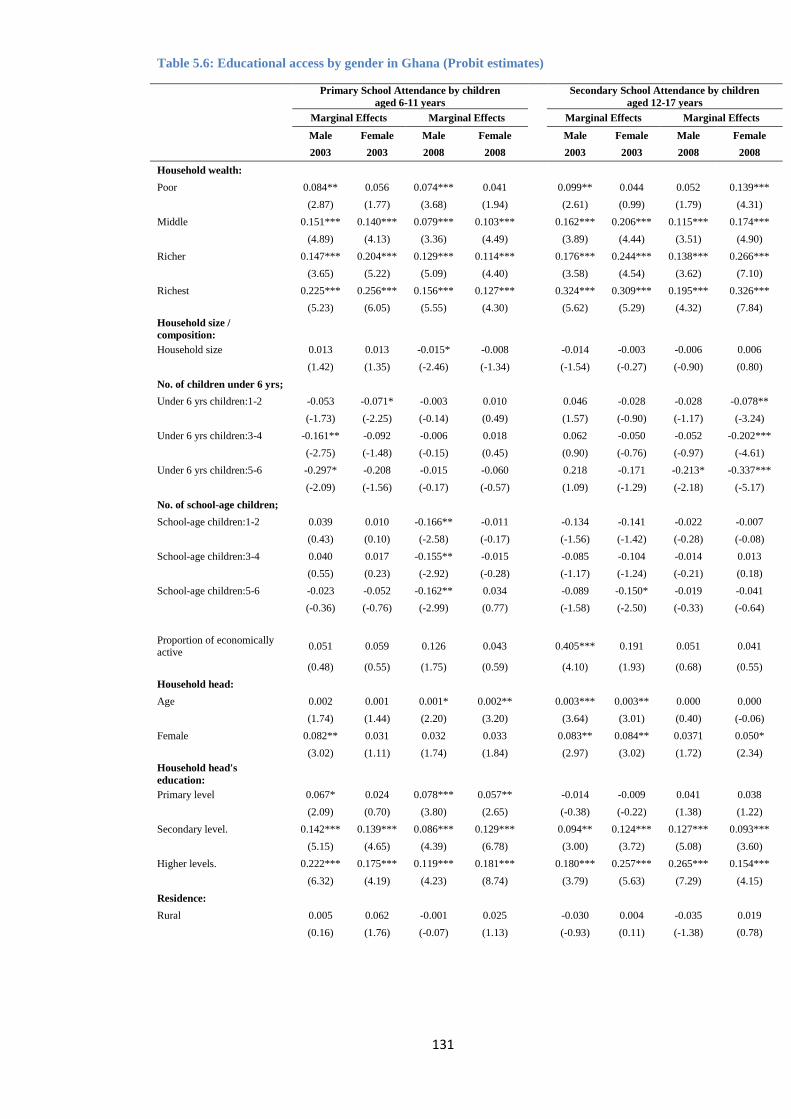
131
Table 5.6: Educational access by gender in Ghana (Probit estimates)
Primary School Attendance by children
aged 6-11 years
Secondary School Attendance by children
aged 12-17 years
Marginal Effects Marginal Effects
Marginal Effects Marginal Effects
Male Female Male Female
Male Female Male Female
2003 2003 2008 2008 2003 2003 2008 2008
Household wealth:
Poor 0.084** 0.056 0.074*** 0.041
0.099** 0.044 0.052 0.139***
(2.87) (1.77) (3.68) (1.94)
(2.61) (0.99) (1.79) (4.31)
Middle 0.151*** 0.140*** 0.079*** 0.103***
0.162*** 0.206*** 0.115*** 0.174***
(4.89) (4.13) (3.36) (4.49)
(3.89) (4.44) (3.51) (4.90)
Richer 0.147*** 0.204*** 0.129*** 0.114***
0.176*** 0.244*** 0.138*** 0.266***
(3.65) (5.22) (5.09) (4.40)
(3.58) (4.54) (3.62) (7.10)
Richest 0.225*** 0.256*** 0.156*** 0.127***
0.324*** 0.309*** 0.195*** 0.326***
(5.23) (6.05) (5.55) (4.30)
(5.62) (5.29) (4.32) (7.84)
Household size /
composition:
Household size 0.013 0.013 -0.015* -0.008
-0.014 -0.003 -0.006 0.006
(1.42) (1.35) (-2.46) (-1.34)
(-1.54) (-0.27) (-0.90) (0.80)
No. of children under 6 yrs;
Under 6 yrs children:1-2 -0.053 -0.071* -0.003 0.010
0.046 -0.028 -0.028 -0.078**
(-1.73) (-2.25) (-0.14) (0.49)
(1.57) (-0.90) (-1.17) (-3.24)
Under 6 yrs children:3-4 -0.161** -0.092 -0.006 0.018
0.062 -0.050 -0.052 -0.202***
(-2.75) (-1.48) (-0.15) (0.45)
(0.90) (-0.76) (-0.97) (-4.61)
Under 6 yrs children:5-6 -0.297* -0.208 -0.015 -0.060
0.218 -0.171 -0.213* -0.337***
(-2.09) (-1.56) (-0.17) (-0.57)
(1.09) (-1.29) (-2.18) (-5.17)
No. of school-age children;
School-age children:1-2 0.039 0.010 -0.166** -0.011
-0.134 -0.141 -0.022 -0.007
(0.43) (0.10) (-2.58) (-0.17)
(-1.56) (-1.42) (-0.28) (-0.08)
School-age children:3-4 0.040 0.017 -0.155** -0.015
-0.085 -0.104 -0.014 0.013
(0.55) (0.23) (-2.92) (-0.28)
(-1.17) (-1.24) (-0.21) (0.18)
School-age children:5-6 -0.023 -0.052 -0.162** 0.034
-0.089 -0.150* -0.019 -0.041
(-0.36) (-0.76) (-2.99) (0.77)
(-1.58) (-2.50) (-0.33) (-0.64)
Proportion of economically active
0.051 0.059 0.126 0.043
0.405*** 0.191 0.051 0.041
(0.48) (0.55) (1.75) (0.59)
(4.10) (1.93) (0.68) (0.55)
Household head:
Age 0.002 0.001 0.001* 0.002**
0.003*** 0.003** 0.000 0.000
(1.74) (1.44) (2.20) (3.20)
(3.64) (3.01) (0.40) (-0.06)
Female 0.082** 0.031 0.032 0.033
0.083** 0.084** 0.0371 0.050*
(3.02) (1.11) (1.74) (1.84)
(2.97) (3.02) (1.72) (2.34)
Household head's
education:
Primary level 0.067* 0.024 0.078*** 0.057**
-0.014 -0.009 0.041 0.038
(2.09) (0.70) (3.80) (2.65)
(-0.38) (-0.22) (1.38) (1.22)
Secondary level. 0.142*** 0.139*** 0.086*** 0.129***
0.094** 0.124*** 0.127*** 0.093***
(5.15) (4.65) (4.39) (6.78)
(3.00) (3.72) (5.08) (3.60)
Higher levels. 0.222*** 0.175*** 0.119*** 0.181***
0.180*** 0.257*** 0.265*** 0.154***
(6.32) (4.19) (4.23) (8.74)
(3.79) (5.63) (7.29) (4.15)
Residence:
Rural 0.005 0.062 -0.001 0.025
-0.030 0.004 -0.035 0.019
(0.16) (1.76) (-0.07) (1.13)
(-0.93) (0.11) (-1.38) (0.78)
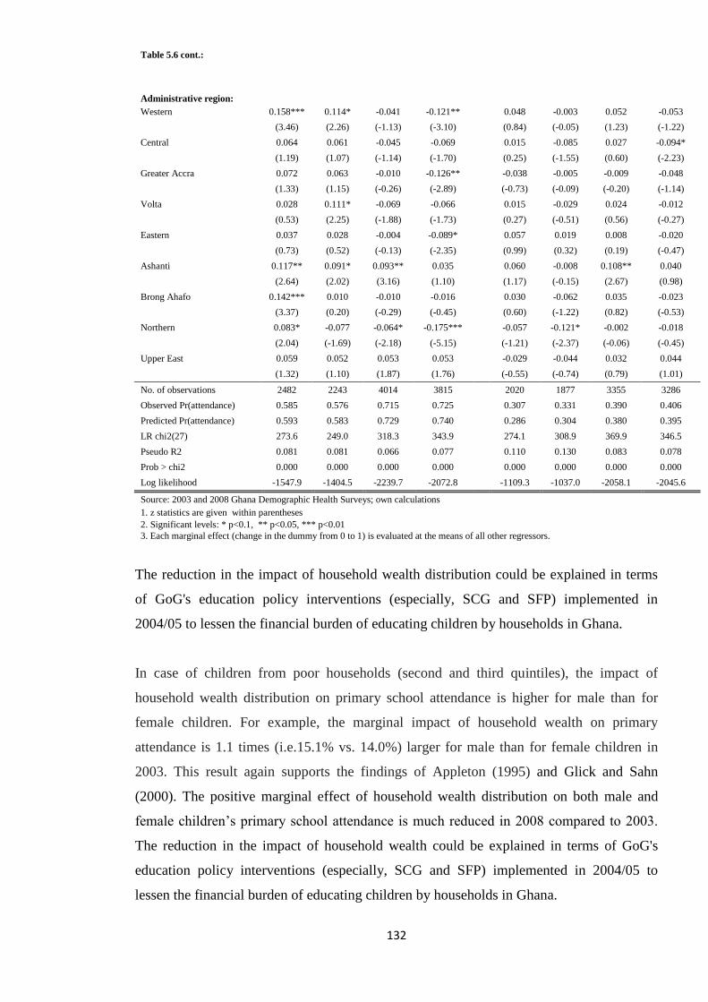
132
Table 5.6 cont.:
Administrative region:
Western 0.158*** 0.114* -0.041 -0.121**
0.048 -0.003 0.052 -0.053
(3.46) (2.26) (-1.13) (-3.10)
(0.84) (-0.05) (1.23) (-1.22)
Central 0.064 0.061 -0.045 -0.069
0.015 -0.085 0.027 -0.094*
(1.19) (1.07) (-1.14) (-1.70)
(0.25) (-1.55) (0.60) (-2.23)
Greater Accra 0.072 0.063 -0.010 -0.126**
-0.038 -0.005 -0.009 -0.048
(1.33) (1.15) (-0.26) (-2.89)
(-0.73) (-0.09) (-0.20) (-1.14)
Volta 0.028 0.111* -0.069 -0.066
0.015 -0.029 0.024 -0.012
(0.53) (2.25) (-1.88) (-1.73)
(0.27) (-0.51) (0.56) (-0.27)
Eastern 0.037 0.028 -0.004 -0.089*
0.057 0.019 0.008 -0.020
(0.73) (0.52) (-0.13) (-2.35)
(0.99) (0.32) (0.19) (-0.47)
Ashanti 0.117** 0.091* 0.093** 0.035
0.060 -0.008 0.108** 0.040
(2.64) (2.02) (3.16) (1.10)
(1.17) (-0.15) (2.67) (0.98)
Brong Ahafo 0.142*** 0.010 -0.010 -0.016
0.030 -0.062 0.035 -0.023
(3.37) (0.20) (-0.29) (-0.45)
(0.60) (-1.22) (0.82) (-0.53)
Northern 0.083* -0.077 -0.064* -0.175***
-0.057 -0.121* -0.002 -0.018
(2.04) (-1.69) (-2.18) (-5.15)
(-1.21) (-2.37) (-0.06) (-0.45)
Upper East 0.059 0.052 0.053 0.053
-0.029 -0.044 0.032 0.044
(1.32) (1.10) (1.87) (1.76) (-0.55) (-0.74) (0.79) (1.01)
No. of observations 2482 2243 4014 3815
2020 1877 3355 3286
Observed Pr(attendance) 0.585 0.576 0.715 0.725
0.307 0.331 0.390 0.406
Predicted Pr(attendance) 0.593 0.583 0.729 0.740
0.286 0.304 0.380 0.395
LR chi2(27) 273.6 249.0 318.3 343.9
274.1 308.9 369.9 346.5
Pseudo R2 0.081 0.081 0.066 0.077
0.110 0.130 0.083 0.078
Prob > chi2 0.000 0.000 0.000 0.000
0.000 0.000 0.000 0.000
Log likelihood -1547.9 -1404.5 -2239.7 -2072.8
-1109.3 -1037.0 -2058.1 -2045.6
Source: 2003 and 2008 Ghana Demographic Health Surveys; own calculations
1. z statistics are given within parentheses
2. Significant levels: * p<0.1, ** p<0.05, *** p<0.01
3. Each marginal effect (change in the dummy from 0 to 1) is evaluated at the means of all other regressors.
The reduction in the impact of household wealth distribution could be explained in terms
of GoG's education policy interventions (especially, SCG and SFP) implemented in
2004/05 to lessen the financial burden of educating children by households in Ghana.
In case of children from poor households (second and third quintiles), the impact of
household wealth distribution on primary school attendance is higher for male than for
female children. For example, the marginal impact of household wealth on primary
attendance is 1.1 times (i.e.15.1% vs. 14.0%) larger for male than for female children in
2003. This result again supports the findings of Appleton (1995) and Glick and Sahn
(2000). The positive marginal effect of household wealth distribution on both male and
female children’s primary school attendance is much reduced in 2008 compared to 2003.
The reduction in the impact of household wealth could be explained in terms of GoG's
education policy interventions (especially, SCG and SFP) implemented in 2004/05 to
lessen the financial burden of educating children by households in Ghana.
133
It also appears the policy interventions might have helped to reduce the impact of
household wealth on primary school attendance and consequently increased access to
primary education for both male and female children. However, it is worth noting that in
2008, household wealth distribution has larger marginal effect on primary school
attendance of male children than the female children from rich households. While in the
poor households the impact of the household wealth distribution was larger for the female
than male children.
However, taking the average impact of wealth distribution on primary school attendance in
2003 and 2008, the results from Table 5.6 appear to indicate that the disparity in primary
school attendance of both male and female children is greater at lower wealth levels and
declines with higher wealth levels. This finding corroborates the findings of Garg and
Morduch (1998), Alderman and King (1998) and it is also supported by the descriptive
findings in Table 5.2.
Primary school attendance is also strongly dependent on household head's educational
attainment levels. The positive impact of household head's education level is consistent
with the findings of other studies (Glick and Sahn 2000; Deininger 2003; Sackey 2007;
Mani et al. 2009). A possible explanation could be that educated household heads are able
to provide home inputs, such as supervision and support which encourage educational
participation of children. An increase in household head's educational attainment level
from primary school to higher levels increases the probability of primary school attendance
from 6.7% to 22.2% for male children and 2.4% to 17.5% for female children in 2003.
This implies that in 2003 the education attainment levels of household heads had a greater
impact on male children’s primary school attendance than that of female children.
However, by 2008 the trend of the impact has changed in favour of the female children.
Household heads’ educational attainment at all levels increases the probability of male
children’s primary school attendance by 7.8% to 11.9%, and female children’s primary
school attendance by 5.7% to 18.1%. Although the marginal effect of household head
educational attainment levels did not reveal much gender inequality in access to primary
education, the key finding is that, the higher the level of the household head educational
attainment the more favourable is the school attendance of both male and female children
in the household.
134
5.3.1.2 Access to secondary education
The positive impact of household wealth distribution on secondary school attendance of
both male and female children shown in Table 5.6 is relatively higher compared to primary
school attendance by both sexes. A plausible explanation is that at the secondary education
level, there is no policy intervention by the GoG to reduce the cost of education borne by
households. Consequently, household wealth is more likely to be crucial in determining
access to secondary education than primary education. In addition, borrowing constraints
are more likely to have remained a major barrier to secondary education access by poor
households. The marginal effect of household wealth is statistically significant at all levels
of wealth distribution on secondary school attendance of male children in 2003 and female
children in 2008. For female children in 2003 and male children in 2008, the impact of
household wealth is also statistically significant at all levels of wealth distribution except at
the second wealth quintile level (i.e. poor). In both 2003 and 2008, the impact of household
wealth on secondary school attendance is higher for female than male children.
The marginal effect of moving from the third quintile (middle welfare group) to the fifth
quintile (richest household) increases the probability of female secondary school
attendance from 20.6% to 30.9% compared to 16.2% to 32.4% for male children. Although
in 2008 the marginal effect of wealth distribution of households on male children’s
secondary school attendance reduced from 11.5% (middle quintile) to 19.5% (fifth
quintile), the marginal effect of wealth distribution on female children’s secondary school
attendance increased from 13.9% (second quintile) to 32.6% (fifth quintile). These results
are consistent with the results obtained from primary school attendance and corroborate the
findings of other researchers (Appleton 1995; Glick and Sahn 2000; Sackey 2007). The
plausible explanations for the increase in probability of female school attendance as one
moves up the household wealth distribution has been explored under the primary education
access and these explanations also apply to secondary education access by the female
children.
Another variable which has strong marginal effect on secondary school attendance of both
sexes is household head’s level of education attained. Unlike primary school attendance,
the marginal effect of the level of household head’s educational attainment is only
statistically significant at secondary and higher levels with reference to no education
(reference category). An increase in household head's educational attainment level from
secondary to higher levels increases the probability of secondary school attendance from
9.4% to 18.0% for male children and 12.4% to 25.7% for female children in 2003 (see
135
Table 5.6). At both levels of household head education, the probability of secondary school
attendance is higher for female than male children. Although in 2008 the probability of
school attendance increases as the level of household education increases, male children
have recorded higher school attendance than the female children. There appears to be no
consistent trend in the impact of household head level of education attainment to reveal
gender inequality in access to secondary education between 2003 and 2008. However,
there is an indication that the higher the level of the household head educational attainment
the more favourable is secondary school attendance of both male and female children in
the household. The positive impact of household head's education level supports the earlier
findings with respect to primary education access and also corroborates the findings of
other studies (Glick and Sahn 2000; Deininger 2003; Sackey 2007; Mani et al. 2009;
Filmer 2005).
5.3.2 Inequality in primary and secondary school completion
Table 5.7 shows marginal effects (with the corresponding z-values) from the binary probit
estimation of educational attainment (school completion) based on Equation 5.1. We
estimate educational attainment based on age cohort 15-20 years (for primary completion)
and age cohort 18-23 years (for secondary completion) for both males and females in 2003
and 2008. The likelihood ratio 2
test shows that the model is well fit. The predicted
probability for primary school completion increased from 73.4% in 2003 to 77.1% in 2008
for the male age cohort. For female age cohort, the predicted probability for primary school
completion increased from 66.9% in 2003 to 74.0% in 2008. At the secondary school level,
the predicted probabilities for male and female age cohorts are very low in both 2003 and
2008 compared to primary school completion probabilities within the same periods. The
predicted probabilities for secondary school completion were 8.3% in 2003 and 17.6% in
2008 for the male age cohort, and 5.0% in 2003 and 11.4% in 2008 for the female age
cohort. The results at both primary and secondary school levels support the results from the
descriptive analysis in Section 5.2 based on Tables 5.4 and 5.5.
5.3.2.1 Primary education attainment
The results in Table 5.7 indicate that wealth distribution positively influences primary
school attainment of children irrespective of gender. The household wealth impact on
primary completion in 2003 is statistically significant at all levels of wealth distribution
except at the second wealth quintile (i.e. poor) with first wealth quintile (poorest) being the
reference category. Table 5.7 shows that the marginal effect of moving from the third
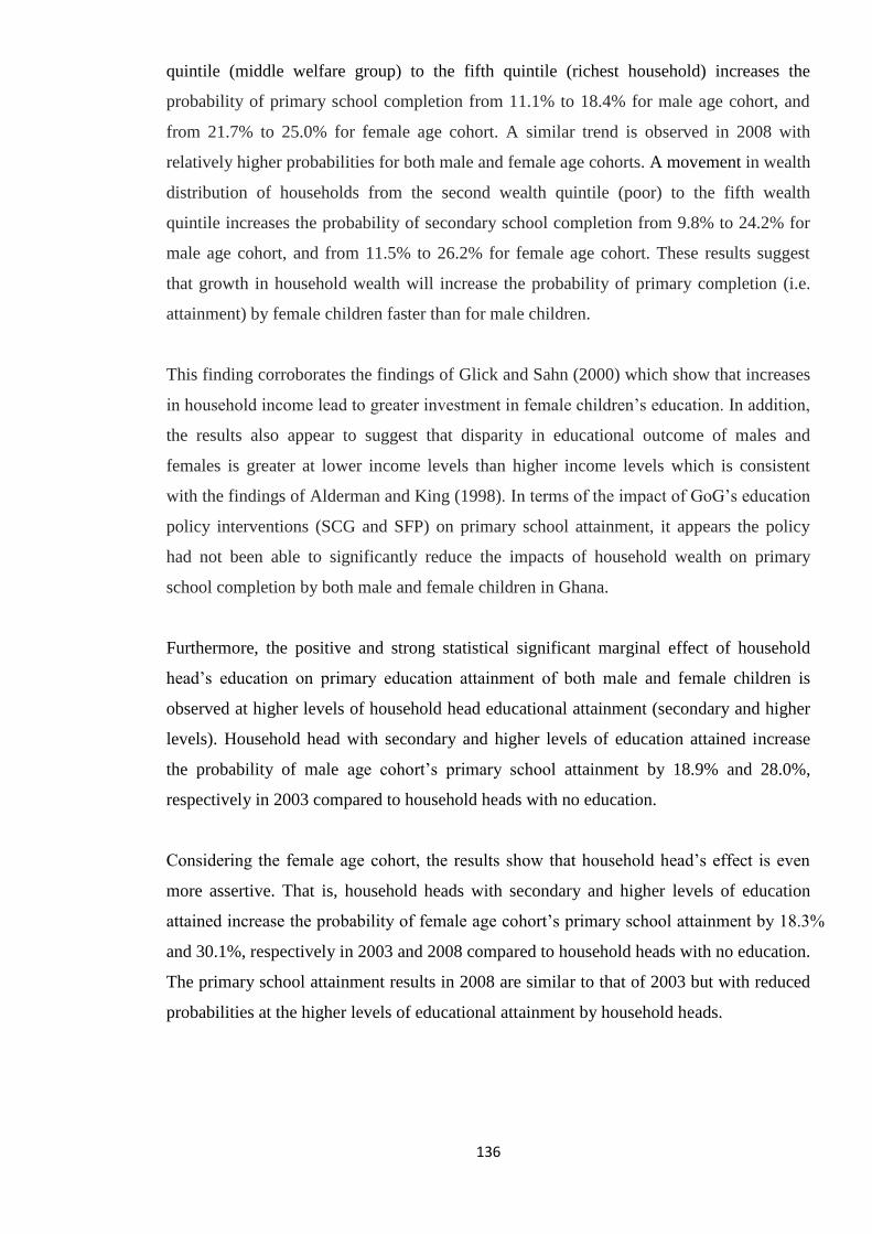
136
quintile (middle welfare group) to the fifth quintile (richest household) increases the
probability of primary school completion from 11.1% to 18.4% for male age cohort, and
from 21.7% to 25.0% for female age cohort. A similar trend is observed in 2008 with
relatively higher probabilities for both male and female age cohorts. A movement in wealth
distribution of households from the second wealth quintile (poor) to the fifth wealth
quintile increases the probability of secondary school completion from 9.8% to 24.2% for
male age cohort, and from 11.5% to 26.2% for female age cohort. These results suggest
that growth in household wealth will increase the probability of primary completion (i.e.
attainment) by female children faster than for male children.
This finding corroborates the findings of Glick and Sahn (2000) which show that increases
in household income lead to greater investment in female children’s education. In addition,
the results also appear to suggest that disparity in educational outcome of males and
females is greater at lower income levels than higher income levels which is consistent
with the findings of Alderman and King (1998). In terms of the impact of GoG’s education
policy interventions (SCG and SFP) on primary school attainment, it appears the policy
had not been able to significantly reduce the impacts of household wealth on primary
school completion by both male and female children in Ghana.
Furthermore, the positive and strong statistical significant marginal effect of household
head’s education on primary education attainment of both male and female children is
observed at higher levels of household head educational attainment (secondary and higher
levels). Household head with secondary and higher levels of education attained increase
the probability of male age cohort’s primary school attainment by 18.9% and 28.0%,
respectively in 2003 compared to household heads with no education.
Considering the female age cohort, the results show that household head’s effect is even
more assertive. That is, household heads with secondary and higher levels of education
attained increase the probability of female age cohort’s primary school attainment by 18.3%
and 30.1%, respectively in 2003 and 2008 compared to household heads with no education.
The primary school attainment results in 2008 are similar to that of 2003 but with reduced
probabilities at the higher levels of educational attainment by household heads.
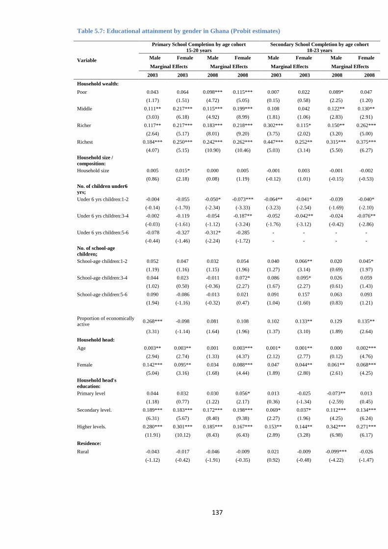
137
Table 5.7: Educational attainment by gender in Ghana (Probit estimates)
Variable
Primary School Completion by age cohort
15-20 years
Secondary School Completion by age cohort
18-23 years
Male Female Male Female Male Female Male Female
Marginal Effects Marginal Effects Marginal Effects Marginal Effects
2003 2003 2008 2008 2003 2003 2008 2008
Household wealth:
Poor 0.043 0.064 0.098*** 0.115*** 0.007 0.022 0.089* 0.047
(1.17) (1.51) (4.72) (5.05) (0.15) (0.58) (2.25) (1.20)
Middle 0.111** 0.217*** 0.115*** 0.199*** 0.108 0.042 0.122** 0.130**
(3.03) (6.18) (4.92) (8.99) (1.81) (1.06) (2.83) (2.91)
Richer 0.117** 0.217*** 0.183*** 0.218*** 0.302*** 0.115* 0.150** 0.262***
(2.64) (5.17) (8.01) (9.20) (3.75) (2.02) (3.20) (5.00)
Richest 0.184*** 0.250*** 0.242*** 0.262*** 0.447*** 0.252** 0.315*** 0.375***
(4.07) (5.15) (10.90) (10.46) (5.03) (3.14) (5.50) (6.27)
Household size /
composition:
Household size 0.005 0.015* 0.000 0.005 -0.001 0.003 -0.001 -0.002
(0.86) (2.18) (0.08) (1.19) (-0.12) (1.01) (-0.15) (-0.53)
No. of children under6
yrs;
Under 6 yrs children:1-2 -0.004 -0.055 -0.050* -0.073*** -0.064** -0.041* -0.039 -0.040*
(-0.14) (-1.70) (-2.34) (-3.33) (-3.23) (-2.54) (-1.69) (-2.10)
Under 6 yrs children:3-4 -0.002 -0.119 -0.054 -0.187** -0.052 -0.042** -0.024 -0.076**
(-0.03) (-1.61) (-1.12) (-3.24) (-1.76) (-3.12) (-0.42) (-2.86)
Under 6 yrs children:5-6 -0.078 -0.327 -0.312* -0.285 - - - -
(-0.44) (-1.46) (-2.24) (-1.72) - - - -
No. of school-age
children;
School-age children:1-2 0.052 0.047 0.032 0.054 0.040 0.066** 0.020 0.045*
(1.19) (1.16) (1.15) (1.96) (1.27) (3.14) (0.69) (1.97)
School-age children:3-4 0.044 0.023 -0.011 0.072* 0.086 0.095* 0.026 0.059
(1.02) (0.50) (-0.36) (2.27) (1.67) (2.27) (0.61) (1.43)
School-age children:5-6 0.090 -0.086 -0.013 0.021 0.091 0.157 0.063 0.093
(1.94) (-1.16) (-0.32) (0.47) (1.04) (1.60) (0.83) (1.21)
Proportion of economically active
0.268*** -0.098 0.081 0.108 0.102 0.133** 0.129 0.135**
(3.31) (-1.14) (1.64) (1.96) (1.37) (3.10) (1.89) (2.64)
Household head:
Age 0.003** 0.003** 0.001 0.003*** 0.001* 0.001** 0.000 0.002***
(2.94) (2.74) (1.33) (4.37) (2.12) (2.77) (0.12) (4.76)
Female 0.142*** 0.095** 0.034 0.088*** 0.047 0.044** 0.061** 0.068***
(5.04) (3.16) (1.68) (4.44) (1.89) (2.80) (2.61) (4.25)
Household head's
education:
Primary level 0.044 0.032 0.030 0.056* 0.013 -0.025 -0.073** 0.013
(1.18) (0.77) (1.22) (2.17) (0.36) (-1.34) (-2.59) (0.45)
Secondary level. 0.189*** 0.183*** 0.172*** 0.198*** 0.069* 0.037* 0.112*** 0.134***
(6.31) (5.67) (8.40) (9.38) (2.27) (1.96) (4.25) (6.24)
Higher levels. 0.280*** 0.301*** 0.185*** 0.167*** 0.153** 0.144** 0.342*** 0.271***
(11.91) (10.12) (8.43) (6.43) (2.89) (3.28) (6.98) (6.17)
Residence:
Rural -0.043 -0.017 -0.046 -0.009 0.021 -0.009 -0.099*** -0.026
(-1.12) (-0.42) (-1.91) (-0.35) (0.92) (-0.48) (-4.22) (-1.47)
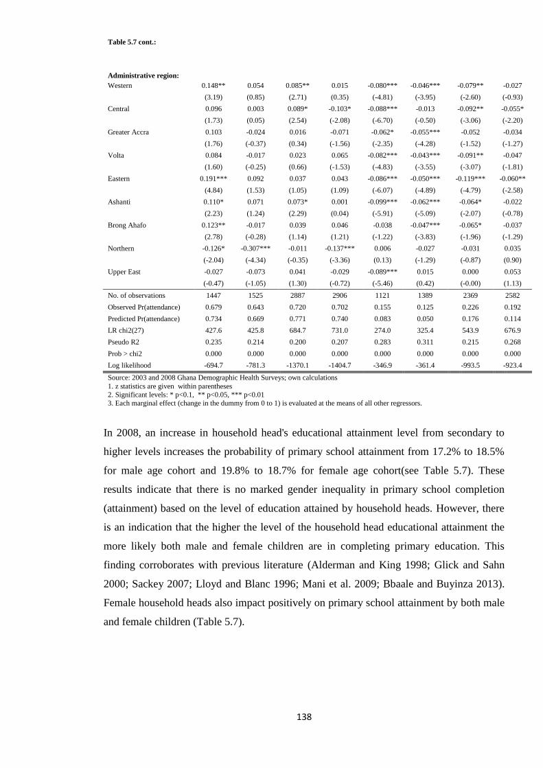
138
Table 5.7 cont.:
Administrative region:
Western 0.148** 0.054 0.085** 0.015 -0.080*** -0.046*** -0.079** -0.027
(3.19) (0.85) (2.71) (0.35) (-4.81) (-3.95) (-2.60) (-0.93)
Central 0.096 0.003 0.089* -0.103* -0.088*** -0.013 -0.092** -0.055*
(1.73) (0.05) (2.54) (-2.08) (-6.70) (-0.50) (-3.06) (-2.20)
Greater Accra 0.103 -0.024 0.016 -0.071 -0.062* -0.055*** -0.052 -0.034
(1.76) (-0.37) (0.34) (-1.56) (-2.35) (-4.28) (-1.52) (-1.27)
Volta 0.084 -0.017 0.023 0.065 -0.082*** -0.043*** -0.091** -0.047
(1.60) (-0.25) (0.66) (-1.53) (-4.83) (-3.55) (-3.07) (-1.81)
Eastern 0.191*** 0.092 0.037 0.043 -0.086*** -0.050*** -0.119*** -0.060**
(4.84) (1.53) (1.05) (1.09) (-6.07) (-4.89) (-4.79) (-2.58)
Ashanti 0.110* 0.071 0.073* 0.001 -0.099*** -0.062*** -0.064* -0.022
(2.23) (1.24) (2.29) (0.04) (-5.91) (-5.09) (-2.07) (-0.78)
Brong Ahafo 0.123** -0.017 0.039 0.046 -0.038 -0.047*** -0.065* -0.037
(2.78) (-0.28) (1.14) (1.21) (-1.22) (-3.83) (-1.96) (-1.29)
Northern -0.126* -0.307*** -0.011 -0.137*** 0.006 -0.027 -0.031 0.035
(-2.04) (-4.34) (-0.35) (-3.36) (0.13) (-1.29) (-0.87) (0.90)
Upper East -0.027 -0.073 0.041 -0.029 -0.089*** 0.015 0.000 0.053
(-0.47) (-1.05) (1.30) (-0.72) (-5.46) (0.42) (-0.00) (1.13)
No. of observations 1447 1525 2887 2906 1121 1389 2369 2582
Observed Pr(attendance) 0.679 0.643 0.720 0.702 0.155 0.125 0.226 0.192
Predicted Pr(attendance) 0.734 0.669 0.771 0.740 0.083 0.050 0.176 0.114
LR chi2(27) 427.6 425.8 684.7 731.0 274.0 325.4 543.9 676.9
Pseudo R2 0.235 0.214 0.200 0.207 0.283 0.311 0.215 0.268
Prob > chi2 0.000 0.000 0.000 0.000 0.000 0.000 0.000 0.000
Log likelihood -694.7 -781.3 -1370.1 -1404.7 -346.9 -361.4 -993.5 -923.4
Source: 2003 and 2008 Ghana Demographic Health Surveys; own calculations
1. z statistics are given within parentheses
2. Significant levels: * p<0.1, ** p<0.05, *** p<0.01
3. Each marginal effect (change in the dummy from 0 to 1) is evaluated at the means of all other regressors.
In 2008, an increase in household head's educational attainment level from secondary to
higher levels increases the probability of primary school attainment from 17.2% to 18.5%
for male age cohort and 19.8% to 18.7% for female age cohort(see Table 5.7). These
results indicate that there is no marked gender inequality in primary school completion
(attainment) based on the level of education attained by household heads. However, there
is an indication that the higher the level of the household head educational attainment the
more likely both male and female children are in completing primary education. This
finding corroborates with previous literature (Alderman and King 1998; Glick and Sahn
2000; Sackey 2007; Lloyd and Blanc 1996; Mani et al. 2009; Bbaale and Buyinza 2013).
Female household heads also impact positively on primary school attainment by both male
and female children (Table 5.7).
139
5.3.2.2 Secondary education attainment
Considering secondary school attainment, Table 5.7 indicates that the marginal effect of
wealth distribution on secondary school attainment of both male female age cohorts is
statistically significant at fourth and fifth wealth quintile levels in 2003 and also at third,
fourth and fifth wealth quintile levels in 2008. Thus, a movement in wealth distribution of
households from fourth wealth quintile (richer households) to the fifth wealth quintile
(richest households) increases the probability of secondary school completion from 30.2%
to 44.7% for male age cohort, and from 11.5% to 25.2% for female age cohort (Table 5.7).
This effect is only statistically significant at the higher income levels and the resultant
gender inequality in secondary school attainment or completion favours the male age
cohort.
However, in 2008 the disparity in the secondary school completion appears to favour the
female age cohort. That is, the marginal effect of moving from the third quintile (middle
welfare group or relatively poor households) to the fifth quintile (richest household)
increases the probability of secondary school completion from 12.2 to 31.5 percentage
points for male age cohort and 13.0 to 37.5 percentage points for female age cohort for the
same level of wealth distribution (Table 5.7). These results support the descriptive analysis
in Section 5.2 based on Tables 5.4 and 5.5. In addition, the findings are consistent with the
findings at the primary education attainment level which further support the assumption
that growth in household wealth or income will increase the probability of education
attainment by female children. The plausible explanation given for this effect is that
wealthy households can afford to hire help for childcare and other household work that
negatively affect the schooling outcomes of female children from poor households. In
addition, as household income levels increase, the wealth effect will disproportionately
benefit female children’s education by relaxing the time constraints that female children
face (Appleton 1995; Glick and Sahn 2000).
Household head educational attainment level also has statistical significant marginal effect
on secondary education attainment of both male and female age cohorts. The significant
marginal effect is observed at higher levels of household head educational attainment
(secondary and higher levels). Educational attainment by households at secondary and
higher levels increases the probability of male age cohort’s secondary school attainment by
6.9% and 15.3%, respectively in 2003 compared to household heads with no education.
Considering the female age cohort, the results in Table 5.7 show that household heads with
secondary and higher levels of education attained, increase the probability of female age
140
cohort’s secondary education attainment by 3.7% and 14.4%, respectively in 2003
compared to household heads with no education. In 2008 an increase in household head's
educational attainment level from secondary to higher levels increases the probability of
secondary school attainment from 11.2% to 34.2% for male age cohort and 13.4% to 27.1%
for female age cohort. These results indicate that higher levels of educational attainment by
household heads are more likely to favour secondary education attainment of male age
cohorts than the female age cohorts. Again, there is evidence that the higher the level of the
household head educational attainment, the higher the probability of both male and female
children residing in the household will be completing secondary education. This finding
once again is consistent with the findings in the literature (Alderman and King 1998; Glick
and Sahn 2000; Sackey 2007; Mani et al. 2009; Bbaale and Buyinza 2013).
In addition to household wealth distribution and household head education attainment
levels, our findings also reveal the importance of other factors that can influence the
disparity in educational outcomes of male and female children in Ghana. These factors
include the number of under-six year old children in the household and independence of
women in taking key household decisions (proxied by female headed households). For
example, in 2008 the number of under-six year old children from 1-2 and 3-4 reduces the
probability of; primary school completion of female age cohorts from 7.3% to 18.7%
respectively, and secondary school completion of female age cohorts from 4.0% to 7.6%,
respectively. The effect of the presence of under-six year old children on education
attainment of male age cohorts, on the other hand, was either statistically insignificant or
weakly significant (see Table 5.7). These findings corroborate the findings in the previous
literature (Lloyd and Blanc 1996; Alderman and King 1998; Glick and Sahn 2000). For
example, Glick and Sahn (2000) find that the number of under-five year olds has stronger
negative effect on female children’s educational outcomes but no statistical significant
effect on male children’s educational outcomes in Conakry, Guinea.
5.3.3 Robustness check
The same robustness test which we undertook in Chapter 4 was carried out in this chapter
to test the results reported in Tables 5.6 and 5.7. The results obtained by estimating
different version of the model with the inclusion of dummy variables for: religion (no
religion, Christianity, Muslim, and Traditional religion); ethnicity (Akan, Ga/Dangme,
Ewe, Guan, Mole/Dagbani, Grussi, Gruma, and Hausa/Mande) and resource control
(household spending) were highly statistically insignificant and did not change the stability
141
of the final results reported in Tables 5.6 and 5.7. Furthermore, we also carried out linktest
and none of the linktest result (hatsq) is statistically significant.23
Thus the link test reveals
no problems with our specification since the prediction squared does not have explanatory
power. We check our model against the theories of determinants of educational inequality
to make sure that our model is valid based on the theoretical underpinnings of educational
disparity between male and female children, especially in developing countries.
5.4 Policy perspective
Our analysis of educational access and attainment by gender provides a consistent picture
of the importance of household wealth, female household head, household head education
and household composition as factors in schooling decisions. First, the estimates suggest
that growth in household wealth or incomes will raise schooling investments for both
female and male school children but a bit faster for girls than for boys and could have
equalising effect in educational access and attainment. Therefore, policies that raise
household wealth or incomes will, in general, increase gender equity in schooling. Though
this will also depend on whether and how these policies change the relative opportunity
costs of female and male children and the relative labour market returns to female and
male schooling. Such policies, of course, would also have direct benefits for overall
household welfare.
On the other hand, policies that focus specifically on education may be more effective in
increasing educational access and attainment at primary and secondary levels for both
female and male children. However, education interventions targeted specifically at female
children would have beneficial impacts on the gender schooling inequality and these
impacts would be compounded intergenerationally. This can be inferred from the average
effect of female household head and education of household head on the probability of
increase in educational access and attainment of female children. For example, increasing
23
Primary school attendance of boys, hatsq: p = 0.225 in 2003 and p = 0.198 in 2008
Primary school attendance of girls, hatsq: p = 0.916 in 2003 and p = 0.168 in 2008
Secondary school attendance, hatsq: p = 0.600 in 2003 and p = 0.899 in 2008
Secondary school attendance, hatsq: p = 0.086 in 2003 and p = 0.220 in 2008
Primary school completion of boys, hatsq: p = 0.573 in 2003 and p = 0.812 in 2008
Primary school completion of girls, hatsq: p = 0.097 in 2003 and p = 0.120 in 2008
Secondary school completion, hatsq: p = 0.125 in 2003 and p = 0.365 in 2008
Secondary school completion, hatsq: p = 0.703 in 2003 and p = 0.204 in 2008
Where = .05 (significance level)
142
access to both primary and secondary education for female children now is equivalent to
raising the schooling of mothers and household heads in the next generation. Thus, there
are intergenerational increasing returns for education equity to improvements in female
schooling. However, it would hardly be wise to suggest that all education efforts be
directed at female children. Therefore, policies to promote gender equity in education
generally (instead of targeting female education only) will also serve to reduce future
gender gaps in schooling outcomes of male children.
With regard to the opportunity costs of education, we can infer from our analysis (based on
the impact of the presence of under-six year olds) that female children of school-age may
be constrained in their schooling in part by the demands placed on their time. These
constraints may be derived from parental or household head beliefs about female children’s
roles in the household economy in Ghana as well as other developing countries. Although
removing the constraints will be a difficult task for policy, in the long run, parental
attitudes may change with education, and increased availability of market substitutes for
domestic work and changes in home technology (the use of electricity, refrigerators,
washing machines etc.) could reduce households’ dependence on the labour of female
children (Schultz 1993 cited in Glick and Sahn 2000).
Government can also directly address the issue of opportunity cost of female children’s
education. For example, free or subsidised childcare in community day-care centres near
women’s places of work is often proposed as a way to reduce the time burden of working
mothers, but it may also be a means of reducing the opportunity cost of female children’s
time, thereby increasing their school attendance and completion rates. Promotional
campaigns to raise the parental awareness of non-market benefits of investing in female
education, such as improved child survival and health could be another avenue for policy
consideration (Glick and Sahn 2000).
5.5 Conclusions
This chapter presented an analysis of the impact of wealth distribution and other
determinants on gender inequality in educational outcomes in Ghana. We used data drawn
from 2003 and 2008 GDHS datasets to estimate a binary probit regression model that
captures the determinants of gender inequality in educational access and attainment.
Whereas the results show that increase in household wealth increases probability of
children's educational outcomes, it is not without inclination. There is evidence from both
143
the descriptive and regression analysis that gender specific differences in educational
outcomes of children decline with increasing household wealth and household head
educational attainment level and reflect resource constraints among the poor households
which corroborates the findings of Parish and Willis (1993).
Furthermore, at higher wealth distribution levels, household wealth tends to favour female
children's educational access and attainment. This suggests that income levels of
households are an important determinant of gender inequality in educational outcomes in
Ghana. It also appears that the government of Ghana's intended pro-poor education policy
interventions (SCG and SFP) did not reduce the significance of the impact of household
wealth on children's primary school attendance and completion. In addition, we also found
that the higher the household head's educational attainment level (secondary and higher
levels) the more likely female children will have access to and attain primary and
secondary education.
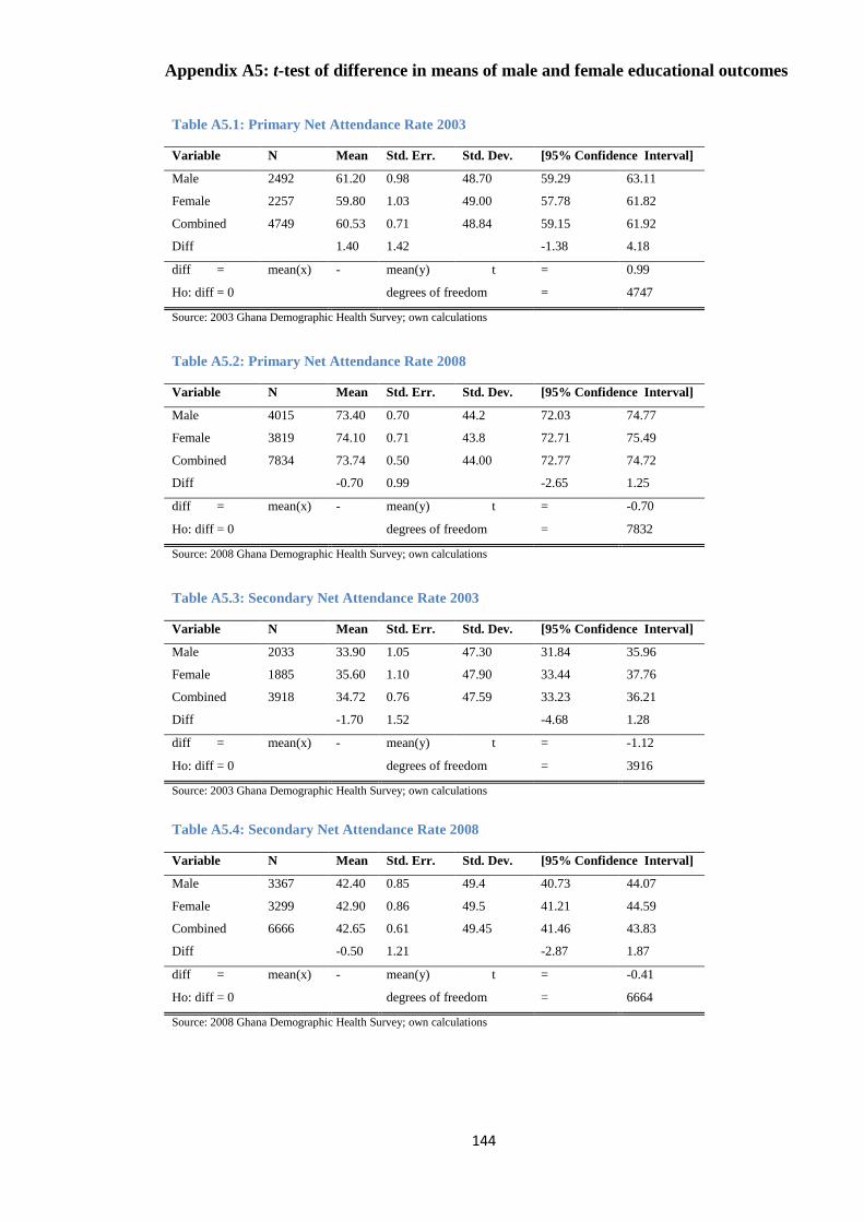
144
Appendix A5: t-test of difference in means of male and female educational outcomes
Table A5.1: Primary Net Attendance Rate 2003
Variable N Mean Std. Err. Std. Dev. [95% Confidence Interval]
Male 2492 61.20 0.98 48.70 59.29 63.11
Female 2257 59.80 1.03 49.00 57.78 61.82
Combined 4749 60.53 0.71 48.84 59.15 61.92
Diff 1.40 1.42 -1.38 4.18
diff = mean(x) - mean(y) t = 0.99
Ho: diff = 0 degrees of freedom = 4747
Source: 2003 Ghana Demographic Health Survey; own calculations
Table A5.2: Primary Net Attendance Rate 2008
Variable N Mean Std. Err. Std. Dev. [95% Confidence Interval]
Male 4015 73.40 0.70 44.2 72.03 74.77
Female 3819 74.10 0.71 43.8 72.71 75.49
Combined 7834 73.74 0.50 44.00 72.77 74.72
Diff -0.70 0.99 -2.65 1.25
diff = mean(x) - mean(y) t = -0.70
Ho: diff = 0 degrees of freedom = 7832
Source: 2008 Ghana Demographic Health Survey; own calculations
Table A5.3: Secondary Net Attendance Rate 2003
Variable N Mean Std. Err. Std. Dev. [95% Confidence Interval]
Male 2033 33.90 1.05 47.30 31.84 35.96
Female 1885 35.60 1.10 47.90 33.44 37.76
Combined 3918 34.72 0.76 47.59 33.23 36.21
Diff -1.70 1.52 -4.68 1.28
diff = mean(x) - mean(y) t = -1.12
Ho: diff = 0 degrees of freedom = 3916
Source: 2003 Ghana Demographic Health Survey; own calculations
Table A5.4: Secondary Net Attendance Rate 2008
Variable N Mean Std. Err. Std. Dev. [95% Confidence Interval]
Male 3367 42.40 0.85 49.4 40.73 44.07
Female 3299 42.90 0.86 49.5 41.21 44.59
Combined 6666 42.65 0.61 49.45 41.46 43.83
Diff -0.50 1.21 -2.87 1.87
diff = mean(x) - mean(y) t = -0.41
Ho: diff = 0 degrees of freedom = 6664
Source: 2008 Ghana Demographic Health Survey; own calculations
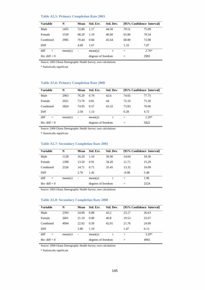
145
Table A5.5: Primary Completion Rate 2003
Variable N Mean Std. Err. Std. Dev. [95% Confidence Interval]
Male 1455 72.80 1.17 44.50 70.51 75.09
Female 1530 68.20 1.19 46.60 65.86 70.54
Combined 2985 70.44 0.84 45.64 68.80 72.08
Diff 4.60 1.67 1.33 7.87
diff = mean(x) - mean(y) t = 2.76*
Ho: diff = 0 degrees of freedom = 2983
Source: 2003 Ghana Demographic Health Survey; own calculations
* Statistically significant
Table A5.6: Primary Completion Rate 2008
Variable N Mean Std. Err. Std. Dev. [95% Confidence Interval]
Male 2903 76.20 0.79 42.6 74.65 77.75
Female 2921 73.70 0.81 44 72.10 75.30
Combined 5824 74.95 0.57 43.32 73.83 76.06
Diff 2.50 1.13 0.28 4.72
diff = mean(x) - mean(y) t = 2.20*
Ho: diff = 0 degrees of freedom = 5822
Source: 2008 Ghana Demographic Health Survey; own calculations
* Statistically significant
Table A5.7: Secondary Completion Rate 2003
Variable N Mean Std. Err. Std. Dev. [95% Confidence Interval]
Male 1128 16.20 1.10 36.90 14.04 18.36
Female 1398 13.50 0.91 34.20 11.71 15.29
Combined 2526 14.71 0.71 35.45 13.32 16.09
Diff 2.70 1.42 -0.08 5.48
diff = mean(x) - mean(y) t = 1.90
Ho: diff = 0 degrees of freedom = 2524
Source: 2003 Ghana Demographic Health Survey; own calculations
Table A5.8: Secondary Completion Rate 2008
Variable N Mean Std. Err. Std. Dev. [95% Confidence Interval]
Male 2393 24.90 0.88 43.2 23.17 26.63
Female 2601 21.10 0.80 40.8 19.53 22.67
Combined 4994 22.92 0.59 42.01 21.76 24.09
Diff 3.80 1.19 1.47 6.13
diff = mean(x) - mean(y) t = 3.20*
Ho: diff = 0 degrees of freedom = 4992
Source: 2008 Ghana Demographic Health Survey; own calculations
* Statistically significant
146
Chapter 6
Socioeconomic inequality in educational access and attainment in Ghana
6.1. Introduction
Who benefits from educational expansion and education policies and programmes in
Ghana? It has been argued that most of the education reforms developed to improve
educational efficiency in developing countries mainly focus on changing the educational
systems (Chowa et al. 2013). The 1987 Ghana education reforms is regarded as one of
such reforms where policy planners generally recommend revising the curriculum,
reducing the number of pre-university years of education, increasing the number of schools,
and distributing educational materials more widely and equitably to improve educational
outcomes (Akyeampong et al. 2007; Chowa et al. 2013) . For example, the 1987 education
reforms set out measures to improve access to basic education, equity in the education
sector, improve quality and efficiency. One of the main objectives of the reforms is to
expand education and make educational access more equitable at all levels in Ghana
(Akyeampong et al. 2007).
However, the implementation of the education programmes may have overlooked the role
of households’ socioeconomic factors in shaping the academic trajectories of income
groups in Ghana. This may contribute to socioeconomic inequality in educational access
and attainment. It has also been argued that although Ghana has implemented School
Capitation Grant, School Feeding Programme, and enforced the laws that support the
implementation of Free Compulsory Universal Basic Education, poor households still
struggle with; additional costs (including transportation, text books, and uniforms) of
sending children to schools, and child labour which disproportionately affects children
from poor households (Chowa et al. 2010).
This chapter, therefore, gives us insight into whether public social spending programmes
that the country has embarked upon have impacted positively on the income-poor
households in terms of educational access and attainment, and whether educational
inequalities have improved between 2003 and 2008. The contribution of this chapter is to
estimate the contributions of socioeconomic factors to inequality in educational access and
attainment in Ghana, using a concentration index framework. Measuring socioeconomic
inequalities in educational access and attainment is very important in assessing an
educational system. However, potentially interesting from policy perspective is to identify
and explain the sources of educational access and attainment inequality. The objective of
147
this chapter is, therefore, to quantify for the first time the contributions of the determinants
of educational inequality to socioeconomic inequality in children’s educational access and
attainment in Ghana by applying concentration index methodology used by Wagstaff et al.
(1991), and Wagstaff et al. (2003) in health economics research.
The empirical questions we seek to address are: What are the main contributing factors of
educational inequalities?; What is the change in educational inequality over time (between
2003 and 2008)?; and Has the relatively sustained economic growth in Ghana for the past
decade, and educational expansions impacted positively on educational inequalities?
The rest of the chapter is structured as follows. Section 6.2 describes the concept of
concentration index for analysing socioeconomic inequality and its application in the area
of education inequality research, focusing on the decomposition of the sources and
contributions of determinants of educational inequalities. The section also includes an
extension of the concentration index approach to analyse and explain changes in
educational inequalities. Section 6.3 presents and discusses decomposition results, and
Sections 6.4 concludes the chapter.
6.2 Models
6.2.1 Measuring education inequality
Various measures have been proposed and used to measure educational inequality in both
within country and cross country studies. Common among them are: Education Standard
Deviation and Coefficient of Variation of Schooling (Zhang and Li 2002; SITEAL 2005);
Gini Coefficient or Education Gini Index (Maas and Criel 1982; Thomas et al. 2001;
Zhang and Li 2002; SITEAL 2005; Sahn and Younger 2007); and Generalised Entropy
indices and Atkinson Index (Thomas et al. 2001; SITEAL 2005; Sahn and Younger 2007).
Least known and used in education inequality measurement is Concentration Index
(SITEAL 2005; Oppedisano and Turati 2012), but widely used in health inequality
measurement. These indices, however, have their advantages and disadvantages in
measuring education inequality.
Gini Coefficient/Education Gini Coefficient
The Gini Coefficient is a single statistic measure that can be used to summarise relative
inequality across all groups in the population. Though, it is commonly used to measure
inequality between income groups, it is also used to measure education inequality among
148
individuals. For example, Education Gini Coefficient is used to measure education
inequality based on enrolment ratios, educational attainment (average years of schooling)
and education finance (Maas and Criel 1982; Thomas et al. 2001; Zhang and Li 2002;
SITEAL 2005; Sahn and Younger 2007). Although the Education Gini Coefficient is
sensitive to the distribution of the population between social groups and has good
statistical properties (Pigou-Dalton transfer sensitivity, scale invariant, bounded between
0 and 1) it has its own limitations. 24
The index does not reflect the socioeconomic
dimensions of inequalities in education and also does not tell us which social groups are
disadvantaged. Again, the Education Gini Coefficient is computed on individual data and
measures only the inequality between individuals but not inequality between social groups
(d' Hombres 2010). Most importantly, it lacks the property of additive decomposition and,
therefore, cannot be used to determine the sources of educational inequalities.
Generalised Entropy Indices and Atkinson Indices
The indices can be used to measure inequality in education. These indices have the
property of additive decomposition between and within selected groups. Although it is
possible to decompose the overall inequality among individuals into two components;
between social groups, and within social groups indices, and have good statistical
properties (Pigou-Dalton transfer sensitivity, and scale invariant), the indices are limited
for the purpose of this research. Just like the Education Gini Coefficient, the indices: (i) do
not reflect the socioeconomic dimension of inequalities in education, (ii) do not tell us
which social or income groups are disadvantaged, and (iii) cannot be used to determine the
sources of educational inequalities, which is one of the main policy foci of this thesis.
6.3 Concentration Index
Since the two popular indices reviewed above are not able to determine the sources and the
contributions of the sources to educational inequalities (which are the main objectives of
Chapter 6), we prefer to use a concentration index as our measure of both absolute and
relative socioeconomic-related inequality in access to education and attainment of
24 - Principle of transfers (Pigou-Dalton condition), says that a transfer of income from a richer to a poorer
individual will result in a reduction in the indicator of disparity, assuming that the income of other
individuals remains unchanged and the transfer is not large enough to reverse anyone’s relative position.
- Scale independence, says that if the value of the education indicator doubles for each of the equity groups,
the value associated with the inequality indicator does not change.
- Boundness of the indicator, states that the interpretation of the value assigned to the inequality indicator will
be easier if this indicator has a lower bound and an upper bound.
149
education in Ghana. The concentration index has been used widely in health economics
research and the index can shed light on the pro-poor and pro-rich distributions of
determinants of a given dependent variable. It is calculated in similar way as the Gini
Coefficient but its values range from -1 to +1. As argued by d' Hombres (2010), the
concentration index is a good measure of socioeconomic inequalities in education. The
favourable properties of concentration index make the index more appropriate to apply in
the estimation and decomposition of educational inequalities among income groups. The
index can be used for both individual data and data aggregated by income group, and it can
also provide a summary index of education inequalities. Besides, it can reflect the
socioeconomic dimension of inequalities in education, and there is the possibility to adjust
the index for the effect of other confounding factors of the determinants of educational
inequalities (d' Hombres 2010; Oppedisano and Turati 2012). Furthermore, the index has
good statistical properties (Pigou-Dalton transfer sensitivity, scale invariant, and bounded
between -1 and +1), sensitive to the proportion of the population in each group, and it is
capable of revealing the sources contributing to a given inequality (Wagstaff et al. 2003;
van Doorslaer et al. 2004; Oppedisano and Turati 2012).
Most importantly, the concentration index is sensitive to the direction of social gradient in
education and as a result, it can measure how educational status varies with socioeconomic
position (d' Hombres 2010; Oppedisano and Turati 2012). Also, the index can be derived
from an estimate in multivariate context and this makes it possible to control for factors
that may simultaneously correlate with educational outcomes and the income groups to
which the individual belongs. However, the concentration index is not without limitations.
The value of the index does not change if the living standard variable (income or wealth)
changes and the income or welfare group must be defined on an interval scale (d' Hombres
2010; Wagstaff et al. 2003; Wagstaff and Watanabe 2003).
The above desirable qualities of the concentration index make the it, probably, the more
appropriate educational inequality measure among others (such as Education Gini
Coefficient, Generalised Entropy Indices and Atkinson Indices) considered to examine the
sources of educational inequalities which is one of the main objectives the thesis. As a
result, the concentration index model is used to estimate and decompose socioeconomic
inequality in educational access and attainment in Ghana. The use of the model is to reveal
the main sources of educational inequalities, the contributions of the sources to educational
150
inequalities. The application of concentration index is vital in revealing any inequality in
the distribution of educational access and attainment among households.
In contrast to the comparative literature on socioeconomic inequalities in health where
concentration index methodology is extensively applied (Wagstaff et al. 1991; Wagstaff
2002; Wagstaff and Watanabe 2003; Doorslaer and Koolman 2004; Doorslaer and Jones
2004), the focus in this thesis is on the application of the concentration index framework to
analyse education inequalities in Ghana. To the best of our knowledge, this study
constitutes the only first attempt to quantify and decompose educational inequalities
among the school going-age children (6-17 year olds) in Ghana using concentration index
approach.
6.3.1 Concentration index approach
This section illustrates the application of concentration index in measuring inequality in
educational access and attainment. We use a concentration index as our measure of relative
socioeconomic-related inequality in access to education, and attainment of education in
Ghana. The concentration index is widely used in the area of health economics research
(Wagstaff et al. 1991; Wagstaff 2002; Wagstaff and Watanabe 2003; Wagstaff et al. 2003).
Although the use of the index is relatively new to inequality measurement in education,
SITEAL ( 2005) apply the technique to estimate education concentration indices in Chile
and Costa Rica. Oppedisano and Turati (2012) also used the methodology to measure and
decompose inequality in educational performance (reading score) in Europe. However, in
Ghana and Africa, there is no known published research which has used the methodology
to measure educational inequality. This study follows the methodology used by Wagstaff
et al. (2003) and we apply it to estimate and decompose socioeconomic inequality in
education in Ghana. We quantify the degree to which educational access (school
attendance) and attainment (school completion) are unequally distributed to the
disadvantage of poor children and the extent to which the inequalities in education are
more or less pronounced over time in Ghana. The use of the model is to reveal the main
sources of educational inequalities, and the contributions of determinants of educational
inequalities. The application of concentration index is vital in revealing any inequality in
the distribution of educational access and attainment among households.
In contrast to the comparative literature on socioeconomic inequalities in health where
concentration index methodology is extensively applied (Wagstaff et al. 1991; Wagstaff
151
2002; Wagstaff and Watanabe 2003; Doorslaer and Koolman 2004; Doorslaer and Jones
2004), the focus of the chapter is on the application of the concentration index framework
to analyse education inequalities. To the best of our knowledge, this study constitutes the
only first attempt to estimate and decompose educational inequalities among the school
going-age children (6-17 year olds) in Ghana using concentration index approach.
The concentration index is standardised and its value ranges between -1 (more educational
outcomes concentrated among the poor) and +1(more educational outcomes concentrated
among the rich). When the index is zero, it implies everyone enjoys, for example, the same
educational access and attainment irrespective of one's living standards or household
wealth. The application of concentration index model is designed to address two main
objectives: firstly, to estimate the effect of socioeconomic inequality in education of school
going-age children (6-17 year olds) using households’ economic status thereby to calculate
the contribution of the key explanatory factors to the total explained inequalities by
performing the decomposition of concentration index. Keeping this in mind, the second
objective is to compare the educational inequalities and its contributory factors over time
(between 2003 and 2008).25
By estimating the impact and the degree of contribution of
each determinant to the inequality in educational access and attainment could aid an
effective policy intervention to reduce educational inequalities in Ghana.
6.3.2 Empirical specification
Following the approach used by Wagstaff et al. (1991 & 2003), the concentration index (C)
can be mathematically expressed as follows:
𝐶 =2
𝑛𝜇∑ 𝑦𝑖𝑅𝑖
𝑛
𝑖=1
− 1, 6.1
where 𝑦𝑖 is the education variable (e.g. educational access and attainment) whose
inequality is being measured, µ is the mean of 𝑦𝑖, 𝑅𝑖 is the ith individual’s fractional rank
in the socioeconomic or living standard distribution (e.g. the individual’s rank in the
wealth distribution), and n is the number of individuals. C, like the Gini coefficient, is a
measure of relative inequality. C can take on values between -1 and +1, depending on
whether inequalities favour the poor or the rich in the society. Its negative values imply
25
These two periods represent GDHS years. The 2003 and 2008 GDHS are comparable because the DHS has
standard survey questionnaires that are comparable over periods. The 2003 GHDS questionnaire on
education indicators and household characteristics are the same as that of 2008 GDHS. Again, these periods
enable us to capture the impacts of the Ghana government’s educational policies (CGI and SFP) which were
implemented in 2005. We use 2003 as a base year (i.e. a year before the implementation of the “anti-poverty
educational” programmes) to capture the impacts of the programmes on educational inequalities in 2008.
152
that a variable is concentrated among the poor or disadvantage people and vice versa.
When there is no inequality, the C will be zero.
However, for convenient computation of the concentration index, the concentration index
can be defined in terms of the covariance between the dependent variable and the fractional
rank in the living standards distribution (O’Donnell et al. 2008; d' Hombres 2010).
According to O’Donnell et al. (2008) “convenient covariance” formula can be stated as:
𝐶 =2
𝜇𝑐𝑜𝑣(𝑦, 𝑅) 6.2
In our application, y is the education variable (e.g. educational access and attainment)
whose inequality is being measured, µ is the mean of y, and R is the fractional ranking by
welfare level or economic status of individuals. Thus, C can be computed from micro-data
by using Equation 6.3. Given the relationship between covariance and ordinary least
squares regression (OLS), an equivalent estimate of the concentration index can be
obtained from a “convenient regression” by transforming the education variable of interest
on the fractional rank in the living standards distribution ( d' Hombres 2010).
The “convenient regression” formula is given as:
2𝜎𝑟2 (𝑦𝑖
𝜇) = 𝛼 + 𝛽𝑟𝑖 + 𝛿𝑥𝑖휀𝑖, 6.3
Where 𝜎𝑟2 is the variance of the fractional rank variable (income or wealth), the OLS
estimate of β is then equivalent to C in Equation 6.2, and 𝑥𝑖 is a set of covariates to control
for potential confounding effects.26
The regression approach facilitates the decomposition
of the degree of inequality into the contributions of different explanatory variables under
investigation (O’Donnell et al. 2008). Thus, from Equation 6.3 we can explore whether a
given education system is unequal based on income or wealth distribution. For instance, an
education system will be unequal if children with different socioeconomic status are
characterised by unequal access to education (𝑦𝑖). The concentration index decomposition
approach is explored in the next sub-section.
6.3.4 Decomposition of inequality and its evolution over time
Inequalities across income or wealth distribution in a variable 𝑦𝑖 can be decomposed into
their sources or determinants. Changes in inequality in 𝑦𝑖 can also be decomposed into the
effects of changes in the means and inequalities in the determinants of 𝑦𝑖, and changes in
the elasticities (impacts) of the determinants of 𝑦𝑖. The method used by Wagstaff et al.
26
If 𝑥𝑖 is simultaneously correlated with 𝑦𝑖 the estimated β will capture the effect of socioeconomic status on
education and also the impact of the other covariates, 𝑥𝑖 (d' Hombres 2010:30).
153
(2003) in analysing health inequality is adopted to decompose socioeconomic inequality in
school attendance and completion into their determinants. The decomposition analysis
allows us to estimate how determinants proportionally contribute to inequality (e.g. the gap
between the poor and the rich at a point in time and over a period of time) in a given
education variable.
6.3.4.1 Decomposition of inequality by socioeconomic determinants
For policy purposes, it is important to quantify the contributions of various determinants of
education indicators to their degrees of inequality and impact on socioeconomic inequality.
The decomposition indicates how each determinant’s contribution to total education
inequality ( 𝑦𝑖) can be decomposed into two parts: (i) its impact on education, measured
by the education elasticity (𝜂𝑘), and (ii) its degree of unequal distribution across income
groups, measured by the concentration index (𝐶𝑘). The decomposition method, therefore,
not only allows us to separate the contributions of the various determinants of a given
education variable, but also to identify the importance of each of the two components
within each factor’s contribution. Thus, the concentration index decomposition
methodology makes it possible to disaggregate the mechanisms contributing to a country’s
degree of education inequality.
The decomposition method is based on the linear additive relationship between the
outcome variable yi, the intercept α, the relative contributions of xki determinants and the
residual error 휀𝑖 in Equation 6.4. Following Wagstaff et al. (2003), any linear regression
model linking dependent variable (e.g. education indicator of interest), 𝑦𝑖 to a set of k
education determinants, xk can be specified as:
𝑦𝑖 = 𝛼 + ∑ 𝛽𝑘
𝑘
𝑥𝑘𝑖 + 휀𝑖 , 6.4
Where α and 𝛽𝑘 are coefficients to be estimated and εi is a standard random disturbance
term. It is assumed that everyone in the selected sample, irrespective of their income or
household wealth faces the same coefficient vector, 𝛽𝑘 . Interpersonal variations in 𝑦𝑖 are,
thus, assumed to derive from systematic variations across income groups in the
determinants of 𝑦𝑖, that is the 𝑥𝑘 (Wagstaff et al. 2003). One could consider Equation 6.4
as a reduced form of demand for educational outcomes (i.e. educational access, and
educational attainment) equation where the x variables are exogenous determinants.
154
6.3.4.2 Decomposition of concentration index
The decomposition of concentration indices is aimed at generating useful information
regarding the relative importance of various determinants of inequitable outcomes of the
dependent variable of interest. Given the relationship between 𝑦𝑖 and 𝑥𝑘𝑖, it is now possible
to decompose the concentration index of 𝑦𝑖 by using the means and the concentration
indices of the determinants. Consequently, from Equation 6.4, the relationship between 𝑦𝑖
and 𝑥𝑘𝑖, the concentration index for 𝑦𝑖, can be written as:
𝐶 = ∑ (𝛽𝑘�̅�𝑘
𝜇) 𝐶𝑘
𝑘
+𝐺𝐶𝜀
𝜇, 6.5
Where µ is the mean of 𝑦𝑖, �̅�𝑘 is the mean of 𝑥𝑘 , and 𝐶𝑘 is the concentration index for 𝑥𝑘.
The elasticity, (𝛽𝑘�̅�𝑘/𝜇) estimates the impact of each determinant on dependent variable
(educational outcome), and the degree of unequal distribution of each determinants across
income groups is measured by 𝐶𝑘. In the last term, 𝐺𝐶𝜀 is a generalised concentration index
for 휀𝑖, defined as:
𝐺𝐶𝜀 =2
𝑛∑ 휀𝑖𝑅𝑖
𝑛
𝑖=1
, 6.6
Equation 6.5 shows that C can be thought of as being made up two components. The first
is the deterministic component, equal to the concentration indices of the k regressors,
weighted by the elasticity of 𝑦𝑖 with respect to 𝑥𝑘 (evaluated at the sample mean). In other
words, (𝛽𝑘�̅�𝑘/𝜇)𝐶𝑘, is the absolute contribution of each determinant of the concentration
index for 𝑦𝑖. The residual component (Equation 6.6) reflects the inequality in educational
access and attainment that is not explained by systematic variations across income groups
in the determinants of outcomes, 𝑥𝑘 . Empirically, the residual can be obtained as the
difference between the concentration index of the dependent variable, 𝑦𝑖 and the sum of
the factor contributions (i.e. Σ (𝛽𝑘�̅�𝑘/𝜇)𝐶𝑘) (O’Donnell et al. 2008). However, the problem
in this context is that demand for educational outcomes we are interested in (school
attendance, and completion) are binary response variables from the DHS datasets and,
therefore, may not be very well modelled using linear estimation techniques such as OLS.
An examination of the variables reveals that the dependent variables are binary taking the
value of 0, or 1. In the section below we explain how we have been to change the linear
model in Equation 6.4 to the non-linear model specified in Equation 6.7.
155
6.3.5 Non-linear regression model
The concentration index decomposition model was first introduced to use with a linear
health sector variables (Wagstaff et al. 2003). However, because health sector variables are
intrinsically non-linear, an appropriate statistical technique for non-linear settings was
proposed by van Doorslaer et al. (2004). The two common choices yielding probabilities in
the range (0, 1) are the logit and the probit models, both of which are fitted by maximum
likelihood. Since we are dealing with a discrete change from 0 to 1 (i.e. attended school or
not, completed school or not) we can conveniently use marginal or partial effects (dh/dx),
which give the change in predicted probability associated with unit change in an
explanatory variable. An approximation of the non-linear relationship using marginal
effects approximately restores the mechanism of the decomposition framework in
Equations 6.4 through 6.7 (Yiengprugsawan et al. 2007). Consequently, a linear
approximation of the non-linear estimations is given by Equation 6.7, where 휀𝑖 indicates
the error generated by the linear approximation used to obtain the marginal effects.
Marginal or partial effects have been analysed in the analysis of health sector inequalities
in non-linear settings (van Doorslaer et al. 2004; O’Donnell et al. 2008).
Therefore, the continuous model proposed by Wagstaff et al. (2003) can be modified to
accommodate non-linear settings (e.g. binary dependent variable) using either probit
regression or Generalised Linear Models (GLM) (van Doorslaer et al. 2004;
Yiengprugsawan et al. 2007 & 2010). We, therefore, apply the probit regression model by
following van Doorslaer et al. (2004), and Yiengprugsawan et al. (2007).
6.3.5.1 Probit model
From Equation 6.4 and following van Doorslaer et al. (2004), the general functional form
G, of a non-linear model (e.g. a probit) can be written as:
𝑦𝑖 = 𝐺(𝛼 + ∑ 𝛽𝑘
𝑘
𝑥𝑘𝑖) + 휀𝑖 , 6.7
Then a linear approximation of this function is given by:
𝑦𝑖 = 𝛼𝑚 + ∑ 𝛽𝑘𝑚
𝑘
𝑥𝑘𝑖 + 휀𝑖 , 6.8
Where 𝛼𝑚 and 𝛽𝑘𝑚 are defined as the marginal effects (dh/dx), of each 𝑥𝑘 treated as fixed
parameters and evaluated at the mean and 휀𝑖 is the error term.
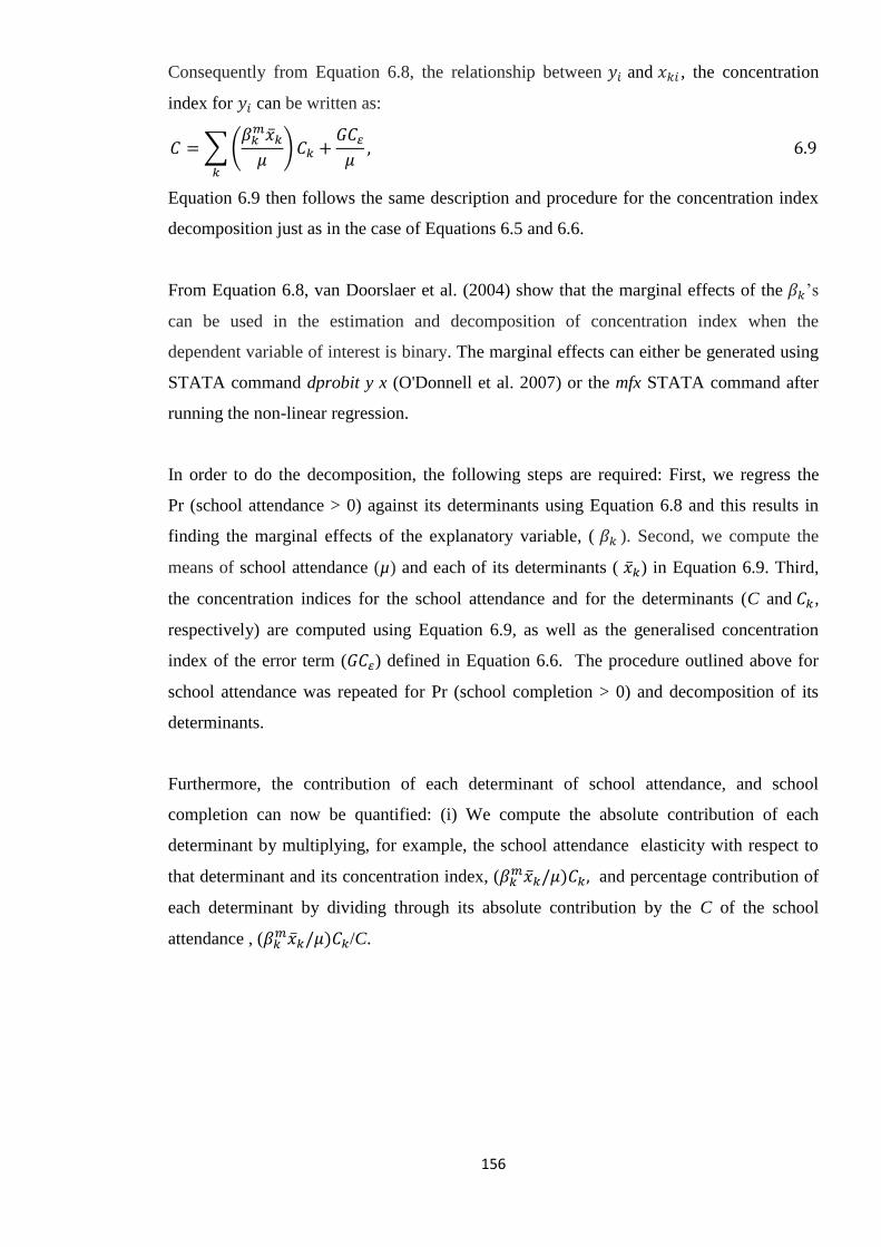
156
Consequently from Equation 6.8, the relationship between 𝑦𝑖 and 𝑥𝑘𝑖 , the concentration
index for 𝑦𝑖 can be written as:
𝐶 = ∑ (𝛽𝑘
𝑚�̅�𝑘
𝜇) 𝐶𝑘
𝑘
+𝐺𝐶𝜀
𝜇, 6.9
Equation 6.9 then follows the same description and procedure for the concentration index
decomposition just as in the case of Equations 6.5 and 6.6.
From Equation 6.8, van Doorslaer et al. (2004) show that the marginal effects of the 𝛽𝑘’s
can be used in the estimation and decomposition of concentration index when the
dependent variable of interest is binary. The marginal effects can either be generated using
STATA command dprobit y x (O'Donnell et al. 2007) or the mfx STATA command after
running the non-linear regression.
In order to do the decomposition, the following steps are required: First, we regress the
Pr (school attendance > 0) against its determinants using Equation 6.8 and this results in
finding the marginal effects of the explanatory variable, ( 𝛽𝑘 ). Second, we compute the
means of school attendance (µ) and each of its determinants ( �̅�𝑘) in Equation 6.9. Third,
the concentration indices for the school attendance and for the determinants (C and 𝐶𝑘,
respectively) are computed using Equation 6.9, as well as the generalised concentration
index of the error term (𝐺𝐶𝜀) defined in Equation 6.6. The procedure outlined above for
school attendance was repeated for Pr (school completion > 0) and decomposition of its
determinants.
Furthermore, the contribution of each determinant of school attendance, and school
completion can now be quantified: (i) We compute the absolute contribution of each
determinant by multiplying, for example, the school attendance elasticity with respect to
that determinant and its concentration index, (𝛽𝑘𝑚�̅�𝑘/𝜇)𝐶𝑘, and percentage contribution of
each determinant by dividing through its absolute contribution by the C of the school
attendance , (𝛽𝑘𝑚�̅�𝑘/𝜇)𝐶𝑘/C.
157
6.3.5.2 Decomposition of changes in educational inequalities
The most general approach to unravelling the sources of changes in inequalities would be
to allow for the possibility that all the components of the decomposition in Equation 6.9
have changed and to take the difference of equation 6.9 (Wagstaff et al. 2003).
Δ𝐶 = ∑ (𝛽𝑘𝑡
𝑚�̅�𝑘𝑡
𝜇𝑡) 𝐶𝑘𝑡
𝑘
− ∑ (𝛽𝑘𝑡−1
𝑚 �̅�𝑘𝑡−1
𝜇𝑡−1)
𝑘
+ Δ (𝐺𝐶𝜀𝑡
𝜇𝑡) , 6.10
According to Wagstaff et al. (2003) equation 6.10 is somewhat uninformative. Fortunately,
Equation 6.11 or 6.12 enables us to explain how far the changes in inequality in education
reveal by Equation 6.10 were attributable to changes in inequalities in the determinants of
educational access and attainment rather than to changes in the other influences on these
education inequalities.
In addition, inequality can also be considered in its evolution over time. In this case, once
decomposition of inequality into its observable components has been carried out in two
different time periods (t-1 and t), it becomes more interesting to decompose the observed
differences (over time) in socioeconomic inequality due to variations in; (i) the
determinants of educational access and attainment, and (ii) the impact of these
determinants on educational access and attainment. The approach used by Wagstaff et al.
(2003) consists in applying Oaxaca-type decomposition to the expression of the
concentration index, C (Equation 6.9). Our main interest is in the change in educational
inequality over time due to changes in the impacts of the determinants measured by the
educational elasticity (∆η), and the degree of unequal distribution across income levels
measured by concentration index (∆C). These changes can be analysed using Oaxaca
decomposition (Wagstaff et al. 2003; Oaxaca 1973).
Thus, if we denote 𝜂𝑘 = 𝛽𝑘𝑚�̅�𝑘/𝜇, the elasticity of 𝑦𝑖 with respect to 𝑥𝑘 at time t, and
apply the Oaxaca-type decomposition method, we obtain the following equation (Wagstaff
et al. 2003):
∆𝐶 = 𝐶𝑡 − 𝐶𝑡−1 = ∑ 𝜂𝑘𝑡
𝑘
(𝐶𝑘𝑡 − 𝐶𝑘𝑡−1) + ∑ 𝐶𝑘𝑡−1
𝑘
(𝜂𝑘𝑡 − 𝜂𝑘𝑡−1) + Δ (𝐺𝐶𝜀𝑡
𝜇𝑡) , 6.11
Alternatively, Equation 6.10 can be re-written as:
Δ𝐶 = ∑ 𝜂𝑘𝑡−1
𝑘
(𝐶𝑘𝑡 − 𝐶𝑘𝑡−1) + ∑ 𝐶𝑘𝑡
𝑘
(𝜂𝑘𝑡 − 𝜂𝑘𝑡−1) + Δ (𝐺𝐶𝜀𝑡
𝜇𝑡) , 6.12
158
The Oaxaca-type decomposition allows us to identify for each 𝑥𝑘 the extent to which
changes in educational inequality are due to changes in inequality in the determinants of
educational access and attainment (the first term in Equation 6.11 or 6.12), rather than in
their elasticities (the second term in Equation 6.11 or 6.12).
The concentration index (C) is considered as a good measure of socioeconomic inequalities
in education (Oppedisano and Turati 2012; d' Hombres 2010; SITEAL 2005). Fortunately,
the application of C in measurement of inequality in education is free from some of the
problems that have been encountered when the index is applied in health inequality
measurement.27
The education concentration index is measured in cardinal scale. However,
the application of C in education also has its own shortcomings. Although the education
concentration index captures the relationship that exists between educational access or
attainment variables, and household wealth and its determinants, as far as wealth or income
is concerned the C takes into account only the ranks and not the levels of household wealth
or income. A given ranking of wealth or incomes may hide very different levels of
household wealth or income (Wagstaff et al. 2003). Both a relatively equal and a relatively
unequal distribution of income are compatible with any given ranking. Therefore, if
changes occur in the distribution of wealth or income which does not affect the welfare
ranks (e.g. a series of transfers which make the distribution more equal) there will be no
effect on C.28
In other words, the value of the index does not change if the living standard
variable (wealth or income) changes.
6.4 Results and discussions
The data, outcome and predictor variables for the analysis are discussed in Chapter 3. The
concentration index and decomposition results are based on Equations 6.8 to 6.12. The
analysis focuses on inequality in the four key areas of interest: primary education access
(primary school attendance); secondary education access (secondary school attendance);
primary education attainment (primary school completion); and secondary education
attainment (secondary school completion). The inequalities are presented through a
27
The most appropriate scale for health status measurement is perhaps an ordinal variable, not a cardinal one.
Health status indicator is an essentially qualitative variable which might be used to order people according to
their health situation, but it will be difficult to draw conclusions about the intensity corresponding to a
specific value of the health indicator. In order to solve this problem, health C assumes cardinal comparability
in order to draw conclusions (Wagstaff et al. 1991; Wagstaff 2002; and Wagstaff and Watanabe 2003). 28 The concentration index depends only on the relationship between the education variable and the rank of
the living standards variable and not on the variation in the living standards variable itself. A change in the
degree of income inequality need not affect the concentration index measure of income-related education
inequality.
159
concentration index decomposition analysis of inequality. We examine which factors
contribute the most to socioeconomic inequality in educational access and educational
attainment (at primary and secondary levels) by decomposing the concentration indices
year-by-year, with reference to Equation 6.9. The decomposition shows how each
determinant, 𝑥𝑘 's separate contribution to total education inequalities can be decomposed
into two main parts: (i) its impact on each of the education access, and educational
attainment, as measured by their elasticity (𝜂𝑘), and (ii) their degree of unequal distribution
across income or household wealth, measured by the concentration index (𝐶𝑘).
The first two columns of the Tables 6.1, 6.3, 6.5, and 6.7 show the mean of the outcome
and determinants; the third and fourth columns present the elasticities of determinants,
(𝜂𝑘 = 𝛽𝑘𝑚�̅�𝑘/𝜇); and the fifth and sixth columns indicate the values of the concentration
indices, (𝐶𝑘) of the determinants. The last five columns present estimates of; the absolute
contribution of the determinants (a by-product of how marginal effects, means and
concentration indices of determinants translate into absolute contributions to the total
observed socioeconomic inequality in educational outcomes), the absolute change
(empirical analog of Equation 6.10), and relative percentage contribution (absolute
contribution divided by the total inequality of the educational outcome) of determinants to
socioeconomic inequality in the educational outcomes, respectively. A positive (negative)
value of the concentration index suggests a pro-rich (pro-poor) distribution of the 𝑥𝑘
determinants of inequality. Furthermore, a positive (negative) absolute contribution of a
determinant means that the combined effect of the marginal effect of the respective
determinant on educational access and attainment and its distribution by economic status is
increasing (lowering) socioeconomic inequality in educational access and attainment in
favour of the rich (poor). In other words, the positive (negative) contributions of the
determinants can be interpreted as indicating that the total educational inequality would be
lower (higher) if that determinant had no impact on the educational outcome or was
equally distributed across the income groups (Yiengprugsawan et al. 2007; Van de Poel et
al. 2007). Also, positive (negative) relative contribution of a determinant means that the
combined effect of the marginal effect of the determinant and its distribution by economic
status is increasing (lowering) socioeconomic inequality in educational access and
attainment.
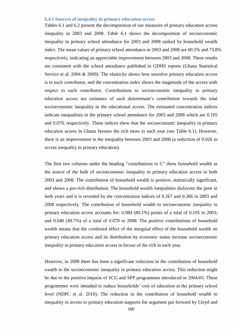
160
6.4.1 Sources of inequality in primary education access
Tables 6.1 and 6.2 present the decomposition of our measures of primary education access
inequality in 2003 and 2008. Table 6.1 shows the decomposition of socioeconomic
inequality in primary school attendance for 2003 and 2008 ranked by household wealth
index. The mean values of primary school attendance in 2003 and 2008 are 60.5% and 73.8%
respectively, indicating an appreciable improvement between 2003 and 2008. These results
are consistent with the school attendance published in GDHS reports (Ghana Statistical
Service et al. 2004 & 2009). The elasticity shows how sensitive primary education access
is to each contributor, and the concentration index shows the magnitude of the access with
respect to each contributor. Contributions to socioeconomic inequality in primary
education access are estimates of each determinant’s contribution towards the total
socioeconomic inequality in the educational access. The estimated concentration indices
indicate inequalities in the primary school attendance for 2003 and 2008 which are 0.105
and 0.079, respectively. These indices show that the socioeconomic inequality in primary
education access in Ghana favours the rich more in each year (see Table 6.1). However,
there is an improvement in the inequality between 2003 and 2008 (a reduction of 0.026 in
access inequality in primary education).
The first two columns under the heading "contributions to C" show household wealth as
the source of the bulk of socioeconomic inequality in primary education access in both
2003 and 2008. The contribution of household wealth is positive, statistically significant,
and shows a pro-rich distribution. The household wealth inequalities disfavour the poor in
both years and it is revealed by the concentration indices of 0.267 and 0.266 in 2003 and
2008 respectively. The contribution of household wealth to socioeconomic inequality in
primary education access accounts for: 0.084 (80.1%) points of a total of 0.105 in 2003;
and 0.040 (49.7%) of a total of 0.079 in 2008. The positive contributions of household
wealth means that the combined effect of the marginal effect of the household wealth on
primary education access and its distribution by economic status increase socioeconomic
inequality in primary education access in favour of the rich in each year.
However, in 2008 there has been a significant reduction in the contribution of household
wealth to the socioeconomic inequality in primary education access. This reduction might
be due to the positive impacts of SCG and SFP programmes introduced in 2004/05. These
programmes were intended to reduce households’ cost of education at the primary school
level (NDPC et al. 2010). The reduction in the contribution of household wealth to
inequality in access to primary education supports the argument put forward by Lloyd and
161
Blanc (1996) that if government spends generously on education and provides universal
access to primary education, inequality in access due to household wealth will fall. The
column headed "change" (i.e. the empirical analog of Equation 6.10) indicates that the bulk
of the improvement in primary education access inequality between 2003 and 2008 (-0.026
points) was due to a change of -0.044 points in respect of household wealth. These results
are consistent with the findings of other studies conducted in Ghana (Ghana Statistical
Service et al. 2004 & 2009; World Bank 2004; Akyeampong et al. 2007). These studies
also recognise the importance of household wealth in the distribution of education in
Ghana. The studies highlight the pattern of educational distribution in Ghana and argue
that there is inequality in education which is linked to income poverty and gender. For
example, Ghana Statistical Service et al. (2009) reveal that children from poor households
have lower school enrolment and attendance rates, and they are more likely to drop out in
the course of the primary cycle, than the children from non-poor households.
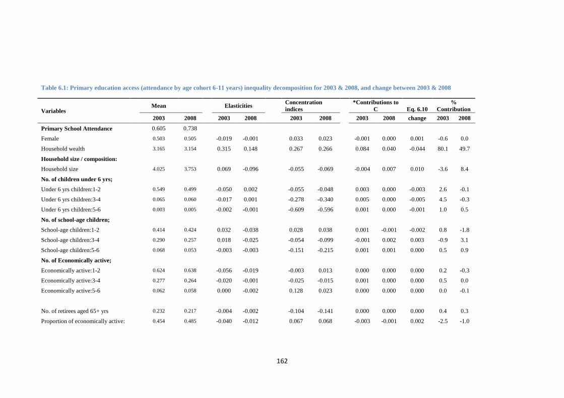
162
Table 6.1: Primary education access (attendance by age cohort 6-11 years) inequality decomposition for 2003 & 2008, and change between 2003 & 2008
Variables Mean
Elasticities
Concentration
indices *Contributions to
C Eq. 6.10
%
Contribution
2003 2008 2003 2008 2003 2008
2003 2008 change 2003 2008
Primary School Attendance
0.605 0.738
Female
0.503 0.505
-0.019 -0.001
0.033 0.023
-0.001 0.000 0.001 -0.6 0.0
Household wealth
3.165 3.154
0.315 0.148
0.267 0.266
0.084 0.040 -0.044 80.1 49.7
Household size / composition:
Household size
4.025 3.753
0.069 -0.096
-0.055 -0.069
-0.004 0.007 0.010 -3.6 8.4
No. of children under 6 yrs;
Under 6 yrs children:1-2
0.549 0.499
-0.050 0.002
-0.055 -0.048
0.003 0.000 -0.003 2.6 -0.1
Under 6 yrs children:3-4
0.065 0.060
-0.017 0.001
-0.278 -0.340
0.005 0.000 -0.005 4.5 -0.3
Under 6 yrs children:5-6
0.003 0.005
-0.002 -0.001
-0.609 -0.596
0.001 0.000 -0.001 1.0 0.5
No. of school-age children;
School-age children:1-2
0.414 0.424
0.032 -0.038
0.028 0.038
0.001 -0.001 -0.002 0.8 -1.8
School-age children:3-4
0.290 0.257
0.018 -0.025
-0.054 -0.099
-0.001 0.002 0.003 -0.9 3.1
School-age children:5-6
0.068 0.053
-0.003 -0.003
-0.151 -0.215
0.001 0.001 0.000 0.5 0.9
No. of Economically active;
Economically active:1-2
0.624 0.638
-0.056 -0.019
-0.003 0.013
0.000 0.000 0.000 0.2 -0.3
Economically active:3-4
0.277 0.264
-0.020 -0.001
-0.025 -0.015
0.001 0.000 0.000 0.5 0.0
Economically active:5-6
0.062 0.058
0.000 -0.002
0.128 0.023
0.000 0.000 0.000 0.0 -0.1
No. of retirees aged 65+ yrs
0.232 0.217
-0.004 -0.002
-0.104 -0.141
0.000 0.000 0.000 0.4 0.3
Proportion of economically active:
0.454 0.485
-0.040 -0.012
0.067 0.068
-0.003 -0.001 0.002 -2.5 -1.0
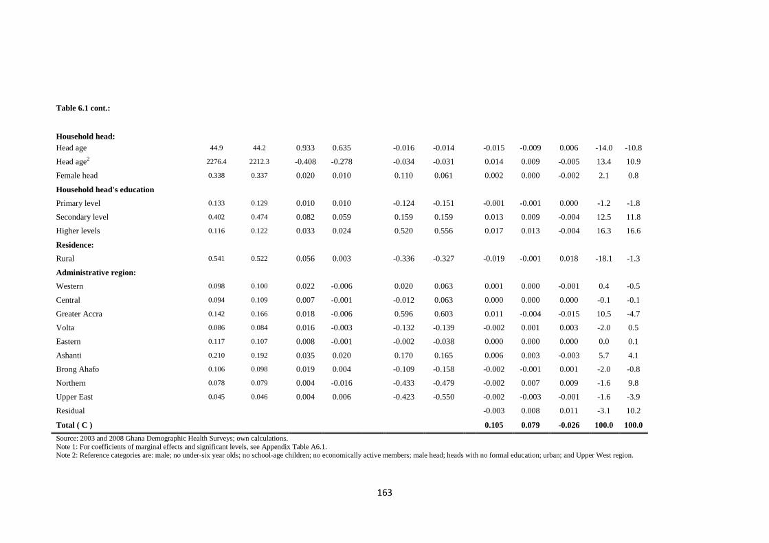
163
Table 6.1 cont.:
Household head:
Head age
44.9 44.2
0.933 0.635
-0.016 -0.014
-0.015 -0.009 0.006 -14.0 -10.8
Head age2
2276.4 2212.3
-0.408 -0.278
-0.034 -0.031
0.014 0.009 -0.005 13.4 10.9
Female head
0.338 0.337
0.020 0.010
0.110 0.061
0.002 0.000 -0.002 2.1 0.8
Household head's education
Primary level
0.133 0.129
0.010 0.010
-0.124 -0.151
-0.001 -0.001 0.000 -1.2 -1.8
Secondary level
0.402 0.474
0.082 0.059
0.159 0.159
0.013 0.009 -0.004 12.5 11.8
Higher levels
0.116 0.122
0.033 0.024
0.520 0.556
0.017 0.013 -0.004 16.3 16.6
Residence:
Rural
0.541 0.522
0.056 0.003
-0.336 -0.327
-0.019 -0.001 0.018 -18.1 -1.3
Administrative region:
Western
0.098 0.100
0.022 -0.006
0.020 0.063
0.001 0.000 -0.001 0.4 -0.5
Central
0.094 0.109
0.007 -0.001
-0.012 0.063
0.000 0.000 0.000 -0.1 -0.1
Greater Accra
0.142 0.166
0.018 -0.006
0.596 0.603
0.011 -0.004 -0.015 10.5 -4.7
Volta
0.086 0.084
0.016 -0.003
-0.132 -0.139
-0.002 0.001 0.003 -2.0 0.5
Eastern
0.117 0.107
0.008 -0.001
-0.002 -0.038
0.000 0.000 0.000 0.0 0.1
Ashanti
0.210 0.192
0.035 0.020
0.170 0.165
0.006 0.003 -0.003 5.7 4.1
Brong Ahafo
0.106 0.098
0.019 0.004
-0.109 -0.158
-0.002 -0.001 0.001 -2.0 -0.8
Northern
0.078 0.079
0.004 -0.016
-0.433 -0.479
-0.002 0.007 0.009 -1.6 9.8
Upper East
0.045 0.046
0.004 0.006
-0.423 -0.550
-0.002 -0.003 -0.001 -1.6 -3.9
Residual
-0.003 0.008 0.011 -3.1 10.2
Total ( C ) 0.105 0.079 -0.026 100.0 100.0
Source: 2003 and 2008 Ghana Demographic Health Surveys; own calculations.
Note 1: For coefficients of marginal effects and significant levels, see Appendix Table A6.1.
Note 2: Reference categories are: male; no under-six year olds; no school-age children; no economically active members; male head; heads with no formal education; urban; and Upper West region.
164
Our results are also consistent with the findings of (Filmer and Pritchett 1999b & 2001).
The authors examine socioeconomic inequalities in educational outcomes in India and
discover a large school enrolment differences which they attributed to income inequality
that varies widely across India states between the poor and the non-poor. They also come
to similar conclusions in their cross country study of 35 countries in Africa and Asia. In
particular, the authors find that in most of the 35 countries examined, children from
households at the top 20% of the wealth index (household wealth distribution) have higher
school attendance rate than children from households who occupied the bottom 40% of the
wealth index.
Contributions of female household head and household head's education (secondary and
higher levels) are all positive, statistically significant, and show a pro-rich distribution.
Inequalities in household head’s education attainment (shown by the concentration indices)
disfavour the poor in both years and their contributions to socioeconomic inequality in
primary education access are the second largest, accounting for 0.030 (28.8%) points of a
total of 0.105 in 2003, and 0.022 (28.4%) of a total of 0.079 in 2008. The contributions in
both years are positive, implying that household head’s level of education increases
socioeconomic inequality in primary education access in favour of the rich. This finding
supports the findings of Rolleston (2011), Lloyd and Hewett (2009) Sackey (2007),
Haveman and Wolfe (1995), Lloyd and Blanc (1996), and Chernichovsky (1985). These
authors show that the human capital of parents reflects a sort of intergeneration
transmission of socioeconomic status that affects the educational outcomes of their
children. Also, a household head’s educational level may serve as a predictor of the
household head’s market earnings potential that could be invested in children’s education
and this may have contributed to inequality in children’s educational outcomes in Ghana.
On average, 33.8% and 33.7% of households are headed by females in 2003 and 2008,
respectively which is consistent with the findings of (Ghana Statistical Service et al. 2004
& 2009). The inequality depicted by households headed by females, disfavours the poor in
both years but the contribution of female household head to socioeconomic inequality in
primary education access is fairly small, accounting for only 0.002 (2.1%) points of the
total inequality in 2003. The concentration indices of these (female household head and
household head's level of education) indicate that their inequalities are more concentrated
among the rich households in both 2003 and 2008. In other words, children from
165
households with these household characteristics have more access to primary education
than the children from poor households where these characteristics are lacking.
These results corroborate the findings of: Lloyd and Blanc (1996), and Thomas (1990 &
1994) with respect to households headed by females; and Chernichovsky (1985),
Tsakloglou (1993), Jacoby (1994), Lillard and Willis (1994), Lloyd and Blanc (1996),
Glick and Sahn (2000), Tansel (2002), Sackey (2007), and Rolleston (2011) with respect to
the educational level of household heads and parents. For example, Lloyd and Blanc
(1996), and Thomas (1990 & 1994) find that female household head with more education
have increased bargaining power in the household and may choose to allocate more
resources towards children and their human capital development than would their
counterpart, male household head .
The concentration indices for household size are negative (-0.055 and -0.069 in 2003 and
2008 respectively) indicating that the socioeconomic inequality in primary education
access with respect to household size is more concentrated among the poor households.
The contribution of household size to the total socioeconomic inequality is -0.004 in 2003
and 0.006 in 2008, resulting in a change of 0.010 in the total inequality. Considering the
household composition, the number of children under-six year olds have negative marginal
effect (see Table A6.1 in the Appendix 6) and are statistically significant in 2003 (for
households with 1 to 2, and 3 to 4 children), and their inequalities are more concentrated
among the poor households. For example, the concentration index for children under-six
year olds is -0.055 for a maximum of two children, and -0.278 for maximum of four
children in 2003. In 2003, these determinants contribute a fairly small amount of
inequalities (0.008 or 7.1%) to the total inequality.
With respect to the number of school-age children, the concentration indices for
households with 1 to 2 children are positive, indicating that the inequalities are more
concentrated among the rich, and contributing a change of -0.002 to the total inequality.
On the other hand, the concentration indices for households with 3 to 4 children are
negative, indicating that the inequalities are more concentrated among the poor, and
contributing a change of 0.003 to the total inequality. In addition, household composition
comprising a number of economically active and retirees and the proportion of
economically active members are not statistically significant in explaining the variations in
166
the primary education access. Consequently, their total contributions to the socioeconomic
inequality in primary education access are also negligible (see columns 7 to 9 of Table 6.1).
The mean of rural residency also indicates that the majority of households in Ghana reside
in the rural areas (Ghana Statistical Service et al. 2004 & 2009; Ghana Statistical Service
2007; Ghana Statistical Service 2008). The concentration indices (-0.336 and -0.327 in
2003 and 2008 respectively) indicate that inequalities in rural areas with respect to
socioeconomic inequality in primary education access are more concentrated among the
poor. These findings are also consistent with other findings (Ghana Statistical Service et al.
2004 & 2009; Sackey 2007). However, the contribution of rural areas to the total inequality
is statistically insignificant.
There are also regional inequalities that are pro-rich and pro-poor in the distribution of
primary education access, revealed by the concentration indices. Greater Accra and
Ashanti regions which are the richest regions in Ghana (Ghana Statistical Service et al.
2004 & 2009) are associated with higher primary education access. For Greater Accra
region, its contribution to the inequality is only statistically significant in 2003, but for the
Ashanti region, the contribution is statistically significant in both years. In both regions,
the distribution of primary education access is pro-rich. That is, the regional inequality in
these two regions disfavour the children from poor households. The concentration indices
for Greater Accra are 0.596 and 0.603 in 2003 and 2008, respectively. The Greater Accra
regional inequality contribution to socioeconomic inequality in access to primary education
accounts for 0.011 (10.5%) points of the total of 0.105 in 2003. The region also contributes
a change of -0.015 points (the third largest change) in inequality to overall change of
-0.026 in socioeconomic inequality in access to primary education.
Ashanti region inequality is shown by the concentration indices of 0.170 in 2003 and 0.165
in 2008. The region contributes 0.006 (5.7%) in 2003 and 0.003 (4.1%) inequality to the
total inequality of 0.105 and 0.079 in access to primary education in 2003 and 2008,
respectively. Thus, the region contributes a change of -0.003 points in inequality to the
total change in socioeconomic inequality in access to primary education. The contributions
of Volta and Brong Ahafo regions are statistically significant only in 2003. For example,
Volta region contributes a change of 0.003 points, whilst Brong Ahafo region contributes a
change of 0.001 points in inequality to the total change in socioeconomic inequality in
access to primary education in Ghana. The regions’ inequality in access to primary
167
education distributions is pro-poor. In other words, the inequality in access to primary
education (-0.132 and -0.139 for Volta in 2003 and 2008 respectively, and -0.109 and -
0.158 for Brong Ahafo in 2003 and 2008 respectively) is more concentrated among
children from the poor households.
All the regional inequality results presented so far are from the southern part of Ghana.
There are three regions in the northern part of Ghana; Northern, Upper East, and Upper
West regions. The Upper West region which is the poorest region in Ghana (Ghana
Statistical Service et al. 2004 & 2009) is used as reference category for the analysis. The
concentration index for the Northern region in 2008 is -0.479 which shows that lower
access to primary education is more concentrated among the children from poor
households in the region. The region contributes 0.007 (9.8%) points in inequality to the
total inequality of 0.079 in access to primary education which is statistically significant in
2008, and a change of 0.009 points in inequality to the total change in socioeconomic
inequality in access to primary education in Ghana.
The Upper East region’s concentration indices are negative in both years (-0.423 in 2003
and -0.550 in 2008), implying that access to primary education in the region is more
concentrated among children from poor households. In other words, the distribution of
access to primary education in the region is pro-poor. The region contributes -0.002 points
in inequality to the total inequality of 0.105 in 2003 and -0.003 to the total inequality of
0.079, and a change of -0.001 points in inequality to the total change in socioeconomic
inequality in access to primary education between the two periods (see Table 6.1).
Overall, the regional inequality in access to primary education disfavour the poor in the
regions in the north than regions in the south which is consistent with the findings of other
studies (Ghana Statistical Service et al. 2004 & 2009; Ghana Statistical Service 2008;
Ghana Statistical Service 2007; Sackey 2007).
For policy lessons, the results in Table 6.1 shows that the most important determinants that
contribute to pro-rich socioeconomic inequality in access to primary education are;
household wealth; female household head, and household head's educational attainment
levels (secondary and higher levels). However, the bulk of the sources of socioeconomic
inequality in access to primary education (i.e. inequality in primary school attendance) in
both 2003 and 2008 is attributed to household wealth, thereby disproportionately
168
benefiting the non-poor households. This finding corroborates with the findings of other
researchers (Psacharopoulos and Arriagada 1986; Sathar and Lloyd 1994; Lloyd and Blanc
1996; Gage et al. 1997; Buchmann and Hannum 2001). It should also be noted that the
residual (the part of the concentration index that cannot be traced back to the determinants
included in the decomposition analysis) has a negative sign in 2003 and a positive sign in
2008. This implies that some of the negative and positive association between household
wealth rank and primary education access in 2003 and 2008 respectively, are unexplained.
However, the results in Table 6.1 do not enable us to see how far the changes in the
determinants were due to changes in elasticities (i.e. changes in the impact of each
determinant on primary school attendance) rather than changes in inequalities (i.e. changes
in the degree of unequal distribution of each determinants across income groups).
Therefore, to further analyse the development in socioeconomic inequality in access to
primary education for policy purpose, we have applied Oaxaca-type decomposition of
change in concentration index between 2003 and 2008 based on Equations 6.11 and 6.12
(Wagstaff et al. 2003). The Oaxaca-type decomposition results in Table 6.2 allow us to
answer the questions the Table 6.1 results failed to answer.
Policy perspective
Table 6.2 depicts the decomposition results based on the Oaxaca-type decomposition (the
empirical analog of either equation 6.11 or 6.12) which are the estimates of the
contributions of the determinants to the concentration indices as well as the change
between 2003 and 2008. The column with header ‘ΔC * η’ are the contributions of the
respective determinants to the change in inequality in the total concentration index due to
the change of the concentration index of the predictor variables themselves. Furthermore,
the column with the header ‘Δη * C’ indicates the contribution due to the change in the
elasticity (or impact) of the determinants. The column ‘Total’ corresponds to the sum of
the two components, and coincides with the column headed ‘Change’ in Table 6.1
(balancing effect), but for the row total. Interesting insights emerge from the Oaxaca-type
decomposition results. The total change to be explained is a decrease in socioeconomic
inequality in access to primary education of 0.026.
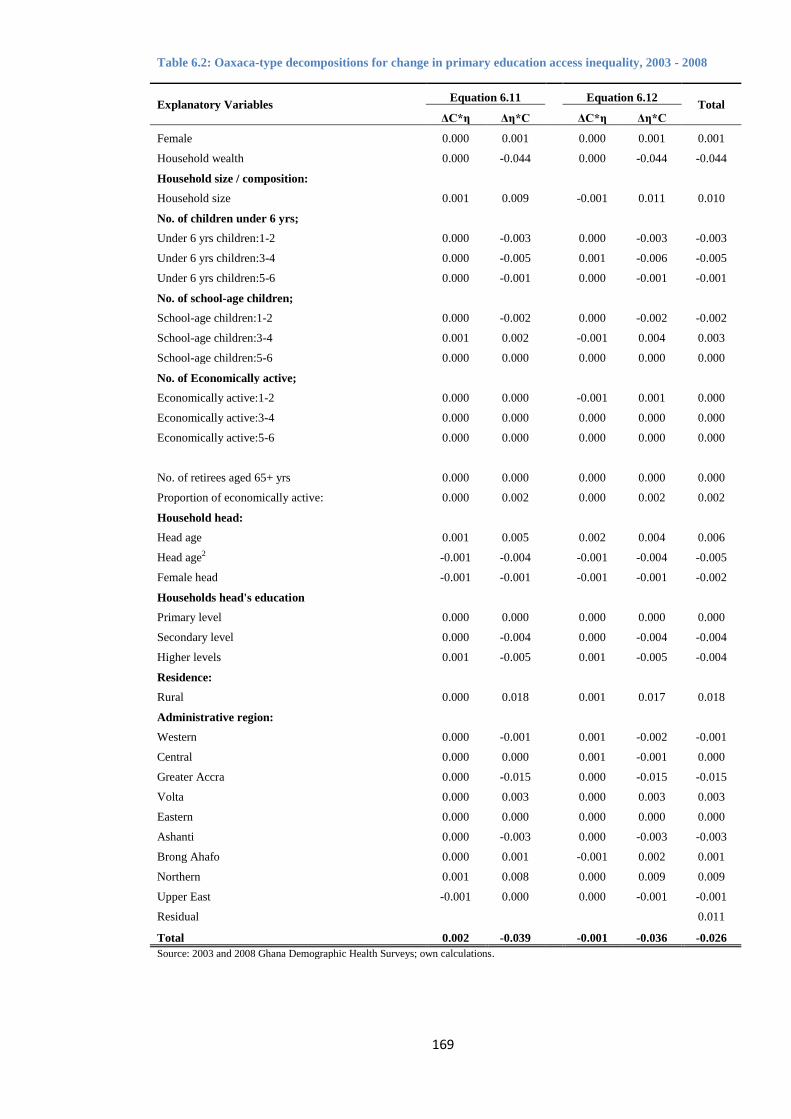
169
Table 6.2: Oaxaca-type decompositions for change in primary education access inequality, 2003 - 2008
Explanatory Variables Equation 6.11
Equation 6.12 Total
ΔC*η Δη*C ΔC*η Δη*C
Female 0.000 0.001
0.000 0.001 0.001
Household wealth 0.000 -0.044
0.000 -0.044 -0.044
Household size / composition:
Household size 0.001 0.009
-0.001 0.011 0.010
No. of children under 6 yrs;
Under 6 yrs children:1-2 0.000 -0.003
0.000 -0.003 -0.003
Under 6 yrs children:3-4 0.000 -0.005
0.001 -0.006 -0.005
Under 6 yrs children:5-6 0.000 -0.001
0.000 -0.001 -0.001
No. of school-age children;
School-age children:1-2 0.000 -0.002
0.000 -0.002 -0.002
School-age children:3-4 0.001 0.002
-0.001 0.004 0.003
School-age children:5-6 0.000 0.000
0.000 0.000 0.000
No. of Economically active;
Economically active:1-2 0.000 0.000
-0.001 0.001 0.000
Economically active:3-4 0.000 0.000
0.000 0.000 0.000
Economically active:5-6 0.000 0.000
0.000 0.000 0.000
No. of retirees aged 65+ yrs 0.000 0.000
0.000 0.000 0.000
Proportion of economically active: 0.000 0.002
0.000 0.002 0.002
Household head:
Head age 0.001 0.005
0.002 0.004 0.006
Head age2 -0.001 -0.004
-0.001 -0.004 -0.005
Female head -0.001 -0.001
-0.001 -0.001 -0.002
Households head's education
Primary level 0.000 0.000
0.000 0.000 0.000
Secondary level 0.000 -0.004
0.000 -0.004 -0.004
Higher levels 0.001 -0.005
0.001 -0.005 -0.004
Residence:
Rural 0.000 0.018
0.001 0.017 0.018
Administrative region:
Western 0.000 -0.001
0.001 -0.002 -0.001
Central 0.000 0.000
0.001 -0.001 0.000
Greater Accra 0.000 -0.015
0.000 -0.015 -0.015
Volta 0.000 0.003
0.000 0.003 0.003
Eastern 0.000 0.000
0.000 0.000 0.000
Ashanti 0.000 -0.003
0.000 -0.003 -0.003
Brong Ahafo 0.000 0.001
-0.001 0.002 0.001
Northern 0.001 0.008
0.000 0.009 0.009
Upper East -0.001 0.000
0.000 -0.001 -0.001
Residual
0.011
Total 0.002 -0.039 -0.001 -0.036 -0.026
Source: 2003 and 2008 Ghana Demographic Health Surveys; own calculations.
170
Some of the variables that contribute to the year-by-year indices are also important for
explaining the change. However, by far the largest contribution to the reduction in
socioeconomic inequality in access to primary education comes from household wealth,
due to the elasticity (i.e. impact) of use which has been drastically reduced from 0.315 in
2003 to 0.148 in 2008 (see Table 6.1). The result in Table 6.2 suggests that it is the
changing elasticity rather than household wealth inequality that accounts for the bulk of the
decrease in access to primary education inequality associated with changes in respect of
household wealth in 2008.
The change in elasticity of household wealth (Δη*C) is -0.044 whether we use Equation
6.11 or Equation 6.12. Overall, taking the changes of all the determinants of primary
education access into account, the fall in socioeconomic inequality in access to primary
education is largely attributable to changing elasticities (which is around -0.039 or -0.036,
depending on whether we use Equation 6.11 or Equation 6.12), rather than changing
inequalities in the determinants of the primary education access in Ghana. The reduced
elasticity of household wealth which has reduced socioeconomic inequality in access to
primary education could be attributed to the implementation of SCG, SFP, in 2004/05 and
the enforcement the laws that support FCUBE in 2000. These policy interventions were
implemented to lessen the cost of education to parents and to increase access to primary
education in Ghana, especially for the poor. The result indicates that the policy might have
improved access to primary education (especially to the poor household, even though the
non-poor appear to benefit disproportionately), just as in the case of Uganda where the
implementation of the UPE programme led to reduction in the cost of primary education
and increase in access to primary education (Deininger 2003).
Considering the changes in the elasticities for household wealth, educational level of
household head (secondary and higher levels), and regional effects of Greater Accra and
Ashanti regions, in particular, show a reduction in the elasticities (depicted in Table 6.1).
Therefore, there is some indication that these determinants are contributing to reducing
inequality more via their reduced impacts (i.e. elasticities) on the access to primary
education (school attendance) than via changes in inequality in the given determinants.
Consequently, the total socioeconomic inequality in access to primary education among
children of official primary school-age in Ghana has fallen from 0.105 points in 2003 to
0.079 points in 2008. This implies that access to primary education between 2003 and 2008
has improved which may be due the GoG’s education policy and programmes. Evidence
171
from other countries which are consistent with our findings show that universal access to
primary education increased primary school attendance in Uganda (Deininger 2003) and
in Japan as early as the early 1900s (Hasegawa T. 2001 cited in Maika et al. 2013).
6.4.2 Sources of inequality in secondary education access
The results for secondary education access (school attendance) are also based on Equations
6.8 to 6.12. Tables 6.3 and 6.4 present the decomposition results of socioeconomic
inequality in access to secondary education for 2003 and 2008 ranked by household wealth
index. The mean values of secondary attendance in 2003 and 2008 are 34.7% and 42.6%
respectively, indicating an appreciable improvement in average school attendance status
between 2003 and 2008. These results are consistent with the results published in Ghana
Statistical Service et al. (2004 & 2009) for secondary school attendance for Ghana in 2003
and 2008. The elasticities in Table 6.3 show the impact of each determinant on the
socioeconomic inequality in access to secondary education, and the concentration indices
show the magnitude of socioeconomic inequality in access to secondary education with
respect to each determinant. Contributions to socioeconomic inequality in access to
secondary education are estimates of each predictor variable’s contribution towards the
total socioeconomic inequality in access to secondary education. The estimated
concentration indices indicate socioeconomic inequalities of 0.129 and 0.120 points in the
access to secondary education for 2003 and 2008, respectively. These indices show that the
socioeconomic inequality in access to secondary education favours the rich more than the
poor in each year. Although, the results indicate an improvement between 2003 and 2008,
the reduction (-0.009) is very small compared to the reduction (-0.026) in socioeconomic
inequality in access to primary education within the same period (see Table 6.1).
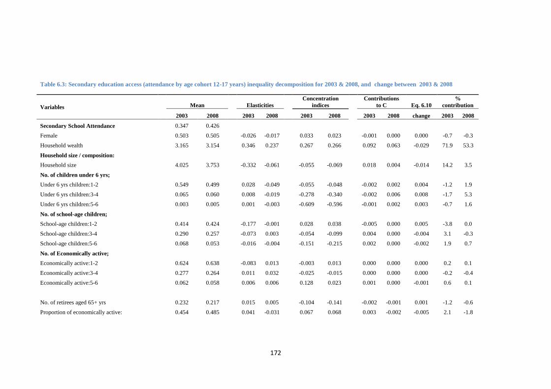
172
Table 6.3: Secondary education access (attendance by age cohort 12-17 years) inequality decomposition for 2003 & 2008, and change between 2003 & 2008
Variables
Mean
Elasticities
Concentration
indices
Contributions
to C Eq. 6.10
%
contribution
2003 2008 2003 2008 2003 2008
2003 2008 change 2003 2008
Secondary School Attendance
0.347 0.426
Female
0.503 0.505
-0.026 -0.017
0.033 0.023
-0.001 0.000 0.000 -0.7 -0.3
Household wealth
3.165 3.154
0.346 0.237
0.267 0.266
0.092 0.063 -0.029 71.9 53.3
Household size / composition:
Household size
4.025 3.753
-0.332 -0.061
-0.055 -0.069
0.018 0.004 -0.014 14.2 3.5
No. of children under 6 yrs;
Under 6 yrs children:1-2
0.549 0.499
0.028 -0.049
-0.055 -0.048
-0.002 0.002 0.004 -1.2 1.9
Under 6 yrs children:3-4
0.065 0.060
0.008 -0.019
-0.278 -0.340
-0.002 0.006 0.008 -1.7 5.3
Under 6 yrs children:5-6
0.003 0.005
0.001 -0.003
-0.609 -0.596
-0.001 0.002 0.003 -0.7 1.6
No. of school-age children;
School-age children:1-2
0.414 0.424
-0.177 -0.001
0.028 0.038
-0.005 0.000 0.005 -3.8 0.0
School-age children:3-4
0.290 0.257
-0.073 0.003
-0.054 -0.099
0.004 0.000 -0.004 3.1 -0.3
School-age children:5-6
0.068 0.053
-0.016 -0.004
-0.151 -0.215
0.002 0.000 -0.002 1.9 0.7
No. of Economically active;
Economically active:1-2
0.624 0.638
-0.083 0.013
-0.003 0.013
0.000 0.000 0.000 0.2 0.1
Economically active:3-4
0.277 0.264
0.011 0.032
-0.025 -0.015
0.000 0.000 0.000 -0.2 -0.4
Economically active:5-6
0.062 0.058
0.006 0.006
0.128 0.023
0.001 0.000 -0.001 0.6 0.1
No. of retirees aged 65+ yrs
0.232 0.217
0.015 0.005
-0.104 -0.141
-0.002 -0.001 0.001 -1.2 -0.6
Proportion of economically active:
0.454 0.485
0.041 -0.031
0.067 0.068
0.003 -0.002 -0.005 2.1 -1.8
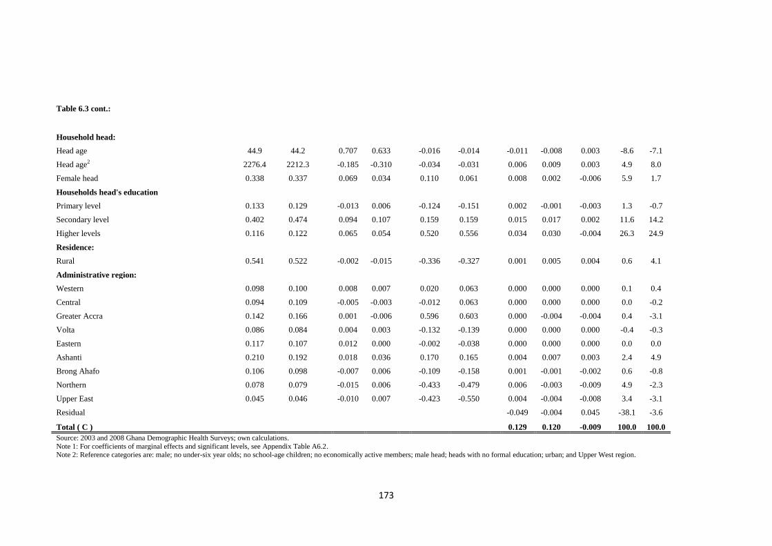
173
Table 6.3 cont.:
Household head:
Head age
44.9 44.2
0.707 0.633
-0.016 -0.014
-0.011 -0.008 0.003 -8.6 -7.1
Head age2
2276.4 2212.3
-0.185 -0.310
-0.034 -0.031
0.006 0.009 0.003 4.9 8.0
Female head
0.338 0.337
0.069 0.034
0.110 0.061
0.008 0.002 -0.006 5.9 1.7
Households head's education
Primary level
0.133 0.129
-0.013 0.006
-0.124 -0.151
0.002 -0.001 -0.003 1.3 -0.7
Secondary level
0.402 0.474
0.094 0.107
0.159 0.159
0.015 0.017 0.002 11.6 14.2
Higher levels
0.116 0.122
0.065 0.054
0.520 0.556
0.034 0.030 -0.004 26.3 24.9
Residence:
Rural
0.541 0.522
-0.002 -0.015
-0.336 -0.327
0.001 0.005 0.004 0.6 4.1
Administrative region:
Western
0.098 0.100
0.008 0.007
0.020 0.063
0.000 0.000 0.000 0.1 0.4
Central
0.094 0.109
-0.005 -0.003
-0.012 0.063
0.000 0.000 0.000 0.0 -0.2
Greater Accra
0.142 0.166
0.001 -0.006
0.596 0.603
0.000 -0.004 -0.004 0.4 -3.1
Volta
0.086 0.084
0.004 0.003
-0.132 -0.139
0.000 0.000 0.000 -0.4 -0.3
Eastern
0.117 0.107
0.012 0.000
-0.002 -0.038
0.000 0.000 0.000 0.0 0.0
Ashanti
0.210 0.192
0.018 0.036
0.170 0.165
0.004 0.007 0.003 2.4 4.9
Brong Ahafo
0.106 0.098
-0.007 0.006
-0.109 -0.158
0.001 -0.001 -0.002 0.6 -0.8
Northern
0.078 0.079
-0.015 0.006
-0.433 -0.479
0.006 -0.003 -0.009 4.9 -2.3
Upper East
0.045 0.046
-0.010 0.007
-0.423 -0.550
0.004 -0.004 -0.008 3.4 -3.1
Residual
-0.049 -0.004 0.045 -38.1 -3.6
Total ( C ) 0.129 0.120 -0.009 100.0 100.0
Source: 2003 and 2008 Ghana Demographic Health Surveys; own calculations.
Note 1: For coefficients of marginal effects and significant levels, see Appendix Table A6.2. Note 2: Reference categories are: male; no under-six year olds; no school-age children; no economically active members; male head; heads with no formal education; urban; and Upper West region.
174
The contributions of; household wealth, female household head, and household head's
educational attainment levels (secondary and higher levels) are all statistically significant.
The concentration indices of these variables indicate a pro-rich distribution of access to
secondary education among the households. This suggests that these determinants are more
concentrated among the rich households in both 2003 and 2008. The implication is that the
rich households gained more access to secondary education than the poor households in
both years.
Household wealth inequality favours the rich in both years and it is revealed by the
concentration indices of 0.267 and 0.266 in 2003 and 2008 respectively. Contributions of
the determinants to the total inequality in access to secondary education show that
household wealth constitutes the bulk of the sources of the inequality in secondary school
attendance in both 2003 and 2008. The contribution of household wealth to the
socioeconomic inequality in access to secondary education accounts for: 0.092 (71.9%)
points of the total inequality of 0.129 in 2003; and 0.063 (53.3%) of the total inequality of
0.120 in 2008. In addition, the "change" column (i.e. the empirical analog of equation 6.10)
indicates a fall (-0.029) in household wealth inequality which in turn contributes to a
decrease in socioeconomic inequality in access to secondary education between 2003 and
2008.
Considering household head characteristics, inequality in household head’s educational
attainment increases with the education level attained. For example, a household head with
secondary education has concentration index of 0.159 in both 2003 and 2008. For a
household head with educational level attained higher than secondary level (equivalent to
tertiary education attainment) the concentration indices are 0.520 and 0.556 in 2003 and
2008, respectively. This implies that inequality in these determinants disfavours the poor in
both years. Furthermore, the contributions of these determinants to socioeconomic
inequality in access to secondary education are the second largest, accounting for; 0.049
(37.9%) of the total inequality of 0.129 in 2003, and 0.047 (39.1%) of the total inequality
of 0.120 in 2008. Interesting, however, is the trend of the contribution of the two
determinants. For example, whilst the inequality contribution of household heads with
secondary education attainment increases [from 0.015 (11.6%) in 2003 to 0.017 (14.2%)],
that of household heads with higher levels of educational attainment decreases [from 0.034
(26.3%) in 2003 to 0.030 (24.9%)].
175
The inequality depicted by households headed by females, disproportionately benefit the
rich in both years. However, between the two periods, there has been a fall in the
inequality of female household head (from 0.110 in 2003 to 0.061 in 2008). The
contribution of female household head to socioeconomic inequality in access to secondary
education has also reduced from 0.008 (5.9%) in 2003 to 0.002 (1.7%) in 2008. Thus,
female household head contributes fairly small change in inequality (-0.006) towards the
total reduction in socioeconomic inequality in access to secondary education between 2003
and 2008.
These results show that children who reside in households with these household head
characteristics have more access to secondary education than the children from poor
households where these characteristics are lacking. These findings are consistent with the
findings in the empirical literature on the impacts of household head education level and
the positive impacts of households headed by females on children’s educational outcomes
(Chernichovsky 1985; Thomas 1994; Tsakloglou 1993; Jacoby 1994; Lloyd and Blanc
1996; Sackey 2007; Rolleston 2011). For example, Lloyd and Blanc (1996), and
Chernichovsky (1985) find that household head’s education serves as a predictor of
household head’s market earnings potential that could be invested in children’s education.
Thomas (1994) also finds that a female household head with more education may have
increased bargaining power in the household and may choose to allocate more resources
towards children and their human capital development than would their counterpart, male
household head.
The concentration indices for household size are negative (-0.055 and -0.069 in 2003 and
2008 respectively) indicating that the socioeconomic inequality in access to secondary
education is concentrated more among the poor households. The contribution of household
size to the total inequality is 0.018 (14.2%) in 2003 and 0.004 (3.5%) in 2008, resulting in
a change of -0.014 in the total inequality. The inequality in household size associated with
lower secondary education attainment of children from poor households has also been
established in the empirical literature. Although the findings of the effects of household
size on educational outcomes in the literature are mixed, our results are consistent with the
findings of; Blake (1981), Downey (1995) Knodel et al. (1990), and Pong (1997). These
studies show negative relationship between family size and inequality in educational
outcomes which is mostly concentrated among the poor.
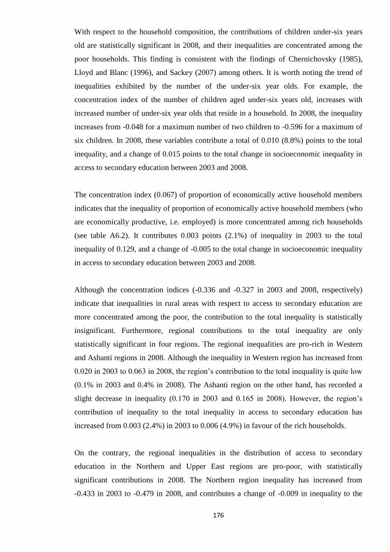
176
With respect to the household composition, the contributions of children under-six years
old are statistically significant in 2008, and their inequalities are concentrated among the
poor households. This finding is consistent with the findings of Chernichovsky (1985),
Lloyd and Blanc (1996), and Sackey (2007) among others. It is worth noting the trend of
inequalities exhibited by the number of the under-six year olds. For example, the
concentration index of the number of children aged under-six years old, increases with
increased number of under-six year olds that reside in a household. In 2008, the inequality
increases from -0.048 for a maximum number of two children to -0.596 for a maximum of
six children. In 2008, these variables contribute a total of 0.010 (8.8%) points to the total
inequality, and a change of 0.015 points to the total change in socioeconomic inequality in
access to secondary education between 2003 and 2008.
The concentration index (0.067) of proportion of economically active household members
indicates that the inequality of proportion of economically active household members (who
are economically productive, i.e. employed) is more concentrated among rich households
(see table A6.2). It contributes 0.003 points (2.1%) of inequality in 2003 to the total
inequality of 0.129, and a change of -0.005 to the total change in socioeconomic inequality
in access to secondary education between 2003 and 2008.
Although the concentration indices (-0.336 and -0.327 in 2003 and 2008, respectively)
indicate that inequalities in rural areas with respect to access to secondary education are
more concentrated among the poor, the contribution to the total inequality is statistically
insignificant. Furthermore, regional contributions to the total inequality are only
statistically significant in four regions. The regional inequalities are pro-rich in Western
and Ashanti regions in 2008. Although the inequality in Western region has increased from
0.020 in 2003 to 0.063 in 2008, the region’s contribution to the total inequality is quite low
(0.1% in 2003 and 0.4% in 2008). The Ashanti region on the other hand, has recorded a
slight decrease in inequality (0.170 in 2003 and 0.165 in 2008). However, the region’s
contribution of inequality to the total inequality in access to secondary education has
increased from 0.003 (2.4%) in 2003 to 0.006 (4.9%) in favour of the rich households.
On the contrary, the regional inequalities in the distribution of access to secondary
education in the Northern and Upper East regions are pro-poor, with statistically
significant contributions in 2008. The Northern region inequality has increased from
-0.433 in 2003 to -0.479 in 2008, and contributes a change of -0.009 in inequality to the
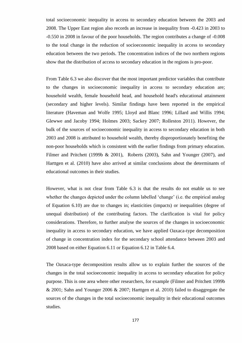
177
total socioeconomic inequality in access to secondary education between the 2003 and
2008. The Upper East region also records an increase in inequality from -0.423 in 2003 to
-0.550 in 2008 in favour of the poor households. The region contributes a change of -0.008
to the total change in the reduction of socioeconomic inequality in access to secondary
education between the two periods. The concentration indices of the two northern regions
show that the distribution of access to secondary education in the regions is pro-poor.
From Table 6.3 we also discover that the most important predictor variables that contribute
to the changes in socioeconomic inequality in access to secondary education are;
household wealth, female household head, and household head's educational attainment
(secondary and higher levels). Similar findings have been reported in the empirical
literature (Haveman and Wolfe 1995; Lloyd and Blanc 1996; Lillard and Willis 1994;
Glewwe and Jacoby 1994; Holmes 2003; Sackey 2007; Rolleston 2011). However, the
bulk of the sources of socioeconomic inequality in access to secondary education in both
2003 and 2008 is attributed to household wealth, thereby disproportionately benefiting the
non-poor households which is consistent with the earlier findings from primary education.
Filmer and Pritchett (1999b & 2001), Roberts (2003), Sahn and Younger (2007), and
Harttgen et al. (2010) have also arrived at similar conclusions about the determinants of
educational outcomes in their studies.
However, what is not clear from Table 6.3 is that the results do not enable us to see
whether the changes depicted under the column labelled ‘change’ (i.e. the empirical analog
of Equation 6.10) are due to changes in; elasticities (impacts) or inequalities (degree of
unequal distribution) of the contributing factors. The clarification is vital for policy
considerations. Therefore, to further analyse the sources of the changes in socioeconomic
inequality in access to secondary education, we have applied Oaxaca-type decomposition
of change in concentration index for the secondary school attendance between 2003 and
2008 based on either Equation 6.11 or Equation 6.12 in Table 6.4.
The Oaxaca-type decomposition results allow us to explain further the sources of the
changes in the total socioeconomic inequality in access to secondary education for policy
purpose. This is one area where other researchers, for example (Filmer and Pritchett 1999b
& 2001; Sahn and Younger 2006 & 2007; Harttgen et al. 2010) failed to disaggregate the
sources of the changes in the total socioeconomic inequality in their educational outcomes
studies.
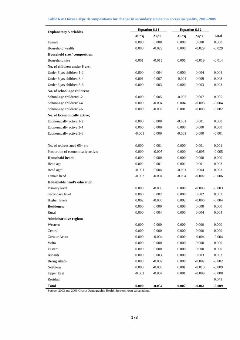
178
Table 6.4: Oaxaca-type decompositions for change in secondary education access inequality, 2003-2008
Explanatory Variables Equation 6.11
Equation 6.12
Total ΔC*η Δη*C
ΔC*η Δη*C
Female 0.000 0.000
0.000 0.000 0.000
Household wealth 0.000 -0.029
0.000 -0.029 -0.029
Household size / composition:
Household size 0.001 -0.015
0.005 -0.019 -0.014
No. of children under 6 yrs;
Under 6 yrs children:1-2 0.000 0.004
0.000 0.004 0.004
Under 6 yrs children:3-4 0.001 0.007
-0.001 0.009 0.008
Under 6 yrs children:5-6 0.000 0.003
0.000 0.003 0.003
No. of school-age children;
School-age children:1-2 0.000 0.005
-0.002 0.007 0.005
School-age children:3-4 0.000 -0.004
0.004 -0.008 -0.004
School-age children:5-6 0.000 -0.002
0.001 -0.003 -0.002
No. of Economically active;
Economically active:1-2 0.000 0.000
-0.001 0.001 0.000
Economically active:3-4 0.000 0.000
0.000 0.000 0.000
Economically active:5-6 -0.001 0.000
-0.001 0.000 -0.001
No. of retirees aged 65+ yrs 0.000 0.001
0.000 0.001 0.001
Proportion of economically active: 0.000 -0.005
0.000 -0.005 -0.005
Household head: 0.000 0.000
0.000 0.000 0.000
Head age 0.002 0.001
0.002 0.001 0.003
Head age2 -0.001 0.004
-0.001 0.004 0.003
Female head -0.002 -0.004
-0.004 -0.002 -0.006
Households head's education
Primary level 0.000 -0.003
0.000 -0.003 -0.003
Secondary level 0.000 0.002
0.000 0.002 0.002
Higher levels 0.002 -0.006
0.002 -0.006 -0.004
Residence: 0.000 0.000
0.000 0.000 0.000
Rural 0.000 0.004
0.000 0.004 0.004
Administrative region:
Western 0.000 0.000
0.000 0.000 0.000
Central 0.000 0.000
0.000 0.000 0.000
Greater Accra 0.000 -0.004
0.000 -0.004 -0.004
Volta 0.000 0.000
0.000 0.000 0.000
Eastern 0.000 0.000
0.000 0.000 0.000
Ashanti 0.000 0.003
0.000 0.003 0.003
Brong Ahafo 0.000 -0.002
0.000 -0.002 -0.002
Northern 0.000 -0.009
0.001 -0.010 -0.009
Upper East -0.001 -0.007
0.001 -0.009 -0.008
Residual
0.045
Total 0.000 -0.054
0.007 -0.061 -0.009
Source: 2003 and 2008 Ghana Demographic Health Surveys; own calculations.
179
Policy perspective
The total change to be explained is a decrease in socioeconomic inequality in access to
secondary education of 0.009 points. Again, some of the variables that contribute to the
year-by-year indices are also important for explaining the change. By far, the largest
contribution to the change in socioeconomic inequality in access to secondary education
comes from household wealth. This finding is consistent with the findings of Filmer and
Pritchett (1999b & 2001), (Harttgen et al. 2010), and (Porta et al. 2011) where they find
household wealth as the main contributor to disparities in educational outcomes of
household across developing countries (Africa, Asia, Latin America, Caribbean and the
Pacific). The source of the change is the elasticity of use with respect to household wealth
which has been reduced from 0.346 in 2003 to 0.237 in 2008. The result depicted by Table
6.4 suggests it is the changing elasticity (-0.029) rather than the inequality in household
wealth that accounts for the bulk of the decrease in socioeconomic inequality in access to
secondary education between the two periods.
Changes in the elasticities of other determinants such as; proportion of economically active
household members (-0.027), household size (-0.015 or -0.019), and Northern and Upper
East regions (-0.016 or -0.019) also contribute to the total reduction in the socioeconomic
inequality in access to secondary education. However, from Table 6.4, it is evidenced that
these covariates contribute to reducing socioeconomic inequality in access to secondary
education more via their reduced impacts on the secondary attendance than via changes in
their inequalities.
Overall, taking the changes of all the determinants of access to secondary education into
account, the decrease in socioeconomic inequality in secondary education access is largely
attributable to changing elasticities, rather than changing inequalities in the determinants of
the access to secondary education. In all, there has been a decrease in total socioeconomic
inequality in access to secondary education from 0.129 in 2003 to 0.120 in 2008. This
finding is also consistent with the findings of (Harttgen et al. 2010) where the authors find
that inequalities in secondary school attendance rates decline with rising average
attendance in most of the 37 developing countries they have studied, including Ghana.
180
6.4.3 Sources of inequality in primary education attainment
The results for primary education attainment (primary school completion) are also derived
from Equations 6.8 to 6.12. Tables 6.5 and 6.6 present the decomposition results showing
sources of inequalities in primary education attainment in 2003 and 2008. The mean values
of primary school completion in 2003 and 2008 are 70.4% and 75.0% respectively,
indicating an improvement in the primary education attainment status between 2003 and
2008. The elasticities in Table 6.5 show the impact of each determinant on the primary
education attainment inequality, and the concentration indices show the magnitude of the
socioeconomic inequality in primary education attainment. Contributions to the
socioeconomic inequality are estimates of each determinant’s contribution towards the
total socioeconomic inequality in the primary education attainment. The estimated
concentration indices indicate total inequality of 0.145 and 0.142 points in primary
education attainment for 2003 and 2008, respectively. These indices show that the
socioeconomic inequality in primary education attainment favours the rich more than the
poor in each year. Although, the results indicate an improvement in the primary school
completion inequality between 2003 and 2008, the reduction (-0.003) is fairly negligible.
The concentration indices for female age cohort who have completed primary education
are more concentrated among the rich (0.033 and 0.023 concentration indices in 2003 and
2008, respectively). The result shown in Table 6.5 is consistent with the findings of other
similar studies; Lloyd and Gage-Brandon (1994) and Sackey (2007) for Ghana, Lloyd and
Hewett (2009) for Africa, and Holmes (2003) for Pakistan. In terms of inequality
contributions, female pupil contributes -0.002 and -0.001 points to socioeconomic
inequality in primary school completion in 2003 and 2008, respectively. Thus, a change of
0.001 to the total change in socioeconomic inequality in primary education completion
between the two periods comes from female pupil which is statistically significant.
Furthermore, considering the association between the primary education attainment and the
key household variables, the marginal effects of; household wealth, female household head,
and household head's educational attainment (secondary and higher levels) are all positive
and statistically significant. The concentration indices of these variables indicate a pro-rich
distribution of primary education attainment among the households.
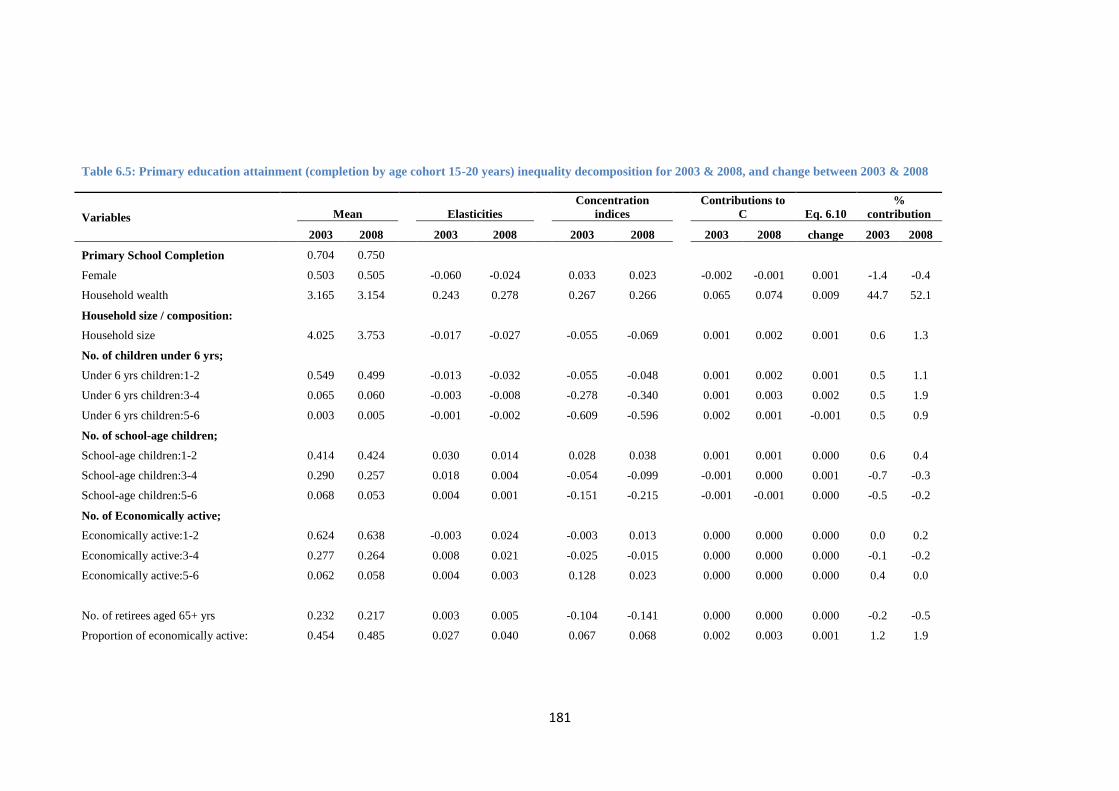
181
Table 6.5: Primary education attainment (completion by age cohort 15-20 years) inequality decomposition for 2003 & 2008, and change between 2003 & 2008
Variables
Mean
Elasticities
Concentration
indices
Contributions to
C Eq. 6.10
%
contribution
2003 2008 2003 2008 2003 2008
2003 2008 change 2003 2008
Primary School Completion
0.704 0.750
Female
0.503 0.505
-0.060 -0.024
0.033 0.023
-0.002 -0.001 0.001 -1.4 -0.4
Household wealth
3.165 3.154
0.243 0.278
0.267 0.266
0.065 0.074 0.009 44.7 52.1
Household size / composition:
Household size
4.025 3.753
-0.017 -0.027
-0.055 -0.069
0.001 0.002 0.001 0.6 1.3
No. of children under 6 yrs;
Under 6 yrs children:1-2
0.549 0.499
-0.013 -0.032
-0.055 -0.048
0.001 0.002 0.001 0.5 1.1
Under 6 yrs children:3-4
0.065 0.060
-0.003 -0.008
-0.278 -0.340
0.001 0.003 0.002 0.5 1.9
Under 6 yrs children:5-6
0.003 0.005
-0.001 -0.002
-0.609 -0.596
0.002 0.001 -0.001 0.5 0.9
No. of school-age children;
School-age children:1-2
0.414 0.424
0.030 0.014
0.028 0.038
0.001 0.001 0.000 0.6 0.4
School-age children:3-4
0.290 0.257
0.018 0.004
-0.054 -0.099
-0.001 0.000 0.001 -0.7 -0.3
School-age children:5-6
0.068 0.053
0.004 0.001
-0.151 -0.215
-0.001 -0.001 0.000 -0.5 -0.2
No. of Economically active;
Economically active:1-2
0.624 0.638
-0.003 0.024
-0.003 0.013
0.000 0.000 0.000 0.0 0.2
Economically active:3-4
0.277 0.264
0.008 0.021
-0.025 -0.015
0.000 0.000 0.000 -0.1 -0.2
Economically active:5-6
0.062 0.058
0.004 0.003
0.128 0.023
0.000 0.000 0.000 0.4 0.0
No. of retirees aged 65+ yrs
0.232 0.217
0.003 0.005
-0.104 -0.141
0.000 0.000 0.000 -0.2 -0.5
Proportion of economically active:
0.454 0.485
0.027 0.040
0.067 0.068
0.002 0.003 0.001 1.2 1.9
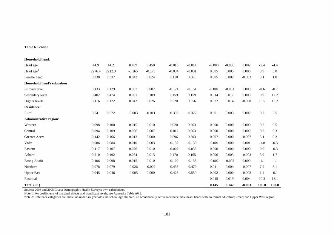
182
Table 6.5 cont.:
Household head:
Head age
44.9 44.2
0.499 0.458
-0.016 -0.014
-0.008 -0.006 0.002 -5.4 -4.4
Head age2
2276.4 2212.3
-0.165 -0.175
-0.034 -0.031
0.005 0.005 0.000 3.9 3.8
Female head
0.338 0.337
0.042 0.024
0.110 0.061
0.005 0.002 -0.003 3.1 1.0
Household head's education
Primary level
0.133 0.129
0.007 0.007
-0.124 -0.151
-0.001 -0.001 0.000 -0.6 -0.7
Secondary level
0.402 0.474
0.091 0.109
0.159 0.159
0.014 0.017 0.003 9.9 12.2
Higher levels
0.116 0.122
0.043 0.026
0.520 0.556
0.022 0.014 -0.008 15.5 10.2
Residence:
Rural
0.541 0.522
-0.003 -0.011
-0.336 -0.327
0.001 0.003 0.002 0.7 2.5
Administrative region:
Western
0.098 0.100
0.015 0.010
0.020 0.063
0.000 0.000 0.000 0.2 0.5
Central
0.094 0.109
0.006 0.007
-0.012 0.063
0.000 0.000 0.000 0.0 0.3
Greater Accra
0.142 0.166
0.012 0.000
0.596 0.603
0.007 0.000 -0.007 5.1 0.2
Volta
0.086 0.084
0.010 0.003
-0.132 -0.139
-0.001 0.000 0.001 -1.0 -0.3
Eastern
0.117 0.107
0.026 0.010
-0.002 -0.038
0.000 0.000 0.000 0.0 -0.3
Ashanti
0.210 0.192
0.034 0.015
0.170 0.165
0.006 0.003 -0.003 3.9 1.7
Brong Ahafo
0.106 0.098
0.015 0.010
-0.109 -0.158
-0.002 -0.002 0.000 -1.1 -1.1
Northern
0.078 0.079
-0.026 -0.009
-0.433 -0.479
0.011 0.004 -0.007 7.9 3.1
Upper East
0.045 0.046
-0.005 0.000
-0.423 -0.550
0.002 0.000 -0.002 1.4 -0.1
Residual
0.015 0.019 0.004 10.3 13.1
Total ( C ) 0.145 0.142 -0.003 100.0 100.0
Source: 2003 and 2008 Ghana Demographic Health Surveys; own calculations.
Note 1: For coefficients of marginal effects and significant levels, see Appendix Table A6.3. Note 2: Reference categories are: male; no under-six year olds; no school-age children; no economically active members; male head; heads with no formal education; urban; and Upper West region.
183
This suggests that these determinants are more concentrated among the rich households in
both 2003 and 2008. In other words, the inequalities disfavour the poor in the distribution
of primary school completion or attainment which is a stepping stone for transition into a
higher level of education.
Household wealth inequality favours the rich more than the poor in both years and it is
revealed by the concentration indices of 0.267 and 0.266 in 2003 and 2008, respectively.
This is consistent with the evidence from Western and Central Africa that show low
enrolment and high dropout rates resulting in more than 40% of children from poor
households never able to complete Grade 1 and only one in four completed Grade 5
(Filmer and Pritchett 1999b). Furthermore, the contributions of the determinants to the
total socioeconomic inequality in primary education attainment show that household
wealth constitutes the bulk of the sources of the inequality in both 2003 and 2008. The
contribution of household wealth to socioeconomic inequality in primary education
attainment accounts for: 0.065 (44.7%) points of the total inequality of 0.145 in 2003; and
0.074 (52.1%) of the total inequality of 0.142 in 2008. The trend shows an increased
change of 0.009 points contribution in household wealth inequality between 2003 and 2008
to the total change in socioeconomic inequality in primary education attainment.
The inequality depicted by households headed by females, favours the rich households
more than the poor households in both years. However, between the two periods, there has
been a fall in the inequality of female household head (from 0.110 in 2003 to 0.061 in
2008). The contribution of female household head to socioeconomic inequality in primary
education attainment has also fallen from 0.005 (3.1%) in 2003 to 0.002 (1.0%) in 2008.
Consequently, female household head contributes -0.003 change in inequality towards the
total reduction in socioeconomic inequality in primary education attainment between 2003
and 2008.
The contribution of secondary and higher levels of education attained by household head to
inequality is statistically significant. However, the decomposition of the inequality reveals
that the impact of household head’s educational attainment measured by the elasticity is
lower for household heads with primary education (concentrated among the poor
households) than household heads with at least secondary education (concentrated among
the rich households). Also the degree of unequal distribution of the primary education
attainment across households favours the rich households. In addition, inequality in
184
household head’s educational attainment increases with the level of education attained. It is
also possible to note that within the socioeconomic status, the rich households are more
likely to invest more resources in facilitating the education of children living in the
household. These findings corroborate the findings of Lloyd and Blanc (1996) Patrinos and
Psacharopoulos (1997) Deininger (2003), Sackey (2007), and Harttgen et al. (2010). These
studies demonstrate that household wealth is a key determinant of a household’s ability to
invest in children's education and as a result, it can lead to inequality in educational
outcomes between children from poor and the non-poor households. For example, in Table
6.5, a household head who has attained secondary education level has concentration index
of 0.159 in both 2003 and 2008. For a household head with higher levels of education than
secondary (equivalent to tertiary education attainment) the concentration index increases
from 0.520 in 2003 to 0.556 in 2008. The educational attainment inequalities are more
concentrated among the rich households in both years and this is consistent with the
findings of Maika et al. (2013) in Indonesia, where household head’s years of education or
parental education contribute to inequality in children’s cognitive achievement and are
more concentrated among the higher economic groups.
Furthermore, the contributions of household head’s educational attainment to
socioeconomic inequality in primary education attainment are the second largest,
accounting for 0.036 (25.4%) of the total inequality of 0.145 in 2003, and 0.031 (22.4%) of
the total inequality of 0.142 in 2008. Interesting, however, is the trend of the contribution
of the two determinants. For example, while the inequality contribution of household heads
with secondary education attainment increases [from 0.014 (9.9%) in 2003 to 0.017 (12.2%)
in 2008], that of household heads with higher levels of attainment than secondary level
decreases [from 0.022 (15.5%) in 2003 to 0.014 (10.2%) in 2008] between the two periods.
In total, household head’s educational attainment inequalities contribute a change of -0.005
to the total reduction in socioeconomic inequality in primary education attainment.
With respect to the household composition, the inequalities associated with number of
children under-six years are concentrated more among the poor households. It is worth
noting the trend of inequalities exhibited by the number of the under-six year olds. For
example, the concentration index of the number of children aged under-six years old
increases as the number of the under-six year olds increases. In 2003, the inequality
increases from -0.055 for a maximum number of two children to -0.609 for a maximum of
six children. Also, the inequality increases from -0.048 for a maximum number of two
185
children to -0.596 for a maximum of six children in 2008. The results corroborate well
with other findings (Sathar and Lloyd 1994; Lloyd and Blanc 1996). These variables
contribute a total of 0.003 (1.5%) and 0.006 (3.9%) points to the total socioeconomic
inequality in 2003 and 2008, respectively. In all, a change of 0.004 points to the total
change in socioeconomic inequality in primary education attainment between 2003 and
2008 was contributed by the number of the under-six year olds. This implies that these
determinants are increasing socioeconomic inequality in primary education attainment. On
the other hand, the inequality contributions of the number of school-age children, retirees,
economically active, and the proportion of economically active household members to the
inequality in primary education attainment are negligible and statistically insignificant.
At the regional level, the inequality contributions of; Western, Eastern, Ashanti, and Brong
Ahafo regions are statistically significant in both years. In the Western region, the regional
inequality is more concentrated among the rich households with increasing trend (from
0.020 in 2003 to 0.063 in 2008). However, the region’s inequality contribution to
socioeconomic inequality in primary education attainment is fairly negligible. The Ashanti
region’s inequality is also more concentrated among the rich households, however, with a
decreasing trend between the two periods (from 0.170 to 0.165). The Ashanti region
contributes 0.006 (3.9%) and 0.003 (1.7%) to the total socioeconomic inequality in primary
education attainment in 2003 and 2008, respectively. In effect, the region contributes a
change of -0.003 to the total change in socioeconomic inequality in primary education
attainment.
The Eastern and Brong Ahafo regions show pro-poor distribution of primary education
attainment in both years. Although both regions record an increase in socioeconomic
inequality in primary education attainment in favour of the poor, their contributions to the
total inequality in both years are fairly negligible. At the northern part of the country, the
result is different. The concentration indices of the Northern region show that the region’s
inequality in primary education attainment increases from -0.433 in 2003 to -0.479 in 2008
which is more concentrated among the children from poor households. An examination of
the marginal effect of the Northern region shows that the negative concentration index in
both 2003 and 2008 is associated with low probability of completing primary education
which is concentrated among the poor households (see Table A6.3). Furthermore, the
region contributes 0.011 (7.9%) and 0.004 (3.1%) in inequality to the total socioeconomic
inequalities of 0.145 and 0.142 in primary education attainment in 2003 and 2008,
186
respectively. Overall, the levels and trends in regional inequality contribution to
socioeconomic inequality in primary educational attainment disfavour the poor households
and these findings are consistent with Ghana Statistical Service et al. (2004 & 2009)
reports. The reports show that there are disparities in educational attainment in all the 10
regions in favour of rich households.
From Table 6.5 it is evidenced that the bulk of the sources contributing to socioeconomic
inequality in primary education attainment in both 2003 and 2008 is attributed to
household wealth which favours the rich households more than the poor households.
Although Table 6.5 shows that the most important sources of socioeconomic inequality in
primary education attainment include: household wealth, female household head,
household head's level of education (secondary and higher levels), and some regional
effects, again the results do not enable us to distinguish between the changes in the
contributions due to changes in elasticities and changes in inequalities. Therefore, further
analysis became imperative to disaggregate the changes in the primary school completion
inequality between 2003 and 2008 for policy purpose. Consequently, we apply Oaxaca-
type decomposition of change in concentration index to scrutinise the sources of the
changes in the socioeconomic inequality in primary education attainment.
Policy perspective
From Table 6.5, the total change to be explained is a decrease in socioeconomic inequality
in primary education attainment of 0.003. Although some of the variables that contribute to
the indices are also important for explaining the change, by far the largest contributor of
inequality change to the total change in socioeconomic inequality in primary education
attainment comes from household wealth. The source of change in the household wealth
and its impact on the primary education attainment, measured by the elasticity of use has
increased from 0.243 in 2003 to 0.278 in 2008. Table 6.6 suggests it is the changing
elasticity (Δη) rather than the changing household wealth inequality (ΔC) that accounts for
the reduction in socioeconomic inequality in primary education attainment between 2003
and 2008. Again, this finding may be explained in terms of positive impact of the
government of Ghana’s education policy interventions (FCUBE, SCG, and SFP) discussed
in Chapters 1 and 2.
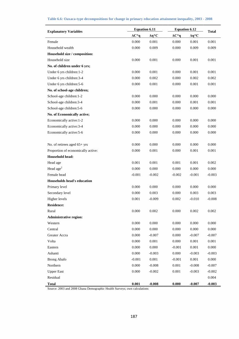
187
Table 6.6: Oaxaca-type decompositions for change in primary education attainment inequality, 2003 - 2008
Explanatory Variables Equation 6.11
Equation 6.12 Total
ΔC*η Δη*C ΔC*η Δη*C
Female 0.000 0.001
0.000 0.001 0.001
Household wealth 0.000 0.009
0.000 0.009 0.009
Household size / composition:
Household size 0.000 0.001
0.000 0.001 0.001
No. of children under 6 yrs;
Under 6 yrs children:1-2 0.000 0.001
0.000 0.001 0.001
Under 6 yrs children:3-4 0.000 0.002
0.000 0.002 0.002
Under 6 yrs children:5-6 0.000 0.001
0.000 0.001 0.001
No. of school-age children;
School-age children:1-2 0.000 0.000
0.000 0.000 0.000
School-age children:3-4 0.000 0.001
0.000 0.001 0.001
School-age children:5-6 0.000 0.000
0.000 0.000 0.000
No. of Economically active;
Economically active:1-2 0.000 0.000
0.000 0.000 0.000
Economically active:3-4 0.000 0.000
0.000 0.000 0.000
Economically active:5-6 0.000 0.000
0.000 0.000 0.000
No. of retirees aged 65+ yrs 0.000 0.000
0.000 0.000 0.000
Proportion of economically active: 0.000 0.001
0.000 0.001 0.001
Household head:
Head age 0.001 0.001
0.001 0.001 0.002
Head age2 0.000 0.000
0.000 0.000 0.000
Female head -0.001 -0.002
-0.002 -0.001 -0.003
Households head's education
Primary level 0.000 0.000
0.000 0.000 0.000
Secondary level 0.000 0.003
0.000 0.003 0.003
Higher levels 0.001 -0.009
0.002 -0.010 -0.008
Residence:
Rural 0.000 0.002
0.000 0.002 0.002
Administrative region:
Western 0.000 0.000
0.000 0.000 0.000
Central 0.000 0.000
0.000 0.000 0.000
Greater Accra 0.000 -0.007
0.000 -0.007 -0.007
Volta 0.000 0.001
0.000 0.001 0.001
Eastern 0.000 0.000
-0.001 0.001 0.000
Ashanti 0.000 -0.003
0.000 -0.003 -0.003
Brong Ahafo -0.001 0.001
-0.001 0.001 0.000
Northern 0.000 -0.008
0.001 -0.008 -0.007
Upper East 0.000 -0.002
0.001 -0.003 -0.002
Residual
0.004
Total 0.001 -0.008 0.000 -0.007 -0.003
Source: 2003 and 2008 Ghana Demographic Health Surveys; own calculations
188
Generally, taking the changes of all the determinants of the primary education attainment
into account, the inequality reduction in the primary education attainment is largely
attributable to changing elasticities, rather than changing inequalities in the determinants of
the primary school attainment (see the row total in Table 6.6). From Table 6.6 we can,
therefore, suggest that the key determinants contribute either to increasing or decreasing
inequality more via their impact on primary school completion than via changes in the
degree of unequal distribution across income groups. In all, there has been a decrease in
the total socioeconomic inequality in primary education attainment from 0.145 in 2003 to
0.142 in 2008, although the decrease has been very minimal.
6.4.4 Sources of inequality in secondary education attainment
Tables 6.7 and 6.8 present the decomposition of the measures of socioeconomic inequality
in secondary education attainment for 2003 and 2008. The mean values of secondary
completion in 2003 and 2008 samples are 14.7% and 22.8% respectively, indicating an
improvement in the secondary completion status between 2003 and 2008. The elasticities
in Table 6.7 show the impact of each determinant on the secondary education attainment
inequality, and the concentration indices show the magnitude of the inequality with respect
to each determinant. Contributions to socioeconomic inequality in secondary completion
are estimates of each determinant’s contribution towards the total inequality in the
secondary education attainment. The estimated concentration indices indicate total
inequality of 0.109 and 0.148 points in secondary education attainment for 2003 and 2008,
respectively. These indices show that the inequality in secondary education attainment
favours the rich households more in each year than the poor households. The results also
indicate a significant increase (0.040) in the secondary education attainment inequality
between 2003 and 2008 in favour of the rich households.
The concentration indices (0.033 and 0.023) for female age cohort are positive, indicating
that the inequality associated with female age cohort’s secondary education attainment are
more concentrated among the rich households. Female age cohort contributes -0.001 points
each year to socioeconomic inequality in secondary education attainment. This means that
the combined effect of female student’s marginal effect and its distribution by household
wealth was lowering the socioeconomic inequality in secondary education attainment.
Other findings also suggest that there is inequality in the distribution of education in Ghana
which is linked to gender and income poverty (Ghana Statistical Service et al. 2009;
Akyeampong et al. 2007; World Bank 2004; Lloyd and Hewett 2009).
189
In Table 6.7, the contributions of; household wealth, proportion of economically active
household members, female household head, and household head’s educational attainment
levels (secondary and higher levels) are all statistically significant in both years. The
concentration indices of these determinants indicate that their inequalities are more
concentrated among the rich households. This implies the inequalities favour the rich
households more than the poor households in the distribution of secondary education
attainment in Ghana.
Household wealth inequalities favour the rich households in both years as indicated by its
concentration indices. Contributions of the determinants to the total inequalities in
secondary education attainment show that household wealth constitutes the bulk of the
sources of the socioeconomic inequality in the of secondary school completion in both
2003 and 2008. The contribution of household wealth to inequalities in of secondary
education attainment accounts for; 0.097 (89.0 %%) points of a total of 0.109 in 2003, and
0.065 (43.9%) of a total of 0.148 in 2008. The positive contributions to socioeconomic
inequality imply that the household wealth is increasing socioeconomic inequality in
secondary education attainment in favour of the rich households. However, there is a
decrease in the contribution of household wealth by 0.032 between the two periods,
primarily owing to a lower elasticity (0.246 in 2008 compared to 0.366 in 2003) of the
secondary education attainment.
The change column in Table 6.7 shows that the increase in the socioeconomic inequality in
the secondary education attainment in Ghana between 2003 and 2008 is largely due to
changes in household wealth. For example, Ghana Statistical Service et al. (2009) also
reveal that children from poor households have lower educational attainment, and they are
more likely to drop out in the course of their educational cycle, than the children from non-
poor households. Filmer and Pritchett (1999b) also find that the dropout rates for the poor
are consistently higher than for the non-poor across 37 developing countries.
There are, however, changes in other determinants that have contributed to the total change
in the socioeconomic inequality over time. The inequality depicted by households headed
by females is more concentrated among the rich households in both years. However,
between the two periods, there has been a fall in the inequality of female household head
from 0.110 in 2003 to 0.061 in 2008. The contribution of female household head to
socioeconomic inequality in secondary education attainment has also fallen from 0.012
190
(11.2%) in 2003 to 0.003 (2.3%) in 2008. Consequently, female household head
contributes -0.009 change in inequality towards the total change in socioeconomic
inequality in secondary education attainment between 2003 and 2008. This implies that the
inequality contribution of female household head is lowering socioeconomic inequality in
secondary education attainment. This supports the argument that “female household heads
are more likely to invest resources, including time, money and emotional support, in
facilitating the education of children living in their households” (Lloyd and Blanc
1996:288).
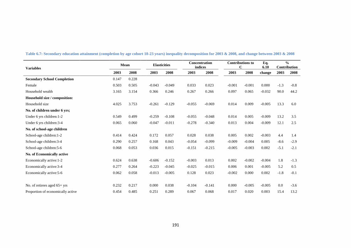
191
Table 6.7: Secondary education attainment (completion by age cohort 18-23 years) inequality decomposition for 2003 & 2008, and change between 2003 & 2008
Variables
Mean
Elasticities
Concentration
indices Contributions to
C
Eq.
6.10
%
Contribution
2003 2008 2003 2008 2003 2008
2003 2008 change 2003 2008
Secondary School Completion
0.147 0.228
Female
0.503 0.505
-0.043 -0.049
0.033 0.023
-0.001 -0.001 0.000 -1.3 -0.8
Household wealth
3.165 3.154
0.366 0.246
0.267 0.266
0.097 0.065 -0.032 90.0 44.2
Household size / composition:
Household size
4.025 3.753
-0.261 -0.129
-0.055 -0.069
0.014 0.009 -0.005 13.3 6.0
No. of children under 6 yrs;
Under 6 yrs children:1-2
0.549 0.499
-0.259 -0.108
-0.055 -0.048
0.014 0.005 -0.009 13.2 3.5
Under 6 yrs children:3-4
0.065 0.060
-0.047 -0.011
-0.278 -0.340
0.013 0.004 -0.009 12.1 2.5
No. of school-age children
School-age children:1-2
0.414 0.424
0.172 0.057
0.028 0.038
0.005 0.002 -0.003 4.4 1.4
School-age children:3-4
0.290 0.257
0.168 0.043
-0.054 -0.099
-0.009 -0.004 0.005 -8.6 -2.9
School-age children:5-6
0.068 0.053
0.036 0.015
-0.151 -0.215
-0.005 -0.003 0.002 -5.1 -2.1
No. of Economically active
Economically active:1-2
0.624 0.638
-0.606 -0.152
-0.003 0.013
0.002 -0.002 -0.004 1.8 -1.3
Economically active:3-4
0.277 0.264
-0.223 -0.045
-0.025 -0.015
0.006 0.001 -0.005 5.2 0.5
Economically active:5-6
0.062 0.058
-0.013 -0.005
0.128 0.023
-0.002 0.000 0.002 -1.8 -0.1
No. of retirees aged 65+ yrs
0.232 0.217
0.000 0.038
-0.104 -0.141
0.000 -0.005 -0.005 0.0 -3.6
Proportion of economically active
0.454 0.485
0.251 0.289
0.067 0.068
0.017 0.020 0.003 15.4 13.2
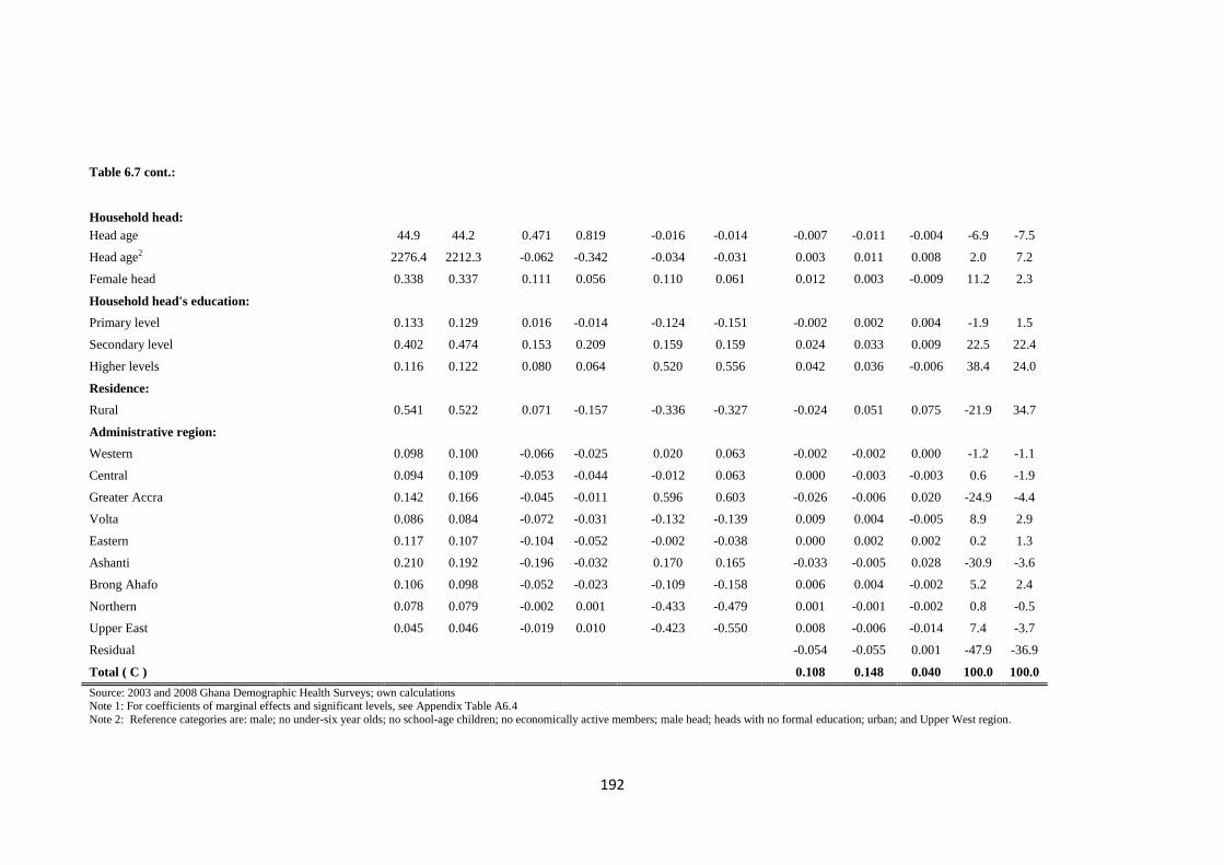
192
Table 6.7 cont.:
Household head:
Head age
44.9 44.2
0.471 0.819
-0.016 -0.014
-0.007 -0.011 -0.004 -6.9 -7.5
Head age2
2276.4 2212.3
-0.062 -0.342
-0.034 -0.031
0.003 0.011 0.008 2.0 7.2
Female head
0.338 0.337
0.111 0.056
0.110 0.061
0.012 0.003 -0.009 11.2 2.3
Household head's education:
Primary level
0.133 0.129
0.016 -0.014
-0.124 -0.151
-0.002 0.002 0.004 -1.9 1.5
Secondary level
0.402 0.474
0.153 0.209
0.159 0.159
0.024 0.033 0.009 22.5 22.4
Higher levels
0.116 0.122
0.080 0.064
0.520 0.556
0.042 0.036 -0.006 38.4 24.0
Residence:
Rural
0.541 0.522
0.071 -0.157
-0.336 -0.327
-0.024 0.051 0.075 -21.9 34.7
Administrative region:
Western
0.098 0.100
-0.066 -0.025
0.020 0.063
-0.002 -0.002 0.000 -1.2 -1.1
Central
0.094 0.109
-0.053 -0.044
-0.012 0.063
0.000 -0.003 -0.003 0.6 -1.9
Greater Accra
0.142 0.166
-0.045 -0.011
0.596 0.603
-0.026 -0.006 0.020 -24.9 -4.4
Volta
0.086 0.084
-0.072 -0.031
-0.132 -0.139
0.009 0.004 -0.005 8.9 2.9
Eastern
0.117 0.107
-0.104 -0.052
-0.002 -0.038
0.000 0.002 0.002 0.2 1.3
Ashanti
0.210 0.192
-0.196 -0.032
0.170 0.165
-0.033 -0.005 0.028 -30.9 -3.6
Brong Ahafo
0.106 0.098
-0.052 -0.023
-0.109 -0.158
0.006 0.004 -0.002 5.2 2.4
Northern
0.078 0.079
-0.002 0.001
-0.433 -0.479
0.001 -0.001 -0.002 0.8 -0.5
Upper East
0.045 0.046
-0.019 0.010
-0.423 -0.550
0.008 -0.006 -0.014 7.4 -3.7
Residual
-0.054 -0.055 0.001 -47.9 -36.9
Total ( C ) 0.108 0.148 0.040 100.0 100.0
Source: 2003 and 2008 Ghana Demographic Health Surveys; own calculations Note 1: For coefficients of marginal effects and significant levels, see Appendix Table A6.4
Note 2: Reference categories are: male; no under-six year olds; no school-age children; no economically active members; male head; heads with no formal education; urban; and Upper West region.
189
Whilst the inequality in the household head’s secondary education attainment level
remains constant in both years, that of a household head with higher levels of education
attainment increases from 0.520 in 2003 to 0.556 in 2008. The inequality contribution of a
household head’s secondary education attainment, (in absolute term) increases from 0.024
in 2003 to 0.033 in 2008, partly due to the increase in its elasticity. However, the relative
contribution shows a decrease of 0.1% (from 22.5% to 22.4%) between the two periods.
On the other hand, the contribution of household head with higher levels of education
decrease in both absolute and relative terms from 0.042 (38.4%) in 2003 to 0.036 (24.0%)
in 2008. In total, household head’s education levels contribute a change of 0.007 to the
total increase in socioeconomic inequality in secondary education attainment in favour of
the rich households. This means that household head’s educational attainment increases
socioeconomic inequality in secondary education attainment of children. Another
noticeable observation from Table 6.7 is that inequality in household head’s educational
level increases with the higher levels of education attained. For example, the inequality
increases from 0.159 for household head with secondary to 0.520, and 0.556 for household
head with a higher level of education in 2003 and 2008, respectively in favour of the rich
households. This finding is consistent with the empirical literature that have found positive
relationship between educational level of household heads or parents and children's
educational outcomes (Glewwe and Jacoby 1994; Oliver 1995; Tansel 1997; Sathar and
Lloyd 1994; Chernichovsky 1985).
With respect to the household composition, the contribution of a household with a
maximum of two children under-six years old to the inequality in secondary school
completion is statistically significant in both years. The inequality is more concentrated
among the poor households. In addition, contribution of households with a maximum of
four under-six year olds to the total inequality in 2003 is also statistically significant. The
inequality associated with the number of children under-six years old contributes 0.029
(26.7%) and 0.009 (6.0%) points to the total socioeconomic inequality in secondary
education attainment in 2003 and 2008, respectively. In all, a change of -0.020 points to
the total change in socioeconomic inequality in secondary education attainment (0.040)
between 2003 and 2008 was attributed to the number of the under-six year olds. These
findings corroborate studies that show that the presence of very young children in poor
households in particular, can increase the time needed for childcare and this can affect
school attendance and completion of school children (Sathar and Lloyd 1994; Lloyd and
Blanc 1996).
194
The inequality contribution of a maximum of two school-age children to secondary
education attainment is statistically significant only in both 2003 and 2008. Its associated
inequality is more concentrated among rich households. The inequality increases from
0.028 in 2003 to 0.038 in 2008, and contributes 0.005 (4.4%) and 0.002 (1.4%) to the total
socioeconomic inequality in 2003 and 2008, respectively. In effect, households with 1 to 2
school-going-age children contribute a change of -0.003 in inequality to the total change
(0.040) in inequality between the two periods. This means that households with a
maximum of two school-age children contribute to lowering the socioeconomic inequality
in secondary education attainment between the two periods. In addition, the contribution of
a maximum of four school-age children to the total inequality in secondary school
completion is statistically significant in both years. Compared to the maximum number of
two school-age children inequality, the inequality is more concentrated among the poor
households. The inequality associated with the households with 3 to 4 school-age children
increases from -0.054 in 2003 to -0.099 in 2008. It contributes -0.009 and -0.004 to the
total socioeconomic inequality of 0.108 and 0.148 in 2003 and 2008, respectively.
The change in contribution to the total change in socioeconomic inequality in secondary
education attainment is, however, an increase of 0.005 points. In short, the inequality
associated with the number of school-age children contributes a total of -0.009 and -0.005
points to the total socioeconomic inequality in secondary education attainment in 2003 and
2008, respectively. However, the combined change in contribution to the total change in
the socioeconomic inequality in secondary educational attainment between 2003 and 2008
is an increase of 0.004 points. Thus, the inequality associated with the number of school-
age children in a household and its impact on secondary education attainment disfavour the
poor. This is consistent with the findings with Butcher and Case (1994) who argue that the
presence of more school-age children in the household could put more pressure on
household resources, thereby affecting children's school attendance and completion
negatively.
The contribution of the proportion of economically active household members is
statistically significant in both 2003 and 2008. The positive contribution shows that the
proportion of household members is economically productive, thereby creating positive
effect on the secondary education attainment. The concentration indices also show that the
inequality in the proportion of economically active household members favours the rich
households in both years. The proportion of economically active household members
195
contributes 0.017 (15.4%) and 0.020 (13.2%) to the total socioeconomic inequality in 2003
and 2008, respectively. Although the absolute inequality contribution increases between
the two periods (an increase of 0.003 points to the total change in socioeconomic
inequality in secondary completion), the relative inequality contribution decreases between
the two periods.
The concentration index also shows that inequality associated with rural areas is more
concentrated among the poor households. In 2008, rural areas contribute 0.051 (34.7%),
and a change of 0.075 points to the total socioeconomic inequality in secondary education
attainment. The socioeconomic inequality in secondary school attainment revealed by the
decomposition is in line with the findings of Sackey (2007). Sackey observes locality
differences with respect to children’s school attendance and attainment which is highly
associated with socioeconomic inequality in educational outcomes between the urban and
rural areas in Ghana.
In terms of regional effect, the contributions of most of the regions to the total inequality
are statistically in both 2003 and 2008. With exception of Western and Ashanti regions (in
2003 and 2008) and Central region (in 2008), the regional inequality is more concentrated
among the poor households. Western, Central, Volta, Eastern, Ashanti, and Brong Ahafo
regions have contributed -0.020 points to the total socioeconomic inequality in secondary
education attainment in 2003. Although these regions have made fairly negligible
inequality contribution to the total socioeconomic inequality in 2008, their total change in
inequality contribution (0.020) to the total change in secondary education attainment
inequality (0.040) is fairly and statistically significant. Unsurprisingly, the fall in the
secondary education attainment is mostly concentrated among the poor households in the
regions. Ghana Statistical Service et al. (2004 & 2009) find similar trend in regional
educational inequality associated with socioeconomic inequality in Ghana.
From Table 6.7, we also discover that the most important determinants or sources that
contribute to the changes in socioeconomic inequality in secondary school completion are;
household wealth, household head's education, household size, female household head,
rural residency effect, and regional effects of Western, Central, Volta, Eastern, Ashanti,
and Brong Ahafo, regions in particular.
196
Although Table 6.7 appears to have revealed some sources of educational inequality in
secondary completion, the changes in the contribution of the sources of socioeconomic
inequality in secondary education attainment, however, do not enable us to explain whether
the changes are either due to changes in elasticities or changes in inequality or both.
Therefore, to further analyse the changes in the inequality, we have once again applied an
Oaxaca-type decomposition of change in concentration index for the secondary education
attainment between 2003 and 2008 educed from either equation 6.11 or 6.12. The Oaxaca-
type decomposition results in Table 6.8 allow us to explain the sources of the changes in
the inequality for policy purposes.
Policy perspective
Yet again, interesting insights emerge from the decomposition results. The total change to
be explained is an increase in socioeconomic inequality of 0.040. By far the largest
inequality contributions to the change in socioeconomic inequality in secondary education
attainment come from household wealth and rural residency. The impact of household
wealth on the secondary school completion (measured by the elasticity of use) has been
very high over time, even though the elasticity has decreased from 0.366 in 2003 to 0.246
in 2008. Table 6.8 moreover, suggests it is the changing elasticity (Δη) and not the
changing household wealth inequality (ΔC) that contributes to the socioeconomic
inequality in secondary education attainment. On the whole, taking the changes of all the
determinants of the socioeconomic inequality in secondary education attainment into
account, the increase in the inequality (see the row total contributions to C in Table 6.7) is
largely attributable to changing elasticities, rather than changing inequalities in the
determinants (row total in Table 6.8).
There is, therefore, an indication that these key determinants are contributing to either
increasing or decreasing socioeconomic inequality more via their impact (Δη) on the
secondary school completion than via changes in inequality (ΔC) in the determinants.
Overall, the socioeconomic inequality in secondary education attainment has increased
from 0.108 in 2003 to 0.148 in 2008 in favour of the rich households. The finding is
consistent with the findings of (Harttgen et al. 2010). The authors studied 37 developing
countries and find that the socioeconomic inequality in school completion has increased in
favour of rich households.
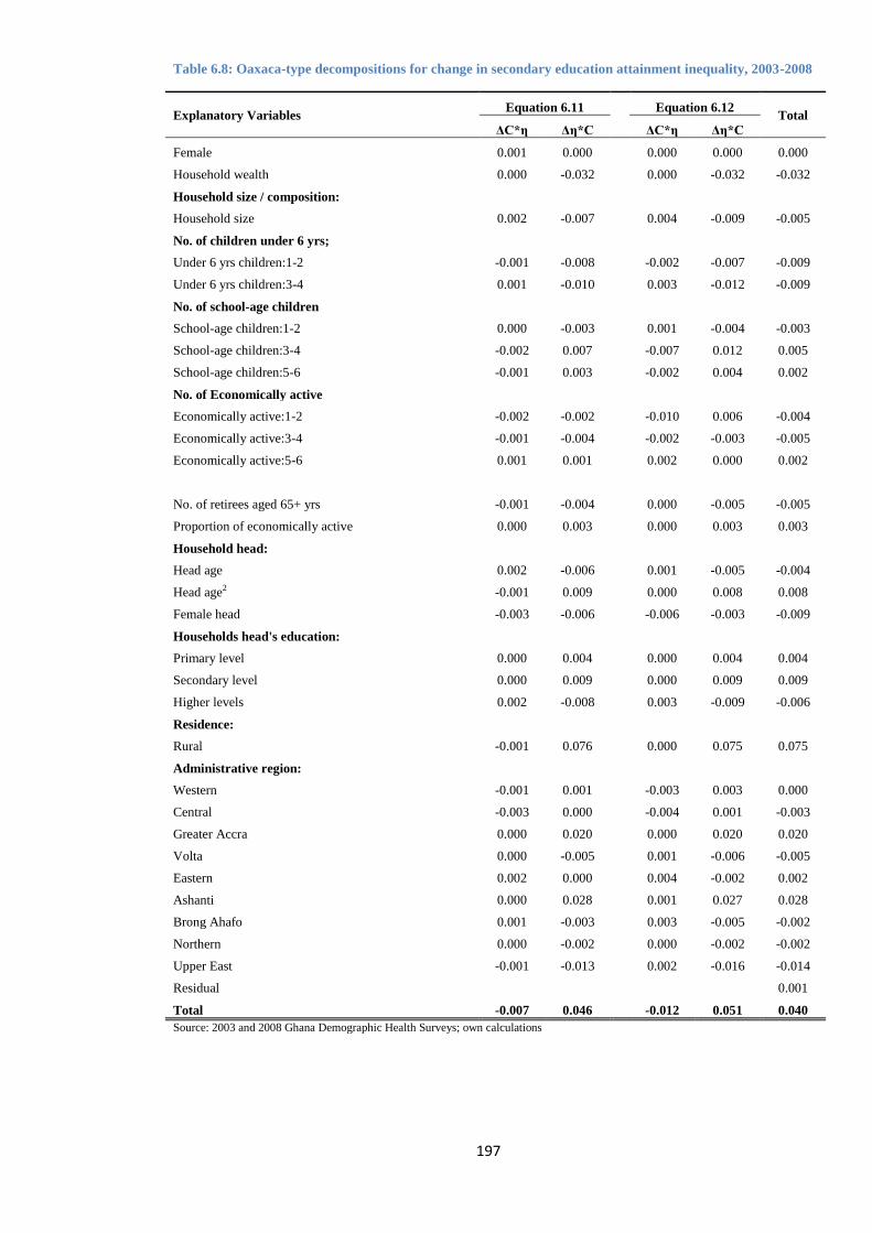
197
Table 6.8: Oaxaca-type decompositions for change in secondary education attainment inequality, 2003-2008
Explanatory Variables Equation 6.11
Equation 6.12 Total
ΔC*η Δη*C ΔC*η Δη*C
Female 0.001 0.000
0.000 0.000 0.000
Household wealth 0.000 -0.032
0.000 -0.032 -0.032
Household size / composition:
Household size 0.002 -0.007
0.004 -0.009 -0.005
No. of children under 6 yrs;
Under 6 yrs children:1-2 -0.001 -0.008
-0.002 -0.007 -0.009
Under 6 yrs children:3-4 0.001 -0.010
0.003 -0.012 -0.009
No. of school-age children
School-age children:1-2 0.000 -0.003
0.001 -0.004 -0.003
School-age children:3-4 -0.002 0.007
-0.007 0.012 0.005
School-age children:5-6 -0.001 0.003
-0.002 0.004 0.002
No. of Economically active
Economically active:1-2 -0.002 -0.002
-0.010 0.006 -0.004
Economically active:3-4 -0.001 -0.004
-0.002 -0.003 -0.005
Economically active:5-6 0.001 0.001
0.002 0.000 0.002
No. of retirees aged 65+ yrs -0.001 -0.004
0.000 -0.005 -0.005
Proportion of economically active 0.000 0.003
0.000 0.003 0.003
Household head:
Head age 0.002 -0.006
0.001 -0.005 -0.004
Head age2 -0.001 0.009
0.000 0.008 0.008
Female head -0.003 -0.006
-0.006 -0.003 -0.009
Households head's education:
Primary level 0.000 0.004
0.000 0.004 0.004
Secondary level 0.000 0.009
0.000 0.009 0.009
Higher levels 0.002 -0.008
0.003 -0.009 -0.006
Residence:
Rural -0.001 0.076
0.000 0.075 0.075
Administrative region:
Western -0.001 0.001
-0.003 0.003 0.000
Central -0.003 0.000
-0.004 0.001 -0.003
Greater Accra 0.000 0.020
0.000 0.020 0.020
Volta 0.000 -0.005
0.001 -0.006 -0.005
Eastern 0.002 0.000
0.004 -0.002 0.002
Ashanti 0.000 0.028
0.001 0.027 0.028
Brong Ahafo 0.001 -0.003
0.003 -0.005 -0.002
Northern 0.000 -0.002
0.000 -0.002 -0.002
Upper East -0.001 -0.013
0.002 -0.016 -0.014
Residual
0.001
Total -0.007 0.046 -0.012 0.051 0.040
Source: 2003 and 2008 Ghana Demographic Health Surveys; own calculations
198
It is not surprising to see this emerging trend in socioeconomic inequality in secondary
education attainment in Ghana. This is because secondary education in Ghana is not free.
Thus, the distribution of secondary education disproportionally benefits the rich
households more than the poor households. This finding corroborates the findings of
Ghana Statistical Service et al. (2004 & 2009).
6.5 Conclusions
The main aim of this chapter has been to estimate and decompose socioeconomic
inequality in school attendance and completion at both primary school and secondary
school levels in Ghana. The decomposition enables us to unravel the main sources of
educational inequalities, and their change over time, and to answer the questions posed at
the beginning of the chapter. The empirical questions we seek to address with the
decomposition method were: what are the sources or contributing factors of school
attendance and completion inequalities in Ghana?; is wealth distribution the main source of
educational inequalities?; what is the change in educational inequality over time?; have the
relatively sustained economic growth in Ghana for the past decade and educational
expansions impacted positively on educational inequalities?; and who benefits from
educational access and attainment in Ghana?
The concentration index analysis shows that the rich households benefit disproportionally
from access to, and attainment of both primary and secondary education in Ghana
compared to the poor households. Furthermore, the concentration indices of the primary
attendance, primary completion and the secondary attendance reveal that inequality in
these indicators of educational access and attainment has decreased over time, specifically
from 2003 to 2008. Conversely, the concentration indices of secondary school completion
show that inequality in this indicator of educational attainment has increased from 2003 to
2008 by 0.040 points. We then moved on to decompose each observed inequality into its
sources, and analyse its evolution over time (i.e. between 2003 and 2008). In particular,
following Wagstaff et al. (2003) and Oppedisano and Turati (2012) and applying the
concentration index framework to the selected education indicators, we decomposed the
change in each educational inequality at both primary and secondary levels on standardised
tests into shares due to: (i) changes in the inequality of the determinants of educational
indicators (ΔC*η), and (ii) changes due to the impact of the determinants (Δη*C) or the
rate of return of its determinants.
199
The results highlight that besides the inequality of; household head's educational
attainment levels, female household head, certain categories of economically productive
household members, and some regional effects, the most important determinant of
socioeconomic inequality in school attendance and completion in Ghana is the household
wealth. From the decomposition results, we found a positive contribution from household
wealth, especially towards reducing socioeconomic inequality in primary and secondary
school attendance, and secondary school completion between 2003 and 2008. Conversely,
we also observed a positive contribution from household wealth towards increasing
inequality in primary school completion, coming from the evolution of socioeconomic
inequality over time (from 2003 to 2008).
Another interesting question which we are able to answer in this chapter through the
concentration index decomposition analysis is: which of the two components of change in
the contributions of the determinants to the education inequality (i.e. elasticity and
inequality of the determinants) is the most important contributor to the estimated education
inequalities? This distinction is essential from a policy perspective, since in many cases
education policies may not directly alter the distribution of these characteristics by
household wealth, but they may be able to influence the education elasticity of some of
these characteristics. Again, some important observations emerged. In all the four cases of
socioeconomic inequality estimated, the elasticity differences (i.e. changes in the impact of
each determinant on the dependent variables) are greater than the inequality differences (i.e.
changes in the degree of unequal distribution of each determinant across income groups).
This implies that an equitable distribution of educational opportunities is preferable to a
redistribution of existing assets or incomes. As a result, an equitable distribution of
educational access and attainment will build new assets and improve social welfare by its
spill-over effect, without making anyone worse off (Thomas et al. 2001). Therefore,
ensuring access to educational opportunities by attending to both the supply and demand
sides by the government of Ghana will be a win-win policy gaining support in Ghana.
Take the contribution of household wealth for instance, without exception, the relative
change in elasticity (Δη*C) is much greater than the relative change in inequality (ΔC*η).
This implies that it is not so much the differences in household wealth inequality per se,
but the partial association between household wealth and the education indicators that
matters for income related education inequality. This is an important and interesting new
finding which can aid effective education policy interventions and implementation. This is
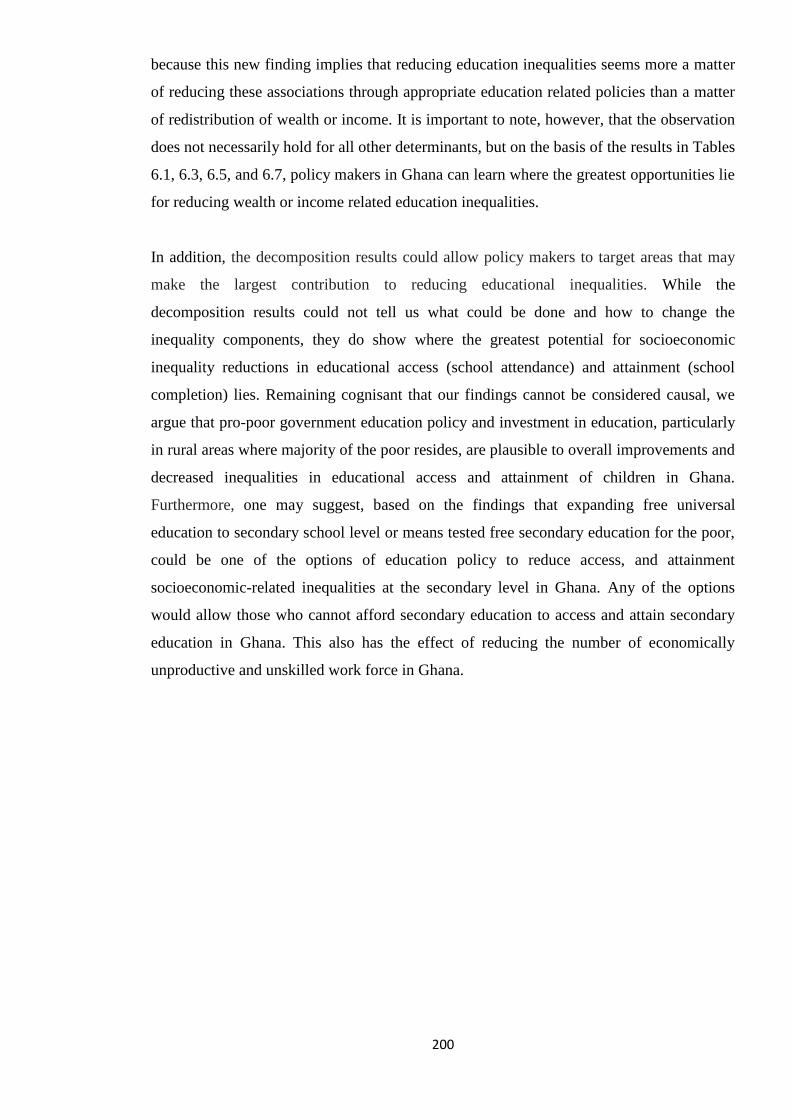
200
because this new finding implies that reducing education inequalities seems more a matter
of reducing these associations through appropriate education related policies than a matter
of redistribution of wealth or income. It is important to note, however, that the observation
does not necessarily hold for all other determinants, but on the basis of the results in Tables
6.1, 6.3, 6.5, and 6.7, policy makers in Ghana can learn where the greatest opportunities lie
for reducing wealth or income related education inequalities.
In addition, the decomposition results could allow policy makers to target areas that may
make the largest contribution to reducing educational inequalities. While the
decomposition results could not tell us what could be done and how to change the
inequality components, they do show where the greatest potential for socioeconomic
inequality reductions in educational access (school attendance) and attainment (school
completion) lies. Remaining cognisant that our findings cannot be considered causal, we
argue that pro-poor government education policy and investment in education, particularly
in rural areas where majority of the poor resides, are plausible to overall improvements and
decreased inequalities in educational access and attainment of children in Ghana.
Furthermore, one may suggest, based on the findings that expanding free universal
education to secondary school level or means tested free secondary education for the poor,
could be one of the options of education policy to reduce access, and attainment
socioeconomic-related inequalities at the secondary level in Ghana. Any of the options
would allow those who cannot afford secondary education to access and attain secondary
education in Ghana. This also has the effect of reducing the number of economically
unproductive and unskilled work force in Ghana.
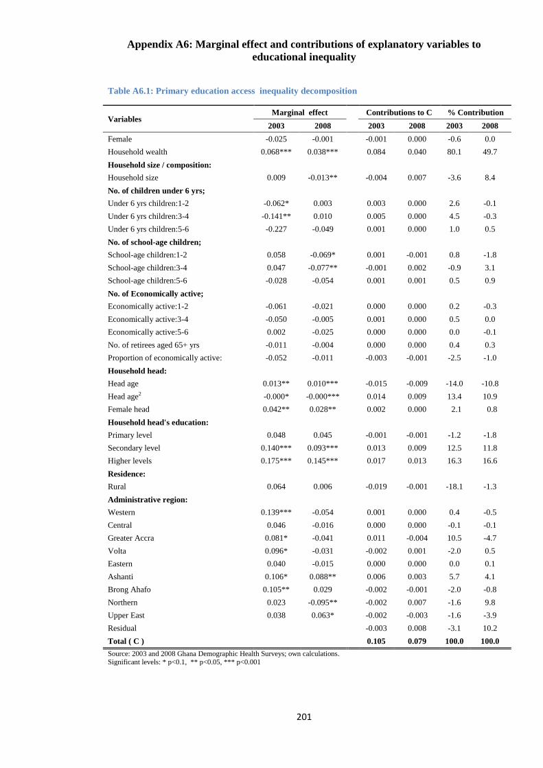
201
Appendix A6: Marginal effect and contributions of explanatory variables to
educational inequality
Table A6.1: Primary education access inequality decomposition
Variables Marginal effect
Contributions to C % Contribution
2003 2008 2003 2008 2003 2008
Female -0.025 -0.001
-0.001 0.000 -0.6 0.0
Household wealth 0.068*** 0.038***
0.084 0.040 80.1 49.7
Household size / composition:
Household size 0.009 -0.013**
-0.004 0.007 -3.6 8.4
No. of children under 6 yrs;
Under 6 yrs children:1-2 -0.062* 0.003
0.003 0.000 2.6 -0.1
Under 6 yrs children:3-4 -0.141** 0.010
0.005 0.000 4.5 -0.3
Under 6 yrs children:5-6 -0.227 -0.049
0.001 0.000 1.0 0.5
No. of school-age children;
School-age children:1-2 0.058 -0.069*
0.001 -0.001 0.8 -1.8
School-age children:3-4 0.047 -0.077**
-0.001 0.002 -0.9 3.1
School-age children:5-6 -0.028 -0.054
0.001 0.001 0.5 0.9
No. of Economically active;
Economically active:1-2 -0.061 -0.021
0.000 0.000 0.2 -0.3
Economically active:3-4 -0.050 -0.005
0.001 0.000 0.5 0.0
Economically active:5-6 0.002 -0.025
0.000 0.000 0.0 -0.1
No. of retirees aged 65+ yrs -0.011 -0.004
0.000 0.000 0.4 0.3
Proportion of economically active: -0.052 -0.011
-0.003 -0.001 -2.5 -1.0
Household head:
Head age 0.013** 0.010***
-0.015 -0.009 -14.0 -10.8
Head age2 -0.000* -0.000***
0.014 0.009 13.4 10.9
Female head 0.042** 0.028**
0.002 0.000 2.1 0.8
Household head's education:
Primary level 0.048 0.045
-0.001 -0.001 -1.2 -1.8
Secondary level 0.140*** 0.093***
0.013 0.009 12.5 11.8
Higher levels 0.175*** 0.145***
0.017 0.013 16.3 16.6
Residence:
Rural 0.064 0.006
-0.019 -0.001 -18.1 -1.3
Administrative region:
Western 0.139*** -0.054
0.001 0.000 0.4 -0.5
Central 0.046 -0.016
0.000 0.000 -0.1 -0.1
Greater Accra 0.081* -0.041
0.011 -0.004 10.5 -4.7
Volta 0.096* -0.031
-0.002 0.001 -2.0 0.5
Eastern 0.040 -0.015
0.000 0.000 0.0 0.1
Ashanti 0.106* 0.088**
0.006 0.003 5.7 4.1
Brong Ahafo 0.105** 0.029
-0.002 -0.001 -2.0 -0.8
Northern 0.023 -0.095**
-0.002 0.007 -1.6 9.8
Upper East 0.038 0.063*
-0.002 -0.003 -1.6 -3.9
Residual
-0.003 0.008 -3.1 10.2
Total ( C ) 0.105 0.079 100.0 100.0
Source: 2003 and 2008 Ghana Demographic Health Surveys; own calculations. Significant levels: * p<0.1, ** p<0.05, *** p<0.001
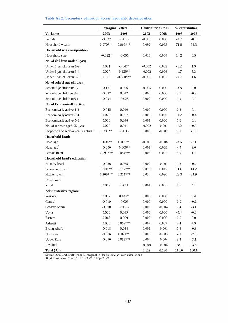
202
Table A6.2: Secondary education access inequality decomposition
Variables
Marginal effect
Contributions to C % contribution
2003 2008
2003 2008 2003 2008
Female -0.022 -0.016
-0.001 0.000 -0.7 -0.3
Household wealth 0.070*** 0.066***
0.092 0.063 71.9 53.3
Household size / composition:
Household size -0.022* -0.005
0.018 0.004 14.2 3.5
No. of children under 6 yrs;
Under 6 yrs children:1-2 0.021 -0.047*
-0.002 0.002 -1.2 1.9
Under 6 yrs children:3-4 0.027 -0.129**
-0.002 0.006 -1.7 5.3
Under 6 yrs children:5-6 0.109 -0.300***
-0.001 0.002 -0.7 1.6
No. of school-age children;
School-age children:1-2 -0.161 0.006
-0.005 0.000 -3.8 0.0
School-age children:3-4 -0.097 0.012
0.004 0.000 3.1 -0.3
School-age children:5-6 -0.094 -0.028
0.002 0.000 1.9 0.7
No. of Economically active;
Economically active:1-2 -0.045 0.010
0.000 0.000 0.2 0.1
Economically active:3-4 0.022 0.057
0.000 0.000 -0.2 -0.4
Economically active:5-6 0.033 0.048
0.001 0.000 0.6 0.1
No. of retirees aged 65+ yrs 0.023 0.011
-0.002 -0.001 -1.2 -0.6
Proportion of economically active: 0.285** -0.036
0.003 -0.002 2.1 -1.8
Household head:
Head age 0.006** 0.006**
-0.011 -0.008 -8.6 -7.1
Head age2 -0.000 -0.000**
0.006 0.009 4.9 8.0
Female head 0.091*** 0.054***
0.008 0.002 5.9 1.7
Household head's education:
Primary level -0.036 0.025
0.002 -0.001 1.3 -0.7
Secondary level 0.100** 0.112***
0.015 0.017 11.6 14.2
Higher levels 0.205*** 0.211***
0.034 0.030 26.3 24.9
Residence:
Rural 0.002 -0.011
0.001 0.005 0.6 4.1
Administrative region:
Western 0.037 0.042*
0.000 0.000 0.1 0.4
Central -0.019 -0.008
0.000 0.000 0.0 -0.2
Greater Accra -0.000 -0.016
0.000 -0.004 0.4 -3.1
Volta 0.020 0.019
0.000 0.000 -0.4 -0.3
Eastern 0.045 0.009
0.000 0.000 0.0 0.0
Ashanti 0.036 0.092***
0.004 0.007 2.4 4.9
Brong Ahafo -0.018 0.034
0.001 -0.001 0.6 -0.8
Northern -0.076 0.021**
0.006 -0.003 4.9 -2.3
Upper East -0.070 0.056***
0.004 -0.004 3.4 -3.1
Residual
-0.049 -0.004 -38.1 -3.6
Total ( C )
0.129 0.120 100.0 100.0
Source: 2003 and 2008 Ghana Demographic Health Surveys; own calculations.
Significant levels: * p<0.1, ** p<0.05, *** p<0.001

203
Table A6.3: Primary education attainment inequality decomposition
Variables Marginal effect
Contributions to C % contribution
2003 2008 2003 2008 2003 2008
Female -0.101*** -0.039***
-0.002 -0.001 -1.4 -0.4
Household wealth 0.059*** 0.071***
0.065 0.074 44.7 52.1
Household size / composition:
Household size -0.002 -0.003
0.001 0.002 0.6 1.3
No. of children under 6 yrs;
Under 6 yrs children:1-2 -0.019 -0.060***
0.001 0.002 0.5 1.1
Under 6 yrs children:3-4 -0.023 -0.088
0.001 0.003 0.5 1.9
Under 6 yrs children:5-6 -0.167 -0.243
0.002 0.001 0.5 0.9
No. of school-age children;
School-age children:1-2 0.053 0.021
0.001 0.001 0.6 0.4
School-age children:3-4 0.044 -0.004
-0.001 0.000 -0.7 -0.3
School-age children:5-6 0.045 -0.005
-0.001 -0.001 -0.5 -0.2
No. of Economically active;
Economically active:1-2 -0.003 0.037
0.000 0.000 0.0 0.2
Economically active:3-4 0.032 0.073*
0.000 0.000 -0.1 -0.2
Economically active:5-6 0.066 0.043
0.000 0.000 0.4 0.0
No. of retirees aged 65+ yrs 0.012 0.017
0.000 0.000 -0.2 -0.5
Proportion of economically active: 0.063 0.069
0.002 0.003 1.2 1.9
Household head:
Head age 0.007 0.008***
-0.008 -0.006 -5.4 -4.4
Head age2 -0.000 -0.000***
0.005 0.005 3.9 3.8
Female head 0.106*** 0.057***
0.005 0.002 3.1 1.0
Household head's education:
Primary level 0.033 0.029
-0.001 -0.001 -0.6 -0.7
Secondary level 0.173*** 0.173***
0.014 0.017 9.9 12.2
Higher levels 0.257*** 0.155***
0.022 0.014 15.5 10.2
Residence:
Rural -0.005 -0.016
0.001 0.003 0.7 2.5
Administrative region:
Western 0.093* 0.064***
0.000 0.000 0.2 0.5
Central 0.032 0.023
0.000 0.000 0.0 0.3
Greater Accra 0.041 -0.012
0.007 0.000 5.1 0.2
Volta 0.058 0.000
-0.001 0.000 -1.0 -0.3
Eastern 0.144*** 0.042**
0.000 0.000 0.0 -0.3
Ashanti 0.099* 0.045**
0.006 0.003 3.9 1.7
Brong Ahafo 0.072* 0.051***
-0.002 -0.002 -1.1 -1.1
Northern -0.182** -0.049***
0.011 0.004 7.9 3.1
Upper East -0.047 0.006
0.002 0.000 1.4 -0.1
Residual
0.015 0.019 10.3 13.1
Total ( C ) 0.145 0.142 100.0 100.0
Source: 2003 and 2008 Ghana Demographic Health Surveys; own calculations.
Significant levels: * p<0.1, ** p<0.05, *** p<0.001
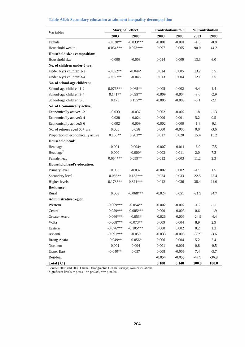
204
Table A6.4: Secondary education attainment inequality decomposition
Variables Marginal effect
Contributions to C % Contribution
2003 2008 2003 2008 2003 2008
Female -0.020** -0.033***
-0.001 -0.001 -1.3 -0.8
Household wealth 0.064*** 0.073***
0.097 0.065 90.0 44.2
Household size / composition:
Household size -0.000 -0.008
0.014 0.009 13.3 6.0
No. of children under 6 yrs;
Under 6 yrs children:1-2 -0.052** -0.044*
0.014 0.005 13.2 3.5
Under 6 yrs children:3-4 -0.057** -0.048
0.013 0.004 12.1 2.5
No. of school-age children;
School-age children:1-2 0.076*** 0.065**
0.005 0.002 4.4 1.4
School-age children:3-4 0.141** 0.099**
-0.009 -0.004 -8.6 -2.9
School-age children:5-6 0.175 0.155**
-0.005 -0.003 -5.1 -2.1
No. of Economically active;
Economically active:1-2 -0.033 -0.037
0.002 -0.002 1.8 -1.3
Economically active:3-4 -0.028 -0.024
0.006 0.001 5.2 0.5
Economically active:5-6 -0.002 -0.009
-0.002 0.000 -1.8 -0.1
No. of retirees aged 65+ yrs 0.005 0.056
0.000 -0.005 0.0 -3.6
Proportion of economically active 0.156** 0.203**
0.017 0.020 15.4 13.2
Household head:
Head age 0.001 0.004*
-0.007 -0.011 -6.9 -7.5
Head age2 0.000 -0.000*
0.003 0.011 2.0 7.2
Female head 0.054*** 0.059**
0.012 0.003 11.2 2.3
Household head's education:
Primary level 0.005 -0.037
-0.002 0.002 -1.9 1.5
Secondary level 0.056** 0.135***
0.024 0.033 22.5 22.4
Higher levels 0.173*** 0.321***
0.042 0.036 38.4 24.0
Residence:
Rural 0.008 -0.068***
-0.024 0.051 -21.9 34.7
Administrative region:
Western -0.069*** -0.054**
-0.002 -0.002 -1.2 -1.1
Central -0.059*** -0.085***
0.000 -0.003 0.6 -1.9
Greater Accra -0.066*** -0.053*
-0.026 -0.006 -24.9 -4.4
Volta -0.068*** -0.073**
0.009 0.004 8.9 2.9
Eastern -0.076*** -0.105***
0.000 0.002 0.2 1.3
Ashanti -0.091*** -0.050
-0.033 -0.005 -30.9 -3.6
Brong Ahafo -0.049** -0.056*
0.006 0.004 5.2 2.4
Northern 0.001 0.004
0.001 -0.001 0.8 -0.5
Upper East -0.040** 0.057
0.008 -0.006 7.4 -3.7
Residual
-0.054 -0.055 -47.9 -36.9
Total ( C ) 0.108 0.148 100.0 100.0
Source: 2003 and 2008 Ghana Demographic Health Surveys; own calculations.
Significant levels: * p<0.1, ** p<0.05, *** p<0.001
205
Chapter 7
Summary and Conclusions
7.1 Introduction
This thesis sets out to analyse the distributional dimension of educational access and
attainment in Ghana. The broad aim of the thesis was to investigate the effect of household
socioeconomic factors and the government of Ghana’s education policy interventions on
education distribution and educational inequalities in Ghana. Specifically, the focus has
been on the extent to which wealth distribution and policy interventions have impacted on
the educational inequalities across households in Ghana between 2003 and 2008. The
specific objectives of the thesis were to: measure the socioeconomic determinants of
educational access and attainment of school-age children; estimate gender disparities in
educational outcomes by wealth distribution and; estimate the contributions of key
determinants of socioeconomic inequality in educational access and attainment. These
objectives are intended to deepen our understanding of the distributional and inequality
patterns of education provision in Ghana. The findings from the empirical chapters show
that these objectives have been achieved. This concluding chapter, therefore, summarises
the major findings of the thesis. In addition, the chapter outlines the main contributions of
the thesis to the literature on inequality in education. The chapter also outlines the key
policy implications of the findings, limitations in the thesis, and identifies areas of further
research.
7.2 Summary
Chapter 1 sets the stage for discussion of the importance of equitable distribution of
educational opportunities. The chapter also highlights some of the consequences of
inequality in educational access and attainment for welfare and production considerations.
For example, inequality in educational attainment increases income inequality and restrict
socioeconomic mobility. Thus, lack of socioeconomic mobility of the poor are largely
attributed to inequalities in educational outcomes and opportunities. In addition, the
chapter heralds the concern that educational outcomes of children reflect a series of factors
such; as the prevailing socioeconomic inequalities to which they are exposed to, household
SES and public policy on education. Therefore, if we are concern about poverty reduction
and equality of opportunity then there is the need to address inequality in educational
outcomes of children today. Furthermore, the chapter emphasises that inequalities in
education and the associated knock-on effects for; employment, wealth, and participation
in society are equally large and an equity based policy or approach in the distribution of
206
educational access is important if developing countries are to equalise socioeconomic and
political opportunities.
In Chapter 2, we analysed the context of the economic performance in the last two decades,
poverty reduction, educational policies and progress in education distribution in Ghana.
The analysis appears to show that Ghana has made some gains in terms of economic
growth and educational outcomes after the education reforms and policy interventions.
However, an analytical review of education sector reforms and policy interventions, and
trends in educational outcomes suggest that there are still questions that remained to be
answered about educational access and attainment for the poor in Ghana, in spite of the
country’s good economic performance.
Chapter 3 examines both the theoretical and empirical literature on educational distribution
and inequalities in educational outcomes in developing countries. We examined findings in
the literature on what determines educational inequality in developing countries and how
economic growth can impact on educational outcomes and other non-income dimensions
of inequality and poverty. The examination of the determinants of educational inequalities
in conjunction with the objectives the thesis formed the basis of selecting explanatory
variables used in the empirical analysis. Furthermore, the second part the chapter outlines
and discusses the theoretical framework of the thesis. The theoretical framework focuses
on the demand-side of educational inequalities and lays the theoretical foundation for the
empirical analysis in Chapters 4, 5 and 6. Summary statistics of the variables for the
analysis were also discussed and justified based on both theoretical and empirical literature.
Reasons for selecting the key dependent variables for analysing inequalities in educational
access and attainment were also thoroughly discussed and justified which are in line with
the objectives of the research.
One major finding from the literature review that motivates the whole thesis is that there is
no indication of any empirical study that has decomposed the contributions of the various
determinants reviewed in the literature. Yet, knowing the proportion of the contribution of
each determinant of educational inequality to the total inequality in educational access and
attainment is important when designing policy interventions. Also, by identifying the key
sources and their contributions to educational inequalities, policy interventions could be
tailored to deal with some of the root causes of educational inequality in Ghana as well as
other developing countries with similar challenges.
207
Furthermore, where educational inequalities are analysed and discussed, the focus is
mainly on primary education, and less attention is been directed towards secondary
education where returns to education could be high. However, for children from poor
households to benefits from economic growth and to break the poverty-cycles in their
households, they will need to progress to higher levels of education to acquire the
necessary skills needed for the job market and for life. This is where the secondary
education comes to the fore.
Also in Chapter 3, we examined the findings of the impact of economic growth on non-
income dimensions of inequality and poverty such as education and health. It emerges that
economic growth is a necessary condition but not a sufficient condition for reducing non-
income dimensions of inequality and poverty in developing countries (Klasen 2008;
Grosse et al. 2008; Gunther and Klasen 2009; Christiaensen et al. 2003; Harttgen et al.
2010). From capability expansion point of view, economic growth can expand capabilities
directly. Thus, as average incomes increase, the population has greater access to relevant
non-income dimensions of well-being such as basic education and healthcare among others
(Drèze and Sen 1991). This implies that all capabilities can expand with economic growth,
thus promoting human capital development.
Other findings in Chapter 3 include the main channels through which overall economic
growth can promote education. First by lessening the extent of income poverty which
constraints households in their ability to send children to school, and secondly by
increasing public educational investments which leads to greater school access and better
quality education (Anand and Ravallion 1993). It also emerged that if progress in
education is combined with a focused public spending in education sector, it will lead to
declining inequality and poverty reduction in education, even in an environment of
stagnant or worsening levels of income poverty (Sahn and Younger 2006 & 2007; Filmer
and Pritchett 1999b) . However, evidence gathered in the review also suggest that there are
socioeconomic inequalities in educational outcomes across developing countries and that
the attainment of MDGs 2 and 3, for example, is in doubt in most developing countries,
especially in SSA countries. Finally, household resources emerged as the key contributing
factor in educational inequalities and poverty. From a gender perspective, the extent of
inequality among girls in primary school attendance and completion rates according to SES,
208
is found to be substantially greater than for boys (Lloyd and Hewett 2009; Harttgen et al.
2010).
In Chapter 4, we discussed the empirical model used for the estimations in Chapters 4 and
5. We then empirically examined socioeconomic determinants of educational access (i.e.
school attendance) and attainment (i.e. school completion) to enable us to identify the key
household socioeconomic factors that influence educational access and attainment in
Ghana. In addition, we carried out trend analysis to appraise the extent to which the
government of Ghana’s intended pro-poor education policy interventions and education
expansions reduce disparities in educational access and attainment, especially at primary
school level between 2003 and 2008. We also examined the extent of educational
disparities at the secondary education level (where there is no specific policy intervention
to reduce the cost of education borne by households) between 2003 and 2008.
Chapter 4 confirms the significance of household wealth as an important explanatory
variable in addition to other covariates in estimating the persistent disparities in
educational access and attainment of school-age children in Ghana. At the secondary
school level, the disparity between the poor and the non-poor with respect to access and
attainment is worrying in terms of the magnitude of the impact. The household wealth
appears to be the most important determining factor in explaining the disparity in children's
school attendance and completion. This is evident throughout the multivariate regression
analysis, both in terms of strong statistical significance and in terms of the magnitude of
the overall impact on children's educational access and attainment.
The variations in educational access and attainment between children from poor and non-
poor households at different levels of education may constitute an evidence of households'
continuing financial burden in educating children and the probable ineffectiveness of the
state (the government of Ghana) in transcending those economic differences. The
particularly strong marginal effect of household wealth on children educational outcomes
confirms the increasing importance of household wealth distribution for children if they are
going to successfully progress from grade to grade and from level to level in the Ghanaian
education system. It also appears that, within the socioeconomic status, the rich households
are more likely to invest more resources in facilitating the education of their children than
the poor households. In addition, the descriptive statistics in Tables 4.1 and 4.2 also show
that there is huge disparity in net attendance rate between primary and secondary school
209
levels. The primary net attendance rate is almost doubled the secondary net attendance rate.
The completion rate at secondary school level compared to primary school level is even
more worrying. For example, about 70% and 75% primary completion rates were recorded
for age cohort 15-20 in 2003 and 2008, respectively compared to about 15% and 23%
secondary completion rates for age cohort 18-23 in the same periods.
The findings also indicate a positive and strong statistically significant marginal effect of
female household head on the probability of school attendance and completion. The
marginal effect suggests that there is a direct link between the impact of households headed
by female and educational outcomes of children. This finding also illustrates the crucial
role played by women in educating children. This finding is consistent with the findings of
Lloyd and Gage-Brandon (1994), Lloyd and Blanc (1996), and Bbaale and Buyinza (2013).
In Chapter 5, we analysed educational outcomes of males and females by wealth
distribution to answer the question; to what extent do disparities in educational outcomes
of males and females increase or decrease with household wealth distribution?
Consequently, the chapter estimates inequality in educational access and attainment of
males and females and we found that the inequality is larger at lower household wealth
distribution levels than at higher levels. At higher wealth distribution levels, household
wealth tends to favour female children's educational access and attainment. This suggests
that wealth levels of households are an important determinant of gender inequality in
educational outcomes in Ghana. It also appears that the government of Ghana's education
policy interventions failed to reduce the significance of the impact of household wealth
distribution on disparities in primary school attendance and completion male and female
children. In addition, we also found that the higher the household heads’ educational
attainment level the more likely female children will have access to and attain primary and
secondary education.
A possible explanation for the consistent gender-wealth inequality in educational access
and attainment in favour of male children in Ghana in both descriptive and econometric
regression analysis, could be that aspect of investment in education where in the
developing countries, parents tend to expect higher return in investing in male children's
education than females’ (Oxaal 1997; Holmes 2003; Filmer 2005). It has also been argued
that if parents or households value the education of sons more than that of daughters, one
would observe more male children schooling than female children. This conjecture,
210
however, supports the findings of Garg and Morduch (1998) on child health outcomes in
Ghana.
In Chapter 6, we explored who benefits from education policies and educational expansion,
and then estimate both absolute and relative contributions of key determinants of
educational inequalities in Ghana. Thus, Chapter 6 analyses socioeconomic inequalities in
educational access and attainment by estimating and decomposing the main determinants
of educational inequalities. The main aim of Chapter 6 has been to estimate the inequality
in both primary and secondary education and also to calculate the absolute and relative
contributions of each determinant of the educational inequalities. The concentration indices
of the primary school attendance, primary school completion and the secondary school
attendance reveal that inequality in these indicators of educational access and attainment
has decreased over time, specifically from 2003 to 2008. Conversely, the concentration
indices of secondary school completion show that inequality in this indicator of
educational attainment has increased from 2003 to 2008 by 0.040 points. For trend analysis,
we further decomposed the change in each educational inequality at both primary and
secondary levels on standardised tests into shares due to changes in the inequality of the
determinants of educational indicators, and changes due to the impact on the determinants.
The findings in Chapter 6 show that the most important determinant of socioeconomic
inequality in school attendance and completion in Ghana is the household wealth. From the
decomposition results, we observed a positive contribution from household wealth,
especially, towards reducing socioeconomic inequality in primary and secondary school
attendance, and secondary school completion between 2003 and 2008. Conversely, we also
observed a positive contribution from household wealth towards increasing inequality in
primary school completion, coming from the evolution of socioeconomic inequality over
time (from 2003 to 2008).
Another interesting finding from the Oaxaca decomposition-type in Chapter 6 is that in all
the four cases of socioeconomic inequality estimated, the elasticity (i.e. impact) differences
are greater than the inequality differences. The explanation for this finding is that an
equitable distribution of educational opportunities will be preferable to a redistribution of
wealth or incomes. For policy direction, the finding implies that the partial association
between household socioeconomic factors and the education indicators matters more for
socioeconomic-related education inequality. The concentration index decomposition
211
analysis also shows that the non-poor households benefit disproportionately from both
access to, and attainment of primary and secondary education in Ghana.
7.3 Major contributions to the literature
For the first time in the education literature on educational outcomes, we have been able to
decompose and quantify key factors that contribute to educational inequalities (access and
attainment). Also, the relative change in elasticity of the factors contributing to educational
inequality was found to be much greater than the relative change in the inequality in
educational access and attainment in Ghana. This is an important contribution and
interesting finding because, it implies that reducing education inequalities seems more a
matter of reducing the associations of the key determinants of educational inequalities
through appropriate education related policies than a matter of redistributing wealth or
income. These findings can guide and aid effective policy interventions to reduce
educational inequalities in Ghana. In addition, the study contributes to the literature by
expanding the discussion on the effectiveness of government of Ghana’s education policy
interventions on educational outcomes in Ghana. Finally, the study brings into the fore the
impact of key socioeconomic factors on gender inequality in educational access and
attainment which will help to identify where intervention is most appropriate and effective
in reducing gender inequality gap in education as well as strengthening female
empowerment efforts.
7.4 Policy implications
While the analysis in the thesis is largely descriptive, a number of policy lessons may be
derived from this analysis based on the key findings. First, the findings from the entire
thesis show that the poor and less educated households are typically disadvantaged and the
effects of higher levels of education attained by household heads or parents improved
educational access and attainment of children. However, secondary education remains
unaffordable for most households in Ghana. Yet this is the phase of education which is
found to have the highest marginal returns in consumption and perhaps the greatest welfare
enhancing potential (Lavy 1996).
Contingent on these findings, expanding free universal education to secondary school
levels or means tested free secondary education for the poor, could be one of the options of
education policy to reduce access, and attainment socioeconomic related inequalities at the
secondary level in Ghana. Any of the options would allow those who cannot afford
212
secondary education to access and attain secondary education in Ghana. This also has the
effect of reducing the number of economically unproductive and unskilled work force in
Ghana.
The findings and the suggestion of expanding free universal secondary education or means
tested free secondary education are testaments to what is happening in the upper secondary
schools in particular, across Ghana. According to Daily Graphic ( 2013) most Senior High
Schools (SHS) could soon run into serious financial difficulties, if parents fail to pay huge
sums of money (school fees) owed to the schools by students who had finished writing the
West African Senior School Certificate Examination (WASSCE) in 2013. For example,
out of the 600 SHSs across the Ghana, 10 of them were owed in school fees totalling
GH¢332, 844 (about US$168,384) by parents. The most worrying aspect is that the trend
of school fees arrears is replicated in almost all the schools in the country (Daily Graphic
2013).
Furthermore, the Director General of the Ghana Education Service (GES) also confirmed
that the issue of indebtedness by final year students had over time been a great challenge to
the GES, and attributed the problem to a number of policies that had been adopted. It is
worrying that in spite of Ghana being classified as LMIC, some secondary schools in
Ghana do prevent students from writing final external examinations because parents could
not afford to pay their children’s school fees. A typical example is where some students at
Okuapeman SHS had been prevented from writing their final external examinations
because they owed school fees (Daily Graphic 2013).
Another policy area for policy direction is gender inequality in educational outcomes in
Ghana. The effect of household wealth in increasing gender inequality in educational
outcomes at lower household wealth distribution levels, but decreasing gender inequality at
higher wealth distribution levels has important policy implications. This finding supports
the argument that larger wealth or income effect or increases in household wealth or
income disproportionately benefits female children’s educational outcomes. This is
because wealthier household can afford to hire help for childcare and other domestic tasks
usually carried out by the female children in developing countries, including Ghana.
Although removing such constraints will be difficult tasks for policy, government policies
that aim at increasing income levels of poor households in Ghana could be one way to
reduce gender inequality in educational outcomes at low income levels. Policies that
213
reduce the opportunity cost of female children's time in low income households may also
increase female children's educational outcomes.
Another policy lesson is that, whereas household heads’ educational attainment is
associated with higher overall children's education outcomes, higher levels of education
tend to increase the probability of female children's educational outcomes than the male
children's education outcomes. This implies that government policies that aim at educating
male and female children at secondary school levels and beyond will in the long run tend
to reduce gender disparities in educational outcomes, ceteris paribus.
Another interesting question which we are able to answer in this thesis through the
concentration index decomposition analysis is: which of the two components of change in
the contributions of the determinants to the education inequality (i.e. elasticity and
inequality of the determinants) is the most important contributor to the estimated education
inequalities? This distinction is essential from a policy perspective, since in many cases
education policies may not directly alter the distribution of these characteristics by
household wealth, but they may be able to influence the education elasticity of some of
these characteristics. Again, some important observations emerged from the Oaxaca
decomposition. The elasticity differences were greater than the inequality differences of
the determinants of the educational inequalities. The implication of this finding for policy
direction is that an equitable distribution of educational opportunities will be preferable to
a redistribution of existing assets or incomes. The point here is that an equitable
distribution of educational access and attainment will build new assets and improve social
welfare by its spill-over effect, without making anyone worse off. Therefore, ensuring
access to educational opportunities by attending to both the supply-side and demand-side
by the government of Ghana will be a win-win policy gaining support in Ghana and other
developing countries where similar trend exists.
The policy implication of the findings from the Oaxaca decomposition can be illustrated
using the results for household wealth (as a key determinant) in any of Tables 6.2, 6.4, 6.6
and 6.8. Take the contribution of household wealth for instance, without exception, the
relative change in elasticity (Δη*C) is much greater than the relative change in inequality
(ΔC*η). This implies that it is not so much the differences in income or household wealth
inequality per se, but the partial association between household wealth and the education
indicators that matters for income related education inequality. This is an important and
214
interesting finding because, it implies that reducing education inequalities seems more a
matter of reducing these associations through appropriate education related policies than a
matter of redistributing wealth or income. It is important to note, however, that the
observation does not necessarily hold for all other determinants, but on the basis of the
results in Tables 6.1, 6.3, 6.5, and 6.7, policy makers in Ghana can learn where the greatest
opportunities lie for reducing income related education inequalities.
In addition, the decomposition results could guide policy makers to target areas that may
make the largest contribution to reducing educational inequalities. While the
decomposition results could not tell us what could be done and how to change the
inequality components, they do show where the greatest potential for socioeconomic
inequality reductions in educational access (school attendance) and attainment (school
completion) lies. Remaining cognisant that our findings cannot be considered causal, we
argue that pro-poor government education policy and investment in education, particularly
in rural areas where majority of the poor resides, are plausible to overall improvements and
decreased inequalities in educational access and attainment of children in Ghana.
Finally, it is important to note that the trend of inequality in educational outcomes,
especially between the poor and the non-poor households is likely to continue unless there
are changes to public policy that promote the human capital of children in a way that offers
relatively greater benefits to the relatively disadvantaged households.
7.5 Limitations
This thesis has not been able to shed light on some important aspect of educational
inequalities due to data limitations. For example, a quantifiable data on social-cultural
norms might underlie gender disparities in educational access and attainments at both
primary and secondary school levels analysed in Chapter 5. Furthermore, a selection bias
is probably present at the secondary school level estimation since the decision to attend
secondary school is likely to be determined by cognitive skills in combination of the
explanatory variables used in the regression analysis. The non-availability of cognitive
variable in DHS dataset may attenuate the estimated marginal effect of the selected
socioeconomic determinants on the educational access and attainment. In spite of these
limitations, the results of the model are consistent with other empirical research (Jacoby
1994; Sathar and Lloyd 1994; Lillard and Willis 1994; Chernichovsky 1985; Oliver 1995;
Lloyd and Blanc 1996; Lloyd and Gage-Brandon 1994; Tansel 1997; Filmer and Pritchett
215
1999b; Glick and Sahn 2000; Tansel 2002; Sackey 2007; Rolleston 2011) which use
household surveys without the inclusion of cognitive skills variable as part of the
explanatory variables.
It is also important to note that the estimated results are subject to the usual caveats
regarding the casual interpretation of cross-sectional results. In other words, it is
descriptive analysis of cross-sectional data in 2003 and 2008 and does not suggest any
causal effect. For example the estimates of the magnitude and contribution to inequality
calculated using the 2003 and 2008 GDHS datasets are based on the socioeconomic
measure used (household wealth quintile). Also, the results from the decomposition
analysis are sensitive to which determinants are selected for inclusion in the model.
Finally, it is worth noting that the GDHS datasets do not distinguish between public and
private school attendance and completion. As a result, this must be taking into account
when interpreting the results in terms of the impact of government education policy
interventions (FCUBE, SCG and SFP) on educational access and attainment at primary
school level in Ghana.
7.6 Further research
This thesis also highlights two potential areas of further inquiry. First, as part of
government of Ghana’s effort to meet EFA goal 2 and MDG 2, pre-primary education is
now free for all children aged 3 to 5 years in Ghana. Therefore, there is the need to also
understand the availability of, and access to pre-primary education by all households in
Ghana and how pre-primary education impacts on access and attainment at the primary
school level. Is there also inequality in access and attainment due to household
socioeconomic factors? Answers to this question are vital to help design policies that will
make sure pre-primary education is equitably distributed and all households have equal
access. Second, in 2012 General Election in Ghana, the opposition party (NPP) manifesto
promised free secondary education for all. However, the main question that the civil
society in Ghana want answers to still remains. How do we finance free secondary
education for all in Ghana? There is, therefore, the need for empirical research on how to
finance free secondary education in Ghana in order to make secondary education more
accessible and equitable to low income and poor households.
216
References
Tansel, A. (1997). Schooling Attainment, Parental Education, and Gender in Côte d'Ivoire
and Ghana. Economic Development and Cultural Change, 45(4), 825-856.
Adam, R. H. & Page, J. (2001). Holding the Line: Poverty Reduction in the Middle East
and North Africa Poverty Reduction Group. Available:
http://www.mafhoum.com/press3/96E14.pdf [Accessed 09/10/10].
Adamu-Issah, M., Elden, L., Forson, M. & Schrofer, T. (2007). Achieving Universal
Primary Education in Ghana by 2015: A Reality or a Dream? Division of Policy
and Planning Working Papers. New York: United Nations Children's Fund
(UNICEF).
Adjasi, C. K. D. & Osei, K. A. (2007). Poverty profile and correlates of poverty in Ghana.
International Journal of Social Economics, 34(7), 449-471.
Aghion, P. & Bolton, P. (1997). A Theory of Trickle-Down Growth and Development. The
Review of Economic Studies, 64(2), 151-172.
Aghion, P., Caroli, E. & García-Peñalosa, C. (1999). Inequality and Economic Growth:
The Perspective of the New Growth Theories. Journal of Economic Literature,
37(4), 1615-1660.
Akyeampong, K. (2009). Revisiting Free Compulsory Universal Basic Education (FCUBE)
in Ghana. Comparative Education, 45(2), 175-195.
Akyeampong, K. (2011). (Re)Assessing the Impact of School Capitation Grants on
Educational Access in Ghana. CREATE Pathways to Access Series, Research
Monograph Number 71. Falmer, UK: Centre for International Education,
Department of Education, University of Sussex.
Akyeampong, K., Djangmah, J., Oduro, A., Seidu, A. & Hunt, F. (2007). Access to Basic
Education in Ghana: The Evidence and the Issues – Country Analytic Report:
CREATE, University of Sussex.
Al-Samarrai, S. (2006). Achieving education for all: how much does money matter?
Journal of International Development, 18(2), 179-206.
Alderman, H. & Gertler, P. (1997). Family resources and gender differences in human
capital investments: the demand for children’s medical care in Pakistan. In: Haddad,
L., Hoddinott, J., Alderman, H. (ed.) Intrahousehold Resource Allocation in
Developing Countries: Methods, Models, and Policy. Baltimore: Johns Hopkins
University Press.
Alderman, H. & King, E. M. (1998). Gender differences in parental investment in
education. Structural Change and Economic Dynamics, 9(4), 453-468.
Alesina, A. & Rodrik, D. (1994). Distributive Politics and Economic Growth. The
Quarterly Journal of Economics, 109(2), 465-490.
Alkire, S. & Santos, M. (2010). Acute Multidimensional Poverty: A New Index for
Developing Countries. Human Development Research Paper 2010/11
217
Anand, S. & Ravallion, M. (1993). Human Development in Poor Countries: On the Role of
Private Incomes and Public Services. The Journal of Economic Perspectives, 7(1),
133-150.
Appiah, K., Demery, L. & Laryea-Adjei, S. G. (2000). Poverty in a Changing Environment.
In: Aryeetey, E., Harrigan, J. & Nissanke, M. (eds.) Economic Reforms in Ghana:
The Miracle and the Mirage. Oxford: James Currey Ltd.
Appleton, S. (1995). The Interaction between Poverty and Gender in Human Capital
Accumulation: the Case of the Primary Leaving Examination in Côte d'lvoire.
Journal of African Economies, 4(2), 192-224.
Appleton, S., Hoddinott, J. & MacKinnon, J. (1996). Education and health in sub-Saharan
Africa. Journal of International Development, 8(3), 307-339.
Banerjee, A. (2000). A dynamic framework for educational policy analysis. Cambridge,
MA: Mimeo, MIT.
Banerjee, A. V. & Newman, A. F. (1993). Occupational Choice and the Process of
Development. Journal of Political Economy, 101(2), 274-298.
Bbaale, E. & Buyinza, F. (2013). Parents' Education and Child Schooling Outcome:
Evidence from Uganda. Journal of Politics and Law, 6(4), 77-89.
Beauchemin, E. (1999). The Exodus: The Growing Migration of Children From Ghana’s
Rural Areas To the Urban Centres. Catholic Action for Street Children (CAS) and
UNICEF. http://www.childmigration.net/Beauchemin_99 [Accessed 04/10/11].
Becker, G. (1975). A theoretical and empirical analysis with special reference to
education . Chicago: : University of Chicago Press.
Becker, G. (1991). A Treatise on the Family (Enlarged Edition). Cambridge, MA: Harvard
University Press.
Becker, G. S. & Tomes, N. (1986). Human Capital and the Rise and Fall of Families.
Journal of Labor Economics, 4(3), S1-S39.
Behrman, Jere R., Andrew D. Foster, Mark R. Rosenzweig & Prem Vashishtha (1999).
Women's Schooling, Home Teaching, and Economic Growth. Journal of Political
Economy, 107(4), 682-714.
Berthélemy, J.-C. (2006). To What Extent are African Education Policies Pro-poor?
Journal of African Economies, 15(3), 434-469.
Bhalotra, S. & Heady, C. (2003). Child Farm Labor: The Wealth Paradox. The World Bank
Economic Review, 17(2), 197-227.
Blake, J. (1981). Family Size and the Quality of Children. Demography, 18(4), 421-442.
Blake, J. (1989). Family size and achievement Berkeley, CA: University of California
Press.
218
Bogetic, Z. (2007). Ghana's Growth Story. Ghana CEM: Meeting the Challenge of
Accelerated and Shared Growth. (1). Available:
http://papers.ssrn.com/sol3/papers.cfm?abstract_id=1809931 [Accessed 04/04/12].
Bonnet, M. (1993). Child labour in Africa. International Labour Review, 132(3), 371.
Bourguignon, F. & Chakravarty, S. (2003). ‘The Measurement of Multidimensional
Poverty’. Journal of Economic Inequality, 1(1), 25-49.
Bredie, J. W. B. & Beeharry, G. K. (1998). ‘School Enrolment Decline in Sub-Saharan
Africa: beyond the supply constraint’. World Bank Discussion Paper No. 395,
http://www-
wds.worldbank.org/external/default/WDSContentServer/IW3P/IB/1998/08/01/0000
09265_3980929150110/Rendered/PDF/multi_page.pdf [Accessed 04/10/11].
Bruce J, Cynthia B Lloyd & Leonard, A. (1995). Families in Focus: New Perspectives on
Mothers, Fathers, and Children. New York: The Population Council.
Bruce Judith & Lloyd, C. B. (1996). "Finding the ties that bid: Beyond headship and
household,". In: Lawrence Haddad, John Hoddwitt & Alderman, H. (eds.)
Intrahousehold Resource Allocation in Developing Countries: Methods, Models
and Policy. Baltimore: John Hopkins University Press.
Buchmann, C. & Hannum, E. (2001). Education and Stratification in Developing Countries:
A Review of Theories and Research. Annual Review of Sociology, 27(1), 77-102.
Burchi, F. (2009). On the Contribution of Mother’s Education to Children’s Nutritional
Capabilities in Mozambique. Working Paper no. 101. Available: http://www.die-
gdi.de/uploads/media/WP101.pdf [Accessed 25/06/13].
Butcher, K. F. & Case, A. (1994). The Effect of Sibling Sex Composition on Women's
Education and Earnings. The Quarterly Journal of Economics, 109(3), 531-563.
Canagarajah, S. & Coulombe, H. (1997). Child labour and schooling in Ghana. World
Bank Policy Research Working Paper No. 1844. Washington DC: World Bank.
http://papers.ssrn.com/sol3/papers.cfm?abstract_id=620598 [Accessed 04/10/11].
Cardozo, A. & Grosse, M. (2009). Pro-Poor Growth Using Non-Income Indicators: An
Empirical Illustration for Colombia. Discussion Papers 9. Available:
http://www2.vwl.wiso.uni-goettingen.de/courant-papers/CRC-PEG_DP_9.pdf
[Accessed 13/03/12].
Chao, S. & Alper, O. (1998). Accessing Basic Education in Ghana .Studies in Human
Development No.1. Washington DC: World Bank.
Chaudhuri, S. & Ravallion, M. (2006). Partially Awakened Giants : Uneven Growth In
China And India: The World Bank.
Chernichovsky, D. (1985). Socioeconomic and Demographic Aspects of School
Enrollment and Attendance in Rural Botswana. Economic Development and
Cultural Change, 33(2), 319-332.
219
Chowa, G., Ansong, D. & Masa, R. (2010). Assets and child well-being in developing
countries: A research review. Children and Youth Services Review, 32(11), 1508-
1519.
Chowa, G. A. N., Masa, R. D., Wretman, C. J. & Ansong, D. (2013). The impact of
household possessions on youth's academic achievement in the Ghana Youthsave
experiment: A propensity score analysis. Economics of Education Review, 33(0),
69-81.
Christiaensen, L., Demery, L. & Paternostro, S. (2002). Growth, Distribution, and Poverty
in Africa: Messages from the 1990s. Policy Research Working Paper 2810.
Available:http://www-
wds.worldbank.org/servlet/WDSContentServer/WDSP/IB/2002/04/12/000094946_
02040304241195/Rendered/PDF/multi0page.pdf [Accessed 12/03/12].
Christiaensen, L., Demery, L. & Paternostro, S. (2003). “Macro and Micro Perspectives of
Growth and Poverty in Africa”. World Bank Economic Review, 17(3), 317-347.
Corak, M. (2013). Income Inequality, Equality of Opportunity, and Intergenerational
Mobility. Journal of Economic Perspectives, 27(3), 79-102.
Coulombe, H. & McKay, A. (2007). Growth with Selective Poverty Reduction-Ghana in
the 1990s. World Bank Working Paper 79:9-44. In: Wodon, Q. (ed.) Growth and
poverty reduction : case studies from West Africa. Washington DC: World Bank.
Coulombe, H. & Wodon, Q. (2007). "Poverty, Livelihoods, and Access to Basic Services
in Ghana" Ghana CEM: Meeting The Challenges of Accelerated and Shared
Growth.Available:
http://siteresources.worldbank.org/INTGHANA/Resources/CEM_poverty.pdf
[Accessed 04/04/12].
d' Hombres, B. (2010). Inequality in Tertiary Education Systems: Which Metric Should
We Use for Measuring and Benchmarking? Available:
http://web.worldbank.org/WBSITE/EXTERNAL/TOPICS/EXTEDUCATION/0,,c
ontentMDK:22614893~menuPK:282391~pagePK:148956~piPK:216618~theSiteP
K:282386,00.html [Accessed 25/01/2013].
Daily Graphic. ( 2013). Audit accounts of Senior High Schools (SHSs) - Parent. Daily
Graphic: 23rd July edition. Available: http://graphic.com.gh/General-News/audit-
accounts-of-shss-parent.html [Accessed 31/07/13].
De Janvry, A. & Sadoulet, E. (2000). Growth, Poverty, and Inequality in Latin America: A
Casual Analysis, 1970-94. Review of Income & Wealth, 46(3), 267-287.
Deininger, K. (2003). Does cost of schooling affect enrollment by the poor? Universal
primary education in Uganda. Economics of Education Review, 22(3), 291-305.
Deininger, K. & Squire, L. (1998). New ways of looking at old issues: inequality and
growth. Journal of Development Economics, 57(2), 259-287.
Dollar, D. & Kraay, A. (2002). Growth Is Good for the Poor. Journal of Economic Growth
7(3), 195-225.
220
Doorslaer, E. v. & Jones, A. M. (2004). Income-related inequality in health and health care
in the European Union. Health Economics, 13(7), 605-608.
Doorslaer, E. v. & Koolman, X. (2004). Explaining the differences in income-related
health inequalities across European countries. Health Economics, 13(7), 609-628.
Downey, D. B. (1995). When Bigger Is Not Better: Family Size, Parental Resources, and
Children's Educational Performance. American Sociological Review, 60(5), 746-
761.
Doyle, M. W. & Stiglitz, J. E. (2014). Eliminating Extreme Inequality: A Sustainable
Development Goal, 2015–2030. Ethics & International Affairs, 28(01), 5-13.
Drèze, J. & Sen, A. (1991). Economic Growth and Public Support: Oxford University
Press.
Duclos, J.-Y. (2009). What is "Pro-Poor"? Social Choice and Welfare, 32(1), 37-58.
Dutta, J., Sefton, J. & Weale, M. (1999). Education and public policy. Fiscal Studies, 20(4),
351-386.
Eckstein, Z. & Zilcha, I. (1994). The effects of compulsory schooling on growth, income
distribution and welfare. Journal of Public Economics, 54(3), 339-359.
Farmer, T. W., Estell, D. B., Leung, M.-C., Trott, H., Bishop, J. & Cairns, B. D. (2003).
Individual characteristics, early adolescent peer affiliations, and school dropout: an
examination of aggressive and popular group types. Journal of School Psychology,
41(3), 217-232.
FASAF, UNESCO, UNICEF, USAID & ORC Macro. (2002). Guide to the Analysis and
Use of Household Survey and Census Education Data Montreal, Quebec Canada:
UNESCO Institute of Statistics. http://pdf.usaid.gov/pdf_docs/Pnadf701.pdf
[Accessed 04/10/11].
FASAF, UNESCO, UNICEF, USAID & ORC Macro. (2004). Guide to the Analysis and
Use of Household Survey and Census Education Data. Montreal, Quebec Canada:
UNESCO Institute of Statistics.
http://www.uis.unesco.org/Library/Documents/hhsguide04-en.pdf [Accessed
04/10/11].
Filmer, D. (2000). The Structure of Social Disparities in Education: Gender and Wealth.
Policy Research Working Paper 2268. Available: http://www-
wds.worldbank.org/servlet/WDSContentServer/WDSP/IB/2000/02/09/000094946_
00012505525066/Rendered/PDF/multi_page.pdf [Accessed 26/03/12].
Filmer, D. (2005). Gender and wealth disparities in schooling: Evidence from 44 countries.
International Journal of Educational Research, 43(6), 351-369.
Filmer, D. & Pritchett, L. (1999a). “Determinants of Education Enrollment in India: Child,
Household, Village and State Effects,” Journal of Educational Planning and
Administration.
221
Filmer, D. & Pritchett, L. (1999b). The Effect of Household Wealth on Educational
Attainment: Evidence from 35 Countries. Population and Development Review,
25(1), 85-120.
Filmer, D. & Pritchett, L. H. (2001). Estimating Wealth Effects without Expenditure Data-
or Tears: An Application to Educational Enrollments in States of India.
Demography, 38(1), 115-132.
Francis, P. A., Agi, S. P. I., Alubo, S. O., Biu, H. A., Daramola, A. G., Nzewi, U. M. &
Shehu., D. J. (1998). Hard Lessons: Primary Schools, Community and Social
Capital in Nigeria. Technical Paper No. 420. African Region Series. Washington,
D.C.: The World Bank.
Fredriksen, B. (2007). School Grants: One Efficient Instrument to Address Key Barriers to
Attaining Education for All. Capacity Development Workshop “Country
Leadership and Implementation for Results in the EFA FTI Partnership” Cape
Town, South Africa, July 16-19, 2007.
Gage, A. J., Sommerfelt, A. E. & Piani, A. L. (1997). Household Structure and Childhood
Immunization in Niger and Nigeria. Demography, 34(2), 295-309.
Garg, A. & Morduch, J. (1996). Sibling Rivalry and the Theory of the Household. Harvard
University: Mimeo.
Garg, A. & Morduch, J. (1998). Sibling Rivalry and the Gender Gap: Evidence from Child
Health Outcomes in Ghana. Journal of Population Economics, 11(4), 471-493.
Ghana Statistical Service (2014). Gross Domestic Product 2014. National Accounts
Statistics. Accra: Ghana Statistical Service (GSS).
Ghana Statistical Service (1995). The Pattern of Poverty in Ghana: 1988-1992 Accra:
Ghana Statistical Service (GSS).
Ghana Statistical Service (2000). Poverty Trends in Ghana in the 1990s. Accra: Ghana
Statistical Service (GSS).
Ghana Statistical Service (2007). Patterns and Trends of Poverty in Ghana. Accra: Ghana
Statistical Service (GSS).
Ghana Statistical Service (2008). Ghana living standards survey: Report of the fifth round.
Accra: Ghana Statistical Service (GSS).
Ghana Statistical Service (2010). “New Series of the Gross Domestic Product (GDP)
Estimates: Highlights of the Rebased Series of the GDP- formal press release.”
Statistical Newsletter No. B12-2003. November 3. Accra: Ghana Statistical Service
(GSS).
Ghana Statistical Service (2011). 2011 Ghana's Economic Performance. Accra: Ghana
Statistical Service (GSS).
Ghana Statistical Service (2012). 2010 Population and Housing Census. Summary Results
of Final Report. Accra: Ghana Statistical Service (GSS).
222
Ghana Statistical Service (2013a). 2010 Population & Housing Census Report. Non-
Monetary Poverty in Ghana. ccra: Ghana Statistical Service (GSS).
Ghana Statistical Service (2013b). 2010 Population and Housing Census. National
Analytical Report. Accra: Ghana Statistical Service (GSS).
Ghana Statistical Service, Ghana Health Service & ICF Macro (2004). Ghana
Demographic and Health Survey 2003. Accra: Ghana Statistical Service (GSS),
Ghana Health Service (GHS), ICF, Macro.
Ghana Statistical Service, Ghana Health Service & ICF Macro (2009). Ghana
Demographic and Health Survey 2008. Accra: Ghana Statistical Service (GSS),
Ghana Health Service (GHS) and ICF Macro.
Glewwe, P. (1999). The economics of school quality investments in developing countries:
An empirical study of Ghana. London: Macmillan Press.
Glewwe, P. & Jacoby, H. (1994). Student Achievement and Schooling Choice in Low-
Income Countries: Evidence from Ghana. The Journal of Human Resources, 29(3),
843-864.
Glick, P. & Sahn, D. E. (2000). Schooling of girls and boys in a West African country: the
effects of parental education, income, and household structure. Economics of
Education Review, 19(1), 63-87.
Gomes, M. (1984). Family Size and Educational Attainment in Kenya. Population and
Development Review, 10(4), 647-660.
Gopal, G. & Salim, M. (1998). “Gender and Law: East Africa Speaks”. In: Gopal and M.
Salim (ed.) Directions in Development. Washington, D.C: The World Bank
Gravelle, H. (2003). Measuring income related inequality in health: standardisation and the
partial concentration index. Health Economics, 12(10), 803-819.
Greeley, M. (1994). Measurement of Poverty and Poverty of Measurement. IDS Bulletin,
25(2), 50-58.
Gregorio, J. D. & Lee, J. W. (2002). Education and Income Inequality: New Evidence
From Cross-Country Data. Review of Income and Wealth, 48(3), 395-416.
Grimm, M., GuÉnard, C. & MesplÉ-Somps, S. (2002). What has Happened to the Urban
Population in Côte d'Ivoire Since the 1980s? An Analysis of Monetary Poverty and
Deprivation Over 15 Years of Household Data. World Development, 30(6), 1073-
1095.
Grosse, M., Harttgen, K. & Klasen, S. (2008). Measuring pro-poor growth in non-income
dimensions. World Development, 36(6), 1021-1047.
Gunther, I. & Klasen, S. (2009). Measuring Chronic Non-Income Poverty. In: Addison, T.,
Hulme, D. & Kanbur, R. (eds.) Poverty Daynamics: Interdisciplinary Perspectives.
New York: Oxford University Press.
223
Gyimah-Brempong, K. & Asiedu, E. (2014). Remittances and investment in education:
Evidence from Ghana. The Journal of International Trade & Economic
Development, 1-28.
Hanushek, E. A. & Lavy, V. (1994). ‘School Quality, Achievement Bias, and Dropout
Behaviour in Egypt’. LSMS Working Paper No. 107 http://www-
wds.worldbank.org/external/default/WDSContentServer/WDSP/IB/1994/12/01/000
009265_3970311121901/Rendered/PDF/multi_page.pdf [Accessed 04/10/11].
Harttgen, K. & Klasen, S. (2012). A Household-Based Human Development Index. World
Development, 40(5), 878-899.
Harttgen, K., Klasen, S. & Misselhorn, M. (2010). Pro-Poor Progress in Education in
Developing Countries? Review of Economics and Institutions, 1(1), 1-48.
Haveman, R. & Wolfe, B. (1995). The Determinants of Children's Attainments: A Review
of Methods and Findings. Journal of Economic Literature, 33(4), 1829-1878.
Holmes, J. (2003). Measuring the determinants of school completion in Pakistan: analysis
of censoring and selection bias. Economics of Education Review, 22(3), 249-264.
Huebler, F. (2008). Child labour and school attendance: Evidence from MICS and DHS
surveys. Understanding Children’s Work Project. Universidad Carlos III de Madrid,
11-12 September: UNICEF.
http://www.childinfo.org/files/Child_labour_school_FHuebler_2008.pdf [Accessed
04/03/12].
ICF Macro (2010). Millennium Development Goals in Ghana: A new look at data from the
2008 Ghana Demographic and Health Survey. Calverton, Maryland: ICF Macro.
Jacoby, H. G. (1994). Borrowing Constraints and Progress Through School: Evidence from
Peru. The Review of Economics and Statistics, 76(1), 151-160.
Jayachandran, U. (2002). Socio-Economic Determinants of School Attendance in India. .
Working Paper No. 103. http://www.cdedse.org/pdf/work103.pdf [Accessed
04/10/11].
Jensen, P. & Nielsen, H. S. (1997). Child Labour or School Attendance? Evidence from
Zambia. Journal of Population Economics, 10(4), 407-424.
Jimerson, S., Egeland, B., Sroufe, L. A. & Carlson, B. (2000). A Prospective Longitudinal
Study of High School Dropouts Examining Multiple Predictors Across
Development. Journal of School Psychology, 38(6), 525-549.
Kabeer, N. (2003). Gender Mainstreaming in Poverty Eradication and the Millennium
Development Goals: A Handbook for Policy Makers and Other Stakeholders.
London: Commonwealth Secretariat.
Kakwani, N. (1997). Growth Rates of Per-Capita Income and Aggregate Welfare: An
International Comparison. Review of Economics and Statistics, 79(2), 201-211.
Kakwani, N. & Son, H. H. (2008). Poverty Equivalent Growth Rate. Review of Income and
Wealth, 54(4), 643-655.
224
Kanbur, R. & Lustig, N. (1999). Why is Inequality Back on the Agenda. Annual World
Bank Conference on Development Economics. Available:
http://siteresources.worldbank.org/INTPOVERTY/Resources/WDR/kanbur499.pdf
[Accessed 24/03/12].
Kattan, R. B. (2006). Implementation of Free Basic Education Policy. Education Working
Paper Series [Online], 7. Available:
http://siteresources.worldbank.org/EDUCATION/Resources/EDWP_User_Fees.pdf
[Accessed 17/03/12].
Klasen, S. (2000). Measuring Poverty and Deprivation in South Africa. Review of Income
and Wealth, 46(1), 33-58.
Klasen, S. (2008). Economic growth and poverty reduction: Measurement issues using
income and non-income indicators. World Development, 36(3), 420-445.
Knodel, J., Havanon, N. & Sittitrai, W. (1990). Family Size and the Education of Children
in the Context of Rapid Fertility Decline. Population and Development Review,
16(1), 31-62.
Knodel, J. & Wongsith, M. (1991). Family Size and Children's Education in Thailand:
Evidence from a National Sample. Demography, 28(1), 119-131.
Lavy, V. (1996). School supply constraints and children's educational outcomes in rural
Ghana. Journal of Development Economics, 51(2), 291-314.
Lazear, E. (1980). Family Background and Optimal Schooling Decisions. The Review of
Economics and Statistics, 62(1), 42-51.
Leclercq, F. (2001). “Patterns and Determinants of Elementary School Enrolment in Rural
North India”. Working paper, TEAM-CNRS [Online].
Leibowitz, A. (1974). Home Investments in Children. Journal of Political Economy, 82(2),
S111-S131.
Lewin, K. M. (2007). Improving Access, Equity and Transitions in Education: Creating a
Research Agenda. Project Report. Consortium for Research on Educational Access,
Transitions and Equity (CREATE), Falmer, UK.
Lewin, K. M. (2009). Access to education in sub-Saharan Africa: patterns, problems and
possibilities. Comparative Education, 45(2), 151-174.
Lewin, K. M. & Akyeampong, K. (2009). Education in sub-Saharan Africa: researching
access, transitions and equity. Comparative Education, 45(2), 143-150.
Lillard, L. A. & Kilburn, M. R. (1995). Intergenerational Earnings Links: Sons and
Daughters . Santa Monica, CA: RAND Corporation.
http://www.rand.org/pubs/drafts/DRU1125 [Accessed 17/03/12].
Lillard, L. A. & Willis, R. J. (1994). Intergenerational Educational Mobility: Effects of
Family and State in Malaysia. The Journal of Human Resources, 29(4), 1126-1166.
225
Lloyd, C. B. & Blanc, A. K. (1996). Children's Schooling in sub-Saharan Africa: The Role
of Fathers, Mothers, and Others. Population and Development Review, 22(2), 265-
298.
Lloyd, C. B. & Desai, S. (1992). Children's Living Arrangements in Developing Countries.
Population Research and Policy Review, 11(3), 193-216.
Lloyd, C. B. & Gage-Brandon, A. J. (1993). Women's Role in Maintaining Households:
Family Welfare and Sexual Inequality in Ghana. Population Studies, 47(1), 115-
131.
Lloyd, C. B. & Gage-Brandon, A. J. (1994). High Fertility and Children's Schooling in
Ghana: Sex Differences in Parental Contributions and Educational Outcomes.
Population Studies, 48(2), 293-306.
Lloyd, C. B. & Hewett, P. (2009). Educational inequalities in the midst of persistent
poverty: Diversity across Africa in educational outcomes. Journal of International
Development, 21(8), 1137-1151.
Lopez, J. H. (2004). Pro-growth, pro-poor: Is there a tradeoff? Policy Research Working
Paper 3378. Available: http://www-
wds.worldbank.org/servlet/WDSContentServer/WDSP/IB/2004/09/22/000160016_
20040922152917/Rendered/PDF/WPS3378.pdf [Accessed 13/03/12].
Lopez, R., Thomas, V. & Wang, Y. (1998). "Addressing the Education Puzzle: The
Distribution of Education and Economic Reforms". Working Paper 2031. Available:
http://www-
wds.worldbank.org/servlet/WDSContentServer/WDSP/IB/2000/02/24/000094946_
99031911111953/Rendered/PDF/multi_page.pdf [Accessed 24/03/12].
Maas, J. v. L. & Criel, G. (1982). Distribution of Primary School Enrollments in Eastern
Africa. World Bank Staff Working Papers Number 511. Washington, D.C.: World
Bank.
Maika, A., Mittinty, M. N., Brinkman, S., Harper, S., Satriawan, E. & Lynch, J. W. (2013).
Changes in Socioeconomic Inequality in Indonesian Children’s Cognitive Function
from 2000 to 2007: A Decomposition Analysis. PLoS ONE, 8(10), e78809.
Maitra, P. & Ray, R. (2002). The Joint Estimation of Child Participation in Schooling and
Employment: Comparative Evidence from Three Continents. Oxford Development
Studies, 30(1), 41-62.
Mani, S., Strauss, J. & Hoddinott, J. (2009). Determinants of Schooling Outcomes –
Empirical Evidence from Rural Ethiopia. Discussion Paper No: 2009-03.
Department of Economics Fordham University.
McLanahan, S. (1985). Family Structure and the Reproduction of Poverty. American
Journal of Sociology, 90(4), 873-901.
MEASURE DHS+ (2013). Demographic and Health Surveys. Standard Recode Manual
for DHS 6. MEASURE DHS/ICF International.
http://www.measuredhs.com/pubs/pdf/DHSG4/Recode6_DHS_22March2013_DH
SG4.pdf [Accessed 20/04/13].
226
Ministry of Education Science and Sports (2005). “Linking ESP and the White Paper
Reform”, November 2005. Accra: Ministry of Education, Science and Sports
(MOESS).
Ministry of Education Science and Sports (2006a). Preliminary Education Sector
Performance Report Accra: Ministry of Education Science and Sports (MOESS)
Ministry of Education Science and Sports (2006b). “Report on the Education Sector
Annual Review (ESAR) 2006”. Accra: Ministry of Education, Science and Sports
(MOESS).
Ministry of Education Science and Sports (2008). Preliminary Education Sector
Performance Report. Accra: Ministry of Education Science and Sports (MOESS).
Ministry of Education Science and Sports (2010). Education Strategic Plan 2010 - 2020
Volume 1. Policies, Strategies, Delivery, Finance. Accra: Ministry of Education
Science and Sports (MOESS).
Montgomery, M. & Hewett, P. (2005). Poverty and children's schooling in urban and rural
Senegal Council. Policy Research Division Working Paper No.196
http://www.stonybrook.edu/economics/research/papers/2005/MontgomeryHewett.p
df [Accessed 04/10/11].
Moss, T. & Majerowicz, S. (2012). “No Longer Poor: Ghana’s New Income Status and
Implications of Graduation from IDA.” CGD Working Paper 300. Washington,
D.C.: Center for Global Development.
NDPC, GoG & UNDP(Ghana) (2012). 2010 Ghana Millennium Development Goals
Report. Accra:
http://www.ndpc.gov.gh/GPRS/2010%20Ghana's%20MDGs%20Report%20(Final)
%20-%20Nov2012.pdf [Accessed 04/12/12].
NDPC, GoG & UNDP(Ghana). (2010). 2008 Ghana Millennium Development Goals
Report 2010.
Nguyen, M. C. & Wodon, Q. (2014). Analysing the Gender Gap in Education Attainment:
A Simple Framework with Application to Ghana. Journal of International
Development, 26(1), 59-76.
Nordensvard, J. (2014). Gender and education policy in Ghana: The impact of informal
citizenship and informal labour markets on the formal education of girls. Women's
Studies International Forum, (0).
O'Donnell, O., van Doorslaer, E., Wagstaff, A. & Lindelow, M. (2007). Chapter 15:
Measuring and explaining inequity in health service delivery. Analyzing Health
Equity Using Household Survey Data.
O’Donnell, O., van Doorslaer, E., Wagstaff, A. & Lindelow, M. (2008). Analyzing Health
Equity Using Household Survey Data [Online]. Washington DC: The World Bank.
Available:
http://siteresources.worldbank.org/INTPAH/Resources/Publications/459843-
1195594469249/HealthEquityFINAL.pdf [Accessed 24/03/12].
227
Oaxaca, R. (1973). Male-Female Wage Differentials in Urban Labor Markets.
International Economic Review, 14(3), 693-709.
Okumu, I. M., Nakajjo, A. & Isoke, D. (2008). Socioeconomic determinants of primary
school dropout: the logistic model analysis. MPRA Paper No. 7851
http://mpra.ub.uni-muenchen.de/7851/ [Accessed 10/01/12].
Oliver, R. (1995). “Fertility and child schooling in Ghana: Evidence of a quality/quantity
tradeoff”. LSMS Working Paper No.112. Washington, D.C: The World Bank.
Oppedisano, V. & Turati, G. (2012). What are the causes of educational inequality and of
its evolution over time in Europe? Evidence from PISA. Education Economics, 1-
22.
Orr, A. J. (2003). Black-White Differences in Achievement: The Importance of Wealth.
Sociology of Education, 76(4), 281-304.
Osei, R. D., Owusu, G. A., Asem, F. E. & Afutu-Kotey, R. L. (2009). Effects of Capitation
Grant on Education Outcomes in Ghana. Available:
http://depot.gdnet.org/cms/files/GDN_UNDP_ISSER_Paper1.pdf [Accessed
28/04/12].
Oxaal, Z. (1997). 'Education and Poverty: A Gender Analysis', BRIDGE development-
gender , Report prepared for the Gender Equality Unit, Swedish International
Development Cooperation Agency (Sida). Brighton: Institute of Development
Studies.
Palmer, R. (2006). Beyond the Basics: Balancing Education and Training Systems in
Developing Countries. Journal of Education in International Development, 2:1.
Retrieved from http://www.equip123.net/JEID/articles/2/BeyondBasics.pdf
[Accessed 24/03/12].
Parish, W. L. & Willis, R. J. (1993). Daughters, Education, and Family Budgets Taiwan
Experiences. The Journal of Human Resources, 28(4), 863-898.
Patrinos, H. A. & Psacharopoulos, G. (1997). Family Size, Schooling and Child Labor in
Peru: An Empirical Analysis. Journal of Population Economics, 10(4), 387-405.
Pickett, K. E., Wilkinson, R. & Ghosh, J. (2013). RE: The post-2015 development
framework. Available:
http://www.post2015hlp.org/wpcontent/uploads/2013/03/Dr-Homi-Kharas.pdf
[Accessed 20/2/14]
Pong, S.-L. (1996). School Participation of Children from Single-Mother Families in
Malaysia. Comparative Education Review, 40(3), 231-249.
Pong, S.-L. (1997). Sibship Size and Educational Attainment in Peninsular Malaysia: Do
Policies Matter? Sociological Perspectives, 40(2), 227-242.
Pong, S.-L. & Ju, D.-B. (2000). The Effects of Change in Family Structure and Income on
Dropping Out of Middle and High School. Journal of Family Issues, 21(2), 147-
169.
228
Porta, E., Arcia, G., Macdonald, K., Radyakin, M. & Lokshin, M. (2011). Assessing Sector
Performance and Educational Equity:Streamlined Analysis with ADePT Software
Washington D.C: The World Bank.
Pregibon, D. (1980). Goodness of Link Tests for Generalized Linear Models. Journal of
the Royal Statistical Society. Series C (Applied Statistics), 29(1), 15-14.
Psacharopoulos, G. & Arriagada, A. M. (1986). The Educational Composition of the
Labour Force: An International Comparison. International Labour Review, 125(5),
561.
Psacharopoulos, G. & Arriagada, A. M. (1989). The Determinants of Early Age Human
Capital Formation: Evidence from Brazil. Economic Development and Cultural
Change, 37(4), 683-708.
Ravallion, M. (1996). Issues in Measuring and Modelling Poverty. The Economic Journal,
106(438), 1328-1343.
Ravallion, M. (2001). Growth, Inequality and Poverty: Looking Beyond Averages. World
Development, 29(11), 1803-1815.
Ravallion, M. & Chen, S. (1997). What Can New Survey Data Tell Us about Recent
Changes in Distribution and Poverty? The World Bank Economic Review, 11(2),
357-382.
Ravallion, M. & Chen, S. (2003). Measuring pro-poor growth. Economics Letters, 78(1),
93-99.
Ravallion, M. & Wodon, Q. (2000). Does Child Labour Displace Schooling? Evidence on
Behavioural Responses to an Enrollment Subsidy. The Economic Journal, 110(462),
C158-C175.
Ray, R. (2000). Analysis of Child Labour in Peru and Pakistan: A Comparative Study.
Journal of Population Economics, 13(1), 3-19.
Ray, R. & Sinha, K. (2011). Multidimensional Deprivation in China, India and Vietnam: A
Comparative Study on Micro Data. Discussion Paper. Available:
http://www.socialsciences.manchester.ac.uk/disciplines/economics/research/worksh
ops/development/ [Accessed 21/12/11].
Republic of Ghana (1997). Ghana Vision 2020. The First Medium-term Development Plan.
Accra: National Development Planning Commission (NDPC).
Republic of Ghana (2003). Growth and Poverty Reduction Strategy (GPRS I), 2003-2005.
An Agenda for Growth and Prosperity. Accra: National Development Planning
Commission (NDPC).
Rivers, D. & Vuong, Q. H. (1988). Limited information estimators and exogeneity tests for
simultaneous probit models. Journal of Econometrics, 39(3), 347-366.
Roberts, J. (2003). Poverty Reduction Outcomes in Education and Health: Public
Expenditure and Aid. Working Paper 210. Available:
http://www.odi.org.uk/resources/docs/2450.pdf [Accessed 06/05/12].
229
Roemer, M. & Gugerty, M. (1997). Does Economic Growth Reduce Poverty? Technical
Paper. Available: http://pdf.usaid.gov/pdf_docs/PNACA656.pdf [Accessed
23/03/12].
Rolleston, C. (2009). The determination of exclusion: evidence from the Ghana Living
Standards Surveys 1991–2006. Comparative Education, 45(2), 197-218.
Rolleston, C. (2011). Educational access and poverty reduction: The case of Ghana 1991–
2006. International Journal of Educational Development, 31(4), 338-349.
Rose, E. (2000). Gender Bias, Credit Constraints and Time Allocation in Rural India. The
Economic Journal, 110(465), 738-758.
Sackey, H. A. (2007). The Determinants of School Attendance and Attainment in Ghana:
A Gender Perspective. No RP_173, Research Papers.
Sahn, D. E. & Stifel, D. (2003). Exploring Alternative Measures of Welfare in the Absence
of Expenditure Data. Review of Income and Wealth, 49(4), 463-489.
Sahn, D. E. & Younger, S. D. (2006). Chnages in Inequality and Poverty in Latin America:
Looking Beyond Income to Health and Education. Journal of Applied Economics,
9(2), 215-233.
Sahn, D. E. & Younger, S. D. (2007). Inequality and Poverty in Africa in an Era of
Globalization: Looking Beyond Income to Health and Education. Research Paper
No. 2007/74. Available: http://www.wider.unu.edu/stc/repec/pdfs/rp2007/rp2007-
74.pdf [Accessed 26/03/12].
Sandefur, G. D., Meier, A. M. & Campbell, M. E. (2006). Family resources, social capital,
and college attendance. Social Science Research, 35(2), 525-553.
Sathar, Z. A. & Lloyd, C. B. (1994). Who Gets Primary Schooling in Pakistan: Inequalities
among and within Families. The Pakistan Development Review, 33(2), 103-134.
Schaffner, A., Julie (2004). The determinants of schooling investments among primary
school aged children in Ethiopia. . Africa Region human development working
paper series ; no. 85. Washington D.C: The Worldbank.
http://documents.worldbank.org/curated/en/2004/11/6037939/determinants-
schooling-investments-among-primary-school-aged-children-ethiopia. [Accessed
04/10/11]
Schultz, T. P. (1999). Health and Schooling Investments in Africa. The Journal of
Economic Perspectives, 13(3), 67-88.
Schultz, T. W. (1960). Capital Formation by Education. Journal of Political Economy,
68(6), 571-583.
Sen, A. (1985). Commodities and Capabilities. North-Holland Amsterdam.
Sen, A. (1998). Development as Freedom. New York: Knopf.
230
Shavit, Y. & Pierce, J. L. (1991). Sibship Size and Educational Attainment in Nuclear and
Extended Families: Arabs and Jews in Israel. American Sociological Review, 56(3),
321-330.
SITEAL ( 2005). Medidas de Desigualdad para Variables Educativas. Boletín No. 4.
Santiago . SITEAL.
Smits, J., Huisman, J. & Webbink, E. (2007). Family Background, District and National
Determinants of Primary School Enrollment in 62 Developing Countries Paper
presented at the XIII World Congress of Comparative Education Societies.
Sarajevo 3-7 September.
Steelman, L. C. & Powell, B. (1991). Sponsoring the Next Generation: Parental
Willingness to Pay for Higher Education. American Journal of Sociology, 96(6),
1505-1529.
Strauss, J. & Thomas, D. (1995). “Human Resources: Empirical Modeling of Household
and Family Decisions”, . In: Behrman, J. & Srinivasan, T. N. (eds.) Handbook of
Development Economics (Vol. 3). Amsterdam, North Holland.
Subrahmanian, R. (2003). Gender equality in education: Definitions and measurements.
Background paper for UNESCO GMR 2003-043. UNESCO.
Sutherland-Addy, E. (2002). Impact Assessment Study of the Girls’ Education Programme
in Ghana. http://www.unicef.org/evaldatabase/files/GHA_2002_022.pdf [Accessed
04/10/11].
Swada, Y. & Lokshin, M. (1999). Household Schooling Decisions in Rural Pakistan.
Policy Research Working paper series No.2541
http://elibrary.worldbank.org/content/workingpaper/10.1596/1813-9450-2541
[Accessed 04/10/11].
Tansel, A. (1997). Schooling Attainment, Parental Education, and Gender in Côte d'Ivoire
and Ghana Economic Development and Cultural Change, 45(4), 825-856.
Tansel, A. (2002). Determinants of school attainment of boys and girls in Turkey:
individual, household and community factors. Economics of Education Review,
21(5), 455-470.
Thomas, D. (1990). Intra-Household Resource Allocation: An Inferential Approach. The
Journal of Human Resources, 25(4), 635-664.
Thomas, D. (1994). Like Father, like Son; Like Mother, like Daughter: Parental Resources
and Child Height. The Journal of Human Resources, 29(4), 950-988.
Thomas, V., Wang, Y. & Fan, X. (2001). Measuring Education Inequality: Gini
Coefficients of Education. World Bank Policy Research Working Paper 2525.
Available:http://www-
wds.worldbank.org/servlet/WDSContentServer/WDSP/IB/2001/02/17/000094946_
01020605310354/Rendered/PDF/multi_page.pdf [Accessed 22/04/12].
231
Tilak, J. B. G. (1989). ‘Female Schooling in East Asia: A Review of Growth, Problems
and Possible Determinants’. PHREE Background Paper Series, Document No.
PHREE/89/13. Washington D.C: The World Bank. http://www-
wds.worldbank.org/external/default/WDSContentServer/WDSP/IB/1989/05/01/000
009265_3960929045236/Rendered/PDF/multi_page.pdf [Accessed 04/10/11].
Tsakloglou, P. (1993). Aspects of inequality in Greece: Measurement, decomposition and
intertemporal change: 1974, 1982. Journal of Development Economics, 40(1), 53-
74.
Tuwor, T. & Sossou, M. A. (2008). Gender discrimination and education in West Africa:
strategies for maintaining girls in school. International Journal of Inclusive
Education, 12(4), 363-379.
UN (2000). A Better World for All. New York: United Nations
UNESCO. (2000). The Dakar Framework for Action. Paris: UNESCO. Available:
http://unesdoc.unesco.org/images/0012/001211/121147e.pdf [Accessed13/03/10].
UNESCO (2002a). Education for All: An international strategy to operationalize the Dakar
Framework for Action on Education for All (EFA). UNESCO.
http://www.unesco.org/education/efa/global_co/global_initiative/strategy_2002.pdf
[Accessed 04/10/11].
UNESCO (2002b). Education for All: Is the world on track? EFA Global Monitoring
Report 2002. UNESCO.
http://www.unesco.org/education/efa/global_co/policy_group/hlg_2002_monitorin
g_complete.pdf. [Accessed 04/10/11].
UNESCO. (2007). Demand-side fi nancing in education. Paris: UNESCO. Available:
http://www.unesco.org/iiep/PDF/Edpol7.pdf [Accessed 15/01/14].
UNESCO (2008). Education for All by 2015 - Will we Make it? EFA Global Monitoring
Report 2008. Paris: UNESCO.
USAID. ( 2007). “School Fees and Education for All: Is Abolition the Answer?” A
Working Paper for EQUIP2. Available: http://www.equip123.net/docs/e2-
SchoolFees_WP.pdf [Accessed 15/01/2014].
Van de Poel, E., Hosseinpoor, A., Speybroeck, N., Van Ourti, T. & Vega, J. (2007).
Socioeconomic inequalities in malnutrition in developing countries. Bulletin of the
World Health Organization.
van Doorslaer, E., Koolman, X. & Jones, A. (2004). Explaining income-related inequalities
in doctor utilisation in Europe. Health Econ, 13(7), 629 - 47.
Wagstaff, A. (2002). Inequality aversion, health inequalities and health achievement.
Journal of Health Economics, 21(4), 627-641.
Wagstaff, A., Paci, P. & van Doorslaer, E. (1991). On the measurement of inequalities in
health. Social Science & Medicine, 33(5), 545-557.
232
Wagstaff, A., van Doorslaer, E. & Watanabe, N. (2003). On decomposing the causes of
health sector inequalities with an application to malnutrition inequalities in
Vietnam. Journal of Econometrics, 112(1), 207-223.
Wagstaff, A. & Watanabe, N. (2003). What difference does the choice of SES make in
health inequality measurement? Health Economics, 12(10), 885-890.
Wilhelm, V. & Fiestas, I. (2005 ). “Exploring the Link between Public Spending and
Poverty Reduction: Lessons from the 1990s” WBI Working Papers. Available:
http://unpan1.un.org/intradoc/groups/public/documents/APCITY/UNPAN028789.p
df [Accessed 24/03/12].
Woldehanna, T., Jones, N. & Tefera, B. (2005). Children’s Educational Completion Rates
and Achievement: Implications for Ethiopia’s Second Poverty Reduction Strategy
(2006-10) Working Paper 18.
http://www.younglives.org.uk/publications/WP/children2019s-educational-
completion-rates-and-achievement-implications-for-ethiopia2019s-second-poverty-
reduction-strategy-2006-10 [Accessed 04/1/12].
World Bank (1995). World development report. Washington, DC: The World Bank.
World Bank (2001). Engendering Development through Gender Equality in Rights,
Resources and Voice. World Bank Policy Research Report. Washington, DC: The
World Bank.
World Bank (2002). Achieving Education for All by 2015: simulation results for 47 low-
income countries. Human Development Network, Africa Region and Education
Department,. Washington, DC: World Bank.
World Bank (2004). Books, Buildings and Learning Outcomes: An impact evaluation of
World Bank support to basic education in Ghana. Report No. 28779. Washington,
DC: World Bank.
World Bank. (2005). World development report: Equity in development New York: Oxford
University Press.
World Bank. (2006). World Development Report 2006 – Equity and Development. New
York: Oxford University Press.
World Bank (2011a). Education in Ghana: Improving Equity, Efficiency and
Accountability of Education Service Delivery‖AFTED – Africa Region. Report No.
59755-GH. Washington DC.: World Bank.
World Bank (2011b). Gender Equality and Development: World Development Report
2012. Washington, DC: The World Bank:.
World Bank. (2013). World Development Indicators 2012 [Online]. Washington D.C.:
World Bank Available: https://openknowledge.worldbank.org/handle/10986/13191
[Accessed 02/01/2014].
World Bank (2014). World Development Indicators. Online.
233
Yamada, S. (2005). Educational Finance and Poverty Reduction: The Cases of Kenya,
Tanzania, and Ethiopia. Discussion Paper No.8 GRIPS Development Forum.
National Graduate Institute for Policy Studies, Japan
Yiengprugsawan, V., Lim, L., Carmichael, G., Sidorenko, A. & Sleigh, A. (2007).
Measuring and decomposing inequity in self-reported morbidity and self-assessed
health in Thailand. International Journal for Equity in Health, 6(1), 23.
Zhang, J. & Li, T. (2002). International Inequality and Convergence in Educational
Attainment, 1960–1990. Review of Development Economics, 6(3), 383-392.