APPLICATIONS OF THE THICK DISTRIBUTIONALCALCULUS

YUNYUN YANG AND RICARDO ESTRADA

Abstract. We give several applications of the thick distributionalcalculus. We consider homogeneous thick distributions, point sourcefields, and higher order derivatives of order 0.

1. Introduction

The aim of this note is to give several applications of the recentlyintroduced calculus of thick distributions in several variables [16], gen-eralizing the thick distributions of one variable [3]. The thick distribu-tional calculus allows us to study problems where a finite number ofspecial points are present; it is the distributional version of the analy-sis of Blanchet and Faye [1], who employed the concepts of Hadamardfinite parts as developed by Sellier [13] to study dynamics of point par-ticles in high post-Newtonian approximations of general relativity. Wegive a short summary of the theory of thick distributions in Section 2.

Our first application, given in Section 3, is the computation of thedistributional derivatives of homogeneous distributions in Rn by firstcomputing the thick distributional derivatives and then projecting ontothe space of standard distributions. Our analysis makes several delicatepoints quite clear.

Next, in Section 4, we consider an application to point source fields.In [2], Bowen computed the derivative of the distribution

(1.1) gj1,...,jk(x) =

nj1 · · ·njk

r2,

of D0 (R3) , where r = |x| and n = (ni) is the unit normal vector toa sphere centered at the origin, that is, ni = xi/r. His result can be

1991 Mathematics Subject Classification. 46F10.Key words and phrases. Thick points, delta functions, distributions, generalized

functions.The authors gratefully acknowledge support from NSF, through grant number

0968448.1

2 YUNYUN YANG AND RICARDO ESTRADA

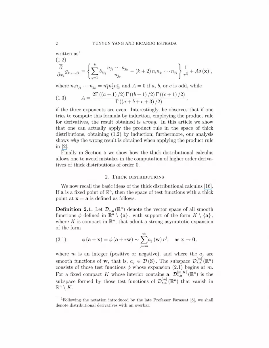
written as1

(1.2)

@

@xigj1,...,jk

=

(

kX

q=1

�ijq

nj1 · · ·njk

njq

� (k + 2) ninj1 · · ·njk

)

1

r3+ A� (x) ,

where ninj1 · · ·njk= na

1nb2n

c3, and A = 0 if a, b, or c is odd, while

(1.3) A =2� ((a + 1) /2) � ((b + 1) /2) � ((c + 1) /2)

� ((a + b + c + 3) /2),

if the three exponents are even. Interestingly, he observes that if onetries to compute this formula by induction, employing the product rulefor derivatives, the result obtained is wrong. In this article we showthat one can actually apply the product rule in the space of thickdistributions, obtaining (1.2) by induction; furthermore, our analysisshows why the wrong result is obtained when applying the product rulein [2].

Finally in Section 5 we show how the thick distributional calculusallows one to avoid mistakes in the computation of higher order deriva-tives of thick distributions of order 0.

2. Thick distributions

We now recall the basic ideas of the thick distributional calculus [16].If a is a fixed point of Rn, then the space of test functions with a thickpoint at x = a is defined as follows.

Definition 2.1. Let D⇤,a (Rn) denote the vector space of all smoothfunctions � defined in Rn \ {a} , with support of the form K \ {a} ,where K is compact in Rn, that admit a strong asymptotic expansionof the form

(2.1) � (a + x) = � (a + rw) ⇠1X

j=m

aj (w) rj, as x! 0 ,

where m is an integer (positive or negative), and where the aj are

smooth functions of w, that is, aj 2 D (S) . The subspace D[m]⇤,a (Rn)

consists of those test functions � whose expansion (2.1) begins at m.

For a fixed compact K whose interior contains a, D[m;K]⇤,a (Rn) is the

subspace formed by those test functions of D[m]⇤,a (Rn) that vanish in

Rn \K.

1Following the notation introduced by the late Professor Farassat [8], we shalldenote distributional derivatives with an overbar.

THICK DISTRIBUTIONAL CALCULUS 3

Observe that we require the asymptotic development of � (x) asx ! a to be “strong”. This means [7, Chapter 1] that for any di↵er-entiation operator (@/@x)p = (@p1 ...@pn) /@xp1

1 ...@xpnn , the asymptotic

development of (@/@x)p � (x) as x! a exists and is equal to the term-by-term di↵erentiation of

P1j=m aj (w) rj. Observe that saying that the

expansion exists as x! 0 is the same as saying that it exits as r ! 0,uniformly with respect to w.

We call D⇤,a (Rn) the space of test functions on Rn with a thick pointlocated at x = a. We denote D⇤,0 (Rn) as D⇤ (Rn) .

The topology of the space of thick test functions is constructed asfollows.

Definition 2.2. Let m be a fixed integer and K a compact subset ofRn whose interior contains a. The topology of D[m;K]

⇤,a (Rn) is given by

the seminormsn

k kq,s

o

q>m,s�0defined as

(2.2) ||�||q,s = supx�a2K

sup|p|s

�

�

�

�

�

�

@p�

@x(a + x)�

q�1X

j=m�|p|

aj,p (w) rj

�

�

�

�

�

�

rq,

where x = rw and

(2.3)@p�

@x(a + x) ⇠

1X

j=m�|p|

aj,p (w) rj.

The topology of D[m]⇤,a (Rn) is the inductive limit topology of the

D[m;K]⇤,a (Rn) as K % 1. The topology of D⇤,a (Rn) is the inductive

limit topology of the D[m]⇤,a (Rn) as m & �1.

A sequence {�l}1l=0 in D⇤,a (Rn) converges to if and only thereexists l0 � 0, an integer m, and a compact set K with a in its interior,such that �l 2 D[m;K]

⇤,a (Rn) for l � l0 and || � �l||q,s ! 0 as l ! 1 ifq > m, s � 0. Notice that if {�l}1l=0 converges to in D⇤,a (Rn) then�l and the corresponding derivatives converge uniformly to and itsderivatives in any set of the form Rn \B, where B is a ball with centerat a; in fact, r|p|�m (@/@x)p �l converges uniformly to r|p|�m (@/@x)p over all Rn. Furthermore, if

�

alj

are the coe�cients of the expansionof �l and {bj} are those for , then al

j ! bj in the space D (S) for eachj � m.

We can now consider distributions in a space with one thick point,the “thick distributions.”

4 YUNYUN YANG AND RICARDO ESTRADA

Definition 2.3. The space of distributions on Rn with a thick pointat x = a is the dual space of D⇤,a (Rn) . We denote it D0

⇤,a (Rn) , or just

as D0⇤ (Rn) when a = 0.

Observe that D (Rn) , the space of standard test functions, is a closedsubspace of D⇤,a (Rn) ; we denote by

(2.4) i : D (Rn) ! D⇤,a (Rn) ,

the inclusion map and by

(2.5) ⇧ : D0⇤,a (Rn) ! D0 (Rn) ,

the projection operator, dual of the inclusion (2.4).The derivatives of thick distributions are defined in much the same

way as the usual distributional derivatives, that is, by duality.

Definition 2.4. If f 2 D0⇤,a (Rn) then its thick distributional derivative

@⇤f/@xj is defined as

(2.6)

⌧

@⇤f

@xj,�

�

= �⌧

f,@�

@xj

�

, � 2 D⇤,a (Rn) .

We denote by E⇤ (Rn) the space of smooth functions in Rn \{a} thathave a strong asymptotic expansion of the form (2.1); alternatively, 2E⇤ (Rn) if = 1 + 2, where 1 2 E (Rn)2 and where 2 2 D⇤ (Rn) .The space E⇤ (Rn) is the space of multipliers of D⇤ (Rn) and of D0

⇤ (Rn) .Furthermore [16], the product rule for derivatives holds,

(2.7)@⇤ ( f)

@xj=@

@xjf +

@⇤f

@xj,

if f is a thick distribution and is a multiplier. Notice that @ /@xj

is the ordinary derivative in (2.7).Let g (w) is a distribution in S. The thick delta function of degree q,

denoted as g�[q]⇤ , or as g (w) �[q]

⇤ , acts on a thick test function � (x) as

(2.8)⌦

g�[q]⇤ ,�

↵

D0⇤(Rn)⇥D⇤(Rn)

=1

Chg (w) , aq (w)iD0(S)⇥D(S) ,

where � (rw) ⇠P1

j=m aj (w) rj, as r ! 0+, and where

(2.9) C =2⇡n/2

� (n/2),

2In general E (U) is the space of all smooth functions in the open set U.

THICK DISTRIBUTIONAL CALCULUS 5

is the surface area of the unit sphere S of Rn. If g is locally integrablefunction in S, then

(2.10)⌦

g�[q]⇤ ,�

↵

D0⇤(Rn)⇥D⇤(Rn)

=1

C

Z

Sg (w) aq (w) d� (w) .

Thick deltas of order 0 are called just thick deltas, and we shall use thenotation g�⇤ instead of g�

[0]⇤ .

Let g 2 D0 (S) . Then

(2.11)@⇤

@xj

�

g�[q]⇤�

=

✓

�g

�xj� (q + n) njg

◆

�[q+1]⇤ .

Here �g/�xj is the ��derivative of g [4, 6]; in general the ��derivativescan be applied to functions and distributions defined only on a smoothhypersurface ⌃ of Rn. Suppose now that the surface is S, the unit spherein Rn and let f be a smooth function defined in S, that is, f (w) is de-fined if w 2 Rn satisfies |w| = 1. Observe that the expressions @f/@xj

are not defined and, likewise, if w = (wj)1jn the expressions @f/@wj

do not make sense either; the derivatives that are always defined andthat one should consider are the �f/�xj, 1 j n. Let F0 be theextension of f to Rn \ {0} that is homogeneous of degree 0, namely,F0 (x) = f (x/r) where r = |x| . Then [16]

(2.12)�f

�xj=@F0

@xj

�

�

�

�

S.

Also, if we use polar coordinates, x = rw, so that F0 (x) = f (w) ,then @F0/@xj is homogeneous of degree �1, and actually @F0/@xj =r�1�f/�xj if x 6= 0.

The matrix µ = (µij)1i,jn , where µij = �ni/�xj, plays an importantrole in the study of distributions on a surface ⌃. If ⌃ = S then µij =�ni/�xj = �ij � ninj. Observe that µij = µji, an identity that holds inany surface.

The di↵erential operators �f/�xj are initially defined if f is a smoothfunction defined on ⌃, but we can also define them when f is a distri-bution. We can do this if we use the fact that smooth functions aredense in the space of distributions on ⌃.

3. The thick distribution Pf (1)

Let us consider one of the simplest functions, namely, the function1, defined in Rn. Naturally this function is locally integrable, and thusit defines a regular distribution, also denoted as 1, and the ordinaryderivatives and the distributional derivatives both coincide and give thevalue 0. On the other hand, 1 does not automatically give an element

6 YUNYUN YANG AND RICARDO ESTRADA

of D0⇤ (Rn) since if � 2 D⇤ (Rn) the integral

R

Rn � (x) dx could be diver-gent, and thus we consider the spherical finite part3 thick distributionPf (1) given as

(3.1) hPf (1) ,�i = F.p.

Z

Rn

� (x) dx =F.p. lim"!0+

Z

|x|�"

� (x) dx .

The derivatives of Pf (1) do not vanish, since actually we have thefollowing formula [16].

Lemma 3.1. In D0⇤ (Rn) ,

(3.2)@⇤

@xi(Pf (1)) = Cni�

[�n+1]⇤ ,

where C is given by (2.9).

Proof. One can find a proof of a more general statement in [16], but inthis simpler case the proof can be written as follows,

⌧

@⇤

@xi(Pf (1)) ,�

�

= �⌧

Pf (1) ,@�

@xi

�

= �F.p. lim"!0+

Z

|x|�"

@�

@xidx

= F.p. lim"!0+

Z

"Sn�1

ni� d� ,

so that if � 2 D⇤ (Rn) has the expansion � (x) ⇠P1

j=m aj (w) rj, asx! 0, then

Z

"Sn�1

ni� d� ⇠1X

j=m

✓

Z

Sniaj (w) d� (w)

◆

"n�1+j,

as "! 0+. The finite part of the limit is equal to the coe�cient of "0,thus

F.p.lim"!0

Z

"Sn�1

ni� d� =

Z

Snia1�n (w) d� (w)

=⌦

Cni�[1�n]⇤ ,�

↵

,

as required. ⇤

3If instead of removing balls of radius ", solids of other shapes are removed oneobtains a di↵erent thick distribution.

THICK DISTRIBUTIONAL CALCULUS 7

If 2 E⇤ (Rn) is a multiplier of D⇤ (Rn) , then we define, in a similarway, the thick distribution Pf ( ) 2 D0

⇤ (Rn) , and we clearly have theuseful formula

(3.3) Pf ( ) = Pf (1) ,

which immediately gives the thick distributional derivative of Pf ( )as

@⇤

@xi(Pf ( )) =

@

@xiPf (1) +

@⇤

@xi(Pf (1)) ,

so that we obtain the ensuing formula.

Proposition 3.2. If 2 E⇤ (Rn) then

(3.4)@⇤

@xi(Pf ( )) = Pf

✓

@

@xi

◆

+ Cni �[1�n]⇤ .

Notice that, in general, the term Cni �[1�n]⇤ is not a thick delta of

order 1 � n. Indeed, let us now consider the case when 2 E⇤ (Rn)is homogeneous of order k 2 Z. Then (x) = rk 0 (x) , where 0 is

homogeneous of order 0. Since rk�[q]⇤ = �

[q�k]⇤ [16, Eqn. (5.16)] we obtain

the following particular case of (3.4), where now the term Cni 0�[1�n�k]⇤

is a thick delta of order 1� n� k.

Proposition 3.3. If 2 E⇤ (Rn) is homogeneous of order k 2 Z, then

(3.5)@⇤

@xi(Pf ( )) = Pf

✓

@

@xi

◆

+ Cni 0�[1�n�k]⇤ ,

where 0 (x) = |x|�k (x) .

If we now apply the projection ⇧ onto the usual distribution spaceD0 (Rn) , we obtain the formula for the distributional derivatives ofhomogeneous distributions. Observe first that if k > �n then is integrable at the origin, and thus is a regular distribution and⇧ (Pf ( )) = . If k �n then ⇧ (Pf ( )) = Pf ( ) , since in thatcase the integral

R

Rn (x)� (x) dx would be divergent, in general, if� 2 D (Rn) . A particularly interesting case is when k = �n, since if is homogeneous of degree �n and

(3.6)

Z

S (w) d� (w) = 0 ,

then the principal value of the integral

(3.7) p.v.

Z

Rn

(x)� (x) dx = lim"!0+

Z

|x|�"

(x)� (x) dx ,

8 YUNYUN YANG AND RICARDO ESTRADA

actually exists for each � 2 D (Rn) , so that Pf ( ) = p.v. ( ) , the prin-cipal value distribution4. Condition (3.6) holds whenever = @⇠/@xj

for some ⇠ homogeneous of order �n + 1.

Proposition 3.4. Let be homogeneous of order k 2 Z in Rn \ {0} .Then, in D0 (Rn) the distributional derivative @ /@xi is given as fol-

lows:

(3.8)@

@xi=@

@xi, k > 1� n ,

equality of regular distributions;

(3.9)@

@xi= p.v.

✓

@

@xi

◆

+ A� (x) , k = 1� n ,

where A =R

S ni 0 (w) d� (w) = h 0, niiD0(S)⇥D(S) , while

(3.10)@

@xi= Pf

✓

@

@xi

◆

+ D (x) , k < 1� n ,

where D (x) is a homogeneous distribution of order k � 1 concentrated

at the origin and given by

(3.11)

D (x) = (�1)�k�n+1X

j1+···+jn=�k�n+1

⌦

ni 0,w(j1,...,jn)↵

j1! · · · jn!D(j1,...,jn)� (x) .

Proof. It follows from (3.4) if we observe [16, Prop. 4.7] that if g 2D0 (S) then

(3.12) ⇧�

g�[q]⇤�

=(�1)q

C

X

j1+···+jn=q

⌦

g (w) ,w(j1,...,jn)↵

j1! · · · jn!D(j1,...,jn)� (x) ,

and, in particular,

(3.13) ⇧ (g�⇤) =1

Chg (w) , 1i � (x) ,

if q = 0. ⇤

4Let ⌃ be a closed surface in Rn that encloses the origin. We describe ⌃ byan equation of the form g(x) = 1, where g(x) is continuous in Rn \ {0} and ho-mogeneous of degree 1. Then hR⌃ ( (x)) ,�(x)i = lim

"!0

R

g(x)>" (x)�(x) dx , definesanother regularization of , but in general R⌃ ( (x)) 6= p.v. ( (x)) [15], a factobserved by Farassat [8], who indicated its importance in numerical computations,and studied by several authors [11, 15].

THICK DISTRIBUTIONAL CALCULUS 9

Our next task is to compute the second order thick derivatives ofhomogeneous distributions. Indeed, if is homogeneous of degree kthen we can iterate the formula (3.5) to obtain

@⇤2

@xi@xj(Pf ( )) =

@⇤

@xi

✓

Pf

✓

@

@xj

◆

+ Cnj 0�[1�n�k]⇤

◆

(3.14)

= Pf

✓

@2

@xi@xj

◆

+ Cni⇠0�[2�n�k]⇤ +

@⇤

@xi

�

Cnj 0�[1�n�k]⇤

�

,

where ⇠ = @ /@xj is homogeneous of degree k � 1 and ⇠0 (x) =|x|1�k ⇠ (x) is the associated homogeneous of degree 0 function. Useof (2.11) and (??) allows us to write

@⇤

@xi

�

Cnj 0�[1�n�k]⇤

�

= C

✓

�

�xi(nj 0) + (k � 1) ninj 0

◆

�[2�n�k]⇤

(3.15)

= C

✓

(�ij � ninj) 0 + nj� 0

�xi+ (k � 1) ninj 0

◆

�[2�n�k]⇤

= C

✓

(�ij + (k � 2) ninj) 0 + nj� 0

�xi

◆

�[2�n�k]⇤ ,

while the equation = rk 0 yields @ /@xj = rk�1{knj 0 + � 0/�xj},so that

(3.16) ⇠0 = knj 0 +� 0

�xj.

Collecting terms we thus obtain the following formula.

Proposition 3.5. If 2 E⇤ (Rn) is homogeneous of order k 2 Z, then

@⇤2

@xi@xj(Pf ( )) = Pf

✓

@2

@xi@xj

◆

(3.17)

+ C

✓

(�ij + 2 (k � 1) ninj) 0 + nj� 0

�xi+ ni

� 0

�xj

◆

�[2�n�k]⇤ .

where 0 (x) = |x|�k (x) .

Projection onto D0 (Rn) of (3.17) gives the formula for the distribu-

tional derivatives @2/@xi@xj(Pf ( )) if 2 E⇤ (Rn) is homogeneous of

order k 2 Z. In case k = 2� n we obtain the following formula.

10 YUNYUN YANG AND RICARDO ESTRADA

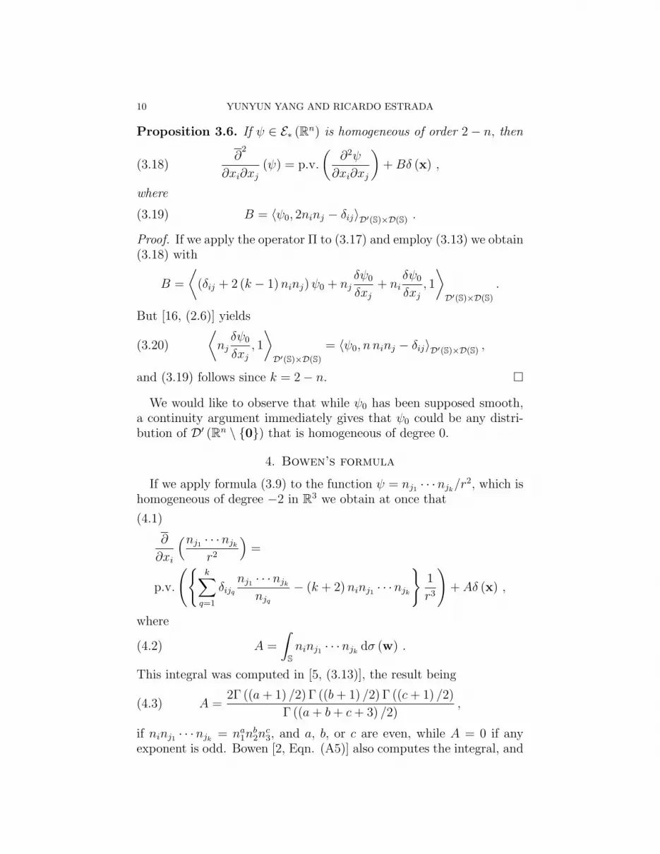
Proposition 3.6. If 2 E⇤ (Rn) is homogeneous of order 2� n, then

(3.18)@

2

@xi@xj( ) = p.v.

✓

@2

@xi@xj

◆

+ B� (x) ,

where

(3.19) B = h 0, 2ninj � �ijiD0(S)⇥D(S) .

Proof. If we apply the operator ⇧ to (3.17) and employ (3.13) we obtain(3.18) with

B =

⌧

(�ij + 2 (k � 1) ninj) 0 + nj� 0

�xj+ ni

� 0

�xj, 1

�

D0(S)⇥D(S)

.

But [16, (2.6)] yields

(3.20)

⌧

nj� 0

�xj, 1

�

D0(S)⇥D(S)

= h 0, n ninj � �ijiD0(S)⇥D(S) ,

and (3.19) follows since k = 2� n. ⇤

We would like to observe that while 0 has been supposed smooth,a continuity argument immediately gives that 0 could be any distri-bution of D0 (Rn \ {0}) that is homogeneous of degree 0.

4. Bowen’s formula

If we apply formula (3.9) to the function = nj1 · · ·njk/r2, which is

homogeneous of degree �2 in R3 we obtain at once that

@

@xi

⇣nj1 · · ·njk

r2

⌘

=

(4.1)

p.v.

(

kX

q=1

�ijq

nj1 · · ·njk

njq

� (k + 2) ninj1 · · ·njk

)

1

r3

!

+ A� (x) ,

where

(4.2) A =

Z

Sninj1 · · ·njk

d� (w) .

This integral was computed in [5, (3.13)], the result being

(4.3) A =2� ((a + 1) /2) � ((b + 1) /2) � ((c + 1) /2)

� ((a + b + c + 3) /2),

if ninj1 · · ·njk= na

1nb2n

c3, and a, b, or c are even, while A = 0 if any

exponent is odd. Bowen [2, Eqn. (A5)] also computes the integral, and

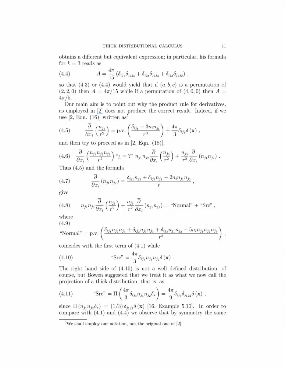
THICK DISTRIBUTIONAL CALCULUS 11

obtains a di↵erent but equivalent expression; in particular, his formulafor k = 3 reads as

(4.4) A =4⇡

15(�ij1�j2j3 + �ij2�j1j3 + �ij3�j1j2) ,

so that (4.3) or (4.4) would yield that if (a, b, c) is a permutation of(2, 2, 0) then A = 4⇡/15 while if a permutation of (4, 0, 0) then A =4⇡/5.

Our main aim is to point out why the product rule for derivatives,as employed in [2] does not produce the correct result. Indeed, if weuse [2, Eqn. (16)] written as5

(4.5)@

@xi

⇣nj1

r2

⌘

= p.v.

✓

�ij1 � 3ninji

r3

◆

+4⇡

3�ij1� (x) ,

and then try to proceed as in [2, Eqn. (18)],

(4.6)@

@xi

⇣nj1nj2nj3

r2

⌘

“¿ = ?” nj1nj2

@

@xi

⇣nj3

r2

⌘

+nj3

r2

@

@xi(nj1nj2) .

Thus (4.5) and the formula

(4.7)@

@xi(nj1nj2) =

�ij1nj2 + �ij2nj1 � 2ninj1nj2

r,

give

(4.8) nj1nj2

@

@xi

⇣nj3

r2

⌘

+nj3

r2

@

@xi(nj1nj2) = “Normal” + “Src” ,

where(4.9)

“Normal” = p.v.

✓

�ij1nj2nj3 + �ij2nj1nj3 + �ij3nj1nj2 � 5ninj1nj2nj3

r3

◆

,

coincides with the first term of (4.1) while

(4.10) “Src” =4⇡

3�ij3nj1nj2� (x) .

The right hand side of (4.10) is not a well defined distribution, ofcourse, but Bowen suggested that we treat it as what we now call theprojection of a thick distribution, that is, as

(4.11) “Src” = ⇧

✓

4⇡

3�ij3nj1nj2�⇤

◆

=4⇡

9�ij3�j1j2� (x) ,

since ⇧ (nj1nj2�⇤) = (1/3) �j1j2� (x) [16, Example 5.10]. In order tocompare with (4.1) and (4.4) we observe that by symmetry the same

5We shall employ our notation, not the original one of [2].

12 YUNYUN YANG AND RICARDO ESTRADA

result would be obtained if j3 and j1, or j3 and j2, are exchanged, sothat if in the term “Src” we do these exchanges, add the results anddivide by 3, we would get

(4.12) “SrcSym” =4⇡

27(�ij1�j2j3 + �ij2�j1j3 + �ij3�j1j2) � (x) ,

and thus the symmetric version of the (4.8) is “Normal”+“SrcSym”,which of course is di↵erent from (4.1) since the coe�cient in (4.4) is4⇡/15, while that in (4.12) is 4⇡/27. Therefore, the relation “¿=?” in(4.6) cannot be replaced by = .

Hence the product rule for derivatives fails in this case. The question

is why? Indeed, when computing the right side of (4.6), that is, the leftside of (4.8), we found just one irregular product, namely nj1nj2� (x) ,but using the average value (1/3) �j1j2� (x) seems quite reasonable.

In order to see what went wrong let us compute @/@xi (nj1nj2nj3/r2)

by computing the thick derivative @⇤/@xiPf (nj1nj2nj3/r2) , applying

the product rule for thick derivatives, and then taking the projection⇡ of this. We have,

@⇤

@xiPf⇣nj1nj2nj3

r2

⌘

=@⇤

@xi

h

nj1nj2Pf⇣nj3

r2

⌘i

= nj1nj2

@⇤

@xiPf⇣nj3

r2

⌘

+@ (nj1nj2)

@xiPf⇣nj3

r2

⌘

,

and taking (3.5) into account, we obtain

nj1nj2

⇢

Pf

✓

�ij3 � 3ninj3

r3

◆

+ 4⇡nj3ni�⇤

�

+�ij1nj2 + �ij2nj1 � 2ninj1nj2

rPf⇣nj3

r2

⌘

,

that is, @⇤/@xiPf (nj1nj2nj3/r2) equals

Pf

✓

�ij1nj2nj3 + �ij2nj1nj3 + �ij3nj1nj2 � 5ninj1nj2nj3

r3

◆

(4.13)

+ 4⇡nj1nj2nj3ni�⇤ .

Applying the projection operator ⇧ we obtain that the Pf becomesa p.v., so that the term “Normal” given by (4.9) is obtained, while(3.13) yields that the projection of thick delta is exactly A� (x) whereA =

R

S ninj1nj2nj3 d� (w) , that is, the correct term

4⇡

15(�ij1�j2j3 + �ij2�j1j3 + �ij3�j1j2) � (x) .

The reason we now obtain the correct result is while it is true that⇧ (nj1nj2�⇤) = (1/3) �j1j2� (x) and that ⇧ (nj3ni�⇤) = (1/3) �ij3� (x) , it

THICK DISTRIBUTIONAL CALCULUS 13

is not true that the projection ⇧ (4⇡nj1nj2nj3ni�⇤) can be obtained as4⇡ (1/3) �ij3⇧ (nj1nj2�⇤) nor as 4⇡ (1/3) �j1j2⇧ (nj3ni�⇤) , and actuallynot even the symmetrization of such results, given by (4.12), works.Put in simple terms, it is not true that the average of a product is theproduct of the averages!

One can, alternatively, compute @⇤/@xiPf (nj1nj2nj3/r2) as

(4.14)@

@xi

⇣nj3

r2

⌘

Pf (nj1nj2) +⇣nj3

r2

⌘ @⇤

@xiPf (nj1nj2) ,

since(4.15)@⇤

@xiPf (nj1nj2) = Pf

✓

�ij1nj2 + �ij2nj1 � 2ninj1nj2

r

◆

+4⇡nj1nj2ni�[�2]⇤ .

Here the thick delta term in (4.14) is 4⇡ (nj3/r2) nj1nj2ni�

[�2]⇤ , which

becomes, as it should, 4⇡nj1nj2nj3ni�⇤.Complications in the use of the product rule for derivatives in one

variable were considered in [3] when analysing the formula [14]

(4.16)d

dx(Hn (x)) = nHn�1 (x) � (x) ,

where H is the Heaviside function; see also [12].

5. Higher order derivatives

We now consider the computation of higher order derivatives in the

space⇣

D[0]⇤ (Rn)

⌘0. If f 2 D0

⇤ (Rn) then, of course, the thick derivative

@⇤f/@xi is defined by duality, that is,

(5.1)

⌧

@⇤f

@xi,�

�

= �⌧

f,@�

@xi

�

,

for � 2 D⇤ (Rn) . Suppose now that A is a subspace of D⇤ (Rn) thathas a topology such that the imbedding i : A ,! D⇤ (Rn) is continuous;then the transpose iT : D0

⇤ (Rn) ! A0 is just the restriction operator⇧A. If A is closed under the di↵erentiation operators6, then we can alsodefine the derivative of any f 2 A0, say @Af/@xi, by employing (5.1)for � 2 A. Then

(5.2) ⇧A

✓

@⇤f

@xi

◆

=@A@xi

(⇧A (f)) ,

6The space A0 would be a space of (thick) distributions in the sense of Zemanian[18].

14 YUNYUN YANG AND RICARDO ESTRADA

for any thick distribution f 2 D0⇤ (Rn) . In the particular case when A =

D (Rn) then @Af/@xi = @f/@xi, the usual distributional derivative,and thus (5.2) becomes [16, Eqn. (5.22)],

(5.3) ⇧

✓

@⇤f

@xi

◆

=@⇧ (f)

@xi.

What this means is that one can use thick distributional derivatives tocompute @Af/@xi, as we have already done to compute distributionalderivatives.

WhenA is not closed under the di↵erentiation operators then @Af/@xi

cannot be defined by (5.1) if f 2 A0 since in general @�/@xi does notbelong to A and thus the right side of (5.1) is not defined. How-ever, if f 2 A0 has a canonical extension ef 2 D0

⇤ (Rn) then we could

define @Af/@xi as ⇧A

⇣

@⇤ ef/@xi

⌘

. This applies, in particular when

A = D[0]⇤ (Rn) : if f 2

⇣

D[0]⇤ (Rn)

⌘0then @⇤0f/@xi = @Af/@xi cannot

be defined, in general, but if f has a canonical extension ef 2 D0⇤ (Rn)

then @⇤0f/@xi is understood as ⇧D[0]⇤ (Rn)

⇣

@⇤ ef/@xi

⌘

.

Our aim is to point out that, in general, if P = RS is the prod-uct of two di↵erential operators with constant coe�cients, then while,with obvious notations, P ⇤ = R⇤S⇤, PA = RASA, if A is closed underdi↵erential operators, and P = R S, it is not true that P ⇤

0 = R⇤0S

⇤0 .

Therefore the space⇣

D[0]⇤ (Rn)

⌘0is not a convenient framework to gen-

eralize distributions to thick distributions; the whole D0⇤ (Rn) is needed

if we want a theory that includes the possibility of di↵erentiation.

Example 5.1. Let us consider the second order derivatives of the dis-tribution Pf (1) . Formula (3.17) yields

(5.4)@⇤2

@xi@xj(Pf (1)) = C (�ij � 2ninj) �

[�n+2]⇤ .

In particular, in R2, @⇤2/@xi@xj (Pf (1)) = 2⇡ (�ij � 2ninj) �⇤. If we

consider the function 1 as an element of⇣

D[0]⇤ (R2)

⌘0then it has the

canonical extension Pf (1) 2 D0⇤ (R2) and so

@⇤0 (1)

@xj= ⇧D[0]

⇤ (R2)

�

2⇡nj�[�1]⇤�

= 0 ,

and consequently,

(5.5)@⇤0@xi

✓

@⇤0 (1)

@xj

◆

=@⇤0@xi

(0) = 0 6= 2⇡ (�ij � 2ninj) �⇤ =@⇤2 (1)

@xi@xj.

THICK DISTRIBUTIONAL CALCULUS 15

Observe that ⇧ (2⇡ (�ij � 2ninj) �⇤) = 0, but observe also that thismeans very little.

Example 5.2. It was obtained in [16, Thm. 7.6] that in D0⇤ (R3)

(5.6)@⇤2Pf (r�1)

@xi@xj=�

3xixj � �ijr2�

Pf�

r�5�

+ 4⇡ (�ij � 4ninj) �⇤ .

Since ⇧ (ninj�⇤) = (1/3) �ij� (x) in R3, this yields the well known for-mula of Frahm [9]

(5.7)@

2

@xi@xj

✓

1

r

◆

= p.v.

✓

3xixj � r2�ijr5

◆

�✓

4⇡

3

◆

�ij� (x) .

We also immediately obtain that

(5.8)@⇤20 Pf (r�1)

@xi@xj= Pf

✓

3xixj � r2�ijr5

◆

+ 4⇡ (�ij � 4ninj) �⇤ ,

a formula that can also be proved by other methods [17]. On the otherhand, in [10] one can find the computation of

(5.9)@⇤0@xi

✓

@⇤0@xj

✓

1

r

◆◆

= Pf

✓

3xixj � r2�ijr5

◆

� 4⇡ninj�⇤ .

The fact that@⇤0@xi

✓

@⇤0@xj

◆

6= @⇤20

@xi@xjis obvious in the Example 5.1,

but it is harder to see it in cases like this one7. Observe that theprojection of both 4⇡ (�ij � 4ninj) �⇤ and of �4⇡ninj�⇤ onto D0 (R3)is given by � (4⇡/3) �ij� (x) , but this does not mean that they areequal; observe also that one needs the finite part in (5.8) and in (5.9)since the principal value, as used in (5.7), exists in D0 (R3) but not in⇣

D[0]⇤ (R3)

⌘0.

.

References

[1] Blanchet, L. and Faye, G., Hadamard regularization, J. Math. Phys. 41 (2000),7675-7714.

[2] Bowen, J. M., Delta function terms arising from classical point-source fields,Amer. J. Phys. 62 (1994), 511-515.

[3] Estrada, R. and Fulling, S. A., Spaces of test functions and distributions inspaces with thick points, Int. J. Appl. Math. Stat. 10 (2007), 25-37.

[4] Estrada, R. and Kanwal, R. P., Distributional analysis of discontinuous fields,J.Math.Anal.Appl. 105 (1985), 478-490.

7That the two results are di↵erent is overlooked in [10].

16 YUNYUN YANG AND RICARDO ESTRADA

[5] Estrada, R. and Kanwal, R. P.,Regularization and distributional derivatives of�

x

21 + · · ·x2

p

�n/2 in D0 (Rp) , Proc.Roy. Soc. London A 401 (1985), 281-297.[6] Estrada, R. and Kanwal, R. P., Higher order fundamental forms of a sur-

face and their applications to wave propagation and distributional derivatives,Rend. Cir. Mat. Palermo 36 (1987), 27-62.

[7] Estrada, R. and Kanwal, R.P., A distributional approach to Asymptotics. The-

ory and Applications, second edition, Birkhauser, Boston, 2002.[8] Farassat, F., Introduction to generalized functions with applications in aerody-

namics and aeroacoustics, NASA Technical Paper 3248 (Hampton, VA: NASALangley Research Center) (1996); http://ntrs.nasa.gov.

[9] Frahm, C. P., Some novel delta-function identities, Am. J. Phys. 51 (1983),826–29.

[10] Franklin, J., Comment on ‘Some novel delta-function identities’ by Charles PFrahm (Am. J. Phys 51 826–9 (1983)), Am. J. Phys. 78 (2010), 1225–26.

[11] Hnizdo, V., Generalized second-order partial derivatives of 1/r, Eur. J. Phys.

32 (2011), 287–297.[12] Paskusz, G.F., Comments on “Transient analysis of energy equation of dynam-

ical systems”, IEEE Trans. Edu. 43 (2000), 242.[13] Sellier, A., Hadamard’s finite part concept in dimensions n � 2. definition

and change of variables, associated Fubini’s theorem, derivation, Math. Proc.

Cambridge Philos. Soc. 122 (1997), 131-148.[14] Vibet, C., Transient analysis of energy equation of dynamical systems, IEEE

Trans. Edu. 42 (1999), 217-219.[15] Yang, Y. and Estrada, R., Regularization using di↵erent surfaces and the sec-

ond order derivatives of 1/r, Applicable Analysis 92 (2013), 246-258.[16] Yang, Y. and Estrada, R., Distributions in spaces with thick points, J. Math.

Anal. Appls. 401 (2013), 821-835.[17] Yang, Y. and Estrada, R., Extension of Frahm formulas for @i@j (1/r), Indian

J. Math., in press.[18] Zemanian, A. H., Generalized Integral Transforms, Interscience, New York,

1965.

Department of Mathematics, Louisiana State University, Baton Rouge,LA 70803

E-mail address: yyang18@math.lsu.edu

E-mail address: restrada@math.lsu.edu