ELSEVIER

Discrete-time queueing models with feedback for input-buffered ATM

Performance Evaluation 27&28 (1996) 71-87

switches *

K. Laevens *, H. Bruneel

SMACS Research Group, Laboratory for Communications Engineering, University of Ghent, Sint-Pietersnieuwstraat 41, B-9000 Ghent, Belgium

Abstract

We present the analysis of some discrete-time single-server queueing models with feedback that capture the behavior of the head-of-line request queues in large input-buffered ATM switches when correlation in the destinations of the cell streams at the input links is present. Three different switch selection policies are considered: message based first-in- first-out, cell based first-in-first-out or round-robin and cell based random-order-of-service. Although some close analogy exists with continuous-time feedback queueing models, the discrete-time nature of the models considered here brings about some complications not found in the former. The joint analysis, based on generating functions, of the system contents and the waiting time of a tagged message leads to a number of (functional) equations. Without explicitly solving these equations, mean values and higher-order moments for the (conditional) waiting time are obtained. Numerical results illustrate the effect of correlation in the cell destinations and of burstiness in the input traffic on switch perfor- mance.

Keywords: ATM switches; Queues with feedback; Round-robin; Random-order-of-service; Discrete-time queues

1. Introduction

The study of queues with feedback dates back as far as 1963, when Takacs [18] analyzed, as a model of a telephone exchange, the continuous-time M/G/l queue with so-called Bernoulli feedback, i.e., where, with constant probability, a customer immediately rejoins the queue after the completion of its service. Since then the subject has received a lot of attention, mainly in the context of time-sharing in computer systems [7,9]. Especially extensions of the Bernoulli feedback mechanism have been focussed upon [5,12] so as to obtain results for the continuous-time M/G/l processor-sharing queue [9,16,19], by making the quantum size shrink to zero. These feedback models are also closely related to queueing models with the so-called round-robin service discipline [4,9,16]. Although most relevant papers deal

* The authors wish to thank the Belgian Federal Office for Scientific, Technical and Cultural Affairs (D.W.T.C.) and the Belgian National Fund for Scientific Research (N.F.W.O.) for support of this research. * Corresponding author. E-mail: koen.laevens@lci.rug.ac.be.

0166-5316/96/$15.00 Copyright 0 1996 Elsevier Science B.V. All rights reserved. PI1 SO1 66-53 16(96)00028-4

72 K. Laevens, H. Bruneel/Performance Evaluation 27&28 (1996) 71-87

with continuous-time models, some have also considered discrete-time models [4,10,16], the motivation for doing so being a finite and fixed-sized quantum.

The need for results on discrete-time queueing models with feedback has recently re-emerged in

the context of ATM switching systems (see e.g. [1,8] for a survey of switch architectures). In the performance analysis of switches where all or some buffering is done at the inputs, the introduction

of the concept of virtual queues (VQ’s) [3,8] has often been a key step. These logical queues consist of all head-of-line (HOL) requests of the various input queues (IQ’s) destined for a specific output port. In [8] it was shown that for large, i.e., infinite, switch sizes and for uncorrelated traffic (i.e., without correlation in the arrivals and the destinations of cells [l]) these VQ’s can be modelled as discrete-time GI-D-l queues with a Poisson distribution for the general independent (GI) arrival process. (Throughout this paper, we will use the modified Kendall notation for discrete-time queueing systems, as introduced in [2].) Even in the presence of correlation in the arrivals and imbalance in the destinations of cells, this model remains valid [3,13]. The situation becomes quite different, however, when correlation in the cell destinations is introduced, i.e., when the destination of one HOL request from a certain IQ is no longer independent from that of the previous HOL request of that IQ. This type of correlation may have a serious effect on the switch performance, which may even become so drastic that input-buffered architectures can outperform output-buffered ones, as shown through simulation in [ 151. Certain modelling approaches taking this correlation into account, lead to a VQ model with feedback [6,14]. It is the purpose of this paper to present some analytic results for such type of models and to study the effect of correlation in the input traffic on switch performance.

We will analyze three different switch selection policies. These determine the order in which different HOL requests for the same output port are routed and thus determine the service discipline inside the VQ’s. The first selection policy is called message based first-in-first-out (FIFO). Under this selection policy, messages - a collection of consecutive cells with the same destination, see Section 2.1 - are routed uninterruptedly at a rate of one cell per slot, in the order in which they arrive to the HOL position of their respective IQ’s. (A message is said to arrive at the HOL position when the first cell it contains moves up to the HOL position.) This makes the VQ’s FIFO queues for the messages. Note, this is not a global FIFO selection policy [l], under which messages are routed in the order in which they arrive at their respective IQ’s. Under the second selection policy, called cell based FIFO or round-robin (RR), cells are routed in the order in which they arrive to the HOL position of their respective IQ’s. The possible correlation in the destinations of consecutive cells within an IQ is thus not taken into account. This results in a round-robin service discipline for messages inside the VQ’s. Finally, under the third selection policy, called cell based random-order-of-service (ROS), cells are routed in a totally random way. Unlike the former two, this selection policy does not require information concerning the time of arrival of cells to the HOL position - the HOL arrival times for short - and therefore seems to be the more interesting one from an implementations point of view. Although the switch operates at cell level, we will analyze its performance on message level mainly, notably in the analysis of the VQ’s. Strictly speaking, these (logical) queues contain cells only, but we will model them as queues handling messages.

The structure of the paper is as follows. In the next section we introduce the mathematical model and analyze the waiting time of a tagged message inside an IQ. In Sections 3 to 5, we analyze the VQ’s under the different selection policies. In Section 3, the message based FIFO selection policy is considered. Since under the assumptions made, the VQ system contents and the maximum switch throughput do not depend upon the specific selection policy adopted, these quantities are also analyzed in that section. In

K. Laevens, H. Bruneel/Pe~orrnance Evaluation 27&28 (1996) 71-87 73

1 I +

! T, T*+l time ----------x--

t

Ii A ml f

hi hi+si-li=hi+Wi I hi+l=[hi+wi-mi]+

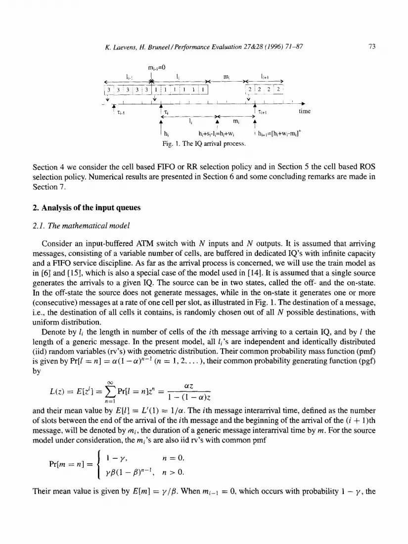
Fig. 1. The IQ arrival process.

Section 4 we consider the cell based FIFO or RR selection policy and in Section 5 the cell based ROS selection policy. Numerical results are presented in Section 6 and some concluding remarks are made in Section 7.

2. Analysis of the input queues

2.1. The mathematical model

Consider an input-buffered ATM switch with N inputs and N outputs. It is assumed that arriving messages, consisting of a variable number of cells, are buffered in dedicated IQ’s with infinite capacity and a FIFO service discipline. As far as the arrival process is concerned, we will use the train model as in [6] and [ 151, which is also a special case of the model used in [14]. It is assumed that a single source generates the arrivals to a given IQ. The source can be in two states, called the off- and the on-state. In the off-state the source does not generate messages, while in the on-state it generates one or more (consecutive) messages at a rate of one cell per slot, as illustrated in Fig. 1. The destination of a message, i.e., the destination of all cells it contains, is randomly chosen out of all N possible destinations, with uniform distribution.

Denote by li the length in number of cells of the ith message arriving to a certain IQ, and by 1 the length of a generic message. In the present model, all ii’s are independent and identically distributed (iid) random variables (rv’s) with geometric distribution. Their common probability mass function (pmf) is given by Pr[l = n] = a(1 -(Y)‘+’ (n = 1,2, . . . ), their common probability generating function (pgf)

by

L(z) = Etz’] = FPr[l = nlz” = 1 _ (y’ a)z ?I=1

and their mean value by E[1] = L’(1) = l/a. The ith message interarrival time, defined as the number of slots between the end of the arrival of the ith message and the beginning of the arrival of the (i + 1)th message, will be denoted by mi, the duration of a generic message interarrival time by m. For the source model under consideration, the rn; ‘s are also iid rv’s with common pmf

Pr[m = n] =

1

l-y, ?z =o,

v/3(1 - fi>“-1, Iz > 0.

Their mean value is given by E [m] = y //?. When rni _ 1 = 0, which occurs with probability 1 - y , the

74 K. Laevens, H. Bruneel/Pe$ormance Evaluation 278~28 f1996) 71-87

ith message arrives immediately after the (i - l)th, as in Fig. 1. The mean number of messages arriving in this way, i.e., without off-slots between them, equals l/y. The durations of the off-periods, i.e., of the non-zero message interarrival times, are iid rv’s with geometric distribution and mean l/B.

The average number of messages arriving per slot to a single IQ is given by

1 1

h = E[Z] + E[m] = l/a + Y/B

while the average number of cells arriving per slot to a single IQ equals

A* = WI l/a

E[E] + E[ml = I/@ + Y/B = h/a.

Note that for increasing values of l/y or l/B but fixed values of v/p, the average number of messages arriving per slot remains constant, but the clustering or burstiness in the input traffic increases.

2.2. Waiting time and system time

For the remainder of this paper, we will assume that N is very large, i.e., N + 00. The queueing processes inside the different IQ’s then become independent and statistically identical. We thus may focus attention on a single IQ.

Only cells at the HOL positions of the different IQ’s are involved in the contention for the routing to the output ports. The selection policy determines the service time of a cell inside an IQ, i.e., the time it spends at the HOL position before being routed to the appropriate output port. The fact that cells belonging to the same message have the same destination introduces correlation in their individual service times, but due to our assumptions - cells belonging to a same message arriving back to back, homogeneous and uniform traffic conditions and a FIFO discipline within the IQ’s - knowledge of the service time of an entire message, i.e., the sum of the service times of the cells of which it consists, is sufficient for the analysis of the message waiting time inside an IQ, as will be shown next.

Let us denote the service time of the ith message inside the IQ by si and that of a generic message by s. Since the routing of a single cell requires at least one slot, the service time of a message can be decomposed as si = li + Wi, i.e., as the sum of its length and some additional service time, denoted by wi. This additional service time - the sum of the individual waiting times inside a VQ of the cells composing the message - is caused by the output port contention, i.e., by the routing of cells at the HOL positions of other IQ’s to the same output port as that to which the cells of the message are destined. For a generic message, we will denote this waiting time by w, and by W(z) the associated pgf E[zW]. Note that 1 and w may be correlated. Stability of the input queues requires that h E [s] < 1. This stability condition determines the maximum throughput of the switch, as will be shown later on.

In order to analyze the waiting time of a randomly chosen message inside an IQ, consider the embedded Markov chain one obtains by considering the arrival epochs ti, see Fig. 1, defined as the end of the slots during which the first cell of the ith message arrives at the IQ. The amount of unfinished work in the IQ at time ti, not including the contribution of the first cell of the arriving message, will be denoted by hi. Clearly, this is also the waiting time of the message inside the IQ, i.e., the time until the first cell it contains reaches the HOL position. As becomes clear from inspection of Fig. 1, one has the relation

hj+l = [hi + Si - Zj - mj]+ = [hi + Wi - mi]+, (1)

K. Luevens, H. Bruneel / Performance Evaluation 27&28 (I 996) 71-87 75

whereby [xl+ denotes max(x, 0). For H(z), the pgf associated with the equilibrium distribution of the hi’s (i.e., for H(z) = limj-too E[zhl]), one obtains after some elementary algebra - taking into account the specific distribution of the mi ‘s as given above and after determining a single constant by means of the normalization condition H(1) = 1 for pgf’s - the expression

H(z) = (v - B W’(l))(z - 1)

z - (1 - B) - W(z)@ + (1 - y)(z - 1) *

From this, the mean value of h - the mean waiting time of a generic message inside an IQ - can easily be determined by taking the first derivative at z = 1. It is given by

E[h] = H’(1) = fi W”(1) + 2u - r> W’(1)

2(Y - BW’(1)) ’

The system time of a generic message inside an IQ is the sum of its waiting time h and its service time S. However, in this service time, the time to route the message to the output port is included. This time equals the length 1 of the message. A fairer performance measure seems therefore to be the total delay induced by the switch. This switching delay, the sum of the waiting time h inside an IQ and the waiting time w at HOL position, will be denoted by h*. It is the time between (the end of) the slot of arrival of the last cell of a message and (the end of) the slot of the departure of that cell. It does not depend directly on the length I of the message, but only through the correlation that may exist between 1 and w. Its mean value is given by E[h*] = E[h] + E[w]. In the next sections, the waiting time w under the different selection policies is analyzed in more detail.

3. Analysis of the VQ’s: FIFO discipline

3.1. Introduction

Due to the assumptions of homogeneous and uniform traffic conditions and an infinite switch size, all VQ’s are independent and statistically equivalent systems. Consider therefore a single VQ. As mentioned before, the selection policy inside the switch determines the service discipline inside that VQ. In this section, we consider the message based FIFO selection policy, under which messages are routed uninterruptedly at a rate of one cell per slot in the order in which they arrive to the HOL position of their respective IQ’s. This makes the VQ’s FIFO queues in which messages are served without interruption at a rate of one cell per slot.

The arrival process to the VQ consists of requests from messages that just moved to the HOL position of an IQ. When N + 00, this becomes a GI arrival process [2] with mean h and a Poisson distribution for the number of arrivals during a slot. This can be proven by extending the reasoning in [8], as shown in [ 131. Denote the number of arrivals during slot k by ak and their common pgf E[,+] by A(z). In case of a Poisson arrival process this pgf takes the form A(z) = exp(h(z - 1)) and its derivatives at z = 1 equal A(“)(l) = h”. The service requirement of a message inside the VQ equals its length 1. For the present source model, the rv’s li are geometrically distributed, as explained in Section 2. This will greatly simplify the analysis - here and in the following sections - due to the so-called memoryless property of that distribution. This property can, for our purposes, best be expressed as W_li = n(li z n] = a. This implies that, with constant probability a!, there will depart a message from a VQ after a slot of service has been delivered to it, regardless of the number of slots service it already

76 K. Luevens, H. Bruneel/Perfomance Evaluation 27&28 (1996) 71-87

received. (A message departs from a VQ when the last cell it contains has been routed to the appropriate output port.)

3.2. System contents and maximum switch throughput

The system contents of an arbitrary VQ - the number of messages it contains - at the beginning of slot k will be denoted by uk. The Markov chain Uk (for k = 0, 1, . . . ) is governed by the equation

uk = 0,

uk+l = I uk + ak, uk > 0 and no message departs from the queue,

uk +ak - 1, Uk > 0 and a message departs from the queue.

For geometrically distributed message lengths, this does not depend upon the specific service discipline. We can therefore use the results in [2] for the GI-Geo-1 system with FIFO discipline (as a special case of the G&G-l system). It is shown there that

U(z) = A(z)@ - A’tl))(z - 1)

z-A(z)(a+(l -a)~)’

whereby U(z) denotes the pgf of u, the system contents in regime. The mean system contents, for Poisson arrivals, is given by

U’(1) = E[u] = ;;t 1;;.

By virtue of Little’s result and the above mentioned insensitivity of the VQ system contents under the service discipline, the mean system time inside a VQ of a randomly chosen message is

E[ul 2-h E[s] = h =

2(0! - h)

regardless of the switch selection policy. This is also the mean service time at HOL position of a randomly chosen message. Recalling the stability condition hE[s] -C 1 for the IQ’s, we can determine the maximum throughput of the switch (in cells per slot). One obtains hi, = (2 - J~~)/cx. Extremal values are Akax = 0.5857.. . for cz = 1 (no correlation in the cell destinations, see [8]) and

%ax + 0.5 for (Y + 0 (infinitely long correlation in the cell destinations, see [14]). This stability condition is more restrictive than that for the VQ’s, which is A* -C 1.

3.3. Waiting time under the FIFO discipline

The results in [2] concerning the waiting time in the G&G-l system yield the expression

W(z) = (1 - A’(l)L’(l))CA(Uz)) - 11

A’(l)L’(l)[z - AG(z))l

for the pgf W(z) of the message waiting time w inside a VQ. For Poisson arrivals, the mean message waiting time is given by

K. hevens, H. Bruneel/ Performance Evaluation 27&28 (1996) 71-87 71

E[w] = W’(1) = h(2 - a)

2+X - h).

This agrees with Little’s result for the VQ queue contents only, i.e., the VQ system contents without the message being served. Again, this result does not depend upon the switch selection policy, and should thus be obtained for the other selection policies too. The second order derivative of W(z) at z = 1 is, for Poisson arrivals, given by

WN(l) = E[?JJ(w - l)] = h(6(2 - a)(1 - cr) + 2h(3 - 2a) + h2)

6a(a - h)2

From this, the variance of zv can be calculated as Var[w] = W"( 1) + W'( l)( 1 - W'( 1)). Note that for the message based FIFO discipline 1 and w are uncorrelated, i.e., Cov[Z, w] = 0.

4. Analysis of the VQ’s: RR discipline

4. I. Preliminary observations

In this section, we analyze the VQ’s when the switch selection policy is cell based FIFO or round- robin. Under this selection policy, whereby cells get routed in the order in which they arrive to the HOL position of their IQ, the VQ service discipline for messages is as follows. Every message receives exactly one slot of service once it reaches the server of the VQ. If afterwards the message requires more service, it has to rejoin the queue at the rear and wait once more until it reaches the server. A message rejoining the queue is called an internal arrival, while messages arriving to the queue for the first time are called external arrivals, as shown in Fig. 2.

While the simultaneous occurence of arrivals and departures has not to be considered in continuous- time round-robin or feedback models, this no longer holds for the discrete-time counterparts. Therefore, a policy has to be defined describing how externally arriving messages are queued with respect to the message possibly rejoining the queue, i.e., the internal arrival. The studies of [4] and [16] considered Bernoulli arrivals only and assumed that an externally arriving message is granted a welcoming slot of service. The possibility of multiple external arrivals during a slot in our model, does not allow an

unambiguous definition of a welcoming slot, therefore we will not consider this possibility here. Still, a number of other mixing policies can be devised. For instance, one can assume that external arrivals occur during a slot, while the feedback, i.e., the internal arrival, occurs at the end of that slot, and that the former are thus queued ahead of the latter. While this seems a logical choice for queues whereby the external arrivals are not synchronized with the queue, it is not realistic for a switch model. Due to the contention resolution mechanism and the routing, synchronisation is present, so that all arrivals to a VQ

internal arrivals 1

I I I I I I Fig. 2. The VQ model with feedback.

78 K. Luevens, H. Bruneel/Perfomance Evaluation 27&28 (1996) 71-87

occur at the end of a slot and no distinction is or can be made between external and internal arrivals. Therefore, we will assume that all messages arriving during a same slot are queued in a random way with respect to each other.

4.2. Analysis of the waiting time

Consider a generic or tagged message. If it requires n slots service, it has to go through 12 cycles of waiting a number of slots and receiving one slot of service. The first of these cycles differs from the others, since it starts with the message arriving over the external link (possibly together with some other messages), while the others start with the message rejoining the queue over the internal link. It is obvious that messages joining or leaving the queue while the tagged message is inside the system, have an effect on the duration of these cycles. As was done in e.g. [ 181, we will therefore jointly analyze the evolution of the waiting time of the tagged message and the number of other messages in the system, and this at various observation epochs. Clearly, the most important epochs are the beginning and end of the different cycles. The beginning of a cycle is defined as the end of the slot wherein the tagged message joined or rejoined the queue, the end of a cycle as the beginning of the slot wherein the message will receive a slot of service. The slots during which service is received, are thus not part of the cycles. In order to describe the above mentioned evolution and to capture all of the possible correlation between different cycles, we have to define a number of rv’s. By p,, and qn we will denote the number of other messages in the system - respectively in front of and behind the tagged message - at the beginning of the nth cycle. By w,, we will denote the total waiting time accumulated by the message by the end of the nth cycle, and by t,, the number of other messages in the system at that time (necessarily behind the tagged message). The equations describing the evolution from cycle to cycle are

Wl = W-1 + pn, (2)

tn = qn + t(aj + bj) j=l

(3)

for 12 > 1, with the convention that wg = 0, and

pn = rn-1 + e,,

4n = fn

forn > l.Forn = l,onehas

(4)

(5)

p1 = [u* - l]+ + el + e;, (6)

41 = fl + I?* (7)

In the above, the aj’s were used to denote the numbers of external arrivals during the different slots of a cycle, all aj ‘s being iid rv’s with common pgf A(z). The bj ‘s were used to denote the number of internal arrivals during these slots. Since the system is never empty during a cycle, these numbers are Bernoulli IV’S which take on the values 0 and 1 with probability (Y and 1 - ac respectively. For ease of notation, we introduce their common pgf B(z) = E[zbi] = (Y + (1 - (zr)z. The variables e,, and fn were used to denote the numbers of externally arriving messages with which the tagged message has to mix during the transition from the (n - 1)th cycle to the nth cycle and that get queued respectively in front of or

K. Laevens, H. Bruneel/Performance Evaluation 27&28 (1996) 71-87 79

behind that message. Similarly, the variables eT and f;” account for the internally arriving message(s) with which the tagged message has to mix upon arrival. Note that the rv’s e,, fn , e; and fr capture the fine details of the mixing policy and that the above equations are in fact valid for any mixing policy. Finally, the variable U* was used to denote the number of messages inside the VQ at the beginning of the slot wherein the tagged message arrives over the external link. This rv is distributed as the system contents of a VQ in regime, implying E[z”‘] = U(z), and it is correlated with e; and f;” in the sense that

0, u* = 0,

eT+.f;” =

(

1, U* > 0 and a message rejoins the queue, (8)

0, U* > 0 and a message departs from the queue.

The above equations are quite self-explanatory. The number of messages ahead of the tagged message at the beginning of the nth cycle, i.e., pn, determines the duration of that cycle, since these messages get one slot of service before the tagged message gets one. With w,, denoting the total waiting time accumulated by the message at the end of the nth cycle, we easily obtain Eq. (2). During a cycle, the queue builds up behind the tagged message due to external and internal arrivals. From this observation, Eq. (3) readily follows. When the tagged message rejoins the queue over the internal link to start the nth cycle, all messages that where behind it at the end of the previous cycle, r,_t in total, are now ahead of it, together with part of the messages that arrived over the external link during the slot in which the message was receiving service, e, in total. The remaining part of these latter messages, fn in total, will be queued behind the tagged message. From these observations, one obtains Eqs. (4) and (5). Equations (6) and (7) follow in a similar way, taking into account the special nature of the beginning of the first cycle.

Eliminating p,, and q,, for n > 1, introducing generating functions and taking into account the fine details of the mixing policy, one finds from the above for W, (z, x) = E[z”nx”n] and P, (x, y) = E[xP’ yq’] that

Wn(z, x> = W-I(Z, zA(x)W)) GAB A(t)dt

zA(x)B(x) - x (9)

forn > 1,

WI (z, x> = f’l (zA(x)W), x>

for-n = 1, and

U(JC> - U(O) >

A(x) - A(y)

J-.(x -Y> + (1 - CX)

u(x) - u(o) x

X >

.(: tA’(t)dt

UX -Y) *

(10)

Hereby one has to take into account the random position of the message within the total of messages joining or rejoining the queue during the transition from the (n - 1)th to the nth cycle, as explained above. When n > 1, i.e., when the tagged message itself is rejoining the queue, the number of externally arriving messages is distributed as the number of arrivals during a random slot, i.e., it has pgf A(z). One can then easily show that

80 K. Laevens, H. Bruneel/Perfonnance Evaluation 27&28 (1996) 71-87

(The integration sign is used here only as a compact form of notation.) The case n = 1 has to be treated separately. Two observations are important here. One is that a message might or might not rejoin the queue, the second is that the distribution of the total size of the bulk in which the tagged message arrives - denoted by ii - differs from the size of the bulks of arrivals during arbitrary slots - denoted by ak as before. It is shown in e.g. [2) that

Pr[ii = n] = IPr[ak = n].

From this readily follows, similarly as above, that

E[Xel+e;yfl+f;*] = A(x) - A(Y)

W-Y) ’

when eT + f;” = 0 and

Eb el+e~yfl+fFj = j; tA’(t)dt

h(x - Y> ’

when ey + f; = 1. These results, together with Eq. (8) then lead to Eq. (10). The pgf Pt (z, x) captures the situation in the VQ, as experienced by the tagged message, at the beginning of the first cycle. The form given in Eq. (10) follows from Eqs. (6) and (7), that are valid when the VQ is in stochastic regime. An analysis of the waiting time given other initial conditions, i.e., given another distribution of pt and 41, can be performed by simply substituting the corresponding expression for Pr (z, x).

The functions W,,(z, x) represent the joint pgf’s of the waiting time w and the number of other messages in the system t at the end of the last cycle of a message that requires n slots of service, i.e., Wn(z, X) = E [P’x’ II = n]. Deconditioning on the value of 1, one obtains from (9) a functional equation for

W(z, x) = E[zXw’] = .&(l - o)“-%Xz, X)

of the form

W(z, x) = a WI (z, x> + (1 - a)W(z, zA(x)B(x)) $:A(x)B(x) A(t)dt

zA(x)B(x) - x ’

4.3. Moments

(11)

Taking partial derivatives at z = x = 1 of both sides of (9) or (11) up to a certain order and introducing those of 9 (x, y) at x = y = 1, one obtains a (large) number of linear equations, from which the first moments of w, or w can be derived. This can be done symbolically (preferably by a mathematics package) or numerically. The closed-form expressions one obtains by the first approach become quite fast (third order and above) unmanageably complex, and therefore, for computational

K. Laevens, H. Bruneel/Pe$ormance Evaluation 27&28 (19961 71-87 81

purposes, the numerical approach is better suited. Without going into much detail, we give some formulas of interest below, and refer for numerical results to Section 6. To further simplify matters, we only consider Poisson arrivals. For the mean waiting time of a tagged message, conditioned on the number of slots service it requires, one gets

h E[w(Z = n] = n- -

ha

LX-h 2(a, - A)* + k2@(2 - cr) - h(1 - a))

2CX(a! - A)* (1 -(Y + h)n-i.

A term linear in the value of the service time also appears in the formula for the conditional waiting time in the continuous-time processor sharing queue, in fact, it is the only term there [9]. In the discrete-time case, two additional terms, a constant one and a geometrically decaying one, should be added. The difference E [w,] - E[w,_l] represents the mean duration of the n th cycle. It is also the mean interdeparture time between the (n - 1)th and the nth cell of a message. Unlike under the message based FIFO selection policy, a message does not get routed during consecutive slots under the RR selection policy. In Section 6, this interdeparture time is analyzed by means of a numerical example.

For the unconditional mean waiting time, one gets

E[w] = h(2 - (II)

2a(a! -h)

as in Section 3. For the second-order factorial moment of w, one gets

E[w(w - 1)] = h(2 - CY)(~CX*(~ - a)2 + hc~(l2 - 3a - 7a*) - h2(6 - 3c~ - 4a2))

~cx~((Y - h)*(2a - h + ACX - a*)

This is also W”(l), the second-order derivative at z = 1 of W(z) = E[z”], as defined in Section 2. The covariance between 1 and w is given by

Cov[Z, w] = h(2a, - A)(1 - a)(2 - a)

2a2(a, - h)(2cX - h + hcX - a2) ’

which clearly is non-zero.

5. Analysis of the VQ’s: ROS discipline

Under this VQ discipline, a message that rejoins the queue after receiving a slot of service, competes for more service with all other messages in the system at that time, any message being selected with equal probability. This discipline, for the special case of Bernoulli arrivals, was studied by Kobayashi [lo], as reported in [4] and [7]. In [ll], it was shown that the waiting time in a GI-D-l system with ROS discipline without feedback, i.e., for messages consisting of a single cell, can be analyzed by looking at the probabilities Pr[(d > i).(vi = n)], i.e., the probabilities that the system time of a tagged message - denoted by d - will exceed i slots and that the number of other messages in the system at the end of the ith slot of the stay of that tagged message inside the system - denoted by ui here - equals II. For the two-dimensional z-transform of these probabilities an integral equation was then derived. With little extra effort, this integral equation can be transformed into a differential equation for the pgf corresponding with the probabilities Pr[(w = i).(t = n)]. As in the previous sections, w denotes the

82 K. Luevens, H. Bruneel/Perfortnance Evaluation 27&28 (1996) 71-87

waiting time of a generic (single-cell) message and t the number of other messages in the system at the beginning of the (single-slot) service of that message. The differential equation is

aw*k.,x) ax

(x - zA*(x)) + W*(z, x) = v*(x),

whereby W*(z, x) = E[z”x’] is the joint pgf of w and t, A*(x) the pgf of the GI arrival process and V*(x) the pgf of the number of other messages in the queue at the end of the slot during which the message arrived. This result can be used - in the present VQ model - to analyze the evolution during a single cycle of the stay of a tagged message. As in the previous section, one cycle has then to be linked to the next by taking into account the correlations that exist between them. Working along these lines, one can derive the following differential equation for the pgf W(z, x) = E[zWx’]:

a W(Z, X) ax (x - zA(x)B(x)) + W(z, x)(1 - (1 - a)A(x)) = aV(x>.

The pgf V(x) is the pgf of the number of other messages inside the VQ at the end of the slot of arrival of the tagged message. It is given by

A’(x) u(x) V(X) = --

h A(x)

as follows from the derivations in [ 1 I] that yielded V*(x). Taking derivatives (again preferably using a mathematics package), one gets, among others, the

following results, valid for a Poisson arrival process:

E[wll = n] = n--& - “,;fpl__-$ (1 - (1 + a - A)_“),

which is of a similar nature as the expression for E[wlZ = n] under the RR discipline. The mean waiting time is, once more, given by

E[w] = h(2 -a)

2cX(a - h) *

The second-order factorial moment of w equals

Elw(w - 1)] = 31(3a2(2 - a)(1 - a) + hc~(12 - 6a - a’) - h2(6 - 3a - a2))

3&a - h)2(2a - 3L)

and the covariance between the length of a message 1 and its waiting time w is

Cov[Z, w] = h(1 - (r)(4a - 2h - CS)

2c$(a! - h)(2a - h) *

6. Numerical results

In this section, we present some numerical results. We compare the three different selection policies and assess the influence of correlation in the cell streams.

K. Laevens, H. Bruneel/Performance Evaluation 278~2% (1996) 71-87 83

E[1]=4.0 , ;!‘I I/

/.&; E[l]=l .O

- _=______-----

0.3 0.4

load (cells/slot)

0.5

Fig. 3. Variance of the VQ waiting time versus the load.

In Fig. 3, we plotted the variance of the waiting time inside a VQ versus the load (in number of cells per slot). The effect of correlation in the cell destinations clearly shows when the mean message length increases (for fixed values of the VQ load) from 1 .O to 4.0. The ROS discipline always leads to greater variances for the waiting time with respect to the RR discipline, but both can outperform the FIFO discipline for low to moderate loads. In Fig. 4, the mean cell interdeparture times E[w,] - E [w,_~] are plotted versus n. The influence of the mean message length is rather small and the non-constant terms die out quite fast. Note that the ROS discipline leads to shorter mean interdeparture times than the RR discipline for low values of n, but to longer ones as it increases.

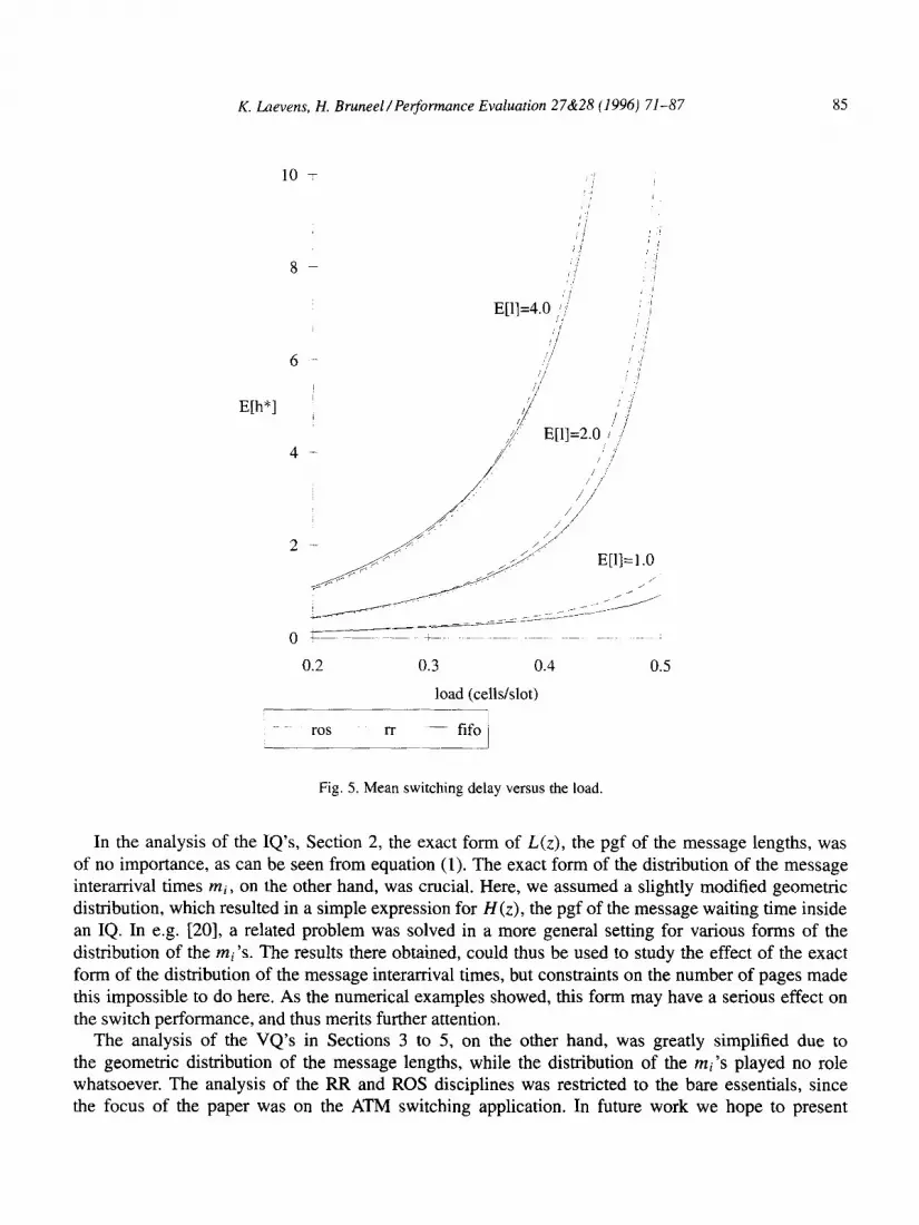
To study the effect of correlation in the cell destinations and of burstiness in the input traffic on switch performance, we plotted in Figs. 5 and 6 the mean switching delay E[h*] versus the load for 1 /v = 1 .O, Fig. 5, and versus l/y for a load of 0.4, Fig. 6. (In Fig. 6, only curves for the FIFO selection policy are shown, the curves for the RR and ROS selection policies being nearly identical.) Recall that l/y is the mean number of messages arriving without off-slots between them and thus serves as a measure

84 K L.aevens, H. Bruneel/Perfomnce Evaluation 27&28 (1996) 71-87

0.6

load 30%

+

/ I 1 1 I 1 I 1

1 2 3 4 5 6 7 8 9 10

I1

Fig. 4. Mean cell interdeparture times.

of the burstiness in the input traffic. Clearly, switch performance degrades as correlation or burstiness increase.

7. Concluding remarks

We have analyzed the performance of input-buffered ATM-switches when correlation in both the ar- rivals and the destinations of cell streams is present. Three different seIection policies were considered: first-in-first-out (taking into account both HOL arrival times and correlation in the cell destinations), round-robin (taking into account only HOL arrival times) and random-order-of-service (not taking into account HOL arrival times or correlation in the destinations of cells). Making extensive use of probability generating functions, we derived closed-form formulas for various performance measures. For the RR and the ROS selection policies, this approach yielded a number of (functional) equations, that, however, did not need to be solved explicitly to obtain the first few moments of the random variables involved.

K. Laevens, H. Bruneel/Pegormance Evaluation 27&28 (1996) 71-87 85

8

6

E[h*l

0.2 0.3 0.4

load (cells/slot)

0.5

ros rr - fifo -__. 1

Fig. 5. Mean switching delay versus the load.

In the analysis of the IQ’s, Section 2, the exact form of L(z), the pgf of the message lengths, was of no importance, as can be seen from equation (1). The exact form of the distribution of the message interarrival times mi, on the other hand, was crucial. Here, we assumed a slightly modified geometric distribution, which resulted in a simple expression for H(z), the pgf of the message waiting time inside an IQ. In e.g. [20], a related problem was solved in a more general setting for various forms of the distribution of the mj's. The results there obtained, could thus be used to study the effect of the exact form of the distribution of the message interarrival times, but constraints on the number of pages made this impossible to do here. As the numerical examples showed, this form may have a serious effect on the switch performance, and thus merits further attention.

The analysis of the VQ’s in Sections 3 to 5, on the other hand, was greatly simplified due to the geometric distribution of the message lengths, while the distribution of the mi’s played no role whatsoever. The analysis of the RR and ROS disciplines was restricted to the bare essentials, since the focus of the paper was on the ATM switching application. In future work we hope to present

K. Laevens, H. Bruneel/Performance Evaluation 27&28 (1996) 71-87

E[h*]

E[1]=2.0

10 $ 1

54

E[l]=l.O

0 !

1.0 2.0 3.0 4.0 5.0

l/Y

Fig. 6. Mean switching delay versus l/y.

a more in-depth analysis of these service disciplines and to extend results to include more general forms of the pgf L(z). Research already showed that the system contents of a VQ is influenced by the service discipline when L(z) is non-geometric. This implies, for instance, that also the maximum switch throughput is influenced by it.

Finally, note that when cells do not arrive back to back over the input links, but with some fixed or random spacing between them, the results obtained for the VQ’s can still be used in an approximate analysis of the IQ’s, As long as the probability of a cell being routed before the next cell of a same message has arrived to the IQ, is negligible, the VQ models presented here remain valid. The above phenomenon causes an interruption or delay in the VQ feedback mechanism, since then the message of which a cell was routed, cannot rejoin the VQ immediately, as the next cell it contains still has to arrive to the IQ. A more complex VQ model is then needed for an exact analysis.

K. Luevens, H. Bruneel/ Pe$ormance Evaluation 27&28 (1996) 71-87 87

References

[1] R.Y. Awdeh and H.T. Mouftah, Survey of ATM switch architectures, Computer Networks and ISDN Systems 27 (1995) 1567-1613.

[2] H. Bmneel and B.G. Kim, Discrete-time Models for Communication Systems Including ATM, Kluwer Academic Publishers (Boston) 1993.

[3] J.S. Chen and T.E. Stem, Throughput reduction due to non-uniform traffic in a packet switch with input and output queueing, Proc. ICC’91, Denver (1991) 413-417.

[4] H. Daduna and R. Schassberger, A discrete-time round-robin queue with Bernoulli input and general arithmetic service time distributions, Acta Informatica 15 (1981) 251-263.

[5] J.J. Hunter, Sojourn time problems in feedback queues, Queueing Systems 5 (1989) 55-76. [6] L. Jacob and A. Kumar, Saturation throughput analysis of an input queueing ATM switch with multiclass bursty

traffic, IEEE Trans. Commun. 43 (1995) 757-761 [7] N.K. Jaiswal, Performance evaluation studies for time-sharing computer systems, PerfI Eval. 2 (1982) 223-236. [8] M.J. Karol, M.G. Hluchyj and S.P. Morgan, Input versus output queueing on a space-division packet switch, IEEE

Trans. Commun. 35 (1987) 1347-1356. [9] L. Kleinrock, Queueing Systems, Vol. II: Computer Applications, Wiley, New York (1976).

[ 101 H. Kobayashi, On discrete-time processes in a packetized communication system, ALOHA System Technical Report B75-28, University of Hawai (1975).

[l l] K. Laevens and H. Bruneel, Delay analysis for ATM queues with random order of service, Electronics Len. 31 (1995) 346-347.

[12] S.S. Lam and A.U. Shankar, A derivation of response time distributions for a multi-class feedback queueing system, Perf Eval. l(l981) 48-61.

[ 131 S.-Q. Li, Nonuniform traffic analysis on a nonblocking space-division packet switch, IEEE Trans. Commun. 38 (1990) 1085-1096.

[14] S.-Q. Li, Performance of a nonblocking space-division packet switch with correlated input traffic, IEEE Trans. Commun. 40 (1992) 97-108.

[ 151 SC. Liew, Performance of input-buffered and output-buffered ATM switches under bursty traffic: simulation study, Proc. GLOBECOM’90, San Diego (1990) 1919-1925.

[16] R. Schassberger, On the response time in a discrete round-robin queue, Actu Informatica 16 (1981) 57-62. [ 171 R. Schassberger, A new approach to the M/G/l processor-sharing queue, Adv. Appl. Probability 16 (1984) 202-2 13. [ 181 L. Takacs, A single-server queue with feedback, Bell Sys. Techn. J. 42 (1963) 505-5 19. [19] J.L. van den Berg and O.J. Boxma, The M/G/l queue with processor sharing and its relation to a feedback queue,

Queue@ Systems 9 (1991) 365-40. [20] B. Vinck and H. Bnmeel, Analyzing the discrete-time G”‘/Geo/l queue using complex contour integration,

Queue& Systems 18 (1994) 47-67.