discrete-event simulation of vessel response time for acute
TRANSCRIPT
Discrete-Event Simulation of VesselResponse Time for Acute Pollution inAquaculture
Mats Thunes
Marine Technology
Supervisor: Bjørn Egil Asbjørnslett, IMT
Department of Marine Technology
Submission date: June 2018
Norwegian University of Science and Technology


i
Preface
This master’s thesis constitutes the final result of a Master of Science in Marine Technology
at the Norwegian University of Science and Technology (NTNU), Trondheim. The thesis was
written during the spring of 2018 and accounts for 30 credits.
The thesis is a continuation of the project thesis that was written in the fall of 2017. The
project thesis provided me with knowledge about developing discrete-event simulations,
and as well an introduction to emergency response for acute pollution. This thesis aims
to use discrete-event simulation as a tool to identify vessel response time for acute pollution
in aquaculture.
In the early stages of the thesis, the main focus was on building a simulation model and col-
lecting input data. The later stages were used for writing the thesis. The workload has been
demanding and challenging, but resulted in a great learning outcome.
I would like to thank my supervisor Bjørn Egil Asbjørnslett at the Department of Marine
Technology, NTNU, for guidance and valuable input throughout the project and the mas-
ter’s thesis. I would also like to extend my gratitude to Silje Marie Bjerkeng for proofreading
and support during this master’s thesis. Additionally, I would like to thank my fellow students
Simen Orvedal, Simon Drønen, Haakon Nordkvist, Sondre Ellingsen and Øystein Bertelsen
for interesting discussions and support.
Trondheim, 11-06-2018
Mats Thunes

ii
iii
Abstract
The aim of this master’s thesis is to identify vessel response time for acute pollution in aqua-
culture. As this is a acute emergency, an imminent response is needed from the vessels
to transport the fish away from contaminated area and deliver the biomass to emergency
slaughter. A discrete-event simulation is developed in Simulink, a program extension found
in MATLAB. A model was built to replicate normal operations for live fish carriers, and to
give a more realistic starting point for emergency response. The output from normal oper-
ations and response times, were the basis in setting a benchmark fleet for operations and
emergency response. Normal operations were limited to loading and unloading of fish, and
all other vessel operations were excluded from the system.
The motivation for conducting this study, was the Norwegian governments goal to increase
aquaculture production, and the increased shipping activity in near-cost areas. An increase
in both industries, could potentially lead to new challenges. Damage to Norwegian aquacul-
ture has so far been avoided from oil spills, but this could change. If a fish farming location
should be threatened by an oil spill, a well developed emergency response system could be
beneficial for rapid transportation of the biomass away from the contaminated area.
The simulation model was run with several fleet compositions in an attempt to establish a
fleet for normal operations and emergency response in the area of interest. The different
fleet compositions were evaluated from performance in normal operations and how fast it
was able to respond to an emergency. Case study 1 used a fleet of three operational live fish
carriers. Case study 2 used two operational vessels, and case study 3 used one operational
vessel. However, the two last fleet compositions were assisted by a dedicated standby vessel
when emergency slaughter was needed.
The results showed that the fleet composition from case study 3 were able to perform well in
operations, and achieved low response time when emergency slaughter was imposed. The
other fleet compositions experienced accumulation of waiting vessels outside farms and
processing facility. The fleet from case study 1 and 2, would cause to much strain on the
slaughter facility when delivering huge amounts of fish at short intervals during normal op-
eration.
In conclusion, further research and increased focus on acute pollution and emergency re-
sponse in aquaculture was found necessary. On-shore infrastructure could need expansion
to have the ability to process the amount of fish in emergency slaughter situations. Further
work should include added complexity in the logistical model, and more accurate input data.

iv
v
Sammendrag
Målet med denne masteroppgaven er å identifisere fartøys responstid for akutt forurensning
i norsk havbruk. Siden dette er en akutt nødsituasjon, kreves det en øyeblikkelig respons
fra fartøyene for å transportere fisk vekk fra det forurensete området og levere den til nød-
slakt. En diskret hendelsessimulering ble utviklet i Simulink, som er en programutvidelse i
MATLAB. Modellen ble bygget for å gjenskape normale operasjoner for brønnbåter. Ved å ha
båter i operasjon, vil det også gi et mer realistisk utgangpunkt for en respons fra fartøyene.
Resultatene fra operasjoner og respons tidene, dannet basisen for etableringen av en refer-
anseflåte for operasjoner og beredskap. Brønnbåtene sine operasjoner ble begrenset til last-
ing og avlasting av fisk.
Motivasjonen for å gjennomføre dette studiet, var den planlagte ekspansjonen i norsk havbruk,
og den økende shipping aktiviteten langs kysten. En økende aktivitet i begge industrier, kan
potensielt føre til flere nye utfordringer. Norsk havbruk har så langt ikke blitt påvirket av et
oljeutslipp, men dette kan imidlertid endre seg med den økende aktiviteten langs kysten.
Hvis en oppdrettslokasjon er truet av et oljeutslipp, kan det være gunstig å ha et godt utviklet
beredskapssystem for å transportere fisken vekk fra det forurensete området.
I et case-studie, ble simuleringen kjørt med tre forskjellige flåtesammensetninger i et forsøk
på å etablere en referanseflåte for operasjon og beredskap i området av interesse for dette
studiet. De ulike flåtesammensetningene ble evaluert basert på utførelse i normale operasjoner
og hvor fort de klarte å respondere til en lokasjon som trengte nødslakt. Case-studie 1 brukte
tre brønnbåter, case-studie 2 brukte to brønnbåter, og case-studie 3 brukte en brønnbåt.
Men de to siste flåtesammensetningene ble assistert av et dedikert beredskapsfartøy når
nødslakt var nødvendig.
Resultatene indikerte at flåtesammensetningen fra casestudie 3, var den mest optimale sam-
mensetningen. Den håndterte laste operasjoner bra, og oppnådde lave responstider når
nødslakt var nødvendig. De andre flåte sammensetningene opplevde en oppsamling av ven-
tende skip utenfor oppdrettsanlegget. Den store mengden fisk fartøyene leverte over kort tid,
ville også ført til at slakteriet hadde opplevd for stor belastning til å prosessere fisken.
Oppgaven konkluderer med at mer forskning og økt fokus på akutt forurensning og bered-
skap i norsk havbruk er nødvendig. Landbaserte anlegg kan potensielt behøve utbyggelse
for å håndtere den store mengden fisk som kommer i nødslakt situasjoner. Videre forskning
bør inkludere en mer kompleks logistisk modell, og forbedring av data som er implementert
i modellen.

vi
Contents
Preface . . . . . . . . . . . . . . . . . . . . . . . . . . . . . . . . . . . . . . . . . . . . . . i
Summary . . . . . . . . . . . . . . . . . . . . . . . . . . . . . . . . . . . . . . . . . . . . . iii
Sammendrag . . . . . . . . . . . . . . . . . . . . . . . . . . . . . . . . . . . . . . . . . . v
1 Introduction 1
1.1 Background . . . . . . . . . . . . . . . . . . . . . . . . . . . . . . . . . . . . . . . . 1
1.2 State of the Art . . . . . . . . . . . . . . . . . . . . . . . . . . . . . . . . . . . . . . . 3
1.3 Objective . . . . . . . . . . . . . . . . . . . . . . . . . . . . . . . . . . . . . . . . . . 5
1.4 Scope . . . . . . . . . . . . . . . . . . . . . . . . . . . . . . . . . . . . . . . . . . . . 5
1.5 Thesis Structure . . . . . . . . . . . . . . . . . . . . . . . . . . . . . . . . . . . . . . 6
2 System Description 7
2.1 System Boundaries . . . . . . . . . . . . . . . . . . . . . . . . . . . . . . . . . . . . 7
2.1.1 Locations . . . . . . . . . . . . . . . . . . . . . . . . . . . . . . . . . . . . . . 8
2.2 Developments in the Industry . . . . . . . . . . . . . . . . . . . . . . . . . . . . . 9
2.3 Challenges in Norwegian Aquaculture . . . . . . . . . . . . . . . . . . . . . . . . . 11
3 Problem Description 13
3.1 Problem Approach . . . . . . . . . . . . . . . . . . . . . . . . . . . . . . . . . . . . 14
3.1.1 Logistical Model . . . . . . . . . . . . . . . . . . . . . . . . . . . . . . . . . 15
3.1.2 Emergency Scenario . . . . . . . . . . . . . . . . . . . . . . . . . . . . . . . 15
3.1.3 Problem Limitations and Assumptions . . . . . . . . . . . . . . . . . . . . 15
4 Methodology 17
4.1 State of the Art . . . . . . . . . . . . . . . . . . . . . . . . . . . . . . . . . . . . . . . 17
4.1.1 Discrete-Event Simulation . . . . . . . . . . . . . . . . . . . . . . . . . . . . 19
4.1.2 SimEvents . . . . . . . . . . . . . . . . . . . . . . . . . . . . . . . . . . . . . 19
4.2 Markov Chain . . . . . . . . . . . . . . . . . . . . . . . . . . . . . . . . . . . . . . . 22
5 Simulation Input 25
5.1 Input . . . . . . . . . . . . . . . . . . . . . . . . . . . . . . . . . . . . . . . . . . . . 25
5.1.1 Units Used in the Simulation . . . . . . . . . . . . . . . . . . . . . . . . . . 25
5.1.2 Weather Data . . . . . . . . . . . . . . . . . . . . . . . . . . . . . . . . . . . 26
5.1.3 Fish Generation . . . . . . . . . . . . . . . . . . . . . . . . . . . . . . . . . . 26
vii
viii CONTENTS
5.1.4 Fleet . . . . . . . . . . . . . . . . . . . . . . . . . . . . . . . . . . . . . . . . . 27
5.1.5 Fuel . . . . . . . . . . . . . . . . . . . . . . . . . . . . . . . . . . . . . . . . . 27
5.1.6 Distances . . . . . . . . . . . . . . . . . . . . . . . . . . . . . . . . . . . . . . 27
5.1.7 Emergency Slaughter . . . . . . . . . . . . . . . . . . . . . . . . . . . . . . . 28
5.1.8 Probability Scenarios . . . . . . . . . . . . . . . . . . . . . . . . . . . . . . . 28
5.1.9 Input Limitations . . . . . . . . . . . . . . . . . . . . . . . . . . . . . . . . . 29
6 Model Construction 31
6.1 Emergency Response Model . . . . . . . . . . . . . . . . . . . . . . . . . . . . . . 32
6.1.1 Flow . . . . . . . . . . . . . . . . . . . . . . . . . . . . . . . . . . . . . . . . . 32
6.1.2 Global Data Stores and Subsystems . . . . . . . . . . . . . . . . . . . . . . 36
6.1.3 Script to Run Simulation Model . . . . . . . . . . . . . . . . . . . . . . . . 39
7 Results 41
7.1 Normal Operation . . . . . . . . . . . . . . . . . . . . . . . . . . . . . . . . . . . . 41
7.1.1 Loading Operations . . . . . . . . . . . . . . . . . . . . . . . . . . . . . . . 42
7.2 Emergency Response . . . . . . . . . . . . . . . . . . . . . . . . . . . . . . . . . . . 45
7.2.1 Case Study 1: Three Operational Vessels and no Standby vessel . . . . . . 46
7.2.2 Case Study 2: Two Operational Vessels and One Standby Vessel . . . . . . 52
7.2.3 Case Study 3: One Operational Vessel and One Standby Vessel . . . . . . 60
8 Discussion 63
9 Conclusion 69
9.1 Recommendations for Further Work . . . . . . . . . . . . . . . . . . . . . . . . . . 70
Bibliography 71
A MATLAB Codes I
A.1 Script within the blocks . . . . . . . . . . . . . . . . . . . . . . . . . . . . . . . . . I
A.2 Separate Script for Running Model . . . . . . . . . . . . . . . . . . . . . . . . . . . XXI
A.3 Script for Making Transition Matrix - Handout Ocean Simulation . . . . . . . . . XXII
B Model Skeleton XXVII
C Run with Small Time Step XXIX
D Results from Case Study 3 XXXI
List of Figures
2.1 The life cycle of salmon, (MarineHarvest, 2018) . . . . . . . . . . . . . . . . . . . 7
2.2 Map of Frøya/Hitra region. The locations chosen for the model are encircled in
the illustration (Kartverket, 2018). . . . . . . . . . . . . . . . . . . . . . . . . . . . 9
2.3 SalMar’s and Nordlaks concepts for offshore fish farming, Ocean Farm 1 and
Havfarm ((SalMar, 2018; Nordlaks, 2018)) . . . . . . . . . . . . . . . . . . . . . . . 10
3.1 Ship traffic in the Frøya/Hitra region in 2017 (Havbase, 2018) . . . . . . . . . . . 13
4.1 Entity Server . . . . . . . . . . . . . . . . . . . . . . . . . . . . . . . . . . . . . . . . 21
4.2 Entity Generator . . . . . . . . . . . . . . . . . . . . . . . . . . . . . . . . . . . . . 21
4.3 Entity Gate . . . . . . . . . . . . . . . . . . . . . . . . . . . . . . . . . . . . . . . . . 21
4.4 Entity Queue . . . . . . . . . . . . . . . . . . . . . . . . . . . . . . . . . . . . . . . . 22
4.5 Scope . . . . . . . . . . . . . . . . . . . . . . . . . . . . . . . . . . . . . . . . . . . . 22
4.6 Entity input and output switch . . . . . . . . . . . . . . . . . . . . . . . . . . . . . 22
4.7 Markov chain transition diagram, (OSS, 2016) . . . . . . . . . . . . . . . . . . . . 23
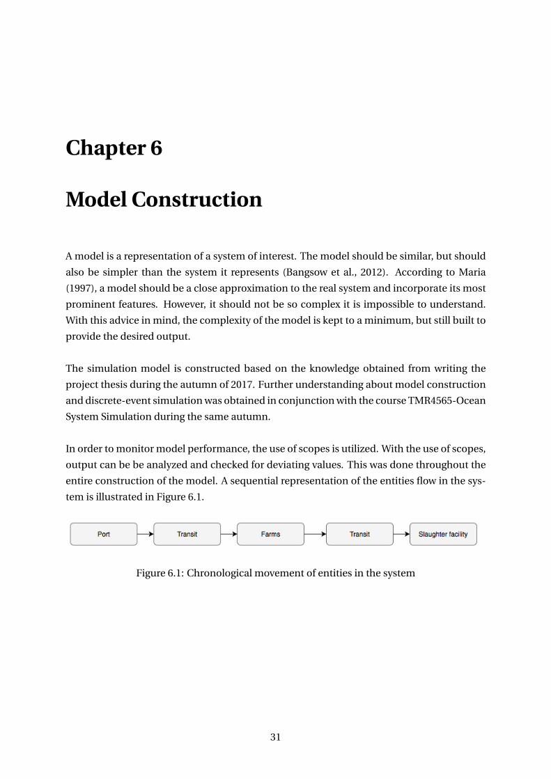
6.1 Chronological movement of entities in the system . . . . . . . . . . . . . . . . . 31
6.2 Basic framework of model construction . . . . . . . . . . . . . . . . . . . . . . . . 32
6.3 Live fish carrier generator . . . . . . . . . . . . . . . . . . . . . . . . . . . . . . . . 33
6.4 Schematic of port for vessels . . . . . . . . . . . . . . . . . . . . . . . . . . . . . . 34
6.5 Sailing blocks . . . . . . . . . . . . . . . . . . . . . . . . . . . . . . . . . . . . . . . 34
6.6 Block sequence that represents the farm . . . . . . . . . . . . . . . . . . . . . . . 35
6.7 Global data stores for emptying farms . . . . . . . . . . . . . . . . . . . . . . . . . 36
6.8 Blocks for fish generation . . . . . . . . . . . . . . . . . . . . . . . . . . . . . . . . 37
6.9 Generation of sea states . . . . . . . . . . . . . . . . . . . . . . . . . . . . . . . . . 38
6.10 Block sequence for emergency generation . . . . . . . . . . . . . . . . . . . . . . 39
6.11 Global data stores for obtaining response time . . . . . . . . . . . . . . . . . . . . 39
7.1 Loading time to empty Håbranden and Ørnøya . . . . . . . . . . . . . . . . . . . 42
7.2 Accumulation of waiting vessels at Håbranden. X-axis shows simulation time,
and y-axis number of waiting ships. Y- axis shows an accumulation of two ves-
sels during loading operation, when using fleet composition from case study
1. . . . . . . . . . . . . . . . . . . . . . . . . . . . . . . . . . . . . . . . . . . . . . . . 43
ix
x LIST OF FIGURES
7.3 Loading time using fleet from case study 3 is seen in the upper figure. In the fig-
ure below it is possible to see that accumulation outside the farm is eliminated
when using this fleet. . . . . . . . . . . . . . . . . . . . . . . . . . . . . . . . . . . . 44
7.4 Probability and density plot for exposed site Håbranden . . . . . . . . . . . . . . 46
7.5 Probability and density plot for exposed site Nystø . . . . . . . . . . . . . . . . . 47
7.6 Probability and density plot for sheltered site Ørnøya . . . . . . . . . . . . . . . . 49
7.7 Probability and density plot for semi-exposed site Salatskjera . . . . . . . . . . . 50
7.8 Probability and density plot for Håbranden with standby vessel . . . . . . . . . 52
7.9 Probability and density plot for Nystø with standby vessel . . . . . . . . . . . . . 54
7.10 Probability and density plot for Ørnøya with standby vessel . . . . . . . . . . . . 56
7.11 Probability and density plot for Salatskjera with standby vessel . . . . . . . . . . 58
7.12 One operational vessel and one standby vessel . . . . . . . . . . . . . . . . . . . . 60
B.1 Model skeleton . . . . . . . . . . . . . . . . . . . . . . . . . . . . . . . . . . . . . . XXVII
C.1 Simulation run with small time step . . . . . . . . . . . . . . . . . . . . . . . . . . XXIX
D.1 Nystø-Case study 3 . . . . . . . . . . . . . . . . . . . . . . . . . . . . . . . . . . . . XXXI
D.2 Ørnøya-Case study 3 . . . . . . . . . . . . . . . . . . . . . . . . . . . . . . . . . . . XXXII
D.3 Salatskjera-Case study 3 . . . . . . . . . . . . . . . . . . . . . . . . . . . . . . . . . XXXIII
List of Tables
4.1 Transition matrix, (OSS, 2016) . . . . . . . . . . . . . . . . . . . . . . . . . . . . . . 23
5.1 Farm capacity . . . . . . . . . . . . . . . . . . . . . . . . . . . . . . . . . . . . . . . 26
5.2 Input data for vessels . . . . . . . . . . . . . . . . . . . . . . . . . . . . . . . . . . . 27
5.3 Distances between locations in nautical miles (nm) . . . . . . . . . . . . . . . . . 28
5.4 Probability scenarios . . . . . . . . . . . . . . . . . . . . . . . . . . . . . . . . . . . 29
7.1 Minimum, maximum and mean response time for Håbranden . . . . . . . . . . 47
7.2 Minimum, maximum and mean response times for Nystø . . . . . . . . . . . . . 48
7.3 Minimum, maximum and mean response times for Ørnøya . . . . . . . . . . . . 50
7.4 Minimum, maximum and mean response times for Salatskjera . . . . . . . . . . 51
7.5 Min, max and mean response times for Håbranden with standby vessel . . . . . 53
7.6 Min, max and mean response times for Nystø with standby vessel . . . . . . . . 55
7.7 Min, max and mean response times for Ørnøya with standby vessel . . . . . . . 57
7.8 Min, max and mean response times for Salatskjera with standby vessel . . . . . 59
7.9 Min, max and mean response time for all four locations in case study 3 . . . . . 61
xi

xii LIST OF TABLES

Chapter 1
Introduction
1.1 Background
Awareness for emergency preparedness has increased in recent years, especially with inci-
dents such as Hurricane Katrina and 9-11 (Jain and Caglar, 2008). Most research and theory
regarding emergency response, discards emergencies in aquaculture, and instead keep the
main focus on the petroleum industry and on-shore activities. The Norwegian aquaculture
industry is gradually moving to more exposed locations, and is preparing for an expansion
in both size and number of farms. Simultaneously, ship traffic along the Norwegian coast is
also increasing (Bellona, 2010). According to SINTEF (2010), oil spills from shipping along
the coast have caused the greatest damage in Norwegian waters. As both industries increases
their activities in near-coast waters, the probability of acute pollution affecting fish farming
locations is growing. The aquaculture industry is nearing a new era, and further research
and developments could be needed within the topic.
Norwegian aquaculture is considered to be a success story in a global context. Since start-
ing in the 1970’s from humble beginnings, the industry has expanded immensely. In 2013,
Norwegian aquaculture produced 1.3 million metric tons of fish with an export value of 39.8
BNOK (Exposed, 2018), and is an important contributor to the Norwegian economy. Ac-
cording to Exposed (2018), the Norwegian aquaculture industry could be able to produce 5
millions tons of fish each year by 2050. However, key environmental and logistical challenges
must be solved before an expansion (Olafsen et al., 2012).
An expansion of the industry in terms of both size and number of farms, demand sites with
more water exchange to ensure good water quality, and reduce the impacts on the seabed
from farm wastes (Jensen et al., 2010). Significant parts of the Norwegian coast are unavail-
able for aquaculture due to large distances from on-shore infrastructure and environmental
conditions. The expansion to exposed areas is also needed due to area conflicts with local
communities (Utne et al. (2015); Bjelland et al. (2015)). Exposed aquaculture is for these rea-
sons seen as ideal for production. Exposed farming also provides a more stable production
1
2 CHAPTER 1. INTRODUCTION
environment due to the constant water flow and more oxygen rich water (Exposed (2018);
Holmer (2010)).
Exposed fish farming poses challenges to operations and structures due to irregular wind,
waves, currents and remoteness. According to Bjelland et al. (2015), many of the opera-
tional challenges seen at sheltered sites are likely to amplify when expanding the industry,
and moving to more exposed locations. Since the industry started its expansion, few tech-
nological and operational changes have accompanied this transition (Bjelland et al., 2015).
Increased production and farming in exposed areas requires novel technological and oper-
ational solution to ensure reliability and safety. When the technological breakthrough oc-
curs, it could be beneficial for the industry to have system in place that ensures good oper-
ational effectiveness, and as well, a preparedness system that is able to safeguard the fish.
Emergency preparedness requires well developed systems for emergency response (Jain and
Caglar, 2008), and it is such a system this master’s thesis aims to comprehend and develop.
An expansion in the aquaculture comes with the prospect of coming in contact with other
industries. Shipping traffic along the Norwegian coast is increasing each year, and transit
routes are in close proximity to commercial activities in the coastal zone (Bellona, 2010).
The petroleum industry has been increasing for many years, although, without a parallel
rise in oil spills. But, increased activity in near-shore areas could change this (SINTEF, 2010).
Oil spills could potentially pollute salmon farming sites, and could prevent the fish from
reaching the consumers market (Oljedirektoratet, 2011). There is also a possibility of closure
of aquaculture sites for an extended period until clean-up is complete (Cattermoul et al.,
2014). Should an aquaculture site be threatened by acute pollution, live fish carriers could
be needed to transport the biomass to emergency slaughter (Sunde, 2009).
Live fish carriers are an integral part of the salmon’s life-cycle. The vessels transports smolt
to farms, and transport fish to slaughter when wanted weight is achieved. In between these
operations, the vessels are also used in delousing operation up to several times, and can
also conduct treatment of fish that are infected with disease (Hauvik, 2018). However, with
the possibility of acute emergencies, these vessels could be needed as an preparedness re-
source. With the expectation of increased production and longer transit routes between
farms and on-shore infrastructure (Fenstad et al. (2009); Bjelland et al. (2015)), using a dedi-
cated standby vessel in the preparedness system as the petroleum industry do (NOFO, 2017),
could be beneficial.
The challenge is to find a fleet composition that performs good in normal operations, but
is still able to deliver relatively low response times for acute emergencies. Including a dedi-
cated standby vessel in the fleet, can be expensive. But, in an industry that has to maintain
a good reputation for delivering "clean" and healthy products (Oljedirektoratet, 2011), the
1.2. STATE OF THE ART 3
cost of a damage reputation could be more expensive. As a consequence of increasing pos-
sibility for acute pollution in aquaculture, this thesis seeks to find a fleet solution that is able
to perform well in normal operations, but still deliver low response times. Discrete-event
simulation has gained popularity for testing systems in the early phases of planning and is
a cheaper option than running full scale tests (Maria, 1997). Thus, this thesis will use simu-
lation to provide an indication for a benchmark fleet for normal operations and emergency
response.
1.2 State of the Art
There are few scientific studies related to acute pollution in aquaculture, and research on
emergency response within this topic, have predominantly been left outside the scope. Most
scientific research regarding emergency response, is mostly dedicated to the offshore oil in-
dustry, and emergency response for on-shore activities. However, the government’s planned
expansion in the future has increased the desire to obtain new knowledge regarding solu-
tions to threats the aquaculture industry faces (Bjelland et al., 2015).
According to OSHA (2013), emergency response is defined as "a response effort by employees
from outside the immediate release area or by other designated responders, to an occurrence
which results, or is likely to result, in an uncontrolled release of a hazardous substance". The
definition excludes responses to accidents where the substance can be controlled or neutral-
ized at the time of the release. Uncontrolled releases of oil spills are of huge concern due to
potential impact on economic and ecological systems, and this has lead to more awareness
of oil spill preparedness and response (Li et al., 2016).
According to SINTEF (2010), there is increasing activity from the shipping industry in near
coast waters, and has been the predominantly source for damage in the coastal zone over
the last 30 years. It was further stated that a rapid response is needed to prevent oil spills
from reaching the coastal zone. Oil spills often occur in close vicinity to natural resources or
commercial interests like aquaculture. Harsh environmental conditions and strong currents
along the coast make it difficult to use traditional oil spill recovery equipment. SINTEF (2010)
also reports of logistical challenges regarding transport of personnel and resources in and
out of contaminated areas along the coast. This was further substantiated by research con-
ducted by Danielsen (2010), who stated that near-coast preparedness needs improvement.
SINTEF (2010) concludes that there should be more cooperation between public and indus-
try actors, and recommend better plans for contingency, support and response. Walker et al.
(2014) also emphasized the importance of better cooperation between stakeholders regard-
ing emergency response for acute pollution, and stated that communication is imperative
for effective oil spill response. Bellona (2010) proposed including the aquaculture industry
in the oil spill preparedness to enhance response and avoid damage to the industry.
4 CHAPTER 1. INTRODUCTION
Acute pollution can lead to negative and long-term impacts on the environment. In 2010, the
largest oil spill in the oil industry occurred when Deep Water Horizon had an blow-out, an
oil spill that had great impact on the environment (BP, 2011). Oil spills have impacts on fish-
ing, tourism and commercial activities in the coastal areas, and according to Cheremisinoff
(2011), the near-coast areas are most impacted by oil spills. He further emphasized that oil
spills could lead to high mortality and tainting of fish maintained in aquaculture enclosures.
An example of such a disaster was seen during the Braer grounding on Shetland, which re-
sulted in the spilling 80 000 tons of crude oil. The oil spill had serious impact on the seafood
industry on Shetland (Goodlad, 1996).
A considerable portion of the world’s fishing industry shares the same locations as numer-
ous other industries; hence, fishery or aquaculture is often in the path of oil spills (Challenger
and Mauseth, 2011). The risk of oil spill impact on aquaculture is increasing as coastal activ-
ities increases, and according to Moller et al. (1999), even small oil spills can can have huge
impacts on industry due to heightened food quality standards. This was also emphasized by
Dipper and Thia-Eng (1997), who stated that farmed fish contaminated by an oil spill, cannot
enter the consumers market. According to Oljedirektoratet (2011), aquaculture sites cannot
be used for fish farming before the site is completely cleaned and approved for further oper-
ation. It is further elaborated that an oil spill can have market consequences that can have
greater economic significance than the actual biological effects. The industry is dependent
on the market perceiving the product as clean, and fish from a contaminated area could be
banned from the consumers market. Alternatively the willingness to pay for the fish from
this area could decrease (Oljedirektoratet, 2011).
The well-being of the aquatic environment is important to the whole world, and for countries
like Norway, the well-being of the marine environment is essential for a continued growth of
the aquaculture industry (Goodlad, 1996). In 2009, TEKMAR held their annual conference
in Trondheim (Sunde, 2009), and several stakeholders from the aquaculture were partici-
pating to discuss the topic of preparedness and response in the industry. Challenges like
lice, mass death and the prospect of acute pollution was something that was thoroughly dis-
cussed. Acute pollution in aquaculture is something the industry actors considered to be a
real threat. Further it was discussed how to manage such a situation, and what challenges
that arises with the prospect of an oil spill. The participants looked at emergency prepared-
ness procedures from the petroleum industry, where a designated standby vessel is used as a
preparedness resource in cases of acute pollution (NOFO, 2017). Having a dedicated standby
vessel for retrieving fish in acute emergencies, was considered to give best response times.
However, the cost of such a vessel can be excessive. The participants further looked at the
possibility of sharing a vessel as a emergency preparedness resource. But it was discussed
that if several locations was in danger of being affected, it would become a capacity problem
1.3. OBJECTIVE 5
for the vessels and on-shore facilities. Several of the industry actors concluded that further
research on the topic is needed, and better communication between industries has room for
improvement.
1.3 Objective
This master’s thesis main objective is to develop a discrete-event simulation model to iden-
tify vessel response time for acute pollution in aquaculture. The thesis will further aim to
establish a benchmark fleet for normal operations and emergency response.
1.4 Scope
• Present the background and relevance for this thesis.
• Perform a state of the art analysis, both regarding emergency response for acute pollu-
tion in aquaculture, and use of simulation within the topic.
• Collect essential input data and calculations for the simulation model.
• Develop a discrete-event simulation in SimEvents which is able to identify emergency
response time for different fleet compositions.
• Present the results from the simulation, and discuss the validity of the findings.
6 CHAPTER 1. INTRODUCTION
1.5 Thesis Structure
To increase the readability of the thesis, it is structured into several chapters and sub-chapters.
The thesis consists of nine chapters, and are further elaborated below.
Chapter 1 focuses on obtaining a better understanding about acute pollution in aquacul-
ture and presents scientific work regarding emergency response within the topic and other
industries. The information is acquired from articles and reports within different scientific
databases like NTNU’s Oria. The thesis objective and scope can also be found here. Chapter
2 presents the systems boundaries and the most important entities. Developments in the
industry is discussed and what challenges the industry faces today and in the future. A fur-
ther explanation of the the problem regarding acute pollution in aquaculture is presented
in Chapter 3. The problem approach, limitations and assumptions can also be found here.
Chapter 4 presents the methodology used in this thesis and relevant scientific approaches
and methods for solving the problem of emergency response. The simulation input is pre-
sented in Chapter 5, and will further elaborate on information that is implemented in the
model. Chapter 6 presents the model construction and will give further information about
the different components the model consists of. Chapter 7 presents the results from the
three case studies that are conducted. A discussion regarding the results validity, strengths
and improvement in the approach and work can be found in Chapter 8. The conclusion and
recommendations for further work is found in Chapter 9.
Chapter 2
System Description
The aquaculture industry consist of many moving parts, and have supply chain movements
from delivering smolt to the fish is delivered to the consumers market. However, the system
of interest is limited to transport of fish from farm to processing facility. Obtaining a bet-
ter comprehension of the system is necessary and will be described further in the following
chapter. This chapter will look at how operations are conducted today, what developments
that has been introduced in the industry, and what challenges Norwegian aquaculture may
face in the future.
2.1 System Boundaries
The aquaculture supply chain is complex, and follows the life cycle of salmon. Starting from
the smolt process to the salmon reaches the consumers market. In the beginning of the
salmon’s life cycle, the fish is raised in fresh water before moving them to net pens in salt
water. The salmon is kept in the cages for around 12 months. After this period, the salmon
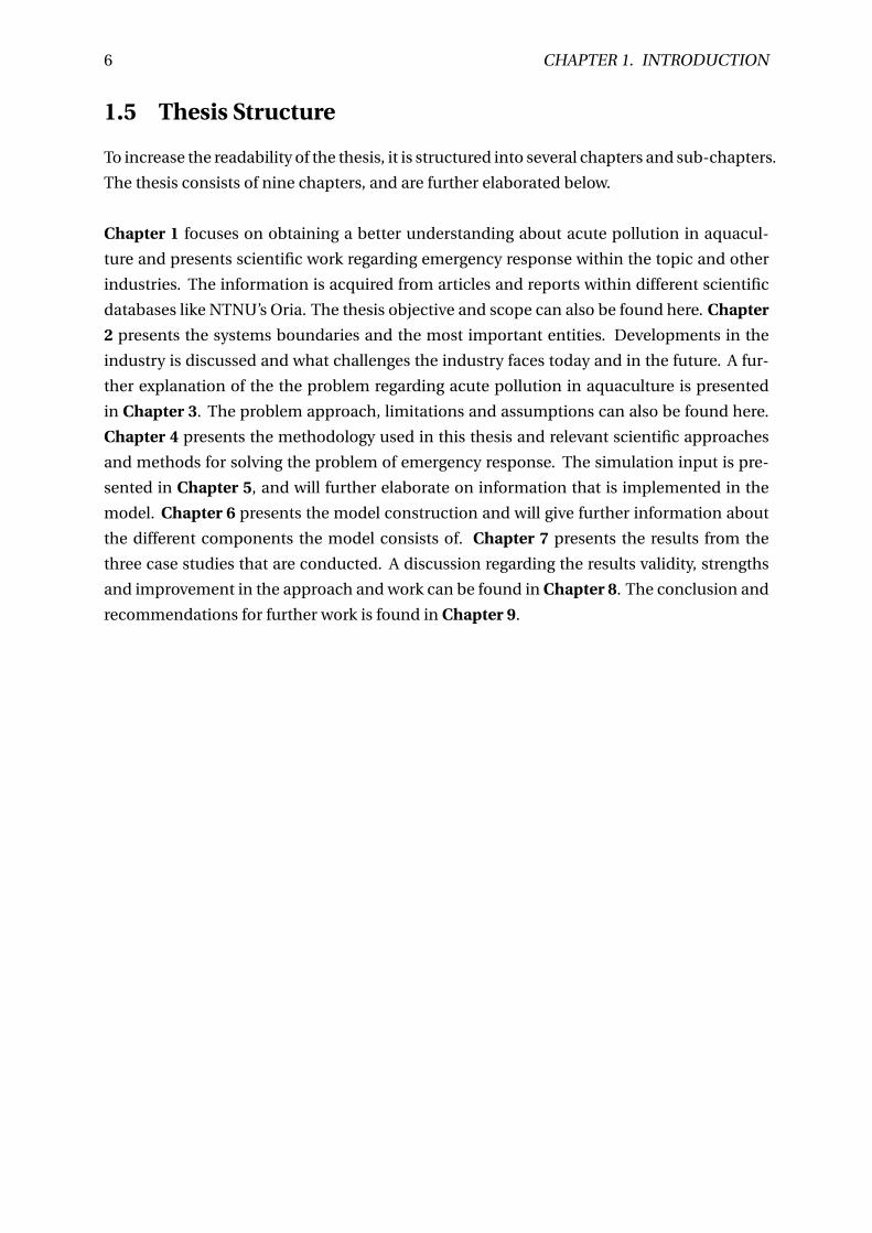
has reached market weight (4.5-5.5 kg) and is transported to processing facilities (Marine-
Harvest, 2018). An illustration of the life cycle of salmon can be seen in Figure 2.1
Figure 2.1: The life cycle of salmon, (MarineHarvest, 2018)
7
8 CHAPTER 2. SYSTEM DESCRIPTION
During the the salmon’s life, the fish will be on-board live fish carriers several times. The ves-
sels are a big part of the aquaculture supply chain, either it is transporting smolt to net pens
or transporting the fish to processing facilities. Live fish carriers are also being used for sea
lice treatment. Lice has become a huge challenge for the industry (Costello (2009); Sunde
(2009)), as a consequence, the fish are deloused 2-3 times during their lifetime.
The illustration in Figure 2.1, shows the life cycle of the salmon. The system boundaries
will however be set from slaughter-ready fish is transferred to the slaughter facilities. This
is also the boundaries for where the vessels will respond to an emergency situation. The
system will consist of a port for the vessels, slaughter facility, and four different aquaculture
facilities. The most important entities in the system are considered to be the fish farms and
vessels.
2.1.1 Locations
This thesis will focus on the aquaculture industry located in region around Frøya/Hitra. This
region was chosen because of it is in close proximity to NTNU. Due to the close geographi-
cal proximity, the possibility of retrieving information about how the current operations are
conducted in the today and future developments in the industry. Restricting the scope to
one specific region also helps setting the boundaries in the simulation model.
In the region of Frøya/Hitra, the largest actors in the aquaculture industry in Norway are
found, SalMar, Marine Harvest and Lerøy. In the region, 1/5 part of Norway’s salmon pro-
duction is slaughtered and accounts for more than 40% of the export values for the county of
Sør-Trøndelag (Hitra, 2018). The locations of farms and the other facilities connected to the
supply chain is located in this enormous cluster. The six different locations chosen for the
simulation model will be presented below.
Sistranda is the chosen location for a port, that the vessels can use for refueling or exchange
of crew. Sistranda is located on Frøya, an island west of Trondheimsfjorden.
InnovaMar is the chosen slaughter facility for the simulation model. InnovaMar is the name
of SalMar’s new slaughter and processing plant on Frøya, which has the goal of becoming the
world’s most innovative and efficient plant for slaughter and processing of farmed salmon.
The plant covers an area of 17,500 square meters and consists of two departments (slaugh-
tering and further processing). The facilities has a capacity of approximately 150,000 tonnes
of salmon, while the state-of-the-art waiting facilities, assembled by four cages, have a ca-
pacity of 350 tons of salmon each (SalMar, 2018).
2.2. DEVELOPMENTS IN THE INDUSTRY 9
Ørnøya is one of the four aquaculture location chosen for the model. Ørnøya is owned by
SalMar and has a capacity of 5000 tons. The site has normal net cages.
Salatskjæra is a aquaculture production site owned by SalMar and has a capacity of 6240
tons of fish. The site has been given so-called "green concessions". This means that SalMar
has to use Midgard mooring construction, or other constructions with properties that will
reduce the risk of escaping (Aqualine (2018); BarentsWatch (2018)).
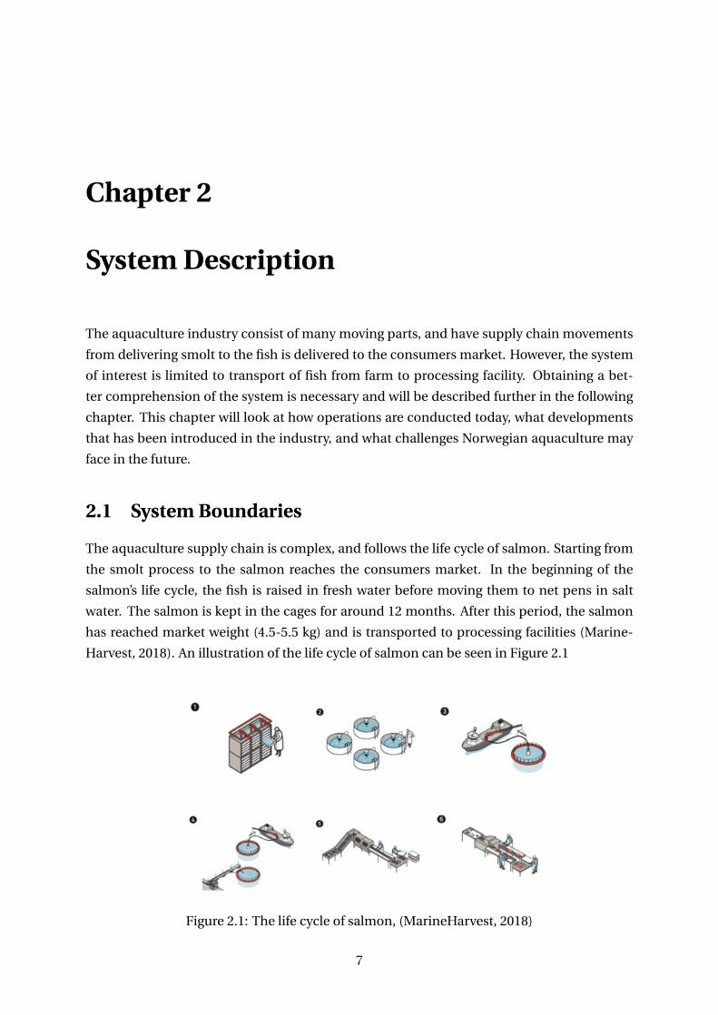
Håbranden and Nystø are the locations where SalMar’s Ocean Farm 1 is located. Ocean Farm
1 is the world’s first offshore fish farm. The two locations are approved for Salmar’s new farm
construction (Kyst, 2017). The farms have a capacity of 6240 tons of salmon. The locations
that has been chosen, can also be seen in the illustration pictured in Figure 2.2.
Figure 2.2: Map of Frøya/Hitra region. The locations chosen for the model are encircled inthe illustration (Kartverket, 2018).
2.2 Developments in the Industry
Traditionally, fish farms are located in more sheltered areas close to the shore or in the fjords.
However, significant parts of the Norwegian coast is unavailable for aquaculture due to ge-
ographical remoteness from onshore infrastructure, exposure to severe wind, waves and
strong currents (Bjelland et al. (2015); Exposed (2018)). Because of the massive expansion
in the industry and competition for sites in sheltered areas, locations for farming has to be
sought elsewhere (Utne et al., 2015). As a consequence of this, the industry have gradually
started to move production of farmed salmon to more exposed sites.
10 CHAPTER 2. SYSTEM DESCRIPTION
Exposed locations for aquaculture could be ideal for production and simultaneously re-
duce key environmental effects, as well as the negative ecological consequences of sea lice
(Costello, 2009). Offshore farming is more demanding, and environmental effects are ampli-
fied. The gradual move to more exposed sites has increased the need for more novel techno-
logical and operational concepts that satisfy safety regulations and ensures safety of struc-
tures, live stock and personnel (Bjelland et al., 2015).
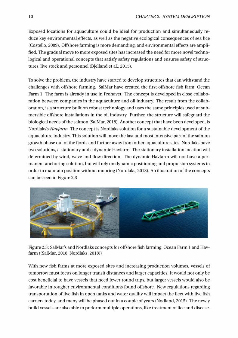
To solve the problem, the industry have started to develop structures that can withstand the
challenges with offshore farming. SalMar have created the first offshore fish farm, Ocean
Farm 1. The farm is already in use in Frohavet. The concept is developed in close collabo-
ration between companies in the aquaculture and oil industry. The result from the collab-
oration, is a structure built on robust technology and uses the same principles used at sub-
mersible offshore installations in the oil industry. Further, the structure will safeguard the
biological needs of the salmon (SalMar, 2018). Another concept that have been developed, is
Nordlaks’s Havfarm. The concept is Nordlaks solution for a sustainable development of the
aquaculture industry. This solution will move the last and most intensive part of the salmon
growth phase out of the fjords and further away from other aquaculture sites. Nordlaks have
two solutions, a stationary and a dynamic Havfarm. The stationary installation location will
determined by wind, wave and flow direction. The dynamic Havfarm will not have a per-
manent anchoring solution, but will rely on dynamic positioning and propulsion systems in
order to maintain position without mooring (Nordlaks, 2018). An illustration of the concepts
can be seen in Figure 2.3
Figure 2.3: SalMar’s and Nordlaks concepts for offshore fish farming, Ocean Farm 1 and Hav-farm ((SalMar, 2018; Nordlaks, 2018))
With new fish farms at more exposed sites and increasing production volumes, vessels of
tomorrow must focus on longer transit distances and larger capacities. It would not only be
cost beneficial to have vessels that need fewer round trips, but larger vessels would also be
favorable in rougher environmental conditions found offshore. New regulations regarding
transportation of live fish in open tanks and water quality will impact the fleet with live fish
carriers today, and many will be phased out in a couple of years (Nodland, 2015). The newly
build vessels are also able to preform multiple operations, like treatment of lice and disease.
2.3. CHALLENGES IN NORWEGIAN AQUACULTURE 11
A larger fleet of vessels and longer sailing routes, opens up for more specialized vessels,
where the slaughter process can be started during the transit. Starting this process at the
vessels would increase the capacity of the slaughtering facilities. These vessels are viewed as
a possibility to increase the production efficiency in the aquaculture supply chain.
2.3 Challenges in Norwegian Aquaculture
The gradual move to more exposed sites are expected to solve some of the ecological chal-
lenges the industry faces today. The exposed locations for aquaculture could be ideal for pro-
duction and simultaneously reduce negative ecological consequences like sea lice (Costello,
2009). However, fish farmers that have already started production at more exposed sites,
report difficulties in maintaining a reliable production (Sandberg et al., 2012). The harsh en-
vironmental conditions are causing problems and downtime at the farms (Holmen et al.).
Some of the ecological challenges that the industry faces today consists of high population
of lice, disease, mass death or acute pollution. The most common disease among fish in
aquaculture is ISA(Infectious salmon anemia virus), a virus that attacks the skin of the fish.
However, infected fish is not harmful for humans consume (Steinum and Budalen, 2013).
When the fish is detected at the site, the owner is responsible for bringing the fish to slaugh-
ter within 80 days of the discovery (Kirkemo, 2008). With these regulations, many choose
to wait as long as possible before bringing the fish to slaughter. The industry today, also
have good control over the lice population at the farms through counting at regular basis.
Mass deaths are often caused by over-medication when conducting lice or disease opera-
tions, meaning a vessel is already present at the site to handle the emergency accordingly.
However, the threat of acute pollution at a farm could mean vessels have to abort their cur-
rent operation to respond to save as much as possible of the biomass (Sunde, 2009). Either
transporting the fish to on-shore slaughter facilities, or towing the farm if possible.
Acute pollution in aquaculture can affect the the industry in many different ways. An oil spill
could pollute the salmon, and the fish would never be able to be sold in the market. Salmon
at aquaculture sites is expected to be more affected than wild fish. This is due to the fact that
fish in cages have no way to escape (Cheremisinoff, 2011). Fish in cage also more affected
because of the cages are located in the upper layer of the water mass, where the concentra-
tion of oil is higher (Oljedirektoratet, 2011). The Norwegian aquaculture industry needs be
prepared for the challenges that faces them and know how to react when emergencies oc-
curs. Thus, leading to the problem for this thesis.

12 CHAPTER 2. SYSTEM DESCRIPTION
Chapter 3
Problem Description
The planned expansion of the industry and aquaculture production have gradually moved
to more exposed sites, few significant technological and operational changes have accom-
panied the transition (Exposed (2018); Bjelland et al. (2015)). The expansion of the industry
is also expected to amplify the challenges that are faced in aquaculture. Since the industry
keeps expanding, the emergency preparedness system also needs to evolve to handle the
new challenges that arises.
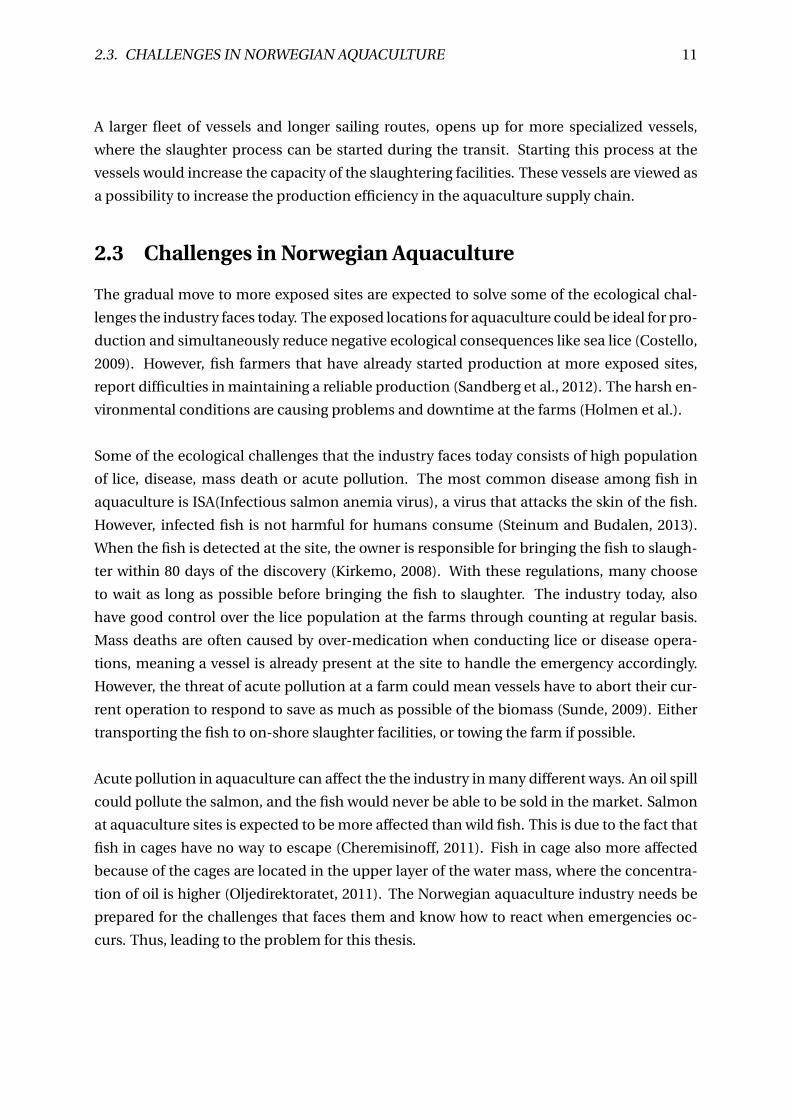
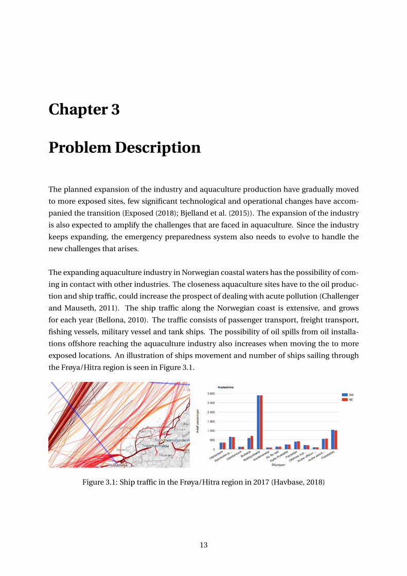
The expanding aquaculture industry in Norwegian coastal waters has the possibility of com-
ing in contact with other industries. The closeness aquaculture sites have to the oil produc-
tion and ship traffic, could increase the prospect of dealing with acute pollution (Challenger
and Mauseth, 2011). The ship traffic along the Norwegian coast is extensive, and grows
for each year (Bellona, 2010). The traffic consists of passenger transport, freight transport,
fishing vessels, military vessel and tank ships. The possibility of oil spills from oil installa-
tions offshore reaching the aquaculture industry also increases when moving the to more
exposed locations. An illustration of ships movement and number of ships sailing through
the Frøya/Hitra region is seen in Figure 3.1.
Figure 3.1: Ship traffic in the Frøya/Hitra region in 2017 (Havbase, 2018)
13
14 CHAPTER 3. PROBLEM DESCRIPTION
Perkovic et al. (2016) states that the primary sources of large oil spills are groundings (33%),
collisions (30%), hull failures (13%), fire and explosion (11%) equipment failures (4%), and
other/unknown causes includes events such as heavy weather damage and human error.
According to Danielsen (2010), the shipping industry poses the most significant threat for
oil spills and the preparedness close to the Norwegian cost have room for improvement re-
garding preparedness and response. The Norwegian coast have one of the harshest coastal
environments in the world. The rough environment along the Norwegian coast can com-
plicate oil spill preparedness, and even the best oil skimmers/booms are ineffective in these
conditions (Bellona, 2010). Because of the closeness to the shipping traffic and the harsh
environmental conditions, it is important that the live fish carriers can respond as fast as
possible to save the biomass should an oil spill occur.
In the oil industry, normal preparedness is to have a dedicated standby vessel near the off-
shore installation to respond if an oil spill or another emergency should occur. The petroleum
companies have responsibility to handle acute pollution close to installations. Measures
shall be implemented to prevent contamination from occurring or stop, remove or limit
damage caused by contamination already present (Kystverket, 2011). However, the cost of
having a dedicated vessels for this purpose alone can be extremely costly. Thus, the oil in-
dustry have a shared preparedness system for acute pollution (NOFO, 2017).
This thesis aims to identify the vessel response time in case of acute pollution in aquacul-
ture, and contribute with useful information regarding future developments on emergency
preparedness in industry within the topic. In order to discover the response times, a discrete-
event simulation model is developed. The input data and initial research formed the foun-
dation for the model construction.
3.1 Problem Approach
This thesis applies two approaches to obtain a better understanding of the flow and interac-
tions between different entities in the system. First it is important to develop a system that
is able to replicate real-life operations for live fish carriers. The second, is to implement a
scenario that forces an alteration in the regular flow pattern in the system. For the emer-
gency situation of acute pollution, the simulation model will conduct three case studies to
investigate the response times using three different fleet composition. This could also help
to give an indication for an optimal fleet composition for normal operation and emergency
response in the area. The three case studies are as follows.
3.1. PROBLEM APPROACH 15
• Case study 1: Three operational vessels and no standby vessel.
• Case study 2: Two operational vessels and one standby vessel.
• Case study 3: One operational vessel and one standby vessel.
3.1.1 Logistical Model
A logistical model is built to replicate the current operations for live fish carriers, where ves-
sels loads fish at farms and transport fish to on-shore slaughter facilities. Replicating normal
operations for live fish carriers will also give a better representation for a starting point for
emergency response. The logistical model also provides information about time used by the
fleet composition to empty the farms. The logistical model can further give an indication if
the fleet needs to be reduced or increased.
3.1.2 Emergency Scenario
The imposed emergency scenario for the simulation is chosen to be an oil spill that threat-
ened the biomass at the farms. Consequently, this will lead to an emergency response from
the vessels to transport fish away from the contaminated area to emergency slaughter at on-
onshore slaughter-processing facilities. The scenario is triggered at a random time in the
simulation, forcing the normal flow pattern out of equilibrium. Thus, revealing the time it
takes for vessels to respond to an emergency site. The fleet needs to prioritize the emergency,
and must abort their current operations if it is possible. This can provide advantageous in-
formation regarding emergency preparedness in aquaculture.
3.1.3 Problem Limitations and Assumptions
Emergency response in aquaculture can come from various emergencies, and the scope
needs to be confined. The thesis will only look at emergencies originating from acute pol-
lution, disregarding diseases, lice and any human related emergencies. Discarding these
emergencies, is partially based on the information provided by Kirkemo (2008). Cases of
disease for example, is not seen as an acute emergency, where fish can await 80 days in the
cages, and do not require vessels to abort current operation to respond. It is also assumed
that on-shore slaughter facilities have the capacity to process all fish received for emergency
slaughter. Due to lack of information and simplification, extreme weather and human inter-
actions restricting the movement of the vessels have also been left outside the scope of this
thesis.

16 CHAPTER 3. PROBLEM DESCRIPTION
Chapter 4
Methodology
As a method to identify the problem at hand, simulation has proven it self as an effective tool.
According to Bangsow et al. (2012), a simulation is an imitation of a real-life system, that de-
scribes processes involving different units and entities. Simulation is used before a system
is changed or new systems are built, reducing the chance of failures, prevent over-utilization
of resources, remove unexpected bottlenecks, and to optimize system performances (Maria,
1997). Simulation is thought to be the next best thing to actually building or testing an ex-
pensive and complicated system (Cassandras and Lafortune, 2006). The following chapter
will present relevant scientific efforts, theory and how simulation is used in this thesis.
4.1 State of the Art
The recognition for being prepared for emergency situations has increased in recent years,
with occurrences like hurricane Katrina and the Deep Water Horizon incident. According
to Jain and Caglar (2008), emergency preparedness requires development good prepared-
ness plans should emergency response situations arise. Jain and Caglar looked at a simu-
lation based-approach to plan for emergency response situations. Applying simulation to
approach emergency response situations can give many advantages, where the prime ad-
vantage was saving precious time. It was concluded that a simulation based approach can
help emergency response efforts through a quick generation of response plans. However, it
was stated that it required a significant effort collecting input data, since emergency situa-
tions are more prone to stochastic variables than other situations.
17
18 CHAPTER 4. METHODOLOGY
According to Henchey et al. (2013), simulation was a powerful tool in studying emergency re-
sponse, where different scenarios could be tested before real-life implementation. Henchy
stated that modelling complex systems could be cumbersome and required a detailed rep-
resentation of the physical layout of the system as well as the numerous interactions. The
aim of the research was to study emergency response in an advanced transportation system.
Their findings demonstrates that simulation provided a reasonable match to the real-world
data collected for comparison. The use of an emergency response simulation also proved to
be useful to assess emergency management or predict the effects of of any changes to current
accidents. Deqi et al. (2012) also presented a similar simulation framework. The simulation
was designed to simulate an emergency response system for highway traffic accident, where
the aim was to minimize the average response time for different accidents.
Håkonsen (2017) investigated preparedness in emergency situations in aquaculture. He de-
veloped a discrete-event simulation model to assess if vessels can achieve same response
times in sheltered and exposed aquaculture for escape and mass death situations. Through
case studies, the diversity of the simulation model was tested with varying input data. The
results from the simulation showed that it was possible to achieve the same response times
for sheltered and exposed fish farms as long as the availability of the vessels were increased.
It was concluded that there were need for increased focus on preparedness and response in
aquaculture.
The use of a simulation based approach to solve emergency response situations was also
found in other industries. Josefsen et al. (2016) studied emergency response for oil spills in
Arctic conditions. A discrete-event simulation was developed in MATLAB that could evalu-
ate the expected emergency response time for a given fleet composition. The model would
serve as decision support tool for operational planning and strategical fleet sizing. Because
of lack of infrastructure and remoteness in the Arctic, the possibility of using vessels from
the operational fleet to respond to oil spills instead of a dedicated standby vessel. The re-
sults showed that simulation is a tool that can be used for operational planning and fleet
sizing. It was further concluded that simulation could provide reasonable results regarding
the emergency response time for the vessels.
Brachner (2015) presented a simulation model that supported the planning for an offshore
emergency response system. The simulation model was based on the guidelines for offshore
preparedness, and could be used for evaluating different emergency systems. A case study
was conducted, which showed possible designs for an emergency response system. It was
concluded that the model needed further validation. Few real incidents have occurred that
can be used as a reference.
4.1. STATE OF THE ART 19
Ulstein and Ehlers (2014) used discrete-event simulation to determine the operational dura-
tion and optimal fleet composition of platform supply vessels in the Arctic. To test the capa-
bility of the simulation model, Ulstein and Ehlers conducted two case studies. The simula-
tion model investigated if it could be used to illustrate operational gaps between the North
Sea and Barents Sea. In the case studies, one representative oil field have been selected for
each location. The results from the first case study confirmed that the simulation model
was capable to analyze the environmental impact on the PSVs operational duration. Results
from the second case study showed that the simulation model could find the optimal fleet
composition.
Aneichyk (2009) developed a simulation model for strategical fleet sizing and operational
planning of the offshore supply process. Stochastic variables like weather conditions and
delays were implemented in the simulation model. The results from the simulation showed
that these variables affected the weekly plans for the platform supply vessels. This resulted
in lack of vessel to fulfill the demand. From the results, the author concluded that hiring
vessels from the spot market is the best way to satisfy the demand from the platforms.
4.1.1 Discrete-Event Simulation
The method of discrete-event simulation is applied in this thesis to build a model that is able
to identify the vessels response times. In the book "Introduction to Discrete Event System",
Cassandras and Lafortune (2006) defines discrete event systems as "A discrete event system is
a discrete state, event driven system, that is its state evolution depends entirely on the occur-
rence of asynchronous discrete events over time.”
Discrete-event simulation (DES) is a discrete-state and event-driven system where the changes
of states depend entirely on the occurrence of discrete events over time (Choi and Kang,
2013). The changes occur instantaneously at a particular instant in time and marks the
changes of states in the system. An occurring event can trigger another event or process.
What happens between the consecutive events is not relevant. This is because it is not as-
sumed changes in the states in this particular time frame. Since it is assumed no changes in
the states, the simulation can jump from one event to another. Typical examples of discrete-
event systems that can be simulated are manufacturing systems, communication systems or
a ship delivering cargo in port.
4.1.2 SimEvents
The software applied to build the discrete-event simulation model, is MATLAB’s SimEvents.
SimEvents is designed to simulate discrete-event simulation (Clune et al., 2006). MathWorks,
whom is the provider of MATLAB, describes SimEvents as a discrete-event simulation en-
20 CHAPTER 4. METHODOLOGY
gine. SimEvents have a component library for analyzing event-driven models and optimiz-
ing performance characteristics such as latency, throughput, and packet loss (Mathworks,
2018a). Sim-Events is a part of MATLAB and operates within Simulink. The program pro-
vides a graphical drag-and-drop interface for building discrete-event models. SimEvents
design allows the program to take advantage of a rich collection of data processing, visu-
alization and computations tools that are available in Simulink and MATLAB.
SimEvents can generate discrete objects of interest. The program can also give entities at-
tributes, such as delays and destinations. The program is based on signals and entities. The
"entity" concept is motivated from the view of a discrete event simulation as an environment
consisting of "users" and "resources" (Clune et al., 2006). An explanation of the terminology
is found below.
Entities are units that are transported through the simulation model. These are handled in
blocks, and will move accordingly to the instructions given in the script. Attributes can also
be assigned to the entities.
Attributes are characteristics or resources that are assigned to the entities. Different at-
tributes can be changed when an entity is moving between system blocks. The entities can
simulate cargo loading, and thereafter sail a decided route.
Global variables are variables that can be obtained anywhere in the simulation model. The
variables are retrieved through the use of MATLAB function blocks, Data Store Write and
Data Store Read. Using data stores, different parts of the model can interact with each other.
For this thesis, generation of sea states can be accessed more easily with the use of these.
Blocks gives the entities a path to follow from generation to termination. In the simulation
model, the blocks are given different functions. Some of the blocks intent are to imitate the
real-life system, and others have functions that for example works as sensors.
SimEvents also provide sets of libraries of blocks with different functionality. Some of the
blocks that have been used in the simulation model is listed below.
Servers are blocks that models different resources and where the different entities are kept
for fixed amount of time. This can for example be simulation of sailing or other time de-
manding events. An entity server can be seen in Figure 4.1.
4.1. STATE OF THE ART 21
Figure 4.1: Entity Server
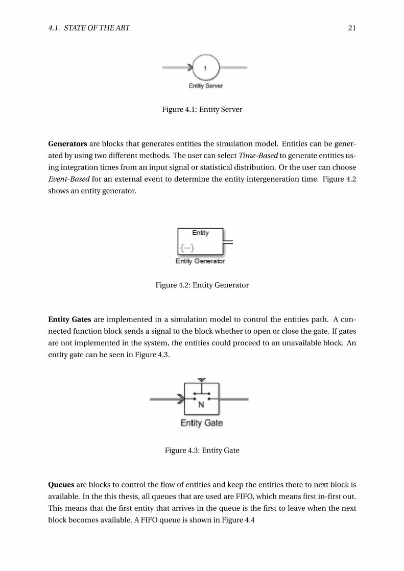
Generators are blocks that generates entities the simulation model. Entities can be gener-
ated by using two different methods. The user can select Time-Based to generate entities us-
ing integration times from an input signal or statistical distribution. Or the user can choose
Event-Based for an external event to determine the entity intergeneration time. Figure 4.2
shows an entity generator.
Figure 4.2: Entity Generator
Entity Gates are implemented in a simulation model to control the entities path. A con-
nected function block sends a signal to the block whether to open or close the gate. If gates
are not implemented in the system, the entities could proceed to an unavailable block. An
entity gate can be seen in Figure 4.3.
Figure 4.3: Entity Gate
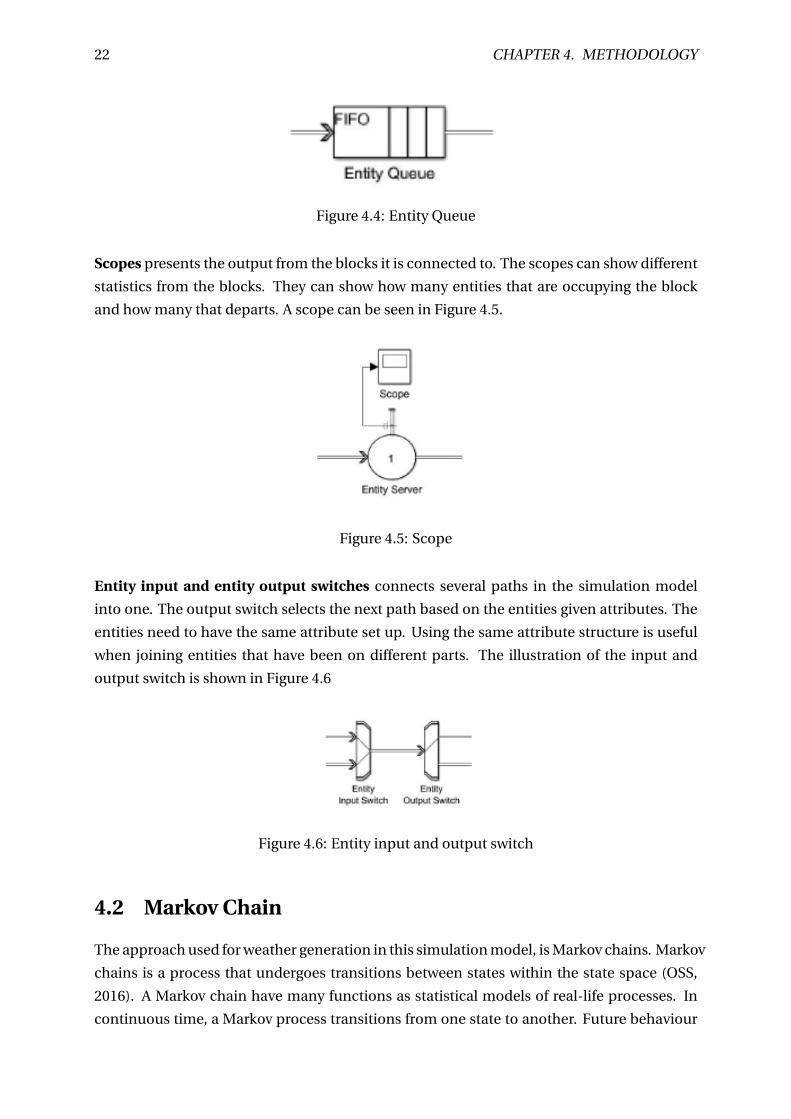
Queues are blocks to control the flow of entities and keep the entities there to next block is
available. In the this thesis, all queues that are used are FIFO, which means first in-first out.
This means that the first entity that arrives in the queue is the first to leave when the next
block becomes available. A FIFO queue is shown in Figure 4.4
22 CHAPTER 4. METHODOLOGY
Figure 4.4: Entity Queue
Scopes presents the output from the blocks it is connected to. The scopes can show different
statistics from the blocks. They can show how many entities that are occupying the block
and how many that departs. A scope can be seen in Figure 4.5.
Figure 4.5: Scope
Entity input and entity output switches connects several paths in the simulation model
into one. The output switch selects the next path based on the entities given attributes. The
entities need to have the same attribute set up. Using the same attribute structure is useful
when joining entities that have been on different parts. The illustration of the input and
output switch is shown in Figure 4.6
Figure 4.6: Entity input and output switch
4.2 Markov Chain
The approach used for weather generation in this simulation model, is Markov chains. Markov
chains is a process that undergoes transitions between states within the state space (OSS,
2016). A Markov chain have many functions as statistical models of real-life processes. In
continuous time, a Markov process transitions from one state to another. Future behaviour
4.2. MARKOV CHAIN 23
of the system, remaining time in current state and and next state, depends only on the cur-
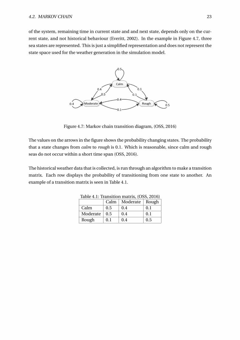
rent state, and not historical behaviour (Everitt, 2002). In the example in Figure 4.7, three
sea states are represented. This is just a simplified representation and does not represent the
state space used for the weather generation in the simulation model.
Figure 4.7: Markov chain transition diagram, (OSS, 2016)
The values on the arrows in the figure shows the probability changing states. The probability
that a state changes from calm to rough is 0.1. Which is reasonable, since calm and rough
seas do not occur within a short time span (OSS, 2016).
The historical weather data that is collected, is run through an algorithm to make a transition
matrix. Each row displays the probability of transitioning from one state to another. An
example of a transition matrix is seen in Table 4.1.
Table 4.1: Transition matrix, (OSS, 2016)Calm Moderate Rough
Calm 0.5 0.4 0.1Moderate 0.5 0.4 0.1Rough 0.1 0.4 0.5

24 CHAPTER 4. METHODOLOGY
Chapter 5
Simulation Input
A simulation can only be as good as the input that is implemented. Maria (1997) stated the
importance of collecting real system data before constructing a simulation model. To imitate
a real-world system, it is necessary with input variables which can give a good representation
of the system. This sections will present and explain the acquired information. The validity
of the input will be discussed further in Chapter 8.
5.1 Input
5.1.1 Units Used in the Simulation
Simulink works without defined entities and time units. Consequently, the units that is used
in the simulation model has to be determined. It is also important that the determined units
are maintained throughout each step of the model to get all relations correct. Transportation
of fish is the basis for the logistical model, thus, the entity units for capacities of the vessels
and farms were important to define. To avoid extensive calculations and results, it is decided
that one entity unit would represent one tonne. This means that a vessels capacity of 700
corresponds to 700 tons, and a farm capacity 6240 is equivalent to 6240 tons.
The units used for vessels and distances are set to be knots and nautical miles respectively.
One nautical mile and knot is equivalent to 1.852 km and km/h. The simulation is set to run
over 500 000 hours. The simulation run time is done to obtain as many response time as
possible and that all possibilities are covered.
25
26 CHAPTER 5. SIMULATION INPUT
5.1.2 Weather Data
Weather data is collected from the geographical area of interest. The simulated weather con-
ditions in the model is significant wave height. Wind and currents would have impact, but
have been decided to excluded due to simplicity and the authors modelling skills. An as-
sumption has been made, that these environmental factors occurs with waves. Low current
and wind with small waves, and strong current and wind with high waves.
One set of weather data is collected for the area, and is used for all the farms due to the close-
ness between them. The met-ocean data that is collected is used in a Markov chain to create
possible sea states that represents significant wave heights. The weather data is retrieved
from SFI EXPOSED and will serve as input to provide weather windows to affect operations
at the farms and time spent sailing. The data is collected over a two year period. The data is
confidential, and will not be presented in the thesis.
Setting operational limitations for the vessels gives a real-life imitation of operations in aqua-
culture. Working in aquaculture is already considered one of the most dangerous jobs in
Norway (Utne et al., 2015), and limiting the operational window will not only be beneficial
for the workers, but can also help avoiding damaging the farms during large waves. The
salmon’s welfare also have to be considered. Loading of fish when waves are high can not
only be dangerous, but can also lead to slamming inside the tanks (Stemland, 2017). This
will cause stress for the fish and can in worst cases lead to death.
5.1.3 Fish Generation
Generation of fish at the farms, is made with some simplifications. It is assumed that the
salmon at the offshore locations is slaughter-ready every 8760 hour, which means once a
year. The fish that is generated for traditional farms are generated every 13140 hour, which
is equivalent to 1,5 years. It is assumed that the smolt at the more exposed farms will be of
greater size and weight when placed there. According to Jensen (2017), smolt that is released
in the new Ocean Farm 1, weighed around 270 gram. It is also assumed that a more stable
temperature around the year at exposed sites will increase the salmon’s growth rate. The
smolt that is released in more sheltered areas, are often smaller since the sites do not have to
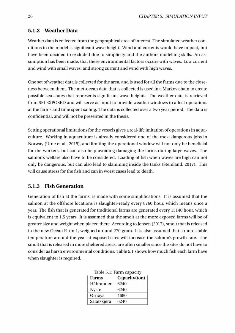
consider as harsh environmental conditions. Table 5.1 shows how much fish each farm have
when slaughter is required.
Table 5.1: Farm capacityFarms Capacity(ton)Håbranden 6240Nystø 6240Ørnøya 4680Salatskjera 6240
5.1. INPUT 27
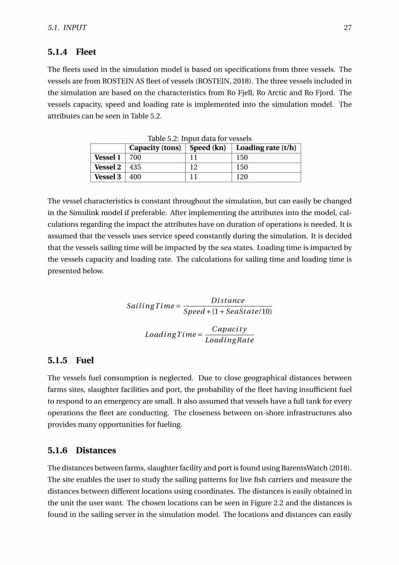
5.1.4 Fleet
The fleets used in the simulation model is based on specifications from three vessels. The
vessels are from ROSTEIN AS fleet of vessels (ROSTEIN, 2018). The three vessels included in
the simulation are based on the characteristics from Ro Fjell, Ro Arctic and Ro Fjord. The
vessels capacity, speed and loading rate is implemented into the simulation model. The
attributes can be seen in Table 5.2.
Table 5.2: Input data for vesselsCapacity (tons) Speed (kn) Loading rate (t/h)
Vessel 1 700 11 150Vessel 2 435 12 150Vessel 3 400 11 120
The vessel characteristics is constant throughout the simulation, but can easily be changed
in the Simulink model if preferable. After implementing the attributes into the model, cal-
culations regarding the impact the attributes have on duration of operations is needed. It is
assumed that the vessels uses service speed constantly during the simulation. It is decided
that the vessels sailing time will be impacted by the sea states. Loading time is impacted by
the vessels capacity and loading rate. The calculations for sailing time and loading time is
presented below.
Sai l i ng T i me = Di st ance
Speed ∗ (1+SeaSt ate/10)
Loadi ng T i me = C apaci t y
Loadi ng Rate
5.1.5 Fuel
The vessels fuel consumption is neglected. Due to close geographical distances between
farms sites, slaughter facilities and port, the probability of the fleet having insufficient fuel
to respond to an emergency are small. It also assumed that vessels have a full tank for every
operations the fleet are conducting. The closeness between on-shore infrastructures also
provides many opportunities for fueling.
5.1.6 Distances
The distances between farms, slaughter facility and port is found using BarentsWatch (2018).
The site enables the user to study the sailing patterns for live fish carriers and measure the
distances between different locations using coordinates. The distances is easily obtained in
the unit the user want. The chosen locations can be seen in Figure 2.2 and the distances is
found in the sailing server in the simulation model. The locations and distances can easily
28 CHAPTER 5. SIMULATION INPUT
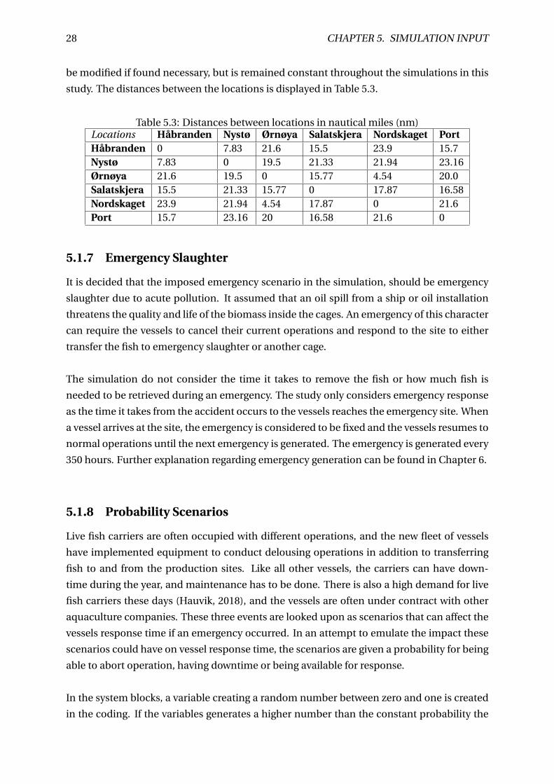
be modified if found necessary, but is remained constant throughout the simulations in this
study. The distances between the locations is displayed in Table 5.3.
Table 5.3: Distances between locations in nautical miles (nm)Locations Håbranden Nystø Ørnøya Salatskjera Nordskaget PortHåbranden 0 7.83 21.6 15.5 23.9 15.7Nystø 7.83 0 19.5 21.33 21.94 23.16Ørnøya 21.6 19.5 0 15.77 4.54 20.0Salatskjera 15.5 21.33 15.77 0 17.87 16.58Nordskaget 23.9 21.94 4.54 17.87 0 21.6Port 15.7 23.16 20 16.58 21.6 0
5.1.7 Emergency Slaughter
It is decided that the imposed emergency scenario in the simulation, should be emergency
slaughter due to acute pollution. It assumed that an oil spill from a ship or oil installation
threatens the quality and life of the biomass inside the cages. An emergency of this character
can require the vessels to cancel their current operations and respond to the site to either
transfer the fish to emergency slaughter or another cage.
The simulation do not consider the time it takes to remove the fish or how much fish is
needed to be retrieved during an emergency. The study only considers emergency response
as the time it takes from the accident occurs to the vessels reaches the emergency site. When
a vessel arrives at the site, the emergency is considered to be fixed and the vessels resumes to
normal operations until the next emergency is generated. The emergency is generated every
350 hours. Further explanation regarding emergency generation can be found in Chapter 6.
5.1.8 Probability Scenarios
Live fish carriers are often occupied with different operations, and the new fleet of vessels
have implemented equipment to conduct delousing operations in addition to transferring
fish to and from the production sites. Like all other vessels, the carriers can have down-
time during the year, and maintenance has to be done. There is also a high demand for live
fish carriers these days (Hauvik, 2018), and the vessels are often under contract with other
aquaculture companies. These three events are looked upon as scenarios that can affect the
vessels response time if an emergency occurred. In an attempt to emulate the impact these
scenarios could have on vessel response time, the scenarios are given a probability for being
able to abort operation, having downtime or being available for response.
In the system blocks, a variable creating a random number between zero and one is created
in the coding. If the variables generates a higher number than the constant probability the
5.1. INPUT 29
scenarios are given, time delays are imposed on the vessels before they can respond. By
using rand function, the variable generates a random number from a uniform distribution
each time it is triggered. The number is only random for one run. When using SimEvents, it
is beneficial that the results can be reproduced for each run.
The probability for aborting an operation is set to 50%, if the random number generated
is higher than 0.5, the vessels is unable to abort current operation and are imposed a time
delay before responding. The second scenario is the probability of having downtime, and
the probability is set to 10%. The last scenario is the availability for response. Being under
contract with other companies, could mean that the vessels are located in another area when
an oil spill occurs. To emulate this, a probability is set to 30%. Further explanation on the
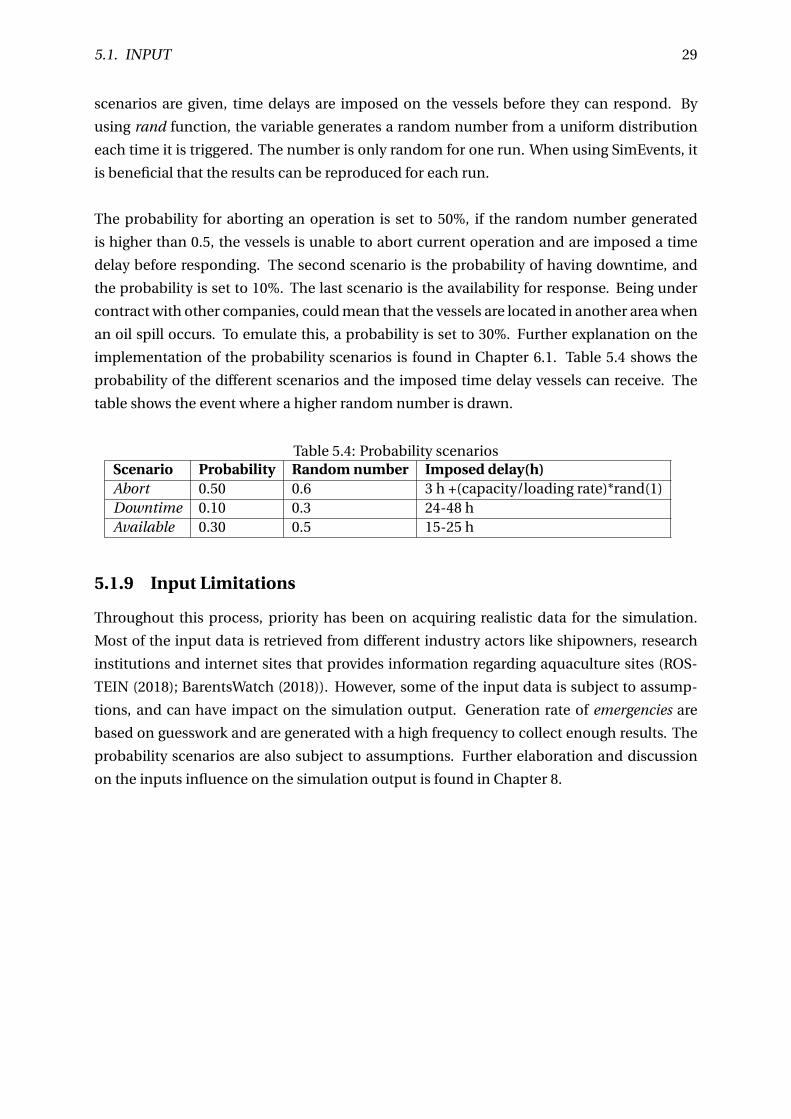
implementation of the probability scenarios is found in Chapter 6.1. Table 5.4 shows the
probability of the different scenarios and the imposed time delay vessels can receive. The
table shows the event where a higher random number is drawn.
Table 5.4: Probability scenariosScenario Probability Random number Imposed delay(h)Abort 0.50 0.6 3 h +(capacity/loading rate)*rand(1)Downtime 0.10 0.3 24-48 hAvailable 0.30 0.5 15-25 h
5.1.9 Input Limitations
Throughout this process, priority has been on acquiring realistic data for the simulation.
Most of the input data is retrieved from different industry actors like shipowners, research
institutions and internet sites that provides information regarding aquaculture sites (ROS-
TEIN (2018); BarentsWatch (2018)). However, some of the input data is subject to assump-
tions, and can have impact on the simulation output. Generation rate of emergencies are
based on guesswork and are generated with a high frequency to collect enough results. The
probability scenarios are also subject to assumptions. Further elaboration and discussion
on the inputs influence on the simulation output is found in Chapter 8.

30 CHAPTER 5. SIMULATION INPUT
Chapter 6
Model Construction
A model is a representation of a system of interest. The model should be similar, but should
also be simpler than the system it represents (Bangsow et al., 2012). According to Maria
(1997), a model should be a close approximation to the real system and incorporate its most
prominent features. However, it should not be so complex it is impossible to understand.
With this advice in mind, the complexity of the model is kept to a minimum, but still built to
provide the desired output.
The simulation model is constructed based on the knowledge obtained from writing the
project thesis during the autumn of 2017. Further understanding about model construction
and discrete-event simulation was obtained in conjunction with the course TMR4565-Ocean
System Simulation during the same autumn.
In order to monitor model performance, the use of scopes is utilized. With the use of scopes,
output can be be analyzed and checked for deviating values. This was done throughout the
entire construction of the model. A sequential representation of the entities flow in the sys-
tem is illustrated in Figure 6.1.
Figure 6.1: Chronological movement of entities in the system
31
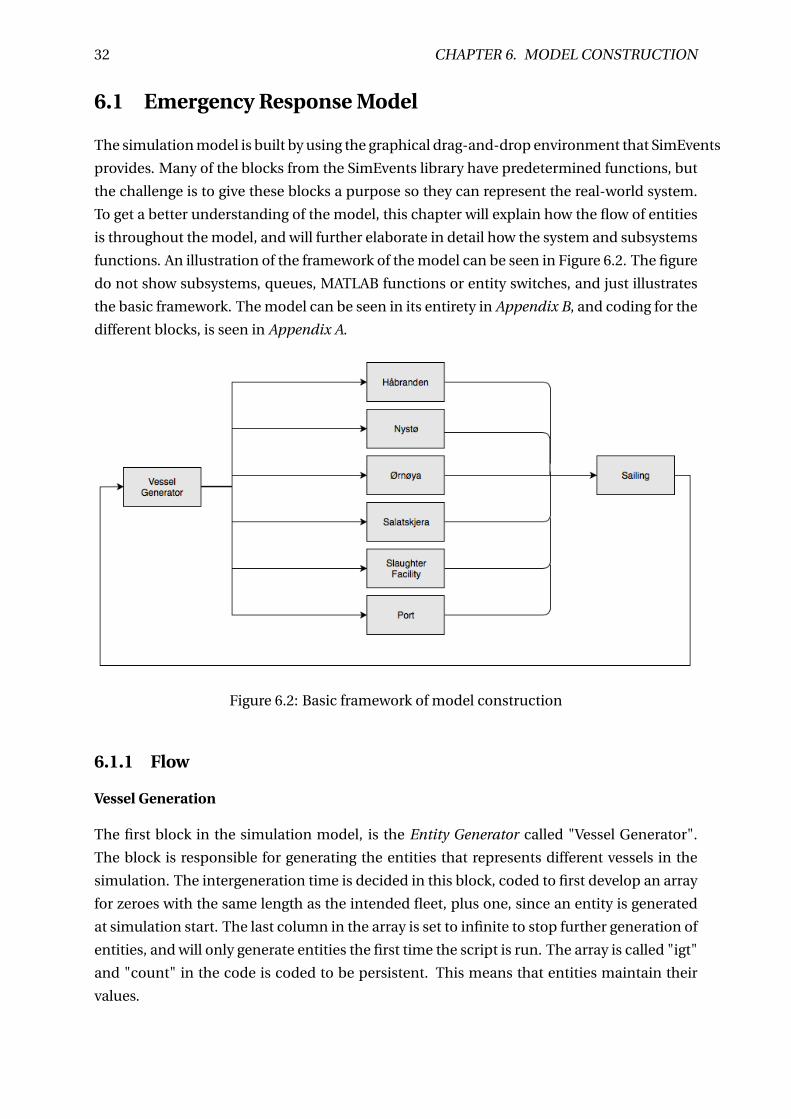
32 CHAPTER 6. MODEL CONSTRUCTION
6.1 Emergency Response Model
The simulation model is built by using the graphical drag-and-drop environment that SimEvents
provides. Many of the blocks from the SimEvents library have predetermined functions, but
the challenge is to give these blocks a purpose so they can represent the real-world system.
To get a better understanding of the model, this chapter will explain how the flow of entities
is throughout the model, and will further elaborate in detail how the system and subsystems
functions. An illustration of the framework of the model can be seen in Figure 6.2. The figure
do not show subsystems, queues, MATLAB functions or entity switches, and just illustrates
the basic framework. The model can be seen in its entirety in Appendix B, and coding for the
different blocks, is seen in Appendix A.
Figure 6.2: Basic framework of model construction
6.1.1 Flow
Vessel Generation
The first block in the simulation model, is the Entity Generator called "Vessel Generator".
The block is responsible for generating the entities that represents different vessels in the
simulation. The intergeneration time is decided in this block, coded to first develop an array
for zeroes with the same length as the intended fleet, plus one, since an entity is generated
at simulation start. The last column in the array is set to infinite to stop further generation of
entities, and will only generate entities the first time the script is run. The array is called "igt"
and "count" in the code is coded to be persistent. This means that entities maintain their
values.
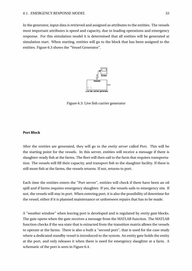
6.1. EMERGENCY RESPONSE MODEL 33
In the generator, input data is retrieved and assigned as attributes to the entities. The vessels
most important attributes is speed and capacity, due to loading operations and emergency
response. For this simulation model it is determined that all entities will be generated at
simulation start. When starting, entities will go to the block that has been assigned to the
entities. Figure 6.3 shows the "Vessel Generator".
Figure 6.3: Live fish carrier generator
Port Block
After the entities are generated, they will go to the entity server called Port. This will be
the starting point for the vessels. In this server, entities will receive a message if there is
slaughter-ready fish at the farms. The fleet will then sail to the farm that requires transporta-
tion. The vessels will fill their capacity, and transport fish to the slaughter facility. If there is
still more fish at the farms, the vessels returns. If not, returns to port.
Each time the entities enters the "Port server", entities will check if there have been an oil
spill and if farms requires emergency slaughter. If yes, the vessels sails to emergency site. If
not, the vessels will stay in port. When entering port, it is also the possibility of downtime for
the vessel, either if it is planned maintenance or unforeseen repairs that has to be made.
A "weather window" when leaving port is developed and is regulated by entity gate blocks.
The gate opens when the gate receives a message from the MATLAB function. The MATLAB
function checks if the sea state that is extracted from the transition matrix allows the vessels
to operate at the farms. There is also a built a "second port", that is used for the case study
where a dedicated standby vessel is introduced to the system. An entity gate holds the entity
at the port, and only releases it when there is need for emergency slaughter at a farm. A
schematic of the port is seen in Figure 6.4.
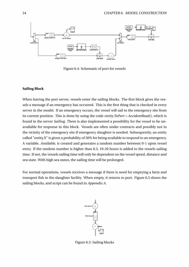
34 CHAPTER 6. MODEL CONSTRUCTION
Figure 6.4: Schematic of port for vessels
Sailing Block
When leaving the port server, vessels enter the sailing blocks. The first block gives the ves-
sels a message if an emergency has occurred. This is the first thing that is checked in every
server in the model. If an emergency occurs, the vessel will sail to the emergency site from
its current position. This is done by using the code entity.ToPort = AccidentRead(), which is
found in the server Sailing. There is also implemented a possibility for the vessel to be un-
available for response in this block. Vessels are often under contracts and possibly not in
the vicinity of the emergency site if emergency slaughter is needed. Subsequently, an entity
called "entity.X" is given a probability of 30% for being available to respond to an emergency.
A variable, Available, is created and generates a random number between 0-1 upon vessel
entry. If the random number is higher than 0.3, 10-20 hours is added to the vessels sailing
time. If not, the vessels sailing time will only be dependent on the vessel speed, distance and
sea state. With high sea states, the sailing time will be prolonged.
For normal operations, vessels receives a message if there is need for emptying a farm and
transport fish to the slaughter facility. When empty, it returns to port. Figure 6.5 shows the
sailing blocks, and script can be found in Appendix A.
Figure 6.5: Sailing blocks
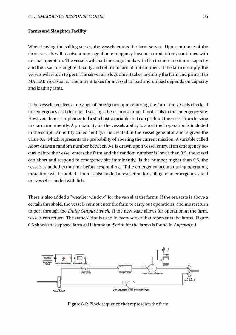
6.1. EMERGENCY RESPONSE MODEL 35
Farms and Slaughter Facility
When leaving the sailing server, the vessels enters the farm server. Upon entrance of the
farm, vessels will receive a message if an emergency have occurred, if not, continues with
normal operation. The vessels will load the cargo holds with fish to their maximum capacity
and then sail to slaughter facility and return to farm if not emptied. If the farm is empty, the
vessels will return to port. The server also logs time it takes to empty the farm and prints it to
MATLAB workspace. The time it takes for a vessel to load and unload depends on capacity
and loading rates.
If the vessels receives a message of emergency upon entering the farm, the vessels checks if
the emergency is at this site, if yes, logs the response time. If not, sails to the emergency site.
However, there is implemented a stochastic variable that can prohibit the vessel from leaving
the farm imminently. A probability for the vessels ability to abort their operation is included
in the script. An entity called "entity.Y" is created in the vessel generator and is given the
value 0.5, which represents the probability of aborting the current mission. A variable called
Abort draws a random number between 0-1 is drawn upon vessel entry. If an emergency oc-
curs before the vessel enters the farm and the random number is lower than 0.5, the vessel
can abort and respond to emergency site imminently. Is the number higher than 0.5, the
vessels is added extra time before responding. If the emergency occurs during operation,
more time will be added. There is also added a restriction for sailing to an emergency site if
the vessel is loaded with fish.
There is also added a "weather window" for the vessel at the farms. If the sea state is above a
certain threshold, the vessels cannot enter the farm to carry out operations, and must return
to port through the Entity Output Switch. If the new state allows for operation at the farm,
vessels can return. The same script is used in every server that represents the farms. Figure
6.6 shows the exposed farm at Håbranden. Script for the farms is found in Appendix A.
Figure 6.6: Block sequence that represents the farm
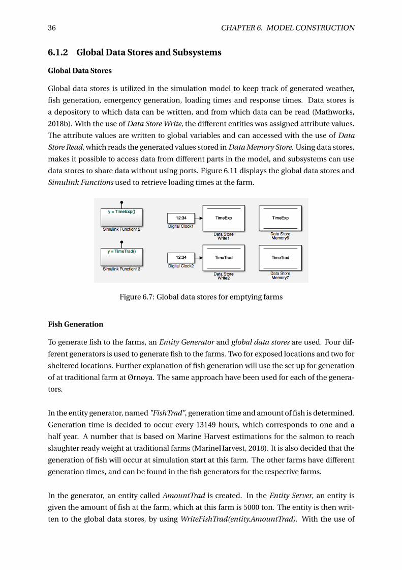
36 CHAPTER 6. MODEL CONSTRUCTION
6.1.2 Global Data Stores and Subsystems
Global Data Stores
Global data stores is utilized in the simulation model to keep track of generated weather,
fish generation, emergency generation, loading times and response times. Data stores is
a depository to which data can be written, and from which data can be read (Mathworks,
2018b). With the use of Data Store Write, the different entities was assigned attribute values.
The attribute values are written to global variables and can accessed with the use of Data
Store Read, which reads the generated values stored in Data Memory Store. Using data stores,
makes it possible to access data from different parts in the model, and subsystems can use
data stores to share data without using ports. Figure 6.11 displays the global data stores and
Simulink Functions used to retrieve loading times at the farm.
Figure 6.7: Global data stores for emptying farms
Fish Generation
To generate fish to the farms, an Entity Generator and global data stores are used. Four dif-
ferent generators is used to generate fish to the farms. Two for exposed locations and two for
sheltered locations. Further explanation of fish generation will use the set up for generation
of at traditional farm at Ørnøya. The same approach have been used for each of the genera-
tors.
In the entity generator, named "FishTrad", generation time and amount of fish is determined.
Generation time is decided to occur every 13149 hours, which corresponds to one and a
half year. A number that is based on Marine Harvest estimations for the salmon to reach
slaughter ready weight at traditional farms (MarineHarvest, 2018). It is also decided that the
generation of fish will occur at simulation start at this farm. The other farms have different
generation times, and can be found in the fish generators for the respective farms.
In the generator, an entity called AmountTrad is created. In the Entity Server, an entity is
given the amount of fish at the farm, which at this farm is 5000 ton. The entity is then writ-
ten to the global data stores, by using WriteFishTrad(entity.AmountTrad). With the use of
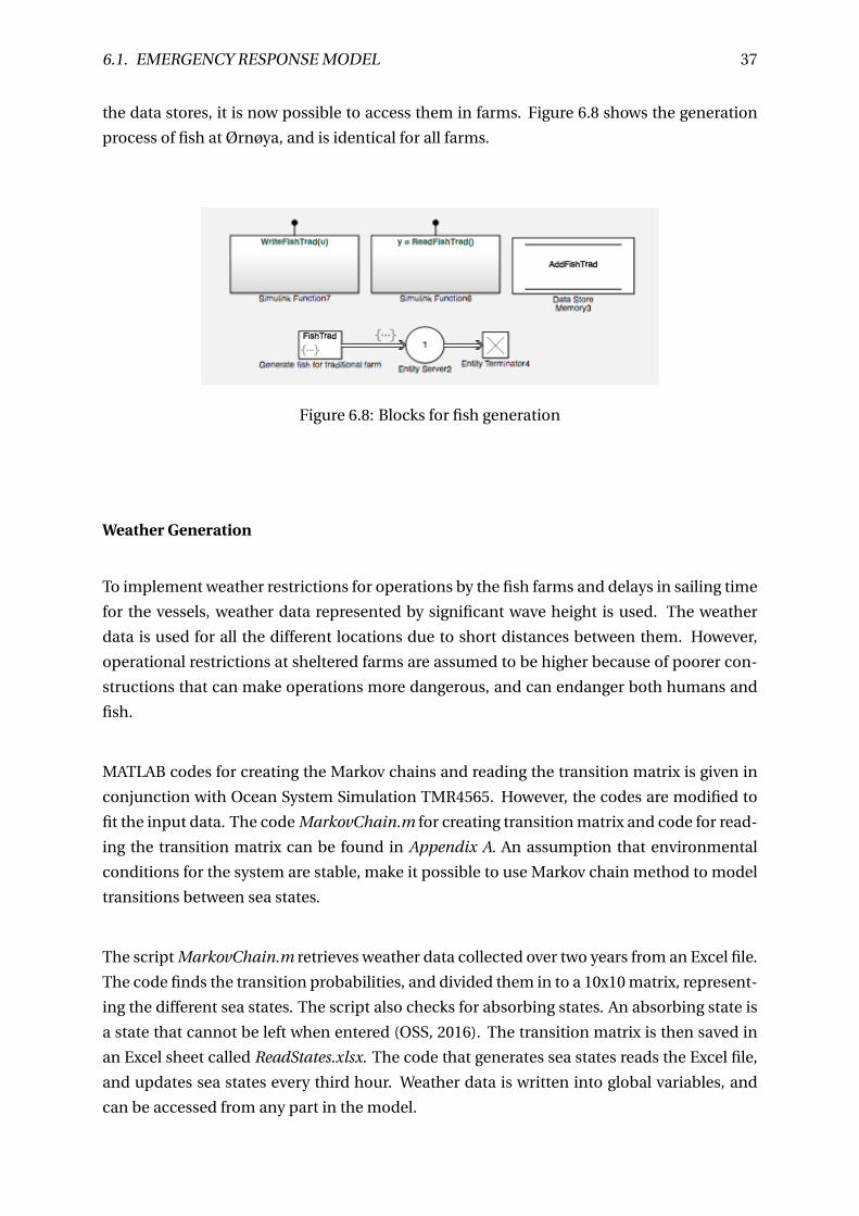
6.1. EMERGENCY RESPONSE MODEL 37
the data stores, it is now possible to access them in farms. Figure 6.8 shows the generation
process of fish at Ørnøya, and is identical for all farms.
Figure 6.8: Blocks for fish generation
Weather Generation
To implement weather restrictions for operations by the fish farms and delays in sailing time
for the vessels, weather data represented by significant wave height is used. The weather
data is used for all the different locations due to short distances between them. However,
operational restrictions at sheltered farms are assumed to be higher because of poorer con-
structions that can make operations more dangerous, and can endanger both humans and
fish.
MATLAB codes for creating the Markov chains and reading the transition matrix is given in
conjunction with Ocean System Simulation TMR4565. However, the codes are modified to
fit the input data. The code MarkovChain.m for creating transition matrix and code for read-
ing the transition matrix can be found in Appendix A. An assumption that environmental
conditions for the system are stable, make it possible to use Markov chain method to model
transitions between sea states.
The script MarkovChain.m retrieves weather data collected over two years from an Excel file.
The code finds the transition probabilities, and divided them in to a 10x10 matrix, represent-
ing the different sea states. The script also checks for absorbing states. An absorbing state is
a state that cannot be left when entered (OSS, 2016). The transition matrix is then saved in
an Excel sheet called ReadStates.xlsx. The code that generates sea states reads the Excel file,
and updates sea states every third hour. Weather data is written into global variables, and
can be accessed from any part in the model.

38 CHAPTER 6. MODEL CONSTRUCTION
Figure 6.9: Generation of sea states
Emergency Generation
The emergency scenario in the model is as mentioned acute pollution, in form of an oil spill
in close proximity to the farm. An emergency that leads to an immediate response for the
vessels to transport fish to emergency slaughter before the fish get affected by oil. The sce-
nario is implemented in the system by using several blocks and global data stores. The emer-
gency schematics consists of two entity generators. The first entity creator generates the
emergency, and trigger for generation is time-based. The emergency occurs once every 400
hours, and a specific seed is implemented so recreation of results is possible. The second en-
tity creator generates an entity upon vessel arrival at emergency site. When the vessel arrives
at the emergency site, a signal will be sent to the Simulink Function "AccidentArrival", and
an entity is released.
After creating entities at the generators, they combine paths at Entity Input Switch and enters
a server. Within the block, the entity "Accident" is written to the global data stores, by using
the code AccidentWrite(entity.Accident). It is then possible to use the data store read func-
tion to check for accidents at farms. Three persistent variables are also created in the block,
called "AccidentStart", "AccidentArrive" and "location", where the two first are connected to
the global function GetTime and "location" is connected to "AccidentRead". The function
"GetTime" is connected to a clock and records when the emergency occurs and when a ves-
sels reaches the farm. "AccidentRead" is used to check if an emergency has occurred at one
of the farms and to retrieve the location of the emergency. The time step in the simulation is
set to one hour.
To obtain the response times for the vessels, simple calculations are done in the script where
time collected from. "AccidentStart" is subtracted from the time obtained from "Acciden-
tArrive". To acquire the response time and location of the emergency, a "To Workspace"
block is connected to the variables, and then printed to MATLAB workspace. This is done
by using the global function Print and PrintL respectively. Figure 6.10 and Figure 6.11 shows
the block sequence for creating the emergency and acquiring time for emergency start and
vessel arrival. The script within the blocks can be found in Appendix A.
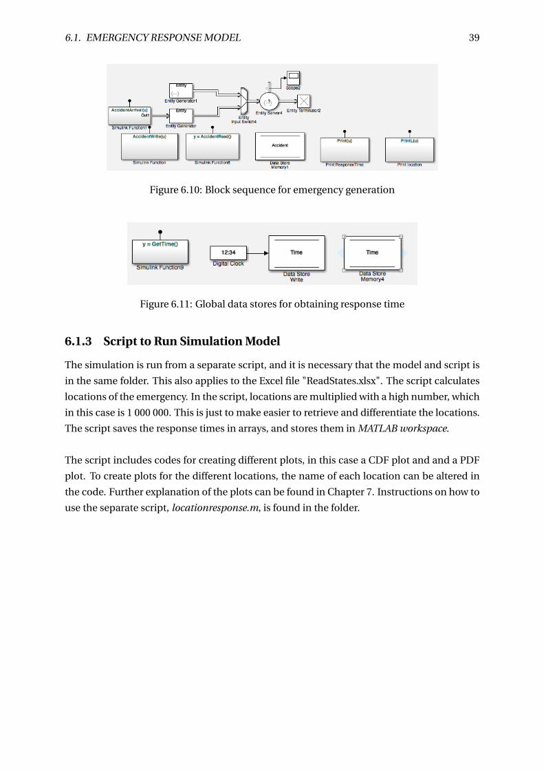
6.1. EMERGENCY RESPONSE MODEL 39
Figure 6.10: Block sequence for emergency generation
Figure 6.11: Global data stores for obtaining response time
6.1.3 Script to Run Simulation Model
The simulation is run from a separate script, and it is necessary that the model and script is
in the same folder. This also applies to the Excel file "ReadStates.xlsx". The script calculates
locations of the emergency. In the script, locations are multiplied with a high number, which
in this case is 1 000 000. This is just to make easier to retrieve and differentiate the locations.
The script saves the response times in arrays, and stores them in MATLAB workspace.
The script includes codes for creating different plots, in this case a CDF plot and and a PDF
plot. To create plots for the different locations, the name of each location can be altered in
the code. Further explanation of the plots can be found in Chapter 7. Instructions on how to
use the separate script, locationresponse.m, is found in the folder.

40 CHAPTER 6. MODEL CONSTRUCTION
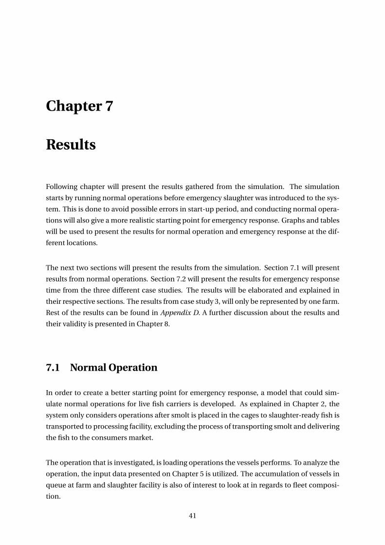
Chapter 7
Results
Following chapter will present the results gathered from the simulation. The simulation
starts by running normal operations before emergency slaughter was introduced to the sys-
tem. This is done to avoid possible errors in start-up period, and conducting normal opera-
tions will also give a more realistic starting point for emergency response. Graphs and tables
will be used to present the results for normal operation and emergency response at the dif-
ferent locations.
The next two sections will present the results from the simulation. Section 7.1 will present
results from normal operations. Section 7.2 will present the results for emergency response
time from the three different case studies. The results will be elaborated and explained in
their respective sections. The results from case study 3, will only be represented by one farm.
Rest of the results can be found in Appendix D. A further discussion about the results and
their validity is presented in Chapter 8.
7.1 Normal Operation
In order to create a better starting point for emergency response, a model that could sim-
ulate normal operations for live fish carriers is developed. As explained in Chapter 2, the
system only considers operations after smolt is placed in the cages to slaughter-ready fish is
transported to processing facility, excluding the process of transporting smolt and delivering
the fish to the consumers market.
The operation that is investigated, is loading operations the vessels performs. To analyze the
operation, the input data presented on Chapter 5 is utilized. The accumulation of vessels in
queue at farm and slaughter facility is also of interest to look at in regards to fleet composi-
tion.
41
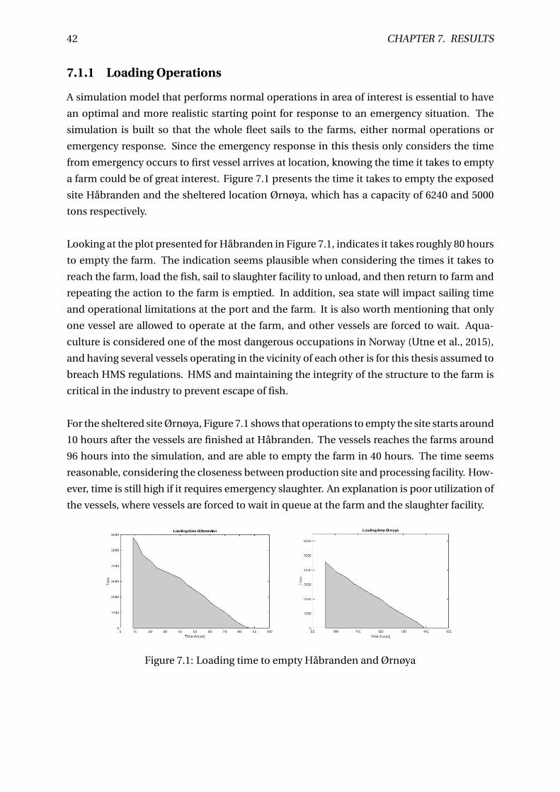
42 CHAPTER 7. RESULTS
7.1.1 Loading Operations
A simulation model that performs normal operations in area of interest is essential to have
an optimal and more realistic starting point for response to an emergency situation. The
simulation is built so that the whole fleet sails to the farms, either normal operations or
emergency response. Since the emergency response in this thesis only considers the time
from emergency occurs to first vessel arrives at location, knowing the time it takes to empty
a farm could be of great interest. Figure 7.1 presents the time it takes to empty the exposed
site Håbranden and the sheltered location Ørnøya, which has a capacity of 6240 and 5000
tons respectively.
Looking at the plot presented for Håbranden in Figure 7.1, indicates it takes roughly 80 hours
to empty the farm. The indication seems plausible when considering the times it takes to
reach the farm, load the fish, sail to slaughter facility to unload, and then return to farm and
repeating the action to the farm is emptied. In addition, sea state will impact sailing time
and operational limitations at the port and the farm. It is also worth mentioning that only
one vessel are allowed to operate at the farm, and other vessels are forced to wait. Aqua-
culture is considered one of the most dangerous occupations in Norway (Utne et al., 2015),
and having several vessels operating in the vicinity of each other is for this thesis assumed to
breach HMS regulations. HMS and maintaining the integrity of the structure to the farm is
critical in the industry to prevent escape of fish.
For the sheltered site Ørnøya, Figure 7.1 shows that operations to empty the site starts around
10 hours after the vessels are finished at Håbranden. The vessels reaches the farms around
96 hours into the simulation, and are able to empty the farm in 40 hours. The time seems
reasonable, considering the closeness between production site and processing facility. How-
ever, time is still high if it requires emergency slaughter. An explanation is poor utilization of
the vessels, where vessels are forced to wait in queue at the farm and the slaughter facility.
Figure 7.1: Loading time to empty Håbranden and Ørnøya
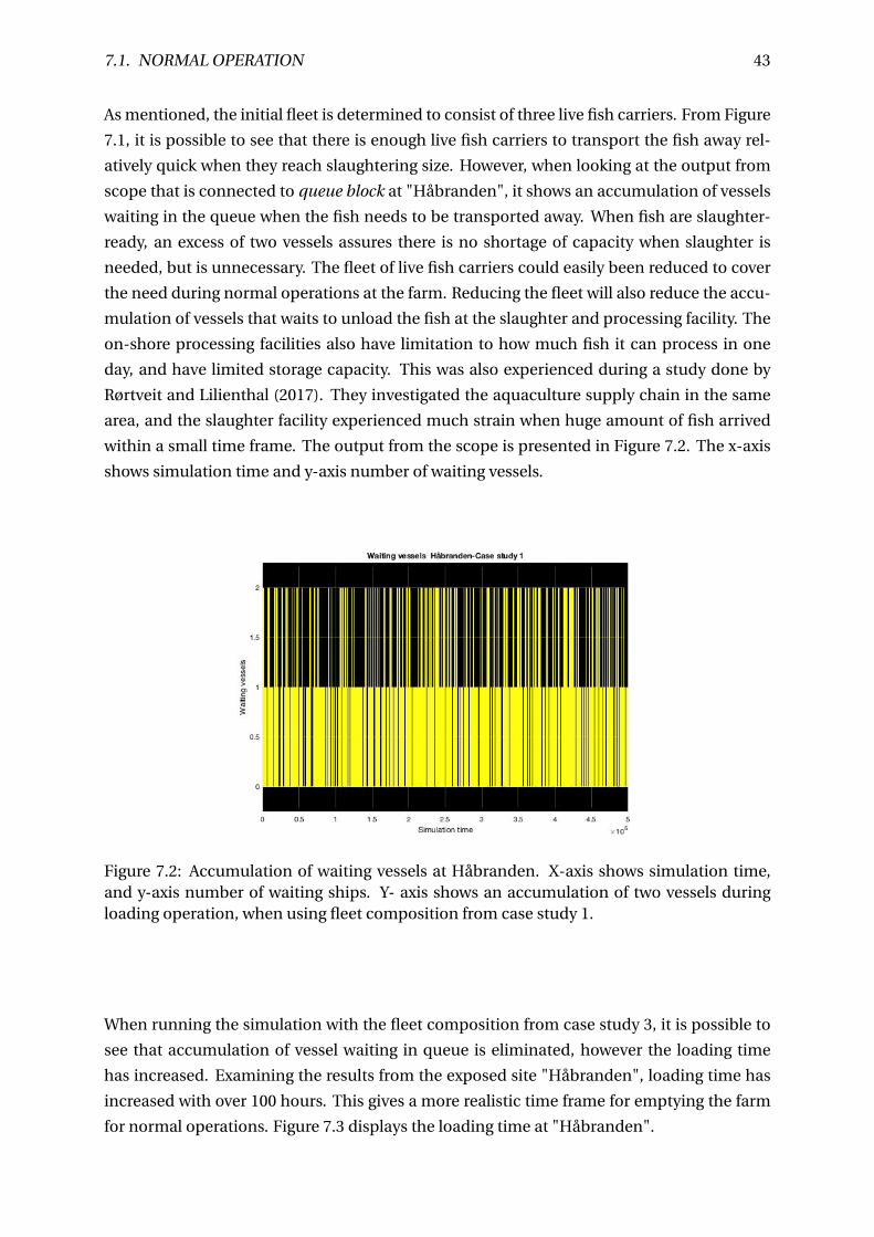
7.1. NORMAL OPERATION 43
As mentioned, the initial fleet is determined to consist of three live fish carriers. From Figure
7.1, it is possible to see that there is enough live fish carriers to transport the fish away rel-
atively quick when they reach slaughtering size. However, when looking at the output from
scope that is connected to queue block at "Håbranden", it shows an accumulation of vessels
waiting in the queue when the fish needs to be transported away. When fish are slaughter-
ready, an excess of two vessels assures there is no shortage of capacity when slaughter is
needed, but is unnecessary. The fleet of live fish carriers could easily been reduced to cover
the need during normal operations at the farm. Reducing the fleet will also reduce the accu-
mulation of vessels that waits to unload the fish at the slaughter and processing facility. The
on-shore processing facilities also have limitation to how much fish it can process in one
day, and have limited storage capacity. This was also experienced during a study done by
Rørtveit and Lilienthal (2017). They investigated the aquaculture supply chain in the same
area, and the slaughter facility experienced much strain when huge amount of fish arrived
within a small time frame. The output from the scope is presented in Figure 7.2. The x-axis
shows simulation time and y-axis number of waiting vessels.
Figure 7.2: Accumulation of waiting vessels at Håbranden. X-axis shows simulation time,and y-axis number of waiting ships. Y- axis shows an accumulation of two vessels duringloading operation, when using fleet composition from case study 1.
When running the simulation with the fleet composition from case study 3, it is possible to
see that accumulation of vessel waiting in queue is eliminated, however the loading time
has increased. Examining the results from the exposed site "Håbranden", loading time has
increased with over 100 hours. This gives a more realistic time frame for emptying the farm
for normal operations. Figure 7.3 displays the loading time at "Håbranden".
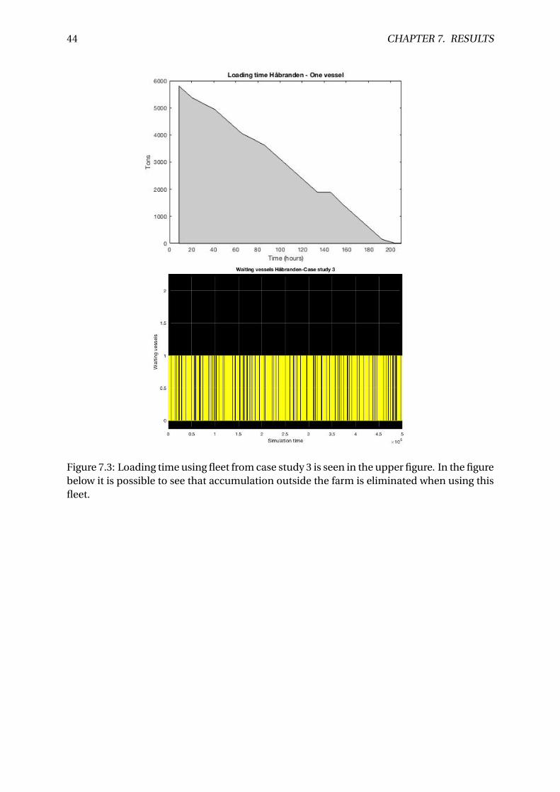
44 CHAPTER 7. RESULTS
Figure 7.3: Loading time using fleet from case study 3 is seen in the upper figure. In the figurebelow it is possible to see that accumulation outside the farm is eliminated when using thisfleet.
7.2. EMERGENCY RESPONSE 45
7.2 Emergency Response
The main objective of this thesis is to find vessels response time for acute pollution, an emer-
gency that subsequently could lead to emergency slaughter. Emergency slaughter is a situa-
tion the aquaculture industry can be exposed to. The emergency is introduced to the system
where a message from a farm being threatened by an oil spill. The emergency response time
is considered from emergency start to the vessel arrives at farm. The following section will
present the response time results from the case studies, where case study 1 use a operational
fleet of three vessels. Case study 2, use two operational vessels and one standby vessel, and
case study 1, use one operational vessel and one standby vessel. Reducing the fleet and
adding a standby vessel could help give an indication for setting a benchmark fleet for nor-
mal operations and emergency response situations.
The results for response times for each of the four aquaculture sites can be found under their
respective sections. The results from each location will be presented graphically. To present
the results, a Cumulative Distribution Function (CDF) is plotted for the response times ob-
tained from the simulation. The probability function shows the cumulative probability of
achieving a response time. In addition to the CDF, a Probability Density Function (PDF) for
the response times is presented. The histograms illustrates the density of retrieved response
times, where the tallest bars in the figures represents the most likely response time to be
achieved by the vessels. Regarding the CDF, the author of this thesis wants to emphasize
that this is not a "true" CDF, but the best estimate the simulation can provide. The rough-
ness of the graphs in the CDF is also created because of the time step the simulation model
is recorded in. This will be discussed further in Chapther 8 and an example of a CDF with
smaller time step, is presented in Appendix C. Tables that shows minimum, mean and maxi-
mum values of the results is also presented in the sections.
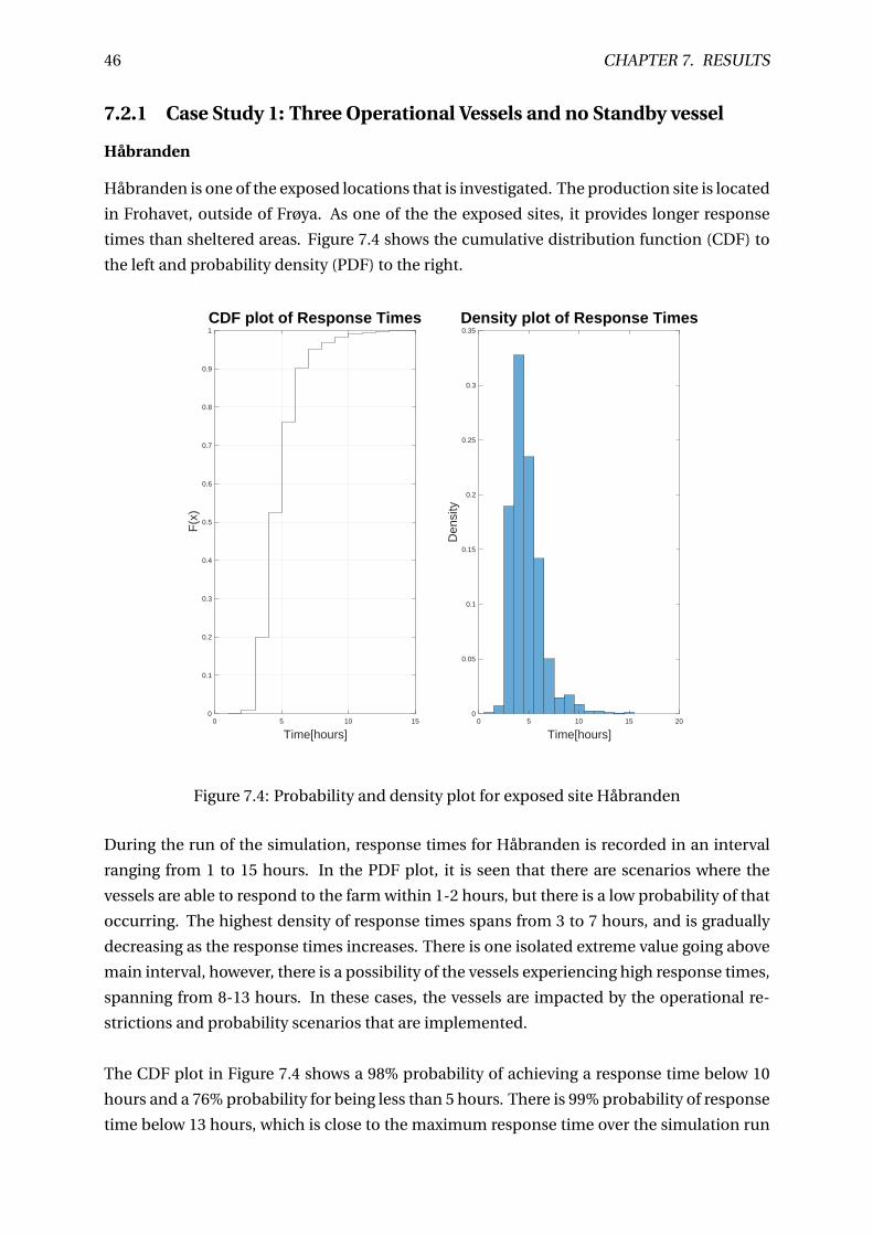
46 CHAPTER 7. RESULTS
7.2.1 Case Study 1: Three Operational Vessels and no Standby vessel
Håbranden
Håbranden is one of the exposed locations that is investigated. The production site is located
in Frohavet, outside of Frøya. As one of the the exposed sites, it provides longer response
times than sheltered areas. Figure 7.4 shows the cumulative distribution function (CDF) to
the left and probability density (PDF) to the right.
0 5 10 15
Time[hours]
0
0.1
0.2
0.3
0.4
0.5
0.6
0.7
0.8
0.9
1
F(x
)
CDF plot of Response Times Density plot of Response Times
0 5 10 15 20
Time[hours]
0
0.05
0.1
0.15
0.2
0.25
0.3
0.35
Den
sity
Figure 7.4: Probability and density plot for exposed site Håbranden
During the run of the simulation, response times for Håbranden is recorded in an interval
ranging from 1 to 15 hours. In the PDF plot, it is seen that there are scenarios where the
vessels are able to respond to the farm within 1-2 hours, but there is a low probability of that
occurring. The highest density of response times spans from 3 to 7 hours, and is gradually
decreasing as the response times increases. There is one isolated extreme value going above
main interval, however, there is a possibility of the vessels experiencing high response times,
spanning from 8-13 hours. In these cases, the vessels are impacted by the operational re-
strictions and probability scenarios that are implemented.
The CDF plot in Figure 7.4 shows a 98% probability of achieving a response time below 10
hours and a 76% probability for being less than 5 hours. There is 99% probability of response
time below 13 hours, which is close to the maximum response time over the simulation run
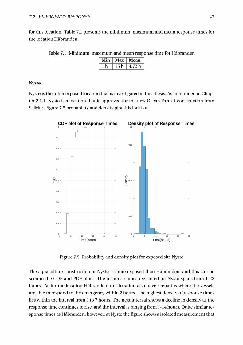
7.2. EMERGENCY RESPONSE 47
for this location. Table 7.1 presents the minimum, maximum and mean response times for
the location Håbranden.
Table 7.1: Minimum, maximum and mean response time for Håbranden
Min Max Mean1 h 15 h 4.72 h
Nystø
Nystø is the other exposed location that is investigated in this thesis. As mentioned in Chap-
ter 2.1.1, Nystø is a location that is approved for the new Ocean Farm 1 construction from
SalMar. Figure 7.5 probability and density plot this location.
0 5 10 15 20 25
Time[hours]
0
0.1
0.2
0.3
0.4
0.5
0.6
0.7
0.8
0.9
1
F(x
)
CDF plot of Response Times Density plot of Response Times
0 5 10 15 20 25
Time[hours]
0
0.05
0.1
0.15
0.2
0.25
0.3D
ensi
ty
Figure 7.5: Probability and density plot for exposed site Nystø
The aquaculture construction at Nystø is more exposed than Håbranden, and this can be
seen in the CDF and PDF plots. The response times registered for Nystø spans from 1-22
hours. As for the location Håbranden, this location also have scenarios where the vessels
are able to respond to the emergency within 2 hours. The highest density of response times
lies within the interval from 3 to 7 hours. The next interval shows a decline in density as the
response time continues to rise, and the interval is ranging from 7-14 hours. Quite similar re-
sponse times as Håbranden, however, at Nystø the figure shows a isolated measurement that
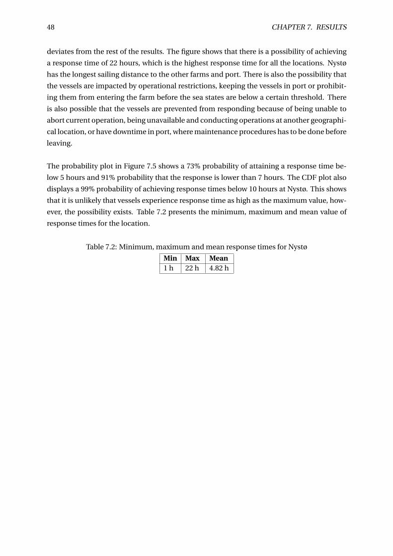
48 CHAPTER 7. RESULTS
deviates from the rest of the results. The figure shows that there is a possibility of achieving
a response time of 22 hours, which is the highest response time for all the locations. Nystø
has the longest sailing distance to the other farms and port. There is also the possibility that
the vessels are impacted by operational restrictions, keeping the vessels in port or prohibit-
ing them from entering the farm before the sea states are below a certain threshold. There
is also possible that the vessels are prevented from responding because of being unable to
abort current operation, being unavailable and conducting operations at another geographi-
cal location, or have downtime in port, where maintenance procedures has to be done before
leaving.
The probability plot in Figure 7.5 shows a 73% probability of attaining a response time be-
low 5 hours and 91% probability that the response is lower than 7 hours. The CDF plot also
displays a 99% probability of achieving response times below 10 hours at Nystø. This shows
that it is unlikely that vessels experience response time as high as the maximum value, how-
ever, the possibility exists. Table 7.2 presents the minimum, maximum and mean value of
response times for the location.
Table 7.2: Minimum, maximum and mean response times for Nystø
Min Max Mean1 h 22 h 4.82 h
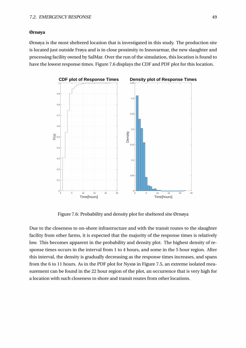
7.2. EMERGENCY RESPONSE 49
Ørnøya
Ørnøya is the most sheltered location that is investigated in this study. The production site
is located just outside Frøya and is in close proximity to Innovarmar, the new slaughter and
processing facility owned by SalMar. Over the run of the simulation, this location is found to
have the lowest response times. Figure 7.6 displays the CDF and PDF plot for this location.
0 5 10 15 20 25
Time[hours]
0
0.1
0.2
0.3
0.4
0.5
0.6
0.7
0.8
0.9
1
F(x
)
CDF plot of Response Times Density plot of Response Times
0 5 10 15 20 25
Time[hours]
0
0.05
0.1
0.15
0.2
0.25
0.3
0.35
Den
sity
Figure 7.6: Probability and density plot for sheltered site Ørnøya
Due to the closeness to on-shore infrastructure and with the transit routes to the slaughter
facility from other farms, it is expected that the majority of the response times is relatively
low. This becomes apparent in the probability and density plot. The highest density of re-
sponse times occurs in the interval from 1 to 4 hours, and some in the 5 hour region. After
this interval, the density is gradually decreasing as the response times increases, and spans
from the 6 to 11 hours. As in the PDF plot for Nystø in Figure 7.5, an extreme isolated mea-
surement can be found in the 22 hour region of the plot, an occurrence that is very high for
a location with such closeness to shore and transit routes from other locations.
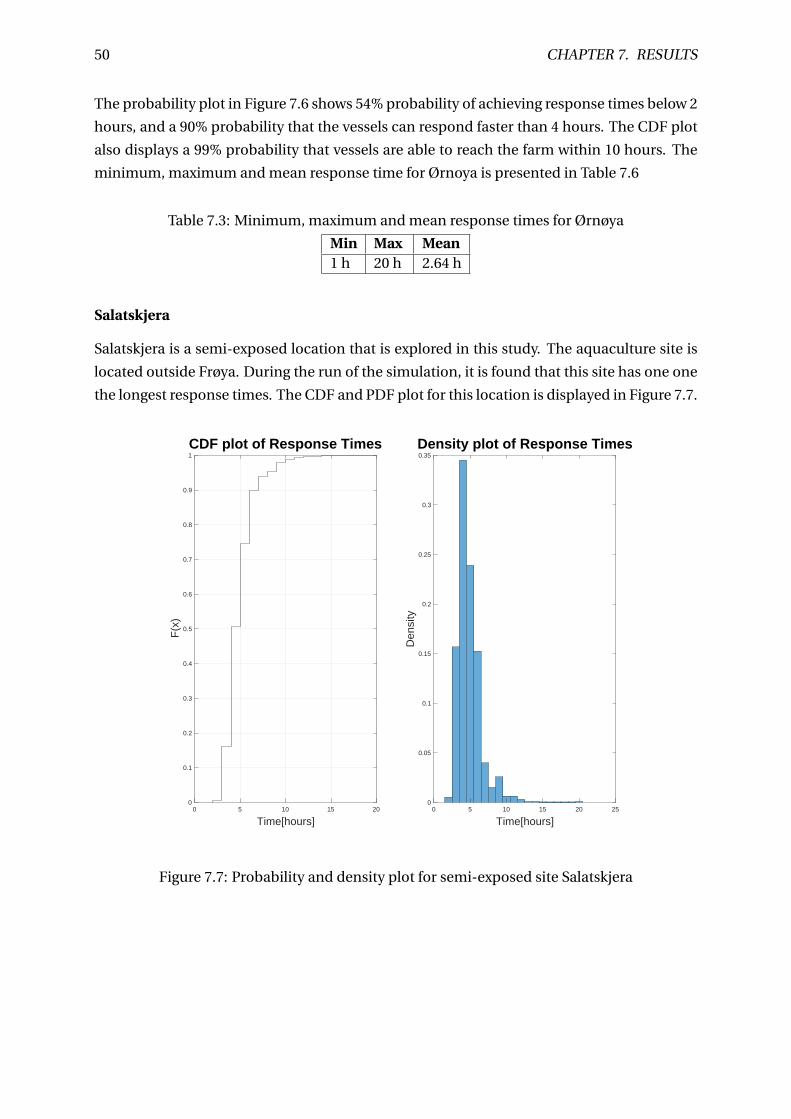
50 CHAPTER 7. RESULTS
The probability plot in Figure 7.6 shows 54% probability of achieving response times below 2
hours, and a 90% probability that the vessels can respond faster than 4 hours. The CDF plot
also displays a 99% probability that vessels are able to reach the farm within 10 hours. The
minimum, maximum and mean response time for Ørnoya is presented in Table 7.6
Table 7.3: Minimum, maximum and mean response times for Ørnøya
Min Max Mean1 h 20 h 2.64 h
Salatskjera
Salatskjera is a semi-exposed location that is explored in this study. The aquaculture site is
located outside Frøya. During the run of the simulation, it is found that this site has one one
the longest response times. The CDF and PDF plot for this location is displayed in Figure 7.7.
0 5 10 15 20
Time[hours]
0
0.1
0.2
0.3
0.4
0.5
0.6
0.7
0.8
0.9
1
F(x
)
CDF plot of Response Times Density plot of Response Times
0 5 10 15 20 25
Time[hours]
0
0.05
0.1
0.15
0.2
0.25
0.3
0.35
Den
sity
Figure 7.7: Probability and density plot for semi-exposed site Salatskjera
7.2. EMERGENCY RESPONSE 51
Even tough the location is regarded as sheltered, the location is located in a remote area
outside Frøya, and operating under "green" concessions, to reduce the environmental chal-
lenges with escape of farmed fish and spread of salmon lice. As a consequence, the produc-
tion site is placed in a semi-exposed location, with longer transit routes to the other farms,
on-shore infrastructure and normal transit routes. This can also be seen in the plots in Figure
7.7. Salatskjera is the only location that vessels are unable to respond to in under two hours,
and shows that only a small density of the times occurs here. The main bulk of response
times occurs within the interval from 3 to 6 hours, and there is a relatively high density of
times that occurs for 7 hours. After this interval the plot displays a decreasing density in
response times, apart from a peak at the 9 hour mark, and ends at 14 hours. As at the lo-
cation Nystø and Ørnøya, Salatskjera experience an isolated measure that occurs at the 20
hour mark.
The probability plot in Figure 7.7 shows a 51% probability of achieving a response time
within 4 hours, and a 74% probability that the vessel are able to respond faster than 5 hours
to this location. A 99% probability of responding faster than 10 hours is also found at this
location, the same discoveries made at the location Nystø. Table 7.4 presents the minimum,
maximum and mean response time values for Salatskjera.
Table 7.4: Minimum, maximum and mean response times for Salatskjera
Min Max Mean2 h 20 h 4.88 h
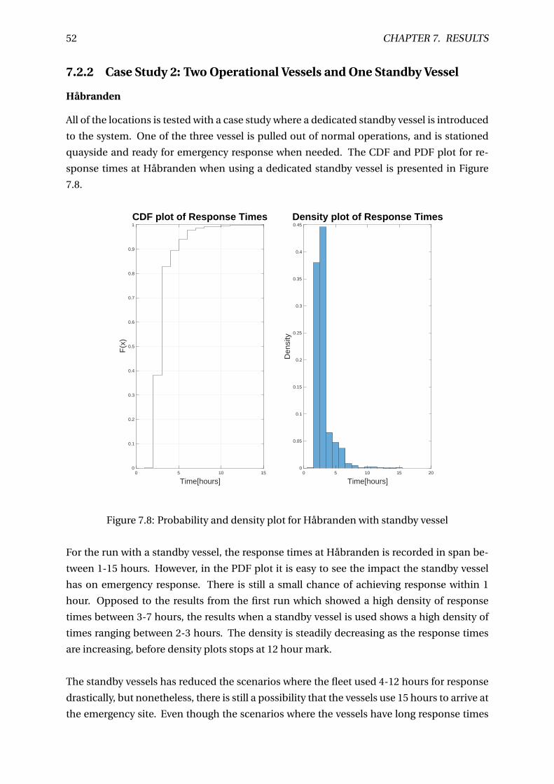
52 CHAPTER 7. RESULTS
7.2.2 Case Study 2: Two Operational Vessels and One Standby Vessel
Håbranden
All of the locations is tested with a case study where a dedicated standby vessel is introduced
to the system. One of the three vessel is pulled out of normal operations, and is stationed
quayside and ready for emergency response when needed. The CDF and PDF plot for re-
sponse times at Håbranden when using a dedicated standby vessel is presented in Figure
7.8.
0 5 10 15
Time[hours]
0
0.1
0.2
0.3
0.4
0.5
0.6
0.7
0.8
0.9
1
F(x
)
CDF plot of Response Times Density plot of Response Times
0 5 10 15 20
Time[hours]
0
0.05
0.1
0.15
0.2
0.25
0.3
0.35
0.4
0.45
Den
sity
Figure 7.8: Probability and density plot for Håbranden with standby vessel
For the run with a standby vessel, the response times at Håbranden is recorded in span be-
tween 1-15 hours. However, in the PDF plot it is easy to see the impact the standby vessel
has on emergency response. There is still a small chance of achieving response within 1
hour. Opposed to the results from the first run which showed a high density of response
times between 3-7 hours, the results when a standby vessel is used shows a high density of
times ranging between 2-3 hours. The density is steadily decreasing as the response times
are increasing, before density plots stops at 12 hour mark.
The standby vessels has reduced the scenarios where the fleet used 4-12 hours for response
drastically, but nonetheless, there is still a possibility that the vessels use 15 hours to arrive at
the emergency site. Even though the scenarios where the vessels have long response times
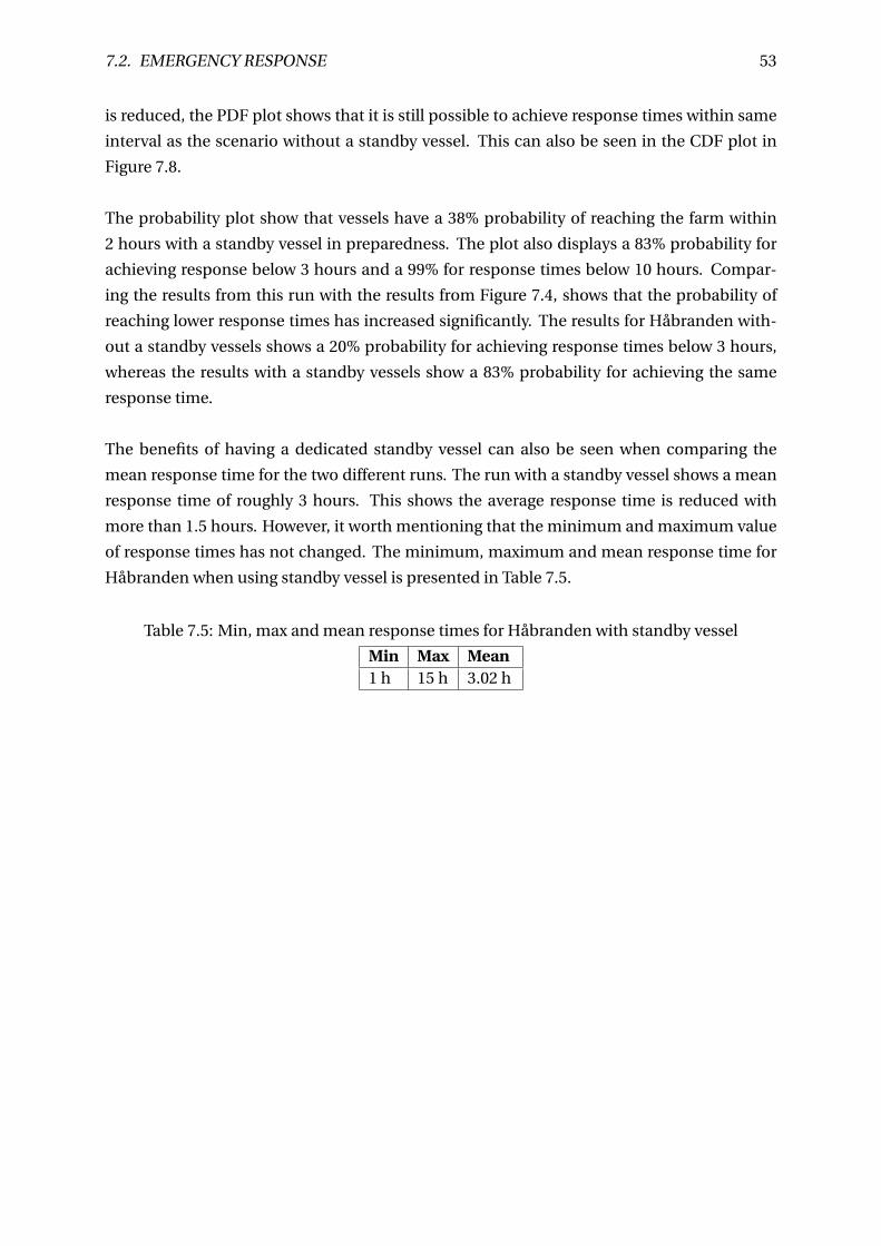
7.2. EMERGENCY RESPONSE 53
is reduced, the PDF plot shows that it is still possible to achieve response times within same
interval as the scenario without a standby vessel. This can also be seen in the CDF plot in
Figure 7.8.
The probability plot show that vessels have a 38% probability of reaching the farm within
2 hours with a standby vessel in preparedness. The plot also displays a 83% probability for
achieving response below 3 hours and a 99% for response times below 10 hours. Compar-
ing the results from this run with the results from Figure 7.4, shows that the probability of
reaching lower response times has increased significantly. The results for Håbranden with-
out a standby vessels shows a 20% probability for achieving response times below 3 hours,
whereas the results with a standby vessels show a 83% probability for achieving the same
response time.
The benefits of having a dedicated standby vessel can also be seen when comparing the
mean response time for the two different runs. The run with a standby vessel shows a mean
response time of roughly 3 hours. This shows the average response time is reduced with
more than 1.5 hours. However, it worth mentioning that the minimum and maximum value
of response times has not changed. The minimum, maximum and mean response time for
Håbranden when using standby vessel is presented in Table 7.5.
Table 7.5: Min, max and mean response times for Håbranden with standby vessel
Min Max Mean1 h 15 h 3.02 h
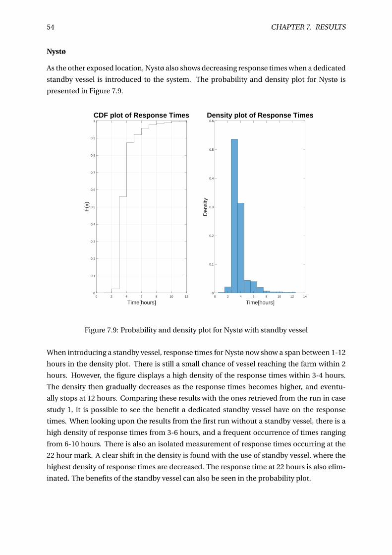
54 CHAPTER 7. RESULTS
Nystø
As the other exposed location, Nystø also shows decreasing response times when a dedicated
standby vessel is introduced to the system. The probability and density plot for Nystø is
presented in Figure 7.9.
0 2 4 6 8 10 12
Time[hours]
0
0.1
0.2
0.3
0.4
0.5
0.6
0.7
0.8
0.9
1
F(x
)
CDF plot of Response Times Density plot of Response Times
0 2 4 6 8 10 12 14
Time[hours]
0
0.1
0.2
0.3
0.4
0.5
0.6
Den
sity
Figure 7.9: Probability and density plot for Nystø with standby vessel
When introducing a standby vessel, response times for Nystø now show a span between 1-12
hours in the density plot. There is still a small chance of vessel reaching the farm within 2
hours. However, the figure displays a high density of the response times within 3-4 hours.
The density then gradually decreases as the response times becomes higher, and eventu-
ally stops at 12 hours. Comparing these results with the ones retrieved from the run in case
study 1, it is possible to see the benefit a dedicated standby vessel have on the response
times. When looking upon the results from the first run without a standby vessel, there is a
high density of response times from 3-6 hours, and a frequent occurrence of times ranging
from 6-10 hours. There is also an isolated measurement of response times occurring at the
22 hour mark. A clear shift in the density is found with the use of standby vessel, where the
highest density of response times are decreased. The response time at 22 hours is also elim-
inated. The benefits of the standby vessel can also be seen in the probability plot.
7.2. EMERGENCY RESPONSE 55
The CDF plot show that this fleet has a 56% probability of achieving response times below
3 hours, and a 88% probability that vessels can respond within 4 hours. This shows a stark
contrast to the results collected from the run without a standby vessel. The results from case
study 1 showed a probability of 19 and 48 for responding within the same time span. This
means it is almost 3 times as likely to achieve response times below 3 hours and almost two
times as likely to respond below 4 hours with the use of a standby vessel versus not using one.
When comparing the min, max and mean value for the response time for this run with a
standby vessel versus the run without one, it is also possible to see the benefits such a vessel
has on this location to. The minimum response time is still the same, and maximum re-
sponse time is reduced by 10 hours. The results from this run also show a reduction in mean
response time by more than one hour. The response times min, max and mean value with a
standby vessel for this location is presented in Table 7.6.
Table 7.6: Min, max and mean response times for Nystø with standby vessel
Min Max Mean1 h 12 h 3.71
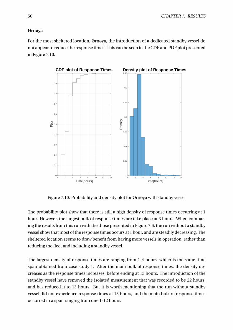
56 CHAPTER 7. RESULTS
Ørnøya
For the most sheltered location, Ørnøya, the introduction of a dedicated standby vessel do
not appear to reduce the response times. This can be seen in the CDF and PDF plot presented
in Figure 7.10.
0 2 4 6 8 10 12 14
Time[hours]
0
0.1
0.2
0.3
0.4
0.5
0.6
0.7
0.8
0.9
1
F(x
)
CDF plot of Response Times Density plot of Response Times
0 2 4 6 8 10 12 14
Time[hours]
0
0.05
0.1
0.15
0.2
0.25
0.3
0.35
Den
sity
Figure 7.10: Probability and density plot for Ørnøya with standby vessel
The probability plot show that there is still a high density of response times occurring at 1
hour. However, the largest bulk of response times are take place at 3 hours. When compar-
ing the results from this run with the those presented in Figure 7.6, the run without a standby
vessel show that most of the response times occurs at 1 hour, and are steadily decreasing. The
sheltered location seems to draw benefit from having more vessels in operation, rather than
reducing the fleet and including a standby vessel.
The largest density of response times are ranging from 1-4 hours, which is the same time
span obtained from case study 1. After the main bulk of response times, the density de-
creases as the response times increases, before ending at 13 hours. The introduction of the
standby vessel have removed the isolated measurement that was recorded to be 22 hours,
and has reduced it to 13 hours. But it is worth mentioning that the run without standby
vessel did not experience response times at 13 hours, and the main bulk of response times
occurred in a span ranging from one 1-12 hours.
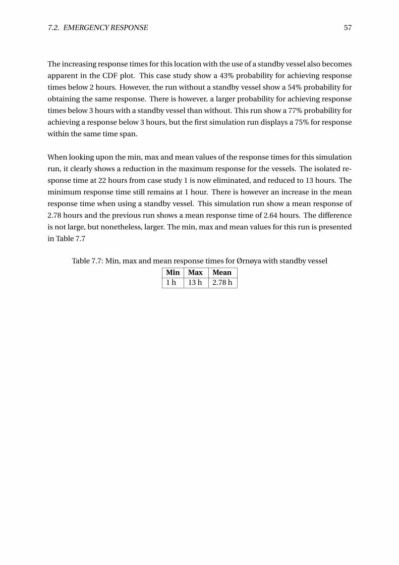
7.2. EMERGENCY RESPONSE 57
The increasing response times for this location with the use of a standby vessel also becomes
apparent in the CDF plot. This case study show a 43% probability for achieving response
times below 2 hours. However, the run without a standby vessel show a 54% probability for
obtaining the same response. There is however, a larger probability for achieving response
times below 3 hours with a standby vessel than without. This run show a 77% probability for
achieving a response below 3 hours, but the first simulation run displays a 75% for response
within the same time span.
When looking upon the min, max and mean values of the response times for this simulation
run, it clearly shows a reduction in the maximum response for the vessels. The isolated re-
sponse time at 22 hours from case study 1 is now eliminated, and reduced to 13 hours. The
minimum response time still remains at 1 hour. There is however an increase in the mean
response time when using a standby vessel. This simulation run show a mean response of
2.78 hours and the previous run shows a mean response time of 2.64 hours. The difference
is not large, but nonetheless, larger. The min, max and mean values for this run is presented
in Table 7.7
Table 7.7: Min, max and mean response times for Ørnøya with standby vessel
Min Max Mean1 h 13 h 2.78 h
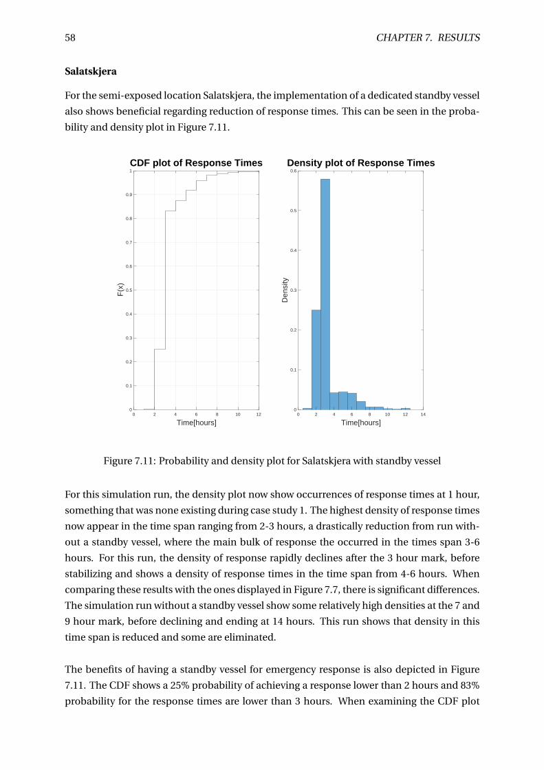
58 CHAPTER 7. RESULTS
Salatskjera
For the semi-exposed location Salatskjera, the implementation of a dedicated standby vessel
also shows beneficial regarding reduction of response times. This can be seen in the proba-
bility and density plot in Figure 7.11.
0 2 4 6 8 10 12
Time[hours]
0
0.1
0.2
0.3
0.4
0.5
0.6
0.7
0.8
0.9
1
F(x
)
CDF plot of Response Times Density plot of Response Times
0 2 4 6 8 10 12 14
Time[hours]
0
0.1
0.2
0.3
0.4
0.5
0.6
Den
sity
Figure 7.11: Probability and density plot for Salatskjera with standby vessel
For this simulation run, the density plot now show occurrences of response times at 1 hour,
something that was none existing during case study 1. The highest density of response times
now appear in the time span ranging from 2-3 hours, a drastically reduction from run with-
out a standby vessel, where the main bulk of response the occurred in the times span 3-6
hours. For this run, the density of response rapidly declines after the 3 hour mark, before
stabilizing and shows a density of response times in the time span from 4-6 hours. When
comparing these results with the ones displayed in Figure 7.7, there is significant differences.
The simulation run without a standby vessel show some relatively high densities at the 7 and
9 hour mark, before declining and ending at 14 hours. This run shows that density in this
time span is reduced and some are eliminated.
The benefits of having a standby vessel for emergency response is also depicted in Figure
7.11. The CDF shows a 25% probability of achieving a response lower than 2 hours and 83%
probability for the response times are lower than 3 hours. When examining the CDF plot
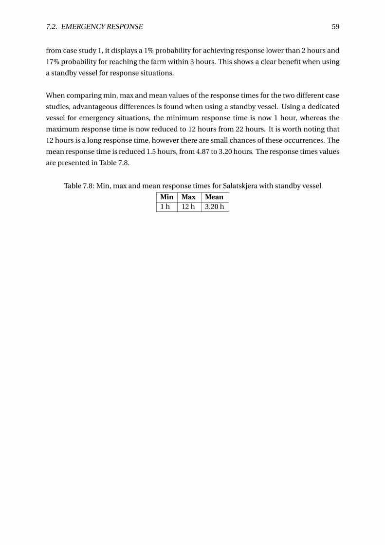
7.2. EMERGENCY RESPONSE 59
from case study 1, it displays a 1% probability for achieving response lower than 2 hours and
17% probability for reaching the farm within 3 hours. This shows a clear benefit when using
a standby vessel for response situations.
When comparing min, max and mean values of the response times for the two different case
studies, advantageous differences is found when using a standby vessel. Using a dedicated
vessel for emergency situations, the minimum response time is now 1 hour, whereas the
maximum response time is now reduced to 12 hours from 22 hours. It is worth noting that
12 hours is a long response time, however there are small chances of these occurrences. The
mean response time is reduced 1.5 hours, from 4.87 to 3.20 hours. The response times values
are presented in Table 7.8.
Table 7.8: Min, max and mean response times for Salatskjera with standby vessel
Min Max Mean1 h 12 h 3.20 h
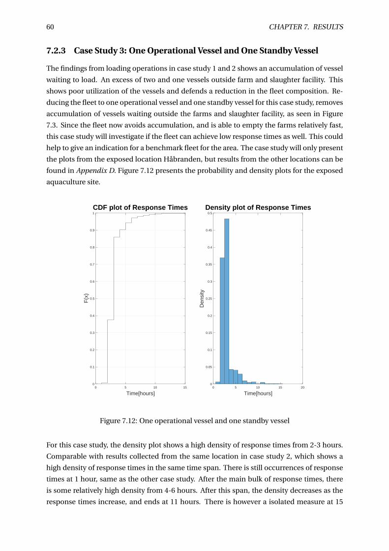
60 CHAPTER 7. RESULTS
7.2.3 Case Study 3: One Operational Vessel and One Standby Vessel
The findings from loading operations in case study 1 and 2 shows an accumulation of vessel
waiting to load. An excess of two and one vessels outside farm and slaughter facility. This
shows poor utilization of the vessels and defends a reduction in the fleet composition. Re-
ducing the fleet to one operational vessel and one standby vessel for this case study, removes
accumulation of vessels waiting outside the farms and slaughter facility, as seen in Figure
7.3. Since the fleet now avoids accumulation, and is able to empty the farms relatively fast,
this case study will investigate if the fleet can achieve low response times as well. This could
help to give an indication for a benchmark fleet for the area. The case study will only present
the plots from the exposed location Håbranden, but results from the other locations can be
found in Appendix D. Figure 7.12 presents the probability and density plots for the exposed
aquaculture site.
0 5 10 15
Time[hours]
0
0.1
0.2
0.3
0.4
0.5
0.6
0.7
0.8
0.9
1
F(x
)
CDF plot of Response Times Density plot of Response Times
0 5 10 15 20
Time[hours]
0
0.05
0.1
0.15
0.2
0.25
0.3
0.35
0.4
0.45
0.5
Den
sity
Figure 7.12: One operational vessel and one standby vessel
For this case study, the density plot shows a high density of response times from 2-3 hours.
Comparable with results collected from the same location in case study 2, which shows a
high density of response times in the same time span. There is still occurrences of response
times at 1 hour, same as the other case study. After the main bulk of response times, there
is some relatively high density from 4-6 hours. After this span, the density decreases as the
response times increase, and ends at 11 hours. There is however a isolated measure at 15
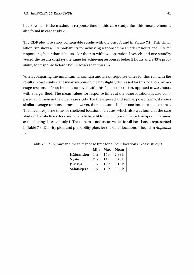
7.2. EMERGENCY RESPONSE 61
hours, which is the maximum response time in this case study. But, this measurement is
also found in case study 2.
The CDF plot also show comparable results with the ones found in Figure 7.8. This simu-
lation run show a 38% probability for achieving response times under 2 hours and 86% for
responding faster than 3 hours. For the run with two operational vessels and one standby
vessel, the results displays the same for achieving responses below 2 hours and a 83% prob-
ability for response below 3 hours, lower than this run.
When comparing the minimum, maximum and mean response times for this run with the
results in case study 2, the mean response time has slightly decreased for this location. An av-
erage response of 2.99 hours is achieved with this fleet composition, opposed to 3.02 hours
with a larger fleet. The mean values for response times at the other locations is also com-
pared with them in the other case study. For the exposed and semi exposed farms, it shows
similar average response times, however, there are some higher maximum response times.
The mean response time for sheltered location increases, which also was found in the case
study 2. The sheltered location seems to benefit from having more vessels in operation, same
as the findings in case study 1. The min, max and mean values for all locations is represented
in Table 7.9. Density plots and probability plots for the other locations is found in Appendix
D.
Table 7.9: Min, max and mean response time for all four locations in case study 3
Min Max MeanHåbranden 1 h 15 h 2.99 hNystø 2 h 14 h 3.78 hØrnøya 1 h 12 h 3.15 hSalatskjera 1 h 13 h 3.23 h

62 CHAPTER 7. RESULTS
Chapter 8
Discussion
The discrete-event simulation model and results will be discussed in conjunction with the
problem description and scope that is presented in this thesis. Due to lack of previous stud-
ies that used discrete-event simulation within the topic of emergency response in aquacul-
ture, emphasis has been put on the validity of the results and reliability of the model. As a
consequence, a comprehensive part of the discussion will concentrate on this. The discus-
sion will first present and asses the results, before evaluating the results and models validity.
Case study 1, consisted of a fleet of three operational vessels, and no standby vessel. The
fleet composition showed that the vessels never experienced shortage of capacity and was
able to remove fish rapidly during normal operations. This also showed that this feature
would be beneficial in an emergency situation that could require emergency slaughter. The
fleet composition was able to empty the presented farms in Figure 7.1 in 40-80 hours, where
sheltered farm experienced the lowest loading time. This was due to lower amounts of fish at
the farm and shorter distances to processing facility. However, it was found that fleet could
be reduced. Scope output showed an accumulation of vessels outside the farms and process
facility. There were an excess of two vessels, and fleet could easily be reduced to improve
normal operations. But, removal of vessels would impact the fleets ability to empty a farm
in a short amount of time. The case study showed a high density of response times within
the time span from 3-10 hours, and some isolated measures around the 20 hour mark. The
exposed location experienced highest response times, but sheltered had reasonably low re-
sponse due to closeness of infrastructure and other transit routes.
The introduction of a standby vessels in case study 2, where the fleet consisted of two op-
erational vessels and one standby vessel, proved to reduce response times at the exposed
locations. The average response time was reduced more than one hour at several locations,
and high isolated measurements were eliminated. The probability of achieving low response
times, was also increased. But, the sheltered location experienced higher response times,
and seemed to benefit from more vessels in operation. However, during normal operations
an accumulation of waiting vessels were found. The fleet was able to empty the farms rapidly,
63
64 CHAPTER 8. DISCUSSION
but was not seen as a viable solution for normal operations, as an large amount of fish rushed
to the processing facility would put to much strain at the facility. This was also experienced
in a study by Rørtveit and Lilienthal (2017).
Case study 3, the fleet was reduced to one operational vessel and one standby vessel. The
results showed to be the optimal fleet for normal operations and emergency response. The
fleet composition removed the accumulation outside the farm and slaughter facility, and de-
livers the fish in a time span, that would have enabled the facility to process the fish. The
fleet composition also achieved similar response times as the fleet in case study 2, and pro-
vided an even higher probability for obtaining lower response times. However, more isolated
measures was found around the 15 hour mark, but shows a low probability for these occur-
rences. Only four farms was considered in this simulation, and expanding the model could
be needed to get more realistic results. However, the simulation provided a good indication
for a benchmark fleet for the region.
The response time was presented as a cumulative distribution function and a probability
density function. However, the functions cannot be considered to be an absolute "true" rep-
resentation of the cumulative probability, but the best estimate provided by the simulation
model. The CDF plot provided a graph that displayed the probability for achieving a re-
sponse time below a certain threshold. The roughness of the graphs was a consequence of
the time step the response times was recorded in. For more accurate response times, the time
step must be reduced and requires a run over a long period to obtain as many outcomes as
possible. A simulation run with these settings, required high computational power and was
time consuming. As a consequence, a compromise was made to run the simulation over a
longer time period, but with larger time steps. A long simulation run provided extreme iso-
lated measurements of response times, whereas a simulation short time step and run time
did not. It seemed sensible that worst case scenarios also should be showcased. Because of
the time step, the response times were recorded in "whole hours", but nonetheless, it gave
a clear indication for what expected response time could be. A comparable figure that used
small time steps, can be found in Appendix B.
Using discrete-event simulation to analyze different fleet composition for normal operations
and emergency situations, proved to be an appropriate method for the scope of this master’s
thesis. The user-friendly drag-and-drop interface provided by SimEvents, made it easy build
a model with low complexity, but still strong enough to provide realistic output. The simula-
tion model provided reasonable results in the case studies, and was able to provide an indi-
cation for an benchmark fleet. However, a simulation can never replicate the real-life system
to be completely accurate (Maria, 1997). Modelling emergency situations, need a significant
effort in collecting input data, because of emergency situations sensitivity to stochastic vari-
ables (Jain and Caglar, 2008). The model structure and input data in this thesis, was subject
65
to simplifications and assumptions. Consequently, the results validity are impacted by the
compromises made through the development of the model.
A logistical model was developed to give a more realistic starting point for emergency re-
sponse. However, the vessels are limited to only transport fish from a farm to on-shore
slaughter and processing facilities. Live fish carriers today, are able to conduct several other
operations at the farms (Hauvik, 2018). The newest fleet of vessels are equipped to conduct
delousing operations and treatment for disease at the farms. In addition, live fish carriers
are also used to transport smolt from hatchery to farms. Limiting the vessels to only one
operation in the logistical model, do not represent the real-life accurately, and need more
complexity. However, as the underlying purpose of the model was to investigate vessel re-
sponse times, the logistical model complexity was kept to a minimum.
Chapter 7.1 presented results obtained from normal loading operation. Through the two first
case studies, the farms and processing facility experienced an accumulation of vessels wait-
ing to load and unload. For normal operation in a real-life system, three vessels would not
sail to the farm simultaneously. But the case studies helped to establish a benchmark fleet,
that indicated that one operational live fish carrier was enough for loading operations. Had
three vessels emptied a farm in 40 hours, practical problems like storage and processing ca-
pacity would arise. Nordskaget, which was used as the processing facility in the simulation,
would not have the ability to handle the amount of fish over a short period of time, which was
seen in the study done by Rørtveit and Lilienthal (2017). The facility has four waiting cages
with the capacity of 350 tons of fish (SalMar, 2018), and an entire farm could have several
thousand tons of fish. This further defends the decision for reducing the fleet. The fleet from
case study 3 was able to empty a farm within 200 hours. Within this time limit, the facility
would be able to process the amount and store it. Reducing the fleet would also makes sense
in an economic context for the farm owners, as hiring a vessel is expensive.
From an emergency preparedness perspective, a fleet of three vessels would be beneficial for
rapid removal of the fish at the site. But again, there are practical problems like processing
and capacity ability at the slaughter facility. The shortage of capacity and processing ability
during an emergency like acute pollution, could be a bottleneck in emergency preparedness
in these situations (Sunde, 2009). Development of on-shore infrastructure to handle these
amounts of fish could be needed. There could also be a possibility of cooperation between
slaughter facilities. However, the low frequency of oil spills along the Norwegian coast may
defend the lack of adequate infrastructure at this time. But as near-coast activity increases in
shipping and aquaculture (SINTEF, 2010), development of infrastructure may be needed in
the future. The possibility of introducing processing vessels in emergency situations, could
also reduce the strain on processing facilities, as the vessels can begin slaughter in transit.
66 CHAPTER 8. DISCUSSION
For simplicity and lack of data, assumptions was made for input data in the simulation. Ves-
sels was given one speed mode, where in a real life system, vessels would naturally decrease
on approaching port or farms, and increase in open water and in emergency response. This
assumption impacts the validity of the response times, as well for results for normal op-
erations, and different speed modes should be implemented to give more realistic results.
More weaknesses in the input data can be found in the implementation of probability sce-
narios. The scenarios represented the vessels unavailability, ability to abort operations or
possibility of being confined in port due to maintenance. In an attempt to emulate real-life
operations for the live fish carriers, time delays were imposed on the vessel should they be
subject to the scenarios. Due to lack of historic data, the probabilities of the scenarios was
based on assumptions, and will provide unreliable results. As an example, maintenance of
vessel would be scheduled to calmer periods of the year, but in the simulation, maintenance
can be imposed during all periods. Nonetheless, it gave a notion of what the vessels could
experience if an emergency occurred.
Another disadvantage with the simulation model, was that only one farm experience an
emergency, where in a real-life situation, several farms would experience the same due to
closeness (Sunde, 2009). This would again cause strain on the slaughter facility, but could
also lead to lack capacity on vessels. In the possibility of to much strain on the processing
facility, vessel would have to wait with fish on-board to the facility was able to process it.
Leaving the vessels unable to collect more fish during emergency situations. Further draw-
backs can be found in the generation of sea states. The sea states was generated to impact the
vessels sailing time and for creation of a "weather window" to restrict the vessels operational
possibilities. However, the simulation do not consider seasonal variations, where operations
during winter months could be more heavily impacted than than during the summer. Op-
erational restrictions at farms was hard to obtain, and restrictions is for that reason based
on assumptions. Further work with the model should also use different weather data for ex-
posed and sheltered locations, to produce more reliable results. But, it was assumed in this
thesis that one set was enough due to short distances between the locations.
All simplifications and assumptions made, can impact the validity of the results. However,
the simulation provided useful information for the scope of the thesis. The results gave a
clear indication on how different fleet compositions was able to perform in normal opera-
tion and emergency response, and was able to establish a benchmark fleet. The lack of data
and assumptions contribute to uncertainty, but the runs in the different case studies may
suffer less than expected, as the same preconditions was applied to all case studies.
The prospect of acute pollution, will require swift a removal of fish from their cages. Using
the fleet from case study 3, could result in lack of capacity for removing the fish fast enough.
However, it is also worth mentioning that this thesis only considers removal of an entire site,
67
but a real-life emergency could only require a portion of this to be removed for emergency
slaughter. A removal of an entire farm would require increased infrastructure on-shore, or
collaboration between several slaughter facilities to cope with the amount of fish. The cost of
a emergency response vessel, could prove costly, but the region Hitra/Frøya is a cluster of the
biggest aquaculture companies in the world, and a shared preparedness resource between
them could be recommended. The cost of such a vessel could be worth taking, consider-
ing the industry depended on keeping a "clean" image (Oljedirektoratet, 2011). Loss of large
amounts of fish due to an oil spill, could also prove more costly than sharing an emergency
resource. A shared emergency resource do not have to be confined to just acute pollution,
but could also help in other emergencies, and can thus defend the price of such a vessel.
With the preconditions, input and system limitations, the fleet that is proposed for opera-
tional and emergency situations, was assumed sufficient enough. The results showed that it
was capable to achieve similar response times for as the fleet in case study 2 and lower than
the results in case study 3. But, with more exposed fish farming in the future, this fleet may
not be optimal. Maintaining a fleet without a dedicated standby vessel, can also be argued
for. Specially with a low frequency in oil spills. This can be substantiated by research done by
SINTEF. (SINTEF, 2010) stated that oil spills are rare occurrences, and only 11 major oil spills
have occurred from ships during the last 30 years. However, the increasing expansion in the
aquaculture industry and shipping traffic along the Norwegian coast could lead to situations
where oil spills affects the aquaculture sites. During this master’s thesis, there is found lack
of sufficient research on the topic. For an expansion in the industry, more research on the
topic of acute pollution and emergency response is recommended.

68 CHAPTER 8. DISCUSSION
Chapter 9
Conclusion
This study is relevant in conjunction with the increasing developments in Norwegian aqua-
culture, and increasing shipping and petroleum activity in near-coast areas along the coast.
With the expanding aquaculture industry, it is important to be attentive toward new vulnera-
bilities and challenges that can arise with this growth. In assessment of emergency response,
simulation has proven it self to be a powerful tool for testing new solutions, without running
expensive full-scale test.
This thesis used a discrete-event simulation in order to identify vessel response time for
acute pollution in aquaculture. The simulation was run with several different fleet composi-
tions, providing an indication for a benchmark fleet for operations and emergency response
in the area of interest. This can support decision making for operational and emergency
planning in the future. Through the case studies, it was proved that the simulation could
provide realistic response times, and further give an indication for a fleet solution.
The results showed that the industry would benefit from having a dedicated standby vessel
in case emergency slaughter was needed. The introduction of such a vessel, reduced the re-
sponse times at several locations, and eliminated extreme measurements of response times.
The probability for achieving response times in the time span ranging from 5-10 hours, were
also drastically reduced. Especially, the fleet composition from case study 3 showed signif-
icantly low response times, with a high density of the response times in the time span from
2-3 hours.
Further, the results from the two first case studies, showed an accumulation of vessel outside
the farms, waiting to collect fish. This gave reason for reducing the fleets. Further analyzes
of the fleet compositions, showed that the fleet from case study 3 removed the accumulation
of waiting vessels, and was able to deliver the fish in time span that would not put strain on
the processing facility.
69
70 CHAPTER 9. CONCLUSION
The results showed the benefits of including a dedicated standby vessel for emergency situ-
ations, and should be considered when increasing the production and moving to more ex-
posed locations. Most scientific studies regarding emergency response and acute pollution,
focus on the petroleum industry and on-shore activities. The aquaculture industry has so far
been left outside the scope of these studies. With the fast growing aquaculture industry, fur-
ther research and focus on the topic is recommended. On-shore processing facilities could
need further expansion to increase their ability to process the fish that is brought in during
emergency slaughter situations. One solution for the industry today, can be better commu-
nication and cooperation between slaughter facilities in emergency situations. Where one
facility can provide extra capacity in emergency slaughter situations and relieve some of the
strain on the other facility.
9.1 Recommendations for Further Work
As the underlying purpose of the model was to identify vessel response time for different
fleet compositions, minimal complexity was built into the logistical model. More complex-
ity should be added for more realistic output. Furthermore, more realistic input data needs
to be collected to provide more reliable results. This regards both for the logistical model,
and especially for emergency response, which is more prone to stochastic variables. A more
precise model must be developed, and future development of the model should avoid lim-
itations which have been introduced here. Adding restrictions to slaughter facility could be
critical, as this potentially could have great impact on the vessels response time. In conjunc-
tion with vessels operations, more precise operational limitations and environmental data
from different locations should be used to obtain more dependable results.
Bibliography
Aneichyk, T. (2009). Simulation model for strategical fleet sizing and operational planning in
offshore supply vessels operations. Thesis.
Aqualine (2018). Aqualine Midgard System. http://aqualine.no/produkter/aqualine-midgard-system. [Online; accessed 05-06-2018].
Bangsow, S., Bangsow, S., and SpringerLink (2012). Use Cases of Discrete Event Simulation :
Appliance and Research. Springer Proceedings in Physics. Springer Berlin Heidelberg.
BarentsWatch (2018). Fiskehelse. https://www.barentswatch.no/fiskehelse/. [Online;
accessed 09-05-2018].
Bellona (2010). Oljevernberedskap. http://bellona.no/nyheter/olje-og-gass/2010-03-oljevernberedskap. [Online; accessed 16-04-2018].
Bjelland, H. V., Føre, M., Lader, P., Kristiansen, D., Holmen, I. M., Fredheim, A., Grøtli, E. I.,
Fathi, D. E., Oppedal, F., Utne, I. B., and Schjølberg, I. (2015). Exposed aquaculture in
norway. In OCEANS 2015 - MTS/IEEE Washington, pages 1–10.
BP (2011). Deepwater Horizon Accident Investigation Report. District of Columbia.
Brachner, M. (2015). A simulation model to evaluate an emergency response system for off-
shore helicopter ditches. In 2015 Winter Simulation Conference (WSC), pages 2366–2377.
Cassandras, C. G. and Lafortune, S. (2006). Introduction to Discrete Event Systems. Springer-
Verlag New York, Inc.
Cattermoul, B., Brown, D., and Poulain, F. (2014). Fisheries and aquaculture emergency re-
sponse guidance. FAO Fisheries and Aquaculture Department.
Challenger, G. and Mauseth, G. (2011). Chapter 32 - Seafood Safety and Oil Spills A2 - Fingas,
Mervin, pages 1083–1100. Gulf Professional Publishing, Boston.
Cheremisinoff, N. P. (2011). Emergency response management of offshore oil spills : guidelines
for emergency responders. Wiley Scrivener, Hoboken, N.J. Salem, Mass.
Choi, B. K. and Kang, D. (2013). Modeling and Simulation of Discrete Event Systems. Wiley,
Somerset, UNITED STATES.
71
72 BIBLIOGRAPHY
Clune, M. I., Mosterman, P. J., and Cassandras, C. G. (2006). Discrete Event and Hy-
brid System Simulation with SimEvents . http://citeseerx.ist.psu.edu/viewdoc/download?doi=10.1.1.709.4110&rep=rep1&type=pdf. [Online; accessed 23-01-2018].
Costello, M. J. (2009). How sea lice from salmon farms may cause wild salmonid declines in
europe and north america and be a threat to fishes elsewhere. Proceedings of the Royal
Society B, 276(1672):3385–3394.
Danielsen, P. (2010). Skimming the oil (of water) - thriving development or status quo? : a
study of oil spill preparedness through an organizational approach. Thesis.
Deqi, H., Xiumin, C., and Zhe, M. (2012). A simulation framework for emergency response
of highway traffic accident. Procedia Engineering, 29:1075–1080.
Dipper, F. and Thia-Eng, C. (1997). Biological impacts of oil pollution: Fisheries. Report 8.
Everitt, B. (2002). The Cambridge Dictionary of Statistics, volume 2nd ed. Cambridge Univer-
sity Press, Cambridge, UK.
Exposed (2018). About Exposed, Background. http://exposedaquaculture.no/en/about-exposed2/. [Online; accessed 01-02-2018].
Fenstad, J., Osmundsen, T., and Størkesen, K. (2009). Fare på merde? : behov for endret
sikkerhetsarbeid ved norske oppdrettsanlegg. Rapport (Studio apertura). NTNU samfunns-
forskning, Studio apertura, Trondheim.
Goodlad, J. (1996). Effects of the braer oil spill on the shetland seafood industry. Science of
The Total Environment, 186(1):127–133.
Hauvik (2018). Antall brønnbåter minker hver dag. https://ilaks.no/antall-bronnbater-minker-for-hver-dag/. [Online; accessed 13-03-2018].
Havbase (2018). Tema kart. https://havbase.no. [Online; accessed 12-05-2018].
Henchey, M. J., Batta, R., Blatt, A; Flanigan, M., and Majka, K. (2013). A simulation approach
to study emergency response. Journal of Simulation, 8:115–128.
Hitra (2018). Næringsliv. https://www.hitra.kommune.no/om-hitra-kommune/naeringsliv/. [Online; accessed 20-04-2018].
Holmen, I. M., Utne, I. B., and Haugen, S. Organisational safety indicators in aquaculture—a
preliminary study. page 295.
Holmer, M. (2010). Environmental issues of fish farming in offshore waters: Perspectives,
concerns and research needs. Aquaculture Environment Interactions, 1(1):57–70.
BIBLIOGRAPHY 73
Håkonsen, H. (2017). Emergency Preparedness and Response in Aquaculture - Simulation of
Vessel Response Time for Sheltered and Exposed Fish Farms. Thesis.
Jain, S. and Caglar, T. (2008). Simulation based emergency response planning. PMI, Research
Conference: Defining the Future of Project Management.
Jensen, O., Dempster, T., Thorstad, E., Uglem, I., and Fredheim, A. (2010). Escapes of fishes
from norwegian sea-cage aquaculture: causes, consequences and prevention. Aquac. En-
viron. Interact., 1:71–83.
Jensen, P. (2017). Erfaringene fra Salmars havmerd så langt. https://www.kyst.no/article/erfaringene-fra-salmars-havmerd-saa-langt/. [Online; accessed 08-05-
2018].
Josefsen, D., Asbjørnslett, B. E., and Johnsen, T. (2016). Simulation of Vessel Response Time
for Emergency Preparedness Against Acute Pollution. Thesis.
Kartverket (2018). Thematic map. https://kystinfo.no. [Online; accessed 20-04-2018].
Kirkemo, A.-M. (2008). Fakta om infeksiøs lakseanemi. https://forskning.no/fiskesykdommer/2008/11/fakta-om-infeksios-lakseanemi. [Online; accessed 17-
04-2018].
Kyst (2017). Salmars gigantiske havmerd overlevert i Kina. https://www.kyst.no/article/salmars-gigantiske-havmerd-overlevert-i-kina/. [Online; accessed 22-
04-2018].
Kystverket (2011). Preparedness against acute pollution. http://www.kystverket.no/en/EN_Preparedness-against-acute-pollution/Protection-against-acute-pollution/Preparedness/. [Online; accessed 15-
11-2018].
Li, P., Cai, Q., Lin, W., Chen, B., and Zhang, B. (2016). Offshore oil spill response practices and
emerging challenges. Marine Pollution Bulletin, 110(1):6–27.
Maria, A. (1997). Introduction to modeling and simulation. In Proceedings of the 29th Con-
ference on Winter Simulation, WSC ’97, pages 7–13, Washington, DC, USA. IEEE Computer
Society.
MarineHarvest (2018). Seafood value chain = trusted quality.
://marineharvest.com/product/seafood-value-chain/. [Online; accessed 14-03-2018].
Mathworks (2018a). Model and simulate discrete-event systems. https://se.mathworks.com/products/simevents.html. [Online; accessed 23-01-2018].
74 BIBLIOGRAPHY
Mathworks (2018b). Model Global Data by Creating Data Stores. https://www.mathworks.com/help/simulink/ug/model-global-data-using-data-stores.html. [Online; ac-
cessed 23-05-2018].
Moller, T., Dicks, B., Whittle, K., and Girin, M. (1999). Fishing and harvesting bans in oil spill
response. In International Oil Spill Conference.
Nodland, E. (2015). – Antall brønnbåter minker for hver dag. https://ilaks.no/antall-bronnbater-minker-for-hver-dag/. [Online; accessed 23-04-2018].
NOFO (2017). Preparedness. http://www.nofo.no/en/preparedness2/. [Online; ac-
cessed 13-05-2018].
Nordlaks (2018). Nordlaks-Havfarmene. http://www.nordlaks.no/Havfarmene. [Online;
accessed 23-04-2018].
Olafsen, T., Winther, U. Olsen, Y., and Skjermo, J. (2012). Value created from productive
oceans in 2050. Report Royal Norwegian Society of Sciences and Letters (DKNVS) and the
Norwegian Academy of Technological Sciences (NTVA).
Oljedirektoratet (2011). Akutte utslipp av olje til sjø fra petrolumsvirk-
somheten. http://www.npd.no/no/Publikasjoner/Rapporter/Helhetlig-forvaltningsplan-for-Nordsjoen-og-Skagerrak-/6-Akutte-utslipp-av-olje-til-sjo-fra-petrolumsvirksomheten/#6.5.2. [On-
line; accessed 16-04-2018].
OSHA (2013). Occupational Safety and Health Administration: EMERGENCY RESPONSE
PROGRAM. https://www.epa.gov/sites/production/files/2013-11/documents/chap-08-final.pdf. [Online; accessed 15-05-2018].
OSS (2016). Simulating ocean engineering systems. Compendium, handout in class Ocean
System Simulation.
Perkovic, M., Ristea, M., and Łazuga, K. (2016). Simulation based emergency response train-
ing. 19.
ROSTEIN (2018). Båter. http://www.rostein.no/bater/. [Online; accessed 09-05-2018].
Rørtveit, R. and Lilienthal, R. E. (2017). Discrete-Event Simulation of a Multimodal Down-
stream Supply Chain for Future Norwegian Aquaculture. Thesis.
SalMar (2018). YNGEL OG SMOLT – SETTEFISKPRODUKSJON. https://www.salmar.no/vare-virksomhetsomrader/. [Online; accessed 20-04-2018].
Sandberg, M. G., Lien, A. M., Sunde, L. M., Størkersen, K. V., Stien, L. H., and Kristiansen,
T. S. (2012). Erfaringer og analyser fra drift av oppdrettsanlegg på eksponerte lokaliteter.
Report 978-82-14-05431-6, SINTEF Fiskeri og havbruk.
BIBLIOGRAPHY 75
SINTEF (2010). Oil Spill Response - recommendation for further development. https://www.sintef.no/globalassets/project/oilandgas/pdf/oil-spill-response.pdf.
[Online; accessed 15-05-2018].
Steinum, S. and Budalen, A. (2013). 69.000 laks må nødslaktes i Lofoten. https://www.nrk.no/nordland/69.000-laks-ma-nodslaktes-1.11006470. [Online; accessed 17-
04-2018].
Stemland, R. (2017). Assessment of Service Vessel Operability In Exposed Aquaculture - An
exploratory approach combining vessel response and discrete-event simulation. Thesis.
Sunde, L. (2009). ”omdømme, beredskap og håndtering av laks – alltid beredt?”. In TEKMAR
2009 – Innovasjon i havbruk, pages 1–32.
Ulstein, M. and Ehlers, S. (2014). A simulation-based decision support tool for arctic field
logistics. Thesis.
Utne, I., Schjølberg, I., and Holmen, I. M. (2015). Reducing risk in aquaculture by imple-
menting autonomous systems and integrated operations. Safety and Reliability of Com-
plex Engineered Systems, pages 3661–3669.
Walker, A. H., Pavia, R., Bostrom, A., Leschine, T. M., and Starbird, K. (2014). Communica-
tion practices for oil spills: Stakeholder engagement during preparedness and response.
Human and Ecological Risk Assessment: An International Journal, 21(3):667–690.

76 BIBLIOGRAPHY
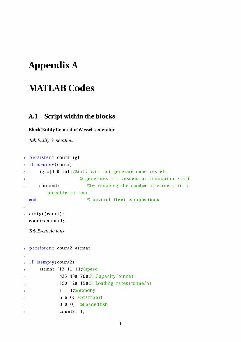
Appendix A
MATLAB Codes
A.1 Script within the blocks
Block(Entity Generator):Vessel Generator
Tab:Entity Generation
1 p e r s i s t e n t count i g t
2 i f isempty ( count )
3 i g t =[0 0 i n f ] ;%inf , w i l l not generate more v essel s
4 % generates a l l v esse ls at simulation s t a r t
5 count =1; %by reducing the number of zeroes , i t i s
possible to t e s t
6 end % several f l e e t compositions
7
8 dt= i g t ( count ) ;
9 count=count +1;
Tab:Event Actions
1 p e r s i s t e n t count2 attmat
2
3 i f isempty ( count2 )
4 attmat =[12 11 11;%speed
5 435 400 700;% Capacity ( tonne )
6 150 120 150;% Loading rates ( tonne/h)
7 1 1 1 ;%Standby
8 6 6 6 ; %Startport
9 0 0 0 ] ; %Loadedfish
10 count2= 1 ;
I
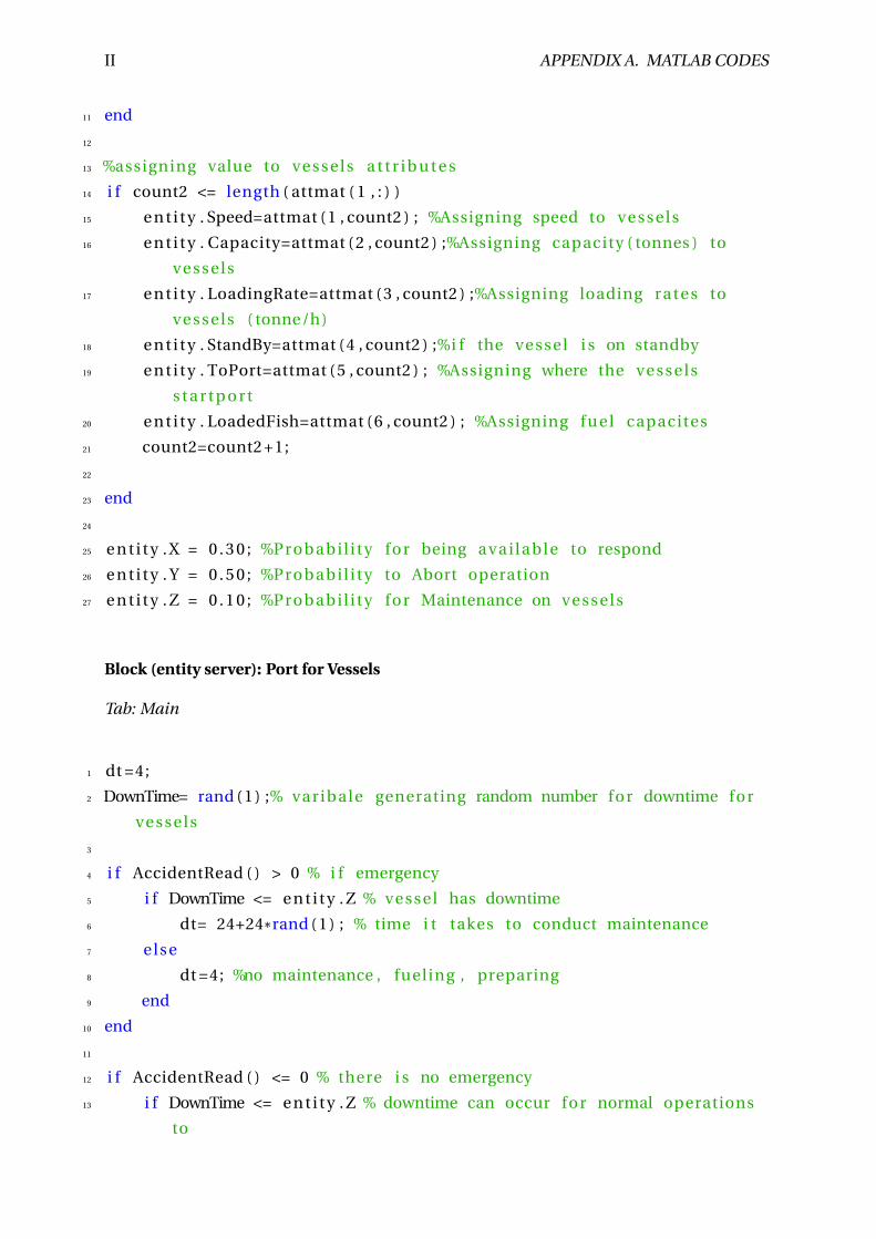
II APPENDIX A. MATLAB CODES
11 end
12
13 %assigning value to ve ssel s a t t r i b u t e s
14 i f count2 <= length ( attmat ( 1 , : ) )
15 e n t i t y . Speed=attmat ( 1 , count2 ) ; %Assigning speed to v esse ls
16 e n t i t y . Capacity=attmat ( 2 , count2 ) ;%Assigning capacity ( tonnes ) to
v esse ls
17 e n t i t y . LoadingRate=attmat ( 3 , count2 ) ;%Assigning loading rates to
v esse ls ( tonne/h)
18 e n t i t y . StandBy=attmat ( 4 , count2 ) ;%i f the vessel i s on standby
19 e n t i t y . ToPort=attmat ( 5 , count2 ) ; %Assigning where the v essel s
s t a r t p o r t
20 e n t i t y . LoadedFish=attmat ( 6 , count2 ) ; %Assigning f u e l capacites
21 count2=count2 +1;
22
23 end
24
25 e n t i t y . X = 0 . 3 0 ; %Probabi l i ty for being a v a i l a b l e to respond
26 e n t i t y . Y = 0 . 5 0 ; %Probabi l i ty to Abort operation
27 e n t i t y . Z = 0 . 1 0 ; %Probabi l i ty for Maintenance on v esse ls
Block (entity server): Port for Vessels
Tab: Main
1 dt =4;
2 DownTime= rand ( 1 ) ;% varibale generating random number for downtime for
v esse ls
3
4 i f AccidentRead ( ) > 0 % i f emergency
5 i f DownTime <= e n t i t y . Z % vessel has downtime
6 dt= 24+24*rand ( 1 ) ; % time i t takes to conduct maintenance
7 else
8 dt =4; %no maintenance , fueling , preparing
9 end
10 end
11
12 i f AccidentRead ( ) <= 0 % there i s no emergency
13 i f DownTime <= e n t i t y . Z % downtime can occur for normal operations
to
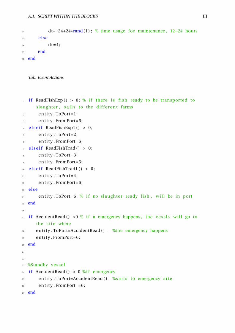
A.1. SCRIPT WITHIN THE BLOCKS III
14 dt= 24+24*rand ( 1 ) ; % time usage for maintenance , 12−24 hours
15 else
16 dt =4;
17 end
18 end
Tab: Event Actions
1 i f ReadFishExp ( ) > 0 ; % i f there i s f i s h ready to be transported to
slaughter , s a i l s to the d i f f e r e n t farms
2 e n t i t y . ToPort =1;
3 e n t i t y . FromPort=6;
4 e l s e i f ReadFishExp1 ( ) > 0 ;
5 e n t i t y . ToPort =2;
6 e n t i t y . FromPort=6;
7 e l s e i f ReadFishTrad ( ) > 0 ;
8 e n t i t y . ToPort =3;
9 e n t i t y . FromPort=6;
10 e l s e i f ReadFishTrad1 ( ) > 0 ;
11 e n t i t y . ToPort =4;
12 e n t i t y . FromPort=6;
13 else
14 e n t i t y . ToPort =6; % i f no slaughter ready fish , w i l l be in port
15 end
16
17 i f AccidentRead ( ) >0 % i f a emergency happens , the v e s s l s w i l l go to
the s i t e where
18 e n t i t y . ToPort=AccidentRead ( ) ; %the emergency happens
19 e n t i t y . FromPort=6;
20 end
21
22
23 %Standby vessel
24 i f AccidentRead ( ) > 0 %i f emergency
25 e n t i t y . ToPort=AccidentRead ( ) ; %s a i l s to emergency s i t e
26 e n t i t y . FromPort =6;
27 end
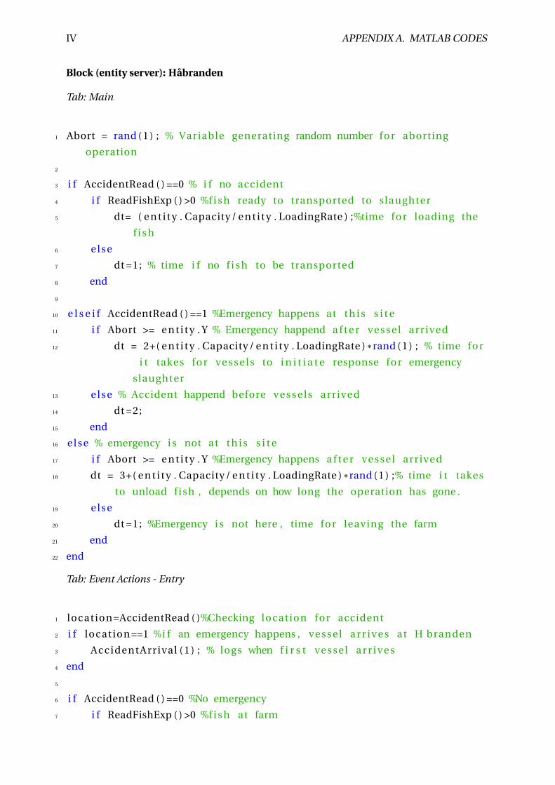
IV APPENDIX A. MATLAB CODES
Block (entity server): Håbranden
Tab: Main
1 Abort = rand ( 1 ) ; % Variable generating random number for aborting
operation
2
3 i f AccidentRead ( ) ==0 % i f no accident
4 i f ReadFishExp ( ) >0 %f i s h ready to transported to slaughter
5 dt= ( e n t i t y . Capacity / e n t i t y . LoadingRate ) ;%time for loading the
f i s h
6 else
7 dt =1; % time i f no f i s h to be transported
8 end
9
10 e l s e i f AccidentRead ( ) ==1 %Emergency happens at t h i s s i t e
11 i f Abort >= e n t i t y . Y % Emergency happend a f t e r vessel arrived
12 dt = 2+( e n t i t y . Capacity / e n t i t y . LoadingRate ) * rand ( 1 ) ; % time for
i t takes for v esse ls to i n i t i a t e response for emergency
slaughter
13 else % Accident happend before v ess els arrived
14 dt =2;
15 end
16 else % emergency i s not at t h i s s i t e
17 i f Abort >= e n t i t y . Y %Emergency happens a f t e r vessel arrived
18 dt = 3+( e n t i t y . Capacity / e n t i t y . LoadingRate ) * rand ( 1 ) ;% time i t takes
to unload fish , depends on how long the operation has gone .
19 else
20 dt =1; %Emergency i s not here , time for leaving the farm
21 end
22 end
Tab: Event Actions - Entry
1 location=AccidentRead ( )%Checking location for accident
2 i f location==1 %i f an emergency happens , vessel a r r i v e s at H branden
3 AccidentArrival ( 1 ) ; % logs when f i r s t vessel a r r i v e s
4 end
5
6 i f AccidentRead ( ) ==0 %No emergency
7 i f ReadFishExp ( ) >0 %f i s h at farm
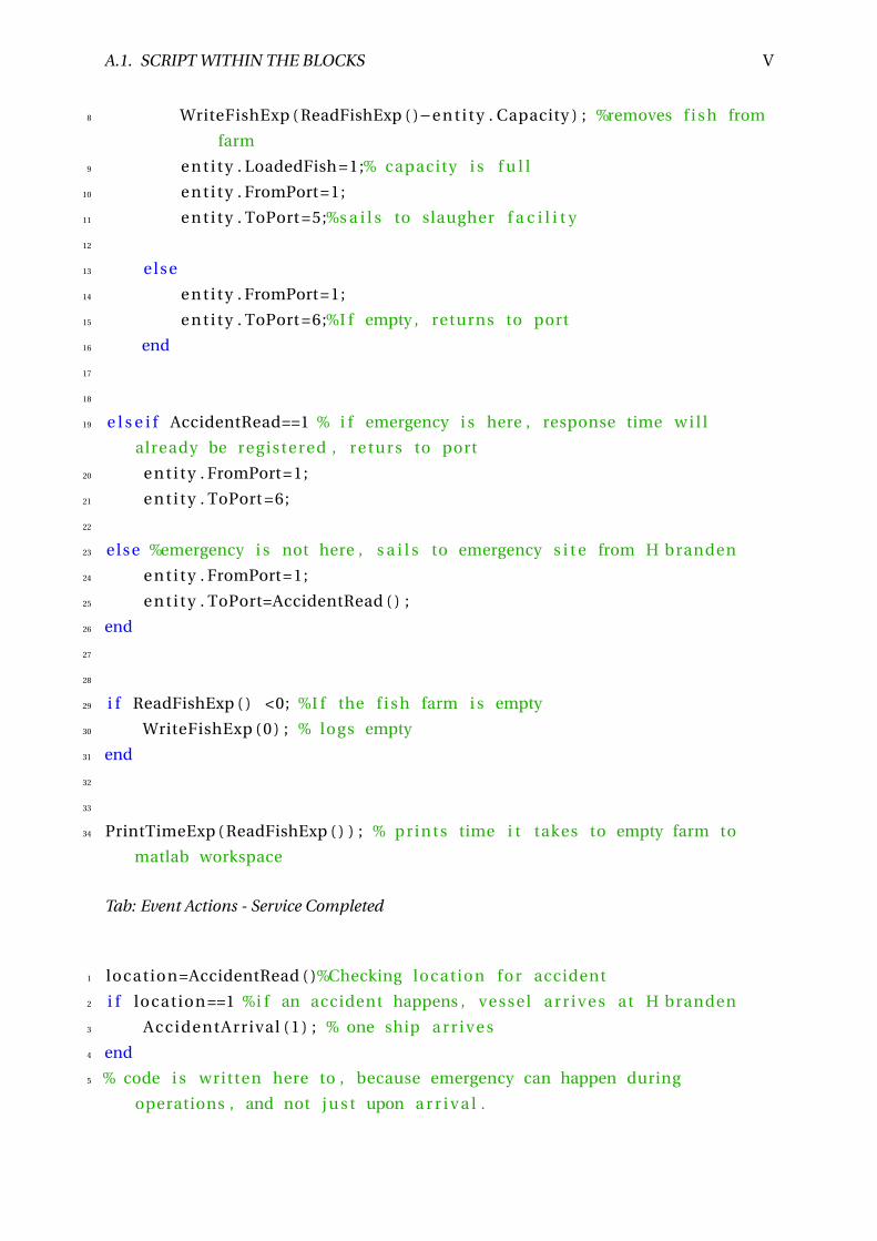
A.1. SCRIPT WITHIN THE BLOCKS V
8 WriteFishExp ( ReadFishExp ( )−e n t i t y . Capacity ) ; %removes f i s h from
farm
9 e n t i t y . LoadedFish =1;% capacity i s f u l l
10 e n t i t y . FromPort=1;
11 e n t i t y . ToPort =5;%s a i l s to slaugher f a c i l i t y
12
13 else
14 e n t i t y . FromPort=1;
15 e n t i t y . ToPort =6;%I f empty , returns to port
16 end
17
18
19 e l s e i f AccidentRead==1 % i f emergency i s here , response time w i l l
already be registered , returs to port
20 e n t i t y . FromPort=1;
21 e n t i t y . ToPort =6;
22
23 else %emergency i s not here , s a i l s to emergency s i t e from H branden
24 e n t i t y . FromPort=1;
25 e n t i t y . ToPort=AccidentRead ( ) ;
26 end
27
28
29 i f ReadFishExp ( ) <0; %I f the f i s h farm i s empty
30 WriteFishExp ( 0 ) ; % logs empty
31 end
32
33
34 PrintTimeExp ( ReadFishExp ( ) ) ; % prints time i t takes to empty farm to
matlab workspace
Tab: Event Actions - Service Completed
1 location=AccidentRead ( )%Checking location for accident
2 i f location==1 %i f an accident happens , vessel a r r i v e s at H branden
3 AccidentArrival ( 1 ) ; % one ship a r r i v e s
4 end
5 % code i s written here to , because emergency can happen during
operations , and not j u s t upon a r r i v a l .
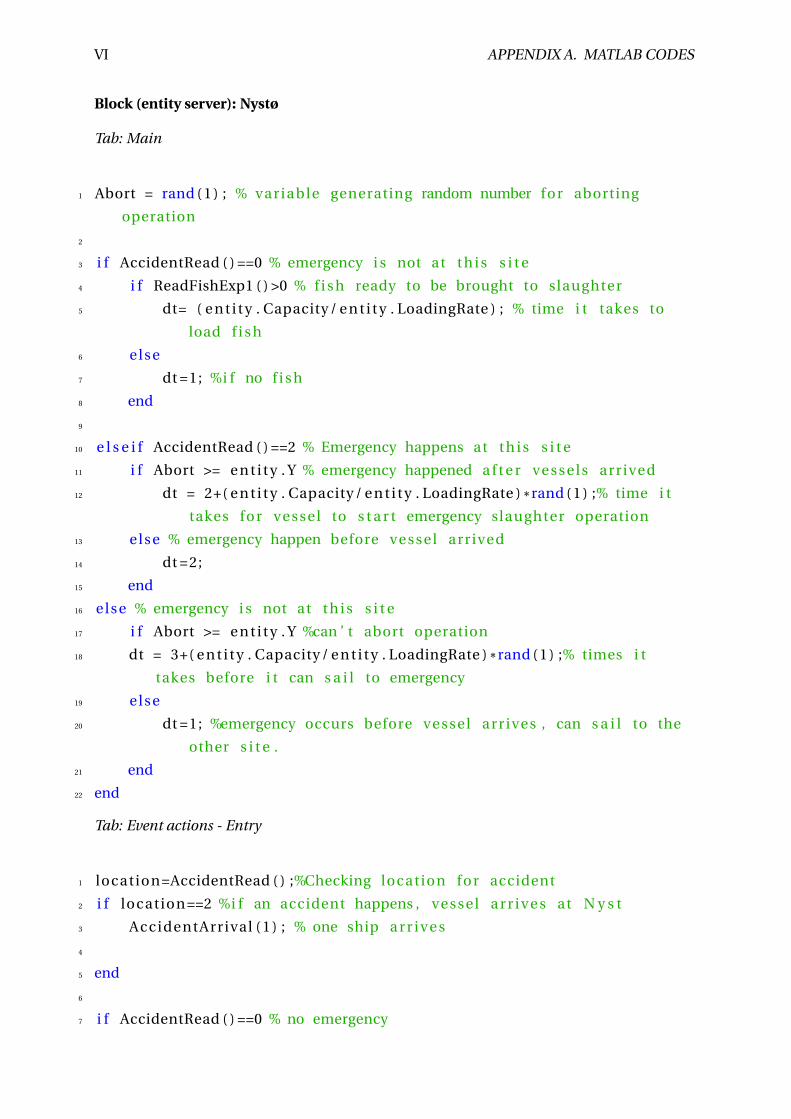
VI APPENDIX A. MATLAB CODES
Block (entity server): Nystø
Tab: Main
1 Abort = rand ( 1 ) ; % variable generating random number for aborting
operation
2
3 i f AccidentRead ( ) ==0 % emergency i s not at t h i s s i t e
4 i f ReadFishExp1 ( ) >0 % f i s h ready to be brought to slaughter
5 dt= ( e n t i t y . Capacity / e n t i t y . LoadingRate ) ; % time i t takes to
load f i s h
6 else
7 dt =1; %i f no f i s h
8 end
9
10 e l s e i f AccidentRead ( ) ==2 % Emergency happens at t h i s s i t e
11 i f Abort >= e n t i t y . Y % emergency happened a f t e r v esse ls arrived
12 dt = 2+( e n t i t y . Capacity / e n t i t y . LoadingRate ) * rand ( 1 ) ;% time i t
takes for vessel to s t a r t emergency slaughter operation
13 else % emergency happen before vessel arrived
14 dt =2;
15 end
16 else % emergency i s not at t h i s s i t e
17 i f Abort >= e n t i t y . Y %can ’ t abort operation
18 dt = 3+( e n t i t y . Capacity / e n t i t y . LoadingRate ) * rand ( 1 ) ;% times i t
takes before i t can s a i l to emergency
19 else
20 dt =1; %emergency occurs before vessel arr ives , can s a i l to the
other s i t e .
21 end
22 end
Tab: Event actions - Entry
1 location=AccidentRead ( ) ;%Checking location for accident
2 i f location==2 %i f an accident happens , vessel a r r i v e s at N y s t
3 AccidentArrival ( 1 ) ; % one ship a r r i v e s
4
5 end
6
7 i f AccidentRead ( ) ==0 % no emergency
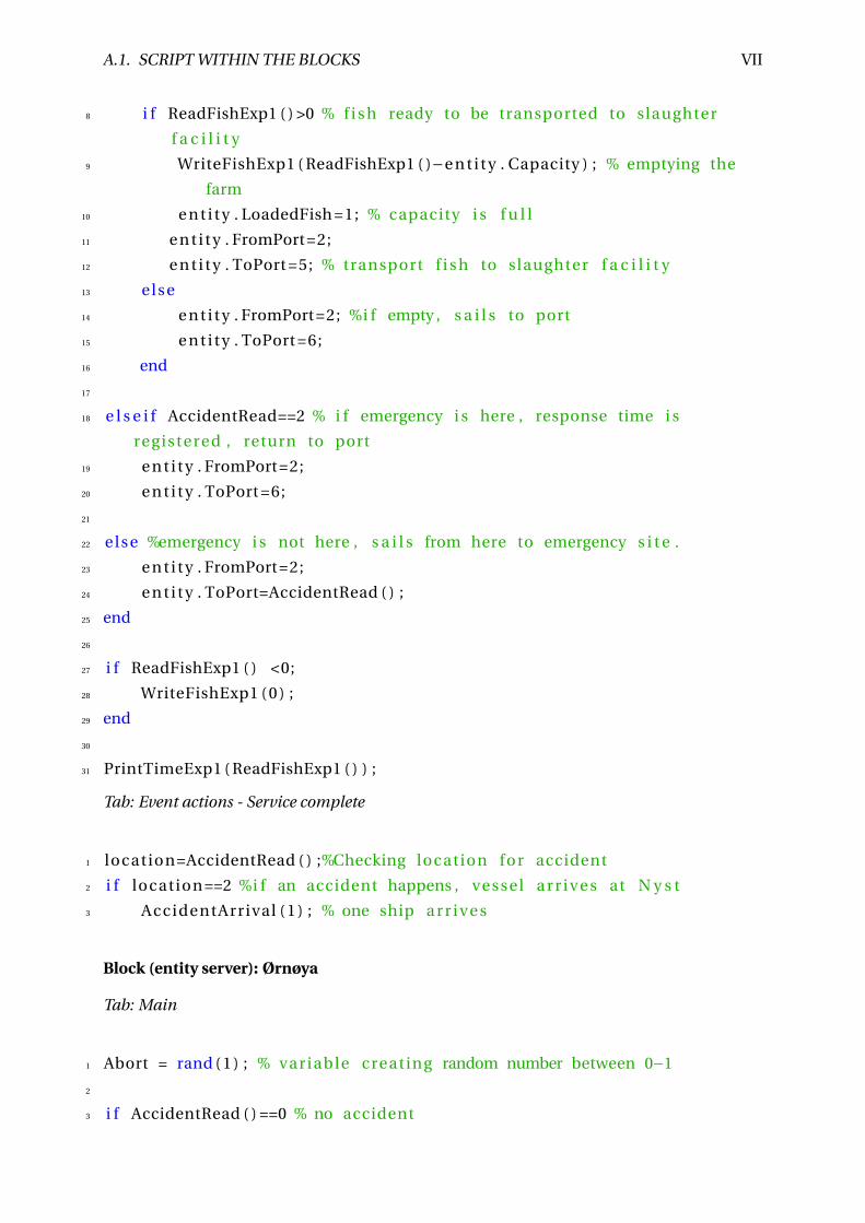
A.1. SCRIPT WITHIN THE BLOCKS VII
8 i f ReadFishExp1 ( ) >0 % f i s h ready to be transported to slaughter
f a c i l i t y
9 WriteFishExp1 ( ReadFishExp1 ( )−e n t i t y . Capacity ) ; % emptying the
farm
10 e n t i t y . LoadedFish =1; % capacity i s f u l l
11 e n t i t y . FromPort=2;
12 e n t i t y . ToPort =5; % transport f i s h to slaughter f a c i l i t y
13 else
14 e n t i t y . FromPort=2; %i f empty , s a i l s to port
15 e n t i t y . ToPort =6;
16 end
17
18 e l s e i f AccidentRead==2 % i f emergency i s here , response time i s
registered , return to port
19 e n t i t y . FromPort=2;
20 e n t i t y . ToPort =6;
21
22 else %emergency i s not here , s a i l s from here to emergency s i t e .
23 e n t i t y . FromPort=2;
24 e n t i t y . ToPort=AccidentRead ( ) ;
25 end
26
27 i f ReadFishExp1 ( ) <0;
28 WriteFishExp1 ( 0 ) ;
29 end
30
31 PrintTimeExp1 ( ReadFishExp1 ( ) ) ;
Tab: Event actions - Service complete
1 location=AccidentRead ( ) ;%Checking location for accident
2 i f location==2 %i f an accident happens , vessel a r r i v e s at N y s t
3 AccidentArrival ( 1 ) ; % one ship a r r i v e s
Block (entity server): Ørnøya
Tab: Main
1 Abort = rand ( 1 ) ; % variable creating random number between 0−1
2
3 i f AccidentRead ( ) ==0 % no accident
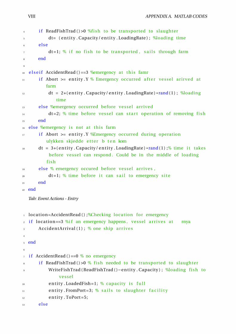
VIII APPENDIX A. MATLAB CODES
4 i f ReadFishTrad ( ) >0 %f i s h to be transported to slaughter
5 dt= ( e n t i t y . Capacity / e n t i t y . LoadingRate ) ; %loading time
6 else
7 dt =1; % i f no f i s h to be transported , s a i l s through farm
8 end
9
10 e l s e i f AccidentRead ( ) ==3 %emergency at t h i s famr
11 i f Abort >= e n t i t y . Y % Emergency occurred a f t e r vessel arirved at
farm
12 dt = 2+( e n t i t y . Capacity / e n t i t y . LoadingRate ) * rand ( 1 ) ; %loading
time
13 else %emergency occurred before vessel arrived
14 dt =2; % time before vessel can s t a r t operation of removing f i s h
15 end
16 else %emergency i s not at t h i s farm
17 i f Abort >= e n t i t y . Y %Emergency occurred during operation
ulykken skjedde e t t e r b t e n kom
18 dt = 3+( e n t i t y . Capacity / e n t i t y . LoadingRate ) * rand ( 1 ) ;% time i t takes
before vessel can respond . Could be in the middle of loading
f i s h
19 else % emergency occured before vessel arr ives ,
20 dt =1; % time before i t can s a i l to emergency s i t e
21 end
22 end
Tab: Event Actions - Entry
1 location=AccidentRead ( ) ;%Checking location for emergency
2 i f location==3 %i f an emergency happens , vessel a r r i v e s at rnya
3 AccidentArrival ( 1 ) ; % one ship a r r i v e s
4
5 end
6
7 i f AccidentRead ( ) ==0 % no emergency
8 i f ReadFishTrad ( ) >0 % f i s h needed to be transported to slaughter
9 WriteFishTrad ( ReadFishTrad ( )−e n t i t y . Capacity ) ; %loading f i s h to
vessel
10 e n t i t y . LoadedFish =1; % capacity i s f u l l
11 e n t i t y . FromPort=3; % s a i l s to slaughter f a c i l i t y
12 e n t i t y . ToPort =5;
13 else
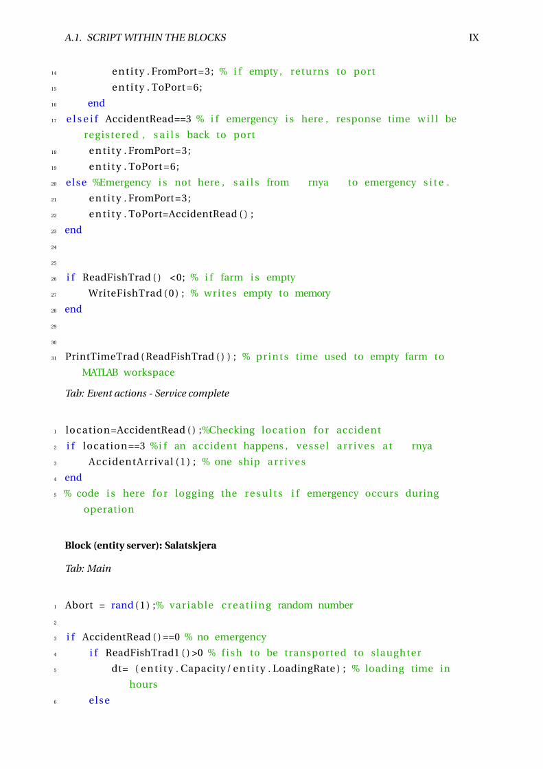
A.1. SCRIPT WITHIN THE BLOCKS IX
14 e n t i t y . FromPort=3; % i f empty , returns to port
15 e n t i t y . ToPort =6;
16 end
17 e l s e i f AccidentRead==3 % i f emergency i s here , response time w i l l be
registered , s a i l s back to port
18 e n t i t y . FromPort=3;
19 e n t i t y . ToPort =6;
20 else %Emergency i s not here , s a i l s from rnya to emergency s i t e .
21 e n t i t y . FromPort=3;
22 e n t i t y . ToPort=AccidentRead ( ) ;
23 end
24
25
26 i f ReadFishTrad ( ) <0; % i f farm i s empty
27 WriteFishTrad ( 0 ) ; % writes empty to memory
28 end
29
30
31 PrintTimeTrad ( ReadFishTrad ( ) ) ; % prints time used to empty farm to
MATLAB workspace
Tab: Event actions - Service complete
1 location=AccidentRead ( ) ;%Checking location for accident
2 i f location==3 %i f an accident happens , vessel a r r i v e s at rnya
3 AccidentArrival ( 1 ) ; % one ship a r r i v e s
4 end
5 % code i s here for logging the r e s u l t s i f emergency occurs during
operation
Block (entity server): Salatskjera
Tab: Main
1 Abort = rand ( 1 ) ;% variable c r e a t i i n g random number
2
3 i f AccidentRead ( ) ==0 % no emergency
4 i f ReadFishTrad1 ( ) >0 % f i s h to be transported to slaughter
5 dt= ( e n t i t y . Capacity / e n t i t y . LoadingRate ) ; % loading time in
hours
6 else
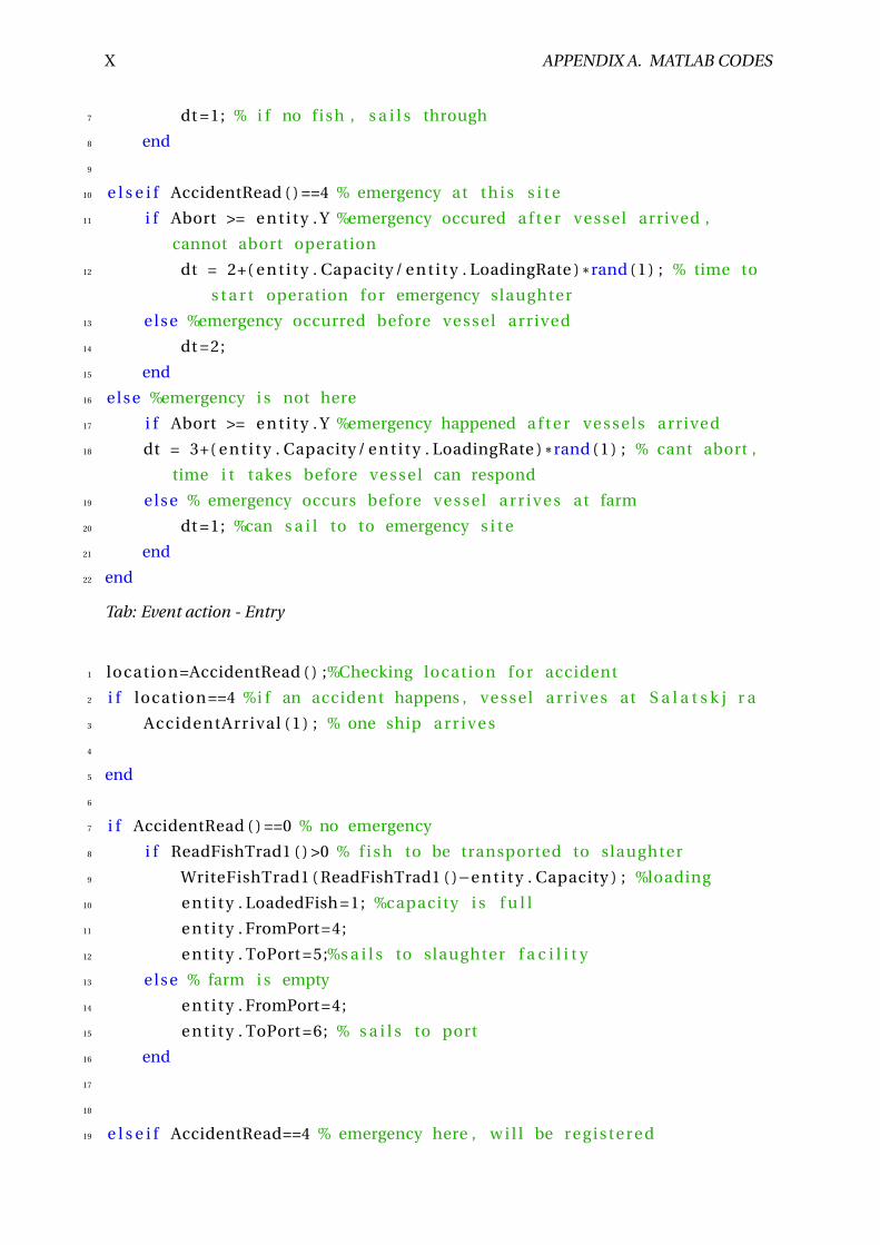
X APPENDIX A. MATLAB CODES
7 dt =1; % i f no fish , s a i l s through
8 end
9
10 e l s e i f AccidentRead ( ) ==4 % emergency at t h i s s i t e
11 i f Abort >= e n t i t y . Y %emergency occured a f t e r vessel arrived ,
cannot abort operation
12 dt = 2+( e n t i t y . Capacity / e n t i t y . LoadingRate ) * rand ( 1 ) ; % time to
s t a r t operation for emergency slaughter
13 else %emergency occurred before vessel arrived
14 dt =2;
15 end
16 else %emergency i s not here
17 i f Abort >= e n t i t y . Y %emergency happened a f t e r v esse ls arrived
18 dt = 3+( e n t i t y . Capacity / e n t i t y . LoadingRate ) * rand ( 1 ) ; % cant abort ,
time i t takes before vessel can respond
19 else % emergency occurs before vessel a r r i v e s at farm
20 dt =1; %can s a i l to to emergency s i t e
21 end
22 end
Tab: Event action - Entry
1 location=AccidentRead ( ) ;%Checking location for accident
2 i f location==4 %i f an accident happens , vessel a r r i v e s at S a l a t s k j r a
3 AccidentArrival ( 1 ) ; % one ship a r r i v e s
4
5 end
6
7 i f AccidentRead ( ) ==0 % no emergency
8 i f ReadFishTrad1 ( ) >0 % f i s h to be transported to slaughter
9 WriteFishTrad1 ( ReadFishTrad1 ( )−e n t i t y . Capacity ) ; %loading
10 e n t i t y . LoadedFish =1; %capacity i s f u l l
11 e n t i t y . FromPort=4;
12 e n t i t y . ToPort =5;%s a i l s to slaughter f a c i l i t y
13 else % farm i s empty
14 e n t i t y . FromPort=4;
15 e n t i t y . ToPort =6; % s a i l s to port
16 end
17
18
19 e l s e i f AccidentRead==4 % emergency here , w i l l be registered
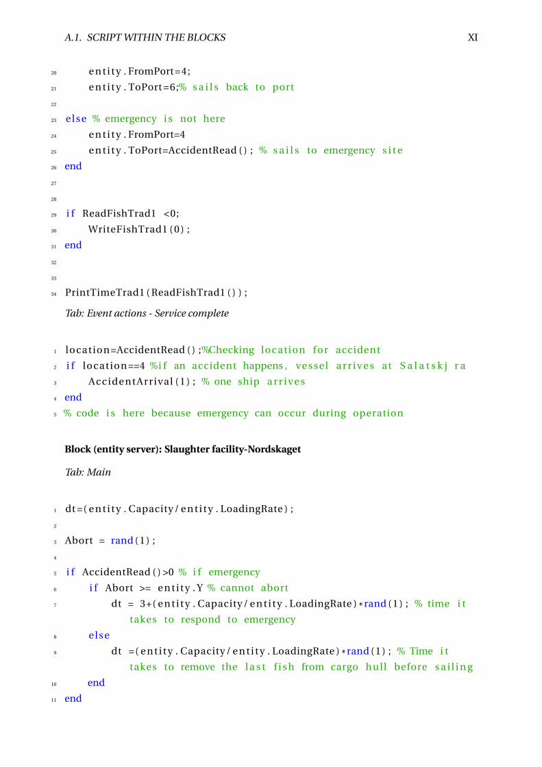
A.1. SCRIPT WITHIN THE BLOCKS XI
20 e n t i t y . FromPort=4;
21 e n t i t y . ToPort =6;% s a i l s back to port
22
23 else % emergency i s not here
24 e n t i t y . FromPort=4
25 e n t i t y . ToPort=AccidentRead ( ) ; % s a i l s to emergency s i t e
26 end
27
28
29 i f ReadFishTrad1 <0;
30 WriteFishTrad1 ( 0 ) ;
31 end
32
33
34 PrintTimeTrad1 ( ReadFishTrad1 ( ) ) ;
Tab: Event actions - Service complete
1 location=AccidentRead ( ) ;%Checking location for accident
2 i f location==4 %i f an accident happens , vessel a r r i v e s at S a l a t s k j r a
3 AccidentArrival ( 1 ) ; % one ship a r r i v e s
4 end
5 % code i s here because emergency can occur during operation
Block (entity server): Slaughter facility-Nordskaget
Tab: Main
1 dt =( e n t i t y . Capacity / e n t i t y . LoadingRate ) ;
2
3 Abort = rand ( 1 ) ;
4
5 i f AccidentRead ( ) >0 % i f emergency
6 i f Abort >= e n t i t y . Y % cannot abort
7 dt = 3+( e n t i t y . Capacity / e n t i t y . LoadingRate ) * rand ( 1 ) ; % time i t
takes to respond to emergency
8 else
9 dt =( e n t i t y . Capacity / e n t i t y . LoadingRate ) * rand ( 1 ) ; % Time i t
takes to remove the l a s t f i s h from cargo hull before s a i l i n g
10 end
11 end
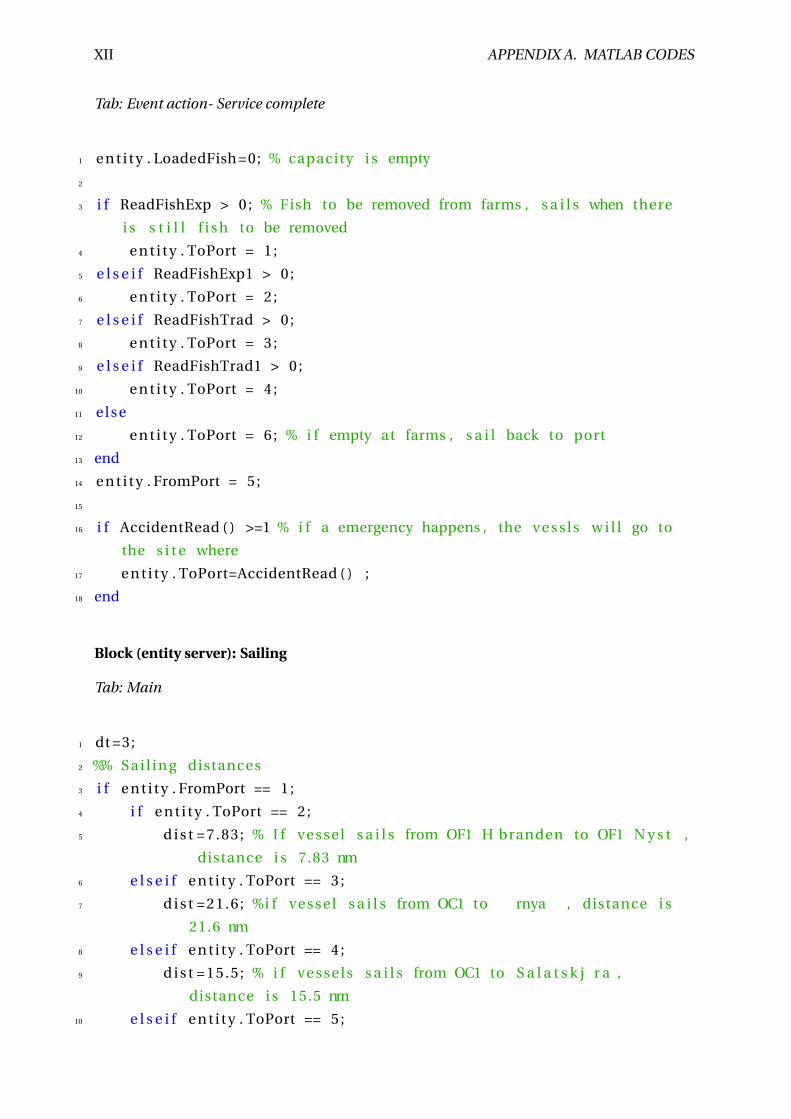
XII APPENDIX A. MATLAB CODES
Tab: Event action- Service complete
1 e n t i t y . LoadedFish =0; % capacity i s empty
2
3 i f ReadFishExp > 0 ; % Fish to be removed from farms , s a i l s when there
i s s t i l l f i s h to be removed
4 e n t i t y . ToPort = 1 ;
5 e l s e i f ReadFishExp1 > 0 ;
6 e n t i t y . ToPort = 2 ;
7 e l s e i f ReadFishTrad > 0 ;
8 e n t i t y . ToPort = 3 ;
9 e l s e i f ReadFishTrad1 > 0 ;
10 e n t i t y . ToPort = 4 ;
11 else
12 e n t i t y . ToPort = 6 ; % i f empty at farms , s a i l back to port
13 end
14 e n t i t y . FromPort = 5 ;
15
16 i f AccidentRead ( ) >=1 % i f a emergency happens , the v e s s l s w i l l go to
the s i t e where
17 e n t i t y . ToPort=AccidentRead ( ) ;
18 end
Block (entity server): Sailing
Tab: Main
1 dt =3;
2 %% S a i l i n g distances
3 i f e n t i t y . FromPort == 1 ;
4 i f e n t i t y . ToPort == 2 ;
5 d i s t =7.83; % I f vessel s a i l s from OF1 H branden to OF1 N y s t ,
distance i s 7.83 nm
6 e l s e i f e n t i t y . ToPort == 3 ;
7 d i s t =21.6; %i f vessel s a i l s from OC1 to rnya , distance i s
21.6 nm
8 e l s e i f e n t i t y . ToPort == 4 ;
9 d i s t =15.5; % i f ves sel s s a i l s from OC1 to S a l a t s k j r a ,
distance i s 15.5 nm
10 e l s e i f e n t i t y . ToPort == 5 ;
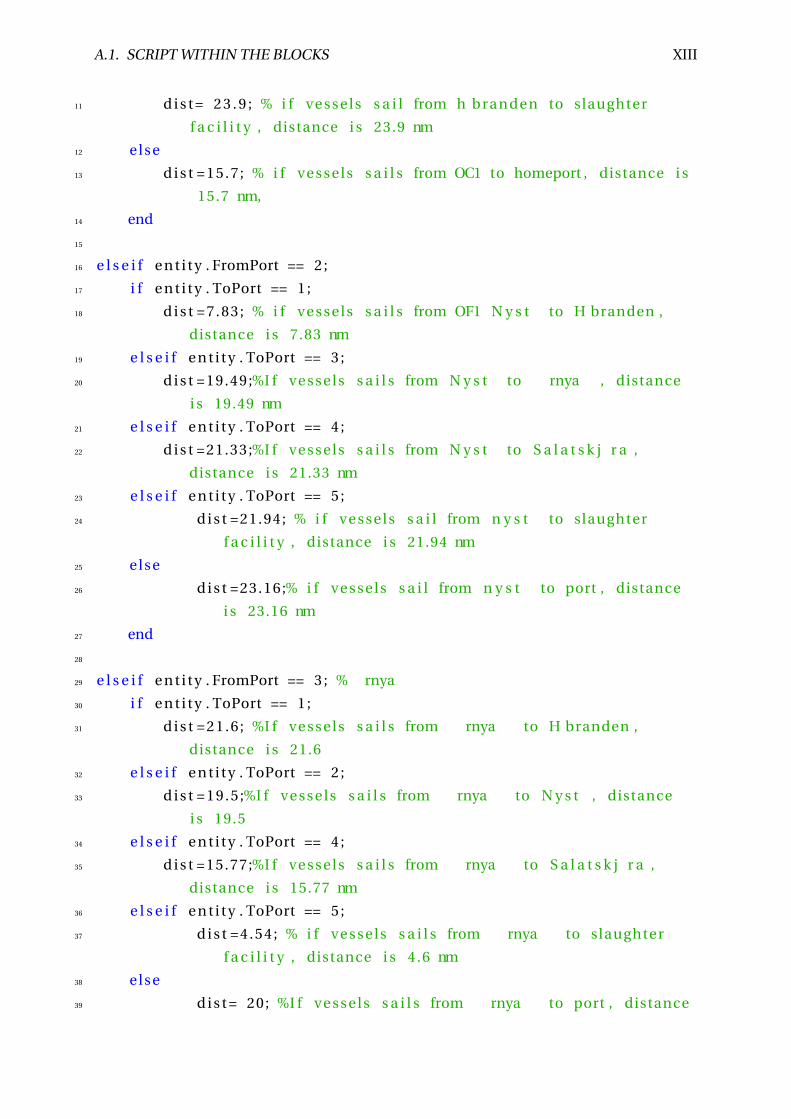
A.1. SCRIPT WITHIN THE BLOCKS XIII
11 d i s t = 2 3 . 9 ; % i f v ess el s s a i l from h branden to slaughter
f a c i l i t y , distance i s 23.9 nm
12 else
13 d i s t =15.7; % i f ves sel s s a i l s from OC1 to homeport , distance i s
15.7 nm,
14 end
15
16 e l s e i f e n t i t y . FromPort == 2 ;
17 i f e n t i t y . ToPort == 1 ;
18 d i s t =7.83; % i f ves sel s s a i l s from OF1 N y s t to H branden ,
distance i s 7.83 nm
19 e l s e i f e n t i t y . ToPort == 3 ;
20 d i s t =19.49;%I f ve ssel s s a i l s from N y s t to rnya , distance
i s 19.49 nm
21 e l s e i f e n t i t y . ToPort == 4 ;
22 d i s t =21.33;%I f ve ssel s s a i l s from N y s t to S a l a t s k j r a ,
distance i s 21.33 nm
23 e l s e i f e n t i t y . ToPort == 5 ;
24 d i s t =21.94; % i f v ess el s s a i l from n y s t to slaughter
f a c i l i t y , distance i s 21.94 nm
25 else
26 d i s t =23.16;% i f v es sel s s a i l from n y s t to port , distance
i s 23.16 nm
27 end
28
29 e l s e i f e n t i t y . FromPort == 3 ; % rnya
30 i f e n t i t y . ToPort == 1 ;
31 d i s t =21.6; %I f ve ssel s s a i l s from rnya to H branden ,
distance i s 21.6
32 e l s e i f e n t i t y . ToPort == 2 ;
33 d i s t =19.5;%I f ve ssel s s a i l s from rnya to N y s t , distance
i s 19.5
34 e l s e i f e n t i t y . ToPort == 4 ;
35 d i s t =15.77;%I f ve ssel s s a i l s from rnya to S a l a t s k j r a ,
distance i s 15.77 nm
36 e l s e i f e n t i t y . ToPort == 5 ;
37 d i s t =4.54; % i f ves sel s s a i l s from rnya to slaughter
f a c i l i t y , distance i s 4.6 nm
38 else
39 d i s t = 20; %I f ve ssel s s a i l s from rnya to port , distance
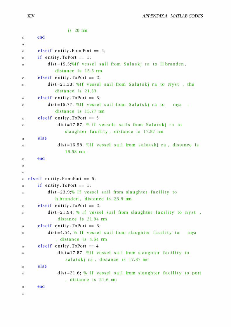
XIV APPENDIX A. MATLAB CODES
i s 20 nm
40 end
41
42 e l s e i f e n t i t y . FromPort == 4 ;
43 i f e n t i t y . ToPort == 1 ;
44 d i s t =15.5;%I f vessel s a i l from S a l a s k j r a to H branden ,
distance i s 15.5 nm
45 e l s e i f e n t i t y . ToPort == 2 ;
46 d i s t =21.33; %I f vessel s a i l from S a l a t s k j r a to N y s t , the
distance i s 21.33
47 e l s e i f e n t i t y . ToPort == 3 ;
48 d i s t =15.77; %I f vessel s a i l from S a l a t s k j r a to rnya ,
distance i s 15.77 nm
49 e l s e i f e n t i t y . ToPort == 5
50 d i s t =17.87; % i f v ess el s s a i l s from S a l a t s k j r a to
slaughter f a c i l i t y , distance i s 17.87 nm
51 else
52 d i s t =16.58; %I f vessel s a i l from s a l a t s k j r a , distance i s
16.58 nm
53 end
54
55
56 e l s e i f e n t i t y . FromPort == 5 ;
57 i f e n t i t y . ToPort == 1 ;
58 d i s t =23.9;% I f vessel s a i l from slaughter f a c i l i t y to
h branden , distance i s 23.9 nm
59 e l s e i f e n t i t y . ToPort == 2 ;
60 d i s t =21.94; % I f vessel s a i l from slaughter f a c i l i t y to n y s t ,
distance i s 21.94 nm
61 e l s e i f e n t i t y . ToPort == 3 ;
62 d i s t =4.54; % I f vessel s a i l from slaughter f a c i l i t y to rnya
, distance i s 4.54 nm
63 e l s e i f e n t i t y . ToPort == 4
64 d i s t =17.87; %I f vessel s a i l from slaughter f a c i l i t y to
s a l a t s k j r a , distance i s 17.87 nm
65 else
66 d i s t =21.6; % I f vessel s a i l from slaughter f a c i l i t y to port
, distance i s 21.6 nm
67 end
68
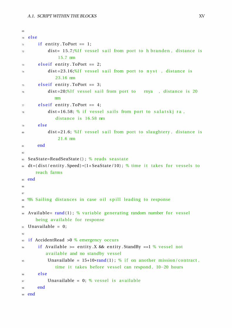
A.1. SCRIPT WITHIN THE BLOCKS XV
69
70 else
71 i f e n t i t y . ToPort == 1 ;
72 d i s t = 1 5 . 7 ;%I f vessel s a i l from port to h branden , distance i s
15.7 nm
73 e l s e i f e n t i t y . ToPort == 2 ;
74 d i s t =23.16;%I f vessel s a i l from port to n y s t , distance i s
23.16 nm
75 e l s e i f e n t i t y . ToPort == 3 ;
76 d i s t =20;%I f vessel s a i l from port to rnya , distance i s 20
nm
77 e l s e i f e n t i t y . ToPort == 4 ;
78 d i s t =16.58; % i f vessel s a i l s from port to s a l a t s k j r a ,
distance i s 16.58 nm
79 else
80 d i s t =21.6; %I f vessel s a i l from port to slaughtery , distance i s
21.6 nm
81 end
82
83 SeaState=ReadSeaState ( ) ; % reads seastate
84 dt =( d i s t / e n t i t y . Speed ) *(1+ SeaState /10) ; % time i t takes for ve ssel s to
reach farms
85 end
86
87
88 %% S a i l i n g distances in case o i l s p i l l leading to response
89
90 Available= rand ( 1 ) ; % variable generating random number for vessel
being a v a i l a b l e for response
91 Unavailable = 0 ;
92
93 i f AccidentRead >0 % emergency occurs
94 i f Avai lable >= e n t i t y . X && e n t i t y . StandBy ==1 % vessel not
a v a i l a b l e and no standby vessel
95 Unavailable = 15+10*rand ( 1 ) ; % i f on another mission/ contract ,
time i t takes before vessel can respond , 10−20 hours
96 else
97 Unavailable = 0 ; % vessel i s a v ai l a b l e
98 end
99 end
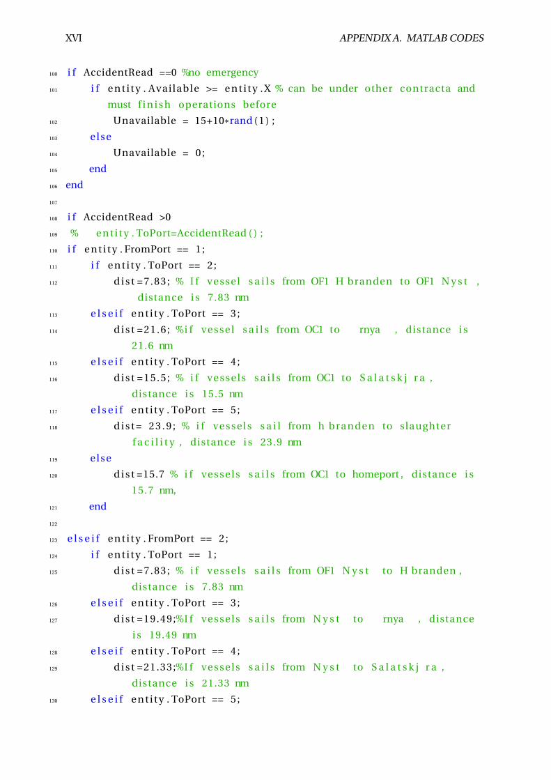
XVI APPENDIX A. MATLAB CODES
100 i f AccidentRead ==0 %no emergency
101 i f e n t i t y . Avai lable >= e n t i t y . X % can be under other contracta and
must f i n i s h operations before
102 Unavailable = 15+10*rand ( 1 ) ;
103 else
104 Unavailable = 0 ;
105 end
106 end
107
108 i f AccidentRead >0
109 % e n t i t y . ToPort=AccidentRead ( ) ;
110 i f e n t i t y . FromPort == 1 ;
111 i f e n t i t y . ToPort == 2 ;
112 d i s t =7.83; % I f vessel s a i l s from OF1 H branden to OF1 N y s t ,
distance i s 7.83 nm
113 e l s e i f e n t i t y . ToPort == 3 ;
114 d i s t =21.6; %i f vessel s a i l s from OC1 to rnya , distance i s
21.6 nm
115 e l s e i f e n t i t y . ToPort == 4 ;
116 d i s t =15.5; % i f ves sel s s a i l s from OC1 to S a l a t s k j r a ,
distance i s 15.5 nm
117 e l s e i f e n t i t y . ToPort == 5 ;
118 d i s t = 2 3 . 9 ; % i f v ess el s s a i l from h branden to slaughter
f a c i l i t y , distance i s 23.9 nm
119 else
120 d i s t =15.7 % i f ve ssel s s a i l s from OC1 to homeport , distance i s
15.7 nm,
121 end
122
123 e l s e i f e n t i t y . FromPort == 2 ;
124 i f e n t i t y . ToPort == 1 ;
125 d i s t =7.83; % i f ves sel s s a i l s from OF1 N y s t to H branden ,
distance i s 7.83 nm
126 e l s e i f e n t i t y . ToPort == 3 ;
127 d i s t =19.49;%I f ve ssel s s a i l s from N y s t to rnya , distance
i s 19.49 nm
128 e l s e i f e n t i t y . ToPort == 4 ;
129 d i s t =21.33;%I f ve ssel s s a i l s from N y s t to S a l a t s k j r a ,
distance i s 21.33 nm
130 e l s e i f e n t i t y . ToPort == 5 ;
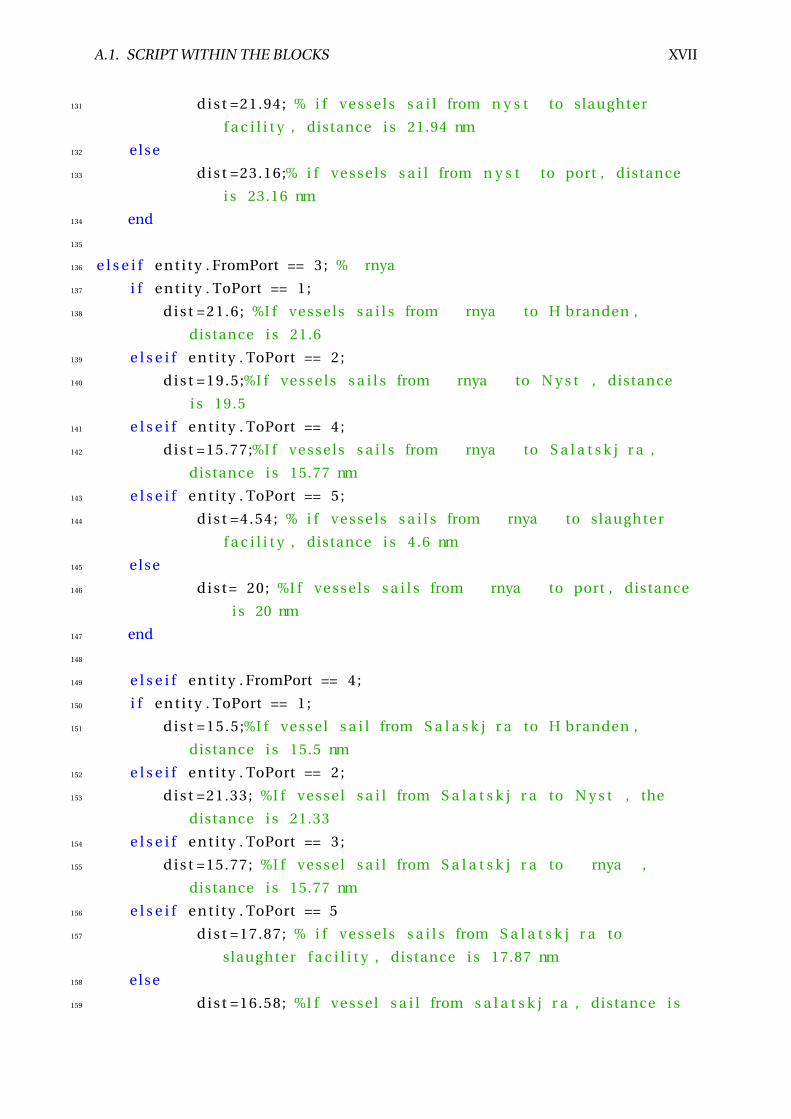
A.1. SCRIPT WITHIN THE BLOCKS XVII
131 d i s t =21.94; % i f v es sel s s a i l from n y s t to slaughter
f a c i l i t y , distance i s 21.94 nm
132 else
133 d i s t =23.16;% i f ve ssel s s a i l from n y s t to port , distance
i s 23.16 nm
134 end
135
136 e l s e i f e n t i t y . FromPort == 3 ; % rnya
137 i f e n t i t y . ToPort == 1 ;
138 d i s t =21.6; %I f ve ssel s s a i l s from rnya to H branden ,
distance i s 21.6
139 e l s e i f e n t i t y . ToPort == 2 ;
140 d i s t =19.5;%I f ve ssel s s a i l s from rnya to N y s t , distance
i s 19.5
141 e l s e i f e n t i t y . ToPort == 4 ;
142 d i s t =15.77;%I f ve ssel s s a i l s from rnya to S a l a t s k j r a ,
distance i s 15.77 nm
143 e l s e i f e n t i t y . ToPort == 5 ;
144 d i s t =4.54; % i f v es sel s s a i l s from rnya to slaughter
f a c i l i t y , distance i s 4.6 nm
145 else
146 d i s t = 20; %I f ve ssel s s a i l s from rnya to port , distance
i s 20 nm
147 end
148
149 e l s e i f e n t i t y . FromPort == 4 ;
150 i f e n t i t y . ToPort == 1 ;
151 d i s t =15.5;%I f vessel s a i l from S a l a s k j r a to H branden ,
distance i s 15.5 nm
152 e l s e i f e n t i t y . ToPort == 2 ;
153 d i s t =21.33; %I f vessel s a i l from S a l a t s k j r a to N y s t , the
distance i s 21.33
154 e l s e i f e n t i t y . ToPort == 3 ;
155 d i s t =15.77; %I f vessel s a i l from S a l a t s k j r a to rnya ,
distance i s 15.77 nm
156 e l s e i f e n t i t y . ToPort == 5
157 d i s t =17.87; % i f v ess el s s a i l s from S a l a t s k j r a to
slaughter f a c i l i t y , distance i s 17.87 nm
158 else
159 d i s t =16.58; %I f vessel s a i l from s a l a t s k j r a , distance i s
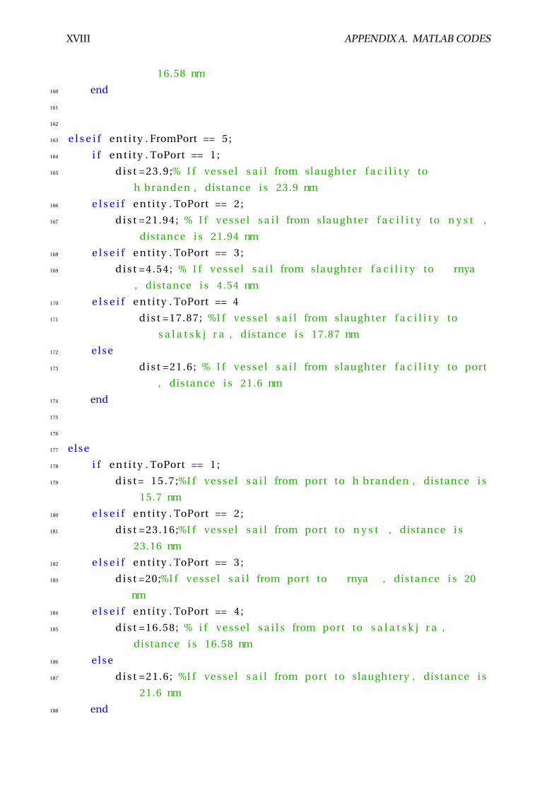
XVIII APPENDIX A. MATLAB CODES
16.58 nm
160 end
161
162
163 e l s e i f e n t i t y . FromPort == 5 ;
164 i f e n t i t y . ToPort == 1 ;
165 d i s t =23.9;% I f vessel s a i l from slaughter f a c i l i t y to
h branden , distance i s 23.9 nm
166 e l s e i f e n t i t y . ToPort == 2 ;
167 d i s t =21.94; % I f vessel s a i l from slaughter f a c i l i t y to n y s t ,
distance i s 21.94 nm
168 e l s e i f e n t i t y . ToPort == 3 ;
169 d i s t =4.54; % I f vessel s a i l from slaughter f a c i l i t y to rnya
, distance i s 4.54 nm
170 e l s e i f e n t i t y . ToPort == 4
171 d i s t =17.87; %I f vessel s a i l from slaughter f a c i l i t y to
s a l a t s k j r a , distance i s 17.87 nm
172 else
173 d i s t =21.6; % I f vessel s a i l from slaughter f a c i l i t y to port
, distance i s 21.6 nm
174 end
175
176
177 else
178 i f e n t i t y . ToPort == 1 ;
179 d i s t = 1 5 . 7 ;%I f vessel s a i l from port to h branden , distance i s
15.7 nm
180 e l s e i f e n t i t y . ToPort == 2 ;
181 d i s t =23.16;%I f vessel s a i l from port to n y s t , distance i s
23.16 nm
182 e l s e i f e n t i t y . ToPort == 3 ;
183 d i s t =20;%I f vessel s a i l from port to rnya , distance i s 20
nm
184 e l s e i f e n t i t y . ToPort == 4 ;
185 d i s t =16.58; % i f vessel s a i l s from port to s a l a t s k j r a ,
distance i s 16.58 nm
186 else
187 d i s t =21.6; %I f vessel s a i l from port to slaughtery , distance i s
21.6 nm
188 end
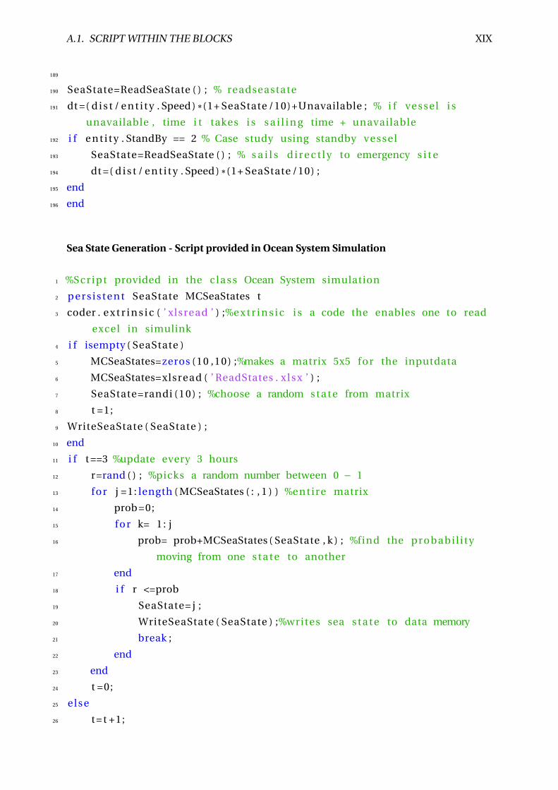
A.1. SCRIPT WITHIN THE BLOCKS XIX
189
190 SeaState=ReadSeaState ( ) ; % readseastate
191 dt =( d i s t / e n t i t y . Speed ) *(1+ SeaState /10)+Unavailable ; % i f vessel i s
unavailable , time i t takes i s s a i l i n g time + unavailable
192 i f e n t i t y . StandBy == 2 % Case study using standby vessel
193 SeaState=ReadSeaState ( ) ; % s a i l s d i r e c t l y to emergency s i t e
194 dt =( d i s t / e n t i t y . Speed ) *(1+ SeaState /10) ;
195 end
196 end
Sea State Generation - Script provided in Ocean System Simulation
1 %Script provided in the c l a s s Ocean System simulation
2 p e r s i s t e n t SeaState MCSeaStates t
3 coder . e x t r i n s i c ( ’ xlsread ’ ) ;%e x t r i n s i c i s a code the enables one to read
excel in simulink
4 i f isempty ( SeaState )
5 MCSeaStates=zeros (10 ,10) ;%makes a matrix 5x5 for the inputdata
6 MCSeaStates=xlsread ( ’ ReadStates . x l s x ’ ) ;
7 SeaState=randi (10) ; %choose a random s t a t e from matrix
8 t =1;
9 WriteSeaState ( SeaState ) ;
10 end
11 i f t ==3 %update every 3 hours
12 r=rand ( ) ; %picks a random number between 0 − 1
13 for j =1: length ( MCSeaStates ( : , 1 ) ) %entire matrix
14 prob =0;
15 for k= 1 : j
16 prob= prob+MCSeaStates ( SeaState , k ) ; %find the probabi l i ty
moving from one s t a t e to another
17 end
18 i f r <=prob
19 SeaState= j ;
20 WriteSeaState ( SeaState ) ;%writes sea s t a t e to data memory
21 break ;
22 end
23 end
24 t =0;
25 else
26 t = t +1;
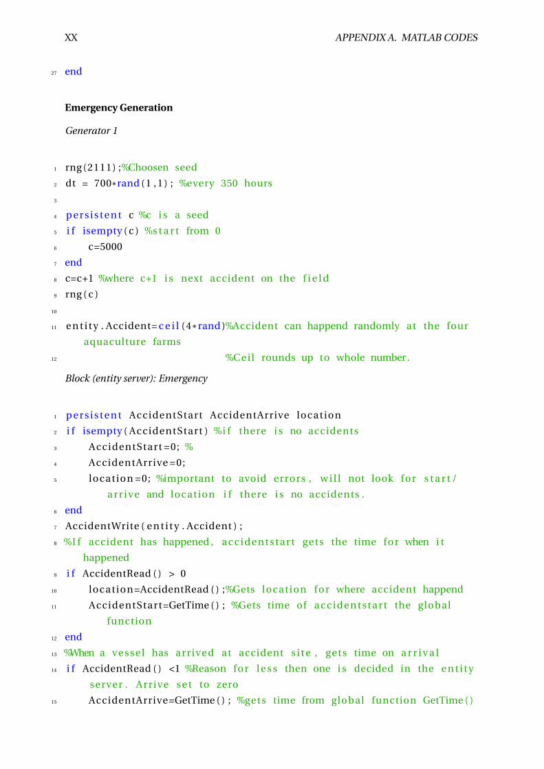
XX APPENDIX A. MATLAB CODES
27 end
Emergency Generation
Generator 1
1 rng (2111) ;%Choosen seed
2 dt = 700*rand ( 1 , 1 ) ; %every 350 hours
3
4 p e r s i s t e n t c %c i s a seed
5 i f isempty ( c ) %s t a r t from 0
6 c=5000
7 end
8 c=c+1 %where c+1 i s next accident on the f i e l d
9 rng ( c )
10
11 e n t i t y . Accident= c e i l (4* rand )%Accident can happend randomly at the four
aquaculture farms
12 %Ceil rounds up to whole number .
Block (entity server): Emergency
1 p e r s i s t e n t AccidentStart AccidentArrive location
2 i f isempty ( AccidentStart ) %i f there i s no accidents
3 AccidentStart =0; %
4 AccidentArrive =0;
5 location =0; %important to avoid errors , w i l l not look for s t a r t /
a r r i v e and location i f there i s no accidents .
6 end
7 AccidentWrite ( e n t i t y . Accident ) ;
8 %I f accident has happened , accidentstart gets the time for when i t
happened
9 i f AccidentRead ( ) > 0
10 location=AccidentRead ( ) ;%Gets location for where accident happend
11 AccidentStart=GetTime ( ) ; %Gets time of accidentstart the global
function
12 end
13 %When a vessel has arrived at accident s i t e , gets time on a r r i v a l
14 i f AccidentRead ( ) <1 %Reason for l e s s then one i s decided in the e n t i t y
server . Arrive set to zero
15 AccidentArrive=GetTime ( ) ; %gets time from global function GetTime ( )
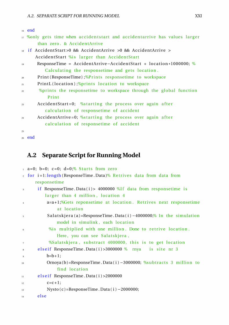
A.2. SEPARATE SCRIPT FOR RUNNING MODEL XXI
16 end
17 %only gets time when accidentstart and accidentarrive has values l a r g e r
than zero . & AccidentArrive
18 i f AccidentStart >0 && AccidentArrive >0 && AccidentArrive >
AccidentStart %i s l a r g e r than AccidentStart
19 ResponseTime = AccidentArrive−AccidentStart + location *1000000; %
Calculating the responsetime and gets location .
20 Print ( ResponseTime ) ;%Prints responsetime to workspace
21 PrintL ( location ) ;%prints location to workspace
22 %prints the responsetime to workspace through the global function
23 AccidentStart =0; %s t a r t i n g the process over again a f t e r
calculat ion of responsetime of accident
24 AccidentArrive =0; %s t a r t i n g the process over again a f t e r
calculat ion of responsetime of accident
25
26 end
A.2 Separate Script for Running Model
1 a =0; b=0; c =0; d=0;% S t a r t s from zero
2 for i =1: length ( ResponseTime . Data )% Retrives data from data from
responsetime
3 i f ResponseTime . Data ( i ) > 4000000 %I f data from responsetime i s
l a r g e r than 4 million , location 4
4 a=a +1;%Gets reponsetime at location . Retr ives next responsetime
at location
5 S a l a t s k j e r a ( a ) =ResponseTime . Data ( i ) −4000000;% In the simulation
model in simulink , each location
6 %i s multiplied with one mill ion . Done to r e t r i v e location .
Here , you can see Salatskjera ,
7 %Salatskjera , substract 4000000 , t h i s i s to get location
8 e l s e i f ResponseTime . Data ( i ) >3000000 % rnya i s s i t e nr 3
9 b=b+1;
10 Ornoya (b) =ResponseTime . Data ( i ) −3000000; %subtracts 3 mill ion to
find location
11 e l s e i f ResponseTime . Data ( i ) >2000000
12 c=c +1;
13 Nysto ( c ) =ResponseTime . Data ( i ) −2000000;
14 else
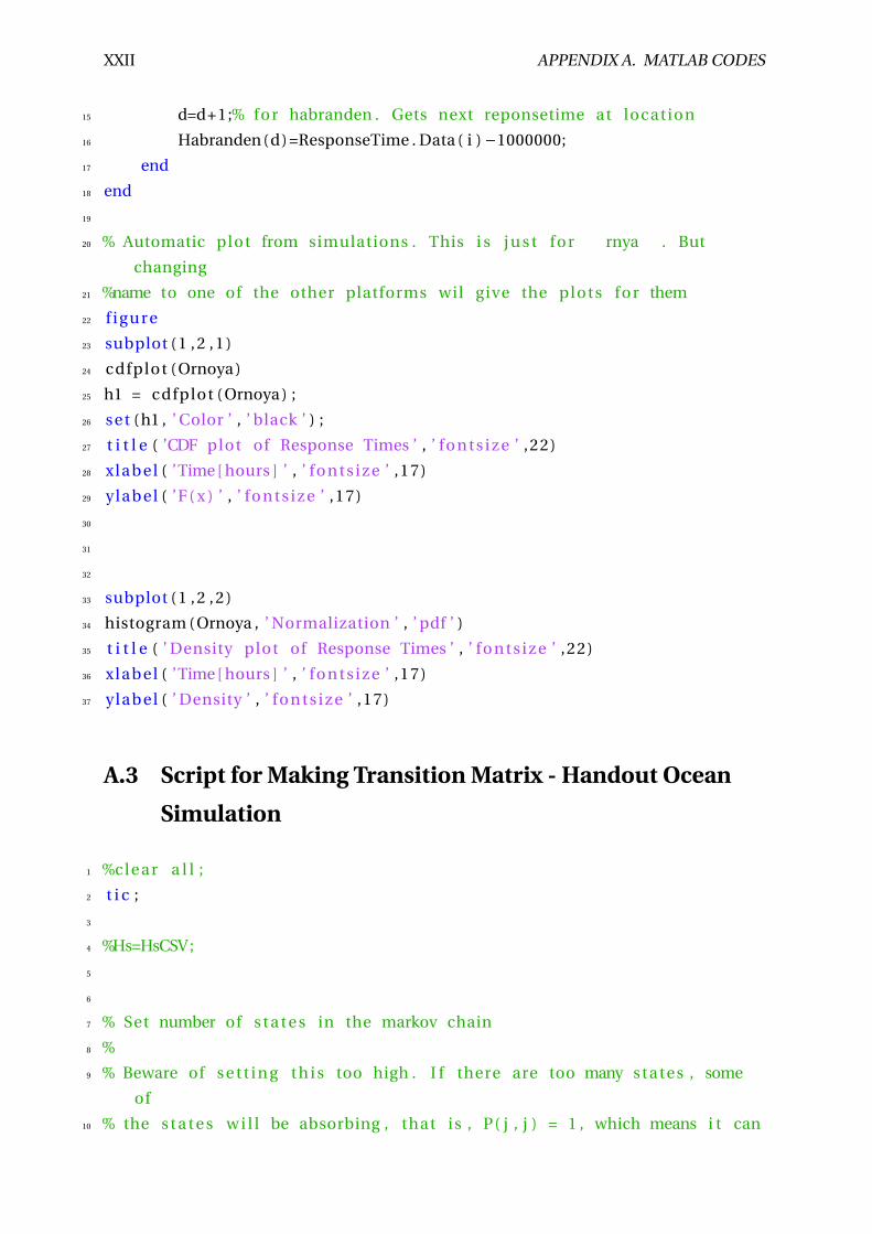
XXII APPENDIX A. MATLAB CODES
15 d=d+1;% for habranden . Gets next reponsetime at location
16 Habranden(d) =ResponseTime . Data ( i ) −1000000;
17 end
18 end
19
20 % Automatic plot from simulations . This i s j u s t for rnya . But
changing
21 %name to one of the other platforms wil give the plots for them
22 f i g u r e
23 subplot ( 1 , 2 , 1 )
24 cdfplot ( Ornoya )
25 h1 = cdfplot ( Ornoya ) ;
26 set ( h1 , ’ Color ’ , ’ black ’ ) ;
27 t i t l e ( ’CDF plot of Response Times ’ , ’ fonts i z e ’ ,22)
28 xlabel ( ’Time[ hours ] ’ , ’ fo nts i z e ’ ,17)
29 ylabel ( ’F( x ) ’ , ’ fo nts i ze ’ ,17)
30
31
32
33 subplot ( 1 , 2 , 2 )
34 histogram ( Ornoya , ’ Normalization ’ , ’ pdf ’ )
35 t i t l e ( ’ Density plot of Response Times ’ , ’ fo nts i z e ’ ,22)
36 xlabel ( ’Time[ hours ] ’ , ’ fo nts i z e ’ ,17)
37 ylabel ( ’ Density ’ , ’ fonts i z e ’ ,17)
A.3 Script for Making Transition Matrix - Handout Ocean
Simulation
1 %clear a l l ;
2 t i c ;
3
4 %Hs=HsCSV ;
5
6
7 % Set number of s t a t e s in the markov chain
8 %
9 % Beware of s e t t i n g t h i s too high . I f there are too many states , some
of
10 % the s t a t e s w i l l be absorbing , that is , P( j , j ) = 1 , which means i t can
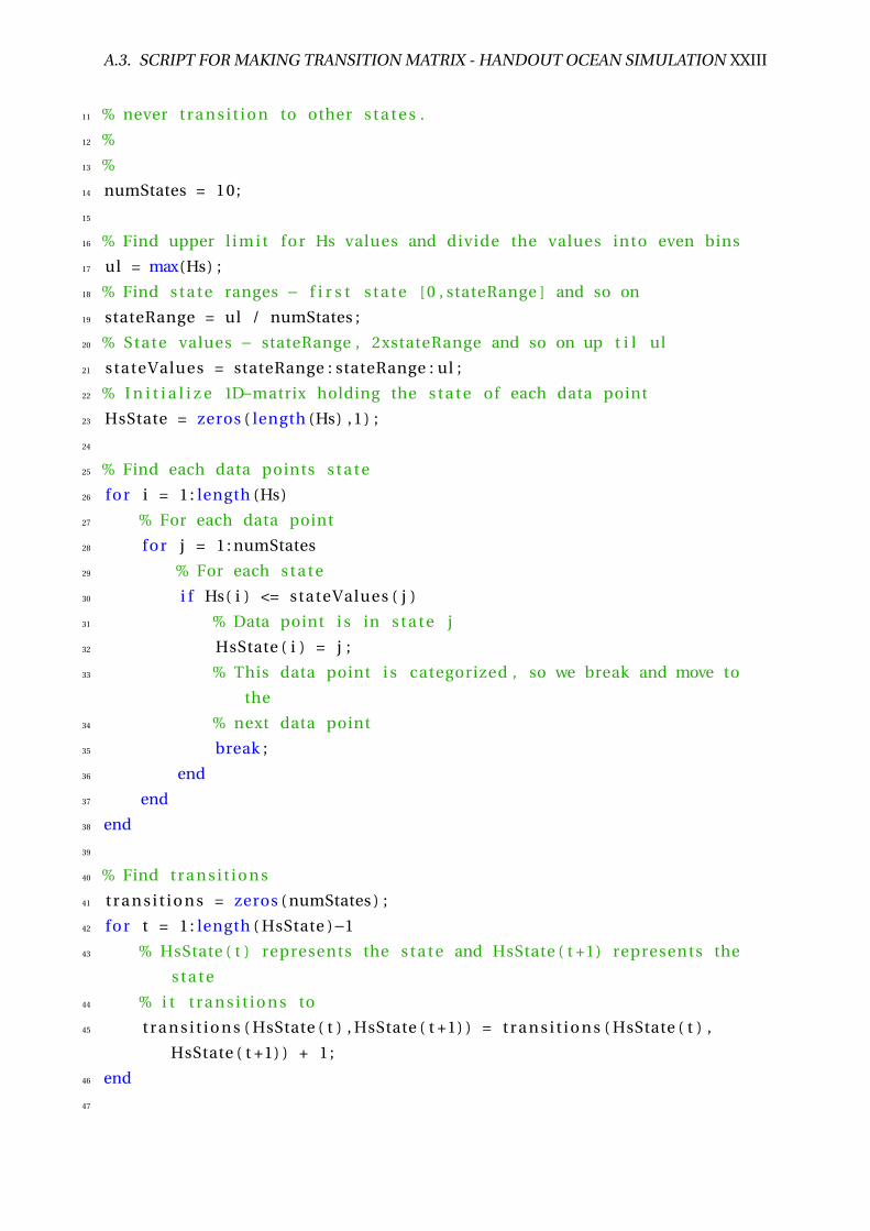
A.3. SCRIPT FOR MAKING TRANSITION MATRIX - HANDOUT OCEAN SIMULATION XXIII
11 % never t r a n s i t i o n to other s t a t e s .
12 %
13 %
14 numStates = 10;
15
16 % Find upper l i m i t for Hs values and divide the values into even bins
17 ul = max(Hs) ;
18 % Find s t a t e ranges − f i r s t s t a t e [ 0 , stateRange ] and so on
19 stateRange = ul / numStates ;
20 % State values − stateRange , 2xstateRange and so on up t i l ul
21 stateValues = stateRange : stateRange : ul ;
22 % I n i t i a l i z e 1D−matrix holding the s t a t e of each data point
23 HsState = zeros ( length (Hs) , 1 ) ;
24
25 % Find each data points s t a t e
26 for i = 1 : length (Hs)
27 % For each data point
28 for j = 1 : numStates
29 % For each s t a t e
30 i f Hs( i ) <= stateValues ( j )
31 % Data point i s in s t a t e j
32 HsState ( i ) = j ;
33 % This data point i s categorized , so we break and move to
the
34 % next data point
35 break ;
36 end
37 end
38 end
39
40 % Find t r a n s i t i o n s
41 t r a n s i t i o n s = zeros ( numStates ) ;
42 for t = 1 : length ( HsState )−1
43 % HsState ( t ) represents the s t a t e and HsState ( t +1) represents the
s t a t e
44 % i t t r a n s i t i o n s to
45 t r a n s i t i o n s ( HsState ( t ) , HsState ( t +1) ) = t r a n s i t i o n s ( HsState ( t ) ,
HsState ( t +1) ) + 1 ;
46 end
47
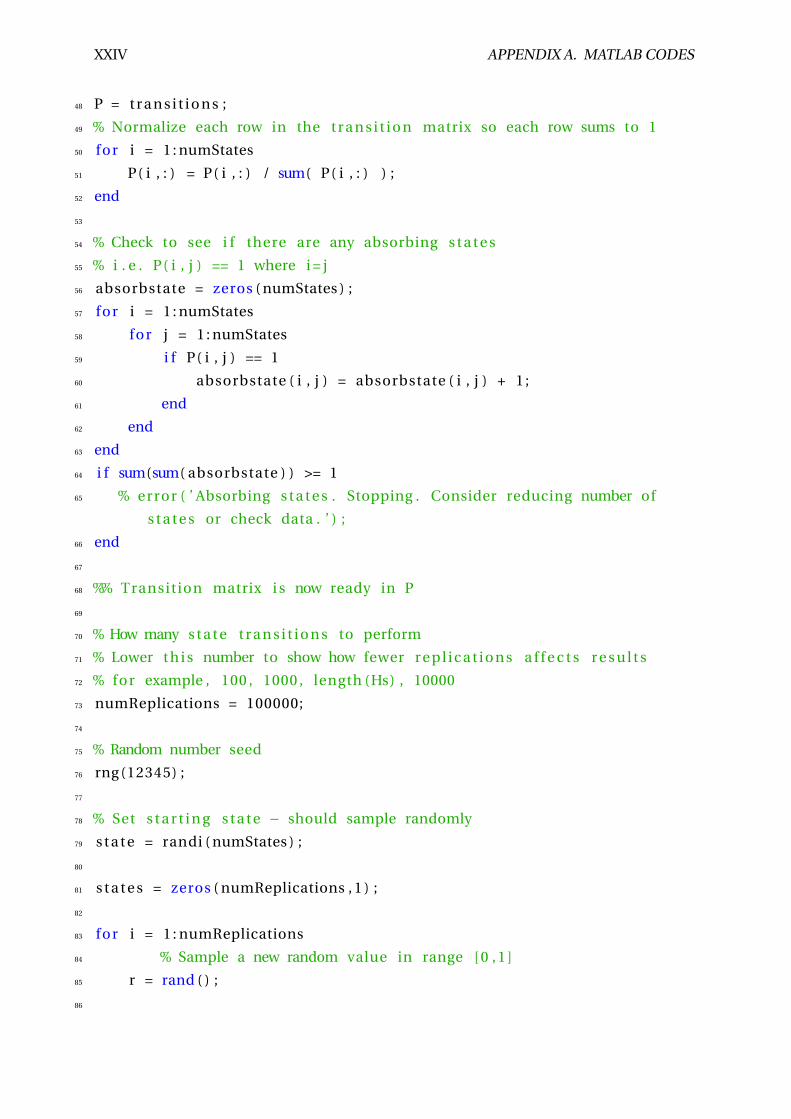
XXIV APPENDIX A. MATLAB CODES
48 P = t r a n s i t i o n s ;
49 % Normalize each row in the t r a n s i t i o n matrix so each row sums to 1
50 for i = 1 : numStates
51 P( i , : ) = P( i , : ) / sum( P( i , : ) ) ;
52 end
53
54 % Check to see i f there are any absorbing s t a t e s
55 % i . e . P( i , j ) == 1 where i = j
56 absorbstate = zeros ( numStates ) ;
57 for i = 1 : numStates
58 for j = 1 : numStates
59 i f P( i , j ) == 1
60 absorbstate ( i , j ) = absorbstate ( i , j ) + 1 ;
61 end
62 end
63 end
64 i f sum(sum( absorbstate ) ) >= 1
65 % error ( ’ Absorbing s t a t e s . Stopping . Consider reducing number of
s t a t e s or check data . ’ ) ;
66 end
67
68 %% Transition matrix i s now ready in P
69
70 % How many s t a t e t r a n s i t i o n s to perform
71 % Lower t h i s number to show how fewer r e p l i c a t i o n s a f f e c t s r e s u l t s
72 % for example , 100 , 1000 , length (Hs) , 10000
73 numReplications = 100000;
74
75 % Random number seed
76 rng (12345) ;
77
78 % Set s t a r t i n g s t a t e − should sample randomly
79 s t a t e = randi ( numStates ) ;
80
81 s t a t e s = zeros ( numReplications , 1 ) ;
82
83 for i = 1 : numReplications
84 % Sample a new random value in range [ 0 , 1 ]
85 r = rand ( ) ;
86
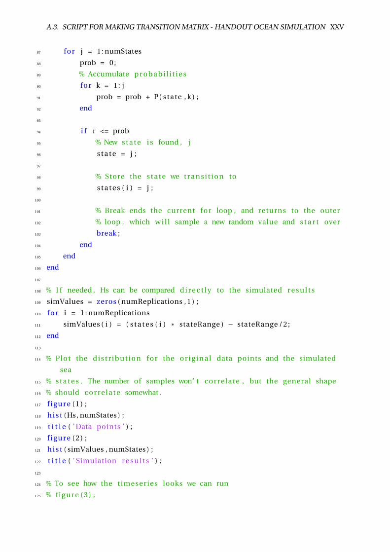
A.3. SCRIPT FOR MAKING TRANSITION MATRIX - HANDOUT OCEAN SIMULATION XXV
87 for j = 1 : numStates
88 prob = 0 ;
89 % Accumulate p r o b a b i l i t i e s
90 for k = 1 : j
91 prob = prob + P( state , k ) ;
92 end
93
94 i f r <= prob
95 % New s t a t e i s found , j
96 s t a t e = j ;
97
98 % Store the s t a t e we t r a n s i t i o n to
99 s t a t e s ( i ) = j ;
100
101 % Break ends the current for loop , and returns to the outer
102 % loop , which w i l l sample a new random value and s t a r t over
103 break ;
104 end
105 end
106 end
107
108 % I f needed , Hs can be compared d i r e c t l y to the simulated r e s u l t s
109 simValues = zeros ( numReplications , 1 ) ;
110 for i = 1 : numReplications
111 simValues ( i ) = ( s t a t e s ( i ) * stateRange ) − stateRange / 2 ;
112 end
113
114 % Plot the d i s t r i b u t i o n for the o r i g i n a l data points and the simulated
sea
115 % s t a t e s . The number of samples won’ t correlate , but the general shape
116 % should c o r r e l a t e somewhat .
117 f i g u r e ( 1 ) ;
118 h i s t (Hs, numStates ) ;
119 t i t l e ( ’ Data points ’ ) ;
120 f i g u r e ( 2 ) ;
121 h i s t ( simValues , numStates ) ;
122 t i t l e ( ’ Simulation r e s u l t s ’ ) ;
123
124 % To see how the timeseries looks we can run
125 % f i g u r e ( 3 ) ;

XXVI APPENDIX A. MATLAB CODES
126 % plot ( simValues ( 1 : 5 0 ) ) ;
127
128 toc ;
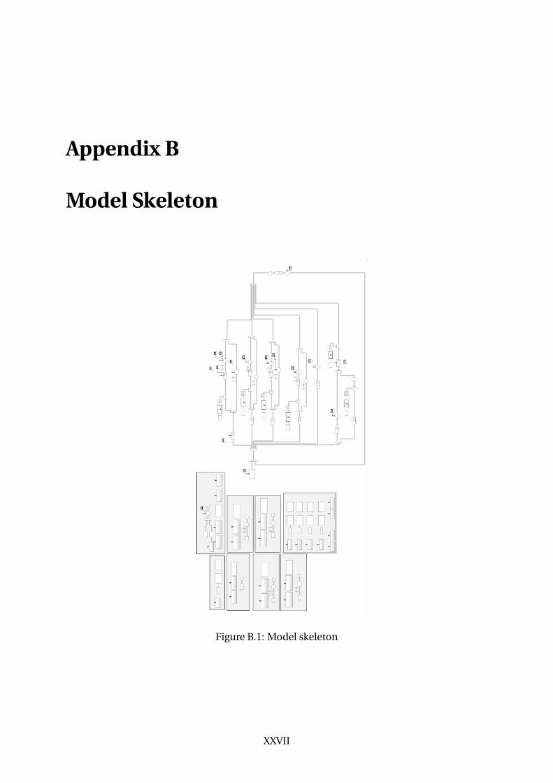
Appendix B
Model Skeleton
Figure B.1: Model skeleton
XXVII

XXVIII APPENDIX B. MODEL SKELETON
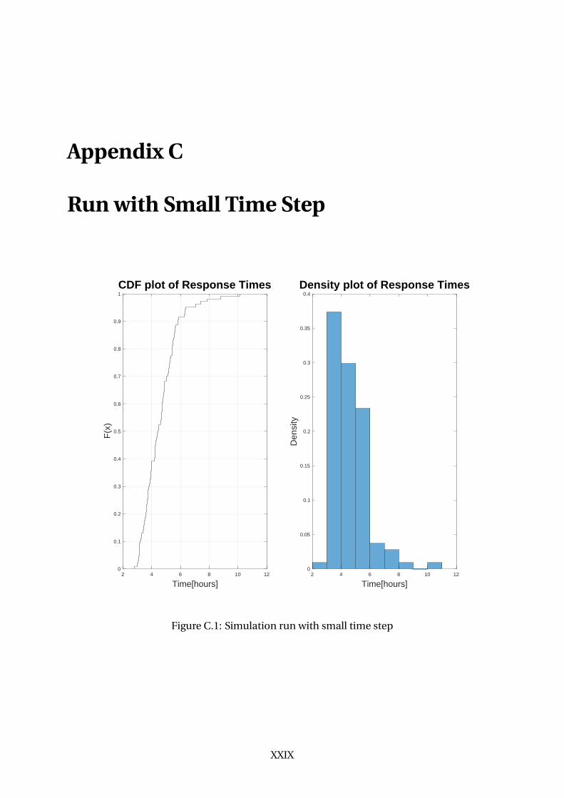
Appendix C
Run with Small Time Step
2 4 6 8 10 12
Time[hours]
0
0.1
0.2
0.3
0.4
0.5
0.6
0.7
0.8
0.9
1
F(x
)
CDF plot of Response Times Density plot of Response Times
2 4 6 8 10 12
Time[hours]
0
0.05
0.1
0.15
0.2
0.25
0.3
0.35
0.4D
ensi
ty
Figure C.1: Simulation run with small time step
XXIX

XXX APPENDIX C. RUN WITH SMALL TIME STEP
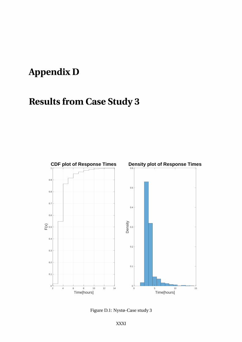
Appendix D
Results from Case Study 3
2 4 6 8 10 12 14
Time[hours]
0
0.1
0.2
0.3
0.4
0.5
0.6
0.7
0.8
0.9
1
F(x
)
CDF plot of Response Times Density plot of Response Times
0 5 10 15
Time[hours]
0
0.1
0.2
0.3
0.4
0.5
0.6
Den
sity
Figure D.1: Nystø-Case study 3
XXXI
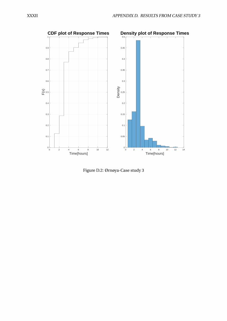
XXXII APPENDIX D. RESULTS FROM CASE STUDY 3
0 2 4 6 8 10 12
Time[hours]
0
0.1
0.2
0.3
0.4
0.5
0.6
0.7
0.8
0.9
1
F(x
)
CDF plot of Response Times Density plot of Response Times
0 2 4 6 8 10 12 14
Time[hours]
0
0.05
0.1
0.15
0.2
0.25
0.3
0.35
0.4
0.45
0.5
Den
sity
Figure D.2: Ørnøya-Case study 3

XXXIII
0 2 4 6 8 10 12 14
Time[hours]
0
0.1
0.2
0.3
0.4
0.5
0.6
0.7
0.8
0.9
1
F(x
)
CDF plot of Response Times Density plot of Response Times
0 2 4 6 8 10 12 14
Time[hours]
0
0.1
0.2
0.3
0.4
0.5
0.6
0.7
Den
sity
Figure D.3: Salatskjera-Case study 3