direct numerical simulation of the brownian motion of particles by using fluctuating hydrodynamic...

www.elsevier.com/locate/jcp

Journal of Computational Physics 201 (2004) 466–486

Direct numerical simulation of the Brownian motionof particles by using fluctuating hydrodynamic equations

Nitin Sharma, Neelesh A. Patankar *

Department of Mechanical Engineering, Northwestern University, 2145 Sheridan Road, Evanston, IL 60208-3111, USA

Received 6 February 2004; received in revised form 28 May 2004; accepted 6 June 2004

Available online 6 July 2004

Abstract

In this paper, we present a direct numerical simulation scheme for the Brownian motion of particles. In this ap-

proach, the thermal fluctuations are included in the fluid equations via random stress terms. Solving the fluctuating

hydrodynamic equations coupled with the particle equations of motion result in the Brownian motion of the particles.

There is no need to add a random force term in the particle equations. The particles acquire random motion through the

hydrodynamic force acting on its surface from the surrounding fluctuating fluid. The random stress in the fluid

equations are easy to calculate unlike the random terms in the conventional Brownian dynamics type approaches. We

present a three-dimensional implementation along with validation.

� 2004 Elsevier Inc. All rights reserved.

Keywords: Fluctuating hydrodynamics; Mesoscopic scale; Brownian motion; Micro/nanoscale computational fluid dynamics; Direct

numerical simulation; Distributed Lagrange multiplier method; Control volume method

1. Introduction

The interaction of sub-micron/nanoscale objects (such as macromolecules or small particles or small

devices) with fluids is an important problem in small scale devices. A better understanding of fluid dynamics

is critical in, e.g., bio-molecular transport, manipulating and controlling chemical and biological processes

using small particles. These objects could be moving in an environment with varying temperatures and fluid

properties. Thermal fluctuations can influence the motion of such objects.Direct numerical simulation (DNS) of particle motion in fluids is a tool that has been developed over the

past 12 years [3,7,8,13,15]. In this approach, the fluid equations are solved coupled with the equations of

motion of the particles. DNS allows investigation of a wide variety of problems including particles in

Newtonian or viscoelastic fluids with constant or varying properties. DNS can be an excellent tool to

*Corresponding author. Tel.: +1-847-491-3021; fax: +1-847-491-3915.

E-mail address: [email protected] (N.A. Patankar).

0021-9991/$ - see front matter � 2004 Elsevier Inc. All rights reserved.

doi:10.1016/j.jcp.2004.06.002

mail to: [email protected]

N. Sharma, N.A. Patankar / Journal of Computational Physics 201 (2004) 466–486 467

investigate the motion of sub-micron particles in varying fluid environments. The objective of this paper is

to find a convenient way to incorporate the effect of thermal fluctuations in the DNS schemes.

A particle suspended in a fluid experiences a hydrodynamic force due to the average motion of the fluidaround it. The average motion of the fluid is represented by the usual continuum equations – the Navier–

Stokes equations. Small particles in fluids, in addition to the average force, experience a random force due

to the thermal fluctuations in the fluid. In Brownian dynamic (BD) simulations the principle is to model this

thermal force from the fluid in terms of a random force in the particle equation of motion.

The conventional approach to perform BD simulations is based on the algorithm by Ermak and

McCammon [2]. Their numerical method is based on the Langevin equation for particle motion. Properties

of the random force in the particle equation of motion depend on the hydrodynamic interactions between

the particles. Typically, approximate expressions are used to model the hydrodynamic interactions.Brady and Bossis [1] presented Stokesian dynamics technique for simulating the Brownian motion of

many particles. They also considered the Langevin equations for the motion of the Brownian particles.

They computed the hydrodynamic interactions through a grand resistance tensor instead of using ap-

proximations as was done by Ermak and McCammon [2]. Using these techniques to objects of irregular

shapes and to cases where the fluid exhibits varying properties is not straightforward. This is mainly be-

cause the properties of the random force in the particle equations depend on the grand resistance tensor,

which in turn depends on the particle positions, shapes and the fluid properties.

In accordance with the BD approach, it is possible to envisage a DNS scheme where the Navier–Stokesequations for the fluid are solved coupled with the Langevin equation (which includes a random force term)

for particle motion. Again, as stated above, generation of the random force term is not straightforward

because it depends on the particle resistance tensor. A different approach is preferred.

An alternate approach is to model the thermal fluctuations in the fluid (instead of in the particle

equations) via random stress terms in its governing equations. A general theory of fluctuating hydrody-

namics is given by Landau and Lifshitz [11]. Solving the fluctuating hydrodynamic equations coupled with

the particle equations of motion result in the Brownian motion of the particles. There is no need to add a

random force term in the particle equations. The particles acquire random motion through the hydrody-namic force acting on its surface from the surrounding fluctuating fluid. The random stress in the fluid

equations are easy to calculate unlike the random terms in the BD approach. In this paper, we present a

three-dimensional implementation of this approach along with validation.

Ladd [10] presented a Lattice–Boltzmann (LB) method to simulate the Brownian motion of solid par-

ticles. They added a fluctuating term in the LB equation for the fluid which was equivalent to the random

stress term in the fluctuating hydrodynamic equations of Landau and Lifshitz [11]. Fluctuating LB

equations were solved to get results for the decay of an initially imposed translational and rotational ve-

locity of an isolated Brownian sphere in a fluid. The current work in this paper is aimed at adding therandom fluctuating terms directly into the Navier–Stokes equations instead of the Lattice–Boltzmann

equations. It can therefore be easily incorporated in existing conventional solvers for Navier–Stokes

equations to model fluid–particle behavior at small scales.

Zwanzig [24] showed that motion of an isolated Brownian particle computed using fluctuating hydro-

dynamic equations is consistent with the traditional Langevin description in the long time (dissipative)

limit. Hauge and Martin-L€of [5] showed that the Langevin equation describing the Brownian motion is a

contraction from the more fundamental, but still phenomenological, description of an incompressible fluid

governed by fluctuating hydrodynamics in which a Brownian particle with no-slip boundary condition isimmersed. They showed that the fluctuating hydrodynamics approach captures the algebraic tail (t�3=2) in

the velocity autocorrelation function consistent with the molecular time correlation functions. The

Langevin description gives an exponential tail in the velocity autocorrelation function. Hauge and Martin-

L€of [5] also identified conditions under which the classical Langevin description is applicable. These results

imply that the simulation of the Brownian motion of particles based on fluctuating hydrodynamic

468 N. Sharma, N.A. Patankar / Journal of Computational Physics 201 (2004) 466–486

equations is a sound phenomenological approach. In this work, we will consider only the long time dis-

sipative limit, which is equivalent to neglecting the inertia terms (Section 2.2) in the governing equations. As

a result, we will not consider the velocity autocorrelation function. However, we will test our code bycomparing the Brownian diffusion (in the long time limit) obtained from the simulations with known

analytic values. Problem involving the solution of the fluctuating hydrodynamic equations including the

inertia terms will be considered in future work.

Patankar [14] presented preliminary results for the Brownian motion of a cylinder by solving the fluc-

tuating hydrodynamic equations of the fluid coupled with the particle equation of motion. They considered

a 2D problem.

Fluctuating hydrodynamic equations have been solved for the pure fluid case by Serrano and Espa~nol[19] using a finite volume Lagrangian discretization based on Voronoi tessellation. They obtained a discreteform of the governing equations that satisfied the fluctuation dissipation theorem. They ensured this by

casting their discrete equations in the GENERIC (General Equation for Non-Equilibrium Reversible/Ir-

reversible Coupling) structure. The GENERIC structure proposed by Grmela and €Ottinger [4] and €Ottinger

and Grmela [12] ensures that the equations describing the macroscopic dynamics of a system are ther-

modynamically consistent and that the fluctuation dissipation theorem is satisfied. Serrano and Espa~nol[19] considered an ideal gas in a 2D box with periodic boundary conditions.

In this paper, we present a DNS technique for solving fluctuating hydrodynamic equations of Landau

and Lifshitz [11] coupled with the particle equations of motion. In our approach, the entire fluid–particledomain is considered to be a fluid. It is ensured that the ‘fluid’ occupying the particle domain moves

rigidly by adding a rigidity constraint [3,13,15]. Solution of this system of equations results in the

Brownian motion of the particles. We validate the technique by comparing numerical results with an-

alytic values.

The paper is organized as follows. In Section 2, we discuss the mathematical formulation of the problem.

Section 3 contains a discussion of the discretization of the governing equations. The numerical algorithm is

presented in Section 4. Numerical results are presented in Section 5 and conclusions in Section 6.

2. Mathematical formulation

2.1. Governing equations

Let X be the computational domain which includes both the fluid and the particle domain. Let P be the

particle domain. Assume that the computational domain is periodic in all directions. Consider one particle

in the computational domain. The particle can be of any shape but in this paper we will solve only for aspherical particle. The formulation to be presented is not restricted to periodic boundary condition it can be

extended to non-periodic domains. We assume the entire fluid–particle domain to be a single fluid governed

by Patankar and coworkers [13,15]

qou

ot

�þ u � rð Þu

�¼ r � rþ f in X; ð1Þ

r � u ¼ 0 in X; ð2Þ

r � D u½ �ð Þ ¼ 0 in P ; ð3aÞ

D u½ � � n ¼ 0 on oP ; ð3bÞ


ujt¼0 ¼ u0ðxÞ in X; ð4Þ

where q is the fluid and particle density (we assume neutrally buoyant particles although the formulationcan be easily generalized to heavy or light particles – see [13]), u is the fluid velocity, n is the outward normal

on the particle surface and r is the stress tensor. The initial velocity u0 should satisfy Eqs. (2) and (3).

Eq. (3) represents the rigidity constraint and Eq. (2) is the incompressibility constraint. The rigidity

constraint, imposed only in the particle domain, ensures that the deformation-rate tensor

D u½ � ¼ 12ru�

þruT�¼ 0 in P : ð5Þ

Thus the ‘fluid’ in the particle domain is constrained to move rigidly as required.Eq. (3) represents three scalar constraint equations at a point in the particle domain. They give rise to a

force f in the particle domain similar to the presence of pressure due to the incompressibility constraint [15].

This is the distributed lagrange multiplier (DLM) approach for particulate flows [3,13,15]. f is zero in the

fluid domain. Details on how to compute f will be presented later.

The stress r is given by

r ¼ �pIþ sþ ~S; ð6Þ

where p is the dynamic pressure (i.e., without the hydrostatic component) due to the incompressibility

constraint (Eq. (2)) and I is the identity tensor. Note that since we have neutrally buoyant particles, the

gravitational force is balanced by the hydrostatic pressure component throughout the domain. s is extra-

stress tensor given by

s ¼ l ruh

þ ruð ÞTi; ð7Þ

for a Newtonian fluid, where l is the viscosity of the fluid. s is zero in the particle domain due to the rigidityconstraint (Eq. (3)). Nevertheless, the term is retained in the particle domain to facilitate the solution

procedure [15].~S in Eq. (6) is the random stress tensor. We take its value to be zero in the particle domain while in the

region not occupied by the particle it is computed as proposed by Landau and Lifshitz [11]. ~S is included in

the Navier–Stokes equations to model the fluid at mesoscopic scales. Hydrodynamics as such is a mac-

roscopic theory. At the macroscopic level the hydrodynamic variables represent an average value over a

macroscopic length and timescale. Consequently, information regarding the random fluctuations arising

due to the molecular nature of the fluid is lost. ~S accounts for these fluctuations when modeling flows atmesoscopic scales. By mesoscopic scales, we typically imply scales ranging from tens of nanometers to

micron, depending on the problem.~S has the following property [11]:

h~Siji ¼ 0;h~Sik x1; t1ð Þ~Slm x2; t2ð Þi ¼ 2kBTl dildkm þ dimdkl � 2

3dikdlm

� �d x1 � x2ð Þd t1 � t2ð Þ;

)ð8Þ

where h i denotes averaging over an ensemble, kB is the Boltzmann constant, T is temperature of the fluid

and we have used indicial notation. The above equations are in accordance with the fluctuation dissipation

theorem for the fluid [11]. For the case of an incompressible fluid, the term 2=3dikdlm in Eq. (8) becomes

irrelevant [11]. Hence, Eq. (8) can be rewritten as

h~Siji ¼ 0;h~Sik x1; t1ð Þ~Slmðx2; t2Þi ¼ 2kBTl dildkm þ dimdklð Þd x1 � x2ð Þd t1 � t2ð Þ:

�ð9Þ


Solution of Eqs. (1)–(4), (6), (7) and (9) give the velocity field u in the entire domain. The particle

translational and angular velocities, U and x, respectively, can then be computed by

MU ¼ZP

qudx and IPx ¼ZP

r� qudx; ð10Þ

where r is the position vector of a point with respect to the centroid of the particle, IP is the moment of

inertia of the particle and M its mass.

In this work, we will neglect inertia (left-hand side of Eq. (1)) and solve the resultant Stokes problem that

is driven by the random stress in the fluid. In this case, the velocity field u and the particle velocities U and xshould be interpreted carefully.

2.2. Interpretation of velocity in the Stokes limit of the fluctuating hydrodynamics equations

We will discuss the appropriate interpretation by considering an analogous problem below. Consider the

problem of Brownian motion of an isolated particle in an infinite domain. According to the Langevin

description, in the absence of external force fields, the momentum, pðtÞ, of the isolated Brownian particle

satisfies the following equation [9]:

dp

dt¼ � f

m

� �pþ ~fðtÞ; ð11Þ

where f is the friction coefficient, m is the mass of the Brownian particle and ~fðtÞ is the random force. This is

the typical BD approach where the random force is imposed in the particle equation of motion. The

properties of the random force are

h~fðtÞi ¼ 0;

h~fðtÞ~fðt0Þi ¼ cdðt � t0Þ;

)ð12Þ

where c is the strength of the random force given by

c ¼ 2kBT fI: ð13Þ

Eq. (13) arises because of the fluctuation dissipation theorem. It relates the strength c of the

random forces to the dissipative friction coefficient f. Physically, it means that the energy acquired bythe particle, due to the random fluctuations in the fluid, is dissipated back into the fluid at an ap-

propriate rate.

The solution of Eq. (11) describes a Gaussian and Markov process. The mean and variance of the

process contains an exponentially decaying part with a relaxation time sR ¼ mf . The stationary equilibrium

velocity distribution corresponds to the Maxwell distribution. The mean square displacement of the

Brownian particle can be shown to be [9]

rðDtÞjD

� r0j2E¼ 6kBT

fDt

�þ exp

�� Dtf

m

�� 1

�mf

�; ð14Þ

where r0 is the initial location of the particle and rðDtÞ is its location after time Dt. Two time limits can be

considered for the above expression – short times compared to sR and long times compared to sR. ForDt � sR, Eq. (14) gives

rðDtÞjD

� r0j2E¼ 6kBTDt

f: ð15Þ


This is the dissipative limit. The same solution (Eq. (15)) is obtained by solving

�fvþ g ¼ 0; ð16Þ

where

gh i ¼ 0 and ggh i ¼ 2kBT fDt

I; ð17Þ

and we define

v ¼ r Dtð Þ � r0

Dt: ð18Þ

Eq. (16) can be regarded as the time discretization of Eq. (11) after neglecting the inertia term (i.e., takingthe Stokes limit). v in Eq. (16) is not the true velocity of the particle at any instant. It is the average velocity

of the particle based on its Brownian displacement, rðDtÞ � r0, in time Dt. Thus, we see that solving the

Langevin equation (11) for the Brownian particle and then taking the long time limit (i.e., Dt � sR) isequivalent to solving the time discretized Stokes equation (16). The velocity in the Stokes equation (16) is

interpreted as in Eq. (18).

We extend this principle to the fluctuating hydrodynamic equations. Eq. (1) is analogous to Eq. (11).

Taking the long time limit is equivalent to neglecting the inertia terms in Eq. (1) to give the following Stokes

equation driven by the random stress:

�rp þr � l ru�

þruT�

þr � ~Sþ f ¼ 0 in X; ð19Þ

where the time discretized properties of the random stress are given by

h~Siji ¼ 0;

h~Sik x1ð Þ~Slm x2ð Þi ¼ 2kBTlDt dildkm þ dimdklð Þd x1 � x2ð Þ:

)ð20Þ

Eqs. (19) and (20) are analogous to Eqs. (16) and (17). Solution of the Stokes problem represented by Eqs.

(19), (2), (3) and (20) give the velocity u in the entire domain. The velocity field u in Eq. (19) is not the true

velocity of the fluid material point at any instant. Analogous to Eq. (18) it is the Brownian diffusion of the

fluid material point in time Dt divided by Dt. Consequently, the translational and angular velocities of the

particle as computed by Eq. (10) must be interpreted similarly. This is the interpretation that will be used in

this paper.In the next section, we present the discretization of the governing equations.

3. Spatial discretization

The governing equations to be solved are stochastic. We know that, for deterministic equations, central

differencing ensures second-order accuracy. Discretization of stochastic equations based on central differ-

encing may not be sufficient to obtain thermodynamically consistent discrete equations. A consistent dis-cretization should ensure that the resultant discrete equations satisfy the corresponding fluctuation

dissipation theorem (FDT). It must be noted that even if the differential equations satisfy the FDT it does

not imply that the corresponding discretized equations based on central differencing will necessarily satisfy

the FDT for the discrete equations.

Thermodynamic consistency of the discrete equations can be ensured if we discretize the equations such

that they are in the GENERIC form as proposed by Grmela and €Ottinger [4] and €Ottinger and Grmela [12].


Serrano and Espa~nol [19] and Serrano et al. [20] have presented a systematic derivation of two-dimensional

discrete equations that obey the GENERIC structure for the case of a fluid (i.e., no particles in the domain).

They used a finite volume Lagrangian discretization based on Voronoi tessellation. They showed thatsimple central differencing does not ensure thermodynamically consistent discretized equations but this can

be corrected by adding certain terms to the discrete equations. They also argued that these additional terms

may be neglected under certain condition.

In this paper, we use control (finite) volume Eulerian discretization based on cubic cells. A fixed uniform

grid is used. We choose to use a staggered control volume scheme for solving the fluid equations [16]. The

formulation can also be implemented on a non-staggered grid without difficulty.

In the following, we will first present the spatial discretization for the fluid only, i.e., there are no

particles. The discretization of the fluid–particle equations will be considered after that.

3.1. Spatial discretization of the fluid equations

We will first consider the spatial discretization of the fluid only, i.e., we have f ¼ 0 in Eq. (19). Aspects

pertaining to the presence of the particle will be discussed later. We consider a fluid of constant material

properties at uniform temperature. It is possible to extend the formulation to varying temperature and

material properties; this will be the subject of our future work. We will assume a uniform grid such that the

discretization in the x; y and z directions are Dx ¼ Dy ¼ Dz ¼ Dh. The scheme can be extended to non-uniform grids.

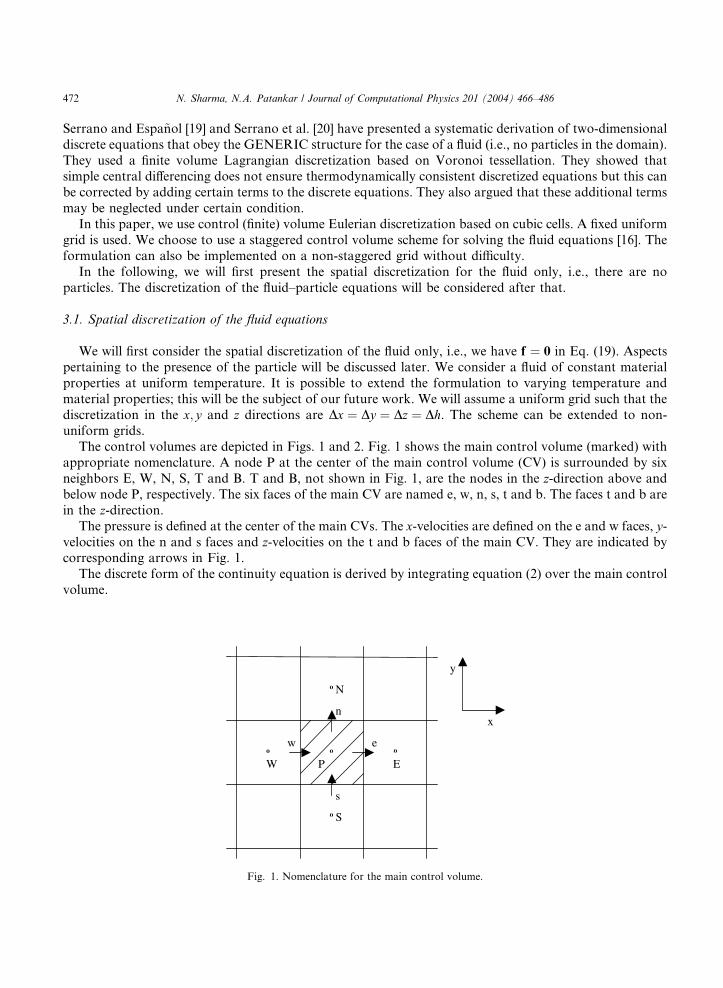
The control volumes are depicted in Figs. 1 and 2. Fig. 1 shows the main control volume (marked) with

appropriate nomenclature. A node P at the center of the main control volume (CV) is surrounded by six

neighbors E, W, N, S, T and B. T and B, not shown in Fig. 1, are the nodes in the z-direction above and

below node P, respectively. The six faces of the main CV are named e, w, n, s, t and b. The faces t and b are

in the z-direction.The pressure is defined at the center of the main CVs. The x-velocities are defined on the e and w faces, y-

velocities on the n and s faces and z-velocities on the t and b faces of the main CV. They are indicated bycorresponding arrows in Fig. 1.

The discrete form of the continuity equation is derived by integrating equation (2) over the main control

volume.

o

o o

o

o

N

S

E W P

e w

n

s

y

x

Fig. 1. Nomenclature for the main control volume.

(a) (b)

P E

ne

se

eo o

o

o

o o

o

o

enwn

N

P

n

y

x

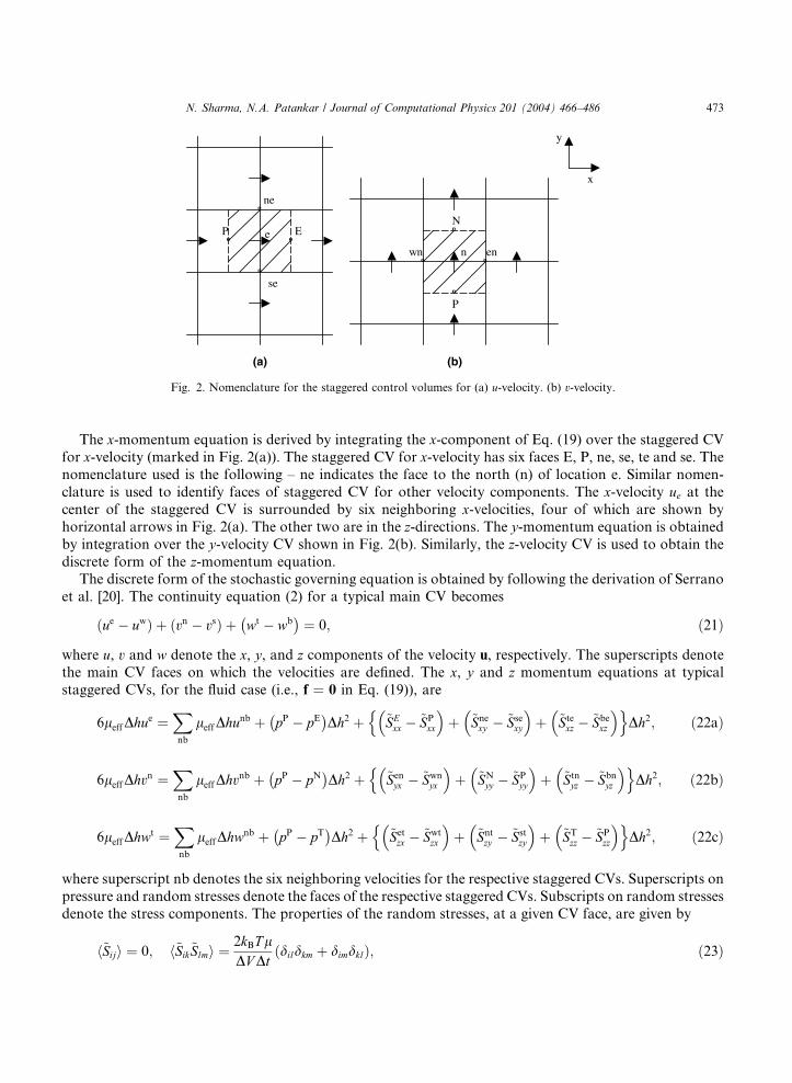
Fig. 2. Nomenclature for the staggered control volumes for (a) u-velocity. (b) v-velocity.


The x-momentum equation is derived by integrating the x-component of Eq. (19) over the staggered CV

for x-velocity (marked in Fig. 2(a)). The staggered CV for x-velocity has six faces E, P, ne, se, te and se. The

nomenclature used is the following – ne indicates the face to the north (n) of location e. Similar nomen-

clature is used to identify faces of staggered CV for other velocity components. The x-velocity ue at the

center of the staggered CV is surrounded by six neighboring x-velocities, four of which are shown by

horizontal arrows in Fig. 2(a). The other two are in the z-directions. The y-momentum equation is obtained

by integration over the y-velocity CV shown in Fig. 2(b). Similarly, the z-velocity CV is used to obtain the

discrete form of the z-momentum equation.The discrete form of the stochastic governing equation is obtained by following the derivation of Serrano

et al. [20]. The continuity equation (2) for a typical main CV becomes

ueð � uwÞ þ vnð � vsÞ þ wt�

� wb�¼ 0; ð21Þ

where u, v and w denote the x, y, and z components of the velocity u, respectively. The superscripts denote

the main CV faces on which the velocities are defined. The x, y and z momentum equations at typical

staggered CVs, for the fluid case (i.e., f ¼ 0 in Eq. (19)), are

6leffDhue ¼

Xnb

leffDhunb þ pP

�� pE

�Dh2 þ ~SE

xx

�n� ~SP

xx

�þ ~Sne

xy

�� ~Sse

xy

�þ ~Ste

xz

�� ~Sbe

xz

�oDh2; ð22aÞ

6leffDhvn ¼

Xnb

leffDhvnb þ pP

�� pN

�Dh2 þ ~Sen

yx

�n� ~Swn

yx

�þ ~SN

yy

�� ~SP

yy

�þ ~Stn

yz

�� ~Sbn

yz

�oDh2; ð22bÞ

6leffDhwt ¼

Xnb

leffDhwnb þ pP

�� pT

�Dh2 þ ~Set

zx

�n� ~Swt

zx

�þ ~Snt

zy

�� ~Sst

zy

�þ ~ST

zz

�� ~SP

zz

�oDh2; ð22cÞ

where superscript nb denotes the six neighboring velocities for the respective staggered CVs. Superscripts on

pressure and random stresses denote the faces of the respective staggered CVs. Subscripts on random stresses

denote the stress components. The properties of the random stresses, at a given CV face, are given by

h~Siji ¼ 0; h~Sik~Slmi ¼2kBTlDV Dt

dildkmð þ dimdklÞ; ð23Þ


and leff in Eq. (22) is given by Serrano et al. [20]

leff ¼ l 1

�þ kB2C

�; ð24Þ

where C is the heat capacity of the fluid inside the CV. Random stresses on different CV faces are con-

sidered independent of each other. Note that in the discrete form the co-variance of the random stress is

inversely proportional to the volume of the CV. Eq. (24) ensures that the discrete equations (21) and (22)are in the GENERIC structure and obey the FDT. kB=C is typically a small quantity and is proportional to

the inverse of the number of atom in the ‘mesoparticle’, i.e., the CV. Hence, if it is neglected we get leff ¼ l.The resulting discrete momentum equations with leff ¼ l are the same as those obtained by simple central

difference discretization of Eq. (19). In this case, the FDT is not strictly satisfied but the error is small if

kB=C is small.

In the next section, we will consider the case where there are particles in the fluid.

3.2. Spatial discretization of the fluid–particle equations

The momentum equation in the fluid–particle domain is given by Eq. (19), where f is non-zero and ~S is

zero in the particle region. The procedure to compute f by using the rigidity constraint (Eq. (3)) will be

discussed later. In the following, we will present the discretization of Eq. (19) by assuming that the value of

f is known.

We define a variable u as the fraction of the volume occupied by the particle in a main CV. The value

of u is thus available at the center of every main CV. u ¼ 1 for every main CV entirely within the

particle region and u ¼ 0 for main CVs entirely out of the particle region. All the main CVs partiallyoccupied by the particle have a value of u between 0 and 1. The fluid–particle boundary is therefore

smeared in this approach, but this is a drawback of every immersed boundary type of technique. On the

other hand such techniques can be conveniently extended to the case of moving particles since there is

no need to remesh the computational domain. Details of the computation of u are given by Sharma and

Patankar [21].

Eqs. (22a)–(22c) are now modified to account for the presence of the particle to give

AVue ¼Xnb

Anbunb þ Bex þ pP

�� pE

�Dh2 þ uef e

x Dh3; ð25aÞ

AVvn ¼Xnb

Anbvnb þ Bny þ pP

�� pN

�Dh2 þ unf n

y Dh3; ð25bÞ

AVwt ¼Xnb

Anbwnb þ Btz þ pP

�� pT

�Dh2 þ utf t

zDh3; ð25cÞ

where

AV ¼ 6lDh; Anb ¼ lDh ð26Þ

and

Bex ¼ 1

��n� uE

�~SExx � 1

�� uP

�~SPxx

�þ 1ð�

� uneÞ~Snexy � 1ð � useÞ~Sse

xy

�þ 1ð�

� uteÞ~Stexz � 1

�� ube

�~Sbexz

�oDh2; ð27aÞ


Bny ¼ 1ð

�n� uenÞ~Sen

yx � 1ð � uwnÞ~Swnyx

�þ 1

�� uN

�~SNyy � 1

�� uP

�~SPyy

�þ 1ð�

� utnÞ~Stnyz � 1

�� ubn

�~Sbnyz

�oDh2; ð27bÞ

Btz ¼ 1ð

�n� uetÞ~Set

zx � 1ð � uwtÞ~Swtzx

�þ 1ð�

� untÞ~Sntzy � 1ð � ustÞ~Sst

zy

�þ 1

�� uT

�~STzz � 1

�� uP

�~SPzz

�oDh2: ð27cÞ

We have put leff ¼ l in Eq. (26) and fx; fy ; fz are the x; y and z components of f, respectively. The super-

scripts on u and f s indicate locations where their values are required. As discussed above, the values of uare computed at the center of the main CVs. Its value at other locations is obtained by linear interpolation.

Note that the values of ~S are smeared at the particle boundaries since the grid does not necessarily conform

to the particle shape.Eq. (27) denote source terms in the momentum equation due to random stresses. It can be easily verified

that if we add the source terms Bex over all the control volumes for x-velocity then the sum is zero. This

implies that there is no net force on the fluid–particle domain in the x-direction. Similarly, summations in

the y and z directions are also zero. This ensures that the mean force on the computational domain due to

the random stresses is zero.

In the fluid–particle case, the continuity equation remains the same as Eq. (21). As we will see later,

the continuity equation is used to obtain the pressure field and the rigidity constraint is used to

compute f.In the next section, we will present the numerical algorithm to solve the fluid–particle equations.

4. Numerical algorithm

Our numerical algorithm is an extension of the SIMPLER algorithm for fluids, by Patankar [16], to

the case of the fluid–particle problem. The modification pertains to the presence of the rigidity

constraint in the particle domain. We use a simple block correction based multigrid solver proposedby Sathyamurthy and Patankar [18] to solve the resulting linear equations. We consider a spherical

particle placed at the center of a periodic domain. The problem to be solved is a steady Stokes flow

driven by the random stresses. We need to solve the momentum equations together with the conti-

nuity equation and the rigidity constraint in the particle domain. The algorithm presented below is

based on that presented by Sharma et al. [22]. The sequence of operations in the algorithm are

presented below.

4.1. Computation of volume fraction u

The first step involves computing the volume of fractionuoccupied by the particle in each of themainCV’s.

4.2. Guess a velocity field

We start with an initial guess ~u, for the velocity field. In this work, we take ~u ¼ 0 everywhere as our

initial guess.


After the first iteration ~u is taken to be the velocity field at the end of the previous iteration.

4.3. Get the pressure and the force due to the rigidity constraint

We first define pseudo velocities u and û whose components are given by

ue ¼P

nb Anb~unb þ Bex

AV

; ûe ¼ ue þ pP � pEð ÞDh2AV

; ð28aÞ

vn ¼P

nb Anb~vnb þ Bny

AV

; ^vn ¼ vn þ pP � pNð ÞDh2AV

; ð28bÞ

wt ¼P

nb Anb~wnb þ Btz

AV

; ^wt ¼ wt þ pP � pTð ÞDh2AV

: ð28cÞ

Inserting ~u into the momentum equations (25a)–(25c) and using Eq. (28), we get

~ue ¼ ûe þ F ex ;

~vn ¼ ^vn þ F ny ;

~wt ¼ ^wt þ F tz ;

9>=>; ð29Þ

where

F ex ¼ uef ex Dh

3

AV;

F ny ¼ unf ny Dh

3

AV;

F tz ¼ utf tzDh

3

AV:

9>>>>=>>>>;

ð30Þ

In Eq. (30), F s denote the total force in the respective staggered CVs due to the rigidity constraint

divided by AV. It is non-zero only in the particle domain. We need to compute the pressure p and

F s.Extending the ideas of the SIMPLER algorithm [16], we require that ûþ F (where F is a vector based on

Fx; Fy and Fz) must satisfy the continuity equation in the entire domain and the rigidity constraint in theparticle domain. An equivalent statement is to say that û satisfies the continuity equation in the entire

domain and ûþ F satisfies the rigidity constraint in the particle domain. We use these conditions to obtain

the equations for pressure and F s, respectively. Note that the rigidity constraint also implies a divergence

free velocity field.

4.3.1. Compute pressure

(i) Compute the pseudo velocity u according to Eq. (28).

(ii) We require that û satisfies continuity equation (21). Substitute û in terms of u and pressure (as in Eq.

(28)) into the continuity equation (21). Since u is known, we get an equation for pressure given by

6Dh2

AV

pP ¼ Dh2

AV

Xnb

pnb þ uw�n

� ue�þ vs�

� vn�þ wb�

� wt�o

: ð31Þ

The pressure equation above is identical to the one generated in the traditional SIMPLER algorithm. Eq.

(31) for all CVs is solved simultaneously by a block correction based multigrid solver [18].


4.3.2. Compute the force due to the rigidity constraint

(i) Once p is obtained from the step above, compute the pseudo velocity û according to Eq. (28).

(ii) The force due to the rigidity constraint can be computed by the procedure presented by Patankar [13].Here, we will discuss that procedure only briefly. If ûþ F satisfies the rigidity constraint (3) within the

particle domain then it must be a rigid body motion in that region, i.e.,

ûþ F ¼ ûr; ð32Þwhere ûr is the rigid motion component of û in the particle domain. By conservation law, the total linear

and angular momenta in the particle domain due to û and ûr must be equal. Thus ûr, defined only in the

particle domain, is computed as follows:

ûr ¼ Ûþ ^x� r; ð33Þ

where

M Û ¼

ZP

qûdx and IP ^x ¼ZP

r� qûdx: ð34Þ

F then follows from Eq. (32) and can be computed at any required location. Note that since the rigidity

constraint is present only in the particle domain, F is defined (i.e., non-zero) only in the particle

domain.

4.4. Solve the momentum equations

Using Eq. (30) in Eq. (25) we get

AV�ue ¼Xnb

Anb�unb þ Bex þ pP

�� pE

�Dh2 þ AVF e

x ; ð35aÞ

AV�vn ¼Xnb

Anb�vnb þ Bny þ pP

�� pN

�Dh2 þ AVF n

y ; ð35bÞ

AV�wt ¼Xnb

Anb�wnb þ Btz þ pP

�� pT

�Dh2 þ AVF t

z ; ð35cÞ

where p and F s are known. We solve the momentum equations (35a)–(35c) for all the CVs to get the ve-locity field �u.

The velocity field �u does not satisfy the continuity equation and the rigidity constraint unless it is the

converged solution. We correct the velocity field �u in two steps described below.

4.5. Projection of �u on to a divergence free velocity field

First we correct �u to ��u such that ��u satisfies the continuity equation. To this end, we use the pressure

correction formulation of the standard SIMPLER algorithm [16]. In this approach, we write ��u as

��ue ¼ �ue þ p0P � p0

E� �

Dh2

AV;

��vn ¼ �vn þ p0P � p0

N� �

Dh2

AV;

��wt ¼ �wt þ p0P � p0

T� �

Dh2

AV;

9>>>=>>>;

ð36Þ


where p0 is the pressure correction that is used to correct the velocity field �u to get the continuity satisfying

velocity field ��u. Inserting ��u in the continuity equation (21) and using Eq. (36) we get an equation for the

pressure correction

6Dh2

AV

p0P ¼ Dh2

AV

Xnb

p0nb þ �uw

�n� �ue

�þ �vs�

� �vn�þ �wb�

� �wt�o

: ð37Þ

Solving Eq. (37) gives p0, which is used in Eq. (36) to get the corrected velocity field ��u.

4.6. Projection of ��u on to a rigid motion in the particle domain

The velocity field ��u is not a rigid motion in the particle domain. Hence, ��u needs to be corrected. However,��u will remain unchanged in the region outside the particle. Thus the velocity u at the end of the currentiteration is such that u ¼ ��u in the fluid region and u ¼ ��ur in the particle region, where ��ur is the rigid motion

component of ��u in the particle domain. Similar to Eqs. (33) and (34) ��ur is computed as follows:

��ur ¼ ��Uþ ��x� r; where M ��U ¼ZP

q��udx and IP ��x ¼ZP

r� q��udx: ð38Þ

4.7. Check convergence or iterate

If the solution is not converged (which can be checked by some criterion) then set ~u ¼ u and go back to

step 3. Iterate until convergence.

5. Results and discussion

In this section, we will present test cases to validate the code. In the first set of simulations (Section 5.1) therandom stresses are equal to zero (~S ¼ 0). We calculate the drag on a sphere when an external force is applied

on it. In the second set of simulations (Section 5.2) the random stresses are non-zero.We calculate the diffusion

of a periodic array ofBrownian spheres. In both cases, the numerical results are comparedwith analytic values.

5.1. Drag on a periodic array of spheres (~S ¼ 0)

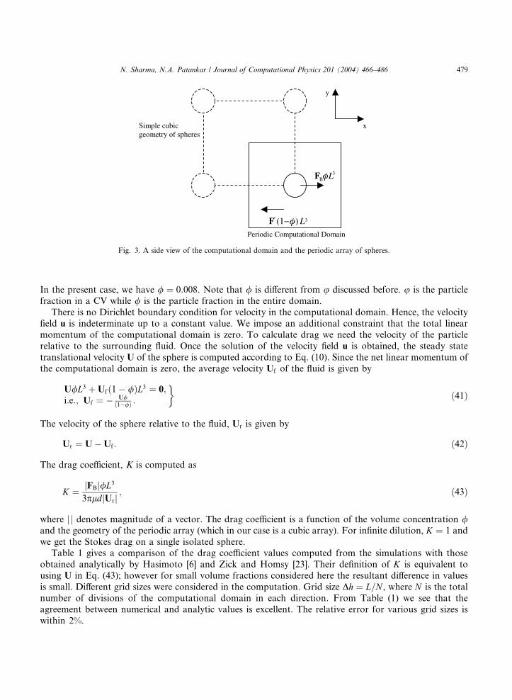
Consider a single sphere, in a fluid, placed at the center of a cubic periodic box. This implies a simple

cubic array of spheres. In Fig. 3, the solid lines outline the side view of the periodic computational domain.The dotted lines show that the sphere in the computational domain lies at the corner of a simple cubic

arrangement of spheres.

The diameter of the sphere d was set equal to 0.248 m and the edge length of the cubic domain L was set

equal to 1 m. The computational domain of size L3 was discretized uniformly. The fluid viscosity l was 1 kg/

m s. A constant body force FB ¼ 29:5 N/m3 was applied on the sphere in the positive x-direction. To ensure

that the net force was zero on the computational domain we added a constant body force F0 ¼ �0:238 N/m3

in the fluid domain. This was done to prevent the whole flow field from accelerating. Since the net force on

the computational domain is zero, the value of F0 was calculated by the following equation

FB/L3 þ F0 1� /ð ÞL3 ¼ 0;i:e:; F0 ¼ � FB/

1�/ð Þ ;

9=; ð39Þ

where / is the volume concentration of the spheres in the fluid and is given by

/ ¼ 16pd3

� �=L3: ð40Þ

Periodic Computational Domain

Simple cubicgeometry of spheres

x

y

'

Fig. 3. A side view of the computational domain and the periodic array of spheres.


In the present case, we have / ¼ 0:008. Note that / is different from u discussed before. u is the particle

fraction in a CV while / is the particle fraction in the entire domain.

There is no Dirichlet boundary condition for velocity in the computational domain. Hence, the velocity

field u is indeterminate up to a constant value. We impose an additional constraint that the total linear

momentum of the computational domain is zero. To calculate drag we need the velocity of the particle

relative to the surrounding fluid. Once the solution of the velocity field u is obtained, the steady state

translational velocity U of the sphere is computed according to Eq. (10). Since the net linear momentum of

the computational domain is zero, the average velocity Uf of the fluid is given by

U/L3 þUf 1� /ð ÞL3 ¼ 0;i:e:; Uf ¼ � U/

1�/ð Þ :

�ð41Þ

The velocity of the sphere relative to the fluid, Ur is given by

Ur ¼ U�Uf : ð42Þ

The drag coefficient, K is computed as

K ¼ FBj j/L3

3pld Urj j ; ð43Þ

where j j denotes magnitude of a vector. The drag coefficient is a function of the volume concentration /and the geometry of the periodic array (which in our case is a cubic array). For infinite dilution, K ¼ 1 and

we get the Stokes drag on a single isolated sphere.Table 1 gives a comparison of the drag coefficient values computed from the simulations with those

obtained analytically by Hasimoto [6] and Zick and Homsy [23]. Their definition of K is equivalent to

using U in Eq. (43); however for small volume fractions considered here the resultant difference in values

is small. Different grid sizes were considered in the computation. Grid size Dh ¼ L=N , where N is the total

number of divisions of the computational domain in each direction. From Table (1) we see that the

agreement between numerical and analytic values is excellent. The relative error for various grid sizes is

within 2%.

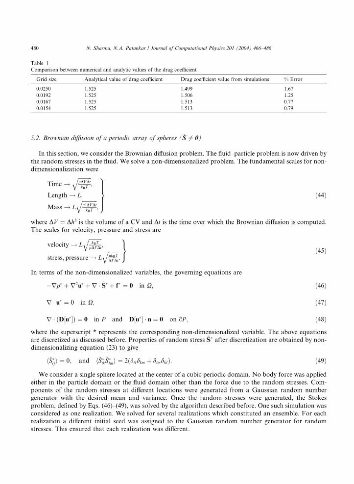
Table 1

Comparison between numerical and analytic values of the drag coefficient

Grid size Analytical value of drag coefficient Drag coefficient value from simulations % Error

0.0250 1.525 1.499 1.67

0.0192 1.525 1.506 1.25

0.0167 1.525 1.513 0.77

0.0154 1.525 1.513 0.79


5.2. Brownian diffusion of a periodic array of spheres (~S 6¼ 0)

In this section, we consider the Brownian diffusion problem. The fluid–particle problem is now driven by

the random stresses in the fluid. We solve a non-dimensionalized problem. The fundamental scales for non-

dimensionalization were

Time !ffiffiffiffiffiffiffiffiffiffilDV DtkBT

q;

Length ! L;

Mass ! Lffiffiffiffiffiffiffiffiffiffiffil3DV DtkBT

q;

9>>>=>>>;

ð44Þ

where DV ¼ Dh3 is the volume of a CV and Dt is the time over which the Brownian diffusion is computed.

The scales for velocity, pressure and stress are

velocity ! LffiffiffiffiffiffiffiffiffiffikBT

lDV Dt

q;

stress; pressure ! LffiffiffiffiffiffiffiffilkBTDV Dt

q:

9=; ð45Þ

In terms of the non-dimensionalized variables, the governing equations are

�rp� þ r2u� þ r � ~S� þ f� ¼ 0 in X; ð46Þ

r � u� ¼ 0 in X; ð47Þ

r � D u�½ �ð Þ ¼ 0 in P and D u�½ � � n ¼ 0 on oP ; ð48Þ

where the superscript * represents the corresponding non-dimensionalized variable. The above equationsare discretized as discussed before. Properties of random stress ~S� after discretization are obtained by non-

dimensionalizing equation (23) to give

h~S�iji ¼ 0; and h~S�

ik~S�lmi ¼ 2 dildkmð þ dimdklÞ: ð49Þ

We consider a single sphere located at the center of a cubic periodic domain. No body force was applied

either in the particle domain or the fluid domain other than the force due to the random stresses. Com-

ponents of the random stresses at different locations were generated from a Gaussian random numbergenerator with the desired mean and variance. Once the random stresses were generated, the Stokes

problem, defined by Eqs. (46)–(49), was solved by the algorithm described before. One such simulation was

considered as one realization. We solved for several realizations which constituted an ensemble. For each

realization a different initial seed was assigned to the Gaussian random number generator for random

stresses. This ensured that each realization was different.


As discussed in Section 2, the velocity field u, obtained for a given realization, is not the true velocity at

any instant. It should be interpreted as the Brownian displacement of the material point in time Dt dividedby Dt. The same interpretation applies to the particle velocities. Hence, in the following we shall refer tothese as the apparent velocities. Non-dimensional values of the apparent velocities were obtained from the

simulations.

In a given realization, the apparent velocity U� of the sphere was computed from u� according to Eq.

(10). The average apparent velocity U�f of the fluid was computed as in Eq. (41) and the relative apparent

velocity of the particle U�r was determined as in Eq. (42). The unbiased variance (to be defined later) of the

magnitude of U�r , denoted by hjU�

r j2i, can be computed based on the solution from all the realizations. As

discussed below hjU�r j2i can be used to obtain the drag coefficient K.

The Brownian diffusion constant D can be expressed in terms of variance of (dimensional) relativeapparent velocity as

D ¼Ur Dtð Þj j2

D EDt

6; ð50Þ

where Ur (Dt) is relative apparent velocity of the particle over time Dt. The diffusion constant D is also

related to the drag coefficient K by [9]

D ¼ kBT3pldK

: ð51Þ

From Eqs. (50) and (51) we get

K ¼ 6kBT

3pldDt Ur Dtð Þj j2D E ; ð52Þ

which in terms of the non-dimensional variables becomes

K ¼ 6

3pN 3d� U�r

�� 2D E : ð53Þ

Note that N ¼ L=Dh ¼ 1=Dh� gives information regarding the degree of discretization in the computational

domain. We used Eq. (53) to compute the drag coefficient from the numerical simulation. This numerical

value of the drag coefficient value was then compared with the analytic value obtained by Hasimoto [6] and

Zick and Homsy [23].

The value of hjU�r j2i was computed from an ensemble consisting of finite number of realizations n. A

different ensemble consisting of same number of realizations would give a different value of hjU�r j2i. This is

because our computations are stochastic. Hence, to interpret the value of hjU�r j2i computed from one en-

semble in a meaningful manner, we must assign to it a confidence interval and a confidence percentage. This

will be explained next.

Consider an ensemble of n values of U�r – Y1; Y2; Y3; . . . ; Yn – computed from n realizations. For a given

discretization N of the computational domain, the value of U�r obeys a Gaussian distribution of mean lN

and variance r2N . We compute the unbiased variance value hjU�

r j2i from the n values by [17]

U�r

�� 2D E¼

Xn

i¼1

Yi � �Y� �2

n� 1; ð54Þ

where


�Y ¼Xn

i¼1

Yin: ð55Þ

The confidence interval is the range in which we can state that r2N will lie given that we know the value

hjU�r j2i from computed ensemble. Associated with the confidence interval is a confidence percentage. The

confidence percentage ascribes a percentage of surety with which we can state the confidence interval.

Define a variable G as

G ¼Xn

i¼1

Yi � lN

rN

� �2

: ð56Þ

If we now assume lN ¼ �Y , then Eqs. (54) and (56) give

U�r

�� 2D E¼ r2

N

n� 1

� �G: ð57Þ

The random variable G is known to follow a Chi-square ðv2Þ distribution [17]. When lN ¼ �Y , G is a Chi

square distribution with n� 1 degrees of freedom (df), i.e., G ¼ v2n�1 [17].

Unlike a Gaussian distribution which is symmetric about the mean, the Chi square distribution is not

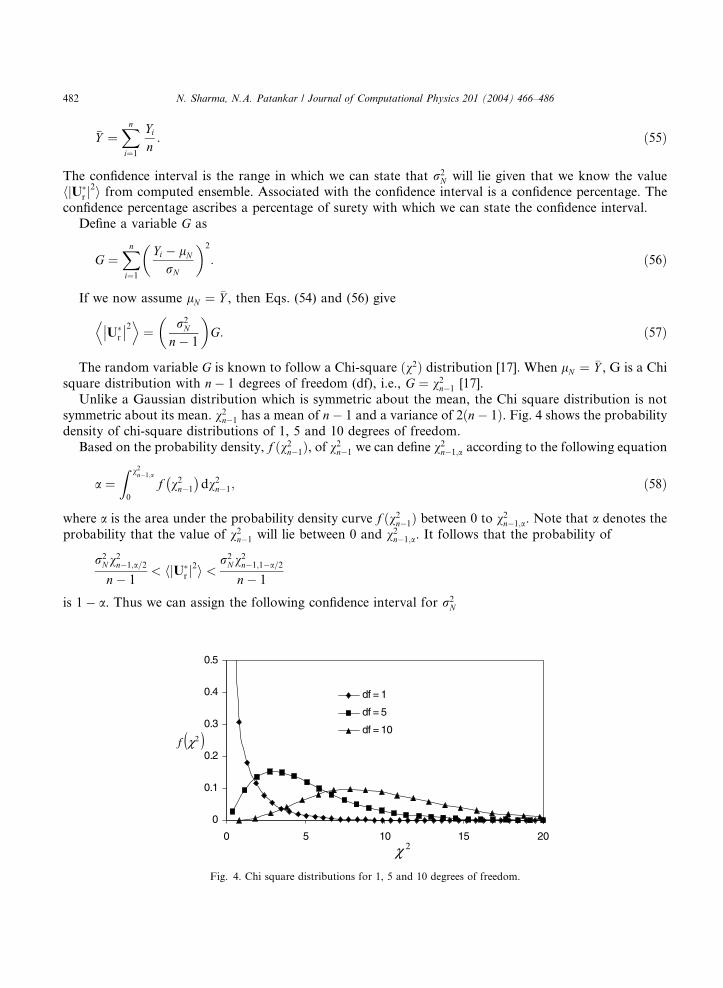
symmetric about its mean. v2n�1 has a mean of n� 1 and a variance of 2ðn� 1Þ. Fig. 4 shows the probability

density of chi-square distributions of 1, 5 and 10 degrees of freedom.

Based on the probability density, f ðv2n�1Þ, of v2n�1 we can define v2n�1;a according to the following equation

a ¼Z v2n�1;a

0

f v2n�1

� �dv2n�1; ð58Þ

where a is the area under the probability density curve f ðv2n�1Þ between 0 to v2n�1;a. Note that a denotes the

probability that the value of v2n�1 will lie between 0 and v2n�1;a. It follows that the probability of

r2Nv

2n�1;a=2

n� 1< hjU�

r j2i <

r2Nv

2n�1;1�a=2

n� 1

is 1� a. Thus we can assign the following confidence interval for r2N

Fig. 4. Chi square distributions for 1, 5 and 10 degrees of freedom.


n� 1ð Þ U�r

�� 2D Ev2n�1;1�a=2

< r2N <

n� 1ð Þ U�r

�� 2D Ev2n�1;a=2

; ð59Þ

with 100ð1� aÞ % confidence percentage (certainty). The values of v2n�1;a are tabulated in standard texts

[17]. Correspondingly, using Eq. (53) we form a confidence interval for the drag coefficient K.Based on the above methodology we shall now present the results from the simulations. We first con-

sidered a sphere of diameter d� ¼ 0:248. This corresponds to a volume concentration / ¼ 0:008. The

number of divisions in the computational domain were N ¼ 40. We considered an ensemble of 300 real-

izations. In each realization the apparent velocity of the Brownian sphere was computed by solving Eqs.

(46)–(49). The relative apparent particle velocity U�r was computed as described before.

By symmetry, stochastic properties of the three components of U�r along the three co-ordinate directions

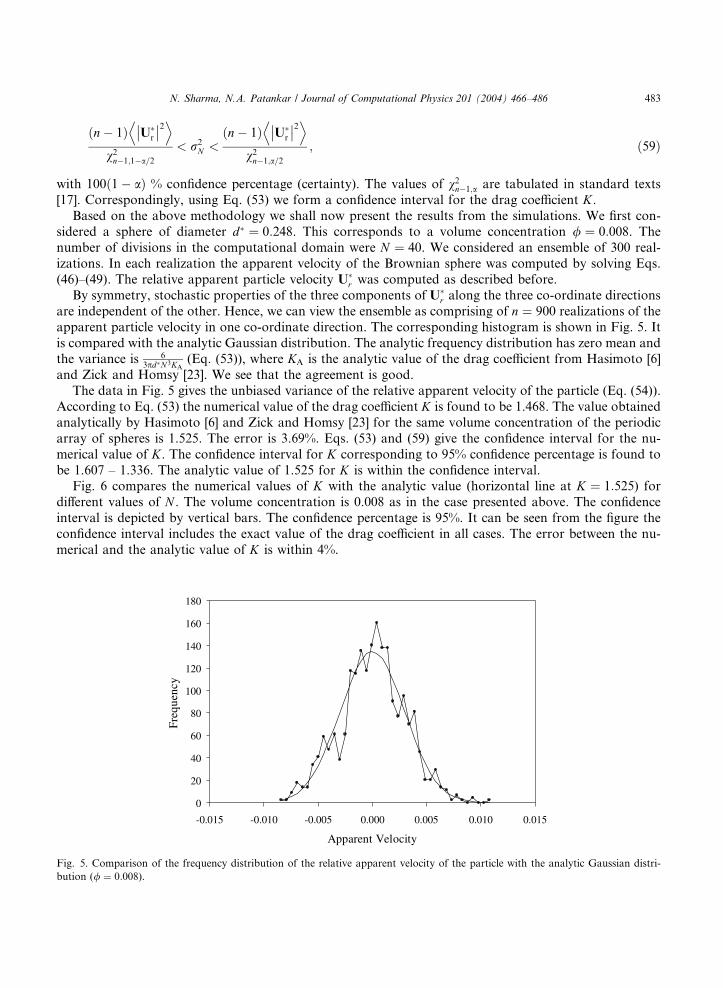
are independent of the other. Hence, we can view the ensemble as comprising of n ¼ 900 realizations of the

apparent particle velocity in one co-ordinate direction. The corresponding histogram is shown in Fig. 5. It

is compared with the analytic Gaussian distribution. The analytic frequency distribution has zero mean andthe variance is 6

3pd�N3KA(Eq. (53)), where KA is the analytic value of the drag coefficient from Hasimoto [6]

and Zick and Homsy [23]. We see that the agreement is good.

The data in Fig. 5 gives the unbiased variance of the relative apparent velocity of the particle (Eq. (54)).

According to Eq. (53) the numerical value of the drag coefficient K is found to be 1.468. The value obtained

analytically by Hasimoto [6] and Zick and Homsy [23] for the same volume concentration of the periodic

array of spheres is 1.525. The error is 3.69%. Eqs. (53) and (59) give the confidence interval for the nu-

merical value of K. The confidence interval for K corresponding to 95% confidence percentage is found to

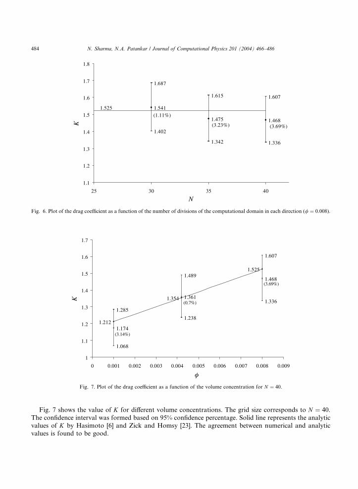
be 1.607 – 1.336. The analytic value of 1.525 for K is within the confidence interval.Fig. 6 compares the numerical values of K with the analytic value (horizontal line at K ¼ 1:525) for

different values of N . The volume concentration is 0.008 as in the case presented above. The confidence

interval is depicted by vertical bars. The confidence percentage is 95%. It can be seen from the figure the

confidence interval includes the exact value of the drag coefficient in all cases. The error between the nu-

merical and the analytic value of K is within 4%.

0

20

40

60

80

100

120

140

160

180

-0.015 -0.010 -0.005 0.000 0.005 0.010 0.015

Apparent Velocity

Freq

uenc

y

Fig. 5. Comparison of the frequency distribution of the relative apparent velocity of the particle with the analytic Gaussian distri-

bution (/ ¼ 0:008).

1.541

1.475 1.468

1.402

1.342 1.336

1.687

1.615 1.607

1.1

1.2

1.3

1.4

1.5

1.6

1.7

1.8

25 30 35 40

N

K

1.525

(3.69%)(3.23%)

(1.11%)

Fig. 6. Plot of the drag coefficient as a function of the number of divisions of the computational domain in each direction (/ ¼ 0:008).

1.212

1.354

1.525

1.174

1.361

1.468

1.068

1.238

1.336

1.285

1.489

1.607

1

1.1

1.2

1.3

1.4

1.5

1.6

1.7

0 0.001 0.002 0.003 0.004 0.005 0.006 0.007 0.008 0.009

K

(3.14%)

(3.69%)

(0.7%)

Fig. 7. Plot of the drag coefficient as a function of the volume concentration for N ¼ 40.


Fig. 7 shows the value of K for different volume concentrations. The grid size corresponds to N ¼ 40.

The confidence interval was formed based on 95% confidence percentage. Solid line represents the analytic

values of K by Hasimoto [6] and Zick and Homsy [23]. The agreement between numerical and analyticvalues is found to be good.


6. Conclusions

We have presented a DNS scheme for the Brownian motion of particles. The thermal fluctuations wereincluded in the fluid equations via random stress terms. Solving the fluctuating hydrodynamic equations

coupled with the particle equations of motion resulted in the Brownian motion of the particles. The par-

ticles acquired random motion through the hydrodynamic force acting on its surface from the surrounding

fluctuating fluid. The random stress in the fluid equations were easy to calculate unlike the random terms in

the conventional Brownian Dynamics (BD) type approaches. A three-dimensional implementation was

presented along with validation.

We have discussed in detail the discretization of the governing equations in the above mentioned for-

mulation of the problem. The problem was solved in the long time dissipative limit. Solution of the gov-erning equations gave the Brownian displacements of the particle. The numerical results were used to find

the corresponding drag coefficient acting on the particle. The numerical values of the drag coefficient were

compared with analytic values. The agreement was found to be good.

We considered a single spherical particle in a periodic domain suspended in a constant property New-

tonian fluid. The method can be extended to particles of any shape and fluids with varying properties. This

will be the subject of our future work.

Acknowledgements

This work was supported by National Science Foundation through the CAREER Grant CTS-0134546.

References

[1] J.F. Brady, G. Bossis, Stokesian dynamics, Ann. Rev. Fluid Mech. 20 (1988) 111–157.

[2] D.L. Ermak, J.A. McCammon, Brownian dynamics with hydrodynamic interactions, J. Chem. Phys. 69 (4) (1978) 1352–1360.

[3] R. Glowinski, T.W. Pan, T.I. Hesla, D.D. Joseph, A distributed Lagrange multiplier/fictitious domain method for particulate

flows, Int. J. Multiphase Flow 25 (1999) 755–794.

[4] M. Grmela, H.C. €Ottinger, Dynamics and thermodynamics of complex fluids. I. Development of a general formalism, Phys. Rev.

E 56 (6) (1997) 6620–6632.

[5] E.H. Hauge, A. Martin-L€of, Fluctuating hydrodynamics and Brownian motion, J. Stat. Phys. 7 (3) (1973) 259–281.

[6] H. Hasimoto, On the periodic fundamental solution of the Stokes equations and their application to viscous flow past a cubic

array of spheres, J. Fluid Mech. 5 (1959) 317–328.

[7] H.H. Hu, D.D. Joseph, M.J. Crochet, Direct numerical simulation of fluid particle motions, Theoret. Comput. Fluid Dyn. 3

(1992) 285–306.

[8] H.H. Hu, N.A. Patankar, M.Y. Zhu, Direct numerical simulations of fluid solid systems using Arbitrary Lagrangian-Eulerian

technique, J. Comput. Phys 169 (2001) 427–462.

[9] J. Keizer, Statistical Thermodynamics of Nonequilibrium Processes, Springer-Verlag, 1987.

[10] A.J.C. Ladd, Short time motion of colloidal particles: numerical simulation via a fluctuating Lattice–Boltzmann equation, Phys.

Rev. Lett. 70 (9) (1993) 1339–1342.

[11] L.D. Landau, E.M. Lifshitz, Fluid Mechanics, Pergamon Press, London, 1959.

[12] H.C. €Ottinger, M. Grmela, Dynamics and thermodynamics of complex fluids. II. Development of a general formalism, Phys. Rev.

E 56 (6) (1997) 6633–6655.

[13] N.A. Patankar, A formulation for fast computations of rigid particulate flows center for turbulence research, Ann. Res. Briefs

(2001) 185–196.

[14] N.A. Patankar, Direct Numerical Simulation of moving charged, flexible bodies with thermal fluctuations, Technical Proceedings

of the 2002 International Conference on Modeling and Simulation of Microsystems (2002) 32–35.

[15] N.A. Patankar, P. Singh, D.D. Joseph, R. Glowinski, T.W. Pan, A new formulation of the distributed Lagrange multiplier/

fictitious domain method for particulate flows, Int. J. Multiphase Flow 26 (2000) 1509–1524.

[16] S.V. Patankar, Numerical Heat Transfer and Fluid Flow, Taylor and Francis, 1980.


[17] A.D. Rickmers, H.N. Todd, Statistics An Introduction, McGraw-Hill Book Company, 1967.

[18] P.S. Sathyamurthy, S.V. Patankar, Block-correction-based multigrid method for fluid flow problems, Numer. Heat Transf., Part B

25 (1994) 375–394.

[19] M. Serrano, P. Espa~nol, Thermodynamically consistent mesoscopic fluid particle model, Phys. Rev. E 64 (4) (2001) 046115.

[20] M. Serrano, D.F. Gianni, P. Espa~nol, E.G. Flekkøy, P.V. Coveney, Mesoscopic dynamics of Voronoi fluid particles, J. Phys. A 35

(7) (2002) 1605–1625.

[21] N. Sharma, N.A. Patankar, A fast computation technique for the Direct Numerical Simulation of rigid particulate flows. J.

Comput. Phys (2004a) (submitted).

[22] N. Sharma, Y. Chen, N.A. Patankar, A Distributed Lagrange Multiplier based steady state algorithm for particulate flows (to be

submitted).

[23] A.A. Zick, G.M. Homsy, Stokes flow through periodic arrays of spheres, J. Fluid Mech. 115 (1982) 13–26.

[24] R. Zwanzig, Hydrodynamic fluctuations and Stokes’ law friction, J. Res. Natl. Bur. Std. (US) 68B (1964) 143–145.

direct numerical simulation of the brownian motion of particles by using fluctuating hydrodynamic...

Documents