direct hydrocarbon exploration and gas reservoir ... - osti.gov
TRANSCRIPT
rRN4jQ
n\ 1 n ^ s.•d *1 m m M
<R —95(T) —6
Direct Hydrocarbon Exploration and Gas Reservoir
Development Technology
# %
#
IISTSIBtmflH IF m OtOJEHT IS UM1UHTEIFiifflH im mama pg,
*11 1 Lj £a ^ M JL Ai
<R —95(T) —6
W$fc( I )
Direct Hydrocarbon Exploration and Gas Reservoir
Development Technology
m %
MtlSSA
DISCLAIMER
Portions of this document may be illegible in electronic image products. Images are produced from the best available original document.
* #### #41 1 7>^4 70#7|# If"
mmi m-A^m ###&
1995# 41
3=#9F##B845:# B9 3 # 3% 9% Bfm@3?9s*e# : m ^ mffi % M : S#%m#92gG ^ % m
s#%mi?9G#B # # m
5#mm#9Ga FF * E
576SM2£S $ I f
# W ^BifiS«5ESB # # # 5%mmw^eG # m $
u mm{tmfrVxw^ m wl m
smjgrnmeaG ^ c m
5%g##95@B # # m5%mm3?92§G & £ S
^ % ^
sMBrnmesE A # m
Q °J= SL
1.
l-iMM 44 17} 4 ^ 7}5* 7H144 -34
2. oif S| Ej-f foAj
4* 4*7} 44 44*44 44* **5 44 #4 4#44 4 ^444 *4 44 #4 4 44444. 3-44 44 441-4 5*531 *44* 44 4445.4 4444 444 44 45.444**5*, 44 444 5.^4-5.5.4 441 4* 7} 47} #44*4 455 444 *4 45444 14 4#4 4* *44* * 45 44*4 47> *4. 444 14-14, 14-51*- 31* 4# 4 444 *4 45# 4*-4#31 444* *#*55 *4 4* 7]#457} 4544. 44 4514 4*431 **4 #5* *# 4 * 4 *5 *4#44 544 5*= 1 4)4 1* 4445 #4 4 51*45 *5 44* 14 44* 31* *4 &* 4*'* *4 *4 4 * 4*4.
4** 4 #4 4 4 44** ^5 14*14 sfl 4 4 * * 7H44 4*45 14* *44 5*4 ## 14*4 44# a31 114 4 #4. 14* *44 44* 447>554* 4 #4 444 41 155 14 31** 3H 4f* *171-5 44 #4 4*4 #4H *4. *** 44* *44 1**4* 41* 447}** 44# Tfl 5*5 5 7}4 *31# #7] * 411*5 *3131 1* 44*17}
—3 —
1441AS4 #4 €444A =l €### €#4 ## 44#^} # 431 $14.
44 €47>s€ 54# A€ #?H 4444 &AS 444 4 4444 4S.7> 4444 444 4444 #4 4 44 44 7}s ffl4 4 #7}# #7M1 44 44. 44 4 4 44 45-4 444 44444 7}A 4444 S.#4AS ;H# s€## 44# 3i€## 4 4 #^-44. 7>>i4 s# 7}7i€€4 4^-4€ m&4€4- A#7l
#4 *B471 7}#4# 41# 44 4^-4 144 is# 444
4 44444 44. 7}s€ M$# torn4# 44 444 #A4 4-4 4444 4 44 1€4 #444. A#€ 7}d- 4 7}^^n 4^4 4'4A A€€# 44 iEEAS *1444 #44 4## A 4-31 44*-.
3. i-H-e- % y#i wn^'dJE)
€#-€=#, €#-544 44 4## €#4 144ll^l #4 4,4, #4 s€4 ##4 #4#4 ##s€# 444-31 44 4s.# 7].€#444 44 4AS 444 s€## 44#ASl #
44 4€€ 7]### #s#^4. 1&4# #4 €€-&#€ 44 44# 14431, #4 4#A# 4444 4# 4 444 4s4 1 4 444- 4s4^4. 3142. 14 7]#4 #4 4#€ €44# 444-71 €44 41 #44 7}-g-€ 4s# €4444 #4# 4144 31 44# €ih.-s>^4. 45. 444 #7}ig 4444# #1€## #44 4544 #M €€#4 14 #44# #444 1 44 AS 14 #€ €4#A 7>s #4 4# #s# 44 ##as
—4 —
44 453-0-4, 4 7l#o)l 7}+ f # 44# a]-s^2}-s>374# 4## 453#. aft" 4 4# #4# 4# #44 #4471 4 44 3444# 44-0-3. 4 4444 4# 44# 4## 34### 4#4##0.3.4 ## 7>44# #&4^#.
f43-4^33.44 44 ###44 #4 4 #44# 44 # 4* 444 #44 44444 f44 4444 4#4 4444 #, 7>4^-4## # ###4 444 43# ##44 34453#. 44443# #44 #4# #4-434 4 44 4441 7># #3# M°J 44 434 44# 444, #444 4##4 44 4## 4 ### 4# 4 7>4 4#^4 ##4^1# 4444 4### 7fl #444. 4## #44^4### 4#44 ^4#4 4 44 #44^4. 2t #44 #4 #34 #3# 4444 444 ### # 44a4 4#4#3 ##4^4. 4 ### ^4# 4-33.44 & 4# ##4 4 #41 ####s# 4 4#  4# 4#4 4# 4# #4 #4 #t3. 44# 4 443 7>44j7, 444 4 43 s. ##44 ##4#4#4 ### ##437} 4^4.
7^4 ##4 444## MS# ##44-4 firMSE^ 4#
4444-3S. #4 4 4 $14. 4##4 4#44-44# ##4# 4^#^14-4 #-#& ### 4 ### 34 4# (unconditionalsimualtion)4 $k@fWs 34 4 # (conditional simulation)#4# til 3 ^.4§>5^4. jeMSH 4# #4 44-44# ffr«fS4 #4 4 ffl ##4 4# 4## 4*3453#. e^m#4 4 3444 #44 4 44 444 4 #44# 7}i43l 444 4# #4, #^c# 4 44#, #nat «M4#, HrMB# lean gas44 444# #4 fflSB 41## #44534.
-5-
4. oi^-7HW W ##4| cm
1#-*14, 1*-1* tfltiio)] 4#4<y ^4 &?]# ^ sy ^ y
44 544 a-y§>3i yjitb &#*4- 54444 4# 44#4 #4# ^^4. 44 *44 4*4 4&4 44 545 *4 4545 444 # 4 14-7} 44 *4 444 144* 455*4 44 4## #44 4 44 #4 4*4 ytijAjo] 455 4W4. 44#4 44# 54
44 4**4 44 44# #5. 4)44 414# 4444* 4444, E* 4 610.5m, F# 667.2m 4&* *4 44 444* 54*4. ^43. 54 44 *4*4 *4 4*57} #4 #44 4*44 4*5. 7>yx^7> 44=44 *7>4-4, 44455* 44* 4:44 4*4 y** 44-1
4. 4 44-* 5E# 444 4# 454- 444* 444. S55 44#, 544# 444 44 #41-4 4## 44 #4#4 #4 4 444 4
4 4*7} 4 #4 55 14444= # 444 44 #11 4 44 44 #
4*4 4* 4*4 445.444 *7} ##4 ##44. 44 #4* *4 4 4)4 4*o] y-y-sr] s}i4i #44 *4 71)14 ##444 # 44 4, 4*7*1 s§7\) s4* *44*# 4#* #4 *44 4# 4*5 7}
*# 14 4-.4) #4 **4 4 $1* 7] 7i] #4 # 4 # 4 444 4 * 4#
*4 #4- * 1U 5x io~4me 4455 *#44 4* 44*5* *#44 7}a aL545zi5}45 *4* * ^44. 4 44 #4* 4 #71144. 7}5 ***47} 4)4=444 4 5 444 444 4*1 * &#* 54 ** 444. 44*5 4 #**4 4)4 44*4 4*# #414, 44*4 44*5 7} 5 7} 4^4 ^4 4*4 4 4.* 455 444 4 444 44 44*54 44 44* 4*#
—6 —
1 4* 4 41^154 *1 444 1 #11 4444 444 1#1 * $1* 7}*## *44. zz.44 444 14 *±7} 44 44^±o]$XSLE.g. 7}^ 14*±1 44 4*# *4 #11 1*1 1 4 n 7>444 54 444 4 $14 4 44.
444 4 414 4 4441 4114 #41 411* 4444 14 44 4#7}a 4 fa>£ 4444 !#4&# 5444 44 444 44 7}a4 444 444 14 4144 7>*44 444 414 4 4114 414$14. 4 57] 7>1 5*1 sl!4 14 4^-4 45 4*4* 4 4 47] 44 451 14# 1# 4 $1 $14. 4 #4 44143.4: 31 44 4, 44 44 4 444= *4- ne]jl 414441 #44 4145 544±3. #41 444.
7}5 4 7}^H4454 7]]#4# 134 144 $144 21* 4# 4114 41 4444 44314 444 1111*1 444 444 * #5 4544 4#4 #21# 4#4114 441 1*4 1454 1 441 *$14. 7>^ ME144 E*f! 4 ±11* Mil *4 # ±44* 1441 11 $1* 4#4-4 441 *1414 41 *4 44 #44 *##44 *4411 14. 11 ffl* 41* 4**14 443.4 4*41 4*#4 *7>4 4# 4 #5 54 411 4**14 *1 4 Ml£4 411 #4411 4# *±41 41 14 4*14,1 4141, ##:# ME41* 11144 4±4 1 1441±1 lean
gas44 4441* 4**14 44 1*4 114 444 11 1441
4. 14 1* 14* 417144 41 44 76ffl 4 7>^b 7H#4 1*1
* $1±1 *4 *1444 7>3B 7H! ±11 7>444* 4414 1#
4 11* 45-1 7fiEl 41 @Sr 4 5S4#4 411-7]- 4144.
—7—

w
SUMMARY
"Direct Hydrocarbon Exploration and Gas Reservoir Development Technology"
In order to enhance the capability of petroleum exploration and
development techniques, three year project(1994 - 1997) was initiated on
the research of direct hydrocarbon exploration and gas reservoir
development. This project consists of four sub-projects. Three
f sub-projects are concerned with exploration technologies including
geochemical and geophysical methods.- The other project is focused on
the development of gas and/or gas-condensate reservoirs.
For the sub-project of oil to source rock correlation, the overview of
biomarker parameters which are applicable to hydrocarbon exploration
has been illustrated. Experimental analysis of saturated hydrocarbon and
biomarkers of the Pohang #E and #F core samples has been carried out.
Samples were extracted by stirring in dichrolomethane at 40-50°C for 10
hours. The saturated, aromatic and resin fractions of the extract were
obtained using thin layer chromatogram. The relative abundance of *
normal alkane fraction of the samples is low except lowest interval,
which is probably due to the biodegradation. The biomarker assemblage
of hopanoids and steranes has been characterized. According to the
analysis of saturated hydrocarbons and biomarkers, the sedimentary
environment of the Pohang core samples is marine and transitional zone
except the terrestrial environment of the lowest samples such as 610.5m
-9-
from #E core and 667.2m from #F core. The thermal maturity through
the studied intreval did not reach oil window even though slight
increase in thermal maturity with depth, which coincide with Rock Eval
pyrolysis data.
In order to check the validation of analysis of the biomarkers, same
samples were analyzed by the University of Louis Pasteur, France. The
distribution and relative peak area of the biomarkers were identical with
those by laboratory of KIGAM. For the 2nd stage of the research,
analysis of biomarkers other than hopanoids and steranes should be
continued:
For the part of the surface geochemistry & microbiological
study, the test results of the experimental device for extraction of
dissolved gases from water show that the device can be utilized
for ‘the g$s geochemistry of water. The device is capable of
determining, hydrocarbon gases in water to the concentration of
less than. 5x10H mien. According to the results of
microbiological studies, the plate count technique can be a useful
supplementary method for hydrocarbon exploration. This is based on the
facts that the average survival rate to hydrocarbons (pentane, hexane)
for heterotrophs is higher in the area known as containing considerable
hydrocarbon gases than other areas in the Pohang region. Howevr, it is
still necessary to develop techniques to treat the bacteria with gaseous
hydrocarbons.
In the study of numeical modeling of seismic wave propagation and
full waveform inversion, 3 individual sections are presented. The first
-10-
one is devoted to the inversion theory in general sense. In this section,
inversion schemes such as gradient method, Gauss Newton method, and
the full Newton method are reviewed to establish the new aspect of the
inversion theory on the basis of numerical tool such as finite-elements
in the frequency domain. The second and the third sections deal with
the frequency domain pseudo waveform inversion of seismic reflection
data and refraction data respectively. This inversion scheme is an
eclectic type inversion that lies between waveform inversion and
traveltime inversion. The forward response is generated in the frequency
domain as the pseudo waveform data obtained by low-pass filtering the
unit-amplitude delta-function data. - These data have phase shift
corresponding to traveltimes calculated by the shooting ray-tracing
technique. The Jacobian for a damped least square method is computed
analytically at each step of the forward ray tracing. The applicability
and feasibility of the proposed inversion algorithm is demonstrated with
prestack field data as well as with synthetic data generated by
finite-difference modeling. The estimated model of synthetic data
matches the true model closely, and the estimated model of prestack
field data provides a reasonable solution in comparison with nearby
sonic log data (reflection inversion) or in comparison with published
results (refraction inversion).
Due to the industrialization of the Asian countries including Korea,
the consumption of natural gas in this area will be drastically increased.
It is also anticipated that the consumption of natural gas will increase
more rapidly than oil consumption because of the environmental
-11
problems such as acid rain and green-house effect. It" is important to
participate on the gas development projects in foreign countries
including CIS to secure the stable supply of oil and gas.
In the study of gas reservoir development, the first year topics are
restricted on reservoir characterization. There are two types of reservoir
characterization. One is the reservoir formation characterization and the
other is the reservoir fluid characterization. For the reservoir formation
characterization, calculation of conditional simulation was compared with
that of unconditional simulation. The results of conditional simulation
has higher confidence level than the unconditional simulation because
conditional simulation considers the sample location as well as distance
correlation.
In the reservoir fluid characterization, phase behavior calculations
revedled that the component grouping is more important than the
increase of number of components. From the liquid volume fraction with
pressure drop, the phase behavior of reservoir fluid can be estimated.
The calculation results of fluid recombination, constant composition
expansion, and constant volume depletion are matched very well with
the experimental data. In swelling test of the reservoir fluid with lean
gas, the accuracy of dew point pressure forecast depends on the
component characterization.
-12-
CONTENTS
PART 1. INTRODUCTION............................................................................. 21
PART 2. OIL(GAS) - SOURCE ROCK CORRELATIONTECHNIQUE.................................................................................... 27
Chapter 1. Generalities............................................................................... 291- 1. Definition of the biomarker............................................................. 29.1-2. Review of the biomarker parameters used for petroleum
exploration.................................................................... 311-2-1. Depositional environment & organic matter input............. 311-2-2. Thermal maturation..................................................................... 451-2-3. Biodegradation.................... 521-2-4. Correlation...................................................................................... 541- 2-5. Migration........................................................................................ 55
Chapter 2. Application of the biomarker analysis technology............... 572- 1 Separation and Extraction.................................................................. 572-2 Analysis of Saturated hydrocarbons............................................... 612-3 Analysis of biomarkers....................................................................... 642-4 Result and Discussion .......................................................................... 67
2- 4-1. Sedimentary Environment.......................................................... 672-4-2. Stage of Thermal maturity....................................................... 772-4-3. Discussion...................................................................................... 79
PART 3. STUDY ON SURFACE GEOCHEMISTRY AND MICROBIOLOGY FOR HYDROCARBON EXPLORATION.............. 8l
Chapter 1. Review of previous studies........................................................ 831-1. Vertical migration of hydrocarbon................................................ 841-2. Microbiological exploration ........................................................... 871-2-1. Bacteria............................................................................................ 911-2-3. Chimney........................................................................................... 931-2-4. Biogenic methane.......................................................................... 95
-13-
1-2-5. Halos.......... _•..................................................................................... 971-3. Onshore hydrocarbon analysis........................................................... 98
1-3-1. Soil-air hydrocarbon analysis.................................................... 981-3-2. Soil-sorbed hydrocarbon analysis............................................. 991-3-3. Soil-occluded hydrocarbon analysis......................................... 991- 3-4. Integrative absorbtion............................................. .................... 100
1- 4. Offshore hydrocarbon analysis.......................................................... 101Chapter 2. Selected method............................................................................. 103
2- 1. Device for gas extraction from sea water..................................... 1032- 1-1. Component...................................................................................... 1052- 1-2. Operation......................................................................................... 105
2- 2. Test operation........................................................................................ 106Chapter 3.' Microbiologic study....................................................................... 107
3- 1. Materials methods................................................................................. Ill3- 1-1. Sampling.......................................................................................... Ill3-1-2. Methods........................................................................................... 113
3-2. Results...................................................................................................... 1133-2-1.. Determination of concentration for heavy metal ions and
hydrocarbon treatment .............................................................. 1133-2-2; Average number of heterotrophic bacteria
in Pohang area.............................................................................. 1173-2-3. Survival rate for heavy metal ions and hydrocarbons
at site A......................................................................................... 1173-2-4. Survival rate for heavy metal ions and hydrocarbons
at site B.........................................................................:............... 1233-2-5. Survival rate for heavy metal ions and hydrocarbons
at site C.................................................................. 1283-2-6. Survival rate for heavy metal ions and hydrocarbons
at site D................................................................................*........ 128Chapter 4. Conclusions..................................................................................... 136
PART 4. DEVELOPMENT OF GAS AND GAS-CONDENSATERESERVOIRS............................................................................ -139
Chapter 1. Introduction...................................................................................... 141Chapter 2. Reservoir characterization.............................................................144
—14—
2-1. General characters of reservoir....................................................... 1442-2. Stochastic model.................................................................................. 1482-3. Model type............................................................................................ 1522- 4. Application of stochastic model....................................................... 153
Chapter 3. Characteristics of reservoir fluids.............................................1603- 1. Composition of reservoir fluid........................................................... 1603-2. Classification of reservoir fluid......................................................... 1643-3. Sampling of reservoir fluid.................................................................. 1743- 4. Analysis of reservoir fluid................................................................... 180
Chapter 4. Phase behavior of reservoir fluids............................................1834- 1. Fluid recombination................................................................................ 1834-2. Constant composition expansion test................................................ 1854-3. Constant volume depletion test........................................................... 1924-4. Swelling test of reservoir fluid .with lean gas............................... igg
PART 5. NUMERICAL MODELING OF SEISMIC WAVEPROPAGATION AND FULL WAVEFORM INVERSION.....2Q3
Chapter 1. Seismic inversion theory............................................................. 2051-1. Introduction............................................................................................. 2051-2. Finite-element and finite-difference formulation of wave
equation ................................................................................................. 2061-3. Inversion algorithm............................................................................... 2071-4. The Gradient method........................................................................... 2091-5. The Gauss Newton method................................................................2161-6. The full Newton method.....................................................................2261- 7. Efficient calculation of Hessian matrix........................................... 230
Chapter 2. Pseudo waveform inversion of reflection seismogramsin the frequency domain............................................................. 234
2- 1. Introduction....................................... 2342-2. Theory...................................................................................................... 236
-15-
2-2-1. Damped least square method................................................. 2362-2-2. Parameterization and Forward calculation............................ 2372-2-3. Calculation of Analytical Derivatives...................................... 2402-2-4. The frequency band characteristic of the objective
function................................ 2442-3. Examples................................................................................................ 249
2-3-1. Synthetic data............................................................................... 2492- 3-2. Field data....................................................................................... 260
2- 4. Discussion.............................................................................................. 266Chapter 3. Inversion of seismic refraction data in the frequency
domain using ray tracing........................................................... 2683- 1. Introduction............................................................................................ 2683-2. Theory.......................................................................................... 2693-3. Examples................................................................................................ 277
3- 3-1. Synthetic data............................................................................... 2773-3-2. Field data....................................................................................... 284
3^4. Discussion .................................. 290
PART 6. CONCLUSION ...................................................................... 291
APPENDIX ......................................................................................................... 317
—16—
X\
41% 4#......... :....................... 214)2# €-n-(7>dh) - 44 7)# ................................................ 2741% 29
1-1. 44 54 #4 44 ........................................................................,..... 291- 2. 4f W 4-§-4^ -94 541- 4444........................... si
l-2-i. 44 44 4 e€ #4 4"9.................................................. 311-2-2. 14 445=....................................................................... 451-2-3. 4# ■§"4 ................... —................................................ 521-2-4. 44 ................................................................................... 541- 2-5. 4-W".................................................................................................. 55
4124 -g-g- 572- 1. #4# f# 4 24 e4....................................................... 572-2. 54 44 #2 ^4 ............................................................... 612-3. 44) 57) ir ^-4 ......................................... ........................ - 642-4. %% 44 4 5#.................... ..... ;......................... ......................... . 67
2- 4-1. 44 #4 44*114.............. 672-4-2. 44 4 #5 44*114................................... 772-4-3. 79
71)34 45 ^ #44 444 4-4-4#................................................ si41% 71)5 ..........:...................... 83
1-1. #44^- *117M#........................................ 841-2. 4 4 #44 #4........................................................ 87
1-2-1.4444.................................................................. 881-2-2 4445.4.......................................................................... 911-2-3. ##................................................................................................... 931-2-4. -^#7)1 #4.................................................................................. 951-2-5. HALOS............................................................................................ 97
-17-
1-3. 43 444 981-3-1. 5. #-57] 11455 54 .................. gg1-3-2. 5. #-54 11455 54 ............................................................. 991-3-3. 5.#-BS.iiE 3:455 54 ............................................................. 991- 3-4. 555 3455 54 ................................................................... 100
1- 4. 4# x)44 34-................................................................................... ioi423 444 34 33 4# ^ 44.................. 103
2- 1. 7>^ f# 344 54 ^ 4#......................................................... 103■ 2-1-1. 54 ............................. 105
2- 1-2. 4"#"................................................................................................... 1052- 2. 43 54 ............................. 106
4134 44544 4-44 #5..................... 1073- 1. 4s. 7# ^ 44.............................................................................. Ill
3- 1-1. 454]#)........................................................................................... Ill3-1-2. 44............................................. :.................................................... 113
3-2. 3534 ................................................................................................. 1133-2-1. #354 3455 #S. #4 ..................................................... 1133-2-2. 54444 44 #5##43 55......................................... 1173-2-3. A 44 s#434 #354 34554 44 #1.. 1173-2-4. B 44 54454 #544 44454 44 45* ••:...... 1233-2-5. C 44 s#434 #554 44554 44 45#......... 1283-2-6. D 44 s#434 #544 44554 44 49#*......... !28
444 7}^ 3 7}^^ #4 4 5 4##4 7M44........... 139413 4#...............•;................. hi42# 4## .4444 ......................... 144
2-1. 45#4 #34 44...................... 1442-2. 44€4 5# .:......................... 1482-3. S.’S-S].#-#.......................................................................................... 1522- 4. S.34 ## ^ 44^ .................................................................. 153
434 45 544 44 1603- 1. 45 544 &4 160
-18-
3-2. 4*1)4 1643-3. 7}^ #54 7# 1743- 4. 7>i #54 £•# iso
7)14# #7]# 1834- 1. #£ #-# ## 1834-2. ##4 #^ 1854-3. #7)1# #<# ## 1924-4. ## #7)14 lean gas4 ^4 ## 198
7)15# 4#s.^5£zL#i 44 ##4 4# 44 #4.....................2037)114 ##4444#................................................................. 205
1-1. 4#............................................................................. 2051-2. 4####4 ##J3-£#4 #444#............................... 2061-3. 44 4#............................•••........................................ 2071-4. 44##-#..................................................................... 2091-5. 7>4^-#4# ................................................................ 2161-6. ### ................................................... .................. ..... 2261- 7. §1144 *314 3:44 <2 44............................................ 230
7)12# 444444# 4#-# #-a}a}54 f-Al-4^4#................... 2342- 1. 4#............................................................................. 2342-2. 4-B............................................................................. 236
2-2-1. 4421^4## ......................................................... 2362-2-2. 4 44 7H 4444 ##44444 #4......................... 2372-2-3. 4144 4444 44................................................ 2402-2-4. 44444 444 44 44...................................... 244
2-3. ## 4.................................................................................... 2492-3-1. ##-4445............................................................. 2492-3-2. 4445.................................................................. 260
2- 4. £4 ............................................................................. 2667fl3# 4#4#-& #44 44444444 ### 4s. 4#............. 268
3- 1. #€■............................................................................. 2683-2. ##............................................................................. 2693-3. ## 4 ......................................................................... 277
—19 —
• .3-3-1. ....................... :......................................................... 2773-3-2. €^x}5........................................................................................... 284
.......................................................................................................... 291
APPENDIX ......................................................................................................... 317
—20—
• -7?:
,v- V'v .££■V
•: --f
—21 —

*111 a
#4 4* #4 4** 444 7T)#4 4*4 440)] ^o] #* #4* 4#484# 6He &* *** 4*4 4*4 4 #45 $143:444 a>4 44 4 f.40]] 44-g-o] -ti444. 5 #4 #*(7)
5) - e#* tflti] 4*# 44 444 4-o}4 444 4*5 e4$}44 447} 444J7 o]^44 7144-4 444* #&# 44# 4 $1* 44
4 444 45 44. ^-44 *4H4* 4 7] #4 ##471 #$)# #44 4444 44S4 44444 #4 4444. 4 444 444 44 44 4 4# 44# 44 # #4 444 45444 444 4444 444
4 &# 4 $14 #*(7M) - e€# 44 4#4 7}^3)4-4 444. 4 4] #54* 444 ** 244 #4 4#4 444* 4*44 444 4f* 4&# 4^^.43)4 4# 444 *4444 454-37, 354*o]i
44 44*3 414, 44 4*5 44* 4^4^4. 44*444 5# 44 4** 4S7) A)-g-£)0^0.4, 414 *4* 54^ *4 4545 44
44 4*4#4. *4 #4* 4*44 4443 *0445 #4 445# #444 4 #4 7)&4 4h#$4.
*4 444 44# *44AM 7]$ 713)44 #3)*^ 4a) hj- #*4* 4444. 5 el 4 4# 4**4 4#, *5, *5, 54 *44 7)7] 5#4 444 ## 44* 4* #55. 44#4. 4# 4 3fl 4 °0 a1 * 4] * (4 4 #*)4 ##4 4 $1* 44*5 7)7%# *44* 4# 4 *4444 fA*)^ *54 4 4* 45# * #* #55 3444. 4 44 *4 *4 #44 *4 4444 4*4a) #*4 *& 4*444 oi-f-oi^jL $1^. ^4- 31444 444AM 7]44 444** 3.7) ** #55 4#4. ^044AM 44*4
-23-
*4-49 44 #4 *94 4 *9 *445 *4 4 7>1- 7]#19
##4 §>4-44. 4 9*49 *# 7}54 ##4 1^4^ 4
#' 49-4ie 54 444-31 5414 7>5 f#44# 44444-4
5 4 4# *59^4.9* 44## 4## 4# #4 ##5 44444 #4 494
4944 *54 444-4 1#* *#44 4#4 &4. 4 4 49 444 444 4* #9*4 *4455 4444 5 19*# 24 49 449 44 4 *445 #44 4*1 9 494* 5* 4 4 * 4955 <394$*. St 44# 944 4# 5*4149 4 4 l*7r*55 94449 44* 449 94 4*4 949 * ** 54' *4 4*44.
*44*49* 95, 4 4444 4 4 4 494*4(Lines and Kelly ,1986; personal communication; Tarantola, 1984; Kolb *, 1986;
Gauthier- *, 1986; Mora, 1987; Pratt *, 1990). Gauss Newton# * Shin(l988-)4 9494 4 44 #955## 4*94 *4449# 9 4999= $1-4 4*4#54, Full Newton#4 *444944 4# *99 Santos a *(1987)4 494 49* 4 $1*. “4 4 94#, 7># 5-99#: * *### 4*9 4*49"99 9*449 494 37> 4 49##„*94 *94# 4*94 *9455 5*944.
*44 *414 944 4444 49 5 49# 499 559 9**59 *5 Dix *44 44 14*4. 544 4 *#* 91 957} 4*9 54449 4*4 94194, 4# 449 49# 4 49 *52.14 914 59*4. 49 49## 4949 44 44 9*9-54 49 15* *1144 1494 199 4 *9 91# 7>l5 *4. 544 *9494 91*4, *14*4 49
-24-
# 7l* ## o]B|^ *^44*## ^.^7] *
4# ZlltM^M 33#* #4 #4 4 $14. #44*4 ## *4#44# 4*** tiU>^A] ^Xj-^d. 4^^ ^A]o^ 3# * **4# 2:7lxld)l **44 4*4 ##4#** *4 4 $14. "44# 4# 4#* ###44444 #4## 4 ###"4 4# #4f 43 5. 4444 4#4# 4444 4444 4**4 *** 4^#^ 4*33*4 #**34 44 43# *4433 44# 4 $14 #44*44 444 444 44 * 7>4 44^4 44^44 *4*#4 4*4(pseudo waveform inversion)# 7H #444- 44 #44 444 444 444 44^44 444^44 #4 4444 **43 $14. "#*#4* 4-§-4 *#*4 4 4714 ##4*34** #"44444 44 #444 44 4#* 4 #33 #44*44 ^
44 444 3144 #44*44 444 4444 4 4 444 44 44 44# *#44 #4# 4 444 4 #44 444# 7^#44 4. 444 *44 #44 ^ #44 *a 4*44 &## 444 7l *4 #*#*^33 #4 #4*4 4 *3# 4*4 # 4# # 44 3*4 e4 4# "SHI- **#.
4# *44 4471-43. #4 ##3 4#4#3 #4# 44-41 44 4*4 444 4##*4, 444 #33 44 443# ## 44 **7>34 ^47} #7>* 4*44. #4 **7}34 #4* 3tiH tflal44 £33 *44* ##*4 #371- 4444 #<y4 4*44 #4 4 44 44 7}^b4 4 #7}# #7}Ai4d> 4#. s. 4 4 4 d}# til 5.4 44444 444 7} 3 #*## 31*433 ?H # 3*4* #4 # 34 4# 44 #34#.
7>3* a* *#71143*4 IE#*## A#*## JSfflcfl# 4
-25-
-§-44- 7] € 4 44 4—7] 4 xr-o]] 4 3.xr H 4 4 A] 444 4 4
4. 7>r^S] #B4^ 14 114 &H4 41 1144 42]4 ^344 4444. ^344 7}^ 4 4#44^4 4 4H H!4
4 44 iWBHS. 4 44 4 414 7]## 44.37]] l ilHS. 4 £4 7>^ 1 y^A]]c,]E x]#&4 7H44#
444 141 Hi 4f-%#@4 fill! 41H5. @JBc7]#i itb 4 4# tI^^i 244Hi4 AA^i4 ##444 H7]#i i
44 441 i 144. 444 344Hi# 4 44 M ^ 147]# & €44 1444 14 14 1 BM 41& 44# 4144.
—26—
-27-

*ii 2 a jjgutt - mt
4] 14 7fl A
1-1. 4i*l| S7|#°| go|
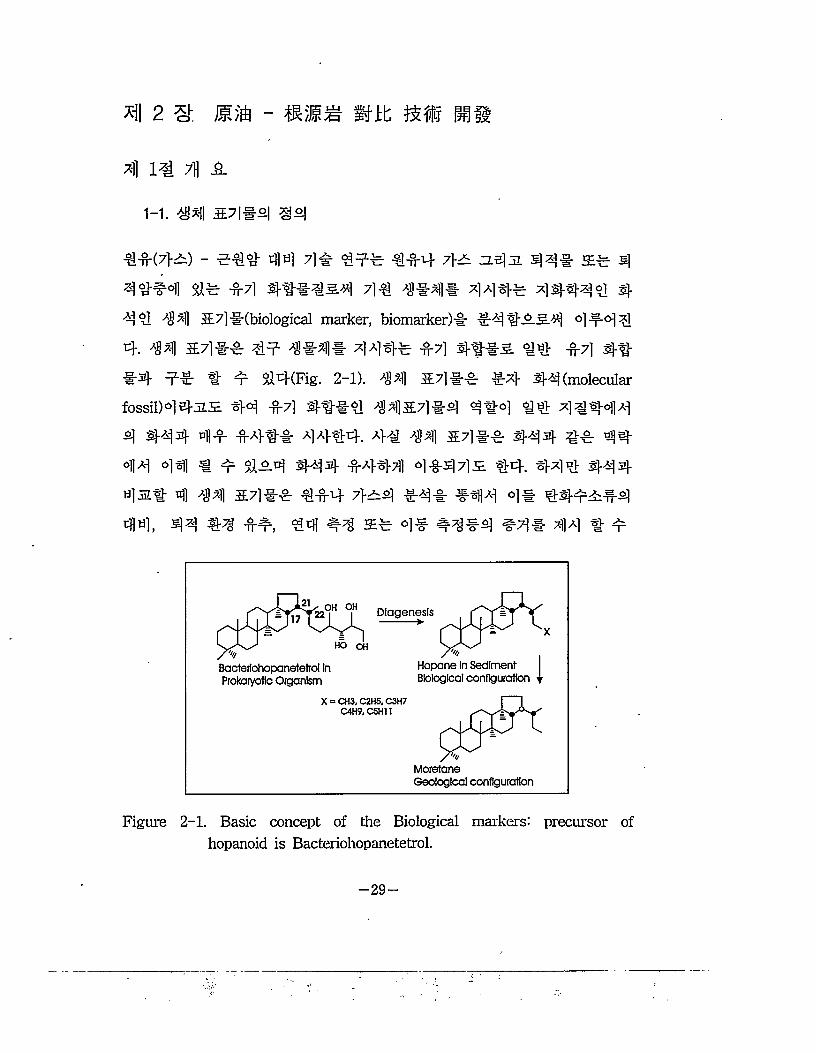
■a-fr(7>i) - ^€4 tflti] 7]# 4% 444 7>^1 ZL5]jl 5)3-1- SE4 s|44#4 4# 44 44 4 #71]# 44 s}# 4 4-4-4 4 #44 4 4 5E7]# (biological marker, biomarker)& -£44 #4 4 4. m &4#4 4# ^@#4# 44% 47] ###& 44 47] 4# #4 4"# s’ 4 44(Fig. 2-1). 4*11 &7]#-cr 47]- 44 (molecular fossil) 4 4m #4 47] 4##4 44&7]#4 4#4 44 44444 4 444 44 4444 4444. 44 44 Z444 444 44 44 44 4# € 4 $1-^.4 444 444t1] 444 4^ 44. 444 444 %# 4 « &7]#4 444 7>^4 #44 #^H4 4# 444^44
44, 44 44 44 44 % 4# #4#4 #4# 44 4 #
OH OH Biogenesis
HO OH
Hopone In Sediment Biological configuration
Bacteriohopanetetrol In Prokaiyoflc Organism
X = CH3, C2H5, C3H7 C4H9.C5H11
MoretaneGeological configuration
Figure 2-1. Basic concept of the Biological markers: precursor of hopanoid is Bacteriohopanetetrol.
—29 —
$144 ^44 4444 4$4$ # # $14. 444 44 $4 #4 §f^ 544 4#$7l- 144$ 4# #441 4# 444 4#4$3. 45. 44 4 #4, 414441 4144 #4# -2-44.
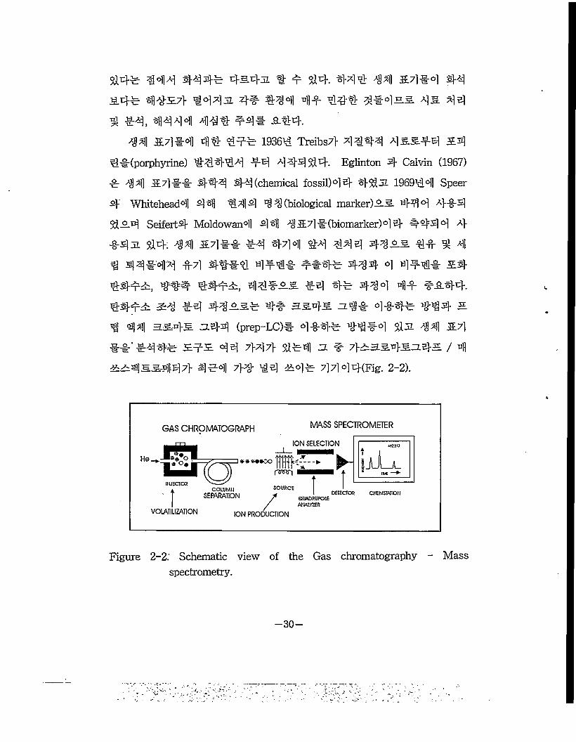
441 $711-41 44 444 19364 Treibs7> 4 #44 a]3.5#e1 $4 4#(porphyrine) #4414 44 444 44- Eglinton 4 Calvin (1967) # 44 $71#-#- 444 44 (chemical fossil)°14 41$ 1969441 Speer 4 Whitehead4l 44 4414 4 4 (biological marker)$5 444 4441$4 Seifert4 Moldowan4l 4# 4 $4#(biomarker)44 #444 4 #4$ 44. 44 $7l## #4 4441 44 444 44-2.5. 44 4 4 1 4 4 #414 44 ^ft°J 4 #4# ##4# 444 4 4?-## $4 444^, 444 444^, 4 4 #-2.5. #4 4# 444 4 4- #$44. 444^ #4 44 $5.# 4# $54-5 $f# 4444 M4 $4 44 3.5.-4S. $44 (prep-LC)# 4-§-44 #4 #4 $1$ 44 $7l ##'#444 $4$ 4 4 7M4 $1#4 $ # 7}$$54-5$4$ / 4 $$45544 4- 444 7>4 #4 $44 714 44(Fig. 2-2).
GAS CHROMATOGRAPH MASS SPECTROMETER
ION SELECTION
SOURCECOLUMN
SEPARATION
VOLATILIZATION ION PRODUCTION
Figure 2-2: Schematic view of the Gas chromatography - Mass spectrometry.
—30—
1-2. ## 0|#44 ^4 57|# 4^4^
44 #44 44 5* #4 4*4 #44 *## 44 #4 4144 44 444 4444. 4, 44 54## #44 #44 e##4 44 4 4, #4 #*5# 4 4 *54, #44 ##, #44 ###, e#4* e #44 4til7> 7>#4jl, e#*4# #44 4# #4 #5# #44 °1 # #&* ** # 4 44.
44 #44 4444 447>4 44 54 #4 45 *7>4 A#4 4 4 *455 4tifl 4fe 44 4# #45. #55.5. 444 447>4 44
44* Jl44°> #4. 4* #4 Ts/Tm 4 44 445* 7># #4# 4 4544 441 54*44* 5# e# ##4 44 4^£ ##=# #4 4 #55.5. 4 ##55 #44 5# #4 1# #45# 4*4 4 414 #44 7] 4 4 #4.
1-2-1. 44 4# * e# 4# 44###44 #44 e# *# * 4# ##4 *4^4 #41
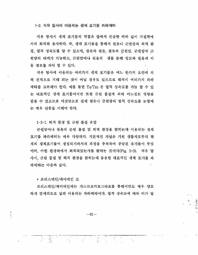
5.714 4#444 44 4#44. 4#44 ?H#4 4# ##7ii5#* * 4# #45711-4 ##471444 4-44 4444 ### 44#4 4# 44, 4# ##44# 444##7}# #44 44#(Fig. 2-3). 44 # 44, e# ## # 4# ##* #444 44* 454* #41 54# * #4#fe #44 ##. ■'
* 54544/44 4* lb5454*/*44*4# 71-5315*5.3.4-5# #4##5 44 *5
#4 ##455 *4 4444- *4-4*4*. 44 ##54 #4- #7> *
-31-
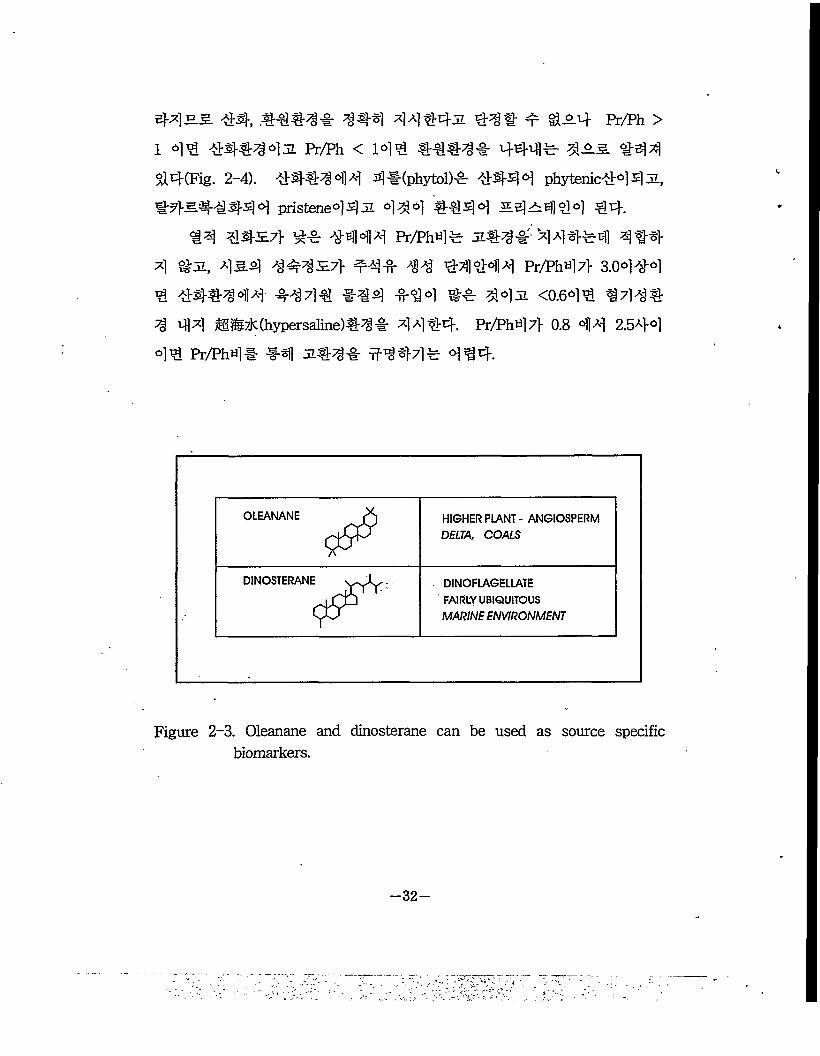
5MH5. ft#, ftlftlft 4 #4 44ft4JZ 44 ft 4= 1^-4 Pr/Ph >
1 41 44ft443. Pr/Ph < 141 ftftftl# 444ft #44
$14(Fig. 2-4). ftftftl 4 4 4#(phytol)-Er 4444 phytenicft4 431,
#45.4^45)<4 pristene0]s)Jl 444 =4^414 44-
14 1ftH7} ^-Er 4444 Pr/Ph4ft Jift4#' 4 4 4ft 4 4ft4
4 &5L, 45.4 4^4JE7> ^4-n- 44 14144 Pr/Ph«l7} 3.0444 1 1ftft444 4-441 #14 4-44 #ft 44^ <0.641 444ft
4 44 SSzK(hypersaline)ft4 # 4 4 44. Pr/Ph^l 7} 0.8 44 2.544
41 Pr/Phtilt- #4 J7ft4# #444ft 414.
OLEANANE r4<j$P HIGHER PLANT- ANGIOSPERM
DELTA, COALS
DINOSTERANE x^U- DINOFLAGELLATEFAIRLY UBIQUITOUSMARINE ENVIRONMENT
Figure 2-3. Oleanane and dinosterane can be used as source specific biomarkers.
-32
Prista ne
Phytol (Chlorophyll)
CH20H
Phytane
Figure 2-4. Pristane / Phytane ratio can be used to indicate the redox potential of the source sediment.
* 441
444 44#4 44-2 424 15. &44, 44 ^424 44
441 44 2 #4. i£lt (Csi-Css)^ 4442244^151(bacteriohopanetetrol) °N- 4^ 4#^M1 444b polyfunctional C35 2
4144 144442 443l4(Ourisson et al, 1979, 1984; Rohmer,
1987). 14 C35 I£M° 1 &b 44b #^o] 42
5 4144. 4^44 1-fHM 444b C31-C35 17ff (H), 21 /3(H), 22S
4 22R4 444 b 44444 4+4, 4-4 42(Eh)# 4444. C35-25.
24 7] q(homohopane index) b C35/XC31-C35) 25241 4441b 425
C33, C34, C35- 22244 m°l C31, C32 54 4444 44 44
4444 124(free oxygen) H4 7)4 17}H 444b 44 444
4 44 1&4 44dl 4444 441-44 44142244131514 aj-sj.
44 C324 42 4-5H41 ^7ll 44 C3i4 44 4 C3i4 144 44 b oxic44 suboxic#4°1 42 Cs27> 1414 4b suboxic lb dysoxic442S. lb# 1 $14. 22244 b3Eb 14 4424 444
-33-
144 SLS-SL^: 41 [Css/CC3i+Cs5)homohopane]^ 44^7} #7}44 4
4 #4 #4 44 #3 1*44 14 44^4 441 jz.444 14.
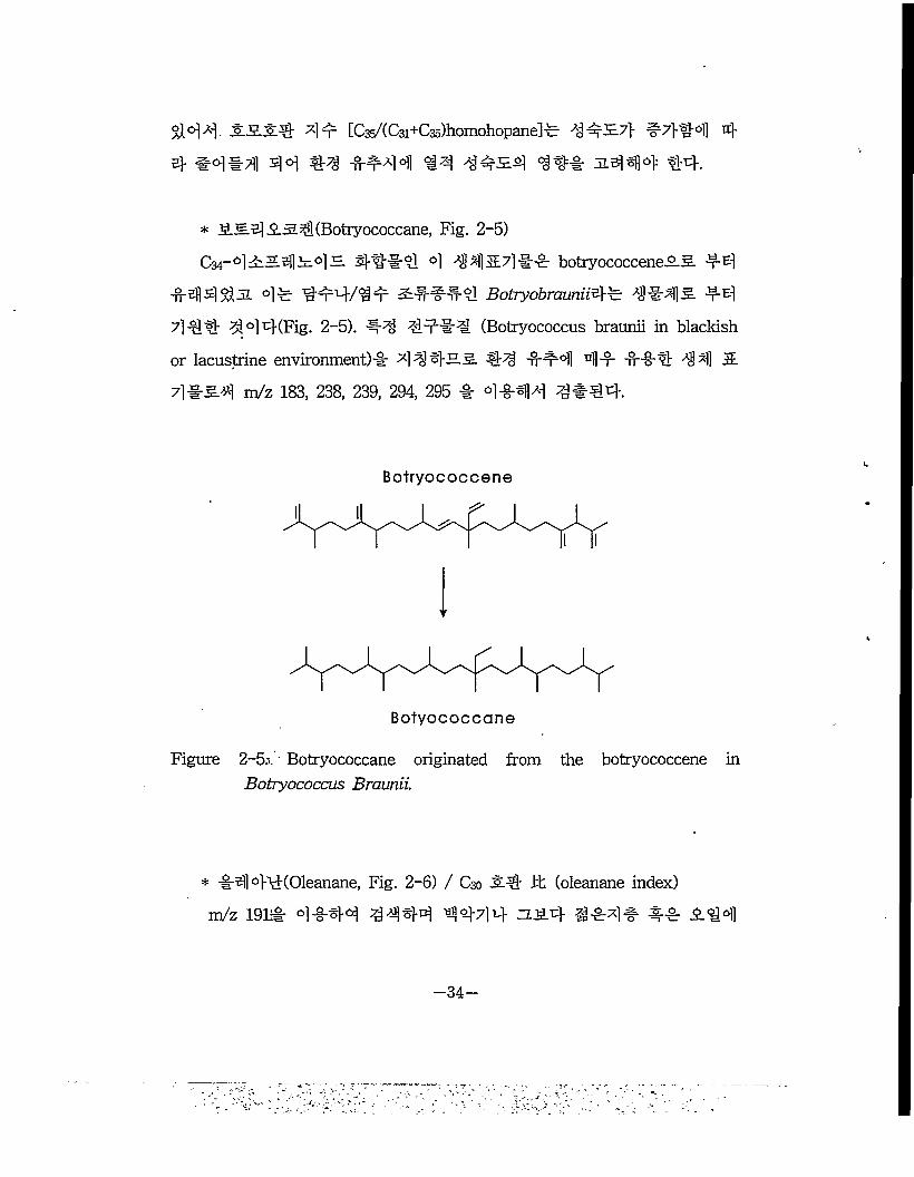
* iLE^I ^.S^KBotryococcane, Fig. 2-5)
C34-°l^—4^4— H#4 4 4 4 3-7] H botryococcene^.5. *4
14442. 41 H4/H 2:1114 BotryobraunivQ^ 4145. *E]
7] H 444(Fig. 2-5). 44 If #4 (Botryococcus braunii in blackish
or lacustrine environment)* 4 4 4—5. #4 1*4 41 114 44] 5.
7]#&4 m/z 183, 238, 239, 294, 295 & 4144 4*44.
Botryococcene
Botyococcane
Figure 2-5?. ■ Botryococcane originated from the botryococcene in Botryococcus Braunii.
* *44K01eanane, Fig. 2-6) / C30 2.4 it (oleanane index)
m/z 191* 4144 4444 4444 zis.4 ^14* 11 -$-44
—34—
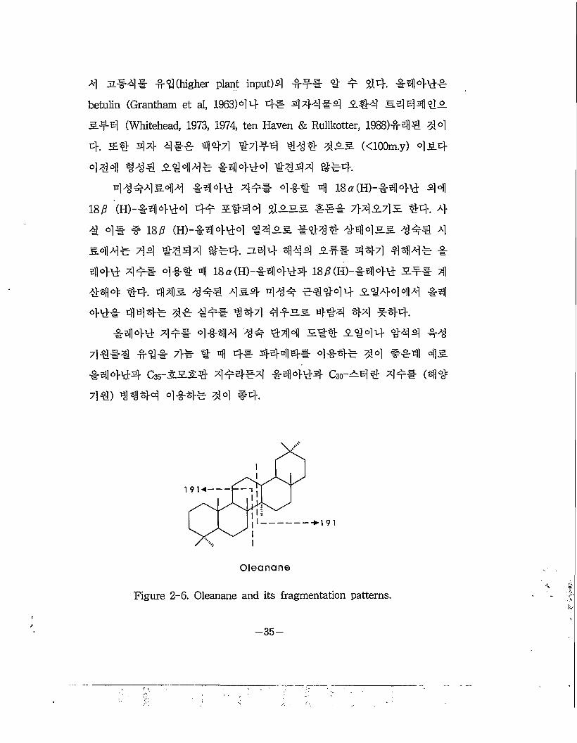
4 5#4# -n't](higher plant input) 4 # 4^ $14. #5))###
betulin (Grantham et al, 1963)44 4# 4 44 #4 -2.44 54444-2.
5^f£1 (Whitehead, 1973, 1974, ten Haven & Rullkotter, 1988)44€ 44
4. s# 44 4## 44-71 4:7144 44 # 42.5 «i00m.y) 45#
444 444 5IH4# #5)14-#4 #444 &##.
4 4 4-4 4 &51144 44# 4-8-# 4 18g(H)-#4## 44
18/3 (H)—141444 #t ##44 #2.55 ### 7}4545 #4. 4 # 4# # 18/3 (H)-#5)i4\+o) #44# #4455 4#4 4s.44# 7)4 4444 ###. 54# 4144 -2.## 444 444# #5)14# 4## 4-8-# 4 18a(H)-#4##4 18y9(H)-#5)14-# 5.## 4 #41# #4. 445. 4#4 45.4- 444 #4#4# 5##444 #5)1 4-## 444# 4# #4# #44 4455 ##4 44 #44.
#44# 44# 4#44 44 #44 5## 544# #44 #4 4### #4# 7># # 4 ## 4444# 4#4# 44 ##4 45 ir^ll### C35-555# 4#4#4 #5)1 ##4 Cso-^44 4## (44 7l#) 4444 4#4# 44 ##.
Oleanane
Figure 2-6. Oleanane and its fragmentation patterns.
-35-
*5)1444 17ff(H)-544 **<>1 &3l4#<q 7$*-
*444 m/z 4124 m/z 3974 2)37} 17 a (H)-5454 44 37)1 44
44. 3LB1JL S4* m/z 3697> 4711 444* 3] til§H *5)144*
ZL 43.7} $14. 5# *5)1444 259, 274 43.7} 44444 C30 3
4* 3^4 4444 444.
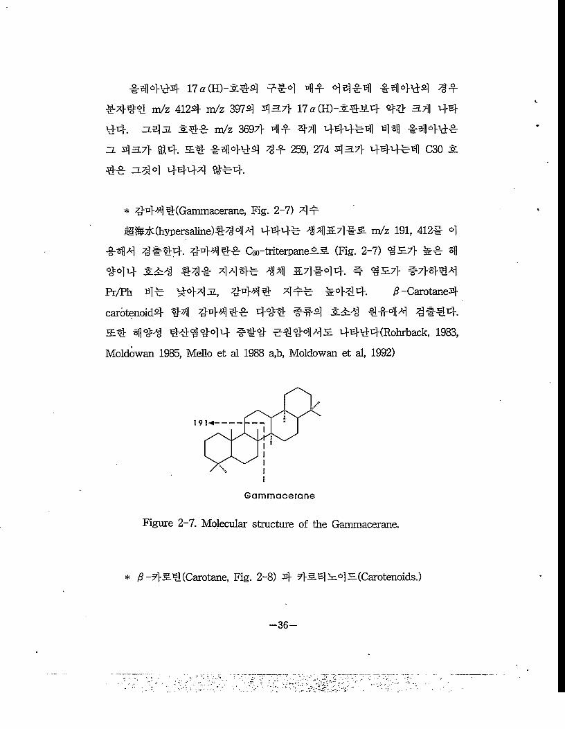
* 44*1^(Gammacerane, Fig. 2-7) 4*
@#%K(hypersaline)#/0 °f| 4 4444 41411571 #3. m/z 191, 412# °1
#414 4 #44. 4444* Cso-triterpaneAS (Fig. 2-7) ^57} ** §H
444 5*4 #4* 444* 44 571 #4 4. # cl 57} *7}444
Pr/Ph 4* 4443, 4-444 4** *444. iff~Carotane4
carotenoid4 44 4*44 4* 444 ##4 554 4*414 4 #44.
54 §1144 44^4°14 #44 *44445 4444(Rohrback, 1983,
Moldowan 1985, Hello et al 1988 a,b, Moldowan et al, 1992)
1914
Gammacerane
Figure 2-7. Molecular structure of the Gammacerane.
* iff -7}5.4(Carotane, Fig. 2-8) 4 454 3°15(Carotenoids.)
36-
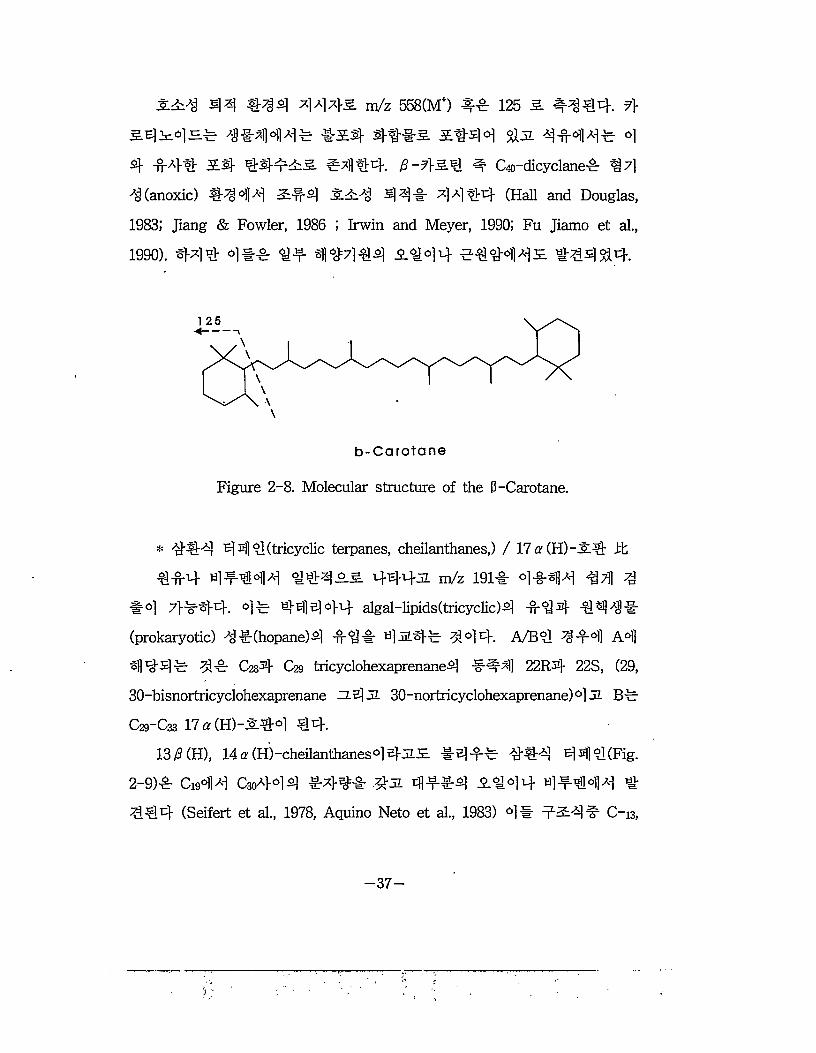
S.±$ ##4^4 444& m/z 558(M+) 11 125 5. 4*J44. 4
5# In# Hi ####7ll #3E# 4##5 ^##4 4 31 41##1 °14 144 5# 441&& 1*1] 44. /3"4^4 4 C^-dicyclanel ^7] 4(anoxic) 44 #4 &1# 514 ##1 #444 (Hall and Douglas, 1983; Jiang & Fowler, 1986 ; Irwin and Meyer, 1990; Fu Jiamo et al., 1990). 444 oll-g: 14 #47141 54 4 4 144#7^ 14114.
b-Carotane
Figure 2-8. Molecular structure of the (3-Carotane.
* HI H4(tricyclic terpanes, cheilanthanes,) / 17 a (H)-Jl4 it
414 14-4#4 441 6.5. 44431 m/z 1911 l-g-sfli 4t11 4
#°] 7H44- °]1 4# 144 algal-lipids (tricyclic) 4 144 4##1
(prokaryotic) 4 Khopane)# 141 til IH.41 4°14 A/B4 41# A#
#441 41 Cas4 C29 tricyclohexaprenane# 1## 22R4 22S, (29,
30-bisnortricyclohexaprenane ZL2\3L 30-nortricyclohexaprenane) °]jz. B1
C29-C33 17ff(H)-s46l 44.
13/3(H), 14a (H)-cheilanthanes°143Z.H. 1411 114 ##4(Fig.
2-9)1 Cig## C3o4di4 e^l-H 43L #11# 5444 ti)^.### 1 144 (Seifert et al., 1978, Aquino Neto et al., 1983) 45# 1 C-13,
-37-
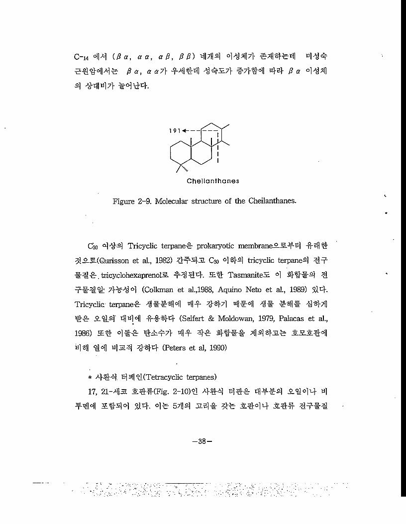
C—14 44 (0 a, a a, a0, 0 0) 47H4 4447}- #7l|5}# 4 444
5-1144# 0 a, a a7} #444 14:E7} #7}#4 44 0 a 414
4 4-447} #444.
Cheilanthanes
Figure 2-9. Molecular structure of the Cheilanthanes.
C30 444 Tricyclic teipane# prokaryotic membrane #44
^-AS/Qurisson et al., 1982) JL C30 444 tricyclic teipane4 14
#44.trucyclohexaprenolS. #144. S# TasmaniteS. 4 #4#4 4
4#H 7}444 (Colkman et al.,1988, Aquino Neto et al., 1989) $14".
Tricyclic terpane# 4 #54 4 44 4471 4#4 4# #4# 4441
1# 414 44 4 4444 (Seifert & Moldowan, 1979, Palacas et al.,
1986) 3E4 4## 44#7} 4# 4# 44## 44431# Ifiltl
44 14 4314 444 (Peters et al, 1990)
* 444 441 (Tetracyclic terpanes)
17, 21-4 s 44#(Fig. 2-10)1 4#4 44# 4554 4144- 4#14 3E444 14. 4# 57H4 314# 4# M44 41# !##!
-38-
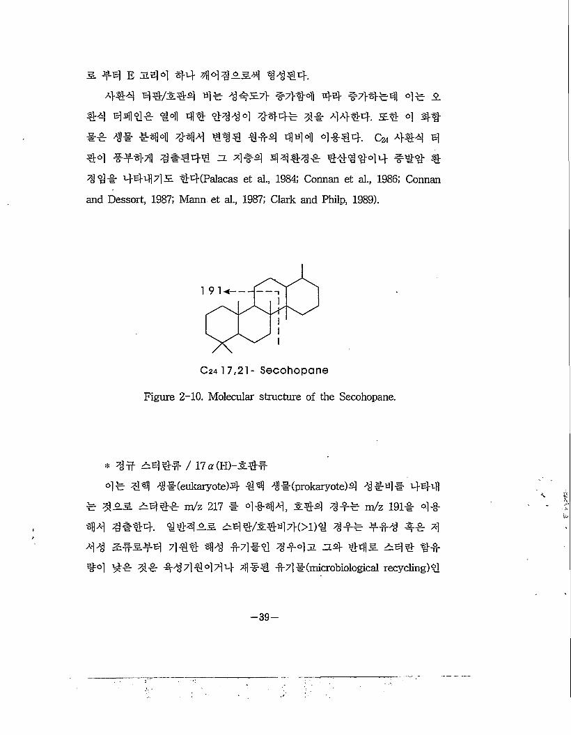
5 f # E jlbM 44- 444554 4^44-.44# 44/3:44 ##57} #7}#41 44 #7}#-^] 4# 5
#4 444# #4 44 4444 444# 4# 4444 54 4 44
#4 4# #«H 444 444 444 444 4444. C24 444 4
44 #444 4#444 n 4#4 44444 444444 #44 4
44# 444 7] 5 44(Palacas et al., 1984; Connan et al., 1986; Connan
and Dessort, 1987; Mann et al., 1987," Clark and Philp, 1989).
1 9 !◄■
C24 17,21- Secohopane
Figure 2-10. Molecular structure of the Secohopane.
* 44 54 44 / 17 a (H)-3:4#4# 4"^] # # (eukaryote)4 44 4# (prokaryote) 4 444# 444
# 455. 5El## m/z 217 # 4-§4)4, 3:44 4#4 m/z 1914 4# #4 4 #44. 44455. 5E] 4/3:447>(>1) 4 44# 444 44 4
44 54544 444 414 44#4 4#45 zz.# 445 544 4#
44 4# 44 #4714444- 4#4 #71 #(microbiological recycling)4
-39-
#4 (Tissot & Welte, 1984).
S4 3if 34= 43# 43 233 #
3 7] €4] 3# 3# 33 (041 7}##) #3^4. 3if ^44# Czz,
C28, C29 & a a (20S+20R) 242 a ,9 /?(20S+20R)3#32 23##
C29-C33 ##3"1K#' Csi.33 C3s44# 22S, 22R 4^1 2# 5.4) 2# 4 443= 44.
* C27-C28-C29 —3 4
.C27, C28, C29 243# 44 2S3-3 S344 43#4 43 43 3 43(ecosystem)# 3 4 44. 3# 3 4444# 3443 43# 34 3 ##44# 3144 243# 3#4 #4 2S# 234 4#31# 4
44# 4# 44 ##44 3 #4 2. 44 (Peters et 4, 1989)
—4 4# 3 #4 443 3#» #4 2S3 S3 44 4344 34# #4 '443 7>44 3## 3414-2-3. C2s4 43 #342. C294 43 # 3 #4. 3# 442 Cas 243# 4 #3 ##2#3 4444 34 4, if5:#(diatom), 2#4 ^(cocolithophores), 445.##(dinoflagellates)#°1 #
444 99471331 #34 33 4 44# 3-2.5. 3434 C2&/C29 243
3# ##2344 224 533 #333# 0.53432, ##234 4
##44 343# 0.433 0.733 4# #44 #4 43#3 244 4
#3# 0.7 343 44. ## 3# 4-54 345# 4# 3^3 4W3
' 443434 43, 33 43 #344 4#34 4#34.
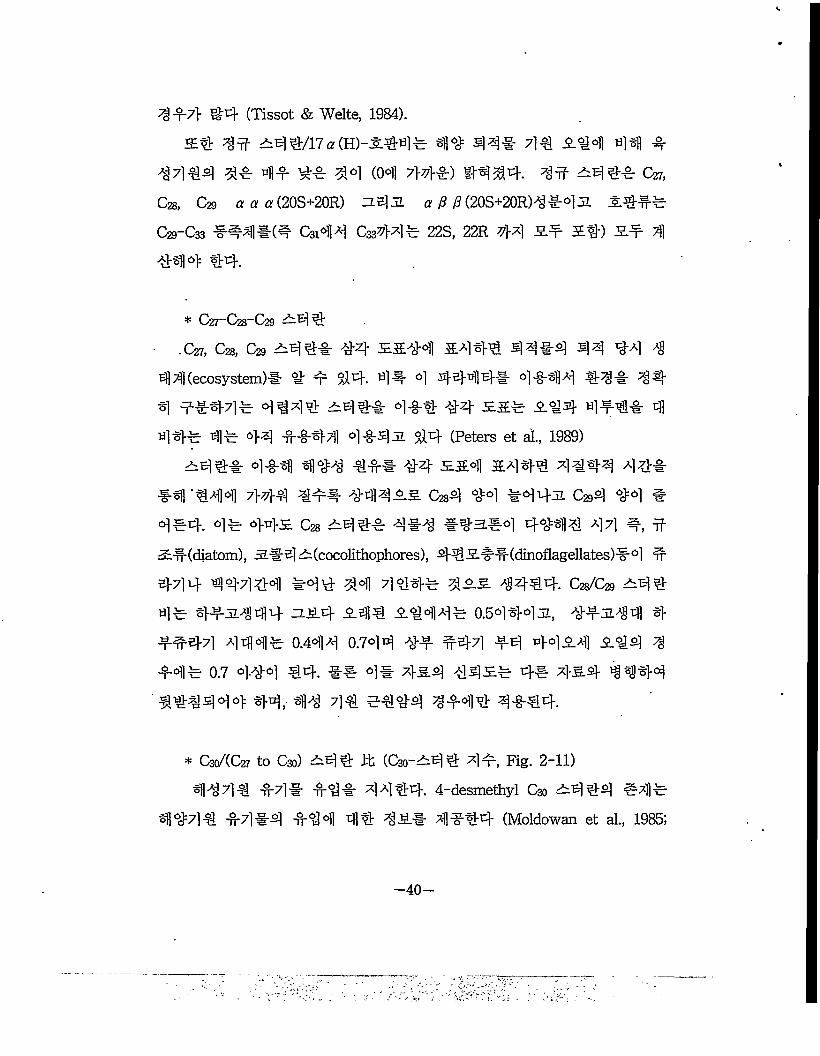
* C3o/(C27 to C30) 243 it (C30-54 4 4#, Fig. 2-11)
41343 #4# #3# 4344. 4-desmethyl C30 2434 #3# 414=43 #4 #4 #43 34 35# 3#44 (Moldowan et al., 1985;
—40—
Peters et al., 1986). 4 ###4=- 24-n-3.&# (propyl)
24-n-5.5.:S #5)1—^1]# (Moldowan et al., 1990)4 444 $14- °1 44
#^cr Sfl'cH-S Chrysophyte Sarcinochry sidales4 4 4 A34 444 4
ss. s}]-^#4 #4 4444 4^4ss. 1^4 44
"rS $14. 24-n-propylcholestane4 -g-4-c: GCMSMS (nVz 414->217) 1r
-S.44.
21 7 ◄-
Cao Sterane
Figure' 2-11. Molecular structure of the C30 sterane.
C30/XC27 - C30) —4 4 4 &4 b:5!! 4*4/5.44 *8* 4 h44 7] 4 -n*7!
#4 414 44 #4 ^44 ^s.1- <£-§: $14. 4S444 5 444
Si 4^1^- C30 ^444 44 M44 #$1^4 4fe Cso^4#4 4^
4 #4 4 44 #7#7l 444^7] 4wSS 4444 (Moldowan et al.,
1985).
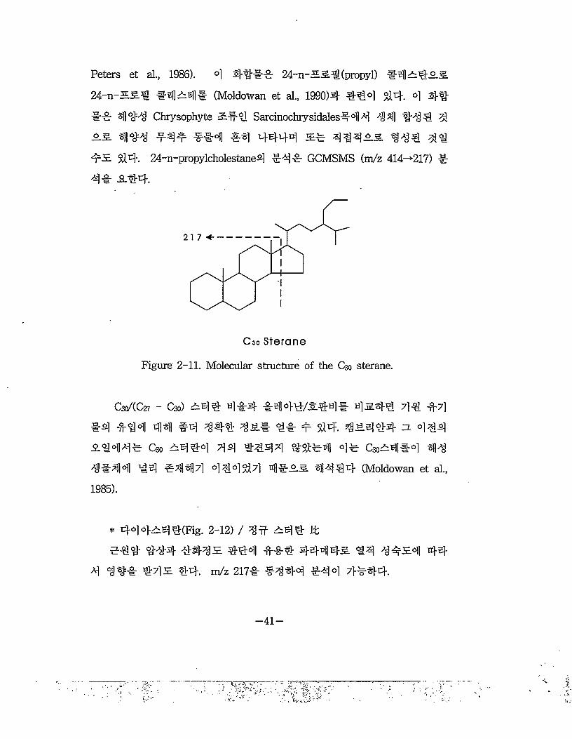
* 444^44(Fig. 2-12) / w ^44 it
44-4 444 £ 444 tH-4 4444s. 14 ^4^4 44 44s 44. m/z 2174 4444 444 7>^44.
—41 —
^7’ -
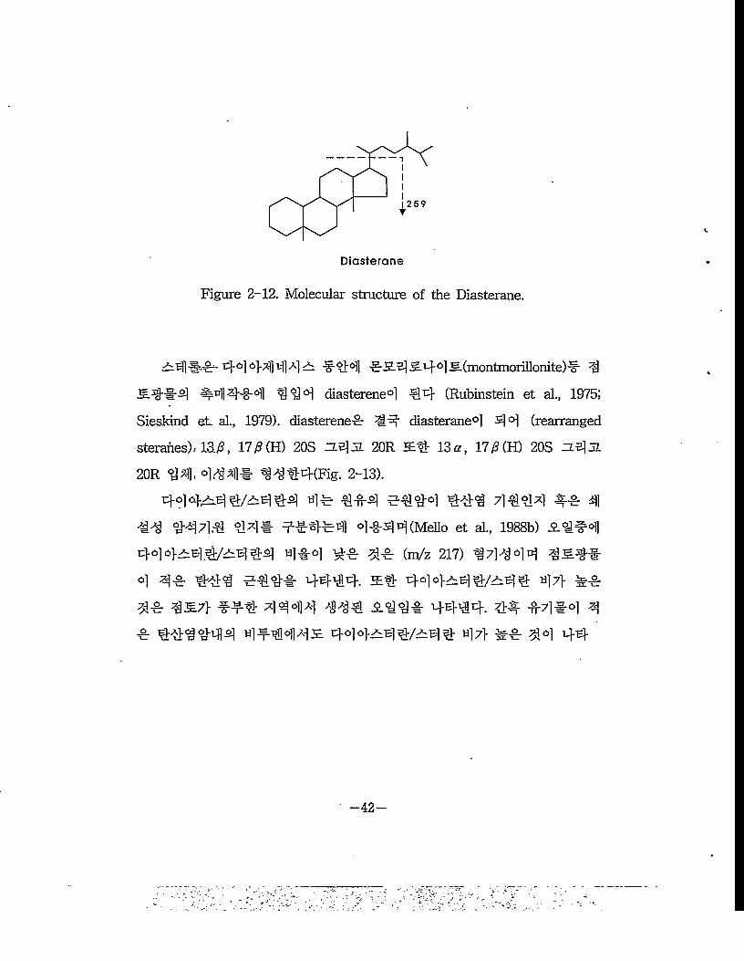
Diasterane
Figure 2-12. Molecular structure of the Diasterane.
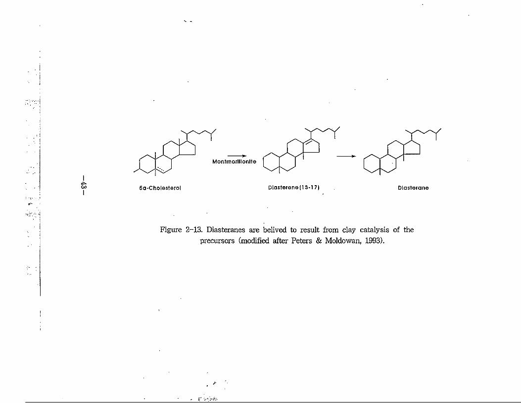
^4 4461-^1 4 4 "F^M] 4-S.4 5-44 e.(montmorillonite)^ 4
5-4ir4 #4444 444 diasterene6] 44 (Rubinstein et al., 1975;
Sieskind eL al., 1979). diasterene-c- 4# diasterane0! 44 (rearranged
sterahes), 13/3, 17/3(H) 20S zz.^31 20R S4 13 a, 17/3(H) 20S zzb]jl
20R 44, 4.^4# ^^W(Fig. 2-13).
444-^44/^444 ti!^ ^4°! ^444 444 ^4 44^ 4444 44* f44#4 4-§-44(Mello et al., 1988b) ^4#4
444^4.4/^444 ti]ir°! #4 44 (m/z 217) 44444 45.44 °] 44 444 e444 4444. £4 444-^44/^44 47} #4 44 4S7} 444 4444 444 -^444 4444. 44 44#4 4 4 444444 4^444^ 444^44/^44 47} #4 44 44
-42-
I
Montmorlllonlte
Sa-Cholesterol Dlas1erene(13-1 7) Dlasterane
Figure 2-13. Diasteranes are belived to result from clay catalysis of the precursors (modified after Peters & Moldowan, 1993).
4#4 4# #44 4# (low pH), 4# (high Eh) #544 44 # 52
5. ## #4(Moldowan et al., 1992). 344 <5f5 542 (Seifert &
Moldowan, 1978)4 A3##47> 44 ## 5442 44 #24 4/2# #u]
7} ^4 4444.
* 4-44 24#
444 444 444 47> 4jl 44 54 24424 444 J=4 # 44 4 24 4 4-f 4444 444 4 #24 4444 44# 442-4 4 44 4444# #4 5 #4 2 4444. 444 444# 4-44 25
4# #5. 442f#4 4a-4# 24*44 444 422. 444 44
(Wolff et al. 1986). 444 3 442 Pavlova^-4 prymnesiophyte 4 2#
4(Volkman et al, 1990) Methylococcus capsulatus (Bird et al, 1971) 4
42 444 422 #44 #4.
* V/(V+Ni) 24 #
5S# 44#44 44, 44244 444 44442 #5 3242
3444 44 4442 444 34223342 #444. 4444 4 # 2444 4#4# 444 #4, 44-5-44 444 4444 (Lewan, 1984). an4=4 44#4 V/(V+Ni) 24447} #4 54 444 suboxic #444 4442 47} 44 54 #45 444 4444(Moldowan, 1986). 22444 #444# 4444(Vanadium)4 42 4#(Nickel) 2444 44422 4444.
—44—
1-2-2. 14 4<lE
114 444 14 ##11 44 &4#4 4144 121 ^
#1 44 14 1141 141 14-14 414 41 14-1- 4144 14 445=* 7>11 f 14. 41 11 41444 #1
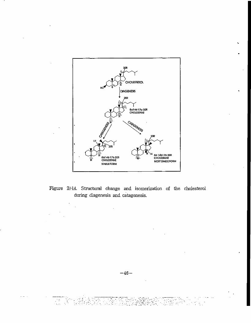
41 #4^414 444 4144 5a 14a 17a 20R 14^14 4^-4 1 7l 4414 14-^s. 14-44 44- C-20, C-14, C17 4444 4144- 44 S-4 1441 444 44 mi 5a 14a 17a 20S #4^144 41 5LS.4 4 144 441 5a 149 179 20R 14^1^5. 14 44 44(Fig. 2-14). 4441 144 4144-4 44 14#4 4444 4 1 *414 1414 14 11 1711! 11 4 1 14. 1 415=1 7>l 411 4141 1^41 441 ail-444 41 414- 14.
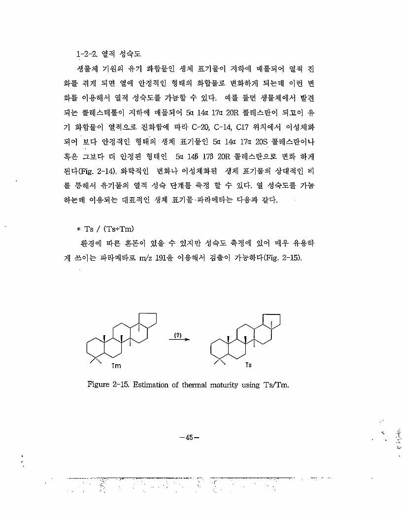
* Ts / (Ts+Tm)
444 41 114 11 1 141 4451 #44 14 11 114
1 &41 44-44-s. nVz 1911 4144 414 7>i44(Fig. 2-15).
Figure 2-15. Estimation of thermal maturity using Ts/Tm.
-45-
Sr CHOLESTHtOL
6al4al7a 2 OR CHOLESLANE
5al4bl 7b 20R CHOLESTANE MOST STABLE FORM
Sal 4a 17a 20$ CHOIESTANE STABLE FORM
Figure 2fl4. Structural change and isomerization of the cholesterol during diagenesis and catagenesis.
-46-
13 13* 151 C27 17a(H)-eh]^^(trisnorhopane Tm)l
C27 18 ff(H)-5.el 5^55:4 n OW4 1357} 34 3-4355. Ts 3
14 1413(Seifet & Moldowan, 1978). Ts/(Ts+Tm) 41# (Ts/Tm
433lh 3) 3*s i# #41-14 43 13371 s 344 4430.5.
13 2:4 c 13 33s 443 34 54!- 334344. Ts/(Ts+Tm)
411 #3 345. 43# #4*14 13 Si: 344 7>3 3434 4
314.
* 22S / (22S+22R); 4343C31-35 l7ff(H)-M3 3# 2214 4# 3343 1441 4343c
(Ensminger et al., 1977) 4# 34 54 #3 333 435.4c 4^3 4 # #543 1445.5. 434 3s4 &4 3444 35.3 1345. 4 44 53-3 334344. 4, 31-4433 54# 22R 3445 434 334 41-34 34313 31331 344 22R, 22S5. 434.
mJz 191 543 3#3c C31-35 343 22R, 22s 434 31 I£l
443 34. 14355. C31 4# C32 JL5S43 22S/C22S+22R) 37} 4
54 54 J7 ZL 37} 0.50 - 0.5441 31333:71 4445 0.57 - 0.62
41 4 3133144 4# 355 1114.
22SA22S+22R) 541(Moretane)3 35 C31-C35 513 3*34 13
3*57} 17}#4 33 133c4 22S/(22S+22R)37} 0.443 1 313
3144 513 355. 1114.
* iff or -5.4 5 / o' /3 - Jll and /9 /? - JL4
33*44 27l 3*143 43445 1134. 314 313 17/9
(H), 21 /?(H)-54 (1/9)# 41 14334 5143c 1433 ^#4.
-47-
4* 0 0 cr-2-4 44 4 a /9-M-9.3. 444 4# 14 *4
44-
17 a (H), 21a(H)-5444 44 17flr(H), 21l(H)-M:4 ti]
* 144*57} *7}44 44 !£44 44* 4*44 1* 0.8* 44
4* 44 4*4 4444 -$-44 1# 0.15 44 0.05 44 4444
(Mackenzie et al., 1980; Seifert and Moldowan, 1980). 544/544# 4
4# 4*44 C29 44 &7] #* 4*444 (Seifert and Moldowan,
1980), C%,4 C30* *44 4* 44 £ 44(Mackenzie et al., 1980).
* 444 444 / 17a-54
4#4 444 / l7a(H)-544 4* 14 1*57} *7}44 444
*7>44 (Seifert & Moldowan, 1978). 1*57} 4144 44 45454
4 4444 44 5454 zz.^4 44 444 4 4 4(cheilanthanes)4£454 45455*4 ®4 *444 4555 444-$-5. 44 144
4. 444 *1#!4 4# £144 44# 444 44]4/17a(H)-lt
4 45-4 1*5# 7}*4* 4* 4* *4* 4*44 44.
* 20SA20S+20R) £44 4 4 Wig. 2-16)
m/z 2175. 1444 44444 4*444 **4 444444.
C29 5 a (H), 14a(H)-£44 44*4 2044 45 44444 4444 4
4) 4*44 44 20S /(20S+20R) 4*4 044 0.544 4444 (0.524
4 0.55* 444"41- Seifert and Moldowan, 1986, Fig. 28). 4#44
* 020 R *444 #44*4 4*4 4*44 4144 4144 R,
5 *44 44 4444 44 4 4** #44 4444 5*145 *
*44 4 *44(Mackenzie & Mckenzie, 1983; Beaumont et al., 1985;
-48-
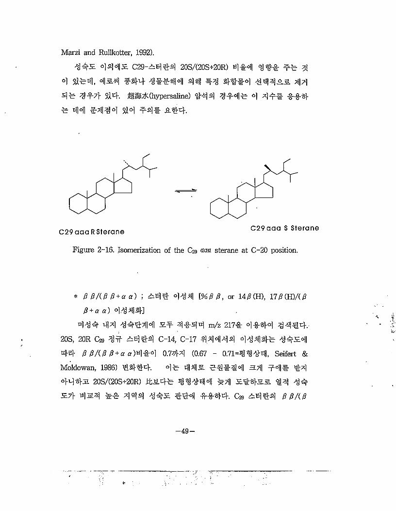
Marzi and Rullkotter, 1992).
^45. °Wl:E C29-3B} sis) 20S/C20S+20R) 4 #4 1## ## ^
4 114, 4&4 #4-4 4H 4^ 4#14 14423 4441 ^#7> #4. m#zK(hypersaline) #44 3 #4! 4 *141- ##4
1 44 1414 14 #41 244.
C29aaa RSteraneC29aaa S Sterane
Figure 2-16. Isomerization of the C29 acta sterane at C-20 position.
* 0 0/(0 0 +a a) ; 244 4^4 [%/3 0, or 14,9(H), 17^(H)/(/9
0 + a a) 4# 441
4#1 4*1 #4444 2.4 4#44 rn/z 217# 4#44 ^444.
20S, 20R C29 4# 2444 C-14, c-17 4*1444 44441 ##34
44 /3 /?/(/? /3 + a a)4#4 0.74*1 (0.67 - 0.71=444-4, Seifert &
Moldowan, 1986) 4444- 41 445. #4#! 4 3.4 #41 4*1
44#3 20SA20S+20R) it2.4-1 ^^#44 14 314-2.5. 14 44
37> 4h4 1# *114 ##3 114 ##44-. C29 2444 ,9 j9/(/9
-49-
0 + a a)4 20S/C20S+20R)# #4i #€444 €#4
Mi if ##44(Seifert & Moldowan, 1986). #7lf #44 €# 4
Mii Mi5. M4 4 #4 444^.5. ##44 £4-4
fj^7} Mi 4 #4 4 4 4#£ S14.
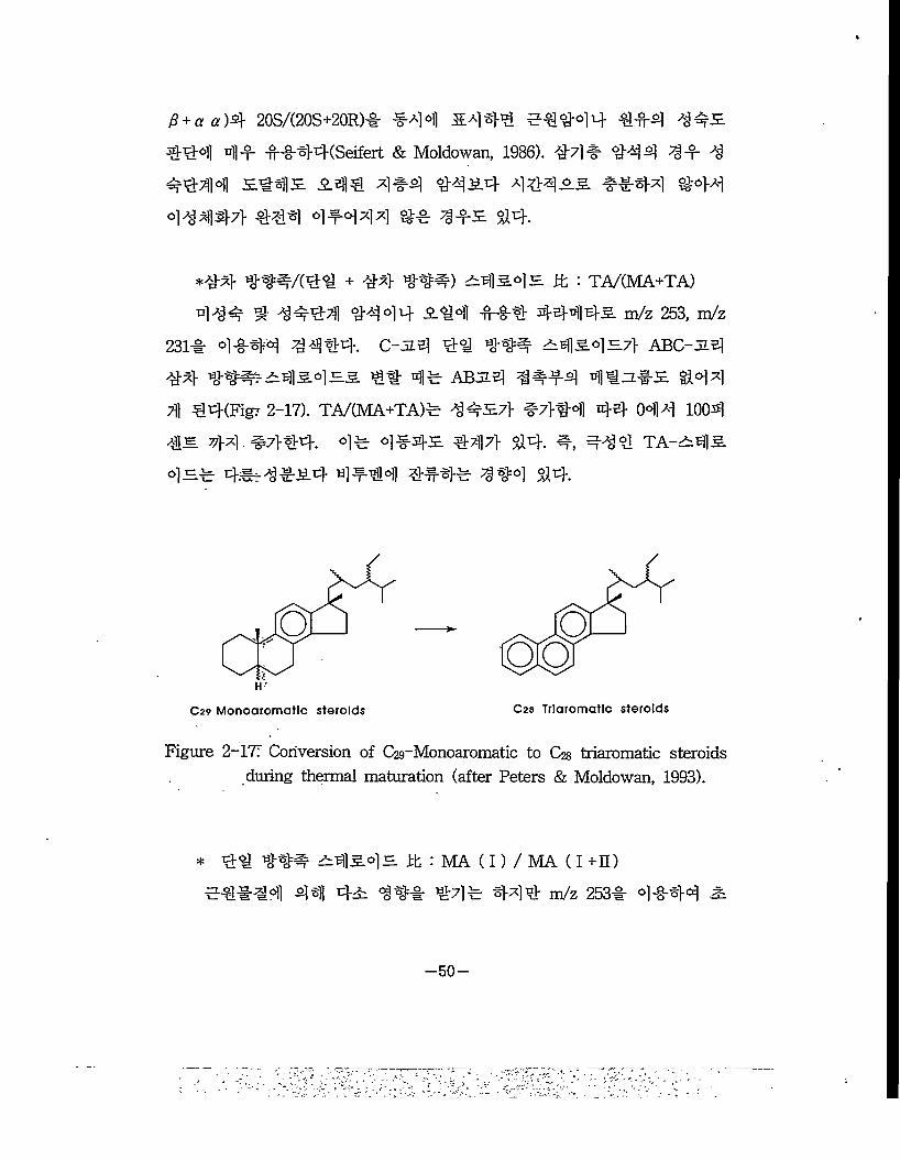
*44- W^/CM + #4 #W) lb : TA/CMA+TA)44# 4 4 #44 #444 Mi ##4 4444& m/z 253, m/z
23i# 4 #44 c-2.i m m# ^4&4M ABC-31 i#4- €# 4# ABJii 4##4 ii):2.-i-;E 44 4i 44(Figr 2-17). TA/CMA+TA)# ##E7} #7}#4 44 044 1004 4#. 44 #7}#4. 4# 4#M 447} 44. 4, #44 TA-M5-
4h# 4#r4#&4 ifii 4#4# 4#4 44
C29 Monoatomatlc steroids C28 Trlaromatlc steroids
Figure 2-ITT Conversion of Czg-Monoaromatic to Cgg triaromatic steroids during thermal maturation (after Peters & Moldowan, 1993).
* 44 4## 431 lb : MA (I) / MA (I+n)#€#4i 44 4^ 44# #4# 444 m/z 253# 4#44 &
-50-
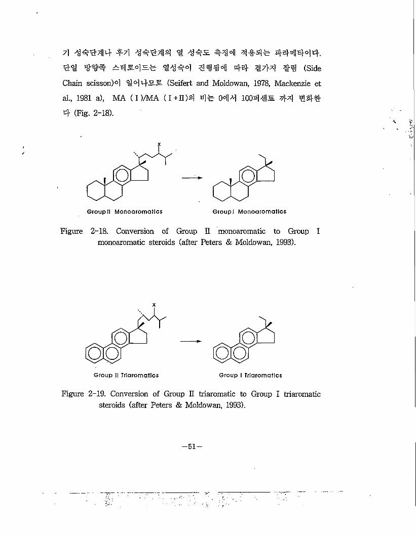
7l 44444 ^A 44444 ! 44s #44 444^ 4444014. 4^ 4## ^4s.o]h^ 1444 44^4 44 444 44 (Side
Chain scisson)4 444—5. (Seifert and Moldowan, 1978, Mackenzie et
al., 1981 a), MA (I )/MA (1+11)4 4vr 044 1004 fc 44
4 (Fig. 2-18).
Group II Monoaromatics Group I Monoaromatics
Figure 2-18. Conversion of Group II monoaromatic to Group I monoaromatic steroids (after Peters & Moldowan, 1993).
x
Group II Trlaromatlcs Group I Trlaromatlcs
Figure 2-19. Conversion of Group II triaromatic to Group I triaromatic steroids (after Peters & Moldowan, 1993).
-51
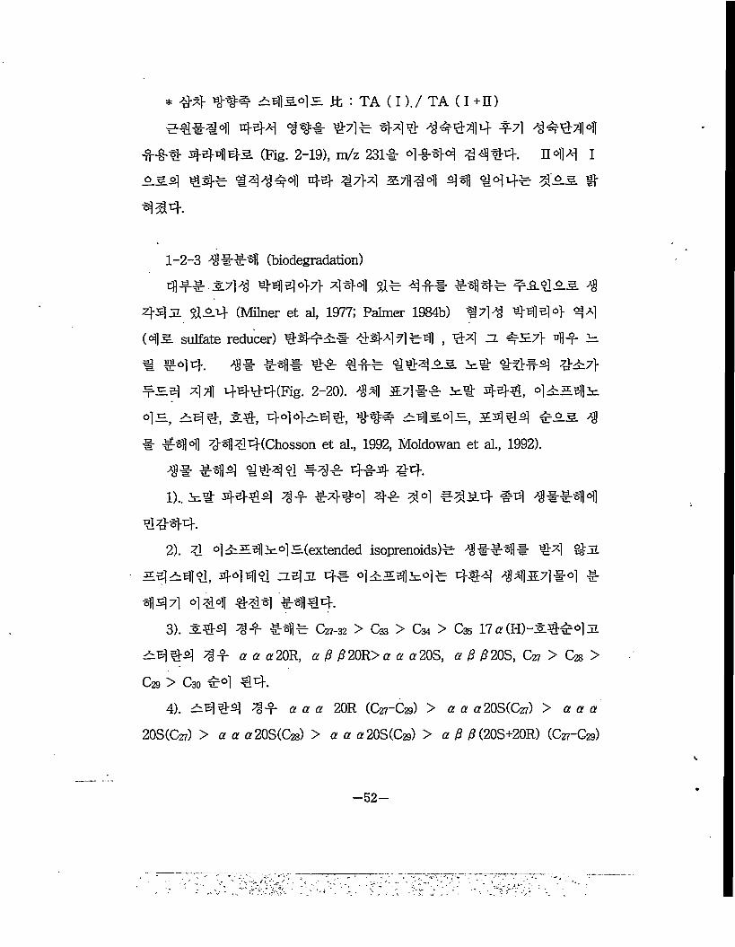
* #4 ### 24545 Jt : TA (I)./ TA (I +H)
e4#44 444 4## #4* 444 4*444 *4 44444 44# 4444-5. (Fig. 2-19), m/z 2314 4444 44#4. n44 I
55.4 #44 14444 44 444 &;H44 4^0 1444 44-5 4 4 #4.
1-2-3 ^8##4 (biodegradation)
444 s44 4444-4 444 4* 44# #sfl#* r^-?I—5 4
44JL 454 (Milner et al, 1977; Palmer 1984b) #4^ 4444 44
(45. sulfate reducer) 4##5# ##44#4 , #4 5 *57]- 41* —
1 #44. ^8# #41* 4* #4* 144-5.5 2=4 4*44 427}
#H4 44 4444(Fig. 2-20). ^4 54#* 2=4 44-4, 42545
45, 244 5:#, 444-^44, 4#* 24545, 5444 *55. ^
# *414 44 4 4(Chosson et al., 1992, Moldowan et al., 1992).
## #44 1441 *4* 4*4- 44.1) .. 2=4 4444 4-f #444 4* 44 #454 #4 ^*#314
4444.2) . 4 4 554 2=4 ^(extended isoprenoids)* -^8 ##41# #4 #5
5.4 2^14, 4444 zte]5 4# 455454* 4*4 ^84157] #4 -g- 444 444 #44 #4144.
3) . 2.44 4* #41* C27-32 > C33 > C34 > C35 17 of (H)-24*4 5
5444 4* a a or20R, a 0 j@20R>a a a20S, u- £ £20S, Czi > C28 > C29 > C30 *4 44.
4) . 5444 4* a a a 20R (C27-C29) > a a a20S(Czi) > a a a 20S (C27) > a a a 20S(C2s) > a a a 20S(Cz9) > a 0 0 (20S+20R) (C27-G29)
-52-
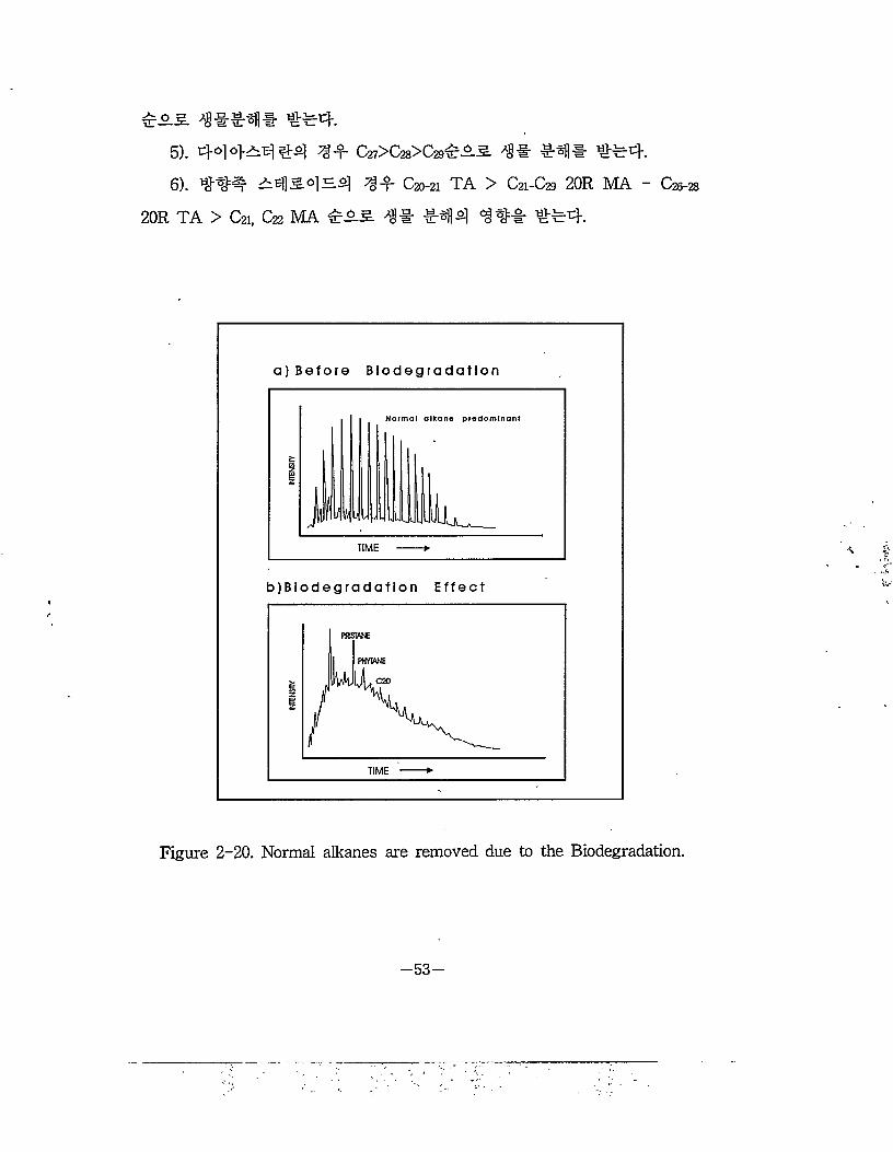
4 As. 444.5) . 4°14—^ 4-^ 44 C27>C28>C29T—s. A8# 4^0# 444-6) . 444 —^11 -S.°l —-^1 44 C20-21 TA > C21-C29 20R MA - C26-28
20R TA > C21, C22 MA 4AS. 4# 4^4 444 444
a) Before Biodegradation
Noimol olkone piedomlnont
b)Biodegradation Effect
Figure 2-20. Normal alkanes are removed due to the Biodegradation.
-53-
1-2-4. tflti]
#4 54#* 4 #4 4 *#4 1#, *#4 e*#, e€*4 *1# & 444* 4* #44 1*# 444 4444# 4#44 7}*44. * 454 44 *4, #€ #4 #1, 14 4*2, 4# #4 *24 °1#4* 444 44 541-01 4#, 4# 244 44 44# #4.
444 43-# 4# #4 54# 4444 442 444 ##* 44 44s. 54* 44 54## 444 44.
* Cz7-Ci8-C29 444244
7>4 4#4# 444444 #4 444 ##44. m/z 217# 4#4 4 444' 7>#44. 4# [C% 13/3, 17a(20S+20R) 444244] / [C27-C28-G29 13/3, 17 a (20S+20R) 444 24434 4* 44 44 #■&* 4#4- G28, C294 4442 4471-4 ##25 4444.
U 27; 28, 29 444244 44447} 7>4 ##44 24# 4# ## #47} #44 24425. #27} 43# ##4 ##27} ## 214 1 44455^4.23 44 7} 42 4442344 4# ##44.
* C27-G28-C29 C-24 41 #4# 24542
44 4.4445 ##44 244 44 ##4 #14 #442, m/z
253# #4. 4#4 7}#44. C24 #4# 24542# 271 4444
442 #44 47}4 4# 14# 4# 24#44 #41 1425.
(Riolo et ali, 1986; Moldowan & Fago, 1986) 24454 41# !##!
* 4444. C27-C28-C29 MA-Steroid #425* *44 44 #1###* 1# 14* **2 *44 144 (Moldowan et al„ 1985) 445 4
*1* 4*4 40J43 o_ 1* 41 4*4 4*4 2154 C29 412*
-54-
^45457} *Al]*51 ^71-^rgr Czi, C% 4*31.4 ^454^7} 7]*
*4- 2% ** 7] ■* ^1^-5] Cgs /(Czs+Cgg)^!^" 0.5# 44*4-
* nVz 191# 4## 44* *4 4444
44 **4 4*4* 44445. 4# 4^4 444 4
3L4 4# 4 444 44# 3*s 44. 4**4 44## 44^#4
444444 #44^(Ourisson et al., 1982) 4#4 ###4# 444,
4#4, #44, 4*4, 544(S4*)*4 #4*4. 44*4 4*44
m/z 1914 4* C3o5*/C295*4 44 154 #4 C29544 4 *4*
*#* *7] #4 **4 ##*, 4*44444 (Zumberge, 1984; Connan
et al 1986; Clark & Phip, 1989) #444 #44 4* 4## 44*4
(Brooks, 1986).
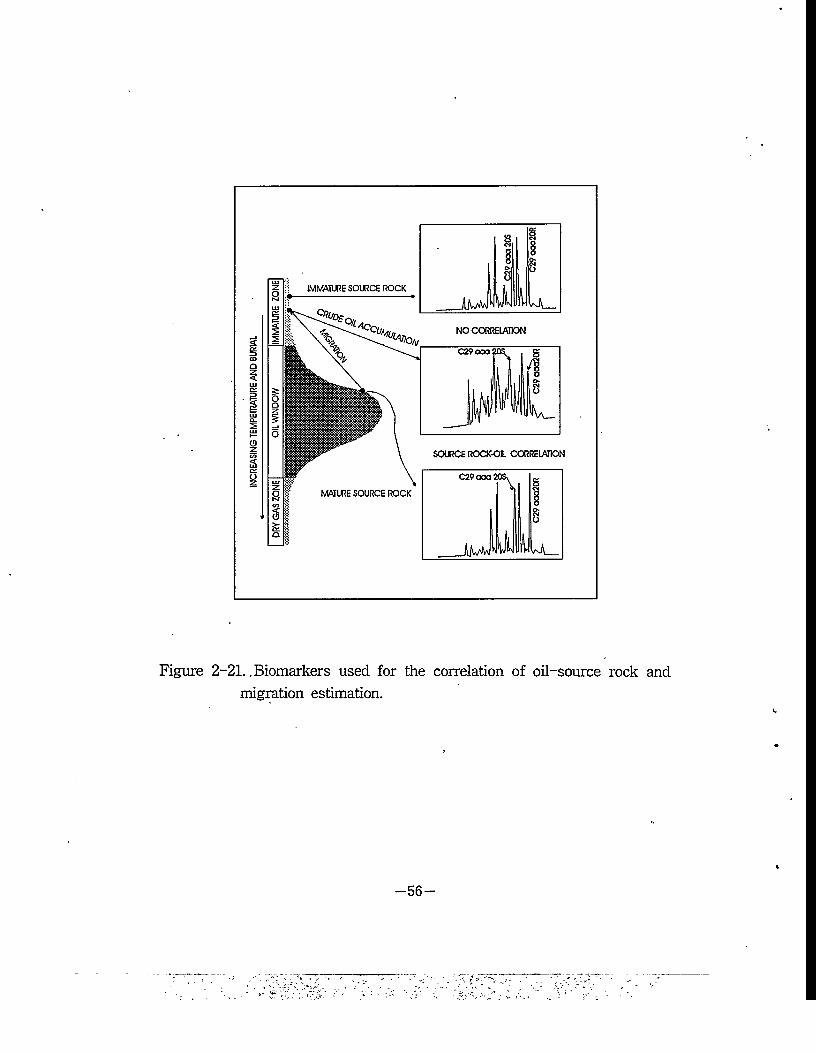
1-2-5. 4 #
4**4 ** 4*4 ^4 3.71*# *4*4 4# #4*4 « 3
4*4 *4*55.4 4*4 4* *5# 4* * * *4. 4, 4*7} #
44 4*# *4 #4*4 « 34## ** * #4 4*4 « 34
*4 *4* 4* *444 *4 ** *4# 444# 4*7} *4. 4#
4*7} 4*44 *** 44# 4# 4* *4 4*4 41*4 *44#
*#44. 4* 4*4 4*#54 4*4 #**4 444* 44 34*
# #4*4 €*4 441 34*4 44 *554 *## 444 #€*#
*4 # * *4(Fig. 2-21). 4*4 #*** 44*4* *44 44 *
** ** 4*11 34* 4444# 4* 44 **4 ## *5 4# 4*
#4-4# 44 (negative correlation) ** 4# *** 4 (positive
correlation) 5* 54444.
-55-
IMMATURE SOURCE ROCK
AAvAa
8 1CS §& §8
lUI k rJ\NO CORRELATION
C29 ooo ?0S. g
ft
SOURCE ROCK-Ol CORRELATION
C29ooa1
8uu w
Figure 2-21. .Biomarkers used for the correlation of oil-source rock and migration estimation.
-56-
*11 24 -8- -g*
^•is 19# #44 419 44 &9# 94 4 114 ?]#&41 44# 4s4 9 #44 9*4 14# 7js 9-83 #9 <994#1 99# 4s= 484. 44 #9# 94 994 999# 8£4911) 4 = 4^ 94 4^9 s 4444 #9 *15.1- 94, 9## 99 484.'
41 19# 1114 44 499# E9, F944 94 Is. 44 12, 117H 4si 98484. 914 4s9 9-4 H99, 49 =ls4£nl 4 44 9# 4 94 4^ji HP 5890 44s n 7}*3£4e zl4s4 HP 5989 A *%4ssil4# 49414 944499, 94 &9# 9 49 484. 944 941 29## 41444 94 444 44 #9, 19 44s# 9948S4 4# 4 #4 4s4 9h 4 £484.
2-1. 9*l# 9# 1 3E9 95-1
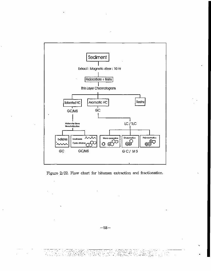
9441 44 4 s# E 9 12711 4s, F 9 11711 4si 9944 4 #1 4# 4 s9 94# 94 484. 491 4# 4 £4 949 Figure 2-22 4 19 944 44 494 84.
, 2-1-1. 991- 9#
#7l# 9# H# 49 3.7)1 97>4s. 494 494 7l7l# 4#4
9 114 44 31944 44914 4#49 114 84. 949soxhtec 44 soxhlet## 4944 9#4# 844.
-57-
Sediment
Extract: Magnetic stirrer: 10 Hr
Thin Layer Chromatogram
Saturated HC
Hydrocarbons + Resins
Aromatic HC
GC/MS GC
1Molecular Sieve [C / TLGureaAaaucnon
n-aikanes-Wv\
Mono aomafcs
Cyck) dkcnes
GC GC/MS GC/MS
Figure 2f22. Flow chart for bitumen extraction and fractionation.
-58-
*7]# 5*4 44* 54434- S}5 *7] *4 #44 444 ^* 4444. 5 4444 44 52* 5*# 4*4* 4ti£lM 4 -§-4 5*44 554 44 43i 44 44 52 44 45-44 #3* 4 5 #4 #4 44## #33. # 5*4* tssif 4 44#, *54# #47} 44 5*44.
5.4 444 44 #4# 4M4 4*4 5# 44# 4*44 4#4
44.® *4 444 4s. 50 3^* 100 - 150 44 3.43. 544 44.
© *4 45# 4#4 554 ¥3 24 44 #4 52, 55# 4444.
© 524 45# 4444 ¥3 Ajs. <$o] 2-344 4=4 444* 4 #3.3.44# 47> 44.
© 454 #47> *4 $1* 4 47i* 7>14 44 34444 ¥3
40-50°C2 4 12 44 45 44544 #4** 5*44.© #4# 5*4 #4 454 #4* 4* 44 4444 4454 4
44* 4*44 #44 #4*# 4444.© 5*4 *44 *4#5 #4* 44 **444 5# 44 *4*
# 4*4.
2-1-2. 54 *4
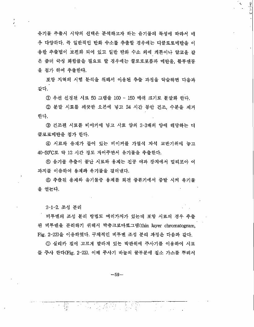
4*44 24 #4 M5 447>47> 4*4 54 454 55 5*4 4*4# 544*7] 444 4#3345zz.4(thin layer chromatogram,
Fig. 2-23)* 4*4^4. #444 4*4 24 *4 45* 4#4 44.® #44 44 3=7]] #44 4* 4444 *44# 4*44 45
* 54 44(Fig. 2-23). 44 544 4*4 **#4 42 7}^* 544
-59-
57.5.711 T€4(Fig. 2-23). S4 44* 4&* ™5l7] 4si ^7121M »M1S._0 5. ^7fl X\ ?1 Ck
SYRINGE .NHROGBJ SUPPLY
-UC PLATE
Figure 2-23. Schematic view of the Thin Layer Chromatogram(TLC).
© 444 44*0)1 515.711 4W 4#^ 4€* c>l-H14 £ 7H 2:4^1 ^7H 444. €*- €44 44 44*444. «fl^ol 444 ^°)1 id ^=4 444 ^44^#4 44* 01-B-4°1 444 44-t^ 4**5. *44-4 €44 €*#4 *4.
© #44 €44 4* #a&3E#4 444 ** 44 4444 44
* ^4 44 ** 4444 MM** #4 444.© 444 444^ 4#4 4711* 4 f *4* €444. -
—60—
4# 4# 444 4314 #44 ##44 5## Table 2-14 444 ■$14. 4 # 4# #### 4# #5-e?M 4# 444 44
4 4444 #^4. 44 Rock Eval 1 44 44 444 44 #4#4443# Tmax7> #54] 44 3.711 4444 &# 44 444 435.4 4 $14.
2-2. 54 B4 43 44 W 44
4514 54 E#, F#4 ^ 54 43H 7}5 3.545 345# a>#
44 54 4443 44 & 4 4 44 4( Appendix #5).E# 4 #;#4 54 4443 3545344 44# $1 #44 4#4
44. 4, 34 444 454 44 444 4)4 #34 C% 44 C3i4#4
4 34 444 431 5513444 44444 44 #31341 4# 4^#
(4# 4# 45 2-3) 44 435 544(Appendix #3). 34 444 4
4435 4-711 4444 444 4444 44 44 444 445 71-44
34 444 434 44 47> #71-44 610m #^<21 4444 44#4
34 444 45 444 4444(Appendix 4*5). E 44 120.6m,
250.3m, 518m, 560.3m #£#41# # 44#4 444 4444(Appendix
45). 5515314 44 3144 4# 429.4m, 370.7m, 570m, 610m#5# 31
443# 154 #4-4 #4 444 # # f}c}(Table 2-2). E#4 45.4
43 #31 4## 0.76 - 1.585 44 714 #711-4 4 #44 44457}
4-44 ## #35 4# 443 # # $134 4# 4# 43154# # 711-4 #5 4144471 4 #4 43 #41 4 #7} 43# #41 444 4
35 31# 44.
55153144 C17 34 44, 443144 Ci8 34 444 45# #7l
#4 4# 4# 4 #44 #41-# 4# 54 E # 43.4 tfl##4 3#
—61 —
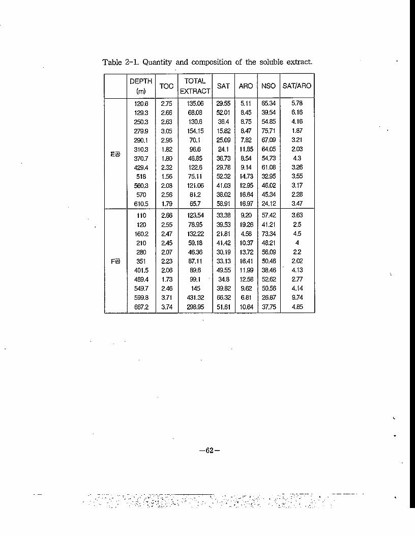
Table 2-1. Quantity and composition of the soluble extract.
DEPTH(m)
TOCTOTAL
EXTRACTSAT ARO NSO SAT/ARO
120.6 2.75 135.06 29.55 5.11 65.34 5.78129.3 2.66 68.08 52.01 8.45 39.54 6.16250.3 2.63 130.6 36.4 8.75 54.85 4.16279.9 3.05 154.15 15.82 8.47 75.71 1.87290.1 2.96 70.1 25.09 7.82 67.09 3.21
ES 310.3 1.82 96.6 24.1 11.85 64.05 2.03370.7 1.80 46.85 36.73 8.54 54.73 4.3429.4 2.32 122.6 29.78 9.14 61.08 3.26518 1.56 75.11 52.32 14.73 32.95 3.55
560.3 2.08 121.06 41.03 12.95 46.02 3.17570 2.56 81.2 38.02 16.64 45.34 2.28
610.5 1.79 65.7 58.91 16.97 24.12 3.47110 2.66 123.54 33.38 9.20 57.42 3.63120 2.55 78.95 39.53 19.26 41.21 2.5
160.2 2.47 132.22 21.81 4.58 73.34 4.5210 2.45 59.18 41.42 10.37 48.21 4280 2.07 46.36 30.19 13.72 56.09 2.2
F5 351 2.23 87.11 33.13 16.41 50.46 2.02401.5 2.06 89.6 49.55 11.99 38.46 4.13489.4 1.73 99.1 34.8 12.58 52.62 2.77549.7 2.46 145 39.82 9.62 50.56 4.14599.8 3.71 431.32 66.32 6.81 26.87 9.74667.2 3.74 298.95 51.61 10.64 37.75 4.85
-62-
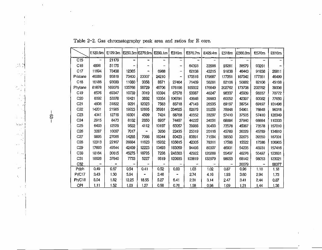
Table 2-2. Gas chromatography peak area and ratios for E core.
E 120.6m E 129.3m E250.3m E279.9m E290.1m E310m E370.7m E429.4m E518m E560.3m E570m E610mC15 - 21179 - - - - - - - - - -C16 4898 51175 - - - - 64393 33586 93261 38579 93261 -C17 11694 73438 12365 - 6988 - 62138 43215 91838 46443 91838 26811
Frisians 40089 95819 73400 23007 24210 - 170516 179687 177351 167042 177351 46499C18 10186 93099 11080 3058 8871 27464 71439 56281 82106 50882 82106 45106
Phytane 81878 169076 135766 56729 46706 176156 165322 176649 202762 173708 202762 39336C19 6576 69347 10739 3019 10394 67578 53987 46247 98337 45939 98337 70772C20 6092 53378 10421 3892 10354 106791 43648 39983 60052 42397 60052 77650C21 4606 31822 9291 12023 7583 83718 47143 26535 69197 38754 69197 101496C22 14201 21985 19223 12695 35981 334625 62679 55259 78848 54901 78848 96018C23 4341 12719 10301 4599 7424 68768 40552 33297 57410 37505 57410 126349C24 .2915 8473 8102 2650 6907 74497 44225 34031 68884 37840 68884 110333C25 6493 12529 9522 4112 10197 63057 39988 30400 73578 45367 73578 157010C26 3287 10097 7017 - 3936 22435 25019 20116 45789 36029 45789 134810C27 9895 27065 14285 7066 16344 80423 83891 71584 39550 32675 39550 187001C28 12313 22167 26884 11623 15932 135615 42005 78311 17586 15522 17586 106905C29 17693 49544 42409 12223 13493 183059 94496 80307 46931 54235 46931 157416G30 18164 30615 45275 18795 7298 246383 42922 120288 55497 46276 55497 123601C31 18626 37840 7733 5227 9819 120935 103819 132979 98053 68142 98053 123021C32 - ' - - - - - - - - 30079 - 66077
Pr/ph 0.49 0.57 0.54 0.41 0.52 0.00 1.03 1.02 0.87 0.96 1.10 1.18Pr/C17 3.43 1.30 5.94 - 3.46 - 2.74 4.16 1.93 3.60 2.94 1.73Ph/C18 8.04 1.82 ■ 12.25 18.55 5.27 6.41 2.31 3.14 2.47 3.41 2.44 0.87
CPI 1.11 1.52 1.03 1.27 0.98 0.76 1.58 0.98 1.09 1.21 1.44 1.36
4 ^#1 44 4! 455. 44454 44 429.4m 4 610m 451 4. °] tfl (transitional zone) 4 141 4444(Fig 2-24).
F# 45.4 35.# 44H HS4Sn^^ 145 E#4 44 41 1
/}#& 4444. 54 44 M4 #44# 5# #44 155 E#4 14-44 #1 ill 44 43# Cie 44 C3i4444 5# tiH] 441 54^444 44444 14N4 S# M#(S# #4 45 2-3) 4-4 4—S. 54 4(Appendix #5). 4 4-4 4 #5 E#4 4444 445. 7} 44 #4 #44 599.7m 44 4444# 5# 444 43.7} 4-44.03. 1444 4444. F#4 54 44 15314 4 44#4 444# 43.1 110m, 160.2m, 210m, 351m, 401.5m, 549.7m°l 4(Appendix #5). F #4 54531# 44 4 #4 4# 0.35 - 1.014 15# 4444 44 4^1 4444(Table 2-3). #5 4% 41* 34 Sir 4 0.95 - 2.154 Ml- 444#^] 4# #453. 444 44 #35 #143 444 1
4#4 44 #453. #4 44.=4^444 On ill #4, 44444 Ci8 3# #41 43*11 ! 4
4 F # 45.4 4!## S14 441 #4 11 453 4443. #4
# 444 441 44S4. FI 667.2m 45.4 41 54531## 41 1444 444# 44 44314! 44 4# 44 #44 14 44 4 14 14# 144 #1 41 4444. F 1 667.2 m # C29 aaa R 5
444 14 444 3% 131444 4, &44 5444 Jt*4 44 5.41 14 4-4-3145 44 14 44 441 4414.
2-3. #!4I 5711- 14
54 4i 45 E, F #44 444# 44 5411 slKhopanoid)
—64—
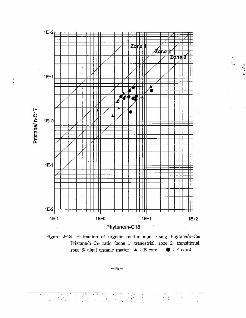
Prist
ane/
n-C
17
1E-1 1E+0 1E+1 1E+2
Phytane/n-C18
Figure 2-24. Estimation of organic matter input using Phytane/n-Cia Pristane/n-Cn ratio (zone 1: trenestrial, zone 2- transitional, zone 3: algal organic matter A : E core # : F core)
-65-
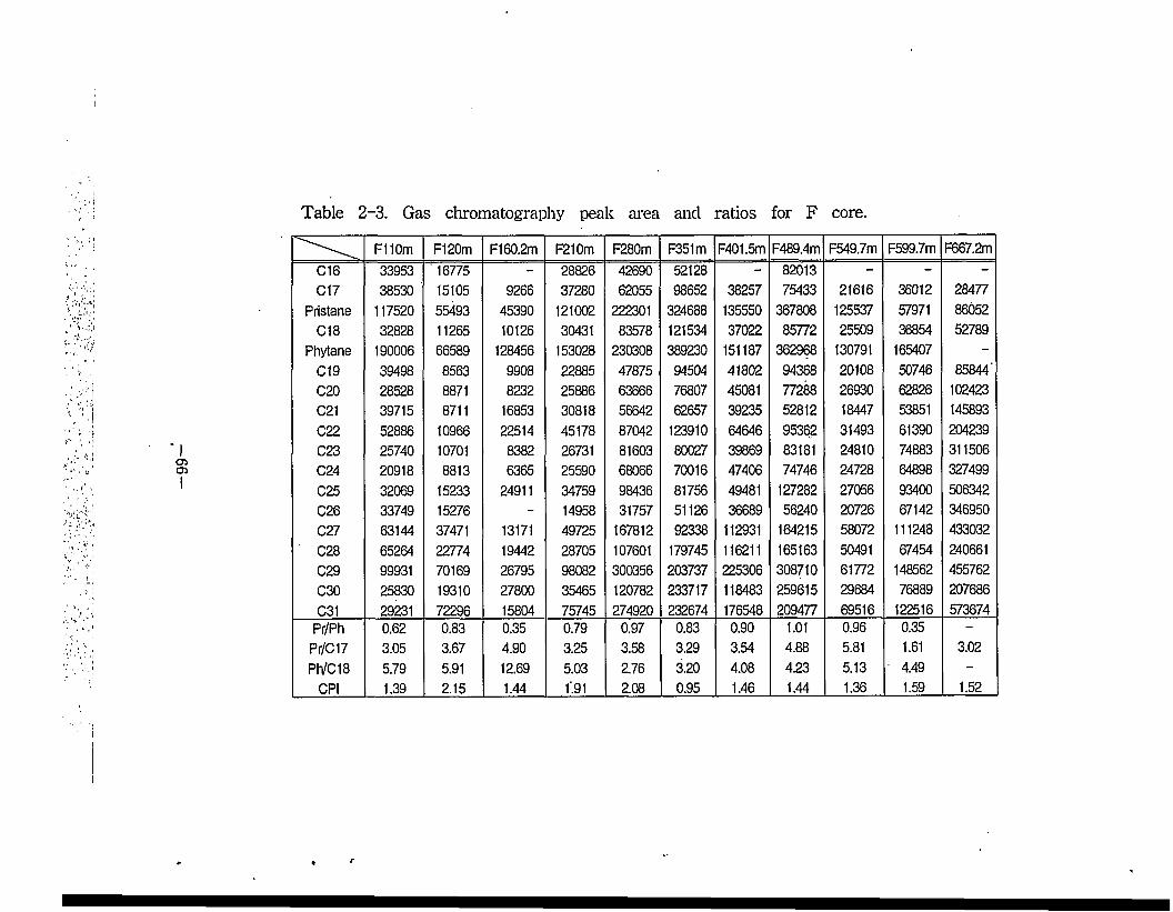
Table 2-3. Gas chromatography peak area and ratios for F core.
FI 10m F120m F160.2m F210m F280m F351m F401.5m F489.4m F549.7m F599.7m F667.2mC16 33953 '16775 - 28826 42690 52128 - 82013 - - -
C17 38530 15105 9266 37280 62055 98652 38257 75433 21616 36012 28477Pristane 117520 55493 45390 121002 222301 324688 135550 367808 125537 57971 86052
C18 32828 11265 10126 30431 83578 121534 37022 85772 25509 36854 52789Phytane 190006 66589 128456 153028 230308 389230 151187 362968 130791 165407 -
C19 39498 8563 9908 22885 47875 94504 41802 94368 20108 50746 85844"C20 28528 8871 8232 25886 63666 76807 45081 77288 26930 62826 102423C21 39715 8711 16853 30818 56642 62657 39235 52812 18447 53851 145893C22 52886 10966 22514 45178 87042 123910 64646 95362 31493 61390 204239C23 25740 10701 8382 26731 81603 80027 39869 83181 24810 74883 311506C24 20918 8813 6365 25590 68066 70016 47406 74746 24728 64898 327499C25 32069 15233 24911 34759 98436 81756 49481 127282 27056 93400 506342C26 33749 15276 - 14958 31757 51126 36689 56240 20726 67142 346950C27 63144 37471 13171 49725 167812 92338 112931 164215 58072 111248 433032
' C28 65264 22774 19442 28705 107601 179745 116211 165163 50491 67454 240661C29 99931 70169 26795 98082 300356 203737 225306 308710 61772 148562 455762C30 25830 19310 27800 35465 120782 233717 118483 259615 29684 76889 207686C31 29231 72296 15804 75745 274920 232674 176548 209477 69516 122516 573674
Pr/Ph 0.62 0.83 0.35 0.79 0.97 0.83 0.90 1.01 0.96 0.35 -
Pr/C17 3.05 3.67 4.90 3.25 3.58 3.29 3.54 4.88 5.81 1.61 3.02PIVC18 5.79 5.91 12.69 5.03 2.76 3.20 4.08 4.23 5.13 4.49 -
CPI 1.39 2.15 1.44 1.91 2.08 0.95 1.46 1.44 1.36 1.59 1.52
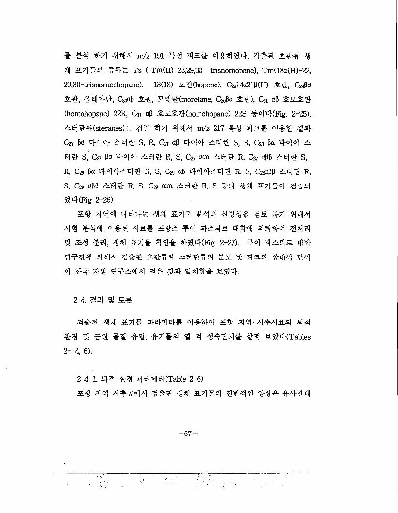
* *4 44 m/z 191 14 3)3-1- 4*4^4. 3*4 541 4
4 57)14 111 Ts ( 17a(H)-22,29,30 -trisnorhopane), Tm(18a(H)-22,
29,30-trisnomeohopane), 13(18) 54(hopene), C2gl4a2iP(H) 54, C^Pa
54, *s))44, CsoaP 54, 21) 4(moretane, CsoPa 54), C31 aP 52.54
(homohopane) 22R, C31 aP 5254(homohopane) 22S -F0H(Fig. 2-25).
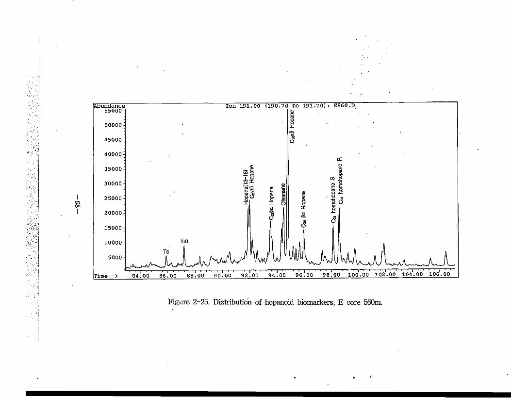
5e) *l(steranes)# 3* #7] 44)4 m/z 217 14 3)31 °1*4 34
C27 Pet 4tiH 544 S, R, C27 ap 444 5e)* s, R, Cgg pa 444 5
44 S, C27 Pa 444 5e)* R, S, C% acta 5E)* R, C27 aPP 5E-)* S,
R, C29 Pa 444^44 R, S, C% ap 444^44 R, S, Cggapp 3E)* R,
S, C29 aPP 5e)* R, S, C29 aaa 344 R, S 14 5414 4*4%4(Fig 2-26).
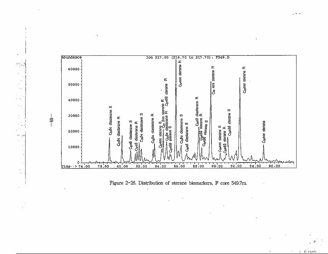
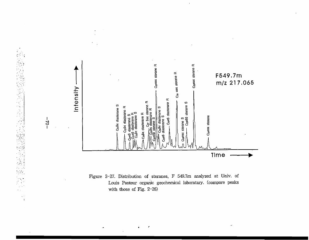
54 444) 144-141 3.7] 1 144 434* 45 44 4#444 *44 4*4 451 545 14 4-342 444 4444 444
^ 34 *4, 44 57)1 44* 444(Fig. 2-27). 14 4-543 44 4144 44)4 4*4 3414- 34*14 *3 4 434 14)4 44
4 *1 14 41544 4* 44 44#* 344.
2-4. S4 W 5#
4*4 14 57)1 4444* 4*44 5# 44- 41434 44
43 4 14 *4 *4, *7)14 * 4 4144* *4 3&4(Tables
2- 4, 6).
2-4-1. 44 43 4444(Table 2-6)
5# 44 4*144 3*4 44 5414 4444 *** *444
—67—
Ion 191.00 (190.70 to 191.70): E560.DAbundance 55000H
50000 -
45000 -
40000 -
35000-
30000 -co o
25000 -
20000 -
15000 -
10000-
5000 -
100.00 102.00 104.00 106.0098.0096.0094.0092.00rime- -> 88.00 90.0086.0084.00
Figure 2-25. Distribution of hopanoid biomarkers, E core 560m.
Abundance 217 .70)Ion 217.00 (216 .70 F549.D
60000 -
50000 -
40000 -
30000 -to. tt>
$ 0)W CD
20000 - c 92£ <9
10000 -
94.00 96.0092.0090.0086.00 88.00rime--> 76.00 78.00 80.00 82.00 84.00
Figure 2-26. Distribution of sterane biomarkers, F core 549.7m.
Inte
nsity
F549.7m
a. %
Time
Figure 2-27. Distribution of steranes, F 549.7m analyzed at Univ. of Louis Pasteur organic geochemical laboratary. (compare peaks with those of Fig. 2-26)
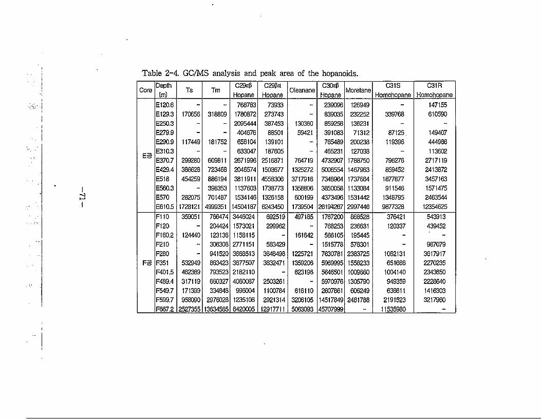
Table 2-4. GC/MS analysis and peak area of the hopanoids.
Core Depth(m) Ts Tm
C29a(5Hopane
C29paHopane Oleanane CSOctP
Hopane Moretane C31SHomohopane
C31RHomohopane
E120.6 - - 768783 73933 - 239096 126949 - 147155E129.3 170656 318809 1780872 273743 - 839035 232252 339768 610590E250.3 - - 2095444 387453 130360 859256 136231 - -
E279.9 - - 404676 88501 59421 391083 71312 87125, 149407E290.9 117449 181752 656104 139101 - 765489 200238 119396 444986
ES E310.3 - - 633047 187605 - 465231 127038 - 113602E370.7 299280 609811 2671996 2516871 764719 4732907 1788750 796276 2717119E429.4 386628 723468 2046574 1503677 1325272 5006554 1467963 859452 2413872E518 454259 886194 3811911 4558306 3717916 7348964 1737664 1877877 3457163E560.3 - 398353 1137603 1738773 1358806 3850058 1133084 911546 1571475E570 282075 701487 1534146 1326158 600199 4373496 1531442 1348795 2463544E610.5 1728121 4999351 14504187 6243450 1739504 26194267 2997446 9877328 12354625F110 359051 766474 3446024 692519 497185 1767200 868528 376421 543913Ft 20 - 204424 1573021 299962 - 768253 236631 120337 439452Ft 60.2 124440 123136 1158115 - 161642 566105 195445 - 'F210 - 306306 2771151 583429 - 1515778 578301 - 987079F280 - 941520 3668513 3648498 1225721 7630781 2383725 1062131 3617917
FS F351 532949 863423 3677507 3832471 1359206 5969995 1558233 651686 2270235F401.5 462389 793523 2182110 - 623196 5646501 1009660 1004140 2343650F489.4 317119 660327 4060087 2503261 - 5970976 1305790 949359 2228640F549.7 171399 334848 996004 1100784 616110 2607861 606249 638611 1416303F599.7 958090 2976028 1235108 2921314 3206105 14517849 2481788 2191523 3217960F667.2 2527355 13634565 6420005 12917711 5063093 45707999 - 11535980 -
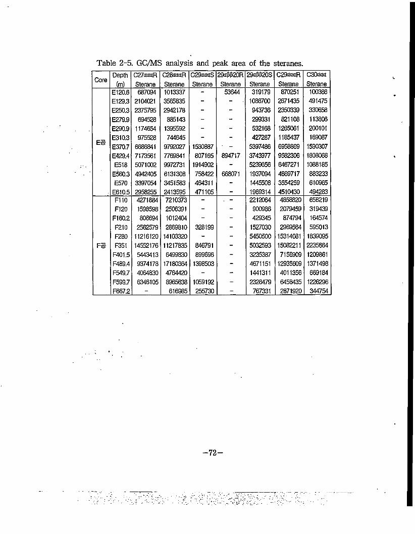
Table 2-5. GC/MS analysis and peak area of the steranes.
Core Depth C27ctctaR C28actoR C29actaS 29tipp20R 29OPP20S C29actaR CSOctcttt(m) Sterane Sterane Sterane Sterane Sterane Sterane Sterane
E120.6 687094 1013337 - 53644 319179 870251 100386E129.3 2104021 3565835 - - 1086700 2671435 491475E250.3 2375795 2942178 - - 943736 2350339 330658E279.9 694528 885143 - - 299331 821108 113806E290.9 1174654 1395592 - - 532168 1265061 200101
ES E310.3 975528 744645 - - 427287 1185437 169087E370.7 6686841 9792027 1530887 - - 5397486 6958869 1590307E429.4 7173561 7769841 807165 894717 3743977 9582306 1808068E518 5071002 9972731 1914902 - 5239656 6467271 1088185
E560.3 4942405 6131308 758422 668071 1937094 4869717 883233E570 3397054 3451583 464311 - 1445508 3554259 610965
E610.5 2958255 2413595 471105 - 1969314 4510430 494283F110 4271884 7210373 - . - 2212064 4858820 658219F120 1598598 2506391 - - 900986 2079459 319439
F160.2 806694 1012404 - - 429345 874794 164574F210 2562579 2869810 328199 - 1527030 2969564 595013F280 11216120 14103320 - - 5450500 15314081 1839095
F5 F351 14552176 11217835 846791 - 5032593 15082211 2235664F401.5 5443413 6499830 899696 - 3235387 7156909 1209861F489.4 9374178 17180364 1398503 - 4671151 12935609 1371498F549.7 4064830 4764420 - - 1441311 4011356 669184F599.7 6346105 8965638 1059192 - 2326479 6458435 1226296F667.2 - 616985 255730 - 767331 2871920 344754
-72-
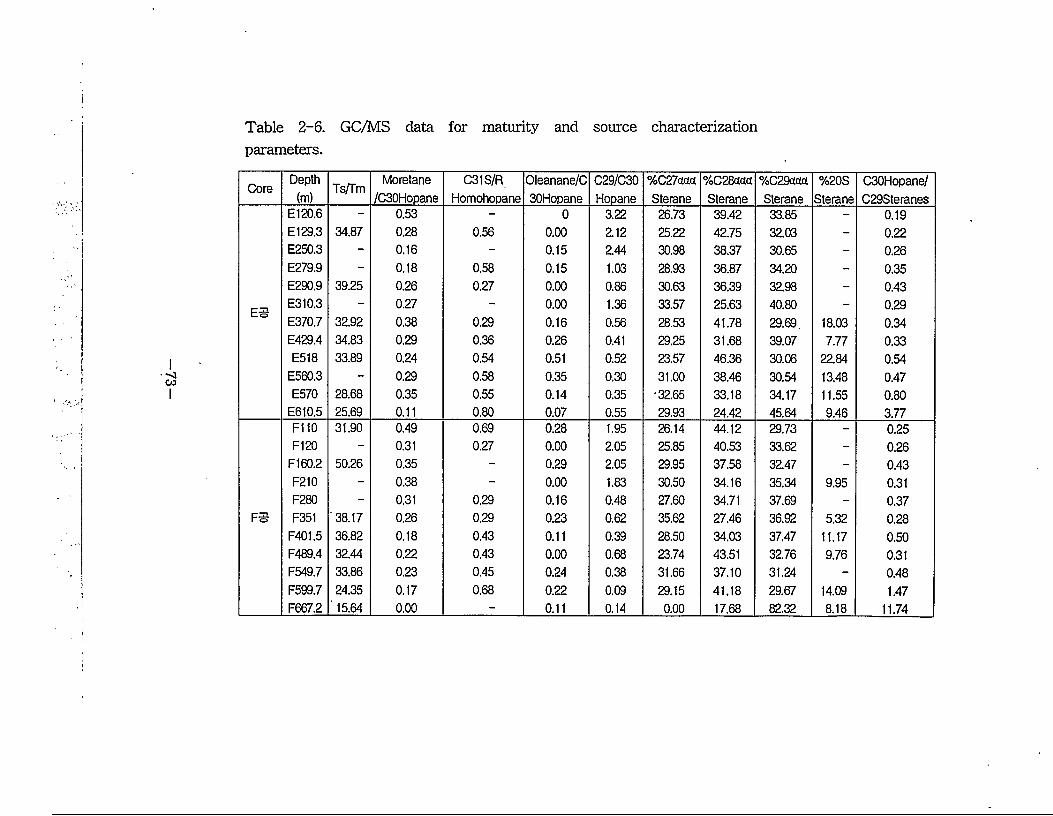
Table 2-6. GC/MS data for maturity and source characterization parameters.
Core Depth Ts/fm Moretane C31S/R Oleanane/C C29/C30 %C27ctctct %C28aaa %C29aaa %20S CSOHopane/(m) /C30Hopane Homohopane 30Hopane Hopane Sterane Sterane Sterane Sterane C29Steranes
E 120.6 - 0.53 - 0 3.22 26.73 39.42 33.85 - 0.19E 129.3 34.87 0.28 0.56 0.00 2.12 25.22 42.75 32.03 - 0.22E250.3 - 0.16 - 0.15 2.44 30.98 38.37 30.65 - 0.26E279.9 - 0.18 0.58 0.15 1.03 28.93 36.87 34.20 - 0.35E290.9 39.25 0.26 0.27 0.00 0.86 30.63 36.39 32.98 - 0.43
E3 E310.3 - 0.27 - 0.00 1.36 33.57 25.63 40.80 - 0.29E370.7 32.92 0.38 0.29 0.16 0.56 28.53 41.78 29.69, 18.03 0.34E429.4 34.83 0.29 0.36 0.26 0.41 29.25 31.68 39.07 7.77 0.33E518 33.89 0.24 0.54 0.51 0.52 23.57 46.36 30.06 22.84 0.54
E560.3 - 0.29 0.58 0.35 0.30 31.00 38.46 30.54 13.48 0.47E570 28.68 0.35 0.55 0.14 0.35 -32.65 33.18 34.17 11.55 0.80
E610.5 25.69 0.11 0.80 0.07 0.55 29.93 24.42 45.64 9.46 3.77F110 31.90 0.49 0.69 0.28 1.95 26.14 44.12 29.73 - 0.25F120 - 0.31 0.27 0.00 2.05 25.85 40.53 33.62 - 0.26
F 160.2 50.26 0.35 - 0.29 2.05 29.95 37.58 32.47 - 0.43F210 - 0.38 - 0.00 1.83 30.50 34.16 35.34 9.95 0.31F280 - 0.31 0.29 0.16 0.48 27.60 34.71 37.69 - 0.37
FS F351 38.17 0.26 0.29 0.23 0.62 35.62 27.46 36.92 5.32 0.28F401.5 36.82 0.18 0.43 0.11 0.39 28.50 34.03 37.47 11.17 0.50F489.4 32.44 0.22 0.43 0.00 0.68 23.74 43.51 32.76 9.76 0.31F549.7 33.86 0.23 0.45 0.24 0.38 31.66 37.10 31.24 - 0.48F599.7 24.35 0.17 0.68 0.22 0.09 29.15 41.18 29.67 14.09 1.47F667.2 ' 15.64 0.00 - 0.11 0.14 0.00 17.68 82.32 8.18 11.74
3:4#4 5# E#4 370.7m, F#4 210m 44 #44 4-4 C29 aD&44 C30 ctPJL^r^l 4 #4 43711 44#4- 4, ###5:4 C29M /C30 3.44 4# IS-4 "§"4 441 4# 444 4 ## 1 443 Cso344 444# 44$4. C295L4/C30 3:44 47} 1S.4 # 54 4444 44 4 4431 437> 44# 44 444 #4#4 ##4 444, 4444, 4# #4 44# 4444. $4 44 444 434 4# #444 C29
3:44 #41 441 444# 5# #44, 4444, #4 44# 444# 5444 S.4# 44# 43414 444# 4433. 4#44.
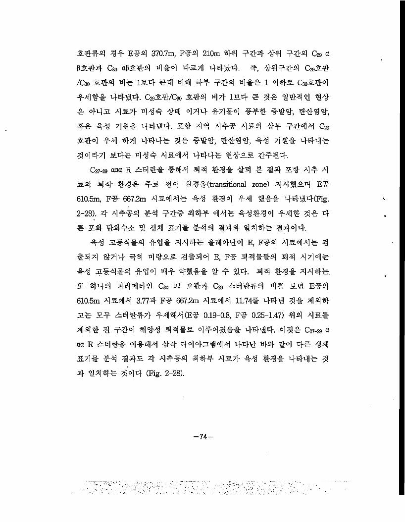
C27-29 acta R 344# #414 44 44# #4 4 44 #4 4# 43.4 44' #5# #3 44 45#(transitional zone) 4 4 #34 E# 610.5m, F#- 667.2m 4344# #4 454 #4 ### 4444(Fig.2-28). 4 4##4 #4 #4# 44# 44# #4454 #414 5# 4 # #4 44## 5 44 $711- #44 444 444-# 4444.
#4 3.#4#4 #4# 444# #314-44 E, F#4 4344# 4 #44 %44 44 4533 4#44 E, F# 44##4 44 444# #4 ##4#4 #44 4# #1## # # 44. 44 #5# 444#3 444 44444 C30 ctp M4 C29 344#4 4# 34 E#4 610.5m 43.44 3.774 F# 667.2m 4344 11.74# 444 5# 444 Jl# 3# 344#7> #444(E# 0.19-0.8, F# 0.25-1.47) 44 43# 444 4 #44 444 44#3 4#45## 44^4. 45# Czz-29 a aa R 344# 4#44 #4 444-^44 444 44 44 4# 44 $4# #4 443 4 4##4 44# 437} 44 45# 444# 54 #44# 544 (Fig. 2-28).
—74—
Gs?
▲ E core • F core
Lacustrine
C28 C29
Figure 2-28. Ternary diagram showing C27-29 octet R sterane distribution.
-75-
9
Abundance Ion 217.00 (216.70 to 217.70): F667.D
35000 -
30000 -
25000 -
20000 -
15000 -
10000 -
5000 -
100.0096.00 98.00rime--> 78.00 94.0082.00 84.00 88.00 90.00 92.0080.00 86.00
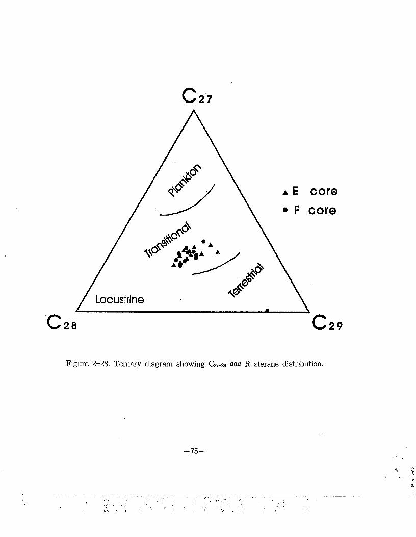
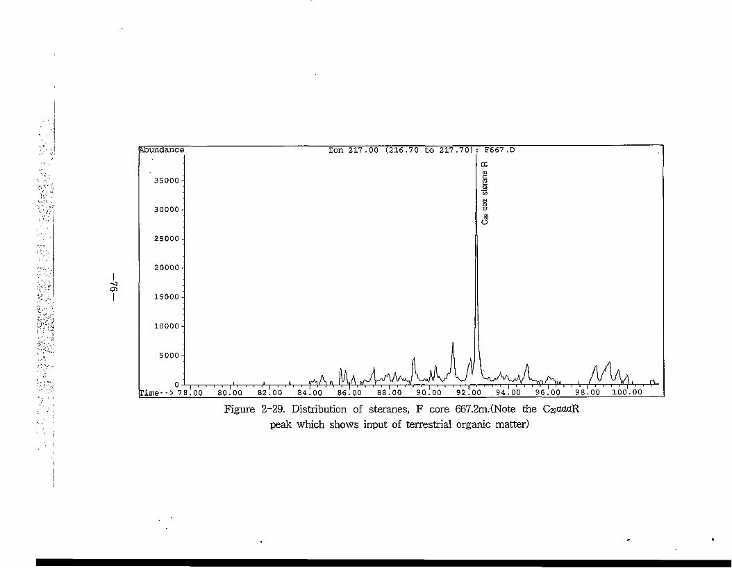
2-29. Distribution of steranes, F core 667.2m.(Note the CgguaaR peak which shows input of terrestrial organic matter)
Figure
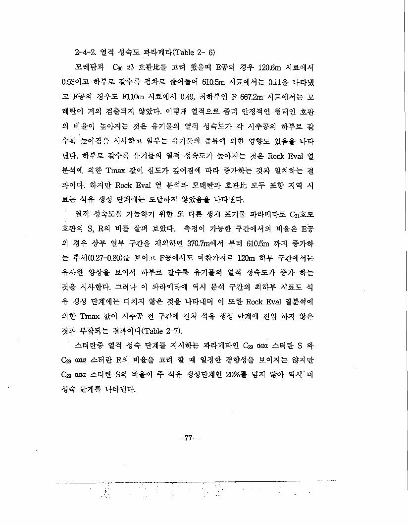
2-4-2. 13 345 H44(Table 2- 6)5414 Cso a3 aUt* JIB] ##4 E#4 3# 120.6m 3&43
0.5345 1#5 #4# 33-s. #4 #4 610.5m 3&43# 0.11# 441
Jl F#4 3 #5 FllOm 3&43 0.49, 4444 F 667.2m 3543# a
414 44 4#44 &14. 4#4 145a #4 1341 341 it
4 44-4 #13# 4# 44 #4 14 3 #57]- 4- 3 #44 l#a l
#4 414# 344a 1## #7] #4 #14 41 43=5 1## 14
14". 1#5 1## #7] #4 14 3 #57} #13 # 3# Rock Eval 1
#44 41 Tmax 314 3 57} 4444 4-4- #41# 34- 131# 1
444. 131 Rock Eval 1 #44 5414 alJt 5# 51 31 3
a# 4# 33 134# 5113 #### 1414.
14 3 #5# 7># 13 41 5 4# 34 53# 44445 Csi&a all S, R4 4# 14 511. #44 3#1 #1434 4## E# 4 4# 3-# 1# #1# 4411 370.7m43 #4 610.5m 43 #7>4# #4(0.27-0.80)# 545 F#435 4#7>35 120m 1# #443# #11 4=3"# 543 1#5 4## #3 #4 14 3157} #7} 4# 3# 3114. 544 4 4-4444 43 #3 #44 41# 355 3# 33 444# 433 4# 3# 4444 4 51 Rock Eval !#34 41 Tmax 14 3## 1 #44 43 3# 33 144 41 13 4# 34 #14# 4444(Table 2-7).
544# 14 34 14# 331# 44441 C% acta #41 S 4 C29 aaa 541 R4 4## 54 1 4 131 313# 543# #34 C29 aaa 544 S3 4#4 # 3# 33141 20%-E 13 1=4 13 4 3# 44# 1414.
—77—
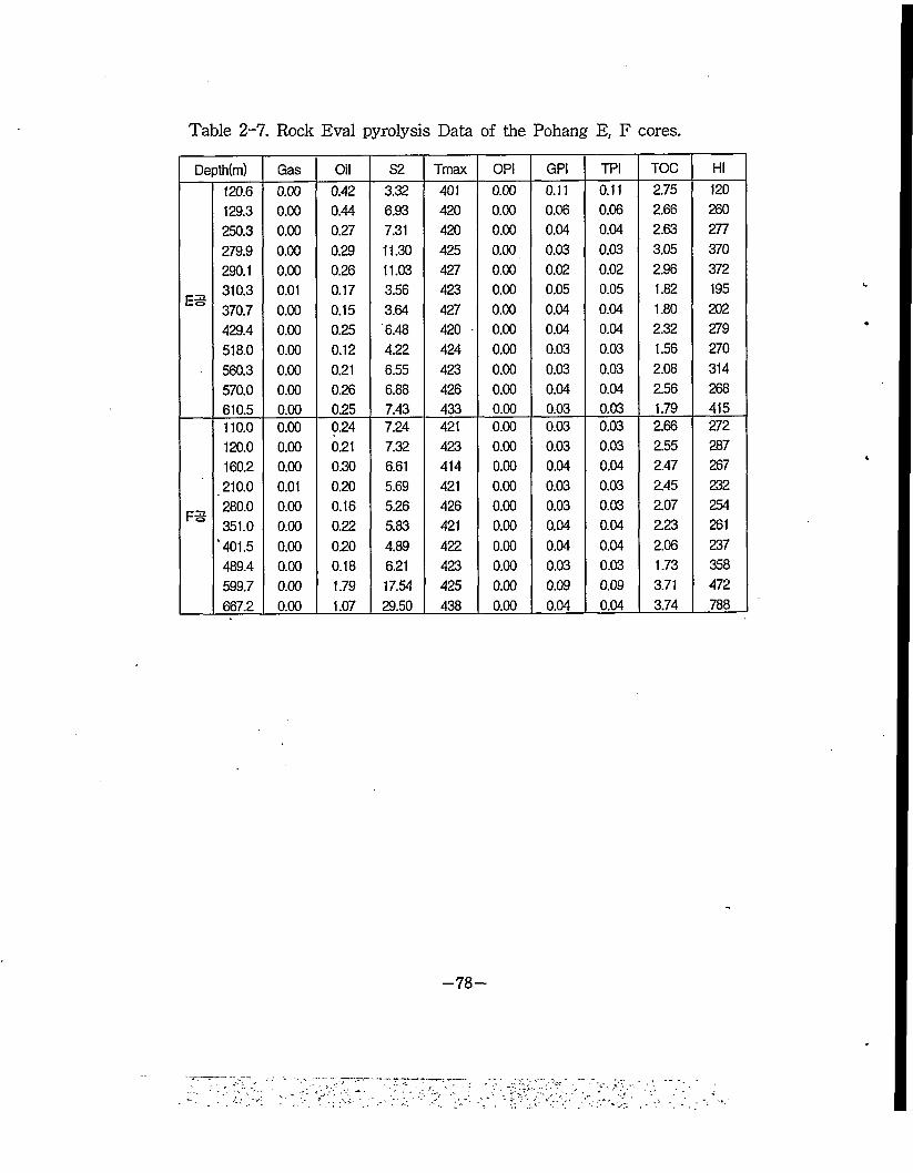
Table 2-7. Rock Eval pyrolysis Data of the Pohang E, F cores.
Depth(m) Gas Oil S2 Tmax OPI GPI TPI TOC HI120.6 0.00 0.42 3.32 401 0.00 0.11 0.11 2.75 120129.3 0.00 0.44 6.93 420 0.00 0.06 0.06 2.66 260250.3 0.00 0.27 7.31 420 0.00 0.04 0.04 2.63 277279.9 0.00 0.29 11.30 425 0.00 0.03 0.03 3.05 370290.1 0.00 0.26 11.03 427 0.00 0.02 0.02 2.96 372
E3 310.3 0.01 0.17 3.56 423 0.00 0.05 0.05 1.82 195370.7 0.00 0.15 3.64 427 0.00 0.04 0.04 1.80 202429.4 0.00 0.25 6.48 420 0.00 0.04 0.04 2.32 279518.0 0.00 0.12 4.22 424 0.00 0.03 0.03 1.56 270560.3 0.00 0.21 6.55 423 0.00 0.03 0.03 2.08 314570.0 0.00 0.26 6.88 426 0.00 0.04 0.04 2.56 268610.5 0.00 0.25 7.43 433 0.00 0.03 0.03 1.79 415110.0 0.00 0.24 7.24 421 0.00 0.03 0.03 2.66 272120.0 0.00 0.21 7.32 423 0.00 0.03 0.03 2.55 287160.2 0.00 0.30 6.61 414 0.00 0.04 0.04 2.47 267210.0 0.01 0.20 5.69 421 0.00 0.03 0.03 2.45 232
FS 280.0 0.00 0.16 5.26 426 0.00 0.03 0.03 2.07 254351.0 0.00 0.22 5.83 421 0.00 0.04 0.04 2.23 261401.5 0.00 0.20 4.89 422 0.00 0.04 0.04 2.06 237489.4 0.00 0.18 6.21 423 0.00 0.03 0.03 1.73 358599.7 0.00 1.79 17.54 425 0.00 0.09 0.09 3.71 472667.2 0.00 1.07 29.50 438 0.00 0.04 0.04 3.74 788
—78 —
2-4-3. S-E-
£1 44 E, F 4 #141 11 I27fl, ii;M 4&# 4414 4^
314444 41## ##M 4# hs4-s:z#41 1112* 1-4 S
4. 144 41# 1 £# 11124 Ml- HIM 54 1112
14 £4###1 44 4444s fit 41-4 s#*l 24###
1-4 444. £4 44 41# 45.4 £4 1112# Ml-, 24*1
44 £4#* 14 144 44 £4 44 4114 44 #41 is. 4
4=4 44 444 #41 44‘M, E14 610.5m, FI 667.2ml £* *
4 44 #4* 4-4M. 44 £4# Ml 1* £1 44 14#4 1
4 4 Ml 14 14:44 4-144 41s ?M4 4M4- 4444 #
7T-4-1 7}14 4.44SS.1 41 44 #441 444 1# 441 44]
* 44-44. Rock Eval #141 1# 14#4 #4 4M #41 44
£4# 144 4# 44 #444.
£4 444 4441 44 £4# 144 141* is 44 4414
44 144 41# 4si £#2 14 424 s 444 444 14 S
#14 24#14 M # 43.4 444 #44 #44# *1241 4
1 44 41 t4S4.
2# #s 4^iSr M* 34## 444 £###12# 14 £
41-4- 11# 14 £41-4 1# 4 444 4*l££ 44444 #
444 44 #4# 4 44 44 £414 4# 4-14- 14£444 #
7}7} #£#4-. 2.# 11 41 441 11 14 144- 411 44£s
1413, 44# 114 444- #112*4Is 14 £4## 1444
1 41 4 #4 #44- 4# 1# 4# 4-#14 24 114 £!#!.
-79-

*113# *15. ^ ^i#^ ^*}7i#
Q
—81 —

I
*1139 W eHx-jy
*ll 1S 7H2.
444 4*4 7}* 544 4* 4 7}5 ¥#4 (seeps)* #* 3144. 2# rfl^ 444 4**4
4if5 4* 44* 4* # 7>^4 t#44 4*4 $1*4, 4* t# 4 4* 4* ^-4 4*4 444 44. 4 if a. *#4* 4* *4 4 4*44 *4**5. 4444. ^*4 44 4* 4* 5* 4**4 44*4 9X?}s. 44. 4 4 44 *4* ^x> (*44 »4)* 4 if * *#4 (macroseepsHl *44*4. zi#4 4 3*5
*4444 4* 4 4^3* *44 44* 4* *44 4* 45* 7] #4 5* * 4 44 44*5 ** 4 415* (microseeps)4 *4 * 7}*4t11 4*4.
4414 45. 4/** *7^ 444 44* 4 41 5*4 444
4 44*5 44 *4-*5 4*4 44 4* 44 7>4 *m*\ 4
44# 344554 44*54 *# 4 4* #443.4 4* 40]
4. 4 44* 4*455 44*5 4455*4 4 44 44*57}
*435. 4*44* 7}4°11 44* *4, 44 444 44114- 4
4 4 44 47}4 * 7}4 5 4*444.
■ 44444 44-4* 44*5 *455*4 Ci - C5 44*5 7} 4*4 4 *4 7}*4 455 *4 4 4 44 4 +444# #4 4* 3144. 3 5^4 44* 4 4 4 44*5 444* 4 44* 4 4 4435 444* #*4. 444 C2 - C5 44*5* 5# 1 44 44*5 444* 44435 c2 - C5 44*5 *5 44
-83-
4 7H> 4# 4945)3. $14. 4 44# #4,4, 444", 414" #4 #4# #4#5 #4 4 ## 5444. 44 444 4444 44 4 7}4& ##€ 4" $144 444 4 44 4"4 q# 44^^01] 4 444 4 44 444 4#43 4# 44# 4"4 4# 44#54 444 $4 4 44#5# 444 44€ 7>444 $14 4## 444. #7}# 444"&. 4435#4 4"4 55 4 #4# 444"5# 444"5 44 44 4 a £# 45 7>4 4 $14 5.4 5# 444 #44 44# 4544 44444# 7} 4 4 #444. 4 44 444 44 4 444## 44 #4 44
-M444JE - 4 41§# 444 #4, redox potential, 4
## #4, 54=4 #4, 4### 5# 4#45 #4, 4#4#4 #4, 4=4# #4, 44 #4 ## ##44.
1-1. #4o|# 444#
4 #-4-4# #4 7) #4 444"54 4# #4 4# (microseepage)
4 #4'4 4 Ci - Cs 444"5#4 #4 55 4 #4# 444## 4 4)4# 4# 4 #4 44 44^4.54 4# ### 7>#44 4 4" $1# 443„4 44 4 54 # 444# #44 444. 4 444###4 44 444 44# 11 7>4## 54 4# (diffusion; Rosaire,
1974; Kartsev et al., 1959; Baijal, 1962; Siegel, 1974; Donovan and
Dalziel, 1977; Duchscherer, 1980, 1981, 1983; Dennison, 1983), ##
(effusion! Rosaire, 1940; Kartsev et al., 1959; Baijal, 1962; Donovan
and Dalziel, 1977; Dennison, 1983; Duchscherer, 1981,1983), ## #4
4 4 444"54 4"4 #4 (Pirson, 1960, 1962; Donovan gnd
Dalziel, 1977; Davidson, 1981; Duchscherer, 1981, 1983), 4#
—84—
(permeation; Horvitz, 1950; Baijal, 1962) 43 $14.
34313## (1976)# 44# "#4, €4 ## 3 #3#3 S# 441 33 #55, 4 system^ 5# ##3 #5* #
143 4# 4455 33 444 3 ”55 33414. 3 33 3
344 444 44## 443 344 4444 halo ## 43#
4 4 §14. 54 444 344 43 444 3 44 3433 4#444 #1# 43 4344 34 #3 3 333# 4435, 43= 443 44## 3 3 #13 433 34 37}3#343 3a 34 34 435.44 44 44 C6+ 44### 33 4 4 33 4
4# (effusion)4 44## 33#14 4 4 45.5. 5^3# #
3 34. 3#313### 4#4 "#445.44 #44 45.3 4” 3 45. 4 3434. 3444 33 34 4## 43, 44 4aii #3 3 43 #3 4# 5# 5# ##& 444. 443 3 4=3 44#5 #3 (micro seepage) 4 # 5#34. 3 3 4 4 33 53, 5#4 34 4# 337}#7> Darcy 433 343 4#34 !## 44 434# 414 5# 3444 44 &#, 4 44 #4 434^ 3 345 Jl# (macroseepage)# 14# 334. 4#3 3 4 331 #1# 444 C6+ 343 44## #554 13 3 #35 34 3 44## #5# 7>3# 3 34.
3 4 3#34# 44## 3 31 #4 34# 3 #43 ##33# 4# #3 #3 313 3 4 #3 #3 3# ## 344 ^#7} 4 4## 44# #443 355 344# 33 713445 #444(Pirson, 1960, 1963, 1964, 1969; Donovan and Dalziel, 1977;
Roberts, 1980; Davidson, 1982, 1984). 34 43 #355 3#4#
—85 —
6## 44#£4 #4 #### 44-4 4"9=% 144 4#4*
1144-3. 4444. Pirson4 Roberts# "44 #4#"9
(forced draft)” ## “444 4# (deep water discharge)” 4 ##
444^4. °1 4 -E- °1H # 144 —5. 44 4 #4 44 4 # 44 44 441 7>44t11 4 £44 43.44 4444 44#£
444 4#444, 444 #4 44## 444 #444 444 £444 44# 444. 344 £44 44, 4# 4 444 444 44 4 4#4#44 44 41 #4 <344 44#, Pirson
(1960, 1963, 1964, 1969), Roberts (1980, 1981)4 4## #7>#4
4£3 3.44. 44 #4 #4# £# 41## ##7} 44#£ ### #444 -45E4 44#£ 4 4^4 (## 44) 444# 1 #4# 4# #7>#4 4£3 1444. 44# (D 444 44# #£. ###4 0# 414# #44# #44 44 #4 3#4 #7} #44# 4# 444£, (2) 44 #4 £#4 444 444 #1 44 4 # #47> &4. 4 4 4# #44 #44 #4 #43:## #7H ##43i 4# 43-4 4# ## 4# 4#4* 11# 44 31, ##4 ## C6+ 44##4 #4# 7>4# 444.
4#44 #4 4 7>?§ 44 44#£4 4 4^4 4# 444#
# 4144# 4# 7}4#4 $%£4, 3 #44£ &44 3.71 (# £4£ 371)4 7>3 4 $4 44 ##4 444 44#£ 44^4
4 4#444# MacElvain (1969)4 444 #44 ##4 $14 3.
44. 4 4 4# 44134 4 3&4SZZ.4-4 £44 4# 44 7>4
44# #1# # $14.4# 4## #4 4-71 4# 4 4 7>4 7ii##4 $144 444
4444 ## #4# #4 ##14 04 #4# 44## #44#
i.
—86 —
7>54 ##44. 44* #4 44 444 4 414 4 4# #
44 4-<3 4 4 4#4 4-5.4 7># # <344* 334 44*54 4 44 ##4 (microfracture system)# *4 447]-^ 7] S-4
*#44. 44# 4& 44*5 44*44 *7fl ^ 4# 4#44 #44 #4 *5* 4# 444 *444 44 4#4 44*5 4 4 44 ***4 4# 44 1441- #44 444:4# 4# 4444 4#44. Price et al. (1984)4 444 3=4# -$-44 *5. 244fat 44 #44# 5.4 4 4 4#* #44, #* 5S #4 5. #4# 4 ri 5.4* *44 44*4 (*# 444 44 44* 4) *4 4 #4 S4* 44 4 4 4. 44 4 #4 *4* 5.445. 5. 4*4 * #7] ## *7] 4 #5-' 4 *# #4 45.5.4 444 * 4* 4 44. 4 44 *4 4 #5.4 4* *5. 4*4# a* 4* 4 24 4# #a 44 44*4 4414*4 444* 44* 41# 44. 2-* 4444 4 4 4# *4 #2:*# 4* 4* #4 4 4 4 **4 4 4 4 #*# 7J4 *5. 44. Park Jones* 444 # 4 44 3E* *7H 5L7l 455 4* 714 *44 7>4*“cryptocrack"5.5. #4 4 4 $1## 4*4314 (Davidson, 1963)
1-2. o|^*44 #A|-
4 ##44 54* 441 *# 44*54 44 45.5. 4 44*45 s* 4* 7>44 4 4#* ### 44 45.4- 4* 4 4 4. 4 *44 *#* # 5444 44-4 4 7># #*4 4*4 #4. 5si4 4#414* 4# #47} 44 #544 ##4.
Kartsev et al. (1959)* 5444 **34* *5 4#* 44^
—87—
# 4 7}z15 *4484= (1) 24, (2) #4 5# *4
£4 a]^254e1 45# 4*4 41#*# sa>, (3) a4 *5
.4 4# 41# 24 (biologging), (4) *49 41# 24 #44.
4fi 4# *5# i^Ht 244 #4^#* 44 7}# #5
# 4444 #4 44s. 14*4. *57} #4*8 44 847}
4-71 4-E 444 4#& 7M& 4"5 $14. 7}* *44 41# *
#4 4*4- 54#o]H 44 44. 4#4 4492# 441
9# 4 44- 7>* # 44 4 4 *44 *4* *55. 14## #4
4. 2m# 5444 *544 #44 444 4 ### 5*-*4 7}
#54 *2# 2#4#4 $1^4 tfl7l ##4 4?)7) 41 #4 414
# ## *44. 4*# 5* 244 #** *54* *5o)i 44
4 *4* 4## §14. Strawinski (1955)# 0.61m# #4485,
Kartsev et al. (1959)# 45 2 - 3m# 4*444. ZL## 4##
4 &4#, 4# 15-30m #4 4*5 ** 49-71- 414 4# 44*
4, 2-4m #444 41484. Volz and Schwartz (1958, 1962)#
1.5-2.5m# 5#484. Davis (1967)* 0.92m54 ** *4 4 #
45 *4# 48** 0.3 - 0.46m# 9€484- ZL# 0.3 -15m*
#5o)H ** 44# 41484. Miller (1976)# 0.61-0.92m* *
5*4 #5# -#4484.
1-2-1. 4E)|E|0|-
4*4 #5*# ###5 7>4 #*#55 444# *4924*2*4 4 52# 4**55 4 #4# 44#24 4444# *5**44. 4 *-5*#* 4##4 *5 *4* #4 *84 # # #71# *8# #* 4-4# halo 4*4, 44*# 4*4, 94
—88—
(chimney), 4 #4-# (radiation lows), i!/## 4 #31, 44# 53=
1 4# ##45 4415# tt3141- #3 #4. 344 44 44
# 444 ^^0)1 $M4 3143. ^5444 #3. ##4^5 44^
14 ### #41 1315 44#3 $14.#314 4# 4 #4 4 ±44, H 14#, 14 #445
3. 4¥4#4. 11 144## #57} $14 #4 Sr I ^ 4 444. #f 144# 15#1 #5 #55 4-§-44 . ## 45-E 44444 44 #44 ±44 43114 145 3=5# 4 44 43114#5 #4#4 (4, 4 #5 44 443 44 4314 4). ±e 431444 ##4^51 ##541 ##7>54 444# 4444. a #<*ii 441 44 4314 44 ##4^5* 4##a # #5 4314 44 44 #54 #5# 4444 4##4. Davis
(1956)4 4314 4^-4 44 4 4444 444 (actinomycetes)5 £4 #4 ##45* 4 31 444 44a- 434.
45 4 4# ##4 ±714 4314 4, 44# 4 actinomycettel
1#4 4& 5# 5-4# 455 4#444. al# 4# 43144
# W# 144 5444 ##44. 4314 4 #*! 4# 54#
#5, 3 4#, 44 #4 #44 44# 3 314 #5 4 3 4 ###
4 4(Davis, 1967). Zobell (1946)# #5 ###5 #544# 44
4 41 ±14 ## ###54 ##4 4314 4 ### H.31 #44
#4a #34.
45444 ##45 ### 53= #554# 53=4 #54 4
414 54 4 3 4# 4# 455 544. 4# 53= #5# 53= 4^34^ ##* a.711 #54444 4# 4444444 #4
(Soli, 1954; Kartsev, 1959; Davis, 1967).
-89-
^4## 4 #4# #4##4 44 ###313). til-B]]
4 44 €#4€ ### £# 5£f^l4 7}# #444 (Kartsev,
1959; Sokolov et al., 1959). 444 444 ##4 44# €47} 5.
4= 44444 444 #4##4# ## #4?} 44. #&, 4## 444 s.4, 445## 44 444 t*4 3 J2.44 4] #44 ^4°1 4# #55. 4444 44 4444: 44 444 44 #4
4 4#4# 444a 44s. 44#a 44.44 4 4 ##4 &S44 7}4 #444 4 #### #4 t#
t#4 2.-E 4S-44 4444 ##4 44 s: 4=- 44. Kartsev et al. (1959)4 #### #4 44 4 #5# #4##4 #### # 4 ##=r (edge water)44 444 #44# #4 4444?} ## 4 $1431 4 #4. Telegina et al. (1963)# 45 2680m4 4#44 4441# #4 444 4# s"4443L, Rybakova (1957)# Apsheron #54 #5. 4200m# €444 % 4# 4 # 4# 444 4# #4 4 $14.
Kartsev et al. (1959)4 €4# 44### 44 3.7} 4#4 4 4 €4, 44## #7)1 4444 €444 ###4. 5# a7]7} #71 444 4 4## ^##€4 44 4 €### 7}# 4. ze]E 5. 44=4 47}a} 4 ^#4 444 44 €4 44444, ##4 4 4## 4 €4 7}a #€## 4 44 ##€#5 44# 4 $14 #4. 44 €4 444 4# #44# #4 €4 441 €44# € Til €#43l, 45 fis 444# #44## 444 € 444.
#4## 4#4# #s}##4 4 4 #4 4# 44 #44 45. 44# #7} 4-^ x>44 44 4€44 &$J;4. 4 44 444 7}4 44 4 €44 £#-#4 #4 #4##, #4# #4#
—90—
#3 53# ###£, 4 54 54= #4 35 44 35
71-71-4 4 (7}3 #4# 43# #44 #445)334 557} # £#5 3144. Kartsev et al. (1959)5 434 "3##3 4 43 "4
JL ##53 44143 £45 (44 44# 4=355 4444) #
#f£5 45. 444 £4 35# #444 4444 434 #4
44 4# #4. 4#4 ### 44 #5 4 4# #3:4 3 444 3
7>34 43 43# 44 45 £ 43-4 4#3 444 4543
5 #4. 4 C2+ #4554 4334 443 4- #54 #5 (4 3#
43 #4), 54-S4 #4 ##4=£ 55, £3 54 #455 5
£.4 4. 4# 3 7}3 43 2-5-71- 53# £#4 #55 #45£
4 3 £#4 #343 #5# 4 3 #43 4347} £354 5# £
3-#3 #4 #45£ 43-44 #343 ^545 3# £4 5#
4 (Kartsev et al., 1959). 43# 4 3# ##4 #5 #435 45
3-3# ##4=£ 4 4 £3 4 45 ##3 4£ #45£ 4 3)£#
43-47} £.454 55 54-#3 #4 #45£ 43*4 444 3
3# 5 #4-
1-2-2. 43=! 53(paraffin dirt)
35 4 3# #54 44# 5# 4 7}£ 4 3l£#4 ### 4
£3 3 545 53=4 ##44, 4 44# 545 ##4=£ #3-4
#3# 3335 34#4. 44# 53=5 Gulf Coast 3 4 43 #4.
#43 ##4 4, Colombia, Romania, and Burma #4 #5 #4
43 4#4. 3 4 335 44445 53.4 44 (Milner, 1925). 4r5
44=##5 #3# ##34 #3#53 53=4 43-5 #33 44
44 (n £35 4#45 #4 #343 454). 4 ##4 ##4=
-91-
9 7}55#4 =14 4 $149 4°H9 444 447} &4. ZL^# 7> 5 5^4 $19 #444 4445, #5 44# 5#4 ?£4 2]
4455 «1 ^ #4. 14^-^s 7}# 4499 7} 5 7} ##
# #4 #5 %#4$1# #£ $1jz., 44# tiVB|]^d> ##^ 44s. 5.014.
0)44- 4^444 9^4 444 54=4 4# 49-444 44 4 4"4 o)] a) 444 S'Sr gas microseepage 49 macroseepage4 4 4 9#44. Zi4 J1 ^9 49 ^ 49 444- 7}4 4 44 4
44 44s4 944499# 7>44. 444 54# 44 444
49 #44 494 15% 4 4 44 494# 54994 4 44 4
44 54=# #4 49# 4499 4 419444 #414 57004 4
#4 5-41-4 495 #5 94 44 $1## 44 44 (Davis, 1967).
444 54= #4 #4## 44 455 4444 45#, 455, 4
454*115 4 444o}4 41544 44 #4 44 44# 549
4.
4.4-4. 5#4 D^6)! 45# 455 549 44 #44 4 4# 44# #2}# # 49 4#4 4=4 gas microseepage# 4 ## 9 9 54= 9544. 444 444 54=4 44 44 4-14 49# 4471- §1# 4 4 44 44€ 9 $1$1# 4 44.
444 54=4 44 4499 4*1154 4 444 4 #4449 4 4 4 44 49 4 45 4#4 4#5 9#4 444 $1^4-. 4#4 4 4 444 503=4 94 4 4#449 444 44 444 44 4 #45, Gulf Coast 44-44 444 4=4 4#* 4449 4 $144 95 4 444 4444. 44-4. 5444 944 45 444 449 4# 444 444 944 #445# #4 4# 4# 44# 7}4St4.
-92-
1-2-3. ##
(chimney)”# 4 #4# 444^ A0)] 444 ##444^A 4#°11 4 44# 4# #444 4#4 4 44 4#
€ 4 AS ^#4# #4 4 444A 4# 4 44# #44. 4 44 44 4S-4 44^rA 44 44 #4#4 # #4 #A4 ^4#4#4 44 #7> 4-4) 444 4##4 44 44& 4# 4as. 4444. 444 444 #44 “# #"# 444A 4# 4 4 44 44. 4# #444 44# #44 #44/444 "44 4 444 4444. Pirson (1964) 444 “#4”4 4# 447> 44as 444 4as s4 4 a 7l]4# 4 44A5 4#4 #4 #4. Pirson (1960, 1963, 1964, 1969)4 4# 4 4
4 4#4 # 4 #444 (radiation lows)0)] 47)44 A.4 #4 7}
## ##4^4 444A 4# 4 70004H44A A4# #4# 4 ##4. zz.s)4 zz.4 4#4# 444 444#4 4 444 4## ^ ##4. #4 4## #4# 4# 44s #44 44, 4 4# #44 44, M44 #4 #4 #4.
4 4#4 4 4 444=A4 #4°)]# 4 A 7} a>#£] jli o] #2]-4# ### ##7>S4 444. 4A4 A4# 4A# 44 eH°)] €4# 4## 4# 4 44, 444 4#7>s# 4^ ifi °] ph°)1 4 4# 44# 444# 44 4 44. 4#7>s 44 444 ## #4
4 4# 44#A# 4444. Zobel! (1946)# #4444 ### 4 4#A 4 #44 a 4#4. 44 ## pH/eH4 44# 444 4]s# 4# #44 field# 7>4Aa, 4# 4## ##44t)1 4 4 #4 4 as 4 ##4 4 #7)] 44. a4a 4# 4##4 44as#4
##44. 44# ##4 4#4 44 4# ### #4 #4## #
-93-
411# 4#!5!4 4## 44. 44 ## €4# (pH4 #7})
4# 4#4 -H-HH 444 1444. 447}5 #54 €4 4 #7}
5#b) 4444 7}4 #4 4 41-44 444 44=4 444 44
44144 4444.444-4 44#54 44#4 44 444 7144 4
4 44 7} 5 444 44144 4444 44 4 4 44 444 44
4 444 44 444 1st 4444714 44144 4444- #
#4 4# Sfkll4. 44- 4# 154 41# 44 4 4 444#
442- radiation lows 4t halos4 7}4 # 444 41# #5 44-. 154 €-41 5# 414 40K# 544# K# 155#4 €4 443i, 4 44 5.4 4-444 7}1 # 514 44. 3l 44 444 €5## 444 fsH 444 15 445.44 4444 ### 4 44. 444 4444 €H# 444 154 ##14 44 11 € 44 4. 44 4# 157} 3L system55#B] 114 4€141 1411 1# 44€ 414 "hole" 44 low# 7>44 144.
4.1411 4#7}54 44 7] 14# 1441 444# (54 441 44, 1 44€, S41# 11 1 54 4414 444 (occluded) 4445# 5444)4 1 11 4445 44#4 H4 4 # #11 (nonspecific)4 4. 41411 447>5l #1# 411 51 44454 41 #4 44 44 41 514 4HI5 144 € 14. 4 4. 1# 51 #4 11, 14 (1# 44), 41 #4 4 1 *# (#4 4# €4 4 4 14 141 44 #414 4& 1 -§-), #4 447}5 #455#44 411511 tS 14. 1# € 141 445 414 444 14 5#7} 44#5 444 4HI 41 € 14 4. 3iS14 4# 1441 14 41# 444 4-11
-94-
s. 5.14. 5.# 1# 4444# 4#7>^ i#4 7] #41 444 ^41 7M2.1 4# 45. 4444 4411 4412: 444 4
4# 44 4 4 4.
1-2-4. ^#7|S! nUU-
44# 3##4 42: 1#42: #4, 41 7M 44, -n-H #4 4
4 #1 4411 4 414 ^os #141 44H# 41 41
i 114 #5.3. #11 4444: 441 44# 1 #4. 344 #4
4 44H 44# #4 #4# 4412: 444 41 444. 342.
& 44 4#3.1 71-444 4 414 1 is 44. 4# 4444 4
1 ## 4 44 4# 44 44 4 41-41 4#444 4444 4 4
#4 444 4 444 444 441 7>4 # 1 #1 4ss. 444
44 5.144 (Rice and Claypool, 1981). 4 44 444 #4 44 1
4 44 4 4 444 H2.3. 4 4 444 5.34 4 #2.4 (Rice,
1980; Rice and Claypool, 1981; Gautier, 1981; and Mattavelli et al.,
1983), 4 44 4# 7]4 44 44 4 44444 42. ^44, 444
4^4 E.42.5.H #44 1 #41 41 4444. 444 ##7}^
4444 44 4# 4 4 444 71#jei 4443. #1 45.4 #4
3.4. Rice and Claypool (1981)4 "4# 4 #4 7}^7> 4 4 4444
12.4 4 4* 44 (20% 44). 141 4# 4# 7>^7> 44 4 4
4.44 12.# 444 5.4 34 444 433 ##44"3 4#4.
4#4 4 444 4-r 44 4 4 Ci/(Ci-C5)#7l- #4 0.99444
4 (Rice end Claypool, 1981). 4# #4 Po Valley 41 7] # 7}^
41-4 CH4 #44 99.40%44 99.97% 44 44 (Mattavelli et al.,
1983). 4 14 C2+l #442.3. 4 44 4. 5.1 4412: 4414
-95-
4#7>4 3. 7)% 4# 44## ##4 %7\] €44S 4 4#
m 4^4 xl##4 ##4 #7l]* 6>7lxl^l4. Rice and
Claypool (1981)# “41 4=-shelf #4 44 #4#4 4 5H4 444
SS # -^-71-i-ol #4# mud4 clayS. #444 €S
4 £5flr ^# 714 444 m% 1€4 ^€4 44 44# s#
4 7l]##4"s #44.
1# 7]4 7>x; 44SS444 4 4^44 44, s.4 444 (4 44 EE COz* 5#) 4 4#444 44 44 7>4 444# #4 44 44# 7>4#4. 44 44 4444 € 44 4444 44SS 44 #444 4 41^4 4 444 444# 4444 4#4 4 4 4. 44# 444 4 4# 444 444 44 ##44 #4# 444. &# 44 4#7]4 4# 444 #4# 4#4 #4 4 4€# 4# 51
4 44 €54 4144 ##4 4 444 #7]] 7} 4#€ 4s 4# #4
4. “tight” Tg#7l# 4# 44#4 44s 444 #4# 45. 444
44 €44 #444# 4 4 4. C2-C5 4#4S* 4#4# 44 4
## 44 4#€ 44 4# #71]4- 4444 44# 4# 4# 444
# C2-C5 4##S7} ut7] ^#44.
454:## *4 4## 444 4##4 444 4# #4 si 44 4# #4 447]- 4## 4#44 #4 4 4# 44s#s# 4 ## 47])^# 7>x]2. $14. zls]4 #4 4 s 4# #€ 4 444 4#7] # 4 4 444 44 444s (Rice and Claypool, 1981; Gautier,
1981: and Rice, 1984), 4# 444 4### “tight" 4#444. 45.
4 444 44 44## 4### 444## 4 4 #4 4 #44 4 ir
# 44 444 444# 4# 4-@ 444 4 44# 7}444 7}#4# #4 €s 44 4 #4.
-96-
1-2-5. HALOS
. £l $1 4##5 ##5|# halo 41*114 Q°)d\] rfl
§><4 £#44 #4 44# 41 4#4 44 1!££ 4# 3# 4
44 £14 444 4 444 7]] ##4°> # 444. 4 44 44#
4 halo 44 4 4# 4 #4 4 5:4## #444. Kartsev et al.
(1959)4 Sokolov (1970)# ##4# 44454 #4 o)^6\] 4)%
44# 444 £14 444 £4444. 4 4# £l## apical
(focal), annular (halo) 4 linear4 4. apical -^# focal 444# 4
4#5 4# #4 4^4££ 444# £#£ zl43l 444 # 5
4(patch) 144 444# 44.4#, 4# 4 44 #4 #444 4
# 5# (patch)## ##44 (#44)# 4 44. halo 444##
4445 444 5## #44# ## 4#4 jl4# 7}4# 5#
1444, ## #1 # 41 4# 7>#4. halo## #44# 5#
14# £4 # t£ #4. ^-44 ##44# 4#7> £# #4.
halo # apical 414# t£ ###54 44 ##4 4 #4-
linear 414# ##, 1# ## S'# #1, 1# 41#54 45.4
4 #444. 4# linear 414# C6+ ###5# 5#4jl, 11# 14 #4)4 ###5# ##4# ## #444 1# 4# 44 4 #4 4# 4 44. #4 4 4# ###57> 4$ 7}#4 £### 4444 414-0-4 444 #144. 44 #4 #14 4# 414# apical 4144 4##7l7> 414.
1# #44#4 #1# 44 #4 halo 414# £1 EE
(soil-occluded) 1##54 #4 #14# 7># ## 14 44
(Horvitz, 1950, 1954, 1957, 1969, 1980, 1981; Soli, 1957; and Siegel,
1974). £1 #4 ###5 #44 111 414 £!# 4144.
-97-
Kartsev et al (1959)# S<£ #4 44#^: S<$-#7l 4
4^r& 4444- #44 5-4 (#4# ## 4# apical ## Halo
444)# 7}#t)-5L 444.
1-3. 4H X|## #A|.
lil 4&444 #4^4 44 7>^4 4 #4C2-C5 444=^4 444 444 (C6+ 44444 44&#)* #444 44 444 44444 14^ 44#a 4441
4 444. 4 4 4^#s# #4 #4 44#a# 4 4 s<£44, s4-471 44, 44# 44, # #4 #4 $14.4444 4 44 44 7>4 44 s.#7} 4 444 4 44# s
°1 jl," 4 4 4 4 414# 444 4#4 # $1# 4# 444. 4# 4
44# 4# 4## 445. 431, 44# 47144 44 4-44 ## 444-4 4 4 7> a#44. 4#°1 s4 4 444 auger4 #^-4# #4<4144 4#4# 3.4 4#444. 4# 4 7>4 4^44# 4 s 7I144- 4s. #4 4 ## 44# #444, 4# #a $X
4. 44 7>4 ae 44# 44 4# #44# 44 7>4s 44.
1-3-1. 5.4-#7| #4
s4-#7l #4 ^# C2-C5 44#a #s# 4 s 71)44- #4 a## 4^7)1 ##3L e a7>4 7>#4# 412 $14. S44 fi
R3 a#, #4 a4=4 “a#”47)1 4# 4# 44 (44. 4, 4, # 4, #, tflvl# 4 #a)# s4-#7l a/Ml #s4 44& 7>44. #44 4# ^ #4 a# 44 W# 4 44 sa>7> # $1
-98-
31, *\3. 4# 444 7>S# 4 44 AS Lfltijl ^ §i4.
1-3-2. S#-## B4tA #4A^=-#4 E##A 44 #4144 %4. 444-4 ^
4 # 444^4 #4 4 $144 4 44 sorption ^ desorption^ 4
44#4 4 444 #$1#4 44# 44iAi 4 444#4 4#
44471 4 #4 44 4. s4, 444 44, #a 44
444 4-T* 444 #4# A #4 4 #4-. A<5:-#4 44
#A 44 4 $144 & 4# 4414 s$M1 #44 4444# ##
4 4=45. ##4# 4 4 4. rit 4# 444 7>44 44 ##
47>4 444 4&# # 4 44.
1-3-3. S&-B6S E4t^ #4A4-#4 444^4 #44 444 ^4 #44## A4=-#4"
(occluded) 444^# 44 #4444 4 444 444 4444. S44 4 4 el4 £.4 “4 7}# 4 4” (4##4 444 4 4 4)4 444 #444AS4 #44 ###A## 44AS ##4 -ft-5]
4 4 # 44. 44el# 444 4 M 44A 4 4##4 #4 4 A #4= 444 444 4444 4as #4a, 44A ##4 4 4#A4 44 4 #4 44 44 4 4el# 7}45.# 4as S44. 4 4 4 444 4444 # #44 44#A4 44 #44 (sorbed) 4r4#A4 4=s4 44 ## #A $14. 4 4 444 4 4 4/} # 44 44#A# 44 as #444^44 4## &4A 44 &# 4. a4=-#4 44#A &4# S4-44, A4=-## 44#A sa> 7> 44-4# 444 44 (449# ##4 4a 4444 4 44)#
-99-
344 g#4, 44# 3# 4414 41# #^3^-4 #4# 4 4#3# S.5L-s>7l 4#44. ^4 4 34-#4 44#34 #37} 3#-^!- 44#34 #334 H44 4^# ##4# 3#-## #4 444^3 #44 3#-#4 44#34 #4 4 4#4 #3#
Til l #s $14. 43. 43-44 4444,4 44~4#4 44 44# #4 44#3 4 #4 44#34 444 #4 44 447} 444
# 4 4 4.
1-3-4: SSt 44t^ #4
4 #4^# 44 4& 44 4 (0.3 41^1 o.6m)44 # 3# 44 4 4 44 ##44 4# 44 44# 4444 44 4 4 44 #44# 44#34 44 #44 444 44# 444# 444. #-## 44 4 #3 44# #444# 4~§-44 4#4 444
4 #4 3,4 4 44 34# # 4 #4# 4°14. 3#-#7] ^ 34-#4. 4443 &44 4^44 #44# 4 2 444 #4.4 4A1. 44t3 #44 #44# ### 44## 4 4 4 -E 4
#44 # # $14 4#4 7|4, 4#, #4 44 4 444 44
443 #4.1 # #4. 4-8-4# #444 4 44 #-## #4#
34#4 ## 34-#4 44#3 #4 4 444 4# 432., 4 44 #41 ■# 44.
4 44- 444 44 #-## 414# #44#3 44. #3
4 #4# 2 414 7}4 444 #4, 15 - 60 cm 444 34
44 34# #« # 44# 444 4444. #*343 44#
3# 7}4 #14 4 4# 38 4# ##4 4 4 44. Kartsev et al.
(1959)# 7}4 ## 444 4 #3, 444 444 1444 44
100-
4# 7}# 4444 5"# 7} 4 %4 4 444.4 #4 4# ## 34#4 #7#}# £4 -B-4 ###4 4%
4 #7} t)4 4 #4 4 4 . 4 4### 4 s* 4^*°14 4#4 ##4 3.711 #34# #£44 444# s4=-#4, s°J=*# ## 3#-#4 #44=3 #44 3.7)1 #4^i: 4344 #
#44 4#44. 444 4# #^4 4# £4 44 #44 4 "44 4# 44. 344 4-4# M4 4# 4# 4##4 4# #4# 7}#7§4 #4. 3 ##4 ##44 4=# 444 4 44 4##4 44 4=343 444 444 44 4 4## 4 444 #44 43# # 7}#44 &7l 444 4.
1-4. 6H4 4## ei-a|.
4444# ##4 344 444 #44=3 7>37> 47)a. 4*
4# 44 #4 44 44 4#4# #44=3 # ##7> #4-8-444. 444 4# #4 #44=3 #3* #444 444# 44-# 334 44#3 4AM 4-8-# 4= 44. #44=34 #4# 4 4= 4s# 4444 4#s#4 -8-4 44# f#44 #3# 4# # #44# 4 4 7># 43^0] 4. ZL 44 .44 4 4#4 3## 7>3 4# 44 #44=3# #4443 43, #4 #4-3 4)4=#4 #44=34 44 #44# #%# #4443 44.
44= #4 444=3 #3 #4# 444 4 lm 434 #34# 44=# 4444 -8-#44 Si# 44# ##44 #44=3 4# 4 4 44 4## #44# 4 44. 44= 44 44 4# "Inter Ocean
System"^ "Sniffer"7> 7}# # #44 #4. 44# 444 4 43
-101-
#44 Cl - C4 44#^# ### 7>#4t]1 44, 4# 4 #4 4
2 44# ##4 4 a!-## 4# 44 4# 4 4 s. 444 #9)1 4<9 ir 442 #4. 4 #f 4 =42 4 44 44 44# #244. 4 #44 #4# 444 %14 ### #4471 4# 44 |s, 44 #2# 444 3# jl 444 ### #442 4# 444^1- 4
#44 £tis. ##44 44. 44#^ #44 7>2 32422
444 444 4# 4422 ##44. ##, #4, #2 44 #4 4## #4441 44 444 4 #44.
## #4 44#2 ### 44 4# 4 7># 4#4 44 44444# ##4# 444. 4 44# ### #44# a># 44 4) #4 4 lm #24# #&* #4 44. ### 4#44 # 44. #5.2#-# #-# 7l Tj]# #r#44 7I-232423442 44
#2 ### ##44. 4 4## #5 44 7}3 4# #47>4#'4442, a>^-4# 444 ##4 $14.
-102-
*112! U-e W All
1 144 14 # H ^o] 4^V ti Bfl^-oll^ X[^ # &#
4& 411 14 141 41 4114, 444 114 444 4 4 4 $14. 342 44 44 (44, 44)4 414# 44 4 44 144 14dll 41# 41 1 $1# Al#2 4444. 4444 4 4 441-4 444 44# 143.4 44444 &414 414443.4 44 144 4## 41 7}#44 4 11 43.3. 444
4. 4# 14 44441 414 4# 44 &44 444 44 (S S@7jc)44ti-4 4 # 43.3. 4444, 4144 41444 # 43.3. 4444. 441 44 2414 4 44 414 41 ,5.3. 143, 14 141 444 4147M14 114 44444. 13.4-4 7]41 f#4-71 41 44 4 41471-44 4 141 14 444 ^44 4#4 4 4 4# 1#7>4 bias,
44 4 1 41* 44 411^4.
2-1. 7|-^ ## 144 11 W 1#
44 4 4-1 4444 4 4— i# 111 4 44 44 #433.4 4 1# 23 342 H |ss 111 41 111 144 4 (Fig. 3-1). 2 514 414 144 4 -6-14# 44 14 4 44
4114 11# 41 7>3 #4 4 114 111 4—3. 114 4, 143. 444 4-4- 4-444 44# 111 11 147} 3.# 411 $11 (Obzhirov, 1993).
-103-
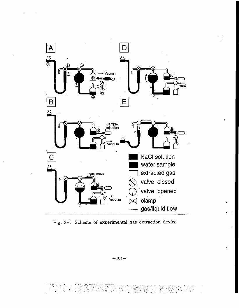
Sampleinjection
Vaccum
, gas move
■ NaCI solution■ water sample I | extracted gas
valve closed(2) valve opened
1X1 clamp —» gas/liquid flow
Fig. 3-1. Scheme of experimental gas extraction device
-104-
— SOT—
Bp^'SIy b#"M" b Ifc# h HS-# b"o"E£ ## H> "m-k to© H
7 4a# ##3bbb w-fE Ho 'bbkFo# #b# kbB #©
wrn (V7 #E-Z b) a abb Trbbk## 4^74z (^(3 toT-S -SH) bbkb lb© "E7b# b4&## #7
4z auk atH^ kb# #© fTB a4s-kk bk#b lo# a 4-1 "to
g. bWb to© H^-ta# 4a-b lb & ^*o ££ {z© H^F-ta# (8
'(3 toI-S -SM) -bis #© "E7-ta» * IMvfoi #-g
k iMH^ ^"o© kbB biv © -a© (2
•(V bl-S 'SMQ -bl^lYiSrk
totems tb"5 k ■&k "5"© "E^-ta# io-B'n Ikfo^ {z"g k (T
z-i-z
"bb-§-b h # k # b^■p® tviz akW lb© #© ^7-ta* 'bb# #4sbH^ #7k
to # k"R b4° k? #4o iris k i£ #7{z a## ' b b & b -a®
-bb# qb-kk kfo #7b a#& klb-ek 4^b£ bka# ^
■o»a-b #b bwb qibbw q© irb# qab# b^k #©
H7-ta# '-blo^a q4s b# kkk bb# #ab bb bwb
. a® T=7-ta# is~q k # a k a tb^a -§-a q©"E74a# a? #q b a^74a# b bis- bb4° k -k #k -blob ^5 #k 4?b
# 4z^k q b k ak to-gk '-bisbk ^k kfe-§-b
#k b ^b-§- ik b74a# q© 'bio bbikb ^ p'#7W tob
"c h a # a a I& =&-ks a bs hy-^-§ a "o' a b 9 ‘ b ■§■ 1? k a74a# b#To q # klbV a% k"e q k# a b-k ## 74z
R"z& " I--1--Z
4 444 7>344 (Fig. 3-14 D).
5) 4 2-31- 44* is. @4 ©# s* 1JL *43a ©* d>2fl
3 444 #433 ©oi] 44 7]^t #433© 33. 4*444
(Fig. 3-14 E).
6) #433 ©4 434 144s# -§-14 *4# ©4 -§-1
=r44 41 #4s 34 4 1 4Sl4 7>34 4* 44
4 * 7}3* *47]* 4-8-414 431- 1444 7>333.4S34
36)1 ^444 14 44.
2-2. 4^ 14 .
144 7} 3 1# 44 4 4 4* 4447] 114 4€4 444
443 44 441 44 4 si 1144 144 7} 3 4# 44s 7>3# 4*444. f #4 4 7>34 41 44 9ml(44), lOmld
43 144) 4$14. i#4 7>34 14 4** 1444 444
^^lBfl^SS] 5890 4 43 II 7>33^4S. 34^4] 7}if 114
4 *'4 414. 7}34 14* 44 7l-3aLS.4s3.4s4 &41
*4* Is 120°C, 4*4 is 200°cs 4441S4, si isi
100°C 44 5* 4 #4 4 4* 150°C44 5°C/ minSS. *1443
150°C44; 51 4*14. 4 34444 *44 4# 7}3 * *114
4 *S7>-44 702ppm, 50ppm4l4. 441 * 1 -H 444 44
63.2 xkTW, 5X10"W *14 4 1* 43S. 4 44 7> 44 4 4
4 444] 4*1 * 1** S414. 44- 44 4 4 444 7>3
**7]4 4*4 4 4 *4ss 444144 14 1444 *44
4 4*4 44 4 4 44.
—106 —
413H U-AI-a
41455 4##! 414]## 14#54 & 1##54] 1#
44 4# #5##4] #4# 54 I3#r5 5# #5#4] 5#4 4# 1-f 4-144 44. 544 44 #44 4] 5# °1# 44# 54 #5#4] 5#44# 44 o]#o,] tfisf] ^Tfl 4 444 4#14 44 4 54s| °ll-4 °141- 4 44 444 444 4 44 5
445 44 (Davis, 1967; Barkay et al., 1985; Mergeay et al.,
1985; Zelibor et al., 1987; Nies and Silver, 1989; Masters et al.,
1994) 44454 4440] e444 4445 44 4 # 44. s
44 #4 44 44#5# 4444 ##145(heterotrophic
organisms) #4 #5 44 4 44 #4]44 4#44 4 4 445 4
44 4544 444 44 144, 544, 544 144555 4 4# # $14(Brock and Madigan, 1991). °] #414 1##5# 44
44 4444 454 544555 »1## 44#5# 4444 4
44454 4444 44 44. £4 444154 4444154 4
4 144 4155 44#5# ol-g-sfi 44 454 4:444 44#5
* 4 4 (Krieg and Holt, 1984)44 415# 44 4 445, #445
44#5# # °l#14(Oudot et al., 1987).
444 4444#5 44# 45 #4 4 #4# 44#5# »1#4# 415o] 41 441441# #01 4, 4 44 4 £4 44 4##4# 544 5# 4] 4 44 3L7fl 4444(Price, 1986). 5 45#4]4 4#4# 14## 144154 ## 4 4 4#4] 4 41 4151 5.4 lg 1 254, 44 44 *H4# 1# 45^1 45 1# 4 4(Pelczar et a/., 1986). H2-14 415# 414 55 37] 7} 1 4
—107 —
5.44(Um)5 4# 44 543 4## <%7\] #3#}2.3. #43 g
4 #44 4 #4 # $13 2680m3 443 4(Telegina
et al, 1963), 3.7] 7} #4 44 X44 3 W4 44^4 4 7)1 4#4
4= $1555 7}5A3 #4, #3 4*1147)1 54 # 44451: ^7)1 4
-0-# 4" 44 444# 3# 44#53 4=4 4# , 4^3
#4 44) 5# ^444 4444 445# 4 #4 4 SM5 44.5E #4455 31#4 #5, f£, 4:4 5# 444 4 44 45
(S042'5# N032"), 4 4=4, #54 #4 44 4$444 4 4# #
4 4 444(Bell ef of., 1980), #44#4# 44454 4# 4*3#
4 44# 4 4#°)1 44 457)1 444 4X444 44444 #4
4 ## 544 €4#'4#445. 44.
z%4 4 4 44# 4# 43}#5# 444# 4*3#4 -4 4F1 4&
44 44 4f7} 4444. Gulf Coast4 44444 44$1#
paraffin dirt (Kartsev et al., 1959), 4 A3 # #4 4 4 4 pH4
redox potential°1 444-2., 5. 4(acid)4 A34 55 $14 4#4 -§-
4 Hi# 444 44 444# (Duchscherer, 1980; Sivenas and
Beales, 1984), hs)ji 4*3# #4 44 *3*34# 444455 $]
4 4*34# halo (Donovan and Dalziel, 1977) #4 4 X 444 4
44 #54 4X5. 4444.
44444 44444 $14 4 4#4 4 *3 #4*3 4 #54 #4
# ### 4 4, 4 44# 444# 4 *3#4*3# 4 4 #444
44444 444# 44 4*3#44 44 44#4 7))#34, 4
4 4 85.7%4 *3### 44^4# 55(Sealey, 1974)5 $154 4
4# 4*3#43 44447} #4455. 4443 $14 #4. &?1
4 4 *3#44 44# Mogilevskii(l940)7> 44444# 4444
-108-
544$154, *))## 4^#4 4 4) *$^5\7}S. -B>5.
5(Stanier eta/., 1986) #4#o] $1$14. 5e)M 5# 4^#4 4
4 44 «4 #43# 44-7] 44 1.5m 34 4444 5#4&
# 4444 #1445, 4 4###5# 4 #4# 4 41-44 4
•44 l7i)4£ /}#45 44. a 4444 44, 444
4 444 44 #455 44#44# 4s. 4 $5 4 (Davis, 1967;
1969) zl 444 44 43)5=4# 44 444 $14.
44#44# s.44s., 4 ## 4 #4 44 4# *8"4(cutting
chips), a 44 & (core sample), 5 5)5 44## 4 4 4 S-# 4 #4
4 4 # 4 # $1 5(Kartsev et al., 1959) 5 4 & # 44 4# 345.
0.92m 4 4(Davis, 1967), 0.61-0.92m (Miller, 1976), 2-4m(Kartsev
et al, 1959)# 44 4 44 $154 #4455. 4 4## 4#44
444# 44# Qmanometric 4 4 (gas-uptake) ©visual #4 ®
444 4 #455 ### # $14. manometric #4# 5445#
4# 54# 444 #4 4 #4 ##4 #, 4 4#4 ###4 #
45# 7}ii) #4# manometer# 4444 #44# 4 45
(Davis, 1969), visual #4 4# 44#4 44 454 ##34 #4
4# 415 film4 ## 444# #455 1954444 4444 # 4 455 4 #14 4 $14 (Kartsev et al, 1959). 4444 #
1(£# plating #1)# 45 agar 44 4 £## ^4 444# 4 54 4 4(colony) ## #444 #4455 5445 #44# # 1 4 4. Michaelis and Riese (1991)# 4 444 4 #1# 544 4 45.# 4155 44#44 4#44# 45484. 4 45# #544 44#57> #7})# 4#, 4#4 4#4# 45# 4#4 4, zif 4 #44 4444. 444 44457} 4 44#4# 44
—109 —
* 45*#* *###*3* 4*0ll ### #5*4 4# 4#*
** *44# #4 4**4, €4 **7> 4**3 ** **4 44 7H#*# **4 44 441 (sediment)44 44# 4S.4
#*4=34- ##^444 4#* #3# $4 444 4 444 4*
4 4# 44# 4= 4431 33*^*.
344 2-# 4 41*4 44 ##4# 4s444 4444 3
43 4 4114 4*3°)1 4# 44# 4**4 # 4# #44 4
44. 44#4 ##2.3. 4#44 4# 4 44# 43# 4#4 3
344, 4 4444 #44 4 4*4# 4=3 #444. 3# #*
4S.4 4443 4S44 4 414 *3# 4 4 44 4 4
4# 4*4 ##444 *344, #44# 4 4 44 3# 44#4
4&* 44# 4*4# #4 44# 44, 4*4 44# 44 4#
#4 1:17} #444(Davis, 1967). #4*3# 4 4*33 44 5
* 4 4# 4 43 4***4 4*44 #4 #4 434 #44#
#4*3 #45-34 #4 4 *# 4(Strawinski and Tortovich,1955). 34# 4# *7)141-* 4 41*4 ##s 44* 4##* #4. 1 #444# 4*44 41 44# 4 4* 4& 4*4 4
33 415 ** #*43(Karl, 1980) #3* 4#** 4 *444
4# ##44 4 3*4 * 34# *3* 44 (Michaelis and Riese,
1987), £ **1*4* ##33 711** Probe* 4*44 4*14
4*44*4 *4# 45# 4# *#4* *(Barkay et al., 1985;
Diels and Mergeay, 1990) *33, 4# ##14 4*14 4*#4
4 3##*# ## *## #** ** * ## *44.
4*4 * *** 71*4 14, 4*4 ##4 4 4 #* 4*4
oil 4^# 4*33 4* #4-* # * #* # 4 1*4# 4*1
-no-
#4 711#44 4n ##4 44 aM 44
##4=34 ##44 4# ^e*4 ^it 4# 4##^# 4-§-•§>
4 #443., #4##4 44 4## &444 444#44 44
4 4 &444 4-33 ##% 4= SSI#4* #7}-b}jl4 4 £4.
3-1. 4S. %H#| W 4e|
3-1-1. 4sxH#|
44 444 a>-§-^ 5.445.^ 4# 445- #4|#4 44 4 3
## 44 ^ #4 #44 4^4 444*\ 44 444 (Fig. 3-1).
45.44# 44 4 4433 4444 444# 4 4 44 44*44
4 4^44} 444 3# #44 4#4 44#435. 444 44 4 4 44 ### 44 444435 44444. 3# 43# 4 X4 4##4 4 4# 4## 7}## 44 44 44 4X44 34=4 4 #44# 54 50-60cm(Davis, 1967)4Ai 4444 ^#3##
4 #^#3 ##44 ##4 A>#4^4.
3443# #3 4 433 4# 444# 4##4(Chough et
al, 1993) ##a> 4# ### 4#33 # 397fl 444 (A 4 4), 4 4, A>#, 444 3 443 4# #4#4, 3# ##34 #4 #
4# 4435. # 15711 4 4 (B 4 4)4 30711 4 4 (D 4 4)44
100m #435. 444434, 43 447} #7>## ^ ## 150m
#435. 44444. 3 444= 4## 7>^7> ##4#4 4#3
3 #4# 4x44 43#4 44# 4#'4#4 3°0MC 44)3
20-30m #433 44444.
—ill—
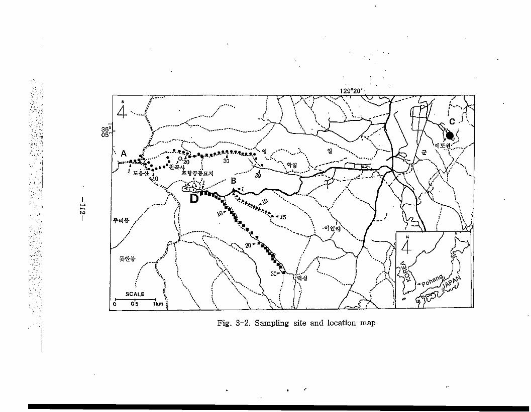
129°20' •
• P.4,
Y -15
SCALE
Fig. 3-2. Sampling site and location map
3-1-2. x-lE|
414 £4=4 £## 44 £4= lgi- I00ml4 1544 4^4=
4 ^444 244 ^4 44 44=(160rpm)& # # 3044 444
4 4-S-414. 30# 44f ^71)4 4144 4#4 10ml 4# 4
7] ##44 44# 4£# (control)£, 444 44# 44 #£4
#54 (nickel, 600 ppm; cobalt, 500 ppm; cadmium, 100 ppm;
mercury, 20 ppm; zinc, 400 ppm; lead, 500 ppm) Sr 4444.
(pentane, 20 %; hexane, 20 %)# l7>44, 444 4 4 4 4 4 2
44:, 444^ 44 4 44 1444 4 44 4^ 44=# 4 44. 4 4= 4 42? 444 4s.4 44 1044 441££ 44 4444 44 44 4 4 (nutrient agar) 4 4 4 44 4#4 4 30 "C 44 544 4 4=44 144# 44 (colony) 4# 44Jt 4# 4# 41444(CFU; Colony Forming Unit).
3-2. 214114
3-2-1. 4544 4444: 4E 94
4444 4 4 444^4 £ 444^4 444 4541-4 4 444 $14 €4 4:444 44444 444#4# 444 £4=4 4 4# #4#4 44 4 44 44 #4 &tj-. zl^M- 4.# 4544 444^4 ^@#4 #!##£ 4-§-4££, £44 AS
14# 4# #44 #4# £4# 44# 414:%, 444#44 1## 4 $14. £°<M1#, 44 £4415# 444^4 #5 44 44 4 ##14 44 3 44(Chen et al, 1985; Atlas, 1981) 1## 7}#4 4 4# 114 4 44 #4, 441-44 44 #54
113-
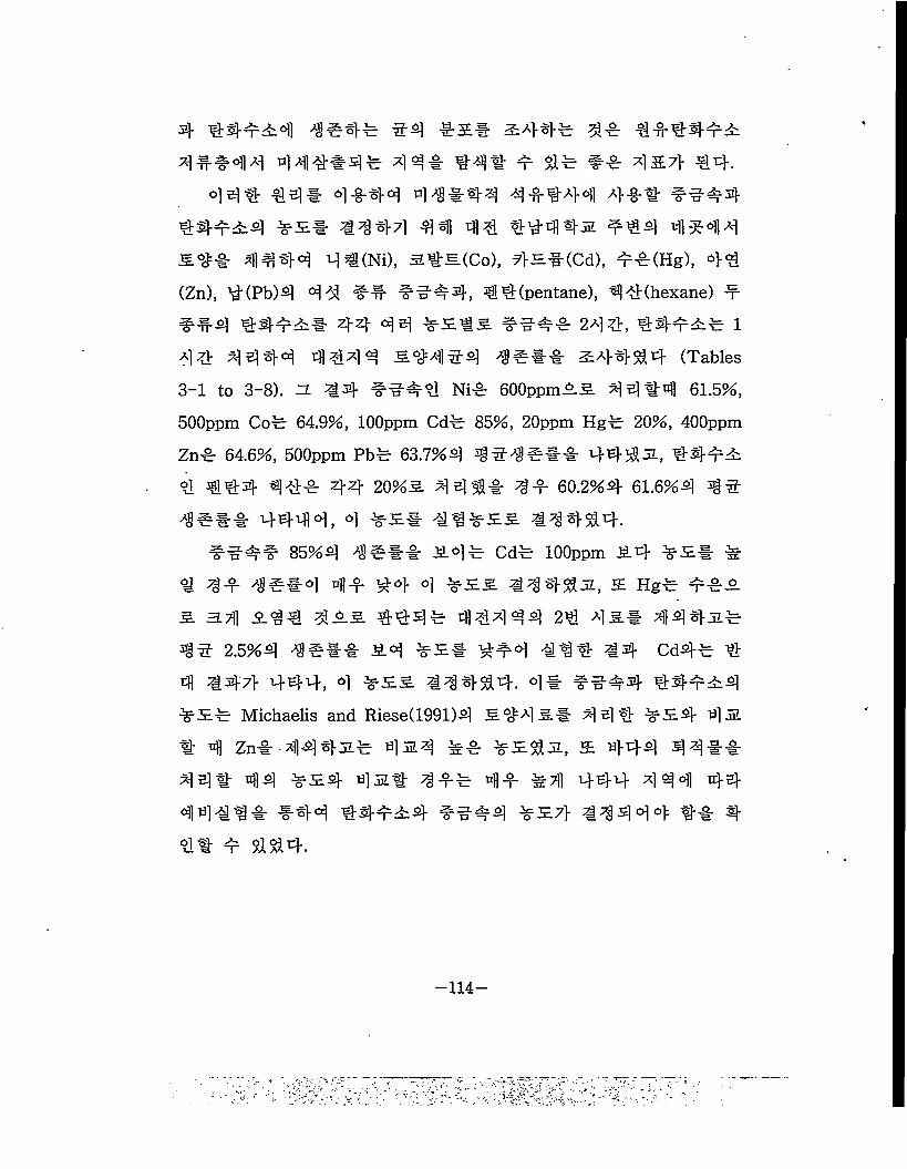
2}- 44## 4 € #4# # -^-1 1.5E.1 #44# # 1 €1441# €1144 44#14# € €1 4€1 # 4# #1 €&7} €4.
4 €4 €211- €-§-44 4€#4€ €4€44 411 #^-44
44##4 €€471 €41 44 44445 #4€ €1€4
all €€44 4€(Ni), a#5(Co), 45.#(Cd), #l(Hg), 4-4
(Zn), 4(Pb)€ 44 #1 ##44, 4 4 (pentane), 4 4 (hexane) 1
##€ 44##1 44 4 4 #5#5 ##44 244, 44### 1
44 42144 444 4 s#4#€ €#11 #44^4 (Tables
3-1 to 3-8). a €4 ##44 Nil 600ppm55 4 4 €4 61.5%,
500ppm Co# 64.9%, lOOppm Cd# 85%, 20ppm Hg# 20%, 400ppm
Zn# 64.6%, 500ppm Pb# 63.7%€ €####4 44535, 444#
4 €44 €44 44 20%5 €414 €4 60.2%4 61.6%€ €#
€#11 4444, 4 #5.1- €€#55. €€444.
##4# 85%€ €#11 #4# Cd# lOOppm 54 #5* #
4 €4 €#14 €4 #4 4 #55. €€445, a Hg# 4155 a.€ 544 €55 444# €€€ 4€ 24 45# €€€-5# €# 2.5%€ €#11 54 #5# 444 141 €4 Cd4# 4 € #47} 444, 4 #55 €€4534. 41 ##44 44##€ #5# Michaelis and Riese(1991)€ 54451 4 €4 #54 45 1 4 Znl €445# 45€ #1 #5535, a 444 4411 4214 €€ #54 45# €4# €1 #4 444 €44 44 441€1 144 44##4 ##14 #57} #€4 4 4 "tl 4 €1 1 4^4.
-114-
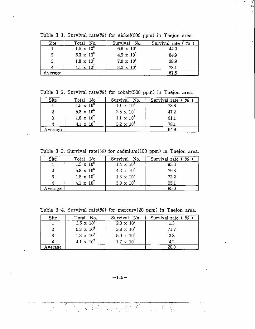
Table 3-1. Survival rate(%) for nickel(600 ppm) in Taejon area.
Site Total No. Survival No. Survival rate ( % )1 1.5 x 10* 6.6 x 107 44.02 5.3 x 10⁶ 4.5 x 10⁶ 84.93 1.8 x 10⁷ 7.0 x 10⁶ 38.94 4.1 x 10⁷ 3.2 x 10⁷ 78.1
Average 61.5
Table 3-2. Survival rate(%) for cobalt(500 ppm) in Taejon area.
Site Total No. Survival No. Survival rate ( % )1 1.5 x 10* 1.1 x 10* 73.32 5.3 x 10* 2.5 x 10* 47.23 1.8 x 10⁷ 1.1 x 10⁷ 61.14 4.1 x 10⁷ 3.2 x 10⁷ 78.1
Average 64.9
Table 3-3. Survival rate(%) for cadmium(100 ppm) in Taejon area.
Site Total No. Survival No. Survival rate ( % )1 1.5 x 10* 1.4 x 10* 93.32 5.3 x 10* 4.2 x 10* 79.33 1.8 x 10⁷ 1.3 x 10⁷ 72.24 4.1 x 10⁷ 3.9 x 10⁷ 95.1
Average - 85.0
Table 3-4. Survival rate(%) for mercury(20 ppm) in Taejon area.
Site Total No. Survival No. Survival rate ( % )1 1.5 x 10* 2.0 x 10* 1.32 5.3 x 10* 3.8 x 10* 71.73 1.8 x 10⁷ 5.0 x 10* 2.84 4.1 x 10⁷ 1.7 x 10* 4.2
Average 20.0
-115-
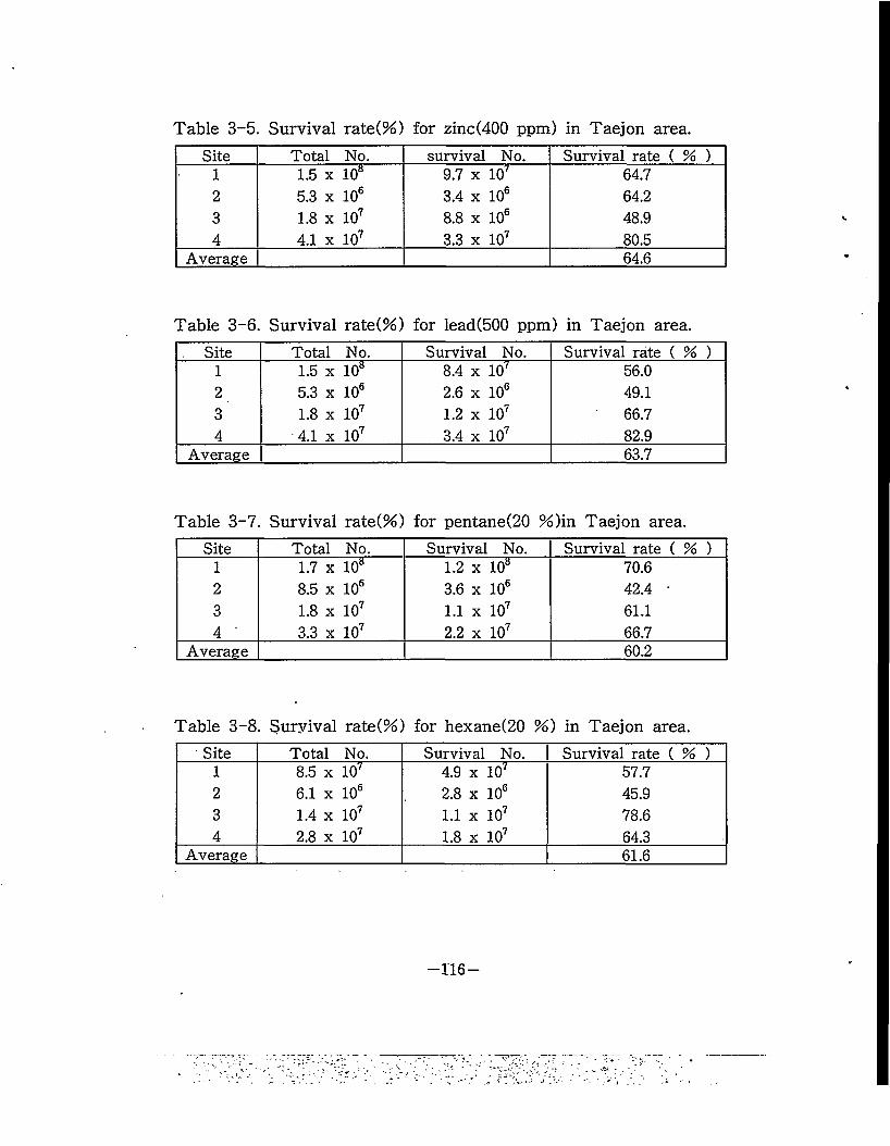
Table 3-5. Survival rate(%) for zinc(400 ppm) in Taejon area.
Site Total No. survival No. Survival rate ( % )1 1.5 x 10* 9.7 x 107 64.72 5.3 x 10⁶ 3.4 x 10⁶ 64.23 1.8 x 10⁷ 8.8 x 10s 48.94 4.1 x 10⁷ 3.3 x 10⁷ 80.5
Average 64.6
Table 3-6. Survival rate(%) for lead(500 ppm) in Taejon area.
Site Total No. Survival No. Survival rate ( % )1 1.5 x 10* 8.4 x 10Y 56.02 5.3 x 10⁶ 2.6 x 10⁶ 49.13 1.8 x 10⁷ 1.2 x 10⁷ 66.74 4.1 x 10⁷ 3.4 x 10⁷ 82.9
Average 63.7
Table 3-7. Survival rate(%) for pentane(20 %)in Taejon area.
Site Total No. Survival No. Survival rate ( % )1 1.7 x 10* 1.2 x 10* 70.62 8.5 x 10⁶ 3.6 x 10⁶ 42.4 •3 1.8 x 10⁷ 1.1 x 10⁷ 61.14 3.3 x 10⁷ 2.2 x 10⁷ 66.7
Average 60.2
Table 3-8. Survival rate(%) for hexane(20 %) in Taejon area.
Site Total No. Survival No. Survival rate ( % )1 8.5 x 10Y 4.9 x 10Y 57.72 6.1 x 10s 2.8 x 10⁶ 45.93 1.4 x 10⁷ 1.1 x 10⁷ 78.64 2.8 x 10⁷ 1.8 x 10⁷ 64.3
Average 61.6
-116-
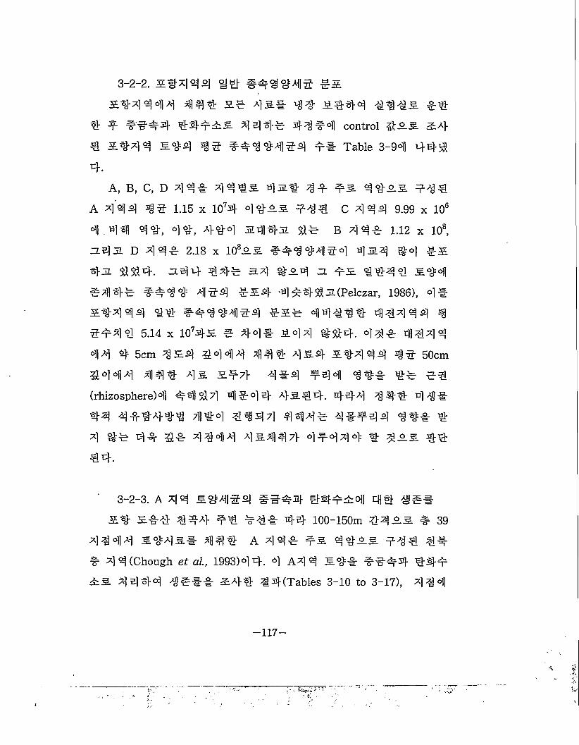
3-2-2. 94444 gy.
944444 44# s# 4 s# #4 s#44 ###3 ##
# -f- ###4 ###33 4 4##• 44 #4 control ^93 34-
# 9#4 4 5-44 3g# ##4 4=71)$^ 4# Table 3-94 44-1&
4.A, B, C.D^I 4 4 #3 4 Hi; #3 4 %>-A3 94€
A 4 44 45 1.15 x 1074 °1#93 C 4 44 9-99 x 106
4.441 4 4, 44, 444 h44-31 B 444 1.12 x 10⁸,
3#jl d 4 44 2.18 x 10893 #444454 4h4 ^4 1-9
43i 444- 3.44 444 =14 #94 3 #9 444 4 £°<M
4444 ##4 4 454 494 4###31(Pelczar, 1986), 4#
94444 44 ##444)54 494 44444 444 4 4 4 5#4# 5.14 x 1074-9 e #4* 944 ##4. 444 444 4 44 4= 5cm 494 44 44 444 4s.4- 94444 45 50cm
44 44 44 4 4s s#4 4#4 944 4## ## e#(rhizosphere)4 #41 $14 4#d14- 4-S44. 444 444 4 4# 44 4##4-M 71) #4 4^14 4 4 414# 4 #94 4 4## # 4 ## 4# 5# 44 44 4s*fl47> 49444 # 4S3 44 €4.
3-2-3. A 4 4 3 #4 5 4 #### 4##9ol| mil ^##
94 3## 4#4 #4 #4# 44 100-150m 4493 # 39
4444 S44S-E 44# A 4 4# #s 4 493 944 4# # 4 4 (Chough e! a/., 1993)44. 4 A4 4 s## ###4 44#
93 4 444 4### 94# #4(Tables 3-10 to 3-17), 444
-'■ V
-117-
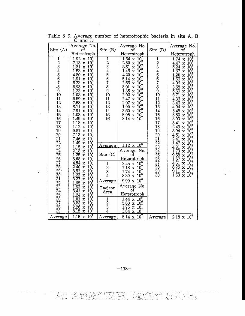
Table 3-9. Average number of heterotrophic bacteria in site A, B, C and D
Site (A)Average No
ofHeterotroph
1 1.92 X 10² 7.13 X 10®3 1.31 X 10%4 1.53 X 10%5 4.80 X 10%6 1.91 X 10%7 5.23 X 10®8 5.93 X 10®9 1.23 X 10%10 1.08 X 10%11 5.59 X 10®12 7.58 X 10®13 8.11 X 10®14 7.91 X 10®15 1.08 X 10%16 1.49 X 10%17 1.18 X 10%18 1.12 X 10%
. 19 9.81 X 10®20 7.13 X 10®21 7.46 X 10®22 1.49 X 10%23 1.15 X 10%2'4 2.18 X 10®25 1.25 X 10%26 3.68 X 10®27 4.54 X 10®28 2.40 X 10®29- 3.53 X 10®30 1.23 X 10%31 3.27 X 10%32 1.65 X 10%33 1.53 X 10%34 3.41 X 10®35 1.24 X 10%36 1.01 X 10%37 3.23 X 10®38 2.26 X 10%39 ‘ 8.15 X 10®
Average 1.15 X 10⁷
Site (B)Average No.
ofHeterotroph
Site (D)
1 1.54 x 10% 12 2.80 x 10® 23 8.51 x 10% 34 1.48 x 10® 45 4.20 x 10% 56 5.14 x 10% 6
■ 7 2.65 x 10% 78 8.01 x 10% 89 1.35 x 10® 910 2.02 x 10® 1011 2.47 x 10% 1112 2.07 x 10% 1213 1.99 x 10® 1314 3.50 x 10® 1415 5.05 x 10% 1516 8.14 x 10⁷ 16
1718192021222324
Average 1.12 x 10*
Site (C)Average No.
of 25Heterotroph 26
1 2.45 x 10% 272 1.18 x 10% 283 1.74 x 10% 294 8.30 x 10® 30
Average 9.99 x 10®Taejeon Average No.
ofHeterotrophArea
1 1.44 x 10®2 5.80 x 10%3 1.75 x 10%4 3.84 x 10⁷
Average 5.14 x 10⁷ Average
Average No. of
Heterotroph1.74 X lo:4.47 X 10,5.24 X io!1.67 X 10,1.20 X 101.55 X 104.06 X 103.68 X 105.69 X 10,6.71 X 10,4.36 X 10:3.46 X 10,4.94 X 103.43 X 103.59 X 103.09 X 103.41 X 102.43 X 103.04 X 10:4.51 X 10,2.41 X 101.47 X 104.91 X 101.73 X 10:9.58 X 10,1.67 X 104.61 X 108.25 X io:9.11 X 10,1.53 X 10*
2.18 x 10s
—118—
Table 3-10. Survival rate for nickel(600 ppm) in site A
Site TotalNo.
SurvNo.
Survivalrate(%) Site Total No. Survival
No.Survivalrate(%)
1 1.5 X 10 8.0 X 10® 53.3 21 8.3 X Tof 6.9 X 10® 83.12 3.7 X io! 6.7 X 10® >100.0 22 8.6 X 10® 5.0 X 10® 58.13 1.0 X 10? 1.3 X 10? >100.0 23 1.3 X 10" 1.2 X 10" 92.34 2.4 X io? 2.8 X 10 >100.0 24 1.8 X 10® 1.9 X 10® >100.05 2.2 X 10? 6.0 X 10® 27.3 25 8.5 X 10® 6.4 X 10® 75.36 1.1 X 10® 8.0 X 10® 72.7 26 8.0 X 10® 1.7 X 10® >100.07 3.3 X 10® 6.2 X 10® >100.0 27 4.5 X 10® 4.2 X 10® 93.38 5.2 X 10® ND „ ND 28 3.0 X 10® 2.5 X 10® 83.39 2.2 X 10® 3.8 X 10° >100.0 29 4.0 X 10® 3.0 X 10® 75.010 1.3 X 10® 1.1 X 10® 84.6 30 1.1 X 10" 9.5 X 10® 86.411 4.5 X 10® 4.4 X 10® 97.8 31 9.5 X 10® 7.7 X 10® 8.112 1.4 X 10? 7.0 X 10® 50.0 32 2.0 X 10" 1.1 X 10" 55.013 1.0 X 10" 8.7 X 10® 87.0 33 1.2 X 10" 7.0 X 10® 58.314 8.2 X 10® 8.0 X 10® 97.6 34 5.3 X 10® 5.0 X 10® 94.315 1.2 X 10? 4.3 X 10® 35.8 35 1.1 X 10" 1.0 X 10" 90.916 1.2 X 10" 5.7 X 10® 47.5 36 1.7 X 10? 6.0 X 10® 35.317 9.0 X 10® 3.0 X 10® 33.3 37 4.0 X 10® 1.0 X 10® 25.018 1.5 X 10? 1.3 X 10" 86.7 38 3.3 X 10" 3.1 X 10" 93.919 1.2 X 10? 8.2 X 10® 68.3 39 1.0 X 10" 7.6 X 10® 76.020 9.9 X 10® 7.5 X 10® 75.8
Average 73.7ND : not detected
Table 3-11. Survival rate for cobalt(500 ppm) in site ASite Total
No.Survival
No.Survivalrate(%) Site Total No. Survival
No.Survivalrate(%)
1 6.5 X 10' 8.0 X 10® 12.3 21 2.0 X 10° 1.4 X 10° 70.02 3.3 X 10 2.4 X 10® 72.7 22 6.2 X 10? 6.3 X 10? >100.03 1.3 X 10" 1.3 X 10" 100.0 23 1.3 X 10" 1.2 X 10" 92.34 1.7 X 10" 1.6 X 10? 94.1 24 2.0 X 10® 1.0 X 10® 50.05 4.8 X 10? 7.0 X 10? >100.0 25 1.3 X 10® 5.0 X 10® 38.56 2.6 X 10" 1.7 X 10" 65.4 26 3.3 X 10® ND . ND7 4.1 X 10® 4.0 X 10® 97.6 27 8.0 X 10® 6.0 X 10® 75.08 9.0 X 10® 7.0 X 10? >100.0 28 1.1 X 10® 3.0 X 10" 27.39 1.4 X 10" 6.0 X 10® 42.9 29 2.0 X 10" 2.0 X 10" 100.010 5.0 X 10® 1.7 X 10" >100.0 30 2.8 X 10? 2.6 X 10" 92.911 2.9 X 10® 2.5 X 10® 86.2 31 1.1 X 1.0? 1.2 X 10" 100.012 2.3 X 10® 2.7 X 10® >100.0 32 1.2 X 10" 1.1 X 10" 91.713 6.2 X 10® 6.2 X 10 100.0 33 8.5 X 10® 5.5 X 10® 64.714 9.8 X 10® 8.8 X 10® 89.8 34 8.0 X 10" 9.0 X 10" >100.015 4.9 X 10® 5.0 X 10® >100.0 35 7.0 X 10® 6.8 X 10 97.116 4.7 X 10® 5.0 X 10® >100.0 36 5.3 X 10® 5.5 X 10® >100.017 5.4 X 10® 4.8 X 10® 88.9 37 6.0 X 10" 2.9 X 10® >100.018 9.5 X 10® 8.6 X 10® 90.5 38 2.1 X 10® 1.8 X 10® 85.719 6.3 X 10® 3.9 X 10® 61.9 39 2.2 X 10® 1.4 X 10® 63.620 2.8 X 10® 2.5 X 10® 89.3
Average 82.6ND : not detected
—119 —
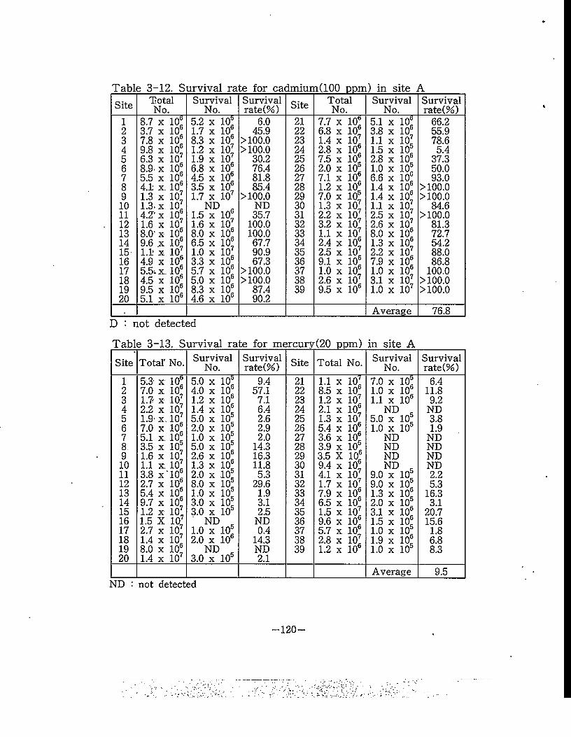
Table 3-12. Survival rate for cadmium(100 ppm) in site A
Site TotalNo.
SurvivalNo.
Survivalrate(%) Site Total
No.Survival
No.Survivalrate(%)
1 8.7 X 10° 5.2 X 10% 6.0 21 7.7 X 10® 5.1 X 10® 66.22 3.7 X 10® 1.7 X 10® 45.9 22 6.8 X 10® 3.8 X 10® 55.93 7.8 X 10® 8.3 X 10® >100.0 23 1.4 X 10% 1.1 X 10% 78.64 9.8 X 10® 1.2 X 10% >100.0 24 2.8 X 10® 1.5 X 10® 5.45 6.3 X io% 1.9 X 10% 30.2 25 7.5 X 10 2.8 X 10® 37.36 8.9- X 10® 6.8 X 10® 76.4 26 2.0 X 10® 1.0 X 10® 50.07 5.5 X 10® 4.5 X 10® 81.8 27 7.1 X 10® 6.6 X 10® 93.08 4.1 X. 10® 3.5 X 10 85.4 28 1.2 X 10 1.4 X 10® >100.09 1.3 X 10% 1.7 X 10⁷ >100.0 29 7.0 X 10® 1.4 X 10® >100.010 1.3- X 10% ND „ ND 30 1.3 X 10% 1.1 X 10% 84.611 4.2- X 10® 1.5 X 10: 35.7 31 2.2 X 10% 2.5 X 10% >100.012 1.6 X 10% 1.6 X 10% 100.0 32 3.2 X 10% 2.6 X 10% 81.313 8.0’ X 10® 8.0 X 10® 100.0 33 1.1 X 10% 8.0 X 10® 72.714 9.6 X 10® 6.5 X 10® 67.7 34 2.4 X 10® 1.3 X 10® 54.215 1.1 X 10% 1.0 X 10% 90.9 35 2.5 X 10% 2.2 X 10% 88.016 4.9 X 10® 3.3 X 10® 67.3 36 9.1 X 10® 7.9 X 10® 86.817 5.5i X. 10® 5.7 X 10® >100.0 37 1.0 X 10® 1.0 X 10® 100.018 4.5 X 10® 5.0 X 10® >100.0 38 2.6 X 10% 3.1 X 10% >100.019 9.5 X 10® 8.3 X 10® 87.4 39 9.5 X 10® 1.0 X 10⁷ >100.020 5.1 X 10® 4.6 X 10® 90.2
Average 76.8D : not detected
Table 3-13. Survival rate for mercury(20 ppm) in site A
Site Total' No. SurvivalNo.
Survivalrate(%) Site Total No. Survival
No.Survivalrate(%)
1 5.3- X To!" 5.0 X 10® 9.4 21 1.1 X 10% 7.0 X 10® 6.42 7.0 X 10 4.0 X 10® 57.1 22 8.5 X 10® 1.0 X 10® 11.83 1.7 X 10% 1.2 X 10® 7.1 23 1.2 X 10% 1.1 X 10® 9.24 2.2 X 10% 1.4 X 10 6.4 24 2.1 X 10% ND „ ND5 1.9- X. 10% 5.0 X 10® 2.6 25 1.3 X 10% 5.0 X 10: 3.86 7.0 X 10® 2.0 X 10 2.9 26 5.4 X 10® 1.0 X 10® 1.97 5.1 X. 10% 1.0 X 10 2.0 27 3.6 X 10® ND ND8 3.5 X 10 5.0 X 10® 14.3 28 3.9 X 10® ND ND9 1.6 X 10% 2.6 X 10® 16.3 29 3.5 X 10® ND ND10 1.1 XL 10% 1.3 X 10 11.8 30 9.4 X 10® ND „ ND11 3.8 X 10® 2.0 X 10® 5.3 31 4.1 X 10% 9.0 X io: 2.212 2.7 X 10® 8.0 X 10 29.6 32 1.7 X 10% 9.0 X 10® 5.313 5.4 X 10® 1.0 X 10 1.9 33 7.9 X 10® 1.3 X 10 16.314 9.7 X 10® 3.0 X 10® 3.1 34 6.5 X 10® 2.0 X 10® 3.115 1.2 X 10% 3.0 X 10® 2.5 35 1.5 X 10% 3.1 X 10® 20.716 1.5 X 10% ND „ ND 36 9.6 X 10® 1.5 X 10 15.617 2.7 X 10% 1.0 X io: 0.4 37 5.7 X 10® 1.0 X 10® 1.818 1.4 X 10% 2.0 X 10® 14.3 38 2.8 X 10% 1.9 X 10® 6.819 8.0 X 10® ND _ ND 39 1.2 X 10® 1.0 X 10® 8.320 1.4 X 10⁷ oC
O X 10° 2.1Average 9.5
ND : not detected
—120—
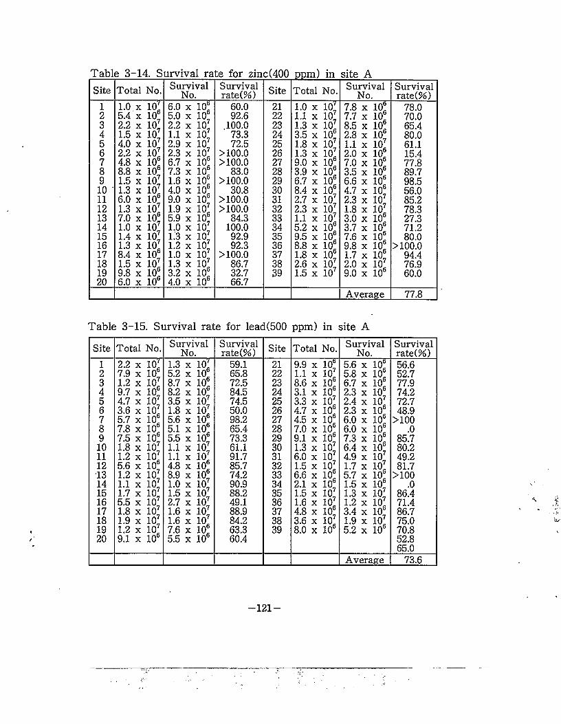
Table 3-14. Survival rate for zinc(400 ppm) in site A
Site Total No. SurvivalNo.
Survivalrate(%) Site Total No. Survival
No.Survivalrate(%)
1 1.0 x 10: 6.0 X 10® 60.0 21 1.0 X 10' 7.8 X 10® 78.02 5.4 X 10® 5.0 X 10® 92.6 22 1.1 X io! 7.7 X 10® 70.03 2.2 X ioI 2.2 X iol ,100.0 23 1.3 X io! 8.5 X 10® 65.44 1.5 X 10l 1.1 X iol 73.3 24 3.5 X 10® 2.8 X 10® 80.05 4.0 X io! 2.9 X io7 72.5 25 1.8 X iol 1.1 X 10⁷ 61.16 2.2 X 101 2.3 X 10⁶ >100.0 26 1.3 X 10⁷ 2.0 X 10® 15.47 4.8 X 10® 6.7 X 10® >100.0 27 9.0 X 10® 7.0 X 10® 77.88 8.8 X 10® 7.3 X 10® 83.0 28 3.9 X 10® 3.5 X 10® 89.79 1.5 X iol 1.6 X 10® >100.0 29 6.7 X 10® 6.6 X 10® 98.510 ' 1.3 X io! 4.0 X 10® 30.8 30 8.4 X 10® 4.7 X 10® 56.011 6.0 X 10® 9.0 X 10® >100.0 31 2.7 X 10 2.3 X 10 85.212 1.3 X io! 1.9 X 10⁷ >100.0 32 2.3 X io7 1.8 X 10⁷ 78.313 7.0 X 10 5.9 X 10 84.3 33 1.1 X 10⁷ 3.0 X 10® 27.314 1.0 X io7 1.0 X 10 100.0 34 5.2 X 10® 3.7 X 10® 71.215 1.4 X 10⁷ 1.3 X IO! 92.9 35 9.5 X 10® 7.6 X 10® 80.016 1.3 X 10⁶ 1.2 X iol 92.3 36 8.8 X 10® 9.8 X 10® >100.017 8.4 X 10® 1.0 X 10⁷ >100.0 37 1.8 X 10® 1.7 X 10® 94.418 1.5 X io! 1.3 X io! 86.7 38 2.6 X 10⁷ 2.0 X 10⁷ 76.919 9.8 X 10® 3.2 X 10® 32.7 39 1.5 X 10⁷ 9.0 X 10® 60.020 6.0 X 10® 4.0 X 10® 66.7
Average 77.8
Table 3-15. Survival rate for lead(500 ppm) in site A
Site Total No. SurvivalNo.
Survivalrate(%) Site Total No. Survival
No.Survivalrate(%)
1 2.2 X "To!" 1.3 X 10' 59.1 21 9.9 X 10® 5.6 X 10® 56.62 7.9 X 10® 5.2 X 10® 65.8 22 1.1 X 10⁷ 5.8 X 10® 52.73 1.2 X 10⁷ 8.7 X 10® 72.5 23 8.6 X 10® 6.7 X 10® 77.94 9.7 X 10® 8.2 X 10® 84.5 24 3.1 X 10® 2.3 X 10® 74.25 4.7 X 10⁷ 3.5 X io! 74.5 25 3.3 X 10⁷ 2.4 X io7 72.76 3.6 X io! 1.8 X io! 50.0 26 4.7 X 10® 2.3 X 10® 48.97 5.7 X 10® 5.6 X 10® 98.2 27 4.5 X 10® 6.0 X 10® >1008 7.8 X 10® 5.1 X 10® 65.4 28 7.0 X 10® 6.0 X 10® .09 7.5 X 10® 5.5 X 10® 73.3 29 9.1 X 10® 7.3 X 10® 85.710 1.8 X 10⁷ 1.1 X io7 61.1 30 1.3 X 10⁷ 6.4 X 10® 80.211 1.2 X 10⁷ 1.1 X io! 91.7 31 6.0 X io! 4.9 X io! 49.212 5.6 X 10® 4.8 X 10® 85.7 32 1.5 X io7 1.7 X io7 81.713 1.2 X io! 8.9 X 10® 74.2 33 6.6 X 10® 5.7 X 10® >10014 1.1 X 10⁷ 1.0 X io7 90.9 34 2.1 X 10® 1.5 X 10® .015 1.7 X io! 1.5 X 10⁷ 88.2 35 1.5 X io! 1.3 X io7 86.416 5.5 X 10⁷ 2.7 X 10⁷ 49.1 36 1.6 X io7 1.2 X io7 71.417 1.8 X io7 1.6 X io! 88.9 37 4.8 X 10® 3.4 X 10® 86.718 1.9 X io! 1.6 X io! 84.2 38 3.6 X io! 1.9 X io7 75.019 1.2 X 10 7.6 X 10® 63.3 39 8.0 X 10® 5.2 X 10® 70.820 9.1 X 10® 5.5 X 10® 60.4 52.8
65.0Average 73.6
121-
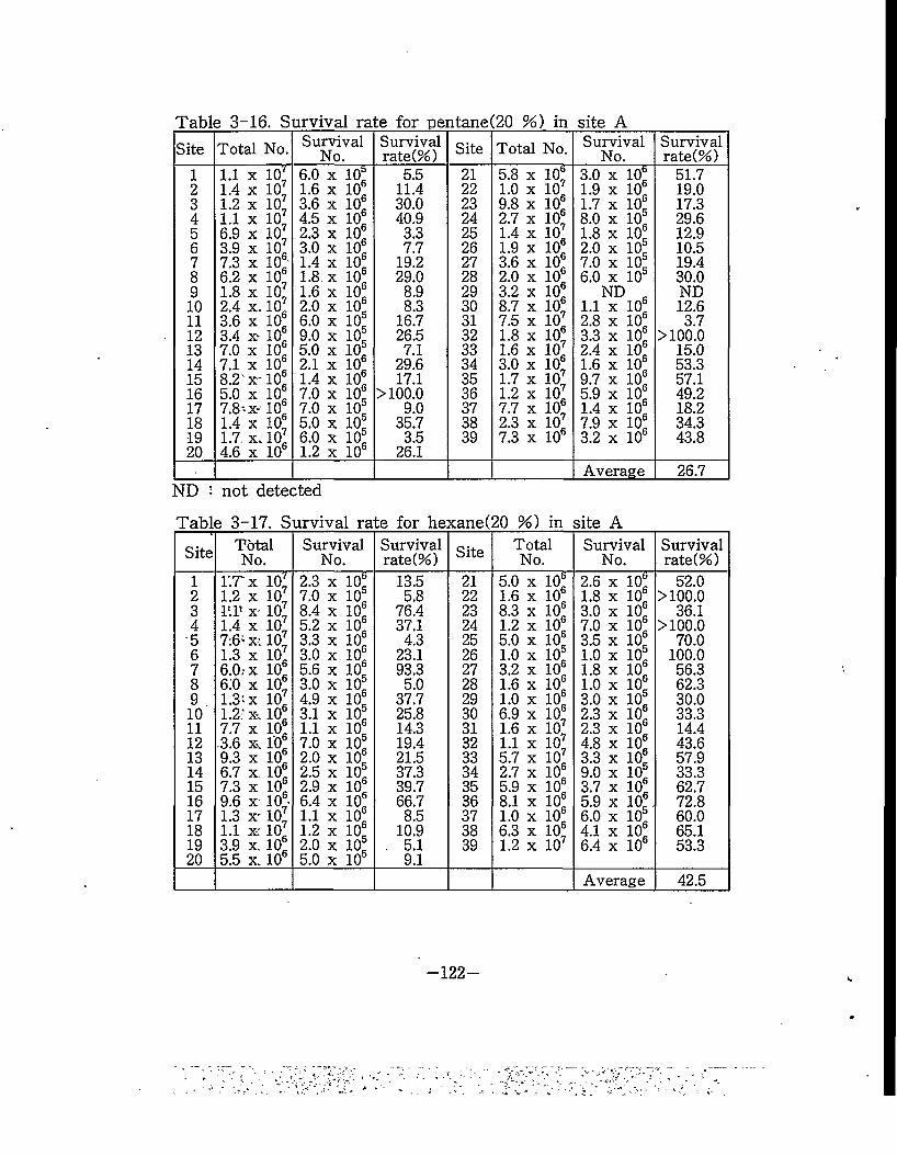
Table 3-16. Survival rate for pentane(20 %) in site A
Site Total No. SurvivalNo.
Survivalrate(%) Site Total No. Survival
No.Survivalrate(%)
1 1.1 X 10% 6.0 X 10! 5.5 21 5.8 X "ToT 3.0 X 10! 51.72 1.4 X 10% 1.6 X 10® 11.4 22 1.0 X 10% 1.9 X 10® 19.03 1.2 X 10% 3.6 X 10® 30.0 23 9.8 X 10® 1.7 X 10 17.34 1.1 X 10% 4.5 X 10® 40.9 24 2.7 X 10® 8.0 X 10® 29.65 6.9 X 10% 2.3 X 10® 3.3 25 1.4 X 10% 1.8 X 10 12.96 3.9 X 10% 3.0 X 10® 7.7 26 1.9 X 10® 2.0 X 10% 10.57 7.3 X 10® 1.4 X 10® 19.2 27 3.6 X 10® 7.0 X 10% 19.48 6.2 X 10® 1.8 X 10® 29.0 28 2.0 X 10® 6.0 X 10® 30.09 1.8 X 10% 1.6 X 10® 8.9 29 3.2 X 10® ND „ ND10 2.4 X. 10% 2.0 X 10® 8.3 30 8.7 X 10® 1.1 X 10! 12.611 3.6 X 10® 6.0 X 10® 16.7 31 7.5 X 10% 2.8 X 10% 3.712 3.4 X' 10® 9.0 X 10 26.5 32 1.8 X 10® 3.3 X 10% >100.013 7.0 X 10® 5.0 X 10® 7.1 33 1.6 X 10% 2.4 X 10% 15.014 7.1 X 10® 2.1 X 10® 29.6 34 3.0 X 10® 1.6 X 10% 53.315 8.2' X 10® 1.4 X 10® 17.1 35 1.7 X 10% 9.7 X 10% 57.116 5.0 X 10® 7.0 X 10% >100.0 36 1.2 X 10% 5.9 X 10% 49.217 7.8- X- 10® 7.0 X 10® 9.0 37 7.7 X 10® 1.4 X 10% 18.218 1.4 X 10® 5.0 X 10® 35.7 38 2.3 X 10% 7.9 X 10% 34.319 1.7 X. 10% 6.0 X 10® 3.5 39 7.3 X 10® 3.2 X 10® 43.820 4.6 X 10® 1.2 X 10® 26.1
Average 26.7SID : not detected
Table 3-17. Survival rate for hexane(20 %) in site A
Site TotalNo.
SurvivalNo.
Survivalrate(%) Site Total
No.Survival
No.Survivalrate(%)
1 ITT x 10% 2.3 x 10% 13.5 21 5.0 x 10% 2.6 x 10% 52.02 1.2 x 10% 7.0 x 10% 5.8 22 1.6 x 10% 1.8 x 10% >100.03 V.V x 10% 8.4 x 10% 76.4 23 8.3 x 10% 3.0 x 10% 36.14 1.4 x 10% 5.2 x 10% 37.1 24 1.2 x 10% 7.0 x 10% >100.05 7:6- x: 10% 3.3 x 10% 4.3 25 5.0 x 10% 3.5 x 10% 70.06 1.3 x 10% 3.0 x 10% 23.1 26 1.0 x 10% 1.0 x 10% 100.07 6.0; x 10% 5.6 x 10% 93.3 27 3.2 x 10% 1.8 x 10% 56.38 6:0 x 10® 3.0 x 10% 5.0 28 1.6 x 10% 1.0 x 10% 62.39 . 1.3- x 10% 4.9 x 10% 37.7 29 1.0 x 10% 3.0 x 10% 30.010 1.2' x, 10% 3.1 x 10% 25.8 30 6.9 x 10® 2.3 x 10% 33.311 7.7 x 10% 1.1 x 10% 14.3 31 1.6 x 10% 2.3 x 10% 14.412 3.6 xx 10% 7.0 x 10% 19.4 32 1.1 x io! 4.8 x 10% 43.613 9.3 x 10% 2.0 x 10% 21.5 33 5.7 x 10% 3.3 x 10% 57.914 6.7 x. 10% 2.5 x 10% 37.3 34 2.7 x 10% 9.0 x 10% 33.315 7.3 x 10% 2.9 x 10% 39.7 35 5.9 x 10% 3.7 x 10% 62.716 9.6 x 10®. 6.4 x 10% 66.7 36 8.1 x 10% 5.9 x 10%, 72.817 1.3 x- 10% 1.1 x 10% 8.5 37 1.0 x 10% 6.0 x 10% 60.018 1.1 x: 10% 1.2 x 10% 10.9 38 6.3 x 10® 4.1 x 10% 65.11920
3.9 x. 10% 5.5 x. 10®
2.0 x 10%5.0 x 10®
. 5.19.1
39 1.2 x 10⁷ 6.4 x 10® 53.3
Average 42.5
-122-
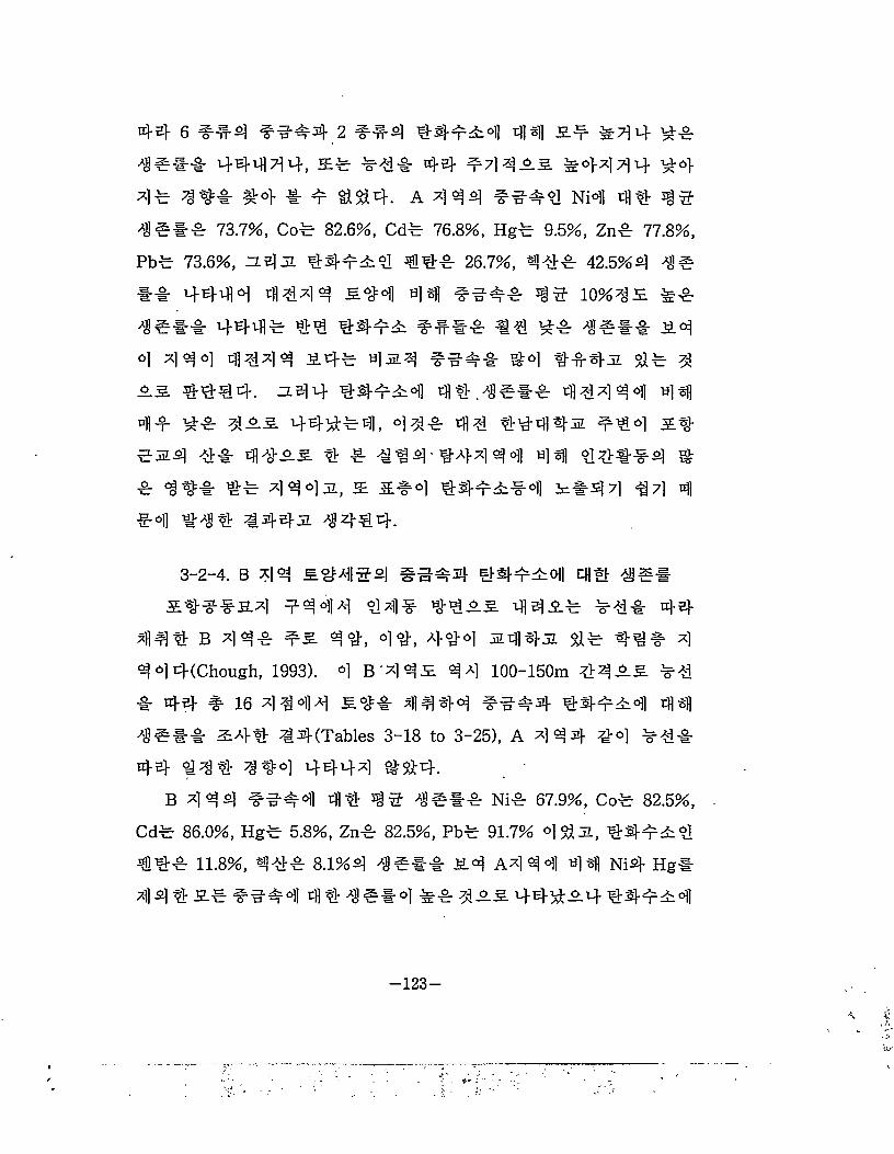
44 6 9*4 9*4 #4934] tflsfl 2.5 4595#* 44444, £5 5#* 44 94 4 35. #44 4 4 4"445 4 4* #4 # 9 &$4. A 444 9994 NH 44 99 95*5 73.7%, Co5 82.6%, Cd5 76.8%, Hg5 9.5%, Zn* 77.8%, Pb5 73.6%, 3.431 #4934 ##5 26.7%, 444 42.5%4 95 #4 4444 444 4 £44 44 9995 99 10%4£ 55 95** 4445 44 #493 9**5 14 45 95** £4 4 4 4 4 444 4 £45 4^4 999* Sr4 #443 44 4 £5. 4444. 3a14 Mt^°1 4# .95*5 44444 441
44 45 435. 44#54, 4 44 44 *44*3 944 5# 93* *& 4*35. * 4 444'444 4 4 44] 4**54 # 4 9#* 4# 4 4 4 3, £ Z*4 #493*4 3#4 4 #445-4 #1# 44-4-3 9##4.
3-2-4. B 44 £44154 #594 #493011 41# *5#£#55s4 9-4 44 445- #435. 4435 54* 44
44# B 4 45 95. 4#, 4#, 4#4 34#3 4* #1# 4 4 4 4(Chough, 1993). 4 B '4 43 44 100-150m #435. *4 * 44- 5 16 4 4 44 £5* 4444 5954 #4934 441 49#* 34# 44(Tables 3-18 to 3-25), A 444 #4 54* 44 44# 9 44 4444 ##4.
B 4 44 9994 4# 99 95*5 Ni5 67.9%, Co5 82.5%, Cd5 86.0%, Hg5 5.8%, Zn5 82.5%, Pb5 91.7% 4^3, #4934 #45 11.8%, 9*5 8.1%4 95** £4 A4 4 9 49 Ni4 Hg* 94 #£5 9994 4*95*4 55 435 44*3# ##934
-123-
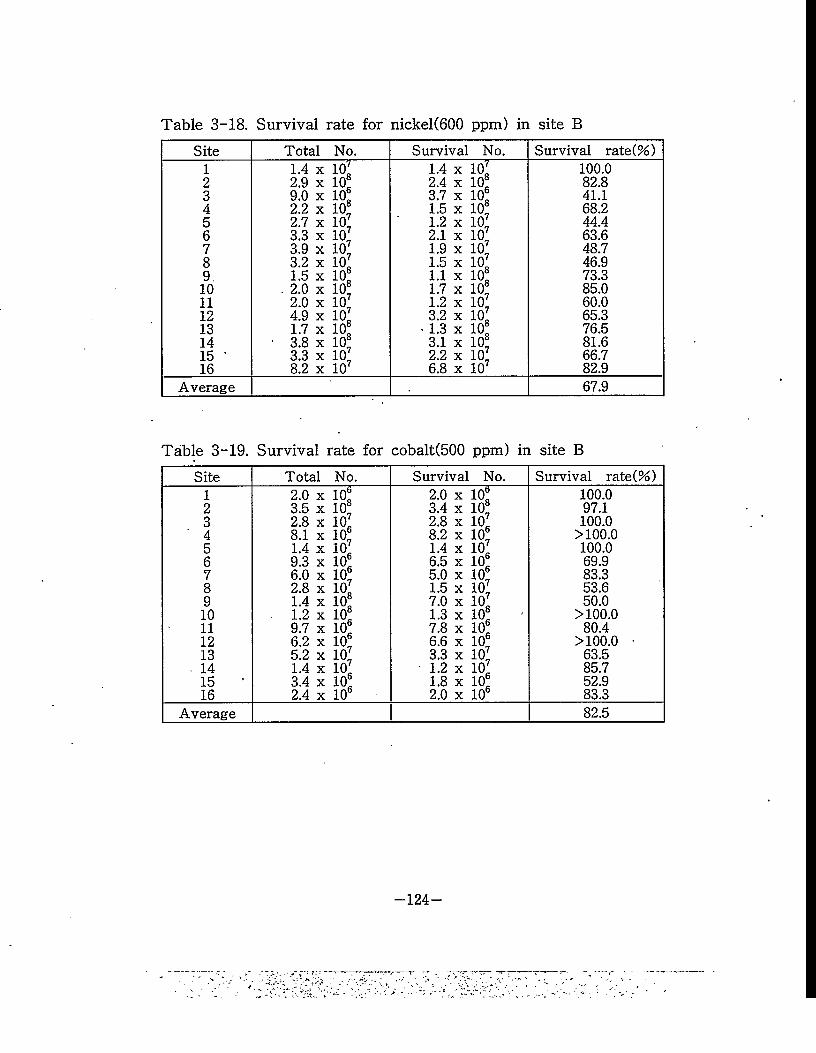
Table 3-18. Survival rate for nickel(600 ppm) in site B
Site Total No. Survival No. Survival rate(%)1 1.4 x 10' 1.4 x 10’ 100.02 2.9 x 10! 2.4 x 10® 82.83 9.0 x 10® 3.7 x 10® 41.14 2.2 x 10® 1.5 x 10® 68.25 2.7 x 10’ 1.2 x 10’ 44.46 3.3 x 10’ 2.1 x 10’ 63.67 3.9 x 10’ 1.9 x 10’ 48.78 3.2 x 10’ 1.5 x 10’ 46.99. 1.5 x 10® 1.1 x 10® 73.310 . 2.0 x 10® 1.7 x 10® 85.011 2.0 x 10’ 1.2 x 10’ 60.012 4.9 x 10’ 3.2 x 10’ 65.313 1.7 x 10® • 1.3 x 10® 76.514 • 3.8 x 10® 3.1 x 10® 81.615 ' 3.3 x 10’ 2.2 x 10’ 66.716 8.2 x 10’ 6.8 x 10’ 82.9
Average 67.9
Table 3-19. Survival rate for cobalt(500 ppm) in site B
Site Total No. Survival No. Survival rate(%)1 2.0 x 10® 2.0 x 10® 100.02 3.5 x 10® 3.4 x 10® 97.13 2.8 x 10’ 2.8 x 10’ 100.04 8.1 x 10® 8.2 x 10® >100.05 1.4 x 10’ 1.4 x 10’ 100.06 9.3 x 10® 6.5 x 10® 69.97 6.0 x 10® 5.0 x 10® 83.38 2.8 x 10’ 1.5 x 10’ 53.69 1.4 x 10® 7.0 x 10’ 50.010 ■ 1.2 x 10® 1.3 x 10® >100.011 9.7 x 10® 7.8 x 10® 80.412 6.2 x 10® 6.6 x 10® >100.0 •13 5.2 x 10’ 3.3 x 10’ 63.5
■ 14 1.4 x 10’ ■ 1.2 x 10’ 85.715 3.4 x 10® 1.8 x 10® 52.916 2.4 x 10® 2.0 x 10® 83.3
Average 82.5
-124-
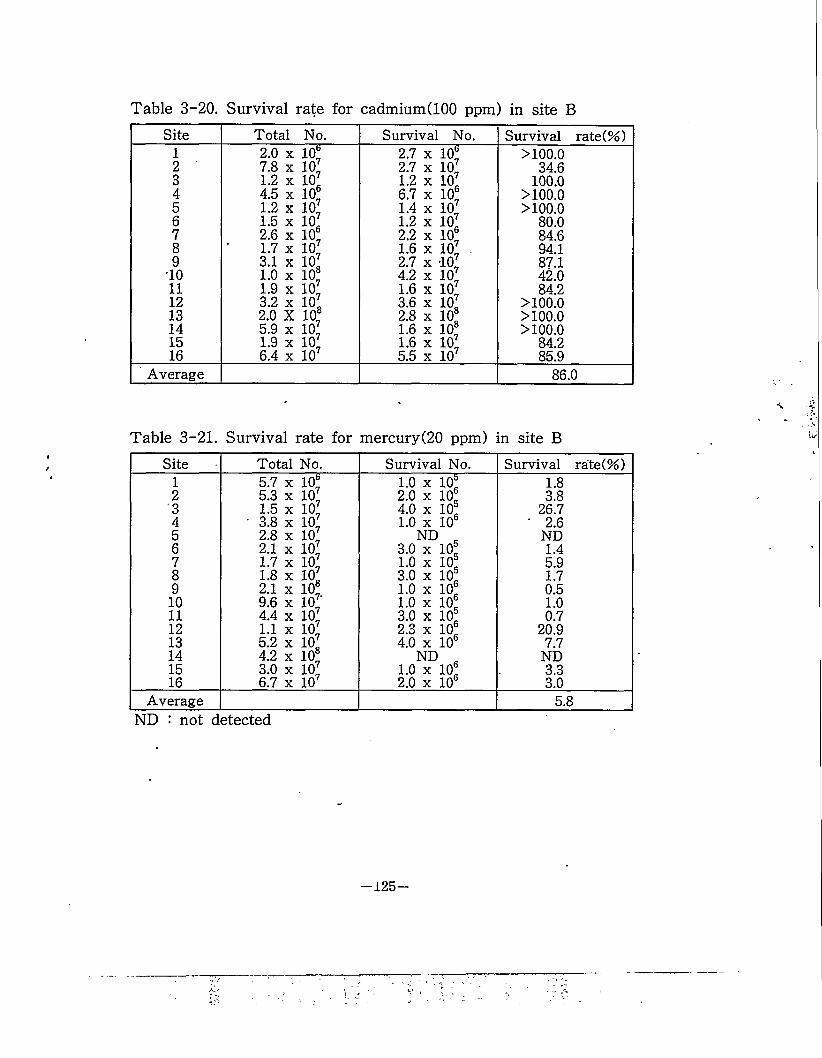
Table 3-20. Survival rate for cadmium(100 ppm) in site B
Site Total No. Survival No. Survival rate(%)1 2.0 x 10“ 2.7 x 10® >100.02 ' 7.8 x 10’ 2.7 x 10’ 34.63 1.2 x 10’ 1.2 x 10’ 100.04 4.5 x 10® 6.7 x 10® >100.05 1.2 x 10’ 1.4 x 10’ >100.06 1.5 x 10’ 1.2 x 10’ 80.07 2.6 x 10® 2.2 x 10® 84.68 1.7 x 10’ 1.6 x 10’ . 94.19 3.1 x 10’ 2.7 x 10’ 87.1
10 1.0 x 10® 4.2 x 10’ 42.011 1.9 x 10’ 1.6 x 10’ 84.212 3.2 x 10’ 3.6 x 10’ >100.013 2.0 X 10® 2.8 x 10® >100.014 5.9 x 10’ 1.6 x 10® >100.015 1.9 x 10’ 1.6 x 10’ 84.216 6.4 x 10’ 5.5 x 10’ 85.9
Average 86.0
Table 3-21. Survival rate for mercury(20 ppm) in site B
Site Total No. Survival No. Survival rate(%)1 5.7 x 10® 1.0 x 10® 1.82 5.3 x 10’ 2.0 x 10® 3.83 1.5 x 10’ 4.0 x 10® 26.74 • 3.8 x 10’ 1.0 x 10® " 2.65 2.8 x 10’ ND c ND6 2.1 x 10’ 3.0 x 10® 1.47 1.7 x 10’ 1.0 x 10® 5.98 1.8 x 10’ 3.0 x 10® 1.79 2.1 x 10® 1.0 x 10® 0.5
10 9.6 x 10! 1.0 x 10® 1.011 4.4 x 10’ 3.0 x 10® 0.712 1.1 x 10’ 2.3 x 10® 20.913 5.2 x 10’ 4.0 x 10® 7.714 4.2 x 10® ND ND15 3.0 x 10’ 1.0 x 10® 3.316 6.7 x 10’ 2.0 x 10® 3.0
Average 5.8ND : not detected
-125-
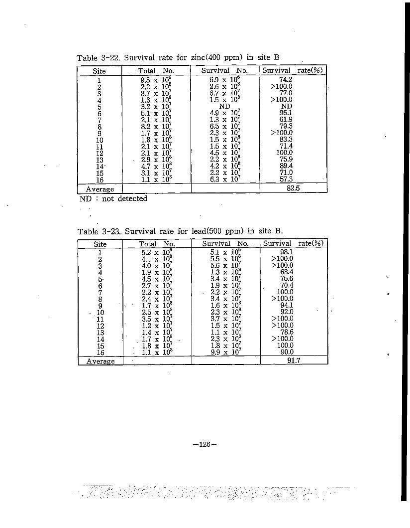
Table 3-22. Survival rate for zinc(400 ppm) in site B
Site Total No. Survival No. Survival rate(%)1 9.3 x 10“ 6.9 x 10% 74.22 2.2 x 10® 2.6 x 10® >100.03 8.7 x 10% 6.7 x 10% 77.04 1.3 x 10® 1.5 x 10® >100.05 3.2 x 10% ND ND6 5.1 x 10% 4.9 x 10% 96.17 2.1 x 10% 1.3 x 10% 61.98 8.2 x 10% 6.5 x 10% 79.39 1.7 x 10% 2.3 x 10% >100.010 1.8 x 10® 1.5 x 10® 83.311 2.1 x 10% 1.5 x 10% 71.412 2.1 x 10% 4.5 x 10% 100.013 ■ 2.9 x 10® 2.2 x 10® 75.914 4.7 x 10% 4.2 x 10® 89.415 3.1 x 10% 2.2 x 10% 71.016 1.1 x 10® 6.3 x 10⁷ 57.3
Average 82.5ND : not detected
Table 3-23.. Survival rate for lead(500 ppm) in site B.
Site Total No. Survival No. Survival rate(%)1 5.2 x 10% 5.1 x 10% 98.12 4.1 x 10® 5.5 x 10% >100.03 4.0 x 10% 5.6 x 10% >100.04 1.9 x 10% 1.3 x 10% 68.45- 4.5 x 10% 3.4 x 10% 75.66 2.7 x 10% 1.9 x 10% 70.47 2.2 x 10% . 2.2 x 10% 100.08 2.4 x 10% 3.4 x 10% >100.09 - ' 1.7 x 10® 1.6 x 10® 94.1
• 10 2.5 x 10% 2.3 x 10% 92.011 3.5 x 10% 3.7 x 10% >100.012 1.2 X 10% 1.5 x 10% >100.013 1.4 x 10% 1.1 x 10% 78.614 ' 1.7 x 10% ■ 2.3 x. 10% >100.015 . 1.8 x 10% . 1.8 x 10% 100.016 . 1.1 x 10® 9.9 x 10⁷ 90.0
Average 91.7
-126-
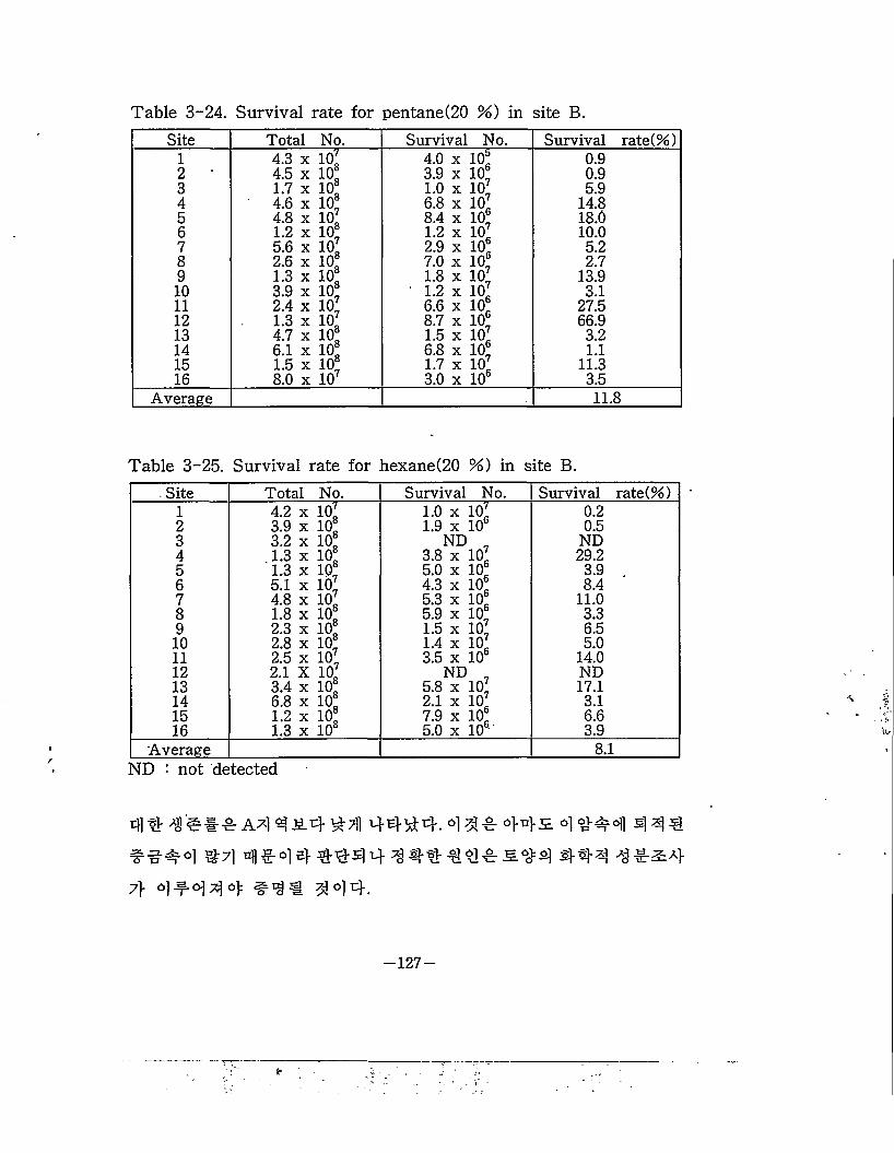
Table 3-24. Survival rate for pentane(20 %) in site B.
Site Total No. Survival No. Survival rate(%)1 4.3 X To! 4.0 X 10% 0.92 4.5 X io! 3.9 X 10= 0.93 1.7 X io! 1.0 X 10% 5.94 4.6 X io% 6.8 X 10% 14.85 4.8 X 10% 8.4 X 10% 18.06 1.2 X 10= 1.2 X 10% 10.07 5.6 X 10% 2.9 X 10= 5.28 2.6 X 10= 7.0 X 10% 2.79 1.3 X 10= 1.8 X 10% 13.910 3.9 X 10= ’ 1.2 X 10% 3.111 2.4 X 10% 6.6 X 10= 27.512 1.3 X 10% 8.7 X 10% 66.913 4.7 X 10= 1.5 X 10% 3.214 6.1 X 10= 6.8 X 10% 1.115 1.5 X 10= 1.7 X 10% 11.316 8.0 X 10⁷ 3.0 X 10= 3.5
Average 11.8
Table 3-25. Survival rate for hexane(20 %) in site B.
Site Total No. Survival No. Survival rate(%)1 4.2 x 10% 1.0 x 10% 0.22 3.9 x 10= 1.9 x 10= 0.53 3.2 x 10= ND 7 ND4 . 1.3 x 10= 3.8 x 10% 29.25 1.3 x 10% 5.0 x 10= 3.9 .6 5.1 x 10% 4.3 x 10= 8.47 4.8 x 10% 5.3 x 10= 11.08 1.8 x 10= 5.9 x 10= 3.39 2.3 x 10= 1.5 x 10% 6.510 2.8 x 10% 1.4 x 10% 5.011 2.5 x 10% 3.5 x 10= 14.012 2.1 X 10% ND „ ND13 3.4 x 10= 5.8 x 10% 17.114 6.8 x 10= 2.1 x 10% 3.115 1.2 x 10= 7.9 x 10= 6.616 1.3 x 10= 5.0 x 10= 3.9
Average 8.1SfD : not detected
#444 ^7] 41 ^4 4 444 4 4 44 44^^4=^
7} 4f-44 4 #4# ?M4.
-127-
3-2-5. C 44 5&4I54 ##14 #415o1| 4#
4 41 7fl#S# 7>57> ##4&4 45-S 4 4# #5 4 #5
5. 1^4 4 4 55(Chough, 1993), 7}i7} ##4$14 1 44 # ### §32]IS @4 45.1- 1 $$5, 444 4
#4 14# 20-30m 4:455. 54451 4444 !#!4 44
15 444 4# 4### 24444(Tables 3-26 to 3-33). C
4 4 144 !#!4 44 4e#4 Ni4 87.8%, Co4 79.8%,
Cd7} 87.5%, Hg7> 7.0%, Zn4 84.2%, Pb7> 47.7%# 5^5 441
54 44 4 44.3%, 444 36.2%4 41## 444 4 Pb4 41
Co# 4445# A, B, D 444 44 14455 l#44 441
54 tfl< 454 &# 41## 4# 455 244^4. 4 4#
4 4#4 15 4 455 144 4 444 111 #14=4 4^4#5, 2 7>57> ##4 7j55 54 44#52 4—45 ##47]
4)#44 4444.
3-2-6. D 44 54414 #114 Ei415oi|
5###5444 44 4455 445# #1# 44 100 - 150m
#455 # 30 4 444 54# 44ft d 44# 54##&4#4
4 4 4 44 15 4 455 #44 4##45 444 41## B 4 4
4 ### 4 4, 44, 444 5445 4# 44#44(Chough,
1993). 4 D 4 4 54454 #414 4415 444 4# 4###
24-4 44(Tables 3-34 to 3-41), NH 4# 4141## 71.8%, Co
# 76.0%, Cd# 85.9%, Hg# 1.2%, Zn# 79.6%, Pb# 88.3%# ^45
44154 #44 44r# 44 12.0%4 3.5%4 4### 44444.
0} D 444 ##14 44-154 4# 4141## A 4 44 45#
W; ;rc.
—128—
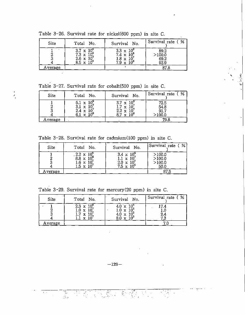
Table 3-26. Survival rate for nickel(600 ppm) in site C.
Site Total No. Survival No. Survival ^rate ( %
1 ' 3.7 x 10" 3.3 x 10® 89.22 7.3 x 10® 7.4 x 10® >100.03 2.6 x 10% 1.8 x 10% 69.24 8.5 x 10⁶ 7.9 x 10⁶ 92.9
Average ' 87.8
Table 3-27. Survival rate for cobalt(500 ppm) in site C.
Site Total No. Survival No. Survival rate ( %)
1 5.1 x 10⁵ 3.7 x 10® 72.52 3.1 x 10⁷ 1.7 x 10% 54.83 2.4 x 10%
6.1 x 1062.2 x 10% 91.7
4 8.7 x 10⁶ >100.0Average 79.8
Table 3-28. Survival rate for cadmiumClOO ppm) in site C.
Site Total No. Survival No. Survival rate ( %)
1 . 2.2 x 10® 3.4 x 10" >100.02 8.8 x 10® 1.1 x 10% >100.03 1.6 x 10% 2.0 x 10% >100.04 1.5 x 10⁷ 7.5 x 10⁶ 50.0
Average 87.5
Table 3-29. Survival rate for mercury(20 ppm) in site C.
Site Total No. Survival No. Survival rate ( %)
• 1 2.3 x 10® 4.0 x 10" 17.42 1.0 x 10% 1.0 x 10 1.03 1.7 x 10% 4.0 x 10 2.44 1.1 x 10⁷ 8.0 x 10⁵ 7.3
Average 7.0
-129-
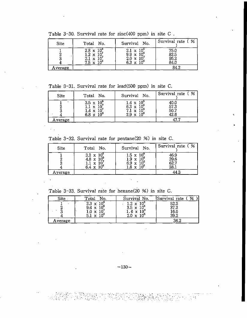
Table 3-30. Survival rate for zinc(400 ppm) in site C .
Site Total No. Survival No. Survival rate ( %)
1 2.8 x 10“ 2.1 x 10“ 75.02 1.2 x 10% 9.9 x 10% 82.53 2.1 x 10% 2.0 x 10% 95.24 7.5 x 10⁶ 6.3 x 10⁶ 84.0
Average 84.2
Table 3-31. Survival rate for lead(500 ppm) in site C.
Site Total No. Survival No. Survival rate ( %)
1 3.5 x 10% 1.4 x 10“ 40.02 1.1 x 10% 6.3 x 10% 57.33 1.4 x 10% 7.1 x 10% 50.74 6.8 x 10s 2.9 x 10s 42.6
Average 47.7
Table 3-32. Survival rate for pentane(20 %) in site C.
Site Total No. Survival No. Survival rate ( %)
1 3.2 x 10“ 1.5 x 10% 46.92 4.8 x 10% 1.9 x 10% 39.63 1.1 x 10% 6.9 x 10% 62.74 6.4 x 10“ 1.8 x 10“ 28.1
Average 44.3
Table 3-33. Survival rate for hexane(20 %) in site C.
Site Total No. Survival No. Survival rate ( % )1 • : 2.3 x 10% ■ 1.2 x 10“ 52.22 9:4 x 10% 3.5 x 10“ 37.23 1.0 x 10% 1.6 x 10® 16.04 5.1 x 10® 2.0 x 10“ 39.2
Average 36.2
-130-
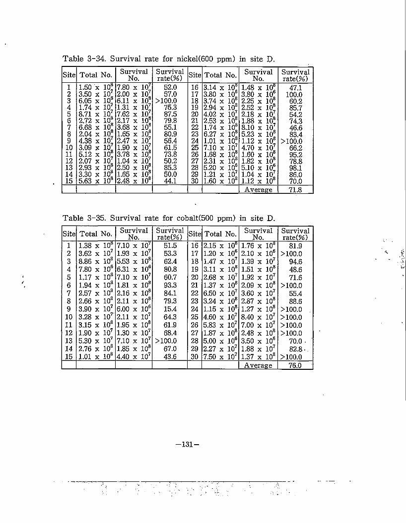
Table 3-34. Survival rate for nickel(600 ppm) in site D.
Site Total No. SurvivalNo.
Survivalrate(%) Site Total No. Survival
No.Survivalrate(%)
1 1.50 X 10° 7.80 X io; 52.0 16 3.14 X 10° 1.48 X 10° 47.12 3.50 X l0O 2.00 X 10Z 57.0 17 3.80 X io8 3.80 X IO8 100.03 6.05 X io? 6.11 X 10⁸ >100.0 18 3.74 X 10⁸ 2.25 X 10⁸ 60.24 1.74 X 101 1.31 X 10 75.3 19 2.94 X 10⁸ 2.52 X io8 85.75 8.71 X 10⁸ 7.62 X 10Z 87.5 20 4.02 X 10" 2.18 X 10" 54.26 2.72 X io? 2.17 X io8 79.8 21 2.53 X IO8 1.88 X 10⁸ 74.37 6.68 X io? 3.68 X io8 55.1 22 1.74 X 10⁸ 8.10 X 10" 46.68 2.04 X 10? 1.65 X io8 80.9 23 6.27 X 10⁸ 5.23 X io8 83.49 4.38 X 10Z 2.47 X 10Z 56.4 24 1.01 X 10? 1.12 X 10? >100.010 3.09 X 10Z 1.90 X 10Z 61.5 25 7.10 X 10" 4.70 X 10" 66.211 5.12 X io? 3.78 X io8 73.8 26 1.68 X 10? 1.60 X io8 95.212 2.07 X 10o 1.04 X 10" 50.2 27 2.31 X 10⁸ 1.82 X io8 78.813 2.93 X io? 2.50 X io? 85.3 28 5.20 X 10⁸ 5.10 X io8 98.114 3.30 X 10O 1.65 X io8 50.0 29 1.21 X 10" 1.04 X 10" 86.015 5.63 X 10⁸ 2.48 X 10⁸ 44.1 30 1.60 X 10⁸ 1.12 X 10⁸ 70.0
Average 71.8
Table 3-35. Survival rate for cobalt(500 ppm) in site D.
Site Total No. SurvivalNo.
Survivalrate(%) Site Total No. Survival
No.Survivalrate(%)
1 1.38 X 10⁸ 7.10 X 10' 51.5 16 2.15 X 10a 1.76 X 10ti 81.92 3.62 X 10" 1.93 X 10" 53.3 17 1.20 X 10⁸ 2.10 X IO8 >100.03 8.86 X 10⁸ 5.53 X 10⁸ 62.4 18 1.47 X 10" 1.39 X 10" 94.64 7.80 X 10⁸ 6.31 X 10⁶ 80.8 19 3.11 X 10⁸ 1.51 X 10⁸ 48.65 1.17 X 10⁸ 7.10 X 10" 60.7 20 2.68 X 10" 1.92 X 10" 71.66 1.94 X 10⁸ 1.81 X 10⁸ 93.3 21 1.37 X 10⁸ 2.09 X 10⁸ >100.07 2.57 X 10⁸ 2.16 X 10⁸ 84.1 22 6.50 X 10" 3.60 X 10" 55.48 2.66 X 10⁸ 2.11 X 10⁸ 79.3 23 3.24 X 10⁸ 2.87 X 10⁸ 88.69 3.90 X 10" 6.00 X 10⁸ 15.4 24 1.15 X 10⁸ 1.27 X 10⁸ >100.0 .10 3.28 X 10" 2.11 X 10" 64.3 25 4.60 X 10" 8.40 X 10" >100.011 3.15 X 10⁸ 1.95 X 10⁸ 61.9 26 5.83 X 10" 7.00 X 10" >100.012 1.90 X 10" 1.30 X 10" 68.4 27 1.87 X 10⁸ 2.48 X 10⁸ >100.013 5.30 X 10" 7.10 X 10" >100.0 28 5.00 X 10⁸ 3.50 X 10⁸ 70.0 •14 2.76 X 10⁸ 1.85 X 10⁸ 67.0 29 2.27 X 10" 1.88 X 10" 82.8 •.15 1.01 X 10⁸ 4.40 X 10" 43.6 30 7.50 X 10" 1.37 X 10⁸ >100.0
Average 76.0
-131-
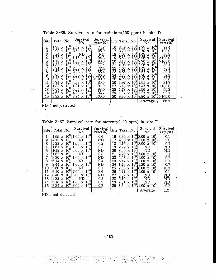
Table 3-36. Survival rate for cadmium(100 ppm) in site D.
Site Total No. SurvivalNo.
Survivalrate(%) Site Total No. Survival
No.Survivalrate(%)
1 1.98 X 10! 1.47 X 10! 74.2 16 3.49 X 10! 2.77 X 10= 79.42 2.99 X 10l 2.84 X 10⁷ 95.0 17 2.70 X 10= 2.70 X 10= 100.03 5.24 X 10= ND ND 18 1.63 X 10= 1.48 X 10= 90.84 1.20 X io! 1.13 X 10⁷ 94.2 19 5.62 X 10= 5.95 X 10= >100.05 1.19 X 10= 1.08 X io! 90.8 20 6.10 X io7 7.70 X 10⁷ >100.06 1.33 X 10= 1.03 X 10= 77.4 21 4.93 X 10= 3.95 X 10= 80.17 3.91 X 10= 2.83 X 10= 72.4 22 1.66 X 10= 1.43 X 10= 86.18 2.60 X 10= 2.22 X 10= 85.4 23 4.58 X 10= 3.67 X 10= 80.19 6.70 X io! 7.60 X io! >100.0 24 2.77 X 10= 2.75 X 10= 99.310 6.30 X 10O 7.90 X io7 >100.0 25 4.90 X 10⁷ 1.90 X 10⁷ 38.811 5.71 X 10= 4.88 X 10= 85.5 26 1.97 X 10= 1.61 X 10= 81.712 1.33 X 10O 1.21 X io7 91.0 27 6.13 X 10= 7.47 X io! >100.013 5.67 X 10= 5.64 X 10= 99.5 28 1.73 X 10⁷ 1.56 X io7 90.214 4.53 X 10= 4.20 X 10= 92.7 29 1.37 X 10= 1.27 X 10= 92.715 3.32 X 10= 3.94 X 10= 100.0 30 9.20 X 10⁷ 9.90 X 10⁷ >100.0 -
Average 85.9ND : not detected
Table 3-37. Survival rate for mercury( 20 ppm) in site D.
Site .Total No. SurvivalNo.
Survivalrate(%) Site Total No. Survival
No.Survivalrate(%)
1 1.65 X 10! 1.00 x 10= 0.6 16 3.50 X 10= 3.00 x 10 0.12 4.10 X io7 ND ND 17 4.00 X 10= 1.00 x 10= 2.53 4.23 X 10= 1.00 x 10= 0.2 18 2.16 X 10= 3.00 x 10= 0.14 1.61 X 10⁷ 1.00 x 10= 0.3 19 2.79 X 10= ND ND5 1:19 X 10= 4.00 x 10= ND 20 3.99 X 10⁷ ND
10=ND
6 1.62 X 10= ND10=
0.3 21 2.29 X 10= 7.00 x 3.17 3.30 X 10= 1.00 x ND 22 2.58 X 10= 1.00 x 10= 0.18 5.14 X 10= ND 0.4 23 5.47 X 10= 1.00 x 10= 0.19 2.44 X io! 1.00 x 10= ' ND 24 1,73 X 10= 1.20 x 10= 0.7
10 2.80 X 10⁷ ND 0.1 25 7.80 X 10 8.00 x 10 10.311 6.10 X 10= 7.00 x 10= 3.6 26 2.77 X 10= 1.00 x 10= 0.112 8.40 X io7 3.00 x 10 ND 27 5.32 X 10= ND ND13 4.32 X 1.0= ND 0.2 28 5.10 X 10= ND ND •14 5.16 X 10= 1.00 x 10= 0.2 29 1.81 X 10= ND ND15 2.34 X 10= 5.00 x 10= 0.2 30 1.54 X 10= 1.00 x 10= 0.1
Average 1.2ND : not detected
-132-
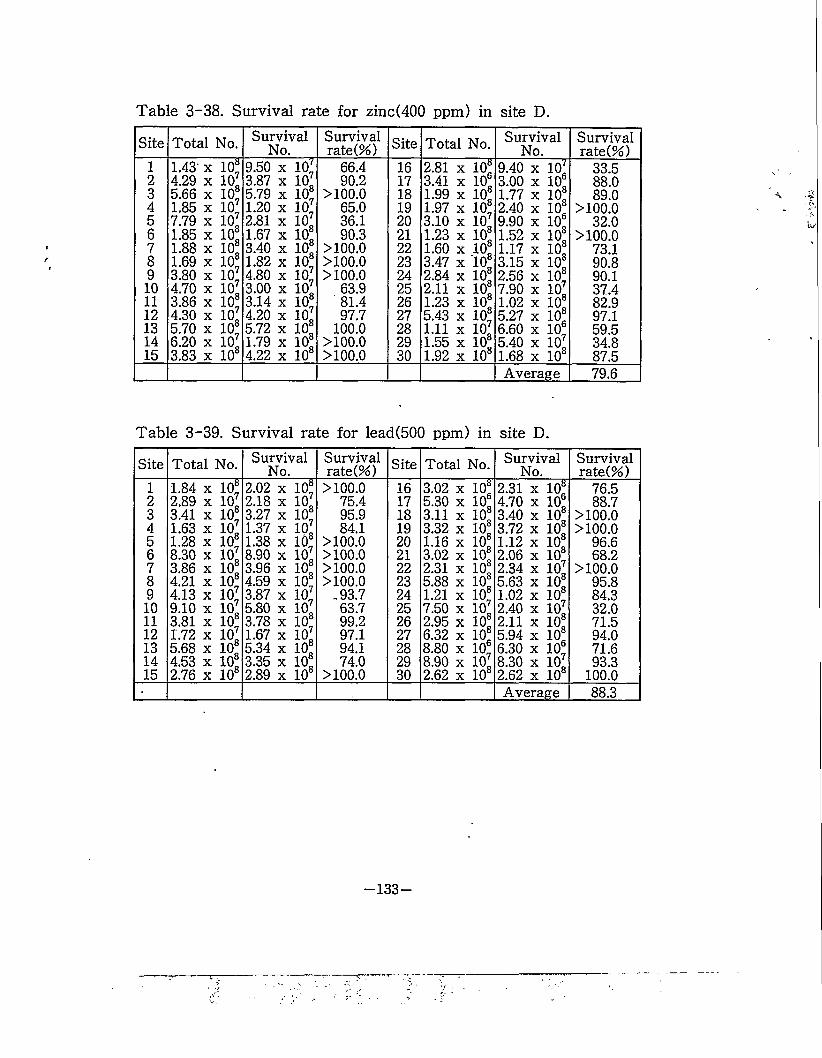
Table 3-38. Survival rate for zinc(400 ppm) in site D.
Site Total No. SurvivalNo.
Survivalrate(%) Site Total No. Survival
No.Survivalrate(%)
1 1.43- X 10! 9.50 X io; 66.4 16 2.81 X 10= 9.40 X 10' 33.52 4.29 X 1° 3.87 X 10 90.2 17 3.41 X 10= 3.00 X 10= 88.03 5.66 X io! 5.79 X 10= >100.0 18 1.99 X 10= 1.77 X 10= 89.04 1.85 X 10" 1.20 X 10" 65.0 19 1.97 X 10= 2.40 X 10= >100.05 7.79 X 10o 2.81 X io" 36.1 20 3.10 X 10" 9.90 X 10= 32.06 1.85 X 10= 1.67 X 10= 90.3 21 1.23 X 10= 1.52 X 10= >100.07 1.88 X io! 3.40 X 10= >100.0 22 1.60 X 10= 1.17 X 10= 73.18 1.69 X 10= 1.82 X 10= >100.0 23 3.47 X 10= 3.15 X 10= 90.89 3.80 X io! 4.80 X io! >100.0 24 2.84 X 10= 2.56 X 10= 90.110 4.70 X io" 3.00 X 10" 63.9 25 2.11 X 10= 7.90 X 10" 37.411 3.86 X 10= 3.14 X 10= 81.4 26 1.23 X 10= 1.02 X 10= 82.912 4.30 X 10" 4.20 X 10" 97.7 27 5.43 X 10= 5.27 X 10= 97.113 5.70 X 10= 5.72 X 10= 100.0 28 1.11 X 10" 6.60 X 10= 59.514 6.20 X 10 1.79 X 10= >100.0 29 1.55 X 10= 5.40 X 10" 34.815 3.83 X 10= 4.22 X 10= >100.0 30 1.92 X 10= 1.68 X 10= 87.5
Average 79.6
Table 3-39. Survival rate for lead(500 ppm) in site D.
Site Total No. SurvivalNo.
Survivalrate(%) Site Total No. Survival
No.Survivalrate(%)
1 1.84 X 10! 2.02 X 10! >100.0 16 3.02 X 10= 2.31 X 10= 76.52 2.89 X 10" 2.18 X io! 75.4 17 5.30 X 10= 4.70 X 10= 88.73 3.41 X 10= 3.27 X 10= 95.9 18 3.11 X 10= 3.40 X 10= >100.04 1.63 X 10" 1.37 X 10" 84.1 19 3.32 X 10= 3.72 X 10= >100.05 1.28 X 10= 1.38 X 10= >100.0 20 1.16 X 10= 1.12 X 10= 96.66 8.30 X 10" 8.90 X 10" >100.0 21 3.02 X 10= 2.06 X 10= 68.27 3.86 X 10= 3.96 X 10= >100.0 22 2.31 X 10= 2.34 X 10" >100.08 4.21 X 10= 4.59 X 10= >100.0 23 5.88 X 10= 5.63 X 10= 95.89 4.13 X 10" 3.87 X io! ,93.7 24 1.21 X 10= 1.02 X 10= 84.310 9.10 X 10" 5.80 X 10" 63.7 25 7.50 X 10" 2.40 X 10" 32.011 3.81 X 10= 3.78 X 10= 99.2 26 2.95 X 10= 2.11 X 10= 71.512 1.72 X 10" 1.67 X 10" 97.1 27 6.32 X 10= 5.94 X 10= 94.013 5.68 X 10= 5.34 X 10= 94.1 28 8.80 X 10= 6.30 X 10= 71.614 4.53 X 10= 3.35 X 10= 74.0 29 8.90 X 10" 8.30 X 10" 93.315 2.76 X 10= 2.89 X 10= >100.0 30 2.62 X 10= 2.62 X 10= 100.0
Average 88.3
-133-
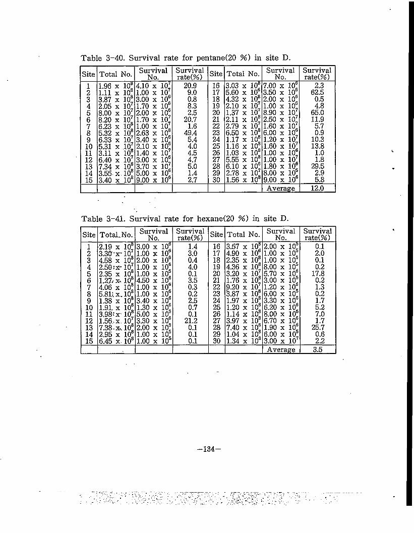
Table 3-40. Survival rate for pentane(20 %) in site D.
Site Total No. SurvivalNo.
Survivalrate(%) Site Total No. Survival
No.Survivalrate(%)
1 1.96 X 10= 4.10 X 10% 20.9 16 3.03 X 10= 7.00 X 10= 2.32 1.11 X 10= 1.00 X 10% 9.0 17 5.60 X 10= 3.50 X 10= 62.53 3.87 X 10= 3.00 X 10= 0.8 18 4.32 X 10= 2.00 X 10= 0.54 2.05 X 10⁷ 1.70 X 10= 8.3 19 2.10 X 10% 1.00 X 10= 4.85 8.00 X 10⁷ 2.00 X 10= 2.5 20 1.37 X 10% 8.90 X 10% 65.06 8.20 X 10 1.70 X 10% 20.7 21 2.11 X 10= 2.50 X 10% 11.97 6.23 X 10= 1.00 X 10% 1.6 22 2.79 X 10% 1.60 X 10% 5.78 5.32 X 10= 2.63 X 10= 49.4 23 6.50 X 10= 6.00 X 10= 0.99 6.33 X 10⁷ 3.40 X 10= 5.4 24 1.17 X 10= 1.20 X 10% 10.310 5.31 X 10 2.10 X 10= 4.0 25 1.16 X 10= 1.60 X 10% 13.811 3.11 X 10= 1.40 X 10% 4.5 26 1.03 X 10= 1.00 X 10% 1.012 6.40 X 10% 3.00 X 10= 4.7 27 5.55 X 10= 1.00 X 10% 1.813 7.34 X 10= 3.70 X 10% 5.0 28 6.10 X 10= 1.80 X 10% 29.514 3.55 X 10= 5.00 X 10= 1.4 29 2.78 X 10% 8.00 X 10= 2.915 3.40 X 10= 9.00 X 10= 2.7 30 1.56 X 10= 9.00 X 10= 5.8
Average 12.0
Table 3-41. Survival rate for hexane(20 %) in site D.
Site TotaLNo. SurvivalNo.
Survivalrate(%) Site Total No. Survival
No.Survivalrate(%)
1 2.19 x 10% 3.00 X 10= 1.4 16 3.57 X 10= 2.00 x 10= 0.12 3.30 “x~ 10% 1.00 X 10= 3.0 17 4.90 X 10= 1.00 x 10= 2.03 4.58 x 10= 2.00 X 10= 0.4 18 2.35 X 10= 1.00 x 10= 0.14 2.50 ix-10% 1.00 X 10 4.0 19 4.36 X 10= 8.00 x 10= 0.25 2.35 x 10= 1.00 X 10= 0.1 20 3.20 X 10% 5.70 x 10= 17.86 1.27/ x, 10= 4.50 X 10= 3.5 21 1.76 X 10= 3.00 x 10= 0.27 4.06 x 10= 1.00 X 10= 0.3 22 9.20 X 10% 1.20 x 10= 1.38 5.811 x. 10= 1.00 X 10= 0.2 23 3.87 X 10= 6.00 x 10= 0.29 1.38 x 10= 3.40 X 10= 2.5 24 1.97 X 10= 3.30 x 10= 1.710 1.91 x 10= 1.30 X 10 0.7 25 1.20 X 10= 6.20 x 10= 5.211 3.98? x' 10% 5.00 X 10= 0.1 26 1.14 X 10= 8.00 x 10= 7.012 1.56, x. 10% 3.30 X 10= 21.2 27 3.97 X 10= 6.70 x 10= 1.713 7.38-Xx 10= 2.00 X 10= 0.1 28 7.40 X 10= 1.90 x 10= 25.714 2.95 x 10= 1.00 X 10= 0.1 29 1.04 X 10= 6.00 x 10= 0.615 6.45 x. 10= 1.00 X 10= 0.1 30 1.34 X 10= 3.00 x 10⁷ 2.2
Average 3.5
-134-
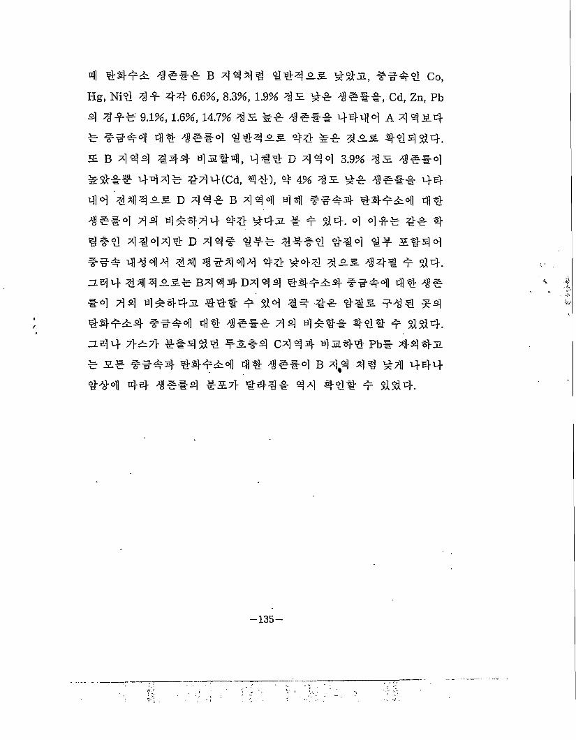
4 Ilf A *f B 4 44 4 ##a, Co,
Hg, Nil If 44 6.6%, 8.3%, 1.9% IS #f ^###, Cd, Zn, Pb
4 If# 9.1%, 1.6%, 14.7% 451 ## 4#** 4444 a 4 4A4# f #f 4 44 4##4 114AS 44 #f 4as 44444.
s. B 4 44 144 45i#4, 414 D 444 3.9% 4s let-4
###%& 4444 144(Cd, 44), 4= 4% 4 s #f ^f## 44
44 44]4as D 4 44- B 4 4 4 41 ###4 Ilf A4 4#
1#*4 44 4f 144 44 44a # f 44. 4 4## 1# 1
4#1 41444 D 4 4# If# 41## 414 If A44 4
### 4^44 44 4 #4 4 4 44 444 4as 141 f 44.
a a] 4 444as^ B4 44 D4 4 4 Ilf A# ##f 4 411#
#4 44 h]*44a 44# f 44 14 If 41 s f 41 f 4
Ilf A4 #444 41 l##f 44 4*1# 44# f 444.
A44 7}A7} f#444 fs#4 C444 1a 4# Pb# 441A# s# ##44 Ilf A 4 41 1##4 B 4,4 4 4 ^41 444 #14 44 1#*4 f A7> #41# 44 11# f #$^4.
-135-
*11411 21#
4 ##44 44*#* 4*44 ##4 5#4 44 5## #4) 4 45# 4 4 44 3§2- 50cm 345 #- 88 4 3 3# jl tj)##<tf 44 5#* 4444 4 51 ***(243)4 ##*3(143) 4 si 4 tfl# ** 4 4 4#4 4*## 34 4h#$4-. ##335 s.4 4 *44^ 44 *# 44 4#4 *5* 4)4444 54444 4*4454,54444 544 *44* *444454 #54 4 4# 4**4 444 4 544 44# 44##44 &4# 4 ##5# 45i4 *$13, ##454 4# 4*## 444 454 34 44#4. ### 4##3 4#54# #4 444 4 4 #444, 444 4 44 4= 5cm 454 34 44 4## 43* 5# 4 44 #5 50cm 34 44 44# 45 5*7} 4#4 *44 4 #=* #* 5#(rhizosphere)4 44 $14 4*4 ## ##44=#4 #57} #*# 455 **##. ***4 4# 4**4 ** 4*
4
5#44 4**4 44 #44 ***4 #34$1* 7}*4* 44 44, ##*34 4# 4**4 4* 4* ##*34 *#4 #4* ##*3 3 347} &** 44* *5 $14.
##4 4# ##4*5 *#4 5** 5#4 34 4 454 4# #*4 #* 4#* #4 #* 4 4 45, 5 5*4 ##*34 3*5)4 #7) 4*4 5#44 54 ##*34 4# 4**4 *7)1 44# 335 ###4. 444 4## 4 4##3 4####3 4#4 $144* 3**44 4#* #4 ^* 4* 3* 43 44 45447} 4*444 # 335 44#4.
*3-44 ##*3 4 #4 54 *5* 4## 4 4*#3 #44
-136-
4 s#4 4 s#454 #544 ##^A4i 4# #44
11 4# 5441 #Al## 44# 5 44. zi5)4 11-ss 4 #4#S4# (A 4 4) 4 4, 4 4, 444 A44# #4# (B, D 4 4)4 #44^ ##4445#4 #4#4 4# 4#44 4# 4.as #2i, #s}#Al 4# 4#44 #4 4414. a #4) 4 44—4 ##411 44as 44# #s# (C 4 4)4 #444 451-4 #544 445A1 44 A# 4##1 #4 4414. 4 4# 4as 4#4 4#4 44 #544 #44A4 4# 4# 454 #A7> #44# 4As # 4 1A4 44# €4# s#4# #44- #41 444 4 4 #4 44. ## #4 #1#1 B4 4 4 D4 44 #544 444A 4#454 #A14 # 4 44 #1 44 4 #A 4444s 500 - 1,000 m 4A 144 #-§-4a ##
#2i 4 4 4 fi-T #544 #4#A1 4 4 4## 4 #454 # A# ## 4 as S# #s}#A4 #5# 4 4 44 4154 #4 4# 4## &4 1# 147} 42i4 144 4 44## 41# # 14.
1 ### ## Ni, Co, Cd, Hg, Zn, Pb# 6##4 #544 1 #, 4# "T" #54 #4#A 4 4 44, #541 Hg# Michaelis
and Riese (1991)7} 444 44#4 ##4 4 44 A## 44# #
4 4 44 44 # 41# 444as 1# s#4s# 4#as #
A ^-y o]) a-) ^ 1-S-4 7H #41# 4as ##41, #544 #4
#A4 4 4 #AS # ##14 4#4 #A# Michaelis and
Riese(1991)l 441 4~§-4 #AS4 1#4AS #4 4 44 44, A si, ##, 41#, 4 4# # 4Si 44 4 #544 ###A4 #A7} 44### #41 14414 ## 41# 5 114.
-137-
444 #9-#4 44, 44#e 444 44#54 44 44#
54 ^£24 4 4 44-t^- 4^4 44, 44, 55#, 4-4 ##
444fe 54 45* 24tr 44& ;H#4 f, 44-444 44
44 44 44-7} 444 4 4^ 4 44 44 #^#4 44#^ 4
445 f£24 4 44#^ 7} 5 4454 247} 4#444 4 4 #44 24 44 4 44444 444 55 45.5. #44 # %1
& 44 4 4544.
-138-
—681—
to TaT t^
to tkOki^'P-l^ -f&rftk

*11 4# : 7}+ ^ 7>^y^Ai]dlH 7^7)^(Development of Gas and Gas Condensate Reservoirs)
4] l'S : S* Ira
4# 10##4 4 #44# 44# ### ^4 #4. 1985# 44 444
#M ### 4# #4 4# 44# #4444 15 - 20# 444 # #
#&4 fr^ls]v. $14. W 2147] #44# ##o] 7]4# ##4 §1# 5
33 4#44 4# 447} 441 4444. 4^1 444 444 444 ^4# 4444 44 #7}# 34 7}*44 434 4 444
47Rr #44# 444 #34 444## #43-4* 44444 ## 4 #7}33 44# 4444. 5# i£^4 ji2:5]3i $1# #4 11334 44
44 4443.4 ### 4444# *3e]7} #444 44 444# 3# 34# ##7}34 A]~g-4 4433 #tfl€ 4## 344.
#4 44s 444#3 4## 4# 444 444 4-^44-t1# ##,
444 *33 4# #43# #444 #47}^4 347} *7}* 444
4. 4-4 #47}^4 #4# 3«H 4444 433 4444 4444 #
37} ##44 #44 44## #44 44 414 7}3B44 *7}* *7}
444 #4. #4 444# 4## #4444 ### 7}3 «## &# 433 7H# 3$]## #4* zls)## 44 #344.
#*7}^# 4 15044 #4 4#44 #34 44 4 ##4 44#
4#4 a. 3444 IK# 4 44] 44# #44$134 4#4 ##7}3 4 44# 4 44344 4#4 ##4 #44 3l a}-§-o] *^4 *7}#jl
44. #47}^4 £#3# #4#, 44#, #4# 44 4# 3444#, #### #44 #33 4#4 3 44.
7}3# 3# ##4143#4 @J&7]4# ^#7]*# ?6e44 4###
-141-
4 #4 44 4371 #444 4 4 #4. 7>^4 0### #m4# #4 4-44 #34 7>y ^-^446)1 44 444 #444. 444 7>3 ^ 4444^4 44^ 3#4# #4 KB33 4444 # 14 444 44-31 44. 4444 7}-3 1 44414^4 44 If4 Figure 4-14 44 44.
37114 Tll^ AS 43# 7>3 1 4 4^11 oi s 4 #.&*! 7H#7l 9 49-4
144£4 4#mm# *### 4435. 0^719*11 44 49# 944 43i 24434 4 A#4441 9444 4 44:719*11 444 494 44 44. 444 344^44 444 0J& 4 44:49# 444 4-8-44 4 Til #4 4 0#$ 44# 44# 4444.
*B4 7>^a 7114-4#4 4### 944 7>3 e@# 7fl#4 444 ##4 444 0#$# 44 44 493 3 #### 444 e
@444 44 444 4444. M444 444 44# 3.711 27}43
4# 9 $l#4 44# rajf# #44444 4# 44# Ht*1§*11 4 4 #444*14. B@#4 #444# 3# 4@#4 7}3e@#4 4*1>> 714 ^34 #444 lr@P-447194 4944#4 414 444 4 2444 44444. 4444 49#4#4 #1# 4#4 9 ##4= &4 4 4 (unconditional simualtion)4 #fM# 34 4 # (conditional simulation)# 4# 4 3 #4444.
4 3#4-4#44# SiSSil 4# #44433 M«4 #44 m#SM tfl# 7114# 94444. 4 3444# IrMfl #4444 7># #343 7l^7> 4# e@m#4 43444 #44 444 494 # 4 4444# 4444 7)3=434] 444 4# #4, 444#, #Hm MB4#, B@m#4 lean gas44 444# #4 %## 44# #4 4^4.
-142-
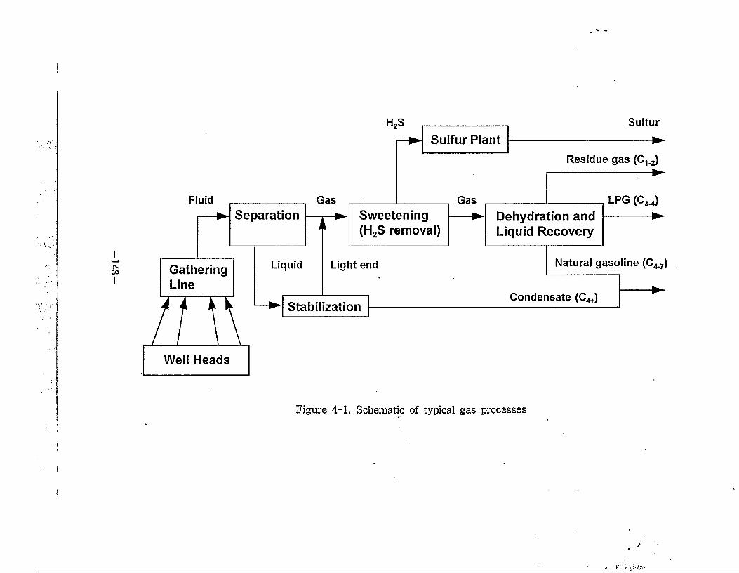
Sulfur
Residue gas (C1-2)
Natural gasoline (C4.7)Liquid Light end
Condensate (C4+)Stabilization
Sulfur Plant
GatheringLine
Well Heads
Separation Sweetening (H2S removal)
Dehydration and Liquid Recovery
Figure 4-1. Schematic of typical gas processes
4] ^44
444444 444 4444 44 to 5d# 444 ^ 4# #444 ^}&# ^s]i} 4 #44 444 444 4# 4#44 #4 %# 944# 4# #44- (Fig. 4-2). 444 444 41 #
11 ZL 41# 14414 #444 tol, #44# 4#44 #!& 4# 94 #4 El (stochastic model) 4 4-0-4# 494 #e>]-x] jl to.
%iee #44-4-4 44) 4## 7]#to44 ^4#§H4 4#4#4444 4 toss. l-g-44, 4 #9 tol4# 4## 444 4 -0-43, 499-444# to# 4 44 4 # ## 4#4#4 4-0-44. #4 7>^ 1 y^ie-iE^^ 4##1# 444# #w 4 #94 #4 444 39.44. 444 4 1944# 94## &## 4-0-4 449 4 444# 444 4## 44# 444 94, 7] 7i]44 2.4* 44-44 4 #94 #944# 99 4 to.
4 444# 44 4994 444 #9# 3##ss4 9494 2.#
* 9-0-t 4 to 444 444 44 4#4to4, #4 444 49#
#7]s. 44 2.14 994# 4-44 44 44to, 44 94444 2.1
4 #44 44 444 to 94. tos x}9 44 94# 4971
(automatic minipermeameter)# 4 #4-4 3.7] 7]- 16“xl6“4 44 #42.
(slab) 4 4 444 94# Dr# t21t 4 #444 (unconditional
simulator)4 2:19- 4 #4 4 4 (conditional simulator)4 9 #44 3 1
4-# #4444-. •
2-1. 4##o| gui${
494#444# 4 #44 7>a 4 1144^14 444# 444#
—144—
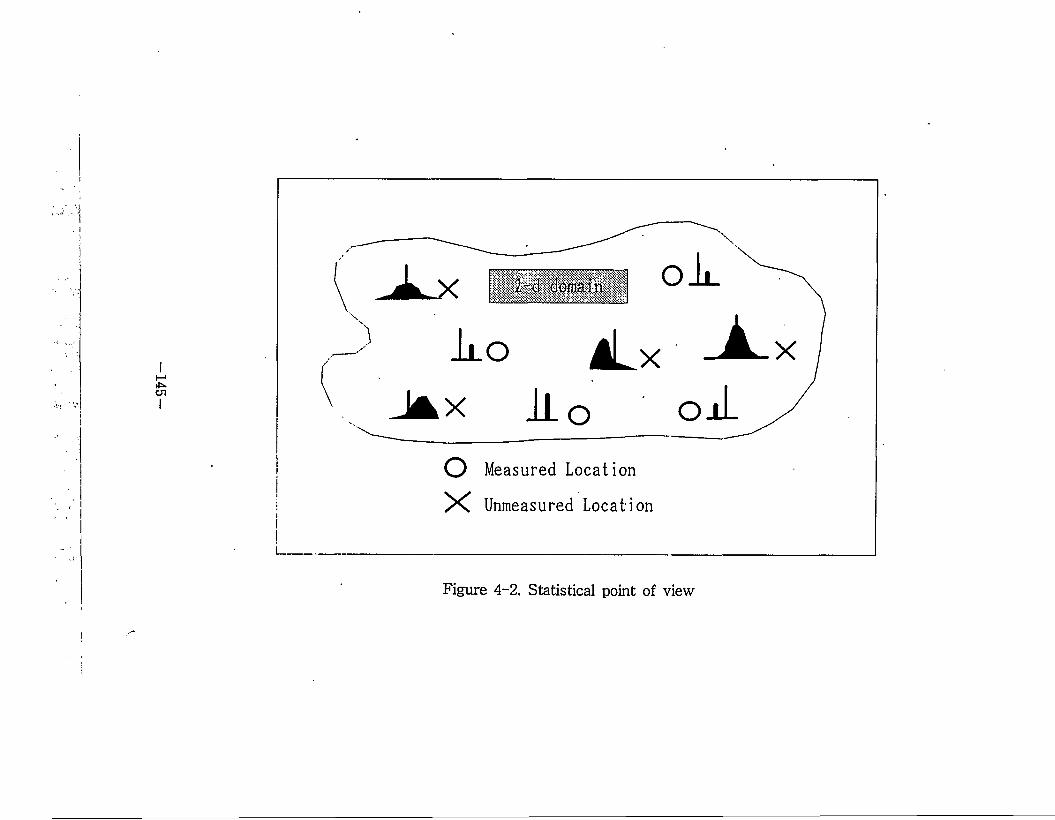
&
)
domain
iio iLx
x lL0 ojLO Measured Location
Unmeasured Location
Figure 4-2. Statistical point of view
4 €4, €#€ 44# ##€% 4##4 #4 (reservoir characteri -zation)# 7}#% € €%%7)) 444# 444. 32] 4 7]### #4€ #€ %# 44% 444€# 4444 #M% 44& 444 444. 4 #€44 tSlt 444 4444 4# €44 3.4 37>4 4445. 4
4 # $14. 4, 44 (sedimentary), 44 (diagenetic), 3 2] 3 43:44 (tectonics)44°14. 44 444 44 "94# 44 44# €4 444# 35 .44-44 44 444 44 4# 344 45.7)1 4# €44 €4. # 4] 44# 444 4-f-4€ 44 #4 444 €44 44 444*4 441 ### €#44 444 34# €444 24 #4# 44445 44, # 4i.oi 14- <£40] 4# *o)l 44# €4, €4#3.s] #5444 444 7)1 4# €€4 €4.44) 44# 4#4 4# 3# #44 #44# 4 4 4 #4 €€4 44 4##4 #444 #4 32)3 4% ## #4 €# 44##4 44# €4 €44 .44 4#€4 #%4 €4# €€4 €4. 44% €€#4 €4 4## ## (#4# ^ ### #)# €44 44 ##€44 44, 35)€ ##€# #443 4€ #34€ €444 4 €#44 #444) €4. 444 4##€ W# #€€ #3# 4# #4 €# 443 44# 4= €4. 44 45-44 €€4# €4 45.7} € 4% 4#4 tf)% 712l €4 €%# €# %#7} €4 (A.J. Sultan 1989).
*M 7]#^4 4-4 #4# 3#47) €4)4# #€€ 444 ##4 % 4## #&# %4 4^44 4# 4#4 €4 444 %#4, 4# €% 4 €4 €4# #€€ €€ €44 ## (#4-3)# 4€ #4% 44# 44# # €# #4%€ €35 €#444 %4. 3# 4#4 4 €# 4*# #5 %# (probability density function) %#5 5.444 4 %4. 4714 4# #3 %## #44 €44 €4 #44 #€€ €# €4 44## 4# €4)4€ €3# 44%4. 4€4 ## # 7}4 #4# 4€%7]
146-
4# Warren^ Price (1961)€ 444 ## (€4-5)& 4 4444 €4#<LS if444 54€54 444 4€ 4 5444 4W £€ 4# 4 4 (correlation length)4 7TN& 54 4—5.4 44444. 2144 4 4 3M4€ 44 54€5<>11 44 €4€ 4 €4 44 &&54, n 44 4 444 4iz 44 ## (€45)4 44 €54 44 4 4414 45* 4 4 Warren4 Price (1961)7} 444 4 4444 44 #& (€45)4€ €44 445 7}4431, 4444 4^47} €4 €5 €44 444 #4 (454 £4 €4)4 44 4€€ 444 7}4 44, 444 444 44 €4 4:4 M455 44 # € 44 4^4 (A.J. Sultan et al. 1990).
4# 45 €5 (probability density distribution)4 4 4 £5. 5.44 €45-4 44 :o4€54 44 ^44 Greenkem4- Kessler (1969)4 °1 €££€4 54 444. >, 4# 45 4€i 44 54 4 € $1€#4 €4€ €544 (heterogeneity), 4 5€4 (nonuniformity), zis)5 4 44 (anisotropy)€55 4# € $14- 4# #4, 544 4)4 (uniform media)4-^ ,4€'444 44 (€4-5)5 44 444 4€ 9:55.544 7}€44€ 4€ 44 44. ^.44 44144 €4€4 44 PDF(probability density function)€ 44 €44 444 k444 4444. °1 44 4°) 444 5€4 (uniform)€ 444 € &€ 4€€ Dirac €4 4€4 44, d(&)5 57] 44. Dirac 447} €44444, 5.44 €4
444 4445, 5.7} 4€44°ll 5444, 444 44 4€ %
!dwdk£ 14 44 4 54 44 4 €44 PDF€ N€44 4454 4
€7} 1 444 44€ 44 44 ^4 4€ €471)4 €4ir 444 44 4 71)4 44€ 44€ 4 4444 455, 444 PDF€ 4€ 4414 € 4€^°> 44
-147-
(1).FU5D=SrA«1=1
47]*| N* 4*4 *44, £V* 4* 7]]* (weight coefficient)^. *
* 31* 4444 4*4 4* 14 44. 44# *444 47} Fig. 4-34
4 # ^445 4*4, 0i Si4 ^** 5*# 44 (uniform media)44,
5*# 4 tM^4 4* *^* *4 #-#5 444. 444. 44 5*A544 (homogeneous media)4 4* 44 444 44 #*7} #4431, #
5## 44 (heterogeneous media)4 4* *4 4 44 44 **7} #4
4* 4* 4 # 44. * 44 #** Greenkom4 Kessler(1969)4 44
u]5*^ 44 (nonuniform media)7} ^4 4 4*4, 4* 4444 #4
#*5# # * 4* 4# 45. #* (probability density function)5.
4 44* ^4 444. 45*4 4444 5*4* 444 4*^5.4*5 M4 7}*4 44, 4445 15144 445 44 44-4
4* *5 #45 s# 44** * * 44 (Fig.4-3).4 44 #* *34** *44 4## (random variables)4 *4 *5
# #3144 4*4 4444 44# 4554, 444 4** 4&5 44 *54 4**4 *4 4-4* 4* 5*4 4* 4$14.
2-2. *4IB4 51 (stochastic model)
244 4444 45 444 444 44 *4 4:* 43.7} 5£#4 *4 444 44 7144: (expected values)* *4* 444. 4* #4, 45 444 43-47} #4 *4# 4*. ** 45* 4*4 4*44 *4 44 5* 4444 44 *4. 44* 455 4444 4*4 *4 (4 2).
148-
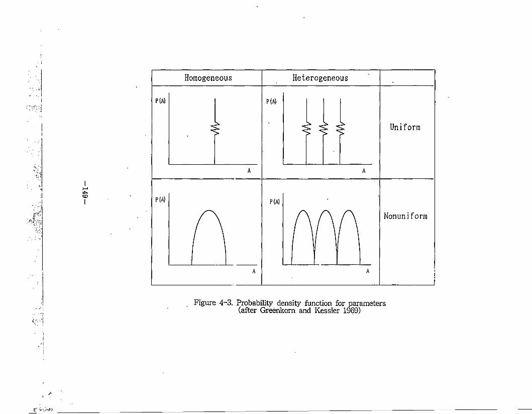
%
jiI
'\
Figure 4-3. Probability density function for parameters (after Greenkorn and Kessler 1969)
Z
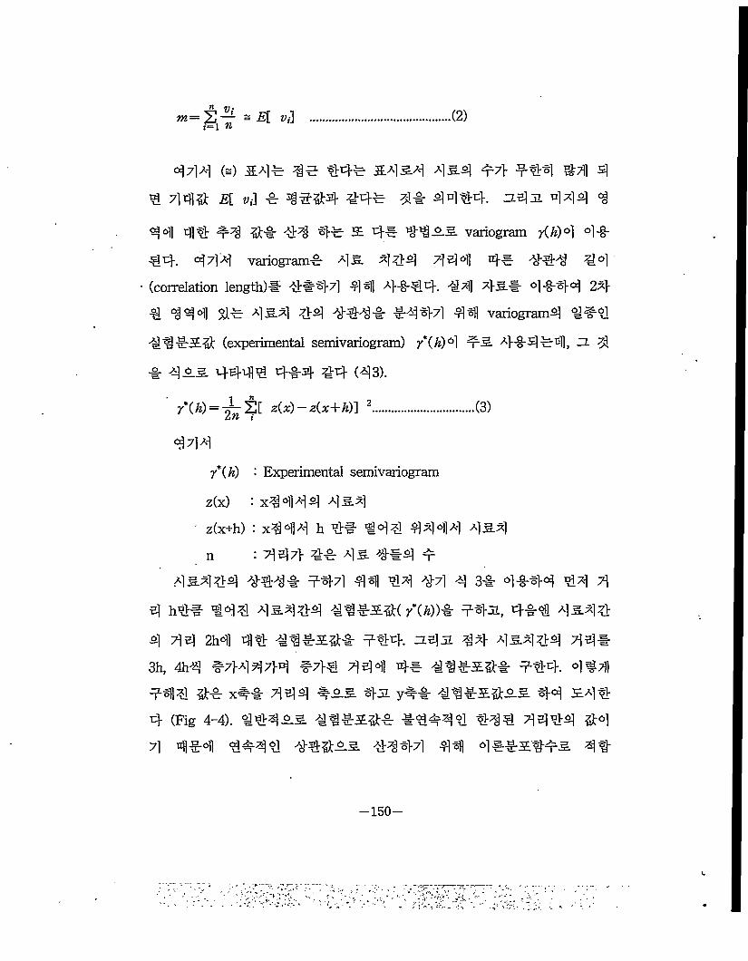
(2)m= 2-^- s £[ «/]
444 (=) 5E4# #e 44# #A13-*\ 4&4 t7> #44 #4 s) 4 44% £[ y,] # TO%4 44# 4# 4444. zLSjjL 444 #
#4 tfltb #4 %# 44 4# m 4# variogram X^)4 4#44- 4 7] "4 variogram# 45. 444 444 4# 444 #4(correlation length)# 4#47l 4^0 4#44. 44] 4-5-# 4 #44 24 -# 444 ## 4-S-4 44 4441# #4471 44 variogram4 #### 4 #54 (experimental semivariogram) r*(/z)6l #S 4#4#4, 31 3}
# 4 as 4444 4#4 #4 (43).
/*(/&) =z(,x) — z(x+Ji)\ 2............................(3)
4447* (A) : Experimental semivariogram
z(x) : x#444 4S4 ' z(x+h) : x#44 h 4# #44 4444 4&4
n : 447> ## 4a ##4 #4a444 444# #44 44 44 4-4 4 3# 4 #44 44 4
4 h## #44 4&4#4 44##4( r*U))# #4a, 4#4 4&44
4 44 2hi 44 44M4# #44 tl^ji #4 4s4#4 44# 3h, 4h4 #7>447>4 #7># 444 4# #1##%# #44 444 #4# &r# x## 444 fAS 431 y## #^##%as 44 s44 4 (Fig 4-4). #44as. ##### 4#4 4444 #44 4#4 #44# 44^as 4#44 44 4#####& 44
-150-
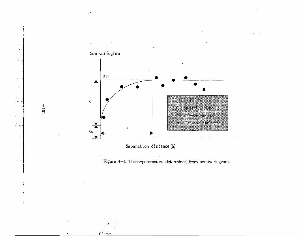
Semivariogram
SiH - C + Co
Co : Random variance
a - Ranges of influences
Separation distance(h)
Figure 4-4. Three-parameters determined from semivariogram.
(fitting)*^) #4. ###38# 4##3##2 #4 #4# 4# 4# 4# #2# (trial and error), 434## (least-squares), Gauss-Newton, ## 4# (linear-tangent)## 4# ##22 4#47l^4, 484 7>4 %4 52.51^ 444 844, #44-5-2 ###2 ### Wt2! #44 44471 4#4 4442#4 ^5. 4444 (444,1992). ###284 4##2#*#2 444 4# 4444 #8## (spatial variance) 444 44 (random variance), #44 (sill), zl^zl ### (range of influence)>4 #91' 44 (Fig4-4). 444 4414 44#### #24# .4444 44 544 4#91444 .4444 28# 444 4 ^#24 4# 44 4 44 822 ##84.
2-3. sl4 ##
2-M4 ##4# 44444 44# 4a^l 444 4% 42# 44 444 44 4544 4#91444 544 4#9144-5-3. 4# 4 88. 4544 4#9144# 44 44# 444 444 43.4:4 434 44 4# 4-484 44 444 2#8 444 4# 444 #4 (4#4 ##) 4 4# 4## #4# 4444 ##8 #4 844. 444 #58# 4 #91444 491 ##8 4##8#4 8# #914 #44 4444 #4 4fHF4 4'3#2. 4# 444 44 #44# 44 4# #4 84 4# € # 44. 4# #4, #54# 4#9144 444# FFTM (fast fourier
transform method), SPM (source point method), ZL^ZL TBM (turning
bands method) 44 #4 84. 4 4444# 4# #44 FFTM###4-#44 4##8 #48# ##484. #4, 54# 4 #914 4# 48. 4 91## #7} #32.4, 44# #4# 3# 48#4, 4# #54# 4
-152-
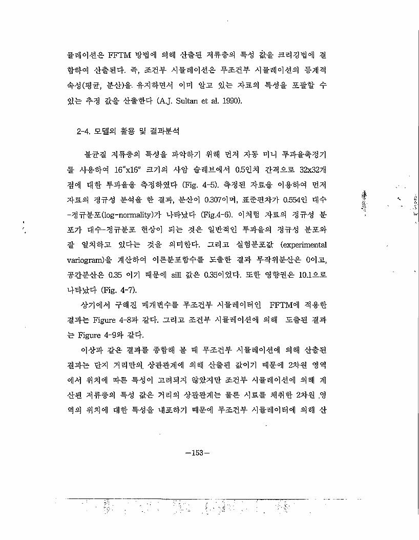
*44** FFTM W4 44 *#4 *##4 #* it* 3* *^0)1 4
#44 *#44. 4, 2^-t- **44** *54* *#44*4 #44 **(**, **)* #*#** 44 to safe 4&^ *** 5## *
&fe ** St# *#44 (A.J. Sultan et al. 1990).
2-4. £|S| #g SS S4fe*
#** 71**4 *## 4444 44 47i 4# 44 #4**471
# 4*44 16“xl6" 3.714 44 #454* 0.544 4:455. 32x32?H
44 44 *4** *4444 (Fig. 4-5). #4* to* 4*44 44 to si 4*4 #4* 4 44, 444 0.30744, 5*# to 0.5544 4*
-4**5E.(log-normality)7> 4444 (Fig.4-6). 4*4 4-^-4 4*4 *
57> 4 *-4**5 444 4* 4* *444 *4*4 4*4 *54-* *443 *4* 4* 4444. 34JL (experimental
variogram)* 4*44 4#*5.4*# 5## #4 *44*#* 04 3,
***** 0.35 44 4*4 sill St* 0.354 #4. 5# 4#** 10.155.
44)*4 (Fig. 4-7).
*7144 *44 47H#** *5** 4*51144* FFTM4 4*4 #4* Figure 4-84 #4- 3*3 ^4* 4*44*4 44 5*4 #4 fe Figure 4-94 *4.
4*4 4* #4* ##4 # nfl *5*# 4*44*4 44 *#* #4* 44 4444. *44414 4# **4 St47l 41*4 244 44 4* *1^1 oil 4# ##4 3444 tot## 54* 4*5114*4 44 4 *4 4*#4 ** St* Tlelsi #444* *# **# 4** 24€ .4 44 444 4# *** 45*71 4*4 *5#* *#4444 44 *
-153-
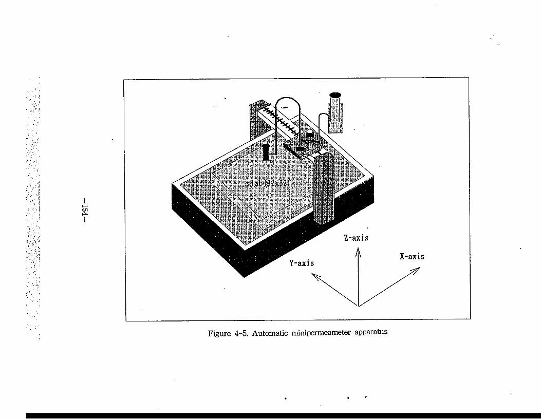
cn
Figure 4-5. Automatic minipermeameter apparatus
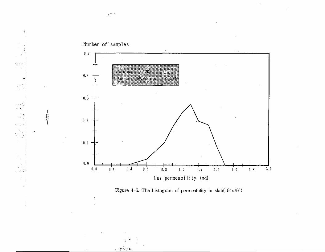
Number of samples
standard deviation
Gas permeability (md)
Figure 4-6. The histogram of permeability in slab(16"x!6")
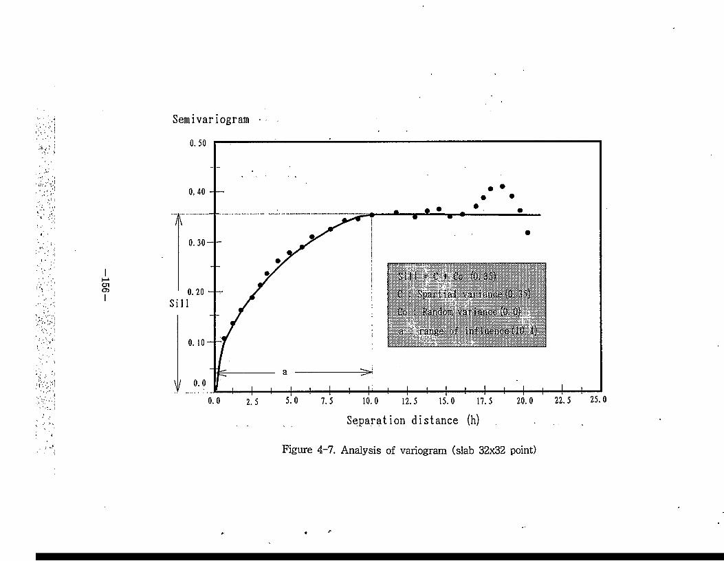
Semivariogram
C ■ Spartial variance(£h 35) Co : Random variance (6.0} a : range of influenced. 1)
Separation distance (h)
Figure 4-7. Analysis of variogram (slab 32x32 point)
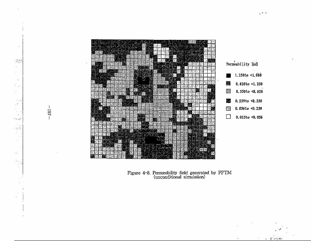
157
Permeability (md)
g 1.250 to <1.880
H 0.620 to <1.250
H 0.350to <0.620.
g 0.239 to <0.350
g 0.056to <0.239
□ 0.013 to <0.056
Figure 4-8. Permeability field generated by FFTM (unconditional simulation)
I
Z
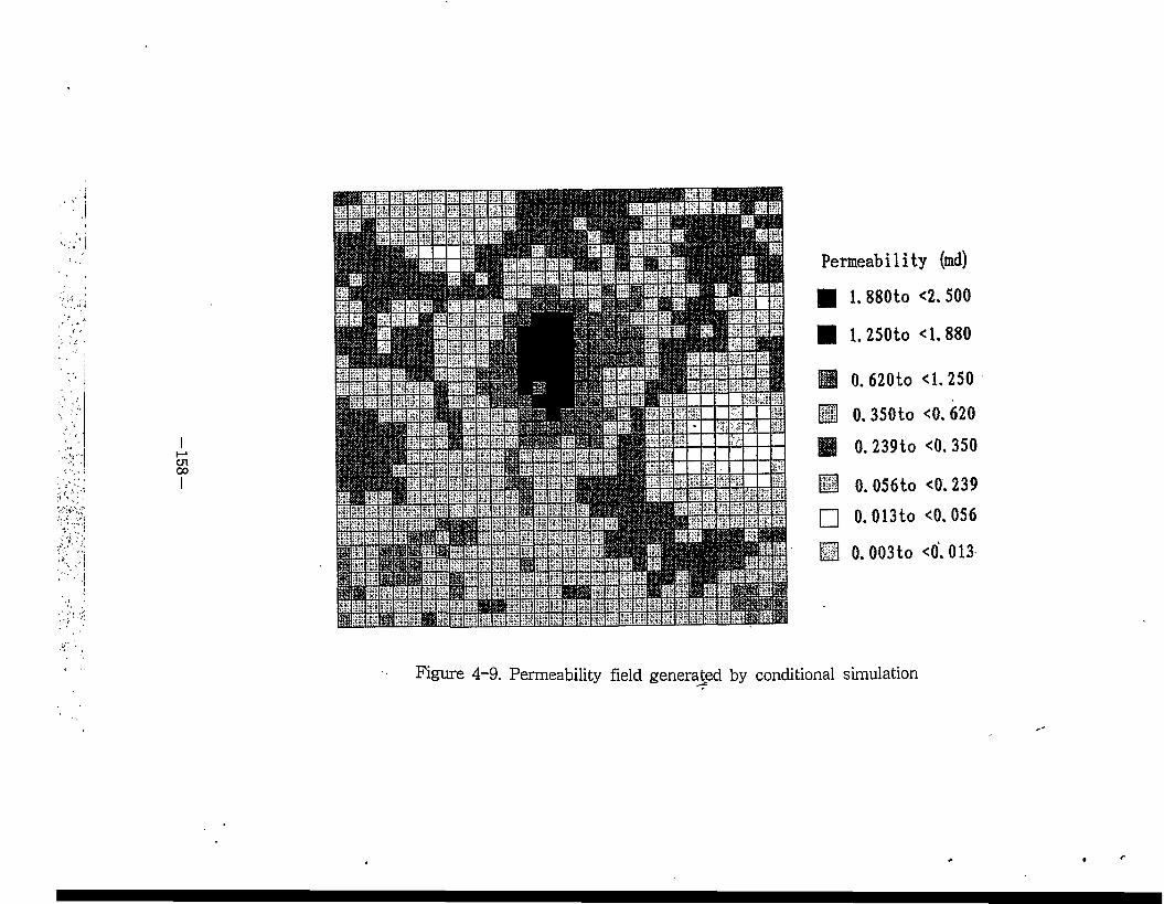
inoo
Permeability (md)
■ 1.880to <2. 500
■ 1. 250to <1.880
0. 620to <1.250
0. 350to <0. 620
0. 239to <0. 350
m 0.056to <0. 239
□ 0. 013 to <0.056
11 0. 003to <0.013
Figure 4-9. Permeability field generated by conditional simulation
•-ha IKfS ^ agr
#-§-# ^"g-kWR) k kMlalHWirk Ms-to-fc k^k fc#-^k k>
-k-§-k -f-^k #kh Ma-h "h!o ^ # nrk# hkkk aws'k R#
#M3 M3ED3 344 44# 4# 44# e»#3 4 4 #44444. »«II4 43# 444# ss# e@114 1?$#
s., 3.4 JL lif?gmi§4 3444. 4 343# MmfI4 #3# 4444
444 SrSIK S343 #4, 44, 434 4^-4444 44 3#&
334s3 44. 43 JtrMIS 434 344 444 444# MJE4
3 4&31 3M- 4# 34 44 5.4s #A44. MM3 «34
SH 3&# 43 4444 43 4 ffl¥flr 35.71 a# 3334 143
34# 544 5# 334 343 443 4444.
3-1. ftpjg 3Sifs| S3
M mm# 443S4 4443S3 444 44#5 44 44. Hr Ml 434# 4443S3 *# 543 M. 44353 #s3 44 ammm* =la 33-4 44#5(aiiPhatic ho# 44# 44#5
(aromatic HC) 2713 5 4#4(Table 4-1). 34# 44#5# 43 443 44#5(alkane), 4143 44#5(alkene), 43143 44#5(alkyne), #43 4435(cyclic) 4 4713 & 4#4. e@mm3 44435# #, 3 5, 437>s, 1#, 443571 34#& 4344 IS, 4, 454 s#3 44#4' resin# asPhaltene3 54454, 3*71 431 41, 444##5 544s- 44.
444 443S(alkanes)# CnH2n+24 #33# 33 s 354 54 4 435 5# 4443 443555 #3 #4. 343 4435# 454 #7} #7144 44 #53, ##3, 4 #3 #714# 34# 4414.
-160-
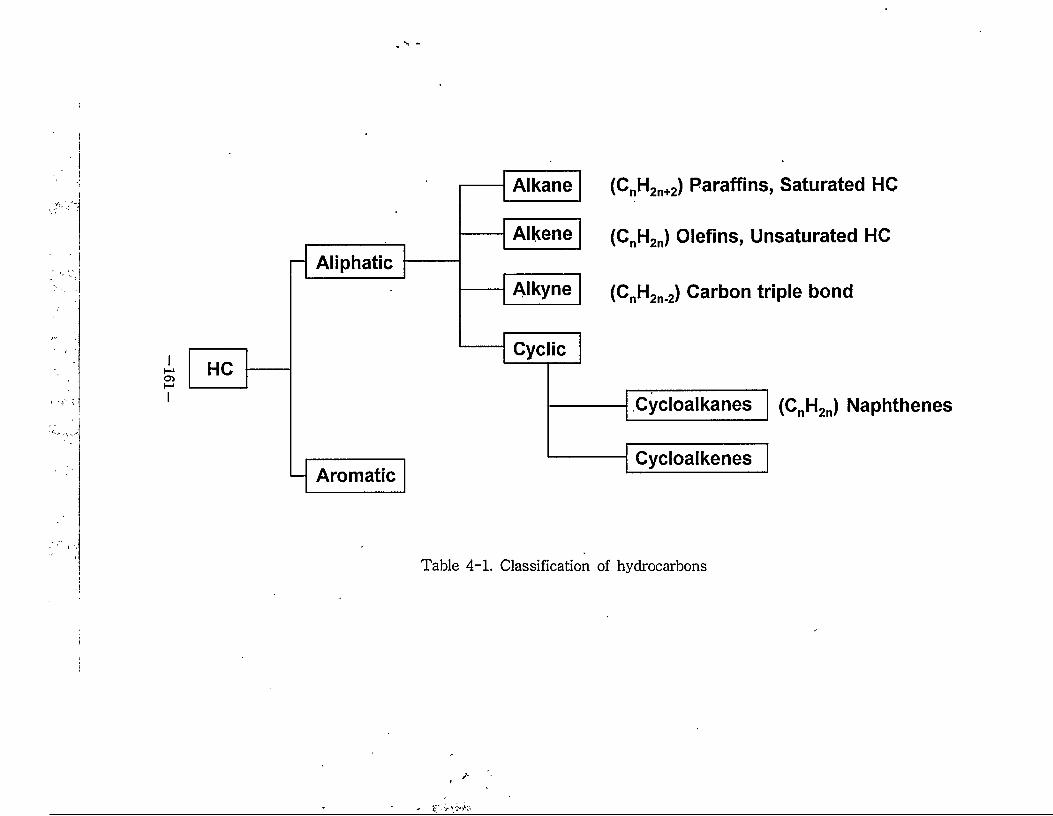
(CnH2n+2) Paraffins, Saturated HC
(CnH2n) Olefins, Unsaturated HC
(CnH2n.2) Carbon triple bond
(CnH2n) Naphthenes
Alkyne
Alkene
Alkane
■— Aromatic
- Aliphatic
Cycloalkenes
Cycloalkanes
Table 4-1. Classification of hydrocarbons
Figure 4-104H 5# 44 41 ##1* 14471 4435 411 44 130°F4 #7l* S.e-14 4#*7l #7144! 44 *7l#l 4^41 l7fl
4#%# 4 35 - 55 °F1 ti]H4 444 #7}# 4444. ##14# 4 = 7ll 4444 444 #7l!## 3°H 4% 44.
44 7>44 3.4 (branched chain)* 1# 141 44*## 47>47> #444 #14#* *7> 444 4444 4#4! ##44 ##44 5* 4#4t11 44. 141 44*## 4# **! 44*# #4 444 35 444444 444 4*44 44. 344 3.444 *#1 44 4 4344 44# *444. *#7l #*4 5*444 4*71^4 *5! 414#7l 71*44.
4444 44*#(alkene)# *5.4 444# 5# *44-—-S- *4* 715.44 CnH2„4 *7M* 5>#4. 4144 44*#! W* 444 44*#4 *444 ##1# 14 4#* *7M 4 35 - 55 °Fl 114 *7>* 543 14. 344 4#4 4#444 4#14 *5# 444 4 4*#34 *4144 441 4*14 *4.
44144 44*#(alkyne)# 4#4 4#444 3# 44 *5* 7}
14 CnBbn-zl #714# *3 44. 44144 44### 444 1 4 144 44*#4 3 ##4 #7144. 44144 44*#! 441 4 #1* 444 44*#4 4144 44*#! *444.
4** 44*## 4435 451# 44*#5 4*# Ml 1 * #* 1* *5 43 44.-44! 1*5# 4#4 4#7MM 2# 44*
43 4# 4* 44*#!-* 1! 44135 4# 4144. 44# 44*## 3 4#47-1 4 * 4*4 411- 143 $114 44135 #1 °1 1*44. 44* 44### #41 44*#4# H 441 4# #4 5 441 1*#* SI &*4.
-162-
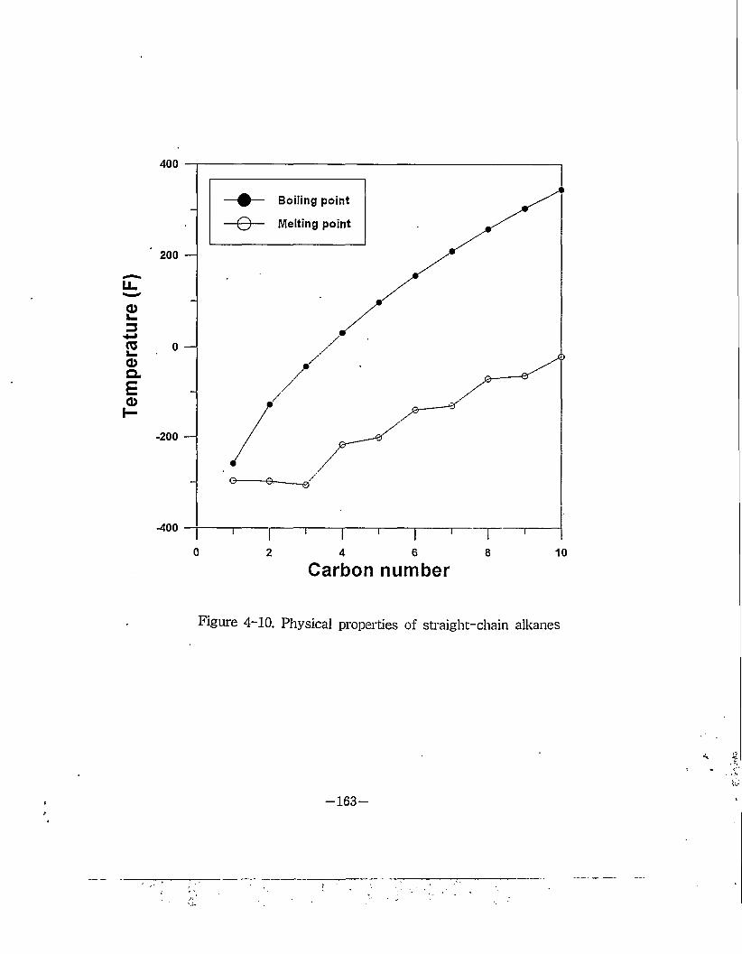
Tem
pera
ture
(F)
-#— Boiling point
■0— Melting point
Carbon number
Figure 4-10. Physical properties of straight-chain alkanes
-163-
44 #4 4444 444^34 4444^34 44#3 44 $14 M -^15. n -§-37} 4444 (Table 4-2) 4 444 444 447}
^s. Ci44 Cg444 44& 7}431 $134, 7^44414^44 ^3 Ci44 Cie4444.
3-2. If* Sftta-21
3# «4 441- 4^44 44, 43, 41:44. *044
7}^b44 ^44^ 3444 7}it M444 43, ^4 4»444 444 43, 454 444 44 3 * (phase) 4 44 444. M44T 444 114' M-4 H?«fi4 44, 43, 4M 444 34, 7}3, 7}^4#4433 4¥444. 7}]4437} §}^ *044 7}^ 04
#4' 44 4#4 4444 4 4£4 44 44-434 Fig.
4-114 44 4444 44. ffi¥E@7} 4444 flr*444fe 44 &4 M434 444 34, 7}^, 7}344443 ME33. 4M4. 4, 4*437} 4 443(critical temperature) 444 ^444 3^ Hr*# 4 44 4*437} 44434 4443(cricondentherm) 44oj] 4144: ^4
44 7}^^#443 e*#4 43 e*437} 4443 444 ^44
7K#*#4 44.34 E*@4 ^4 117} ^3414 44 444 437} 4344 A3
4444 244433. #47}4 44 434 444 444711 44 44 Bf*m#*]M 7}37} 4444. 444 344 44 7}37}^444. 7}34«43 Kt*®444 li?*44444 «7} 7}3*g33 #7#}4 m^7} 73444 44 4#4 44& 44711 44 454 444 7}^M4 444 44711437} 4444. 44, U*444 43
-164-
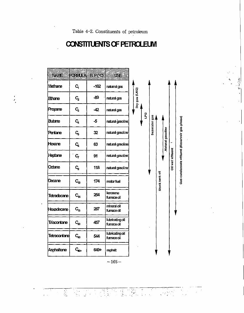
Table 4-2. Constituents of petroleum
CCNSmUBITS OF PETROLEUM
| NAME FCRMJLA BP(°Q USE
Methane c, -162 naturalgas
Ethane 0, -89 natualgas
Rnpane Q -42 natuaigas
Butane Q -5 natual gasoline
Pentane Q 32 natual gasoline
Hexane Q 63 natual gasoline
Heptane q 91 natual gasoline
Octane q. 118 natual gasoline
Decane C.0 174 motor fud
Tetradecane ^14 254 terceenefunaoedi
Hexacfecane C.6 287mineral dl funaoedi
Triacontane Qo 457liiaicab'ngdlfunaoedi
Tetracontane Qo 544liixicatingdlfunaoedi
Asphaltene 649<- asphalt
—165 —
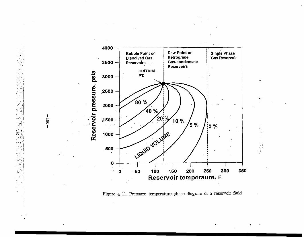
Res
ervo
ir pr
essu
re, p
sia
4000 —|
Bubble Point or 1 Dew Point orDissolved Gas '! Retrograde
3500 — Reservoirs [ Gas-condensateReservoirs
3000 -CRITICAL j PT. |
2500 -
Single Phase Gas Reservoir
50 100 150 200 250 300Reservoir temperaure, f
350
Figure 4-11. Pressure-temperature phase diagram of a reservoir fluid
-Z9I-
toiilkb •p'k kb bbb brSkHkio kt# -obb lb Utlk fo bH"t-
‘Is* bkbb t-kir #b i?k bb Ib^M tMM b# "S' bistHk #tln bklk Ip Si lb fc bis to tb##S# #b lbbkk btk Wo&b tMM tb Mdz® kk&b tlkbb
bio t # #-#-&b H"o"
## kb k#b to tY"fe"H"iS k lb## kir kWk io kif""n"iY' b k Ik toks ’-bio "zrja-s- b ’S'rSt'k^r k lbH"-k"b# lb k-S- bis# b "§“o"kio t# klbk-kM bbk Si2 bb lb#fek •s-oSib'S" klbSb?b bn wa b# -bb IbZI-fr ’Sm b@SM toMM kb#k b#
bkbt 5* y{z tlbM Io3XS/j[0S
000*001 ablkF^vb tk kHXS/XOS 000*001 - 000*8 b^Tfl
"o-^b bistt ToS -irk baxs/aos ooo's b^bT-?bbtb kbb bb ^vtktt toiisii *q?b?-?b 1st bb b##b ## %# to bib ‘bln bR>"5" *?TR,'5'-?b kk klbS-fr TO
bisk kistb biB @#tBi t-k bTT-k ’3H klbbBbis# #bk t b kk bb^ lb# b?b bklb'S'k bb#
b k&z bkbkk #b Ikkk Mb kb bis# #bk b bH3B -§■’5' "^-to kbkk biib'5' ^klb^k b# kbb# 'S’tbb k #2 bktkk kb@#dzSi bb lbkba"b bkk #?bkb bis ## "g-t# 2 ^bk# b?bkk Mkkfo Mb bSM ?b
bbkk Ibkt b"abibbk b?b #klk>$k kbb bbbfo b tat Si bisTb blk bsb bkb kW#^ ’bb Ik# ^#bw bb blM iris# k« bis# kkb tip#bw kb ttb tSibir bkk kb btac bb Ik is Ik# bk# bBipo^ b#7b TklbSM bb Ikbb# bk&2 bis
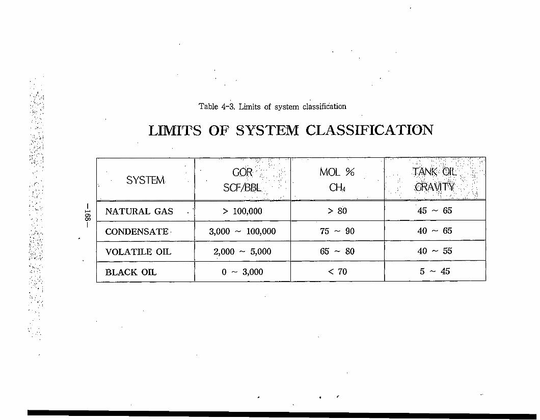
Table 4-3. Limits of system classification
LIMITS OP SYSTEM CLASSIFICATION
SYSTEMCOR
SQ7BB1.MOL %
ch4
.... WWLir
NATURAL GAS > 100,000 > 80 45 ~ 65
CONDENSATE 3,000 ~ 100,000 75 ~ 90 40 ~ 65
VOLATILE OIL 2,000 ~ 5,000 65 ~ 80 40 ~ 55
BLACK OIL 0 ~ 3,000 < 70 5-45
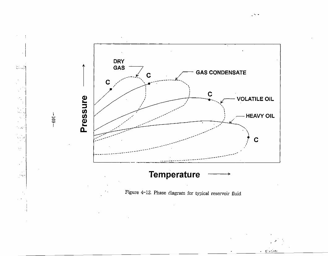
Pres
sure
GAS CONDENSATE
VOLATILE OIL
HEAVY OIL
Temperature ------- >
Figure 4-12. Phase diagram for typical reservoir fluid
Z
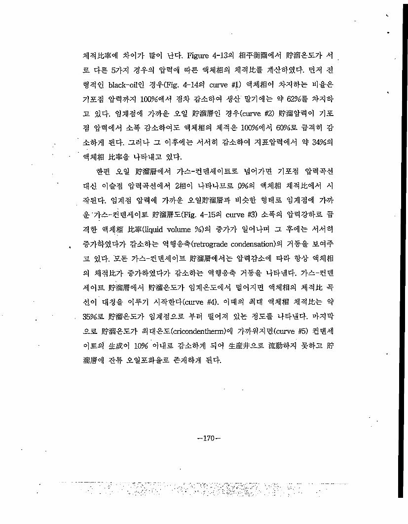
4*JtM *47} %4 l+4. Figure 4-134 *f#@44 #@*57} *3 4-E 57M #** 444 4# 44*4 44it* 4*444. *4 * ### black-oil4 #*(Fig. 4-144 curve #1) 44*4 444* 4** 7] 3# 4444 100%44 44 *5*4 4* #44* 4= 62%* 444 ji $14. 4444 7>4ir 3# #@@* 4-f(curve #2) #@#44 434 #444 54 #5*45 44*4 44* 100%44 60%3 #44 * 5*t]] *4. ^4# ^ 4*4* 444 #5*4 4*#444 * 34%# 44* Jt$i #4-4zl #4.
4* 3# #@@44 7}5-# #4 4 S3 447}# 45# #4#4 44 4#4 #4*444 2*4 4*45.3. 0%# 44* 44It44 4 444. 444 #44 7}** 3##@@* 4*4 #43 4444 7}* *7}5-##44S #@@5(Fig. 4-154 curve #3) 5*4 #4*45 * 44 44* It#(liquid volume %)# *7}7} #444 5. *4* 444 *7}4#47> #54#- 44-S-*(retrograde condensation)# 4** 34* 31 #4. 3* 7}5-# #4 4 s #@@44* #4*54 4# 4* 44* 4 44Jt7} *7>4#47> #54* ##*# 4** 4*44. 7}5-## 44s #@@44 #@*57} #4*544 *44# 44*4 441b *4.4 4** 4*7] 4*44(curve #4). 444 #4 44* 44lb* #= 35%3 #@*57} *4*33 144 #* #5# *##*. *4*33 #@*57} 4 4*5(ciicondentherm)4 7}## 4 #(curve #5) ##4 4S* Am4 10% 443 *5*7]] #4 A##33 m#*4 ^*jl ^@@4 *# 3#3**3 *4*7)1 **.
-170
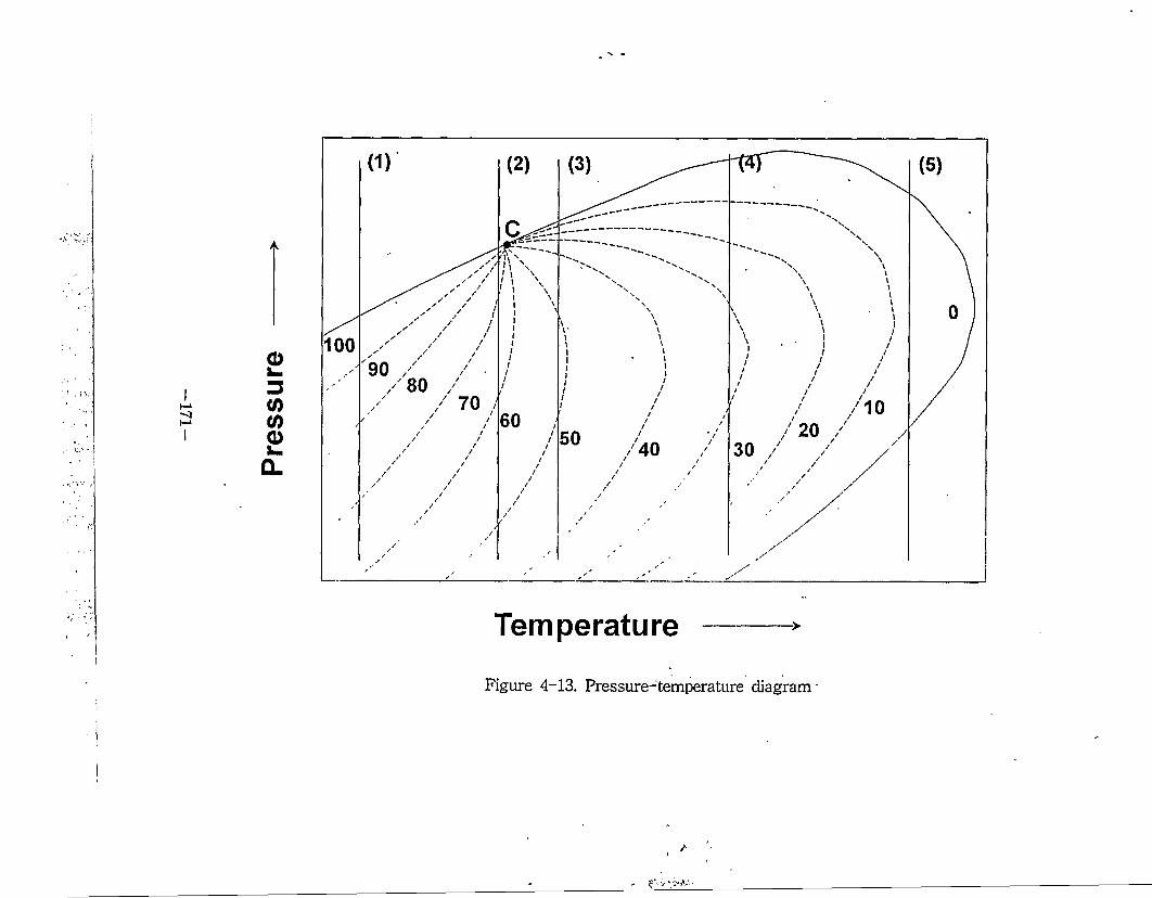
Pres
sure
Temperature
Figure 4-13. Pressure-temperature diagram *
/*
Liqu
id v
olum
e (%
)
80 —
60 —
20 —
Pressure (psia)
Figure 4-14. Liquid volume profile of oil reservoir
-172-
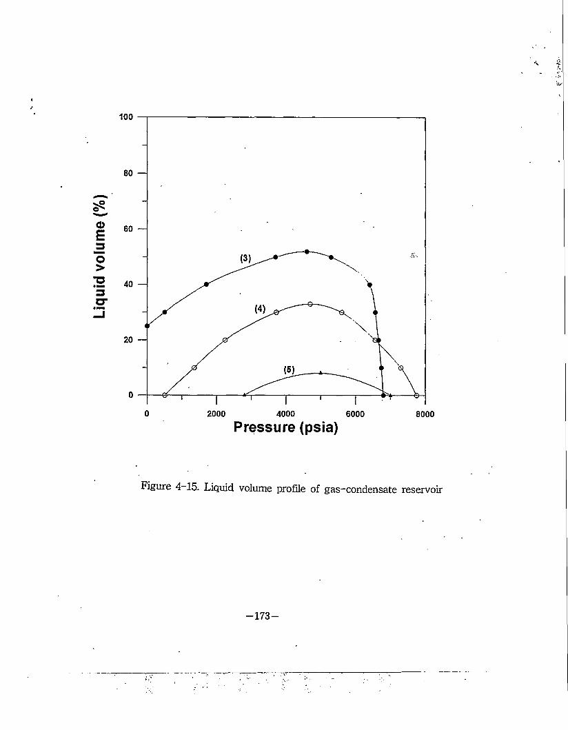
80 —
60 —
40 —
20 —
Pressure (psia)
Figure 4 15. Liquid volume profile of gas-condensate reservoir
-173-
3-3. A|SS| xH*|
7} A A# 7>^Mo]h EH^S. 4# #A*}
4. 4 All sexist 7WM41 e@E4 4% ffl¥ir 4441 4 #4 7l#44# ¥1# ¥ $14. m#§4a# 44 %#4
#4# A## #A4 $14.Ir®miI4 114# 27H7]- $14. 44# 44 7114 (bottom
.hole sampling) HAS. ¥& #A# A#Ir®E47l 4444. tit A
.4 ¥®)f# ME444 BH7]- MAS. #4471 444 4444 # ffi mm# 41 7fl44# 44 A#444. 4# 44# A# i|»»l 4 7>aE^E(7}a-4 #7ii 4 a 4##- jE#)44 ¥5. 4444 44 7fl4 (surface sampling) H AS. 44 #5} 71 (separator)4 4 #44 7>A4" A
4# 44 7# 44 44 G0R4#4 44 If4444 M# 444. 7> a It®® 4 4 A# A 4 It®®71 b) ^4 4444 244 msi7> #44 #71144 44 44 m MAS.# 4A4$l# 4^7#7} 414 4# 4 #4444 4A# 7#4# 44714 11# 4#44 #4. ## #A 4 A# B®#44A 447W1# 7}## # $14. %± 7114*14# 7}
A-AMl 444 44# 4444 44. 4 5%4 7>A-A$)J:k4 A7># 100 psi 444 4#4 41 A4# ##44 €4.
7>a*1s# 71447I 444# 44 %#4 44# A4(well
conditioning)44 4 44. 7}#44 I?®E4 -^4&7l 4 4IL# 71)444
4 44 A#¥4 414# 4A444 444 I$4 17> 4A44¥ 4&# 7H#1444 44. 44 ^34 GOR7> ^44 444 4444 4
4. A# 444 43.7H4-B 4444 4#44# 44 #7>#44 4#4
71A7H4# 41## 4 #4-4 4#§H 4 #444 44, 4&44 41#
174-
444^ 4e# ir^s, %m4a-44.
A)S7l)#H 7) ##4 4 # ^1-SSr 444 7}S, 4S7))4 #-
W# 544 7H^|4s4 454 "W4, 444 #5 ne]3i a) #2}- ^.<g-
71-54, 7^7) #4 tifly. ## *j)^ 4s^) MA4 4444 #44.
7>54s4 *113# 544 s# 7^0)1 a).#*}# #7)5.4 ##4# a}#s>
4 44. 45.7))#] 444 <#§)# #444 444 4-f444 #4455
100 psig 4M4 44 #M4 444 #57> 4S7H^| s# ##4711 #
44s# #4444 #4. 7>dh#oflx] ^#4# 4&44 4 s*(representative sample) 47) 444 5# 2-37)14 7}iA]sf 4] 447)1
44 7))#)4 4s# #1*5 54)4 mm, rn#44* #44 l7l) 4 s*
44441 44 7fl#)4s<>)l 44 44, 4444# #5. 7)^4 444 4
a#7)4 44& #444 424 4# 4s# 4447)1 44. 54 444
44 4#s. 44 444 4&# *}&*}*] #47)1 4 4# 4 ##55 4
#47) 444 2-37)1 444 4 a# 44444 44.
44 4s7fl#)A) #4# a>%o.s. 4#4 4# 44 44.
® A) 57)144(sampling line) 444 trap# #4# 4
© 457)144# 7y#44 #4# 44# 4
© 4 5 7)|44# 7>#4 4 #7)1# 4© 4a 7fl#)4 M4 1/344 ### 4444 4 s*'7)14# ^
© 500cc##4 stainless steel, carbon steel# a)-## 3)
© 45 7))#)|u #7)# 44 ^544 4#4#^© H2S7> Hf-4 7}AzA)S# ^4* 4##7)4 #5) 5# Ell#
€1S 554 #7l# A}## a
© H2S, C027> 544 71-54S# 4444 #4# 4© #44 27114 #714 #** 4#55. 4s# 44# 4
-175-
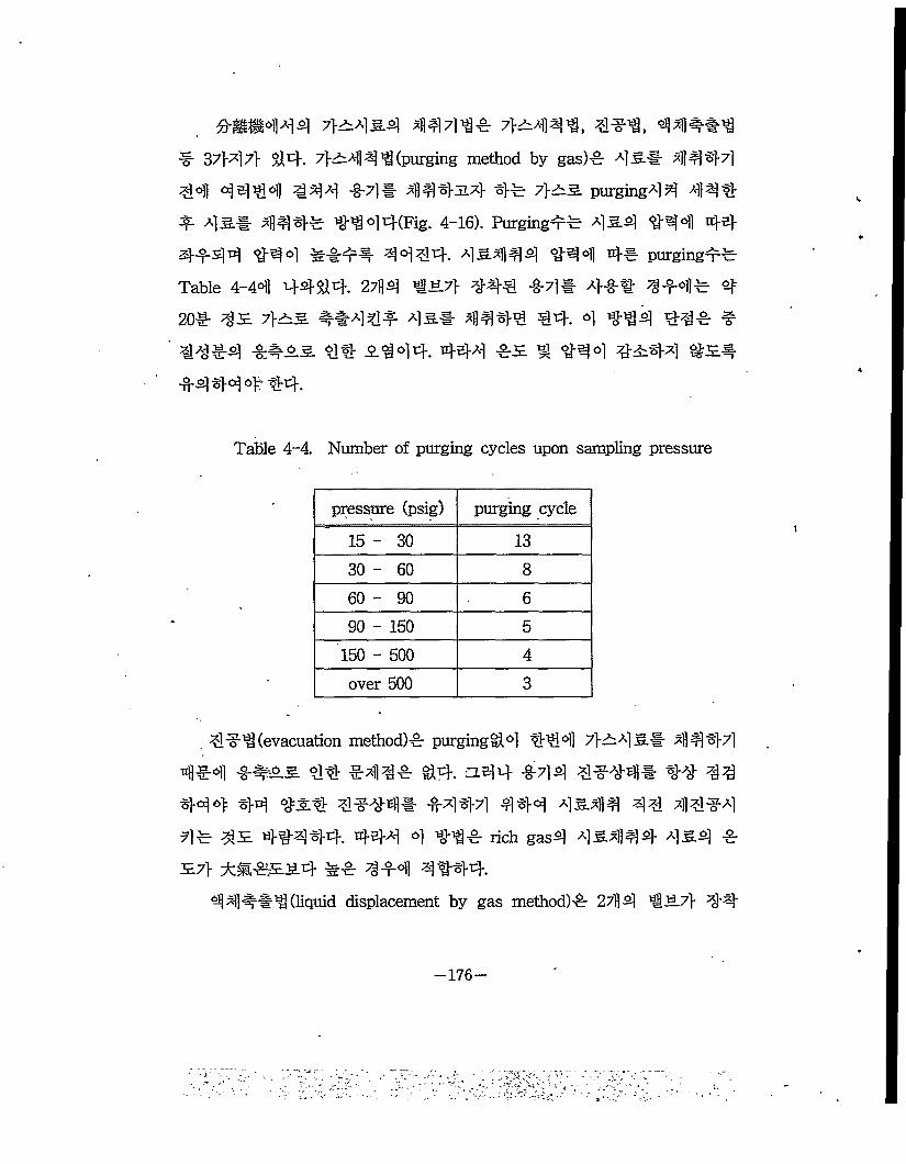
!B§H44 7>^Al5.d] ^y^l 7}^]^^, 414, 444*4
1 37>^17} $14". 71-^1444 (purging method by gas)-Sr a]5-§- 4#) 47]
4°)] o] B] 4 °)1 144 -S-7]# 7i)^y>317,> 4! 7>^hS. purging A] M 444
1 A) 5.1- ^44! 4444(?ig. 4-16). Purgingl! a] 52] 4^4 44
4144 4^4 ^111 4444. 45*1144 444 41 purging^! Table 4-44 4444. 2?M 1S.7> 444 14# Aj-g-1- 4141 4=
201 4s 7}Az& 4#A) 41 A) 5.1 4444 44. °1 444 441 1
4414 1*S3. 44 S.444. 444 is 4 444 4^44 #s#
14 440^ 44.
Table 4-4. Number of purging cycles upon sampling pressure
pressure (psig) purging cycle
15 - 30 13
30 - 60 8
60 - 90 6
90 - 150 5
150 - 500 4
over 500 3
. 4(evacuation method)! purging§14 444 7>a^a] 5.1 *]] 4 47]
4114 44 *44! §14. -t44 144 4144* 44 44444 44 4&4 4144* 1444 444 4544 44 4414 41 4s 44444. 444 4 44! rich gas4 454#] 4 a]5.4 1
S7> ±#!SS4 ^r! 414 4444.4 4 4#4 (liquid displacement by gas method)! 27]] 2] #5.7]- 44
-176-
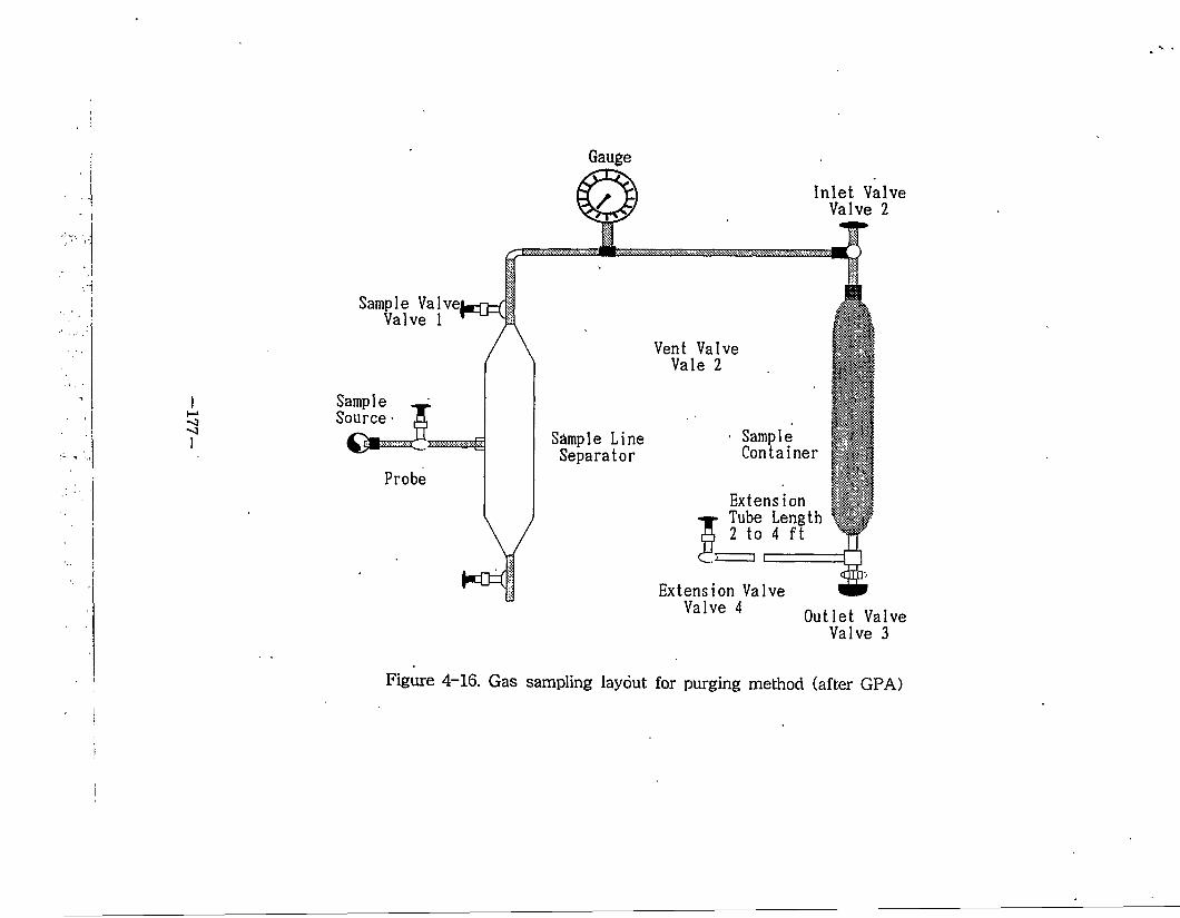
Gauge
Sample Source■
Probe
ko=(l
Sample Line Separator
Inlet Valve Valve 2
Vent Valve Vale 2
l
SampleContainer
Extension |§llSi Tube Length lbs2 to 4 ft
3 C
Extension Valve Valve 4 Outlet Valve
Valve 3
Figure 4-16. Gas sampling layout for purging method (after GPA)
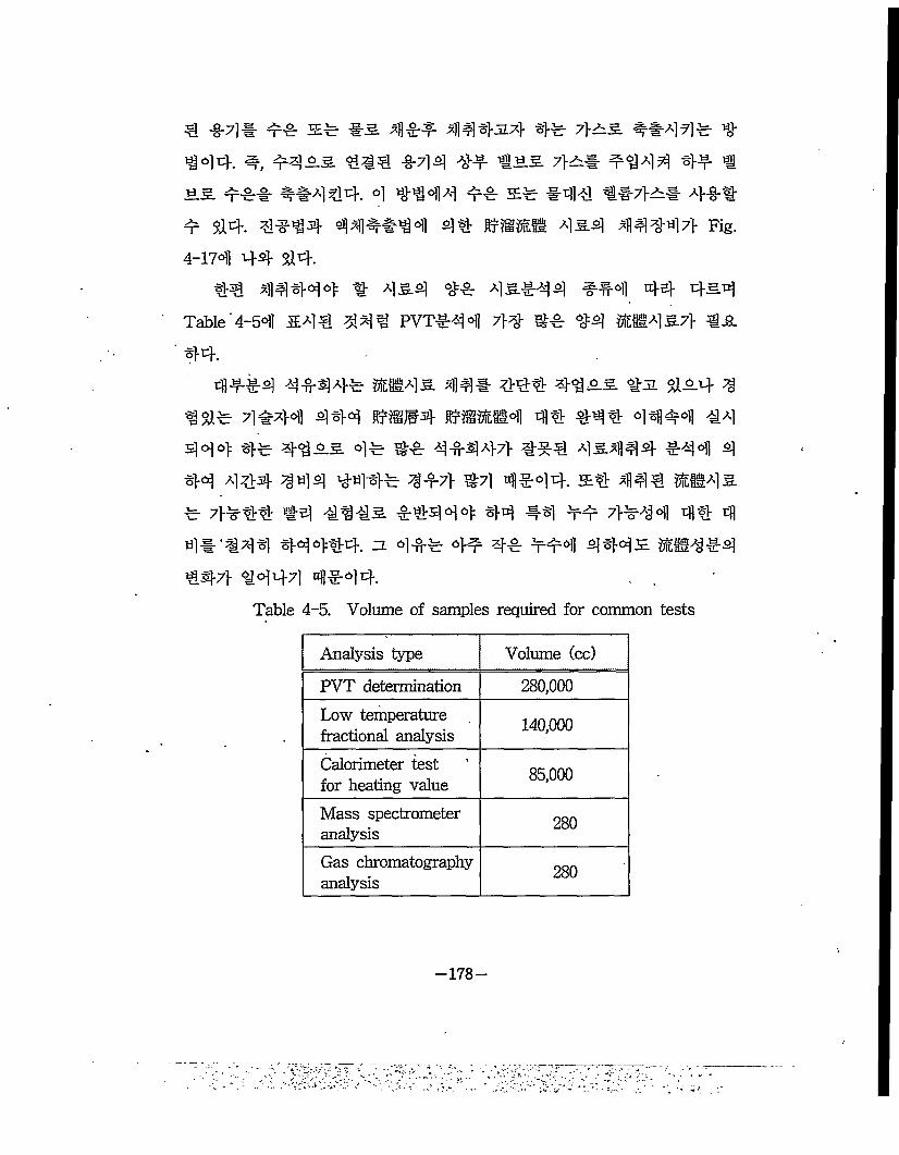
4 -0-7]* ** s* #3. 7]]*f 4* 7}^3 **A]7]* tij-^»]4. 4, *4^3 444 -0-7]a] ^ *ti5. 7>^* to44 §pf #
33 *** 4#444. 4 Mto ** £* #44 1*7>^* A}** 4" $14. 4to4 to## to 44 flx«fi 4^4 443-47} Fig. 4-174 44 $14.
44 44444 # 4&4 4# 4 3.*# 4 ##4 44 4toTable 4—54] &44 443 PVT* to 7>4 #* 44 EH437} *3
444**4 4444* m#§4& 7#* 444 44£-3. to $134 4
3$1* 4*;<M 444 ra@4 E=M®4 44 444 441*4 44 444 4* 4433 44 44 44447} 4*4 4&7]|^4 *44 4 44 444 344 to'to 3*7} #7] 41*44. a# 4144 «43 * 7}*44 #4 toto *4444 44 44 to 7}*34 44 4 4#'to 4 44444. =l 44* 4* 4* to4 4443 EH3*4 44-7} 4444 4to4.
Table 4-5. Volume of samples required for common tests
Analysis type Volume (cc)
PVT determination 280,000
Low temperature fractional analysis 140,000
Calorimeter test for heating value 85,000
Mass spectrometer analysis 280
Gas chromatography analysis 280
-178-
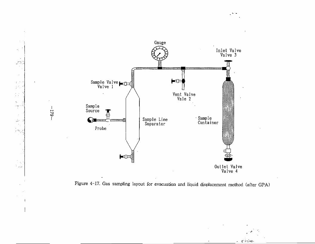
GaugeInlet Valve
Valve 3
Sample ValValve 1
Vent ValveVale 2
SampleSource
• SampleSample Line Separator Container
Probe
Outlet Valve Valve 4
Figure 4 17. Gas sampling layout for evacuation and liquid displacement method (after GPA)
3-4. ?\— 4.5.—I #4
7}2 2# 7}2ll4]o]E Mjf^l 2|7># 44 2.0} ^||
2#24 Fig. 4-183} Fig. 4-194] 44 44 $14. so} ##oj] 444#
2444, tKE #4 4# 7}224# 44, 7}^-21 4-4#4# 444 44 #244. EE1-44] $144# 4 #4 #4, 4-441 #4, 144# 44, 42444 #se}c}.
#444 7}2a]s.7} 2444 44 ##1 44# 44447] 444
4^ 140 °f 2# mm m$/M 24 20 °f #4 4-22 7}<s44°} 44. 444] 4 24-4 424-44 44 42421- 424-4 41-4 2# 7}2
# 42440} 44. 124 #444 42#4# 414% 4 #4] 1:2414
444 24?}4 #44 4-4# #44-4 ## 4## 1444. 44 42
44 #23} #41:24 #44 41 #44 $14 41 144 !#4 4
#4 44#2 44-22 7}##44 14. 4#4 14 44, 4414-7}
#41 7}4: 4&41 42# 4444 4444# 444 GC4 #414.
Fig. 4-194 44 44 14 7}24 21424 44 44# GC4 4 44 444-4 #1144 fifS WT4 mm2 4441] 14. 7}i42 4 4444# 14422 Ci44 Cell #444 2#42# 0444 C35 44 #447]] 44. C?+* 244 »44# 4#44 1 1# M44 4 44 444 #4444 44. 444 UrMSIt- 4 #44 flr^#2 144 4# 7121 #4(bubble point pressure)6]4 4#1 #4(dew point pressure)#- #4 44.
—180—
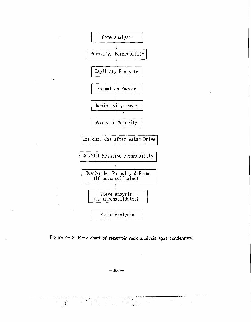
Fluid Analysis
Acoustic Velocity
Resistivity Index
Capillary Pressure
Formation Factor
Core Analysis
Porosity, Permeabi1ity
Sieve Anaysis (if unconsolidated)
Gas/Oil Relative Permeability
Residual Gas after Water-Drive
Overburden Porosity & Perm, (if unconsolidated)
Figure 4-18. Flow chart of reservoir rock analysis (gas condensate)
-181-
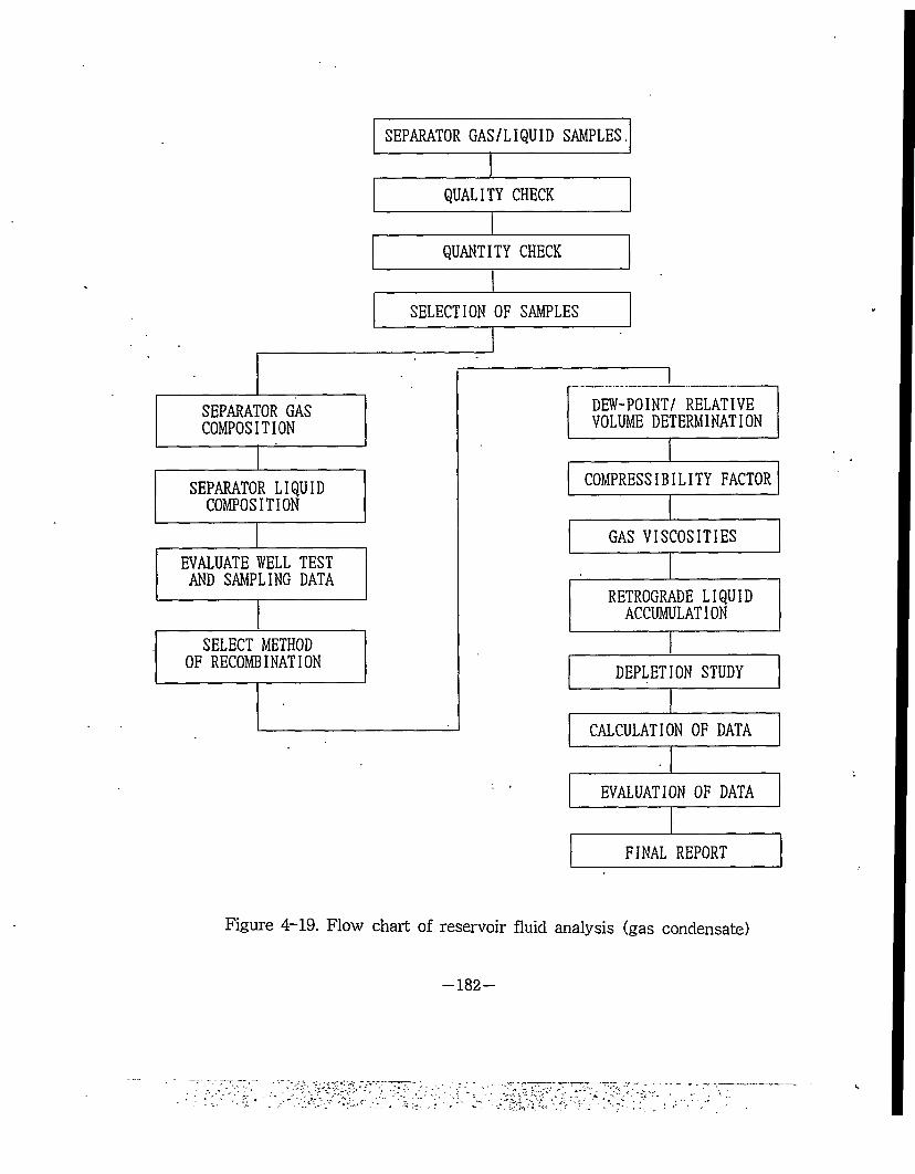
DEW-POINT/ RELATIVE VOLUME DETERMINATION
CALCULATION OF DATA
COMPRESSIBILITY FACTOR
FINAL REPORT
GAS VISCOSITIES
DEPLETION STUDY
EVALUATION OF DATA
QUALITY CHECK
SEPARATOR GAS/LIQUID SAMPLES
QUANTITY CHECK
SELECTION OF SAMPLES
SEPARATOR GAS COMPOSITION
EVALUATE WELL TEST AND SAMPLING DATA
SELECT METHOD OF RECOMBINATION
RETROGRADE LIQUID ACCUMULATION
SEPARATOR LIQUID COMPOSITION
Figure 4-19. Flow chart of reservoir fluid analysis (gas condensate)
—182—
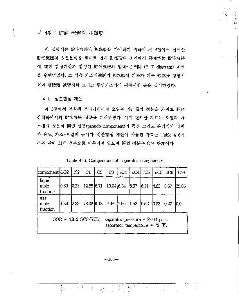
4<g : mm ###
4 4o!]a^ «M! 444-71 4)4-4 4 3444 444MM! 4##4-& stfls 44 e@#4 ^444 #444 e^m# 4 44 44444 444 MM! 44-#£83 (P-T diagram) 44 -6- #44534. =l 4# 7>^MJ»! *#®4 7W> 44 #^4 444
14 #HE ##44 ZZ.4JL #^71-^44 4441 #4 444534.
4-1. 4##4 44
4 3444 #44 #471444 A<a4 7}^#! 4#& 7}4jl u® 444444 MM 4## 444534. 44 %A4 4s.# A!4 7>—4 #4 #0 4#(pseudo component)! ^-4 zisl JL #5]7l! 4! 4 #3, 7}3~344 #44. 4 #1-4 7)144 4#4 7}&# Table 4-64 44 #4 11711 4#A3. 4 #4 4 31A4 4## C7+ 471144.
Table 4-6. Composition of separator components
component C02 N2 Cl C2 C3 iC4 nC4 iC5 nC5 fC6 C7+
liquidmolefraction
0.39 0.23 12.55 6.71 10.04 6.34 8.37 6.21 4.63 8.67 35.86
gasmolefraction
1.39 2.33 78.03 9.13 4.98 1.50 1.52 0.52 0.33 0.27 0.0
GOR = 4,812 SCF/STB, separator pressure = 2,000 psia,separator temperature = 72 °F.
—183—
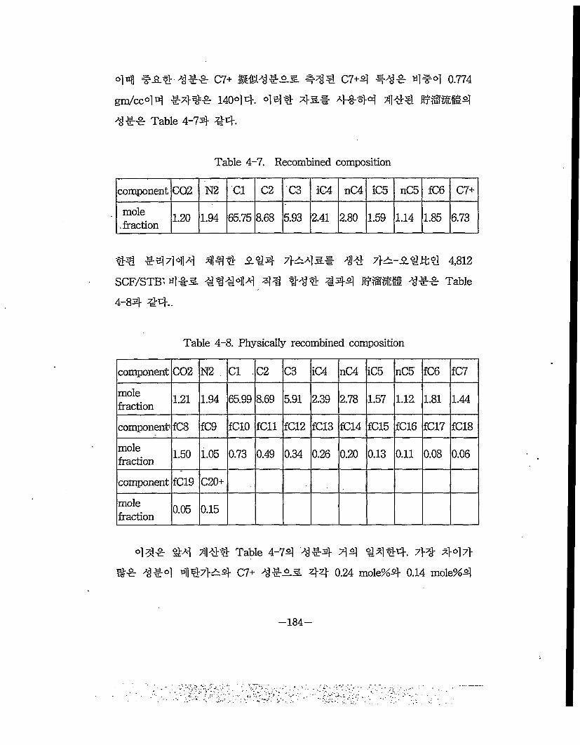
e»H C7+ 4^4 C7+4 4## 4 #4 0.774gm/cc»H #7}## 14044. 444 4&# 4-0-44 44€ HtWH4 4 #4 Table 4-74 44.
Table 4-7. Recombined composition
component C02 N2 Cl C2 C3 K% nC4 1C5 %C5 fC6 C7+mole.fraction 1.20 1.94 65.75 8.68 5.93 2.41 2.80 1.59 1.14 1.85 6.73
44 #4444 44# A#4 7>a4M 4# 7}A-A41k4 4,812 SCF/STB' tilirS. #4444 44 #4# 444 Br«II 4## Table4-84 44-
Table 4-8. Physically recombined composition
component C02 ! N2 Cl C2 C3 iC4 nC4 iC5 nC5: fC6 fC7molefraction 1.21 1.94 65.99 8.69 5.91 2.39 2.78 1.57 1.12 1.81 1.44
component? fC8 fC9 fCIO K%1 fC12 fC13 (C14 fC15 fC16 fC17 fC18molefraction 1.50 1.05 0.73 0.49 0.34 0.26 0.20 0.13 0.11 0.08 0.06
component fC19 C20+molefraction 0.05 0.15
44# 44 4## Table 4-74 4#4 44 44#4. 7}4 447} ## 4 #4 4#7}A4 C7+ 4#AS. 44 0.24 mole%4 0.14 mole%4
—184—
#47} 44 444 4** 44 44431 44. 444 4#44 314* *#*314 444 m®#4* 44 44#* 4 * 44.
4** 44444 #44 IfMlt 7}# 5 *4-*5# *S¥@i*31*4*4. *4-*5# 31#* 4 4 7}# #4##4* 4*4 ^4—4 7}# ££4 4*4* 4*4 4* Peng-Robinson *4*44* °1 *#44.
, = _____ ____________gLn__________p V - b ■ V{ V + b) + b{ V - b)
Fig. 4-204 444 44 #4 4 lf*®4 431*5* 152.6 °F43l 431*4* 3535.5 psiaS. 4**57} 200 °F4 7] 4*4 7}^44 45 #@#31 4**4 &7] #@#31314* s*31 «5 *3)#5 *4. 2*7] 44 44*4(cricondenbar)* 3545.83 ' psia°]4 44*5 (cricondentherm)* 390.135 °FS. 4444. 431*44 #4*44 44 * ##5 *4 4S<§ 7) 3}(retrograde vaporization)* *4471 *54 *31* 54 44*544 #47} 5714*31 4***(retrograde condensation)0!*44* *4* 4*4 W4. *4 2*4 *44* *47} W4 44# ffl*#* 444* If*®* #@*57} *°} 7}5** ^445 **4
4*4 *44* **4 *## #4431 44.
4-2. 4W (Constant Composition Expansion Test)
Table 4-831 *44 #4 If*®# **44 #5%* ^*44* * *34*4. ^#4#* if*®* mm #*-* *#4 7}* *4*##* *## 445 If* 54*^44 4*44 5-64 45 mm
—185 —
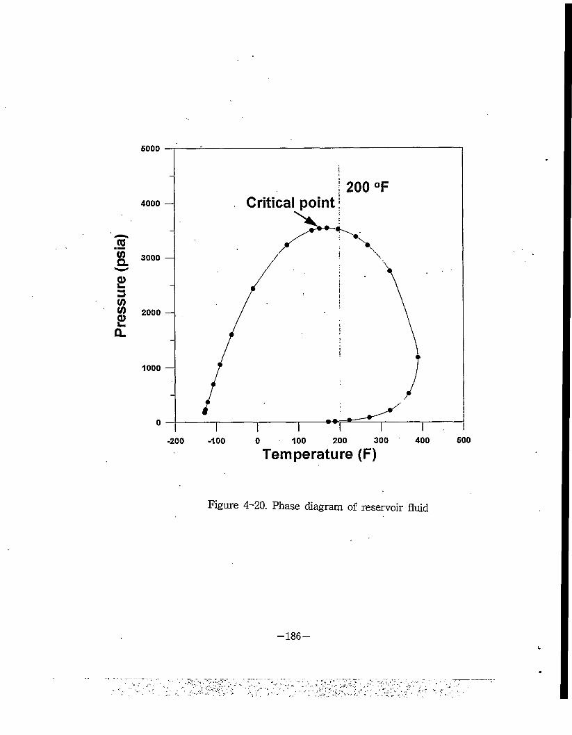
Pres
sure
(psi
a)
6000
4000 —
3000 —
2000 —
1000 —
Critical pointX
200 °F
i r-200 -100 100 200 300 400
Temperature (F)
Figure 4-20. Phase diagram of reservoir fluid
600
—186 —
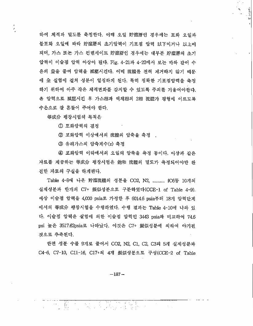
44 ^1144 #414. 44 £! 4 #4# £4 £#4#£l £#4 44 Mif4 £7)#^ 4 7] £3 #?) WT444 U_L4 44, 7M= £# 7>^ 1144s em#4 3-Mir 44#- #@#4 £7)
444 4#1 44 444 €4. Fig. 4-214 4-2244 £# 44 44 # 44 44 #4 444 *414. 44 mm# 44 4444 44 4# 4 & 4"94 44 4#4 44441 14- #4 444 4M444 #4 44 444 4# 4# 4444# 44# # Sis# #4# 4 #4 444.& 4^ss. *44 # 7>dhffl4 44*4 2* E1S7> ^44 4s£#
##££ # 4-1-4 #44 44.^5%^ 14414 #44
0 £4444 440 £444 44444 m#4 4## #4 .(3) #47>s»] <g-#7))#(z) #40 £444 44444 £14 44# #4 #44. 444 4#
4&# 4 #-4-# 4441# #% mm #S7> #41444 4
44 4-5.4 ### 44144.Table 4-84 4# 0*114 4## C02, N2, .......... fC6# 1071)4
44444 #7114 C7+ 4#444(CCE-1 of Table 4-9).
44- 4#4 #4# 4,000 psiaS. 7>41 £ 6014.6 psia#4 187)) SH44
441 #)&# 4441# #1444. #1 #4# Table 4-104 44 Si
4. 4#1 #1# #14 41 4#1 414 3443 psia4 til H.40I 745
psi ## 3517.62psia£ 4414. 44# C7+ »4#°)1 444 44 4 4£5 4444.
11 1# ## 97)1 & #44 C02, N2, Cl, C2, C34 57)) #41 #4
C4-6, C7-10, Cll-16, C17+4 471) g§M#£S #4(CCE-2 of Table
-187-
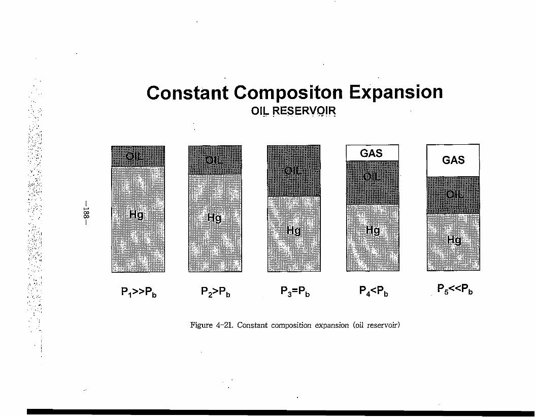
Constant Compositon ExpansionOIL RESERVOIRe « m ' » . » ^ , w
Figure 4-21. Constant composition expansion (oil reservoir)
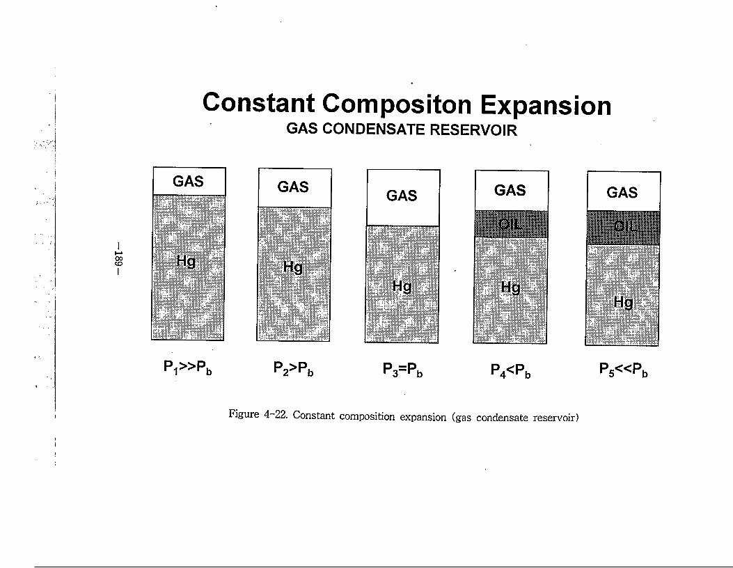
Constant Compositon ExpansionGAS CONDENSATE RESERVOIR
GAS GAS GAS GAS
Hg HgHg
•
Hg
Pi»Pb P2>Pb P3=Pb P4<Pb
Figure 4 22. Constant composition expansion (gas condensate reservoir)
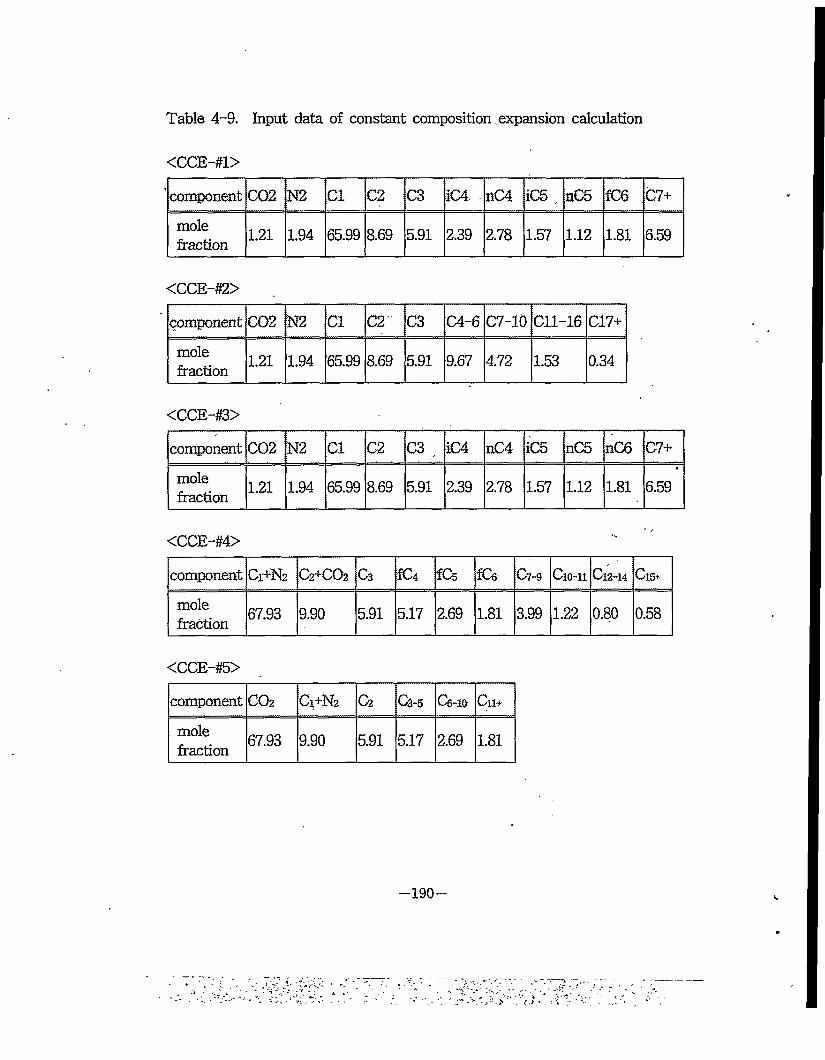
Table 4-9. Input data of constant composition expansion calculation
<CCE-#1>
component C02 N2 Cl C2 C3 iC4 nC4 iC5 , nC5 fC6 ^7+
molefraction 1.21 1.94 65.99 8.69 5.91 2.39 2.78 1.57 1.12 1.81 6.59
<CCE-#2>
component C02 N2 Cl C2 C3 C4-6 C7-10 Cll-16 C17+
molefraction
1.21 1.94 65.99 8.69 5.91 9.67 4.72 1.53 0.34
<CCE-#3>
component C02 N2 Cl C2 C3 _ iC4 nC4 iC5 nC5 nC6 C7+
molefraction 1.21 1.94 65.99 8.69 5.91 2.39 2.78 1.57 1.12 1.81 6.59
<CCE-#4>
component Ci+N2 Cs+COa c3 % fCe C7-9 Cmmi C12-14 Cl5t
molefraction 67.93 9.90 5.91 5.17 2.69 1.81 3.99 1.22 0.80 0.58
<CCE-#5>
component COz C3+N2 c2 C3-5 Ce-io Cu+
molefraction 67.93 9.90 5.91 5.17 2.69 1.81
-190-
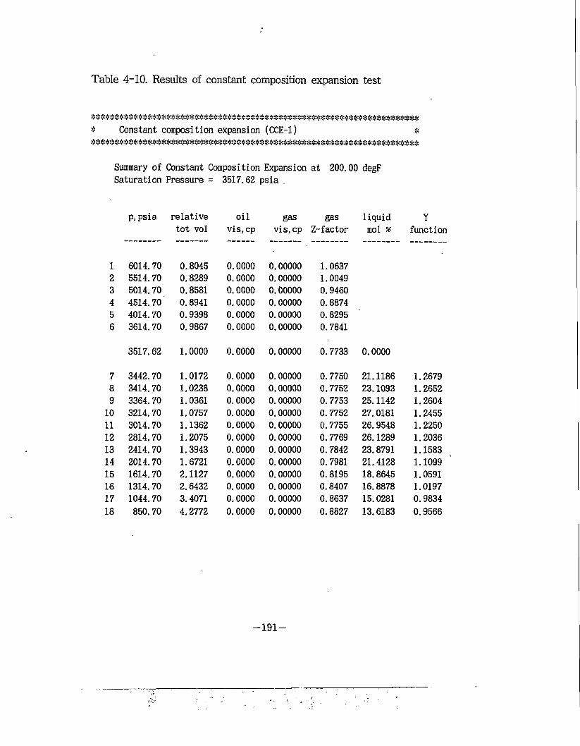
Table 4-10. Results of constant composition expansion test
* Constant composition expansion (CCE-1) %-'!<» » * * * :;<»t< * * * * * >!< * * * * * * * * £ * * * * * * % * % * * * * X * * * * * * * % * * * % * * * * * * * * * >:< $ * * * * * % * % *
Summary of Constant Composition Expansion at 200.00 degF Saturation Pressure = 3517.62 psia
P, psia relative oil gas gas liquid Ytot vol vis.cp vis, cp Z-factor mol % function
1 6014.70 0.8045 0.0000 0.00000 1.06372 5514.70 0.8289 0.0000 0.00000 1.00493 5014.70 0.8581 0.0000 0.00000 0.94604 4514.70 0.8941 0.0000 0.00000 0.88745 4014.70 0.9398 0.0000 0.00000 0.82956 3614.70 0.9867 0.0000 0.00000 0.7841
3517.62 1.0000 0.0000 0.00000 0.7733 0.0000
7 3442.70 1.0172 0.0000 0.00000 0.7750 21.1186 1.26798 3414.70 1.0238 0.0000 0.00000 0.7752 23.1093 1.26529 3364.70 1.0361 0.0000 0.00000 0.7753 25.1142 1.2604
10 3214.70 1.0757 0.0000 0.00000 0.7752 27.0181 1.245511 3014.70 1.1362 0.0000 0.00000 0.7755 26.9548 1.225012 2814.70 1.2075 0.0000 0.00000 0.7769 26.1289 1.203613 2414.70 1.3943 0.0000 0.00000 0.7842 23.8791 1.158314 2014.70 1.6721 0.0000 0.00000 0.7981 21.4128 1.109915 1614.70 2.1127 0.0000 0.00000 0.8195 18.8645 1.059116 1314.70 2.6432 0.0000 0.00000 0.8407 16.8878 1.019717 1044.70 3.4071 0.0000 0.00000 0.8637 15.0281 0.983418 850.70 4.2772 0.0000 0.00000 0.8827 13.6183 0.9566
-191-
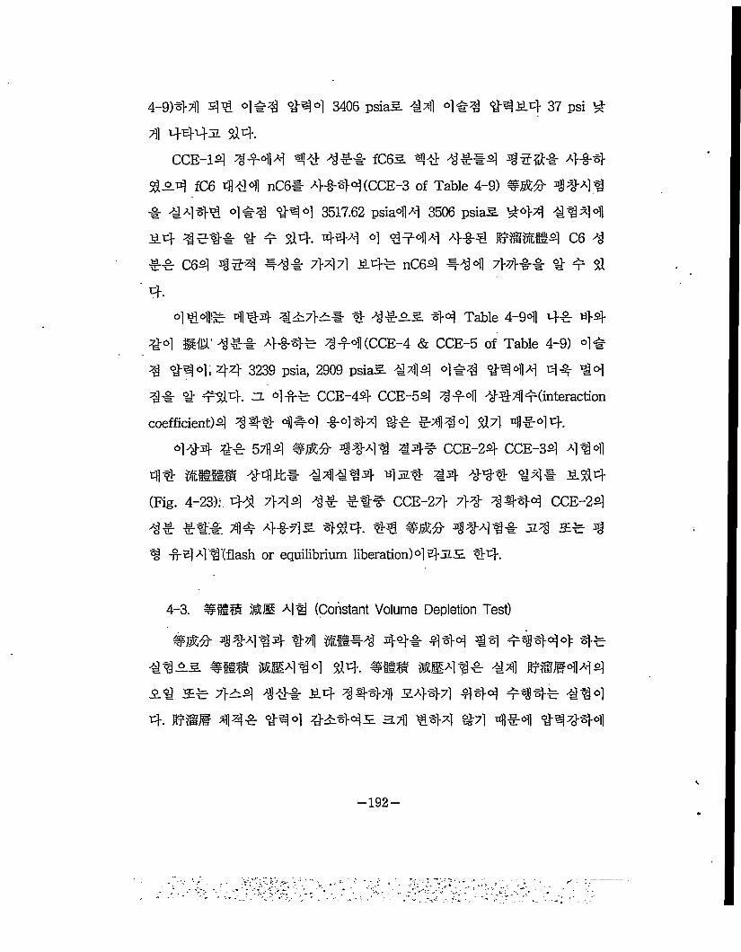
4-9)-§>t11 44 °114 14 °1 3406 psiaS. 14 °1#4 14 54 37 psi 4
Til 4445 $14.
CCE-15 114^1 451 fees. 44 441-4 4511 444
l°-4 fC6 444 nC6* 4144(CCE-3 of Table 4-9) #S! 1144
I 4444 414 144 3517.62 psia44 3506 psiaS. 444 4444
54 45-41 4 1 $14. 444 4 4144 414 ie*Hl C6 4
II C64 454 141 444 5.4! nC6l 144 7>411 11$%
4.
444! 444 457}^# 4 4555 44 Table 4-941 41 44
14 W 451 414! 414 (CCE-4 & CCE-5 of Table 4-9) °11
4 114:44 3239 psia, 2909 psiaS. #41 °114 1144 41 44
41 1 1$14. 3 41! CCE-44 CCE-54 414 1441 (interaction
coefficient)! 444 414 1444 11 1444 $%7l 4)544.
444 41 571)1 #S1 4444 141 CCE-24 CCE-31 414
w mmmm 4-4it# #4144 4574 44 4-w 14» 5.14
(Fig. 4-23):. 44 7>41 45 511 CCE-27> 7>1 4444 CCE-21
45 511. 41 414s. 414. 14 IS! 41411 s4 &! 4
1 1444 (flash or equilibrium liberation)0) 435 44.
4-3. ### ME 44 (Constant Volume Depletion Test)
#S1 4444 4t)1 441 444 -S4 14444 4!#455. ### MM44°1 14. ##§# MM441 44 ME441 .2-4 si 7}di! 441 5.4 444>)] 5.447] 444 144! 444
4. ME 7)145 14 °1 45445 3.7)1 444 14 454 14144
-192-
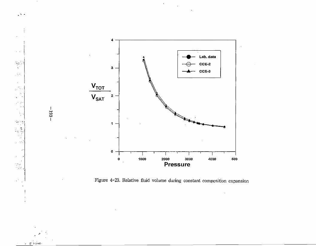
4
0 1000 2000 3000 4000
Pressure
Figure 4-23. Relative fluid volume during constant composition
z
600
expansion
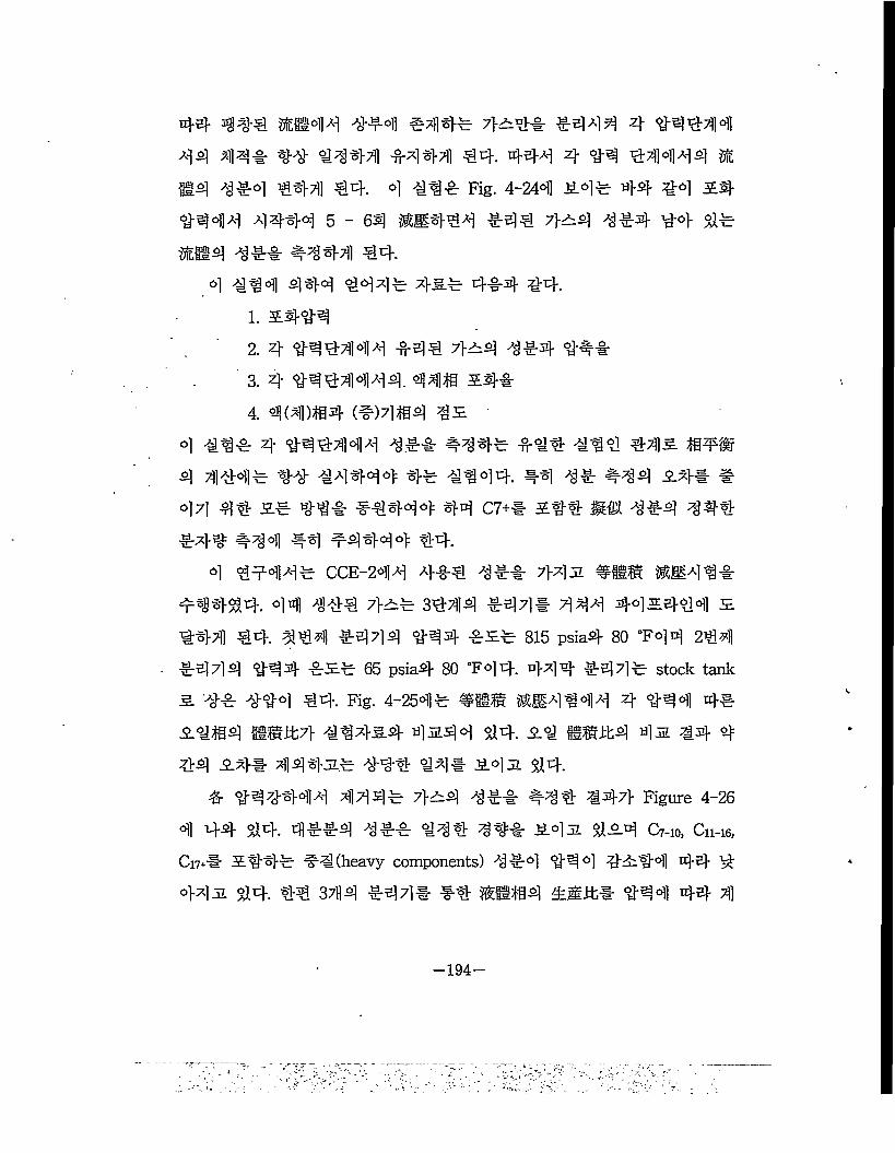
44 4W 444 #14* 7}$** *444 4 *441444 44& 44 4444 4444 44. 444 4 "84 44444 % #4 4#4 441 44. 4 #4* Fig. 4-244 $4* 44 44 $4 4444 4444 5 - 64 M444 444 7}$4 1*4 44 **
m@4 44* 4444 44.4 €"94 444 444* 4s* 4*4 #4.
1. $4*4
2. 4 *44444 *44 7}$4 4*4 *4*
' 3. z} «y-444444. 44S $4*
4 4(4)ffl4 (*)4ffi4 4$ '4 *4* 4 *44444 4** #44* **4 *4* 44& ffl¥E 4 444* 44 4444* 4* 4444. *4 4* #44 .2.4# # 47] 44 $* *** #444* 44 C7+* $44 MW 4*4 *44 *7>* #*4 #4 *444* 44.
4 **44* CCE-244 4*4 4*4 7}* jl ### MM4 4 *
*14*4. 44 144 7}$* 3414 *44* 444 44$4*4 $
*44 44 444 *444 *44 *$* 815 psia4 80 "F44 2*4
*B] 7] 4 *44 *$* 65 psia4 80 °F44- 44* *44* stock tank
5. '** 4*4 44. Fig. 4—25*1 * #HS Ml 411 4 <9-44 4#
$*ffl4 ##hb7} *!4-&4 4^44 *4. $* ##lt4 4s. 44 *
44 $4# 4144s* #44 *1* $4s *4.
# *44444 It]4* 7}^4 1** #44 #47} Figure 4-26 4 44 *4. 4**4 4** *44 44* $4s *$4 C7-10, Cn-i6, C17+* $44* **(heavy components) 4*4 *44 #*44 44 #4-1 s *4. 4# 37114 *4711- #4 EM4 A#it# *44 44 1
-194-
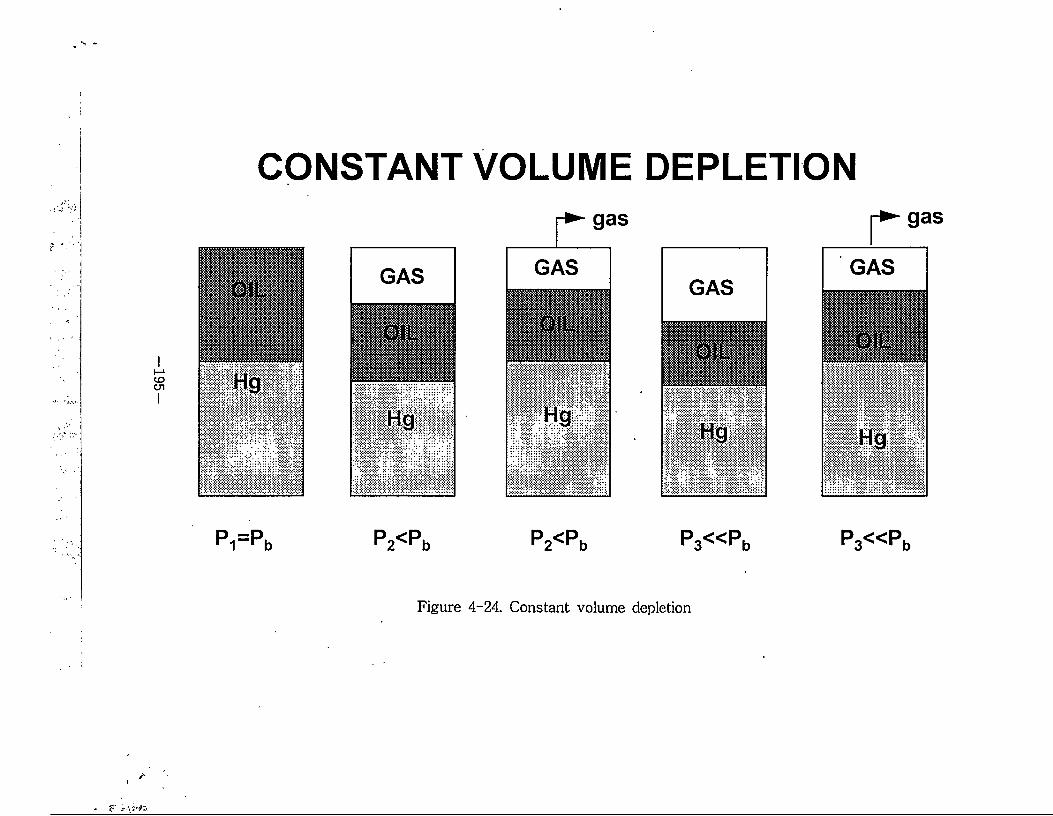
CONSTANT VOLUME DEPLETION
Figure 4-24. Constant volume depletion

20 —
0 —— Lab. data
0— CVD-2
1000 2000
Pressure (psia)3000
Figure 4-25. Relative liquid volume during constant volume depletion
-196-
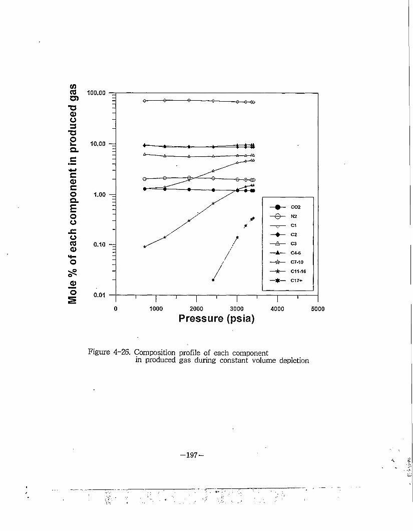
Mol
e %
of e
ach c
ompo
nent
in pr
oduc
ed ga
s
100.00
10.00
■Q— N2
—A—
C7-10
C11-16
C17+
Pressure (psia)
Figure 4-26. Composition profile of each componentin produced gas during constant volume depletion
-197-
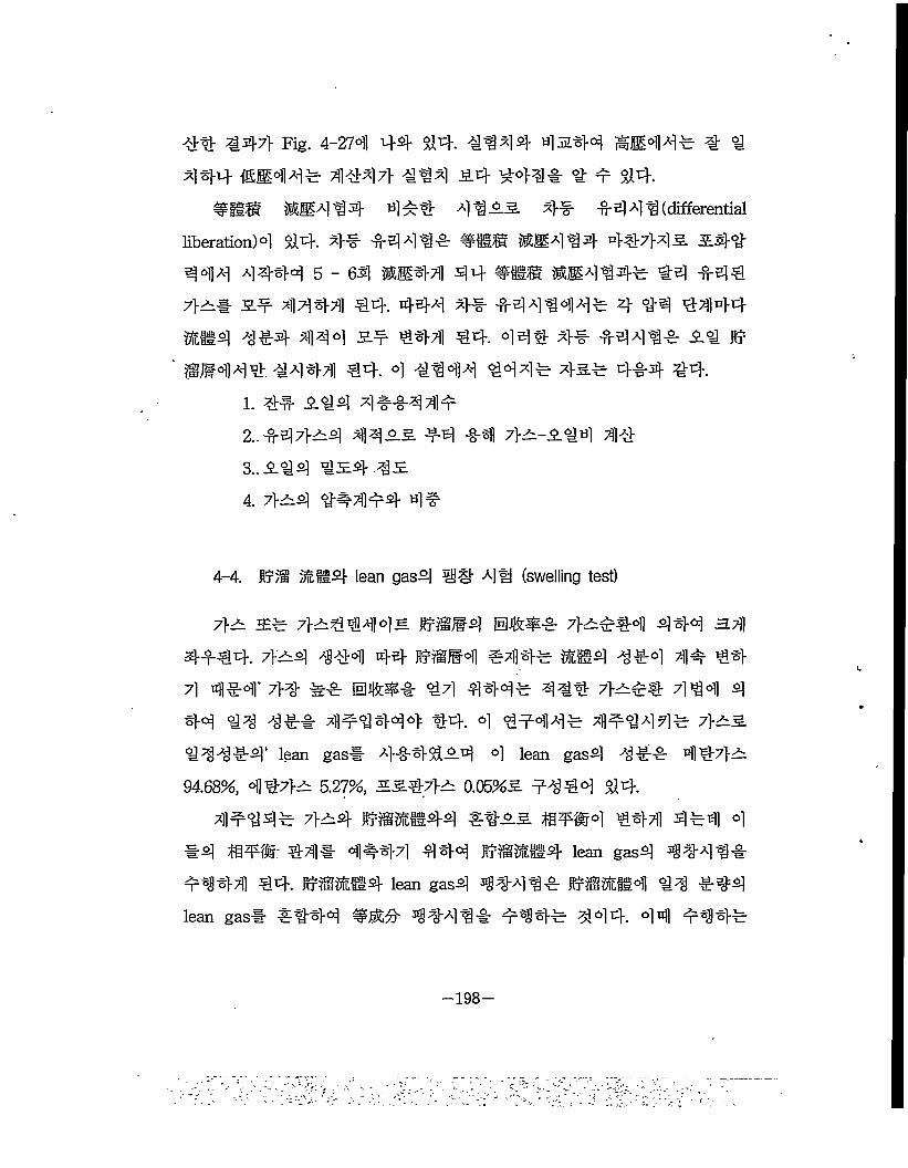
44 447} Fig. 4-274 44 5£4. 4494 4^44 *44# 4 4 444 «44# 4447} 444 54 444& 4 5 44.
### MM 4 4 4 459 4455 4# 44 4 4 (differentialliberation)4 44. 9# 44 A1 n-c- ##§# MM4 44 497}4 5 5.44444 4444 5-64 MM441 44 #HS MM494# 4:4 444 7}5» 54 444711 44. 444 4# #44444# 4 44 4444 M§4 9 #4 444 5# 44t)1 44. 444 4# 44444 5^ R? ##444 4444 44. 4 4444 4444 7}&# 444 44.
1. W 544 4#-8-4 442.. 447}^4 4455 #4 ^-sfl 7}^-544 44:3.. 51)4 #54 454. 7}54 ##71154 4#
4-4. It)b imifsf lean gas4 ## 49 (swelling test)
7W= 5# 7}^4#445 MJE9 0ftlr 7}5^4°)1 444 a?)]
4544. 7}54 944 44 ME4 #7#}# EH4 4#4 44 94 4 4#4 7H> #:# @i|$| ^4 444# 499 7}^5# 444 4
44 4# 9## 4^4444 -#4. 4 4544# 4)5444# 7>-s#99#9‘ lean gas# 454454 4 lean gas4 4## 447}5
94.68%, 4#7M= 5.27%, lSf7}i 0.05%5 4444 114-
711594# 7}54 B#m#44 #455 W#4 447)1 4 #31 4 #4 tWS: 44# 4444 1144 Hr«uE4 lean gas4 9944# 5447)1 44. Dt#MlE4 lean gas9 4449# fir ME 4 #9 #49 lean gas# #444 #J0c# 9444# 594# 444. 44 594#
-198-
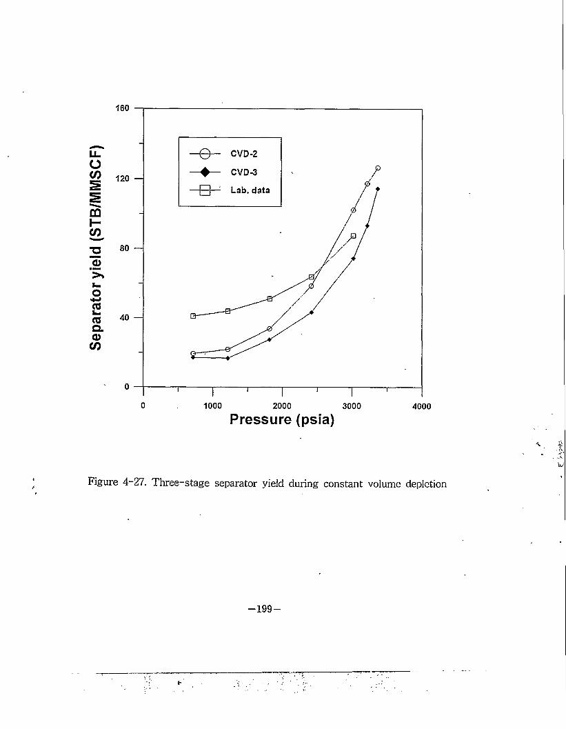
Sepa
rato
r yie
ld (S
TB/M
MSC
F)160
0 1000 2000 3000 4000Pressure (psia)
Figure 4 27. Three-stage separator yield during constant volume depiction
-199-
##4## &4#^5 1 &4##& 4545 #4 4 #444 i?r*l§4 lean gas4# Stti 44 4 #4 4# 4 57}# 7l 4 5-4 M®# 2:714-^ s.4 ^5 ##5 4-0-# 5£ 44. Lean gas4 4 #44#44 45 4" 4c 7}3.tt MM4 lean gas4# 5#5# #4444 5### £444# #4#* # 5 44. 44 5##5 lean gas# S4 44 3E4444 4 ####44 7li#4#ji3. SE5 43L# #444 4*444-2-3. 444je. 44. lean gas## #44#44 5# #4 71144# #44 444- 4444 44 a.# 5# 4 #4#54 45 45. 44444 #4.
415# 7>^4 tir MEIS# lean gas4 5##4 4# 12.71,
30.46, 53.84, ^#31 65.38 5% 47}# #5^ 7}#44 414444. 4 # 44 4-0-4 jt?WE4 45-5-## 7}#:n. lean gas4# ##4#4 5# 4 444-#4 44444# #44#4# 432444 Fig. 4-284 44 44. zi#44 55 44 #4 97H #555. 4544 ItMH# #57}
##44 5444 11711 #555. 5#4 #55 4## 4## 4444 #44 447}jl 455 # 5 44. 445 45## #7}7} #4- #4#
#### 45445 44 4#4 45E5 #4=543= MM 454 4# 44# 54444 s.4 55#5 4444 54.
-200-
5000
3000 I ' I ' I 1 I '500 1000 1500 2000 2500SCF/BBL of dew point gas
Figure 4-28. Dew point pressures during swelling test
-201-

45# ^12.^5.5.0.44 4%
444#
-203-

I
!
i
45#(Seismic Waveform Inversion by Numerical Modeling)
41# (Seismic inversion theory)
1-1. Introduction
For the last ten years, seismic full waveform inversion has been
tackled and attacked by applied mathematicians and geophysicists. To
author's knowledge, the first attempt of full waveform inversion has
been done by Lines and Kelly (1983, personal communication). For the
computation of partial derivative seismograms with respect to the
coordinate of the wedge shape model, they used the numerical difference
scheme via finite-difference modeling technique. At that time, it was too
expensive research even to test the synthetic seismograms. Tarantola
(1984) claimed that the adjoint operator of wave equation makes one
compute the gradient vectors with respect to the velocity efficiently
without computing the partial derivative seismograms. Numerical result
using adjoint operator was given by Kolb et al.(1986) and Gauthier et
al.(1986). Mora(1987) extended it to the elastic problems with examples
of complex geologic structures. Unlike the way of inverting the
seismograms in the time domain, Pratt et al.(1990) applied the adjoint
operator in imaging the subsurface via the frequency domain
finite-difference modeling technique. Beside these gradient approach for
seismic inversion and imaging, Shin(1988) applied Gauss newton method
-205-
to invert the seismograms using the frequency domain finite-element
method. The possibility of using the Full newton method has been
investigated by Santosa et al.(1987). In this paper, the author(Shin)
review three different inverse algorithms such as gradient method,
Gauss Newton method and the full Newton method.
1-2. Finite-element and finite-difference formulation of wave equation
The discretized equation for the acoustic or the elastic wave
equation using the finite-difference method or the finite-element method
can be written (Marfurt, 1984) as
Mu{ t) +Ku( t) = F(t) (1)
where M is the mass matrix, K is the stiffness matrix and F(t) is the
source vector. If damping is included, the equation (1) is
. Mu( t) + Cu{ t) +Ku( t) = F{ t) (2)
where the C is the damping matrix.
Equation (2) can be solved in either the time domain or in the
frequency domain. The details on solving equation (2) in the time
domain can be found in many textbooks (Zienkiewicz, 1977; Bathe and
Wilson, 1986). However, recent inversion algorithm employed by
Tarantola (1984), Chavent (1986), Mora (1986) , Kolb et al. (1986), Shin
(1988) and Pratt et al. (1990) can be easily manipulated by Fourier
transforming equation (2). Taking Fourier transform of equation (2)
-206-
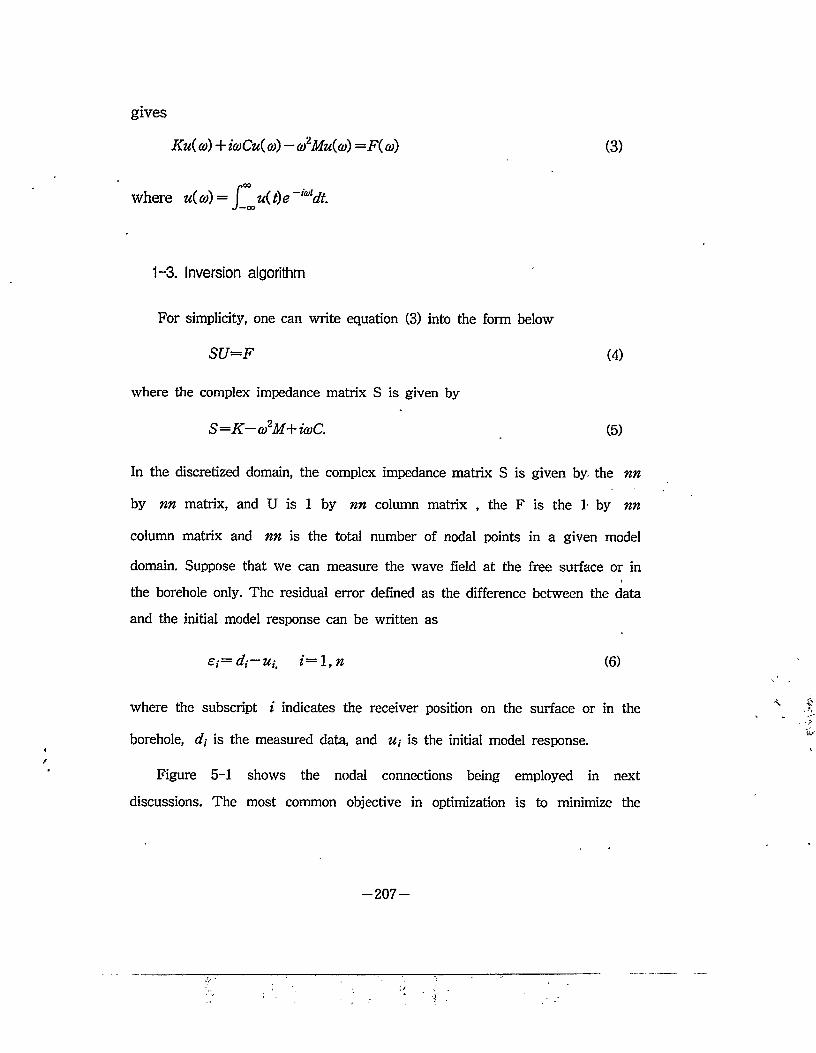
gives
Ku{ co) + ia)Cu{ <y)—aolMu(cd) =F( co) (3)
1-3. Inversion algorithm
For simplicity, one can write equation (3) into the form below
SU=F (4)
where the complex impedance matrix S is given by
S=K— mlM+ icoC. (5)
In the discretized domain, the complex impedance matrix S is given by the nn
by nn matrix, and U is 1 by nn column matrix , the F is the 1 by nn
column matrix and nn is the total number of nodal points in a given model
domain. Suppose that we can measure the wave field at the free surface or in
the borehole only. The residual error defined as the difference between the data
and the initial model response can be written as
£i=di~Ui, i=l,n (6)
where the subscript i indicates the receiver position on the surface or in the
borehole, dt is the measured data, and u -t is the initial model response.
Figure 5-1 shows the nodal connections being employed in next
discussions. The most common objective in optimization is to minimize the
-207-
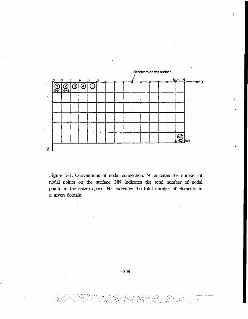
Receivers on the surface
Figure 5-1. Conventions of nodal connection. N indicates the number of nodal points on the surface. NN indicates the total number of nodal points in the entire space. NE indicates the total number of elements in a given domain.
—208—
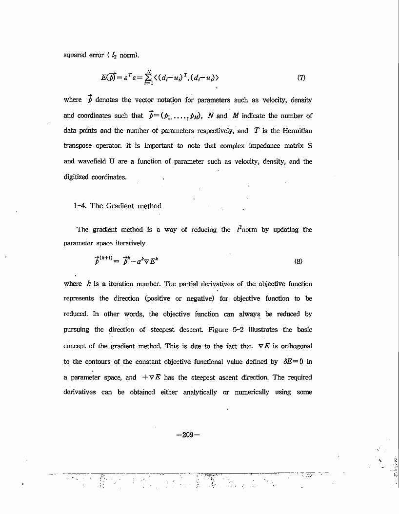
squared error ( /2 norm).
E(]>) = eT£= S <(dj—ui)T, (7)/= 1
where p denotes the vector notation for parameters such as velocity, density
and coordinates such that p=(p\,___,Pu), N and M indicate the number of
data points and the number of parameters respectively, and T is the Hermitian
transpose operator. It is important to note that complex impedance matrix S
and wavefield U are a function of parameter such as velocity, density, and the
digitized coordinates.
1-4. The Gradient method
The gradient method is a way of reducing the /2norm by updating the
parameter space iteratively
?lw>= T-SvE" (8)
where k is a iteration number. The partial derivatives of the objective function
represents the direction (positive or negative) for objective function to be
reduced. In other words, the objective function can always be reduced by
pursuing the direction of steepest descent Figure 5-2 illustrates the basic
concept of the gradient method. This is due to the fact that VE is orthogonal
to the contours of the constant objective functional value defined by 8E= 0 in
a parameter space, and +VE has the steepest ascent direction. The required
derivatives can be obtained either analytically or numerically using some
-209-
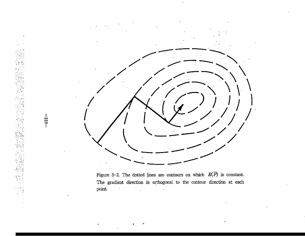
210
Figure 5-2. The dotted lines are contours on which E(P) is constant
The gradient direction is orthogonal to the contour direction at each point
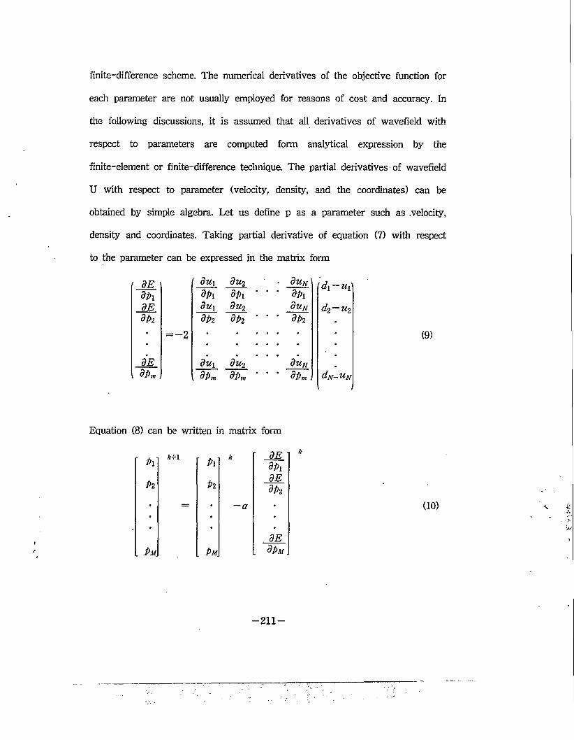
finite-difference scheme. The numerical derivatives of the objective function for
each parameter are not usually employed for reasons of cost and accuracy. In
the following discussions, it is assumed that all derivatives of wavefield with
respect to parameters are computed form analytical expression by the
finite-element or finite-difference technique. The partial derivatives-of wavefield
U with respect to parameter (velocity, density, and the coordinates) can be
obtained by simple algebra. Let us define p as a parameter such as .velocity,
density and coordinates. Taking partial derivative of equation (7) with respect
to the parameter can be expressed in the matrix form
BE Bu\ 3u2 • 3um d\ — u{\dpi dpi dpi " BpiBE Bu\ 3u2 du^ d2 — U2dp2 Bp2 3p2 ' Bp2
= —2
BE Bu\ Bu2 Bun•
dPm) „ Bpm 3pm * ' ‘ Bpm, dtf— Ufj
(9)
Equation (8) can be written in matrix form
" P\k+\ ' Pi
k r bedpi
P2 P2BE
— — a
dp2
• •BE
. Pm. Pm. . dPM.
(10)
—211 —
where k is the iteration step and the step length a is yet to be determined.
The above iteration can be performed until one encounters the step which
does not reduce the objective function. In this case, the step length can be
adjusted and the procedure continued from the optimal point. There are several
techniques to adjust the step length a. For example, conjugate gradient method
can be applied to make convergence be faster than the simple gradient method.
The efficient calculation of the gradient vectors in seismic inverse
problems. In seismic inverse problems, the problem we have to consider in the
calculation of the gradient vectors is to compute the partial derivatives of the
wavefield with respect to the parameter P. In stead of the direct computation
of the partial derivatives, the gradient vectors can be efficiently calculated by
the adjoint operator "or the the transpose operator. Suppose that we are dealing
with a limited amount of surface or borehole data, the gradient vectors can be
expressed by-
r dE i r dui du2' dPi dpi dpy
= —2 •
dEdPm
dui du2dpm dpm
da,,dpi
du„dpm
d\ — %i
dn — un
(ID
where the- /(= 1,m) indicates number of parameters, and i= 1,, ,n
indicates surface or borehole data such that equation (11) can be written
v.
-212-
(12)
dui du„ dun+l du„n 1
dE 1 dpi dpi dpi dpi CLi-Ui
dpi ...
=—2 d„—un3E dUi dun dun+1 du„n
0
. dPm. dpm dpm dpm Hm 0 .
where n indicates the number of receiver points, and nn indicates the number
of total nodal points in the entire space. Let us consider the transpose of the
partial derivative wavefield with respect to one parameter. The partial
derivative of equation (4) with respect to p\ yields
9SS dpi dp\ u. (13)
Multiplying equation (13) by the inverse of S gives
<14)
The matrix notation of equation (14) is given by
r duidpi ' /l1'
• = 5_1
dunn dpi _ /r.
where the virtual source distribution /j is given by
(16)
/l1] UidS
. dp .
/l”” Wnn
making the transpose of equation (15) results in
dux du„„dpi dpi = [ A1- A””] 5-1 T
while similar procedures for /=2, •••, m results in
dui dUnn. dPi dPz .
dui dllnndPm dpm ,
= [ A1- hnn] S"lT
= [ fj- S"lT
(17)
(18)
(19)
Substituting equations (17), (18) and (19) into .equation (12) gives
dEdp i di~u{
dE
=—2 s~lT dn un 0
0 .dpm .
Equation (20) Can be rewritten as
dEdpi F A1 Vl
. ... %• = —2 ... ;
d£ *
dpM .[ Vnn\
(21)
-214-
where the back-propagated wavefield of residual on the surface or in the
borehole is defined as
di-Ui'V\ d-i—u-iv2 •
• = S~lT d„—unv„0
Vjin 0 .
The impedance matrix is equivalent to the time reversed impulse response
function (Green's function). Because of linearity and Hermitian conjugate of
Green's function, equation (22) can be written as
di-Uivi dz—u-iV2
• =s~l d„—unV„0
Vnn 0 .
(23)
Equation (23) means that when one propagates the time reversed residual, one
has the back-propagated wavefields to be correlated with the virtual sources
for the computation of the partial derivative wavefields in equation (20).
Talrantola(1985), Chavent(1986), Mora(1986) and Kolb et al.(1986) have exploited
this efficiency to solve the nonlinear least squares wave inversion by the
gradient method.
To test the adjoint operator of wave equation, the point diffractor model is
-215
taken for the computation of the gradient vectors. Figure 5-3 shows the point
diffractor model embedded in the homogeneous model. The velocity of point
difffactor is 1800 m/sec and the velocity of background velocity is 1600 m/sec.
Source point is located at the center of the surface and receivers are located on
the whole surface. Figure 5-4 shows the contour of gradient vectors with
respect to the velocity parameter of each grid point by back-propagating the
residual and multiplying the back-propagated wavefield with the virtual sources.
At the center of the model, the point diffractor has the biggest value except
the surface near the source point
1-5. The: Gauss Newton method
The second and simple approach for solving nonlinear least squares
problem is based on the fact that in the neighborhood of initial parameter, the
model response can expanded by Taylor series. Assume that the model
response can, be expanded in a Taylor series around initial parameter p: then, if
the data d\ is the measured data corresponding to the true parameter, we have
+
*5 (- -) + - -
-216-
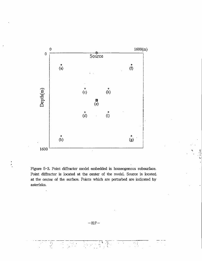
0 1600(m)
&P
1600
*
(a)
*
(b)
Source
(c) (h)
(e)
*
(d) (i)
(f)
*
(g)
Figure 5-3. Point diffractor model embedded in homeogenous subsurface. Point diffractor is located at the center of the model. Source is located, at the center of the surface. Points which are perturbed are indicated by asterisks.
-217-
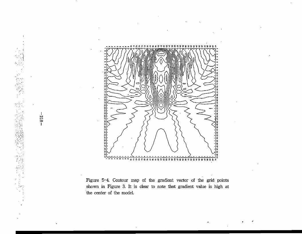
218
^NUAt*oiNie«eo!25vi*tn5i!i55oi?»56i*t86»t}p$6>$Si2$Stitduifc!'5i»«oS2»
%8*y%s&
Figure 5-4. Contour map of the gradient vector of the grid points shown in Figure 3. It is clear to note that gradient value is high at the center of the model.
dji-Un $p\du„dpi + dp2
dun dp2
■9 ( 8p\
+ dp„
1 f ^2 dZu„
du„dPm
) + • • o(d/>3)
(24)
where n denotes the number of receiver points, m denotes the number of
parameters, §P;= p‘i™~Pi , and o( ops) is the remaining term of Taylor
series expansion. Gauss Newton method consists of linearizing equation (24),
which gives
dux dux duxdx—ux dpi dp2 dpm
du2 du2 du2d2-u2 dpi dp2 dpm
du„ du„ dundn — u„ dpi dp2 dpm
#1
Sp‘2(25)
Because of mode and measurement errors, equation(25) can be solved by the .
standard least squares method, resulting in what are called the normal
equations
dux du„dpi dpi
du\ duxdpi dpm 8px dux du\
dpi dPm di—Ui
dux dun. dpm dpm
du„ du„ dpi dpm .
dun dun dPi dpm d„—u„
(26)
or
-219-
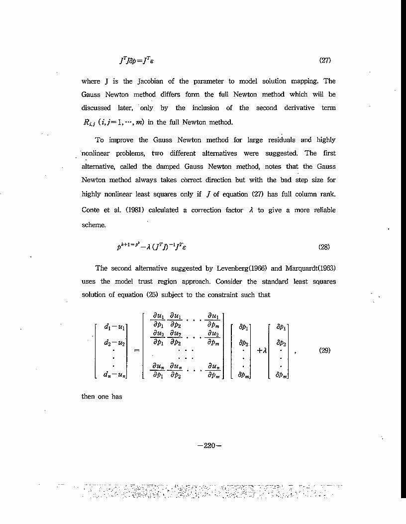
JTJ8p=JTe (27)
where J is the Jacobian of the parameter to model solution mapping. The
Gauss Newton method differs form the full Newton method which will be
discussed later, only by the inclusion of the second derivative term
Ri.i — ,m) in the full Newton method.
To improve the Gauss Newton method for large residuals and highly
nonlinear problems, two different alternatives were suggested. The first
alternative, called the damped Gauss Newton method, notes that the Gauss
Newton method always takes correct direction but with the bad step size for
highly nonlinear least squares only if / of equation (27) has full column rank.
Conte et al. (1981) calculated a correction factor A to give a more reliable
scheme.
Pk+I=pt-A UTJ)~lJTe (28)
The second alternative suggested by Levenberg(1966) and Marquardt(1963)
uses the model trust region approach. Consider the standard least squares
solution of equation (25) subject to the constraint such that
d\ — u{
d2 — u2
du\ du\ dpi dp2 du2 du2 dpi dp2
duidpmdu2dpm
zg zg- +A
dpi
8Pz
d„ — u„dun du„ dpi dp2
dun dPm . 8pm . 8Pm.
then one has
(29)
-220-
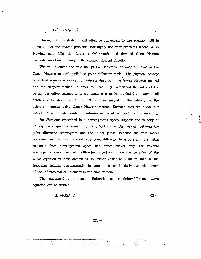
(30)(JTJ+Al)8p=fe.
Throughout this study, it will often be convenient to use equation (30) to
solve the seismic inverse problems. For highly nonlinear problems where Gauss
Newton step fails, the Levenberg-Marquardt and damped Gauss-Newton
methods are close to being in the steepest descent direction.
We will examine the role the partial derivative seismogram play in the
Gauss Newton method applied to point diffractor model. The physical concept
of virtual sources is critical to understanding both the Gauss Newton method
and the steepest method. In order to more fully understand the roles of the
partial derivative seismograms, we examine a model divided into many small
scatterers, as shown in Figure 5-3. It .gives insight to the behavior of the
seismic inversion using Gauss Newton method. Suppose that we divide our
model into an infinite number of infinitesimal sized cell, and wish to invert for
a point diffractor embedded in a homeogenous space! suppose the velocity of
homogeneous space is known. Figure 5-5(a) shows the residual between the
point diffractor seismogram and the initial guess. Because the true model
response has the direct arrival plus point diffractor hyperbola and the initial
response from homeogenous space has direct arrival only, the residual
seismogram looks like point diffractor hyperbola. Since the behavior of the
wave equation in time domain is somewhat easier to visualize than in the
frequency domain, it is instructive to examine the partial derivative seismogram
of the infinitesimal cell element in the time domain.
The undamped time domain finite-element or finite-difference wave
equation can be written
MU+KU=F (31)
-221-

E
0.790
1.550
I 900
1.790
« 9 000
« 9 550 £ 5.500
* 9 7505 3.000
" 3 POO
b
-W5
VsSYV^"^ "
C
TTTSB"nJy,Miwjr
Figure 5-5. The residual seismogram and the partial derivative seismograms with respect to the velocity of the points shown in Figure 5-3. (a) The residual seismogram between the point diffractor model response and the homogeneous model response (b) partial derivative seismogram with respect to the velocity of point (a) in Figure 5-3. (c) partial derivative seismogram with respect to the velocity of point (b) in Figure5-3. (d) partial derivative seismogram with respect to the velocity of point (c) in Figure 5-3. (e) partial derivative seismogram with respect to the velocity of point (d) in Figure 5-3.
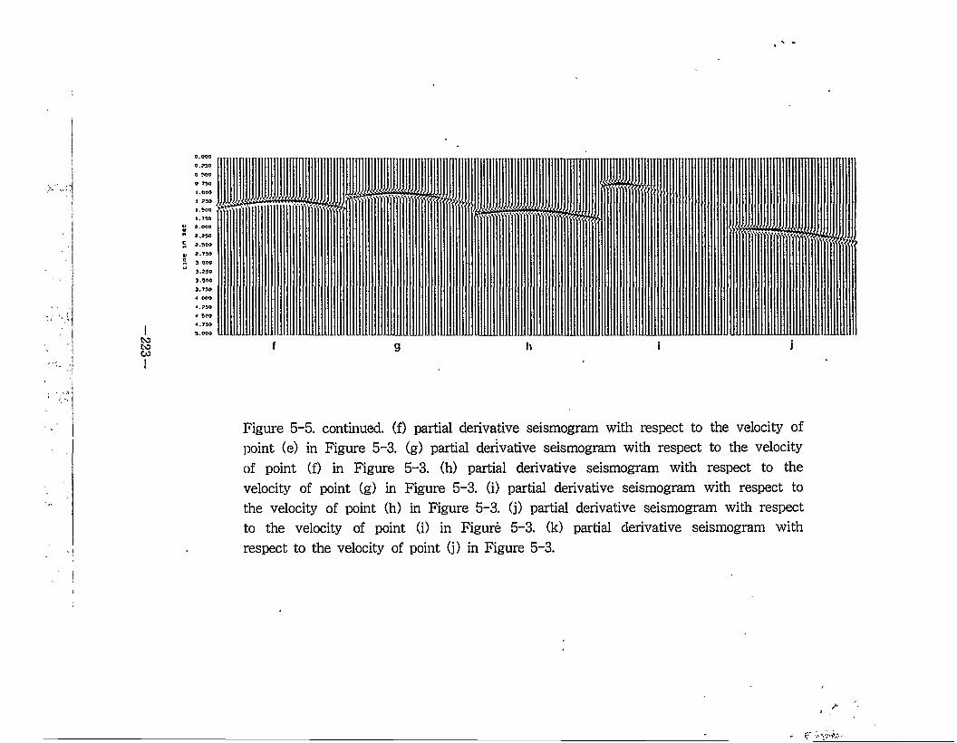
223
Figure 5-5. continued, (f) partial derivative seismogram with respect to the velocity of point (e) in Figure 5-3. (g) partial derivative seismogram with respect to the velocity of point (f) in Figure 5-3. (h) partial derivative seismogram with respect to the velocity of point (g) in Figure 5-3. (i) partial derivative seismogram with respect to the velocity of point (h) in Figure 5-3. (j) partial derivative seismogram with respect to the velocity of point (i) in Figure 5-3. (k) partial derivative seismogram with respect to the velocity of point (j) in Figure 5-3.
Z
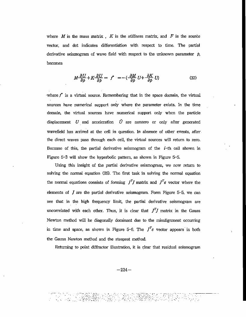
where M is the mass matrix , K is the stiffness matrix, and F is the source
vector, and dot indicates differentiation with respect to time. The partial
derivative seismogram of wave field with respect to the unknown parameter p,
becomes
M~^t +K-^f — f =-(-# U+~^U)dp dp dp dp (32)
•where f is a virtual source. Remembering that in the space domain, the virtual
sources have numerical support only where the parameter exists. In the time
domain, the virtual sources have numerical support only when the particle
displacement U and acceleration U are nonzero or only after generated
wavefield has arrived at the cell in question. In absence of other events, after
the direct waves pass through each cell, the virtual sources will return to zero.
Because of this, the partial derivative seismogram of the z’-th cell shown in
Figure 5-3 will show the hyperbolic pattern, as shown in Figure 5-5.
Using this insight of the partial derivative seismogram, we now return to
solving the normal equation (26). The first task in solving the normal equation
the normal equations consists of forming JTJ matrix and JTs vector where the
elements of J are the partial derivative seismogram. Form Figure 5-5, we can
see that in the high frequency limit, the partial derivative seismogram are
uncorrelated with each other. Thus, it is clear that JTJ matrix in the Gauss
Newton method will be diagonally dominant due to the misalignment occurring
in time and space, as shown in Figure 5-6. The JT£ vector appears in both
the Gauss Newton method and the steepest method.
Returning to point diffractor illustration, it is clear that residual seismogram
-224
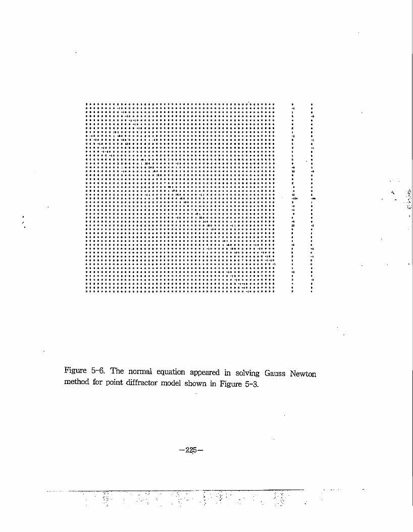
000000000 0000 >10000 00000 >1000 000000 >1 00 1 0 ( 0 0 0 0 *1*1 09000000 >1 009000000 000 *9 *0000 0 0 0 * 190 0 0 0 000 00*0000 0 0 0 0 0 O UO 0 >100000090 •*•10000007 00 >1 000090 000300000 000030000 00000*000 00000 >1 000 000000009 000000000 000000000 000000000 ooooooooo 000000000 ooooooooo ooooooooo ooooooooo ooooooooo ooooooooo ooooooooo ooooooooo ooooooooo ooooooooo ooooooooo ooooooooo ooooooooo ooooooooo 00000000.0 ooooooooo ooooooooo ooooooooo ooooooooo ooooooooo ooooooooo ooooooooo ooooooooo ooooooooo ooooooooo ooooooooo
0 0 0 0 0 0 0 0 0 0 0 0
Figure 5-6. The normal equation appeared in solving Gauss Newton method for point diffractor model shown in Figure 5-3.
225
in Figure 5~5(a) will have a maximum correlation with the partial derivative
seismogram JT at the point diffractor cell number 25 in Figure 5-3. When the
residual seismogram in Figure 5-5(a) is superimposed on all possible diffraction
curve to form the normal equation applied to the Gauss Newton method in
inverting the point diffractor hyperbola (partial derivative seismogram) to form
JTe, the maximum correlation will occur on the point diffractor, as shown in
Figure 5-6. This operation is closely related to early migration work of
Hagedoom(1954) in his discussion of surface of maximum convexity. Thus,
Hagedoom's migration of prestacked data in a homogeneous velocity region has
element of both the Gauss Newton method with strong damping and the
steepest method. However, the situation becomes more complicated as the
geologic structure becomes increasingly complex and Hagedoom's technique
breaks down. However, it is generally true that when we consider wave events,
especially first arrivals activated form the virtual sources of each cell, the JTJ
matrix will be banded and diagonally dominant in form.
It is evident that the more we subdivide our model, the more partial
derivative seismogram with respect to velocity of point resembles the point
diffraction hyperbola. In addition, the partial derivative seismograms of each
velocity of point shown in Figure 5-5 will not strongly correlate with each
other such that JTJ matrix will be a diagonally dominant pseudo-banded
(negligible terms) matrix, although insurmountable difficulties arise when we
try to apply this approach to entire grid velocities.
1-6. The full Newton method
-226-
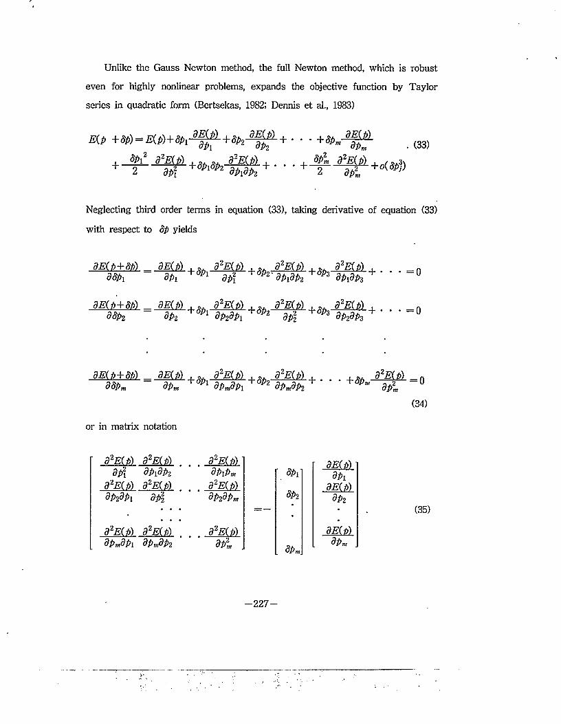
Unlike the Gauss Newton method, the full Newton method, which is robust
even for highly nonlinear problems, expands the objective function by Taylor
series in quadratic form (Bertsekas, 1982; Dennis et al., 1983)
E(p +8p) = E(p)+8pi
, Spi2 d2E(p)2 Jr8pi8p2 82E(P)
dp]8pt8pj 82E(P)2 ^
. (33)
Neglecting third order terms in equation (33), taking derivative of equation (33)
with respect to Sp yields
8E( i)+St>)d8pi + 8pi 82E(t) h 8p2~d2E(i>)
dpidp2 ^8ps 82E(i>)dpydp-i
8E( f}+8f>)dSp2
dE(b)8pt 8pi d2E(t>)
dp2dpi ~8p2 82E(8)#2
h Spz d2E(i>)dp2dp3
• =0
• =0
dE( P+Sp)d8pm
8E(t>)8pm 8pi d2E( t>)
dPmdPi h Sp2 d2E(i>)dpmdp2 + 8p„ 82E(b)
= 0
(34)
or in matrix notation
d2EU)') d2E(t) d2E(t) dE(b)dpi dpydpt dpipm dpi dpidE(p)
dPidPl dpi dp2dpm Spo dp2
d2E(ti) d2E(t>) d2E(t) dE(t)dpmdpi dpmdp2 dpi
.
dpm
-227-
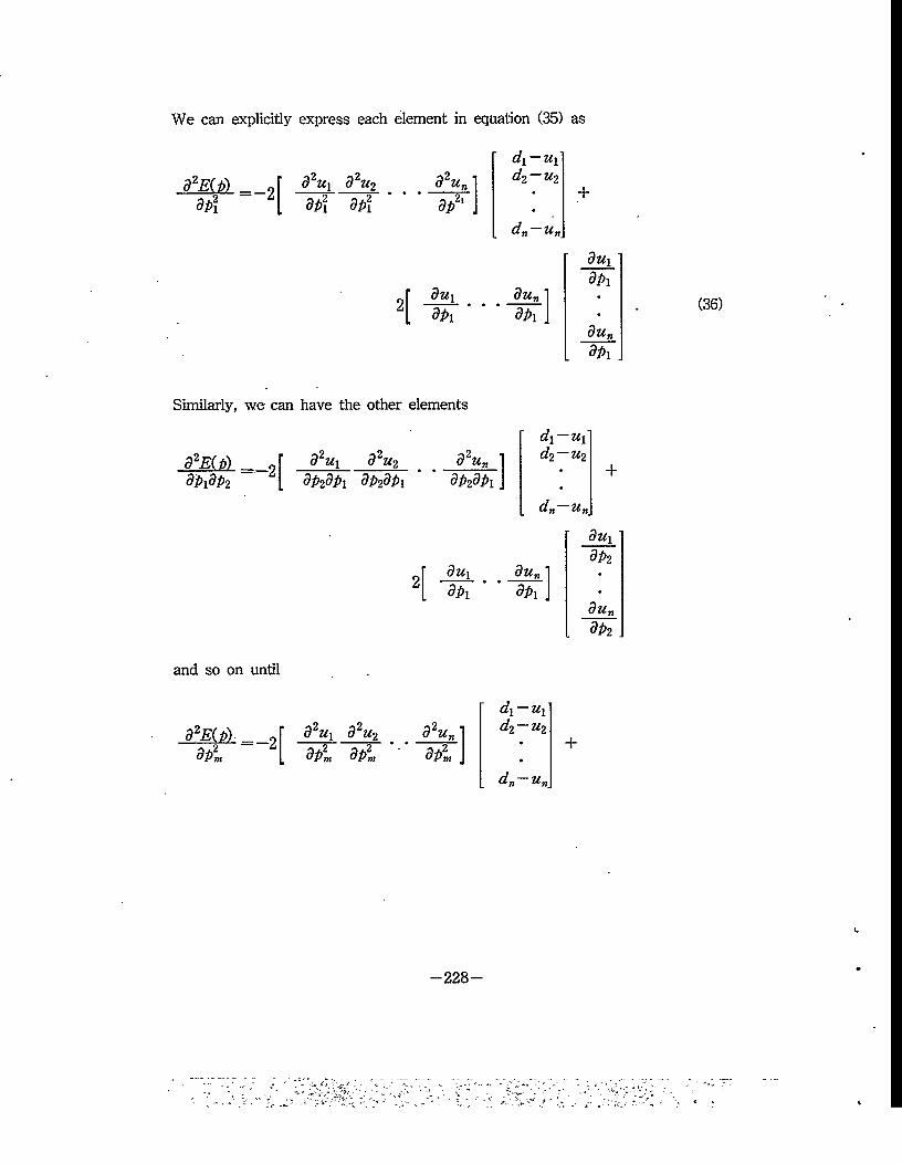
We can explicitly express each element in equation (35) as
d2E(p) odpi z
d2Ui d2U2dpi dpi
d2u„dp2l
du\dp\
di~uid2—u2
d„—un
dundp\
+
du\dpi
du„dpi
Similarly, we can have the other elements
d2E(P)dp\dp2 =—2
and so on until
d2E(P)■%
= —2
d2U\ d2u2dp2dpi dp2dpi
d2U\ d2u2
dp2m dp2m
dp2dpi
duxdpi
dlUr
di~uid2 — u2
dn Un
du„ ‘dPi .
di~Uid2 — u2
d„ — u„
+
du\dp2
du„dp2
+
228-
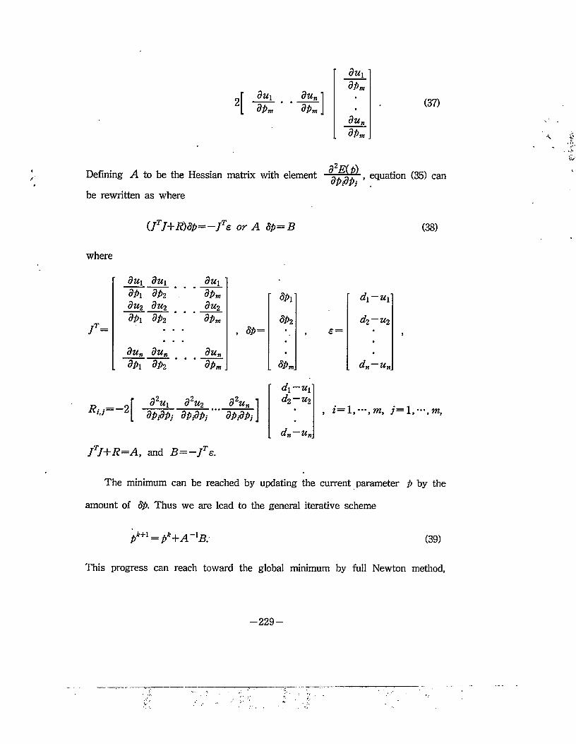
dui du„dpm dpn
duidPm
du„dPm
(37)
Defining A to be the Hessian matrix with element » equation (35) can
be rewritten as where
(JTJ+ R)8p——JTe or A 8p=B (38)
where
f=
dux du\ dux •dpi dp-i . dpm r spx r dx—u{\du2 du2 du2dpi dpm Sp2 d2—u2
, 8p= , £ = •
8un dun dun • •dpi dp2 dpm. [ SPm\ d„ — u„
*/./— 2d2Ui d2u2 d2u„
dpfipj dpjdpj dpjdpj
d\—ux d2 — u2
d„ — u„
jJ+R—A, and B=—Jte.
The minimum can be reached by updating the current parameter p by the
amount of 8p. Thus we are lead to the general iterative scheme
pk+l = pk+A~lB; (39)
This progress can reach toward the global minimum by full Newton method,
-229-
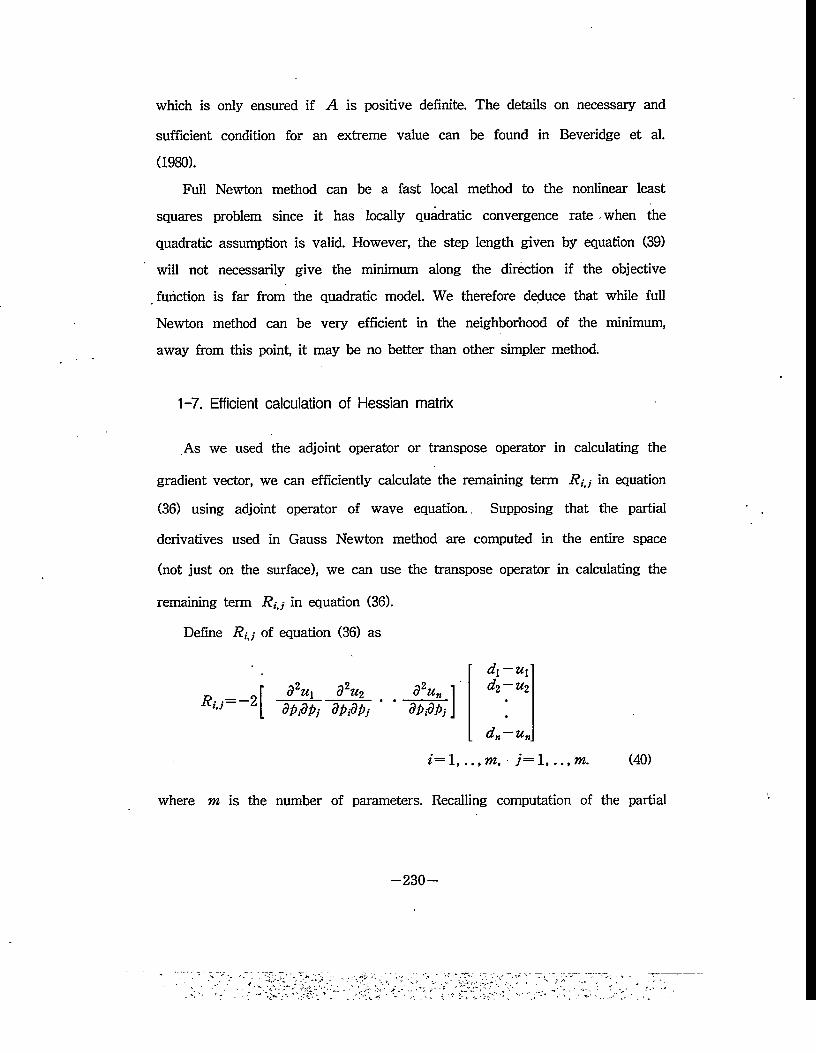
which is only ensured if A is positive definite. The details on necessary and
sufficient condition for an extreme value can be found in Beveridge et al.
(1980).
Full Newton method can be a fast local method to the nonlinear least
squares problem since it has locally quadratic convergence rate when the
quadratic assumption is valid. However, the step length given by equation (39)
will not necessarily give the minimum along the direction if the objective
function is far from the quadratic model. We therefore deduce that while full
Newton method can be very efficient in the neighborhood of the minimum,
away from this point, it may be no better than other simpler method.
1-7. Efficient calculation of Hessian matrix
As we used the adjoint operator or transpose operator in calculating the
gradient vector, we can efficiently calculate the remaining term R;j in equation
(36) using adjoint operator of wave equation. Supposing that the partial
derivatives used in Gauss Newton method are computed in the entire space
(not just on the surface), we can use the transpose operator in calculating the
remaining term Rfj in equation (36).
Define Rij of equation (36) as
d\—U\d2 — u2
d» — un
i=l,m, ■ j=l, ,.,m. (40)
where m is the number of parameters. Recalling computation of the partial
Ru=- 2d2Ui d2u2 9%
dpjdpj dpidpj dpfipj
-230-
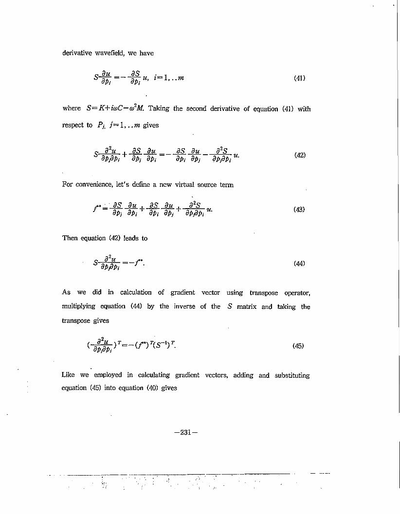
derivative wavefield, we have
s- dudpi
9Sdpi u, (41)
where S= K+icoC—a)2M. Taking the second derivative of equation (41) with
respect to Pu gives
o d2u . dS du _ _ dS du _ d2Sdpjdpi dpj dpi dpi dpj dpjdpi U'
For convenience, let's define a new virtual source term
/** dS du , dS du , d2Sdpj dpj dpi dpj dpjdpj * (43)
Then equation (42) leads to
c—dhe_ =_f* (44)
As we did in calculation of gradient vector using transpose operator,
multiplying equation (44) by the inverse of the 5 matrix and taking the
transpose gives
(-^)r~(/rcs-v. (45)
Like we employed in calculating gradient vectors, adding and substituting
equation (45) into equation (40) gives
-231-
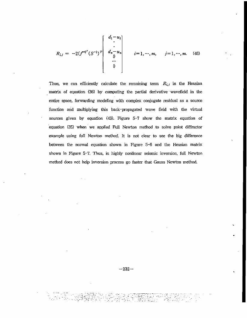
Ru = -2 (f*)T(S~1)T
d\ U\
dn—un0
0
i=l, ‘",m, j=l,—,m. (46)
Thus, we can efficiently calculate the remaining term R;j in the Hessian
matrix of equation (36) by computing the partial derivative" wavefield in the
entire space, forwarding modeling with complex conjugate residual as a source
function and multiplying this back-propagated wave field with the virtual
sources given by equation (43). Figure 5-7 show the matrix equation of
equation (35) when we applied Full Newton method to solve point diffractor
example using full Newton method. It is not clear to see the big difference
between the normal equation shown in Figure 5-6 and the Hessian matrix
shown in Figure 5-7. Thus, in highly nonlinear seismic inversion, full Newton
method does not help inversion process go faster that Gauss Newton method.
-232-
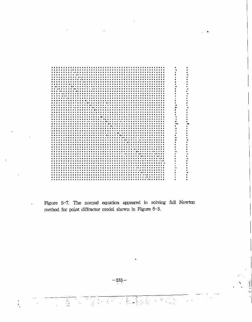
0 0 0 0 0 9 000000000000000000 0 0 0 O 0 o 0 0 0 0 0 0 0
000000000 0 0 0 0 0 0 0
0 0 0 0 0 6 0 0 0 0 0 0 0 6
0 0 0 0 0 0 0 0 0 0 0 0 0 6
0000000000000000
0 -10 0 0 0 0 0 0 0 0 0 0 0 00000000
0 0 0 -10 0 6 0 0 0 0 -|0 0
0 0 0 0 0 0 0 0 0 * 0 0 0 0
000000000000*000
0 00 0 0 9 0 0 00 0 0 0 0 -100 0 * 0 0 1 0
• 0 0 0 0 0 0 I130 0 0 0 0 0 0 0 0 0 0 0 00 0 7 0 0 0 00 0 0 H 1 0 o0 0 0 1 470 0 0 0 0 0 0 30 0
0 0 0 0 0 -1
0 0 0 0 0 0 0 00000 16 000
0 0 0 0 0 0 0 0 0 0 0 0 0 0 03000000
0 0 0 0 0 0 0 0 0 0 0 0 0 0 00000100
0 0 0 0 O 0 < 0 0 0 0 0 0 00 0 0 0 0 0 0 0 0 0 0 0 0 0 0 0 0 0 0 0 0
0 0 0 0 0 0 0 0 0 0 0 0 0 0 0 0 0 0 0 0 0
0 0 0 0 0 0 0 0 0 0 0 0 0 0 0 0 0 0
Figure 5-7. The normal equation appeared in solving full Newton method for point diffractor model shown in Figure 5-3.
-233-
/
(Pseudo waveform inversion of reflection seismograms in the frequency domain)
2-1. Introduction
In the seismic reflection method, the velocity distribution of the
subsurface plays an important role in seismic data processing and
interpretation, such as in the processes of stacking, migration and depth
conversion. Interval velocity is commonly calculated by applying the Dix
formula to a prior measured rms velocity and traveltime at zero-offset.
Since, for the most part, a realistic geologic model does not satisfy
Dix's assumption, it is necessary to estimate the velocity model by an
inversion method.
According to the technique used to solve the Green's function of the
wave equation, seismic inversion may be classified into two groups. One
approach is waveform inversion based on the wave equation. Linearized
waveform, inversion is based on the Bom approximation, where weak
scattering is valid (Tarantola, 1984a," Bleistein et al, 1985).
Non-linearized waveform inversion makes use of the full information of
the observed data, and this inverse problem can be solved using an
iterative method, where the gradient is usually computed by using the
adjoint equation (Tarantola, 1984b, 1986," Kolb et al, 1986; Mora, 1987;
Shin, 1988; Pratt and Worthington, 1990; Zhou et al, 1993). This
waveform inversion can estimate the low frequency information of the
velocity distribution, but it en ounters great difficulty when applied to
-234-
real seismic data, as seen in source wavelet estimation, non-linear
behavior of wave propagation, intensive computation in solving the wave
equation by numerical methods, and so on.
Another approach is traveltime inversion by a ray tracing algorithm.
In this kinematic inversion, the velocity model can be estimated by
using an optimization technique which minimizes the difference between
the traveltime calculated by forward modeling and the traveltime picked
in the recorded data (Gjoystdal and Ursin, 1981; Bishop et al, 1985;
Keydar et al, 1989; Lines et al, 1993). Unlike traveltime inversion,
coherency inversion maximizes some measure of coherency computed for
unstacked trace gathers in a time- window along traveltime curves
generated by ray tracing through the model (Landa et al, 1988; Reshef
et al, 1991). But traveltime and coherency inversion may lead to a
failure of the inverse procedure when the initial model is far from the
true model.
In this study, we introduce a pseudo waveform inversion in order to
estimate the velocity model from prestack data. The following trick is
used to imitate the waveform inversion: the high frequency limit
seismogram computed by ray tracing is low-pass filtered and then used
to match the residual and perturbation seismogram when the initial
model is more or less far from the true model. Even though the initial
model is not in the neighborhood of the true model, the low frequency
band information can be employed to improve the reliability and
effectiveness of the inversion. The following technique is applied in
order to make improvements on the stability of the inversion process;
-235-
(1) layer after layer determination of inversion parameters,
(2) an alternative choice of velocity and interface coordinate parameter,
(3) frequency band increasing technique.
We will describe the proposed method and demonstrate its application to
synthetic and field data.
2-2. Theory
2-2-1. Damped least square method
In seismic exploration, the wavefield recorded at the surface or in a.
borehole is, a function of the source-receiver position and the material
parameters of the subsurface, such as velocity, density, attenuation
factor, and so on. The purpose of inversion is to quantitatively
determine, the model parameter, velocity distribution, from the observed
data. Since the model parameter is essentially non-linear with its model
response, we can use iteratively an optimization technique that
minimizes the sum of squares of the differences between the observed
data and the calculated data. In the damped least square method, the
solution vector is given as (Lines and Treitel, 1984),
dp = (JTJ + PlT'fg (1)
where <5p is the parameter correction vector, J the Jacobian matrix, JT
the transpose of J, g the error vector, and I the identity matrix of the
order of JTJ, and 0 is the damping factor. The parameter correction
vector dp should be real-valued, but the Jacobian matrix J and the
-236-
error vector g are complex-valued in the frequency domain. The real-valued dp can be obtained as follows; Let J= a+bi and g = c+di.
Augment the matrix J by its complex conjugate, similarly augment g. We thus obtain the new matrices J and g given as following
(2)
The complex conjugate represents the negative frequency terms.Consequently, JTJ and JTg are always real-valued so that we can
always obtain the parameter correction vectors as the real values.
j'Tj' = 2(a2 + b2) , j'V = 2{ac + bd) (3)
2-2-2. Parameterization and Forward calculation The velocity model (Fig. 5-8) is 2-dimensional with horizontal
distance x and with depth z measured downward. The surface, given by the line z= 0, is called interface n = 1. Below the surface there are N— 1 interface which are labeled n=2,3,“\N. Each subsurface
interface is continuous and is made up of straight line segments. A node-point of an interface is a point where two straight line segments connect. Let (Xmn,Zmn) be the coordinate of the tfzth nodepoint of interface n. The model contains N layers designated by Layer n
(>z = 2,3,***, AO, which is the layer that lies between interface n (on top) and interface n+1 (on bottom), has constant interval velocity v„.
The model is characterized by the model parameter vector
-237-
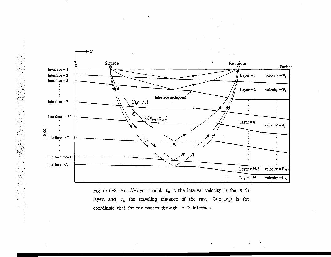
238
>x
Source ReceiverSurface
Interface = 1
Interface = 2
Interface = 3
Layer = 1 velocity =Vr
Layer = 2 velocity = V.
Interface nodepointInterface =n
Interface —n+1
Layer -itvelocity =V
Interface =m
Interface =N-1
Interface =NLayer =N-1 velocity =VAr.i
Layer=N velocity =VN
Figure 5-8. An TV-layer model. v„ is the interval velocity in the w-th
layer, and rn the traveling distance of the ray. C( xn,zn) is the
coordinate that the ray passes through %-th interface.
(4)
This method makes up of ray tracing. The shooting ray technique
considers a ray that travels from the source to the reflecting point A
and then back to the receiver. As shown in Figure 5-8, let the position
of the source and the position of the receiver be fixed. Each raypath
considered will start at the source and end at the receiver. We will
consider a raypath for a primary reflection from each subsurface
interface m, where m=2,3,•••,N.
The ray that reflects from point A on subsurface interface m is
shown at the raypath from the source to A to the receiver. The
traveltime is the sum of the traveltime from the source to A and the
traveltime from A to the receiver. By the principle of reciprocity, the
traveltime from A to the receiver is the same as the traveltime from
the receiver to A. Thus we need to treat only the downgoing path of
source to A, as the other path will have a similar treatment. For the
given downgoing path, let the ray pass through interface n at point
C— (xn _ z„). The travel distance in the %-th layer is
r„ = V (**+i -xn)2 + (zn+1-z„)2 (5)
and the traveltime in the %-th layer is rjvn. Thus the traveltime for
the primary reflection from interface m is
P — [ y«. X mn, Zmn]
-239-
(6)
In this analysis we consider only traveltimes and do not take into
account amplitudes of reflections. Thus for an impulsive source, the
primary reflection from interface m can be represented by the wavefield
um{i) = 8(t—Tm). (7)
The primary reflections from all the N interfaces can thus be
represented by
NNu(t)= 2 Um(t)= 2 8(t—Tm).
m=2 m=2(8)
The Fourier transform of this equation gives
(9)
This wavefield can be low-pass filtered to yield more realistic input
data.
2-2-3. Calculation of Analytical Derivatives
The derivatives with respect to the model parameter vector or
Jacobians are essential in an iterative damped least square method. The
numerical partial derivatives are not usually employed for reasons of
cost and accuracy. Jacobians are analytically, computed for the efficiency
—240—
of the inversion procedure. The partial derivatives of U(co) with respect
to the interval velocity vt becomes
= -fj'-«®> 00)
The partial derivatives of U{(o) with respect to the crossing interface
point C( xn , z„) become
dUico) _ • / xn xn-\dxn Vrt—1 xn—1
and
9U(cd) . f Zn %n—l—=---- . = 1(0 (----------------OZn Vn—\ Yn—1
%n+l%n
■^n+1 xnVn r„ ) • U(co).
(11)
(12)
For the derivatives of the model parameters, let us consider the
interfaces that consist of two straight segments AB and BC, which
have three nodepoints A(Xi,Z,), B(Xm,Zm), and C(Xr,Zr) (Fig. 5-9).
The coordinates that the ray cuts the interface AB and BC are given
by Dix/Z,) and E(xj, zj). Perturbing the nodepoint B to an arbitrary
position S’, the derivatives with respect to the model parameter B
have something to do with the derivatives of the crossing points D and
E. Applying the chain rule toau
ax. andau
az„
dU = dU dx,- 8Xm dx; 8Xm (13)
-241-
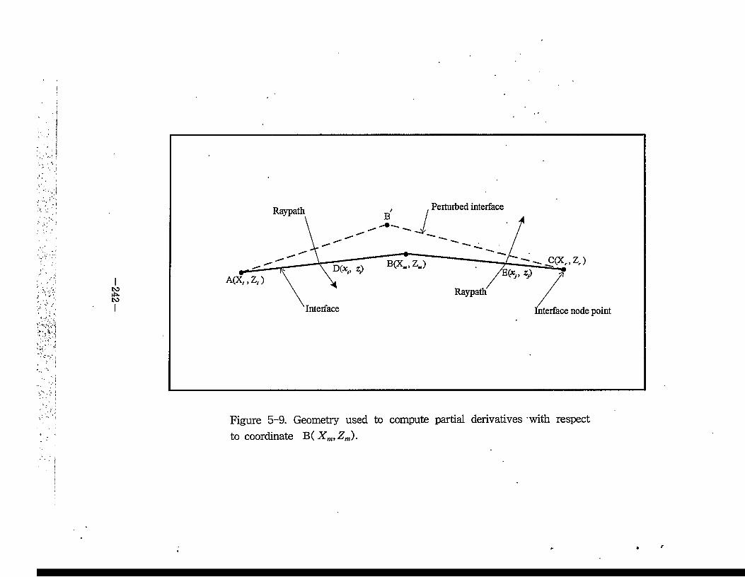
242
Perturbed interfaceRaypath
Raypath
Interface Interface node point
Figure 5-9. Geometry used to compute partial derivatives with respect to coordinate B( Xm,Zm).
3U du dZiaz« dZi az^
dU du dXj
i
dXj a%«
du du dzjaz„ dzj az,
The mathematical notation of the above relationship are given by (Shin,1988) !
X{ =Xm-Xi Xm—Xi \
__7 y __7 &n.m(14)
Zi = ■^‘-Z'-x,+Z.Xm—X/
Zm-Z, X,
•n / i y __ m7—7 zj'^m 7 _7
_Zm_Zr_ ,y Zm Zr
Taking the partial derivatives of equation (14) with respect to Xm and
Zm leads to
_ i _ | -±l>»___l |axm 1 1 Zm—Zt 1 (15)
=i_| . • |
243-
From equation (15) and equation (13) we have
ML - + w*i%
ML % dudzi + Wu dU
dZj
(16)
where WXi = . W* ~ SXm w« = -&:•mi w“ = -§£
The weighting function has maximum value 1 at the nodepoint B
and minimum value 0 at the nodepoint A or C. The amplitude and the
phase of the forward wavefield is constant. However, the amplitude and
the phase of the partial derivatives that are analytically computed in the
frequency domain are function of frequency, the medium velocity, and
the ray trajectories.
2-2-4. The frequency band characteristic of the objective function
In the damped least square method, we minimize the residual. The
residual is defined as the sum of squares of the differences between the
observed data and the calculated data. The objective function can be
given by
5f(p) = (d - u)T(d - u) (17)
where d is the observed data, u the calculated data, and T denotes the
transpose.
For the purpose of illustrating the frequency band characteristic of
the objective function, we compute equation (16) for the syncline model
shown in Figure 5-10. The syncline axis Hi.0,0.8) is moved to each
grid point and the size of grid cell is 25m. In this case the parameters
of the objective function are the x-and 2-coordinate of the syncline
axis. Figures 5-ll(a), (b), (c) and (d) show contours of the objective
function when the frequency bands are at 5, 10, 15 and 20Hz,
respectively. From Figure 5-ll(a), it can be noted that the objective
function has a global minimum at the correct position of the syncline
axis and has a very smooth contour line. As we high-pass filter the
data, the local minimum begins to appear as shown in Figures 5-11(b),
(c) and (d). Even though the initial value is not adjacent to the true
model, inversion in the low frequency band can be stable and robust
because of the larger convergence radius. We infer that the convergence
rate in the low frequency band is faster than in the high frequency
band. But the resolution in the low frequency band is low. Therefore,
the lower frequency band is used in the first stage of the minimum
search. The model parameters computed from this stage are used as
initial guess for the next high frequency band.
Then, let us examine the objective function of traveltime inversion.
Figure 5-12 shows the contour of the objective function obtained by the
-245-
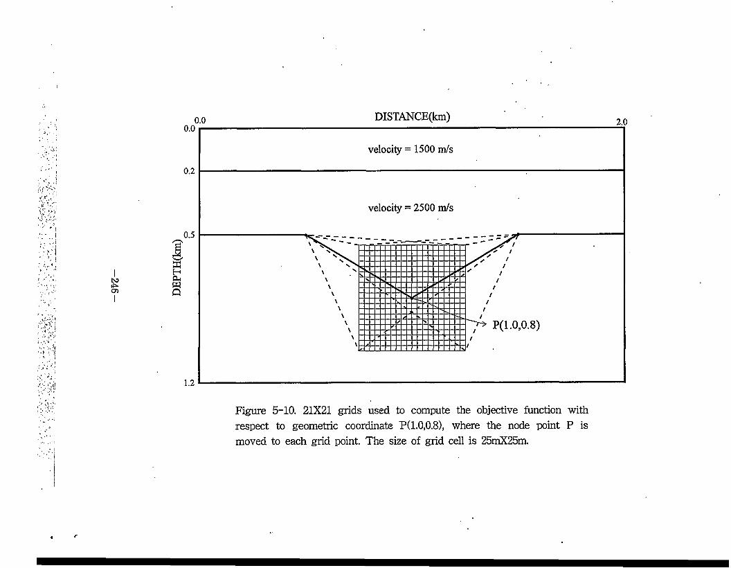
DEP
TH
(km
)
DISTANCE(km) 2.00.0
velocity = 1500 m/s
velocity = 2500 m/s
Figure 5-10. 21X21 grids used to compute the objective function with respect to geometric coordinate P(1.0,0.8), where the node point P is moved to each grid point The size of grid cell is 25mX25m.
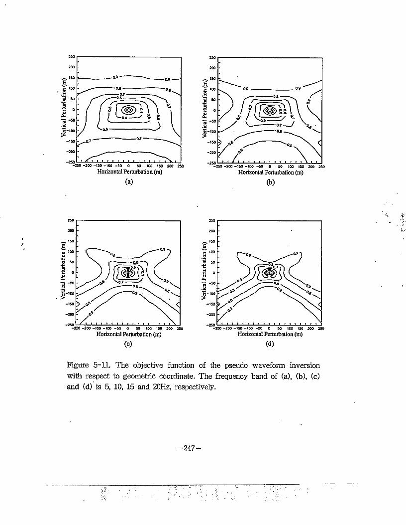
Ver
tical
Pert
urba
tion
(m)
Ver
tical
Per
turb
atio
n (m
)
>250 -200 -150 -100 -50 0 50 100 150 200 250
Horizontal Perturbation (m)
-200 v
i i t i•250 -200 -150 -100 -50 0 50 100 150
Horizontal Perturbation (m)
(a) (b)
-250 -200 -150 -100 -50 0 50 100 150 200 250
Horizontal Perturbation (m)
100 -
-200 -
-250 -200 -150 -100 -50 50 100 150 200 250
Horizontal Perturbation (m)
(c) (d)
Figure 5-11. The objective function of the pseudo waveform inversion with respect to geometric coordinate. The frequency band of (a), (b), (c) and (d) is 5, 10, 15. and 20Hz, respectively.
-247-
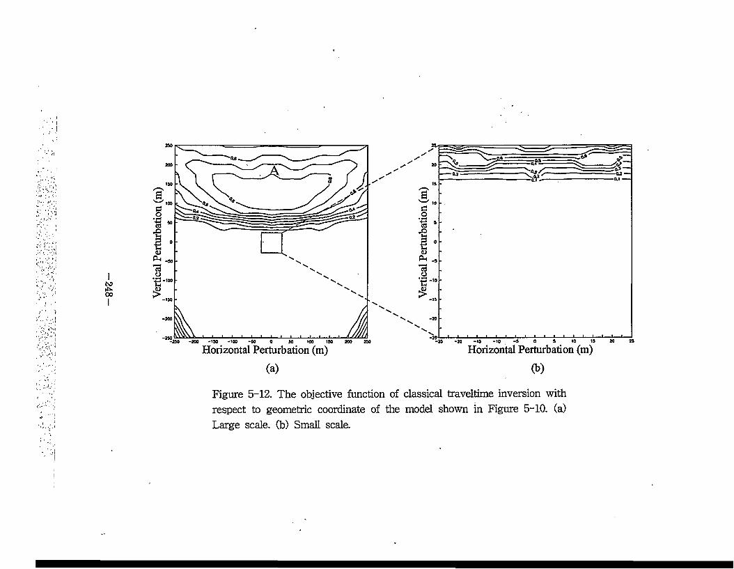
Ver
tical
Per
turb
atio
n (m
)
Figure 5-12. The objective function of classical traveltime inversion with respect to geometric coordinate of the model shown in Figure 5-10. (a) Large scale, (b) Small scale.
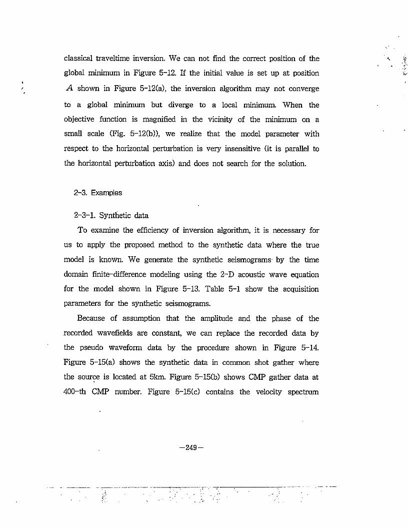
classical traveltime inversion. We can not find the correct position of the \
global minimum in Figure 5-12. If the initial value is set up at position
A shown in Figure 5-12(a), the inversion algorithm may not converge
to a global minimum but diverge to a local minimum. When the
objective function is magnified in the vicinity of the minimum on a
small scale (Fig. 5-12(b)), we realize that the model parameter with
respect to the horizontal perturbation is very insensitive (it is parallel to
the horizontal perturbation axis) and does not search for the solution.
2-3. Examples
2-3-1. Synthetic data
To examine the efficiency of inversion algorithm, it is necessary for
us to apply the proposed method to the synthetic data where the true
model is known. We generate the synthetic seismograms by the time
domain finite-difference modeling using the 2-D acoustic wave equation
for the model shown in Figure 5-13. Table 5-1 show the acquisition
parameters for the synthetic seismograms.
Because of assumption that the amplitude and the phase of the
recorded wavefields are constant, we can replace the recorded data by
the pseudo waveform data by the procedure shown in Figure 5-14.
Figure 5-15(a) shows the synthetic data in common shot gather where
the source is located at 5km. Figure 5-15(b) shows CMP gather data at
400-th CMP number. Figure 5-15(c) contains the velocity spectrum
-249-
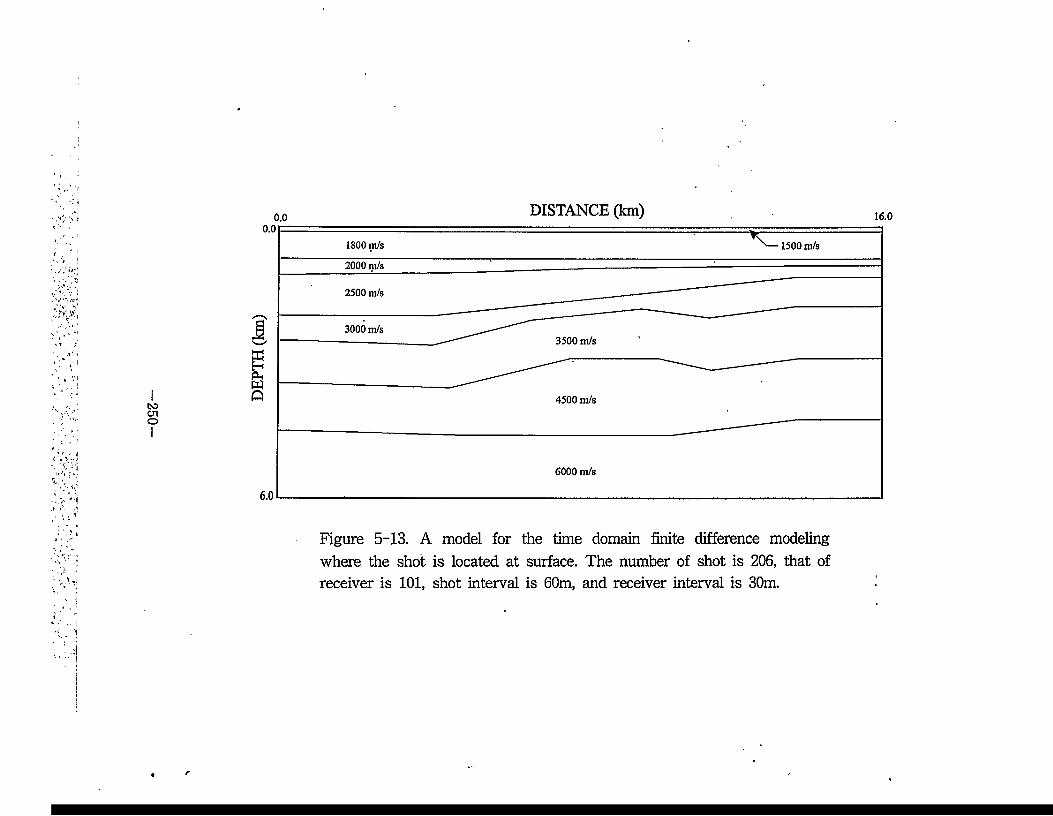
DEP
TH (k
m)
DISTANCE (km) 16.00.0
1800 m/s 1500 m/s
2000 m/s
2500 m/s
3000 m/s3500 m/s
4500 m/s
6000 m/s
Figure 5-13. A model for the time domain finite difference modeling where the shot is located at surface. The number of shot is 206, that of receiver is 101, shot interval is 60m, and receiver interval is 30m.
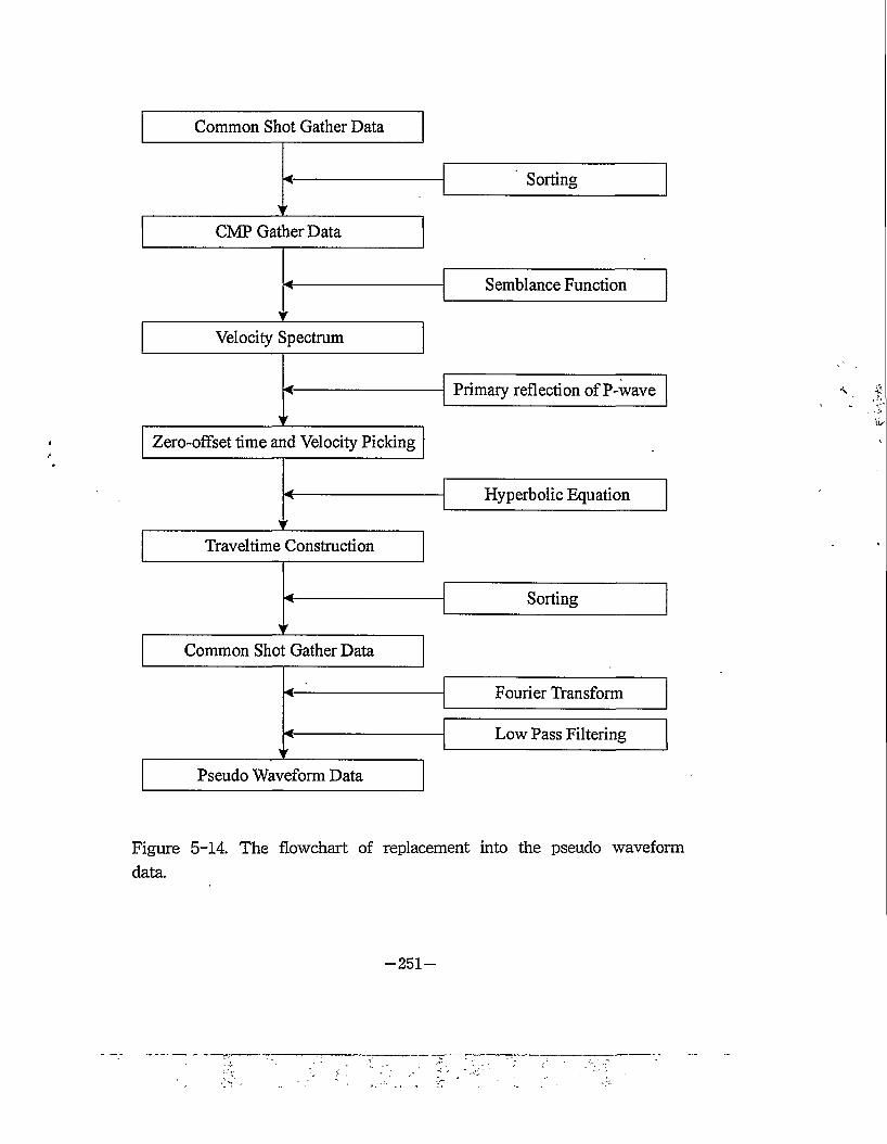
Hyperbolic Equation
Low Pass Filtering
Fourier Transform
Primary reflection ofP-wave
Sorting
Semblance Function
Traveltime Construction
Common Shot Gather Data
Velocity Spectrum
Zero-offset time and Velocity Picking
Pseudo Waveform Data
Common Shot Gather Data
CMP Gather Data
Figure 5-14. The flowchart of replacement into the pseudo waveform data.
-251-
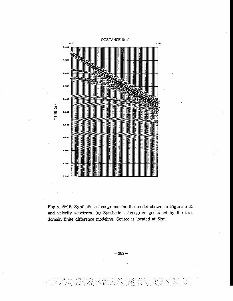
0.00DISTANCE (km)
Figure 5-15. Synthetic seismograms for the model shown in Figure 5-13 and velocity sepctrum. (a) Synthetic seismogram generated by the time domain finite difference modeling. Source is located at 5km.
-252-
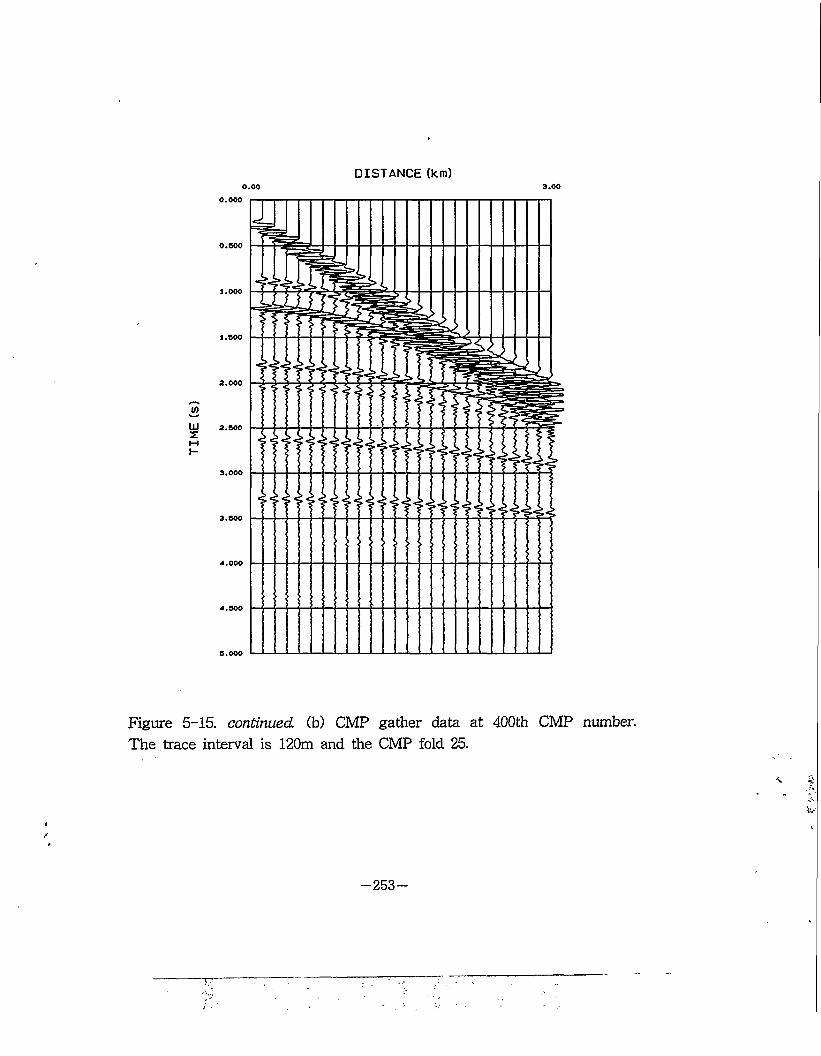
0.00
DISTANCE (km)3.00
0.000
0.900
1.000
2.000
2.500
3.000
3.900
4.000
4.500
5.000
Figure 5-15. continued, (b) CMP gather data at 400th CMP number. The trace interval is 120m and the CMP fold 25.
—253 —
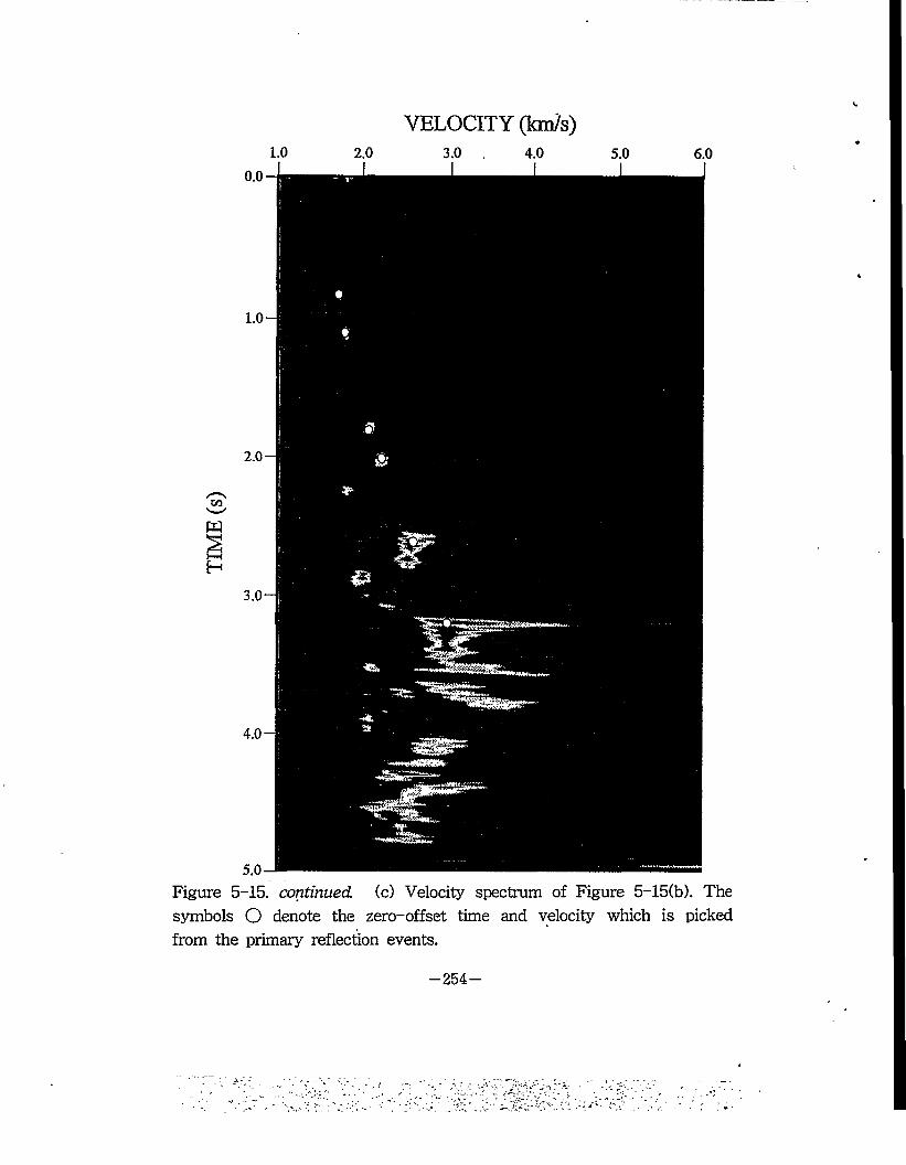
TIM
E (s
)
VELOCITY (km/s)
Figure 5-15. continued, (c) Velocity spectrum of Figure 5-15(b). The symbols O denote the zero-offset time and velocity which is picked from the primary reflection events.
-254-
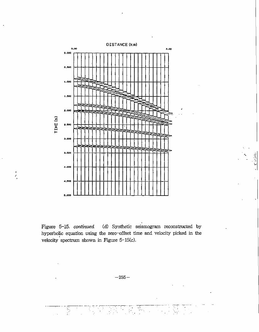
0.00DISTANCE (km)
3.00
0.000
0.500
1.500
2.000
2.600
3.000
3.600
4.000
6.000
Figure 5-15. continued. (d) Synthetic seismogram reconstructed by hyperbolic equation using the zero-offset time and velocity picked in the velocity spectrum shown in Figure 5-15(c).
-255-
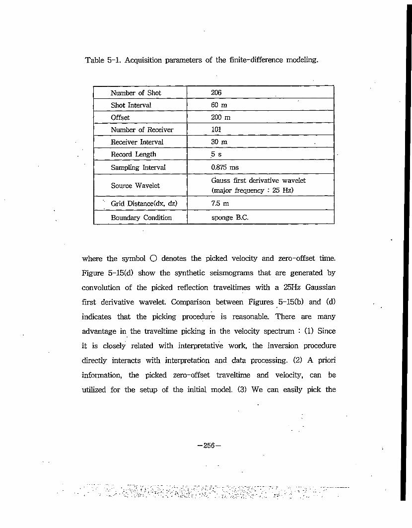
Table 5-1. Acquisition parameters of the finite-difference modeling.
Number of Shot 206
Shot Interval 60 m
Offset 200 m
Number of Receiver 101
Receiver Interval 30 m
Record Length 5 s
Sampling Interval 0.875 ms
Source WaveletGauss first derivative wavelet (major frequency : 25 Hz)
Grid Distance(dx, dz) 7.5 m
Boundary Condition sponge B.C.
where the symbol O denotes the picked velocity and zero-offset time.
Figure 5~15(d) show the synthetic seismograms that are generated by
convolution of the picked reflection traveltimes with a 25Hz Gaussian
first derivative wavelet. Comparison between Figures 5—15(b) and (d)
indicates that the picking procedure is reasonable. There are many
advantage in the traveltime picking in the velocity spectrum • (1) Since
it is closely related with interpretative work, the inversion procedure
directly interacts with interpretation and data processing. (2) A priori
information, the picked zero-offset traveltime and velocity, can be
utilized for the setup of the initial model. (3) We can easily pick the
-256-
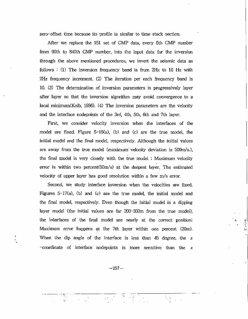
zero-offset time because its profile is similar to time stack section.
After we replace the 151 set of CMP data, every 5th CMP number
from 90th to 840th CMP number, into the input data for the inversion
through the above mentioned procedures, we invert the seismic data as
follows : (1) The inversion frequency band is from 2Hz to 10 Hz with
2Hz frequency increment. (2) The iteration per each frequency band is
10. (3) The determination of inversion parameters is progressively layer
after layer so that the inversion algorithm may avoid convergence to a
local minimum(Kolb, 1986). (4) The inversion parameters are the velocity
and the interface nodepoints of the 3rd, 4th, 5th, 6th and 7th layer.
First, we consider velocity inversion when the interfaces of the
model are fixed. Figure 5-16(a), (b) and (c) are the true model, the
initial model and the final model, respectively. Although the initial values
are away from the true model (maximum' velocity deviation is 500m/s.),
the final model is very closely with the true model ; Maximum velocity
error is within two percent(50m/s) at the deepest layer. The estimated
velocity of upper layer has good resolution within a few m/s error.
Second, we study interface inversion when the velocities are fixed.
Figures 5-17(a), (b) and (c) are the true model, the initial model and
the final model, respectively. Even though the initial model is a dipping
layer model (the initial values are far 200-300m from the true model),
the interfaces of the final model are nearly at the correct position:
Maximum error happens at the 7th layer within one percent (20m).
When the dip angle of the interface is less than 45 degree, the z
-coordinate of interface nodepoints is more sensitive than the x
-257-
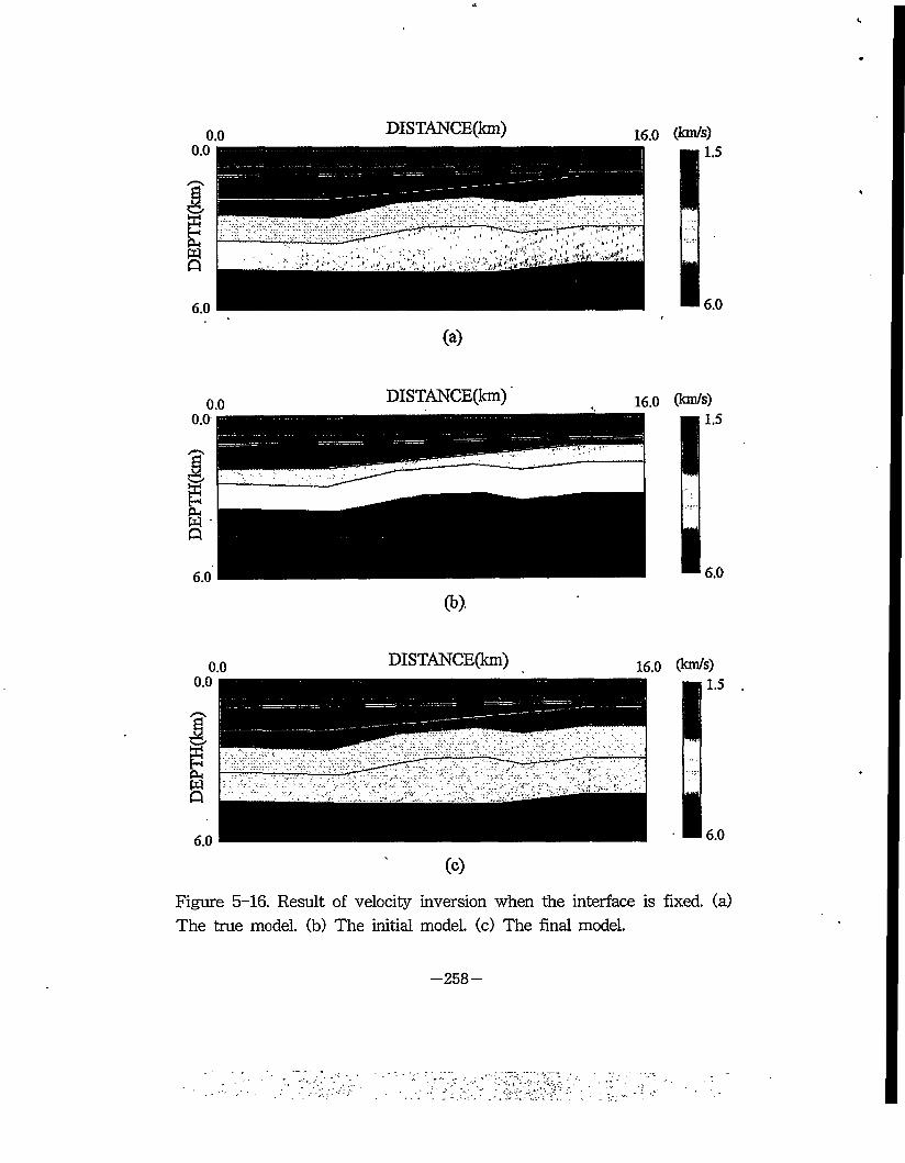
DISTANCE(km) 160 (km/s)
(b>
DISTANCE(km) (km/s)
(c)Figure 5-16. Result of velocity inversion when the interface is fixed, (a) The true model, (b) The initial model, (c) The final model.
-258-
r'',»: ■J
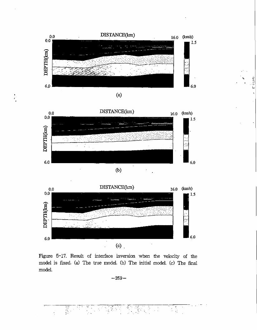
16.0 (km/s) 1.5
I6.0
(a)
(b)
DISTANCE(km) q (km/s)
(c) .Figure 5-17. Result of interface inversion when the velocity of the model is fixed, (a) The true model, (b) The initial model, (c) The final model.
-259-
-coordinate. If the ^-coordinate of the interface nodepoint is perturbed
in the horizontal layer, the change of traveltimes can not occur.
Finally, we examine simultaneous interface and velocity inversion.
When there are excessively changes in the magnitudes of the parameter
correction components, inversion can be unstable. In order to overcome
this problem, we introduce an alternative choice of velocity and
geometric coordinate parameter. The velocity inversion is performed at
the first iteration, the interface inversion at the next iteration step, and
simultaneously the velocity-interface inversion at the third iteration.
Thirty iterations are run in each frequency band. Figures 5-18(a), (b)
and (c) contain the true model, the initial model and the final model,
respectively. The results of inversion are in agreement with the true
model. But this inversion result gives lower resolution than the above
inversion result when the interface or the velocity is fixed. Especially,
the result of the deepest layer is not so good ; Maximum interface and
velocity error is about 50m and lOOm/s, respectively. In the progressive
downward determination technique, the velocity distribution of the
shallowest layer should be accurately estimated if we want that of the
deepest layer to be evaluated.
2-3-2. Field data
We apply the pseudo waveform inversion to the prestack field data
of Korea offshore. Before picking the reflection traveltimes, we carry out
some preprocessing (such as CMP sorting, gain, muting, velocity
filtering, arid so on) so that it may be preferable to identify reflection
—260 —
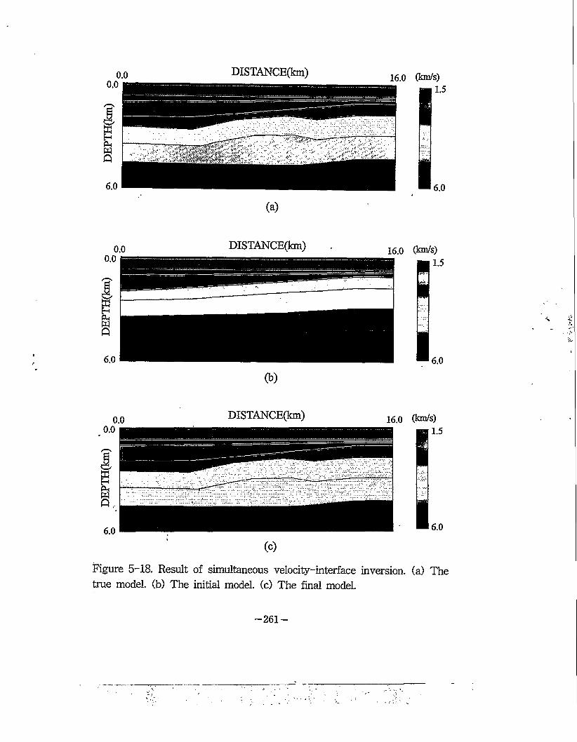
DISTANCE(km) 16.0 (km/s) 1.5
I 6.0
(b)
DISTANCE(km) jgg (km/s)
(c)Figure 5-18. Result of simultaneous velocity-interface inversion, (a) The true model, (b) The initial model, (c) The final model.
-261-
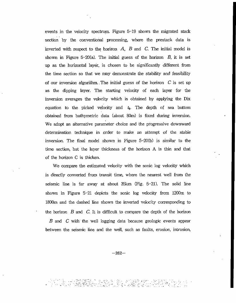
events in the velocity spectrum. Figure 5-19 shows the migrated stack
section by the conventional processing, where the prestack data is
inverted with respect to the horizon A, B and C. The initial model is
shown in Figure 5-20(a). The initial guess of the horizon B, it is set
up as the horizontal layer, is chosen to be significantly different from
the time section so that we may demonstrate the stability and feasibility
of our inversion algorithm. .The initial guess of the horizon C is set up
as the dipping layer. The starting velocity of each layer for the
inversion averages the velocity which is obtained by applying the Dix
equation to the picked velocity and t0. The depth of sea bottom
obtained from bathymetric data (about 80m) is fixed during inversion.
We adopt an alternative parameter choice and the progressive downward
determination technique in order to make an attempt of the stable
inversion. The final model shown in Figure 5-20(b) is similar to the
time section, but the layer thickness of the horizon A is thin and that
of the horizon C is thicken.
We compare the estimated velocity with the sonic log velocity which
is directly converted from transit time, where the nearest well from the
seismic line is far away at about 35km (Fig. 5-21). The solid line
shown in Figure 5-21 depicts the sonic log velocity from 1200m to
1800m and the dashed line shows the inverted velocity corresponding to
the horizon B and C. It is difficult to compare the depth of the horizon
B and C with the well logging data because geologic events appear
between the seismic line and the well, such as faults, erosion, intrusion,
-262-
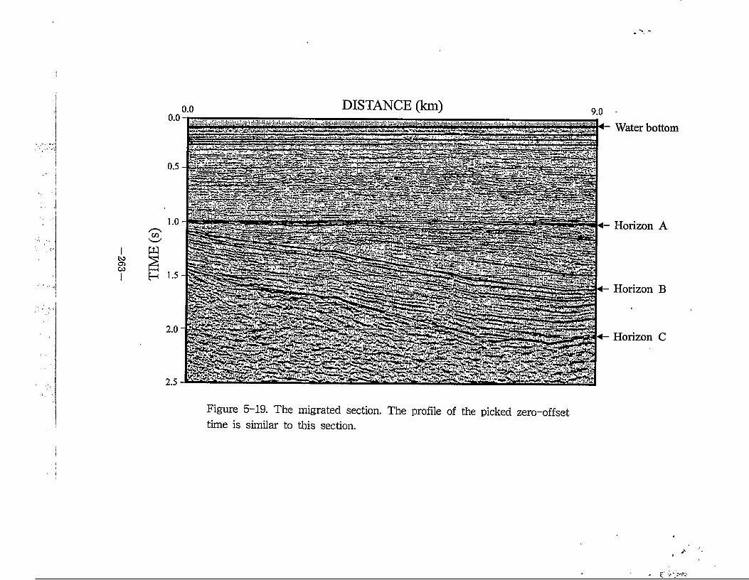
TIM
E (s
)
DISTANCE (km)
Water bottom
Horizon A
Horizon B
Horizon C
Figure 5-19. The migrated section. The profile of the picked zero-offset time is similar to this section.
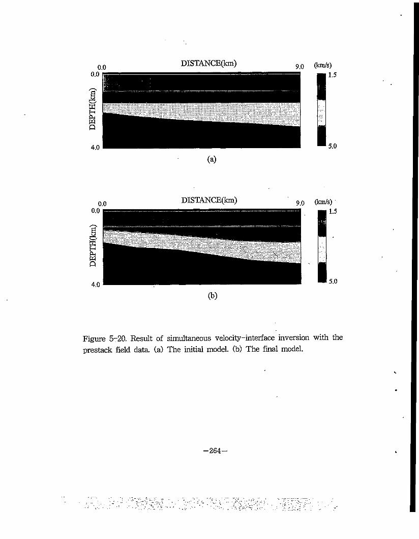
DISTANCE(km) 9.0 (km/s)
(a)
I
I
1.5
5.0
DISTANCE(km) 90 (km/s)
(b)
Figure 5-20. Result of simultaneous velocity-interface inversion with the prestack field data, (a) The initial model, (b) The final model.
—264—
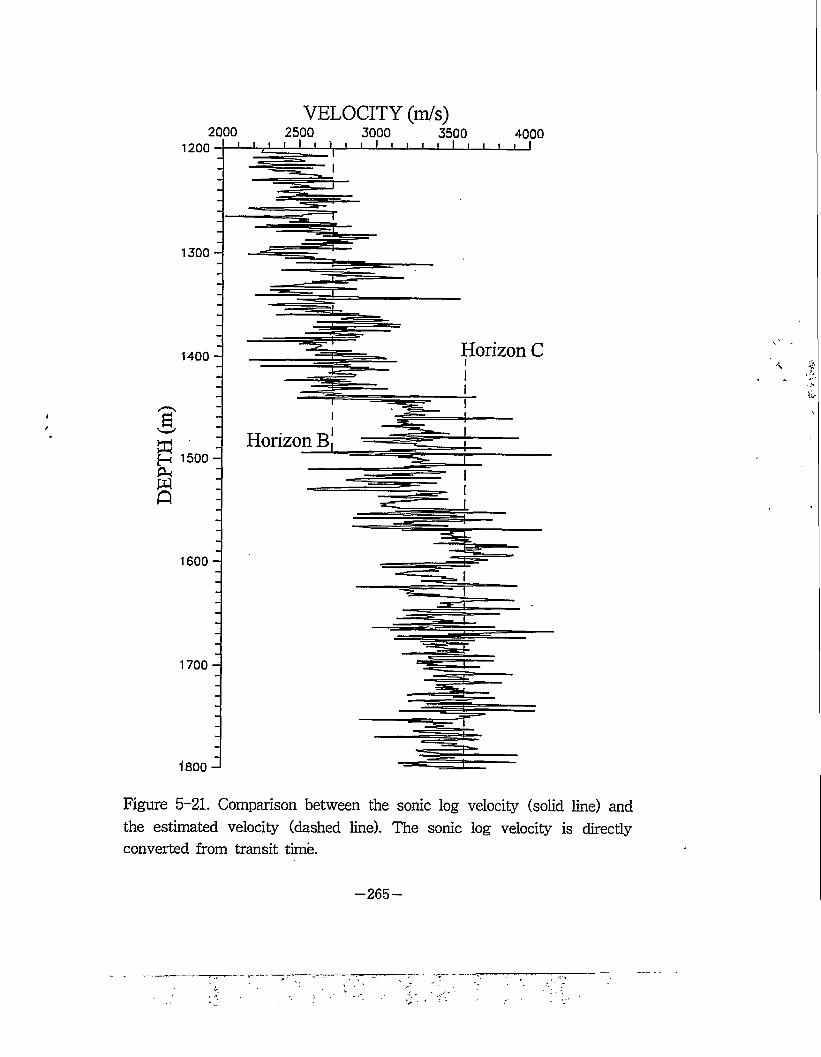
VELOCITY (m/s)2000 2500 3000 3500 4000
J L i L
1300 -
Horizon C1400 -
Horizon Bf—i 1500 -
1600 -
1700 -
1800 -1
Figure 5-21. Comparison between the sonic log velocity (solid line) and the estimated velocity (dashed line). The sonic log velocity is directly converted from transit time.
-265-
and so on. The estimated velocity of the horizon B is in accord with
the sonic log velocity trend to about 1450m. That of the horizon C is
to some extent higher than the velocity distribution of sonic log below
1450m, because the depth of the horizon C is more deep (the seismic
line is located toward the middle part of basin).
2-4. Discussion
In order to estimate the velocity model of subsurface, we develop
the pseudo, waveform inversion. We can obtain following conclusions
from our experiments.
(1) Since- the perturbation seismograms can be computed analytically by
using- ray tracing, the proposed method can much reduce
computational cost.
(2) In order to improve the reliability, effectiveness and stability of the
inversion, the low frequency band information can be employed so
that the- pseudo waveform inversion can be more stable and robust
than traveltime inversion.
(3) Even though the traveltime picking which is based on hyperbolic
approximation may include an error to some extent, especially in
steep dip with low signal-to-noise ratio, our inversion has been
successfully applied to the synthetic and the prestack field data. But,
it is necessary to improve the accuracy of traveltime picking because
a# Si
—266 —
the traveltime picking plays an important roles in our inversion
algorithm.
(4) The proposed algorithm can be easily applied to the time-to-depth
conversion in the stacked data by normal -incidence ray tracing as
well as to the traveltime tomography.
-267-
(Inversion of seismic refraction data in the frequency domain using ray tracing)
3-1. Introduction
Seismic refraction technique has been widely used to delineate the
shallow subsurface. The refraction data inversion has been used for a
long time to calculate the field static correction (Russell, 1989) and to
estimate the velocity-depth model (Landa, 1994).
The seismic traveltime inversion can be classified into two methods,
depending upon the choice of objective function. One is to minimize the
error (or difference) between the field data and the synthetic
seismograms. The other is to maximize the cross-correlation between
the synthetics and the observations (Sen, 1991). Waveform inversion
methods can be broadly classified into the direct inversion methods
(Clarke, 1984; Yagle and Levy, 1985) and the iterative inversion schemes
or nonlinear least-square inversion methods (Tarantora, 1987; Pan et al.,
1988).
In order to accomplish seismic inversion, ray tracing is one of
important tools to calculate the forward seismogram or the traveltime. In
shooting ray methods of ray tracing (Cassel, 1982; Cerveny, 1977), a fan
of rays is shot from a source point to the general direction of the
medium of interest. The correction path and travel time to connect the
two points may then be approached with successively more accurate
—268—
guesses or by adjusting the shooting angle carefully. When structure is
complex or receiver is arranged in a line, the shooting ray method is
very effective for the calculation of traveltime. Bending ray methods
(Um & Thurber, 1987; Perey, 1988) start with an initial, probably
incorrect guess for the incorrect raypath. The raypath is bent by a
perturbation method until it satisfies a minimum traveltime criterion.
When structures can be represented into analytic function to define
velocity function, it has the merit of being simple and efficient. There is
a method using finite-difference method (Vidale, 1988), but it is difficult
to express the traveltime in function of velocity and coordinates of the
medium.
In this paper, it assumes that every geologic models can be
subdivided into polygon regions having constant velocity, we designed
the shooting raytracing algorithm which is applicable to the complex
structural problem, and analytic calculation of the partial derivative
seismogram. Inversion process is based on the fact that first break of
head waves can be simplified into the delta function having unit
amplitude and with phase shift due to traveltime. In this way, we can
exploit the advantage of the full waveform and the travel time inversion.
We used the damped least-squares method (which is the Gauss Newton
method) for the inversion of head wave data. We applied this inversion
method to the synthetic and real seismogram.
3-2. Theory
-269-
To calculate the travel time of head wave, we assume that
subsurface can be divided into the blocky regions consisting of straight
line segments and head waves travel along the interface, as shown in
Figure 5-22. Unlike the conventional shooting ray tracing of fan of rays
from the source, a series of rays along the interface at infinitesimal
distance interval are shooted according to the Snell's law. After
collecting the rays which is nearest the source and the receivers,
calculating the travel time corresponding to the those ray paths and
adding the. travel time along the interface gives travel time as below
where, L is the number of ray path segments, y(r^) is the velocity of
medium, rk is the distance defined as
rk = f,{xk+l-x^)2 + (zk+r~Zk)2 , k= 1,2,3,—,/
where, k- is the number of ray path segments, and %k and are the
coordinates of the points on the interfaces which ray passes through.
Since we are dealing with the first break in seismic refraction
prospecting; we discarded the wave events following the first breaks
and assume, that seismogram can be a unit delta function without any
reflection, diffraction and other waves. Picked seismogram can be given
as
u(t) = 6( t - T ) (2)
-270-
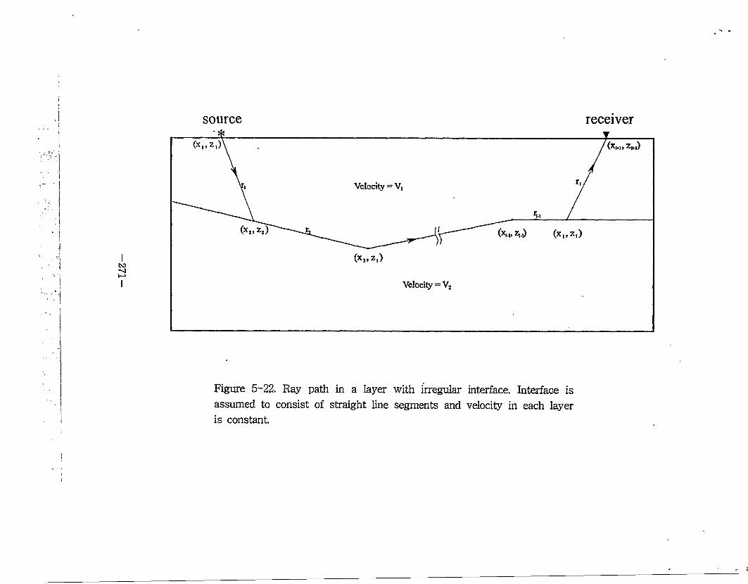
source receiver
Figure 5-22. Ray path in a layer with irregular interface. Interface is assumed to consist of straight line segments and velocity in each layer is constant.
where T is the travel time of headwave. Because the travel time of
head wave is a function of the velocity and the coordinates of the
interface, we can take the partial derivatives of Equation (1) with
respect to velocity and coordinates. The key point to note is that we
will take Fourier transform of Equation (2) in the frequency domain.
Fourier transforming Equation(2) gives
U(o>) = eiwT. (3)
Figure 5-23(b) is a synthetic head wave seismogram, convolved
with Gaussian first derivative wavelet having 50 Hz major frequency
whereas Figure 5-23(a) shoes the ray paths computed by shooting ray
tracing.
In frequency domain, the partial derivative with respect to the
velocity of n-l'th layer is calculated by single algebra
~dv'Q)^ =------+ U(co). (4)ut'n—1 y„-i
The partial derivatives with respect to interface coordinates can be
given as
dU(a>) _ • / xi xi-1dx; \ v(ri-x) r,-i
Xj+1 ~ Xj
v (rt) Yi (5)
-272-
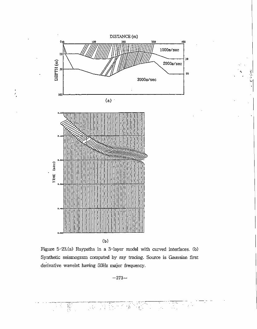
DISTANCE (m)
lOOOm/sec
2000m/sec
3000m/sec
Figure 5-23.(a) Raypaths in a 3-layer model with curved interfaces, (b)
Synthetic seismogram computed by ray tracing. Source is Gaussian first
derivative wavelet having 50Hz major frequency.
-273-
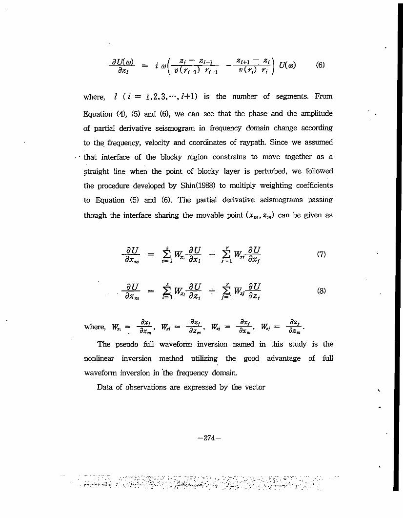
dU(co)dz{
wf) «•> (6)%j—iv(r{-1) n-i
where, / (i = 1,2,3, •••, /+1) is the number of segments. From
Equation (4), (5) and (6), we can see that the phase and the amplitude
of partial derivative seismogram in frequency domain change according
to the frequency, velocity and coordinates of raypath. Since we assumed
that interface of the blocky region constrains to move together as a
straight line when the point of blocky layer is perturbed, we followed
the procedure developed by Shin(1988) to multiply weighting coefficients
to Equation (5) and (6). The partial derivative seismograms passing
though the interface sharing the movable point (xm, zm) can be given as
- -dx (7)
it - +1,^ (8)
where, Wx. = , % = , Wxi = 3£l , Ffc =dZj dzm *
The pseudo full waveform inversion named in this study is the
nonlinear inversion method utilizing the good advantage of full
waveform inversion in the frequency domain.
Data of observations are expressed by the vector
-274-
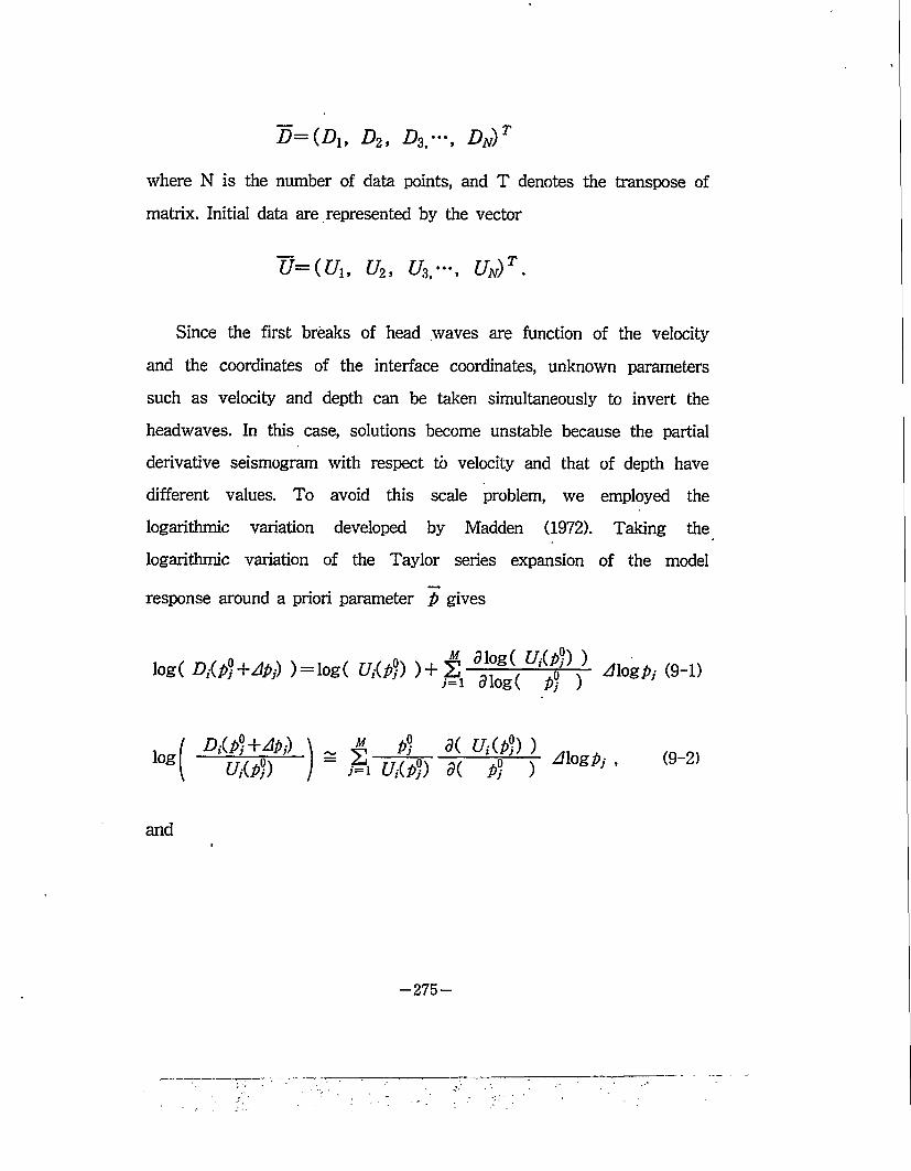
D— (Di, D2, D$'Dn)t
where N is the number of data points, and T denotes the transpose of
matrix. Initial data are represented by the vector
Since the first breaks of head waves are function of the velocity
and the coordinates of the interface coordinates, unknown parameters
such as velocity and depth can be taken simultaneously to invert the
headwaves. In this case, solutions become unstable because the partial
derivative seismogram with respect to velocity and that of depth have
different values. To avoid this scale problem, we employed the
logarithmic variation developed by Madden (1972). Taking the
logarithmic variation of the Taylor series expansion of the model
response around a priori parameter p gives
log( Diitfj+Apj) ) = log( Ujiptj) )+ 2̂ aiog( u,W)J= i 91og( p] ) Alogpj (9-1)
log u.iti)~ & $ % gj(rf) )- A u,w 3( pJ ) Alogpj , (9-2)
and
-275-
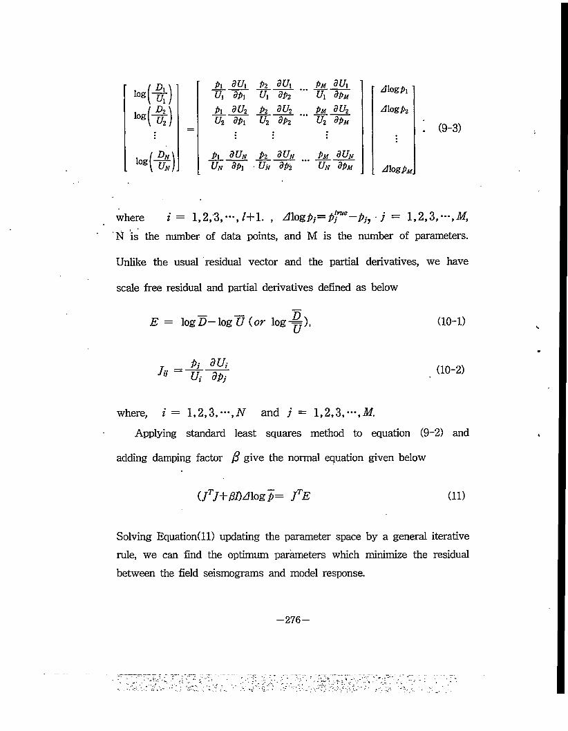
Pi dux Pz dux Pm dUiUi dpi Ui BPi Ui BPm
Pi du2 Pz du2 Pm dU2U2
£
u2 dPz u2 BPm
Pi BUh Pz suN Pm dUNUN dpi ■ Un dpz Un BPm
A\ogPi
A\ogp2
. (9-3)
Alogpu
where i = 1,2,3,—, /+1. , Allogpp^—pj, ■ j = 1,2,3,—,M N is the number of data points, and M is the number of parameters.
Unlike the usual residual vector and the partial derivatives, we have
scale free residual and partial derivatives defined as below
E = log.D—log U (or log-=), (10-1)
hPi dUjUi dpj
(10-2)
where, i = 1,2,3,—,iV and j = 1,2,3,—,MApplying standard least squares method to equation (9-2) and
adding damping factor 0 give the normal equation given below
(/7+#Mlog p= fE (11)
Solving Equation(ll) updating the parameter space by a general iterative rule, we can find the optimum parameters which minimize the residual between the field seismograms and model response.
-276-
3-3. Examples
3-3-1. Synthetic data
To verify the accuracy of traveltime of head waves, we compared
the traveltime curve computed by finite-difference method originally
developed by Vidale (1988) to the traveltime curve computed by
shooting method. Figure 5-24(a) shows a wavefront calculated by using
finite-difference method for a syncline model while Figure 5-24(b)
shows traveltime curves calculated by using shooting method and
finite-difference method. We can note that these curves match closely.
Figure 5-25 shows a fault model taken to compare the analytical
partial derivative wavefield to the partial derivative wavefield by
numerical differencing. By adjusting the difference interval of the
vertical coordinate of the point F in Figure 5-25, we calculated thez
partial derivative wavefield by central difference method, and compared
it to the analytic derivative wavefield. As shown in Figures 5-26 and
5-27, the analytic partial derivative wavefield matches with the
numerical partial derivative wavefield obtained by finite-differences.
Figure 5-26(a) shows partial derivative wavefield with respect to
vertical coordinate of point F at 40 Hz, whereas Figure 5-26(b) shows
the partial derivative wavefield with respect to the horizontal coordinate
of point F. Figures 5-27(a) and (b) show the real part and the
imaginary part of partial derivative wavefield with respect to the
-277-
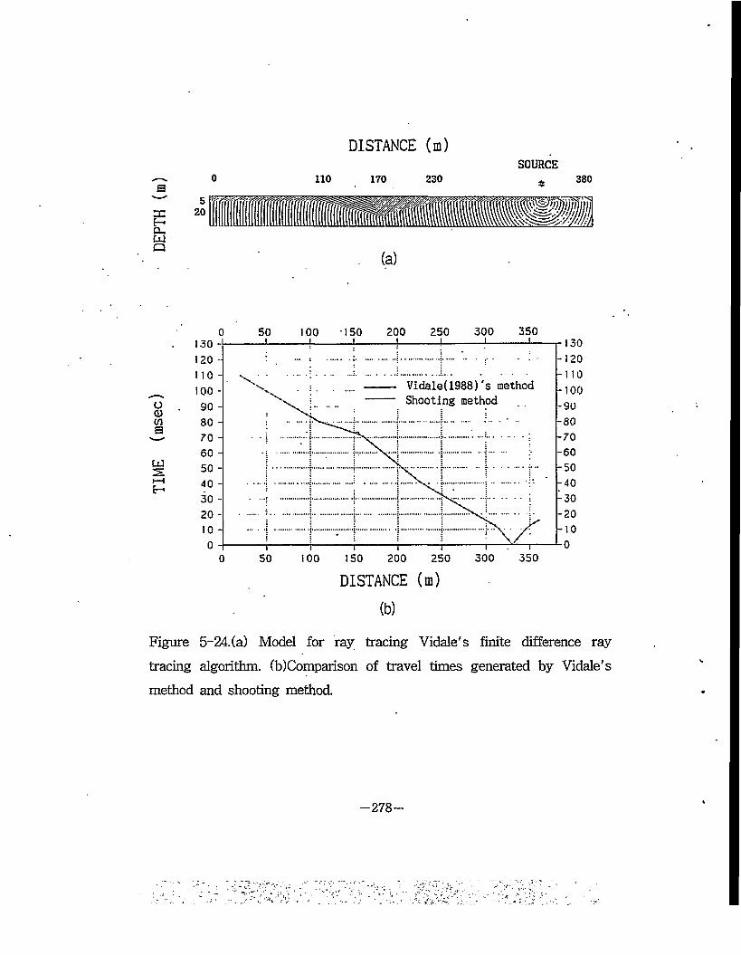
TIME (m
sec)
DEPTH (m)
DISTANCE (m)SOURCE
0 110 170 230 380
(a)
0 50 100 150 200 250 300 350130 -120 -
-1 10110-
Vidale(1988)'s method Shooting method
. •. -100
70 -
...... ! ....
DISTANCE (m)(b)
Figure 5-24. (a) Model for ray tracing Vidale's finite difference ray
tracing algorithm. (b)Comparison of travel times generated by Vidale's
method and shooting method.
-278
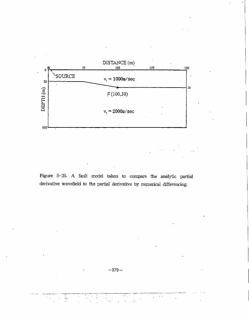
DEP
TH(m
)
50
\SOURCE20
DISTANCE (m) 100
v, - lOOOm/sec
150 200
30
F (100,30)
v. = 2000m/sec
too
Figure 5-25. A fault model taken to compare the analytic partial
derivative wavefield to the partial derivative by numerical differencing.
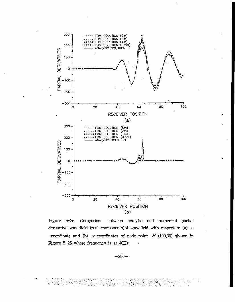
300 -1 FDM SOLUTION (5m) FDM SOLUTION (2m) FDM SOLUTION 1m) FDM SOLUTION (0.5m) ANALYTIC SOLUTION ■
200 -
100 -
2= -100-
-200 -
-300
RECEIVER POSITION
300 -| FDM SOLUTION (5m) FDM SOLUTION (2m) FDM SOLUTION 1m) FDM SOLUTION (0.5m) ANALYTIC SOLUTION
200 -
100 -
-100-
-200-
-300
RECEIVER POSITION (b)
Figure 5-26. Comparison between analytic and numerical partial
derivative wavefield (real components)of wavefield with respect to (a) z
-coordinate and (b) ^-coordinates of node point F (100,30) shown in
Figure 5-25 where frequency is at 40Hz.
-280-
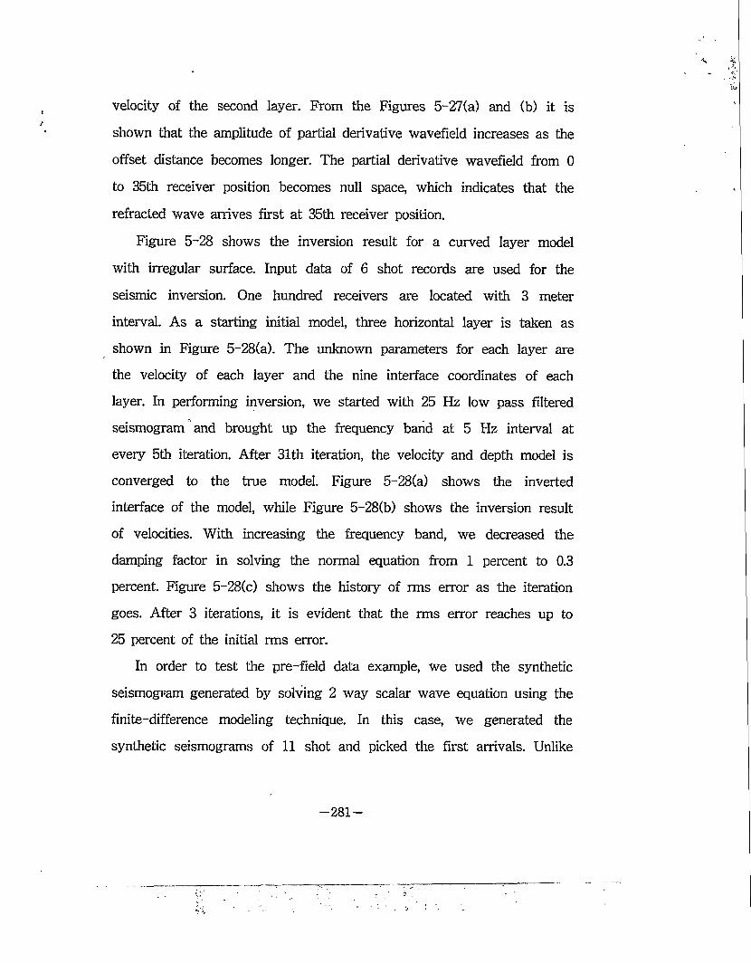
velocity of the second layer. From the Figures 5-27(a) and (b) it is
shown that the amplitude of partial derivative wavefield increases as the
offset distance becomes longer. The partial derivative wavefield from 0
to 35th receiver position becomes null space, which indicates that the
refracted wave arrives first at 35th receiver position.
Figure 5-28 shows the inversion result for a curved layer model
with irregular surface. Input data of 6 shot records are used for the
seismic inversion. One hundred receivers are located with 3 meter
interval. As a starting initial model, three horizontal layer is taken as
shown in Figure 5~28(a). The unknown parameters for each layer are
the velocity of each layer and the nine interface coordinates of each
layer. In performing inversion, we started with 25 Hz low pass filtered
seismogram and brought up the frequency band at 5 Hz interval at
every 5th iteration. After 31th iteration, the velocity and depth model is
converged to the true model. Figure 5-28(a) shows the inverted
interface of the model, while Figure 5-28(b) shows the inversion result
of velocities. With increasing the frequency band, we decreased the
damping factor in solving the normal equation from 1 percent to 0.3
percent. Figure 5~28(c) shows the history of rms error as the iteration
goes. After 3 iterations, it is evident that the rms error reaches up to
25 percent of the initial rms error.
In order to test the pre-field data example, we used the synthetic
seismogram generated by solving 2 way scalar wave equation using the
finite-difference modeling technique. In this case, we generated the
synthetic seismograms of 11 shot and picked the first arrivals. Unlike
—281 —
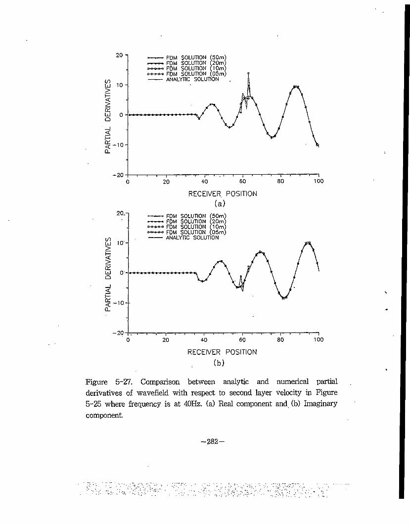
FDM SOLUTION (50m' FDM SOLUTION (20m FDM SOLUTION (10m' FDM SOLUTION (05m ANALYTIC SOLUTION
— 10 -
RECEIVER POSITION (a)
FDM SOLUTION (50m FDM SOLUTION (20m' FDM SOLUTION MOm' FDM SOLUTION (05m ANALYTIC SOLUTION
— 10-"*"
RECEIVER POSITION
Figure 5-27. Comparison between analytic and numerical partial derivatives of wavefield with respect to second layer velocity in Figure 5-25 where frequency is at 40Hz. (a) Real component and (b) Imaginary component.
-282-
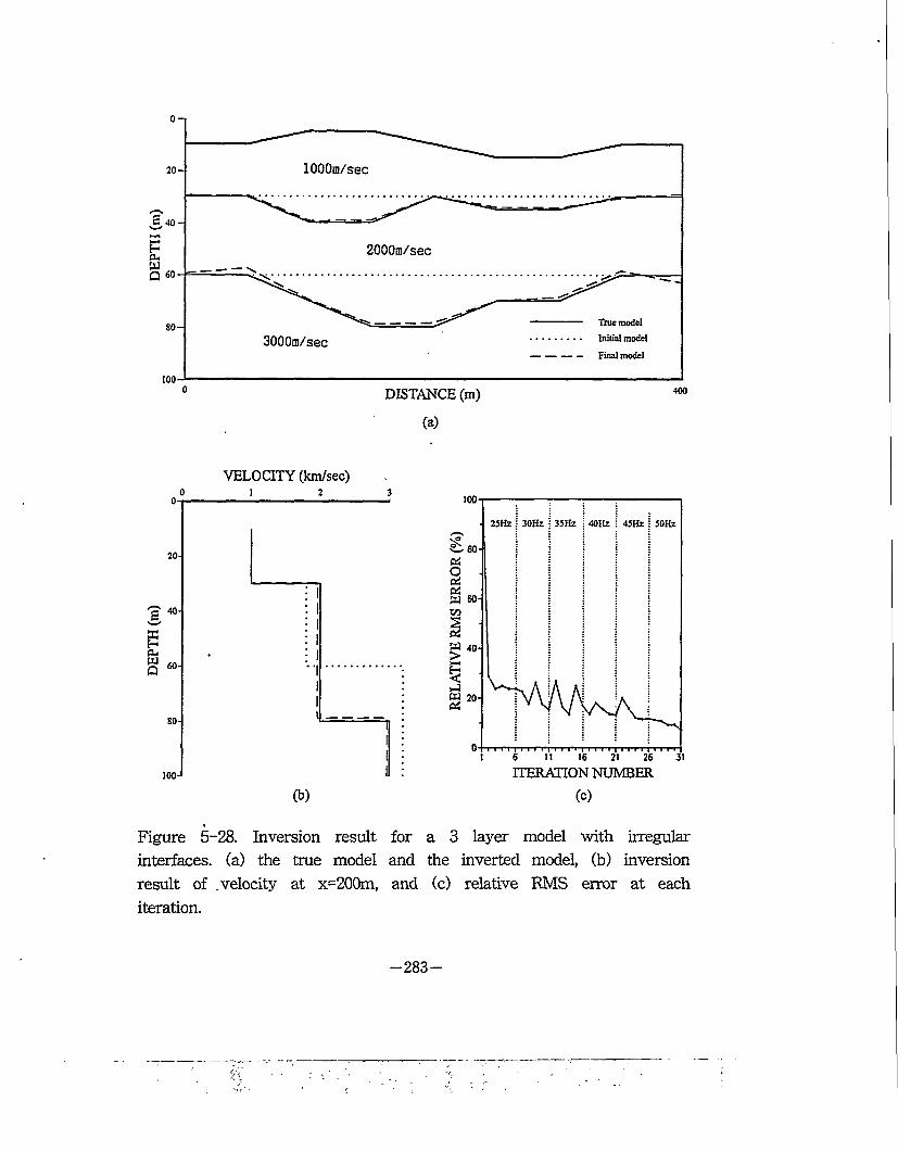
0-1
lOOOm/sec
2000m/sec
True model
Initial model3000m/secFinal model
DISTANCE (m)
VELOCITY (km/sec)0 12 3
0 — — — — ... . i
20
!40
60-
80-
100-J
I
(b)
50Hz
O -
Sti 60-
M 40-
ITERATION NUMBER
(c)
Figure 5-28. Inversion result for a 3 layer model with irregular interfaces, (a) the true model and the inverted model, (b) inversion result of .velocity at x=200m, and (c) relative RMS error at each iteration.
-283-
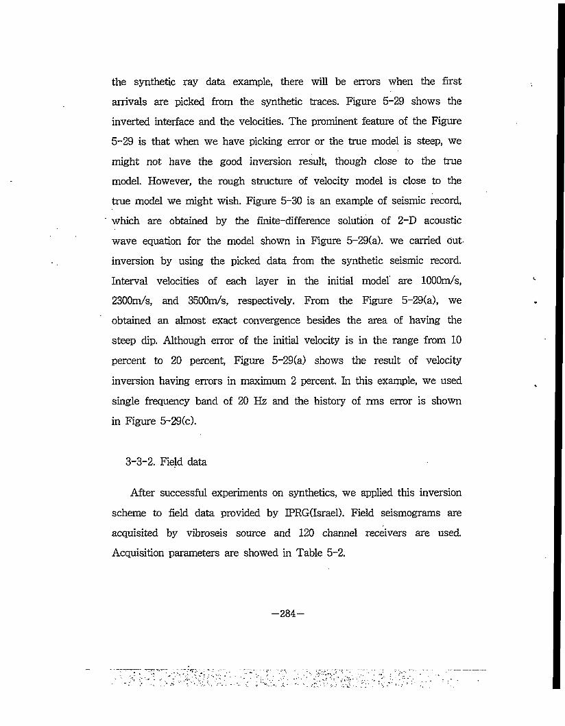
the synthetic ray data example, there will be errors when the first
arrivals are picked from the synthetic traces. Figure 5-29 shows the
inverted interface and the velocities. The prominent feature of the Figure
5-29 is that when we have picking error or the true model is steep, we
might not have the good inversion result, though close to the true
model. However, the rough structure of velocity model is close to the
true model we might wish. Figure 5-30 is an example of seismic record,
which are obtained by the finite-difference solution of 2-D acoustic
wave equation for the model shown in Figure 5-29(a). we carried Out
inversion by using the picked data from the synthetic seismic record.
Interval velocities of each layer in the initial model are lOOOm/s,
2300m/s, and 3500m/s, respectively. From the Figure 5-29(a), we
obtained an almost exact convergence besides the area of having the
steep dip. Although error of the initial velocity is in the range from 10
percent to 20 percent, Figure 5-29(a) shows the result of velocity
inversion having errors in maximum 2 percent. In this example, we used
single frequency band of 20 Hz and the history of rms error is shown
in Figure 5-29(c).
3-3-2. Field data
After successful experiments on synthetics, we applied this inversion
scheme to field data provided by IPRG(Israel). Field seismograms are
acquisited by vibroseis source and 120 channel receivers are used.
Acquisition parameters are showed in Table 5-2.
-284
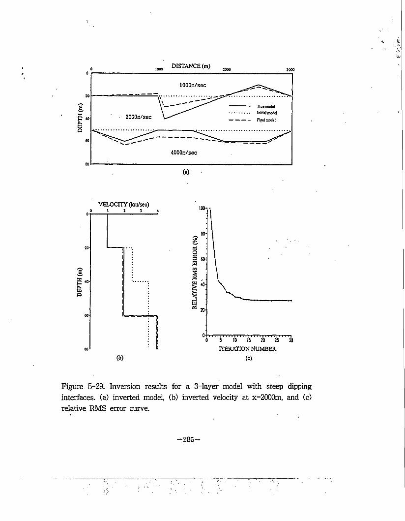
DISTANCE (m) ;gog
lOOOn/sec
True model
• • • • Initial model
— — Final model• 2000m/sec
VELOCITY (km/sec)0 12 3 40 | ii — i i i
IQ
20'
40
60
80'(b)
M i 1'1 I l 1 I | M 1 l I I l l-l |'l l I“f“| 'I I
ITERATION NUMBER
(c)
Figure 5-29. Inversion results for a 3-layer model with steep dipping interfaces, (a) inverted model, (b) inverted velocity at x=2000m, and (c) relative RMS error curve.
-285-
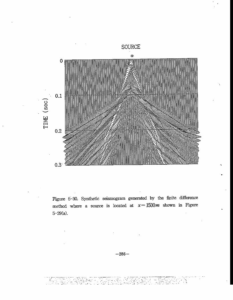
TIM
E (sec
)SOURCE
Figure 5-30. Synthetic seismogram generated by the finite difference
method where a source is located at x= 1500m shown in Figure
5-29(a).
—286 —
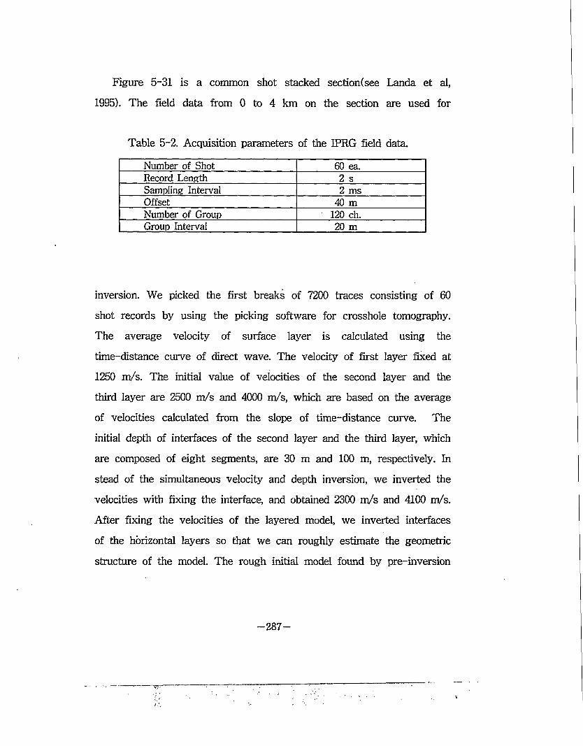
Figure 5-31 is a common shot stacked section(see Landa et al,
1995). The field data from 0 to 4 km on the section are used for
Table 5-2. Acquisition parameters of the IPRG field data.
Number of Shot 60 ea.Record Length 2 sSampling Interval 2 msOffset 40 mNumber of Group 120 ch.Group Interval 20 m
inversion. We picked the first breaks of 7200 traces consisting of 60
shot records by using the picking software for crosshole tomography.
The average velocity of surface layer is calculated using the
time-distance curve of direct wave. The velocity of first layer fixed at
1250 m/s. The initial value of velocities of the second layer and the
third layer are 2500 m/s and 4000 m/s, which are based on the average
of velocities calculated from the slope of time-distance curve. The
initial depth of interfaces of the second layer and the third layer, which
are composed of eight segments, are 30 m and 100 m, respectively. In
stead of the simultaneous velocity and depth inversion, we inverted the
velocities with fixing the interface, and obtained 2300 m/s and 4100 m/s.
After fixing the velocities of the layered model, we inverted interfaces
of the horizontal layers so that we can roughly estimate the geometric
structure of the model. The rough initial model found by pre-inversion
-287-
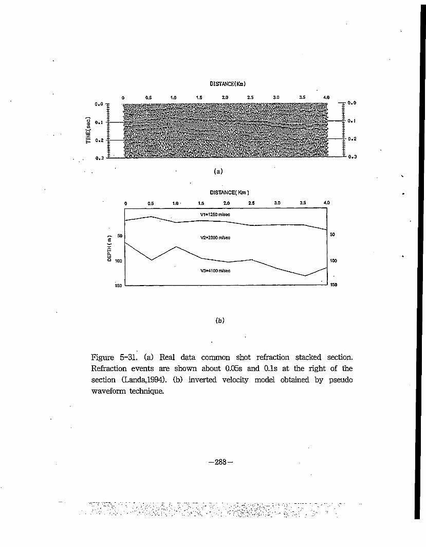
TlM
E(se
c)DISTANCE(Km)
0 0.5 1.0 1.5 2.0 2.5 3.0 3.5 4.0
(a)
DISTANCE! Km)
0 0.5 1.0 ■ 1.5 2.0 2.5 3.0 3.5 4.0
V1=1250 m/sec
V2=2300 m/sec
V3=4100 m/sec
(b)
Figure 5-31. (a) Real data common shot refraction stacked section. Refraction events are shown about 0.05s and 0.1s at the right of the section (Landa,1994). (b) inverted velocity model obtained by pseudo waveform technique.
-288-
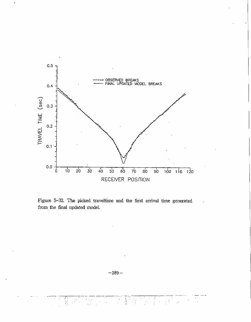
TRA
VEL
TIME (s
ec
0.5 i
OBSERVED BREAKSFINAL UPDATED MODEL BREAKS0.4- -
0.3 -
0.2 -
0.1 -
100 110 120
RECEIVER POSITION
Figure 5-32. The picked traveltime and the first arrival time generated from the final updated model.
-289
process discussed above is used as the initial model for the
simultaneous velocity and interface inversion. After 16 iterations, we
could obtain the velocity model shown in Figure 5-31 (b). In this seismic
inversion, we used the 20 Hz low pass filtered seismogram. Figure 5-32
shows the traveltimes between the finally inverted model and picked
field seismogram, it is clear to note that these two traveltimes matches
well. Note that our inversion results are in a good agreement with the
results obtained by Landa et al.(1995) from the same data set.
3-4. Discussion
In this paper, we have proposed a new method for the determination
of velocity-depth model using the seismic refraction data. One of the
advantage over other methods is that, unlike the traveltime inversion,
this inversion technique can be performed in the frequency domain using
the damped Gauss Newton method. The shooting ray tracing allows us
to calculate the travel time efficiently for the complex layered structure
with irregular topography. In addition to this efficiency in the forward
modeling, the analytic partial derivative seismogram with respect to the
velocity and coordinates of the interface can be obtained by simple
algebra. Not only can we use the low frequency data when the initial
model is far from the true model, but also we can refine the resolution
with increasing the frequency band of the seismic data.
—290—
*116#
-291-

*i| 6 &
3E* 4 44 4#* E, F 4**44 44 127fl, 117M 45# 444-4 n)*^ *# ^ *4 ^L5]ji ji^.^. » ^4 a7]
.#4 4# 4*# *D444. If 44 4*454 If ##*5 *5fe 3-4€ 9-4 # 44 4*# 44#5fe 4# 444 444 44 455 4-4)854 444 #4 44* 44)84. if 44 5 4# 44 444 If 4 4 444 44*4 44 #4 4 45. 44 4 444 44444* 4 4 $54, E44 610.5m, F* 667.2m 4& 4 44 4 4 44 44 44 44*4 4^4 *4* 455 4-4# 4. 44*4 *4 44324 *4 4-4 444 4444 445 7} 4 4 4 4=4-4 44444 444 4445S.fe.4-B- 44 444 54 44 ** 455. 44)84-. 4 4* 44]&4# 44 444 5* 4 44 4# 454 4* 4444, *4 44=5 44*44 *** 4 55 # * $14. 44 54* *44 4°J4* *544 44)4 4* *4 4 4*4 45# Ifi #4 4545 44 4**4 44 44 *4* *4 54*4 544*4 *5 4 454 *44 44 4 4**4 *44 * *444 4* 4** #44 454 457]* *4 4*4 4*4 4 4* 455. # * 44.
*4 4444 4*44 **4 4**4 41444 4*445, 4
5444 44 *44 4## 4* * $1* 544 #44454 44
44 4h4 %44 4*4 444 444* *444* 4* #4 4 4*5 *4 4* 45# 14-4 4 <3* ##55. #4 4^4. 4* * 4 *4*5 *444* 544* *# 7>^ *#4 4* 45 44 4 *4 #*4 455 #4 *54 45 f# #4# 4*44-44 4*
-293-
*111-a- 4 $4. #*13. # 14# 5xl0"4me 41S3. -§-fe44 4fe Wit fe#44 fell fe $1 a#. 441 14fe 1141 41 7>fe: f # #*]7> 41 fe fe4 44fes fe!4 5:41-9-3. 41-1
4" $lfe& 24fefe 144.il £-§-4 fefe 37fl 4 44 (A, B, D 4 4)4 oflH^a 4 4(C
4 4)4 £<$ 4 ^##4 ##4 n 444 tni #e#e a 41
fe 26.7%4 42.5%, B 41fe 11.8%4 8.1%, C 4 4fe 44.3% 4 36.2%4, D 4 4fe 12%4 3.5%3 C 444 fe#4 4-E 415.4 4h4 fefe 444S4 4# lfe#& 3.4 fe4. C41 411-1-4 14fe&4 4# lfe#4 fefe Ife 414= sfe s# #4 114=5 114 fefe 44 4Hfe 4^-5. 44# 4" $134, 4 4fe 4 4 4fe44 4=11 44#44 114 44 #44 441 4= $)fe 7>fe4* 3.4 fefe 433 # 4=s 4& 444.
7f^ ^ 7}^114]4sl 7i]#4# 444 144 $144 si
4 41:4 444 4# 4444 44 &fe 4 44 444 444 11 s 4^44 4fe4 feslfe 41:4414 444 !#! 14-3.4 144 4 fe&4. 11 m## 41fe IfefeiHl 4 4 3.711 !fe!4 lfe#4 #7} 4 4# 14s 34 111 Ife
fe#4- fell mmife4 111 1-1414 44- 1314 41 14- ifeii,mmiife 1114-4- 4Hi 1 141^34 lean gas44 #1411 Ifefel6!] 44 4 #1 14 4 447} #4 !#!&4.
4=42.1114 41 4fell411 4 1141411fes^-4 141 life 4fe4 14 -9-4=1 4= $14.
(1) 441411 7}-fsfell4 441 fes, is fefe 4life
-294-
^ 41 4 H H 7)14*4 # 4] 444 7}4* 4 (virtual source) 4* *11^4* H4 5a4. 7}*a:*41* 7>Hti] 41 7)144 4* 414 $14. *4^* S7l^7> 444 5-44 4* 4 4* 414 4414 1 4 $134, ZL#^1 $4 1* *1 414 44 4 ^o] 4^. *7)H ^6]x\^ 7}*>z-*4^34 4 #
s] *1 *7i 5 *44.(2) 4*1 ^144 444 A34* 444 4
444 444 4 14144, 1*4* 4 4 44 W* *^414 4# *l*s# 4*4. £4 a714 44 4 4 4* 44 44 4 * 44 4 4 444 44.
(3) 44*1* 4*4 #44 4444s *4414444* 1&3 44 7)14*37} 4-3.44 41* **44. £4 4 44 4144 7H*5|* 441 7>stii4* 4* 41144. 4*1*4 441 *514 is* *14 144*3. 1* 1* 441 447} 4s41 *4 1*3 $134, 144*1 41* &* 4*44 4# 41133 *# * $14.
(4) s*7}5. ^ 447}3.4 444 *7}4114^4 #41 4 7}7}s. 44^* 1*4 44 *14 *£3*4 1* *14 14 a* 4* * $1*34, 43*4 444 44 444 4*1* 4 4444.
-295

-297-

1.
1
#2 St!
4 44, 1992, ^49-2^1 14* 44 444 44#4 44:
144 ^^SL, <gS«g, : "4f#MI41 44* 4-0-4 *^1 MM4 *4*44 #4 4*." 19924 #M| 4* 44*44
**4 -§-44, 444, 4*1, 1989, -5M 4*44 4 Ml ^4 4-4 4*, 44*^444*^ 4*iLJi KR-89-3B
441, 44f, 44*, 1995, 44444 444 *4*4 4 Mm 444414: 4444^444, 32, 22-36.
44-1, #11, 444, 441, 1991, GC/MS4 14 4*5-44 #1 4 Ml *4* 49-,44#l7}44% 4^_m (KR-90-B)-33
Americal Geoogical Institute, 1976. Dictionary of Geological Terms: New York, Anchor Bookes, 472p
Aquino Neto, F. R, Triguis, J., Azevedo, D. A., et al, 1989, Oraganic geochemistry of geographically unrelated Tasmanites. 14 th International Meeting on Oraganic Geochemistry, Paris, September 18-22, 1989, Abstract No. 189
Arnold, K. and Stewart, M. 1989, : "Surface Production Operations" Gulf Publishing Company
Atlas, R. M., 1981. Microbial degradation of petroleumhydrocarbons', an environmental perspective. Microbiol. Riv., 45, 1, 180-209.
Barkay, T., D. L. Pouts, and B. H. Olsen, 1985. Preparation of a DNA gene probe for detection of mercury resistance genes in Gram-) bacterial communities. Appl. Environ. Microbiol., 49, 3, 686-692.
Barkay, T., S. C. Tripp, and B. H. Olson, 1985. Effect of metal-rich sewage sludge application on the bacterial communities of grasslands. Appl. Environ. Microbiol., 49, 2,
—299 —
333-337.
Bathe, K. J., and Wilson, E. L., 1986, Numerical methods in finite element analysis: Prentice Hall, Inc., Englewood Cliffs, New Jersey.
Beaumont, C., Boutilier, R, Mackenzie, A.S., and Rullkotter, J., 1985, Isomerization and aromazation of hydrocarbons and the paleothermometry and burial history of Alberta Foreland Basin. Aamerican Association of Petroleum Geologists Bulletin, Vol. 69, P.546-566
Beggs, H.D., 1985, "Gas Production Operation" Oil & Gas Consultants International Inc., Tulsa
Bell, C.R., M.A. Holder-Franklin, and M. Franklin, 1980. Heterotrophic bacteria in two Canadian rivers. Water Research, 14, 449-460.
Bertsekas,, D. P., 1982, Constrained optimization and Lagrange multiplier methods: Academic Press, New York.
Beveridge, G. S. G., and Schecheter, R. S., 1980, Optimization theory and practice: McGraw Hill book company, New York.
Bird, C.' W., Lynch, J. M., et al, 1971, Steroids and squalene in Methlococcus capsulatus grown on methane Nature, Vol. 230, p. 473
Bishop, T.N., Bube, K.P., Cutler, R.T., Langan R.T., Love, P.L., Resnick, J.R., Shuey, R.T., Spindler, D.A., and Wyld, H.W., 1985,Tomographic determination of velocity and depth in laterally varying media: Geophysics, 50, 903-923.
Bleistein, N., Cohen, J.K., and Magin, F.G., 1985, Computational and asymptotic aspects of velocity inversion: Geophysics, 50, 1253-1265.
Bordenave,. M.L., 1993, Applied petroleum geochemistry Editions Technip, Paris p.523
Brock, T. D., and M. T. Madigan, 1991. Biology ofmicroorganisms 6th ed., Prentice Hall, New Jersey.
Brooks, P. W. 1986, Unusual biological marker geochemistry of oils and possible source rocks, offshore Beaufort-Mackenzie Delta, Canada.
-300-
In: Adances in Oraganic Geochemistry 1985 D. Leythaeuser and J. Rullkotter, eds) Pergamon, p.401-406
Brooks, J., Welte, D. 1984, Advances in Petroleum Geochemistry Academic press Vol.l p. 344
Cassel, B.R., 1982, A method for calculating synthetic seismograms in laterally varying media: Geophys. J. Roy. Astr. Soc., 38, 9-19.
Cerveny, V., Molotkov, I.A., and Psencik, I., 1977, Ray methods inseismology: University of Karlova Press, Prague.
Chavent, G., 1986, Determination of velocities and reflectivity by multiple migration fitting
Chen, C. M., Mobley, H. L. T., and Rosen, B. P., 1985. Seperate resistance to arsenate and arsenite (antimonate) encoded by the arsenical resistance operon of R factor R773. J. Bacteriol., 161, 158-763.
Chooson, P., Connan, J., Dessort, D., and Lanau, C, 1992, In vitrobiodegradation of steranes and teipanes; A clue to understanding geological situations. In; Biological Markers in Sediments and Petroleum (J. M. Moldowan, P., Albercht, and R. P. Philp, eds.) Prentice Hall, Engiewood Cliffs, N.J.,p.320-349.
Chough, S. K., M. Y. Choe, and I. G. Hwang, 1993. Fan Deltas in the Pohang Basin (Miocene), SE Korea. 3rd InternationalWorkshop on Fan Deltas Field Excursion Guidebook.
Claerbout, J. F., 1976, Fundamentals of geophysical data processing: McGraw-Hill, Inc.
Clark, J. P., and Philp, R. P., 1989, Geochemical characterization ofevaporite and carbonate depositional environments and correlation of associated crude oils in the Black Creek Basin, Alberta. Canadian Petroleum Geologists Bulletin, Vol.37, p.401-416
Clarke, J. T., 1984, Full reconstruction of a layered elastic medium for P-SV slant stacked data: Geophys. J. Roy. Astr. Soc., 78, 775-793.
Connan, J., and Dessort, D., 1987, Novel family of hexacyclic hopanoid alkanes (C32 -Cssloccuring in sediments and oils from anoxic
-301-
paleoenvironments. Organic Geochemistry,vol.ll,p.103-113
Connan, J,, Bouroullec, J., Dessort, D., and Albrecht, P., 1986, The ' microbial input in carbonate-anhydrite facies of a sabkha
paleoenvironment from Guatemala: A molecular approach. Organic Geochemistry, Vol.10, p.29-50
Cooper, B., 1990, Practical petroleum geochemistry Robertson scientific publications p.174
Curry, W. H., 1984. Evaluation of surface gamma radiation surveys for petroleum exploration in the deep Powder River Basin. Wyoming in Davidson, M. J., and Gottlieb, B. M., eds., Unconventional methods in exploration for petroleum and natural gas III. Dallas, Southern Methodist Unviersity Press, 25-39.
Davidoson, M. J., 1963, Geochemistry can help find oil if properly used: World Oil, July, p94-100.
Davidoson, M. J., 1982, State of the art and direction of unconventional oil and gas exploration, in Davidoson, M. J., and Gottlieb, B. M. eds, Unconvetional methods in exploration for petroleum and natural gas III: Dallas, Southern Methodist University Press, p.4-8.
Davidoson, M. J., 1982, Toward a general theory of vertical migration: Oil and Gas Journal, June 21, p.288-300.
Davis, J. B., 1956, Microbial decomposition of hydrocarbons: Industrial and Engeinering Chemistry, v 48, no. 9, p.1444 -1448.
Davis, J. B., 1967. Petroleum microbiology, Elsevier, New York, 604.
Davis, J. B., 1969. Microbiology in petroleum exploration. Heroy, W. B., ed., Unconventional methods in exploration for petroleum and natural gas. Dallas, Southern Methodist University Press, 139-158.
Dennis, J. E., and Schnabel, R. B., 1983, Numerical methods for
-302-
unconstrained optimization and nonlinear equations- Prentice-Hall, Inc., Englewood cliffs, New Jersey.
Diels, L., and M. Mergeay, 1990. DNA-probe mediated detection of resistant bacteria from soils highly polluted by heavy metals. Appl. Environ. Microbiol., 56, 5, 1485-1491.
Docherty, P., 1992, Solving for the thickness and velocity of the weathering layer using 2-D refraction tomography: Geophysics, 57, 1307-1318.
Donovan, T. J., and Dalziel, M. C., 1977. Late diagenctic indicators of buried oil and gas. U.S. Geological survey Open-File Report, 77-817, 44.
Duchscherer, W., 1980. Geochemical methods of prospecting for hydrocarbons. Oil and Gas Journal, December 1, 194-208.
Duchscherer, W., 1982. Geochemical exploration for hydrocarbons'- No new tricks but an old dog. Oil and Gas Journal, July 5, 163-176
Ensminger, A., Albrecht, P., Ourisson, G., and Tissot, B., 1977, Evolution of polycyclic alkanes under the effect of burial (Early Toarcian shales, Paries Basin).In: Advances in Organic Geochemistry 1975 (R.Campos and J.Goni, eds.)ENADIMSA,Madrid, P.45-52
Fu Jiamo, Sheng Guoying, Xu Jiayou, Eglinton, G., Gowar, A. P., et al, 1990, Application of biological markers in the assessment of paleoenvironments of Chinese non-marin sediments. Organic Geochemistry, Vol.16, p.769-779
’GPA Standard 2166-86, 1988, ; Obtaining Natural Gas Samples for Analysis by Gas Chromatography
Gauthier, Odile, Virieux, Jean, and Tarantora, Albert, 1986, Two-dimensional nonlinear inversion of seismic waveform: Numerical results: Geophysics, 51, 1389-1403.
Gautier, D. L., 1981, Lithology, reservoir properties, and burial history of a portion Gammon shale (Cretaceous), sout- Mprtj Dakota'- Americal Association of Petroleum Geologists
-303-
Bulletin, v. 65, p.208
Gjoystdal; H., and Ursin, B., 1981, Inversion of reflection times in three dimensions: Geophysics, 46, 972-983.
Grantham, P.J., Posthuma, J., and Baak, A., 1983, Triterpanes in a number of Far-Eastern crude oils. In: Advances in Oraganic Geochemistry 1981 (M.Bjoroy et al., eds.)J.Wiley and Sons, New York, p.675-683
Hagedoom, J. G., 1954, A process of seismic reflection interpretation, Geophys. Prosp., 2, 85-127.
Hall, P. B.,. and Douglas, A. G., 1983, The distribution of cyclic alkanes in two lacustrine deposits. In:Aadvances in Organic Geochemistry 1981 (MJBjoroy et al., eds.) J.Wiley and Sons, New York, p.576-587
Hampson, D;, and Russell, B., 1984, First break interpretation using generalized linear inversion, 54th SEG meeting, Atlanta : Expanded Abstracts, 532-534.
ten Haven, H. L., and Rullkotter, J., 1988, The diagenetic fate of taraxer-14-ene and oleanee isomers. Geochimica et Cosmochimica Acta, Vol.52, p.2543-2548Horvitz, L., 1950, Chemical methods, in Jakosky, J. J., ed., Exploration geophysics, (2nd ed): Los Angeles. Trija Publishing, p. 938-965.
Irwin, H., and Meyer, T., 1990, Lacustrine organic facies. A biomarker study using multivariate statistical analysis. Organic Geochemistry, Vol.l:6iP.176-210
Jiang, Z. S., and Flower, M. G., 1986, Carotenoid-derived alkanes in oils from northwestern China, Organic Geochemistry, Vol. 10, p. 831-839.
Johns, R. B., 1986, Biological markers in the sedimentary records ELSIVIER p.364
Karl, D. M., 1980. Cellular nucleotide measurements andapplications in microbial ecology. Microbiol. Rev., 44, 739-796.
Kartsev, A. A., Tabasaranskii, Z. A., Subbota, M. I., and Mogilevskii, G. A., 1959. Geochemical methods of prospecting
-304-
and exploration for petroleum and natural gas. Los Angeles, University of Califormia Press, 349 (English Translation edited by P. A. Witherspoon, and W. D. Romey. The Russian original was published in 1954.)
Katz, D. L. and Lee, R. L., 1990, /'Natural Gas Engineering" McGraw- Hill Publishing Company
Kenyon, D. E. and Behie, G. A., August, 1987, /'Third SPE Comparative Solution Project : Gas Cycling of Retrograde Condensate Reservoirs" JPT 981-997
Keydar, S., Koren, Z., Kosloff, D., and Landa, E., 1989, Optimum time-to-depth conversion: Geophysics, 54, 1001-1005
Kolb, P., Collino, F., and Lailly, P., 1986, Pre-stack inversion of 1-D medium: Proceedings of the IEEE, 74, 498-508.
Krieg, N. R., and J. G. Holt, 1984. Bergey's manual of systematic bacteriology, Vol. I, Williams and Wilkins, Baltimore.
Kumar, S., 1987, : "Gas Production Engineering" Gulf Publishing Co. Houston, TX.
Landa, E., Keydar, S., and Kravtsov, A., 1995, Determination of shallow velocity-depth model from seismic refraction data by coherency inversion: Geophys. Prosp., 43, 177-190.
Landa, E., Kosloff, D., Keydar, S., Koren, Z., and Reshef, M., 1988, A method for determination of velocity and depth from seismic reflection data: Geophys. Prosp., 36, 223-243.
Lewan, M. D., 1984, Factors controlling the proportionality of vanadium to nickel in crude oils. Geochmica et Cosmochimica Acta, Vo. 48, p.2231-2238.
Lines, L. R., and Treitel, S., 1984, Tutorial-Review of least-squares in inversion and its application to geophysical problems : Geophys. Prosp., 32, 159-186.
Lines, L. R„ Rahimain, F., and Kelly, K. R., 1993, A model-based comparison of modem velocity analysis methods: The Leading Edge, 12, 750-754.
-305-
1
MacElvain, R., 1969,, Mechanics of gaseous ascension through a sedimentary column, in Heroy, W. B., ed., Unconvetional methods in exploration for petroleum and natural gas: Dallas, Southern Methodist University Press, p. 15-28.
Mackenzie, A. S., Disko, U., and Rullkotter, J., 1983, Determination of hydrocarbon distribution in oils and sediment extracts by gas chromatography-high resolution mass spectrometry. Organic Geochemistry, Vol. 5, p.57-63.
Mackenzie, A. S., Patience, R. L., Maxewll, J. R., Vandenbroucke, M., and Durand, B., 1980, Molecular parameters of maturation in the Toarcian shales, Paris Basin, France-I. Changes in the configuration of acyclie isoprenoid alkanes, steranes, and triteipanes. Geochemica et Cosmochimica Acta. Vol. 44, p.1709-1721.
Mackenzie, A. S., and McKenzie, D., 1983, isomerization and aromatization of hydrocarbons in sedimentary basins formed by extension. Geology Magazine, Vol. 120. p. 417-470.
Madden, T. R., 1972, Transmission systems and network analogies togeophysical forward and inverse problems : Tech. Report No. 72-3, Department of Earth Sciences, MIT.
Mann, A. L., Goodwin, N. S., and Lowe, S., 1987, Geochemical characteristics of lacustrine source rock: A combinedpalynologicl/molecular study of a Tertiary sequence from offshore China. In: Proceedings of the Indonesian Petroleum Association, Sixteenth Annual Convention. Jakarta, Indonesian PetroleumAssociation, Vol. 1, p. 241-258.
Marfurt, K. J., 1984, Accuracy of finite difference and finite element modeling of scalar and elastic wave equations: Geophysics, 49, 533-549.
Marzi, R., and Rullkotter, J., 1982, Qualitative and quantitative evolution and kinetics of biological marker transformation-Laboratory experiments and application to the Michigan Basin. In: Biological Markers in Sediments and Petroleum (J. M. Moldowan, P. Albrecht, and R.P. Philp, eds.) Prentice Hall, Englewood Cliffs, N.J., p. 18-41.
Masters, B. A., E. J. Kelly, C. J. Quaife, R. L. Brinster, and R. D.
-306-
Palmiter, 1994. Targeted disrupthin of metallothionein I and II genes increases sensitivity to cadmium. Proc. Nat. Acad. Sci. USA., 91, 584 -588.
Mattavelli, 1., Ricchiuto, t., Griganani, D., and Schoell, M., 1983, Geochemistry and habitat of natural gases in Po basin, northern Italy: American Association of Petroleum Geologists Bulletin, v. 67, p. 2239-2254.
McCrossan, R. G., Ball, N. L., and Snowdon, L. R., 1972. An evaluation of surface geochemical prospecting for petroleum. Olds-Caroline area. Alberta. Geological Survey of Canada. Department of Energy, Mines and Resources Paper, 71-101.
Mello, M.R., Gaglianone, P.C., Brassell, S.C., and Maxwell, J.R., 1988a, Geochemical and biological marker assessment of depositional enviroments using Brazilian offshore oils. Marine and Petroleum Geology, Vol. 5, p. 205-223.
Mello, M. R, Telnaes, N., Gaglianone, P. C., Chicarelli, M. I., Brassell, S. C., and Maxwell, J. R, 1988b, Organic geochemical characterization of depositional paleonvironments in Brazilian marginal basins.Organic Geochemistry, Vol. 13, p. 31-46.
Mergeay, M., D. Nies, H. G. Schlegel, J. Gerits, P. Charles, and F. Van Gijsegem, 1985. Alcaligenes eutrophus CH34 is a facultative chemo- lithotroph with plasmid-bound resistance to heavy metal. J. Bacteriol., 162, 1, 328-334.
Michaelis, G. B., and W. C. Riese, 1987. Luminometry andisotropy in microbiological exploration for mineral deposits, Appl. Geochem., 1, 5, 559-565.
Michaelis, G. B., and W. C. Riese, 1991. Geomicrobiologicalmethods of ore and petroleum exploration. U. S. Patent, 5055397.
Miller, G. H., 1976. Microbial surveys help evaluate geological,geophysical prospects. Oil and Gas Journal, October 4, 192-202.
Milner, C. W. D., Rogers, M. A., and Evans, C. R., 1977, Petroleum
-307-
transformation in reservoirs, Journal of Geochemical Exploration, Vol. 7, p. 101-153.
Milner, H. B., 1925, "Paraffin dirt": Its nature, origin, mode of occurrence, and significance as an indication of petroleum: Mining Magazine, v.32, p.73-55.
Mitchell, M., 1974. Indroduction to environmental microbiology. Prentice-Hall Inc., New Jersey.
Mogilevskii, G. A., 1940. The bacterial methods of prospecting for oil and natural gases. Razvedka Nedr., 12, 32-43.
Moldowan, J. M., Fago, F. J., Lee, C. Y., Jacobson, S. R, Watt, D. S., Slougui, N. E., Jeganathan, A., and Young, D. C., 1990, Sedimentary 24-n-propylcholestanes, molecular fossils diagnostic of marine algae. Science, Vol. 247, p. 309-312.
Moldowan, J. M., Seifert, W. K, and Gallegos, E. J., 1985, Relationship between petroleum composition and depositional environment of petroleum source rocks. American Association of Petroleum Geologists Bulletin, Vol. 69, p. 1255-1268.
Moldowan, J. M., Sundararaman, P., Salvatori, T., Alajbeg, A, Gjukic, B., Lee,- C. Y., and Demaison, G. J., 1992, Source correlation and maturity assessment of select oils and rocks from the. Central Adriatic- Basin (Italy and Yugoslavia). In: Biological Markers in sediments and Petroleum (J.M. Moldowan, RAlbrecht, and R.P. Philp. eds) Prentice Hall, Englewood Cliffs, N.J., p. 370-401.
Moldowan, J. M., Sundararaman, P., and Schoell, M., 1986, Sensitivity of biomarker propehies to depositional environment and/or source input in the Lower Toarcian of S.W. Germany. Organic Geochemistry, Vol. 10,». p. 915-926.
Moldowan, J.’ M., and Fago, F. J., 1986, Struture and significance of a novel rearranged monoaromatic steroid hydrocarbon in petroleum. Geochemical et Cosmochimica Acta, Vol. 50, p. 343-351.
Moldowan, J. Michael, Albrecht, P., Philp, R. P., 1992, Biological markers in sediments and petroleum Prentice Hall, Englewood Cliffs, New Jersey p.411
—308—
Mora, P., 1986, Nonlinear two-dimensional elastic inversion of multioffset seismic data: Stanford exploration project, Rep. No. 48, Stanford University.
Mora, R, 1987, Nonlinear two-dimensional elastic inversion of multioffset seismic data: Geophysics, 52, 1211-1228.
Nies, D. H., and S. Silver, 1989. Metal ion uptake by a plasmid-free metal-sensitive Alcaligenes eutrophus strain. J. Bacteriol., 171, 7, 4073- 4075.
Obzhiov, A. I., 1993, rASorEoxHMECKHE nojifl npnaoHHoro caoa mopeh h OKEAHOB, MOCKBA, HAYKA.
Oudot, J., Fusey. ?., Abdelouahid, D. E., Haloui, S., and Roquebert, M. F., 1987. Degradative capability of bacteria and fungi isolated from a fuel contaminated soil. Can. J. Microbiol., 33, 3, 232-243.
Ourisson, G. Albrecht, P., and Rohmer, M., 1984, The microbial origin of fossil fuels. Scientific American, Vol. 251, p. 44-51.
Ourisson, G., Albrecht, P., and Rohmer, M., 1982, Predictive microbial biochemistry, from molecular fossils to procaryotic menbranes. Trends in Biochemical Sciences, Vol. 7, p. 236-239.
Oursisson, G., Albrecht, P., and Rohmer, M., 1979, The hopanoid. Palaeochemistry and biochemistry of a group of natural products. Pure and Applied Chemistry, Vol. 51. p. 709-729.
Palacas, J. G., Anders, D. E., and King, J.d., 1984, South Florida Basin-A prime example of carbonate source rocks in petroleum. In: Petroleum geochemistry and Source Rock Potential of Carbonate Rock (J.g. Palacas, ed.) American Association of Petroleum Gologists, Studies in Geology No. 18, p. 71-96.
Palacas, J. G., Monopolis, D., Nicolaou, C. A., and Anders, D. E., 1986, Geochemical correlation of surface and subsurface oils, western Greece. Organic Geochemistry, Vol. 10, p. 417-423.
Palmer, S. E., 1984b, Effect of water washing on Cis + hydrocarbon fraction of crude oils from northwest Palawan, Philippines.
-309-
American Association of Petroleum Geologists Bulletin, Vol. 68, p. 137-149.
Pan, G. S., Phinney, R. A., and Odom, R. L, 1988, Full waveform inversion of plane wave seismograms in stratified acoustic media, Theory and feasibility: Geophysics, 53, 21-31.
Pelczar, M. J. Jr., E. C. S. Chan, N. R. Krieg, 1986. Microbiology of soil. Microbiology(5th ed.), McGraw-Hill, New York.
Perey, V., 1988 Numerical methods for inverse problems in three dimensional geophysical mdeling : Appl. Numer. Math., v. 4, p. 97-139.
Peters, K. E., Moldowan J. M., Driscole, A. R., and Demaison, G. J., 1989, Origin of Beatrice oil by co-sourcing from devonian and middle jurassic source rocks, Inner Moray Firth, U.K., American Association of Petroleum Geologists Bulletin, Vol. 73, p. 454-471.
Peters, K. E., Moldowan J. M., Schoell, M., and Hempkins, W. B., 1986, Petroleum isotopic and biomarker composition related to source rock organic matter and depositional environment. Organic Geochemistry, Vol. 10, p. 17-27.
Peters, K. E., Moldowan, J. M., and Sundararaman, P., 1990, Effects of hydrous pyrolysis on biomarker thermal maturity parameters: Monterey Phosphatic and Siliceous Members. Organic Geochemistry, Vol. 15, p. 249-265.
Peters, K. E., Moldowan, J. M., 1993, The biomarker guide Prentice Hall, Englewood Cliffs, New Jersey p.363
Philip, R.P., 1985, Fossil fuel biomarkers Elsevier p. 294
Pirson, S.J., 1960, How to make geochemical exploration succeed: World Oil, April, p.93-96.
Pirson, S.J./ 1963, Projective well log interpretation, World Oil, October, p.116-120.
Pirson, S.J., 1969, Geological, Geophysical and chemicalmodifications of sedments in the environment of oil fields, in Heroy, W. B., Unconvetional Methods in exploration for
-310-
petroleum and natural gas: Dallas, Southern Methodis University Press, p. 159-186.
Pratt, R. G., 1990, Inverse theory applied to multi-source cross-hole tomography Part 2: Elastic wave-equation method: Geophys. Prosp., 38, 311-329.
Pratt, R. G, and Worthington, M.H., 1990, Inverse theory applied to multi-source cross-hole tomography. Part 1: Acoustic wave-equation method: Geophys. Prosp., 38, 287-310.
Pratt, L. M., Comber,J.B. and Brassell.S.C., 1992, Geochemistry of Organic matter in sediments and sedimentary rocks SEPM Short Course 27 p.100
Price, L. C., 1986. A Critical overview and proposed working model of surface geochemical exploration. M. J. Davidson ed., Unconventional methods in exploration, for petroleum and natural gas. Dallas, Southern Methodist University Press, 245-304.
Reshef, M., Landa, E., and Ravid, T., 1991, Elastic parameter estimation by coherency optimization: Geophys. Prosp., 39, 241-252.
Rice, D. D., 1980, Chemical and isotopic evidence of the origins of natural gases in Offshore Gulf of Mexico: Gulf Coast Association of Geological Societies, Transactions, v.30, p. 203-213.
Rice, D. D., 1984, Relation of hydrocarbon occurrence to thermal maturity of organic matter in the Upper Cretaceous Niobrara Formation, Eastern Denver basin: Evidence of biogenic versus thermogenic origin of hydrocarbons, in Woodward. J., Meissner, F. F., Clayton, J. L., eds., Hydrocarbon source rocks of the greater Rocky Mountain Region: Rocky Mountain Association of Geologists, p. 365-368.
Rice, D. D., and Claypool, G. E., 1981, Generation, accumulation, and resource potential of biogenic gas: American Association of Petroleum Geologists Bulletin, V. 65 p.5-25.
Riolo, J., Hussler, G., Albrecht, P., and Connan, J., 1986, Distribution of
-311
aromatic steroids in geological samples: Their evaluation as geochemical parameters. Organic Geochemistry, Vol. 10, p. 981-990.
Robert, W. H., 1980, Design and function of oil and gas traps, in Roberts W. H., and Cordell, R. J., eds., Probelems of petrleum migration: American Association of Petroleum Geologists Studies in Geology, no. 10, p. 217-240.
Robert, W. H., 1981, Some uses of temperature data inexploration, in Gottlieb, B. M., ed., Unconvetional methods in exploration for petroleum and natural gas ID Dallas, Southern Methodis University Press, p.8-9.
Rohmer, M., 1987, The hopanoids, prokaryotic triterpenoids and sterol surrogates. In: Surface Structures of Microorganisms and Their Interactions with the Mammalian Host (E. Schriner et al., eds.) Proceedings of the Eighteeth Workshop Conference, Hocchst, Schloss Ringberg, October 20-23, 1987, VCH, p.227-242.
Rohrback,, B. G., 1983, Crude oil geochemistry of the Gulf of Suez. In: Advances in Organic Geochemistry 1981 (M. Bjor y y et al., eds.) J. Wiley ans Sons, New York. p. 39-48.
Russell, B. H., 1989, Static correction : A tutorial. Can. Soc. Expl. Geophys. Recorder, 16-30.
Rybakova, S. G., 1957, Microflora in crude oil from deep tertiary formations on the Apsheron Peninsula: Doklady Akademia Nauk SSSR, v.115 p.813-815.
Santosa, Radii, and Symes, William W., 1987, Least-squares inversion for velocity profiles from band-limited data: 57th Annual Intemat. Mtg., Soc. Expl. Geophys., Expanded Abstract, Soc. Expl. Geophys., Session:S2.4
Sealey, J. Q., 1974. A geomicrobiological method of prospecting for petroleum. Part 2. Oil and Gas Journal, April 15, 98-102.
Seifert, W.K., and Moldowan, J.M., 1978, Application of steranes, terpanes, and monoaromatic to the maturation, migration and source of crude oils. Geochimica et Cosmochimica Acta, Vol. 42, p. 77-95.
-312-
.-r
Seifert, W. K., and Moldowan, J. M., 1979, The effect of biodegradation on steranes and terpanes in crude oils. Geochimica et Cosmochimica Acta, Vol. 43, p. 111-126.
Seifert, W. K, and Moldowan, J. M., 1980, The effect of thermal stress on source-rock quality as measured by hopane stereochemistry. Physics and chemistry of the Earth, Vol. 12, p.229-237.
Seifert, W. K, and Moldowan, J. M., 1986, Use of biological markers in petroleum exploration. In: Methods in Geochemistry and Geophysics, (R.B. Johns, ed.) Vol.24, p. 261-290.
Sen, M. K, and Stoffa, P. L., 1991, Nonlinear one-dimensional seismic waveform inversion using simulated annealing: Geophysics, 56, 1624-1638.
Shin, C. S., 1988, Nonlinear elastic wave inversion by blocky papameterization : Univ. of Tulsa,. Ph. D. thesis.
Siegel, F. R., 1974, Applied geochemistry, in Geochemicalprospecting for hydrocarbons: New York, John Wiley and Sons, p.228-255.
Sivenas, P., and Beales. F., • 1984. Electrochemical aspects of hydrocarbon reservoirs and surface seeps, AmericanAssociation of Petroleum Geologists Bulletin, 68, 528.
Sokolov, V. A., 1970, The theoretical foundations of geochemical prospecting for petroleum and natural gas and the tendencies of its development, in Geochemical Exploration, Third International Geochemical Exploration Symposium, Toronto, Proceedings, Aprill6-18, 1970: Canadian Institute of Mining and Metrallurgy, special volume 11, p. 544-549.
Sokolov, V. A., Alexeyv, F. A., Bars, E. A., Geodekyan, A. A., Mogilevsky, G. A., Yurovsky, Y. M., and Yasenev, B. P., 1959, Investigations into direct oil detection methods, in Fifth World Petrleum Congress, Proceedings, Section I: Geology and- Geophysics, p.667-687.
Soli, G,. 1957, Microorganisms and geochemical methods of oil prospecting: American Association of Petroleum Geologists
-313-
Bulletin, v.41, p.134-140.
Soli, G., 1954, Geomicrobiological prospecting: Amercan Association of Petroleum Geologists Bulletin, v. 38, p. 2255-2558.
Stanier, R. Y., J. L. Ingraham, M. L. Wheelis, and P. R. Painter, 1986. The Archaebacteria. The Microbial World(5th ed.), Prentice Hall, New Jersey.
Strawinski, R. J., 1955, A microbiological method of prospecting for oil: World Oil, November, p.104-115.
■ Strawinski, R. J., and Tortorvich, J. A., 1955. Preliminary studies of methane-oxidizing bacteria and their possible role in oil prospecting. Bacteriological Proceedings, 56, 27.
Sultan A. J. , and J.P. Heller : "Rock heterogenity and geostatistical method." Aug. 1989. PRRC No. 89-9
Sultan A. J. , and Allan Gutjahr : "Generation and Testing of random fields and the conditional simulation of reservoirs." June 10 to 13, 1990. International technical meeting in calgary.
Tarantola, A., 1984a, Linearized inversion of seismic reflection data: Geophys. Prosp., 32, 998-1015.
Tarantola, A., 1984b, Inversion of seismic reflection data in the acoustic approximation: Geophysics, 49, 1259-1266.
Tarantola, A.', 1986, A strategy for nonlinear elastic inversion of seismic reflection data: Geophysics, 51, 1893-1903.
Tarantora, A., 1987, Inverse problem theory, Methods for data fitting and parameter estimation: Elsevier Science Publ. Co. Inc.
Telegina, Z. P., Subbota, M. I., and Nikitina, E. A., 1963, Regularities underlying the occurence of hydrocarbon oxidizing bacteria in the waters of the Izbaskent oil-gas bed: Mikrobiologiya, v.32, p. 33-38.
Telegina, Z. P., Subbota, M. I., and Nikitina, E. A., 1963. Regularities underlying the occurence of hydrocarbon oxidizing bacteria in the waters of the Izbaskent oil-gas bed.
—314—
Mikrobiologiya, 32, 33-38.
Tissot, B. P., and Welte, D. H., 1984, Petroleum Formation and Occureence, Springer-Verlag, New York, 699p.
Treibs, A., 1936, Chlorophyll and hemin derivatives in organic mineral substances. Angewandte Chemie, Vol. 49, p. 682-686.
Um, J. and Thurber, C., 1987, A fast algorithm for two-point seismic ray tracing: Bull. Seis. Soc. Am., 77, 972-986.
Vidale, J., 1988, Finite-differrence calculation of travel times: Bull. Seis. Soc. Am., 78, 2062-2076.
Volkman, J. K, Kearney, P., and Jeffrey, S. W., 1990, A new source of4-methyl and 5 a (H)-stands in sediments', prymnesiophytemicrolgae of the genus Pavlova, Organic Geochemistry, Vol. 15, p. 489-497.
Waples, D. W., 1985, Geochemistry in Petroleum . ExplorationInternational Human Resources Development Co.p.232
Whitehead, E. V., 1973, Molecular evidence for the biogenesis of petroleum and natural gas In: Proceedings of Symposium on Hydrogeochemistry and Biogeochemistry (E. Ingerson, ed.) Vol. H, The Clarke Co., p.-158-211.
Whitehead, E. V, 1974, The structure of petroleum pentacyclanes. In: Advances in Organic Geochemistry 1973 (B. Tissot and F. Bienner, eds.) Editions Technip, p. 225-243.
Wolff, G. A., Lamb, N. A., and Maxwell, J. R., 1986, The origin and fate of 4-methyl steroid hydrocarbons I. 4-methyl sterenes. Geochimica et Cosmochimica Acta, Vol. 50, p. 335-342.
Yagle, A. E., and Levy, B. C., 1985, A layer stripping solution of the inverse problem for a one-dimensional elastic medium: Geophysics, 50, 425-433.
Zelibor, J. L. Jr., M. W. Doughten, D. J. Grimes, and R. R. Colwell, 1987. Testing for bacterial resistance to arsenic in "monitoring well water by the direct viable counting method. Appl. Environ. Microbiol., 53, 12, 2929-2934.
-315-
Zhou, C., Luo, W. C. Y., Schuster, G., and Hassanzadeh, S., 1993, High-resolution cross-well imaging by seismic traveltime+waveform inversion: The Leading Edge, 12, No.10, 988-991.
Zienkiewiez, O. C., 1977, The finite element method: McGraw-Hill, London.
Zobell, C. E., 1946, Action of microorganisms on hydrocarbons:. Bacteriological Review, v.10. p.1-50.
Zumberge, J. E., 1984, Source rocks of the La Luna (Upper Cretaceous) in the Middle Magdalena Valley, Colombia. In: Geochemistry and Source rock Potential of Carbonate Rocks (J.G.Palacas, ed.) American Association of Petroleum Geologists, Studies in Geology No. 18, p. 127-133.
-316-
APPENDIX
Chgromatograms of the Saturated Hydrocarbons &
Tables for Normalized n-alkane %
i
-317-

I
f
I
4.
I
J
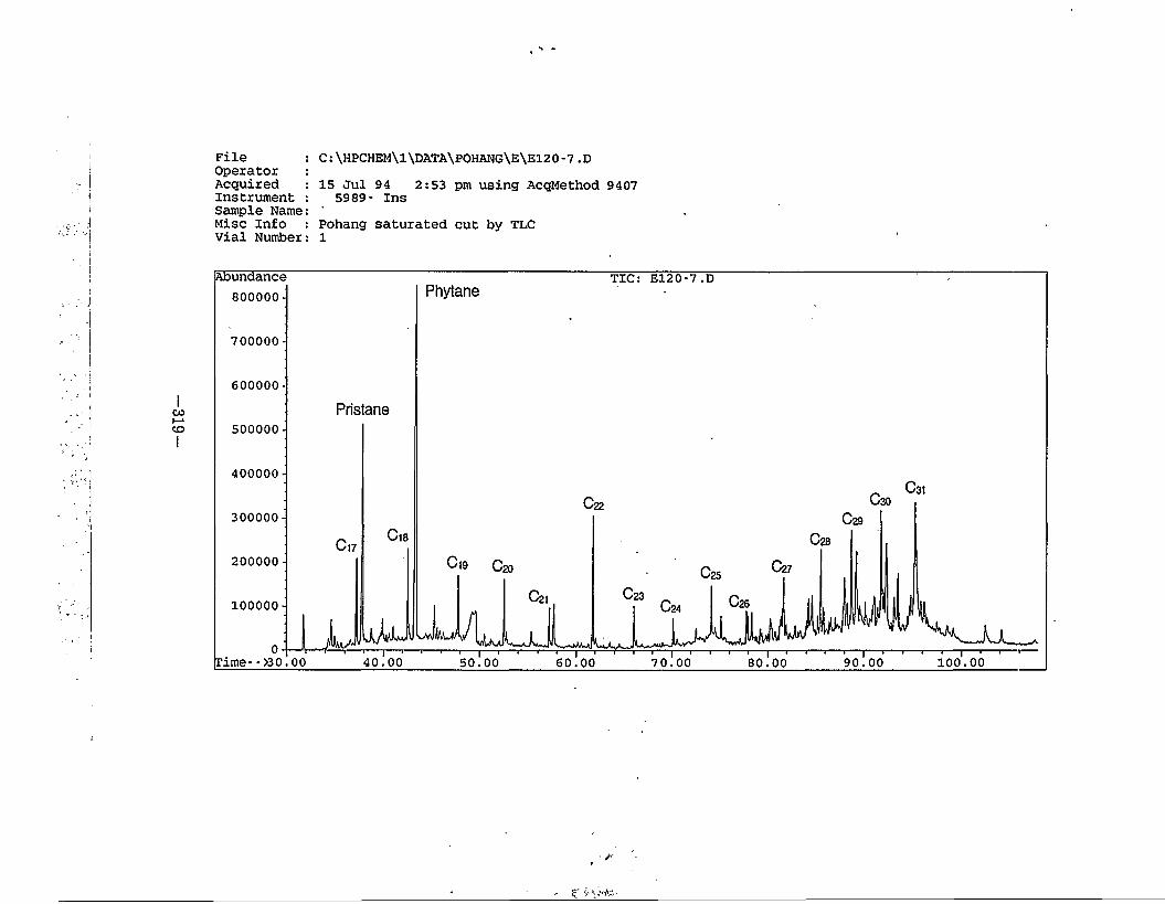
319
File : C:\HPCHEM\l\DATA\POHANG\E\E120-7.DOperator :Acquired : 15 Jul 94 2:53 pm using AcqMethod 9407Instrument : 5989- InsSample Name: 'Misc Info : Pohang saturated cut by TLC Vial Number: 1
Abundance TIC: E120-7.DPhytane800000 -
700000-
600000 -
Pristane500000-
400000-
300000-
200000-
100000-
rime-->30.00 40.00 100.0050.00 60.00 70.00 80.00 90.00
z
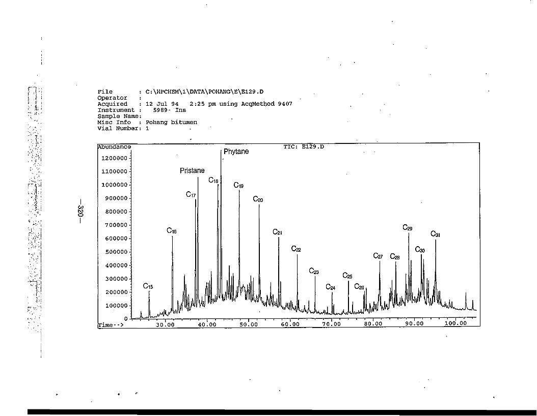
File : C:\HPCHEM\l\DATA\POHANG\E\E129.DOperator :Acquired : 12 Jul 94 2:25 pm using AcqMethod 9407Instrument : 5989 - InsSample Name:Misc Info : Pohang bitumen Vial Number: l
TIC: E129.DAbundancePhytane
1200000 -
Pristanenooooo -
1000000-
900000 -
800000 -
700000 -
600000 -
500000 -
400000 -
300000-
200000 -
100000-
100.0090.0080.0070.0060.00Time--> 40.00 50.0030.00
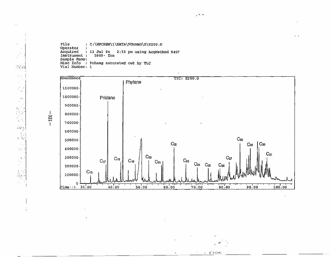
File : Operator : Acquired : Instrument : Sample Name: Misc Info : Vial Number:
13 Jul 94 2:32 pm using AcqMethod 94075989- Ins
Pohang saturated cut by TLC 1
C:\HPCHEM\1\DATA\POHANG\E\E250.D
Abundance TIC: E250.DPhytane
nooooo -
1000000 - Pristane
900000 -
800000 -
7 00000 -
600000 -
500000 -
400000 -
300000 -
200000 -
100000 -
0 I Irime--> 30.00 90.00 100.0040.00 50.00 60.00 70.00 80.00
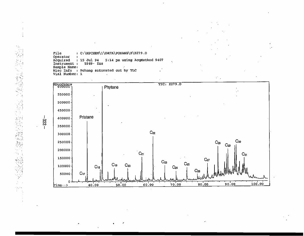
File : Operator : Acquired : Instrument : Sample Name: Misc Info : Vial Number:
15 Jul 94 5:14 pm using AcqMethod 94075989- Ins
Pohang saturated cut by TLC 1
C:\HPCHEM\l\DATA\POHANG\E\E27 9.D
TIC: E279.DPhytane
550000-
500000-
450000 -
Pristane400000 -
350000 -
300000 -
250000-
200000 -
150000 -
100000-
50000 -
100.0090.0080.0070.0060.00rime- -> 50.0040.00
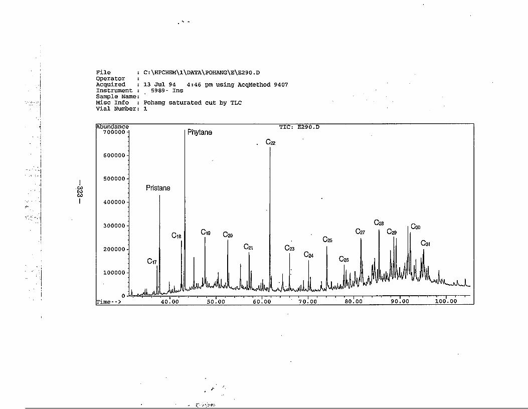
File : Operator : Acquired : Instrument : Sample Name: Misc Info : Vial Number:
13 Jul 94 4:46 pm using AcqMethod 94075989- Ins
Pohang saturated cut by TLC 1
C:\HPCHEM\l\DATA\POHANG\E\E29 0.D
Abundance 700000 H
TIC: E290.DPhytane
600000 -
500000 -
Pristane
400000 -
300000 -
200000 -
100000 -
100.0070.00 90.00rime- -> 80.0060.0040.00 50.00
5‘- •r'V'1’"'
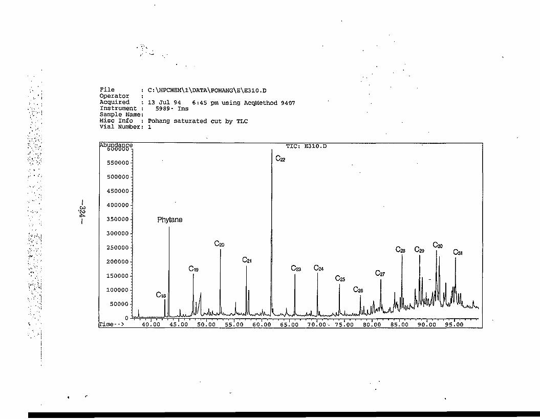
C:\HPCHEM\1\DATA\POHANG\E\E310.DFileOperatorAcquired : 13 Jul 94 6:45 pm using AcqMethod 9407Instrument : 5989- InsSample Name:Wise Info : Pohang saturated cut by TLC vial Number: l
TIC: E310.D
550000 -
500000 -
450000 -
400000 -
Phytane350000 -
300000 -
250000 -
200000 -
150000 -
100000 -
50000 -
■I—)—I--I I I—Irime- -> 40.00 45.00 55.0050.00 60.00 70.00- 75.00 80.00 85.00 90.00 95.0065.00
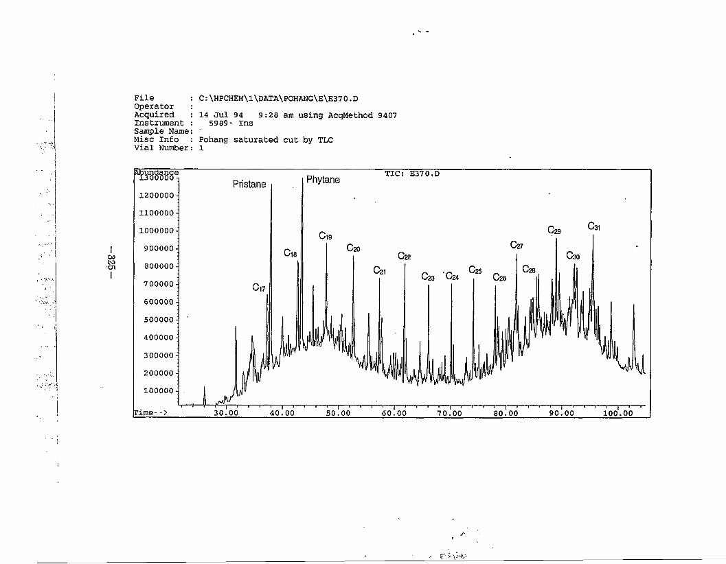
I File : Operator : Acquired : Instrument : Sample Name: Misc Info : Vial Number:
C:\HPCHEM\1\DATA\POHANG\E\E370.D
14 Jul 94 9:28 am using AcqMethod 94075989- Ins
Pohang saturated cut by TLC 1
TIC: E370.DPhytanePristane1200000 -
nooooo -
1000000-
900000-
800000 -
700000 -
600000 -
500000 -
400000 -
300000 -
200000 -
100000-
rime--> 30.00 40.00 50.00 60.00 90.0080.00 100.00
/■
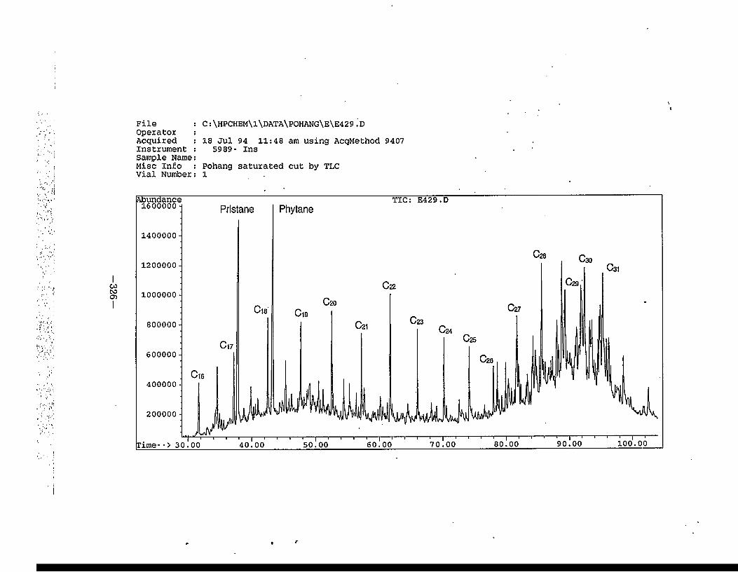
326
File : Operator : Acquired : Instrument : Sample Name: Misc Info : Vial Number:
18 Jul 94 11:48 am using AcqMethod 94075989- Ins
Pohang saturated cut by TLC 1
C:\HPCHEM\l\DATA\POHANG\E\E429!d
Abundance 1600000 h
TIC: E429.DPhytanePristane
1400000 -
1200000 -
1000000 -
800000 -
600000 -
400000 -
200000 -
100.0090.0080.0070.00rime--> 30.00 60.0050.0040.00
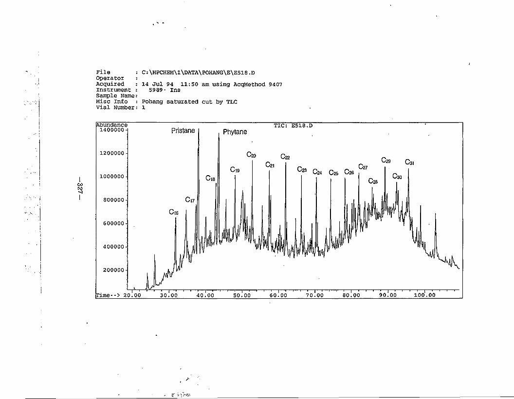
327
FileOperator Acquired Instrument Sample Name Misc Info Vial Number
14 Jul 94 11:50 am using AcqMethod 94075989- Ins
Pohang saturated cut by TLC 1
C:\HPCHEM\l\DATA\POHANG\E\E518.D
Abundance TIC: E518.D1400000 H Pristane Phytane
1200000 -
^23 C24 C25 Cae1000000 -
800000 -
600000 -
400000 -
200000-
rime--> 20.00 90.00 100.0030.00 60.00 70.00 80.0040.00 50.00
/-
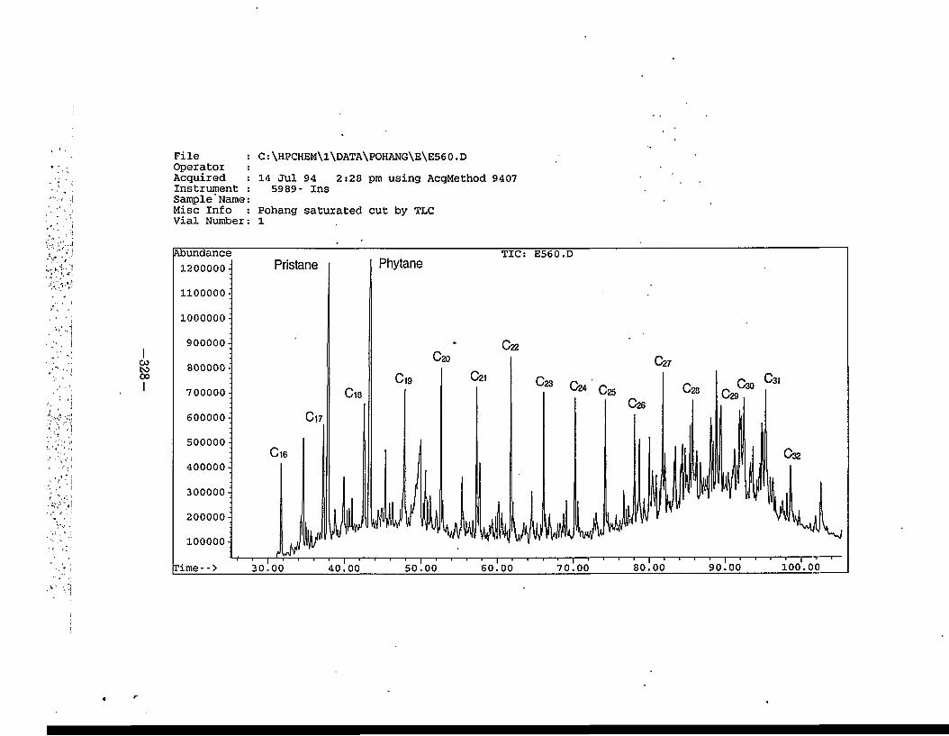
C:\HPCHEM\l\DATA\POHANG\E\E560.DFileOperator Acquired Instrument Sample'Name Misc Info Vial Number
14 Jul 94 2:28 pm using AcqMethod 94075989 - Ins
Pohang saturated cut by TLC 1
abundance TIC: E560.DPhytanePristane1200000-
nooooo -
1000000 -
900000-
800000 -
024 Css700000 -
600000 •
500000 -
400000 -
300000 -
200000 -
100000-
100.00rime--> 80.00 90.0070.0030.00 40.00 50.00 60.00
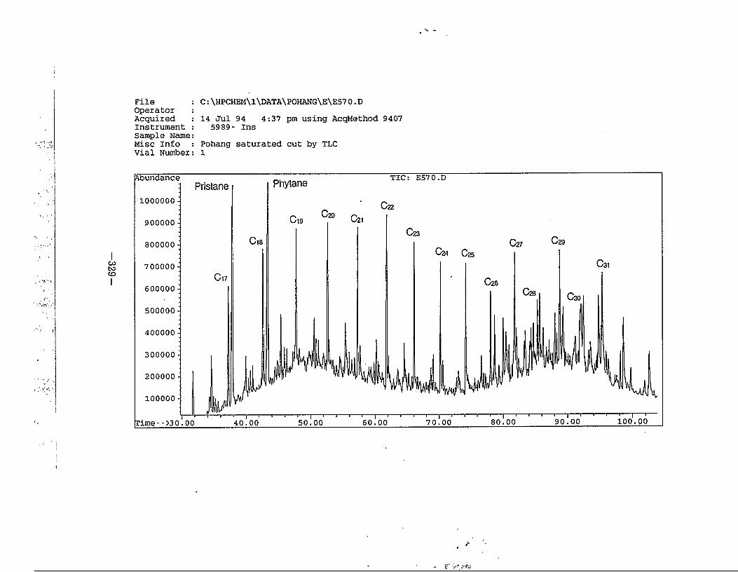
File : Operator : Acquired : Instrument : Sample Name: Misc Info : Vial Number:
14 Jul 94 4:37 pm using AcqMethod 94075989- ins
Pohang saturated cut by TLC 1
C:\HPCHEM\l\DATA\P0HANG\E\E57 0.D
TIC: E570.DPhytanePristane
1000000 -
900000 -
800000 -
700000 -
600000 -
500000 -
400000 -
300000 -
200000 -
100000 -
100.0090.0080.00rime-->30.00 70.0050.00 60.0040.00
1
/•
- if"
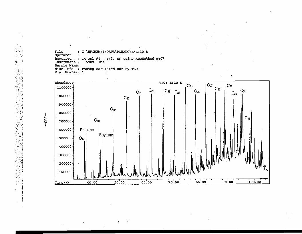
330
'• \ i
■ -./> .'i
FileOperator Acquired Instrument Sample Name Misc Info vial Number
14 Jul 94 6:37 pm using AcqMethod 94075989- Ins
Pohang saturated cut by TLC 1
C:\HPCHEM\1\DATA\POHANG\E\E610.D
TIC: E610.D
1000000 -
900000 -
800000 -
700000 -
Pristane600000 -
Phytane500000 -
400000 -
300000 -
200000 -
100000-
100.0090.0080.00rime- -> 70.0050.00 60.0040.00
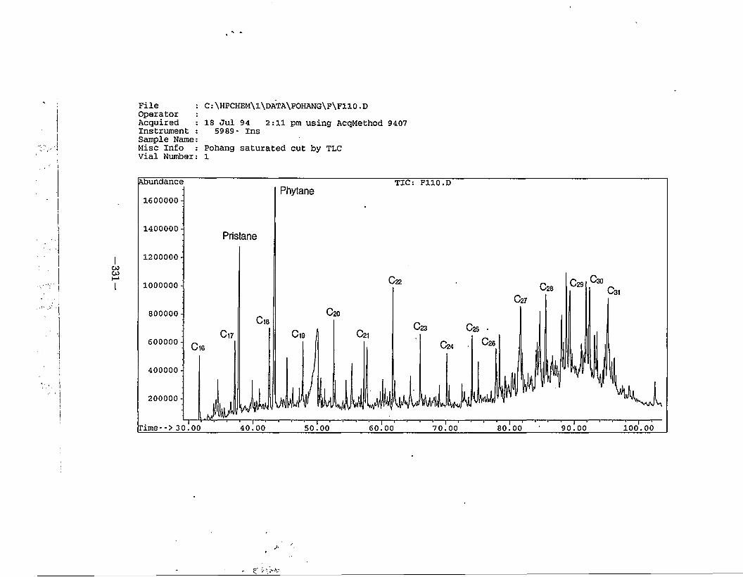
File : Operator : Acquired : Instrument : Sample Name: Misc Info : vial Number:
18 Jul 94 2:11 pm using AcqMethod 94075989- Ins
Pohang saturated cut by TLC 1
C:\HPCHEM\l\DATA\POHANG\F\F110.D
Abundance TIC: F110.DPhytane
1600000 -
1400000 -Pristane
1200000 -
1000000 -
800000 -
600000 -
400000 -
200000 -
rime-->30.00 40.00 100.0050.00 60.00 70.00 80.00 90.00
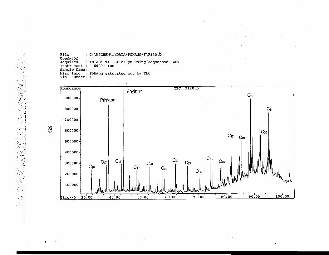
332
FileOperator Acquired Instrument Sample Name Misc Info Vial Number
18 Jul 94 4:23 pm using AcqMethod 94075989- Ins
Pohang saturated cut by TLC 1
C:\HPCHEM\1\DATA\POHANG\F\F120.D
Abundance TIC: F120.DPhytane
900000 - Pristane
800000 -
700000 -
600000 -
500000 -
400000 -
300000 -
200000 -
100000 -
100.0090.0080.0070.0060.00Time--> 30.00 50.0040.00
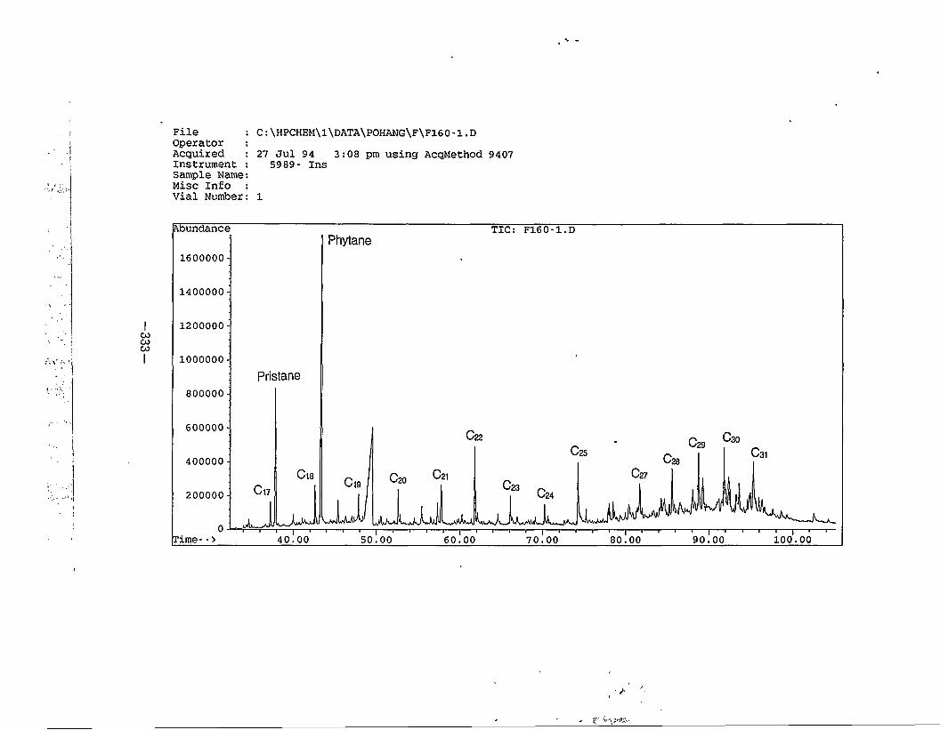
FileOperator Acquired Instrument Sample Name Misc Info Vial Number
27 Jul 94 3:08 pm using AcqMethod 94075989- Ins
C:\HPCHEM\l\DATA\P0HANG\F\F160-1.D
1
Abundance TIC: F160-1.DPhytane
1600000 -
1400000 -
1200000 -
1000000 -Pristane
800000 -
600000 -
400000 -
200000 -
rime--> 40.00 100.0050.00 60.00 70.00 80.00 90.00
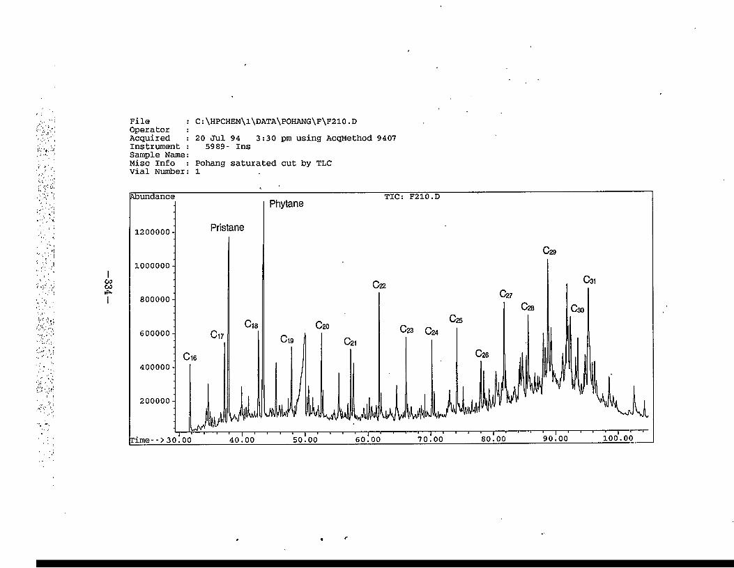
334
File : Operator : Acquired : Instrument : Sample Name: Misc Info : vial Number:
20 Jul 94 3:30 pm using AcqMethod 94075989- Ins
Pohang saturated cut by TLC l
C:\HPCHEM\1\DATA\POHANG\F\F210.D
Abundance TIC: F210.DPhytane
Pristane1200000 -
1000000 -
800000 -
600000 -
400000 -
200000 -
100.0090.0080.0070.00rime-->30.00 60.0050.0040.00
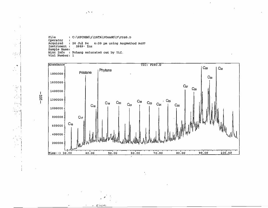
FileOperator : Acquired : Instrument : Sample Name: Misc Info : vial Number:
20 Jul 94 6:20 pm using AcqMethod 94075989- Ins
Pohang saturated cut by TLC.1
C:\HPCHEM\1\DATA\POHANG\F\F280.D
Abundance TIC: F280.D
PhytanePristane1800000 -
1600000 -
1400000 -
1200000 -
1000000 -
800000 -
600000 -
, 400000 -
200000 -
rime--> 30.00 90.00 100.0060.00 80.0040.00 50.00 70.00
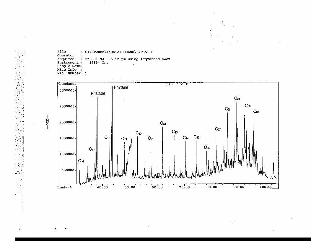
336
FileOperator Acquired Instrument Sample Name Misc Info Vial Number
27 Jul 94 6:12 pm using AcqMethod 94075989- Ins
C:\HPCHEM\1\DATA\P0HANG\F\F351.D
1
Abundance TIC: F351.DPhytane
3000000 -Pristane
2500000 -
2000000 -
1500000 -
1000000 -
500000 -
100.00rime- -> 90.0080.0070.0040.00 50.00 60.00
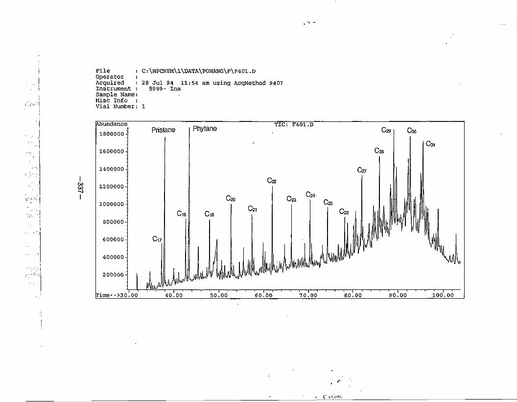
337
FileOperator Acquired Instrument Sample Name Misc Info Vial Number
28 Jul 94 11:54 am using AcqMethod 94075989- Ins
C:\HPCHEM\1\DATA\POHANG\F\F401.D
1
Abundance TIC: F401.DPhytanePristane1800000 -
1600000 -
1400000 -
1200000 -
1000000 -
800000 -
600000 -
400000 -
200000 -
rime-->30.00 90.00 100.0040.00 80.0050.00 60.00 70.00
Z
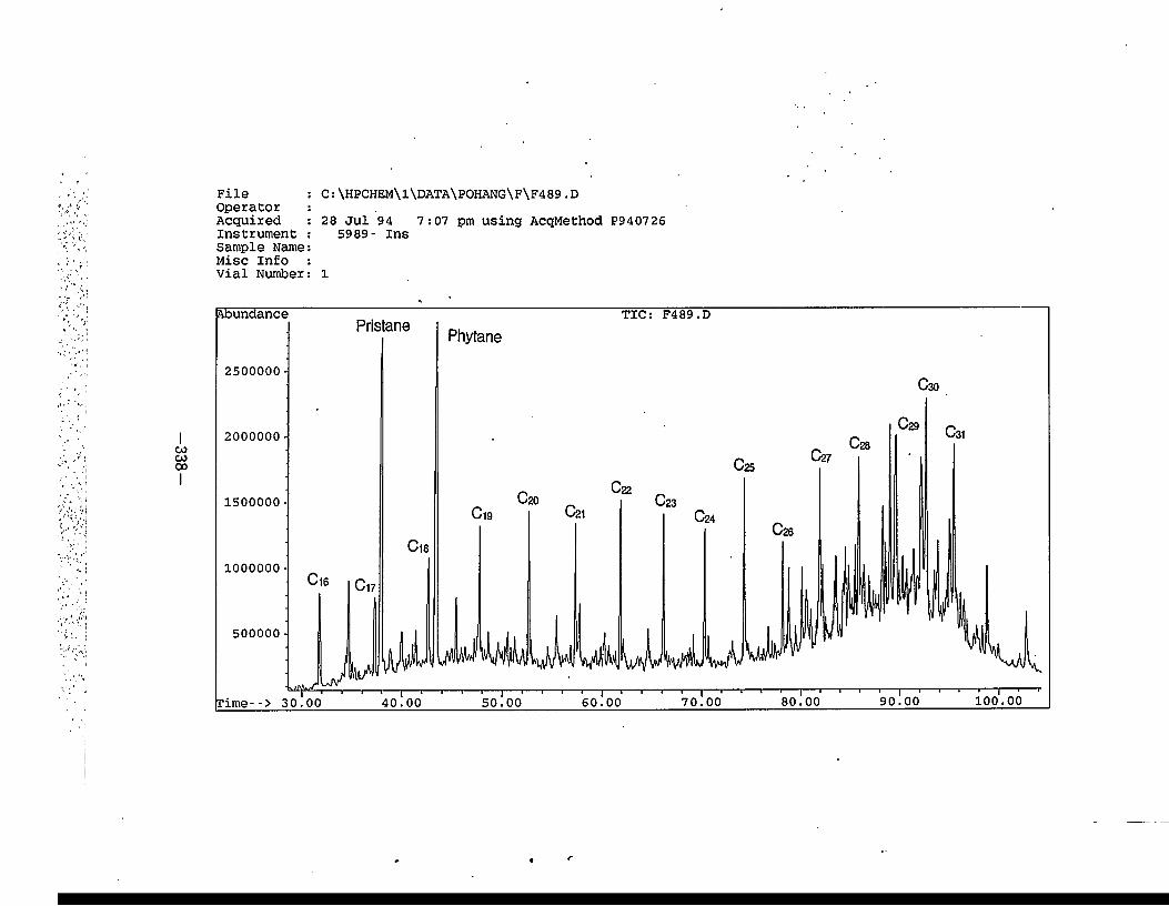
338
C:\HPCHEM\l\DATA\POHANG\F\F489.DFileOperatorAcquired : 28 Jul 94 7:07 pm using AcqMethod P940726Instrument : 5989- InsSample Name:Misc Info : vial Number: l
Abundance TIC: F489.DPristane
Phytane
2500000 -
2000000 -
1500000 -
1000000 -
500000 -
100.0090.0080.0070.00rime--> 30.00 50.00 60.0040.00
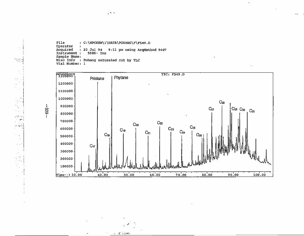
C:\HPCHEM\1\DATA\P0HANG\F\F549.DFileOperator Acquired Instrument Sample Name Misc Info Vial Number
20 Jul 94 9:11 pm using AcqMethod 94075989- Ins
Pohang saturated cut by TLC 1
TIC: F549.DPhytanePristane
1200000 -
nooooo -
1000000 :
900000 -
800000 -
700000 -
600000 -
500000 -
400000 -
300000 :
200000 -
100000 -
rime--> 30.00 60.00 90.00 100.0040.00 50.00 70.00 80.00
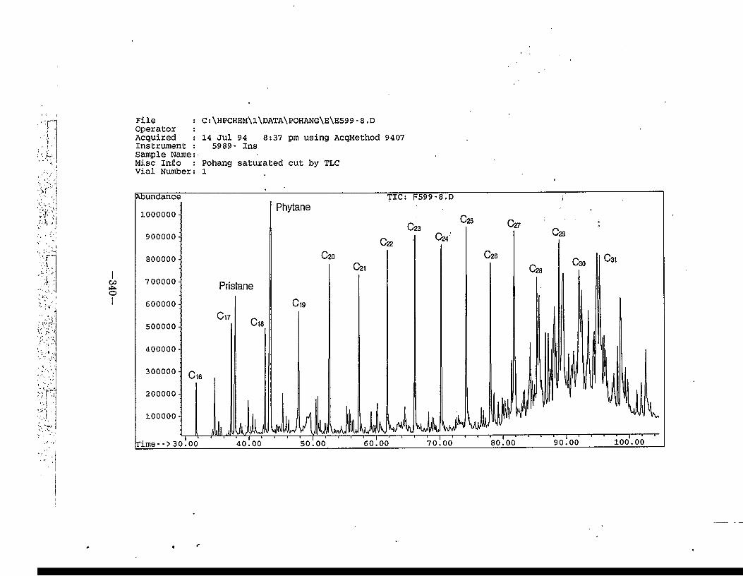
340
File : C: \HPCHEM\1\DATA\P0HANG\E\E599-8.DOperator :Acquired : 14 Jul 94 8:37 pm using AcqMethod 9407Instrument : 5989 - InsSample Name:Misc Info : Pohang saturated cut by TLC Vial Number: 1
Abundance TIC: F599-8.DPhytane1000000 -
900000 -
800000 -
700000 - Pristane
600000 -
500000 -
400000 -
300000 -
200000 -
100000 -
100.0090.0080.0070.00rime--> 30.00 60.0040.00 50.00
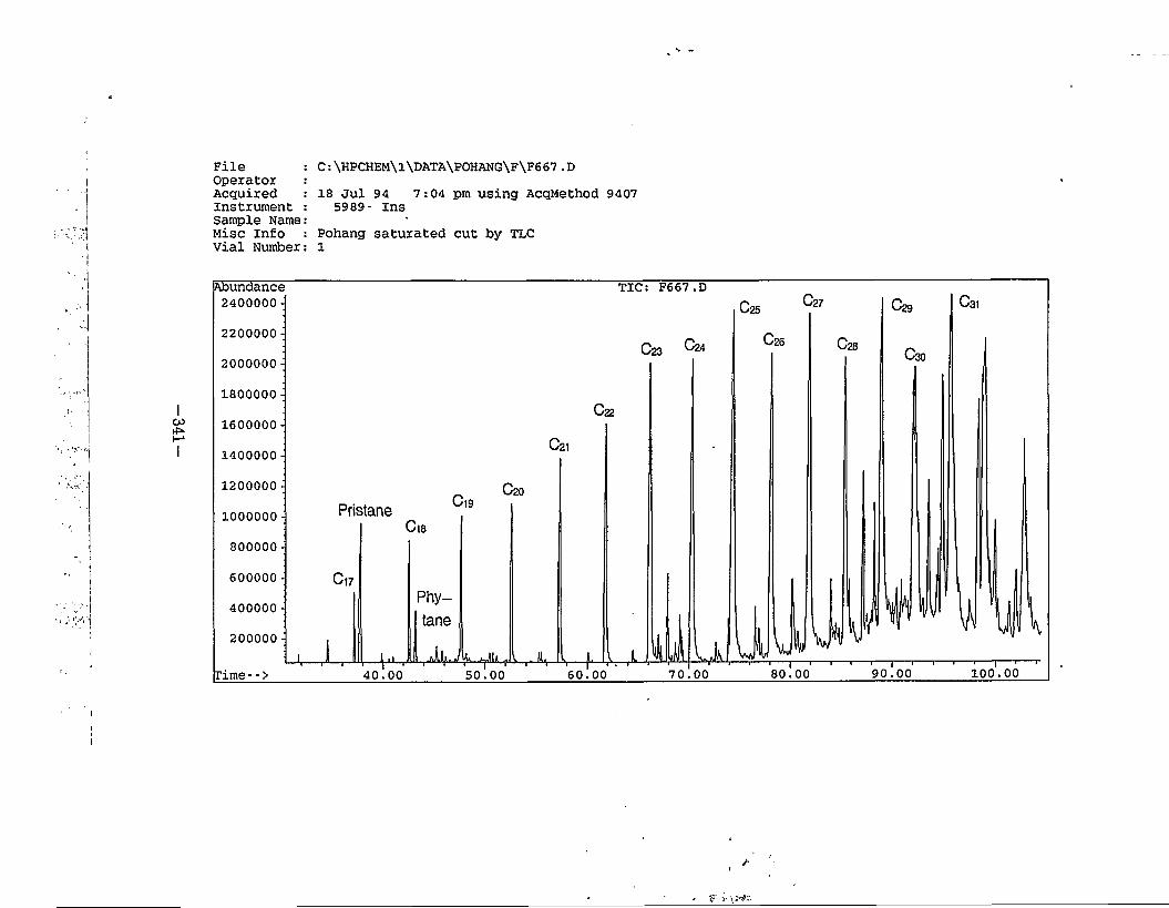
FileOperator Acquired Instrument Sample Name Misc Info Vial Number
18 Jul 94 7:04 pm using AcqMethod 94075989- Ins
Pohang saturated cut by TLC 1
C:\HPCHEM\l\DATA\POHANG\F\F667.D
Abundance 2400000 -
TIC: F667.D
2200000 :
2000000 -
1800000 -
1600000 -
1400000 -
1200000 -
Pristane1000000 -
800000 -
600000 -
400000 -
200000 -
100.0090.0080.00rime--> 70.0060.0040.00 50.00
i
z
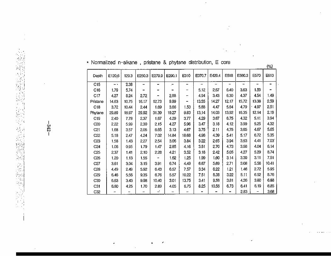
342
* Normalized n-alkane , pristane & phytane distribution, E core______________ (%)
Depth E 120.6 129.3 E250.3 E279.9 E290.1 E310 E370.7 E429.4 E518 E560.3 E570 E610
C15 - * 2.38 - - - - - - - - - -
016 1.79 5.74 - - - - 5.12 2.67 6.40 3.63 1.59 -
017 4.27 8.24 2.72 - 2.88 - 4.94 3.43 6.30 4.37 4.54 1.49
Pristane 14.63 10.75 16.17 12.73 9.99 - 13.55 14.27 12.17 15.72 13:38 2.59
018 3.72 10.44 2.44 1.69 3.66 1.53 5.68 4.47 5.64 4.79 ' 4.97 2.51
Phytane 29.89 18.97 29.92 31.39 19.27 9.83 13,14 14.03 13.92 16.35 12.14 2.19
019 2.40 7.78 2.37 1.67 4.29 3.77 4.29 3.67 6.75 4.32 5.11 3.94
020 2.22 5.99 2.30 2.15 4.27 5.96 3.47 3.18 4.12 3.99 5.25 4.32
021 1.68 3.57 2.05 6.65 3.13 4.67 3.75 2.11 4.75 3.65 4.67 5.65
022 5.18 2.47 4.24 7.02 14.84 18.68 4.98 4.39 5.41 5.17 6.72 5.35
023 1.58 1.43 2.27 2.54 3.06 3.84 3.22 2.65 3.94 3.53 4.41 7.03024 1.06 0.95 1.79 1.47 2.85 4.16 3.51 2.70 4.73 3.56 4.04 6.14
025 2.37 1.41 2.10 2.28 4.21 3.52 3.18 2.42 5.05 4.27 5.29 8.74
026 1.20 1.13 1.55 - 1.62 1.25 1.99 1.60 3.14 3.39 3.11 7.51
027 3.61 3.04 3.15 3.91 6.74 4.49 6.67 5.69 2.71 3.08 5.56 10.41
028 4.49 2.49 5.92 6.43 6.57 7.57 3.34 6.22 1.21 1.46 2.72 5.95
029 6.46 5.56 9.35 6.76 5.57 10.22 7.51 6.38 3.22 5.11 6.52 8.76
030 6.63 3.43 9.98 10.40 3.01 13.75 3.41 9.56 3.81 4.36 3.80 6.88
031 6.80 4.25 1.70 2.89 4.05 6.75 8.25 10.56 6.73 6.41 6.19 6.85
032 - - - - - - - - - 2.83 - 3.68
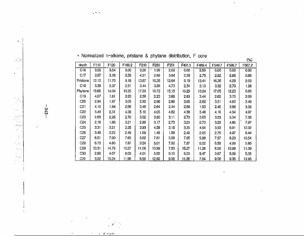
343
I
* Normalized n-alkane, pristane & phytane distribution, F core
depth F110 F120 FI 60.2 F210 F280 F351 F401.5 F489.4 F549.7 F599.7 F667.2C16 3.50 3.54 0.00 3.26 " 1.99 2.03 0.00 2.99 0.00 0.00 0.00017 3.97 3.18 2.59 4.21 2.89 3.84 2.59 2.75 2.82 2.66 0.69
Pristane 12.12 11.70 9.19 • 13.67 10.35 12.64 9.19 13.41 16.36 4.29 2.09018 3.39 2.37 2.51 3.44 3.89 4.73 2.51 3.13 3.32 2.73 1.28
Phytane 19.60 14.04 10.25 17.29 10.72 15.15 10.25 13.24 17.05 12.23 0.00019 4.07 1.81 2.83 2.59 2.23 3.68 2.83 3.44 2.62 3.75 2.09020 2.94 1.87 3.05 2.92 2.96 2.99 3.05 2.82 3.51 4.65 2.49021 4.10 1.84 2.66 3.48 2.64 2.44 2.66 1.93 2.40 3.98 3.55022 5.46 2.31 4.38 5.10 4.05 4.82 4.38 3.48 4.10 4.54 4.97023 2.66 2.26 2.70 3.02 3.80 3.11 2:70 3.03 3.23 5.54 7.58024 2.16 1.86 3.21 2.89 3.17 2.73 3.21 2.73 3.22 4.80 ' 7.97
025 3.31 3.21 3.35 3.93 4.58 3.18 3.35 4.64 3.53 6.91 12.32026 3.48 3.22 2.49 1.69 1.48 1.99 2.49 2.05 2.70 4.97 8.44027 6.51 7.90 7.65 5.62 7.81 3.59 7.65 5.99 7.57 8.23 10.54
028 6.73 4.80 7.87 3.24 5.01 7.00 7.87 6.02 6.58 4.99 5.86029 10.31 14.79 15.27 11.08 13.99 7.93 15.27 11.26 8.05 10.99 11.09030 2.66 4.07 8.03 4.01 5.62 9.10 8.03 9.47 3.87 5.69 5.05031 3.02 15.24 11.96 8.56 12.80 9.06 11.96 7.64 9.06 9.06 13.96