diffusion flames upwardly propagating over pmma: theory, experiment and numerical modeling
TRANSCRIPT

1
Diffusion Flames Upwardly Propagating over PMMA: Theory, Experiment and Numerical Modeling
J-L CONSALVI (1), B. PORTERIE (1), M. COUTIN (2), L. AUDOUIN (2), C. CASSELMAN (2), A. RANGWALA (3), S.G. BUCKLEY (3) and J.L. TORERO (4)
(1) Polytech’Marseille/DME, UMR/CNRS 6595, 5 rue E. Fermi, 13453 Marseille Cedex 13, France (2) Institut de Radioprotection et de Sûreté Nucléaire, DPAM, Cadarache, 13108 Saint Paul lez Durance, France
(3) Department of Mechanical and Aerospace Engineering, University of California, San Diego, La Jolla, CA 92093-0411, USA (4) BRE/Edinburgh Centre for Fire Research, The University of Edinburgh, Edinburgh, EH9 3JL, UK All correspondences have to be addressed to: Dr Jean-Louis Consalvi; Tel (33) 491 106 927; Fax: (33) 491 106 969; email: [email protected]
ABSTRACT
A numerical model and experiments over PMMA are used to evaluate the main
assumptions used in the theoretical description of a diffusion flame established in a
natural boundary layer. Flow characteristics (2-D Boundary Layer) and surface thermal
balance are identified as the critical assumptions to be evaluated. Comparison of
experiments, numerical results, and theoretical model serve to validate the assumptions
leading to the definition of a mass transfer number but establish the need to model all
three-dimensional features of the flow.
KEYWORDS: Diffusion Flame, Upward Spread, Mass Transfer Number.
NOMENCLATURE
B Mass transfer number Tig Ignition temperature
Cp Specific heat xp Pyrolysis front
G Average incident radiation yfl Stand-off distance
Grx Grashoff number Greek
J Mixture fraction Emissivity
Lfl Flame Length Similarity variable
Lv Heat of pyrolysis Conductivity "pm Fuel mass flux Subscript
Q Losses at the fuel surface s Solid
Qp Heat of combustion per unit mass of
oxygen
fl Flame
"q Heat Flux inc Incident
2
INTRODUCTION
The two main visible geometrical characteristics of a diffusion flame are the flame length
and stand-off distance. For condensed phase fuels a pyrolysis length generally
complements these parameters. The flame length and stand-off distance can be carefully
measured using video cameras while the pyrolysis length using thermocouples. The
pyrolysis and flame lengths are the time integrated outcome of the processes occurring
along the burning fuel therefore are global quantities that depend on many variables. The
stand-off distance is, in contrast, defined by transport in the vicinity of the reaction, and
thus is mostly affected by the external supply of oxidizer and fuel transport from the
surface. So, the stand-off distance represents a quantity that can be linked to the fuel in a
more direct manner than the flame length. Nevertheless, the flame and pyrolysis lengths,
since they are more relevant to fire growth, have been exploited extensively while the
stand-off distance has not.
Theoretical formulations showing the link between the mass transfer number and the
stand-off distance were developed in the 1950’s. The pioneering study of Spalding [1]
developed the first expression for the droplet burning-rate as a function of the mass
transfer or B number. The expression proposed by Spalding has been later extended to
describe the burning rate of fire flames such as pool fires [2]:
)1ln( BC
hm
PP
(1)
The same approach was used by Emmons [3] to provide a solution for the burning rate
induced by a diffusion flame established over a liquid fuel and subject to a forced flow
parallel to the surface:
2/1))/.((Re2
)'()(
Lx
ffUmP
(2)
where f is a normalized mixture fraction variable that comes from the solution of the
following differential equation
0 fff (3)
with the associated boundary conditions:
2,
2,0,0
f
B
f
ff
where
ydy
x 0
2/1Re
2
1
and where the mass transfer number as defined by Emmons [3] is as follows:
QL
TTCpYQB
V
igOP
)()( ,2 (4)
The term Q represents the normalized non-convective heat transfer at the surface
P
frsC
m
qqqQ
,
(5)
3
Cq represents in-depth conduction, r,sq surface re-radiation and fq the radiative
feedback from the flame.
Pagni and Shih [4] also developed a parallel analysis for a vertical wall subject to natural
and mixed convection. A series of similar analyses together with experimental validation
have been published subsequently [5, 6]. Including buoyancy gives a set of normalized
momentum and species equations
0Pr3
)1(1)(23 2
JfJ
BJQLffff V (6)
With the associated boundary conditions
00,
1Pr3/)0()0(,0,0
Jandf
JandJBff
where the similarity variable is now
y
x dyxGr0
4/1)2/(
and
T
TTgxGr W
x 2
3 )(
Making a flame sheet approximation allows to solve for the stand-off distance. The
pyrolysis length remains a parameter of the solution while the flame length is generally
calculated by means of an integral solution [4, 5]. Roberts and Quince [7] extended this
analysis to show that extinction could be predicted as a function of a critical B number.
Recently this concept has been revived to describe the quenching limit of micro-gravity
diffusion flames [8, 9] showing that a critical mass transfer number can be linked with a
critical Damköhler Number and thus with an extinction limit. This extinction limit was
shown to be essential in the calculation of the flame length. Finally, the heat flux from the
flame to the surface appears as a function of f from the boundary conditions associated
with Eqs. 5 and 6. The main assumption being that the dominant mode of heat transfer is
due to convection and therefore the net radiative contribution is assumed negligible.
Several studies have discussed this assumption, notable is that of Mathews and Sawyer
[10] but no clear conclusion has been reached. The practical importance of this method
stems in its potential use to describe co-current flame spread. Co-current flame spread
can be predicted using a simplified methodology based on the method proposed by
Quintiere [11] for opposed flame spread and later extended to co-current (or upwards)
flame spread, as reviewed by Fernandez-Pello [12]. Many solutions have been proposed
in the literature and are described in detail by Drysdale [13]. Nevertheless, direct
application of the above-described methodology has failed to provide adequate results,
thus flame length and heat-fluxes have been substituted by a series of appropriate
correlations and empirical constants that can lead to very good results when predicting
co-current flame spread [14, 15]. This approach to co-current flame spread has been
favored in CFD codes [16]. Only recently, attempts have been made to revisit the original
analysis to explore the reasons for the lack of agreement between experiments and model
[9] concluding that two independent sets of assumptions need to be verified, those of the
nature of the flow and the assumptions leading to the definition of the mass transfer
number. This new analysis differs from previous attempts in that it makes extensive use
of stand-off distance measurements.
4
The theoretical analysis assumes a 2D laminar flow that conforms to boundary layer
assumptions. These constraints have been shown to have significant effects on the flame
length and heat release rate. Orloff et al. [14] showed that the flame length correlates
linearly with the pyrolysis length while the flow is laminar but shows a decaying
dependency ( 781.0)(625.0 Pf xL ) as soon as the flow becomes turbulent. Tsai and
Drysdale [15] explored the effect of lateral entrainment on the flame length and energy
release rate showing significant three-dimensional effects. Hirano and co-workers [17]
explored the limitations of boundary layer approximations. In contrast, a study under
idealized conditions showed that even when the flow problems were resolved
discrepancies between predictions and experiments still existed. A claim was made that
the reason for the poor correlation between experimental results and theory was the
improper definition of the mass transfer number [9].
This study calculates the upward spread of a flame by means of a transient 2-D CFD code
providing the evolution of the pyrolysis and flame length as well as the stand-off
distance. While keeping a 2-D formulation it eliminates boundary layer and constant
property assumptions. Following a similar approach to that of Lewis et al. [18],
comparison between model predictions and a set of experiments with PMMA allows
exploration of the different assumptions. Emphasis is given to the importance of three-
dimensional effects. Furthermore, independent estimation of all gas phase quantities
permits the numerical evaluation of all the components of the mass transfer number. This
enables a detailed evaluation of the assumptions that relate to the gas phase.
METHODS
Experimental Apparatus
The experimental combustion set-up consists of a vertical sample of Poly-Methyl
Methacrylate (PMMA) 40 cm in height, 1.2 cm in thickness, and 5 cm, 10 cm and 15 cm
in width, mounted on an insulation board and covered with a metal plate, as illustrated in
Fig. 1. The metallic cover, extending several cm on each side of the sample, allows only
the front surface of the PMMA to ignite and burn. The sample is ignited at the bottom
using an electrical wire. A ruled reference on the plate provides a visual indication of the
extent of flame spread at a given time. Five thermocouples are fed through holes drilled
from the back of the sample and melted on to the surface, and five additional
thermocouples are placed on the back of the sample between the fuel and the insulation.
The thermocouples are evenly spaced to provide temperature data, indicating the
progression of the pyrolysis front and an estimate of the thermal thickness of the material.
The sample is ignited in a ventilated enclosure with an electrically heated Kanthal wire.
Two CCD cameras (720 x 576 pixels) are used to obtain a frontal and a side view of the
flame. The field of view is chosen to obtain an error on the stand-off distance of less than
5%. Based on the characteristic times scales for propagation, an average of all images in
a 10 second period was used to obtain an average stand-off distance and flame shape.
First, each image is converted to grey levels (0-255) and then all values are averaged
leading to an average image. The stand-off distance and flame length where determined
establishing a threshold grey level. The threshold value was varied as apart of a
sensitivity analysis showing that both stand-off distance and flame length did not vary
significantly with the choice of grey level. The stand-off distance was corrected for fuel
regression. This was done through measurements of the burnt samples after the test.

5
Linear functions of time and location where established for the regression rates and added
to the stand-of distance. The correction never exceeded 10% of the total value. Overall 6
replicate experiments were conducted and generally good agreement was found between
runs.
Numerical Model
The reactive flow is computed by solving the Favre density-weighted Navier-Stokes
equations in connection with the RNG k- turbulence model [19]. Near a solid surface,
the velocity components parallel to the wall, the turbulent kinetic energy, and its rate of
dissipation are treated through a local equilibrium wall log-law. The complete set of
equations along with thermodynamic properties and equations of state can be found in
[20].
Combustion model
In the present study, the Methyl-Methacrylate (MMA)/air reactive system is modeled as a
simplified one-step chemical reaction
C5H8O2 +6O2+22.57N25CO2+4H2O+22.57N2 (7)
The consumption rate of fuel is calculated as the minimum of the Eddy Break-Up
expression [21] (mixing-controlled regime) and an Arrhenius expression (kinetically-
controlled regime) given by Wu et al [22] for the MMA.
Radiation Model
In the radiation model, the grey assumption is used which implies that the absorption
coefficient is independent of the wavelength of radiation. The model requires the solution
of the radiative transfer equation (RTE). The absorption coefficient is calculated from the
contributions from soot [23] and from the combustion products [21].
Soot formation model
To quantify soot formation, the model proposed by Moss and Stewart [24] that includes
the processes of nucleation, heterogeneous surface growth and coagulation is used. This
model requires the solution of two additional conservation equations for the soot mass
fraction and number density. Soot oxidation is included using the model of Naggle and
Strickland-Constable [25].
Pyrolysis model
The volatilisation of PMMA is modelled as a phase change at a constant surface
temperature of 630K. In the solid, the one-dimensional heat transfer equation
x
T
xt
TC spss
(8)
is solved and surface regression is neglected. At the solid surface exposed to the flame
the boundary conditions are as follows
- before pyrolysis:
4", TqTTh
x
Tincrgs
(9)
- after pyrolysis :

6
4",
" TqTThLmx
T
TT
incrgvps
ig
(10)
At the rear surface of the slab, the boundary condition is:
4", aincras TqTTh
x
T
(11)
The incident radiative flux, ",incrq , is computed from the radiation model.
Numerical Procedure
The conservation equations are discretized on a staggered, non-uniform Cartesian grid by
a finite-volume procedure with a second-order backward Euler scheme for time
integration. Diffusion terms are approximated from a second-order central difference
scheme. For the convective terms, the ULTRASHARP approach [26] is used. The
pressure-velocity linked equations are solved using the Iterative PISO algorithm [27].
The RTE is solved using the FVM with a 2×16 angular mesh [28]. The heat and mass
transfer conjugated problem at the gas solid interface is treated through a blocked-off
region procedure [20].
Computational Details
The model is applied to a two-dimensional configuration. The physical problem involves
a 10 cm×65 cm domain. A 1.2 cm×40 cm PMMA slab is located at 7cm from the west
boundary (Fig. 1). A non-uniform mesh with 43×250 cells is used and the time step is
0.025s. The origin of the coordinate axis is the bottom exposed corner of the PMMA slab.
Ignition is produced by means of a radiative heat flux applied between 0< x <0.2 cm. The
ignition flux is eliminated immediately after the onset of the combustion reaction. Time
zero is defined as the instant when the fuel surface attains the pyrolysis temperature. The
values of the pyrolysis model parameters adopted in this study are:s =1200 kg/m3 [29],
0.1874W/m2/K [29], Cp=2100J /kg/K [4], Lv= 2.7 106 J/kg [30], ε=0.927 and
Tp=630K [29].
RESULTS AND DISCUSSIONS
Flames were allowed to propagate upwards and the flame and pyrolysis lengths were
recorded. The pyrolyis length was extracted from the thermocouple histories and defined
as the location where the thermocouple reached 630K [9]. Figure 2 presents the evolution
of these variables with time. All length scales are normalized by the plate length (Lplate)
and times by the characteristic residence time
( TLTTgU withUL plateigBBplatec ). To avoid crowding of the figure
only data for 5 cm and 15 cm width is presented.
The flame length shows a linear dependency with time. This tendency is well reproduced
by the numerical model. The width of the sample seems to have no effect on this variable.
The evolution of the pyrolysis length seems to follow a similar trend initially but
eventually the wider sample accelerates. The numerical model seems to follow this trend
in a more precise manner. These observations seem to evidence some three-dimensional

7
effects unaccounted by the 2-D model. Figure (2c) compares the current results with
experiments from the literature. In all cases some level of confinement is present in the
results of references [14, 31, 32]. The data from the literature is consistent among
different studies and shows a more pronounced accelerating trend than the current
experiments. It is important to note that none of these experiments were conducted under
the same conditions as the current tests, nevertheless the comparison serves to highlight
the importance of the flow assumptions. Orloff [14] uses a 157cm high, 4.5cm thick and
41 cm wide PMMA sample with water-cooled sidewalls. Given the larger width it is
expected to see a more pronounced accelerating trend. It is important to reiterate that for
these experiments lateral entrainment was precluded by side walls. Saito [32] uses a
30cm wide sample with wire mesh side screens placed at 75 cm from the sample. Given
that the width of the sample is smaller, it will be expected for the pyrolysis length to
increase at a rate bounded by the 15 cm and 41 cm samples; nevertheless, this data shows
a more pronounced acceleration. In this case there is no lateral confinement. Tewarson et
[31] uses a 10cm wide 2.5cm thick and 30-60cm in height PMMA sample with a co-flow
of 0.09 m/s was used. The co-flow is intended to reduce 3-D effects. These results clearly
show that the exact nature of the flow determines the rate at which the flame spreads.
Furthermore, it indicates that side entrainment accelerates or decelerates the propagation
rate and that the width of the sample represents a relevant length scale for this buoyantly
induced flow. Side entrainment affects spread but does not seem to affect the evolution of
the flame height. This could be due to a simultaneous increase in the oxidizer supply,
thus a reduction of the flame length.
Pyrolysis and flame length show that a 2-D representation of this problem might not be
sufficient. The stand-off distance is therefore defined numerically and experimentally.
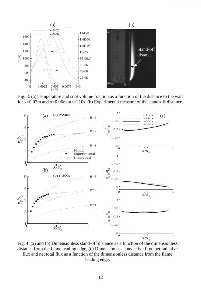
As indicated in Fig. (3b) the flame evidences an abrupt transition between the visible
yellow zone and a weaker blue region. The transition indicates the completion of the soot
oxidation process (absence of soot). Any soot in the proximity of the flame will glow,
thus the absence of yellow glow indicates the absence of soot. Figure (3a) shows two
representative cross sections of the soot volume fraction and the temperature. It can be
clearly seen that the complete consumption of soot coincides with the peak temperature.
Therefore, numerically, the stand-off distance will be defined as the location of the peak
temperature.
The stand-off distance (yfl) is presented in Fig. 4 at two different instants. The results are
compared with the numerical formulation and with the theoretical solution as defined by
Pagni and Shih [4]:
dGr
xy
fl
x
fl
04/1
2. The stand-off distance is non-
dimensionalized by a characteristic boundary layer thickness
( plateBplatec LUL ). The solution to the stand-off distance requires a B
number. Values in the literature range from 1 to approximately 3 [4, 10], therefore the
theoretical stand-off distance was evaluated for three representative values within this
range.
The experimental results show discrepancies with the theoretical model, independent of
the value of B. In contrast, the numerical solution seems to reproduce well the stand-off
distance. Close to the leading edge, there is disagreement between the numerical
formulation and the experimental results. This could be due to three potential sources of

8
error: increased experimental error at the leading edge, separation of the flow, which is
difficult to model numerically, or the influence of the artificial numerical ignition.
The above results clearly show that the numerical solution captures the features of the
flame geometry in a more precise manner. This could be attributed to a better prediction
of the flow field. In addition, the numerical model solves the energy balance at the
surface to obtain the burning rate (Eq. 10), thus the discrepancy could be related to an
improper definition of the mass transfer. Torero et al. [9] evaluated the mass transfer
number for micro-gravity diffusion flames by comparing experimental and theoretical
stand-off distances. These flames corresponded to a forced flow, thus followed the forced
flow analysis [3, 4]. The comparison showed an evolving mass transfer number
controlled by the different losses (Q in Eq. 5). This observation is of great practical
importance because it suggests that an empirically evaluated mass transfer number could
be used to accurately apply the present model to the prediction of upward flame spread.
To clarify the role of the different components of this analysis it is important to use the
numerical formulation to evaluate the main assumption behind the definition of the mass
transfer number. The scaling leading to the definition of the mass transfer number
requires that heat transfer is to be dominated by convection. The numerical formulation
can provide all heat transfer components. The results are presented in Fig. (4c). The
results are normalized by the theoretical convective heat flux at the surface:
w
xv
pth
T
T
x
GrJBL
Cq
20
4/1'"
. The value for the B number used is that that produces
the best match between theoretical and numerical predictions of the stand-off distance.
Figure (4c) shows that the magnitude of the net heat-flux is consistent between theory
and numerical model. It also shows that the net radiative exchange is decreases away
from the leading edge to negligible values verifying the original assumption by Emmons
[3]. There is a 30% discrepancy between the net heat flux evaluated numerically and the
theoretical prediction, this corresponds to in-depth heat conduction through the PMMA
sample.
CONCLUSIONS
A combination of a numerical model, experimental results, and a theoretical formulation
has been used to describe the stand-off distance, flame and pyrolysis lengths in an
upwardly propagating flame. The results verify the main thermal assumptions leading to
the definition of a mass transfer number but indicate that three-dimensional effects have a
significant effect on the flame geometry. A three-dimensional formulation of the flow is
therefore necessary to describe the behavior of an upward spreading flame.
Acknowledgements: The funding for J.L. Consalvi and B. Porterie was provided by
IRSN while funding for A. Rangwala, S.G. Buckley, and J.L. Torero was provided by
NASA Fire Safety Program of the Bioastronautics Initiative, grant # NAG-32568.
REFERENCES
[1] D.B. Spalding, The Combustion of Liquid Fuel, Fuel 30:6-121 (1951).
[2] D.B. Spalding, Some Fundamentals of Combustion, Butterworths, London,
1955.

9
[3] H.W. Emmons, The Film Combustion of Liquid Fuel, Zeitschrift fur Angewande
Mathematik und Mechanik 36:60-71 (1956).
[4] P.J. Pagni and T.M. Shih, Excess Pyrolyzate, Proceedings of the 16th
International Symposium on Combustion, The Combustion Institute, 1978, pp.
1329-1343.
[5] K. Annamalai and M. Sibulkin, Flame Spread over Combustible Surfaces for
Laminar Flow Systems, Part I: Excess Fuel and Heat Flux, Combustion Science
and Technology 19:167-183 (1979).
[6] F.J. Kosdon, F.A. Williams, and C. Buman, Combustion of Vertical Cellulosic
Cylinders in Air, Proceedings of the 12th International Symposium on
Combustion, The Combustion Institute, 1968, pp. 253-264.
[7] A.F Roberts and B.W. Quince, A Limiting Condition for the Burning of
Flammable Liquids, Combustion and Flame 20:245-251 (1973).
[8] C.T. Yang and J.S. T’ien, Numerical Simulation of Combustion and Extinction
of a Solid Cylinder in Low-Speed Cross Flow, Journal of Heat Transfer
120:1055-1063 (1998).
[9] J.L. Torero, T. Vietoris, G. Legros, and P. Joulain, Estimation of a Total Mass
transfer Number from the Stand-off Distance of a Spreading Flame, Combustion
Science and Technology 174:187-203 (2002).
[10] R.D. Mathews and R.F. Sawyer, Limiting Oxygen in Index Measurement and
Interpretation in an Opposed Flow Diffusion Apparatus, Journal of Fire and
Flammability 7:200-216 (1976).
[11] J.G. Quintiere, A Simplified Theory for Generalizing Results from a Radiant
Planel Rate of Flame Spread Apparatus, Fire and Materials 5(2) (1981).
[12] A.C. Fernandez-Pello, “The Solid Phase,” Combustion Fundamentals of Fire,
Cox J. (Ed.), Academic Press, 1995.
[13] D.D. Drysdale, Introduction to Fire Dynamics, John Wiley and Sons, 2nd
Edition, 1999.
[14] L. Orloff, J. De Ris, and G.H. Markstein, Upward Turbulent Fire Spread and
Burning of Fuel Surface, Proceedings of the 15th International Symposium on
Combustion, The Combustion Institute, 1974, pp 183-192.
[15] K.G. Tsai and D.D. Drysdale, Modelling the early stages of upward flame
spread, Interflam 2001, pp. 707-718, Edinburgh, UK, 2001.
[16] K.B. McGrattan, H.R. Baum, R.G. Rehm, A. Hamins, G.P. Forney, and J.E.
Floy, Fire Dynamics Simulator – Technical Reference Guide (Version 2), 2001.
[17] T. Hirano, K. Iwai and Y. Kanno, Measurement of the Velocity Distribution in
the Boundary Layer over a Flat Plate with a Diffusion Flame, Acta Astronautica
17:811-818 (1972).
10
[18] M.J. Lewis, P.A. Rubini, and J.B. Moss, Field Modelling of Non-Charring
Flame Spread, Proceedings of the 6th International. Symposium on Fire Safety
Science, 1999, pp. 683-694.
[19] V. Yakhot and S. Orszag, Renormalization Group Analysis of Turbulence,
Journal of Scientific Computing 1:3-51 (1986).
[20] J.L. Consalvi, B. Porterie, and J.C. Loraud, A Blocked-off Region Strategy to
Compute Fire Spread Scenarios Involving Internal Flammable Target,
Numerical Heat transfer, Part B, to appear, 2004.
[21] B.F. Magnussen and B.H. Hjertager, On Mathematical Modeling of Turbulent
Combustion with Special Emphasis on Soot Formation and Combustion,
Proceedings of the 16th International Symposium on Combustion, The
Combustion Institute, 1976, pp. 719-729.
[22] K.K. Wu, W.F. Fan, C.H. Chen, T.M. Liou, and I.J. Pan, Downward Flame
Spread over a Thick PMMA Slab in an opposed Flow Environment: Experiment
and Modelling, Combustion and Flame 132:697-707 (2003).
[23] J.H. Kent and D.R. Honnery, A Soot Formation Rate Map for a Laminar
Ethylene Diffusion Flame, Combustion and Flame 79:287-298 (1990).
[24] J.B. Moss and C.D. Stewart, Flamelet-based Smoke Properties for Field
Modelling of Fires, Fire Safety Journal. 30:229-250 (1998).
[25] J. Nagle and R.F. Strickland-Constable, Oxidation of Carbon between 1000-
2000°C, Proceedings of the 5th Carbon Conference, 1962, pp. 154-164.
[26] B.P. Leonard and J.E. Drummond, Why You Should Not Use Hybrid, Power-
Law or Related Exponential Schemes for Convective Modelling. There Are
Much Better Alternatives, International Journal for Numerical Methods in
Fluids 20:421-442 (1995).
[27] W.K. Chow and Y.L. Cheung, Selection of Differencing Scheme on Simulating
the Sprinkler Hot-Air Layer Problem, Numerical Heat Transfer, Part A 35:311-
330 (1999).
[28] G.D. Raithby and E.H. Chui, A Finite Volume Method for Predicting a Radiant
Heat Transfer in Enclosures with Participating Media, Journal of Heat Transfer
112:415-423 (1990).
[29] E. Vallot and M. Coutin, Etude pour l’Evolution de la Puissance du Feu –
Rapport de Fin d’Etude, Note technique DPAM/SEMIC 2004/27, IRSN, 2004.
[30] J.G. Quintiere and B. Rhodes, Fire Growth Models for Materials, NIST-GCR-
94-647, 1994.
[31] A. Tewarson and S.D. Ogden, Fire Behavior of PolyMethylMethacrylate,
Combustion and Flame 89:237-259 (1992).
[32] K. Saito, J.G. Quintiere, and F.A. Williams, Upward Turbulent Flame Spread,
Proceedings of the 1st International Symposium on Fire Safety Science, 1985.

11
Fig. 1. Experimental Set-up and computational domain
t/c
xp/L
pla
te
0 1000 2000 30000
0.5
1
1.5
t/c
Lfl
/Lpla
te
0 1000 20000
0.5
1
1.5 Model
Exp. z=5cm
Exp. z=15cm
t (s)
xp
(m)
0 200 400 6000
0.2
0.4
0.6
0.8
1
1.2
1.4
Model
z=15cm
z=5cm
Saito
Tewarson
Orloff
Fig. 2. Characteristic length scales as a function of time, comparison of model and
experiments: (a) Flame Length (b) Pyrolysis Length, and (c) Comparison of current
data with other experiments in the literature: Tewarson [31], Orloff [14], and Saito
[32].
Cover to hold
PMMA sample
PMMA slab 5cm
×1.2cm× 40cm
Flame spreading
upwards
Lateral air
entrainment
Digital
Camera
(Side View)
Frontal air
entrainment
Digital Camera
(Top View)
65 cm 40 cm
x
y
Computational
Domain
7 cm
8.2 cm
10 cm
Inert
Inert
(a)
(b)
(c)
12
(a) (b)
T(K
)
0
400
600
800
1000
1200
1400
1600
x=0.02m
x=0.06m
t=100s
y (m)f v
s
0 0.0025 0.005 0.0075 0.010
2E-06
4E-06
6E-06
8E-06
1E-05
1.2E-05
1.4E-05
1.6E-05
Fig. 3. (a) Temperature and soot volume fraction as a function of the distance to the wall
for x=0.02m and x=0.06m at t=210s. (b) Experimental measure of the stand-off distance.
x/xp
y fl/
c
0 0.5 11
2
3
4
5 (a) t=240s
ModelExperimental
Theoretical
B=1
B=2
B=3
x/xp
y fl/c
0 0.5 11
2
3
4
5 (b) t=300s
B=1
B=2
B=3
x/xp
q" conv
/q" th
0 0.5 10
0.25
0.5
0.75
1t=180s
t=240s
t=300s
t=360s
x/xp
q" r,ne
t/q" th
0 0.5 1
0
0.25
0.5
0.75
1
x/xp
q" tot,
net/q
" th
0 0.5 10
0.25
0.5
0.75
1
Fig. 4. (a) and (b) Dimensionless stand-off distance as a function of the dimensionless
distance from the flame leading edge, (c) Dimensionless convective flux, net radiative
flux and net total flux as a function of the dimensionless distance from the flame
leading edge.
Stand-off
distance
(a)
(b)
(c) (c)