This article appeared in a journal published by Elsevier. The attachedcopy is furnished to the author for internal non-commercial researchand education use, including for instruction at the authors institution

and sharing with colleagues.

Other uses, including reproduction and distribution, or selling orlicensing copies, or posting to personal, institutional or third party

websites are prohibited.

In most cases authors are permitted to post their version of thearticle (e.g. in Word or Tex form) to their personal website orinstitutional repository. Authors requiring further information

regarding Elsevier’s archiving and manuscript policies areencouraged to visit:

http://www.elsevier.com/copyright

Author's personal copy

Energy and Buildings 43 (2011) 3635–3645

Contents lists available at SciVerse ScienceDirect

Energy and Buildings

j ourna l ho me p age: www.elsev ier .com/ locate /enbui ld

Difficulties and limitations in performance simulation of a double skin fac adewith EnergyPlus

Deuk-Woo Kim, Cheol-Soo Park ∗

Department of Architectural Engineering, College of Engineering, Sungkyunkwan University, Cheoncheon-Dong, Jangan-Gu, Suwon, Gyeonggi 440-746, Suwon 440-746, South Korea

a r t i c l e i n f o

Article history:Received 28 February 2011Received in revised form10 September 2011Accepted 26 September 2011

Keywords:Double-skin fac ade (DSF)EnergyPlusSimulationValidationMeasurement

a b s t r a c t

Currently, several whole-building simulation tools (e.g., esp-r, EnergyPlus, TRNSYS, TAS, IES VE, IDA ICE,VA114, BSim, etc.) are used to assess the energy performance of double-skin fac ade (DSF) buildings. Theaforementioned tools are well suited to assess energy performance of conventional building systems orwhole buildings; however, it is questionable whether such tools can accurately describe the transientheat and mass transfer phenomena that occur in the complex three-dimensional geometry of DSFs. Thispaper describes an empirical validation of the EnergyPlus simulation tool for performance simulation ofa DSF. A series of experiments were conducted for cavity airflow and thermal behavior of the DSF andthen compared with simulation outputs. In this paper, it is shown that there are significant differencesin both thermal and airflow behavior of DSFs between the measurements and simulation predictions byEnergyPlus. This study investigates three cases causing the differences and elucidates what should beconsidered when modeling DSFs using EnergyPlus.

© 2011 Elsevier B.V. All rights reserved.

1. Introduction

Many studies with regard to energy performance of the doubleskin fac ade (DSF) have been performed using various simulationtools. However, there are still many researchers who are uncertainabout the DSF’s actual performance and simulation results [1,2].Wong et al. [3], Hamza [4], and Chan et al. [5] reported that the DSFcan achieve significant cooling energy savings through the reduc-tion of transmitted solar radiation afforded by its two layers ofglazing. On the contrary, Gertis [6] claimed that existing simulationtools are insufficient to model the DSF with an acceptable level ofaccuracy and that, in reality, the DSF cavity air temperature is oftenincreased too high, compared to the outdoor air temperature inthe summer, thereby increasing the cooling load. Gratia and Herde[7,8] also pointed out that the DSF itself is not an energy saver, butrather actually increases cooling energy.

Generally, several whole building simulation tools (e.g., Ener-gyPlus, ESP-r, TRNSYS, TAS, IDA ICE, VA114, BSim, etc.) are usedfor energy performance assessment of the DSF. However, thereis an accountability issue as to whether such tools can accu-rately describe the transient heat and mass transfer phenomenathat occur in the complex three-dimensional (3-D) geometry of

∗ Corresponding author. Tel.: +82 31 290 7567; fax: +82 31 290 7570.E-mail addresses: deukwookim@skku.edu (D.-W. Kim), cheolspark@skku.ac.kr,

csparkbt@yahoo.com (C.-S. Park).URL: http://bs.skku.ac.kr (C.-S. Park).

DSFs because these tools are developed to conventional buildingenvelopes (with shadings) [9]. According to Kalyanova and Heisel-berg [10], the different calculation algorithms of each tool can leadto different performance prediction and simulation errors of theDSFs. Since there is a lack of consensus regarding the reliability orprediction accuracy of these simulation tools for the DSFs, a furtherstudy is necessary to more fully address this issue.

A report on the empirical validation of building simulation toolsfor the DSFs conducted by the International Energy Agency (IEA),Annex43, Task 34 was released in 2009 [10]. The main objectiveof the study by Kalyanova and Heiselberg [10] was to performempirical validation of and to assess the suitability of current build-ing energy analysis tools for predicting energy use, heat transfer,ventilation flow rates, solar protection effects, and cavity air tem-peratures of the DSFs. In summary, after comparing simulationresults with experimental data, it was shown that none of the cur-rent models offer consistently accurate results. The current modelsare still rough and may need further improvements. According toHensen et al. [11], it is not a trivial exercise to predict the per-formance of the DSFs. The temperatures and airflows of the DSFsare influenced by simultaneous thermal, optical and fluid flow pro-cesses, which interact and are highly dynamic. These processesdepend on geometric, thermophysical, optical, and aerodynamicproperties of the various components of the DSF and of the buildingitself.

For these reasons, this study aims to investigate the causes ofthe discrepancies between the simulation results and experimentaldata and what should be considered when modeling the DSF using a

0378-7788/$ – see front matter © 2011 Elsevier B.V. All rights reserved.doi:10.1016/j.enbuild.2011.09.038

Author's personal copy

3636 D.-W. Kim, C.-S. Park / Energy and Buildings 43 (2011) 3635–3645

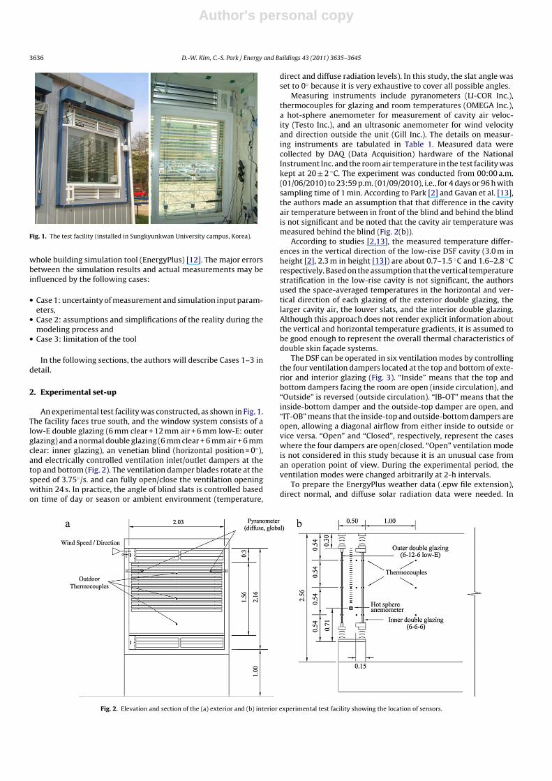
Fig. 1. The test facility (installed in Sungkyunkwan University campus, Korea).

whole building simulation tool (EnergyPlus) [12]. The major errorsbetween the simulation results and actual measurements may beinfluenced by the following cases:

• Case 1: uncertainty of measurement and simulation input param-eters,

• Case 2: assumptions and simplifications of the reality during themodeling process and

• Case 3: limitation of the tool

In the following sections, the authors will describe Cases 1–3 indetail.

2. Experimental set-up

An experimental test facility was constructed, as shown in Fig. 1.The facility faces true south, and the window system consists of alow-E double glazing (6 mm clear + 12 mm air + 6 mm low-E: outerglazing) and a normal double glazing (6 mm clear + 6 mm air + 6 mmclear: inner glazing), an venetian blind (horizontal position = 0◦),and electrically controlled ventilation inlet/outlet dampers at thetop and bottom (Fig. 2). The ventilation damper blades rotate at thespeed of 3.75◦/s. and can fully open/close the ventilation openingwithin 24 s. In practice, the angle of blind slats is controlled basedon time of day or season or ambient environment (temperature,

direct and diffuse radiation levels). In this study, the slat angle wasset to 0◦ because it is very exhaustive to cover all possible angles.

Measuring instruments include pyranometers (LI-COR Inc.),thermocouples for glazing and room temperatures (OMEGA Inc.),a hot-sphere anemometer for measurement of cavity air veloc-ity (Testo Inc.), and an ultrasonic anemometer for wind velocityand direction outside the unit (Gill Inc.). The details on measur-ing instruments are tabulated in Table 1. Measured data werecollected by DAQ (Data Acquisition) hardware of the NationalInstrument Inc. and the room air temperature in the test facility waskept at 20 ± 2 ◦C. The experiment was conducted from 00:00 a.m.(01/06/2010) to 23:59 p.m. (01/09/2010), i.e., for 4 days or 96 h withsampling time of 1 min. According to Park [2] and Gavan et al. [13],the authors made an assumption that that difference in the cavityair temperature between in front of the blind and behind the blindis not significant and be noted that the cavity air temperature wasmeasured behind the blind (Fig. 2(b)).

According to studies [2,13], the measured temperature differ-ences in the vertical direction of the low-rise DSF cavity (3.0 m inheight [2], 2.3 m in height [13]) are about 0.7–1.5 ◦C and 1.6–2.8 ◦Crespectively. Based on the assumption that the vertical temperaturestratification in the low-rise cavity is not significant, the authorsused the space-averaged temperatures in the horizontal and ver-tical direction of each glazing of the exterior double glazing, thelarger cavity air, the louver slats, and the interior double glazing.Although this approach does not render explicit information aboutthe vertical and horizontal temperature gradients, it is assumed tobe good enough to represent the overall thermal characteristics ofdouble skin fac ade systems.

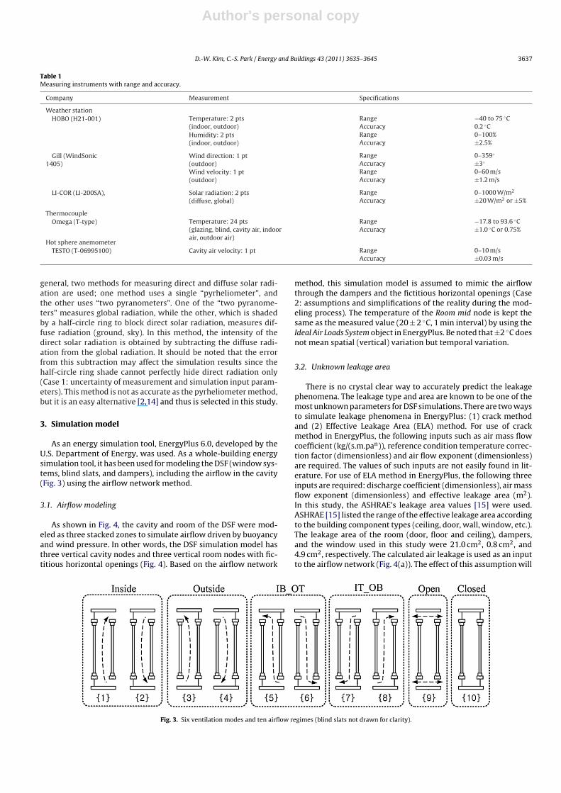
The DSF can be operated in six ventilation modes by controllingthe four ventilation dampers located at the top and bottom of exte-rior and interior glazing (Fig. 3). “Inside” means that the top andbottom dampers facing the room are open (inside circulation), and“Outside” is reversed (outside circulation). “IB-OT” means that theinside-bottom damper and the outside-top damper are open, and“IT-OB” means that the inside-top and outside-bottom dampers areopen, allowing a diagonal airflow from either inside to outside orvice versa. “Open” and “Closed”, respectively, represent the caseswhere the four dampers are open/closed. “Open” ventilation modeis not considered in this study because it is an unusual case froman operation point of view. During the experimental period, theventilation modes were changed arbitrarily at 2-h intervals.

To prepare the EnergyPlus weather data (.epw file extension),direct normal, and diffuse solar radiation data were needed. In

Fig. 2. Elevation and section of the (a) exterior and (b) interior experimental test facility showing the location of sensors.

Author's personal copy

D.-W. Kim, C.-S. Park / Energy and Buildings 43 (2011) 3635–3645 3637

Table 1Measuring instruments with range and accuracy.

Company Measurement Specifications

Weather stationHOBO (H21-001) Temperature: 2 pts

(indoor, outdoor)Range −40 to 75 ◦CAccuracy 0.2 ◦C

Humidity: 2 pts(indoor, outdoor)

Range 0–100%Accuracy ±2.5%

Gill (WindSonic1405)

Wind direction: 1 pt(outdoor)

Range 0–359◦

Accuracy ±3◦

Wind velocity: 1 pt(outdoor)

Range 0–60 m/sAccuracy ±1.2 m/s

LI-COR (LI-200SA), Solar radiation: 2 pts(diffuse, global)

Range 0–1000 W/m2

Accuracy ±20 W/m2 or ±5%

ThermocoupleOmega (T-type) Temperature: 24 pts

(glazing, blind, cavity air, indoorair, outdoor air)

Range −17.8 to 93.6 ◦CAccuracy ±1.0 ◦C or 0.75%

Hot sphere anemometerTESTO (T-06995100) Cavity air velocity: 1 pt Range 0–10 m/s

Accuracy ±0.03 m/s

general, two methods for measuring direct and diffuse solar radi-ation are used; one method uses a single “pyrheliometer”, andthe other uses “two pyranometers”. One of the “two pyranome-ters” measures global radiation, while the other, which is shadedby a half-circle ring to block direct solar radiation, measures dif-fuse radiation (ground, sky). In this method, the intensity of thedirect solar radiation is obtained by subtracting the diffuse radi-ation from the global radiation. It should be noted that the errorfrom this subtraction may affect the simulation results since thehalf-circle ring shade cannot perfectly hide direct radiation only(Case 1: uncertainty of measurement and simulation input param-eters). This method is not as accurate as the pyrheliometer method,but it is an easy alternative [2,14] and thus is selected in this study.

3. Simulation model

As an energy simulation tool, EnergyPlus 6.0, developed by theU.S. Department of Energy, was used. As a whole-building energysimulation tool, it has been used for modeling the DSF (window sys-tems, blind slats, and dampers), including the airflow in the cavity(Fig. 3) using the airflow network method.

3.1. Airflow modeling

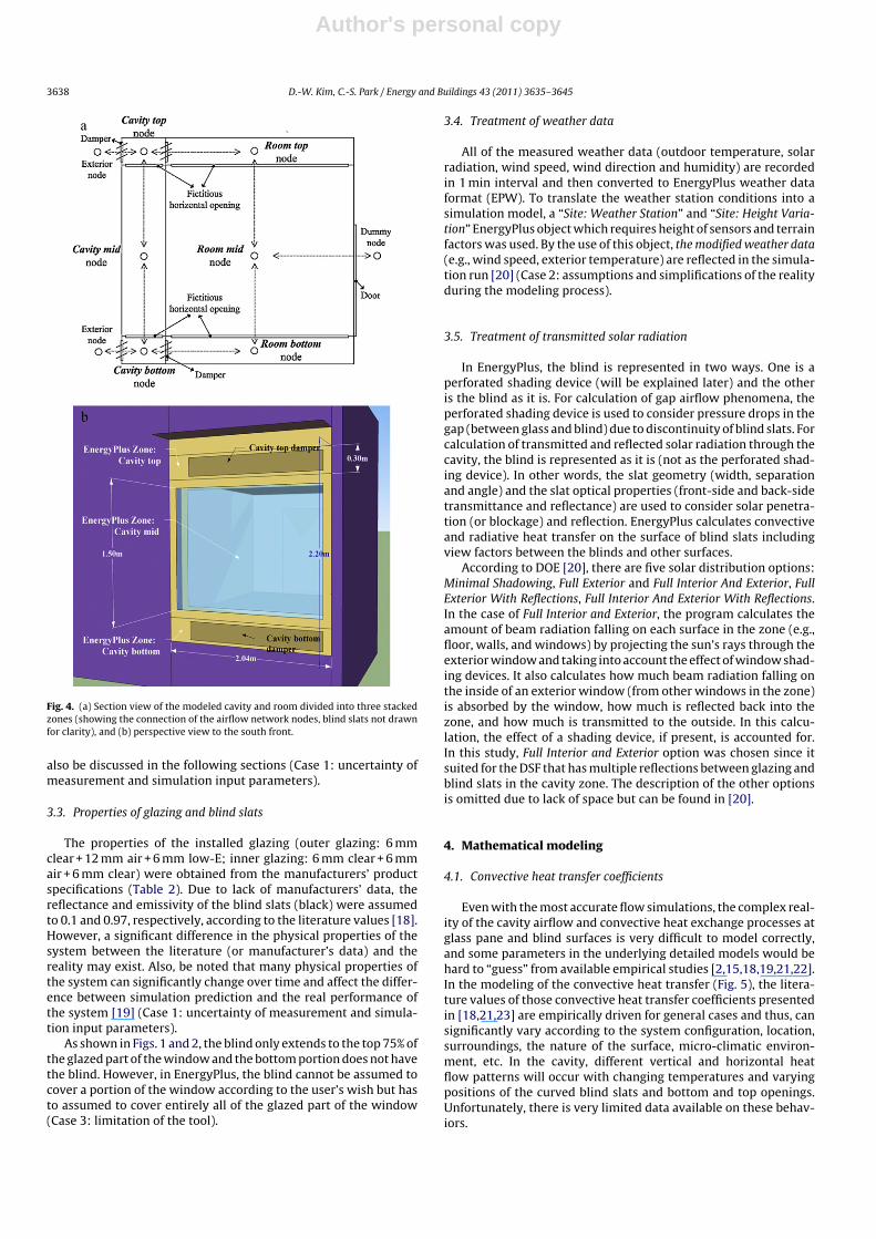
As shown in Fig. 4, the cavity and room of the DSF were mod-eled as three stacked zones to simulate airflow driven by buoyancyand wind pressure. In other words, the DSF simulation model hasthree vertical cavity nodes and three vertical room nodes with fic-titious horizontal openings (Fig. 4). Based on the airflow network

method, this simulation model is assumed to mimic the airflowthrough the dampers and the fictitious horizontal openings (Case2: assumptions and simplifications of the reality during the mod-eling process). The temperature of the Room mid node is kept thesame as the measured value (20 ± 2 ◦C, 1 min interval) by using theIdeal Air Loads System object in EnergyPlus. Be noted that ±2 ◦C doesnot mean spatial (vertical) variation but temporal variation.

3.2. Unknown leakage area

There is no crystal clear way to accurately predict the leakagephenomena. The leakage type and area are known to be one of themost unknown parameters for DSF simulations. There are two waysto simulate leakage phenomena in EnergyPlus: (1) crack methodand (2) Effective Leakage Area (ELA) method. For use of crackmethod in EnergyPlus, the following inputs such as air mass flowcoefficient (kg/(s.m.pan)), reference condition temperature correc-tion factor (dimensionless) and air flow exponent (dimensionless)are required. The values of such inputs are not easily found in lit-erature. For use of ELA method in EnergyPlus, the following threeinputs are required: discharge coefficient (dimensionless), air massflow exponent (dimensionless) and effective leakage area (m2).In this study, the ASHRAE’s leakage area values [15] were used.ASHRAE [15] listed the range of the effective leakage area accordingto the building component types (ceiling, door, wall, window, etc.).The leakage area of the room (door, floor and ceiling), dampers,and the window used in this study were 21.0 cm2, 0.8 cm2, and4.9 cm2, respectively. The calculated air leakage is used as an inputto the airflow network (Fig. 4(a)). The effect of this assumption will

Fig. 3. Six ventilation modes and ten airflow regimes (blind slats not drawn for clarity).

Author's personal copy

3638 D.-W. Kim, C.-S. Park / Energy and Buildings 43 (2011) 3635–3645

Fig. 4. (a) Section view of the modeled cavity and room divided into three stackedzones (showing the connection of the airflow network nodes, blind slats not drawnfor clarity), and (b) perspective view to the south front.

also be discussed in the following sections (Case 1: uncertainty ofmeasurement and simulation input parameters).

3.3. Properties of glazing and blind slats

The properties of the installed glazing (outer glazing: 6 mmclear + 12 mm air + 6 mm low-E; inner glazing: 6 mm clear + 6 mmair + 6 mm clear) were obtained from the manufacturers’ productspecifications (Table 2). Due to lack of manufacturers’ data, thereflectance and emissivity of the blind slats (black) were assumedto 0.1 and 0.97, respectively, according to the literature values [18].However, a significant difference in the physical properties of thesystem between the literature (or manufacturer’s data) and thereality may exist. Also, be noted that many physical properties ofthe system can significantly change over time and affect the differ-ence between simulation prediction and the real performance ofthe system [19] (Case 1: uncertainty of measurement and simula-tion input parameters).

As shown in Figs. 1 and 2, the blind only extends to the top 75% ofthe glazed part of the window and the bottom portion does not havethe blind. However, in EnergyPlus, the blind cannot be assumed tocover a portion of the window according to the user’s wish but hasto assumed to cover entirely all of the glazed part of the window(Case 3: limitation of the tool).

3.4. Treatment of weather data

All of the measured weather data (outdoor temperature, solarradiation, wind speed, wind direction and humidity) are recordedin 1 min interval and then converted to EnergyPlus weather dataformat (EPW). To translate the weather station conditions into asimulation model, a “Site: Weather Station” and “Site: Height Varia-tion” EnergyPlus object which requires height of sensors and terrainfactors was used. By the use of this object, the modified weather data(e.g., wind speed, exterior temperature) are reflected in the simula-tion run [20] (Case 2: assumptions and simplifications of the realityduring the modeling process).

3.5. Treatment of transmitted solar radiation

In EnergyPlus, the blind is represented in two ways. One is aperforated shading device (will be explained later) and the otheris the blind as it is. For calculation of gap airflow phenomena, theperforated shading device is used to consider pressure drops in thegap (between glass and blind) due to discontinuity of blind slats. Forcalculation of transmitted and reflected solar radiation through thecavity, the blind is represented as it is (not as the perforated shad-ing device). In other words, the slat geometry (width, separationand angle) and the slat optical properties (front-side and back-sidetransmittance and reflectance) are used to consider solar penetra-tion (or blockage) and reflection. EnergyPlus calculates convectiveand radiative heat transfer on the surface of blind slats includingview factors between the blinds and other surfaces.

According to DOE [20], there are five solar distribution options:Minimal Shadowing, Full Exterior and Full Interior And Exterior, FullExterior With Reflections, Full Interior And Exterior With Reflections.In the case of Full Interior and Exterior, the program calculates theamount of beam radiation falling on each surface in the zone (e.g.,floor, walls, and windows) by projecting the sun’s rays through theexterior window and taking into account the effect of window shad-ing devices. It also calculates how much beam radiation falling onthe inside of an exterior window (from other windows in the zone)is absorbed by the window, how much is reflected back into thezone, and how much is transmitted to the outside. In this calcu-lation, the effect of a shading device, if present, is accounted for.In this study, Full Interior and Exterior option was chosen since itsuited for the DSF that has multiple reflections between glazing andblind slats in the cavity zone. The description of the other optionsis omitted due to lack of space but can be found in [20].

4. Mathematical modeling

4.1. Convective heat transfer coefficients

Even with the most accurate flow simulations, the complex real-ity of the cavity airflow and convective heat exchange processes atglass pane and blind surfaces is very difficult to model correctly,and some parameters in the underlying detailed models would behard to “guess” from available empirical studies [2,15,18,19,21,22].In the modeling of the convective heat transfer (Fig. 5), the litera-ture values of those convective heat transfer coefficients presentedin [18,21,23] are empirically driven for general cases and thus, cansignificantly vary according to the system configuration, location,surroundings, the nature of the surface, micro-climatic environ-ment, etc. In the cavity, different vertical and horizontal heatflow patterns will occur with changing temperatures and varyingpositions of the curved blind slats and bottom and top openings.Unfortunately, there is very limited data available on these behav-iors.

Author's personal copy

D.-W. Kim, C.-S. Park / Energy and Buildings 43 (2011) 3635–3645 3639

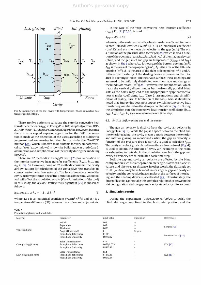
Fig. 5. Section view of the DSF cavity with temperatures (T) and convective heattransfer coefficients (h).

There are five options to calculate the exterior convective heattransfer coefficient (hout) in EnergyPlus 6.0: Simple algorithm, DOE-2, TARP, MoWiTT, Adaptive Convection Algorithm. However, becausethere is no accepted superior algorithm for the DSF, the selec-tion is made at the discretion of the users according to subjectivejudgment and engineering intuition. In this study, the “MoWiTT”method [24], which is known to be suitable for very smooth verti-cal surfaces (e.g., windows) in low-rise buildings, was used (Case 2:assumptions and simplifications of the reality during the modelingprocess).

There are 32 methods in EnergyPlus 6.0 [25] for calculation ofthe interior convective heat transfer coefficients (hblind, hcav, andhin in Fig. 5). However, none of 32 methods considers the cavityairflow pattern for calculation of the convective heat transfer; noconnection to the airflow network. This lack of consideration of thecavity airflow pattern is one of the limitations of the simulation tooland will affect the simulation results (Case 3: limitation of the tool).In this study, the ASHRAE Vertical Wall algorithm [25] is chosen asfollows:

hblind or hcav or hin = 1.31 �T1/3 (1)

where 1.31 is an empirical coefficient (W/(m2 K4/3)) and �T is atemperature difference (◦K) between the surface and adjacent air.

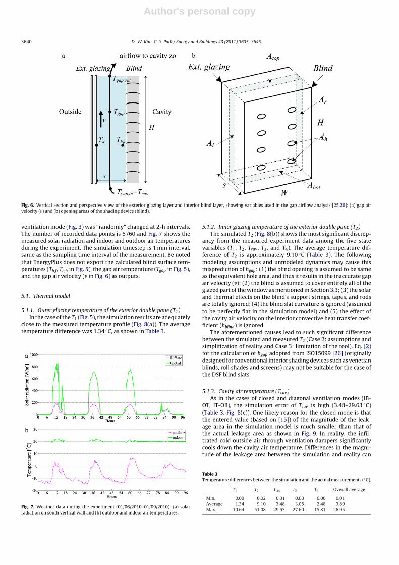
In the case of the “gap” convective heat transfer coefficient(hgap), Eq. (2) [25,26] is used:

hgap = 2hc + 4v (2)

where hc is the surface-to-surface heat transfer coefficient for non-vented (closed) cavities (W/m2 K), 4 is an empirical coefficient(J/m3 K), and v is the mean air velocity in the gap (m/s). The v isa function of the pressure drop factor (Z) [25] which is also a func-tion of the opening areas (Abot, Atop, Al, Ar, Ah) of the shading devices(blind) and the gap inlet and gap air temperature (Tgap,in and Tgap)as shown in Fig. 6 where Abot is the area of the bottom opening (m2),Atop is the area of the top opening (m2), Al is the area of the left-sideopening (m2), Ar is the area of the right-side opening (m2), and Ahis the air permeability of the shading device expressed as the totalarea of openings (“holes”) in the shade surface (these openings areassumed to be uniformly distributed over the shade and change asthe blind slats rotate) (m2) [25]. However, this simplification, whichtreats the vertically discontinuous but horizontally parallel blindslats as the holes, may lead to the inappropriate “gap” convectiveheat transfer coefficient, hgap (Case 2: assumptions and simplifi-cation of reality, Case 3: limitation of the tool). Also, it should benoted that EnergyPlus does not support switching convective heattransfer regimes based on the damper combination (Fig. 3). Duringthe simulation run, the convective heat transfer coefficients (hout,hgap, hblind, hcav, hin) are re-evaluated each time step.

4.2. Vertical airflow in the gap and the cavity

The gap air velocity is distinct from the cavity air velocity inEnergyPlus (Fig. 5). While the gap is a space between the blind andthe exterior glazing, the cavity means a space between the exteriorand interior glazing. As mentioned earlier, the gap air velocity, afunction of the pressure drop factor (Z), is used to calculate hgap.The cavity air velocity, calculated from the airflow network (Fig. 4),is used to obtain the amount of cavity air incoming to the roomor exhausting to outside. In the simulation run, both the gap andcavity air velocity are re-evaluated each time step.

Both the gap and cavity air velocity are affected by the blindconfiguration such as slat separation, slat angle, slat width, slat cur-vature, and slat-to-glass distance. In other words, the slat angle setto 90◦ (vertical) may be in favor of increasing the gap and cavity airvelocity, and the convective heat transfer at the surfaces of the glaz-ing and the shading device is accelerated [27]. Unfortunately, theEnergyPlus tool cannot take this complex relationship between theslat configuration and the gap and cavity air velocity into account.

5. Simulation results

During the experiment (01/06/2010–01/09/2010, 96 h), theblind slat angle was fixed in the horizontal position and the

Table 2Properties of glazing and blind slats.

Material Parameter Input value Dimension References

Venetian blind

Width 0.05 m

Somfy [16]Separation 0.45 mThickness 0.003 mAngle (Horizontal) 0 DegreeFront/Back Reflectance 0.1/0.1 –

Incropera et al. [18]Front/Back Emissivity 0.97/0.97 –

Clear glazing (6 mm)Solar Transmittance 0.77 –

KCC [17]Front/Back Reflectance 0.073/0.073 –Front/Back Emissivity 0.83/0.83 –

Low-e glazing (6 mm)Solar Transmittance 0.54 –

KCC [17]Front/Back Reflectance 0.18/0.25 –Front/Back Emissivity 0.09/0.84 –

Author's personal copy

3640 D.-W. Kim, C.-S. Park / Energy and Buildings 43 (2011) 3635–3645

Fig. 6. Vertical section and perspective view of the exterior glazing layer and interior blind layer, showing variables used in the gap airflow analysis [25,26]: (a) gap airvelocity (v) and (b) opening areas of the shading device (blind).

ventilation mode (Fig. 3) was “randomly” changed at 2-h intervals.The number of recorded data points is 5760 and Fig. 7 shows themeasured solar radiation and indoor and outdoor air temperaturesduring the experiment. The simulation timestep is 1 min interval,same as the sampling time interval of the measurement. Be notedthat EnergyPlus does not export the calculated blind surface tem-peratures (Tb,f, Tb,b in Fig. 5), the gap air temperature (Tgap in Fig. 5),and the gap air velocity (v in Fig. 6) as outputs.

5.1. Thermal model

5.1.1. Outer glazing temperature of the exterior double pane (T1)In the case of the T1 (Fig. 5), the simulation results are adequately

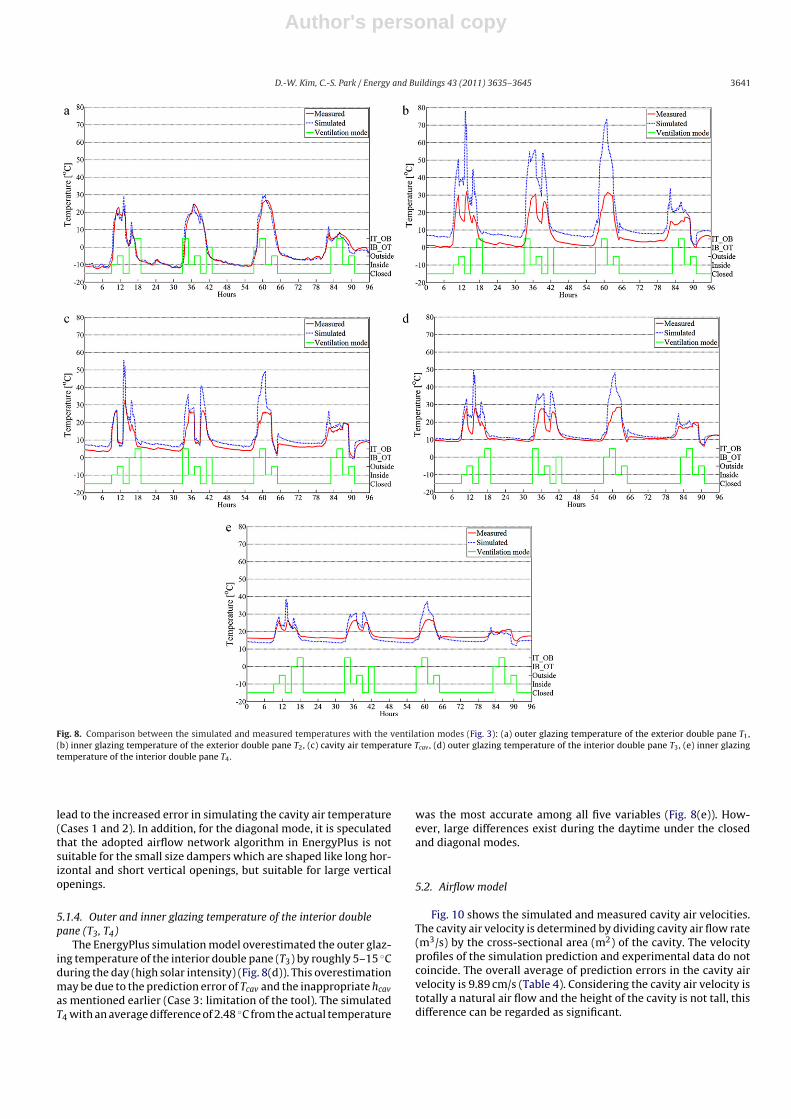
close to the measured temperature profile (Fig. 8(a)). The averagetemperature difference was 1.34 ◦C, as shown in Table 3.

Fig. 7. Weather data during the experiment (01/06/2010–01/09/2010): (a) solarradiation on south vertical wall and (b) outdoor and indoor air temperatures.

5.1.2. Inner glazing temperature of the exterior double pane (T2)The simulated T2 (Fig. 8(b)) shows the most significant discrep-

ancy from the measured experiment data among the five statevariables (T1, T2, Tcav, T3, and T4). The average temperature dif-ference of T2 is approximately 9.10 ◦C (Table 3). The followingmodeling assumptions and unmodeled dynamics may cause thismisprediction of hgap: (1) the blind opening is assumed to be sameas the equivalent hole area, and thus it results in the inaccurate gapair velocity (v); (2) the blind is assumed to cover entirely all of theglazed part of the window as mentioned in Section 3.3; (3) the solarand thermal effects on the blind’s support strings, tapes, and rodsare totally ignored; (4) the blind slat curvature is ignored (assumedto be perfectly flat in the simulation model) and (5) the effect ofthe cavity air velocity on the interior convective heat transfer coef-ficient (hblind) is ignored.

The aforementioned causes lead to such significant differencebetween the simulated and measured T2 (Case 2: assumptions andsimplification of reality and Case 3: limitation of the tool). Eq. (2)for the calculation of hgap adopted from ISO15099 [26] (originallydesigned for conventional interior shading devices such as venetianblinds, roll shades and screens) may not be suitable for the case ofthe DSF blind slats.

5.1.3. Cavity air temperature (Tcav)As in the cases of closed and diagonal ventilation modes (IB-

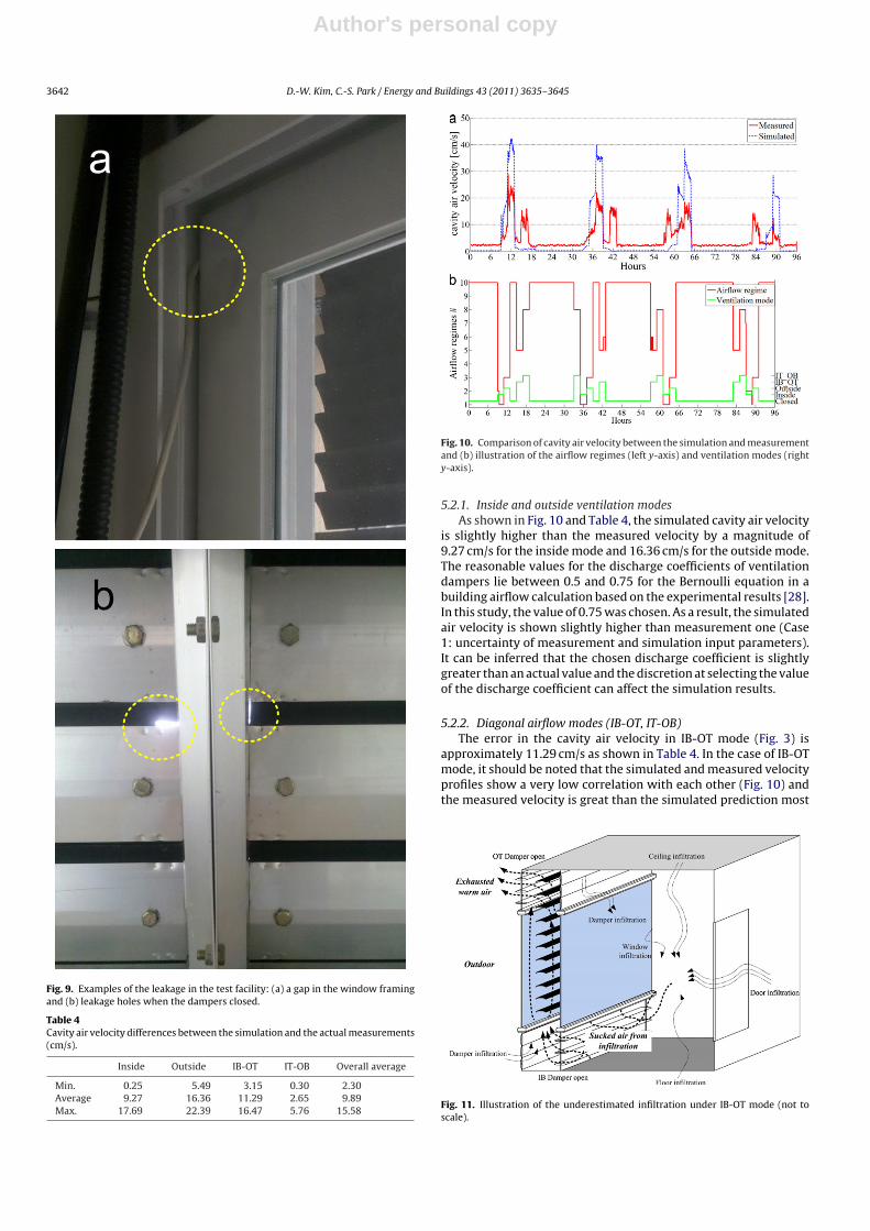
OT, IT-OB), the simulation error of Tcav is high (3.48–29.63 ◦C)(Table 3, Fig. 8(c)). One likely reason for the closed mode is thatthe entered value (based on [15]) of the magnitude of the leak-age area in the simulation model is much smaller than that ofthe actual leakage area as shown in Fig. 9. In reality, the infil-trated cold outside air through ventilation dampers significantlycools down the cavity air temperature. Differences in the magni-tude of the leakage area between the simulation and reality can

Table 3Temperature differences between the simulation and the actual measurements (◦C).

T1 T2 Tcav T3 T4 Overall average

Min. 0.00 0.02 0.01 0.00 0.00 0.01Average 1.34 9.10 3.48 3.05 2.48 3.89Max. 10.64 51.08 29.63 27.60 15.81 26.95

Author's personal copy

D.-W. Kim, C.-S. Park / Energy and Buildings 43 (2011) 3635–3645 3641

Fig. 8. Comparison between the simulated and measured temperatures with the ventilation modes (Fig. 3): (a) outer glazing temperature of the exterior double pane T1,(b) inner glazing temperature of the exterior double pane T2, (c) cavity air temperature Tcav , (d) outer glazing temperature of the interior double pane T3, (e) inner glazingtemperature of the interior double pane T4.

lead to the increased error in simulating the cavity air temperature(Cases 1 and 2). In addition, for the diagonal mode, it is speculatedthat the adopted airflow network algorithm in EnergyPlus is notsuitable for the small size dampers which are shaped like long hor-izontal and short vertical openings, but suitable for large verticalopenings.

5.1.4. Outer and inner glazing temperature of the interior doublepane (T3, T4)

The EnergyPlus simulation model overestimated the outer glaz-ing temperature of the interior double pane (T3) by roughly 5–15 ◦Cduring the day (high solar intensity) (Fig. 8(d)). This overestimationmay be due to the prediction error of Tcav and the inappropriate hcav

as mentioned earlier (Case 3: limitation of the tool). The simulatedT4 with an average difference of 2.48 ◦C from the actual temperature

was the most accurate among all five variables (Fig. 8(e)). How-ever, large differences exist during the daytime under the closedand diagonal modes.

5.2. Airflow model

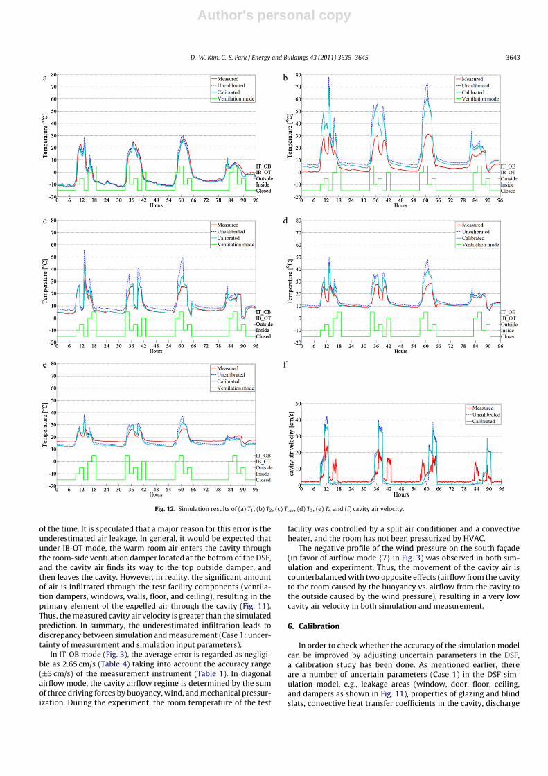
Fig. 10 shows the simulated and measured cavity air velocities.The cavity air velocity is determined by dividing cavity air flow rate(m3/s) by the cross-sectional area (m2) of the cavity. The velocityprofiles of the simulation prediction and experimental data do notcoincide. The overall average of prediction errors in the cavity airvelocity is 9.89 cm/s (Table 4). Considering the cavity air velocity istotally a natural air flow and the height of the cavity is not tall, thisdifference can be regarded as significant.

Author's personal copy

3642 D.-W. Kim, C.-S. Park / Energy and Buildings 43 (2011) 3635–3645

Fig. 9. Examples of the leakage in the test facility: (a) a gap in the window framingand (b) leakage holes when the dampers closed.

Table 4Cavity air velocity differences between the simulation and the actual measurements(cm/s).

Inside Outside IB-OT IT-OB Overall average

Min. 0.25 5.49 3.15 0.30 2.30Average 9.27 16.36 11.29 2.65 9.89Max. 17.69 22.39 16.47 5.76 15.58

Fig. 10. Comparison of cavity air velocity between the simulation and measurementand (b) illustration of the airflow regimes (left y-axis) and ventilation modes (righty-axis).

5.2.1. Inside and outside ventilation modesAs shown in Fig. 10 and Table 4, the simulated cavity air velocity

is slightly higher than the measured velocity by a magnitude of9.27 cm/s for the inside mode and 16.36 cm/s for the outside mode.The reasonable values for the discharge coefficients of ventilationdampers lie between 0.5 and 0.75 for the Bernoulli equation in abuilding airflow calculation based on the experimental results [28].In this study, the value of 0.75 was chosen. As a result, the simulatedair velocity is shown slightly higher than measurement one (Case1: uncertainty of measurement and simulation input parameters).It can be inferred that the chosen discharge coefficient is slightlygreater than an actual value and the discretion at selecting the valueof the discharge coefficient can affect the simulation results.

5.2.2. Diagonal airflow modes (IB-OT, IT-OB)The error in the cavity air velocity in IB-OT mode (Fig. 3) is

approximately 11.29 cm/s as shown in Table 4. In the case of IB-OTmode, it should be noted that the simulated and measured velocityprofiles show a very low correlation with each other (Fig. 10) andthe measured velocity is great than the simulated prediction most

Fig. 11. Illustration of the underestimated infiltration under IB-OT mode (not toscale).

Author's personal copy

D.-W. Kim, C.-S. Park / Energy and Buildings 43 (2011) 3635–3645 3643

Fig. 12. Simulation results of (a) T1, (b) T2, (c) Tcav , (d) T3, (e) T4 and (f) cavity air velocity.

of the time. It is speculated that a major reason for this error is theunderestimated air leakage. In general, it would be expected thatunder IB-OT mode, the warm room air enters the cavity throughthe room-side ventilation damper located at the bottom of the DSF,and the cavity air finds its way to the top outside damper, andthen leaves the cavity. However, in reality, the significant amountof air is infiltrated through the test facility components (ventila-tion dampers, windows, walls, floor, and ceiling), resulting in theprimary element of the expelled air through the cavity (Fig. 11).Thus, the measured cavity air velocity is greater than the simulatedprediction. In summary, the underestimated infiltration leads todiscrepancy between simulation and measurement (Case 1: uncer-tainty of measurement and simulation input parameters).

In IT-OB mode (Fig. 3), the average error is regarded as negligi-ble as 2.65 cm/s (Table 4) taking into account the accuracy range(±3 cm/s) of the measurement instrument (Table 1). In diagonalairflow mode, the cavity airflow regime is determined by the sumof three driving forces by buoyancy, wind, and mechanical pressur-ization. During the experiment, the room temperature of the test

facility was controlled by a split air conditioner and a convectiveheater, and the room has not been pressurized by HVAC.

The negative profile of the wind pressure on the south fac ade(in favor of airflow mode {7} in Fig. 3) was observed in both sim-ulation and experiment. Thus, the movement of the cavity air iscounterbalanced with two opposite effects (airflow from the cavityto the room caused by the buoyancy vs. airflow from the cavity tothe outside caused by the wind pressure), resulting in a very lowcavity air velocity in both simulation and measurement.

6. Calibration

In order to check whether the accuracy of the simulation modelcan be improved by adjusting uncertain parameters in the DSF,a calibration study has been done. As mentioned earlier, thereare a number of uncertain parameters (Case 1) in the DSF sim-ulation model, e.g., leakage areas (window, door, floor, ceiling,and dampers as shown in Fig. 11), properties of glazing and blindslats, convective heat transfer coefficients in the cavity, discharge

Author's personal copy

3644 D.-W. Kim, C.-S. Park / Energy and Buildings 43 (2011) 3635–3645

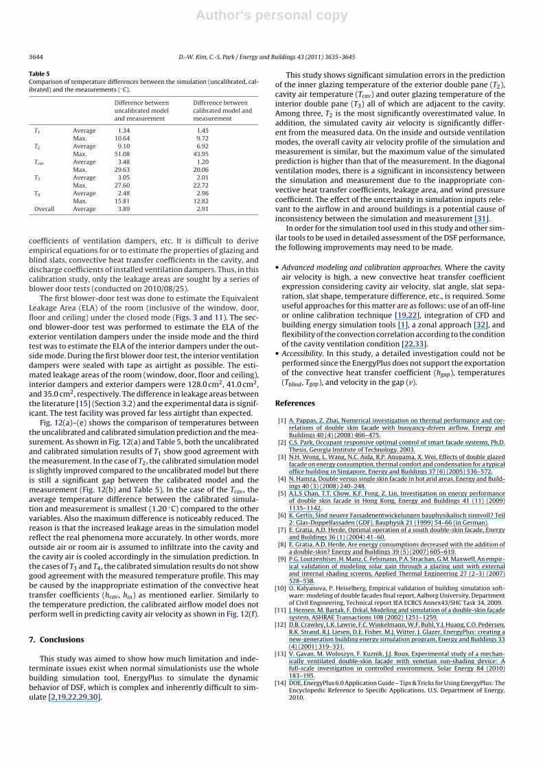
Table 5Comparison of temperature differences between the simulation (uncalibrated, cal-ibrated) and the measurements (◦C).

Difference betweenuncalibrated modeland measurement

Difference betweencalibrated model andmeasurement

T1 Average 1.34 1.45Max. 10.64 9.72

T2 Average 9.10 6.92Max. 51.08 43.95

Tcav Average 3.48 1.20Max. 29.63 20.06

T3 Average 3.05 2.01Max. 27.60 22.72

T4 Average 2.48 2.96Max. 15.81 12.82

Overall Average 3.89 2.91

coefficients of ventilation dampers, etc. It is difficult to deriveempirical equations for or to estimate the properties of glazing andblind slats, convective heat transfer coefficients in the cavity, anddischarge coefficients of installed ventilation dampers. Thus, in thiscalibration study, only the leakage areas are sought by a series ofblower door tests (conducted on 2010/08/25).

The first blower-door test was done to estimate the EquivalentLeakage Area (ELA) of the room (inclusive of the window, door,floor and ceiling) under the closed mode (Figs. 3 and 11). The sec-ond blower-door test was performed to estimate the ELA of theexterior ventilation dampers under the inside mode and the thirdtest was to estimate the ELA of the interior dampers under the out-side mode. During the first blower door test, the interior ventilationdampers were sealed with tape as airtight as possible. The esti-mated leakage areas of the room (window, door, floor and ceiling),interior dampers and exterior dampers were 128.0 cm2, 41.0 cm2,and 35.0 cm2, respectively. The difference in leakage areas betweenthe literature [15] (Section 3.2) and the experimental data is signif-icant. The test facility was proved far less airtight than expected.

Fig. 12(a)–(e) shows the comparison of temperatures betweenthe uncalibrated and calibrated simulation prediction and the mea-surement. As shown in Fig. 12(a) and Table 5, both the uncalibratedand calibrated simulation results of T1 show good agreement withthe measurement. In the case of T2, the calibrated simulation modelis slightly improved compared to the uncalibrated model but thereis still a significant gap between the calibrated model and themeasurement (Fig. 12(b) and Table 5). In the case of the Tcav, theaverage temperature difference between the calibrated simula-tion and measurement is smallest (1.20 ◦C) compared to the othervariables. Also the maximum difference is noticeably reduced. Thereason is that the increased leakage areas in the simulation modelreflect the real phenomena more accurately. In other words, moreoutside air or room air is assumed to infiltrate into the cavity andthe cavity air is cooled accordingly in the simulation prediction. Inthe cases of T3 and T4, the calibrated simulation results do not showgood agreement with the measured temperature profile. This maybe caused by the inappropriate estimation of the convective heattransfer coefficients (hcav, hin) as mentioned earlier. Similarly tothe temperature prediction, the calibrated airflow model does notperform well in predicting cavity air velocity as shown in Fig. 12(f).

7. Conclusions

This study was aimed to show how much limitation and inde-terminate issues exist when normal simulationists use the wholebuilding simulation tool, EnergyPlus to simulate the dynamicbehavior of DSF, which is complex and inherently difficult to sim-ulate [2,19,22,29,30].

This study shows significant simulation errors in the predictionof the inner glazing temperature of the exterior double pane (T2),cavity air temperature (Tcav) and outer glazing temperature of theinterior double pane (T3) all of which are adjacent to the cavity.Among three, T2 is the most significantly overestimated value. Inaddition, the simulated cavity air velocity is significantly differ-ent from the measured data. On the inside and outside ventilationmodes, the overall cavity air velocity profile of the simulation andmeasurement is similar, but the maximum value of the simulatedprediction is higher than that of the measurement. In the diagonalventilation modes, there is a significant in inconsistency betweenthe simulation and measurement due to the inappropriate con-vective heat transfer coefficients, leakage area, and wind pressurecoefficient. The effect of the uncertainty in simulation inputs rele-vant to the airflow in and around buildings is a potential cause ofinconsistency between the simulation and measurement [31].

In order for the simulation tool used in this study and other sim-ilar tools to be used in detailed assessment of the DSF performance,the following improvements may need to be made.

• Advanced modeling and calibration approaches. Where the cavityair velocity is high, a new convective heat transfer coefficientexpression considering cavity air velocity, slat angle, slat sepa-ration, slat shape, temperature difference, etc., is required. Someuseful approaches for this matter are as follows: use of an off-lineor online calibration technique [19,22], integration of CFD andbuilding energy simulation tools [1], a zonal approach [32], andflexibility of the convection correlation according to the conditionof the cavity ventilation condition [22,33].

• Accessibility. In this study, a detailed investigation could not beperformed since the EnergyPlus does not support the exportationof the convective heat transfer coefficient (hgap), temperatures(Tblind, Tgap), and velocity in the gap (v).

References

[1] A. Pappas, Z. Zhai, Numerical investigation on thermal performance and cor-relations of double skin facade with buoyancy-driven airflow, Energy andBuildings 40 (4) (2008) 466–475.

[2] C.S. Park, Occupant responsive optimal control of smart facade systems, Ph.D.Thesis, Georgia Institute of Technology, 2003.

[3] N.H. Wong, L. Wang, N.C. Aida, R.P. Anupama, X. Wei, Effects of double glazedfacade on energy consumption, thermal comfort and condensation for a typicaloffice building in Singapore, Energy and Buildings 37 (6) (2005) 536–572.

[4] N. Hamza, Double versus single skin facade in hot arid areas, Energy and Build-ings 40 (3) (2008) 240–248.

[5] A.L.S Chan, T.T. Chow, K.F. Fong, Z. Lin, Investigation on energy performanceof double skin facade in Hong Kong, Energy and Buildings 41 (11) (2009)1135–1142.

[6] K. Gertis, Sind neuere Fassadenentwickelungen bauphysikalisch sinnvoll? Teil2: Glas-Doppelfassaden (GDF), Bauphysik 21 (1999) 54–66 (in German).

[7] E. Gratia, A.D. Herde, Optimal operation of a south double-skin facade, Energyand Buildings 36 (1) (2004) 41–60.

[8] E. Gratia, A.D. Herde, Are energy consumptions decreased with the addition ofa double-skin? Energy and Buildings 39 (5) (2007) 605–619.

[9] P.G. Loutzenhiser, H. Manz, C. Felsmann, P.A. Strachan, G.M. Maxwell, An empir-ical validation of modeling solar gain through a glazing unit with externaland internal shading screens, Applied Thermal Engineering 27 (2–3) (2007)528–538.

[10] O. Kalyanova, P. Heiselberg, Empirical validation of building simulation soft-ware: modeling of double facades final report, Aalborg University, Departmentof Civil Engineering, Technical report IEA ECBCS Annex43/SHC Task 34, 2009.

[11] J. Hensen, M. Bartak, F. Drkal, Modeling and simulation of a double-skin fac adesystem, ASHRAE Transactions 108 (2002) 1251–1259.

[12] D.B. Crawley, L.K. Lawrie, F.C. Winkelmann, W.F. Buhl, Y.J. Huang, C.O. Pedersen,R.K. Strand, R.J. Liesen, D.E. Fisher, M.J. Witter, J. Glazer, EnergyPlus: creating anew-generation building energy simulation program, Energy and Buildings 33(4) (2001) 319–331.

[13] V. Gavan, M. Woloszyn, F. Kuznik, J.J. Roux, Experimental study of a mechan-ically ventilated double-skin fac ade with venetian sun-shading device: Afull-scale investigation in controlled environment, Solar Energy 84 (2010)183–195.

[14] DOE, EnergyPlus 6.0 Application Guide – Tips & Tricks for Using EnergyPlus: TheEncyclopedic Reference to Specific Applications, U.S. Department of Energy,2010.

Author's personal copy

D.-W. Kim, C.-S. Park / Energy and Buildings 43 (2011) 3635–3645 3645

[15] ASHRAE, ASHRAE Handbook Fundamentals, ASHRAE, 2001.[16] Somfy, http://www.somfy.co.kr/common files/sub7 page2.asp?keyword=

(%B5%B5%B8%E9-06) (accessed on January 2010, in Korean).[17] KCC, http://www.kccworld.co.kr/korea/2 main/4 product/vShow.asp?nodeid

=251 (accessed on January 2010, in Korean).[18] F.P. Incropera, D.P. DeWitt, T.L. Bergman, A.S. Lavine, Fundamentals of Heat and

Mass Transfer, 6th ed., John Wiley & Sons, 2008.[19] S.H. Yoon, C.S. Park, G. Augenbroe, On-line parameter estimation and opti-

mal control strategy of a double-skin system, Building and Environment 46(5) (2011) 1141–1150.

[20] DOE, EnergyPlus 6. 0 Input/Output Reference: The encyclopedic Reference toEnergyPlus Input and Output, U. S. Department of Energy, 2010.

[21] J.A. Clarke, Energy Simulation in Building Design, Butterworth-Heinemann,2001.

[22] C.S. Park, G. Augenbroe, T. Messadi, M. Thitisawat, N. Sadegh, Calibration of alumped simulation model for double-skin facade systems, Energy and Buildings36 (11) (2004) 1117–1130.

[23] ASHRAE, ASHRAE Handbook Fundamentals, ASHRAE, 2009.[24] M. Yazdanian, J.H. Klems, Measurement of the exterior convective film coeffi-

cient for windows in low-rise buildings, ASHRAE Transactions 100 (1) (1994)1087–1096.

[25] DOE, EnergyPlus 6.0 Engineering Reference: The Encyclopedic Reference toEnergyPlus Calculations, U.S. Department of Energy, 2010.

[26] ISO 15099, Thermal Performance of Windows, Doors, and Shading Devices– Detailed Calculations, first ed., International Standardization Organization,November 2003.

[27] D. Naylor, H. Shahid, Energy performance assessment of a window with a hor-izontal venetian blind, Energy and Buildings 37 (8) (2005) 836–843.

[28] J. van der Maas, Air Flow Through Large Openings in Buildings, Switzerland,Lausanne, Ecole Polytechnique Federale de Lausanne, LESO-PB, 1992.

[29] D. Faggembauu, M. Costa, M. Soria, A. Oliva, Numerical analysis of the ther-mal behaviour of ventilated glazed Facadesin Mediterranean climates. Part I:development and validation of a numerical model, Solar Energy 75 (3) (2003)217–228.

[30] N. Mingottia, T. Chenvidyakarna, A.W. Woods, The fluid mechanics of thenatural ventilation of a narrow-cavity double-skin facade, Building and Envi-ronment 46 (4) (2011) 807–823.

[31] S. de Wit, Uncertainty in predictions of thermal comfort in buildings, Ph.D.Thesis, Delft TechnischeUniversiteit, 2001.

[32] T.E. Jiru, F. Haghighat, Modeling ventilated double skin facade-A zonalapproach, Energy and Buildings 40 (8) (2008) 1567–1576.

[33] R. Høseggen, B.J. Wachenfeldt, S.O. Hanssen, Building simulation as an assist-ing tool in decision making case study: with or without a double-skin facade,Energy and Buildings 40 (5) (2008) 821–827.