dfit and the mantel-haenszel/liu-agr - core
TRANSCRIPT
Georgia State UniversityScholarWorks @ Georgia State University
Educational Policy Studies Dissertations Department of Educational Policy Studies
12-18-2014
A Simulation Study Comparing Two Methods OfEvaluating Differential Test Functioning (DTF):DFIT and the Mantel-Haenszel/Liu-AgrestiVarianceCharles Hunter
Follow this and additional works at: https://scholarworks.gsu.edu/eps_diss
This Dissertation is brought to you for free and open access by the Department of Educational Policy Studies at ScholarWorks @ Georgia StateUniversity. It has been accepted for inclusion in Educational Policy Studies Dissertations by an authorized administrator of ScholarWorks @ GeorgiaState University. For more information, please contact [email protected].
Recommended CitationHunter, Charles, "A Simulation Study Comparing Two Methods Of Evaluating Differential Test Functioning (DTF): DFIT and theMantel-Haenszel/Liu-Agresti Variance." Dissertation, Georgia State University, 2014.https://scholarworks.gsu.edu/eps_diss/114
ACCEPTANCE
This dissertation, A SIMULATION STUDY COMPARING TWO METHODS OF
EVALUATING DIFFERENTIAL TEST FUNCTIONING (DTF): DFIT AND THE MANTEL-
HAENSZEL/LIU-AGRESTI VARIANCE, by CHARLES VINCENT HUNTER, JR., was
prepared under the direction of the candidate’s Dissertation Advisory Committee. It is accepted
by the committee members in partial fulfillment of the requirements for the degree Doctor of
Philosophy in the College of Education, Georgia State University.
The Dissertation Advisory committee and the student’s Department Chair, as representatives of
the faculty, certify that this dissertation has met all standards of excellence and scholarship as
determined by the faculty. The Dean of the College of Education concurs.
T. C. Oshima, Ph.D.
Committee Chair
Hongli Li, Ph.D.
Committee Member
Frances McCarty, Ph.D.
Committee Member
Date
William Curlette
Chair, Department of Educational Policy
Studies
Paul A. Alberto, Ph.D.
Dean and Regents’ Professor
College of Education
William Curlette
Committee Member
Teresa K. Snow, Ph.D.
Committee Member
Author’s Statement
By presenting this dissertation as a partial fulfillment of the requirements for the advanced
degree from Georgia State University, I agree that the library of Georgia State University shall
make it available for inspection and circulation in accordance with its regulations governing
materials of this type. I agree that permission to quote, to copy from, or to publish this
dissertation may be granted by the professor under whose direction it ws written, by the College
of Education’s Director of Graduate Studies, or by me. Such quoting, copying, or publishing
must be solely for scholarly purposes and will not involve potential financial gain. It is
understood that any copying from or publication of this dissertation which involves potential
financial gain will not be allowed without my written permission.
_____________________________________________________________
Charles Vincent Hunter, Jr.
Notice to Borrowers
All dissertations deposited in the Georgia State University library must be used in accordance
with the stipulations prescribed by the author in the preceding statement. The author of this
dissertations is :
Charles Vincent Hunter, Jr.
Department of Educational Policy Studies
College of Education
30 Pryor Street
Georgia State University
Atlanta, GA 30303 -3083
The director of this dissertation is:
T. C. Oshima
Department of Educational Policy Studies
College of Education
30 Pryor Street
Georgia State University
Atlanta, GA 30303 -3083
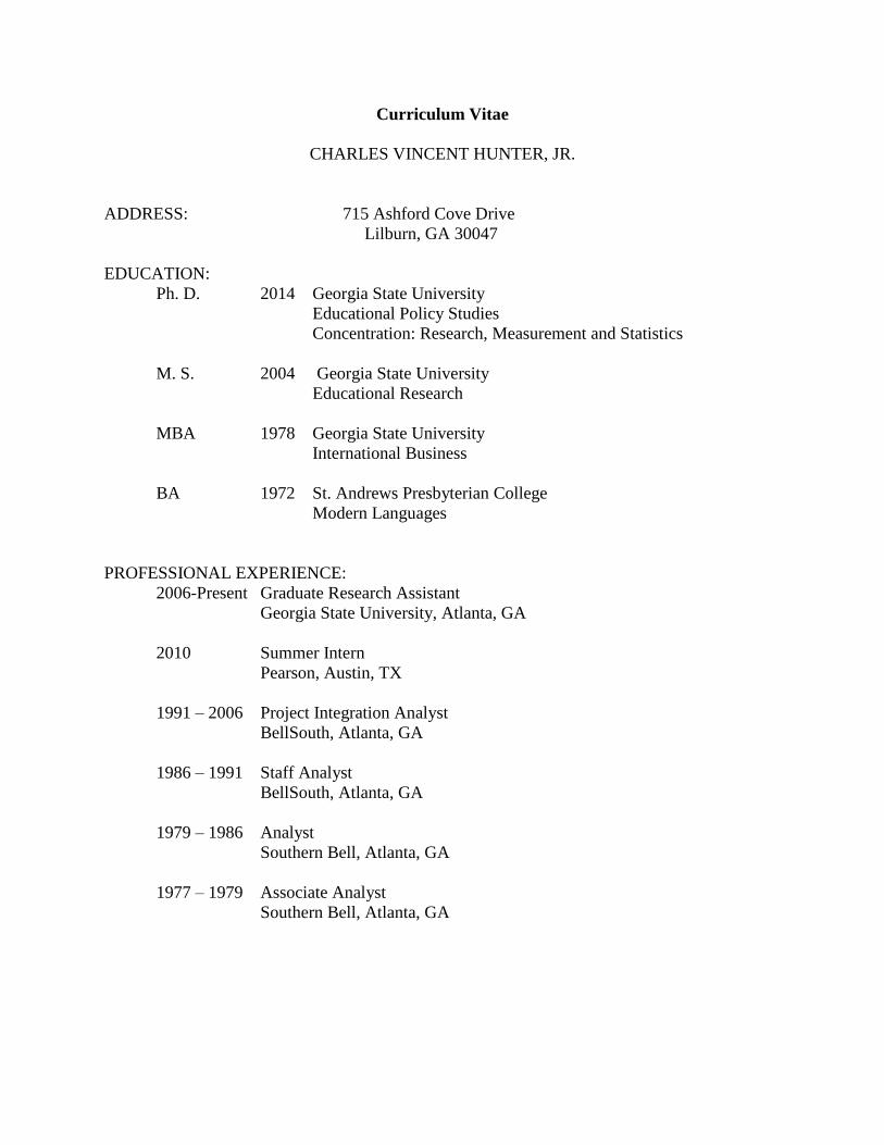
Curriculum Vitae
CHARLES VINCENT HUNTER, JR.
ADDRESS: 715 Ashford Cove Drive
Lilburn, GA 30047
EDUCATION:
Ph. D. 2014 Georgia State University
Educational Policy Studies
Concentration: Research, Measurement and Statistics
M. S. 2004 Georgia State University
Educational Research
MBA 1978 Georgia State University
International Business
BA 1972 St. Andrews Presbyterian College
Modern Languages
PROFESSIONAL EXPERIENCE:
2006-Present Graduate Research Assistant
Georgia State University, Atlanta, GA
2010 Summer Intern
Pearson, Austin, TX
1991 – 2006 Project Integration Analyst
BellSouth, Atlanta, GA
1986 – 1991 Staff Analyst
BellSouth, Atlanta, GA
1979 – 1986 Analyst
Southern Bell, Atlanta, GA
1977 – 1979 Associate Analyst
Southern Bell, Atlanta, GA
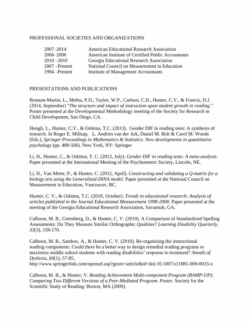
PROFESSIONAL SOCIETIES AND ORGANIZATIONS
2007–2014 American Educational Research Association
2006–2006 American Institute of Certified Public Accountants
2010 –2010 Georgia Educational Research Association
2007 –Present National Council on Measurement in Education
1994 –Present Institute of Management Accountants
PRESENTATIONS AND PUBLICATIONS
Branum-Martin, L., Mehta, P.D., Taylor, W.P., Carlson, C.D., Hunter, C.V., & Francis, D.J.
(2014, September) “The structure and impact of instruction upon student growth in reading.”
Poster presented at the Developmental Methodology meeting of the Society for Research in
Child Development, San Diego, CA.
Hongli, L., Hunter, C.V., & Oshima, T.C. (2013). Gender DIF in reading tests: A synthesis of
research. In Roger E. Millsap, L. Andries van der Ark, Daniel M. Bolt & Carol M. Woods
(Eds.), Springer Proceedings in Mathematics & Statistics: New developments in quantitative
psychology (pp. 489-506). New York, NY: Springer
Li, H., Hunter, C., & Oshima, T. C. (2012, July). Gender DIF in reading tests: A meta-analysis.
Paper presented at the International Meeting of the Psychometric Society, Lincoln, NE.
Li, H., Van Meter, P., & Hunter, C. (2012, April). Constructing and validating a Q-matrix for a
biology test using the Generalized-DINA model. Paper presented at the National Council on
Measurement in Education, Vancouver, BC.
Hunter, C. V., & Oshima, T.C. (2010, October). Trends in educational research: Analysis of
articles published in the Journal Educational Measurement 1998-2008. Paper presented at the
meeting of the Georgia Educational Research Association, Savannah, GA.
Calhoon, M. B., Greenberg, D., & Hunter, C. V. (2010). A Comparison of Standardized Spelling
Assessments: Do They Measure Similar Orthographic Qualities? Learning Disability Quarterly,
33(3), 159-170.
Calhoon, M. B., Sandow, A., & Hunter, C. V. (2010). Re-organizing the instructional
reading components: Could there be a better way to design remedial reading programs to
maximize middle school students with reading disabilities’ response to treatment? Annals of
Dyslexia, 60(1), 57-85.
http://www.springerlink.com/openurl.asp?genre=article&id=doi:10.1007/s11881-009-0033-x
Calhoon, M. B., & Hunter, V. Reading Achievement Multi-component Program (RAMP-UP):
Comparing Two Different Versions of a Peer-Mediated Program. Poster. Society for the
Scientific Study of Reading: Boston, MA (2009).
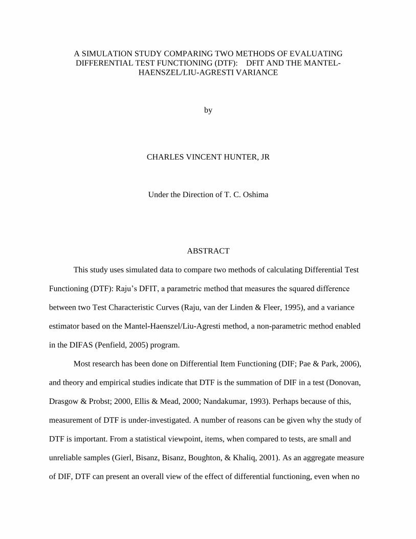
A SIMULATION STUDY COMPARING TWO METHODS OF EVALUATING
DIFFERENTIAL TEST FUNCTIONING (DTF): DFIT AND THE MANTEL-
HAENSZEL/LIU-AGRESTI VARIANCE
by
CHARLES VINCENT HUNTER, JR
Under the Direction of T. C. Oshima
ABSTRACT
This study uses simulated data to compare two methods of calculating Differential Test
Functioning (DTF): Raju’s DFIT, a parametric method that measures the squared difference
between two Test Characteristic Curves (Raju, van der Linden & Fleer, 1995), and a variance
estimator based on the Mantel-Haenszel/Liu-Agresti method, a non-parametric method enabled
in the DIFAS (Penfield, 2005) program.
Most research has been done on Differential Item Functioning (DIF; Pae & Park, 2006),
and theory and empirical studies indicate that DTF is the summation of DIF in a test (Donovan,
Drasgow & Probst; 2000, Ellis & Mead, 2000; Nandakumar, 1993). Perhaps because of this,
measurement of DTF is under-investigated. A number of reasons can be given why the study of
DTF is important. From a statistical viewpoint, items, when compared to tests, are small and
unreliable samples (Gierl, Bisanz, Bisanz, Boughton, & Khaliq, 2001). As an aggregate measure
of DIF, DTF can present an overall view of the effect of differential functioning, even when no
single item exhibits significant DIF (Shealy & Stout, 1993b). Decisions about examinees are
made at the test level, not the item level (Ellis & Raju, 2003; Jones, 2000; Pae & Park, 2006;
Roznowski & Reith, 1999; Zumbo, 2003).
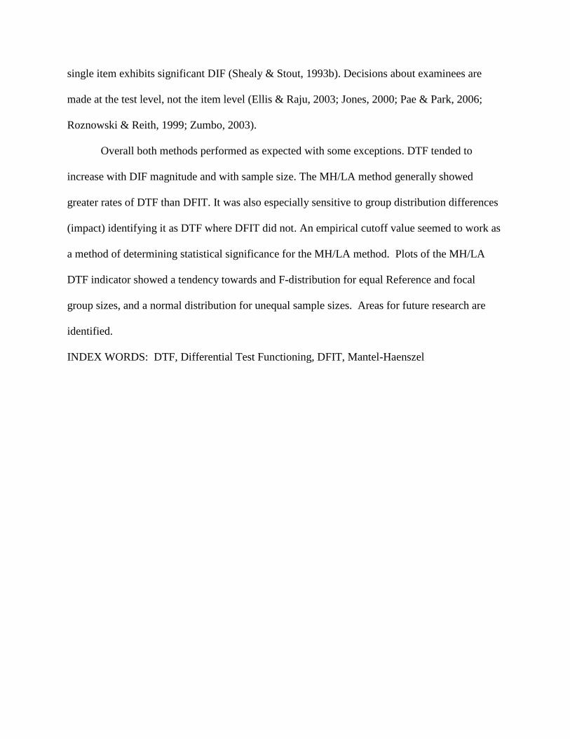
Overall both methods performed as expected with some exceptions. DTF tended to
increase with DIF magnitude and with sample size. The MH/LA method generally showed
greater rates of DTF than DFIT. It was also especially sensitive to group distribution differences
(impact) identifying it as DTF where DFIT did not. An empirical cutoff value seemed to work as
a method of determining statistical significance for the MH/LA method. Plots of the MH/LA
DTF indicator showed a tendency towards and F-distribution for equal Reference and focal
group sizes, and a normal distribution for unequal sample sizes. Areas for future research are
identified.
INDEX WORDS: DTF, Differential Test Functioning, DFIT, Mantel-Haenszel
A SIMULATION STUDY COMPARING TWO METHODS OF EVALUATING
DIFFERENTIAL TEST FUNCTIONING (DTF): DFIT AND THE MANTEL-
HAENSZEL/LIU-AGRESTI VARIANCE
by
Charles Vincent Hunter, Jr.
A Dissertation
Presented in Partial Fulfillment of Requirements for the
Degree of
Doctor of Philosophy
in
Educational Policy Studies
in
the Department of Educational Policy Studies
in
the College of Education
Georgia State University
Atlanta, Georgia
2014

Copyright by
Charles Vincent Hunter, Jr.
2014

DEDICATION
To the memory of my Uncle,
William Joseph Rycroft, Sr.,
Who said to me,
“Vince, you need to get a Ph.D. We need a doctor in the family,
and I finally realized that none of my children are going to do it.”
ii
ACKNOWLEDGEMENTS
To all of my professors and fellow students, too numerous to name, who each in his or
her own special way furthered my education and stimulated my growth as a scholar, Thank You.
Special thanks go to Dr. T.C. Oshima, who, while I was a Master’s student in her
“Educational Statistics I and III” courses, saw in me something which I never had—“You
understand this. You should think about getting the Ph.D.” Her continuing belief in and support
of me has brought me to today.
To Drs. Kentaro Hayashi and Carolyn Furlow for getting me through the Master’s thesis,
and for teaching me to write in my own voice.
To Drs. James Algina, Phill Gagne, Jihye Kim, Alice Nanda, and Keith Wright for the
technical work of sharing coding and of helping me to resolve coding problems
To Dr. Bill Curlette, who keeps opening up new insights into what more that statistics has
to offer.
To Dr. Dennis Thompson, who showed me that human development is a life-long process
that does not end with adolescence, confirming my personal experience.
And, most especially, I thank my wife, Doris, whose unwavering love, support and
commitment, even to the point of giving me up to the books, and who, “when push came to
shove,” started pushing and shoving, has made this possible.

iii
TABLE OF CONTENTS
Page
List of Tables ............................................................................................................................v
List of Figures ...........................................................................................................................vi
List of Abbreviations ..............................................................................................................vii
Chapter
1 INTRODUCTION .........................................................................................1
Background and Research Questions.............................................................2
2 LITERATURE REVIEW ..............................................................................7
Introduction to methods of evaluating Differential Test Functioning
(DTF) .............................................................................................................7
Measurement of differential functioning .......................................................11
Methods of studying DTF ..............................................................................12
Factor analysis ...............................................................................................13
Variance analysis ...........................................................................................16
SIBTEST .......................................................................................................22
DFIT ..............................................................................................................25
Comparative Studies among the Methods ....................................................29
Discussion .....................................................................................................32
3 METHOD ......................................................................................................34
Study Design ..................................................................................................34
Conditions of Study .......................................................................................34
Fixed Factors ..................................................................................................34
iv
Data Generation .............................................................................................34
Replications....................................................................................................38
Test Length ....................................................................................................35
Type of DIF....................................................................................................38
Varied Factors ................................................................................................36
Ability ............................................................................................................36
Percent DIF ....................................................................................................37
Magnitude of DIF ..........................................................................................37
Balanced and Unbalanced DIF ......................................................................37
Sample Size ....................................................................................................38
Data Generation .............................................................................................34
Calibration, Equating and Linking .................................................................41
Evaluation of Results .....................................................................................43
4 RESULTS ......................................................................................................45
5 DISCUSSION ................................................................................................64
References ........................................................................................................................76
Appendices ..........................................................................................................................95
v
LIST OF TABLES
1 2x2 Contingency Table at Level J of 1 – J levels .....................................................18
2 Lord’s (1968) item parameters from the SAT-Verbal test .........................................35
3 Fixed Factors in the Study Design .............................................................................38
4 Varied Factors in the Study Design ..........................................................................39
5 Count of Files that Did Not Converge in BILOG .....................................................50
6 DFIT: Number of Tests with Significant DTF – Null Condition ..............................51
7 DFIT: Number of Tests with Significant DTF – Balanced ........................................54
8 DFIT: Number of Tests with Significant DTF – Unbalanced ...................................55
9 DFIT: Number of Tests with Significant DTF – Impact ...........................................56
10 Counts of Negative τ2 ...............................................................................................57
11 MH/LA: Number of Tests with Significant DTF using Empirical Cutoff–
Null Condition ...........................................................................................................57
12 Empirical Cutoffs for τ2 ............................................................................................58
13 Frequency Counts to Determine Empirical Cutoffs for τ2 : Test Size 20 Sample
Sizes 3000_3000 ........................................................................................................58
14 MH/LA: Number of Tests with Significant DTF using Empirical Cutoff –
Balanced .....................................................................................................................59
15 MH/LA: Number of Tests with Significant DTF using Empirical Cutoff –
Unbalanced ................................................................................................................61
16 MH/LA: Number of Tests with Significant DTF using Empirical Cutoff – Impact .62
vi
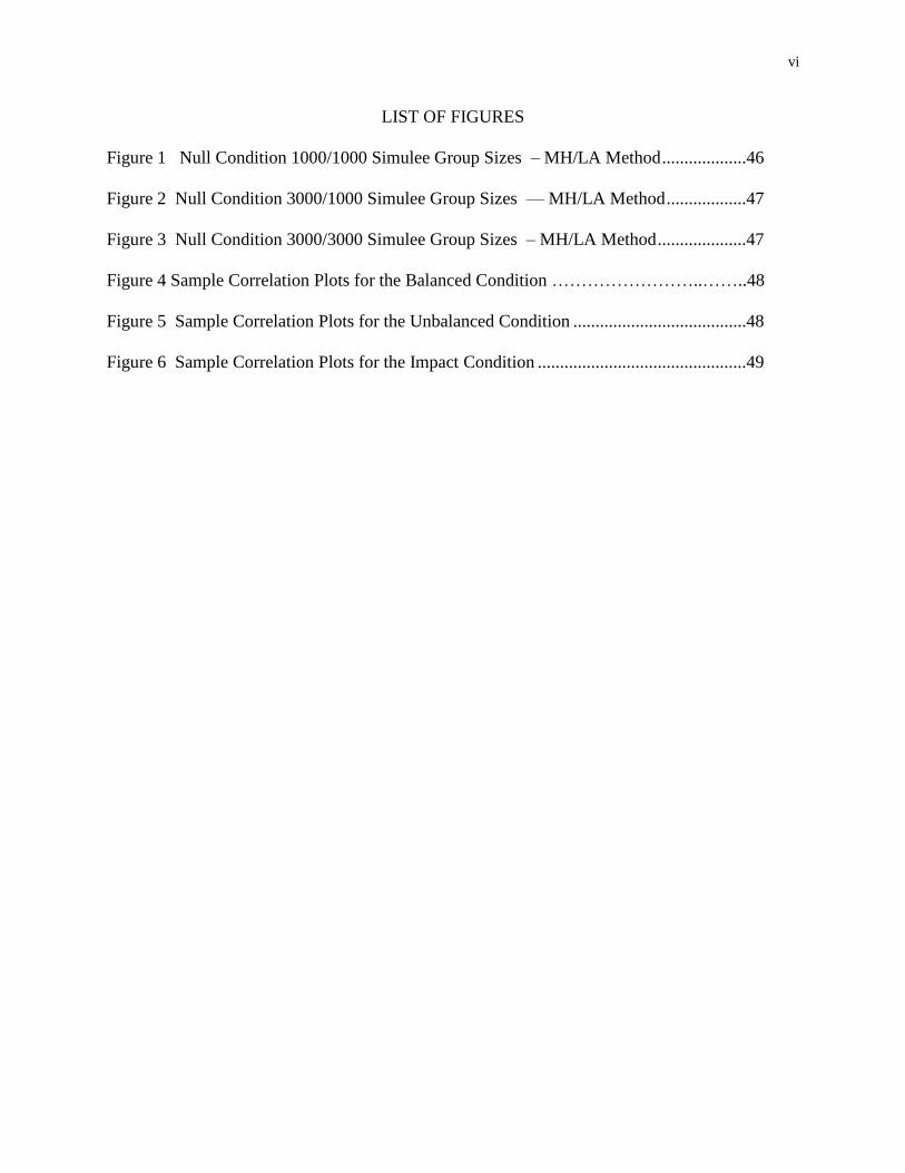
LIST OF FIGURES
Figure 1 Null Condition 1000/1000 Simulee Group Sizes – MH/LA Method ...................46
Figure 2 Null Condition 3000/1000 Simulee Group Sizes –– MH/LA Method ..................47
Figure 3 Null Condition 3000/3000 Simulee Group Sizes – MH/LA Method ....................47
Figure 4 Sample Correlation Plots for the Balanced Condition ……………………..……..48
Figure 5 Sample Correlation Plots for the Unbalanced Condition .......................................48
Figure 6 Sample Correlation Plots for the Impact Condition ...............................................49
vii
List of Abbreviations
1PL One Parameter Logistic Model
2PL Two Parameter Logistic Model
3PL Three Parameter Logistic Model
AERA American Educational Research Association
APA American Psychological Association
CDIF Compensatory Differential Item Functioning
CFA Confirmatory Factor Analysis
CTT Classical Test Theory
DF Differential Functioning
DBF Differential Bundle Functioning
DFIT Differential Functioning of Items and Tests
DIF Differential Item Functioning
DIFAS Differential Item Functioning Analysis System
DTF Differential Test Functioning
EFA Exploratory Factor Analysis
ETS Educational Testing Service
ICC Item Characteristic Curve
IRF Item Response Function
IRT Item Response Theory
LOR Log Odds Ratio
MH Mantel-Haenszel Method
MH/LA Mantel-Haenszel/Liu-Agresti Method
viii
MML Marginal Maximum Likelihood
NCDIF Non-Compensatory Differential Item Functioning
NCME National Council on Measurement in Education
OCI Observed Conditional Invariance
REM Random Effects Model
RMSEA Root Mean Squared Error of Approximation
RMWSD Root Mean Weighted Squared Difference
SE Standard Error of Measurement
SIBTEST Simultaneous Item Bias Test
UCI Unobserved Conditional Invariance
1
CHAPTER 1
INTRODUCTION
Ensuring that tests are valid for their intended purposes is a major concern of
measurement theory. Modern measurement theory developed as a response to social concerns
about the fairness of tests and their application (Rudner, Getson, & Knight, 1980) in areas of
employment (Drasgow, 1987) and education, but it is equally necessary in the areas of
psychological and medical assessment (Cameron, Crawford, Lawton, & Reid, 2013; Van den
Broeck, Bastiaansen, Rossi, Dierckx, & De Clercq, 2013).
While modern measurement (Item Response Theory) focuses on the individual test item
as the unit of study, decisions about individual persons are made based on test level data (Wang
& Russell, 2005; Ellis & Raju, 2003; Jones, 2000; Pae & Park, 2006; Roznowski & Reith, 1999;
Russell, 2005). Test functioning may be conceived of as the aggregate of item functioning
(Rudner, Getson, & Knight, 1980; Shealy & Stout, 1993a). Therefore, studying Differential Test
Functioning (DTF) to determine how best to control test validity is both appropriate and
worthwhile. Using simulated data, this present study compares two methods of calculating DTF:
DFIT by (Raju, van der Linden and Fleer, 1995), and the Mantel-Haenszel/Liu Agresti Variance
method (Penfield & Algina, 2006) with the purposes of understanding better how each functions,
and how they relate to each other.
2
Background and Research Questions
The modern study of measurement grew out of the science of psychology that began in
the 1880’s. To defend their work from critics in the physical sciences and philosophy,
psychologists began to quantify their findings. As psychology enlarged its scope from physical to
mental phenomena, the need arose to measure what could not be directly observed. The
unobservable mental phenomena (generically called constructs) were measured by observable
behaviors that were theorized to express them. For example, knowledge of mathematics is
observed by performance on a mathematics test (Crocker & Algina, 1986).
Measurement theory is concerned with the quantification of observable behaviors that
express the existence of non-observable mental skills and conditions. An integral part of
measuring behaviors is the degree to which measurements are done correctly and with precision.
An imperfect measurement produces measurement error that must be taken into account when
performing statistical analyses. This is done in Classical Test Theory (CTT) with the definition
of a measurement as the sum of the true score plus measurement error (Crocker & Algina, 1986):
𝑋 = 𝑇 + 𝐸
Beyond this, Crocker and Algina (1986) also discuss issues of reliability and validity.
Reliability is defined as the production of consistent scores by a test from one administration to
another. That is, test administrators (teachers, researchers) will get similar results from a test
when it is administered to similar groups of examinees under similar conditions. Measurement
error negatively affects test reliability. Error may be divided into random error and systematic
error. Random error is sporadic and varies from one test administration to the next. It may be
caused by such things as ambient temperature or lighting. Systematic error is consistent by
examinee (or group of examinees) among all test administrations. It may be caused by such
3
things as hearing impairment or personality traits. Systematic error that occurs over a
demographic group may be related to test validity and issues of differential functioning (DF) and
multidimensionality (see also Camilli, 1993). Kunnan (1990) states that tests with large numbers
of DF items are potentially unreliable, meaning that the tests also would be invalid for all
examinees.
Validity deals with the appropriateness of a test for evaluating an examinee for a given
purpose. It is generally studied as content validity, criterion validity, and construct validity.
Content validity relates to a test’s being an adequate representation of a given area of knowledge.
Criterion validity relates to using a test to measure performance where a direct measurement of
performance is not easily available. These tests are often used in a selection process as
predictors of expected performance, such as in college or on a job. Construct validity relates to
measuring unobservable or intangible things generally dealt with in psychology and education,
such as intelligence and personality traits. Messick (1995) asserts that validity needs to be
understood as pertaining to the meaning of test scores, not to the test itself. Overall it is an
evaluation of how appropriate decisions based on test scores are.
A fourth aspect of validity, fairness, rose to prominence beginning in the 1960’s. Fairness
is a cluster of concepts, not strictly related, that center around the relation between tests and test
takers. Four of the main uses of the term fairness are a lack of statistical bias, a test process that
is equitable for all examinees, similar outcomes for all demographic groups of examinees, and an
opportunity to learn the material of the test by all examinees (AERA, APA, & NCME, 1999).
The perception that all groups should have similar results on tests was an early driver of the
focus on fairness. Drasgow (1987) discusses two of these cases relating to standardized tests
from the 1980’s. In both cases, the parties settled on future tests having minimal (proportions of
4
.05 to .15) differences in pass rates between different demographic groups. While this is a
politically acceptable resolution, it is not defensible scientifically, because it confounds
Differential Functioning (DF) with Impact.
Impact is the group difference on the construct being measured where the difference is
relevant to the testing purpose (Clauser & Mazor, 1998; Drasgow, 1987; Millsap & Everson,
1993). DF is the currently preferred term for statistical bias, because of the popular
understanding of bias as prejudicial intent against groups of people. DF occurs when test items
consistently produce different results for different demographic groups which are not related to
the purpose of the test.
CTT had difficulty dealing with these problems. The principal difficulty of CTT is that
test characteristics and examinees characteristics are confounded. They can only be interpreted
jointly: this set of examinees with this set of test questions. If either set is changed, then the
interpretation changes. This makes it difficult to compare different versions of a test, and to
predict how any examinee will perform on a given test. As a way out of this difficulty, Item
Response Theory (IRT) became the dominant measurement theory. IRT provides the theoretical
basis for item and examinee-level measurement vs. test and group-level measurement. Said
differently, under the assumptions of IRT, the probability that any given examinee will answer
correctly any given question can be estimated, but the assumptions of CTT allow only estimating
the probability of the proportion of correct answers on a test from a given group of examinees.
Thus, under IRT, item traits are independent of the test takers, and examinee scores can be
described independently of the set of test items (Bock, 1997; Hambleton, Swaminathan &
Rogers, 1990).
5
In contrast to Classical Test Theory which focuses on the test as a whole, IRT takes the
individual test question, or item, as its basic unit of study. It is this focus on the item that enables
practitioners to measure the difficulty, and other characteristics, of individual items. Thus, it
becomes possible to describe examinees by the difficulty of the questions that they can
successfully answer. Bock (1997) points out that this description is most appropriately called
“proficiency” in educational settings, although the literature generally refers to it as ability.
Items, however, are generally not used in isolation. They are compiled into groups
measuring constructs of interest. These groups may be divided into sub-tests and tests. There are
two kinds of sub-test groupings. Testlets are groups of test items grouped contiguously and
associated with a common probe, often a reading passage. Bundles are groups of items that have
a common organizing theme, but do not necessarily appear together or refer to a common probe
(McCarty, Oshima, & Raju, 2007). Items and DF can be studied both in isolation, and at all
levels of aggregation. This study focuses on the entire test, and different methods of measuring
DTF.
When looking at DF at the test level, both the distribution of DF over the items, and the
summative nature of DF must be considered. The distribution of DF over the items derives from
the fact that each item is measured for DIF separately. Because of this, tests may exist where all
DIF favors the same group of examinees. However, it is also possible that some items may show
DIF favoring one group of examinees, while other items show DIF favoring other groups of
examinees. DIF that systematically favors a single group of examinees is called “unbalanced” or
unidirectional DIF, whereas, DIF that does not systematically favor either group is called
“balanced” or bidirectional DIF (Gierl, Gotzman, & Boughton, 2004; Oshima, Raju, & Flowers,
1997). The summative nature of DF is expressed in the concepts of amplification and
6
cancellation (Nandakumar, 1993). Amplification refers to the fact that multiple items each
exhibiting non-significant DIF, may, when aggregated at the test level, exhibit significant DF.
Cancellation is the opposite of amplification. Significant DIF may exist in different items
favoring different demographic groups, but, when aggregated at the test level, DF is not
detectable because the DF favoring one group offset that favoring the other group. Obviously,
balanced DIF would emphasize cancelation effects, while unbalanced DIF would emphasize
amplification effects.
This study looks at two methods of assessing DTF under conditions of impact, and
differential functioning. Under differential functioning, it looks at cancellation and amplification
effects on DTF under balanced and unbalanced DIF. The two methods of assessing DTF are
Differential Functioning of Items and Tests (DFIT; Raju, van der Linden, and Fleer [1995]), and
the Mantel-Haenszel/Liu-Agresti variance method as implemented in DIFAS (Penfield, 2007).
The methods are explained in the literature review.
7
CHAPTER 2
LITERATURE REVIEW
Introduction to methods of evaluating Differential Test Functioning (DTF)
Measuring performance, both past and potential, is a fact of contemporary life. From the
beginning of a child’s formal schooling through the end of a person’s work career, measurement
is an on-going process. Modern measurement theory has developed, as a response to social
concerns about the fairness of the testing instruments used, and their application (Rudner,
Getson, & Knight, 1980), and to legal and ethical imperatives to avoid bias (Gierl, Bisanz,
Bisanz, Boughton, & Khaliq, 2001). Unfair tests, that is, tests that inhibit a person’s rights and
opportunities, are, in the words of Cronbach (1988), “inherently disputable” (p. 6). They suffer
not only the weakness of social disapprobation, but are also weak in scientific validity (Millsap
& Everson, 1993; Rudner, et al.). The current consensus on standards for fairness is published in
the Standards for Educational and Psychological Testing of the American Educational Research
Association, American Psychological Association, and National Council on Measurement in
Education (AERA, APA, & NCME, 1999). In the context of measurement, the standard of bias-
free tests requires special attention.
Bias can be defined as measurement inaccuracy that occurs systematically in a test
(Millsap & Everson, 1993). More precisely, bias is a different probability of attaining a correct
answer by members of one group than by members of another group, where the reasons for this
8
difference are unexpected and unrelated to the purpose of the test (Clauser & Mazor, 1998; Raju
& Ellis, 2003). Mathematically this may be expressed in the dichotomous answer model as
Pi(+|θs, Ga) ≠ Pi(+|θs, Gb) (1)
where Pi is the probability of an answer for item i, + is a correct answer, θs is the ability level for
examinee s, and Gx are the different groups (Raju & Ellis).
Groups may, however, have different probabilities of attaining a correct score for reasons
that are relevant to test purposes. A lack of bias, then, does not mean that different groups will
have equal scores. Group differences where bias does not exist are referred to as impact (Clauser
& Mazor, 1998; Ellis & Raju, 2003; Millsap & Everson, 1993). Shealy and Stout (1993a) specify
that impact occurs from different distributions of the ability trait among the different groups.
Because of this contrast between impact and bias, the preferred terminology for group
differences in testing is differential functioning (DF; Hambleton, et al., 1991; Holland & Thayer,
1988).
Millsap and Everson (1993) state that the presence of DF indicates an incomplete
understanding of the latent construct that the test is measuring. That is, after different groups
have been matched on the ability that the test purports to measure, differences between group
performances depend on another, unidentified ability. DF thus indicates the presence of multi-
dimensionality in the test instrument (Gierl, et al., 2004; Shealy & Stout, 1993b). That is, the
item is measuring more than one construct or dimension. Zhou, Gierl, and Tan (2006) define
dimension as any trait that can affect the probability of a correct answer for a test item.
Where the test purpose is to measure a single primary dimension, the other dimensions
are nuisance traits (Clauser & Mazor, 1998; Shealy & Stout, 1993b). However, Oshima and
Miller (1992) point out that by itself multidimensionality does not produce DF. Where in the
9
distributions of the nuisance traits are the same among the various group, DF does not occur.
Also, intentional multidimensionality that is not identified before analysis can be misidentified as
DF (Zhou, et al., 2006).
Where DF does exist, researchers have different approaches towards resolving the
differential functioning. Some make the assumption that identifying and removing items that
exhibit DF will reduce or eliminate DF at the test level (Raju & Ellis, 2003). Other researchers
hold that it is incumbent upon the test developer/researcher to evaluate the studied item and
determine whether the differences measure something relevant to the test purpose or irrelevant to
it, because removal of items, without first doing this evaluation, does not automatically create a
fair test, or ensure the test’s appropriate use, and runs the risk of letting the statistics drive the
analysis (Clauser & Mazor, 1998; Rudner, et al., 1980; Gierl, et al., 2001). From a similar
viewpoint, still other researchers hold that removing DF items may make for a weaker test,
because the variance that produces DIF is likely to come from a variety of sources, and removing
DF items may make that variance stronger in relation to the variance of the studied construct,
leading to an overall weaker test (Roznowski & Reith, 1999).
Differential functioning exists at two levels: the individual item level and the aggregate
(test or bundle) level (Rudner, et al., 1980). Item level DF is referred to as differential item
functioning (DIF), and test level DF is referred to as differential test functioning (DTF). Item and
test level DF seem to be related, with DTF being the sum of DIF. Raju and colleagues (1995)
conceptualize DIF as Compensatory DIF, which sums to DTF, and Non-Compensatory DIF,
which does not sum. As a sum, DIF that favors different groups in different items may offset at
the test level. This is called cancellation (Flora, Curran, Hussong, & Edwards, 2008;
Nandakumar, 1993; Rudner, et al., 1980; Takala, & Kaftandjieva, 2000). Nandakumar points out
10
that, conversely, multiple items with small DIF favoring the same group can add up to significant
DTF, a process called amplification. Research using confirmatory factor analysis gives
inconsistent evidence of DIF at the test level. Pae and Park (2006) indicate that DIF may be
carried to the test level (so if DIF exists, assume that DTF exists), because DIF does not cancel at
the test level.1 Zumbo (2003), who also used factor analysis, indicates that cancelled DIF does
not appear at the test (scale) level.
Most research to date has been done on DIF (Pae & Park, 2006), and theory and
empirical studies indicate that DTF is the summation of DIF in a test. Perhaps because of this,
measurement of DTF is under-investigated. However, a number of reasons can be given why the
study of DTF is important. From a statistical viewpoint, items, when compared to tests, are small
and unreliable samples (Gierl, et al., 2001). Because DTF is an aggregate measure of DIF, DTF
can present an overall view of the effect of differential functioning, even when no single item
exhibits significant DF (Shealy & Stout, 1993a). Where a test is stratified using a variable (such
as the total score) that is internal to the test, DIF in one item can affect the estimate of DIF in
other items in the same stratification. In this case, DTF can give an index of the potential effect
of the stratifying variable on DF (Penfield & Algina, 2006). From a non-statistical, yet eminently
practical viewpoint, decisions about examinees (e.g., school or job promotion, professional
certification) are made at the test level, not the item level (Ellis & Raju, 2003; Jones, 2000; Pae
& Park, 2006; Roznowski & Reith, 1999; Russell, 2005), therefore studying DTF to determine
how best to control test validity is both appropriate and worthwhile. Also, because of the expense
and time required for creating test items, being able to use already created items saves time, and
financial and human resources (Bergson, Gershon, & Brown, 1993; Bolt & Stout, 1996).
1 Pae and Park (2006) bring out an important point. Balanced DIF does not “remove” DIF. It only masks it at the test level (DTF). If items exhibiting DIF are removed carelessly, then the entire test can exhibit DTF, and no longer be considered “fair” overall.
11
Therefore, studying DTF to determine how best to control test validity is both appropriate and
worthwhile.
Related to this is the predictive value of a test. That is, differential functioning is related
to the psychometric properties of a test, but using a test to select persons for a position based on
the results of the test is qualitatively different in that it seeks to determine how well a person will
perform in the future based on the results of the test. Whereas DF analysis may detect
statistically significant differences between groups (caused, in part by the large sample sizes used
in IRT analysis), the practical importance of these differences is often nil. To use DTF in the
prediction process requires the use of an effect size (Stark, Chernyshenko, & Drasgow, 2004).
Measurement of differential functioning. The analysis of differential functioning is a part
of the larger task of assessing the reliability and validity of test scores. The researcher must,
therefore, keep in mind the purpose of the test and choose the method of analysis that is best
suited to the data while accomplishing the intended purpose, keeping in mind that all analysis
techniques have problems and limitations as well as strengths (Clauser & Mazor, 1998;
Roznowski & Reith, 1999; Rudner, et al., 1980).
While much work currently is being done on test items that are intentionally
multidimensional (Ackerman, 1996; Ackerman, Gierl, & Walker, 2003; Oshima, et al., 1997;
Yao & Schwarz, 2006), traditionally tests and items are considered unidimensional. They
measure only one construct. In practice, this is seldom, if ever, achieved. Differential functioning
then becomes, not a quality that exists or does not exist, but a quality that exists in different
degrees in different items. The amount of differential functioning detected may vary with the
analysis used (Rudner, et al., 1980). An example of this would be trying to detect non-uniform
DIF with the Mantel-Haenszel (MH) technique, which is not sensitive to non-uniform DIF
12
(Millsap & Everson, 1993; Raju & Ellis, 2003), as opposed to the two-parameter logistic
regression model, which was developed to detect non-uniform DIF (Hambleton, et al., 1991).
Differential functioning detection and analysis methods work with multiple groups of
examinees: a base group (in bias studies usually the group suspected of benefiting from bias, or
in standardization studies, the group with more stable scores), also called the reference group;
and one or more study groups, also called focal groups (Dorans & Kulick, 1986). Differential
functioning is measured with two broad classes of statistics: parametric and non-parametric.
Millsap & Everson (1993) refer to them respectively as unobserved conditional invariance (UCI)
and observed conditional invariance (OCI) based on their use of an unobserved logical construct
to segregate examinees into ability groups, or an observed construct, such as raw test score. IRT
methods of DF measurement fall in the UCI group because they work by using an unobserved
ability parameter derived for each of the test groups to measure DF. Some methods, such as
SIBTEST, use elements from both of these two general groups: an observed Z-score like the
non-parametric methods, and adjusting group means before comparing them like the parametric
methods (Millsap & Everson). Wainer (1993), who uses a different classification system, points
out that classification schema are somewhat arbitrary. For example, the Mantel-Haenszel non-
parametric model is closely related to the Rasch (a special case of the one-parameter logistic
model; Takala & Kaftandjieva, 2000; Weeks, 2010) model, and the standardization model is
conceptually similar to models that compare item response functions (Shealy & Stout, 1993b).
Methods of studying DTF
One is tempted to look for the “best” method to detect DF that will function well in all
situations. Such a method does not exist. Rather, each method has its own shortcomings and
advantages (Anastasi & Urbina, 1997). For example, analysis using the Rasch or the Mantel-
13
Haenszel methods cannot detect crossing DF, but these methods can be used effectively on
smaller sample sizes than are required by IRT methods. IRT methods can detect crossing DF but
generally need large sample sizes to function well (Ferne & Rupp, 2007; Lai, Teresi, & Gershon,
2005).
Three principal approaches to studying DF have been developed. These are factor
analysis, methods based on CTT using traditional statistical methods, and methods based on IRT
(Magis & Facon, 2012). The first two approaches are generally non-parametric methods that are
not based on IRT, whereas IRT methods generally require the calculation of parameters to
estimate the various characteristics (such as difficulty and discrimination) of the items
(Hambleton, Swaminathan, & Rogers, 1991). The Mantel-Haenszel method is an example of a
traditional statistical method, and DFIT, which requires the calculation of item parameters, is an
IRT method. SIBTEST (Shealy & Stout, 1993a) is a bridge between CTT and IRT in that it uses
traditional non-parametric statistical mathematics with an IRT approach to analysis.
Factor analysis is generally performed using one of the standard programs (e.g., LISREL,
Jöreskog & Sörbom, 1993) that analyze covariance matrices. Variance analysis has been
operationalized by Penfield (2005, 2007) using an estimator based on the Mantel-Haenszel/ Liu-
Agresti (MH/LA) method, and published in the DIFAS program. SIBTEST (Shealy & Stout,
1993a) is both a method and a computer program that produces a standardized measure of
differential functioning. DFIT (Raju, et al., 1995) is both a method and a computer program that
measures the squared difference between two Test Characteristic Curves.
Factor analysis. In a measurement context, factor analysis is performed at the test level
rather than at the item level that then is summed to the test level (Pae & Park, 2006; Zumbo,
2003). Factor analysis takes the data of the groups (whether persons or tests) to be compared,
14
and, based on the factors used, evaluates how close the factor matrices are between the groups.
As an example, one assumes that gender and ethnicity are related to test results. A confirmatory
factor analysis would evaluate how closely these two variables are associated with the level of
test scores. Zumbo used factor analysis in the context of comparing two different versions of the
same test, an example of measurement equivalence; that is, whether a test has the same meaning
for different groups. Measurement equivalence (DTF) is measured as the differences between the
correlation matrices of the different groups being examined.
Factor analysis works by taking a group of observed variables (say, the items on a test
and tries to relate them to a smaller set of “unobserved” variables (latent or explanatory factors;
say the gender and ethnicity of the test takers) that can explain the variations in correlations
among the observed variables. There are two main types of factor analysis: Exploratory Factor
Analysis (EFA), and Confirmatory Factor Analysis (CFA; Lance & Vandenberg, 2002). If the
factors need to be identified, then an Exploratory Factor Analysis may be used to identify a set of
factors for later confirmation (Zumbo, 2003). However, if a set of explanatory factors associated
with measurement outcomes has already been identified before hand, then Confirmatory Factor
Analysis is used to evaluate how closely that set of factors match outcomes (Jöreskog & Sörbom,
1993). There are two major differences between EFA and CFA that come from their different
purposes. In EFA with its focus on finding relationships, correlations between all observed and
latent variables are calculated, and model fit is not a big concern. In CFA, which is trying to
verify propositions, only observed and latent variables that are hypothesized to have a
relationship are allowed to co-vary, and model-data fit is of great importance (Lance &
Vandenberg). CFA is the principal method used in DTF analysis.
15
The explanation that the factors give is determined by partialing out the correlations
among the observed variables. Jöreskog and Sörbom (1993) describe this process using the
following model.
𝑥𝑖 = 𝜆𝑖1𝜉1 + … + 𝜆𝑖𝑛𝜉𝑛 + 𝛿𝑖 (2)
where 𝑥𝑖 is the ith observed variable, 𝜉𝑛 is the nth factor, 𝜆𝑖𝑛 is the factor loading of observed
variable i onto factor 𝜉𝑛, and 𝛿𝑖 represents factors unique to 𝑥𝑖. Two items need more
explanation.
If 𝑥𝑖 does not depend on 𝜉𝑛, then 𝜆𝑖𝑛 = 0. The unique part, 𝛿𝑖, of the observed variable
has two pieces: a factor specific to that variable, and error measurement, which are confounded
in most designs (Jöreskog & Sörbom, 1993; Lance & Vandenberg, 2002). That is, Factor
Analysis looks for invariance (also called measurement equivalence) in the factors, with the tests
for this being model fit (e.g., the Root Mean Squared Error of Approximation, RMSEA) and 𝜒2
tests of invariance on factor loadings, and variance and covariance matrices (Pae & Park, 2006).
Two major model fit indices identified by Lance and Vandenberg are the least squares difference
𝐹𝐿𝑆 = 𝑡𝑟[𝑆 − Σ̂(Θ)2] (3)
where tr is the trace of a matrix, and the function minimizes the squared differences (S) between
the sample data and the covariance matrices (Σ̂(Θ)2); and the maximum likelihood function
𝐹𝑀𝐿 = 𝑙𝑛|Σ̂(Θ)| + 𝑡𝑟[𝑆Σ̂(Θ)−1] − 𝑙𝑛|𝑆| − 𝑝 (4)
where ln|A| is the base e log of matrix A, p is the number of observed variables, and the function
minimizes differences between variances between the sample (S) and covariance (Σ̂(Θ)) matrices
(Lance & Vandenberg, 2002).
A concern in using factor analysis is the determination of model fit. Most goodness of fit
indices have a Chi-square distribution. The common maximum likelihood fit function is
16
distributed as Chi-square only for large sample sizes. Because Chi-square is greatly influenced
by sample size, even trivial differences are likely to appear as significant. CFA is also very
dependent on model specification. The researcher must understand the theory driving the model
in order to specify it well (Lance & Vandenberg, 2002).
Variance Analysis. The analysis of the variance of DF was sparked by an observation of
Rubin (1988) that, even though DTF were small, there could be wide variability among the
various DIF indices for the various items. He suggested that this variability be measured.
Following this, Longford, Holland, & Thayer (1993) developed an iterative non-parametric
measure of DTF. Camilli and Penfield (1997), on this basis, developed a variance estimator of
global unsigned DTF. They took the log odds ratio (LOR), as an index of differential
functioning, and its standard error from the Mantel-Haenszel statistic (Holland & Thayer, 1988;
Mantel & Haenszel, 1959) to develop a non-iterative, non-parametric measure of DTF for
dichotomous items. This was generalized to the polytomous, and mixed dichotomous-
polytomous cases by Penfield and Algina (2006) using the Liu-Agresti generalization of the
Mantel-Haenszel statistic. Following Camilli and Penfield’s (1997) format, I briefly discuss the
Logistic IRT model, the Mantel-Haenszel procedure, Longford, et al.’s procedure, and then
Camilli and Penfield’s procedure, before I discuss Penfield and Algina’s generalization.
The three parameter logistic (3PL) model for DIF expresses the probability of a correct
response as
𝑃𝐺𝑖(1|𝜃) = 𝑐𝑖 + (1 − 𝑐𝑖)exp(𝐷𝑎𝑖(𝜃−𝑏𝑖))
1+ exp(𝐷𝑎𝑖(𝜃−𝑏𝑖)) (5)
where the left hand side of the equation, ≡ PG , is the probability of a member of group G, who
has an ability level θ, providing a correct answer to item i. On the right hand side of the equation
ci is the guessing parameter for item i, ai is the discrimination (used to separate examinees into
17
ability groups) parameter for item i, bi is the difficulty (the point where half of the examinees
answer the item incorrectly and half answer it correctly, i.e., the mean) parameter for item i, and
D is a scaling factor, generally set to 1.7 to make the logistic Item Characteristic Curve (ICC)
approximate the normal ICC (Hambleton, et al., 1991; Raju, 1988).
This formula may be expanded to show the presence of DIF as a shift in the ICC
𝑃𝐺𝑖(1|𝜃) = 𝑐𝑖 + (1 − 𝑐𝑖)exp(𝐷𝑎𝑖(𝜃−𝑏𝑖)+ 𝐺𝜉𝑖)
1+ exp(𝐷𝑎(𝜃−𝑏)+ 𝐺𝜉𝑖) (6)
In this model G is an indicator of group membership (0 for the focal group, 1 for the reference
group), and 𝜉𝑖 is the amount of DIF for item i. When 𝜉𝑖 is positive, DIF is against the focal
group; negative, against the reference group; and zero indicates no DIF (Camilli & Penfield,
1997; Penfield & Algina, 2006). The other symbols are as defined for equation (5).
Gξi may be indexed by the log-odds ratio (LOR). Thus, for a 1PL model (where the c
parameter = 0, and the a parameters (discrimination) are the same for both groups), for a given
ability level
𝐿𝑂𝑅 = 𝜆(𝜃) = 𝑙𝑛 [𝑃𝑅(𝜃)/𝑄𝑅(𝜃)
𝑃𝐹(𝜃)/𝑄𝐹(𝜃)] (7)
Where θ is the ability level, P is the probability of a correct response, Q is the probability of an
incorrect response, R is the reference group, and F is the focal group (Camilli & Penfield, 1997).
This leads to a digression on the Mantel-Haenszel LOR, which is the basis for Camilli and
Penfield’s model.
Mantel and Haenszel (1959) developed a model of relative risk given certain risk factors.
Using a non-iterative 2x2 contingency table (see Table 1), they show that the expected value of
any cell in the table can be tested as a χ2 with one degree of freedom, calculated as the ratio of a
squared deviation from the expected value of the cell to its variance, where the variance is
defined as the marginal totals divided by the squared total times the total minus one
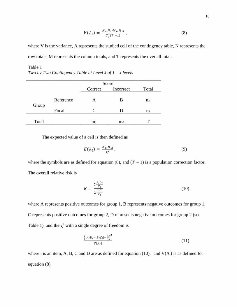
18
𝑉(𝐴𝑖) = 𝑁1𝑖𝑁2𝑖𝑀1𝑖𝑀2𝑖
𝑇𝑖2(𝑇𝑖−1)
, (8)
where V is the variance, A represents the studied cell of the contingency table, N represents the
row totals, M represents the column totals, and T represents the over all total.
Table 1
Two by Two Contingency Table at Level J of 1 – J levels
Score
Correct Incorrect Total
Group
Reference A B nR
Focal C D nF
Total m1 m0 T
The expected value of a cell is then defined as
𝐸(𝐴𝑖) = 𝑁1𝑖𝑀1𝑖
𝑇𝑖2 , (9)
where the symbols are as defined for equation (8), and (Ti – 1) is a population correction factor.
The overall relative risk is
𝑅 = ∑
𝐴𝑖𝐷𝑖𝑇𝑖
∑𝐵𝑖𝐶𝑖
𝑇𝑖
(10)
where A represents positive outcomes for group 1, B represents negative outcomes for group 1,
C represents positive outcomes for group 2, D represents negative outcomes for group 2 (see
Table 1), and the χ2 with a single degree of freedom is
(|𝐴𝑖𝐷𝑖− 𝐵𝑖𝐶𝑖|−
1
2)
2
𝑉(𝐴𝑖) (11)
where i is an item, A, B, C and D are as defined for equation (10), and V(Ai) is as defined for
equation (8).

19
Holland and Thayer (1988) generalize the Mantel-Haenszel χ2 procedure to education,
substituting ability level for risk factor, highlighting that the table works at k levels of the ability
level, and noting that the overall significance test proposed by Mantel and Haenszel (1959) is a
common odds ratio that exists on a scale of 0 to ∞ with 1 being the null hypothesis of no DIF.
They describe the odds ratio as
�̂�𝑀𝐻 = ∑
𝐴𝑗𝐷𝑗
𝑇𝑗
∑𝐵𝑗𝐶𝑗
𝑇𝑗
(12)
which is the same as Mantel and Haenszel’s risk ratio. They define this ratio as the average odds
that a member of the reference group has an equal score to a member of the focal group at the
same level of ability.
Camilli and Penfield (1997) emphasize that each test item exists at 1, . . . , J levels of
ability. They re-write the formula to explicitly indicate the levels, and clarify that cells A and B
represent the probability of correct responses (P), and C and D represent the probability of
incorrect responses (Q). Thus for score level j, the odds ratio is
𝑎𝑗 = 𝑃𝑅𝑗/𝑄𝑅𝑗
𝑃𝐹𝑗/𝑄𝐹𝑗=
𝑃𝑅𝑗𝑄𝐹𝑗
𝑃𝐹𝑗𝑄𝑅𝑗 (13)
Using the Mantel-Haenszel statistic as presented by Holland and Thayer (1988; equation [12])
the Mantel-Haenszel log odds ratio is
�̂� = 𝑙𝑛(�̂�𝑀𝐻) (14)
Longford, et al. (1993) developed a measure of global DTF based on the Mantel-Haenszel log
odds ratio as a random effects model:
−2.35�̂� = 𝑦𝑖𝑘 = 𝜇 + 𝜉𝑖 + 휀𝑖𝑘 (15)
where -2.35 is a scaling factor to make the Mantel-Haenszel statistic equal the Educational
Testing Service (ETS) difficulty (delta) scale; i is item 1, . . . , I, and k is test administration 1, . .
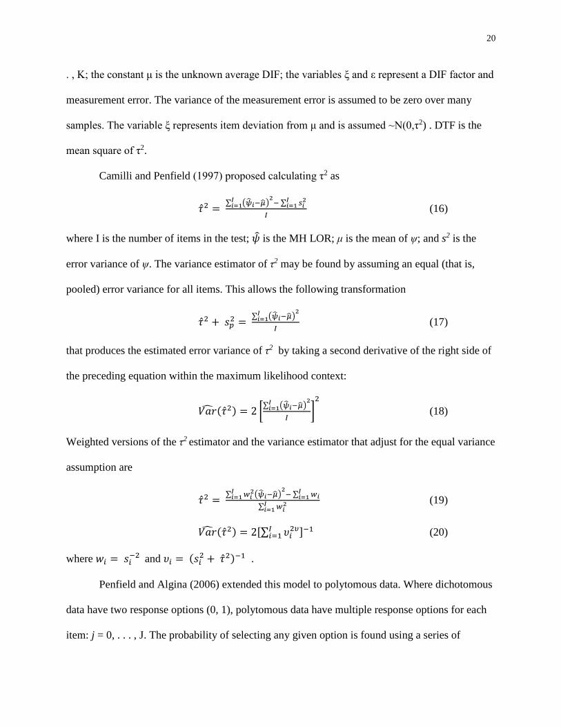
20
. , K; the constant μ is the unknown average DIF; the variables ξ and ε represent a DIF factor and
measurement error. The variance of the measurement error is assumed to be zero over many
samples. The variable ξ represents item deviation from μ and is assumed ~N(0,τ2) . DTF is the
mean square of τ2.
Camilli and Penfield (1997) proposed calculating τ2 as
�̂�2 = ∑ (�̂�𝑖−�̂�)
2𝐼𝑖=1 − ∑ 𝑠𝑖
2𝐼𝑖=1
𝐼 (16)
where I is the number of items in the test; �̂� is the MH LOR; μ is the mean of ψ; and s2 is the
error variance of ψ. The variance estimator of τ2 may be found by assuming an equal (that is,
pooled) error variance for all items. This allows the following transformation
�̂�2 + 𝑠𝑝2 =
∑ (�̂�𝑖−�̂�)2𝐼
𝑖=1
𝐼 (17)
that produces the estimated error variance of τ2 by taking a second derivative of the right side of
the preceding equation within the maximum likelihood context:
𝑉𝑎�̂�(�̂�2) = 2 [∑ (�̂�𝑖−�̂�)
2𝐼𝑖=1
𝐼]
2
(18)
Weighted versions of the τ2 estimator and the variance estimator that adjust for the equal variance
assumption are
�̂�2 = ∑ 𝑤𝑖
2(�̂�𝑖−�̂�)2𝐼
𝑖=1 − ∑ 𝑤𝑖𝐼𝑖=1
∑ 𝑤𝑖2𝐼
𝑖=1
(19)
𝑉𝑎�̂�(�̂�2) = 2[∑ 𝜐𝑖2𝜐𝐼
𝑖=1 ]−1 (20)
where 𝑤𝑖 = 𝑠𝑖−2 and 𝜐𝑖 = (𝑠𝑖
2 + �̂�2)−1 .
Penfield and Algina (2006) extended this model to polytomous data. Where dichotomous
data have two response options (0, 1), polytomous data have multiple response options for each
item: j = 0, . . . , J. The probability of selecting any given option is found using a series of
21
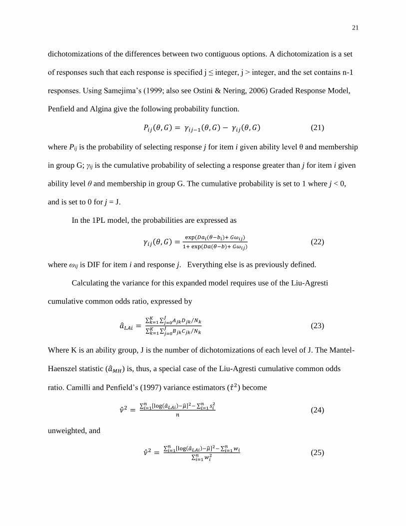
dichotomizations of the differences between two contiguous options. A dichotomization is a set
of responses such that each response is specified j ≤ integer, j > integer, and the set contains n-1
responses. Using Samejima’s (1999; also see Ostini & Nering, 2006) Graded Response Model,
Penfield and Algina give the following probability function.
𝑃𝑖𝑗(𝜃, 𝐺) = 𝛾𝑖𝑗−1(𝜃, 𝐺) − 𝛾𝑖𝑗(𝜃, 𝐺) (21)
where Pij is the probability of selecting response j for item i given ability level θ and membership
in group G; γij is the cumulative probability of selecting a response greater than j for item i given
ability level θ and membership in group G. The cumulative probability is set to 1 where j < 0,
and is set to 0 for j = J.
In the 1PL model, the probabilities are expressed as
𝛾𝑖𝑗(𝜃, 𝐺) =exp(𝐷𝑎𝑖(𝜃−𝑏𝑖)+ 𝐺𝜔𝑖𝑗)
1+ exp(𝐷𝑎(𝜃−𝑏)+ 𝐺𝜔𝑖𝑗) (22)
where ωij is DIF for item i and response j. Everything else is as previously defined.
Calculating the variance for this expanded model requires use of the Liu-Agresti
cumulative common odds ratio, expressed by
�̂�𝐿𝐴𝑖 = ∑ ∑ 𝐴𝑗𝑘𝐷𝑗𝑘 𝑁𝑘⁄𝐽
𝑗=0𝐾𝑘=1
∑ ∑ 𝐵𝑗𝑘𝐶𝑗𝑘 𝑁𝑘⁄𝐽𝑗=0
𝐾𝑘=1
(23)
Where K is an ability group, J is the number of dichotomizations of each level of J. The Mantel-
Haenszel statistic (�̂�𝑀𝐻) is, thus, a special case of the Liu-Agresti cumulative common odds
ratio. Camilli and Penfield’s (1997) variance estimators (�̂�2) become
�̂�2 = ∑ [log(�̂�𝐿𝐴𝑖)−�̂�]2𝑛
𝑖=1 − ∑ 𝑠𝑖2𝑛
𝑖=1
𝑛 (24)
unweighted, and
�̂�2 = ∑ [log(�̂�𝐿𝐴𝑖)−�̂�]2𝑛
𝑖=1 − ∑ 𝑤𝑖𝑛𝑖=1
∑ 𝑤𝑖2𝑛
𝑖=1
(25)
22
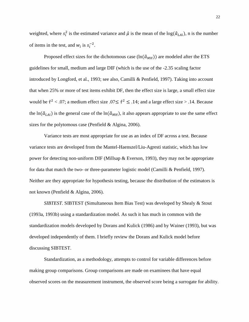
weighted, where 𝑠𝑖2 is the estimated variance and �̂� is the mean of the log(�̂�𝐿𝐴𝑖), n is the number
of items in the test, and 𝑤𝑖 is 𝑠𝑖−2.
Proposed effect sizes for the dichotomous case (ln(�̂�𝑀𝐻)) are modeled after the ETS
guidelines for small, medium and large DIF (which is the use of the -2.35 scaling factor
introduced by Longford, et al., 1993; see also, Camilli & Penfield, 1997). Taking into account
that when 25% or more of test items exhibit DF, then the effect size is large, a small effect size
would be �̂�2 < .07; a medium effect size .07≤ �̂�2 ≤ .14; and a large effect size > .14. Because
the ln(�̂�𝐿𝐴𝑖) is the general case of the ln(�̂�𝑀𝐻), it also appears appropriate to use the same effect
sizes for the polytomous case (Penfield & Algina, 2006).
Variance tests are most appropriate for use as an index of DF across a test. Because
variance tests are developed from the Mantel-Haenszel/Liu-Agresti statistic, which has low
power for detecting non-uniform DIF (Millsap & Everson, 1993), they may not be appropriate
for data that match the two- or three-parameter logistic model (Camilli & Penfield, 1997).
Neither are they appropriate for hypothesis testing, because the distribution of the estimators is
not known (Penfield & Algina, 2006).
SIBTEST. SIBTEST (Simultaneous Item Bias Test) was developed by Shealy & Stout
(1993a, 1993b) using a standardization model. As such it has much in common with the
standardization models developed by Dorans and Kulick (1986) and by Wainer (1993), but was
developed independently of them. I briefly review the Dorans and Kulick model before
discussing SIBTEST.
Standardization, as a methodology, attempts to control for variable differences before
making group comparisons. Group comparisons are made on examinees that have equal
observed scores on the measurement instrument, the observed score being a surrogate for ability.

23
That is, given two related variables, group differences on one variable are controlled for before
comparing the groups on the second variable. This is done for both items and group abilities
(Dorans & Kulick, 1986; Zhou, et al., 2006).
The standardization model has two weighted indices of DF (Dorans & Kulick, 1986).
Score weights for calculating the indices are calculated for each score group based on the
reference group. These weights are first applied to individual difference scores, and then
summed across score levels to calculate the indices. The first index is a standardized p-difference
(DSTD). It permits DIF cancellation; that is, DIF of opposite signs may cancel out at the test level.
DSTD is calculated as
𝐷STD =∑ 𝐾
𝑠[𝑃𝑓𝑠−𝑃𝑟𝑠]𝑆𝑠=1
∑ 𝐾𝑠𝑆𝑠=1
(26)
where s is the ability level, Pfs is the probability of a correct answer by the focal group at the
ability level, Prs is the probability of a correct answer by the reference group at the ability level,
and Ks is the number of examinees in the focal group at the ability level.
The second index is a root mean weighted squared difference (RMWSD). It does not
allow for DIF cancellation, and requires relatively large sample sizes to avoid bias from
sampling error. The RMWSD is calculated as the square root of the squared, standardized p-
difference plus the variance of the difference between the probabilities of the studied groups.
RMWSD = [DSTD2 + VAR(Pfs − Prs)].5 (27)
SIBTEST is an implementation of the standardization approach that is built on Shealy
and Stout’s (1993a) multidimensional IRT model of DF. The model holds that there are two
classes of abilities that affect scores: target ability, which is intentionally measured, and nuisance
determinants, which are inadvertently measured. DF comes from nuisance determinants having
different levels of prevalence in different examinee groups.

24
SIBTEST uses an internal set of test items as the matching criterion. This requires a valid
sub-test score
𝑋 = ∑ 𝑈𝑖𝑛𝑖=1 (28)
and a studied sub-test score
𝑌 = ∑ 𝑈𝑖𝑁𝑖=𝑛+1 (29)
where Ui is the set of answers. The difference scores are calculated as
�̅�𝑅𝑘 − �̅�𝐹𝑘
where k is the test score level on the valid sub-test, R and F are the reference and focal groups
respectively, and �̅�𝐺𝑘 is the average Y-score for all examinees in group G at score level k. If DF
is not present, then �̅�𝑅𝑘 − �̅�𝐹𝑘 ≅ 0 for all levels of k, and if DF is present then �̅�𝑅𝑘 − �̅�𝐹𝑘 <> 0,
where the inequality indicates which group is favored by the DF (> for Reference, and < for
Focal). Thus, defining the difference function as
𝐵(𝜃𝑘) ≡ �̅�𝑅𝑘 − �̅�𝐹𝑘 (30)
Then the estimated test index of unidirectional DF is
�̂�𝑈 = ∑ �̂�𝑘𝑛0 (�̅�𝑅𝑘 − �̅�𝐹𝑘) (31)
where �̂�𝑘 is the proportion of all examinees at valid sub-test score level X = k. Nandakumar
(1993) proposes guidelines for estimating the effect size of the DF index ( �̂�𝑈). A small effect
size is �̂�𝑈 < .05. A medium effect size is .05 < �̂�𝑈 < .1, and a large effect size is .1 < �̂�𝑈.
The continuously weighted index of unidirectional DF (precisely, marginal item response
functions, IRFs) is
𝛽𝑈 = ∫ 𝐵𝜃𝑓𝐹(𝜃)𝑑𝜃𝜃
(32)
where 𝑓𝐹(𝜃) is the probability density function of θ. The estimated test statistic (�̂�𝑈) is Dorans
and Kulick’s (1986) p-difference, DSTD, index. The 𝛽𝑈 index can also be weighted by the
25
reference- or focal-groups, but the combined focal-reference group adheres more closely to
nominal significance than using either group examinee population alone (Shealy & Stout,
1993b).
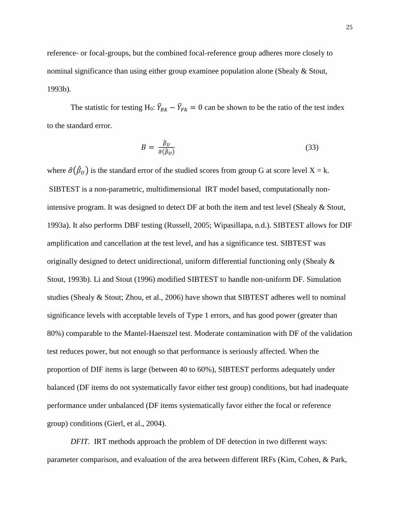
The statistic for testing H0: �̅�𝑅𝑘 − �̅�𝐹𝑘 = 0 can be shown to be the ratio of the test index
to the standard error.
𝐵 = �̂�𝑈
�̂�(�̂�𝑈) (33)
where �̂�(�̂�𝑈) is the standard error of the studied scores from group G at score level X = k.
SIBTEST is a non-parametric, multidimensional IRT model based, computationally non-
intensive program. It was designed to detect DF at both the item and test level (Shealy & Stout,
1993a). It also performs DBF testing (Russell, 2005; Wipasillapa, n.d.). SIBTEST allows for DIF
amplification and cancellation at the test level, and has a significance test. SIBTEST was
originally designed to detect unidirectional, uniform differential functioning only (Shealy &
Stout, 1993b). Li and Stout (1996) modified SIBTEST to handle non-uniform DF. Simulation
studies (Shealy & Stout; Zhou, et al., 2006) have shown that SIBTEST adheres well to nominal
significance levels with acceptable levels of Type 1 errors, and has good power (greater than
80%) comparable to the Mantel-Haenszel test. Moderate contamination with DF of the validation
test reduces power, but not enough so that performance is seriously affected. When the
proportion of DIF items is large (between 40 to 60%), SIBTEST performs adequately under
balanced (DF items do not systematically favor either test group) conditions, but had inadequate
performance under unbalanced (DF items systematically favor either the focal or reference
group) conditions (Gierl, et al., 2004).
DFIT. IRT methods approach the problem of DF detection in two different ways:
parameter comparison, and evaluation of the area between different IRFs (Kim, Cohen, & Park,
26
1995). Item parameters being a summary of the Item Response Function determine the shape of
the Item Characteristic Curve (ICC). Comparing either the parameters or the ICCs are thus
equivalent methods (Thissen, Steinberg, & Wainer, 1988). DF estimation by measuring the area
between ICCs was in use in the late 1970s (Rudner, et al., 1980). Raju (1988) expanded on this
early work by developing formulas for calculating the exact areas between ICCs for the one-,
two- and three- parameter logistic models, and in the process demonstrating a major limitation of
this method:, when the guessing (“c”) parameters are not equal, the area between the ICCs is
infinite. Another limitation of this method is the lack of weighting by examinee density: that is,
sparsely populated areas between the ICF’s contribute equally with heavily populated areas to
setting the DF index (Oshima & Morris, 2008.)
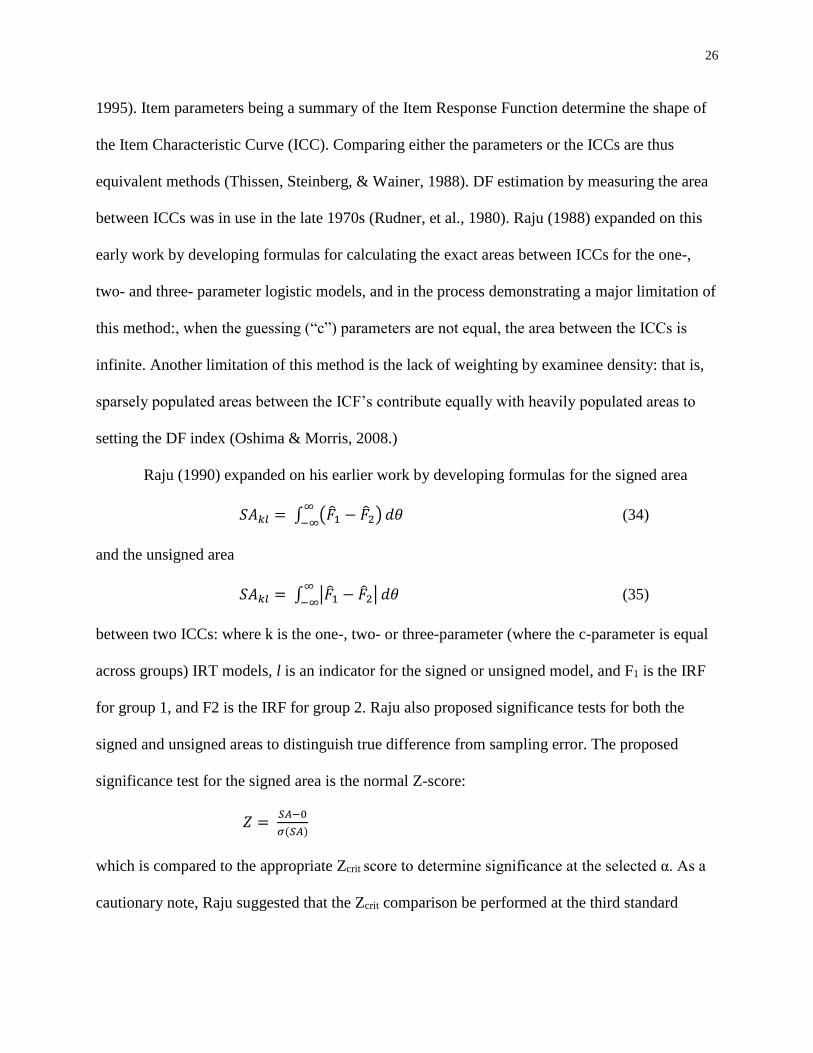
Raju (1990) expanded on his earlier work by developing formulas for the signed area
𝑆𝐴𝑘𝑙 = ∫ (�̂�1 − �̂�2)∞
−∞𝑑𝜃 (34)
and the unsigned area
𝑆𝐴𝑘𝑙 = ∫ |�̂�1 − �̂�2|∞
−∞𝑑𝜃 (35)
between two ICCs: where k is the one-, two- or three-parameter (where the c-parameter is equal
across groups) IRT models, l is an indicator for the signed or unsigned model, and F1 is the IRF
for group 1, and F2 is the IRF for group 2. Raju also proposed significance tests for both the
signed and unsigned areas to distinguish true difference from sampling error. The proposed
significance test for the signed area is the normal Z-score:
𝑍 = 𝑆𝐴−0
𝜎(𝑆𝐴)
which is compared to the appropriate Zcrit score to determine significance at the selected α. As a
cautionary note, Raju suggested that the Zcrit comparison be performed at the third standard
27
deviation (i.e., 3* Zcrit) because the standard deviation of the signed area depends on sample size,
and IRT analysis requires large sample sizes.
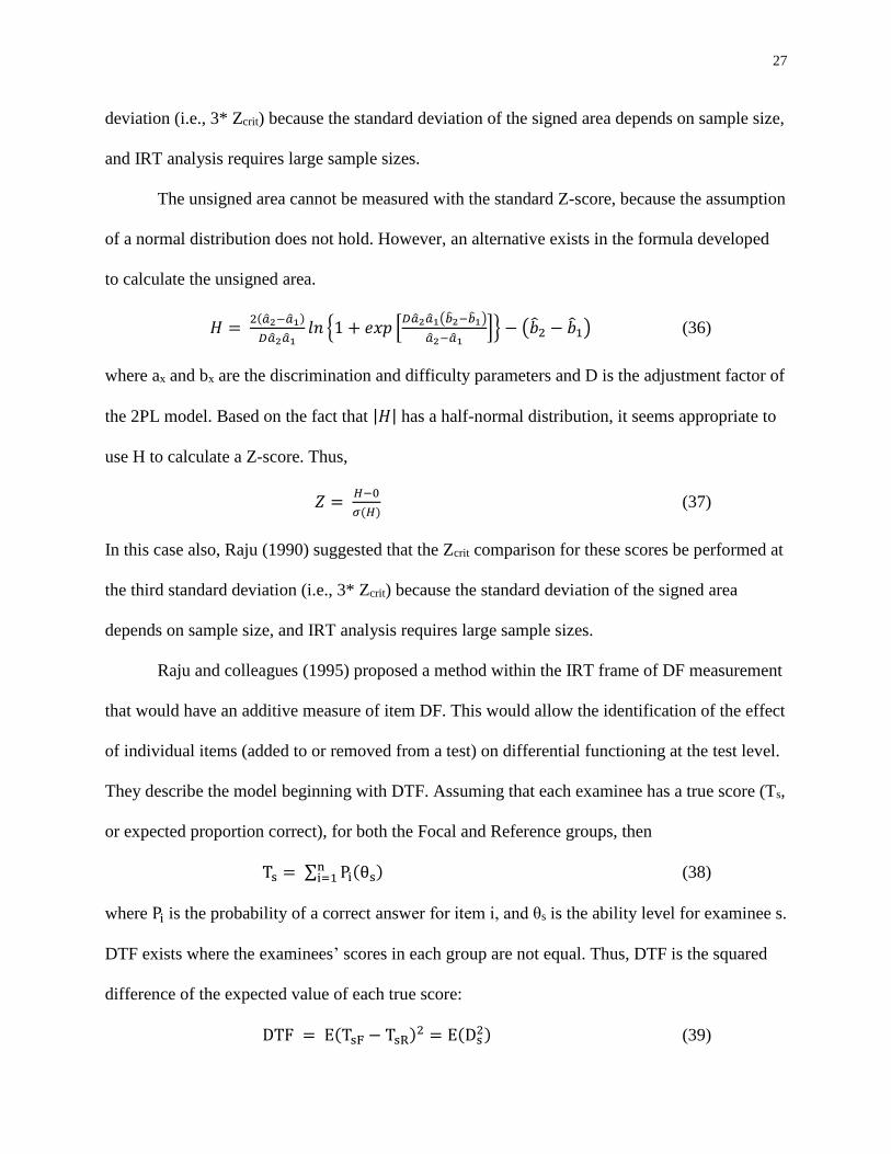
The unsigned area cannot be measured with the standard Z-score, because the assumption
of a normal distribution does not hold. However, an alternative exists in the formula developed
to calculate the unsigned area.
𝐻 = 2(�̂�2−�̂�1)
𝐷�̂�2�̂�1𝑙𝑛 {1 + 𝑒𝑥𝑝 [
𝐷�̂�2�̂�1(�̂�2−�̂�1)
�̂�2−�̂�1]} − (�̂�2 − �̂�1) (36)
where ax and bx are the discrimination and difficulty parameters and D is the adjustment factor of
the 2PL model. Based on the fact that |𝐻| has a half-normal distribution, it seems appropriate to
use H to calculate a Z-score. Thus,
𝑍 = 𝐻−0
𝜎(𝐻) (37)
In this case also, Raju (1990) suggested that the Zcrit comparison for these scores be performed at
the third standard deviation (i.e., 3* Zcrit) because the standard deviation of the signed area
depends on sample size, and IRT analysis requires large sample sizes.
Raju and colleagues (1995) proposed a method within the IRT frame of DF measurement
that would have an additive measure of item DF. This would allow the identification of the effect
of individual items (added to or removed from a test) on differential functioning at the test level.
They describe the model beginning with DTF. Assuming that each examinee has a true score (Ts,
or expected proportion correct), for both the Focal and Reference groups, then
Ts = ∑ Pi(θs)ni=1 (38)
where Pi is the probability of a correct answer for item i, and θs is the ability level for examinee s.
DTF exists where the examinees’ scores in each group are not equal. Thus, DTF is the squared
difference of the expected value of each true score:
DTF = E(TsF − TsR)2 = E(Ds2) (39)
28
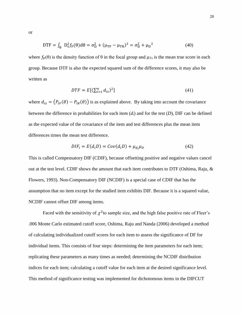
or
DTF = ∫ Ds2𝑓F(θ)dθ
θ= σD
2 + (μTF − μTR)2 = σD2 + μD
2 (40)
where 𝑓F(θ) is the density function of θ in the focal group and μTx is the mean true score in each
group. Because DTF is also the expected squared sum of the difference scores, it may also be
written as
𝐷𝑇𝐹 = 𝐸[(∑ 𝑑𝑖𝑠𝑛𝑖=1 )2] (41)
where 𝑑𝑖𝑠 = (𝑃𝑖𝐹(𝜃) − 𝑃𝑖𝑅(𝜃)) is as explained above. By taking into account the covariance
between the difference in probabilities for each item (di) and for the test (D), DIF can be defined
as the expected value of the covariance of the item and test differences plus the mean item
differences times the mean test difference.
𝐷𝐼𝐹𝑖 = 𝐸(𝑑𝑖𝐷) = 𝐶𝑜𝑣(𝑑𝑖𝐷) + 𝜇𝑑𝑖𝜇𝐷 (42)
This is called Compensatory DIF (CDIF), because offsetting positive and negative values cancel
out at the test level. CDIF shows the amount that each item contributes to DTF (Oshima, Raju, &
Flowers, 1993). Non-Compensatory DIF (NCDIF) is a special case of CDIF that has the
assumption that no item except for the studied item exhibits DIF. Because it is a squared value,
NCDIF cannot offset DIF among items.
Faced with the sensitivity of 𝜒2to sample size, and the high false positive rate of Fleer’s
.006 Monte Carlo estimated cutoff score, Oshima, Raju and Nanda (2006) developed a method
of calculating individualized cutoff scores for each item to assess the significance of DF for
individual items. This consists of four steps: determining the item parameters for each item;
replicating these parameters as many times as needed; determining the NCDIF distribution
indices for each item; calculating a cutoff value for each item at the desired significance level.
This method of significance testing was implemented for dichotomous items in the DIFCUT
29
procedure (Nanda, Oshima, & Gagné, 2006), and was adapted to use with polytomous items by
Raju et al. (2009).
DFIT works effectively with polytomous and dichotomous data, with either a
unidimensional or multidimensional model (Flowers, Oshima, Raju, 1999). It performs tests of
DIF, Differential Bundle Functioning (DBF) and DTF (Oshima, Raju, & Domaleski, 2006).
DFIT can analyze DF at adjacent and non-adjacent ability levels, and can bundle examinees as
well as test items (Oshima, et al.). Oshima, Raju, and Nanda (2006) developed an effective test
of significance for DFIT for dichotomous data, which has been extended to polytomous data
(Raju, et al., 2009).
DFIT is calculation intensive. It works well when parameter calibration and linking are
accurate, and when the data fit the IRT model. DFIT requires a large sample for accurate
parameter estimation. Linking requires a DF free anchor set of test items, so iterative linking is
necessary. The first linking uses all test items as the anchor set. Items with large DF are
removed, and a second linking is performed with the remaining, non-DIF items as the anchor set
(Oshima & Morris, 2008; Oshima, et al., 1997). DTF, in particular, cannot be interpreted before
linking (Oshima, et al.).
Comparative Studies Among the Methods
While there are many studies comparing the different methods of evaluating DF, the great
majority of them compare the methods at the item level (Finch, 2005; Navas-Ara, & Gómez-
Benito, 2002; Roussos & Stout, 1996; Wanichtanom, 2001; Zwick, 1990). There are few
comparative studies that look at DTF across methods (Wipasillapa, n.d.). Some studies look at
DTF in one method but look at DIF or DBF for another (Russell, 2005).

30
In the context of evaluating a translated test, Zumbo (2003) compared both Exploratory
Factor Analysis and Confirmatory Factor Analysis at the test level to both the Mantel-Haenszel
procedure and to logistic regression at the item level. He simulated 5000 responses using a 3PL
model with only uniform DIF, and using a 2 x 4 design and one test per design condition. DIF
ranged from about 3% to 42%. The Exploratory Factor Analysis produced a single-factor model
that matched the original model under all conditions of DIF, and the Confirmatory Factor
Analysis indicated statistical equivalence of the original and the translated models at all DIF
levels.
Pae and Park (2006) tested performance on a 33 item dichotomous subset of a
standardized test of English using 15,000 Korean college students equally divided among males
and females, and among humanities and sciences students. Logistic Regression was used to
evaluate DIF. Logistic Regression indicated the presence of DIF in 22 of the items. Following
this, separate Confirmatory Factor Analyses were run on a set of four nested data models
comparing males to females. Each model was based on a single latent factor and differed in the
variance constraints imposed on the data. In all cases model fit indices were acceptable,
however, Chi-square difference statistics between each model and the unconstrained model
indicated in all cases that the factor matrices were different for men and women. Looking
specifically for a DIF cancellation effect, Pae and Park took 5 items favoring men and 5 items
favoring women, each set having the same cumulative amount of DIF, and checked them with
CFA. Chi-square tests of the differences in factor loading, error variances and factor variances
indicated that there was no DIF cancellation.
Four dissertations have compared DTF using different methods. Fesq (1995) compared
Marginal Maximum Likelihood (MML) with the Random Effects Model (REM; Longford, et al.,
31
1993) and with the Summed Chi-square Statistic (SCS; Camilli & Penfield, 1997). She found the
MML and REM methods to be comparable. All methods controlled Type I error well for the 1PL
model but not for the 3PL model. DTF estimates were poor in the presence of embedded DIF.
Petroski (2005) compared DTF for DFIT with several bootstrap methods. He found very high
Type I error rates for DFIT, but acceptable Type I error rates and power for the bootstrap
methods. Russell (2005) compared SIBTEST for DBF (differential bundle functioning) with
DFIT for DTF, noting that the two methods “are used for different practical applications and at
different levels of analysis” (p. 3). He found that both methods had inflated Type I error, and
that DFIT had low power while SIBTEST had adequate power. Russell’s choice of test levels to
compare is confusing because SIBTEST also calculates DTF (Shealy & Stout, 1993a), and DFIT
also calculates DBF (Oshima, Raju, Flowers, & Slinde, 1998). Wipasillapa (n.d.) compared
SIBTEST and DFIT for DIF, DBF, and DTF. For DTF, she found that for 50 item tests with
1000 or fewer students SIBTEST had greater power than DFIT.
Theoretical comparisons include Takane and de Leeuw (1987) who presented a formal
proof of the equivalence of Factor Analysis and IRT, and Raju, Lafitte, and Byrne (2002), who
presented a theoretical comparison of CFA and IRT approaches. Raju, et al. noted five
similarities and six differences and called for further research into the relative advantages of each
approach and into their comparability. The similarities are 1) both look at how a theoretical
construct is related to a set of measurements; 2) both look at true score similarities between
persons from different groups who have been matched on the construct; 3) neither implies equal
population distributions of scores on the construct; 4) both can identify the source of
measurement nonequivalence; and 5) both can make use of graphs of the item response
functions. The differences between the approaches are 1) CFA assumes a linear relationship
32
between the construct and the true score, while IRT assumes a non-linear relationship; 2) logistic
regression is better for expressing relationships between continuous constructs and dichotomous
scores, so IRT is better in this case, but the advantage decreases as the number of score points
increase; 3) CFA can easily handle several latent constructs, while IRT has only begun to look at
multidimensionality; 4) a strict form of CFA requires equivalent item error variance, while IRT
does not consider it because it can vary as a function of the construct; 5) IRT is explicit about the
probabilities of answer selection at a given value of the construct, which is difficult to obtain in
CFA; and 6) DIF amplification/cancellation is explicit in IRT, but mostly ignored in CFA.
Discussion
Each of the methods discussed have different strengths and weaknesses. The
computational simplicity and the ability to use relatively small sample sizes are shared by CFA,
Variance Analysis and SIBTEST. DFIT on the other hand is computationally intensive and
requires (in most cases) sample sizes greater than 500 (Oshima & Morris, 2008; Rudner, et al.,
1980). Yet the extra effort required to compute the item parameters enables DFIT to keep item
difficulty and discrimination from being confounded with group differences (Raju & Ellis,
2003). CFA, DFIT and SIBTEST have tests of significance, where Variance Analysis depends
on the experience of the researcher to decide the importance of the computed DTF (Camilli &
Penfield, 1997). CFA significance tests are many and the subject of much controversy, primarily
because of the influence that sample size has on Chi-square tests (Lance & Vandenberg, 2002).
Because of its base in Mantel-Haenszel DIF analysis, Variance Analysis is mostly restricted to
analysis of tests with uniform DF. CFA, DFIT and SIBTEST have no restriction on the kinds of
DF that can be effectively analyzed.
33
The importance of a DF measure depends on its intended use. Being able to select the
most appropriate measure is an advantage of having all four measures of differential functioning
available (Raju, et al., 1995). The importance of a method of analyzing DF, as seen in the above
synopsis, similarly depends on the circumstances of its application. Having a precise knowledge
of the capabilities of each of these methods will enable the researcher and practitioner to select
the best method for the task at hand.
34
CHAPTER 3
METHOD
Study Design
This study is a simulation to evaluate and compare two DTF detection methods: Variance
(using DIFAS 4.0; Penfield, 2007), and DFIT (using DIFCUT; Nanda, Oshima, & Gagne, 2006).
Simulation studies are common in quantitative literature, especially in situations where statistical
theory is weak or non-existent or where the assumptions for theory have been violated (Fan,
Felsölvályi, Sivo, & Keenan, 2001). Such situations commonly occur both for studying different
conditions within a method and for comparing different methods (Fidalgo, Hashimoto, Bartram
& Muñiz, 2007; Meade, Lautenschlager, and Johnson, 2007; Nandakumar, 1993; Raju, et al.,
1995).
Conditions of Study
Fixed Factors
Data Generation. Simulated data were generated using the three parameter logistic (3PL)
model with a fixed guessing parameter for dichotomous items using Lord’s (1968) item
parameters2 from the SAT-Verbal test (Table 2.) Parameters for 80 items are available. The
guessing parameter for the DF items was set to .20, which is commonly used in the literature
(Güler & Penfield, 2009; Monahan & Ankenmann, 2005) and represents the expected random
guessing parameter for an item with five answer options.
2 Parameters were provided by Ratna Nandakumar, personal communication, April 4, 2009.
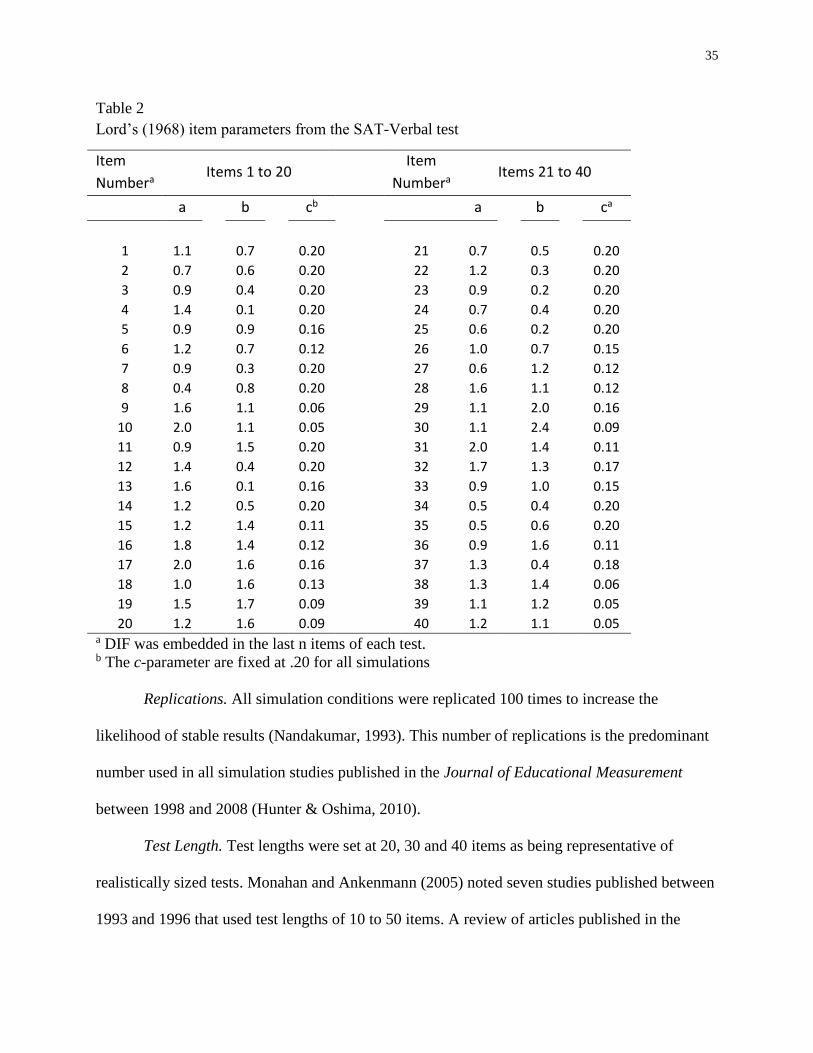
35
Table 2
Lord’s (1968) item parameters from the SAT-Verbal test
Item
Numbera Items 1 to 20
Item
Numbera Items 21 to 40
a b cb a b ca
1
22
1.1 0.7 0.20 21 0.7 0.5 0.20
2 0.7 0.6 0.20 22 1.2 0.3 0.20
3 0.9 0.4 0.20 23 0.9 0.2 0.20
4 1.4 0.1 0.20 24 0.7 0.4 0.20
5 0.9 0.9 0.16 25 0.6 0.2 0.20
6 1.2 0.7 0.12 26 1.0 0.7 0.15
7 0.9 0.3 0.20 27 0.6 1.2 0.12
8 0.4 0.8 0.20 28 1.6 1.1 0.12
9 1.6 1.1 0.06 29 1.1 2.0 0.16
10 2.0 1.1 0.05 30 1.1 2.4 0.09
11 0.9 1.5 0.20 31 2.0 1.4 0.11
12 1.4 0.4 0.20 32 1.7 1.3 0.17
13 1.6 0.1 0.16 33 0.9 1.0 0.15
14 1.2 0.5 0.20 34 0.5 0.4 0.20
15 1.2 1.4 0.11 35 0.5 0.6 0.20
16 1.8 1.4 0.12 36 0.9 1.6 0.11
17 2.0 1.6 0.16 37 1.3 0.4 0.18
18 1.0 1.6 0.13 38 1.3 1.4 0.06
19 1.5 1.7 0.09 39 1.1 1.2 0.05
20 1.2 1.6 0.09 40 1.2 1.1 0.05 a DIF was embedded in the last n items of each test. b The c-parameter are fixed at .20 for all simulations
Replications. All simulation conditions were replicated 100 times to increase the
likelihood of stable results (Nandakumar, 1993). This number of replications is the predominant
number used in all simulation studies published in the Journal of Educational Measurement
between 1998 and 2008 (Hunter & Oshima, 2010).
Test Length. Test lengths were set at 20, 30 and 40 items as being representative of
realistically sized tests. Monahan and Ankenmann (2005) noted seven studies published between
1993 and 1996 that used test lengths of 10 to 50 items. A review of articles published in the
36
Journal of Educational Measurement between 1998 and 2008 (Hunter & Oshima, 2010) found
that simulation studies dealing with DIF used 20 to 360 items. Güler & Penfield (2009) chose 60
items as being realistic in respect to the number of items on standardized, multiple-choice tests.
Swaminathan and Rogers (1990) used test sizes of 40, 60 and 80 items.
Type of DIF. Embedded DIF was uniform, because contingency table methods (e.g.,
Mantel-Haenszel, on which DIFAS is built) are known for being insensitive to non-uniform DIF
(Millsap & Everson, 1993).
Varied Factors
Ability. The ability (θ) parameters were randomly assigned, ~N(0,1), for each simulee for
assessing the effect of the different levels of DIF. The sensitivity of the methods to different
levels of ability between the groups (i.e., impact) was assessed using both mean differences, and
differences in the standard deviations. Holding the standard deviation at 1, group mean
differences were varied by 0, .5, and 1.0 to simulate no, moderate and large differences
respectively (Russell, 2005).
While the manipulation of mean ability is common in simulation studies of DF (Garrett,
2009; Oshima, et al., 1997; Penfield & Algina, 2006: Russell, 2005), standard deviation has
rarely been considered outside of studies investigating the ability distribution (Monahan &
Ankenmann, 2005; Woods, 2007, 2008). Woods suggests looking at different ability
distributions from the ones she studied to see whether DF conditions would be consistent with
previous research. Monahan and Ankenmann found that having both unequal means and
variance ratios increased the Type I error rate. Holding the mean differences at 0, and the
standard deviation in the Reference group at 1, standard deviation in the focal group is set to 1.0,
1.5, and 2.0, to investigate the effect of the variation of sample distribution.
37
Percent DIF. Four DIF conditions were created with DIF embedded in 0, 5, 10 and 20
percent of the items. The last items of each test were used as the DIF items. Using the first or the
last test items to embed DIF, instead of scattering DIF, throughout the test is relatively common
(Oshima, et al., 1997; Snow & Oshima, 2009; Güler & Penfield, 2009; Penfield, 2007). This
procedure has the advantage of making the DIF items easy to locate during analysis.
Magnitude of DIF. Recent studies have used DIF magnitude ranging from small to large
(.10, .25, .40, .50, .75, and 1.0). Those authors chose these values both to be able to compare
their findings with other studies and to investigate the effect of values of magnitude outside of
the range previously studied (Garrett, 2009; Raiford-Ross, 2008; Stephens-Bonty, 2008;
Thurman, 2009). Because I was looking at the effects of DIF amplification to produce significant
DTF, and at the effects of DIF cancellation to eliminate DTF, I used very small to medium
magnitudes of DIF: specifically.02, .20 and.40. I simulated uniform DF by adding the magnitude
constant to the b-parameter (Raju, Fortmann-Johnson, et al., 2009). I did not simulate non-
uniform DF because of the insensitivity of contingency table methods to non-uniform DF
(Millsap & Everson, 1993).
Balanced and Unbalanced DIF. Balanced DIF was assigned equally favoring the
reference and focal groups for each of the three DIF percentage conditions (5, 10, and 20)
defined above. Different sets of items were used for the reference and focal groups
(Nandakumar, 1993.) For example, a 20-item test with four DF items, would have items 17 and
18 with DF in the reference group, and items 19 and 20 with DF in the focal group (see
Nandakumar, 1993). Unbalanced DIF was assigned favoring the Reference group for each of the
three DIF percentage conditions (5, 10, and 20) defined above using the last items of each test.
38
Sample Size. Studies in the JEM between 1998 and 2008 set the number of simulated
participants ranged from 1 to 200,000. The four most common numbers were 500 (33 studies),
1000 (25 studies), 2000 (12 studies), and 3000 (13 studies). Over half of the studies used a single
group size (Hunter & Oshima, 2010). In this study, I used two different sample sizes (1000 and
3000) with each program to compare DTF statistics, and power variations. Larger sample sizes
are chosen because DFIT requires sample sizes greater than 500 (Oshima & Morris, 2008;
Rudner, et al., 1980), and because small sample sizes used with Mantel-Haenszel methods yield
unstable results (Zwick, Ye, & Isham, 2012).
Sample sizes for the reference and focal group sample sizes were set to 1000:1000 and to
3000:3000 for assessing the effect of sample size on impact and balanced DF. Blitz and Morris
(2011) found that the IPR method of DIF detection used in DFIT is sensitive to unequal sample
sizes, producing error rates much lower than the nominal rate when the reference group is larger
than the focal group, and much higher than the nominal rates when the focal group is larger. To
assess whether this effect carries over into DTF, unequal sample sizes were set to 3000:1000
(reference:focal) to assess the effect of large differences in sample sizes.
For the impact condition this resulted in a 1 X 3 X 3 (mean x standard deviation x sample
size; varying the standard deviation for a constant mean) plus a 3 X 1 X 3 (mean x standard
deviation x sample size, varying the mean for a constant standard deviation) design for 15
conditions. The DF conditions had a 3 X 3 X 2 X 3 (% DF x DF magnitude x direction x sample
size) design. Table 3 lists the fixed factors examined in the study. Varied factors appear in
Table 4.
Table 3
Fixed Factors in the Study Design
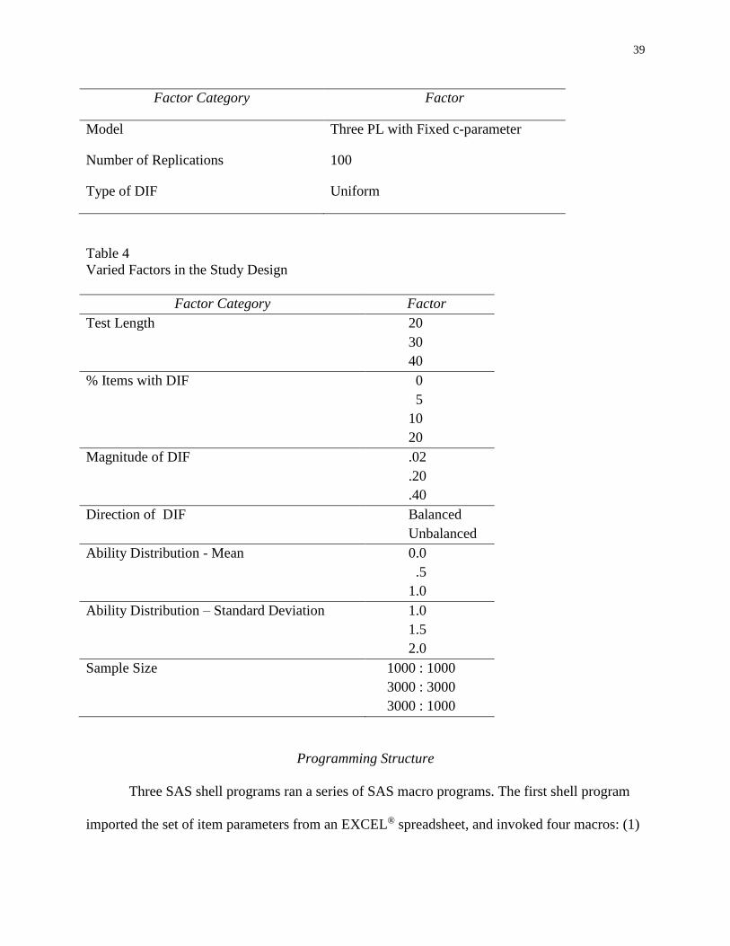
39
Factor Category Factor
Model Three PL with Fixed c-parameter
Number of Replications 100
Type of DIF Uniform
Table 4
Varied Factors in the Study Design
Factor Category Factor
Test Length 20
30
40
% Items with DIF 0
5
10
20
Magnitude of DIF .02
.20
.40
Direction of DIF Balanced
Unbalanced
Ability Distribution - Mean 0.0
.5
1.0
Ability Distribution – Standard Deviation 1.0
1.5
2.0
Sample Size 1000 : 1000
3000 : 3000
3000 : 1000
Programming Structure
Three SAS shell programs ran a series of SAS macro programs. The first shell program
imported the set of item parameters from an EXCEL® spreadsheet, and invoked four macros: (1)
40
to manipulate the parameters to create three sets of parameters with 20, 30 and 40 parameters
each, (2) to add the appropriate amount of DF to the appropriate parameters for each input file,
(3) to create files with balanced DF, and (4) to create files with unbalanced DF.
The second shell program generated 100 files of simulated data for each set of study
conditions. It ran two macros. The first macro invoked program IRTGEN (Whittaker,
Fitzpatrick, Williams, & Dodd, 2003), which had been modified to run as a SAS macro, to
generate data for the balanced and unbalanced conditions. The second macro invoked program
IRTGEN, which had been modified to run as a SAS macro and to apply differences to the mean
and sample deviation of selected files to simulate differences in sample distribution, for impact
conditions.
The third shell program invoked five SAS macros that performed item calibration,
linking and analysis. The first macro formatted the SAS data files as text files with a “.dat”
extension, which is the format required by BILOG-MG3 (Zimowski, Muraki, Mislevy, & Bock;
2003). The second macro created a BILOG command file to process each data file, and invoked
BILOG-MG33 to perform item calibration. The third macro created an R (R Core Team; 2014)
command file for plink (Weeks, 2010) to process each data file, and invoked plink to perform
file linking. The fourth macro invoked DIFCUT (Nanda, Oshima, & Gagne, 2006), which is a
SAS implementation of the DFIT method. DIFCUT had been modified to (1) run as a SAS
macro program, and (2) produce a file listing linking items identified as free of DIF for use in
second stage linking, and a file containing the DTF value and significance level for each file.
The fifth macro read the linking items file created a new command file to process each data file,
3 In order to run BILOG from the command line using SAS, BILOG must be installed using a perpetual license. It will not run using a temporary license. (L. Stam, personal communication, August 4, 2011).
41
and invoked plink to perform second stage file linking. The macro to invoke DIFCUT was then
invoked a second time to complete the analysis.
Data Generation
Data for both analysis streams (DFIT and MH/LA) was generated using a SAS 9.2 macro
program to invoke the SAS macro program IRTGEN (Whittaker, Fitzpatrick, Williams, & Dodd,
2003) to generate data for all of the different combinations of test conditions. Seed values for
each condition entered to IRTGEN were selected using the randbetween function of Microsoft
Excel 2007® with arbitrarily selected limit values. All seed numbers generated were unique.
Where ability (θ) parameters with other than a normal distribution are needed, Whittaker
and colleagues (2003) suggest commenting out the ability parameter generator within IRTGEN,
and entering the parameters on a separate file. As an alternative to this, I modified IRTGEN
using the formulas in Fan et al. (2001) to adjust the parameters created by IRTGEN before the
item responses were generated. Additionally, to meet a requirement of BILOG-MG3 (Zimowski
al., 2003), I added code to create an examinee (case) number for each record.
DFIT Analysis
Calibration, Equating and Linking
Another SAS macro program automated the processing of the IRT parameter estimation
(Gagné, Furlow, & Ross, 2009) by running BILOG-MG 3.0 (Zimowski et al., 2003) for each
reference and focal simulated dataset. Separate calibration estimation was done for each set of
conditions and replications. While there is some evidence that concurrent estimation performs
better than separate estimation, it is not strong enough to warrant always using it (Hanson &
Béguin, 2002). On the contrary, other studies have found that separate estimation generally gives
42
better results than concurrent estimation, except where all examinee groups are from the same
population (Lee & Ban, 2010).
Item parameters to enter to DIFCUT (Nanda, Oshima, & Gagne, 2006) were generated
from each file using linking between pairs of reference and focal files. Linking was done with
plink (Weeks, 2010), an R (R Core Team, 2014) package using the Stocking and Lord Test
Characteristic Curve method, which links files based on the sum of squared differences between
the TCCs at a given θ. The Stocking and Lord method is similar to the Haebara method, a
characteristic curve method that for each item sums the squared differences between the ICCs
over the examinees at a given θ (Kolen & Brennan, 2004). Studies indicate that both methods
give similar results (Hanson & Béguin, 2002; Lee & Ban, 2010; Oshima, Davey, & Lee, 2000).
Kolen and Brennan reviewed studies that compared different kinds of equating, and concluded
that “separate estimation using the test characteristic curve methods seems to be safest” (p. 174).
Also, Oshima, Davey, and Lee suggest that the purpose of the linking determine the method
used. Because this study looks at DTF, the Stocking and Lord Method, which looks at TCCs,
seems preferable theoretically to the Haebara method. Linking was performed iteratively, as
suggested by Kim and Cohen (1992) and Stark, Chernyshenko and Drasgow (2004). Only two
iterations were performed, as indicated in Oshima and Morris (2008). All items were used to
calculate the linking constant in the first DIFCUT run. Items identified as DIF-free were then
entered to a second run of plink to generate a second linking constant for each replication and set
of conditions.
Variance Analysis
Variance analysis was performed using DIFAS 4.0 (Penfield, 2007). The matching
variable to estimate the ability levels was the equal interval method. This reduces the Type I
43
error rate of finding DIF (Donoghue & Allen, 1993). Only a single estimation was used for this
analysis because DIFAS uses a Mantel-Haenszel estimation method. Research indicates that
more accurate results are obtained by not removing items identified as having DF, and
reanalyzing the data without them (Zwick, Ye, & Isham, 2012).
Evaluation of Results
Type I errors are the misidentification of non-DF items as containing DF. Power analysis
is the ability of a method to adequately detect the existence of DF where it actually exists. Both
of these evaluative methods are typically used in simulation studies of DF detection. Type I error
of detecting DTF was assessed using Bradley’s (1978) liberal rate of 7.5 percent for each
condition, and compared across the two methods of DTF analysis. Similarly, a power analysis
was performed for each condition for both methods of DTF analysis.
While Type I error analysis and power analysis are both important indicators of the
effectiveness of a measurement instrument, they can also indicate that a small or trivial effect is
statistically significant, possibly giving the impression that the results are practically important.
Because the statistical significance of DTF depends on sample size, the interpretation of
significance is difficult (Stark et al., 2004). This difficulty increases when the sample sizes are
large and even more likely when power is high (Monahan, McHorney, Stump, & Perkins, 2007).
An analysis of effect size can be used to estimate the practical importance of the results, and may
help to reduce the acceptance of Type I and Type II errors (Hidalgo & López-Pina, 2004). This is
especially important because of the large sample sizes (1000 and greater) used in this study.
A number of different effect size measures have been proposed for the Mantel-Haenszel
test and for logistic-regression (Hidalgo & López-Pina, 2004; Monahan, et al., 2007; Penny &
Johnson, 1999), but few have been proposed for DFIT. Stark and his colleagues (2004) proposed
44
three effect size indices for DFIT: DTFR, a measure, in raw score units, based on the differences
in the TCCs between the reference and focal groups; dDTF, the DTFR standardized using the
standard deviation of the observed focal group scores; and the RSR which compares the
proportions of examinees from the reference and focal groups at a given cut score. Wright (2011)
investigated the effect size for NCDIF in DFIT comparing it with the effect size for the Mantel-
Haenszel statistic. However, I find no investigation of comparative effect sizes between Mantel-
Haenszel and DFIT for DTF.
45
CHAPTER 4
RESULTS
The results are organized into three main groupings: the distribution of τ2, correlations
between DFIT and MH/LA DTF indicators, and significance testing. A primary area of interest is
the distribution of τ2. Because τ2is a variance measure, it is bound from zero to positive infinity,
and is presumably not normally distributed. Therefore, its usefulness as an indicator for testing
the null hypothesis is in question (Penfield & Algina, 2006). Determining empirical distributions
may provide further information on this issue. Strong correlations between the DFIT- DTF
indicator and MH/LA τ2 would provide support for the usefulness of the MH/LA DTF indicator.
Significance testing examines the obtained amounts of significant DTF for DFIT and τ2, looking
at τ2 using an empirically derived cutoff method of determining the rate of statistical
significance. Results obtained from DFIT and MH/LA are compared.
Distributions4
One of the noted problems of using the MH/LA variance method to determine the
presence of DTF is that the distribution of its output statistic (τ2) is unknown (Penfield & Algina,
2006), leaving in doubt the appropriate method to use to determine significance. Penfield (2005)
4 Because DFIT already has a proven method of identifying significance (IPR; Oshima, Raju & Nanda, 2006), it is not
necessary to determine the distribution of its outputs.
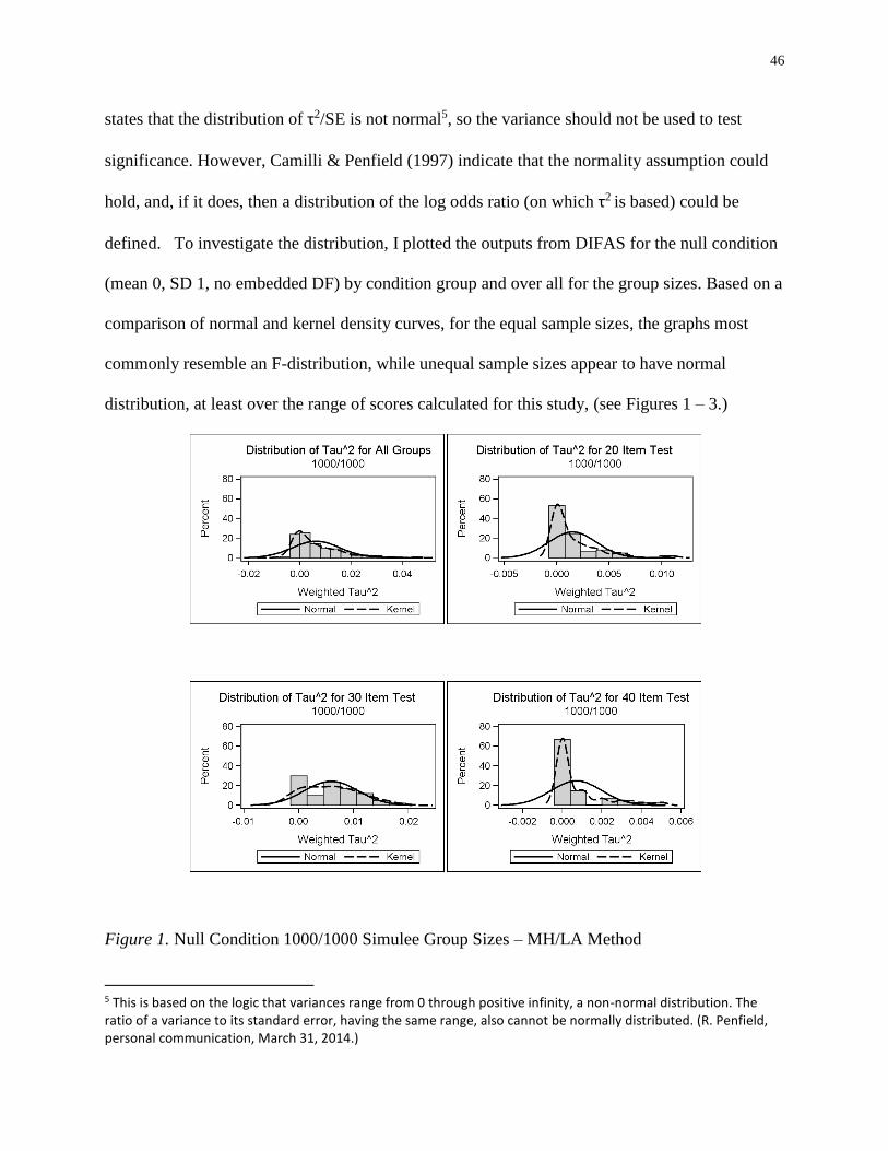
46
states that the distribution of τ2/SE is not normal5, so the variance should not be used to test
significance. However, Camilli & Penfield (1997) indicate that the normality assumption could
hold, and, if it does, then a distribution of the log odds ratio (on which τ2 is based) could be
defined. To investigate the distribution, I plotted the outputs from DIFAS for the null condition
(mean 0, SD 1, no embedded DF) by condition group and over all for the group sizes. Based on a
comparison of normal and kernel density curves, for the equal sample sizes, the graphs most
commonly resemble an F-distribution, while unequal sample sizes appear to have normal
distribution, at least over the range of scores calculated for this study, (see Figures 1 – 3.)
Figure 1. Null Condition 1000/1000 Simulee Group Sizes – MH/LA Method
5 This is based on the logic that variances range from 0 through positive infinity, a non-normal distribution. The ratio of a variance to its standard error, having the same range, also cannot be normally distributed. (R. Penfield, personal communication, March 31, 2014.)
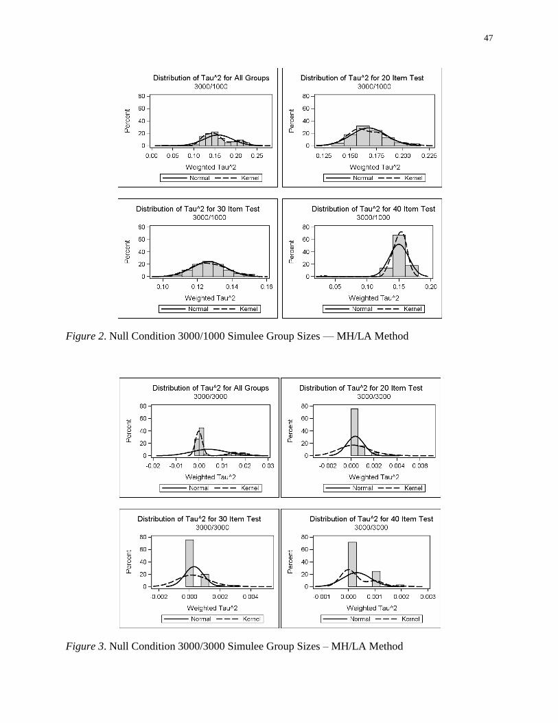
47
Figure 2. Null Condition 3000/1000 Simulee Group Sizes –– MH/LA Method
Figure 3. Null Condition 3000/3000 Simulee Group Sizes – MH/LA Method
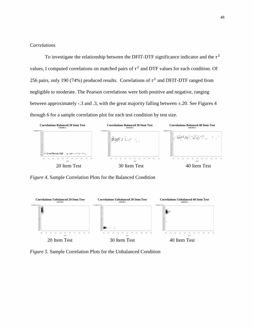
48
Correlations
To investigate the relationship between the DFIT-DTF significance indicator and the 𝜏2
values, I computed correlations on matched pairs of 𝜏2 and DTF values for each condition. Of
256 pairs, only 190 (74%) produced results. Correlations of 𝜏2 and DFIT-DTF ranged from
negligible to moderate. The Pearson correlations were both positive and negative, ranging
between approximately -.3 and .3, with the great majority falling between ±.20. See Figures 4
through 6 for a sample correlation plot for each test condition by test size.
20 Item Test 30 Item Test 40 Item Test
Figure 4. Sample Correlation Plots for the Balanced Condition
20 Item Test 30 Item Test 40 Item Test
Figure 5. Sample Correlation Plots for the Unbalanced Condition
Weighted Tau^2
-0.02-0.010.000.010.020.030.040.050.060.070.080.090.100.110.120.130.140.150.160.170.180.190.20
DTF
0.0 0.1 0.2 0.3 0.4 0.5 0.6 0.7 0.8 0.9 1.0
Correlations Balanced 20 Item Testb20440K11
Weighted Tau^2
-0.02-0.010.000.010.020.030.040.050.060.070.080.090.100.110.120.130.140.150.160.170.180.190.20
DTF
0.0 0.1 0.2 0.3 0.4 0.5 0.6 0.7 0.8 0.9 1.0
Correlations Balanced 30 Item Testb30202K31
Weighted Tau^2
-0.02-0.010.000.010.020.030.040.050.060.070.080.090.100.110.120.130.140.150.160.170.180.190.20
DTF
0.0 0.1 0.2 0.3 0.4 0.5 0.6 0.7 0.8 0.9 1.0
Correlations Balanced 40 Item Testb40440K31
Weighted Tau^2
-0.02-0.010.000.010.020.030.040.050.060.070.080.090.100.110.120.130.140.150.160.170.180.190.20
DTF
0.0 0.1 0.2 0.3 0.4 0.5 0.6 0.7 0.8 0.9 1.0
Correlations Unbalanced 20 Item Testu20102k31
Weighted Tau^2
-0.02-0.010.000.010.020.030.040.050.060.070.080.090.100.110.120.130.140.150.160.170.180.190.20
DTF
0.0 0.1 0.2 0.3 0.4 0.5 0.6 0.7 0.8 0.9 1.0
Correlations Unbalanced 30 Item Testu30620k11
Weighted Tau^2
-0.02-0.010.000.010.020.030.040.050.060.070.080.090.100.110.120.130.140.150.160.170.180.190.20
DTF
0.0 0.1 0.2 0.3 0.4 0.5 0.6 0.7 0.8 0.9 1.0
Correlations Unbalanced 40 Item Testu40402k31
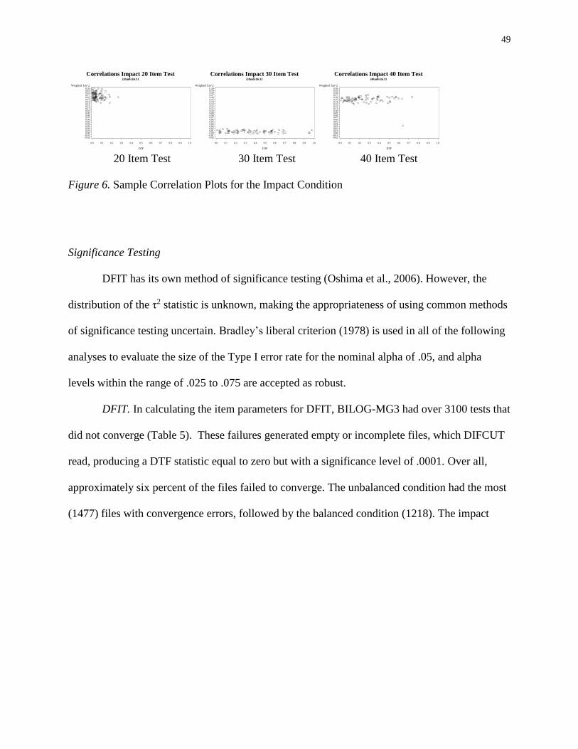
49
20 Item Test 30 Item Test 40 Item Test
Figure 6. Sample Correlation Plots for the Impact Condition
Significance Testing
DFIT has its own method of significance testing (Oshima et al., 2006). However, the
distribution of the τ2 statistic is unknown, making the appropriateness of using common methods
of significance testing uncertain. Bradley’s liberal criterion (1978) is used in all of the following
analyses to evaluate the size of the Type I error rate for the nominal alpha of .05, and alpha
levels within the range of .025 to .075 are accepted as robust.
DFIT. In calculating the item parameters for DFIT, BILOG-MG3 had over 3100 tests that
did not converge (Table 5). These failures generated empty or incomplete files, which DIFCUT
read, producing a DTF statistic equal to zero but with a significance level of .0001. Over all,
approximately six percent of the files failed to converge. The unbalanced condition had the most
(1477) files with convergence errors, followed by the balanced condition (1218). The impact
Weighted Tau^2
-0.02-0.010.000.010.020.030.040.050.060.070.080.090.100.110.120.130.140.150.160.170.180.190.20
DTF
0.0 0.1 0.2 0.3 0.4 0.5 0.6 0.7 0.8 0.9 1.0
Correlations Impact 20 Item Testi20m0s1K31
Weighted Tau^2
-0.02-0.010.000.010.020.030.040.050.060.070.080.090.100.110.120.130.140.150.160.170.180.190.20
DTF
0.0 0.1 0.2 0.3 0.4 0.5 0.6 0.7 0.8 0.9 1.0
Correlations Impact 30 Item Testi30m0s1K11
Weighted Tau^2
-0.02-0.010.000.010.020.030.040.050.060.070.080.090.100.110.120.130.140.150.160.170.180.190.20
DTF
0.0 0.1 0.2 0.3 0.4 0.5 0.6 0.7 0.8 0.9 1.0
Correlations Impact 40 Item Testi40m0s1K31
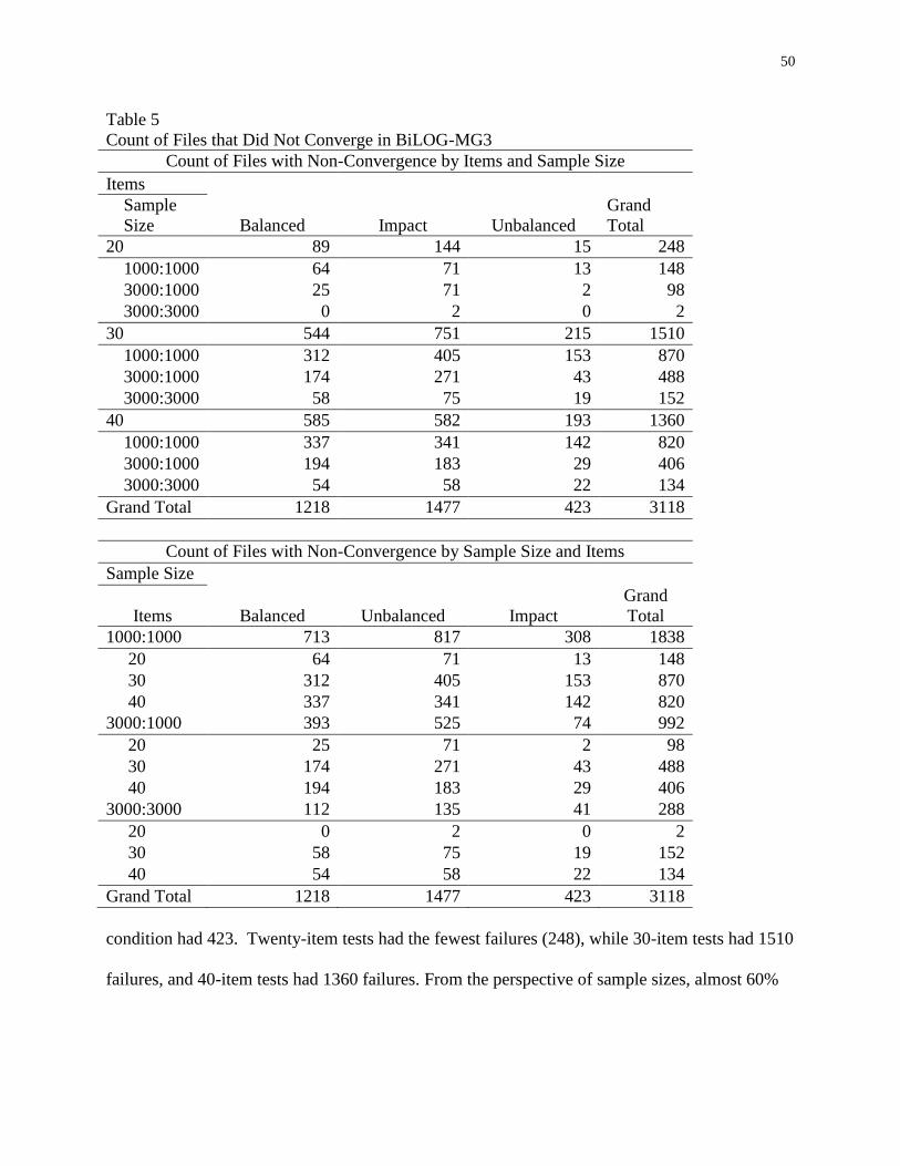
50
Table 5
Count of Files that Did Not Converge in BiLOG-MG3
Count of Files with Non-Convergence by Items and Sample Size
Items
Sample
Size Balanced Impact Unbalanced
Grand
Total
20 89 144 15 248
1000:1000 64 71 13 148
3000:1000 25 71 2 98
3000:3000 0 2 0 2
30 544 751 215 1510
1000:1000 312 405 153 870
3000:1000 174 271 43 488
3000:3000 58 75 19 152
40 585 582 193 1360
1000:1000 337 341 142 820
3000:1000 194 183 29 406
3000:3000 54 58 22 134
Grand Total 1218 1477 423 3118
Count of Files with Non-Convergence by Sample Size and Items
Sample Size
Items Balanced Unbalanced Impact
Grand
Total
1000:1000 713 817 308 1838
20 64 71 13 148
30 312 405 153 870
40 337 341 142 820
3000:1000 393 525 74 992
20 25 71 2 98
30 174 271 43 488
40 194 183 29 406
3000:3000 112 135 41 288
20 0 2 0 2
30 58 75 19 152
40 54 58 22 134
Grand Total 1218 1477 423 3118
condition had 423. Twenty-item tests had the fewest failures (248), while 30-item tests had 1510
failures, and 40-item tests had 1360 failures. From the perspective of sample sizes, almost 60%
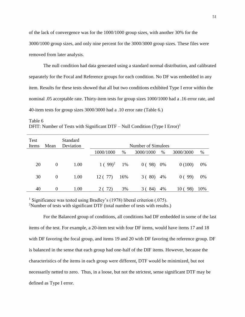
51
of the lack of convergence was for the 1000/1000 group sizes, with another 30% for the
3000/1000 group sizes, and only nine percent for the 3000/3000 group sizes. These files were
removed from later analysis.
The null condition had data generated using a standard normal distribution, and calibrated
separately for the Focal and Reference groups for each condition. No DF was embedded in any
item. Results for these tests showed that all but two conditions exhibited Type I error within the
nominal .05 acceptable rate. Thirty-item tests for group sizes 1000/1000 had a .16 error rate, and
40-item tests for group sizes 3000/3000 had a .10 error rate (Table 6.)
Table 6
DFIT: Number of Tests with Significant DTF – Null Condition (Type I Error)1
Test
Items Mean
Standard
Deviation
Number of Simulees
1000/1000 % 3000/1000 % 3000/3000 %
20 0 1.00
1 ( 99)2 1% 0 ( 98) 0% 0 (100) 0%
30 0 1.00
12 ( 77)1 16% 3 ( 80) 4% 0 ( 99) 0%
40 0 1.00
2 ( 72)1 3% 3 ( 84) 4% 10 ( 98) 10%
1 Significance was tested using Bradley’s (1978) liberal criterion (.075). 2Number of tests with significant DTF (total number of tests with results.)
For the Balanced group of conditions, all conditions had DF embedded in some of the last
items of the test. For example, a 20-item test with four DF items, would have items 17 and 18
with DF favoring the focal group, and items 19 and 20 with DF favoring the reference group. DF
is balanced in the sense that each group had one-half of the DIF items. However, because the
characteristics of the items in each group were different, DTF would be minimized, but not
necessarily netted to zero. Thus, in a loose, but not the strictest, sense significant DTF may be
defined as Type I error.
52
For the Balanced DIF condition and 20-item test, all conditions except two exhibited less
than Bradley’s 7.5 percent detection rates. For tests with four DF items and group sizes
1000/1000, where DF magnitude was .20, eight tests exhibited significant DTF, and where test
magnitude was .40, 26 tests exhibited significant DTF, 8 and 27 percent respectively. For 30-
item tests, all conditions for the 1000/1000 group sizes exhibited detection rates greater than 7.5
percent. Additionally, for the 3000/3000 group sizes where DF magnitude was large (.40), both
the two DF item and 6 DF item conditions exhibited detection rates greater than Bradley’s liberal
criterion of 7.5 percent. For 40 item tests, all 3000/3000 group sizes conditions had less than 7.5
percent significant DTF, and none had a detection rate greater than 7.5 percent for the 3000/1000
group sizes. However, for the 1000/1000 group sizes, detection rates greater than 7.5 percent
were found at the moderate DF magnitude (.20) for the two DF item condition, at .20 and .40
levels of magnitude for the four DF item condition, and at all levels of magnitude for both the
four and eight DF item conditions. For the 3000/1000 group sizes detection rates less than 7.5
percent occurred for all conditions. For all test sizes, group sizes of 1000/1000 showed
unexpected amounts of DTF in most cases, especially as the number of items with DF increased
and as the magnitude of DF increased (Table 7). Overall for the balanced condition, the
1000/1000 group sizes had the most conditions with identified DTF greater than 7.5 percent (15
out of 21 cases, or approximately 70%.)
All Unbalanced conditions had DF embedded in some items of the Focal group. So,
detection of DTF was expected, and detection rates may be considered a surrogate for power. For
the Unbalanced DIF condition and 20-item tests, only two combination of conditions for group
sizes 1000/1000 detected significant DTF: one test for one DF item with .02 magnitude, and four
53
tests for four DF items with .20 magnitude. All other conditions showed no DTF detection. For
30-item tests, significant DTF was detected for all group sizes. The 1000/1000 group sizes
showed the most cases of DTF over all. There was a modest increase of detection as the number
of DF items and magnitude increased for the 1000/1000 group sizes, but not for the 3000/1000 or
the 3000/3000 group sizes. The 40-item tests showed a similar pattern as30-item tests, but
significant DTF was detected for the 1000/1000 group sizes at higher rates. For all combinations
of conditions, only three for the 40-item tests with 1000/1000 group sizes exceeded Bradley’s
liberal criterion (Table 8).
For the Impact condition, which had no embedded DF, but which varied the group mean
or standard deviation in four combinations over three test sizes and three group size
combinations, DTF did not occur in any condition (Table 9). This is probably an effect of the
effective linking process.
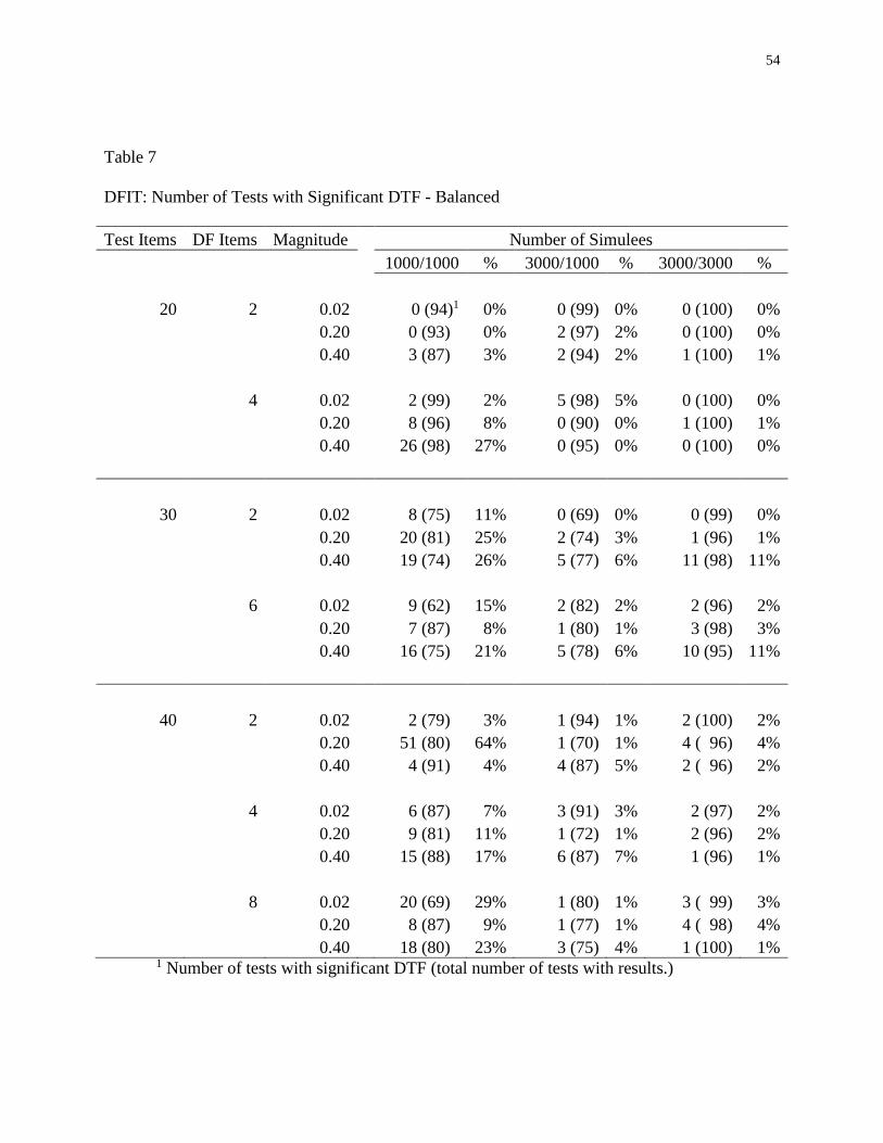
54
Table 7
DFIT: Number of Tests with Significant DTF - Balanced
Test Items DF Items Magnitude
Number of Simulees
1000/1000 % 3000/1000 % 3000/3000 %
20 2 0.02
0 (94)1 0% 0 (99) 0% 0 (100) 0%
0.20
0 (93)1 0% 2 (97) 2% 0 (100) 0%
0.40
3 (87)1 3% 2 (94) 2% 1 (100) 1%
4 0.02
2 (99)1 2% 5 (98) 5% 0 (100) 0%
0.20
8 (96)1 8% 0 (90) 0% 1 (100) 1%
0.40
26 (98)1 27% 0 (95) 0% 0 (100) 0%
30 2 0.02
8 (75)1 11% 0 (69) 0% 0 (99) 0%
0.20
20 (81)1 25% 2 (74) 3% 1 (96) 1%
0.40
19 (74)1 26% 5 (77) 6% 11 (98) 11%
6 0.02
9 (62)1 15% 2 (82) 2% 2 (96) 2%
0.20
7 (87)1 8% 1 (80) 1% 3 (98) 3%
0.40
16 (75)1 21% 5 (78) 6% 10 (95) 11%
40 2 0.02
2 (79)1 3% 1 (94) 1% 2 (100) 2%
0.20
51 (80)1 64% 1 (70) 1% 4 ( 96) 4%
0.40
4 (91)1 4% 4 (87) 5% 2 ( 96) 2%
4 0.02
6 (87)1 7% 3 (91) 3% 2 (97) 2%
0.20
9 (81)1 11% 1 (72) 1% 2 (96) 2%
0.40
15 (88)1 17% 6 (87) 7% 1 (96) 1%
8 0.02
20 (69)1 29% 1 (80) 1% 3 ( 99) 3%
0.20
8 (87)1 9% 1 (77) 1% 4 ( 98) 4%
0.40
18 (80)1 23% 3 (75) 4% 1 (100) 1% 1 Number of tests with significant DTF (total number of tests with results.)
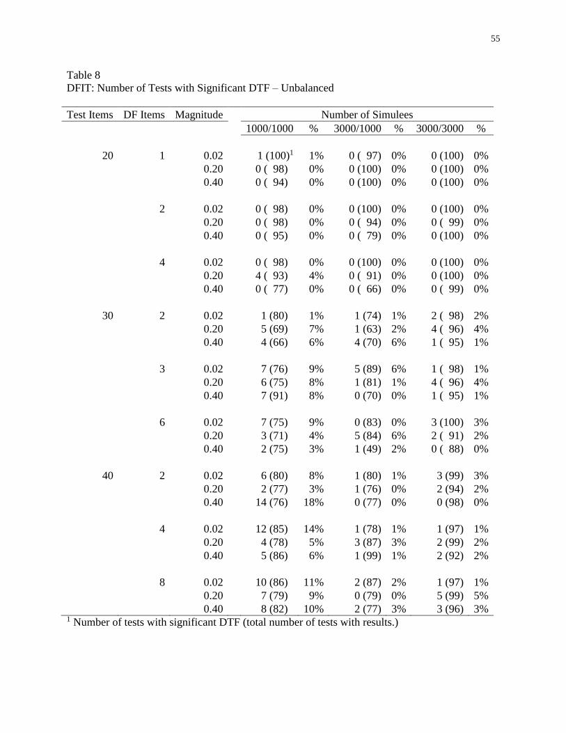
55
Table 8
DFIT: Number of Tests with Significant DTF – Unbalanced
Test Items DF Items Magnitude
Number of Simulees
1000/1000 % 3000/1000 % 3000/3000 %
20 1 0.02
1 (100)1 1% 0 ( 97) 0% 0 (100) 0%
0.20
0 ( 98)1 0% 0 (100) 0% 0 (100) 0%
0.40
0 ( 94)1 0% 0 (100) 0% 0 (100) 0%
2 0.02
0 ( 98)1 0% 0 (100) 0% 0 (100) 0%
0.20
0 ( 98)1 0% 0 ( 94) 0% 0 ( 99) 0%
0.40
0 ( 95)1 0% 0 ( 79) 0% 0 (100) 0%
4 0.02
0 ( 98)1 0% 0 (100) 0% 0 (100) 0%
0.20
4 ( 93)1 4% 0 ( 91) 0% 0 (100) 0%
0.40
0 ( 77)1 0% 0 ( 66) 0% 0 ( 99) 0%
30 2 0.02
1 (80)1 1% 1 (74) 1% 2 ( 98) 2%
0.20
5 (69)1 7% 1 (63) 2% 4 ( 96) 4%
0.40
4 (66)1 6% 4 (70) 6% 1 ( 95) 1%
3 0.02
7 (76)1 9% 5 (89) 6% 1 ( 98) 1%
0.20
6 (75)1 8% 1 (81) 1% 4 ( 96) 4%
0.40
7 (91)1 8% 0 (70) 0% 1 ( 95) 1%
6 0.02
7 (75)1 9% 0 (83) 0% 3 (100) 3%
0.20
3 (71)1 4% 5 (84) 6% 2 ( 91) 2%
0.40
2 (75)1 3% 1 (49) 2% 0 ( 88) 0%
40 2 0.02
6 (80)1 8% 1 (80) 1% 3 (99) 3%
0.20
2 (77)1 3% 1 (76) 0% 2 (94) 2%
0.40
14 (76)1 18% 0 (77) 0% 0 (98) 0%
4 0.02
12 (85)1 14% 1 (78) 1% 1 (97) 1%
0.20
4 (78)1 5% 3 (87) 3% 2 (99) 2%
0.40
5 (86)1 6% 1 (99) 1% 2 (92) 2%
8 0.02
10 (86)1 11% 2 (87) 2% 1 (97) 1%
0.20
7 (79)1 9% 0 (79) 0% 5 (99) 5%
0.40 8 (82)1 10% 2 (77) 3% 3 (96) 3% 1 Number of tests with significant DTF (total number of tests with results.)
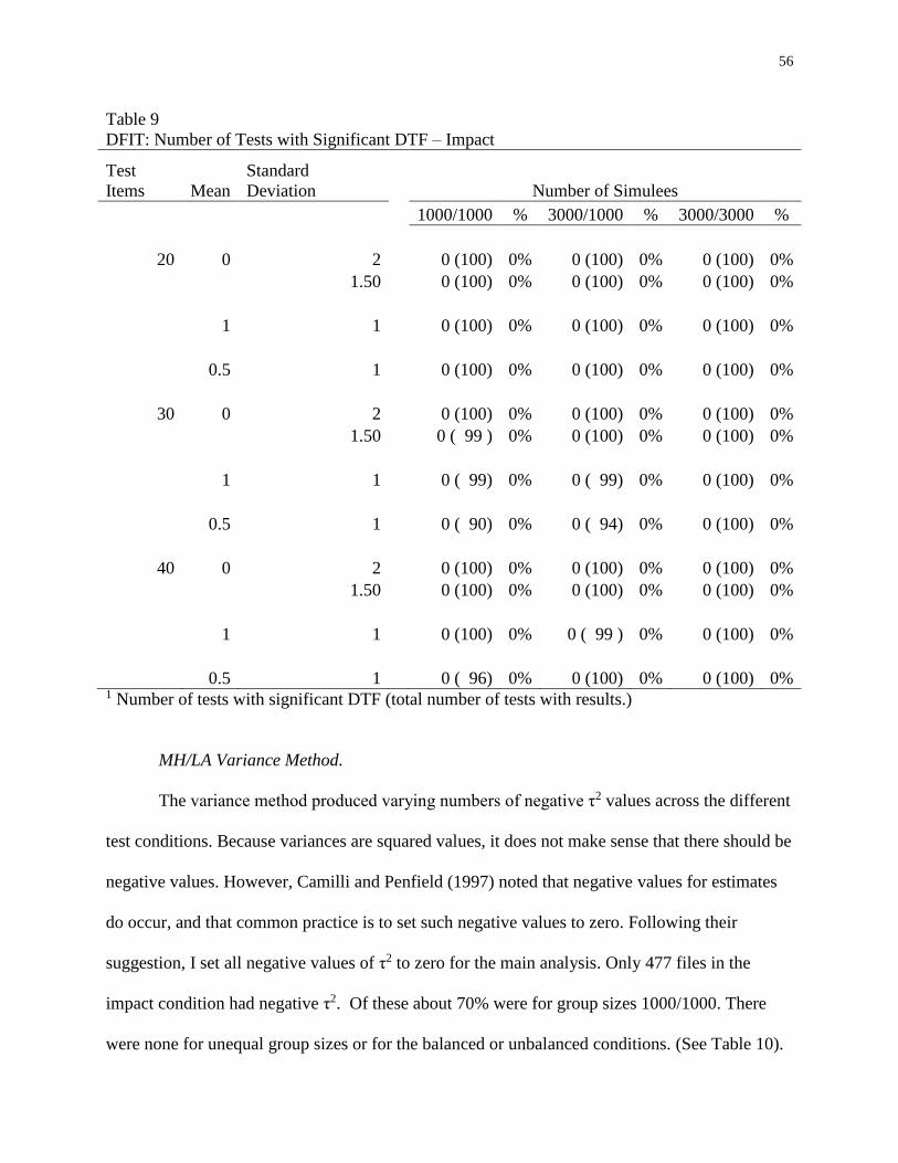
56
Table 9
DFIT: Number of Tests with Significant DTF – Impact
Test
Items Mean
Standard
Deviation
Number of Simulees
1000/1000 % 3000/1000 % 3000/3000 %
20 0 2
0 (100) 0% 0 (100) 0% 0 (100) 0%
1.50
0 (100) 0% 0 (100) 0% 0 (100) 0%
1 1
0 (100) 0% 0 (100) 0% 0 (100) 0%
0.5 1
0 (100) 0% 0 (100) 0% 0 (100) 0%
30 0 2
0 (100) 0% 0 (100) 0% 0 (100) 0%
1.50
0 ( 99 ) 0% 0 (100) 0% 0 (100) 0%
1 1
0 ( 99) 0% 0 ( 99) 0% 0 (100) 0%
0.5 1
0 ( 90) 0% 0 ( 94) 0% 0 (100) 0%
40 0 2
0 (100) 0% 0 (100) 0% 0 (100) 0%
1.50
0 (100) 0% 0 (100) 0% 0 (100) 0%
1 1
0 (100) 0% 0 ( 99 ) 0% 0 (100) 0%
0.5 1 0 ( 96) 0% 0 (100) 0% 0 (100) 0% 1 Number of tests with significant DTF (total number of tests with results.)
MH/LA Variance Method.
The variance method produced varying numbers of negative τ2 values across the different
test conditions. Because variances are squared values, it does not make sense that there should be
negative values. However, Camilli and Penfield (1997) noted that negative values for estimates
do occur, and that common practice is to set such negative values to zero. Following their
suggestion, I set all negative values of τ2 to zero for the main analysis. Only 477 files in the
impact condition had negative τ2. Of these about 70% were for group sizes 1000/1000. There
were none for unequal group sizes or for the balanced or unbalanced conditions. (See Table 10).
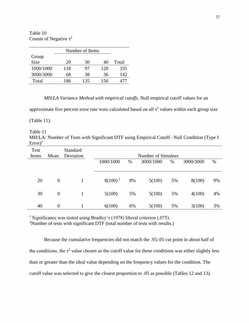
57
Table 10
Counts of Negative τ2
Number of Items
Group
Size 20 30 40 Total
1000/1000 118 97 120 335
3000/3000 68 38 36 142
Total 186 135 156 477
MH/LA Variance Method with empirical cutoffs. Null empirical cutoff values for an
approximate five percent error rate were calculated based on all τ2 values within each group size
(Table 11).
Table 11
MH/LA: Number of Tests with Significant DTF using Empirical Cutoff– Null Condition (Type I
Error)1
Test
Items Mean
Standard
Deviation Number of Simulees
1000/1000 % 3000/1000 % 3000/3000 %
20 0 1 8(100) 2 8% 5(100) 5% 8(100) 9%
30 0 1 5(100)1 5% 5(100) 5% 4(100) 4%
40 0 1 6(100)1 6% 5(100) 5% 3(100) 3%
1 Significance was tested using Bradley’s (1978) liberal criterion (.075). 2Number of tests with significant DTF (total number of tests with results.)
Because the cumulative frequencies did not match the .95/.05 cut point in about half of
the conditions, the τ2 value chosen as the cutoff value for these conditions was either slightly less
than or greater than the ideal value depending on the frequency values for the condition. The
cutoff value was selected to give the closest proportion to .05 as possible (Tables 12 and 13).
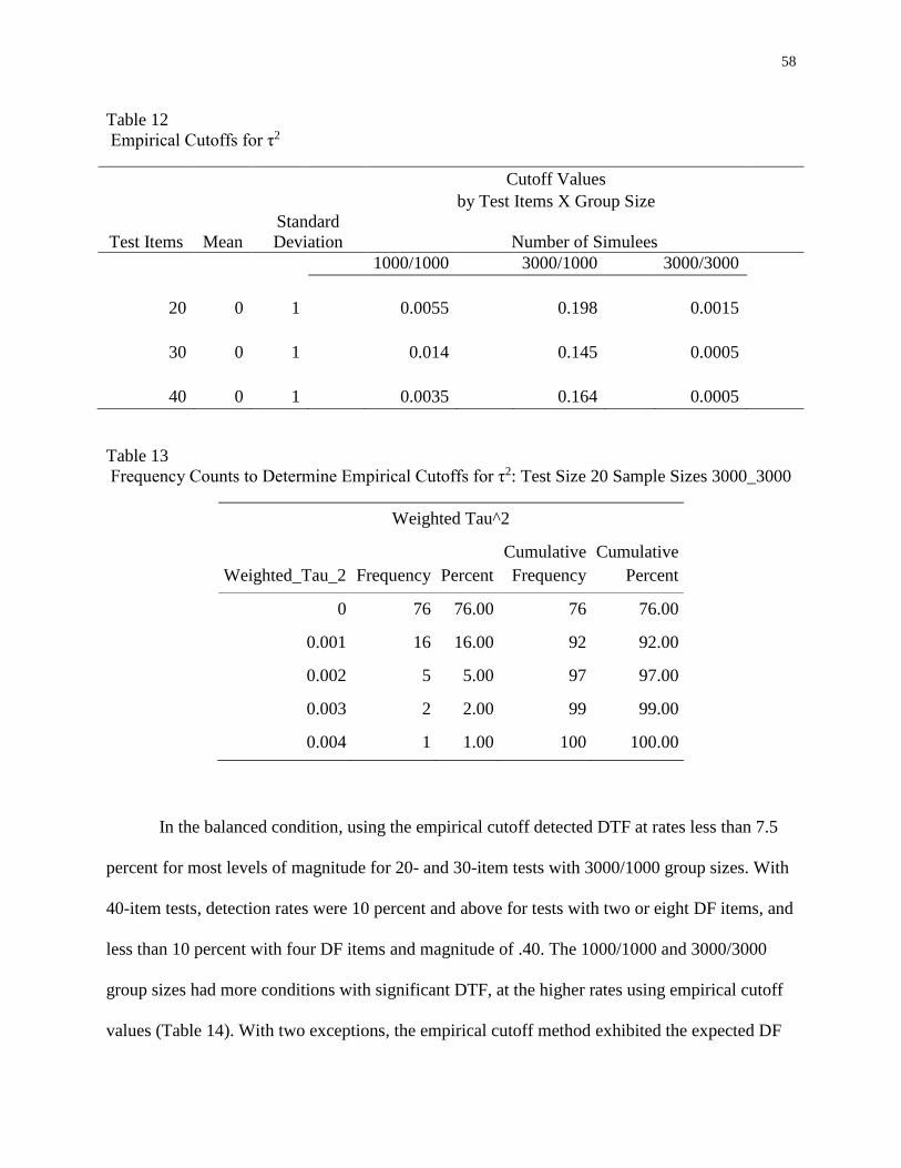
58
Table 12
Empirical Cutoffs for τ2
Cutoff Values
by Test Items X Group Size
Test Items Mean
Standard
Deviation Number of Simulees
1000/1000 3000/1000 3000/3000
20 0 1 0.0055 0.198 0.0015
30 0 1 0.014 0.145 0.0005
40 0 1 0.0035 0.164 0.0005
Table 13
Frequency Counts to Determine Empirical Cutoffs for τ2: Test Size 20 Sample Sizes 3000_3000
Weighted Tau^2
Weighted_Tau_2 Frequency Percent
Cumulative
Frequency
Cumulative
Percent
0 76 76.00 76 76.00
0.001 16 16.00 92 92.00
0.002 5 5.00 97 97.00
0.003 2 2.00 99 99.00
0.004 1 1.00 100 100.00
In the balanced condition, using the empirical cutoff detected DTF at rates less than 7.5
percent for most levels of magnitude for 20- and 30-item tests with 3000/1000 group sizes. With
40-item tests, detection rates were 10 percent and above for tests with two or eight DF items, and
less than 10 percent with four DF items and magnitude of .40. The 1000/1000 and 3000/3000
group sizes had more conditions with significant DTF, at the higher rates using empirical cutoff
values (Table 14). With two exceptions, the empirical cutoff method exhibited the expected DF
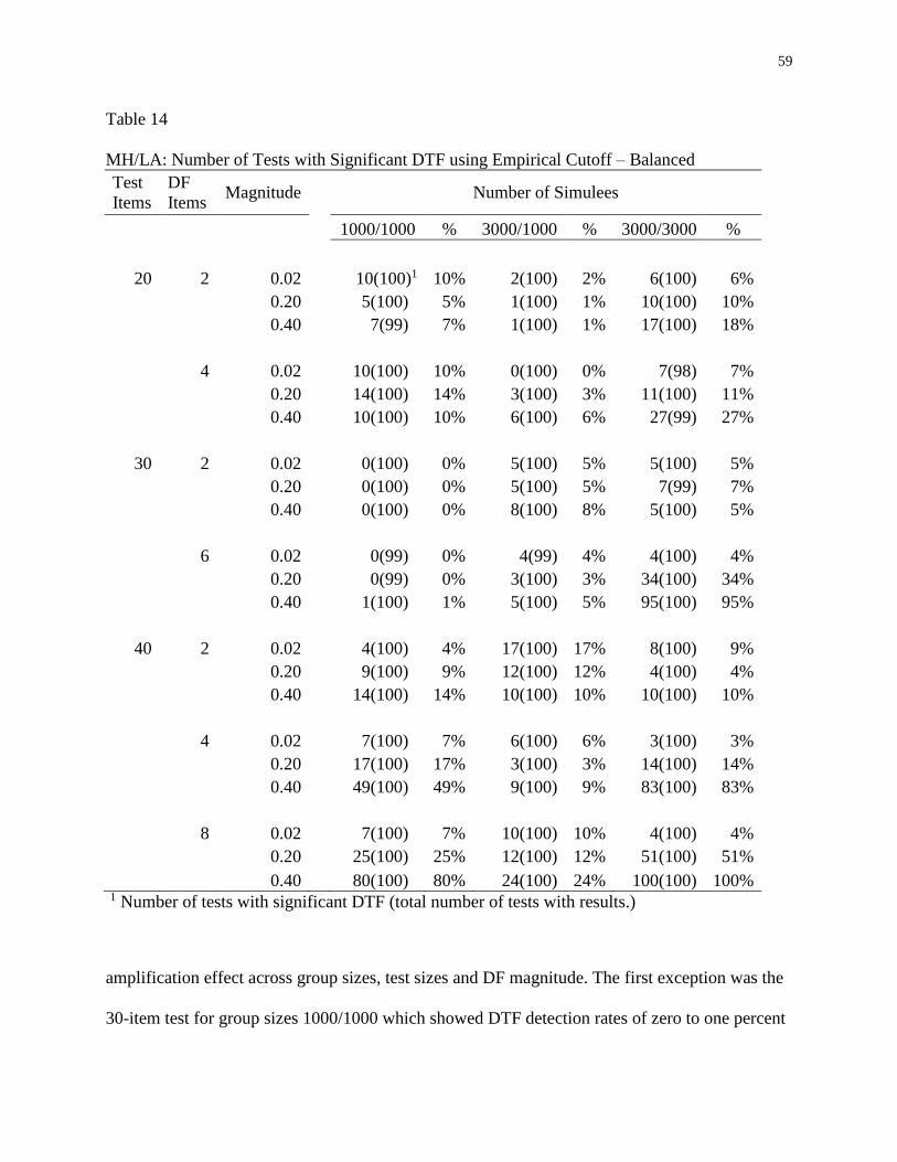
59
Table 14
MH/LA: Number of Tests with Significant DTF using Empirical Cutoff – Balanced
Test
Items
DF
Items Magnitude
Number of Simulees
1000/1000 % 3000/1000 % 3000/3000 %
20 2 0.02
10(100)1 10% 2(100) 2% 6(100) 6%
0.20
5(100)1 5% 1(100) 1% 10(100) 10%
0.40
7(99)1 7% 1(100) 1% 17(100) 18%
4 0.02
10(100)1 10% 0(100) 0% 7(98) 7%
0.20
14(100)1 14% 3(100) 3% 11(100) 11%
0.40
10(100)1 10% 6(100) 6% 27(99) 27%
30 2 0.02
0(100)1 0% 5(100) 5% 5(100) 5%
0.20
0(100)1 0% 5(100) 5% 7(99) 7%
0.40
0(100)1 0% 8(100) 8% 5(100) 5%
6 0.02
0(99)1 0% 4(99) 4% 4(100) 4%
0.20
0(99)1 0% 3(100) 3% 34(100) 34%
0.40
1(100)1 1% 5(100) 5% 95(100) 95%
40 2 0.02
4(100)1 4% 17(100) 17% 8(100) 9%
0.20
9(100)1 9% 12(100) 12% 4(100) 4%
0.40
14(100)1 14% 10(100) 10% 10(100) 10%
4 0.02
7(100)1 7% 6(100) 6% 3(100) 3%
0.20
17(100)1 17% 3(100) 3% 14(100) 14%
0.40
49(100)1 49% 9(100) 9% 83(100) 83%
8 0.02
7(100)1 7% 10(100) 10% 4(100) 4%
0.20
25(100)1 25% 12(100) 12% 51(100) 51%
0.40 80(100)1 80% 24(100) 24% 100(100) 100%
1 Number of tests with significant DTF (total number of tests with results.)
amplification effect across group sizes, test sizes and DF magnitude. The first exception was the
30-item test for group sizes 1000/1000 which showed DTF detection rates of zero to one percent
60
for all conditions. These rates were much smaller than the comparable rates for 20-item tests.
The second exception was that twenty-item tests showed unexpectedly large amounts of DTF for
magnitude .02.
For the unbalanced condition, using the empirical cutoff method detected DTF for the
3000/1000 group sizes exceeding the liberal criterion of 7.5 percent in only three conditions, all
for 40-item tests. These rates overall were smaller than those detected for the 1000/1000 and the
3000/3000 group sizes. The detection rates for the 1000/1000 and the 3000/3000 group sizes
were similar to those of the balanced condition. The 30-item tests for group sizes 1000/1000 also
presented the anomalous pattern of negligible DTF detection rates (Table 15).
Using the empirical cutoff values with the impact condition produced Type I error rates at
unacceptably high levels except for three cases for the 30-item tests with group sizes 1000/1000,
and for six cases in the 3000/1000 group sizes for the zero mean difference in each test size
(Table 16).
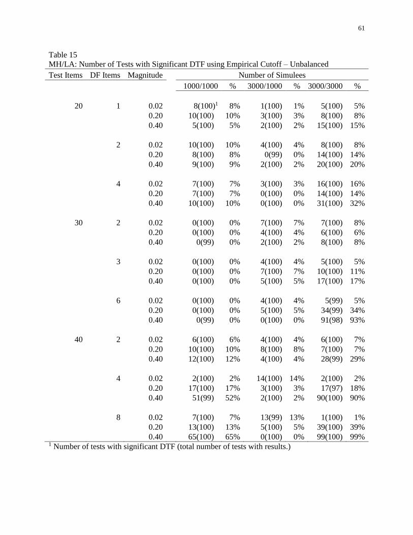
61
Table 15
MH/LA: Number of Tests with Significant DTF using Empirical Cutoff – Unbalanced
Test Items DF Items Magnitude
Number of Simulees
1000/1000 % 3000/1000 % 3000/3000 %
20 1 0.02
8(100)1 8% 1(100) 1% 5(100) 5%
0.20
10(100)1 10% 3(100) 3% 8(100) 8%
0.40
5(100)1 5% 2(100) 2% 15(100) 15%
2 0.02
10(100)1 10% 4(100) 4% 8(100) 8%
0.20
8(100)1 8% 0(99) 0% 14(100) 14%
0.40
9(100)1 9% 2(100) 2% 20(100) 20%
4 0.02
7(100)1 7% 3(100) 3% 16(100) 16%
0.20
7(100)1 7% 0(100) 0% 14(100) 14%
0.40
10(100)1 10% 0(100) 0% 31(100) 32%
30 2 0.02
0(100)1 0% 7(100) 7% 7(100) 8%
0.20
0(100)1 0% 4(100) 4% 6(100) 6%
0.40
0(99)1 0% 2(100) 2% 8(100) 8%
3 0.02
0(100)1 0% 4(100) 4% 5(100) 5%
0.20
0(100)1 0% 7(100) 7% 10(100) 11%
0.40
0(100)1 0% 5(100) 5% 17(100) 17%
6 0.02
0(100)1 0% 4(100) 4% 5(99) 5%
0.20
0(100)1 0% 5(100) 5% 34(99) 34%
0.40
0(99)1 0% 0(100) 0% 91(98) 93%
40 2 0.02
6(100)1 6% 4(100) 4% 6(100) 7%
0.20
10(100)1 10% 8(100) 8% 7(100) 7%
0.40
12(100)1 12% 4(100) 4% 28(99) 29%
4 0.02
2(100)1 2% 14(100) 14% 2(100) 2%
0.20
17(100)1 17% 3(100) 3% 17(97) 18%
0.40
51(99)1 52% 2(100) 2% 90(100) 90%
8 0.02
7(100)1 7% 13(99) 13% 1(100) 1%
0.20
13(100)1 13% 5(100) 5% 39(100) 39%
0.40
65(100)1 65% 0(100) 0% 99(100) 99% 1 Number of tests with significant DTF (total number of tests with results.)
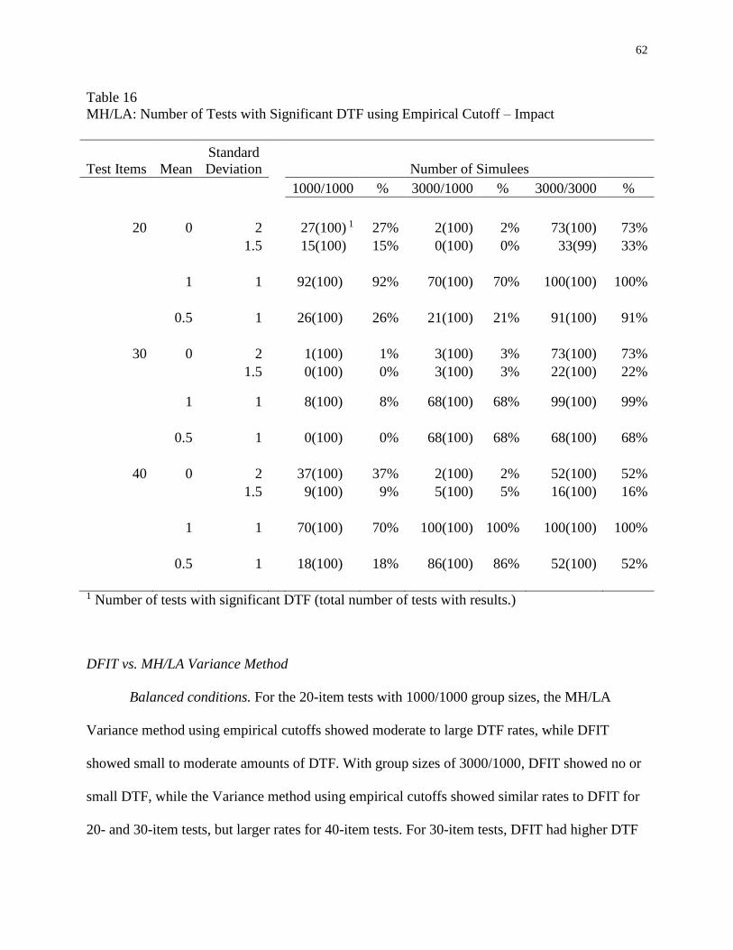
62
Table 16
MH/LA: Number of Tests with Significant DTF using Empirical Cutoff – Impact
Test Items Mean
Standard
Deviation
Number of Simulees
1000/1000 % 3000/1000 % 3000/3000 %
20 0 2
27(100) 1 27% 2(100) 2% 73(100) 73%
1.5
15(100)1 15% 0(100) 0% 33(99) 33%
1 1
92(100) 1 92% 70(100) 70% 100(100) 100%
0.5 1
26(100) 1 26% 21(100) 21% 91(100) 91%
30 0 2
1(100) 1 1% 3(100) 3% 73(100) 73%
1.5
0(100) 1 0% 3(100) 3% 22(100) 22%
1 1
8(100) 1 8% 68(100) 68% 99(100) 99%
0.5 1
0(100) 1 0% 68(100) 68% 68(100) 68%
40 0 2
37(100) 1 37% 2(100) 2% 52(100) 52%
1.5
9(100) 1 9% 5(100) 5% 16(100) 16%
1 1
70(100) 1 70% 100(100) 100% 100(100) 100%
0.5 1
18(100) 1 18% 86(100) 86% 52(100) 52%
1 Number of tests with significant DTF (total number of tests with results.)
DFIT vs. MH/LA Variance Method
Balanced conditions. For the 20-item tests with 1000/1000 group sizes, the MH/LA
Variance method using empirical cutoffs showed moderate to large DTF rates, while DFIT
showed small to moderate amounts of DTF. With group sizes of 3000/1000, DFIT showed no or
small DTF, while the Variance method using empirical cutoffs showed similar rates to DFIT for
20- and 30-item tests, but larger rates for 40-item tests. For 30-item tests, DFIT had higher DTF
63
detection rates than the MH/LA Variance method for the 1000/1000 group sizes, but much lower
rates for the 3000/1000 and 3000/3000 group sizes. Results for the 40-item tests were similar to
those for the 30 item tests.
Unbalanced conditions. DFIT had smaller percentages of significant DTF for all
conditions of 20-item tests when compared to the variance method. For 30-item tests DFIT had
larger rates of DTF with group sizes 1000/1000 than the variance method, and similar rates to the
variance method with group sizes 3000/1000. DFIT had smaller rates with group sizes
3000/3000 than the variance method. For 40-item tests, DFIT produced smaller rates of DTF for
all cases of group sizes 3000/1000 and 3000/3000 than the variance method with either type of
cutoff. DFIT produced similar rates as the variance method using empirical cutoffs for group
sizes 1000/1000.
Impact conditions. DFIT produced smaller percentages of DTF across all conditions for
all test sizes than the variance method. This indicates that equating is resolving the distributional
differences between the reference and focal groups for DFIT, while the MH/LA variance method
identifies them as DTF.
64
CHAPTER 5
DISCUSSION
Comparing different methods of detecting DF under different conditions is a commonly
used technique (Drasgow, 1987; Li & Stout, 1996; Raju, Drasgow, & Slinde, 1993; Wipasillapa,
n.d.; Zumbo, 2003) that permits benchmarking different methods to see whether any method has
a relative advantage under the conditions tested. Additionally, this helps verify whether a new
method performs at least as well as existing methods. Knowledge of the strengths and
weaknesses of different detection methods helps practitioners to select the most appropriate one
for their data analyses.
The Mantel-Haenszel/Liu-Agresti (MH/LA) variance method has not been compared
with any other method of calculating DTF. This study, comparing it with an established method,
helps to situate it among the existing methods of DF detection. This comparison also helps to
understand variance methods of evaluating differential functioning, and aids in understanding
whether, and to what extent, these methods may be used to verify a null hypothesis of DTF not
being present (Penfield & Algina, 2006).
Three major conditions were modeled in this study: (1) items in which DF was divided
equally between the reference and focal groups; (2) items in which DF was inserted only in the
focal group, and (3) items without DF, but in which the reference and focal groups differed on
their distribution characteristics (mean and standard deviation). Data for these three conditions
were processed using two different methods of DTF detection: DFIT (Raju, van der Linden, &
65
Fleer, 1995) as implemented in the DIFCUT program (Nanda, Oshima, & Gagne, 2006) and a
variance method based on the MH/LA contingency table model (Camilli & Penfield, 1997;
Penfield & Algina, 2006) as implemented in DIFAS 5.0 (Penfield, 2005). Results derived from
these two methods were expected to differ because of their differing approaches to modeling
DTF. DFIT models DTF as a sum of the signed DIF for each item. The variance method models
DTF as a sum of the unsigned DIF variances (Camilli & Penfield, 1997). Thus, Penfield and
Algina indicate that small amounts of DIF may add up to indicate large effects in overall DTF,
but cancellation cannot exist.
DFIT. In DFIT, the null condition which had no embedded DIF, and the same
distribution, ~N (0, 1) showed DTF in excess of Bradley’s liberal 7.5 percent criterion in two
conditions. This supports Petroski’s (2005) finding of high Type I error rates for DFIT.
However, the fact that only two out of nine conditions showed Type I error suggests that these
present results may come from the randomness of the data generation process.
The impact condition had no DF added into the data. Therefore, the DTF indices should
not exhibit DTF, and none was found for the impact condition in DFIT. The probable cause for
no significant DTF’s being detected (i.e., desirable results) would be that the linking process was
very successful in putting the focal and reference groups on the same scale. Another possible
cause is that DFIT may have low sensitivity to the distributional differences included in this
study.
The balanced conditions showed a general increase of DTF detections from smaller levels
of magnitude to greater and from tests with fewer DF items to more DF items. This was as
expected given that there is a greater likelihood for the occurrence of amplification with higher
levels of DF and more items over which to accumulate it. Similar patterns were found for the
66
unbalanced condition. An unexpected finding was that group sizes of 1000/1000 had much
higher rates of DTF detection than both group sizes of 3000/1000 and of 3000/3000. Greater
amounts of DTF would be expected in the larger group sizes, because there is more opportunity
for DF to occur. This finding could be related to DFIT’s known inaccuracies with small sample
sizes. However, all group sizes were greater than recommendations in the literature, which are
for greater than 200 examines per group with the 1PL model, greater than 500 examinees with
the 2PL model and greater than 1,000 examinees with the 3PL model (Oshima & Morris, 2008).
A broader comparison of the balanced and unbalanced conditions shows several
unexpected patterns. Contrary to expectations, the balanced condition had higher rates of
identified DTF than the unbalanced condition. In about half of the cases, the balanced condition
produced rates over twice as large as the unbalanced condition. Generated parameters were
verified to ensure that DIF magnitude was correctly assigned to both the reference and focal
groups. This indicates that DF amplification and cancellation may not be functioning as
expected in DFIT.
Group sizes 1000/1000 were problematic. For most conditions, group sizes 1000/1000
exhibited over twice as much DTF as the other two group sizes. Similarly, trivial DF magnitude
(.02) showed unexpectedly high levels of DTF. These levels were frequently greater than those
for magnitude .20, and occasionally greater than those for magnitude .40. Almost all of this was
within group sizes 1000/1000. I can find no explanation for these two occurrences.
For both the balanced and the unbalanced conditions with unequal sample sizes, rates of
DTF were all within Bradley’s liberal rate of 7.5 percent. Blitz and Morris (2011), investigating
the Item Parameter Replication (IPR) method, the method that DFIT uses to detect significance,
found that for a reference group larger than the focal group under conditions of no DIF the Type
67
I error rate was lower than expected. This characteristic should under identify DTF when the
reference group is larger than the focal group. This appears to be what happened in the current
study with 3000 reference group size and 1000 focal group size. Thus, it is reasonable to expect
that the observed rate of DTF would have been larger had separately estimated covariance files
for both the focal and reference groups been used.
MH/LA Variance. An empirical cutoff method of determining significance for the
MH/LA variance method was evaluated. In determining the cutoff points for the empirical
cutoff method, both sample sizes and test sizes should be considered. Cutoff points were
calculated in two ways: 1) using sample sizes only, and 2) using test sizes crossed with sample
sizes. Data was processed using both methods. A comparison of the two results showed that
using cutoffs calculated using sample sizes only can put all of the detected DTF within a single
test size. Whereas cutoffs calculated using test size crossed with sample size put approximately
five percent of DTF in each test x sample size group. Once appropriate cutoffs have been
determined, the empirical cutoff method seems to work reasonably well as a method of
evaluating the relative importance of the results of the different methods. The empirical cutoff
method of significance testing showed consistent DTF detection rates among all three sample
size groups. Still, there is sensitivity to sample size, with more DTF being shown for those
conditions with more simulees. Rates of DTF detection were consistently high for samples with
distributional differences. Only eight out of 36 conditions showed DTF at less than the liberal
7.5% rate.
Overall, the MH/LA method showed elevated rates of DTF detection. This is not
unexpected in that it deals only with positive values (the τ2 variances), which allows for DIF
amplification, but not for DIF cancellation (Camilli & Penfield, 1997). It is also sensitive to
68
distributional differences between the studied groups. Because of this, comparisons of the score
distributions for each of the studied groups need to be done to ensure their comparability before
using the MH/LA method.
Comparison.
DFIT and the MH/LA variance method measure DTF in different ways, so are not strictly
comparable, but are useful for different objectives. As such they may be considered
complementary. Because the MH/LA variance method cannot offset DF for the Reference group
against DF for the Focal group, it is not able to provide a picture of whether a test is fair overall
to examinees, but only an indication of how much DF exists for all groups. By doing this, it can
serve as a preliminary indicator of whether an in depth DIF study needs to be conducted,
especially for a newly developed instrument, or one used for a new purpose, such as a test
normed on a national population being used for immigrants with limited cultural or language
familiarity to those of the norm group.
DFIT is a summative method of DTF evaluation. Where DIF favoring one group may
have positive values, DIF favoring the other group would have negative values. By combining
the positive and the negative values, DFIT is able to derive an estimate of whether the instrument
as a whole favors one group over the other. Where no group has an advantage at the test level,
the need for a DIF study is obviated.
Practical Implications
A concern among applied researchers is “Which method should I use?” Both DFIT and
the Variance method as implemented in DIFAS (Penfield, 2005) have been used in applied
studies across different content areas and in cross-cultural studies. Both methods have been used
to assess translated versions of different instruments (Ellis, & Mead, 2000; Guerrero 2001; He &
69
Wolf, 2010; Morales, Flowers, Gutierrez, Kleinman, & Teresi, 2006; Price and Oshima, 1998;
van den Broeck Bastiaansen, Rossi, Dierckx, and De Clercq, 2013; and Wang, and Russell,
2005). In the area of industrial and organizational psychology, Baker, Caison, and Meade (2007)
used DFIT to study a test for predicting college student attrition. (Also see Braddy, Meade, &
Johnson, 2006; Maurer, Raju, & Collins, 1998; Meriac, Poling, & Woehr, 2009; Meriac, Woehr,
& Banister, 2010; O’Brien, 2007; O’Brien & LaHuis, 2011; and Wang, & Russell, 2005.) In the
area of mental health, Cameron, Crawford, Lawton, & Reid, 2013; Kim, Pilkonis, Frank, Thase,
and Reynolds (2002); van den Broeck Bastiaansen, Rossi, Dierckx, and De Clercq (2013) have
made contributions. In other areas, Donovan and Drasgow (1999) used DFIT to look at a survey
to measure experiences of sexual harassment; Wipasillapa (n.d.) used DFIT to assess DTF in a
mathematics test; and using DIFAS, Baer, Samuel, & Lykins,(2011), and Van Dam, Earleywine,
and Danoff-Burg (2009) studied a questionnaire to assess mindfulness.
Because either method is suited for such a wide range of content areas, selecting a
method becomes a question of the conditions of the research and the data. DFIT requires a large
number of observations (at least 200 per group for a 1PL model; Oshima & Morris, 2008). The
variance method, implemented in DIFAS 4.0 (Penfield, 2007) will work with small sample sizes
(Ferne & Rupp, 2007; Lai, Teresi, & Gershon, 2005). Baer and her colleagues (2011) had a total
sample of 230 participants. Van Dam (Van Dam, et al., 2009) and van den Broeck (van den
Broeck, et al., 2013) both had sample sizes of less than 500. The model fitted to the data is also
a concern. Like other contingency table models, the variance method works with 1PL, and 2PL
without crossing DIF models. It will not handle data with crossing DF (Millsap & Everson,
1993), 3-PL models, or multidimensional data. However, DFIT can handle those kinds of data
70
(Oshima, et al., 1997), but requires large sample sizes for adequate parameter estimation
(Oshima & Morris, 2008).
Penfield and Algina (2006) state that testing for significance is not appropriate with the
variance method . However, Baer (Baer, et al., 2011), apparently ignoring Penfield and Algina’s
guidance, affirm that, for a subset of the instrument, the DTF indicator was “nonsignificant” (p.
7). In lieu of effect size, Penfield and Algina have suggested an indicator of DTF magnitude
based on the number of items exhibiting moderate to large DIF as described by the ETS scale,
where 25% or more of the items in an assessment exhibit moderate or large DIF, then assessment
as a whole exhibits a large amount of DIF. Determination of this effect size requires that a DIF
analysis be run in addition to the DTF analysis. DIFAS can process small sample sizes, although
results may be unstable (Zwick, et al., 2012). DFIT has an established test of statistical
significance (Oshima, et al., 2006) and an effect size for NCDIF, but needs an effect size
indicator for CDIF and DTF (Wright, 2011).
Because DFIT and DIFAS analyze data differently, and provide answers to different
questions, the requirements of the two programs should not be a concern in selecting which one
to use. However, given that the requirements of the study have been defined, knowledge of the
requirements of the selected program is needed. DIFAS is a Windows® based application,
available from author without charge. It has a user friendly, point and click GUI interface. Data
input files require simple formatting before entry. DIFAS runs very quickly (seconds for a single
file), but running many files requires much operator intervention, because, DIFAS cannot be
automated to process large numbers of files, as in a simulation study.
As a program, DFIT exists in three forms: DFIT8 (Raju, Oshima, & Wolach, 2009), R
package DFIT (Cervantes, 2014) available from CRAN, and the SAS® program DIFCUT (the
71
form used in this study; Nanda, et al., 2006) available from the author. DFIT requires
preprocessing to obtain item parameters and to link files from different groups to a common
scale, before it can be run. Once DFIT has run, the linking process and DFIT processing must be
run a second time to ensure correct estimation of DF (Oshima & Morris, 1998).
DFIT is computationally intensive because of the IPR method (Oshima, et al., 2006) that
calculates the cutoff levels used to determine statistical significance. Because of this, DFIT takes
minutes to run a file that requires seconds to run by DIFAS. In situations where many files need
to be run sequentially, the required time can be weeks depending on the number of items in the
assessment, and the sample size being processed. DIFCUT, which is written in SAS/IML®, is
easily modifiable to test extensions of the DFIT model, and is easy to run as a macro program
where many files need to be processed in sequence.
Limitations/Problems
As with all studies, this one has its limitations. The first is that the distribution of the
variance estimator (τ2) is not known. Until the distribution is determined, standard tests of
significance cannot be used. While the empirical cutoff methods for determining significant DTF
offers a potential method for determining significance, the number of replications used to
calculate the cutoff was small, 900 for each set of group sizes.
The type and manner of embedding DTF in the data is the next limitation. DIF was added
to the last items of each set of parameters. This was based on the assumption that DTF resulted
from multiple DIF items. Other methods of DTF generation could have been used by differing
the structure of the test: for example, generating data using parameters based on a
multidimensional model (Ackerman, 1989; Oshima, & Miller, 1992).
72
The large convergence problems in BILOG-MG3 caused the loss of a large amount of
data. Greater precision and reduced error rates may have been expected had all test data been
available. The version of DIFCUT used did not incorporate the suggestions of Blitz and Morris
(2011) to use separate covariance files for the reference and focal groups. Use of covariance files
generated for each group, instead of assuming that the covariances for the reference group are the
same as those for the focal group, increases the accuracy of the Type I error when the sample
sizes are unequal. This may have changed the error rate for the 3000/1000 sample size groups
that were noted in this study.
Future research
Future research in this area would include large simulation studies to evaluate the
distribution of τ2. Although the data from the current study indicated that τ2 may have an
approximate normal distribution, the uncertainty about the distribution expressed by Penfield and
Algina (2006), and the theoretical assertion by Penfield (2005) that τ2 is not normally distributed
warrant a detailed investigation into the distribution. In this regard, investigation into the
distribution of the log odds ratio (Camilli & Penfield, 1997) needs to be done. Once the
distribution is known, more exact and appropriate methods of evaluating significance6 can be
determined, as well as more precise methods of determining effect size (see Penfield & Algina).
Beyond distribution studies, investigation into the setting of empirical cutoff values of
significance using a large simulation (perhaps a Markov Chain Monte Carlo study) would be
useful. Studies comparing results of data created using different methods of embedding DF (such
as simple multidimensional , or multidimensional where the dimensions differ in strength or
quality among the different groups; see Sinharay & Holland, 2007 ), or where the data does not
6 Perhaps similar logic to the half-normal distribution that Raju (1990) proposed for area measures could be used to determine a Z-score for MH/LA variance
73
match the model could inform researchers decisions on appropriate methods of analysis when a
particular kind of DF is suspected by shedding light on how these analysis methods react to
different kinds of DF and to misfit data (such as 3-PL data which has non-zero asymptotes with a
1-PL model which expects asymptotes to be equal to zero, Rogers & Swaminathan, 1993).
Penfield and Algina (2006) offered a suggestion for effect size measures based on the
assumption of a normal distribution of τ2. However, these suggestions are tentative pending a
determination of the actual distribution of τ2. Wright (2011) has begun investigation of effect
size in DFIT, but to date this is limited to non-compensatory DIF, and needs to be expanded to
DTF. A comparison of effect sizes between these methods must wait for these two lines of
research.
While DFIT handles the three models (1PL, 2PL and 3PL) of dichotomous data, plus
models of polytomous data, the MH/LA contingency table is strongest in processing 1PL data,
and works with 2PL data where there is no interaction of the discrimination parameter (θ) with
examinee skill level, that is, there are no crossing ICCs. The current study used a 3PL model
with the guessing parameter fixed—basically a 2PL model. In addition, no skill level (θ)
interaction was incorporated into the discrimination parameter. While this meets the minimum
requirements of the MH/LA method, it would be worthwhile to repeat this study using data that
fits the 1PL model and to compare it with data that fits the 2PL model without crossing.
The DFIT data needs to be rerun using separate covariance files for the reference and
focal groups. These were both estimated in the current study, so only modifications to DIFCUT
(Nanda et al., 2006) to read both files would need to be made, the data reprocessed, and the
outputs compared with the current study’s outputs. This would permit seeing the effect of the
new method on DTF.
74
Finally, more empirical studies using collected data need to be performed. These would
help to evaluate the usefulness of both methods of DTF detection in situations that actually
occur.
Summary. This study contributes to the literature in several ways. First, kernel plot
graphs of distributions of the τ2 DTF indicator from the MH/LA variance test give indications
that for equal group sizes this statistic may have and F-distribution, while for unequal group sizes
the kernel plots indicate a tendency towards normal. This indicates that τ2,may have a
distribution such that standard tests of significance may be used. Second, correlations of DTF
values between matched pairs of variance and DFIT results show at the most a weak correlations,
indicating that the two methods measure different things. They are, thus, not comparable, and
may be used in conjunction to gain greater insights into the data.
For the null condition with no embedded DF, DFIT produced Type I error within the
nominal rate for seven out of nine conditions. Smaller samples (1000 simulees in each of the
reference and focal groups) showed unexpectedly greater levels of DTF than the larger sample
sizes. Other than this, DFIT produced increasing amounts of DTF for tests with more items and
larger sample sizes. DFIT unexpectedly showed very low rates of DTF for the Impact condition,
where there was no embedded DF, but the distributions (mean and standard deviation) varied
between the reference and focal groups. This is probably because of the linking process.
The MH/LA variance method, like DFIT, generally produced less DTF at smaller test
sizes and sample sizes, with increasing rates as both test and sample sizes increased. This method
produced lower DTF detection rates for unequal sample sizes (3000 reference group, and 1000
focal group) than for the equal sample sizes. This was unexpected in that the variance method
allows only DF amplification. For the unbalanced condition where all DF was in the focal

75
(smaller) group, DTF rates similar to those of the 1000//1000 group sizes were expected, and for
the balanced condition where DF was embedded in both reference and focal groups, rates
between the two equal group sizes were expected. The variance method proved exceptionally
sensitive to the impact condition.
76
References
Ackerman, T. A. (1989). Unidimensional IRT calibration of compensatory and noncompensatory
multidimensional items. Applied Psychological Measurement, 13, 113-127.
Ackerman, T. (1996). Graphical representation of multidimensional item response theory
analyses. Applied Psychological Measurement, 20(4), 311-329. Retrieved February 9,
2008, from Sage Journals Online database.
Ackerman, T., Gierl, M. & Walker, C. (2003). Using multidimensional item response theory to
evaluate educational and psychological tests. Educational Measurement: Issues and
Practice, 22(3), 37-53.
American Educational Research Association, American Psychological Association, & National
Council on Measurement in Education. (1999). Standards for educational and
psychological testing. Washington, DC: Author.
Anastasi, A., & Urbina, S. (1996). Psychological Testing. Upper Saddle River, NJ: Prentice Hall.
Baer, R. A., Samuel, D. B., & Lykins, E. L. (2010). Differential item functioning on the Five
Facet Mindfulness Questionnaire is minimal in demographically matched meditators and
nonmeditators. Assessment, 18(1) 3–10.
Baker, B. A., Caison, A. L., & Meade, A. W. (2007). Assessing gender-related differential item
functioning and predictive validity with the institutional integration scale. Educational
and psychological measurement, 67(3), 545-559.
Bergson, B., Gershon, R., & Brown, W. (1993, April). Differential item functioning vs
differential test functioning. Paper presented at the annual meeting of the American
Education Research Association, Atlanta, GA.
Blitz, D. L., & Morris, S. B. (2011, April). Improving the accuracy of DFIT when sample sizes
77
are unequal. Paper presented at the 26th Annual Conference for the Society for Industrial
and Organizational Psychology, Chicago, IL.
Bock, D. (1997). A brief history of item theory. Educational Measurement: Issues and Practice,
16(4) 21-33.
Bolt, D., & Stout, W. (1996). Differential item functioning: Its multidimensional model and
resulting SIBTEST detection procedure. Behaviormetrika, 23(1) 67-95.
Braddy, P. W., Meade, A. W., & Johnson, E. C. (2006). Practical implications of using different
tests of measurement invariance for polytomous measures. In 21st Annual Conference of
the Society for Industrial and Organizational Psychology, Dallas, TX.
Bradley, J. V. (1978). Robustness? The British Journal of Mathematical and Statistical
Psychology, 31, 144-152.
Cameron, I. M., Crawford, J. R., Lawton, K., & Reid, I. C. (2013). Differential item functioning
of the HADS and PHQ-9: An investigation of age, gender and educational background in
a clinical UK primary care sample. Journal of affective disorders, 147(1), 262-268.
Camilli, G. (1993). The case against item bias detection techniques based on internal criteria: Do
item bias procedures obscure test fairness issues? In Paul W. Holland and Howard
Wainer (Eds.), Differential item functioning (pp. 397-417). Hillsdale, NJ: Erlbaum.
Camilli, G., & Penfield, D. (1997). Variance estimation for differential test functioning based on
Mantel-Haenszel statistics. Journal of Educational Measurement, 34, 123-139. Retrieved
March 11, 2008, from Blackwell Synergy Journals database.
Camilli, G., & Shepard, L. A. (1994). Methods for identifying biased test items. Thousand Oaks,
CA: Sage.
78
Cervantes, V. H. (2014). DFIT: An R package for the Differential Functioning of Items nd Tests
framework. Instituto Colombiano para la Evaluación de la Educación [ICFES], Bogotá,
Colombia.Clauser, B., & Mazor, K. (1998). Using statistical procedures to identify
differentially functioning test items. Educational Measurement: Issues and Practice,
17(1), 31-44.
Crocker, L., & Algina, J. (1986). Introduction to classical and modern test theory. Belmont, CA:
Wadsworth.
Cronbach, L. (1988). Five perspectives on the validity argument. In H. Wainer & H. I. Braun
(Eds.), Test validity, (pp. 129-145). Hillsdale, NJ: Erlbaum.
Donoghue, J. R., & Allen, N. L. (1993), Thin versus thick matching in the Mantel-Haenszel
procedure for detecting DIF. Journal of Educational Statistics, 18, 131-154.
Donovan, M. A., & Drasgow, F. (1999). Do men's and women's experiences of sexual
harassment differ? An examination of the differential test functioning of the Sexual
Experiences Questionnaire. Military Psychology, 11(3), 265-282.
Donovan, M. A., Drasgow, F., & Probst, T. M. (2000). Does computerizing paper-and-pencil job
attitude scales make a difference? New IRT analyses offer insight. Journal of Applied
Psychology, 85, 305-313.
Dorans, N., & Kulick, E. (1986). Demonstrating the utility of the standardization approach to
assessing unexpected differential item performance on the scholastic aptitude test.
Journal of Educational Measurement, 23, 355-368. Retrieved April 23, 2008, from
Blackwell Synergy Journals database.
Drasgow, F. (1987). Study of the measurement bias of two standardized psychological tests.
Journal of Applied Psychology, 72(1) 19-29.
79
Ellis, B. B., & Mead, A. D. (2000). Assessment of the measurement equivalence of a Spanish
translation of the 16PF questionnaire. Educational and Psychological Measurement, 60,
787-807.
Ellis, B., & Raju, N. (2003). Test and item bias: What they are, what they aren’t, and how to
measure them. In J. E. Wall & G. R. Walz (Eds.) Measuring Up: Assessment issues for
teachers, counselors, and administrators. (pp. 89-98). Greensboro, N.C.: CAPS.
Retrieved March 8, 2008 from EBSCOhost database. (ERIC Document Reproduction
Service No. ED480042)
Fan, X., Felsölvályi, A., Sivo, S., & Keenan, S. (2001). SAS for Monte Carlo Studies: A guide
for quantitative researchers. Cary, NC: SAS Institute.
Ferne, T., & Rupp, A. A. (2007). A Synthesis of 15 Years of Research on DIF in Language
Testing: Methodological Advances, Challenges, and Recommendations. Language
Assessment Quarterly, 4(2), 113–148.
Fesq, J. (1995). Variance measures of differential item functioning. Ed.D. dissertation, Rutgers
The State University of New Jersey - New Brunswick, United States -- New Jersey.
Retrieved March 9, 2010, from Dissertations & Theses: A&I. (Publication No. AAT
9524588).
Fidalgo, A., Hashimoto, K., Bartram, D., & Muñiz, J. (2007). Empirical Bayes versus standard
Mantel-Haenszel statistics for detecting differential item functioning under small sample
conditions. The Journal of Experimental Education, 75(4), 293-314.
Finch, H. (2005). The MIMIC model as a method for detecting DIF: Comparison with Mantel-
Haenszel, SIBTEST, and the IRT likelihood ratio. Applied Psychological Measurement,
29(4), 278-295.
80
Flora, D., Curran, P., Hussong, A., & Edwards, M. (2008). Incorporating measurement
nonequivalence in a cross-study latent growth curve analysis. Structural Equation
Modeling, 15, 676-704.
Flowers, C., Oshima, T. & Raju, N. (1999). A description and demonstration of the polytomous-
DFIT framework. Applied Psychological Measurement, 23(4), 309-326. Retrieved
October 17, 2007, from Sage Journals Online database.
Gagne, P., Furlow, C., & Ross, T. (2009). Increasing the number of replications in item response
theory simulations: Automation through SAS and disk operating system. Educational and
Psychological Measurement, 69(1), 79-84.
Garrett, P., (2009). A Monte Carlo study investigating missing data, differential item
functioning, and effect size (Doctoral dissertation, Georgia State University, 2009).
Educational Policy Studies Dissertations. Paper 35.
http://digitalarchive.gsu.edu/eps_diss/35.
Gierl, M., Bisanz, J., Bisanz, G., Boughton, K., & Khaliq, S. (2001). Illustrating the utility of
differential bundle functioning analyses to identify and interpret group differences on
achievement tests. Educational Measurement: Issues and Practice, 20(2), 26-36.
Gierl, M., Gotzmann, A., & Boughton, K. (2004). Performance of SIBTEST when the
percentage of DIF items is large. Applied Measurement in Education, 17(3), 241-264.
Retrieved January 21, 2008 from JSTOR database.
Guerrero, G. (2001). Measurement equivalence of English and Spanish versions of the Campbell
Interest and Skill Survey. (Doctoral dissertation, University of Texas at El Paso, 2001).
UMI – Dissertations Publishing, 3035097.
Güler, N., & Penfield, R. (2009). A comparison of the logistic regression and contingency table
81
methods for simultaneous detection of uniform and nonuniform DIF. Journal of
Educational Measurement, 46, 314-329.
Hambleton, R., Swaminathan, H., & Rogers, H. (1991). Fundamentals of item response theory.
Newbury Park: Sage.
Hanson, B. A., & Béguin, A. A. (2002). Obtaining a common scale for item response theory item
parameters using separate versus concurrent estimation in the common-item equating
design. Applied Psychological Measurement, 26(1), 32-24.
He, W., & Wolfe, E. W. (2010). Item equivalence in English and Chinese translation of a
cognitive development test for preschoolers. International Journal of Testing, 10(1), 80-
94.
Hidalgo, M. D., & López-Pina, J. A. (2004). Differential item functioning detection and effect
size: A comparison between logistic regression and Mantel-Haenszel procedures.
Educational and Psychological Measurement, 64(6), 903-915. Retrieved September 23,
2010, from Sage database.
Holland, P. & Thayer, D. (1988). Differential item performance and the Mantel-Haenszel
procedure. In H. Wainer & H. I. Braun (Eds.), Test validity, (pp. 129-145). Hillsdale, NJ:
Erlbaum.
Hunter, C.V., & Oshima, T.C. (2010, October). Trends in educational research: Articles
published in the Journal of Educational Measurement 1998-2008. Paper presented at the
annual meeting of the Georgia Educational Research Association, Savannah, GA.
Jones, J. A. (2000). Differential functioning and cutoff scores in personnel decision making.
Dissertation Abstracts International, 60(8-B), 4283. (AAT No. 3175804).
82
Jöreskog, K., & Sörbom, D. (1993). LISREL 8: Structural equation modeling with the SIMPLIS
command language. Lincolnwood, IL: SSI.
Kim, S., & Cohen, A. (1992). Effects of linking methods on detection of DIF. Journal of
Educational Measurement, 29, 51-66.
Kim, S., Cohen, A., & Park, T. (1995). Detection of differential item functioning in multiple
groups. Journal of Educational Measurement, 32, 261-276. Retrieved April 11, 2008,
from Blackwell Synergy Journals database.
Kim, Y., Pilkonis, P. A., Frank, E., Thase, M. E., & Reynolds, C. F. (2002). Differential
functioning of the Beck depression inventory in late-life patients: use of item response
theory. Psychology and aging, 17(3), 379.
Kolen, M. J., & Brennan, R. L. (2004). Test Equating, Scaling, and Linking: Methods and
Practices. (2nd Ed.) New York: Springer.
Kunnan, A. J. (1990). DIF in native language and gender groups in an ESL placement test.
TESOL Quarterly, 24, 741-746.
Lai, J. S., Teresi, J., & Gershon, R. (2005). Procedures for the analysis of differential item
functioning (DIF) for small sample sizes. Evaluation & the Health Professions, 28 (3),
283-294.
Lance, C., & Vandenberg, R. (2002). Confirmatory factor analysis. In Fritz Drasgow & Neal
Schmitt (Eds.), Measuring and analyzing behavior in organizations: Advances in
measurement and data analysis, (pp. 121-254). San Francisco: Jossey-Bass.
Lee, W. C., & Ban, J. C. (2010). A comparison of IRT linking procedures. Applied Measurement
in Education, 23, 23-48.
83
Li, H., & Stout, W. (1996). A New Procedure for Detection of Crossing DIF. Psychometrika,
61(4), 647-677. Retrieved April 29, 2008, from Springer Link Historical Archives
Behavioral Sciences Online database.
Longford, N., Holland, P., & Thayer, D. (1993). Stability of the MH D-DIF statistics across
populations. In Paul W. Holland and Howard Wainer (Eds.), Differential item functioning
(pp. 171-196). Hillsdale, NJ: Erlbaum.
Magis, D., & Facon, B. (2012). Angoff’s delta method revisited: Improving DIF detection under
small samples. British Journal of Mathematical and Statistical Psychology, 65, 302–321.
Retrieved May 13, 2012, from Wiley’s Online database.
Mantel, N., & Haenszel, W. (1959). Statistical aspects of the analysis of data from retrospective
studies of disease. Journal of the National Cancer Institute, 22(4), 719-748.
Maurer, T. J., Raju, N. S., & Collins, W. C. (1998). Peer and subordinate performance appraisal
measurement equivalence. Journal of Applied Psychology, 83(5), 693.
McCarty, F., Oshima, T., & Raju, N. (2007). Identifying possible sources of differential
functioning using differential bundle functioning with polytomously scored data. Applied
Measurement in Education, 20(2), 205-225.
Meade, A., Lautenschlager, G., & Johnson, E. (2007). A Monte Carlo examination of the
sensitivity of the differential functioning of items and tests framework for tests of
measurement invariance with Likert data. Applied Psychological Measurement, 31(5),
430-455. Retrieved March 8, 2008, from Sage Journals Online database.
Meriac, J. P., Poling, T. L., & Woehr, D. J. (2009). Are there gender differences in work ethic?
An examination of the measurement equivalence of the multidimensional work ethic
profile. Personality and individual differences, 47(3), 209-213.
84
Meriac, J. P., Woehr, D. J., & Banister, C. (2010). Generational differences in work ethic: An
examination of measurement equivalence across three cohorts. Journal of Business and
Psychology, 25(2), 315-324.
Messick, S. (1995). Validation of inferences from person’s responses and performances as
scientific inquiry into score meaning. American Psychologist, 50, 741–749.
Millsap, R., & Everson, H. (1993). Methodology review: Statistical approaches for assessing
measurement bias. Applied Psychological Measurement, 17(4), 297-334. Retrieved
January 21, 2008, from Sage Journals Online database.
Monahan, P. & Ankenmann, R. (2005). Effect of unequal variances in proficiency distributions
on Type-I error of the Mantel-Haenszel chi-square test for differential item functioning.
Journal of Educational Measurement, 42, 101-131.
Monahan, P., McHorney, C., Stump, T., & Perkins, A. (2007). Odds ratio, delta, ETS
classification, and standardization measures of DIF magnitude for binary logistic
regression. Journal of Educational and Behavioral Statistics, 32, 92-109.
Morales, L. S., Flowers, C., Gutierrez, P., Kleinman, M., & Teresi, J. A. (2006). Item and scale
differential functioning of the Mini-Mental State Exam assessed using the differential
item and test functioning (DFIT) framework. Medical care, 44(11 Suppl 3), S143.
Nanda, A., Oshima, T., & Gagne, P. (2006). DIFCUT: A SAS/IML program for conducting
significance tests for Differential Functioning of Items and Tests (DFIT). Applied
Psychological Measurement, 30(2), 150-151.
Nandakumar, R. (1993). Simultaneous DIF amplification and cancellation: Shealy-Stout’s test
for DIF. Journal of Educational Measurement, 30, 293-311. Retrieved April 1, 2008
from JSTOR database.
85
Navas-Ara, M., & Gómez-Benito, J. (2002) Effects of ability scale purification on the
identification of DIF. European Journal of Psychological Assessment, 18(1), 9-15.
O'Brien, E. L. (2010). Do applicants and incumbents respond to personality items similarly? A
comparison using an ideal point response model (Doctoral dissertation, Wright State
University).
O'Brien, E., & LaHuis, D. M. (2011). Do applicants and incumbents respond to personality items
similarly? A comparison of dominance and ideal point response models. International
Journal of Selection and Assessment, 19(2), 109-118.
Oshima, T. C., Davey, T. C., & K. Lee, K. (2000). Multidimensional Linking: Four Practical
Approaches. Journal of Educational Measurement, 37, 357-373.
Oshima, T., & Miller, M. (1992). Multidimensionality and item bias in item response theory.
Applied Psychological Measurement, 16(3), and 237-248. Retrieved April 8, 2008, from
Sage Journals Online database.
Oshima, T., & Morris, S. (2008). An NCME instructional module on Raju’s differential
functioning of items and tests (DFIT). Educational Measurement: Issues and Practice.
27(3) 43-50.
Oshima, T., Raju, N., & Domaleski, C. (2006, April). Conditional DIF and DTF. Paper presented
at the annual meeting of the National Council on Measurement in Education. San Diego,
CA.
86
Oshima, T., Raju, N., & Flowers, C. (1993, April). Evaluation of DTF and DIF in two-
dimensional IRT. Paper presented at the annual meeting of the American Educational
Research Association. Atlanta, GA. Retrieved March 8, 2008 from EBSCOhost database.
(ERIC Document Reproduction Service No. ED365707)
Oshima, T., Raju, N., & Flowers, C. (1997). Development and demonstration of
multidimensional IRT-based internal measures of differential functioning of items and
tests. Journal of Educational Measurement, 34, 253-272. Retrieved April 21, 2008 from
JSTOR database.
Oshima, T., Raju, N., Flowers, C., & Slinde, J. (1998). Differential Bundle Functioning using the
DFIT framework: Procedures for identifying possible sources of differential functioning.
Applied Measurement in Education, 34(3), 253-272. Retrieved October 17, 2007 from
EBSCOhost database.
Oshima, T., Raju, N., & Nanda, A. (2006). A new method for assessing the statistical
significance in the differential functioning of items and tests (DFIT) framework. Journal
of Educational Measurement, 43, 1-17.
Ostini, R., & Nering, M. (2006). Polytomous item response theory models. Thousand Oaks, CA:
Sage.
Pae, T., & Park, G. (2006). Examining the relationship between differential item functioning and
differential test functioning. Language Testing, 23(4), 475-496. Retrieved March 20,
2008 from EBSCOhost database.
Penfield, R. (2005). DIFAS: Differential item functioning analysis system. Applied
Psychological Measurement, 29(2), 150-151. Retrieved September 11, 2007 from
EBSCOhost database.
87
Penfield, R. (2007). DIFAS 4.0: Differential item functions analysis system. User’s manual.
Retrieved September 9, 2007, from
http://www.education.miami.edu/facultysites/penfield/index.html.
Penfield, R., & Algina, J. (2006). A generalized DIF effect variance estimator for measuring
unsigned differential test functioning in mixed format tests. Journal of Educational
Measurement, 43, 295-312.
Penny, J., & Johnson, R. (1999). How group differences in matching criterion distribution and
IRT item difficulty can influence the magnitude of the Mantel-Haenszel chi-square DIF
index. The Journal of Experimental Education, 67(4), 343-366. Retrieved October 10,
2010 from JSTOR database.
Petroski, Gregory F. (2005). Statistical tests in the DFIT framework: A Monte Carlo evaluation
of conventional methods and a bootstrap alternative. Ph.D. dissertation, University of
Missouri - Columbia, United States -- Missouri. Retrieved March 9, 2010, from
Dissertations & Theses: A&I.(Publication No. AAT 3189946).
Price, L. R., & Oshima, T. C. (1998, April). Differential Item Functioning and Language
Translation: A Cross-National Study with a Test Developed for Certification. Paper
presented at the Annual Meeting of the American Educational Research Association (San
Diego, CA. ED421498
R Core Team. (2014). R: A Language and Environment for Statistical Computing. Vienna,
Austria: R Foundation for Statistical Computing. http://www.R-project.org
Raiford-Ross, T. (2008). The impact of multidimensionality on the detection of differential
bundle functioning using SIBTEST (Doctoral dissertation, Georgia State University,
88
2008). Educational Policy Studies Dissertations. Paper 14.
http://digitalarchive.gsu.edu/eps_diss/14.
Raju, N. (1988). The area between two item characteristic curves. Psychometrika, 53(4), 495-
502. Retrieved April 6, 2008, from Springer Link Historical Archives Behavioral
Sciences Online database.
Raju, N. (1990). Determining the significance of estimated signed and unsigned areas between
two item response functions. Applied Psychological Measurement, 14(2), 197-207.
Retrieved April 6, 2008, from Sage Journals Online database.
Raju, N., Drasgow, F., & Slinde, J. (1993). An Empirical Comparison of the Area Methods,
Lord's Chi-Square Test, and the Mantel-Haenszel Technique for Assessing Differential
Item Functioning. Educational & Psychological Measurement, 53(2), 301-314.
Raju, N., & Ellis, B. (2003). Differential item and test functioning. In F. Drasgow & N. Schmitt
(Eds.) Measuring and analyzing behavior in organizations: Advances in measurement
and data analysis. (pp. 156-188). San Francisco: Jossey-Bass.
Raju, N., Fortmann-Johnson, K., Kim, W., Morris, S., Nering, M., & Oshima, T. (2009). The
item parameter replication method for detecting differential functioning in the
polytomous DFIT framework. Applied Psychological Measurement, 33(2), 133-147.
Raju, N., Lafitte, L., & Byrne, B. (2002). Measurement equivalence: A comparison of methods
based on confirmatory factor analysis an item response theory. Journal of Applied
Psychology, 87(3), 517-529.
Raju, N. S., Oshima, T., & Wolach, A. H. (2009). DFIT8: A computer to perform differential
item functioning (DIF) analyses utilizing the DFIT framework [Computer program]. St.
Paul, MN: Assessment Systems Corporation.
89
Raju, N., van der Linden, W., & Fleer, P. (1995). IRT-based internal measures of differential
functioning of items and tests. Applied Psychological Measurement, 19(4), 353-368.
Retrieved January 18, 2008, from Sage Journals Online database.
Rogers, H. J., & Swaminathan, H. (1993). A Comparison of Logistic Regression and Mantel-
Haenszel Procedures for Detecting Differential Item Functioning. Applied Psychological
Measurement, 17, 105-116.
Roussos, L., & Stout, W. (1996). Simulation studies of the effects of small sample size and
studied item parameters on SIBTEST and Mantel-Haenszel Type I error performance.
Journal of Educational Measurement, 33, 215-230.
Roznowski, M., & Reith, J. (1999). Examining the measurement quality of tests containing
differentially functioning items: Do biased items result in poor measurement?
Educational and Psychological Measurement, 59(2), 248-269.
Rubin, D. (1988). Discussion. In H. Wainer & H. I. Braun (Eds.), Test validity, (pp. 241-256).
Hillsdale, NJ: Erlbaum.
Rudner, L., Getson, P. & Knight, D. (1980). Biased item detection techniques. Journal of
Educational Statistics, 5, 213-233. Retrieved April 11, 2008 from JSTOR database.
Russell, S. S. (2005). Estimates of Type I error and power for indices of differential bundle and
test functioning. Ph.D. dissertation, Bowling Green State University, United States -- Ohio.
Retrieved February 3, 2010, from Dissertations & Theses: A&I. (Publication No. AAT
3175804).
Samejima, F. (1999, April). General graded response model. Paper presented at the annual
meeting of the National Council on Measurement in Education. Montreal, PQ. Retrieved
90
March 23, 2010, from EBSCOhost database. (ERIC Document Reproduction Service No.
ED435619)
Shealy, R., and Stout, W. (1993a). An item response theory model for test bias and differential
test functioning. In P. Holland & H. Wainer (Eds.), Differential item functioning, (pp.
123-135). Hillsdale, NJ: Erlbaum.
Shealy, R., and Stout, W. (1993b). A model-based standardization approach that separates true
bias/dif from group ability differences and detects test bias/DTF as well as item bias/DIF.
Psychometrika, 58(2), 159-194.
Sinharay, S., & Holland, P. W. (2007). Is It Necessary to Make Anchor Tests Mini-Versions of
the Tests Being Equated or Can Some Restrictions Be Relaxed? Journal of Educational
Measurement, 44, 249-275.
Snow, T., & Oshima, T.C. (2009). A comparison of unidimensional and three-dimensional
differential item functioning analysis using two-dimensional data. Educational and
Psychological Measurement, 69(5), 732-747.
Stark, S., Chernyshenko, O., & Drasgow, F. (2004). Examining the effects of differential item
(functioning and differential) test functioning on selection decisions: When are
statistically significant effects practically important? Journal of Applied Psychology,
89(3), 497-508.
Stephens-Bonty, T, (2008). Using three different categorical data analysis techniques to detect
differential item functioning (Doctoral dissertation, Georgia State University,
2008).Educational Policy Studies Dissertations. Paper 24.
http://digitalarchive.gsu.edu/eps_diss/24
91
Takala, S., and Kaftandjieva, F. (2000). Test fairness: A DIF analysis of an L2 vocabulary test.
Language Testing, 117(3), 323-340. Retrieved April 18, 2008, from Sage Journals Online
database.
Takane and de Leeuw (1987). On the relationship between item response theory and factor
analysis of discretized variables. Psychometrika, 52(3), 392-408.
Thissen, D., Steinberg, L., & Wainer, H. (1988). Use of item response theory in the study of
group differences in trace lines. In H. Wainer & H. I. Braun (Eds.), Test validity, (pp.
147-169). Hillsdale, NJ: Erlbaum.
Thurman, C. (2009). A Monte Carol Study Investigating the Influence of Item Discrimination,
Category Intersection Parameters, and Differential Item Functioning in Polytomous Items
(Doctoral dissertation, Georgia State University, 2009). Educational Policy Studies
Dissertations. Paper 48. http://digitalarchive.gsu.edu/eps_diss/48
Swaminathan, H., & Rogers, H. J. (1990). Detecting differential item functioning using logistic
regression procedures, Journal of Educational Measurement, 27, 361-370.
Van Dam, N. T., Earleywine, M., & Danoff-Burg, S. (2009). Differential item function across
meditators and non-meditators on the Five Facet Mindfulness Questionnaire. Personality
and Individual Differences, 47, 516-521.
Van den Broeck, J., Bastiaansen, L., Rossi, G., Dierckx, E., & De Clercq, B. (2013). Age-
neutrality of the trait facets proposed for personality disorders in DSM-5: a DIFAS
analysis of the PID-5. Journal of Psychopathology and Behavioral Assessment, 35(4),
487-494.
92
Wainer, H. (1993). Model-based standardized measurement of an item’s differential impact. In
P. Holland & H. Wainer (Eds.), Differential item functioning, (pp. 123-135). Hillsdale,
NJ: Erlbaum.
Wang, M., & Russell, S. S. (2005). Measurement Equivalence of the Job Descriptive Index
Across Chinese and American Workers: Results from Confirmatory Factor Analysis and
Item Response Theory. Educational and Psychological Measurement, 65, 709-732.
Wanichtanom, R. (2001). Methods of detecting differential item functioning: A comparison of
item response theory and confirmatory factor analysis. Ph.D. dissertation, Old Dominion
University, United States -- Virginia. Retrieved March 9, 2010, from Dissertations &
Theses: A&I.(Publication No. AAT 3008231).
Weeks, J. P. (2010). plink: An R Package for Linking Mixed-Format Tests Using IRT-Based
Methods. Journal of Statistical Software, 35(12), 1-33.
Whittaker, T., Fitzpatrick, S., Williams, N., & Dodd, B. (2003). IRTGEN: A SAS Macro
Program to Generate Known Trait Scores and Item Responses for Commonly Used Item
Response Theory Models. Applied Psychological Measurement, 27(4), 299-300.
Wipasillapa, S. (n.d.). An empirical comparison of SIBTEST and DFIT differential functioning
detection methods for item, bundle and test levels based on multidimensional response
data (Doctoral dissertation, Srinakarinwirot University, n.d.). Retrieved January 18, 2008,
Website: http://www.watpon.com/journal/abstract3.htm
Woods, C. (2007). Ramsay curve IRT for Likert-type data. Applied Psychological Measurement,
31(3), 195-212. Retrieved October 8, 2010, from Sage Journals Online database.
93
Woods, C. (2008). Likelihood-ratio DIF testing: Effects of nonnormality. Applied Psychological
Measurement, 32(7), 511-526. Retrieved October 8, 2010, from Sage Journals Online
database.
Wright, K. D. (2011). Improvements for Differential Functioning of Items and Tests (DFIT):
Investigating the addition of reporting an effect size measure and power (Doctoral
dissertation, Georgia State University, United States -- Georgia.) Retrieved February 14,
2014, from
http://scholarworks.gsu.edu/cgi/viewcontent.cgi?article=1075&context=eps_diss
Yao, L., & Schwarz, R. (2006). A multidimensional partial credit model with associated item and
test statistics: An application to mixed-format tests. Applied Psychological Measurement,
30(4), 469-492. Retrieved March 19, 2008, from Sage Journals Online database.
Zhou, J., Gierl, M, & Tan, X. (2006). Evaluating the performance of SIBTEST and MULTISIB
using different matching criteria. Paper presented at the annual meeting of the National
Council on Measurement in Education. San Diego, CA. Retrieved from University of
Alberta, Centre for Research in Applied Measurement and Evaluation (CRAME) on
March18, 2008, Website:
http://www.education.ualberta.ca/educ/psych/crame/files/ncme06_JZ.pdf
Zimowski, M., Muraki, E., Mislevy, R., & Bock, R. D. (2003). BILOG-MG (Version 3)
[computer software]. Lincolnwood, IL: Scientific Software International, Inc.
Zumbo, B. (2003). Does item-level DIF manifest itself in scale-level analyses? Implications for
translating language tests. Language Testing, 20, 136-146.
Zwick, R. (1990). When do item response function and Mantel-Haenszel definitions of
differential item functioning coincide? Journal of Educational Statistics, 15, 185-197.

94
Zwick, R., Ye, L., & Isham, S. (2012). Improving Mantel-Haenszel DIF estimation through
Bayesian updating. Journal of Educational and Behavioral Statistics, 37, 601-629.
95
APPENDICES
Appendix A PROGRAM CREATE PARAMETERS7,8
OPTIONS linesize=80;
libname prmtrs "F:\Dissertation Data\Parms" ;
PROC IMPORT out= params
datafile= 'F:\Dissertation Data\ITEMPARAMS.xls'
dbms= EXCEL replace ;
getnames= yes;
* mixed = yes;
run;
/* Macro GenParams takes a set of input parameters from an EXCEL spreadshet and
creates
4 SAS data sets with 20 30 40 and 80 parameters by reading the 1st n records from the input
spreadsheet.
*/
%macro GenParams ;
/* i represents the number of items
This generates parameter datasets with 20, 30, 40 and 80 items */
%Do i = 1 %to 4 ;
%if &i = 1 %then %let numi = 20 ;
%else %if &i = 2 %then %let numi = 30 ;
%else %if &i = 3 %then %let numi = 40 ;
%else %let numi = 80 ;
Data prmtrs.Parm&numi ;
keep A B C;
set params (obs = &numi) ;
%end; /* end DO i= */
%mend GenParams ;
/* macro createDIFparams
7 PROC IML code from P. Gagne, personal communication, February 21, 2011. Macro coding was written by author. 8 Most of the macro calls at the end of the program have been deleted to conserve space.
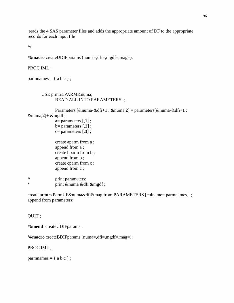
96
reads the 4 SAS parameter files and adds the appropriate amount of DF to the appropriate
records for each input file
*/
%macro createUDIFparams (numa=,dfi=,mgdf=,mag=);
PROC IML ;
parmnames = { a b c } ;
USE prmtrs.PARM&numa;
READ ALL INTO PARAMETERS ;
Parameters [&numa-&dfi+1 : &numa,2] = parameters[&numa-&dfi+1 :
&numa,2]+ &mgdf ;
a= parameters [,1] ;
b= parameters [,2] ;
c= parameters [,3] ;
create aparm from a ;
append from a ;
create bparm from b ;
append from b ;
create cparm from c ;
append from c ;
* print parameters;
* print &numa &dfi &mgdf ;
create prmtrs.ParmUF&numa&dfi&mag from PARAMETERS [colname= parmnames] ;
append from parameters;
QUIT ;
%mend createUDIFparams ;
%macro createBDIFparams (numa=,dfi=,mgdf=,mag=);
PROC IML ;
parmnames = { a b c } ;
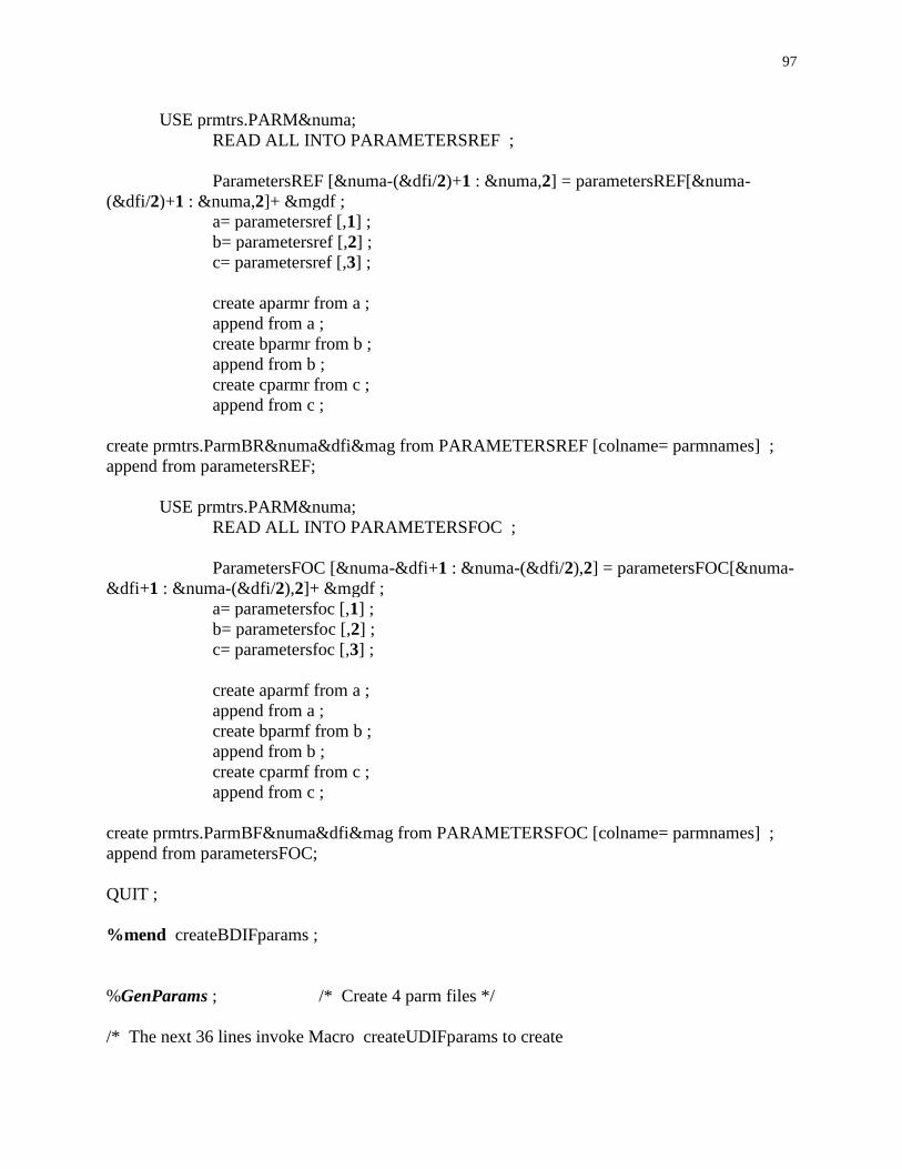
97
USE prmtrs.PARM&numa;
READ ALL INTO PARAMETERSREF ;
ParametersREF [&numa-(&dfi/2)+1 : &numa,2] = parametersREF[&numa-
(&dfi/2)+1 : &numa,2]+ &mgdf ;
a= parametersref [,1] ;
b= parametersref [,2] ;
c= parametersref [,3] ;
create aparmr from a ;
append from a ;
create bparmr from b ;
append from b ;
create cparmr from c ;
append from c ;
create prmtrs.ParmBR&numa&dfi&mag from PARAMETERSREF [colname= parmnames] ;
append from parametersREF;
USE prmtrs.PARM&numa;
READ ALL INTO PARAMETERSFOC ;
ParametersFOC [&numa-&dfi+1 : &numa-(&dfi/2),2] = parametersFOC[&numa-
&dfi+1 : &numa-(&dfi/2),2]+ &mgdf ;
a= parametersfoc [,1] ;
b= parametersfoc [,2] ;
c= parametersfoc [,3] ;
create aparmf from a ;
append from a ;
create bparmf from b ;
append from b ;
create cparmf from c ;
append from c ;
create prmtrs.ParmBF&numa&dfi&mag from PARAMETERSFOC [colname= parmnames] ;
append from parametersFOC;
QUIT ;
%mend createBDIFparams ;
%GenParams ; /* Create 4 parm files */
/* The next 36 lines invoke Macro createUDIFparams to create
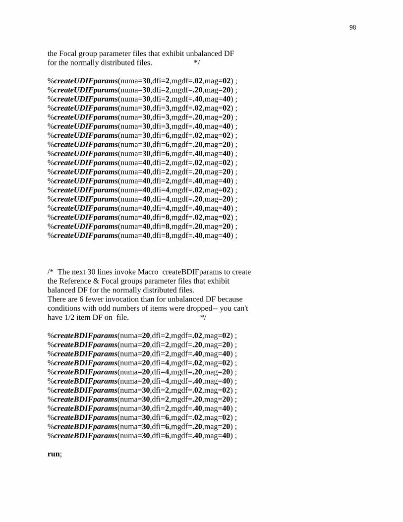
98
the Focal group parameter files that exhibit unbalanced DF
for the normally distributed files. */
%createUDIFparams(numa=30,dfi=2,mgdf=.02,mag=02) ;
%createUDIFparams(numa=30,dfi=2,mgdf=.20,mag=20) ;
%createUDIFparams(numa=30,dfi=2,mgdf=.40,mag=40) ;
%createUDIFparams(numa=30,dfi=3,mgdf=.02,mag=02) ;
%createUDIFparams(numa=30,dfi=3,mgdf=.20,mag=20) ;
%createUDIFparams(numa=30,dfi=3,mgdf=.40,mag=40) ;
%createUDIFparams(numa=30,dfi=6,mgdf=.02,mag=02) ;
%createUDIFparams(numa=30,dfi=6,mgdf=.20,mag=20) ;
%createUDIFparams(numa=30,dfi=6,mgdf=.40,mag=40) ;
%createUDIFparams(numa=40,dfi=2,mgdf=.02,mag=02) ;
%createUDIFparams(numa=40,dfi=2,mgdf=.20,mag=20) ;
%createUDIFparams(numa=40,dfi=2,mgdf=.40,mag=40) ;
%createUDIFparams(numa=40,dfi=4,mgdf=.02,mag=02) ;
%createUDIFparams(numa=40,dfi=4,mgdf=.20,mag=20) ;
%createUDIFparams(numa=40,dfi=4,mgdf=.40,mag=40) ;
%createUDIFparams(numa=40,dfi=8,mgdf=.02,mag=02) ;
%createUDIFparams(numa=40,dfi=8,mgdf=.20,mag=20) ;
%createUDIFparams(numa=40,dfi=8,mgdf=.40,mag=40) ;
/* The next 30 lines invoke Macro createBDIFparams to create
the Reference & Focal groups parameter files that exhibit
balanced DF for the normally distributed files.
There are 6 fewer invocation than for unbalanced DF because
conditions with odd numbers of items were dropped-- you can't
have 1/2 item DF on file. */
%createBDIFparams(numa=20,dfi=2,mgdf=.02,mag=02) ;
%createBDIFparams(numa=20,dfi=2,mgdf=.20,mag=20) ;
%createBDIFparams(numa=20,dfi=2,mgdf=.40,mag=40) ;
%createBDIFparams(numa=20,dfi=4,mgdf=.02,mag=02) ;
%createBDIFparams(numa=20,dfi=4,mgdf=.20,mag=20) ;
%createBDIFparams(numa=20,dfi=4,mgdf=.40,mag=40) ;
%createBDIFparams(numa=30,dfi=2,mgdf=.02,mag=02) ;
%createBDIFparams(numa=30,dfi=2,mgdf=.20,mag=20) ;
%createBDIFparams(numa=30,dfi=2,mgdf=.40,mag=40) ;
%createBDIFparams(numa=30,dfi=6,mgdf=.02,mag=02) ;
%createBDIFparams(numa=30,dfi=6,mgdf=.20,mag=20) ;
%createBDIFparams(numa=30,dfi=6,mgdf=.40,mag=40) ;
run;
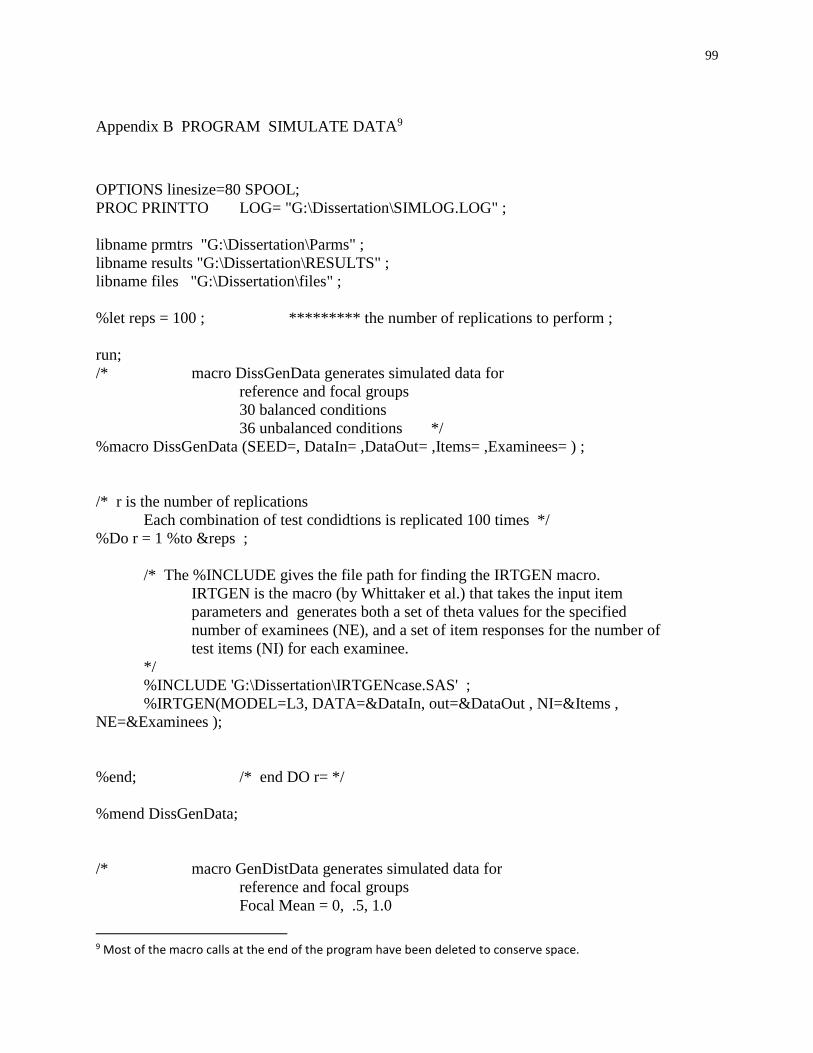
99
Appendix B PROGRAM SIMULATE DATA9
OPTIONS linesize=80 SPOOL;
PROC PRINTTO LOG= "G:\Dissertation\SIMLOG.LOG" ;
libname prmtrs "G:\Dissertation\Parms" ;
libname results "G:\Dissertation\RESULTS" ;
libname files "G:\Dissertation\files" ;
%let reps = 100 ; ********* the number of replications to perform ;
run;
/* macro DissGenData generates simulated data for
reference and focal groups
30 balanced conditions
36 unbalanced conditions */
%macro DissGenData (SEED=, DataIn= ,DataOut= ,Items= ,Examinees= ) ;
/* r is the number of replications
Each combination of test condidtions is replicated 100 times */
%Do r = 1 %to &reps ;
/* The %INCLUDE gives the file path for finding the IRTGEN macro.
IRTGEN is the macro (by Whittaker et al.) that takes the input item
parameters and generates both a set of theta values for the specified
number of examinees (NE), and a set of item responses for the number of
test items (NI) for each examinee.
*/
%INCLUDE 'G:\Dissertation\IRTGENcase.SAS' ;
%IRTGEN(MODEL=L3, DATA=&DataIn, out=&DataOut , NI=&Items ,
NE=&Examinees );
%end; /* end DO r= */
%mend DissGenData;
/* macro GenDistData generates simulated data for
reference and focal groups
Focal Mean = 0, .5, 1.0
9 Most of the macro calls at the end of the program have been deleted to conserve space.
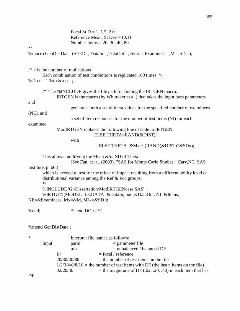
100
Focal St D = 1, 1.5, 2.0
Reference Mean, St Dev = (0,1)
Number Items = 20, 30, 40, 80
*/
%macro GenDistData (SEED=, DataIn= ,DataOut= ,Items= ,Examinees= ,M= ,SD= );
/* r is the number of replications
Each combination of test condidtions is replicated 100 times */
%Do r = 1 %to &reps ;
/* The %INCLUDE gives the file path for finding the IRTGEN macro.
IRTGEN is the macro (by Whittaker et al.) that takes the input item parameters
and
generates both a set of theta values for the specified number of examinees
(NE), and
a set of item responses for the number of test items (NI) for each
examinee.
ModIRTGEN replaces the following line of code in IRTGEN
ELSE THETA=RAND(&DIST);
with
ELSE THETA=&Mx + (RAND(&DIST)*&SDx);
This allows modifying the Mean &/or SD of Theta
(See Fan, et. al. (2003). "SAS for Monte Carlo Studies." Cary,NC. SAS
Institute. p. 60.)
which is needed to test for the effect of impact resulting from a different ability level or
distributional variance among the Ref & Foc groups.
*/
%INCLUDE 'G:\Dissertation\ModIRTGENcase.SAS' ;
%IRTGEN(MODEL=L3,DATA=&DataIn, out=&DataOut, NI=&Items,
NE=&Examinees, Mx=&M, SDx=&SD );
%end; /* end DO r= */
%mend GenDistData ;
* Interpret file names as follows:
Input parm = parameter file
u/b = unbalanced / balanced DF
f/r = focal / reference
20/30/40/80 = the number of test items on the file
1/2/3/4/6/8/16 = the number of test items with DF (the last n items on the file)
02/20/40 = the magnitude of DF (.02, .20, .40) in each item that has
DF
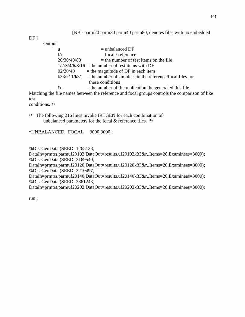
101
[NB - parm20 parm30 parm40 parm80, denotes files with no embedded
DF ]
Output
u = unbalanced DF
f/r = focal / reference
20/30/40/80 = the number of test items on the file
1/2/3/4/6/8/16 = the number of test items with DF
02/20/40 = the magnitude of DF in each item
k33/k11/k31 = the number of simulees in the reference/focal files for
these conditions
&r = the number of the replication the generated this file.
Matching the file names between the reference and focal groups controls the comparison of like
test
conditions. */
/* The following 216 lines invoke IRTGEN for each combination of
unbalanced parameters for the focal & reference files. */
*UNBALANCED FOCAL 3000:3000 ;
%DissGenData (SEED=1265133,
DataIn=prmtrs.parmuf20102,DataOut=results.uf20102k33&r.,Items=20,Examinees=3000);
%DissGenData (SEED=3169540,
DataIn=prmtrs.parmuf20120,DataOut=results.uf20120k33&r.,Items=20,Examinees=3000);
%DissGenData (SEED=3210497,
DataIn=prmtrs.parmuf20140,DataOut=results.uf20140k33&r.,Items=20,Examinees=3000);
%DissGenData (SEED=2861243,
DataIn=prmtrs.parmuf20202,DataOut=results.uf20202k33&r.,Items=20,Examinees=3000);
run ;
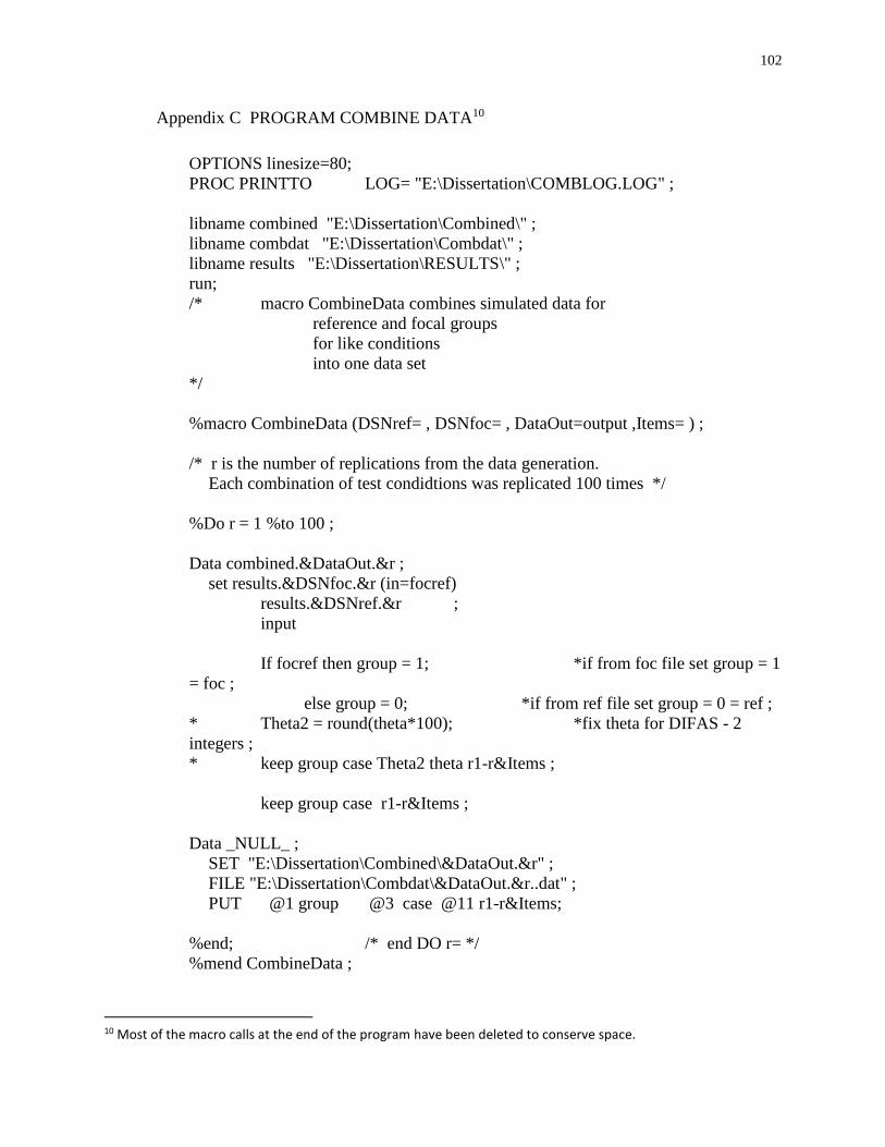
102
Appendix C PROGRAM COMBINE DATA10
OPTIONS linesize=80;
PROC PRINTTO LOG= "E:\Dissertation\COMBLOG.LOG" ;
libname combined "E:\Dissertation\Combined\" ;
libname combdat "E:\Dissertation\Combdat\" ;
libname results "E:\Dissertation\RESULTS\" ;
run;
/* macro CombineData combines simulated data for
reference and focal groups
for like conditions
into one data set
*/
%macro CombineData (DSNref= , DSNfoc= , DataOut=output ,Items= ) ;
/* r is the number of replications from the data generation.
Each combination of test condidtions was replicated 100 times */
%Do r = 1 %to 100 ;
Data combined.&DataOut.&r ;
set results.&DSNfoc.&r (in=focref)
results.&DSNref.&r ;
input
If focref then group = 1; *if from foc file set group = 1
= foc ;
else group = 0; *if from ref file set group = 0 = ref ;
* Theta2 = round(theta*100); *fix theta for DIFAS - 2
integers ;
* keep group case Theta2 theta r1-r&Items ;
keep group case r1-r&Items ;
Data _NULL_ ;
SET "E:\Dissertation\Combined\&DataOut.&r" ;
FILE "E:\Dissertation\Combdat\&DataOut.&r..dat" ;
PUT @1 group @3 case @11 r1-r&Items;
%end; /* end DO r= */
%mend CombineData ;
10 Most of the macro calls at the end of the program have been deleted to conserve space.
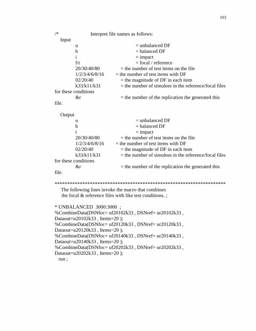
103
/* Interpret file names as follows:
Input
u = unbalanced DF
b = balanced DF
i = impact
f/r = focal / reference
20/30/40/80 = the number of test items on the file
1/2/3/4/6/8/16 = the number of test items with DF
02/20/40 = the magnitude of DF in each item
k33/k11/k31 = the number of simulees in the reference/focal files
for these conditions
&r = the number of the replication the generated this
file.
Output
u = unbalanced DF
b = balanced DF
i = impact
20/30/40/80 = the number of test items on the file
1/2/3/4/6/8/16 = the number of test items with DF
02/20/40 = the magnitude of DF in each item
k33/k11/k31 = the number of simulees in the reference/focal files
for these conditions
&r = the number of the replication the generated this
file.
********************************************************************
The following lines invoke the macro that combines
the focal & reference files with like test conditions. ;
* UNBALANCED 3000:3000 ;
%CombineData(DSNfoc= uf20102k33 , DSNref= ur20102k33 ,
Dataout=u20102k33 , Items=20 );
%CombineData(DSNfoc= uf20120k33 , DSNref= ur20120k33 ,
Dataout=u20120k33 , Items=20 );
%CombineData(DSNfoc= uf20140k33 , DSNref= ur20140k33 ,
Dataout=u20140k33 , Items=20 );
%CombineData(DSNfoc= uf20202k33 , DSNref= ur20202k33 ,
Dataout=u20202k33 , Items=20 );
run ;
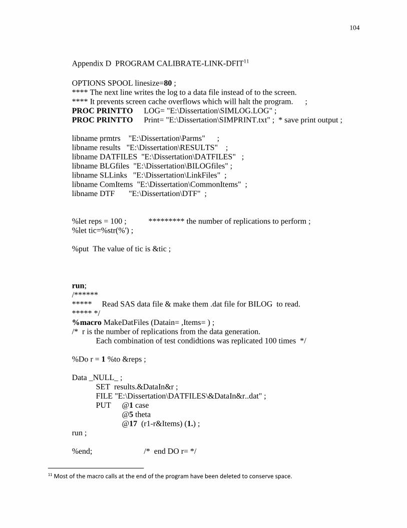
104
Appendix D PROGRAM CALIBRATE-LINK-DFIT11
OPTIONS SPOOL linesize=80 ;
**** The next line writes the log to a data file instead of to the screen.
**** It prevents screen cache overflows which will halt the program. ;
PROC PRINTTO LOG= "E:\Dissertation\SIMLOG.LOG" ;
PROC PRINTTO Print= "E:\Dissertation\SIMPRINT.txt" ; * save print output ;
libname prmtrs "E:\Dissertation\Parms" ;
libname results "E:\Dissertation\RESULTS" ;
libname DATFILES "E:\Dissertation\DATFILES" ;
libname BLGfiles "E:\Dissertation\BILOGfiles" ;
libname SLLinks "E:\Dissertation\LinkFiles" ;
libname ComItems "E:\Dissertation\CommonItems" ;
libname DTF "E:\Dissertation\DTF" ;
%let reps = 100 ; ********* the number of replications to perform ;
%let tic=%str(%') ;
%put The value of tic is &tic ;
run;
/******
***** Read SAS data file & make them .dat file for BILOG to read.
***** */
%macro MakeDatFiles (Datain= ,Items= ) ;
/* r is the number of replications from the data generation.
Each combination of test condidtions was replicated 100 times */
%Do r = 1 %to &reps ;
Data _NULL_ ;
SET results.&DataIn&r ;
FILE "E:\Dissertation\DATFILES\&DataIn&r..dat" ;
PUT @1 case
@5 theta
@17 (r1-r&Items) (1.) ;
run ;
%end; /* end DO r= */
11 Most of the macro calls at the end of the program have been deleted to conserve space.
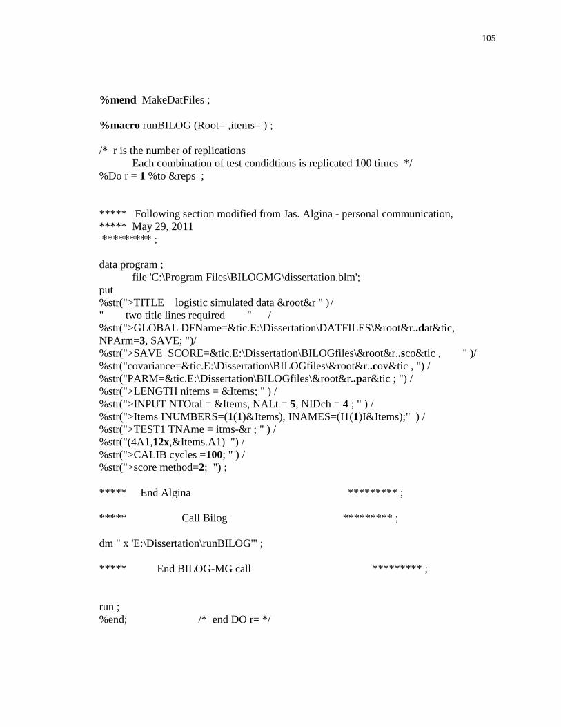
105
%mend MakeDatFiles ;
%macro runBILOG (Root= ,items= ) ;
/* r is the number of replications
Each combination of test condidtions is replicated 100 times */
%Do r = 1 %to &reps ;
***** Following section modified from Jas. Algina - personal communication,
***** May 29, 2011
********* ;
data program ;
file 'C:\Program Files\BILOGMG\dissertation.blm';
put
%str(">TITLE logistic simulated data &root&r " ) /
" two title lines required " /
%str(">GLOBAL DFName=&tic.E:\Dissertation\DATFILES\&root&r..dat&tic,
NPArm=3, SAVE; ")/
%str(">SAVE SCORE=&tic.E:\Dissertation\BILOGfiles\&root&r..sco&tic , " )/
%str("covariance=&tic.E:\Dissertation\BILOGfiles\&root&r..cov&tic , ") /
%str("PARM=&tic.E:\Dissertation\BILOGfiles\&root&r..par&tic ; ") /
%str(">LENGTH nitems = &Items; " ) /
%str(">INPUT NTOtal = &Items, NALt = 5, NIDch = 4 ; " ) /
%str(">Items INUMBERS=(1(1)&Items), INAMES=(I1(1)I&Items);" ) /
%str(">TEST1 TNAme = itms-&r ; " ) /
%str("(4A1,12x,&Items.A1) ") /
%str(">CALIB cycles =100; " ) /
%str(">score method=2; ") ;
***** End Algina ********* ;
***** Call Bilog ********* ;
dm " x 'E:\Dissertation\runBILOG'" ;
***** End BILOG-MG call ********* ;
run ;
%end; /* end DO r= */

106
%mend runBILOG ;
%macro runPLINK (ref= , foc= , items= ) ;
/* r is the number of replications
Each combination of test condidtions is replicated 100 times */
%Do r = 1 %to &reps ;
***** Following section creates file to run R and plink ********* ;
************************************************************************
***** Each line of the R code does the following:
************************************************************************
***** library(lattice) # loads lattice which plink requires ;
***** library(plink) # loads plink ;
***** setwd('E:/Dissertation/BILOGfiles') # set directory to read input ;
***** gr.pars <- read.bilog("&ref&r..par") # reads reference file ;
***** gf.pars <- read.bilog("&foc&r..par") # reads focal file ;
***** common <- matrix (c(1:&items,1:&items), &items, 2) # specify the common
items ;
***** # where 1:&items = the items in common in reference & focal files
&items = the number of items in the
2 = the number of groups ;
***** pars <- combine.pars(list(gr.pars, gf.pars), common) # combine the elements
;
***** # put parameters onto scale of first group (This is the default of "base.grp".
See p. 15 JSS article) ;
***** out <- plink(pars, rescale = 'SL', method = 'SL', ;
***** weights.t = as.weight(30, normal.wt = TRUE) ) # call to plink ;
***** conname <- link.con(out) # extract linking constants ;
***** setwd("E:/Dissertation/LinkFiles") # set directory to save output file
;
***** write.csv(conname,"L&foc&r..csv") # save the
linking constants to output file ;
***** q() # close R ;
***** n # does not save R work space ;
********************************************************************** ;
data _null_ ;
file 'C:\Program Files\R\R-2.15.2\bin\runlink.r';
PUT " library(lattice)" ;
PUT " library(plink)" ;
PUT " setwd('E:/Dissertation/BILOGfiles')" ;
PUT " gf.pars <- read.bilog('&foc&r..par')" ;
PUT " gr.pars <- read.bilog('&ref&r..par')" ;
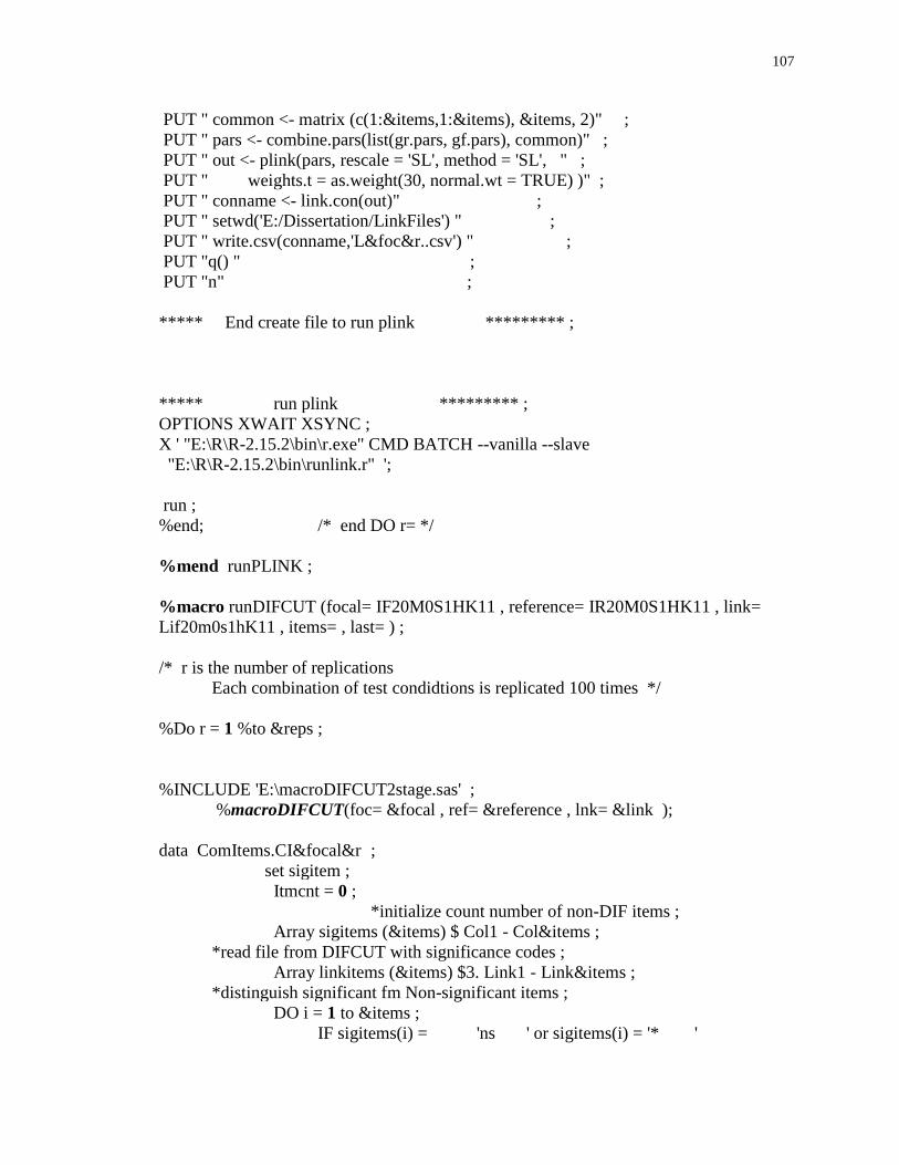
107
PUT " common <- matrix (c(1:&items,1:&items), &items, 2)" ;
PUT " pars <- combine.pars(list(gr.pars, gf.pars), common)" ;
PUT " out <- plink(pars, rescale = 'SL', method = 'SL', " ;
PUT " weights.t = as.weight(30, normal.wt = TRUE) )" ;
PUT " conname <- link.con(out)" ;
PUT " setwd('E:/Dissertation/LinkFiles') " ;
PUT " write.csv(conname,'L&foc&r..csv') " ;
PUT "q() " ;
PUT "n" ;
***** End create file to run plink ********* ;
***** run plink ********* ;
OPTIONS XWAIT XSYNC ;
X ' "E:\R\R-2.15.2\bin\r.exe" CMD BATCH --vanilla --slave
"E:\R\R-2.15.2\bin\runlink.r" ';
run ;
%end; /* end DO r= */
%mend runPLINK ;
%macro runDIFCUT (focal= IF20M0S1HK11 , reference= IR20M0S1HK11 , link=
Lif20m0s1hK11 , items= , last= ) ;
/* r is the number of replications
Each combination of test condidtions is replicated 100 times */
%Do r = 1 %to &reps ;
%INCLUDE 'E:\macroDIFCUT2stage.sas' ;
%macroDIFCUT(foc= &focal , ref= &reference , lnk= &link );
data ComItems.CI&focal&r ;
set sigitem ;
Itmcnt = 0 ;
*initialize count number of non-DIF items ;
Array sigitems (&items) $ Col1 - Col&items ;
*read file from DIFCUT with significance codes ;
Array linkitems (&items) $3. Link1 - Link&items ;
*distinguish significant fm Non-significant items ;
DO i = 1 to &items ;
IF sigitems(i) = 'ns ' or sigitems(i) = '* '
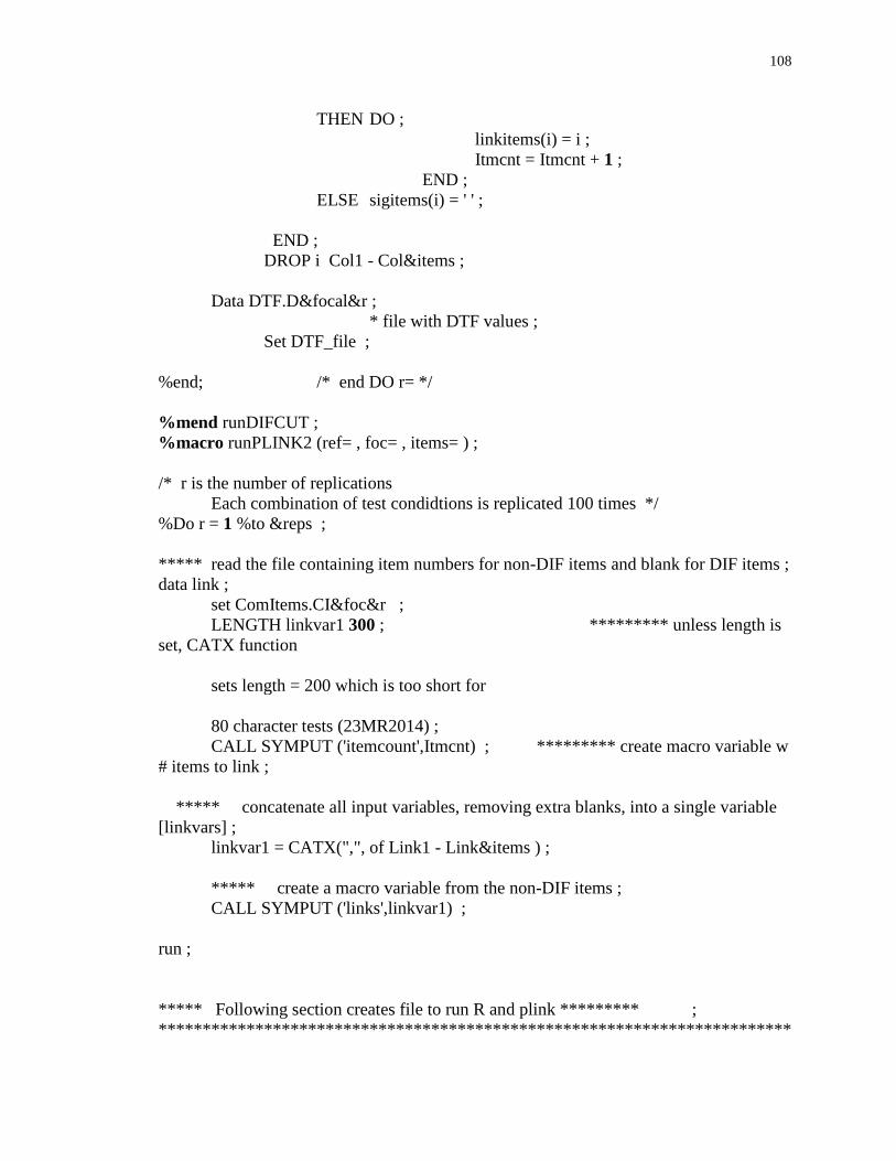
108
THEN DO ;
linkitems(i) = i ;
Itmcnt = Itmcnt + 1 ;
END ;
ELSE sigitems(i) = ' ' ;
END ;
DROP i Col1 - Col&items ;
Data DTF.D&focal&r ;
* file with DTF values ;
Set DTF_file ;
%end; /* end DO r= */
%mend runDIFCUT ;
%macro runPLINK2 (ref= , foc= , items= ) ;
/* r is the number of replications
Each combination of test condidtions is replicated 100 times */
%Do r = 1 %to &reps ;
***** read the file containing item numbers for non-DIF items and blank for DIF items ;
data link ;
set ComItems.CI&foc&r ;
LENGTH linkvar1 300 ; ********* unless length is
set, CATX function
sets length = 200 which is too short for
80 character tests (23MR2014) ;
CALL SYMPUT ('itemcount',Itmcnt) ; ********* create macro variable w
# items to link ;
***** concatenate all input variables, removing extra blanks, into a single variable
[linkvars] ;
linkvar1 = CATX(",", of Link1 - Link&items ) ;
***** create a macro variable from the non-DIF items ;
CALL SYMPUT ('links',linkvar1) ;
run ;
***** Following section creates file to run R and plink ********* ;
************************************************************************
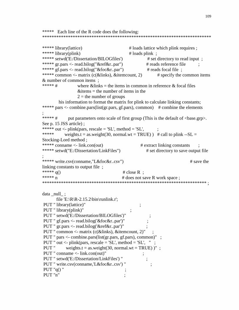
109
***** Each line of the R code does the following:
************************************************************************
***** library(lattice) # loads lattice which plink requires ;
***** library(plink) # loads plink ;
***** setwd('E:/Dissertation/BILOGfiles') # set directory to read input ;
***** gr.pars <- read.bilog("&ref&r..par") # reads reference file ;
***** gf.pars <- read.bilog("&foc&r..par") # reads focal file ;
***** common <- matrix (c(&links), &itemcount, 2) # specify the common items
& number of common items ;
***** # where &links = the items in common in reference & focal files
&items = the number of items in the
2 = the number of groups
his information to format the matrix for plink to calculate linking constants;
***** pars <- combine.pars(list(gr.pars, gf.pars), common) # combine the elements
;
***** # put parameters onto scale of first group (This is the default of <base.grp>.
See p. 15 JSS article) ;
***** out <- plink(pars, rescale = 'SL', method = 'SL', ;
***** weights.t = as.weight(30, normal.wt = TRUE) ) # call to plink --SL =
Stocking-Lord method ;
***** conname <- link.con(out) # extract linking constants ;
***** setwd("E:/Dissertation/LinkFiles") # set directory to save output file
;
***** write.csv(conname,"L&foc&r..csv") # save the
linking constants to output file ;
***** q() # close R ;
***** n # does not save R work space ;
********************************************************************** ;
data _null_ ;
file 'E:\R\R-2.15.2\bin\runlink.r';
PUT " library(lattice)" ;
PUT " library(plink)" ;
PUT " setwd('E:/Dissertation/BILOGfiles')" ;
PUT " gf.pars <- read.bilog('&foc&r..par')" ;
PUT " gr.pars <- read.bilog('&ref&r..par')" ;
PUT " common <- matrix (c(&links), &itemcount, 2)" ;
PUT " pars <- combine.pars(list(gr.pars, gf.pars), common)" ;
PUT " out <- plink(pars, rescale = 'SL', method = 'SL', " ;
PUT " weights.t = as.weight(30, normal.wt = TRUE) )" ;
PUT " conname <- link.con(out)" ;
PUT " setwd('E:/Dissertation/LinkFiles') " ;
PUT " write.csv(conname,'L&foc&r..csv') " ;
PUT "q() " ;
PUT "n" ;
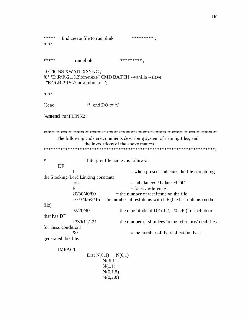
110
***** End create file to run plink ********* ;
run ;
***** run plink ********* ;
OPTIONS XWAIT XSYNC ;
X ' "E:\R\R-2.15.2\bin\r.exe" CMD BATCH --vanilla --slave
"E:\R\R-2.15.2\bin\runlink.r" ';
run ;
%end; /* end DO r= */
%mend runPLINK2 ;
************************************************************************
The following code are comments describing system of naming files, and
the invocations of the above macros
***********************************************************************;
* Interpret file names as follows:
DF
L = when present indicates the file containing
the Stocking-Lord Linking constants
u/b = unbalanced / balanced DF
f/r = focal / reference
20/30/40/80 = the number of test items on the file
1/2/3/4/6/8/16 = the number of test items with DF (the last n items on the
file)
02/20/40 = the magnitude of DF (.02, .20, .40) in each item
that has DF
k33/k11/k31 = the number of simulees in the reference/focal files
for these conditions
&r = the number of the replication that
generated this file.
IMPACT
Dist N(0,1) N(0,1)
N(.5,1)
N(1,1)
N(0,1.5)
N(0,2.0)
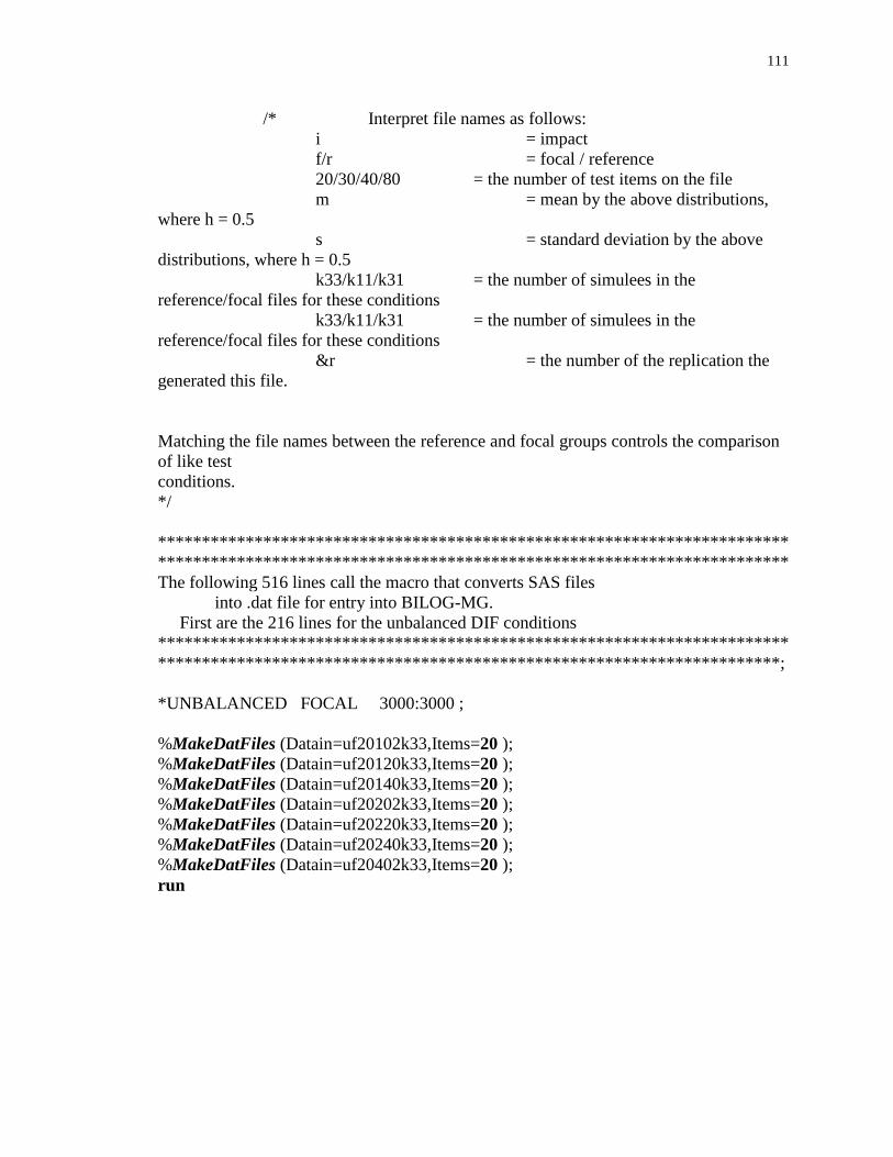
111
/* Interpret file names as follows:
i = impact
f/r = focal / reference
20/30/40/80 = the number of test items on the file
m = mean by the above distributions,
where h = 0.5
s = standard deviation by the above
distributions, where h = 0.5
k33/k11/k31 = the number of simulees in the
reference/focal files for these conditions
k33/k11/k31 = the number of simulees in the
reference/focal files for these conditions
&r = the number of the replication the
generated this file.
Matching the file names between the reference and focal groups controls the comparison
of like test
conditions.
*/
************************************************************************
************************************************************************
The following 516 lines call the macro that converts SAS files
into .dat file for entry into BILOG-MG.
First are the 216 lines for the unbalanced DIF conditions
************************************************************************
***********************************************************************;
*UNBALANCED FOCAL 3000:3000 ;
%MakeDatFiles (Datain=uf20102k33,Items=20 );
%MakeDatFiles (Datain=uf20120k33,Items=20 );
%MakeDatFiles (Datain=uf20140k33,Items=20 );
%MakeDatFiles (Datain=uf20202k33,Items=20 );
%MakeDatFiles (Datain=uf20220k33,Items=20 );
%MakeDatFiles (Datain=uf20240k33,Items=20 );
%MakeDatFiles (Datain=uf20402k33,Items=20 );
run