development of fractional trigonometry and an application of
TRANSCRIPT
Western Kentucky UniversityTopSCHOLAR®
Masters Theses & Specialist Projects Graduate School
5-2011
Development of Fractional Trigonometry and anApplication of Fractional Calculus toPharmacokinetic ModelAmera AlmusharrfWestern Kentucky University, [email protected]
Follow this and additional works at: http://digitalcommons.wku.edu/theses
Part of the Mathematics Commons
This Thesis is brought to you for free and open access by TopSCHOLAR®. It has been accepted for inclusion in Masters Theses & Specialist Projects byan authorized administrator of TopSCHOLAR®. For more information, please contact [email protected].
Recommended CitationAlmusharrf, Amera, "Development of Fractional Trigonometry and an Application of Fractional Calculus to Pharmacokinetic Model"(2011). Masters Theses & Specialist Projects. Paper 1048.http://digitalcommons.wku.edu/theses/1048

DEVELOPMENT OF FRACTIONAL TRIGONOMETRY AND AN APPLICATION OF
FRACTIONAL CALCULUS TO PHARMACOKINETIC MODEL
A Thesis
Presented to
The Faculty of the Department of Mathematics and Computer Science
Western Kentucky University
Bowling Green, Kentucky
In Partial Fulfillment
Of the Requirements for the Degree
Master of Science
By
Amera Almusharrf
May 2011
Dean, Graduate Studies and Research
DEVELOPMENT OF FRACTIONAL TRIGONOMETRY AND AN APPLICATIONOF FRACTIONAL CALCULUS TO PHARMACOKINETIC MODEL
Date Recommended _04_/_2_1/_20_1_1 _
ilkcAh-JDr. Ferhan Atici, Director of Thesis
,vCfUe-- N~ _Dr. Ngoc Nguyen
~£~Dr. Mark Robinson

iii
ACKNOWLEDGMENTS
Sincere gratitude is extended to the following people who never ceased in helping until
this thesis was structured. I want to thank God for all the blessings in my life and the
ability that he has given to me. I would like to express my gratitude to Dr. Ferhan Atici
for her encouragement and her patience. Through this experience, she has given me better
understanding in mathematical research and mathematical writing. Also, I would like to
acknowledge Dr. Ngoc Nguyen, Dr. Mark Robinson and Dr. Bruce Kessler for helping
to make this thesis possible. I want to thank my parents for their praying for me every
single day. Last, but certainly not least, I would like to thank my husband, Ibrahim, who
has the biggest role to make this thesis possible and thanks a lot to my children. They are
the loves of my life and all my hard work that I do for them.
iv
TABLE OF CONTENTS
ABSTRACT……………………………………………………………………………...vi
CHAPTER 1: Introduction to Fractional Calculus………………………………………..1
1.1 Historical Development of Fractional Calculus………………………………………2
1.2 Special Function of the Fractional Calculus…………………………………………..5
CHAPTER 2: Fractional Integral and Derivative………………………………………..10
2.1 Definition of the Fractional Integral…………………………………………………10
2.2 Properties of the Fractional Integral…………………………………………………12
2.3 Definition of the Fractional Derivative………………………………………………13
2.4 Applications of Fractional Integral and Derivative………………………………….16
CHAPTER 3: Laplace Transform………………………………………………………..19
3.1 Definition of the Laplace Transform………………………………………………...19
3.2 Properties of the Laplace Transform…………………………………………………20
3.3 Laplace Transform of the Fractional Integral………………………………………..20
3.4 Laplace Transform of the Fractional Derivative……………………………………..21
CHAPTER 4: Fractional Trigonometric Functions……………………………………...25
4.1 Generalized Exponential Function…………………………………………………...25
4.2 Generalized Trigonometric Functions……………………………………………….26
4.3 Properties of Fractional Trigonometric Functions…………………………………...27
4.4 Laplace Transform of the Fractional Trigonometric Functions……………………...30
4.5 Generalized Wronskian and Linear Independence…………………………………..31
4.6 Fractional Derivative of Trigonometric Functions…………………………………..37
4.7 System of Linear Fractional Differential Equations with Constant Matrix
Coefficients………………………………………………………………………………38
v
CHAPTER 5: An Application of Fractional Calculus to Pharmacokinetic Model……...48
5.1 One Compartment Model……………………………………………………………49
5.2 Graphical results……………………………………………………………………..51
5.3 Initial Parameter Estimation…………………………………………………………52
5.4 Model of Best Prediction………………………………………….............................58
CONCLUSION AND FUTURE WORK………………………………………………..67
APPENDIX………………………………………………………………………………69
REFRENCES…………………………………………………………………………….73
vi
DEVELOPMENT OF FRACTIONAL TRIGONOMETRY AND AN APPLICATION
OF FRACTIONAL CALCULUS TO PHARMACOKINETIC MODEL
Amera Almusharrf May 2011 75 Pages
Directed by: Dr. Ferhan Atici
Department of Mathematics and Computer Science Western Kentucky University
Our translation of real world problems to mathematical expressions relies on calculus,
which in turn relies on the differentiation and integration operations. We differentiate or
integrate a function once, twice, or any whole number of times. But one may ask what
would be the 1/2-th or square root derivative of x. Fractional calculus generalize the
operation of differentiation and integration to non-integer orders. Although it seems not
to have significant applications, research on this subject could be valuable in
understanding the nature.
The main purpose of this thesis is to develop fractional trigonometry and generalize
Wronskian determinant that can be used to determine the linear independence of a set of
solutions to a system of fractional differential equations. We also introduce a new set of
fractional differential equations whose solutions are fractional trigonometric functions.
The first chapter gives a brief introduction to fractional calculus and the mathematical
functions which are widely used to develop the theory of this subject. The second chapter
introduces the reader to fractional derivative and fractional integral, and the
most important properties of these two operators that are used to develop the following
chapters. The third chapter focuses on the Laplace transform which is the means that will
vii
be used to solve the fractional differential equations. In the fourth chapter, we develop
fractional trigonometric functions, generalized Wronskian, also classes of fractional
homogeneous differential equations and the characteristic equations, as well as the
solution to these types of equations. Also, we present a new method to solve a system of
fractional differential equations, and by using this method we solve a system that
generates a solution of a linear combination of two fractional trigonometric functions.
The fifth chapter is the conclusion of this thesis and is devoted to demonstrating an
application of fractional calculus to pharmacokinetic model, which is used to study the
drug concentration in the body.
CHAPTER 1
Introduction to Fractional Calculus
The fractional calculus is a natural extension of the traditional calculus. It is like
many other mathematical branches and ideas; it has its origin in the pursuing for the
extension of meaning. Well known examples are the extension of the integer numbers to
the rational numbers, of the rational numbers to the real numbers, and of the real numbers
to the complex numbers. The question of extension of meaning in differential and integral
calculus: Can the derivativedny
dxnof integer order n > 0, be extended to n any order -
fractional, irrational or complex? The answer of this question has led to the development
of a new theory which is called fractional calculus.
Fractional calculus is a new subject; it may find its way into innumerable questions
and applications. Some of the mathematical theory applicable to the study of the fractional
calculus was developed prior to the turn of the 20th Century. In this thesis, we develop
"fractional trigonometric functions" with investigation of the behavior of "fractional cosine"
and "fractional sine" curves. Also, we generalize the Wronskian determinant theory to
determine the linear independence of a set of solutions to higher order fractional differential
equations. We will introduce a system of differential equations where "fractional cosine"
and "fractional sine" appear as a solution for that system.
The purpose of studying theories is to apply them to real world problems. Over the last
few years, mathematicians pulled the subject of fractional calculus to several applied fields
of engineering, science and economics [1,2,7,22,23]. In this work, we present an application
of fractional calculus to the pharmacology field. In particular to Pharmacokinetic science
which studies the drug metabolite kinetics in the body.
1
1.1 Historical Development of Fractional Calculus
The concept of fractional calculus is believed to have emerged from a question raised in
the year 1695 by Marquis de L’Hôpital. In a letter dated September 30th, 1695 L’Hôpital
wrote to Leibniz asking him about a particular notation he had used in his publications for
the n−th derivative dnf(x)
dxnof the linear function f(x) = x. L’Hôpital posed the question
to Leibniz, what would be the result be if n = 1/2. Leibniz responded to the question,
that "d1/2x will be equal to x√dx : x". In these words, fractional calculus was born [8,9].
Following this question, many mathematicians contributed to the fractional calculus. In
1730, Euler mentioned interpolating between integral orders of a derivative. In 1812, Laplace
defined a fractional derivative by means of an integral, and in 1819 there appeared the first
discussion of fractional derivative in a calculus text written by S.F.Lacroix [24].
Starting with
y = xm (1.1)
where m is a positive integer, Lacroix found that the n−th derivative of xm :
dnxm
dxn=
m!
(m− n)!xm−n, m ≥ n. (1.2)
Then, he replaced n with 1/2 and let m = 1, thus the derivative of order 1/2 of the function
x is
d1/2
dx1/2x =
2√x√π. (1.3)
2
This result obtained by Lacroix is the same as that yielded by the present day Riemann-
Liouville definition of a fractional derivative. But Lacroix considered the question of inter-
polating between integral orders of a derivative. He devoted only two of the 700 pages of
his text to this topic.
Fourier, in 1822, was the next to mention a derivative of arbitrary order. But like Euler,
Laplace, and Lacroix, he gave no application. The first use of fractional operation was by
Niel Henrik Abel in 1823 [21]. Abel applied the fractional calculus to the solution of an
integral equation, which arose in his formulation of the tautochrone problem: to find the
shape of a frictionless wire lying in a vertical plane, such that the time required for a bead
placed on the wire to slide to the lowest point of the wire is the same regardless of where
the bead is first placed. We will present Abel’s elegant solution later in Chapter 3, after
developing appropriate notation and terminology for the fractional calculus.
Probably Joseph Liouville was fascinated by Laplace’s and Fourier’s brief comments
or Abel’s solution, so he made the first major study of fractional calculus. He published
three large memoirs on this topic in 1832 (beginning with [15]) followed by more papers
in rapid succession. Liouville’s first definition of a derivative of arbitrary order ν involved
an infinite series. This had the disadvantage that ν must be restricted to those values
for which the series converges. Liouville seemed aware of the restrictive nature of his first
definition, therefore, Liouville tried to put his effort to define fractional derivative again of
x−a whenever x and a are positive.
Starting with a definite integral we have:
I =
∫ ∞0ua−1e−xu du. (1.4)
3
With the change of variable xu = t, we obtain
I = x−a∫ ∞0ta−1e−t dt.
This integral is closely related to the Gamma integral of Euler which is defined as
Γ(a) =
∫ ∞0ta−1e−t dt.
Therefore, equation (1.4) can be written in term of Legendre’s symbol Γ for the generalized
factorial
I = x−aΓ(a) (1.5)
which implies
x−a =I
Γ(a). (1.6)
By "operating" on both sides of this equation with dν/dxν , and by assuming that dν(eax)/dxν =
aνeax for any ν > 0, Liouville was able to obtain the result known as his second definition:
dν
dxνx−a =
(−1)νΓ(a+ ν)
Γ(a)x−a−ν . (1.7)
After these attempts, still the second definition of fractional derivative is restricted to
some functions like f(x) = x−a. The (−1)ν term in this expression suggests the need to
broaden the theory to include complex numbers. Indeed, Liouville was able to extend
this definition to include complex values for a and ν. By piecing together the somewhat
disjointed accomplishments of many notable mathematicians, especially Liouville and Rie-
mann, modern analysts can now define the integral of arbitrary order. The fractional
integral of order ν is defined as follows
D−νf(x) =1
Γ(ν)
∫ x
c(x− t)ν−1 f(t) dt. (1.8)
4
1.2 Special Function of the Fractional Calculus
There are some basic mathematical functions which are important in the study of the
theory of fractional calculus. In the next subsection, we will concentrate on the Gamma
function, and we will list some well known properties of this function.
1.2.1 Gamma Function
One of the basic fractional functions is Euler’s Gamma function. This function is tied
to fractional calculus by the definition as we will see later on in the fractional-integral
definition. The most basic interpretation of the Gamma function is simply an extension of
the factorial function to noninteger values. The Gamma function is defined by the integral
Γ(x) =
∫ ∞0e−ttx−1 dt, x ∈ R+. (1.9)
Its relation to the factorials is that for any natural number n, we have
Γ(n) = (n− 1)! (1.10)
The Gamma function satisfies the following functional equation
Γ(x+ 1) = xΓ(x), x ∈ R+. (1.11)
This can be shown through a simple integration by parts:
Γ(x+ 1) = limb→∞
∫ b
0e−ttx dt = lim
b→∞
[−e−tx
]b0
+ limb→∞
[x
∫ b
0tx−1e−t dt
]= xΓ(x).
In 1730, Euler generalized the formula
dn
dxnxm =
m!
(m− n)!xm−n.
By using the following property
Γ(m+ 1) = (m)!
5
we obtain
dn
dxnxm =
Γ(m+ 1)
Γ(m− n+ 1)xm−n. (1.12)
The incomplete Gamma function is more generalized form of the Gamma function, it is
given by
Γ∗(ν, t) =1
Γ(ν)tν
∫ t
0e−xxν−1 dx, Re ν > 0. (1.13)
[For more details on the Gamma function, you may refer to any book on introductory frac-
tional calculus, for example, “Fractional Differential Equation”by Igor Podlubny (1999).]
1.2.2 The Beta Function
One of the useful mathematical functions in fractional calculus is the Beta function. Its
solution is defined through the use of multiple Gamma functions. Also, it shares a form
that is characteristically similar to the fractional integral or derivative of many functions,
particularly polynomials of the form ta. The Beta function is defined by a definite integral.
The following equation demonstrates the Beta integral and its solution in terms of the
Gamma function
B(p, q) =
∫ 1
0(1− u)p−1uq−1 du =
Γ(p)Γ(q)
Γ(p+ q), where p, q ∈ R+.
1.2.3 The Mittag-Leffl er Function
Another important function of the fractional calculus is the Mittag-Leffl er function which
plays a significant role in the solution of non-integer order differential equations. The one-
parameter representation of the Mittag-Leffl er function is defined over the entire complex
6
plane by
Eα(x) =∞∑k=0
xk
Γ(αk + 1), α > 0, x ∈ C. (1.14)
and is named after Mittag-Leffl er who introduced it in 1903 [11], therefore, it is known as
the Mittag-Lffl er function. In particular, when α = 1/n, (n ∈ N\{1}), the function E1/n(x)
has the following representation
E1/n(x) = exn
{1 + n
∫ x
0e−z
n
[n−1∑k=1
zk−1
Γ(k/n)
]dz
}. (1.15)
The two parameter generalized Mittag-Leffl er function, which was introduced later, is also
defined over the entire complex plane, and is given by
Eα,β(x) =∞∑k=0
xk
Γ(αk + β), α > 0, β > 0, x ∈ C. (1.16)
It may be noted that when β = 1, Eα,1(x) = Eα(x). Also notice that if we replace α, β by
1, we obtain
E1,1(x) =
∞∑k=0
xk
Γ(k + 1)=
∞∑k=0
xk
k!= ex. (1.17)
And this also, can be written in terms of one-parameter of Mittag-Leffl er function
E1(x) = E1,1(x) = ex. (1.18)
If we let x = 0 in (1.16), we have
Eα,β(0) = 1. (1.19)
The Mittag-Leffl er function is a natural extension of the exponential function. solutions of
fractional order differential equations are often expressed in terms of Mittag-Leffl er functions
in much the same way that solutions of many integer order differential equations may be
expressed in terms of exponential functions. The following lemma lists some properties of
Mittag-Leffl er function which are useful in the study of fractional calculus.
7
LEMMA 1.2.1
(i)1
Γ(β)+ xEα,α+β(x) = Eα,β(x), where x ∈ C .
(ii) ex[1 + Erf (x)]− 1 = xE1/2,3/2(x),
where Erf (x) is the error function and is given by
Erf (x) =2√π
∫ x
0e−t
2dt, x ∈ R.
(iii)d
dx[Eα,β(x)] =
1
αx[Eα,β−1(x)− (β − 1)Eα,β(x)].
Proof. Using the definition of the Mittag-Leffl er function, the proofs can be shown directly
as below.
(i) We will proceed the proof by using the definition of Mittag-Leffl er function in (1.16) and
the properties of the summation, thus
1
Γ(β)+ xEα,α+β(x) =
1
Γ(β)+ x
∞∑k=0
xk
Γ(αk + α+ β)
=1
Γ(β)+∞∑k=0
xk+1
Γ(α(k + 1) + β)
If we let m = k + 1 in the above sum notation, we obtain
1
Γ(β)+ xEα,α+β(x) =
1
Γ(β)+∞∑m=1
xm
Γ(αm+ β)
=1
Γ(β)+
∞∑m=0
xm
Γ(αm+ β)− 1
Γ(β)
=
∞∑m=0
xm
Γ(αm+ β)
= Eα,β(x)
(ii) By using the definition of the fractional Mittag-Leffl er function in (1.15), we have
E1/2(x) = ex2[1 +
2√π
∫ x
0e−z
2dz]
= ex2
[1 + Erf(x)] .
From the property in (i), it can be seen easily that
8
xE1/2,3/2(x) = E1/2,1(x)− 1 = E1/2(x)− 1
By observing the above two equation, we may conclude that
ex[1 + Erf (x)]− 1 = xE1/2,3/2(x)
(iii) By looking at the left hand side of the equation in (iii), we have
d
dx[Eα,β(x)] =
d
dx
[ ∞∑k=0
xk
Γ(αk + β)
]
=∞∑k=0
[1
Γ(αk + β)
]d
dxxk
=
∞∑k=0
kxk−1
Γ(αk + β)
Then, the right hand side of the equation is
1
αx[Eα,β−1(x)− (β − 1)Eα,β(x)] =
1
αx
[ ∞∑k=0
xk
Γ(αk + β − 1)− (β − 1)
∞∑k=o
xk
Γ(αk + β)
]
=1
αx
[ ∞∑k=0
xk(αk + β − 1)
(αk + β − 1)Γ(αk + β − 1)−∞∑k=o
xk(β − 1)
Γ(αk + β)
]
=1
αx
[ ∞∑k=0
(αk)xk + βxk − xkΓ(αk + β)
−∞∑k=o
βxk − xkΓ(αk + β)
]
=
∞∑k=0
(αk)xk
Γ(αk + β)
(1
αx
)
=∞∑k=0
kxk−1
Γ(αk + β).
Hence, we conclude that
ddx [Eα,β(x)] = 1
αx [Eα,β−1(x)− (β − 1)Eα,β(x)].
properties of the Mittag-Leffl er function have been summarizes in several references [1,11,12,14].
9
CHAPTER 2
Fractional Integral and Derivative
There are more than one version of the fractional integral exist. For example, it was
touched above in the introduction that the fractional integral can be defined as follows
cD−νx f(x) =
1
Γ(ν)
∫ x
c(x− t)ν−1 f(t) dt, ν > 0. (2.1)
It is called the Riemann version, where cD−νx f(x) denote the fractional integration of
a function to an arbitrary order ν, and ν is any nonnegative real number. In this notation,
c and x are the limits of integration operator.
The other version of the fractional integral is called the Liouville version. The case
where negative infinity in place of c in (2.1), namely,
−∞D−νx f(x) =
1
Γ(ν)
∫ x
−∞(x− t)ν−1 f(t) dt. (2.2)
In the case where c = 0 in (2.1), we obtain what is called the Riemann-Liouville fractional
integral:
0D−νx f(x) =
1
Γ(ν)
∫ x
0(x− t)ν−1 f(t) dt. (2.3)
However, our main focus in this thesis will be on what is called the Riemann-Liouville
version. For convenience, we will omit the limits of integration from the operator. That is,
instead of cD−νx , we will simply write D−ν .
2.1 Definition of the Fractional Integral
As we have stated before, our development of the fractional calculus will be based on
the Riemann-Liouville fractional integral. We begin this section with a formal definition of
the Riemann-Liouville fractional integral as we see below.
10
Let ν be a real number. Let f be piecewise continuous on J = (0,∞) and integrable
on any finite subinterval of J = [0,∞). Then for x > 0 we call
D−ν f(x) =1
Γ(ν)
∫ x
0(x− t)ν−1 f(t) dt, ν > 0 (2.4)
the Riemann-Liouville fractional integral of f of order ν. The definition of the Riemann-
Liouville integral can be obtained in several ways. One approach uses the theory of linear
differential equations (See Fractional Calculus: Definitions and Applications[7]).
EXAMPLE 2.1.1. Let evaluate D−ν xµ, where µ > −1 and ν > 0.
By definition of the Riemann-Liouville fractional integral, we have
D−ν xµ =1
Γ(ν)
∫ x
0(x− t)ν−1tµ dt.
=1
Γ(ν)
∫ x
0xν−1(1− t
x)ν−1tµ dt.
By changing the variable t/x = u, then dt = xdu, we obtain
D−ν xµ =1
Γ(ν)
∫ 1
0xν(1− u)ν−1(xu)µ du.
=1
Γ(ν)xν+µ
∫ 1
0(1− u)ν−1uµ du.
=1
Γ(ν)xν+µB(ν, µ+ 1)
=1
Γ(ν)xν+µ
Γ(µ+ 1)Γ(ν)
Γ(µ+ 1 + ν)
=Γ(µ+ 1)
Γ(µ+ 1 + ν)xν+µ.
Hence, we conclude thatD−ν xµ =
Γ(µ+ 1)
Γ(µ+ 1 + ν)xν+µ. (2.5)
If we let µ = 0 above, then xµ = x0 = 1. then by (2.5), the fractional integral of a constant
k of order ν is
D−ν k =k
Γ(1 + ν)xν , ν > 0. (2.6)
11
In particular, if ν =1
2
D−1/2x0 =1
Γ(3/2)x1/2 = 2
√x
π. (2.7)
EXAMPLE 2.1.2. Let f(t) = eat, where a is a constant. Then by (2.4) we have
D−νeat =1
Γ(ν)
∫ t
0(t− x)ν−1 eax dx, ν > 0.
By changing the variable y = t− x, we obtain
D−νeat =eat
Γ(ν)
∫ t
0yν−1 e−ay dy, ν > 0. (2.8)
If we refer to (1.18), we observe that the above equation may be expressed in terms of the
incomplete Gamma function
D−νeat = tνeatΓ∗(ν, at). (2.9)
2.2 Properties of the Fractional Integral
One of the most important properties in the development of fractional calculus is the law
of exponents which is very useful to calculate fractional integral and fractional derivative for
some functions, also to prove some relations that are related to fractional calculus theory.
In this section we state the theorem of the law of exponents for fractional calculus without
proof.
THEOREM 2.1.1. [16] Let f be continuous function on J and let µ, ν > 0. Then for all
t > 0,
D−µ[D−νf(t)] = D−(µ+ν)f(t) = D−ν [D−µf(t)]. (2.10)
Another useful property in the study of fractional calculus is the commutative property.
Many mathematical proofs rely on the commutative property where we can interchange the
12
integer order of the derivative and the fractional order of the integral. So it is worthwhile
to mention it here.
THEOREM 2.1.2. [16] Let f be continuous on J and let ν > 0, If Df is continuous, then
for all t > 0,
D[D−νf(t)] = D−ν [Df(t)] +f(t)|t=0
Γ(ν)tν−1. (2.11)
2.3 Definition of the Fractional Derivative
The notation that is used to denote the fractional derivative is Dα f(x) for any arbitrary
number of order α. Fractional derivative can be defined in terms of the fractional integral
as follows
Dαf(t) = Dn[D−uf(t)], (2.12)
where 0< u < 1, and n is the smallest integer greater than α such that u = n− α.
EXAMPLE 2.2.1. If f(x) = xµ, where µ ≥ 0. Then, for n = 1, the α derivative of xµ is
Dαxµ = D1[D−(1−α)xµ], where u = 1− α.
= D1
[Γ(µ+ 1)
Γ((µ− α+ 1) + 1)xµ−α+1
]= (µ− α+ 1)
Γ(µ+ 1)
(µ− α+ 1)Γ(µ− α+ 1)xµ−α
=Γ(µ+ 1)
Γ(µ− α+ 1)xµ−α.
Hence, we conclude
Dαxµ =Γ(µ+ 1)
Γ(µ− α+ 1)xµ−α. (2.13)
Notice that if f(x) = k, where k is a constant, then α order derivative of a constant is
Dαk =k
Γ(−α+ 1)x−α.
13
It is interesting to observe that for any constant k, Dαk is not zero where 0 < α < 1. For
example, the 1/2 order derivative of k is
D1/2k =k
Γ(1/2)x−1/2 =
k√πx.
REMARK 2.2.1. Let f be a real valued function. In the traditional calculus, we have
DD−1f = f . For any positive real number α, this equality valid for fractional calculus
as well. To see this, we use definition of the fractional derivative and the exponent law
(Theorem 2.1.1) ,
DαD−αf(x) = Dn[D−(n−α)(D−αf(t))].
= Dn[D−(n−α+α)f(x)] = DnD−nf(x) = f(x),
where n is the smallest integer greater than α.
REMARK 2.2.2. Let y be continuous on J. Then the following equality holds
D1/2[D1/2y(t)] = Dy(t).
We can prove this equality directly by using definition of fractional derivative and the
commutative law (Theorem 2.1.2)
D1/2[D1/2y(t)] = D1/2[D(D−1/2y(t))]
= D1/2
{[D−1/2(Dy(t))] +
y(t)|t=0Γ(1/2)
t−1/2}.
Let y(0)|t=0 = 0, this implies
D1/2D1/2y(t) = D1/2[D−1/2(Dy(t))].
Using (Remark 2.2.1), we obtain
D1/2D1/2y(t) = Dy(t).
14
LEMMA 2.2.1. Let f be continuous on J, then the fractional equation
D1/2y(t)− y(t) = −1, (2.14)
can be converted to the following differential equation
D y(t)− y(t) = −1− 1√πt. (2.15)
Proof. Using the distributive property of fractional derivative and (Remark 2.2.2), proof
can be shown directly as below.
Taking the 1/2 order derivative on both sides of equation (2.14) yields :
D1/2[D1/2y(t)]−D1/2y(t) = D1/2(−1).
This implies
Dy(t)−D1/2y(t) =−1√πt.
If we refer to equation (2.14), we may write the above equation as:
D y(t)− (y(t)− 1) =−1√πt.
This implies
D y(t)− y(t) = −1− 1√πt.
REMARK 2.2.3. A useful tool for computation of the fractional derivative of a product of
two functions f(x) and g(x) is the generalized Leibniz rule [26]:
Dαf(x)g(x) =∞∑n=0
(α
n
)Dnf(x)Dα−ng(x), (2.16)
where Dn is the ordinary differentiation operator dn/dxn, Dα−n is a fractional operator
and(αn
)is the generalized binomial coeffi cient
Γ(α+ 1)
n!Γ(α− n+ 1). When taking the arbitrary
15
derivative of a product, it is often convenient to choose the factor in such a way that the
series above terminates after n ordinary differentiation. For example,
D1/2(xg(x)) = xD1/2g(x) + 12D−1/2g(x)
terminates for n = 1. The generalized Leibniz rule can be used in applications as we will
see in the next section.
2.4 Applications of Fractional Integral and Derivative
The first to use a fractional operation was by Niel Henrik Abel in 1823. Abel applied
the fractional calculus to the solution of an integral equation which arose in his formulation
of the tautochrone problem : A bead on a frictionless wire starts from rest at some point
(x0,y0) and falls under the influence of gravity. What shape wire has the property that the
time it takes the bead to descend is independent of its srarting point? Since the kinetic
energy gained equals the potential energy lost, 1/2m(dλ/dt)2 = mg(y0 − y),where λ is the
distance of the bead along the wire, m is the mass, and g is the gravitational acceleration.
Thus
− dλ√y0 − y
=√
2gdt
and integration from top to bottom (time t = 0 to time t = T ), gives
√2gT =
∫ y=y0
y=0(y0 − y)−1/2dλ.
The tautochrone problem requires that the left side of this integral be a constant which
we will denote by k. The path length λ may be expressed as a function of the height, say
λ = F (y), so that dλ/dy = F ′(y). If we change variable y0 and y to x and t, and replace
F ′ by f , the tautochrone integral equation becomes k =
∫ x
0(x− t)−1/2f(t)dt. Our problem
16
is to determine the function f. this can be done by the convolution theorem of Laplace
transform theory. Abel, however, multiplied the equation by 1/Γ(1/2) to obtain
k
Γ(1/2)=
1
Γ(1/2)
∫ x
0(x− t)−1/2f(t)dt = D−1/2f(x)
By operationg on the extreme terms of this equation with D1/2 , he obtained D1/2k =
√πf(x). Then by computing the derivative of order 1/2 of the constant k (as in Example
2.2.1, for instance) Able obtained f(x) = k/π√x. He then went on to show that the solution
to tautochrone problem is a cycloid.
As another application, consider the problem of determine f(x) explicitly from the
integral equation
xf(x) =
∫ x
0(x− t)−1/2f(t)dt.
The right side of this equation is Γ(1/2)D−1/2f(x), thus we can write this equation as
follows
xf(x) = Γ(1/2)D−1/2f(x). (2.17)
Operating on both sides with D1/2 yields
D1/2{xf(x)}=√πf(x).
Using the generalized Leibniz rule (2.16) yields
xD1/2f(x) + 12D−1/2f(x) =
√πf(x).
Using the fractional derivative definition, we have
xD[D−1/2f(x)] + 12D−1/2f(x) =
√πf(x).
17
If we refer to equation (2.17), we may write the above equation as
xD{xf(x)/√π}+ 1
2{xf(x)/√π} =
√πf(x).
By using the chain rule to compute the first derivative of xf(x), we obtain
x{[xf ′(x) + f(x)]/√π}+ 1
2{xf(x)/√π} =
√πf(x).
Multiplying both side by√π yields
x{[xf ′(x) + f(x)]}+ 12{xf(x)} = πf(x),
which implies
x2f ′(x) + (3x2 − π)f(x) = 0,
which has the solution
f(x)=ke−π/xx−3/2.
The same result can be obtained from the original integral equation by the use of Laplace
transform. However, fractional calculus might suggest a solution to a complicated functional
equation without using other means, like Laplace transform.
18
CHAPTER 3
Laplace Transform
The main idea behind the Laplace transform is that we can solve an equation (or system
of equations) containing differential and integral terms by transforming the equation in "t-
space" to one in "s-space". Laplace transform makes the problem much easier to solve by
converting the differential equation to an algebraic equation and is particularly suited for
differential equations with initial conditions.
In this chapter, we present definition of the Laplace transform and its properties. Then
we calculate the Laplace transform of the fractional integral and fractional derivative.
3.1 Definition of the Laplace Transform
The Laplace transform of a function f(t) of a real variable t ∈ R+ = (0,∞) is defined
by
L{f(t)} =
∫ ∞0e−st f(t) dt = F (s) (s ∈ C). (3.1)
The Laplace transform of the function f(t) is said to exist if (3.1) is a convergent integral.
The requirement for this is that f(t) does not grow at a rate higher than the rate at which
the exponential term e−stdecreases. We use the notation L−1{F (s)}to denote the inverse
Laplace transform of F (s). Using basic elementary calculus, we obtain a short table of
Laplace transforms of some functions:
L{tµ} =Γ(µ+ 1)
sµ+1, µ ≥ −1.
L{eat} =1
s− a, a ∈ R, s 6= a.
L{cos at} =s
s2 + a2, a ∈ R.
L{sin at} =a
s2 + a2, a ∈ R,
19
where they are well-defined.
3.2 Properties of the Laplace Transform
If the Laplace transformation of f(t) and g(t) exist, then
(i) L{f(t) + g(t)} = L{f(t)}+ L{g(t)}.
(ii) L{cf(t)} = cL{f(t)}, where c is a constant .
(iii) If F (s) and G(s) are the Laplace transform of f(t) and g(t), respectively, then
L{f(t) ∗ g(t)} = F (s)G(s),
where the operator ∗ is a convolution product and is defined by
f(t) ∗ g(t) =
∫ t
0f(t− z) g(z) dz.
(iv) The Laplace transform of the n− th derivative of the function f(t) is given by
L{f (n)(t)} = snF (s)−n−1∑k=0
sn−k−1f (k)(t)|t=0.
where n is an integer order.
In the next two sections, we present the Laplace transform of the fractional integral and
derivative.
3.3 Laplace Transform of the Fractional Integral
The fractional integral of f(t) of order α is
D−αf(t) =1
Γ(α)
∫ t
0(t− z)α−1f(z) dz, 0 < α ≤ 1.
This equation is actually a convolution product. So, by taking the Laplace transform we
have
20
L{D−αf(t)} =1
Γ(α)L{∫ t
0(t− z)α−1f(z) dz
}=
1
Γ(α)L{tα−1 ∗ f(t)}
=1
Γ(α)L{tα−1}L{f(t)}
=1
Γ(α)
Γ(α)
sαL{f(t)} = s−αL{f(t)}
By using the Laplace transform of the fractional integral, one can simply calculate the
Laplace transform of the following functions
L{D−αtµ} =Γ(µ+ 1)
sµ+α+1.
L{D−αeat} =1
sα(s− a).
L{D−α cos at} =1
sα−1(s2 + a2).
L{D−α sin at} =a
sα(s2 + a2).
where they are well-defined.
3.4 Laplace Transform of the Fractional Derivative
We recall that the fractional derivative of f(t) is
Dαf(t) = Dn[D−(n−α)f(t)],
where n is the smallest integer greater than α. Now, let’s calculate the Laplace transform
of Dα f(t) :
L{Dαf(t)} = L{Dn[D−(n−α)f(t)]}
= snL{D−(n−α)f(t)} −n−1∑k=0
sn−k−1Dk[D−(n−α)f(t)|t=0.]
= sns−(n−α)L{f(t)} −n−1∑k=0
sn−k−1Dk−n+αf(t)|t=0
= sαL{f(t)} −n−1∑k=0
sn−k−1Dk−n+αf(t)|t=0.
21
In particular, if 0 < α ≤ 1, then n = 1 and the Laplace transform of the fractional derivative
of f(t) becomes
L{Dαf(t)} = sαL{f(t)} −D−(1−α)f(t)|t=0.
EXAMPLE 3.4.1 Let’s solve the following initial value problem
Dαy(t) = 0.02y(t),
D−(1−α)y(t)|t=0 = 1.
where 0 < α ≤ 1.
By taking the Laplace transform of both sides of the equation above, we have
L{Dαy(t)} = 0.02L{y(t)},
which implies that
sαY (s)−D−(1−α)y(t)|t=0 = 0.02Y (s), .
where Y (s) = L{y(t)}. By replacing D−(1−α)y(0) by 1, we obtain
sαY (s)− 1 = 0.02Y (s).
Solving for Y (s), we obtain
Y (s) =1
sα − 0.02.
Finally, by using Table 3.1, we find the inverse Laplace transform of Y (s)
y(t) = tα−1Eα,α(0.02 tα).
Remark 3.4.1. The above example show that, if y(t) = tα−1Eα,α(a tα), then
22
Dαtα−1Eα,α(a tα) = atα−1Eα,α(a tα)
where a 6= 0 is a constant and 0 < α ≤ 1. Also, we notice that y(t) can not be equal to zero
for all t > 0.
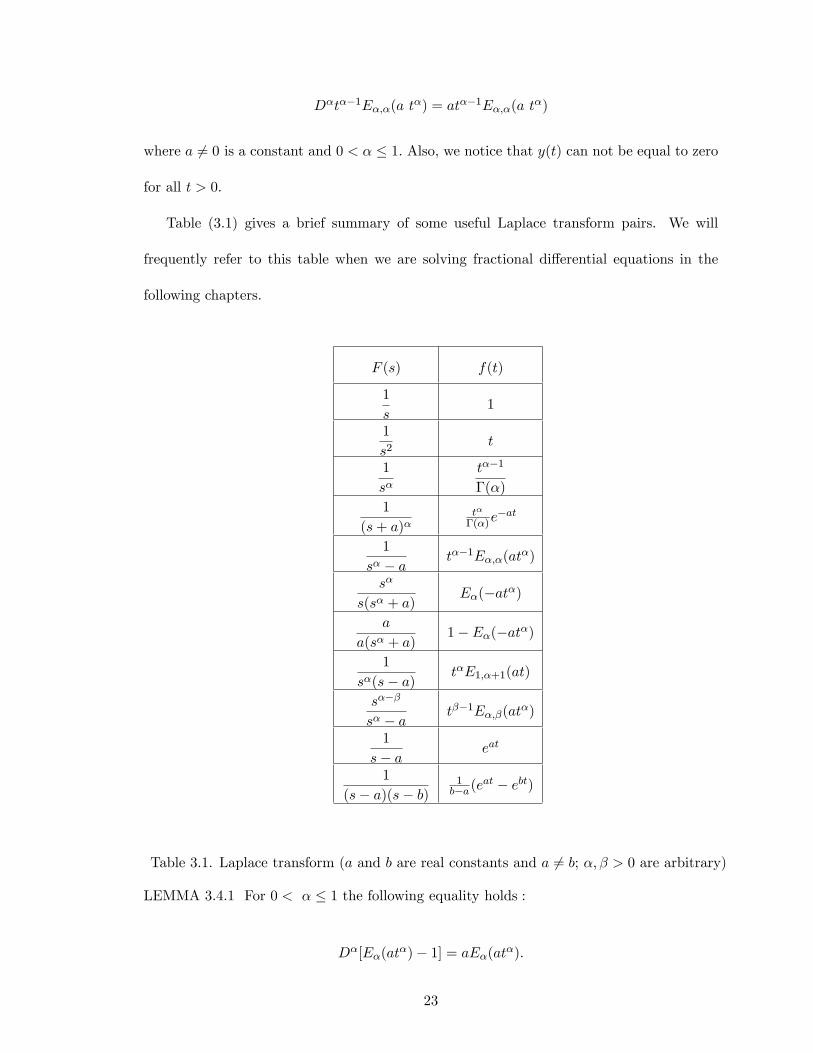
Table (3.1) gives a brief summary of some useful Laplace transform pairs. We will
frequently refer to this table when we are solving fractional differential equations in the
following chapters.
F (s) f(t)
1
s1
1
s2t
1
sαtα−1
Γ(α)
1
(s+ a)αtα
Γ(α)e−at
1
sα − a tα−1Eα,α(atα)
sα
s(sα + a)Eα(−atα)
a
a(sα + a)1− Eα(−atα)
1
sα(s− a)tαE1,α+1(at)
sα−β
sα − a tβ−1Eα,β(atα)
1
s− a eat
1
(s− a)(s− b)1b−a(eat − ebt)
Table 3.1. Laplace transform (a and b are real constants and a 6= b; α, β > 0 are arbitrary)
LEMMA 3.4.1 For 0 < α ≤ 1 the following equality holds :
Dα[Eα(atα)− 1] = aEα(atα).
23
where Eα is the Mittag-Leffl er function in one parameter.
Proof. By taking the Laplace transform of the left hand side of the equation, we have
L{Dα[Eα(atα)− 1]} = sαL{Eα(atα)− 1)} −D−(1−α)[Eα(0)− 1]
= sα[L{Eα(atα)} − L{1}]−D−(1−α)(t)|t=0
= sα(
sα
s(sα − a)− 1
s
)− 0
=asα
s(sα − a)
Applying the inverse Laplace transform to each sides of the above equation, we have the
desired result
Dα[Eα(atα)− 1] = aEα(atα).
24
CHAPTER 4
Fractional Trigonometric Functions
In this chapter we develop fractional trigonometry based on the multi-valued fractional
generalization of the exponential function, Mittag-Leffl er function. Mittag-Leffl er function
plays an important role in the solution of fractional order differential equations. The de-
velopment of fractional calculus has involved new functions that generalize the exponential
function. These functions allow the opportunity to generalize the trigonometric functions to
“fractional”or “generalized”versions. In this chapter, we discuss the relationships between
Mittag-Leffl er function and the new fractional trigonometric functions. Laplace transform
are derived for the new functions and are used to generate the solution sets for various
classes of fractional differential equations. Then we generalize the Wronskian for a system
of fractional derivative equations as well. Also, a new method is presented for solving system
of fractional differential equations.
4.1 Generalized Exponential Function
As we pointed out, Mittag-Leffl er function can be written in terms of two parameters α
and β as
Eα,β[t] =∞∑n=0
tn
Γ(nα+ β), α, β > 0.
This function will often appear with the argument atα, thus it can be written as
Eα,β[atα]=∞∑n=0
(atα)n
Γ(nα+ β), where α, β > 0 and a ∈ C.
The exponential function can be written in terms of Mittag-Leffl er function as
E1,1[at]=∞∑n=0
(at)n
Γ(n+ 1)= eat.
25
Based on Mittag-Leffl er function, the generalized form of the exponential function can be
written as
eα,α(a, t) = tα−1Eα,α[atα], t > 0. (4.1)
4.2 Generalized Trigonometry
This section develops fractional trigonometry based on the generalization of the ex-
ponential function eα,α(a, t). Because of the fractional characteristics of α we will see
trigonometric functions to have families of functions for fractional trigonometric functions
instead of a single function. "Fractional" or "generalized" trigonometric functions can be
derived from eα,α(a, t).
One way to define the (integer order) trigonometry is based on the close relation to the
exponential function.
cos t =eit + e−it
2, (4.2)
and
sin t =eit − e−it
2i. (4.3)
To derive the multi-valued character of the new trigonometric functions we consider the
generalization of the exponential function, Then fractional cosine can be defined as
cosα,α(a, t) =eα,α(ai, t) + eα,α(−ai, t)
2, t > 0, (4.4)
and fractional sine can be defined as
26
sinα,α(a, t) =eα,α(ai, t)− eα,α(−ai, t)
2i, t > 0. (4.5)
Also, we can define fractional tangent function as
tanα,α(a, t) =sinα,α(a, t)
cosα,α(a, t), t > 0. (4.6)
The development for the remaining functions (i.e. secα,α(a, t), cscα,α(a, t) and cotα,α(a, t))
would be based on the relationship between these functions and the two functions cosine
and sine.
These functions, identities (4.4)-(4.6), generalize the circular functions of the normal or
integer order trigonometry and are used as the basis of the relationships that follow.
4.3 Properties of Fractional Trigonometric Functions
It is directly observed from the definition of cosα,α(a, t) and sinα,α(a, t), equation (4.4)
and (4.5), that
cosα,α(−a, t) = cosα,α(a, t), (4.7)
and
sinα,α(−a, t) = − sinα,α(a, t). (4.8)
Substituting equation (4.7) and (4.8) into (4.6) gives
tanα,α(−a, t) =− sinα,α(a, t)
cosα,α(a, t)= − tanα,α(a, t), t > 0. (4.9)
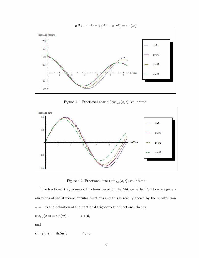
Figure 4.1 and 4.2 show the fractional cosine and the fractional sine for various values of
α. We notice that two curves of fractional cosine at α = .98 and α = .95 behave similarly.
27
Notice that the curves of both fractional cosine and sine are approaching the traditional
cosine and sine, respectively as α approaches 1.
It is directly follows from (4.4) and (4.5) that
eα,α(ai, t) = cosα,α(a, t) + i sinα,α(a, t), t > 0. (4.10)
From the above equation and equations (4.7) and (4.8) , it follows that
eα,α(−ai, t) = cosα,α(a, t)− i sinα,α(a, t), t > 0. (4.11)
Squaring equation (4.4) yields
cos2α,α(a, t) =1
4{e2α,α(ai, t) + e2α,α(−ai, t) + 2eα,α(ai, t)eα,α(−ai, t)}. (4.12)
And squaring equation (4.5) yields
sin2α,α(a, t) =−1
4{e2α,α(ai, t) + e2α,α(−ai, t)− 2eα,α(ai, t)eα,α(−ai, t)}. (4.13)
Adding the above two equations (4.12) and (4.13) gives
cos2α,α(a, t) + sin2α,α(a, t) = eα,α(ai, t)eα,α(−ai, t), t > 0. (4.14)
Substituting α and a by 1 in equation (4.14) yields
cos2 t− sin2 t = 1
Subtracting (4.13) from (4.12) yields
cos2α,α(a, t)− sin2α,α(a, t) =1
2{e2α,α(ai, t) + e2α,α(−ai, t) }, t > 0. (4.15)
Let α and a be equal to 1 in equation (4.15), we obtain
28
cos2 t− sin2 t = 12{e
2it + e−2it} = cos(2t).
Figure 4.1. Fractional cosine ( cosα,α(a, t)) vs. t-time
Figure 4.2. Fractional sine ( sinα,α(a, t)) vs. t-time
The fractional trigonometric functions based on the Mittag-Leffl er Function are gener-
alizations of the standard circular functions and this is readily shown by the substitution
α = 1 in the definition of the fractional trigonometric functions, that is;
cos1,1(a, t) = cos(at) , t > 0,
and
sin1,1(a, t) = sin(at), t > 0.
29
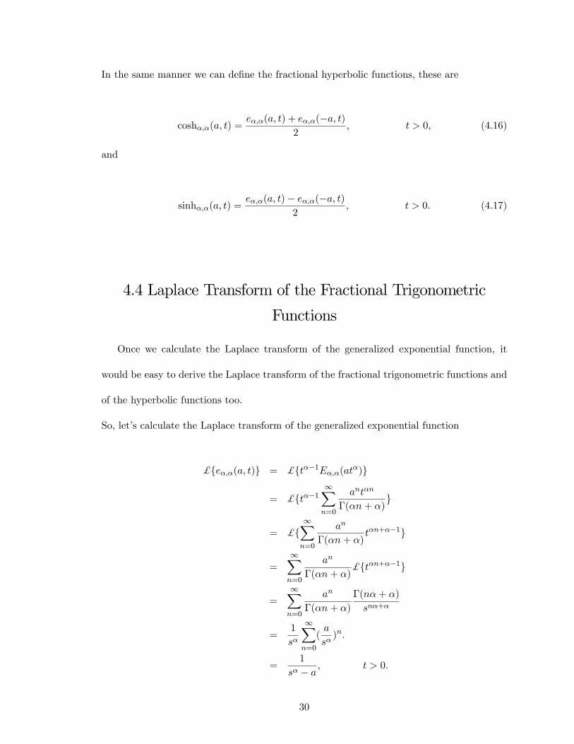
In the same manner we can define the fractional hyperbolic functions, these are
coshα,α(a, t) =eα,α(a, t) + eα,α(−a, t)
2, t > 0, (4.16)
and
sinhα,α(a, t) =eα,α(a, t)− eα,α(−a, t)
2, t > 0. (4.17)
4.4 Laplace Transform of the Fractional Trigonometric
Functions
Once we calculate the Laplace transform of the generalized exponential function, it
would be easy to derive the Laplace transform of the fractional trigonometric functions and
of the hyperbolic functions too.
So, let’s calculate the Laplace transform of the generalized exponential function
£{eα,α(a, t)} = £{tα−1Eα,α(atα)}
= £{tα−1∞∑n=0
antαn
Γ(αn+ α)}
= £{∞∑n=0
an
Γ(αn+ α)tαn+α−1}
=∞∑n=0
an
Γ(αn+ α)£{tαn+α−1}
=∞∑n=0
an
Γ(αn+ α)
Γ(nα+ α)
snα+α
=1
sα
∞∑n=0
(a
sα)n.
=1
sα − a, t > 0.
30
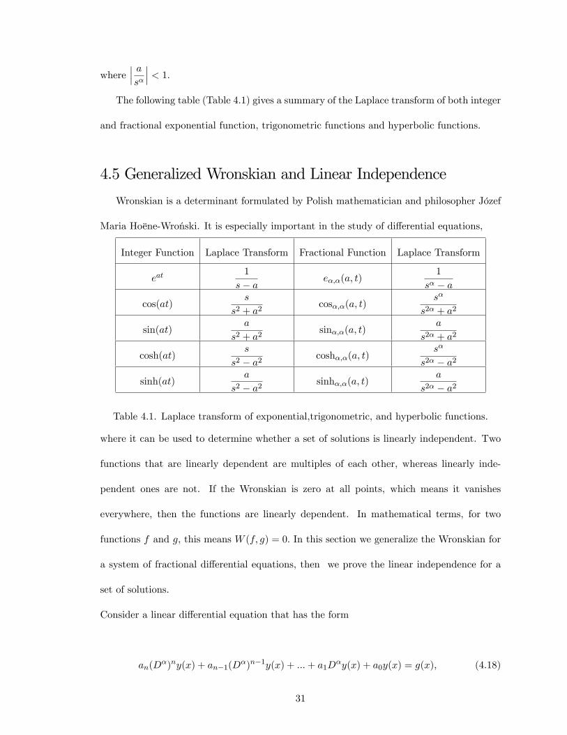
where∣∣∣ asα
∣∣∣ < 1.
The following table (Table 4.1) gives a summary of the Laplace transform of both integer
and fractional exponential function, trigonometric functions and hyperbolic functions.
4.5 Generalized Wronskian and Linear Independence
Wronskian is a determinant formulated by Polish mathematician and philosopher Józef
Maria Hoëne-Wronski. It is especially important in the study of differential equations,
Integer Function Laplace Transform Fractional Function Laplace Transform
eat1
s− a eα,α(a, t)1
sα − a
cos(at)s
s2 + a2cosα,α(a, t)
sα
s2α + a2
sin(at)a
s2 + a2sinα,α(a, t)
a
s2α + a2
cosh(at)s
s2 − a2 coshα,α(a, t)sα
s2α − a2
sinh(at)a
s2 − a2 sinhα,α(a, t)a
s2α − a2
Table 4.1. Laplace transform of exponential,trigonometric, and hyperbolic functions.
where it can be used to determine whether a set of solutions is linearly independent. Two
functions that are linearly dependent are multiples of each other, whereas linearly inde-
pendent ones are not. If the Wronskian is zero at all points, which means it vanishes
everywhere, then the functions are linearly dependent. In mathematical terms, for two
functions f and g, this means W (f, g) = 0. In this section we generalize the Wronskian for
a system of fractional differential equations, then we prove the linear independence for a
set of solutions.
Consider a linear differential equation that has the form
an(Dα)ny(x) + an−1(Dα)n−1y(x) + ...+ a1D
αy(x) + a0y(x) = g(x), (4.18)
31
where (Dα)n = DαDα...Dα︸ ︷︷ ︸n−times
, 0 < α ≤ 1 ,and (Dα)n 6= Dαn, also, aj are constants, where
j = 0, 1, 2, ..., n, and g(x) depends solely on the variable x. In other words, they do not
depend on y or any derivative of y.
If g(x) = 0, then the equation (4.18) is called homogeneous; if not, (4.18) is called a non-
homogeneous fractional equation.
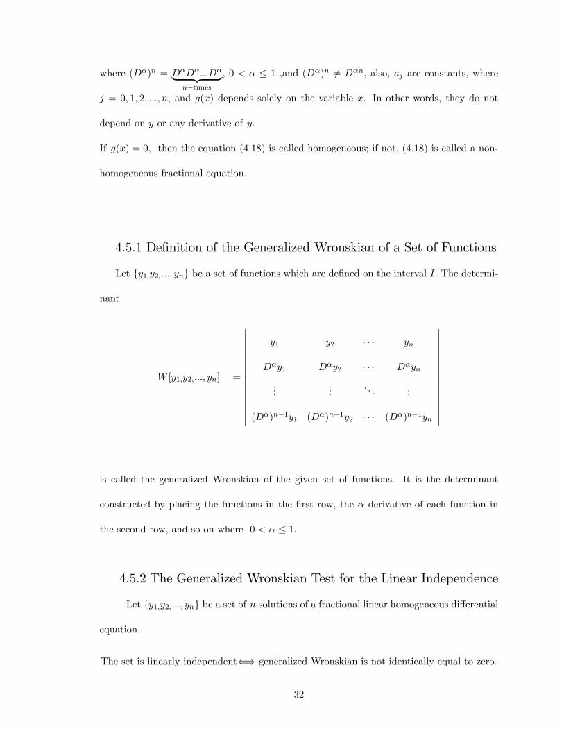
4.5.1 Definition of the Generalized Wronskian of a Set of Functions
Let {y1,y2,..., yn} be a set of functions which are defined on the interval I. The determi-
nant
W [y1,y2,..., yn] =
∣∣∣∣∣∣∣∣∣∣∣∣∣∣∣∣
y1 y2 · · · yn
Dαy1 Dαy2 · · · Dαyn
......
. . ....
(Dα)n−1y1 (Dα)n−1y2 · · · (Dα)n−1yn
∣∣∣∣∣∣∣∣∣∣∣∣∣∣∣∣
is called the generalized Wronskian of the given set of functions. It is the determinant
constructed by placing the functions in the first row, the α derivative of each function in
the second row, and so on where 0 < α ≤ 1.
4.5.2 The Generalized Wronskian Test for the Linear Independence
Let {y1,y2,..., yn} be a set of n solutions of a fractional linear homogeneous differential
equation.
The set is linearly independent⇐⇒ generalized Wronskian is not identically equal to zero.
32
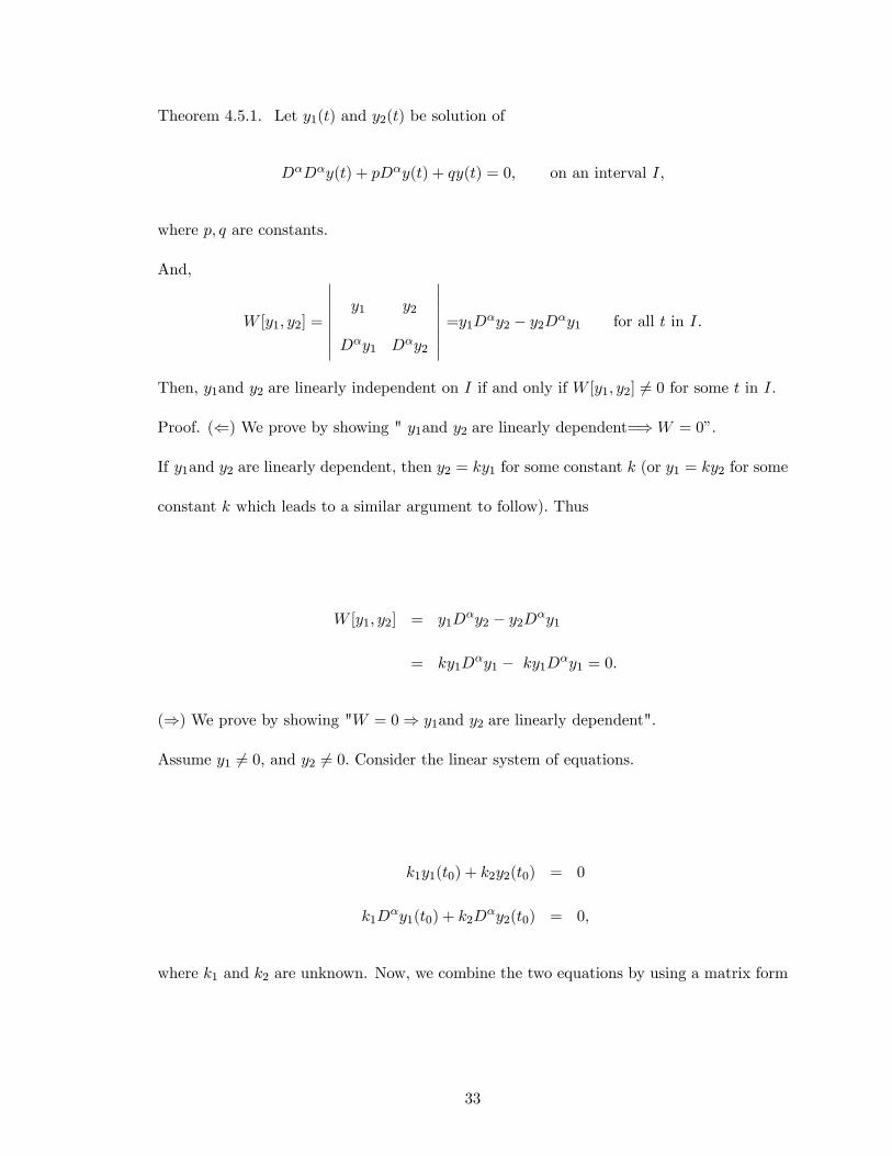
Theorem 4.5.1. Let y1(t) and y2(t) be solution of
DαDαy(t) + pDαy(t) + qy(t) = 0, on an interval I,
where p, q are constants.
And,
W [y1, y2] =
∣∣∣∣∣∣∣∣y1 y2
Dαy1 Dαy2
∣∣∣∣∣∣∣∣ =y1Dαy2 − y2Dαy1 for all t in I.
Then, y1and y2 are linearly independent on I if and only if W [y1, y2] 6= 0 for some t in I.
Proof. (⇐) We prove by showing " y1and y2 are linearly dependent=⇒W = 0”.
If y1and y2 are linearly dependent, then y2 = ky1 for some constant k (or y1 = ky2 for some
constant k which leads to a similar argument to follow). Thus
W [y1, y2] = y1Dαy2 − y2Dαy1
= ky1Dαy1 − ky1D
αy1 = 0.
(⇒) We prove by showing "W = 0⇒ y1and y2 are linearly dependent".
Assume y1 6= 0, and y2 6= 0. Consider the linear system of equations.
k1y1(t0) + k2y2(t0) = 0
k1Dαy1(t0) + k2D
αy2(t0) = 0,
where k1 and k2 are unknown. Now, we combine the two equations by using a matrix form
33
y1(t0) y2(t0)
Dαy1(t0) Dαy2(t0)
k1
k2
= 0
By Cramer’s theorem, if
∣∣∣∣∣∣∣∣y1(t0) y2(t0)
Dαy1(t0) Dαy2(t0)
∣∣∣∣∣∣∣∣ = 0 (i.e W = 0),
the system has non-trivial solution; that is k1 and k2 are not both zero. using these k1 and
k2 to construct a function
y(t) = k1y1(t) + k2y2(t).
Then y(t) = k1y1 + k2y2 is a solution of
DαDαy(t) + pDαy(t) + qy(t) = 0, and satisfies the initial conditions
D−(1−α)y(t0) = 0, and Dαy(t0) = 0.
By Existence and Uniqueness theorem [16], we know that the solution of the IVP
DαDαy(t) + pDαy(t) + qy(t) = 0
D−(1−α)y(t0) = 0, and Dαy(t0) = 0.
is unique and k1y1+k2y2 = 0 on I. Since k1 and k2 are not both zero, y1 and y2 are linearly
dependent. �
The proof for a set of n solutions is almost identical to the proof in the special case n = 2.
4.5.3 The Characteristic Equation
Corresponding to the fractional differential equation
DαDαy(t) + pDαy(t) + qy(t) = 0, (4.19)
34
in which p and q are constants, is the algebraic equation
λ2 + pλ+ q = 0, (4.20)
which is obtained from equation (4.19) by replacing DαDαy(t), Dαy(t) and y by λ2, λ1, and
λ0= 1, respectively. Equation(4.20) is called characteristic equation of (4.19).
In general, the characteristic equation of fractional homogeneous equation (4.18) is given
by
anλn + an−1λ
n−1 + ...+ a1λ+ a0 = 0.
4.5.4 Solution of Homogeneous Equation
If λ1 and λ2 are two distinct roots of (4.20). Then the solution of (4.19) can be written
as a linear combination of two functions y1 and y2 where
y1 = tα−1Eα,α( λ1tα)
and
y2 = tα−1Eα,α(λ2tα).
Then, the general solution of (4.19) is
y(t) = c1tα−1Eα,α( λ1t
α) + c2tα−1Eα,α(λ2t
α)
= c1eα,α(λ1, t) + c2eα,α(λ2, t),
where c1 and c2 are constants.
EXAMPLE 4.5.1. We claim that the following equation
DαDαy + 5Dαy + 6y = 0, (4.21)
35
where 0 < α ≤ 1 and t > 0 has the solution
y(t) = c1y1 + c2y2,
where y1 = eα,α(−3, t) and y2 = eα,α(−2, t).
y1 and y2 are two solutions of (4.21), then y1 and y2 must satisfy equation (4.21), so we
have
DαDαy2 + 5Dαy2 + 6y2
= DαDαeα,α(−3, t) + 5Dαeα,α(−3, t) + 6eα,α(−3, t).
Using Remark 3.4.1, this implies
DαDαy2 + 5Dαy2 + 6y2
= −3Dαeα,α(−3, t)− 15eα,α(−3, t) + 6eα,α(−3, t)
= 9eα,α(−3, t)− 15eα,α(−3, t) + 6eα,α(−3, t)
= 0.
This completes the proof of the claim. �
We expect to obtain the same result by finding the roots of the characteristic equation of
(4.21), so we have
λ2 + 5λ+ 6 = 0.
This implies
(λ+ 3)(λ+ 2) = 0.
36
Thus, the roots of the characteristic equation are
λ1 = −3 and λ2 = −2.
Finally, the solution of equation (4.21) is
y(t) = c1eα,α(−3, t) + c2eα,α(−2, t).
Similarly, one can show that y2 satisfies equation (4.21).
4.6. Fractional Derivative of Trigonometry
Derivative operator plays an important role in calculus. Therefore, in this section, we
derive the derivative of fractional trigonometric functions, in particular, fractional cosine
and fractional sine.
We calculate the derivative of fractional cosine directly by using the definition of cosα,α(a, t)
and the derivative of the fractional exponential function
Dα cosα,α(a, t) = Dα{eα,α(ai, t) + eα,α(−ai, t)2
}
=1
2{Dαeα,α(ai, t) +Dαeα,α(−ai, t)}
=1
2{aieα,α(ai, t)− aieα,α(−ai, t)}
=−a2i{eα,α(ai, t)− eα,α(−ai, t)}
= −a sinα,α(a, t).
Then, we conclude that
Dα cosα,α(a, t) = −a sinα,α(a, t), where 0<α ≤ 1
In similar manner, one can show that the α derivative of sinα,α(a, t) is
Dα sinα,α(a, t) = a cosα,α(a, t).
37
In Carl F.Lorenzo and Tom T.Hartley’s paper in 2004, there was an open question
about finding classes of special fractional differential equations that have solutions of the
new fractional trigonometry functions or a linear combination of them. In this section we
develop classes of fractional differential equation with the solution of a linear combination
of cosα,α(a, t) and sinα,α(a, t).
4.7 System of Linear Fractional Differential Equations with
Constant Matrix Coeffi cients.
This section deals with the study of the following system of linear fractional equations.
We present a new proof for the solution for a system of fractional differential equations.
DαY (t) = AY (t) + F (t) (4.22)
D−(1−α)Y (t)|t=0 = C,
where DαY (t) is the fractional derivative of order 0 < α ≤ 1, and C is n × 1 vector, Y (t)
and F (t) are n× 1 vector valued functions, A is n× n constant matrix.
We will formulate the unique solution of the system by using the Laplace transform.
Let’s define L{Y (t)} = Y ∗(s) and L{F (t)} = F ∗(s), so taking the Laplace transform of
both sides of the equation (4.22) yields
L{DαY (t)} = AL{Y (t)}+ L{F (t)}
Using the role of Laplace transform of the fractional derivative, we obtain
sαY ∗(s)−D−(1−α)Y (t)|t=0 = AY (s) + F ∗(s).
Since D−(1−α)Y (t)|t=0 = C, we have
38
(Isα −A)Y ∗(s)− C = F ∗(s),
which implies
(Isα −A)Y ∗(s) = C + F ∗(s).
Taking the inverse of (Isα −A) yields
Y ∗(s) = (Isα −A)−1[C + F ∗(s)]
= (sα(I − s−αA))−1[C + F ∗(s)]
= s−α(I − s−αA)−1[C + F ∗(s)]
= s−α∞∑k=0
(As−α)k[C + F ∗(s)]
=∞∑k=0
(As−α)ks−αC + F ∗(s)∞∑k=0
(As−α)ks−α
=∞∑k=0
Ak
sαk+αC + F ∗(s)
∞∑k=0
Ak
sαk+α.
Let∞∑k=0
Ak
sαk+α= G∗(s), then
G(t) = L−1{∞∑k=0
Ak
sαk+α}
=∞∑k=0
AkL−1{ 1
sαk+α}
=
∞∑k=0
Aktαk+α−1
Γ(αk + α)
= tα−1Eα,α{atα).
Thus,
Y (s) =∞∑k=0
Ak
sαk+αC + L{F (t) ∗G(t)},
39
where L{G(t)} = G∗(s).
Then, taking the inverse Laplace Transform of the last equation and using Table 3.1, we
obtain
Y (t) =∞∑k=0
Aktαk+α−1
Γ(αk + α)C +
∫ t
0F (t− z)G(z)dz
= tα−1Eα,α(Atα)C +
∫ t
0(t− z)α−1Eα,α(A(t− z)α)F (z)dz
Replacing α = 1 , we obtain
Y (t) = E1,1(At)C +
∫ t
0E1,1(A(t− z))F (z)dz
= eAtC +
∫ t
0eA(t−z)F (z)dz
Since solving equation (4.22) involves the matrix Mittag-Leffl er function, tα−1Eα,α(Atα),
we will first look at this important function. We will state the next two theorems without
proof.
THEOREM 4.7.1 [16]. (Extended Putzer Algorithm) If A is 2 × 2 constant matrix, then
the solution to the IVP
DαY (t) = AY (t), D−(1−α)Y (t)|t=0 = C, (4.23)
where
A =
a b
c d
, Y (t) =
y1(t)y2(t)
, 0 < α ≤ 1.
40
is given by
Y (t) = kα,α(Atα)C
where
kα,α(Atα) = tα−1Eα,α(Atα),
and kα,α(Atα), is the matrix Mittag-Leffl er function, and C is 2× 1 vector.
THEOREM 4.7.2 [16]. If λ1 and λ2 are (not necessarily distinct) eigenvalues of the 2× 2
matrix A, then
kα,α(Atα) = p1(t)M0 + p2(t)M1,
where
M0 = I =
1 0
0 1
, M1 = A− λ1I =
a− λ1 b
c d− λ1
,and the vector function p defined by
p(t) =
p1(t)
p2(t)
, t ∈ R,
is a solution to the IVP
Dαp(t) =
λ1 0
1 λ2
p(t), D−(1−α)p1(t)|t=0
D−(1−α)p2(t)|t=0
=
1
0
.EXAMPLE 4.7.1. Let 0 < α ≤ 1, then the following IVP
DαDαy(t) + a2y(t) = 0 (4.24)
Dαy(t)|t=0 = c1 and D−(1−α)y(t)|t=0 = c2
41
can be transformed into a system of fractional differential equations by the change of the
variables, such that
y1 = y and y2 = Dαy
This implies
Dαy1 = Dαy = y2
and
DαDαy = −a2y = −a2y1,
where y1(t)|t=0 = c1 and y2(t)|t=0 = c2. Then, we have the following linear system of
fractional differential equations
DαY (t) = AY (t), D−(1−α)Y (t)|t=0 = C,
where
A =
0 1
−a2 0
, Y (t) =
y1(t)y2(t)
, and C =
c1c1
which has the solution
Y (t) = kα,α(Atα)C.
Let’s compute kα,α(Atα) by using Theorem 4.6.2.
First, we calculate λ1 and λ2, where λ1 and λ2 are the eigenvalues of A
λ1 =(a+ d)−
√a2 − 2ad+ 4bc+ d2
2.
Thus,
42
λ1 = −ai.
And,
λ2 =(a+ d) +
√a2 − 2ad+ 4bc+ d2
2.
Thus,
λ1 = ai.
By the Extended Putzer algorithm,
kα,α(Atα) =∑1
k=0 pk+1(t)Mk = p1(t)M0 + p2(t)M1,
where,
M0 = I =
1 0
0 1
, M1 = A− λ1I =
ai 1
−a2 ai
.The vector function is p(t) given by
p(t) =
p1(t)
p2(t)
, t ∈ R,
is a solution to the IVP
Dαp(t) =
λ1 0
1 λ2
p(t), D−(1−α)p(t)|t=0 =
1
0
.The first component p1(t) of p(t) solve the IVP
Dαp1(t) = (−ai)p1(t), D−(1−α)p1(t)|t=0 = 1.
Taking the Laplace transform of both sides, we have
L{Dαp1(t)} = (−ai)L{p1(t)}
43
Using the rule of the Laplace transform of the fractional derivative yields
sαP1(s)−D−(1−α)p1(t)|t=0 = (−ai)P1(s),
where L{p1(t)} = P1(s).
Since D−(1−α)p1(t)|t=0 = 1, then we have
sαP1(s)− 1 = (−ai)P1(s),
which implies
P1(s) =1
sα + ai.
Using Table 3.1, we obtain the inverse Laplace transform of P1(s)
p1(t) = tα−1Eα,α(−aitα)
= eα,α(−ai, t).
The second component p2(t) of p(t) solves the IVP
Dαp2(t) = tα−1Eα,α(−aitα) + (ai)p2(t), D−(1−α)p2(t)|t=0 = 0.
Using the Laplace transform, we have that
L{Dαp2(t)} = L{tα−1Eα,α(−aitα)}+ (ai)L{p2(t)},
Again, by using the rule of the Laplace transform of the fractional derivative, we obtain
sαP2(s)−D−(1−α)p2(t)|t=0 =1
sα + ai+ (ai)P2(s),
44
where L{p2(t)} = P2(s).
Since D−(1−α)p2(t)|t=0 = 0, then we have
(sα − ai)P2(s) =1
sα + ai,
which implies
P2(s) =1
(sα + ai)(sα − ai) .
Using partial fractions yields,
1
(sα + ai)(sα − ai) =1
−2ai
[1
sα + ai− 1
sα − ai
]
By employing Table 3.1, we obtain the inverse Laplace transform of P2(s) as follows
p2(t) =tα−1
−2ai[Eα,α(−aitα)− Eα,α(aitα)]
=1
−2ai[eα,α(−ai, t)− eα,α(ai, t)].
Finally, we have
kα,α(Atα) = p1(t)M0 + p2(t)M1
=
1
2[eα,α(ai, t) + eα,α(−ai, t)] 1
2ai[eα,α(ai, t)− eα,α(−ai, t)]
a
−2i[eα,α(ai, t)− eα,α(−ai, t)] 1
2[eα,α(ai, t) + eα,α(−ai, t)]
=
cosα,α(a, t)1
asinα,α(a, t)
−a sinα,α(a, t) cosα,α(a, t)
=
cosα,α(a, t)1
asinα,α(a, t)
Dα[cosα,α(a, t)] Dα[1
asinα,α(a, t)]
.Thus, the solution of equation (4.27) is
45
Y (t) = kα,α(Atα)C =
cosα,α(a, t)1
asinα,α(a, t)
Dα[cosα,α(a, t)] Dα[1
asinα,α(a, t)]
C.Therefore, the general solution to (4.28) is given by
y(t) = c1 cosα,α(a, t) +c2a
sinα,α(a, t),
where c1 and c2 are arbitrary real constants.
In this example, we showed that the general solution of equation (4.28) is a linear
combination of two fractional trigonometric functions (fractional cosine and fractional sine).
THEOREM 4.7.3. Fractional cosine (cosα,α(a, t)) and fractional sine (sinα,α(a, t)) are two
linearly independent functions for all t > 0.
Proof. In Example 4.7.1, the homogeneous fractional differential equation
DαDαy(t) + a2y(t) = 0
generates a solution of linear combination of fractional cosine and fractional sine.
To show that cosα,α(a, t) and sinα,α(a, t) are two linearly independent solutions, we use
generalized Wronskian test (Theorem 4.5.1), that is
W [y1, y2] =
∣∣∣∣∣∣∣∣cosα,α(a, t) sinα,α(a, t)
Dα cosα,α(a, t) Dα sinα,α(a, t)
∣∣∣∣∣∣∣∣=
∣∣∣∣∣∣∣∣cosα,α(a, t) sinα,α(a, t)
−a sinα,α(a, t) a cosα,α(a, t)
∣∣∣∣∣∣∣∣= a cos2α,α(a, t)− a sin2α,α(a, t)
=a
2{e2α,α(ai, t) + e2α,α(−ai, t) }
46
Since eα,α(a, t) 6= 0 for all t > 0 and a any arbitrary number, then e2α,α(a, t) 6= 0.
Therefore
W [y1, y2] 6= 0
which implies cosα,α(a, t) and sinα,α(a, t) are two linearly independent functions. �
47
CHAPTER 5
An Application of Fractional Calculus to Pharmacokinetic
Model
Development of new drugs or recommending drugs for patients requires large numbers of
statistics to assist the researcher in the study. Therefore, we need an effi cient method to help
us to compensate missing data. For example, in the study of changing drug concentration
over time after intravenous bolus administration to the body, we need to collect large
numbers of plasma samples to see how the change happens. However, taking large numbers
of samples from a patient is diffi cult. As a consequence, mathematical models are used to
predict missing data. Specifically, pharmacokinetic is the model that is used to study drugs.
Pharmacokinetic, abbreviated as PK, is a branch of pharmacology dedicated to studying
the mechanisms of absorption and distribution of an administered drug, the rate at which
a drug action begins and the duration of the effect, the chemical changes of the substance
in the body and the effects and routes of excretion of the metabolites of the drug. The
study of these processes plays a significant role for choosing an appropriate dose and dosing
regimen for a particular patient.
Pharmacokinetic analysis is performed by noncompartment or compartment methods.
Noncompartment methods estimate the exposure to a drug by estimating the area under the
curve of a concentration-time graph. Compartment methods estimate the concentration-
time graph.
The most commonly used models in pharmacokinetic analysis are compartment mod-
els. All drugs initially distribute into a central compartment before distributing into the
peripheral compartment. If a drug rapidly distribute within the tissue compartment, the
disposition kinetics of the drug can be described as one compartment model. It is called
48
one compartment because all accessible sites have the same distribution kinetics. However,
drugs which exhibit as low equilibration with the peripheral tissues, are described with a
two compartment model.
In this thesis, we specifically consider one compartmental model with the newly devel-
oping fractional calculus. We compare our model with the ordinary calculus by utilizing
real data. The core of comparison is based on statistical evidences. Also, we employ a new
theory to give the best parameter estimation. Once we have the best model and suitable
parameter values, one can use the model to make predictions.
5.1 One Compartment Model
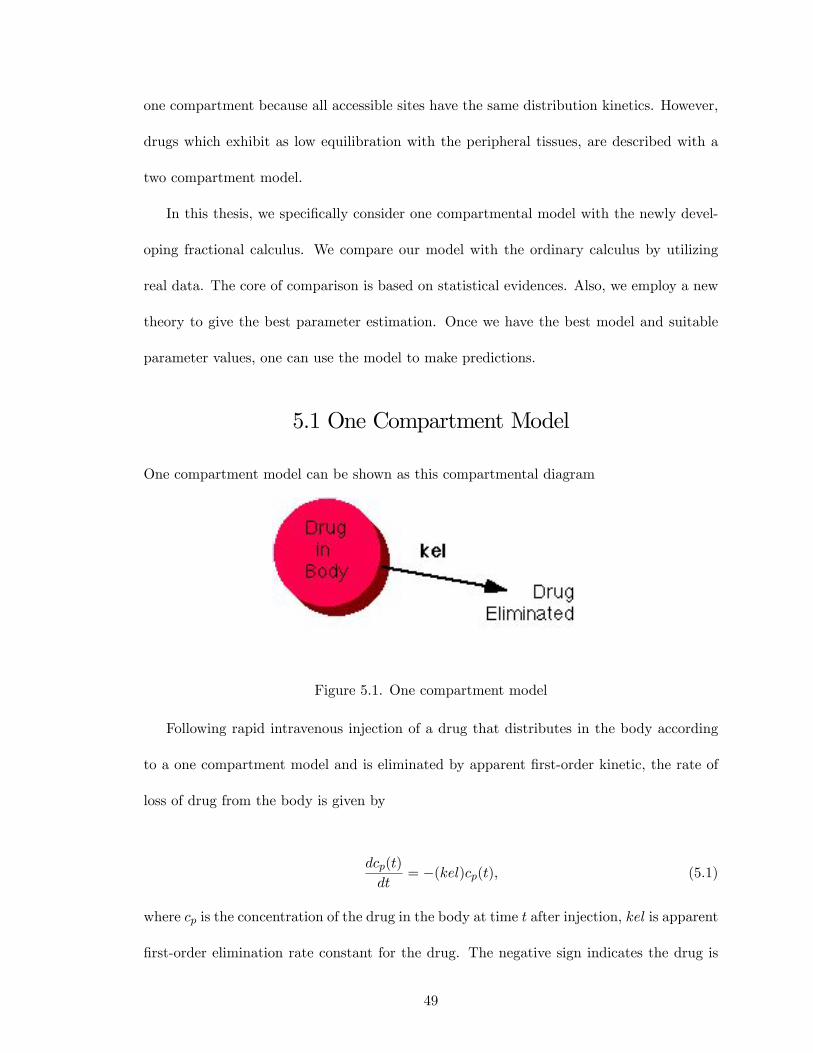
One compartment model can be shown as this compartmental diagram
Figure 5.1. One compartment model
Following rapid intravenous injection of a drug that distributes in the body according
to a one compartment model and is eliminated by apparent first-order kinetic, the rate of
loss of drug from the body is given by
dcp(t)
dt= −(kel)cp(t), (5.1)
where cp is the concentration of the drug in the body at time t after injection, kel is apparent
first-order elimination rate constant for the drug. The negative sign indicates the drug is
49
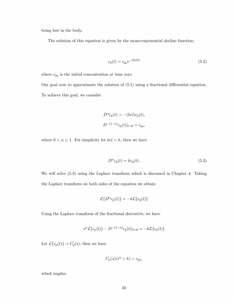
being lost in the body.
The solution of this equation is given by the mono-exponential decline function:
cp(t) = cp0e−(kel)t (5.2)
where cp0 is the initial concentration at time zero.
Our goal now to approximate the solution of (5.1) using a fractional differential equation.
To achieve this goal, we consider
Dαcp(t) = −(kel)cp(t),
D−(1−α)cp(t)|t=0 = cp0 ,
where 0 < α ≤ 1. For simplicity let kel = k, then we have
Dαcp(t) = kcp(t). (5.3)
We will solve (5.3) using the Laplace transform which is discussed in Chapter 4. Taking
the Laplace transform on both sides of the equation we obtain
L{Dαcp(t)} = −kL{cp(t)}
Using the Laplace transform of the fractional derivative, we have
sαL{cp(t)} −D−(1−α)cp(t)|t=0 = −kL{cp(t)}
Let L{cp(t)} = Cp(s), then we have
Cp(s)(sα + k) = cp0 ,
which implies
50
Cp(s) =cp0
sα + k.
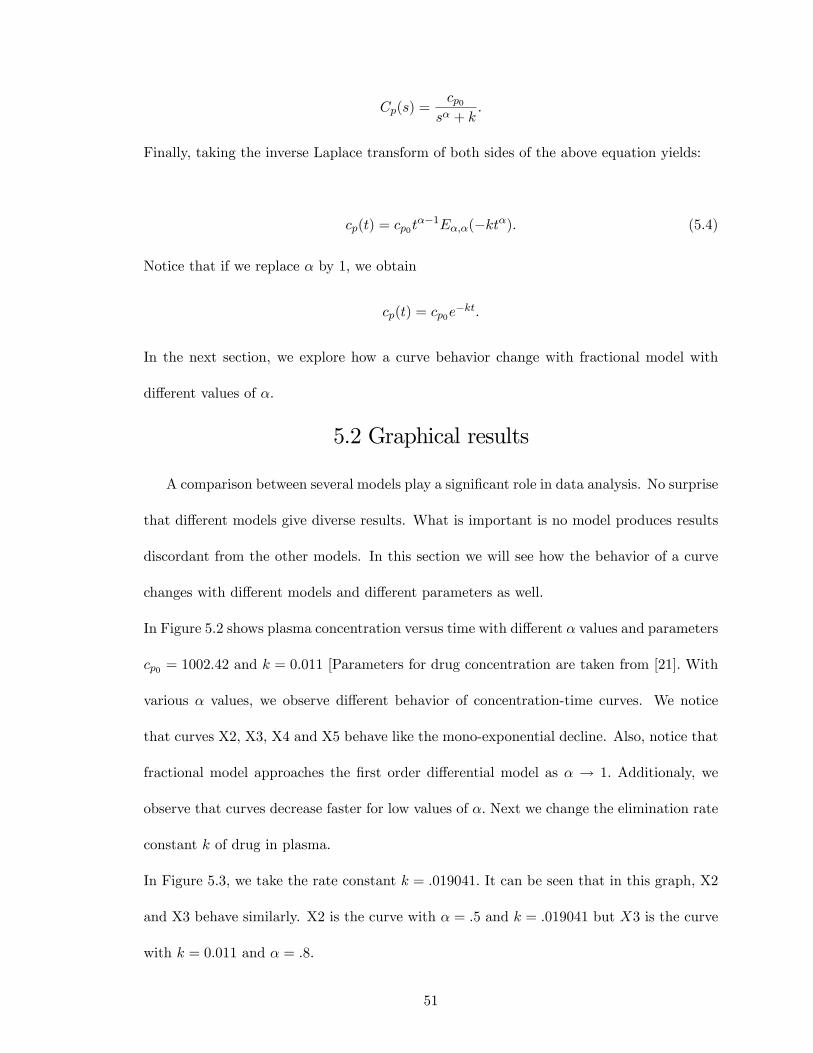
Finally, taking the inverse Laplace transform of both sides of the above equation yields:
cp(t) = cp0tα−1Eα,α(−ktα). (5.4)
Notice that if we replace α by 1, we obtain
cp(t) = cp0e−kt.
In the next section, we explore how a curve behavior change with fractional model with
different values of α.
5.2 Graphical results
A comparison between several models play a significant role in data analysis. No surprise
that different models give diverse results. What is important is no model produces results
discordant from the other models. In this section we will see how the behavior of a curve
changes with different models and different parameters as well.
In Figure 5.2 shows plasma concentration versus time with different α values and parameters
cp0 = 1002.42 and k = 0.011 [Parameters for drug concentration are taken from [21]. With
various α values, we observe different behavior of concentration-time curves. We notice
that curves X2, X3, X4 and X5 behave like the mono-exponential decline. Also, notice that
fractional model approaches the first order differential model as α → 1. Additionaly, we
observe that curves decrease faster for low values of α. Next we change the elimination rate
constant k of drug in plasma.
In Figure 5.3, we take the rate constant k = .019041. It can be seen that in this graph, X2
and X3 behave similarly. X2 is the curve with α = .5 and k = .019041 but X3 is the curve
with k = 0.011 and α = .8.
51
Following the above results, we observe that the curve behavior shows significant vari-
ation with respect to α. Since fractional model have one more fitting parameter, α, in
addition to the model parameters.
Observed and fitted data are shown in Figure 5.4. Data are taken from [10]. The
difference between the integer model (thin line) and fractional model (thick line) is clearly
demonstrated, thin curve (α = 1) does not go through our data but most of our data are
closer to the thick curve (α = .91). As a result, fractional calculus for curve fitting may
give more accurate results for data analysis.
5.3 Initial Parameter Estimation
In this section, we evaluate fractional model with various values of α for prediction
of plasma concentration. Then we compare the models searching for a better fit for the
observed data points of drug concentration. Two approaches are employed to show that
fractional calculus gives the best model for data analysis of drug concentration over time.
One approach determines that fractional model gives the best fit to the given data. The
second approach determines that fractional model is the best model for prediction. To start
off, let’s first estimate the initial parameters which are the theoretical concentration at time
zero, cp0 , and the elimination rate constant, k. Notice that the two models (5.1) and (5.3)
have the same parameters. Therefore, we just need to determine the parameters for one
of these models. Then we can use the result parameters for both models. The predicted
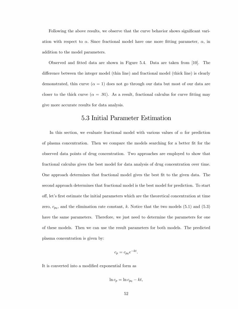
plasma concentration is given by:
cp = cp0e−kt.
It is converted into a modified exponential form as
ln cp = ln cp0 − kt,
52
which can also be written as
Y (t) = A+Bt, (5.5)
where Y (t) = ln cp, A = ln cp0 and B = −k.
In Table 5.1, plasma samples were obtained following bolus intravenous dosing and the
data follow a mono-exponential decline. We estimate the two parameter A and B and fit
the modified exponential decline curve to the given data and the fractional model as well.
Notice that the time is not periodic in Table 5.1. There are missing data which would
affect the result in parameter estimation. Therefore, a new theory is proposed to handle
the parameter estimation in an effective way without losing information.
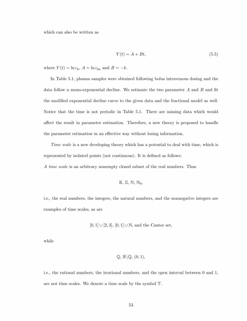
Time scale is a new developing theory which has a potential to deal with time, which is
represented by isolated points (not continuous). It is defined as follows:
A time scale is an arbitrary nonempty closed subset of the real numbers. Thus
R, Z, N, N0,
i.e., the real numbers, the integers, the natural numbers, and the nonnegative integers are
examples of time scales, as are
[0, 1] ∪ [2, 3], [0, 1] ∪ N, and the Cantor set,
while
Q, R\Q, (0, 1),
i.e., the rational numbers, the irrational numbers, and the open interval between 0 and 1,
are not time scales. We denote a time scale by the symbol T.
53
Forward and backward operators are two important operators in time scale calculus and
their definitions are given as follows
Let T be a time scale. For t ∈ T we define the forward jump operator σ : T −→ T by
σ(t) := inf{s ∈ T : s > t},
while the backward jump operator ρ : T −→ T by
ρ(t) := sup{s ∈ T : s < t}.
In this definition we put inf(φ) = sup(T) (i.e., σ(t) = t if T has a maximum t) and
sup(φ) = inf(T ) (i.e., ρ(t) = t if T has a minimum t), where φ denotes the empty set. If
σ(t) > t, we say that t is right-scattered, while if ρ(t) < t we say that t is left-scattered.
Points that are right-scattered and left-scattered at the same time are called isolated.
ThEOREM 5.3.1 [22]. Assume a and b ∈ T and f : T −→ R is ld-continuous.
(i) If T = R, then
∫ ba f(t)∇(t) =
∫ ba f(t)dt,
where the integral on the right is the Riemann integral from calculus.
(ii) If T consists of only isolated points, then
∫ b
af(t)∇(t) =
∫[a,b]∩T
f(t)∇(t) =∑
t∈(a,b]∩Tf(t)ν(t), if a < b.
where ν(t) is called graininess function and defined as
ν(t) = t− ρ(t).
As we point out the solution of (5.1) can be written in the form
Y (t) = A+Bt.
54
The given time-scale data in Table 5.1 are split up into two sets S1 and S2
S1 =∫
[0,50]∩TY (t)∇(t),
which implies
S1 =∑
t∈(0,50]∩TY (t)ν(t)
and
S2 =∫
[50,110]∩TY (t)∇(t),
which implies
S2 =∑
t∈(50,110]∩TY (t)ν(t).
where π is time scale and is given by
T = {10, 20, 30, 40, 50, 60, 70, 90, 110, 150}.
Substituting equation (5.5) in S1 and S2, we get
S1 =∑
t∈(0,50]∩T(A+Bt)ν(t)
= (10 + 10 + 10 + 10 + 10)A+B[(10)(10) + (20)(10) + (30)(10) + (40)(10) + (50)(10)]
= 50A+ 1500B
Similarly,
S2 =∑
t∈(50,150]∩T(A+Bt)ν(t)
= (10 + 10 + 20 + 20 + 40)A+B[(60)(10) + (70)(10) + (90)(20) + (110)(20) + (150)(40)]
= 100A+ 11300B.
55
S1 is the sum of the product of natural logarithm of the observed values times the backward
graininess function, so that
S1 =∑
t∈(0,50]∩Tln cp(t)ν(t)
= 10 ln(920) + 10 ln(800) + 10 ln(750) + 10 ln(630) + 10 ln(610)
= 315.61606
Similarly,
S2 =∑
t∈(50,150]∩Tln cp(t)ν(t)
= 10 ln(530) + 10 ln(520) + 20 ln(380) + 20 ln(350) + 40 ln(200)
= 519.9368.
To obtain A and B, we solve the following system of equations
315.61606 = 50A+ 1500B.
519.9368 = 100A+ 11300B
Hence, we get
A = 6.91067 and B = −0.010434
Since ln cp0 = 6.91067, this implies cp0 = 1002.92, and B = −k, this implies k = 0.010434.
We fit our model with the estimated elimination rate k, and by gussing method we
consider the initial concentration as cp0 = 1070. Based on these parameters, the exponential
decline curve of the predicted drug concentration is given by:
56
cp(t) = 1070e−0.010434t.
We fit fractional model with the same parameters as well, so that
cp(t) = 1070tα−1Eα,α(−0.010434tv).
Visually, each curve gives reasonably good fit to the given data. However, if we look
closely at the curves in Figure 5.5, we observe that data points are closer to the curves with
α = 0.99 and α = 0.98 than the curve with α = 1. To determine which curve gives the best
"fitting", we perform the square of residuals (SQR) analysis between the observed values
and the predicted values, which is given by
ei = yi − yi,
where yi is the observed value and yi is the predicted at time ti and i = 1, 2, ..., 10. Then,
we compute the mean squared error (MSE), which defined as
MSE=e21 + e
22 + ...+ e
2n
n,
where n = 10 in this example. The best model is the one showing the least mean squared
error (MSE).
Table 5.2 and 5.3 present the data points and the square of residuals between the
observed values and the predicted values with MSE as well for fractional model with α =
1, 0.99, 0.98, and 0.97.
Based on MSE analysis for each model, the best fit is given by fractional model with
α = 0.98, which gives the least mean squared error. It can also be seen that the fractional
model with α = 0.99 and α = 0.97 give more accurate results than the model with α = 1.
To make sure that our model works better, we compare between the results that we
have for MSE with the results that is given in [10] for the same data set. In that book
57
[10], linear regression was used to determine the parameters. MSE was 432.738 using the
first order differential model. However, our model with the method of time scale, MSE was
(426.2016023) with α = 0.98. These results support our insight that fractional model is
stronger than the integer model in this particular example. In the next section, we show
that fractional model gives the best prediction, not just the best fitting.
5.4 Model of Best Prediction
Statisticians believe that how well the model fits statistics is not a good guide to deter-
mine how well a model will predict. Evaluating such a model may demonstrate adequate
prediction capability on the training set, but might fail to predict future unseen data. Cross-
validation is primarily a way of measuring the predictive performance of a model. The idea
of cross-validation was originated in 1930s [25]. A clear statement to cross-validation which
is similar to current version of k−fold of cross-validation, first appeared in [19]. In 1970s,
Stone [20] employed cross-validation as means for choosing proper model parameters, as
opposed to using cross-validation purely for estimating model performance. The goal of
cross-validation is to measure the predictive ability of a model by testing it on a set of data
not used in estimation. This is called as a “test set,”and the data used for estimation is the
“training set”. The predictive accuracy of a model can be measured by the mean squared
error (MSE) on the test set.
In k−fold of cross-validation, the original data sample randomly partitioned into k
subsamples are used as training set. The cross-validation process then is repeated k times
and in each step, m observations are left out as validation data for testing the model. Each
of the k subsamples are used once as the validation data. Then, the accuracy measures are
obtained as follows.
Suppose there are n independent observations y1,y2,..., yn. We let m observations of the
58
original sample form the test set, and we fit the model for the remaining data (training set).
Then, we compute the square of the residual error (ei = yi − yi). We repeat the same steps
for each of the k supsamples. Finally, we compute the mean squared error (MSE).
In Table 5.1, we randomly split our data into five subsamples G1, G2,..., G5 such that
each subsample consists of eight observations as a training set, and for each a training set
there is one test set Ti (i = 1, 2, ..., 5) consists of two observations (the remaining data)
corresponding to that set. Table 5.4 shows the five training sets and the corresponding test
sets where where yi is the observed value at time ti, for i = 1, 2, ..., 10.
We fit our model for each training set to estimate the parameters using time scale
calculus as we did in the previous section, then we employ the result parameters to compute
the predicted value for each corresponding test set.
For G1, T = {20, 30, 40, 50, 60, 70, 90, 150}
where G1 = {800, 750, 630, 610, 530, 520, 380, 200}, then S1 and S2 can be written as
S1 =∑
t∈(0,50]∩TY (t)ν(t),
and
S2 =∑
t∈(50,150]∩TY (t)ν(t).
But S1 =∑
t∈(0,50]∩π(A+Bt)ν(t) and S2 =
∑t∈(50,150]∩π
(A+Bt)ν(t), so to obtain the parameters
A and B we solve the following system
S1 =∑
t∈(0,50]∩π(A+Bt)ν(t)
S2 =∑
t∈(50,150]∩π(A+Bt)ν(t).
After solving the above system of equations, we have
cp0 = 1003.52, where A = ln cp0 , and
59
k = 0.010674, where -k = B
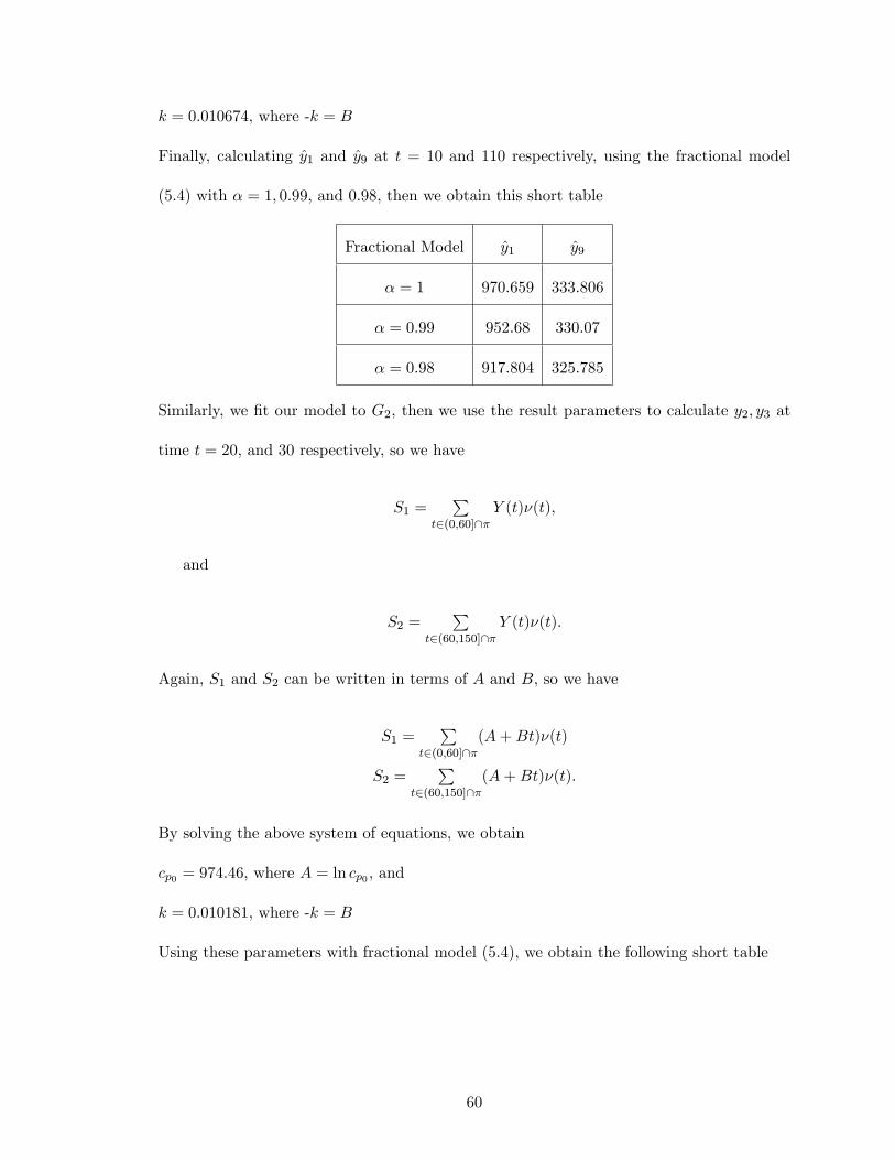
Finally, calculating y1 and y9 at t = 10 and 110 respectively, using the fractional model
(5.4) with α = 1, 0.99, and 0.98, then we obtain this short table
Fractional Model y1 y9
α = 1 970.659 333.806
α = 0.99 952.68 330.07
α = 0.98 917.804 325.785
Similarly, we fit our model to G2, then we use the result parameters to calculate y2, y3 at
time t = 20, and 30 respectively, so we have
S1 =∑
t∈(0,60]∩πY (t)ν(t),
and
S2 =∑
t∈(60,150]∩πY (t)ν(t).
Again, S1 and S2 can be written in terms of A and B, so we have
S1 =∑
t∈(0,60]∩π(A+Bt)ν(t)
S2 =∑
t∈(60,150]∩π(A+Bt)ν(t).
By solving the above system of equations, we obtain
cp0 = 974.46, where A = ln cp0 , and
k = 0.010181, where -k = B
Using these parameters with fractional model (5.4), we obtain the following short table
60
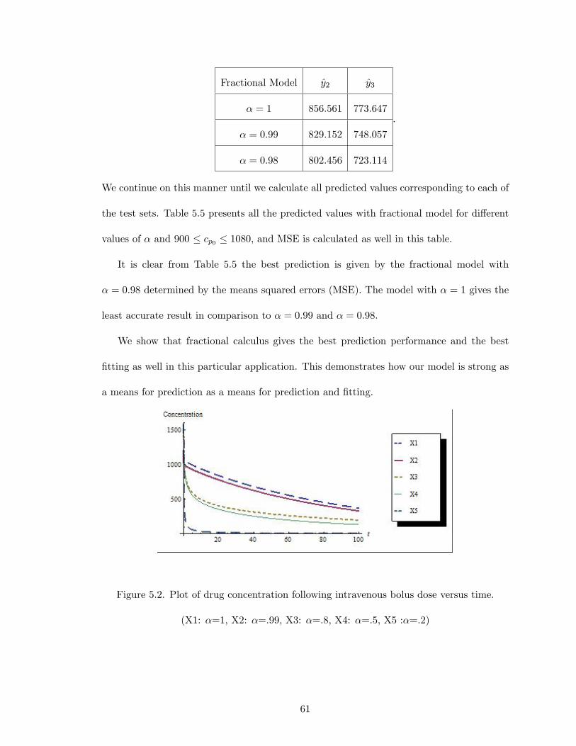
Fractional Model y2 y3
α = 1 856.561 773.647
α = 0.99 829.152 748.057
α = 0.98 802.456 723.114
.
We continue on this manner until we calculate all predicted values corresponding to each of
the test sets. Table 5.5 presents all the predicted values with fractional model for different
values of α and 900 ≤ cp0 ≤ 1080, and MSE is calculated as well in this table.
It is clear from Table 5.5 the best prediction is given by the fractional model with
α = 0.98 determined by the means squared errors (MSE). The model with α = 1 gives the
least accurate result in comparison to α = 0.99 and α = 0.98.
We show that fractional calculus gives the best prediction performance and the best
fitting as well in this particular application. This demonstrates how our model is strong as
a means for prediction as a means for prediction and fitting.
Figure 5.2. Plot of drug concentration following intravenous bolus dose versus time.
(X1: α=1, X2: α=.99, X3: α=.8, X4: α=.5, X5 :α=.2)
61
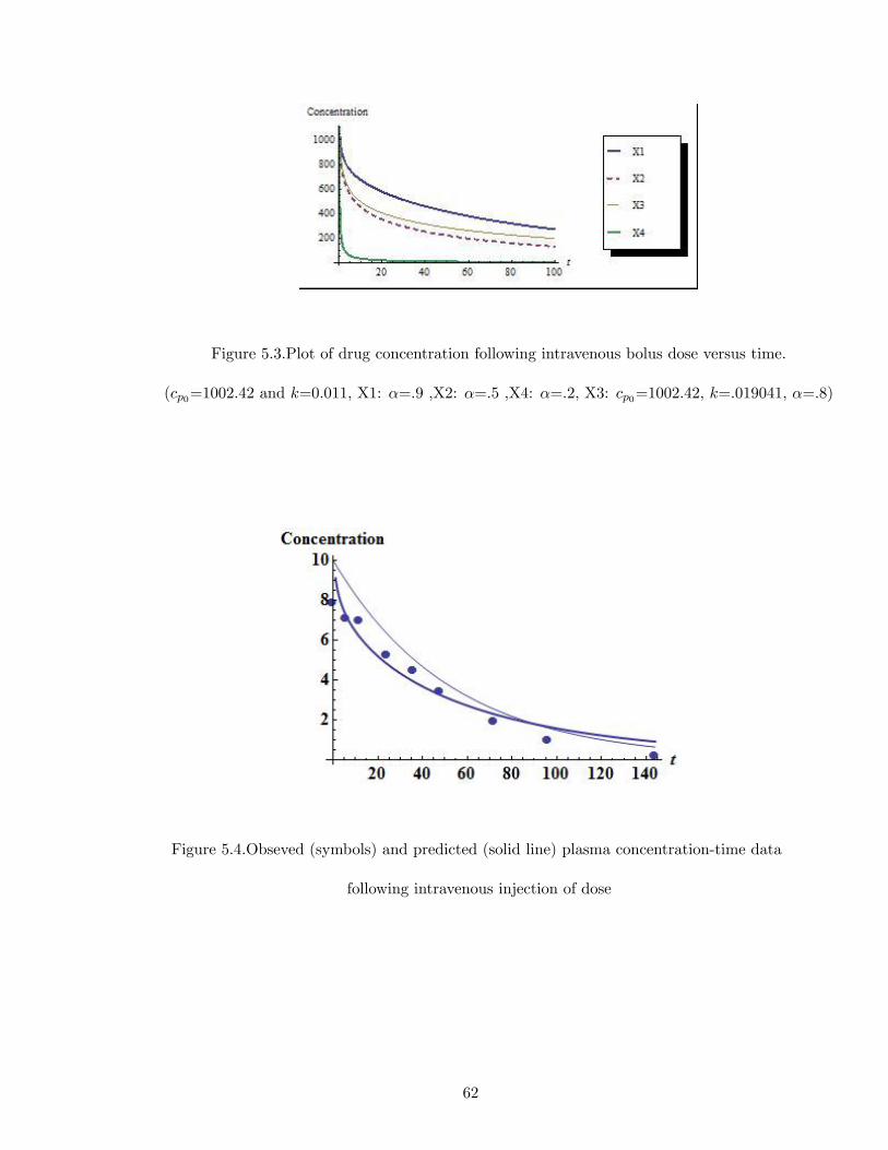
Figure 5.3.Plot of drug concentration following intravenous bolus dose versus time.
(cp0=1002.42 and k=0.011, X1: α=.9 ,X2: α=.5 ,X4: α=.2, X3: cp0=1002.42, k=.019041, α=.8)
Figure 5.4.Obseved (symbols) and predicted (solid line) plasma concentration-time data
following intravenous injection of dose
62
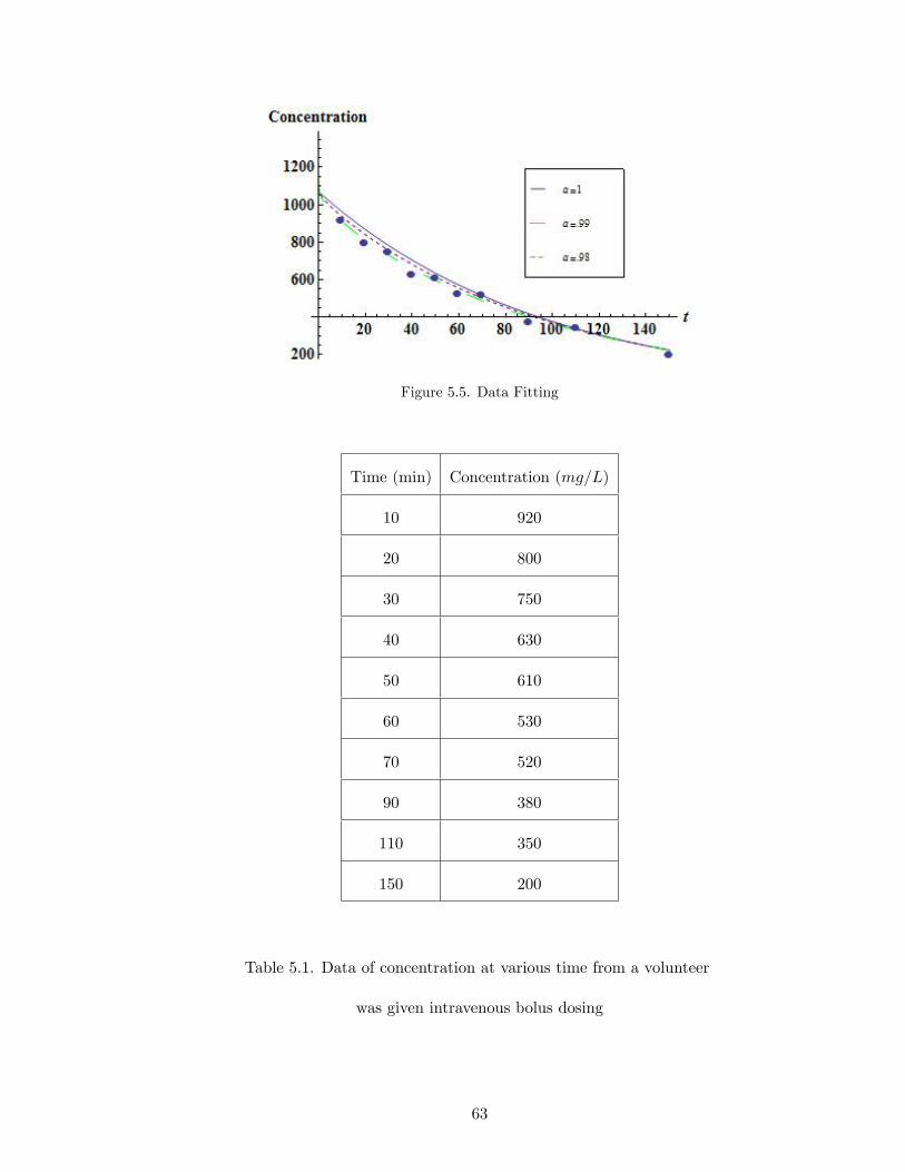
Figure 5.5. Data Fitting
Time (min) Concentration (mg/L)
10 920
20 800
30 750
40 630
50 610
60 530
70 520
90 380
110 350
150 200
Table 5.1. Data of concentration at various time from a volunteer
was given intravenous bolus dosing
63
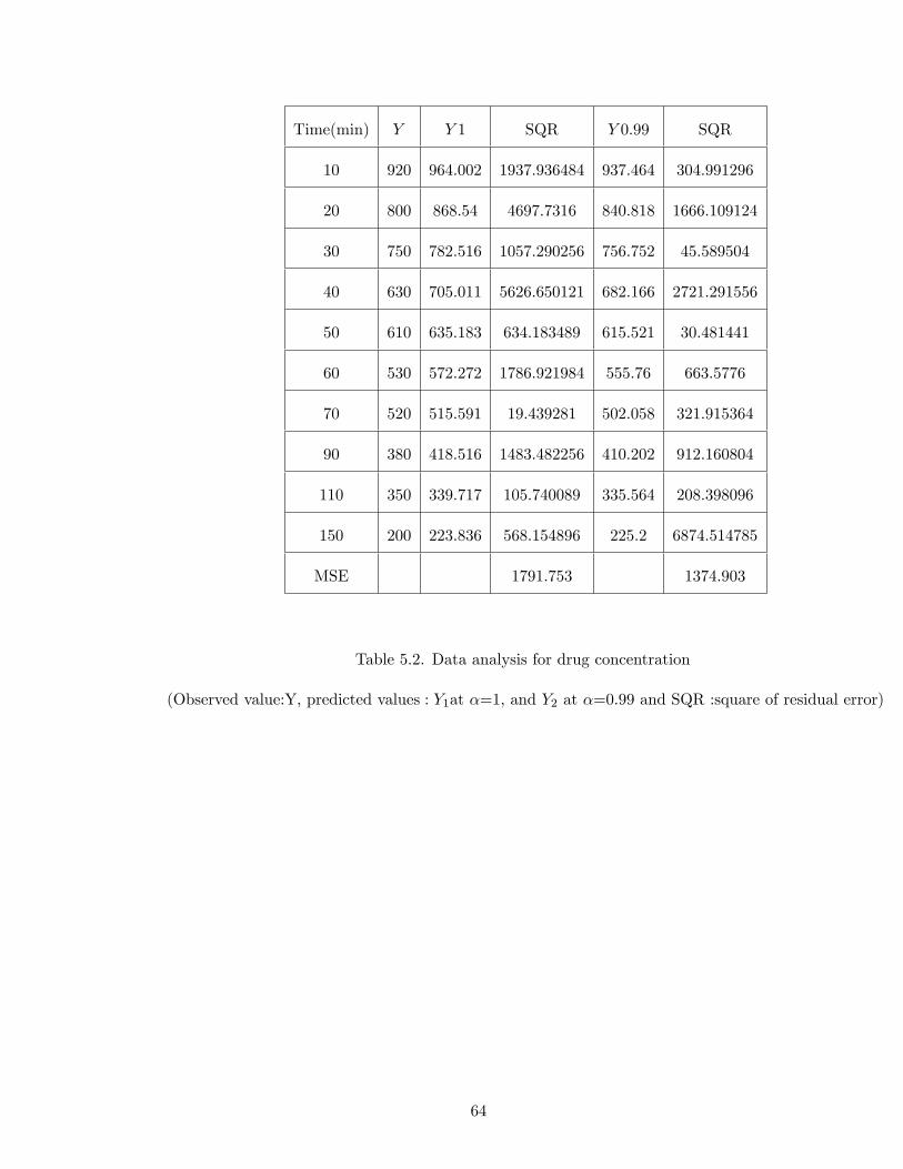
Time(min) Y Y 1 SQR Y 0.99 SQR
10 920 964.002 1937.936484 937.464 304.991296
20 800 868.54 4697.7316 840.818 1666.109124
30 750 782.516 1057.290256 756.752 45.589504
40 630 705.011 5626.650121 682.166 2721.291556
50 610 635.183 634.183489 615.521 30.481441
60 530 572.272 1786.921984 555.76 663.5776
70 520 515.591 19.439281 502.058 321.915364
90 380 418.516 1483.482256 410.202 912.160804
110 350 339.717 105.740089 335.564 208.398096
150 200 223.836 568.154896 225.2 6874.514785
MSE 1791.753 1374.903
Table 5.2. Data analysis for drug concentration
(Observed value:Y, predicted values : Y1at α=1, and Y2 at α=0.99 and SQR :square of residual error)
64
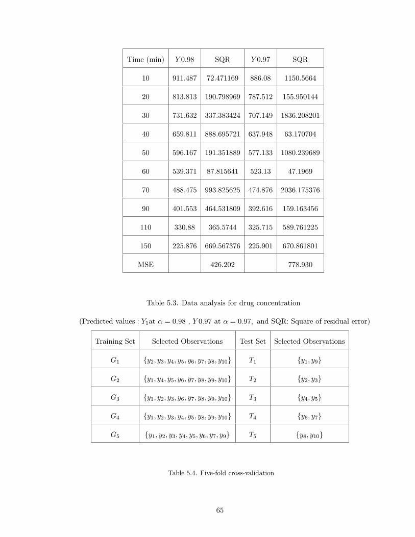
Time (min) Y 0.98 SQR Y 0.97 SQR
10 911.487 72.471169 886.08 1150.5664
20 813.813 190.798969 787.512 155.950144
30 731.632 337.383424 707.149 1836.208201
40 659.811 888.695721 637.948 63.170704
50 596.167 191.351889 577.133 1080.239689
60 539.371 87.815641 523.13 47.1969
70 488.475 993.825625 474.876 2036.175376
90 401.553 464.531809 392.616 159.163456
110 330.88 365.5744 325.715 589.761225
150 225.876 669.567376 225.901 670.861801
MSE 426.202 778.930
Table 5.3. Data analysis for drug concentration
(Predicted values : Y1at α = 0.98 , Y 0.97 at α = 0.97, and SQR: Square of residual error)
Training Set Selected Observations Test Set Selected Observations
G1 {y2, y3, y4, y5, y6, y7, y8, y10} T1 {y1, y9}
G2 {y1, y4, y5, y6, y7, y8, y9, y10} T2 {y2, y3}
G3 {y1, y2, y3, y6, y7, y8, y9, y10} T3 {y4, y5}
G4 {y1, y2, y3, y4, y5, y8, y9, y10} T4 {y6, y7}
G5 {y1, y2, y3, y4, y5, y6, y7, y9} T5 {y8, y10}
Table 5.4. Five-fold cross-validation
65
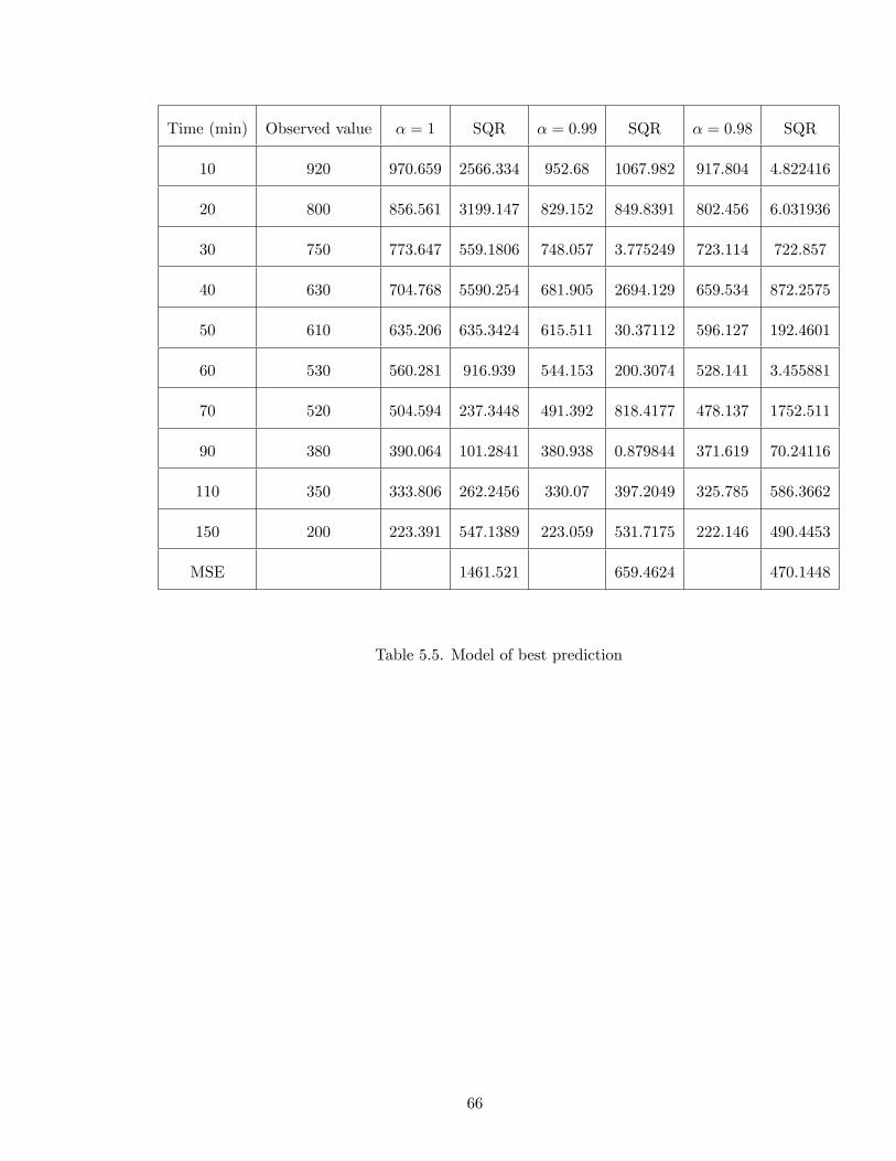
Time (min) Observed value α = 1 SQR α = 0.99 SQR α = 0.98 SQR
10 920 970.659 2566.334 952.68 1067.982 917.804 4.822416
20 800 856.561 3199.147 829.152 849.8391 802.456 6.031936
30 750 773.647 559.1806 748.057 3.775249 723.114 722.857
40 630 704.768 5590.254 681.905 2694.129 659.534 872.2575
50 610 635.206 635.3424 615.511 30.37112 596.127 192.4601
60 530 560.281 916.939 544.153 200.3074 528.141 3.455881
70 520 504.594 237.3448 491.392 818.4177 478.137 1752.511
90 380 390.064 101.2841 380.938 0.879844 371.619 70.24116
110 350 333.806 262.2456 330.07 397.2049 325.785 586.3662
150 200 223.391 547.1389 223.059 531.7175 222.146 490.4453
MSE 1461.521 659.4624 470.1448
Table 5.5. Model of best prediction
66
CONCLUSION AND FUTURE WORK
Fractional calculus is a generalized form of the ordinary calculus. The operations in
classical calculus are restricted to integer order, however, fractional calculus extends the
order to include all positive real numbers. There are still many open questions in this
newly developing theory needed to be answered. In this thesis we closed some of the gaps in
the theory of fractional calculus. We developed fractional trigonometry based on the multi-
valued fractional generalization of the exponential function, Mittag-Leffl er function. We
introduced the characteristic polynomials of fractional homogenous differential equations
and the solutions of these equations as well. Generalized Wronskian determinant which
is worthwhile in the study of linearly independence of solutions to a system of fractional
differential equations was developed. Also, we presented a new method of solving a system
of fractional differential equations. A linear combination of two fractional trigonometric
functions was generated by solving a system of fractional differential equations with the
new method.
After investigation, we noticed that the fractional calculus has a great potential in
analyzing real world problems. We demonstrated that fractional calculus performs better
in the modeling in particular applications. For that, we proposed an application of fractional
calculus to pharmacokinetic model. This model is important in clinical study to recommend
a dose or regimen. In particular, we applied our theory to one compartment model which
gives the relationship between drug concentration and time. We first approximate the
solutions using fractional model. Then we compare between our theory to ordinary calculus
by using real data. Our study showed that fractional models gave the best fitting to the
given data, not just that, also the best prediction to the future data.
67
In the next step to broaden this research, we would like to investigate the inverse frac-
tional trigonometry. What would be the identities, the Laplace transform and the derivative
of the inverse fractional trigonometric functions? Are they similar to what we have in the
integer order inverse trigonometry?
Also, we hope to extend fractional model applications to approximate the solution of
two compartment models. Such models study the plasma concentration over time in two
compartments instead of one compartment.
68
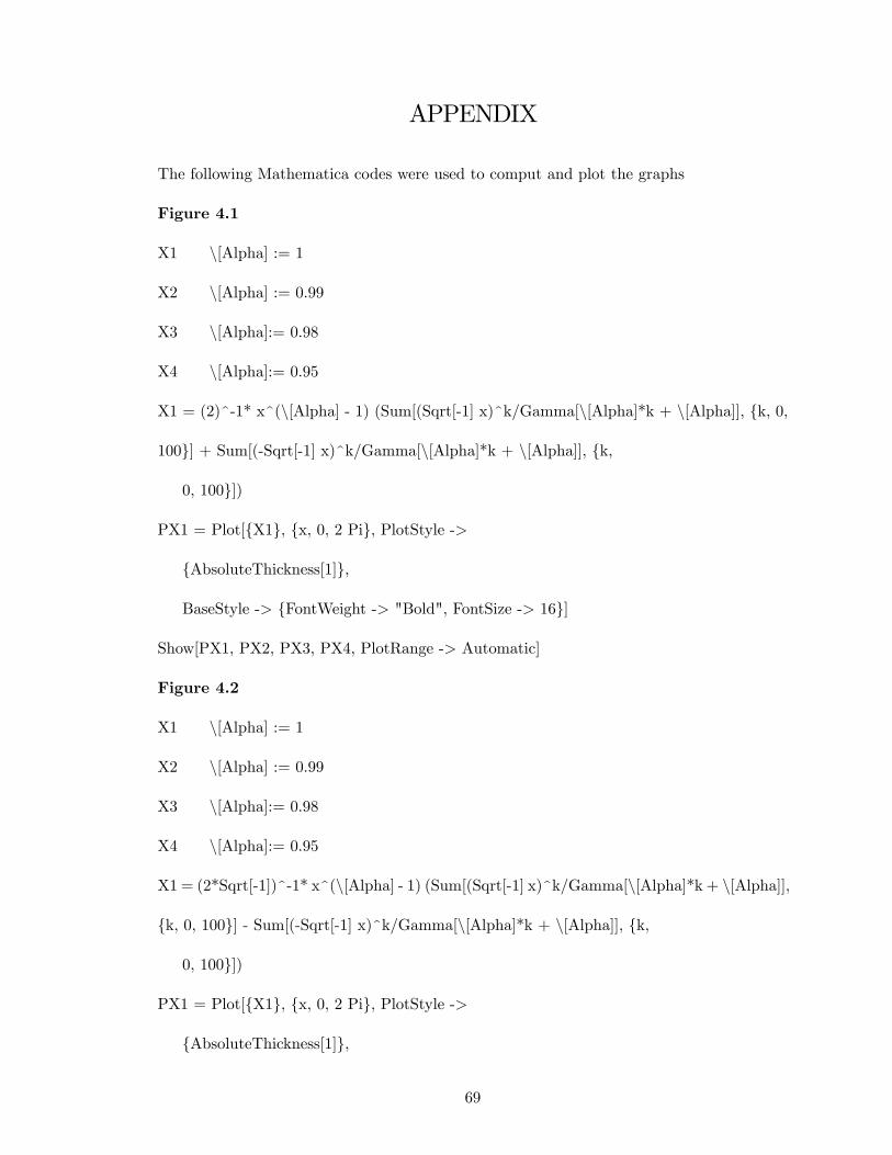
APPENDIX
The following Mathematica codes were used to comput and plot the graphs
Figure 4.1
X1 \[Alpha] := 1
X2 \[Alpha] := 0.99
X3 \[Alpha]:= 0.98
X4 \[Alpha]:= 0.95
X1 = (2)^-1* x^(\[Alpha] - 1) (Sum[(Sqrt[-1] x)^k/Gamma[\[Alpha]*k + \[Alpha]], {k, 0,
100}] + Sum[(-Sqrt[-1] x)^k/Gamma[\[Alpha]*k + \[Alpha]], {k,
0, 100}])
PX1 = Plot[{X1}, {x, 0, 2 Pi}, PlotStyle ->
{AbsoluteThickness[1]},
BaseStyle -> {FontWeight -> "Bold", FontSize -> 16}]
Show[PX1, PX2, PX3, PX4, PlotRange -> Automatic]
Figure 4.2
X1 \[Alpha] := 1
X2 \[Alpha] := 0.99
X3 \[Alpha]:= 0.98
X4 \[Alpha]:= 0.95
X1 = (2*Sqrt[-1])^-1* x^(\[Alpha] - 1) (Sum[(Sqrt[-1] x)^k/Gamma[\[Alpha]*k + \[Alpha]],
{k, 0, 100}] - Sum[(-Sqrt[-1] x)^k/Gamma[\[Alpha]*k + \[Alpha]], {k,
0, 100}])
PX1 = Plot[{X1}, {x, 0, 2 Pi}, PlotStyle ->
{AbsoluteThickness[1]},
69
BaseStyle -> {FontWeight -> "Bold", FontSize -> 16}]
Show[PX1, PX2, PX3, PX4, PlotRange -> Automatic]
Figure 5.2
a:=1002,42; b:=0.011
X1 \[Alpha] := 1;
X2 \[Alpha] := 0.99;
X3 \[Alpha]:= 0.80;
X4 \[Alpha]:= 0.50;
X5 \[Alpha]:= 0.20;
X1 := a*x^(\[Alpha] - 1)*Sum[(-(b) x^\[Alpha])^k/Gamma[\[Alpha]*k +\[Alpha]], {k, 0,
100}]
Plot[{X1}, {x, 0, 100}, PlotStyle ->
{Thick}, AxesLabel -> {t, Concentration}]
Show[PX1, PX2, PX3, PX4,PX5, PlotRange -> Automatic]
Figure 5.3
a:=1002,42; b:=0.011
X1 \[Alpha]:= 0.90;
X3 \[Alpha]:= 0.50;
X4 \[Alpha]:= 0.20;
X2 \[Alpha]:= 0.80; a:=1002,42; b:=0.019041
X1 := a*x^(\[Alpha] - 1)*Sum[(-(b) x^\[Alpha])^k/Gamma[\[Alpha]*k +\[Alpha]], {k, 0,
100}]
Plot[{X1}, {x, 0, 100}, PlotStyle ->
{Thick}, AxesLabel -> {t, Concentration}]
70
Show[PX1, PX2, PX3, PX4,PX5, PlotRange -> Automatic]
Figure 5.4
Lp := {{0, 7.88}, {6, 7.10}, {12, 6.97}, {24, 5.27}, {36, 4.52}, {48,
3.43}, {72, 1.97}, {96, 1.01}, {144, .23}}
P = ListPlot[Lp, PlotMarkers -> {Automatic, Medium}]
a:=10; b:=0.019
X1 \[Alpha]:= 1;
X2 \[Alpha]:= 0.91;
X1 := a*x^(\[Alpha] - 1)*Sum[(-(b) x^\[Alpha])^k/Gamma[\[Alpha]*k +\[Alpha]], {k, 0,
100}]
Needs["PlotLegends‘"]
Plot[{X1, X2}, {x, 0, 144}, PlotStyle ->
{Thin, Thick}, PlotLegend -> {"\[Alpha]=1", "\[Alpha]=.91"},
LegendPosition -> {1.1, -0.4}]
PX1 = Plot[{X1}, {x, 0, 144}, PlotStyle ->
{Thick, Purple}, BaseStyle -> {FontWeight -> "Bold", FontSize -> 16}]
Show[PX1, PX2, P, AxesLabel -> {t, Concentration}, PlotRange -> All]
Figure 5.5
Lj = {{10, 920}, {20, 800}, {30, 750}, {40, 630}, {50, 610}, {60,
530}, {70, 520}, {90, 380}, {110, 350}, {150, 200}}
J = ListPlot[Lj, PlotMarkers -> {Automatic, Medium}]
a:=1070; b:=0.010434
X1 \[Alpha]:= 1;
X2 \[Alpha]:= 0.99;
71
X3 \[Alpha]:= 0.98;
X1 := a*x^(\[Alpha] - 1)*Sum[(-(b) x^\[Alpha])^k/Gamma[\[Alpha]*k +\[Alpha]], {k, 0,
100}]
PX1 = Plot[{X1}, {x, 0, 144}, PlotStyle ->
{Thick, Purple}, BaseStyle -> {FontWeight -> "Bold", FontSize -> 16}]
Needs["PlotLegends‘"]
Plot[{X1, X2}, {x, 0, 144}, PlotStyle ->
{Thin, Thick}, PlotLegend -> {"\[Alpha]=1", "\[Alpha]=.91"},
LegendPosition -> {1.1, -0.4}]
Show[PX1, PX2, P, AxesLabel -> {t, Concentration}, PlotRange -> All]
Table 5.2 and Table 5.3
a:=1070; b:=0.010434
X1 \[Alpha]:= 1;
X2 \[Alpha]:= 0.99;
X3 \[Alpha]:= 0.98;
X1 := a*x^(\[Alpha] - 1)*Sum[(-(b) x^\[Alpha])^k/Gamma[\[Alpha]*k +\[Alpha]], {k, 0,
10000}]
Table[X1, {x, 10, 150, 10}].
72
REFERENCES
[1] A. A. Kilbas, H. M. Srivastava, and Juan J. Trujillo, Theory and Applications of
Fractional Differential Equations, Amsterdam: Elsevier, 2006.
[2] A. A. Kilbas and M. Saigo, Fractional Integrals and Derivatives of functions of Mittag-
Leffl er type, Dokl, Akad. Nauk Belarusi, 39 (4), (1995) 22-26.
[3] B. Bonilla, M. Rivero, J.J. Trujillo, On System of Linear Fractional Differential equa-
tions with Constant Coeffi cients, Applied Mathematics and Computation 187.1 (2007):
68-78. Department of de Análisis Matemático, Universidad de La Laguna, 2005.
[4] Bertram Ross, Fractional Calculus, Mathematical Association of America, Mathemat-
ics Magazine. Vol. 50, No. 3, May, 1977.
[5] Corl F.Lorenzo & Tom T.Hartly, A Solution to the Fundmental Linear Fractional
order Differential equations , Nasa/TP-1998-208693, National Aeronautics and Space
Administration, Lewis Research Center, December, 1998.
[6] Corl F.Lorenzo & Tom T.Hartly, Fractional Trigonometry and the Spiral Functions,
Kluwer Academic, 2004.
[7] Corl F.Lorenzo & Tom T.Hartly, Generalized Functions for the Fractional Calculus,
Nasa/TP-1999-209424/REV1, National Aeronautics and Space Administration, Glenn
Research Center, October, 1999.
[8] Damian P. Watson, Fractional Calculus and its Applications, Department of Mathe-
matics, Mary Washington College Fredericksburg, VA 22401, April 27, 2004.
73
[9] Department of Aerospace and mechanical Engineering of Netro Dame University, Frac-
tional Calculus: History, Definitions and applications for Engineer , May 8,2004.
[10] D. Weiner Gabrielsson, Pharmacokinetic and Pharmacodynamic Data Analysis: Con-
cepts and Applications, 3rd edition, Grander’s UK, 2002.
[11] G. M. Mittag-Leffl er, Sopra Ia funsione Eα(x), rend. accad. Lincei, ser. 5, 13, (1904).
[12] G. M. Mittag-Leffl er, Sur Ia representationanalytique d’une branche uniforme d’une
fonction, acta math., 29, (1905) 101-182.
[13] Harvey Motulsky and Arthur Christopoulos, Fitting Models to Biological Data Using
Linear and Nonlinear Regression, Oxford University press, New york, 2004.
[14] Igor Podlubny, Fractional Differential Equation: Introduction to Fractional Derivatives,
Academic Press, 1999.
[15] Josiph Liouville, Mémoire sur Ie théorème des complèmentaires, J. Reine Angew.
Math., 11 (1843)-1-19.
[16] Joseph M. Kimeu, Fractional Calculus : Definitions and Applications, Western Ken-
tucky University, 2009.
[17] Joseph T. DiPiro, William J. Spruill, William E. Wade, Concepts in Clinical Pharma-
cokinetics, American Society of Health-System Pharmacists, Fifth Edition, 2010.
[18] Martin Bohner and Allan Peterson, Dynamic Equations on Time Scale, Birkäuser
Boston, 2001.
[19] Mosteller F. and Turkey J.W, Data analysis, including statistics .In Handbook of Social
Psychology. Addison-Wesley, Reading,MA, 1968.
74
[20] M. Stone, Cross-validatory choice and assessment of statistical predictions. J. Royal
Stat. Soc., 36(2):111—147,1974.
[21] Niel H. Abel, Solution de quelques problèms à I’aide d’intégrales défines, Oevres Com-
plètes, Christiania (GrondahI) 1 (1881) 16-18.
[22] Riccardo Caponetto, Giovanni Dongola, Luigi Fortuna, Fractional Order System: Mod-
eling and Control Applications, World Scientific, 2010.
[23] S. Das, Functional Fractional Calculus for System Identification and Controls. Berlin:
Springer, 2008.
[24] S. F. Lacroix, Traité du Calcul Différentiel et du Calcul Integral, Paris (Courcier) 3,
sec. ed., 1819, pp. 409-410.
[25] S. Larson, The shrinkage of the coeffi cient of multiple corelation. J. Educat. Psychol.,
22:45—55,1931.
[26] Thomas j. Osler, Leibniz Rule for Fractional Derivative Generalized and An Application
to Infinite Series, Siam J. Appl. Math. Vol 18, No 3. May 1970.
[27] http://www.boomer.org/c/p3/c05/c0504.html.
75
