development of a compliant controller for a generic 6dof
TRANSCRIPT
FACULTEIT INDUSTRIËLE INGENIEURSWETENSCHAPPEN
CAMPUS BRUGGE
Development of a compliantcontroller for a generic 6DOFrobot in Python
Maarten DETAILLEUR
Promotor: prof. dr. ir. M. Versteyhe Masterproef ingediend tot het behalen van degraad van master of Science in de industriele
Begeleider: ing. M. De Ryck wetenschappen: energie , automatisering
Academiejaar 2019 - 2020

c©Copyright KU Leuven
Zonder voorafgaande schriftelijke toestemming van zowel de promotor(en) als de auteur(s) isovernemen, kopieren, gebruiken of realiseren van deze uitgave of gedeelten ervan verboden. Vooraanvragen i.v.m. het overnemen en/of gebruik en/of realisatie van gedeelten uit deze publicatie,kan u zich richten tot KU Leuven Campus Brugge, Spoorwegstraat 12, B-8200 Brugge, +32 50 6648 00 of via e-mail [email protected].
Voorafgaande schriftelijke toestemming van de promotor(en) is eveneens vereist voor het aanwendenvan de in deze masterproef beschreven (originele) methoden, producten, schakelingen en programma’svoor industrieel of commercieel nut en voor de inzending van deze publicatie ter deelname aanwetenschappelijke prijzen of wedstrijden.
Acknowledgements
Throughout this master’s thesis, several people have assisted me and helped me to successfullycomplete this assignment. First I would like to thank my promotor Mr Versteyhe and co-promoterMr De Ryck for the interesting thesis subject. Further I would like to thank Mr De Ryck once morefor the good guidance. He was always available and gave constructive feedback and tips at the twoweekly meetings. In addition, I could always reach him with any question by e-mail. I would liketo thank my parents for being able to follow these studies and to support me continuously. Theyalso provided the ideal balance between taking my lessons and investing the necessary time inmy master thesis. My parents and my sister checked my thesis for language and typing errors forwhich I am also grateful to them. I am also grateful to all those who have written literature that Ihave used on this subject. Finally, I would like to thank my girlfriend, the rest of my family and mydearest friends for the mental support.
v
Abstract
Het hoofddoel van deze thesis is het ontwerpen van een krachtgeregelde controller in Python vooreen zes vrijheidsgraden robotarm en het uitwerken van enkele toepassingen met deze controller.Daarvoor moet kennis van kinematica en dynamica van een robotsysteem aanwezig zijn en iskennis van de krachtregeltechnieken noodzakelijk. In deze thesis wordt admittantie krachtregelinggebruikt om een vooraf bepaald traject te volgen. Wanneer een externe kracht optreedt, kan eenaanpassing worden gedaan aan het vooraf bepaalde traject aan de hand van een virtuele veer,een demper en een massasysteem. Deze applicatie is ontworpen voor een UR3 CB-series robot.Om de werking van het systeem te testen, werden verschillende parameters, zoals verwachtegewrichtsposities of Cartesiaanse posities, de reele gewrichtsposities of Cartesiaanse positiesbijgehouden en uitgezet in functie van de tijd. De krachten die door de omgeving op het systeemworden uitgeoefend, worden vergeleken met de eerder verkregen resultaten. Hierdoor kan aan dehand van controleberekeningen nagegaan worden of het systeem naar de wens van het ontwerpfunctioneert. Er wordt geen rekening gehouden met wrijving omdat dit niet gekend is, alsook met deinverse dynamica wordt geen rekening gehouden wegens verwaarloosbaar en een te trage werkingin realtime processing van Python.
Om deze applicatie te bekomen werden simulaties in MATLAB gemaakt voor toepassingen vanzowel twee vrijheidsgraden als zes vrijheidsgraden. Uiteindelijk werd de kennis die hierbij werdverkregen in een Python controller verwerkt waarbij de uiteindelijke applicatie, path tracking withdisturbance, werd ontworpen voor de UR3 CB-series robot. Dit is enkel getest in simulatieomgevingvanwege onvoorziene omstandigheden. Als extra werd de dynamica omschreven aan de hand vande Euler-Lagrange methode. Hiervoor werd een algemeen MATLAB script geschreven dat functiesgenereert in MATLAB die de dynamische parameters van het systeem omvatten, om deze daarnaverder te kunnen gebruiken in de Python controller.
Om meer waarde te geven aan deze applicatie werd een tweede applicatie theoretisch benaderd.Het gaat hierbij om een applicatie waarbij een bout in een niet exact geboord gat moet geleidworden aan de hand van de admittance controle die eerder werd gebruikt. Deze applicatie werdniet in praktijk uitgewerkt.
Keywords: admittance controle, Universal Robots, Python, interactieve robot, Matlab
vi
Summary
This thesis is a study within the domain of robotics and control engineering. It is created to servefuture research and educational purposes. The goal is to design a force compliant controller fora six degrees of freedom robot through a Python interface. The Universal Robots 3 CB-seriescollaborative robot is used for this. Two applications have been designed for this purpose: the firstapplication involves path tracking with disturbance and the second application involvles turning in abolt using force-compliant control. Unfortunately, this second application was only treated in theory.
The thesis contains a gradual rapprochement to the problem starting with an extensive literaturestudy. This literature study contains all the necessary information to understand the theory on thistopic, namely: (1) kinematics and dynamics of a robot arm, (2) general position control of joints,(3) compliant force control, (4) trajectory generation, (5) Universal Robots properties, (6) TCP/IPprotocol and (7) Python pros and cons. In these sections, the general principles are clarified andreference is often made to literature where a detailed explanation can be found.
The included theory is gradually incorporated into a number of partial experiments. For this purposeMATLAB simulations are used with an interactive GUI to display the first properties of admittancecontrol. The dynamic behavior of an admittance control is presented and worked out in a twodegrees of freedom application. First, an application is created in which a fixed target is taken. Forthis purpose, the dynamic behavior of the manipulator and properties of the admittance control hasbeen examined. Secondly, a variable target is added. For this purpose, it became clear that withadmittance control and with extension impedance control, a devitation occurs when a variable targetis given. This result has been checked for correctness in SIMULINK. Then the same application isreworked from Cartesian space to joint space to observe the influence of this. As a result of thecomparison between Cartesian and joint space, it is decided to develop the following applicationsin Cartesian space. During these first applications it already has become clear that the calculationsof inverse kinematics via iterative methods were too slow. As for the final applications in Python,it was assumed that a frequency of 125Hz would be achieved. This means that slow calculationsare not desirable. For this purpose, the various solver parameters that can be set, are discussed inmore detail.
After the two degrees of freedom applications have been made and discussed, a six degrees offreedom application is made. The two degrees of freedom application with fixed target is redesignedin MATLAB for six degrees of freedom, using the Peter Corke robotics toolbox. This applicationleans closer to the first purpose that had to be achieved, namely the path tracking with disturbanceapplication. The general control used is an extension of the two degrees of freedom applicationand uses the same control technique, i.e. admittance control. The inputs here are: the currentCartesian positions, velocities and the external force acting on the manipulator. In this experimentit has been experienced that several calculations such as the inverse kinematics, are processed too
vii
SUMMARY viii
slowly. No solution has been found for this, so the simulations do run in slow motion, but producerepresentative real time data.
At this point of the thesis the transition has been made to the Python environment. To startwith, it was first foreseen that communication with the Universal Robots would be possible. Thecommunication consists of two classes: (1) a broadcasting class and (2) a monitor class. Laterclasses have been created and obtained to: (1) get a robot description, (2) generate a trajectoryand (3) create a GUI that was needed for simulation purposes.
Due to the COVID-19 pandemia, it was not possible to test the obtained controller in practice. Thetrajectory generation and the force reading of the robot have been tested in practice, after whichthere was no longer access to the campus. The controller is further finished for the first application,namely path tracking with disturbance, but is never tested in practice. The application is only testedby means of the URSim simulation environment in a virtual linux machine.
As a result, an externally applied force creates a response in the robot’s end-effector position thatcan be compared to the response of a second order spring, damper and mass system. As this wasthe goal of this application, it is considered successful. However, for path tracking a PID controllercan be built in to eliminate the error during path tracking. As a result, the second order systemresponse will no longer be able to be detected, which is why this is not executed.
Finally, a theoretical approach to the second application, turn in a bolt using force compliant control,is included in the experiments. In addition, an approach of the dynamic parameters is made usingthe Lagrange equations quoted in the literature study for a two degrees of freedom application, butelaborated for a six degrees of freedom application. This determination cannot be found in thisthesis, but can be found on my GitHub page [49].
Contents
Acknowledgements v
Abstract vi
Summary viii
Contents xii
List of Figures xiii
List of Tables xvi
List of Symbols xviii
List of Abbreviations xix
1 Introduction 1
1.1 Motivation . . . . . . . . . . . . . . . . . . . . . . . . . . . . . . . . . . . . . . . . 1
1.2 Purpose of the thesis . . . . . . . . . . . . . . . . . . . . . . . . . . . . . . . . . . 1
1.3 Goal of the thesis . . . . . . . . . . . . . . . . . . . . . . . . . . . . . . . . . . . . 2
1.4 Thesis structure . . . . . . . . . . . . . . . . . . . . . . . . . . . . . . . . . . . . 2
2 Literature study 3
2.1 Kinematics and dynamics of a robot arm . . . . . . . . . . . . . . . . . . . . . . . . 4
2.1.1 Introduction . . . . . . . . . . . . . . . . . . . . . . . . . . . . . . . . . . . 4
2.1.2 Rigid-body motions . . . . . . . . . . . . . . . . . . . . . . . . . . . . . . . 4
2.1.3 Forward kinematics . . . . . . . . . . . . . . . . . . . . . . . . . . . . . . . 6
2.1.4 Inverse kinematics . . . . . . . . . . . . . . . . . . . . . . . . . . . . . . . 9
2.1.5 Velocity kinematics . . . . . . . . . . . . . . . . . . . . . . . . . . . . . . . 16
2.1.6 Dynamics of open chains . . . . . . . . . . . . . . . . . . . . . . . . . . . . 18
2.2 General position control of joints . . . . . . . . . . . . . . . . . . . . . . . . . . . . 21
2.3 Compliant force control . . . . . . . . . . . . . . . . . . . . . . . . . . . . . . . . . 24
2.3.1 Introduction . . . . . . . . . . . . . . . . . . . . . . . . . . . . . . . . . . . 24
General response in compliant force control . . . . . . . . . . . . . . . . . . 24
2.3.2 Passive versus active compliance . . . . . . . . . . . . . . . . . . . . . . . 26
ix
CONTENTS x
Passive control . . . . . . . . . . . . . . . . . . . . . . . . . . . . . . . . . 26
Active control . . . . . . . . . . . . . . . . . . . . . . . . . . . . . . . . . . 27
2.3.3 Direct versus indirect force control . . . . . . . . . . . . . . . . . . . . . . . 28
Direct force control . . . . . . . . . . . . . . . . . . . . . . . . . . . . . . . 28
Indirect force control . . . . . . . . . . . . . . . . . . . . . . . . . . . . . . 28
2.3.4 Types of compliant force control . . . . . . . . . . . . . . . . . . . . . . . . 29
Overview . . . . . . . . . . . . . . . . . . . . . . . . . . . . . . . . . . . . 29
Impedance control . . . . . . . . . . . . . . . . . . . . . . . . . . . . . . . 31
Admittance control . . . . . . . . . . . . . . . . . . . . . . . . . . . . . . . 34
Hybrid control . . . . . . . . . . . . . . . . . . . . . . . . . . . . . . . . . . 35
Adaptive force control . . . . . . . . . . . . . . . . . . . . . . . . . . . . . . 37
Robust force control . . . . . . . . . . . . . . . . . . . . . . . . . . . . . . 38
Learning algorithm force control . . . . . . . . . . . . . . . . . . . . . . . . 38
2.3.5 Implementation choice . . . . . . . . . . . . . . . . . . . . . . . . . . . . . 39
2.3.6 Implementation . . . . . . . . . . . . . . . . . . . . . . . . . . . . . . . . . 40
2.4 Trajectory generation . . . . . . . . . . . . . . . . . . . . . . . . . . . . . . . . . . 41
2.4.1 Definitions . . . . . . . . . . . . . . . . . . . . . . . . . . . . . . . . . . . . 41
2.4.2 Types of trajectory generation . . . . . . . . . . . . . . . . . . . . . . . . . 43
Straight line trajectory . . . . . . . . . . . . . . . . . . . . . . . . . . . . . 43
Non-normalized trajectory . . . . . . . . . . . . . . . . . . . . . . . . . . . 43
Normalized trajectory . . . . . . . . . . . . . . . . . . . . . . . . . . . . . . 44
Cubic interpolation . . . . . . . . . . . . . . . . . . . . . . . . . . . . . . . 44
Quintic interpolation . . . . . . . . . . . . . . . . . . . . . . . . . . . . . . 46
Higher order polynomials . . . . . . . . . . . . . . . . . . . . . . . . . . . . 46
Path generation . . . . . . . . . . . . . . . . . . . . . . . . . . . . . . . . . 46
2.5 Universal Robots properties . . . . . . . . . . . . . . . . . . . . . . . . . . . . . . 47
2.5.1 UR3 kinematics and dynamics . . . . . . . . . . . . . . . . . . . . . . . . . 49
2.5.2 UR3 programming . . . . . . . . . . . . . . . . . . . . . . . . . . . . . . . 49
2.6 TCP/IP protocol . . . . . . . . . . . . . . . . . . . . . . . . . . . . . . . . . . . . 50
2.6.1 Definition TCP/IP . . . . . . . . . . . . . . . . . . . . . . . . . . . . . . . . 50
2.6.2 TCP/IP in OSI model . . . . . . . . . . . . . . . . . . . . . . . . . . . . . . 50
2.6.3 TCP/IP with UR3 robot in Python . . . . . . . . . . . . . . . . . . . . . . . . 52
2.7 Python . . . . . . . . . . . . . . . . . . . . . . . . . . . . . . . . . . . . . . . . . 53
3 Methodology 54
4 Experiments 56
4.1 MATLAB simulations . . . . . . . . . . . . . . . . . . . . . . . . . . . . . . . . . . 57
4.1.1 Two degrees of freedom fixed point . . . . . . . . . . . . . . . . . . . . . . . 57
Working method . . . . . . . . . . . . . . . . . . . . . . . . . . . . . . . . 57
CONTENTS xi
Structure of the program . . . . . . . . . . . . . . . . . . . . . . . . . . . . 59
4.1.2 Two degrees of freedom circle path . . . . . . . . . . . . . . . . . . . . . . 60
Working method . . . . . . . . . . . . . . . . . . . . . . . . . . . . . . . . 60
Structure of the program . . . . . . . . . . . . . . . . . . . . . . . . . . . . 60
4.1.3 Six degrees of freedom . . . . . . . . . . . . . . . . . . . . . . . . . . . . . 61
Working method . . . . . . . . . . . . . . . . . . . . . . . . . . . . . . . . 61
Structure of the program . . . . . . . . . . . . . . . . . . . . . . . . . . . . 62
4.2 Python controller . . . . . . . . . . . . . . . . . . . . . . . . . . . . . . . . . . . . 63
4.2.1 Communication with UR3 robot . . . . . . . . . . . . . . . . . . . . . . . . . 63
Working method . . . . . . . . . . . . . . . . . . . . . . . . . . . . . . . . 63
Structure and use of the classes . . . . . . . . . . . . . . . . . . . . . . . . 63
4.2.2 Robot definition . . . . . . . . . . . . . . . . . . . . . . . . . . . . . . . . . 64
Working method . . . . . . . . . . . . . . . . . . . . . . . . . . . . . . . . 64
Structure and use of the class . . . . . . . . . . . . . . . . . . . . . . . . . 64
4.2.3 Trajectory generation . . . . . . . . . . . . . . . . . . . . . . . . . . . . . . 65
Working method . . . . . . . . . . . . . . . . . . . . . . . . . . . . . . . . 65
Structure of these functions . . . . . . . . . . . . . . . . . . . . . . . . . . 65
4.2.4 Main program . . . . . . . . . . . . . . . . . . . . . . . . . . . . . . . . . . 65
Working method . . . . . . . . . . . . . . . . . . . . . . . . . . . . . . . . 65
Structure of the program . . . . . . . . . . . . . . . . . . . . . . . . . . . . 66
General control system . . . . . . . . . . . . . . . . . . . . . . . . . . . . . 66
4.3 Theoretical approach additional application . . . . . . . . . . . . . . . . . . . . . . 67
4.3.1 Bolt in hole application . . . . . . . . . . . . . . . . . . . . . . . . . . . . . 67
Situation sketch . . . . . . . . . . . . . . . . . . . . . . . . . . . . . . . . . 67
Program sequence . . . . . . . . . . . . . . . . . . . . . . . . . . . . . . . 68
4.3.2 Other applications . . . . . . . . . . . . . . . . . . . . . . . . . . . . . . . 68
5 Results 69
5.1 Two degrees of freedom MATLAB simulations . . . . . . . . . . . . . . . . . . . . . 70
5.1.1 Simulation results fixed target point . . . . . . . . . . . . . . . . . . . . . . 70
Admittance control fixed point . . . . . . . . . . . . . . . . . . . . . . . . . 70
Influence of the manipulators dynamics . . . . . . . . . . . . . . . . . . . . 73
5.1.2 Simulation results circle tracking . . . . . . . . . . . . . . . . . . . . . . . . 74
Cartesian space . . . . . . . . . . . . . . . . . . . . . . . . . . . . . . . . 74
Joint space . . . . . . . . . . . . . . . . . . . . . . . . . . . . . . . . . . . 77
Issues . . . . . . . . . . . . . . . . . . . . . . . . . . . . . . . . . . . . . . 79
5.2 Six degrees of freedom MATLAB simulations . . . . . . . . . . . . . . . . . . . . . 80
Issues . . . . . . . . . . . . . . . . . . . . . . . . . . . . . . . . . . . . . . 82
5.3 Six degrees of freedom Python simulations . . . . . . . . . . . . . . . . . . . . . . 83
Issues . . . . . . . . . . . . . . . . . . . . . . . . . . . . . . . . . . . . . . 89
CONTENTS xii
6 Conclusions 91
7 Bibliography 93
A Attachments 97
A.1 Classes diagram Python controller . . . . . . . . . . . . . . . . . . . . . . . . . . . 98
A.2 Cyclus diagram Python controller . . . . . . . . . . . . . . . . . . . . . . . . . . . 99
List of Figures
2.1 Translation and rotation of a frame . . . . . . . . . . . . . . . . . . . . . . . . . . . 4
2.2 UR robot kinematics [1] . . . . . . . . . . . . . . . . . . . . . . . . . . . . . . . . 6
2.3 Two link manipulator[1] . . . . . . . . . . . . . . . . . . . . . . . . . . . . . . . . . 7
2.4 Frames of a 6DOF robot arm[2] . . . . . . . . . . . . . . . . . . . . . . . . . . . . 9
2.5 θ1 sketch [2] . . . . . . . . . . . . . . . . . . . . . . . . . . . . . . . . . . . . . . 10
2.6 θ5 sketch[2] . . . . . . . . . . . . . . . . . . . . . . . . . . . . . . . . . . . . . . . 11
2.7 θ6 sketch [2] . . . . . . . . . . . . . . . . . . . . . . . . . . . . . . . . . . . . . . 12
2.8 Sketch to determine θ3,θ2and θ4 [2] . . . . . . . . . . . . . . . . . . . . . . . . . . 13
2.9 Outline of the working principle of the Newton-Raphson method [3] . . . . . . . . . . 14
2.10 Newton-Raphson method [1] . . . . . . . . . . . . . . . . . . . . . . . . . . . . . . 14
2.11 Two-link example [1] . . . . . . . . . . . . . . . . . . . . . . . . . . . . . . . . . . 16
2.12 Six revolute joint space Jacobian [4] . . . . . . . . . . . . . . . . . . . . . . . . . . 16
2.13 2DOF example [1] . . . . . . . . . . . . . . . . . . . . . . . . . . . . . . . . . . . 19
2.14 DC electrical scheme [5] . . . . . . . . . . . . . . . . . . . . . . . . . . . . . . . . 21
2.15 DC motor system [6] . . . . . . . . . . . . . . . . . . . . . . . . . . . . . . . . . . 21
2.16 Current controller [6] . . . . . . . . . . . . . . . . . . . . . . . . . . . . . . . . . . 22
2.17 Speed controller [6] . . . . . . . . . . . . . . . . . . . . . . . . . . . . . . . . . . . 22
2.18 Position controller [6] . . . . . . . . . . . . . . . . . . . . . . . . . . . . . . . . . . 23
2.20 Soft joint examples [7] [8] . . . . . . . . . . . . . . . . . . . . . . . . . . . . . . . . 26
2.21 Backdrivability [9] . . . . . . . . . . . . . . . . . . . . . . . . . . . . . . . . . . . . 26
2.22 Classifications in active and passive compliance [10] . . . . . . . . . . . . . . . . . 28
2.23 Indirect force control with internal position control [11] . . . . . . . . . . . . . . . . . 28
2.24 Spring/damper system [12] . . . . . . . . . . . . . . . . . . . . . . . . . . . . . . . 31
2.25 Impedance control schema [10] . . . . . . . . . . . . . . . . . . . . . . . . . . . . 31
2.26 Impedance control schema [13] . . . . . . . . . . . . . . . . . . . . . . . . . . . . 32
2.27 1DOF example . . . . . . . . . . . . . . . . . . . . . . . . . . . . . . . . . . . . . 33
2.28 Simulation results 1DOF example [14] . . . . . . . . . . . . . . . . . . . . . . . . . 33
2.29 Admittance control schema [10] . . . . . . . . . . . . . . . . . . . . . . . . . . . . 34
2.30 Detailed admittance control schema [15] . . . . . . . . . . . . . . . . . . . . . . . . 34
2.31 Hybrid position/force control schema[13] . . . . . . . . . . . . . . . . . . . . . . . . 35
2.32 Robot environment and gravity compensation [13] . . . . . . . . . . . . . . . . . . . 35
xiii
LIST OF FIGURES xiv
2.33 Hybrid impedance control schema [13] . . . . . . . . . . . . . . . . . . . . . . . . 36
2.34 Adaptive control schema [13] . . . . . . . . . . . . . . . . . . . . . . . . . . . . . . 37
2.35 Robust force control schema [13] . . . . . . . . . . . . . . . . . . . . . . . . . . . 38
2.36 Simplified overall control loop . . . . . . . . . . . . . . . . . . . . . . . . . . . . . 40
2.37 Smooth interpolation between several points [16] . . . . . . . . . . . . . . . . . . . 41
2.38 Trapezoidal velocity profile in terms of position, velocity and acceleration [17] . . . . 42
2.39 Non-normalized trajectory [18] . . . . . . . . . . . . . . . . . . . . . . . . . . . . . 43
2.40 Normalized trajectory [18] . . . . . . . . . . . . . . . . . . . . . . . . . . . . . . . 44
2.41 Cubic polynomial timing law, position, velocity and acceleration [17] . . . . . . . . . 45
2.42 UR3 CB-series collaborative Robot [19] . . . . . . . . . . . . . . . . . . . . . . . . 47
2.43 Joint names [20] . . . . . . . . . . . . . . . . . . . . . . . . . . . . . . . . . . . . 48
2.44 Maximum joint torques [21] . . . . . . . . . . . . . . . . . . . . . . . . . . . . . . . 49
2.45 Port information for TCP/IP control [22] . . . . . . . . . . . . . . . . . . . . . . . . 49
2.46 OSI model layers [23] . . . . . . . . . . . . . . . . . . . . . . . . . . . . . . . . . 51
2.47 TCP/IP in OSI model [24] . . . . . . . . . . . . . . . . . . . . . . . . . . . . . . . 51
2.48 An overview of client interfaces [25] . . . . . . . . . . . . . . . . . . . . . . . . . . 52
2.49 Python features overview [26] . . . . . . . . . . . . . . . . . . . . . . . . . . . . . 53
4.1 Overview of the used control method . . . . . . . . . . . . . . . . . . . . . . . . . 61
4.2 Step response . . . . . . . . . . . . . . . . . . . . . . . . . . . . . . . . . . . . . 61
4.3 The applied control scheme . . . . . . . . . . . . . . . . . . . . . . . . . . . . . . 66
4.4 Application sketch . . . . . . . . . . . . . . . . . . . . . . . . . . . . . . . . . . . 67
4.5 Situation sketch . . . . . . . . . . . . . . . . . . . . . . . . . . . . . . . . . . . . 67
5.1 Manipulator from rest position to steady state position with applied force . . . . . . . 70
5.2 Forces in x and y . . . . . . . . . . . . . . . . . . . . . . . . . . . . . . . . . . . . 71
5.3 Coordinates in x . . . . . . . . . . . . . . . . . . . . . . . . . . . . . . . . . . . . 71
5.4 Coordinates in y . . . . . . . . . . . . . . . . . . . . . . . . . . . . . . . . . . . . 72
5.5 Error due to dynamic integration . . . . . . . . . . . . . . . . . . . . . . . . . . . . 73
5.6 Manipulator from rest position to steady state position with applied force and back . . 74
5.7 Graphs obtained from the execution in Figure 5.6 . . . . . . . . . . . . . . . . . . . 75
5.8 Feedforward control robot [27] . . . . . . . . . . . . . . . . . . . . . . . . . . . . . 76
5.9 Manipulator from rest position to steady state position with applied force and back . . 77
5.10 Graphs obtained from the execution in Figure 5.9 . . . . . . . . . . . . . . . . . . . 78
5.11 Manipulator with external force in x direction . . . . . . . . . . . . . . . . . . . . . 80
5.12 Applied external force and the corresponding displacements . . . . . . . . . . . . . 80
5.13 Joint torques . . . . . . . . . . . . . . . . . . . . . . . . . . . . . . . . . . . . . . 81
5.14 GUI layout . . . . . . . . . . . . . . . . . . . . . . . . . . . . . . . . . . . . . . . 83
5.15 Simulated applied external force . . . . . . . . . . . . . . . . . . . . . . . . . . . . 84
5.16 Response on the external forces small mass . . . . . . . . . . . . . . . . . . . . . 84

LIST OF FIGURES xv
5.17 Response on the external forces large mass . . . . . . . . . . . . . . . . . . . . . . 85
5.18 Response with servoj gain equal to 500 . . . . . . . . . . . . . . . . . . . . . . . . 86
5.19 Response with servoj gain equal to 2000 . . . . . . . . . . . . . . . . . . . . . . . 86
5.20 Response in first approach . . . . . . . . . . . . . . . . . . . . . . . . . . . . . . . 88
5.21 Response in second approach . . . . . . . . . . . . . . . . . . . . . . . . . . . . . 88
List of Tables
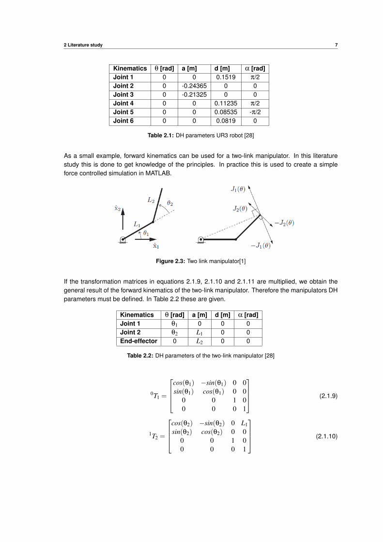
2.1 DH parameters UR3 robot [28] . . . . . . . . . . . . . . . . . . . . . . . . . . . . . 7
2.2 DH parameters of the two-link manipulator [28] . . . . . . . . . . . . . . . . . . . . 7
2.3 Example Newton-Raphson method two degrees of freedom [1] . . . . . . . . . . . . 15
2.4 A comparison between active and passive compliances [29] . . . . . . . . . . . . . 27
2.5 Algorithm overview [13] . . . . . . . . . . . . . . . . . . . . . . . . . . . . . . . . 29
2.6 Advanced algorithms [13] . . . . . . . . . . . . . . . . . . . . . . . . . . . . . . . 30
5.1 Rise time sample points . . . . . . . . . . . . . . . . . . . . . . . . . . . . . . . . 81
5.2 Data record servoj gain=500, Figure 5.18 . . . . . . . . . . . . . . . . . . . . . . . 87
5.3 Data record servoj gain=2000, Figure 5.19 . . . . . . . . . . . . . . . . . . . . . . 87
5.4 Difference in error between the two approaches on the same point in the trajectory . 89
5.5 Table with algorithm calculation times in milliseconds . . . . . . . . . . . . . . . . . 90
xvi
List of Symbols
• sT b: Transformation of the b-frame relative to the s-frame
• sRb: Rotation of the b-frame relative to the s-frame
• sPb: Translation of the b-frame relative to the s-frame
• θ, θ, θ: Joint configurations
• θd , θd , θd : Desired joint configurations
• x, x, x: Cartesian configurations
• xd , xd , xd : Desired Cartesian configurations
• α: Fixed joint angle
• J(θ): Jacobian matrix
• J(θ): Derivative of the Jacobian matrix
• τ: Joint torques
• τext : Joint torques caused by an external force
• Ftip: Force at the end-effector
• Fext : The external applied force
• g: Gravitational constant
• Li: Length of link i
• mi: Mass of link i
• L : Lagrange total energy
• K : Kinetic energy
• P : Potential engery
• Vd : Desired twist matrix
• M(θ): The mass matrix in joint space
• c(θ, θ): Coriolis and centripetal torques matrix
xvii
LIST OF SYMBOLS xviii
• g(θ): Gravity compensation matrix in joint space
• b(θ): Friction force matrix in joint space
• h(θ, θ): Lumped forces matrix in joint space
• Λ(x): The mass matrix calculated in Cartesian space
• µ(x, x): Coriolis forces matrix in Cartesian space
• γ(x): Gravity compensation matrix in Cartesian space
• η(x): Friction force matrix in Cartesian space
• ωm: Mechanical rotation speed
• ψ: Flux
• U : Input voltage
• T : Torque
• R: Resistor
• E: Elektromotive force
• J: Inertia DC motor
• ωn: Natural frequency
• ζ: Damping ratio
• D: Mechanical damping DC motor
• KP: Virtual stiffness parameter
• KD: Virtual damping parameter
• M: Virtual mass
• τ: Time constant
List of Abbreviations
• DA: Direct Adaptive
• DOF: Degrees Of Freedom
• ERSP: Evolution Robotics Software Platform
• GUI: Graphical User Interface
• IA: Indirect Adaptive
• IOS: Internetwork Operating System
• IT: Information Technology
• ITEA: Integrated Time-multiplied Absolute Error
• LIDAR: LIght Detection And Ranging or Laser Imaging Detection And Ranging
• LTS: Long-Term Support
• MSRDS: Microsoft Robotics Developer Studio
• NAOqiOS: NAO humanoid robot Operation System
• OS: Operating System
• OpenRTM: Open Robotics Technology Middleware
• OPROS: Open Platform for RObotics Services
• OROCOS: Open RObot COntrol Software
• OSI: Open Systems Interconnection
• PC: Personal Computer
• PhD: Doctor of Philosophy
• PID: Proportional Integral Differential
• ROS: Robot Operating System
• UR3: Universal Robots 3 CB-series
• TCP/IP: Transmission Control Protocol/Internet Protocol
xix
1Introduction
1.1 Motivation
This master thesis was chosen as a continuation of my bachelor thesis which also took place inthe robotics field. I fully committed myself and built up the fascination for robotics. Since there wasonly limited contact with robots in the bachelor’s thesis and because there are no courses aboutrobotics in this four-year course, I decided to continue with this subject.
First a master thesis in the industry was considered. However, it was established that the pace ofcommunication did not meet my expectations. My supervisor from my bachelor thesis, Mr De Ryckhad prepared some theses for his doctorate together with Mr Versteyhe. Since the topic industry 4.0is well represented on our campus with ’The Ultimate Factory’, I also decided to make my masterthesis on the campus. In addition to that, communication with my promoters would certainly gowell.
1.2 Purpose of the thesis
The purpose of this thesis was to develop a force compliant controller in Python. Therefore, it wassupposed to be able to describe the kinematics and dynamics of a robot arm. In addition, it wasexpected to get a feeling for Python and to write code myself that causes a force compliance on anUR3 robot. An application for this force compliant controller had to be worked out. As additionalapplication there was chosen to let the robot arm turn in a bolt in a hole that is not drilled in theexact location. Mr De Ryck has experienced experimentally that screwing in a bolt, with a robotarm, is not always going smoothly. That is why this thesis will be attempted on the basis of forcecompliance.
1
1 Introduction 2
1.3 Goal of the thesis
The goal of this thesis is to develop and implement a compliant controller in Python for a generalsix degrees of freedom robot. To enhance the applicability of the controller, two applications wereworked out in this thesis: (1) path tracking with a disturbance and (2) screw in a bolt. The firstapplication needs to work when started up, in regime. This last application needs to have a highsuccess ratio, as 6-sigma is often used as a target in industry. A minimum reliability of 4-sigma willbe achieved in this thesis. This means that only 0.62% of the actions will go wrong.Therefore some partial objectives were made. The first goal was to have a robot that can go from Ato B and be disrupted along the way. Later, the previously discussed application had to be workedout. Unfortunately due to time constraints this has only been discussed theoretically. The maintask was to learn Python and apply knowledge of robot kinematics and dynamics to a compliantcontroller.
1.4 Thesis structure
In chapter 2, the literature study, a short explanation is given of all subjects that will be used.The subjects include: the kinematics and dynamics of a robot arm, followed by a description ofthe control techniques and finally it discusses trajectory generation, the specifications of the UR3robot, pros and cons of Python and the connection through TCP/IP. The method of elaboration isdescribed in chapter 3 and finally an overview of the experiments performed with the correspondingresults is given in chapters 4 and 5. Finally, chapter 6 concludes this thesis.
2Literature study
The aim of the literature study is to incorporate all the necessary knowledge into related chapters.Both the kinematics and dynamics of a robot with multiple degrees of freedom are discussed insection 2.1. In addition the internal joint position control loop is discussed in section 2.2. Hereafter,in section 2.3, the different force control methods are discussed with their properties, followed by thetheory of trajectory generation in section 2.4. Finally, some topics are discussed that are necessaryto achieve the final goal. In section 2.5 an overview is given of the UR3 properties and sections 2.6and 2.7 discuss the used communication protocol and the pros and cons of using Python.
3

2 Literature study 4
2.1 Kinematics and dynamics of a robot arm
2.1.1 Introduction
In this thesis a six degree of freedom robot was used. Mastering the kinematics and dynamics of anarm-type robot was therefore necessary. Two books were used as a basis for this study: ’Robotics,Vision and Control’ and ’Modern Robotics’ [30] [1]. The book ’Modern Robotics’ comes with videolessons on YouTube, suitable for self-study and other educative purposes. In this literature studyyou can find some of the fundamentals about the kinematics of a robot arm.The following subsections are a summary of the book. Taking into account the knowledge ofspecialists, only the most fundamental content is described.
2.1.2 Rigid-body motions
To describe a movement of any rigid-body in a second or third dimensional space, from the linearalgebra, it is known that translations and rotations are used. As Figure 2.1 shows in two dimensionalspace, a vector can be defined to move the s-frame to another location in space. This is called atranslation. If a rotation and a translation took place, all coordinates in the s-frame from Figure 2.1are first multiplied by a rotation matrix and afterwards translated to a new point in space. As a resultthe b-frame in Figure 2.1 is defined.
Figure 2.1: Translation and rotation of a frame
In a two dimensional space this could be described by using a column vector with two elementsused for the translation [sPb] and a two by two matrix used for the rotation part [sRb].
sPb =
[sPbxsPby
]=
[∆x∆y
](2.1.1)
sRb =
[sXbxsYbx
sXbysYby
]=
[cos(θ) −sin(θ)sin(θ) cos(θ)
](2.1.2)
If both equations 2.1.1 and 2.1.2 are combined, then equation 2.1.3 applies.
sTb =s Pb ∗s Rb =
sXbxsYbx 0
sXbysYby 0
0 0 1
1 0 sPbx0 1 sPby0 0 1
=
sXbxsYbx
sPbxsXby
sYbysPby
0 0 1
(2.1.3)
In this example, work was done in a plane. Only three variables are required to describe adisplacement: the angular displacement and the distance for displacement in x- and y-coordinates
2 Literature study 5
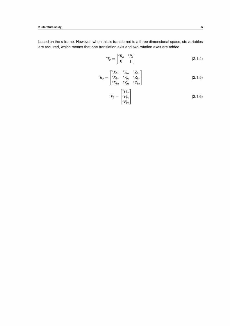
based on the s-frame. However, when this is transferred to a three dimensional space, six variablesare required, which means that one translation axis and two rotation axes are added.
sTb =
[sRbsPb
0 1
](2.1.4)
sRb =
sXbxsYbx
sZbxsXby
sYbysZby
sXbzsYbz
sZbz
(2.1.5)
sPb =
sPbxsPbysPbz
(2.1.6)
2 Literature study 6
2.1.3 Forward kinematics
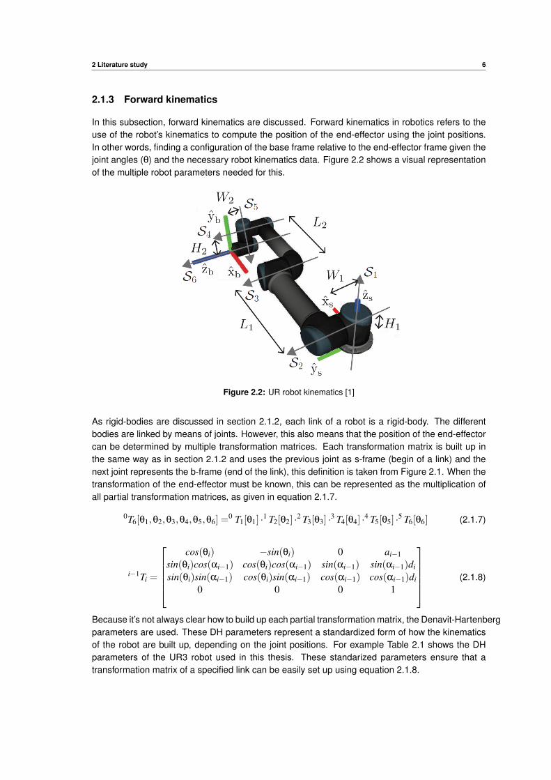
In this subsection, forward kinematics are discussed. Forward kinematics in robotics refers to theuse of the robot’s kinematics to compute the position of the end-effector using the joint positions.In other words, finding a configuration of the base frame relative to the end-effector frame given thejoint angles (θ) and the necessary robot kinematics data. Figure 2.2 shows a visual representationof the multiple robot parameters needed for this.
Figure 2.2: UR robot kinematics [1]
As rigid-bodies are discussed in section 2.1.2, each link of a robot is a rigid-body. The differentbodies are linked by means of joints. However, this also means that the position of the end-effectorcan be determined by multiple transformation matrices. Each transformation matrix is built up inthe same way as in section 2.1.2 and uses the previous joint as s-frame (begin of a link) and thenext joint represents the b-frame (end of the link), this definition is taken from Figure 2.1. When thetransformation of the end-effector must be known, this can be represented as the multiplication ofall partial transformation matrices, as given in equation 2.1.7.
0T6[θ1,θ2,θ3,θ4,θ5,θ6] =0 T1[θ1] ·1 T2[θ2] ·2 T3[θ3] ·3 T4[θ4] ·4 T5[θ5] ·5 T6[θ6] (2.1.7)
i−1Ti =
cos(θi) −sin(θi) 0 ai−1
sin(θi)cos(αi−1) cos(θi)cos(αi−1) sin(αi−1) sin(αi−1)di
sin(θi)sin(αi−1) cos(θi)sin(αi−1) cos(αi−1) cos(αi−1)di
0 0 0 1
(2.1.8)
Because it’s not always clear how to build up each partial transformation matrix, the Denavit-Hartenbergparameters are used. These DH parameters represent a standardized form of how the kinematicsof the robot are built up, depending on the joint positions. For example Table 2.1 shows the DHparameters of the UR3 robot used in this thesis. These standarized parameters ensure that atransformation matrix of a specified link can be easily set up using equation 2.1.8.
2 Literature study 7
Kinematics θ [rad] a [m] d [m] α [rad]Joint 1 0 0 0.1519 π/2Joint 2 0 -0.24365 0 0Joint 3 0 -0.21325 0 0Joint 4 0 0 0.11235 π/2Joint 5 0 0 0.08535 -π/2Joint 6 0 0 0.0819 0
Table 2.1: DH parameters UR3 robot [28]
As a small example, forward kinematics can be used for a two-link manipulator. In this literaturestudy this is done to get knowledge of the principles. In practice this is used to create a simpleforce controlled simulation in MATLAB.
Figure 2.3: Two link manipulator[1]
If the transformation matrices in equations 2.1.9, 2.1.10 and 2.1.11 are multiplied, we obtain thegeneral result of the forward kinematics of the two-link manipulator. Therefore the manipulators DHparameters must be defined. In Table 2.2 these are given.
Kinematics θ [rad] a [m] d [m] α [rad]Joint 1 θ1 0 0 0Joint 2 θ2 L1 0 0End-effector 0 L2 0 0
Table 2.2: DH parameters of the two-link manipulator [28]
0T1 =
cos(θ1) −sin(θ1) 0 0sin(θ1) cos(θ1) 0 0
0 0 1 00 0 0 1
(2.1.9)
1T2 =
cos(θ2) −sin(θ2) 0 L1sin(θ2) cos(θ2) 0 0
0 0 1 00 0 0 1
(2.1.10)

2 Literature study 8
2Tend =
1 0 0 L20 1 0 00 0 1 00 0 0 1
(2.1.11)
0T2 =0 T 1
1 T 22 Tend =
cos(θ1 +θ2) sin(θ1 +θ2) 0 L1cos(θ1)+L2cos(θ1 +θ2)sin(θ1 +θ2) cos(θ1 +θ2) 0 L1sin(θ1)+L2sin(θ1 +θ2)
0 0 1 00 0 0 1
(2.1.12)
[x1x2
]=
[L1cos(θ1)+L2cos(θ1 +θ2)L1sin(θ1)+L2sin(θ1 +θ2)
](2.1.13)
Equation 2.1.13 is the translation part of the transformation matrix of the two-link manipulator.The other elements of the transformation matrix in equation 2.1.12 are the rotation values of theend-effector. Conclusion, the forward kinematics give us the end-effector coordinates and rotations,given the joint angles.
2 Literature study 9
2.1.4 Inverse kinematics
The forward kinematics were relatively easy to describe on the basis of a few transformationmatrices. Completing the inverse is a lot harder due to the nonlinearity. In most cases there areseveral options to achieve the same configuration of the robot arm. There are two solution methods,the analytic closed-form and the iterative numerical method. The latter is most used because for ananalytic closed-form equation we need an exact geometry and the equation has multiple solutions.In the alternative, there is only one solution, when starting from a guess. The Newton-Raphsonalgorithm is used as an iterative method in this example, but there are many more algorithms asdiscussed on page 90.
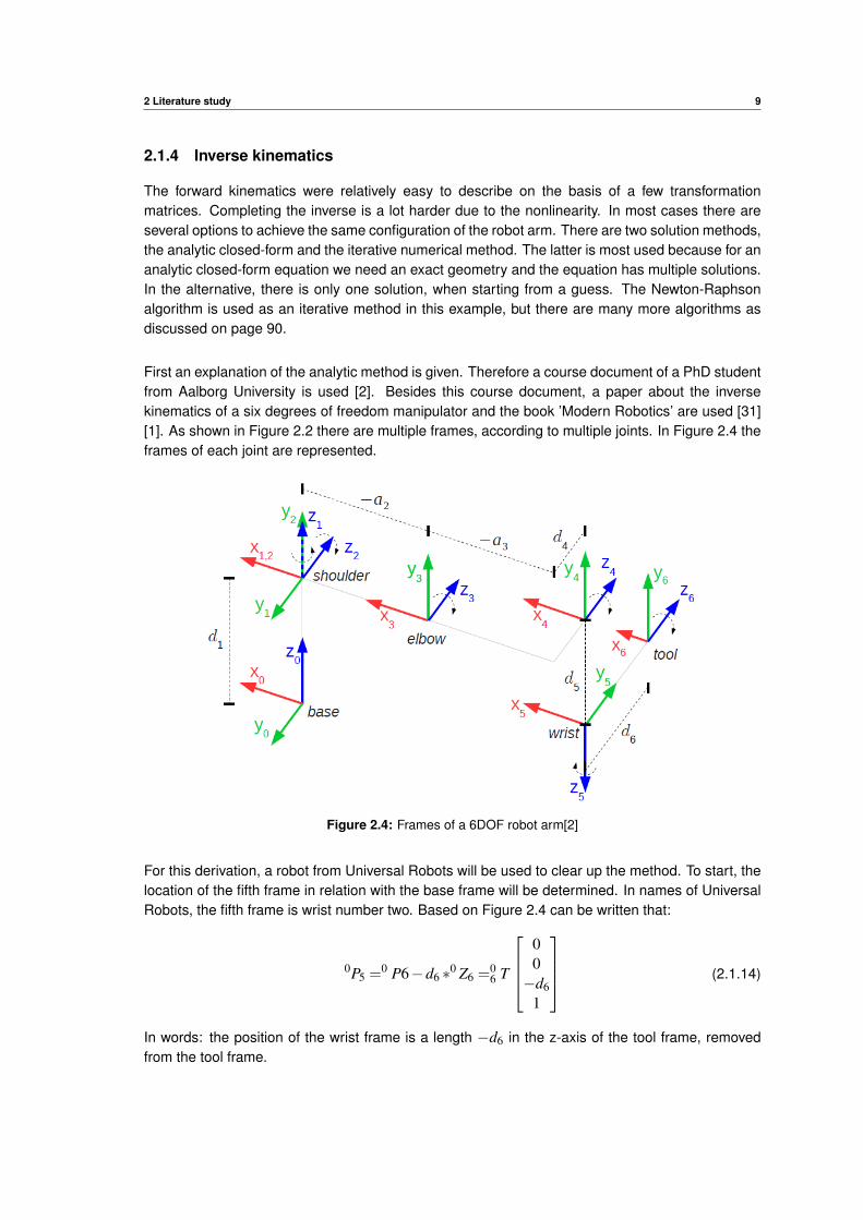
First an explanation of the analytic method is given. Therefore a course document of a PhD studentfrom Aalborg University is used [2]. Besides this course document, a paper about the inversekinematics of a six degrees of freedom manipulator and the book ’Modern Robotics’ are used [31][1]. As shown in Figure 2.2 there are multiple frames, according to multiple joints. In Figure 2.4 theframes of each joint are represented.
Figure 2.4: Frames of a 6DOF robot arm[2]
For this derivation, a robot from Universal Robots will be used to clear up the method. To start, thelocation of the fifth frame in relation with the base frame will be determined. In names of UniversalRobots, the fifth frame is wrist number two. Based on Figure 2.4 can be written that:
0P5 =0 P6−d6 ∗0 Z6 =
06 T
00−d6
1
(2.1.14)
In words: the position of the wrist frame is a length −d6 in the z-axis of the tool frame, removedfrom the tool frame.

2 Literature study 10
Figure 2.5: θ1 sketch [2]
In Figure 2.5 a view from above is taken. The following equations can be derived.
θ1 = φ1 +φ2 +π
2(2.1.15)
φ1 = atan( 0P5y
0P5x
)(2.1.16)
φ2 =±acos(
d4
|0P5xy|
)=±acos
d4√0P2
5x +0 P2
5y
(2.1.17)
Substituting 2.1.16 and 2.1.17 in 2.1.15 we obtain equation 2.1.18 for the angle θ1.
θ1 = arctan( 0P5y
0P5x
)±arccos
d4√0P2
5x +0 P2
5y
+π
2(2.1.18)
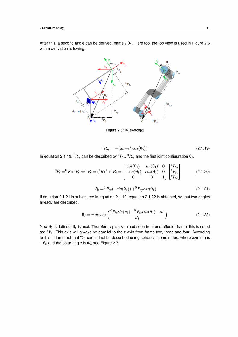
2 Literature study 11
After this, a second angle can be derived, namely θ5. Here too, the top view is used in Figure 2.6with a derivation following.
Figure 2.6: θ5 sketch[2]
1P6y =−(d4 +d6cos(θ5)) (2.1.19)
In equation 2.1.19, 1P6y can be described by 0P6x, 0P6y and the first joint configuration θ1.
0P6 =01 R∗1 P6⇔1 P6 = (0
1R)> ∗0 P6 =
cos(θ1) sin(θ1) 0−sin(θ1) cos(θ1) 0
0 0 1
0P6x0P6y0P6z
(2.1.20)
1P6 =0 P6x(−sin(θ1))+
0 P6ycos(θ1) (2.1.21)
If equation 2.1.21 is substituted in equation 2.1.19, equation 2.1.22 is obtained, so that two anglesalready are described.
θ5 =±arccos(0P6xsin(θ1)−0 P6ycos(θ1)−d4
d6
)(2.1.22)
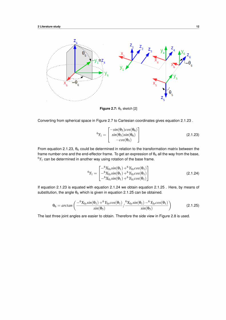
Now θ5 is defined, θ6 is next. Therefore y1 is examined seen from end-effector frame, this is notedas: 6Y1. This axis will always be parallel to the z-axis from frame two, three and four. Accordingto this, it turns out that 6Y1 can in fact be described using spherical coordinates, where azimuth is−θ6 and the polar angle is θ5, see Figure 2.7.
2 Literature study 12
Figure 2.7: θ6 sketch [2]
Converting from spherical space in Figure 2.7 to Cartesian coordinates gives equation 2.1.23 .
6Y1 =
−sin(θ5)cos(θ6)sin(θ5)sin(θ6)−cos(θ5)
(2.1.23)
From equation 2.1.23, θ6 could be determined in relation to the transformation matrix between theframe number one and the end-effector frame. To get an expression of θ6 all the way from the base,6Y1 can be determined in another way using rotation of the base frame.
6Y1 =
−6X0xsin(θ1)+6 Y0xcos(θ1)
−6X0ysin(θ1)+6 Y0ycos(θ1)
−6X0zsin(θ1)+6 Y0zcos(θ1)
(2.1.24)
If equation 2.1.23 is equated with equation 2.1.24 we obtain equation 2.1.25 . Here, by means ofsubstitution, the angle θ6 which is given in equation 2.1.25 can be obtained.
θ6 = arctan(−6X0ysin(θ1)+
6 Y0ycos(θ1)
sin(θ5)/
6X0ysin(θ1)−6 Y0ycos(θ1)
sin(θ5)
)(2.1.25)
The last three joint angles are easier to obtain. Therefore the side view in Figure 2.8 is used.
2 Literature study 13
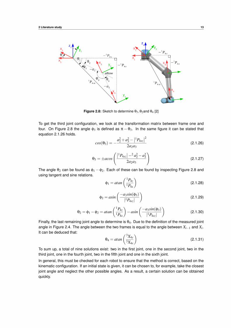
Figure 2.8: Sketch to determine θ3,θ2and θ4 [2]
To get the third joint configuration, we look at the transformation matrix between frame one andfour. On Figure 2.8 the angle φ3 is defined as π− θ3. In the same figure it can be stated thatequation 2.1.26 holds.
cos(θ3) =−a2
2 +a23−∣∣1P4xz
∣∣22a2a3
(2.1.26)
θ3 =±acos
(∣∣1P4xz∣∣−2 a2
2−a23
2a2a3
)(2.1.27)
The angle θ2 can be found as φ1−φ2. Each of these can be found by inspecting Figure 2.8 andusing tangent and sine relations.
φ1 = atan( 1P4z
1P4x
)(2.1.28)
φ2 = asin(−a3sin(φ3)
|1P4xz|
)(2.1.29)
θ2 = φ1−φ2 = atan( 1P4z
1P4x
)−asin
(−a3sin(φ3)
|1P4xz|
)(2.1.30)
Finally, the last remaining joint angle to determine is θ4. Due to the definition of the measured jointangle in Figure 2.4. The angle between the two frames is equal to the angle between Xi−1 and Xi.It can be deduced that:
θ4 = atan( 3X4y
3X4x
)(2.1.31)
To sum up, a total of nine solutions exist: two in the first joint, one in the second joint, two in thethird joint, one in the fourth joint, two in the fifth joint and one in the sixth joint.
In general, this must be checked for each robot to ensure that the method is correct, based on thekinematic configuration. If an initial state is given, it can be chosen to, for example, take the closestjoint angle and neglect the other possible angles. As a result, a certain solution can be obtainedquickly.
2 Literature study 14
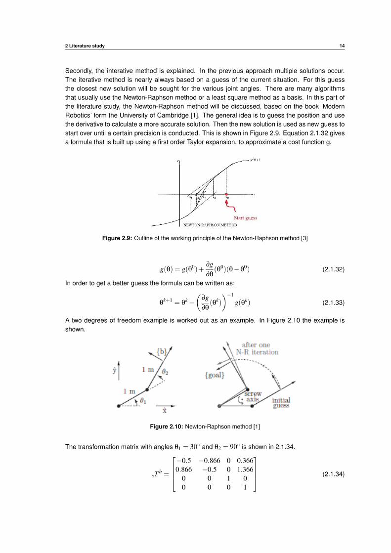
Secondly, the interative method is explained. In the previous approach multiple solutions occur.The iterative method is nearly always based on a guess of the current situation. For this guessthe closest new solution will be sought for the various joint angles. There are many algorithmsthat usually use the Newton-Raphson method or a least square method as a basis. In this part ofthe literature study, the Newton-Raphson method will be discussed, based on the book ’ModernRobotics’ form the University of Cambridge [1]. The general idea is to guess the position and usethe derivative to calculate a more accurate solution. Then the new solution is used as new guess tostart over until a certain precision is conducted. This is shown in Figure 2.9. Equation 2.1.32 givesa formula that is built up using a first order Taylor expansion, to approximate a cost function g.
Figure 2.9: Outline of the working principle of the Newton-Raphson method [3]
g(θ) = g(θ0)+∂g∂θ
(θ0)(θ−θ0) (2.1.32)
In order to get a better guess the formula can be written as:
θk+1 = θ
k−(
∂g∂θ
(θk)
)−1
g(θk) (2.1.33)
A two degrees of freedom example is worked out as an example. In Figure 2.10 the example isshown.
Figure 2.10: Newton-Raphson method [1]
The transformation matrix with angles θ1 = 30◦ and θ2 = 90◦ is shown in 2.1.34.
sT b =
−0.5 −0.866 0 0.3660.866 −0.5 0 1.366
0 0 1 00 0 0 1
(2.1.34)
2 Literature study 15
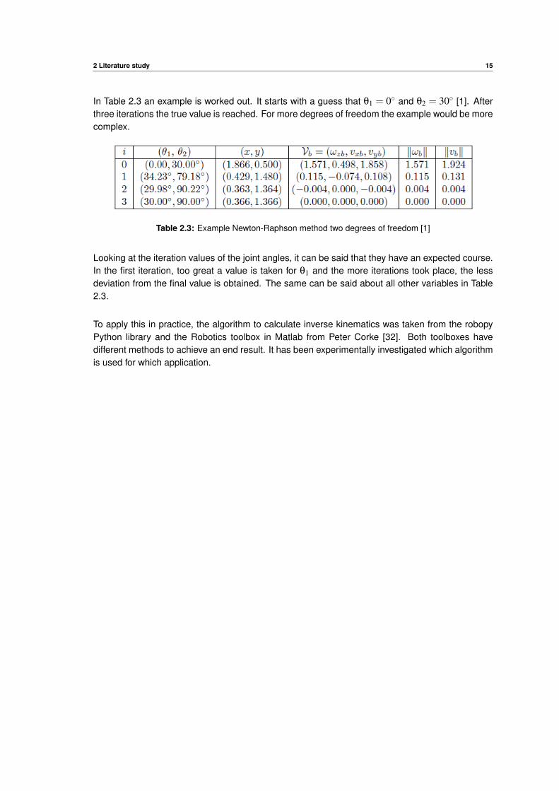
In Table 2.3 an example is worked out. It starts with a guess that θ1 = 0◦ and θ2 = 30◦ [1]. Afterthree iterations the true value is reached. For more degrees of freedom the example would be morecomplex.
Table 2.3: Example Newton-Raphson method two degrees of freedom [1]
Looking at the iteration values of the joint angles, it can be said that they have an expected course.In the first iteration, too great a value is taken for θ1 and the more iterations took place, the lessdeviation from the final value is obtained. The same can be said about all other variables in Table2.3.
To apply this in practice, the algorithm to calculate inverse kinematics was taken from the robopyPython library and the Robotics toolbox in Matlab from Peter Corke [32]. Both toolboxes havedifferent methods to achieve an end result. It has been experimentally investigated which algorithmis used for which application.
2 Literature study 16
2.1.5 Velocity kinematics
In this chapter we will take a look at the velocity kinematics. In comparison to the forward kinematics,the velocity of the end-effector can be described in function of the joint velocities.
x = J(θ)θ (2.1.35)
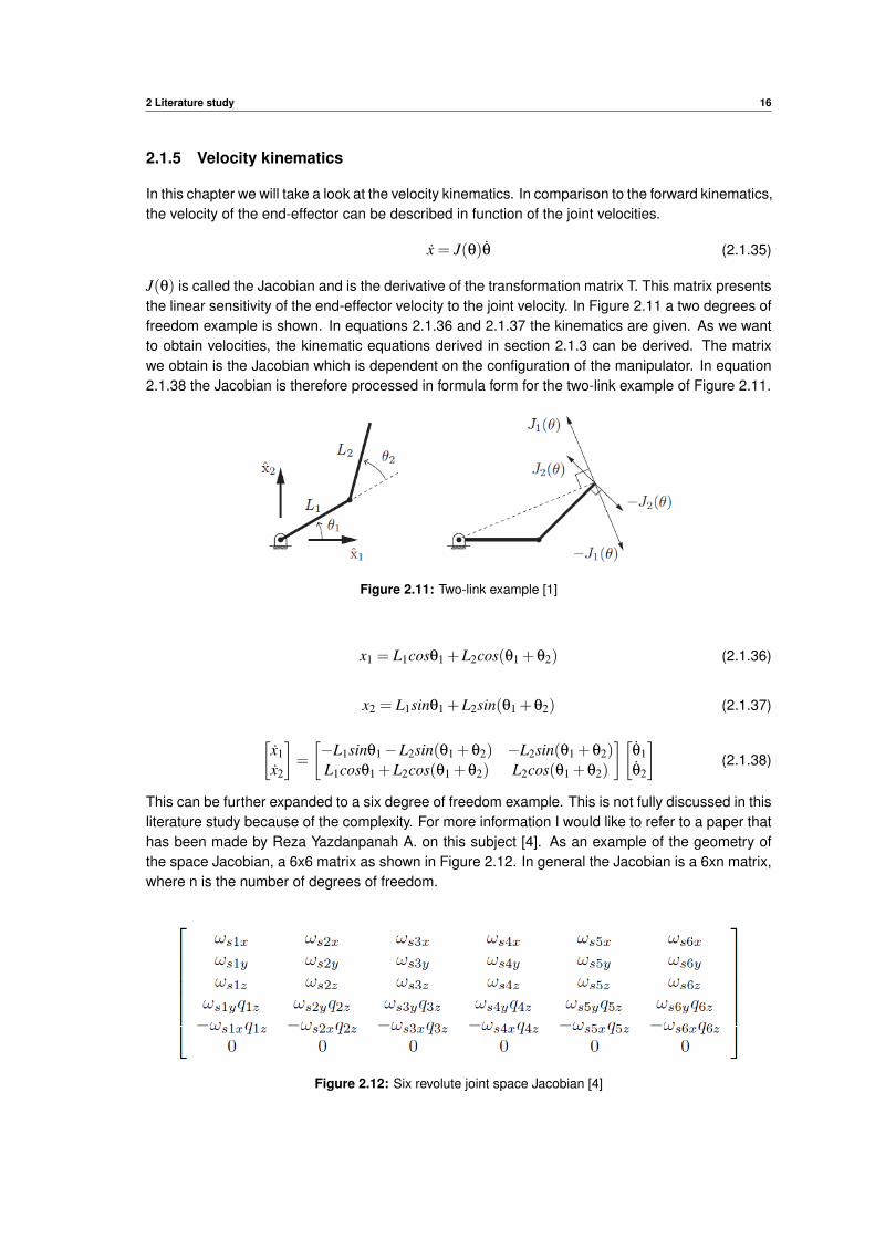
J(θ) is called the Jacobian and is the derivative of the transformation matrix T. This matrix presentsthe linear sensitivity of the end-effector velocity to the joint velocity. In Figure 2.11 a two degrees offreedom example is shown. In equations 2.1.36 and 2.1.37 the kinematics are given. As we wantto obtain velocities, the kinematic equations derived in section 2.1.3 can be derived. The matrixwe obtain is the Jacobian which is dependent on the configuration of the manipulator. In equation2.1.38 the Jacobian is therefore processed in formula form for the two-link example of Figure 2.11.
Figure 2.11: Two-link example [1]
x1 = L1cosθ1 +L2cos(θ1 +θ2) (2.1.36)
x2 = L1sinθ1 +L2sin(θ1 +θ2) (2.1.37)
[x1x2
]=
[−L1sinθ1−L2sin(θ1 +θ2) −L2sin(θ1 +θ2)L1cosθ1 +L2cos(θ1 +θ2) L2cos(θ1 +θ2)
][θ1θ2
](2.1.38)
This can be further expanded to a six degree of freedom example. This is not fully discussed in thisliterature study because of the complexity. For more information I would like to refer to a paper thathas been made by Reza Yazdanpanah A. on this subject [4]. As an example of the geometry ofthe space Jacobian, a 6x6 matrix as shown in Figure 2.12. In general the Jacobian is a 6xn matrix,where n is the number of degrees of freedom.
Figure 2.12: Six revolute joint space Jacobian [4]
2 Literature study 17
An other type of Jacobian, the body Jacobian corresponds to a screw axis expressed in theend-effector frame. In this thesis the space Jacobian will be used. As earlier described, the inversekinematics could be done with a Newton-Raphson algoritm. If the desired twist and the Jacobianare described in the same frame the general solution could be written as:
θ = J†(θ)Vd (2.1.39)
In equation 2.1.39, J†(θ) is the pseudoinverse matrix of J(θ) and Vd is the desired twist or velocitymatrix. The pseudoinverse Jacobian is used, because the Jacobian is not square or it’s singularso J−1 does not exist. Because the inverse does not exist, the Moore-Penrose pseudoinverseapproach is used. In equation 2.1.40 a general way to find the pseudoinverse is given, when theJacobian has more rows than columns or when there are singularities [1].
J† = (JT J)−1JT (2.1.40)
J† = JT (JT J)−1 (2.1.41)
2 Literature study 18
2.1.6 Dynamics of open chains
In the previous sections, we went through the kinematics of the system. In this chapter the generaldynamics are delineated. To describe these dynamics, a second order differential equation is used,this is shown in 2.1.42.
τ = M(θ)θ+ c(θ, θ)+g(θ)+b(θ)+ JT (θ)Ftip (2.1.42)
In equation 2.1.42, τ is the vector of joint torques, M(θ) is the mass matrix, which includes eachlink’s inertia. The torques that lump together cetripetal and Coriolis term are given by c(θ, θ),while g(θ) is included to compensate the gravity force on each link. The viscous friction torquesare described by b(θ) and JT (θ)Ftip are the additional torques due to an external force on theend-effector.
In general the viscous friction term is neglected due to ignorance, because certain specificationssuch as the inertia and viscous friction of the joints are usually not released by the manufacturer.For the other terms in this equation, a list was made to clarify the specific properties of each termbased on a PowerPoint of a lecture given by Dr Surya Singh [33].
• M(θ): The mass matrix could be determined using the Jacobian. By recalculating theJacobian to both translations and rotations, each in a separate Jacobian, respectively Jvi
and Jωi. In a six degree of freedom, these two Jacobians are determined for each link andhave three rows and six columns. In total the mass matrix is calculated using equation 2.1.43,where mi is the mass of a specified link and ICi contains all inertias of a link in a 6x6 matrix.The mass matrix is symmetric and positive definite [33].
M(θ) =∞
∑n=1
(miJTvi(θ)Jvi(θ)+ Jωi(θ)ICiJ
Tωi(θ)) (2.1.43)
• c(θ, θ): The Coriolis and centripetal component can also be written as C(θ, θ)θ. The off-diagonalterms of the Coriolis matrix C(θ, θ), Ci, j represent coupling of joint j velocity to the generalizedforce action on joint i and is just like the mass matrix a square matrix [30].
• g(θ): The gravity matrix takes the masses of the different links into account, in order to obtaintorque compensation. These torques are calculated on the center of gravity of each joint.
• JT Ftip: To confirm whether this expression is indeed correct, we can make a derivation:
δX ∗F = δθ∗ τ (2.1.44)
FT ∗δX = τT ∗δθ (2.1.45)
δX = J ∗δθ (2.1.46)
FT ∗ J = τT (2.1.47)
JT F = τ (2.1.48)
From this we can conclude that the Jacobian can also be used to convert the force on theend-effector to joint torques or reverse.
2 Literature study 19
To determine these dynamic parameters I refer to chapter eight in the book ’Modern Robotics’ [1].Two options are discussed here. First, a general equation is drawn up using the Lagrage equation,given in equation 2.1.49. The aim of this comparison is to primarily determine the torques andto derive the various parameters from the torque equations. Secondly, Newton-Euler’s method isexplained, in which all parameters can be determined in a closed form.
τi =ddt
∂L∂θi− ∂L
∂θi(2.1.49)
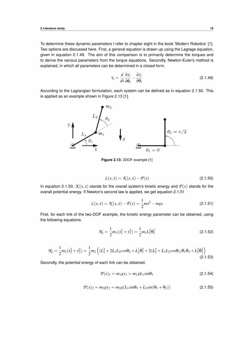
According to the Lagrangian formulation, each system can be defined as in equation 2.1.50. Thisis applied as an example shown in Figure 2.13 [1].
Figure 2.13: 2DOF example [1]
L(x, x) = K (x, x)−P (x) (2.1.50)
In equation 2.1.50, K (x, x) stands for the overall system’s kinetic energy and P (x) stands for theoverall potential energy. If Newton’s second law is applied, we get equation 2.1.51
L(x, x) = K (x, x)−P (x) =12
mx2−mgx (2.1.51)
First, for each link of the two-DOF example, the kinetic energy parameter can be obtained, usingthe following equations.
K1 =12
m1(x21 + y2
1) =12
m1L21θ
21 (2.1.52)
K2 =12
m2(x22 + y2
2) =12
m2
((L2
1 +2L1L2cosθ2 +L)2θ
21 +2(L2
2 +L1L2cosθ2)θ1θ2 +L22θ
22
)(2.1.53)
Secondly, the potential energy of each link can be obtained.
P (x)1 = m1gy1 = m1gL1sinθ1 (2.1.54)
P (x)2 = m2gy2 = m2g(L1sinθ1 +L2sin(θ1 +θ2)) (2.1.55)
2 Literature study 20
From the Euler-Lagrange equation in 2.1.49, the partial torques can be defined for this two degreesof freedom example.
τ1 = (m1L21 +m2(L2
1 +2L1L2cosθ2 +L22))θ+m2(L1L2cosθ2 +L2
) )θ2
−m2L1L2sinθ2(2θ1θ2 + θ22)+(m1 +m2)L1gcosθ1 +m2gL2cos(θ1 +θ2)
(2.1.56)
τ2 = m2(L1L2cosθ2 +L22)θ1 +m2L2
2θ2 +m2L1L2θ21sinθ2 +m2gL2cos(θ1 +θ2) (2.1.57)
These torque equations can then be split up into the form of the general equation 2.1.42. Thedifferent parameters can be extracted from this, by isolating the angular acceleration, velocities andpositions.
M(θ) =
[m1L2
1 +m2(L21 +2L1L2cosθ2 +L2
2) m2(L1L2cosθ2 +L22)
m2(L1L2cosθ2 +L22) m2L2
2
](2.1.58)
c(θ, θ) =[−m2L1L2sinθ2(2θ1θ2 + θ2
2)m2L1L2θ2
1sinθ2
](2.1.59)
g(θ) =[(m1 +m2)L1gcosθ1 +m2gL2cos(θ1 +θ2)
m2gL2cos(θ1 +θ2)
](2.1.60)
This chapter cited how the dynamic model of the robot can be build up. Due to the complexity of,for example, the mass matrix and the Coriolis and centripetal torques, these have not been workedout in detail for a six degree of freedom example. During the experiments, the Peter Corke toolboxcould be used in MATLAB. In the end, there was no need to determine the dynamic parameters inPython. Why these are neglected, will be discussed in section 2.3.5.
2 Literature study 21
2.2 General position control of joints
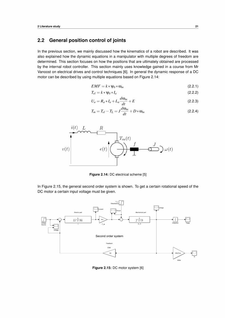
In the previous section, we mainly discussed how the kinematics of a robot are described. It wasalso explained how the dynamic equations in a manipulator with multiple degrees of freedom aredetermined. This section focuses on how the positions that are ultimately obtained are processedby the internal robot controller. This section mainly uses knowledge gained in a course from MrVanoost on electrical drives and control techniques [6]. In general the dynamic response of a DCmotor can be described by using multiple equations based on Figure 2.14:
EMF = k ∗ψ0 ∗ωm (2.2.1)
Tel = k ∗ψ0 ∗ Ia (2.2.2)
Ua = Ra ∗ Ia +Ladωm
dt+E (2.2.3)
Tm = Tel−TL = Jdωm
dt+D∗ωm (2.2.4)
Figure 2.14: DC electrical scheme [5]
In Figure 2.15, the general second order system is shown. To get a certain rotational speed of theDC motor a certain input voltage must be given.
Figure 2.15: DC motor system [6]
2 Literature study 22
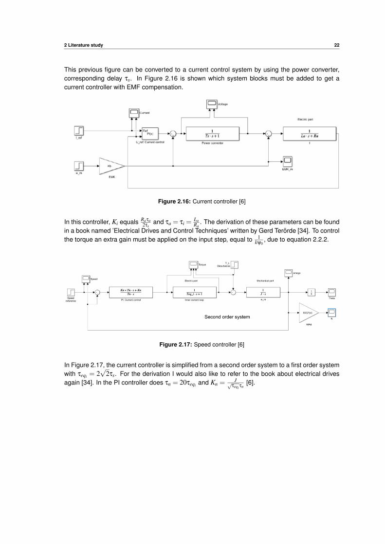
This previous figure can be converted to a current control system by using the power converter,corresponding delay τs. In Figure 2.16 is shown which system blocks must be added to get acurrent controller with EMF compensation.
Figure 2.16: Current controller [6]
In this controller, Ki equals Raτa2τs
and τa = τi =LaRa
. The derivation of these parameters can be foundin a book named ’Electrical Drives and Control Techniques’ written by Gerd Terorde [34]. To controlthe torque an extra gain must be applied on the input step, equal to 1
kψ0, due to equation 2.2.2.
Figure 2.17: Speed controller [6]
In Figure 2.17, the current controller is simplified from a second order system to a first order systemwith τeqi = 2
√2τs. For the derivation I would also like to refer to the book about electrical drives
again [34]. In the PI controller does τn = 20τeqi and Kn =J√
τeqi τn[6].
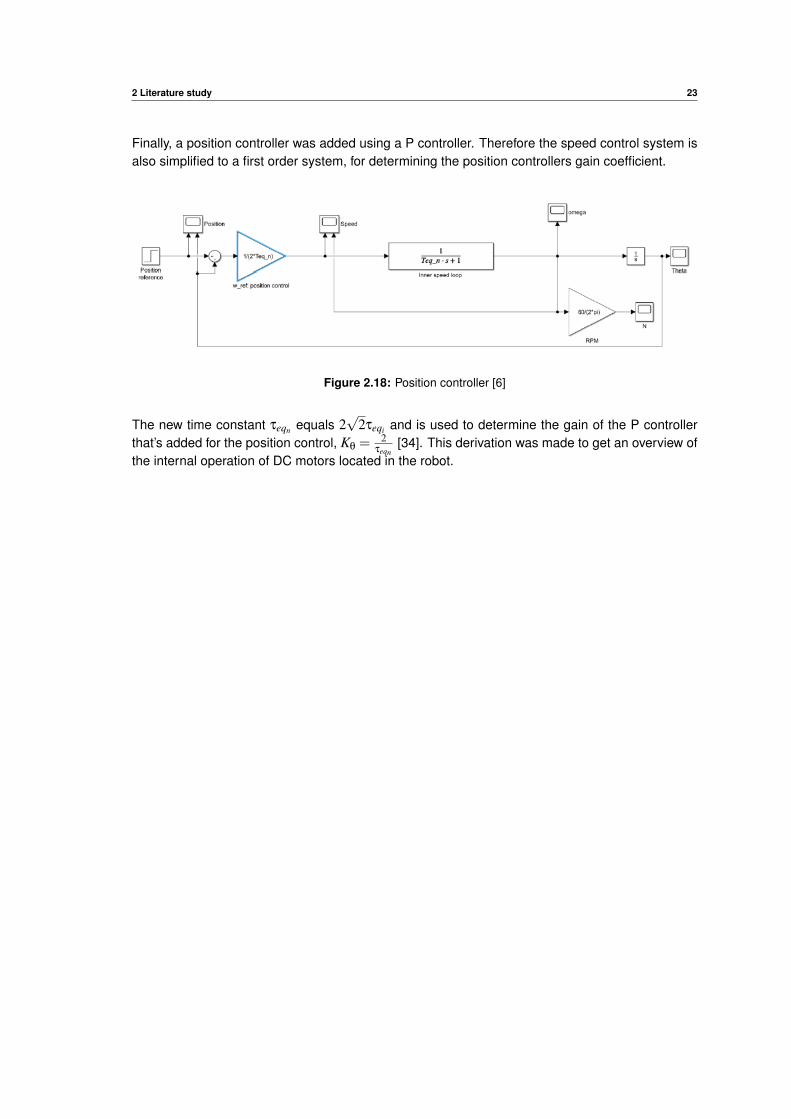
2 Literature study 23
Finally, a position controller was added using a P controller. Therefore the speed control system isalso simplified to a first order system, for determining the position controllers gain coefficient.
Figure 2.18: Position controller [6]
The new time constant τeqn equals 2√
2τeqi and is used to determine the gain of the P controllerthat’s added for the position control, Kθ =
2τeqn
[34]. This derivation was made to get an overview ofthe internal operation of DC motors located in the robot.
2 Literature study 24
2.3 Compliant force control
2.3.1 Introduction
The control technolgy to produce a compliant motion is called compliant control. Historicallycompliant motion has been defined as: ”Any robot motion where the end-effector trajectory ischanged or even generated based on online sensor information”. Today the interest in compliantcontrol is related to approaches where the controller forms the mechanical impedance of the robotsystem. In other words compliant control is related to dynamic relationships between robot positionor velocity and external forces. By shaping the mechanical impedance, the unknown environmentcould be safely handled because, instead of controlling a position or force, the force transmitted tothe environment through the energetic pair force-velocity is controlled [10].
At this point in my research some articles were found with an overview of compliant force controltechniques [13] [10]. Furthermore, matters such as: the obtained response by the compliant forcecontroller, definitions in the field of compliant force control, an overview of compliant force controllaws and the implementation choice for this thesis are discussed in this chapter.
General response in compliant force control
The response required in compliant force control is described using a second order system. Thebest known second order system is a spring, damper and mass system. First, the general equation2.3.1 is applied, to describe the dynamics of the spring, damper and mass system.
F = Md2x(t)
dt2 +Ddx(t)
dt+Kx(t) (2.3.1)
Secondly the transition is made to the Laplace domain in equation 2.3.2.
F(s) = KY (s) = MX(s)s2 +DX(s)s+KX(s) (2.3.2)
Finally, the equation was transformed into a transfer function in equation 2.3.3.
X(s)Y (s)
=K
Ms2 +Ds+K(2.3.3)
In this mechanical system, two parameters are often considered, namely the natural frequency (ωn)and the damping coefficient (ζ). The natural frequency indicates at what frequency the system willoscillate when no damper is applied. The damping is described by a number greater than zero andhas an influence on the course of the response. For example, a damping coefficient of zero ensuresossciliations with a step response. A damping of, for example, two ensures a gradual progressionto a desired value. As the definitions say: a damping coefficient of zero provides an undampedsystem, a damping coefficient between zero and one provides an underdamped system, if ζ equalsone there is a critically damped system and a damping coefficient greater than one, the system isoverdamped.
O(s)I(s)
=ω2
n
s2 +2ζωns+ω2n
(2.3.4)
2 Literature study 25
In comparison with the general second order system given in equation 2.3.4, the natural frequency(ωn) en damping coefficient (ζ) can be written as:
ωn =
√KM
(2.3.5)
ζ =D
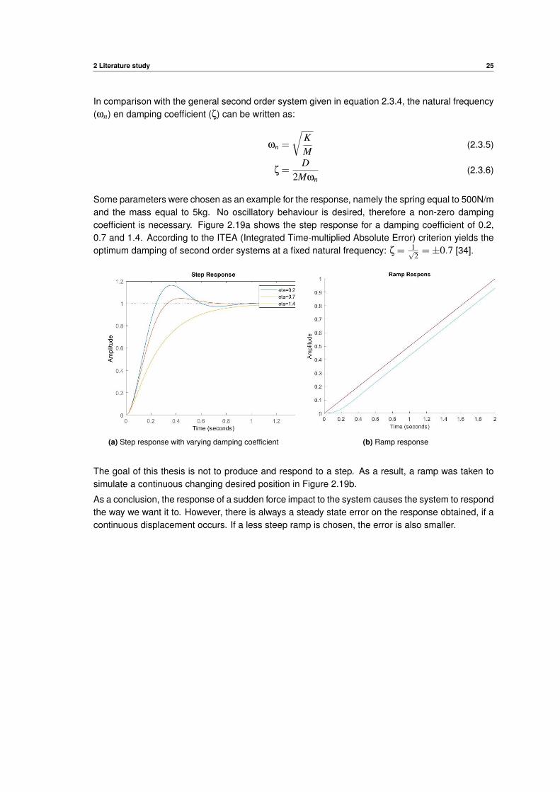
2Mωn(2.3.6)
Some parameters were chosen as an example for the response, namely the spring equal to 500N/mand the mass equal to 5kg. No oscillatory behaviour is desired, therefore a non-zero dampingcoefficient is necessary. Figure 2.19a shows the step response for a damping coefficient of 0.2,0.7 and 1.4. According to the ITEA (Integrated Time-multiplied Absolute Error) criterion yields theoptimum damping of second order systems at a fixed natural frequency: ζ = 1√
2=±0.7 [34].
(a) Step response with varying damping coefficient (b) Ramp response
The goal of this thesis is not to produce and respond to a step. As a result, a ramp was taken tosimulate a continuous changing desired position in Figure 2.19b.
As a conclusion, the response of a sudden force impact to the system causes the system to respondthe way we want it to. However, there is always a steady state error on the response obtained, if acontinuous displacement occurs. If a less steep ramp is chosen, the error is also smaller.
2 Literature study 26
2.3.2 Passive versus active compliance
In order to get started with the multiple control laws, some definitions are given. Starting with acomparison between passive and active compliance. This comparison is especially about whethera system must be controlled by another system or whether it will be controlled by nature.
Passive control
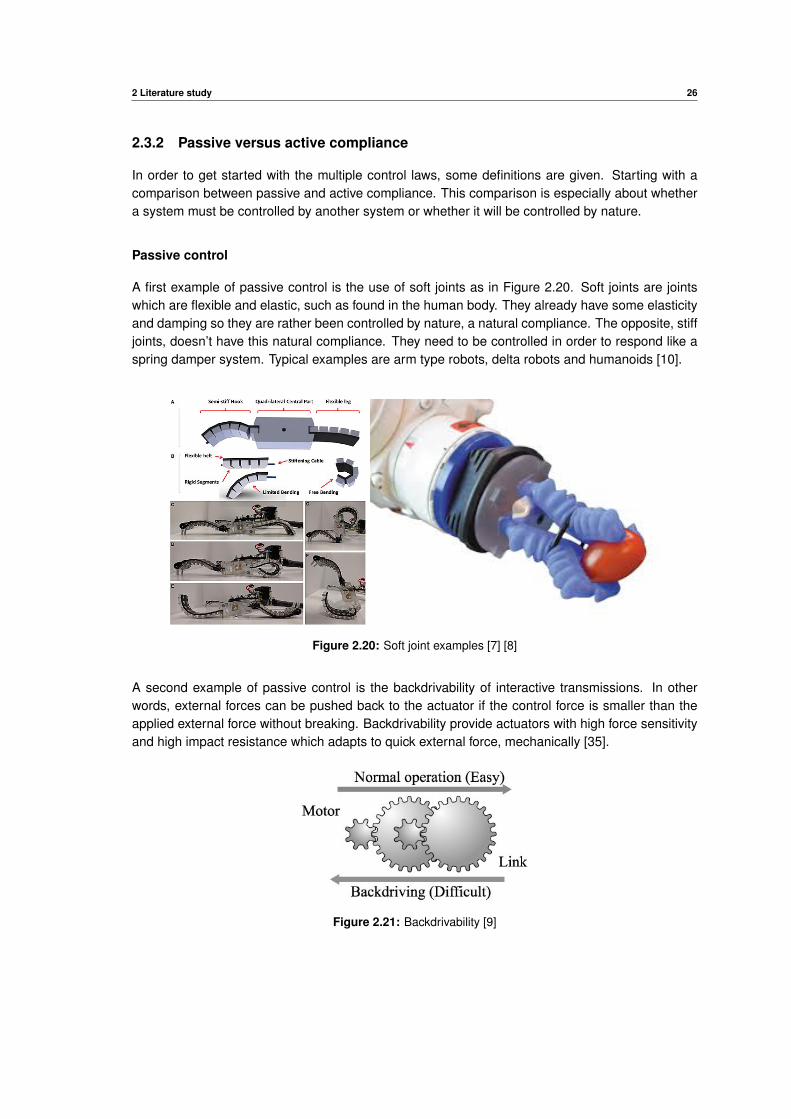
A first example of passive control is the use of soft joints as in Figure 2.20. Soft joints are jointswhich are flexible and elastic, such as found in the human body. They already have some elasticityand damping so they are rather been controlled by nature, a natural compliance. The opposite, stiffjoints, doesn’t have this natural compliance. They need to be controlled in order to respond like aspring damper system. Typical examples are arm type robots, delta robots and humanoids [10].
Figure 2.20: Soft joint examples [7] [8]
A second example of passive control is the backdrivability of interactive transmissions. In otherwords, external forces can be pushed back to the actuator if the control force is smaller than theapplied external force without breaking. Backdrivability provide actuators with high force sensitivityand high impact resistance which adapts to quick external force, mechanically [35].
Figure 2.21: Backdrivability [9]
2 Literature study 27
Active control
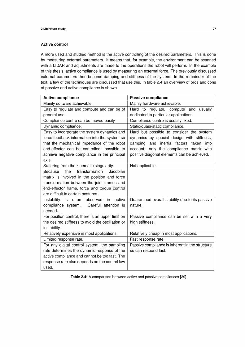
A more used and studied method is the active controlling of the desired parameters. This is doneby measuring external parameters. It means that, for example, the environment can be scannedwith a LIDAR and adjustments are made to the operations the robot will perform. In the exampleof this thesis, active compliance is used by measuring an external force. The previously discussedexternal parameters then become damping and stiffness of the system. In the remainder of thetext, a few of the techniques are discussed that use this. In table 2.4 an overview of pros and consof passive and active compliance is shown.
Active compliance Passive complianceMainly software achievable. Mainly hardware achievable.Easy to regulate and compute and can be ofgeneral use.
Hard to regulate, compute and usuallydedicated to particular applications.
Compliance centre can be moved easily. Compliance centre is usually fixed.Dynamic compliance. Static/quasi-static compliance.Easy to incorporate the system dynamics andforce feedback information into the system sothat the mechanical impedance of the robotend-effector can be controlled; possible toachieve negative compliance in the principalaxis.
Hard but possible to consider the systemdynamics by special design with stiffness,damping and inertia factors taken intoaccount; only the compliance matrix withpositive diagonal elements can be achieved.
Suffering from the kinematic singularity. Not applicable.Because the transformation Jacobianmatrix is involved in the position and forcetransformation between the joint frames andend-effector frame, force and torque controlare difficult in certain postures.Instability is often observed in activecompliance system. Careful attention isneeded.
Guaranteed overall stability due to its passivenature.
For position control, there is an upper limit onthe desired stiffness to avoid the oscillation orinstability.
Passive compliance can be set with a veryhigh stiffness.
Relatively expensive in most applications. Relatively cheap in most applications.Limited response rate. Fast response rate.For any digital control system, the samplingrate determines the dynamic response of theactive compliance and cannot be too fast. Theresponse rate also depends on the control lawused.
Passive compliance is inherent in the structureso can respond fast.
Table 2.4: A comparison between active and passive compliances [29]
2 Literature study 28
2.3.3 Direct versus indirect force control
Secondly, the difference between direct force control and indirect force control is considered. Adescription is given on the basis of the definition of the respective force control method.
Direct force control
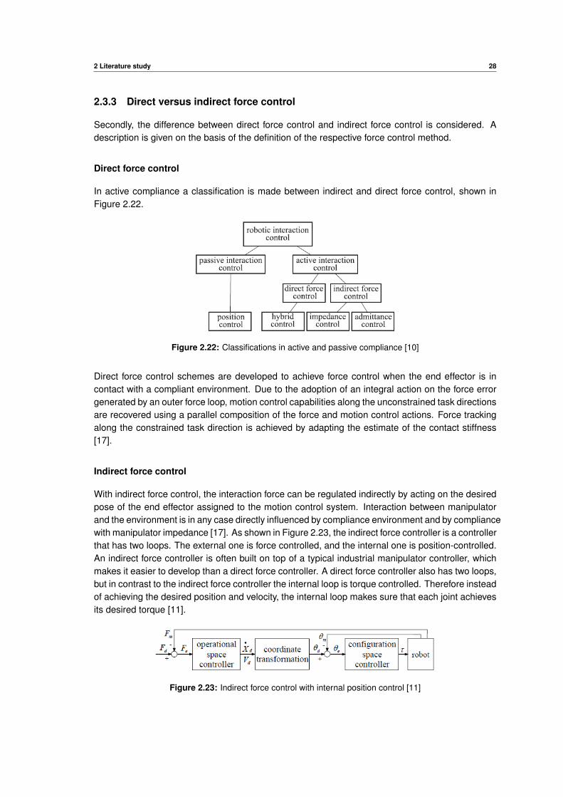
In active compliance a classification is made between indirect and direct force control, shown inFigure 2.22.
Figure 2.22: Classifications in active and passive compliance [10]
Direct force control schemes are developed to achieve force control when the end effector is incontact with a compliant environment. Due to the adoption of an integral action on the force errorgenerated by an outer force loop, motion control capabilities along the unconstrained task directionsare recovered using a parallel composition of the force and motion control actions. Force trackingalong the constrained task direction is achieved by adapting the estimate of the contact stiffness[17].
Indirect force control
With indirect force control, the interaction force can be regulated indirectly by acting on the desiredpose of the end effector assigned to the motion control system. Interaction between manipulatorand the environment is in any case directly influenced by compliance environment and by compliancewith manipulator impedance [17]. As shown in Figure 2.23, the indirect force controller is a controllerthat has two loops. The external one is force controlled, and the internal one is position-controlled.An indirect force controller is often built on top of a typical industrial manipulator controller, whichmakes it easier to develop than a direct force controller. A direct force controller also has two loops,but in contrast to the indirect force controller the internal loop is torque controlled. Therefore insteadof achieving the desired position and velocity, the internal loop makes sure that each joint achievesits desired torque [11].
Figure 2.23: Indirect force control with internal position control [11]
2 Literature study 29
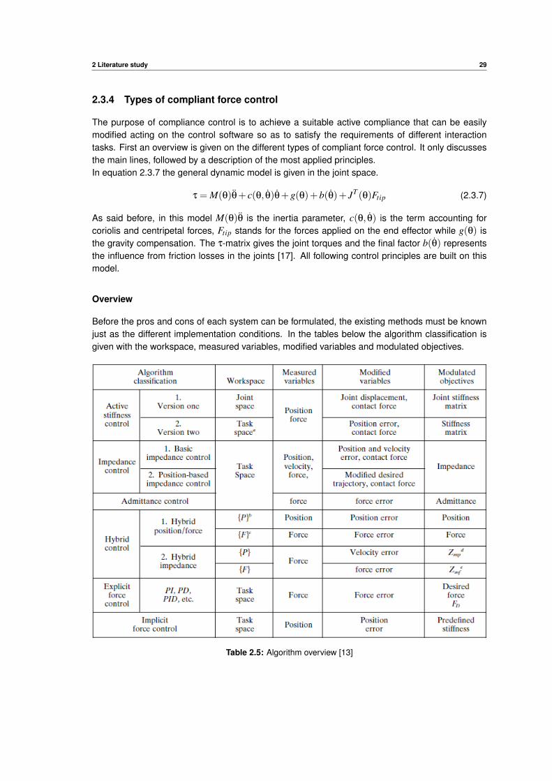
2.3.4 Types of compliant force control
The purpose of compliance control is to achieve a suitable active compliance that can be easilymodified acting on the control software so as to satisfy the requirements of different interactiontasks. First an overview is given on the different types of compliant force control. It only discussesthe main lines, followed by a description of the most applied principles.In equation 2.3.7 the general dynamic model is given in the joint space.
τ = M(θ)θ+ c(θ, θ)θ+g(θ)+b(θ)+ JT (θ)Ftip (2.3.7)
As said before, in this model M(θ)θ is the inertia parameter, c(θ, θ) is the term accounting forcoriolis and centripetal forces, Ftip stands for the forces applied on the end effector while g(θ) isthe gravity compensation. The τ-matrix gives the joint torques and the final factor b(θ) representsthe influence from friction losses in the joints [17]. All following control principles are built on thismodel.
Overview
Before the pros and cons of each system can be formulated, the existing methods must be knownjust as the different implementation conditions. In the tables below the algorithm classification isgiven with the workspace, measured variables, modified variables and modulated objectives.
Table 2.5: Algorithm overview [13]
2 Literature study 30
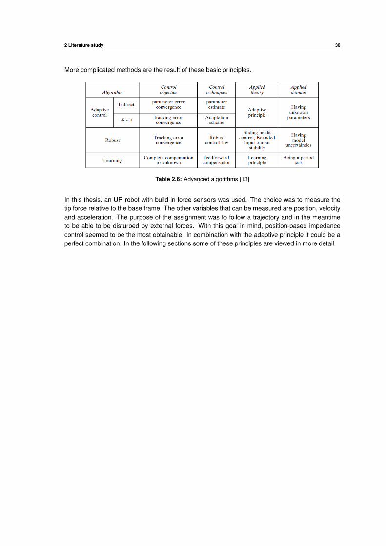
More complicated methods are the result of these basic principles.
Table 2.6: Advanced algorithms [13]
In this thesis, an UR robot with build-in force sensors was used. The choice was to measure thetip force relative to the base frame. The other variables that can be measured are position, velocityand acceleration. The purpose of the assignment was to follow a trajectory and in the meantimeto be able to be disturbed by external forces. With this goal in mind, position-based impedancecontrol seemed to be the most obtainable. In combination with the adaptive principle it could be aperfect combination. In the following sections some of these principles are viewed in more detail.
2 Literature study 31
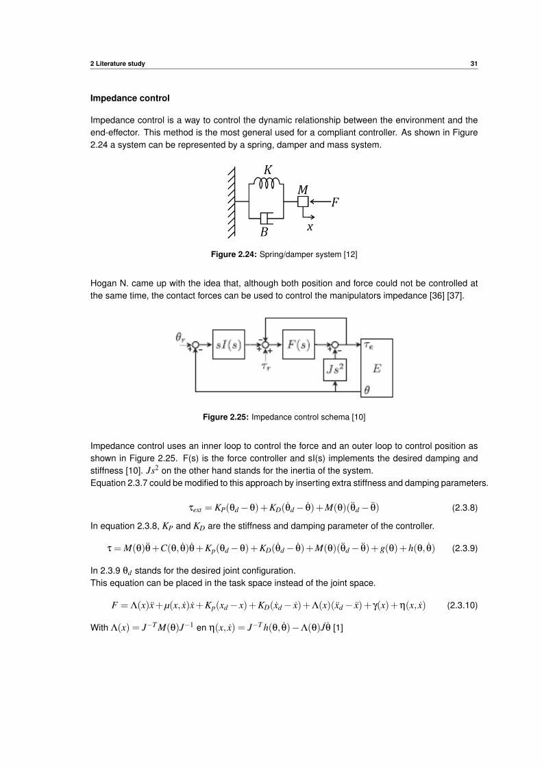
Impedance control
Impedance control is a way to control the dynamic relationship between the environment and theend-effector. This method is the most general used for a compliant controller. As shown in Figure2.24 a system can be represented by a spring, damper and mass system.
Figure 2.24: Spring/damper system [12]
Hogan N. came up with the idea that, although both position and force could not be controlled atthe same time, the contact forces can be used to control the manipulators impedance [36] [37].
Figure 2.25: Impedance control schema [10]
Impedance control uses an inner loop to control the force and an outer loop to control position asshown in Figure 2.25. F(s) is the force controller and sI(s) implements the desired damping andstiffness [10]. Js2 on the other hand stands for the inertia of the system.Equation 2.3.7 could be modified to this approach by inserting extra stiffness and damping parameters.
τext = KP(θd−θ)+KD(θd− θ)+M(θ)(θd− θ) (2.3.8)
In equation 2.3.8, KP and KD are the stiffness and damping parameter of the controller.
τ = M(θ)θ+C(θ, θ)θ+Kp(θd−θ)+KD(θd− θ)+M(θ)(θd− θ)+g(θ)+h(θ, θ) (2.3.9)
In 2.3.9 θd stands for the desired joint configuration.This equation can be placed in the task space instead of the joint space.
F = Λ(x)x+µ(x, x)x+Kp(xd− x)+KD(xd− x)+Λ(x)(xd− x)+ γ(x)+η(x, x) (2.3.10)
With Λ(x) = J−T M(θ)J−1 en η(x, x) = J−T h(θ, θ)−Λ(θ)Jθ [1]
2 Literature study 32
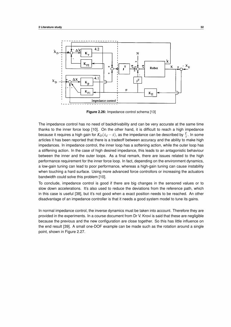
Figure 2.26: Impedance control schema [13]
The impedance control has no need of backdrivability and can be very accurate at the same timethanks to the inner force loop [10]. On the other hand, it is difficult to reach a high impedancebecause it requires a high gain for KD(xd− x), as the impedance can be described by F
x . In somearticles it has been reported that there is a tradeoff between accuracy and the ability to make highimpedances. In impedance control, the inner loop has a softening action, while the outer loop hasa stiffening action. In the case of high desired impedance, this leads to an antagonistic behaviourbetween the inner and the outer loops. As a final remark, there are issues related to the highperformance requirement for the inner force loop. In fact, depending on the environment dynamics,a low-gain tuning can lead to poor performance, whereas a high-gain tuning can cause instabilitywhen touching a hard surface. Using more advanced force controllors or increasing the actuatorsbandwidth could solve this problem [10].
To conclude, impedance control is good if there are big changes in the sensored values or toslow down accelerations. It’s also used to reduce the deviations from the reference path, whichin this case is useful [38], but it’s not good when a exact position needs to be reached. An otherdisadvantage of an impedance controller is that it needs a good system model to tune its gains.
In normal impedance control, the inverse dynamics must be taken into account. Therefore they areprovided in the experiments. In a course document from Dr V. Krovi is said that these are negligiblebecause the previous and the new configuration are close together. So this has little influence onthe end result [39]. A small one-DOF example can be made such as the rotation around a singlepoint, shown in Figure 2.27.
2 Literature study 33
Figure 2.27: 1DOF example
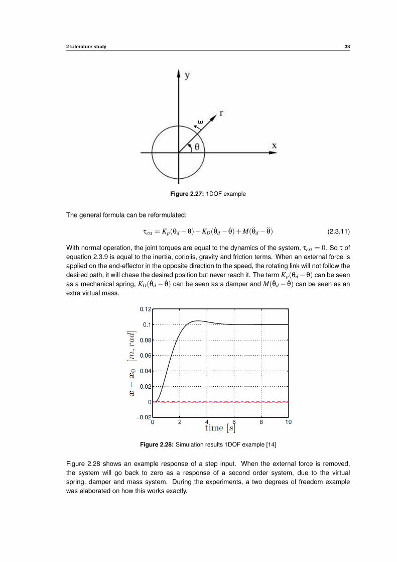
The general formula can be reformulated:
τext = Kp(θd−θ)+KD(θd− θ)+M(θd− θ) (2.3.11)
With normal operation, the joint torques are equal to the dynamics of the system, τext = 0. So τ ofequation 2.3.9 is equal to the inertia, coriolis, gravity and friction terms. When an external force isapplied on the end-effector in the opposite direction to the speed, the rotating link will not follow thedesired path, it will chase the desired position but never reach it. The term Kp(θd−θ) can be seenas a mechanical spring, KD(θd− θ) can be seen as a damper and M(θd− θ) can be seen as anextra virtual mass.
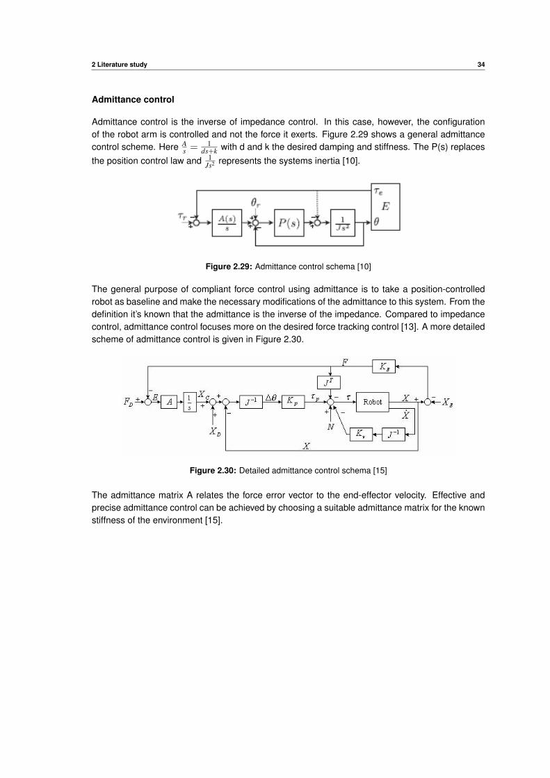
Figure 2.28: Simulation results 1DOF example [14]
Figure 2.28 shows an example response of a step input. When the external force is removed,the system will go back to zero as a response of a second order system, due to the virtualspring, damper and mass system. During the experiments, a two degrees of freedom examplewas elaborated on how this works exactly.
2 Literature study 34
Admittance control
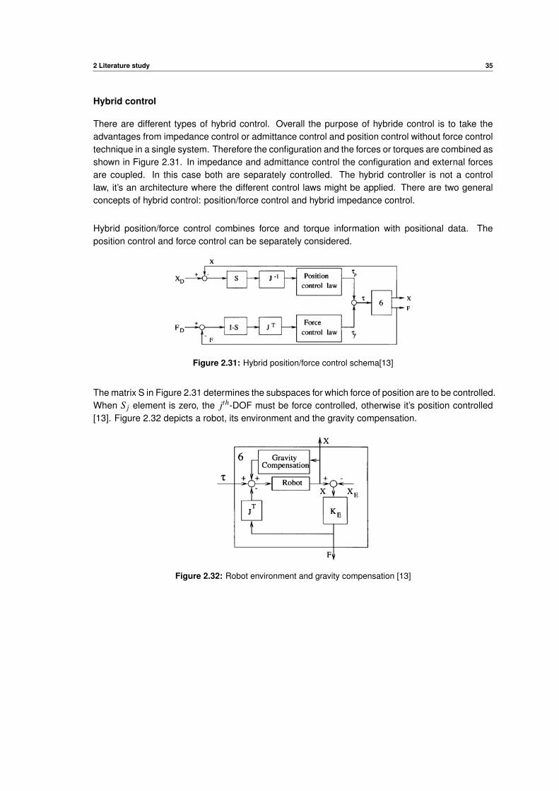
Admittance control is the inverse of impedance control. In this case, however, the configurationof the robot arm is controlled and not the force it exerts. Figure 2.29 shows a general admittancecontrol scheme. Here A
s = 1ds+k with d and k the desired damping and stiffness. The P(s) replaces
the position control law and 1Js2 represents the systems inertia [10].
Figure 2.29: Admittance control schema [10]
The general purpose of compliant force control using admittance is to take a position-controlledrobot as baseline and make the necessary modifications of the admittance to this system. From thedefinition it’s known that the admittance is the inverse of the impedance. Compared to impedancecontrol, admittance control focuses more on the desired force tracking control [13]. A more detailedscheme of admittance control is given in Figure 2.30.
Figure 2.30: Detailed admittance control schema [15]
The admittance matrix A relates the force error vector to the end-effector velocity. Effective andprecise admittance control can be achieved by choosing a suitable admittance matrix for the knownstiffness of the environment [15].
2 Literature study 35
Hybrid control
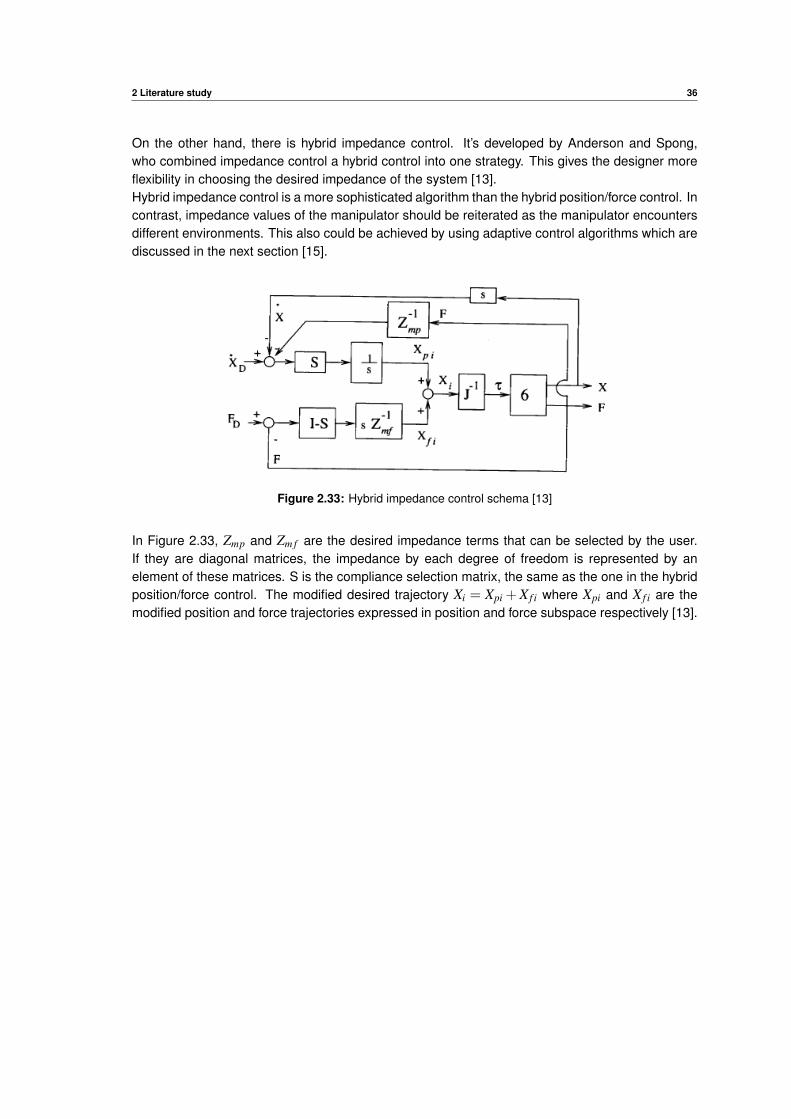
There are different types of hybrid control. Overall the purpose of hybride control is to take theadvantages from impedance control or admittance control and position control without force controltechnique in a single system. Therefore the configuration and the forces or torques are combined asshown in Figure 2.31. In impedance and admittance control the configuration and external forcesare coupled. In this case both are separately controlled. The hybrid controller is not a controllaw, it’s an architecture where the different control laws might be applied. There are two generalconcepts of hybrid control: position/force control and hybrid impedance control.
Hybrid position/force control combines force and torque information with positional data. Theposition control and force control can be separately considered.
Figure 2.31: Hybrid position/force control schema[13]
The matrix S in Figure 2.31 determines the subspaces for which force of position are to be controlled.When S j element is zero, the jth-DOF must be force controlled, otherwise it’s position controlled[13]. Figure 2.32 depicts a robot, its environment and the gravity compensation.
Figure 2.32: Robot environment and gravity compensation [13]
2 Literature study 36
On the other hand, there is hybrid impedance control. It’s developed by Anderson and Spong,who combined impedance control a hybrid control into one strategy. This gives the designer moreflexibility in choosing the desired impedance of the system [13].Hybrid impedance control is a more sophisticated algorithm than the hybrid position/force control. Incontrast, impedance values of the manipulator should be reiterated as the manipulator encountersdifferent environments. This also could be achieved by using adaptive control algorithms which arediscussed in the next section [15].
Figure 2.33: Hybrid impedance control schema [13]
In Figure 2.33, Zmp and Zm f are the desired impedance terms that can be selected by the user.If they are diagonal matrices, the impedance by each degree of freedom is represented by anelement of these matrices. S is the compliance selection matrix, the same as the one in the hybridposition/force control. The modified desired trajectory Xi = Xpi +X f i where Xpi and X f i are themodified position and force trajectories expressed in position and force subspace respectively [13].
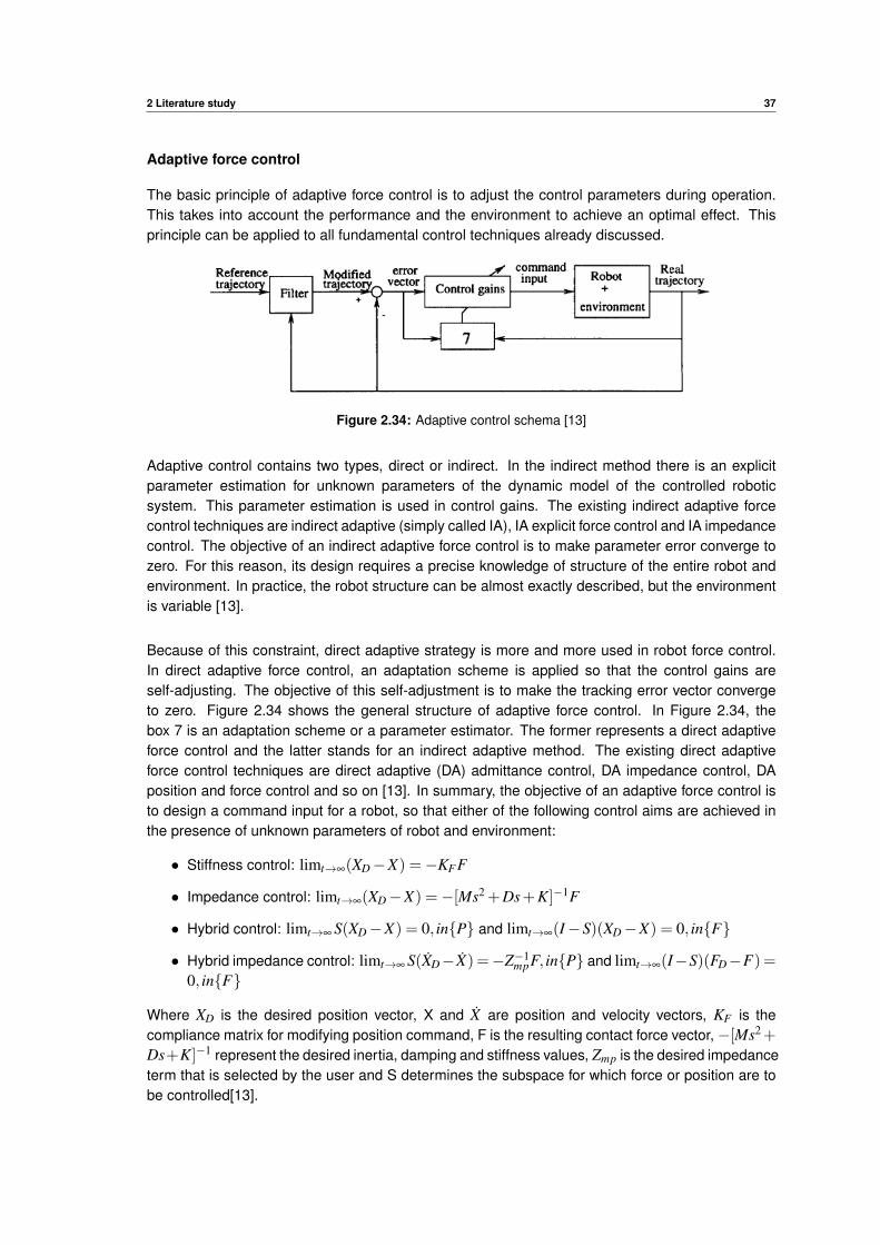
2 Literature study 37
Adaptive force control
The basic principle of adaptive force control is to adjust the control parameters during operation.This takes into account the performance and the environment to achieve an optimal effect. Thisprinciple can be applied to all fundamental control techniques already discussed.
Figure 2.34: Adaptive control schema [13]
Adaptive control contains two types, direct or indirect. In the indirect method there is an explicitparameter estimation for unknown parameters of the dynamic model of the controlled roboticsystem. This parameter estimation is used in control gains. The existing indirect adaptive forcecontrol techniques are indirect adaptive (simply called IA), IA explicit force control and IA impedancecontrol. The objective of an indirect adaptive force control is to make parameter error converge tozero. For this reason, its design requires a precise knowledge of structure of the entire robot andenvironment. In practice, the robot structure can be almost exactly described, but the environmentis variable [13].
Because of this constraint, direct adaptive strategy is more and more used in robot force control.In direct adaptive force control, an adaptation scheme is applied so that the control gains areself-adjusting. The objective of this self-adjustment is to make the tracking error vector convergeto zero. Figure 2.34 shows the general structure of adaptive force control. In Figure 2.34, thebox 7 is an adaptation scheme or a parameter estimator. The former represents a direct adaptiveforce control and the latter stands for an indirect adaptive method. The existing direct adaptiveforce control techniques are direct adaptive (DA) admittance control, DA impedance control, DAposition and force control and so on [13]. In summary, the objective of an adaptive force control isto design a command input for a robot, so that either of the following control aims are achieved inthe presence of unknown parameters of robot and environment:
• Stiffness control: limt→∞(XD−X) =−KFF
• Impedance control: limt→∞(XD−X) =−[Ms2 +Ds+K]−1F
• Hybrid control: limt→∞ S(XD−X) = 0, in{P} and limt→∞(I−S)(XD−X) = 0, in{F}
• Hybrid impedance control: limt→∞ S(XD− X) =−Z−1mpF, in{P} and limt→∞(I−S)(FD−F) =
0, in{F}
Where XD is the desired position vector, X and X are position and velocity vectors, KF is thecompliance matrix for modifying position command, F is the resulting contact force vector,−[Ms2+Ds+K]−1 represent the desired inertia, damping and stiffness values, Zmp is the desired impedanceterm that is selected by the user and S determines the subspace for which force or position are tobe controlled[13].
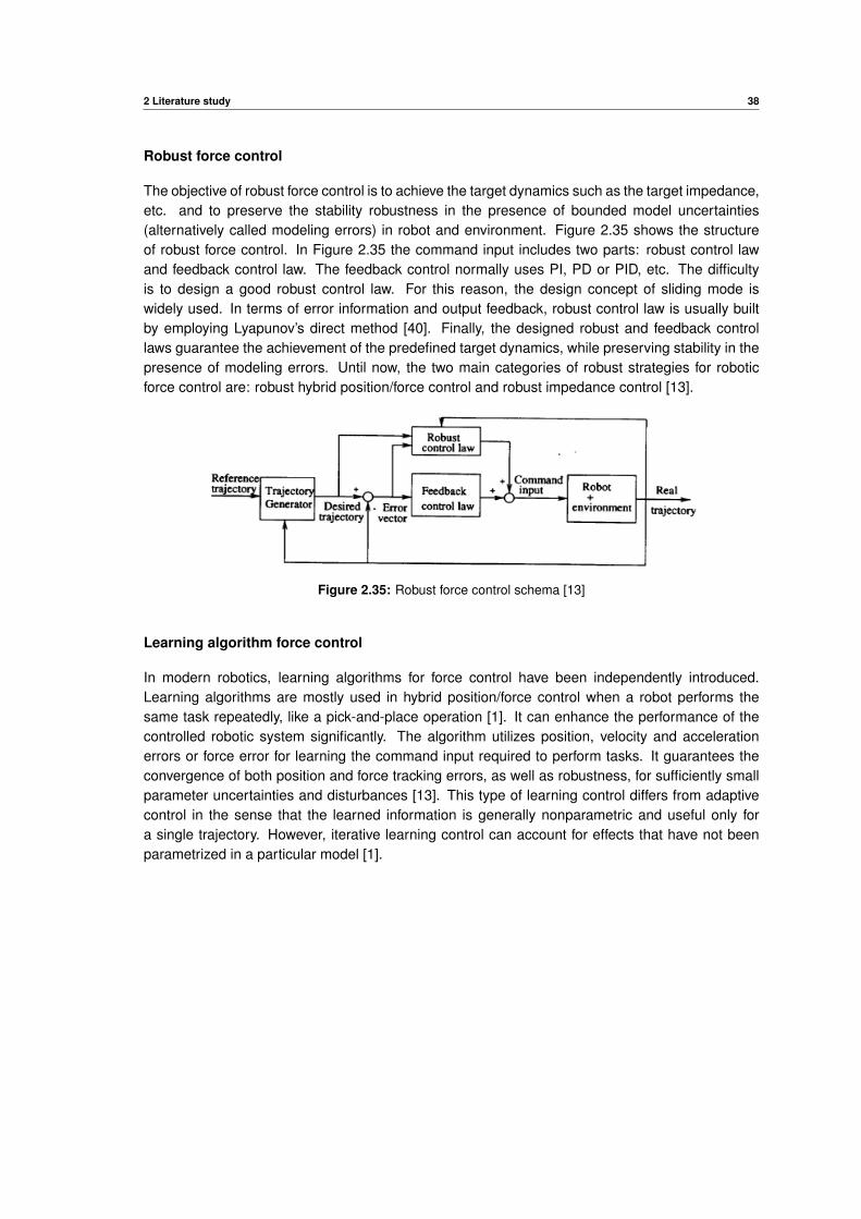
2 Literature study 38
Robust force control
The objective of robust force control is to achieve the target dynamics such as the target impedance,etc. and to preserve the stability robustness in the presence of bounded model uncertainties(alternatively called modeling errors) in robot and environment. Figure 2.35 shows the structureof robust force control. In Figure 2.35 the command input includes two parts: robust control lawand feedback control law. The feedback control normally uses PI, PD or PID, etc. The difficultyis to design a good robust control law. For this reason, the design concept of sliding mode iswidely used. In terms of error information and output feedback, robust control law is usually builtby employing Lyapunov’s direct method [40]. Finally, the designed robust and feedback controllaws guarantee the achievement of the predefined target dynamics, while preserving stability in thepresence of modeling errors. Until now, the two main categories of robust strategies for roboticforce control are: robust hybrid position/force control and robust impedance control [13].
Figure 2.35: Robust force control schema [13]
Learning algorithm force control
In modern robotics, learning algorithms for force control have been independently introduced.Learning algorithms are mostly used in hybrid position/force control when a robot performs thesame task repeatedly, like a pick-and-place operation [1]. It can enhance the performance of thecontrolled robotic system significantly. The algorithm utilizes position, velocity and accelerationerrors or force error for learning the command input required to perform tasks. It guarantees theconvergence of both position and force tracking errors, as well as robustness, for sufficiently smallparameter uncertainties and disturbances [13]. This type of learning control differs from adaptivecontrol in the sense that the learned information is generally nonparametric and useful only fora single trajectory. However, iterative learning control can account for effects that have not beenparametrized in a particular model [1].
2 Literature study 39
2.3.5 Implementation choice
Since the different types were discribed, the choice had to be made by combining the specificationsdue to the application. Various simplifications were made in this application. We neglected allfriction and other losses like centripetal and Coriolis forces and the gravity compensation. This isbecause impedance control must take place in Cartesian space and the influence of the dynamicswas neglected. This is said in a course document written by Dr V. Krovi on this subject and it’scorroborated by a small experiment [39]. In the UR3, a PID controller is incorporated, that controlsthe joint angles. In turn, they ensure that the maximum torque is not exceeded by controlling themaximum joint accelerations.
The admittance force control has been chosen because of its general properties such as: easy toimplement on top of the robots controller, it’s usable in a path tracking environment and it can beapplied in joint and task space. In the overview table, Table 2.5 we see that impedance controlcould be used when we need a desired performed force on a surface. In this application a pathneeds to be tracked so there is no desired force. When the system is completely known, the desiredforce could be recalculated and impedance control could be used. Therefore the system must bewell defined, which is not the case and the torques must be controllable in the robot’s controller.
Another approach could be the use of hybrid control. Therefore the desired force on a surface couldbe used and controlled by impedance control while the position on the surface could be controlledby admittance control. For example, sanding a surface can be used.
Other more advanced purposes such as direct adaptive control could also be used. For this thebasics must be known first, because this technique adjusts the stiffness and damper parametersin the equation for maximum performance. Other more advanced algorithms such as learningalgorithms are not applicable since there is no sequential task to perform.

2 Literature study 40
2.3.6 Implementation
As we chose admittance control for this application the general equations were used. In this sectionall parameters and assumptions will be described. In the previous sections, the torques werealways used. In the actual implementation the Cartesian coordinates are used. In most of theequations the joint angles were used, this is because the formulas are more understandable thanin task space.
τ=M(θ)θ+c(θ, θ)+Kp(θd−θ)+KD(θd− θ)+M(θ)(θd− θ)+g(θ)+h(θ, θ)+JT Fext (2.3.12)
Equation 2.3.12 can be simplified because coriolis forces, gravity compensation, torques caused byfriction and the inertia were neglected. This is because it was previously stated that the dynamicscould be omitted because there was only a minimal difference between the previous point and thenext point that must be reached [39].
In general, it can therefore be said that admittance control is applied in Cartesian coordinates.Equation 2.3.13 is the equation to be applied in all applications. We assume that the forces aremeasured in base frame. As a result, there is a fixed reference and the admittance control can beobserved.
0 = Fext − [Kp(xd− x)+Kd(xd− x)+M(xd− x)] (2.3.13)
This equation could be transformed to a control system in combination with the robot and itssensors. In Figure 2.36 the control scheme is given.
Figure 2.36: Simplified overall control loop
We know from previous chapters that the KP and KD parameters for stiffness and damping arealways diagonal matrices in joint space and M is a virtual mass. In examples found from varioussources, stiffnesses of 20N/m to 3000N/m have been used. In most of the lecture, the dampingparameters are not described. These parameters formulas are not defined because the desiredstiffness and damping are linked to the type of application. In this application there is some freedomin choosing them. The ideal parameters must not be known and will be experimentally recorded[41].
In addition, in the simulations, the torque limits were compared with the calculated torques to makecorrections, where necessary using the inverse dynamics of the robot. This way the maximumtorque would never be exceeded and there would be no damage to the joints of the UR3 robot.This can be said if the joints were to be controlled directly. Since URScript commands were used,this was unnecessary, because the controller of the robot itself takes this into account as shown inthe control scheme in Figure 2.36.
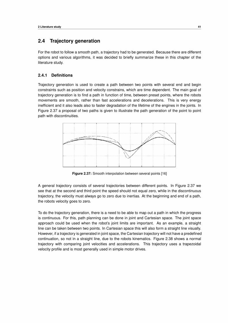
2 Literature study 41
2.4 Trajectory generation
For the robot to follow a smooth path, a trajectory had to be generated. Because there are differentoptions and various algorithms, it was decided to briefly summarize these in this chapter of theliterature study.
2.4.1 Definitions
Trajectory generation is used to create a path between two points with several end and beginconstraints such as position and velocity constrains, which are time dependent. The main goal oftrajectory generation is to find a path in function of time, between preset points, where the robotsmovements are smooth, rather than fast accelerations and decelerations. This is very energyinefficient and it also leads also to faster degradation of the lifetime of the engines in the joints. InFigure 2.37 a proposal of two paths is given to illustrate the path generation of the point to pointpath with discontinuities.
Figure 2.37: Smooth interpolation between several points [16]
A general trajectory consists of several trajectories between different points. In Figure 2.37 wesee that at the second and third point the speed should not equal zero, while in the discontinuoustrajectory, the velocity must always go to zero due to inertias. At the beginning and end of a path,the robots velocity goes to zero.
To do the trajectory generation, there is a need to be able to map out a path in which the progressis continuous. For this, path planning can be done in joint and Cartesian space. The joint spaceapproach could be used when the robot’s joint limits are important. As an example, a straightline can be taken between two points. In Cartesian space this will also form a straight line visually.However, if a trajectory is generated in joint space, the Cartesian trajectory will not have a predefinedcontinuation, so not in a straight line, due to the robots kinematics. Figure 2.38 shows a normaltrajectory with comparing joint velocities and accelerations. This trajectory uses a trapezoidalvelocity profile and is most generally used in simple motor drives.
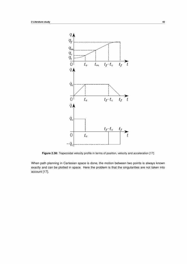
2 Literature study 42
Figure 2.38: Trapezoidal velocity profile in terms of position, velocity and acceleration [17]
When path planning in Cartesian space is done, the motion between two points is always knownexactly and can be plotted in space. Here the problem is that the singularities are not taken intoaccount [17].
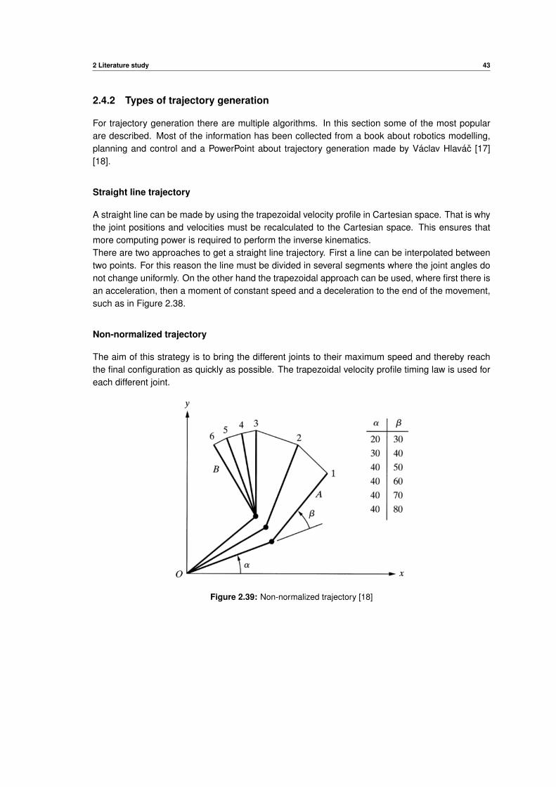
2 Literature study 43
2.4.2 Types of trajectory generation
For trajectory generation there are multiple algorithms. In this section some of the most popularare described. Most of the information has been collected from a book about robotics modelling,planning and control and a PowerPoint about trajectory generation made by Vaclav Hlavac [17][18].
Straight line trajectory
A straight line can be made by using the trapezoidal velocity profile in Cartesian space. That is whythe joint positions and velocities must be recalculated to the Cartesian space. This ensures thatmore computing power is required to perform the inverse kinematics.There are two approaches to get a straight line trajectory. First a line can be interpolated betweentwo points. For this reason the line must be divided in several segments where the joint angles donot change uniformly. On the other hand the trapezoidal approach can be used, where first there isan acceleration, then a moment of constant speed and a deceleration to the end of the movement,such as in Figure 2.38.
Non-normalized trajectory
The aim of this strategy is to bring the different joints to their maximum speed and thereby reachthe final configuration as quickly as possible. The trapezoidal velocity profile timing law is used foreach different joint.
Figure 2.39: Non-normalized trajectory [18]
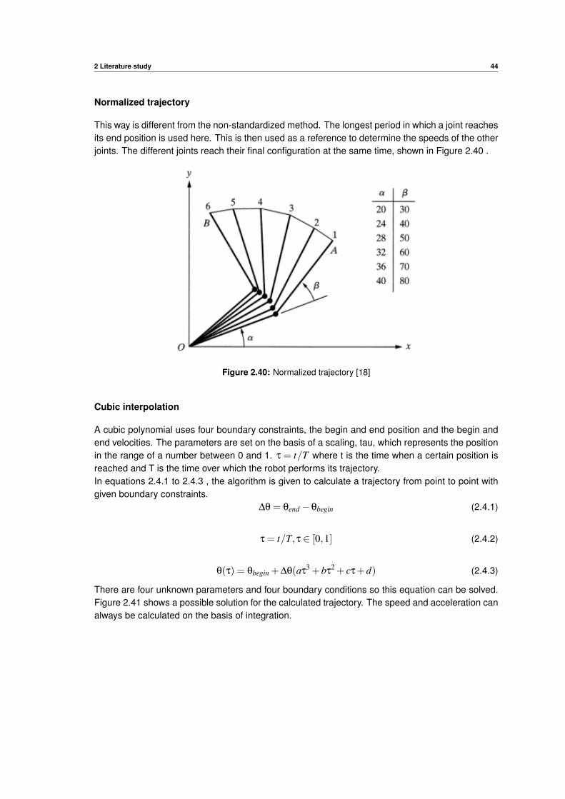
2 Literature study 44
Normalized trajectory
This way is different from the non-standardized method. The longest period in which a joint reachesits end position is used here. This is then used as a reference to determine the speeds of the otherjoints. The different joints reach their final configuration at the same time, shown in Figure 2.40 .
Figure 2.40: Normalized trajectory [18]
Cubic interpolation
A cubic polynomial uses four boundary constraints, the begin and end position and the begin andend velocities. The parameters are set on the basis of a scaling, tau, which represents the positionin the range of a number between 0 and 1. τ = t/T where t is the time when a certain position isreached and T is the time over which the robot performs its trajectory.In equations 2.4.1 to 2.4.3 , the algorithm is given to calculate a trajectory from point to point withgiven boundary constraints.
∆θ = θend−θbegin (2.4.1)
τ = t/T,τ ∈ [0,1] (2.4.2)
θ(τ) = θbegin +∆θ(aτ3 +bτ
2 + cτ+d) (2.4.3)
There are four unknown parameters and four boundary conditions so this equation can be solved.Figure 2.41 shows a possible solution for the calculated trajectory. The speed and acceleration canalways be calculated on the basis of integration.
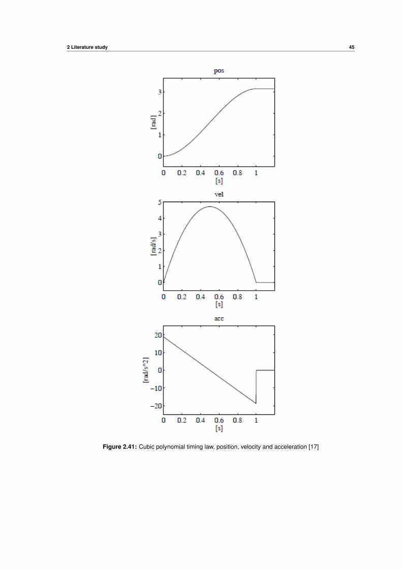
2 Literature study 45
Figure 2.41: Cubic polynomial timing law, position, velocity and acceleration [17]
2 Literature study 46
Quintic interpolation
This is roughly the same as the cubic polynomial. It is more extensive since the acceleration is nowalso integrated and a fifth order polynomial can be calculated. In most cases, the acceleration isequal to zero, giving us comparison 2.4.7.
θ(0) = θ0;θ(1) = θ1; θ(0) = θ0T ; θ(1) = θ1T ; θ(0) = θ0T 2; θ(1) = θ1T 2 (2.4.4)
τ = t/T,τ ∈ [0,1] (2.4.5)
θ(τ) = aτ5 +bτ
4 + cτ3 +dτ
2 + eτ+ f (2.4.6)
θ(τ) = θ0 +∆θ(6τ5−15τ
4 +10τ3);∆θ = θ1−θ0 (2.4.7)
Higher order polynomials
A certain polynomial can always be drawn by a certain number of points. For example, a specificline can always be drawn through two points. Only a second order polynomial can be drawn throughthree points.
Higher order polynomials provide a suitable solution class for satisfying symmetric boundary conditionsin a point-to-point motion that imposes values on higher order derivatives. Here the interpolatingpolynomial is always of the odd degree and the coefficients are always integers, alternate in sign,sum up to unity and are zero for all term up to the power degree−1
2 [18].
Path generation
The previous examples of traject generation can be used to travel from point to point. However, ifseveral points have to be reached, these different line segments must be joined together as a wholeto make a smooth path. This is called a spline. As an example, a cubic spline curve is a piecewisecubic curve with continuous second derivation. More examples and algorithms can be found in acourse PowerPoint made by Vaclav Hlavac and a book named ’Robotics Modelling, Planning andControl’ [18] [17].

2 Literature study 47
2.5 Universal Robots properties
In the user manual, all necessary specifications of the UR3 robot were found. Among other things,it discusses the hardware installation and the polyscope manual.
In addition, the technical manual contains numerous features that could be further related to thisassignment such as: weight, payload, reach, joint ranges and speeds, repeatability, degrees offreedom ...Some necessary parameters, such as the link’s inertia, viscous friction coefficients and motorinertia, were not found in manuals of the UR3 robot, these were requested from various distributorsin Belgium and The Netherlands. But unfortunately these were not released.
Finally the Universal Robot URScript Programming Language manual was reviewed. It describesall possible commands.In the following subsections there is a more detailed approach of the UR3 specifications in kinematics,dynamics and programming.
Figure 2.42: UR3 CB-series collaborative Robot [19]
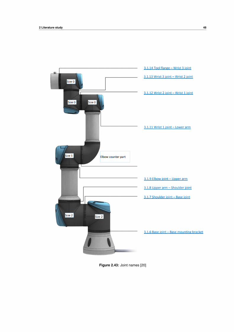
2 Literature study 48
Figure 2.43: Joint names [20]
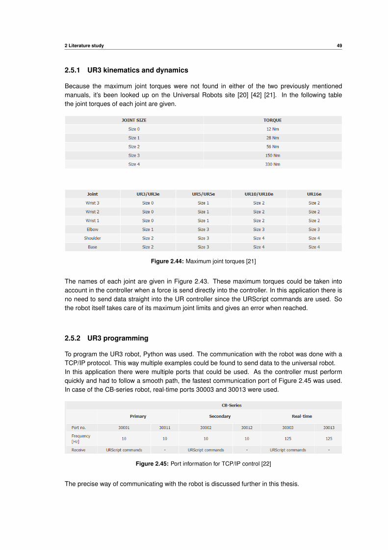
2 Literature study 49
2.5.1 UR3 kinematics and dynamics
Because the maximum joint torques were not found in either of the two previously mentionedmanuals, it’s been looked up on the Universal Robots site [20] [42] [21]. In the following tablethe joint torques of each joint are given.
Figure 2.44: Maximum joint torques [21]
The names of each joint are given in Figure 2.43. These maximum torques could be taken intoaccount in the controller when a force is send directly into the controller. In this application there isno need to send data straight into the UR controller since the URScript commands are used. Sothe robot itself takes care of its maximum joint limits and gives an error when reached.
2.5.2 UR3 programming
To program the UR3 robot, Python was used. The communication with the robot was done with aTCP/IP protocol. This way multiple examples could be found to send data to the universal robot.In this application there were multiple ports that could be used. As the controller must performquickly and had to follow a smooth path, the fastest communication port of Figure 2.45 was used.In case of the CB-series robot, real-time ports 30003 and 30013 were used.
Figure 2.45: Port information for TCP/IP control [22]
The precise way of communicating with the robot is discussed further in this thesis.
2 Literature study 50
2.6 TCP/IP protocol
As previously mentioned in this thesis, the robot was controlled through the TCP/IP interface. Thissection discusses what TCP/IP is and how it was applied in the Python application.
2.6.1 Definition TCP/IP
TCP/IP or transmission control protocol over the internet protocol, is a series of network protocolsthat are used in network communication between computers. The internet is the best-knownexample of TCP/IP. TCP/IP is a packet switched protocol in which the data is sent independently insmall packages. The communication software puts the packets back in the correct order, detectsany errors in the reception and, if necessary, requests certain packets again until all packets arereceived. TCP service is obtained by both the sender and receiver creating end points, calledsockets. Each socket has a socket number (address) consisting of the IP-address of the host anda 16-bit number local to that host, called a port. For TCP service to be obtained, a connection mustbe explicitly established between a socket on the sending machine and a socket on the receivingmachine. A socket may be used for multiple connections at the same time. In other words, two ormore connections may terminate at the same socket [23]. In this thesis there is no need to knowhow the communication exactly works because in Python there are preformed libraries that takecare of the exact communication syntax.
2.6.2 TCP/IP in OSI model
OSI-model or Open System Interconnection model, is an ISO-standardized reference model fordata communication standards, promoting interoperability between heterogeneous network topologies.The OSI model has somewhat lost its meaning, as the data communication world has become defacto standardized on Ethernet as a network topology and TCP/IP as a communication protocol.In Figure 2.46 the different layers of the OSI model are shown, each visualized with an animationand subscription of where the layer stands for. For more information about each layer and a moredefined description, I would like to refer to a book named ’ComputerNetworks’ written by AndrewS. Tanenbaum and David J. Wetherall [23].

2 Literature study 51
Figure 2.46: OSI model layers [23]
The TCP/IP protocol can be fitted in the seven layers OSI model. TCP/IP protocol uses all theseseven layers, but some of them are put toghether in one layer of TCP/IP protocol. For example,the application, presentation and session layer are put together into one application layer. Thetransport layer is TCP (Transmission Control Protocol), a IP based network protocol that ensures astable connection. The use of IP adresses is located in the network layer while the data link layerand the physical layer are represented by Ethernet and UTP cables [23] [24]. All of this is shownvisually in Figure 2.47.
Figure 2.47: TCP/IP in OSI model [24]
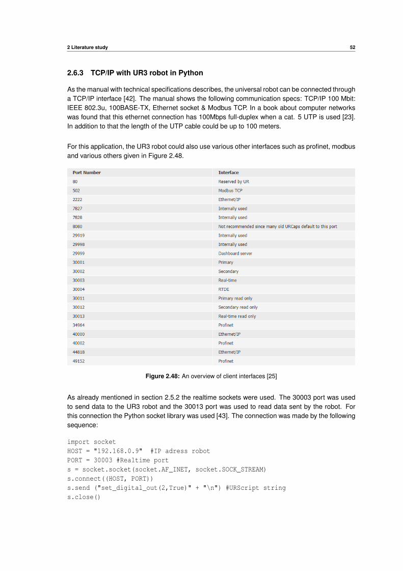
2 Literature study 52
2.6.3 TCP/IP with UR3 robot in Python
As the manual with technical specifications describes, the universal robot can be connected througha TCP/IP interface [42]. The manual shows the following communication specs: TCP/IP 100 Mbit:IEEE 802.3u, 100BASE-TX, Ethernet socket & Modbus TCP. In a book about computer networkswas found that this ethernet connection has 100Mbps full-duplex when a cat. 5 UTP is used [23].In addition to that the length of the UTP cable could be up to 100 meters.
For this application, the UR3 robot could also use various other interfaces such as profinet, modbusand various others given in Figure 2.48.
Figure 2.48: An overview of client interfaces [25]
As already mentioned in section 2.5.2 the realtime sockets were used. The 30003 port was usedto send data to the UR3 robot and the 30013 port was used to read data sent by the robot. Forthis connection the Python socket library was used [43]. The connection was made by the followingsequence:
import socketHOST = "192.168.0.9" #IP adress robotPORT = 30003 #Realtime ports = socket.socket(socket.AF_INET, socket.SOCK_STREAM)s.connect((HOST, PORT))s.send ("set_digital_out(2,True)" + "\n") #URScript strings.close()
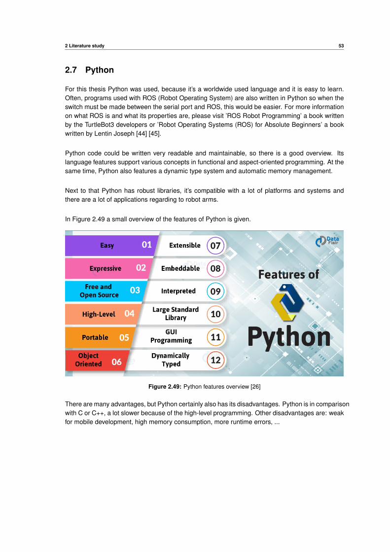
2 Literature study 53
2.7 Python
For this thesis Python was used, because it’s a worldwide used language and it is easy to learn.Often, programs used with ROS (Robot Operating System) are also written in Python so when theswitch must be made between the serial port and ROS, this would be easier. For more informationon what ROS is and what its properties are, please visit ’ROS Robot Programming’ a book writtenby the TurtleBot3 developers or ’Robot Operating Systems (ROS) for Absolute Beginners’ a bookwritten by Lentin Joseph [44] [45].
Python code could be written very readable and maintainable, so there is a good overview. Itslanguage features support various concepts in functional and aspect-oriented programming. At thesame time, Python also features a dynamic type system and automatic memory management.
Next to that Python has robust libraries, it’s compatible with a lot of platforms and systems andthere are a lot of applications regarding to robot arms.
In Figure 2.49 a small overview of the features of Python is given.
Figure 2.49: Python features overview [26]
There are many advantages, but Python certainly also has its disadvantages. Python is in comparisonwith C or C++, a lot slower because of the high-level programming. Other disadvantages are: weakfor mobile development, high memory consumption, more runtime errors, ...
3Methodology
I started my master’s thesis in September 2019. First of all, I met with Mr De Ryck so he couldexplain the details of my master’s dissertation. After some research, the actual purpose becameclear: design a force compliant controller for the UR3 robot using Python and make an application.Collecting papers, books and other lecture that could help me to succeed my dissertation was thenext step.
Thereafter, the literature study was created chapter by chapter using the formerly collected information.This was done from September until December 2019. In my schedule it was provided that a first partof the programming assignment would already have been concluded by then. Unfortunately, thiswas postponed to the second semester due to tasks and lessons. As a result of the postponement,I was able to do everything directly one after the other. However, this also meant that a servo testsetup such as requested by Mr De Ryck was not executed. The necessary parts still had to belooked for, ordered and delivered and from my experience, this takes a lot of time often with littleresult.
Moving on to the second semester, research on previous projects was started using an impedancecontroller in MATLAB as a replacement for the servo application. An example was found forimpedance control on path tracking, i.e. pure position [46]. This example was stripped and someparts were reused to create a well-organized program that could further be used to provide insightsinto impedance control.
First, an application was created simulating a two-link manipulator. Initially, no path was followedand the impedance control was done on a fixed target. As an extension to this, a circular target wasadded for simplicity. During these two experiments, the intention was to test the influence of theinverse dynamics and whether the control could possibly take place in joint space. In the end, it wasdecided to neglect the influence of the dynamics and to do the regulation in Cartesian coordinates.However, this meant that inverse kinematics had to be applied to obtain the joint angles. Forthis mainly a book by the University of Cambridge on modern robotics, written by Kevin M. Lynch
54
3 Methodology 55
and Frank C. Park was used [1]. This book about robotics tells in detail how the kinematics anddynamics of rigid bodies are structured, including chapters about force control and motion control.
After the experiments with the two degrees of freedom simulation in MATLAB, a six degrees offreedom example was made. Only an impedance controller was made for a fixed target such asin two degrees of freedom, because MATLAB did work too slow and it was not the goal to designa complete controller in MATLAB that peers with the final application. Eventually, a performancewas created that had to work in slow motion to obtain representative graphs. For this part the PeterCorke toolbox was used [32].
Finally, a Python controller was designed. The first part of this assignment was to provide communicationbetween the robot and a Python program. To monitor the robot’s data, a class was found on theGitHub page of SintefManufacturing, but no stand-alone class was found to send commands to therobot [47]. Since this wasn’t that much work and it had to be straightforward and easy to use, it waswritten from scratch. To test all this, an opportunity was sought for simulation programs. There wasa possibility to do the simulation in Python itself, but this would have given no added value whentesting the connection. We first looked at RoboDK. This is software that simulates a conversionand adds different objects with various robots that could be programmed in different languages.It would have been ideal if this had been free software, which unfortunately was not the case.The second possible solution was to look at URSim. This is an option to write a program withouta physical robot and later transfer it to the robot via USB. This software runs in a Linux virtualmachine and can be obtained free of charge from Univeral Robots [48]. After the connection withthe simulated robot was finalized, this was also done with the physical robot. After this, functionsfrom both classes were tested and small programs were made to correct errors. Combined with theinterpolator, received from Mr De Ryck, a program was put together before the open day so thatthe robot followed a certain path for the entire day. A second part of the Python controller consistedof writing a program in which impedance control is applied to the continuous trajectory of the robot.For this, it was originally thought to simply read and process the force that the robot measures itself.Because testing the inverse kinematics already showed that the application is relatively slow andthat the desired frequency of 125Hz would not be achievable, it was decided to try an external forcesensor. The force emitted by the robot also contains the force of movement or, in other words, thetorque of movement. An Axia80 force sensor of Schunk was available but no data was read fromthe sensor after several attempts. As a result, it was decided to use the force from the robot andto subtract the dynamic force such as coriolis and inertia. Due to the COVID-19 pandemic this waspostponed for a while and only continued later when all bugs were out of the program. Becausethere was always an error on the final result, an attempt was made to provide a controller thatallows this error to converge to zero. Looking into the theory and simulations made in the literaturestudy about the second order response, the obtained response was expected.
The Euler-Lagrange representation was used to calculate the dynamic parameters. This wasreported in MATLAB and symbolically solved. This resulted in functions that could be used inthe Python class which describes the robot. However, these calculations are very time consumingand the results cannot be converted to a Python syntax. This was solved by using a library whichallows the use of MATLAB functions. The dynamic functions are also written specifically for theUR3 robot since obtaining the functions with only the joint positions and velocities took about threedays. Finally, all programs were cleaned up so that only the essential code remained. It is availableon my GitHub repository [49].

4Experiments
To achieve the ultimate goal of this thesis, which is to write an force compliant controller for the UR3robot in Python, several partial experiments were done first. The main aim of these experimentswas to gain insight into the kinematics and dynamics of robot arms. Since Python was not yetknown and there was a better knowledge of MATLAB, some MATLAB simulations were made toget started. The aim was to test various matters with both a two degrees of freedom example and asix degrees of freedom example. Because MATLAB is often used to simulate things, there alreadyare some pre-made toolboxes for this that accelerate the design. Ultimately, a Python controllerwas created that has a similar functionality. To finish a theoretical example is given of how thisapplication and / or insights can be used in other applications.
56
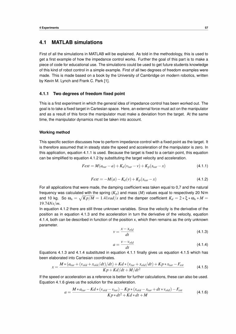
4 Experiments 57
4.1 MATLAB simulations
First of all the simulations in MATLAB will be explained. As told in the methodology, this is used toget a first example of how the impedance control works. Further the goal of this part is to make apiece of code for educational use. The simulations could be used to get future students knowledgeof this kind of robot control in a simple example. First of all two degrees of freedom examples weremade. This is made based on a book by the University of Cambridge on modern robotics, writtenby Kevin M. Lynch and Frank C. Park [1].
4.1.1 Two degrees of freedom fixed point
This is a first experiment in which the general idea of impedance control has been worked out. Thegoal is to take a fixed target in Cartesian space. Here, an external force must act on the manipulatorand as a result of this force the manipulator must make a deviation from the target. At the sametime, the manipulator dynamics must be taken into account.
Working method
This specific section discusses how to perform impedance control with a fixed point as the target. Itis therefore assumed that in steady state the speed and acceleration of the manipulator is zero. Inthis application, equation 4.1.1 is used. Because the target is fixed to a certain point, this equationcan be simplified to equation 4.1.2 by substituting the target velocity and acceleration.
Fext = M(atar−a)+Kd(vtar− v)+Kp(xtar− x) (4.1.1)
Fext =−M(a)−Kd(v)+Kp(xtar− x) (4.1.2)
For all applications that were made, the damping coefficient was taken equal to 0,7 and the naturalfrequency was calculated with the spring (Kp) and mass (M) values equal to respectively 20 N/mand 10 kg. So ωn =
√K p/M = 1.41rad/s and the damper coefficient Kd = 2 ∗ ξ ∗ωn ∗M =
19.74Ns/m.In equation 4.1.2 there are still three unknown variables. Since the velocity is the derivative of theposition as in equation 4.1.3 and the acceleration in turn the derivative of the velocity, equation4.1.4, both can be described in function of the position x, which then remains as the only unknownparameter.
v =x− xold
dt(4.1.3)
a =v− vold
dt(4.1.4)
Equations 4.1.3 and 4.1.4 substituted in equation 4.1.1 finally gives us equation 4.1.5 which hasbeen elaborated into Cartesian coordinates.
x =M ∗ (atar +(vold + xold/dt)/dt)+Kd ∗ (vtar + xold/dt)+K p∗ xtar−Fext
K p+Kd/dt +M/dt2 (4.1.5)
If the speed or acceleration as a reference is better for further calculations, these can also be used.Equation 4.1.6 gives us the solution for the acceleration.
a =M ∗atar−Kd ∗ (vold− vtar)−K p∗ (xold− xtar +dt ∗ vold)−Fext
K p∗dt2 +Kd ∗dt +M(4.1.6)
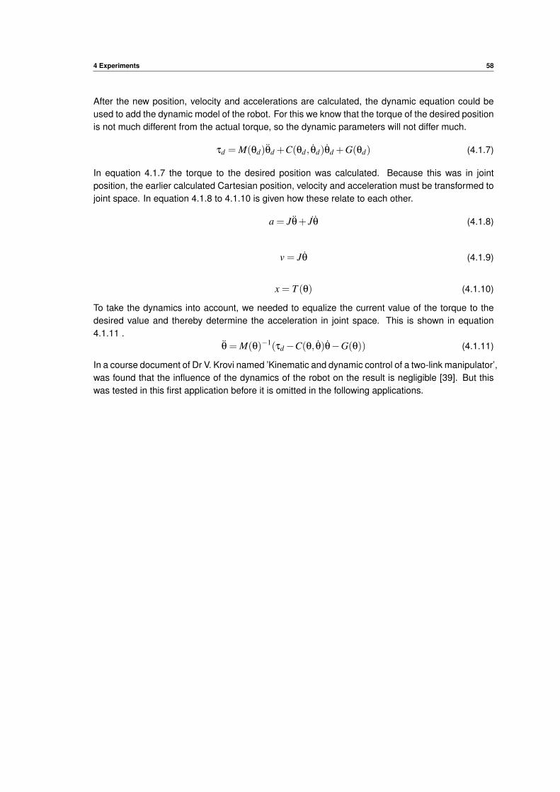
4 Experiments 58
After the new position, velocity and accelerations are calculated, the dynamic equation could beused to add the dynamic model of the robot. For this we know that the torque of the desired positionis not much different from the actual torque, so the dynamic parameters will not differ much.
τd = M(θd)θd +C(θd , θd)θd +G(θd) (4.1.7)
In equation 4.1.7 the torque to the desired position was calculated. Because this was in jointposition, the earlier calculated Cartesian position, velocity and acceleration must be transformed tojoint space. In equation 4.1.8 to 4.1.10 is given how these relate to each other.
a = Jθ+ Jθ (4.1.8)
v = Jθ (4.1.9)
x = T (θ) (4.1.10)
To take the dynamics into account, we needed to equalize the current value of the torque to thedesired value and thereby determine the acceleration in joint space. This is shown in equation4.1.11 .
θ = M(θ)−1(τd−C(θ, θ)θ−G(θ)) (4.1.11)
In a course document of Dr V. Krovi named ’Kinematic and dynamic control of a two-link manipulator’,was found that the influence of the dynamics of the robot on the result is negligible [39]. But thiswas tested in this first application before it is omitted in the following applications.
4 Experiments 59
Structure of the program
To start quickly, a program was sought where the main frame was already present. This was foundon the MathWorks site but did not have the functionality applicable to this application [46]. Asa result, the program was completely gutted and rebuilt. Some parts such as the main and theplotting functions were retained. Others such as the calculation of the new coordinates, the inversekinematics, the forward kinematics and the torque calculations are completely self-made from thebook ’Modern Robotics’ made by the University of Cambridge and the information gained about therobotic toolbox from MATLAB [1] [32]. The following list shows the main functions used throughoutthis application.
• Main
In the main program, the initial parameters are passed over and created a global variablethat can be accessed anywhere in the program. In addition, the two-link is created and thespring damper mass parameters are given.
• Plotter
The plotter is used to: initialize the figure, keep track of the elapsed time, update thecoordinates, display the data on the screen, read the force created by dragging the mouseand finally collecting the data to save in a CSV file.
• NewCoAndTorques
This function is used to determine the new coordinates. Here the new joint positionsas well as Cartesain coordinates are recalculated. Therefore, a function was used thatcalculates the torques and the inverse kinematics. To perform the dynamics test, an additionalfunction was created that calculated inertia, coriolis and gravity matrices. This was donebased on the book ’Modern Robotics’ [1].
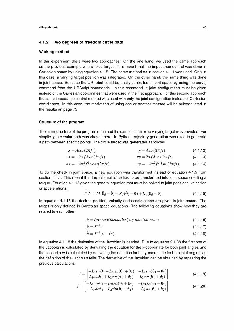
4 Experiments 60
4.1.2 Two degrees of freedom circle path
Working method
In this experiment there were two approaches. On the one hand, we used the same approachas the previous example with a fixed target. This meant that the impedance control was done inCartesian space by using equation 4.1.5. The same method as in section 4.1.1 was used. Only inthis case, a varying target position was integrated. On the other hand, the same thing was donein joint space. Because the UR robot could be easily controlled in joint space by using the servojcommand from the URScript commands. In this command, a joint configuration must be giveninstead of the Cartesian coordinates that were used in the first approach. For this second approachthe same impedance control method was used with only the joint configuration instead of Cartesiancoordinates. In this case, the motivation of using one or another method will be substantiated inthe results on page 79.
Structure of the program
The main structure of the program remained the same, but an extra varying target was provided. Forsimplicity, a circular path was chosen here. In Python, trajectory generation was used to generatea path between specific points. The circle target was generated as follows.
x = Acos(2π f t) y = Asin(2π f t) (4.1.12)
vx =−2π f Asin(2π f t) vy = 2π f Acos(2π f t) (4.1.13)
ax =−4π2 f 2Acos(2π f t) ay =−4π
2 f 2Asin(2π f t) (4.1.14)
To do the check in joint space, a new equation was transformed instead of equation 4.1.5 fromsection 4.1.1. This meant that the external force had to be transformed into joint space creating atorque. Equation 4.1.15 gives the general equation that must be solved to joint positions, velocitiesor accelerations.
JT F = M(θd− θ)+Kd(θd− θ)+Kp(θd−θ) (4.1.15)
In equation 4.1.15 the desired position, velocity and accelerations are given in joint space. Thetarget is only defined in Cartesian space equations. The following equations show how they arerelated to each other.
θ = InverseKinematics(x,y,manipulator) (4.1.16)
θ = J−1v (4.1.17)
θ = J−1(v− Ja) (4.1.18)
In equation 4.1.18 the derivative of the Jacobian is needed. Due to equation 2.1.38 the first row ofthe Jacobian is calculated by derivating the equation for the x-coordinate for both joint angles andthe second row is calculated by derivating the equation for the y-coordinate for both joint angles, asthe definition of the Jacobian tells. The derivative of the Jacobian can be obtained by repeating theprevious calculations.
J =
[−L1sinθ1−L2sin(θ1 +θ2) −L2sin(θ1 +θ2)L1cosθ1 +L2cos(θ1 +θ2) L2cos(θ1 +θ2)
](4.1.19)
J =
[−L1cosθ1−L2cos(θ1 +θ2) −L2cos(θ1 +θ2)−L1sinθ1−L2sin(θ1 +θ2) −L2sin(θ1 +θ2)
](4.1.20)
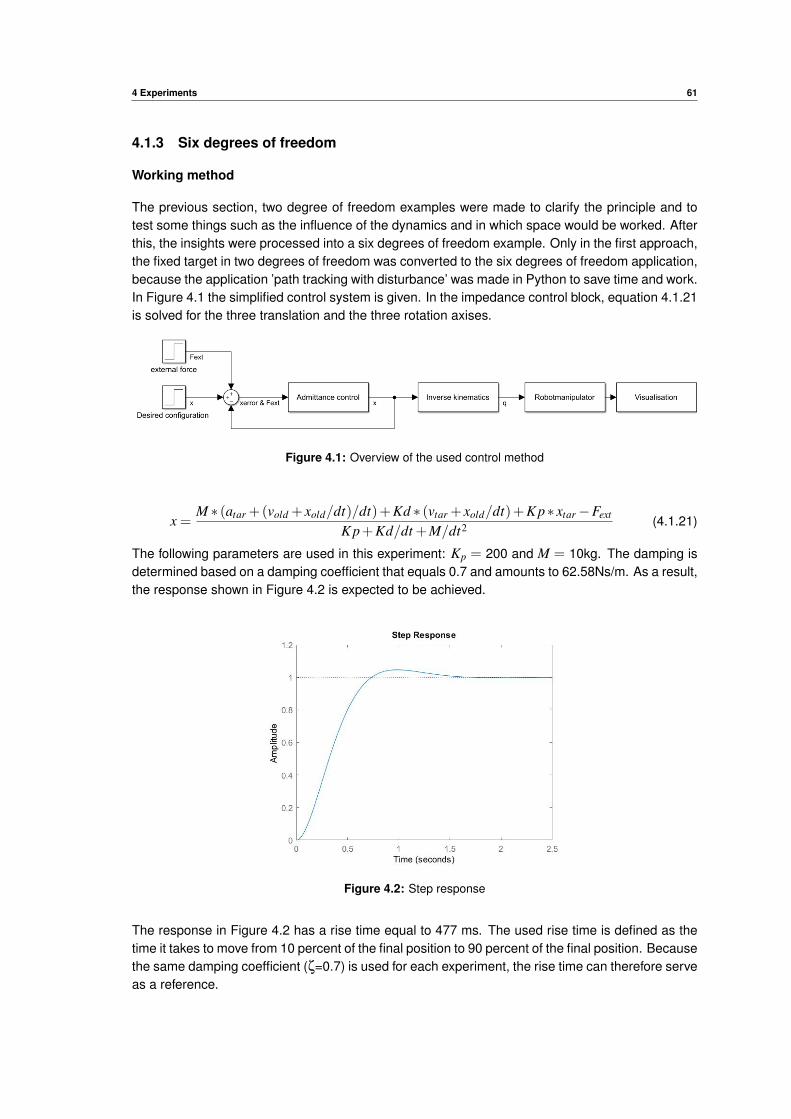
4 Experiments 61
4.1.3 Six degrees of freedom
Working method
The previous section, two degree of freedom examples were made to clarify the principle and totest some things such as the influence of the dynamics and in which space would be worked. Afterthis, the insights were processed into a six degrees of freedom example. Only in the first approach,the fixed target in two degrees of freedom was converted to the six degrees of freedom application,because the application ’path tracking with disturbance’ was made in Python to save time and work.In Figure 4.1 the simplified control system is given. In the impedance control block, equation 4.1.21is solved for the three translation and the three rotation axises.
Figure 4.1: Overview of the used control method
x =M ∗ (atar +(vold + xold/dt)/dt)+Kd ∗ (vtar + xold/dt)+K p∗ xtar−Fext
K p+Kd/dt +M/dt2 (4.1.21)
The following parameters are used in this experiment: Kp = 200 and M = 10kg. The damping isdetermined based on a damping coefficient that equals 0.7 and amounts to 62.58Ns/m. As a result,the response shown in Figure 4.2 is expected to be achieved.
Figure 4.2: Step response
The response in Figure 4.2 has a rise time equal to 477 ms. The used rise time is defined as thetime it takes to move from 10 percent of the final position to 90 percent of the final position. Becausethe same damping coefficient (ζ=0.7) is used for each experiment, the rise time can therefore serveas a reference.
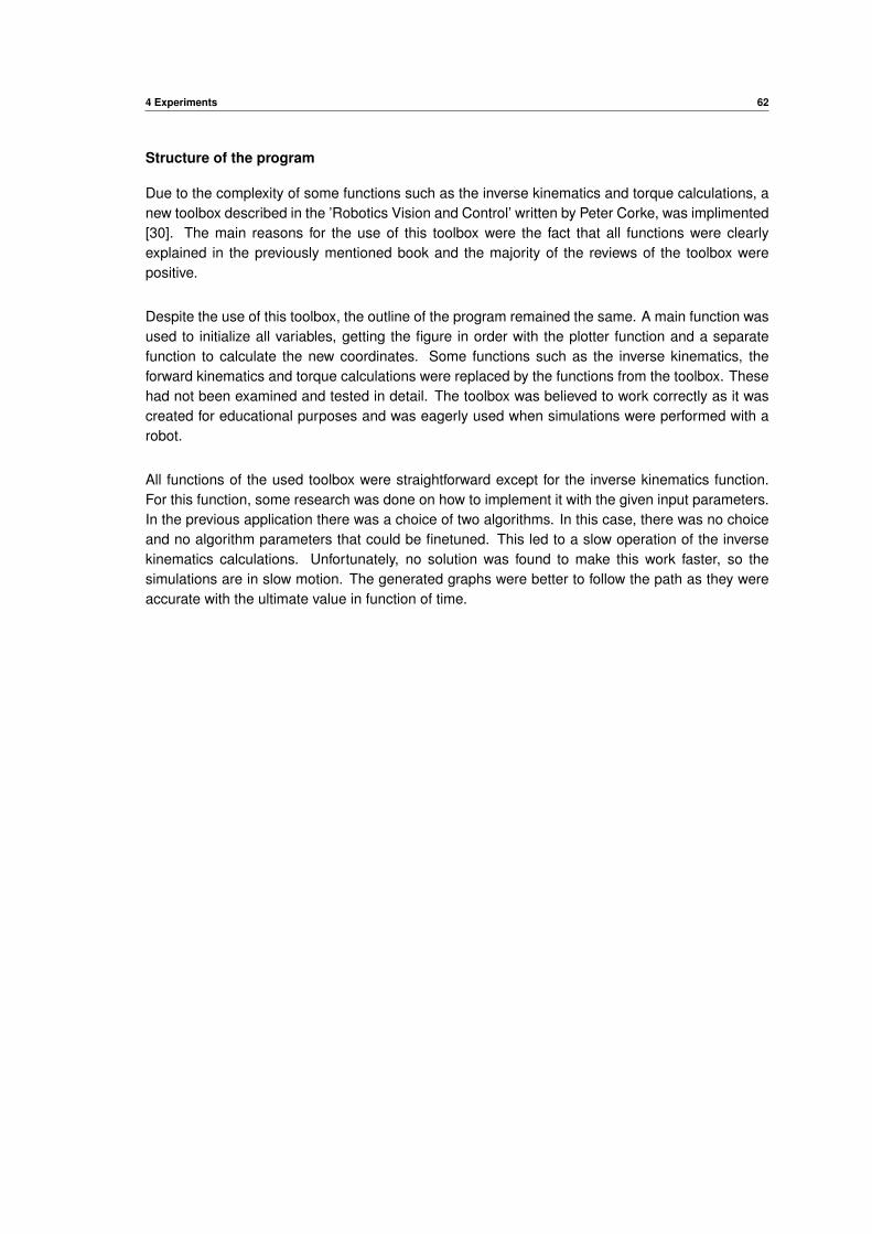
4 Experiments 62
Structure of the program
Due to the complexity of some functions such as the inverse kinematics and torque calculations, anew toolbox described in the ’Robotics Vision and Control’ written by Peter Corke, was implimented[30]. The main reasons for the use of this toolbox were the fact that all functions were clearlyexplained in the previously mentioned book and the majority of the reviews of the toolbox werepositive.
Despite the use of this toolbox, the outline of the program remained the same. A main function wasused to initialize all variables, getting the figure in order with the plotter function and a separatefunction to calculate the new coordinates. Some functions such as the inverse kinematics, theforward kinematics and torque calculations were replaced by the functions from the toolbox. Thesehad not been examined and tested in detail. The toolbox was believed to work correctly as it wascreated for educational purposes and was eagerly used when simulations were performed with arobot.
All functions of the used toolbox were straightforward except for the inverse kinematics function.For this function, some research was done on how to implement it with the given input parameters.In the previous application there was a choice of two algorithms. In this case, there was no choiceand no algorithm parameters that could be finetuned. This led to a slow operation of the inversekinematics calculations. Unfortunately, no solution was found to make this work faster, so thesimulations are in slow motion. The generated graphs were better to follow the path as they wereaccurate with the ultimate value in function of time.
4 Experiments 63
4.2 Python controller
This part of the thesis discusses how exactly the Python controller is built. The code is madeavailable to the supervisor and co-supervisor. It is not the intention to explain all lines of code, onlythe main structure and the build-up of some classes are discussed here.
4.2.1 Communication with UR3 robot
First, communication with the UR robot was made. Due to the research that is done about thecommunication with UR3, two classes had to be written: one class where commands could be sentand another class that processes the data returned by the robot. Research was conducted to findout whether this already existed. To process the received data, a library was found on a GitHubrepository of SintefManufacturing [47]. This library is old and not up to date, so it needed to beupdated. No other library was found for sending data to the UR3 robot. Hence, the decision wasmade to write this from scratch.
Working method
First the urx library was disassembled in order to separate the necessary piece from the ones thatturned out to be unnecessary. Because only a few parameters of the robot were read and manymore parameters could be read, the class was extended with more attributes. According to anExcel file on the Universal Robots support page, the data coming out of the robot with softwareversion 3.11 contains 1060 bytes [25]. This library was written for an older software version whereonly 86 bytes could be read. It is ensured that all data sent by the robot could also be read usingthis class by upgrading it.
To send data to the robot, URScripts commands are used. These are scripts that are used toprogram the robot using the teach pendant or the UR simulator in a virtual machine. When astring with the correct URScript syntax is sent to the robot, the robot will execute it. This onlyhappens if the robot is not running a program or if the overwrite function is enabled. All the URScirptcommands that are integrated and the functions details can be found on the URScript manual [50].
Structure and use of the classes
The monitor is build-up with functions that can return all available parameters of the robot. Thereforefirst the full data must be received. The total package size is 1060 bytes, split up in multiplesubpackages such as joint targets, actual joint positions, joint temperatures and so on. To use thisclass only a host IP adress must be given and the start function must be called. From that momentthe class is making connection to the UR3 robot and the wait function must be used to ensure theconnection has been made. As already shown in section 2.5.2 of the literature study, different portscan be used. For the monitoring class, port 30013 is used.The send class has common properties. Again, only an IP address needs to be provided to run thereal time command sender. Just as the monitor class, it uses a real-time port of the universal robot,port 30003. All major URScript functions are made in this class. To send the strings these functionsreturn, an extra function has been made that converts the strings to a byte, which is understood bythe robot.
4 Experiments 64
4.2.2 Robot definition
Working method
Just as in the MATLAB environment, there was a need for a class that contains the properties of therobot. First of all, a library was sought that could be used. Because Peter Corke’s MATLAB toolboxwas clear and easy to work with, it was first searched whether it was never processed into a Pythonlibrary. In fact this was the case, Peter Corke himself started writing a Python library. Unfortunately,it was not fully developed. For example, the kinematic functions and transformations are includedin the library, but the dynamic functions have not yet been developed. The most recent version canbe found at the GitHub repository of Aditya Dua and this library is called robopy [51].
Structure and use of the class
My co-supervisor Mr De Ryck first asked me how I would like to do this. Finally, when I came upwith the idea to use the robopy library, he offered me his version. All non-essential classes wereremoved and the classes were left with the necessary functionality. This left us with only a class forthe links, a class for the robot that describes all functions such as inverse and forward kinematicsand a number of methods to calculate transformations.Another function for the Jacobian was added based on the Peter Corke toolbox from MATLAB[32]. Using the MATLAB symbolic math toolbox and Euler-Lagrange equations, a function wasthen drawn up for the mass matrix, the Coriolis and centripetal matrix and the gravitation matrix.This specifically happened for the UR3 robot because the symbolic calculation with all parameterswas an impossible task. It took forever for a symbolic function to be generated, so it was decidedto manually enter the kinetic and dynamic parameters such as DH-parameters, inertias, center orgravities and the masses of the links. Because of this the robots parameters did not become aninput of these functions and the calculations were performed much faster. Inspiration was takenfrom the GitHub repository of Nathalie Majcherczyk where the same was done but for a sevendegrees of freedom link in two dimensions [52]. Because in this thesis work has to be done inthree-dimensional space, it took much longer to determine all functions. Ultimately, these functionscould be used in Python using the matlab.engine library. In section 2.1.6, the algorithm using theEuler-Lagrange equations, is shown for a two degree of freedom manipulator.
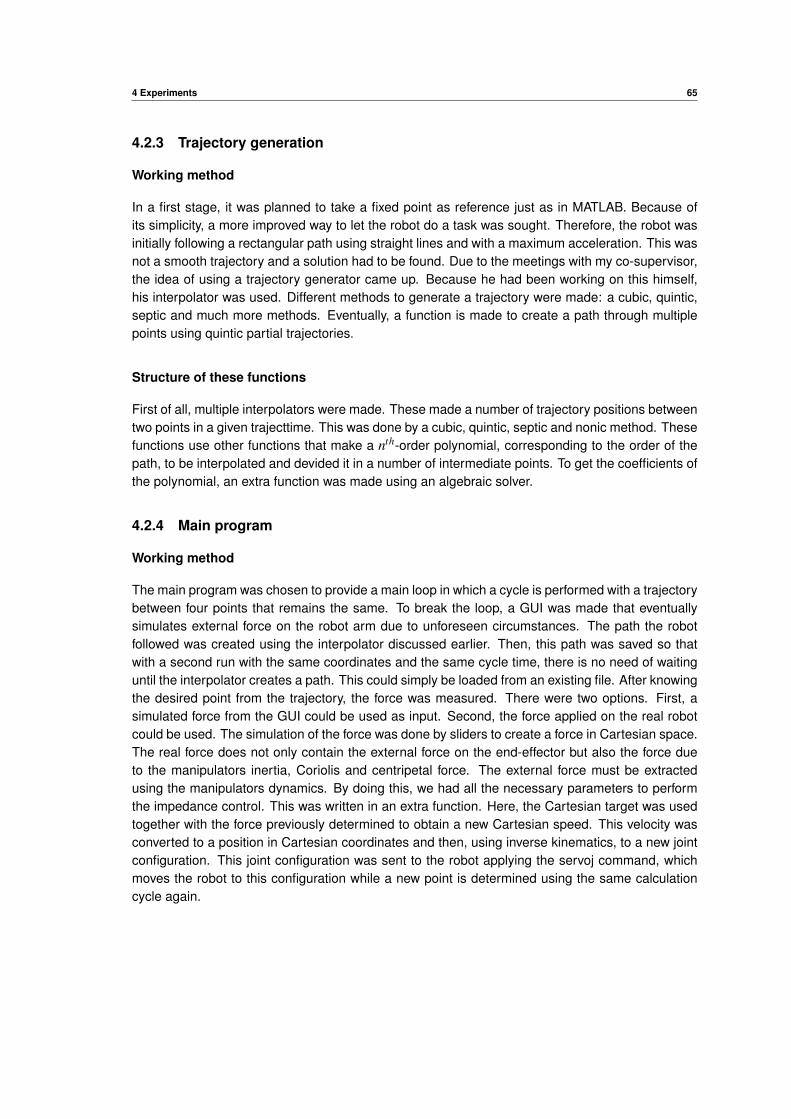
4 Experiments 65
4.2.3 Trajectory generation
Working method
In a first stage, it was planned to take a fixed point as reference just as in MATLAB. Because ofits simplicity, a more improved way to let the robot do a task was sought. Therefore, the robot wasinitially following a rectangular path using straight lines and with a maximum acceleration. This wasnot a smooth trajectory and a solution had to be found. Due to the meetings with my co-supervisor,the idea of using a trajectory generator came up. Because he had been working on this himself,his interpolator was used. Different methods to generate a trajectory were made: a cubic, quintic,septic and much more methods. Eventually, a function is made to create a path through multiplepoints using quintic partial trajectories.
Structure of these functions
First of all, multiple interpolators were made. These made a number of trajectory positions betweentwo points in a given trajecttime. This was done by a cubic, quintic, septic and nonic method. Thesefunctions use other functions that make a nth-order polynomial, corresponding to the order of thepath, to be interpolated and devided it in a number of intermediate points. To get the coefficients ofthe polynomial, an extra function was made using an algebraic solver.
4.2.4 Main program
Working method
The main program was chosen to provide a main loop in which a cycle is performed with a trajectorybetween four points that remains the same. To break the loop, a GUI was made that eventuallysimulates external force on the robot arm due to unforeseen circumstances. The path the robotfollowed was created using the interpolator discussed earlier. Then, this path was saved so thatwith a second run with the same coordinates and the same cycle time, there is no need of waitinguntil the interpolator creates a path. This could simply be loaded from an existing file. After knowingthe desired point from the trajectory, the force was measured. There were two options. First, asimulated force from the GUI could be used as input. Second, the force applied on the real robotcould be used. The simulation of the force was done by sliders to create a force in Cartesian space.The real force does not only contain the external force on the end-effector but also the force dueto the manipulators inertia, Coriolis and centripetal force. The external force must be extractedusing the manipulators dynamics. By doing this, we had all the necessary parameters to performthe impedance control. This was written in an extra function. Here, the Cartesian target was usedtogether with the force previously determined to obtain a new Cartesian speed. This velocity wasconverted to a position in Cartesian coordinates and then, using inverse kinematics, to a new jointconfiguration. This joint configuration was sent to the robot applying the servoj command, whichmoves the robot to this configuration while a new point is determined using the same calculationcycle again.
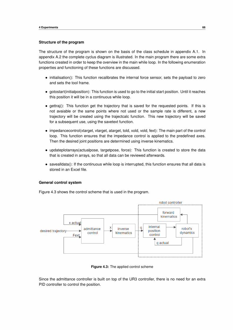
4 Experiments 66
Structure of the program
The structure of the program is shown on the basis of the class schedule in appendix A.1. Inappendix A.2 the complete cyclus diagram is illustrated. In the main program there are some extrafunctions created in order to keep the overview in the main while loop. In the following enumerationproperties and functioning of these functions are discussed.
• initialisation(): This function recalibrates the internal force sensor, sets the payload to zeroand sets the tool frame.
• gotostart(initialposition): This function is used to go to the initial start position. Until it reachesthis position it will be in a continuous while loop.
• gettraj(): This function get the trajectory that is saved for the requested points. If this isnot avaiable or the same points where not used or the sample rate is different, a newtrajectory will be created using the trajectcalc function. This new trajectory will be savedfor a subsequent use, using the savetext function.
• impedancecontrol(xtarget, vtarget, atarget, told, xold, vold, fext): The main part of the controlloop. This function ensures that the impedance control is applied to the predefined axes.Then the desired joint positions are determined using inverse kinematics.
• updateplotarrays(actualpose, targetpose, force): This function is created to store the datathat is created in arrays, so that all data can be reviewed afterwards.
• savealldata(): If the continuous while loop is interrupted, this function ensures that all data isstored in an Excel file.
General control system
Figure 4.3 shows the control scheme that is used in the program.
Figure 4.3: The applied control scheme
Since the admittance controller is built on top of the UR3 controller, there is no need for an extraPID controller to control the position.
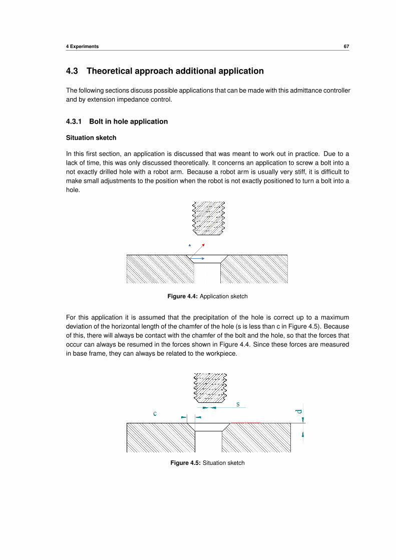
4 Experiments 67
4.3 Theoretical approach additional application
The following sections discuss possible applications that can be made with this admittance controllerand by extension impedance control.
4.3.1 Bolt in hole application
Situation sketch
In this first section, an application is discussed that was meant to work out in practice. Due to alack of time, this was only discussed theoretically. It concerns an application to screw a bolt into anot exactly drilled hole with a robot arm. Because a robot arm is usually very stiff, it is difficult tomake small adjustments to the position when the robot is not exactly positioned to turn a bolt into ahole.
Figure 4.4: Application sketch
For this application it is assumed that the precipitation of the hole is correct up to a maximumdeviation of the horizontal length of the chamfer of the hole (s is less than c in Figure 4.5). Becauseof this, there will always be contact with the chamfer of the bolt and the hole, so that the forces thatoccur can always be resumed in the forces shown in Figure 4.4. Since these forces are measuredin base frame, they can always be related to the workpiece.
Figure 4.5: Situation sketch
4 Experiments 68
Program sequence
The robot will first use the bolt to check whether there is a workpiece and if so at what distance. Todo this, the robot will make a slow downward movement next to the hole (red strip in Figure 4.5)until a certain force is reached in the vertical direction. When completed, the robot will move to thepreset position above the hole. It will then sink until the lower surface of the bolt is parallel to thesurface of the workpiece. When this is achieved, the admittance control and turning of the bolt ata certain speed proportional to the vertical displacement speed is activated. Then the bolt slowlysinks with the set value, the end position of the bolt fully screwed in. When the spring damper massprinciple works in the three translation axis, the bolt will move itself to the middle of the hole, thusobtaining a grip on the thread. When the bolt is at its end position, it can be chosen to provide acertain tightening torque, which can also be measured with the robot arm force measurements.
Reflections on this design:
• If the bolt has found the middle of the hole, there will be no force in the horizontal direction.Because of this, the target value in x and y direction must always be updated to the calculatedvalues of the admittance controller. Taken the axis of the bolt and the hole seen as z axis.
• This method does not take into account deviations in the parallelism of the workpiece surfaceto the xy plane. This can be incorporated into the probing of the workpiece on the red surfaceof Figure 4.5. It is always known that the contact force is perpendicular to this surface. If thez axis positions itself according to this perpendicular axis, the same method can be obtained.
• In the admittance controller a difference has to be made in stiffness. The force in z directiongradually increases because the target also drops lower. If the same stiffness is taken for thez axis as for the x and y axis, a too large displacement will be observed. If l equals the holedepth and c is the horizontal length of the chamfer, we can state the following:
Fzmax = l ∗Kz (4.3.1)
Fxymax = c∗Kxy (4.3.2)
As the force in z direction equals the force in x and y direction due to the chamfer of 45degree and l is normally larger than c. The spring coefficient in z axis (Kz) must be smallerthan the spring coefficient in x and y direction (Kxy).
4.3.2 Other applications
With force control in general, many different applications can be made. It is especially interestingto use this when there is interaction between the robot and its environment, as in the previousapplications. For general moving applications however, this can be used less well, due to thecontrol error that occurs. For force control, for example, sanding a surface with a robot arm can beused, in this case impedance control would be applied. Also when gripping fragile products, thiscan certainly be used when, for example, a maximum force can be applied to an object, for examplefruit. When pressed too hard, rotten spots can occur, which is not desirable. Admittance controlcan mainly be used when any environmental force acts on the system. For example, helping tomove a heavy object, is a good application.
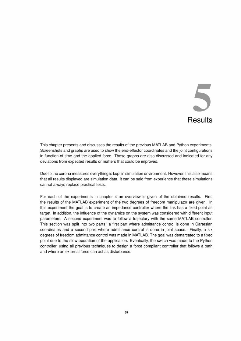
5Results
This chapter presents and discusses the results of the previous MATLAB and Python experiments.Screenshots and graphs are used to show the end-effector coordinates and the joint configurationsin function of time and the applied force. These graphs are also discussed and indicated for anydeviations from expected results or matters that could be improved.
Due to the corona measures everything is kept in simulation environment. However, this also meansthat all results displayed are simulation data. It can be said from experience that these simulationscannot always replace practical tests.
For each of the experiments in chapter 4 an overview is given of the obtained results. Firstthe results of the MATLAB experiment of the two degrees of freedom manipulator are given. Inthis experiment the goal is to create an impedance controller where the link has a fixed point astarget. In addition, the influence of the dynamics on the system was considered with different inputparameters. A second experiment was to follow a trajectory with the same MATLAB controller.This section was split into two parts: a first part where admittance control is done in Cartesiancoordinates and a second part where admittance control is done in joint space. Finally, a sixdegrees of freedom admittance control was made in MATLAB. The goal was demarcated to a fixedpoint due to the slow operation of the application. Eventually, the switch was made to the Pythoncontroller, using all previous techniques to design a force compliant controller that follows a pathand where an external force can act as disturbance.
69
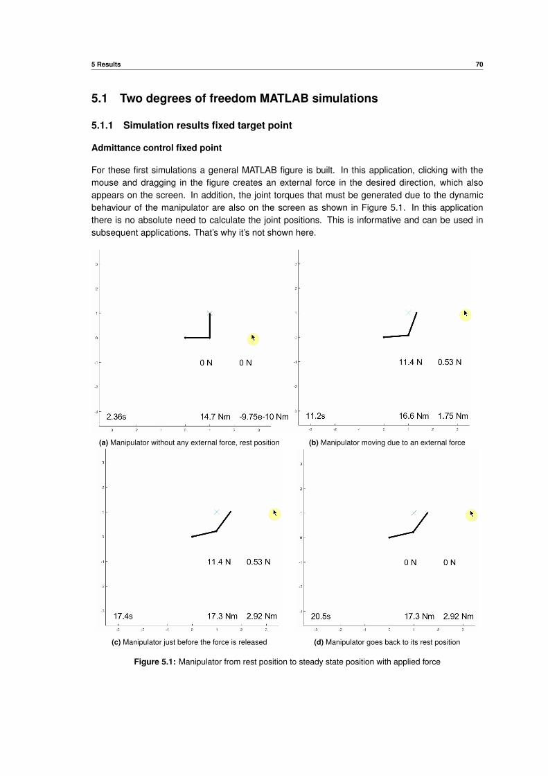
5 Results 70
5.1 Two degrees of freedom MATLAB simulations
5.1.1 Simulation results fixed target point
Admittance control fixed point
For these first simulations a general MATLAB figure is built. In this application, clicking with themouse and dragging in the figure creates an external force in the desired direction, which alsoappears on the screen. In addition, the joint torques that must be generated due to the dynamicbehaviour of the manipulator are also on the screen as shown in Figure 5.1. In this applicationthere is no absolute need to calculate the joint positions. This is informative and can be used insubsequent applications. That’s why it’s not shown here.
(a) Manipulator without any external force, rest position (b) Manipulator moving due to an external force
(c) Manipulator just before the force is released (d) Manipulator goes back to its rest position
Figure 5.1: Manipulator from rest position to steady state position with applied force
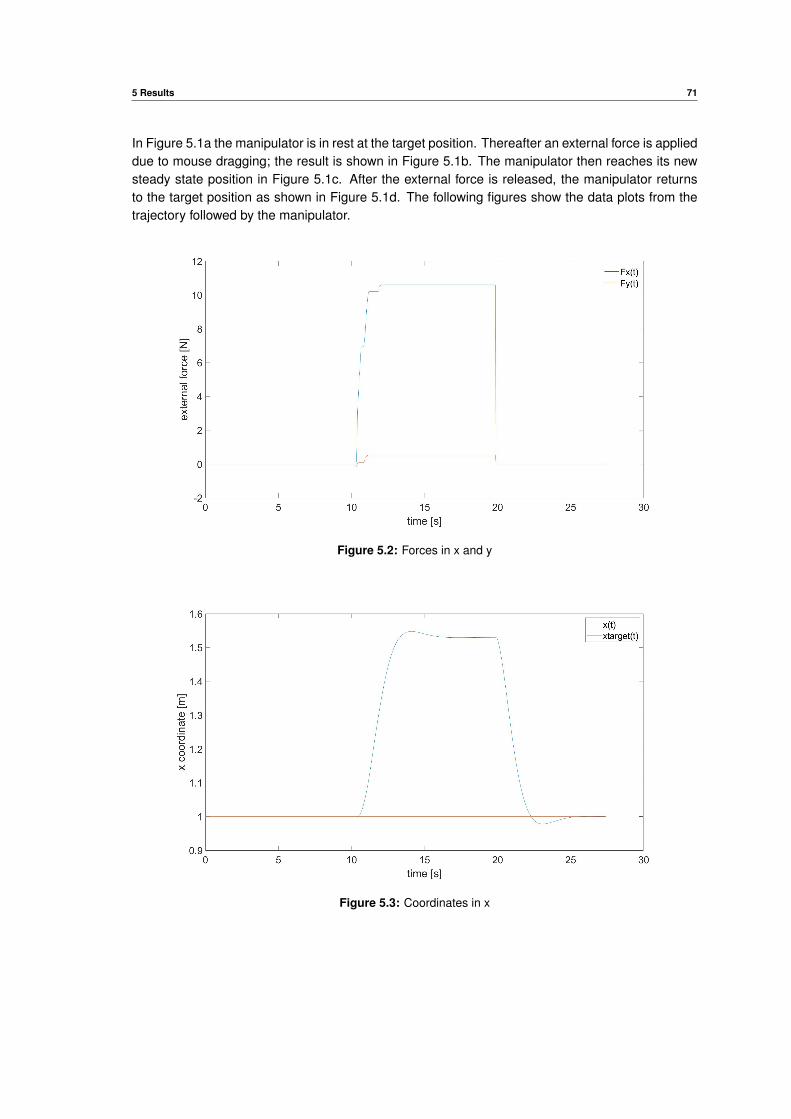
5 Results 71
In Figure 5.1a the manipulator is in rest at the target position. Thereafter an external force is applieddue to mouse dragging; the result is shown in Figure 5.1b. The manipulator then reaches its newsteady state position in Figure 5.1c. After the external force is released, the manipulator returnsto the target position as shown in Figure 5.1d. The following figures show the data plots from thetrajectory followed by the manipulator.
Figure 5.2: Forces in x and y
Figure 5.3: Coordinates in x
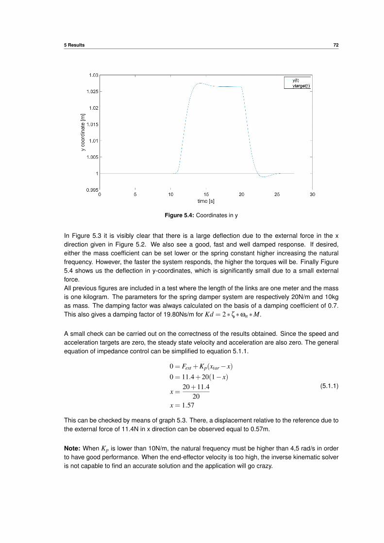
5 Results 72
Figure 5.4: Coordinates in y
In Figure 5.3 it is visibly clear that there is a large deflection due to the external force in the xdirection given in Figure 5.2. We also see a good, fast and well damped response. If desired,either the mass coefficient can be set lower or the spring constant higher increasing the naturalfrequency. However, the faster the system responds, the higher the torques will be. Finally Figure5.4 shows us the deflection in y-coordinates, which is significantly small due to a small externalforce.All previous figures are included in a test where the length of the links are one meter and the massis one kilogram. The parameters for the spring damper system are respectively 20N/m and 10kgas mass. The damping factor was always calculated on the basis of a damping coefficient of 0.7.This also gives a damping factor of 19.80Ns/m for Kd = 2∗ζ∗ωn ∗M.
A small check can be carried out on the correctness of the results obtained. Since the speed andacceleration targets are zero, the steady state velocity and acceleration are also zero. The generalequation of impedance control can be simplified to equation 5.1.1.
0 = Fext +Kp(xtar− x)
0 = 11.4+20(1− x)
x =20+11.4
20x = 1.57
(5.1.1)
This can be checked by means of graph 5.3. There, a displacement relative to the reference due tothe external force of 11.4N in x direction can be observed equal to 0.57m.
Note: When Kp is lower than 10N/m, the natural frequency must be higher than 4,5 rad/s in orderto have good performance. When the end-effector velocity is too high, the inverse kinematic solveris not capable to find an accurate solution and the application will go crazy.
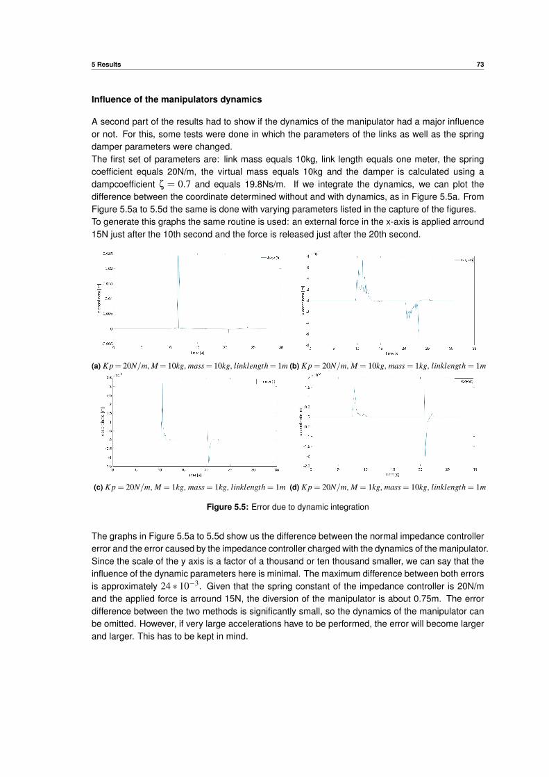
5 Results 73
Influence of the manipulators dynamics
A second part of the results had to show if the dynamics of the manipulator had a major influenceor not. For this, some tests were done in which the parameters of the links as well as the springdamper parameters were changed.The first set of parameters are: link mass equals 10kg, link length equals one meter, the springcoefficient equals 20N/m, the virtual mass equals 10kg and the damper is calculated using adampcoefficient ζ = 0.7 and equals 19.8Ns/m. If we integrate the dynamics, we can plot thedifference between the coordinate determined without and with dynamics, as in Figure 5.5a. FromFigure 5.5a to 5.5d the same is done with varying parameters listed in the capture of the figures.To generate this graphs the same routine is used: an external force in the x-axis is applied arround15N just after the 10th second and the force is released just after the 20th second.
(a) K p= 20N/m, M = 10kg, mass= 10kg, linklength= 1m (b) K p = 20N/m, M = 10kg, mass = 1kg, linklength = 1m
(c) K p = 20N/m, M = 1kg, mass = 1kg, linklength = 1m (d) K p = 20N/m, M = 1kg, mass = 10kg, linklength = 1m
Figure 5.5: Error due to dynamic integration
The graphs in Figure 5.5a to 5.5d show us the difference between the normal impedance controllererror and the error caused by the impedance controller charged with the dynamics of the manipulator.Since the scale of the y axis is a factor of a thousand or ten thousand smaller, we can say that theinfluence of the dynamic parameters here is minimal. The maximum difference between both errorsis approximately 24 ∗ 10−3. Given that the spring constant of the impedance controller is 20N/mand the applied force is arround 15N, the diversion of the manipulator is about 0.75m. The errordifference between the two methods is significantly small, so the dynamics of the manipulator canbe omitted. However, if very large accelerations have to be performed, the error will become largerand larger. This has to be kept in mind.
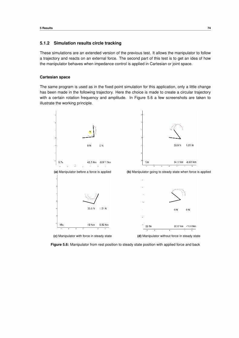
5 Results 74
5.1.2 Simulation results circle tracking
These simulations are an extended version of the previous test. It allows the manipulator to followa trajectory and reacts on an external force. The second part of this test is to get an idea of howthe manipulator behaves when impedance control is applied in Cartesian or joint space.
Cartesian space
The same program is used as in the fixed point simulation for this application, only a little changehas been made in the following trajectory. Here the choice is made to create a circular trajectorywith a certain rotation frequency and amplitude. In Figure 5.6 a few screenshots are taken toillustrate the working principle.
(a) Manipulator before a force is applied (b) Manipulator going to steady state when force is applied
(c) Manipulator with force in steady state (d) Manipulator without force in steady state
Figure 5.6: Manipulator from rest position to steady state position with applied force and back
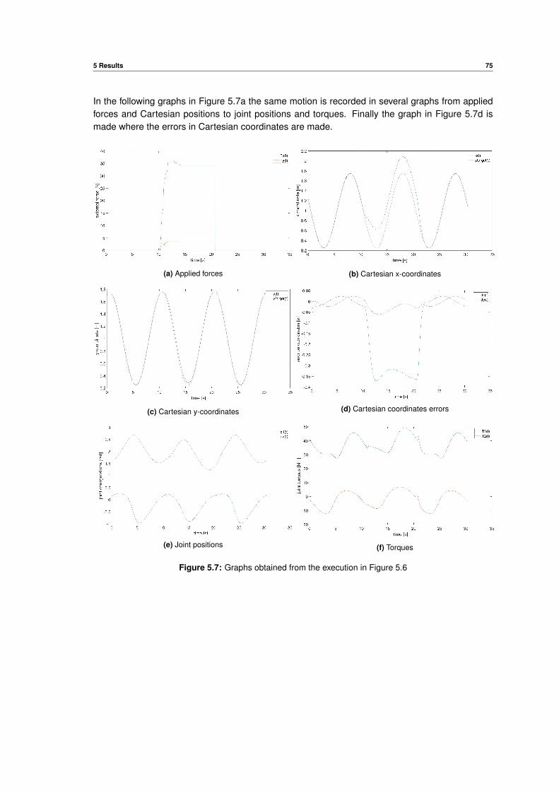
5 Results 75
In the following graphs in Figure 5.7a the same motion is recorded in several graphs from appliedforces and Cartesian positions to joint positions and torques. Finally the graph in Figure 5.7d ismade where the errors in Cartesian coordinates are made.
(a) Applied forces (b) Cartesian x-coordinates
(c) Cartesian y-coordinates (d) Cartesian coordinates errors
(e) Joint positions (f) Torques
Figure 5.7: Graphs obtained from the execution in Figure 5.6
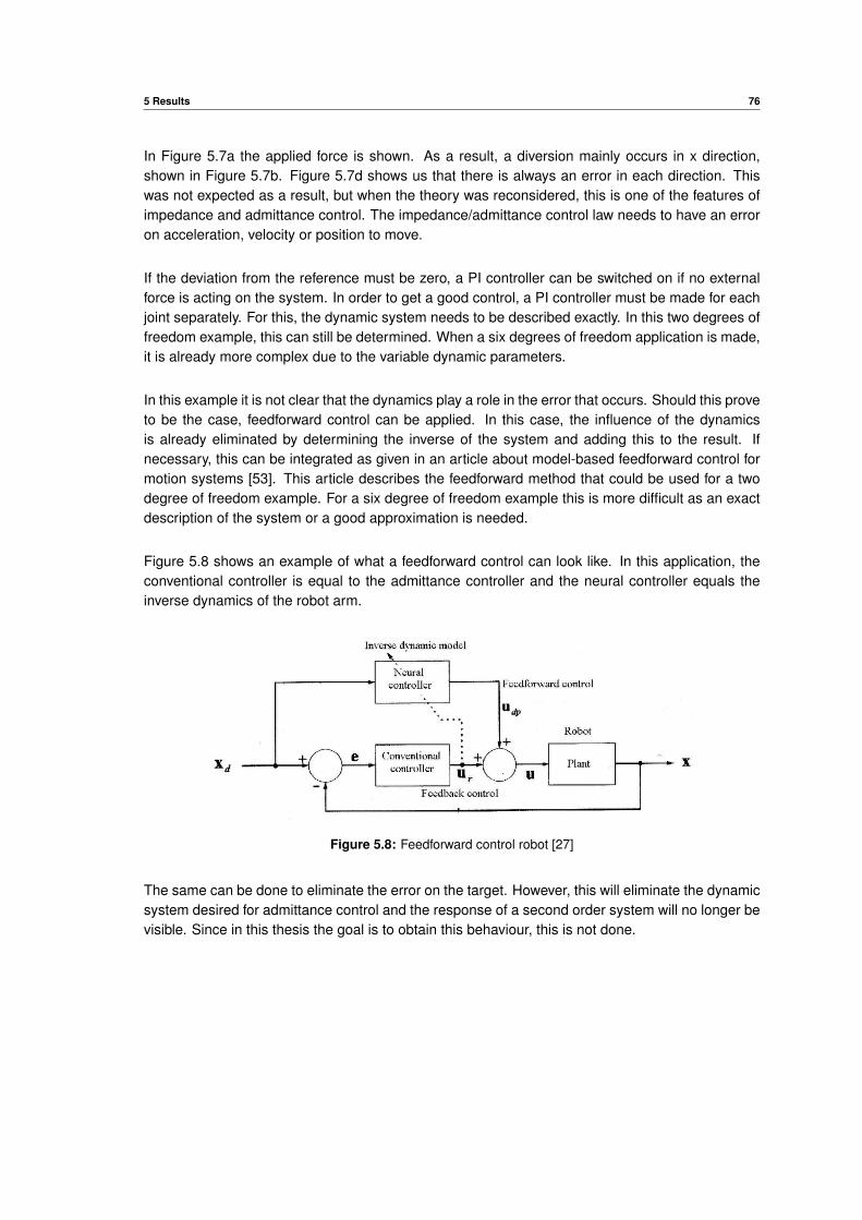
5 Results 76
In Figure 5.7a the applied force is shown. As a result, a diversion mainly occurs in x direction,shown in Figure 5.7b. Figure 5.7d shows us that there is always an error in each direction. Thiswas not expected as a result, but when the theory was reconsidered, this is one of the features ofimpedance and admittance control. The impedance/admittance control law needs to have an erroron acceleration, velocity or position to move.
If the deviation from the reference must be zero, a PI controller can be switched on if no externalforce is acting on the system. In order to get a good control, a PI controller must be made for eachjoint separately. For this, the dynamic system needs to be described exactly. In this two degrees offreedom example, this can still be determined. When a six degrees of freedom application is made,it is already more complex due to the variable dynamic parameters.
In this example it is not clear that the dynamics play a role in the error that occurs. Should this proveto be the case, feedforward control can be applied. In this case, the influence of the dynamicsis already eliminated by determining the inverse of the system and adding this to the result. Ifnecessary, this can be integrated as given in an article about model-based feedforward control formotion systems [53]. This article describes the feedforward method that could be used for a twodegree of freedom example. For a six degree of freedom example this is more difficult as an exactdescription of the system or a good approximation is needed.
Figure 5.8 shows an example of what a feedforward control can look like. In this application, theconventional controller is equal to the admittance controller and the neural controller equals theinverse dynamics of the robot arm.
Figure 5.8: Feedforward control robot [27]
The same can be done to eliminate the error on the target. However, this will eliminate the dynamicsystem desired for admittance control and the response of a second order system will no longer bevisible. Since in this thesis the goal is to obtain this behaviour, this is not done.
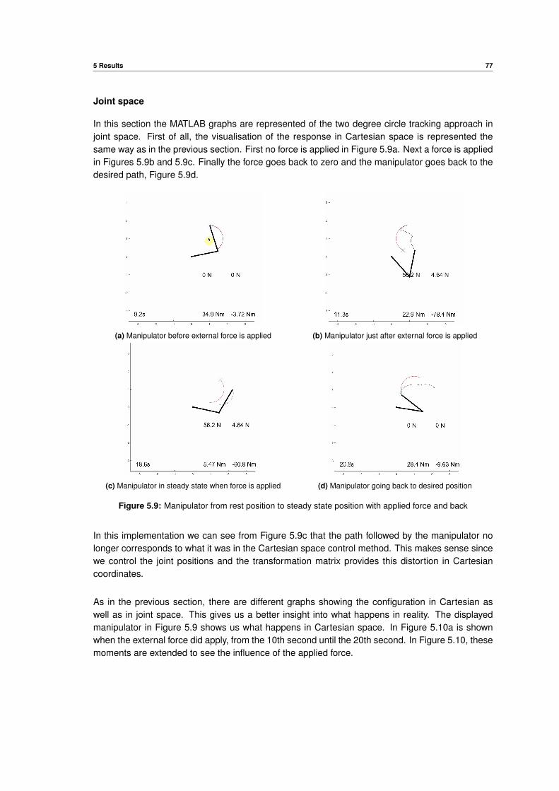
5 Results 77
Joint space
In this section the MATLAB graphs are represented of the two degree circle tracking approach injoint space. First of all, the visualisation of the response in Cartesian space is represented thesame way as in the previous section. First no force is applied in Figure 5.9a. Next a force is appliedin Figures 5.9b and 5.9c. Finally the force goes back to zero and the manipulator goes back to thedesired path, Figure 5.9d.
(a) Manipulator before external force is applied (b) Manipulator just after external force is applied
(c) Manipulator in steady state when force is applied (d) Manipulator going back to desired position
Figure 5.9: Manipulator from rest position to steady state position with applied force and back
In this implementation we can see from Figure 5.9c that the path followed by the manipulator nolonger corresponds to what it was in the Cartesian space control method. This makes sense sincewe control the joint positions and the transformation matrix provides this distortion in Cartesiancoordinates.
As in the previous section, there are different graphs showing the configuration in Cartesian aswell as in joint space. This gives us a better insight into what happens in reality. The displayedmanipulator in Figure 5.9 shows us what happens in Cartesian space. In Figure 5.10a is shownwhen the external force did apply, from the 10th second until the 20th second. In Figure 5.10, thesemoments are extended to see the influence of the applied force.
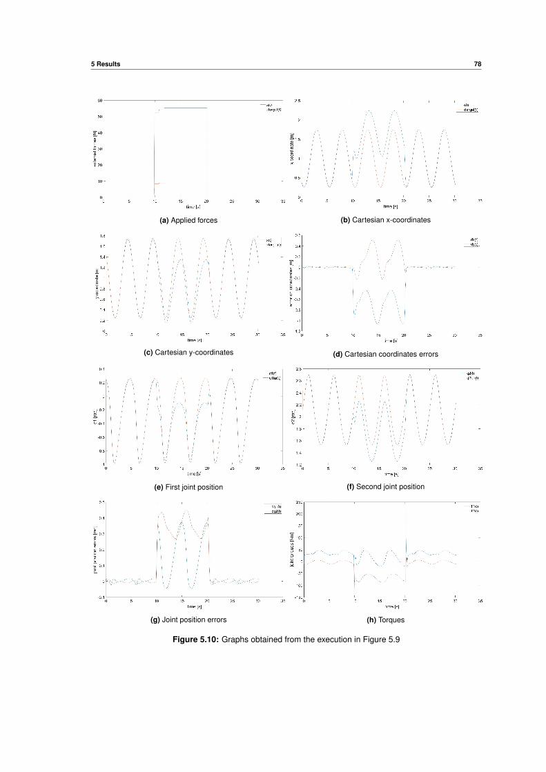
5 Results 78
(a) Applied forces (b) Cartesian x-coordinates
(c) Cartesian y-coordinates (d) Cartesian coordinates errors
(e) First joint position (f) Second joint position
(g) Joint position errors (h) Torques
Figure 5.10: Graphs obtained from the execution in Figure 5.9

5 Results 79
Figures 5.10b and 5.10c give a picture of how the x and y coordinate progress. There is a smoothtransition in the coordinates when a force occurs as seen in the overview of Figure 5.9. Unlikethe experiment in Cartesian space, we cannot conclude that the error in both x and y directions inFigure 5.10d remains approximately constant at steady state. However, if we look at what happensin joint space, we see that in Figures 5.10e and 5.10f the spring, damper and mass control is morevisible. When the external force is released, an adjustment to the target is visible with a smallovershoot. Looking at the error on the joint positions, in Figure 5.10g is shown that this is alsonot constant. This can be explained by the fact that the external force creates a torque that isnot constant because it depends on the Jacobian or the joint configuration and it changes overtime. Finally, we can see in Figure 5.10h that when the external force is removed, a peak in torqueoccurs due to the acceleration. Thereafter it seems that the value before the peak in the first jointand after the peak is almost the same. While for the second joint it has a certain offset, due to thedisplacement of the target position and the resulting change in gravitational compensation torques.
Issues
A major problem arose during execution. The inverse kinematics of MATLAB’s rigidbody toolboxwere too slow for this application, about seven milliseconds each calculation. As a result, a closerlook was taken at the function. The possible adjustable parameters were looked up in order toobtain an accurate result. Since the MATLAB rigidbody class was used to create the manipulator,the inverse kinematic solver of this class was also used.
An inverse kinematic solver needed to be defined using the function: inverseKinematics(’RigidBodyTree’,’SolverAlgorithm’, SolverParameters’). On the MathWorks site about the inverse kinematic solver,the two different solvers are explained in detail, according to which principle they work and whatparameters can be given [54].
First, there is the BFGS gradient protection algorithm that could be used. This solver algorithm isbased on the quasi-Newton method and uses the second derivative to determine the step that mustbe taken in the second iteration. A gradient projection method is used to deal with boundary limitson the cost function that the joint limits of the robot model creates. The parameters that can beobtained with this algorithm are: maximum number of iterations, maximum time, gradient tolerance,solution tolerance, joint limits, if random restarts are allowed and the minimum step that is allowed.
Secondly, there is the Levenberg-Marquardt algorithm. This algorithm uses an error-dampedleast-squares method. In addition to the BFGS gradient projection algorithm, this algorithm hassome extra input parameters such as: threshold on the change in end-effector pose, a constant fordamping and an indicator for the use or non-use of the damping.
Both algorithms could be studied in detail but this was not the purpose of this thesis. For moreinformation, reference is made to the MathWorks site about the BFGS algorithm and the Levenberg-Marquardtalgorithm [55][56]. In general the BFGS algorithm is set default because it is more robust at findingsolutions and it’s more effective for configurations near the joint limits or when the initial guessis not close to the solution. If the initial guess is close to the solution, the Levenberg-Marquardtalgorithm is faster. In this application the previous joint configuration was known and therefore theLevenberg-Marquardt algorithm was prefered [54].
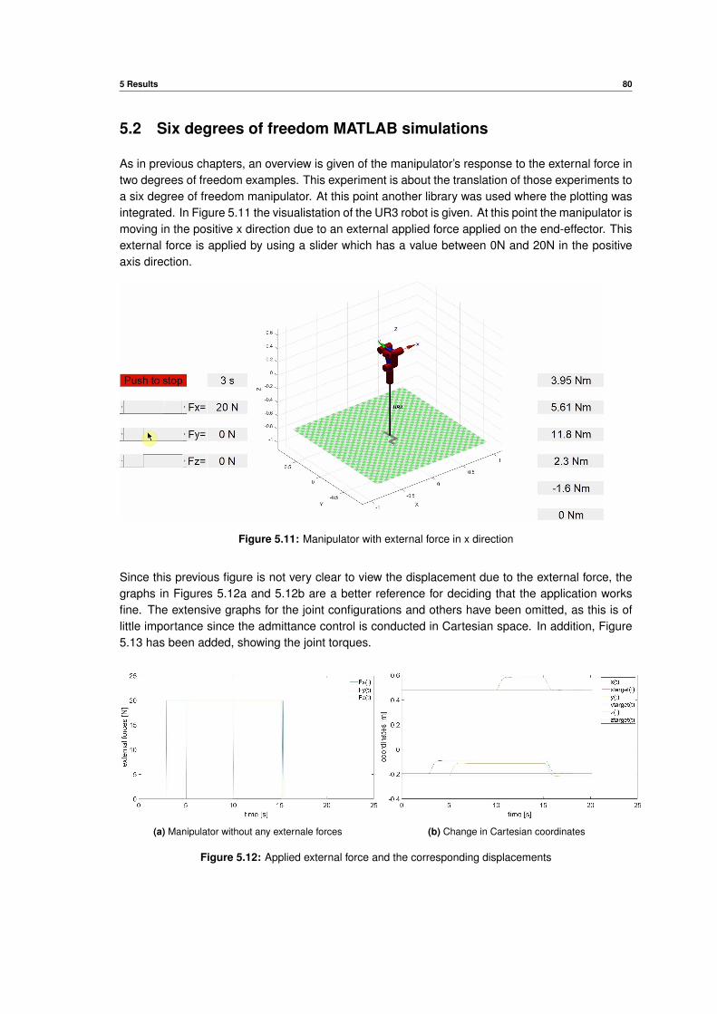
5 Results 80
5.2 Six degrees of freedom MATLAB simulations
As in previous chapters, an overview is given of the manipulator’s response to the external force intwo degrees of freedom examples. This experiment is about the translation of those experiments toa six degree of freedom manipulator. At this point another library was used where the plotting wasintegrated. In Figure 5.11 the visualistation of the UR3 robot is given. At this point the manipulator ismoving in the positive x direction due to an external applied force applied on the end-effector. Thisexternal force is applied by using a slider which has a value between 0N and 20N in the positiveaxis direction.
Figure 5.11: Manipulator with external force in x direction
Since this previous figure is not very clear to view the displacement due to the external force, thegraphs in Figures 5.12a and 5.12b are a better reference for deciding that the application worksfine. The extensive graphs for the joint configurations and others have been omitted, as this is oflittle importance since the admittance control is conducted in Cartesian space. In addition, Figure5.13 has been added, showing the joint torques.
(a) Manipulator without any externale forces (b) Change in Cartesian coordinates
Figure 5.12: Applied external force and the corresponding displacements

5 Results 81
This response can be compared to the expected response shown in Figure 4.2. There a rising timeof 477ms is measured. Since a sample time of 50ms is taken, this cannot be observed at the sameprecision. Table 5.1 shows the measuring points in which the rise time can be determined.
y value [m] time [s]rest state -0.2132 5.0510% -0.2032 5.2590% -0.1233 5.75steady state -0.1133 7.15
Table 5.1: Rise time sample points
From Table 5.1 it can be concluded that the system responds as previously desired, since the risetime between the two sampled points is approximately 500ms.
Figure 5.13: Joint torques
The maximum moments are never exceeded in Figure 5.13. If this does happen in the program,another joint acceleration with the maximum torque is calculated on the basis of the dynamics ofthe manipulator. However, this means that the path that has been followed no longer follows thedesired trajectory, the coordinates are adjusted in function of the accelerations of the joints, so thatan unexpected movement can occur.
The maximum torques are [56,56,28,12,12,12]Nm for base, shoulder, elbow, wrist one, wristtwo and wrist three. If for example the torque of the elbow must exceed the maximum torque of28Nm for instance [20,14,32,5,4,3]Nm, the maximum value will be inserted in the actual torquesτad justed = [20,14,28,5,4,3]Nm and a new joint acceleration will be calculated using equation5.2.1. The new final coordinates wil then be determined for this, as has been done previously.
θ = M(θ)−1(τad justed−C(θ, θ)θ−G(θ)) (5.2.1)
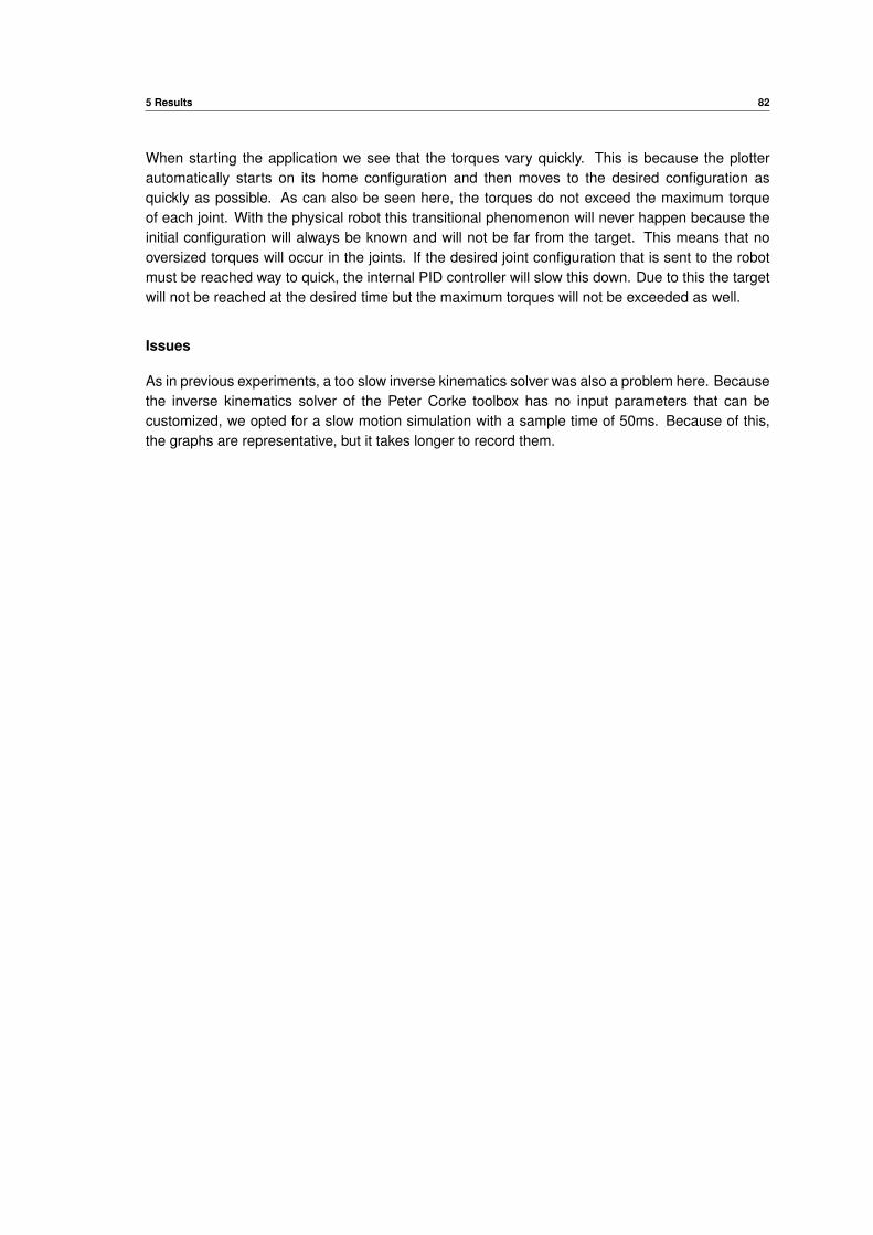
5 Results 82
When starting the application we see that the torques vary quickly. This is because the plotterautomatically starts on its home configuration and then moves to the desired configuration asquickly as possible. As can also be seen here, the torques do not exceed the maximum torqueof each joint. With the physical robot this transitional phenomenon will never happen because theinitial configuration will always be known and will not be far from the target. This means that nooversized torques will occur in the joints. If the desired joint configuration that is sent to the robotmust be reached way to quick, the internal PID controller will slow this down. Due to this the targetwill not be reached at the desired time but the maximum torques will not be exceeded as well.
Issues
As in previous experiments, a too slow inverse kinematics solver was also a problem here. Becausethe inverse kinematics solver of the Peter Corke toolbox has no input parameters that can becustomized, we opted for a slow motion simulation with a sample time of 50ms. Because of this,the graphs are representative, but it takes longer to record them.
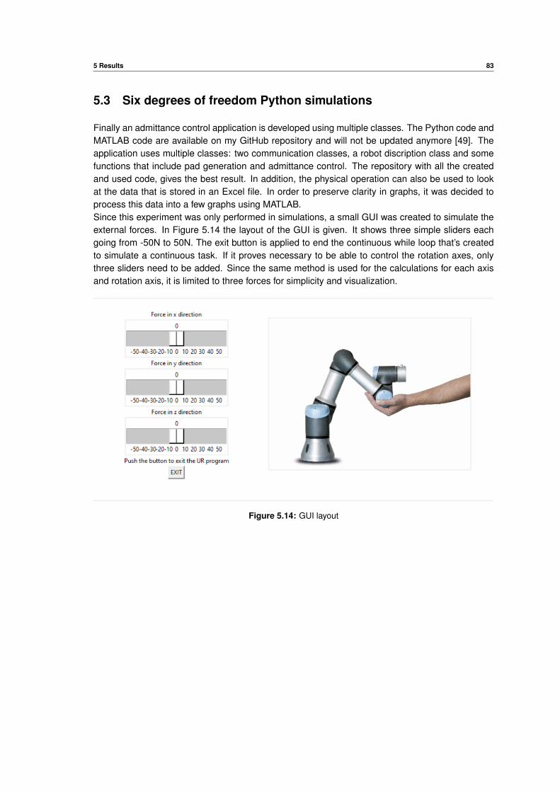
5 Results 83
5.3 Six degrees of freedom Python simulations
Finally an admittance control application is developed using multiple classes. The Python code andMATLAB code are available on my GitHub repository and will not be updated anymore [49]. Theapplication uses multiple classes: two communication classes, a robot discription class and somefunctions that include pad generation and admittance control. The repository with all the createdand used code, gives the best result. In addition, the physical operation can also be used to lookat the data that is stored in an Excel file. In order to preserve clarity in graphs, it was decided toprocess this data into a few graphs using MATLAB.Since this experiment was only performed in simulations, a small GUI was created to simulate theexternal forces. In Figure 5.14 the layout of the GUI is given. It shows three simple sliders eachgoing from -50N to 50N. The exit button is applied to end the continuous while loop that’s createdto simulate a continuous task. If it proves necessary to be able to control the rotation axes, onlythree sliders need to be added. Since the same method is used for the calculations for each axisand rotation axis, it is limited to three forces for simplicity and visualization.
Figure 5.14: GUI layout
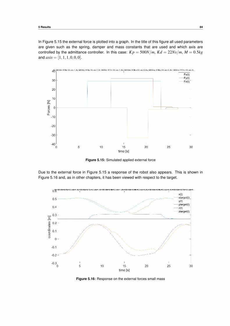
5 Results 84
In Figure 5.15 the external force is plotted into a graph. In the title of this figure all used parametersare given such as the spring, damper and mass constants that are used and which axis arecontrolled by the admittance controller. In this case: K p = 500N/m, Kd = 22Ns/m, M = 0.5kgand axis = [1,1,1,0,0,0].
Figure 5.15: Simulated applied external force
Due to the external force in Figure 5.15 a response of the robot also appears. This is shown inFigure 5.16 and, as in other chapters, it has been viewed with respect to the target.
Figure 5.16: Response on the external forces small mass
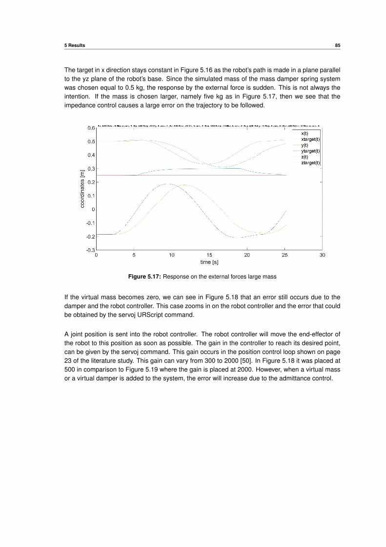
5 Results 85
The target in x direction stays constant in Figure 5.16 as the robot’s path is made in a plane parallelto the yz plane of the robot’s base. Since the simulated mass of the mass damper spring systemwas chosen equal to 0.5 kg, the response by the external force is sudden. This is not always theintention. If the mass is chosen larger, namely five kg as in Figure 5.17, then we see that theimpedance control causes a large error on the trajectory to be followed.
Figure 5.17: Response on the external forces large mass
If the virtual mass becomes zero, we can see in Figure 5.18 that an error still occurs due to thedamper and the robot controller. This case zooms in on the robot controller and the error that couldbe obtained by the servoj URScript command.
A joint position is sent into the robot controller. The robot controller will move the end-effector ofthe robot to this position as soon as possible. The gain in the controller to reach its desired point,can be given by the servoj command. This gain occurs in the position control loop shown on page23 of the literature study. This gain can vary from 300 to 2000 [50]. In Figure 5.18 it was placed at500 in comparison to Figure 5.19 where the gain is placed at 2000. However, when a virtual massor a virtual damper is added to the system, the error will increase due to the admittance control.
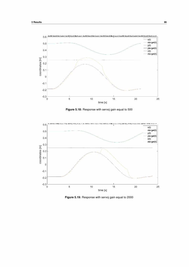
5 Results 86
Figure 5.18: Response with servoj gain equal to 500
Figure 5.19: Response with servoj gain equal to 2000
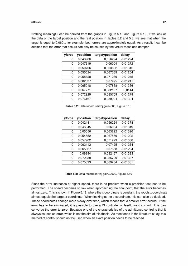
5 Results 87
Nothing meaningful can be derived from the graphs in Figure 5.18 and Figure 5.19. If we look atthe data of the target position and the real position in Tables 5.2 and 5.3, we see that when thetarget is equal to 0.060... for example, both errors are approximately equal. As a result, it can bedecided that the error that occurs can only be caused by the virtual mass and damper.
yforce yposition targetyposition deltay0 0,043986 0,056224 -0,012240 0,047319 0,06004 -0,012720 0,050706 0,063822 -0,013120 0,055024 0,067569 -0,012540 0,058828 0,071279 -0,012450 0,062537 0,07495 -0,012410 0,065018 0,07858 -0,013560 0,067771 0,082167 -0,01440 0,072929 0,085709 -0,012780 0,076167 0,089204 -0,01304
Table 5.2: Data record servoj gain=500, Figure 5.18
yforce yposition targetyposition deltay0 0,042441 0,056224 -0,013780 0,046845 0,06004 -0,013190 0,05056 0,063822 -0,013260 0,054652 0,067569 -0,012920 0,057902 0,071279 -0,013380 0,062412 0,07495 -0,012540 0,065637 0,07858 -0,012940 0,06894 0,082167 -0,013230 0,072338 0,085709 -0,013370 0,075893 0,089204 -0,01331
Table 5.3: Data record servoj gain=2000, Figure 5.19
Since the error increases at higher speed, there is no problem when a precision task has to beperformed. The speed becomes so low when approaching the final point, that the error becomesalmost zero. This is shown in Figure 5.18, where the x-coordinate is constant, the robots x-coordinatealmost equals the target x-coordinate. When looking at the z-coordinate, this can also be decided.These coordinates change more slowly over time, which means that a smaller error occurs. If theerror has to be eliminated, it is possible to use a PI controller or feedforward control. This canconverge the error to zero. Because one of the characteristics of the admittance control is that italways causes an error, which is not the aim of this thesis. As mentioned in the literature study, thismethod of control should not be used when an exact position needs to be reached.
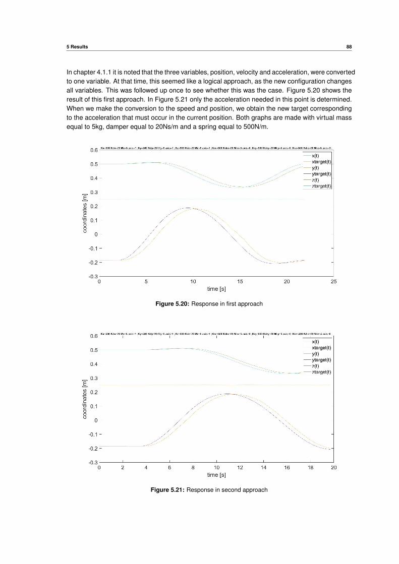
5 Results 88
In chapter 4.1.1 it is noted that the three variables, position, velocity and acceleration, were convertedto one variable. At that time, this seemed like a logical approach, as the new configuration changesall variables. This was followed up once to see whether this was the case. Figure 5.20 shows theresult of this first approach. In Figure 5.21 only the acceleration needed in this point is determined.When we make the conversion to the speed and position, we obtain the new target correspondingto the acceleration that must occur in the current position. Both graphs are made with virtual massequal to 5kg, damper equal to 20Ns/m and a spring equal to 500N/m.
Figure 5.20: Response in first approach
Figure 5.21: Response in second approach
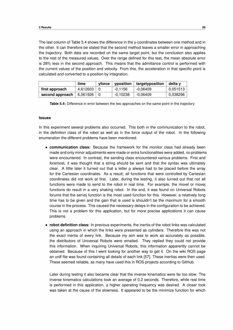
5 Results 89
The last column of Table 5.4 shows the difference in the y-coordinates between one method and inthe other. It can therefore be stated that the second method leaves a smaller error in approachingthe trajectory. Both data are recorded on the same target point, but the conclusion also appliesto the rest of the measured values. Over the range defined for this test, the mean absolute erroris 28% less in the second approach. This means that the admittance control is performed withthe current values of the position and velocity. From this, the acceleration in that specific point iscalculated and converted to a position by integration.
time yforce yposition targetyposition delta yfirst approach 4,612603 0 -0,1156 -0,06409 0,051513second approach 6,061926 0 -0,10238 -0,06409 0,038296
Table 5.4: Difference in error between the two approaches on the same point in the trajectory
Issues
In this experiment several problems also occurred. This both in the communication to the robot,in the definition class of the robot as well as in the force output of the robot. In the followingenumeration the different problems have been mentioned.
• communication class: Because the framework for the monitor class had already beenmade and only minor adjustments were made or extra functionalities were added, no problemswere encountered. In contrast, the sending class encountered various problems. First andforemost, it was thought that a string should be sent and that the syntax was ultimatelyclear. A little later it turned out that a letter p always had to be placed before the arrayfor the Cartesian coordinates. As a result, all functions that were controlled by Cartesiancoordinates did not work at first. Later, during the testing, it also turned out that not allfunctions were made to send to the robot in real time. For example, the movel or movejfunctions do result in a very shaking robot. In the end, it was found on Universal Robotsforums that the servoj function is the most used function for this. However, a relatively longtime has to be given and the gain that is used is shouldn’t be the maximum for a smoothcourse in the process. This caused the necessary delays in the configuration to be achieved.This is not a problem for this application, but for more precise applications it can causeproblems.
• robot definition class: In previous experiments, the inertia of the robot links was calculatedusing an approach in which the links were presented as cylinders. Therefore this was notthe exact inertia of every link. Because my aim was to work as accurately as possible,the distributors of Universal Robots were emailed. They replied they could not providethis information. When inquiring Universal Robots, this information apparently cannot beobtained. Because of this I went looking for another way to get it. On the wiki ROS pagean urdf file was found containing all details of each link [57]. These inertias were then used.These seemed reliable, as many have used this in ROS projects according to GitHub.
Later during testing it also became clear that the inverse kinematics were far too slow. Theinverse kinematics calculations took an average of 0.2 seconds. Therefore, while real timeis performed in this application, a higher operating frequency was desired. A closer lookwas taken at the cause of the slowness. It appeared to be the minimize function for which
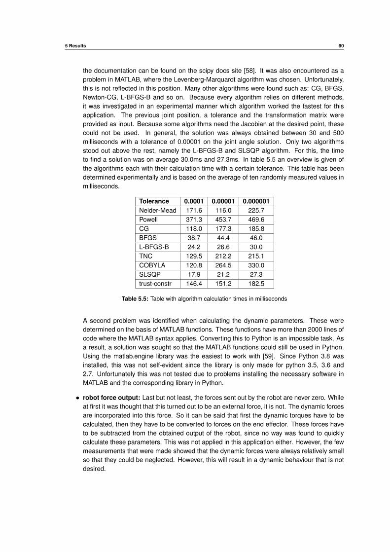
5 Results 90
the documentation can be found on the scipy docs site [58]. It was also encountered as aproblem in MATLAB, where the Levenberg-Marquardt algorithm was chosen. Unfortunately,this is not reflected in this position. Many other algorithms were found such as: CG, BFGS,Newton-CG, L-BFGS-B and so on. Because every algorithm relies on different methods,it was investigated in an experimental manner which algorithm worked the fastest for thisapplication. The previous joint position, a tolerance and the transformation matrix wereprovided as input. Because some algorithms need the Jacobian at the desired point, thesecould not be used. In general, the solution was always obtained between 30 and 500milliseconds with a tolerance of 0.00001 on the joint angle solution. Only two algorithmsstood out above the rest, namely the L-BFGS-B and SLSQP algorithm. For this, the timeto find a solution was on average 30.0ms and 27.3ms. In table 5.5 an overview is given ofthe algorithms each with their calculation time with a certain tolerance. This table has beendetermined experimentally and is based on the average of ten randomly measured values inmilliseconds.
Tolerance 0.0001 0.00001 0.000001Nelder-Mead 171.6 116.0 225.7Powell 371.3 453.7 469.6CG 118.0 177.3 185.8BFGS 38.7 44.4 46.0L-BFGS-B 24.2 26.6 30.0TNC 129.5 212.2 215.1COBYLA 120.8 264.5 330.0SLSQP 17.9 21.2 27.3trust-constr 146.4 151.2 182.5
Table 5.5: Table with algorithm calculation times in milliseconds
A second problem was identified when calculating the dynamic parameters. These weredetermined on the basis of MATLAB functions. These functions have more than 2000 lines ofcode where the MATLAB syntax applies. Converting this to Python is an impossible task. Asa result, a solution was sought so that the MATLAB functions could still be used in Python.Using the matlab.engine library was the easiest to work with [59]. Since Python 3.8 wasinstalled, this was not self-evident since the library is only made for python 3.5, 3.6 and2.7. Unfortunately this was not tested due to problems installing the necessary software inMATLAB and the corresponding library in Python.
• robot force output: Last but not least, the forces sent out by the robot are never zero. Whileat first it was thought that this turned out to be an external force, it is not. The dynamic forcesare incorporated into this force. So it can be said that first the dynamic torques have to becalculated, then they have to be converted to forces on the end effector. These forces haveto be subtracted from the obtained output of the robot, since no way was found to quicklycalculate these parameters. This was not applied in this application either. However, the fewmeasurements that were made showed that the dynamic forces were always relatively smallso that they could be neglected. However, this will result in a dynamic behaviour that is notdesired.

6Conclusions
91
6 Conclusions 92
The goal of this dissertation was to create a force compliant controller and use it in an application.For this purpose, a fluent thesis has been provided with all the necessary information to bring this toa successful conclusion. Starting with the necessary knowledge and ending with some experimentsand results.
This thesis mainly contains all the content that is needed to: (1) understand the kinematics of arobot, (2) describe the dynamics of a robot with multiple degrees of freedom, (3) choose a forcecontrol method and (4) apply all of this to a two or six degrees of freedom application. In addition,several things have been discussed such as the neglectable influence of the dynamics in the controlloop and why for example it is not recommended to do force control in joint space.
In the first experiments, namely the one’s in MATLAB, the admittance control loop was tested witha simple example such as a two degrees of freedom application with a fixed target. This applicationwas gradually extended to an application with two degrees of freedom where a moving target wasgiven. Finally a six degrees of freedom application was made in MATLAB where a fixed target hadto be reached as well. After this, the switch was made to a Python controller for the UR3 robot.
In this Python admittance controller, different classes were created for this robot in order to establishcommunication between the program and the UR3 robot on the one hand, and to obtain a desiredrobot path and behaviour on the other hand. This program was tested and the obtained results werediscussed. A correct operation is obtained in which the predetermined goal was achieved, namelyto create a path tracking application in which an external force results in a defection. However, thiswas only tested in the URSim simulation environment due to the COVID-19 pandemic. A secondapplication using admittance control is discussed in theory during the experiments, but was notmade due to lack of time and the unavailability of labs due to the pandemic.
In the end, it is clear that this thesis created a profound base for future research and educationpurposes. People who are not yet familiar with robot arms and want to learn something about themquickly, can make use of the literature study. Those who start working with a robot from UniversalRobots in combination with Python, will mainly find information in the written Python code that isavailable on GitHub [49]. Those who would like to know more about admittance control and how itworks can consult this thesis and the MATLAB examples.
7Bibliography
[1] F. C. P. Kevin M. Lynch, MODERN ROBOTICS MECHANICS, PLANNING, AND CONTROL,2017.
[2] R. S. Andersen, “Kinematics of a ur5.”
[3] J. Dinesh, Robu.in.
[4] R. Y. A., “Geometric jacobians derivation and kinematic singularity analysis for smokie robotmanipulator and the barrett wam,” 5th International Conference on Robotics and Mechatronics(ICROM), 2017.
[5] “Motor description,” ctrl-elec. [Online]. Available: http://www.ctrl-elec.fr/ctrl-clec/commande-de-moteur/commande-mcc/modelisation-et-commande-dun-moteur-cc/
[6] D. I. D. Vanoost, “Dc-drives,” 2018, course slides.
[7] S. L. Yoonho Kim, German A. Parada and X. Zhao, “Ferromagnetic soft continuum robots,”Science Robotics, vol. 4, no. 33, August 2019.
[8] G. Jeronimidis, “Materials strategies and systems for soft robotics,” 2014. [Online]. Available:http://www.robosoftca.eu/public downloads/plenary1/RoboSoft GeorgeJeronimidis.pdf
[9] C. P. Gabriel Felippe, “Desenvolvimento e implementaCao do controle de uma mao roboticado tipo multifinger,” p. 9, December 2014.
[10] P. F. Andrea Calanca, Riccardo Muradore, “A review of algorithms for compliant control of stiffand fixed-compliance robots,” IEEE/ASME TRANSACTIONS ON MECHATRONICS, vol. 21,no. 2, pp. 613–624, April 2016.
[11] A. W. Tomasz Winiarski, “Indirect force control development procedure,” Cambridge UniversityPress: Robotica, vol. 31, pp. 465–478, July 2012.
93

7 Bibliography 94
[12] D. M. Sergio A. Pertuz, Carlos H. Llanos, “Simulation and implementation of impedancecontrol in robotic hand,” 24th ABCM International Congress of Mechanical Engineering, 2017.
[13] A. H. Ganwen Zeng, “An overview of robot force control,” Cambridge University Press, vol. 15,no. 1, pp. 473–482, December 1996.
[14] Y. N. Christian Ott, “Admittance control using a base force or torque sensor,” pp. 1–6.
[15] M. S. C. DEDE, “Position/force control of robot manipulators,” Master’s thesis, THEGRADUATE SCHOOL OF NATURAL AND APPLIED SCIENCES OF THE MIDDLE EASTTECHNICAL UNIVERSTY, 2003.
[16] R. N. J. Mohamed Elbanhawi, Milan Simic, “Continuous path smoothing for car-like robotsusing b-spline curves,” Journal of Intelligent and Robotic Systems, January 2015.
[17] L. V. G. O. Bruno Siciliano, Lorenzo Sciavicco, Robotics Modelling, Planning and Control,2009.
[18] V. Hlavac, “Robot trajectory generation,” 2009, p. 161-189.
[19] “Universal robots ur3,” Universal Robots. [Online]. Available: https://www.robots.com/robots/universal-robots-ur3
[20] UR3 Service manual, Universal Robots. [Online]. Available: https://www.pi4.de/fileadmin/material/Produktkatalog/Universal Robots/pdf components partner/UR3 docs en/ServiceManual UR3 en 3.1.3.pdf
[21] “Max. joint torques - 17260,” Universal Robots. [Online]. Available: https://www.universal-robots.com/how-tos-and-faqs/faq/ur-faq/max-joint-torques-17260/
[22] “Real-time data exchange (rtde) guide,” Universal Robots. [Online]. Available: https://www.universal-robots.com/articles/ur-articles/real-time-data-exchange-rtde-guide/
[23] A. S. Tanenbaum and D. J. Wetherall, Computer Networks, 2012.
[24] D. S. Aditya Sundararajan, Aniket Chavan and A. I. Sarwat, “A survey of protocol-levelchallenges and solutions for distributed energy resource cyber-physical security,” Energies,September 2018.
[25] “Overview of client interfaces,” Universal Robots. [Online].Available: https://www.universal-robots.com/how-tos-and-faqs/how-to/ur-how-tos/overview-of-client-interfaces-21744/
[26] “13 unique features of python programming language,” Data Flair. [Online]. Available:https://data-flair.training/blogs/features-of-python/
[27] V. S. Lavdim KurtaJ, Ilir Limani, “Dependence of cmac neural network properties at initial,during, and after learning phase from input mapping function,” ResearchGate, August 2012.
[28] “Parameters for calculations of kinematics and dynamics,” UniversalRobots. [Online]. Available: https://www.universal-robots.com/articles/ur-articles/parameters-for-calculations-of-kinematics-and-dynamics/
7 Bibliography 95
[29] E. Y. G. Wei Wang, Robert N.K. Loh, “Passive compliance versus active compliance inrobotbased automated assembly systems,” Industrial Robot, vol. 25, no. 1, pp. 48–57, 1998.
[30] P. Corke, Robotics, vision and control, 2017.
[31] Z. X. W. L. Q. Asghar khan, Cheng Xiangming, “Closed form inverse kinematics solutionfor 6-dof underwater manipulator,” IEEE/International Conference on Fluid Power andMechatronics, pp. 1171–1176, August 2015.
[32] P. Corke, “Peter corke toolbox.” [Online]. Available: http://petercorke.com/wordpress/toolboxes
[33] D. S. Singh, “Key slides from lectures 1-5 robotics and automation,” 2018, homework fromcourse ”Robotic Manipulation and Mobility” given by Dr. V. Krovi.
[34] G. Terorde, Electrical Drives and Control Techniques, 2009.
[35] A. Sabanovic and K. Ohnishi, MOTION CONTROL SYSTEMS, 2011.
[36] H. Neville, “Impedance control of industrial robots,” Robotics and Computer-IntegratedManufacturing, vol. 1, no. 1, pp. 97–113, 1984.
[37] M. W. S. Robert J. Anderson, “Hybrid impedance control of robotic manipulators,”IEEE/JOURNAL OF ROBOTICS AND AUTOMATION, vol. 4, no. 5, pp. 549–556, October1988.
[38] G. H. Friedrich Lange, Mirko Frommberger, “Is impedance-based control suitable for trajectorysmooting,” pp. 1–6, 2006.
[39] S. C. Hrishi Shah, “Kinematic and dynamic control of a two link manipulator,” homework fromcourse ”Robotic Manipulation and Mobility” given by Dr. V. Krovi.
[40] C. X. Yimei Chen, Dapeng Wu, “Nonlinear direct robust adaptive control using control lyapunovmethod,” TELKOMNIKA Indonesian Journal of Electrical Engineering, vol. 12, no. 1, pp.477–486, January 2014.
[41] O. B. Haifa Mehdi, “Stiffness and impedance control using lyapunov theory for robot- aidedrehabilitation,” International Journal of Social Robotics, vol. 4, no. 1, pp. 107–119, November2012.
[42] User Manual, Universal Robots. [Online]. Available: https://www.usna.edu/Users/weaprcon/kutzer/ files/documents/User%20Manual,%20UR3.pdf
[43] G. McMillan, “Socket programming howto,” Python. [Online]. Available: https://docs.python.org/3/howto/sockets.html
[44] R. J. T. L. YoonSeok Pyo, HanCheol Cho, ROS Robot Programmingfrom the basic concept to practical programming and robot application,December 2017. [Online]. Available: http://www.pishrobot.com/wp-content/uploads/2018/02/ROS-robot-programming-book-by-turtlebo3-developers-EN.pdf
[45] L. Joseph, Robot Operating System (ROS) for Absolute Beginners, 2018.
7 Bibliography 96
[46] “Impedance control for a 2-link robot arm - user-interactive,”Mathworks. [Online]. Available: https://nl.mathworks.com/matlabcentral/fileexchange/57853-impedance-control-for-a-2-link-robot-arm-user-interactive
[47] “Python-urx,” Sintef Manufacturing. [Online]. Available: https://github.com/SintefManufacturing/python-urx
[48] “Universal robots support download,” Universal Robots. [Online]. Available: https://www.universal-robots.com/download/?option=18940
[49] M. Detailleur, Github.
[50] The URScript Programming Language, Universal Robots. [Online]. Available: http://www.me.umn.edu/courses/me5286/robotlab/Resources/scriptManual-3.5.4.pdf
[51] A. Dua, “robopy.” [Online]. Available: https://github.com/adityadua24/robopy
[52] N. Majcherczyk, “Seven link manipulator.” [Online].Available: https://github.com/NathalieMajcherczyk/RBE501-Balancing-Posture/tree/ce87f3e0ccd2db2fd812658cafb6d46b749ba125/SevenLinkManipulator
[53] P. L. M. v. d. W. Matthijs Boerlage, Maarten Steinbuch, “Model-based feedforward formotion systems,” IEEE International Conference on Control Applications (CCA), vol. 2, pp.1158–1163, June 2003.
[54] “Inverse kinematics algorithms,” Mathworks. [Online]. Available: https://nl.mathworks.com/help/robotics/ug/inverse-kinematics-algorithms.html
[55] W. J. L. Mohd. Asrul Hery Bin Ibrahim, Mustafa Mamat, “Bfgs method: A new search direction,”Sains Malaysiana, vol. 43, pp. 1593–1599, October 2014.
[56] M. I. A. Lourakis, “A brief description of the levenberg-marquardt algorithm implemened,”February 2005.
[57] “Ur3 joint limited robot urdf xacro,” ROS. [Online]. Available: http://ros.org/wiki/xacro
[58] “scipy.optimize.minimize,” SciPy. [Online]. Available: https://docs.scipy.org/doc/scipy/reference/generated/scipy.optimize.minimize.html
[59] “Calling matlab from python,” MathWorks. [Online]. Available: https://nl.mathworks.com/help/matlab/matlab-engine-for-python.html

AAttachments
97

A Attachments 98
A.1 Classes diagram Python controller
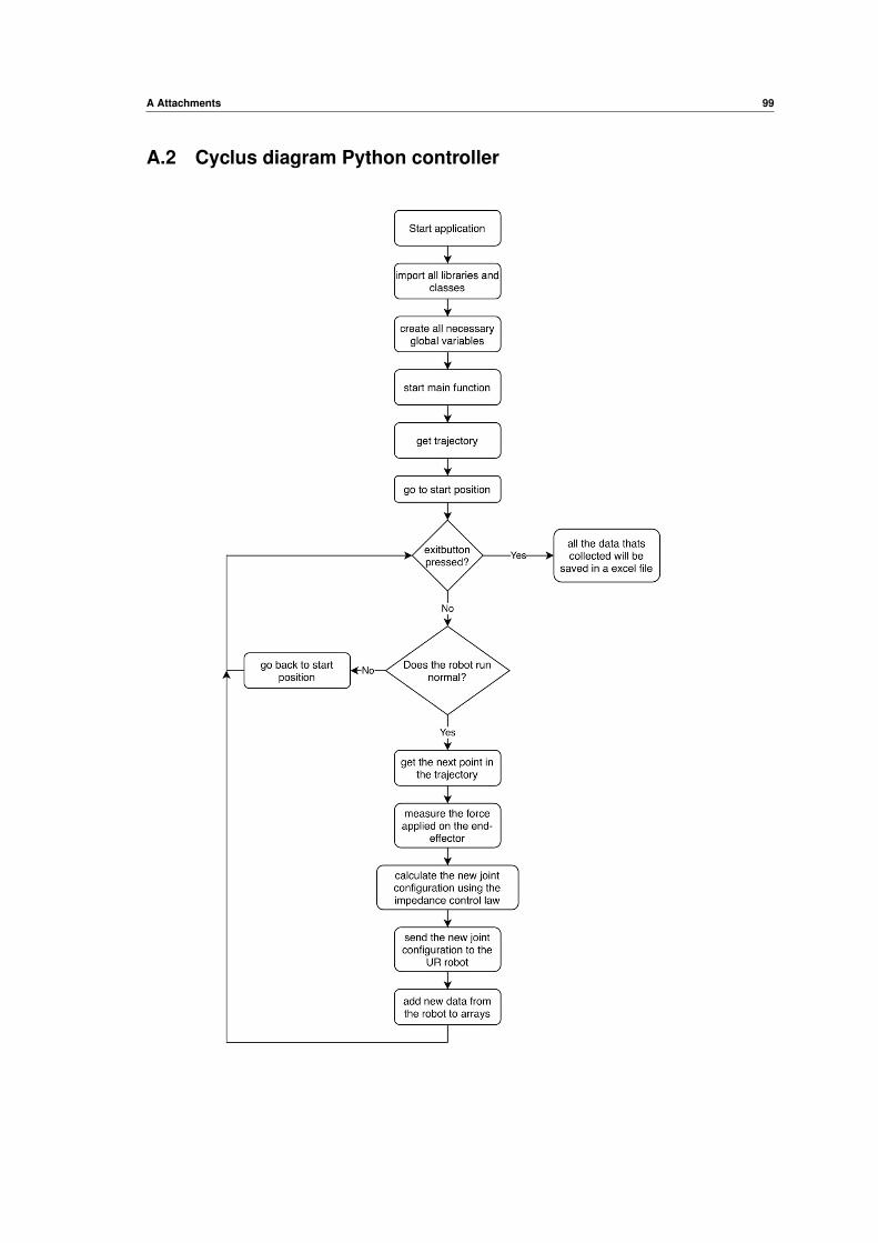
A Attachments 99
A.2 Cyclus diagram Python controller


FACULTEIT INDUSTRIËLE INGENIEURSWETENSCHAPPEN CAMPUS BRUGGE Spoorwegstraat 12
8200 BRUGGE, België tel. + 32 50 66 48 00
[email protected] www.iiw.kuleuven.be
101