Deterministic Latent Variable Models and their Pitfalls

Max Welling∗ Chaitanya Chemudugunta Nathan SutterBren School of Information and Computer Science

University of California, Irvine{welling,chandra,nsutter}@ics.uci.edu

Abstract

We derive a number of well known deterministic latent variablemodels such as PCA, ICA, EPCA, NMF and PLSA as variationalEM approximations with point posteriors. We show that the oftenpracticed heuristic of “folding-in” can lead to overly optimisticestimates of the test-set log-likelihood and we verify this resultexperimentally. We trace this problem back to an infinitely negativeentropy term that is ignored in the variational approximation.

1 Introduction

Deterministic latent variable models (DLVM) such asK-means, PCA, NMF [10], PLSA [1] and EPCA [2] arepopular data-analysis tools in the machine learning anddata-mining communities. The latent variables in thesemodels become deterministic because they are set to theirMAP (maximum a posteriori) values1. In the context ofPLSA, it has been observed in the literature (see e.g. [5])that this seriously complicates its interpretation as a validprobabilistic model over the space of all allowable inputconfigurations. In fact, one could argue that the resultingmodel assigns zero probability to all input configurationsthat are not in the training set. To enable PLSA to as-sign non-zero probability to test-set data configurations,researchers proposed the heuristic of “folding-in”[1]. Thefolding-in procedure first assigns the latent variables of thetest-datato their MAP values before computing the test-setperplexity. In [5], it is mentioned that this procedure wouldgive an unfair advantage to PLSA because “parameters arefit on the test-data”. One of the conclusions of our analysisis that this characterization does not clarify the real problem.

We approach this issue through the variational-EM(VEM) framework [7]. This framework has the distinctadvantage of shifting the approximation from the model tothe learning and testing ofalgorithms. Moreover, PLSA cannow be seen to fall in line with a long tradition of similarapproximations underlying algorithms such as K-means,PCA, NMF, and sparse ICA. In the VEM framework, we

∗At the time of submission M. Welling was on sabbatical at the RadboudUniversity Nijmegen, Netherlands, Dept. of Biophysics

1For PLSA this fact was recently shown in [3, 4].

bound the training (or testing) log-likelihood by approxi-mating the posterior distribution of the latent variables by aparameterized family of tractable distributions over the sameinput space. We show that DLVMs withdiscretelatent vari-ables can be obtained by approximating the true posteriordistribution by a simplistic variational substitute, namely adelta-peak at its MAP value. In this case, learning DLVMsbecomes an instance of variational EM. However, thisapproach also reveals the pitfall for deterministiccontinuouslatent variables: in the continuous case the entropy term ofthe variational distribution becomes−∞ and ignoring itviolates the bounding property of the variational objective.Using this perspective, we show that the standard learningalgorithms for PLSA and EPCA optimize an objectivefunction that is numerically unrelated to the log-likelihoodor a bound thereof.

Perhaps the most important conclusion is that thefolding-in heuristic for continuous DLVMs, as it is routinelyused in the research community, can lead to hugely opti-mistic estimates of test-set perplexity. We argue that this ef-fect worsens in high dimensional spaces and in cases wherethe posterior is highly concentrated. This conclusion, how-ever, isnot valid for discrete latent variables (where the en-tropy term is actually0) or for mean field approaches (wherethe entropy term is finite and taken into account), in fact inthose cases we can show that folding-in will lead to pes-simistic estimates of test-set perplexity (i.e. an upper bound).Our explanation is, therefore, intrinsically different to theone offered in [5] because one also seemingly fits (varia-tional) parameters on test-data for the cases above but herethey only pessimistically bias the result.

We thoroughly investigated these issues empirically bycomparing different models (different versions of PLSA,EPCA and LDA) with different objective measures (perplex-ity using folding-in based on all and half of the words in thetest document, which we refer to as full folding-in and halffolding-in respectively) on various datasets. As predicted,full folding-in gives much lower (that is, better) perplexityresults than half folding-in. Moreover, the perplexity resultswith full folding-in keep improving as we increase the num-

196

ber of topics, never showing any sign of overfitting (unlikehalf folding-in where we can not “cheat” in any way).

2 Variational EM with Point Estimates

Letx be a collection of observable (visible) random variablesand h be a collection of unobservable (hidden) randomvariables2. The joint probability distribution of a two-layerdirected model is defined as follows,

(2.1) pθ(x,h) = pν(x|h) pγ(h).

We have introduced parametersθ = {ν, γ} which could bevector valued. Estimation of these parameters from the datacan be done conveniently in the expectation maximization(EM) framework. It can be shown that the following objec-tive is a lower bound on the log-likelihood [6],

B(θt|θt−1, X) = Q(θt|θt−1) +H(θt−1) =(2.2)∑

n

∑

hn

pθt−1(hn|xn) log [pνt

(xn|hn)pγt(hn)]

−∑

n

∑

hn

pθt−1(hn|xn) log

[

pθt−1(hn|xn)

]

where X indicates the data-matrix. This bound isiteratively maximized over the parametersθt = {νt, γt},keepingθt−1 fixed. Since the last term, which is the entropyof the posterior at timet − 1, does not depend onθt, it canbe ignored in the optimization process. It is not hard to showthat the following identity holds,(2.3)L(θt) = B(θt|θt−1) + KL[pθt−1

(hn|xn)||pθt(hn|xn)]

where KL is the Kullback-Leibler divergence. This equationconfirms that the log-likelihood is larger than or equal tothe bound,L ≥ B and that the bound saturates whenpθt−1

(hn|xn) = pθt(hn|xn), i.e. L(θt) = B(θt|θt). The

above analysis is easily repeated in a slightly more generalsetting where the posterior at timet − 1 is replaced withan arbitrary variational distribution over the hidden variables[7],

(2.4) pθ(hn|xn)→ qα(hn|xn)

The parametersα will be optimized in the variational esti-mation (VE) step in such a way that the bound is made astight as possible. Note that this now also involves the en-tropy term in Equation 2.2 because it explicitly depends onqα. Often, the family of distributionsqα does not containthe actual posterior distribution, in which case the bound isnever tight. Given the updatedqα distributions, we can do

2In the following we will use the words “latent”, “hidden” and “unob-servable” interchangeably.

a variational maximization (VM) step whereQ(θt|αt−1) ismaximized overθt. In the following we will make a veryspecial choice of this variational distribution, namely,

(2.5) qhn

(hn|xn) = δ(hn − hn) =∏

j

δ(hjn − hjn)

where the variational parameters are given by{hin}. Notethat there is a separate parameter for every hidden variableand for every data-case.

If h takes discrete values then the entropy of the dis-tribution in Equation 2.5 is zero. This, however, is not truefor continuous variables. In cases where the domain ofh

is unbounded we can, for instance, define the delta func-tion as the limit of an isotropic Gaussian distribution withdecreasing variance. Since the entropy of a Gaussian dis-tribution is given byD log(σ

√2πe), the entropy converges

to −∞ as σ → 0. Similarly, if h is continuous but nor-malized,

∑

j hj = 1, we can model a delta-function as thelimit of a Dirichlet distributionD(εα) whenε → ∞. Us-ing Sterling’s approximation one can then determine that theentropy converges to−∞ as 1−J

2log ε whenε → ∞ where

J is the number of latent variables (i.e. the dimension ofh). From this we conclude that for continuous latent vari-ables the MAP approximation leads to an infinitely negativeentropy contribution to the variational objective. Ignoring itrenders the resulting objective numerically unrelated to thelog-likelihood. As we will show in the next sections, wellknown learning algorithms for EPCA [2] and PLSA [1] canprecisely be interpreted as maximizing the variational ob-jective with variational point posteriors andignoring the in-finitely negative entropy contribution, i.e. maximizing

(2.6) O(θ, h) =∑

n

log[

pν(xn|hn)]

+∑

n

log[

pγ(hn)]

The VEM algorithm then consists of a VE-step where wemaximizeO over{hn} and a VM-step where we maximizeit overθ = {ν, γ}.

In the following we will provide some examples ofalgorithms that fall under this umbrella.

3 Examples of Deterministic Latent Variable Models

To appreciate the unifying principle of VEM, we derivethe following well known algorithms in the machine learn-ing literature as VEM approximations of other algorithms:K-means, Pricipal Component Analysis (PCA), Indepen-dent Component Analysis (ICA), Non-negative Maxtrix Fac-torization (NMF), Probabilistic Latent Semantic Analysis(PLSA) and Exponential family PCA (EPCA).

3.1 K-Means We start with the mixture of Gaussians(MoG) model where the discrete hidden variables take val-ues in1, ..., K with K being the total number of mixture

197

components,

(3.7) pmog(x, h = k) = Nµk,Σk

(x|h = k)pπk(h = k)

If we use point posteriors of the form shown in Equation2.5 then, since the latent variables are discrete, the entropycontribution of the variational posterior is zero,S = 0.Hence, we find the following VEMbound on the log-likelihood,

B =∑

n

∑

k

δhn,k

[

−1

2(xn − µk)T Σ−1

k (xn − µk)

−1

2log detΣk + log (πk)

]

(3.8)

Alternating optimization over{hn} and {µk, Σk, πk}represents a generalized K-means algorithm where we havethe opportunity to fit full covariance matrices and mixtureweights for each cluster. If we chooseπk = 1/K andΣk = σI with some fixed value forσ, then the non-constantterms in the bound are proportional to,

(3.9) B′ = −1

2

∑

n

∑

k

δhn,k

[

(xn − µk)2]

which is, of course, the (negative) K-means objective.VE and VM steps then indeed correspond to K-means. Thisshows that K-means is a VEM approximation of MoG.

A related example is given by “Viterbi-HMM”. In thiscase, one alternates Viterbi decoding in the E-step with theusual parameter updating in the M-step. This algorithm alsomaximizes a proper lower bound on the log-likelihood.

3.2 PCA and ICA We start with the Factor analysis modelwith normal variables both in the hidden and in the visiblelayer. The visible variables are noisy versions of linearcombinations of fewer hidden factors,x = Wh + ε withε an axis aligned Gaussian noise variable with diagonalcovarianceΣ. h is also distributed according to a standardnormal distribution,

(3.10) p(x,h) = GW,Σ(x|h)∏

j

G(hj)

In this case the latent variables are continuous, hence varia-tional point posteriors lead to an infinitely negative entropycontribution. Simply ignoring this term leads to the follow-ing objective,

O = −1

2

∑

n

[

(xn −W hn)T Σ−1(xn −W hn)

+ log detΣ + ||hn||2L2

]

(3.11)

UsingΣ = λI, definingO′ = λO and taking the limitλ→ 0, we find,

(3.12) O′ = −1

2

∑

n

[

(xn −W hn)T (xn −W hn)]

as our objective. The VE-step is obtained by maximiz-ing this w.r.t. the variational variablesH = {hjn} while theVM-step optimizes this bound w.r.t.W ,

W ← (XHT )(HHT )−1(3.13)

H ← (WWT )−1(WT X)(3.14)

whereX = {xin} . This is precisely the SPCA algorithmderived in [12].

Above we have taken the limitλ → 0 which has theeffect of nullifying the prior. For independent componentanalysis, the prior is essential. In this case we should usea non-Gaussian, factorized prior forh with high kurtosis,p(h) =

∏

j pj(hj). If we choose a Laplace prior we shouldsimply replace theL2 norm in Equation 3.11 with anL1

norm. In trying to maximize this bound one quickly findsout thatH = 0 is the optimal solution due to the fact thata transformation of the formW → WT andH → T−1Hleaves the first term invariant but can be used to set the priorterm onh to zero. This phenomenon is a direct consequenceof ignoring the entropy. The entropy term, if included,would have induced a counteracting “force” that would haveprevented the collapse ofh.

In this case we can however salvage the algorithm byrequiring that the columns ofW be normalized. This wasindeed the approach taken in [11]. Their approximationtranslates to an even simpler VEM approximation, namelyq(h) = δ(h − h) independent ofn. For ICA, the VE andVM steps can not be solved analytically. However, one canalternate gradient steps forW andH until convergence.

3.3 Non-negative Matrix Factorization Non-negativematrix factorization (NMF) [10] is a method where a posi-tive matrix is factorized into two positive lower rank matri-ces. To derive it from VEM, we use a conditional Poissondistribution for the observed variables and write the Poissonrate as a linear combination of hidden factors,

(3.15) p(x|h) =∏

i

(∑

j Wijhj)xi

xi!exp[−

∑

j

Wijhj ]

Applying the point-VEM approximation and again ig-noring the infinitely negative entropy we derive the objec-tive,(3.16)

O =∑

i,n

xin log[∑

j

Wij hjn]−∑

j

Wij hjn − log(xin!)

198

Since the Poisson rate is positive, the same must be truefor WH which is achieved by separately constraining bothto be positive. We now bound the non-constant part of theobjectiveB ≤ O + log(xi!), with

B =

∑

i,n

∑

j

xinQin(j) log(Wij hjn)−∑

j

Wij hjn + S(Qin)

where

(3.17) Qin(j) =Wij hjn

∑

j′ Wij′ hj′n

and S(Q) is its entropy. In [10], the authors add theconstraint

∑

i Wij = 1 to reduce the degeneracy associatedwith W → WT andH → T−1H . Adding the appropriateLagrange multipliers we find the following EM updates3,which are equal to the NMF update rules of [10],

Wij ← 1

γj

Wij

∑

n

XinHjn

[WH ]in(3.18)

Hjn ← Hjn

∑

i

XinWij

[WH ]in(3.19)

whereγj is a constant to normalizeWij overi.The authors actually relax the constraint on the discrete-

ness ofx by noting that the objectiveB still makes sense inthis more general setting.

3.4 Probabilistic Latent Semantic Analysis The insightthat PLSA can be viewed as a MAP estimate of LDA waspublished in [4], while very similar remarks on the relationbetween LDA and PLSA were also noted in [3]. Here, wewill re-derive those results in the variational EM frameworkand show the striking similarity to NMF.

Let us consider an LDA model ([5]). The conditionalprobability in this case is a multinomial distribution whilethe prior on the factors is given by a Dirichlet distribution,

(3.20) p(x,h) =

∏

i

∑

j

Wijhj

xi

Dh[α]

whereWij is the probability of wordi for topic j. xi

is the count of the number of times wordi is sampled andhj is the prior probability that topicj is used. To make aconnection to PLSA we use the variational approximation

3Note that this EM algorithm does not refer to the same variational EMargument to derive the objectiveO. So, one could say that this an EMalgorithm within a VEM algorithm.

with point posteriors and choose a constant prior,α =1. Note that since we have continuous latent variables wewill ignore an infinitely negative entropy contribution in thevariational objective to arrive at the following objective,

(3.21) O =∑

i,n

xin log

∑

j

Wij hjn

plus two Lagrange multiplier terms to enforce∑

i Wij = 1 and∑

j hjn = 1.Analogous to the derivation for NMF, we can now

boundO with B ≤ O, and(3.22)

B =∑

i,n

∑

j

xinQin(j) log(Wij hjn) + S(Qin)

whereS(Q) is the entropy ofQ. Again, we should alsoinclude the Lagrange multiplier terms which we left outfor convenience. This bound is valid for any variationaldistribution Q, but the expression that maximizes (in factsaturates) the bound is given by,

(3.23) Qin(j) =Wij hjn

∑

j′ Wij′ hj′n

This can be viewed as the E-step of an EM algorithm.The M-step is then given by fixingQ and maximizing overW, h. Combining E and M steps, we find the followingupdate equations that are guaranteed to improveO,

Wij ←1

γj

Wij

∑

n

XinHjn

[WH ]in(3.24)

Hjn ←1

λn

Hjn

∑

i

XinWij

[WH ]in

which are identical to NMF except for an extra normal-ization ofH . Retaining Dirichlet priors in the derivation forbothW andH would translate into constant off-sets in theupdate equation 3.24.

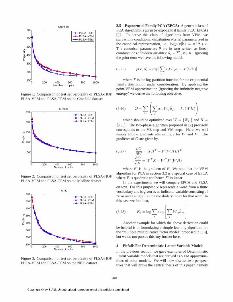
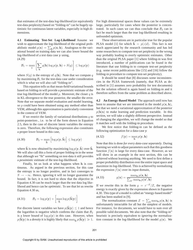
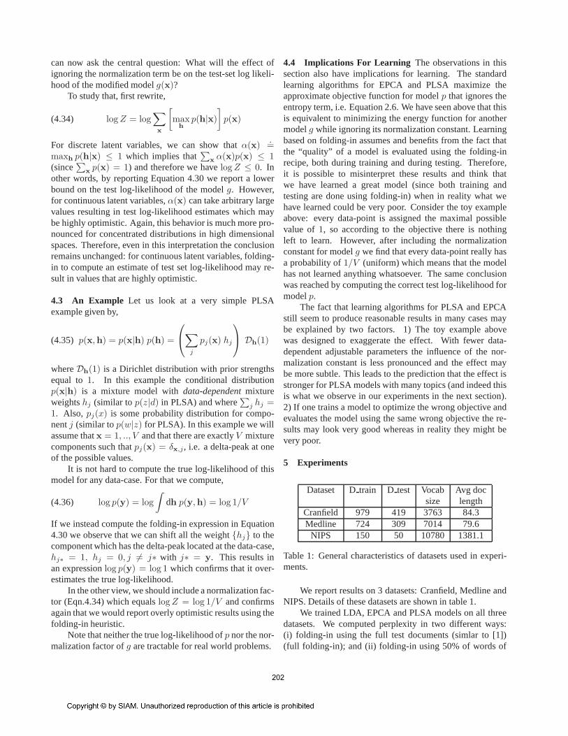
To connect this to the PLSA updates derived in [1]we note that this model contains three factors:p(w|z),p(d|z) andp(z). We can absorbp(z) into p(d|z) and re-parameterize asp(z|d) ∝ p(d|z)p(z). The factorp(d) thatremains in this parametrization is chosen constant (each doc-ument has the same weight). If we make the identificationWij ↔ p(w|z) andHjn ↔ p(z|d), then the model and thelearning updates become identical to those in [1]. In figures1,2 and 3 we have verified that the standard PLSA imple-mentation of [1] indeed gives almost identical results to theupdates derived above.

199

0 200 400 600 800 1000100

200

300

400

500

600

700

Number of topics

Per

plex

ityCranfield

PLSA−HOFPLSA−VEMPLSA−TEM

Figure 1: Comparison of test set perplexity of PLSA-HOF,PLSA-VEM and PLSA-TEM on the Cranfield dataset

0 200 400 600 800 10000

500

1000

1500

2000

2500

Number of topics

Per

plex

ity

Medline

PLSA−HOFPLSA−VEMPLSA−TEM

Figure 2: Comparison of test set perplexity of PLSA-HOF,PLSA-VEM and PLSA-TEM on the Medline dataset

0 200 400 600 800 10002000

2200

2400

2600

2800

3000

3200

3400

Number of topics

Per

plex

ity

NIPS

PLSA−HOFPLSA−VEMPLSA−TEM

Figure 3: Comparison of test set perplexity of PLSA-HOF,PLSA-VEM and PLSA-TEM on the NIPS dataset

3.5 Exponential Family PCA (EPCA) A general class ofPCA algorithms is given by exponential family PCA (EPCA)[2]. To derive this class of algorithms from VEM, westart with a conditional distributionp(x|h) parameterized inthe canonical representation, i.e.log p(x|h) = xT θ + c.The canonical parametersθ are in turn written as linearcombinations of hidden variables:θi =

∑

j Wijhj . Ignoringthe prior term we have the following model,

(3.25) p(x,h) = exp[∑

i,j

xiWijhj − F (Wh)]

whereF is the log-partition function for the exponentialfamily distribution under consideration. By applying thepoint-VEM approximation (ignoring the infinitely negativeentropy) we derive the following objective,

(3.26) O =∑

i,n

∑

j

xinWij hjn − Fn(WH)

which should be optimized overW = {Wij} andH =

{hjn}. The two-phase algorithm proposed in [2] preciselycorresponds to the VE-step and VM-steps. Here, we willsimply follow gradients alternatingly forW and H . Thegradients ofO are given by,

∂O∂W

= XHT − F ′(WH)HT(3.27)

∂O∂H

= WT X −WT F ′(WH)

whereF ′ is the gradient ofF . We note that the VEMalgorithm for PCA in section 3.2 is a special case of EPCAwhereF is quadratic and henceF ′ is linear.

In the experiments we will compare EPCA and PLSAon text. For this purposex represents a word from a finitevocabulary and is given as an indicator variable consisting ofzeros and a single1 at the vocabulary index for that word. Inthis case we find that,

(3.28) Fn = log∑

i

exp

∑

j

Wij hjn

Another example for which the above derivation couldbe helpful is in formulating a simple learning algorithm forthe “multiple multiplicative factor model” proposed in [13],but we do not pursue this any further here.

4 Pitfalls For Deterministic Latent Variable Models

In the previous section, we gave examples of DeterministicLatent Variable models that are derived as VEM approxima-tions of other models. We will now discuss two perspec-tives that will prove the central thesis of this paper, namely

200

that estimates of the test-data log-likelihood (or equivalentlytest-data perplexity) based on “folding-in” can be hugely op-timistic for continuous latent variables, especially in high di-mensions.

4.1 Estimating Test-Set Log-Likelihood Assume wewish to approximate the log-likelihood of the original prob-abilistic modelp(x) =

∑

hp(x,h). Analogous to the vari-

ational bound on training data we can also lower bound thelog-likelihood of atestdata casey using,(4.29)

B1 = maxq

[

∑

h

q(h) log p(y,h) + S(q)

]

≤ log p(y)

whereS(q) is the entropy ofq(h). Note that we computeqby maximizingB1 for the test-data case under considerationwhich is what we will also call “folding-in”.

This equation tells us that mean-field/variational boundsbased on folding-in will provide apessimisticestimate of thetrue log-likelihood of the modelp. Moreover, the closerq isin KL-divergence to the true posterior, the smaller the error.Note that we separate model evaluation and model learning,sop could have been obtained using any method other thanVEM, although this approximation is particularly convenientin the context of VEM.

If we restrict the family of variational distributionsq topoint-posteriors , i.e. to be of the form shown in Equation2.5, then in the case of discrete latent variables the entropyis zero. Therefore, the following expression also constitutesa proper lower bound in this case,

(4.30) B2 = maxh

[

log p(y, h)]

≤ log p(y)

whereh is now obtained by maximizinglog p(y, h) overh.We will also call this a form of proper folding-in in the sensethat although we “fit” something on test-data it still providesapessimisticestimate of the test-log-likelihood.

Finally, let us look at what happens whenh is con-tinuous. As argued in the previous section, for this casethe entropy is no longer positive, and in fact converges toS → −∞. Hence, ignoring it will no longer guarantee thebound. In fact, it is not hard to show that the objective inEquation 4.30 can be much larger than the test data log like-lihood and hence can beoptimistic. To see that let us rewriteEquation 4.30 as,

(4.31) B2 = log p(y) +

[

maxh

log p(h|y)

]

For discrete latent variables we havep(h|y) ≤ 1 and hencethe logarithm is negative which confirms the claim thatB2

is a lower bound oflog p(y) in this case. However, whenp(h|y) is adensityit is highly likely thatmax

hp(h|y)≫ 1.

For high dimensional spaces these values can be extremelylarge, particularly for cases where the posterior is concen-trated. In such cases we can thus conclude thatB2 can infact be much larger than the true log-likelihood resulting inunfounded optimism.

These observations are in particular true for the popularPLSA model [1] for whichh = p(z|d). This fact is notmuch appreciated by the research community and has ledsome researchers to compute test-set perplexity in the wrongway probably leading to overly optimistic estimates. Otherthan the original PLSA paper [1] where folding-in was firstintroduced, a number of publications can be found in theliterature that use folding-in to compute test-set perplexity(e.g. some recent publications like [15] and [16] follow thefolding-in procedure to compute test-set perplexity).

It should be noted that [8] discusses some inconsisten-cies in the PLSA framework (namely, that PLSA as de-scribed in [1] assumes zero probability for test documents)but the solution offered is again based on folding-in and ittherefore suffers from the same problem as described above.

4.2 An Energy-Based Model The approach until now hasbeen to assume that we are interested in the modelp(x,h),but that we need a variational approximation of the posteriorp(h|x) to make learning and prediction tractable. In thissection, we will take a slightly different perspective. Insteadof changing the algorithm, we will change the model so thatit matches well with the folding-in procedure.

We first notice that folding-in can be defined as thefollowing optimization for a data-casey

(4.32) f(y) = maxh

p(y,h)

Note that this is donefor every data-case separately. Duringlearning we wish to adjust parameters such that this goodnessfunctionf(x) is large for every data-case. However, as wewill show in an example in the next section, this can beachieved without learning anything. We need to first define aproper probability distribution over the entire input space andmaximize its log-likelihood. This is achieved by normalizingthe expressionf(x) over its input domain,

(4.33) g(x) =maxh p(x,h)

∑

x′ maxh p(x′,h)

If we rewrite this in the formg = e−E/Z, the negativeenergy is exactly given by the expression shown in Equation4.30. This type of a model is called an “energy-based model”and has been studied in [9].

The normalization constantZ =∑

xmaxh p(x,h) is

unfortunately intractable for all but the simplest of models.For instance, for documents, we would have to sum over allpossible valid documents. We also note that the “folding-in”heuristic is precisely equivalent toignoring the normaliza-tion constant in the log-likelihood for the modelg(x). We

201

can now ask the central question: What will the effect ofignoring the normalization term be on the test-set log likeli-hood of the modified modelg(x)?

To study that, first rewrite,

(4.34) log Z = log∑

x

[

maxh

p(h|x)

]

p(x)

For discrete latent variables, we can show thatα(x).=

maxh p(h|x) ≤ 1 which implies that∑

xα(x)p(x) ≤ 1

(since∑

xp(x) = 1) and therefore we havelog Z ≤ 0. In

other words, by reporting Equation 4.30 we report a lowerbound on the test log-likelihood of the modelg. However,for continuous latent variables,α(x) can take arbitrary largevalues resulting in test log-likelihood estimates which maybe highly optimistic. Again, this behavior is much more pro-nounced for concentrated distributions in high dimensionalspaces. Therefore, even in this interpretation the conclusionremains unchanged: for continuous latent variables, folding-in to compute an estimate of test set log-likelihood may re-sult in values that are highly optimistic.

4.3 An Example Let us look at a very simple PLSAexample given by,

(4.35) p(x,h) = p(x|h) p(h) =

∑

j

pj(x) hj

Dh(1)

whereDh(1) is a Dirichlet distribution with prior strengthsequal to1. In this example the conditional distributionp(x|h) is a mixture model withdata-dependentmixtureweightshj (similar top(z|d) in PLSA) and where

∑

j hj =1. Also, pj(x) is some probability distribution for compo-nentj (similar top(w|z) for PLSA). In this example we willassume thatx = 1, .., V and that there are exactlyV mixturecomponents such thatpj(x) = δx,j, i.e. a delta-peak at oneof the possible values.

It is not hard to compute the true log-likelihood of thismodel for any data-case. For that we compute,

(4.36) log p(y) = log

∫

dh p(y,h) = log 1/V

If we instead compute the folding-in expression in Equation4.30 we observe that we can shift all the weight{hj} to thecomponent which has the delta-peak located at the data-case,hj∗ = 1, hj = 0, j 6= j∗ with j∗ = y. This results inan expressionlog p(y) = log 1 which confirms that it over-estimates the true log-likelihood.

In the other view, we should include a normalization fac-tor (Eqn.4.34) which equalslog Z = log 1/V and confirmsagain that we would report overly optimistic results using thefolding-in heuristic.

Note that neither the true log-likelihood ofp nor the nor-malization factor ofg are tractable for real world problems.

4.4 Implications For Learning The observations in thissection also have implications for learning. The standardlearning algorithms for EPCA and PLSA maximize theapproximate objective function for modelp that ignores theentropy term, i.e. Equation 2.6. We have seen above that thisis equivalent to minimizing the energy function for anothermodelg while ignoring its normalization constant. Learningbased on folding-in assumes and benefits from the fact thatthe “quality” of a model is evaluated using the folding-inrecipe, both during training and during testing. Therefore,it is possible to misinterpret these results and think thatwe have learned a great model (since both training andtesting are done using folding-in) when in reality what wehave learned could be very poor. Consider the toy exampleabove: every data-point is assigned the maximal possiblevalue of 1, so according to the objective there is nothingleft to learn. However, after including the normalizationconstant for modelg we find that every data-point really hasa probability of1/V (uniform) which means that the modelhas not learned anything whatsoever. The same conclusionwas reached by computing the correct test log-likelihood formodelp.

The fact that learning algorithms for PLSA and EPCAstill seem to produce reasonable results in many cases maybe explained by two factors. 1) The toy example abovewas designed to exaggerate the effect. With fewer data-dependent adjustable parameters the influence of the nor-malization constant is less pronounced and the effect maybe more subtle. This leads to the prediction that the effect isstronger for PLSA models with many topics (and indeed thisis what we observe in our experiments in the next section).2) If one trains a model to optimize the wrong objective andevaluates the model using the same wrong objective the re-sults may look very good whereas in reality they might bevery poor.

5 Experiments

Dataset D train D test Vocab Avg docsize length

Cranfield 979 419 3763 84.3Medline 724 309 7014 79.6

NIPS 150 50 10780 1381.1

Table 1: General characteristics of datasets used in experi-ments.

We report results on 3 datasets: Cranfield, Medline andNIPS. Details of these datasets are shown in table 1.

We trained LDA, EPCA and PLSA models on all threedatasets. We computed perplexity in two different ways:(i) folding-in using the full test documents (simlar to [1])(full folding-in); and (ii) folding-in using 50% of words of

202

0 200 400 600 800 10000

500

1000

1500

2000

2500

3000

3500

4000

1E−1

1E−2

1E−3

1E−4 to 1E−10

Number of topics

Per

plex

ity

Cranfield

0 200 400 600 800 10000

500

1000

1500

2000

2500

3000

3500

4000

1E−1

1E−2

1E−3

1E−4

1E−5

1E−61E−7

1E−8

1E−9

1E−10

Number of topics

Per

plex

ity

Cranfield

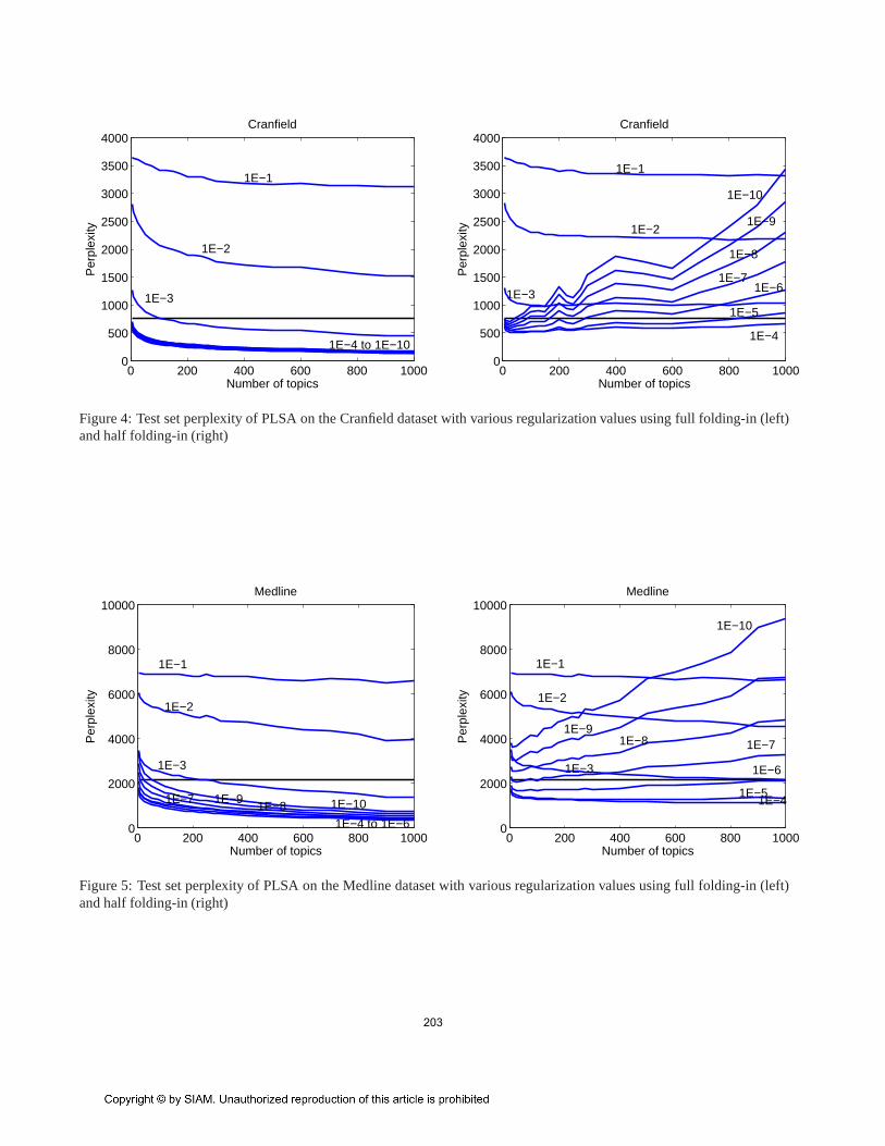
Figure 4: Test set perplexity of PLSA on the Cranfield dataset with various regularization values using full folding-in (left)and half folding-in (right)

0 200 400 600 800 10000

2000

4000

6000

8000

10000

1E−1

1E−2

1E−3

1E−4 to 1E−6

1E−71E−8

1E−9 1E−10

Number of topics

Per

plex

ity

Medline

0 200 400 600 800 10000

2000

4000

6000

8000

10000

1E−1

1E−2

1E−3

1E−41E−5

1E−6

1E−71E−81E−9

1E−10

Number of topics

Per

plex

ity

Medline

Figure 5: Test set perplexity of PLSA on the Medline dataset withvarious regularization values using full folding-in (left)and half folding-in (right)

203

0 200 400 600 800 10000

2000

4000

6000

8000

10000

12000

1E−1

1E−2

1E−3

1E−4 to 1E−71E−81E−9 1E−10

Number of topics

Per

plex

ity

NIPS

0 200 400 600 800 10000

2000

4000

6000

8000

10000

12000

1E−11E−2

1E−3

1E−4 to 1E−71E−81E−9 1E−10

Number of topics

Per

plex

ity

NIPS

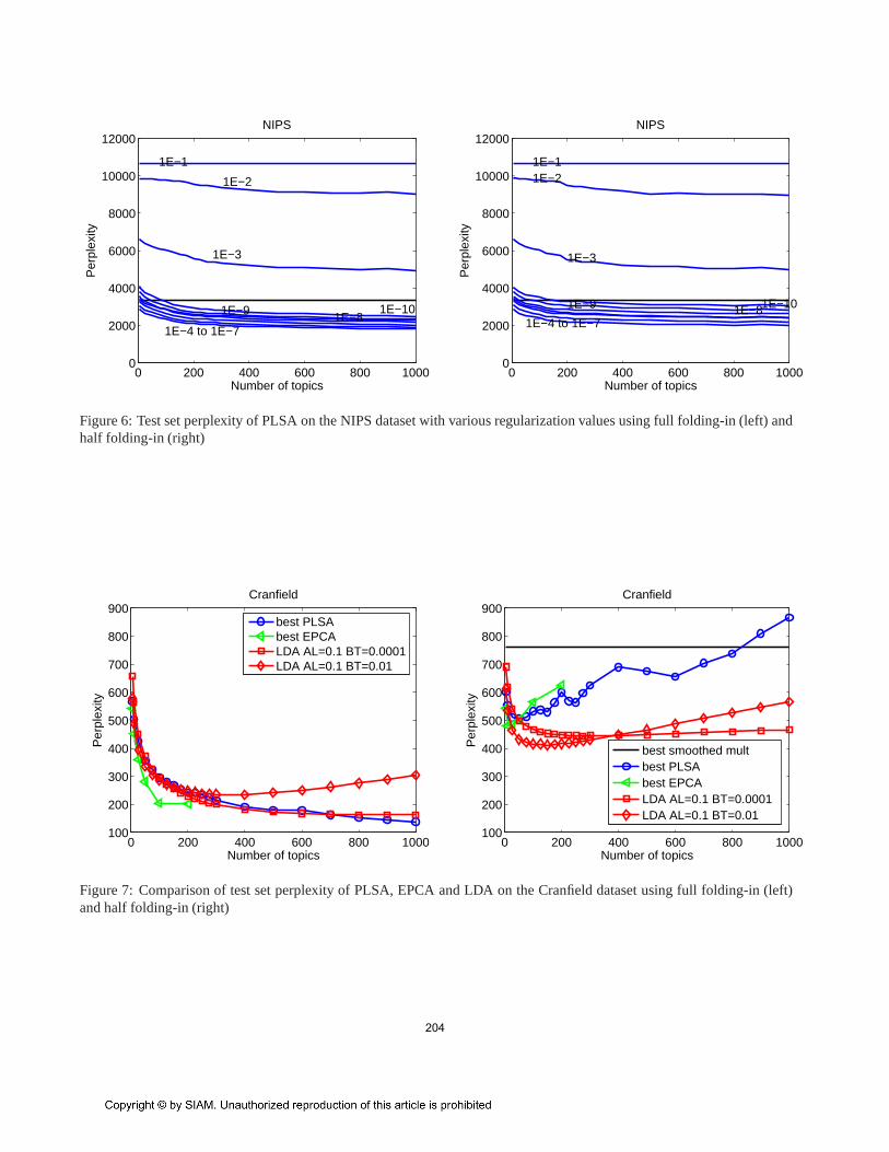
Figure 6: Test set perplexity of PLSA on the NIPS dataset with various regularization values using full folding-in (left) andhalf folding-in (right)

0 200 400 600 800 1000100

200

300

400

500

600

700

800

900

Number of topics

Per

plex

ity

Cranfield

best PLSAbest EPCALDA AL=0.1 BT=0.0001LDA AL=0.1 BT=0.01

0 200 400 600 800 1000100

200

300

400

500

600

700

800

900

Number of topics

Per

plex

ity

Cranfield

best smoothed multbest PLSAbest EPCALDA AL=0.1 BT=0.0001LDA AL=0.1 BT=0.01

Figure 7: Comparison of test set perplexity of PLSA, EPCA and LDAon the Cranfield dataset using full folding-in (left)and half folding-in (right)

204

0 200 400 600 800 10000

500

1000

1500

2000

2500

3000

Number of topics

Per

plex

ity

Medline

best PLSAbest EPCALDA AL=0.1 BT=0.0001LDA AL=0.1 BT=0.01

0 200 400 600 800 10000

500

1000

1500

2000

2500

3000

Number of topics

Per

plex

ity

Medline

best smoothed multbest PLSAbest EPCALDA AL=0.1 BT=0.0001LDA AL=0.1 BT=0.01

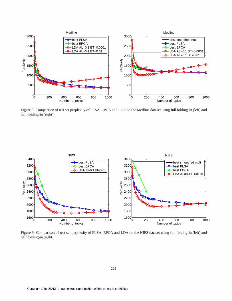
Figure 8: Comparison of test set perplexity of PLSA, EPCA and LDAon the Medline dataset using full folding-in (left) andhalf folding-in (right)

0 200 400 600 800 10001600

1800

2000

2200

2400

2600

2800

3000

3200

3400

Number of topics

Per

plex

ity

NIPS

best PLSAbest EPCALDA al=0.1 bt=0.01

0 200 400 600 800 10001600

1800

2000

2200

2400

2600

2800

3000

3200

3400

Number of topics

Per

plex

ity

NIPS

best smoothed multbest PLSAbest EPCALDA AL=0.1 BT=0.01

Figure 9: Comparison of test set perplexity of PLSA, EPCA and LDAon the NIPS dataset using full folding-in (left) andhalf folding-in (right)

205

a test document, and computing perplexity on the remainingwords (half folding-in). We argue that the half folding-inapproach used in our experiments to measure perplexity is afair measure because unlike the full folding-in approach, thehalf folding-in approach does not see the part of the data onwhich we measure the test likelihood. It, therefore, cannotoverfit on the test data and lead to incorrect and optimisticperplexity values.

Perplexity for PLSA is computed by first folding-in:computinghjn (or p(z|d)) by iterating only the E-step ofEM. After that we compute the log-probability of the test-data and transform it to perplexity as follows:

(5.37) Perplexity= exp

[

−∑

i,d log∑

k Wxtestid

,kHkd∑

d Nd

]

A similar procedure was followed for EPCA.For LDA we implemented the collapsed Gibbs sampler

described in [14]. Test-set perplexity was computed byaveraging over10 independent Gibbs samplers. After theMarkov chains converged on the training set we fixed theassignments to the last iteration on the training data andsampled the assignments on the test data until convergence(this is analogous to folding-in). For the last sample on thetraining set we then compute,

(5.38) φswk =

Nswk + β

Nsk + V β

where Nswk =

∑

i,j I[xij = w]I[zsij = k], Ns

k =∑

i Nsik

andV is the vocabulary size. Using the last sample from theGibbs sampling chain on the test-set we compute,

(5.39) θskd =

Nskd + α

Nsd + Kα

whereNskd =

∑

i I[zsid = k] andK is the number of topics.

These are then used to compute the test-set perplexity. In thecase of half folding-in the topic assignments for only 50%of the words of the test data were sampled and perplexity ismeasured on the rest of the words of the test documents (thisis analogous to half folding-in of PLSA described earlier).

We experimented with three different versions of PLSA:1) PLSA-HOF: the standard approach described in [1]; 2)PLSA-VEM using Equation 3.25 as described in Section 3.4;and 3) PLSA-TEM: “tempered EM” as described in [1] butsearching for the annealing parameter,β, between[0.5, 1]in increments of0.02 on the test set directly (hence, thisrepresents an upper bound on performance). We comparedperplexity of PLSA-HOF, PLSA-VEM and PLSA-TEM onCranfield, Medline and NIPS datasets for both full folding-in and half folding-in. From Figures 1, 2 and 3, it can beobserved that all three approaches give similar results onCranfield, Medline and NIPS. Unlike in [1], we did not find

any advantage of “tempering”. A similar result was alsofound in [8]. As the performance is similar for all threeversion of PLSA, in the subsequent experimental results weonly show the results for PLSA-HOF.

To avoid overfitting both PLSA and EPCA were regu-larized by adding a constantα to p(w|z) and renormalized.We triedα = [1E-10, 1E-9, ..., 1E-1] and show results for allvalues in the PLSA plots and best values when comparingwith other models.

We now compare the perplexity results of PLSA-HOFusing full folding-in and half folding-in for a range ofregularization parameters,α. Figures 4, 5, and 6 show theperplexity results using full folding-in and half folding-in forCranfield, Medline and NIPS respectively. For the smallerdatasets (Cranfield and Medline), it can be seen that theperplexity values are significantly higher for half folding-incompared to full folding-in. Additionally, it can also be seenthat in both these datasets perplexity results for half folding-in are very sensitive to the regularization parameter,α.

Since full folding-in is given more information to baseits predictive probabilities on, we expect full folding-in toproduce somewhat better perplexity than half folding-in.This in itself does therefore not prove the claim that fullfolding-in is overly optimistic. Observe however that forfull folding-in perplexity always improves with increasingnumber of topics, irrespective of the regularization valueapplied. In fact, in some of our experiments we increased thenumber of topics,T , to a value greater than the vocabularysize and the perplexity value still kept decreasing. Hence,we see no sign of overfitting with full folding-in. Thisis not, however, true for half folding-in where for smallregularization parameters one can clearly observe overfittingas the model complexity grows. These results supportour claim about the overly optimistic perplexity estimatesof full folding-in, especially for largeT . These effectsare alleviated in NIPS as NIPS documents are significantlylonger (by more than a factor of 10, see Table 1) and hencefolding-in on 50% of words (half folding-in case) gives abetter estimate ofH resulting in a relatively lower perplexity.

Additionally, we compare LDA with the best perplexity(best is defined as the curve with the lowest perplexity value)results for PLSA and EPCA using both full folding-in andhalf folding-in approaches. We show EPCA results only until200 topics as EPCA was extremely slow to run and prone tonumerical instabilities.

Figures 7, 8, and 9 show the results of these experimentsfor Cranfield, Medline and NIPS respectively. It can be notedthat the perplexity results of LDA are generally better thanthose of the best perplexity results of PLSA and EPCA, moreso for the half folding-in case. The perplexity results ofPLSA and EPCA are similar to each other but we found thatPLSA is easier to train than EPCA.

206

6 Discussion

In this paper we discuss a class of deterministic latent vari-able models and their learning algorithms under a unifyingframework. We classify these models into two categoriesbased on the type of latent variables used, namely, (i) discretevariables (e.g. K-means and Viterbi on HMM) or (ii) contin-uous variables (e.g. NMF, PLSA, PCA, ICA and EPCA).Hence NMF, PLSA, PCA, ICA and EPCA fall under thesame umbrella within this framework and are different onlyin the way they mix the latent variables: NMF and PLSAmix latent variables in the probability domain while EPCA,PCA and ICA mix latent variables in the log-probability do-main. In our experiments, we found that EPCA and PLSAproduce models with similar performance and that learningfor EPCA is relatively difficult. We also found that LDAproduced better models than PLSA or EPCA.

Our main contribution, however, is the observation thatthe standard learning algorithms for the category (ii) modelsoptimize a questionable objective. To derive the objectivefrom the variational objective one has to dismiss an entropyterm with a value of−∞ which renders the resulting objec-tive numerically unrelated (and certainly not a bound) to thelog-probability. While these models, in general, can learnreasonable parameters in training, the test data probabilityusing folding-in can be highly optimistic, especially whenthere are a large number of latent variables. Models withdiscrete latent variables do not suffer from these issues astheir entropy contribution is0 in the MAP approximation.

One can try to fix this problem, in theory, by switch-ing to a mean field approach which incorporates an approx-imation to the dismissed entropy, or by changing the modeland incorporating a normalization factor. The latter approachnaturally leads to the view of an “energy-based” model. Wenote, however, that computing the normalization factor isusually intractable.

We have also experimentally verified that computingtest-set perplexity using the “folding-in” recipe can easilylead to overly optimistic results.

Acknowledgments

We thank Geoff Hinton for his deep insights that helpedshape this paper.

Max Welling was supported by NSF grants IIS-0535278and IIS-0447903.

The research reported here is part of the Interactive Col-laborative Information Systems (ICIS) project, supported bythe Dutch Ministry of Economic Affairs, grant BSIK03024.

We acknowledge use of the computer clusters supportedby NIH grant LM-07443-01 and NSF grant EIA-0321390 toPierre Baldi and the Institute of Genomics and Bioinformat-ics.

References

[1] Thomas Hofmann. Probabilistic latent semantic analysis.In Proc. of Uncertainty in Artificial Intelligence, UAI’99,Stockholm, 1999.

[2] M. Collins, S. Dasgupta, and R. E. Schapire. A generalizationof principal components analysis to the exponential family.In T. G. Dietterich, S. Becker, and Z. Ghahramani, editors,Neural Information Processing Systems 14. MIT Press, 2002.

[3] Wray Buntine. Variational Extensions to EM and Multino-mial PCA Volume 2430 ofLecture Notes in Computer Sci-ence, Helsinki, Finland, 2002. Springer.

[4] M. Girolami and A. Kaban. On an equivalence between PLSIand LDA. InProceedings of SIGIR 2003, 2003.

[5] D. M. Blei, A. Y. Ng, and M. I. Jordan. Latent Dirichletallocation. Journal of Machine Learning Research, 3:993–1022, 2003.

[6] A. Dempster, N. Laird, and D. Rubin. Maximum likelihoodfrom incomplete data via the EM algorithm.Journal of theRoyal Statistical SocietyB, 39:1–38, 1977.

[7] R.M. Neal and G.E. Hinton. A view of the EM algorithm thatjustifies incremental, sparse and other variants. 1999.

[8] T. Brants. Test data likelihood for plsa models.Inf. Retr.,8(2):181–196, 2005.

[9] Y.W. Teh, M. Welling, S. Osindero, and G.E. Hinton. Energy-based models for sparse overcomplete representations.Jour-nal of Machine Learning Research - Special Issue on ICA,4:1235–1260, 2003.

[10] D.D. Lee and H.S. Seung. Learning the parts of objectsby non-negative matrix factorization.Nature, 401:788–791,1999.

[11] A. Olshausen and D. Field. Sparse coding with over-completebasis set: A strategy employed by V1?Vision Research,37:3311–3325, 1997.

[12] S.T. Roweis. EM algorithms for PCA and SPCA. InNeuralInformation Processing Systems, volume 10, pages 626–632,1997.

[13] B. Marlin and R. Zemel. The multiple multiplicative factormodel for collaborative filtering. InProceedings of the 21stInternational Conference on Machine Learning, volume 21,2004.

[14] T.L. Griffiths and M. Steyvers. A probabilistic approach tosemantic representation. InProceedings of the 24th AnnualConference of the Cognitive Science Society, 2002.

[15] D. Downey, S. Dumais and E. Horvitz Head and tails:Studies of Web Search with Common and Rare Queries InProceedings of the 30th Annual International ACM SIGIRConference, 847-848, 2007

[16] Y. Akita and T. Kawahara. Language Model AdaptationBased on PLSA of Topics and Speakers for Automatic Tran-scription of Panel Discussions. InJournal of IEICE Transac-tions, 3:439–445, 2005.

207