detection of snowmelt using spaceborne microwave radiometer data in eurasia from 1979 to 2007

2996 IEEE TRANSACTIONS ON GEOSCIENCE AND REMOTE SENSING, VOL. 47, NO. 9, SEPTEMBER 2009

Detection of Snowmelt Using Spaceborne MicrowaveRadiometer Data in Eurasia From 1979 to 2007

Matias Takala, Jouni Pulliainen, Senior Member, IEEE, Sari J. Metsämäki, and Jarkko T. Koskinen, Member, IEEE

Abstract—Determining the date of snowmelt clearance is animportant issue for hydrological and climate research. Spaceborneradiometers are ideally suited for global snowmelt monitoring.In this paper, four different algorithms are used to determinethe snowmelt date from Scanning Multichannel Microwave Ra-diometer and Special Sensor Microwave/Imager data for a nearly30-year period. Algorithms are based on thresholding channeldifferences, on applying neural networks, and on time series analy-sis. The results are compared with ground-based observations ofsnow depth and snowmelt status available through the RussianINTAS-SSCONE observation database. Analysis based on Mod-erate Resolution Imaging Spectroradiometer data indicates thatthese pointwise observations are applicable as reference data. Theobtained error estimates indicate that the algorithm based on timeseries analysis has the highest performance. Using this algorithm,a time series of the snowmelt from 1979 to 2007 is calculated forthe whole Eurasia showing a trend of an earlier snow clearance.The trend is statistically significant. The results agree with earlierresearch. The novelty here is the demonstration and validationof estimates for a large continental scale (for areas dominated byboreal forests) using extensive reference data sets.

Index Terms—Eurasia, radiometer, Scanning MultichannelMicrowave Radiometer (SMMR), snowmelt, Special SensorMicrowave/Imager (SSM/I), time series.

I. INTRODUCTION

SNOW cover and its evolution strongly affect hydrologicaland climate processes. Snow-covered terrain has an albedo

that is considerably higher than that of bare terrain, fundamen-tally affecting the processes of the atmosphere. Consequently,snow is an important parameter in weather forecasting andclimate models (global circulation models and Earth systemmodeling [1]). Concerning hydrological processes, informa-tion on snow depth (SD) or snow water equivalence helps inpredicting the water discharge during the melting period [2].Estimating the timing of snowmelt, either the melting onsetor snow clearance, indicates when this takes place, althoughhuman activities such as dams and topography also have sig-nificant effects to water systems. Satellite data can be usedfor detecting the snowmelt [3]–[10]. This has also variousoperational applications. Hydropower plants can better adjustwater flow, and authorities can be prepared for possible floodhazards. Melting takes place rapidly, and this is a special chal-

Manuscript received September 26, 2008; revised February 2, 2009. Firstpublished May 12, 2009; current version published August 28, 2009.

M. Takala, J. Pulliainen, and J. T. Koskinen are with the Finnish Meteoro-logical Institute, 00101 Helsinki, Finland (e-mail: [email protected]; [email protected]; [email protected]).

S. J. Metsämäki is with the Geoinformatics and Land Use Division, FinnishEnvironment Institute, 00251 Helsinki, Finland (e-mail: [email protected]).

Digital Object Identifier 10.1109/TGRS.2009.2018442

lenge for spaceborne snowmelt monitoring. For hydrologicalapplications, snowmelt must be determined in a time scale ofone week or even on a daily basis [11]. The timing of thesnowmelt is also an important factor for the length of the annualgrowing season at northern latitudes [12]. As snow melts, thecarbon uptake from the atmosphere magnifies [13]. The amountof carbon dioxide in the atmosphere is one of the key factorsin global climate change, and thus, the onset and progress ofsnowmelt provide information that is relevant to annual carbonbalance.

A certain amount of heat is needed to initiate the snowmelt.The long-term evolution of the dates of the onset of snowmeltand of snow clearance gives insight whether the snow meltsearlier presently than 30 years ago, and thus, informationrelated to global warming is obtained. When the time series ofglobal/large scale maps on the snowmelt are compared (in astatistical manner) with simulations made with existing climatemodels, the reliability of model predictions can be analyzed.

The time series of global observations on snow cover havebeen available for three decades from various types of satelliteinstruments. Passive microwave radiometers have one substan-tial advantage over optical instruments. Optical instrumentsobserving the Earth’s surface, such as spectrometers and scan-ners, are dependent on the Sun illumination and on cloud-freeconditions. Clouds can hinder the use of optical instrumentsfor weeks, which is a critical handicap concerning the mappingof the snowmelt. Microwave instruments, such as multichannelmicrowave radiometers, do not have this drawback. Addition-ally, at microwave frequencies, the dielectric constant of wateris much larger than that of ice and snow (and majority of naturalsubstances). Thus, the presence of liquid water in a snowpackhas a strong effect on microwave emission signatures.

Microwave radiometers have a coarse resolution (on theorder of 5–50 km, depending on instrument and frequency)but a wide swath width. For example, the Special SensorMicrowave/Imager (SSM/I) [14] has a swath of 1440 km.Hence, it can measure most of the globe within 24 h. In climateresearch applications, the coarse spatial resolution is quite ac-ceptable since the resolution of climate models is typically evencoarser. For example, the Hadley Centre uses high-resolutionregional climate models with a resolution of 50 km × 50 kmand global atmosphere–ocean general circulation models witha resolution of over 100 km [1]. As the resolution of climatemodels is coarser than that of radiometer data, radiometer-derived products can be used as input and validation data forclimate models.

The continuous time series of radiometer data are availablestarting from 1978. The Scanning Multichannel MicrowaveRadiometer (SMMR) [15] was launched in 1978 onboard the

0196-2892/$26.00 © 2009 IEEE

TAKALA et al.: DETECTION OF SNOWMELT USING SPACEBORNE MICROWAVE RADIOMETER DATA 2997

Nimbus-7 satellite. It operated until 1987. In 1987, the DefenseMeteorological Satellite Program launched its first satellite withthe SSM/I onboard. A series of satellites with SSM/I instru-ments have operated since then, producing nearly continuousstream of data. In 2002, NASA launched the Aqua satellite withthe Advanced Scanning Microwave Radiometer onboard.

Algorithms to detect snowmelt from spaceborne microwaveradiometer data have been investigated by several authors, typi-cally applying brightness temperatures observed at frequenciesof 19 and 37 GHz. The onset of snowmelt in Greenland wasinvestigated by Abdalati and Steffen [3] using a so-called cross-polarized gradient ratio, i.e., XGPR=T19h−T37v/T19h+T37v,where v and h denote vertical and horizontal polarizations,respectively. Additionally, Hall et al. [16] used the cross-polarized gradient ratio for snowmelt detection. A slightly dif-ferent algorithm was proposed by Drobot and Anderson [4], asthey applied the brightness temperature difference T19h − T37h.Accordingly, Smith [17] employed the brightness temperaturedifference T19v − T37v. Takala et al. [8] used two channeldifferences T37v − T19v and T37h − T19v in a corresponding al-gorithm for the detection of the onset of snowmelt. Takala et al.[8] tested and validated the algorithm for boreal forests (taigabelt) of Finland, whereas Drobot and Anderson [4] and Smith[17] applied their algorithms over the Arctic sea ice.

A time series analysis for snowmelt detection from ra-diometer data was introduced by Mognard et al. [7]. Theyused channel differences T19h − T37h in order to obtain globalestimates of the snowmelt for a 20-year period. The resultsobtained are interesting but lack validation against ground truth.Joshi et al. [6] also successfully applied a time series analysisfor radiometer observations over Greenland. In this paper, atime-series-based algorithm is introduced for the taiga beltutilizing the channel difference T37v − T19v.

Artificial neural networks have been used to some extent tomap the properties of snow. Tedesco et al. [18] applied neuralnetwork methods to estimate snow water equivalence and SD.Simpson and McIntire [19] used a feedforward neural networkwith Advanced Very High Resolution Radiometer data to es-timate the properties of snow cover. Takala et al. used a self-organizing map (SOM) to estimate the onset of snowmelt withSSM/I data. In this paper, the SOM-based algorithm is modifiedin such a way that the dependence on knowing snow waterequivalence and physical temperature has been eliminated. Forcomparison, a feedforward neural network is also tested here.

A general problem in earlier work has been the lack of properground-truth reference data. In particular, the lack of referencedata has been hampering the validation of algorithms for acontinent-scale mapping [7] and for periods of several decades[3], [5], [16]. Foster et al. [20] have used weather observationand in situ radiometer data to validate satellite estimates in tun-dra, but their work does not cover recent times. Moreover, thework carried out for forested regions has been limited, althoughthe data in [13] and. [7] include forests. The earlier work ofthe authors of this paper [8], [10] has been focused to borealforests. In the earlier work, data from the Watershed Simulationand Forecasting System of the Finnish Environment Institute(SYKE) were used as a reference for testing and validating thedetection of the onset of snowmelt for the region of Finland.However, the accuracy of model simulations poses a problem.

In [9], reference data from the Meteorological Archival andRetrieval System of the European Centre for Medium-RangeWeather Forecasts was applied. However, due to the gaps in SDdata, referencing had to be performed using surface temperaturedata. In this paper, extensive Russian INTAS-SSCONE [21]in situ SD data covering most of Eurasia are used. This madepossible the testing and validation of algorithms covering north-ern Eurasia for a long time span.

Snow cover and climate changes in Eurasia have been studiedextensively using ground-based data, satellite instruments otherthan microwave radiometers, and physical parameters apply-ing reference information from other than the snowmelt date.Brown [22] has constructed snow cover extent (SCE) and snowwater equivalent data from 1915 to 1997 using station datafrom China, Canada, the U.S., and the former Soviet Union.The results show a reduction of SCE in Eurasia. Serreze et al.[23] discuss many physical parameters, which include the snowcover area (SCA) that has been derived using optical satellitedata. Their values show below-normal SCA values in the 1990s.Dye [24] has used the last-observed snow cover in spring [weekof last snow (WLS)] and other parameters and constructed timeseries from 1972–2000 using optical satellite observations. Hisresults show three to five days/decade shift in WLS. Bamzai[25] used satellite-derived snow cover data, including snowmeltdate, and compared the results to the values of arctic oscilla-tion. His work shows an increase of snow-free days per year.Smith et al. [13] have analyzed trends in soil freeze and thawcycles from 1988 to 2002 using radiometer data. Their resultsshow that soil thaws three to five days/decade earlier, dependingon land cover. The results of Foster et al. [26] indicate that snowmelts four to seven days earlier on Arctic areas since the late1980s compared to the previous 20 years.

Brown [22] utilizes observations from the station network.This has the advantage of spanning the time series to thebeginning of the twentieth century. On the other hand, thespatial and, to some degree, also temporal resolutions are poor.Serreze et al. [23], Dye [24], Bamzai [25], and Foster et al.[26] use optical data that have excellent resolution but arelimited by weather and illumination conditions. Smith et al.[13] use microwave radiometer data. They detect the soil freezeand thaw; the latter is a related phenomenon compared to thesnowmelt. The time series of Smith et al. [13] ended in 2002.This work includes estimates for 2003–2007.

II. MATERIALS AND METHODS

In this paper, a time series of brightness temperatures cover-ing Eurasia from 1979 to 2007 was used together with INTAS-SSCONE SD and status data. The data are described in detailin Sections II-A and B. Four different algorithms were used toestimate the day of snowmelt. The algorithms are as follows:1) a channel difference algorithm; 2) a self-organizing neural-network-based algorithm; 3) a feedforward neural-network-based algorithm; and 4) a time series thresholding algorithm.These algorithms are explained in Sections II-C–E.

A. Radiometer Data

A complete time series of radiometer data from 1978 to 2007has been acquired from the National Snow and Ice Data Center


Fig. 1. Locations of SD-measuring stations in INTAS-SSCONE data set.

in Boulder, CO. For the years 1978–1987, the SMMR [15] datafrom Nimbus 7 are used, whereas for 1987–2007, the SSM/Idata from Defense Meteorological Satellite Programs (DMSPs)D-11 and D-13 are used. All data are EASE gridded [14],which means that the projection used is north azimuthal equalarea with a nominal resolution of 25 km × 25 km. Geolocationfiles and exact overpass time (UTC) are provided with the data.For each channel per day, there is a different file for ascendingand descending nodes. Since the orbits of DMSP series andNimbus 7 are Sun synchronous, the local time in every ascend-ing or descending image is the same for all pixels, regardless ofthe overpass UTC time. The local overpass time varies in time,but the difference between randomly chosen dates is not largerthan 2 h. The descending-node image corresponds to earlymorning (5:00–7:00 A.M. local), while the ascending-node onecorresponds to late afternoon (3:00–5:00 P.M. local). In the caseof SSM/I, the local time also depends on which DSMP satellitethe instrument has been onboard. In this paper, descending andascending data have been applied separately for each other.

The SMMR has frequencies of 6.6, 10.7, 18.0, 21.0, and37.0 GHz. At each frequency, vertical and horizontal polariza-tions are measured, resulting to ten channels. The swath widthof the SMMR is about 600 km. The SSM/I has frequencies of19.3, 22.2, 37.0, and 85.5 GHz. Both horizontal and vertical po-larizations are measured, except for 22.2 GHz where vertical po-larization is only measured. The swath width is about 1400 km.

The most important frequencies for snow detection are bandsaround 18 and 37 GHz (available for all instruments). WithSSM/I, the footprint sizes are 70 km × 45 km and 38 km ×30 km at 19.3 and 37 GHz, respectively. The SSM/I providesdata on a daily basis, and due to the wide swath (1400 km), mostof Eurasia can be mapped in 24 h. There are still some data gapsin both time and space. The SMMR had a much more narrowswath (600 km), and thus, averaging over time is a necessityto obtain the necessary areal coverage. The SMMR data areavailable on every other day only. There are also some longperiods when the instrument was switched off.

B. In Situ on Snow Status and Optical Satellite Reference Data

The used reference data are the INTAS-SSCONE SD dataset [21] from years 1978–2001. The snowmelt date is estimatedfrom a specific snow status flag included in the data set.Measurements have been made at 223 different locations, asshown in Fig. 1. Depending on the date, some of the data aremissing. The worst case is when the data are not availablefor half of the stations, and the best case is when only tenstations lack observations. There are 1704 and 2205 snowclearance date estimates for the SMMR and SSM/I data withproper validation data, respectively. For each measurement site,there is a WMO station index, date of the measurement, SDin centimeters, a qualitative estimate of the snow-covered area

Fig. 2. SD (in centimeters) and snow status codes from FMI weather stationdata and brightness temperature T37v − T19v from SSM/I data [14]. The snowstatus code has a value of nine for dry snow with 100% coverage and a valueof seven for wet snow with 100% coverage. The value of six is wet snow withcoverage > 50%, and the value of five is snow with coverage < 50%. The90% level of difference between the maximum and minimum of the brightnesstemperature serves as the detection limit.

(SCA), and a status flag value. The flag describes whetherthe melt is temporary or continuous (snow clearance) andwhether the value of SD is correct or to be rejected. TheINTAS-SSCONE data set also has a short description of stationcharacteristics, for example, information on whether the stationis protected from strong wind or not. As to snowmelt, it isconsidered to take place if the flag changes from value “SDis correct” to either “temporary melting” or to “continuousmelting.” If there is more than one such change (typically twoto three), only the last one in the 180-day period is taken intoaccount. There are no error estimates in the INTAS-SSCONEdata, but in general, the SD measurement can be consideredaccurate. SD is customarily manually measured with a rod,ensuring reliable data. The automated measurements have also,in general, a proper accuracy. On the other hand, the snowmeltflag is subjective to the observer. Fig. 2 compares the pointwisemeasurements with satellite-observed brightness temperatures.This demonstrates the correspondence of spatially distributedsatellite observations to snow status observations at a singlelocation representing the Eurasian boreal forest belt.

Since the INTAS-SSCONE data embody pointwise obser-vations while the nominal resolution of radiometer data is25 km × 25 km, it should be investigated whether the INTAS-SSCONE snow flags are suited for validation work consideringthis discrepancy. We approached this task by investigatingthe spatial variation of snow cover characteristics within theradiometer resolution cell. Should there be homogenous snowconditions (at least at the time of melting onset or snowclearance when we are most interested at) within the pixel, theupscaling of pointwise measurements to the 25 km × 25 kmarea is well justified. In the investigation, the optical dataprovided by the Moderate Resolution Imaging Spectroradiome-ter (MODIS) was used in order to generate maps describingthe fraction of SCA for 0.005◦ × 0.005◦ resolution cells (re-sembling a MODIS nominal resolution of 500 m × 500 m).This was carried out using the SCAmod algorithm by


Fig. 3. Example on the MODIS-based SCA map of a large area in Eurasia, also indicating smaller test sites applied for analysis here.

Metsämäki et al. [27], which was particularly developed forthe boreal zone. As a result, the SCA time series (17 SCAmaps) for the snow-melting period of 2001 was obtained for anapproximately 1500 km × 1600 km area in northwestern Russia(see Fig. 3). From these maps, 49 subareas corresponding to thesize of a radiometer resolution cell were selected for analyzingthe spatial variance of SCA at different stages of snow melting.In Fig. 4(a), the evolution of SCAs inside a 25 km × 25 kmsubarea is presented. The time series include the mean andstandard deviation of SCA estimates inside the 25 km × 25 kmresolution cell, complemented with individual SCA estimatesfor 500 m × 500 m sized grid cells.

Fig. 4(a) clearly shows how snow coverage is very evenlydistributed at the time of melting onset and snow clearance,while this is not the case during snow melting, e.g., aroundthe average SCA of 40%. The behavior of SCA in the other48 subareas is very similar to the one shown in Fig. 4(a).This is also shown in Fig. 4(b), where the average standarddeviation of SCA as a function of SCA is presented. Clearly,close to the time of snow clearance, the SCA shows verylittle variation (0.13%). This is evidently due the escalatingmelting process caused by the gradually increasing proportionof absorptive snow-free ground, again powering the meltingof the neighboring snow patches. SD, land cover variability,and other issues are also involved. The analyses show that thedifference between snow clearances in the scale of 500 m whencompared to the scale of 25 km is typically on the order of±10 days. This indicates that a pointwise observation of snowclearance can be applied (in a statistical manner) as referencedata to radiometer observations.

C. Channel Difference Algorithm

Takala et al. [8], [10] described a simple channel differencealgorithm to estimate the snowmelt. The algorithm was modi-fied [9] in order to avoid the dependence on ground-based ob-served physical temperature. In this paper, the modified version[9] is used. The algorithm detects the snowmelt situation when

(T37v − T19v) > − 21 K (1)(T37h − T19v) < − 10 K. (2)

Fig. 4. Spatial variability of snow cover in 25 km × 25 km EASE-Gridcells during the snowmelt period. (a) Example for a single grid cell showingthe variability of SCA within the area (all samples, and their mean andstandard deviation observed for the 500 m × 500 m MODIS pixels within theEASE-Grid pixel. (b) Overall standard deviation as a function of SCA for allinvestigated 25 km × 25 km EASE-Grid pixels.

T denotes the brightness temperature and subindices the fre-quency and polarization of the radiometer. Frequencies of 19and 37 GHz are available only on the SSM/I. With SMMR, the19-GHz frequency is replaced with 18 GHz. According to abrightness temperature modeling by Pulliainen et al. [28], this


can induce an error of 1–2 K to the frequency difference, whichaffects the generation of time series based on various instru-ments. However, one should note that time series algorithmsare much more insensitive to such an error since they operatewith relative values (see Section V in the following).

Additionally, if, in a period of seven days before the givendate, there are no dry snow estimations, the snowmelt onsetestimate is discarded. The dry snow estimate is calculated usingthe algorithm developed by Hall et al. [5].

Chang et al. [29] determine SD by

SD = 1.59(T19h − T37h). (3)

If conditions

SD > 80 T37v < 250 K T37h < 240 K (4)

are met, data are classified as dry snow according to the methodby Hall et al. [5].

D. Neural Network Algorithms

Supervised and unsupervised neural network structures werealso tested to estimate the day of snowmelt.

Takala et al. [10] described a snowmelt detection algorithmbased on SOM [30]. As with other snowmelt detection algo-rithms, the dependence on knowing the snow water equiva-lence or physical temperature as prior information is typicallyundesirable. Thus, in this paper, the SOM-based algorithm issimplified to be used only with brightness temperature data.

SOM consists of a layer of neurons, which usually form a2-D grid. For each neuron, there is a weight vector w, and all theneurons share the input vector T. In this paper, the input vectoris T = [T19v T22v T37v T19h T37h]. The 22-GHz channel has nosignificant effect to the results and could be left out. The trainednetwork normally operates as follows [31]. The input vector Tis presented to every neuron in the network. All the neuronshave a different weight vector w, and the Euclidean distance ofthe weight and input vector for every neuron is calculated. Theneuron whose weights are closest to the input is activated. Thiscan be interpreted so that the input vector T presented to thenetwork is classified to belong to the vector class of neuron k.SOM learns unsupervised, which means that it is unknown thata particular neuron responds to a certain class of input vectors.

The trained network is used by feeding the input vectorand checking out which neuron is activated. After training,only such input vectors are selected, for which SD is less than1 cm. The neuron winning in most cases is then selected to rep-resent the case when snowmelt takes place. Typical for a SOMis that the classes presented by adjacent neurons in the fullytrained network have more similar classification properties thanthat by distant neurons. This means that a group of neighboringneurons, instead of a single neuron, can represent the correctclassification of snowmelt. In this paper, 3 × 3 neurons havebeen used.

The other tested method is the use of a feedforward neuralnetwork [31], a network whose neurons do not have any feed-back from their output back to the input. Each neuron consistsof a weight vector w and an input vector x. There can bean additional bias term that always has a constant value of

one and its own weight. The dot product between the inputvector and the weight vector is calculated, and an activationfunction is applied to this value. An activation function can belinear or nonlinear. If the backpropagation algorithm is used,the activation must be differentiable. Commonly, a linear orsigmoidal function is used. The trained network is used asfollows. First, all the outputs of the neurons in the hidden layerare calculated. Next, the outputs of the neuron(s) of the outputlayer are calculated. The signal propagates from the input layerto the hidden layer and then to the output layer. The outputvector y corresponding to the input vector x is thus obtained.

Unlike SOM, a feedforward neural network learns super-vised. Initially, the weights of every neuron are randomlyassigned. The input vector x is presented to the network, and theoutput y′ is calculated. For a supervised network, the desiredoutput y is known. The error y′ − y is then calculated. Thefunctional form of the activation function is known, as well asthe current values of the weights. The relative amount of theerror of each hidden-layer neuron can thus be propagated backfrom the output layer. The error is calculated backward until theinput layer is reached. Since the error for each neuron is known,the weights are then adjusted such that the error gets smaller.The amount of adjusted weight is controlled with a learningparameter that gradually decays in time. Thus, it is ensuredthat the network reaches some state of equilibrium. This back-propagation of error and adjustment of weights are calculatedfor each pair of training input vector x and output vector y.When the adjustments of the weights or the error of the outputis reasonably small, the training is considered to be finished.

In this paper, the input vector T = [T19v T22v T37v T19h

T37h] is the same as for the case of SOM (again, the 22-GHzchannel can be left out). The feedforward network has an inputlayer, a hidden layer, and an output layer. The network consistsof five neurons in the hidden layer and one neuron in the outputlayer. The activation function is sigmoid for all neurons. Otherfunctional forms like tangent sigmoid and linear activation[31] were tested but discarded. The training output vector isdetermined as follows. If SD is less than 1 cm, the output isone; otherwise, the output is zero.

E. Time Series Thresholding Algorithm

The three previously presented algorithms attempt to de-termine the snowmelt on a daily basis. For the purpose ofclimatic analysis, the time series approach may be better suited.The channel difference T37v − T19v is commonly used [4],[17] in passive microwave remote sensing of snow. A typicalexample of the time series of SD and the channel differenceis shown in Fig. 2. As the snow melts and SD decreases,the channel difference increases. This observation leads to thefollowing algorithm. Determine the maximum and minimumof the channel difference T37v − T19v, and when a certain levelabove the minimum is achieved, the snowmelt is considered totake place. This is shown as a detection limit in Fig. 2.

Sometimes, depending on location, the pointwise-observedsnow status flag and the melt indices based on brightnesstemperature channel difference fluctuate considerably. Sincethe measurements of a radiometer are sensitive to the presenceof liquid water, possibly, the observed fluctuation is related


to cyclic melting and freezing of the surface of the snow-pack. However, in most cases, the difference between the finalsnowmelt and these temporary melt–refreeze cycles is distin-guishable. Thus, the snowmelt is more accurately estimatedfrom the maximum and minimum of the time average of thechannel difference.

Thus, we obtain

D(t) = T37v(t) − T19v(t) (5)Dmax,tavg = max 〈D(t0),D(t1), . . . , D(tN )〉 (6)Dmin,tavg = min 〈D (t0) ,D (t1) , . . . , D(tN )〉 (7)

〈D(t)〉 ≥ p · [Dmax,tavg − Dmin,tavg] + Dmin,tavg (8)

where D is the channel difference, t is the time (in days), andp is the level of detection (often 90%; p = 0.9). For each timet, condition (8) is evaluated. If it holds, the estimate for time thas a value of one; otherwise, it is zero.

The averaging period of seven to eight days gave the best re-sults when many different averaging periods were tested. Sinceaveraging determines only the detection limit, and detectionis made from the original channel difference data, the spikesproduced by temporary melt events are quite often detected. Forsome purposes, this is desirable. Typically, the most importantmelting incident is the actual snow clearance date. To determinethat time, one must eliminate the temporary melts from the data.This can be satisfactorily achieved by averaging the estimatevector and thresholding at some level between zero and one(value of 0.9 found here). The threshold value of 0.9 wasempirically determined to obtain a good fit.

III. METHOD VALIDATION AND RESULTS

The validation is based on qualitative pointwise observa-tions (INTAS-SSCONE snow flags), as described earlier. InSection II, we concluded that the pointwise nature of snowclearance data is not a problem when validating the radiometer-based estimates. In this investigation, snow status coding withmore quantification levels than the INTAS-SSCONE data canoffer is appreciated. In practice, this was only possible for theregion of Finland, for which FMI weather station observationswith detailed snow status information were available. There-fore, we compared the brightness temperature data with SD andsnow status codes from FMI observations. The snow status codehas values of nine for dry snow with 100% coverage, seven forwet snow with 100% coverage, six for wet snow with coverage> 50%, and five for snow with coverage < 50%. The temporary(value of two) and continuous melting (value of one) flags inthe INTAS-SSCONE database correspond to the values that aregreater than seven in the FMI weather observation data flag.

Fig. 2 shows an example of the FMI snow status codeand SD in comparison to the brightness temperature channeldifference. The detection limit of the algorithm described inSection II-E is also plotted. Fig. 2 shows that the qualitativeestimate agrees relatively well with the observed changes inbrightness temperature difference for this case. The observeddifference between the regional satellite-databased estimate andobservations at a single station is about five days. The SD mea-surements and flag estimates are made at a single location only.Uncertainties arise as the measurements in a single location

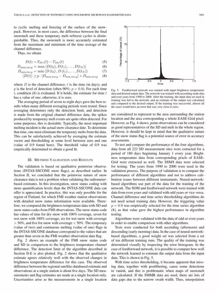
Fig. 5. Feedforward network was trained with input brightness temperaturedata and desired output data. The network was trained with ascending-node dataand even years from 1990 to 2000. After the training, the input data set used intraining was fed to the network, and an estimate of the output was calculatedand compared to the desired output. If the training was successful, almost allthe cases would have an error that was very close to zero.

are considered to represent to the area surrounding the stationlocation and the area corresponding a whole EASE-Grid pixel.However, as Fig. 4 shows, point observations can be consideredas good representatives of the SD and melt in the whole region.However, it should be kept in mind that the qualitative natureof the snow status flag is a potential source of error in accuracyassessments.

To test and compare the performance of the four algorithms,data from all 223 SD measurement sites were extracted for aperiod of 180 days beginning January 1 every year. Bright-ness temperature data from corresponding pixels of EASE-Grid were extracted as well. The SSM/I data were selectedfor testing. The years from 1990 to 2000 were used in thevalidation process. The purpose of validation is to compare theperformance of different algorithms and not to address cali-bration issues between different instruments. Neural-network-based algorithms use part of the data for the training of thenetwork. The SOM and feedforward network were trained withdata from even years and validated with odd years or vice versa.Channel difference and time series thresholding algorithms donot need actual training data. However, the triggering valuep = 0.9 was empirically selected for the time series algorithm(8), as that value gave the highest performance in algorithmtesting.

Algorithms were validated with the data of odd or even yearsin order to enable comparison with other algorithms.

Tests were conducted for both ascending (afternoon) anddescending (early morning) data. In the case of neural-network-based algorithms, a good weight set was selected from a setof ten different training runs. The quality of the training wasdetermined visually by inspecting the error histogram. In thecase of feedforward network, it is possible to compare how wellthe network learned to estimate the output data from the inputdata. This is shown in Fig. 5.

With time series thresholding, it became apparent that miss-ing data, together with postfiltering, cause some detectionsto vanish, and this is problematic when maps of snowmeltare calculated. If the SMMR data are used, there are lots ofdata gaps due to the narrow swath width. Thus, interpolation


TABLE ISTATISTICAL ERROR CHARACTERISTICS OF DIFFERENT ALGORITHMS

WITH DIFFERENT PARAMETERS VARIED DURING THE

1990–2000 TEST PERIOD

of channel difference data with time series thresholding wasincluded in order to obtain a full spatial coverage.

The estimation error for a particular year at a particular testsite is

ε = tobserved − testimated. (9)

The unit of melt detection moment t is one day; tobserved refersto the INTAS-SSCONE-data-derived snow clearance date (ac-cording to the snow flag value), and testimated refers to theestimated date of snowmelt using a particular algorithm. Foreach algorithm, the mean, median, and standard deviation of allthe errors are calculated for a testing period of 1990–2000. Ifeither observation or estimate is missing, the value is not takeninto account. The results are presented in Table I. Four differentsets of values are presented, depending whether ascending ordescending data are used and whether the testing material hasbeen taken from even or odd years. Results clearly suggest thattime series thresholding is the most accurate algorithm in termsof mean (from −4.25 to 2.1 days) and standard deviation ofestimation error (from 15.3 to 22.3 days), so this is the mostapplicable one among the tested algorithms for the purpose ofclimatic studies.

Since the comparison of different algorithms in Table I wascarried out only using the SSM/I data, it was crucial to testthe time series thresholding algorithm with the SMMR data inorder to verify their similar behavior. Therefore, snowmelt dayestimates using both SSM/I and SMMR data were calculatedfor as long periods as possible (both reference and satellite dataavailable). Interpolation of missing brightness temperature val-ues was used for both sensors. The results are shown in Fig. 6,showing a very good performance of snowmelt estimations withmean errors (biases) of only 0.6 and 1.1 days for the SMMRand SSM/I, respectively. Both SMMR and SSM/I data gavesimilar results with respect to the reference INTAS-SSCONE

Fig. 6. Error distribution according to (9) of the time series thresholdingalgorithm (5)–(8), together with interpolation of lacking brightness temperaturedata. There are 1704 and 2205 applicable snow clearance estimates for theSMMR and SSM/I, respectively.

data, indicating that the joint use of these two sensors in long-term climate analyses is feasible.

The performance of radiometer-databased snowmelt map-ping is shown in Fig. 8. The calculated maps of the snowmeltin northern Eurasia for 1980, 1990, 2000, and 2007 clearlyindicate how the melt is distributed geographically. The resultsalso show interannual variations. For a few chosen test sites thatare circular in shape with radius of 250 km and the center inSodankylä, Verhoyansk, Tunguska, Novosibirsk, and Moscow,the time series of snowmelt estimates are shown in Fig. 7. Themean (averaged over time) snowmelt dates for these locationsare the days of year 139, 146, 132, 113, and 100, respec-tively. The corresponding standard deviations in the timing ofsnowmelt are 6.7, 5.6, 9.1, 6.7, and 11.7 days. The slopes ofthe linear fits are −0.34, −0.24, −0.43, −0.07, and −0.69, re-spectively. The statistical significance was tested by calculating95% and 90% confidence levels for the slope. The results arepresented in Table II. Comparisons of the confidence intervalswith slope 0 indicate that the trends are, in general, significant.

Detailed analysis of the difference between INTAS-SSCONEobservations and radiometer-databased melt estimates, as afunction of time, was also carried out. The results indicate thatmean yearly bias can show values that are slightly differentfor the early years (SMMR data) than for the later period(SSM/I data). This would cause an effect of about −1.6 days


Fig. 7. Snowmelt in five different test sites in Eurasia on 1979–2007. Theonset of snowmelt is averaged for a circular area having a radius of 250 km,and the place in the title is in the center of the area. The confidence levels of theslopes are presented in Table II.

TABLE IISLOPES AND 90% AND 95% CONFIDENCE LEVELS

CALCULATED FOR THE SLOPES IN FIG. 7

per decade for the estimated trend of snowmelt. In practice,the analysis suggests that a value of 2.6 days should be addedto the snowmelt dates representing years 1979–1987, resultingto slightly delayed snow clearance dates. Moreover, a value of1.0 day should be subtracted starting from the year 1992 indi-cating earlier snowmelt dates than those shown in Fig. 7. Thus,if this correction is made, the negative trends shown in Table IIand Fig. 7 would magnify (a decrease of 0.16 to slope factorsin Table II). For 1988–1991, the analysis of temporal bias in-

dicates a mismatch between INTAS-SSCONE snowmelt datesand radiometer retrievals higher than that obtained for other19 years. This may indicate problems in either reference orsatellite data (first SSM/I instrument onboard the F08 satellite).

The slope of the linear fit was calculated for every pixel inEurasia [Fig. 9, (top)] to demonstrate the evolution of snowclearance date in the period of 29 years. Red tones with negativevalues indicate earlier melt, whereas blue tones with positivevalues indicate later melt. The corresponding slopes were alsocalculated using the station-wise data from INTAS-SSCONEstations [Fig. 9, (bottom)]. Fig. 9 (top) is determined by in-cluding the bias correction between the SMMR and SSM/I dataretrievals discussed earlier. However, this has only a marginaleffect to the results (it decreases the shown trend with a constant−1.6 days/decade). Years 1988–1991 were excluded from thetrend analysis of Fig. 9 (top).

IV. DISCUSSION

The comparison of different algorithms in Table I revealsimmediately one important aspect. When channel differenceand neural-network-based algorithms are used, the standarddeviation between the estimated snow clearance date and thereference data is as high as over 30 days, but when time-series-analysis-based algorithms are used, the standard deviation re-duces to slightly above 20 or even less. This is explained by thefact that the first three mentioned algorithms examine the dataon a daily basis with only current and historical observationsavailable, whereas the time series algorithm takes the wholetime series of radiometer observations into account. This justi-fies the offline use of time-series-based algorithms when accu-racy is the main concern, such as in historical climate studies.However, in operational (near real time) use, data can only beanalyzed using current day or past observations. An importantfactor contributing to the error distribution is the accuracy ofestimation of the snowmelt date from the snow status flag. Theflag is a qualitative estimate and can thus be inaccurate.

The channel difference algorithm (1)–(4) has a standarddeviation that is close to 35 days, regardless if even or odd yearsare used or whether the data used are either from ascendingor descending node. It is evident that the selection of orbitalnode affects the mean and median. This can be explained bythe local time that is either early morning or late afternoon.The diurnal melting cycle during the day causes the signaturesto be different and, hence, the difference in mean. The cleardifference between median and mean indicates an asymmetricdeviation of error. Since the algorithm was originally developedusing snow wetness data from hydrological model predictionsonly, it is possible that the asymmetry is due to the differentkinds of data applied for algorithm development.

The self-organizing network-based algorithm seems to workbetter when trained and tested with ascending-node data. Bothmean and median errors are closer to zero when using ascend-ing node instead of observations from descending node.

Switching between even and odd years does not seem toaffect the quality of the algorithm. The error distribution is moresymmetric than in the case of the channel difference algorithm.Although the SOM-based algorithm seems to work, it does notoffer any significant advantage over the much simpler channeldifference algorithm.


Fig. 8. Maps of the onset of snowmelt for 1980, 1990, 2000, and 2007. The results are calculated using the time series thresholding algorithm. The color code isthe number of days since January 1 corresponding year.

The standard deviation using the feedforward neural-network-based algorithm seems to be slightly lower whentested with data from odd years. Mean and median errors tendto be closer to zero also when data are from odd years. Thedistribution of error is quite symmetric. Again, no significantadvantage over the simpler algorithm is seen. Since the feedfor-ward algorithm is trained supervised, it is possible to check howwell the neural network can be trained (Fig. 5). If a supervisedneural network is perfectly trained, the output error is very closeto zero when the network is fed with an input vector used in thetraining.

After a particular training feeding, the network with inputvectors used in training ends up with about 50% of the cases

that are close to zero and about 50% that are not. This suggeststhat the differentiation between snow-covered area and bareground is sometimes possible and sometimes not. This is logicalsince very wet snow and bare wet ground contain liquid water,and the microwave emissivity can be close to one in bothcases. Although different training sessions and varying trainingparameters have been applied, the result can be a consequenceof improper training. To overcome this problem, additionaldata, such as temperature data derived from synoptic stationsor infrared satellite observations, could be used.

The time series thresholding algorithm (5)–(8) without chan-nel data interpolation performs better when descending-node(early morning) data are used. However, the mean and median


Fig. 9. Change in snow clearance date per decade estimated applying (top) the channel difference algorithm to satellite data and derived from (bottom) INTAS-SSCONE test sites. The red tones and negative values mean earlier melt, and the blue tones and positive values mean later melt. The numerical value is days perdecade.

are closer to zero when ascending data are used. The use ofeven or odd years does not affect the results. By plotting themaps, it became evident that some cases in error analysis werediscarded due to the missing data. When channel differencedata are interpolated for the missing dates, the results becomesomewhat different. The standard deviation is larger than in thecase of noninterpolated channel data, but this could be easilyexplained as the error contribution from missing data cases isdiscarded in postprocessing. The error then does not depend onthe node or the years used. Using ascending data, the mean andmedian are very near to zero.

Since gaps are typical with SMMR observations, the erroranalysis was extended to the SMMR data using channel datainterpolation for years 1979–1987. The same procedure wasconducted for the SSM/I data for every year from 1988 to 2001.Fig. 6 shows that the mean, median, and standard deviationare almost the same for both instruments. As presented inSection II-B, the pointwise measurement of SD represents the25 km × 25 km EASE-Grid pixels when the snow cover is fullor almost melted.

In Fig. 8, the snowmelt for the whole Eurasia is shownfor 1980, 1990, 2000, and 2007. Although there is variationbetween years, the maps feature a different development ofsnowmelt in Europe when compared with Asia. Very earlysnowmelt dates obtained for the southwest part of the mapregion indicate that the actual seasonal (permanent) snow coverdoes not typically exist for this part of Europe. This overallbehavior is most probably due to the effect of Arctic oscil-lation [23], [25] and North Atlantic oscillation [23]. Somegeographical features, such as Scandinavian mountains andUral, are visible since the snow begins to melt later on the highmountains. The effects of topography and land use affect themicrowave brightness temperature. Recently, many global landuse maps have become available, but their usefulness in analysisis limited [32], [33]. This is somewhat true for local land coverdata too [34]. The authors will address this problem in a moredetailed manner in future work.

In Fig. 6, the temporal behavior of the snowmelt for some lo-cations in Eurasia is presented. The negative slopes indicate thatthe snow now melts 1–7 days earlier than it did ten years ago.

The 95% and 90% confidence intervals for the slopes arepresented in Table II. The negative trend is a statisticallysignificant trend in most cases. The geographic location of thetest site is significant. The more to the south and the more tothe west the location is, the earlier the snowmelt is. The largestnegative slope value around Moscow indicates that the changein snowmelt in the European side of Eurasia has been morerapid than in the Asian side. The results are, in general, in linewith the analyses performed by Dye [24] and Smith et al. [13].

In Fig. 9 (top), the decadal trend map of snow clearance datederived from satellite data demonstrates that the snow meltsearlier today than it did 29 years ago in most parts of Eurasia,particularly in the European side of Eurasia. On mountains suchas Ural and Scandinavia, on some wetlands, and on large areasof Arctic tundra, the melt appears to take place later in recentyears. This can either be a real phenomenon caused, for ex-ample, by increased snow fall or an anomaly due to land coverand/or topography, which needs to be researched further. Forapplicable INTAS-SSCONE stations, the trend map has beenderived [Fig. 9, (bottom)]. These results do not show such clearspatial trends as the satellite-data-derived map do [Fig. 9, (top)].A possible reason is that the available pointwise observationsmay exhibit a higher variance with respect to the real timingof snowmelt than the satellite data retrievals (as areal meltingcharacteristics for grid cells of 25 km × 25 km are consideredhere). Additionally, the spatial distribution of INTAS-SSCONEmonitoring stations is sparse. Thus, ground-based observationscannot be interpolated to yield the trend map derived from satel-lite data, even though they can be used to calibrate and validatesatellite-databased snow clearance date estimates. An importantfinding is that the mean annual difference between pointwiseINTAS-SSCONE reference data and satellite data retrievalsonly shows a slight difference between SMMR and SSM/I dataretrievals but not otherwise. The difference between the sensors


can be accounted for in trend analysis, which is performed inFig. 9. The magnitude of this correction for the decadal trend is−1.6 (days per decade). The results of Fig. 9 (top) only slightlychange if this correction factor is excluded. It can be con-cluded that the satellite-data-derived snowmelt trend shownin Fig. 9 (top) is a realistic estimate; the level of error cannot,in general, exceed the value of about 1.6 days per decade.

In the case of real-time operational use, the time seriesalgorithm cannot be used as such since it requires the brightnesstemperatures to be available for the period when the snowmelthad already taken place. The performance of channel differenceand neural network algorithms are not at the same level withthat of the time series algorithm. However, the error estimatesare based on comparisons with point observations, and theaccuracy characteristics over larger areas may be higher thanthe quantitative values reported here.

The accuracy of snow clearance date estimates could bepossibly improved by applying in future work in situ dataas supplementary data to radiometer observations. The effectof land use must also be addressed. Land use classificationGLC2000 [35] suggests that the land use of the Tunguska siteis “water bodies.” This partly explains the largest value ofstandard deviation of snowmelt in Fig. 6. Although the timeseries approach is much better in terms of accuracy, the effectof land use may be present.

V. CONCLUSION

This paper has shown that it is possible to estimate snowmeltdates accurately in Eurasia from spaceborne microwave bright-ness temperature data. The results showed a standard deviationof ∼20 days when compared with pointwise reference in situdata. MODIS-databased analysis showed that the pointwiseobservation was a valid representation for the 25 km × 25 kmpixels at the time of snow clearance, and thus, the INTAS-SSCONE data can be used as reference data for satellite ob-servations. Altogether, four algorithms to map snowmelt wereproposed and tested. The best agreement with reference datawas obtained using the time series thresholding algorithm.

Snowmelt maps were derived and analyzed for 29 sepa-rate years from 1979 to 2007. The melting trend had beenmapped for the whole Eurasia, and the results showed thatsnow melted earlier in the European part of Eurasia than inthe Asian part. Examples for a few chosen locations aroundthe area show statistically significant negative trends indicatingthat snow melted even a month earlier than it did 29 yearsago. The results also suggested that interpolating the trendfrom pointwise observation was not feasible, whereas satelliteobservations provided such information.

REFERENCES

[1] L. C. Shaffrey, I. G. Stevens, W. A. Norton, M. J. Roberts, P. L. Vidale,J. D. Harle, A. Jrrar, D. P. Stevens, M. J. Woodage, M. E. Demory,J. Donners, D. B. Clark, A. Clayton, J. W. Cole, J. C. King, A. L. New,J. M. Slingo, A. Slingo, L. Steenman-Clark, and G. M. Martin, “UK-HiGEM: The new UK high resolution global environment model. Modeldescription and basic evaluation,” J. Climate, vol. 22, pp. 1861–1896,2009, doi:10.1175/2008JCLI2508.1.

[2] J. Martinec and K. Seidel, “Remote sensing in snow hydrology; Runoffmodelling,” in Effect of Climate Change. New York: Springer-Verlag,2004.

[3] W. Abdalati and K. Steffen, “Passive microwave-derived snow melt re-gions on the Greenland ice sheet,” Geophys. Res. Lett., vol. 22, no. 7,pp. 787–790, 1995.

[4] S. D. Drobot and M. R. Anderson, “An improved method for determiningsnowmelt onset dates over Arctic sea ice using Scanning Multichan-nel Microwave Radiometer and Special Sensor Microwave/Imager data,”J. Geophys. Res., vol. 106, no. D20, pp. 24 033–24 049, 2001.

[5] D. K. Hall, R. E. J. Kelly, G. A. Riggs, A. T. C. Chang, and J. L. Foster,“Assessment of the relative accuracy of hemispheric-scale snow-covermaps,” Ann. Glaciol., vol. 34, pp. 24–30, 2002.

[6] M. Joshi, C. J. Merry, K. C. Jezek, and J. F. Bolzan, “An edge detec-tion technique to estimate melt duration, season and melt extent on theGreenland ice sheet using passive microwave data,” Geophys. Res. Lett.,vol. 28, no. 18, pp. 3497–3500, 2001.

[7] N. M. Mognard, A. V. Kouraev, and E. G. Josberger, “Globalsnow-cover evolution from twenty years of satellite passive microwavedata,” in Proc. IEEE IGARSS, Toulouse, France, Jul. 21–25, 2003,pp. 2838–2840.

[8] M. Takala, J. Pulliainen, M. Huttunen, and M. Hallikainen, “Estimationof the beginning of snow melt period using SSM/I data,” in Proc. IEEEIGARSS, Toulouse, France, Jul. 21–25, 2003, pp. 2841–2843.

[9] M. Takala, J. Pulliainen, and P. Lahtinen, “Estimating the snow melt onsetusing AMSR-E data in Eurasia,” in Proc. IGARSS, Barcelona, Spain,Jul. 23–27, 2007, pp. 4221–4224.

[10] M. Takala, J. Pulliainen, M. Huttunen, and M. Hallikainen, “Detecting theonset of snow-melt using SSM/I data and the self-organizing map,” Int. J.Remote Sens., vol. 29, no. 3/4, pp. 755–766, Feb. 2008.

[11] S. P. Anderton, S. M. White, and B. Alvera, “Micro-scale spatial variabil-ity and the timing of snow melt runoff in a high mountain catchment,”J. Hydrol., vol. 268, no. 1–4, pp. 158–176, Nov. 2002.

[12] M. Grippa, L. Kergoat, T. Le Toan, N. M. Mognard, N. Delbart,J. L’Hermitte, and S. Vincente Serrano, “Impact of snow depth andsnowmelt on vegetation activity in Siberia: A 12 years study using remotesensing data from SSM/I and AVHRR,” Geophys. Res. Abstr., vol. 7,p. 08 048, 2005.

[13] N. V. Smith, S. S. Saatchi, and J. T. Randerson, “Trends in northernlatitude soil freeze and thaw cycles from 1988 to 2002,” J. Geophys. Res.,vol. 109, no. D12, p. D12 101, 2004.

[14] R. L. Armstrong, K. W. Knowles, M. J. Brodzik, and M. A. Hardman,DMSP SSM/I Pathfinder Daily EASE-Grid Brightness Temperatures, Jan.1987–Jul. 2007. Boulder, CO: Nat. Snow Ice Data Center. DigitalMedia, 1994.

[15] K. Knowles, E. Njoku, R. Armstrong, and M. J. Brodzik, Nimbus-7SMMR Pathfinder Daily EASE-Grid Brightness Temperatures. Boulder,CO: Nat. Snow Ice Data Center, 2002. Digital Media and CD-ROM.

[16] D. K. Hall, R. S. Williams, K. Steffen, and J. Y. L. Chien, “Analysisof summer 2002 melt extent on the Greenland sheet using MODIS andSSM/I data,” in Proc. IEEE IGARSS, Anchorage, AK, Sep. 20–24, 2004,pp. 3029–3032.

[17] D. M. Smith, “Observation of perennial Arctic sea ice melt and freeze-up using passive microwave data,” J. Geophys. Res., vol. 103, no. C12,pp. 27 753–27 769, 1998.

[18] M. Tedesco, J. Pulliainen, M. Takala, M. Hallikainen, and P. Pampaloni,“Artificial neural network-based techniques for the retrieval of SWE andsnow depth from SSM/I,” Remote Sens. Environ., vol. 90, no. 1, pp. 76–85, Mar. 2004.

[19] J. J. Simpson and T. J. McIntire, “A recurrent neural network classifier forimproved retrievals of areal extent of snow cover,” IEEE Trans. Geosci.Remote Sens., vol. 39, no. 10, pp. 2135–2147, Oct. 2001.

[20] J. L. Foster, J. W. Winchester, and E. G. Dutton, “The data of snow disap-pearance on the Arctic tundra as determined from satellite meteorologicalstation and radiometric in situ observations,” IEEE Trans. Geosci. RemoteSens., vol. 30, no. 4, pp. 793–798, Jul. 1992.

[21] L. Kitaev, A. Kislov, A. Krenke, V. Razuvaev, R. Martuganov, andI. Konstantinov, “The snow characteristics of northern Eurasia and theirrelationship to climatic parameters,” Boreal Environm. Res., vol. 7,pp. 437–445, 2002.

[22] R. D. Brown, “Northern hemisphere snow cover variability and change,1915–1997,” J. Clim., vol. 13, no. 13, pp. 2339–2355, Jul. 2000.

[23] M. C. Serreze, J. E. Walsh, F. S. Chapin, III, T. Osterkamp,M. Dyurgerov, V. Romanovsky, W. C. Oechel, J. Morison, T. Zhang, andR. G. Barry, “Observational evidences of recent change in the northernhigh-latitude environment,” Clim. Change, vol. 46, no. 1/2, pp. 159–207,Jul. 2000.

[24] D. G. Dye, “Variability and trends in the annual snow-cover cycle inNorthern Hemisphere land areas,” Hydrol. Process., vol. 16, no. 15,pp. 3065–3077, Oct. 2002.


[25] A. S. Bamzai, “Relationship between snow cover variability and arcticoscillation index on a hierarchy of time scales,” Int. J. Climatol., vol. 23,no. 2, pp. 131–142, Feb. 2003.

[26] J. Foster, D. Robinson, D. Hall, and T. Estilow, “Spring snow melt timingand changes over Arctic lands,” Polar Geogr., vol. 31, no. 3/4, pp. 145–157, Jan. 2008.

[27] S. Metsämäki, S. T. Anttila, J. M. Huttunen, and J. A. Vepsäläinen, “Afeasible method for fractional snow cover mapping in boreal zone basedon a reflectance model,” Remote Sens. Environ., vol. 95, no. 1, pp. 77–95,Mar. 2005.

[28] J. Pulliainen, J. Grandell, and M. Hallikainen, “HUT snow emissionmodel and its applicability to snow water equivalent retrieval,” IEEETrans. Geosci. Remote Sens., vol. 37, no. 3, pp. 1378–1390, May 1999.

[29] A. T. C. Chang, J. L. Foster, and D. K. Hall, “Nimbus-7 SMMR derivedglobal snow cover parameters,” Ann. Glaciol., vol. 9, pp. 39–44, 1987.

[30] T. Kohonen, “Self-organized formation of topologically correct featuremaps,” Biol. Cybern., vol. 43, no. 1, pp. 59–69, Jan. 1982.

[31] S. Haykin, Neural Networks, A Comprehensive Foundation, 2nd ed.Englewood Cliffs, NJ: Prentice–Hall, 1999.

[32] I. McCallum, M. Obersteiner, S. Nilsson, and A. Shvidenko, “A spatialcomparison of four satellite derived 1 km global land cover datasets,” Int.J. Appl. Earth Obs. Geoinf., vol. 8, no. 4, pp. 246–255, Dec. 2006.

[33] M. Herold, C. Woodcock, P. Mayaux, A. Baccini, and C. Schmullius,“Some challenges in global land cover mapping,” Remote Sens. Environ.,vol. 112, no. 5, pp. 2538–2556, May 2008.

[34] K. E. Frey and L. C. Smith, “How well do we know northern landcover? Comparison of four global vegetation and wetland products with anew ground-truth database for West Siberia,” Glob. Biogeochem. Cycles,vol. 21, p. GB1 016, 2007. DOI: 10.1029/2006GB002706.

[35] The Global Land Cover Map for the Year 2000. GLC2000 Data-base, European Commision Joint Research Centre. [Online]. Available:http://bioval.jrc.ec.europa.eu/products/glc2000/glc2000.php

Matias Takala received the M.Sc. degree in technology from the HelsinkiUniversity of Technology (TKK), Espoo, Finland, in 2001.

From 2001 to 2006, he was a Research Scientist with TKK and has beena Research Scientist with the Finnish Meteorological Institute, Helsinki, since2007. His research interests include microwave remote sensing of snow coverand developing remote sensing applications.

Jouni Pulliainen (S’91–M’95–SM’03) received the M.Sc., Lic.Tech., andDr.Sc. (Tech.) degrees from the Helsinki University of Technology (TKK),Espoo, Finland, in 1988, 1991, and 1994, respectively.

From 1993 to 1994, he was the Acting Director of the Laboratory of SpaceTechnology, TKK. From 2001 to 2006, he was a Professor of space technologywith TKK, where he specialized in remote sensing. He is currently a ResearchProfessor with the Finnish Meteorological Institute (FMI), Helsinki, Finland,where he is also the Head of the Arctic Research Centre. Recently, his workhas focused on the active and passive remote sensing of boreal forests andsnow cover applying both microwave and optical data (including atmosphericcorrection). He has been the Principal Investigator or Project Manger for severalnationally funded and international research projects, including several ESAand EC contracts. His research interests include direct and inverse modelingin remote sensing and, additionally, remote sensing data assimilation andapplication development e.g., for the needs of climate change investigations.He has authored about 250 scientific papers and technical reports in the field ofremote sensing.

Dr. Pulliainen was a member of the ESA Advisory Committee on Education(2001–2007). He is also a member of the ESA CoreH2O MAG (2007 onward)and the ESF European Space Sciences Committee (2008 onward).

Sari J. Metsämäki was born in Helsinki, Finland, in 1965. She received theM.Sc. degree from the Helsinki University of Technology, Espoo, Finland,in 1991.

Since then, she has been a Remote Sensing Scientist with the Geoinformaticsand Land Use Division, Finnish Environment Institute, Helsinki. Her majorscientific interest includes optical remote sensing of snow, particularly related tohydrological modeling. She is currently focusing on running and developing theBaltic Sea Area snow cover monitoring service under the Polar View programof the ESA/EU GMES initiative.

Jarkko T. Koskinen (S’96–A’98–M’02) received the Dr.Sc. (Tech.) degreefrom the Helsinki University of Technology (TKK), Espoo, Finland.

He is currently a Research Professor with the Finnish Meteorological Insti-tute (FMI), Helsinki, Finland. He was with TKK, with SYKE as a ResearchScientist, and with Tekes, where his responsibility was the coordination of thenational Earth observation program. He worked twice abroad in 1994–1995 asa Young Graduate Trainee with ESA-ESRIN and in 1999–2000 as a VisitingScientist with the NASA Jet Propulsion Laboratory. His research interestsinclude microwave remote sensing of snow and boreal forest and syntheticaperture radar interferometry. He has authored over 80 scientific papers.

Prof. Koskinen holds several international positions of trust. He is delegateto ESA’s Programme Board on Earth Observation, EUMETSAT’s Policy Ad-visory Committee, the E.U.’s High Level GMES Advisory Council, and theGroup on Earth Observation (GEO). He is also a member of the NationalSpace Council. He was the Chairman of ESA’s Data Operations Scientific andTechnical Advisory Group in 2003–2005. He has also acted as Reviewer ofseveral international journals and conferences.

detection of snowmelt using spaceborne microwave radiometer data in eurasia from 1979 to 2007

Documents