designing scientific software for heterogeneous computing with
TRANSCRIPT

General rights Copyright and moral rights for the publications made accessible in the public portal are retained by the authors and/or other copyright owners and it is a condition of accessing publications that users recognise and abide by the legal requirements associated with these rights.
Users may download and print one copy of any publication from the public portal for the purpose of private study or research.
You may not further distribute the material or use it for any profit-making activity or commercial gain
You may freely distribute the URL identifying the publication in the public portal If you believe that this document breaches copyright please contact us providing details, and we will remove access to the work immediately and investigate your claim.
Downloaded from orbit.dtu.dk on: Oct 12, 2022
Designing Scientific Software for Heterogeneous ComputingWith application to large-scale water wave simulations
Glimberg, Stefan Lemvig
Publication date:2013
Document VersionPublisher's PDF, also known as Version of record
Link back to DTU Orbit
Citation (APA):Glimberg, S. L. (2013). Designing Scientific Software for Heterogeneous Computing: With application to large-scale water wave simulations. Technical University of Denmark. DTU Compute PHD-2013 No. 317

Designing Scientic Software for
Heterogeneous Computing
With application to large-scale water wave simulations
Stefan Lemvig Glimberg
Kongens Lyngby 2013
IMM-PhD-2013-317

Technical University of Denmark
Department of Applied Mathematics and Computer Science
Matematiktorvet, building 303B,
2800 Kongens Lyngby, Denmark
Phone +45 4525 3351
www.compute.dtu.dk IMM-PhD-2013-317

Preface
This thesis was prepared at the Technical University of Denmark in fulllmentof the requirements for acquiring a PhD degree. The work has been carried outduring the period of May 2010 to November 2013 at the Department of AppliedMathematics and Computer Science at the Scientic Computing section.
Part of the work has been carried out during my research visit to the ScienticComputing section at University of Illinois at Urbana-Champaign, USA, autumn2011. The visit was hosted by Prof. Luke Olson and partially sponsored by OttoMønsteds Fond for which I am grateful.
Lyngby, October 30th, 2013.
Stefan Lemvig Glimberg

ii

Summary (English)
The main objective with the present study has been to investigate parallel nu-merical algorithms with the purpose of running eciently and scalably on mod-ern many-core heterogeneous hardware. In order to obtain good eciency andscalability on modern multi- and many- core architectures, algorithms and datastructures must be designed to utilize the underlying parallel architecture. Thearchitectural changes in hardware design within the last decade, from singleto multi and many-core architectures, require software developers to identifyand properly implement methods that both exploit concurrency and maintainnumerical eciency.
Graphical Processing Units (GPUs) have proven to be very eective units forcomputing the solution of scientic problems described by partial dierentialequations (PDEs). GPUs have today become standard devices in portable, desk-top, and supercomputers, which makes parallel software design applicable, butalso a challenge for scientic software developers at all levels. We have developeda generic C++ library for fast prototyping of large-scale PDEs solvers based onexible-order nite dierence approximations on structured regular grids. Thelibrary is designed with a high abstraction interface to improve developer pro-ductivity. The library is based on modern template-based design concepts asdescribed in Glimberg, Engsig-Karup, Nielsen & Dammann (2013). The libraryutilizes heterogeneous CPU/GPU environments in order to maximize computa-tional throughput by favoring data locality and low-storage algorithms, whichare becoming more and more important as the number of concurrent cores perprocessor increases.
We demonstrate in a proof-of-concept the advantages of the library by assem-
iv Summary (English)
bling a generic nonlinear free surface water wave solver based on unied potentialow theory, for fast simulation of large-scale phenomena, such as long distancewave propagation over varying depths or within large coastal regions. Simula-tions that are valuable within maritime engineering because of the adjustableproperties that follow from the exible-order implementation. We extend thenovel work on an ecient and robust iterative parallel solution strategy pro-posed by Engsig-Karup, Madsen & Glimberg (2011), for the bottleneck problemof solving a σ-transformed Laplace problem in three dimensions at every timeintegration step. A geometric multigrid preconditioned defect correction schemeis used to attain high-order accurate solutions with fast convergence and scalablework eort. To minimize data storage and enhance performance, the numericalmethod is based on matrix-free nite dierence approximations, implemented torun eciently on many-core GPUs. Also, single-precision calculations are foundto be attractive for reducing transfers and enhancing performance for both puresingle and mixed-precision calculations without compromising robustness.
A structured multi-block approach is presented that decomposes the probleminto several subdomains, supporting exible block structures to match the phys-ical domain. For data communication across processor nodes, messages are sentusing MPI to repeatedly update boundary information between adjacent cou-pled subdomains. The impact on convergence and performance scalability usingthe proposed hybrid CUDA-MPI strategy will be presented. A survey of theconvergence and performance properties of the preconditioned defect correctionmethod is carried out with special focus on large-scale multi-GPU simulations.Results indicate that a limited number of multigrid restrictions are required, andthat it is strongly coupled to the wave resolutions. These results are encourag-ing for the heterogeneous multi-GPU systems as they reduce the communicationoverhead signicantly and prevent both global coarse grid corrections and inef-cient processor utilization at the coarsest levels.
We nd that spatial domain decomposition scales well for large problems sizes,but for problems of limited sizes, the maximum attainable speedup is reachedfor a low number of processors, as it leads to an unfavorable communicationto compute ratio. To circumvent this, we have considered a recently proposedparallel-in-time algorithm referred to as Parareal, in an attempt to introducealgorithmic concurrency in the time discretization. Parareal may be perceivedas a two level multigrid method in time, where the numerical solution is rst se-quentially advanced via course integration and then updated simultaneously onmultiple GPUs in a predictor-corrector fashion. A parameter study is performedto establish proper choices for maximizing speedup and parallel eciency. TheParareal algorithm is found to be sensitive to a number of numerical and physi-cal parameters, making practical speedup a matter of parameter tuning. Resultsare presented to conrm that it is possible to attain reasonable speedups, inde-pendently of the spatial problem size.

v
To improve application range, curvilinear grid transformations are introducedto allow representation of complex boundary geometries. The curvilinear trans-formations increase the complexity of the implementation of the model equa-tions. A number of free surface water wave cases have been demonstrated withboundary-tted geometries, where the combination of a exible geometry rep-resentation and a fast numerical solver can be a valuable engineering tool forlarge-scale simulation of real maritime scenarios.
The present study touches some of the many possibilities that modern hetero-geneous computing can bring if careful and parallel-aware design decisions aremade. Though several free surface examples are outlined, we are yet to demon-strate results from a real large-scale engineering case.

vi

Summary (Danish)
Hovedformålet med dette studie har været, at undersøge parallele numeriskealgoritmer der kan eksekveres eektivt og skalerbart på moderne mange-kerneheterogen hardware. For at opnå eektivitet og skalerbarhed på moderne multi-og mange-kerne arkitekuterer må algoritmer og datastrukturer designes til atudnytte den underliggende parallelle arkitektur. De seneste års skift indenforhardware design, fra enkelt- til multi-kerne arkitekturer, kræver at software-udviklere identicerer og implementerer metoder der udnytter parallelitet ogbevarer numerisk eektivitet.
Graphical Processing Units (GPU'er) har vist sig at være særdeles gode be-regningsenheder til løsning af videnskabelige problemer beskrevet ved partielledierential ligninger (PDE'er). GPU'er er i dag standard i både bærbare, desk-top og supercomputere, hvilket gør parallel software design aktuelt, men ogsåudfordrende, for videnskabelige softwareudviklere på alle niveauer. Vi har udik-let et generisk C++ bibliotek til hurtig proto-typing af stor-skala løsere, ba-seret på eksibel-ordens nite dierence approximationer på strukturerede ogregulære net. Biblioteket er designet med at abstract interface for at forbedreudviklerens produktivitet. Biblioteket er baseret på moderne template-baserededesignkoncepter som beskrevet i Glimberg, Engsig-Karup, Nielsen & Dammann(2013). Biblioteket udnytter heterogene CPU/GPU systemer for at maximereberegningseektiviteten ved at udnytte datalokalitet og hukommelsesbesbaren-de algoritmer, hvilket kun bliver vigtigere og vigtigere i takt med at der kommerere kerner per processor.
Vi demonstrerer, i et proof-of-concept, fordelene ved biblioteket ved at sammen-sætte en ikke-linær vandbølgeløser baseret på potential ow teori, til eektiv

viii Summary (Danish)
simulering af stor-skala fænomener, såsom langdistance bølgetransformationerover varierende vanddybder eller indenfor større kystområder. Sådanne simu-leringer har stor værdi indenfor maritime analyser på grund af de justerbareegenskaber der følger med den eksibel-ordens implementering. Vi udvider arbej-det af en eektiv og robust iterativ parallel strategi, foreslået af Engsig-Karup,Madsen & Glimberg (2011), til løsning af et σ-transformeret Laplace problemi tre dimensioner. En geometrisk multigrid pre-konditioneret defect correctionmetode er benyttet til at opnå høj-ordens nøjagtige løsninger med hurtig kon-vergens og skalerbar beregningsarbejde. For at minimere hukommelsesforbrugetog forbedre performance er den numeriske metode baseret på matrix-frie nitedierence approximationer, implementeret til eektivt eksekvering på mange-kerne GPU'er. Derudover er det vist at single-præcisions beregninger kan væreattraktive til at reducere hukommelsesoverførsler og forbedre performance, udenat kompromitere nøjagtigheden af resultaterne.
En struktureret multi-blok teknik er præsenteret der inddeler problemet i eredelproblemer, der kan tilpasses det fysiske domæne. Beskeder sendes via MPIfor at opdatere randinformationer mellem nabo-blokke. Indvirkningen på kon-vergens og performanceskalering med den foreslåede CUDA-MPI hybridmetodeer undersøgt og præsenteres. En undersøgelse af konvergens og performanceaf defect correction metoden er lavet, med særlig fokus på stor-skala multi-GPU simuleringer. Resultaterne indikerer at et begrænset antal af multigridrestriktioner er nødvendigt og at antallet er stærkt koblet til bølgeopløsningen.Disse resultater tilskyndes heterogene multi-GPU systemer, fordi de reducererkommunikations-overhead signikant og forhindrer både global coarse grid kor-rektioner og ineektiv udnyttelse af processorerne på de grove grid niveauer.
Vi demonstrerer at spatial domæne dekompositionering skalerer godt for sto-re problemstørrelser, men at for mindre problemer opnås den maksimale ha-stighedsforøgelse for et lavt antal processorer, da det fører til et ugunstigtkommunikations-til-beregnings forhold. For at imødekomme dette, har vi un-dersøgt en algoritme til parallelisering i den tidslige dimension, kaldet Parare-al. Parareal kan betragtes som en to-niveau multigrid metode i tid, hvor dennumeriske løsning først propageres med store tidsskridt. Disse mellemliggendetidsskridt kan så benyttes som begyndelsesbetingelser for nøjagtigere beregnin-ger der kan udføres parallelt vha. ere GPU'er. Et parameterstudie er udførtfor at demonstrere valg der optimerer speedup og parallel eektivitet. Pararealalgoritmen har vist sig at være sensitiv overfor er række af numeriske og fysiskeparametre, hvilket gør eektiv speedup til et spørgsmål om parametertuning.Resultater præsenteres der bekræfter at der er muligt at opnå fornuftige hastig-hedsforøgelser, uafhængigt at den rumlige diskretisering.
For at forbedre anvendelsesmulighederne indenfor mere komplekse modeller in-troduceres kurvilinære koordinater. Brug af kurvilinære koordinater er demon-

ix
streret på en række testeksempler for bølgemodellen, hvor kombinationen afeksible geometrier og en hurtig numerisk løser kan være et værdifuldt inginør-værktøj til stor-skala simulering af virkelige maritime scenarier.
Dette studie berører mange af de muligheder moderne heterogene beregningerkan bringe hvis omhyggelige og parallel-bevidste beslutninger tages. Selvom ereeksempler på bølgesimuleringer er præsenteret, mangler vi endnu at vise en stor-skala test baseret på en virkelig inginøropgave.
x

Acknowledgements
First, I would like to give great thanks to my main supervisor Assoc. Prof.Allan P. Engsig-Karup for his strong commitment to the project and for all ofhis knowledge-sharing. I truly appreciate all of the guidance and the strongeort he has put into this project.
I would also like to thank all the people involved in the GPUlab project atthe Technical University of Denmark, in particular my co-supervisor Assoc.Prof. Bernd Dammann and fellow students Nicolai Gade-Nielsen and HansHenrik B. Sørensen, for all of the inspiring and interesting conversations. I alsoacknowledge the guidance and advice I have received from all those involved inthe OceanWave3D developer group meetings, and I thank Ole Lindberg for thecollaboration we have had.
I would also like to thank Prof. Jan S. Hesthaven, Wouter Boomsma, and AndyR. Terrel for granting access to the latest hardware and large-scale computefacilities. Scalability and performance tests were carried out at the GPUlabat DTU Compute, the Oscar GPU cluster at the Center for Computing andVisualization, Brown University, and the Stampede HPC cluster at the TexasAdvanced Computing Center, University of Texas. The NVIDIA Corporationis also acknowledged for generous hardware donations to GPUlab.
This work was supported by grant no. 09-070032 from the Danish ResearchCouncil for Technology and Production Sciences (FTP). I am very grateful forthe nancial support that I have received from FTP, and from Otto MønstedsFond and Oticon Fonden to cover parts of my travel expenses.

xii
Last, I would like to thank my beloved wife and our wonderful children for theirendless and caring support.
Declarations
The work presented in this dissertation is a compilation of all the work that hasbeen carried out during the project's three year period, some of which has beendescribed in the following published references:
• Engsig-Karup, A. P., Glimberg, S. L., Nielsen, A. S., Lindberg, O..Designing Scientic Applications on GPUs, Chapter: Fast hydrodynamicson heterogenous many-core hardware. Chapman & Hall/CRC. NumericalAnalysis and Scientic Computing Series, 2013.
• Engsig-Karup, A. P., Madsen, M. G., Glimberg, L. S.. A massivelyparallel gpu-accelerated model for analysis of fully nonlinear free surfacewaves. In: International Journal for Numerical Methods in Fluids, vol.70, pp. 2036, 2011.
• Glimberg, S. L., Engsig-Karup, A. P., Nielsen, A. S., Dammann, B..Designing Scientic Applications on GPUs, Chapter: Development of soft-ware components for heterogeneous many-core architectures. Chapman &Hall/CRC Numerical Analysis and Scientic Computing Series, 2013.
• Glimberg, S. L., Engsig-Karup, A. P., Madsen, M. G.. A Fast GPU-accelerated Mixed-precision Strategy for Fully Nonlinear Water Wave Com-putations, In: Proceedings of European Numerical Mathematics and Ad-vanced Applications (ENUMATH), 2011.
• Lindberg, O., Glimberg, S. L., Bingham, H. B., Engsig-Karup, A. P.,Schjeldahl, P. J.. Real-Time Simulation of Ship-Structure and Ship-ShipInteraction. In 3rd International Conference on Ship Manoeuvring in Shal-low and Conned Water, 2013.

xiv
• Lindberg, O., Glimberg, S. L., Bingham, H. B., Engsig-Karup, A. P.,Schjeldahl, P. J.. Towards real time simulation of ship-ship interaction -Part II: double body ow linearization and GPU implementation. In: Pro-ceedings of The 28th International Workshop on Water Waves and FloatingBodies (IWWWFB), 2012.
Parts of these references have provided a basis for the work presented in thisdissertation as follows:
• Most of Chapter 2 has previously been published in Glimberg et al. (2013)
• Parts of Chapter 4 have previously been published in Glimberg et al.(2013) and Engsig-Karup et. al. (2013)
• Parts of Chapter 5 have previously been published in Glimberg et al.(2013) and Engsig-Karup et. al. (2013)

xv

xvi Contents

Contents
Preface i
Summary (English) iii
Summary (Danish) vii
Acknowledgements xi
Declarations xiii
1 Introduction to heterogeneous computing 11.1 HPC on aordable emerging architectures . . . . . . . . . . . . . 2
1.1.1 Programmable Graphical Processing Units . . . . . . . . 31.2 Scope and main contributions . . . . . . . . . . . . . . . . . . . . 6
1.2.1 Setting the stage 2010 2013 . . . . . . . . . . . . . . . . 91.3 Hardware resources and GPUlab . . . . . . . . . . . . . . . . . . 10
2 Software development for heterogeneous architectures 132.1 Heterogeneous library design for PDE solvers . . . . . . . . . . . 15
2.1.1 Component and concept design . . . . . . . . . . . . . . . 162.1.2 A matrix-free nite dierence component . . . . . . . . . 16
2.2 Model problems . . . . . . . . . . . . . . . . . . . . . . . . . . . . 202.2.1 Heat conduction equation . . . . . . . . . . . . . . . . . . 212.2.2 Poisson equation . . . . . . . . . . . . . . . . . . . . . . . 27
2.3 Multi-GPU systems . . . . . . . . . . . . . . . . . . . . . . . . . 31
3 Free surface water waves 333.1 Potential ow theory . . . . . . . . . . . . . . . . . . . . . . . . . 353.2 The numerical model . . . . . . . . . . . . . . . . . . . . . . . . . 37

xviii CONTENTS
3.2.1 Ecient solution of the Laplace equation . . . . . . . . . 37
3.2.2 Preconditioned defect correction method . . . . . . . . . . 39
3.2.3 Time integration . . . . . . . . . . . . . . . . . . . . . . . 42
3.2.4 Wave generation and wave absorption . . . . . . . . . . . 42
3.3 Validating the free surface solver . . . . . . . . . . . . . . . . . . 44
3.3.1 Whalin's test case . . . . . . . . . . . . . . . . . . . . . . 45
3.4 Performance breakdown . . . . . . . . . . . . . . . . . . . . . . . 49
3.4.1 Defect correction performance breakdown . . . . . . . . . 54
3.4.2 A fair comparison . . . . . . . . . . . . . . . . . . . . . . 54
4 Domain decomposition on heterogeneous multi-GPU hardware 59
4.1 A multi-GPU strategy . . . . . . . . . . . . . . . . . . . . . . . . 60
4.1.1 A multi-GPU strategy for the Laplace problem . . . . . . 61
4.2 Library implementation and grid topology . . . . . . . . . . . . . 62
4.3 Performance benchmarks . . . . . . . . . . . . . . . . . . . . . . 64
4.4 Decomposition of the free surface model . . . . . . . . . . . . . . 68
4.4.1 An algebraic formulation of the Laplace problem . . . . . 69
4.4.2 Validating algorithmic convergence . . . . . . . . . . . . . 70
4.4.3 The eect of domain decomposition . . . . . . . . . . . . 71
4.4.4 The performance eect of multigrid restrictions . . . . . . 73
4.4.5 The algorithmic eect of multigrid restrictions . . . . . . 74
4.4.6 Performance Scaling . . . . . . . . . . . . . . . . . . . . . 76
4.5 Multi-block breakwater gap diraction . . . . . . . . . . . . . . . 79
5 Temporal decomposition with Parareal 83
5.1 The Parareal algorithm . . . . . . . . . . . . . . . . . . . . . . . 85
5.2 Parareal as a time integration component . . . . . . . . . . . . . 86
5.3 Computational complexity . . . . . . . . . . . . . . . . . . . . . . 87
5.4 Accelerating the free surface model using parareal . . . . . . . . 90
5.5 Concluding remarks . . . . . . . . . . . . . . . . . . . . . . . . . 93
6 Boundary-tted domains with curvilinear coordinates 95
6.1 Generalized curvilinear transformations . . . . . . . . . . . . . . 97
6.1.1 Boundary conditions . . . . . . . . . . . . . . . . . . . . . 99
6.2 Library implementation . . . . . . . . . . . . . . . . . . . . . . . 100
6.2.1 Performance benchmark . . . . . . . . . . . . . . . . . . . 101
6.3 Free surface water waves in curvilinear coordinates . . . . . . . . 106
6.3.1 Transformed potential ow equations . . . . . . . . . . . . 106
6.3.2 Waves in a semi-circular channel . . . . . . . . . . . . . . 107
6.3.3 Wave run-up around a vertical cylinder in open water . . 112
6.4 Concluding remarks . . . . . . . . . . . . . . . . . . . . . . . . . 116

CONTENTS xix
7 Towards real-time simulation of ship-wave interaction 1197.1 A perspective on real-time simulations . . . . . . . . . . . . . . . 1207.2 Ship maneuvering in shallow water and lock chambers . . . . . . 1237.3 Ship-wave interaction based immersed boundaries . . . . . . . . . 1267.4 Current status and future work . . . . . . . . . . . . . . . . . . . 1297.5 Conclusion and outlook . . . . . . . . . . . . . . . . . . . . . . . 1317.6 Future work . . . . . . . . . . . . . . . . . . . . . . . . . . . . . . 132
A The GPUlab library 135A.1 Programming guidelines . . . . . . . . . . . . . . . . . . . . . . . 135
A.1.1 Templates . . . . . . . . . . . . . . . . . . . . . . . . . . . 136A.1.2 Dispatching . . . . . . . . . . . . . . . . . . . . . . . . . . 137A.1.3 Vectors and device pointers . . . . . . . . . . . . . . . . . 137A.1.4 Conguration les . . . . . . . . . . . . . . . . . . . . . . 138A.1.5 Logging . . . . . . . . . . . . . . . . . . . . . . . . . . . . 138A.1.6 Input/Output . . . . . . . . . . . . . . . . . . . . . . . . . 139A.1.7 Grids . . . . . . . . . . . . . . . . . . . . . . . . . . . . . 139A.1.8 Matlab supporting le formats . . . . . . . . . . . . . . . 140
A.2 Conguring a free surface water wave application . . . . . . . . . 140A.2.1 Conguration le . . . . . . . . . . . . . . . . . . . . . . . 140A.2.2 The Matlab GUI . . . . . . . . . . . . . . . . . . . . . . . 141
Bibliography 143

xx CONTENTS

Chapter 1
Introduction toheterogeneous computing
Based on few years of observations, Gordon E. Moore predicted in 1965, thatthe number of processor on an integrated circuit would double approximatelyevery two years [Moo65]. Though this prediction is almost fty years old, it hasbeen remarkably accurate, though today it has become more of a prophecy ortrend setter for the industry to follow in order to keep up with their competitors.
Figure 1.1: Moore's law until 2011.
For many years, chip manufactureswere able to produce single-core pro-cessors with increased clock frequen-cies following Moore's law, enablingfaster execution of any software appli-cation, with no modications to theunderlying code required. However,within the last ten years there hasbeen a remarkable change in the ar-chitectural design of microprocessors.Issues with power constraints anduncontrollable heat dissipation haveforced manufactures to favor multi-core chip design in order to keep up
2 Introduction to heterogeneous computing
with Moore's law [ITRon]. These architectural design changes have caused aparadigm shift, and as a consequence software developers can no longer rely onincreased performance as a result of new and faster hardware. Sequential legacycodes will have to be redesigned and re-implemented to t the emerging parallelplatforms. Unfortunately, these parallel paradigms tend to introduce additionaloverhead, causing less than linear performance improvements as the number ofprocessors increases. Well-designed algorithms with little or no sequential de-pendency and communication overhead are essential for good performance andscalability on parallel computers. Though the rst parallel computers datesback to the 1950s and high-performance computing (HPC) topics have been re-searched for decades, parallel computing has been limited to few developers andmostly focused on utilizing distributed clusters for advanced applications. Withrecent trends, parallel computing is now more accessible for the masses thanever before, and therefore it is nowmore than everfundamentally importantthat basic principles of ecient, portable, and scalable parallel algorithms anddesign patterns are investigated and developed.
1.1 HPC on aordable emerging architectures
As a consequence of these emerging multi-core processors, there has been arapidly growing market for low-cost, low energy, and easy accessible HPC re-sources, with a broad target group of software developers and engineers fromdierent research areas. Optimal utilization of all processor cores is becoming adesirable feature for software developers and a necessity in almost any commer-cial application. Today, multi-core processors have become the standard in anypersonal desktop or laptop computer, many of them are also accompanied witha many-core co-processing Graphical Processing Unit (GPU). This combinedsetup constitutes a heterogeneous setup, where the GPU can be used as a spe-cialized compute accelerator for given applications. The intense promotion ofprogrammable GPUs, has been a key contributor to the breakthrough in HPCon mass-produced commodity hardware and they have opened up new oppor-tunities within scientic computing and mathematical modeling. Pioneered byNvidia and AMD, graphics hardware has developed into easily programmablehigh-performance platforms, suitable for many kinds of general purpose appli-cations with no connection to computer graphics.

1.1 HPC on aordable emerging architectures 3
1.1.1 Programmable Graphical Processing Units
Graphical processors became popular as part of the growing gaming indus-try during the 1990's. Back then, GPUs only supported specialized xed-function pipelines. During the early 2000s, the rst work on General PurposeGPU (GPGPU) computing was initiated, but required profound understandingof graphical programming interfaces and shader languages, such as the OpenGraphics Library (OpenGL), Direct3D, OpenGL Shading Language (GLSL),C for Graphics (Cg), or the High-level Shader Language (HLSL). These earlyand promising results, presented by the rising GPGPU community, led to thedevelopment of several high-level languages for graphics hardware, to help devel-opers run applications on the GPUs. Though several languages were proposed,e.g., BrookGPU[BFH+04, JS05] developed at Stanford University or Close-to-The-Metal by ATI (now AMD), only two programming models remain as themain competitors today; CUDA and OpenCL. CUDA (Compute Unied De-vice Architecture) is developed and maintained by the Nvidia Corporation andtherefore runs exclusively on Nvidia GPUs. The CUDA project was initiated in2006, and has been subject to an aggressive promotion campaign by Nvidia, inorder to ensure a solid market share in both industrial, academic, and personalcomputing. Therefore the proportion of CUDA documentation, articles, codeexamples, user guides, etc. are still dominating, though the interest seems tohave peaked compared to OpenCL. OpenCL was initially developed by Applein 2008 with support from AMD, and was released later in 2008 and is nowmaintained by the Khronos Group. OpenCL is a more versatile model as itis designed for execution on any multiprocessor platform and not limited toGPUs. Throughout this work we are using CUDA as our programming model,both because it has proven to be the most mature and because it directly sup-ports generic programming via C++ templates. We note that this dissertationis not an introduction to CUDA or MPI programming. We expect the readerto be familiar with the basic concepts of HPC and GPU programming, such asthe CUDA thread hierarchy, shared memory, kernels, ranks, etc. For a thor-ough introduction to GPU architecture and CUDA programming we refer thereader to the books [KmWH10, Coo12, Nvi13] or [SK10, Far11, Hwu11] formore application oriented introductions. Introduction to MPI can be found in[GLS99, GLT99].
The GPU obtained its popularity from its massively parallel design architecture,based on the Single Instruction Multiple Thread (SIMT) model, meaning thatthe multiprocessors execute the same instructions with multiple threads, yetallowing conditional operations. The promotion of parallel GPU programminghas been carried by the manufacturers (Nvidia in particular), who have usedtheir noticeable peak performance numbers in comparisons to the traditionalCPU alternatives to emphasize their eligibility on the HPC market, cf. Figure

4 Introduction to heterogeneous computing
1.2.
Though the majority of GPUs are still produced and sold to the gaming in-dustry, they have also established themselves as important components in high-performance accelerated computing, by entering several of the top rankings onthe Top500 list of the most powerful computers in the world[Gmb]. In Novem-ber 2012, the Titan supercomputer at Oak Ridge National Laboratory toppedthe list with more than 27PFlops peak performance, at only 8209kW. Titanhas 18.688 compute nodes, each equipped with an Nvidia Tesla K20 GPU, pro-viding more than 80% of its total peak performance. Titan was assembled asan upgrade to the previous supercomputer Jaguar, achieving almost 10 timesperformance speedup at approximately the same power consumption.
As of 2013, several of the fastest supercomputers in the world rely on co-processing accelerators for high-performance, with Nvidia GPUs being the mostprominent. More than 50 of the Top500 supercomputers use accelerators tospeed up their computational performances. This number has increased frombelow ve in just six years [Gmb]. In addition, the increasing need for energyecient supercomputers, as we approach the exascale era[DBM+11, BMK+10],have forced supercomputer vendors to pay more and more attention to het-erogeneous computers, because co-processors, such as the GPU, oer an fa-vorable performance to watt ratio. Today, the top of the Green500 list (mea-sured in Flops/watt) is dominated by heterogeneous systems [FC]. The mostenergy-ecient supercomputer as of June 2013, breaks through the three billionoating-point operations per second per watt barrier for the rst time. GPUsare energy ecient compared to CPUs, because the cores are running at approx-imately one-forth of the speed of a CPU core. The GPU achieves its superiorperformance because of the high number of cores running in parallel.
Traditionally supercomputers have been proled against the Linpack bench-mark. However, this tradition seems to be changing, as Linpack is no longer agood representative for supercomputing performance proling. The number ofapplications that rely on sparse matrix-vector products, stencil operations, andirregular memory access patterns, such as those based on dierential equations,is increasing. In practice this means that these applications will be limitedby the memory bandwidth wall and cannot obtain the optimistic performancemeasures in Figure 1.2a but rather those in 1.2b. Therefore, a new benchmark,the High Performance Conjugate Gradient (HPCG), has been proposed to meetthe requirements of modern applications. Future Top500 lists will therefore beavailable based on this performance scale as well.

1.1 HPC on aordable emerging architectures 5
(a) Floating point performance.
(b) Memory bandwidth
Figure 1.2: Peak performance and memory bandwidth for recent generationsof CPUs and GPUs. From [Nvi13].

6 Introduction to heterogeneous computing
1.2 Scope and main contributions
In this thesis we will try to address some of the challenges that face software de-velopers when introduced to new programming paradigms for massively parallelexecutions on GPUs. We will in particular discuss and present the challengesthat are related to computing the solution of partial dierential equation (PDE)problems and the related important components, as discussed by [ABC+06]. Wepresent results based on a generic software library, designed to handle simplemathematical operations to more advanced and distributed computations, usinga high abstraction level. The library is referred to as the GPUlab library. Ourstrategy has been to implement a proof-of-concept framework that utilize mod-ern GPUs for parallel computations, in a heterogeneous CPU-GPU hardwaresetup. Such a hardware setup constitutes what can be considered an aordablestandard consumer desktop environment. Therefore these new HPC program-ming paradigms potentially have a much broader target group than previousHPC software packages.
We present a generic strategy to build and implement software components forthe solution of PDEs based on regular and curvilinear structured grids andmatrix-free stencil operations. The library is implemented with generic C++templates to allow a exible, extensible, and ecient framework to assemble cus-tom PDE solvers. An overview of basic components, essential for the solution ofdierent types of PDEs, is presented, with special emphasis on components thatcan be used and modied with little or no GPU programming experience. Dur-ing the duration of this project, several GPU-supporting software libraries andapplications with dierent objectives have emerged. Some libraries integratedsupport for heterogeneous computing, e.g., PETSc[MSK10, BBB+13, BBB+11]or Matlab. Other libraries emerged as purely GPU-accelerated frameworks;Thrust[BH11], CUSP[BG09], Magma, ArrayFire, pyCUDA, ViennaCL, Open-Current, etc.. The GPUlab library falls in the latter category and has similar-ities to some of these libraries. A similar generic template based approach isalso used in the sparse matrix library CUSP, and to some extent in the vectorbased Thrust library. The GPUlab library derives from Thrust, for easy andportable vector manipulations. Though some of the aforementioned software li-braries oer functionalities that matched some of our requirements, we decidedto implement our own library, in order to ensure that we would have full con-trol and a deep understanding of the implementations on all levels. Secondly, ahigh-level library for PDE solvers utilizing some of the generic features availablein C++, was not fully developed at the beginning of our research.
As a recurring case study throughout this thesis, we have adopted and continuedthe development of a fully nonlinear free surface water wave implementation:OceanWave3D. Our work can be seen as a continuation to the work rst initiated

1.2 Scope and main contributions 7
by Li & Fleming in 1997 [LF97], as they proposed an ecient geometric multi-grid strategy for solving the computationally expensive σ-transformed Laplaceequation. A strategy for accurate high-order nite dierence discretization anda fourth-order Runge-Kutta scheme was later proposed by Bingham and Zhangin two spatial dimensions [BZ07] and later extended to three dimensions byEngsig-Karup et al. [EKBL09]. The latter demonstrates an alternative use ofghost points to satisfy boundary conditions and proposes to employ multigrid asa precondioner to GMRES to allow ecient higher order discritizations. Furtherdevelopment and changes to the algorithmic strategy with respect to improvedparallel feasibility was carried out in [EKMG11], where an ecient single-GPUparallel implementation of a multigrid method for high-order discretizationswas proposed, which can be seen as a generalization of the original work dueto Li & Fleming[LF97]. As an outcome to the promising eciency and scala-bility results presented in [EKMG11], we decided to continue development ofthe unied free surface model and to port the dedicated solver into the genericGPUlab library to establish a performance portable application with betterdevelopment productivity, maintenance, and to enable large-scale simulationson heterogeneous hardware systems ranging from desktops to large supercom-puters. The redesigned free surface water wave solver has been the basis formuch of the research in this thesis, leading up to an industrial collaborationon ship-wave interaction[LGB+12, LGB+13], two book chapters on scienticGPU programming[GEKND13, EKGNL13] two articles [GEKM11, EKMG11],and several conference contributions. The OceanWave3D model has also servedas a platform and benchmark application for almost all the software, includinglibrary components, that has been developed throughout this PhD project. Themathematical and the numerical model contain several properties and compo-nents that are present in many PDE problems in various important engineeringapplications and they are well-suited for ecient parallel implementations. Thetemplate-based GPUlab library has provided us with a basis for improving andextending the free surface water wave implementation with library componentsthat can be reused for the solution of other PDE problems and explore newparadigms for scientic computing and engineering applications.
As an extension to previous work, we present the addition of both spatial andtemporal decomposition techniques for fast simulation of large-scale phenomena.We present the extension from a single-block into a multi-block strategy, withautomatic memory distribution across multiple GPUs, based on an extensibleand generic grid topology. In order to allow local low-storage grid operations inparallel, articial overlapping boundary layers are introduced and updated viamessage passing (MPI [GLS99, GLT99]). The challenges of ecient and scalabledata distribution and domain decomposition techniques on heterogeneous sys-tems are discussed, where strong scaling is often challenging for PDE problems,as the ratio between surface and volume increases while work per core decreases.We have demonstrated that good weak scaling for large-scale modeling, based

8 Introduction to heterogeneous computing
on unied potential ow theory for engineering computations is indeed possiblewith the recent advancement of high-performance accelerators. With these re-sults we address the limitation observed by P. Lin in 2008 [Lin08], stating thatno unied model exists for practical large-scale engineering applications, untilfuture advancement in computer power is made. Thus, present work clearlydemonstrates how modern heterogeneous high-performance computing can beutilized to the advancement of numerical modeling of water waves, for accuratewave propagation over varying depths from deep to shallow water. In Chap-ter 4 we demonstrate examples of such large-scale simulations that can have agreat value in a wide range of engineering applications, such as long distancewave propagation over varying depths or within large coastal regions. In thesame chapter we present and discuss performance measurements and scalabilityaspects of using multiple compute devices to speed up the time-to-solution. Nu-merical experiments based on distributed multi-block computations show thatvery large-scale simulations are possible on present computer systems, for sys-tem sizes in the order of billions of grid points in spatial resolution.
Multiple GPUs have also been utilized to extract parallelism in the time do-main for initial value problems, using the parareal algorithm[LMT01, BBM+02,Nie12]. Parareal is implemented as a regular time integrator component intothe library, with exibility to dene and congure the integrators for ne andcoarse time stepping. Reasonable performance speedups are reported for botha heat conduction problem and for the free surface water wave problem. It hasbeen the rst time that a heterogeneous multi-GPU setup has been utilized tosolve a free surface problem with temporal parallelization techniques.
A nal extension to the library includes routines for curvilinear grid transforma-tions, that allow representation of boundary-tted geometries. These routinesare proled and demonstrated on a number of cases for the free surface waterwave model, i.e., water ow in a circular channel and around oshore mono-piles in open water. Such an extension has value in marine engineering as itallows for much more realistic settings and can in combination with the domaindecomposition techniques be utilized to reconstruct large maritime areas, suchas harbors and shore lines.
Besides the completion of this PhD project and the results presented in this the-sis, perhaps the most important contribution that has come out of the projectand the development of the GPUlab library, are the possibilities that it hasopened for advanced engineering applications. With a thoroughly tested andbenchmarked library, researchers and industrial collaborators are now able tobenet from our research, relevant to their own projects or engineering ap-plications. An industrial collaboration with FORCE Technology on real-timeship-wave interaction in full mission marine simulators has already been estab-lished and is ongoing. Such a project on real-time simulation with engineering

1.2 Scope and main contributions 9
accuracy shows how HPC on heterogeneous hardware can be used to make adierence in the industry today, and is also an example of how the industry canbenet from the expertise and research that are carried out at the universities.In addition to this collaboration, two student research projects have been ableto benet from the GPUlab library.
1.2.1 Setting the stage 2010 2013
Within the last three years, during the time period of this project, there havebeen some signicant changes to the architectural design and the programmingguidelines for optimal utilization of the GPU. When GPGPU rst became popu-lar, there was a signicant dierence between single- and double-precision arith-metic performance. Some of the early CUDA-enabled devices did not even sup-port double precision arithmetic. As a consequence, researchers used mixedprecision iterative renement techniques to obtain accurate double precision so-lutions, with partial use of single-precision operations [GS10, G10, BBD+09].We also made a contribution using templates to setup a mixed precision ver-sion of our solver [GEKM11]. Recent generations of the Nvidia Tesla series forscientic computing have a more balanced ratio between single and double pre-cision performance, so today mixed techniques receive less attention. The rstgenerations of CUDA enabled GPUs had only a small user controllable sharedmemory cache. Optimal performance for near-neighbor-type operations, e.g.,stencil or matrix-like operations, is only achievable if the shared cache is fullyutilized[DMV+08, Mic09]. Today there are both an automatic L1 and L2 cacheavailable, signicantly reducing the programming eort of implementing devicekernels with good performance. Interestingly, the GPU core clock frequency hasbeen almost unchanged during the three years. What has changed is the totalnumber of cores, from a few hundreds to several thousands, e.g. 240 cores in theTesla C1060 to 2,688 cores in the Tesla K20x. Maintaining core frequency, butincreasing the core count has been a deliberate choice from the manufacturersto limit the power consumption. Though the memory bandwidth between thechip and device memory has increased, it has not increased at the same rate asthe number of cores. This is a potential bottleneck problem, not only present inGPU computing, but is appointed to be one of the major diculties in futureHPC and a problem that will have to be addressed before we can reach theexascale era[Key11].
During the last few years, improvements have been introduced to address thebottleneck problem of data transfers on multi-GPU systems. Memory accessand message passing have been improved via new hardware features, such as in-creased cache sizes, ECC support, Remote Direct Memory Access (RDMA), andUnied Virtual Address (UVA). In [WPL+11b, WPL+11a] the authors demon-

10 Introduction to heterogeneous computing
strate more than 60% latency reduction for exchanging small messages usingGPU-Direct with RDMA. In addition, two MPI distributions (MVAPICH2 andOpenMPI) have pushed the lead towards more intuitive device memory trans-fers, enabling support for direct device memory pointers. This is denitely theroad for future heterogeneous multi-device systems, because it enables transpar-ent implementations with high productivity and high performance. However,these features are at present limited to specic GPU generations and Innibandinterconnect drivers, that are not standard in many systems.
As a reaction to the emerging HPC market in commodity hardware, Intel pro-posed an alternative to the GPU, when they launched their Many IntegratedCore Architecture (Intel MIC) in 2012. Though the MIC in many aspects issimilar to the GPU, it oers some interesting alternatives. Most noticeable isthat the MIC processor runs its own operating system, allowing more exibleand direct interaction. The present work was initiated as a research projecton GPU programming, and therefore we will only consider this throughout thethesis.
1.3 Hardware resources and GPUlab
Several computer systems have been used for software development and perfor-mance measuring during this PhD project. Whenever relevant, we will refer tothree of these systems. The rst two computers are desktop computers, locatedat the Technical University of Denmark. They are both equipped with NvidiaGPUs, one with two Tesla K20c GPUs, kindly donated by Nvidia, and one withtwo GeForce GTX590 GPUs. The third test setup is a GPU cluster, locatedat Brown University. Each compute node has an Inniband interconnectionequipped with two Tesla M2050 GPUs. Technical details are summarized inTable 1.1.

1.3 Hardware resources and GPUlab 11
Name G4 G6 Oscar
No. Nodes 1 1 44
CPU Intel Xeon E5620 Intel Core i7-3820 Intel Xeon E5630Cores 4 4 4Clock rate 2.40 GHz 3.60 GHz 2.53 GHzTotal memory 12 GB 32 GB 24 GB
GPU† 2 x GeForce GTX590 2 x K20c 2 x Tesla M2050CUDA driver 5.0 5.0 5.0CUDA capability 2.0 3.5 2.0CUDA cores 1024 2496 448Clock rate 1215 MHz 706 MHz 1150 MHz
Peak performance‡ 2488.3 Gops 3520 Gops 1030.46 GopsTotal memory 1.5 GB 5 GB 3 GBMem. bandwidth? 328 GB/s 208 GB/s 148 GB/sL2 chache 768 KB 1280 KB 768 KBShared mem/block 48 KB 48 KB 48 KBRegisters/block 32768 65536 32768
Table 1.1: Hardware congurations used throughout the thesis. Stats are perGPU. †GTX590 consists of two GTX580 GPUs, e.i. a total of 4GPUs in G4. ‡Single precision arithmetics. ?With ECC o.

12 Introduction to heterogeneous computing

Chapter 2
Software development forheterogeneous architectures
Massively parallel processors designed for high throughput, such as graphicalprocessing units (GPUs), have in recent years proven to be eective for a vastnumber of scientic applications. Today, most desktop computers are equippedwith one or more powerful GPUs, oering heterogeneous high-performance com-puting to a broad range of scientic researchers and software developers. ThoughGPUs are now programmable and can be highly eective computing units, theystill pose challenges for software developers to fully utilize their eciency. Se-quential legacy codes are not always easily parallelized, and the time spent onconversion might not pay o. This is particularly true for heterogeneous comput-ers, where the architectural dierences between the main and co-processor canbe so signicant that they require completely dierent optimization strategies.The cache hierarchy management of CPUs and GPUs is an evident exampleof this. In the past, industrial companies were able to boost application per-formance solely by upgrading their hardware systems, with an overt balancebetween investment and performance speedup. Today, the picture is dierent;not only do they have to invest in new hardware, but they must also accountfor the adaption and training of their software developers. What traditionallyused to be a hardware problem, addressed by the chip manufacturers, has nowbecome a software problem for application developers.
14 Software development for heterogeneous architectures
Software libraries can be a tremendous help for developers as they make it easierto implement an application, without requiring special knowledge of the underly-ing computer architecture and hardware. A library may be referred to as opaquewhen it automatically utilizes the available resources, without requiring specicdetails from the developer[ABC+06]. The ultimate goal for a successful libraryis to simplify the process of writing new software and thus to increase devel-oper productivity. Since programmable heterogeneous CPU/GPU systems are arather new phenomena, there are only a limited number of established softwarelibraries that take full advantage of such heterogeneous high performance sys-tems, and there are no de facto design standards for such systems either. Someexisting libraries for conventional homogeneous systems have already added sup-port for ooading computationally intense operations onto co-processing GPUs.However, this approach comes at the cost of frequent memory transfers acrossthe low bandwidth PCIe bus.
In this chapter, we focus on the use of a software library to help applicationdevelopers achieve their goals without spending an immense amount of time onoptimization details, while still oering close-to-optimal performance. A goodlibrary provides performance-portable implementations with intuitive interfaces,that hide the complexity of underlying hardware optimizations. Unfortunately,opaqueness sometimes comes at a price, as one does not necessarily get thebest performance when the architectural details are not visible to the program-mer [ABC+06]. If, however, the library is exible enough and permits developersto supply their own low-level implementations as well, this does not need to bean issue. These are some of the considerations library developers should takeinto account, and what we will try to address in this chapter.
For demonstrative purposes we present details from a generic CUDA-based C++library for fast assembling of partial dierential equation (PDE) solvers, utiliz-ing the computational resources of GPUs. This library has been developed aspart of research activities associated with the GPUlab, at the Technical Uni-versity of Denmark and, therefore, is referred to as the GPUlab library. Itfalls into the category of computational libraries, as categorized by Hoeer andSnir [HS11]. Memory allocation and basic algebraic operations are supportedvia object-oriented components, without the user having to write CUDA specickernels. As a back-end vector class, the parallel CUDA Thrust template-basedlibrary is used, enabling easy memory allocation and a high-level interface forvector manipulation [BH11]. Inspirations for good library design, some of whichwe will present in this chapter, originate from guidelines proposed throughoutthe literature [HS11, GHJV95, SDB94]. An identication of desirable proper-ties, which any library should strive to achieve, is pointed out by Korson andMcGregor [KM92]. In particular we mention being easy-to-use, extensible, andintuitive.

2.1 Heterogeneous library design for PDE solvers 15
The library is designed to be eective and scalable for fast prototyping of PDEsolvers, (primarily) based on matrix-free implementations of nite dierence(stencil) approximations on logically structured grids. It oers functionalitiesthat will help assemble PDE solvers that automatically exploit heterogeneousarchitectures much faster than manually having to manage GPU memory allo-cation, memory transfers, kernel launching, etc.
In the following sections we demonstrate how software components that play im-portant roles in scientic applications can be designed to t a simple frameworkthat will run eciently on heterogeneous systems. One example is nite dier-ence approximations, commonly used to nd numerical solutions to dierentialequations. Matrix-free implementations minimize both memory consumptionand memory access, two important features for ecient GPU utilization andfor enabling the solution of large-scale problems. The bottleneck problem formany PDE applications is to solve large sparse linear systems, arising from thediscretization. In order to help solve these systems, the library includes a setof iterative solvers. All iterative solvers are template-based, such that vectorand matrix classes, along with their underlying implementations, can be freelyinterchanged. New solvers can also be implemented without much coding eort.The generic nature of the library, along with a predened set of interface rules,allows assembling components into PDE solvers. The use of parameterized-typebinding allows the user to assemble PDE solvers at a high abstraction level,without having to change the remaining implementation.
Since this chapter is mostly dedicated to the discussion of software developmentfor high performance heterogeneous systems, the focus will be more on the devel-opment and usage of the GPUlab library, than on specic scientic applications.We demonstrate how to use the library on two elementary model problems andrefer the reader to Chapter 3 for a detailed description of an advanced applica-tion tool for free surface water wave simulations. These examples are assembledusing library components similar to those presented in this chapter.
2.1 Heterogeneous library design for PDE solvers
In the following, we present an overview of the library and the supported fea-tures, introduce the concepts of the library components, and give short codeexamples to ease understanding. The library is a starting point for fast assem-bling of GPU-based PDE solvers, developed mainly to support nite dierenceoperations on regular grids. However, this is not a limitation, since existingvector objects could be used as base classes for extending to other discretizationmethods or grid types as well.

16 Software development for heterogeneous architectures
2.1.1 Component and concept design
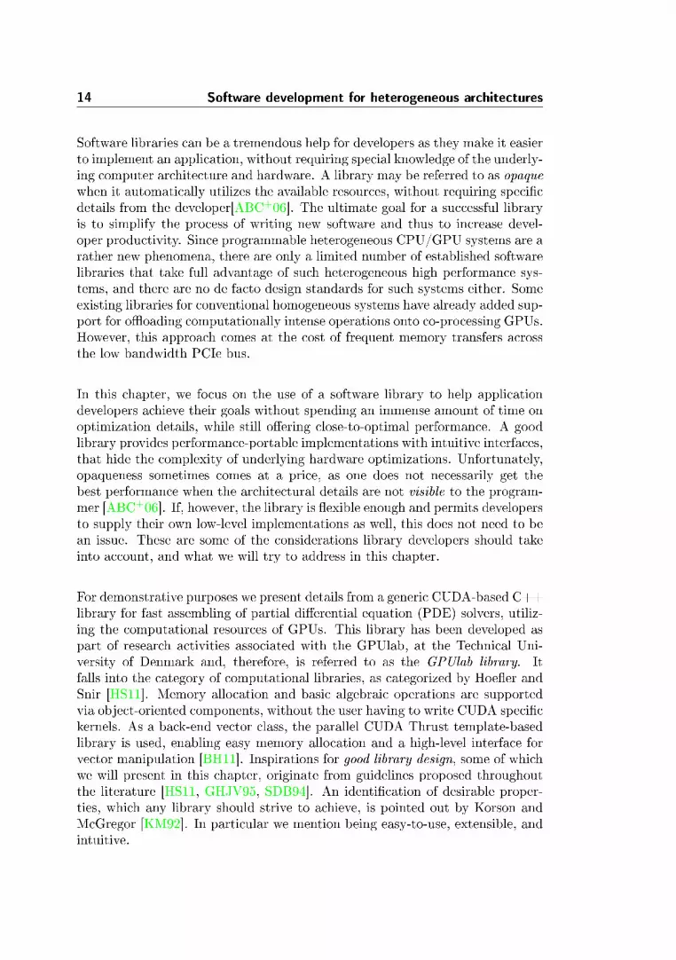
The library is grouped into component classes. Each component should fulll aset of simple interface and template rules, called concepts, in order to guaranteecompatibility with the rest of the library. In the context of PDE solving, wepresent ve component classes: vectors, matrices, iterative solvers for linear sys-tem of equations, preconditioners for the iterative solvers, and time integrators.Figure 2.1 lists the ve components along with a subset of the type denitionsthey should provide and the methods they should implement. It is possible toextend the implementation of these components with more functionality thatrelate to specic problems, but this is the minimum requirement for compatibil-ity with the remaining library. With these concept rules fullled, componentscan rely on other components to have their respective functions implemented.
A component is implemented as a generic C++ class, and normally takes as atemplate arguments of the same types that it oers through type denitions:a matrix takes a vector as template argument, and a vector takes the work-ing precision type. The matrix can then access the working precision throughthe vector class. Components that rely on multiple template arguments cancombine these arguments via type binders to reduce the number of argumentsand maintain code simplicity. We will demonstrate use of such type bindersin the model problem examples. A thorough introduction to template-basedprogramming in C++ can be found in [VJ02].
The generic conguration allows the developer to dene and assemble solverparts at the very beginning of the program using type denitions. ChangingPDE parts at a later time is then only a matter of changing type denitions.We will give two model examples of how to assemble PDE solvers in Section 2.2.
2.1.2 A matrix-free nite dierence component
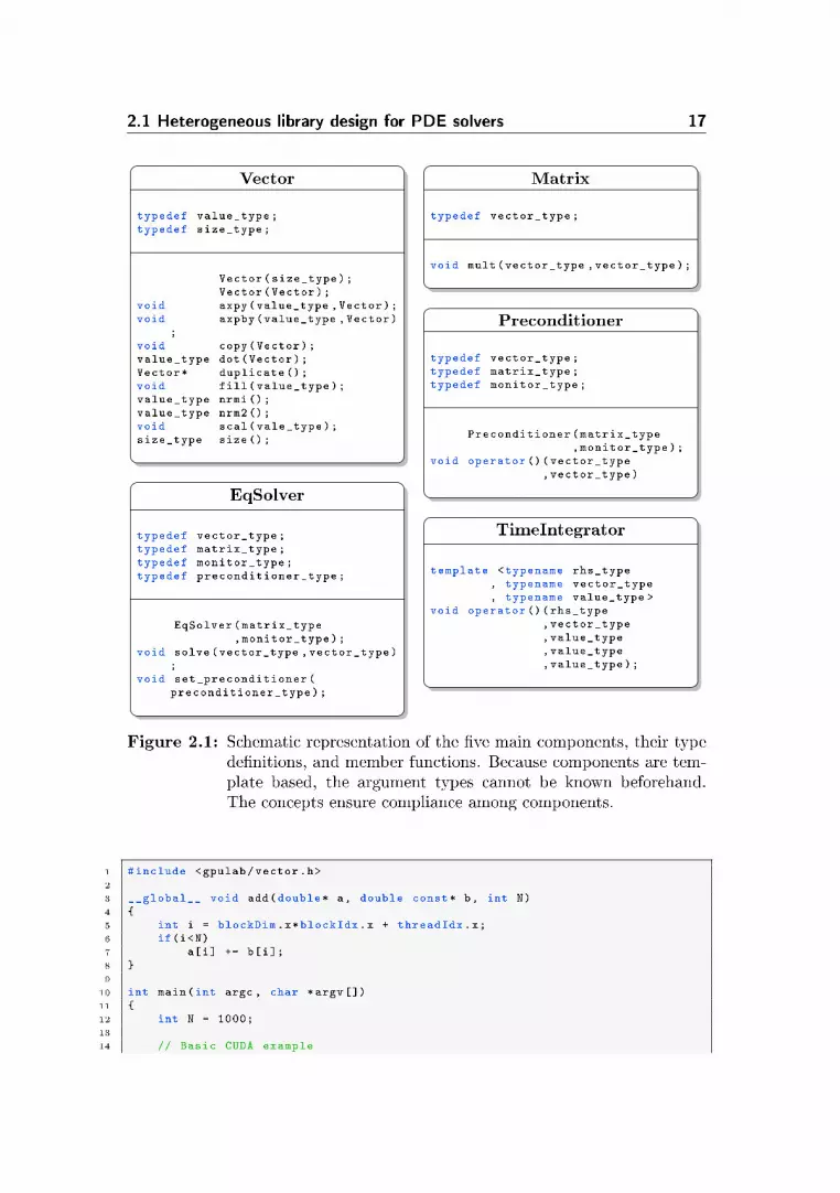
Common vector operations, such as memory allocation, element-wise assign-ments, and basic algebraic transformations, require many lines of codes for apurely CUDA-based implementation. These CUDA-specic operations and ker-nels are hidden from the user behind library implementations, to ensure a highabstraction level. The vector class inherits from the CUDA-based Thrust li-brary and therefore oers the same level of abstraction that enhances developerproductivity and enables performance portability. Creating and allocating de-vice (GPU) memory for two vectors can be done in a simple and intuitive wayusing the GPUlab library, as shown in Listing 2.1 where two vectors are addedtogether.
2.1 Heterogeneous library design for PDE solvers 17
Vector
typedef value_type;typedef size_type;
Vector(size_type);Vector(Vector);
void axpy(value_type ,Vector);void axpby(value_type ,Vector)
;void copy(Vector);value_type dot(Vector);Vector* duplicate ();void fill(value_type);value_type nrmi();value_type nrm2();void scal(vale_type);size_type size();
Matrix
typedef vector_type;
void mult(vector_type ,vector_type);
EqSolver
typedef vector_type;typedef matrix_type;typedef monitor_type;typedef preconditioner_type;
EqSolver(matrix_type,monitor_type);
void solve(vector_type ,vector_type);
void set_preconditioner(preconditioner_type);
Preconditioner
typedef vector_type;typedef matrix_type;typedef monitor_type;
Preconditioner(matrix_type,monitor_type);
void operator ()(vector_type,vector_type)
TimeIntegrator
template <typename rhs_type, typename vector_type, typename value_type >
void operator ()(rhs_type,vector_type,value_type,value_type,value_type);
Figure 2.1: Schematic representation of the ve main components, their typedenitions, and member functions. Because components are tem-plate based, the argument types cannot be known beforehand.The concepts ensure compliance among components.
1 #include <gpulab/vector.h>2
3 __global__ void add(double* a, double const* b, int N)4 5 int i = blockDim.x*blockIdx.x + threadIdx.x;6 if(i<N)7 a[i] += b[i];8 9
10 int main(int argc , char *argv [])11 12 int N = 1000;13
14 // Basic CUDA example
18 Software development for heterogeneous architectures
15 double *a1 , *b1;16 cudaMalloc ((void **)&a1, N*sizeof(double));17 cudaMalloc ((void **)&b1, N*sizeof(double));18 cudaMemset(a1 , 2.0, N);19 cudaMemset(b1 , 3.0, N);20 int blocksize = 128;21 add <<<(N+blocksize -1)/blocksize ,blocksize >>>(a1, b1, N);22
23 // gpulab example24 gpulab ::vector <double ,gpulab :: device_memory > a2(N, 2.0);25 gpulab ::vector <double ,gpulab :: device_memory > b2(N, 3.0);26 a2.axpy (1.0, b2); // BLAS1: a2 = 1*b2 + a227
28 return 0;29
Listing 2.1: Allocating, initializing, and adding together two vectors on theGPU: rst example uses pure CUDA C; second example uses thebuilt-in library template-based vector class
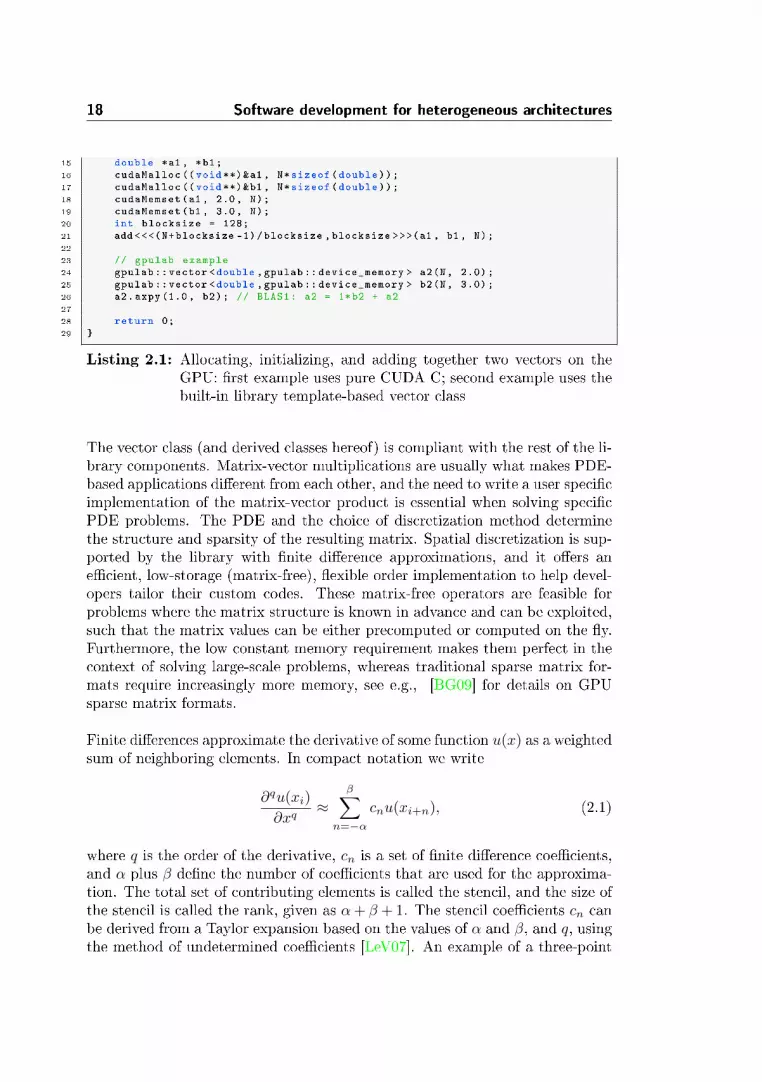
The vector class (and derived classes hereof) is compliant with the rest of the li-brary components. Matrix-vector multiplications are usually what makes PDE-based applications dierent from each other, and the need to write a user specicimplementation of the matrix-vector product is essential when solving specicPDE problems. The PDE and the choice of discretization method determinethe structure and sparsity of the resulting matrix. Spatial discretization is sup-ported by the library with nite dierence approximations, and it oers anecient, low-storage (matrix-free), exible order implementation to help devel-opers tailor their custom codes. These matrix-free operators are feasible forproblems where the matrix structure is known in advance and can be exploited,such that the matrix values can be either precomputed or computed on the y.Furthermore, the low constant memory requirement makes them perfect in thecontext of solving large-scale problems, whereas traditional sparse matrix for-mats require increasingly more memory, see e.g., [BG09] for details on GPUsparse matrix formats.
Finite dierences approximate the derivative of some function u(x) as a weightedsum of neighboring elements. In compact notation we write
∂qu(xi)
∂xq≈
β∑n=−α
cnu(xi+n), (2.1)
where q is the order of the derivative, cn is a set of nite dierence coecients,and α plus β dene the number of coecients that are used for the approxima-tion. The total set of contributing elements is called the stencil, and the size ofthe stencil is called the rank, given as α+ β + 1. The stencil coecients cn canbe derived from a Taylor expansion based on the values of α and β, and q, usingthe method of undetermined coecients [LeV07]. An example of a three-point
2.1 Heterogeneous library design for PDE solvers 19
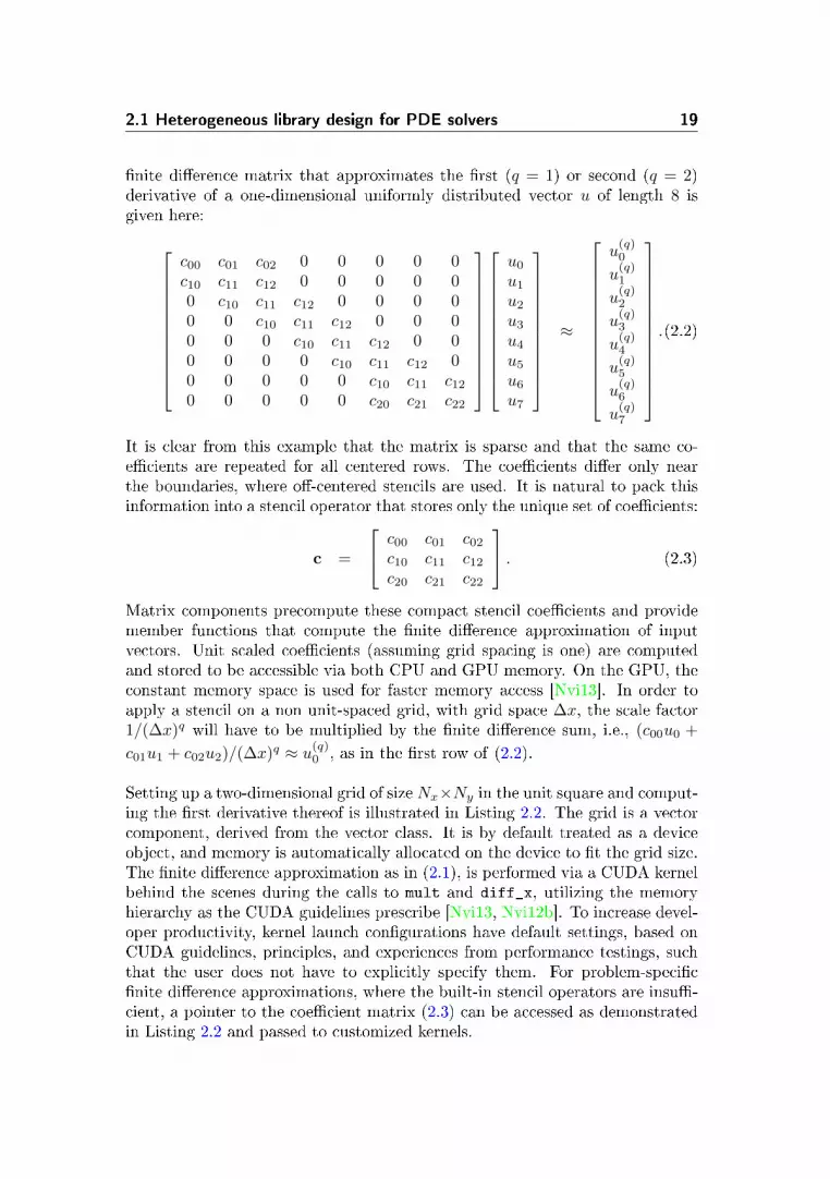
nite dierence matrix that approximates the rst (q = 1) or second (q = 2)derivative of a one-dimensional uniformly distributed vector u of length 8 isgiven here:
c00 c01 c02 0 0 0 0 0c10 c11 c12 0 0 0 0 00 c10 c11 c12 0 0 0 00 0 c10 c11 c12 0 0 00 0 0 c10 c11 c12 0 00 0 0 0 c10 c11 c12 00 0 0 0 0 c10 c11 c12
0 0 0 0 0 c20 c21 c22
u0
u1
u2
u3
u4
u5
u6
u7
≈
u(q)0
u(q)1
u(q)2
u(q)3
u(q)4
u(q)5
u(q)6
u(q)7
.(2.2)
It is clear from this example that the matrix is sparse and that the same co-ecients are repeated for all centered rows. The coecients dier only nearthe boundaries, where o-centered stencils are used. It is natural to pack thisinformation into a stencil operator that stores only the unique set of coecients:
c =
c00 c01 c02
c10 c11 c12
c20 c21 c22
. (2.3)
Matrix components precompute these compact stencil coecients and providemember functions that compute the nite dierence approximation of inputvectors. Unit scaled coecients (assuming grid spacing is one) are computedand stored to be accessible via both CPU and GPU memory. On the GPU, theconstant memory space is used for faster memory access [Nvi13]. In order toapply a stencil on a non unit-spaced grid, with grid space ∆x, the scale factor1/(∆x)q will have to be multiplied by the nite dierence sum, i.e., (c00u0 +
c01u1 + c02u2)/(∆x)q ≈ u(q)0 , as in the rst row of (2.2).
Setting up a two-dimensional grid of size Nx×Ny in the unit square and comput-ing the rst derivative thereof is illustrated in Listing 2.2. The grid is a vectorcomponent, derived from the vector class. It is by default treated as a deviceobject, and memory is automatically allocated on the device to t the grid size.The nite dierence approximation as in (2.1), is performed via a CUDA kernelbehind the scenes during the calls to mult and diff_x, utilizing the memoryhierarchy as the CUDA guidelines prescribe [Nvi13, Nvi12b]. To increase devel-oper productivity, kernel launch congurations have default settings, based onCUDA guidelines, principles, and experiences from performance testings, suchthat the user does not have to explicitly specify them. For problem-specicnite dierence approximations, where the built-in stencil operators are insu-cient, a pointer to the coecient matrix (2.3) can be accessed as demonstratedin Listing 2.2 and passed to customized kernels.

20 Software development for heterogeneous architectures
1 #include <gpulab/grid.h>2 #include <gpulab/FD/stencil.h>3
4 int main(int argc , char *argv [])5 6 // Initialize grid dimensions7 unsigned int Nx = 10, Ny = 10;8 gpulab ::grid_dim <unsigned int > dim(Nx ,Ny);9 gpulab ::grid <double > u(dim); // 2D function u10 gpulab ::grid <double > ux(u); // 1st order derivative in x11 gpulab ::grid <double > uxy(u); // Mixed derivative in x/y12
13 // Put meaningful values into u here ...14
15 // Stencil size , alpha=beta=2, 9pt 2D stencil16 int alpha = 2;17 // 1st order derivative18 gpulab ::FD:: stencil_2d <double > stencil(1, alpha);19 // Calculate uxy = du/dx + du/dy20 stencil.mult(u,uxy);21 // Calculate ux = du/dx22 stencil.diff_x(u,ux);23 // Host and device pointers to stencil coeffs24 double const* hc = stencil.coeffs_host ();25 double const* dc = stencil.coeffs_device ();26
27 return 0;28
Listing 2.2: Two-dimensional nite dierence stencil example: computing therst derivative using ve points (α = β = 2) per dimension, atotal nine-point stencil
In the following sections we demonstrate how to go from an initial value prob-lem (IVP) or a boundary value problem (BVP) to a working application solverby combining existing library components along with new custom-tailored com-ponents. We also demonstrate how to apply spatial and temporal domain de-composition strategies that can make existing solvers take advantage of systemsequipped with multiple GPUs. The next section demonstrates how to rapidlyassemble a PDE solver using library components. Appendix A contains addi-tional examples and guidelines on how to use the GPUlab library.
2.2 Model problems
We present two elementary PDE model problems, to demonstrate how to assem-ble PDE solvers, using library components that follow the guidelines describedabove. The rst model problem is the unsteady parabolic heat conduction equa-tion; the second model problem is the elliptic Poisson equation. The two modelproblems consist of elements that play important roles in solving a broad rangeof more advanced PDE problems.

2.2 Model problems 21
We refer the reader to Chapter 3 for an example of a scientic applicationrelevant for coastal and maritime engineering analysis that has been assembledusing customized library components similar to those presented in the following.
2.2.1 Heat conduction equation
Firstly, we consider a two-dimensional heat conduction problem dened on aunit square. The heat conduction equation is a parabolic partial dierentialdiusion equation, including both spatial and temporal derivatives. It describeshow the diusion of heat in a medium changes with time. Diusion equationsare of great importance in many elds of sciences, e.g., uid dynamics, wherethe uid motion is uniquely described by the Navier-Stokes equations, whichinclude a diusive viscous term [CM93, FP96].
The heat problem is an IVP, it describes how the heat distribution evolvesfrom a specied initial state. Together with homogeneous Dirichlet boundaryconditions, the heat problem in the unit square is given as
∂u
∂t− κ∇2u = 0, (x, y) ∈ Ω([0, 1]× [0, 1]), t ≥ 0, (2.4a)
u = 0, (x, y) ∈ ∂Ω, (2.4b)
where u(x, y, t) is the unknown heat distribution dened within the domain Ω,t is the time, κ is a heat conductivity constant (let κ = 1), and ∇2 is thetwo-dimensional Laplace dierential operator (∂xx + ∂yy). We use the followinginitial condition:
u(x, y, t0) = sin(πx) sin(πy), (x, y) ∈ Ω, (2.5)
because it has a known analytic solution over the entire time span, and it satisesthe homogeneous boundary condition given by (2.4b). An illustrative exampleof the numerical solution to the heat problem, using (2.5) as the initial condition,is given in Figure 2.2.
We use a Method of Lines (MoL) approach to solve (2.4). Thus, the spatialderivatives are replaced with nite dierence approximations, leaving only thetemporal derivative as unknown. The spatial derivatives are approximated fromun, where un represents the approximate solution to u(tn) at a given time tnwith time step size δt such that tn = nδt for n = 0, 1, . . .. The nite dierenceapproximation can be interpreted as a matrix-vector product as sketched in(2.2), and so the semi-discrete heat conduction problem becomes
∂u
∂t= Au, A ∈ RN×N , u ∈ RN , (2.6)

22 Software development for heterogeneous architectures
00.5
1
0
0.5
10
0.5
1
xy
u
(a) t = 0.00s
00.5
1
0
0.5
10
0.5
1
xy
(b) t = 0.05s
00.5
1
0
0.5
10
0.5
1
xy
(c) t = 0.10s
Figure 2.2: Discrete solution, at times t = 0s and t = 0.05s, using (2.5) as theinitial condition and a small 20× 20 numerical grid.
where A is the sparse nite dierence matrix and N is the number of unknownsin the discrete system. The temporal derivative is now free to be approximatedby any suitable choice of a time-integration method. The most simple integra-tion scheme would be the rst-order accurate explicit forward Euler method,
un+1 = un + δtAun, (2.7)
where n + 1 refers to the solution at the next time step. The forward Eulermethod can be exchanged with alternative high-order accurate time integra-tion methods, such as Runge-Kutta methods or linear multistep methods, ifnumerical instability becomes an issue, see, e.g., [LeV07] for details on numer-ical stability analysis. For demonstrative purposes, we simply use conservativetime step sizes to avoid stability issues. However, the component-based librarydesign provides exactly the exibility for the application developer to select orchange PDE solver parts, such as the time integrator, with little coding eort.A generic implementation of the forward Euler method that satises the libraryconcept rules is illustrated in Listing 2.3. According to the component guide-lines in Figure 2.1, a time integrator is basically a functor, which means thatit implements the parenthesis operator, taking ve template arguments: a righthand side operator, the state vector, integration start time, integration endtime, and a time step size. The method takes as many time steps as necessaryto integrate from the start to the end, continuously updating the state vectoraccording to (2.7). Notice, that nothing in Listing 2.3 indicates whether GPUsare used or not. However, it is likely that the underlying implementation ofthe right hand side functor and the axpy vector function, do rely on fast GPUkernels. However, it is not something that the developer of the component hasto account for. For this reason, the template-based approach, along with simpleinterface concepts, make it easy to create new components that will t well intoa generic library.

2.2 Model problems 23
1 struct forward_euler2 3 template <typename F, typename T, typename V>4 void operator ()(F fun , V& x, T t, T tend , T dt)5 6 V rhs(x); // Initialize RHS vector7 while(t < tend)8 9 if(tend -t < dt)10 dt = tend -t; // Adjust dt for last time step11
12 (*fun)(t, x, rhs); // Apply rhs function13 x.axpy(dt,rhs); // Update stage14 t += dt; // Next time step15 16 17
Listing 2.3: Generic implementation of explicit rst-order forward Eulerintegration
The basic numerical approach to solve the heat conduction problem has nowbeen outlined, and we are ready to assemble the PDE solver.
2.2.1.1 Assembling the heat conduction solver
Before we are able to numerically solve the discrete heat conduction problem(2.4), we need implementations to handle the the following items:
Grid. A discrete numerical grid to represent the two-dimensional heat distribu-tion domain and the arithmetical working precision (32-bit single precisionor 64-bit double precision).
RHS. A right-hand side operator for (2.6) that approximates the second-orderspatial derivatives (matrix-vector product).
Boundary conditions. A strategy that ensures that the Dirichlet conditionsare satised on the boundary.
Time integrator. A time integration scheme, that approximates the time deriva-tive from (2.6).
All items are either directly available in the library, or can be designed fromcomponents therein. The built-in stencil operator may assist in implementingthe matrix-vector product, but we need to explicitly ensure that the Dirichletboundary conditions are satised. We demonstrated in Listing 2.2 how to ap-proximate the derivative using exible-order nite dierence stencils. However,

24 Software development for heterogeneous architectures
from (2.4b) we know that boundary values are zero. Therefore, we extend thestencil operator with a simple kernel call that assigns zero to the entire bound-ary. Listing 2.4 shows the code for the two-dimensional Laplace right-hand sideoperator. The constructor takes as an argument the stencil half size α andassumes α = β. Thus, the total two-dimensional stencil rank will be 4α + 1.For simplicity we also assume that the grid is uniformly distributed, Nx = Ny.Performance optimizations for the stencil kernel, such as shared memory uti-lization, are handled in the underlying implementation, accordingly to CUDAguidelines [Nvi13, Nvi12b]. The macros, BLOCK1D and GRID1D, are used to helpset up kernel congurations based on grid sizes, and RAW_PTR is used to cast thevector object to a valid device memory pointer.
1 template <typename T>2 __global__ void set_dirichlet_bc(T* u, int Nx)3 4 int i = blockDim.x*blockIdx.x+threadIdx.x;5 if(i<Nx)6 7 u[i] = 0.0;8 u[(Nx -1)*Nx+i] = 0.0;9 u[i*Nx] = 0.0;10 u[i*Nx+Nx -1] = 0.0;11 12 ;13
14 template <typename T>15 struct laplacian16 17 gpulab ::FD:: stencil_2d <T> m_stencil;18
19 laplacian(int alpha) : m_stencil (2,alpha) 20
21 template <typename V>22 void operator ()(T t, V const& u, V & rhs) const23 24 m_stencil.mult(u,rhs); // rhs = du/dxx + du/dyy25
26 // Make sure bc is correct27 dim3 block = BLOCK1D(rhs.Nx());28 dim3 grid = GRID1D(rhs.Nx());29 set_dirichlet_bc <<<grid ,block >>>(RAW_PTR(rhs),rhs.Nx());30 31 ;
Listing 2.4: The right-hand side Laplace operator: the built-in stencilapproximates the two dimensional spatial derivatives, while thecustom set_dirichlet_bc kernel takes care of satisfying theboundary conditions
With the right-hand side operator in place, we are ready to implement the solver.For this simple PDE problem we compute all necessary initial data in the bodyof the main function and use the forward Euler time integrator to compute thesolution until t = tend. For more advanced solvers, a built-in ode_solver classis dened that helps take care of initialization and storage of multiple state

2.2 Model problems 25
variables. Declaring type denitions for all components at the beginning of themain le gives a good overview of the solver composition. In this way, it will beeasy to control or change solver components at later times. Listing 2.5 lists thetype denitions that are used to assemble the heat conduction solver.
1 typedef double value_type;2 typedef laplacian <value_type > rhs_type;3 typedef gpulab ::grid <value_type > vector_type;4 typedef vector_type :: property_type property_type;5 typedef gpulab :: integration :: forward_euler time_integrator_type;
Listing 2.5: Type denitions for all the heat conduction solver componentsused throughout the remaining code
The grid is by default treated as a device object, and memory is allocated onthe GPU upon initialization of the grid. Setting up the grid can be done viathe property type class. The property class holds information about the discreteand physical dimensions, along with ctitious ghost (halo) layers and periodicityconditions. For the heat conduction problem we use a non periodic domain ofsize N ×N within the unit square with no ghost layers. Listing 2.6 illustratesthe grid assembly.
1 // Setup discrete and physical dimensions2 gpulab ::grid_dim <int > dim(N,N,1);3 gpulab ::grid_dim <value_type > p0(0,0);4 gpulab ::grid_dim <value_type > p1(1,1);5 property_type props(dim ,p0,p1);6
7 // Initialize vector8 vector_type u(props);
Listing 2.6: Creating a two-dimensional grid of size N times N and physicaldimension 0 to 1
Hereafter the vector u can be initialized accordingly to (2.5). Finally we needto instantiate the right-hand side Laplacian operator from Listing 2.4 and theforward Euler time integrator in order to integrate from t0 until tend.
1 rhs_type rhs(alpha); // Create right -hand side operator2 time_integrator_type solver; // Create time integrator3 solver (&rhs ,u,0.0f,tend ,dt); // Integrate from 0 to tend using dt
Listing 2.7: creating a time integrator and the right-hand side Laplacianoperator.
The last line invokes the forward Euler time integration scheme dened in List-ing 2.5. If the developer decides to change the integrator into another ex-plicit scheme, only the time integrator type denition in Listing 2.5 needs to bechanged. The heat conduction solver is now complete.

26 Software development for heterogeneous architectures
2.2.1.2 Numerical solutions to the heat conduction problem
Solution time for the heat conduction problem is in itself not very interesting, asit is only a simple model problem. What is interesting for GPU kernels, such asthe nite dierences kernel, is that increased computational work often comeswith a very small price, because the fast computations can be hidden by therelatively slower memory fetches. Therefore, we are able to improve the accu-racy of the numerical solution via more accurate nite dierences (larger stencilsizes), while improving the computational performance in terms of oating pointoperations per second (ops). Figure 2.3 conrms, that larger stencils improvethe kernel performance. Notice that even though these performance results arefavorable compared to single core systems (∼ 10 GFlops double precision on a2.5-GHz processor), they are still far from their peak performance, e.g., ∼ 2.4TFlops single precision for the GeForce GTX590. The reason is that the kernelis bandwidth bound, i.e., performance is limited by the time it takes to movememory between the global GPU memory and the chip. The Tesla K20 performsbetter than the GeForce GTX590 because it obtains the highest bandwidth. Be-ing bandwidth bound is a general limitation for matrix-vector-like operationsthat arise from the discretization of PDE problems. Only matrix-matrix multi-plications, which have a high ratio of computations versus memory transactions,are able to reach near-optimal performance results [KmWH10]. These kinds ofoperators are, however, rarely used to solve PDE problems.
1 2 3 4
10
20
30
40
50
60
α
GFlops
single
double
(a) GeForce GTX590.
1 2 3 40
20
40
60
80
100
α
GFlops
single
double
(b) Tesla K20c.
Figure 2.3: Single and double precision oating point operations per secondfor a two dimensional stencil operator on a numerical grid of size40962. Various stencil sizes are used α = 1, 2, 3, 4, equivalent to5pt, 9pt, 13pt, and 17pt stencils. Host memory transfers are notincluded in timings.
2.2 Model problems 27
2.2.2 Poisson equation
The Poisson equation is a second-order elliptic dierential equation, often en-countered in applications within scientic elds such as electrostatics and me-chanics. We consider the two- dimensional BVP dened in terms of Poisson'sequation with homogeneous Dirichlet boundary conditions of the form
∇2u = f(x, y), (x, y) ∈ Ω([0, 1]× [0, 1]), (2.8a)
u = 0, (x, y) ∈ ∂Ω. (2.8b)
Notice the similarities to the heat conduction equation (2.4). In fact, (2.8)could be a steady-state solution to the heat equation, when there is no temporalchange ∂u
∂t = 0, but a source term f(x, y). Since the Laplace operator and theboundary conditions are the same for both problems, we are able to reuse thesame implementation with few modications.
In contrast to the heat equation, there are no initial conditions. Instead, we seeksome u(x, y) that satises (2.8), given a source term f(x, y), on the right-handside. For simplicity, assume that we know the exact solution, utrue, correspond-ing to (2.5). Then we use the method of manufactured solutions to derive anexpression for the corresponding right-hand side f(x, y):
f(x, y) = ∇2utrue = −2π2 sin(πx) sin(πy). (2.9)
The spatial derivative in (2.8) is again approximated with nite dierences,similar to the example in (2.2), except boundary values are explicitly set tozero. The discrete form of the system can now be written as a sparse linearsystem of equations:
Au = f , u, f ∈ RN , A ∈ RN×N , (2.10)
where A is the sparse matrix formed by nite dierence coecients, N is thenumber of unknowns, and f is given by (2.9). Equation (2.10) can be solvedin numerous ways, but a few observations may help do it more eciently. Di-rect solvers based on Gaussian elimination are accurate and use a nite numberof operations for a constant problem size. However, the arithmetic complexitygrows with the problem size by as much as O(N3) if the sparsity of A is notexploited. Direct solvers are therefore mostly feasible for dense systems of lim-ited sizes. Sparse direct solvers exist, but they are often dicult to parallelize,or applicable for only certain types of matrices. Regardless of the discretizationtechnique, the discretization of an elliptic PDE into a linear system as in (2.10)yields a very sparse matrix A when N is large. Iterative methods for solv-ing large sparse linear systems nd broad use in scientic applications, becausethey require only an implementation of the matrix-vector product, and they

28 Software development for heterogeneous architectures
often use a limited amount of additional memory. Comprehensive introductionsto iterative methods may be found in any of [Saa03, Kel95, BBC+94].
One benet of the high abstraction level and the template-based library design isto allow developers to implement their own components, such as iterative meth-ods for solving sparse linear systems. The library includes three popular iterativemethods: conjugate gradient, defect correction, and geometric multigrid. Theconjugate gradient method is applicable only to systems with symmetric pos-itive denite matrices. This is true for the two-dimensional Poisson problem,when it is discretized with a ve-point nite dierence stencil, because thenthere will be no o-centered approximations near the boundary. For high-orderapproximations (α > 1), we use the defect correction method with multigridpreconditioning. See e.g., [TOS+01] for details on multigrid methods.
We will not present the implementation details for all three methods but brieydemonstrate the simplicity of implementing the body of such an iterative solver,given a textbook recipe or mathematical formulation. The defect correctionmethod iteratively improves the solution to Ax = b, given an initial start guessx0, by continuously solving a preconditioned error equation. The defect correc-tion iteration can be written as
xk+1 = xk +M−1(b−Axk), A,M∈ RN×N , x,b ∈ RN , (2.11)
where k is the iteration number and M is the preconditioner which should bean approximation to the original coecient matrix A. To achieve fast numericalconvergence, applying the preconditioner should be a computationally inexpen-sive operation compared to solving the original system. How to implement (2.11)within the library context is illustrated in Listing 2.8. The host CPU traverseseach line in Listing 2.8 and tests for convergence, while the computationallyexpensive matrix-vector operation and preconditioning, can be executed on theGPU, if GPU-based components are used. The defect correction method hastwo attractive properties. First, global reduction is required to monitor con-vergence only once per iteration, during convergence evaluation, which reducescommunication requirements and provides a basis for ecient and scalable par-allelization. Second, it has a minimal constant memory footprint, making it asuitable method for solving very large systems.
1 while(r.nrm2() > tol)2 3 // Calculate residual4 A.mult(x,r);5 r.axpby(1, -1, b);6
7 // Reset initial guess8 d.fill (0);9
10 // Solve M*d=r11 M(d,r);12

2.2 Model problems 29
13 // Defect correction update14 x.axpy(1, d);15
Listing 2.8: Main loop for the iterative defect correction solver: the solveris instantiated with template argument types for the matrix andvector classes, allowing underlying implementations to be basedon GPU kernels
In the following section we demonstrate how to assemble a solver for the discretePoisson problem, using one of the three iterative methods to eciently solve(2.10).
2.2.2.1 Assembling the Poisson solver
Assembling the Poisson solver follows almost the same procedure as the heatconduction solver, except the time integration part is exchanged with an iter-ative method to solve the system of linear equations (2.10). For the discretematrix-vector product we reuse the Laplace operator from the heat conductionproblem in Listing 2.4 with few modications. The Laplace operator is nowa matrix component, so to be compatible with the component interface rulesin Figure 2.1, a mult function taking two vector arguments is implemented in-stead of the parentheses operator. We leave out this code example as it almostidentical to the one in Listing 2.4.
At the beginning of the solver implementation we list the type denitions forthe Poisson solver that will be used throughout the implementation. Here weuse a geometric multigrid method as a preconditioner for the defect correctionmethod. Therefore the multigrid solver is assembled rst, so that it can beused in the assembling of the defect correction solver. Listing 2.9 denes thetypes for the vector, the matrix, the multigrid preconditioner, and the defectcorrection solver. The geometric multigrid method needs two additional tem-plate arguments that are specic for multigrid, namely, a smoother and a gridrestriction/interpolation operator. These arguments are free to be implementedand supplied by the developer if special care is required, e.g., for a customgrid structure. For the Poisson problem on a regular grid, the library containsbuilt-in restriction and interpolation operators, and a red-black Gauss-Seidelsmoother. We refer the reader to [TOS+01] for extensive details on multigridmethods. The monitor and cong types that appear in Listing 2.9 are usedfor convergence monitoring within the iterative solver and to control runtimeparameters, such as tolerances and iteration limits.
1 typedef double value_type;

30 Software development for heterogeneous architectures
2 typedef gpulab ::grid <value_type > vector_type;3 typedef laplacian <vector_type > matrix_type;4
5 // MULTIGRID solver types6 typedef gpulab :: solvers :: multigrid_types <7 vector_type8 , matrix_type9 , gpulab :: solvers :: gauss_seidel_rb_2d10 , gpulab :: solvers :: grid_handler_2d > mg_types;11 typedef gpulab :: solvers ::multigrid <mg_types > mg_solver_type;12 typedef mg_solver_type :: monitor_type monitor_type;13 typedef monitor_type :: config_type config_type;14
15 // DC solver types16 typedef gpulab :: solvers :: defect_correction_types <17 vector_type18 , matrix_type19 , monitor_type20 , mg_solver_type > dc_types;21 typedef gpulab :: solvers :: defect_correction <dc_types > dc_solver_type;
Listing 2.9: Type denitions for the Laplacian matrix component and themultigrid preconditioned iterative defect correction solver
With the type denitions set up, the implementation for the Poisson solverfollows in Listing 2.10. Some of the initializations are left out, as they followthe same procedure as for the heat conduction example. The defect correctionand geometric multigrid solvers are initialized and then multigrid is set as apreconditioner to the defect correction method. Finally the system is solved viaa call to solve().
1 matrix_type A(alpha); // High -order matrix2 matrix_type M(1); // Low -order matrix3
4 /* Omitted: create and init vectors u, f */5
6 config_type config; // Create configuration7 config.set("iter" ,30); // Set max iteration count8 config.set("rtol",1e-10); // Set relative tolerance9 monitor_type monitor(config); // Create monitor10 dc_solver_type solver(A,monitor); // Create DC solver11 mg_solver_type precond(M,monitor); // Create MG preconditioner12 solver.set_preconditioner(precond); // Set preconditioner13 solver.solve(u,f); // Solve M^-1(Au = f)14 if(monitor.converged ())15 printf("SUCCESS\n");
Listing 2.10: Initializing the preconditioned defect correction solver toapproximate the solution to Au = f
2.2.2.2 Numerical solutions to the Poisson problem
The discrete Poisson problem (2.10) has been solved using the three iterativemethods presented above. Convergence histories for the conjugate gradient

2.3 Multi-GPU systems 31
method and geometric multigrid method, using two dierent resolutions, areillustrated in Figure 2.4a. Multigrid methods are very robust and algorithmi-cally ecient, independent of the problem size. Figure 2.4a conrms that therate of convergence for the multigrid method is unchanged for both problemsizes. Only the attainable accuracy is slightly worsened, as a consequence of amore ill-conditioned system for large problem sizes.
Defect correction in combination with multigrid preconditioning enables ecientsolution of high-order approximations of the Poisson problem, illustrated inFigure 2.4b. The multigrid preconditioning matrix M is based on a low-orderapproximation to (2.10), whereas matrixA is a high-order approximation. WhenM is a close approximation to A, defect correction converges most rapidly. Thisis the eect that can be seen between the three convergence lines in Figure 2.4b.
0 5 10 1510
−14
10−12
10−10
10−8
10−6
10−4
10−2
100
Iteration
||r||2
CG, 1292
CG, 5132
MG, 1292
MG, 5132
(a) Convergence histories for the con-jugate gradient (CG) and multigrid(MG) methods, for two dierentproblem sizes.
0 10 20 30 4010
−20
10−15
10−10
10−5
100
Iteration
||r||2
α = 1
α = 2
α = 3
(b) Defect correction convergence his-tory for three dierent stencil sizes.
Figure 2.4: Algorithmic performance for the conjugate gradient, multigrid,and defect correction methods, measured in terms of the relativeresidual per iteration.
2.3 Multi-GPU systems
CUDA-enabled GPUs are optimized for high memory bandwidth and fast on-chip performance. However, the role as a separate co-processor to the CPU canbe a limiting factor for large-scale scientic applications, because the GPU mem-ory capacity is xed and is only in the range of a few Gigabytes. In comparison,
32 Software development for heterogeneous architectures
it is not unusual for a high-end workstation to be equipped with ∼ 32GB ofmain memory, plus a terabyte hard disk capacity for secondary storage. There-fore, large-scale scientic applications that process Gigabytes of data, requiredistributed computations on multiple GPU devices. Multi-GPU desktop com-puters and clusters can have a very attractive peak performance, but the ad-dition of multiple devices introduces the potential performance bottleneck ofslow data transfers across PCIe busses and network interconnections. The ratiobetween data transfers and computational work has a signicant impact on thepossibility for latency hiding, and thereby on overall application performance.
Developing software that exploit the full computational capabilities of modernclusters, GPU-based or not, is no trivial matter. Developers are faced with thecomplexity of distributing and coordinating computations on nodes consistingof many-core CPUs, GPUs and potentially other types of accelerators as well.These complexities give rise to challenges in nding numerical algorithms, thatare well suited for such systems, forcing developers to search for novel methodsthat utilize concurrency. In Chapter 4 and 5 we address some of the dicul-ties in designing software for distributed systems and demonstrate both spatialand temporal decomposition techniques as a means for enhanced performancethroughput and large-scale simulation.

Chapter 3
Free surface water waves
Applications for hydrodynamic simulations are used in many areas of coastaland oshore engineering. Most models today are based on Boussinesq-type for-mulations, where the three-dimensional unied potential ow problem is sim-plied analytically to a two-dimensional problem under the assumption thatthe vertical prole has polynomial variation. Much research has been doneon Boussinesq-type models for several decades, since the original work of Pere-grine [Per67] and later pioneered by Abott et al. [APS78, AMW84]. More recentresearch focuses on higher-order formulations that more accurately capture theeects of fully nonlinear and dispersive water waves traveling over varying depthsto far oshore. These formulations tend to introduce numerical diculties dueto the higher order derivatives.
The quality and application range of hydrodynamic simulations based on Boussinesq-type formulations are traditionally evaluated against the more accurate poten-tial ow theory, which has been perceived as too computationally expensive forpractical engineering applications [Lin08]. Potential ow theory requires thesolution of a Laplace problem arising from the fully three-dimensional prob-lem. An ecient scalable strategy for solving the transformed Laplace problem,based on low-order nite dierence discretization and geometric multigrid, wasrst proposed by Li and Fleming in 1997 [LF97]. Their strategy led the wayfor more accurate and ecient methods, as it was still unsuitable for large-scaleengineering applications.
34 Free surface water waves
Our work takes oset in the development and improvements to the strategyoriginally proposed by Li and Fleming. The strategy extended in [BZ07] withhigh-order discretizations via high-order numerics and vertical grid clustering toenable accurate and ecient solutions in two dimensions. A exible-order dis-cretization for the three-dimensional problem was then proposed by [EKBL09],with a more robust discretization strategy and a Laplace solver based on multi-grid preconditioned GMRES. The total strategy proposed by [EKBL09] led tothe rst Fortran90 implementation of what was then referred to as the Ocean-Wave3D model1.
The development of new massively parallel high-performance commodity hard-ware, is a perfect driver for developing and revisiting these techniques for ecientsimulation of maritime engineering applications. In [EKMG11], we implementeda dedicated massively parallel solver based on exible-order discretization and amultigrid preconditioned defect correction method, and we demonstrated that itis indeed possible to signicantly reduce the barriers for practical use of poten-tial ow theory as a modeling basis for hydrodynamic simulations. To establishthe model as an ecient parallel tool, the entire algorithm was rst redesigned,implemented, and evaluated using a dedicated solver based on the CUDA for Cprogramming model. The CUDA for C extension was used because no extensionswere available for Fortran90 at the time of the proof-of-concept. The promisingintermediate performance results convinced us to continue the development ofthe GPU-accelerated OceanWave3D solver and to implement the solver usingour generic library in order to enhance portability and productivity of futuredevelopment. The OceanWave3D model, based on unied potential ow theory,is a relevant modeling basis, because it emphasizes some of the new engineeringpossibilities that modern aordable hardware brings. In addition, a potentialow model is a good test bed for prototyping and designing software algorithmsfor PDE solvers, as it contains components that are essential in a broad rangeof scientic applications, such as a computationally demanding elliptic problemalong with hyperbolic free surface conditions. When this work began, therewere few engineering applications that utilized massively parallel heterogeneoussystems. Our focus is to try and demonstrate by a proof-of-concept some of thepossibilities that these modern programming paradigms can oer.
1Development and research based on the OceanWave3D model are currently employed
by researches at the Department of Mechanical Engineering and the Department of Applied
Mathematics and Computer Science at the Technical University of Denmark.

3.1 Potential ow theory 35
3.1 Potential ow theory
The unied potential ow equations are a subclass of the more complete Eulerequations, and are valid only under the assumption of incompressible, irrota-tional, and inviscid ow. A comprehensive introduction to hydrodynamics isgiven by Svendsen and Jonnson [SJ76]. Details on numerical modeling aspectscan be found in e.g., [Lin08] or in the shorter survey by Dias and Bridges [DB06].A variety of numerical techniques for solving such hydrodynamic model problemshave been presented throughout the literature, see e.g., [Yeu82, LF97, EK06].A concise derivation of the the fully nonlinear water wave model based on po-tential ow theory is presented in [EKGNL13]. In this section we intend onlyto present the governing equations as they will be used in the remainder ofthis work and we refer the reader to the above mentioned literature for a morethorough introduction.
Under the assumption of irrotational ow, the velocity vector eld u(x, y, z) ≡(u, v, w)T , is uniquely dened by the gradient of the velocity potential φ(x, y, z),such that u ≡ (∂xφ, ∂yφ, ∂zφ)T . The evolution of the free surface elevation η,
and the potential φ at the free surface, are described by a kinematic and adynamic free surface boundary condition
∂tη =−∇η ·∇φ+ w(1 + ∇η ·∇η), (3.1a)
∂tφ =− gη − 1
2(∇φ ·∇φ− w2(1 + ∇η ·∇η)), (3.1b)
where ∇ is the horizontal dierential operator ∇ ≡ (∂x ∂y)T , g is the gravita-tional acceleration, and w is the vertical velocity evaluated at the free surfacew ≡ ∂zφ|z=η.
Figure 3.1: Setup of a free surface wa-ter wave model.
The unsteady free surface elevationη(x, t) is measured from the still-water level at z = 0. A conceptualillustration of a two-dimensional nu-merical wave tank with a free surfacewater wave setup is given in Figure3.1.
The vertical velocity at the surfacew, can be computed from the full ve-locity potential. Due to mass conti-nuity, the velocity potential satisesthe Laplace equation everywhere in-side the domain. Along with bound-ary conditions the following (elliptic)

36 Free surface water waves
Laplace equation uniquely denes thevelocity potential
φ = φ, z = η (3.2a)
∇2φ+ ∂zzφ = 0, −h ≤ z < η (3.2b)
∂zφ+ ∇h ·∇φ = 0, z = −h, (3.2c)
where h is the still water depth. The system of equations is closed by imposingproper boundary conditions on the outer boundaries ∂Ω, surrounding the do-main of interest. In the vertical direction, the ow is bounded at the bottomz = −h, by the kinematic free-slip condition (3.2c) and at the surface z = η,with Dirichlet conditions given by the time-dependent dynamic free surface con-dition(3.1b).
Along the vertical boundaries we assume only bottom-mounted, vertical surface-piercing, and fully reecting (impermeable) walls with free slip boundary con-ditions. In this case all outward pointing boundary normals are xed to thehorizontal plane, e.i. n ≡ (nx, ny, 0)T , and the uid ows only along the tan-gential direction of the walls,
n · u = nx u+ ny v
= nx ∂xφ+ ny ∂yφ = 0, ∀x ∈ ∂Ω. (3.3)
Wave generation and wave absorption are considered in Section 3.2.4, where wend that with impermeable boundaries in combination with suciently largegeneration and absorption zones, the absence of radiation boundaries is not sig-nicant. Thus, we are able to reuse the boundary condition (3.3), in combinationwith wave generation and absorption zones.
Under some circumstances, when wave amplitudes are small and dispersive waveeects are minor , i.e., ∇η(x, t) ≈ 0,∀x, t, the nonlinear free surface equationscan be reduced to linear form,
∂tη =w, (3.4a)
∂tφ =− gη. (3.4b)
The linear free surface conditions are useful for stability analysis and validationcases where analytic solutions are known. We emphasize that when we refer tothe linear or nonlinear system, it refers to the PDE, and not the Laplace problem,which is always a linear system of equations.
In free surface water wave modeling it is often convenient to use dimensionlessnumbers for comparison and characterization of various waves. The wave num-ber k is given by k ≡ 2π/L, where L is the wavelength. Also the wave number

3.2 The numerical model 37
times the still water depth kh, is used to determine if the wave is propagating ina deep or a shallow water situation. The wave steepness S is dened as the ratiobetween wave height and wavelength S ≡ H/L. Sometimes we refer to wavesteepness in terms of maximum attainable value, i.e., H/L = 50%(H/L)max.For a thorough introduction to wave characterization we refer the reader to[SJ76].
3.2 The numerical model
Numerical solutions to potential ow model problems are attractive to gainunique insight due to the underlying accurate properties. To ensure practicalsolutions of large-scale problems based on potential ow theory, it is of great im-portance that the numerical strategy is based on ecient, scalable, distributed,data-local, and parallel methods. We use a nite dierence discretization forapproximating the spatial derivatives in (3.1) and (3.2), based on the genericmatrix-free implementation presented in Section 2.1.2. The order of accuracycan be controlled via a exible order implementation, which allow the user tocontrol the size of the discretization stencils. Finite dierence methods areamong the simplest and best performing discretization methods, due to highdata-locality (at least along one dimension) and the structured domains, whichrequire no index lookup table.
In the context of GPUs, the above mentioned numerical method translateswell into the GPU programming model, because the computation of each -nite dierence approximation per grid point is embarrassingly parallel, since nocommunication between threads is required. Furthermore, structured grids areeasily represented in memory and allow parallel execution with ecient collo-cated memory access patterns, such that adjacent threads also access adjacentmemory locations.
3.2.1 Ecient solution of the Laplace equation
The Laplace problem (3.2) with boundary conditions is a fully three-dimensionalproblem, whereas the free surface boundary conditions (3.1a) and (3.1b) areonly two-dimensional. Computing the solution to the discrete Laplace problemtherefore involves signicantly more computational work, which makes it theperformance bottleneck. We have implemented and analyzed a scalable andlow-memory iterative strategy for eciently solving the Laplace problem onheterogeneous hardware in [EKMG11, GEKM11]. The numerical strategy is

38 Free surface water waves
z
x0
-h(x)
x
1
0
L
0 L
(x,z,t)
z(x, ,t)
η(x,t)
o(xi,zj)
o(xi, j)
j
ii
j
Figure 3.2: Vertical σ-transormation.
briey outlined in the following sections.
From a numerical point of view it is impractical that the shape of the phys-ical domain changes due to the time-dependent free surface conditions. A σ-transformation is therefore applied in the vertical direction such that
σ(x, z, t) =z + h(x)
d(x, t), 0 ≤ σ ≤ 1, (3.5)
where d(x, t) = η(x, t) + h(x) is the total water depth from the sea bottomto the water surface. This enables a transformation of the physical probleminto a time-invariant computational domain, at the expense of time-varyingcoecients and mixed derivatives. The σ-transformation is illustrated in Figure3.2. Once the σ-transformation is applied, the original Laplace problem (3.2) istransformed as well,
Φ = φ, σ = 1, (3.6a)
∇2Φ + ∇2σ(∂σΦ) + 2∇σ ·∇(∂σΦ)+
(∇σ ·∇σ + (∂zσ)2)∂σσΦ = 0, 0 ≤ σ < 1, (3.6b)
n · (∇, ∂zσ∂σ)Φ = 0, (x, σ) ∈ ∂Ω, (3.6c)
where the transformed velocity potential Φ(x, σ, t) = φ(x, z, t) holds all informa-tion about the ow kinematics in the entire uid volume. The spatial derivatives

3.2 The numerical model 39
of σ appearing in (3.6) can be directly derived from (3.5) as
∇σ =1− σd
∇h− σ
d∇η, (3.7a)
∇2σ =1− σd
(∇2h− ∇h ·∇h
d
)− σ
d
(∇2η − ∇η ·∇η
d
)− 1− 2σ
d2∇h ·∇η − ∇σ
d· (∇h+ ∇η) , (3.7b)
∂zσ =1
d. (3.7c)
All of these σ-coecients can be computed using nite dierence approximationswith the same accuracy as the remaining approximations, given the known freesurface elevation and bottom function at any given instance of time. Underthe assumption of linearized free surface conditions, ∇η(x, t) ≈ 0,∀x, t, thetransformed Laplace problem and the transformation coecient simplies aswell.
We use exible-order nite dierence stencils to discretize the spatial derivativesin (3.6) as well. All derivatives are computed from one dimensional approxima-tions, using a controllable number of adjacent grid points to meet the desiredorder of accuracy. We use a matrix-free implementation to exploit that only afew dierent nite dierence coecients are required. This strategy signicantlyreduces the memory consumption, as the matrix-free operator uses a constantamount of memory, independent of the problem size. When the spatial deriva-tives in (3.6) are approximated with nite dierences, the transformed Laplaceproblem can be written as a linear system of equations,
AΦ = b, A ∈ RN×N , Φ,b ∈ RN , (3.8)
where N is the product of the number of discrete grid points in each dimensionNx, Ny, and Nz, respectively. This discrete system of equations is fully coupled,sparse and non-symmetric. The matrix-free stencil operator based on exible-order nite dierence presented in Section 2.1.2 is utilized to create a custommatrix component that computes the matrix-vector product in (3.8).
3.2.2 Preconditioned defect correction method
In [LF01], the discrete Laplace problem (3.8) was discretized using low-ordernite dierences and solved with a geometric multigrid method. The idea ofmultigrid methods as proposed by Brandt in 1977[Bra77] has since proven to beamong the most ecient iterative methods to solve sparse linear systems arisingfrom the discretization of partial dierential equations. Multigrid methods have

40 Free surface water waves
successfully been used to solve a broad range of applications [TOS+01, BHM00].Multigrid methods possess the very attractive feature, that the computationaltime to satisfy a given convergence criterion is linearly proportional to the num-ber of unknowns. Unfortunately geometric multigrid is not directly applicablefor computing solutions based on high-order discretizations due to stability is-sues [TOS+01].
In recent work we have proposed a preconditioned iterative defect correctionmethod (PDC), to allow high-order accurate discretization with a constant low-storage overhead and scalable work eort as outlined in Section 2.2.2. Insteadof solving (3.8), we solve the left-preconditioned system
M−1AΦ =M−1b, M−1 ∈ RN×N , (3.9)
Where M is a preconditioner, such that M−1 ≈ A−1 can be computed ata low computational cost. The preconditioned defect correction method thengenerates a sequence of iterates, starting from an initial guess Φ[0] and continues,
Φ[k] = Φ[k−1] +M−1r[k−1], r[k−1] = b−AΦ[k−1], k = 1, 2, . . . , (3.10)
until a given convergence criteria is satised. We can also formulate the de-fect correction method as a stationary iterative method, in terms of the time-invariant iteration matrix G,
Φ[k] = Φ[k−1] +M−1r[k−1] (3.11)
= Φ[k−1] +M−1(b−AΦ[k−1]) (3.12)
= (I −M−1A)︸ ︷︷ ︸G
Φ[k−1] +M−1b︸ ︷︷ ︸c
(3.13)
= GΦ[k−1] + c, (3.14)
in which the iteration matrix G can be used for convergence analysis. The choiceof the preconditionerM, and therefore G, is important for the convergence of thedefect correction method, and has been analyzed in the context of free surfacewater waves in [EK14]. The preconditionerM is chosen as a coarse grid solverbased on nested grids to form a geometric multigrid preconditioner. In previouswork it has been demonstrated that M can be based on a linearized second-order nite dierence approximation, for ecient solution of the fully nonlinearsystem in (3.6), as rst used in [EKBL09]. The second-order approximationand linearization reduce the computational work of computing the residuals inthe preconditioning phase. A textbook recipe for the defect correction method,preconditioned with one geometric multigrid V-cycle is presented in in Table3.1.
The most important subroutines are outlined in Table 3.1 and will be proled inSection 3.4. The number of multigrid levels can be controlled with the value of

3.2 The numerical model 41
PDC(A,x,b)1 i = 02 r = b−Ax // Residual3 while ||r|| > τ and i < imax4 GMG(M,d, r) // Precondition5 x = x + d // Correct6 r = b−Ax // Residual7 i = i+ 18 end while
GMG(M,x,b)1 k = K // User dened2 VCYCLE(k,M,x,b)
VCYCLE(k,M,x,b)1 ifk == 02 Smooth(x,b) // Coarse-smooth3 else4 Smooth(x,b) // Pre-smooth5 r = b−Mx // Residual6 Restrict(r,d)7 VCYCLE(k − 1,M, e,d)8 Prolongate(e, r)9 x = x + r // Correct
10 Smooth(x,b) // Post-smooth11 end if
Table 3.1: Recipe for the iterative defect correction (PDC) method, precondi-tioned with a geometric multigrid (GMG) V-cycle using K coars-enings.
K and it will inuence the algorithmic convergence rate. On the coarsest leveleither a direct solve or multiple smoothings should be performed. In order toreuse library components we perform a controllable number of smoothings on thecoarsest grid level. For good numerical and algorithmic convergence it is advisedto restrict until the coarsest level[TOS+01]. However, coarse grid levels reducethe parallel performance, as the ratio between the number of parallel threadsand discrete grid points become less favorable. In Section 4.4.4 we demonstrate,based on numerical experiments, that there is a less strict requirement for solvingthe Laplace problem arising from the discretization of a water wave problem.There are several smoothing (or relaxation) techniques to choose from. Unlessotherwise stated, we will use a Red-Black Z-line Gauss-Seidel smoother basedon a modied Thomas algorithm, see [EKMG11] for details. This smoothingstrategy in combination with semi-coarsening has proven to be very algorithmiceective for both deep and shallow water problems and it can be implementedto run eciently in parallel as a per-thread line solver.
The PDC and GMG algorithms are implemented into our library in the samegeneric way as previously described. Building the solver using a predened typebinder class could look as follows, assuming that proper types for the vector,matrix, and preconditioner are set beforehand.
1 // Defect Correction type binder2 typedef solvers :: defect_correction_types <3 vector_type4 , matrix_type5 , preconditioner_type > dc_types;6 typedef solvers :: defect_correction <dc_types > dc_solver_type;7
8 // Create solver , assume vectors x and b, matrix A, and preconditioner P arealready created
9 dc_solver_type solver( A ); // Create solver10 solver.set_preconditioner( P ); // Set preconditioner11 solver.solve(x, b); // Solve Ax = b

42 Free surface water waves
Listing 3.1: Assembling the defect correction solver to compute the solutionof Ax = b
3.2.3 Time integration
The Initial Value Problem (IVP) dened by the free surface conditions are dis-cretized with a method of lines approach. The discretization of the spatialderivatives yields a system of ordinary dierential equations that we can writeas a semi-discrete system,
∂t(η, φ) = N (η, φ), N : R2M → R2M , (3.15)
where N is a nonlinear operator that approximates the spatial derivatives. Weuse the classical four stage and 4th-order accurate explicit Runge-Kutta method(ERK4) to solve (3.15). Explicit Runge-Kutta schemes are attractive as stabilityconstraints are often well understood and they are straightforward to parallelize.However, for explicit time integration schemes, the Courant-Friedrichs-Lewy(CFL) condition denes a necessary condition on the time step size for stableintegration. For temporal integration of free surface water waves we dene theCFL condition in terms of the dimensionless Courant number Cr and the wavecelerity c,
Cr = c∆t
∆x≤ Crmax. (3.16)
where Crmax depends on the method used to solve (3.15). For explicit timeintegration typically Crmax = 1, though the stability analysis based on the locallinearization (3.4), carried out in [EKGNL13], indicates that the time step is notseverely limited by the horizontal resolution given a specic choice of verticaldiscretization, Nz. Numerical experiments nd that this less strict condition isalso true for the nonlinear model, as long as the waves are not too steep. Theseare attractive properties as they imply that the model is robust, insensitive totime step sizes and applicable for local grid renements.
3.2.4 Wave generation and wave absorption
Wave generation and wave absorption are essential in order to perform a rangeof validation and engineering cases where waves propagate through or into thedomain of interest. In order to generate and absorb waves we insert a generation

3.2 The numerical model 43
zone and an absorption zone in each end of the domain. Unless otherwisestated, the generation zone will be in the west side of the domain and theabsorption zone in the east side. The generation zone forces the impact of ananalytic wave function, while the absorption zone dampens the waves amplitudestowards zero. Several techniques exist for generation of waves. One commonmethod forces a given wave function directly onto the numerical solution in therelaxation zones after each intermediate time step, see e.g. [LD83]. Such anapproach requires that the time integrator is modied, which is not favorable,because it would violate the generic component design and require that thetime integrator is designed specically for a given problem. We prefer a moregeneric approach, introducing an embedded penalty forcing technique that addsa forcing term to the right hand side of the IVP. With this setup, the right handside operator is modied and not the time integrator itself. In terms of a generalIVP, ∂tq = L(q), we add a forcing term such that
∂tq =Γ(x)L(q) +1− Γ(x)
γ(q0(x, t1)− q(x, t)), x ∈ ΩΓ, (3.17)
where γ is scaled to be approximately equal to the time step size γ ≈ ∆t, q0
is the target solution at time t, and ΩΓ denes the relaxation zone. Γ(x) isa function R2 → R, that controls the strength of the forcing terms within therelaxation zones. Outside the relaxation zones Γ = 1 and inside it is 0 ≤ Γ < 1.Furthermore Γ should be chosen so that there is a soft transition between thezones and the inside domain, i.e. ∂xΓ = 0 at the transition. We adopt thefollowing form of relaxation functions, as presented by Engsig-Karup[EK06], forgeneration and absorption, respectively,
Γgen(x) = 1− (1− x)p (3.18)
Γabs(x) = − 2x3 + 3x2, (3.19)
where p can be used to control the curvature of Γgen, see examples in Figure3.3. The size of the relaxations zones can be controlled as an input congurationparameter and will be set in terms of the wavelength, x = x/(βLx), where Lx isthe wavelength and β controls the size of the relaxation zone. It is advisable touse at least one wavelength for each of the relaxation zones. Short zones maycause instability and wave reections.
Propagation of linear sinusoidal waves over a at bottom in a closed two-dimensional domain with generation and absorption zones given by (3.18) and(3.19), with p = 4 is demonstrated. The length of the wave tank is Lx = 8L andthe waves travel in a time period of t = [0, 40]. The wavelength is L = π,kh = 1 and H/L = 30%(H/L)max. The size of the spatial resolution is(Nx, Nz) = (513, 9) and a Courant number Cr = 0.75 is used. Both relax-ation zones are of length L. The free surface elevation at t = 40 s is illustratedin Figure 3.4 and the free surface elevation at x = 5 as a function of time is

44 Free surface water waves
0 0.2 0.4 0.6 0.8 10
0.1
0.2
0.3
0.4
0.5
0.6
0.7
0.8
0.9
1
x
Γ gen(x)
p=2p=4p=6p=8p=10
0 0.2 0.4 0.6 0.8 10
0.1
0.2
0.3
0.4
0.5
0.6
0.7
0.8
0.9
1
xΓ a
bs(x)
Figure 3.3: Relaxation functions for the generation (left) and absorbtion(right) zones.
illustrated in 3.5. There is a good match between the analytic and the numericalsolution both in the spatial and temporal domain, with less than two percentrelative amplitude and phase error.
0 2 4 6 8 10 12 14 16 18 20 22 24−2
−1
0
1
2·10−2
x
z
ηηtrue
Figure 3.4: Linear numeric and analytic free surface elevation at time t = 40using relaxation zones.
3.3 Validating the free surface solver
Stable, robust, and accurate free surface water wave solutions with a consistencyproposed by the spatial and temporal discretizations are paramount for a validimplementation. The OceanWave3D solver, assembled from library parts, hastherefore been subject to a long range of validation tests in both two and threedimensions, most of which we will omit from this work. The spatial exible-order nite dierence approximations and the 4th-order accurate Runge-Kutta

3.3 Validating the free surface solver 45
0 5 10 15 20 25 30 35 40−2
−1
0
1
2·10−2
Time [s]
z[m]
η
Figure 3.5: Linear free surface elevation at η(x = 5, t) using relaxation zones.
integration scheme is however veried here. The conguration is based on a non-linear traveling wave, due to Fenton & Rienecker[FR82], in a two-dimensionalperiodic wave tank of length Lx = 2. The wave number is k = π, kh = 2π, andH = 0.04244. The order of accuracy for the spatial approximations dependson the size of the stencil and is of the order O(∆x2α), where α is the sten-cil half width. The temporal approximations are always of 4th-order accuracy.Consistency results based on α = 1, 2, 3 with the expected convergence ratesare demonstrated in Figure 3.6. The expected orders of accuracy for both thetemporal and spatial approximations of O(k4 + h2α) are conrmed, where k isthe time step size and h is the grid space size.
3.3.1 Whalin's test case
We here validate the solver using a classical benchmark for propagation of non-linear waves over a semicircular shoal. The benchmark is based on Whalin'sexperiment [WoEU71], which is often used in validation of dispersive water wavemodels for coastal engineering applications because it captures all relevant fea-tures of the implemented model. Experimental results exists for incident waveswith wave periods T = 1, 2, 3 s and wave heights H = 0.0390, 0.0150, 0.0136m.All three test cases have been discretized with a computational grid of size(257 × 41 × 7) to resolve the physical dimensions of Lx = 35m, Ly = 6.096m.The still water depth decreases in the direction of the incident waves as a semi-circular shoal from 0.4572m to 0.1524m with an illustration of the free surfacegiven in Figure 3.7a at t = 50 s. The time step ∆t is computed based ona constant Courant number of Cr = c∆x/∆t = 0.8, where c is the incidentwave speed and ∆x is the grid spacing. Waves are generated in the generationzone 0 ≤ x/L ≤ 1.5, where L is the length of incident waves, and absorbedagain in the zone 35 − 2L ≤ x ≤ 35m. All computations are carried out with

46 Free surface water waves
single-precision oating-points, indicating that single-precision is sucient forachieving engineering accuracy for this test case, as there has been no dier-ence, other than machine-precision, between the single- and double-precisionresults. There is an overt performance improvement for single-precision com-pared to double-precision, also reported in [GEKM11]. The reduced memoryrequirement impacts both the total memory footprint, but also doubles thethroughput at all memory levels.
A harmonic analysis of the wave spectrum at the shoal center line is computedand plotted in Figure 3.7 for comparison with the analogous results obtainedfrom the experiments. The three harmonic amplitudes are computed via aFast Fourier Transform (FFT) method using the last three wave periods up tot = 50 s. There is good agreement between the computed and experimentalresults, in addition no loss of accuracy resulting from the use of single-precisionarithmetic has been recorded for the Whalin test case. Double-precision resultsare intentionally left out, as they equal the single-precision results.

3.3 Validating the free surface solver 47
10−1.8
10−1.7
10−1.6
10−1.5
10−1.4
10−8
10−7
10−6
10−5
10−4
10−3
10−2
k [s]
||e|| ∞
ηφk4
10−2
10−1
100
10−5
10−4
10−3
10−2
10−1
h [m]||e
|| ∞
ηφh2
(a) α = 1
10−3
10−2
10−1
10−12
10−11
10−10
10−9
10−8
10−7
10−6
10−5
10−4
10−3
k [s]
||e|| ∞
ηφk4
10−2
10−1
100
10−8
10−7
10−6
10−5
10−4
10−3
h [m]
||e|| ∞
ηφh4
(b) α = 2
10−4
10−3
10−2
10−16
10−14
10−12
10−10
10−8
10−6
10−4
10−2
k [s]
||e|| ∞
ηφk4
10−2
10−1
100
10−11
10−10
10−9
10−8
10−7
10−6
10−5
10−4
10−3
h [m]
||e|| ∞
ηφh6
(c) α = 3
Figure 3.6: Consistency for the temporal ERK4 scheme and the spatial nitedierence approximations with varying stencils sizes. Results aremeasured for the nonlinear travelling wave over.

48 Free surface water waves
(a) Whalin's case at t = 50s and T = 2s
0 10 20 300
1
2
3·10−2
x [m]
Amplitude[m]
(b) T = 1s)
0 10 20 300
0.5
1
·10−2
x [m]
Amplitude[m]
(c) T = 2s)
0 10 20 300
0.5
1
·10−2
x [m]
Exp. 1st
Exp. 2nd
Exp. 3rd
1st
2nd
3rd
(d) T = 3s)
Figure 3.7: Harmonic analysis for the experiment of Whalin for T = 1, 2, 3 s re-spectively. Experimental and computed results are in good agree-ment. Figures are only showing single-precision resutls, howeverdouble-precision results are equal to machine precision.

3.4 Performance breakdown 49
3.4 Performance breakdown
Performance measurements for the free surface model are presented throughoutthis work, in the context where new features are introduced. Here we presenta performance breakdown of the basic single-GPU implementation of the freesurface solver, on some of the most recent GPU architectures.
The free surface water wave problem based on potential ow theory has thespecial property that only the free surface itself has to be integrated in timeand not the fully three-dimensional problem described by the Laplace problem.Thus, the four stage ERK4 time integrator requires a smaller memory footprint,as the state variables are only two-dimensional, and the memory required by theLaplace solver can be reused for each stage evaluation. A memory scaling testis illustrated in Figure 3.8 for increasing problem sizes in terms of total numberof grid points N = NxNy Nz, based on both single- and double-precision. Theproblem size is based on a constant vertical resolution Nz = 9 and increasinghorizontal resolutions. The scaling test conrms that there is linear scaling forboth single- and double-precision as the problem size increases. An impressiveproblem size of almost 108 degrees of freedom can be used for discretizationon a single GPU. For the smaller problem sizes the memory footprint doesnot scale perfectly. We expect that this eect is caused by the generic vectorcontainers, that may automatically allocate more memory than requested, inorder to maintain optimal memory alignment.
104 105 106 107 108100
101
102
103
104
N
Mem
ory
[MB]
K20c (double)
K20c (single)
O(N)
Figure 3.8: Memory scaling test for single- and double-precision.
The memory wall is the performance limiting factor for applications based on

50 Free surface water waves
matrix-vector like operations, such as the nite dierence stencils computationsused to compute the solution of (3.8). The reason is simply that the arith-metic intensity is too low compared to the number of memory transactions.Care should therefore be taken to ensure coalesced and minimal memory accessto reduce the eect of the memory wall. One benet from stencil approxima-tions is that we are able to pre-compute the stencil coecients and access themfrom either the low-latency shared or constant memory for optimal throughput.When a kernel is bandwidth limited, adding extra oating point operations willnot aect the overall execution time signicantly, so-called ops-for-free. Onetechnique that will increase the number of oating-point operations is to in-crease the order of accuracy by increasing the stencil size α. The number ofoating-point operations for a one dimensional nite dierence approximationis 4α+ 1 and the corresponding number of memory reads are 4α+ 2. However,with cached memory from adjacent grid points and stencil coecient, memoryaccess will be less expensive and we are able to obtain an improved perfor-mance throughput in terms of oating-point operations per second (Flop/s).Absolute performance timings for computing the residual r = b − Ax, basedon the matrix-free nite dierence stencil with α = 1, 2, 3 and with single- anddouble-precision oating-points are illustrated in Figure 3.9 and 3.10. Timingsbased on a linearized discretization along with the fully nonlinear system arealso illustrated. There is good linear scaling for problems sizes above 105 gridpoints, whereas for problems below 105 there are not enough degrees of freedomfor the GPU to suciently hide memory latency while also occupying all cores.As one would expect, computations based on higher order approximation aremore time consuming. However, as before proposed, the corresponding increasein oating-point operations leads to a favorable throughput increase as demon-strated in Figure 3.11. Based on the power consumption of a GPU (∼ 250W),an estimated ops per watt performance gure could also be formed on thebasis of the results in Figure 3.11, again highlighting that methods based onhigh-order discretizations are more energy-ecient.
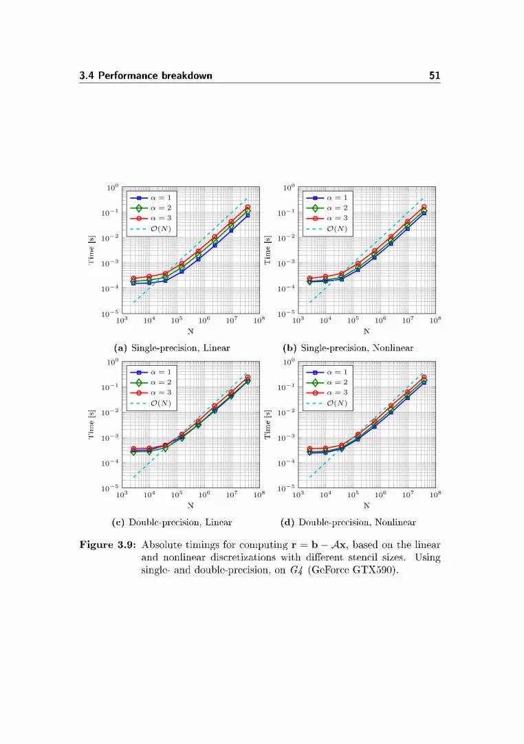
3.4 Performance breakdown 51
103 104 105 106 107 10810−5
10−4
10−3
10−2
10−1
100
N
Time[s]
α = 1
α = 2
α = 3
O(N)
(a) Single-precision, Linear
103 104 105 106 107 10810−5
10−4
10−3
10−2
10−1
100
N
Time[s]
α = 1
α = 2
α = 3
O(N)
(b) Single-precision, Nonlinear
103 104 105 106 107 10810−5
10−4
10−3
10−2
10−1
100
N
Time[s]
α = 1
α = 2
α = 3
O(N)
(c) Double-precision, Linear
103 104 105 106 107 10810−5
10−4
10−3
10−2
10−1
100
N
Time[s]
α = 1
α = 2
α = 3
O(N)
(d) Double-precision, Nonlinear
Figure 3.9: Absolute timings for computing r = b − Ax, based on the linearand nonlinear discretizations with dierent stencil sizes. Usingsingle- and double-precision, on G4 (GeForce GTX590).

52 Free surface water waves
103 104 105 106 107 10810−5
10−4
10−3
10−2
10−1
100
N
Time[s]
α = 1
α = 2
α = 3
O(N)
(a) Single-precision, Linear
103 104 105 106 107 10810−5
10−4
10−3
10−2
10−1
100
N
Time[s]
α = 1
α = 2
α = 3
O(N)
(b) Single-precision, Nonlinear
103 104 105 106 107 10810−5
10−4
10−3
10−2
10−1
100
N
Time[s]
α = 1
α = 2
α = 3
O(N)
(c) Double-precision, Linear
103 104 105 106 107 10810−5
10−4
10−3
10−2
10−1
100
N
Time[s]
α = 1
α = 2
α = 3
O(N)
(d) Double-precision, Nonlinear
Figure 3.10: Absolute timings for computing r = b−Ax, based on the linearand nonlinear discretizations with dierent stencil sizes. Usingsingle- and double-precision, on G6 (Tesla K20c).

3.4 Performance breakdown 53
103 104 105 106 107 10810−1
100
101
102
N
GFlop/s
α = 1
α = 2
α = 3
(a) Single-precision
103 104 105 106 107 10810−1
100
101
102
N
GFlop/s
α = 1
α = 2
α = 3
(b) Double-precision
Figure 3.11: Performance throughput for computing r = b−Ax. Using single-and double-precision, on G4 (GeForce GTX590).

54 Free surface water waves
3.4.1 Defect correction performance breakdown
Computing the solution of the σ-transformed Laplace problem is the perfor-mance bottleneck of the free surface solver. A performance breakdown of thepreconditioned defection correction is therefore carried out, with each of the sub-routines outlined in Table 3.1. We measure the time it takes to complete onedefect correction iteration, because this measure is independent of the physicalproblem and only depends on the discretization parameters. For this perfor-mance test, the vertical resolution is kept xed at Nz = 9 while the horizontalresolution is increased repeatedly in the x- and y-directions. The fully nonlinearsystem is solved with a 6th-order accurate (α = 3) nite dierence approxima-tion in the outer defect correction iteration, while one multigrid V-cycle withtwo Red-Black Z-line Gauss-Seidel smoothings is used for preconditioning to-gether with a linearized 2nd-order nite dierences approximation; in short wewrite DC+MG-ZLGS-1V(1,1). Absolute and relative performance results arepresented in Figure 3.12 and 3.13. From the absolute timings we see the samepattern as from the previous results: that they scale well only for sucientlylarge problem sizes. The relative performance results in Figure 3.13 tell us thatfor large problem sizes, the high-order residual and the smoother are responsiblefor the majority of the compute times. The combined performance scalabilityfor the compute time per defect correction, is summarized in Figure 3.14. Theseresults conrm again that this is a memory bound application as the resultsfollow directly from the memory bandwidth of the individual GPUs. The TeslaK20c GPU has the highest bandwidth of 208GB/s while the Tesla M2050 band-width is lowest at 144GB/s. The high-end gaming GPU, the GeForce GTX590has an intermediate bandwidth of 164GB/s. From these performance tests wesee that with just a single GPU we are able to compute the solution of a freesurface water wave problem with 107 to 108 degrees of freedom in both single-and double-precision, with iteration times well below one second. Furthermore,these performance results are in good agreement with the results previously re-ported in [EKMG11], which was based on a dedicated solver. Thus, we concludethat the generic library implementation does not introduce signicant overheaddespite providing a higher level of abstraction.
3.4.2 A fair comparison
In Figure 3.14 we provided the timings based on an fairly optimized singlethreaded Fortran90 version of the same numerical free surface solver used in[EKBL09, DBEKF10]. The CPU performance results are measured on a Linux-based system equipped with an Intel Core i7 at 2.8GHz and with an eectiveCPU-to-RAM bandwidth of 11.5GB/s.

3.4 Performance breakdown 55
103 104 105 106 107 10810−4
10−3
10−2
10−1
100
101
N
Tim
e[s]
Residual (high)
Residual (low)
Restriction
Prolongation
Smoothing
Axpy
2-norm
O(N)
Figure 3.12: Absolute timings on G6 for each of the subroutines in a defectcorrection iteration. Double-precision.
104 105 106 1070
20
40
60
80
100
N
%
Residual (high)
Residual (low)
Restriction
Prolongation
Smoothing
Axpy
2-norm
Figure 3.13: Percantage of total compute time on G6 for each of the subrou-tines in a defect correction iteration. Double-precision.
It is our experience, that there seems to be some confusion and skepticism inthe literature and among researchers, when it comes to comparing performanceresults. Stating that GPUs are several (100-1000) times faster than equivalentCPUs does not say anything about the reference for achieving such speedups.The key to these problems is that these numbers are often provided with nocontext and without sucient details. In fact it can be quite easy to mislead thereader by leaving out details, as humorously described by Bailey [Bai91, Bai92,Bai09]. No optimized GPU application will be thousand times faster than anequally optimized CPU version that utilizes all CPU cores. However, we believethat a fair comparison is indeed valid, if the right comparison basis is presented.A fair comparison requires that sucient details of the test environments are

56 Free surface water waves
104 105 106 107 10810−3
10−2
10−1
100
101
N
Time/Iter
[s]
Tesla M2050
Tesla K20c
GeForce GTX590
Intel i7
(a) Single-precision
104 105 106 107 10810−3
10−2
10−1
100
101
N
Time/Iter
[s]
Tesla M2050
Tesla K20c
GeForce GTX590
Intel i7
(b) Double-precision
Figure 3.14: Performance comparisons and scalability of timings per pre-condtioned defect correction iteration on dierent heterogeneoushardware.
provided, that details about the algorithms are outlined, and that timings arepresented, preferably both absolute and relative timings. When this informationis provided, it is fair to compare applications that have not received the samelevel of optimization, then the comparison will be of the two applications, andnot necessarily the hardware on which they are executed.
In Figure 3.14 we provide the comparison between the two versions of the same
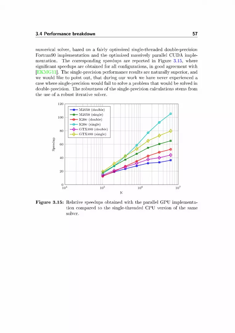
3.4 Performance breakdown 57
numerical solver, based on a fairly optimized single-threaded double-precisionFortran90 implementation and the optimized massively parallel CUDA imple-mentation. The corresponding speedups are reported in Figure 3.15, wheresignicant speedups are obtained for all congurations, in good agreement with[EKMG11]. The single-precision performance results are naturally superior, andwe would like to point out, that during our work we have never experienced acase where single-precision would fail to solve a problem that would be solved indouble-precision. The robustness of the single-precision calculations stems fromthe use of a robust iterative solver.
104 105 106 1070
20
40
60
80
100
120
N
Speedup
M2050 (double)
M2050 (single)
K20c (double)
K20c (single)
GTX590 (double)
GTX590 (single)
Figure 3.15: Relative speedups obtained with the parallel GPU implementa-tion compared to the single-threaded CPU version of the samesolver.
58 Free surface water waves

Chapter 4
Domain decomposition onheterogeneous multi-GPU
hardware
Decomposing a boundary value problem into smaller subdomains is an attractiveway to extract parallelism into an application. There are two main motivationsfor doing so. First, the computational work can be distributed and solved inparallel to achieve better overall performance. Secondly, memory distributionlowers the memory requirements per node and allows for larger global problemsto be solved. However, communication between compute nodes does not comefor free, and frequent message passing tends to dominate the overall perfor-mance, especially for smaller problem sizes. Domain decomposition techniques,such as the class of classical overlapping Schwartz methods, rst introduced bySchwarz in 1870, can be considered as a preconditioners to iterative solvers, seee.g., [SBG96]. Each subdomain solver approximates a local solution (possiblyin parallel) to some accuracy, before communicating and updating boundary in-formation with adjacent subdomains. This procedure is repeated until a globalaccuracy criterion is met. One advantage of these methods is that the localsolutions can be approximated with no communication between subdomains,and even dierent numerical solvers can be used within each subdomain. Thedisadvantages are that global convergence depends on the size of the overlapsand that larger overlaps lead to increasingly redundant computational work.

60 Domain decomposition on heterogeneous multi-GPU hardware
Furthermore, the overlap size and position inuence how rapidly informationtravels between subdomains at each Schwartz iteration, and therefore how fastthe overall method converges. For some elliptic problems, a global coarse gridcorrection strategy can improve convergence by ensuring propagation of infor-mation between all subdomains. For boundary value problems with nite signalspeed, e.g., the weakly dispersive Boussinesq equations, satisfactory convergencespeed can be obtained with reasonable overlaps of the order of the water depth,as presented in [GPL04, CPL05].
4.1 A multi-GPU strategy
CUDA enabled GPUs are optimized for high memory bandwidth and fast on-chip performance. However, the role as a separate co-processor to the CPUcan be a limiting factor for large-scale scientic applications, because the GPUmemory capacity is xed and is only in the range of a few Gigabytes. There-fore, large-scale scientic applications that process Gigabytes of data, requiredistributed computations on multiple GPUs. Multi-GPU desktop computersand clusters can have a very attractive peak performance, but the addition ofmultiple devices introduces the potential performance bottleneck of slow datatransfers across PCI Express busses and network interconnections, as outlinedin Figure 4.1. The ratio between data transfers and computational work hasa signicant impact on the possibility for latency hiding, and thereby overallapplication performance. Thus, speedups should not be expected for smallerproblem sizes where there is an unfavorable ratio between communication andcomputations. In the following sections we investigate the cost of data trans-fers between GPUs and demonstrate how the number of processors and gridtopology inuence the overall performance and scalability.
Device memory Device memory
Host memory Host memory
kernel kernel
PCIe
Network
PCIeGPUDirect/RDMA
Figure 4.1: Message passing between two GPUs involves memory transfersacross lower bandwidth connections. A kernel call is rst requiredif data is not sequentially stored in the GPU memory. Recent gen-erations of Nvidia GPUs, CUDA, and MPI support direct transferswithout explicitely transfering data through the host.

4.1 A multi-GPU strategy 61
The objective of this work is to enable scalable computations on distributedsystems to enable large-scale simulations on heterogeneous clusters, where thesolver can account for a large number of time steps and many billions degreesof freedom in the spatial discretisation. We therefore introduce a natural (butnontrivial) extension of the GPUlab library, to support distributed data andparallel computations on heterogeneous hardware with multiple GPUs, usinga hybrid MPI-CUDA implementation. We implement a multi-block methodbased on a domain decomposition technique that automatically decomposes theglobal computational grid into local subgrids. We detail how this technique canbe used to transparently solve very large linear system of equations arising fromnite dierence discretizations of exible order.
4.1.1 A multi-GPU strategy for the Laplace problem
From previous work [LF97] we know that multigrid convergence for the Laplaceproblem is close-to-optimal and converges in very few iterations to engineeringaccuracy for both deep and shallow waters. Also, the system of equations aris-ing from higher order approximations, based on exible order nite dierences,have been shown to have good convergence with the iterative defect correctionmethod and multigrid preconditioning[EKBL09]. We therefore seek a decompo-sition technique for large scale simulations that preserves the attractive algebraicmultigrid convergence with a low penalty on the overall performance. Our multi-block decomposition technique will therefore introduce articial ghost (halo)layers between adjacent subdomains, with sizes equal to the stencil sizes. Thecomputational domain is rst decomposed into non-overlapping subdomains,then ghost layers are added to account for grid points that are distributed acrossadjacent subdomains, similar to the approach presented e.g. in [ALB98]. Thesize of the ghost layers can be adjusted to match the size of the nite dierencestencils. In practice it can be advantageous to ensure that geometric multigridoperates on grids of uneven dimensions. We therefore allow one layer of gridpoints, next to the ghost layers, to be distributed to both of the adjacent sub-domains, see Figure 4.2. Ghost points are updated block wise, indicated bythe arrows, every time information from adjacent domains are queried. Thus,the subdomains are not decoupled and one subdomain cannot solve the localboundary value problem without communicating with its neighbors. As a con-sequence the iterative solution to the Laplace problem converges exactly as itwould do without decomposition. Any solver that works on the non-distributedproblem therefore works with the same algorithmic eciency on the distributedproblem.
The vertical resolution for any free surface model is much smaller than thehorizontal resolution. Vertical grid points in the order of ten are sucient for

62 Domain decomposition on heterogeneous multi-GPU hardware
Figure 4.2: A one dimensional topology decomposition of a grid of global size17 × 5 into two subgrids with two layers of ghost points. • and represent internal grid points and ghost points respectively. represents internal points that are shared between the two gridsto ensure uneven internal dimensions.
many applications in coastal engineering, while the number of horizontal gridpoints is dictated by the size of the physical domain and the wavelengths. Forpractical applications, it is often desirable to extend the physical domain hori-zontally to restore large maritime areas, long wave propagations or large harborfacilities. In these situations the ratio between internal grid points and ghostpoints becomes more favorable for large-scale simulations because of the volumeto surface ratio. For the same reason communication time is expected to be lessdominant for large-scale free surface problems. Furthermore we will present athorough examination of the multigrid coarsening strategy, to demonstrate thatrapid numerical convergence can be maintained with few restrictions and withno need for coarse global grid corrections.
4.2 Library implementation and grid topology
For message passing we use MPI and create a local communication space in orderto avoid interference with other communicators, as recommended by Hoeer andSnir [HS11]. Appendix A gives examples on how to initialize the library withMPI support.
The multi-block extension should be implemented so that it will not interferewith existing implementations. The library already contains the grid class forsingle-block grid representation. We extend this class with an extra grid topol-ogy template argument, and set the default value as a non-distributed topol-ogy implementation. An update member function is added to the grid class,that simply forwards the grid itself to the topology update function. Withthis exible template-based setup the user is able to create custom topology

4.2 Library implementation and grid topology 63
implementation. The library contains default topology operators for one- andtwo-dimensional grid distributions. Listing 4.1 illustrates a template for thebasic topology interface.
1 template <typename size_type , typename value_type >2 class topology3 4 public:5 int N, S, E, W, T, B; // MPI ranks for neighbors , north , south , ...6 int P, Q, R; // Global grid topology size7 int p, q, r; // Local grid topology IDs8
9 /**10 * Create local grid property dimensions based on global dimensions11 */12 template <typename property_type >13 void create_local_props(property_type const& gprops , property_type*
lprops)14 15 // Fill out local properties (lprops)16 17
18 /**19 * Update grid overlapping zones20 */21 template <typename grid_type >22 void update(grid_type const& g) const23 24 // Communicate with neighbors to update grid ghost layers25 26 ;
Listing 4.1: Template for a grid topology implementation.
When a grid is initialized with the global grid dimensions, the create_local_propsfunction is automatically called to compute the local grid properties based onthe given topology implementation. We use the MPI built-in Cartesian topologyroutines to help partition our grids. This multi-block topology implementationwill be able to signicantly improve developer productivity for creating data-distributed grid and vector objects and for updating boundary information. Theonly thing required to turn a single-block solver into a multi-block solver is tochange the type denition for the grid type, exemplied in Listing 4.2.
1 using namespace gpulab;2 typedef float value_type;3 typedef topology_xy <size_t ,value_type > topology_type;4 typedef grid <value_type ,device_memory ,topology_type > grid_type;
Listing 4.2: Setting up type denitions for a multi-block grid with horizontalgrid decomposition topology_xy).
Instead of initializing a grid from the global grid properties, it is also possible tocreate a custom topology conguration and then use local grid properties. Thistechnique will be utilized in Section 4.5 to manually detach two of the blocks inorder to create a breakwater simulation.

64 Domain decomposition on heterogeneous multi-GPU hardware
One challenge that arises from the multi-block setting is how to ensure good loadbalancing. In the predened library implementations, we use the MPI Cartesiantopology routines to decompose the grid and we ensure that all local grids areof similar discrete sizes. However, if data is distributed to multiple GPUs withdierent performance, or the user manually creates a bad distribution, the solverwill be limited by the slowest link, because updating boundary information is acollective operation. We have not experienced any noticeable performance issueswith load imbalance, but it is an issue that may be relevant in some settings.
4.3 Performance benchmarks
Message passing between GPUs is nontrivial, and only few stable MPI releasessupport pointers to GPU memory. Good progress on ecient and transparentGPU-to-GPU communication is being made within MPI communities, particu-larly MVAPICH2[WPL+11b, WPL+11a, Nvi12a]. However, as of writing, thereare restrictions on the supported InniBand controllers, and MPI requires spe-cialized congurations with non-default settings. In the absence of access tosuch a congured system, the following results are based on an implementa-tion where communication between two or more GPUs are performed by rsttransferring data between the device and host memory, before invoking the ap-propriate MPI calls, cf. Figure 4.1. We believe that simple and transparentintegration of message passing using MPI on heterogeneous systems will be akey feature in the near future as distributors and researches continue to makehybrid message passing easier[ABD+13], and also extending support for non-contiguous data movement as presented by [JDB+12, WPL+11a].
Updating decomposed subgrids with boundary information via ghost layer up-dates imposes a potential performance bottleneck, thus all communication over-head should be minimized if possible. We have created a mirco-benchmark thatwill provide us with information about the eciency and scalability of messagepassing between multiple GPUs on the two test environments G4 and Oscar.For the rst test we use two MPI processes to measure the time it takes toexchange messages of increasing size between two GPUs connected to the samemotherboard. For this test we use both pinned (page-locked) and non-pinnedhost memory. According to the CUDA guidelines[Nvi13], pinned host memorycan be utilized for faster memory transfers between the host and device. Theperformance results are presented in terms of absolute timings in Figure 4.3aand memory bandwidth in Figure 4.3b. There are several important things tonotice from these timings. Firstly, since the two GPUs are on the same board,the MPI send/receive call is a local memory operation that requires no networktransfer. Therefore this is very ecient for all message sizes and requires the

4.3 Performance benchmarks 65
100 101 102 103 104 105 106 107
10−6
10−4
10−2
100
Message size [bytes]
Time[s]
Total
Total pinned
cudaMemcpy
cudaMemcpy pinned
MPI_Sendrecv
MPI_Sendrecv pinned
O(n)
1MB
(a) Absolute timings. Total timings include all transfer times and additional overheadtime to allocate and free memory.
100 101 102 103 104 105 106 10710−1
100
101
102
103
104
Message size (bytes)
Bandwidth
[MB/s]
cudaMemcpy
cudaMemcpy pinned
MPI_Sendrecv
MPI_Sendrecv pinned
cudaMemcpy +MPI_Sendrecv
cudaMemcpy +MPI_Sendrecv pinned
(b) Memory bandwidth performance
Figure 4.3: Performance scaling for two processors on G4. Send/receive trans-fers from GPU to GPU, with and without pinned memory.
least time. The irregular peaks that appear for the MPI calls, are somethingthat we often observe at random locations and therefore something we expect tobe caused by internal MPI controllers. The next thing we should notice is thateven though pinned memory enables the highest peak bandwidth for large mem-ory transfers between the host and the device (cudaMemcpy), there is almostno dierence for memory transfers below 1MB. In order to put these message
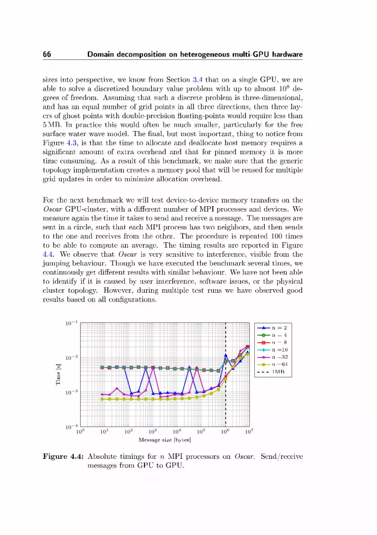
66 Domain decomposition on heterogeneous multi-GPU hardware
sizes into perspective, we know from Section 3.4 that on a single GPU, we areable to solve a discretized boundary value problem with up to almost 108 de-grees of freedom. Assuming that such a discrete problem is three-dimensional,and has an equal number of grid points in all three directions, then three lay-ers of ghost points with double-precision oating-points would require less than5MB. In practice this would often be much smaller, particularly for the freesurface water wave model. The nal, but most important, thing to notice fromFigure 4.3, is that the time to allocate and deallocate host memory requires asignicant amount of extra overhead and that for pinned memory it is moretime consuming. As a result of this benchmark, we make sure that the generictopology implementation creates a memory pool that will be reused for multiplegrid updates in order to minimize allocation overhead.
For the next benchmark we will test device-to-device memory transfers on theOscar GPU-cluster, with a dierent number of MPI processes and devices. Wemeasure again the time it takes to send and receive a message. The messages aresent in a circle, such that each MPI process has two neighbors, and then sendsto the one and receives from the other. The procedure is repeated 100 timesto be able to compute an average. The timing results are reported in Figure4.4. We observe that Oscar is very sensitive to interference, visible from thejumping behaviour. Though we have executed the benchmark several times, wecontinuously get dierent results with similar behaviour. We have not been ableto identify if it is caused by user interference, software issues, or the physicalcluster topology. However, during multiple test runs we have observed goodresults based on all congurations.
100 101 102 103 104 105 106 10710−4
10−3
10−2
10−1
Message size [bytes]
Time[s]
n = 2
n = 4
n = 8
n =16
n =32
n =64
1MB
Figure 4.4: Absolute timings for n MPI processors on Oscar. Send/receivemessages from GPU to GPU.

4.3 Performance benchmarks 67
We now present a benchmark where a grid decomposed into subgrids exchangesboundary information based on a horizontal topology implementation as pre-sented in Section 4.2. We use a numerical grid of increasing global size (Nx, Ny, Nz) =(2i, 2i, 32), for i = 3, 4, . . . , 12 with overlaps of size α = 1, 2, 3, 4. The total num-ber of ghost grid points per subgrid is then bounded up to,
τ ≤ 2αNz
(NxP
+NyQ
), (4.1)
Figure 4.5 illustrates performance scalability for updating a grid decomposedinto two subrids with (P,Q) = (1, 2) on the same compute node on Oscar. Incontrast to the previous benchmarks, these timings also include the kernel callthat is required to rst move ghost layer information into a contiguous memorylocation before the device to host copies. In [WPL+11b] the authors evaluatenon-contiguous MPI data communication on GPU clusters, and propose thesame approach for multi-dimensional data sets. They also emphasize that man-ual data movement in multi-GPU settings poses one of the biggest hurdles tooverall performance and programmer productivity, which again emphasizes theimportance of well-designed library support. There is a natural extra time costfor updating grids with increasing ghost layer sizes, but as Figure 4.5b indicates,there is no extra cost in terms of bandwidth performance.
104 106 10810−4
10−3
10−2
N
Time[s]
α = 1
α = 2
α = 3
α = 4
O(τ)
(a) Absolute timings
103 104 105 106 107100
101
102
103
Message size [bytes]
Bandwidth
[MB/s]
(b) Bandwidth
Figure 4.5: Grid update performance on two GPUs, using four dierent over-lap sizes. The global grid size is N = NxNy Nz. Tested on Oscar,single-precision.
In Figure 4.6 the same setup is tested, this time with eight GPUs on multiplenodes, so that (P,Q) = (2, 4). For the smaller problems of sizes less thanN < 106, there is a noticeable larger overhead for sending multiple messagescompared to the timings in 4.5a. This extra overhead is not surprising sincemessages are now transferred across the network. As a results we also see that

68 Domain decomposition on heterogeneous multi-GPU hardware
the memory bandwidth performance decreases slightly. For larger problem sizesthe performances scales well in both cases.
104 106 10810−4
10−3
10−2
N
Time[s]
α = 1
α = 2
α = 3
α = 4
O(τ)
(a) Absolute timings
103 104 105 106 107100
101
102
103
Message size [bytes]
Bandwidth
[MB/s]
(b) Bandwidth
Figure 4.6: Grid update performance on eight GPUs, using four dierentoverlap sizes. The global grid size is N = NxNy Nz. Testedon Oscar, single-precision.
4.4 Decomposition of the free surface model
To solve the free surface water wave problem on multiple GPUs we use the dataand domain decomposition technique presented above. We will again focus onecient solution of the σ-transformed Laplace problem as this is the perfor-mance bottleneck. The purpose of the proposed decomposition technique is topreserve the attractive algorithmic convergence rate of the multigrid precondi-tioned defect correction method. If the articial ghost boundary information iscontinuously updated before the information is needed, there will be no penaltyon the algorithmic convergence and we will be able to solve the full globalLaplace problem without the additional Schwartz iterations. The disadvantageof this technique is that it requires multiple grid updates, but as described inthe previous section, the time per grid update is small compared to the timeper defect correction as presented in Section 3.4. Thus, we expect the domaindecomposition technique to have satisfactory weak scaling properties for thesolution of the Laplace problem.
We will start by presenting an algebraic formulation of the decomposed Laplaceproblem. Then we will validate and test performance scalability of the multigridpreconditioned defect correction method, with special focus on the multigrid

4.4 Decomposition of the free surface model 69
coarsening strategy. Last, we demonstrate a free surface case where the multi-block solver is utilized to decouple domains, in order to emulate a breakwater.
4.4.1 An algebraic formulation of the Laplace problem
The introduction of new articial ghost layers that connect subdomains canbe introduced into the equations for the discrete Laplace problem (3.6). Toclarify the conceptual change we derive an algebraic formulation of a discreteLaplace problem, that takes into account the extra conditions for the ghostpoints introduced across the articial boundaries between an arbitrary numberof subdomains.
Assume that a domain Ω is decomposed into P non-overlapping domains, suchthat Ω = ∪Pi=1Ωi. Then the transformation of the original system of equations
Ax = b into Ax = b can be described in terms of two sets of restriction matricesRi and Gi. Ri is the restriction matrix that selects exactly the elements xi fromx that belongs to the subdomain Ωi, i.e. so that we have xi = Rix. ThenRi ∈ RNi×N , where Ni is the number of elements in Ωi (excluding ghost points)and N is the total number of elements in Ω. The restriction matrix Ri is sparseand contains only one entry per row. The second restriction matrix Gi selectsexactly the elements in x that will be covered by ghost points belonging tosubdomain Ωi. We have Gi ∈ RQi×N , where Qi is the number of ghost pointsintroduced by subdomain Ωi. Because all ghost points added by subdomain Ωialways represents elements from other subdomains Ωj 6=i, the non-zero columnsof Ri and Gi are distinct.
In the general case, when an arbitrary dimensional domain Ω is decomposedinto P subdomains, the corresponding system of equations Ax = b, based on anite dierence discretization with overlapping ghost points can be written inthe form
A1 R1AGT1A2 R2AGT2
. . .. . .
AP RPAGTP0 G1RT2 · · · G1RTP −I
G2RT1 0 · · · G2RTP −I...
.
.
.. . .
.
.
.. . .
GPRT1 GPRT2 · · · 0 −I
x1
x2
.
.
.xPg1
g2
.
.
.gP
=
b1
b2
.
.
.bP00
.
.
.0
,
where gi is the ghost points added to the system by the ith subdomain. MatrixA can be divided into 4 blocks, indicated by the dotted lines. The upper leftblock contains the original contributions from A, however only the entries that

70 Domain decomposition on heterogeneous multi-GPU hardware
apply internally to each subdomain, and not across articial boundaries, areincluded. The upper right block connects the cut-o portions of A to the ghostpoints added to the system by the extension of x into x. Together, the twolower blocks ensure that each ghost point matches exactly one element in anothersubdomain. This is guaranteed since each equation from the lower blocks reducesto xj − gi = 0, such that ghost point g from subdomain Ωi must be equal to xin subdomain Ωj .
It should be noted that in practice this system is never formed explicitly andthat the introduction of new equations into the original system of equations dueto ghost points, merely indicates the communication that will be required bythe underlying implementation to update all ghost points values.
4.4.2 Validating algorithmic convergence
One advantage of the multi-GPU method presented here is that it preservesthe very attractive algorithmic eciency of multigrid. Figure 4.7 illustrates theconvergence history for the preconditioned defect correction method applied toa simple nonlinear traveling wave simulation. The convergence history conrmsthat in fact the norm of the residual converges equally for both the single-and multi-GPU implementations within machine precision. The notation ΩP=4
represents decomposition into four subdomains, and thus the use of four GPUsto compute the solution.
0 2 4 6 8
10−9
10−7
10−5
10−3
Iter.
||r|| ∞
ΩP=1
ΩP=4
Dierence
Figure 4.7: Convergence history for the defect correction iterations using oneand four subdomains. The results conrm that the algorithmiceciency is preserved. Single-precision arithmetic is used.

4.4 Decomposition of the free surface model 71
4.4.3 The eect of domain decomposition
As a rst test case we consider how the introduction of multiple subdomains, andthereby multiple GPUs, inuence the performance of each individual subroutineof the defect correction algorithm. We refer the reader to Table 3.1 for anoverview of these subroutines.
We compute the average timings based on 100 defect correction iterations for anincreasing number of unknowns. One multigrid V-cycle with Red-Black Z-linesmoothing is used for preconditioning together with 6th-order accurate nitedierence for the spatial discretization. We denote the number of V-cycle levelsby K. In this test we use K =∞, which means that the V-cycle continues untilthe coarsest level (5× 5× 3) is reached for each subdomain. A semi-coarseningstrategy that best preserves the grid isotropy is chosen, meaning that the gridis restricted only in the horizontal dimensions until the grid spacing is of similarsize to the vertical grid spacing. Hereafter all dimensions are restricted. Ateach multigrid level we use 2 pre- and post-smoothings, and 4 smoothings atthe coarsest level. It is important to notice that the smoother is used also atthe coarsest grid level and not a direct solver. The relative and absolute timingsfor each subroutine and for an increasing number of subdomains, ΩP |P=1,2,4,are reported in Table 4.1. 'Residual (high)' in the rst column refers to the6th-order residual evaluation in the defect correction loop, while 'residual (low)'refers to the 2nd-order linear residual evaluation in the preconditioning phase.A graphical representation of the relative time consumption for Ω1 is illustratedin Figure 4.8.
105 106 1070
20
40
60
80
100
N
%
Residual (high)
Residual (low)
Restriction
Prolongation
Smoothing
Axpy
2-norm
Figure 4.8: Performance breakdown of each subroutine of the preconditioneddefect correction method for Ω1. Tested on Oscar.
We note from the numbers in Table 4.1 that increasing the number of subdo-mains, and thereby the number of GPUs, improves the overall computationaltimes only for problems larger than 513 × 513 × 9. This is acceptable, as in

72 Domain decomposition on heterogeneous multi-GPU hardware
129× 129× 9 257× 257× 9 513× 513× 9 1025× 1025× 9Subroutine ΩP Percent Time Percent Time Percent Time Percent TimeResidual (high) 1 15.2 0.0010 25.9 0.0036 34.2 0.0133 39.1 0.0529Residual (low) 1 20.9 0.0014 23.5 0.0033 23.6 0.0092 23.0 0.0311Smoothing 1 37.3 0.0025 32.5 0.0045 28.3 0.0110 27.4 0.0371Restriction 1 11.9 0.0008 10.3 0.0014 7.0 0.0027 4.9 0.0067Prolongation 1 12.1 0.0008 5.7 0.0008 5.0 0.0019 3.9 0.0053Axpy 1 1.6 0.0001 1.4 0.0002 1.4 0.0005 1.3 0.00182-nrm 1 1.0 0.0001 0.7 0.0001 0.6 0.0002 0.4 0.0006Total 1 100.0 0.0068 100.0 0.0139 100.0 0.0389 100.0 0.1355
Residual (high) 2 6.3 0.0009 10.0 0.0021 17.0 0.0071 27.5 0.0271Residual (low) 2 18.7 0.0026 19.5 0.0042 22.8 0.0096 22.0 0.0216Smoothing 2 50.7 0.0070 45.9 0.0099 38.1 0.0160 34.3 0.0337Restriction 2 15.6 0.0022 14.2 0.0031 14.5 0.0061 9.4 0.0092Prolongation 2 7.7 0.0011 9.3 0.0020 6.6 0.0028 5.5 0.0054Axpy 2 0.6 0.0001 0.6 0.0001 0.7 0.0003 1.0 0.00092-nrm 2 0.5 0.0001 0.4 0.0001 0.4 0.0002 0.4 0.0004Total 2 100.0 0.0139 100.0 0.0216 100.0 0.0420 100.0 0.0983
Residual (high) 4 3.7 0.0007 5.2 0.0014 9.9 0.0041 17.8 0.0139Residual (low) 4 12.6 0.0023 14.1 0.0037 18.0 0.0074 18.9 0.0149Smoothing 4 64.1 0.0119 59.1 0.0155 51.8 0.0212 42.0 0.0330Restriction 4 10.8 0.0020 11.5 0.0030 13.2 0.0054 10.5 0.0083Prolongation 4 7.8 0.0015 9.2 0.0024 6.3 0.0026 9.7 0.0076Axpy 4 0.4 0.0001 0.4 0.0001 0.5 0.0002 0.7 0.00052-nrm 4 0.5 0.0001 0.4 0.0001 0.3 0.0001 0.3 0.0003Total 4 100.0 0.0186 100.0 0.0262 100.0 0.0409 100.0 0.0784
Table 4.1: Relative and absolute timings for each of the subroutines basedon an increasing number of unknowns and subdomains. Tested onOscar.
general there is little or no reason for introducing multiple GPUs to solve aproblem that itself ts within the memory of one GPU. Each GPU is massivelyparallel, thus multiple GPUs increase both load balancing issues and costly com-munication overhead. Strong scaling, measured in terms of number of GPUs,for problems of moderate sizes should therefore not be expected to be good ingeneral.
Based on the relative numbers we see that in particular smoothing becomes moredominant as the number of subdomains increases. Table 4.2 lists the number ofsubroutine calls as a function of multigrid levels K. Each of these subroutinesrequires a ghost layer update. It is evident that even for low K, there aresignicantly more calls to the smoothing routine compared to the remainingsubroutines. It is therefore particularly desirable to decrease the number ofrestrictions in order to also reduce the number of smoothings and consequentlylower communication requirements.
However, multigrid achieves its unique linear work scalability and grid indepen-dent convergence properties from the fact that it reduces all error frequenciesby smoothing on all grid levels. This is in general important for elliptic prob-

4.4 Decomposition of the free surface model 73
lems where all grid points are strongly coupled. What we will demonstrate byexample, is that the coupling between distinct water waves are so weak, thatsmoothing only on the multigrid levels where the waves are well sampled is su-cient. Our hypothesis is that once the waves are undersampled due to repeatedcoarsening, there will be little or no eect of further restrictions. Since only thesmoother, and not a direct solver, is applied on the coarsest grid level, reducingthe total number of grid coarsenings will lead to improve overall performance,provided that the algorithmic convergence is preserved.
Subroutine K = 1 K = 3 K = 5 K = 7Residual (high) 1 1 1 1Residual (low) 1 3 5 7Smoothing 8 16 24 32Restriction 1 3 5 7Prolongation 1 3 5 7Axpy∗ 2 4 6 82-nrm† 1 1 1 1
Table 4.2: Number of calls to each subroutine as a function of multigridV-cycle coarsenings K. ∗ is a local operation and can becomputed with no communication. † is a collective operation(MPI_Allreduce), but requires no explicit update of the ghostboundaries.
4.4.4 The performance eect of multigrid restrictions
We now study how the number of multigrid restrictions eect the numericalperformance for both the single- and multi-block solver. We use the absolutetime per outer defect correction iteration, Γ, as a measure of performance. Thus,these timings are independent of any physical properties within the free surfaceproblem as the algebraic convergence is not considered. Γ is measured andreported in Table 4.3 for a variation of restrictionsK and number of subdomainsΩP . The remainder of the settings are the same as in the previous example.
Two dierent speedup measures are reported in Table 4.3; Ψ∞ is the speedupusing fewer restrictions: K = 1, 2, 5 compared to K =∞, with the same numberof subdomains ΩP . Ψ1 is the speedup from using multiple subdomains ΩP |P =2, 4, 8 compared to Ω1, with the same number of restrictions K. We see thatΨ∞ ≥ 1 and that Ψ∞|K=1 ≥ Ψ∞|K=3 ≥ Ψ∞|K=5 ≥ Ψ∞|K=∞, which is to beexpected, since the time to compute one V-cycle with K = i is a subproblemof computing a V-cycle with K = i+ 1. Ψ1 is a measure of strong scaling withrespect to the number of GPUs (subdomains). As mentioned before, multipleGPUs are feasible only for problems of reasonable size. Based on the reportednumbers we conclude that there is good potential for improving the overallnumerical performance, given that few restrictions (low K) is sucient for rapid

74 Domain decomposition on heterogeneous multi-GPU hardware
129× 129× 9 257× 257× 9 513× 513× 9 1025× 1025× 9ΩP K Γ Ψ∞ Ψ1 Γ Ψ∞ Ψ1 Γ Ψ∞ Ψ1 Γ Ψ∞ Ψ1
1 ∞ 0.0068 1.0 1.0 0.0139 1.0 1.0 0.0389 1.0 1.0 0.1355 1.0 1.01 1 0.0042 1.6 1.0 0.0097 1.4 1.0 0.0322 1.2 1.0 0.1218 1.1 1.01 3 0.0055 1.2 1.0 0.0119 1.2 1.0 0.0363 1.1 1.0 0.1315 1.0 1.01 5 - - - 0.0132 1.0 1.0 0.0376 1.0 1.0 0.1336 1.0 1.0
2 ∞ 0.0139 1.0 0.5 0.0216 1.0 0.6 0.0420 1.0 0.9 0.0983 1.0 1.42 1 0.0055 2.5 0.8 0.0108 2.0 0.9 0.0237 1.8 1.4 0.0735 1.3 1.72 3 0.0119 1.2 0.5 0.0164 1.3 0.7 0.0335 1.3 1.1 0.0854 1.2 1.52 5 - - - 0.0216 1.0 0.6 0.0400 1.1 0.9 0.0929 1.1 1.4
4 ∞ 0.0186 1.0 0.4 0.0262 1.0 0.5 0.0409 1.0 1.0 0.0784 1.0 1.74 1 0.0074 2.5 0.6 0.0114 2.3 0.9 0.0185 2.2 1.7 0.0451 1.7 2.74 3 0.0153 1.2 0.4 0.0196 1.3 0.6 0.0297 1.4 1.2 0.0590 1.3 2.24 5 - - - 0.0262 1.0 0.5 0.0377 1.1 1.0 0.0709 1.1 1.9
8 ∞ 0.0150 1.0 0.5 0.0210 1.0 0.7 0.0308 1.0 1.3 0.0543 1.0 2.58 1 0.0069 2.2 0.6 0.0084 2.5 1.1 0.0145 2.1 2.2 0.0288 1.9 4.28 3 - - - 0.0177 1.2 0.7 0.0230 1.3 1.6 0.0416 1.3 3.28 5 - - - - - - 0.0308 1.0 1.2 0.0509 1.1 2.6
Table 4.3: Absolute timings per defect corretion iteration and attainablespeedups for four dierent problem sizes. Tested on Oscar (TeslaM2050). Time in seconds.
convergence. For example, for a problem size of (1025× 1025× 9) decomposedinto four subdomains and solved on four GPUs Ω4, there is a 1.3 speedup ifthree multigrid restrictions (K = 3) are sucient compared to K = ∞, andthere is a 2.2 speedup compared to the single-block solver. The following testis set up to clarify whether these speedups can in fact be achieved by reducingthe number of multigrid levels.
4.4.5 The algorithmic eect of multigrid restrictions
To unify the ndings from the previous examples we now introduce and solve aspecic nonlinear free surface problem. The purpose of this numerical experi-ment is to clarify whether the hypothesis of imposing fewer restrictions, and thusfewer smoothings to minimize communication, based on the ndings in Table4.1, can in fact lead to performance improvements as reported in Table 4.3. Thenal link that we need to demonstrate is whether the algebraic convergence canbe maintained with few restrictions. We use a two-dimensional Gaussian distri-bution as the initial condition to the free surface elevation within a numericalwave tank with no ux boundaries,
η(x, y, t) = κ e−x2+y2
2σ2 , t = 0, (4.2)
where σ = 0.15 and κ = 0.05. The wavelength is approximately λ = 1 and thewavenumber k = 2π. The distance from the seabed to still water level is h = 1

4.4 Decomposition of the free surface model 75
and therefore kh = 2π, which is intermediate depth. The physical size of thedomain is stretched to t the initial wave with approximately the number ofgrid points that we wish to examine. The number of grid points per wave isdenoted Nw, and we test for four dierent values Nw = 4, 8, 16, 32. Figure 4.9illustrates how the nonlinear wave travels within the rst seconds with dierentwave resolutions. We see that the initial wave rapidly propagates throughoutthe domain and creates multiple waves of various amplitudes and wavelengths.
Nw = 32
Nw = 16
Nw = 8
(a) T = 0s (b) T = 2s (c) T = 4s
Figure 4.9: Nonlinear waves traveling in a closed basin with no ux bound-aries, illustrated at three distinct time steps. Horizontal grid di-mensions are 129 × 129. The inital Gaussian wave is discretizedwith approximatelly Nw = 32, 16, 8 grid points.
At each time stage, the Laplace problem (3.8) is solved to a relative accuracytolerance of 10−4. Then the number of outer defect corrections are counted. Wetake sucient time steps for the average number of iterations to settle withinthree digits of accuracy. The results are collected in Table 4.4, where the numberof grid points per wavelength and number of restrictions are varied. The resultsare encouraging as they indeed conrm that the number of useful restrictionsdepends strongly on the discretization of the waves. Load balancing betweenthe GPU threads and multiple GPUs will therefore not be an issue as there is no

76 Domain decomposition on heterogeneous multi-GPU hardware
reason to restrict beyond the wave resolution. The average number of iterationsin the table also conrms that convergence is independent on the global gridresolution.
The convergence history in Figure 4.7 conrmed that convergence is independentof the number of subdomains. Thus the average iteration counts reported inTable 4.4 apply, regardless of how many subdomains (GPUs) are used.
129× 129× 9 257× 257× 9 513× 513× 9 1025× 1025× 9K Nw Avg. Iter. Avg. Iter. Avg. Iter. Avg. Iter.1 32 19.31 19.30 19.30 19.302 32 10.74 10.64 10.64 10.643 32 7.41 7.26 7.24 7.244 32 5.97 5.85 5.84 5.845 32 5.79 5.75 5.75 5.75∞ 32 5.79 5.75 5.74 5.74
1 16 10.95 10.95 10.95 10.952 16 7.52 7.51 7.51 7.513 16 6.54 6.54 6.54 6.544 16 6.46 6.46 6.46 6.465 16 6.44 6.44 6.44 6.44∞ 16 6.44 6.44 6.44 6.44
1 8 6.34 6.34 6.34 6.342 8 4.78 4.78 4.78 4.783 8 4.12 4.12 4.12 4.124 8 4.08 4.08 4.08 4.085 8 4.08 4.08 4.08 4.08∞ 8 4.08 4.08 4.08 4.08
1 4 4.73 4.73 4.73 4.732 4 4.13 4.13 4.13 4.133 4 4.12 4.12 4.12 4.124 4 4.12 4.12 4.12 4.125 4 4.12 4.12 4.12 4.12∞ 4 4.12 4.12 4.12 4.12
Table 4.4: The average number of iterations for obtaining a relative toleranceof 10−4 for various numbers of multigrid levels.
4.4.6 Performance Scaling
We use again the time per defect correction iteration as a measure of perfor-mance. To reduce communication we utilize the multigrid analysis and assumethat three multigrid levels are sucient. The GPU cluster performance resultsare summarized in Figure 4.10a and 4.10b. The single block timings, Ω1, evolveas expected: the overhead of launching kernels is evident only for the smallestproblem sizes, while for larger problems the time per iteration scales well. Fromthe multi-GPU timings we observe a clear dierence when communication over-head dominates and when it does not. Almost exactly after one million degrees

4.4 Decomposition of the free surface model 77
of freedom, communication overhead becomes less signicant, and the use ofmultiple compute units becomes benecial.
Figure 4.10b illustrates weak scaling relative to one GPU, as the ratio betweenthe number of GPUs and the problem size is kept constant. There is penaltyof approximately 15% when introducing multiple GPUs, indicated by the dropfrom one to multiple GPUs. Hereafter weak scaling remains almost constantand there is no critical penalty for adding extra GPUs.
103 104 105 106 107 108 10910−3
10−2
10−1
100
N
Time/Iter
[s]
Ω1
Ω2
Ω4
Ω8
Ω16
(a) Absolute timings.
0 2 4 6 8 10 12 14 160
0.5
1
No. GPUs
Eciency
Weak scaling
Ideal
(b) Weak scaling, using N ≈ 3.5 · 107 per GPU.
Figure 4.10: Performance scaling for the defect correction iteration, on Oscar,single-precision.
For this performance scale test we have gained access to the Stampede clusterat the University of Texas. Stampede is a Dell Linux cluster based on computenodes equipped with two Intel Xeon E5 (Sandy Bridge) processors, 32GB ofhost memory, and one Nvidia Tesla K20m GPU, all connected with Mellanox

78 Domain decomposition on heterogeneous multi-GPU hardware
FDR InniBand controllers. The Stampede cluster is congured such that upto 32 GPU nodes can be occupied at once. Performance results are illustratedin Figure 4.11. The conguration is the same as for the previous performancetest on Oscar. These performance results are even better than those obtainedon Oscar and we observe weak scaling with less than a 10% eciency drop. Wealso notice that with a setup of just 16 GPUs, we are able to solve problemswith more than one billion degrees of freedom in practical times. With anapproximate time per iteration of tit = 0.5 s at N = 109, it would be possible tocompute a full time step in 10 to 20 seconds, assuming convergence in 5 to 10iterations. With a time step size of ∆t = 0.05, a one minute simulation can becomputed in 3 to 6 hours. This is well within a time frame considered practicalfor engineering purposes. If all 32 GPUs are available, that time would reduceto almost half.
104 105 106 107 108 109 101010−3
10−2
10−1
100
N
Time/Iter
[s]
Ω1
Ω2
Ω4
Ω8
Ω16
Ω32
(a) Absolute timings.
0 5 10 15 20 25 30 350
0.5
1
No. GPUs
Eciency
Weak scaling
Ideal
(b) Weak scaling, using N ≈ 3.5 · 107 per GPU.
Figure 4.11: Performance scaling for the defect correction iteration, on Stam-pede, single-precision.

4.5 Multi-block breakwater gap diraction 79
4.5 Multi-block breakwater gap diraction
Breakwaters are built along populated coastal regions, such as beaches and har-bors, to reduce and diract incoming water waves before they reach the coast.Accurate simulation of breakwater diraction is therefore of engineering inter-est as a tool for optimizing coastal protection with proper structural designs.Wave diraction through a breakwater gap transform the water waves into semi-circular wave fronts with the largest wave heights remaining along the directionof incident waves. In these waters it is particularly important to locate unwantedwave accumulation causing damaging eects.
Figure 4.12: Breakwater gap diraction solution with a gap of size 2L.
Experimental studies have been carried out by Pos and Kilner [PK87] in 1987 forsix dierent gap congurations, using the breakwater gap-to-wavelength b, as adimensionless measure. In the same paper they also compare the experimentaldata to numerical results based on a nite element model with good resultsthat conrm that wave diraction is primarily a linear wave phenomenon. Nu-merous numerical studies based on dierent model equations and discretizationstrategies have been carried out for analysis of breakwater gap diraction, seee.g., [EK06]. A common challenge for many numerical models arises due to thepresence of the (innitely) thin breakwater and singularities around the break-water tip. Ordinary use of ghost points in a nite dierence setup is impossible,because such points coincide with internal grid points at the other side of thebreakwater. Consequently the user would have to implement ad hoc solutions tocircumvent this issue. Numerical treatment of the breakwater tip is also pointedout by Pos and Kilner to be error prone and may be the main reason for thedierences between the experimental and numerical data.
In this study our goal is not to contribute with new or thorough analysis of wa-ter wave diraction results, but to demonstrate some of the nice features thatthe multi-block approach brings. An example of a breakwater gap diraction

80 Domain decomposition on heterogeneous multi-GPU hardware
-5 -2 0 9
0
-7
x/L
y/L Zgen
Zabs
Figure 4.13: Example of a breakwater gap diraction setup. Incident wavesare generated in the generation zone Zgen at the western bound-ary before encountering the breakwater.
5
6
9
6
5
1
9
1
n0 n1
n2 n3
Figure 4.14: Domain decomposition of the breakwater gap diraction domainfrom Figure 4.13 into four subdomains. The ghost layer bound-ary connection (red) between node n0 and n1 are deatached andexchanged with a traditional Neumann condition.
setup is illustrated in Figure 4.13, where the breakwater is assumed to be in-nitely thin. Symmetry across the direction of incident waves at y/L = 0 isutilized to model only half of the domain. Using the multi-block solver witha two-dimensional horizontal topology we are able to split the domain intofour subdomains, such that the breakwater becomes the interface between twoblocks, see Figure 4.14. Since the boundary conditions can be set individually

4.5 Multi-block breakwater gap diraction 81
for each subdomain, we can easily change the boundary condition for the easternboundary of subdomain n0 and western boundary for subdomain n1 into theclassical no ux condition using Neuman boundaries. Manually setting up thesubdomain for n0 using the topology implementation presented in Section 4.2is illustrated in Listing 4.3.
1 // Setup topology connections and dimensions2 topology_type topo;3 topo.P = 2; // 2x nodes along x-direction4 topo.Q = 2; // 2x nodes along y-direction5 topo.R = 1; // 1x node along z-direction6 BC_TYPE bc_east , bc_west , bc_south , bc_north;7 if(rank ==0) // This is n08 9 topo.p = 0; // Grid x-index = 010 topo.q = 0; // Grid y-index = 011 topo.E = MPI_PROC_NULL; // No neighbor to the east (Breakwater)12 topo.W = MPI_PROC_NULL; // No neighbor to the west13 topo.N = 2; // Node 2 to the north14 topo.S = MPI_PROC_NULL; // No neighbor to the south15
16 // Boundary conditions17 bc_east = BC_NEU;18 bc_west = BC_NEU;19 bc_north = BC_DD;20 bc_south = BC_NEU;21
22 // Create grid properties here using the bc types ...23 24 // ... Do the same for rank=1,2,3 and create grids using topo ...
Listing 4.3: Manually setting up a 2× 2 topology and the connections for thenode with rank= 0 (n0 in Figure 4.14).
The decomposition into individual subdomains solves the problem with insuf-cient ghost points across the breakwater, because each domain now has anindividual set of ghost points that do not need to represent internal grid points.This kind of topology control in combination with boundary tted domainsopens up new perspectives for ecient large-scale simulation of applicationswith complex scenery.
To test the breakwater gap diraction model we generate incident monochro-matic linear sinusoidal waves within the generation zone Zgen = 3L, with waveheight of size H = 0.055m, wave period T = 0.59s, and wavelength L = 0.495m.A at seabed with still-water depth of h = 0.125 is used throughout the domainand a gap with a total width of b = 2L. For the discretization we use 17 gridpoints per wavelength, a vertical resolution of Nz = 9, and a Courant numberCr = 0.5 resulting in a time step ∆t = 0.0184s. In practice we exploit that thenumerical solver is very fast, to create a large domain behind the breakwater,large enough for the waves not to reect and interfere with the solution close tothe gap. This also avoids unintended wave reections from the absorption zonesto aect the solution.

82 Domain decomposition on heterogeneous multi-GPU hardware
Wave diraction is computed as the size of the wave envelope relative to theincident wave height Hcomp/H. The diraction contours are plotted in Figure4.15 and are in good agreement with the numerical results by e.g., Engsig-Karup [EK06] in the vicinity of the gap. It is again emphasized that these resultscome with no special treatment or ad hoc solutions to model the breakwater, butis a positive result of a well-designed generic multi-block approach for distributedcomputing.
Figure 4.15: Linear diraction close to the breakwater gap. Values are relativeto the incident wave height. The total gap size is equal to twowavelengths, b = 2L.
Chapter 5
Temporal decompositionwith Parareal
The use of spatial domain decomposition methods is widespread, as they haveproven to be ecient for a wide range of problems. These data-parallel meth-ods are ecient for solving large-scale problems and for reducing computationaltimes by distributing data and thereby reducing the work load per processor.However, applications that are facing numerical problems of limited sizes canrapidly reach a speedup limit for a low number of processors, due to a perfor-mance decrease when the number of processors increases, as this leads to anincreasingly unfavorable ratio between communication and computation. Thisissue is continuously worsened by the memory wall [ABC+06]; the fact thatcommunication speed is increasing at a far slower pace than compute speed,This trend is even expected to continue for years to come and is considered oneof the grand challenges facing development and architectural design of futurehigh-performance systems [Kea11, BMK+10]. Also, there are applications basedon ordinary dierential equations, where classical domain decomposition meth-ods are not even applicable [Mad08]. For these types of applications, a methodfor adding parallelism in the temporal domain is of great interest. Decouplingthe temporal domain is however, not as straightforward as spatial decomposi-tion, since time is sequential by nature. For this reason these methods have notreceived the same attention in the literature and have not been proven to workeciently on as many cases. However, with the continuously increasing num-ber of parallel compute units in modern hardware, alternative parallelization

84 Temporal decomposition with Parareal
strategies than data-parallel methods, are becoming more and more attractive.
The book by Burrage[Bur95] in 1995 presents a survey of numerical methods forcomputing the solution of evolution problems using parallel computers. He clas-sies these methods into three groups of parallelism - across the system, acrossthe method, and across the time. The rst two groups often have strict limi-tations to their application range and on performance scalability. Parallelismacross the method, such as parallel Runge-Kutta methods[IN90], have the dis-advantages that they only work with a xed number of processors and thereforeare not suitable for arbitrarily large-scale parallelism. The third category, con-taining the multishooting methods due to Bellen and Zennaro[BZ89], is of moreinterest, as these methods are often suitable for a broader range of problems.One such method that introduces concurrency across the time is the Parareal al-gorithm, proposed by Lion et al. (2001)[LMT01]. Parareal is a parallel iterativemethod based on task-parallelism, via temporal decomposition. Thus, Pararealis an algorithm that is purely designed for parallization, by introducing moreconcurrency to the solution of initial value problems, as it would only lead to anadditional workload in its sequential version. Gander and Vandewalle showed in[GV07] that the algorithm can be written both as a multiple shooting methodand as a two-level multigrid-in-time approach, even though the original ideacame from spatial domain decomposition. The method has many exciting fea-tures: it is fault resilient and has dierent communication characteristics thanthose of the classical spatial domain decomposition methods. Fault resiliencefollows from the iterative nature of the algorithm and implies that a processcan be lost during computations and regenerated without restarting the entirecomputations. Regeneration can be exploited to minimize total run time incase of such temporary hardware failures. This is an attractive feature for HPCsystems as the total number of compute nodes continues to grow. Parareal hasalso been demonstrated to work eectively on a wide range of problems and itis not limited by any number of parallel tasks, thus enabling large-scale par-allelism. Also, once the proper distribution infrastructure is implemented, itcan be wrapped around any type of numerical integrator, for any type of initialvalue problem.
Our work on temporal domain decomposition with the Parareal algorithm is acontinuation to some of the work presented in [Nie12], where a thorough feasibil-ity study of the algorithm was presented. Parareal results based on our work, onthe parallelization of the free surface water wave model, was initiated and basedon these experiences we have implemented the Parareal algorithm as a genericlibrary component. By experiments we have demonstrated its applicability tofully three-dimensional free surface water waves. Our main focus is to investi-gate whether it is possible, based on a number of test cases, to obtain practicalspeedups with the Parareal algorithm on heterogeneous multi-GPU systems. Tothe authors knowledge, this is the rst time that temporal parallelization using

5.1 The Parareal algorithm 85
multple GPUs has been demonstrated.
5.1 The Parareal algorithm
The Parareal algorithm was rst presented in 2001, in a paper by Lions etal. [LMT01], and later introduced in a slightly revised predictor-corrector formin 2002 by Baco et al. [BBM+02]. The Parareal-in-time approach proposes tobreak the global problem of time evolution into a series of independent evolutionproblems on smaller intervals, see Figure 5.1. Initial states for these problems are
T0 T1 TN TN+1
Space
T ime
GPU 1 GPU N
Figure 5.1: Time domain decomposition. A process is assigned to each in-dividual time subdomain to compute the initial value problem.Consistency at the time subdomain boundaries is obtained withthe application of a computationally ecient integrator in con-junction with the Parareal iterative predictor-corrector algorithm.
needed and computed by a simple, less accurate, but computationally ecientsequential integrator. The smaller independent evolution problems can thenbe solved in parallel. The solution generated during the concurrent integrationwith accurate propagators but inaccurate initial states, is used in a predictor-corrector fashion in conjunction with the coarse integrator to propagate thesolution faster, now using the information generated in parallel. We dene thedecomposition in N intervals, that is,
T0 < T1 < · · · < Tn = n∆T < Tn+1 < TN , (5.1)
where ∆T is the size of the time intervals and n = 0, 1, . . . , N . The generalinitial value problem on the decomposed time domain is dened as
∂u
dt+A(u) = 0, u(T0) = u0, t ∈ [T0, TN ] , (5.2)

86 Temporal decomposition with Parareal
where A can be a linear or nonlinear operator on u. To solve the dierentialproblem (5.2) we dene an operator F∆T that operates on some initial stateUn ≈ u(Tn) and returns an approximate solution to (5.2), at time Tn+∆T . Suchan operator is achieved by the implementation of a numerical time integrator,using some small time-step δt ∆T in the integration. The numerical solutionto (5.2) can then be obtained by applying the ne propagator sequentially forn = 1, 2, . . . , N .
Un = F∆T
(Tn−1, Un−1
), U0 = u0. (5.3)
For the purpose of Parallel acceleration of the otherwise purely sequential pro-cess of computing FN∆Tu0 ≈ u(TN ), we dene the coarse propagator G∆T . G∆T
also operates on some initial state Un, propagating the solution over the timeinterval ∆T , now using another time step δT . Typically δt < δT < ∆T . Forthe Parareal algorithm to be eective, the coarse propagator G∆T has to besubstantially faster to evaluate than the ne propagator F∆T . There are manyways of constructing the coarse propagator, the simplest one being to applythe same numerical integrator as for the ne propagator, but taking larger timesteps. We refer the reader to [Nie12] for an introduction to other methods. Thecoarse operator reads
Un = G∆T
(Tn−1, Un−1
), U0 = u0. (5.4)
Using the dened F∆T and G∆T operators, the predictor-corrector form of theParareal algorithm can be written in a single line as
Uk+1n = G∆T
(Uk+1n−1
)+ F∆T
(Ukn−1
)− G∆T
(Ukn−1
), Uk0 = u0, (5.5)
with the initial prediction U0n = Gn∆Tu0 for n = 1 . . . N and k = 1 . . .K. N
being the number of time subdomains, while K ≥ 1 is the number of predictor-corrector iterations applied.
5.2 Parareal as a time integration component
The Parareal algorithm is implemented in the GPUlab library as a separatetime integration component, using a fully distributed work scheduling model, asproposed by Aubanel [Aub11]. The model is schematically presented in Figure5.2. The Parareal component hides all communication and work distributionfrom the application developer. It is generically implemented such that a useronly has to decide what coarse and ne propagators to use. Setting up thetype denitions for Parareal time integration using forward Euler for coarse

5.3 Computational complexity 87
propagation and fourth order Runge-Kutta for ne propagation could then bedened as in Listings 5.1. The number of GPUs used for parallelization dependson the number of MPI processes that execute the application.
1 typedef gpulab :: integration :: forward_euler coarse;2 typedef gpulab :: integration ::ERK4 fine;3 typedef gpulab :: integration ::parareal <coarse ,fine > integrator;
Listing 5.1: Assembling a Parareal time integrator using forward Euler forcoarse propagation and an explicit Runge-Kutta method for nepropagation
Time
Iter. k = 0 Iter. k = 1 Iter. k = 2 Iter. k = 3
GPU. 1
GPU. 2
GPU. 3
GPU. 4
GPU. 5
GPU. 6
TG
TG
TG
TG
TG
TG
TF
TF
TF
TF
TF
TF
TG
TG
TG
TG
TG
TF
TF
TF
TF
TF
TG
TG
TG
TG
TF
TF
TF
TF
TG
TG
TG
Figure 5.2: Visualization of the fully distributed work scheduling model forthe Parareal algorithm. Each GPU is responsible for computingthe solution on a single time subdomain. The computation isinitiated at rank 0 and cascades through to rank N where thenal solution is updated.
5.3 Computational complexity
In the analysis of the computational complexity, we rst recognize that boththe coarse and the ne propagators, regardless of the type of discretization,involve a complexity that is proportional to the number of time steps beingused. Let us dene two scalar values CF and CG as the computational cost ofperforming a single step with the ne and coarse propagators, respectively. Thecorresponding computational complexity of integrating over an interval ∆T isthen given by CF ∆T
δt and CG ∆TδT . R is introduced as the relation between the two;
that is, R measures how much faster the coarse propagator is compared to thene propagator for integrating the time interval ∆T . The total computational

88 Temporal decomposition with Parareal
cost for Parareal over N intervals is then proportional to
(K + 1)NCG∆T
δT+KNCF
∆T
δt. (5.6)
Recognizing that the second term can be distributed over N processors, we areleft with
(K + 1)NCG∆T
δT+KCF
∆T
δt. (5.7)
The above should be compared to the computational complexity of a purelysequential propagation, using only the ne operator,
TN − T0
δtCF = N
∆T
δtCF . (5.8)
We can now estimate the speedup, here denoted ψ, as the ratio between thecomputational complexity of the purely sequential solution, and the complexityof the solution obtained using the Parareal algorithm (5.7). Neglecting theinuence of communication speed and correction time, we are left with theestimate
ψ =N ∆T
δt CF(K + 1)NCG ∆T
δT + kCF ∆Tδt
=N
(K + 1)N CGCFδtδT +K
. (5.9)
If we additionally assume that the time spent on coarse propagation is negligiblecompared to the time spent on the ne propagation, i.e., the limit CGCF
δtδT → 0,
the estimate reduces to ψ = NK . It is thus clear that the number of iterations
K for the algorithm to converge sets an upper bound on the obtainable paralleleciency. The number of iterations needed for convergence is intimately coupledwith the ratio R between the speed of the ne and the coarse integrators CFCG
δTδt .
Using a slow, but more accurate coarse integrator will lead to convergence infewer iterations K, but at the same time it also makes R smaller. Ultimately,this will degrade the obtained speedup as can be deduced from (5.9). Thus,R cannot be made arbitrarily large since the ratio is inversely proportional tothe number of iterations K needed for convergence. The estimated theoreticalspeedup for given values of R and K is illustrated in Figure 5.3, it is evidentthat the eciency drops rapidly when k increases. This relationship between Rand K imposes a challenge in obtaining speedup and is a trade-o between timespent on the fundamentally sequential part of the algorithm and the number ofiterations needed for convergence. It is particularly important to consider thistrade-o in the choice of stopping strategy; a more thorough discussion on thistopic is available in [Nie12] for the interested reader. Measurements on paralleleciency are typically observed to be less than 50%[Nie12], depending on theproblem and the number of time subdomains, which is also conrmed by ourmeasurements using multiple GPUs. This suggests that data-parallel methods

5.3 Computational complexity 89
5 10 15 20 25 300
5
10
15
20
25
30
N (no. procs)
Estimated Speedup
k=1
1IdealR = 2R = 4R = 8R = 16R = 32R = 64R = 128R = 256R = 512R = 1024
(a) K = 1.
5 10 15 20 25 300
5
10
15
20
25
30
N (no. procs)
Estimated Speedup
k=2
(b) K = 2.
Figure 5.3: Theoretical speedup for two dierent values ofK and an increasingnumber of processors.
are often a better choice for speeding up PDE solvers, as we have demonstratedin Section 4.4.6. Though, Parareal may have the advantage for problems wherethere is not enough data for data-parallel methods to be fully eective.
For demonstrative purpose we rst present a small parameter study using Pararealon the two-dimensional heat problem (2.4), at a coarse resolution (Nx, Ny) =(16, 16) and for a integration period t = [0, 1] s. The value of R is regulated byusing a suciently small constant time step size for the ne integrator and thenadjusting the time step size for the coarse integrator. We use simple forward Eu-ler integration for both coarse and ne integration. The problem is rst solvedpurely with the ne integrator to be able to compare the solution obtained withthe Parareal algorithm. The error after the rst Parareal iteration is reportedin Figure 5.4a, and the total number of iterations to obtain a solution with arelative error less than 10−5 is reported in Figure 5.4b. In Figure 5.5 speedupand parallel eciency measurements are presented. When R increases, at somepoint an extra Parareal iteration is required for the relative error to go belowthe tolerance, as illustrated in Figure 5.4b, this extra iteration clearly impactsthe attained speedup and parallel eciency depicted in Figure 5.5. The resultsconrm that speeding up a PDE solver is possible on a heterogeneous system,but it also conrms that the attainable speedups depend on several factors andthat it can be dicult to predict.

90 Temporal decomposition with Parareal
0
100
0
10
20
0.5
1
·10−2
RGPUs
||erel|| ∞
(a) The relative error after one pararealiteration (k = 1).
50100
15010
201
2
3
RGPUs
K(b) Iterations K needed to obtain a rel-
ative error less than 10−5.
Figure 5.4: Parareal convergence properties as a function of R and numberof GPUs used. The error is measured as the relative dierencebetween the purely sequential solution and the parareal solution.
0 50 100 1500
10
200
5
10
RGPUs
Speedup
(a) Measured parallel speedup
0 50 100 1500
10
200
0.5
1
RGPUs
Eciency
(b) Measured parallel eciency
Figure 5.5: Parareal performance properties as a function of R and numberGPUs used. Notice how the obtained performance depends greatlyon the choice of R as a function of the number of of GPUs. Testedon Oscar.
5.4 Accelerating the free surface model using parareal
The Parareal library component makes it possible to easily investigate potentialopportunities for further acceleration of the water wave model on a heteroge-neous system and to assess practical feasibility of this algorithmic strategy forvarious wave types.

5.4 Accelerating the free surface model using parareal 91
In section 5.3 it is assumed that communication costs can be neglected anda simple model for the algorithmic work complexity is derived. It is foundthat there are four key discretization parameters for Parareal that need to bebalanced appropriately in order to achieve high parallel eciency. They are thenumber of coarse-grained time intervals N , the number of iterations K, the ratiobetween the computational cost of the coarse to the ne propagator CG/CF andthe ratio between ne and coarse time step sizes δt/δT .
Ideally, the ratio CG/CF is small and convergence happens in just one iteration,K = 1. This is rarely the case, as it requires the coarse propagator to achieveaccuracy close to that of the ne propagator, while at the same time beingsubstantially more eciently, these two objectives obviously being conicting.Obtaining the highest possible speedup is a matter of trade-o, typically, themore GPUs used, the faster the coarse propagator should be. The performanceof Parareal depends on the given problem and the discretization. Thus, onewould suspect that dierent wave parameters inuence the feasibility of thealgorithm. This was investigated in [Nie12] and indeed the performance doeschange with wave parameters. Typically the algorithm works better for deepwater waves with low to medium wave amplitude. In this case nonlinear anddispersive eects are minor and only small changes to the wave characteristichappens within each time step.
103 105 10710−1
100
101
102
103
N (problem size)
Tim
e[s]
1 GPU
2 GPUs
4 GPUs
8 GPUs
16 GPUs
(a) Performance scaling.
104 105 1060
2
4
6
N (problem size)
Speedup
(b) Speedup.
Figure 5.6: Parareal timings for an increasing number of water waves travelingone wavelength, each wave resolution is (33 × 9). Speedup fortwo to sixteen compute nodes compared to the purely sequentialsingle-GPU solver. Tested on Oscar.
We have performed a scalability study for Parareal applied to two-dimensional

92 Temporal decomposition with Parareal
nonlinear stream function waves to demonstrate that there is a spatial inde-pendence on the attainable speedup. Each wave is discretized with (Nx, Nz) =(33, 9) grid points, and the total problem size N = NxNy is assembled frommultiple waves in a periodic domain. For this test we adjust the time step ofthe ne and coarse solver such that R ≈ 8, in which case one iteration K = 1, issucient. The study shows that moderate speedups are possible for this hyper-bolic system, see Figure 5.6. Using four GPU nodes a speedup of slightly morethan two was achieved while using sixteen GPU nodes resulted in a speedupof slightly less than ve. What should be noticed is the Parareal algorithm iscompletely insensitive to the size of the problem solved. Parareal is a time de-composition technique, thus scalability applies to the temporal dimension notthe spatial. The Parareal algorithm can therefore be a competitive alternativefor parallelization of problems of limited spatial sizes. As demonstrated in Fig-ure 5.6, parallel eciency decreases quite fast for this case when using moreGPUs. This limitation is due to the use of a fairly slow and accurate coarsepropagator and linked to a known diculty with Parareal applied to hyperbolicsystems. For hyperbolic systems, instabilities tend to arise when using a veryinaccurate coarse propagator. This prevents using a large number of time sub-domains, as this by Amdahl's law also requires a very fast coarse propagator.The numbers are still impressive though, considering that it comes as additionalspeedup to an already ecient solver.
2 4 6 80.5
1
1.5
2
2.5
R
Speedup
2 4 6 80
0.2
0.4
0.6
R
Eciency
2 GPUs
4 GPUs
8 GPUs
16 GPUs
32 GPUs
Figure 5.7: Parallel time integration using the Parareal method. R is the ratiobetween the complexity of the ne and coarse propagators. Testedon Oscar.
Performance results for the Whalin test case, as presented in Section 3.3.1, isalso reported in Figure 5.7. There is a natural limitation to how much we canincrease R, because of stability issues with the coarse propagator. In this testcase we simulate from t = [0, 1]s, using up to 32 GPUs. For low R and only twoGPUs, there is no attained speedup, but for conguration with eight or moreGPUs and R ≥ 6, we are able to get more than 2 times speedup as illustrated in

5.5 Concluding remarks 93
Figure 5.7. Though these hyperbolic systems are not optimal for performancetuning using the Parareal method, results still conrm that reasonable speedupsare in fact possible on heterogenous systems.
5.5 Concluding remarks
The Parareal method is observed to be a potential approach for speeding upsmall-scale problems due to the reduced communication and overhead involved.For suciently large problems, where sucient work is available to hide thelatency in data communication, we nd that the spatial domain decompositionmethod is more favorable, as it does not involve the addition of extra iterationsand thereby allows for ideal speedup, something usually out of reach for theParareal algorithm. An important thing to note here is that it is technicallypossible to extend the work and wrap the Parareal method around the domaindecomposition method, thereby obtaining a combined speedup of both methods.This can be of great interest in the sense that for any problem size, increasingthe number of spatial subdomains will eventually degrade speedup due to thelatency in communication of boundaries. However, such a combination requiresa non-trivial support for handling multiple MPI communicators, which is yet tobe supported by the library.
We recognize that some of the results presented for the free surface water wavemodel were obtained by setting an pessimistic time step for the ne integratorin order to increase R. For explicit time integration of hyperbolic problemsthere are strict stability requirements on the time step sizes and the coarseintegrator cannot violate these. In this work we have only considered ne andcoarse integrators based on similar explicit schemes. However, there are optionsto increase R, by reducing the computational work of the coarse integrator thathave not been investigated in present work. We see ve possible modicationsthat will allow a more ecient coarse integration: 1) Use the linearized potentialow system. 2) Use only low-order discretizations. 3) Use a coarser numericalgrid, 4) set a less strict tolerance for the solution to the Laplace equation. 5)Use mixed-precision calculations. Though these modications will be able tosignicantly speedup the coarse integration part, there are no guarantees thatthe total time-to-solution will be faster, because it can also lead to extra Pararealiterations. We intend to pursue some of the answers to these questions in futurework.

94 Temporal decomposition with Parareal

Chapter 6
Boundary-tted domainswith curvilinear coordinates
Spatial discretization based on nite dierences is a popular choice within abroad range of scientic applications for several reasons; it is probably the mostsimple and widely used discretization method available, high-order accuracy isstraight forward, consistency analysis is well understood, and the absence of ex-tra index maps reduces the memory requirement, enhances the performance,and possibly increases developer productivity. Furthermore, the one-to-onemapping between discrete grid points and the thread hierarchy of massivelyparallel processors, such as the GPU, is ideal for high performance throughput,as demonstrated in some of the early articles on heterogeneous computing, e.g.,[KDW+06, DMV+08, Mic09]. The above mentioned reasons have been drivingmotivations for the present work, and to the authors knowledge, the nite dif-ference based free surface water wave solver is now one of the most versatile andecient tools available for simulation of dispersive and nonlinear water waves.
However, nite dierence methods also pose challenges for certain types of ap-plications, particularly because of problems with mass conservation in uids,and because of the diculties in representing complex geometries. To address-ing these problems, the classes of nite volume or nite element methods incombination with unstructured grids have traditionally been utilized[EGH03].As an additional step towards a complete and applicable tool for coastal en-gineering, we address the latter issue by introducing generalized curvilinear

96 Boundary-tted domains with curvilinear coordinates
coordinate transformations in order to represent exible and user-controllablegeometries. Curvilinear coordinate transformations is a widely used approachto reduce the limitations of nite dierence approximations and have also beenused to analyze both linear and nonlinear free surface wave-structure interac-tions [LF01, SDK+01, BN04, ZZY05, zFlZbLwY12], though only few are con-cerned with fully three-dimensional models[DBEKF10]. In order to representthe mapping we use a unique one-to-one mapping between all horizontal gridpoints, from a suciently smooth (dierentiable) physical region to a logicallyrectangular region. The coordinate transformation introduces additional termsto the partial dierential equations, that will have to be accounted for. We ex-tend the GPUlab library with additional kernel-based nite dierence routinesthat will support developers in computing the solution of coordinate transformedspatial derivatives. Explicit numerical dierentiation of the physical coordinatesis utilized to allow a generic implementation, that can be used for any valid user-generated input grid. The introduction of algebraic grid transformations reducesthe performance throughput because the number of memory transactions is in-creased. The computation of spatial derivatives based on nite dierence ap-proximations are no longer able to rely on constant grid spacing, but has tocompute grid-specic transformation coecients by reading information from agrid that holds the physical information. The challenge is therefore to minimizethe additional memory overhead, therefore we present a numerical benchmarkthat will reveal some of the performance characteristics of the chosen method.
Grid (or mesh) generation can be dicult for highly detailed and complex ge-ometries and therefore developers often rely on third party software to generatethe grids. Dierent grid types exist with various properties to match dierentgeometries and numerical approaches. Either structured or unstructured gridsbased on triangular, quadrilateral, or tetrahedral elements are among the mostused. Fast and optimal grid generation is a topic of its own, and will not beextensively covered in this thesis, instead we refer the reader to the work avail-able in the literature on this subject, e.g., [HX96]. We will comment on someof the issues related to grid generation relevant to the given examples. Manysoftware libraries for grid generation exist and it can be advantageous to rely onsuch third party packages to avoid cumbersome grid renements. The test casespresented in this chapter all have boundary-tted grids that can be computedfairly easy from analytic expressions and so we will not detail the process of gridgeneration further.
In the following sections we rst consider curvilinear transformations of the hor-izontal coordinates to represent fully surface penetrating and bottom mountedstructures. The transformation equations between a physical domain of in-terest and a classical Cartesian reference domain (computational domain) arepresented along with a generic implementation strategy. Examples of dierentapplications are also examined and compared to either analytic or experimental
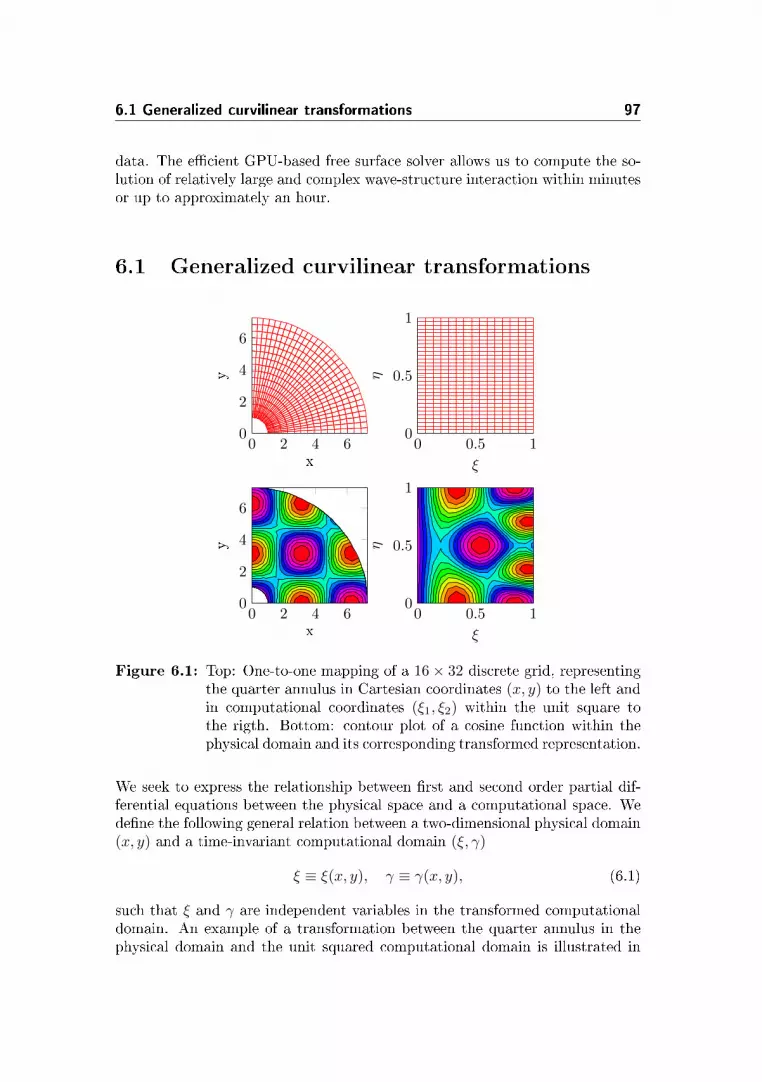
6.1 Generalized curvilinear transformations 97
data. The ecient GPU-based free surface solver allows us to compute the so-lution of relatively large and complex wave-structure interaction within minutesor up to approximately an hour.
6.1 Generalized curvilinear transformations
0 2 4 60
2
4
6
x
y
0 0.5 10
0.5
1
ξ
η
0 0.5 10
0.5
1
ξ
η
0 2 4 60
2
4
6
x
y
Figure 6.1: Top: One-to-one mapping of a 16× 32 discrete grid, representingthe quarter annulus in Cartesian coordinates (x, y) to the left andin computational coordinates (ξ1, ξ2) within the unit square tothe rigth. Bottom: contour plot of a cosine function within thephysical domain and its corresponding transformed representation.
We seek to express the relationship between rst and second order partial dif-ferential equations between the physical space and a computational space. Wedene the following general relation between a two-dimensional physical domain(x, y) and a time-invariant computational domain (ξ, γ)
ξ ≡ ξ(x, y), γ ≡ γ(x, y), (6.1)
such that ξ and γ are independent variables in the transformed computationaldomain. An example of a transformation between the quarter annulus in thephysical domain and the unit squared computational domain is illustrated in

98 Boundary-tted domains with curvilinear coordinates
Figure 6.1. If the computational grid is chosen to be rectangular as in the gure,the grid spacing is constant along each dimension. Thus, in the computationaldomain we are able to reuse the same constant coecient stencil operators basedon nite dierence approximations, as we use in a regular (non-curvilinear)setup. However, the coordinate transformation introduces additional terms tothe dierential equations. Using the above notation and the chain rule for partialdierential equations, rst order derivatives with respect to the original physicalcoordinates (x, y) of a function u, can be described in the computational domain(ξ, γ) via the following relations
∂u
∂x=∂ξ
∂x
∂u
∂ξ+∂γ
∂x
∂u
∂γ, (6.2a)
∂u
∂y=∂ξ
∂y
∂u
∂ξ+∂γ
∂y
∂u
∂γ, (6.2b)
or simply, using the short notation ∂u/∂x = ux
ux = ξxuξ + γxuγ , (6.3a)
uy = ξyuξ + γyuγ . (6.3b)
These equations contain derivatives with respect to the physical coordinates.In practice we prefer the derivatives to be dened in terms of the computationdomain, because it allows us to use constant stencil coecient operators. Inaddition, what is known beforehand is usually the mapping from the computa-tional to the physical domain. Thus, since the mapping is required to be uniqueand any mapping and its inverse would lead to the original point in the startingcoordinate system, the following relations hold
ξx =1
Jyγ , ξy = − 1
Jxγ , (6.4a)
γx = − 1
Jyξ, γy =
1
Jxξ. (6.4b)
where J is the Jacobian, given as the determinant of the Jacobi matrix
J = det(J) = det
([xξ xγyξ yγ
])= xξyγ − xγyξ. (6.5a)
The value of the Jacobian determines how much an area under transformationcontracts of expands. Given the above equations, the rst order derivatives ofu can now be described exclusively within the computational reference domainas
ux =yγuξ − yξuγ
J, (6.6a)
uy =xξuγ − xγuξ
J, (6.6b)

6.1 Generalized curvilinear transformations 99
and for the second order and mixed derivatives the following relations can bederived
uxx = (y2γuξξ − 2yξyγuξγ + y2
ξuγγ)/J2
+ [(y2γyξξ − 2yξyγyξγ + y2
ξyγγ)(xγuξ − xξuγ)
+ (y2γxξξ − 2yξyγxξγ + y2
ξxγγ)(yξuγ − yγuξ)]/J3, (6.7a)
uyy = (x2γuξξ − 2xξxγuξγ + x2
ξuγγ)/J2
+ [(x2γyξξ − 2xξxγyξγ + x2
ξyγγ)(xγuξ − xξuγ)
+ (x2γxξξ − 2xξxγxξγ + x2
ξxγγ)(yξuγ − yγuξ)]/J3, (6.7b)
uxy = [(xξyγ + xγyξ)uξγ − xξyξuγγ − xγyγuξξ]/J2
+ [(xξyγγ − xγyξγ)/J2 + (xγyγJξ − xξyγJγ)/J3]uξ
+ [(xγyξξ − xξyξγ)/J2 + (xξyξJγ − xγyξJξ)/J3]uγ , (6.7c)
where the derivatives of the Jacobian with respect to the computational coor-dinates, appearing in (6.7c), can be derived as
Jξ = xξξyγ − yξξxγ − xξγyξ + yξγxξ, (6.8a)
Jγ = xξγyγ − yξγxγ − xγγyξ + yγγxξ. (6.8b)
The derivations for all of the above equations and their mathematical propertiesare quite comprehensive and not particularly relevant for the present work.We refer to literature, e.g., the book by Liseikin [Lis99] for a mathematicalintroduction to grid generation methods, or for a more practical approach, thework by Kopriva [Kop09].
6.1.1 Boundary conditions
Boundary conditions may be dened in terms of the physical boundary normals,such as the no-ux Neumann boundary conditions stating that no uid is allowedto pass through the boundary,
n · ∇u = 0, (x, y) ∈ ∂Ω, (6.9)
where n = (nx, ny)T is the normal dened at the physical domain boundary∂Ω, expressed in Cartesian coordinates. We also need a relation that allowus to approximate (6.9) based on the boundary of the computational domain.We notice that the boundary normals on the regular computational domainare trivial, ne = (1, 0)T , nw = (−1, 0)T , nn = (0, 1)T , and ns = (0, −1)T
for the east, west, north, and south boundaries respectively. The relationship

100 Boundary-tted domains with curvilinear coordinates
between the normals in the two coordinate systems can be described in termsof a rotation matrix R where the following relation holds,
(nxny
)= R−1
(nξnγ
)=
ξx√ξ2x+γ2
x
γx√ξ2x+γ2
xξy√ξ2y+γ2
y
γy√ξ2y+γ2
y
( nξnγ
), (6.10)
where nc = (nξ, nγ)T is one of the trivial normals at the boundary of thecomputational domain. Combining (6.10) and (6.4) we are able to compute thenormals at the physical boundary with the same order of accuracy as our nitedierence approximations.
6.2 Library implementation
First of all, adding support for curvilinear domains in the GPUlab library mustnot interfere with existing implementations and should provide an intuitive wayof extending solvers to utilize curvilinear domains. To achieve this, we haveextended the original grid class with one extra member pointer, pointing to atransformation object. When this pointer is null (default) no curvilinear trans-formation is associated with the grid, thus existing implementations need nomodication. If the pointer is not null, then it points to a simple container thatagain points to two grids that dene the horizontal coordinates of the physicaldomain (the x and y (6.1)). These two coordinate-grids are of the same ob-ject type as the grid itself. Creating a grid object and assigning it a specictransformation is illustrated in Listing 6.1.
1 typedef gpulab ::grid <double ,gpulab :: device_memory > grid_type;2 typedef grid_type :: transformation_type transformation_type;3
4 grid_type U;5 grid_type X;6 grid_type Y;7
8 // Fill X and Y with geometric information9
10 transformation_type transform(alpha);11 transform.set_X(&X);12 transform.set_Y(&Y);13 U.set_transformation (& transform);
Listing 6.1: Initialize a grid for the solution (U) and two grids for the physicalcoordinate information (X and Y).
The transformation object only stores pointers to the two grids to allow multiplesolutions to share the same coordinate transformation. This will signicantlyreduce the memory footprint, as only one copy of X and Y needs to be stored.

6.2 Library implementation 101
When a grid contains a valid pointer to their transformation object, they shouldpass along the X and Y pointers to the GPU kernels, and library subroutines willprovide support for computing the spatial derivatives in (6.6) and (6.7). Theimplementation of the nite dierence approximations in curvilinear coordinatesis validated in Figure 6.2, based on the quarter annulus grid from Figure 6.1.
10−3 10−2 10−1 10010−10
10−7
10−4
10−1
∆ ξ
||e|| ∞
uxuyuxxuyyuxy
O(∆ξ2)
(a) α = 1
10−3 10−2 10−1 10010−10
10−7
10−4
10−1
∆ ξ
||e|| ∞
uxuyuxxuyyuxy
O(∆ξ4)
(b) α = 2
Figure 6.2: Consistency verication for approximating the rst and secondorder derivatives in a curvilinear domain using two dierent stencilsizes α = 1, 2. Results are computed and compared to the analyticknown cosine function in the quarter annulus grid as illustrted inFigure 6.1
6.2.1 Performance benchmark
The range of applications that will benet from accurate representation of com-plex geometry is greatly increased with the addition of curvilinear grid support.However, as emphasized by the derived transformation equations (6.6) and (6.7),these computations require an increased number of oating-point operations andmemory accesses. Thus, a performance decrease is expected for applications re-lying heavily on the calculation of transformed spatial dierential equations. Abenchmark of two approaches for computing the rst and second order trans-formed derivatives in one direction is presented. The two versions have distinctadvantages, so it is not obvious which is the most optimal.
The rst version (v1) computes all transformations coecients based on the xand y coordinates for each grid point. This leads to restricted memory accessfor these two coordinates, but it also requires each thread to access more thanone element in order to perform the stencil computation. The stencil size, α,

102 Boundary-tted domains with curvilinear coordinates
determines how many extra memory accesses that are required to compute thederivative. An example of how threads within one thread-block collaborateto read from global memory into shared memory is illustrated in Figure 6.3.The increased number of operations required to compute the derivative alsosignicantly increase the register count, causing the kernel occupancy to drop.All kernel implementations have been evaluated on G6, with a Tesla K20c GPU,supporting compute capability 3.5. In this case, there is a decrease from 100% to75% for the kernel computing the rst-order transformed derivatives comparedto the non-transformed version. Accordingly, there is a decrease from 100% to50% for the second-order derivative kernel.
Figure 6.3: An (8 × 8) thread-block reading global memory into a (10 × 10)shared memory block. Since α = 2 there are two layers on eachside of the block that will have to be read from global memory.An (8× 8) thread-block is used for illustrative purpose, in praticea (16× 16) thread-block gives better performance.
The second version (v2) simply reads the coecients from pre-computed grids.This version requires additional kernel input arguments. Up to ten extra ar-guments (xξ, xγ , xξγ , xξξ, xγγ , yξ, yγ , yξγ , yξξ, and yγγ), compared to thetwo for the rst version. However, the second version is somewhat more simpleimplementation-wise, as there are less on-the-y computations. The reducednumber of registers causes the occupancy to remain at 100%, for the rst-order kernel. Computing the second-order derivatives causes the occupancy

6.2 Library implementation 103
to decrease to 50%, because of additional registers required to compute therst-order and cross-derivatives of u according to (6.7). The time it takes topre-compute the transformation coecients is not included in the following tim-ings, because these coecients can be pre-computed once and will then remainconstant throughout the application lifetime, assuming the domain is time in-dependent.
For both of the above versions, it applies that increased memory access to thegrid u, from which the derivatives are computed, is also increased accordingto (6.6) and (6.7). A template for the kernels that have been benchmarked isillustrated in Listing 6.2. Best performance has been found with a CUDA kernelconguration of 16× 16 threads per thread-block, we refer the reader to [Nvi13]for details on kernel congurations. Performance timings per grid point areplotted in Figure 6.4, as a function of increasing problem size. The numericaldomain ratio is kept constant such that Nx = Ny for all tests and a ve pointstencil (α = 2) is used for approximation of all spatial derivatives. The bluelines indicate the time it takes to compute the derivatives in the computationaldomain, without applying any transformation to it. Thus, it represents a lowerbound for the two transformed versions, as they include the same amount ofwork plus the computation of the additional transformation coecients. Noticethat the blue lines are almost identical for the rst- and second-order derivatives(uξ, uξξ). This is because the number of memory accesses and computations arethe same, only the values of the stencil coecient diers. This is not the casefor the transformed derivatives, as the computation of second-order derivativesinvolves signicantly more oating-point and memory transactions.
1 __global__2 void Ux(double const* u // Input3 , double* ux // Output4 , double const* X5 , double const* X_xi1 // [v2]6 , double const* X_xi2 // [v2]7 , double const* Y8 , double const* Y_xi1 // [v2]9 , double const* Y_xi2 // [v2]10 , double dxi111 , double dxi212 , int Nx13 , int Ny14 , double const* Dx // Stencil coeffs15 , int alpha)16 17 int i = threadIdx.x*blockDim.x + threadIdx.x;18 int j = threadIdx.y*blockDim.y + threadIdx.y;19
20 // Shared memory index identifiers21 dim3 T(threadIdx.x+alpha ,threadIdx.y+alpha);22 dim3 B(blockDim.x+2*alpha ,blockDim.y+2* alpha);23
24 // Load Dx to shared memory Dxs25 // Load u to shared memory Us26 // [v1] Load X to shared memory Xs27 // [v1] Load Y to shared memory Ys

104 Boundary-tted domains with curvilinear coordinates
28
29 // Only internal grid points30 if(i>=alpha && i<Nx-alpha && j>=alpha && j<Ny-alpha)31 32 double idxi1 = 1.0/ dxi1;33 double idxi2 = 1.0/ dxi2;34
35 // First order u-derivatives36 double u_xi1 = FD:: FD2D_x(Us,idxi1 ,T,B,alpha ,Dxs);37 double u_xi2 = FD:: FD2D_y(Us,idxi2 ,T,B,alpha ,Dxs);38
39 // First order X- and Y-derivatives40 double x_xi1 = // [v1] Compute , [v2] Read41 double x_xi2 = // [v1] Compute , [v2] Read42 double y_xi1 = // [v1] Compute , [v2] Read43 double y_xi2 = // [v1] Compute , [v2] Read44
45 ux[i+j*Nx] = FD:: transformation :: FD2D_x(u_xi1 , u_xi2 , x_xi1 , x_xi2 , y_xi1, y_xi2);
46 47
Listing 6.2: and [v2] refer to code that only applies to version 1 or 2,respectively.]Template for computing the derivative of a twodimensional grid in curvilinear coordinates. [v1] and [v2] referto code that only applies to version 1 or 2, respectively.
Interestingly, the second version (v2), outperforms the rst version for all prob-lem sizes. Thus, the increased number of input arguments and distinct memorylocations do not slow performance as much as the additional computationalwork, misaligned memory accesses, and increased register count required by therst version (v1). We also recognize the classical two-phase GPU performancecharacteristic; an intermediate phase where there is not enough work to fullyexhaust all processors and a second phase (in this case N > 105) where thecomputational time scales strongly with the problem size.
The corresponding bandwidth throughput for each kernel is illustrated in Figure6.5. The throughput is computed as the number of bytes required to store thediscrete grid times the number of eective read/writes. All kernels will be atbest memory bound, as the computational work per grid point is constant andrelatively low, independent of the problem size. The non-transformed and thesecond version approach a throughput of 100GB/s, which is relatively close tothe eciently bandwidth on this system (Tesla K), measured to be ∼ 140GB/susing the standard CUDA bandwidth test. Thus, these results are satisfactory,taking into account that also the stencil coecients are loaded from global mem-ory and are not included in the throughput computations. These performanceresults lead to thesomewhat surprisingconclusion, that for this setup, it isbenecial to pre-compute the transformation coecients and avoid the extraon-the-y computations. The results also indicate, that with the introductionof curvilinear coordinate transformation, we should expect up to one order of

6.2 Library implementation 105
102 104 106 10810−4
10−3
10−2
10−1
100
N (prob. size)
time/N
[µs]
uξ
ux, (v1)
ux, (v2)
(a) First order derivatives.
102 104 106 10810−4
10−3
10−2
10−1
100
N (prob. size)
time/N
[µs]
uξξ
uxx, (v1)
uxx, (v2)
(b) Second order derivatives.
Figure 6.4: Absolute timings per grid point for computing the non-transformed (uξ, uξξ) and transformed (ux, uxx) derivatives. Tim-ings are based on ve point nite dierence stencils, α = 2. Testedon G6, double-precision, and with ECC on.
102 104 106 10810−2
10−1
100
101
102
N (prob. size)
Bandwidth
[GB/s]
uξ
ux, (v1)
ux, (v2)
(a) First order derivatives.
102 104 106 10810−2
10−1
100
101
102
N (prob. size)
Bandwidth
[GB/s]
uξξ
uxx, (v1)
uxx, (v2)
(b) Second order derivatives.
Figure 6.5: Bandwidth α = 2. Tested on G6, double precision, and with ECCon.
magnitude performance reduction for the computation of second-order deriva-tives, which is also what we experience for the potential ow solver. Even withthis performance reduction, we expect this approach to be superior comparedto unstructured methods, where irregular memory patterns and load balancingcan be signicant performance barriers.

106 Boundary-tted domains with curvilinear coordinates
6.3 Free surface water waves in curvilinear coor-
dinates
The addition of curvilinear coordinates nds many applications in free surfacewater wave modeling, where the boundary can be tted to match those of a realscene. It enables complex modeling of o-shore structures, harbors, shorelines,or combinations hereof, that have signicant engineering value over traditionalregular domains. A exible representation of the discrete domain can also beutilized to adapt the grid to the wavelengths, such that a higher resolution isused where shorter waves are present and thus minimize over- or under-resolvedwaves.
The use of curvilinear grids in free surface modeling has been proposed for vari-ous numerical models and applications in literature before. A movable curvilin-ear two-dimensional shallow water model was derived in [SS95] to simulate andstudy the eect of storm surge ooding in the Bohai Sea. A nonlinear Boussi-nesq model was later proposed by the same author in generalized curvilinearcoordinates, and was applied to several test examples, including the Ponce deLeon Inlet in Florida [SDK+01]. More work on free surface models in curvilinearcoordinates are found in [LZ01, BN04, ZZY05, zFlZbLwY12].
6.3.1 Transformed potential ow equations
The kinematic and dynamic free surface boundary conditions in (3.1) along withthe σ-transformed Laplace problem contain rst- and second-order derivativesin both horizontal directions, described by ∇ ≡ (∂x, ∂y)T . These equationstransform due to the curvilinear coordinate transformation according to (6.6)and (6.7), such that,
∇ =
(∂x∂y
)=
(yγ∂ξ−yξ∂γ
Jxξ∂γ−xγ∂ξ
J
), (6.11)
and
∇2 = ∂xx + ∂yy =1
J2[(y2
γ + x2γ)∂ξξ − 2(yξyγ + xξxγ)∂ξγ + (y2
ξ + x2ξ)∂γγ ]
+1
J3[(T1 + T3)(xγ∂ξ − xξ∂γ) + (T2 + T4)(yξ∂γ − yγ∂ξ)]
(6.12)

6.3 Free surface water waves in curvilinear coordinates 107
where the four variables
T1 = (y2γyξξ − 2yξyγyξγ + y2
ξyγγ), (6.13a)
T2 = (y2γxξξ − 2yξyγxξγ + y2
ξxγγ), (6.13b)
T3 = (x2γyξξ − 2xξxγyξγ + x2
ξyγγ), (6.13c)
T4 = (x2γxξξ − 2xξxγxξγ + x2
ξxγγ), (6.13d)
are all constant under the same coordinate transformation. The free surfacesolver has been modied according to these new expressions based on the im-plementation techniques outlined in the previous section. An eigenvalue test hasbeen carried out to conrm the stability of the linearized system in curvilinearcoordinates. The linearized system matrix-vector notations is given by(
∂tη
∂tφ
)=
(0 ∂z−g 0
)︸ ︷︷ ︸
A
(η
φ
). (6.14)
We have assembled the full matrix A for a small problem size of (Nx, Ny, Nz) =(17, 33, 9), based on the coordinate transformation of the quarter annulus fromFigure 6.1. The water depth is h = 1m and a symmetric three point stencil isused for approximation of the transformation coecients. With this discretiza-tion, the eigenvalues of A must be purely imaginary, which is conrmed by theeigenspectra in Figure 6.6.
6.3.2 Waves in a semi-circular channel
To test and verify the capability of the boundary-tted free surface solver, wedemonstrate two classical water wave problems where solutions are available forlinear waves and a nonlinear problem where experimental data are provided.
For the rst test we propagate linear waves through a semi-circular channelwith vertical walls and a constant water depth, for which analytic solutionshave been studied, see work by Dalrymple et al.[DKM94]. There exist severalnumerical results based on curvilinear coordinat transformed Boussinesq-typemodels[SDK+01, wZsZ10], with nite dierence approximations in staggeredgrids[zFlZbLwY12] and based on mild slope equations as well[ZZY05]. Thephysical coordinates to the circular channel can be described in terms (ξ, γ),
x = (r1 + ξ(r2 − r1)) cos(πγ), (6.15)
y = (r1 + ξ(r2 − r1)) sin(πγ), (6.16)

108 Boundary-tted domains with curvilinear coordinates
−1 −0.5 0 0.5 1
−10
0
10
Re(λ)
Im(λ)
Eigenspectrum of Jacobian matrix for linearized system
Figure 6.6: Eigenspectrum based on the linearized system with coordinatetransformations. The imaginary part of all eigenvalues are lessthan 10−14.
where r1 is the inner radius and r2 is the outer radius. We create a semi-circularchannel with dimensions r1 = π and r2 = 2π, discretized with a numericalgrid of size (Nξ, Nγ , Nz) = (129, 257, 9). The incoming waves are generatedwith a wavelength of L = 1m, the wave depth is h = 1m, and a wave periodof T = 0.8 s. The wave height is H = 0.042m corresponding to (H/L) =30%(H/L)max. We use 6th-order accurate nite dierence approximations anda Courant number Cr = 0.4. Waves are generated in a generation zone infront of the channel corresponding to the technique presented in Section 3.2.4.However, to support more exible generation and relaxation zones we now usea discrete grid function to determine the location of the two zones as illustratedin Figure 6.7. Positive values correspond to generation zones, wheres negativevalues are absorption zones. We utilize our fast GPU-based solver to create along channel behind the circular channel to avoid a negative impact from wavesreected from the absorption zone. The total discrete problem size thereforeamounts to (Nξ, Nγ , Nz) = (129, 1025, 9).
After the waves are propagated through the channel and settled at a steadystate, the wave prole at the inner and outer walls are captured. The numericalwave proles are depicted in Figure 6.8 together with the analytic solution byDalrymple. As a measure of the quantitative mismatch between the analyticand the numerical solutions we use the index of agreement proposed by Willmott

6.3 Free surface water waves in curvilinear coordinates 109
Figure 6.7: Wave generation and absorption zones. The long relaxation chan-nel is used to minimize spurious wave reections.
in 1981 [Wil81],
d = 1−∑Ni=1 (yi − xi)2∑N
i=1 (|yi − x|+ |xi − x|)2, (6.17)
where xi are the true values, yi are the numerically approximated values, and x isthe mean value of xi. The index of agreement d, was developed as a standardizedagreement measure for model predictions and varies between 0 and 1, where 1is a perfect match. Based on the solution wave proles in Figure 6.8 we getdin = 0.9992 and dout = 0.9989. These numbers agree well with the resultspresented both by Zhang et al. [ZZY05] and Shi et al. [SDK+01]. However,due to the high-order nite dierences approximation, we have obtained theseresults with only half the number of grid points at the free surface inside thechannel.
An illustrative example of the initial waves propagating into the channel atfour distinct stages is given in Figure 6.9. The rst waves travel almost in astraight line until they hit the outer wall and are reected around the bend. Aqualitative comparison to the analytic solution is given in Figure 6.10, wherethere are almost no noticeable dierences.

110 Boundary-tted domains with curvilinear coordinates
0 20 40 60 80 100 120 140 160 180−1
−0.5
0
0.5
1
ω[]
2η(ω)
H
Numerical Exact Error
0 20 40 60 80 100 120 140 160 180
−2
0
2
ω[]
2η(ω)
H
Figure 6.8: The solution at the inner (top) and outer (bottom) walls of thesemi-curcular channel at t = 65T .
x/L
y/L
−5 0 50
2
4
6
2η
H
−2
−1
0
1
2
(a) t = 10T.
x/L
y/L
−5 0 50
2
4
6
2η
H
−2
−1
0
1
2
(b) t = 20T.
x/L
y/L
−5 0 50
2
4
6
2η
H
−2
−1
0
1
2
(c) t = 30T.
x/L
y/L
−5 0 50
2
4
6
2η
H
−2
−1
0
1
2
(d) t = 40T.
Figure 6.9: Propagating wave contours in a semi circular channel at four dif-fernt stages. The waves enter at the southeast corner and arereected in the northeastern region of the channel creating largewave amplitudes.

6.3 Free surface water waves in curvilinear coordinates 111
2η
H
−2
−1
0
1
2
Figure 6.10: Comparison between the analytic (right) and numerical (left)solution at t = 60T . High-order approximations with α = 3 areused. Visually the match is close to perfect as there are almostno detectable dierences.

112 Boundary-tted domains with curvilinear coordinates
6.3.3 Wave run-up around a vertical cylinder in open wa-ter
Figure 6.11: Wave run-up around avertical cylinder.
Accurate prediction of wave scatter-ing and wave loads around a bottommounted circular cylinder is a valu-able engineering tool for construc-tion design of e.g., oshore wind-mills or oil rigs. Most often it isdesirable to avoid ill-positioned ge-ometries to cause wave amplicationclose to oshore structures. How-ever, the opposite can also be true,as demonstrated by Hu and Chan(2005) [HC05], where a carefully or-ganized forest of pillars are placed ina lens-shaped array to refract wavesinto a wave energy converter.
In this test we consider the wave run-up around a single cylinder surfaceboundary in open water. This is oneof only a few cases including wave-structure interaction, where an analytic so-lution is known. For linear plane incident waves scattering around a cylinderwith at sea bed, the closed form solution due to MacCamy and Fuchs [MF54]is used for comparison.
As for the breakwater gap diraction test in Section 4.5, one approach to rep-resent the cylinder is to decomposed the global domain of interest and use themulti-block solver in combination with boundary-tted domains to reassemblethe cylinder geometry. A grid decomposed into three subdomain that reassem-bles the vertical cylinder well is illustrated in Figure 6.12. Though this approachseems promising, there is a grid singularity that will have to be addressed. Thereare no discontinuities within each subdomain, but there exists two critical pointsin this setup, directly at the front and at back of the cylinder. These points areshared between two adjacent subdomains and the transition across the border isdiscontinuous and the corner nite dierence approximations would be wrong,see close up in Figure 6.13. Ad hoc solutions can be implemented to impose theno-ux boundary condition explicitly at the corner points, but we prefer not tomake case-specic corrections as they interfere with the generic library design.

6.3 Free surface water waves in curvilinear coordinates 113
−1
−0.8
−0.6
−0.4
−0.2
0
0.2
0.4
0.6
0.8
1
Figure 6.12: Decomposition of the computational domain into three subdo-mains. The colors indicate wave generation (red) and wave ab-sorption (blue). The grid is coarsened in order to enhance thevisual presentation.
Figure 6.13: Ghost point overlap at the front of the cylinder. The blue pointsare continuous across the interface. The red point creates a dis-continuous transition accross the interface.
Instead we use a modied version of the circular coordinates,
x = (r1 + ξ(r2 − r1) cos(γπ)/2) (1 + (ξ(1 + ω)− ω cos(4γπ)) , (6.18)
y = (r1 + ξ(r2 − r1) sin(γπ)/2) (1 + (ξ(1 + ω)− ω cos(4γπ)) , (6.19)
where ω controls how much the circular channel is stretched, we have usesω = 0.2 in for the frid illustrated in Figure 6.14. To avoid spurious wavereections we again set up a computational domain that is large enough toprevent wave reections to return before the waves are fully evolved at thevicinity of the cylinder. A cylinder centered at (0, 0) with a radius of a = 0.5mis used along with a domain of physical dimensions Lx ≈ 20m and Ly ≈ 10m.

114 Boundary-tted domains with curvilinear coordinates
Linear plane waves are generated with wavelength L = 1m over a at sea bedwith a water depth of h = 1/(2π)m to give a constant dimensionless depthkh = 1. The wave generation absorption zones are illustrated in Figure 6.14. Atime step of ∆t = 0.01 is used to ensure stable behavior close to the cylindertogether with a resolution of (Nξ, Nγ , Nz) = (1025, 129, 9) and a 6th-order nitedierence approximations.
Figure 6.14: Numerical grid and relaxation zones for the vertical cylinder inopen water. The grid is coarsened in order to enhance the visualpresentation.
As a measure of the wave load that would impact the cylinder, the maximumwave crest around the cylinder is recorded. For comparison we show the com-puted and the analytic wave envelopes in Figure 6.15. If we again use the indexof agreement (6.17), we get an almost perfect match of d = 0.9999. The contourplot and the polar coordinate representation of the wave run-up also conrmthe good match with the analytic solution in Figure 6.16.
The inuence of nonlinear diraction on bottom mounted cylinder structures isdemonstrated by Kriebel[Kri90, Kri92], to be of signicant importance, wherethe inclusion of second-order Stokes theory is found to change the wave ampli-tudes around the cylinder predicted by linear theory with up to 50%. Resultsalso indicate that Stokes second-order theory is insucient to fully capture allnonlinear eects present in their experimental results for steep waves. We re-peat the experiment with one of the experimental setup as proposed by Kriebelin [Kri92], numerical results are also presented in [DBEKF10]. The cylinder
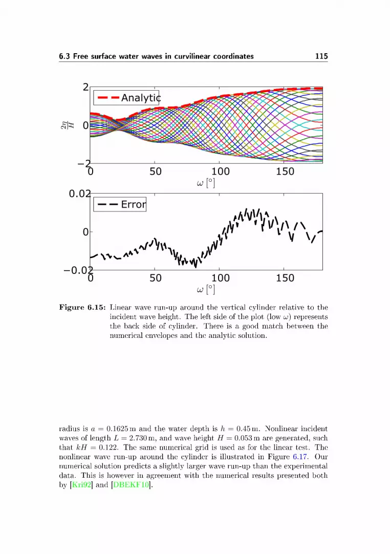
6.3 Free surface water waves in curvilinear coordinates 115
0 50 100 150−2
0
2
ω []
2η H
0 50 100 150−0.02
0
0.02
ω []
Analytic
Error
Figure 6.15: Linear wave run-up around the vertical cylinder relative to theincident wave height. The left side of the plot (low ω) representsthe back side of cylinder. There is a good match between thenumerical envelopes and the analytic solution.
radius is a = 0.1625m and the water depth is h = 0.45m. Nonlinear incidentwaves of length L = 2.730m, and wave height H = 0.053m are generated, suchthat kH = 0.122. The same numerical grid is used as for the linear test. Thenonlinear wave run-up around the cylinder is illustrated in Figure 6.17. Ournumerical solution predicts a slightly larger wave run-up than the experimentaldata. This is however in agreement with the numerical results presented bothby [Kri92] and [DBEKF10].

116 Boundary-tted domains with curvilinear coordinates
x/L
y/L
−2 0 2 4−2
−1
0
1
2
2η
H
0
0.5
1
1.5
(a) Maximum wave envelope contours. Top: numer-ical solution. Bottom: analytic solution.
0.5
1
1.5
2
30
210
60
240
90
270
120
300
150
330
180 0
Numerical
Analytic
(b) Wave run-up in polar coordi-nates.
Figure 6.16: The linear wave envelopes relative to the incident wave heights.
0 50 100 1500
0.5
1
1.5
2
ω []
2η H
Numerical
Experiment
(a) Wave run-up.
0.5
1
1.5
30
210
60
240
90
270
120
300
150
330
180 0
Numerical
Experimental
(b) Polar
Figure 6.17: Nonlinear wave run-up around the cylinder. kH = 0.122, kh =1.036, ka = 0.374. Experimental data from Kriebel [Kri92].
6.4 Concluding remarks
The introduction of generalized curvilinear coordinates has signicantly in-creased the range of applications that can benet from boundary-tted domainsto better reassemble real engineering problems. With some classical exampleswe have demonstrated how the free surface water wave solver can be used tosimulate both linear and nonlinear waves in complex scenery. Combined withthe multi-block solver to solve large-scale problems, as indicated by the perfor-mance scaling results in Section 4.4.6, the present free surface tool oers some

6.4 Concluding remarks 117
unique opportunities for fast and accurate assessment of coastal engineeringapplications.
We point out, that we have experienced a degradation of the algorithmic per-formance of the Laplace solver for some of the boundary-tted examples. Thenumber of preconditioned defect correction iterations has increased between50% to 100% for the above examples. We know that the most ecient multi-grid coarsening strategy is based on coarsening along those dimensions that willbest preserve the physical grid isotropy. When working on the computationaldomain, the multigrid coarsening strategy selects the coarsening dimensionsbased on ∆ξ and ∆γ and not the physical properties ∆x and ∆y. However,due to the curved coordinate lines, ∆x and ∆y are not constant, and it can beimpossible to select a coarsening strategy that always preserves isotropy in theglobal domain. This remains a challenge, and more analysis has to be carriedout to fully understand the impact.

118 Boundary-tted domains with curvilinear coordinates

Chapter 7
Towards real-timesimulation of ship-wave
interaction
A solid foundation for further development and collaborations with industry hasbeen established with the implementation and demonstration of the generic andhigh performance free surface water wave simulation tool. As motivated in theformer chapters, the portable GPUlab library and the ecient free surface solver,accurately accounting for dispersive and nonlinear eects can be a valuabletool in many aspects of marine engineering. The remainder of this chapter isdedicated to the research that has been carried out in close collaboration withFORCE Technology, a Danish approved Technology Service (GTS) companywith leading world-wide assets in maritime technologies.
The joint collaboration focuses on the development of a ship hydrodynamicmodel for real-time simulation, including ship-wave and ship-ship interactionas part of a full mission marine simulator. Such full-scale marine simulatorsare used for educating and training of marine ocers and maritime engineering.Accurate and realistic interaction with ship generated wave forces are importantto maintain as realistic an environment as possible. Eects such as the forcesthat occur when two ships approach each other are particular critical and impor-tant for safely maneuvering of tugboats. Current state-of-the-art hydrodynamic

120 Towards real-time simulation of ship-wave interaction
models implemented in full-mission simulators are based on fast interpolationand scaling of experimental model data and the results are therefore limited bythe amount and accuracy of the available data. The main challenge for real-timeship-wave interaction is to nd a proper balance between an approximate repre-sentation of ships that maximizes computational performance, but it also givesmore accurate and reliable results compared to previous interpolation methods.There isto the author's knowledgeno other tools that are able to overcome thereal-time restriction with a model as accurate as the one proposed. Thus, thiswill be pioneering work and a unique opportunity for FORCE Technology to berst movers on an international marked.
The collaboration with FORCE Technology has led to an intermediate step onthe path towards achieving real-time ship-wave interaction. Research at FORCETechnology continues to be active and the following sections demonstrate a se-lection of the most important ndings achieved until now. The generic andcomponent-based GPUlab library signicantly improved the developer produc-tivity for the extension of OceanWave3D into supporting ship-wave and ship-shipinteractions.
7.1 A perspective on real-time simulations
With the present GPU-based implementation of the OceanWave3D solver, real-time simulations should be within reach and the solver would be suitable forthese applications as it is both scalable, ecient, and robust. The potentialow model is also very attractive since it accurately accounts for dispersivewaves from deep to shallow waters, setups that will be relevant in any marinesimulator. In previous work we roughly estimated the time to compute a waveperiod for various wave resolutions[EKMG11], from which we concluded thatreal-time simulations can be achieved within an additional speedup factor ofapproximately one order of magnitude for three dimensional problems with onemillion degrees of freedom. Let us reconsider some of these approximations andinclude recent hardware trends to better estimate and predict future capabilities.If we wish to estimate the compute time t it takes to compute one wave periodT , as a function of time per defect correction iteration It, we get,
t
T≈ ItK, K ≈ SRK Iavg NPPW
Cr, (7.1)
where SRK is the number of Runge-Kutta ODE solver stages, Iavg is the averagenumber of defect correction iterations per solve, NPPW is the number of pointsper wavelength, and Cr is the Courant number.

7.1 A perspective on real-time simulations 121
The value of K depends heavily on the wave characteristics, but we are able toestimate a lower and upper bounds based on a few assumptions. The numberof Runge-Kutta stages is constant for this method, at SRK = 4. We will alsoassume a constant Courant number Cr = 0.8. Nonlinear wave eects in com-bination with the water depth determine the algorithmic convergence rate ofthe preconditioned defect correction method together with the stopping crite-ria [EK14]. The average number of iterations for mildly to fully nonlinear wavesand a tolerance of 10−5 are usually within the range Iavg = 4-15. The num-ber of points per wavelength should be set according to the order of the nitedierence approximations and will inuence the accuracy of wave dispersion.Reasonable results are often achievable with NPPW = 8-16. In combinationthese numbers give us the following estimates Klow = 160 and Khigh = 1200.In order to achieve real-time simulations it is evident that the time to computeone wave period is less than the wave period itself, i.e., t < T , which leads to,
It <1
K. (7.2)
For a given K we can now compute 1/K and compare it directly to the per-formance measurements. Timings based a high-end consumer GPU, GeForceGTX590 is illustrated in Figure 7.1. We can immediately see that real-time isachievable only for low values of K, thus, when there is fast convergence and fewpoints per wavelength, and for resolutions up to 3 ·105 degrees of freedom. Thatwould cover a fully three dimensional simulation with e.g, 257× 129× 9 degreesof freedom. As demonstrated in Chapter 4, even the multi-GPU setup will notimprove performance at these resolutions. From the gure we see that there isalmost no dierence between high- and low-order discretizations in the regionfeasible for real-time computations, which only favors high-order discretizationsfurther, because K would be able to be smaller for high-order discretizations,due to a less strict requirement on the number of points per wavelength.
For practical ship hydrodynamics setups in a numerical wave tank, the tankwould have to be at least 3Lpp long in the sailing direction and 1Lpp in thetransverse direction, where Lpp is the ship length. The number of points pership length is then determined by the wavelength l, generated by the ship,and the number of points per wavelength NPPW , which leads to the followingestimate for total number of degrees of freedom,
N ≈ 3
(Lpp
lNPPW
)2
Nz, (7.3)
where Nz is the number of vertical grid points. As an example, consider a largetanker of length Lpp = 270m sailing with an intermediate speed, such that theFroude number Fr = 0.08, dened as Fr = U/
√g Lpp, where U is the sailing
speed. Then the waves generated by the tanker will be of length l ≈ 11m

122 Towards real-time simulation of ship-wave interaction
104 105 106 107 10810−4
10−3
10−2
10−1
100
N
Time/Iter
[s]
6th-order
4th-order
2nd-order
K = 160
K = 1200
Figure 7.1: Real-time perspectives based on the two extreme values of K andthe defect correction iteration time It. Using the GeForce GTX590(G4 ), single precision, MG-RBZL-1V(1,1).
resolved with e.g., NPPW = 10 grid points. The total degrees of freedom,assuming that 9 vertical grid points are sucient, will then be N ≈ 1.6 · 106.Figure 7.1 demonstrates that this is not within the real-time limit for the givensetup. However, for N ≈ 1.6 · 106 we see that It ≈ 0.02, from which we canconclude that K can be no more than 50 for this to be real-time, or in otherwords, we need at least another speedup factor of 3.2 to achieve the goal ofreal-time computations with the given setup.
It is now tempting to ask when will it be possible to do real-time computationsfor these hydrodynamic ships models? One should be careful when speculatingabout future hardware trends, but if we assume the following: 1) The solver iscompletely memory bound. 2) No further optimizations are made. 3) The GPUmemory bandwidth increases with the same rate as the previous generations.Then we should be able to make an estimated guess. Comparing two consecutivegenerations of GPUs, e.g., the GeForce GTX480 and GTX580 or Tesla C2070and K20, there is a bandwidth increase of approximately 40%. If this trendcontinues, a 3.2 speedup is achievable within two to three GPU generations,which historically translates to a maximum of ve years.
Though all these numbers are based on rough estimates and heavily depends onthe wave characteristics and ship hydrodynamics, they do indicate that withina reasonable near time horizon, interactive free surface water wave simulationswith engineering accuracy will be a reality. This suggest that now is a goodtime to invest and pursue this goal.

7.2 Ship maneuvering in shallow water and lock chambers 123
7.2 Ship maneuvering in shallow water and lock
chambers
A feasible model for fast and accurate ship hydrodynamics has been developedand improved continuously during the collaboration period. The rst functionalmodel was developed and evaluated for the 3rd International Conference onShip Maneuvering in Shallow and Conned Water, with non-exclusive focuson ship behavior in locks [VDM12, LGB+13]. The objective was to reconstructnumerically a set of experiments carried out with an 1/80 scale laboratory modelas seen in Figure 7.2. The experiments reassemble a large 12.000 TEU containercarrier entering the newly designed locks in the Panama canal. Experimentaldetails are available in [VDM12].
Figure 7.2: Experimental setup of a large vessel entering a lock chamber inthe new Panama Canal. 1/80 scale.
In order to maximize performance the rst version of the ship hydrodynamicmodel is based on potential ow theory with linear free surface boundary con-ditions and 2nd-order nite dierence approximations. The motivation for thesesimplications is to rst produce a proof-of-concept implementation that willbe stable and have the best possible performance before introducing the moreadvanced nonlinear parts. In future versions the nonlinear conditions will beconsidered when compute times are within or close to the real-time restrictionfor interactive applications.
A moving frame of reference is introduced in the time dependent equations tokeep the ship xed at the center of the numerical wave eld such that
x = x0 − Ut, y = y0, z = z0, (7.4)
where (x0, y0, z0) is origin in the xed global coordinate system and U is theship velocity in the x-direction. The linear kinematic and dynamic free sur-face boundary conditions are likewise modied to reect the moving frame of

124 Towards real-time simulation of ship-wave interaction
reference,
∂tη − U∂xη − w = 0, z = 0, (7.5a)
∂tφ− U∂xφ+ gη +p
ρ= 0, z = 0, (7.5b)
where the new quantities ρ are the water density and p is the free surface pres-sure. The velocity vector u ≡ (u, v, w) is dened in the forward, transverse, andvertical directions, respectively. We consider again no-ux boundary conditionson the seabed and on the surface of the rigid bodies,
n · ∇φ = 0, z = −h (7.6a)
n · ∇φ = n · uB , (x, y, z) ∈ SB (7.6b)
where n ≡ (nx, ny, nz)T is the normal to the boundary surface SB , and uB =
(U, 0, 0)T .
A pressure distribution and a double body linearization is utilized to capturethe main ow characteristics as a steady state solution [Rav10], that can bepre-computed and scaled linearly with respect to the reference velocity U . Thisrather simple approach was selected to minimize its inuence on the overalleciency. For further details on this hydrodynamic ship model we refer thereader to [LGB+13].
In addition to the hydrodynamic ship model, the GPUlab library was extendedwith support for handling multiple captive objects in the computational domain.A captive body was implemented, derived as a special instance of a oating body,with the main objective of controlling physical position and velocity as a functionof time. A brief example of creating and adding a captive body (e.g., a ship)to the simulation is illustrated in Listing 7.1. The brief example demonstratesthat once the underlying implementations are complete, the assembly phase canbe implemented generically using an object oriented approach.
1 using namespace gpulab;2
3 // Create body and set shape4 captive_body <double > ship;5 ship.set_shape(/* set ship hull shape */);6
7 // Assign a pair of time and position8 ship.get_time_position ().insert( /* time , position */ );9
10 captive_scene <captive_body <double > > scene;11 scene.add(ship);12
13 // Apply pressures on eta at time t=1s14 scene.update (1.0,eta);

7.2 Ship maneuvering in shallow water and lock chambers 125
Listing 7.1: Constructing a ship object and assigning captive data and a shape.The ship is added to the scene manager and pressure is applied tothe free surface elevation according to the hull shape and positionat time t = 1s.
Both the ship hull and the locks are approximated with a pressure distributionin the dynamic free surface condition (7.5b). The pressure is approximated witha quasistatic assumption such that the pressure on is given by
p = −ρ(−U∂xφ+1
2u · u + gη0), (7.7)
where ηo is the draft from either the ship hull of the lock. The pressure contri-bution acting on the free surface allows a convex representation of the ship hulland locks. Therefore the bulbous bow was removed from the original containercarrier mesh to be represented by a single valued function in the horizontal co-ordinates. Though this kind of approximation based on pressure contributionshas shown to be applicable for ships sailing at low Froude numbers, it turns outnot to be a good approximation to the locks [Rav10]. The vertical lock walls arerepresented via a pressure contributions that pushes the surface almost downto the seabed. Large gradients in the free surface elevation and potential willtherefore occur regardless of the numerical resolution.
A numerical experiment was performed according to the guidelines in [VDM12],with a 12,000 TEU container carrier entering the lock at very low Froude num-bers. The numerical resolution is Nx ×Ny ×Nz = 513× 193× 17, all variablesare normalized with the ship length Lpp = 348m, such that the domain size isLx = 5, Ly = 1, and Lz = 0.048. The hydrodynamic ship model results in areasonable wave eld generated by the carrier in the entrance part of the lock,illustrated in Figure 7.3. The steep gradients that are present at the interfacebetween the locks and the free surface generate spurious waves as the carrierenters the lock. These articial waves dominate the relatively small waves gener-ated by the ship, as clearly visible in Figure 7.4. Though ltering methods couldbe applied to remove some of the spurious waves in the vicinity of the locks,it would unintentionally also aect the waves generated by the ship when theship approaches the lock walls. The present hydrodynamic ship model thereforeproved not to be suitable for representation of near-vertical geometries such asthe lock in a moving frame of reference. Since the present model is to be imple-mented in a full mission marine simulator where such geometries are likely toexist, alternative methods have been investigated.

126 Towards real-time simulation of ship-wave interaction
Figure 7.3: Free surface elevation and potential amplitudes before the shipenterns the lock, shortly after the startup phase. Numbers arenormaliced by the ship length Lpp = 348m.
Figure 7.4: Free surface elevation and potential amplitudes when the shipenters the lock. Numbers are normaliced by the ship lengthLpp = 348m.
7.3 Ship-wave interaction based immersed bound-
aries
The previous hydrodynamic ship model based on pressure distributions is notapplicable for scenery that we want to consider. The lock entrance exampleclearly demonstrated weaknesses in the numerical modeling of deep and dis-

7.3 Ship-wave interaction based immersed boundaries 127
continuous geometries. Also the single value representation of ship hulls is asimplication that puts signicant restrictions on the application range.
In the search for alternatives we explored a technique based on immersed bound-ary conditions, because these methods potentially have a exible and accuraterepresentation of geometries based on computational inexpensive techniques.The idea for an immersed boundary was originally introduced by Peskin, usedfor blood ow simulations in the heart using the Navier-Stokes equations [Pes02].It has also been applied in the context of turbulent modeling of oating bodiesinteraction with water waves [YSW+07, YS09]. It is however, to the authorsknowledge, the rst time with this joint work, that it is applied to with thepurpose of real-time simulation of ship generated water waves.
The principle of the immersed boundary method is to represent geometries vianite dierence or nite volume boundary approximations directly at the bound-ary of the geometry. Immersed boundaries are therefore treated much like theoriginal outer domain boundaries. For the representation of ship hulls we imposethe inhomogeneous Neumann condition (7.6b) for the solution of the Laplaceequation, by introducing ctitious ghost points inside the ship hull and then ap-proximating the boundary conditions with stencils that take into account theseghost points. This is an attractive approach because the original fast GPU-basedimplementation of the Laplace operator can be re-used with small modication,both preserving performance and improving developer productivity.
Figure 7.5: Discrete representation of a ship hull using immeresed boundaries.© is uid grid points, ⊗ is body ghost points, • is a body point,× is inactive interior body points.
One challenge for the immersed boundary method lies in the setup phase, wherewe need to properly identify the internal ghost points and compute the corre-

128 Towards real-time simulation of ship-wave interaction
sponding nite dierence coecients satisfying (7.6b). A pre-processing phaseis introduced where ghost points inside the body, which belong to a nite dif-ference stencil, are identied and the corresponding body points are found vianormal projections to the body surface, see Figure 7.5. The stencil coecientsare pre-computed via Taylor expansions from the body point to each uid pointat the outer tangential plane within a given Euclidean distance plus the ghostpoint, as illustrated in red. Taylor expansions up to second order are used toreduce the size of the resulting system of equations, but can be generalized tohigher orders. The Taylor expansion from the body point to each of the uidpoints in three spatial dimensions is
f(x1 + ∆1, x2 + ∆2, x3 + ∆3) ≈2∑i=0
2∑j=0
2∑k=0
∆i1∆j
2∆k3
i!j!k!f (i,j,k)(x1, x2, x3).
The expansions with respect to each point can be arranged in an overdeterminedlinear system of equations (assuming there is more uid points than expansionterms),
Af = b, A ∈ Rα×β , f ∈ Rβ ,b ∈ Rα, (7.8)
where A is assembled from the Taylor expansion coecients, f represents eachderivative f (i,j,k) at the body point, and b holds the values of each uid andghost points. β is equal to the number of expansion terms up to second order (27in three dimensions) and α is the number of points considered. A is assembledusing a coordinate system with a normal basis spanned by the tangential planeand the body normal. The rst derivative, normal to the body surface, is thendirectly represented in one entry of f . The system can be solved with a weightedleast squares method,
ATWAf = ATWb, W ∈ Rβ×α, (7.9)
where W is a diagonal matrix containing the weights. The coecients corre-sponding to the surface normal derivative are now located in the second row of[ATWA]−1ATW. These coecients can be pre-computed for each body ghostpoint and then later be used for satisfying the inhomogeneous Neumann bound-ary condition, by isolating the value for the ghost point using,
α∑p=1
cmφi(p),j(p),k(p) ≈ n · uB. (7.10)
This calculation is performed in parallel on the GPU for each ghost point everytime the boundary condition needs to be satised. Promising results have beenobtained with the present immersed boundary method. Research is still active,and investigation for e.g., optimal search radii size and least square weights areongoing. A parameter analysis of the weight matrix W is part of ongoing work.

7.4 Current status and future work 129
The immersed boundary method has additional advantageous properties; Themethod is not restricted to either oating bodies or oor mounted and surfacepiercing geometries, which means that we can easily represent submerged bodiesor complex ship hulls with bulbous bows. The method also seems promising withrespect to performance, since most of the computational work is part of the pre-processing phase and because the original fast Laplace operator works with nochanges. Only ghost points close to the body surface need to be updated, whichis a relatively small task due to the volume to surface ratio.
7.4 Current status and future work
The project on real-time simulation of ship-ship interaction continues at FORCETechnology after the completion of the present work. The development of thenumerically and computationally ecient hydrodynamic model is now beingrigorously tested and validated. A snapshot of waves generated by a containercarrier, based on the current immersed boundary implementation, is illustratedin Figure 7.6. The next step is to merge the computational model into thefull mission marine simulator software, which will increase the requirements forreliability and robustness due to human interaction and complex simulation en-vironments. Also a thorough performance optimization analysis will be carriedout to pursue real-time performance at reasonable resolutions, to match the re-quirements of the marine simulator and to clearly set the standards within inter-active ship-ship simulations. Performance results obtained with spatial domaindecomposition in Section 4.4.6 indicated that there is no attainable speedup forthe problem sizes considered for the hydrodynamic ship-wave model. However,a parameter study of the Parareal algorithm and the present model can possiblylead to speedups on heterogeneous systems where multiple GPUs are available.This will be investigated if single-GPU optimizations do not lead to sucientspeedup.
This collaboration is a good example of the possibilities that become availableafter development of a generic software framework. The GPUlab library, andthe free surface water wave tool in particular, have been a perfect starting pointfor the collaboration on which the ship hydrodynamic research has been ableto build directly on. The hardware abstraction provided by the library hasenabled a lighter coding eort, that still enables execution in parallel on many-core heterogeneous computer systems.

130 Towards real-time simulation of ship-wave interaction
Figure 7.6: Free surface wave generation based on immersed boundary condi-tions. Waves are generated by a KCS container ship with Froudenumber Fr = 0.2.

7.5 Conclusion and outlook 131
7.5 Conclusion and outlook
Massively parallel heterogeneous systems continue to enter the consumer mar-ket, and there has been no identication that this trend will stop in years tocome. Though these massively parallel many-core architectures have provento be computationally ecient, with high performance throughput for a vastamount of applications[BG09, Mic09, GWS+09, G10, EKMG11], they still posesignicant challenges for software developers[EBW11], and they are still to be-come standard within the industry.
The present work can be considered as a reaction to the recent developmentof massively parallel architectures where we attempt to address some of thequestions and challenges that follow from the new generation of hardware. Oneof the main challenges is that these heterogeneous systems require softwarevendors to adjust to new programming models and optimization strategies. Wehave presented our ideas for a generic GPU-based library for fast proto-typing ofPDE solvers. A high-level interface with simple implementation concepts havebeen presented with the objective of enhancing developer productivity and toensure performance portability and scalability.
Based on the proof-of-concept nonlinear free surface water wave model, wehave presented details of a domain decomposition technique in three spatialdimensions for distributed parallel computations on both desktop and clusterplatforms. The spatial domain decomposition technique preserves algorithmiceciency and further improves performance of the single-block version of thesolver, cf. recent studies [EKBL09, EKMG11, GEKM11]. If the performancespeedups that we have reported for the single-block solver in Section 3.4 of upto 100 compared to the single-threaded CPU solver, are combined with eitherthe results reported with spatial domain decomposition or Parareal, then weachieve speedups that signicantly beat Moore's law. We mean by this that theperformance improvements we have achieved within 3-4 years of development,cannot be explained only by Moore's law, but is a product of Moore's law andimproved algorithmic design choices and ecient implementations.
The numerical model is implemented using the GPUlab library based on Nvidia'sCUDA programming model and is executed on a recent generation of pro-grammable GPUs. In performance tests, we have demonstrated good weakscalability in absolute as well as measures for relative speedups and eciencyin comparison to the single-GPU implementation. Scaling results based on themulti-block solver have detailed how the free surface model is capable of solv-ing systems of equations with more than one billion degrees of freedom for therst time. These impressive numbers can be obtained with a reasonable sizedcluster equipped with 16 or more GPUs. Even at these large-scale problems

132 Towards real-time simulation of ship-wave interaction
we outlined that simulations are in fact possible within reasonable turn-around-times. Also, we highlight that multi-GPU implementations can be a means forfurther acceleration of run-times in comparison with single-GPU computations.A study of the multigrid coarsening strategy has led to the conclusion that fewmultigrid levels are sucient for fast convergence of the Laplace problem. Theseresults imply that a signicant reduction in communication can be obtained tomaximize performance throughput.
The library has already successfully been used for development of a fast toolintended for scientic applications within maritime engineering, cf. Chapter 7.We intend to further extend the library, as we explore new techniques, suitablefor parallelization on heterogeneous systems, that t the scope of our applica-tions. The library and the free surface water wave solver, in their present stages,are ideal for further collaboration on PDE applications that may benet fromparallelization on heterogeneous systems.
The GPUlab library has been developed and designed exclusively by the authorhimself. A major eort has been put into the development of all the genericdesign and implementation of iterative solvers, time integrators, the matrix-freestencil operators etc.. Also, the implementation and validation of the free sur-face wave solver on heterogeneous hardware have taken a signicant amount oftime. This conrms our motivation for the project itself, that software devel-opment for massively parallel processors is very time consuming, and the needfor well designed, portable, and ecient software libraries is key to future de-velopments. In particular, the process of debugging parallel programs runningon heterogeneous hardware is a troublesome procedure.
7.6 Future work
Our work has tried to address a number challenges that arise in heterogeneouscomputing and software design. However, along the way there have been a num-ber of unanswered questions and new challenges that arise. We suggest that thefollowing topics can be used for directing future research towards supplementingor improving our work.
Large-scale engineering case The combination of an ecient multi-blockand boundary-tted free surface wave solver opens up new opportunitiesfor fully three-dimensional large-scale applications of practical interest inmaritime engineering. With interconnected and boundary-tted domainsit would be possible to construct large and complex harbor facilities. In

7.6 Future work 133
future work we would like to demonstrate practical examples based on thepresent free surface solver.
Parareal fault resilience Parareal possesses several interesting features, faultresilience being a highly relevant feature of execution on massively paral-lel HPC clusters. A numerical experiment that rst of all conrms thisproperty along with a deeper analysis of how well and fast Parareal is ableto fully recover from an erroneous process would be of interest. A studyof how stable Parareal will be if multiple processors are lost may also beof interest.
Autotuning There is a number of kernel conguration parameters that arebased on basic knowledge of good programming practice. However, thesecongurations are not guaranteed to be optimal on any heterogeneoussystem. An autotuning module that can be executed on specic heteroge-neous systems can be used to reveal if there are alternative congurationsthat would result in improved performance. Such a module would be avaluable tool to maximize performance portable settings.
OpenCL In this work we have exclusively considered the CUDA for C pro-gramming model. Though OpenCL traditionally has not been able tooer the same degree of documentation, it is not designed specically forGPU programming, but is designed to execute on heterogeneous systemin general. An interesting analysis of CUDA vs. OpenCL or especiallyOpenCL on alternative systems, e.g., multi-core CPUs or the Intel MIC,would be of interest. The CUDA programming model has proven very at-tractive for development of Nvidia GPU-based applications. However, webelieve that the restriction to Nvidia GPUs will eventually cause CUDAto play a minor role in future HPC environments.
Green computing Massively parallel processors are able to oer an eectiveperformance per watt ratio, and therefore they are expected to play animportant role in future HPC systems where energy consumption is aprimary challenge. A better understanding of the power consumption ofthe GPU and the system as a whole in relation to performance throughputis a relevant concern and will be important for future hardware design.

134 Towards real-time simulation of ship-wave interaction

Appendix A
The GPUlab library
The GPUlab library is a generic C++/CUDA/MPI library designed for fastprototyping of large-scale PDE solvers without compromising performance.
The library hides CUDA-specic implementation details behind a generic in-terface that will allow developers to assemble PDE solvers at a much higherabstraction level. The library is designed to be ecient, portable and to en-hance developer productivity. The library is component-based, and it providesa good starting point, from which custom designed components can be imple-mented, to assemble advanced PDE solvers. Thus, it is expected that the usersare able to implement custom components that may contain CUDA specicimplementations. The library will provide the basis for many of these customcomponents. The following sections will present a brief introduction to theprogramming guidelines and principles. Examples will demonstrate the use ofspecic components.
A.1 Programming guidelines
The GPUlab library is a header-only library, which means that everything iscontained in header les. Therefore the library should not be pre-compiled and

136 The GPUlab library
there is no linking stage.
For the GPUlab library to work properly in multi-GPU settings, it needs tosetup a private MPI communicator and assign each GPU to individual processes.Therefore a program should at least follow this template:
1 #include <gpulab/gpulab.h>2
3 int main(int argc , char** argv)4 5 using namespace gpulab;6
7 // Initialize GPUlab8 if(gpulab ::init(argc , argv))9 10 // DO STUFF HERE11 12 // Finalize GPUlab13 gpulab :: finalize ();14 return 0;15
There is always one optional input parameter that can be passed to the pro-gram, it is the name of a conguration le. If not specied, the default valueconfig.ini is used.
A.1.1 Templates
The library heavily depends on template arguments, which allow a exible anduser-controllable environment. We therefore recommend to use type denitionsat the very beginning of the program to control the assembling of the PDEsolvers. The program might start with:
1 // Basic type definitions2 typedef float value_type;3 typedef gpulab ::vector <value_type ,gpulab :: device_memory > vector_type;4 typedef gpulab ::vector <value_type ,gpulab :: host_memory > host_vector_type;5 typedef myLaplaceMatrix <device_vector_type > matrix_type;6
7 typedef typename grid_type :: property_type property_type;8 typedef typename grid_type :: dim_size_type dim_size_type;9 typedef typename grid_type :: dim_value_type dim_value_type;
This will allow you to control e.g., the working precision or the matrix imple-mentation only one place in the code.

A.1 Programming guidelines 137
A.1.2 Dispatching
Due to the template-based design it is not directly possible to determine thetype of objects, but sometimes it is convenient to treat host and device vectorsdierently. To do this one can create a overloaded function with dispatching:
1 typedef gpulab ::vector <double ,gpulab :: device_memory > d_vector_type;2 typedef gpulab ::vector <double ,gpulab :: device_memory > h_vector_type;3
4 int main(int argc , char** argv)5 6 if(gpulab ::init(argc , argv))7 8 d_vector_type x(10); // Device vector9 h_vector_type y(10); // Host vector10
11 foo(x); // Will be dispatched to device code12 foo(y); // Will be dispatched to host code13 14 gpulab :: finalize ();15 return 0;16 17
18 template <class V>19 void foo(V &a)20 21 // Dispatch to the right function22 foo(a,typename V:: memory_space ());23 24
25 template <class V>26 void foo(V &a, gpulab :: device_memory)27 28 // a is a device vector29 30
31 template <class V>32 void foo(V &a, gpulab :: host_memory)33 34 // a is a host vector35
A.1.3 Vectors and device pointers
The vector class is derived from the Thrust[BH11] vector objects and thereforeoers the same container iterators and operators, e.g.:
1 typedef gpulab ::vector <double ,gpulab :: device_memory > vector_type;2
3 vector_type a(20); // vector of size 204 thrust :: sequence(a.begin (),a.end()); // Fill a with 1,2,...,19
The vector class is also a wrapper for a pointer that points to either host ordevice memory. If a device pointer is required to send to a kernel function, then

138 The GPUlab library
do:
1 typedef gpulab ::vector <double ,gpulab :: device_memory > vector_type;2
3 vector_type a(10); // vector of size 104 double* ptr = RAW_PTR(a); // pointer to device memory
A.1.4 Conguration les
The GPUlab is initialized with a (possibly empty) conguration le, namedconfig.ini that should be in the same directory as the executable. The cong-uration le is a simple text le. Every line in the le denes a key and a value.In order to retrieve information from the conguration le use:
1 double tol;2 int N;3 GPULAB_CONFIG_GET("N",&N,100); // Get N from config , default value
= 1004 GPULAB_CONFIG_GET("tolerance",&tol ,0.0); // Get tolerance from config ,
default value = 0
If the key is not found in the conguration database, the default value will beused. The GPUlab library will automatically try to convert the value onto thesame type as provided.
it is also possible to insert entries into the conguration database. They onlyexist during the lifetime if the program and are not stored in the text le.
1 double tol = 0.1;2 int N = 30;3 GPULAB_CONFIG_SET("N",N); // Set N to 304 GPULAB_CONFIG_SET("tolerance",tol); // Set tolerance to 0.1
A.1.5 Logging
The GPUlab library will automatically log some information to the screen duringa run. The level at which information will be displayed can be controlled viathe conguration le and can be any of:
1 log_level DEBUG2 log_level INFO3 log_level WARNING4 log_level ERROR
From anywhere in your code you can log information by doing:

A.1 Programming guidelines 139
1 int N = 100;2 GPULAB_LOG_DBG("This is debugging\n");3 GPULAB_LOG_INF("For your information , N = %i \n", N);4 GPULAB_LOG_WRN("This is a warning\n");5 GPULAB_LOG_ERR("This is an error\n");
A.1.6 Input/Output
There is build in routines for reading and writing vectors to binary format.
1 #include <gpulab/io/print.h>2 #include <gpulab/io/read.h>3
4 using namespace gpulab;5 vector <double ,device_memory > a(100);6 vector <double ,device_memory > b;7 io:: print(a,io:: TO_BINARY_FILE ,1,"a.bin"); // Print to file a.bin8 io::read("b.bin",io::BINARY ,1); // Read from file b.bin
A.1.7 Grids
The grid class is an extension to the vector class and it holds extra dimensionalinformation. Here is an example of how to to create a two-dimensional gridwith Dirichlet boundary conditions in the x-direction and Neumann boundaryconditions in the y-direction:
1 #include <gpulab/grid.h>2 typedef gpulab ::grid <double ,gpulab :: device_memory > grid_type;3 typedef typename grid_type :: property_type property_type;4 typedef typename grid_type :: dim_size_type dim_size_type;5 typedef typename grid_type :: dim_value_type dim_value_type;6
7 dim_size_type dim (100 ,50); // Grid size 100 x 508 dim_value_type p0 ( 0, 0); // Physical x0 , y09 dim_value_type p1 ( 1, 1); // Physical x1 , y110 dim_size_type g0 ( 0, 2); // Ghost layers x0, y011 dim_size_type g1 ( 0, 2); // Ghost layers x1, y112 dim_size_type o0 ( 0, 0); // Offset x0 , y013 dim_size_type o1 ( 0, 0); // Offset x1 , y114 dim_size_type bc0( BC_DIR , BC_NEU); // Boundary conditions15 dim_size_type bc1( BC_DIR , BC_NEU); // Boundary conditions16
17 property_type props2d(dim ,p0 ,p1,g0,g1,o0 ,o1,bc0 ,bc1);18
19 grid_type U(props2d);20 grid_type* W = U.duplicate ();

140 The GPUlab library
A.1.8 Matlab supporting le formats
To support post- and pre-processing in Matlab we have also created functionsto read, write and reshape vectors and grids in binary les. Simply use:
1 v1 = 1:100;2 print2gpu('v.bin',v1 ,'precision ','double ')3 v2 = readgpu('v.bin','precision ','double ')
A.2 Conguring a free surface water wave appli-
cation
A.2.1 Conguration le
The conguration of a free surface application can be controlled with the GPU-lab input conguration le. Most of the conguration parameters have defaultvalues, but in order to control the wave characteristics one can specify:
1 # WAVE CHARACTERISTICS2 L 1.03 Lx 4.04 Ly 1.05 h 1.06 k 6.2831857 H 0.0424368 c 1.2613169 T 0.79282310 percent 30.011 linear 012 periodic 0
For the discretization settings the following parameters can be specied:
1 # DISCRETIZATION PARAMETERS2 alpha 33 Nx 2574 Ny 1295 Nz 96 Cr 0.67 tend 20
And nally some of the conguration parameters that controls the multigridpreconditioned defect correction solver:
1 # LAPLACE SOLVER PARAMETERS2 iter 203 v1 2

A.2 Conguring a free surface water wave application 141
4 v2 25 vc 46 K 47 rtol 0.00018 atol 0.000019 mgcycle V
A.2.2 The Matlab GUI
Manually conguring the wave characteristics can be troublesome as they haveto match each other. We have therefore creates a simple Matlab GUI that willhelp create the conguration les, see Figure A.1
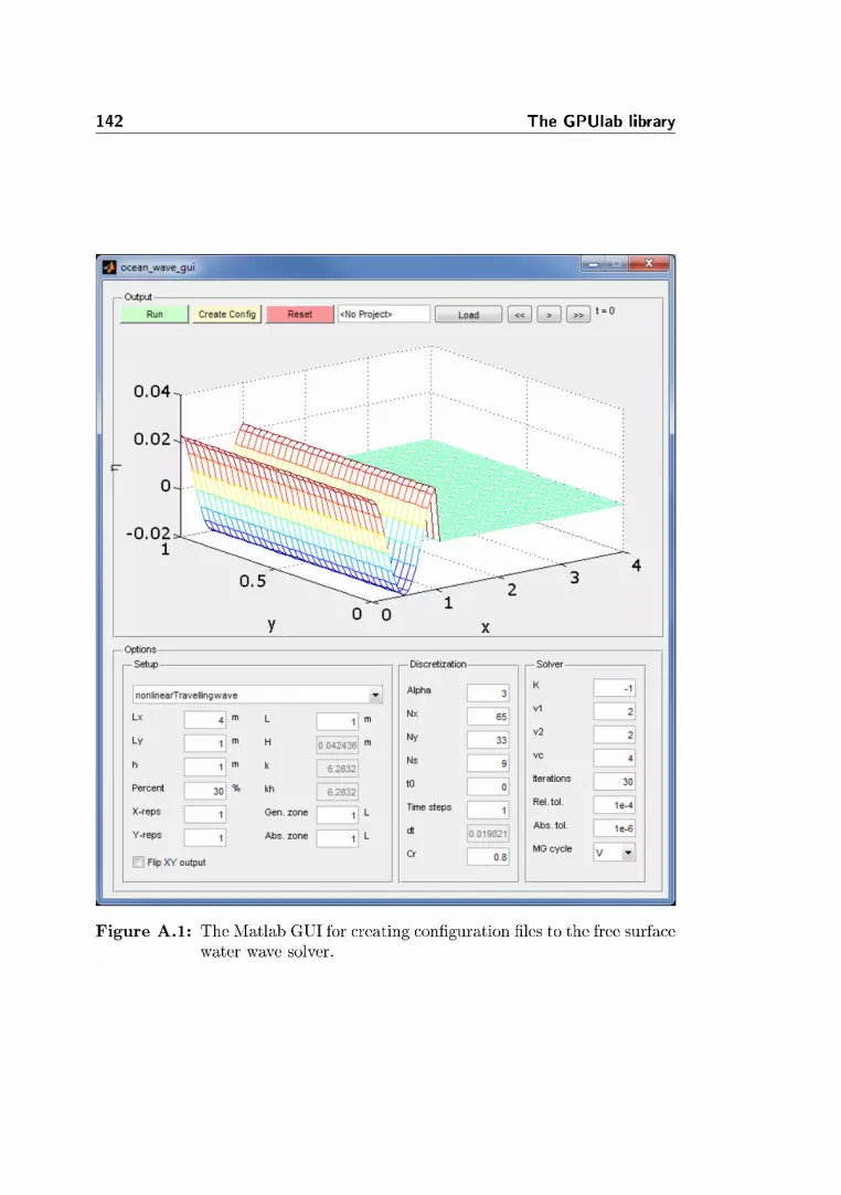
142 The GPUlab library
Figure A.1: The Matlab GUI for creating conguration les to the free surfacewater wave solver.

Bibliography
[ABC+06] K. Asanovic, R. Bodik, B. C. Catanzaro, J. J. Gebis, P. Hus-bands, K. Keutzer, D. A. Patterson, W. L. Plishker, J. Shalf,S. W. Williams, and K. A. Yelick. The landscape of parallelcomputing research: A view from Berkeley. Technical ReportUCB/EECS-2006-183, EECS Department, University of Cali-fornia, Berkeley, 2006.
[ABD+13] A. M. Aji, P. Balaji, J. Dinan, W.-C. Feng, and R. Thakur.Synchronization and ordering semantics in hybrid MPI+GPUprogramming. In 3rd International Workshop on Acceleratorsand Hybrid Exascale Systems (AsHES), 2013.
[ALB98] E. Acklam, H. P. Langtangen, and A. M. Bruaset. Parallelizationof explicit nite dierence schemes via domain decomposition,1998.
[AMW84] M. Abott, A. McCowan, and I. Warren. Accuracy of short-wave numerical models. ASCE Journal of Hydraulic Engineer-ing, 110(10):12871301, 1984.
[APS78] M. Abott, H. Petersens, and O. Skovgaard. On the numericalmodelling of short waves in shallow water. Journal of HydraulicResearch, 16(3):173203, 1978.
[Aub11] E. Aubanel. Scheduling of tasks in the parareal algorithm. Par-allel Computing, 37:172182, 2011.

144 BIBLIOGRAPHY
[Bai91] D. H. Bailey. Twelve ways to fool the masses when giving per-formance results on parallel computers. Supercomputing Review,pages 5455, 1991.
[Bai92] D. H. Bailey. Misleading performance reporting in the super-computing eld. Technical report, Numerical Aerodynamic Sim-ulation (NAS) Systems Division, NASA Ames Research, 1992.
[Bai09] D. H. Bailey. Misleading performance claims in parallel compu-tations. In Proceedings of the 46th Annual Design AutomationConference, DAC '09, pages 528533. ACM, 2009.
[BBB+11] S. Balay, J. Brown, K. Buschelman, V. Eijkhout, W. D. Gropp,D. Kaushik, M. G. Knepley, L. C. McInnes, B. F. Smith, andH. Zhang. PETSc developers manual. Technical report, ArgonneNational Laboratory, 2011.
[BBB+13] S. Balay, J. Brown, K. Buschelman, V. Eijkhout, W. D. Gropp,D. Kaushik, M. G. Knepley, L. C. McInnes, B. F. Smith, andH. Zhang. PETSc users manual. Technical Report ANL-95/11 -Revision 3.4, Argonne National Laboratory, 2013.
[BBC+94] R. Barrett, M. Berry, T. F. Chan, J. Demmel, J. Donato, J. Don-garra, V. Eijkhout, R. Pozo, C. Romine, and H. V. der Vorst.Templates for the Solution of Linear Systems: Building Blocksfor Iterative Methods, 2nd Edition. SIAM, 1994.
[BBD+09] M. Baboulin, A. Buttarib, J. Dongarra, J. Kurzak, J. Langouc,J. Langou, P. Luszczek, and S. Tomov. Accelerating scien-tic computations with mixed precision algorithms. ComputerPhysics Communications, 180:25262533, 2009.
[BBM+02] L. Baco, S. Bernard, Y. Maday, G. Turinici, and G. Zérah.Parallel in time molecular dynamics simulations. Physical ReviewE., 66(057701), 2002.
[BFH+04] I. Buck, T. Foley, D. Horn, J. Sugerman, K. Fatahalian, M. Hous-ton, and P. Hanrahan. Brook for GPUs: stream computing ongraphics hardware. ACM Trans. Graph., 23(3):777786, 2004.
[BG09] N. Bell and M. Garland. Implementing sparse matrix-vectormultiplication on throughput-oriented processors. In SC '09:Proceedings of the Conference on High Performance ComputingNetworking, Storage and Analysis, pages 111. ACM, 2009.
[BH11] N. Bell and J. Hoberock. Thrust: A productivity-oriented libraryfor CUDA. in GPU Computing Gems, Jade Edition, Edited byWen-mei W. Hwu, 2:359371, 2011.

BIBLIOGRAPHY 145
[BHM00] W. L. Briggs, V. E. Henson, and S. F. McCormick. A MultigridTutorial. Society of Industrial and Applied Mathematics, SIAM,2000.
[BMK+10] D. L. Brown, P. Messina, D. Keyes, J. M. , R. Lucas, J. Shalf,P. Beckman, R. B. , A. Geist, J. Vetter, B. L. Chamberlain,E. Lusk, J. Bell, M. S. Shephard, M. Anitescu, D. Estep, D. Es-tep, A. Pinar, and M. A. Heroux. Scientic grand challenges,crosscutting technologies for computing at the exascale. Techni-cal report, U.S. Department of Energy, 2010.
[BN04] S. Beji and K. Nadaoka. Fully dispersive nonlinear water wavemodel in curvilinear coordinates. Journal of ComputationalPhysics, 198(2):645658, 2004.
[Bra77] A. Brandt. Multi-level adaptive solutions to boundary-valueproblems. Mathematics of Computation, 31(138):333390, 1977.
[Bur95] K. Burrage. Parallel and Sequential Methods for Ordinary Dier-ential Equations. Monographs on Numerical Analysis. ClarendonPress, 1995.
[BZ89] A. Bellen and M. Zennaro. Parallel algorithms for initial-valueproblems for dierence and dierential equations. Journal ofComputational and Applied Mathematics, 25(3):341350, 1989.
[BZ07] H. B. Bingham and H. Zhang. On the accuracy of nite-dierence solutions for nonlinear water waves. Journal of En-gineering Mathematics, 58:211228, 2007.
[CM93] A. Chorin and J. Marsden. A Mathematical Introduction to FluidMechanics. Texts in Applied Mathematics. Springer, 1993.
[Coo12] S. Cook. CUDA Programming: A Developer's Guide to ParallelComputing with GPUs. Applications of GPU Computing Series.Elsevier Science, 2012.
[CPL05] X. Cai, G. Pedersen, and H. Langtangen. A parallel multi-subdomain strategy for solving boussinesq water wave equations.Advances in Water Resources, 28:215233, 2005.
[DB06] F. Dias and T. J. Bridges. The numerical computation of freelypropagating time-dependent irrotational water waves. Fluid Dy-namics Research, 38(12):803 830, 2006. Free-Surface and In-terfacial Waves.

146 BIBLIOGRAPHY
[DBEKF10] G. Ducrozet, H. Bingham, A. Engsig-Karup, and P. Ferrant.High-order nite dierence solution for 3d nonlinear wave-structure interaction. Journal of Hydrodynamics, 22(5):225230,2010.
[DBM+11] J. Dongarra, P. Beckman, T. Moore, P. Aerts, G. Aloisio,J.-C. Andre, D. Barkai, J.-Y. Berthou, T. Boku, B. Braun-schweig, F. Cappello, B. Chapman, X. Chi, A. Choudhary,S. Dosanjh, T. Dunning, S. Fiore, A. Geist, B. Gropp, R. Har-rison, M. Hereld, M. Heroux, A. Hoisie, K. Hotta, Z. Jin,Y. Ishikawa, F. Johnson, S. Kale, R. Kenway, D. Keyes,B. Kramer, J. Labarta, A. Lichnewsky, T. Lippert, B. Lucas,B. Maccabe, S. Matsuoka, P. Messina, P. Michielse, B. Mohr,M. S. Mueller, W. E. Nagel, H. Nakashima, M. E. Papka,D. Reed, M. Sato, E. Seidel, J. Shalf, D. Skinner, M. Snir,T. Sterling, R. Stevens, F. Streitz, B. Sugar, S. Sumimoto,W. Tang, J. Taylor, R. Thakur, A. Trefethen, M. Valero, A. VanDer Steen, J. Vetter, P. Williams, R. Wisniewski, and K. Yelick.The international exascale software project roadmap. Inter-national Journal of High Performance Computing Applications,25(1):360, 2011.
[DKM94] R. A. Dalrymple, J. T. Kirby, and P. Martin. Spectral meth-ods for forward-propagating water waves in conformally-mappedchannels. Applied Ocean Research, 16(5):249 266, 1994.
[DMV+08] K. Datta, M. Murphy, V. Volkov, S. Williams, J. Carter,L. Oliker, D. Patterson, J. Shalf, and K. Yelick. Stencil computa-tion optimization and auto-tuning on state-of-the-art multicorearchitectures. In SC '08: Proceedings of the 2008 ACM/IEEEconference on Supercomputing, pages 112. IEEE Press, 2008.
[EBW11] D. Eschweiler, D. Becker, and F. Wolf. Patterns of inecientperformance behavior in GPU applications. In Proceedings ofthe 2011 19th International Euromicro Conference on Parallel,Distributed and Network-Based Processing, PDP '11, pages 262266. IEEE Computer Society, 2011.
[EGH03] R. Eymard, T. Gallouët, and R. Herbin. Handbook of NumericalAnalysis, chapter Finite Volume Methods, pages 7131020. 2003.
[EK06] A. P. Engsig-Karup. Unstructured Nodal DG-FEM Solution ofHigh-Order Boussinesq-type Equations. Technical University ofDenmark, Department of Mechanical Engineering, 2006.

BIBLIOGRAPHY 147
[EK14] A. P. Engsig-Karup. Analysis of ecient preconditioned defectcorrection methods for nonlinear water waves. To appear: Inter-national Journal for Numerical Methods in Fluids, 2014.
[EKBL09] A. Engsig-Karup, H. Bingham, and O. Lindberg. An ecientexible-order model for 3D nonlinear water waves. Journal ofComputational Physics, 228:21002118, 2009.
[EKGNL13] A. P. Engsig-Karup, S. L. Glimberg, A. S. Nielsen, and O. Lind-berg. Designing Scientic Applications on GPUs, chapter Fasthydrodynamics on heterogenous many-core hardware. Chapman& Hall/CRC Numerical Analysis and Scientic Computing Se-ries, 2013.
[EKMG11] A. P. Engsig-Karup, M. G. Madsen, and S. L. Glimberg. Amassively parallel GPU-accelerated model for analysis of fullynonlinear free surface waves. International Journal for Numeri-cal Methods in Fluids, 70(1):2036, 2011.
[Far11] R. Farber. CUDA Application Design and Development. Appli-cations of GPU computing. Morgan Kaufmann, 2011.
[FC] W. Feng and K. W. Cameron. Top 500 green supercomputersites, www.green500.org.
[FP96] J. Ferziger and M. Peri¢. Computational methods for uiddynamics. Numerical methods: Research and development.Springer-Verlag, 1996.
[FR82] J. D. Fenton and M. M. Rienecker. A fourier method for solv-ing nonlinear water-wave problems: application to solitary-waveinteractions. Journal of Fluid Mechanics, 118:411443, 1982.
[G10] D. Göddeke. Fast and Accurate Finite-Element Multigrid Solversfor PDE Simulations on GPU Clusters. PhD thesis, Der Fakultätfür Mathematik der Technischen Universität Dortmund, 2010.
[GEKM11] S. L. Glimberg, A. P. Engsig-Karup, and M. G. Madsen. Afast GPU-accelerated mixed-precision strategy for fully nonlin-ear water wave computations. Proceedings of European Nu-merical Mathematics and Advanced Applications (ENUMATH),pages 645652, 2011.
[GEKND13] S. L. Glimberg, A. P. Engsig-Karup, A. S. Nielsen, andB. Dammann. Designing Scientic Applications on GPUs,chapter Development of software components for heterogeneousmany-core architectures. Chapman & Hall/CRC NumericalAnalysis and Scientic Computing Series, 2013.

148 BIBLIOGRAPHY
[GHJV95] E. Gamma, R. Helm, R. Johnson, and J. Vlissides. Design Pat-terns - Elements of Reusable Object-Oriented Software. Addison-Wesley Professional Computing Series, 1995.
[GLS99] W. Gropp, E. Lusk, and A. Skjellum. Using MPI: Portable Par-allel Programming with the Message Passing Interface, 2nd edi-tion. MIT Press, 1999.
[GLT99] W. Gropp, E. Lusk, and R. Thakur. Using MPI-2: AdvancedFeatures of the Message-Passing Interface. MIT Press, 1999.
[Gmb] P. GmbH. Top 500 supercomputer sites, www.top500.org.
[GPL04] S. Glimsdal, G. Pedersen, and H. P. Langtangen. An inves-tigation of domain decomposition methods for one-dimensionaldispersive long wave equations. Advances in Water Resources,27(11):11111133, 2004.
[GS10] D. Göddeke and R. Strzodka. Cyclic reduction tridiag-onal solvers on GPUs applied to mixed precision multi-grid. IEEE Transactions on Parallel and Distributed Systems,99(PrePrints):113, 2010.
[GV07] M. Gander and S. Vandewalle. Analysis of the parareal time-parallel time-integration method. SIAM Journal of ScienticComputing, 29(2):556578, 2007.
[GWS+09] D. Göddeke, H. Wobker, R. Strzodka, J. Mohd-Yusof, P. Mc-Cormick, and S. Turek. Co-processor acceleration of an unmod-ied parallel solid mechanics code with FEASTGPU. Interna-tional Journal of Computational Science and Engineering, 2009.
[HC05] X. Hu and C. T. Chan. Refraction of water waves by periodiccylinder arrays. Physical Review Letters, 95:154501, 2005.
[HS11] T. Hoeer and M. Snir. Writing parallel libraries with MPI- common practice, issues, and extensions. In Y. Cotronis,A. Danalis, D. Nikolopoulos, and J. Dongarra, editors, RecentAdvances in the Message Passing Interface, volume 6960 of Lec-ture Notes in Computer Science, pages 345355. Springer Berlin/ Heidelberg, 2011.
[Hwu11] W. Hwu. GPU Computing Gems Jade Edition. Applications ofGPU Computing Series. Elsevier Science, 2011.
[HX96] J. Häuser and Y. Xia. Modern Introduction to Grid Genera-tion. Department of Parallel Computing Center of Logistics andExpert Systems, 1996.

BIBLIOGRAPHY 149
[IN90] A. Iserles and S. P. Norsett. On the Theory of Parallel RungeKutta Methods. IMA Journal of Numerical Analysis, 10(4):463488, 1990.
[ITRon] ITRS. International Technology Roadmap for Semiconductors,Assembly and Packaging, 2011 Edition.
[JDB+12] J. Jenkins, J. Dinan, P. Balaji, N. F. Samatova, and R. Thakur.Enabling fast, noncontiguous GPU data movement in hybridMPI+GPU environments. 2012 IEEE International Conferenceon Cluster Computing, 0:468476, 2012.
[JS05] C. Jiang and M. Snir. Automatic tuning matrix multiplicationperformance on graphics hardware. In IEEE PACT, pages 185196. IEEE Computer Society, 2005.
[KDW+06] S. Kamil, K. Datta, S. Williams, L. Oliker, J. Shalf, andK. Yelick. Implicit and explicit optimizations for stencil com-putations. In Proceedings of the 2006 workshop on Memory sys-tem performance and correctness, MSPC '06, pages 5160. ACM,2006.
[Kea11] D. Keyes and V. T. et al. Task force on software for scienceand engineering. Technical report, National Science Foundation.Advisory Committee for CyberInfrastructure, 2011.
[Kel95] C. Kelley. Iterative Methods for Linear and Nonlinear Equations.Society for Industrial and Applied Mathematics, 1995.
[Key11] D. E. Keyes. Exaop/s: The why and the how. Journal ofComptes Rendus Mecanique, 339:7077, 2011.
[KM92] T. Korson and J. D. McGregor. Technical criteria for the spec-ication and evaluation of object-oriented libraries. Journal ofSoftware Engineering, 7(2):8594, 1992.
[KmWH10] D. B. Kirk and W. mei W. Hwu. Programming Massively Par-allel Processors: A Hands-on Approach (Applications of GPUComputing Series). Morgan Kaufmann, 1st edition, 2010.
[Kop09] D. Kopriva. Implementing Spectral Methods for Partial Dieren-tial Equations: Algorithms for Scientists and Engineers. Math-ematics and Statistics. Springer Science+Business Media B.V.,2009.
[Kri90] D. Kriebel. Nonlinear wave interaction with a vertical circularcylinder. part i: Diraction theory. Ocean Engineering, 17(4):345 377, 1990.
150 BIBLIOGRAPHY
[Kri92] D. Kriebel. Nonlinear wave interaction with a vertical circularcylinder. part ii: Wave run-up. Ocean Engineering, 19(1):75 99, 1992.
[LD83] J. Larsen and H. Dancy. Open boundaries in short wave simu-lations - a new approach. Coastal Engineering, 7:285297, 1983.
[LeV07] R. J. LeVeque. Finite dierence methods for ordinary and par-tial dierential equations - steady-state and time-dependent prob-lems. SIAM, 2007.
[LF97] B. Li and C. A. Fleming. A three dimensional multigrid modelfor fully nonlinear water waves. CE, 30:235258, 1997.
[LF01] B. Li and C. A. Fleming. Three-dimensional model of navier-stokes equations for water waves. Waterway, Port, Coastal, andOcean Engineering, pages 1625, 2001.
[LGB+12] O. Lindberg, S. L. Glimberg, H. B. Bingham, A. P. Engsig-Karup, and P. J. Schjeldahl. Towards real time simulation ofship-ship interaction - part ii: double body ow linearization andGPU implementation. In Proceedings of The 28th InternationalWorkshop on Water Waves and Floating Bodies (IWWWFB),2012.
[LGB+13] O. Lindberg, S. L. Glimberg, H. B. Bingham, A. P. Engsig-Karup, and P. J. Schjeldahl. Real-time simulation of ship-structure and ship-ship interaction. In 3rd International Con-ference on Ship Manoeuvring in Shallow and Conned Water,2013.
[Lin08] P. Lin. Numerical Modeling of Water Waves. Taylor & Francis,2008.
[Lis99] V. D. Liseikin. Grid Generation Methods. Scientic Computa-tion. Springer-Verlag, 1999.
[LMT01] J.-L. Lions, Y. Maday, and G. Turinici. Résolution d'edp par unschéma en temps pararéel. C.R. Acad Sci. Paris Sér. I math,332:661668, 2001.
[LZ01] Y. S. Li and J. M. Zhan. Boussinesq-type model with boundary-tted coordinate system. Journal of Waterway, Port, Coastal,and Ocean Engineering, 127(3):152160, 2001.
[Mad08] Y. Maday. The parareal in time algorithm. Technical ReportR08030, Universite Pierré et Marie Curie, 2008.
BIBLIOGRAPHY 151
[MF54] R. MacCamy and R. Fuchs. Wave Forces on Piles: A DiractionTheory. Technical memorandum. U.S. Beach Erosion Board,1954.
[Mic09] P. Micikevicius. 3d nite dierence computation on GPUs usingCUDA. In GPGPU-2: Proceedings of 2nd Workshop on GeneralPurpose Processing on Graphics Processing Units, pages 7984.ACM, 2009.
[Moo65] G. E. Moore. Cramming more components onto integrated cir-cuits. Electronics, 38(8), 1965.
[MSK10] V. Minden, B. Smith, and M. Knepley. Preliminary implementa-tion of petsc using GPUs. Proceedings of the 2010 InternationalWorkshop of GPU Solutions to Multiscale Problems in Scienceand Engineering, 2010.
[Nie12] A. S. Nielsen. Feasibility study of the parareal algorithm. Masterthesis, Technical University of Denmark, Department of Infor-matics and Mathematical Modeling, 2012.
[Nvi12a] Nvidia. Nvidia GPUDirect technology and cluster computing.online matrial. 2012.
[Nvi12b] Nvidia. CUDA C Best Practices Guide. online material, 2012.
[Nvi13] Nvidia. CUDA C Programming Guide. online material. 2013.
[Per67] D. Peregrine. Long waves on a beach. Journal of Fluid Mechan-ics, 27(4):815827, 1967.
[Pes02] C. S. Peskin. The immersed boundary method. Acta Numerica,11:479517, 2002.
[PK87] J. Pos and F. Kilner. Breakwater gap wave diraction: an ex-perimental and numerical study. Journal of Waterway, Port,Coastal, and Ocean Engineering, 113(1):121, 1987.
[Rav10] H. C. Raven. Validation of an approach to analyse and under-stand ship wave making. 15:331344, 2010.
[Saa03] Y. Saad. Iterative Methods for Sparse Linear Systems. Societyfor Industrial and Applied Mathematics, 2003.
[SBG96] B. F. Smith, P. E. Bjørstad, and W. D. Gropp. Domain Decom-position: Parallel Multilevel Methods for Elliptic Partial Dier-ential Equations. Cambridge University Press, 1996.

152 BIBLIOGRAPHY
[SDB94] A. Skjellum, N. E. Doss, and P. V. Bangaloret. Writing librariesin MPI. Technical report, Department of Computer Science andNSF Engineering Research Center for Computational Fiels Sim-ulation. Mississippi State University, 1994.
[SDK+01] F. Shi, R. A. Dalrymple, J. T. Kirby, Q. Chen, and A. Kennedy.A fully nonlinear boussinesq model in generalized curvilinear co-ordinates. Coastal Engineering, 42:337358, 2001.
[SJ76] I. A. Svendsen and I. G. Jonsson. Hydrodynamics of coastal re-gions, volume 3. Den private inginoerfond, Technical Universityof Denmark, 1976.
[SK10] J. Sanders and E. Kandrot. CUDA by Example: An Introduc-tion to General-Purpose GPU Programming. Addison-WesleyProfessional, 1st edition, 2010.
[SS95] F. Shi and W. Sun. A variable boundary model of storm surgeooding in generalized curvilinear grids. International Journalfor Numerical Methods in Fluids, 21(8):641651, 1995.
[TOS+01] U. Trottenberg, C. W. Oosterlee, A. Schuller, contributions byA. Brandt, P. Oswald, and K. Stuben. Multigrid. AcademicPress, 2001.
[VDM12] M. Vantorre, G. Delefortrie, and F. Mostaert. Behaviour of shipsapproaching and leaving locks: Open model test data for vali-dation purposes. Technical report, WL2012R815_08e. FlandersHydraulics Research and Ghent University - Division of Mar-itime Technology: Antwerp, Belgium, 2012.
[VJ02] D. Vandevoorde and N. M. Josuttis. C++ Templates: The Com-plete Guide. Addison-Wesley Professional, 1st edition, 2002.
[Wil81] C. J. Willmott. On the validation of models. Physical Geography,2(2):184194, 1981.
[WoEU71] R. W. Whalin, U. S. A. C. of Engineers, and W. E. S. (U.S.).The Limit of Applicability of Linear Wave Refraction Theory ina Convergence Zone. Research report. Waterways ExperimentStation, 1971.
[WPL+11a] H. Wang, S. Potluri, M. Luo, A. K. Singh, X. Ouyang, S. Sur,and D. K. Panda. Optimized non-contiguous MPI datatype com-munication for GPU clusters: Design, implementation and eval-uation with MVAPICH2. In Proceedings of the 2011 IEEE In-ternational Conference on Cluster Computing, CLUSTER '11,pages 308316. IEEE Computer Society, 2011.

BIBLIOGRAPHY 153
[WPL+11b] H. Wang, S. Potluri, M. Luo, A. K. Singh, S. Sur, and D. K.Panda. MVAPICH2-GPU: optimized GPU to GPU communi-cation for inniband clusters. Computer Science - Research andDevelopment, 26(3-4):257266, 2011.
[wZsZ10] H. wei Zhou and H. sheng Zhang. A numerical model of nonlin-ear wave propagation in curvilinear coordinates. China OceanEngineering, 24(4):597610, 2010.
[Yeu82] R. W. Yeung. Numerical methods in free-surface ows. In An-nual review of uid mechanics, Vol. 14, pages 395442. AnnualReviews, 1982.
[YS09] J. Yang and F. Stern. Sharp interface immersed-boundary/level-set method for wave-body interactions. Journal of Computa-tional Physics, 228:65906616, 2009.
[YSW+07] J. Yang, N. Sakamoto, Z. Wang, P. Carrica, and F. Stern. Twophase level-set/immersed-boundary cartesian grid method forship hydrodynamics. Ninth International Conference on Nu-merical Ship Hydrodynamics, 2007.
[zFlZbLwY12] K. zhao FANG, Z. li ZOU, Z. bo LIU, and J. wei YIN. Boussi-nesq modelling of nearshore waves under body tted coordinate.Journal of Hydrodynamics, Ser. B, 24(2):235 243, 2012.
[ZZY05] H. Zhang, L. Zhu, and Y. You. A numerical model for wave prop-agation in curvilinear coordinates. Coastal Engineering, 52:513533, 2005.