J :l. 7gr r

"'":,LA. C t t-tL

~h­\(~ 2.. c...a-,.. U'~

PMFSEL REPORT NO. 88-1

MAY 1988

DESIGN OF MOMENT CONNECTIONS

FOR COMPOSITE FRAMED

STRUCTURES

By

Gregory G. Deierleln

Joseph A. Yura

James O. Jirsa

Sponsored by

National Sclenc. Foundation Grant No. MSM·8412111

American Instltut. of St •• 1 Construction

CBM Engineers. tnc.

PHIL M. FERGUSON STRUCTURAL ENGINEERING LABORATORY Department of Civil Engineering I Bureau of Engineering Research

The University of Texas at Austin

·, ., . , .Q

~

DESIGN OF MOMENT CONNECTIONS FOR

COMPOSITE FRAMED STRUCTURES

by

Gregory G. Deierlein

Joseph A. Yura.

James O. Jirsa

National Science Foundation

Grant No. MSM-84121l1

American Institute of Steel Construction

CBM Engineers, Inc.

Phil M. Ferguson Structural Engineering Laboratory

Bureau of Enginedng Research

The University of Texas at Austin

PMFSEL REPORT NO. 88-1

MAY 1988

Any opinions, findings, and conclusions or reco=endations expressed

in this publication are those of the authors and do not necessarily reflect the

views of the National Science Foundation.

ii

• I

.,

ABSTRACT

Increasingly, engineers are designing composite and mixed building sys­

tems of structural steel and reinforced concrete to produce more efficient struc­

tures than either material alone affords. Recent literature has pointed the out

need for design guidelines in several areas related to composite structural sys­

tems. One such area is in detailing of moment connections in composite framed

structures which consist of steel beams and reinforced concrete or composite

columns. Such composite frames have been employed for buildings in the 40 to

70 story height range.

Based on experimental research conducted at The University of Texas,

the design of moment connections between steel beams and reinforced concrete or

composite columns is addressed. An analytic model for calculating joint strength

and design recommendations are developed from test data for composite connec­

tions and design recommendations for structural steel and reinforced concrete

joints. Experimental results are reported for eight 2/3 scale interior composite

joint specimens tested under reverse cyclic loading. Also summarized are results

from nine composite joint specimens tested in an earlier phase of the research.

The aim in the tests is to gain understanding of connection behavior by examin­

ing the influence of various joint details in mobilizing shear capacity of concrete

in the connection. Attention is focussed on formation of internal mechanisms

which transfer load between the steel beam and reinforced concrete.

iii

ACKNOWLEDGMENTS

This report is the Ph.D. dissertation of Gregory G. Deierlein, under the

direction of Professors Joseph A. Yura and James o. Jirsa. The material is based

upon work supported primarily by the National Science Foundation under Grant

No. MSM-8412111 and by the University of Texas through university fellowship

support. The American Institute of Steel Construction and CBM Engineers,

Inc., of Houston, Texas, provided funds to initiate the project. This research is a

continuation of work initiated at the University of Texas by Dr. Tauqir Sheikh.

The experimental work was conducted in the Ferguson Structural En­

gineering Laboratory of The University of Texas at Austin. The help of the many

graduate students who assisted in the construction of the test specimens and the

actual testing, and the technical and administrative staff of the Laboratory is

greatly appreciated. Carol Booth typed the report.

iv

. . TABLE OF CONTENTS

Chapter Page

1. INTRODUCTION. 1

1.1 Composite Framed Structures 1

1.2 Composite Connection . 2

1.2.1 Description . 2

1.2.2 Current Practice 4

1.2.3 Internal Mechanisms 5

1.2.4 Steel Details 10

1.3 SlImmary of Phase I . 10

1.3.1 General 10

1.3.2 Phase I: Experimental Program . 12

1.3.3 Phase I: Conclusions 13

1.4 Objective and Scope . 13

2. EXPE~NTALPROGRAM 16

2.1 General . 16

2.2 Description of Specimens . 16

2.2.1 Typical Details 16

2.2.2 Specimen Details 17

2.3 Specimen Fabrication 26

2.4 Material Properties 26

2.5 Experimental Setup 28

2.5.1 Overview and Loading System 28

2.5.2 Deformation Measurement 29

2.5.3 Strain Measurement 36

2.5.4 Data Acquisition 40

2.6 Test Procedure 40

v

3. EXPERIMENTAL RESULTS. 42 . .

3.1 Introduction 42

3.2 Summary of Behavior 44

3.2.1 General 44

3.2.2 Specimen Behavior Summaries 52

3.3 Comparison of Test Results 71

3.3.1 Nominal Strengths 72

3.3.2 Cyclic Load Behavior 80

3.3.3 Components of Joint Distortion 81

3.3.4 Concrete Embedment Gages 85

3.3.5 Longitudinal Flange Stresses 86

3.3.6 Column Bar Stresses . 92

3.3.7 Dywidag Bar Stresses 95

3.3.8 Steel Column Stresses 98

3.3.9 Face Bearing Plate Stresses 100

3.3 .10 Column Tie Stresses 102

3.3.11 Dissection of Specimens . 106

4. THEORETICAL JOINT CAPACITY 109

4.1 Int roduction 109

4.1.1 Deformation Level 109

4.1.2 Inner and Outer Shear Panels . 110

4.1.3 Shear Mechanisms and Failure Modes 113

4.1.4 Procedure for Assessing Joint Strength 118

4.2 Outer Shear Panel 119

4.3 Inner Shear Panel . 125

4.4 Internal Transfer Mechanisms . 134

4.4.1 Horizontal Transfer to Outer Panel 134

4.4.2 Concrete Bearing Stresses 138

4.5 Solution of Joint Shear Equations 138

vi

. ~

. . 4.6 Comparison of Measured and Calculated Strengths 145

5. DESIGN RECOMMENDATIONS 148

5.1 Introduction 148

5.2 Design Philosophy 148

5.2.1 Required Strength 150

5.2.2 Design Strength . 151

5.3 Calculation of Nominal Joint Strength 153

5.3.1 Simplifications to Model for Design 153 5.3.2 Comparison with Phase I Model . 154 5.3.3 Effective Joint Width 155 5.3.4 Joint Shear Mechanisms 156 5.3.5 Vertical Force Couple 159 5.3.6 Joint Equilibrium 160 5.3.7 Solution of Design Equations 164

5.4 Evaluation of Design Model 164

5.4.1 Test Specimens 166

5.4.2 Representative Examples 166

5.5 Structural Steel Detailing 171

5.5.1 Bearing Plate Thickness 171 5.5.2 Web Stiffeners (FBPs and WSPs) 174

5.5.3 Extended FBP 175 5.5.4 Steel Colunm Section 175

5.5.5 Welded Shear Studs 177

5.5.6 Vertical Joint Reinforcement 179 5.5.7 Steel Beam Flanges 180

5.6 Reinforcing Steel Detailing 182

5.6.1 Horizontal Column Ties 182

5.6.2 Vertical Column Bars 189

5.7 Limitation of Recommendations 190

vii

-5.8 Additional Considerations 191 .

5.8.1 Concrete Placement 191

5.8.2 Coordination .. 193

5.8.3 Alternate Joint Configurations 193

6. SUMMARY AND CONCLUSIONS 202

6.1 Summary 202

6.2 Conclusions 203

6.2.1 General 203

6.2.2 Strength Behavior 203

6.2.3 Attractive Design Alternative 204

6.3 Future Research .. 205

Al SUMMARY OF PHASE I: SPECIMENS 1 THROUGH 9 207

A2 EVALUATION OF SHEAR STUD GROUP CAPACITY 219

A2.1 Push Out Tests 219

A2.2 Direct Shear Tests 221

A2.3 Calculated Steel Capacity 221

A2.4 Analysis of Test Results 223

A3 DESIGN EXAMPLES 226

Glossary of Nomenclature 252

References . . . . . . 257

viii

,

LIST OF TABLES

Table

2.1 Structural and Reinforcing Steel Properties

2.2 Concrete Strengths and Mix Properties . .

3.1 Summary of Transition Loads and Deformations

3.2 Summary of Connection Strengths at Given Deformations

3.3 ormalized Joint Strengths . .

3,4 Components of Joint Distortion

3.5a Summary of Relative Flange Stress Dissipation.

3.5b Comparison of Strength AUocation

4.1 Horizontal Transfer Forces. . . .

4.2 Summary of Measured and Calculated Loads

5.1 Comparison of Measured and Calculated Capacities .

5.2 Comparison of Calculated Capacities For Representative

Connections . . . . . . . . . . .

5.3a Column 40 X 40, Steel Column and

Page

28

29

45

73

74

82

91

91

137

146

167

. ... 168

Web Stiffener Plate . . . . . . . . . . . . . 170

5.3b Column 30 X 30, Steel Column and

Web Stiffener Plate .. ....... 170

A1.1 Summary of Connection Capa.cities at Given

Deformations . . . . . . . . . . .. ......... 208

A1.2 Material Properties- Steel Coupons and

Reinforcing Bars . . . . . 209

A1.3 Concrete Cylinder Strength 210

A1,4 Summary of Calculated and Measured

Stud Strengths ............. . ........ 224

XI

LIST OF FIGURES

Figure Page

1.1a Composite Frame Construction Sequence. . 3

l.lb Forty-nine Story First City Tower, Houston. 3

1.2a Frame Subjected to Lateral Loading 6

1.2b Forces on Interior Joint 6

1.3a Joint Shear Failure 6

1.3b Joint Bearing Failure 6

1.4a Steel Web Panel . . . 7

1.4 b Concrete Compression Strut 7

l.4c Concrete Compression Field 7

1.5a Flange Bearing . . . . . . 9

1.5 b Vertical Joint Reinforcement 9

l.6 Stiffener Plate Detai~ . . . 11

1.7 Extended FBP and Steel Column Details 11

1.8 Welded Shear Stud Detail. 12

2.1 Typical Test Specimen . . 18

2.2 Typical Reinforcing Steel Detail 18

2.3 Summary of Phase II Specimens 19

2.4a Specimen 10: Split Face Baring Plates 22

2.4b Specimen 11: Face Bearing Plates, Doubler Plates and

Dywidag Bars . . . . . . 22

2.4c Specimen 12: Shear Studs 23

2.4d Specimen 13: Face Bearing Plates and Shear Studs 23

2.4e Specimen 14: Web Stiffener Plates and Column 24

2.4f Specimen 15: Face Bearing Plates and Column 24

2.4g Specimen 16: Face Bearing Plates, Column and Clip Angle. 25

xii

· ,

2.<lh Specimen 17: Face Bearing Plates, Column and Dywidag Bars . 25

2.5 Specimen Fabrication 27

2.6 Specimen 10: Joint Detai l 27

2.7 Schematic of Test Setup and Loading System 30

2.8 Experimental Test Setup 31

2.9 Measurement and Calculation of Drift 33

2.10 Instrumentation for Joint Distortion 33

2.11 Joint Deformation Instrumentation 34

2.12 Components of Joint Distortion . 35

2.13 Strain Gages: Web, Flange and Face Bearing Plate 37

2.14 Strain Gages: Steel Column and Clip Angle 37

2.15 Strain Gages: Shear Studs 38

2.16 Strain Gages: Dywidag Bars 38

2.17 Strain Gages: Reinforcing Bars 39

2.18 Concrete Embedment Strain Gages 39

2.19 Loading Agenda . 41

2.20 Response Curve . 41

3.1 Member Stresses under Primary Loading 43

3.2 Typical Load-Deformation Response 43

3.3 Concrete Panel Terminology 47

3.4 Typical Crack Pattern 47

3.5a Cracking During Stage 2 49

3.5b Cracking at 1% TJD . 49

3.5c Cracking after lst- l % Cycle 50

3.5d Cracking after 2nd- 2% Cycle 50

3.6 Cracking after 2nd- 2% Cycle [Specimen 12 - Studs[ 51

xiii

3.7 Cracking after 2nd- 2% Cycle [Specimen 10 - FBP (Split)1 51

3.8 Cracking after 2nd- 2% Cycle [Specimen 13 - FBP-Studsl 52

3.9a Load-Deformation: Specimen 10 [FBP (split)] 54

3.9b Load-Deformation: Specimen 11 IFBP-D.P.- Dywi] 54

3.9c Load-Deformation: Specimen 12 [Studs] 55

3.9d Load-Deformation: Specimen 13 [FBP - Studs] . 55

3.ge Load-Deformation: Specimen 14 [WSP- Column] 56

3.9f Load-Deformation: Specimen 15 [FBP- Column] 56

3.9g Load-Deformation: Specimen 16 [FBP-Col.-Clip] 57

3.9h Load-Deformation: Specimen 17 [FBP-Col.-Dywi.] 57

3.1Oa Concrete Embedment Strain Gages 58

3.10b Transverse Tie Strain Gages 58

3.1Oc Face Bearing Plate Strain Gages 58

3.1Od Dywidag and Vertical Bar Gages 59

3.1Oe Shear Stud Gages . 59

3.11 Local Plastic Hinge (kink) in Steel Beam . 61

3.12 Yield Lines on Face Bearing Plates 61

3.13 Cracking in Specimens 11 and 17 (Dywidag bars) 65

3.14 Cracking in Specimens 12 and 13 (shear studs) 65

3.15 Horizontal Transfer Mechanisms . 69

3.16 Total Joint Distortion versus Drift (Specimen 15) 76

3.17 Comparison of Normalized Joint Strengths 76

3.18 Idealized Monotonic Joint Response 80

3.19 Equivalent Viscous Damping . 80

3.2Oa Concrete Panel Shear (Specimen 12) . 83

3.20b Local Flange Bearing (Specimen 12) . 83

3.2Oc Steel Panel Shear (Specimen 12) 84

xiv

3.21 Components of Joint Distortion . . 84

3.22 Diagonal Strut Compressive Strains 85

3.23a Inner Strut Compressive Strains 87

3.23b Outer Strut Compressive Strains 87

3.24 Strain Gage Locations on Beam Flange 88

3.25a Longitudinal Flange Stress (Specimen 10) 88

3.25b Longitudinal Flange Stress (Specimen 12) 89

3.2Sc Longitudinal Flange Stress (Specimen 13) 89

3.2& Column Bar Axial Stress (Specimen 11) 93

3.26b Column Bar Bond Transfer (Specimen ll) 93

3.27 Column Bar Bond Transfer - Summary 94

3.28a Dywidag Bar Axial Stress (Specimen 11) . 96

3.28b Dywidag Bar Axial Stress (Specimen 17) . 96

3.29 Axial Stress along Dywidag Bar (Specimen 11) 98

3.3Oa Steel Column- Transverse Flange Bending (Specimen 17) . 99

3.30b Steel Column-Major Axis Bending (Specimen 17) 99

3.3la FBP Bending Stress (Specimen 15) .. 101

3.3lb FBP Axial Stress (Specimen 15) . . . 101

3.32a Column Tie T1 Axial Stress (Specimen 10) . 103

3.32b Column Tie Tl Axial Stress (Specimen 14) . 103

3.33a Column Tie T6 Axial Stress (Specimen 10) . 104

3.33b Column Tie T6 Axial Stress (Specimen 14) . 104

3.34a Column Tie T9 Axial Stress (Specimen 10) . lOS

3.34b Column Tie T9 Axial Stress (Specimen 14) . lOS

3.35 Concrete Damage in Joint Region . 108

3.36 Voids in Concrete Cast Against Flange . 108

4.1a Inner Compression Strut Region . III

xv

4.1b Outer Compression Strut Region 111

4.1c Outer Compression Field Region 111

4.2a Proportional Member Forces 112

4.2b Superposition of Inner and Outer Panel Capacities 112

4.3a Steel Shear Panel 115

4.3b Concrete Compression Strut 115

4.3c Concrete Compression Field 115

4.4a Vertical Bearing Zone 117

4.4b Vertical Shear Fric tion 117

4.5a Outer Panel: Member Forces 122

4.5b Compression Field Shear . 122

4.6 Outer Panel Mobilization Coefficient . 122

4.7 Out Panel Mobilization Coefficients 124

4.8a Inner Panel: Member Forces 126

4.8b Steel Panel Shear 126

4.8c Concrete Panel Shear 126

4.8d Concrete Column Shear 126

4.9a FBP Mechanism (Specimen 5) 128

4.9b Shear Friction Mechanism (Specimens 3 &. 12) 128

4.9c WSP and Shear Friction Mechanisms (Specimen 14) 128

4.10 Equivalent Vertical Forces on Inner Panel 131

4.11a Horizontal Strut 136

4.11b Shear Transfer 136

4.11c Forces on Flange 136

4.11d Forces on Outer Panel 136

4.12 General Procedure for Joint Assessment 140

4.13 Outer Panel Strength Calculation 141

xvi

4.14a Inner Panel Calculation for MOl 142

4.14b Inner Panel Calculation for v., and id 143

4.14c Inner Panel Cakulation for p •• and in 143

4.14d Inner Panel Calculation for V. 144

4.14e Inner Panel Capacity, Mb; (Shear Governs) . 144

4.14f Inner Panel Capacity, MOl (Bearing Governs) 145

5.1a Effective Joint Width 157

5.1b Outer Panel Mobilization Coefficient. 157

5.2a Steel Web Panel . 158

5.2b Concrete Compression Strut 158

5.2c Concrete Compression Field 158

5.3a Concrete Bearing Zone . 161

5.3b Vertical Joint Reinforcement 161

5.3c Equivalent Vertical Force Couple 161

5.4a Member Forces 162

5.4b Steel Web Panel Forces 162

5.4c Compression Strut Forces . 162

5.4d Compression Field Forces 162

5.5 Calculation of Nominal Joint Strength 165

5.6 Proportional Member Forces 169

5.7a Bearing Plate Examples 172

5.7b Bearing Plate with Two Supported Edges . 172

5.8 FBP Detail . 176

5.9 Extended FBP Detail 176

5.10 Steel Column Detail 178

5.11 Welded Shear Stud Detail 178

5.12 Vertical Joint Reinforcement 181

xvii

5.13 Transverse Loads on Beam Flanges 181

5.14 Lateral Tie Reinforcement 184

5.15 Minimum Lateral Tie Areas 186

5.16 Typical Joint Reinforcement 188

5.17 Detailing Recommendations for Concrete Placement 192

5.1& Planar Interior 194

5.18b Planar Comer 194

5.1& Planar Top Comer 194

5.18d Three Dimensional Comer 194

5.19 Failure Envelope for Biaxial Flexure in Concrete Members 196

5.2Oa Planar Corner Joint . 196

5.20b Force Transfer to FBP . 196

5.21a Top Corner Joint (Inner Panel) 198

5.21b Top Comer Joint (Outer Panel) 198

5.22a Three Dimensional Comer Joint 200

5.22b Compression Field with Transverse Beam 200

5.23 Utilization of Concrete Floor Slab 201

A1.1 Summary of Phase I . 211

A1.2 Test Specimens 1 and 2 212

A1.3 Joint Reinforcement for Specimens 1 and 2 . 213

AlA Joint Details for Specimens 1 and 2 214

Al.5 Typical Test Specimens (Specimens 3 to 9) . 215

A1.6 Typical Reinforcing Steel Detail (Specimens 3 to 9) 215

Al.7 Joint Details for Specimens 3, 4 and 5 216

A1.8 Joint Details for Specimens 6 and 7 217

A1.9 Joint Details for Specimens 8 and 9 218

A2.1 Push Out Test Specimens . 220

xviii

.,

A2.2 Stud Push Out Test Setup 220

A2.3 Diagram of Stud Fractures 222

A2.4 Load-Deformation Response of Push Out Tests 222

A3.1 Design Example 1 . 221

A3.2 Design Example 2 . 228

XIX

I

·" . , .. :> -,

r

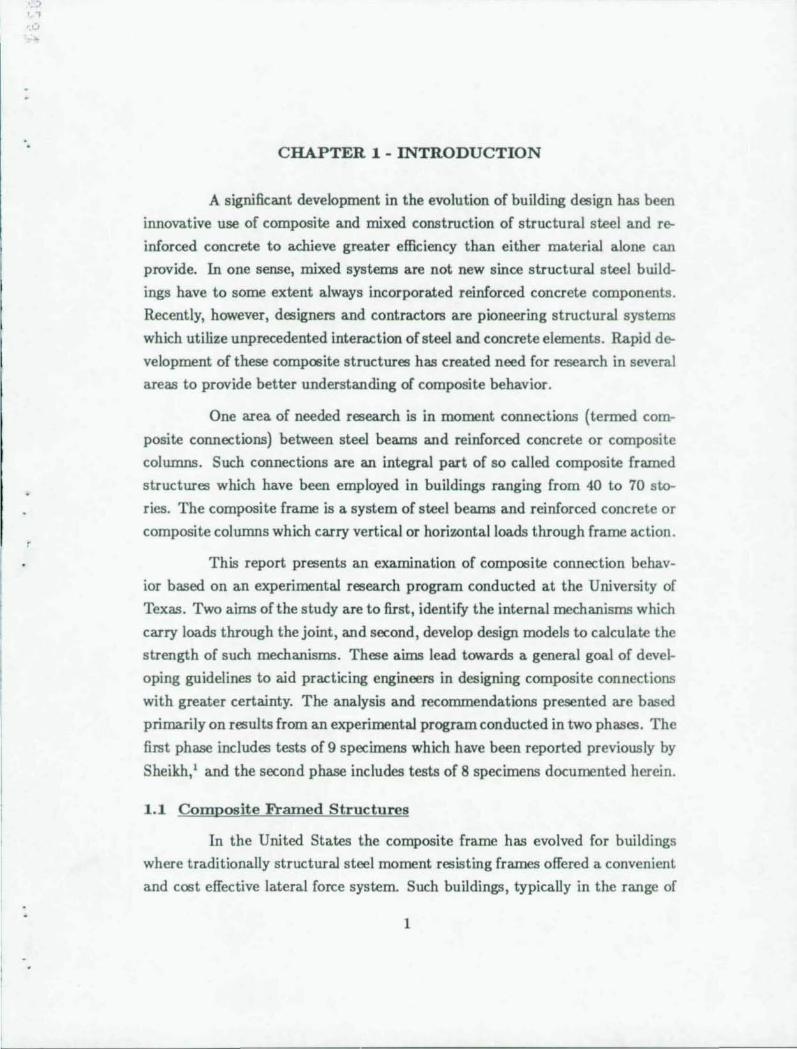
CHAPTER 1 - INTRODUCTION

A significant development in the evolution of building design has been

innovative use of composite and mixed construction of structural steel and re­

inforced concrete to achieve greater efficiency than either material alone can

provide. In one sense, mixed systems are not new since structural steel build­

ings have to some extent always incorporated reinforced concrete components.

Recently, however, designers and contractors are pioneering structural systems

which utilize unprecedented interaction of steel and concrete elements. Rapid de­

velopment of these composite structures has created need for research in several

areas to provide better understanding of composite behavior.

One area of needed research is in moment connections (termed com­

posite connections) between steel beams and reinforced concrete or composite

columns. Such connections are an integral part of so called composite framed

structures which have been employed in buildings ranging from 40 to 70 sto­

ries. The composite frame is a system of steel beams and reinforced concrete or

composite columns which carry vertical or horizontal loads through frame action.

This report presents an examination of composite connection behav­

ior based on an experimental research program conducted at the University of

Texas. Two aims of the study are to first, identify the internal mechanisms which

carry loads through the joint, and second, develop design models to calculate the

strength of such mechanisms. These aims lead towards a general goal of devel­

oping guidelines to aid practicing engineers in designing composite connections

with greater certainty. The analysis and recommendations presented are based

primarily on results from an experimental program conducted in two phases. The

first phase includes tests of 9 specimens which have been reported previously by

Sheikh,' and the second phase includes tests of 8 specimens docurrented herein.

1.1 Composite Framed Structures

In the United States the composite frame has evolved for buildings

where traditionally structural steel moment resisting frames offered a convenient

and cost effective lateral force system. Such buildings, typically in the range of

1

2

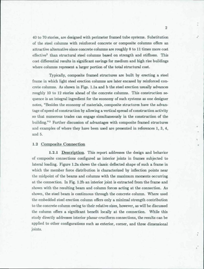
40 to 70 stories, are designed with perimeter framed tube systems. Substitution

of the steel columns with reinforced concrete or composite columns offers an

attractive alternative since concrete columns are roughly 8 to 11 times more cost

effective' than structural steel columns based on strength and stiffness. This

cost differential results in significant savings for medium and high rise buildings

where columns represent a larger portion of the total structural cost.

Typically, composite framed structures are built by erecting a steel

frame in which light steel erection columns are later encased by reinforced con­

crete columns. As shown in Figs. lola and b the steel erection usually advances

roughly 10 to 12 stories ahead of the concrete columns. This construction s&o

quence is an integral ingredient for the economy of such systems as one designer

notes, "Besides the economy of materials, composite structures have the advan­

tage of speed of construction by allowing a vertical spread of construction activity

so that numerous trades can engage simultaneously in the construction of the

bui lding."" Further discussion of advantages with composite framed structures

and examples of where they have been used are presented in references 1, 3, 4,

and 5.

1.2 Composite Connection

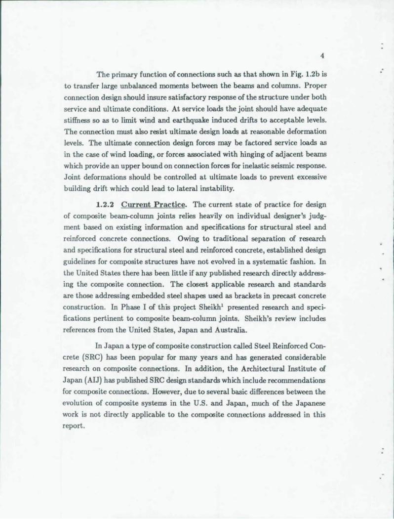
1.2.1 Description. This report addresses the design and behavior

of composite connections configured as interior joints in frames subjected to

lateral loading. Figure lo2a shows the classic deHected shape of such a frame in

which the member force distribution is characterized by inHection points near

the midpoint of t he beams and columns with the maximum moments occurring

at the connection. In Fig. lo2b an interior joint is extracted from the frame and

shown with the resulting beam and column forces acting at the connection . As

shown, the steel beam is continuous through the concrete column. Where used

the embedded steel erection column offers only a minimal strength contribution

to the concrete column owing to their relative sizes, however, as will be discussed

the column offers a significant benefit locally at the connection. While this

study directly addresses interior planar cruciform connections, the results can be

applied to other configurations such as exterior, comer, and three dimensional joints.

,

, , , ,

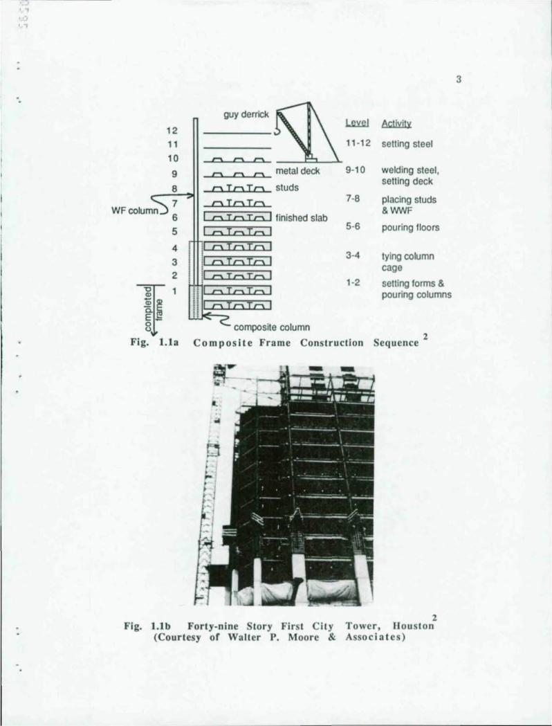
12

11

10

9

8

~~ WFcolum

"0 Q)

Q; a. E o o i

5

4

3 2

1

guy derrick

= = = c = = metal deck

oIoIo studs

oIcIo I oIcIo finished slab

I oIoIo :1 oIoIO 11 oIoIo il oIcIo

n I o IcIt:::l

HI otero .ll. - C.

compoSIte column

1&£aJ AC1jyity

11 -12 selling steel

9-10 welding steel, selting deck

7-8 placing studs &VNJF

5-6 pouring 1Ioors

3-4 tying column cage

1-2 selling forms & pouring columns

Fig. 1.13 2 Composite Frame Construction Sequence

Fig. LIb Forty-nine Story First City (Courtesy of Walter P. Moore &

2 Tower , Houston Associates)

3

4

The primary function of connections such as that shown in Fig. 1.2b is

to transfer large unbalanced moments between the beams and columns. Proper

connection design should insure satisfactory response of the structure under both

service and ultimate conditions. At service loads the joint should have adequate

stiffness so as to limit wind and earthquake induced drifts to acceptable levels.

The connection must also resist ultimate design loads at reasonable deformation

levels. The ultimate connection design forces may be factored service loads as

in the case of wind loading, or forces associated with hinging of adjacent beams

which provide an upper bound on connection forces for inelastic seismic response.

Joint deformations should be controlled at ultimate loads to prevent excessive

building drift which could lead to lateral instability.

1.2.2 Current Practice. The current state of practice for design

of composite beam-column joints relies heavily on individual designer's judg­

ment based on existing information and specifications for structural steel and

reinforced concrete connections. Owing to traditional separation of research

and specifications for structural steel and reinforced concrete, established design

guidelines for composite structures have not evolved in a systematic fashion. In the United States there has been little if any published research directly addres&­

ing the composite connection. The closest applicable research and standards

are those addressing embedded steel shapes used as brackets in precast concrete

construction. In Phase I of this project Sheikh' presented research and speci­

fications pertinent to composite beam-column joints. Sheikh's review includes

references from the United States, Japan and Australia.

In Japan a type of composite construction called Steel Reinforced Con­

crete (SRC) has been popular for many years and has generated considerable

research on composite connections. In addition, the Architectural Institute of

Japan (AlJ) has published SRC design standards which include recommendations

for composite connections. However, due to several basic differences between the

evolution of composite systems in the U.S. and Japan, much of the Japanese

work is not directly applicable to the composite connections addressed in this

report.

,

, 'J'

5

SRC structures gained in popularity in Japan after the 1923 Kanto

earthquake by providing enhanced ductility of reinforced concrete frames in low

and medium rise structures.· Traditional SRC structures consist of framed sys­

tems where both the steel beams and columns are encased by concrete. Early

SRC structures in Japan were similar to schemes for reinforced concrete built in

the V.S. during the early 1900's where built-up open web structural steel mem­

bers served as the primary reinforcement in concrete. More recently, Japanese

SRC structures are evolving to resemble V.S. composite systems where rolled col­

umn shapes are encased in concrete and steel beams remain unencased. However ,

due to its emphasis on ductility the AIJ standard places the following restriction

on the minimum moment capacity of the embedded column:7

0.5 M. < Me < 2.0M. (1.1)

Here M. and Me are the moment capacities of the steel beam and column r~

spectively. This requirement is contrary to V.S. practice where the steel column

is small relative to the steel beam and the reinforced concrete provides most of

the column capacity.

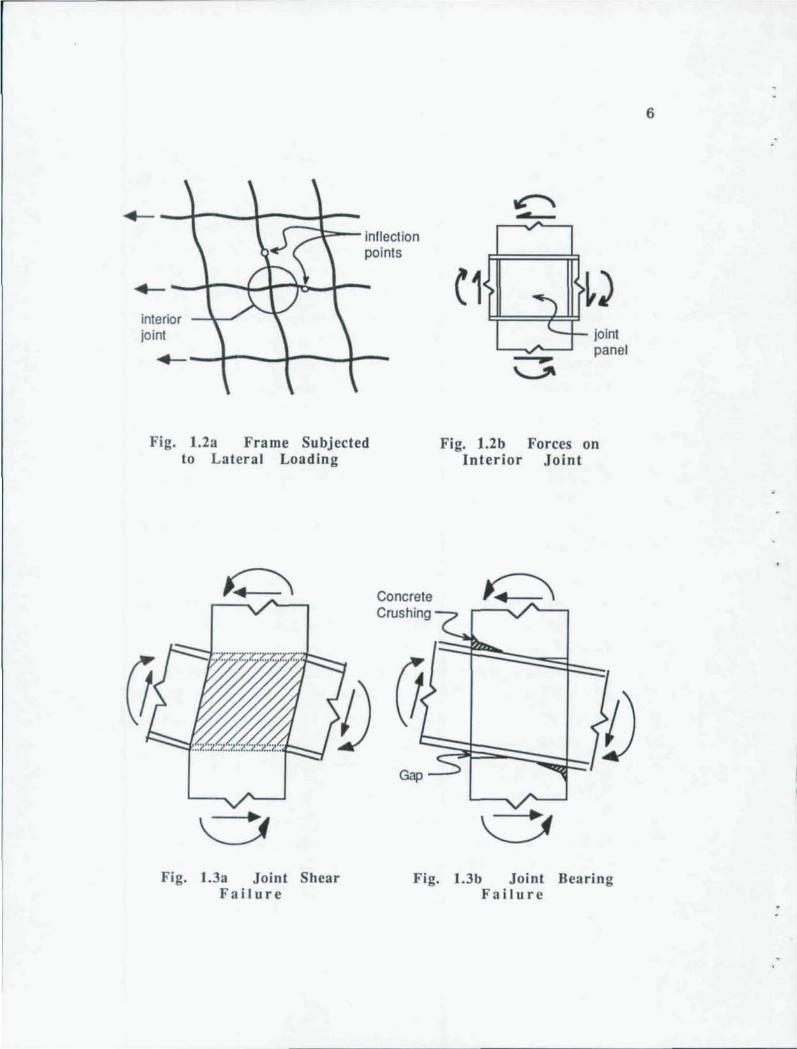
1.2.3 Internal Mechanisms. The two basic modes of failure ob­

served in composite connections are joint shear failure and compressive crushing

or bearing failure. Fig. 1.3a indicates the deformation associated with joint shear

failure. As will be described throughout this report, an important distinction

regarding shear failure in composite connections is that several different mecha­

nism! resist shear in different regions of the connection. The different zones do

not deform equally and hence their contribution to the capacity varies depending

on the joint detailing used. Figure 1.3b shows the compression or bearing failure,

evidenced by concrete crushing and gaps opening against the beam flanges.

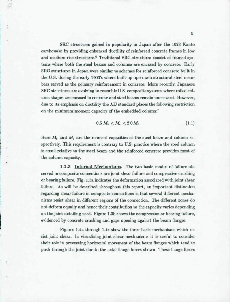
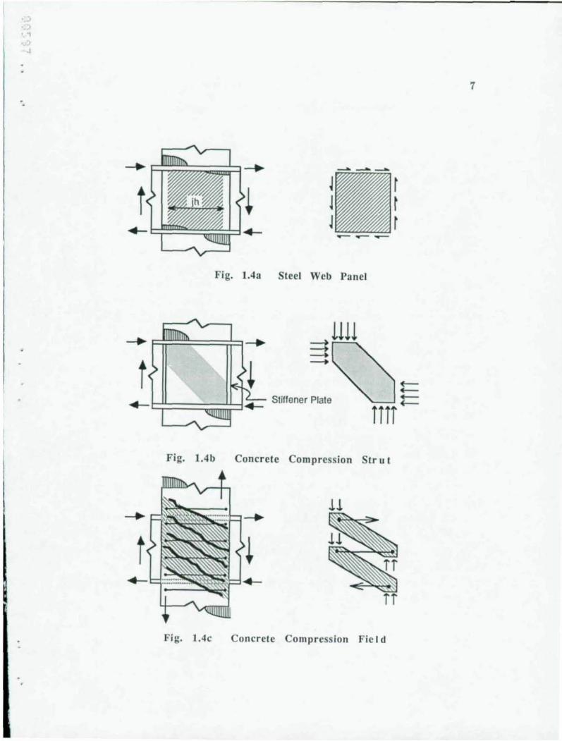
Figures 1.4a through l.4c show the three basic mechanisms which r~

sist joint shear. In visualizing joint shear mechanisms it is useful to consider

their role in preventing horizontal movement of the beam flanges which tend to

push through the joint due to the axial flange forces shown. These flange forces

inflection points

-4---

interior jOint

-4---

Fig. 1.2a Frame Subjected to La tera l Loading

Concrete Crushing

~ ---C1 ~J

joint --- panel

'-"

Fig. 1.2b Forces on Interior Joint

Fig. 1.3a Joint Shear Fig. 1.3b Joint Bearing Fail ure Faiture

6

·) . " .1

t

-.-

t ~

J J J

Fig, 1.43 Steel Web Panel

.-Hi! -. --.

t t t

~ 4--4--Stiffener Plate

TiiT --

Fig. l.4b Concrete Compress ion Str u t

Fi g. l.4c Concrete Compress ion Fie J d

1

8

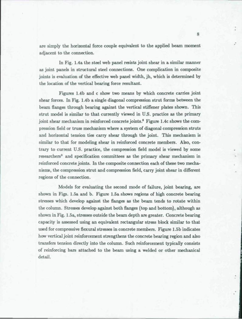
are simply the horizontal force couple equivalent to the applied beam moment

adjacent to the connection.

In Fig. 1.4a the steel web panel resists joint shear in a similar manner

as joint panels in structural steel connections. One complication in composite

joints is evaluation of the effective web panel width, jh, which is determined by

the location of the vertical bearing force resultant.

Figures lAb and c show two means by which concrete carries joint

shear forces. In Fig. 104 b a single diagonal compression strut forms between the

beam flanges through bearing against the vertical stiffener plates shown. This

strut model is similar to that currently viewed in U.S. practice as the primary

joint shear mechanism in reinforced concrete joints.' Figure lAc shows the com­

pression field or truss mechanism where a system of diagonal compression struts

and horizontal tension ties carry shear through the joint. This mechanism is

similar to that for modeling shear in reinforced concrete members. Also, con­

trary to current U.S. practice, the compression field model is viewed by some

researchers" and specification committees as the primary shear mechanism in

reinforced concrete joints. In the composite connection each of these two mecha­

nisms, the compression strut and compression field, carry joint shear in different

regions of the connection.

Models for evaluating the second mode of failure, joint bearing, are

shown in Figs. 1.5a and b. Figure 1.5a shows regions of high concrete bearing

stresses which develop against the flanges as the beam tends to rotate within

the column. Stresses develop against both flanges (top and bottom), although as

shown in Fig. 1.5a, stresses outside the beam depth are greater. Concrete bearing

capacity is assessed using an equivalent rectangular stress block similar to that

used for compressive flexural stresses in concrete members. Figure 1.5b indicates

how vertical joint reinforcement strengthens the concrete bearing region and also

transfers tension directly into the column. Such reinforcement typically consists

of reinforcing bars attached to the beam using a welded or other mechanical detail.

) ,

Ct

Ct ~>

...,

.J

Fig. l.Sa

.A

V

v

..., +

+ j

~

rectangular stress block

section

Flange nearing

+ + .- t\,\ .it----,

L...--li!\..n--'

+ + section

Fig. l.Sb Vertic:11 Joint Reinforce III C n t

9

10

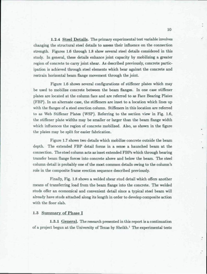
1.2.4 Steel Details. The primary experimental test variable involves

changing the structural steel details to assess their influence on the connection

strength. Figures 1.6 through 1.8 show several steel details considered in this

study. In general, these details enhance joint capacity by mobilizing a greater

region of concrete to carry joint shear. As described previously, concrete partic­

ipation is achieved through steel elements which bear against the concrete and

restrain horizontal beam flange movement through the joint.

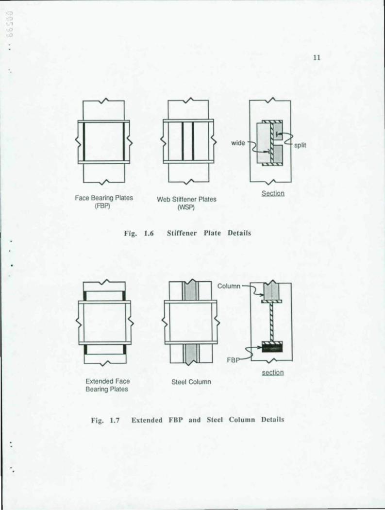
Figure 1.6 shows several configurations of stiffener plates which may

be used to mobilize concrete between the beam flanges. In one case stiffener

plates are located at the column face and are referred to as Face Bearing Plates

(FBP). In an alternate case, the stiffeners are inset to a location which lines up

with the flanges of a steel erection column. Stiffeners in this location are referred

to as Web Stiffener Plates (WSP). Referring to the section view in Fig. 1.6,

the stiffener plate widths may be smaller or larger than the beam flange width

which influences the region of concrete mobilized. Also, as shown in the figure

the plates may be split for easier fabrication.

Figure 1.7 shows two details which mobilize concrete outside the beam

depth. The extended FBP detail forms in a sense a haunched beam at the

connection. The steel column acts as inset extended FBPs which through bearing

transfer beam flange forces into concrete above and below the beam. The steel

column detail is probably one of the most common details owing to the column's

role in the composite frame erection sequence described previously.

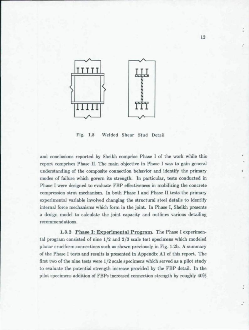
Finally, Fig. 1.8 shows a welded shear stud detail which offers another

means of transferring load from the beam flange into the concrete. The welded

studs offer an economical and convenient detail since a typical steel beam will

already have studs attached along its length in order to develop composite action

with the floor slab.

1.3 Sununary of Phase I

1.3.1 General. The research presented in this report is a continuation

of a project begun at the University of Texas by Sheikh.! The experimental tests

~

~

>

A ~

Face Bearing Plates (FSP)

<

Fig. 1.6

A-

I I

I I ~

Extended Face Bearing Plates

A ~

<

~

Web Stiffener Plates (WSP)

wide ?

Stiffener Plate Details

- Column

>

"

Steel Column

~~

.!.: r-c:: -

A ~

Section

seclion

Fig. 1.7 Extended FUP and tee I Co lumn Detail

11

split

12

Fig. 1.8 Welded Shear Stud Detail

and conclusions reported by Sheikh comprise Phase I of the work while this

report comprises Phase II. The main objective in Phase I was to gain general

understanding of the composite connection behavior and identify the primary

modes of failure which govern its strength. In particular, tests conducted in

Phase I were designed to evaluate FBP effectiveness in mobilizing the concrete

compression strut mechanism. In both Phase I and Phase II tests the primary

experimental variable involved changing the structural steel details to identify

internal force mechanisms which form in the joint. In Phase I, Sheikh presents

a design model to calculate the joint capacity and outlines various detailing

reco=endations.

1.3.2 Phase I: Experimental Program. The Phase I experimen­

tal program consisted of nine 1/2 and 2/3 scale test specimens which modeled

planar cruciform connections such as shown previously in Fig. 1.2b. A su=ary

of the Phase I tests and results is presented in Appendix A 1 of this report . The

first two of the nine tests were 1/2 scale specimens which served as a pilot study

to evaluate the potential strength increase provided by the FBP detail. In the

pilot specimens addition of FBPs increased connection strength by roughly 40%

.,

13

above the plain steel beam. Based on these tests, seven 2/3 scale specimens

were designed to isolate different modes of failure in the connection and eval­

uate parameters affecting the FBP contribution. In Phase I, testing consisted

of monotonically loading specimens to failure first in one direction followed by

loading in the reverse direction. Loads were applied to simulate connection forces

shown in Fig. 1.2b.

1.3.3 Phase I: Conclusions. The primary conclusion from Phase

I is that FBP details increase joint shear capacity significantly by mobilizing

concrete in the joint region. Various configurations of FBPs resulted in strength

gains of 70% to 190% above the plain steel beam. Specific information regarding

the relative strength increases is given by Sheikh. Also, in Chapter 3 of this

report comparison of relative connection capacities is included for Phase I along

with Phase II tests.

Sheikh developed a design model for connection strength in which the

structural steel and concrete contributions are summed. The steel contribution

is given as the capacity of the steel beam web in pure shear. The concrete con­

tribution is calculated based on a diagonal compression strut between the beam

flanges. In the design model, joint capacity as governed by concrete crushing

against the beam flanges is also checked.

1.4 Objective and Scope

The primary objective in this phase is to gain further understanding of

composite joint behavior by continuing and expanding the work begun in Phase

I. Comprehensive and practical guidelines are developed which address design

concerns for a wide range of composite joint details and configurations. Formu­

lation of an analytic design model for calculating the composite joint capacity is

an important component of these guidelines.

Experimental research from the first phase is extended in two areas.

First, additional joint details are tested in order to refine and enhance under­

standing of the internal mechanisms controlling joint strength. The major details

examined in this phase include the embedded steel column (Fig. 1.7), welded

14

shear studs (Fig. 1.8), and vertical joint reinforcement (Fig. 1.5b). The second

extension of the research is examination of joint response under reverse cyclk

loading in the inelastic range. This will provide information which begins to

address design concerns and suitability of composite connections for seismic ap­

plications.

The Phase II experimental program consists of eight 2/3 scale cruciform

specimens with the same geometry as the 2/3 scale specimens tested previously.

The test program description and procedure is described in Chapter 2. In Chap­

ter 3 the results of the eight tests are summarized along with a comparison of

relative strengths for all 2/3 scale specimens from Phases I and II.

Analysis of the joint response, which focuses on development of an an­

alytic design model, is presented in Chapter 4. The development in Chapter 4

draws in part from a design model proposed by Sheikh and from recommenda­

tions for design of structural steel and reinforced concrete joints. In development

of the analytic model two points are emphasized: first, the analysis is kept simple

and straightforward while preserving an appropriate degree of precision, and sec­

ond, joint capacity is calculated by analysis of internal mechanisms which follow

logically from mechanics.

In Chapter 5 design and detailing recommendations for composite con­

nections are presented. A simplified version of the analytic model from Chapter

4 is a central component of the guidelines for calculating the connection capac­

ity. Accuracy of the simplified model is checked by comparing calculated results

with the Chapter 4 analysis and with test results. The recommendations include

a design methodology consistent with the load and resistance factor approach

used in the AlSC-LRFD 10 specification. Detailing recommendations address re­

quirements for horizontal reinforcing bar ties, vertical reinforcing bars sizes and

layout, and structural steel detailing peculiar to composite joints. Finally, Chap­

ter 5 also includes information related to design of alternate joint configurations.

Chapter 6 provides a summary and conclusions of the report.

Three appendices present supplemental information to the report. As

noted previously, in Appendix Al the scope and results of Phase I tests are

15

summarized. In Appendix A2 a satellite study which examines the ultimate

behavior of shear studs in the joint region is presented. Results of this study

are incorporated in the design recommendations of Chapter 5. Finally, sample

calculations for two connection examples are presented in Appendix A3.

CHAPTER 2 - EXPERIMENTAL PROGRAM

2.1 General

The experimental program consists of eight 2/3 scale composite joint

specimens which were built and tested at the Ferguson Structural Engineering

Laboratory at The University of Texas. These tests are designed as a follow up

to Phase I tests reported by Sheikh. l The specimens reported herein comprise

Phase II of the composite joint study, and are numbered 10 through 17 to follow

in sequence with Specimens 1 through 9 from Phase 1. With the exception of pilot

Specimens 1 and 2 from Phase I, all specimens are the same size and geometry

and have similar reinforcing bar arrangements. The main test variable consists

of using different structural steel details in the joint.

The primary differences between Specimens 10 through 17 are struc­

tural steel attachments to the beam. Details evaluated in the tests include FBPs,

vertical joint reinforcement, steel doubler plates, welded shear studs, embedded

steel columns and steel clip angles. Along with evaluating contribution of these

details individually, several of the specimens are designed to examine the inter­

action of different details. The specimens are loaded with reverse cyclic loads

which simulate joint forces due to lateral frame loading.

2.2 Description of Specimens

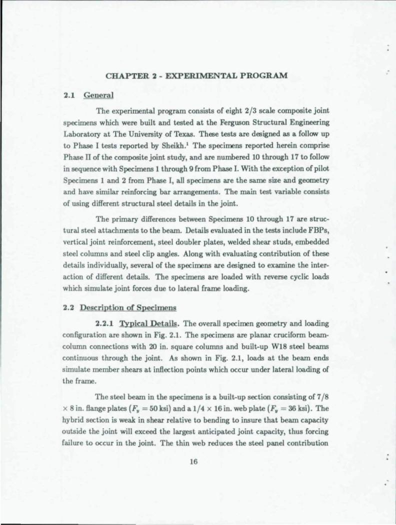
2.2.1 Typical Details. The overall specimen geometry and loading

configuration are shown in Fig. 2.1. The specimens are planar cruciform beam­

column connections with 20 in. square columns and built-up W18 steel beams

continuous through the joint. As shown in Fig. 2.1, loads at the beam ends

simulate member shears at inflection points which occur under lateral loading of

the frame.

The steel beam in the specimens is a built-up section consisting of 7/8

x 8 in. flange plates (F. =50ksi) andal/4 x 16 in. web plate (F. = 36ksi). The

hybrid section is weak in shear relative to bending to insure that beam capacity

outside the joint will exceed the largest anticipated joint capacity, thus forcing

failure to occur in the joint. The thin web reduces the steel panel contribution

16

'J \ >

17

to the joint strength and, therefore, also accentuates load carried by the concrete

panel, The philosophy of forcing failure in the joint is followed for experimental

purposes, and is opposite to design practice where preferably failure occurs in the

members. Finally, as shown in Fig. 2.1, reusable extension beams are attached

to the beam outside the joint region to facilitate handling of the specimens and

reduce the steel beam cost.

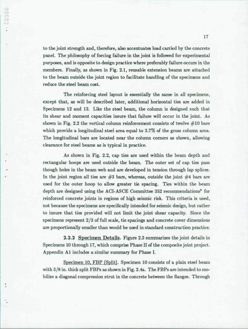
The reinforcing steel layout is essentially the same in all specimens,

except that, as will be described later, additional horizontal ties are added in

Specimens 12 and 13. Like the steel beam, the column is designed such that

its shear and moment capacities insure that failure will occur in the joint. As

shown in Fig. 2.2 the vertical column reinforcement consists of twelve #10 bars

which provide a longitudinal steel area equal to 3.7% of the gross column area.

The longitudinal bars are located near the column corners as shown, allowing

clearance for steel beams as is typical in practice.

As shown in Fig. 2.2, cap ties are used within the beam depth and

rectangular hoops are used outside the beam. The outer set of cap ties pass

though holes in the beam web and are developed in tension through lap splices.

In the joint region all ties are #3 bars, whereas, outside the joint #4 bars are

used for the outer hoop to allow greater tie spacing. Ties within the beam

depth are designed using the ACI-ASCE Committee 352 recommendations" for

reinforced concrete joints in regions of high seismic risk. This criteria is used ,

not because the specimens are specifically intended for seismic design, but rather

to insure that ties provided will not limit the joint shear capacity. Since the

specimens represent 2/3 of full scale, tie spacings and concrete cover dimensions

are proportionally smaller than would be used in standard construction practice.

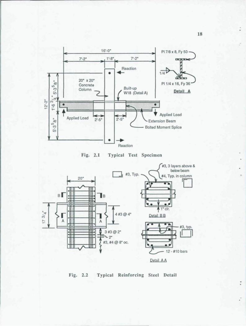
2.2.2 Specimen Details. Figure 2.3 summarizes the joint details in

Specimens 10 through 17, which comprise Phase II of the composite joint project.

Appendix Al includes a similar summary for Phase I.

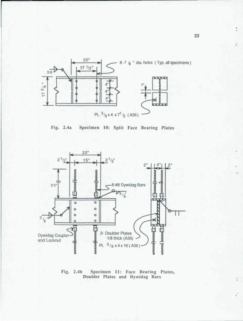
Specimen 10. FBP (Split). Specimen 10 consists of a plain steel beam

with 3/8 in. thick split FBPs as shown in Fig. 2.4a. The FBPs are intended to mo­

bilize a diagonal compression strut in the concrete between the flanges. Through

16'-0"

7'-2" . , 1 '-8" 7'-2"

LI Reaction ~-y-+------------- • ~

, 20" x 20" "'~ Concrete

,Ln C-.. _ W18 (Detail A)

PI 718x8, Fy50

1/4

Detal! A '? Column ~ _ { Built-up

~ "'-"-h=======F==l"""""'!=:!:::=!=====7l '" ~ ,~ ~ ~

'" -'" ..... ~

~ t I::::::===!===I ........... ..-~ J ~ I .. Applied Load

, Applied Load 2'-5" 2' 5" / "'~ - l. Extension Beam

'? '--- Batted Moment Splice Ln

Br

~ >r A

. ~ - Reaction

Fig, 2,1 Typical Test Specimen

20"

~

./'-

Fig, 2,2

D #3,Typ.

~B

~~ A

3 : P'-

#3@2"

#3, 2" #4@8"oc .

#3, 3 layers above & bebwbeam

#4, Typ. in column

o i·, "' ...... " ... " ....... " ... '

1" elr.

Detail B B

,..U.:::::1;:':/in:;- #3, typo o 12 - #10 bars

Detail AA

Typical Reinforcing Steel Detail

18

------------------------------------------ -- - -

,

19

PHASE II TEST SERIES

SPECIMEN DESRIPTIONS

10 i I I t FBP (Split) 14 ¢ WSP - Column

11 q:p FBP -Db.PI.-Dywi. 15 $ FBP - Column

12 0 Studs 16 $ FBP - Col. - Angle

13 @ FBP - Studs 17 q:p FBP - Col. - Dywi.

Fig. 2.3 Summary of Phase II Specimens

comparison with specimens with full height FBPs, Specimen 10 should indicate

whether splitting the FBP has a detrimental effect on strength by increasing the

plate's flexibility. The motivation for splitting the stiffener is the reduction of

fabrication costs by eliminating close fit up required with full height stiffeners.

Also shown in Fig. 2.4a are 7/8 in. diameter holes typical in all specimens which

provide passage for the #3 cap ties through the web.

Specimen 11, FBP-DbPI-Dywi. Specimen 11 is designed to examine

effectiveness of vertical joint reinforcing for strengthening when concrete crushing

against the beam flanges controls the design. The vertical joint reinforcement

consists of eight Dywidag bars (#8 - 3 ft 0 in., Gr. 60) as shown in Fig. 2.4b.

These bars are attached through threaded couplers ~elded to the beam flanges .

Web doubler plates and FBPs are also provided to increase the joint shear panel

capacity above that governed by concrete bearing failure. The doubler plate

20

thickness provides a shear to moment capacity ratio in the beam similar to that

for rolled W18 shapes.

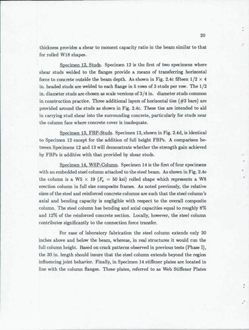
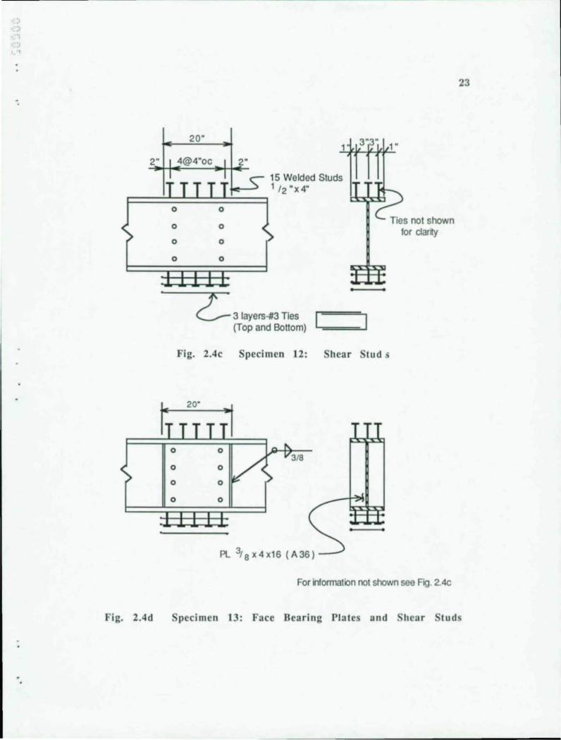
Specimen 12. Studs. Specimen 12 is the first of two specimens where

shear studs welded to the flanges provide a means of transferring horiwntal

force to concrete outside the beam depth. As shown in Fig. 2.4c fifteen 1/2 x 4

in. headed studs are welded to each flange in 5 rows of 3 studs per rCNf. The 1/2

in. diameter studs are chosen as scale versions of 3/4 in. diameter studs co=on

in construction practice. Three additional layers of horizontal ties (#3 bars) are

provided around the studs as shCNfn in Fig. 2.4c. These ties are intended to aid

in carrying stud shear into the surrounding concrete, particularly for studs near

the column face where concrete cover is inadequate.

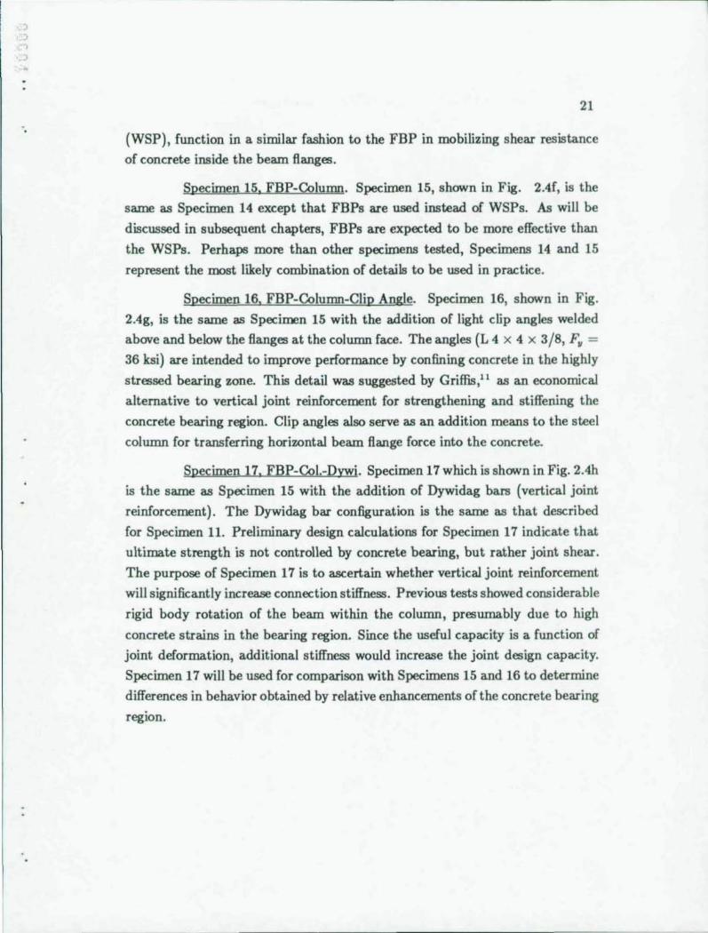
Specimen 13. FBP-Studs. Specimen 13, shown in Fig. 2.4d, is identical

to Specimen 12 except for the addition of full height FBPs. A comparison be­

tween Specimens 12 and 13 will demonstrate whether the strength gain achieved

by FBPs is additive with that provided by shear studs.

Specimen 14. WSP-Column. Specimen 14 is the first of four specimens

with an embedded steel column attached to the steel beam. As shown in Fig. 2.4e

the column is a W5 x 19 (F. = 50 ksi) rolled shape which represents a W8

erection column in fuJI size composite frames. As noted previously, the relative

sizes of the steel and reinforced concrete columns are such that the steel column's

axial and bending capacity is negligible with respect to the overall composite

column. The steel column has bending and axial capacities equal to roughly 8%

and 12% of the reinforced concrete section. Locally, hCNfever, the steel column

contributes significantly to the connection force transfer.

For ease of laboratory fabrication the steel column extends only 30

inches above and belCNf the beam, whereas, in real structures it would run the

full column height. Based on crack patterns observed in previous tests (Phase I),

the 30 in. length should insure that the steel column extends beyond the region

influencing joint behavior. Finally, in Specimen 14 stiffener plates are located in

line with the column flanges. These plates, referred to as Web Stiffener Plates

) ., )

21

(WSP), function in a similar fashion to the FBP in mobilizing shear resistance

of concrete inside the beam flanges.

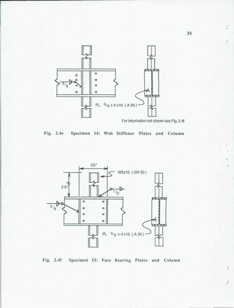
Specimen 15, FBP-Column. Specimen 15, shown in Fig. 2.4f, is the

same as Specimen 14 except that FBPs are used instead of WSPs. As will be

discussed in subsequent chapters, FBPs are expected to be more effective than

the WSPs. Perhaps more than other specimens tested, Specimens 14 and 15

represent the most likely combination of details to be used in practice.

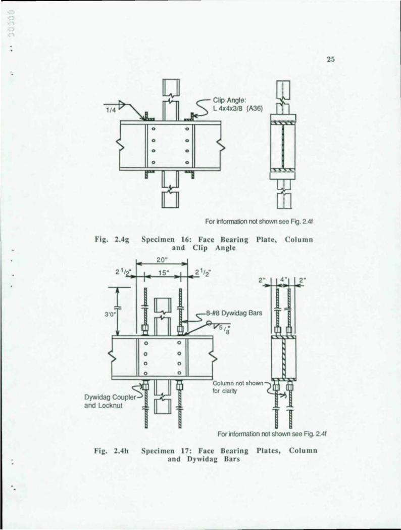
Specimen 16. FBP-Column-Clip Angle. Specimen 16, shown in Fig.

2.4g, is the same as Specimen 15 with the addition of light clip angles welded

above and below the flanges at the column face. The angles (L 4 x 4 x 3/8, F. =

36 ksi) are intended to improve performance by confining concrete in the highly

stressed bearing zone. This detail was suggested by Griffis,11 as an economical

alternative to vertical joint reinforcement for strengthening and stiffening the

concrete bearing region. Clip angles also serve as an addition means to the steel

column for transferring horizontal beam flange force into the concrete.

Specimen 17. FBP-Col.-Dvwi. Specimen 17 which is shown in Fig. 2.41

is the same as Specimen 15 with the addition of Dywidag bars (vertical joint

reinforcement) . The Dywidag bar configuration is the same as that descri bed

for Specimen 11. Preliminary design calculations for Specimen 17 indicate that

ultimate strength is not controlled by concrete bearing, but rather joint shear.

The purpose of Specimen 17 is to ascertain whether vertical joint reinforcement

will significantly increase connection stiffness. Previous tests showed considerable

rigid body rotation of the beam within the column, presumably due to high

concrete strains in the bearing region. Since the useful capacity is a function of

joint deformation, additional stiffness would increase the joint design capacity.

Specimen 17 will be used for comparison with Specimens 15 and 16 to determine

differences in behavior obtained by relative enhancements of the concrete bearing

region.

20" 8 -7 .s " dia. holes (Typ. all specimens)

3'8

4"

4"

4"

Fig. 2.4a Specimen 10: Split Face Bearing Plates

3, " 8

21/2"

T 3 '0"

Dywidag Coupler and Locknut

20"

j 1 0

0

0

0

21/2" 2"

8-#8 Dywidag Bars

5 , " s

2- Doubler Plales 1/8 thick (A36) T PL 3 / 8 X4xI6(A36)

2"

1 j

Fig. 2.4b pecimen II: Face Bearing Plates, Doubler Plates and Dywidag Bars

22

".

23

20" 1 3"3" 1 ..

2"

F=====o~====o~==~

15 Welded Studs 1 ' 2"x4"

Fig. 2.4d

o o Ties not shown lor clarity

o 0

o 0

0

0

0

0

Z; 3 layers-ll3 Ties (Top and Bottom)

Fig. 2.4c Specimen 12: Shear tud s

20·

-I 0

3/S 0

0

0

Pl 3'sX 4X16 (A36)

For information not shown see FIQ. 2.4c

pecimen 13: Face Bearing Plates and hear tuds

24

o rn o o

o o

o

o PL 3/8 x4x16 (A36)

For information not shown see Fig. 2.41

Fig. 2.4e Specimen 14: Web Stiffener Plates and Column

20·

W5x19 (GR 50) m 2'6"

o o

o o

o o

o o

o PL 3/8 x4x16 (A36)

Fig. 2.4f Specimen 15: Face Bearing Plates and alumn

o Clip Angle:

114 L 4x4x3l8 (A36)

o

o

o

o 0

.. \I I"" 10

i ,

m For information not shown see Fr;). 2.4f

Fig. 2.4g Specimen 16: Face Bearing Plate, and Clip Angle

olumn

20"

T 1 1 3'0· 0

Dywidag Coupler and Locknut

o

o o o

o

o o o

2· 4" 2"'

8-#8 Dywidag Bars

Column not shown for clarity

1

T 1 For information not shown see Fig. 2.4f

Fig, 2.4h pecimen 17: Face Bearing Plates, Column and Dywidag Bars

25

26

2.3 Specimen Fabrication

The specimen fabrication and construction sequence is the same as

that described in detail by Sheikh' in Phase I. Only aspects of importance in

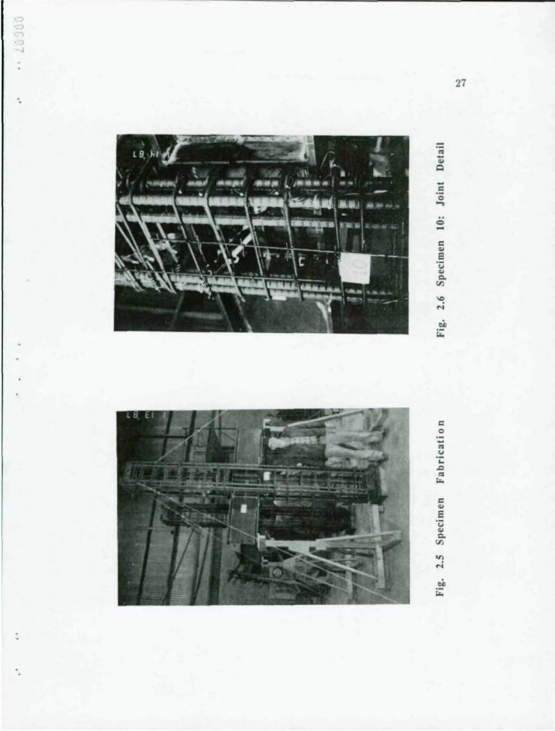
the construction sequence are discussed here. As shown in Fig. 2.5, specimens

were erected and cast in a vertical position as would occur in practice. Casting

position is important since it influences the insitu concrete properties. In par­

t icular, concrete cast beneath the beam Banges is weakened by small air voids,

consolidation, and trapped bleed water. Such conditions cannot economically be

eliminated in practice, and hence should be replicated in experiments.

Figure 2.6 shows the joint detail and reinforcement in Specimen 10,

indicating the degree of congestion in the joint region which necessitates careful

concret e placement. In the laboratory concrete was placed with slumps of 6 to

7 in. which are higher than in normal practice, but were required to insure

against formation of voids. Immersion vibrators (2 in. diameter) were used for

consolidating concrete after placing each lift (lift heights were approximately 12

in.) .

2.4 Material Pro erties

The stat ic yield stress, ultimate stress and percent elongation are re­

ported for the structural and reinforcing steel components in Table 2.1. Static

yield stress provides a lower bound for yielding which corresponds well with

quasi-static loading of the joint specimens. Table 2.1 also includes strain at

commencement of strain hardening and the strain hardening modulus for the

structural steel elements which may undergo large strains in the tests. Proce­

dures and specifications for the material tests are the same as those reported by

Sheikh.'

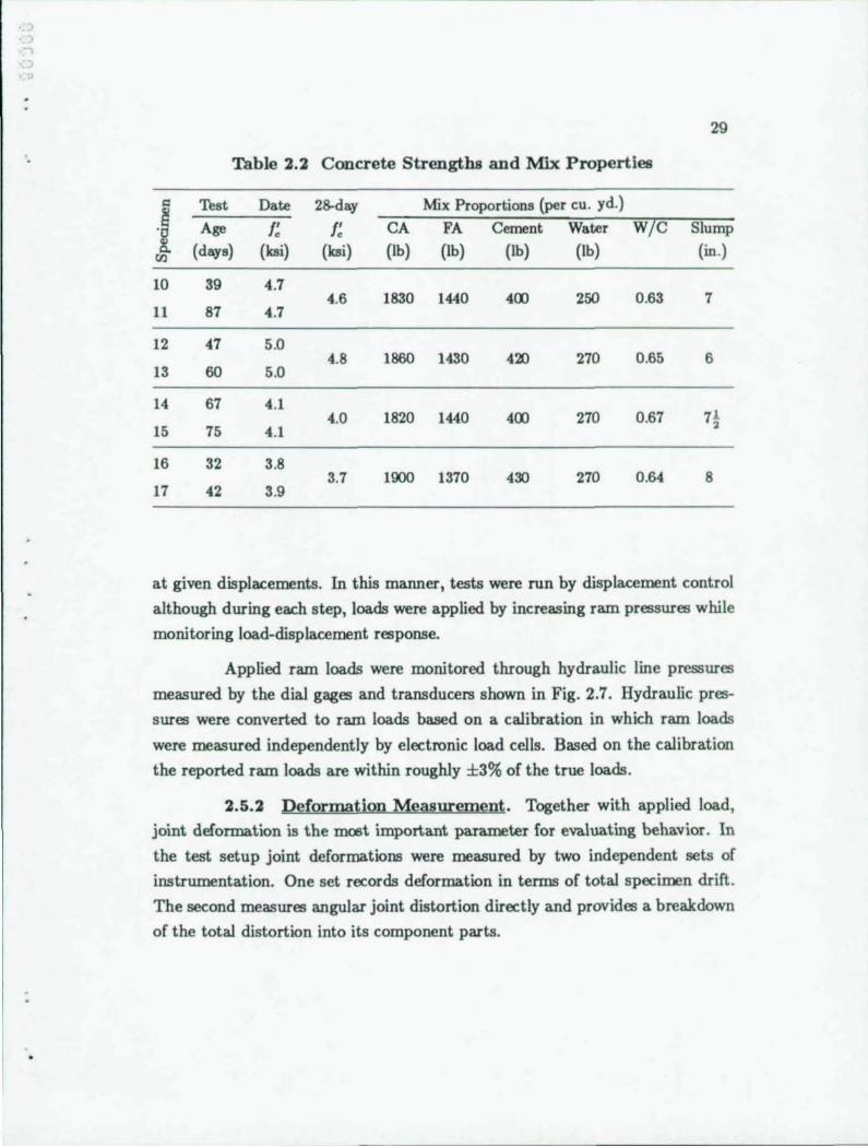
Table 2.2 lists concrete compressive strengths based on 6 X 12 in. cylin­

der tests along with concrete mix proportions. As noted, compressive strengths

on the day of testing ranged between 3.8 ksi to 5 ksi. The water contents listed

in Table 2.2 are based on batch plant reports for quantity of mix water and fine

aggregate moisture content. The calculated water-cement ratios do not always

.,

..

~

c ·0 .....

c OJ

e ·u

OJ c.

CI)

c o

c OJ

e ·u OJ c.

CI)

"! N

27

28

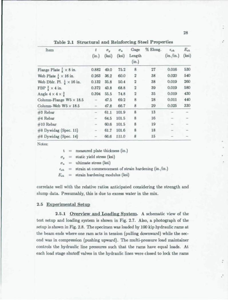
Table 2.1 Structural and Reinforcing Steel Properties

Item t u. Uv Gage % Elong. l.h E.h (in .) (lcsi) (lcsi) Length (in./in.) (lcsi)

(in .)

Flange Plate ~ X 8 in. 0.882 49.0 75.2 8 27 0.016 530

Web Plate t X 16 in. 0.263 36.2 60.0 2 38 0.020 540

Web Oblr. PI. k x 16 in. 0.132 35.8 50.4 2 38 0.019 260

FBP i x 4 in. 0.372 43.8 68.8 2 39 0.019 580

Angle4 x 4 x ~ 0.394 55.5 74.8 2 35 0.019 430

Column-Flange W5 X 18.5 47.5 69.2 8 28 0.011 440

Column-Web W5 X 18.5 47.8 66.7 8 29 0.025 330

# 3 Rebar 61.1 101.9 8 13

#4 Rebar 64.5 101.5 8 16

# 10 Rebar 60.6 101.5 8 19

# 8 Oywidag (Spec. 11) 61.7 101.6 8 18

# 8 Oywidag (Spec. 14) 66.6 111.0 8 15

Notes:

t = measured plate thickness (in .)

u. = static yield stress (lcsi)

Uu = ultimate stress (lcsi)

'.h = strain at commencement of strain hardening (in ./in .)

E.h = strain hardening modulus (lcsi)

correlate well with the relative ratios anticipated considering the strength and

slump data. Presumably, this is due to excess water in the mix.

2.5 Experimental Setup

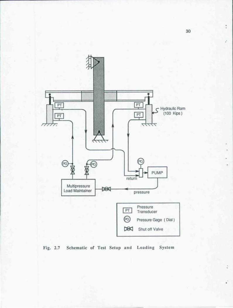
2.5.1 Overview and Loading System. A schematic view of the

test setup and loading system is shown in Fig. 2.7. Also, a photograph of the

set up is shown in Fig. 2.8. The specimen was loaded by 100 kip hydraulic rams at

the beam ends where one ram acts in tension (pulling downward) while the sec­

ond was in compression (pushing upward). The multi-pressure load maintainer

controls the hydraulic line pressures such that the rams have equal loads. At

each load stage shutoff valves in the hydraulic lines were closed to lock the rams

.

, )

0

'.

29

Table 2.2 Concrete Strengths and Mix Properties

'" Test Date 2S-day Mix Proportions (per cu. yd.)

·1 Age /; /: CA FA Cement Water W/C Slump (days) (ksi) (ksi) (lb) (lb) (lb) (lb) (in.) en

10 39 4.7 4.6 1830 1440 400 250 0.63 7

11 87 4.7

12 47 5.0 4.8 1860 1430 42) 270 0.65 6

13 60 5.0

14 67 4.1 4.0 1820 1440 400 270 0.67 71

15 75 4.1 2

16 32 3.8 3.7 1900 1370 430 270 0.64 8

17 42 3.9

at given displacements. In this manner, tests were run by displacement control

although during each step, loads were applied by increasing ram pressures while

monitoring load-displacement response.

Applied ram loads were monitored through hydraulic line pressures

measured by the dial gages and transducers shown in Fig. 2.7. Hydraulic pres­

sures were converted to ram loads based on a calibration in which ram loads

were measured independently by electronic load cells. Based on the calibration

the reported ram loads are within roughly ±3% of the true loads.

2.5.2 Deformation Measurement. Together with applied load,

joint deformation is the most important parameter for evaluating behavior. In

the test setup joint deformations were measured by two independent sets of

instrumentation. One set records deformation in terms of total specimen drift .

The second measures angular joint distortion directly and provides a breakdown

of the total distortion into its component parts.

Mu~ipressure Load Maintainer

return

Hydraulic Ram (100 Kips)

PUMP

pressure

Pressure Transducer

Pressure Gage ( Dial)

Shut off Valve

Fig. 2.7 Schematic of Test etup and Loading System

30

:

., , .,

31

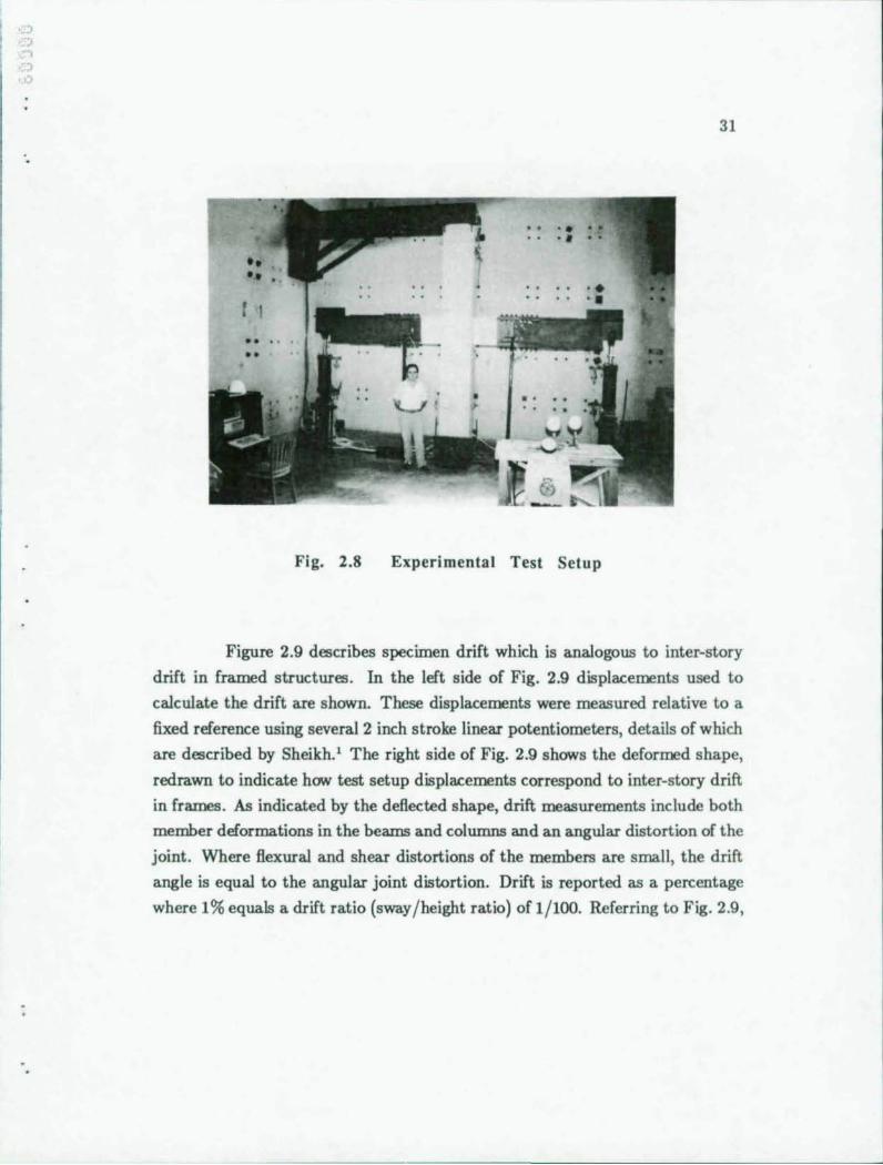
Fig. 2.8 Experimental Test Setup

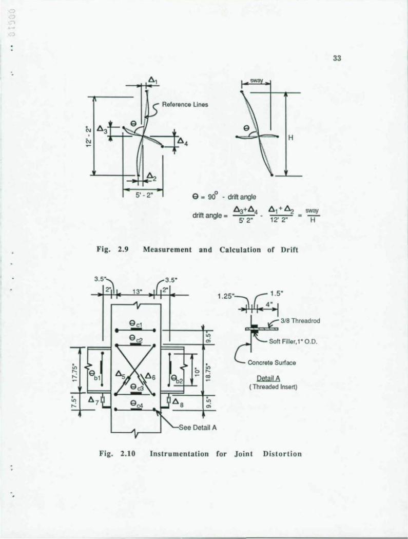
Figure 2.9 describes specimen drift which is analogous to inter-story

drift in framed structures. In the left side of Fig. 2.9 displacements used to

calculate the drift are shown. These displacements were measured relative to a

fixed reference using several 2 inch stroke linear potentiometers, details of which

are described by Sheikh.' The right side of Fig. 2.9 shows the deformed shape,

redrawn to indicate how test setup displacements correspond to inter-story drift

in frames. As indicated by the deflected shape, drift measurements include both

member deformations in the beams and columns and an angular distortion of the

joint. Where flexural and shear distortions of the members are small, the drift

angle is equal to the angular joint distortion. Drift is reported as a percentage

where 1 % equals a drift ratio (sway/height ratio) of 1/100. Referring to Fig. 2.9 ,

32

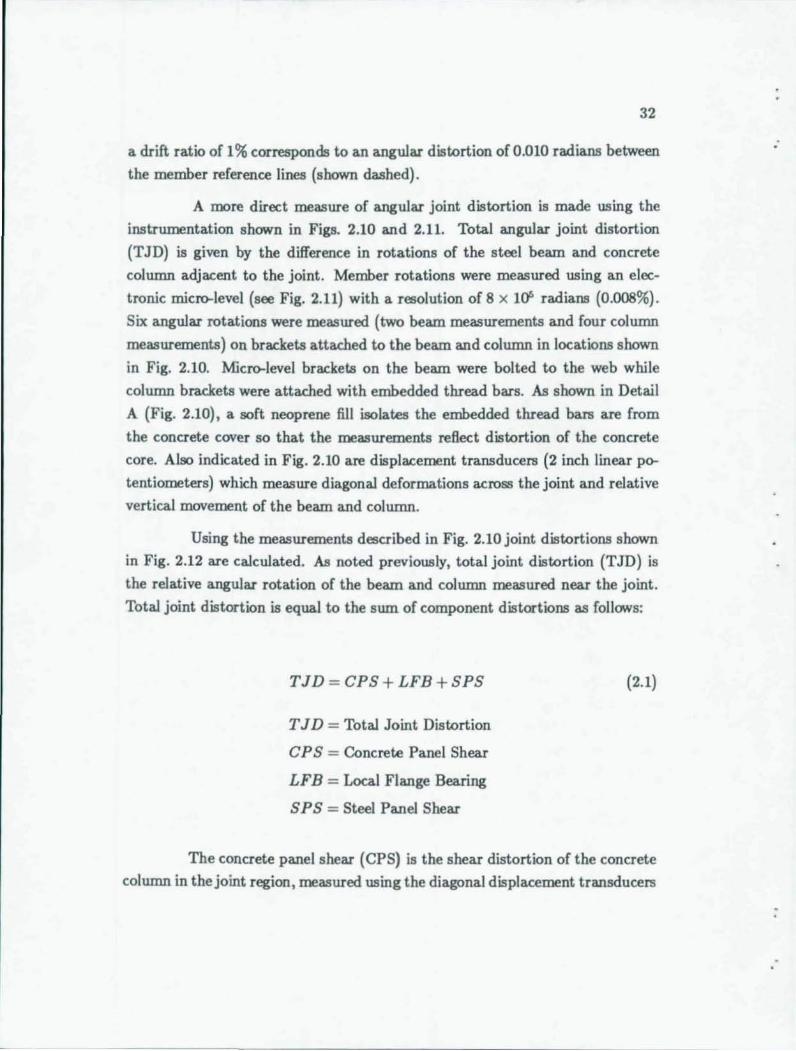
a drift ratio of 1 % corresponds to an angular distortion of 0.010 radians between

the member reference lines (shown dashed).

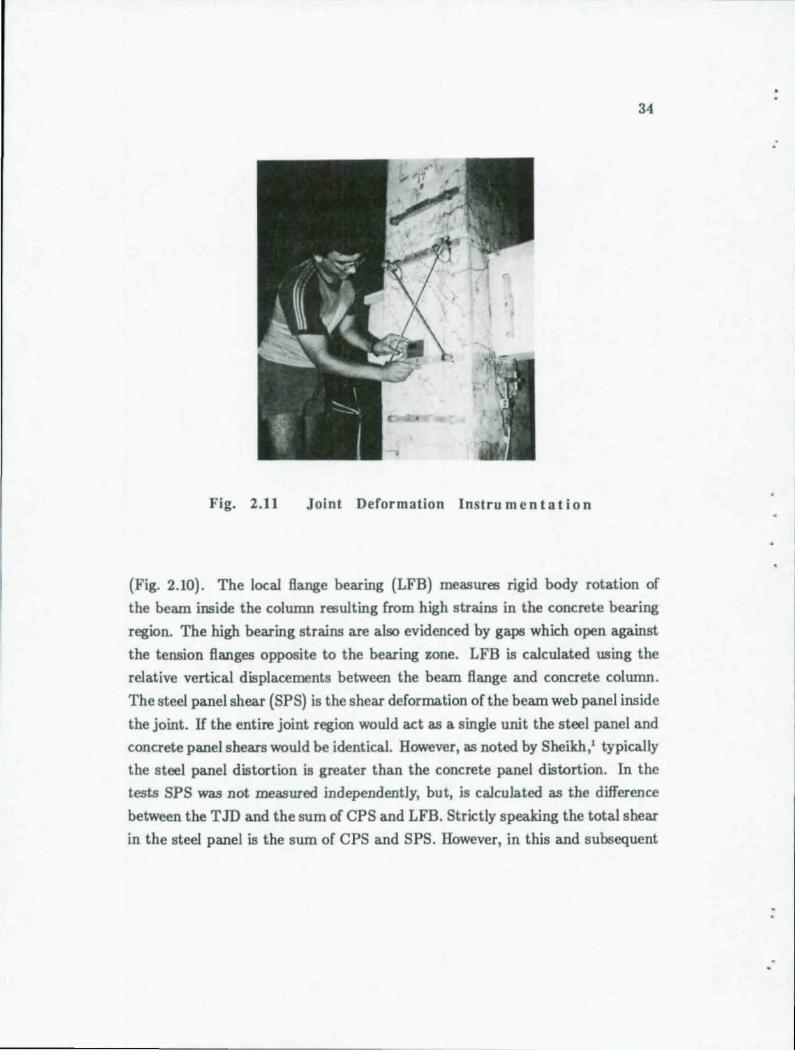
A more direct measure of angular joint distortion is made using the

instrumentation shown in Figs. 2.10 and 2.11. Total angular joint distortion

(TJD) is given by the difference in rotations of the steel beam and concrete

column adjacent to the joint. Member rotations were measured using an elec­

tronic micro-level (see Fig. 2.11) with a resolution of 8 x 10' radians (0.008%).

Six angular rotations were measured (two beam measurements and four column

measurements) on brackets attached to the beam and column in locations shown

in Fig. 2.10. Micro-level brackets on the beam were bolted to the web while

column brackets were attached with embedded thread bars. As shown in Detail

A (Fig. 2.10), a soft neoprene fill isolates the embedded thread bars are from

the concrete cover so that the measurements reflect distortion of the concrete

core. Also indicated in Fig. 2.10 are displacement transducers (2 inch linear po­

tentiometers) which measure diagonal deformations across the joint and relative

vertical movement of the beam and column.

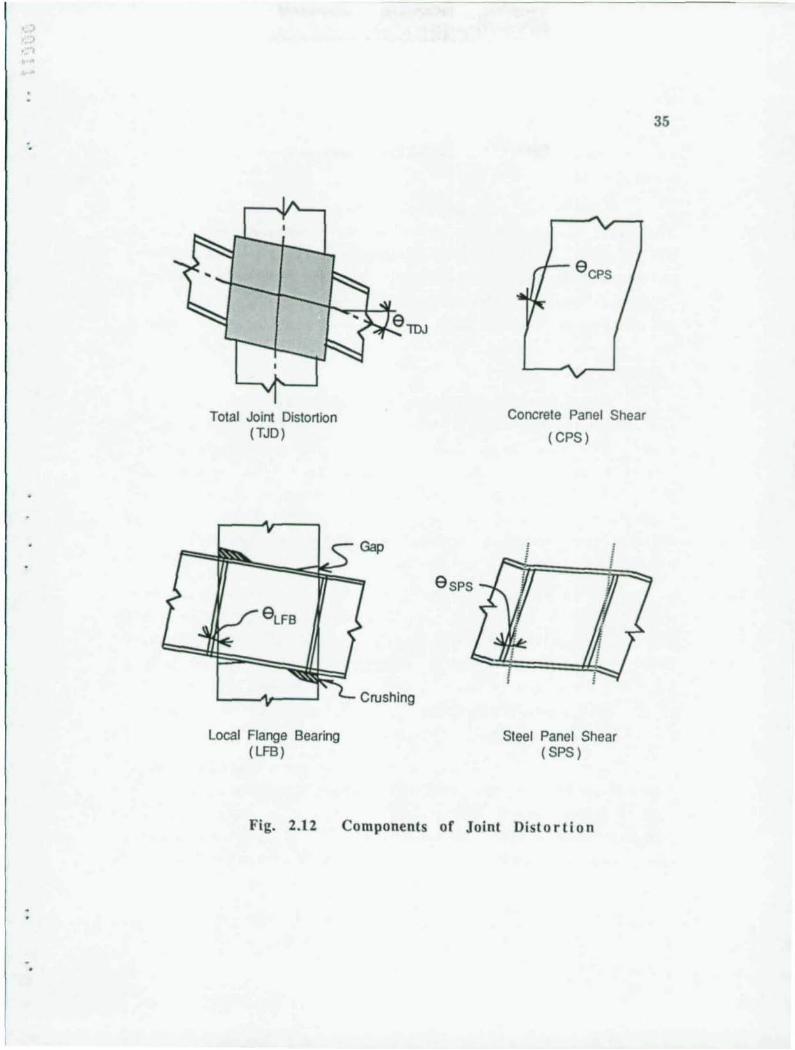
Using the measurements described in Fig. 2.10 joint distortions shown

in Fig. 2.12 are calculated. As noted previously, total joint distortion (T JD) is

the relative angular rotation of the beam and column measured near the joint.

Total joint Ilistortion is equal to the sum of component distortions as follows:

TJD = CPS+LFB + SPS

T J D = Total Joint Distortion

CPS = Concrete Panel Shear

LF B = Local Flange Bearing

SPS = Steel Panel Shear

(2.1)

The concrete panel shear (CPS) is the shear distortion of the concrete

column in the joint region, measured using the diagonal displacement transducers

'.

,

, , !

a l 63+-~"Ci

r ···· , , i , ~ ~ 5' - 2M

A

a = 900

- drift angle

~+64 drift angle . 5' 2"

H

\ , \

61+~ ~ 12' 2" - H

Fig. 2.9 Measurement and Calculation of Drift

3.5",

2",1

acl .• ____ L-~. I_~ ____ ~~ a c2

See Detail A

1.25", . (A ~ . ~ "

~ 3/8 Threadrod

Delail A (Threaded Insert)

Fig. 2.10 Instrumentation for Joint Distortion

33

34

Fig. 2.11 Joint Deformation Instru men tat ion

(Fig. 2.10). The local £lange bearing (LFB) measures rigid body rotation of

the beam inside the column resulting from high strains in the concrete bearing

region. The high bearing strains are also evidenced by gaps which open against

the tension flanges opposite to the bearing zone. LFB is calculated using the

relative vertical displacements between the beam £lange and concrete column.

The steel panel shear (SPS) is the shear deformation of the beam web panel inside

the joint. If the entire joint region would act as a single unit the steel panel and

concrete panel shears would be identical. However, as noted by Sheikh,' typically

the steel panel distortion is greater than the concrete panel distortion. In the

tests SPS was not measured independently, but, is calculated as the difference

between the T JD and the sum of CPS and LFB. Strictly speaking the total shear

in the steel panel is the sum of CPS and SPS. However, in this and subsequent

'.

Total JOint Distortion (TJD)

Local Flange Bearing (LF8)

Fig. 2.12

Concrete Panel Shear

( CPS)

Steel Panel Shear ( SPS)

Components of Joint Distortion

35

36

discussions, following Eq. 2.1 , SPS refers to steel shear panel distortion in excess

of concrete panel distortion.

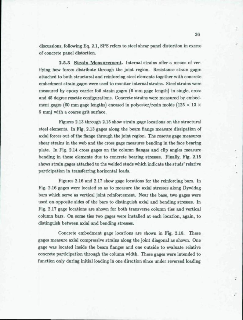
2.5.3 Strain Measurement. Internal strains offer a means of ver­

ifying how forces distribute through the joint region. Resistance strain gages

attached to both structural and reinforcing steel elements together with concrete

embedment strain gages were used to monitor internal strains. Steel strains were

measured by epoxy carrier foil strain gages (6 = gage length) in single, cross

and 45 degree rosette configurations. Concrete strains were measured by embed­

ment gages (60 = gage lengths) encased in polyester/resin molds (125 x 13 x

5 =) with a coarse grit surface.

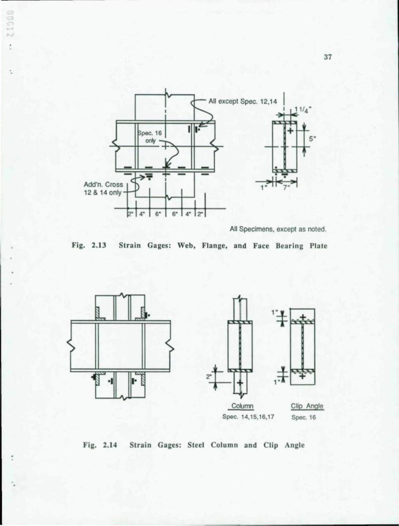
Figures 2.13 through 2.15 show strain gage locations on the structural

steel elements. In Fig. 2.13 gages along the beam flange measure dissipation of

axial forces out of the flange through the joint region. The rosette gage measures

shear strains in the web and the cross gage measures bending in the face bearing

plate. In Fig. 2.14 cross gages on the column flanges and clip angles measure

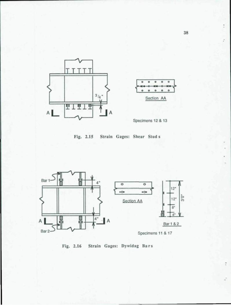
bending in those elements due to concrete bearing stresses. Finally, Fig. 2.15

shows strain gages attached to the welded studs which indicate the studs' relative

participation in transferring horizontal loads.

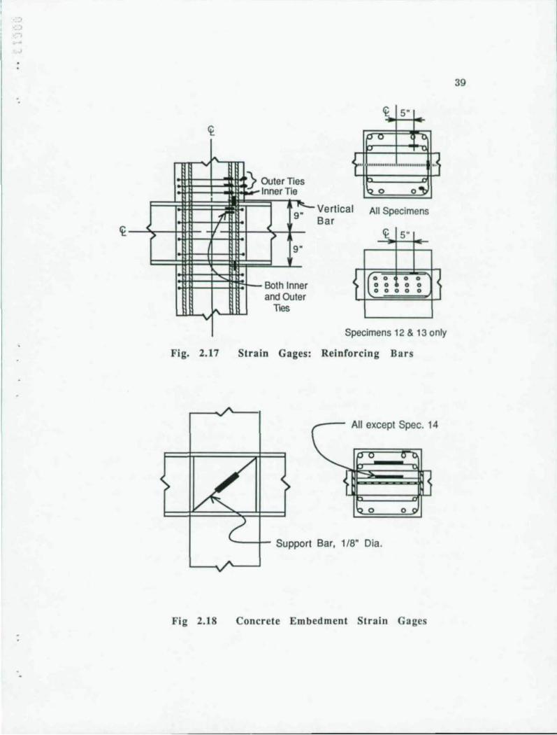
Figures 2.16 and 2.17 show gage locations for the reinforcing bars. In

Fig. 2.16 gages were located so as to measure the axial stresses along Dywidag

bars which serve as vertical joint reinforcement. Near the base, two gages were

used on opposite sides of the bars to distinguish axial and bending stresses. In

Fig. 2.17 gage locations are shown for both transverse column ties and vertical

column bars. On some ties two gages were installed at each location, again, to

distinguish between axial and bending stresses .

Concrete embedment gage locations are shown in Fig. 2.18. These

gages measure axial compressive strains along the joint diagonal as shown. One

gage was located inside the beam flanges and one outside to evaluate relative

concrete participation through the column width. These gages were intended to

function only during initial loading in one direction since under reversed loading

( -All ex

I ~

~pec. 16 I If'""

< on¥ -,......" ( ~

--ross' <: Add'n. C

12 & 14 only -l-

~"~

D I

12-14" 6"

-'? ~

'" - -I

IV -I

6" 4" 12"

cept Spec. 12,14

+ I-f-5"

-I- " I- -1-1-

-

37

All Specimens, except as noted.

Fig. 2.13 Strain Gages: Web, Flange, and Face Bearing Plate

.

l <)

• ~ -I

'W

Fig. 2.14

.J-

>

1-1 CoUmn

Spec. 14,15,16,17

Clip Angle

Spec. 16

train Gages: teel Column and Clip Angle

o 0 0 0 0

~'''' '''01''' __ ''''o""" " ~ o 0 000

Section AA

Specimens 12 & 13

38

Fig. 2.1S Strain Gages: Shear Stud s

BarlS 1

V

1 1 1

\

~5~' 1 1

...... v

A

Bar 2

Fig. 2.16

\

4" o 0

> "'"'"'"'''' .... ' .. '.,' .. II ...... ' .. ' .. ,, ~ '"1 .()e .()t

< > Section AA

4 "

12" 1-- •

12" ~ 1 --

8" .. --:--4"

Barl &2

Specimens 11 & 17

Strain Gages: Dywidag Ba r s

. )

~ ~

~ 5"

00 0

~l Outer Ties Inner Tie

t .. """'"111111111111""""" .. ·1 ~o o"ti

i~ 9" Vertical All Specimens

Bar 'I

I-. v

Fig. 2.17

Fig 2.18

~ 5"

9"

Both Inner and Outer

~ o 0 0 0 o 0 0 0 o 0 o 0 0

TIllS

Specimens 12 & 13 only

Strain Gages: Reinforcing Bars

All except Spec. 14

o 0

--+- Support Bar, 1/8' Dia.

Concrete Embedment Strain Gages

39

40

tension cracks may open perpendicular to the gage which will distort strain

measurements.

2.5.4 Data Acquisition. Data were recorded through a combina­

tion of visual and electronic means. Visual inspection included marking concrete

cracks, and noting concrete spalling and formation of yield lines on the struc­

tural steel. To highlight yield lines, the steel beam was coated with a light lime

whitewash prior to testing. Manual readings included those for hydraulic pres­

sure measured with dial gages and joint rotations measured with the electronic

micro-level. Finally, a personal computer based data acquisition system moni­

tored voltage output from pressure transducers, displacement transducers , and

resistance strain gages. Also, during the test a X-Y pen plotter recorded the

force and displacement in the hydraulic ram pushing upward in compression.

2.6 Test Procedure

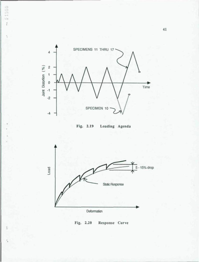
Specimens were loaded in a quasi-static fashion according to the loading

agenda shown in Fig. 2.19. AU of the specimens were loaded first to a low stress

level where concrete cracks began opening at roughly 25% to 40% of the ultimate

joint. Following this specimens were loaded through 2 complete cycles to 1%

TJD and 2 cycles to 2% TJD. The test concluded by loading specimens to a final

deformation of roughly 4% TJD. The final loading sequence for Specimen 10 was

cut short by 1/2 cycle due to scheduling and time constraints in the laboratory.

As discussed previously, tests were displacement controlled by locking

off ram displacements at each loading increment. Data was collected at each

load step after waiting 5 to 15 minutes for the structure to reach steady state

equilibrium. This delay allowed for time dependent concrete cracking and steel

yielding. Difference between the static and real time response is demonstrated

by the plot in Fig. 2.20. As shown, at each load stage displacement is fixed while

load drops off due to relaxation in the structure. In the elastic range the load

drop is negligible while in the inelastic range the load drops 5% to 15% at each

step. Plots such as that in Fig. 2.20 were recorded during testing using an X-V

pen plotter. The lower bound response given by the static load points is used

for interpretat ion and analysis of the data.

4

::!! 2 • c: 1 .2 1:: 0 0 iii

15 C -1

~ -2

-4

SPECIMENS 11 THRU 17

r \ I

SPECIMEN 10 ~I T

Fig. 2.19 Loading Agenda

Time

----ls - 1s%drop

SlatbResponse

Deforrnalicn

Fig. 2.20 Response Curve

41

CHAPTER 3 - EXPERIMENTAL RESULTS

3.1 Introduction

The presentation of experimental data and observations focuses on as­

pects of joint behavior which demonstrate the internal load transfer mechanisms

and their modes of failure. Understanding these mechanisms is essential to the

subsequent task of fornrulating a theoretical model to predict joint strength and

stiffness.

Two approaches are used to effectively present the pertinent data. Ini­

tially individual test chronologies are summarized, first for the general case and

then for each specimen. These summaries provide an overview of the tests and

relate the visible distress, deformations, and internal strains to basic stages of

behavior. The second portion of the chapter consists of a detailed examination

of separate categories of data emphasizing comparison between test specimens.

These comparisons highlight differences in behavior due to the various joint de­

tails. One category of data compares nominal joint strengths of the specimens.

For this comparison data from tests 3 through 9 is included along with that from

tests 10 through 17. Otherwise, only data from tests 10 through 17 are included

since tests 1 through 9 are described in detail by Sheikh.'

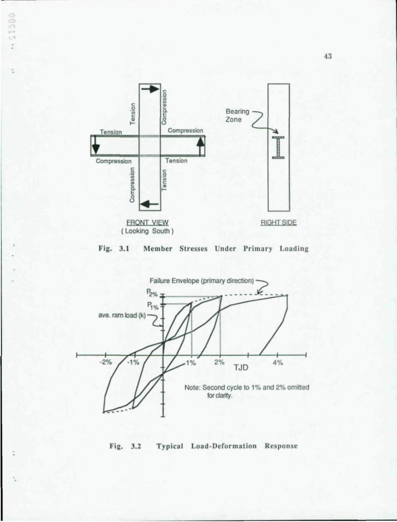
In Figs. 3.1, 3.2 and 3.3, some of the terminology used in subsequent

discussions is presented. In Fig. 3.1 a schematic view of the test specimen depicts

member stresses associated with loading in the primary (initial) direction. These

member stresses are used to distinguish locations in and around the joint. A

typical load versus deformation curve is shown in Fig. 3.2 where the average ram

loads are plotted against the total joint distortion. Recall that the total joint

distortion (TJD) is the angular rotation of the beam relative to the column,

measured directly adjacent to the joint. TJD is reported in percentages where

1 % corresponds to 10 milli-radians of relative rotation. For identification, data

are referred to by deformation cycle (for example: 1st - 1% cycle, 2nd - 1%

cycle, etc.). Unless noted ?therwise such references imply loading in the primary

direction. As noted previously in Chapter 2 the sequence of loading cycles are

as follows:

42

..

-. c:

.Q .. c: ., ~

Tension ::111:111111111 , mmmlllll:

Compression c:

.S! ., .. ., a. E 8 ..... ....

c: .Il .. .. ., a. E 8

Compression

A

Tension

c: .2 .. c: CD ~

Bearing 2 Zone

i

FRONT YIEW (Looking South)

RIGHT SIPE

Fig. 3.1 Member tresses Under Primary Loading

:ailure Envelope (primary direction) ? 2% _____ . ____ ..... --- -- - ..........

--P, %

ave. ram load (k)

Fig. 3.2

2% TJD

4%

Note: Second cycle to 1% and 2% omitted tordarity.

Typical Load-Derormation Re ponse

43

Low Stress Cycle (1/2 cycle)

1st - 1 % Cycle

2nd - 1 % Cycle

1st - 2% Cycle

2nd - 2% Cycle (1/2 Cycle for Test 10 only)

4% Cycle (1/2 Cycle)

44

The distinction made between the inner and outer concrete panels is

sketched in Fig. 3.3. The inner panel consists of the concrete held captive be­

tween the FBP and the beam flanges. The outer panel consists of the remaining

concrete in the joint region.

Aside from measured loads and deformations, internal strain readings

comprise much of the reported data. Strains measured in structural steel and

reinforcing bars are given as measured stresses using elastic constitutive equations

(E = 29500.0 ksi, " = 0.3). Where these reported stresses exceed the yield stress

of the steel, the reader should note that such values are not the true stresses

since the material is outside the elastic range. Arguably, a more correct approach

might be to report strains directly, however, the stress approach is chosen since

stress values are more familiar to engineers. Strains measured in the concrete

are reported directly as strains since the constitutive behavior of concrete is

markedly nonlinear.

3.2 Summary of Behavior

3.2.1 General. The overall behavior of the joint can be considered in

three stages. The distinction between stages is not absolute, and one should be

cautious not to overestimate any implied precision. However, such categorization

is useful in identifying load mechanisms and key modes of failure.

The first stage occurs prior to significant cracking in the concrete and

is characterized by elastic (recoverable) deformations. At low load levels, con­

crete is uncracked and adhesive bond transfers force between the steel beam

· , ...

'.

45

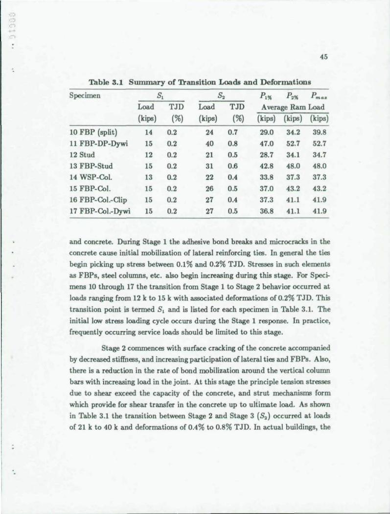
Table 3.1 Summary of 'fransition Loads and Deformations

Specimen 8, 82 P,,, P2"

Pmaz

Load TJD Load TJD Average Ram Load

(kips ) (%) (kips) (%) (kips) (kips) (kips)

10 FBP (split) 14 0.2 24 0.7 29.0 34.2 39.8

11 FBP-DP-Dywi 15 0.2 40 0.8 47.0 52.7 52.7

12 Stud 12 0.2 21 0.5 28.7 34.1 34.7

13 FBP-Stud 15 0.2 31 0.6 42.8 48.0 48.0

14 WSP-COl. 13 0.2 22 0.4 33.8 37.3 37.3

15 FBP-Col. 15 0.2 26 0.5 37.0 43.2 43.2

16 FBP-Col.-Clip 15 0.2 27 0.4 37.3 41.1 41.9

17 FBP-Col.-Dywi 15 0.2 27 0.5 36.8 41.1 41.9

and concrete. During Stage 1 the adhesive bond breaks and microcracks in the

concrete cause initial mobilization of lateral reinforcing ties. In general the ties

begin picking up stress between 0.1% and 0.2% TJD. Stresses in such elements

as FBPs, steel columns, etc. also begin increasing during this stage. For Speci­

mens 10 through 17 the transition from Stage 1 to Stage 2 behavior occurred at

loads ranging from 12 k to 15 k with associated deformations of 0.2% TJD. This

transition point is termed 8, and is listed for each specimen in Table 3.1. The

initial low stress loading cycle occurs during the Stage 1 response. In practice,

frequently occurring service loads should be limited to this stage.

Stage 2 commences with surface cracking of the concrete accompanied

by decreased stiffness, and increasing participation of lateral ties and FBPs. Also,

there is a reduction in the rate of bond mobilization around the vertical column

bars with increasing load in the joint. At this stage the principle tension stresses

due to shear exceed the capacity of the concrete, and strut mechanisms form

which provide for shear transfer in the concrete up to ultimate load. As shown

in Table 3.1 the transition between Stage 2 and Stage 3 (82 ) occurred at loads

of 21 k to 40 k and deformations of 0.4% to 0.8% TJD. In actual buildings, the

46

Stage 2 behavior should correspond to severe service loadings beyond the range

of frequent loading but below ultimate load.

The final sequence, Stage 3, begins with steel web yielding and or

concrete crushing beneath the compression flanges. During this stage, changes in

the relative contribution of various joint deformation modes signal readjustments

in load carried by different internal mechanisms. Presumably, this occurs as the

strength of joint shear mechanisms is exhausted. For example, web yielding

usually causes an increase in steel panel shear (SPS) distortion. During this

stage crack widths increase as there is greater mobilization of the concrete shear

mechanisms (diagonal strut and diagonal compression field). Typically, web

yielding is accompanied by higher stresses in FBPs and other steel elements

which transfer shear into the concrete. Further evidence of this is given by

increasing strains in the concrete as indicated from embedment gage data.

Typically, joints reached peak loads near 2% TJD beyond which the

load was fairly constant. Table 3.1 includes loads at joint deformations of 1%

and 2% along with the peak load. By 2% TID, visible distress in the joint was

severe. As shown in Fig. 3.2, specimens were loaded to a maximum deformation

of roughly 4% TJD which is well beyond the useful design range. At deformations

of 4 %, concrete cover in the joint region was on the verge of spalling. Further

discussion will be made regarding determination of the useful ultimate design

load and deformation. A design limit of 1% TJD, which occurs early in Stage 3,

seems to provide an appropriate index of performance.

Figure 3.4 shows a typical crack pattern. Three basic types of cracks

are diagonal cracks on the front face, diagonal cracks on the side faces, and

horizontal flexural cracks on the side face which extend onto the front face.

Initially, flexural and diagonal cracks on the side radiate from the tension flanges

of the beam. Together with diagonal cracks on the face, these cracks isolate the

region of concrete shown shaded in the figure. The disengagement of this concrete

results in decreased transfer of force to vertical column reinforcement in the joint.

This causes vertical bar stresses adjacent to the joint to vary considerably form

those predicted by bending theory. In particular, a drop in the compressive

:

.' " .....• .. ' .. '

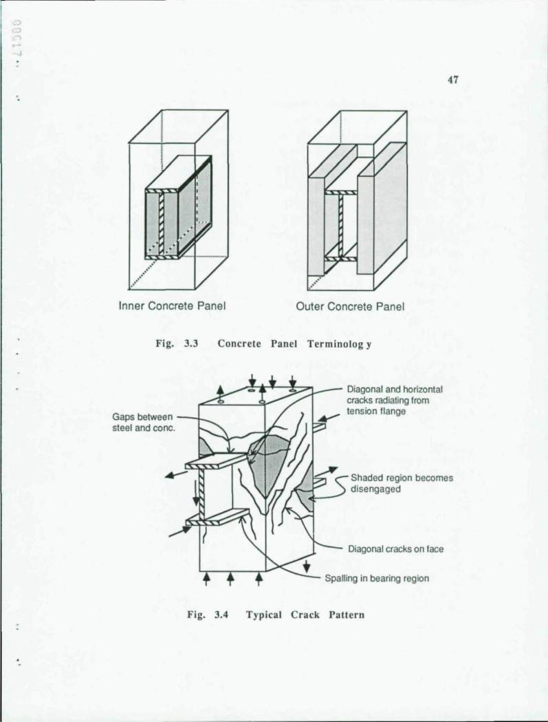
Inner Concrete Panel

47

..•....

Outer Concrete Panel

Fig. 3.3 Concrete Panel Terminolog y

Gaps between --1-_

steel and conc.

Fig. 3.4

Diagonal and horizontal cracks radiating from tension flange

Shaded region becomes disengaged

Diagonal cracks on face

Spalling in bearing region

Typical Crack Pattern

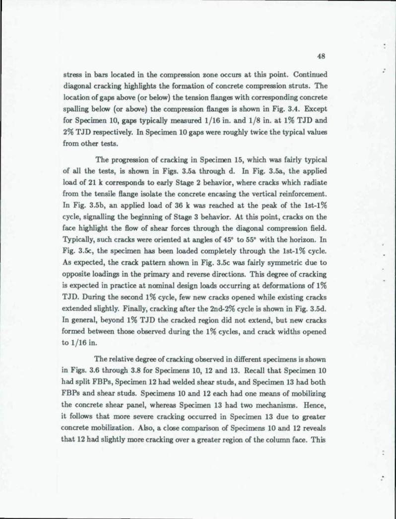
48

stress in bars located in the compression zone occurs at this point. Continued

diagonal cracking highlights the formation of concrete compression struts. The

location of gaps above (or below) the tension flanges with corresponding concrete

spalling below (or above) the compression flanges is shown in Fig. 3.4. Except

for Specimen 10, gaps typically measured 1/16 in. and 1/8 in. at 1% TJD and

2% TJD respectively. In Specimen 10 gaps were roughly twice the typical values

from other tests.

The progression of cracking in Specimen IS, which was fairly typical

of all the tests, is shown in Figs. 3.Sa through d. In Fig. 3.5a, the applied

load of 21 k corresponds to early Stage 2 behavior, where cracks which radiate

from the tensile flange isolate the concrete encasing the vertical reinforcement.

In Fig. 3.Sb, an applied load of 36 k was reached at the peak of the Ist-l %

cycle, signalling the beginning of Stage 3 behavior. At this point, cracks on the

face highlight the flow of shear forces through the diagonal compression field.

Typically, such cracks were oriented at angles of 45· to 55· with the horizon. In

Fig. 3.Se, the specimen has been loaded completely through the lst-l% cycle.

As expected, the crack pattern shown in Fig. 3.Sc was fairly symmetric due to

opposite loadings in the primary and reverse directions. This degree of cracking

is expected in practice at nominal design loads occurring at deformations of 1 %

TJD. During the second 1% cycle, few new cracks opened while existing cracks

extended slightly. Finally, cracking after the 2nd-2% cycle is shown in Fig. 3.Sd.

In general, beyond 1% TJD the cracked region did not extend, but new cracks

formed between those observed during the 1% cycles, and crack widths opened

to 1/16 in.

The relative degree of cracking observed in different specimens is shown

in Figs. 3.6 through 3.8 for Specimens 10, 12 and 13. Recall that Specimen 10

had split FBPs, Specimen 12 had welded shear studs, and Specimen 13 had both

FBPs and shear studs. Specimens 10 and 12 each had one means of mobilizing

the concrete shear panel, whereas Specimen 13 had two mechanisms. Hence,

it follows that more severe cracking occurred in Specimen 13 due to greater

concrete mobilization. Also, a close comparison of Specimens 10 and 12 reveals

that 12 had slightly more cracking over a greater region of the column face. This

. . ..

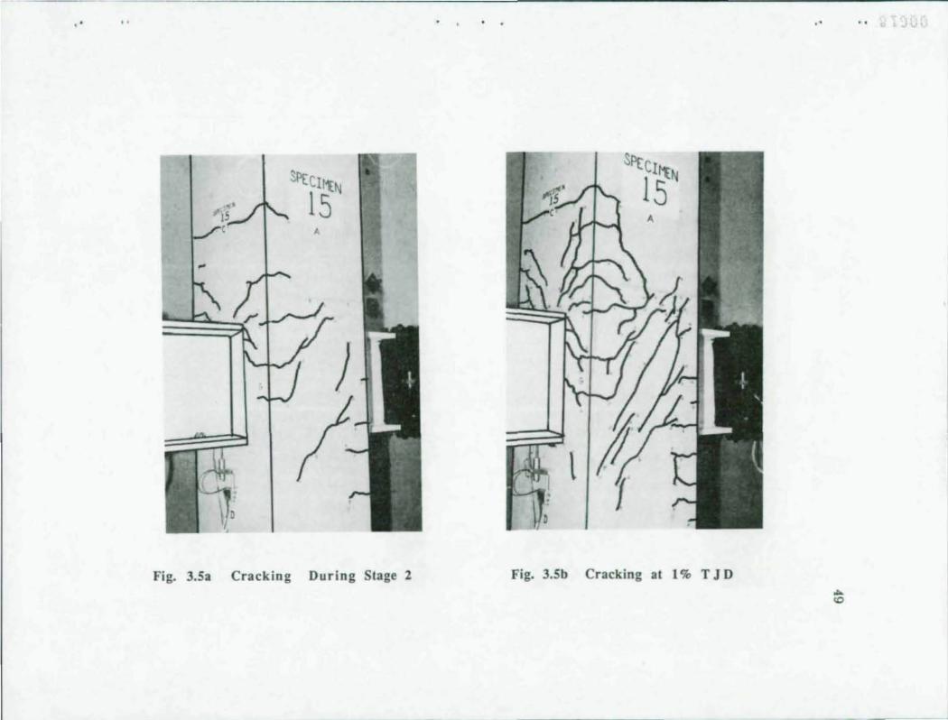
Fig. 3.5a Cracking During Stage 2 Fig. 3.5b Cracking at 1 % T J D

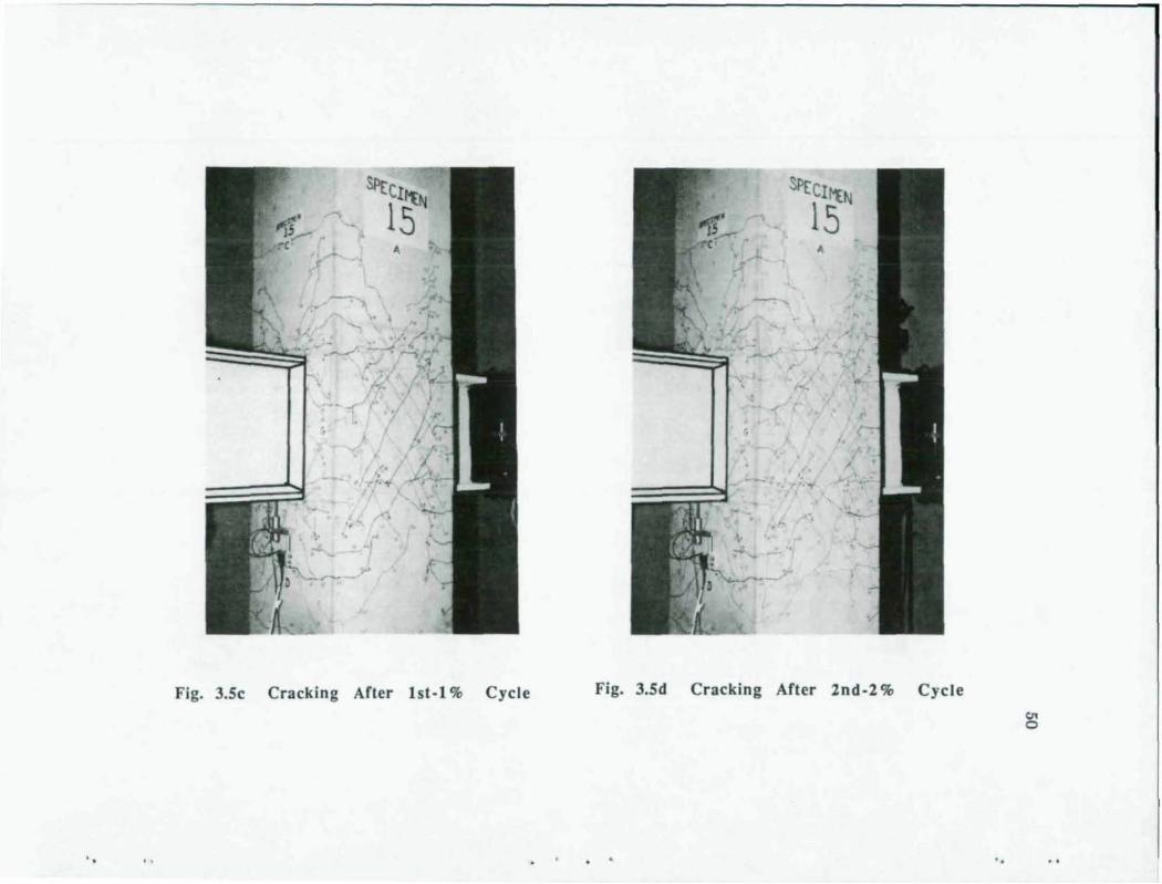
Fig. 3.Sc Cracking After lst·l % Cycle Fig. 3.Sd Cracking After 2nd·2 % Cycle

'.

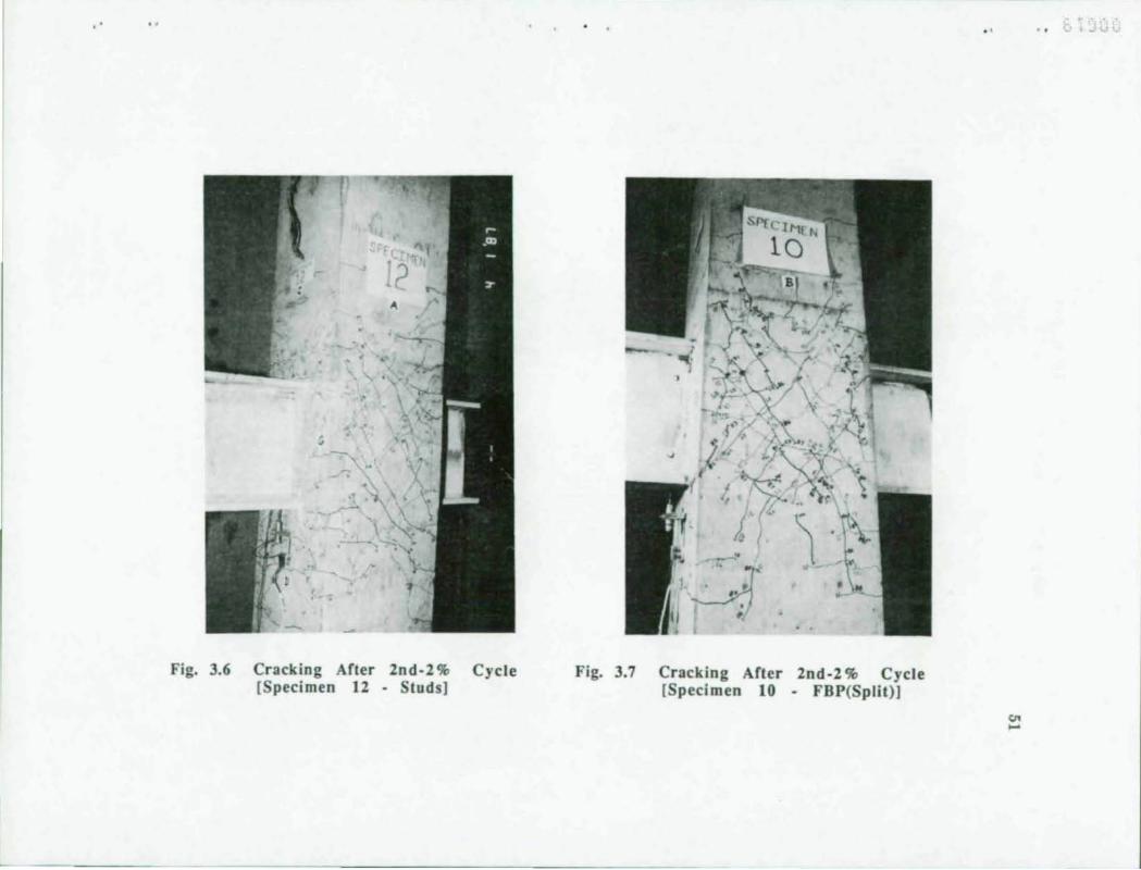
Fig. 3.6 Cracking After 2nd·2 % [Specimen 12 • Studs]

Cycle Fig. 3.7 Cracking After 2nd·2 % Cycle [Specimen 10 • FBP{Split)j

..

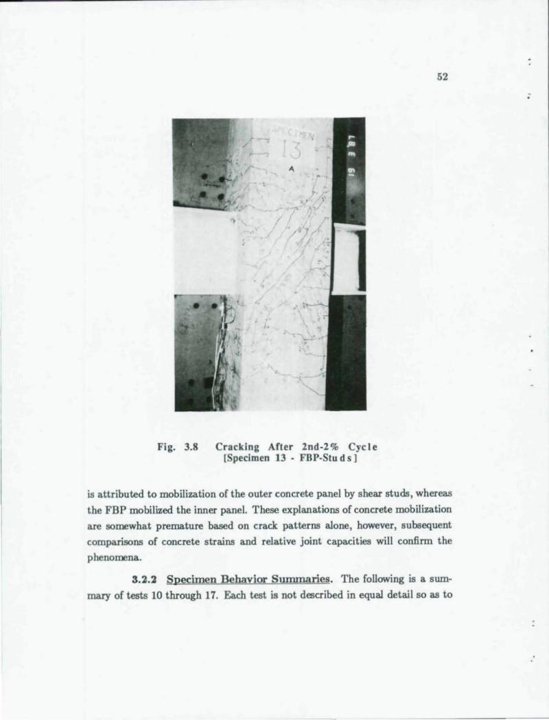
Fig. 3.8 Cracking After 2nd-2 % Cyc I e [Specimen 13 - FBP-Stu d s 1

52

is attributed to mobilization of the outer concrete panel by shear studs, whereas

the FBP mobilized the inner panel. These explanations of concrete mobilization

are somewhat premature based on crack patterns alone, however, subsequent

comparisons of concrete strains and relative joint capacities will confirm the

phenomena.

3.2.2 Specimen Behavior Sununaries. The following is a sum­

mary of tests 10 through 17. Each test is not described in equal detail so as to

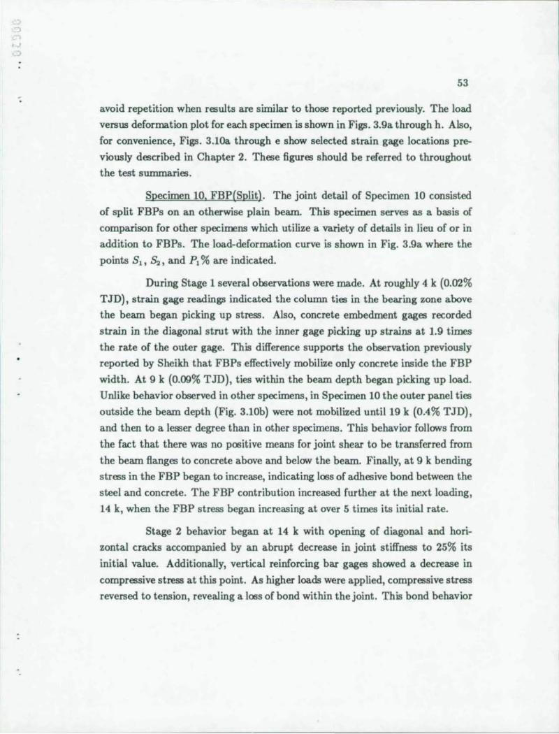
53

avoid repetition when results are similar to those reported previously. The load

versus deformation plot for each specimen is shown in Figs. 3.9a through h. Also,

for convenience, Figs. 3.1Oa through e show selected strain gage locations pre­

viously described in Chapter 2. These figures should be referred to throughout

the test summaries.

Specimen 10. FBP(Split). The joint detail of Specimen 10 consisted

of split FBPs on an otherwise plain beam. This specimen serves as a basis of

comparison for other specimens which utilize a variety of details in lieu of or in

addition to FBPs. The load-deformation curve is shown in Fig. 3.9a where the

points 8 1 , So, and PI % are indicated.

During Stage 1 several observations were made. At roughly 4 k (0.02%

T JD), strain gage readings indicated the column ties in the bearing zone above

the beam began picking up stress. Also, concrete embedment gages recorded

strain in the diagonal strut with the inner gage picking up strains at 1.9 times

the rate of the outer gage. This difference supports the observation previously

reported by Sheikh that FBPs effectively mobilize only concrete inside the FBP

width. At 9 k (0.09% TID), ties within the beam depth began picking up load.

Unlike behavior observed in other specimens, in Specimen 10 the outer panel ties

outside the beam depth (Fig. 3.l0b) were not mobilized until 19 k (0.4% TJD),

and then to a lesser degree than in other specimens. This behavior follows from

the fact that there was no positive means for joint shear to be transferred from

the beam flanges to concrete above and below the beam. Finally, at 9 k bending

stress in the FBP began to increase, indicating loss of adhesive bond between the

steel and concrete. The FBP contribution increased further at the next loading,

14 k, when the FBP stress began increasing at over 5 times its initial rate.

Stage 2 behavior began at 14 k with opening of diagonal and hori­

zontal cracks accompanied by an abrupt decrease in joint stiffness to 25% its

initial value. Additionally, vertical reinforcing bar gages showed a decrease in

compressive stress at this point. As higher loads were applied, compressive stress

reversed to tension, revealing a loss of bond within the joint. This bond behavior

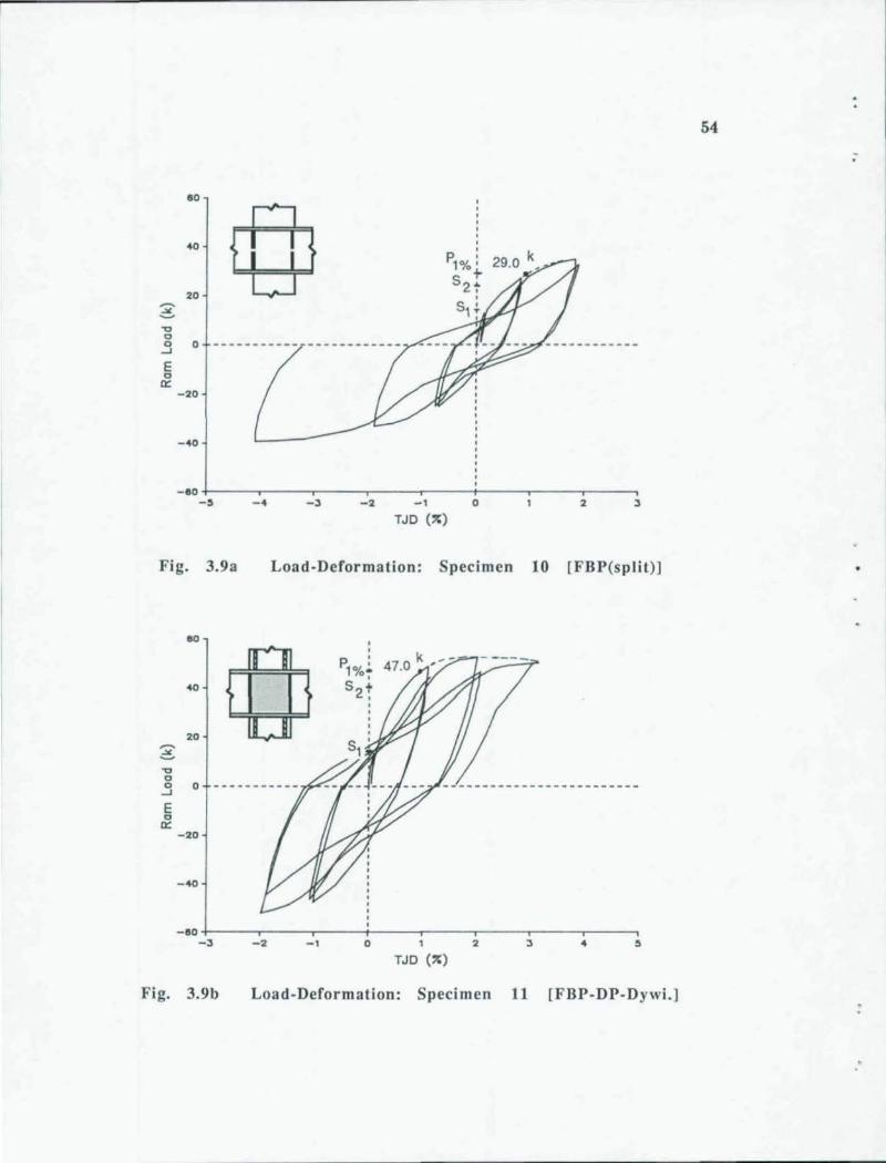
"0 o

eo

40

20

o 0 .~.-------- ----------- ---' E o

a:: -20

-40

-eo+-----,------r----~----~r_----+_----,_----_r----__, -. Fig. 3.9a

eo

40

20 ~

C "0 0 0 --' E 0

a:: -20

-40

-eo -,

Fig. 3.9b

-4

-2

-, -2 -1

TJD (,;) 2 ,

Load-Deformation: Specimen 10 [FBP(split)]

-1

, , P1 %1 5 2 + ,

o 2 4 • TJD (,;)

Load-Deformation: Specimen 11 (FBP-DP-DywL]

54

••

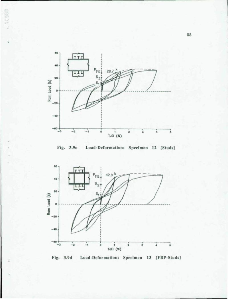
55

:

eo

-----

20 -:;c ~ .., g .... E 0

"" -20

-40

-eo -3 - 2 - 1 0 1 2 J • •

TJD (")

Fig. 3.9c Load-Deformation: Specimen 12 [Studs]

eo 0 0 0

40 Pl%~

20 -:;c ~ .., .3 E 0

"" -20

-eo ~---r----r---~--~~--,---~----~---, -3 -2 - 1 2 J • •

TJD CX)

Fig. 3.9d Load-Deformation: pecimen 13 [FBP- tud sj

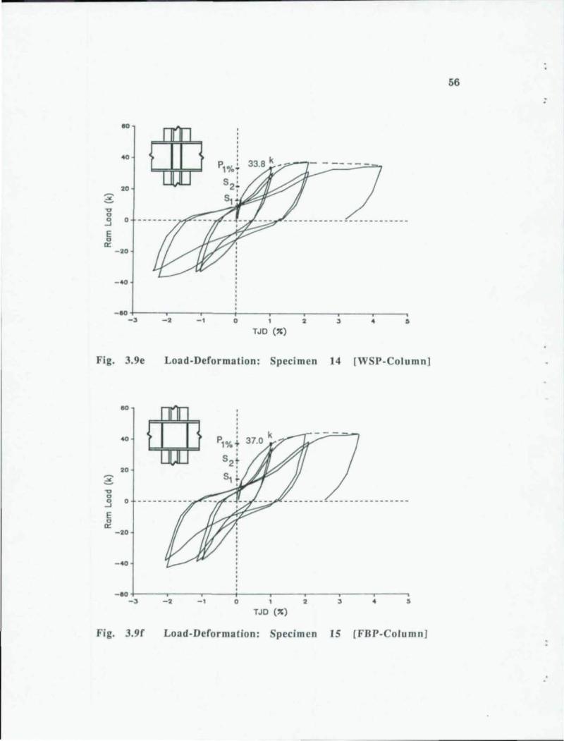
." o .3 E o

0::

10

20

-20

- 40

-OO+-----~----r_--~----~----_r----,_----~--~ -. Fig. 3.ge

." o .3 E o

0::

00

40

20

-20

- 40

-2 -. o 2 • • TJD (X)

Load·Deformation: Specimen 14 [WSP-Column)

-IO+-----~----~----~----~----~----~----~--~ -, -2 -. 2 • • TJD (X)

Fig. 3.9f Load-Deformation: pecimen 15 [FBP-Column1

56

:

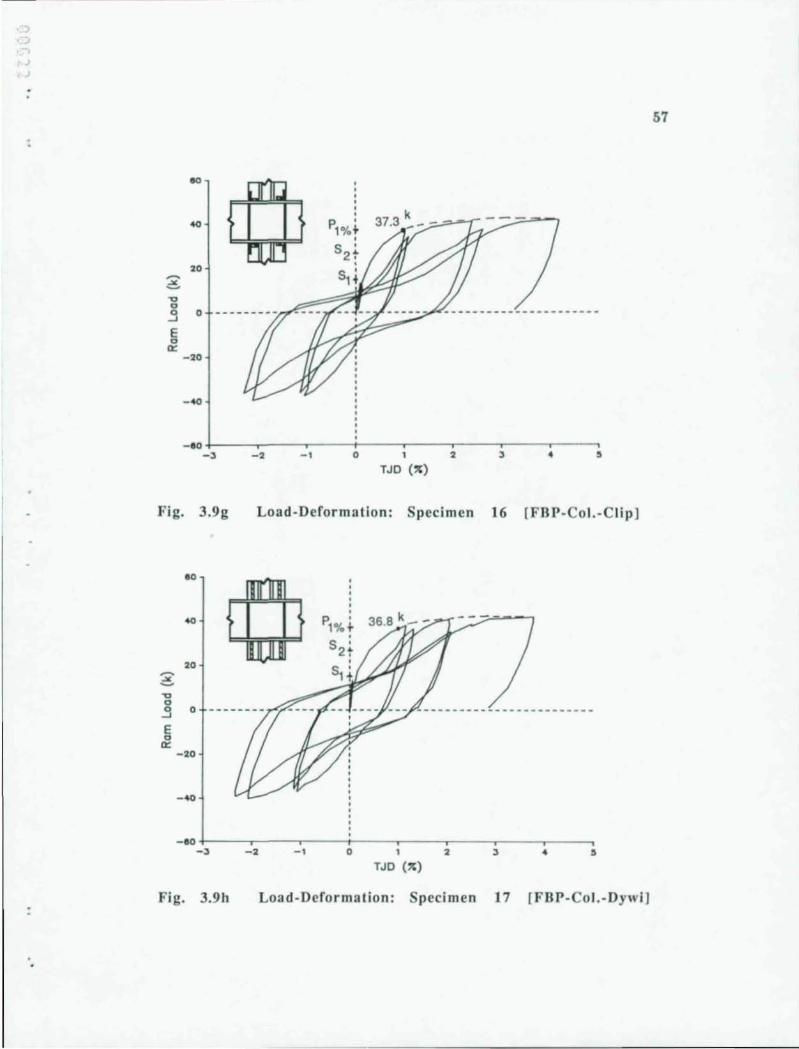
57

00

pwJ ,

2. ~

-" ~ .., <> <>

....J

E <> a: -2.

-40

-e. -3 -2 -, • 2 • ,

TJD (:I:)

Fig. 3.9g Load·Deformatio n: Speci men 16 [Fnr-Col.-C lip]

e. P1%+

2. ~

~ .., <> 0

....J

E <> a:

-2.

-40

-e. -3 -2 -, • 2 • ,

TJD (lI:)

Fig. 3.9h Load-Deformation: Specimen 17 [Fnr- ol.-Dywi]

~ '<

~

./ ..•...

.' .'

---./'. ... ...,

~

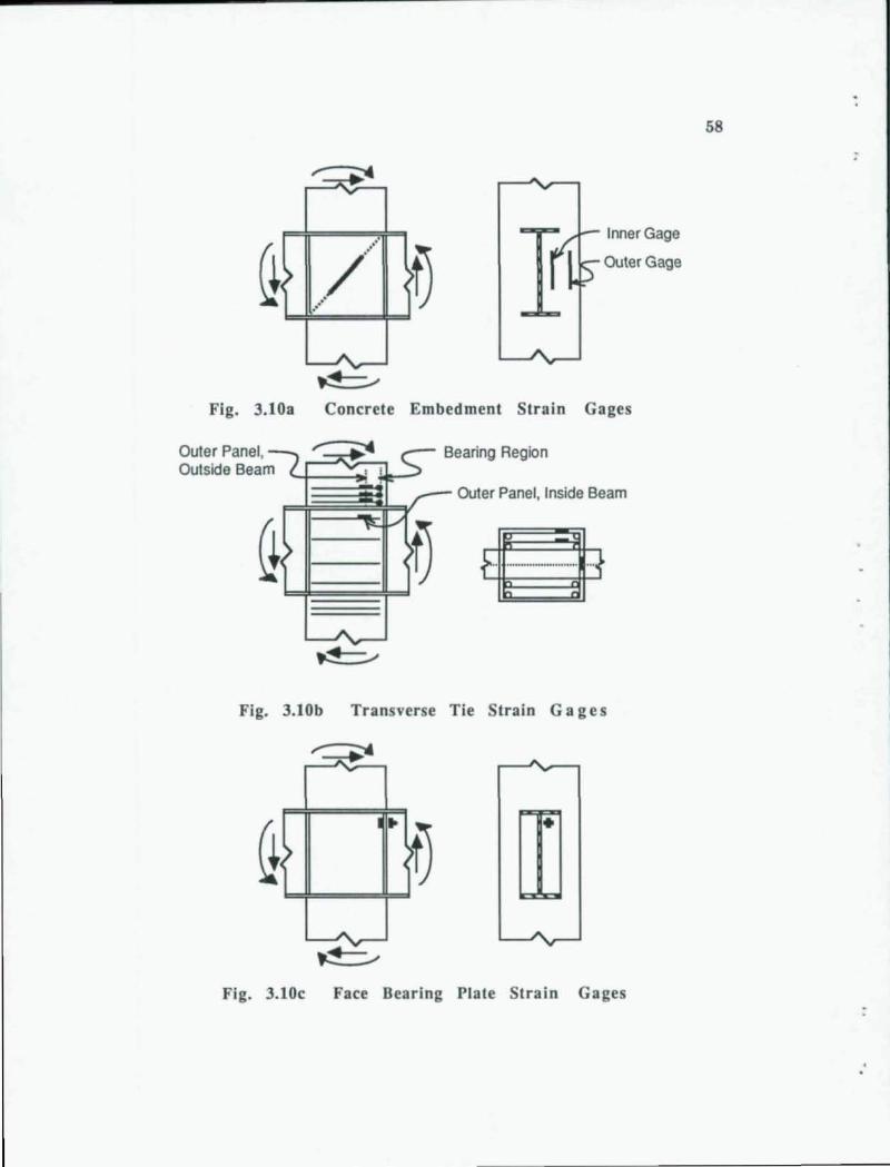
Inner Gage

Outer Gage

Fig. 3.10a Concrete Embedment Strain Gages

Outer Panel, Bearing Region

Outside Beam ;~~~~; Outer Panel, Inside Beam

Fig. 3.10b Transverse Tie Strain Gag e s

.. t <

A

Fig. 3.10c Face Bearing Plate Strain Gages

58

:

•

'.

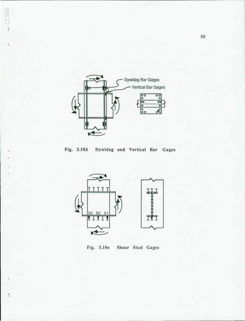
v

... I ?

A

~

;v

Dywidag Bar Gages

Vertical Bar Gages

Fig. J.I0d Dywidag and Vertical Bar Gages

Fig. J.IOe hear Stud Gages

59

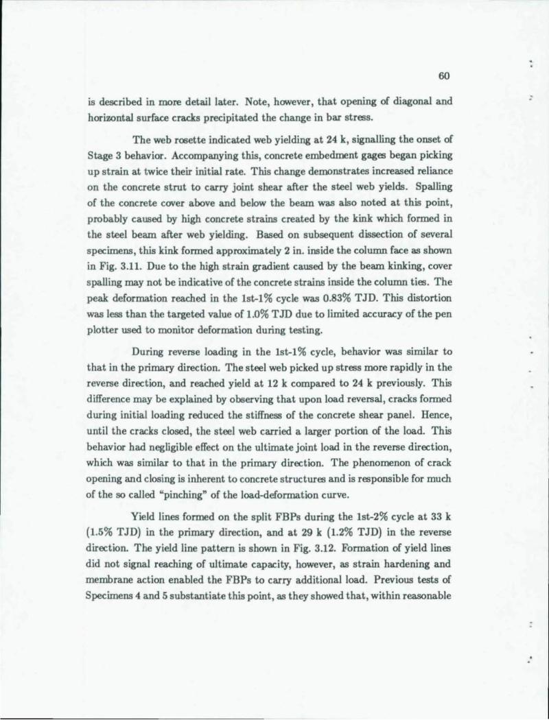
60

is described in more detail later. Note, however, that opening of diagonal and

horizontal surface cracks precipitated the change in bar stre;s.

The web rosette indicated web yielding at 24 k, signalling the onset of

Stage 3 behavior. Accompanying this, concrete embedment gage; began picking

up strain at twice their initial rate. This change demonstrate; increased reliance

on the concrete strut to carry joint shear after the steel web yields. Spalling

of the concrete cover above and below the beam was also noted at this point,

probably caused by high concrete strains created by the kink which formed in

the steel beam after web yielding. Based on subsequent dissection of several

specimens, this kink formed approximately 2 in. inside the column face as shown

in Fig. 3.11. Due to the high strain gradient caused by the beam kinking, cover

spalling may not be indicative of the concrete strains inside the column tie;. The

peak deformation reached in the Ist-l% cycle was 0.83% TJD. This distortion

was less than the targeted value of 1.0% T JD due to limited accuracy of the pen

plotter used to monitor deformation during testing.

During reverse loading in the Ist-l % cycle, behavior was similar to

that in the primary direction. The steel web picked up stre;s more rapidly in the

reverse direction, and reached yield at 12 k compared to 24 k previously. This

difference may be explained by observing that upon load reversal, cracks formed

during initial loading reduced the stiffness of the concrete shear panel. Hence,

until the cracks closed, the steel web carried a larger portion of the load. This

behavior had negligible effect on the ultimate joint load in the reverse direction,

which was similar to that in the primary direction. The phenomenon of crack

opening and closing is inherent to concrete structure; and is re;ponsible for much

of the so called "pinching" of the load-deformation curve.

Yield lines formed on the split FBPs during the 1st-2% cycle at 33 k

(1.5% TJD) in the primary direction, and at 29 k (1.2% TJD) in the reverse

direction. The yield line pattern is shown in Fig. 3.12. Formation of yield line;

did not signal reaching of ultimate capacity, however, as strain hardening and

membrane action enabled the FBPs to carry additional load. Previous tests of

Specimens 4 and 5 substantiate this point, as they showed that, within reasonable

:

•

..

::::::::::::: ....

....... ::;::. .. : .. ... ....-

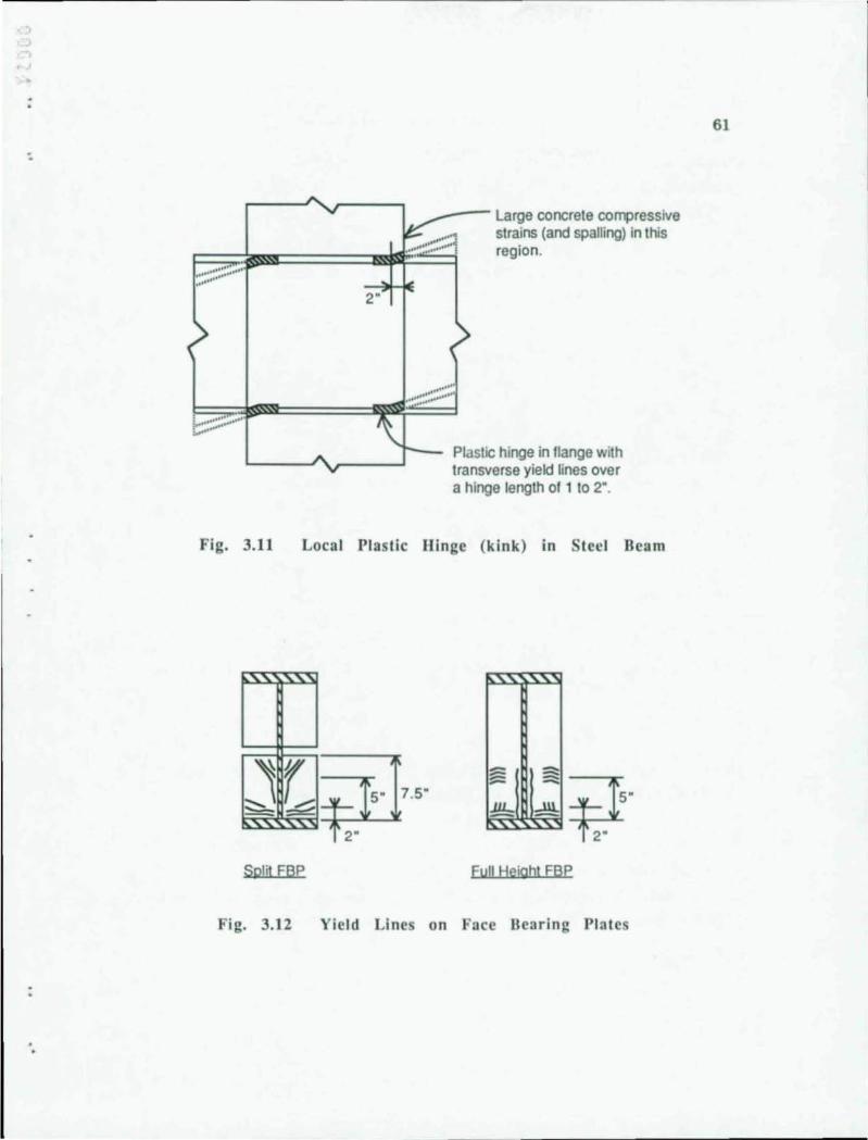
Fig. 3.11

~ ;:-...

2"

--- Large concrete compressive strains (and spatting) in this region.

... ::::::::::::::'

Plastic hinge in flange with transverse yield lines over a hinge length of 1 to 2".

Local Plastic Hinge (kink) in Ste~1 Beam

r -.: ==i.i7.S" ~

Split FBP FyI! Height FBP

Fig. 3.12 Yield Lines on Face Bearing Plates

61

62

limits, FBP thickness (and hence, stiffness) had negligible influence on joint

strength. Of course, the FBP must be designed so that it will not fracture near

the perimeter weld to the beam.

The peak deformation reached during the 1st-2% cycle was 1.8% TID.

Beyond 2% TJD, Specimen 10 continued to pick up load slowly until the test

was stopped at 3.5% TID.

Specimen 11. FBP-DP-Dvwi. In Specimen 11, web doubler plates were

used to increase the steel panel capacity, and full height FBPs were used to

mobilize the inner concrete panel. In addition, Dywidag bars (serving as vertical

joint reinforcement) were expected to improve behavior in three ways. First,

they served as compression reinforcement in the concrete bearing zone. Second,

bars in the tension region transferred tensile forces directly from the steel beam

into the concrete column. Finally, near the connection to the flange, the bars

served as large shear studs which mobilized shear in the outer concrete panel.

Figure 3.9b shows the load-deformation curve for Specimen 11.

Stage 1 behavior was similar to that of Specimen 10 with the variations

and additions noted below. At 4 k (0.03% TID) Dywidag bars attached to the

tension flanges reached the rate of axial tensile stress increase (with respect to

joint load) which then remained constant for the remaining loading. Dywidag

bars which developed compressive stress also picked up load, but to a lesser

degree. More detailed discussion of the Dywidag bar behavior is presented later.

At low loads the inner and outer concrete gages recorded roughly equal strains.

At 13 k (0.15% TJD), as the transition to Stage 2 began, concrete gages recorded

strains at increasing rates: the inner gage at 2 times and the outer gage at 5

times its original rate. The large increase in the outer gage, which was not

observed in other specimens, leads to suspect that this gage data may not be

accurate beyond this point. The change in concrete strain mobilization was

accompanied by increased FBP participation (stress increasing at 3 times its

initial rate), flexural cracks radiating from the tension flanges, and an increase

in the concrete panel shear (CPS) relative to other distortions.

:

)

~

.J . .,

:

63

Stage 2 behavior was evident after diagonal cracks opened and com­

pressive stress dropped in vertical column bars at 15 k (0.2% TJD). At 30 k (0.5%

TJD), vertical cracks formed on sides of the column above the tension flanges

parallel to the Dywidag bars as shown in Fig. 3.13. The effect of this cracking

on bond and development length for the Dywidag bars is discussed later. The

pattern of yield lines which formed on the full height FBP at 36 k (0.6% TJD)

is shown in Fig. 3.12.

Stage 3 co=enced at 40 k (0.8% TJD) with yielding of the web panel,

indicated by the rosette gage. Similar to Specimen 10, concrete spalJing coincided

with web yielding. Note that the cover spalled in spite of reinforcement (Dywidag

bars) in the confined concrete bearing region. The peak deformation in the 1st-

1% cycle was 1.2% TJD.

Similar to Specimen 10, during reverse loading the web picked up stress

more quickly and yielded at a lower load, 30 k (0.5% TJD) versus 40k (0.8%

TJD), than in the primary direction. Also, yielding of the FBPs occurred at 44

k (1.0% TJD).

During the 2% cycles, strain gages on the Dywidag bars showed tensile

stress in some of the bars drop sharply. Subsequent dissection of the specimen

revealed that 7 of the 8 welds between the steel beam and the Dywidag couplers

fractured. This observation is important for two reasons. First, strain gage

readings indicate that the welds were intact through the 1% cycles, and hence,

data and conclusions drawn during those cycles are valid. Also, note that the

load-deflection curve does not show any obvious discontinuities attributable to

the weld failures. Second, the fractures raise questions regarding adequacy of

the weld detail. In this case weld failure was attributed to inadequate throat

thickness and to weld porosity, both of which could be avoided by more thorough

supervision and inspection of welding.

The peak distortion of the 1st-2% cycle was 2.0% TJD where the peak

load of 52.7 k was recorded. At the maximum distortion of 3.4% TJD the load

was 96% of the peak value.

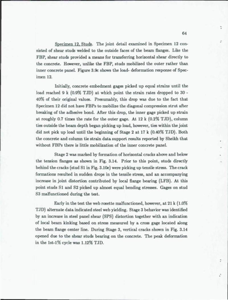
64

Specimen 12. Studs. The joint detail examined in Specimen 12 con­

sisted of shear studs welded to the outside faces of the beam flanges. Like the

FBP, shear studs provided a means for transferring horizontal shear directly to

the concrete. However, unlike the FBP, studs mobilized the outer rather than

inner concrete panel. Figure 3.9c shows the load- deformation response of Spec­

imen 12.

Initially, concrete embedment gages picked up equal strains until the

load reached 9 k (0.9% TID) at which point the strain rates dropped to 30 -

40% of their original values. Presumably, this drop was due to the fact that

Specimen 12 did not have FBPs to mobilize the diagonal compression strut after

breaking of the adhesive bond. After this drop, the inner gage picked up strain

at roughly 0.7 times the rate for the outer gage. At 12 k (0.2% TID), column

ties outside the beam depth began picking up load, however, ties within the joint

did not pick up load until the beginning of Stage 2 at 17 k (0.40% TJD). Both

the concrete and column tie strain data support results reported by Sheikh that

without FBPs there is little mobilization of the inner concrete panel.

Stage 2 was marked by formation of horizontal cracks above and below

the tension flanges as shown in Fig. 3.14. Prior to this point, studs directly

behind the cracks (stud SI in Fig. 3.10e) were picking up tensile stress. The crack

formations resulted in sudden drops in the tensile stress, and an accompanying

increase in joint distortion contributed by local flange bearing (LFB). At this

point studs Sl and S2 picked up almost equal bending stresses. Gages on stud

S3 malfunctioned during the test.

Early in the test the web rosette malfunctioned, however, at 21 k (1.0%

TJD) alternate data indicated steel web yielding. Stage 3 behavior was identified

by an increase in steel panel shear (SPS) distortion together with an indication

of local beam kinking based on stress measured by a cro~ gage located along

the beam flange center line. During Stage 3, vertical cracks shown in Fig. 3.14

opened due to the shear studs bearing on the concrete. The peak deformation

in the Ist-l% cycle was 1.12% TJD.

:

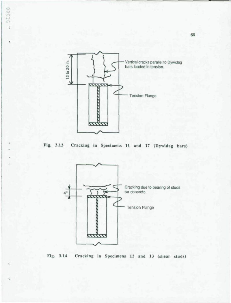
, o

I I

'.

.E o N

,

0

,

I'

"

~

)-I .,

~

~<;-'.-J

r l/

V ertical cracks parallel to Dywidag ars loaded in tension. b

Tension Flange

Fig. 3.13 Cracking in Specimens 11 and 17 (Dywidag bar s)

4 .

Fig. 3. 14

A. ~

...

\ )

A.

~C }"

("

l-

'/

Cracking due to bearing of studs on concrete.

Tension Flange

Cracking in Specimens 12 and 13 (shear stu ds)

65

66

During the Ist-2% cycle, spaJling of concrete adjacent to the compres­

sion flanges was noted at 30 k (1.4% TJD). The crushing coincided with formation

of yield lines due to transverse bending of the beam flanges in the bearing zone.

The maximum deformation in the Ist-2% cycle was 1.9% T JD. The peak load

of 34.4 k was reached during the Ist-2% cycle after which the load dropped off.

At the maximum joint deformation of 3.4% TJD the load reached 97% of its

previous peak value.

Dissect ion of Specimen 12 revealed that 13 of the 15 shear studs on

the bottom flange fractured during the test. It is of interest to determine when

the studs fractured , and why only studs on the lower flange fractured? The

fracture surfaces provided good evidence that the studs all failed during loading

in the primary direction. As seen in the overall load- deformation response,

joint capacity increased through the 1st-2% cycle, suggesting that the fractures

occurred after this point. Fractures were located outside the puddle weld region,

indicating that failures were not attributable to material or fabrication defects.

Two reasons why only the lower studs fractured are as follows. First, as will

be discussed later, concrete cast against the bottom of the flanges is of inferior

quality due to trapped air bubbles and poor consolidation. Weak concrete in

this region will induce higher bending stress in the studs as the lateral bearing

stress shifts away from the flange. The second contributing cause may be the

strain gage protection installed on 3 of the 15 studs (Fig. 3.10e). In effect, the

soft rubber protection precludes concrete bearing for 3/ 4 in. of the stud adjacent

to the flange. The net result is that the remaining 12 studs will carry a larger

portion of the load.

Specimen 13, FBP-Studs. Specimen 13 used both FBPs and shear

studs to mobilize the concrete shear panels. Essentially, these combined the

mechanisms used in Specimens 10 and 12. Figure 3.9d shows the load-deformation

response for Specimen 13.

The Stage 1 behavior was similar to that in previous specimens. The

inner concrete gage picked up strain at 1.4 times the rate of the outer gage. This

ratio lies midway between the ratios of 1.9 and 0.7 observed in Specimens 10 and

:

:> ,., I I

~

67

12. By 13 k (0.14% TID) all of the ties except those in the bearing zone were

picking up stress as were the FBPs.

Stage 2 began at 15 k (0.2% TJD) with formation of horizontal cracks

radiating from the tension flanges and mobilization of ties in the bearing region.

At 21 k (0.34% TJD), diagonal cracks opened on the column face as did horizontal

cracks above the flange as shown previously in Fig. 3.14. Also, bending stress

in stud S2 (Fig. 3.10e) no longer showed an increase. The rosette gage did not

work in this test, however, at 26 k (0.46% TID) the strain rate recorded by the

inner concrete gage increased by 40%, indicating that the web was beginning to

yield.

By 31 k (0.59% TID), Stage 3 began as the steel panel shear (SPS)

distortion, which had been negligible up to this point, abruptly began increasing.

Also, vertical cracks similar to those in Specimen 12 formed above the tension

flanges (Fig. 3.14). At 36 k (0.75% TJD), yield lines formed on the FBP. At 40 k

(0.93% TID), concrete spaJling was noted, and also strain recorded by the inner

concrete gage began increasing sharply. These observations may indicate that

although the web started yielding at 26 k, the beam did not develop kinks until

40 k. The delay may have been due to greater stiffness provided by two (rather

than one) concrete shear mechanisms: the FBPs and shear studs, which picked

up load as the web yielded. The peak deformation in the Ist-l% cycle was 1.1%

TJD.

The maximum load of 48.1 k occurred at 2.0% TID, the peak distortion

of the Ist-2% cycle. At the maximum applied distortion of 3.8% TJD the load

reached 97% of the peak load recorded previously.

Specimen 14, WSP-COl. Specimen 14 was the first of four specimens

with an embedded steel column. The steel column acted similarly to shear studs

in mobilizing the outer concrete panel. Specimen 14 also had web stiffener plates

(WSP) which, although not as effective as FBPs, mobilized the inner concrete

panel. Figure 3.ge shows the load-deformation response of Specimen 14.

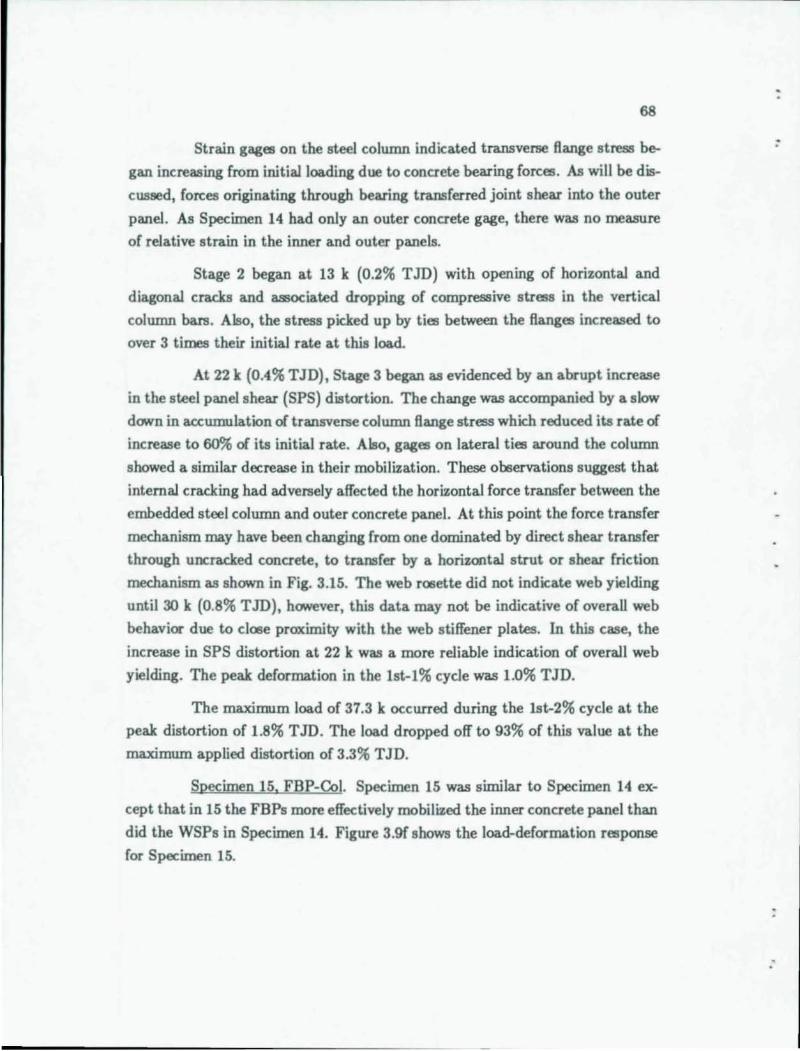
68

Strain gages on the steel colwnn indicated transverse flange stress be­

gan increasing from initial loading due to concrete bearing forces. All will be dis­

cussed, forces originating through bearing transferred joint shear into the outer

panel. As Specimen 14 had only an outer concrete gage, there was no measure

of relative strain in the inner and outer panels.

Stage 2 began at 13 k (0.2% TJD) with opening of horizontal and

diagonal cracks and associated dropping of compressive stress in the vertical

colwnn bars. Also, the stress picked up by ties between the flanges increased to

over 3 times their initial rate at this load.

At 22 k (0.4% TJD), Stage 3 began as evidenced by an abrupt increase

in the steel panel shear (SPS) distortion. The change was accompanied by a slow

down in accumulation of transverse colwnn flange stress which reduced its rate of

increase to 60% of its initial rate. Also, gages on lateral ties around the column

showed a similar decrease in their mobilization. These observations suggest that

internal cracking had adversely affected the horizontal force transfer between the

embedded steel colwnn and outer concrete panel. At this point the force transfer

mechanism may have been changing from one dominated by direct shear transfer

through uncracked concrete, to transfer by a horizontal strut or shear friction

mechanism as shown in Fig. 3.15. The web r06ette did not indicate web yielding

until 30 k (0.8% TJD), however, this data may not be indicative of overall web

behavior due to cl06e proximity with the web stiffener plates. In this case, the

increase in SPS distortion at 22 k was a more reliable indication of overall web

yielding. The peak deformation in the 1st-1% cycle was 1.0% TJD.

The maximum load of 37.3 k occurred during the 1st-2% cycle at the

peak distortion of 1.8% T JD. The load dropped off to 93% of this value at the

maximum applied distortion of 3.3% TJD.

Specimen 15, FBP-Col. Specimen 15 was similar to Specimen 14 ex­

cept that in 15 the FBPs more effectively mobilized the inner concrete panel than

did the WSPs in Specimen 14. Figure 3.9£ shows the load-deformation response

for Specimen 15.

:

:

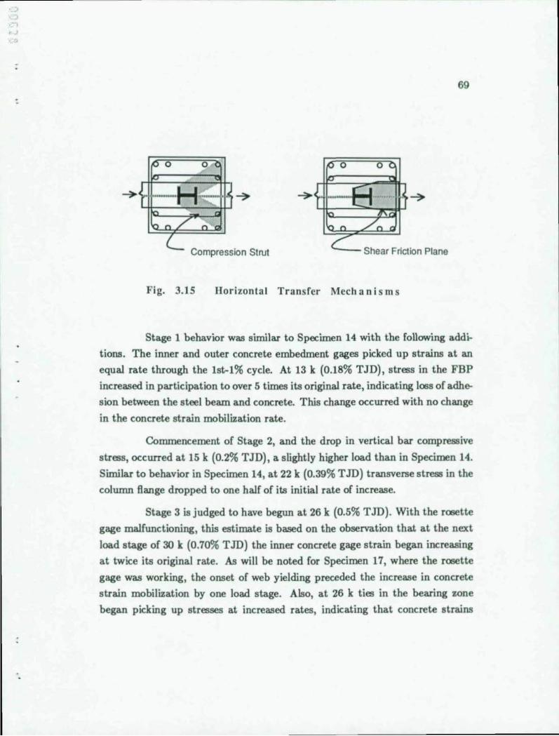
69

o 0

~'''''''''''''' ............ . ~

Compression Strut '--- Shear Friction Plane

Fig. 3.15 Horizontal Transfer Mech ani s m s

Stage 1 behavior was similar to Specimen 14 with the following addi­

tions. The inner and outer concrete embedment gages picked up strains at an

equal rate through the Ist-l% cycle. At 13 k (0.18% TJD), stress in the FBP

increased in participation to over 5 times its original rate, indicating loss of adhe­

sion between the steel beam and concrete. This change occurred with no change

in the concrete strain mobilization rate.

Commencement of Stage 2, and the drop in vertical bar compressive

stress, occurred at 15 k (0.2% TJD), a slightly higher load than in Specimen 14.

Similar to behavior in Specimen 14, at 22 k (0.39% TID) transverse stress in the

column flange dropped to one half of its initial rate of increase.

Stage 3 is judged to have begun at 26 k (0.5% TID). With the rosette

gage malfunctioning, this estimate is based on the observation that at the next

load stage of 30 k (0.70% TID) the inner concrete gage strain began increasing

at twice its original rate. As will be noted for Specimen 17, where the rosette

gage was working, the onset of web yielding preceded the increase in concrete

strain mobilization by one load stage. Also, at 26 k ties in the bearing zone

began picking up stresses at increased rates, indicating that concrete strains

70

were increasing due to kinking of the steel beam. The peak deformation of the

Ist-l% cycle was 1.0% TID.

During the Ist-2% cycle the vertical bar bond began to drop at 40 k

(1.3% TID). Further discussion of bond behavior is included later in this chapter.

A deformation of 1.8% TID was rea.ched during the Ist-2% cycle at which point

the peak load of 43.2 k was recorded. During the final cycle, at the maximum

applied deformation of 3.0% TJD the load equalled the previous peak of 43.2 k.

Specimen 16. FBP-Col-Clip. Specimen 16 was similar to Specimen 15

with the addition of clip angles. Clip angles were intended to provide additional

confinement to the concrete bearing zone above the Ranges, and also assist the

steel column in transferring horizontal joint shear into the concrete. Figure 3.9g

shows the load-deformation response for Specimen 16.

The outer concrete gage malfunctioned in this test, and hence there was

no comparison of inner and outer concrete strains. The FBP and steel column

picked up stress similarly to Specimen 15. In addition, bending stresses were

evident in the clip angle from first loading.

Stage 2 and 3 behavior were similar to Specimen 15. In Specimen 16,

the r03ette gage indicated web yielding at 27 k (0.4% TJD) which coincided with

the yield load estimated for Specimen 15. Also at 27 k, transverse bending stress

in the column Range began increasing at a lesser rate. This change occurred at

a load 5 k higher than in Specimens 14 and 15. The delay may have been due

to formation of more effective compression struts or a larger shear friction plane

than those shown previously in Fig. 3.15 owing to the clip angle.

At 31 k (0.59% TJD), the clip angle bending stress indicated yielding

near its base. This coincided with an increase in steel panel shear (SPS) distor­

tion, and increase of the inner concrete strain rate to 1.4 times its original value.

Finally, at 35 k (0.8% TID) yield lines began forming on the FBP.

The peak deformation reached during the lst-l% cycle was 0.9% TJD

and during the 1st-2% cycle 1.9% TJD. The peak load of 41.9 k was recorded at

:

, ,

71

the maximum applied deformation of 3.2% TJD, This load was only 2% higher

than that recorded during the 2% cycles,

Specimen 17. FBP-Col-Dvwi. Specimen 17 was also similar to 15 ex­

cept for addition of vertical Dywidag bars. The function of the bars was similar

to that described for Specimen 11, hCMIever, in this case utilization of the bars was

less since web doubler plates were not used, and because shear stud type behav­

ior was shadowed by the steel column. Figure 3,9h shows the load-deformation

response for Specimen 17.

The behavior of Specimen 17 was similar to that of Specimens 14

through 16. During Stage I, the Dywidag bars with tensile stress reached their

full mobilization rate at 9 k (0.08% TJD) . This coincided with internal cracking

in the concrete as evidenced by stress increases in the lateral ties. The outer

concrete embedment gage malfunctioned at an early stage, and therefore no

comparison of concrete strains was available.

As in Specimen 16, the rosette gage indicated web yielding at 27 k

(0.5% TJD). Also, transverse bending stress in the column Bange began increas­

ing at a slower rate at thls load. At the next load of 31 k (0.63% TJD) , the inner

concrete gage began recording strains at over 3 times its initial rate , Also, yield

lines formed on FBPs at thls load. The deformation reached during the lst-l%

cycle was 1.1% TID.

The deformation reached during the Ist-2% cycle was 1.7% TID. The

peak load of 42.1 k was recorded at the maximum applied deformation of 2.9%

TJD, This load was roughly 3% above that reached during the 2% cycles.

3.3 Comparison of Test Results

The presentation in thls section includes a quantitative examination of

the data, with emphasis on comparative analyses between tests. Such compar­

ison provides a reliable and convenient means to evaluate significant trends in

the data. Except for general behavior, such as load-deformation response, the

complex behavior in the specimens precludes reliable interpretation of isolated

72

pieces of data which cannot be cross referenced and checked with supporting

data. In this section eleven categories of data and observations are presented.

3.S.1 Nominal Strengths. Perhaps the most important comparison

is that of nominal joint strengths which clearly demonstrate the influence of dif­

ferent joint details and serves as the primary basis for analytic models developed

to predict joint strength. In addition to considering the relative strength, three

associated topics are addressed: the difference in joint deformation measured

by drift versus total joint distortion (TJD)j relative contribution of three joint

shear mechanisms to the total connection strengthj reco=endation of a defor­

mation limit for evaluating nominal joint strength based on the load-deformation

behavior.

In Table 3.2, joint strengths are summarized in terms of applied ram

loads at the noted deformations for Specimens 3 through 17. For Specimens

10 through 17, where cyclic loads were applied, the strengths are based on the

failure envelope in the primary direction as shown previously in Fig. 3.2. In

Specimens 3 through 9, TID was not measured directly. The TJD measurement

is not dependent on the specimen geometry as is the drift. A more thorough

comparison of drift and TID measurements is described below. In evaluating

joint strength the difference between drift and TJD is insignificant in these tests

based on data for Specimens 10 through 17. As shown in Table 3.2, the 1% drift

loads are within +4% to -4% of the 1% TID loads, and the 2% drift loads are

within +0% to -3% of the 2% TID loads.

Figure 3.16 shows the superposition of two load-deformation curves

where deformation is plotted both for TJD and drift. At low deformations the

two measurements agree fairly weU, whereas at higher deformations, drift con­

sistently underestimates joint distortion. A comparison of drift and TID for

Specimens 10 through 17 indicates that at 1% TJD drift differs by +12% to

-13%, and at 2% TID by +0% to -23%. A detailed analysis of the difference be­

tween drift and TJD is given by Sheikh.' Essentially, drift tends to overestimate

TJD when member deformations outside the joint are large, and underestimate

TJD when shear deformations in the joint region are large. The latter reason

:

-.

.., ,

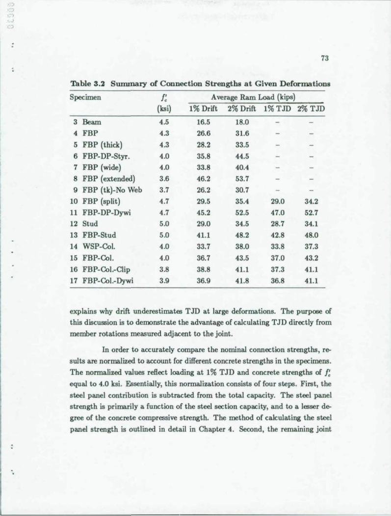
73

Table 3.2 Sumrruory of Connection Strengths at Given Deformations

Specimen f; Average Ram Load (kips)

(ksi) 1% Drift 2% Drift 1% TID 2% TID

3 Beam 4.5 16.5 18.0

4 FBP 4.3 26.6 31.6

5 FBP (thick) 4.3 28.2 33.5

6 FBP-DP-Styr. 4.0 35.8 44.5

7 FBP (wide) 4.0 33.8 40.4

8 FBP (extended) 3.6 46.2 53.7

9 FBP (tk)-No Web 3.7 26.2 30.7

10 FBP (split) 4.7 29.5 35.4 29.0 34.2

11 FBP-DP-Dywi 4.7 45.2 52.5 47.0 52.7

12 Stud 5.0 29.0 34.5 28.7 34.1

13 FBP-Stud 5.0 41.1 48.2 42.8 48.0

14 WSP-Col. 4.0 33.7 38.0 33.8 37.3

15 FBP-Col. 4.0 36.7 43.5 37.0 43.2

16 FBP-Col.-Clip 3.8 38.8 41.1 37.3 41.1

17 FBP-Col.-Dywi 3.9 36.9 41.8 36.8 41.1

explains why drift underestimates TID at large deformations. The purpose of

this discussion is to demonstrate the advantage of calculating TJD directly from

member rotations measured adjacent to the joint.

In order to accurately compare the nominal connection strengths, re­

sults are normalized to account for different concrete strengths in the specimens.

The normalized values reBect loading at 1% TJD and concrete strengths of f; equal to 4.0 ksi. E£sentially, this normalization consists of four steps. First, the

steel panel contribution is subtracted from the total capacity. The steel panel

strength is primarily a function of the steel section capacity, and to a lesser de­

gree of the concrete compressive strength. The method of calculating the steel

panel strength is outlined in detail in Chapter 4. Second, the remaining joint

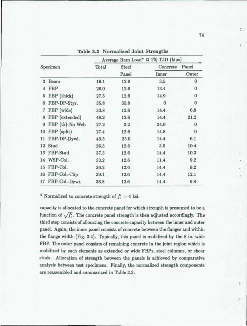
74

Table 3.3 Nonnalized Joint Strengths

Average Ram Load- @ 1% TID (kiJl6~

Specimen Total Steel Concrete Panel

Panel Inner Outer

3 Beam 16.1 12.6 3.5 0

4 FBP 26.0 12.6 13,4 0

5 FBP (thick) 27.5 12.6 14.9 0

6 FBP-DP-Styr. 35.8 35.8 0 0

7 FBP (wide) 33.8 12.6 14,4 6.8

8 FBP (extended) 48.2 12.6 14,4 21.2

9 FBP (tk)-No Web 27.2 3.2 24.0 0

10 FBP (split) 27,4 12.6 14.8 0

11 FBP-DP-Dywi. 43.5 23.0 14,4 6.1

12 Stud 26.5 12.6 3.5 10,4

13 FBP-Stud 37.3 12.6 14,4 10.3

14 WSP-COl. 33.2 12.6 11,4 9.2

15 FBP-Col. 36.2 12.6 14,4 9.2

16 FBP-Col.-Clip 39.1 12.6 14,4 12.1

17 FBP-Col.-Dywi. 36.8 12.6 14,4 9.8

- Normalized to concrete strength of f; = 4 ksi.

capacity is allocated to the concrete panel for which strength is presumed to be a

function of ..Jf.. The concrete panel strength is then adjusted accordingly. The

third step consists of allocating the concrete capacity between the inner and outer

panel. Again, the inner panel consists of concrete between the flanges and within

the flange width (Fig. 3.4). Typically, this panel is mobilized by the 8 in. wide

FBP. The outer panel consists of remaining concrete in the joint region which is

mobilized by such elements as extended or wide FBPs, steel columns, or shear

studs. Allocation of strength between the panels is achieved by comparative

analysis between test specimens. Finally, the normalized strength components

are reassembled and sllmmarized in Table 3.3.

. .

:

J

75

The data in Table 3.3 are also presented in Fig. 3.17 where the joint

strengths are expressed as relative percentages. The capacity of Specimen 5

serves as the basis of the comparisons and is set to 100%. Recall that Specimen

5 is the plain steel beam with a standard FBP (7/8 in. thick) . The detailing of

Specimen 5 is very similar to that of Specimens 4 and 10.

Joint strengths shown in Fig. 3.17 suggest a grouping of the tests into

four categories, denoted A through D. Group A consists solely of Specimen 3

which is the plain steel beam detail. The total capacity of this specimen is 59%

of Specimen 5. In Specimen 3 roughly 80% of its strength is contributed by the

steel panel. Friction between the steel beam and concrete presumably mobilizes

the inner concrete panel which accounts for the remaining strength.

Group B consists of Specimens 4, 5, 9, 10 and 12 whose strengths all

are approximately equal to that of Specimen 5. Results of Specimens 4, 5, and

10 demonstrate the effectiveness of the standard FBP detail, where the inner

concrete panel carries roughly 55% of the total load. As reported by Sheikh,

the FBP mobilizes a diagonal compression strut equal in width to the FBP (8

in.) These tests also show that, within reasonable bounds, concrete mobilization

inside the beam flange width is insensitive to FBP stiffness; recall that Specimen

4 has full height 3/8 in. FBPs, and Specimen 10 split 3/8 in. FBPs. Specimen 12

does not have FBPs, but instead mobilizes concrete in the outer panel through

welded shear studs. In Specimen 12, a small load is also carried by the inner panel

similar to Specimen 3. Specimen 9 is the final test in group B. Although, included

for completeness in this discussion, the results of Specimen 9 are not used in this

paper. As reported by Sheikh, the behavior of Specimen 9 suggests that in the

absence of a strong steel panel the concrete compression strut width increases

up to 50%. Also, increased strength in Specimen 9 may result from improved

concrete quality due to better placement afforded by the large hole in the web.

Since this behavior lacks a well founded explanation based on mechanics, the

results will be omitted until they are verified by future tests.

Group C includes Specimens 6, 7, 13, 14, 15, 16 and 17 which have

strengths ranging from 121% to 142% of Specimen 5. Specimen 7, which utilizes

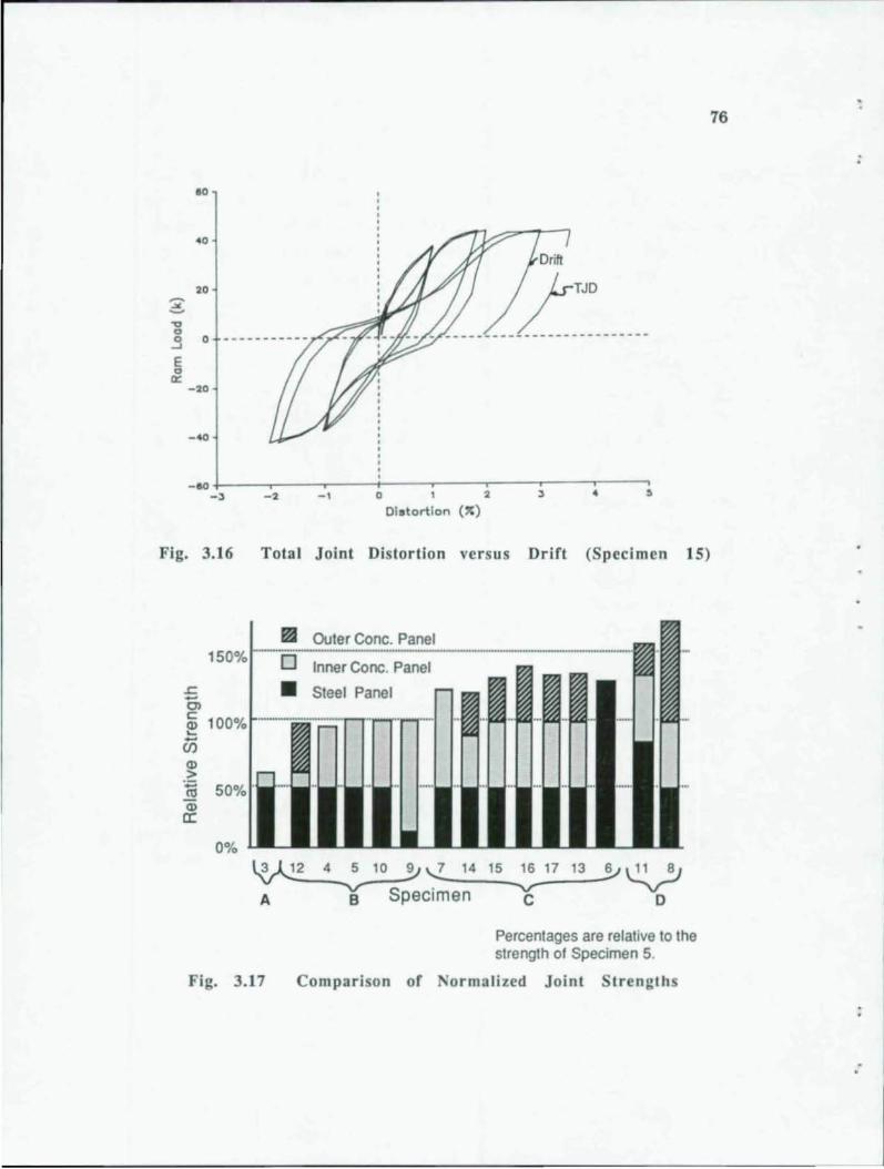
." o a

--' E o

Q:

.0

'0

.0

-'0

-40

_~+-----r----,----~----~----~----~----.r---~. -3 -2 -1 0 1 2 3

Ol.tortlan (:0::)

Fig. 3.16 Total Joint Distortion versus Drift (Specimen 15)

1

.c. -Ol

g 100% ... ii5 ~ ~ Q)

c::

0%

Outer Conc. Panel

Inner Cone. Panel

• Steel Panel

~'! 14 15 ~17 13 .v~ A B Specimen C 0

Percentages are relative to the strength of Specimen 5.

Fig. 3.17 Comparison of Normalized Joint Strengths

76

)

;. ..,

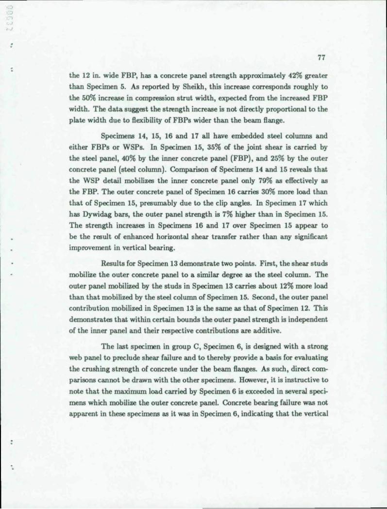
77

the 12 in. wide FBP, has a concrete panel strength approximately 42% greater

than Specimen 5. As reported by Sheikh, this increase corresponds roughly to

the 50% increase in compression strut width, expected from the increased FBP

width. The data suggest the strength increase is not directly proportional to the

plate width due to Bexibility of FBPs wider than the beam Bange.

Specimens 14, 15, 16 and 17 all have embedded steel columns and

either FBPs or WSPs. In Specimen 15, 35% of the joint shear is carried by

the steel panel, 40% by the inner concrete panel (FBP), and 25% by the outer

concrete panel (steel column) . Comparison of Specimens 14 and 15 reveals that

the WSP detail mobilizes the inner concrete panel only 79% as effectively as

the FBP. The outer concrete panel of Specimen 16 carries 30% more load than

that of Specimen 15, presumably due to the clip angles. In Specimen 17 which

has Dywidag bars, the outer panel strength is 7% higher than in Specimen 15.

The strength increases in Specimens 16 and 17 over Specimen 15 appear to

be the result of enhanced horizontal shear transfer rather than any significant

improvement in vertical bearing.

Results for Specimen 13 demonstrate two points. First, the shear studs

mobilize the outer concrete panel to a similar degree as the steel column. The

outer panel mobilized by the studs in Specimen 13 carries about 12% more load

than that mobilized by the steel column of Specimen 15. Second, the outer panel

contribution mobilized in Specimen 13 is the same as that of Specimen 12. This

demonstrates that within certain bounds the outer panel strength is independent

of the inner panel and their respective contributions are additive.

The last specimen in group C, Specimen 6, is designed with a strong

web panel to preclude shear failure and to thereby provide a basis for evaluating

the crushing strength of concrete under the beam Banges. As such, direct corn­

parisons cannot be drawn with the other specimens. However, it is instructive to

note that the maximum load carried by Specimen 6 is exceeded in several speci­

mens which mobilize the outer concrete panel. Concrete bearing failure was not

apparent in these specimens as it was in Specimen 6, indicating that the vertical

78

bearing zone is not confined to the beam 8ange width for joint shear carried by

the outer concrete panel.

Finally, group D includes Specimens 11 and 8 which have strengths

equal to 158% and 175% of Specimen 5. Results of Specimen 11 (which incorpo­

rates FBPs, web doubler plates, and Dywidag bars) indicate that the Dywidag

bars are effective in reinforcing the concrete bearing zone since the total strength

exceeds that of Specimen 6 by 22%. Second, shear transfer by the Dywidag bars

mobilizes the outer panel to roughly 60% of that afforded by shear studs in Spec­

imens 12 and 13. Finally, as evidenced by comparison of tests 11, 15 and 17, the

outer concrete panel strength mobilized by the steel column is not fully additive

with that mobilized by the Dywidag bars. Intuitively this is reasonable since the

embedded column shadows the shear effect of the Dywidag bars, or vice versa.

Specimen 8 is an important test since with very stiff extended FBPs it

provides an upper bound on the outer panel strength which can be mobilized. In

this specimen, relative contributions of the steel panel, inner concrete panel, and

outer concrete panel to the total are 26%, 30% and 44%. Compared with Speci­

men 8, Specimens 13 and 15 show that shear studs and the steel column mobilize

48% and 43% (respectively) of the maxiImlm available outer panel strength.

Finally, a reasonable limit on joint distortion for determining the nom­

inal design strength is evaluated on the basis of load-deformation data. Previ­

ously, Sheikh has proposed 2.0% TJD as a deformation limit. A lower limit of

1.0% TJD is preferable in part based on the reasoning outlined below.

From the average specimen response, the load- deformation envelope

is idealized by the tri-Iinear plot shown in Fig. 3.18. As indicated in the fig­

ure, doubling the joint distortion from 1% to 2% T JD results in only a modest

strength gain of 15%. Additionally, if service load is considered at one half

of ultimate load, the service distortion increases proportionally faster than the

strength gain between 1% and 2% TJD. A design strength at 1% TJD results

in service deformation of roughly 0.2%, whereas the strength at 2% T JD results

in service deformations of 0.25%. Thus, for a strength increase of 15%, service

deformations would increase approximately 25%.

1 J

79

3.3.2 Cyclic Load Behavior. The cyclic load response provides

a measure of joint toughness when subjected to large inelastic deformations.

Toughness is an important and sometimes overlooked aspect of structural relia­

bility. Assessment of the cyclic response also addresses special concerns raised

when the composite connection is used in structures designed for seismic loading.

The loss in strength due to reverse cyclic loading, which was similar in

aU the specimens, is measured from the load-deformation response. After loading

through the Ist-l% cycle, the average load carried at 1% TJD was 89% of the

initial strength at that deformation, and after the 2nd-l% cycle was 83% of the

initial strength. Similarly, after the two additional 2% cycles, the average load

was 86% and 79% (respectively) of the initial strength at 2% TJD. The modest

strength I06S under cyclic loading is comparable to response in well detailed

reinforced concrete elements.12

A second measure of the cyclic behavior is the energy dissipated by

hysteretic response of the joint. Hysteretic response is based on an equivalent

viscous damping coefficient calculated from the area within the load-deformation

curve. In Figure 3.19, calculation of the damping coefficient is described. This

coefficient is the ratio of equivalent viscous damping to the critical viscous damp­

ing of the system. Clough and Penzien1' present a derivation of this coefficient.

The average damping coefficient for all the specimens is 0.18, with

values ranging from 0.15 in Specimen 15 to 0.23 in Specimen 12. These values

are based on the average of the coefficients calculated for each cycle of loading.

While a rigorous appraisal of the damping coefficients is beyond the

scope of this report, a comparison is made with similar values reported for re­

inforced concrete connections. In one study of seismic response of reinforced

concrete joints, Kitayama (et.al.) 14 performed several analyses using a computer

model which incorporated inelastic joint elements. In this study, joint damping

coefficients of 0.10 to 0.25 were used. The 0.25 value corresponded to a well

detailed joint with superior energy dissipation capability, evidenced by a wide

spindle shaped load- deformation curve. According to the report, ajoint detailed

based on current seismic design standards would have a coefficient of 0.15. In

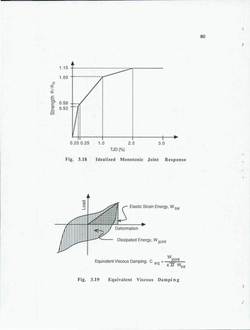
c a: -a: .r::: -Cl c Q) ~ -C/)

1.15 .............................................................. ::; .... "" .. .,-----

1.00

0.58 0.50

0.200.25

Fig. 3.18

"0

'"

1.0 2.0 3.0 TJD (%)

Idealized Monotonic Joint Response

__ .,.j11lnIli.3~mlll.IIL~_"EI~a~stmic~strain Energy, W se

Deformation

Dissipated Energy, W joint

W' I Equivalent Viscous Damping: Ceq - -f} nt 4 Wse

Fig. 3.19 Equivalent Viscous Dampi n g

80

) , , J

~

81

terms of the effect on overall behavior of structural systems, distinction between

damping coefficients is minor as Kitayama reported,

From the results of earthquake response analyses, the effect

of hysteresis energy dissipating capacity on the response was

found relatively small for a range of equivalent viscous damp­

ing ratioe from 0.10 to 0.25 at ductility factor 4.0.

Based on this information the hysteretic response of the composite connection is

comparable to that of well detailed reinforce concrete beam-column joints.

3.3.3 Components of Joint Distortion. The total joint distortion

(TJD) consists of the following three components: concrete panel shear (CPS),

local flange bearing (LFB), and steel panel shear (SPS). Detailed description

of these modes and how they were measured is provided in Chapter 2; brief

definitions are repeated here for convenience. Concrete panel shear is a measure

of shear distortion of the concrete joint panel near the face of the column. Local

flange bearing is a measure of relative rigid body rotation of the beam and

column. This mode results primarily from high concrete strains beneath the

compression flanges. Finally, steel panel shear is a measure of shear distortion of

the steel panel in excess of the concrete panel shear. As noted previously, SPS is

determined indirectly as the difference in measured distortion between TJD and

the sum of CPS and LFB.

Component distortions are superimposed on TID for Specimen 12 in

Figs. 3.2Oa to c. The response shown is typical of that for Specimens 10 through

17. In the case shown, Specimen 12, SPS behavior is the moet interesting. During

the first loading cycle, SPS increased sharply at 21 k, indicating web yielding.

Qualitative observations such as this have already been discussed in the test

summaries.

Table 3,4 provides a snmmary of the distortion data, indicating relative

percentages of each component, measured at the peak loads during the 1st-

1 % and Ist-2% cycles. Figures 3.2Oa to 3.2Oc indicate how the percentages

are obtained from the load-deformation plots. As seen in Table 3,4, relative

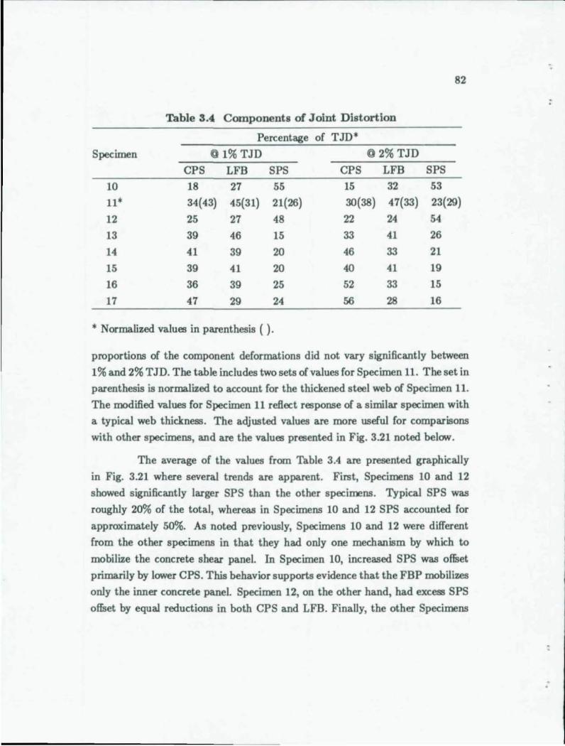
82

Table 3.4 Components of Joint Distortion

Percentage of TID·

Specimen (H% TJD @2%TJD

CPS LFB SPS CPS LFB SPS

10 18 27 55 15 32 53

11· 34(43) 45(31) 21(26) 30(38) 47(33) 23(29)

12 25 27 48 22 24 54

13 39 46 15 33 41 26

14 41 39 20 46 33 21

15 39 41 20 40 41 19

16 36 39 25 52 33 15

17 47 29 24 56 28 16

• Normalized values in parenthesis ( ).

proportions of the component deformations did not vary significantly between

1% and 2% TJD. The table includes two sets of values for Specimen 11. The set in

parenthesis is normalized to account for the thickened steel web of Specimen 11.

The modified values for Specimen 11 reflect response of a similar specimen with

a typical web thickness. The adjusted values are more useful for comparisons

with other specimens, and are the values presented in Fig. 3.21 noted below_

The average of the values from Table 3.4 are presented graphically

in Fig. 3.21 where several trends are apparent. First, Specimens 10 and 12

showed significantly larger SPS than the other specimens. Typical SPS was

roughly 20% of the total, whereas in Specimens 10 and 12 SPS accounted for

approximately 50%. As noted previously, Specimens 10 and 12 were different

from the other specimens in that they had only one mechanism by which to

mobilize the concrete shear panel. In Specimen 10, increased SPS was offset

primarily by lower CPS. This behavior supports evidence that the FBP mobilizes

only the inner concrete panel. Specimen 12, on the other hand, had excess SPS

offset by equal reductions in both CPS and LFB. Finally, the other Specimens

-

.,

;

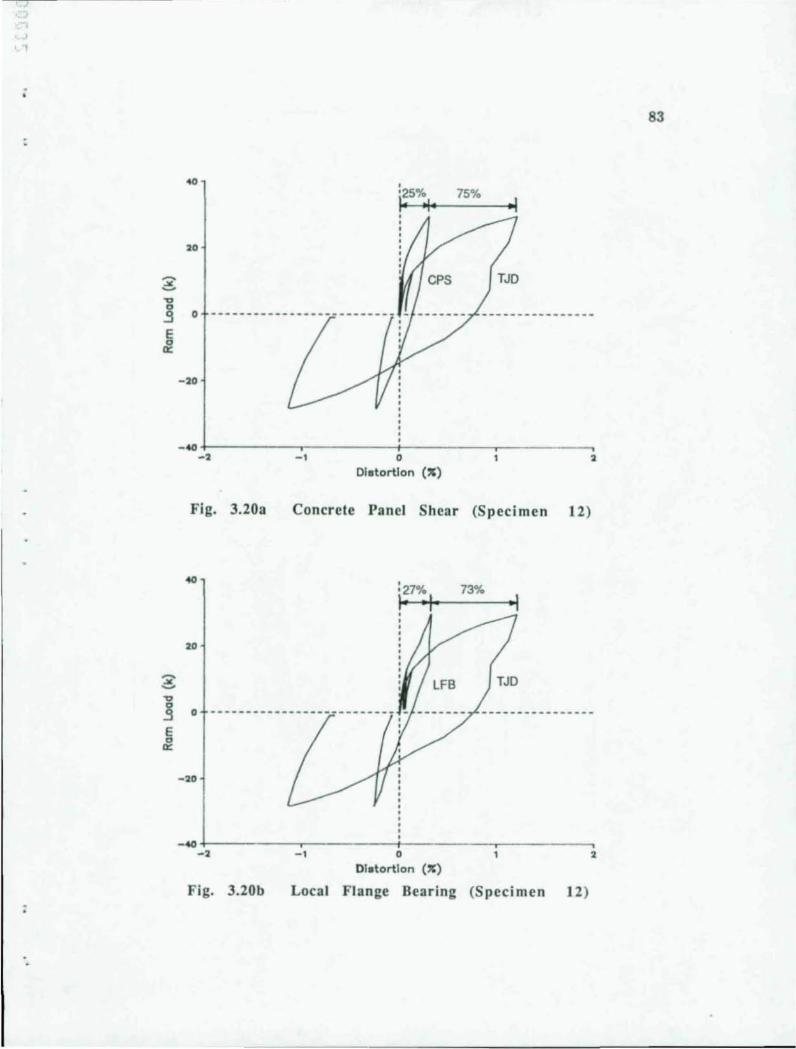
40 , '25% 75% ,. ~ I

20

TJD

...

.9 0

E £

-20

-4O+---------r-------~~------~--------~ -2 -1 0 2

Olotortlon (")

Fig. 3.20a Concrete Panel Shear (Specimen 12)

20

TJD ... .9 0 -------------------------- -

E D

'" -20

-4O+----------r--------~~--.------~--------~, -2 -1 0 2

Olotortlon (:>:)

Fig. 3.20b Local Flange Bearing (Specimen 12)

83

:;<' ~

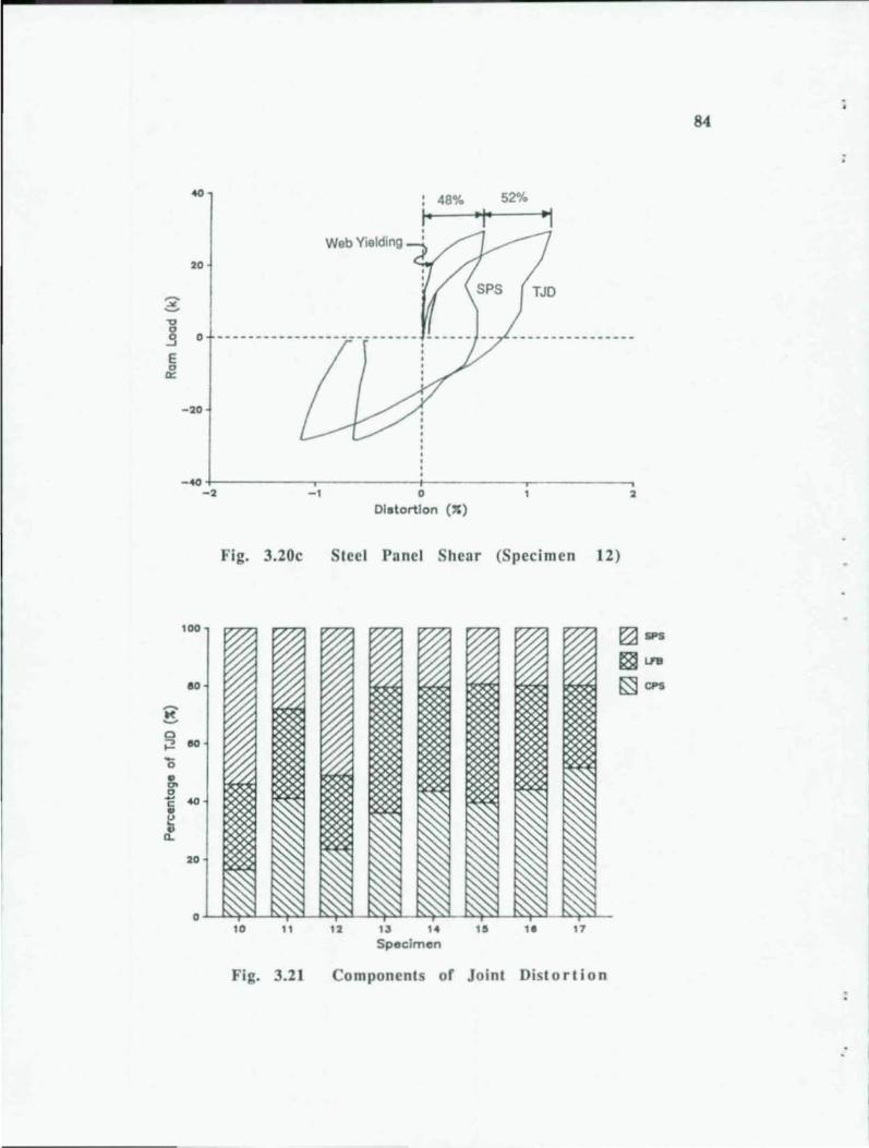
"0 0

..9 E 0 a:

~

K ~

0 ~ -0 .. '" 0 ~

" .. b

C1.

: 48% 52%

I' 'I' , Web Yielding

20

-20

-~+----------r--------~----------~--------~ -2 -1

Fig. 3.20c

100

ao

eo

~

2.

10 11

Fig. 3.21

o Ol.tortlon (%)

2

Steel Panel Shear (Specimen 12)

12 13 14

Specimen ,. ,. 17

Components of Joint Disto rt ion

f2j SPS

~LnI !;SjCPS

84

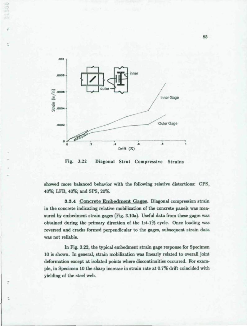
.001

.0008

~ .ooo • .§, .E " ~ .OOO4

.000'

Fig. 3.22

85

inner

/ out er

Inner Gage

Outer Gage

Drift (~)

Diagonal Strut Compressive Strains

showed more balanced behavior with the following relative distortions: CPS ,

40%; LFB, 40%; and SPS, 20%.

3.3.4 Concrete Embedment Gages. Diagonal compression strain

in the concrete indicating relative mobilization of the concrete panels was mea.­

sured by embedment strain gages (Fig. 3.10a). Useful data from these gages was

obtained during the primary direction of the 1st-I % cycle. Once loading was

reversed and cracks formed perpendicular to the gages, subsequent strain data

was not reliable.

In Fig. 3.22, the typical embedment strain gage response for Specimen

10 is shawn. In general, strain mobilization was linearly related to overall joint

deformation except at isolated points where discontinuities occurred. For exam­

ple, in Specimen 10 the sharp increase in strain rate at 0.7% drift coincided wit.h

yielding of the steel web.

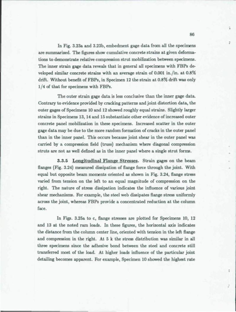
86

In Fig. 3.23a and 3.23b, embedment gage data from aU the specimens

are summarized. The figures shI7N cumulative concrete strains at given defol"IIla­

tions to demonstrate relative compression strut mobilization between specimens.

The inner strain gage data reveals that in general aU specimens with FBPs de­

veloped similar concrete strains with an average strain of 0.001 in. lin. at 0.8%

drift . Without benefit of FBPs, in Specimen 12 the strain at 0.8% drift was only

1/4 of that for specimens with FBPs.

The outer strain gage data is less conclusive than the inner gage data.

Contrary to evidence provided by cracking patterns and joint distortion data, the

outer gages of Specimens 10 and 12 shl7Ned roughly equal strains. Slightly larger

strains in Specimens 13, 14 and 15 substantiate other evidence of increased outer

concrete panel mobilization in these specimens. Increased scatter in the outer

gage data may be due to the more random formation of cracks in the outer panel

than in the ilUler panel. This occurs because joint shear in the outer panel was

carried by a compression field (truss) mechanism where diagonal compression

struts are not as weU defined as in the inner panel where a single strut forIm.

3.3.5 Longitudinal Flange Stresses. Strain gages on the beam

Banges (Fig. 3.24) measured dissipation of Bange force through the joint. With

equal but opposite beam moments oriented as shown in Fig. 3.24, Bange stress

varied from tension on the left to an equal magnitude of compression on the

right. The nature of stress dissipation indicates the influence of various joint

shear mechanisms. For example, the steel web dissipates Bange stress uniformly

across the joint, whereas FBPs provide a concentrated reduction at the column

face.

In Figs. 3.25a to c, Bange stresses are plotted for Specimens 10, 12

and 13 at the noted ram loads. In these figures, the horiwntal axis indicates

the distance from the column center line, oriented with tension in the left Bange

and compression in the right. At 5 k the stress distribution was similar in all

three specimens since the adhesive bond between the steel and concrete still

transferred most of the load. At higher loads influence of the particular joint

detailing becomes apparent. For example, Specimen 10 shl7Ned the highest rate

;

:

.~

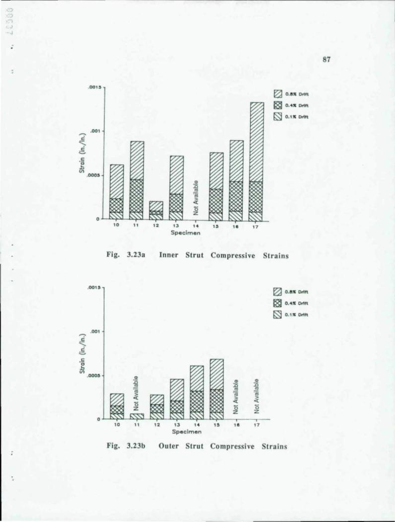
.!> VI

.0013

.001

.000'

10 11

Fig. 3.23a

Fig. 3.23b

12 13 14

Specimen IS .. 17

~ O.IS DrIft

§§ O.4S arlit

r;s;J 0.1" o.1tt

Inner Strut Compressive Strains

CD CD :l5 :l5 .!!l .. OJ ~ > > <{ <{

"6 "6 z Z

12 13 ,. ,. 10 17

SpecImen

Outer Strut Compressive

~ o.as Dr4ft

§§ 0.4S Ottft

~ 0.'" Drift

trains

87

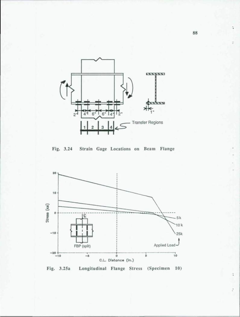
Ao ~

c l< >

2' 4' 6" 6" 4' 2" Ao

~ I, 1 2 13 1 4 1~ Transfer Regions

Fig. 3.24 Strain Gage Locations on Beam Flange

20

10

o f·· .=. --=--.~--.~-- .~-- .;;--.;:--.;;--,~: . --:=;;::--:::::::::::~~~. 5 k 'k

- 10 : FBP (split)

, , 10k

25k

Applied Load J -20+---------~----------~----------r_--------_,

-10 -0 o • 10

C.L. Distance (In .)

Fig. 3.25a Longitudinal Flange Stress (Speci men 10)

88

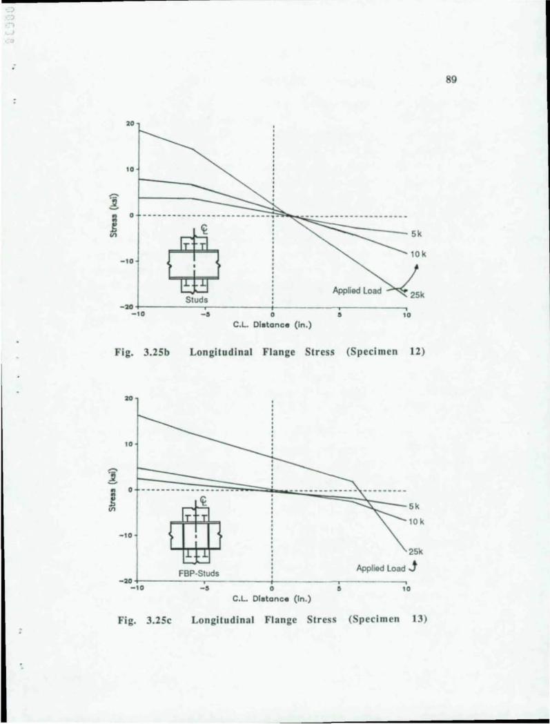
20

'0

o r---=----~----~----~----~----~---:~,-~~== Sk

10 k -.0

Applied Load Studs

-20 ~--------~----------~----------r----------, -1 0 - 5 o • 10

C.L DI.tance (In .)

Fig. 3.2Sb Longitudinal Flange Stress ( pecimen 12)

20

. 0

! ., 0 ... ------------------

~ ~ TOO ' T

-'0 : l.+l

5k

10 k

25k

Applied Load J FBP-Studs

-20 ~---------r--------~~--------~---------, -10 -$ o 10

C.L DI.tance (In.)

Fig. 3.2Sc Longitudin al Fl ange Stress ( peci men 13)

89

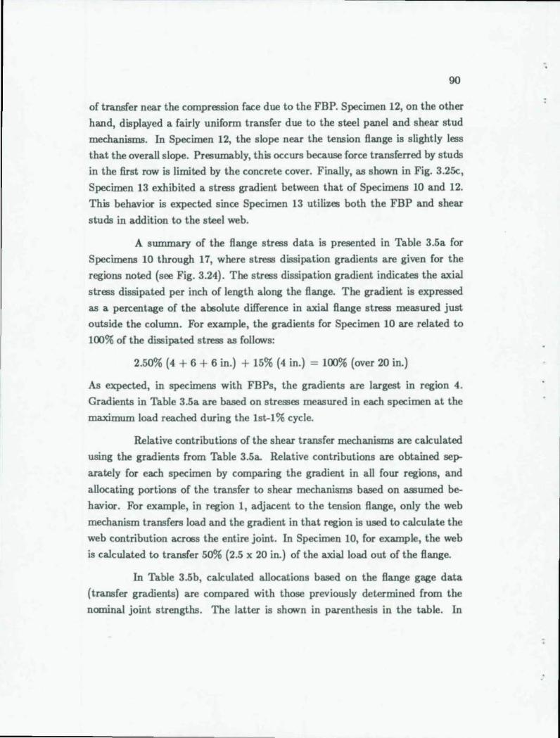
90

of transfer near the compression face due to the FBP. Specimen 12, on the other

hand, displayed a fairly uniform transfer due to the steel panel and shear stud

mechanisms. In Specimen 12, the slope near the tension flange is slightly less

that the overall slope. Presumably, this occurs because force transferred by studs

in the first row is limited by the concrete cover. Finally, as shown in Fig. 3.25c,

Specimen 13 exhibited a stress gradient between that of Specimens 10 and 12.

This behavior is expected since Specimen 13 utilizes both the FBP and shear

studs in addition to the steel web.

A summary of the flange stress data is presented in Table 3.5a for

Specimens 10 through 17, where stress dissipation gradients are given for the

regions noted (see Fig. 3.24). The stress dissipation gradient indicates the axial

stress dissipated per inch of length along the flange. The gradient is expressed

as a percentage of the absolute difference in axial flange stress measured just

outside the column. For example, the gradients for Specimen 10 are related to

100% of the dissipated stress as follows:

2.50% (4 + 6 + 6 in.) + 15% (4 in.) = 100% (over 20 in.)

As expected, in specimens with FBPs, the gradients are largest in region 4.

Gradients in Table 3.5a are based on stresses measured in each specimen at the

maximum load reached during the lst-1% cycle.

Relative contributions of the shear transfer mechanisms are calculated

using the gradients from Table 3.5a. Relative contributions are obtained sep­

arately for each specimen by comparing the gradient in all four regions, and

allocating portions of the transfer to shear mechanisms based on assumed be­

havior. For example, in region 1, adjacent to the tension flange, only the web

mechanism transfers load and the gradient in that region is used to calculate the

web contribution across the entire joint. In Specimen 10, for example, the web

is calculated to transfer 50% (2.5 x 20 in.) of the axial load out of the flange.

In Table 3.5b, calculated allocations based on the flange gage data

(transfer gradients) are compared with those previously determined from the

nominal joint strengths. The latter is shown in parenthesis in the table. In

,

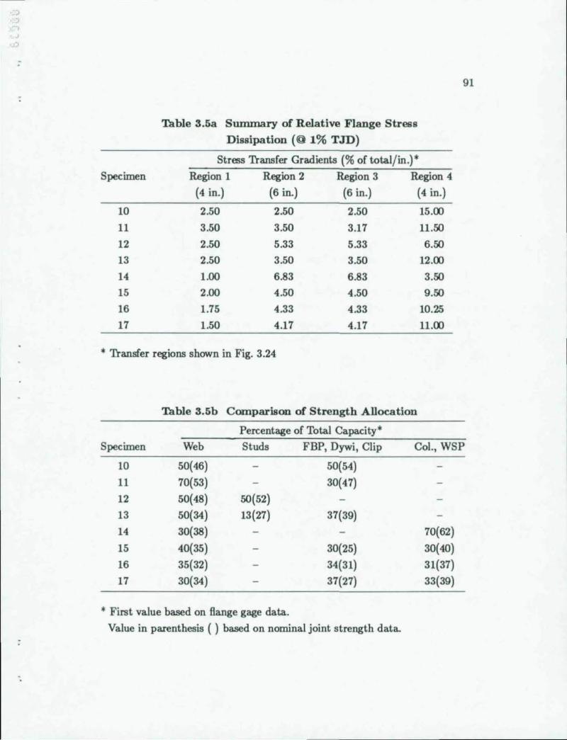
91

Table 3.5a Summary of Relative Flange Stress

Dissipation (@ 1% TJD)

Stress Transfer Gradients (% of total/in.)·

Specimen Region 1 Region 2 Region 3 Region 4

(4 in.) (6 in.) (6 in.) (4 in.)

10 2.50 2.50 2.50 15.00

11 3.50 3.50 3.17 11.50

12 2.50 5.33 5.33 6.50 13 2.50 3.50 3.50 12.00

14 1.00 6.83 6.83 3.50

15 2.00 4.50 4.50 9.50

16 1.75 4.33 4.33 10.25

17 1.50 4.17 4.17 11.00

* Transfer regions shown in Fig. 3.24

Table 3.5b Comparison of Strength Allocation

Percentage of Total Capacity· Specimen Web Studs FBP, Dywi, Clip Col., WSP

10 50(46) 50(54)

11 70(53) 30(47)

12 50(48) 50(52)

13 50(34) 13(27) 37(39)

14 30(38) 70(62)

15 40(35) 30(25) 30(40)

16 35(32) 34(31) 31(37)

17 30(34) 37(27) 33(39)

• First value based on flange gage data.

Value in parenthesis ( ) based on nominal joint strength data.

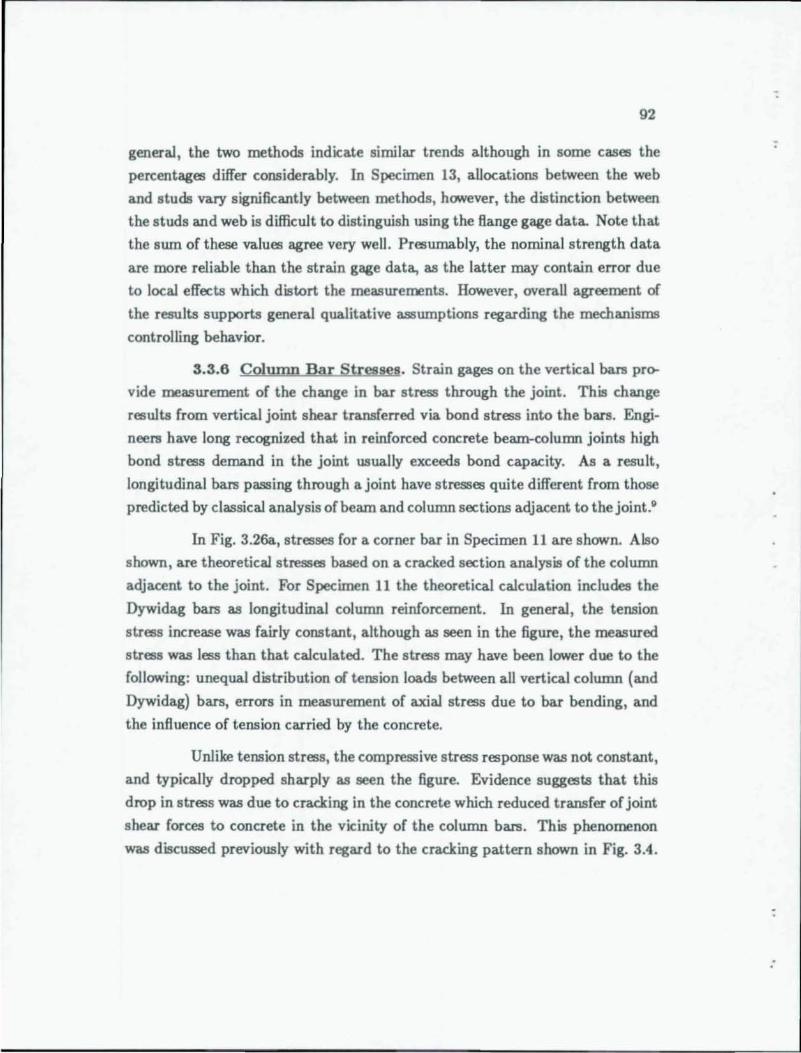
92

general, the two methods indicate similar trends although in some cases the

percentages differ considerably. In Specimen 13, allocations between the web

and studs vary significantly between methods, however, the distinction between

the studs and web is difficult to distinguish using the flange gage data. Note that

the sum of these values agree very well. Presumably, the nominal strength data

are more reliable than the strain gage data, as the latter may contain error due

to local effects wltich distort the measurements. However, overall agreement of

the results supports general qualitative assumptions regarding the mechanisms

controlling behavior.

S.S.6 Colwnn Bar Stresses. Strain gages on the vertical bars pr(;

vide measurement of the change in bar stress through the joint. This change

results from vertical joint shear transferred via bond stress into the bars. Engi­

neers have long recognized that in reinforced concrete beam-column joints high

bond stress demand in the joint usually exceeds bond capacity. As a result,

longitudinal bars passing through a joint have stresses quite different from those

predicted by classical analysis of beam and column sections adjacent to thejoint."

In Fig. 3.200, stresses for a corner bar in Specimen 11 are shown. Also

shown, are theoretical stresses based on a cracked section analysis of the column

adjacent to the joint. For Specimen 11 the theoretical calculation includes the

Dywidag bars as longitudinal column reinforcement. In general, the tension

stress increase was fairly constant, although as seen in the figure, the measured

stress was less than that calculated. The stress may have been lower due to the

following: unequal distribution of tension loads between all vertical column (and

Dywidag) bars, errors in measurement of axial stress due to bar bending, and

the influence of tension carried by the concrete.

Unlike tension stress, the compressive stress response was not constant,

and typically dropped sharply as seen the figure. Evidence suggests that this

drop in stress was due to cracking in the concrete which reduced transfer of joint

shear forces to concrete in the vicinity of the column bars. This phenomenon

was discussed previously with regard to the cracking pattern shown in Fig. 3.4.

. )

;

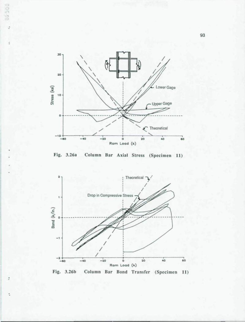
JO

20

~ .=!.

" 10

" " ~ U>

- 10 -80

Fig. 3.26a

2

- 1

\ \

\

-40

\ \ ~

./

- 20

Lower Gage

" '- -< Theoretical

0 20 40

Ram Lood (k)

Column Bar Axial Stress (Specimen

: Theoretical ,,/

/ /

Drop in Compressive Stress , I~~

I /

/

: ~ .

80

11)

/ -2 +-------,---~~,-------~------~------~4~O------~80 -110 -40 - 20 0 20

Ram Load (k)

Fig. 3.26b Column Bar Bond Transfer (Specimen 11 )

93

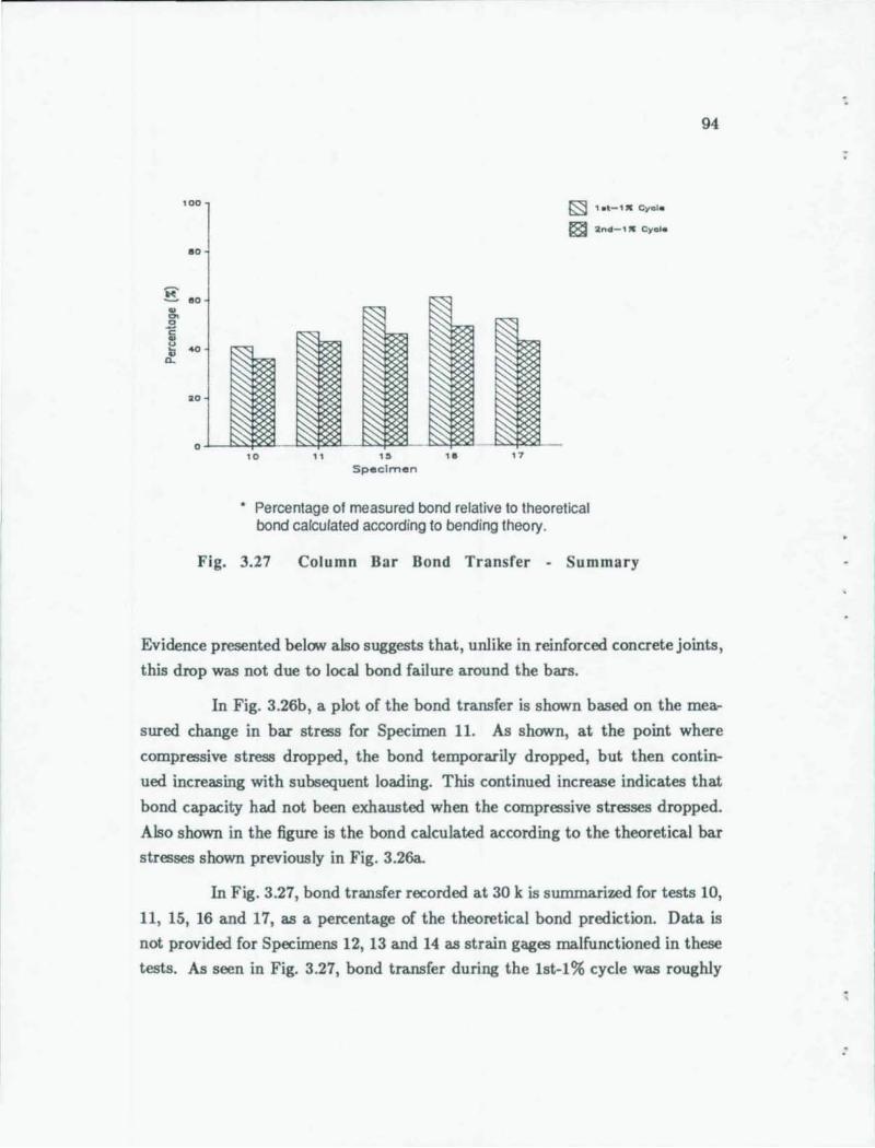
E .. '" ~ .. ~ a..

.00

ao

ao

.0

20

0 '0 " ..

Specimen .. 17

~ , .t-," CyQI.

~ 2n~-1" Cy al.

Percentage of measured bond relative to theoretical bond calculated according to bending theory.

Fig. 3.27 Column Bar Bond Transfer - Summary

94

Evidence presented below also suggests that. unlike in reinforced concrete joints,

this drop was not due to local bond failure around the bars.

In Fig. 3.26b, a plot of the bond transfer is shown based on the mea­

sured change in bar stress for Specimen 11. As shown, at the point where

compressive stress dropped, the bond temporarily dropped, but then contin­

ued increasing with subsequent loading. This continued increase indicates that

bond capacity had not been exhausted when the compressive stresses dropped.

Also shown in the figure is the bond calculated according to the theoretical bar

stresses shown previously in Fig. 3.26a.

In Fig. 3.27, bond transfer recorded at 30 k is summarized for tests 10,

11, 15, 16 and 17, as a percentage of the theoretical bond prediction. Data is

not provided for Specimens 12, 13 and 14 as strain gages malfunctioned in these

tests. As seen in Fig. 3.27, bond transfer during the 1st-1 % cycle was roughly

:

..

;

:

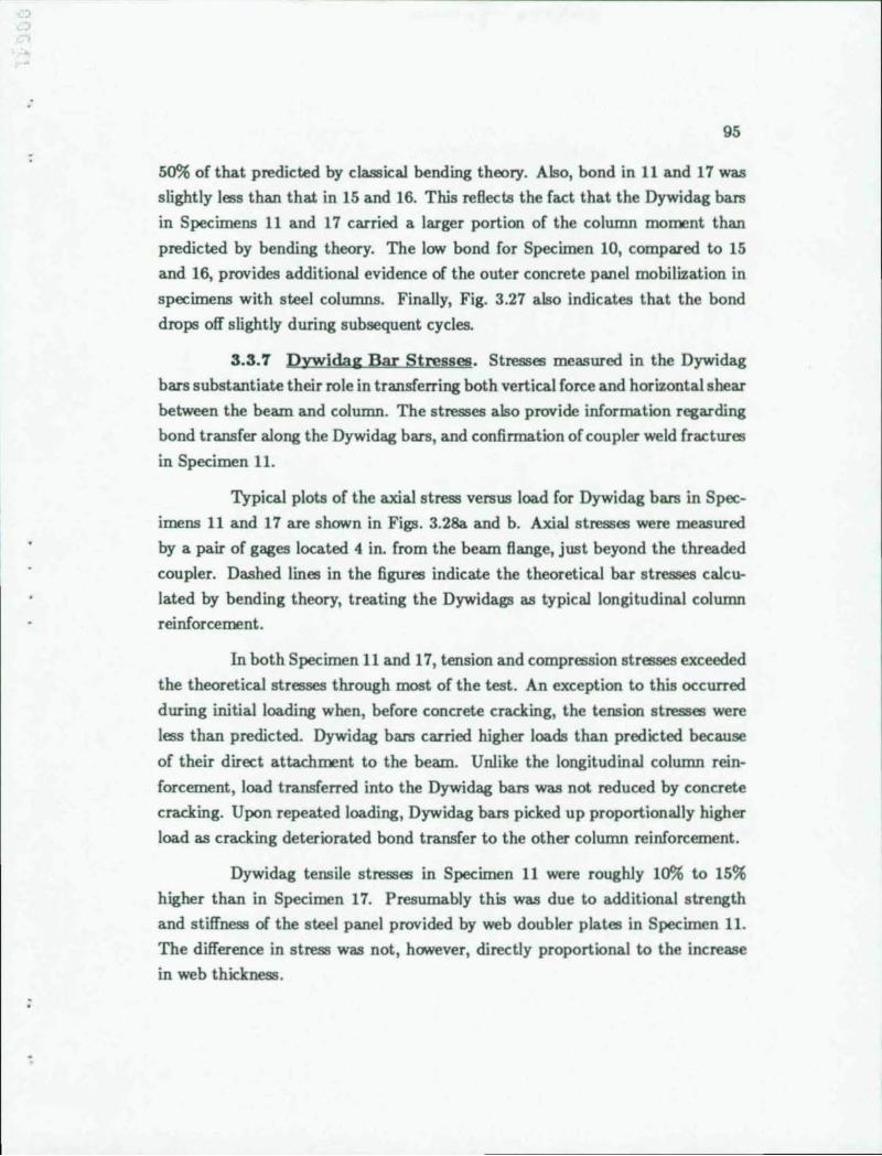
95

50% of that predicted by classical bending theory. Also, bond in 11 and 17 was

slightly less than that in 15 and 16. This reflects the fact that the Dywidag ban!

in Specimens 11 and 17 carried a larger portion of the column moment than

predicted by bending theory. The low bond for Specimen 10, compared to 15

and 16, provides additional evidence of the outer concrete panel mobilization in

specimens with steel columns. Finally, Fig. 3.27 also indicates that the bond

drops off slightly during subsequent cycles.

3.3.7 Dvwidag Bar Stresses. Stresses measured in the Dywidag

bars substantiate their role in transferring both vertical force and horizontal shear

between the beam and column. The stresses also provide information regarding

bond transfer along the Dywidag bars, and confirmation of coupler weld fractures

in Specimen 11.

Typical plots of the axial stress versus load for Dywidag bars in Spec­

imens 11 and 17 are shown in Figs. 3.2& and b. Axial stresses were measured

by a pair of gages located 4 in. from the beam flange, just beyond the threaded

coupler. Dashed lines in the figures indicate the theoretical bar stresses calcu­

lated by bending theory, treating the Dywidags as typical longitudinal column

reinforcement.

In both Specimen 11 and 17, tension and compression stresses exceeded

the theoretical stresses through most of the test. An exception to this occurred

during initial loading when, before concrete cracking, the tension stresses were

less than predicted. Dywidag bars carried higher loads than predicted because

of their direct attachment to the beam. Unlike the longitudinal column rein­

forcement, load transferred into the Dywidag bars was not reduced by concrete

cracking. Upon repeated loading, Dywidag ban! picked up proportionally higher

load as cracking deteriorated bond transfer to the other column reinforcement.

Dywidag tensile stresses in Specimen 11 were roughly 10% to 15%

higher than in Specimen 17. Presumably this was due to additional strength

and stiffness of the steel panel provided by web doubler plates in Specimen 11.

The difference in stress was not, however, directly proportional to the increase

in web thlckness.

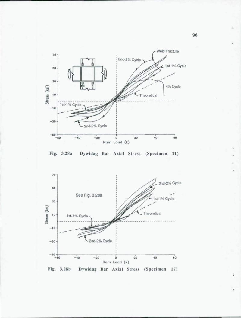
~ " " ~ VI

c-g " " ~

VI

70

.0 a '1

A'-""'" A. 1 st-1 % Cycle

\ 30

~I ~ 40/0 Cycle "V

10

-10

- 30

2nd-2% Cycle

-.o+-------~------~------+_------~------~----__, - 00

Fig_ 3_28a

70

.0

30

-40 -20 o 20 40 00

Ram Load (k)

Dywidag Bar Axia l Stress (Specimen 11)

See Fig. 3 .28a

2nd-2% Cycle

./

1st-1% Cycle

10 1 st -1 % Cycle

- 10 -----30 2nd-2% Cycle

-.0 +-------,-------,-------+-------,-------,---------ao -40 - 20 0 20 40 80

Ram Load (k)

Fig. 3.28b Dywidag Bar Axial Stress (Speci men 17)

96

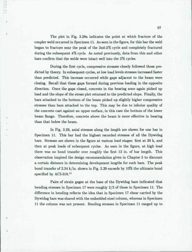
97

The plot in Fig. 3.2& indicates the point at which fracture of the

coupler weld occurred in Specimen 11. As seen in the figure, for this bar the weld

began to fracture near the peak of the 2nd-2% cycle and completely fractured

during the subsequent 4% cycle. As noted previously, data from this and other

bars confirm that the welds were intact well into the 2% cycles.

During the first cycle, compressive stresses closely followed those pre­

dicted by theory. In subsequent cycles, at low load levels stresses increased faster

than predicted. This increase occurred while gaps adjacent to the beam were

closing. Recall that these gaps formed during previous loading in the opposite

direction. Once the gaps closed, concrete in the bearing zone again picked up

load and the slope of the stress plot returned to the predicted slope. Finally, the

bars attached to the bottom of the beam picked up slightly higher compressive

stresses than bars attached to the top. This may be due to inferior quality of

the concrete cast against an upper surface, in this case the bottom of the lower

beam flange. Therefore, concrete above the beam is more effective in bearing

than that below the beam.

In Fig. 3.29, axial stresses along the length are shown for one bar in

Specimen 11. This bar had the highest recorded stresses of all the Dywidag

bars. Stresses are shown in the figure at various load stages: first at 30 k, and

then at peak loads of subsequent cycles. As seen in the figure, at high load

there was no bond transfer over roughly the first 12 in. of bar length. This

observation inspired the design recommendation given in Chapter 5 to discount

a certain distance in determining development lengths for such bars. The peak

bond transfer of 2.34 k/ in. shown in Fig. 3.29 exceeds by 10% the ultimate bond

specified by ACI-318.16

Pairs of strain gages at the base of the Dywidag bars indicated that

bending stresses in Specimen 17 were roughly 2/3 of those in Specimen 11. The

difference in bending reflects the idea that in Specimen 17 shear carried by the

Dywidag bars was shared with the embedded steel column, whereas in Specimen

11 the column was not present. Bending stresses in Specimen 11 ranged up to

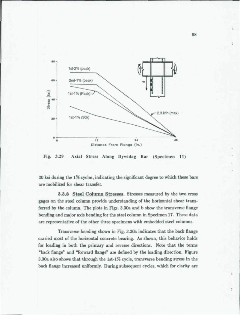
00

1 sl·2% (peak)

80 2nd·l % (peak)

.. 40 .. ~ en

20

0+-------------, - ~ Q 12 24

Distance From Flange (in .)

>

-0

y

2.3 klin (max)

Fig. 3.29 Axial Stress Along Dywidag Bar (Specimen 11)

98

30 ksi during the 1 % cycles, indicating the significant degree to which these bars

are mobilized for shear transfer.

3.3.8 Steel Column Stresses. Stresses measured by the two cross

gages on the steel column provide understanding of the horizontal shear trans­

ferred by the column. The plots in Figs. 3.3Oa and b show the transverse flange

bending and major axis bending for the steel column in Specimen 17. These data

are representative of the other three specimens with embedded steel columns.

'fransverse bending shown in Fig. 3.3Oa indicates that the back flange

carried most of the horizontal concrete bearing. As shown, this behavior holds

for loading in both the primary and reverse directions. Note that the terms

"back flange~ and "forward flange~ are defined by the loading direction. Figure

3.3Oa also shows that through the 1st-I % cycle, transverse bending stress in the

back flange increased uniformly. During subsequent cycles, which for clarity are

.-

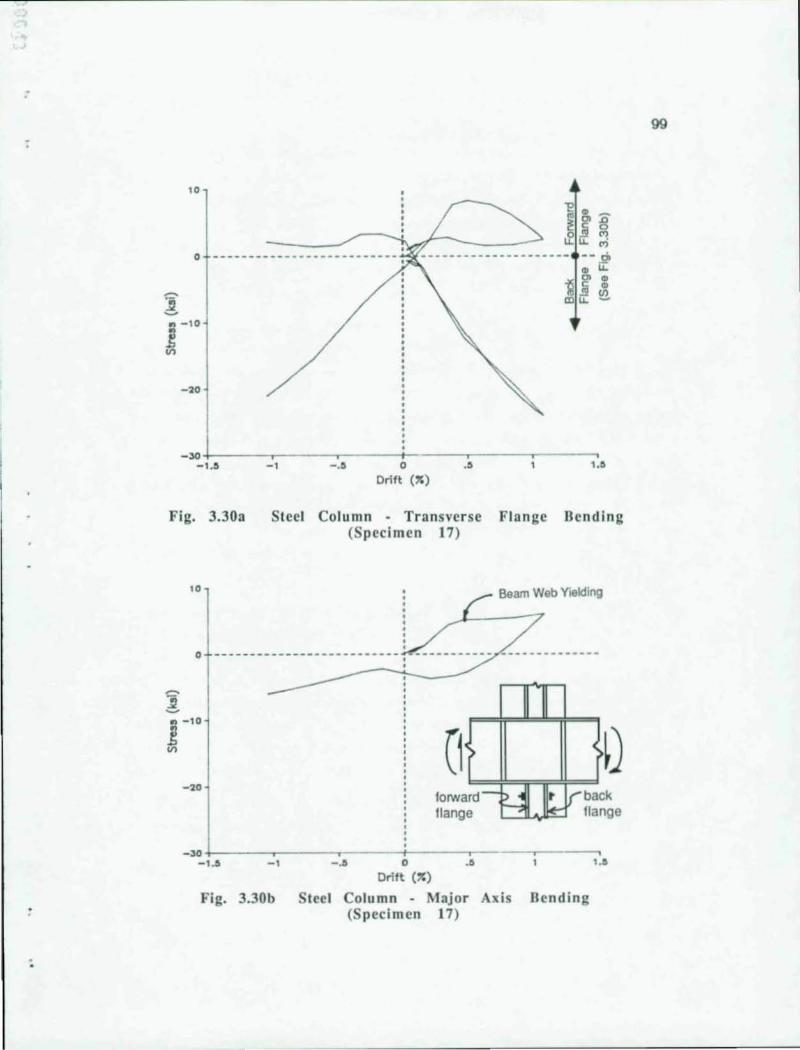
10

o ---------------- --- -------

11 .. nI 0) n L~ l'I

u.. u.. '" --------------------- -- a

co it

'" '" co ~ lij co co it !!l.

., -10

~ -20

-~+-----~------~----~~.----_r, ------r_----_" -1.5 -1 -. e. O.S 1.S

Drift (%)

Fig. 3.30a Steel Column - Transverse Flange Bending (S pecimen 17)

'0

., -10

~ -20

.:

rd--foowa liang e ~ t

~

~

V'ba fla

ck nge

-~+-----~------~----~~----_r------r_----_, -1 .5 -1 -.5 .5 1.e

Fig. 3.30b

Drift (%)

teel Column - Major Axis Bending (Specimen 17)

99

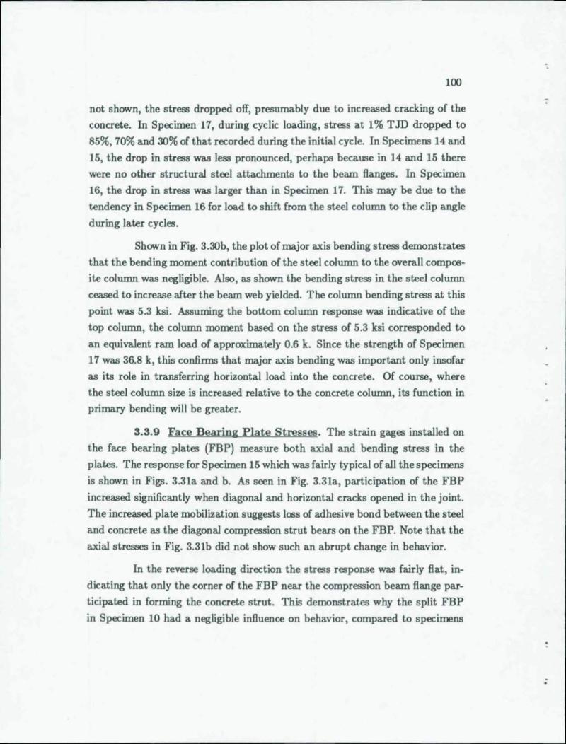
100

not shown, the stress dropped off, presumably due to increased cracking of the

concrete. In Specimen 17, during cyclic loading, stress at 1% TID dropped to

85%,70% and 30% of that recorded during the initial cycle. In Specimens 14 and

15, the drop in stress was less pronounced, perhaps because in 14 and 15 there

were no other structural steel attachments to the beam Banges. In Specimen

16, the drop in stress was larger than in Specimen 17. This may be due to the

tendency in Specimen 16 for load to shift from the steel column to the clip angle

during later cycles.

Shown in Fig. 3.30b, the plot of major axis bending stress demonstrates

that the bending moment contribution of the steel column to the overall compos­

ite column was negligible. Also, as shown the bending stress in the steel column

ceased to increase after the beam web yielded. The column bending stress at this

point was 5.3 ksi. Assuming the bottom column response was indicative of the

top column, the column moment based on the stress of 5.3 ksi corresponded to

an equivalent ram load of approximately 0.6 k. Since the strength of Specimen

17 was 36.8 k, this confirms that major axis bending was important only insofar

as its role in transferring horizontal load into the concrete. Of course, where

the steel column size is increased relative to the concrete column, its function in

primary bending will be greater.

3.3.9 Face Bearing Plate Stresses. The strain gages installed on

the face bearing plates (FBP) measure both axial and bending stress in the

plates. The response for Specimen 15 which was fairly typical of all the specimens

is shown in Figs. 3.31a and b. As seen in Fig. 3.31a, participation of the FBP

increased significantly when diagonal and horizontal cracks opened in the joint.

The increased plate mobilization suggests loss of adhesive bond between the steel

and concrete as the diagonal compression strut bears on the FBP. Note that the

axial stresses in Fig. 3.31b did not show such an abrupt change in behavior.

In the reverse loading direction the stress response was fairly Bat, in­

dicating that only the corner of the FBP near the compression beam flange par­

ticipated in forming the concrete strut. This demonstrates why the split FBP

in Specimen 10 had a negligible influence on behavior, compared to specimens

'.

:

.-

:

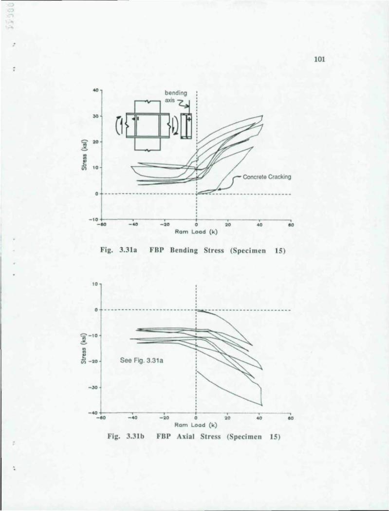
40 bending

] Vl 10 if Concrete Cracking

-10+-------,-------,-------~------,_------,_----~ -00 -20 o 20 40

Rom Load (k)

Fig. 3.31a FBP Bending Stress (Speci men 15)

10

1-10

.. .. 1: Vl -20 See Fig. 3.31 a

-30

-40 +------.-----r-----<>---- -~. ---..... ---eo -40 -20 20 40

Rom Load (k)

Fig. 3.31 b FBP A ial Sires ( pecimen IS)

10

eo

101

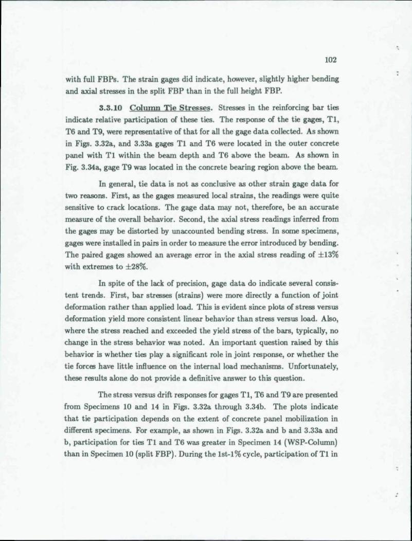
102

with full FBPs. The strain gages did indicate, however, slightly higher bending

and axial stresses in the split FBP than in the full height FBP.

3.3.10 Column Tie Stresses. Stresses in the reinforcing bar ties

indicate relative participation of these ties. The response of the tie gages, Tl,

T6 and T9, were representative of that for all the gage data collected. As shown

in Figs. 3.32a, and 3.33a gages Tl and T6 were located in the outer concrete

panel with Tl within the beam depth and T6 above the beam. As shown in

Fig. 3.34a, gage T9 was located in the concrete bearing region above the beam.

In general, tie data is not as conclusive as other strain gage data for

two reasons. First, as the gages measured local strains, the readings were quite

sensitive to crack locations. The gage data may not, therefore, be an accurate

measure of the overall behavior. Second, the axial stress readings inferred from

the gages may be distorted by unaccounted bending stress. In some specimens,

gages were installed in pairs in order to measure the error introduced by bending.

The paired gages showed an average error in the axial stress reading of ±13%

with extremes to ±28%.

In spite of the lack of precision, gage data do indicate several consis­

tent trends. First, bar stresses (strains) were more directly a function of joint

deformation rather than applied load. This is evident since plots of stress versus

deformation yield more consistent linear behavior than stress versus load. Al<lo,

where the stress reached and exceeded the yield stress of the bars, typically, no

change in the stress behavior was noted. An important question raised by this

behavior is whether ties playa significant role in joint response, or whether the

tie forces have little influence on the internal load mechanisms. Unfortunately,

these results alone do not provide a definitive answer to this question.

The stress versus drift responses for gages Tl, T6 and T9 are presented

from Specimens 10 and 14 in Figs. 3.32a through 3.34b. The plots indicate

that tie participation depends on the extent of concrete panel mobilization in

different specimens. For example, as shown in Figs. 3.32a and band 3.33a and

b, participation for ties Tl and T6 was greater in Specimen 14 (WSP-Column)

than in Specimen 10 (split FBP). During the lst-l % cycle, participation of Tl in

:

.-

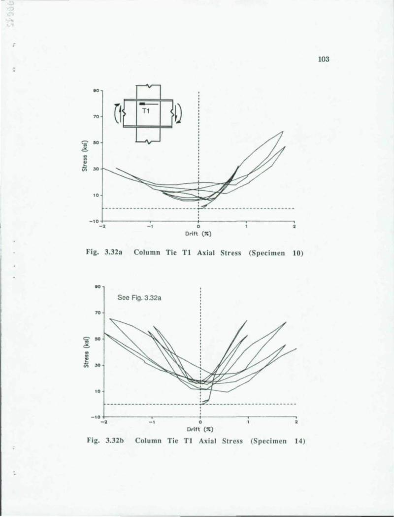
103

00

(1 - Q T1 70

~ .0; SO

~ .. .. .. ;;; '0

.0

-,o+---------~~--------~----------~--------~ -2 -t 0 2

Drift (:c)

Fig. 3.323 Column Tie Tl Axial tress (Specimen 10)

See Rg. 3.32a

70

'ii 50

~ .. .. .. .!> >0 VI

.0

-.o+---------~----------~-----------~--------~o -2 -, 0 2

Drift (:c)

Fig. 3.32b Column Tie T1 Axial Stress (pecimen 14)

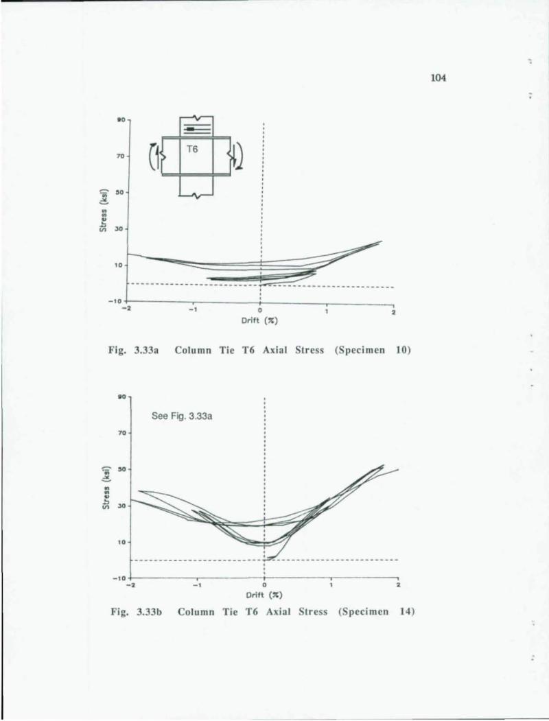
-7D (1'>

T6 ~~) • · ~

"" '0;

~ ~ •

y · • • ~ ~

~ 30 VI

· · · • • • • •

~ • • • -'0

· ~

• ~

~.- - ----------------------~ --------------------------•

-'0 • -2 o

Drift (") 2

Fig. 3.33a Column Tie T6 Axial Stress (Specimen 10)

~

'0;

~ ~ ~

" .!:> VI

See Fig. 3.33a

70

$0

3D

'0

-'O+-----------~----------T_----------~--------__, - 2 -, o

Drift (X) 2

Fig. 3.33b Column Tie T6 Axial Stre S (Speci men 14)

104

. ,

•

.-

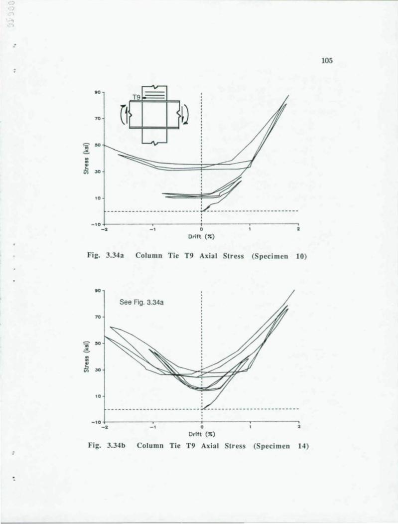
lOS

00 T9

70 C1 0 ~ .0 ';; C .. .. .. .::.

~ Vl

10

-IO+-----------~----------+_----------~--------~ -2 -1 0 2

Drift (,.;)

Fig. 3.343 Column Tic T9 Axial Stress (S pecimen 10)

.., See Fig. 3.34a

70

e-.. .0

c .. .. .. .::. 30 Vl

10

-IO+---------~r_--------~----------,_--------~ -2 -1 0 2

Drift (,.;)

Fig. 3.34b Column Tie T9 Axial Stress ( pccimcn 14) ;

106

Specimens 14 through 17 was roughly 50% greater than in Specimen 10, and in

Specimens 11 and 12 was 20% greater than in Specimen 10. Also, participation

for T6 in Specimens 11 through 17 was approximately 150% greater than in

Specimen 10.

Also seen in Figs. 3.32a through 3.33b, in the reverse direction, partic­

ipation of Tl and T6 was negligible in Specimen 10, whereas in 14 it was almost

equal to that in the primary direction. This behavior indicates that where joint

details utilize shear capacity of the outer concrete panel, ties in that panel carry

forces associated with truss action. The truss mechanism relies on the tension

capacity of the ties in both directions of loading. This behavior in Specimen 14

was also seen in the other specimens.

Response of T9 demonstrates a different type of behavior. As seen in

Fig. 3.34a and b, in the primary loading direction, tie participation was similar in

Specimens 10 and 14 where T9 provided confinement to concrete in the bearing

zone. The response of T9 in Specimens 15 and 17 was similar. In Specimens 11,

12, 13 and 16, where details such as shear studs or the clip angle also provided

confinement, participation of T9 was 30% to 60% less. When loading in the

reverse direction, participation of T9 was negligible in Specimen 10 as concrete

in the region was no longer in compression. However, in Specimen 14 (and other

specimens with attachments to the outside of the flanges), T9 participated to a

similar degree as in the primary direction. In such cases, T9 presumably resisted

load generated by the horizontal strut formation, shown earlier in Fig. 3.15.

Finally, ties within the beam depth showed a larger reduction in stress

during subsequent cycles than those outside the beam depth. This may be due to

the use of 90 degree cap ties within the beam depth and closed rectangular hoops

outside. Hence, the larger stress reduction may be due to bond and anchorage

deterioration of the cap ties. Another contributing factor may be that concrete

within the beam depth is cracked more extensively than that outside.

3.3.11 Dissection of Specimens. Several of the specimens were

dissected after testing in order to examine condition of concrete within the joint.

Concrete was carefully removed with a pneumatic jackhammer. Typically, one

-.

;

, ) ...,

:

:

107

side of the joint was opened with the jackha=er and the beam removed, re­

vealing the opposite side of the joint which was still intact.

The general condition of concrete in the joint is shown in Fig. 3.35.

Concrete in the inner panel showed extensive diagonal cracking. With the joint

opened, most of the inner panel concrete could easily be removed with a hand

held chipping hammer. In Specimen 12, which did not have FBPs, concrete in

the inner panel was not extensively cracked.

Between the inner and outer panels was a layer of pulverized concrete

where the largest pieces were approximately 3/4 in. Presumably, such damage

occurred due to rotation of the steel beam (and captive inner panel) within the

outer concrete panel. Rotation during the initial cycle probably formed a crack

plane between the panels. During subsequent cyclic reversals, concrete adjacent

to the crack was worn through abrasion.

In the outer panel concrete was damaged to varying degrees, roughly

related to the observed mobilization of the outer panel. In Specimen 10, for

example, the outer panel was cracked but still rather intact. On the other hand,

in Specimens 12 and 13 the outer panel was cracked so extensively such that when

the lateral ties were loosened concrete fell apart in 2 to 4 in. pieces. This damage

highlights the need for lateral ties which, as a minimum, provide confinement to

hold damaged concrete in place.

A concrete fragment removed from below the upper flange is shown in

Fig. 3.36. This sample shows the typical condition of concrete cast against an

upper surface. In general, voids 1/8 in. thick and up to 2 in. diameter were found

below the top and bottom flanges. These voids formed in spite of careful concrete

placement and vibration, and high concrete slumps (6 to 7 in.). The condition

of this concrete demonstrates the importance of casting the test components in

a manner similar to actual practice. In this case, vertical casting ensures that

test results will be indicative of the concrete properties expected in the field. As

it is unlikely that field conditions will be better than those in the laboratory,

it should be accepted that these voids will occur, and joints should be designed

taking into account imperfect concrete consolidation.

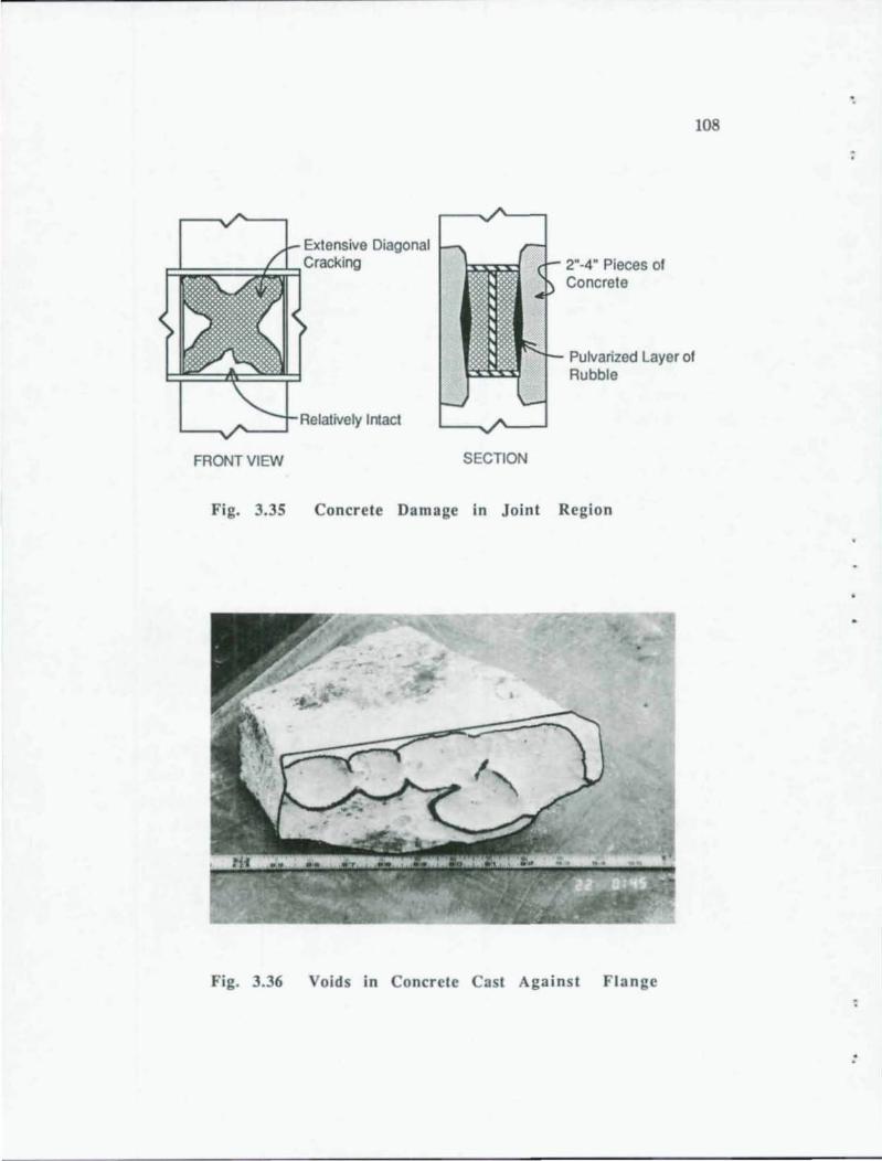
Extensive Diagonal ...... ____ +-.......,Cracking

Relatively Intact

FRONT VIEW SECTION

2""4" Pieces of Concrete

Pulvarized Layer of Rubble

Fig. 3.35 Concrete Damage in Joint Region

Fig. 3.36 Voids in Concrete Cast Against Flange

".

108

:

·~ , • ,

;

----------

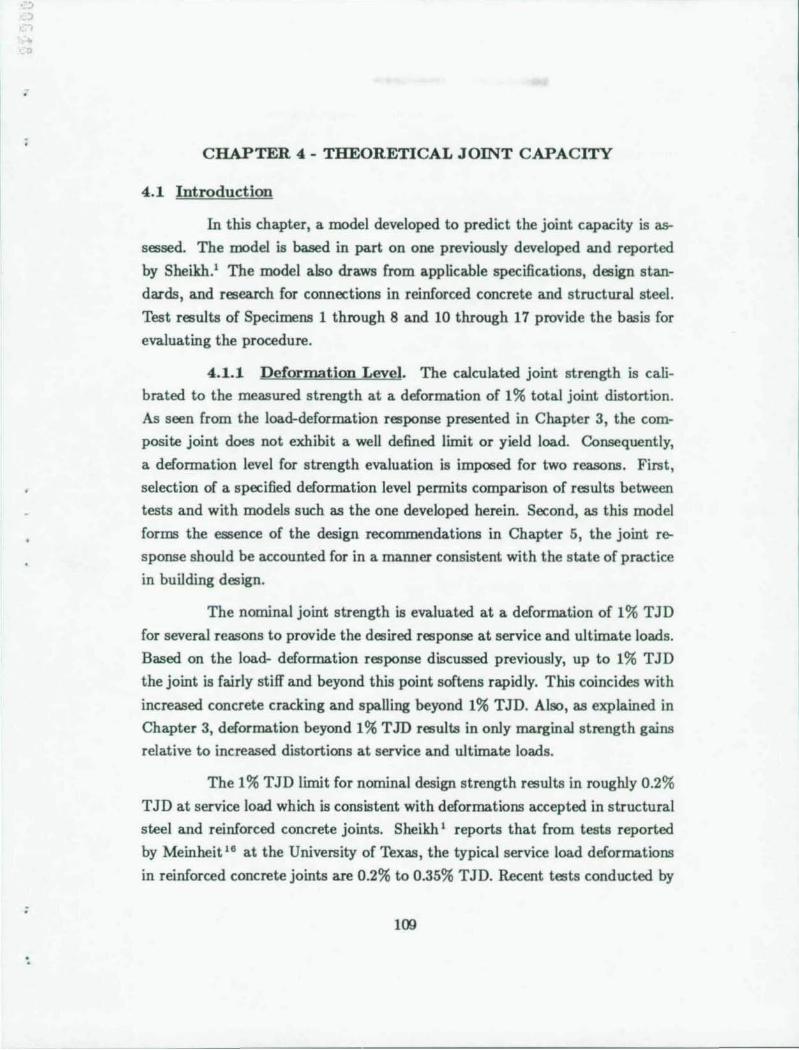
CHAPTER 4 - THEORETICAL JOINT CAPACITY

4.1 Introduction

In this chapter, a model developed to predict the joint capacity is as­

sessed. The model is based in part on one previously developed and reported

by Sheikh.' The model also draws from applicable specifications, design stan­

dards, and research for connections in reinforced concrete and structural steel.

Test results of Specimens 1 through 8 and 10 through 17 provide the basis for

evaluating the procedure.

4.1.1 Deformation Level. The calculated joint strength is cali­

brated to the measured strength at a deformation of 1 % total joint distortion.

As seen from the load-deformation response presented in Chapter 3, the com­

posite joint does not exhibit a well defined limit or yield load. Consequently,

a deformation level for strength evaluation is imposed for two reasons. First,

selection of a specified deformation level permits comparison of results between

tests and with models such as the one developed herein. Second, as this model

forms the essence of the design recommendations in Chapter 5, the joint re­

sponse should be accounted for in a manner consistent with the state of practice

in building design.

The nominal joint strength is evaluated at a deformation of 1% TJD

for several reasons to provide the desired response at service and ultimate loads.

Based on the load- deformation response discussed previously, up to 1% TJD

the joint is fairly stiff and beyond this point softens rapidly. This coincides with

increased concrete cracking and spaUing beyond 1% TJD. Also, as explained in

Chapter 3, deformation beyond 1% TID results in only marginal strength gains

relative to increased distortions at service and ultimate loads.

The 1% TJD limit for nominal design strength results in roughly 0.2%

T JD at service load which is consistent with deformations accepted in structural

steel and reinforced concrete joints. Sheikh' reports that from tests reported

by Meinheit ,. at the University of Texas, the typical service load deformations

in reinforced concrete joints are 0.2% to 0.35% TJD. Recent tests conducted by

109

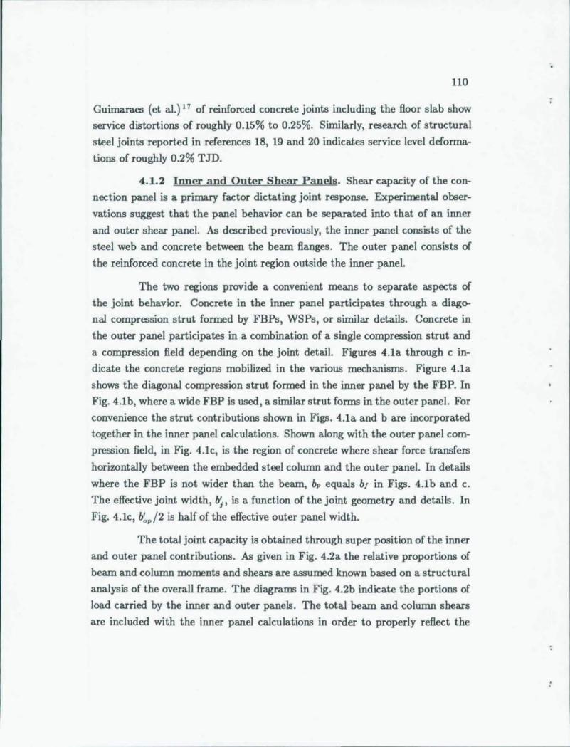
110

Guimara.es (et al.) 17 of reinforced concrete joints including the floor slab show

service distortions of roughly 0.15% to 0.25%. Similarly, research of structural

steel joints reported in references 18, 19 and 20 indicates service level deforma­

tions of roughly 0.2% TJD.

4.1.2 Inner and Outer Shear Panels. Shear capacity of the con­

nection panel is a primary factor dictating joint response. Experimental obser­

vations suggest that the panel behavior can be separated into that of an inner

and outer shear panel. AIl described previously, the inner panel consists of the

steel web and concrete between the beam flanges. The outer panel consists of

the reinforced concrete in the joint region outside the inner panel.

The two regions provide a convenient means to separate aspects of

the joint behavior. Concrete in the inner panel participates through a diago­

nal compression strut formed by FBPs, WSPs, or similar details. Concrete in

the outer panel participates in a combination of a single compression strut and

a compression field depending on the joint detail. Figures 4.1a through c in­

dicate the concrete regions mobilized in the various mechanisms. Figure 4.1a

shows the diagonal compression strut formed in the inner panel by the FBP. In

Fig. 4.1b, where a wide FBP is used, a similar strut forms in the outer panel. For

convenience the strut contributions shown in Figs. 4.1a and b are incorporated

together in the inner panel calculations. Shown along with the outer panel com­

pression field, in Fig. 4.1c, is the region of concrete where shear force transfers

horiwntally between the embedded steel column and the outer panel. In details

where the FBP is not wider than the beam, bp equals b, in Figs. 4.1b and c.

The effective joint width,lt,., is a function of the joint geometry and details. In

Fig. 4.lc, b~./2 is half of the effective outer panel width.

The total joint capacity is obtained through super position of the inner

and outer panel contributions. AIl given in Fig. 4.2a the relative proportions of

beam and column moments and shears are assumed known based on a structural

analysis of the overall frame. The diagrams in Fig. 4.2b indicate the portions of

load carried by the inner and outer panels. The total beam and column shears

are included with the inner panel calculations in order to properly reflect the

:

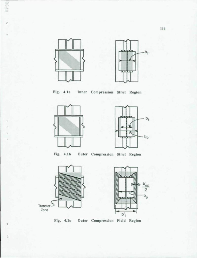
111

A

I""

) > , ,

~ L

Fig. 4.1a Inner Compression trut Region

A A

, , , ! -

> > ~

.('

~ -, bp

A ~

L ....,

Fig. 4.Ib Outer Co mpression Strut Region

Zone

Fig. 4.1 c Outer Compr es ion Field Region ;

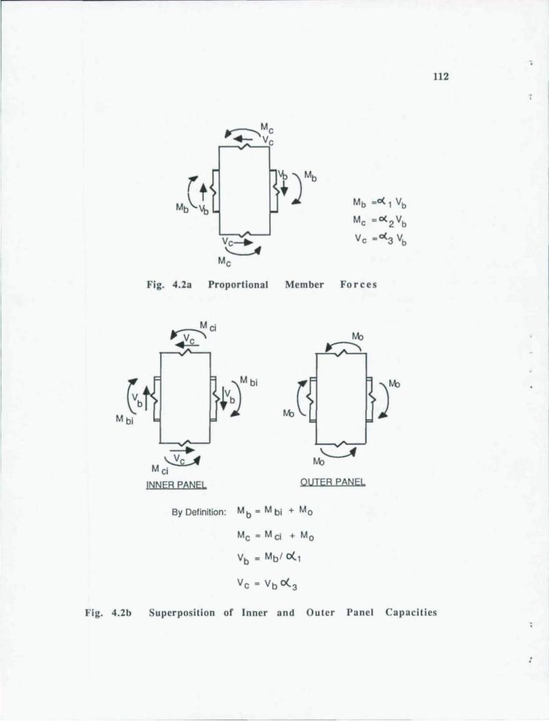
tb

Mbi

Mb =0( 1 Vb

Me = o{2 Vb

Ve = 0(3 Vb

Fig. 4.2a Proportional Member Forces

Mci

~ fv'o ~ ~

t0Mbi

~C ~ fv'o~ ~

Mci

It::It::IEB E~t::IEL Ql.1IEB P~NEL

By Definition: M b = M bi + M 0

MC=MCi +Mo

Vb = Mb/ 0(1

Vc = Vb 0(3

)~

112

Fig. 4.2b Superposition of Inner and Outer Panel Capacities

;

:

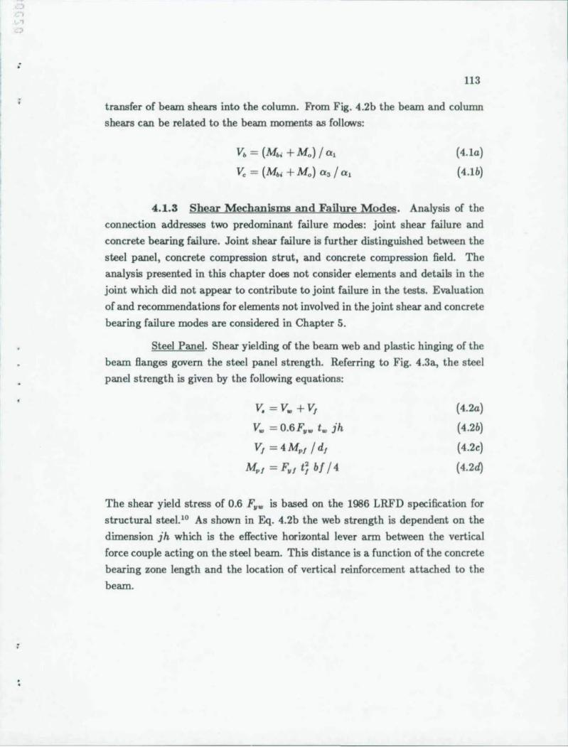
I , ,

:

113

transfer of beam shears into the column. From Fig. 4.2b the beam and column

shears can be related to the beam moments as follows:

Vb = (Mb' +Mo) / £XI

V. = (Mb' + Mo) £X3 / £X,

(4.1a)

(4.1b)

4.1.3 Shear Mechanisms and Failure Modes. Analysis of the

connection addresses two predominant failure modes: joint shear failure and

concrete bearing failure. Joint shear failure is further distinguished between the

steel panel, concrete compression strut, and concrete compression field. The

analysis presented in this chapter does not consider elements and details in the

joint which did not appear to contribute to joint failure in the tests. Evaluation

of and recommendations for elements not involved in the joint shear and concrete

bearing failure modes are considered in Chapter S.

Steel Panel. Shear yielding of the beam web and plastic hinging of the

beam flanges govern the steel panel strength. Referring to Fig. 4.3a, the steel

panel strength is given by the following equations:

v. = V .. + V,

V .. = 0.6F ... t .. ih

V, =4Mp , /d,

Mp , = F., t; bl / 4

(4.2a)

(4.2b)

(4.2c)

(4.2d)

The shear yield stress of 0.6 F... is based on the 1986 LRFD specification for

structural steel." As shown in Eq. 4.2b the web strength is dependent on the

dimension ih which is the effective horizontal lever arm between the vertical

force couple acting on the steel beam. This distance is a function of the concrete

bearing zone length and the location of vertical reinforcement attached to the

beam.

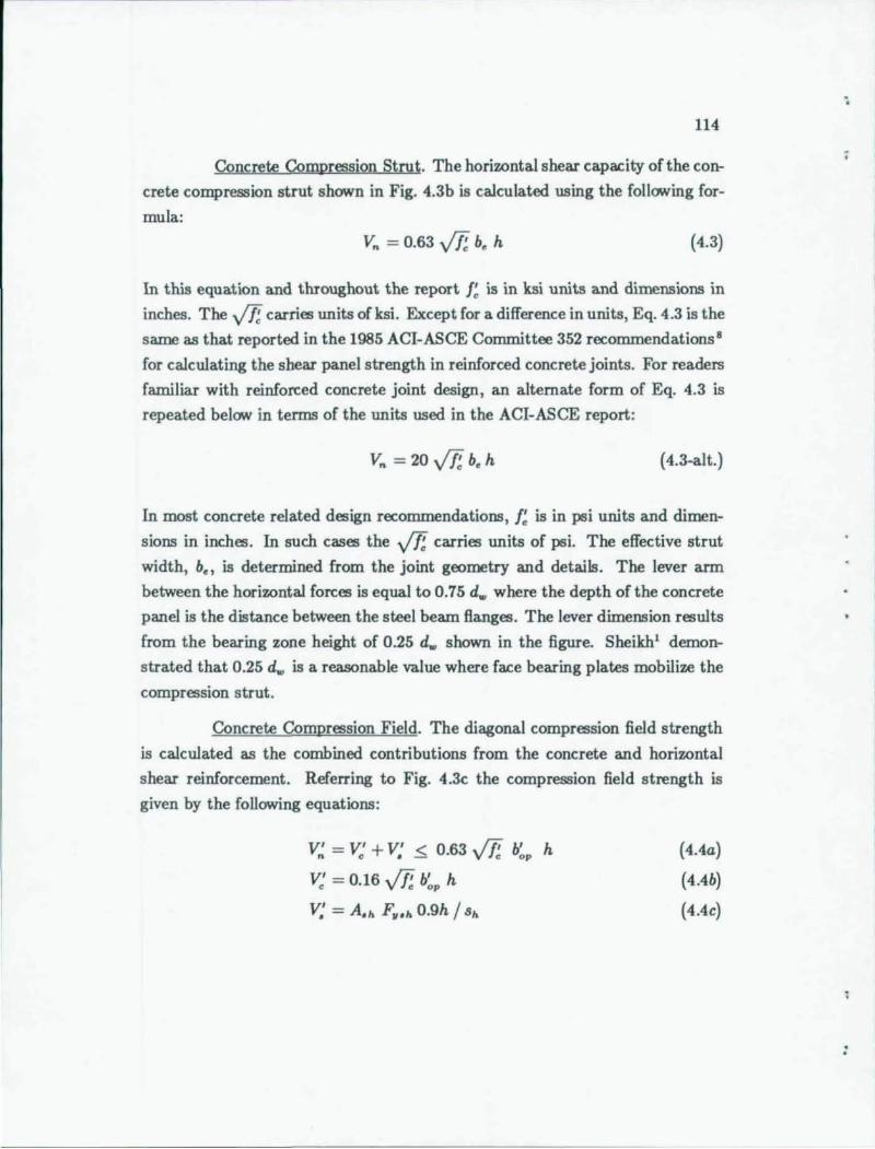
114

Concrete Compression Strut. The horiwntal shear capacity of the con­

crete compression strut shown in Fig. 4.3b is calculated using the following for­

mula:

Vn = 0.63 v'F. b. h (4.3)

In this equation and throughout the report f; is in ksi units and dimensions in

inches. The v'F. carries units of ksi. Except for a difference in units, Eq. 4.3 is the

same as that reported in the 1985 ACI-ASCE Committee 352 reco=endations·

for calculating the shear panel strength in reinforced concrete joints. For readers

familiar with reinforced concrete joint design, an alternate form of Eq. 4.3 is

repeated below in terms of the units used in the ACI-ASCE report:

(4.3-alt. )

In most concrete related design recommendations, f; is in psi units and dimen­

sions in inches. In such cases the .,fff carries units of psi. The effective strut

width, b., is determined from the joint geometry and details. The lever arm

between the horiwntal forces is equal to 0.75 d .. where the depth of the concrete

panel is the distance between the steel beam flanges. The lever dimension results

from the bearing zone height of 0.25 d .. shown in the figure. Sheikh' demon­

strated that 0.25 do. is a reasonable value where face bearing plates mobilize the

compression strut.

Concrete Compression Field. The diagonal compression field strength

is calculated as the combined contributions from the concrete and horiwntal

shear reinforcement. Referring to Fig. 4.3c the compression field strength is

given by the following equations:

V' = V' + V' 0 63 Jr.!., b' h n. c • < . V Je op

V: = 0.16 v'F. b:p h

V; = A.h F •• h 0.9h /8h

- - ------

(4.4a)

( 4.4b)

(4.4c)

;

:

:

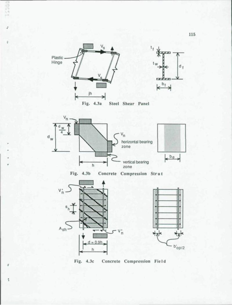
Plastic---' Hinge

jh

Fig. 4.3a

h

Steel Shear Panel

Vn

horizontal bearing zone

vertical bearing zone

Fig. 4.3b Concrete Compression Ir u t

Fig. 4.3c

V' n

oncrele Compression Fie I d

115

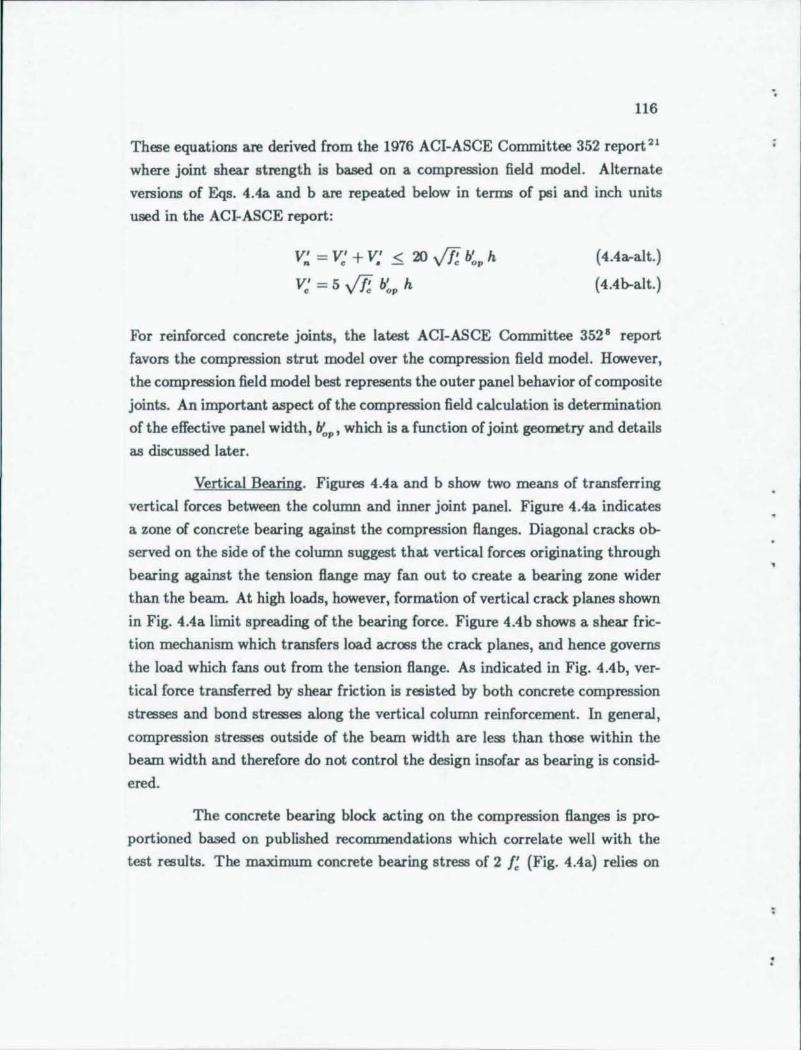
116

These equations are derived from the 1976 ACI-ASCE Committee 352 report 21

where joint shear strength is based on a compression field model. Alternate

versions of Eqs. 4.4a and b are repeated below in terms of Jl5i and inch units

used in the ACI-ASCE report:

V~ = V: + Y,' < 'lJJ VH b:p h

V: = 5 VH y.. h

(4.4 a-al t. )

(4.4b-alt. )

For reinforced concrete joints, the latest ACI-ASCE Committee 352 8 report

favors the compression strut model over the compression field model. However,

the compression field model best represents the outer panel behavior of composite

joints. An important aspect of the compression field calculation is determination

of the effective panel width, y.., which is a function of joint geometry and details

as discussed later.

Vertical Bearing. Figures 4.4a and b show two means of transferring

vertical forces between the column and inner joint panel. Figure 4.4a indicates

a zone of concrete bearing against the compression flanges. Diagonal cracks ob­

served on the side of the column suggest that vertical forces originating through

bearing against the tension flange may fan out to create a bearing zone wider

than the beam. At high loads, however, formation of vertical crack planes shown

in Fig. 4.4a limit spreading of the bearing force. Figure 4.4b shows a shear fric­

tion mechanism which transfers load across the crack planes, and hence governs

the load which fans out from the tension flange. As indicated in Fig. 4.4b, ver­

tical force transferred by shear friction is resisted by both concrete compression

stresses and bond stresses along the vertical column reinforcement. In general,

compression stresses outside of the beam width are less than those within the

beam width and therefore do not control the design insofar as bearing is consid­

ered.

The concrete bearing block acting on the compression flanges is pro­

portioned based on published recommendations which correlate well with the

test results. The maximum concrete bearing stress of 2 f; (Fig. 4.4a) relies on

.,

:

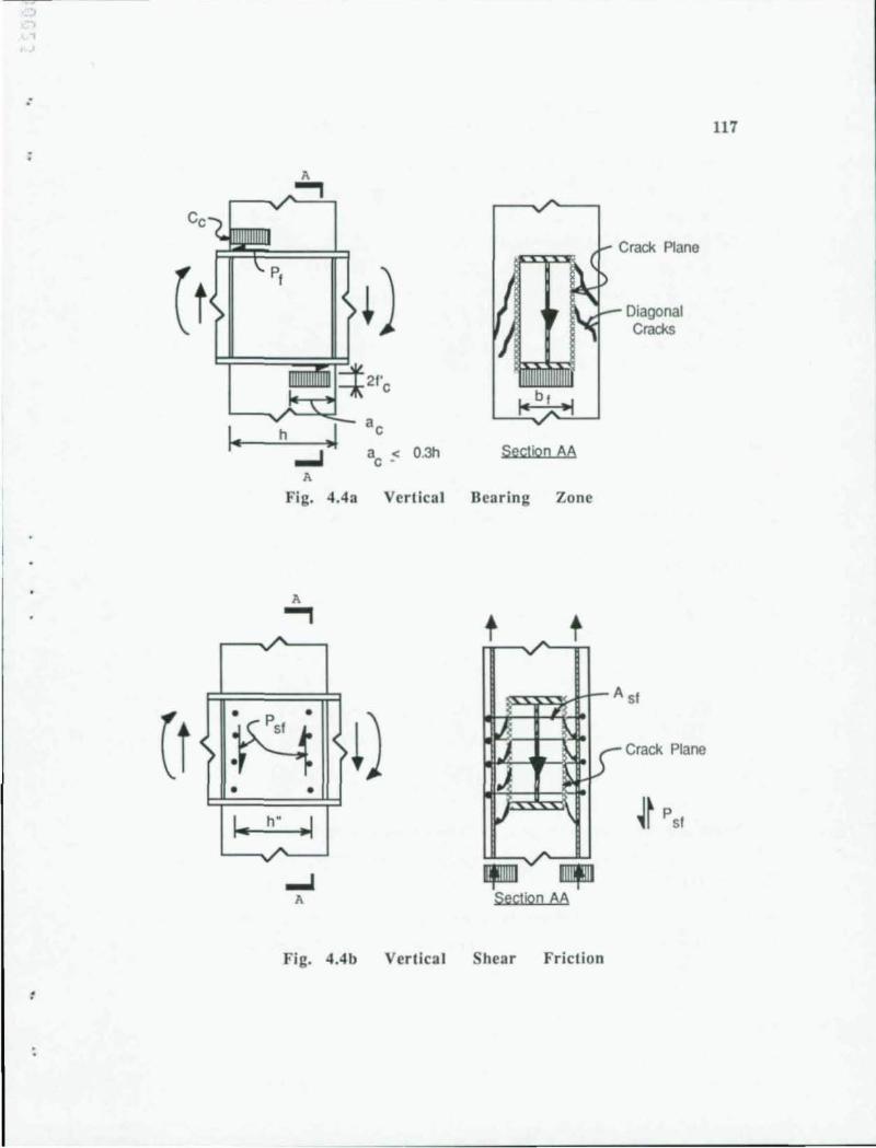
1

.'

\

:

A ..,

h .1 A

ac a < O.3h c . Section AA

Crack Plane

Diagonal Cracks

Fig. 4.4a Vertical Dear ing Zone

A .., A t t

" "

-A sf

~ > Crack Plane

II

J

lr >

• •

I. h" .. I ,J ~~ P sf

A. A. ~

~

~ • Section AA

Fig. 4.4b Vertica I hear Friction

117

118

confinement afforded by the lateral ties, friction against the steel, and the sur­

rounding concrete. Based on tests to simulate the bearing zone under a steel

beam Minami 7 reco=ends a maxinrum stress of 2 f; _ Also, ACI-318 '5 speci­

fies a maxinrum bearing stress of 1.7 f; (twice its typical value of 0_85 f;) when

supporting concrete area is larger than the loaded area. The length of the com­

pression block, ae , is limited to a maxinrum of 0_3 h. This value is reco=ended

in the PCl Design Handbook" for the bearing zone under embedded steel brack­

ets. The resulting concrete bearing force, Ce , shown in Fig_ 404a is given by the

following fornrula:

Ce = 2f~ ae bl

where ae < 0.3 h

(4.5a)

(4_5b)

Figure 404a also shows the horiwntal force, PI' transferred between

the beam flange and concrete by friction. Typically, this friction force is resisted

by concrete column shear. The value of PI is derived from the ACI-318 ' 5 shear

friction recommendations where the force transfer in the bearing region is gov­

erned by the upper limit on shear stress. The resulting expression for the friction

force, PI, is as follows:

(4.6)

The expression for the vertical force, p.I , shown in Fig. 404b is also based on the

ACI-318 16 shear friction reco=endations and is as follows:

P' I = 1.4 A" F" , (4.7)

In this expression A" is the total area of reinforcement fully developed in tension

across the vertical crack planes. A friction coefficient of 104 is used for monolithic

concrete.

4.1.4 Procedure for Assessing Joint Strength. The composite

joints derive their strength through interaction of several mechanism;. As demon­

strated by the variety of test specimens, many joint configurations and details

-.

,

.-

:

119

whkh demand individual consideration are possible. Understanding basic load

paths and modes of failure provides the most reliable guide to the connection

analysis. Two key points in the calculations are identifying the primary joint

shear mechanisms in the inner and outer panels, and evaluating the means by

which these are mobilized by the connection details.

In this chapter parameters are developed for computing shear mobilized

in the outer and inner joint panels, and equations are introduced which relate

internal joint forces to the overall member forces. The outer panel is considered

first, as the moments carried by the outer panel are required for the inner panel

calculations. Included with the inner panel calculation is the influence of the

vertical forces shown in Fi~. 4.4a and b and of vertical joint reinforcement

attached to the flanges.

In addition to the shear panel calculations, requirements for other force

transfer mechanisms are considered. One such mechanism transfers joint shear

horizontally between the outer panel and elements such as steel columns or ex­

tended FBPs. Also, horizontal forces and associated bearing stresses against

elements such as the FBP, WSP, steel column, shear studs, and vertical joint

reinforcement are considered.

Once appropriate parameters and equations are developed, a system­

atic approach to assessing joint capacity is presented. The solution is described

through several flow charts which provide a guide to the equations for the shear

strength contributed by different mechanisms and thereby help illustrate the

interrelation of various parameters.

4.2 Outer Shear Panel

Outer panel contribution to joint strength is determined by resolving

the effective shear resistance of the panel into equivalent beam and column mer ments. The shear resistance depends primarily on various joint details mobilizing

concrete in the outer panel. For example, recall that the outer panel contribu­

tion in Specimens 14 through 17 was roughly 40% of that in Specimen 8, with an

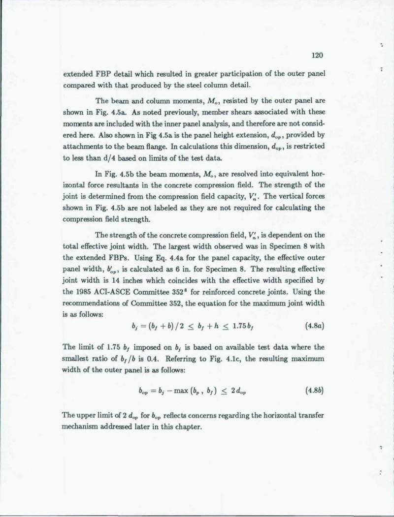
120

extended FBP detail which resulted in greater participation of the outer panel

compared with that produced by the steel column detail.

The beam and column moments, M o , resisted by the outer panel are

shown in Fig. 4.Sa. As noted previously, member shears associated with these

moments are included with the inner panel analysis, and therefore are not consid­

ered here. Also shown in Fig 4.5a is the panel height extension, do. , provided by

attachments to the beam flange. In calculations this dimension, do., is restricted

to less than d/4 based on limits of the test data.

In Fig. 4.5b the beam moments, M o , are resolved into equivalent hor­

izontal force resultants in the concrete compression field. The strength of the

joint is determined from the compression field capacity, V~. The vertical forces

shown in Fig. 4.Sb are not labeled as they are not required for calculating the

compression field strength.

The strength of the concrete compression field, V~, is dependent on the

total effective joint width. The largest width observed was in Specimen 8 with

the extended FBPs. Using Eq. 4.4a for the panel capacity, the effective outer

panel width, b:. , is calculated as 6 in. for Specimen 8. The resulting effective

joint width is 14 inches which coincides with the effective width specified by

the 1985 ACI-ASCE Committee 352 8 for reinforced concrete joints. Using the

recommendations of Committee 352, the equation for the maximum joint width

is as follows:

(4.8a)

The limit of 1.75 b, imposed on b,. is based on available test data where the

smallest ratio of b, /b is 0.4. Referring to Fig. 4.1c, the resulting maximum

width of the outer panel is as follows:

(4.8b)

The upper limit of 2 dop for bop reflects concerns regarding the horizontal transfer

mechanism addressed later in this chapter.

;

:

~------

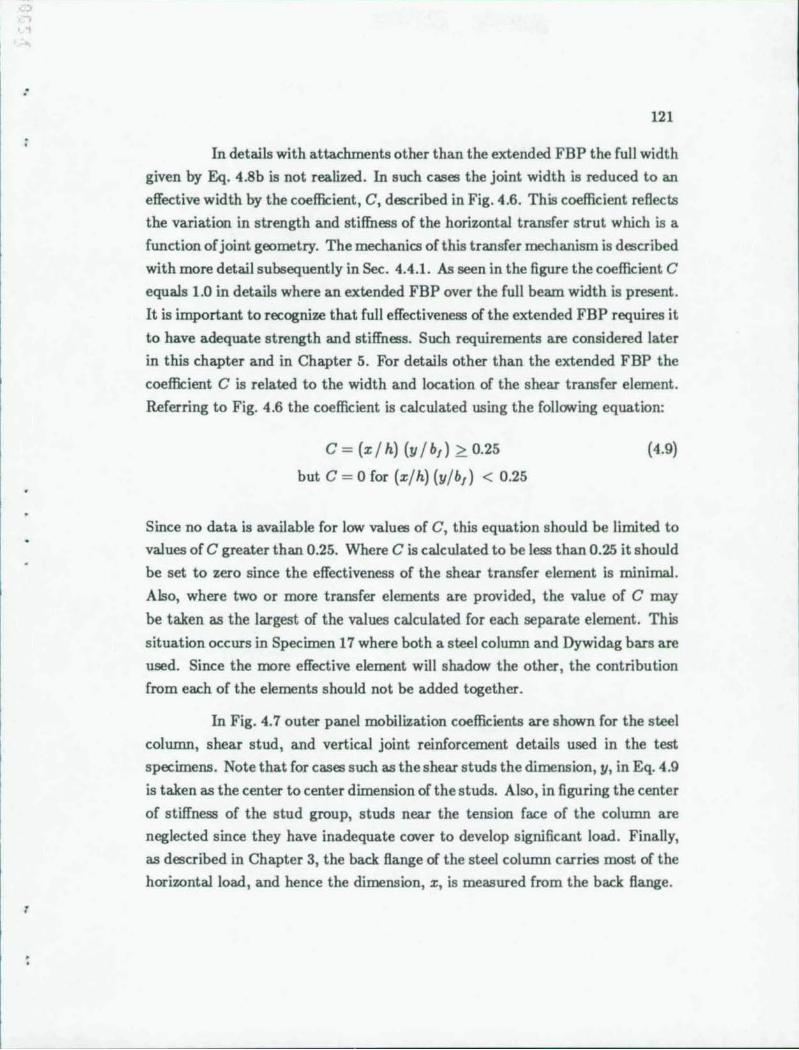
121

In details with attachments other than the extended FBP the full width

given by Eq. 4.8b is not realized. In such cases the joint width is reduced to an

effective width by the coefficient, C, described in Fig. 4.6. This coefficient reflects

the variation in strength and stiffness of the horizontal transfer strut which is a

function of joint geometry. The mechanics of this transfer mechanism is described

with more detail subsequently in Sec. 4.4.1. As seen in the figure the coefficient C

equals 1.0 in details where an extended FBP over the full beam width is present.

It is important to recognize that full effectiveness of the extended FBP requires it

to have adequate strength and stiffness. Such requirements are considered later

in this chapter and in Chapter 5. For details other than the extended FBP the

coefficient C is related to the width and location of the shear t ransfer element.

Referring to Fig. 4.6 the coefficient is calculated using the following equation:

C = (x / h) (y / b,) > 0.25 (4.9)

but C = 0 for (x/h) (y/b,) < 0.25

Since no data is available for low values of C, this equation should be limited to

values of C greater than 0.25. Where C is calculated to be less than 0.25 it should

be set to zero since the effectiveness of the shear transfer element is minimal .

Also, where two or more transfer elements are provided, the value of C may

be taken as the largest of the values calculated for each separate element. This

situation occurs in Specimen 17 where both a steel column and Dywidag bars are

used. Since the more effective element will shadow the other, the contribution

from each of the elements should not be added together .

In Fig. 4.7 outer panel mobilization coefficients are shown for the steel

column, shear stud, and vertical joint reinforcement details used in the test

specimens. Note that for cases such as the shear studs the dimension, y, in Eq. 4.9

is taken as the center to center dimension of the studs. Also, in figuring the center

of stiffness of the stud group, studs near the tension face of the column are

neglected since they have inadequate cover to develop significant load. Finally,

as described in Chapter 3, the back flange of the steel column carries most of the

horizontal load, and hence the dimension, x, is measured from the back flange.

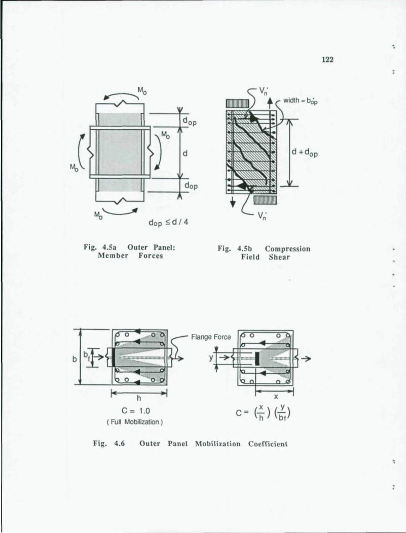
A

" w

1 I d op

~ I c> r' d

1/

~ I d op

A -, ~

dop !> d 14

Fig. 4.5a Outer Panel: Fig. 4.5b Compression Member Forces

h

C = 1.0 (Full Mobilization)

Field Shear

o Flange Force

y-'-~~.: ~::::::::~::I~~·J 7

~~~ x

Fig. 4.6 Outer Panel Mobilization Coefficient

'.

122

..

:

123

In Fig. 4.7 along with the calculated coefficients, values based on the

experimental results are shown. The experimental values are obtained from the

normalized outer panel contributions listed previously in Table 3.3. For Speci­

mens 15 and 12 (Fig. 4.7), the calculated coefficients are slightly less than the ex­

perimental values. For Specimen 11 with the Dywidag bar detail, the computed

coefficient overestimates considerably the test data value. This discrepancy is

most likely due to local crushing of the concrete around the Dywidag bars which

limits the shear panel contribution. Criteria for assessing such local failures is

addressed later.

The coefficient given by Eq. 4.9 is used to modify the maximum outer

panel width given by Eq. 4.8b, resulting in the following expression for the effec­

tive compression field width:

(4.10)

This dimension is used with the general compression field Eqs. 4.4a through c,

to determine the effective compression field strength.

While it may seem reasonable to increase the maximum panel width in

the presence of both wide FBPs and attachments to the flanges (steel columns,

etc.), no data is available to verify such behavior. Therefore, the equations

already developed for the outer panel strength provide a conservative result.

Depending on the compression field mobilization coefficient, C, a higher joint

capacity may result if the contribution of wide FBPs is neglected in calculations,

since it is conservatively assumed that there is no positive interaction of the

mechanisms. In such cases the FBP width used for calculations may be set equal

to bl (See Fig. 4.1). The result is that the compression strut formed by the

wide FBP outside the flanges is neglected and this area of concrete is considered

to participate in the outer panel compression field. As will be noted later, for

calculation purposes the maximum WSP width is limited to bl and hence should

also be set to bl in outer panel calculations.

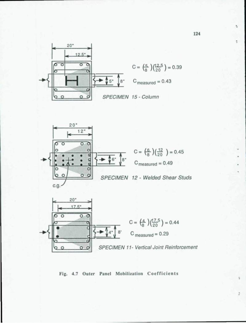
-. 124

20"

1? <;"

P 0 o 0

IV u c= ~)rft)=0.39

) H )~ :S" Is" C measured = 0.43 In a

b 0 o a EN 15 - Column SPECIM

20"

I 12" I

P 0 o 0 0 0

• • • . ~ ~"'1 6" .-I-- : ~ S" A •

c= €t)U~ )=0.45

C measured = 0.49 0 0

o 0 o a SPECIME .J c.g.

N 12 - Welded Shear Studs

r 20" ~ i. 17 S"

p 0 • o a

v u

• a 1-~.

• c

c = Et )C:ciS ) = 0.44

C measured = 0.29

" n

o 0 o 0 SPECIMEN 11- Vertical Joint Reinforcement

Fig. 4.7 Outer Panel Mobilization Coefficients

:

:

:

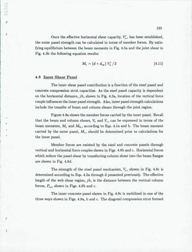
125

Once the effective horizontal shear capacity, V~, has been established,

the outer panel strength can be calculated in terms of member forces. By satis­

fying equilibrium between the beam moments in Fig. 4.5a and the joint shear in

Fig. 4.5b the following equation results:

Mo = (d+ dop) V~ /2 (4.11)

4.3 Inner Sbear Panel

The inner shear panel contribution is a function of the steel panel and

concrete compression strut capacities. As the steel panel capacity is dependent

on the horizontal distance, jh, shown in Fig. 4.3a, location of the vertical force

couple influences the inner panel strength. Also, inner panel strength calculations

include the transfer of beam and column shears through the joint region.

Figure 4.8a shows the member forces carried by the inner panel. Recall

that the beam and column shears, V. and Veo can be expressed in terms of the

beam moments, Mo and Mr,;, according to Eqs. 4.1a and b. The beam moment

carried by the outer panel, M o , should be determined prior to calculations for

the inner panel.

Member forces are resisted by the steel and concrete panels through

vertical and horizontal force couples shown in Figs. 4.8b and c. Horizontal forces

which reduce the panel shear by transferring column shear into the beam flanges

are shown in Fig. 4.8d.

The strength of the steel panel mechanism, V., shown in Fig. 4.8c is

determined according to Eqs. 4.2a through d presented previously. The effective

length of the web shear region, jh, is the distance between the vertical column

forces, p •• , shown in Figs. 4.8b and c.

The inner concrete panel shown in Fig. 4.8c is mobilized in one of the

three ways shown in Figs. 4.9a, b and c. The diagonal compression strut formed

"

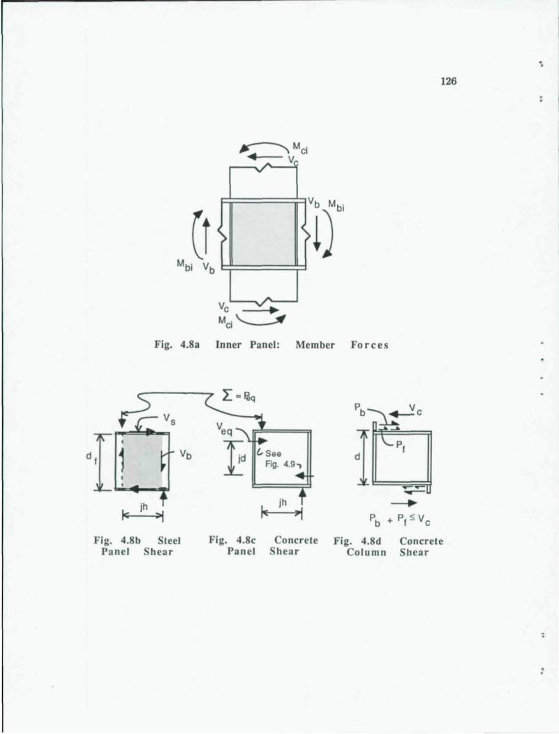
126

~Mei .. II

~

"V

4 I ()

-Ve v. Mci~

Fig. 4.8a Inner Panel: Member Forces

L .ijq

Vs Pb~ Ve

d, 1 Vb £, See 1 ~-:I Fig. 4.9.,

~~ --'h ~

~ J >j Pb + P, $ Ve

Fig. 4.8b Steel Fig. 4.8c Concrete Fig. 4.8d Concrete Panel Shear Panel Shear Column Shear

:

.-

;

127

by FBPs is shown in Fig. 4.9a. Comparing Figs. 4.8c and 4.9a the horiwntal

force and lever arm associated with the FBP detail are as follows:

jd = 0.75d ..

(4.12a)

(4.12b)

The strut shear capacity, Vn , is calculated using Eq. 4.3 in which the strut width,

b., is generally set equal to b. except in cases where the FBP extends beyond

the beam flanges. Test results of Specimen 7 indicate that the strut does not

develop fully over the entire wide FBP width, hence, b. is equal to the reduced

width, 0.95 b •. This behavior is presumably due to the inherent flexibility of the

FBP extending outside the beam width.

Figure 4.9b shows the means by which shear friction between the con­

crete and steel web can mobilize the inner concrete panel where no FBPs or

WSPs are present such as in Specimens 3 and 12. The normalized strengths in

Table 3.3 indicate that in Specimens 3 and 12 the inner concrete panel participa­

tion is approximately 23% of that in specimens with FBPs. Such participation is

accounted for through horiwntal shear friction developed by column ties passing

through the web. The total horizontal force generated by shear friction is gener­

ally small relative to the shear capacity of the inner concrete panel. Therefore,

the panel remains essentially uncracked as the principal tensile stress does not

exceed tensile capacity of the concrete. For this reason the force, Ph" shown in

Fig. 4.9b is included for all of the ties. Comparing Figs. 4.9b and 4.8c, the hor­

iwntal shear force and lever arm associated with the shear friction mechanism

are given as follows:

v •• = L Ph,

Ph , = 1.4 A"" F •• h

jd = L (Ph, jd.;) IV ••

(4.13a)

(4.13b)

(4.13c)

Equation 4.13b is based on ACI-318 16 recommendations for shear friction with

a friction coefficient of 0.7 between the concrete and steel. In Eq. 4.13b, A., is

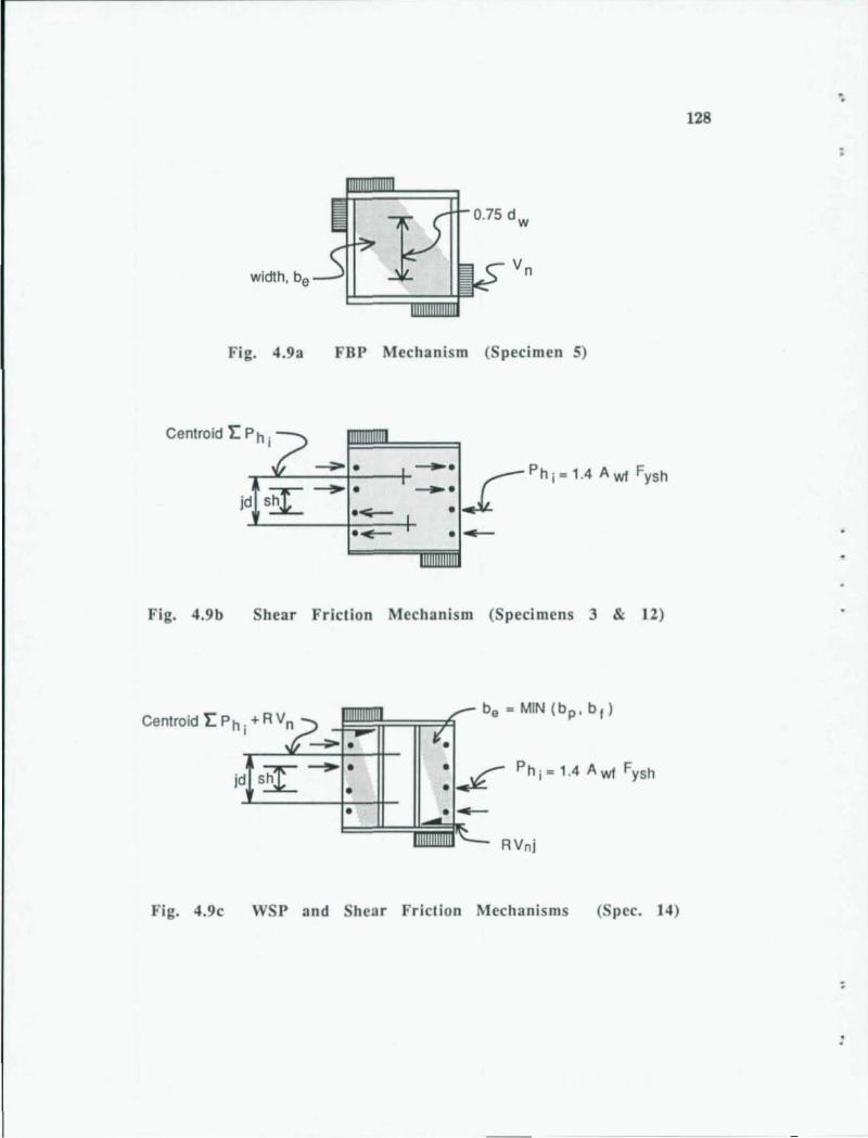
width, be

Fig. 4.9a FBP Mechanism (Specimen 5)

Centroid 1: Ph . I -0 s~

~.

Fig. 4.9b Shear Friction Mechanism (Specimens 3 & 12)

Centroid 1: Ph ' + R Vn I

~~.

jd sh • •

•

.-RVnj

Fig. 4.9c WSP and Shear Friction Mechanisms (Spec. 14)

-. 128

:

:

., )

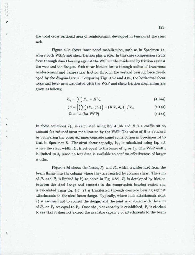
" , o

.-

:

:

129

the total cross sectional area of reinforcement developed in tension at the steel

web.

Figure 4.9c shows inner panel mobilization, such as in Specimen 14,

where both WSPs and shear friction playa role. In this case compression struts

form through direct bearing against the WSP on the inside and by friction against

the web and the flanges. Web shear friction forms through action of transverse

reinforcement and flange shear friction through the vertical bearing force devel­

oped by the diagonal strut. Comparing Figs. 4.9c and 4.&, the horizontal shear

force and lever arm associated with the WSP and shear friction mechanism are

given as follows:

v .• = I: Ph; + R Vn

jd = [(I:(Ph; jd;))+(RVnd .. )] IV ••

R = 0.5 (for WSP)

(4 .14a)

(4 .14b)

(4.14c)

In these equations Ph. is calculated using Eq. 4.13b and R is a coefficient to

account for reduced strut mobilization by the WSP. The value of R is obtained

by comparing the observed inner concrete panel contribution in Specimen 14 to

that in Specimen 5. The strut shear capacity, Vn , is calculated using Eq. 4.3

where the strut width, b" is set equal to the lesser of bp or b,. The WSP width

is limited to b, since no test data is available to confirm effectiveness of larger

widths.

Figure 4.8d shows the forces, P, and p., which transfer load from the

beam flange into the column where they are resisted by column shear. The sum

of PI and p. is limited by V. as noted in Fig. 4.8d. P, is developed by friction

between the steel flange and concrete in the compression bearing region and

is calculated using Eq. 4.6. p. is transferred through concrete bearing against

attachments to the steel beam flange. Typically, where such attachments exist

p. is assumed not to control the design, and the joint is analyzed with the sum

of P, an p. set equal to V.. Once the joint capacity is established, p. is checked

to see that it does not exceed the available capacity of attachments to the beam

130

Bange such as the steel column, extended FBP, etc. For simplicity, both P, and

Pb are conservatively assumed to act with a vertical lever distance equal to d.

The vertical force, p,., shown in Figs. 4.8b and c is the resultant force

resisted by concrete bearing stresses, vertical joint reinforcement (attached to the

beam), and shear friction provided by the ties within the beam depth. Figure 4.10

illustrates the contribution of each of these components to p, •. The bearing zone

capacity is determined using Eq. 4.5aand b. The vertical reinforcing components,

C., and Tv" are based on the nominal compression and tension strength of the

steel reinforcement attached to the beam. The shear friction component, p., , is determined from Eq. 4.7. Referring to Fig. 4.10, the resultant, p, .. and horiwntal

lever arm, jh, are given by the following expressions:

p,. = Cc + T .. + C .. + p.,

jh = [C, (h - a, ) + (Tv, + C. ,) h., + p., (h")] / p,.

(4.15a)

(4.15b)

In evaluating p,., the vertical joint reinforcement and shear friction are assumed

to be stressed to full capacity. Where the connection is not governed by bearing,

the concrete bearing region is not fully stressed and the length, ac , is some value

less than the maximum permissible length of 0.3 h.

Referring again to Figs. 4.8a through d, the force equilibrium between

the member forces (Fig. 4.8a) and internal forces (Fig. 4.8b, c, and d) is devel­

oped. From moment equilibrium, the beam moments and shears, Mo; and Vb, are related to the horizontal joint shear forces by the following equation:

2Mo; + Vb (h - jh) = V. d, + V,. jd + (P, + Pb) d (4. 16a)

The total applied moment given by the left side of Eq. 4.100 is calculated at the

edge of the effective steel shear panel. Hence, the beam moment at the column

face, Mo;, is increased by Vb as indicated. This increase is relatively small and

is neglected in the simplified design equations presented in Chapter 5.

-.

:

:

·,., )

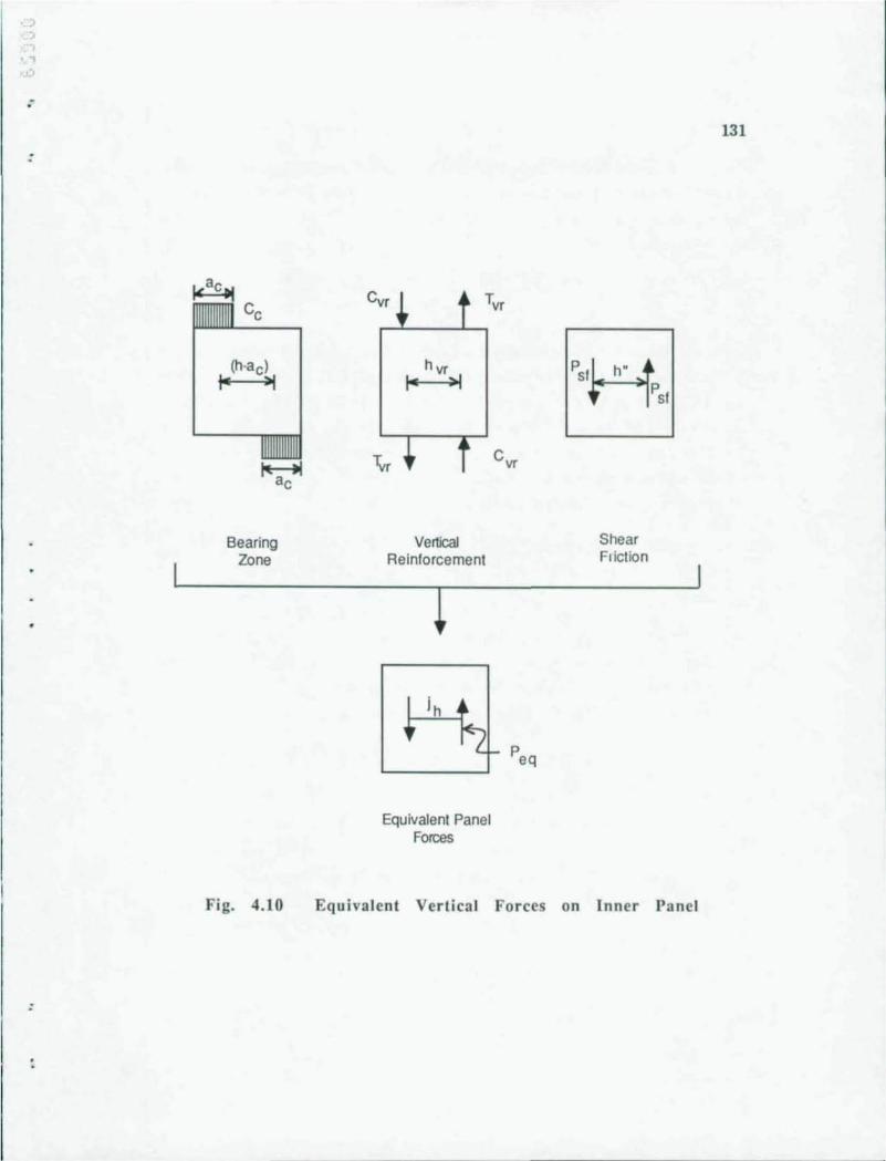
• "I

.",

.-

:

:

Cc

(h-acl

'" >I

Bearing Zone

Fig. 4.10

Cvr Tvr

h vr I- ~I

Tvr

Vertical Reinforcement

~

j h •

Cvr

1--'-'--1

Lr-

Equivalent Panel Forces

PSfM P

Sf

Shear Fliction

Equivalent Vertical Forces on Inner Panel

131

132

In order to solve Eq. 4.16a for Mbl , the beam shear, Yr., is expressed in

terms of Mbi and Mo using the relation given in Eq. 4.1a. Recall that Mo is the

outer panel contribution calculated previously. With this substitution, Eq. 4.16a

is rewritten as follows :

Mbi = V. d, + V,. id + (P, +Pb ) d - Mo (h - ih)/a, 2 + (h - ih) / a,

(4. 16b)

Solution for Mbl using Eq. 4.16b will be simplified by considering two

extreme cases regarding the sum of the forces Pb and PI . Recall that Pb and

P, are the horizontal forces transferred out of the beam flange and resisted by

column shear as shown in Fig. 4.Sd. In the first case, this sum is assumed to be

less than the total column shear, y. . Since this assumption usually applies in

details without attachments to the beam flange, the force Pb is set to zero. With

Pb set to zero, Eq. 4.16b is rewritten as follows:

Mb

• = V.d, + Y..id+P,d - Mo(h - ih)/a, • 2 + (h - ih) / a,

(4.17a)

The second case occurs where the sum of Pb and P, equals the column

shear. Typically this occurs in joints having attachments to the beam flange,

but may occur in other cases where P, is large. In this case the sum of Pb and

P, is set equal to Y.. With y. expressed in terms of the beam moments, Mbi and Mo , as given in Eq. 4.1b, Eq. 4.16b is rewritten as follows:

Mbi = V.d, + Y..id+Mo (da3 - h + ih) / a, 2 - (d a3 - h + ih) / a,

(4.17b)

Where the connection is controlled by the joint shear strengths, V. and Y.., Eqs. 4.17a and b can each be shown to reduce to one equation with two

unknown variables, M b, and a, . Therefore, a second equation is needed to solve

either of these equations. Referring to Figs. 4.Sb and c the following equation

can be derived from moment equilibrium of the steel and concrete shear panels:

(USa)

-.

:

:

.'

:

133

Expressing Vb in Eq. 4.18a in terms of M", and M. using Eq. 4.1a yields the

following equation:

(4.18b)

Like Eqs. 4.17a and b, Eq. 4.18b also reduces to one equation with two

unknown quantities, M". and a •. Equation 4.18b is used with either Eq. 4.17a

or b to solve for the connection strength in terms of M".. When shear panel

strength governs the connection capacity, the concrete bearing zone length, a., is some value less than 0.3 h. Discussed subsequently in Sec. 4.5, where a. is

unknown Eqs. 4.17a or b and 4.18b are conveniently solved by iteration.

Where joint capacity is controlled by vertical concrete bearing, the

bearing length, a., is equal to its maximum value of 0.3 h. For this case,

Eqs. 4.17a and b are combined with Eq. 4.18b to eliminate the joint shear terms ,

V. and V, •. First, Eq. 4.18b is rewritten to obtain the following expression for

V. and V,.:

V. dl + V,. jd = jh (P,. - (Mb; + M. ) I a,) (4.19)

The expression in Eq. 4.19 is substituted into Eq. 4.17a to obtain the

following equation when concrete bearing controls:

(4.20a)

Since Eq. 4.20a is obtained from 4.17a, Eq. 4.2Oa applies to the case where Pb is

set to zero and PI is less than V..

When Eq. 4.19 is substituted into Eq. 4.17b the following equation is

obtained where concrete bearing controls:

M. _ p,. jh + M. (da3 - k) I a, b. - 2 - (d~ - k)/a. (4 .20b)

Similar to Eq. 4.17b, Eq. 4.20b applies where the sum of PI and Pb is set equal

to V •.

134

In summary, where the connection is controlled by joint shear, M",

is obtained using either Eq. 4.17a or b solved simultaneously with Eq. 4.18b.

Where concrete bearing controls, M.; is obtained directly from either Eq. 4.2Oa

or b. Equations 4.17a and 4.2Oa apply where p. is set to zero and PI is less than

the resulting column shear, v.. Equations 4.17b and 4.20b apply where the sum

of p. plus PI is set equal to the column shear, v.. Once the inner panel contribution, M.;, is detennined, the total joint

capacity is given as the sum of the inner and outer panel capacities according to

the expressions given in Figs. 4.2a and 4.2b.

4.4 Internal Transfer Mechanisms

Development of equations for calculating joint capacity from the inner

and outer panel strengths is based on the premise that joint detailing is adequate

to resist internal forces generated. In this section, examination of the internal

force transfers focuses on critical components in the connections. The intent

herein is not to introduce a detailed design method for such components, but

rather to look in general terms at relevant design parameters and imposed forces.

4.4.1 Horizontal Transfer to Outer Panel. Previous discussion

of the outer panel mobilization coefficient (Sec. 4.2) did not directly address

strength aspects of the horizontal load transfer to the outer panel. Figures 4.l1a

and b illustrate two models to assess this transfer: a strut mechanism and a

shear friction mechanism.

In Fig. 4.l1a a pair of compression struts resist the lateral flange force

through bearing on the extended FBP. Similar struts will form when a steel col­

umn, shear studs, or other detail is attached to the steel beam flange. Strut

formation requires lateral ties to resist the transverse thrust, PH' Also, longi­

tudinal column reinforcing bars serve to distribute tie forces vertically over the

strut as shown in Fig. 4.11c. As indicated in Fig. 4.l1c, ties outside the height

d"" probably carry some load, and hence, in calculations ties within the height

1.5 d"p above the beam are considered effective. Ties are also required to drag

the horizontal force, P", across the column where it is resisted by the outer

-.

;

:

.-

:

:

135

panel compression field. This transfer sequence is indicated in Figs. 4.11a, c and

d.

Figure 4.11b shows a shear friction mechanism which offers more direct

transfer of horizontal load into the outer panel. The sequence of this transfer is

shown in Figs. 4.11b, 4.11c, and 4.11d. The shape and size of the shear plane

shown in Fig. 4.11b is an idealization of the actual plane based on the observed

surface cracking. As shown in the figure, shear transfer relies upon the tensile

force, p .. , provided by ties crossing the shear plane.

The two models of the horizontal transfer help explain why details

other than the extended FBP are not as effective in transferring load into the

outer panel. For example, the steel column detail transfers the horizontal force

primarily by transverse bending of the back flange as indicated previously in

Fig. 4.7. In such a case two factors affect behavior. First, the strut mechanism

will not spread out as far and the load Po will be smaller. Also, the transverse

tie force, P", will be larger for a given horizontal load as the strut angle, 8,

increases. Second, the shear friction mechanism will not be as effective since the

column transfers horizontal load into concrete away from the shear plane shown

in Fig. 4.11b. Similar assessments can be made for other details.

Load transferred by the strut mechanism is governed by the weakest

component in the system. The three components are the longitudinal tie force,

Po, the transverse tie force, P", and crushing strength of the strut. By compar­

ing the width of struts in the outer compression field to those of the horizontal

struts, premature crushing of horizontal struts is prevented by limiting the total

effective outer panel width, b~., to 2 d.". Typically, ties which carry the load

PlI will control the strut mechanism capacity since the strut angle, 8, is usually

less than 45 degrees. Thus, the resulting load transfer strength is equal to PH, calculated as the following:

(4.21a)

In Eq. 4.21b, At is the total cross sectional area of ties parallel to the

beam and located with a distance 1.5 do. from the beam.

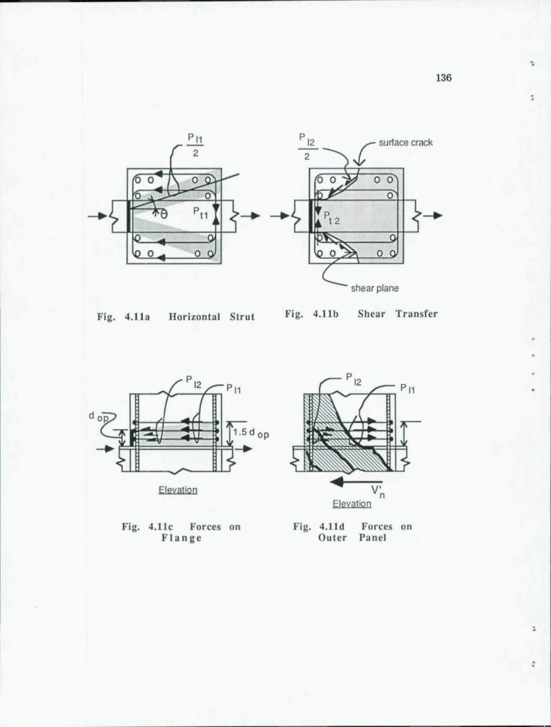
-. 136

f surface crack

shear plane

Fig. 4.11a Horizontal Strut Fig. 4.11b Shear Transrer

Elevation V' n Elevation

Fig. 4.11c Forces on Fig. 4.11d Forces on Flange Outer Panel

:

)

;-

:

:

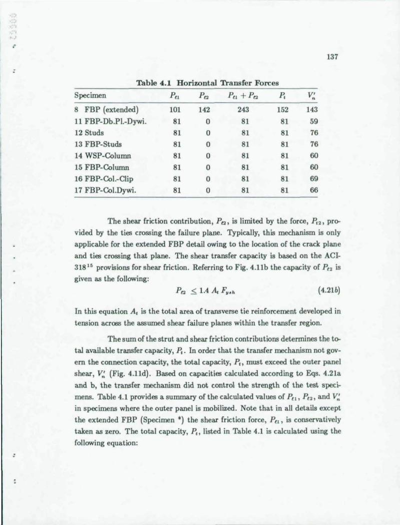
137

Table 4.1 Horizontal Transfer Forces

Specimen Pu Po P'1 + Po P. V' n

8 FBP (extended) 101 142 243 152 143

11 FBP-Db.PI.-Dywi. 81 0 81 81 59

12 Studs 81 0 81 81 76

13 FBP-Studs 81 0 81 81 76

14 WSP -Column 81 0 81 81 60

15 FBP-Column 81 0 81 81 60

16 FBP-CoI.-C1ip 81 0 81 81 69

17 FBP-CoI.Dywi. 81 0 81 81 66

The shear friction contribution, Po, is limited by the force, p.., pro­

vided by the ties crossing the failure plane. Typically, this mechanism is only

applicable for the extended FBP detail owing to the location of the crack plane

and ties crossing that plane. The shear transfer capacity is based on the ACI-

318 1• provisions for shear friction. lU!ferring to Fig. 4.11b the capacity of P" is

given as the following:

(4.21b)

In this equation A, is the total area of transverse tie reinforcement developed in

tension across the assumed shear failure planes within the transfer region.

The sum of the strut and shear friction contributions determines the to­

tal available transfer capacity, p.. In order that the transfer mechanism not gov­

ern the connection capacity, the total capacity, P" must exceed the outer panel

shear, V~ (Fig. 4.11d). Based on capacities calculated according to Eqs. 4.21a

and b, the transfer mechanism did not control the strength of the test speci­

mens. Table 4.1 provides a summary of the calculated values of Pll , PlO, and V~

in specimens where the outer panel is mobilized. Note that in all details except

the extended FBP (Specimen *) the shear friction force, Ptl , is conservatively

taken as zero. The total capacity, P" listed in Table 4.1 is calculated using the

following equation:

138

P, = PlI + P,. < 1.5 PlI (4.21c)

The upper bound on P, of 1.5 times the strut contribution, Po is

imposed to limit reliance on the shear friction mechanism, based on test results

for Specimen 8. In Table 4.1, the value of P, for Specimen 8 determined by

Eq. 4.21c is close to the calculated strut capacity for Specimen 8.

Equations 4.21a, b, and c provide a means to determine the outer panel

participation as limited by the capacity of the transfer mechanism. Where the

mobilized outer panel shear, V~, (calculated according to the effective compres­

sion field strength) exceeds the transfer capacity, the effective outer panel shear

should be reduced accordingly.

4.4.2 Concrete Bearing Stresses. Force transfers between the

steel and concrete elements may be controlled by concrete bearing stresses. The

vertical bearing stress against the steel flanges is one example where such stresses

often control the design. For this reason, vertical bearing stress is directly incor­

porated with the inner panel calculations. bearing may be critical for horizontal

stresses against FBPs, steel column flanges, shear studs, and vertical joint rein­

forcement (Dywidag bars).

The maximum concrete bearing stress in such cases is limited to 2 f:, following the rationale already presented with regard to the vertical bearing stress

against the flanges. Subsequent design recommendations in Chapter 5 outline

the effective bearing areas for each of the particular transfer elements and the

load to considered in each case. When the bearing capacity of a component

cannot develop the load associated with the calculated shear panel capacity, the

shear panel capacity should be reduced. The only test where horizontal bearing

limited the strength was Specimen 11 with the vertical Dywidag bars.

4.5 Solution of Joint Shear Equations

The stepwise procedure given herein for determining the joint strength

is intended as a general guide and should not replace engineering judgment e&­

sential to proper design of such connections. The procedure is summarized in

:

,

J

:

:

139

Figs. 4.12 through 4.14£ in which references for appropriate equations from this

chapter are given. In Fig. 4.12 a flow chart outlining the overall approach is pre­

sented. The procedure begins with given information which includes the joint

details and geometry and known proportions of adjacent beam and column forces.

The beam moments resisted by the inner and outer joint panels are calculated

next. From these the connection capacity is found in terms of the total moments

and shears in the beam and column. The final step in the analysis is a check

to see if various transfer elements can carry the imposed internal forces. If this

check does not confirm assumptions made in the previous calculations, those

calculations should be revised accordingly.

Outer panel calculations are summarized in Fig. 4.13. The flow chart

outlines a convenient sequence to calculate various parameters with the applica­

ble equations from this chapter noted. The three basic steps consist of evaluating

first, the effective outer panel width, second, the compression field shear strength,

and finally, the resulting beam moment, M •.

Figures 4.14a through f outline the inner panel calculations. Figure

4.14a presents an overview of the procedure, referencing sub procedures given in

Figs. 4.14b through f. In Fig. 4.14a the process begins by evaluating the shear

contribution of the concrete panel. As indicated in Fig. 4.14b, this evaluation

depends on the specific joint detail used. Next , in Fig. 4.14a, contributions of

the vertical joint reinforcement and vertical shear friction are detennined. After

this step the remaining solution is part of an iterative process, beginning with an

assumed value for the concrete bearing zone length, ac • Using ac the equivalent

vertical force, p,., and moment arm, jh, are calculated as outline in Fig. 4.14c.

The moment arm, jh, is then used in the next step where the steel panel strength,

v., is calculated following the procedure in Fig. 4.14d . M bi is then calculated

using either Eq. 4.17a or b as shown in Fig. 4.14e, depending on the assumption

regarding the forces PI' Pb and Ye . Referring to Fig. 4.14c, in details where

there are no flange attachments, the assumption that the sum of PI and Pb is

less than V. usually governs. In other cases, the sum of PI and Pb is assumed to

be equal to the column shear, V,. Referring again to Fig. 4.14a, a second value of

M bi is calculated using Eq. 4.18b, and this value is compared to that calculated

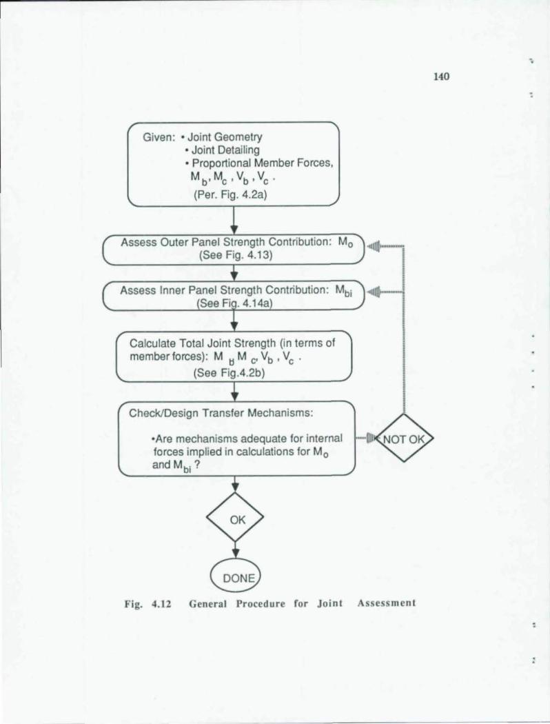
Given: • Joint Geometry • Joint Detailing • Proportional Member Forces, Mb , Mc ' Vb,VC '

(Per. Fig . 4.2a)

Assess Outer Panel Strength Contribution: Mo (See Fig. 4.13)

Assess Inner Panel Strength Contribution: Mbi See Fi . 4.14a

Calculate Total Joint Strength (in terms of member forces) : M tl M c,Vb ' Vc .

(See Fig .4.2b)

Check/Design Transfer Mechanisms:

·Are mechanisms adequate for internal forces implied in calculations for Mo and Mbi?

" III~)"n""''''~

I , , , .,IIIIII ....... · .. ·i

I I I I I •

-I~

Fig. 4.12 General Procedure for Joint Assess ment

140

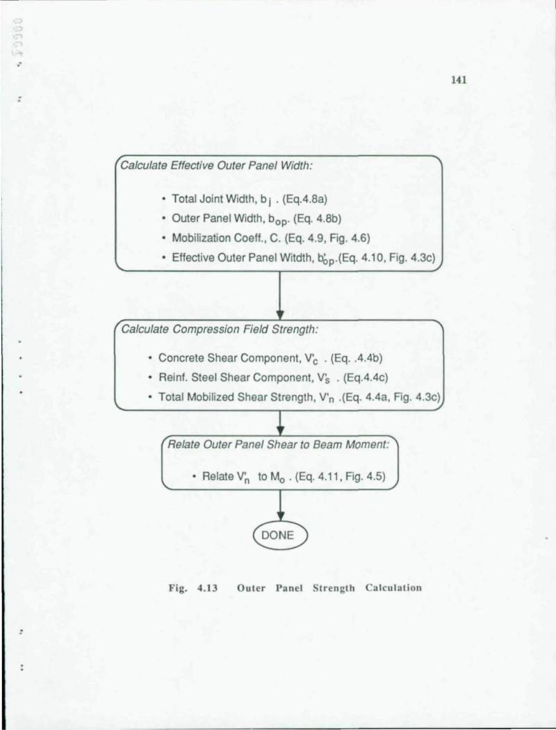
." 141

Calculate Effective Outer Panel Width:

• Total Joint Width, b j • (Eq.4.8a)

• Outer Panel Width, bop. (Eq. 4.8b)

• Mobilization Coeff., C. (Eq. 4.9, Fig. 4.6)

• Effective Outer Panel Witdth, bOp .{Eq. 4.10, Fig. 4.3c)

, Calculate Compression Field Strength:

• Concrete Shear Component, V'c . (Eq .. 4.4b)

• Rein!. Steel Shear Component, Vs . (Eq.4.4c)

• Total Mobilized Shear Strength, V'n .(Eq. 4.4a, Fig. 4.3c)

r Relate Outer Panel Shear to Beam Moment:

• Relate V' n to Mo . (Eq. 4.11 , Fig. 4.5)

DONE

Fig. 4.13 Ouler Panel lrength Calculation

:

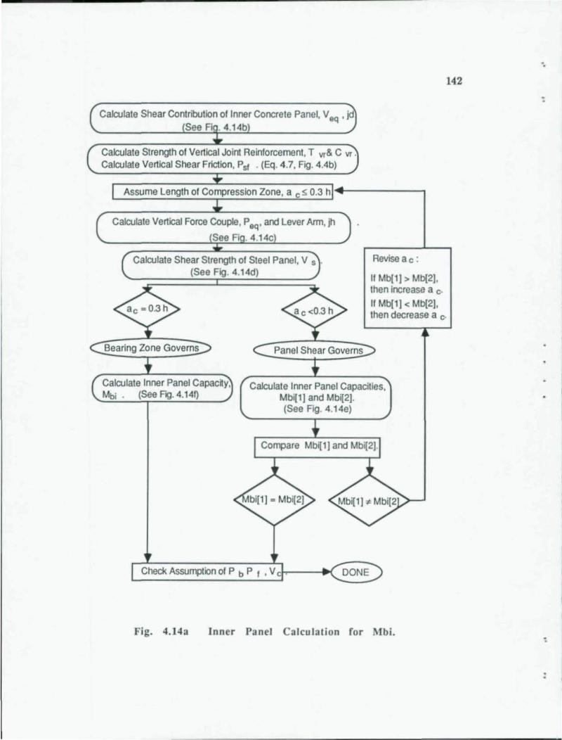
Calculate Strength of Vertical Joint Reinforcement. T vr& C vr . Calculate Vertical Shear Friction. PsI . (Eq. 4.7. Fig. 4.4b)

Assume Length of Compression Zone. a c ~ 0.3 h

Calculate Shear Strength of Steel Panel. V 5 .

(See Fig. 4.14d)

Bearing Zone Governs Panel Shear Governs

Revise ac:

If Mb{1] > Mb{2]. then increase a c. If Mb[1] < Mb[2]. then decrease a c.

Calculate Inner Panel Capac~y. Mbi. (See Fg. 4.141)

Calculate Inner Panel Capacities. Mbi[1 ] and Mbi[2]. (See Fig. 4.14e)

Check Assumption of P bPI • V . DONE

Fig. 4.14a Inner Panel Calculation for Mbi.

-. 142

:

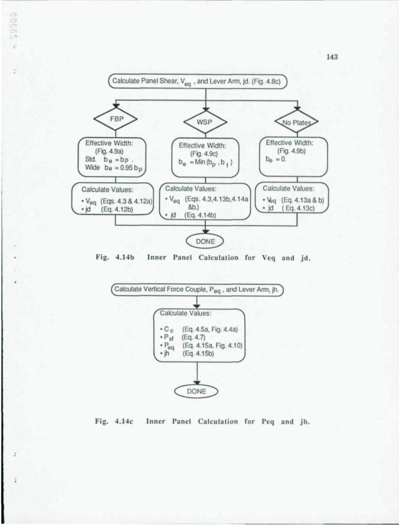
Calculate Panel Shear, Veq , and lever Arm, jd. (Fig. 4.8c)

Effective Width: (FIQ. 4.9a)

Std. be =bp . Wide be = 0.95 b p

Calculate Values:

• Veq (Eqs. 4.3 & 4.12a) • jd (Eq. 4.12b)

Effective Widlh: (Fig. 4.9c)

be - Min (bp ,b I )

Calculale Values:

• Veq (Eqs. 4.3,4.13b,4.14a &b.)

• Jd (Eq. 4.14b)

Effective Widlh: (FIQ. 4.9b)

be ~O.

Calculale Values:

'lGq (Eq. 4.13a&b) • jd ( Eq. 4.13c)

Fig. 4.14b Inner Panel Calculation for Veq and jd.

(Calculale Vertical Force Couple, Peq , and lever Arm, jh.

,J. Calculale Values :

'C c • PsI • P.

'heq • J

(Eq. 4.5a, FIQ. 4.4a) (Eq. 4.7) (Eq. 4.15a, Fig. 4.10) (Eq. 4.15b)

( DONE

Fig. 4.I4c Inner Panel Calculation for Pcq and jh.

143

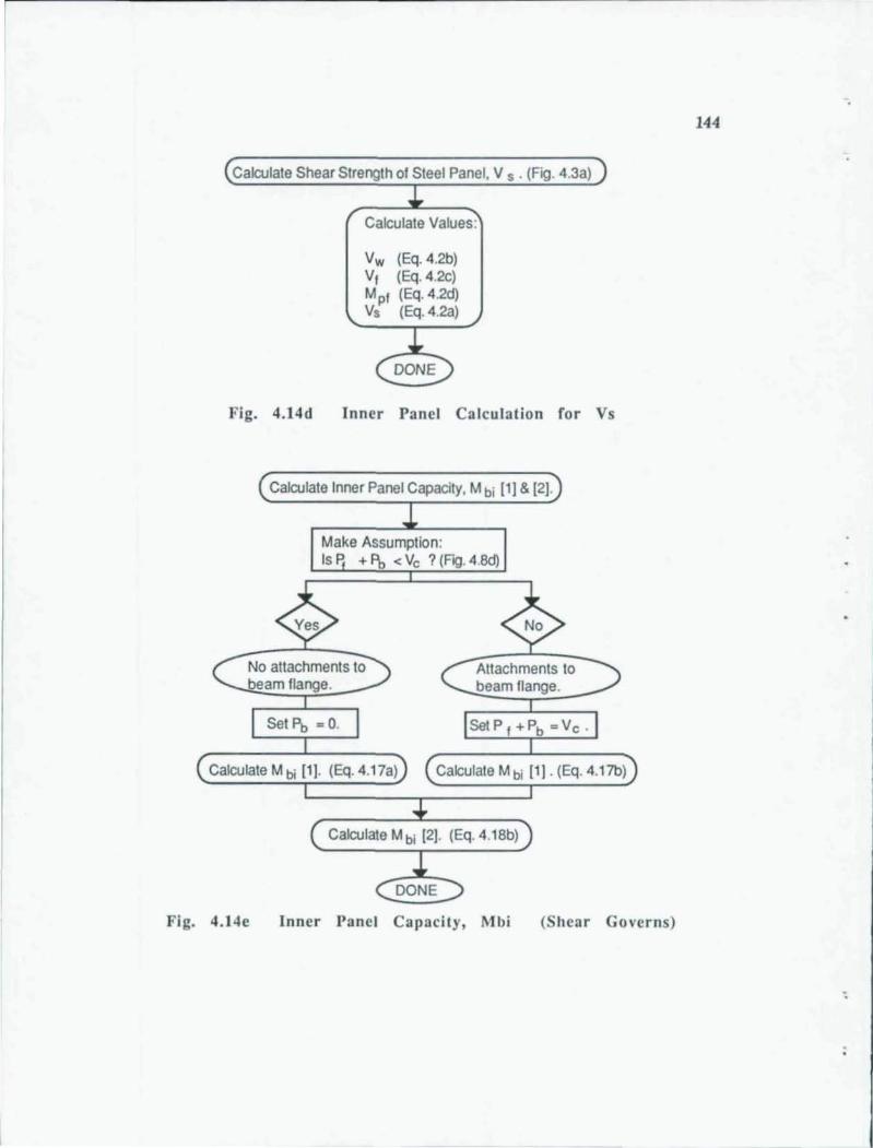
(Calculate Shear Strength of Steel Panel, V s . (Fig. 4.3a) )

J.. Calculate Values:

Vw (Eq. 4.2b) Vf (Eq.4.2c) Mpf (Eq. 4.2d) Vs (Eq. 4.2a)

~ (DONE

Fig. 4.14d Inner Panel Calculation for Vs

Calculate Inner Panel Capacity, M bi [1] & [2].

Make Assumption: Is P. + f\, < Vc ? (Fig. 4.8d)

No attachments to beam flange.

Attachments to beam flange.

Set Pb = O.

Calculate M bi [i::1]~. ~(E:q~. :4:. 1:7a~)~;::c:a:lc:u:,a:te:M=bij[...:1]_ . .:.(E_q:..,. _4._17b-....:./)

Calculate M bi [2]. (Eq.4.18b)

Fig. 4.14e Inner Panel Capacity, Mbi (Shear Governs)

144

:

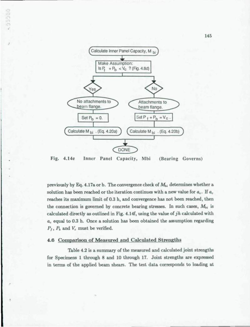
Calculate Inner Panel Capac~y. M bi .

Make Assumption: Is ~ + Fb < Vc ? (Fig. 4.6d)

No attachments to eam flange.

Set Fb = O.

Attachments to beam flange.

Calculate M bi . (Eq. 4.20a) Calculate M bi . (Eq. 4.20b)

Fig. 4.14e Inner Panel Capacity, Mbi (Bearing Governs)

145

previously by Eq. 4.17a or b. The convergence check of M b, determines whether a

solution has been reached or the iteration continues with a new value for a • . If a,

reaches its maximum limit of 0.3 h, and convergence has not been reached, then

the connection is governed by concrete bearing stresses. In such cases, M b• is

calculated directly as outlined in Fig. 4.14f, using the value of jh calculated with

a, equal to 0.3 h. Once a solution has been obtained the assumption regarding

P" Pb and v;, must be verified.

4.6 Comparison of Measured and Calculated Strengths

Table 4.2 is a summary of the measured and calculated joint strengths

for Specimens 1 through 8 and 10 through 17. Joint strengths are expressed

in terms of the applied beam shears. The test data corresponds to loading at

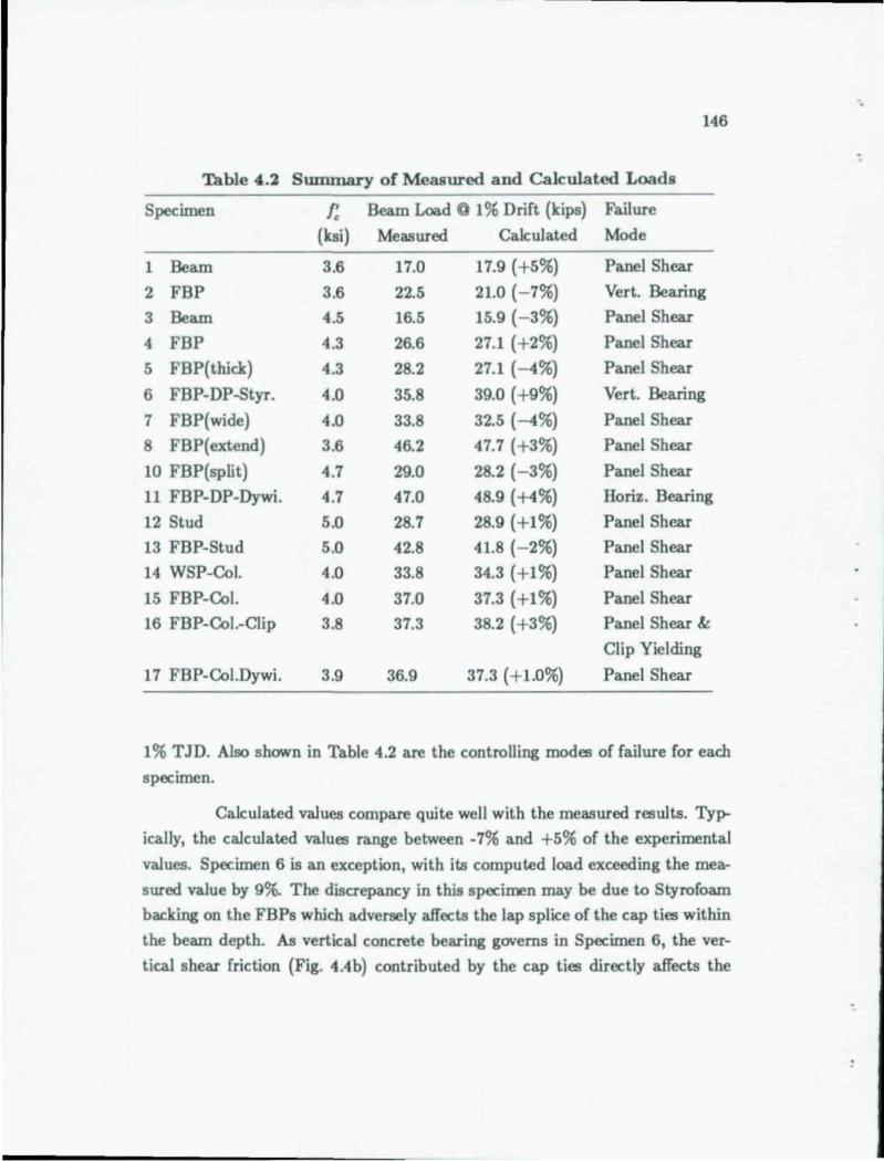
146

Table 4.2 Summary of Measured and Calculated Loads

Specimen f; Beam Load 0 1% Drift (kips) Failure

(ksi) Measured Calculated Mode

1 Beam 3.6 17.0 17.9 (+ 5%) Panel Shear

2 FBP 3.6 22.5 21.0 (- 7%) Vert. Bearing

3 Beam 4.5 16.5 15.9 (- 3%) Panel Shear

4 FBP 4.3 26.6 27.1 (+ 2%) Panel Shear

5 FBP(thick) 4.3 28.2 27.1 (- 4%) Panel Shear

6 FBP-DP-Styr. 4.0 35.8 39.0 (+ 9%) Vert. Bearing

7 FBP(wide) 4.0 33.8 32.5 (-4%) Panel Shear

8 FBP(extend) 3.6 46.2 47.7 (+ 3%) Panel Shear

10 FBP(split) 4.7 29.0 28.2 (- 3%) Panel Shear

11 FBP-DP-Dywi. 4.7 47.0 48.9 (+4%) Honz. Bearing

12 Stud 5.0 28.7 28.9 (+1%) Panel Shear

13 FBP-Stud 5.0 42.8 41.8 (- 2%) Panel Shear

14 WSP-Col. 4.0 33.8 34.3 (+1%) Panel Shear

15 FBP-Col. 4.0 37.0 37.3 (+1%) Panel Shear

16 FBP-Col.-Clip 3.8 37.3 38.2 (+ 3%) Panel Shear &

Clip Yielding

17 FBP-CoI.Dywi. 3.9 36.9 37.3 (+ 1.0%) Panel Shear

1% TJD. Also shown in Table 4.2 are the controUing modes of failure for each

specimen.

Calculated values compare quite well with the measured results. Typ­

ically, the calculated values range between -7% and +5% of the experimental

values. Specimen 6 is an exception, with its computed load exceeding the mea.­

sured value by 9%. The discrepancy in this specimen may be due to Styrofoam

backing on the FBPs which adversely affects the lap splice of the cap ties within

the beam depth. As vertical concrete bearing governs in Specimen 6, the ver­

tical shear friction (Fig. 4.4b) contributed by the cap ties directly affects the

.-147

strength. IT vertical shear friction is neglected, the capacity of Specimen 6 is

31.5 kips. Thus, if one supposes that the cap ties are only 50% effective because

of the Styrofoam, the predicted strength is the average of 31.5k and 39.1 k, 35.3

k. This value is within -2% of the measured value.

As shown in Table 4.2, in most cases strength is controlled by joint

panel shear. The panel shear is typically governed by yielding of the steel beam

and by the concrete panel capacity. In Specimens 1, 3 and 14 the concrete panel

capacity is limited by shear friction between the concrete and steel beam web.

Otherwise, where panel shear controls, the concrete contribution is controlled by

concrete strength and effective panel width. Where the outer panel compression

field mechanism participates, in none of the specimens does shear reinforcement

(lateral ties) control the panel strength. In all cases, the minimum shear rein­

forcement exceeds the amount required to develop the maximum width of the

compression field. Minimum requirements for transverse reinforcement are rec­

ommended in Chapter 5.

Vertical concrete bearing controls the predicted joint strength in Spec­

imens 2 and 6. This agrees with Sheikh's experimental observation' that at 1 %

TJD the steel web panels had not yielded in these specimens. In Specimen 11

the outer panel capacity is limited by the maximum horizontal concrete stress

against the Dywidag bars and couplers.

In Specimens 16 and 17, calculated outer panel capacities are based

on the details which offer largest mobilization of concrete. In Specimen 17,

calculations based on the Dywidag Bar detail indicate about 12% more outer

panel participation than those based on the steel col= detail (see Fig. 4.7).

Upon first inspection the clip angle detail in Specimen 16 appears to mobilize the

outer panel as effectively as the extended FBP in Specimen 8. However, as noted

both experimentally and analytically, the force transferred by the clip angle is

limited by plastic hinging near its base. The predicted load for Specimen 16 is

obtained by adding the small contribution of the clip angle to that of the steel

column detail.

CHAPTER 5 - DESIGN RECOMMENDATIONS

5.1 Introduction

Design recommendations for composite beam-column connections are

presented in this chapter. The underlying design philosophy follows that of the

1986 AISC LRFD specification 10 where the margin of safety is provided through

load and resistance factors . The recommendations include a simplified version

of the analytic model described previously in Chapter 4 to calculate the nominal

connection strength. Detailing recommendations are based on the results of the

research herein and on applicable standards for reinforced concrete and structural

steel connections. The design guidelines also draw in part from reco=endations

for composite joints proposed by Sheikh. 1 Finally, practical concerns involving

construction considerations, limitations of the design guidelines, and applicability

of the design concepts to other joint configurations are addressed.

5.2 Design Philosophy

The objective in connection design is to proportion and detail a beam­

column joint which insures satisfactory frame behavior under both service and

ultimate loads. In evaluating design criteria for the composite joint one of two

approaches may be taken. One approach is to assess the influence of joint r&­

sponse on overall frame behavior through a rigorous analysis accounting for joint

flexibility. Results of such an analysis should be assessed using realistic standards

to define satisfactory behavior. This approach is rarely if ever used in practice for

two reasons. First, sophisticated computer modeling tools are not readily avail­

able to perform the analysis. Second, having evolved gradually the standards

which define satisfactory behavior are closely linked to assumptions inherent in

the analysis . Hence a rigorous analysis would involve not only advanced struc­

tural analysis techniques but also careful reassessment of environmental loadings

and the more basic criteria and standards which define satisfactory behavior. For

enmple, in tall buildings traditional drift indices which serve as rule of thumb

to control wind induced deformations and motion are inextricably tied to the

148

..

.-

149

level of sophistication in the analysis. A second approach for evaluating com­

posite joint design criteria involves comparing behavior with that of structural

steel and reinforced concrete joints. This argument implies that since current

standards for designing structural steel and reinforced concrete joints result in

satisfactory structures, similar standards and performance in composite joints

will produce satisfactory response. The second approach is followed in this re­

port because it utilizes the established reliability of successful joint design in

structural steel and reinforced concrete.

As discussed in Chapter 4, load-deformation behavior of composite

joints is similar to that of structural steel and reinforced concrete joints. Based

on a deformation of 1 % total joint distortion (TJD) for the design strength de­

formations of about 0.2% TJD are expected at service load. The composite joint

deformation at service load is comparable to that reported for structural steel

or reinforced concrete joints. One can reason, therefore, that currently accepted

design practice for st.ructural steel or reinforced concrete joints is applicable to

composite joints.

Since composite connections occur most frequently in buildings con­

sisting primarily of structural steel, the design recommendations incorporate

design methodology of the American Institute of Steel Construction's LRFD

specification. l o In this specification load and resistance factors provide for a

factor of safety against member and connection failures at ultimate load. The

relationship between applied loads and required strength is given by the following

equation 10 :

(5.1)

The left side of this equation is the required strength given as the summation

of applied loads, Qi, multiplied by the appropriate load factors, '1i ' The design

strength given on the right sides is equal to the product of the nominal (calcu­

lated) resistance, R", and a capacity reduction or resistance factor, tP. Equations

for calculating the nominal connection strength are given in Sec. 5.3.

AISC specifications for steel design have traditionally been developed

to provide connections with a larger margin of safety than members. In the LRFD

150

specification, reliability indices (fJ factors) incorporated in the development of

resistance (4)) factors provide the relative difference in safety. The relationship

between reliability and resistance factors is described subsequently. Essentially,

however, the resistance factors in the current LRFD specification are calibrated

to the previous AISC Allowable Stress Specification l. where the factor of safety

for connections is roughly 1.2 times that of members (F.S. Connection = 2.0,

F.S_ Member = 1.67) .

The LRFD specification does not address serviceability criteria directly.

'Traditionally, serviceability criteria and the evaluation of such have been left to

the judgment of structural designers. When assessing serviceability it is rec­

ommended that composite joints be treated like welded joints in steel frames.

Sheikhl summarizes the current state of practice regarding treatment of joint

B.exibility in building design.

5.2.1 Required Strength. The connection design should distin­

guish between cases where lateral loading due to either wind or seismic forces

governs. Under wind loading the structural response is assumed to remain essen­

tiallyelastic. For seismic loading, however, most building code provisions specify

lateral loads based on the premise that under severe earthquakes the structure

will undergo inelastic cyclic loading. The energy dissipation provided by inelastic

response allows the use of equivalent static design loads which are roughly 1/3

of those required for the structure to remain elastic. I' Wind Loading. For wind and other loadings where elastic response is

assumed, the connection should be designed for the most severe combination

of forces in adjacent members following Eq. 5.1 using load factors given in the

LRFD specification. The LRFD specification has adopted load factors from the

American National Standard: Minimum Design Loads for Buildings and Other

Structures, ANSI A58.l.l4 Where wind loading governs the load factor of 1.3

specified in LRFD is nearly the same as the factor of 1.28 (1.7 x 0.75) specified by ACI-318-83. 16.

Earthquake Loading. For seismic loading and other cases where inelas­

tic response is envisioned, the connection should be designed to resist moments

-.

:

, )

.-151

and shears associated with plastic hinging of adjacent members. Following the

ACI-318-83 provisions for seismic design, the concrete (or composite) columns

framing into the joint should have a moment capacity at least equal to 1.2 times

that of the beams framing into the connection. Using such criteria, the composite

connection forces are limited by plastic hinging of the steel beams. The LRFD

load and resistance factors (Eq. 5.1) apply in determining the minimum beam

capacity based on the design lateral loads. For seismic forces the LRFD load

factor of 1.5 exceeds that of 1.4 (1.7 X 1.1 X 0.75) specified by ACI-318-83. The

design capacity of the connection, ¢ Ii.. , should exceed that required to carry

the beam moments and shears associated with the nominal beam capacity, Mp. Since the capacity reduction factors as described below provide a larger average

factor of safety in the connection, the nominal beam capacity does not need to

be increased above Mp to account for such factors as strain hardening which may

increase applied forces due to beam hinging.

5.2.2 Design Strength. The design strength of the connection is

obtained by reducing the nominal strength by a resistance factor , ¢. The nom­

inal joint strength is calculated using the design model and reco=endations

presented later in this chapter. The resistance factor for the composite joint

should be taken as 0.7, the basis for which is described below. This factor is

applied to the overall joint strength.

Theoretically, the LRFD resistance factors are developed on a statisti­

cal basis which provides a consistent and known level of reliability for structural

components. The statistical derivation for the resistance factor is given by the

following equation!o:

(5.2)

In this expression R.... and Ii.. are the actual and calculated mean resistances

(strengths) of the component under consideration, and V, is the coefficient of

variation of the resistance. The (3 value is a reliability index which calibrates the

¢ factor to provide a desired level of safety. In the LRFD specification connections

are targeted for a reliability index ((3) of 4.5 while member values range between

152

1.75 and 3.0. The difference in these values provides the additional margin of

safety for connections.

In reality, current LRFD resistance factors were determined largely by

calibration to provide similar factors of safety with the previous AISC Allowable

Stress specification." This is evidenced by the fact that the reliability factors

(.8) for connections are scattered between values of 1.9 and 5.9. In developing a

resistance factor for composite joints the derivation is similarly based largely on

calibration to currently established resistance factors for other elements. Statis­

tical theory is only addressed insofar as to tie the calibration back to the resulting

reliability, mean value, and coefficient of variation factors.

The capacity reduction factor of 0.7 is obtained through a comparative

analysis of <P factors currently accepted for other components. First, the premise

that the joint should have an additional margin of safety of 1.2 over the adjacent

members is considered. Again, this margin is the same as that implied in Al­

lowable Stress Design of steel structures. In this case the aqjacent members are

considered to be a composite column and a steel beam. The respective <p factors

given by LRFD for these elements are 0.85 and 0.9. Dividing these by 1.2 results

in maximum connection <p factors of 0.71 to 0.75.

A second approach to considering the connection <p factor is by relating

it to factors associated with individual elements and modes of failure in the joint.

Such factors range from a maximum of 0.9 for steel yielding to a minimum of

0.6 (LRFD) or 0.7 (ACI-318) for concrete bearing. The minimum factor of 0.7 is

considered adequate based on the following reasoning. The 0.6 LRFD factor is

derived directly from ACI by adjusting the ACI value of 0.7 based on the ratio of

dead load factors between the specifications. The respective dead load factors in

the LRFD and ACI specifications are 1.2 and 1.4 which result in an adjustment

factor of 0.86. For composite connections this derivation is overly conservative

since the connection is typically governed by wind or seismic loads where the

LRFD load factors in fact exceed those of ACI by the ratios 1.02 (1.3/1.27) to

1.07 (1.5/1.4).

'.

.'

:

153

Finally, the ¢ factor ofO. 7 can be tied to statistical theory using Eq. 5.2.

Where there is not sufficient data to provide a reasonable statistical basis as­

sumed values are used in Eq. 5.2 to estimate the results. By setting ¢ to 0.7, the

ratio of mean strengths (R", / R..) to unity, and (J to 4.5, the resulting coefficient

of variation, V" is 0.144 from Eq. 5.2. This coefficient of variation implies that

in a normally distributed data set roughly 49% of the values will be at least

10% away from the mean value and 17% at least 20% away. In other words, the

desired (J value can be achieved with a population of data having fairly wide scat­

ter. Typically, the situation will be better than that assumed since the analytic

design models underestimate the nominal strength, R.., and hence the ratio of

R", / R.. is greater than unity. Based on comparison to test data made in Sec. 5.3,

the ratio of R", / R.. is 1.06 which when used in the calculation above results in

a coefficient of variation of 0.168.

5.3 Calculation of Nominal Joint Strength

The nominal joint strength is calculated using a simplified version of

the model previously developed in Chapter 4. (Simplifying modifications for the

design model are summarized below.) Description of the design model is limited

to those aspects needed to understand and apply the model; further background

information is given in Chapter 4.

In the model two primary connection failure modes are considered:

joint shear failure and vertical bearing failure. In order for the model to cor­

rectly estimate joint strength, structural steel and reinforcing bar details must

be designed to carry the imposed forces. Where such details cannot carry the in­

ternal forces, the joint capacity should be reduced accordingly. Specific detailing

requirements and recommendations are discussed later.

5.3 .1 Simplifications to Model for Design In formulating the de­

sign model several modifications are made to the model presented previously in

Chapter 4. The end result of the simplifications outlined below is to make the

design model slightly more conservative and easier to use.

154

In the design model contribution of the plastic hinging of the beam

flanges to the steel panel strength is neglected. This change has a more significant

affect on the calculated strength of the experimental joint details than on details

typically used in practice. The hybrid steel beam flange in this study contributes

roughly 12% to the steel panel strength. For rolled beam shapes the flange

contribution is in the range of 2% to 7%. Hence, neglecting the flange in rolled

sections will have less effect.

Also neglected in the design model is the contribution of horizontal

shear friction between the concrete and steel web mobilized by ties passing

through the web. This change will significantly influence the calculated capacity

of Specimens 1 and 3 without FBPs or WSPs between the flanges. For most steel

details and erection procedures, some type of web stiffener is usually included

in the joint region. Neglecting the shear friction contribution eliminates the

uncertainty or concern regarding proper tie arrangements for developing shear

friction.

The vertical component of shear friction provided by the ties is also

neglected in design, thus decreasing computed strength of joint details governed

by concrete bearing. This again eliminates uncertainty or concern regarding

special tie detailing requirements, and encourages use of vertical reinforcement

attached to the beam flanges. Such reinforcement will provide a stiffer and more

reliable means than shear friction to transfer vertical loads into the concrete.

To further simplify the procedure, the inner and outer panel calcula­

tions are combined into one step. To accomplish this the concrete bearing zone

calculation is modified to reflect a width equal to the effective joint width rather

than the beam flange width. The net result is that the bearing calculation is

slightly less conservative, which happens to partially offset the conservative effect

of neglecting the vertical shear friction.

5.3.2 Comparison with Phase I Model. Aspects of this design

model are similar to one presented previously by Sheikh,' however, there are

several major differences in the models. First, this model is calibrated to the

..

:

.'

:

:

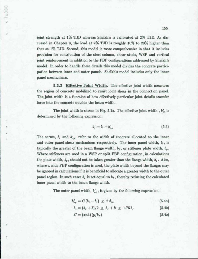
155

joint strength at 1% TID whereas Sheikh's is calibrated at 2% TJD. As dis­

cussed in Chapter 3, the load at 2% TID is roughly 10% to 20% higher than

that at 1% TJD. Second, this model is more comprehensive in that it includes

provision for contribution of the steel column, shear studs, WSP and vertical

joint reinforcement in addition to the FBP configurations addressed by Sheikh's

model. In order to handle these details this model divides the concrete partici­

pation between inner and outer panels. Sheikh's model includes only the inner

panel mechanisms.

5.S.S Effective Joint Width. The effective joint width measures

the region of concrete mobilized to resist joint shear in the connection panel.

The joint width is a function of how effectively particular joint details transfer

force into the concrete outside the beam width.

The joint width is shawn in Fig. S.la. The effective joint width, b; , is

determined by the following expression:

(5.3)

The terms, b; and b;p, refer to the width of concrete allocated to the inner

and outer panel shear mechanisms respectively. The inner panel width, b;, is

typically the greater of the beam flange width, b" or stiffener plate width, bp •

Where stiffeners are used in a WSP or split FBP configuration, in calculations

the plate width, bp , should not be taken greater than the flange width, b, . Also,

where a wide FBP configuration is used, the plate width beyond the flanges may

be ignored in calculations if it is beneficial to allocate a greater width to the outer

panel region. In such cases bp is set equal to b" thereby reducing the calculated

inner panel width to the beam flange width.

The outer panel width, b;p, is given by the following expression:

b;p = C(b; - b;) < 2d.,p

b; = (b, + b) /2 < b, + h < l.7Sb,

C = (x/h) (':J/ b,)

(S.4a)

(SAb)

(SAC)

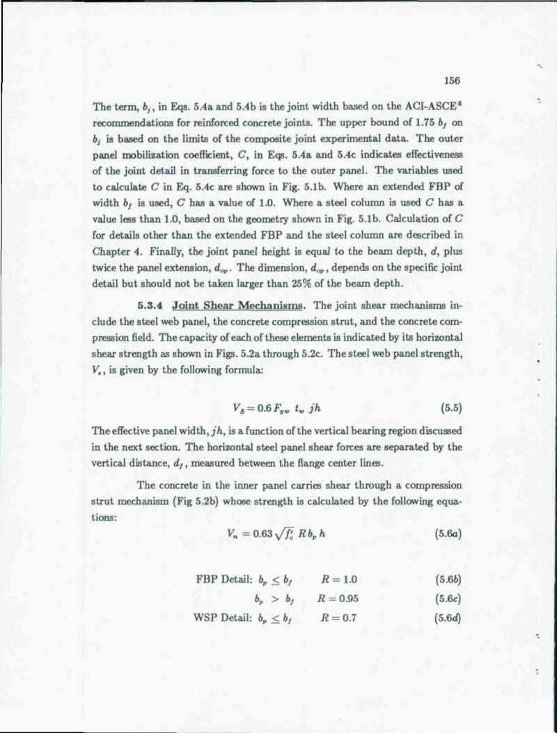
156

The term, b;, in Eqs. 5Aa and SAb is the joint width based on the ACI-ASCE 8

recommendations for reinforced concrete joints. The upper bound of 1.75 b, on

b; is based on the limits of the composite joint experimental data. The outer

panel mobilization coefficient, C, in Eqs. SAa and SAc indicates effectiveness

of the joint detail in transferring force to the outer pane\. The variables used

to calculate C in Eq. 5Ac are shown in Fig. S.lb. Where an extended FBP of

width bl is used, C has a value of 1.0. Where a steel column is used C has a

value less than 1.0, based on the geometry shown in Fig. S.lb. Calculation of C

for details other than the extended FBP and the steel column are described in

Chapter 4. Finally, the joint panel height is equal to the beam depth, d, plus

twice the panel extension, d"". The dimension, d"", depends on the specific joint

detail but should not be taken larger than 25% of the beam depth.

5.3.4 Joint Shear Mechanisms. The joint shear mechanisms in­

clude the steel web panel, the concrete compression strut, and the concrete com­

pression field. The capacity of each of these elements is indicated by its horizontal

shear strength as shown in Figs. S.2a through S.2c. The steel web panel strength,

v., is given by the following formula:

Vs = 0.6F ... to. jh (5.5)

The effective panel width, jh, is a function of the vertical bearing region discussed

in the next section. The horizontal steel panel shear forces are separated by the

vertical distance, d" measured between the flange center lines.

The concrete in the inner panel carries shear through a compression

strut mechanism (Fig 5.2b) whose strength is calculated by the following equa­

tions:

FBP Detail: bp < b,

bp > b,

WSP Detail: bp < b,

R = 1.0

R = 0.95

R = 0.7

(5.6a)

(S.6b)

(5.6c)

(5.6d)

"

:

'.

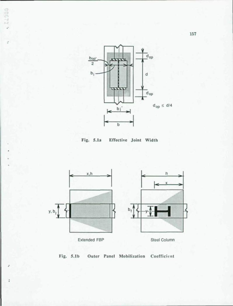
.. 157

: ,., Yj

...- I- I d . --r.-:

op

/' d

H-d

'--op

t""", v d op ~ d/4

I .. bl

b -I Fig. S.h Errective Joint Width

x.h h

:1 /

f ~ .. .. ··.yI·H .. ~

~

Y. b[ ...... t-_____ -'1f-1 b

Extended FBP Steel Column

Fig. S.lb Outer Panel Mobilization Coerricil' lIt

..

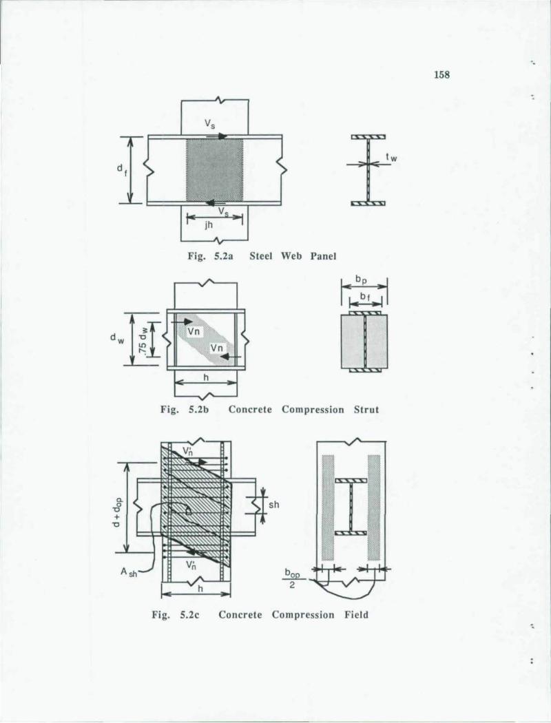
Q.

-8 +

"0

A

Fig. 5.23 Steel Web Panel

h

Fig. 5.2b Concrete Compression Strut

sh

Fig. 5.2c Concrete Compression Field

".

158

:

tw

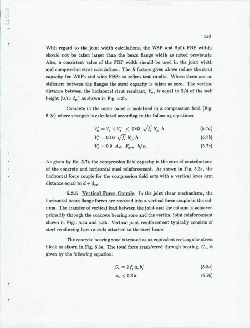
j

.'

:

:

159

With regard to the joint width calculations, the WSP and Split FBP widths

should not be taken larger than the beam flange width as noted previously.

Also, a consistent value of the FBP width should be used in the joint width

and compression strut calculations. The R factors given above reduce the strut

capacity for WSPs and wide FBPs to reflect test results. Where there are no

stiffeners between the flanges the strut capacity is taken as zero. The vertical

distance between the horizontal strut resultant, Vn , is equal to 3/4 of the web

height (0.75 d .. ) as shown in Fig. 5.2b.

Concrete in the outer panel is mobilized in a compression field (Fig.

5.2c) where strength is calculated according to the following equations:

V~ = V: + V: < 0.63 VfI b;. h

V; = 0.16 VfI b;. h V: = 0.9 A.h F •• h h/Sh

(5 .7a)

(5 .7b)

(5 .7c)

As given by Eq. 5.7a the compression field capacity is the sum of contributions

of the concrete and horizontal steel reinforcement. As shown in Fig. 5.2c, the

horizontal force couple for the compression field acts with a vertical lever arm

distance equal to d + do •.

5.3.5 Vertical Force Couple. In the joint shear mechanisms, the

horizontal beam flange forces are resolved into a vertical force couple in the col­

umn. The transfer of vertical load between the joint and the column is achieved

primarily through the concrete bearing zone and the vertical joint reinforcement

shown in Figs. 5.3a and 5.3b. Vertical joint reinforcement typically consists of

steel reinforcing bars or rods attached to the steel beam.

The concrete bearing zone is treated as an equivalent rectangular stress

block as shown in Fig. 5.3a. The total force transferred through bearing, Co, is

given by the following equation:

Co = 2/; ae b}

a, < 0.3h

(5 .8a)

(5.8b)

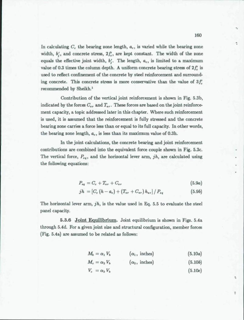
160

In calculating Cc the bearing zone length, ac , is varied while the bearing zone

width, bi, and concrete stress, 2/;, are kept constant. The width of the zone

equals the effective joint width, b;. The length, a., is limited to a maximum

value of 0.3 times the column depth. A uniform concrete bearing stress of 2/! is

used to reflect confinement of the concrete by steel reinforcement and surround­

ing concrete. This concrete stress is more conservative than the value of 3/; recommended by Sheikh.'

Contribution of the vertical joint reinforcement is shown in Fig. S.3b,

indicated by the forces C., and To.. These forces are based on the joint reinforce­

ment capacity, a topic addressed later in this chapter. Where such reinforcement

is used, it is assumed that the reinforcement is fully stressed and the concrete

bearing zone carries a force less than or equal to its full capacity. In other words,

the bearing zone length, a., is less than its maximum value of 0.3h.

In the joint calculations, the concrete bearing and joint reinforcement

contributions are combined into the equivalent force couple shown in Fig. S.3c.

The vertical force, p •• , and the horizontal lever arm, jh, are calculated using

the following equations:

pc. = Cc + T,., + Cn

jh = IC. (h - ac ) + (T .. + C .. )h .. j / p ••

(S.9a)

(S.9b)

The horizontal lever arm, jh, is the value used in Eq. S.S to evaluate the steel

panel capacity.

5.3.6 Joint Equilibrium. Joint equilibrium is shown in Figs. S.4a

through S.4d. For a given joint size and structural configuration, member forces

(Fig. S.4a) are assumed to be related as follows:

M.= a,V.

V. = a3 V•

(a" inches)

( a" , inches)

(S.lOa)

(S.10b)

(5.1Oc)

'.

:

"

..

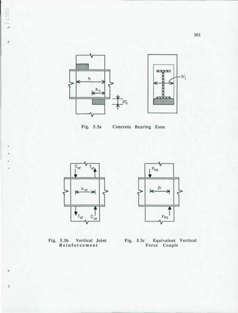
Fig. S.3a

I< hvr >1

Fig. S.3b Vertical Joint Reinforcement

Concrete Bearing Zone

v

req

> IE: jh ~

peqi

v

b' I

?

161

Fig. S.3c Equivalent Vertical Force Couple

~

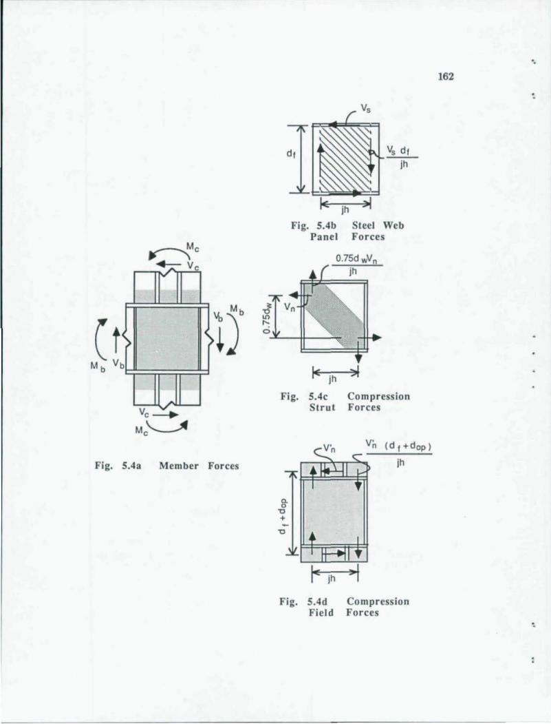
(> > b

~

~

Fig. S.4a Member Forces

oJ I/) ,... o

df Vs df

jh

Fig. S.4b Steel Web Panel Forces

O.7Sd wVn jh

....L..-It-----'~

I< jh

Fig. S.4c Compression

a. o

"0 +

"0

Strut Forces

jh

IE jh

Fig. S.4d Compression Field Forces

.. 162

., ..

:

:

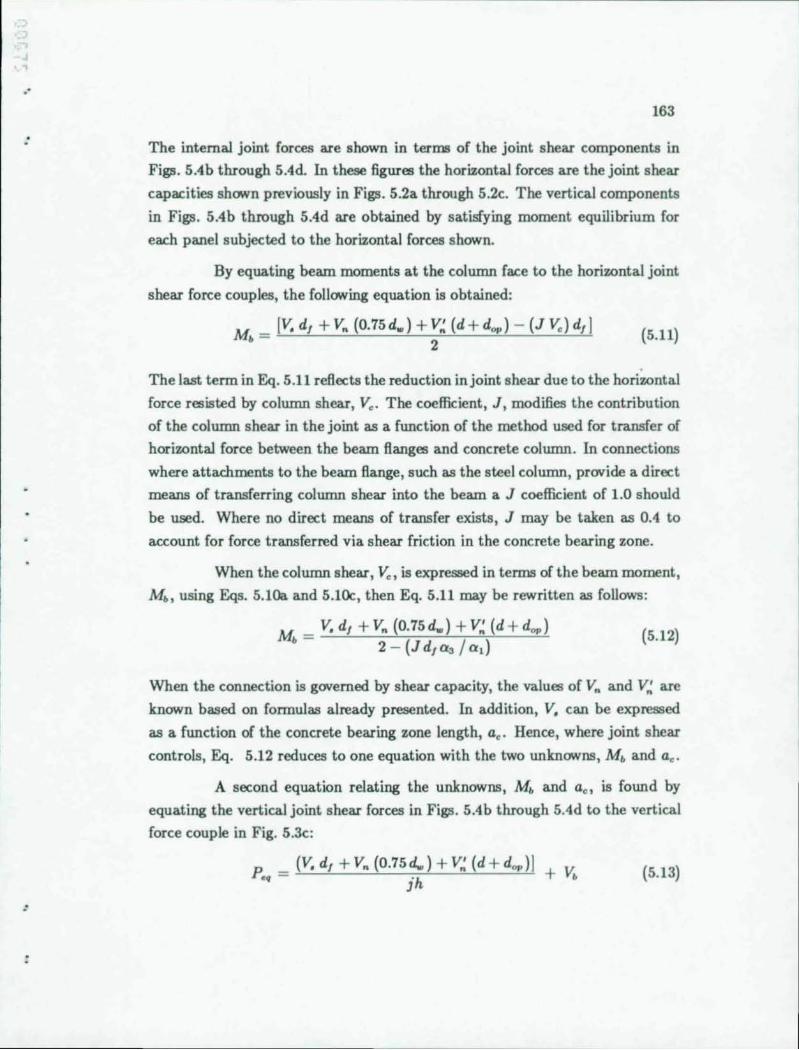
163

The internal joint forces are shown in terms of the joint shear components in

Figs. 5Ab through 5Ad. In these figures the horizontal forces are the joint shear

capacities shown previously in Figs. 5.2a through 5.2c. The vertical components

in Figs. 5Ab through 5Ad are obtained by satisfying moment equilibrium for

each panel subjected to the horizontal forces shown.

By equating beam moments at the column face to the horizontal joint

shear force couples, the following equation is obtained:

The last term in Eq. 5.11 reflects the reduction injoint shear due to the horizontal

force resisted by column shear, Ve. The coefficient, J, modifies the contribution

of the column shear in the joint as a function of the method used for transfer of

horizontal force between the beam flanges and concrete column. In connections

where attachments to the beam flange, such as the steel column, provide a direct

means of transferring column shear into the beam a J coefficient of 1.0 should

be used. Where no direct means of transfer exists, J may be taken as 004 to

account for force transferred via shear friction in the concrete bearing zone.

When the column shear, v., is expressed in terms of the beam moment,

M., using Eqs. 5.1Oa and 5.1Oc, then Eq. 5.11 may be rewritten as follows:

M. = V. d, + Vn (0.75d .. ) + V~ (d + dop) 2 - (Jd,a3 I a.)

(5.12)

When the connection is governed by shear capacity, the values of Vn and V~ are

known based on formulas already presented. In addition, V. can be expressed

as a function of the concrete bearing zone length, a.. Hence, where joint shear

controls, Eq. 5.12 reduces to one equation with the two unknowns, M. and a • .

A second equation relating the unknowns, M. and ac , is found by

equating the vertical joint shear forces in Figs. 5.4b through 5Ad to the vertical

force couple in Fig. 5.3c:

(5.13)

164

When the beam shear, Vh is expressed in terms of the beam moment, Mb , using

Eq. 5.10a, then Eq. 5.13 may be rewritten as follows:

(5.14)

By substituting the joint shear capacities, Eq. 5.14 reduces to one equation with

two unknowns, Mb and a •. Thus, when the joint is controlled by shear capacity,

Eqs. 5.12 and 5.14 can be solved simultaneously for a. and M b • As described in

Chapter 4, such equations are conveniently solved through iteration.

Where the connection is controlled by concrete bearing, the concrete

bearing zone length a. is given as 0.3 h. In this case the joint shear elements are

not stressed to their full capacity and hence the values for V., Vn and V~ become

unknowns in Eqo>. 5.12 and 5.14. The equations may be combined to eliminate

the unknown quantities resulting in the following equation for the beam moment:

M _ jhP •• b - 2 - (J d, as / a,) + jh / al

(5.15)

Once the connection capacity is known in terms of the beam moments

using either Eqs. 5.12 and 5.14 or Eq. 5.15, the remaining member forces can be

calculated by Eqs. 5.lOa through 5.1Oc.

5.3.7 Solution of Design Equations. A schematic diagram for

calculation of the joint panel capacity is shown in Fig. 5.5. The approach outlined

in Fig. 5.5 is similar to that presented previously in Chapter 4, but reflects

the simplifications incorporated in the design equations. In Fig. 5.5 equation

numbers are referenced in applicable steps of the solution.

5.4 Evaluation of Design Model

In this section the design model for calculating the connection strength

(Sec. 5.3) is compared with measured values . Additionally, the design model is

compared with more detailed, and presumably more precise, analysis described in

Chapter 4. Comparison is also made with strengths calculated based on Sheikh's

'.

'.

:

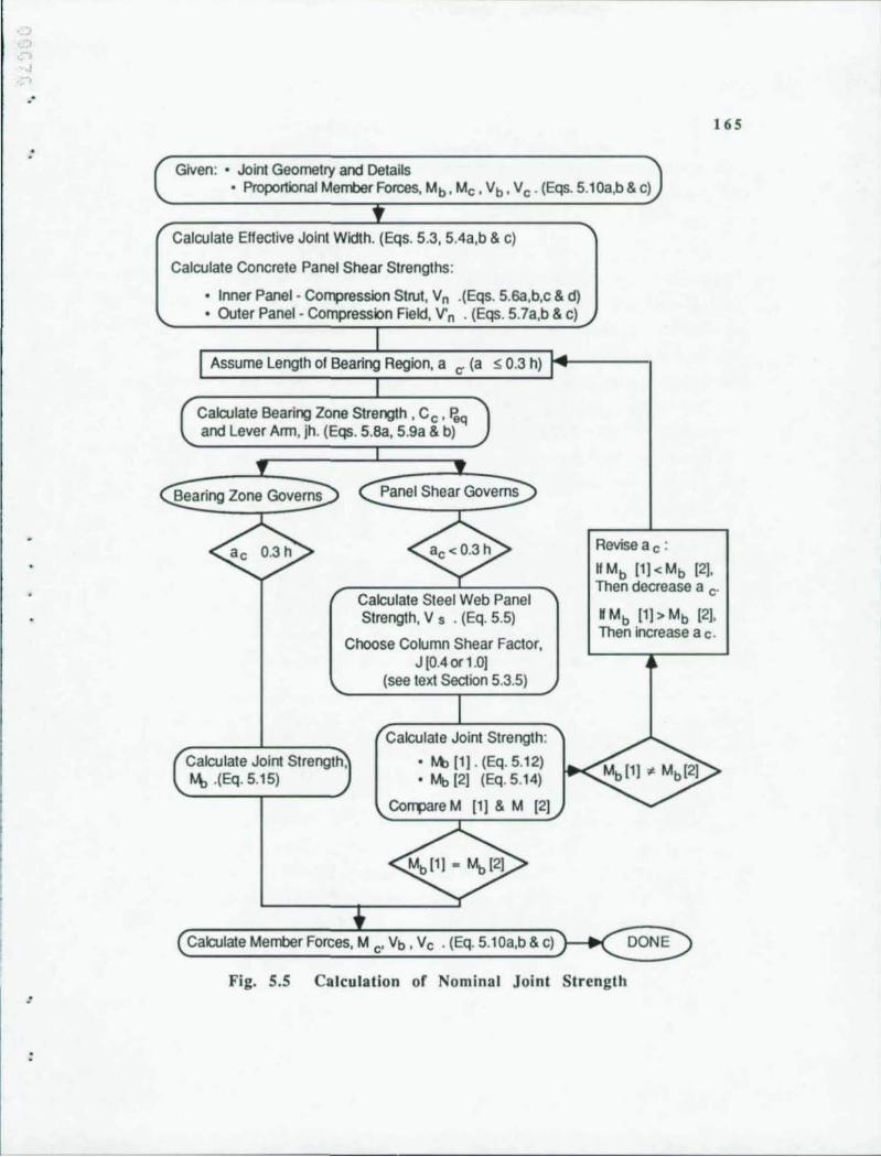
.0

:

:

165

Given: • Joint Geometry and Details • Proportional Member Forces, Mb , Mc , Vb, Vc' (Eqs. 5.10a,b & c)

Calculate Effective Joint Width. (Eqs. 5.3, 5.4a,b & c)

Calculate Concrete Panel Shear Strengths:

• Inner Panel · Compression Strut, Vn .(Eqs. 5.6a,b,c & d) • Outer Panel - Compression Field, V' n . (Eqs. 5.7a,b & c)

Assume Length of Bearing Region, a e (a ~ 0.3 h)

Calculate Bearing Zone Strength, C c ' Paq and Lever Arm, jh. (Eqs. 5.8a, 5.9a & b)

Bearing Zone Governs Panel Shear Governs

Calculate Steel Web Panel Strength, V s . (Eq. 5.5)

Choose Column Shear Factor, J [0.4 or 1.0]

Calculate Joint Strength, ~ .(Eq. 5.15)

(see text Section 5.3.5)

Calculate Joint Strength:

• Mb[1] . (Eq. 5.12) • Mb [2] (Eq. 5.14)

Compare M [1] & M [2]

Calculate Member Forces, M C' Vb, Vc . (Eq. 5.10a,b & c)

Revise ac :

HMb [1]<Mb [2], Then decrease a c.

H Mb [1] > Mb [2], Then increase a c.

Fig, 50S Calculation of Nominal Joint Strength

166

model. Joint strengths for several representative examples of full size connections

are also included. Calculations for two of the connection designs are presented

in Appendix A3.

5.4.1 Test Specimens. Measured and calculated joint capacities for

Specimens 1 through 8 and 10 through 17 are presented in Table 5.1. Table 5.1

also lists the percentage difference between the calculated design and measured

values. The calculated design values per Chapter 5 consistently underestimate

the measured strengths by 1% to 34%. Where values differ by more than 12%

the discrepancy is reconciled in part by considering the particular circumstances

involved. In Specimens 1, 3, and 12 where values differ by -13%, -34% and -21%

respectively, the large differences arise because no FBPs or WSPs are present in

the specimens. Since the design model does not incorporate contribution of the

concrete strut mobilized by friction, joint capacity is purposely underestimated.

Where design strength is controlled by the vertical concrete bearing in Speci­

mens 2 and 6, a conservative estimate of the maximum bearing stress results in

underestimates of -31 % and -15%, respectively. The conservative bearing stress

encourages use of vertical joint reinforcement which is found to be beneficial

when concrete stresses are high. If the conservative results of Specimens 1, 3,

12, 2 and 6 are neglected there is good agreement between the calculated and

measured strengths where the average ratio between the two is 0.95.

5.4.2 Representative Examples. Several representative joint de­

tails are designed using both Chapter 4 and Chapter 5 analyses and are com­

pared to verify assumptions made in simplifying the model. The joints have

cruciform configurations (similar to the test specimens) with 30 in. or 40 in.

square columns and various rolled beam sizes. The beam sizes are chosen such

that plastic moment capacities are approximately 85% of the nominal column

moment capacities. The column capacities are determined by assuming typical

ratios of longitudinal reinforcement, p, as indicated in Table 5.2. The following

material strengths are used in the examples: concrete, f~ = 6 ksi; reinforcement,

F. = 60 ksi ; structural steel, F. = 36 ksi .

'.

,

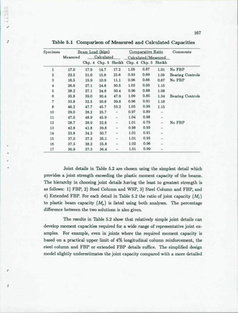
J . .

:

:

167

Table 5.1 Comparison of Measured and Calculated Capacities

Specimen B~ilm L2i1d. (kiJ2l) ComRarativ~ Ratio Comment. Measured Calculated Qills;ylil~ed lMt~!.I[~d.

Chp.4 Chp. 5 Sheikh Chp.4 Chp.5 Sheikh

1 17.0 17.9 14.7 17.2 1.05 0.87 1.01 No FBP 2 22.5 21.0 15.6 23.6 0.93 0.69 1.05 Bearing Controla

3 16.5 15.9 10.9 11.1 0.96 0.66 0.67 No FBP

4 26.6 27.1 24.8 30.5 1.02 0.93 1.15 5 28.2 27.1 24.8 30.4 0.96 0.88 1.08 6 35.8 39.0 30.4 47.9 1.09 0.85 1.34 Bearing Controla 7 33.8 32.5 30.8 39.8 0.96 0.91 1.18 8 46.2 47.7 45.7 53.2 1.03 0.99 1.15

10 29.0 28.2 25.7 0.97 0.89

11 47.0 48.9 45.9 1.04 0.98

12 28.7 28.9 22.8 1.01 0.79 No FBP 13 42.8 41.8 39.8 0.98 0.93

14 33.8 34.3 30.7 1.01 0.91

15 37.0 37.3 35.1 1.01 0.95

16 37.3 38.2 35.8 1.02 0.96

17 36.9 37.3 36.4 1.01 0.99

Joint details in Table 5.2 are chosen using the simplest detail which

provides a joint strength exceeding the plastic moment capacity of the beams.

The hierarchy in choosing joint details having the least to greatest strength is

as follows: 1) FBP, 2) Steel Column and WSP, 3) Steel Column and FBP, and

4) Extended FBP. For each detail in Table 5.2 the ratio of joint capacity (M;) to plastic beam capacity (Mp) is listed using both analyses. The percentage

difference between the two solutions is also given.

The results in Table 5.2 show that relatively simple joint details can

develop moment capacities required for a wide range of representative joint ex­

amples. For example, even in joints where the required moment capacity is

based on a practical upper limit of 4% longitudinal column reinforcement, the

steel column and FBP or extended FBP details suffice. The simplified design

model slightly underestimates the joint capacity compared with a more detailed

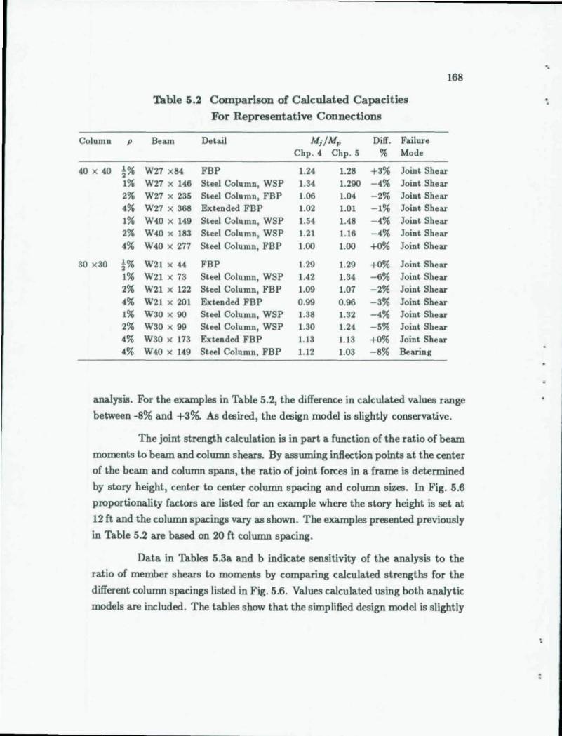
168

Table 5.2 Comparison of Calculated Capacities

For Representative Connections

Column p Beam Detail Mj/Mp Oil£. Failure Chp.4 Chp.5 % Mode

40 X 40 1% 2 W27 x 84 FBP 1.24 1.28 +3% Joint Shear 1% W27 X 146 Steel Column, WSP 1.34 1.290 -4% Joint Shear 2% W27 X 235 Steel Column, FBP 1.06 1.04 - 2% Joint Shear 4% W27 X 368 Extended FBP 1.02 1.01 -1% Joint Shear 1% W40 X 149 Steel Column, WSP 1.54 1.48 - 4% Joint Shear 2% W40 X 183 Steel Column, WSP 1.21 1.16 - 4% Joint Shear 4% W40 X 277 Steel Column, FBP 1.00 1.00 +0% Joint Shear

30 x30 1% 2 W21 X 44 FBP 1.29 1.29 +0% Joint Shear 1% W21 X 73 Steel Column, WSP 1.42 1.34 -6% Joint Sbear 2% W21 X 122 Steel Column, FBP 1.09 1.07 - 2% Joint Shear 4% W21 X 201 Extended FBP 0.99 0.96 - 3% Joint Shear 1% W30 X 90 Steel Column, WSP 1.38 1.32 -4% Joint Shear 2% W30 X 99 Steel Column, WSP 1.30 1.24 - 5% Joint Shear 4% W30 X 173 Extended FBP 1.13 1.13 +0% Joint Sbear 4% W40 X 149 Steel Column, FBP 1.12 1.03 - 8% Bearing

analysis. For the examples in Table 5.2, the difference in calculated values range

between -8% and +3%. As desired, the design model is slightly conservative.

The joint strength calculation is in part a function of the ratio of beam

moments to beam and column shears. By assuming inflection points at the center

of the beam and column spans, the ratio of joint forces in a frame is determined

by story height, center to center column spacing and column sizes. In Fig. 5.6

proportionality factors are listed for an example where the story height is set at

12 ft and the column spacings vary as shown. The examples presented previously

in Table 5.2 are based on 20 ft column spacing.

Data in Tables 5.3a and b indicate sensitivity of the analysis to the

ratio of member shears to moments by comparing calculated strengths for the

different column spacings listed in Fig. 5.6. Values calculated using both analytic

models are included. The tables show that the simplified design model is slightly

..

'.

:

·'

. '

:

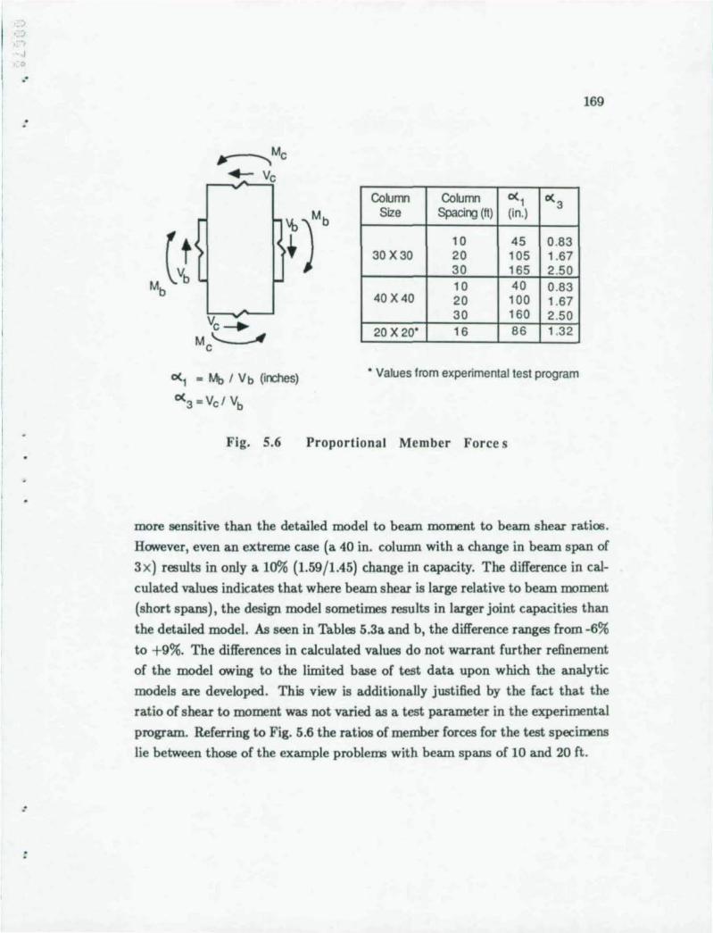
~ m Mb I V b (inches)

0(3 = Vel Vb

Fig. 5.6

169

Column Column 0(1 0(3 Size Spacing (ft) (in.)

10 45 0 .83 30 X30 20 105 1.67

30 165 2.50 10 40 0.83

40X40 20 100 1.67 30 160 2.50

20 X 20' 16 86 1 .32

• Values from experimental test pro9ram

Proportional Member Force s

more sensitive than the detailed model to beam moment to beam shear ratios.

However, even an extreme case (a 40 in. column with a change in beam span of

3 x) results in only a 10% (1.59/1.45) change in capacity. The difference in cal­

culated values indicates that where beam shear is large relative to beam moment

(short spans), the design model sometimes results in larger joint capacities than

the detailed model. AI; seen in Tables 5.3a and b, the difference ranges from -6%

to +9%. The differences in calculated values do not warrant further refinement

of the model owing to the limited base of test data upon which the analytic

models are developed. This view is additionally justified by the fact that the

ratio of shear to moment was not varied as a test parameter in the experimental

program. Referring to Fig. 5.6 the ratios of member forces for the test specimens

lie between those of the example problems with beam spans of 10 and 20 ft .

'.

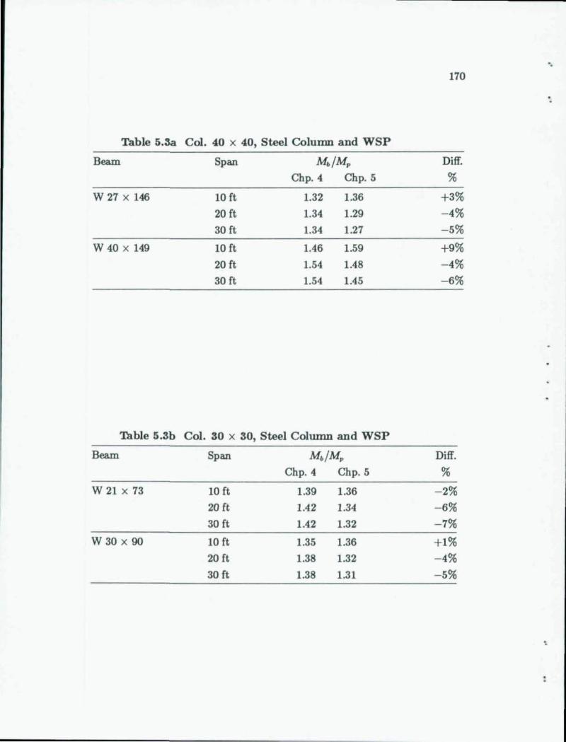
170

Table 5.3a Col. 40 x 40, Steel Column and WSP

Beam Span M./M. Diff.

Chp.4 Chp. 5 %

W 27 x 146 10 ft 1.32 1.36 + 3%

20 ft 1.34 1.29 - 4%

30 ft 1.34 1.27 - 5%

W 40 x 149 10 ft 1.46 1.59 + 9%

20 ft 1.54 1.48 -4%

30 ft 1.54 1.45 - 6%

Table 5.3b Col. 30 x 30, Steel Column and WSP

Beam Span M./M. Diff.

Chp. 4 Chp. 5 %

W 21 x 73 10 ft 1.39 1.36 - 2%

20 ft 1.42 1.34 - 6%

30 ft 1.42 1.32 - 7%

W30 x 90 10 ft 1.35 1.36 +1% 20 ft 1.38 1.32 - 4%

30 ft 1.38 1.31 - 5%

..

:

:

:

171

5.5 Structural Steel Detailing

Detailing requirements for structural steel components in the compos­

ite joint focus on aspects peculiar to composite connections which are not directly

apparent from current design standards for steel structures. Detailing of the fol­

lowing components is considered: web stiffeners (FBPs and WSPs) , steel column

sections, steel beam flanges, welded shear studs and vertical joint reinforcement .

Also developed is a general method for proportioning plates subjected to bending

under concrete bearing stresses.

5.5.1 Bearing Plate Thickness. At several locations in the connec­

tion, plates subject to transverse bending under concrete bearing stresses need

to be detailed. Specifically, the thickness of bearing plates supported on two

or three edges must be determined. Examples include the FBP, WSP, extended

FBP, steel column flange, and the steel beam flanges (Fig. 5.7a). The difficulty in

determining required plate thickness is that no convenient methods are available

to accurately predict the plate capacity including the effects of inelastic plate

bending and membrane action. The problem is further complicated by the fact

that the distribution of concrete bearing stresses against the plates is unknown.

The design method proposed for proportioning such plates is based on

a dimensional analysis of the problem calibrated to the test results . The method

is developed by considering a generic plate bending example shown in Fig. 5.Th

with two edges supported. The two edge support provides conservative results

for cases with three edges supported Given that the plate resists a distributed

load, P, with some unknown stress distribution the problem is to determine the

required plate thickness.

The problem is approached by relating the applied bending moment

to the resisting moment in the plate. The applied moment is proportional to

the product of the applied load, P, times some characteristic length. Similarly,

the moment resistance is proportional to the product of the material strength,

the square of the plate thickness, and a second characteristic length. Referring

to Fig. 5.7b, where Lm .. is much larger than Lmi., the plate is essentially

supported as a cantilever along Lma • . The characteristic length of the applied

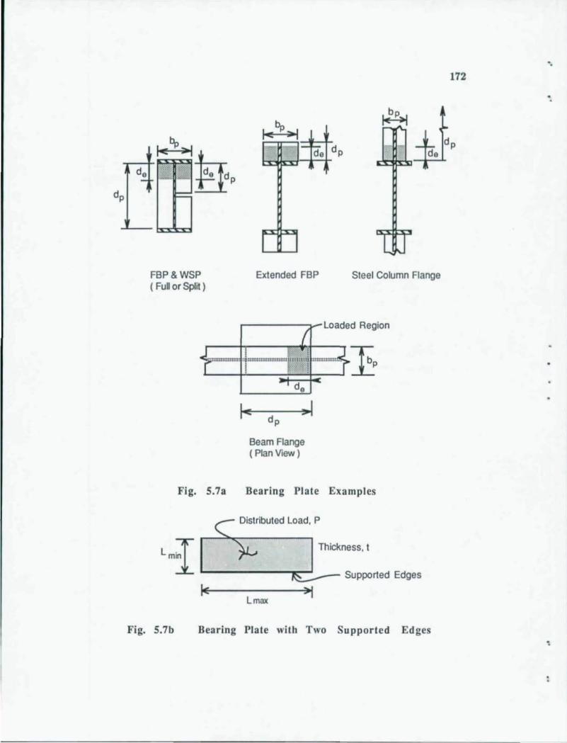
d p

de ::.

I~ "I IWy

'-;":': I ~

1=

FBP& WSP ( Full or Split)

~1II111U1UIII

Fig. S.7a

r 1 Extended FBP

( ! " , :fl ll l :lllllll l l ll llll l : Uiflfil(~ I ! ~

de

~I dp

Beam Flange (Plan View)

Loade

:tmllm:::!'!11 >

Steel Column Flange

d Region

Bearing Plate Examples

Distributed Load, P

L mi L ______ rs-::..Th_iCkness, t

Supported Edges

Lmax

Fig. S.7b Bearing Plate with Two Supported Edges

.. 172

'.

,.

t

173

moment is LmiA and that of the plate bending resistance is Lm ... Thus the

following expression can be written:

P LmiA = K F •• t~ Lm.. (5. 16a)

In this equation K is a proportionality factor. By rearranging Eq. 5.16a the plate

thickness is expressed as follows:

The proportionality constant. K. is determined by correlating Eq. 5.16b with

experUnentaidata

The most severe plate bending occurred in Specimen 10 where extensive

yielding of the split FBP was observed. The results of this test are used to

calibrate Eq. 5.16b. Referring to Fig. 5.7a the two plate lengths used in the

analysis are b./2 and the concrete bearing length, d •. Using the applied load.

plate thickness. and steel properties from Specimen 10. K is 0.18. In this case. the

actual plate length is longer than the loaded region (tI,. exceeds d. in Fig. 5.7a).

and a K value of 0.18 is only valid where d./d, is greater than 1.8. An upper

bound for K where d. equals d, is obtained using the dimension. d. . In this

case. K is equal to 0.24.

In summary:

LmiA = Minimum (b./2. d, )

Lm •• = Maximum (b./2. d. )

P = Applied Load

F •• = Yield Stress of Plate

K = 0.18 where d./d, > 1.8

0.24 where d./d, > 1.8

(5.17)

174

Since this equation is based on a single test where the ratio of Lmin to Lm •• is close to unity, Eq. 5.17 should be applied only to plates under concrete

bearing stresses where the loaded region has a maximum aspect ratio of 2.0

(Lm .. / Lmin < 2.0). Equation 5.17 is similar to one presented by Sheikh,· how­

ever, Sheikh's formulation is specifically intended only for full height FBPs sup­

ported on three edges.

5.5.2 Web Stiffeners (FBPs and WSPs). With regard to com­

posite behavior the primary function of web stiffeners, either in a FBP or WSP

configuration, is to mobilize a concrete compression strut between the flanges.

The stiffeners transfer horizontal load into the concrete through direct bearing

as shown in Fig. 5.8. The total horizontal load is equal to Vn as determined in

the joint panel calculations using Eqs. 5.6a through 5.6d.

Required Plate Width. As described previously, in calculations the

width of WSPs or split FBPs should not be taken greater than the beam flange

width. Where full height FBPs are intended to mobilize concrete outside the

beam flanges, the aUowable plate extension is dependent on the plate thickness.

The following limitation on plate extension is the same as that proposed by Sheikh? ;

(5.18)

The intent of Eq. 5.18 is to ensure adequate stiffness for a plate extending beyond

the beam flanges. Presumably, Eq. 5.18 need not apply if special measures are

taken to stiffen the wide FBP.

Bearing Forces and Weld Requirements. Concrete bearing against the

plate is considered using an equivalent rectangular stress block of width, bp , and

height, d,. As noted in Chapter 4, the bearing zone height is taken as a constant

value equal to 0.25 d.,. The horizontal strut capacity, Vn , is applied uniformly

over the bearing area to calculate the bearing stress. The concrete bearing

stress in this region should not exceed 2 f;. The required weld size between the

beam and bearing plate should be determined with a weld length limited to the

perimeter of the assumed bearing zone as shown in Fig. 5.8. The weld should be

sized to transfer the force, Vn , through shear into the beam.

:

.'

:

:

175

Plate Thickness. The FBP or WSP thickness should be determined

using Eq. 5.17 developed previously. In Eq. 5.17, the load P, applied to the

bearing plates on each side of the web is equal to Vn /2. The characteristic

lengths in Eq. 5.17 are the bearing zone height, d. (equaling 0.25 d .. ), and the

lesser of one-half the plate or flange width, bp /2 or b, /2. Finally, where a split

FBP is used the ratio of dp/d. should be checked to determine the proper K factor to use.

5.5.3 Extended FBP. The extended FBP transfers horizontal force

between the beam flange and the concrete outside the beam depth. A typical

extended FBP detail is shown in Fig. 5.9. In order to be fully effective FBP

height should exceed the distance dop (recall dop .$ 0.25d) indicated in Fig. 5.9.

Also, to mobilize the largest outer panel shear, V~, the FBP width should be

equal to the beam flange width, b,.

As shown in Fig. 5.9 the extended FBP resists a force equal to the

sum of the outer panel shear, V~, and the concrete column shear, Ye . Horizontal

concrete bearing stresses, required plate thickness, stiffener requirements, and

connection to the beam flange must be checked. The concrete stresses should be

calculated by considering the applied load acting over an area of width, b., and

height equal to the lesser of the plate height, d., or do •. The concrete bearing

stress should not exceed 2 f;.

In order to keep the plate to a practical thickness, stiffeners such as

those shown in Fig. 5.9 are usually required. When a single stiffener at the center

is used, the FBP thickness may be determined using Eq. 5.17. The characteristic

lengths for Eq. 5.17 should be equal to b./2 and the lesser of dp or dop. The

load, P, in Eq. 5.17 is taken equal to (V~ + Ye)/2 for one half of the FBP. Since

the ratio d./ d.. is usually less than 1.8, a K value of 0.24 should be used in

Eq. 5.17. Where an unstiffened plate is used, the required thickness is determined

by considering the Extended FBP as a cantilever supported at the beam flange.

5.5.4 Steel Column Section. The only steel column requirements

considered here are related to the transfer of horizontal load from the steel beam

flanges into the concrete through bearing against the column.

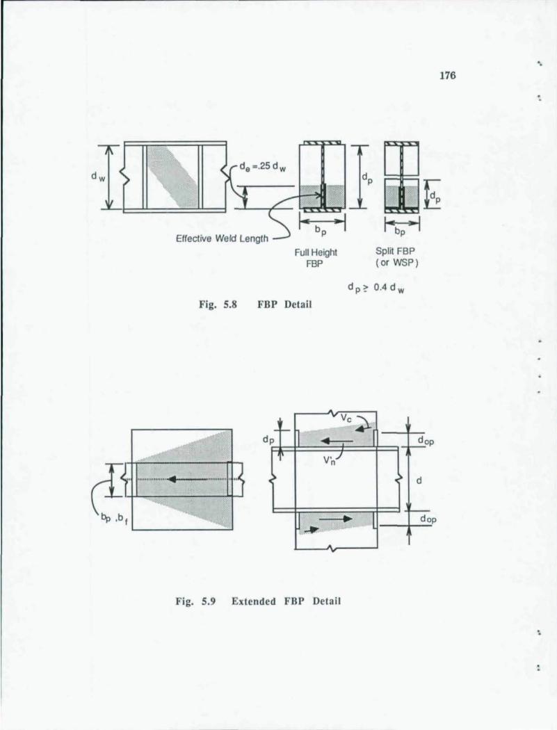
Effective Weld length I .. b

p -I

Full Height FBP

Fig. 5.8 FBP Detail

01..j..L..,.."..· ................ :=4 --4-J

bp .b f

V'n

'--_____ --'''-1

Fig. 5.9 Extended FBP Detail

I"bp -I Split FBP (or WSP)

d op

d

dop

'. 176

"

'.

.'

:

:

:

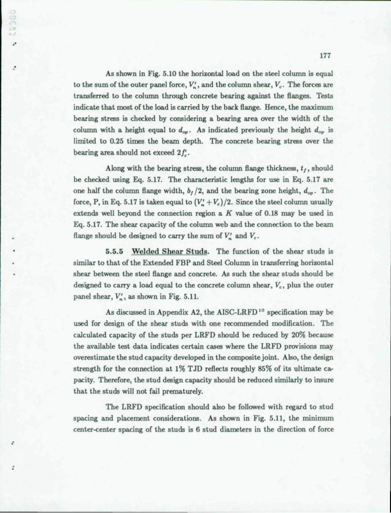
177

As shown in Fig. 5.10 the horizontal load on the steel column is equal

to the sum of the outer panel force, V~, and the column shear, Ve' The forces are

transferred to the column through concrete bearing against the flanges. Tests

indicate that most of the load is carried by the back flange. Hence, the maximum

bearing stress is checked by considering a bearing area over the width of the

column with a height equal to dop. As indicated previously the height d.p is

limited to 0.25 times the beam depth. The concrete bearing stress over the

bearing area should not exceed 2f..

Along with the bearing stress, the column flange thickness, t" should

be checked using Eq. 5.17. The characteristic lengths for use in Eq. 5.17 are

one half the column flange width, b, /2, and the bearing zone height, dop. The

force, P, in Eq. 5.17 is taken equal to (V~ + V.)/2. Since the steel column usually

extends well beyond the connection region a K value of 0.18 may be used in

Eq. 5.17. The shear capacity of the column web and the connection to the beam

flange should be designed to carry the sum of V~ and V..

5.5.5 Welded Shear Studs. The function of the shear studs is

similar to that of the Extended FBP and Steel Column in transferring horizontal

shear between the steel flange and concrete. As such the shear studs should be

designed to carry a load equal to the concrete column shear, V., plus the outer

panel shear, V~, as shown in Fig. 5.11.

As discussed in Appendix A2, the AlSC-LRFD 10 specification may be

used for design of the shear studs with one recommended modification. The

calculated capacity of the studs per LRFD should be reduced by 20% because

the available test data indicates certain cases where the LRFD provisions may

overestimate the stud capacity developed in the composite joint. Also, the design

strength for the connection at 1% T JD reflects roughly 85% of its ultimate ca­

pacity. Therefore, the stud design capacity should be reduced similarly to insure

that the studs will not fail prematurely.

The LRFD specification should also be followed with regard to stud

spacing and placement considerations. As shown in Fig. 5.11, the minimum

center-center spacing of the studs is 6 stud diameters in the direction of force

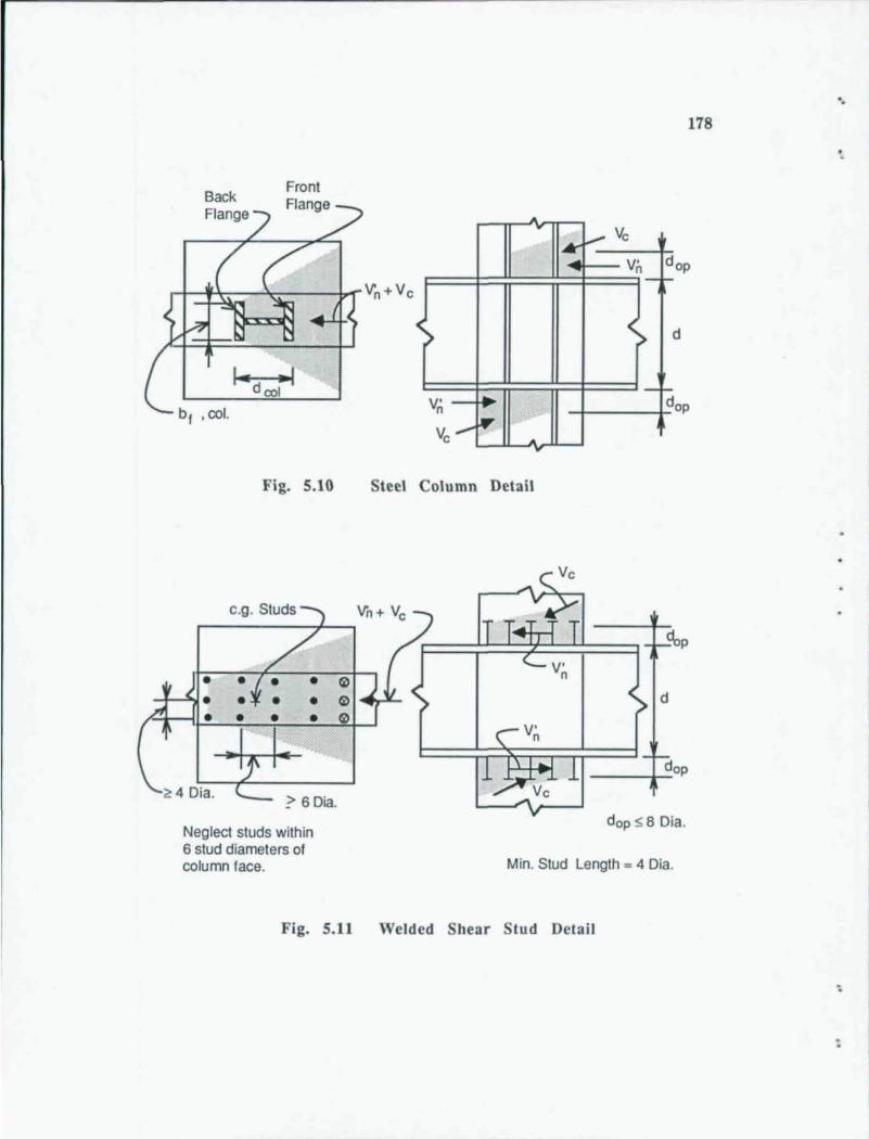
Back Ftange

b f , col.

Fig. S.10

c.g. Studs

• • • • • • • • • • •

~ 4 Oia. ? 60ia.

Neglect studs within 6 stud diameters of column face .

~

~

~

Fig. S.l1

'.

178

'.

'v I-- VC IA-

V' d ~- f-

op

< > d

- f-.. v.' d n op 111'

,.

Vc - v

Steel Column Detail

~p

d

__ --.f-.'.dop

dop S 8 Oia.

Min. Stud Length = 4 Oia.

Welded Shear Stud Detail

..

:

:

179

and 4 diameters transverse to the force. Studs within 6 diameters of the tension

face of the column should not be considered as contributing to the stud group

capacity since such studs have inadequate concrete cover to develop their full

shear capacity. No more than 3 studs per row should be considered in strength

calculations. Finally, the minimum required stud height is 4 stud diameters, and

the calculated dimension of d"" should not exceed 8 diameters or 0.25 d.

5.5.6 Vertical Joint Reinforcement. Joint reinforcement provides

for a direct transfer of vertical tension and compression forces between the beam

flanges and the connection, and for horizontal load transfer in a manner similar

to that of the extended FBP, steel column and shear studs.

Vertical joint reinforcement is needed when concrete bearing stresses

control design. Assessment of the axial capacity of vertical reinforcement should

include consideration of the mechanical connection to the beam and adequate

development of the reinforcement into the concrete. Bar connection to the steel

beam may be by direct welding or through welded couplers. These details should

be checked using applicable standards such as the LR FD specification and the

American Welding Society Standards. ACI-318 should be used to determine

the required bar development length. As shown in Fig. 5.12, the development

length should be evaluated after discounting a distance adjacent to the beam

flange equal to the greater of the following: the connection fixture length, 1/ 4

of the beam depth, or 12 inches. The discounted region is based on the bond

and cracking behavior discussed in Chapter 3. Finally, the reinforcement should

be located within 0.2 h of the column face in order to be fully stressed prior to

crushing of adjacent concrete.

The vertical joint reinforcement may also be considered to provide a

horizontal force transfer similar to that of welded shear studs. Where this is the

case both the shear capacity of the reinforcement and the horizontal concrete

bearing stress against the reinforcement should be checked. The maximum hor­

izontal load resisted by the vertical reinforcement is the sum of the outer panel

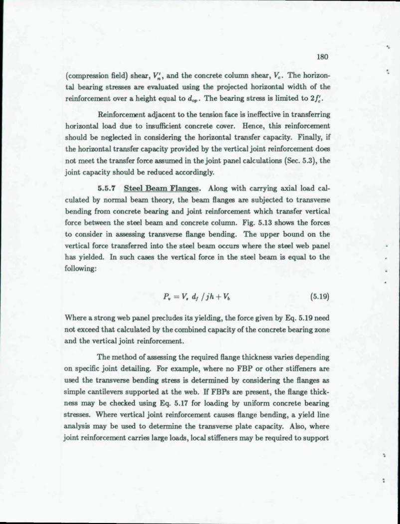
180

(compression field) shear, V~, and the concrete column shear, v.. The horizon·

tal bearing stresses are evaluated using the projected horizontal width of the

reinforcement over a height equal to d.". The bearing stress is limited to 2/: .

Reinforcement adjacent to the tension face is ineffective in transferring

horizontal load due to insufficient concrete cover. Hence, this reinforcement

should be neglected in considering the horizontal transfer capacity. Finally, if

the horizontal transfer capacity provided by the vertical joint reinforcement does

not meet the transfer force assumed in the joint panel calculations (Sec, 5.3), the

joint capacity should be reduced accordingly.

5.5. '1 Steel Beam Flanges. Along with carrying axial load cal­

culated by normal beam theory, the beam flanges are subjected to transverse

bending from concrete bearing and joint reinforcement which transfer vertical

force between the steel beam and concrete column. Fig. 5.13 shows the forces

to consider in assessing transverse flange bending. The upper bound on the

vertical force transferred into the steel beam occurs where the steel web panel

has yielded. In such cases the vertical force in the steel beam is equal to the

following:

p. = V. d, Jih + Vb (5,19)

Where a strong web panel precludes its yielding, the force given by Eq. 5.19 need

not exceed that calculated by the combined capacity of the concrete bearing zone

and the vertical joint reinforcement.

The method of assessing the required flange thickness varies depending

on specific joint detailing, For example, where no FBP or other stiffeners are

used the transverse bending stress is determined by considering the flanges as

simple cantilevers supported at the web. IT FBPs are present, the flange thick­

ness may be checked using Eq. 5.17 for loading by uniform concrete bearing

stresses. Where vertical joint reinforcement causes flange bending, a yield line

analysis may be used to determine the transverse plate capacity. Also, where

joint reinforcement carries large loads, local stiffeners may be required to support

'.

·'

:

:

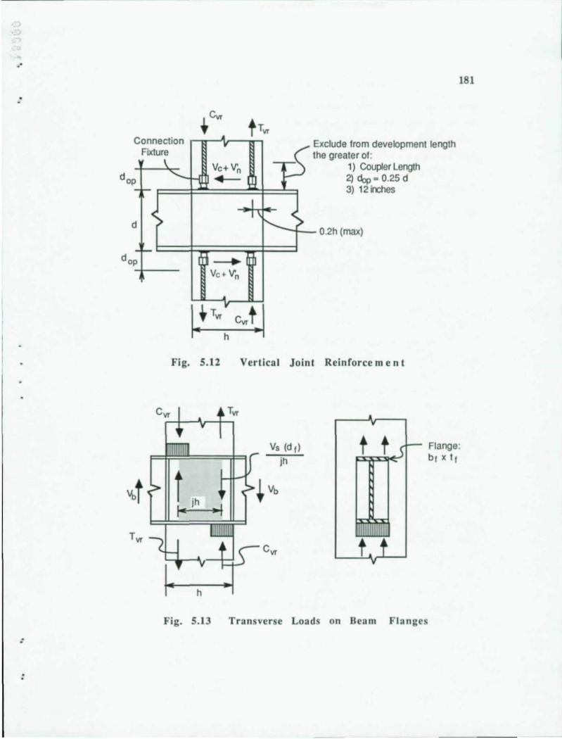
181

.. ~ trw Connection ,-,,...--...)~ .Ir-"--,,.-,

Fixture ./" tEXCIUde from development length ( he greater of :

+-~\ VC+V'n d op '--.-..lTll ~

- r- F==~==~f=~ ) i)

--"-W-' 1) Coupler Length 2) dop = 0.25 d 3) 12 inches

d > "-I --~_ 0.2h (max)

•

Fig. 5.12 Vertical Joint Reinrorce men t

h

Vs (d,)

jh

Fig. 5.13 Transverse Loads on Bcam Flangcs

Flange: b, x t,

182

the flange. Bearing stresses against the compression flange tend to be resisted

in part by the opposite tension Bange due to load transferred by concrete be­

tween the Banges. The range of possible details and configurations is large.

Specific recommendations or equations cannot address properly the wide range

of circumstances that determine required Bange thickness and are, therefore, not

attempted in this report.

5.6 Reinforcing Steel Detailing

Detailing recommendations for the lateral ties and longitudinal column

bars in the joint region are intended to supplement standard detailing practice

and requirements given by applicable reports and standards of the American

Concrete Institute.

Most of the detailing recommendations are drawn from recent research

and detailing recommendations for reinforced concrete joints. Several impor­

tant differences exist, however, between composite joints and reinforced concrete

joints. First, the basic joint shear behavior in the composite joint is a combi­

nation of the steel web, the compression strut and the compression field mecha­

nisms, whereas in reinforced concrete joints typically only the compression strut

mechanism is considered in design. Second, in composite joints detailing is com­

plicated by fabrication difficulties posed by the steel beams and column passing

through the joint.

5,6,1 Horizontai Column Ties, In the composite joint horizontal

ties serve several functions which are considered in the detailing recommenda­

tions. One function is to carry tension forces associated with the compression

field (or truss) mechanism, thereby providing shear resistance in the outer con­

crete panel. The ties above and below the beam must also resist tension forces

associated with the horizontal strut mechanism transferring horizontal shear be­

tween beam Banges and outer panel. The second major function of the ties is

in providing confinement to concrete in and adjacent to the joint region. Such

confinement is particularly important for seismic design where inelastic cyclic

loading is anticipated. Finally, ties in the joint region prevent local buckling of

longitudinal column bars.

"

"

..

:

183

Lateral ties within the beam depth primarily carry joint shear in the

compression field and to a lesser degree provide confinement to the joint core.

The shear requirement for the ties is calculated using Eqs. 5.7a through c based

on concrete controlling the compression field strength. In order for tie capacity

not to govern compression field strength as given by the upper bound in Eq. 5.7c,

the cross sectional tie area, A. h (Fig. 5.14), should satisfy the following equation:

0.52 VII b~p Sh A.h = F.

• (5.20)

To reiterate, this equation applies only when it is desired to develop the full

compression field width, b~p, mobilized by the joint detail.

A minimum tie area is recommended based on recent research and

recommendations in the United States and Japan for minimum lateral ties in

reinforced concrete joints. In the United States, the ACI-ASCE Committee 352'

recommends a minimum tie area given by the greater of the following equations:

A _ 0.3sh hOI f; (A,,/A. -1) .h - F.

• (5.21a)

O.09sh hOI f; A.h = F.

• (5.21b)

The area given by Eqs. 5.19a and 5.19b may be reduced by 1/2 for interior joints

where orthogonally framed beams provide confinement to the joint.

In Japan, Kitayama {et al.l" recommend a minimum tie area which

can be expressed as follows:

A.h = O.OO3bsh (5.22)

Equation 5.22 results in about 1/3 the steel area required by Eqs. 5.21a and

5.21b. Both the US and Japanese recommendations are specified for use in

seismic design, and both primarily intend the requirements to provide a mini­

mum concrete confinement for exterior joints. The large difference between the

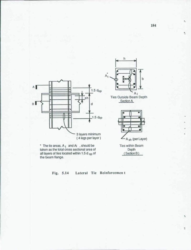
A

B

~

I 1.5 dop

sh

I > (> d

A\

V~

---jf-1 .5 dop

3 layers minimum ( 4 legs per layer)

• The tie areas, A t and AI , should be taken as the total cross sectional area of aU layers of ties located within 1.5 d op of the beam flange.

h

~I

b

AI Ties Outside Beam Depth

Section A

J

~ I • J

• • ( •

L A sh (per Laye~

Ties within Beam Depth

(Section B)

Fig, 5.14 Lateral Tie Reinforcemen t

' . 184

'.

., '-?

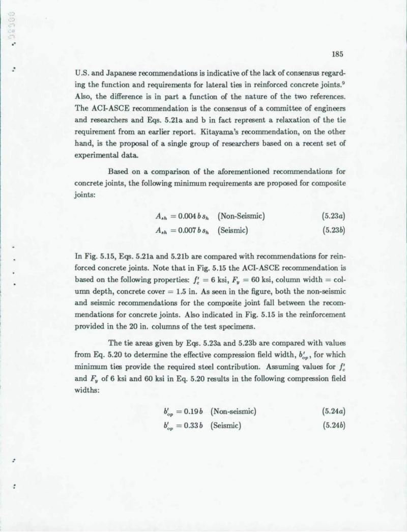
o

"

..

:

185

U,S, and Japanese recommendations is indicative of the lack of consensus regard­

ing the function and requirements for lateral ties in reinforced concrete joints?

Also, the difference is in part a function of the nature of the two references.

The ACI-ASCE recommendation is the consensus of a committee of engineers

and researchers and Eqs. 5.21a and b in fact represent a relaxation of the tie

requirement from an earlier report. Kitayama's recommendation, on the other

hand, is the proposal of a single group of researchers based on a recent set of

experUnentrudat~

Based on a comparison of the aforementioned recommendations for

concrete joints, the following minimum requirements are proposed for composite

joints:

A.h = 0.004 b 8h (Non-Seismic)

A.h = 0.007 bSh (Seismic)

(5 .23a)

(5.23b)

In Fig. 5.15, Eqs. 5.21a and 5.21b are compared with recommendations for rein­

forced concrete joints. Note that in Fig. 5.15 the ACI-ASCE recommendation is

based on the following properties: f~ = 6 ksi, F. = 60 ksi, column width = col­

umn depth, concrete cover = 1.5 in. As seen in the figure, both the non-seismic

and seismic recommendations for the composite joint frul between the recom­

mendations for concrete joints. Also indicated in Fig. 5.15 is the reinforcement

provided in the 20 in. columns of the test specimens.

The tie areas given by Eqs. 5.23a and 5.23b are compared with values

from Eq. 5.20 to determine the effective compression field width, b;p, for which

miniIInlm ties provide the required steel contribution. Assuming values for f~

and F. of 6 ksi and 60 ksi in Eq. 5.20 results in the following compression field

widths:

b:. = 0.19b (Non-seismic)

b:. = 0.33 b (Seismic)

(5 .24a)

(5.24b)

186

.• .4 ACI·ASCE' --ii .>

...... Composite Joint (Seismic) ~ .• t----:.

Compos~e Joint

~:;~~;:;:;:::::::::::~(~No~n~.s=e=is=m=iC=)=,~:;;::::== ., ~ Japanese

Test Specimens O+-------r-----~~----~------_r------~------~

20 30 35 ~ 45 50

Column WIdth (1n.)

• note: ACI·ASCE curve is based on the following values used in Eqs. 5.19a and b: Fy = 6Oksi, fb = 6 ksi, square col., 1.5 in. cover.

Fig. 5.15 Minimum Lateral Tie Area s

In a joint where the beam width is one half the column width, an extended

FBP detail mobilizes a compression field width equal to approximately 0.25 b.

Similarly, an embedded steel column in a similar detail would mobilize a width

equal to roughly 0.12 b. Compared to the widths given in Eqs. 5.24a and 5.24b,

the minimum tie area provides at least 75% of the reinforcing steel required to

develop the available compression field capacity.

Column ties above and below the beam both carry tensile forces which

transfer shear into the outer concrete panel and provide concrete confinement in

the highly stressed bearing zone. The minimum recommended tie requirement

in this region is for three layers of ties located as shown previously in Fig. 5.14.

The recommended bar sizes are related to the column width, b, as follows: b < 20 in., #3 bars; b < 30 in., #4 bars; b > 30 in., #5 bars.

",

'.

, )

d , .,

"

..

187

Where the outer panel compression field is mobilized, additional ties

may be required to transfer the shear force, V~, between the beam flange and

the outer panel. This horizontal force is transferred by combined strut and shear

friction mechanisms described more completely in Chapter 4, Referring to the tie

areas, A, and At shown in Fig. 5.14, the horizontal transfer strength is calculated

by the following equations:

Pc = Ptl + Pel < 1.5 Ptl

Ptl = F •• h At

Pel = 1.4 A, F •• h

(5 .25a)

(5 .25b)

(5.25c)

Ptl in Eq. 5.25 is the capacity of the strut mechanism. Pel in Eq. 5.25c is the

shear friction mechanism strength which usually applies only with the extended

FBP detail. The upper limit on P, of 1.5 Pu in Eq. 5.25a is based on the

maximum horizontal transfer observed in the test specimens .

Figure 5.16 indicates the reinforcement required in a 3 ft square column

based on the proposed miniIIDlm standards. As noted previously, additional ties

may be required where the internal forces exceed those carried by the minimum

steel areas. Also, the ties in the joint region should meet minimum requirements

for the concrete or composite column adjacent to the joint.

The example in Fig. 5.16 demonstrates several practical detailing con­

cerns in composite joints. The cross section above the beam (Sec. A) depicts

a region where detailing is similar to that in reinforced concrete columns. For

non-seismic designs the ties in this region may be closed rectangular hoops with

90 degree hooks or cap ties. Where loss of concrete cover is a design concern due

to seismic loading, rectangular ties should have 135 degree hooks which anchor

the ties in the column core. Within the beam depth (Sec. B), tie detailing is

complicated by steel beam webs passing through the column. Figure 5.16 in­

cludes a transverse floor beam in order to present a realistic example of detailing

considerations within the beam depth. As shown in the figure, the ties within

the beam depth are made up of several pieces. The inner set of reinforcement

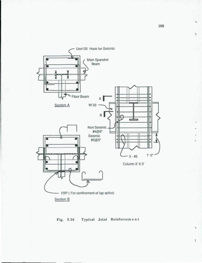
Use13S Hook for Seismic

-,,"" .......... _ ................................. .

I:::: z:m:::::::L--..B:mmm:::

rT""Q ••••••••••••• - ..... ? ••• ~ .. . ............. .

::: ;

~ain Spandrel

Beam

:11lI. ,

FborBeam ~::~'~'::=4t:::~

•

•

Section A W 33

•

Non Seismic #4@6"

Seismic #S@S"

J FBP ( For confinement of lap splice)

Section B

........................................... ,

. ...... . ... :.: ••••••••••••• '1"1 •• • ••• ••• •• :: :: , , , ; , , , , , , , , i ~ , 1 ,

3 - #5 l' 0"

Column 3' X 3'

Fig, 5,16 Typicat Joint Reinforcem e n t

'. 188

-,

:

• ..

:

:

189

consists of hairpin ties which do not pierce the main spandrel beam web. For

seismic design the hairpin ties should have a 135 degree hook on at least one

of the ends. The outer tie is fabricated in three pieces as shown. In such cases

bars should be lap spliced or hooked to provide full tension development of ties

around the column perimeter. Note that particularly for seismic design, the FBP

on both the spandrel and floor beam is recommended to provide confinement for

lap splices of the ties.

5.6.2 Vertical Column Bars. Where vertical column bar sizes are

controlled primarily by column bending moments, the bond stress around the

bars is quite large through the joint region. As observed in the experiments, typ­

ically at a load equal to roughly 1/2 the nominal design load, the rate of increase

in bond stress drops off. This results from concrete cracking which isolates the

vertical bars and surrounding concrete from the joint panel. This phenomenon

is aggravated by reinforcing bar layouts where vertical steel is concentrated in

column corners to provide clearance for steel beams.

In reinforced concrete joints where there is concern over loss of bond

through the joint, the vertical bar sizes are limited as a function of the connection

height. ACI-ASCE Committee 352" recommends that in joints subjected to

seismic loading the bar diameter be limited by the beam depth, d, as follows :

(5.26)

A similar set of recommendations is proposed for composite joints with

two variations. First, separate requirements are proposed for seismic and non­

seismic loadings. Second, the joint height should be taken as the beam depth, d,

plus the joint extension, dop, where elements such as the steel column extend the

region of concrete mobilization. The maximum bar sizes are given as follows:

db < (d + d".) / 15 Non-seismic

db < (d + d".) / 20 Seismic

(5 .27a)

(5 .27b)

190

The less stringent value for the non-seismic case is based on Specimens 3 through

17 in which the ratio of beam depth to column bar diameter was 14.2 and per­

formance was sat isfactory. In addition to the bar size limitation, bundled bars

should not be used where high bond stresses are of concern.

The limi tations on the vertical bars need not apply where the column

reinforcement is provided primarily to carry axial loads. In such cases the bond

stress in the joint is not as critical due to the smaller moment transfer relative to

the size and number of vertical reinforcing bars. Where axial load is significant,

bond requirements may be checked by comparing the actual bond area provided

with that which would exist if axial load were ignored and the vertical bars

detailed to satisfy Eqs. 5.27a and 5.2Th. In other words, in the hypothetical case

the bars would be designed for moment only and smaller bar sizes than maximum

permitted size chosen. The bond areas should be calculated as the product of

the bar perimeter and the connection height .

5.7 Limitations of Recommendations

The design recommendations presented herein should not be indiscrim­

inately applied to composite connections substantially different from the test

specimens upon which the guidelines are based. Since the test specimens consid­

ered in this study are all of similar geometry and concrete strength, limitations

are given to restrict applicability of the design recommendations. The recom­

mendations may provide useful and reliable information for connections not in­

cluded within the limitations, however, careful judgment must be exercised in

extrapolating the results.

The design equations presented in this report directly apply only to

planar connections of cruciform shape such as those tested in the experimental

program. The basic component strengths for the steel and concrete joint shear

mechanisms may be adapted for use in other joint configurations. When used

for other geometries the internal load paths must be examined in order to prop­

erly calculate the joint strengths. Discussion regarding the analysis of alternate

configurations is outlined later in this chapter.

'.

'.

:

..

..

191

Design equations for the concrete panel and compression zone are lim­

ited to normal weight concrete with compressive strengths un equal to or less

than 6 ksi. This limitation follows that given by the ACI-ASCE Committee 352

recommendations, which cite lack of experimental data for light weight and high

strength concrete. Research in progress at the University of Texas ~ G involving

use of high strength concrete in reinforced concrete joints may yield data to in­

crease the applicability of these recommendations for higher strength concretes.

Finally, the recommendations in this report are limited to connections

where the geometry conforms to the following ratios:

Column Depth/Beam Depth: 0.75 < hid < 1.5

Beam Width/ Column Width: 0.3 < bdb < 0.6

(5.28a)

(5 .28b)

Equation 5.28a is the same as that proposed by Sheikh.! Equation 5.28b limits

the recommendations to geometries similar to those tested. Also, limitations on

the maximum beam width address practical concerns regarding concrete place­

ment and passage of column reinforcement through the joint.

5.8 Additional Considerations

Thus far the design recommendations have focused on assessing influ­

ence of joint details on the strength of planar cruciform configurations . Equally

important to successful design of such connections are construction concerns re­

lated to fabrication and erection of the composite system and placement of con­

crete in the joint region. Since buildings require joint configurations other than

the cruciform configuration studied, analysis of alternate joint configurations is

considered in this section.

5.8.1 Concrete Placement. Structural steel members passing thru

the joint pose an obstruction to concrete placement. Special measures should

be taken to insure against voids in the concrete. Such measures include special

attention to detailing to avoid congestion and careful selection of concrete mixes,

vibration procedures, and an adequate inspection program .

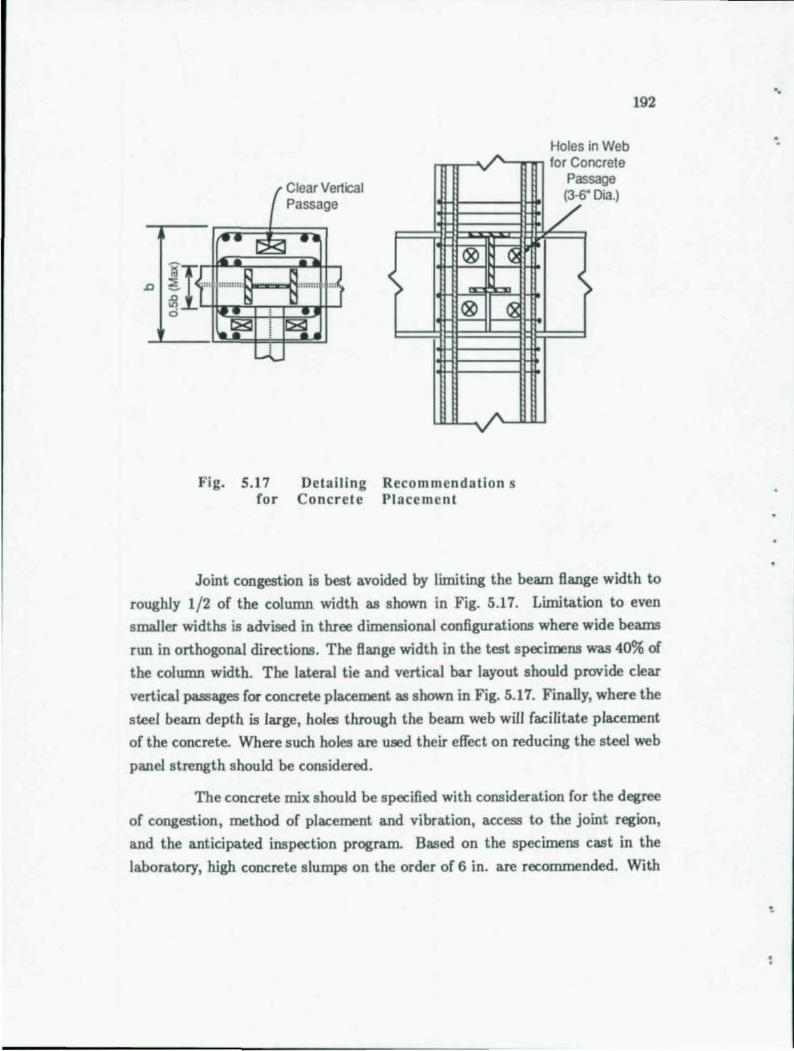
A. v

CI v rtical ear e Passage

,... ~ ~ .11 ® OJ

.0 II'" """'"H ''''''' ''' ) 6! ci

< >

® (g ... '?<' ~ rBl

--L

v

Fig. 5.17 Detailing Recommendation s for Concrete Placement

Holes in Web ncrete sage Dia.)

for Co Pas (3-6"

/'

\

192

Joint congestion is best a.voided by limiting the beam Bange width to

roughly 1/2 of the column width as shown in Fig. 5.17. Limitation to even

sma.ller widths is a.dvised in three dimensiona.l configura.tions where wide beams

run in orthogona.l directions. The Ba.nge width in the test specimens was 40% of

the column width. The la.teral tie a.nd vertical bar la.yout should provide clear

vertical passages for concrete placement as shown in Fig. 5.17. Fina.lly, where the

steel beam depth is large, holes through the beam web will fa.cilita.te placement

of the concrete. Where such holes are used their effect on reducing the steel web

pa.nel strength should be considered.

The concrete mix should be specified with consideration for the degree

of congestion, method of pla.cement a.nd vibra.tion, access to the joint region,

a.nd the a.nticipated inspection program. Based on the specimens cast in the

labora.tory, high concrete slumps on the order of 6 in. are reco=ended. With

'.

'.

..

..

193

such slumps concrete lift heights should be limited to approximately 1 ft between

vibration. In addition, air entrainment of about 5% improves the workability of

the concrete. Where high strength concretes are used, super-plasticizers (water

reducezs) may offer the most economical solution to reliable placement of the

concrete.

5.8.2 Coordination. Recommendations regarding the coordination

of detailing, fabrication, and construction are beyond the scope of this report

other than to advise that such considerations be addressed early in the design

process. Particularly in the joint region, composite construction requires close

coordination of the structural steel, reinforcing steel, and formwork details. ~

ordination of detailing needs to be addressed in the design specifications by either

requiring one agency to be responsible for all the work, or to carefully outline

the detailing responsibilities and channels of communication between different

contractozs and detailers. In design, the proposed erection sequence must be ex­

amined to insure that the envisioned structure can be built. In the joint region,

the main fabrication concern relates to detailing of reinforcing steel such that

it can be conveniently installed around the structural steel. Further discussion

of coordination and construction concerns for composite frames is presented in

references 2, 3, 5 and 27.

5.8.3 Alternate Joint Configurations. As presented in this chap­

ter the design equations are directly applicable to the cruciform (planar interior)

joint configuration as sh<7Nn in Fig. 5.18a. The design recommendations may

be adapted for other configurations through examination of the internal forces

and joint shear mechanisms. In order to demonstrate application to alternate

configurations several representative examples of other joint details are discussed.

Figures 5.18a through 5.ISd show four connection configurations con­

sidered in this section. In these figures beam forces associated with lateral frame

loading are shown along with the proportional column forces. Figures 5.18a,

b, and c include the following planar connections: interior, comer and top cor­ner. Figure 5.1Sd shows a three dimensional corner connection which occurs in

perimeter framed tube structures .

<

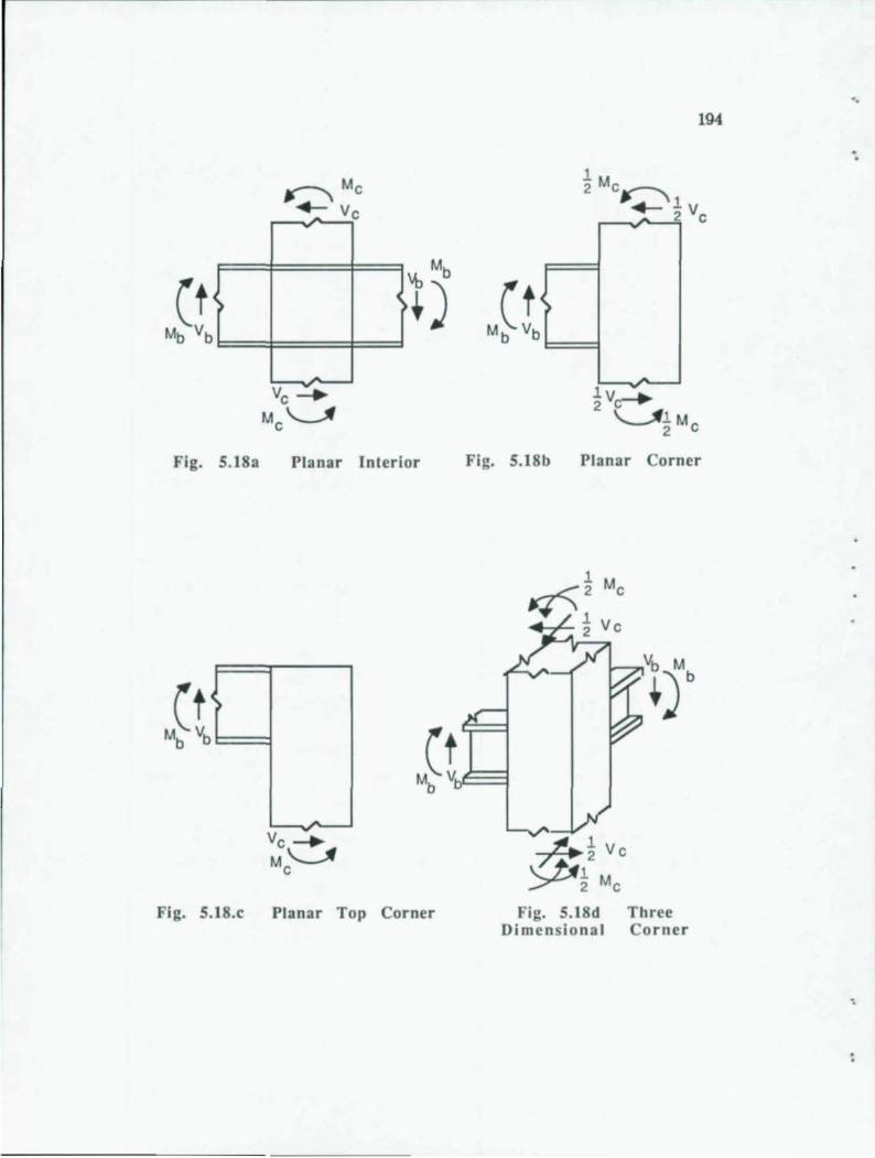
Fig. 5.1Sa

(t< Mb Vb

Fig. S.IS.c

r-'\ Me ~ Ve

<

Planar Interior

Met b

~

Ve ....... M~ e

Planar Top Corner

~V~ ~l M

2 e

194

Fig. 5. ISb Planar Corner

1)b

k~Ve ;fi~ Me

Fig. 5.1Sd Three Dimen ional Corner

..

.'

.'

195

The required joint shear strength is essentially a function of the total

unbalanced beam moment transferred into the columns. Referring to Figs. 5.18a

through 5.18d, the unbalanced moment in the interior connection is twice that

of the planar corner connections. The total unbalanced moment for the three

dimensional corner connection is equal to the planar joint, however, since the

loads are applied about two axes the internal forces in each direction are smaller.

The three dimensional comer is reasoned to be less critical than the planar

case by considering an analogy to biaxial bending of concrete columns . Figure

5.19 shows a typical failure envelope for biaxial bending in reinforced concrete

members. As indicated in this figure biaxial loading equal to 1/ 2 of the ultimate

capacity in each of the two directions is within the safe design region.

By comparison the planar interior joint (Fig. 5.18a) is assumed to be as

critical as any of the other three connection types in a given structure. Strictly

speaking, tills may not always be the case since connection forces will vary de­

pending on location in the structure. However, tills observation implies that in a

given structure the nature of details required for interior joints will probably be

adequate elsewhere. Hence, analysis of interior joints will suffice for feasibility

studies used for determining what special connection details will be required for

a given project.

Planar Corner Detail. The internal shear mechanisms are similar in

the four connection configurations, however, some important differences must be

addressed in detailing the connections. A planar corner detail shown in Fig. 5.20a

is most like an internal joint. The primary difference is that in the corner detail

the unbalanced beam moment enters the joint though only one side of the column.

Also, the unbalanced beam shear alters the joint equilibrium slightly. Note that

in order for the joint shear mechanisms to be fully effective the beam must extend

the entire width of the column as indicated in Fig. 5.20a. Another difference

between the interior and corner details is support of the FBP. As shown in

Fig. 5.20b, where the beam extends outside the connection, the horizontal beam

transfers forces into the bearing plate from the web and flange on both sides of

the plate. Where the beam does not extend outside the joint, force is transferred

only from the web and flange inside the joint. Transfer from one side may not be

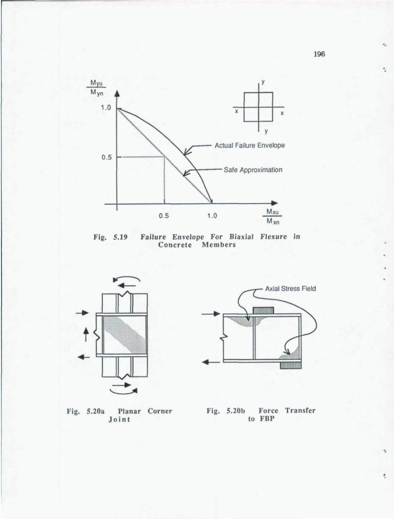
...MY':!.. Myn

1.0

0 .5

y

x x

~"'\....~~ . .",. y

.",.

"'::..._--. _-- Actual Failure Envelope

... . . ..... .......... . .. . .... .. .. ::0.

r·'·~ .~I,,--- Safe Approximation

, , 1

0.5 1.0 Mxu Mxn

Fig. 5.19 Failure Envelope For Biaxial Flexure in Concrete Members

196

Axial Stress Field

.... t ~.., ..

'"."

Fig. 5.20a Planar Corner Fig. 5.20b Force Transfer Join t to FBP

'.

· )

. '

:

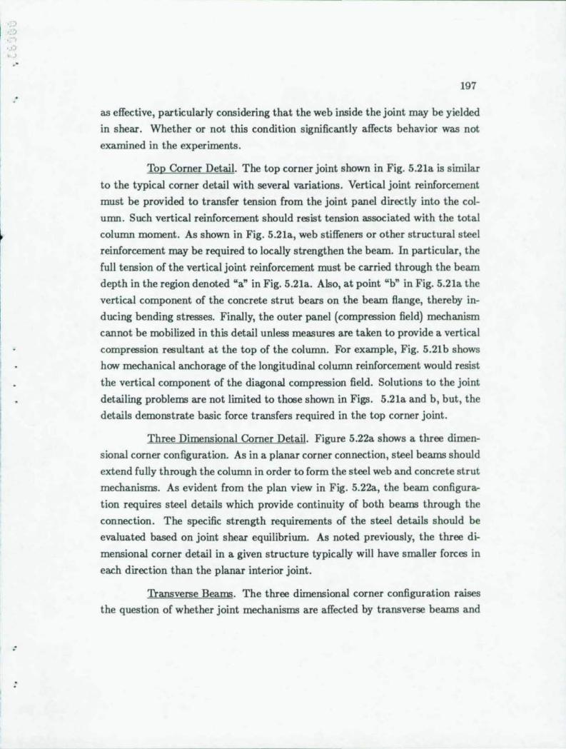
197

as effective, particularly considering that the web inside the joint may be yielded

in shear. Whether or not this condition significantly affects behavior was not

examined in the experiments.

Top Corner Detail. The top corner joint shown in Fig. 5.21a is similar

to the typical corner detail with several variations. Vertical joint reinforcement

must be provided to transfer tension from the joint panel directly into the col­

umn. Such vertical reinforcement should resist tension associated with the total

column moment. As shown in Fig. 5.21a, web stiffeners or other structural steel

reinforcement may be required to locally strengthen the beam. In particular, the

full tension of the vertical joint reinforcement must be carried through the beam

depth in the region denoted "a" in Fig. 5.21a. Also, at point "b" in Fig. 5.21a t he

vertical component of the concrete strut bears on the beam flange, thereby in­

ducing bending stresses. Finally, the outer panel (compression field) mechanism

cannot be mobilized in this detail unless measures are taken to provide a vertical

compression resultant at the top of the column. For example, Fig. 5.21b shows

how mechanical anchorage of the longitudinal column reinforcement would resist

the vertical component of the diagonal compression field. Solutions to the joint

detailing problems are not limited to those shown in Figs. 5.21a and b, but, the

details demonstrate basic force transfers required in the top corner joint.

Three Dimensional Corner Detail. Figure 5.22a shows a three dimen­

sional corner configuration. As in a planar corner connection, steel beams should

extend fully through the column in order to form the steel web and concrete strut

mechanisms. As evident from the plan view in Fig. 5.22a, the beam configura­

tion requires steel details which provide continuity of both beams through the

connection. The specific strength requirements of the steel details should be

evaluated based on joint shear equilibrium. As noted previously, the three di­

mensional corner detail in a given structure typically will have smaller forces in

each direction than the planar interior joint.

Transverse Beams. The three dimensional corner configuration raises

the question of whether joint mechanisms are affected by transverse beams and

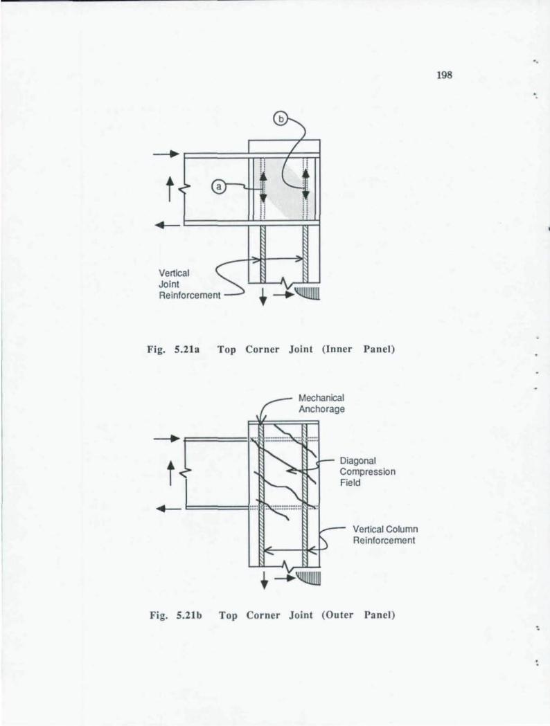
t

Vertical Joint Reinforcement

b

Fig. 5.213 Top Corner Joint (Inner Panet)

Mechanical Anchorage

Diagonal Compression Field

Vertical Column Reinforcement

Fig. 5.21b Top Corner Joint (Outer Panel)

' .

198

:

, . , 'J~ ,

."

""

..

199

biaxial loading in the joint. The transverse beams have both beneficial and nega­

tive influences on the joint shear capacity. First, the beam configuration presents

more difficult fabrication of column ties and placement of concrete. Transverse

beams also create additional planes of discontinuity through the joint. Whether

such discontinuities will decrease the joint strength by forming slip planes is

not known. Referring to Fig. 5.22a, concrete confinement in the compression

strut region tends to mitigate the influence of discontinuities. On the other

hand, in Fig. 5.22b, the discontinuities appear to be of more concern in the less

confined concrete in the outer panel compression field. The transverse beam

may have a positive influence due to out of plane web bending induced by joint

shear deformations. In this instance, web bending helps resist joint shear. An­

other advantage of the transverse beam is in adding confinement to concrete

in the joint region particularly when FBPs are used. The current ACI-ASCE

recommendations" for reinforced concrete connections indicate that transverse

beams increase the joint shear capacity by 20% through confinement. Also, trans­

verse compression struts will induce a biaxial compression state (in the horizontal

plane) which theoretically increases the maximum compression failure stress in

the concrete. Transverse beam effects outlined for the three dimensional corner

joint also exist to a degree in planar connections where transverse floor beams

frame into the connection. The floor beams do not induce significant biaxial

joint forces, but do influence behavior by their presence in the joint region.

Floor Slab. Incorporation of the floor slab in the joint shear mecha­

nisms offers another means of improving the connection strength. The effect of a

concrete slab in mobilizing the outer concrete panel is similar to that of extended

FBPs as shown in Fig. 5.23. In the detail shown the floor slab above the beam

works with the extended FBP below the beam. In utilizing the concrete slab

several factors should be kept in mind. First, the horizontal load transferred

into the joint by the slab cannot exceed the load developed by shear studs along

the beam outside the connection. Second, the effective slab area in compression

is based on a width, b, equal to that of the concrete column. Where the slab is

utilized, the construction details must insure that no gap exists between the floor

slab and column. Third, slab reinforcement continuous through the column will

.------------- -~---

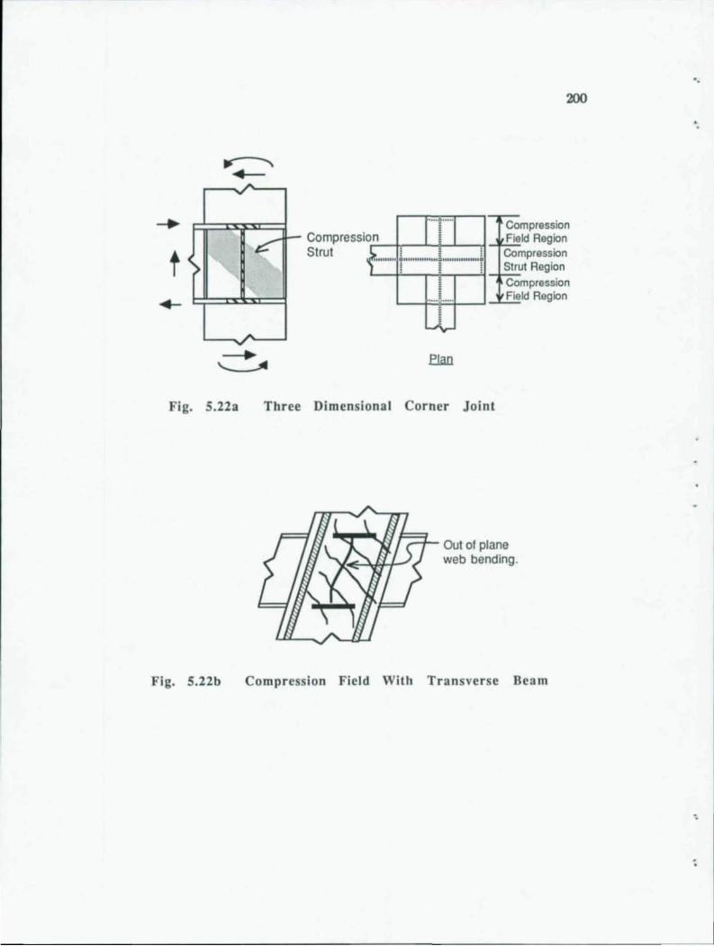
Fig. 5.223

Fig. S.22b

! ~ ~ " .. ,,"" 0 . .. """,,,,,,;. ... , .... ,,,,,,,,.

! i 1 , ! .... ~ .....

Three Dimensional Corner Joint

200

Compression Field Region Compression Strut Region Compression Field Region

Out of plane web bending.

Compression Field With Transverse Beam

'.

;

..

. '

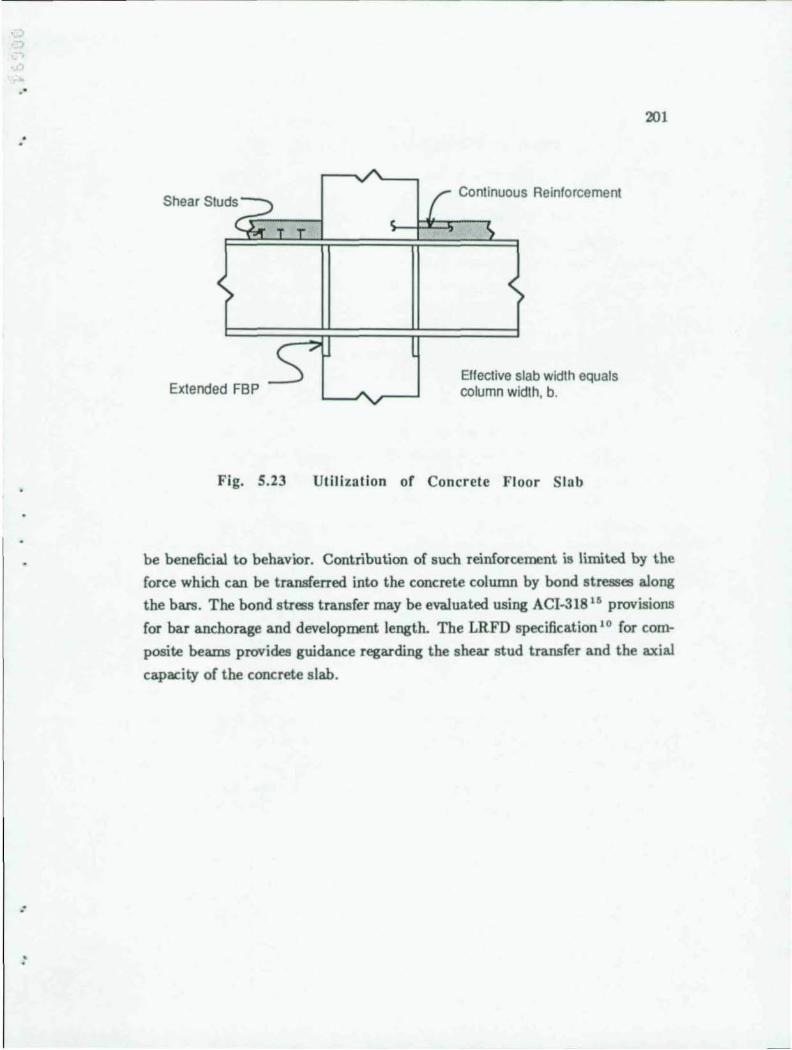
Shear Siuds

Extended FBP

Fig. 5.23

Continuous Reinforcement

Effective slab widlh equals column width, b.

Utilization of Concrete Floor Slab

201

be beneficial to behavior. Contribution of such reinforcement is limited by the

force which can be transferred into the concrete column by bond stresses along

the bars. The bond stress transfer may be evaluated using ACI-318'6 provisions

for bar anchorage and development length. The LRFD specification '0 for com­

posite beams provides guidance regarding the shear stud transfer and the axial

capacity of the concrete slab .

CHAPTER 6 - SUMMARY AND CONCLUSIONS

6.1 Summary

Test were conducted on eight 2/3 scale connections between steel beams

and reinforced concrete columns. The specimens were tested under reverse cyclic

loading. Various structural steel details were tested in order to assess their influ­

ence on the connection strength and stiffness. Details examined include face bear­

ing plates (FBP), web stiffener plates (WSP), embedded steel columns, welded

shear studs, steel doubler plates, and vertical joint reinforcement. Additionally,

results of nine similar tests previously documented by Sheikh' were summarized

for comparison purposes. The tests were analyzed, both qualitatively and quan­

titatively, to determine the internal mechanisms which govern joint behavior.

Based on the experimental results, joint behavior and design were de­

scribed in terms of two primary modes of failure: joint panel shear and vertical

bearing. Joint panel shear strength was calculated as the sum of contributions

from the following three elements: the steel (web) panel, inner concrete panel,

and outer concrete panel. The steel panel strength consisted primarily of the

shear capacity of the beam web which can be increased by doubler plates. The

inner concrete panel was mobilized in a diagonal compression strut by face bear­

ing plates or inset web stiffener plates. Finally, outer panel shear was resisted

by a concrete compression field, mobilized through such details as steel columns,

shear studs, or extended face bearing plates. The compression field strength was

a function of both the concrete strength and horizontal column ties.

Vertical bearing failure occurred when the concrete crushing strength

was exceeded in the column adjacent to the beam flanges in compression. Vertical

joint reinforcement, such as Dywidag bars used in the tests, provided an effective

means of strengthening the bearing zone. Also, confinement provided by column

ties and extended face bearing plates (or clip angles) to some degree enhanced

the concrete compression strength.

200

' .

..

.,

..

203

Design recommendations were presented for joint configurations such

as those tested along with discussion of alternate configurations. The recom­

mendations were drawn in part from recommendations presented previously by

Sheikh, and from current specifications for structural steel and reinforced con­

crete connections. A key component of the recommendations is an analytic design

model for calculating the connection capacity. This model addressed the primary

modes of failure previously discussed, and was calibrated to test results based

on joint deformations at service and ultimate loads of 0.2% and 1.0% total joint

distortion, respectively.

6.2 Conclusions

6.2.1 General. The tests demonstrate that the composite beam­

column connection is a reliable detail with behavior characterized by reasonable

stiffness at service load and ductile failure at ultimate load. Deformations of

the composite joint at service and ultimate load are comparable to those in

reinforced concrete and welded structural steel connections. Additionally, under

reverse cyclic loading, the connection showed toughness comparable to reinforced

concrete joints dQtailed for seismic design.

6.2.2 Strength Behavior. The strength of the connection can be

accurately assessed by applying simple principles of mechanics in analyzing the

governing internal mechanisms and modes of failure. Two major conclusions

addressing aspects of behavior are described below.

Mobilization of Concrete Panel. Details examined in the tests indicate

that joint shear strength was enhanced considerably by mobilization of concrete

in the joint region. Further, this concrete participation was achieved through

simple details which added little complication to the connection. The basic re­

quirement of such details was that they provide a path for transferring horizontal

force between the steel beam flange and the inner or outer concrete panel.

In the test specimens, addition of face bearing plates and web stiffener

plates mobilized the inner joint panel, with resulting strength increases of 70%

and 50% (respectively) over the plain steel beam. In general, the bearing plate

204

effectiveness was not affected by plate thickness or by splitting the plates at

midheight. Also, strength enhancement was roughly proportional to the bearing

plate width.

Attachments to the beam flange, such as the steel column, shear studs,

and extended face bearing plates mobilized concrete in the outer panel. In the

tests, the steel column and shear studs provided roughly a 60% strength increase

over the plain steel beam, and the extended face bearing plates provided a 130%

increase. The difference in strength increase was related to how effectively the

details transfer shear from the beam flange through horizontal struts to the outer

joint panel.

The strength increase provided by separate details mobilizing the inner

and outer panels was additive. For example, the strength increase afforded by the

face bearing plates (inner panel) and shear studs (outer panel) was equal to the

sum of contributions which each detail provides separately. However, strength

gains achieved by details which mobilize the same region of concrete should not

be added together.

Compression Zone Enhancement. Vertical joint reinforcement attached

to the beam flange enhanced connection strength where concrete crushing in the

zone adjacent to the compression flanges controls. The enhanced st rength of

the bearing region equals the sum of the tension and compression strength of

reinforcement attached to the beam flanges .

Where concrete crushing did not control design, vertical joint reinforce­

ment did not noticeably improve the connection strength or stiffness. Vertical

joint reinforcement did, however, reduce the intensity of bond stress on longi­

tudinal column bars through the joint and may be desirable for seismic design

where large inelastic load reversals are of concern. Finally, the tests did not

provide a clear measure of how much concrete bearing strength was improved by

additional confinement provided by clip angles or extended face bearing plates.

6,2.3 Attractive Design Alternative. Several representative de­

sign examples showed that relatively large connection forces could be developed

by such details as the steel column combined with face bearing plates or web

'.

' .

. .

."

:

205

stiffener plates. Typically, these or similar details would already exist in con­

nections due to erection sequence requirements for composite frames. Composite

connections, therefore, were shown to offer an attractive alternative to structural

steel or reinforced concrete connections.

6.3 Future Research

While the experimental results reported both herein and previously by

Sheikh provide answers to many questions, several areas remain where additional

research is needed to more fully understand joint behavior. Topics are presented

below in descending order of priority or importance. Included for completeness,

several of the items listed below were suggested previously by Sheikh.

Horizontal Ties. The role of horizontal ties in the joint region is not

well understood, and deserves investigation since tie detailing and fabrication

are significant costs in the connection. Based on the presumed internal force

mechanisms, the ties appear to serve three functions peculiar to the connection:

1) joint shear reinforcement in the outer panel compression field, 2) participation

in horizontal transfer mechanisms above and below the beam, 3) confinement of

concrete in the joint region.

Alternate Configurations. Alternatejoint configurations and aspect ra­

tios (width - length - height) should be tested to verify the general applicability

and accuracy of design recommendations presented herein. Alternate configu­

rations may include corner and three dimensional details, and connections with

composite beams where slab effects are considered.

High Strength Concrete. In practice, concrete strengths of up to 12

ksi are becoming common, particularly for columns in tall buildings. Currently,

there is no published research data for composite (or reinforced concrete) con­

nections where concrete strengths higher than 6 ksi are reported.

Axial Load Effects. In this research, no axial load was applied to the

column, however, obviously axial loads will exist in practice. As reported by

Sheikh, other research has shown that compressive axial load should improve

206

connection behavior. Such improvement may be considerably beneficial for re­

ducing horizontal tie requirements in the connection, since both the axial load

and ties resist opening of diagonal shear cracks.

Seismic Design. The research herein was not intended to specifically

address the many particular concerns related to seismic design, and hence, fur­

ther work focusing on seismic considerations is warranted. In particu lar, such

research should assess whether the restrictions in the Japanese SRC standards

are appropriate based on current seismic design practice.

THE END

' .

'.

"

."

""

APPENDIX Al Summary of Phase I: Specimens 1 through 9

The test results of Specimens 1 through 9 which comprise Phase I of

the composite joint project have been reported by Sheikh. l For convenience,

descriptions and results of the Phase I tests which are used in developing and

calibrating the design model are summarized herein.

Details tested in Specimens 1 through 9 are summarized in Fig. Al.l.

The strengths for these specimens at given deformation levels are listed in Table

Al.l. Definition of the joint deformation (drift) is the same as that given in

Chapter 2 of this report. Connection strengths in Table Al.l are modified from

the values reported by Sheikh to reflect an updated calibration of the load setup

used in the experiments. Discussion of relative specimen strengths is included in

Chapter 3 of this report. Plots of the load-deformation response and a summary

of the testing procedure for Specimens 1 through 9 are presented in Sheikh's

report. Tables Al.2 and Al.3 indicate the material properties for the structural

steel, reinforcing steel and concrete used in fabricating the Phase I specimens.

Specimens 1 and 2 are 1/2 scale pilot tests designed to examine the

influence of the FBP detail. The overall geometry and the reinforcing bar layout

for these two specimens are shown in Figs. Al.2 and AI.3. Figure AlA shows

the steel details for Specimens 1 and 2. As seen in this figure, the difference

between the two is addition of FBPs in Specimen 2.

Specimens 3 through 9, considered as 2/3 of full scale, all have the

same basic geometry and reinforcing bar arrangements which are also common

to Specimens 10 through 17 tested in Phase II. Figures A1.5 and Al.6 show the

overall geometry and reinforcing bar layout for Specimens 3 through 9. Further

discussion of the specimen configuration is the same as that given for Specimens

10 through 17 in Chapter 2.

Figure Al.7 shows the structural steel details used in Specimens 3

through 5. Specimen 3 consists of a plain steel beam which is continuous through

the column. The built-up beam section which is identical for Specimens 3 through

207

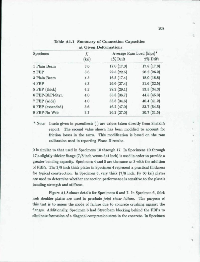
208

Table AI.I Summary of Connection Capacities

at Given Deformations

Specimen f~ Average Ram Load (kips)·

(ksi) 1% Drift 2% Drift

1 Plain Beam 3.6 17.0 (17.0) 17.8 (17.8)

2 FBP 3.6 22.5 (22.5) 26.2 (26.2)

3 Plain Beam 4.5 16.5 (1704) 18.0 (18.8)

4 FBP 4.3 26.6 (2704) 31.6 (32.5)

5 FBP (thick) 4.3 28.2 (29.1) 33.5 (34.3)

6 FBP-DbPI-Styr. 4.0 35.8 (36.7) 44.5 (45.3)

7 FBP (wide) 4.0 33.8 (34.6) 4004 (41.2)

8 FBP (extended) 3.6 46.2 (47.0) 53.7 (54.5)

9 FBP-No Web 3.7 26.2 (27.0) 30.7 (31.5)

• Note: Loads given in parenthesis ( ) are values taken directly from Sheikh's

report. The second value shown has been modified to account for

friction losses in the rams. This modification is based on the ram

calibration used in reporting Phase II results.

9 is similar to that used in Specimens 10 through 1'1. In Specimens 10 through

17 a slightly thicker flange (7/ 8 inch versus 3/ 4 inch) is used in order to provide a

greater bending capacity. Specimens 4 and 5 are the same as 3 with the addition

of FBPs. The 3/8 inch thick plates in Specimen 4 represent a practical thickness

for typical construction. In Specimen 5, very thick (7/8 inch, Fy 50 ksi) plates

are used to determine whether connection performance is sensitive to the plate's

bending strength and stiffness.

Figure A1.8 shows details for Specimens 6 and 7. In Specimen 6, thick

web doubler plates are used to preclude joint shear failure. The purpose of

this test is to assess the mode of failure due to concrete crushing against the

flanges. Addit ionally, Specimen 6 had Styrofoam blocking behind the FBPs to

eliminate formation of a diagonal compression strut in the concrete. In Specimen

-.

'.

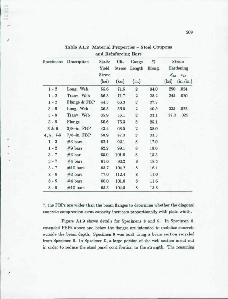
~ 0

_.

--

209

Table A1.2 Material Properties - Steel Coupons

and Reinforcing Bars

Specimens Description Static Vlt. Gauge % Strain

Yield Stress Length Elong. Hardening

Stress E.h f . h

(ksi) (ksi) (in.) (ksi) (in./in.)

1-2 Long. Web 55.6 71.5 2 34.0 290 .024

1-2 Tranv. Web 56.3 71.7 2 28.2 245 .020

1-2 Flange & FBP 44.5 66.3 2 37.7

3-9 Long. Web 36.5 56.5 2 40.5 335 .022

3-9 Tranv. Web 35.9 56.1 2 33.1 27.0 .020

3-9 Flange 50.6 76.3 8 25.1

3&6 3/8- in. FBP 43.4 68.5 2 38.0

4, 5, 7-9 7/ 8- in. FBP 58.9 87.3 2 33.3

1 - 2 #3 bars 62.1 92.1 8 17.0

1 - 2 #9 bars 62.2 99.1 8 18.6

3 - 7 # 3 bar 65.0 101.8 8 15.3

3 - 7 # 4 bars 61.6 90.2 8 18.3

3 - 7 # 10 bars 65.7 104.2 8 16.1

8-9 # 3 bars 77.0 112.4 8 11.0

8-9 # 4 bars 60.0 101.8 8 11.6

8-9 # 10 bars 65.3 104.5 8 15.8

7, t he FBPs are wider than the beam flanges to determine whether the diagonal

concrete compression strut capacity increases proportionally with plate width .

Figure A1.9 shows details for Specimens 8 and 9. In Specimen 8,

extended FBPs above and below the flanges are intended to mobilize concrete

outside the beam depth. Specimen 9 was built using a beam section recycled

from Specimen 5. In Specimen 9, a large portion of the web section is cut out

in order to reduce the steel panel contribution to the strength. The reasoning

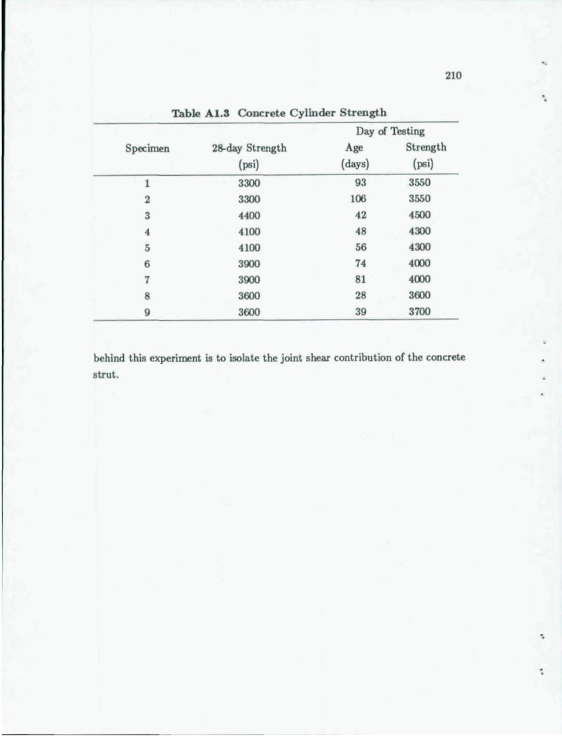
210

Table Al.3 Concrete Cylinder Strength

Day of Testing

Specimen 28-day Strength Age Strength

(psi) (days) (psi)

1 3300 93 3550

2 3300 106 3550

3 4400 42 4500

4 4100 48 4300

5 4100 56 4300

6 3900 74 4000

7 3900 81 4000

8 3600 28 3600

9 3600 39 3700

behind this experiment is to isolate the joint shear contribution of the concrete

strut .

' .

. .

'.

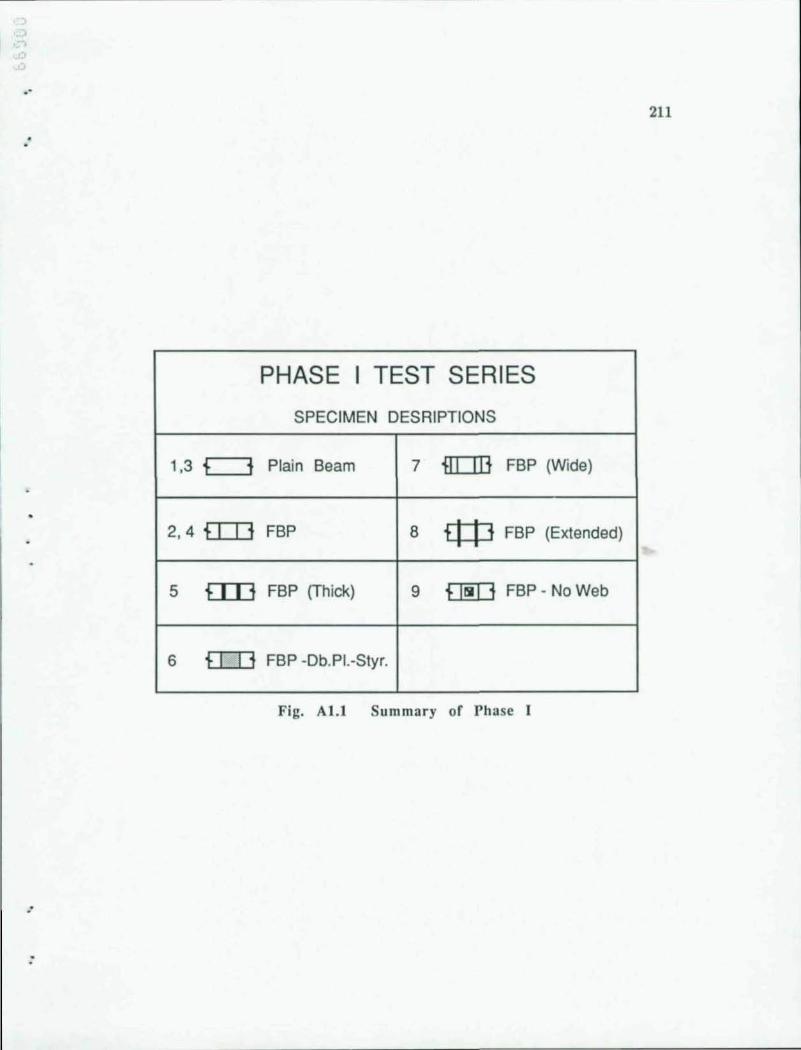
.. 211

PHASE I TEST SERIES SPECIMEN DESRIPTIONS

1.3 { } Plain Beam 7 {II II} FBP (Wide)

2.4 { I I } FBP 8 £1=13 FBP (Extended)

5 { I I } FBP (Thick) 9 { I III I } FBP - No Web

6 {I I } FBP -Db.PI.-Styr.

Fig. A1.1 Summary of Phase I

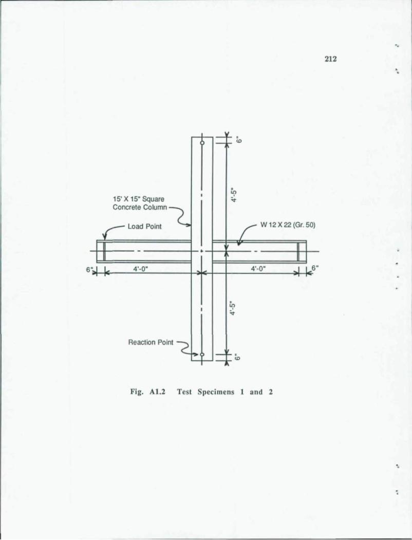
-. 212

- '- . - .-- '"

• 15' X 15" Square

, ~ 'r

Concrete Column ~

Load Point I W 12 X 22 (Gr. 50)

r

- • -

6 " I I. 4 '-0" , , 4'-0" 6" ,- T

• I ~

'r

Reaction Point C I'> I- f- .

1- (- '"

Fig, A1.2 Tes t Specim ens 1 and 2

'.

·'

:

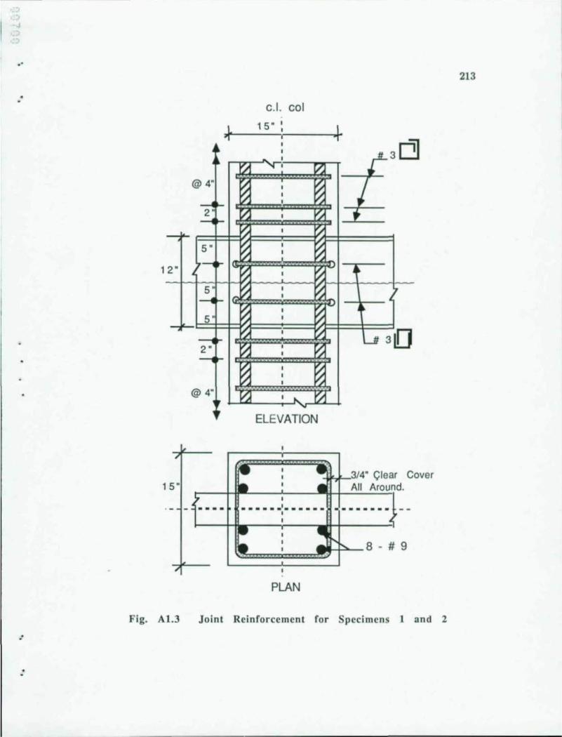
L .. ~ ~

@4" ~ -t ~

~

'/ ~ ~

- io-Z

5" ~ ~ 2"

~ 5' l-i .... ~

~ 5

---1 ... 2" ~ ---1 t-

~ I/: @4" ~

15"

C.1. col 15" I

I

I I I

.... : I I , I

I

I I I

I

I I

I I

, , I

I I , I ..

:7.

~ I/:

I/:

~ ~ I/:

~ ~

V'

~ I')-

ELEVATION

PLAN

1-3

/ "t

~

. '

u 310

Clear Cover

Fig. Al.3 Joint Reinforcement for Specimens 1 and 2

213

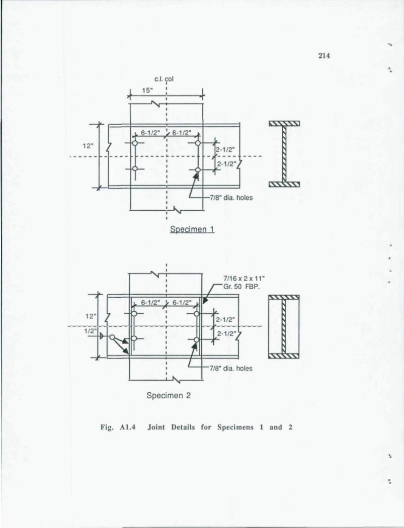
12"

col. col I

L 15" ..

6-1/2" 6-1/2"

I

-----~-----2-1/2"

2-1/2"

I 7/S" dia. holes I

~----~:~

Specimen 1

7/16x2x11" Gr. SO FBP.

~ 6-1/2" I

12" __ 1 ___ ~K,r_-___ -T ____ -+I~~ __ ~ __ ___ __ ........ 2-1/2"

1/2" 2-1/2"

L-+-7/S" dia. holes

Specimen 2

Fig. Al.4 Joint Details for Specimens land 2

-,

214

'-

.'

.-

.'

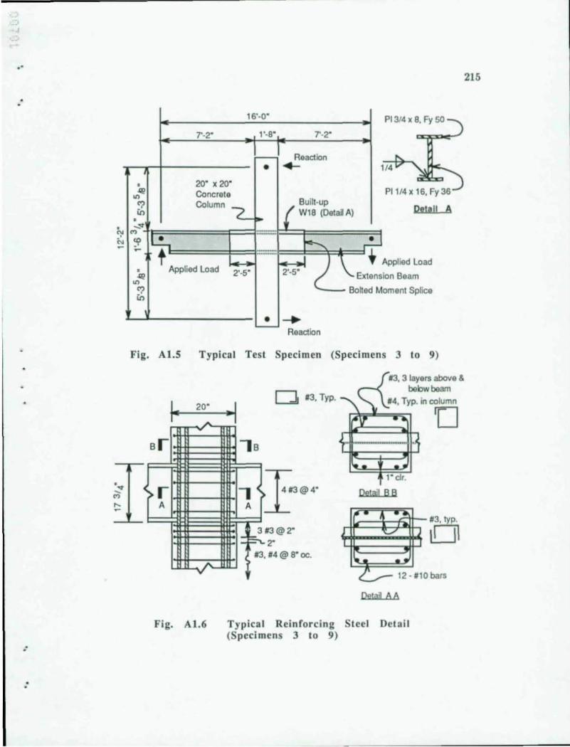
• <:' N

, '" -M

'" ~

16',0"

7'·2" 1'·S"

-•

• 20" X 20" 41 Concrele U'l

~ Column 7_ • -'" M ........... '!? ~ ~

t Applied load

....... _ ..

• ~ 41 U'l

~

• -

PI 3/4 X B, Fy 50

7'·2"

Readlen ~ 1

Buill·up { W1B (Delaa A)

r---. ~

2'·5" ~\.E~!S ~

Readion

Applied load

ion Beam

oment Splice Bohed M

Fig. Al.S Typical Test Specimen (Specimens 3 to 9)

20"

A

Bf""

~ >f"" A

....

Fi g, A 1.6

-I D #3,Typ.

'B ,~

A

3 1= ~

#3@2"

? #3, 2" #4@B'oc.

t

#3, 3 layers above & bebwbeam

#4, Typ. in column o I" clr.

Delail B B

~c::=;k=pn:;- #3, typ, o 12·.10 bars

Detail AA

Typical Reinforcing St eel Detai l (Specimens 3 to 9)

215

"

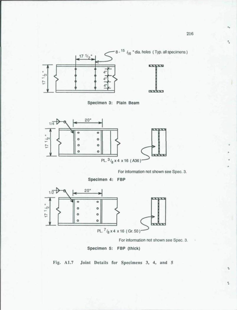
216

8 , 15 ~ 6 "dia. holes (Typ. ali specimens)

• 4"

4"

4"

Specimen 3: Plain Beam

"- '"\. I- 20" ·1 114 V

-r-'01 0 0

• ~ < 0 0 < ~ > > ..... 0 0 - 0 0

-'--

PL. 3/a x 4 x 16 (A36)

For information not shown see Spec. 3.

Specimen 4: FBP

"-1/2 v '"\. I_ 20" ·1 -.---

'01 0 0 • ~ < 0 0 < ..... > 0 0 - 0 0

-'-

PL. 7/aX 4 x16 (Gr. SO)

For information not shown see Spec. 3.

Specimen 5: FBP (thick)

Fig, AI.7 Joint Details for Specimens 3, 4, and 5 "

·'

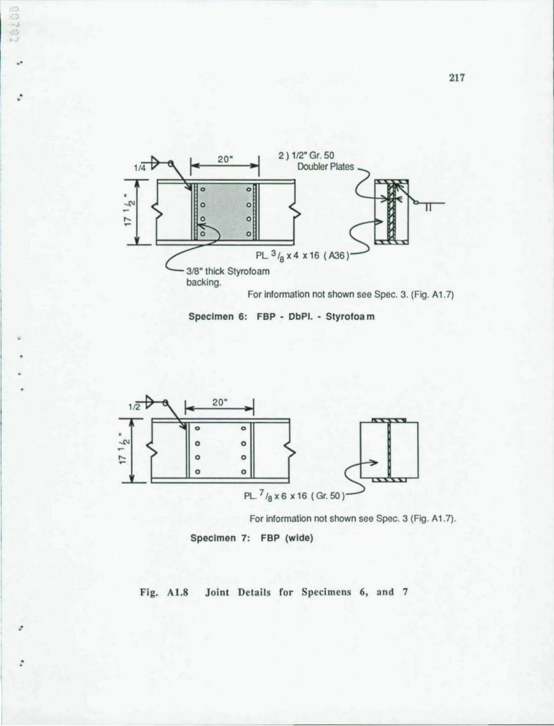
0-

1/4 I" 20"

-------- -

~I 2 ) 1/2" Gr. 50

Doubler Plates

o 0

o

o o

o o

PL 3/a x 4 x 16 (A36)

318" thick Styrofoam backing.

217

For information not shown see Spec_ 3_ (Fig. A 1. 7)

Specfmen 6: FBP - DbPI. - Styroloa m

"'-112 v \. I .. 20" .. I

---,.-- ... 0 0 • -.(\I < 0 0 < ~ > > ..... 0 0 ~

0 0

-''--

Pl. 7/ax6 x16 (Gr_SO)

For information not shown see Spec. 3 (Fig. A1 .7) .

Specimen 7 : FBP (wide)

Fig. A1.8 Joint Details for Specimens 6, and 7

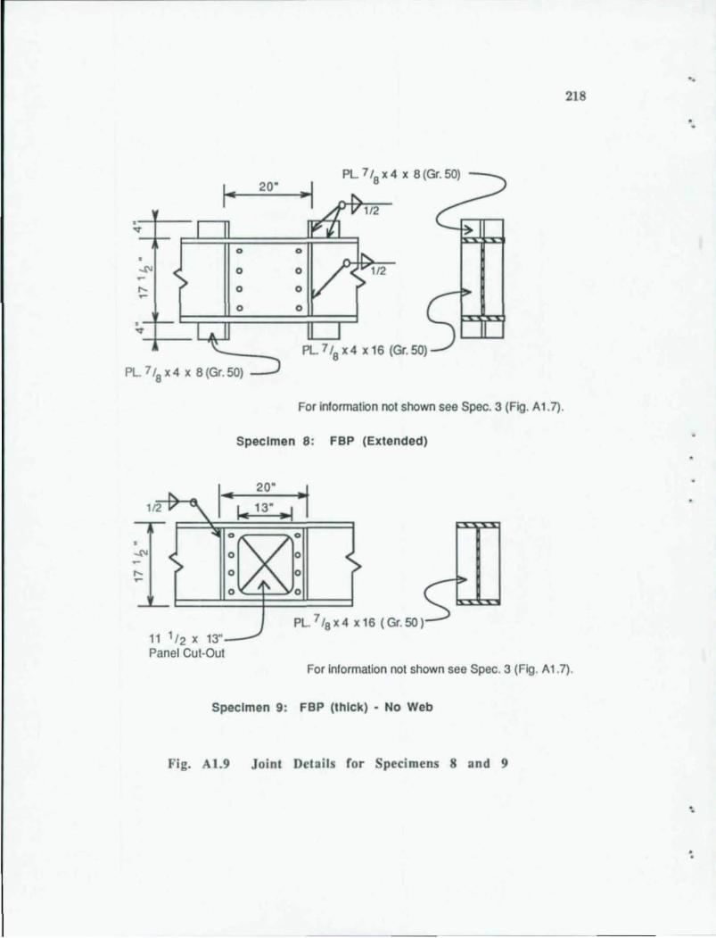
20· PL 7/ex4 x 8 (Gr. 50) -_

• v

0 0

-'" 0 0 1/2 ~

.... 0 0 ~

0 0

• v

PL 7/ex4 x16 (Gr. 50)

PL 7/e X 4 X 8 (Gr. 50)

•

For information not shown see Spec. 3 (Fig. A1.7) .

Specimen 8: FBP (Extended)

I 20· .. .

1. 13 • • 1 I 112

PL 7/e x 4 x 16 (Gr. 50) 11 1/2 x 13"-­Panel Cut-Out

218

For information not shown see Spec. 3 (Fig. A 1.7) .

Specimen 9: FBP (thick) - No Web

Fig. A1.9 Joint Details for Specimens 8 and 9

..

'.

'.

..

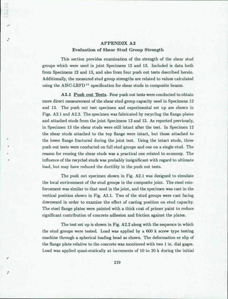
APPENDIXA2

Evaluation of Shear Stud Group Strength

This section provides examination of the strength of the shear stud

groups which were used in joint Specimens 12 and 13. Included is data both

from Specimens 12 and 13, and also from four push out tests described herein.

Additionally, the measured stud group strengths are related to values calculated

using the AISC-LRFD 10 specification for shear studs in composite beams.

A2.1 Push out Tests. Four push out tests were conducted to obtain

more direct measurement of the shear stud group capacity used in Specimens 12

and 13. The push out test specimen and experimental set up are shown in

Figs. A2.1 and A2.2. The specimen was fabricated by recycling the Bange plates

and attached studs from the joint Specimens 12 and 13. As reported previously,

in Specimen 13 the shear studs were still intact after the test. In Specimen 12

the shear studs attached to the top Bange were intact, but those attached to

the lower Bange fractured during the joint test. Using the intact studs, three

push out tests were conducted on full stud groups and one on a single stud. The

reason for reusing the shear studs was a practical one related to economy. The

influence of the recycled studs was probably insignificant with regard to ultimate

load, but may have reduced the ductility in the push out tests.

The push out specimen shown in Fig. A2.1 was designed to simulate

the local environment of the stud groups in the compOlSite joint. The steel rein­

forcement was similar to that used in the joint, and the specimen was cast in the

vertical position shown in Fig. A2.1. Two of the stud groups were cast facing

downward in order to examine the effect of casting position on stud capacity.

The steel Bange plates were painted with a thick coat of primer paint to reduce

significant contribution of concrete adhesion and friction against the plates.

The test set up is shown in Fig. A2.2 along with the sequence in which

the stud groups were tested. Load was applied by a 600 k screw type testing

machine through a spherical loading head as shown. The deformation or slip of

the Bange plate relative to the concrete was monitored with two 1 in. dial gages.

Load was applied quasi-statically at increments of 10 to 20 k during the initial

219

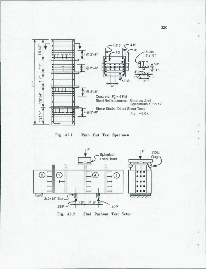
• '" -~ 9' ~

-• ~

~

-• t-

• ~

0 ;.... -

• ... -~ !" ~

-• ... -~ ~ ~

220

.-14----+1 •

~~@2".S" l-

l-

l-

t-

1~~~~~=: 4" ~@ 2".S" Concrete: Pc = 4 Ksi Steel Reinforcement: Same as Joint

Specimens 10 to 17

1~~~~I~f Shear Studs: Direct Shear Test:

Fig. A2.1

4@2". S" Fv =8.6k

Push Out Test Specimen

Spherical Load Head

1"Dial Gage

~ ." . . ~ . e.e . ~ . . ~ .

2x2x19" Bar -l 1"-2"

.SSP .42P

Fig. A2.2 Stud Pushout Test Setup

..

..

'.

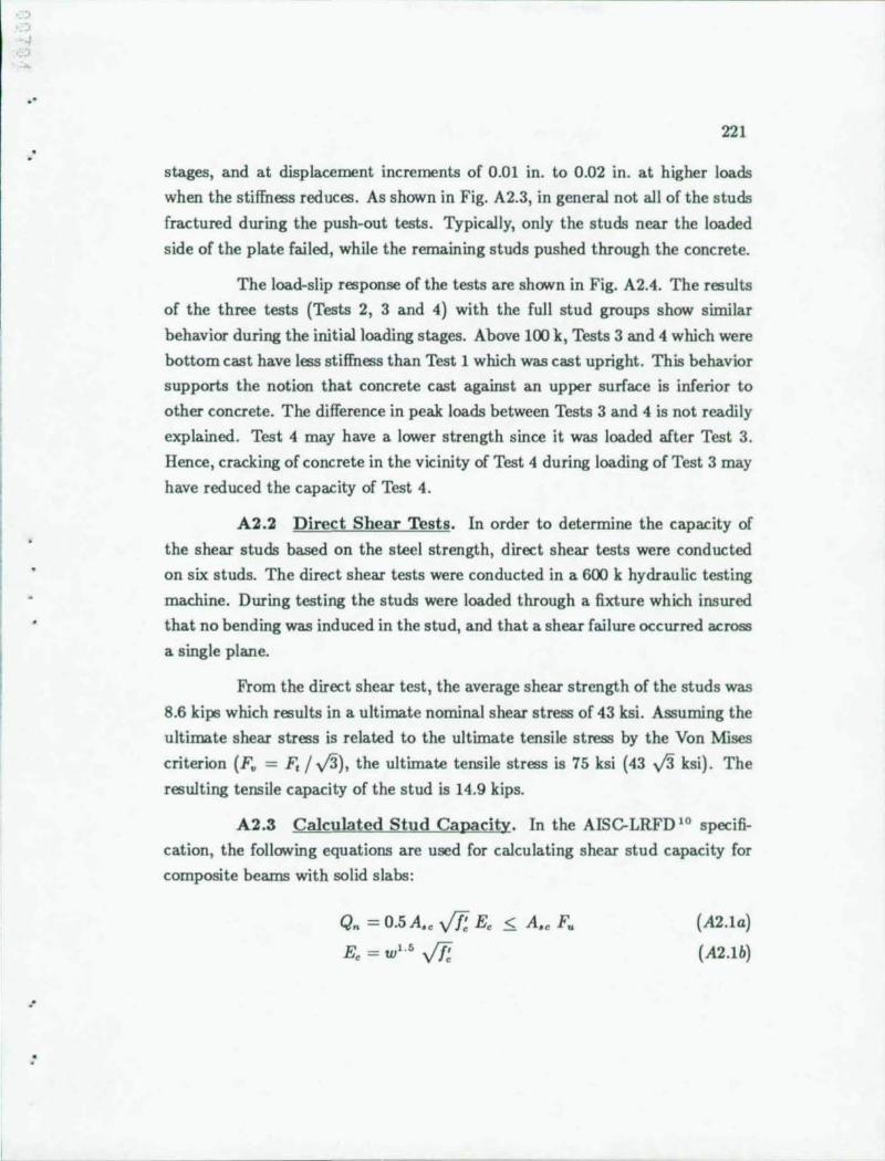
·) J

.. . .

.'

:

221

stages, and at displacement increments of 0.01 in. to 0.02 in. at higher loads

when the stiffness reduces . As shown in Fig. A2.3, in general not all of the studs

fractured during the push-out tests. Typically, only the studs near the loaded

side of the plate failed, while the remaining studs pushed through the concrete.

The load-slip response of the tests are shO'Nn in Fig. A2.4. The results

of the three tests (Tests 2, 3 and 4) with the full stud groups show similar

behavior during the initial loading stages. Above 100 k, Tests 3 and 4 which were

bottom cast have less stiffness than Test 1 which was cast upright. This behavior

supports the notion that concrete cast against an upper surface is inferior to

other concrete. The difference in peak loads between Tests 3 and 4 is not readily

explained. Test 4 may have a lower strength since it was loaded after Test 3.

Hence, cracking of concrete in the vicinity of Test 4 during loading of Test 3 may

have reduced the capacity of Test 4.

A2.2 Direct Shear Tests. In order to determine the capacity of

the shear studs based on the steel strength, direct shear tests were conducted

on six studs. The direct shear tests were conducted in a 600 k hydraulic testing

machine. During testing the studs were loaded through a fixture which insured

that no bending was induced in the stud, and that a shear failure occurred across

a single plane.

From the direct shear test, the average shear strength of the studs was

8.6 kips which results in a ultimate nominal shear stress of 43 ksi. Assuming the

ultimate shear stress is related to the ultimate tensile stress by the Von Mises

criterion (F. = Fe! vIl), the ultimate tensile stress is 75 ksi (43 vIl ksi) . The

resulting tensile capacity of the stud is 14.9 kips.

A2.3 Calculated Stud Capacity. In the AISC-LRFD 1 0 specifi­

cation, the follO'Ning equations are used for calculating shear stud capacity for

composite beams with solid slabs:

Qn = 0.5 A" Vf. Ec < A •• Fu

Ec = wl.6 Vf. (A2.1a)

(A2.1b)

~

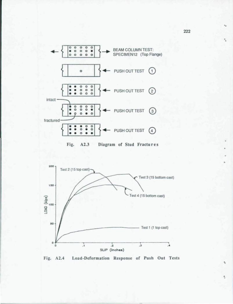
intact

fractured

200

150

~ .. Q.

:;( -tOO

§

.0

{ o 0 0 0 0 BEAM COLUMN TEST:

• 0 0 0 • ~-+ o 0 000 SPECIMEN1 2 (Top Flange)

{ I 0 I f~ PUSH OUT TEST CD

{ • • 0 0 0

CD • • 0 0 0 ? ~ PUSH OUT TEST • • 0 0 0

'\

f. i: g 0 0 0

0) 0 0 • ? ~ PUSH OUT TEST • 5' 0 • 0 ./

• • • 0 0

~ • • 0 • 0

• • 0 • • ~ PUSH OUT TEST 0

Fig. A2.3 Diagram of Stud Fractu res

Test 2 (1 5top cast)

Test 3 (15 bottom cast)

Test 4 (15 bottom cast)

~ __ ---- ------- Test 1 (1 top cast)

. , . 2 . 3 .4

SUP (Inch •• )

Fig. A2.4 Loa d-Deformation Response of Push Out Tes ts

. . 222

. .

'.

·,

..

. '

.'

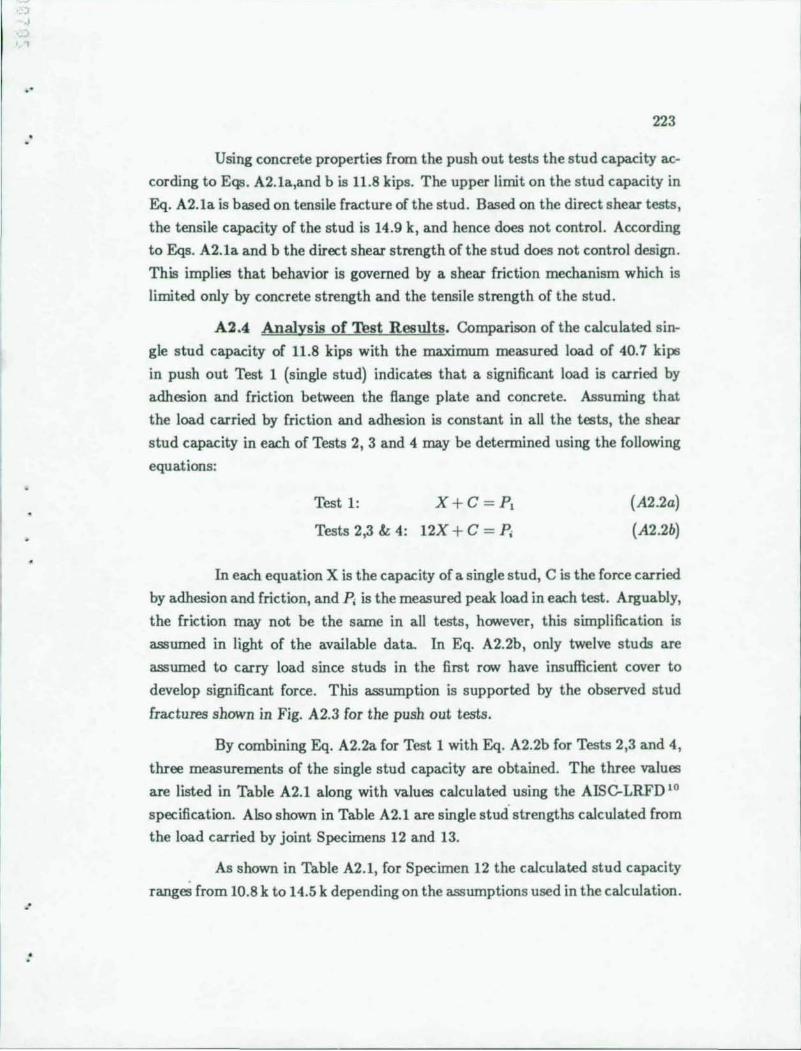
223

Using concrete properties from the push out tests the stud capacity ac­

cording to Eqs. A2.1a,and b is 11.8 kips. The upper limit on the stud capacity in

Eq. A2.1a is based on tensile fracture of the stud. Based on the direct shear tests ,

the tensile capacity of the stud is 14.9 k, and hence does not control. According

to Eqs. A2.1a and b the direct shear strength of the stud does not control design.

This implies that behavior is governed by a shear friction mechanism which is

limited only by concrete strength and the tensile strength of the stud.

A2.4 Analysis of Test Results. Comparison of the calculated sin­

gle stud capacity of 11.8 kips with the maximum measured load of 40.7 kips

in push out Test 1 (single stud) indicates that a significant load is carried by

adhesion and friction between the flange plate and concrete. Assuming that

the load carried by friction and adhesion is constant in all the tests, the shear

stud capacity in each of Tests 2, 3 and 4 may be determined using the following

equations:

Test 1: X + C = P,

Tests 2,3 & 4: 12X + C = Pi

(A2.2a)

(A2 .2b)

In each equation X is the capacity of a single stud, C is the force carried

by adhesion and friction, and Pi is the measured peak load in each test. Arguably,

the friction may not be the same in all tests, however, this simplification is

assumed in light of the available data. In Eq. A2.2b, only twelve studs are

assumed to carry load since studs in the first row have insufficient cover to

develop significant force . This assumption is supported by the observed stud

fractures shown in Fig. A2.3 for the push out tests.

By combining Eq. A2.2a for Test 1 with Eq. A2.2b for Tests 2,3 and 4,

three measurements of the single stud capacity are obtained. The three values

are listed in Table A2.1 along with values calculated using the AISC-LRFD ' 0

specification. Also shown in Table A2.1 are single stud' strengths calculated from

the load carried by joint Specimens 12 and 13.

As shown in Table A2.1, for Specimen 12 the calculated stud capacity

rangeS from 10.8 k to 14.5 k depending on the assumptions used in the calculation .

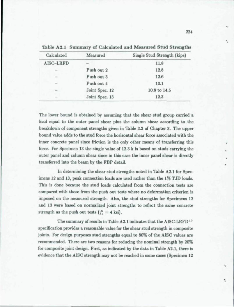
224

Table A2.1 Summary of Calculated and Measured Stud Strengths

Calculated Measured Single Stud Strength (kips)

AISC- LRFD

Push out 2

Push out 3

Push out 4

Joint Spec. 12

Joint Spec. 13

11.8

12.8

12.6

10.1 10.8 to 14.5

12.3

The lower bound is obtained by assuming that the shear stud group carried a

load equal to the outer panel shear plus the column shear according to the

breakdown of component strengths given in Table 3.3 of Chapter 3. The upper

bound value adds to the stud force the horizontal shear force associated with the

inner concrete panel since friction is the only other means of transferring this

force. For Specimen 13 the single value of 12.3 k is based on studs carrying the

outer panel and column shear since in this case the inner panel shear is directly

transferred into the beam by the FBP detail .

In determining the shear stud strengths noted in Table A2.1 for Spec­

imens 12 and 13, peak connection loads are used rather than the 1% TID loads.

This is done because the stud loads calculated from the connection tests are

compared with those from the push out tests where no deformation criterion is

imposed on the measured strength. Also, the stud strengths for Specimens 12

and 13 were based on normalized joint strengths to reflect the same concrete

strength as the push out tests (/; = 4 ksi).

The summary of results in Table A2.1 indicates that the AISC-LRFD 10

specification provides a reasonable value for the shear stud strength in composite

joints. For design purposes stud strengths equal to 80% of the AISC values are

recommended. There are two reasons for reducing the nominal strength by 20%

for composite joint design. First, as indicated by the data in Table A2.1, there is

evidence that the AISC strength may not be reached in some cases (Specimen 12

..

..

'.

· .

. '

225

and Push out test 4) . In both instances where the AISC values were not reached

the studs were located in regions where concrete was cast against an upper

surface. The second reason for the reduction is related to the deformation criteria

in determining the connection design strength. As presented in Chapters 4 and

5 the joint design equations estimate the joint forces at an implied deformation

of 1% TJD. Since the measured peak capacity may exceed the design capacity

by 15% to 20%, it is prudent to design the studs with a similar margin between

design and ultimate capacity. In other words, the additional margin of strength

in the stud design should preclude stud failure prior to the connection reaching

its ultimate capacity .

APPENDIX A3 Design Examples

Two design examples are included which demonstrate application of

the design equations and recommendations from Chapter 5. Also, in the first

example the joint strength is also calculated according to the model from Chapter

4. In each example the nominal strength of the connection is calculated given

a beam and column size and type of detail. Column sizes are chosen to be

representative of actual practice. Beam sizes are chosen such that their plastic

moment is roughly 80% of the nominal column bending strength.

Design Example 1 is shown in Fig. A3.1. In this example a FBP and

steel column detail provide a nominal connection strength which can transfer a

beam moment that is roughly 4% higher than the plastic moment of the W27

x 235 steel beam. Note, however, that this comparison is based on nominal

strengths where the capacity reduction factors have not been considered. IT the

respective ¢> factors for the connection and beam are 0.7 and 0.9, then the connec­

tion design strength is roughly 80% of the beam design strength. IT required, the

connection strength could be increased through the use of extended face bearing

plates, with face bearing plates or web doubler plates. In Example 1, along with

calculating the nominal joint strength (per Chapters 4 and 5) the following items

are determined (checked): horizontal tie requirement, maximum size of vertical

column bars, FBP size and thickness, and minimum required steel column flange

and beam flange thicknesses.

Design Example 2 is shown in Fig. A3.2. In this case the nominal con­

nection strength is calculated for a similar detail (FBP, steel column) but with

and without vertical joint reinforcement. Without vertical joint reinforcement

the connection strength is governed by bearing failure, whereas with reinforce­

ment joint panel shear controls the strength. As shown in Fig. A3.2 the vertical

joint reinforcement increases the joint strength by roughly 11%. In both cases the

nominal connection strength exceeds the plastic moment capacity of the beam

by the ratios, 1.03 and 1.14, respectively. In Example 2 other aspects such as

detailing of the connection are not considered.

226

'.

'.

..

.•

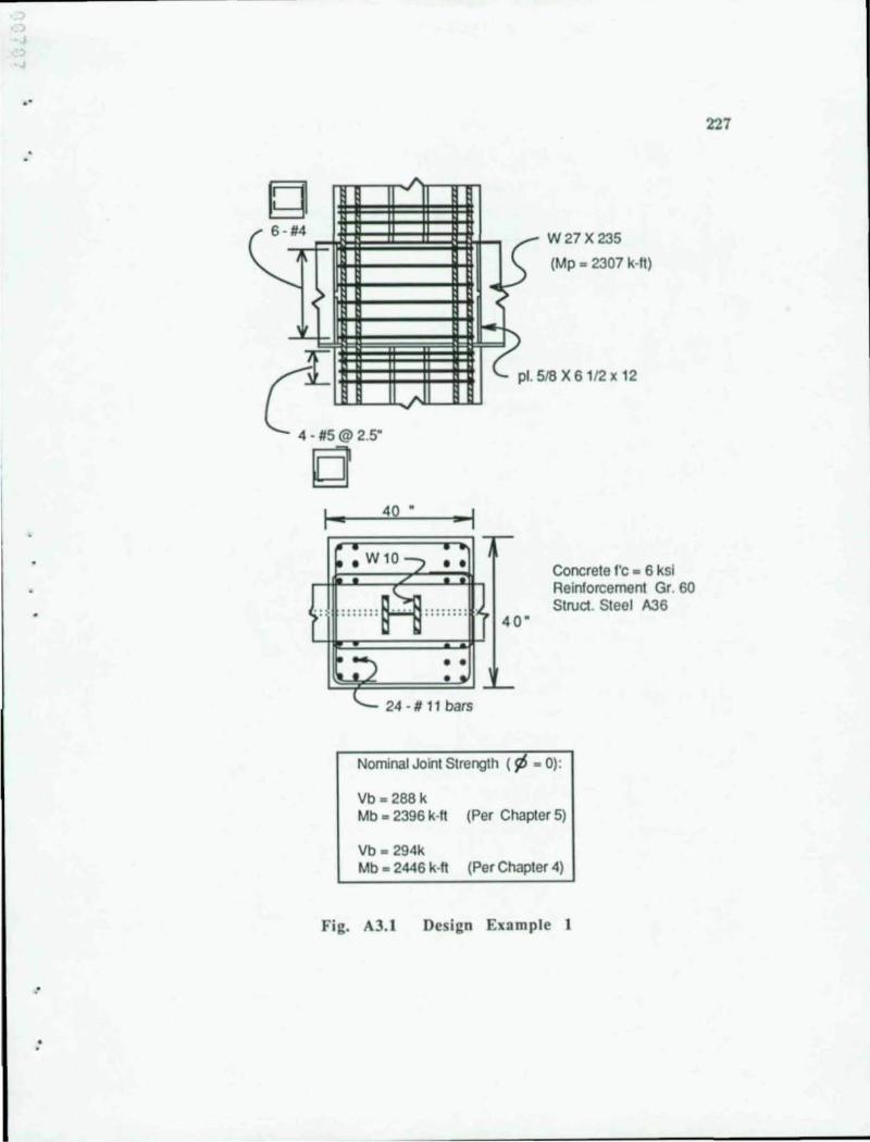
lQ - -C

~>

i

1-

A

A

40 " --I

• •

• • •

24 · # 11 bars

~ W27X235

(Mp - 2307 k·ft)

-)

( pl. 5J8X61 /2x12

40 "

Concrete fc - 6 ksl Reinforcement Gr. 60 Struct. Steel A36

Nominal Joint Strength (!IS - 0) :

Vb - 288 k Mb _ 2396 k·ft (Per Chapter 5)

Vb - 294k Mb - 2446 k·ft (Per Chapter 4)

Fig. AJ.l Design Example 1

227

(

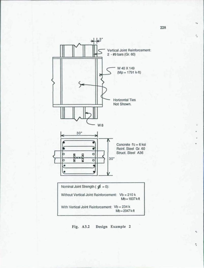
A

IV

~ ( ,I

A i)

V '-30·

E ~

~ • ~ •

ls- Verti 2 -

cal Joint Reinforcement: #9 bars (Gr. 60)

S-... >

(D r-- H

N

W6

,

W40X149 (Mp = 1791 k-ft)

orizontal Ties ot Shown.

Concrete f'c = 6 ksi Reinf. Steel Gr. 60 Slruc!. Steel A36

<1""'" , ~"'''''''''''H'''''''''''': . ",,".~ 30

• ~

• IJ II

Nominal Joint Strength ( ¢ = 0) :

Without Vertical Joint Reinforcement: Vb = 210 k Mb = 1637 k-ft

With Vertical Joint Reinforcement: Vb = 234 k Mb = 2047k.ft

Fig. AJ.2 Design Example 2

-. 228

'.

.'

. -

:

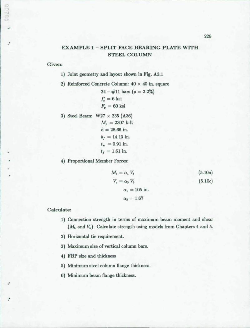
EXAMPLE 1 - SPLIT FACE BEARING PLATE WITH

STEEL COLUMN

Given:

1) Joint geometry and layout shown in Fig. A3.1

2) Reinforced Concrete Colunm: 40 x 40 in. square

24 - #11 bars (p = 2.2%) f; = 6ksi

F. = 60 ksi

3) Steel Beam: W27 x 235 (A36)

M. = 2307 k-ft

d = 28.66 in.

b, = 14.19 in.

t .. = 0.91 in.

t, = 1.61 in.

4) Proportional Member Forces:

Calculate:

M. = a, V.

v. =a. V. a, = 105 in.

a. = 1.67

229

(5 .10a)

(5 .1Oc)

1) Connection strength in terms of maximum beam moment and shear

(M. and Vb) . Calculate strength using models from Chapters 4 and 5.

2) Horizontal tie requirement.

3) Maximum size of vertical colunm bars.

4) FBP size and thickness

5) Minimum steel colunm flange thickness.

6) Minimum beam flange thickness .

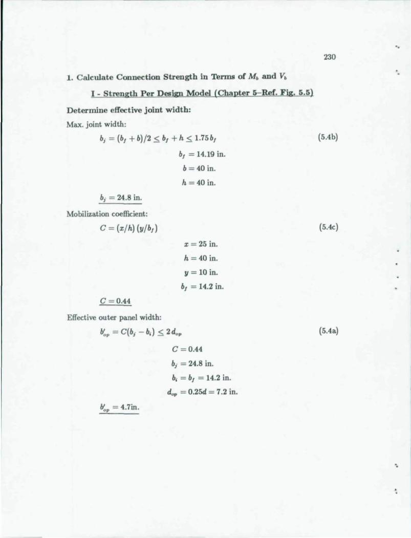
1. Calculate COD.nection Strength in Terms of Mb and Vb

I - Strength Per Design Model (Chapter 5-Ref. Fig. 5.5)

Determine effective joint width:

Max. joint width:

b; = (b, + b)/2 < b, + h < 1.75b,

b; = 24.8 in.

Mobilization coefficient:

C - 0.44

Effective outer panel width:

b, = 14.19 in.

b = 40 in.

h = 40 in.

x = 25 in.

h = 40 in.

Y = 10 in.

b, = 14.2 in.

/1". = C(b; - b;) < 2do•

/1". = 4.7in.

C = 0.44

bi = 24.8 in.

b; = b, = 14.2 in.

dop = 0.25d = 7.2 in.

'.

230

(5.4b)

(5Ac)

(5.4 a)

'.

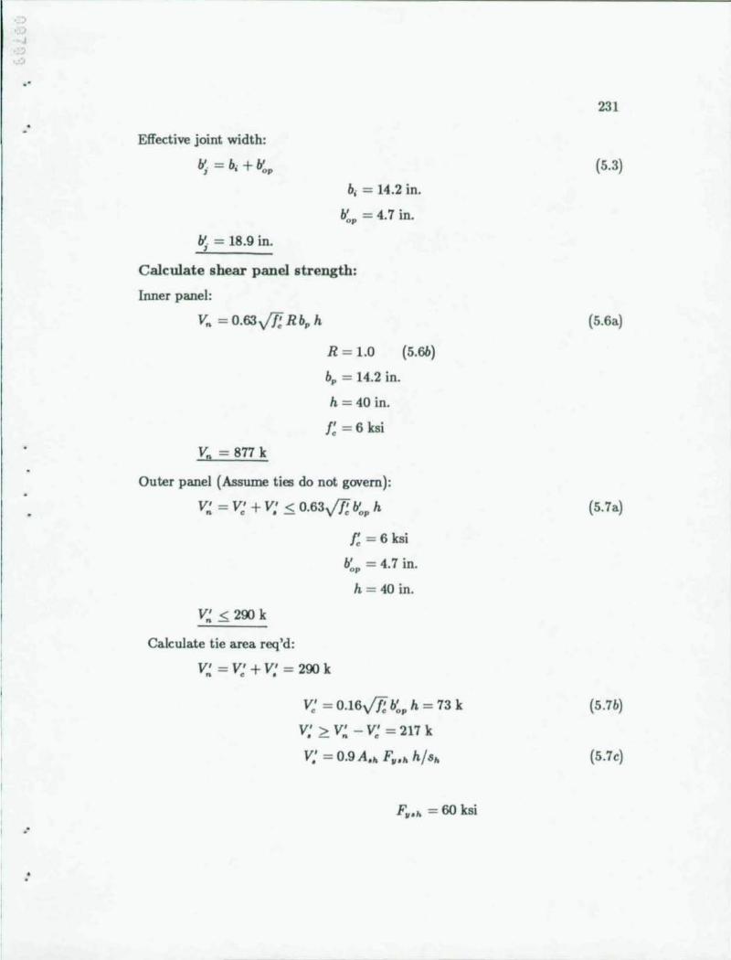
J

.'

.'

Effective joint width:

bj = b; + it..

bj = 18.9 in.

b; = 14.2 in.

b:p = 4.7 in.

Calculate shear panel strength:

Inner panel:

Vn = 0.63v'lf Rbp h

Vn = 877 k

R = 1.0

b. = 14.2 in.

k = 40 in.

f;= 6ksi

(S.6b)

Outer panel (Assume ties do not govern):

V~ = V: + V: < 0.63v'lf it.. h

V~ < 290 k

Calculate tie area req'd:

f;= 6ksi

b:p = 4.7 in.

k = 40 in.

V' = V' + V' = 290 k n < •

V' = 0 16 fT.f.' b' k = 73 k e • V Ie op

V' > V' - V' = 217 k • _ n e

231

(S.3)

(S.6a)

(S.7a)

(S.7b)

(S.7e)

A.h 010. - h>. lU. 8 -

1st Iteration:

Assume Length of Bearing Region

ac < 0.3h (12 in.)

Try a. = 7 in. (panel shear governs)

Calculate pc. and jh:

pc. = C, + T., + Co.

pc. = C, = 1588 k

jh = h - a,

jh = 33 in.

Calculate steel panel, V.:

V. = 0.6F.w tw jh

v. = 649 k

Tv. = Co. = 0

Cc = 2/; ac bj

I; = 6 ksi

a, = 7in.

bj = 18.9 in.

h = 40in.

ac = 7 in.

F ... = 36 ksi

t .. = 0.91 in.

jh = 33 in.

.. 232

(5.8b)

(5.9a)

(5.8a)

(5.9b)

(5.5)

.•

Column shear factor:

J = 1.0 (since steel column is present)

Calculate resulting beam moment, Mb:

Mb [l ] = V, d, + VR (0.7Sd .. ) + V~ (d + d.,,) 2 - (J d, 01./01.)

Mb [l] = 28, 860 k-in.

V, = 649 k

VR = 877 k

V~ = 290 k

d, = 27.05 in.

d~ = 2S.44 in.

d = 28.66 in.

d." = 0.2S d = 7.2 in.

J = 1.0

013 = 1.67

OIl = 100 in.

M [2] = [p. _ V,d, + VR(0. 7Sd~) + V~(d + d.,p )] b OIl c. jh

Mb [2] = 23,380 k-in.

Try ac = 7.27 in.

233

(S.12)

(S.14)

2nd Iteration: p •• = 1649 k

jh = 32.73 in.

V. =643 k

Mb [l] = 28,760 k-in.

Mb !2] = 28,860 k-in.

Mb [l] = Mb[2] (Close enough)

Mb = Mb[l] = 28,760 k-in. = 2396 k-ft

I - Solution Per Design (Chapter 5) Model:

Nominal Joint Strength:

Mb = 2396 k- ft

Vb = 288k

Design Joint Strength:

Md = I$Mn, 1$=0.7 Md = 1677 k-ft

Vd = 202 k-ft

234

IT - Strength Per Chapter 4 Model (Ref.- Figs. 4.12 thru 4.14f)

Assess outer panel strength, Mo:

Total joint width:

b; = (b, + b)/2 < b, + h < 1.7Sb,

bj = 24.8 in.

Outer panel width:

b, = 14.19 in.

b = 40 in.

h = 40 in.

bop = b; - ma.x (bp , b,) < 2do•

(4.8a)

(4.8b)

'.

'.

.'

"

bop = 10.6 in.

Mobilization Coefficient:

C = 0.44

Effective outer panel width:

II.P = C bop

II.P

= 4.7

bj = 24.8 in.

bp = 14.2 in.

b, = 14.19 in.

dop = 0.25d = 7.2 in.

% = 25 in.

h = 40 in.

y = lOin.

b, = 14.2 in.

C = 0.44

bop = 10.6 in.

Calculate compression field strength (Assume ties do not govern) :

V~ = V: + V: < 0.63 v'1I II.P h

V~ < 290 k

Calculate M,,:

Mo = (d+ dop) V~/2

f; = 6ksi

b~p = 4.7 in.

h = 40 in.

235

(4.9)

(4.10)

(4.4a)

(4 .11)

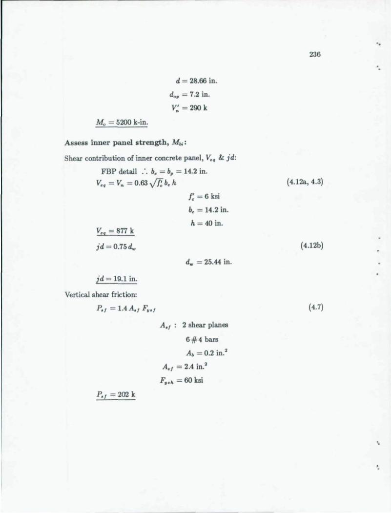
Mo = 5200 k-in.

d = 28.66 in.

do. = 7.2 in.

V~ = 290 k

Assess inner panel strength, M",:

Shear contribution of inner concrete panel, v.. & jd:

FBP detail : . b. = b. = 14.2 in.

v.. = Vn = 0.63 VF. b, h

v.. = 877 k

jd = 0.75d ..

jd = 19.1 in.

Vertical shear friction:

P' I = 1.4 A' I F. ' I

P' I = 202 k

f;= 6 ksi

b. = 14.2 in.

h = 40 in.

d. = 25.44 in.

A./ : 2 shear planes

6#4 bars

A. = 0.2 in"

A' I = 2.4 in.'

F •• h = 60 ksi

'. 236

(4.12a, 4.3)

(4.12b)

(4.7)

"

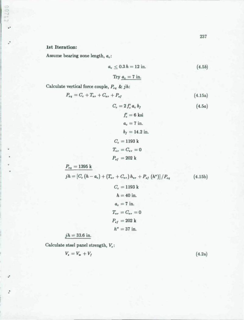
j

1st Iteration:

Assume bearing zone length, ae :

ae < 0.3 h = 12 in.

Try ae = 7 in.

Calculate vertical force couple, p •• &. j h:

p.. = Ce + Tv. + Co. + p.,

p •• = 1395 k

C. = 2/; Be b,

I; = 6 ksi

a. = 7 in.

b, = 14.2 in.

Ce == 1193 k

To. == Co. =0

p., == 202 k

jh == [Ce (h - a.) + (T.. + Co.) h •• + p., (h")] / p ••

C. == 1193 k

j h == 33.6 in.

h == 40 in.

ae == 7 in.

T •• == Co. = 0

p., == 202 k

h" == 37 in.

Calculate steel panel strength, V.:

V. =V. +v,

237

(4.Sb)

(USa)

(4.Sa)

(USb)

(4 .2a)

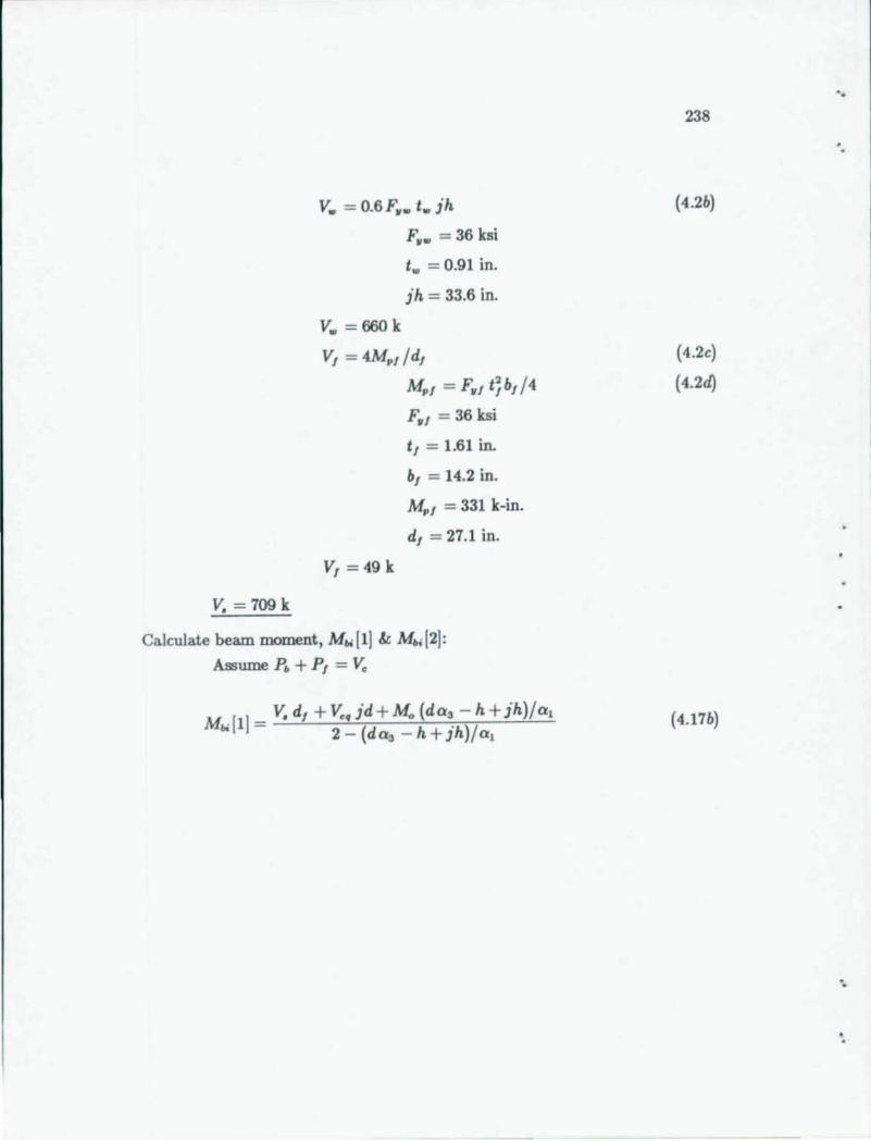
Yo = 709 k

V. = 0.6F •• t. jh

V. = 660 k

F ... = 36 ksi

t .. = 0.91 in.

jh = 33.6 in.

VI = 4Mpl /dl

VI = 49 k

Alpl = F. I t~bl /4

F. I = 36 ksi

tl = 1.61 in.

bl = 14.2 in.

Alpl = 331 k-in.

dl = 27.1 in.

Calculate beam moment, AI",[I] & Alb;[2]:

Assume Pb + PI = V.

238

(4.2b)

(4.2c)

(4 .2d)

(4 .17b)

'.

'.

.'

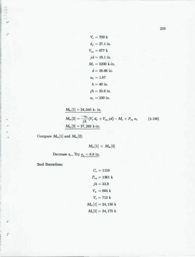
v. = 709 k

d, = 27.1 in.

v., = 877 k

id = 19.1 in.

Mo = 5200 k-in.

d = 28.66 in.

a. = 1.67

h = 40 in.

ih = 33.6 in.

a, = 100 in.

M • .[I] = 24,045 k- in.

- a, . M • .[2] = ;'h (V. d, + v., ]d) - Mo + p., a,

M • .[2] = 27,263 k-in.

Compare M • .[ I] and M.'[2]:

Decrease a., Thy a. = 6.8 in.

2nd Iteration:

C. = 1159

p., = 1361 k

;'h = 33.8

V. = 664 k

V. = 713 k

M • .[I] = 24,150 k

M. !2] = 24,175 k

239

(4 .18b)

M.,[lj = Mh;[2j (close enough)

M •• = M.dlj = 24,150 k-in.

Total Capacity: Mh = Mh• + M. = 29,350 k-in. = 2446 k-ft

II - Solution Per Chapter 4 Model:

Nominal Joint Strength:

M. = 2446 k-ft

V. = 294k

2. Tie Requirements

Inside joint:

Minimum to carry panel shear:

A.~ 0100' -=. m. 8A

Minimum recommended: (non-seismic)

A.~ 004b . (Gov ) - = O. = Q,l§Q m. ems 8~

Say 4 leg - #4; A.A = (0.2 in!) (4) = 0.8 in.'

:. IIA max = 0.8/0.160 = 5 in.

Inside Joint:

USE 4 - #4 a 5 in. max

Outside joint:

Minimum recommended:

3 layers - 4 leg # 5 bars

A, , At = 3 x 4 x 0.31

= 3.72 in.'

-. 240

(5.23a)

(Fig. 5.14)

--

.'

Requirement for horizontal transfer:

Required P. ~ V~ = 290 k

P. = Pu + Po. < 1.5 Pl1

Pl1 = F •• h At

F •• h = 60 ksi

At == 3.72 in.' (min)

Pl1 = 223 k

Pu = 0 (for column detail)

p. = 223 k < 290 k (No Good)

Increase A, , At

USE 4 layers of #5 bars:

P, = Pl1 = 297 k > 290 k (OK)

Outside Joint (within lOt in. of beam)

4 layers - 4 leg - #5 bars

3. Maximum Size of Vertical Bars

Non-seismic:

db < (d + dop )/15

db < 2.38 in.

1 d.., =- d

4

#11 bars < 2.38 in. (OK)

4. FBP Size and Thickness

Horizontal force, Vn = 877 k

Split FBP: t. = K Jp Lmin 7 F •• Lm ••

241

(5.25a)

(5.25b)

(5.27a)

(5.17)

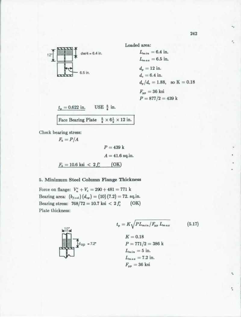
121 · .. I dw/4 - 6.4 in.

~~

6.5 in.

Loaded area:

Lmin = 6.4 in,

Lm .. = 6,5 in,

dp = 12 in. d. = 6.4 in.

242

dp/d. = 1.88, so K = 0.18

F.p = 36 ksi

P = 877/2 = 439 k

tp = 0.622 in. USE ~ in.

I Face Bearing Plate ~ x 6~ x 12 in. I Check bearing stress:

Fb = PIA

P = 439 k

A = 41.6 sq.in.

Fp = 1O.6ksi < 2£ (OK)

5. Minirrrum Steel Column Flange Thickness

Force on flange: V~ + V. = 290 + 481 = 771 k

Bearing area: (bJ co,) (dop) = (1O) (7.2) = 72. sq. in.

Bearing stress: 768/72 = 10.7 ksi < 2 f; (OK)

Plate thickness:

10· ~

K = 0.18

P = 771/2 = 386 k

Lmin = 5 in.

Lm •• = 7.2 in.

F.p = 36 ksi

- ---- ------

(5.17)

' .

"

"

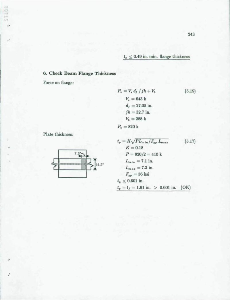
6, Check Beam Flange Thickness

Force on Bange:

Plate thickness:

243

t. < 0.49 in. min. flange thickness

p. = V. d, /ih + V.

V. = 643 k

d, = 27.05 in.

ih = 32.7 in.

V. = 288 k

p. = 820k

(5.19)

tv = K.JPLmin/F •• Lm .. (5 .17) K = 0.18

P = 8'1fJ/ 2 = 410 k

Lmin = 7.1 in.

Lm •• = 7.3 in.

F.p = 36 ksi

t. < 0.601 in.

t. = t, = 1.61 in. > 0.601 in. (OK)

244

EXAMPLE 2 - FACE BEARING PLATE WITH STEEL COLUMN AND VERTICAL JOINT REINFORCEMENT

Given:

1) Joint geometry and layout shown in Fig. A3.2

2) Reinforced Concrete Column: 30 x 30 in. square

p = 4% (max) f; = 6ksi

F. = 60 ksi

3) Steel Beam: W40 x 149 (A36)

Mp = 1791 k-ft

d = 38.2 in.

b, = 11.81 in.

t .. = 0.63 in.

t, = 0.83 in.

4) Proportional Member Forces:

Calculate:

Mb = al v"

V. = a. v" al = 105 in.

a. = 1.67

(5.10a)

(5 .1Oc)

1. Connection strength in terms of maximum beam moment and shear

(Mb and Vb)' Cakulate strength based on design model (Chapter 5)

for two cases: one without and one with vertical joint reinforcement.

"

'.

..

1. Calculate Maximum Beam Forces, Mb &. Vb

Determine effective joint width:

Maximum joint width:

bj = (b, + b) 12 < b, + h < USb,

bi = 20.7 in.

b, = 11.81 in.

b = 30 in.

h = 30 in.

Mobilization coefficient (Neglect vertical joint reinforcement) :

C = (xl h) (ylb,)

C = 0.43

Effective outer panel width:

x = 19 in.

h = 30 in.

y = 8 in.

b, = 11.81 in.

b'.,. = C( bj - b;) < 2 do.

b'op = 3.8 in.

Effective joint width:

hi = b;+ b'.,.

C = 0.43

bj = 20.7 in.

bi = b. = H.8 in.

d." = 0.2Sd = 9.55 in.

bi = 11.8 in.

b:. = 3.8 in .

245

(2.4b)

(SAc)

(SAa)

(5.3)

bi = 15.6 in.

Calculate shear panel strength:

Inner panel:

Vn = 0.63 ..fF. R b. h

Vn = 546 k

R = 1.0

b. = 11.8 in.

h = 30 in.

f:= 6 ksi

Outer panel: Assume ties do not govern:

V' = V' + V' < 063 rr.fl /I h n C! • _ • V J e op

(5.6b)

f!=6ksi

b:. = 3.8 in.

h = 30 in.

V~ < 176 k

246

(5.6a)

(5.7a)

I - Consider Case WITHOUT Vertical Joint Reinforcement

Assume length of bearing region:

Calculate pc. ih:

Pet = C. = 2 f; ac bj

ac < 0.3 h = 9 in.

Try ac = 9 in.

f; = 6ksi

a.= 9in.

bj = 15.6 in.

(5.8b)

(5.9a,5.8a)

' .

'.

Pe. = 1685 k

jh = (h - a, )

jh = 21.0 in. h = 30 in.

Calculate steel panel strength, V.:

V. = 0.6F.~ t~ jh

v. = 286 k

Column shear factor:

F.~ = 36 ksi

tou = 0.63 in.

jh = 21.0 in.

J = 1.0 (since steel column is present)

Calculate resulting beam moment, Mb Assuming shear governs:

v. = 286 k

d, = 37.4 in.

Vn = 546 k

d., = 36.5 in.

V~ = 176 k

d = 38.2 in.

do. = 9.6 in.

J = 1.0

Q3 = 1.67

QI = 105 in.

247

(5.9b)

(5.5)

( 5.12)

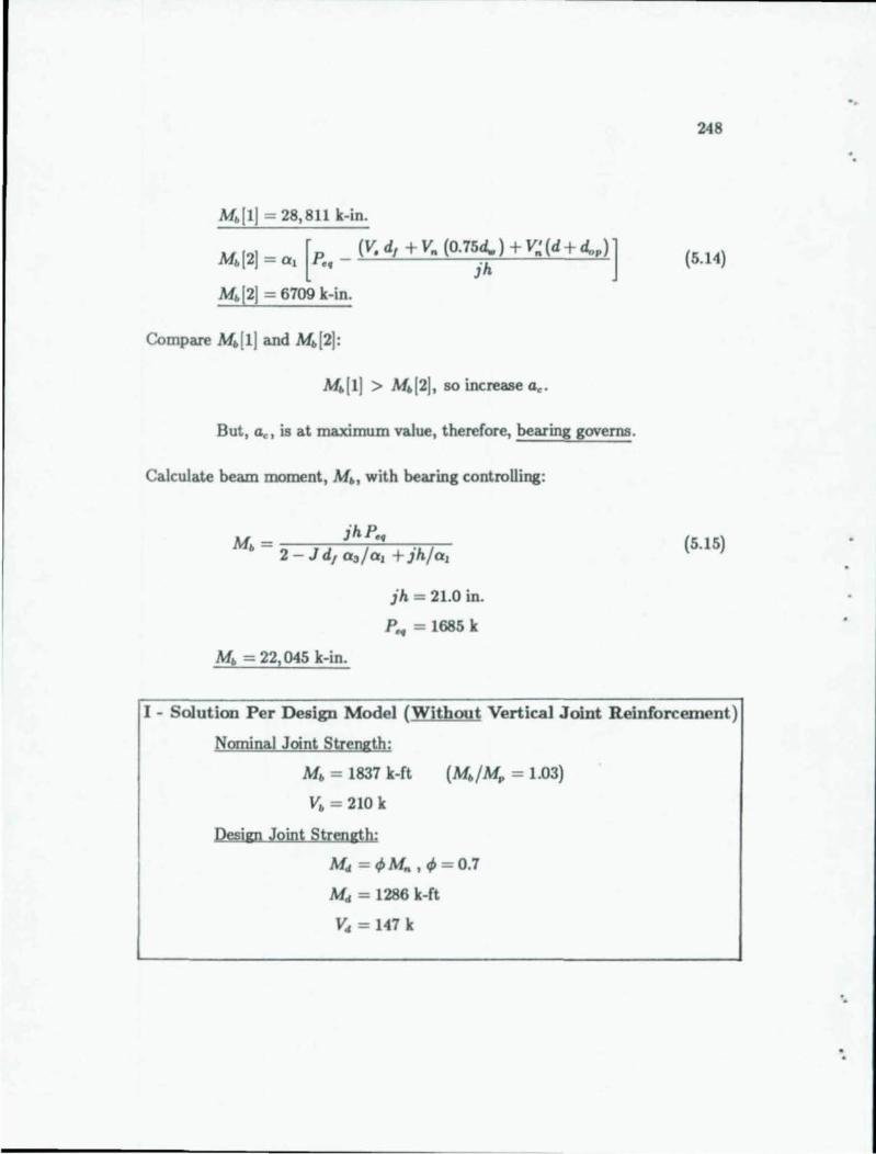
Mbll! = 28,811 k-in.

II I! - [n _ (V, d, + V. (0.75d,.) + V~(d + d"p)] JYAb 2 - a, re. ih Mb12! = 6709 k-in.

Compare M.Il! and M.12!:

M.Il! > M.12!, 50 increase a •.

But , a. , is at maximllID value, therefore, bearing governs.

Calculate beam moment, M., with bearing controlling:

M. = 22,045 k-in.

ih = 21.0 in.

p •• = 1685 k

248

(5.14)

(5.15)

I - Solution Per Design Model (Without Vertical Joint Reinforcement)

Nominal Joint Strength:

M. = 1837 k-ft

V. = 210 k

Design Joint Strength:

M4 = ~M., ~ = 0.7

M4 = 1286 k-ft

V. = 147 k

'.

'.

,-

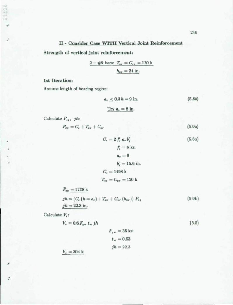
Vi

Strength of vertical joint reinforcement:

1st Iteration:

2 - #9 bars: Tit = CPr = 120 k

h" = 24 in.

Assume length of bearing region:

a. < 0.3 h = 9 in.

Try a, - 8 in.

Calculate p ••• jh:

Pe• = C. + T •• + Cit

Pe , = 1738 k

C. == 2f;a.b~

f;=6ksi

a. =8

b~ = 15.6 in.

C. = 1498 k

T •• = Cit = 120 k

jh == (C. (h == a. ) + Tit + Cit (ho.)) Pe •

j h == 22.3 in.

Calculate V.:

V. == 0.6F •• t. jh

v. == 304 k

F •• = 36 ksi

t. = 0.63

jh = 22.3

249

r

(5.8b)

(5.9a)

(5.84)

(5.9b)

(5.5)

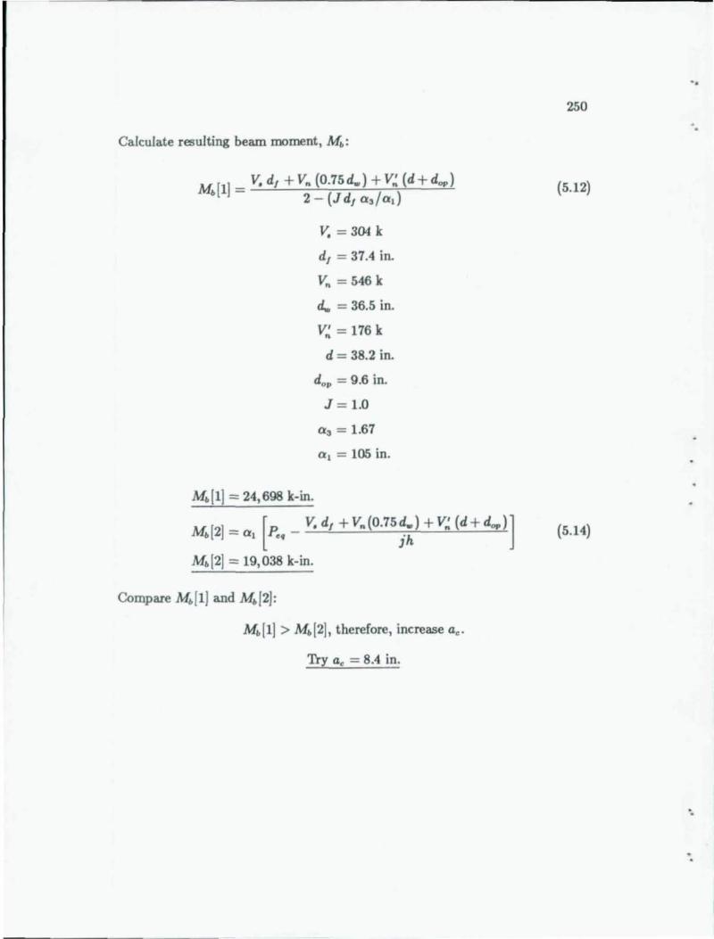
Calculate resulting beam moment , M,, :

M. [l ] = V, d, + Vn (0.7Sd .. ) + V~ (d + dop) 2 - (J d, a.lad

M.[l ] = 24,698 k-in.

v. = 304 k

d, = 37.4 in.

Vn = S46k

d.. = 36.S in.

V~ = 176 k

d = 38.2 in.

d •• = 9.6 in.

J = 1.0

a . = 1.67

a , = lOS in.

Ir [2]- [p. _ V.d' + Vn(0.7Sd .. ) + V~(d + dop )] lY'. - a, e. jh

M.[2] == 19,038 k-in.

Compare M.[l ] and M.[2):

Try ae = 8.4 in.

"

250

(S.12)

(S.14)

'.

· ,

..

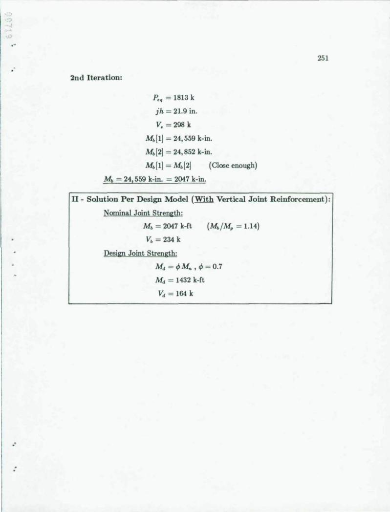
2nd Iteration:

p •• = 1813 k

jh = 21.9 in.

V. = 298k

Mb[l[ = 24,559 k-in.

Mb[2[ = 24,852 k-in.

Mb[l] = M.[2] (Close enough)

Mb = 24,559 k-in. = 2047 k-in.

251

11- Solution Per Design Model (With Vertical Joint Reinforcement):

Nominal Joint Strength:

Mb = 2047 k-ft

Vb = 234 k

Design Joint Strength:

Md = tfoMn, tfo = O.7

Md = 1432 k-ft

Vd = 164 k

Glossary of Nomenclature

A. = cross-sectional area of column core confined by ties, sq. in.

A. = gross cross-tlectional column area, sq. in.

A, = total area of ties parallel to beam in transfer zone as shown in Figs. 4.11

and 5.14, sq. in.

A •• = total cross-sectional area of transverse reinforcement (including cross

ties) with spacing sh and perpendicular to dimension b, sq. in.

A., - total cross-sectional area of transverse reinforcement fully developed

in tension and crossing the vertical crack plane as shown in Fig. 4.4b,

sq. in.

A, = total area of ties perpendicular to beam in transfer zone as shown in

Figs. 4.11 and 5.14, sq. in.

a. = length of concrete bearing zone, in.

b = width of concrete column measured perpendicular to beam, in.

b. = effective width of concrete panel, in.

b, = width of steel beam Banges, in.

b, = effective width of inner panel, in.

b, = maximum width of joint region, in.

~ = effective width of joint region, in.

bop = maximum width of outer panel, in.

b'.. = effective width of outer panel, in.

bp = width of FBP or WSP, in.

C = mobilization coefficient as shown in Figs. 4.6 and 4.7.

C. = nominal compression strength of bearing zone adjacent to the beam,

k.

252

'.

'.

• .'

..

253

C. r = nominal compression strength of vertical reinforcement, k.

d = total height of steel beam, in.

db = diameter of reinforcing bar, in.

d, = distance between centerlines of the steel beam flanges, in.

dop = additional effective joint depth provided by attachments to flanges , in.

d .. = distance between beam flanges (height of web), in.

e = base for natural logarithm.

F. = specified minimum yield stress of steel, ksi .

F •• = specified yield stress of beam web, ksi.

F., = specified yield stress of beam flange, ksi.

F.p = specified yield stress of bearing plate, ksi.

F •• I> = specified yield stress of transverse shear reinforcement, ksi.

f ! = specified compression strength of concrete, psi.

h = total depth of concrete column measured parallel to the beam, in.

h" = total depth of column core confined by ties, in.

h., = horizontal distance between vertical joint reinforcement, in.

J = dimensionless coefficient to account for contribution of column shear

in joint calculations.

jd = vertical distance between the horizontal force couple, Ve., shown in

Fig. 4.8, in.

jh = horizontal distance between the vertical force couple, Pe. , shown in

Figs. 4.10 and S.3c, in.

K = dimensionless coefficient to account for geometry in evaluating bearing

plate thickness .

254

Lm as = maxinrum characteristic length used for evaluating bearing plate thick­

ness, in.

Lm •• = minimum characteristic length used for evaluating bearing plate thick­

ness, in.

Mb = total moment in the steel beam adjacent to the connection, k-in. (unless

otherwise noted).

Me = total moment in the reinforced concrete or composite column adjacent

to the connection, k-in. (unless otherwise noted) .

M b• = moment in the steel beam carried by the inner joint panel, k-in.

M", = moment in the concrete column carried by the inner joint panel, k-in.

M. = moment in the steel beam and concrete column carried by the outer joint panel, k-in.

MpI = plastic moment capacity of beam flange, k-in.

n = number of layers of transverse reinforcement within the beam depth.

P = applied load, k.

Pb = horizontal column shear transferred into the steel flanges by bearing

(Fig. 4 .8E), k.

p •• = resultant of vertical forces acting on the inner panel, k.

PI = horizontal column shear transferred into the steel flange by friction, k.

Ptl = strut transfer force provided by column ties in Fig. 4.1la, band c, k.

Po = shear friction transfer force shown in Fig. 4.llb, c and d, k.

P'I = vertical force transferred by shear friction into the inner concrete panel, k.

p. = total strength of horizontal force transfer to outer panel, k.

PH = tension force provided by column ties in Fig. 4.lla, k.

p.. = tension force provided by column ties in Fig. 4.llb, k.

'.

.•

255

p. = maxinrum vertical force in steel beam associated with web panel yield­

ing, k.

Q; = applied load (DL,LL,W,E,S or other) .

R = reduction coefficient for inner concrete panel strength.

R.n = mean value of measured component strength.

R., = mean value of calculated component strength.

Sh = center to center spacing of transverse column reinforcement, in.

T •• = nominal tension strength of vertical joint reinforcement, k.

t I = thickness of the steel beam flange, in.

t. = thickness of bearing plate, in.

t., = thickness of the steel beam web, in.

"I-b = total shear in the steel beam adjacent to the connection, k.

Vc = total shear in the reinforced concrete or composite column adjacent to

connection, k.

v: = concrete contribution to the compression field mechanism, k.

VI = contribution of local flange bending to steel panel strength, k.

Vn = nominal horizontal shear capacity of the compression strut mechanism,

k.

V~ = nominal horizontal shear capacity of the compression field mechanism,

k.

v.. = coefficient of variation for ratios of resistances, R.n / R..

V, = nominal horizontal shear capacity of the steel web panel, k.

V: = reinforcing steel contribution to the compression field mechanism, k.

V., = contribution of web shear to steel panel strength, k.

x = dimension for calculation of C coefficient. in .

y = dimension for calculation of C coefficient, in.

a; = proportionality constants relating beam and column forces.

{J = reliability (safety) index.

'Y; = load factors as given by AlSC-LRFD specification.

<p = resistance (capacity reduction) factor.

256

'.

. "

REFERENCES

1. Sheikh, T.M., "Moment Connections Between Steel Beams and Concrete Col­

umns," Ph.D. Dissertation, Department of Civil Engineering, The University

of Texas at Austin, Dec. 1987.

2. Griffis, L., "Some Design Considerations for Composite-Frame Structures,"

AlSC Engineering Journal, 2nd Quarter, 1986.

3. Moore, W., Gosain, N., "Mixed Systems: Past Practices, Recent Experience

and Future Direction," Composite and Mixed Construction; Proceedings of

the U.S./Japan Joint Seminar, Edited by C. Roeder, ASCE, 1985.

4. Rastorfer, D., "William J. Le Messurier's Super-tall Structures: A Search

for the Ideal," Architectural Record, Jan. 1985.

5. Iyengar, H., "Recent Developments in Mixed Steel-Concrete Systems," Com­

posite and Mixed Construction; Proceedings of the U.S./Japan Joint Semi­

nar, Edited by C. Roeder, ASCE, 1985.

6. Wakabayashi, M., "Recent Developments for Composite Buildin~ in Japan,"

Composite and Mixed Construction; Proceedings of the U.S./Japan Joint

Seminar, Edited by C. Roeder, ASCE, 1985.

7. Minami, K., "Beam to Column Stress Transfer in Composite Structures,"

Composite and Mixed Construction; Proceedings of the U.S./ Japan Joint

Seminar, Edited by C. Roeder, ASCE, 1985.

8. ACI-ASCE Committee 352, "Recommendations for Design of Beam Column

Joints in Monolithic Reinforced Concrete Structures," Report ACl 352 R-85,

1985.

9. Paulay, T., "Equilibrium Criteria for Beam-Column Joints," Interim Re­port: US-NZ-Japan-China Seminar on Design of RC Beam-Column Joints

for Earthquake Resistance, University of Canterbury, Christchurch, NZ, Aug.

1987 .

257

258

10. American Institute of Steel Construction, "Specifications for the Load and

Resistance Factor Design, Fabrication and Erection of Structural Steel for

Building.<;," AlSC, Chicago, IL, Sept. 1986.

11. Griffis, L., Consulting Structural Engineer with the firm of Walter P. Moore

and Assoc., Houston, TX.

12. Gosain, N., Brown, R., & Jirsa, J ., "Shear Requirements for Load Reversals

on RC Members," Journal of the Structural Division, ASCE, July, 1977.

13. Clough, R., & Penzien, J ., Dynamics of Structures, McGraw Hill, NY, 1975.

14. Kitayama, K. , Otani, S. & Aoyama, H., "Earthquake Resistant Design Cri­

teria for Reinforced Concrete Interior Beam-Column Joints," Proceeclings­

Pacific Conference on Earthquake Engineering, Wairakei, New Zealand, 1987.

15. American Concrete Institute, "Building Code Requirements for Reinforced

Concrete (ACI-318) and Commentary," ACI, Detroit, MI, 1983.

16. Meinheit, D.F., "The Shear Strength of Reinforced Concrete Beam-Column

Joints," Ph.D. Dissertation, Department of Civil Engineering, The University

of Texas at Austin, Dec. 1983.

17. Guimaraes, G., et aI., "Tests of Reinforced Concrete Slab-Beam-Column

Connections- U.S. Designs," Interim Report: US-NZrJapan-China Seminar

on Design of RC Beam-Column Joints for Earthquake Resistance, University

of Canterbury, Christchurch, NZ, Aug. 1987.

18. Krawinkler, H., Bertero, Y., & Popov, E., "Shear Behavior of Steel Frame

Joints," Journal of the Structural Division, ASCE, Nov. 1975.

19. Stelmack, T., Marley, M. & Gerstle, K., "Analysis and Tests of Flexibly

Connected Steel Frames," Journal of Structural Engineering, ASCE, July

1986.

20. Ackroyd, M., Gerstle, K. , "Behavior of Type 2 Steel Frames," Journal of the

Structural Division, ASCE, July, 1982.

"

-.

. -

259

21. ACI-ASCE Committee 352, "RecommendatioIlB for Design of Beam-Column

Joints in Monolithic Reinforced Concrete Structures," 1976.

22. Prestressed Concrete IIlBtitute, PCl Design Handbook- Precast Prestressed

Concrete, PCI, Chicago, IL, 1978.

23. American Institute of Steel COIlBtruction, "Specifications for the Design, Fab­

rication and Erection of Structural Steel Buildings with Commentary," AlSC ,

Chicago, IL, Nov. 1978.

24 . American National Standards Institute, "Minimum Design Loads for Build­

ings and Other Structures, ANSI A58.1," ANSI, 1982.

25. Galambos, T ., "Reliability of ColUlections, Joints and Fasteners," Structural

Engineering Report No. 85-{)5, Department of Civil and Mineral Engineering,

University of Minnesota, Dec. 1985.

26. Guimaraes, G. , & Jirsa, J., Research in progress on the use of high strength

concrete in reinforced concrete slab- beam-column cOlUlections, 1988.

27. Bjorhovde, R., "Design CoIlBideratioIlB for Comp06ite Frames," Las Con­

strucciones De Acero En Zonas Sismicas (Steel COIlBtruction in Seismic Zones) ,

Proceedings, 5th International Symposium of Steel Structures, Morelia, Mi­

choacan, Mexico, Nov. 1987 .

•

•