design, mechanical modeling and 3d printing of
TRANSCRIPT

University of New Hampshire University of New Hampshire
University of New Hampshire Scholars' Repository University of New Hampshire Scholars' Repository
Master's Theses and Capstones Student Scholarship
Fall 2017
DESIGN, MECHANICAL MODELING AND 3D PRINTING OF KOCH DESIGN, MECHANICAL MODELING AND 3D PRINTING OF KOCH
FRACTAL CONTACT AND INTERLOCKING FRACTAL CONTACT AND INTERLOCKING
Mona Monsef Khoshhesab University of New Hampshire, Durham
Follow this and additional works at: https://scholars.unh.edu/thesis
Recommended Citation Recommended Citation Monsef Khoshhesab, Mona, "DESIGN, MECHANICAL MODELING AND 3D PRINTING OF KOCH FRACTAL CONTACT AND INTERLOCKING" (2017). Master's Theses and Capstones. 1130. https://scholars.unh.edu/thesis/1130
This Thesis is brought to you for free and open access by the Student Scholarship at University of New Hampshire Scholars' Repository. It has been accepted for inclusion in Master's Theses and Capstones by an authorized administrator of University of New Hampshire Scholars' Repository. For more information, please contact [email protected].

DESIGN, MECHANICAL MODELING AND 3D PRINTING OF
KOCH FRACTAL CONTACT AND INTERLOCKING
BY
Mona Monsef Khoshhesab
Baccalaureate Degree (BS), University of Guilan, 2015
THESIS
Submitted to the University of New Hampshire
in Partial Fulfillment of
the Requirements for the Degree of
Master of Science
in
Mechanical Engineering
September, 2017
I
This thesis has been examined and approved in partial fulfillment of the requirements for the
degree of Master in Mechanical Engineering by
Thesis Director, Yaning Li, Ph.D.
Assistant Professor, Mechanical Engineering, University of New Hampshire
Christine Ortiz, Ph.D.
Professor, Materials Science and Engineering, Massachusetts Institute of Technology
Igor Tsukrov, Ph.D.
Professor, Mechanical Engineering, University of New Hampshire
On July 31, 2017
Original approval signatures are on file with the University of New Hampshire Graduate
School.

II
Table of Contents
Chapter 1. Background and Introduction ................................................................................... 1
1.1. Motivation ........................................................................................................................ 1
1.2. Fractals ............................................................................................................................. 3
1.3. Topological interlocking .................................................................................................. 5
1.4. Contact mechanics framework ......................................................................................... 8
1.5. Overview ........................................................................................................................ 10
Chapter 2. Theoretical Model of Koch Fractal Interlocking .................................................... 12
2.1. Design of Koch fractal interlocking ............................................................................... 12
2.1. Contact model for slant surfaces .................................................................................... 15
2.2. Fractal contact model ..................................................................................................... 20
2.3. Influence of g, r and μ for N=3 ...................................................................................... 25
2.4. Influence of g, r and μ for cases with different N .......................................................... 27
2.5. Scaling Law .................................................................................................................... 35
2.6. Summary ........................................................................................................................ 40
Chapter 3. Finite Element Analysis of Koch Fractal Interlocking ........................................... 42
3.1 Effects of the number of RVEs ...................................................................................... 42
3.2 Effect of RVE symmetry ................................................................................................ 45
3.3 Parametric study on the overall force displacement behavior for case N=3 (Elastic
model)........................................................................................................................................ 47
3.4 3D FE simulations of Koch fractal interlocks ................................................................ 50
3.5 Comparison between linear elastic and elastic-perfectly plastic model ......................... 54
3.6 FE quantification of Energy ........................................................................................... 58
3.7 Summary of the chapter ................................................................................................. 61
Chapter 4. 3D Printing and Mechanical Experiments .............................................................. 63
4.1 Fabrication and tensile experiments of Koch fractal interlocking with gaps ................. 64
4.2 Fabrication and tensile experiments on Koch interlocking with adhesive layer ............ 67
4.3 Comparison of Koch interlocking with gaps and soft adhesive layers .......................... 69
4.4 Comparison between FE models and experiments ........................................................ 70
4.5 Tensile experiments on Koch fractal interlocking with asymmetric geometry ............. 71
III
4.6 Compact tension experiments of Koch fractal interlocking with asymmetric geometry 76
4.7 Summary ........................................................................................................................ 79
Chapter 5. Conclusions ............................................................................................................. 81
5.1 Specific conclusions for each chapter ............................................................................ 81
5.2 Summary of design guidelines developed ...................................................................... 83
5.3 Discussion ...................................................................................................................... 84
References ..................................................................................................................................... 86
Appendix A. FE Simulations of Flat and Slant Contact ............................................................... 93
Appendix B. Correction on Energy absorption from FE Simulations ........................................ 100
IV
List of Tables
Table 2.1 Number of flat and slant segments generated from 𝑆0°, 𝑆60°,𝑆120°, 𝑆180° units. .... 23
Table 2.2 Number of flat and slant segments in contact that generated from S0°, S60°,S120°,
S180° units ...................................................................................................................................... 24
Table 2.3 Summary of number of flat and slant segments in contact ................................... 25
List of Figures
Figure 1.1 Examples of hierarchical interlocking in nature: (a) cranial sutures in deer’s
skull[19], (b) suture in the shell of red-eared slider turtle[20] (c) Ammonite shell (Craspedites
nodiger)[21] and (d) Ammonite shell (Ceratitic) with suture lines[22]. ........................................ 2
Figure 1.2 Examples of three basic fractals: (a) the simple fractal tree [42], (b) Sierpinski
triangle [43], and (c) Koch snow flake[44]. .................................................................................... 4
Figure 1.3 Examples of fractals in nature across all length scales:(a) frost crystals on cold
glass form fractal pattern [45], (b) Romanesco broccoli [45], and (c) fractal defrosting patterns,
polar Mars [45]. .............................................................................................................................. 5
Figure 1.4 Examples of topological interlocking in nature: (a) linking girdle in Aulacoseira
ambigua [86], (b) in Aulacoseira alpiegena [87], and (c) in Aulacoseira valida [88]; (d) gear-like
joints in a jumping insect Issus [89]. .............................................................................................. 7
Figure 2.1. Koch geometry for N=0, 1, 2, 3. ......................................................................... 12
Figure 2.2. (a) Specimen with Koch fractal gap for N=2, 3 and 4. (b) Koch fractal geometry
for N=0,1,2 and 3 (c) enlarged image of r, g, 𝑎𝑠 and 𝑎𝑓. ............................................................. 14

V
Figure 2.3. (a) Categorizing slant (red) and flat (blue) segments for N=2 case; (black and
white arrows show slant and flat segments in contact, respectively); (b) the free body diagram of
the top piece of a pair of slant segments in contact. (c) Dash line displays the deformed
configuration. ................................................................................................................................ 15
Figure 2.4. Contact/interlocking stages (a) Stage I, when no segment is in contact (b) Stage
II when only some flat segments get in contact (c) Stage III when some of the flat and slant
segments get in contact. ................................................................................................................ 18
Figure 2.5. Schematics of flat and slant segments’ length when (a) r>g and (b) r<g.......... 19
Figure 2.6. (a) Four decomposed sections with N=1 geometry: x, y, z, k rotating counter-
clockwise to the horizontal direction as 0°, 60° , 120°, and 360°, respectively. (b) Reproducing
process of each section𝑆0°, 𝑆60°,𝑆120°, 𝑆180°, in [N]th level from sections in [N-1]th level. ........... 21
Figure 2.7. Influence of (a) gap g, (b) rounded tip radius r and (c) friction coefficient μ
mechanical response of Stages II and III for case N=3. ................................................................ 26
Figure 2.8. Theoretical prediction of the influences of gap g on the mechanical response of
fractal contact models for different N. .......................................................................................... 29
Figure 2.9. (a) Theoretical prediction of the contact area of flat and slant segments in
different stages of deformation, and (b) the total contact area of Koch fractal for N=2, 3 and 4.
(𝐴𝑓 , 𝐴𝑠 and 𝐴𝑓 + 𝐴𝑠 represent contact area of flat, contact area of slant and total area,
respectively.) ................................................................................................................................. 30
Figure 2.10. Influence of rounded tip radius r on mechanical behavior of Koch fractal
contact models. ............................................................................................................................. 32

VI
Figure 2.11. (a) Contact area of flat and slant segments in different stages of deformation.
(b) Total contact area of Koch fractal for N=2, 3,4 and 5. 𝐴𝑓 , 𝐴𝑠 and 𝐴𝑓 + 𝐴𝑠represent contact
area of flat, contact area of slant and total area, respectively. ...................................................... 33
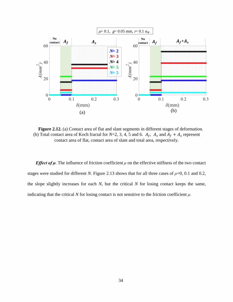
Figure 2.12. (a) Contact area of flat and slant segments in different stages of deformation.
(b) Total contact area of Koch fractal for N=2, 3, 4, 5 and 6. 𝐴𝑓 , 𝐴𝑠 and 𝐴𝑓 + 𝐴𝑠 represent
contact area of flat, contact area of slant and total area, respectively. .......................................... 34
Figure 2.13. Theoretical prediction on the influences of friction coefficient on the load-
displacement relations for different N’s. ....................................................................................... 35
Figure 2.14. Influences of gap g on non-dimensionalized effective stiffness in (a) Stage II
and (b) Stage III. (The solid black curves represent the ideal case of g=0 and r=0 which is the
upper limit of effective stiffness for Koch contact for each N.) ................................................... 37
Figure 2.15. Non-dimensionalized effective stiffness vs. N, when 0 < g <0.1 mm. ............. 38
Figure 2.16. Influence of rounded tip radius r on non-dimensionalized effective stiffness in
(a) Stage II and (b) Stage III. (The solid black curves are for the ideal case of g = 0 and r = 0.) 39
Figure 2.17. Influence of friction coefficient on non-dimensionalized effective stiffness in40
Figure 3.1. Boundary conditions and the finite element mesh with N=2, 3 and 4,
respectively; (b) illustration of the measured displacement. ........................................................ 43
Figure 3.2. Mechanical response of Koch interlocking models. (a) Force-displacement
curves and (b) Stress-strain curves of Koch fractal with different number of RVEs horizontally
oriented when N=2. ....................................................................................................................... 44
Figure 3.3. Mechanical response of Koch interlocking models. (a) Force-displacement
curves and (b) Stress-strain curves of Koch fractal with different number of RVEs horizontally
oriented when N=3. ....................................................................................................................... 45
VII
Figure 3.4. (a) Influence of geometry complexity on mechanical behavior of Koch fractal
with N=2,3 and 4. (b) Stress distribution of cases with different RVE design when δ=0.3 mm. . 46
Figure 3.5. FE Von Misses stress counter of the designs with N=2,3 and 4 at two
displacement δ= 0.15, 0.35 (g=0.1 mm and r=0.15 𝑎𝑁). ............................................................. 47
Figure 3.6. Influences of gap g on the force-displacement response of N=3. ...................... 48
Figure 3.7. Influence of r on mechanical response of Koch fractal design when N=3......... 49
Figure 3.8. Influence of friction coefficient μ on load-displacement response of Koch fractal
contact with N=3. .......................................................................................................................... 50
Figure 3.9. (a) 3D FE models of the Koch fractal design with N=3, r= 0.15 mm, g= 0.1 mm;
(b) Boundary and loading conditions applied to 3D FE models. .................................................. 51
Figure 3.10. Numerical (a) contact area versus overall displacement and (b) force-overall
displacement relation of N=2, 3 and 4. ......................................................................................... 52
Figure 3.11. Comparison between contact area of Koch fractal with different values of (a) g,
....................................................................................................................................................... 53
Figure 3.12. FE comparison between linear-elastic and elasto-perfect plastic material
models for N=2, 3 and 4. ............................................................................................................... 55
Figure 3.13. Influences of gap g on the force-displacement response for N=3. ................... 56
Figure 3.14. Influence of r on mechanical response of N=3 with elasto-perfect-plastic
response......................................................................................................................................... 57
Figure 3.15. Influence of μ on the load-displacement curves of N=3 with linear elastic and
elasto-perfectly plastic material models........................................................................................ 58
Figure 3.16. Distribution of strain energy per volume fraction between top and bottom
pieces for different cases of (a) N=2, (a) N=3 and (a) N=4. ......................................................... 59

VIII
Figure 3.17. Distribution of strain energy per volume fraction between top and bottom
pieces for N=3 with different values of (a) r=0.05 mm, (b) r=0.15 mm and (c) r=0.3 mm. ........ 60
Figure 3.18. FE curves of energy density vs displacement and FE stress distribution
contours for N=3 with r=0.05 mm, (a) g=0.6 mm and (b) g=0.1mm. .......................................... 61
Figure 4.1. Experimental results of 3D-printed Koch fractal interlocking with N=2, 3 and 4,
one RVE, gap g=0.2 mm and r= 0.15 𝑎𝑁. Teeth with large deformations are marked with a
circle. ............................................................................................................................................. 65
Figure 4.2. DIC strain (Ɛ𝑦𝑦) contours of Koch fractal interlock with N=2, 3 and 4 under uni-
axial tension. ................................................................................................................................. 66
Figure 4.3. DIC strain (Ɛ𝑥𝑦) contours of Koch fractal interlock with N=2, 3 and 4 under uni-
axial tension. ................................................................................................................................. 67
Figure 4.4. Experimental results of Koch N=2, 3 and 4 with a soft layer. ........................... 68
Figure 4.5. Comparison between the overall load-displacement curves of the 3D-printed
specimens with and without a soft adhesive layer for N= 2, 3 and 4 (one RVE, gap g=0.2 mm
and r= 0.15 𝑎𝑁.) ............................................................................................................................ 69
Figure 4.6 Comparison between overall force-displacement curve from FE simulation and
experimental results for N=2, 3 and 4. .......................................................................................... 71
Figure 4.7. 3D-printed Koch interlocking specimens with two flipped RVEs and a soft
adhesive layer tested under uni-axial tension for N=0,1 2 and 3. ................................................. 72
Figure 4.8. Experimental load-displacement curves of the 3D-printed specimens tested
under uniaxial tension, with two flipped RVEs and a soft adhesive layer for N=0, 1, 2, and 3. .. 74
Figure 4.9. (a) Nondimensionalized toughness vs. N (b) the finite element stress contours of
the Koch layer with different Ns. .................................................................................................. 75

IX
Figure 4.10. 3D-printed specimens fabricated for compact tension test with N=0,1 2 and 3.
....................................................................................................................................................... 77
Figure 4.11. Experimental results of compact tension test. (a) Force-displacement curves of
four geometries (b) Normalized toughness vs N. The dash line displays the toughness deriving
from the rule of mixture. ............................................................................................................... 78
Figure 4.12. Comparison between toughness of 3D-printed specimens designed for uni-
axial tension and compact tension. Black dash-line displays predication from rule of mixture. . 79

X
ABSTRACT
Design, Mechanical Modeling, and 3D Printing of
Koch Fractal Contact and Interlocking
by
Mona Monsef Khoshhesab
University of New Hampshire, September, 2017
Topological interlocking is an effective joining approach in both natural and engineering
systems. Especially, hierarchical/fractal interlocking were found in many biological systems and
can significantly enhance the system mechanical properties. Inspired by the hierarchical/fractal
topology in nature, mechanical models for Koch fractal interlocking were developed as an example
system to better understand the mechanics of fractal interlocking. In this investigation, Koch fractal
interlocking with and without adhesive layers were designed for different number of iterations N.
Theoretical contact mechanics model was used to capture the deformation mechanisms of the
fractal interlocking with no adhesive layers under relatively small deformation. Then finite element
(FE) simulations were performed to study the mechanical behavior of fractal interlocking under
finite deformation. The designs were also fabricated via a multi-material 3D printer (Objet Connex
260) and mechanical experiments were performed to further explore the mechanical performance
of the new designs.

XI
It was found that the load-bearing capacity of Kotch fractal interlocking can be effectively
increased via fractal design. In general, when the fractal complexity (it is specifically represented
as number of hierarchy N in the present Koch fractal design) increases, the stiffness of the fractal
interlocking will increase significantly. Also, when N increases, the stress are more uniformly
distributed along the fractal boundary of the top and bottom pieces of the fractal interlocking,
which efficiently reduce local stress concentration, and therefore the overall strength of the
interlocking also increases.
However, the mechanical responses of fractal interlocks are also sensitive to imperfections,
such as the gap between the interlocked pieces and the rounded tips. When fractal complexity
increases, the mechanical properties will become more and more sensitive to the imperfection and
eventually, the negative influences from imperfection can even become dominant. Therefore,
considering the imperfection, there is an optimal level of fractal complexity to reach the maximum
mechanical performance. This result is in consistent with fractal interlocks in different biological
systems.
Except topology, the influences of friction, material properties and damage evolution, and
the adhesive layer on the mechanical performance of Koch fractal interlocking were also evaluated
via non-linear FE simulations and mechanical experiments on 3D printed Koch interlocking
specimens. It was found that the adhesive layer can significantly improve the load transmission of
the fractal interlocking and therefore can effectively amplify the interlocking efficiency.
1
Chapter 1. Background and Introduction
1.1. Motivation
In nature, during years of evolution, many biological systems develop complicated
geometrical and material heterogeneity across several length scales to achieve light weight and
high mechanical performance [1-6]. Generally, hierarchical heterogeneity can be achieved via two
different mechanisms: (1) variation of nano/micro structures at different length scale, such as
bones and sea shells [7-9] and (2) self-similarity via fractal geometry, such as gecko feet [10-11]
and biological sutures [12-14]. The fractal interlocking explored in this investigation falls in the
second category. It is a type of fractal-induced self-similar mechanical interlocking, which
provides a specific option of designing hierarchical heterogeneity in any material system.
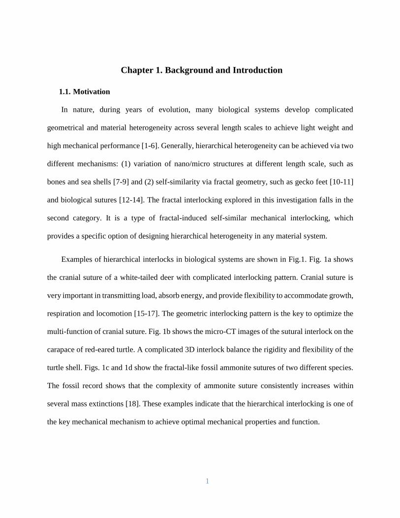
Examples of hierarchical interlocks in biological systems are shown in Fig.1. Fig. 1a shows
the cranial suture of a white-tailed deer with complicated interlocking pattern. Cranial suture is
very important in transmitting load, absorb energy, and provide flexibility to accommodate growth,
respiration and locomotion [15-17]. The geometric interlocking pattern is the key to optimize the
multi-function of cranial suture. Fig. 1b shows the micro-CT images of the sutural interlock on the
carapace of red-eared turtle. A complicated 3D interlock balance the rigidity and flexibility of the
turtle shell. Figs. 1c and 1d show the fractal-like fossil ammonite sutures of two different species.
The fossil record shows that the complexity of ammonite suture consistently increases within
several mass extinctions [18]. These examples indicate that the hierarchical interlocking is one of
the key mechanical mechanism to achieve optimal mechanical properties and function.
2
Figure 1.1 Examples of hierarchical interlocking in nature: (a) cranial sutures in deer’s
skull[19], (b) suture in the shell of red-eared slider turtle[20] (c) Ammonite shell (Craspedites
nodiger)[21] and (d) Ammonite shell (Ceratitic) with suture lines[22].
The evolution and growth of hierarchical interlocks in nature is a mystery to the field. For
example, it is not well understood why the cranial suture of human being develops from a simple
straight line to a complicated zigzag pattern during growth from infant to adult [14, 17], and why
the cranial sutures of mammals with horns exhibit even more complex patterns than those of
humans. Also, why there is a limitation for geometry complexity in these biological systems?
To address these questions, recently, composite mechanical models of biological sutures with
different waveforms were extensively explored [23-32]. The triangular tooth geometry was proved
to be the optimized geometry to maximize strength and load transmission [31-33]. Also, it was
found that by increasing the number of hierarchy, the overall stiffness, strength and fracture
toughness can be tuned by orders of magnitude [22-25, 32-34].
Craspedites nodiger
(c)
Red-eared slider turtle
(b)
Ceratites
(d)
Deer skull
(a)
3
In this investigation, the primary goal is to design Koch fractal interlocking and explore the
influence of number of hierarchy, material properties, and geometry imperfection on the overall
mechanical properties of the designs. Design principles for fractal interlocking will be developed,
which will provide insights to develop optimized design for joining similar/dissimilar materials
through topological interlocking.
1.2. Fractals
Euclidean geometry is a system of geometry considered measurement and the concepts of
congruence, parallelism and perpendicularity with ten common assumptions and postulates. When
any of the postulates is negated, the geometry is non-Euclidean [35]. Fractal geometry is one of
the youngest non-Euclidean geometric concepts which uses simple algorithms to design complex
forms. They were discovered by Mandelbrot [3]. They can not only model the complex forms, but
also act as bridge between regular geometries to irregular ones [3, 36-37]. One interesting
characteristic of fractals is that they exhibit great complexity driven by simplicity [38-41]. Fractals
exhibit repeating patterns that display at every scale. This is one major feature of fractal, called
self-similarity.
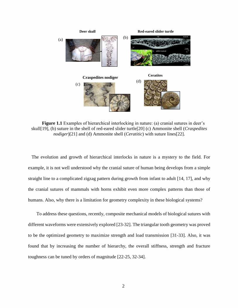
To further understand the definition of fractal, examples of three basic fractals are provided
in Figure 1.2. Figure 1.2a shows a binary fractal tree which is defined recursively by symmetric
binary branching. The trunk of length L splits into two branches of smaller length R, each making
an angle θ with the direction of the trunk. Continuing in this way for infinitely many branching,
the tree is the set of branches, together with their limit points, called branch tips. Figure 1.2b shows
the Sierpinski triangle, which is a basic fractal with the overall shape of an equilateral triangle,
subdivided recursively into smaller equilateral triangles. Another basic fractal is the Koch flakes,

4
as shown in Figure 1.3c. The Koch flakes is also generated from an equilateral triangle, then the
edges are recursively replaced by Koch fractal curves.
Figure 1.2 Examples of three basic fractals: (a) the simple fractal tree [42], (b) Sierpinski
triangle [43], and (c) Koch snow flake[44].
Koch curve is one of the first classical fractals described by Helge von Koch in 1904 as an
example of a non-differentiable curve. It was generated via an iterated function system (IFS) where
the number of iteration defined as N [44]. We will talk about Koch curve in more detail in Chapter
2.
Fractals are also ubiquitous in nature in all length scales, as shown in Fig. 1.3. Natural fractals
include frost crystals occurring naturally on cold glass (Fig.1.3a), Romanesco broccoli,
showing 3D self-similar geometry (Fig.1.3b), and fractal defrosting patterns, polar Mars, where
the patterns are formed by sublimation of frozen CO2. The width of image is about a kilometer
(Figure 1.3c)!
(a) (b) (c)

5
Figure 1.3 Examples of fractals in nature across all length scales:(a) frost crystals on cold
glass form fractal pattern [45], (b) Romanesco broccoli [45], and (c) fractal defrosting patterns,
polar Mars [45].
Fractals have been used by scientists in electrical engineering to produce electronic circuit
with chaotic behavior [46], medical and health care fields to model and measure tumor and
irregular distribution of collagen in tissue [47,48], architecture engineering to design bio-inspired
constructions [49-51].
1.3. Topological interlocking
Topological interlocking has been suggested as a novel method to create architectured
materials [52-72]. This concept relies on segmenting a monolithic material into elementary blocks
with specific shapes. The building blocks are constrained in their movement by the neighboring
ones [53]. Providing structural stability, topological interlocking allows for restricted locomotion
of neighboring building blocks. This ensures that the new architectured material articulated via
topological interlocking is more compliant than a monolithic one, and is also able to absorb
vibrational energy, which is dissipated by frictional losses [53, 61].
Topological interlocking plays a critical role in joining similar/dissimilar materials and
structures. For example, topological interlocking is used in adhesive science and engineering [57,
73] , in the area of friction and tribology [74], in plasticity and creep [75] (interlocking of wavy
(a) (b) (c)

6
grains, with a great resistance to sliding deformation.) of ductile metals and also in fiber reinforced
composites [76].Compared with bonding via adhesive materials or mechanical fasteners,
mechanical interlocking has a similar function with a simpler and more robust method in
manufacturing [53, 61]. The geometry of the interlocked piece is the key to achieve high-quality
joints through topological interlocking [53, 59, 61, 77-85].
As shown in Figure 1.4, topological interlocking is also found in many biological
composites to meet a complex spectrum of functional requirements through hierarchical/fractal
geometries. Bones, woods, nacre, and biological sutures are a few examples of natural composites
that employed hierarchical design to achieve remarkable properties and functionality [1, 11, 37,
71-76]. Figure 1.4a , 4b and 4c show interlocked linking girdles in three species of diatoms. Figure
1.4d displays natural gear in a species of jumping inset, Issus. Having a row of cuticle gear teeth
around the curved medial surfaces of their two hind-leg trochantera, the jumping efficiency of the
nymph, but can be significantly improved [89].

7
Figure 1.4 Examples of topological interlocking in nature: (a) linking girdle in Aulacoseira
ambigua [86], (b) in Aulacoseira alpiegena [87], and (c) in Aulacoseira valida [88]; (d) gear-like
joints in a jumping insect Issus [89].
Recently, topological interlocking has been shown to be an effective method to create
architectured materials [8, 20, 52-53]. Topologically interlocking of building blocks have shown
unusual and attractive combinations of properties [90-96].
Inspired by those remarkable biological systems, innovative designs were recently
developed and fabricated by utilizing different technologies. For example, suture-inspired
composites and nacre-inspired composites were designed [6, 84, 97-100] and fabricated via 3D
printing. Also, inspired by the fractal geometry of gecko feet, dry adhesives were designed and
fabricated [101-104]. In addition, lotus-leaf-inspired super hydrophobic surfaces are industrialized
and are being manufactured in a wide range [105-107]. In all the previous research, it was shown
Aulacoseira ambigua Aulacoseira alpigena
Krammer
2μm
10μm
2μm
Aulacoseira valida(a)(b)
(c)
20μm
(d)
Jumping insect
8
that the mechanical behavior of the mechanical designs have great sensitivity to geometric
hierarchy [5, 9, 12, 14, 23-26 31-32].
1.4. Contact mechanics framework
According to the following classical categorization of the theories for contact mechanics,
Koch fractal contact and interlocking studied in this thesis is a non-Hertzian, mainly non-
adhesive and conforming contact. There is no classical analytical model exist for this specific
problem. Therefore, one of the research goals of this thesis is to derive a new theoretical model to
capture the mechanical behavior of Koch fractal contact/interlocking. Theoretical results, then will
be verified with numerical and experimental ones.
Hertizan theory vs. non-Hertizan theory. The original work in contact mechanics belongs to
Heinrich Hertz [108, 109]. It applies to normal contact between two elastic solids that are smooth
and can be described locally with orthogonal radii of curvature. Further, the size of the actual
contact area must be small compared to the dimensions of each body and to the radii of curvature.
Hertz made these assumptions based on observations that the contact area is elliptical in shape for
such three-dimensional bodies [108]. Closed-form solutions can be derived when the contact area
is circular such as with spheres or cylinders in contact. At extremely elliptical contact, the contact
area is assumed to have constant width over the length of contact such as between parallel cylinders
[108, 109].
Thus, to summarize, there are four basic assumptions for Hertzian contact problems [108]:
(1) the strains are small and the material deforms within the elastic limit, (2) the surfaces are
continuous and non-conforming. This means the area of contact is much smaller than the
characteristic dimensions of the contacting bodies, (3) each body can be considered as an elastic
9
half-space, and (4) the surfaces are frictionless[108, 109]. If some or all these assumptions are
violated the contact problem will be recognized as non-Hertzian contact.
For the Koch fractal contact, the assumptions (2), (3) and (4) are violated, therefore, Koch fractal
contact studied in this thesis is a non-Hertzian contact problem.
Adhesive vs. non-adhesive contact. The classical theory of contact mainly focused on non-
adhesive contact where there is no tension force within the contact area. This means removing
adhesion forces, the contacting bodies can be separated. Non-adhesive contact mechanics
problems can become very sophisticated, which is due to complex forces and moments are
transmitted between the bodies in contact. The contact stresses are also usually a nonlinear
function of the deformation. To simplify both the problem and the solution, a reference can be
defined in which the objects are static and interact through surface tractions at their interface [109].
Based on this definition, the Koch fractal contact with gaps are non-adhesive contact. While the
Koch fractal interlocking with soft adhesive layer fall out of the contact mechanics range, but after
the failure of the interfacial layer material, the contact is adhesive contact.
Conforming vs. non-conforming contact. Based on geometry of contact bodies, the analytical
methods for non-adhesive contact problem can be categorized in two types [108, 109]. A
conforming contact is when the two bodies touch at multiple points before deformation which
means the two bodies are fit together [109]. A non-conforming contact is when the contact area is
very small compared to the sizes of the objects and the stresses are highly concentrated in one area
[109]. Thus Koch fractal contact is a conforming contact problem.

10
1.5. Overview
In this thesis, Koch fractal interlocks are designed as a geometrically imperfect system. We
systematically investigated the role of fractal geometry and imperfection in determining the
contact and interlocking behavior of the designs. Both theoretical and numerical models were
developed to quantify the mechanical properties of Koch fractal contact and interlocking. Also, to
further evaluate the mechanical performance of the designs and the model prediction, the designs
were fabricated via 3D-printing and mechanical experiments were performed.
The main content of this thesis is organized into the four following chapters:
In Chapter 2, Koch fractal interlocks with no adhesive layers were designed and modeled
theoretically. The theoretical framework of fractal contact was proposed and a theoretical model
was developed to quantify the deformation mechanisms. The influences of the number of
hierarchies, geometric imperfection and friction were evaluated via the theoretical model. A
scaling law was then summarized.
In Chapter 3, finite element models of the design was developed. Numerical simulations were
performed to investigate the influences of different geometric parameters and material models on
the overall mechanical behavior of the designs. Both linear elastic and elasto-perfectly plastic
material models were used in FE simulations. In addition to the load-displacement behavior
(equivalent to the effective stress-strain behavior), the contact area and energy absorption behavior
of the designs were also evaluated.
To further prove the concept, Chapter 4 mainly focuses on 3D printing of the designs and
mechanical experiments on the 3D printed specimens. In this Chapter, to evaluate the role of soft
adhesive layer, the designs with gaps and the corresponding designs with soft adhesive layers were
11
compared via both mechanical experiments and FE simulations. Also, both uni-axial tension and
compact tension experiments were conducted to evaluate the stiffness, strength and fracture
toughness of the Koch fractal interlocking with soft adhesive layers under uniform and
concentrated loading cases.
Finally, the major conclusions and future work are summarized in Chapter 5. Based on the
results in Chapters 2-4, a design guideline for 3D printed fractal contact and interlocking were
developed.

12
Chapter 2. Theoretical Model of Koch Fractal Interlocking
2.1. Design of Koch fractal interlocking
As one of the first rigorously defined fractals, Koch curve is a non-differentiable curve, which
was proposed by Helge von Koch [44] in 1904. It was generated via an iterated function system
(IFS) which iteratively separates a straight line with length 𝑎0 into four smaller sections with the
same length 𝑎0/3 as shown in Figure 2.1. Within each iteration, in order to keep the direct distance
between the starting and end points of the new curve to have the same length as the mother curve,
the four smaller sections are connected together with angles of either 120 or 60 degrees between
them as shown in Figure 2.1. The geometries at different iteration level N are self-similar.
Figure 2.1. Koch geometry for N=0, 1, 2, 3.
N=0
N=2
N=1
N=3
60˚
60˚ 120˚
120˚
N= 2
N= 3
N= 1
N= 0

13
Thus, to satisfy the definition of Koch fractal, the smallest section length 𝑎𝑁 of Nth order
Koch curve is related to 𝑎0 and N as:
𝑎𝑁= 𝑎0
3𝑁 . (2.1)
Then, the total arc length 𝐿𝑁 of the Nth order Koch curve is related to 𝑎0 and N as:
𝐿𝑁= 4𝑁𝑎𝑁 = 𝑎0(4/3)𝑁 . (2.2)
Eq.(2.2) shows that the total arc length 𝐿𝑁 experiences exponential growth with N. Full
differentiation of Eq.2.2 gives:
𝑑𝐿𝑁= 𝜕𝐿𝑁
𝜕𝑎0𝑑𝑎0 +
𝜕𝐿𝑁
𝜕𝑁𝑑𝑁, (2.3)
Eqs. (2.1-2.3) yield:
𝑑𝐿𝑁 = (4
3)𝑁 𝑑𝑎0 + ln
4
3𝐿𝑁𝑑𝑁 = 𝐿𝑁(
𝑑𝑎0
𝑎0+ ln
4
3𝑑𝑁),
(2.4)
Eq.2.4 shows that the growth rate of 𝐿𝑁 is actually proportional to the current value of 𝐿𝑁,
indicating the exponantioal growth of 𝐿𝑁 with N.
In order to achieve interlocking for the Koch curve design, N needs to be larger than 1.
Representative volume elements (RVE) of a periodic fractal interlock with N=2, 3 and 4 are shown
in Figure 2.2.a. The RVE includes two pieces with the bottom boundary of the top piece and the
top boundary of the bottom piece follow the geometry of two sections of Koch curve: In the
designs, to avoid potential stress concentration at the tooth tips, all tips were rounded by radius r

14
(shown in Figure 2.2.c) where r is the radius of the rounded tip of the inner edge of the convex
angle and also the tip radius of the outer edge of a concave angle. To ensure self-similarity r is a
function of the Koch geometry and N through r=𝑐𝑎𝑁 ( 0 < 𝑐 < 1). A small gap g between the two
boundaries from the top and bottom pieces was introduced, as shown in Figure 2.2.c. To define g,
first the Koch curve was rounded with radius r and then offset by g and defined the top part of
Koch layer. Therefore, the geometry of the Koch fractal interlocking is determined by four
independent geometry parameters: 𝑎0, N, g, r in addition to friction coefficient μ.
Figure 2.2. (a) Specimen with Koch fractal gap for N=2, 3 and 4. (b) Koch fractal geometry
for N=0,1,2 and 3 (c) enlarged image of r, g, 𝑎𝑠 and 𝑎𝑓.
The mechanical behavior of the Koch contact design will be quantified via mechanical
modeling in the following section.
N=2
N=3
N=4
g
(a) (b)
N= 1
N= 2
N= 3
N= 0
2r
(c)
g N=3
2r 2r
concave
convex
15
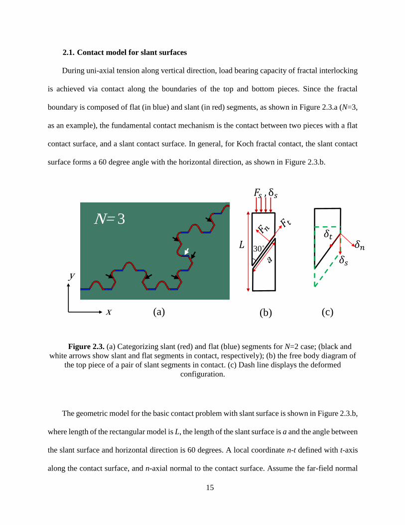
2.1. Contact model for slant surfaces
During uni-axial tension along vertical direction, load bearing capacity of fractal interlocking
is achieved via contact along the boundaries of the top and bottom pieces. Since the fractal
boundary is composed of flat (in blue) and slant (in red) segments, as shown in Figure 2.3.a (N=3,
as an example), the fundamental contact mechanism is the contact between two pieces with a flat
contact surface, and a slant contact surface. In general, for Koch fractal contact, the slant contact
surface forms a 60 degree angle with the horizontal direction, as shown in Figure 2.3.b.
Figure 2.3. (a) Categorizing slant (red) and flat (blue) segments for N=2 case; (black and
white arrows show slant and flat segments in contact, respectively); (b) the free body diagram of
the top piece of a pair of slant segments in contact. (c) Dash line displays the deformed
configuration.
The geometric model for the basic contact problem with slant surface is shown in Figure 2.3.b,
where length of the rectangular model is L, the length of the slant surface is a and the angle between
the slant surface and horizontal direction is 60 degrees. A local coordinate n-t defined with t-axis
along the contact surface, and n-axial normal to the contact surface. Assume the far-field normal
x
y
N= 3
(a) (b) (c)
30˚
16
force is 𝐹𝑠 , and the contact-induced normal force on the contact surface is 𝐹𝑛, and the contact-
induced tangential force on the contact surface is 𝐹𝑡, the equilibrium of the top piece yields:
𝐹𝑠 =𝐹𝑛 cos60˚ + 𝐹𝑡 sin60˚. (2.5)
By defining𝑓𝑠, 𝑓𝑛 and 𝑓𝑡 as forces per unit length as;
𝑓𝑛 = 𝐹𝑛 /𝑎, 𝑓𝑡 = 𝐹𝑡/𝑎, 𝑓𝑠 =𝐹𝑠
𝑎 cos 60˚. (2.6)
Based on the Coulomb's law of friction, 𝑓𝑡=𝜇𝑓𝑛. Where 𝜇 is the static/kinetic friction
coefficient. Thus Eq.(2.5) can be rewrite as;
𝑓𝑠=𝑓𝑛(1 + 𝜇 tan60˚). (2.7)
The normal deflection 𝛿𝑛 around the contact area is related to 𝛿𝑠 as:
𝛿𝑛= 𝛿𝑠 cos60˚. (2.8)
Thus, through the system of Eqs. (2.1)-(2.4), the far-field traction-displacement relation 𝑓𝑠 −
𝛿𝑠 can be obtained via the local normal traction-displacement relation 𝑓𝑛 − 𝛿𝑛 in the contact area.
When the surface is flat, the normal contact traction is:
𝑓𝑛 = 𝑘𝑛𝛿𝑛, (2.9)
where, 𝑘𝑛 = E 𝑡
𝐿,
17
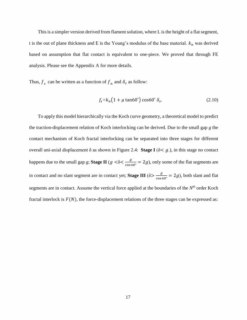
This is a simpler version derived from flament solution, where L is the height of a flat segment,
t is the out of plane thickness and E is the Young’s modulus of the base material. 𝑘𝑛 was derived
based on assumption that flat contact is equivalent to one-piece. We proved that through FE
analysis. Please see the Appendix A for more details.
Thus, 𝑓𝑠 can be written as a function of 𝑓𝑛 and 𝛿𝑠 as follow:
𝑓𝑠=𝑘𝑛(1 + 𝜇 tan60˚) cos60˚ 𝛿𝑠. (2.10)
To apply this model hierarchically via the Koch curve geometry, a theoretical model to predict
the traction-displacement relation of Koch interlocking can be derived. Due to the small gap g the
contact mechanism of Koch fractal interlocking can be separated into three stages for different
overall uni-axial displacement δ as shown in Figure 2.4: Stage I (δ< 𝑔.), in this stage no contact
happens due to the small gap g; Stage II (𝑔 <δ<𝑔
cos 60°= 2𝑔), only some of the flat segments are
in contact and no slant segment are in contact yet; Stage III (δ>𝑔
cos 60°= 2𝑔), both slant and flat
segments are in contact. Assume the vertical force applied at the boundaries of the Nth order Koch
fractal interlock is 𝐹(𝑁), the force-displacement relations of the three stages can be expressed as:

18
Figure 2.4. Contact/interlocking stages (a) Stage I, when no segment is in contact (b) Stage
II when only some flat segments get in contact (c) Stage III when some of the flat and slant
segments get in contact.
Stage I: 𝐹(𝑁) = 0; δ< 𝑔 (2.11)
Stage II: 𝐹(𝑁) = 𝑓𝑛𝑎𝑛 𝑛𝑓𝑐 [𝑁]
; 𝑔 <δ< 2𝑔 (2.12)
Stage III: (𝑁) = 𝑓𝑠𝑎𝑠 𝑛𝑠𝑐 [𝑁]
+ 𝑓𝑛𝑎𝑛𝑛𝑓𝑐 [𝑁]
; δ> 2𝑔 (2.13)
where 𝑎𝑠, and 𝑎𝑓 are the contact areas of each slant and flat segment in the Koch fractal , 𝑛𝑓𝑐 [𝑁]
and 𝑛𝑠𝑐 [𝑁]
are the number of flat and slant segments in contact, respectively. 𝑛𝑓𝑐 [𝑁]
and 𝑛𝑠𝑐 [𝑁]
will
be determined in the next section.
Stage I
No segment in contact
Stage II
Flat segment in contact
Stage III
Flat and Slant segments
in contact
(a) (b) (c)

19
Generally, 𝑎𝑠 and 𝑎𝑓 are directly related to 𝑎𝑁. Due to the rounded tip r and the gap g, 𝑎𝑠 and
𝑎𝑓 will be functions of r and g as well. The schematics of the contact area for flat and slant
segments are shown in Figure 2.5.
Figure 2.5. Schematics of flat and slant segments’ length when (a) r>g and (b) r<g.
According to Figure 2.5 𝑎𝑠 and 𝑎𝑓 can be expressed as a function 𝑎𝑁 , r and g as:
If r>g;
𝑎𝑠=𝑎𝑁 − 2𝑔 𝑠𝑖𝑛60° − 𝑟 𝑡𝑎𝑛60° − 𝑟 𝑡𝑎𝑛30°. (2.14)
𝑎𝑓=𝑎𝑁 − 𝑟 𝑡𝑎𝑛60° − 𝑟 tan30°. (2.15)
rtan(60 ) rtan(30 )
r > g r < g
rtan(60 ) gtan(30 )
Flat
Slant
(a) (b)

20
And if r<g;
𝑎𝑠=𝑎𝑁 − 2𝑔 𝑠𝑖𝑛60° − 𝑟 𝑡𝑎𝑛60° − 𝑔 𝑡𝑎𝑛30°
= 𝑎𝑁 −2𝑔
𝑠𝑖𝑛60°− 𝑟 𝑡𝑎𝑛𝑡60°. (2.16)
𝑎𝑓=𝑎𝑁 − 𝑟 𝑡𝑎𝑛60° − 𝑔 tan30°. (2.17)
2.2. Fractal contact model
Categorization and self-similar reproducing mechanism. In nature, the fractal interlocking is the
contact between flat segments and slant segments in different levels in a fractal manner. Due to
the self-similarity of Koch fractal geometry, for Koch curves with N>2, the geometry can be
decomposed of four sections with the geometry of N=1 rotating with four different angles with the
horizontal direction as shown in Figure 2.6. The four units are shown in Figure 2.6.a, named as
units 𝑆0𝑜, 𝑆60𝑜, 𝑆120𝑜, 𝑆180𝑜 rotating counter-clockwise to the horizontal direction (due to
symmetry) as 0°, 60° /−60°, 120°/−120°, and 180°, respectively.
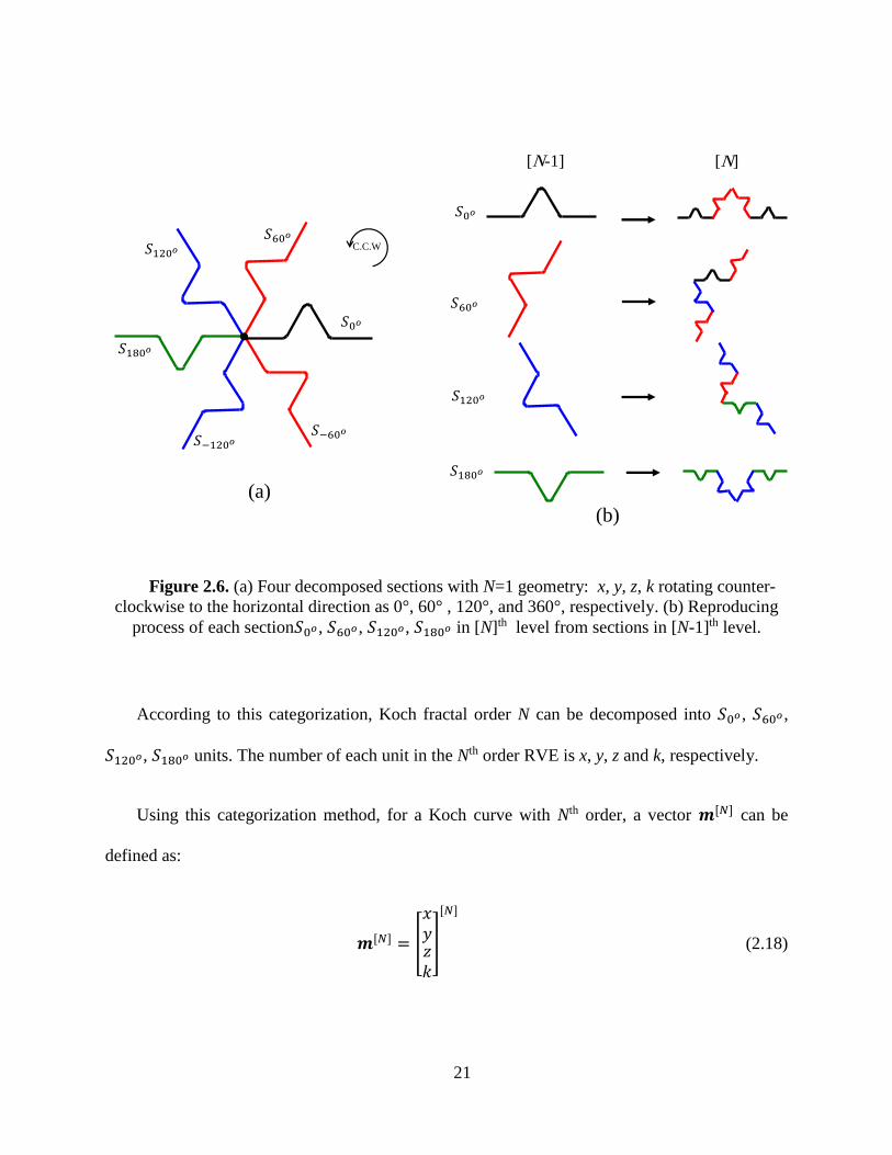
21
Figure 2.6. (a) Four decomposed sections with N=1 geometry: x, y, z, k rotating counter-
clockwise to the horizontal direction as 0°, 60° , 120°, and 360°, respectively. (b) Reproducing
process of each section𝑆0𝑜, 𝑆60𝑜, 𝑆120𝑜, 𝑆180𝑜 in [N]th level from sections in [N-1]th level.
According to this categorization, Koch fractal order N can be decomposed into 𝑆0𝑜, 𝑆60𝑜,
𝑆120𝑜, 𝑆180𝑜 units. The number of each unit in the Nth order RVE is x, y, z and k, respectively.
Using this categorization method, for a Koch curve with Nth order, a vector 𝒎[𝑁] can be
defined as:
𝒎[𝑁] = [
𝑥𝑦𝑧𝑘
]
[𝑁]
(2.18)
(b)
[N-1] [N]
C.C.W
(a)
22
Figure 2.6.b shows that from [N-1] to [N] hierarchy, each 𝑆0𝑜 section will generate two 𝑆0𝑜
sections, and two 𝑆60𝑜 sections, but no 𝑆120𝑜 and 𝑆180𝑜segments; each 𝑆60𝑜 section will generate
one 𝑆0𝑜 section, two 𝑆60𝑜 sections, and one 𝑆120𝑜 section; each 𝑆120𝑜 section will generate one
𝑆60𝑜 section, two 𝑆120𝑜 sections, and one 𝑆180𝑜 section; and each 𝑆180𝑜 section will generate two
𝑆120𝑜 sections and two 𝑆180𝑜 sections in [N] order hierarchy.
Thus, due to self-similarity, the iterative relation of the number of each section at two
neighboring hierarchies can be written as:
𝒎[𝑁] = 𝑹𝒎[𝑁−1] (2.19)
where, R is named as reproducing matrix, and for Koch fractal geometry,
𝑹 = [
2 12 2
0 01 0
0 10 0
2 21 2
] (2.20)
By taking the first row as an example, matrix R means that 𝑆0𝑜 in N hierarchy were generated
from 𝑆0𝑜 and 𝑆60𝑜 in N-1 hierarchy. where two were 𝑆0𝑜, one was 𝑆60𝑜 and non from 𝑆120𝑜 and
𝑆180𝑜 , as gives the first row of R as (2, 1, 0 ,0).
Group matrix. In general Koch curve are composed of two types of segments: flat or slant.
The total number of flat segments 𝑛𝑓, and slant segments 𝑛𝑠, are shown as a vector n as follows;
𝒏 [𝑁] = [𝑛𝑓
𝑛𝑠]
[𝑁]
(2.21)
For each unit, the number of flat and slant segments can be summarized in a table as follows:

23
Table 2.1 Number of flat and slant segments generated from S0o , S60o , S120o and S180ounits.
Table 2.1 means each S0o and S180o units are composed of two flat and two slant segments
and each of S60o and S120o units will generate three slant and one flat segments. Defining G matrix
as a group matrix all segments can be grouped into slant and flat. According to this table G can be
written as:
𝑮 = [2 1 1 22 3 3 2
] . (2.22)
Using matrix G the total number of flat and slant segments can be calculated as:
𝒏 [𝑁] = 𝑮𝒎[𝑁] (2.23)
From another point of view, G is related to the reproducing matrix, R through the following
two equations;
Contact matrix. Furthermore, among all flat and slant segments, only some of them are in
contact/interlocking. We define a vector 𝒏𝑐 to represent the number of segments in contact and it
can be:
𝑆0 𝑆60 𝑆120 𝑆180
𝑛𝑓 2 1 1 2
𝑛𝑠 2 3 3 2
𝐺1𝑗=𝑅1𝑗+𝑅4𝑗 . (2.24)
𝐺2𝑗=𝑅2𝑗+𝑅3𝑗 , j=1,2,3,4 (2.25)

24
𝒏𝑐 [𝑁] = [𝑛𝑓
𝑐
𝑛𝑠𝑐]
[𝑁]
(2.26)
Table 2.2 Number of flat and slant segments in contact that generated from S0o , S60o ,S120o and S180ounits.
Table 2.2 means each S0o unit has neither flat nor slant segments in contact; each of S60o unit
has one slant segment in contact; each S120o unit has one flat and two slant segments in contact;
and each S120o unit has two flat and two slant segments in contact. By defining matrix C as a
contact matrix, all contact segments will be categorized into slant and flat segments. According to
Table 2.2 C can be written as;
𝑪 = [0 0 1 20 1 2 2
] (2.27)
Thus, total number of flat and segments in contact can be determined via:
𝒏𝑐 [𝑁] = 𝑪𝒎[𝑁] (2.28)
According to Eqs. (2.18)-(2.27), for the Nth order Koch fractal interlocking, the numbers of
flat and slant segments in contact can be determined through those at [N-1]th order. A Matlab
code was developed to theoretically explore the influence of each parameter on the mechanical
properties of fractal contact.
𝑆0 𝑆60 𝑆120 𝑆180
𝑛𝑓𝑐 0 0 1 2
𝑛𝑠𝑐 0 1 2 2
25
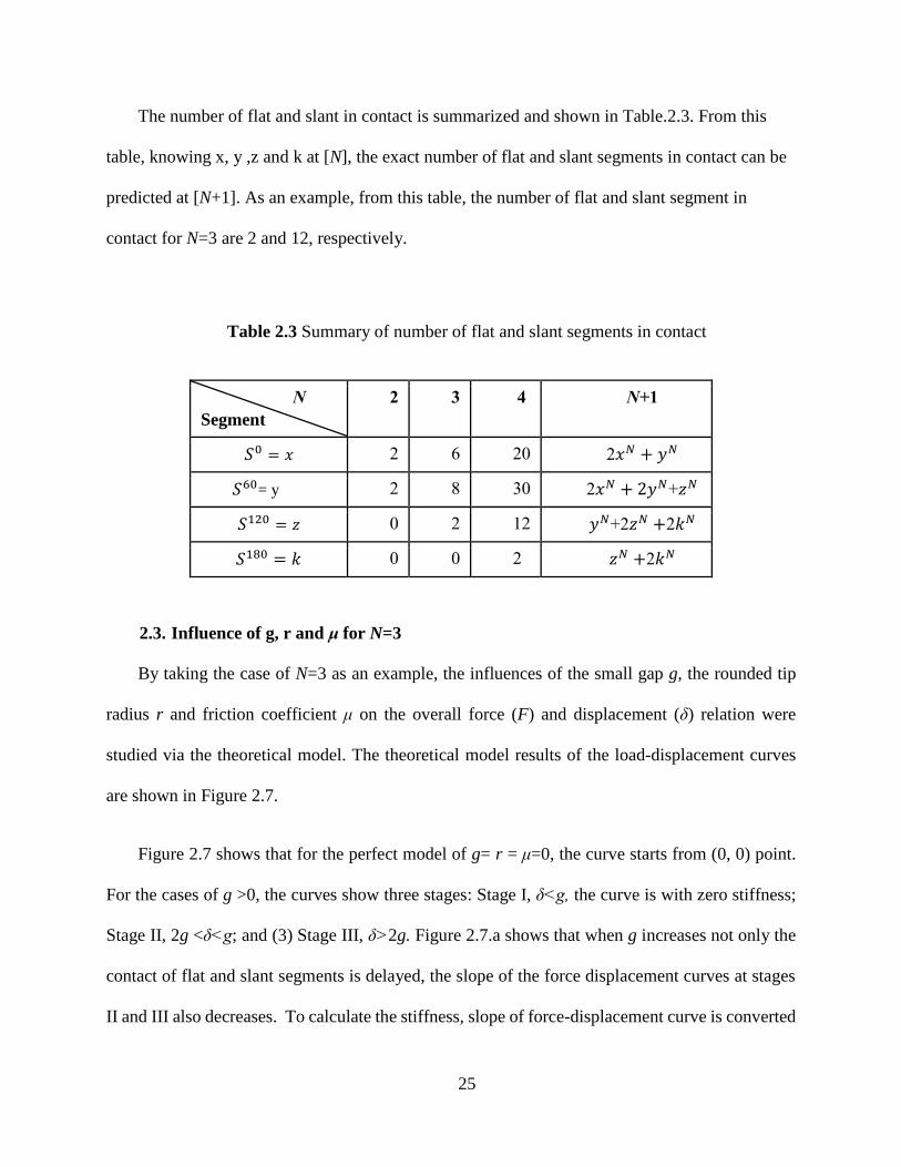
The number of flat and slant in contact is summarized and shown in Table.2.3. From this
table, knowing x, y ,z and k at [N], the exact number of flat and slant segments in contact can be
predicted at [N+1]. As an example, from this table, the number of flat and slant segment in
contact for N=3 are 2 and 12, respectively.
Table 2.3 Summary of number of flat and slant segments in contact
N
Segment
2 3 4 N+1
𝑆0 = 𝑥 2 6 20 2𝑥𝑁 + 𝑦𝑁
𝑆60= y 2 8 30 2𝑥𝑁 + 2𝑦𝑁+𝑧𝑁
𝑆120 = 𝑧 0 2 12 𝑦𝑁+2𝑧𝑁 +2𝑘𝑁
𝑆180 = 𝑘 0 0 2 𝑧𝑁 +2𝑘𝑁
2.3. Influence of g, r and μ for N=3
By taking the case of N=3 as an example, the influences of the small gap g, the rounded tip
radius r and friction coefficient μ on the overall force (F) and displacement (δ) relation were
studied via the theoretical model. The theoretical model results of the load-displacement curves
are shown in Figure 2.7.
Figure 2.7 shows that for the perfect model of g= r = μ=0, the curve starts from (0, 0) point.
For the cases of g >0, the curves show three stages: Stage I, δ<g, the curve is with zero stiffness;
Stage II, 2g <δ<g; and (3) Stage III, δ>2g. Figure 2.7.a shows that when g increases not only the
contact of flat and slant segments is delayed, the slope of the force displacement curves at stages
II and III also decreases. To calculate the stiffness, slope of force-displacement curve is converted
26
to the slope of stress-strain curve by using initial area (w) and initial height (L) of one Koch RVE.
So that stiffness of Stage II Stage III of contact are 𝐸𝐼𝐼and 𝐸𝐼𝐼𝐼, respectively.
Figure 2.7. Influence of (a) gap g, (b) rounded tip radius r and (c) friction coefficient μ
mechanical response of Stages II and III for case N=3.
The effective force-displacement curves for the case of N=3 and g=0.1mm and μ=0.1, with
different values of r=0, 0.05, 0.15 and 0.3mm are shown in Figure 2.7.b. The four curves in
r= 0 , μ= 0g= 0.1 , μ= 0
g= 0.1 ,r= 0
μ= 0
μ= 0.3
μ= 0.2
μ= 0.1
(a)
(c)
(b)

27
Figure 2.7.b show that the contact starts from the same overall displacement due to the same gap,
and then increases through the two stages. It can be seen that when r decreases, the effective
stiffness of the fractal interlocks will increase significantly which is mainly due to the increase in
contact area (Eqs.(2.14)-(2.17)).
To evaluate the effect of friction coefficient μ, the overall load-displacement curves for the
case of N=3, g=0.1mm and r=0.05 with different friction coefficient μ=0, 0.1, 0.2 and 0.3 are
plotted in Figure 2.7.c. It can be seen that when μ increases, the slopes at Stage II are barely
influenced, while the slopes at Stage III increases. This confirms the fact that flat segment’s contact
is independent of friction coefficient μ. However, the contact of slant segments (Stage III) depends
on μ. When μ increases, contact force also increases.
2.4. Influence of g, r and μ for cases with different N
In this section, the influences of the geometric imperfections g, r and the friction coefficient
μ for different Ns were evaluated via the theoretical model. The influence of each parameter was
explored by fixing other parameters in the theoretical model.
Effect of g. The influences of gap g on the effective stiffness of the two contact stages were
studied for different N via the theoretical model. Figure 2.8.a shows that when g=0, as N increases,
theoretically, the effective slope of force-displacement always increases and there is no limitation
for that. This trend continues so that theoretically/conceptually, the stiffness of the Koch fractal
interlock (when N→ ∞) can achieve an even higher stiffness than the base material, although this
sounds intuitively impossible. In this case, there is only one recognizable stage for contact
mechanism (which is a combination of Stages II and III together) since both flat and slant segments
are in contact from the very beginning.

28
However, in reality, g cannot be zero. Figure 2.8.b shows that by keeping μ=0.1, g= 0.1 mm,
and to ensure self-similarity, r=0.15aN, and increasing N, the slopes of F-δ curve increases when
N<5; when N increases beyond 4, the slope starts decreasing and eventually become zero when N
increases beyond 5. This is because that according to Eqs. (2.16) and (2.19), for non-zero g values,
when N increases beyond a critical value, the contact area starts to decrease and eventually goes
to zero due to loss of contact/interlocking. Figure 2.8.c shows that when g increases to 0.2 mm,
when N=5, the force has already gone to zero, indicating when g increases, the critical N for losing
contact decreases.
29
Figure 2.8. Theoretical prediction of the influences of gap g on the mechanical response of
fractal contact models for different N.
It can be concluded that the gap g plays a significant role on determining the contact
behavior of Koch fractal interlocking, which is mainly due to influence of g on the contact area.
The contact area can be quantified via the theoretical model. The contact areas A of the cases of
N=2, 3 and 4, with μ= 0.1, g = 0.2 mm, r = 0.15 𝑎𝑁 are predicted as a function of the overall
displacement, as shown in Figure 2.9.
g= 0 mm
N=5
g= 0.2 mm
g= 0.1 mm
N=6
r= 0.15 mm , μ=0.1
(a) (b)
(c)
30
Figure 2.9 shows the evolution of the contact area of flat segments, 𝐴𝑓 and the contact area of
only slant segments, 𝐴𝑠. It can be seen that no contact occurs at Stage I; at Stage II, when N
increases, 𝐴𝑓 increases. However, at stage III, only N=2 and 3 have slant segments in contact,
with 𝐴𝑠. for N=3 slightly larger than that with N=2. For N=4, 𝐴𝑠=0. This is because that for the
relatively large value of g, the slant segments for the case of N=4 will not be in contact.
Figure 2.9. (a) Theoretical prediction of the contact area of flat and slant segments in
different stages of deformation, and (b) the total contact area of Koch fractal for N=2, 3 and 4.
(𝐴𝑓 , 𝐴𝑠 and 𝐴𝑓 + 𝐴𝑠 represent contact area of flat, contact area of slant and total area,
respectively.)
Figure 2.9.b shows how total contact area changes with displacement during the three stages.
When N increases from 2 to 3, the total contact area increases significantly in both stages.
However, for N=4, the total contact area 𝐴𝑓 + 𝐴𝑠 keeps unchanged from Stage II to Stage III. This
μ= 0.1, g= 0.2 mm, r= 0.15
(a)
+No
contact
(b)
No
contact
N= 2
N= 3
N= 4
31
explains that the slope of the load-displacement curve (shown in Figure 2.8.c) of N=4 does not
change.
Effect of r. The influence of geometric parameter r on the effective stiffness of the two contact
stages were studied for different N. As Figure 2.10.a shows that for r=0 case, when N increases,
the slope of the F-δ curve in Stage II increases until N=5 and then because of the gap g, starts to
decrease when N changes from 5 to 6. Figure 2.10.b and c show that for the cases of r = 0.1𝑎𝑁 mm
and 0.2𝑎𝑁 mm, the slope of the F-δ curve increases until N=5, after which it decreases with N, and
when r increases, the critical number of hierarchy of losing contact will decrease.

32
Figure 2.10. Influence of rounded tip radius r on mechanical behavior of Koch fractal
contact models.
Similarly, the contact areas of the case shown in Figure 2.10.c are plotted for different Ns in
Figure 2.11. Figure 2.11.a shows that at Stage II, when N increases from 2 to 5, the contact area of
flat segments always increases; however, at Stage III, the contact area of slant segments increases
first but then stop increasing (𝐴𝑠 is almost the same for the cases of N=3 and 4) and eventually
becomes zero when N=5.
r= 0 mm r= 0.1 mm
N=7
N=6
r= 0.2 mm
g=0.05 mm , μ=0.1
(a) (b)
(c)

33
Figure 2.11. (a) Contact area of flat and slant segments in different stages of deformation.
(b) Total contact area of Koch fractal for N=2, 3,4 and 5. 𝐴𝑓 , 𝐴𝑠 and 𝐴𝑓 + 𝐴𝑠 represent contact
area of flat, contact area of slant and total area, respectively.
Figure 2.11.b shows the evolution of the total contact area A for the case of r=0.2𝑎𝑁. When
N<5, from Stage II to III, A always increases, when N=5, A become unchanged from Stage II to
Stage III. This is because of the zero 𝐴𝑠 in Stage III for N=5.
Figure 2.12 shows the evolution of the total contact area A for the case of r=0.1𝑎𝑁, it can be
seen that when N>5, the contact area of the flat segments already starts to decreases in Stage II.
The critical value of losing contact in Stage III is N=6, which is larger than the case of r=0.2𝑎𝑁.
This indicates that when r decreases, the critical value of N for losing contact will increase.
No
contact +
(b)(a)
No
contact
N= 2
N= 3
N= 4
N= 5
μ= 0.1, g= 0.05 mm, r= 0.2
34
Figure 2.12. (a) Contact area of flat and slant segments in different stages of deformation.
(b) Total contact area of Koch fractal for N=2, 3, 4, 5 and 6. 𝐴𝑓 , 𝐴𝑠 and 𝐴𝑓 + 𝐴𝑠 represent
contact area of flat, contact area of slant and total area, respectively.
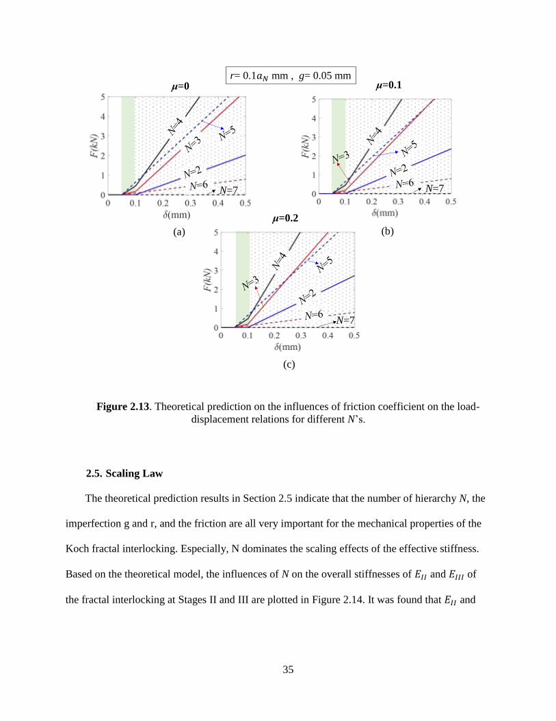
Effect of μ. The influence of friction coefficient μ on the effective stiffness of the two contact
stages were studied for different N. Figure 2.13 shows that for all three cases of μ=0, 0.1 and 0.2,
the slope slightly increases for each N, but the critical N for losing contact keeps the same,
indicating that the critical N for losing contact is not sensitive to the friction coefficient μ.
No
contact +No
contact
μ= 0.1, g= 0.05 mm, r= 0.1
N= 2
N= 3
N= 4
N= 5
N= 5
(b)(a)
35
Figure 2.13. Theoretical prediction on the influences of friction coefficient on the load-
displacement relations for different N’s.
2.5. Scaling Law
The theoretical prediction results in Section 2.5 indicate that the number of hierarchy N, the
imperfection g and r, and the friction are all very important for the mechanical properties of the
Koch fractal interlocking. Especially, N dominates the scaling effects of the effective stiffness.
Based on the theoretical model, the influences of N on the overall stiffnesses of 𝐸𝐼𝐼 and 𝐸𝐼𝐼𝐼 of
the fractal interlocking at Stages II and III are plotted in Figure 2.14. It was found that 𝐸𝐼𝐼 and
r= 0.1 mm , g= 0.05 mmμ=0 μ=0.1
N=7N=7
(a) (b)
μ=0.2
N=7
(c)

36
𝐸𝐼𝐼𝐼 are functions of N, g, r and μ. System of Eqs.(2.4) to (2.31) provides a scaling law to predict
the influences of these parameters on 𝐸𝐼𝐼 and 𝐸𝐼𝐼𝐼 .
Figure 2.14.a shows that the influence of g on the non-dimensionalized effective stiffness of
Stage II , 𝐸𝐼𝐼
𝐸 for different N values, where E is the Young’s modulus of the material. The solid
black curve indicates the stiffness of the perfect system of g= 0 and r= 0. It provides the upper
limit of the effective stiffness for Koch contact for each N. For the perfect system, 𝐸𝐼𝐼 =𝐸𝐼𝐼𝐼, and
they always increase with N, and can goes to infinity. However, for any g>0, and/or r>0, there is
a critical value of 𝑁𝑐𝑟for each stage, when N>=𝑁𝑐𝑟, the top and bottom piece will loss contact, and
therefore a zero stiffness. For example, for the cases shown in Figure 2.14, when g=0.1 mm, 𝑁𝑐𝑟=6,
and when g=0.2 mm, 𝑁𝑐𝑟=5. Also, there is a 𝑁𝑜𝑝𝑡 (2<𝑁𝑜𝑝𝑡<𝑁𝑐𝑟) for each stage, at which the
maximum stiffness is achieved. For example, for the cases shown in Figure 2.14, in Stage II,
𝑁𝑜𝑝𝑡=4, and in Stage III, 𝑁𝑜𝑝𝑡=3.
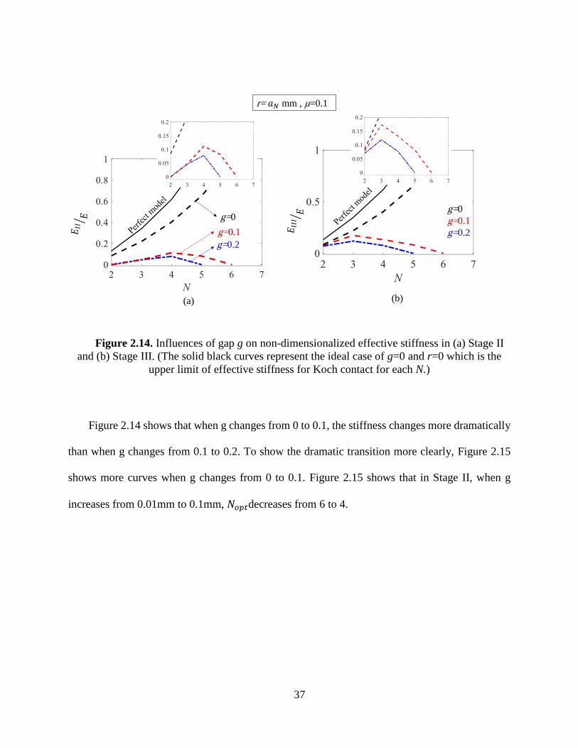
37
Figure 2.14. Influences of gap g on non-dimensionalized effective stiffness in (a) Stage II
and (b) Stage III. (The solid black curves represent the ideal case of g=0 and r=0 which is the
upper limit of effective stiffness for Koch contact for each N.)
Figure 2.14 shows that when g changes from 0 to 0.1, the stiffness changes more dramatically
than when g changes from 0.1 to 0.2. To show the dramatic transition more clearly, Figure 2.15
shows more curves when g changes from 0 to 0.1. Figure 2.15 shows that in Stage II, when g
increases from 0.01mm to 0.1mm, 𝑁𝑜𝑝𝑡decreases from 6 to 4.
g=0
g=0.1
g=0.2
g=0
g=0.1
g=0.2
(a) (b)
r= mm , μ=0.1
38
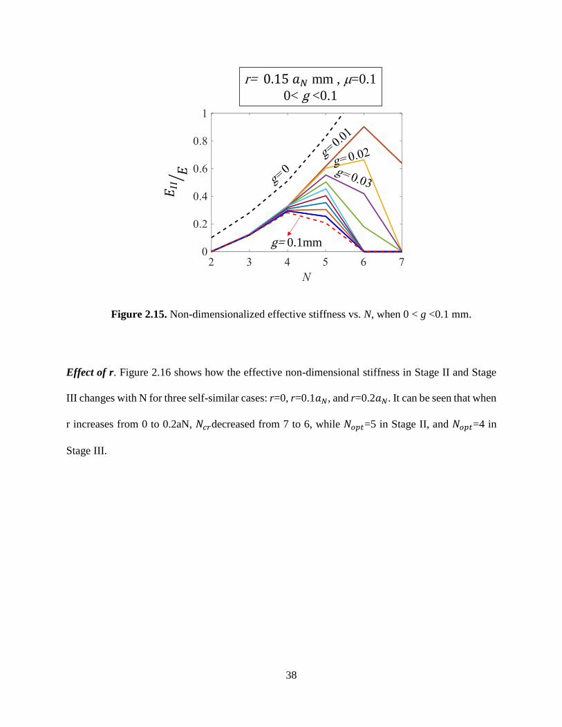
Figure 2.15. Non-dimensionalized effective stiffness vs. N, when 0 < g <0.1 mm.
Effect of r. Figure 2.16 shows how the effective non-dimensional stiffness in Stage II and Stage
III changes with N for three self-similar cases: r=0, r=0.1𝑎𝑁, and r=0.2𝑎𝑁. It can be seen that when
r increases from 0 to 0.2aN, 𝑁𝑐𝑟decreased from 7 to 6, while 𝑁𝑜𝑝𝑡=5 in Stage II, and 𝑁𝑜𝑝𝑡=4 in
Stage III.
g= 0.1mm
r= mm , μ=0.1
0< g <0.1

39
Figure 2.16. Influence of rounded tip radius r on non-dimensionalized effective stiffness in
(a) Stage II and (b) Stage III. (The solid black curves are for the ideal case of g = 0 and r = 0.)
Effect of μ. By taking a specific geometry: g=0.05 and r=0.1𝑎𝑁, as an example, the non-
dimensional stiffness in both stages are plotted as a function of N in Figure 2.17. Figure 2.17.a
shows that in Stage II, the stiffness 𝐸𝐼𝐼 is independent of the friction coefficient μ. This is because
the contact of flat segments is independent on friction. Figure 2.17.b shows that in Stage III, the
stiffness 𝐸𝐼𝐼𝐼 slightly increases, when the friction coefficient μ increases.
r= 0r= 0.1
r= 0.2
g=0.05 mm , μ=0.1
(a) (b)

40
Figure 2.17. Influence of friction coefficient on non-dimensionalized effective stiffness in
(a) Stage II and (b) Stage III. (The solid black curves are for the ideal case of g = 0 and r = 0)
2.6. Summary
In this chapter, a theoretical model was developed to predict the contact area and the load-
displacement relation of both perfect and imperfect Koch fractal contact and interlocking with
different geometries. The Koch fractal interlocking shows a typical three-stage deformation
mechanism, when the gap g is larger than zero.
The influences of the geometric imperfection including the gap g and the tip radius r, and the
friction coefficient was quantified via the theoretical model. It was found that the design is
sensitive to geometric imperfection and friction. Specifically, it was shown that when g increases,
the stiffness in both stages decrease, also initiation of contact delays; when r increases, both the
μ=0.2
μ=0.1
μ=0
μ=0.2
μ=0.1
μ=0
r= 0.1 mm , g= 0.05 mm
(a) (b)

41
overall stiffness and contact area increases; Friction does not influence the contact area and the
stiffness in Stage II, but in Stage III, when μ increases, the overall stiffness slightly increases.
A scaling law for the effective stiffness non-dimenalized with the Young’s modulus of the bulk
material (E=1.7 GPa) was shown in Section 2.6. The scaling law indicates that for the perfect
system, the stiffness will increase exponentially with N. However, the system is imperfection
sensitive so that an optimal N value 𝑁𝑜𝑝𝑡 exists to achieve the maximum stiffness. Also, the Koch
fractal contact area is sensitive to imperfections, so that a critical value N value 𝑁𝑐𝑟 exist, beyond
which no contact occurs and therefore the system shows zero overall stiffness. Specifically, the
stiffness decreases exponentially with the gap g. Compared with g, r and friction has less influence
on the overall stiffness.

42
Chapter 3. Finite Element Analysis of Koch Fractal Interlocking
In this chapter, Finite Element (FE) analysis is performed to evaluate the mechanical behavior
of Koch fractal interlock designed. Both 2D and 3D FE models of both perfect and imperfect Koch
fractal interlocking are developed. Non-linear FE simulations were performed to quantify the
mechanical properties and behavior of the designs.
To choose the correct unit cell for the FE models, the effects of the number of Representative
Volume Elements (RVE), and the geometry of it are present in Sections 3.1 and 3.2, respectively.
Parametric study of the load-displacement behavior of the Koch fractal designs were performed
and presented in Section 3.3. In Section 3.4, 3D FE simulations were performed to further evaluate
the evolution of contact area of the designs during deformation. To further evaluate the influences
of material property on the stiffness and strength of the designs, in Section 3.5, FE simulations
with both linear elastic material model and elasto-perfect-plastic material model were conducted
and the results are compared. In section 3.6, the energy absorption of fractal interlocks with
different geometries were quantified via FE simulations. Finally, the major conclusions are
summarized in Section 3.7.
3.1 Effects of the number of RVEs
FE models of Koch fractal contact with 1 RVE, 2 RVE and 3 RVEs were developed in
ABAQUS 6.13. Two dimensional finite element (FE) models for N=2, 3 and 4 were developed in
ABAQUS/CAE. Four-node, plane stress, quadrilateral, and elements with reduced integration
(CPS4R) were used in all FE models. Elastic model with Young’s modulus of E= 1.7 GPa,

43
Poisson’s ratio of ν=0.4 and density of ρ= 1.1𝑒−9 was used. Very fine mesh were used in the
contact area, as shown in Figure 3.1a. Mesh sensitivity study was performed to balance
computational cost and accuracy. 0.1 mm mesh size was chosen within the fractal zone (L as shown
in Figure 3.1b.) The bottom edges of the FE models are fixed and the top edge subjected to a
prescribed displacement. From the FE simulations, the displacement δ were output as the change
in distance between the peak point and the bottom line of the fractal boundary, as shown in
Figure 3.1b, so that we only focus on the deformation in the fractal contact zone, the deformation
of the shoulders are excluded. The left and right boundaries of the FE models can only move
vertically.
Figure 3.1. Boundary conditions and the finite element mesh with N=2, 3 and 4,
respectively; (b) illustration of the measured displacement.
N=2
N=3
N=4
F, δ
L, δ
(a)
(b)
27 mm

44
The overall load-displacement curves of the FE models with different numbers of RVEs for
the case of N=2, r= 0.45, g=0.1 and μ=0.3 and N=3, r= 0.15, g=0.1 and μ=0.3 are compared in
Figure 3.2.a and Figure 3.3a, respectively. All three cases show the three-stage deformation
mechanism very clearly. To further evaluate the influence of number of RVEs, the effective stress-
strain curves are plotted and shown in Figure 3.2b and Figure 3.3b, respectively. It can be seen
that the stress-strain curves are identical for different numbers of RVE. Figure 3.2 and Figure 3.3
indicate that the results with the rolling boundary condition on the left and right edges are
independent on the number of RVEs.
Figure 3.2. Mechanical response of Koch interlocking models. (a) Force-displacement
curves and (b) Stress-strain curves of Koch fractal with different number of RVEs horizontally
oriented when N=2.
3 RVE
2 RVE
1 RVE
μ= 0.3
r= 0.45 mm
g= 0.1 mm
(b)(a)
N=2

45
Figure 3.3. Mechanical response of Koch interlocking models. (a) Force-displacement
curves and (b) Stress-strain curves of Koch fractal with different number of RVEs horizontally
oriented when N=3.
3.2 Effect of RVE symmetry
To study the effect of RVE symmetry, two types of FE models were developed for each case
of N=2, 3 and 4: Type 1 is with 2 RVEs with the peaks upward, and Type 2 is also with 2 RVEs
but one with the peak upward and the other with the peak flipped 180°, as shown in Figure 3.4a In
all FE models g=0.1 mm, μ=0.3, and to ensure self-similarity, r changes proportionally to the
length of segments in each N i.e r=𝑐a𝑁 (𝑐 = 0.15)mm.
3 RVE
2 RVE
1 RVE
μ= 0.3
r= 0.15 mm
g= 0.1 mm
(b)(a)
N=3

46
Figure 3.4. (a) Influence of geometry complexity on mechanical behavior of Koch fractal
with N=2,3 and 4. (b) Stress distribution of cases with different RVE design when δ=0.3 mm.
The overall load-displacement curves of all FE models are compared in Figure 3.4a shows
that when N increases, stiffness in both Stage II and III increases. The FE results of Type 1 and
Type 2 are almost identical in Stage II. However, in stage III, the Type 2 has a slightly lower
stiffness than Type 1. This is because that for Type 2, due to the asymmetric geometry the local
deformation in Stage III becomes asymmetric (as shown in the stress contour of Figure 3.4b) and
therefore, the contact area might be slightly reduced.
2 RVE - UP
2 RVE - Flipped
2 RVE - UP
2RVE - Flipped
μ= 0.3
g= 0.1 mm
r=
Von Mises
stress
34.04
17.02
4.0e-4
δ= 0.3 mm
(a)
(b)
a
c
b
d
e
47
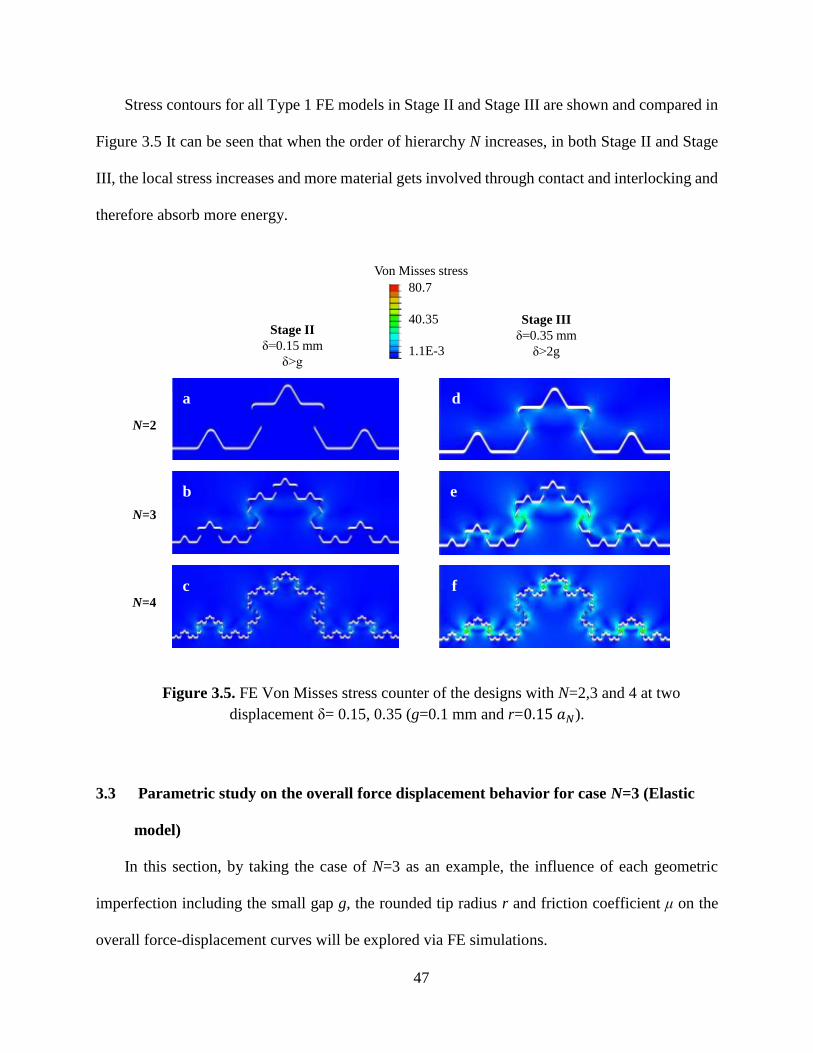
Stress contours for all Type 1 FE models in Stage II and Stage III are shown and compared in
Figure 3.5 It can be seen that when the order of hierarchy N increases, in both Stage II and Stage
III, the local stress increases and more material gets involved through contact and interlocking and
therefore absorb more energy.
Figure 3.5. FE Von Misses stress counter of the designs with N=2,3 and 4 at two
displacement δ= 0.15, 0.35 (g=0.1 mm and r=0.15 𝑎𝑁).
3.3 Parametric study on the overall force displacement behavior for case N=3 (Elastic
model)
In this section, by taking the case of N=3 as an example, the influence of each geometric
imperfection including the small gap g, the rounded tip radius r and friction coefficient μ on the
overall force-displacement curves will be explored via FE simulations.
80.7
40.35
1.1E-3
Von Misses stress
Stage II
δ=0.15 mm
δ>g
Stage III
δ=0.35 mm
δ>2g
N=2
N=3
N=4
a
b
c f
e
d
48
Based on the results in Sections 3.1 and 3.2, for the parametric study, FE models with one
RVE and with rolling constrains on the left and right boundaries will be used to quantify the
mechanical behavior of the designs.
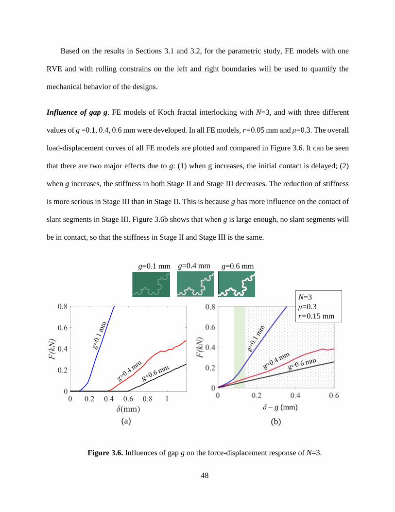
Influence of gap g. FE models of Koch fractal interlocking with N=3, and with three different
values of g =0.1, 0.4, 0.6 mm were developed. In all FE models, r=0.05 mm and μ=0.3. The overall
load-displacement curves of all FE models are plotted and compared in Figure 3.6. It can be seen
that there are two major effects due to g: (1) when g increases, the initial contact is delayed; (2)
when g increases, the stiffness in both Stage II and Stage III decreases. The reduction of stiffness
is more serious in Stage III than in Stage II. This is because g has more influence on the contact of
slant segments in Stage III. Figure 3.6b shows that when g is large enough, no slant segments will
be in contact, so that the stiffness in Stage II and Stage III is the same.
Figure 3.6. Influences of gap g on the force-displacement response of N=3.
N=3
μ=0.3
r=0.15 mm
(a) (b)
g=0.4 mmg=0.1 mm g=0.6 mm
δ – g (mm)

49
Influence of rounded tip radius r. FE models of Koch fractal interlocking with N=3, and r=0.05,
0.15 and 0.3 with three different values of g =0.1, 0.4, 0.6 mm were developed. In all FE models,
g=0.1 mm and μ=0.3. The overall load-displacement curves of all FE models are plotted and
compared in Figure 3.7. This figure shows that r has very little influence on the stiffness of Koch
fractal interlocking.
Figure 3.7. Influence of r on mechanical response of Koch fractal design when N=3.
Influence of friction coefficient μ. FE models of Koch fractal interlocking with N=3, and
μ=0.1 and 0.3 were developed. In all FE models, g=0.1 mm and r=0.15. The overall load-
displacement curves are compared in Figure 3.8. It can be seen that μ does not influence the
stiffness in Stage II, and when μ increases, the stiffness in Stage II slightly increases.
r=0.15 mm
r=0.05 mm
r=0.3 mm
N=3
g=0.1 mm
μ=0.3
r
r=0.15 mm
r=0.3 mm
r=0.05 mm
g
r=0.05 mm r=0.15 mm r=0.3 mm
(a)
(b)
50
Figure 3.8. Influence of friction coefficient μ on load-displacement response of Koch fractal
contact with N=3.
3.4 3D FE simulations of Koch fractal interlocks
From the 2D FE models, the contact area cannot be outputted. While the contact area can be
achieved from 3D FE models. Therefore, 3D FE models were also developed.
3D FE models with N=2, 3 and 4 with g= 0.1 mm, μ=0.3 and r= 0.15 a𝑁 mm were developed
as shown in Figure 3.9. The out of plane thickness for all 3D FE models is 1 mm. The mesh size
is the same with that of the 2D FE models.
μ=0.3
μ=0.1
N=3
g=0.1 mm
r=0.15 mm
μ=0

51
Figure 3.9. (a) 3D FE models of the Koch fractal design with N=3, r= 0.15 mm, g= 0.1 mm;
(b) Boundary and loading conditions applied to 3D FE models.
The evolution of total contact area A and the overall load-displacement curves for different Ns
are plotted and compared in Figure 3.10a and Figure 3.10b, respectively.
F, δ
x
y
(b)x
y
z
16.5mm
(a)
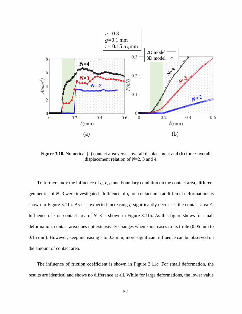
52
Figure 3.10. Numerical (a) contact area versus overall displacement and (b) force-overall
displacement relation of N=2, 3 and 4.
To further study the influence of g, r, μ and boundary condition on the contact area, different
geometries of N=3 were investigated. Influence of g, on contact area at different deformations is
shown in Figure 3.11a. As it is expected increasing g significantly decreases the contact area A.
Influence of r on contact area of N=3 is shown in Figure 3.11b. As this figure shows for small
deformation, contact area does not extensively changes when r increases to its triple (0.05 mm to
0.15 mm). However, keep increasing r to 0.3 mm, more significant influence can be observed on
the amount of contact area.
The influence of friction coefficient is shown in Figure 3.11c. For small deformation, the
results are identical and shows no difference at all. While for large deformations, the lower value
μ= 0.3
g=0.1 mm
r= mm
N= 2
N=3
N=4
(a) (b)
2D model
3D model
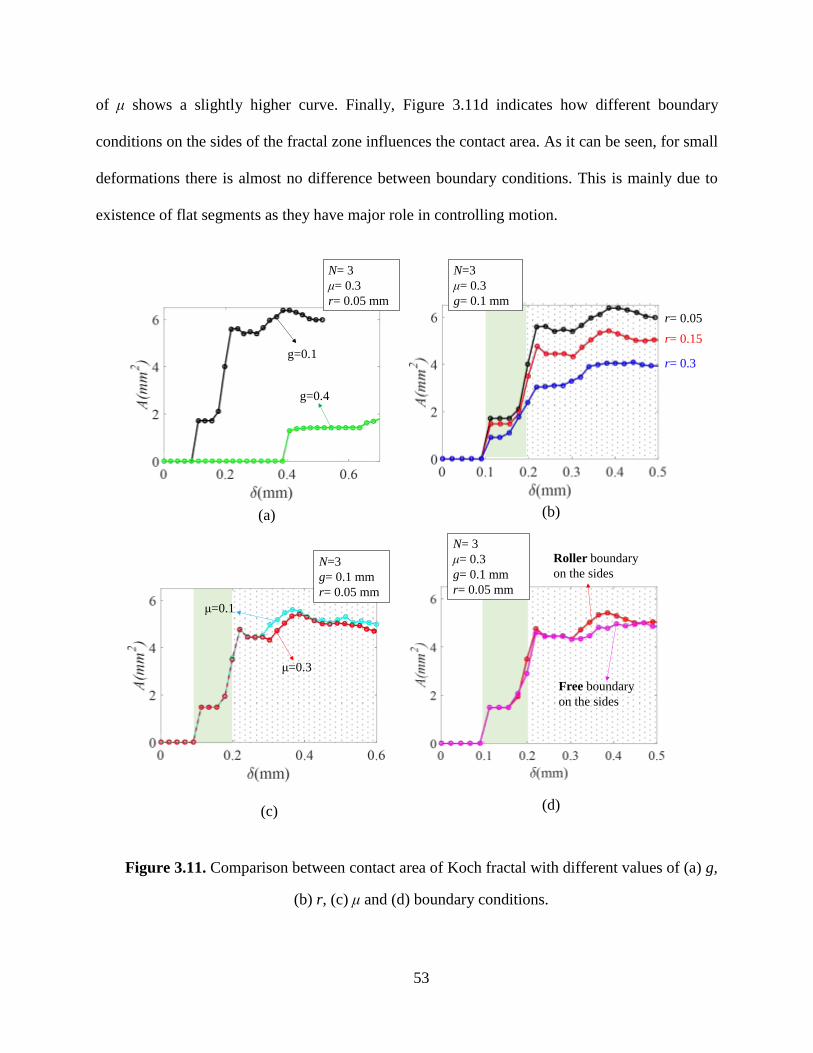
53
of μ shows a slightly higher curve. Finally, Figure 3.11d indicates how different boundary
conditions on the sides of the fractal zone influences the contact area. As it can be seen, for small
deformations there is almost no difference between boundary conditions. This is mainly due to
existence of flat segments as they have major role in controlling motion.
Figure 3.11. Comparison between contact area of Koch fractal with different values of (a) g,
(b) r, (c) μ and (d) boundary conditions.
μ=0.3
μ=0.1
N=3
g= 0.1 mm
r= 0.05 mm
Roller boundary
on the sides
Free boundary
on the sides
N= 3
μ= 0.3
g= 0.1 mm
r= 0.05 mm
(c)
g=0.4
g=0.1
N= 3
μ= 0.3
r= 0.05 mm
(a)
r= 0.3
r= 0.15
r= 0.05
N=3
μ= 0.3
g= 0.1 mm
(b)
(d)

54
3.5 Comparison between linear elastic and elastic-perfectly plastic model
In this Section, to evaluate the influence of material model on the prediction, FE models with
both linear-elastic material model and elasto-perfect-plastic model are developed. For the linear
elastic material model, the Young’s modulus is E=1700 MPa, and the Poisson’s ratio v=0.4. For
the elasto-perfect-plastic model, the Young’s modulus, the Poisson’s ratio and the initial yielding
stress were assumed to be 1700 MPa, 0.4 and 54.32 MPa, respectively. These values are achieved
from performing an experimental uniaxial test on a VeroWhite dog bone.
Influences of N. FE model with N=2, 3 and 4 were developed. In all FE models, g=0.1 mm, μ=
0.3, and to ensure self-similarity, r is proportionally changing to 𝑎𝑁 i. e 𝑟 = 0.15a𝑁 . The FE
results of load-displacement curves are plotted and compared in Figure 3.12. The bifurcation points
of the solid and dash lines indicate the initiation of yielding in the interlocking material. It can be
seen that the interlock softens when part of the material enters into the plastic regime. Generally,
when N increases, local yielding occurs earlier and under a higher load. For example, for N=2,
local yield initiates in Stage III, while for N=3, local yielding initiates in Stage II. This is consistent
with the stress contour shown in Figure 3.5. After the initial local yielding, the yielding propagates
in more area and the load-displacement curves reach a peak. This indicates the strength of the
Koch fractal interlock. When N increases, the overall strength also increases. In addition, when N
increases, the curves after the peak become smoother, indicating a more stable response in the
post-yielding regime.
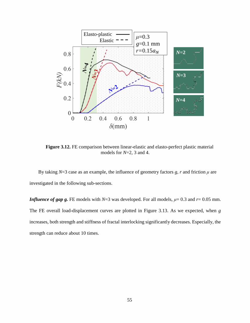
55
Figure 3.12. FE comparison between linear-elastic and elasto-perfect plastic material
models for N=2, 3 and 4.
By taking N=3 case as an example, the influence of geometry factors g, r and friction μ are
investigated in the following sub-sections.
Influence of gap g. FE models with N=3 was developed. For all models, μ= 0.3 and r= 0.05 mm.
The FE overall load-displacement curves are plotted in Figure 3.13. As we expected, when g
increases, both strength and stiffness of fractal interlocking significantly decreases. Especially, the
strength can reduce about 10 times.
Elasto-plastic
Elastic
N=2
N=3
N=4
μ=0.3
g=0.1 mm
r=0.15
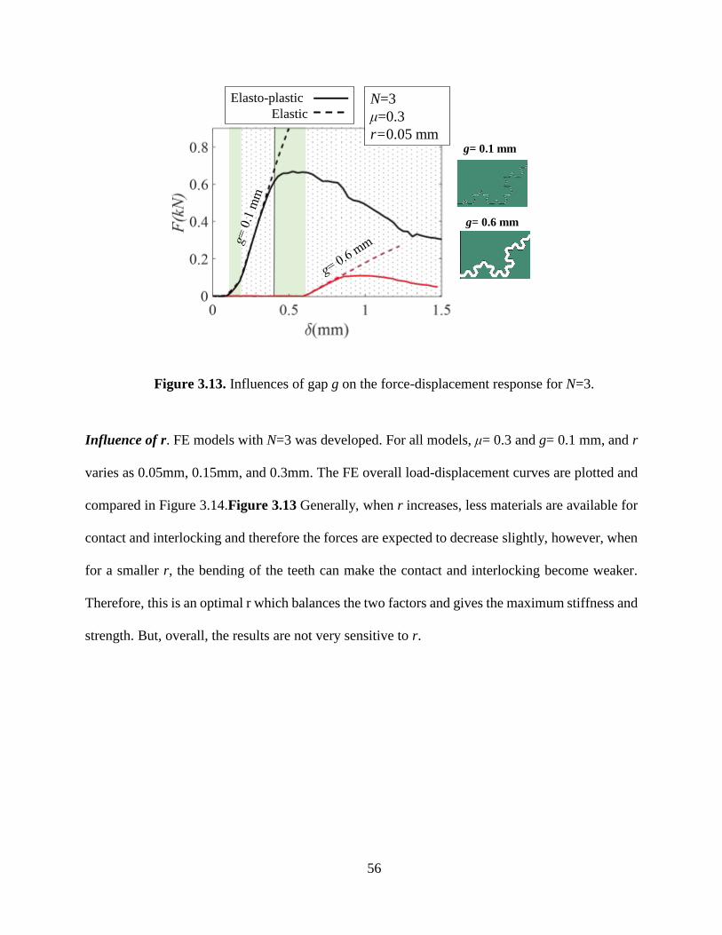
56
Figure 3.13. Influences of gap g on the force-displacement response for N=3.
Influence of r. FE models with N=3 was developed. For all models, μ= 0.3 and g= 0.1 mm, and r
varies as 0.05mm, 0.15mm, and 0.3mm. The FE overall load-displacement curves are plotted and
compared in Figure 3.14.Figure 3.13 Generally, when r increases, less materials are available for
contact and interlocking and therefore the forces are expected to decrease slightly, however, when
for a smaller r, the bending of the teeth can make the contact and interlocking become weaker.
Therefore, this is an optimal r which balances the two factors and gives the maximum stiffness and
strength. But, overall, the results are not very sensitive to r.
N=3
μ=0.3
r=0.05 mmg= 0.1 mm
g= 0.6 mm
Elasto-plastic
Elastic

57
Figure 3.14. Influence of r on mechanical response of N=3 with elasto-perfect-plastic
response.
Influence of friction coefficient μ. FE models with N=3, g=0.1 mm and r=0.05 mm was
developed. Figure 3.15 shows that when μ increases, both stiffness and strength increases. Also,
for larger friction, local yielding occurs earlier.
r=0.05 mm r=0.15 mm r=0.3 mm
(a)
r= 0.15 mm
r=0.05 mm
r= 0.3 mm
N=3
μ=0.3
g=0.1 mm
(b)
Elasto-plastic
Elastic
r
r= 0.15 mm
r= 0.3 mm
r= 0.05 mm
g

58
Figure 3.15. Influence of μ on the load-displacement curves of N=3 with linear elastic and
elasto-perfectly plastic material models.
3.6 FE quantification of Energy
The energy per unit volume absorbed by the top and bottom part of the Koch fractal
interlocking with different geometries were quantified via FE simulations. Elasto-perfect-plastic
material model was used in all FE simulations.
2D FE models were developed. The energy density of the top and bottom parts of the interlock
with N=2, 3, and 4 is plotted and compared in Figure 3.16. Generally, when N increases, the energy
density increases, indicating the more efficient usage of material. For N=2, the top piece absorbs
a little more strain energy than the bottom piece. While for the cases of N>2, the bottom piece
absorbs more energy than the top piece, and it is a trend that a larger N, the energy absorbed by
N=3
g=0.1 mm
r=0.15 mm
Elasto-plastic
Elastic
μ=0.3
μ=0.1μ=0
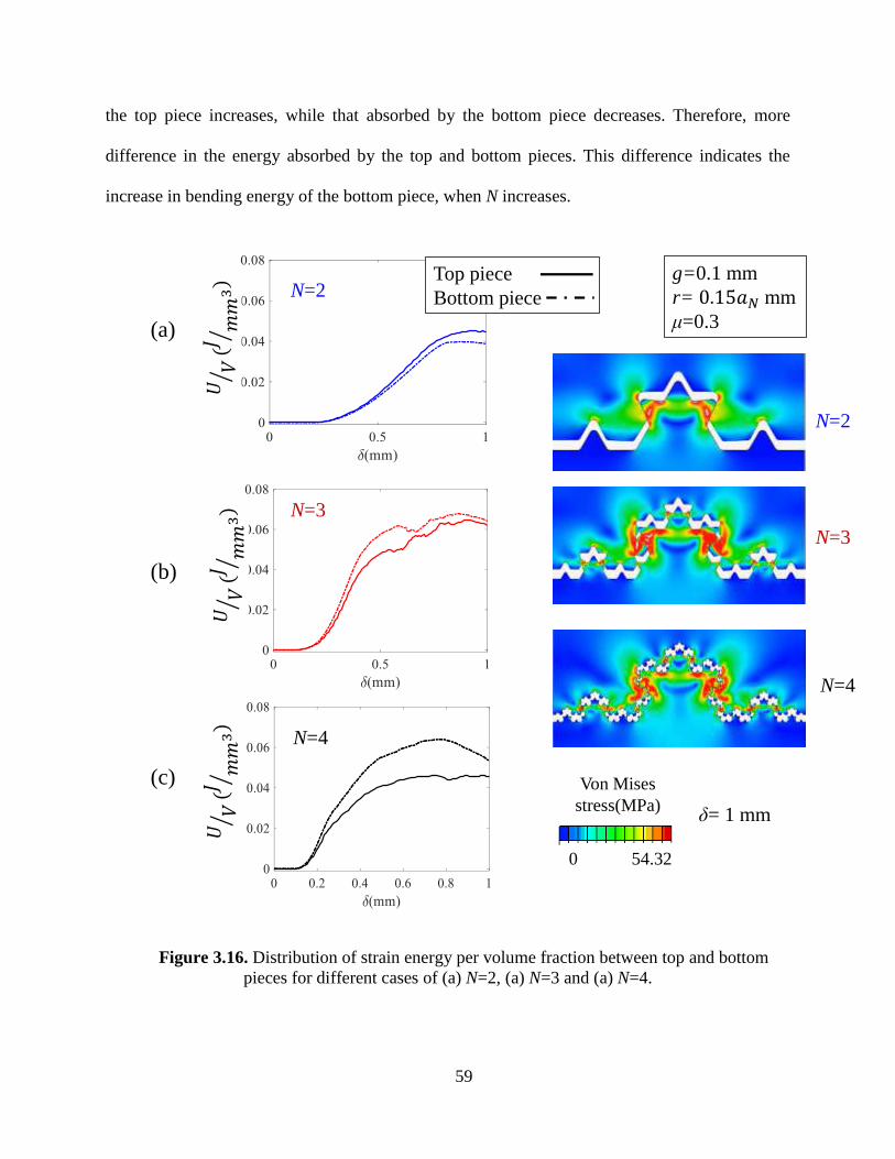
59
the top piece increases, while that absorbed by the bottom piece decreases. Therefore, more
difference in the energy absorbed by the top and bottom pieces. This difference indicates the
increase in bending energy of the bottom piece, when N increases.
Figure 3.16. Distribution of strain energy per volume fraction between top and bottom
pieces for different cases of (a) N=2, (a) N=3 and (a) N=4.
N=2
N=4
N=3
N=2
N=3
N=4
δ= 1 mm
g=0.1 mm
r= mm
μ=0.3
Top piece
Bottom piece
0 54.32
Von Mises
stress(MPa)
(a)
(b)
(c)
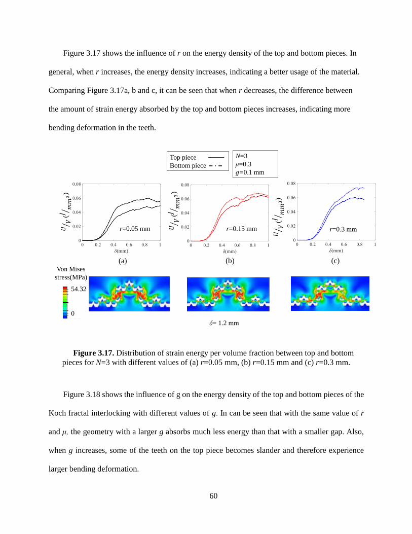
60
Figure 3.17 shows the influence of r on the energy density of the top and bottom pieces. In
general, when r increases, the energy density increases, indicating a better usage of the material.
Comparing Figure 3.17a, b and c, it can be seen that when r decreases, the difference between
the amount of strain energy absorbed by the top and bottom pieces increases, indicating more
bending deformation in the teeth.
Figure 3.17. Distribution of strain energy per volume fraction between top and bottom
pieces for N=3 with different values of (a) r=0.05 mm, (b) r=0.15 mm and (c) r=0.3 mm.
Figure 3.18 shows the influence of g on the energy density of the top and bottom pieces of the
Koch fractal interlocking with different values of g. In can be seen that with the same value of r
and μ, the geometry with a larger g absorbs much less energy than that with a smaller gap. Also,
when g increases, some of the teeth on the top piece becomes slander and therefore experience
larger bending deformation.
r=0.15 mm r=0.3 mmr=0.05 mm
N=3
μ=0.3
g=0.1 mm
δ= 1.2 mm
54.32
0
Von Mises
stress(MPa)
Top piece
Bottom piece
(a) (b) (c)

61
Figure 3.18. FE curves of energy density vs displacement and FE stress distribution
contours for N=3 with r=0.05 mm, (a) g=0.6 mm and (b) g=0.1mm.
3.7 Summary of the chapter
In summary, in this chapter we numerically studied the mechanical behavior of Koch fractal
contact for different geometries. 2D and 3D FE models show to have almost identical results. The
Koch fractal interlocking FE model shows a typical three-stage deformation mechanism, when the
gap g is larger than zero.
The influences of the geometric imperfection including the gap g and the tip radius r, and the
friction coefficient μ were quantified via FE model. It was found that the initial stiffness of designs
is only sensitive to N and geometric imperfection g. It was shown that when g increases, the
g=0.1 mm
g=0.6 mm
Top piece
Bottom piece
N=3
μ=0.3
r=0.05 mm(a)
Von Mises stress
54.32
27.16
0
δ= 1 mm
(b)

62
stiffness in both stages decrease, also initiation of contact delays; tooth radius r shows to have a
slight influence on both contact area and contact force; friction does not influence the contact area
and the stiffness in Stage II, but in Stage III, when μ increases, the overall stiffness slightly
increases.
FE models with elastic perfectly plastic mechanical model were developed. From this
investigation, it was found that strength increases by; increasing complexity of designs i.e
increasing N and decreasing imperfections g and r.
The influences of the geometric imperfection and N were investigated on energy density of top
and bottom pieces of Koch interlock models. It was shown that increasing N, energy density of the
whole model increases which indicates the more efficient usage of material. Increasing N also
increases the amount of energy absorbed by the top piece.
The influences of the geometric imperfection and N were investigated on energy density of top
and bottom pieces of Koch interlock models. It was showed that increasing N, increases energy
density of whole model increases indicating the more efficient usage of material. Increasing N also
shows the energy absorbed by the top piece increases, while that absorbed by the bottom piece.
63
Chapter 4. 3D Printing and Mechanical Experiments
In this Chapter, the Koch fractal interlocking of N=2, 3 and 4 were fabricated via a multi-
material 3D printer (Objet Connex 260). The specimens were two types: (1) with gap g and (2)
with the gap filled with soft adhesive layer. Uni-axial tensions experiments were performed on
both type of specimens. The experimental results of the specimens with gaps were compared with
the theoretical prediction and FE simulations. The results from experiments of both types of
specimens were compared to evaluate the role of the adhesive layer in the Koch fractal
interlocking. In addition, a new design of Koch interlocking with asymmetric geometry was
fabricated with the soft adhesive layer and both uni-axial tension and compact tension experiments
were performed to evaluate the mechanical behavior of the new designs.
In Section 4.1, Koch fractal interlocking with different N and gaps were fabricated and tested
via uni-axial tension experiments. In Section 4.2 Koch fractal interlocking with different N and
soft adhesive layer were fabricated and tested via both uni-axial tension experiments and compact
tension experiments. The results of the two types of specimens were compared in Section 4.3.
Then, in Sections 4.4 and 4.5, to balance the material usage on the top and bottom piece, Koch
interlocking specimens with one RVE upward and the other RVE downward were designed and
fabricated with the soft adhesive layer. Both uni-axial tension and compact tension experiments
were performed to evaluate the toughness of the new design under two different loading cases.
Finally, conclusions were summarized in Section 4.6.
64
4.1 Fabrication and tensile experiments of Koch fractal interlocking with gaps
Koch fractal interlocking with N=2, 3 and 4 with one RVE was designed for experiments. The
dimensions of the specimens are: the width of the specimen, i.e. 𝑎0=54 mm, g = 0.2 mm and
r=0.15 𝑎𝑁.The specimens were printed as VeroWhite material from the 3D printer. Speckle
patterns were put on the surfaces of the specimens and Digital Image Correlations (DIC) (VIC-
2D) was used to track the strain evolution during the experiments. Then the top and bottom pieces
of each specimen were mounted on the Zwick material testing machine. Quasi-static uni-axial
tensile load was controlled for the top piece, the loading rate is 0.024 mm/min. Through performing
mechanical test on a dog bone Vero white the Young’s modulus, Poisson’s ratio, and ultimate
strength are found to be E=1.7 GPa, υ=0.33 and σ =35 MPa, respectively.
From the experiments, the overall force-displacement curves of the 3D-printed specimens
with N=2, 3 and 4 are shown in Figure 4.1.a. It can be seen that generally, when N increases, the
stiffness and strength of the specimens increase. The increase in stiffness and strength is significant
from N=2 to 3. When N increases from 3 to 4, although the stiffness and strength only slightly
increases, but the toughness and the final displacement to breakage increase significantly.
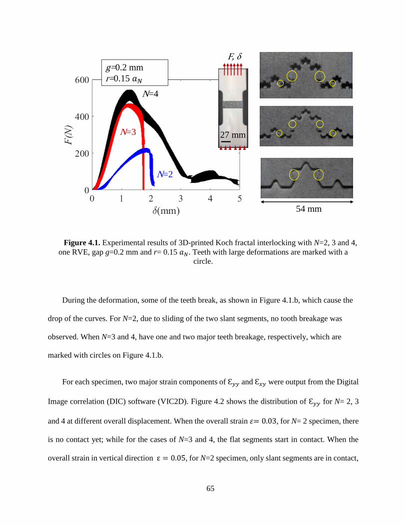
65
Figure 4.1. Experimental results of 3D-printed Koch fractal interlocking with N=2, 3 and 4,
one RVE, gap g=0.2 mm and r= 0.15 𝑎𝑁. Teeth with large deformations are marked with a
circle.
During the deformation, some of the teeth break, as shown in Figure 4.1.b, which cause the
drop of the curves. For N=2, due to sliding of the two slant segments, no tooth breakage was
observed. When N=3 and 4, have one and two major teeth breakage, respectively, which are
marked with circles on Figure 4.1.b.
For each specimen, two major strain components of Ɛ𝑦𝑦 and Ɛ𝑥𝑦 were output from the Digital
Image correlation (DIC) software (VIC2D). Figure 4.2 shows the distribution of Ɛ𝑦𝑦 for N= 2, 3
and 4 at different overall displacement. When the overall strain 휀= 0.03, for N= 2 specimen, there
is no contact yet; while for the cases of N=3 and 4, the flat segments start in contact. When the
overall strain in vertical direction ε = 0.05, for N=2 specimen, only slant segments are in contact,
N=2
N=4
N=3
g=0.2 mm
r=0.15
27 mm
F, δ
54 mm

66
the model experiences sliding and interlocking; for the cases of N=3 and 4, the flat and slant
segments are fully in contact. When the overall strain 휀= 0.08, in shown in Figure 4.2. For all
specimens, some of the segments which were in contact before now lost contact due to large local
deformation and tooth breakage (Marked with circles in Figure 4.1b).
Figure 4.2. DIC strain (휀𝑦𝑦) contours of Koch fractal interlock with N=2, 3 and 4 under uni-
axial tension.
N= 2
N= 3
N= 4
0.0172
-0.0016
-0.0204
Ɛ = 0.03
δ= 0.6 mm
Ɛ = 0.05
δ= 1 mmƐ = 0.08
δ= 1.6 mm
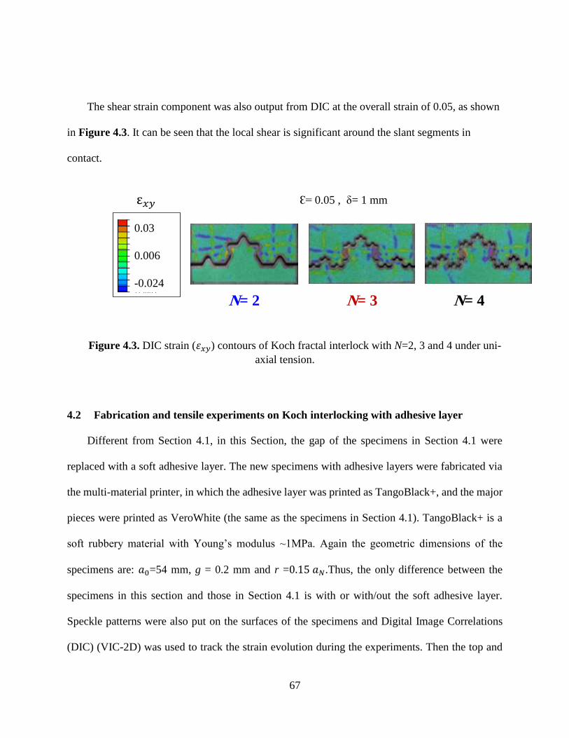
67
The shear strain component was also output from DIC at the overall strain of 0.05, as shown
in Figure 4.3. It can be seen that the local shear is significant around the slant segments in
contact.
Figure 4.3. DIC strain (휀𝑥𝑦) contours of Koch fractal interlock with N=2, 3 and 4 under uni-
axial tension.
4.2 Fabrication and tensile experiments on Koch interlocking with adhesive layer
Different from Section 4.1, in this Section, the gap of the specimens in Section 4.1 were
replaced with a soft adhesive layer. The new specimens with adhesive layers were fabricated via
the multi-material printer, in which the adhesive layer was printed as TangoBlack+, and the major
pieces were printed as VeroWhite (the same as the specimens in Section 4.1). TangoBlack+ is a
soft rubbery material with Young’s modulus ~1MPa. Again the geometric dimensions of the
specimens are: 𝑎0=54 mm, g = 0.2 mm and r =0.15 𝑎𝑁.Thus, the only difference between the
specimens in this section and those in Section 4.1 is with or with/out the soft adhesive layer.
Speckle patterns were also put on the surfaces of the specimens and Digital Image Correlations
(DIC) (VIC-2D) was used to track the strain evolution during the experiments. Then the top and
0.03
0.006
-0.024
N= 2 N= 3 N= 4
Ɛ= 0.05 , δ= 1 mm

68
bottom pieces of each specimen were mounted on the Zwick material testing machine. Quasi-static
uni-axial tensile load was controlled for the top piece, the loading rate was 0.024 mm/min.
From the experiments, the overall load-displacement curves are plotted and shown in
Figure 4.4. It can be seen that generally, the curves show two peaks, and when N increases, the
stiffness is almost the same, while the toughness and the peak strength of both peaks increases
significantly. Although, more improvement was observed when N increases from 2 to 3 than from
3 to 4. The first load drop after the first peak is because of the failure of the soft adhesive layer.
Then after the layer failure, the interlocking still functions through fractal contact between the top
and bottom pieces.
Figure 4.4. Experimental results of Koch N=2, 3 and 4 with a soft layer.
N=2
N=3
N=4
ac
b
N=2
N=3
N=4
a
b
c
g=0.2 mm
r=0.15
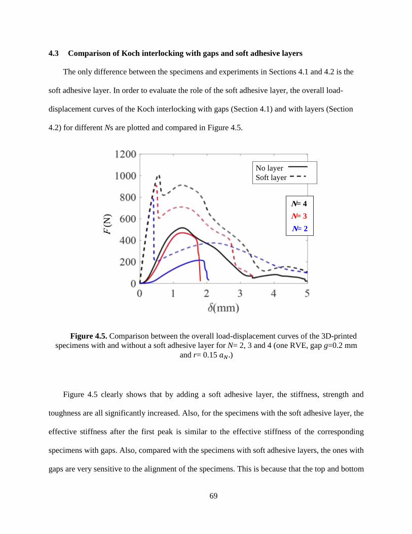
69
4.3 Comparison of Koch interlocking with gaps and soft adhesive layers
The only difference between the specimens and experiments in Sections 4.1 and 4.2 is the
soft adhesive layer. In order to evaluate the role of the soft adhesive layer, the overall load-
displacement curves of the Koch interlocking with gaps (Section 4.1) and with layers (Section
4.2) for different Ns are plotted and compared in Figure 4.5.
Figure 4.5. Comparison between the overall load-displacement curves of the 3D-printed
specimens with and without a soft adhesive layer for N= 2, 3 and 4 (one RVE, gap g=0.2 mm
and r= 0.15 𝑎𝑁 .)
Figure 4.5 clearly shows that by adding a soft adhesive layer, the stiffness, strength and
toughness are all significantly increased. Also, for the specimens with the soft adhesive layer, the
effective stiffness after the first peak is similar to the effective stiffness of the corresponding
specimens with gaps. Also, compared with the specimens with soft adhesive layers, the ones with
gaps are very sensitive to the alignment of the specimens. This is because that the top and bottom
No layer
Soft layer
N= 2
N= 3
N= 4
F (
N)
70
pieces initially are not connected, and any in-plane and/or out-of-plane misalignment can
significantly reduce the contact area and therefore the load-bearing capacity of the specimens.
4.4 Comparison between FE models and experiments
To compare and validate experimental results of 3D-printed dog bone specimens without a
soft layer, with numerical results, 2D FE models of N=2, 3 and 4 with g= 0.2 mm, μ=0.01 and
r= 0.15 a𝑁 mm were developed, where a0 =54 mm. The out of plane thickness is 4 mm. and the
mesh size 0.2 mm was used for Koch surfaces. For all models, plane stress elements (CPS4R) and
elasto perfectly plastic material model with Young’s modulus of E= 1.7 GPa, Poisson’s ratio of
ν=0.33 and failure strength of σ =30 MPa was used.
The overall force-displacement curves of the FE models with gap instead of adhesive layer
are compared with the experimental curves of the specimens with adhesive layer. All other
geometric parameters of the FE models and the specimens are the same. Figure 4.6 shows that the
FE results capture the second peak in the experimental curve. While the second peak in
experiments is after the failure of the adhesive layer and therefore is mainly due to the fractal
contact and interlocking. This indicate that the FE model captured the fractal contact and
interlocking accurately.

71
Figure 4.6 Comparison between overall force-displacement curve from FE simulation and
experimental results for N=2, 3 and 4.
4.5 Tensile experiments on Koch fractal interlocking with asymmetric geometry
Based on the results of Sections 4.1 - 4.3, it is suggested that the Koch fractal interlocking
with soft adhesive layer is preferred for better mechanical performance (i.e. increased stiffness,
strength and fracture toughness) and more stable behavior (insensitive to misalignment etc.). Also,
it was shown in Chap. 3 that the top and bottom pieces deform differently and absorb different
amount of energy. Thus, for practical design, to balance the energy absorbed by the top and bottom
pieces, Koch fractal specimens with neighboring RVEs having opposite directions (as shown in
Figure 4.7) are expected to have better mechanical performance. According to these reasons, in
this Section and the next, we will focus on the Koch fractal interlocking with soft adhesive layers
and also with neighboring RVEs having opposite directions.

72
Figure 4.7. 3D-printed Koch interlocking specimens with two flipped RVEs and a soft
adhesive layer tested under uni-axial tension for N=0,1 2 and 3.
For all specimens, the total width of the two RVEs is 54 mm, the in-plane thickness of the soft
adhesive layer is 0.4 mm (g=0.4 mm) and the out-of-plane thickness is 2 mm. To reduce potential
stress concentration at sharp corners, the Koch interface were rounded at the tips with radius r =
0.15 𝑎𝑁. Thus the designs for different Ns are self-similar.
The new designs for N= 0, 1, 2 and 3 were fabricated via the multi-material 3D printer. As
shown in Figure 4.7, each specimen include two RVEs with opposite directions. Again, the layer
was printed as TangoBlack+, and the top and bottom pieces were printed as VeroWhite. To better
transform load from the grips, shoulders were added to the specimens, as shown in Figure 4.7.
73
Quasi-static uni-axial tension experiments with displacement rate of 0.024 mm/min were
conducted on a material testing machine (ZWICK/Roell Z5.0).
To guarantee repeatability, three identical specimens were printed and tested for each N
(total of 12 tests).
The overall force-displacement curves are plotted and compared in Figure 4.8. For the cases
of N=0 and 1, the curves only contain one peak. While for the cases of N=2 and 3 all curves show
two peaks. This is because the cases of N=0 and 1 do not have interlocking, while the cases of N=2
and 3 have interlocking. The first peak of the four geometries are similar to each other, while the
residual strength (𝜎𝑟) of the second peak increases dramatically when N increases. Also, Figure 4.8
shows that as the number of hierarchy N increases, fracture toughness, Г (area under F-δ curve)
increases.
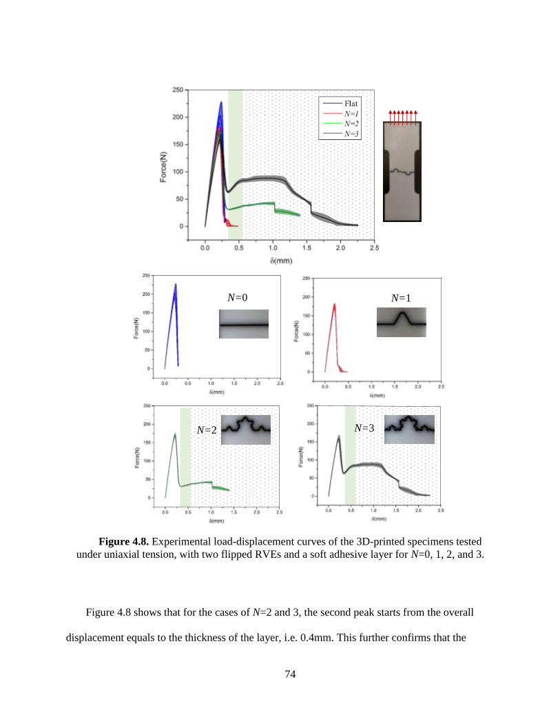
74
Figure 4.8. Experimental load-displacement curves of the 3D-printed specimens tested
under uniaxial tension, with two flipped RVEs and a soft adhesive layer for N=0, 1, 2, and 3.
Figure 4.8 shows that for the cases of N=2 and 3, the second peak starts from the overall
displacement equals to the thickness of the layer, i.e. 0.4mm. This further confirms that the
N=1
N=2
N=0
N=3
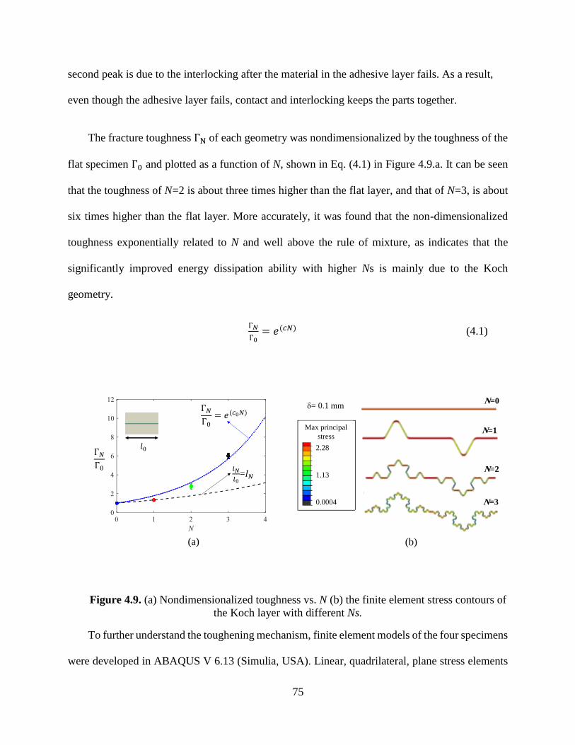
75
second peak is due to the interlocking after the material in the adhesive layer fails. As a result,
even though the adhesive layer fails, contact and interlocking keeps the parts together.
The fracture toughness ГN of each geometry was nondimensionalized by the toughness of the
flat specimen Г0 and plotted as a function of N, shown in Eq. (4.1) in Figure 4.9.a. It can be seen
that the toughness of N=2 is about three times higher than the flat layer, and that of N=3, is about
six times higher than the flat layer. More accurately, it was found that the non-dimensionalized
toughness exponentially related to N and well above the rule of mixture, as indicates that the
significantly improved energy dissipation ability with higher Ns is mainly due to the Koch
geometry.
Г𝑁
Г0= 𝑒(𝑐𝑁) (4.1)
Figure 4.9. (a) Nondimensionalized toughness vs. N (b) the finite element stress contours of
the Koch layer with different Ns.
To further understand the toughening mechanism, finite element models of the four specimens
were developed in ABAQUS V 6.13 (Simulia, USA). Linear, quadrilateral, plane stress elements
2.28
1.13
0.0004
Max principal
stress
N=0
N=3
N=2
N=1
=
(a) (b)
δ= 0.1 mm

76
(CPS4R) were used in the model. Hyperplastic Mooney-Rivlin model were used for the soft Koch
layer. For the hard phase, linear elastic, isotropic material model was used, with Young’s modulus
E=1700 MPa and the Poisson’s ratio υ=0.4. These parameters were obtained from best fitting the
experiment data of N=0. The FE results of the stress contours of the Koch layer with different Ns
are shown in Figure 4.9.b, which that the highest stress is always located in the flat segments and
the tips of the Koch layer. Also, when N increases, damage were distributed in a fractal manner.
In this way, energy can be dissipated more efficiently in the hard phase to avoid the catastrophic
failure.
4.6 Compact tension experiments of Koch fractal interlocking with asymmetric geometry
To investigate damage evolution in Koch fractal layer, similar specimens for compact tension
experiments were designed. The dimensions of the specimens were designed according to
modified ASTM standard size as shown in Figure 4.10. The designed specimens include Koch
interfacial layers with four different geometries, N=0, 1, 2 and 3. The thickness of soft interface is
0.4 mm (g=0.4 mm) and out of plane thickness of samples is 2 mm. The designs were then
fabricated via the multi-material 3D printer. Quasi-static compact tension experiments with
displacement rate of 0.024 mm/min were conducted on a material testing machine (ZWICK/Roell
Z5.0). To ensure repeatability, three identical specimens were printed and tested for each
geometry.
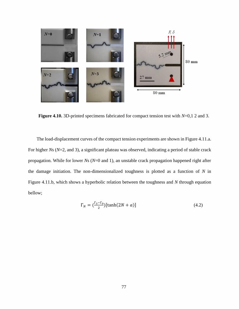
77
Figure 4.10. 3D-printed specimens fabricated for compact tension test with N=0,1 2 and 3.
The load-displacement curves of the compact tension experiments are shown in Figure 4.11.a.
For higher Ns (N=2, and 3), a significant plateau was observed, indicating a period of stable crack
propagation. While for lower Ns (N=0 and 1), an unstable crack propagation happened right after
the damage initiation. The non-dimensionalized toughness is plotted as a function of N in
Figure 4.11.b, which shows a hyperbolic relation between the toughness and N through equation
bellow;
Г𝑁 = (Г3−Г0
2)[tanh(2𝑁 + 𝑎)] (4.2)

78
Figure 4.11. Experimental results of compact tension test. (a) Force-displacement curves of
four geometries (b) Normalized toughness vs N. The dash line displays the toughness deriving
from the rule of mixture.
The toughness of the uni-axial tension specimens and compact tension specimens are
compared with the rule of mixture prediction (dash line) in Figure 4.12. It can be seen that the
toughness of both types of specimens are with toughness beyond the rule of mixture. However,
different from the exponential increases for uni-axial tension, for the compact tension, the increase
slows down when N increases beyond 2, indicating a limit of increasing toughness via Koch fractal
design.
=

79
Figure 4.12. Comparison between toughness of 3D-printed specimens designed for uni-
axial tension and compact tension. Black dash-line displays predication from rule of mixture.
4.7 Summary
In this chapter, Koch interlocking with gaps and with soft adhesive layers with the same
geometries were designed and fabricated via multi-material 3D printing. Quasi-static uni-axial
tension experiments on the Koch interlocking with gaps further proved the concept and the scaling
law developed in Chapters 2 and 3. Also, by comparing the experimental results of the two sets of
specimens, it is demonstrated that the soft adhesive layer plays a very important role in further
improve the mechanical performance of the Koch fractal interlocking. Comparing with the designs
with gaps, those with the soft adhesive layer can significantly improve the strength and toughness,
and also have more stable behavior and less sensitive to the imperfection from loading.

80
In addition, new designs with flipped RVEs and adhesive layers were developed. Both quasi-
static uni-axial tension and compact tension experiments were performed. Interestingly, it is shown
that when N increases, the toughness of the Koch fractal layer can have increased toughness
beyond the rule of mixtures. Under uni-axial tension, the toughness of the Koch fractal interlocking
with soft adhesive layers increases exponentially with N. While under compact tension, the
toughness increases hyperbolically, and slows down when N increases beyond 2 and 3.
81
Chapter 5. Conclusions
In this study, inspired by the topological interlocking and fractal geometry in nature, Koch
fractal interlocking was designed, fabricated and investigated through analytical, numerical and
experimental approaches.
5.1 Specific conclusions for each chapter
In Chapter 2, the theoretical model was introduced to predict the overall load-displacement
relation of both perfect and imperfect Koch fractal contact and interlocking with different
geometries. The Koch fractal interlocking shows a typical three-stage deformation mechanism,
when the gap g is larger than zero. The influences of the geometric imperfection including the gap
g and the tip radius r, and the friction coefficient were quantified. It was found that the mechanical
performance of the design is much more sensitive to geometric imperfection g and r rather than
friction.
The theoretical scaling law indicates that for the perfect system, the stiffness will increase
exponentially with N. However, the system is imperfection sensitive so that an optimal N value
𝑁𝑜𝑝𝑡 exists to achieve the maximum stiffness. Also, the Koch fractal contact area is sensitive to
imperfections, so that a critical value 𝑁𝑐𝑟 exists, beyond which no contact occurs and therefore the
system shows zero overall stiffness. The stiffness was shown to decrease exponentially with the
gap g compared to r and friction.
In Chapter 3, FE models with two cases of elastic and elastic-perfectly plastic mechanical
models were developed. The influences of the geometric imperfection including the gap g and the
tip radius r, and the friction coefficient μ were quantified. It was found that the initial stiffness of
the designs is only sensitive to N and the geometric imperfection g. It was shown that when g
82
increases, the stiffness in both stages decrease, also the initiation of contact delays; tooth radius r
shows to have a slight influence on both contact area and the contact force; friction does not
influence the contact area and the stiffness in Stage II, but in Stage III, when μ increases, the overall
stiffness slightly increases. Through this numerical investigation, it was also found that the strength
of Koch fractals increases when N increases and the imperfections g and r decrease.
In Chapter 3, the influences of the geometric imperfection and N were also investigated on
energy density of top and bottom pieces of Koch interlock models. It was shown that when N
increases, the energy density of whole model increases, indicating the more efficient usage of
material.
In Chapter 4, Koch interlocking with gaps and with soft adhesive layers were designed and
fabricated via a multi-material 3D printer (Objet Connex 260). Quasi-static uni-axial tension
experiments on the Koch interlocking with gaps further proved the concept. Also, by comparing
the experimental results of the two sets of specimens, it is demonstrated that the soft adhesive layer
plays a very important role in further improving the mechanical performance of the Koch fractal
interlocking. Comparing with the designs with gaps, those with the soft adhesive layer can
significantly improve the strength and toughness, and also have more stable behavior and are less
sensitive to the loading and alignment imperfections.
In addition, to ensure same energy absorption of the top and bottom pieces, new designs with
flipped RVEs and adhesive layers were developed. Both quasi-static uni-axial tension and compact
tension experiments were performed. Interestingly, it was shown that when N increases, the
toughness of the Koch fractal layer can have increased toughness beyond the rule of mixtures.
Under uni-axial tension, the toughness of the Koch fractal interlocking with soft adhesive layers
83
increases exponentially with N. While under compact tension, the toughness increases
hyperbolically, and slows down when N increases beyond 2 and 3.
5.2 Summary of design guidelines developed
For the Koch fractal interlocking and contact, geometric parameters (N, g, r, 𝑎0), especially
N and g should be wisely chosen to reach optimal mechanical properties under desired design
objectives. In general, stiffness and strength increases, when the geometric imperfection decreases.
For certain geometric imperfection, there is an optimal N for the maximum stiffness.
A softer adhesive layer is beneficial in enhancing the strength and toughness and reduce the
sensitivity to imperfections. The material properties can be optimized under certain design
requirements.
When applying the Koch fractal design for joining dissimilar materials, based on the results
in Section 3.6, in which showed that if the materials of the top and bottom pieces are the same, the
bottom piece absorbs more energy than the top piece. So for Koch fractal dissimilar joints, a stiffer
and stronger material in bottom can provide a better usage of material and a better balance in
energy absorption from top and bottom pieces.
The Koch fractal interlocking’s response to uni-axial tension and compact tension were
explored. For this two type of loadings, to maximum the load-bearing capacity, the geometry and
material combinations can be optimized. The Koch fractal interlocking under shear should have
similar benefits, although it was not explored in this thesis.

84
5.3 Discussion
Advantages of fractal design. Mechanical interlocking, as a joining mechanism, has been
studied for a long time. For example, the interlocking mechanism of nacre-inspired dove-tail
shaped interlocking building blocks was investigated through experimental, numerical and
theoretical models in previous studies [110-112]. Ammonite-inspired hierarchical deterministic
fractal suture interfaces were also explored analytically and numerically [113-114]. Bio-inspired
jigsaw-like interlocking sutures with snapping feature were investigated [31]. Previous research
mainly focused on either composite modeling of fractal joints [113-114] and surface contact with
fractal roughness [115]. In this work, we focused on Koch fractal contact and interlocking. Using
three geometry factors g, 𝑁 and 𝑎0 various geometries with different mechanical behavior can be
designed and fabricated. Fractals, are good options in generating complex geometries driven by
simplicity due to the self-similarity, and therefore, superior mechanical properties. Due to the
imperfection sensitivity of fractal design, the challenges of applying fractal design in engineering
system are the complexity and accuracy in manufacturing. Additive manufacturing provides an
opportunity to overcome these challenges and enable potential wide application of the concept of
fractal design.
Imperfection sensitivity. In summary, being consistent with the observation of fractal
interlocks in nature, we demonstrated that in general the stiffness of the interlocking can be
effectively increased via fractal design. In general, when the fractal complexity (it is specifically
represented as number of hierarchy N in the present Koch fractal design) increases, the stiffness of
the fractal interlocking will increase significantly [113]. This is mainly attribute to the increase in
contact area when fractal complexity increases. However, the mechanical responses of fractal
interlocks are also sensitive to imperfections, such as the gap between the interlocked pieces and

85
the rounded tips. When fractal complexity increases, the mechanical properties will become more
and more sensitive to the imperfection and eventually, the negative influences from imperfection
can even become dominant. Therefore, it is expected that considering the imperfection, there is an
optimal level of fractal complexity to reach the maximum mechanical performance [116]. This is
again in consistent with fractal interlocks in all different biological systems.
86
References
[1] Wegst, Ulrike GK, et al. "Bioinspired structural materials." Nature materials14.1 (2015): 23-36.
[2] Li, Yaning, Christine Ortiz, and Mary C. Boyce. "Bioinspired, mechanical, deterministic fractal
model for hierarchical suture joints." Physical Review E85.3 (2012): 031901.
[3] Mandelbrot, Benoit B., and Roberto Pignoni. The fractal geometry of nature. Vol. 173. New
York: WH freeman, 1983.
[4] Barthelat, Francois. "Biomimetics for next generation materials." Philosophical Transactions
of the Royal Society of London A: Mathematical, Physical and Engineering Sciences 365.1861
(2007): 2907-2919.
[5] Barthelat, F., et al. "On the mechanics of mother-of-pearl: a key feature in the material
hierarchical structure." Journal of the Mechanics and Physics of Solids 55.2 (2007): 306-337.
[6] Barthelat, Francois. "Nacre from mollusk shells: a model for high-performance structural
materials." Bioinspiration & biomimetics 5.3 (2010): 035001.
[7] W.B. Saunders: Evolution of complexity in paleozoic ammonoidsutures. Science 286(5440),
760 (1999).
[8] Allen, Emily G. "Understanding Ammonoid Sutures: New Insight into the Dynamic Evolution of
Paleozoic Suture Morpholog." Cephalopods Present and Past: New Insights and Fresh Perspectives.
Springer Netherlands, 2007. 159-180.
[9] HEWITT, ROGER A., and GERD EG WESTERMANN. "Mechanical significance of ammonoid septa
with complex sutures." Lethaia 30.3 (1997): 205-212.
[10] Kwak, Jae-Seob, and Tae-Wan Kim. "A review of adhesion and friction models for gecko feet."
International Journal of Precision Engineering and Manufacturing 11.1 (2010): 171-186.
[11] Lutz, T. M., and Boyajian., G.E., 1995, “Fractal geometry of ammonoid sutures”, Paleobiology Vol.
21, No. 3 (Summer, 1995), pp. 329-342.
[12] Li, Y., Oritz, C., and Boyce., 2011, “A generalized mechanical model for suture interfaces of arbitrary
geometry”, Journal of the Mechanics and Physics of Solids 61 (2013) 1144–1167.
[13] Chen, P-Y., et al. "Structure and mechanical properties of selected biological materials." Journal of the
Mechanical Behavior of Biomedical Materials 1.3 (2008): 208-226.
[14] Miura, Takashi, et al. "Mechanism of skull suture maintenance and interdigitation." Journal of
anatomy 215.6 (2009): 642-655.
[15] Herring, Susan W. "Mechanical influences on suture development and patency." Craniofacial Sutures.
Vol. 12. Karger Publishers, 2008. 41-56.
[16] Jaslow, C. R., and A. A. Biewener. "Strain patterns in the horncores, cranial bones and sutures of goats
(Capra hircus) during impact loading." Journal of Zoology 235.2 (1995): 193-210.
[17] Maloul, Asmaa, et al. "Characterization of craniofacial sutures using the finite element
method." Journal of biomechanics 47.1 (2014): 245-252.

87
[18] Villier, Loïc, and Dieter Korn. "Morphological disparity of ammonoids and the mark of Permian mass
extinctions." Science 306.5694 (2004): 264-266.
[19] http://www.andastrongcupofcoffee.com/
[20] Fratzl, Peter, et al. "The mechanics of tessellations–bioinspired strategies for fracture resistance (2016)
[21] http://jsdammonites.fr/177.html
[22] http://www.fossilidentification.org/goniatites.html PICS
[23] Li, Y. , Ortiz, C. , Boyce, M.C. , 2012. Bioinspired, mechanical, deterministic fractal model for
hierarchical suture joints. Phys. Rev. E 85 (3).
[24] Li, Y. , Ortiz, C. , Boyce, M.C. , 2013. A generalized mechanical model for suture interfaces of arbitrary
geometry. J. Mech. Phys. Solids 61 (4), 1144–1167 .
[25] Lin, Erica, et al. "Tunability and enhancement of mechanical behavior with additively manufactured
bio-inspired hierarchical suture interfaces." Journal of Materials Research 29.17 (2014): 1867-1875.
[26] Lin, Erica, et al. "3D printed, bio-inspired prototypes and analytical models for structured suture
interfaces with geometrically-tuned deformation and failure behavior." Journal of the Mechanics and
Physics of Solids 73 (2014): 166-182.
[27] Moazen, Mehran, et al. "Assessment of the role of sutures in a lizard skull: a computer modelling
study." Proceedings of the Royal Society of London B: Biological Sciences 276.1654 (2009): 39-46.
[28] Lin, Erica Erica SC. Bio-inspired design of geometrically-structured suture interfaces and
composites. Diss. Massachusetts Institute of Technology, 2015.
[29] Barthelat, Francois, Zhen Yin, and Markus J. Buehler. "Structure and mechanics of interfaces in
biological materials." Nature Reviews Materials 1 (2016): 16007.
[30] Barthelat, Francois, Ahmad Khayer Dastjerdi, and Reza Rabiei. "An improved failure criterion for
biological and engineered staggered composites." Journal of The Royal Society Interface 10.79 (2013):
20120849.
[31] Malik, I. A., M. Mirkhalaf, and F. Barthelat. "Bio-inspired “jigsaw”-like interlocking sutures:
Modeling, optimization, 3D printing and testing." Journal of the Mechanics and Physics of Solids 102
(2017): 224-238.
[32] Li, Bing-Wei, et al. "Numerical study on the effects of hierarchical wavy interface morphology on
fracture toughness." Computational Materials Science 57 (2012): 14-22.
[33] Liu, L., Jiang, Y., Boyce, M., Ortiz, C., Baur, J., Song, J. and Li, Y. (2017). The Effects of
Morphological Irregularity on the Mechanical Behavior of Interdigitated Biological Sutures under Tension.
Journal of Biomechanics.
[34] Hasseldine, Benjamin PJ, et al. "Mechanical response of common millet (Panicum miliaceum) seeds
under quasi-static compression: Experiments and modeling." Journal of the mechanical behavior of
biomedical materials (2017).
[35] Euclidean and non-euclidean geometr, http://www.math.cornell.edu
[36] Stoyan, D. and Stoyan, H., Fractals, Random Shapes and Point Fields-Methods of Geometrical
Statistics, Wiley series in probability and mathematical statistics, 1994.

88
[37] Li, Yaning, Christine Ortiz, and Mary C. Boyce. "Stiffness and strength of suture joints in nature."
Physical Review E 84.6 (2011): 062904.
[38] Gibert, Josep, and Paul Palmqvist. "Fractal analysis of the Orce skull sutures." Journal of Human
Evolution 28.6 (1995): 561-575.
[39] Khoshhesab, Mona Monsef, and Yaning Li. "The Strength of Dissimilar Fractal Joints." ASME 2016
International Mechanical Engineering Congress and Exposition. American Society of Mechanical
Engineers, 2016.
[40] Rian, Iasef Md, and Shuichi Asayama. "Computational Design of a nature-inspired architectural
structure using the concepts of self-similar and random fractals." Automation in Construction 66 (2016):
43-58.
[41] Wang, Lifeng, et al. "Co‐continuous composite materials for stiffness, strength, and energy
dissipation." Advanced Materials 23.13 (2011): 1524-1529.
[42] http://www.math.union.edu/research/fractaltrees/FractalTreesDefs.html
[43] https://en.wikipedia.org/wiki/Sierpinski_triangle
[44] https://en.wikipedia.org/wiki/Koch_snowflake
[45] https://en.wikipedia.org/wiki/Fractal
[46] Jacquin, Arnaud. "An introduction to fractals and their applications in electrical engineering." Journal
of the Franklin Institute 331.6 (1994): 659-680.
[47] Baish, James W., and Rakesh K. Jain. "Fractals and cancer." Cancer research 60.14 (2000): 3683-
3688.
[48] Rian, Iasef Md, and Shuichi Asayama. "Computational Design of a nature-inspired architectural
structure using the concepts of self-similar and random fractals." Automation in Construction 66 (2016):
43-
[49] Chung, Hsiao-Wen, and Yih-Hwen Huang. "Fractal analysis of nuclear medicine images for the
diagnosis of pulmonary emphysema: interpretations, implications, and limitations." American Journal of
Roentgenology 174.4 (2000): 1055-1059.
[50]Spehar, Branka, et al. "Universal aesthetic of fractals." Computers & Graphics 27.5 (2003): 813-820.
[51] Brown, James H., et al. "The fractal nature of nature: power laws, ecological complexity and
biodiversity." Philosophical Transactions of the Royal Society of London B: Biological Sciences
357.1421 (2002): 619-626.
[52] Mirkhalaf, Mohammad, and Francois Barthelat. "Design, 3D printing and testing of architectured
materials with bistable interlocks." Extreme Mechanics Letters 11 (2017): 1-7.
[53] Djumas, Lee, et al. "Enhanced mechanical performance of bio-inspired hybrid structures utilising
topological interlocking geometry." Scientific reports 6 (2016): 26706.
[54] Dyskin, Arcady V., et al. "Toughening by FragmentationÐ How Topology Helps." Advanced
Engineering Materials 3.11 (2001): 885.
[55] Matsuzaki, Ryosuke, Naoya Tsukamoto, and Jun Taniguchi. "Mechanical interlocking by imprinting
of undercut micropatterns for improving adhesive strength of polypropylene." International Journal of
Adhesion and Adhesives 68 (2016): 124-132.

89
[56] Dyskin, A. V., et al. "Topological interlocking of platonic solids: a way to new materials and
structures." Philosophical Magazine Letters 83.3 (2003): 197-203.
[57] Estrin, Y., et al. "Topological interlocking of protective tiles for the space shuttle." Philosophical
magazine letters 83.6 (2003): 351-355.
[58] Molotnikov, A., et al. "Percolation mechanism of failure of a planar assembly of interlocked
osteomorphic elements." Engineering fracture mechanics 74.8 (2007): 1222-1232.
[59] Schaare, S. et al. Point loading of assemblies of interlocked cube-shaped elements. Int. J. Eng. Sci.
46, 1228–1238 (2008).
[60] Estrin, Y., Dyskin, A. V. & Pasternak, E. Topological interlocking as a material design concept. Mat.
Sci. Eng. C 31, 1189–1194 (2011).
[61] Dyskin, A., Pasternak, E. & Estrin, Y. Mortarless structures based on topological interlocking. Front.
Struct. Civ. Eng. 6, 188–197 (2012).
[62] Krause, T. et al. Mechanical Properties of Topologically Interlocked Structures with Elements
Produced by Freeze Gelation of Ceramic Slurries. Adv. Eng. Mater. 14, 335–341 (2012).
[63] Carlesso, M. et al. Enhancement of sound absorption properties using topologically interlocked
elements. Scripta Mater. 66,483–486 (2012).
[64] Molotnikov, A., Gerbrand, R., Bouaziz, O. & Estrin, Y. Sandwich Panels with a Core Segmented into
Topologically Interlocked Elements. Adv. Eng. Mater. 15, 728–731 (2013).
[65] Molotnikov, A., Gerbrand, R., Qi, Y., Simon, G. P. & Estrin, Y. Design of responsive materials using
topologically interlocked elements. Smart. Mater. Struct. 24, 025034 (2015).
[66] Kanel-Belov, A., Dyskin, A., Estrin, Y., Pasternak, E. & Ivanov-Pogodaev, I. Interlocking of convex
polyhedra: towards a geometric theory of fragmented solids. Mosc. Math. J. 10, 337–342 (2010).
[67] Mather, A., Cipra, R. & Siegmund, T. Structural integrity during remanufacture of a topologically
interlocked material. Int. J. Struct.Integrity 3, 61–78 (2012).
[68] Feng, Y., Siegmund, T., Habtour, E. & Riddick, J. Impact mechanics of topologically interlocked
material assemblies. Int. J. Impact Eng. 75, 140–149 (2015).
[69] Khandelwal, S., Siegmund, T., Cipra, R. J. & Bolton, J. S. Scaling of the Elastic Behavior of Two-
Dimensional Topologically Interlocked Materials Under Transverse Loading. J. Appl. Mech. 81, 031011
(2013).
[70] Khandelwal, S., Siegmund, T., Cipra, R. J. & Bolton, J. S. Transverse loading of cellular
topologically interlocked materials. Int. J. Solids Struct. 49, 2394–2403 (2012).
[71] Estrin, Y. et al. Negative stiffness of a layer with topologically interlocked elements. Scripta Mater.
50, 291–294 (2004).
[72] Schaare, Stephan, Werner Riehemann, and Yuri Estrin. "Damping properties of an assembly of
topologically interlocked cubes." Materials Science and Engineering: A 521 (2009): 380-383.
[73] K. Mittal, The role of the interface in adhesion phenomena, Polym. Eng. Sci. 17 (7) (1977) 467–473.
[74] J.M. Challen, P.L.B. Oxley, Explanation of the different regimes of friction and wear using asperity
deformation models, Wear 53 (2) (1979) 229–243.
[75] R. Raj, M.F. Ashby, On grain boundary sliding and diffusional creep, Metall.
90
Trans. 2 (4) (1971) 1113–1127.
[76] A.G. Evans, F.W. Zok, The physics and mechanics of fibre-reinforced brittlematrix composites, J.
Mater. Sci. 29 (15) (1994) 3857–3896.
[77] Dyskin, A.V., Estrin,Y., Kanel-Belov,A.J., Pasternak, E., 2001 "A New Concept in Design of
Materials And Structures: Assemblies Of Interlocked Tetrahedron-Shaped Elements", Scripta mater, 44
2689–2694.
[78] Dyskin, A.V., Estrin,Y., Kanel-Belov,A.J., Pasternak, E., 2003 "A New Principle In Design of
Composite Materials: Reinforcement by Interlocked Elements", Composites Science and Technology 63,
483–491.
[79] Dyskin, A.V., Estrin,Y., Kanel-Belov,A.J., Pasternak, E., 2003 "Interlocking properties of
buckyballs", Physics Letters A 319, 373–378
[80] Lakes, R., 1993 " Materials with structural hierarchy", Nature, VOL 361, 511-513.
[81] Aksay, I., Weiner, S., 1998 " Biomaterials Is this really a field of research", Editorial overview, Solid
State & Materials Science, 3:219-220.
[82] Gibert, J., & Palmqvist, P., 1995 "Fractal analysis of the Orce skull sutures", Journal of Human
Evolution, 28(6), 561-575.
[83] Dunlop, J. W., & Fratzl, P. 2010, "Biological composites", Annual Review of Materials Research, 40,
1-24.
[84] Fratzl, P., 2013, "Biological Materials with Hierarchical Structure and Mechanical
Function",Handbook of Biomineralization Vol.1, Chapter 25.
[85] Rabiei, R., Dastjerdi, A., & Mirkhalaf, M.,2013, "Hierarchical structure, mechanical properties and
fabrication of biomimetic biomaterials", Biomimetic Biomaterials: Structure and Applications, 67.
[86] Potapova, M., and English, J. (2010). Aulacoseira ambigua . In Diatoms of the United States.
Retrieved July 14, 2017, from http://westerndiatoms.colorado.edu/taxa/species/aulacoseira_ambigu
[87]http://nordicmicroalgae.org/taxon/Aulacoseira%20alpigena?media_id=Aulacoseira%20alpigena_3.
[88] Buczkó, Krisztina, et al. "Diatom-inferred lateglacial and Holocene climatic variability in the South
Carpathian Mountains (Romania)." Quaternary International 293 (2013): 123-135.
[89] Burrows, Malcolm, and Gregory Sutton. "Interacting gears synchronize propulsive leg movements in
a jumping insect." science 341.6151 (2013): 1254-1256.
[90] Dimas, Leon S., et al. "Tough composites inspired by mineralized natural materials: computation, 3D
printing, and testing." Advanced Functional Materials 23.36 (2013): 4629-4638.
[91] O. Bouaziz, Geometrically induced strain hardening, Scr. Mater. 68 (1) (2013) 28–30.
[92] M. Mirkhalaf, J. Tanguay, F. Barthelat, Carving 3D architectures within glass: Exploring new
strategies to transform the mechanics and performance of materials, Extreme Mech Lett (2016).
[93] M. Mirkhalaf, F. Barthelat, A laser-engraved glass duplicating the structure, mechanics and
performance of natural nacre, Bioinspiration Biomimetics 10 (2) (2015) 026005.
[94] A.V. Dyskin, et al., Fracture resistant structures based on topological interlocking with non-planar
contacts, Adv. Energy Mater. 5 (3) (2003) 116–119.

91
[95] S. Khandelwal, et al., Adaptive mechanical properties of topologically interlocking material systems,
Smart Mater. Struct. 24 (4) (2015) 045037.
[96] Derjaguin, BV and Muller, VM and Toporov, Y.P., 1975, Effect of contact deformations on the
adhesion of particles, Journal of Colloid and Interface Science, 53(2), pp. 314-326
[97] Shigley, J.E., Mischke, C.R., 1989, Mechanical Engineering Design, Fifth Edition, Chapter 2,
McGraw-Hill, Inc, 1989, ISBN 0-07-056899-5.
[98] Mirkhalaf, M., and F. Barthelat. "Nacre-like materials using a simple doctor blading technique:
Fabrication, testing and modeling." Journal of the mechanical behavior of biomedical materials 56 (2016):
23-33.
[99] Valashani, Seyed Mohammad Mirkhalaf, and Francois Barthelat. "A laser-engraved glass duplicating
the structure, mechanics and performance of natural nacre." Bioinspiration & biomimetics 10.2 (2015):
026005.
[100] Barthelat, Francois. "Designing nacre-like materials for simultaneous stiffness, strength and
toughness: Optimum materials, composition, microstructure and size." Journal of the Mechanics and
Physics of Solids 73 (2014): 22-37.
[101] Lee, Haeshin, Bruce P. Lee, and Phillip B. Messersmith. "A reversible wet/dry adhesive inspired by
mussels and geckos." Nature 448.7151 (2007): 338.
[102] Sitti, Metin, and Ronald S. Fearing. "Synthetic gecko foot-hair micro/nano-structures as dry
adhesives." Journal of adhesion science and technology17.8 (2003): 1055-1073.
[103] Mahdavi, Alborz, et al. "A biodegradable and biocompatible gecko-inspired tissue adhesive."
Proceedings of the National Academy of Sciences 105.7 (2008): 2307-2312.]
[104] Cheng, Yang-Tse, and Daniel E. Rodak. "Is the lotus leaf superhydrophobic?." Applied physics
letters 86.14 (2005): 144101.
[105] Jiang, Lei, Yong Zhao, and Jin Zhai. "A lotus‐leaf‐like superhydrophobic surface: a porous
microsphere/nanofiber composite film prepared by electrohydrodynamics." Angewandte Chemie 116.33
(2004): 4438-4441.
[106] Koch, Kerstin, et al. "Fabrication of artificial Lotus leaves and significance of hierarchical structure
for superhydrophobicity and low adhesion." Soft Matter 5.7 (2009): 1386-1393.
[107] Liu, Bin, et al. "Fabricating Super‐Hydrophobic Lotus‐Leaf‐Like Surfaces through Soft‐Lithographic Imprinting." Macromolecular rapid communications 27.21 (2006): 1859-1864.
[108] Johnson, Kenneth Langstreth. "Contact mechanics." (1985).
[109] https://en.wikipedia.org/wiki/Contact_mechanics.
[110] Zhang, Yuming, et al. "Bio-inspired interfacial strengthening strategy through geometrically
interlocking designs." journal of the mechanical behavior of biomedical materials 15 (2012): 70-77.
[111] Barthelat, F., et al. "On the mechanics of mother-of-pearl: a key feature in the material hierarchical
structure." Journal of the Mechanics and Physics of Solids 55.2 (2007): 306-337.
[112] Tang, H., F. Barthelat, and H. D. Espinosa. "An elasto-viscoplastic interface model for investigating
the constitutive behavior of nacre." Journal of the Mechanics and Physics of Solids 55.7 (2007): 1410-
1438.
92
[113] Li, Yaning, Christine Ortiz, and Mary C. Boyce. "Bioinspired, mechanical, deterministic fractal
model for hierarchical suture joints." Physical Review E 85.3 (2012): 031901.
[114] Li, Yaning, Christine Ortiz, and Mary C. Boyce. "A generalized mechanical model for suture
interfaces of arbitrary geometry." Journal of the Mechanics and Physics of Solids 61.4 (2013): 1144-1167.
[115] Majumdar, Arunava, and Bharat Bhushan. "Role of fractal geometry in roughness characterization
and contact mechanics of surfaces." ASME J. Tribol 112.2 (1990): 205-216.
[116] Dauskardt, R. H., F. Haubensak, and R. O. Ritchie. "On the interpretation of the fractal character of
fracture surfaces." Acta Metallurgica et Materialia 38.2 (1990): 143-159.
93
Appendix A. FE Simulations of Flat and Slant Contact
In Chapter 2, the theoretical model developed was based on the following assumptions:
1- Deformation is small
2- Material is linear elastic
3- Bending deformation of the teeth during the contact was neglected
4- The compressive load-displacement behavior of the contact between the flat surfaces of
two separate parts is equivalent to that of a one-piece model (Eq. (2.9) 𝑘𝑛 = 𝐸𝑡
𝐿, was
derived based on this assumption)
5- Interaction between the contact-induced deformation of the neighboring flat and slant
surfaces in the fractal design is neglected
6- There is friction between two contacting surfaces. (Therefore the load-displacement
relation of flat and slant surfaces are related via Eq.(2.7).)
7- No relative sliding between the slant surfaces in contact.
To justify the assumptions 4 and 6, three mechanical FE models (as shown in Figure A1)
were developed in ABAQUS : Model 1) Bulk material (one-piece) under compression; Model 2)
Two-piece model with flat surfaces in contact, with the same total dimension and the same material
as Model (1); Model 3) Two-piece model with slant surfaces in contact with the same total
dimension and the same material as Models (1) and (2). For all models, plane stress elements
(CPS4R) were used. Linear elastic material model with Young’s modulus of E=1.7 GPa and
Poisson’s ratio of ν=0.33 were used. In all three FE models, l = 26 mm (excluding the gap for
models 2 and 3), w= 6 mm, and the out-of-plane depth t is 4mm. The friction coefficient is 0.1.

94
Figure A.1 (a) Bulk martial (b) contact of two flat surfaces (c) contact of two slant surfaces.
The vertical displacement of the bottom edges of all three models were constrained, the
nodes on the top edge of the three models were subjected to a prescribed vertical displacement
downward. Thus all three models were under uniaxial compressive loads. For model 3, to avoid
relative sliding, the left and right edges of the model was under the vertical free rolling condition.
The applied loading and boundary condition were schematically shown in Figure A.2. For models
2 and 3, δ is set to be zero when contact initiates.
l
w
l+gg
w
(a) (b) (c)
l+2g
w
2g
Model 1 Model 2 Model 3
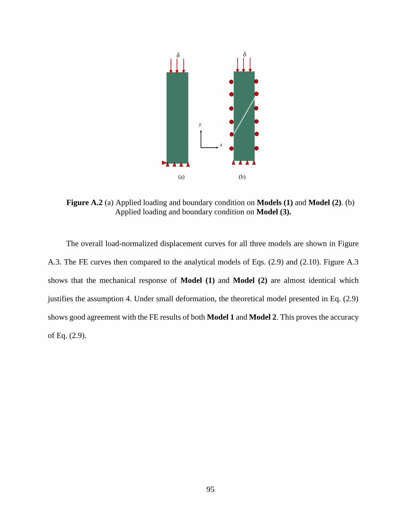
95
Figure A.2 (a) Applied loading and boundary condition on Models (1) and Model (2). (b)
Applied loading and boundary condition on Model (3).
The overall load-normalized displacement curves for all three models are shown in Figure
A.3. The FE curves then compared to the analytical models of Eqs. (2.9) and (2.10). Figure A.3
shows that the mechanical response of Model (1) and Model (2) are almost identical which
justifies the assumption 4. Under small deformation, the theoretical model presented in Eq. (2.9)
shows good agreement with the FE results of both Model 1 and Model 2. This proves the accuracy
of Eq. (2.9).
δδ
x
y
(a) (b)

96
Figure A.3 Force-normalized displacement of Model (1), Model (2) and Model (3) are
compared to theoretical predictions from Eqs. (2.9) and (2.10).
Figure A.3 also shows that the FE results of Model (3) are very close to the prediction from
Eq. (2.10). This verifies the accuracy of Eq. 2.10.
In Figure A.4, the contours of vertical stress, and von-Mises stress for all three FE models are
shown and compared at the same overall displacement of δ=1.9 mm. It can be seen that for models
1 and 2, the stress distribution is uniform and identical, which again justify the assumption 4.
=
l = 26 mm
w = 6 mm
l l
l
w
w
w
Model 1
Model 2
Model 3

97
Figure A.4 Von Misses stress distribution at displacement of δ=1.9 mm for (a) Model (1),
(b) Model (2), and (c) Model (3). Vertical stress distribution S22 (d) Model (1), (e) Model (2),
and (f) Model (3).
δ =1 mm
8.5 E+1
0
Von Misses
stress (MPa)
(c)(b)(a)
Model 1 Model 2 Model 3
(f)(e)(d)
δ =1 mm
-7.3 E+0
-1.2 E+2
S22 (MPa)
2
1

98
To evaluate the influence of model length l on the conclusions, FE Model (1) and Model
(2) were developed with l= 1.5 mm, w = 6, out-of-plane depth t=4 mm. Figure A.5 compares the
force-normalized displacement curves of Model (1), Model (2) and the theoretical prediction from
Eq. (2.9). It can be seen that for models with relatively small length to width ratio of 𝑙
𝑤 =
1
4, the
difference among the three curves are slightly larger than the case with larger length to width ratio
(shown in Figure A.3).
Figure A.5 Force-normalized displacement of Model (1) and Model (2) are compared to
theoretical prediction from Eq.(2.9).
Vertical stress contours for two FE models of Model 1 and Model 2 are shown and compared
at the same displacement of δ=1.9 mm in Figure A.6. It can be seen that the stress distribution is
uniform for both models, and the stress level is close.
l=1.5 mm
w = 6 mm
w
l+g
w
l
Model 1
Model 2
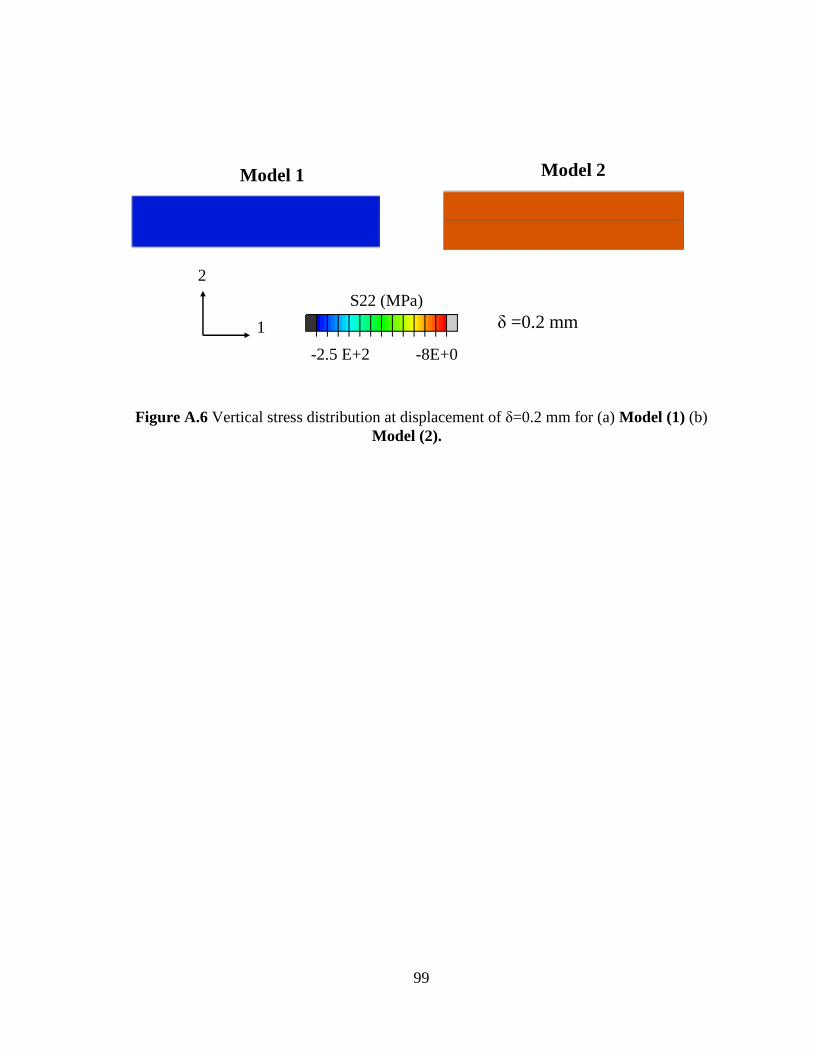
99
Figure A.6 Vertical stress distribution at displacement of δ=0.2 mm for (a) Model (1) (b)
Model (2).
-2.5 E+2 -8E+0
S22 (MPa)
Model 1 Model 2
δ =0.2 mm
2
1
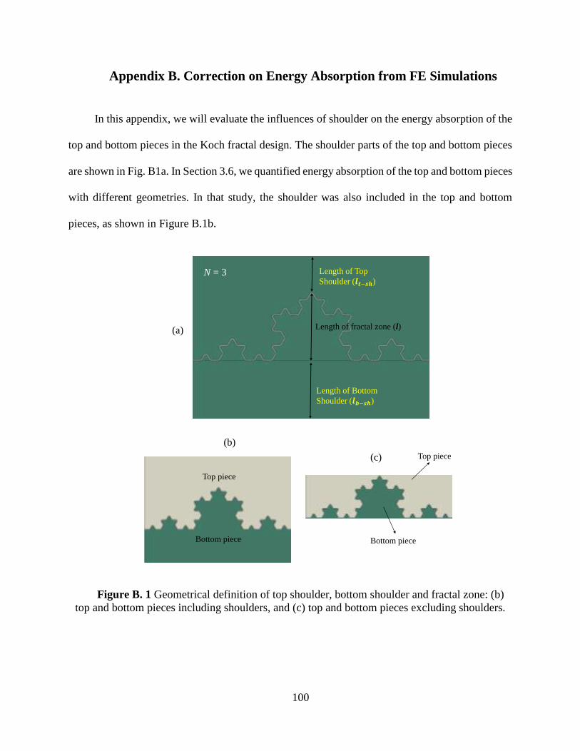
100
Appendix B. Correction on Energy Absorption from FE Simulations
In this appendix, we will evaluate the influences of shoulder on the energy absorption of the
top and bottom pieces in the Koch fractal design. The shoulder parts of the top and bottom pieces
are shown in Fig. B1a. In Section 3.6, we quantified energy absorption of the top and bottom pieces
with different geometries. In that study, the shoulder was also included in the top and bottom
pieces, as shown in Figure B.1b.
Figure B. 1 Geometrical definition of top shoulder, bottom shoulder and fractal zone: (b)
top and bottom pieces including shoulders, and (c) top and bottom pieces excluding shoulders.
Length of Top
Shoulder ( )
Length of Bottom
Shoulder ( )
Length of fractal zone (l)
N = 3
Top piece
Bottom piece
(a)
(b)
(c) Top piece
Bottom piece

101
To more accurately evaluate the energy absorption in the fractal zone, different from the
results in Section 3.6, the energy absorbed by the shoulders were excluded from the top and bottom
pieces (shown in Figure B.1c), i.e.
𝑈𝑡𝑜𝑝 = 𝑈𝑡𝑜𝑡𝑎𝑙_𝑡 − 𝑈𝑡_𝑠ℎ, and (B.1)
𝑈𝐵𝑜𝑡𝑡𝑜𝑚 = 𝑈𝑡𝑜𝑡𝑎𝑙_𝑏 − 𝑈𝑏_𝑠ℎ, (B.2)
where, 𝑈𝑡𝑜𝑝 and 𝑈𝐵𝑜𝑡𝑡𝑜𝑚 are the strain energy of top and bottom pieces in the fractal zone
only, respectively (Figure B.1.c). 𝑈𝑡_𝑠ℎ and 𝑈𝑏_𝑠ℎ are strain energy absorbed by top shoulder and
bottom shoulder, respectively. 𝑈𝑡𝑜𝑡𝑎𝑙_𝑡 and 𝑈𝑡𝑜𝑡𝑎𝑙_𝑏 represent the total strain energy absorbed by
top and bottom pieces including the shoulder area (shown in Figure B.1b.)
2D FE models were developed in ABAQUS with different geometries. For all models, plane
stress elements (CPS4R) and elasto perfectly plastic material model were used with Young’s
modulus of 1.7 GPa, Poisson’s ratio of 0.33 and the initial yielding strength of 54 MPa. In all FE
models, the out-of-plane thickness is t= 4 mm.
𝑈𝑡𝑜𝑡𝑎𝑙_𝑡 and 𝑈𝑡𝑜𝑡𝑎𝑙_𝑏 were directly output from FE models. To calculate 𝑈𝑡𝑜𝑡𝑎𝑙_𝑡 and 𝑈𝑡𝑜𝑡𝑎𝑙_𝑏
in linear elastic regime, it was assumed the stress in the shoulder parts are uniform and equals to
the surface traction applied at the top edge of the model. Thus,
𝑈𝑡_𝑠ℎ =1
2
𝑉𝑡_𝑠ℎ
𝐸 𝜎2 , (B.3)
where, E, 𝜎, 𝑉𝑡_𝑠ℎ and 𝑉𝑏_𝑠ℎ are Young’s modulus, surface traction, volume fraction of top
shoulder and volume fraction of bottom shoulder, respectively.

102
The energy density of the top and bottom parts of the interlock with N=2, 3, and 4 are plotted
and compared in Figure B.2. Generally, when N increases, the total energy density increases,
indicating the more efficient usage of material. For all three models, the bottom piece absorbs
more energy than the top piece. When N increases, the energy absorbed by top piece and that by
bottom piece both increase.
Figure B. 2 Distribution of strain energy per volume fraction between top and bottom pieces
for different cases of (a) N=2, (a) N=3 and (a) N=4.
Figure B.3 shows the influence of r on the energy density of the top and bottom pieces. In
general, when r decreases, the difference between the amount of strain energy absorbed by the top
and bottom pieces increases, indicating more bending deformation in the teeth.
g=0.1 mm
r= mm
μ=0.3
Top piece
Bottom pieceN=2
N=3 N=4
(a)
(b) (c)

103
Figure B. 3 Distribution of strain energy per volume fraction between top and bottom pieces
for N=3 with different values of (a) r=0.05 mm, (b) r=0.15 mm and (c) r=0.3 mm.
Figure B.4 shows the influence of g on the energy density of the top and bottom pieces of
the Koch fractal interlocking. In can be seen that with the same value of r and μ, the geometry with
a larger g absorbs much less energy than that with a smaller gap. Also, when g increases, some of
the teeth on the top piece become slender and therefore experience larger bending deformation.
N=3
μ=0.3
g=0.1 mm
Top piece
Bottom piece
r=0.15 mm
r=0.05 mm
(a)
(b)
r=0.3 mm
(c)

104
Figure B. 4 FE curves of energy density vs displacement for N=3 with r=0.05 mm, (a)
g=0.6 mm and (b) g=0.1mm.
g=0.6 mm g=0.1 mm
Top piece
Bottom piece
N=3
μ=0.3
r=0.05 mm
(a)(b)