Derivative-Free Optimization:new perspectives.

Andrea Ianni ∗

April 15, 2013

∗Department of Computer, Control, and Management Engineering Antonio Ruberti (La Sapienza, Universitadi Roma), Via Ariosto 25, 00185 Rome, Italy, www.dis.uniroma1.it/˜ianni/

1 IntroductionThe present work is contextualized into the Derivative-Free Optimization (DFO) branch ofresearch, and in praticular into the Direct Search methods, in the belief that it is the fieldin which the optimization get the most of the progressions in the last decade. These kindof methods, contrasting with the more traditional gradient-based algorithms for the scarcityof the informations known about the examined problems, are also a basic tool to deal withthe Black-Box optimization: in that case the fuction values (where for functions are intendedthe objective one and the functions defining the constraints of the problem) are not explicitlyknown but given as result of a series of often very complex processes that the most of thetime are unknown: the black boxes.

Introduced in the 60’s for their massive applicability were successively set aside by thescientific comunity for the lack of a solid basis theory creating a discrepancy between thewide actual use and the absence of convergence results. Nevertheless such discrepancybrought to a stronger mathematical effort on the analysis of these methods that, togetherwith the introduction of the parallel computing, brought to a revival of this branch of theoptimization.

The first aim of this work is to retrace the development of these methods starting fromthe first ones, presupposing assumptions that hardly matched with the real ones, and relaxingprogressively the hypothesis from a side increasing the mathematical set of tools from theother side dealing progressively better with the real problems.

The attention has been focused on the branch of the Pattern Search methods trying to puttogether different aspects to a wide literature, unifying the notation often very differentiatedalso when the basis concepts are absolutely similar.

It has been perceived that in the literature usually two conceptual elements are often notproperly distinguished. For this reason the present work is divided in two main parts:

• the exploration of the space;

• the management of the constraints.

To do that initially exclusively the Unconstrained Case has been taken into account to an-alyze only in the second phase the Constrained one. So, removing the issue of the constraintsit has been possible focus on the key point that really differentiates the successive PatternSearch implementations, from the first Coordinate Search until arriving to the last evolution,the Mesh Adaptive Direct Search methods: the way in which the space of the variables isexplored. In this part a particular emphasize has been put on the Coordinate Search that hasnot just presented in its semplicity. In fact we highlighted all those concepts of this methodrepresenting the starting point for the successive developments.

In this part we inserted also a conceptual parallel with another main branch of the DFOclass of problems, the Linesearch methods, trying to point out the main similarities and theconceptual differences.

In the second phase the main constraints management procedures are emphasized study-ing how the different Pattern Search methods deal with the different kinds of the real prob-lems.

1

1.0.1 The innovations

The main innovation of this thesis is presented in the paper ”Reducing the Number of Func-tion Evaluations in Mesh Adaptive Direct Search Algorithms” (SIAM, to appear). We willrefer to the approach presented in that paper as the ORTHOMADS (n+ 1) and it representsthe last evaluation of the MADS algorithms that, in turn, are the last evaluation of the PatternSearch methods. We propose a modification of the poll phase of the MADS algorithms, i.e.the core of the method, such to reduce the function evaluations of the single iteration, keepingthe convergence results.

The second innovation is about the proposal of a new implementation of the search, thesecond phase of the MADS structure. In the paper ”Backtracking: a Search modificationin Mesh Adaptive Direct Search algorithms”, developed with the University of Montreal(Canada) we called this procedure the Back-tracking search. Additional numerical resultsabout this new implementation of the search are the aim of the next phase.

2

Contents1 Introduction 1

1.0.1 The innovations . . . . . . . . . . . . . . . . . . . . . . . . . . . . . 2

2 Target problems 62.1 Keel Fin Design Problem . . . . . . . . . . . . . . . . . . . . . . . . . . . . 62.2 Mathematically . . . . . . . . . . . . . . . . . . . . . . . . . . . . . . . . . 82.3 Limit (curse) of knowledge in the Derivative-Free environment . . . . . . . . 10

I How to explore the space: The Unconstrained Case 12

3 Smooth uncontrained analysis 13

4 Coordinate Search 164.1 The Direct Search methods . . . . . . . . . . . . . . . . . . . . . . . . . . . 164.2 The context . . . . . . . . . . . . . . . . . . . . . . . . . . . . . . . . . . . 174.3 Convergence analysis of the Cooordinate Search algorithm . . . . . . . . . . 214.4 Coordinate Search: the simplest Pattern Search algorithm . . . . . . . . . . . 294.5 Coordinate Search: MADS notation . . . . . . . . . . . . . . . . . . . . . . 334.6 Coordinate Search: two notations . . . . . . . . . . . . . . . . . . . . . . . . 354.7 ∆k: the possibility of the generalization . . . . . . . . . . . . . . . . . . . . . 37

5 Generalized Pattern Search (GPS): introduction 415.1 GPS: the MADS notation . . . . . . . . . . . . . . . . . . . . . . . . . . . . 425.2 Convergence analysis of the Generalized Pattern Search algorithms . . . . . . 525.3 GPS: limitation . . . . . . . . . . . . . . . . . . . . . . . . . . . . . . . . . 58

6 Linesearch 60

7 Linesearch inserted into a GPS approach: a possible algorithm. 66

8 The Mesh Adaptive Direct Search (MADS) algorithms 748.1 Mesh Adaptive Direct Search: the basic concepts . . . . . . . . . . . . . . . 748.2 Convergence analysis of the Generalized Pattern Search algorithms . . . . . . 788.3 LTMADS . . . . . . . . . . . . . . . . . . . . . . . . . . . . . . . . . . . . 838.4 ORTHOMADS . . . . . . . . . . . . . . . . . . . . . . . . . . . . . . . . . . 86

II ORTHOMADS (n+1) 88

9 Introduction 89

3

10 The MADS class of algorithms 9010.1 A brief summary of MADS . . . . . . . . . . . . . . . . . . . . . . . . . . . 9010.2 The polling directions . . . . . . . . . . . . . . . . . . . . . . . . . . . . . . 92

11 A basic framework to reduce the size of the poll set 9311.1 High-level presentation of the basic framework . . . . . . . . . . . . . . . . 9311.2 OrthoMADS with n+1 directions . . . . . . . . . . . . . . . . . . . . . . . . 94

12 A general framework to reduce the size of the poll set 9512.1 High-level presentation of the general framework . . . . . . . . . . . . . . . 9612.2 Strategies to construct the reduced poll set . . . . . . . . . . . . . . . . . . . 9612.3 Completion to a positive basis . . . . . . . . . . . . . . . . . . . . . . . . . 9712.4 Completion using quadratic models . . . . . . . . . . . . . . . . . . . . . . 98

13 Convergence analysis of the general framework 10013.1 A valid MADS instance . . . . . . . . . . . . . . . . . . . . . . . . . . . . . 10013.2 An example that does not cover all directions . . . . . . . . . . . . . . . . . 10213.3 Asymptotically dense normalized polling directions . . . . . . . . . . . . . . 103

14 Numerical results 10414.1 Test problems from the derivative-free optimization literature . . . . . . . . . 10514.2 A pump-and-treat groundwater remediation problem . . . . . . . . . . . . . 109

15 Discussion 110

16 ORTHOMADS n+1 vs ORTHOMADS 2n:Numerical Results on two real problems 11116.1 MDO . . . . . . . . . . . . . . . . . . . . . . . . . . . . . . . . . . . . . . 11216.2 STYRENE . . . . . . . . . . . . . . . . . . . . . . . . . . . . . . . . . . . 112

17 Numerical Results 113

18 Backtracking: the Unconstrained Case 12918.1 From the Coordinate Search to the MADS algorithms: the importance of the

Speculative Search [2006] . . . . . . . . . . . . . . . . . . . . . . . . . . . 12918.2 The Unconstrained Back-tracking search . . . . . . . . . . . . . . . . . . . . 131

18.2.1 The Back-tracking . . . . . . . . . . . . . . . . . . . . . . . . . . . 135

III Introducing the constraints 137

19 Introduction 138

20 Mathematical tools 138

4

21 Constrained exploratory moves: an adapted Pattern Search algorithm 140

22 A new concept of conforming 145

23 X: Bounded constraints 149

24 X: Linear constraints 152

25 Ω: general constraints 155

26 How to manage the constraints: from the EB to the PB 16026.1 A mention to the Penalty Functions . . . . . . . . . . . . . . . . . . . . . . . 16026.2 The barriers . . . . . . . . . . . . . . . . . . . . . . . . . . . . . . . . . . . 16026.3 Notation to handle the infeasibility . . . . . . . . . . . . . . . . . . . . . . . 16326.4 The generalized poll . . . . . . . . . . . . . . . . . . . . . . . . . . . . . . 16426.5 Two levels of successful iterations: dominating vs improving points . . . . . 16526.6 Convergence theory . . . . . . . . . . . . . . . . . . . . . . . . . . . . . . . 168

27 Back-tracking search: the Constrained case 17527.1 The simplest cases: F F F and I I I . . . . . . . . . . . . . . . . . . . . . . . 17727.2 The constrained case (F F I) . . . . . . . . . . . . . . . . . . . . . . . . . . 17727.3 The constrained case (F I I) . . . . . . . . . . . . . . . . . . . . . . . . . . . 18027.4 The constrained case (F I F) . . . . . . . . . . . . . . . . . . . . . . . . . . 18227.5 The constrained case (I F F) . . . . . . . . . . . . . . . . . . . . . . . . . . 18527.6 The constrained case (I I F) . . . . . . . . . . . . . . . . . . . . . . . . . . . 18627.7 The constrained case (I F I) . . . . . . . . . . . . . . . . . . . . . . . . . . . 18827.8 The Algorithm depends on the constraint management: the Extreme Barrier

example . . . . . . . . . . . . . . . . . . . . . . . . . . . . . . . . . . . . . 191

5

2 Target problemsThe main particularity of the Derivative-Free context is that f , X and gi are not given analyt-ically, From that it can be gathered the reason of the Derivative-Free term. It is impossibleto compute the first and second order derivatives as well. At the contrary in the classical realDerivative-Free problem the user interfaces with the characteristic functions of the problemsby black-box functions. These black-boxes represent processes receiving a vector as inputand producing a certain output. No more of that can be said about these processes that areintended to refer to a very general case. It can be the solution of a system of Partial Differ-ential Equations (PDEs) or, as it happens when one deals with the collections of the classicaltest problems, it can be the simple substitution of the variable x in the objective function.

The black-boxes, in general, express both the objective function and the constraints. Al-though, as said, the BB may even contain the analytical expression of a function, that wouldbe just a toy BB used at most to test the behaviour of some new algorithms. The objectivefunctions related to the real problems, instead, have some common features that make the useof the Derivative-Free algorithms necessary:

• The evaluation of f and of the functions defining Ω are usually the result of a computercode (the BB).

• The functions are nonsmooth, with some ”if”s and ”goto”s.

• The functions are expensive black boxes whose processes can take seconds, mintesand, sometimes, days.

• The functions may fail unexpectedly even for x Ω.

• Only a few correct digits are sometimes ensured.

• Accurate approximation of derivatives is problematic.

• The constraints defining may be nonlinear, nonconvex, nonsmooth and may simplyreturn yes/no.

2.1 Keel Fin Design ProblemTo enforce the practical meaning of the DFO here an example of a real problem is chosen inthe marine sector.

In particular it is on the keel fin design of a sailing yatch, i.e. a ship that travels using thewind power only, so without a a complete control of its propulsive system.

Two are the unwanted movements of the ship in this particular case: the rolling along thelongitudinal axes and the shifting along the side direction. In order to solve these problems itis possible to modify two elements of the yatch:

• the bulb, for contrasting the heeling moment produced by the wind (see figure 1);

6

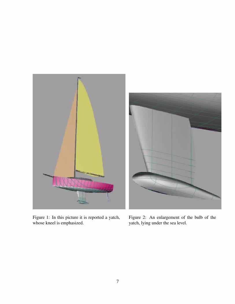
Figure 1: In this picture it is reported a yatch,whose kneel is emphasized.

Figure 2: An enlargement of the bulb of theyatch, lying under the sea level.

7

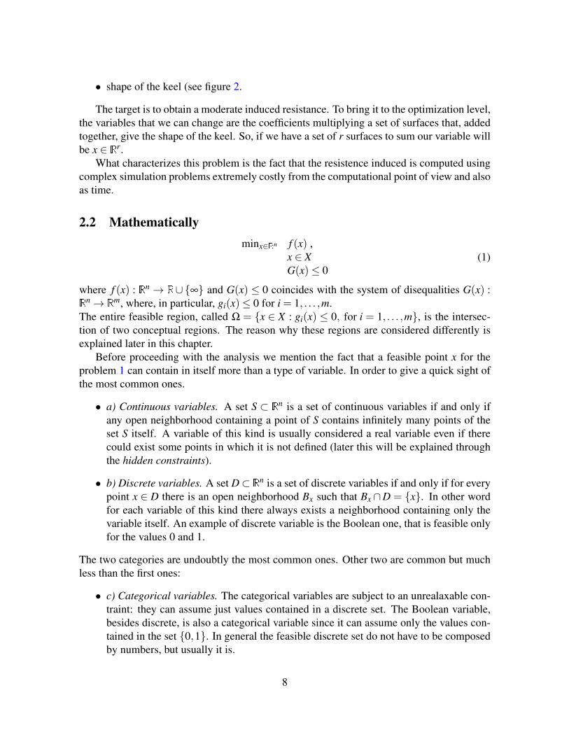
• shape of the keel (see figure 2.

The target is to obtain a moderate induced resistance. To bring it to the optimization level,the variables that we can change are the coefficients multiplying a set of surfaces that, addedtogether, give the shape of the keel. So, if we have a set of r surfaces to sum our variable willbe x ∈ Rr.

What characterizes this problem is the fact that the resistence induced is computed usingcomplex simulation problems extremely costly from the computational point of view and alsoas time.

2.2 Mathematicallyminx∈Rn f (x) ,

x ∈ XG(x)≤ 0

(1)

where f (x) : Rn→ R∪∞ and G(x) ≤ 0 coincides with the system of disequalities G(x) :Rn→ Rm, where, in particular, gi(x)≤ 0 for i = 1, . . . ,m.The entire feasible region, called Ω = x ∈ X : gi(x) ≤ 0, for i = 1, . . . ,m, is the intersec-tion of two conceptual regions. The reason why these regions are considered differently isexplained later in this chapter.

Before proceeding with the analysis we mention the fact that a feasible point x for theproblem 1 can contain in itself more than a type of variable. In order to give a quick sight ofthe most common ones.

• a) Continuous variables. A set S ⊂ Rn is a set of continuous variables if and only ifany open neighborhood containing a point of S contains infinitely many points of theset S itself. A variable of this kind is usually considered a real variable even if therecould exist some points in which it is not defined (later this will be explained throughthe hidden constraints).

• b) Discrete variables. A set D⊂ Rn is a set of discrete variables if and only if for everypoint x ∈ D there is an open neighborhood Bx such that Bx ∩D = x. In other wordfor each variable of this kind there always exists a neighborhood containing only thevariable itself. An example of discrete variable is the Boolean one, that is feasible onlyfor the values 0 and 1.

The two categories are undoubtly the most common ones. Other two are common but muchless than the first ones:

• c) Categorical variables. The categorical variables are subject to an unrealaxable con-traint: they can assume just values contained in a discrete set. The Boolean variable,besides discrete, is also a categorical variable since it can assume only the values con-tained in the set 0,1. In general the feasible discrete set do not have to be composedby numbers, but usually it is.

8

• d) Periodic. The periodic variables are a set Π of closed and bounded variables withperiod t ∈ R if and only if for any x ∈ Π, φ(x + p) = φ(x), where φ represent thefunctions distinctive of the specific problem.

At the first line of this section the general problem has been presented. What catches theeye is the formulation of the constrained part. Usually, in fact, it is normal to see the generaloptimization problem as the minimization of f (x) subject to x ∈Ω, where Ω can have certainproperties as being regular, open, closed, and so on. In this case, instead, the differentiationhas been expressely emphasized, to point out the difference between the constraints that canbe violated and the ones that, instead, are unrelaxable.

• Relaxable Contraints.These kind of contraints are those ones that are possible to ignore for a while. Theycan be computed both in feasible and infeasible points and, in this sense, the amountC(x), if positive, returns the ”amount of violability” of the constraints in the point x.At the contrary, if the point x is feasible for the problem 1 it has to result G(x) ≤ 0,indipendently on how negative G(x) is.A classical example that makes the idea of a relaxable constraint very intuitive is thebudget fixed by a user to produce something. A constraint of this kind is naturallyconsiderable relaxable since one could wonder how the ”product” varies its featuresvarying the budget too. Nevertheless, notice that it is sufficient that the user think to hisbudget as the ”maximum possible ever” that this kind of contraint cannot be considerednaturally relaxable anymore.However it is important to specify that in general the constraints considered relaxablecan also be constraints that ”naturally” do not appear as relaxable. In fact which con-straints are considerable relaxable and which ones not usually is up to the user himself.

• Unrelaxable Constraints.We have just said that a constraint is relaxable only when a user decides that. It is notcompletely true. In fact, there are some constraints that gives a real sense to a problem,i.e., constraints that make the model fit with the reality: those constraints have to beconsidered unrelaxable indipendently by the will of the user.One simple example is given by the natural bounds of the real variables. Suppose thefunction to minimize being the amount of a material to use to build a certain door. Onevariable can be, for example, the maximum height of a generic man xh. Considering thehighest height ever get by a man it is reasonable to write xh ≤ 5.44 (in metres, twice thedimension of Robert Wadlov, the highest man ever existed on the world). Consideringalso men higher than 5.44 metres would not make sense.Also phisical example can be done: in fact, though it is possible to compute the forceproduced by an object with a negative mass, it does have any sense, i.e., it produces anumber that has not a physical correlation with the reality. Following the same line itis not possible to compute a profit making a man work for −2 hours, and so on.

For what has been said here in general the bound constraints are included in the set X .

9

• Hidden Constraints.

What often happens is that the linear constraints are put into the set X , while the mostcomplex ones as the non-linear constraints form the set Ω. The reason because it is doneis often practical: if the easily-evaluable constraints brand a point as ”not-good” it couldmakes sense to save the time to compute the costly constraints and the objective functionon that point. Since the linear constraints can often be identified as the cheap-constraintssometimes it is said that X contains the bounded and the linear constraints and Ω containsthe non-linear constraints. Despite of that we highlight the fact that usually the relaxabilityor the unrelaxability of a constraint depends on the will of the user.

2.3 Limit (curse) of knowledge in the Derivative-Free environmentIn this last part we want to highlight a point that, for its presumed banality, it is often ig-nored. To do that let us introduce two basic concepts of the Optimization. We rewrite theoptimization general problem in a simpler way:

minx f (x) ,x ∈ F.

(2)

The target of the optimization is to find a solution of that problem, but speaking about asolution is not univocal. Not considering the discussion about the stationary points, focusingfor a while on the minima of the objective fuction they are of two kinds:

Definition 2.1 A point x∗∗ ∈ F is said the global minimum of the function f over the set F if

f (x∗∗)≤ f (x)

for every x ∈ F.

The previous definition detects the ”proper” solution of the problem 2 because it actuallyis the minimum of the function f over the feasible space. Unfortunately in the most of realproblem this global minimum is a real rip-off Holy Grail, since it is impossible to certify it. Inparticular this is always true in the derivative-free context. For this reason another definitionis necessary:

Definition 2.2 A point x∗ ∈ F is said to be a local minimum of the function f over the set Fif there exists a neighborhood Bε(x∗) such that

f (x∗)≤ f (x)

for every x ∈ Bε(x∗)∩F.

The last definition represent the kind of point that the derivative-free methods actuallysearch. Why do not find directly the global minima (they can be more than one) of theproblem ??? Two are the reasons: first in the real problems, that are crucial in the derivative-free studying, finding a global minimum is sometimes very hard.Although it is the second

10

reason the real curse on the global minimum. In fact, even supposing that the global minimumof a function on a certain feasible set is found, there is no way recognize that point as theglobal minimum.

From this perspective it is importaant not to make confusion with a definition typical inthe optimization: a generic algorithm is said to be globally convergent when it converges topoints with some specific feature for every starting point in the feasible set. It absolutely doesnot mean that the globally convergent algorithm always find a global optimizer.

11

Part I

How to explore the space: TheUnconstrained Case

12

3 Smooth uncontrained analysisBefore starting the conceptual path that will lead the reader through the successive evolutionsproduced in the Pattern Search context, we spend some time to introduce some mathematicalconcept that will be necessary to explain the properties of the methods that will be introduced.It as been chosen not to present now all the tools that are necessary along the whole work inorder for the reader to have a clear connection between the theory and its application to thesuccessive algorithms. In this way it also results evident that the theory necessary to definethis firts part is extremely simple, involving concepts like the first directional derivative andthe gradient. Notice also that we never speak about derivatives beyond the first degree. Atthe contrary already the concept of f continuously differentiable, assumed very widely inthe most of the otpimization papers, represents here an ”hot potato”, in the sense that it isextremely common that the generic user cannot take it as an assumption applicable to hisspecific problem. Nevertheless, above all in the first Pattern Search methods, assuming fcontinuously differentiable is extremely important to be able to state interesting results. Wewill see what happen to the Coordinate Search theory replacing that condition with a weakerone as assuming the function f Lipschitz continuous in some specific points.

Definition 3.1 The function f : Rn→ R is said to be differentiable at x ∈ Rn if there exists avector g ∈ Rn such that

limy→x

f (y)− f (x)−gT (y− x)|(y− x)|

If f is differentiable at x:

• the vector g is unique and called gradient of f at x: ∇ f (x).

• the directional derivatives of f at x exist and satisfy

f ′(x;v) := limt↓0

f (x+ tv)− f (x)t

= ∇ f (x)T v

where v ∈ Rn is a generic vector.

The contrary, instead, is not true, i.e., also if f is not differentiable all the directionalderivatives of a function may exist.

Example 3.2 The classical example is for one f : R→ R, the absolute value: f = abs(x).Although the gradient of f at 0 is undefined, computing the directional derivative along v∈Rn

it results

f ′(0;v) := limt↓0

f (0+ tv)− f (0)t

= limt↓0

|tv|t

= |v|

It means that for any direction v ∈ Rn either f ′(x;v)≤ 0 or f ′(x;−v)≤ 0.

Moreover v ∈ Rn is a descent direction if f ′(x;v)≤ 0 (strict descent direction if f ′(x;v)<0).

13

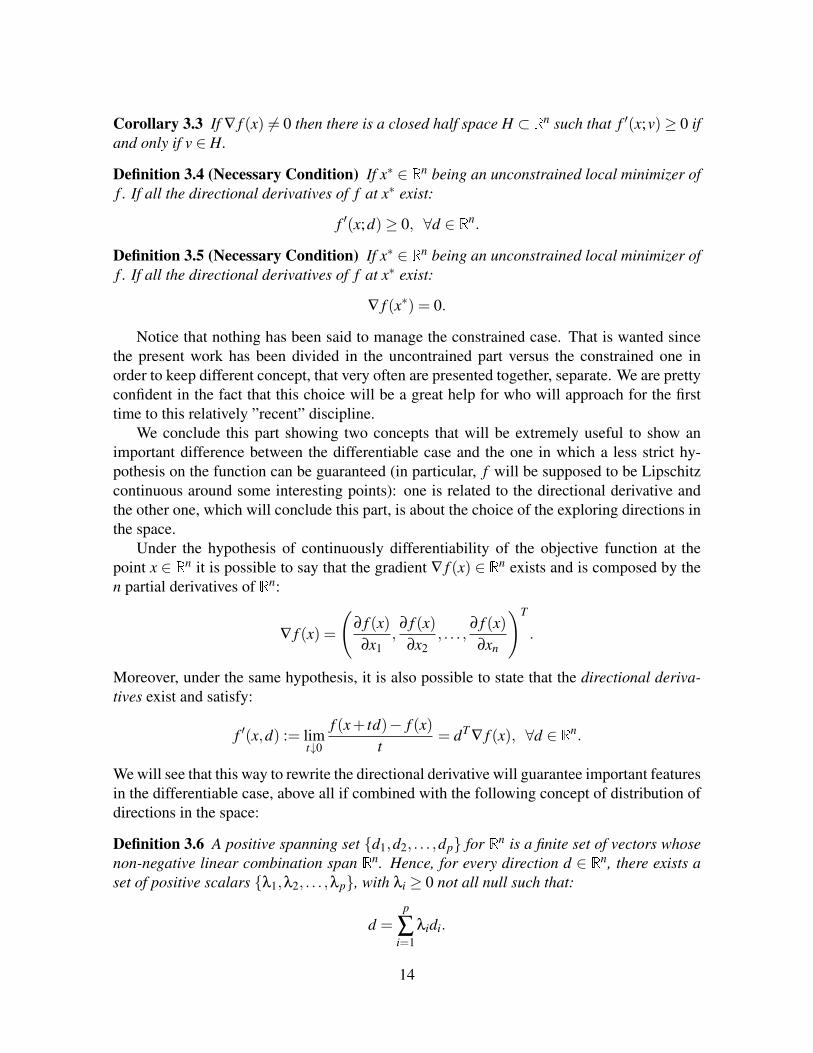
Corollary 3.3 If ∇ f (x) 6= 0 then there is a closed half space H ⊂ Rn such that f ′(x;v)≥ 0 ifand only if v ∈ H.

Definition 3.4 (Necessary Condition) If x∗ ∈ Rn being an unconstrained local minimizer off . If all the directional derivatives of f at x∗ exist:

f ′(x;d)≥ 0, ∀d ∈ Rn.

Definition 3.5 (Necessary Condition) If x∗ ∈ Rn being an unconstrained local minimizer off . If all the directional derivatives of f at x∗ exist:

∇ f (x∗) = 0.

Notice that nothing has been said to manage the constrained case. That is wanted sincethe present work has been divided in the uncontrained part versus the constrained one inorder to keep different concept, that very often are presented together, separate. We are prettyconfident in the fact that this choice will be a great help for who will approach for the firsttime to this relatively ”recent” discipline.

We conclude this part showing two concepts that will be extremely useful to show animportant difference between the differentiable case and the one in which a less strict hy-pothesis on the function can be guaranteed (in particular, f will be supposed to be Lipschitzcontinuous around some interesting points): one is related to the directional derivative andthe other one, which will conclude this part, is about the choice of the exploring directions inthe space.

Under the hypothesis of continuously differentiability of the objective function at thepoint x ∈ Rn it is possible to say that the gradient ∇ f (x) ∈ Rn exists and is composed by then partial derivatives of Rn:

∇ f (x) =

(∂ f (x)∂x1

,∂ f (x)∂x2

, . . . ,∂ f (x)∂xn

)T

.

Moreover, under the same hypothesis, it is also possible to state that the directional deriva-tives exist and satisfy:

f ′(x,d) := limt↓0

f (x+ td)− f (x)t

= dT∇ f (x), ∀d ∈ Rn.

We will see that this way to rewrite the directional derivative will guarantee important featuresin the differentiable case, above all if combined with the following concept of distribution ofdirections in the space:

Definition 3.6 A positive spanning set d1,d2, . . . ,dp for Rn is a finite set of vectors whosenon-negative linear combination span Rn. Hence, for every direction d ∈ Rn, there exists aset of positive scalars λ1,λ2, . . . ,λp, with λi ≥ 0 not all null such that:

d =p

∑i=1

λidi.

14

Moreover a positive basis is a positive spanning set such that there not exists a subset stricltycontained in the set being a positive spanning set.

The positive spanning sets are considered, in the DFO context, a ”proper” way to explorethe space. To understand why consider the important property: a positive spanning set ofdirections contains at least one element in every open half-space. The differentiable casegives an idea of what ”proper way to explore the space” means, in fact: if f is differentiableat a non-stationary point x, then there is at least one element of any positive spanning set thatis a strictly descent direction. In other words, if d1,d2, . . . ,dp is the positive spanning setused to explore the space, there is at least a j ∈ 1, . . . , p such that f ′(x;di)< 0.

Combining the two last observations let see how the directional derivative of a pointdepends on the directional derivatives along a positive spanning set of directions. Let d ∈ Rn

be a generic direction in the space:

f ′(x;d) = ∇ f (x)T d

= ∇ f (x)T∑

pi=1 λidi

= ∑pi=1 λi∇ f (x)T di

= ∑pi=1 λi f ′(x;di).

This consideration will be useful in the section ??.

15

4 Coordinate Search

4.1 The Direct Search methodsIn 1961 R. Hook and T.A. Jeeves used for the first time the phrase ”direct search” in the paper”Direct search solution of numerical and statistical problems”. A direct search method wasdescribed as a sequential examination of trial solutions involving:

• the comparison of each trial solution with the best one obtained up to that time;

• a strategy for determining the next trial solution depending on the earlier results.

This definition was given even before 1966, the years in which it was proved that the methodof steepest descent could be modified to ensure global convergence, result that moved theattention on the use of the first and second derivatives (when existing) to solve efficiently thereaal problems.

While it can be understood the attention on these kind of methods at the time they com-pared for the first time, one can wonder why, after 50 years, we are still speaking about thesekind of methods.The first reason is very simple: these kind of methods work very well in practise.The second one is realistic: if, on a side, it is a common knowledge in the Operational Re-search field, that the quasi-Newton algorithms are surprisingly efficient, they have a price:the knowledge of the first and second derivatives. So, banally, the direct search methods arewidely used today because there is a plethora of real problems for which the quasi-Newtonmethods are not applicable. Maybe for their simplicity the direct search methods succedwhere other more sophisticated methods fail.As thirs reason, the direct search methods are quite easy to implement and do not need a lotof requirements.Moreover, and this can be classified as a fourth reason, sometimes it is necessary a certaintime to realize a more sophisticated algorithms. In cases like those ones also advanced userscan use direct search methods to provide a well-chosen point (an ”hot-start”) to the sophisti-cated method.

The direct search methods born dealing with the unconstrained case:

minx∈Rn

f (x),

with f : Rn→ R. Although at the beginning they assumed f differentiable on Rn, the directsearch methods did not use the information of the gradient neither directly nor indirectly (forexample approximating the derivatives). For this reason they are also called ”Derivative-Freemethods”. Nevertheless, the concept of derivative-free does not express completely the directsearch methods. A more appropriate way to describe them is through the classical Taylor’sseries expansion, evaluating how many terms of the expansion are used.To verify that it makes sense it is enough to think that Newton’s methods is called a second-order methods since it assume the existence of first and second derivatives and uses thesecond-order Taylor polinomial in order to construct local quadratic approximations of f .

16

Similarly, the Steepest Descent method is a first-order method since it assumes the existenceof first derivatives and uses the first-order Taylor polinomial to construct a local linear ap-proximation of the function f .Following this rationale it makes sense to identify the direct search methods as the zero-ordermethods since they do not assume the existence of any derivative and since they do not useany approximation of f .

4.2 The contextWhen no informations are available on the functions of a certain problem and the target isto find that point x∗ ∈ Rn in which the minimum of f is obtained, the first idea is also thesimplest one: look “around” the current point to see if there may be found a better point.In the Unconstrained context speaking about a better point is referred to the function valuecorresponding to those points. Hence x is better than y if and only if f (x)< f (y) (in a secondmoment this concept will be generalized for the Constrained case). Relying on the way inwhich that ”looking around” is implemented, it is possible to construct the whole story of thePattern Search methods, the main branch of the Direct Search methods.

Mathematically. Let us express what written above mathematically. The first point is”where we are”: let x0 ∈ Rn be the initial guess (T. G. Kolda, R. M. Lewis, V. Torczon, 1997)and xk ∈ Rn be the current point at the generic iteration k. For what will be said, there will beproduced sequences of points such that it will result: f (xk)≤ f (xk−1)≤ . . .≤ f (x1)≤ f (x0).The inequalities could be strict or not depending on the used method:

• conservative: a point is taken as current solution only if its function value is strictlyless than the previous one (hence f (x j+1)< f (x j),∀ j = 0,1, . . . ,k−1).

• not-conservative: a current point is updated also if its function value is the same of theprevious solution (hence f (x j+1)< f (x j) or f (x j+1) = f (x j), ∀ j = 0,1, . . . ,k−1).

Clearly the second choice leads to a more moveable method, since there are cases for whichthe first approach forces the sequence not to move when, instead, the second approach pro-duces movements. The standard option is the conservative one, ensuring the reduction of thefunction value at every movement of the sequence.

The second element necessary for the exploration is the set of directions, i.e., ”wherewe are going”. Conceptually, if no informations are available on the function f like thesmoothness (continuity, Lipschitzianity, continuity of the derivatives, etc.) a proper infinitenumber of directions would be necessary to explore exhaustively the neighborhood of a point(where “proper” means that it is not sufficient to have infinite directions, but it is necessarythat those directions cover the entire space). In a finite world like ours this is, unfortunately,impossible.

It is interesting to think to a real case as a parallel of the described situation:

17

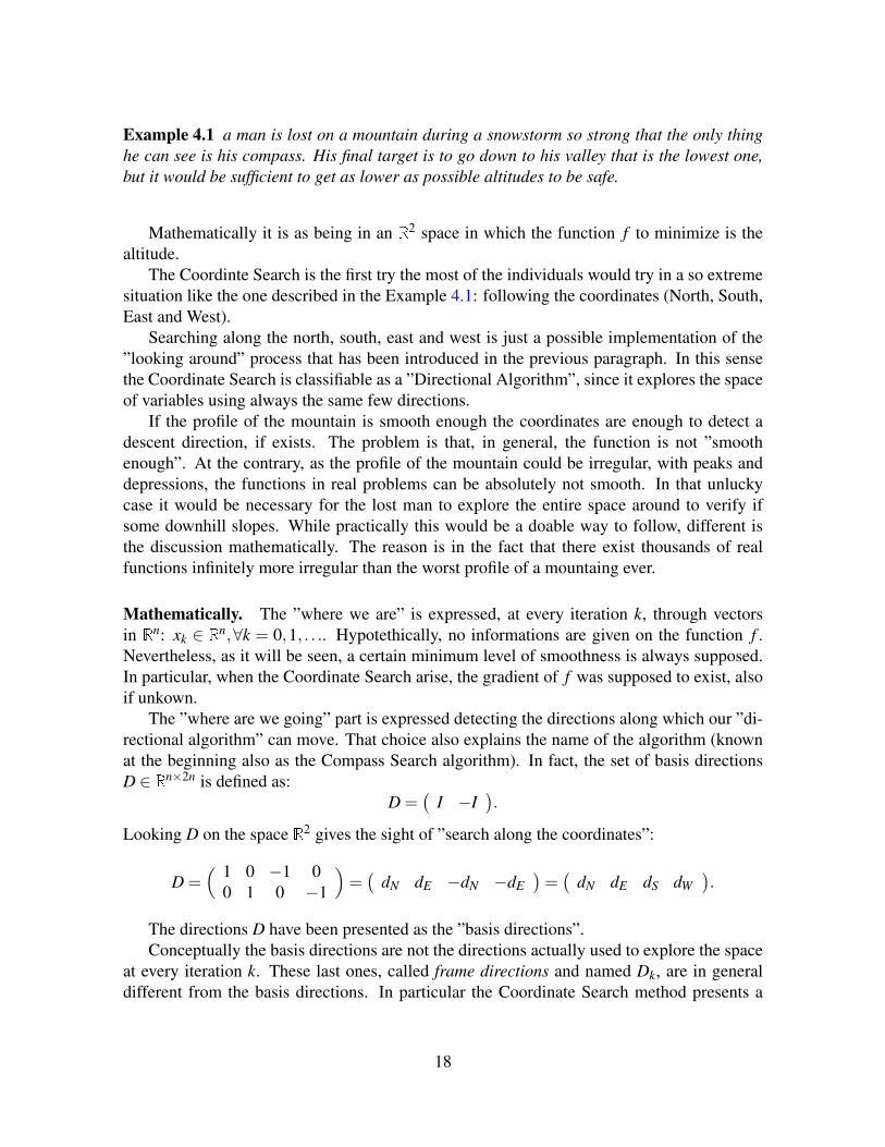
Example 4.1 a man is lost on a mountain during a snowstorm so strong that the only thinghe can see is his compass. His final target is to go down to his valley that is the lowest one,but it would be sufficient to get as lower as possible altitudes to be safe.

Mathematically it is as being in an R2 space in which the function f to minimize is thealtitude.

The Coordinte Search is the first try the most of the individuals would try in a so extremesituation like the one described in the Example 4.1: following the coordinates (North, South,East and West).

Searching along the north, south, east and west is just a possible implementation of the”looking around” process that has been introduced in the previous paragraph. In this sensethe Coordinate Search is classifiable as a ”Directional Algorithm”, since it explores the spaceof variables using always the same few directions.

If the profile of the mountain is smooth enough the coordinates are enough to detect adescent direction, if exists. The problem is that, in general, the function is not ”smoothenough”. At the contrary, as the profile of the mountain could be irregular, with peaks anddepressions, the functions in real problems can be absolutely not smooth. In that unluckycase it would be necessary for the lost man to explore the entire space around to verify ifsome downhill slopes. While practically this would be a doable way to follow, different isthe discussion mathematically. The reason is in the fact that there exist thousands of realfunctions infinitely more irregular than the worst profile of a mountaing ever.

Mathematically. The ”where we are” is expressed, at every iteration k, through vectorsin Rn: xk ∈ Rn,∀k = 0,1, . . .. Hypotethically, no informations are given on the function f .Nevertheless, as it will be seen, a certain minimum level of smoothness is always supposed.In particular, when the Coordinate Search arise, the gradient of f was supposed to exist, alsoif unkown.

The ”where are we going” part is expressed detecting the directions along which our ”di-rectional algorithm” can move. That choice also explains the name of the algorithm (knownat the beginning also as the Compass Search algorithm). In fact, the set of basis directionsD ∈ Rn×2n is defined as:

D =(

I −I).

Looking D on the space R2 gives the sight of ”search along the coordinates”:

D =( 1 0 −1 0

0 1 0 −1

)=(

dN dE −dN −dE)=(

dN dE dS dW).

The directions D have been presented as the ”basis directions”.Conceptually the basis directions are not the directions actually used to explore the space

at every iteration k. These last ones, called frame directions and named Dk, are in generaldifferent from the basis directions. In particular the Coordinate Search method presents a

18

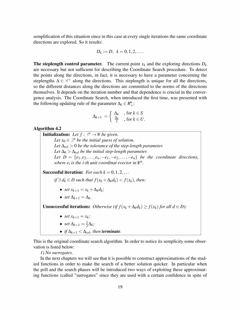
semplification of this situation since in this case at every single iterations the same coordinatedirections are explored. So it results:

Dk := D, k = 0,1,2, . . . .

The steplength control parameter. The current point xk and the exploring directions Dkare necessary but not sufficient for describing the Coordinate Search procedure. To detectthe points along the directions, in fact, it is necessary to have a parameter concerning thesteplengths ∆ ∈ R+ along the directions. This steplength is unique for all the directions,so the different distances along the directions are committed to the norms of the directionsthemselves. It depends on the iteration number and that dependence is crucial in the conver-gence analysis. The Coordinate Search, when introduced the first time, was presented withthe following updating rule of the parameter ∆k ∈ Rn

+:

∆k+1 =

∆k , for k ∈ S∆k2 , for k ∈U.

Algorithm 4.2Initialization: Let f : Rn→ R be given.

Let x0 ∈ Rn be the initial guess of solution.Let ∆tol > 0 be the tolerance of the step-length parameter.Let ∆0 > ∆tol be the initial step-length parameter.Let D = e1,e2, . . . ,en,−e1,−e2, . . . ,−en be the coordinate directions,where ei is the i-th unit coordinat evector in Rn.

Successful iteration: For each k = 0,1,2, . . .

if ∃ dk ∈ D such that f (xk +∆kdk)< f (xk), then:

• set xk+1 = xk +∆kdk;

• set ∆k+1 = ∆k.

Unsuccessful iterations: Otherwise (if f (xk +∆kdk)≥ f (xk) for all d ∈ D):

• set xk+1 = xk;

• set ∆k+1 =12∆k;

• if ∆k+1 < ∆tol , then terminate.

This is the original coordinate search algorithm. In order to notice its semplicity some obser-vation is listed below:

1) No surrogates.In the next chapters we will see that it is possible to construct approximations of the stud-

ied functions in order to make the search of a better solution quicker. In particular whenthe poll and the search phases will be introduced two ways of exploiting these approximat-ing functions (called ”surrogates” since they are used with a certain confidence in spite of

19

the real functions) will be studied. One way, in particular, consists in ordering the pointsxk +∆kdk : dk ∈ D such to explore first the points in which the surrogate function valuesare lower. Obviously the Coordinate Search method did not have that sagacity. In fact nosurrogates are used to order the trial points such to explore the most ”interesting” (in proba-bility) points first.

2) No attempt to move away from locally optimal solutions.For the Coordinate Search method there exists the concept of minimum, but the difference

between ”local” and ”global” minima is not managed in its implementation. When a genericminimum is identified, independently from its function value, the ∆k is reduced more andmore until it becomes less than ∆tol and the stopping criterion terminates the algorithm. Sothe Coordinate Search stops either in the global minimum of the f in the entire space Rn orin a ”very bad” local minimum (i.e. a minimum in which the f value is relatively great).

3) Nothing to identify descent directions for f.Let us compare this simple derivative-free method with the analogous (for semplicity)

method that uses the derivatives of the f , the Steepest Descent method. In that case the infor-mation on the gradient of the objective function in the point x is enough to detect the directiondSD = −∇ f (x) as the best local direction. In addition, when the point x is not stationary, itis possible to guarantee that dSD is a descent direction in the point x for the fuction f . Thisproperty obviously decades with the lack of the gradient information and, since the Coordi-nate Search does not implement any substitutive mechanism, it does not use any procedureto try to detect descent directions.

4) Easy management of the parameter ∆k.Notice that the steplegth parameter is not increased in the successful iterations as it hap-

pens in some successive modifications of the method. Two are the possible mofifications ofthe parameter: it can be reduced or left unchanged. This simple choice limits the behaviour ofthe method but it had the important advantage to semplify massively the proof off the centraltheorem presented in the next section (Theorem 4.3).

Summarizing, the Coordinate Search method was presented as a method looking for theminimum among a set of points called ”frame” and identified in the following set, at everyiteration k:

Pk = xk∪xk +∆kdk : dk ∈ D.

Then the method just moves from xk if there exists a point y ∈ Pk such that f (y) < f (xk),remaining on xk otherwise.

20

4.3 Convergence analysis of the Cooordinate Search algorithmIn this section the convergence theory related to the simple Coordinate Search algorithmexplained in 4.2. Before considering the gradient of the objective function it is necessary topresent a pre-result about another important variable, the steplength control parameter. It ispossible to obtain the following result exclusively supposing the boundness of the iteratesproduced by the method, that is not a big deal being a common assumption also outside thesekinds of methods. This assumption, as it will be sseen, is central in the whole Pattern Searchbranch, and not just for the Coordinate Search.

Theorem 4.3 Let xk be the sequence of iterates produced by the Coordinate Search algo-rithm. If xk belongs to a bounded set for each k→+∞, then

limk→+∞

∆k = 0.

Proof. This proof will be done by contradiction: we assume that ∆k is bounded below forevery k, i.e.:

∆k ≥ ∆min,

for every k = 0,1, . . .. What happens if a quantity does not have to go to zero for k →+∞ is that quantity has to be bounded below. Instead of considering a generic value ∆min,the steplength parameter is written in a proper way: considering that at every unsuccessfuliteration k the steplength parameter is reduced (∆k+1 = ∆k

2 ), for the absurd hypothesis it ispossible to state that only a finite number r ∈ N of unsuccessesful iterations are possible. So,let see what can happen at the iteration k. If the possible failure of the method are r threeare the possible situation at iteration k: the unsuccessful iterations are occurred all before k,or there are unsuccessful iterations both before and after k, or, there have not been occurredunsuccesses until the iteration k.

So, at the worst, i.e. if all the unsuccessful iterations are occured before the current one k,the ∆k parameter assumes the minimum value, having been halved r times respect the initialvalue ∆0. So, in general, it results:

∆min = 2−r∆0

In every case it can be stated that after a certain iteration t ∈N, with t > r, after having oc-curred all the ”available for the absurd hypothesis” unsuccessful iterations, infinite successfuliterations are be obtaind. So it is possible to say that

f (xk2)< f (xk1),

for all k2 > k1 ≥ t. Obviously that also means that from k ≥ t on the steplength parameterwill not change anymore:

∆k = ∆t , ∀ k = t, t +1, t +2, . . . .

Moreover, for each k ≥ t there always exists a direction vk ∈ ±ei : i = 1,2, . . . ,n such thatxk+1 = xk +∆tvk and f (xk +∆tvk) < f (xk), i.e., being all the iterations after t successful,

21

there always exists at least a direction in the frame along which a point with a better functionrespect with the current one is found. It follows that:

xk+1 = xk +∆kvk= xk−1 +∆k−1vk−1 +∆kvk= . . .= xt +∆tvt +∆t+1vt+1 + . . .+∆kvk == xt +∆tvt +∆tvt+1 + . . .+∆tvk =

= xt +∆t ∑kj=t v j.

Now it is sufficient to see that ∑kj=t v j ∈Zn to say that every point generated after the iteration

t (k≥ t) has to lie on a particular invisible lattice created by the point xt as center and integervectors as directions with the translation coefficient ∆t . Such a lattice detects all those pointsthat can be get from a center using certain integer directions scaled with a steplegth parameter.This mesh can be written as:

M = xt +∆tz : z ∈ ZnBeing M an enumerable set it represents a set of an infinite number of points. Nevertheless

it has been assumed for hypothesis that the successive explored points do not lie outside abounded set S, and it is easy to see that M ∩ S contains finitely many points. It means thatthe sequence xk cannot be made by all distinct points, hence also the sequence from theiteration t on. So at most all the points will be explored, but at least one of the points x∈M∩Shas to appear in an infinite number of unsuccessful iterations. Looking at the updating rule ofthe parameter ∆k it also means that in a certain point the the rule ∆k+1 =

∆k2 is run for infinite

iterations. This also leads at the result limk→∞ ∆k = 0 that contradicts the absurd hypothesis.

This theorem can be considered the core of the branch of the Derivative-Free optimizationhere considered, i.e., of those methods that use the concept of pattern.

Although not explicitly, with the Coordinate Search was also introduced the concept ofmesh, that was extremely important in the Pattern Search context as the basis of their conver-gence proves.

The role played by the mesh is observable already in the previous proof.

Remark 4.4 It is possible to compare the tool of the ”mesh” with the ”sufficient reduction”used in the Linesearch algorithms. While the sufficient reductions on the objective functionforces the gradient of the function itself to go to zero, the mesh uses the absurd hypothesis of∆k ≥∆min to show that it would be produced an infinite sequence of points for which f →−∞,leading to a contradiction on the hypotheses.Summarizing the hypothesis of the sequence xk produced by the algorithm lying on a meshof points, implicit in the Coordinate Search and that will become explicit in the GeneralizedPattern Search before and in the Mesh Adaptive Direct Search later (when the choice of thedirections will have more degrees of freedom), leads to the important result:

limk→∞

∆k = 0.

22

When, in the successive developments of the Pattern Search methods, the steplength controlparameter ∆k will be generalized, the result will change as follow:

liminfk→∞

∆k = 0.

That slight difference in the ”form” means that there exists at least one subsequence xkKwhom related ∆k goes to zero. What it will really change theoretically is the focusing thespecific subsequence whom steplength control parameter goes to zero, named ”refining sub-sequence”, and that the theoretical results will be stated for that particular subsequence.

Coming back to the Coordinate Search algorithm we are sure that the main sequence isactually a refining sequence, meaning that we can state the results directly on xk.

The only assumption done to obtain the important result of the Theorem 4.2 is that ”allthe iterates are bounded”, i.e., that the level sets of the function f are limited.

What happens when one deals with unbounded Coordinate Search iterates? It is notpossible to ensure that the steplength parameter goes to zero and so the sequence is not arefining sequence. In the following it will be seen that it is neither possible to ensure that thealgorithm produces a sequence converging to an accumulation point.

In the derivative-free context the derivatives are assumed unkown. Nevertheless, in orderto obtain convergence properties the derivatives are supposed to exist and to be continuous onthe whole space too. Moreover consider that saying that f is continuously differentiable onRn means that the first derivatives exist and are continuous. Requiring that the first derivativesare also Lipschitz functions is more than this. What follows is the central theorem in case oddifferentiability.

Theorem 4.5 Suppose that the iterations produced by the Coordinate Search method xklie in a bounded set. Let x denote a limit point of the subsequence xkK1 such that K1 ⊂U.If f is a continuously differentiable function on Rn, then:

∇ f (x) = 0

Proof. Since the sequence xkK1 belongs to a bounded set, there exists at least a subse-quence xkK , with K ⊆ K1, converging to a limit point x. Then limk∈K,k→+∞ xk = x.

Since also the subsequence xkK has to belong to a bounded set, it is possible to apply thetheorem 4.3 to such subsequence too. So the steplength parameter related to that subsequencewill be such that: limk∈K,k→+∞ ∆k = 0.

At this point we put the attention on the important fact that the Coordinate Search is adirectional algorithm, i.e., that a finite number of directions is used infinitely many times

for a generic k ∈ K let us take two points belonging to the pattern set centered in theminimal frame center xk. The points are chosen on ei, i.e., one of the n coordinate directions(i ∈ [1,2, . . . ,n]):

• xk +∆kei ∈ Pk;

• xk−∆kei ∈ Pk.

23

Consider the first point. Being xk the minimizer over the set Pk: f (xk)≤ f (xk +∆kei). Beingthe function continuous it is possible to use the mean value theorem: there exists a certainα ∈ [0,1] such that:

f (xk)≤ f (xk +∆kei) = f (xk)+∆keTi ∇ f (xk +α∆kei).

Subtracking f (xk) from the first and the last elements of the disequality it results:

0≤ ∆keTi ∇ f (xk +α∆kei).

Since it is ∆k ≥ 0 for each k it is possible to divide for ∆k keeping the sign of the disequality:

0≤ eTi ∇ f (xk +α∆kei).

The last passage is to analyze the behaviour of the iterations for k→ +∞. First of all, sincef ∈C1(Rn) then ∇ f ∈C0(Rn) and it is possible to take the limit inside the gradient:

limk∈K,k→+∞

∇ f (xk +α∆kei) = ∇ f[

limk∈K,k→+∞

xk +α∆kei].

About the limit inside the squared parenteses, for the subsequence k ∈ K, the steplengthparameter goes to zero and xk→k∈K x. Then:

0≤ eTi ∇ f (x).

The same identical procedures can be applied to the point opposite to the previous one, ob-taining:

0≤−eTi ∇ f (x).

It means that the i-th element of the gradient is zero:

0 = eTi ∇ f (x) =

[∇ f (x)

]i.

Notice that same procedure can be repeated for i ∈ 1,2, . . . ,n. It follows that

∇ f (x) = 0,

i.e., ∇ f (x) is a Rn vector null in all its components, and then x is a stationary point for f overRn. That concludes the proof.

Downline of the previous theorem there is a generalized property to notice. It is inter-esting to wonder what happens if aanother set of directions is considered. In fact, in theCoordinate Search case, both v and −v ∈ Dk. In general, if a positive spanning set of direc-tions v1,v2, . . . ,vp is considered (then it will be explained better what it means), following thesame proof of the Theorem 4.5, it is possible to state that:

24

vT1 ∇ f (x)≥ 0,

. . .

. . .vT

p ∇ f (x)≥ 0,

meaning that all the directions of the positive spanning set are descent directions for f in x.In addition, considering that every direction v ∈ Rn can be written as

v =p

∑i=1

λivi,

where λi ≥ 0, for each i = 1, . . . , p it is possible to obtain:

f ′(x;v) = vT ∇ f (x)

=

(∑

pi=1 λivi

)T

∇ f (x)

= ∑pi=1 λivT

i ∇ f (x)≥ 0

The same identical rationale can be done for

−v =p

∑i=1

λi(−vi).

Similarly to what it has been said previously it results:

f ′(x;−v) = (−v)T∇ f (x).

What is interesting is that, also in the case in which the coordinate directions are generalizedwith a positive spanning set of directions, still it is possible to conclude that:

∇ f (x) = 0.

Remark 4.6 In this remark the same result of the Theorem 4.5 is obtained with anotherassumption: ∇ f (xk) is supposed to be a Lipschitz function on Rn. We prefer the assumptiondone by the Theorem 4.5 since that asking ∇ f (x) for x ∈ Rn is stronger than asking thecontinuous differentiability of f on Rn.

The reason because this other theoretical approach is presented is not just to give a dif-ferent idea of the mechanisms behind the Derivative-Free theory, but also to highlight therelation between ∇ f (xk) and ∆k, for each k ∈U.

Going to the theorems:

Theorem 4.7 Let xk being the iterates produced by the Coordinate Search method in theRn space. Suppose that ∇ f (xk) is a Lipschitz function on Rn.Then

25

||∇ f (xk)|| ≤√

nM∆k,

where M ∈ R is a constant.

Proof. In the Derivative-Free context the gradient of the function is usually unknown, notmeaning that the gradient doesn not exist. It is impossible to know the realtive position of anydirection respect with the gradient, but it iss possible to obtain some bound measure. Everyset of directions is such that in a certain point the cosine of the angle θ between the gradientof f and the nearest direction belonging to the set itself has an upper bound. It is possible togive a measure of this angle as:

cos(θ) =∇ f (xk)

T d||∇ f (xk)|| ||d||

≤ c.

It is obvious that the better is the distribution of the directions, the more are the directionsthemselves and the smaller is the upper bound c. Just to make an example of that it is enoughto think that the cosine measure related to a set of infinite directions (with a bad distributionon the space) can be greater than the cosine measure of a set of a finite number of directions(better distributed). Anyway, every set of directions has a certain upper bound on the angleθ.

The Coordinate Search (2n directions distributed uniformly on the space) value for c is1√n . The angle condition for the Coordinate Search case says that for at least one direction

d ∈ D:1√n||∇ f (xk)|| ||d|| ≤ −∇ f (xk)

T d.

Let now use the fact that, at every unsuccessful iteration k ∈U it results f (xk)≤ f (xk +∆k). To relate this measure to the gradient, the mean value theorem is used:

f (xk +∆k) = f (xk)+∆k∇ f (xk +σk∆kd)T d,

for at least one σk ∈ [0,1]. Notice that this is not the Taylor approximation, in fact the equalityis used instead of the almost equality. The amount f (xk +∆kd)− f (xk)≥ 0 is isolated. Thenthe quantity −∆k∇ f (xk)

T d is added at the left and at the right of the previous equality:

∆k[∇ f (xk +σk∆kd)−∇ f (xk)]T d ≥−∆k∇ f (xk)

T d.

Simplifying ∆k at left and right we obtain:

[∇ f (xk +σk∆kd)−∇ f (xk)]T d ≥ ∇ f (xk)

T d. (3)

Let separate this inequality in two parts. Analyzing the first one, considering that ∇ f (x) isLipschitz:

[∇ f (xk +σk∆kd)−∇ f (xk)]T d ≤M1(σk∆kd)T d = M1σk∆kdT d = M∆k ||d||2 .

26

Focusing on the right side of the inequality 5.4 it is possible to write:

−∇ f (xk)T d ≥ 1√

n||∇ f (xk)|| ||d|| .

Simplifying the ||d|| it is finally possible to write:

1√n||∇ f (xk)|| ≤M∆k ||d||= M∆k.

Now, isolating the gradient of the function in the current point it finally results

||∇ f (xk)|| ≤√

nM∆k,

that concludes the proof.

The result shown in the Theorem 4.7 gives an upper bound on the norm of the gradientof the function on a generic point xk. This upper bounds depends on the dimension of thespace n and on the steplength parameter related to the iteration k. It is evident that it wouldbe enough to prove that the steplength cotrol parameter goes to zero to state that the norm ofthe gradient of the function in the limit point x of the sequence xk goes to zero. Going thenorm to zero means that also the gradient itself goes to zero.

The following theorem connects the theorem 4.3 about the steplength parameter with theprevious one, the Theorem 4.7, about the gradient of the function. The meaning is crucial: atunsuccessful iterations there is an implicit bound on the norm of the gradient in terms of thesteplength parameter ∆k.

Theorem 4.8 Suppose that xk are the iterates produced by the Coordinate Search methodshown in 4.2 in the Rn space. If ∇ f (xk) is a Lipschitz function in the feasible space.

limk→+∞

||∇ f (xk)||= 0.

Proof. It follows from the previous results 4.3 and 4.7.

This second theorem concludes this remark. It is important to specify that its target is ex-clusively showing the kind of the theory that has been hystorically important in the derivative-free context: one emblematic example is the use of the cosine measure. The angle condition,in fact, is a way used in the past to put in relation the norm of the gradient with the directionalderivative. That is necessary to state the results on ‖∇ f (xk)‖.

27

A non-smooth anticipation. The case with f continuously differentiable has been ana-lyzed in this section. Now a parallel is done with the work that will be done in the next part.It is considered a relaxation of the hypothesis of differentiability of the obbjective function. Itdoesn not make a sense consider a function completely irregular: a minimal assumption thatis possible to have on the function structure is the Lipschitzianity. In particular it is not con-sidered the Lipschitzianity on the whole space of the variables, but just around the point ofinterest, i.e., around the limit of the sequence produced by the Coordinate Search algorithm.

Theorem 4.9 Let xk be the sequence produced by the Coordinate Search algorithm (4.2)converging to the point x. Suppose that all the iterates xk lie in a bounded set.If the function f is Lipschitz continuous near te point x, then

f o(x;v)≥ 0, ∀v ∈ ±e1,±e2, . . . ,±en.

The real difference with the differentiable case is not just in the fact that along the coordi-nate directions the Clarke generalized derivatives are non-negative instead of the directionalderivatives, but also in the other infinite directions out of the coordinates. The key point is inthe fact that in the differentiable case, hence when the gradient of f exists, it is possible towrite

f ′(x;v) = vT∇ f (x),

for every x ∈ Rn. In other words it is possible to write the directional derivative using the ∇ f .That being so, since it is possible to write v through the coordinate directions, as

v = λ1e1 + . . .+λnen +λn+1(−e1)+ . . .+λ2n(−en),

it results

f ′(x;v) =n

∑i=1

λiei +n

∑i=1

λi(−ei).

The importance of this result is in the fact that, if the directional derivatives along the coor-dinate directions are non-negative, it is possible to conclude that the directional derivativesalog every v ∈ Rn is non-negative too.Since the same rationale cannot be repeated in the Lipschitzianity case, nothing can be saidfor the directions out of the ones considered. To summarize what said: When the functionf is Lipschitz continuos near the limit point of a refining subsequence it is possible to statea result exclusively on the pattern of direcctions considered that, in the Coordinate Searchmethod are the coordinate directions.

28

4.4 Coordinate Search: the simplest Pattern Search algorithmThe Coordinate Search method (known also with other names as alternating directions, al-ternating variable search, axial relaxation and local variation) could be simply defined asthe simplest Pattern Search method. In this subsection we will try to show it mathematicallyreferring to the concept of Pattern Search presented by Dennis and Torczon. In this way wethink it will be also easier to understand the natural evolutions that brought to the GeneralizedPattern Search methods.

In order to show why the CS is the simplest Pattern Search method it is useful to explainwhat the term Pattern means for us and how the CS treats it. So: the Pattern is the schememade by the directions used from an incumbent solution xk ∈ Rn to construct the set of thetrial points Pk. For the Coordinate Search and for the Generalized Pattern Search methods itcan be intended also with the meaning of ”recurrent behaviour” or of ”model for imitation”,since a finite number of searching directions is reproduced at every iteration.So the pattern can be seen as a finite number of directions? Not exactly. In fact a parallelway to see a pattern is from the point of view of the points accessible through the directionsthemselves. A difference exists between the points accessible through the pattern directionsat the single iteration and the points hypothetically achievable by the method along all theiterations. This second concept, in particular, is linked with the concept of the mesh thatwill be crucial, also theoretically, in the successive evolutions of the CS. In fact, though thedirections will be successively defined in a more complex manner, the concept of mesh willhold and will support the whole convergence theory.

For example, it is extremely simple to detect the mesh underlying the Coordinate Searchmethods in the space R2 (see the figure 3), since the fixed directions are very simple andcorrespond to the coordinate directions: north, south, east and west.

In order to see the Coordinate Search from the Torczon perspective a more complex no-tation (respect with the one strictly necessary to present the CS algorithm) is introduced.After that, at page 33, a different notation will be introduced to pave the way to the MADS

algoritms.Presenting the CS method using the GPS notation an example in R2 is always post-poned

because we are pretty confident that it gives a clearer idea of what happens.The final target is to obtain, again, the coordinates directions simply expressed in the

original CS.First, two matrices are generated: the basis matrix B and the generating matrix C. Thesematrices are directly computed in the case of the Coordinate Search. Later they will begeneralized. The real square matrix

B = I =(

1 00 1

)is what it will be named Basis matrix. Both in this particular example and in the next gen-eralization that matrix is constant for all iterations (Bk = B for all k = 0,1,2, . . .). B ∈ Rn×n.This is the only matrix with elements in Rn that gives a real meaning to the whole problemand it is one of the two elements forming the pattern Pk. The generating matrix, that in the

29

Figure 3: The conceptual mesh..

Coordinate Search case is

Mk = I =(

1 00 1

), for all k = 0,1,2, . . .

is the matrix that gives the variability to C. Mk has to be squared and composed by integerelements. Moreover Mk has also to be a non-singular matrix, i.e. Mk ⊂M ∈ Zn×n, where Mis a finite set of non-singular matrices.The generating matric Mk represents the core of Ck, a basis of vectors forming, together withtheir opposites −Mk, a spanning set of 2n directions exploring somehow the space Rn.This is summarized in the matrix Γk:

Γk ≡ [ Mk −Mk ] =

(1 0 −1 00 1 0 −1

)where Γk ∈ Zn×2n forms a Maximal Positive Basis for Rn.In order to give an additional degree of freedom in the choicee of the directions of the pattern,a new matrix is introduced with the purpose to fulfil the basic set Γk, i.e the matrix Lk ∈Zn×(p−2n). In the minimalistic case, if no additional directions have to be inserted, it results:

Lk =

(00

)In this case such a matrix comes down to a zero vector, meaning that there is no a com-

pletion respect with the above exposed positive spanning set. Different will be the discussion

30

about the classical Generalized Pattern Search algorithms. In that case, in fact, the matrix Lkwill enrich Γk.

Finally it is possible to give the scheme of the generating matrix Ck:

Ck ≡ [ Γk Lk ]≡ [ Mk −Mk Lk ] =

(1 0 −1 0 00 1 0 −1 0

)where Ck ∈ Zn×p.The first 2n vectors (p > 2n considering that the zero vector is always present in Ck) presentin the matrix [ Mk −Mk ] are isolated conceptually, forming a set of directions that posi-tively spans uniformly the space Rn. Lk, instead, completes the spanning set creating a richerpositive spanning set.

Notice that, here, p has not an iteration reference because at every iteration there is a fixednumber p of trial points for the function to bee evaluated. It means that at every step at mostp trial points will be explored, depending on the used strategy (whether it is opportunisticor not) and on the functions evaluations themselves. We could also write pk = p for everyk = 0,1,2, . . ., but it has been chosen to use directly the constant p to put emphasis on the factthat the CS algorithm actually has always the same p moving possibilities at every iteration.

In GPS the term pk will be used to refer to the fact that a certain subset of p directionswill be chosen at every iteration. With a meaning different again, also in the MADS case wewill speak about pk exploring directions for every k.

Nevertheless, the p directions contained in Ck are the ones actually used to detect the trialpoints only if B ≡ I. In general, instead, the pattern is computed from the directions in Ck,but lengthening/shortening and turning them with the use of the real matrix B:

Pk ≡ BCk =Ck =

(1 0 −1 0 00 1 0 −1 0

)BCk ∈ Rn×p.

In particular the columns of BC are the directions actually explored by the method to findnew trial points.

Remark 4.10 This is done to lay the foundations for a parallel of notations that will be donein the next parts.

It is useful to notice that this notation refers to the whole set of the directions, named Pk.Then the i-th direction can be referred as

[Pk]i ≡ [BCk]i = BCkei,

where ei ∈ N p×1 is the coordinate vector (where ei = 1 and e j = 0 for j = 0,1, . . . , i−1, i+1, . . . ,n).

Once the pattern has been estabilished, in order to detect the trial points, the step size ∆khas to play its role. The i-th trial step is called exploratory move:

sik = ∆kBCkei = ∆kBci

k,

31

where i = 1, . . . , p and where cik denotes a column of Ck = [ c1

k . . . cpk ]. In other words, si

kis the effective displacement detected along the i-th direction of the pattern with a steplengthparameter ∆k. si

k is what has to be added to the current point xk to obtain the i-th trial point.So the trial points at iteration k are defined as those points of the form

xik = xk + si

k.

The whole set of trial points, as a consequence, is defined without the refer to the column:Sk = ∆kBCk. In the coordinate search case it becomes:

Sk = ∆kBCk = ∆kCk = ∆k

(1 0 −1 0 00 1 0 −1 0

).

To simplify the notation let sk ∈ Rn be the vector chosen among s1k ,s

2k , . . . ,s

pk. Later it will

be seen that the exploratory moves must ensure two hypothesis:

• sk ∈ ∆kPk ≡ ∆kBCk ≡ ∆k[ BΓk BLk ].The direction of any sk accepted at iteration k is defined by the pattern Pk and its lengthis determined by ∆k.

• If min f (xk + y), y ∈ ∆kBΓk < f (xk), then f (xk + sk)< f (xk).If simple decrease on the function value at the current iterate can be found among anyof the 2n trial points defined by ∆kBΓk then the exploratory moves must produce a stepsk that in turn gives a simple decrease on the function.

The second condition means that, if a good direction dik = BCkei is found inside the ”core” of

the pattern (those 2n vectors forming a maximal positive spaning set), the function value ofthe new current iteration f (xk+1) has to be lower or equal respect with the function value ofthe trial point corresponding to the direction di

k:

f (xk + sk)≤ f (xk +∆kBCkei)

. That also means that the set Lk can just improve the results of an iteration.It is important to notice that in the Coordinate Search case the two conditions are trivially

satisfied. So an exploratory move will be one of the steps defined by ∆kPk if there is a trialstep that produces at least a simple decrease of the function. The Coordinate Search trialsteps trivially satisfy those Hypothesis.

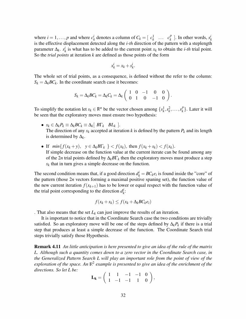
Remark 4.11 An little anticipation is here presented to give an idea of the rule of the matrixL. Although such a quantity comes down to a zero vector in the Coordinate Search case, inthe Generalized Pattern Search L will play an important role from the point of view of theexploration of the space. An R2 example is presented to give an idea of the enrichment of thedirections. So let L be:

Lk =

(1 1 −1 −1 01 −1 −1 1 0

),

32

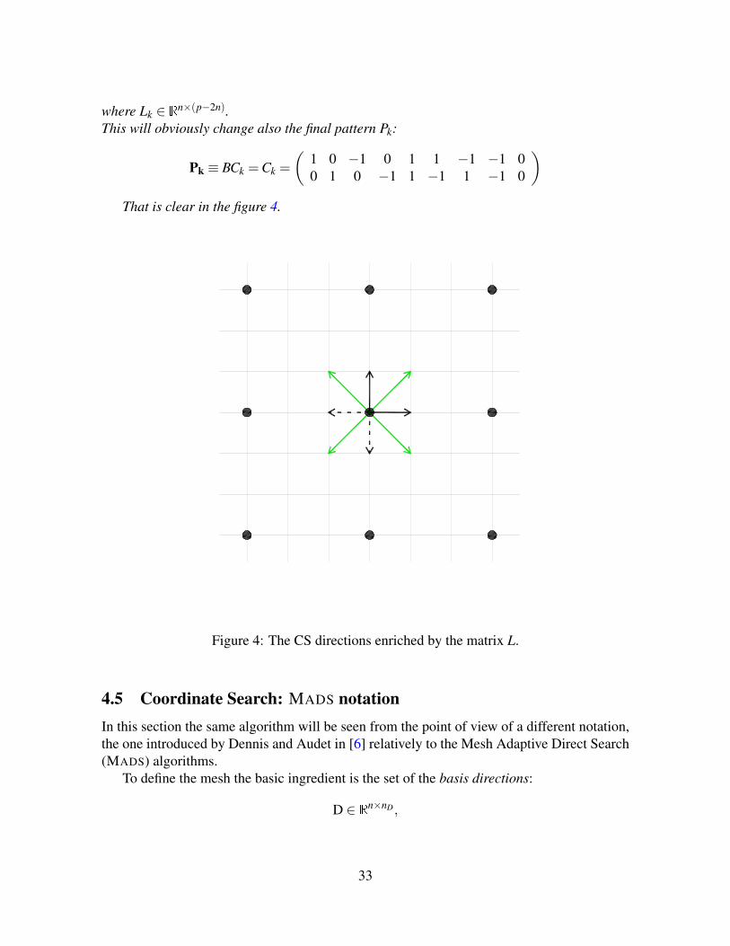
where Lk ∈ Rn×(p−2n).This will obviously change also the final pattern Pk:

Pk ≡ BCk =Ck =

(1 0 −1 0 1 1 −1 −1 00 1 0 −1 1 −1 1 −1 0

)That is clear in the figure 4.

Figure 4: The CS directions enriched by the matrix L.

4.5 Coordinate Search: MADS notationIn this section the same algorithm will be seen from the point of view of a different notation,the one introduced by Dennis and Audet in [6] relatively to the Mesh Adaptive Direct Search(MADS) algorithms.

To define the mesh the basic ingredient is the set of the basis directions:

D ∈ Rn×nD,

33

where the numerosity of this set has been named nD. In the MADS context D are required tobe a positive spanning set of directions (then nD ≥ n+1) such that it results:

D = GZ,

where G ∈ Rn×n is a nonsingular matrix, and Z ∈ Zn×nD is an integer matrix.Coming back to the aim of this subsection let see the specific matrices D, G and Z in the

Coordinate Search context. In this case G is the identity matrix (G = I) and Z = [ I −I ].That is an admissible choice since G is non-singular and Z is an integer matrix. It is nowpossible to compute the set of the basis directions:

D = GZ

= I[ I −I ]

=

(1 00 1

)(1 0 −1 00 1 0 −1

)

=

(1 0 −1 00 1 0 −1

),

hence, the basis directions are actually the coordinate directions.These basis directions, as said, define a conceptual mesh on which all the iterates of the

MADS algorithms are forced to lie. This mesh is named Mk and is described in the following:

Mk = xk +∆kDu : u ∈ ZnD+

In the Coordinate Search there is no difference between the basis directions and the di-rections chosen at iteration k. This is not generally true in the MADS algorithms, so now theemphasis is put on the difference between D and Dk. The columns of Dk are the directionschosen at the iteration k. For semplicity it can be seen as a real matrix, the dimension ofwhich depending on the number of directions considered. In general it should be said thatDk ∈ Rn×pk . To come down to the Coordinate Search case it can be fixed pk = p for everyk = 0,1,2, . . ., being able to write Dk ∈ Rn×p. In this case the relation between Dk and D isextremely simple because:

Dk = D , for every k = 0,1,2, . . .

meaning that the set of basis directions is presented unchanged at every iteration.

Remark 4.12 That connection was not made explicit at the time the Coordinate Search waspresented because the concepts of basis directions D and of trial directions Dk were simplycoincident. Nevertheless, this distinction that we are emphasizing is important relatively tothe introduction of the GPS and MADS, to prove that they are two generalizations of the CS.In this remark we present an anticipation of what will be said later:

34

• GPS: Dk ⊂ D.In that case, obviously, the set D will be chosen such to be a richer set respect withthe Coordinate Search one. At every step just a subset of the basis directions will bechosen in order to make the research quicker.

• MADS: if dk ∈ Dk then dk = Duk, where uk ∈ ZnD .This is just one of the three points of the definition of Dk made in the MADS case.Even just the fact that the definition is less linear suggests that the relation, in thatcase, is much more complicated than in the CS and GPS. Being this just one of thethree conditions defining the set Dk in the MADS context, actually only a subset of thedirections satisfying that condition will be candidates for belonging to Dk. The othertwo conditions will specify that the norm of the directions has an upper bound and thatthe limits of the chosen directions have to be positive spanning set as well. Althoughthe other two conditions will limit the choice of the directions to put in Dk in MADS

algorithm the choice of the directions will be much wider and will lead to importantconvergence results.

Coming back to the Coordinate Search case, a single phase providing the research ona certain region around the current point was presented. Such a region, called Poll regionsince it represents the space containing the poll points (or ”trial points”), depends on theparameter ∆k and on the norms of the directions in D. The Poll region has the followingmeaning: although the directions in D and the steplength parameter ∆k compose ideally amesh containing a certain number of points, at iteration k we are basically interested in asubset of the mesh points that are near the current iteration xk. Since limk→+∞ ∆k = 0 we areable to ensure that for k→+∞ the trial points will tend to collapse to xk. It means that, evenif ∆0 is too great to consider x0 +∆0d : d ∈ D the neighborhood of the examined problem,there will exist a k such that the points xk +∆kd : d ∈ D for k ≥ k are ”sufficiently” closeto the current point. In other words, indipendently from the norm of the directions in D, theamount ||∆kd|| → 0, hence xk +∆kd→ xk.

It is important to notice that for the Coordinate Search the step size ∆k has a doubleworthiness:

• it defines the mesh refinement;

• it defines the Poll region.

In other words the nearest points on the mesh are also the trial points (5).

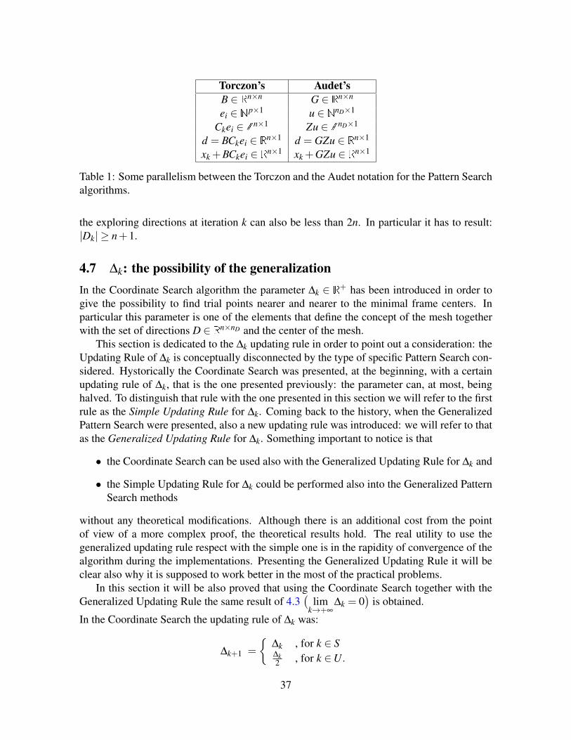
4.6 Coordinate Search: two notationsIn this subsection we briefly compare the notation used by Torczon and Dennis and the oneintroduced by Dennis himself and Audet.

In both the cases there is a basis matrix with real elements and satisfying the property tobe non-singular: for Torczon is B ∈ Rn×n while for Audet it is G ∈ Rn×n.

35

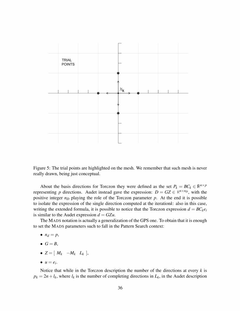
Figure 5: The trial points are highlighted on the mesh. We remember that such mesh is neverreally drawn, being just conceptual.

About the basis directions for Torczon they were defined as the set Pk = BCk ∈ Rn×p

representing p directions. Audet instead gave the expression: D = GZ ∈ Rn×nD , with thepositive integer nD playing the role of the Torczon parameter p. At the end it is possibleto isolate the expression of the single direction computed at the iterationk: also in this case,writing the extended formula, it is possible to notice that the Torczon expression d = BCkeiis similar to the Audet expression d = GZu.

The MADS notation is actually a generalization of the GPS one. To obtain that it is enoughto set the MADS parameters such to fall in the Pattern Search context:

• nd = p,

• G = B,

• Z = [ Mk −Mk Lk ],

• u = ei.

Notice that while in the Torczon description the number of the directions at every k ispk = 2n+ lk, where lk is the number of completing directions in Lk, in the Audet description

36

Torczon’s Audet’sB ∈ Rn×n G ∈ Rn×n

ei ∈ Np×1 u ∈ NnD×1

Ckei ∈ Zn×1 Zu ∈ ZnD×1

d = BCkei ∈ Rn×1 d = GZu ∈ Rn×1

xk +BCkei ∈ Rn×1 xk +GZu ∈ Rn×1

Table 1: Some parallelism between the Torczon and the Audet notation for the Pattern Searchalgorithms.

the exploring directions at iteration k can also be less than 2n. In particular it has to result:|Dk| ≥ n+1.

4.7 ∆k: the possibility of the generalizationIn the Coordinate Search algorithm the parameter ∆k ∈ R+ has been introduced in order togive the possibility to find trial points nearer and nearer to the minimal frame centers. Inparticular this parameter is one of the elements that define the concept of the mesh togetherwith the set of directions D ∈ Rn×nD and the center of the mesh.

This section is dedicated to the ∆k updating rule in order to point out a consideration: theUpdating Rule of ∆k is conceptually disconnected by the type of specific Pattern Search con-sidered. Hystorically the Coordinate Search was presented, at the beginning, with a certainupdating rule of ∆k, that is the one presented previously: the parameter can, at most, beinghalved. To distinguish that rule with the one presented in this section we will refer to the firstrule as the Simple Updating Rule for ∆k. Coming back to the history, when the GeneralizedPattern Search were presented, also a new updating rule was introduced: we will refer to thatas the Generalized Updating Rule for ∆k. Something important to notice is that

• the Coordinate Search can be used also with the Generalized Updating Rule for ∆k and

• the Simple Updating Rule for ∆k could be performed also into the Generalized PatternSearch methods

without any theoretical modifications. Although there is an additional cost from the pointof view of a more complex proof, the theoretical results hold. The real utility to use thegeneralized updating rule respect with the simple one is in the rapidity of convergence of thealgorithm during the implementations. Presenting the Generalized Updating Rule it will beclear also why it is supposed to work better in the most of the practical problems.

In this section it will be also proved that using the Coordinate Search together with theGeneralized Updating Rule the same result of 4.3

(lim

k→+∞∆k = 0

)is obtained.

In the Coordinate Search the updating rule of ∆k was:

∆k+1 =

∆k , for k ∈ S∆k2 , for k ∈U.

37

This can be generalized with a more general coarsening and refining of the mesh than theCS case. Mathematically this does not complicate anything, but in practise it can be veryuseful to make the steps of the algorithm larger when better solution are found.Refining. Halving the steplength parameter is just a way to decrease ∆k. Without additionalinformations on the problem no one could say that it is the best way to reduce the steps for thetrial points to get nearer to the minimal frame center. In general it is possible to implement:

∆k+1 = τwk∆k,

where τ > 1, τ ∈ Z is a constant and wk ∈ w−,w−+ 1, . . . ,−2,−1, with w− ≤ −1. Letnotice that it results: 0 < τwk < 1. When wk =−1 and τ = 2 then τwk = 1/2 and one falls inthe CS case.Coarsening. Following the same reasoning we say that setting ∆k+1 = ∆k surely is not thebest choice when k ∈ S. Actually the generalization of the coarsening is also more importantrespect with the one of the refining because it influences much more the speed of the method.Once one has found a better point in one of the trial points two are the possibilities: eitherthe steplength parameter ∆k has a ”right” length for the analyzed direction or going furtheralong that direction is possible to find better solutions. In other words, one could be such farfrom the local minimum that the chosen ∆k could be relatively ”too small” respect with thedimensions of the examined problem. The best thing, in that case, is to try larger steps:

∆k+1 = τwk∆k,

where τ> 1 is exactly the same used for the refining, but wk changes (wk≥ 0) making τwk ≥ 1.Hence wk ∈ 0,1,2, . . . ,w+. When wk = 0 then τwk = 1 and one falls in the CS case.

Another way to write the steplength control parameter is in the next theorem:

Theorem 4.13 Suppose that the Generalized Updating Rule for ∆k is used.Then

∆k = τrk∆o,

where rk ∈ Z.

Proof. Since ∆k+1 = τwk∆k, where wk ∈ Z is positive or negative depending on the outcomeof the iteration k, it is possible to reiterate the formula:

∆k = τwk−1∆k−1= τwk−1τwk−2∆k−2= τwk−1τwk−2τwk−3∆k−3= . . .= τwk−1τwk−2 . . .τ0∆0= τwk−1+wk−2+...+w0∆0= τrk∆0,

(4)

because even if wk can be positive or negative depending on the outcome of the iterations k,however rk is a sum of k integer number, i.e., rk is an integer numbers.

38

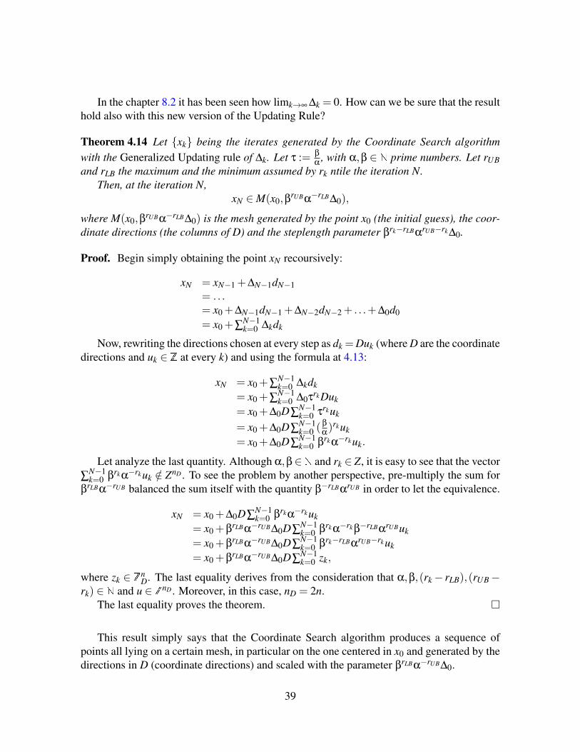
In the chapter 8.2 it has been seen how limk→∞ ∆k = 0. How can we be sure that the resulthold also with this new version of the Updating Rule?

Theorem 4.14 Let xk being the iterates generated by the Coordinate Search algorithmwith the Generalized Updating rule of ∆k. Let τ := β

α, with α,β ∈ N prime numbers. Let rUB

and rLB the maximum and the minimum assumed by rk ntile the iteration N.Then, at the iteration N,

xN ∈M(x0,βrUBα

−rLB∆0),

where M(x0,βrUBα−rLB∆0) is the mesh generated by the point x0 (the initial guess), the coor-

dinate directions (the columns of D) and the steplength parameter βrk−rLBαrUB−rk∆0.

Proof. Begin simply obtaining the point xN recoursively:

xN = xN−1 +∆N−1dN−1= . . .= x0 +∆N−1dN−1 +∆N−2dN−2 + . . .+∆0d0= x0 +∑

N−1k=0 ∆kdk

Now, rewriting the directions chosen at every step as dk =Duk (where D are the coordinatedirections and uk ∈ Z at every k) and using the formula at 4.13:

xN = x0 +∑N−1k=0 ∆kdk

= x0 +∑N−1k=0 ∆0τrkDuk

= x0 +∆0D∑N−1k=0 τrkuk

= x0 +∆0D∑N−1k=0 (

β

α)rkuk

= x0 +∆0D∑N−1k=0 βrkα−rkuk.

Let analyze the last quantity. Although α,β∈N and rk ∈ Z, it is easy to see that the vector∑

N−1k=0 βrkα−rkuk /∈ ZnD . To see the problem by another perspective, pre-multiply the sum for

βrLBα−rUB balanced the sum itself with the quantity β−rLBαrUB in order to let the equivalence.

xN = x0 +∆0D∑N−1k=0 βrkα−rkuk

= x0 +βrLBα−rUB∆0D∑N−1k=0 βrkα−rkβ−rLBαrUBuk

= x0 +βrLBα−rUB∆0D∑N−1k=0 βrk−rLBαrUB−rkuk

= x0 +βrLBα−rUB∆0D∑N−1k=0 zk,

where zk ∈ ZnD. The last equality derives from the consideration that α,β,(rk− rLB),(rUB−

rk) ∈ N and u ∈ ZnD . Moreover, in this case, nD = 2n.The last equality proves the theorem.

This result simply says that the Coordinate Search algorithm produces a sequence ofpoints all lying on a certain mesh, in particular on the one centered in x0 and generated by thedirections in D (coordinate directions) and scaled with the parameter βrLBα−rUB∆0.

39

Now this consideration is used to prove, even in the case with the generalized updatingrule of ∆k, that at the end the parameter goes to zero.

Theorem 4.15 Let xk being the iterations generated by the Coordinate Search algorithmwith the Generalized Updating Rule for ∆k.

Then:lim

k→+∞∆k = 0.

Proof. Using the formula in 4.13 that puts into relationship ∆k with ∆0: ∆k = τrk∆0, withrk ∈ Z. Reasoning always under the basic hypothesis that the iterations all lie in a boundedset, it follows that ∆k has to be bounded above, hence τrk∆0 ≤ ∆UB→ rk ≤ rUB.

To complete the inequality also from the bottom, let assume by contradiction that ∆kis also bounded below, i.e., that the theorem is false. As for the upper bound, from thedisequality τrk∆0 ≥ ∆LB it is possible to obtain that rk ≥ rLB.

So τrk will assume only a finite number of values, being

rk ∈ rLB,rLB +1, . . . ,rUB−1,rUB.

Using 4.14 it is possible to write: xN = x0 +βrLBα−rUB∆0D∑N−1k=0 zk, with a difference, that

rLB and rUB are the minimum and the maximum values get by rk not just until the iterationk = N but for all the k. It is possible to say that those values are finite values for what hasbeen said previously in this proof.

So all the iterates of the method lie on the mesh generated by x0 and the columns ofβrLBαrUB∆0D. That mesh contains infinite but numerable points, but, considering the basicassumption for which all the iterates lie on a bounded set it is possible to say that the pointsreachable from the method are a finite number. One of those mesh points inside the compactset has to be chosen by the method infinite times. Now it is enough to look at the generalizedupdating rule: although for a finite number of times the mesh can be coarsen, an infinitenumber of times the updating rule will decrease ∆k. After a certain iteration on the steplengthparameter will be exclusively decreased for an infinite number of times, meaning that ∆k→ 0,leading to the contradiction.

40

5 Generalized Pattern Search (GPS): introductionThe GPS is the second directional algorithm here presented, since also this class of methodsuse the same few directions to explore the space. It is the natural evolution of the CoordinateSearch method.

The GPS algorithms are a particular class of the direct search methods. This class isdifferent from the others direct search methods in the fact that search is pursued on sets ofpoints detecting a pattern and, in particular, that pattern does not depend on the objectivefunction values.

To prove convergence results for this kind of methods has been an open problem for yearssince the classical notion of sufficient decrease that is the basis to prove convergence resultsfor the line search and the trust region methods is not enforced by the pattern search methods.In this case all the convergence theory lies on the fact that it will be proved that the iteratesof these methods will lie on a certain mesh.

Virginia Torczon, in 1997, was the first who estabilished a strong theory for this branchof the Operational Research. She proved three results: Pattern Search methods are descentmethods; Pattern Search methods are gradient related methods; Pattern Search methods can-not terminate prematurely due to inadequate step lenth control mechanism. A very importanterole is played by the way in which the steplength parameter ∆k is managed that, together withthe invisible presence of an underlying mesh, prevents a pathological choice of the step.

Also without the esplicit knowledge of the gradient of f we will able to say that

liminfk→+∞

||∇ f (xk)||= 0.

In particular to obtain that result the Pattern Search methods do not use a notion of sufficientdecrease (as the Armijo-Goldstein-Wolfe conditions). Nevertheless there are subtle connec-tions with the line search and trust region methods.

It is here specified that the GPS will not be introduced with the notation used by Torczonherself (1997). It will be, instead, used the modified notation introduced by Dennis and Audetsuccessively (2000). Two are the reasons for this choice:

• the focus of the present thesis is the story-line that connects various works studyingthe evolution on the exploration of the space. This excursus will lead the reader to theMADS methods that are the last evolution of the Pattern Search methods for reasonsthat will be explained in the next chapters. It is an idea of the author that, in orderto represent the successive modifications clearly, speaking of the same objects withdifferent notations would introduce confusion.

• inside this process of unification the new (2000) notation is preferred respect with theTorczon one (1997) because it results much easier to understand.

Also in this case, for now, it will be taken the Unconstrained case. The reason is thatat first the target is to understand the evolution of the method from the perspective of theexploration of the space. In a second part of the thesis it will be taken into account theconstrained case presenting different approaches to deal with the constraints.

41

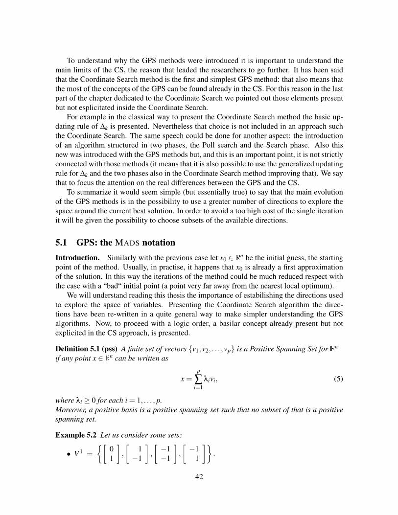
To understand why the GPS methods were introduced it is important to understand themain limits of the CS, the reason that leaded the researchers to go further. It has been saidthat the Coordinate Search method is the first and simplest GPS method: that also means thatthe most of the concepts of the GPS can be found already in the CS. For this reason in the lastpart of the chapter dedicated to the Coordinate Search we pointed out those elements presentbut not esplicitated inside the Coordinate Search.

For example in the classical way to present the Coordinate Search method the basic up-dating rule of ∆k is presented. Nevertheless that choice is not included in an approach suchthe Coordinate Search. The same speech could be done for another aspect: the introductionof an algorithm structured in two phases, the Poll search and the Search phase. Also thisnew was introduced with the GPS methods but, and this is an important point, it is not strictlyconnected with those methods (it means that it is also possible to use the generalized updatingrule for ∆k and the two phases also in the Coordinate Search method improving that). We saythat to focus the attention on the real differences between the GPS and the CS.

To summarize it would seem simple (but essentially true) to say that the main evolutionof the GPS methods is in the possibility to use a greater number of directions to explore thespace around the current best solution. In order to avoid a too high cost of the single iterationit will be given the possibility to choose subsets of the available directions.

5.1 GPS: the MADS notationIntroduction. Similarly with the previous case let x0 ∈ Rn be the initial guess, the startingpoint of the method. Usually, in practise, it happens that x0 is already a first approximationof the solution. In this way the iterations of the method could be much reduced respect withthe case with a “bad“ initial point (a point very far away from the nearest local optimum).

We will understand reading this thesis the importance of estabilishing the directions usedto explore the space of variables. Presenting the Coordinate Search algorithm the direc-tions have been re-written in a quite general way to make simpler understanding the GPSalgorithms. Now, to proceed with a logic order, a basilar concept already present but notexplicited in the CS approach, is presented.

Definition 5.1 (pss) A finite set of vectors v1,v2, . . . ,vp is a Positive Spanning Set for Rn

if any point x ∈ Rn can be written as

x =p

∑i=1

λivi, (5)

where λi ≥ 0 for each i = 1, . . . , p.Moreover, a positive basis is a positive spanning set such that no subset of that is a positivespanning set.

Example 5.2 Let us consider some sets:

• V 1 =

[01

],

[1−1

],

[−1−1

],

[−1

1

].

42

• V 2 =

[01

],

[1−1

],

[−1−1

].

• V 3 =

[10

],

[01

],

[−1

0

],

[0−1

].

• V 4 =

[01

],

[1−1

].

• V 5 =

[10

],

[01

],

[−1

0

],

[0−1

],

[11

],

[1−1

],

[−1−1

],

[−1

1

].

• V 6 =

[01

],

[11

],

[10

],

[1−1

],

[0−1

].

• V 7 =

[1b

]: b ∈ R

.

V 1, V 2, V 3, V 5 are all positive spanning sets though they have different features. The first oneis the dimension: V 5 contains 8 elements, whereas V 2 has just n+1 = 3 vectors. The amountn+1 is specified because it is the minimum number of directions that have the possibility tobuild a spanning set. This is the reason because the n = 2 vectors forming V 4 cannot be abasis, no matter how they are distributed.Neverteless it is not enough to have more than n directions to have a spanning set: V 6

contains 5 directions, but we could say that they are not properly distributed, because V 6

is not a positive spanning set. To prove that consider the point x =

(−10

)and the fact

that it cannot be obtained as a positive linear combination of the vectors in V 6. The same

reasoning could be done for all the vectors of the type x =

(−1a

), with a ∈ R. The same

reasoning is taken to an extreme with V 7. In this case it cannot be a positive spanning setfor two reasons: it is badly distributed in the space of variables and it is not a finite set ofdirections.

To conclude this example we point out a common point between V 2 and V 3: they are bothpositive spanning sets and, though they have a different number of elements in themselves, itis easy to verify that they are both positive bases. In particular they are called respectivelyMinimal Positive Basis and Maximal Positive Basis. This can be generalized, in fact, it hasbeen proved that in Rn a basis contains exactly n elements, while a positive basis contains anumber of elements p ∈ n+1, . . . ,2n.

To understand completely what it has been said in the example 5.2, the main property ofthe positive spanning set is presented:if Vpss = v1,v2, . . . ,vp is positive spanning set of Rn, in every half-space there is at least oneelement of Vpss. That also means that, if f is differentiable at a point x that is not stationary,then there is at least one direction vi ∈ Vpss that is strictly descent for f in x, i.e., for whichf ′(x;vi)< 0.

43

Directions and mesh. Since the topic of the directions is central here we wat to introducethem before the other elements making up the GPS world. understanding the way in whichthe space of variables is explored, in fact, means understanding the real differences of the GPSapproach with respectively its precursor (the Coordinate Search method) and its successiveevolutions (the Mesh Adaptive Direct Search algorithms).

Similarly with the Coordinate Search case, the first step is to define some basis directionsD ∈ Rn×nD , where nD ≥ n+1. Although it is not requested esplicitly, considering the reasonsfor which the GPS methods were born, it is pretty obvious that the upper bound for thenumber of the directions contained in D has to be greater than 2n: nD ≥ 2n. In order todo that two matrices are necessary: G and Z. Going back to the Coordinate Search we haddefined D as:

D = GZ = I [ I −I ] =

(1 00 1

)(1 0 −1 00 1 0 −1

).

That form actually represents the only condition requested on the matrix D. To make thatgeneral also G and Z have to be generalized:

• G ∈ Rn×n is a non-singular real matrix;

• Z ∈ Zn×nD is an integer positive spanning set for Rn.

This elements are enough to introduce a general concept of mesh on the space of variablesRn. The mesh centered at some point x ∈ Rn with a coarseness ∆ ∈ R+ is:

M(x,∆) = x+∆Du : u ∈ NnD.

The way in which the set D has been defined is not casual, but, instead, gives us the possibilityto obtain an important result on the points chosen on the mesh itself. It is summarized in thenext Lemma.

Lemma 5.3 For any x ∈ Rn, ∆ > 0:

minv1 6=v2∈M(x,∆)

||v1− v2|| ≥∆

||G−1||.

for any norm ||.|| such that, applied to an integer vector gives back a value greater or equalto 1.

The classical norms satisfy the Lemma 5.3.Proof. Since v1,v2 ∈M(x,∆), there exist two integer scalars u1,u2 ∈ ZnD such that:

• v1 = x+∆Du1;

• v2 = x+∆Du2.

44

Notice that v1 and v2 not coincident, or u1 6= 0, or u2 6= 0 or both the scalar are nonzero.Rewrite the norm:

||v1− v2||= ∆ ||D(u1−u2)||= ∆ ||GZ(u1−u2)|| (6)

.For what it has been said above u1−u2 6= 0. It is also easy to check that Z is not the zero

vector, since Z is a positive spanning set for Rn. It also means that Z(u1−u2) 6= 0. Moreover,considering that u1,u2 ∈ Z and that Z ∈ Zn×nD it results: ||Z(u1−u2)|| ≥ 1.

Now multiply inside the norm of the last element of the equation 6 for the inverse of thematrix G (it exists because G has been supposed to be a non-singular matrix).

||v1− v2||= ∆

∣∣∣∣∣∣∣∣G−1GZ(u1−u2)

G−1

∣∣∣∣∣∣∣∣= ∆

||G−1||||Z(u1−u2)|| ≥

∆

||G−1||. (7)

The meaning of the Lemma is simple and fundamental as well. Fixed a certain mesh on thespace any two points on the mesh cannot be arbitrately near each other. At the same time, seendifferently, it also is a condition on the upper value of the ∆: lying all the iterates on a compactset (besides on the mesh) we can affirm that ||v1− v2|| < +∞; being also

∣∣∣∣G−1∣∣∣∣ < +∞,∣∣∣∣G−1

∣∣∣∣ ||v1− v2|| represents an upper bound for ∆. Summarizing, if ∆ was greater of a certainupper bound the distance between two mesh points could be larger than the diameter of thebound region X on which all the iterates have to lie. So at least one of the two points v1 andv2 would be outside the allowed region.

In general nD can be much greater than 2n. That also means that a choice of directions asDk = D at every iteration is possible but also impracticable. Such consideration leaded to thesecond important new of the GPS methods respect with the previous CS method. Here theemphasis is put on the difference between D and Dk. The columns of Dk are the directionschosen at the iteration k. For semplicity it can be seen as a real matrix, the dimension of whichdepends on the number of directions considered. In general it should be said that Dk ∈ Rn×pk

has to satisfy the condition of being a positive spanning set of Rn and such that:

Dk ⊆ D, for all k = 0,1,2, . . . .

In other words, even having a richer set of available directions to explore the space, it ispossible to choose just a subset of D at every iteration. Using DCS to refer to the coordinatedirections and DGPS for the basis directions in the GPS case, it is possible to write that:usually DCS ⊂ DGPS.

Remark 5.4 In general it should be said that Dk ∈ Rn×pk . To come down to the CoordinateSearch case it can be fixed pk = p for every k = 0,1,2, . . ., being able to write Dk ∈ Rn×p. Inthis case the relation between Dk and D is extremely simple because:

Dk = D , for every k = 0,1,2, . . .

meaning that the set of basis directions is presented again without modifications at everyiteration.

45

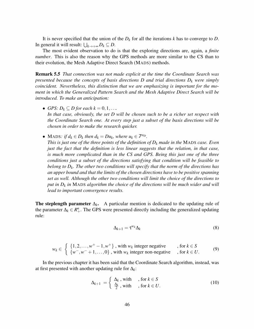
It is never specified that the union of the Dk for all the iterations k has to converge to D.In general it will result:

⋃k→+∞ Dk ⊆ D.

The most evident observation to do is that the exploring directions are, again, a finitenumber. This is also the reason why the GPS methods are more similar to the CS than totheir evolution, the Mesh Adaptive Direct Search (MADS) methods.

Remark 5.5 That connection was not made explicit at the time the Coordinate Search waspresented because the concepts of basis directions D and trial directions Dk were simplycoincident. Nevertheless, this distinction that we are emphasizing is important for the mo-ment in which the Generalized Pattern Search and the Mesh Adaptive Direct Search will beintroduced. To make an anticipation:

• GPS: Dk ⊆ D for each k = 0,1, . . ..In that case, obviously, the set D will be chosen such to be a richer set respect withthe Coordinate Search one. At every step just a subset of the basis directions will bechosen in order to make the research quicker.

• MADS: if dk ∈ Dk then dk = Duk, where uk ∈ ZnD .This is just one of the three points of the definition of Dk made in the MADS case. Evenjust the fact that the definition is less linear suggests that the relation, in that case,is much more complicated than in the CS and GPS. Being this just one of the threeconditions just a subset of the directions satisfying that condition will be feasible tobelong to Dk. The other two conditions will specify that the norm of the directions hasan upper bound and that the limits of the chosen directions have to be positive spanningset as well. Although the other two conditions will limit the choice of the directions toput in Dk in MADS algorithm the choice of the directions will be much wider and willlead to important convergence results.

The steplength parameter ∆k. A particular mention is dedicated to the updating rule ofthe parameter ∆k ∈ Rn

+. The GPS were presented directly including the generalized updatingrule:

∆k+1 = τwk∆k (8)

wk ∈1,2, . . . ,w+−1,w+ , with wk integer negative , for k ∈ Sw−,w−+1, . . . ,0 , with wk integer non-negative , for k ∈U.

(9)

In the previous chapter it has been said that the Coordinate Search algorithm, instead, wasat first presented with another updating rule for ∆k:

∆k+1 =

∆k , with , for k ∈ S∆k2 , with , for k ∈U.

(10)

46

As it is easy to realize the 11 is the generalization of 10. It has been presented brieflythe formula in 11 to create the parallel with the 10 before giving the extended version. Thereason is pointing out the disconnection between the algorithms and the updating rules of thesteplengths of the algorithms themselves. For this purpose it has been added a chapter in theCoordinate Search section to prove that it is possible to prove covergence of the CoordinteSearch also using a different updating rule for ∆k than the ”classical” one. In the same way,being the 11 the generalization of the other, it is easy to say that applying the simple updatingrule for ∆k to the GPS approach will give the same identical convergence results.

Extrapolating the condition that an updating rule has to satisfy for the algorithm respect-ing the convergence results:

∆k+1 =

≥ ∆k , for k ∈ S< ∆k , for k ∈U.

(11)

where ∆kk∈U → 0.That means that, for infinitely many unsuccess iterations the parameter ∆k cannot convergeto a value strictly positive, but it has to get the zero.

The mesh. Before it has been presented a general concept of the mesh M(x,∆;D) identify-ing a single mesh centered on a point x and generated by the directions in D with a coarsenesslevel equal to ∆.Adapt this concept to a mesh on which the iterates of the algorithm have to lie requires an ad-ditional complication. In fact, during the algorithm, as it has seen in the previous paragraph,∆k will assume infinite values, and not just the one required by the general definition of themesh. The same can be said for the center of the mesh x since we have an infinite number ofpoints xk.

The only way to make all the iterations produced in this way lie on a mesh is to definethat as the union of the meshes centered at the visited points, keeping the coarseness constantand equal to the current steplength value, ∆k. It means that, at iteration k, all the meshesare considered of the same coarseness. To express that in formulas it is necessary to identifythe set of the visited points: Vk is the set of points in which the objective function has beenevaluated. In particular V0 is the initial set given by the user and it can be formed by a singlevalue x0 or a set of values. Also in this second case it is necessary to take the points suchthat V0 ⊂M(x0,∆0), i.e., there is some mesh containing all the initial points. Nevertheless, atleast the directions forming the mesh D are fixed in the GPS. So the set of points on whichthe algorithm has to select the trial point is in the following definition.

Definition 5.6 Suppose the algorithm is arrived at iteration k, the current mesh is defined asthe union:

Mk =⋃

x∈Vk

M(x;∆k) = x+∆kDu : u ∈ NnD,x ∈Vk.

47

It is easy to see that the parameter ∆k manages the coarseness or fineness of the mesh.Varying ∆k with the proceeding of the algorithm, also the mesh Mk will vary its ”density” onthe space of variables.

The importance of this concept is understandable looking at one of the two phases con-stituting the GPS structure of the algorithm: the search phase.This phase attempts to find a point on the mesh with the objective function lower than theincumbent value. Two are the possibilities:

• argminx f (x) : x ∈Vk∩X= argminx f (x) : x ∈Mk∩X;In this case there not exists a point on the mesh having the objective function valuelower than the incumbent (defined on the set Vk). It will be necessary to skip to the pollphase.

• if x∗k ∈Mk∩X is such that x∗k = argminx f (x) : x ∈Mk∩X and f (x∗k)< f (xk).This is the most interesting place because effectively there exists a point on the meshand into the allowed region X that is better on the incumbent one. Later it will be seenas exploiting mathematical tools to make this phase useful. For noww it is importantjust to notice that we do not have the certainity to detect the improved point, though itexists on the mesh. The only possibility to do that would be to explore all the points onthe set Mk∩X , but it is also impracticable in the reality.

Search and Poll. Iin the last paragraph we touched on the concept of search. Here it isexplained with more attention because the search itself represents, together with the newconcept of trial directions, the real difference with the Coordinate Search. In that case it hasbeen analyzed a region of exploration representing the neighborhood of the current solution.Changing the concept of Dk, fixed ∆k, it is possible to adapt that definition. The set of thepoints lying on the mesh near the current solution are called here poll points, to differentiatethem from the search points (the new of the GPS algorithm). Different but strictly related isthe concept of poll region, i.e., that region in which the poll points lie.

To simplify it would be possible to give to the poll region the following meaning: althoughthe directions in D and the steplength parameter ∆k ideally compose a mesh containing infi-nite points, at iteration k the poll is basically interested in that subset of the mesh that is nearthe current iteration xk.

Definition 5.7 At iteration k the frame used in the poll step is defined as the set:

Pk = xk∪xk +∆kd : d ∈ Dk,

where Dk ⊆ D is a positive spanning set, and xk is defined the frame center.

Just notice that if it was limk→+∞ ∆k = 0 we would be able to ensure that for k→ +∞

the trial point will tend to collapse to xk. It means that, even if ∆0 is too great to considerthe points x0 + ∆0d : d ∈ D ”neighbour” for x0, there will exist a k for which the pointsxk +∆kd : d ∈ D are ”sufficiently” (it depends on the dimensions of the examined problem)

48

close to the current point. In other words, indipendently from the norms of the directions inD, the amount ||∆kd|| → 0, hence xk +∆kd→ xk.

A common feature between the Coordinate Search and the GPS algorithms is that the stepsize ∆k has a double worthiness:

• it defines the mesh refinement;

• it defines the Poll region.

In other words the nearest points on the mesh are also the trial points (5.7).What about the search phase? It will be seen in 5.9 that the search is executed before

the poll. It makes perfectly sense, because the search is simply an additional freedom degreepermitted to the algorithm before looking around the current solution.It also gives to the concept of the mesh the right practical meaning. In fact, in this phase, inorder to preserve the convergence theory based on the fact that all the points generated bythe algorithm lie on the mesh, the mesh is the tool that leads the search. The central problemabout the search is the way in which a good point is found on the mesh. We remember tobe in a situation in which every function evaaluation is costly. This means that ideally wewould like to evaluate as few points as possible. In a certain sense, every evaluation on apoint that is worse than the current solution is a waste of resources and of time (variablethat is often crucial in the Derivative-Free problems). That being so, it is evident that thedangerousness of the search phase. In fact, if on a side it could increase significantly therapidity of convergence of the algorithm, on the other side it depends on the points chosento be evaluated. We speak of candidate points in the sense that actually the search doesn notdetect a point that is better than the current solution but, if well done, it will detect a pointthat has an high likelihood to be better than the current solution.To do that usually the so-called surrogate functions are used. The better the surrogate functionS(x) approximates the real function f and the more dependable are the results given by thesurrogate function. In particular the two function do not have to be similar on the whole spaceof variables but it is enough to be similar in the mesh points.

Example 5.8 Suppose that there exist two surrogate function of f : S1(x) and S2(x). Supposethat S1(x) is the perfect surrogate: S1(x) = f (x) for each x ∈ X. At the contrary S2(x) 6= f (x)but the surrogate is done such that S2(x) = f (x) for each x ∈Mk∩X.At iteration k, though one of the two functions approximates f infinitely better than the otherone, the two surrogates are equivalent from out point of view.

In particular there exist two type of surrogate functions:

• S(x) is a physical model, less precise than f (x) but also less expensive to evaluate.

• S(x) is a mathematical approximation of f (x), so it is not conceptually related to thereal function but it is computed relying on the evaluated points.

Although here it is spoken about this phase, the discussion is made deiberately very gen-eral. In the follow it will be presented a new practical way to use this phase: the Back-trackingsearch.

49

The search, producing at every iteration k points lying on the mesh Mk does not affect theconvergence theory based on the poll.

When either the search and the poll fail in detecting an improved mesh point, the pointxk is called minimal frame center, since it is the best point of the frame Pk. Notice that if thesearch does not fail the point xk is discarded so, even if it could be the best point in its frame,there is another point arbitrarily far but on the mesh that is better, so it would be inappropriateto call it a ”minimal” point.

50

Algorithm 5.90 - Initialization: Let f : Rn→ R be given.

Let x0 ∈ Rn be the initial guess of solution.Let ∆tol > 0 be the tolerance of the step-length parameter.Let ∆0 > ∆tol be the initial step-length parameter.Let D be the basis directions of the Generalized Pattern Search algorithm.Let w− ∈ Z, w− ≤−1.Let w+ ∈ Z, w+ ≥ 0.

k = 0.

SEARCH if a point xS ∈Mk∩X is found such that f (xS)< f (xk), then

• ∆k+1 = ∆k;

• xk+1 = xS;

• skip to the Step 4.

POLL

1 - Choice of the directions: For each k = 0,1,2, . . .

a subset Dk ⊆ D of pk direction is chosen.

2 - Successful iteration: if ∃ dk ∈ Dk such that f (xk +∆kdk)< f (xk), then:

• set xk+1 = xk +∆kdk;

• set ∆k+1 = τwk∆k, with wk ∈ Z, 0≤ wk ≤ w+;

• go to the Step 4.

3 - Unsuccessful iterations: Otherwise (if f (xk +∆kdk)≥ f (xk) for all d ∈ D):

• set xk+1 = xk;

• set ∆k+1 = τwk∆k, with wk ∈ Z, w− ≤ wk ≤−1;

• if ∆k+1 < ∆tol , then terminate.

4 - k = k+1 and go back to the search.

51

5.2 Convergence analysis of the Generalized Pattern Search algorithmsThe convergence analysis is divided in two conceptual steps. We first is about the steplengthparameter ∆k. The second one is about the convergence of the iterations. Initially focus theattention on the form of the steplength parameter itself respect with the initial value:

∆k = τrk∆0, where τ ∈ R is such that τ > 1 and rk is an integer number depending on theoutcome of the iterates until the iteration k. The greater is the number of successes amongthe first k iterates the greater is rk; the lower is the number of unsuccessful iterations until k,the lower is rk. Depending on the version used rk can be augmented or not at every k ∈ S but,for sure, it is decreased at every k ∈U .

Ensuring that the reason will be clear in the following rows, two measures are fixed:

rLBk = min

0≤i≤kri, (12)

rUBk = max

0≤i≤kri. (13)

It follows that rLBk ≤ rUB

k for every k = 0,1,2, . . ..Repeating the same reasoning for k→+∞, we write:

rLB = min0≤i<+∞

ri, (14)

rUB = max0≤i<+∞

ri<+∞. (15)

A priori nothing can be said on the lower bound of rk while, for the upper bound we recall thatall the iterates lie on a bounded set. Since the norm of the longer direction is fixed, it meansthat ∆k has to be bounded above (∆k = τrk∆0 ≤ ∆M). Being ∆0 fixed it becomes a conditionon the upper bound of τrk , hence on rk: rUB < +∞, i.e., it exists a finite upper bound on rk.About the lower bound rLB it will be important on the convergence proof in the following.

Theorem 5.10 The generic point at iteration k+1 can be written as

xk+1 = x0 +(βrLBk α−rUB

k )∆0Dk

∑i=1

ui,

where

• x0 ∈ Rn is the initial guess;

• ∆0 ∈ R+;

• D ∈ Rn×nD;

• β,α ∈ N relatively prime, with β > α such that τ≡ β

α(hence τ ∈ Q);

• ui ∈ NnD , for each i = 1,2, . . . ,k.

52

Proof. We start writing the generic iterate.

xk+1 = xk +∆kdk= xk−1 +∆k−1dk−1 +∆kdk= xk−2 +∆k−2dk−2 +∆k−1dk−1 +∆kdk= x0 +∑

ki=1 ∆idi.

Considering that dk = Duk, where uk ∈NnD is a vector with all zeros and 1 correspondingto the chosen direction (it would not be right to speak of ”coordinate direction” because uk isnD-dimension, and not n):

xk+1 = x0 +∑ki=1 ∆iDui.

Using the expression of ∆k related to its initial value ∆0: ∆k, jk = τrk∆0. Again, the expressionof xk becomes:

xk+1 = x0 +k

∑i=1

τrk∆0Dui.

To understand what we are going to do in the next rows, let see xk+1 in another way:

xk+1 = x0 +∆0D( k

∑i=1

τrkui

).

Between parenthesis there is a vector. If it was an integer vector that would be the typicalexpression of points lying on a mesh. Unfortunately, it is evident that, being τ not integer alsothat amount cannot be integer. We cannot say that xk+1 belongs to the mesh defined by thecolumns of D scaled of ∆0. Nevertheless, there is another mesh containing the iterates untilk+1.

We use the fact that τ is fractional:

xk+1 = x0 +∆0D[

∑ki=1

(β

α

)ri

ui

]= x0 +∆0D

[∑

ki=1

((β)ri(α)−ri

)ui

].

Here the quantities rLBk , rUB

k are used to isolate a part inside the sum.

xk+1 = x0 +∆0

(β

rLBk α−rUB

k

)D[ k

∑i=1

((β)ri−rLB

k (α)rUBk −ri

)ui

].

To understand the reason of this mathematical trick, notice that β, α are all integer positivenumbers, raised to the power of natural numbers (ri− rLB

k , rUBk − ri ∈ N).

It follows that, for every i ∈ 0,1, . . . ,k,((β)ri−rLB

k (α)rUBk −ri

)∈ N,

53

and the quantity between the square parenthesis is an integer positive vector u. It followsthat:

xk+1 = x0 +∆0

(β

rLBk α−rUB

k

)D

k

∑i=1

ui.

Also if it could seem counterintuitive the meaning of this theorem is extremely simple:at every finite iteration k the iterate xk lies on a mesh. In fact, being ui ∈ ZnD , it results∑

ki=1 ui = u. Then it is possible to write the generic iterate as

xk+1 = x0 +

[(βrLB

k α−rUB

k )∆0

]Du,

with u ∈ ZnD , meaning that the iterate xk+1 belongs to a mesh generated by the directionscontained in the columns od D and scaled by the factor βrLB

k α−rUB

k ∆0. For finite k it results:

rLB ≤ rLBk ≤ rUB

k ≤ rUB, for every k.

While it is easy the reasoning for a finite iteration k, nothing can be said for k→+∞. Asit has been said, in fact, we cannot say that rLB has a lower bound.

Remark 5.11 For a moment suppose that rLB is a finite value. Intuitively, analyzing themultipliers of ∆0D, it would results:(

βrLB

αrUB

)<

(βrLB

k

αrUBk

).

That means that the final mesh on which all the iterates have to lie is a finer mesh.

Theorem 5.12 If the iterates of the algorithm 5.9 lie all in a bounded set, then

liminfk→+∞

∆k = 0.

Proof. What has been said until now is that, since the assumption that all the iterates xkhave to lie on a bounded set:

• rUBk <+∞.

• rUB <+∞.

Nothing has been said about the lower bounds relative rLBk and absolute rLB

k . It depends onthe value of ∆k. Proceeding by contradiction suppose that ∆k has a lower bound: 0 < ∆LB ≤∆k.Moreover, since all the iterates have to lie in a bounded set, ∆k has to be limited above:

54

∆k ≤ ∆UB <+∞.Summarizing:

0 < ∆LB ≤ ∆k ≤ ∆

UB <+∞.

The previous condition can be conceptually transferred to the parameter rk re-writing thedisequality:

0 < ∆LB ≤ τ

rk∆0 ≤ ∆UB <+∞.

Noticing that γ jk is a finite amount for every k it is possible to write:

0 < τLB ≤ τ

rk ≤ τUB <+∞.

The bounds ∆LB and ∆UB can be conveniently chosen such that ∆LB = τrLB∆0 and ∆UB =

τrUB∆0. Being that so it is possible to transfer the limits on the steplength (it is convenient to

remember that one of the two is given by the absurd hypothesis) to limits on rk:

rk ∈ rLB,rLB +1, . . . ,rUB−1,rUB.

Coming back to the previous theorem 7.3, we see that the generic iteration xk+1 can bewritten as:

xk+1 = x0 +(βrLBk α−rUB

k )∆0Duk, (16)

where uk ∈ NnD . It means that at iteration k + 1 the points found so far have to lie on amesh centered in x0 and generated by the directions contained in D scaled by the quantity

(βrLB

k1 α

−rUBk

1 βjLBk

2 α− jUB

k2 )∆0.

What happens for k→+∞? Having stated that

rLB = min0≤k<+∞

rk >−∞

it is possible to substitute the global value for the minimum and maximum of rk concludingthat the whole sequence xk has to belong to the mesh centered in x0 and generated by thedirections contained in D and scaled by the factor (βrLB

α−rUB)∆0. Note that without setting

the upper bound on rk it would have been impossible to ensure that tha scaled factor of themesh was a finite value.

So it exists a mesh M(x0;D;βrLBα−rUB

∆0) that contains all the iterates of the sequencexk generated by the algorithm 5.9. Obviously, since all the iterates have to lie on a boundedset and at the same time on the particular mesh shown above, and since the intersection ofthe two sets is a finite set of points, it follows that infinite points of the sequence xk have tocoincide to a point of this finite set of points:

xk = x, for an infinite subset k ∈ K ⊂U.

Then, looking at the updating rule of the steplength parameter ∆k, we see that ∆k is increaseda finite number of times and decreased infinitey many times (for k ∈U).It would result ∆k→ 0, that represents a contradiction respect with the absurd hypothesis.

55

To give a meaning to the fact that limsupk→∞ ∆k = 0 it is possible to think to the sequencerelated to that parameter. It means that we cannot be sure that for each sequence producedby the GPS the steplength parameter goes to zero, but what it can be said is that there existsat least one subsequence for which the successive udpates of ∆k makes it tending to zero. Inparticular we can focus the attention on a particular subsequence, i.e., the one xkk∈K forwhich, for all the k ∈ K there is a decrease of the steplength parameter: ∆K < ∆k−1 for eachk ∈ K. The points of the sequence for which this decrease is applied are the ones for whichno better points are found between xk+∆kd : d ∈Dk. These points are called mesh isolatedpoints.

Notice that defining a point x ∈ Rn as a mesh isolated point does not mean that x is aminimizer for the function f . It simply means that for the set of directions Dk and for thesteplength ∆k chosen at iteration k, in the ”neighborhood” of that point, x itself is the bestone. There could be one direction d ∈ Dk that improves the function value for another valueof the steplength parameter, or, vice versa, there could be another direction d /∈ Dk for whichf (x+∆kd) < f (x). Nevertheless, the Poll step P = x∪x+∆kDk declares x as the bestpoint in its neighborhood. x is also a mesh local optimizer.

In order to identify that subsequence of the mesh isolated local points the following defi-nition is reported.

Definition 5.13 Let xk be the sequence of the iterates produced by the GPS algorithm. Ifxkk∈K is a subsequence composed of mesh local optimizer such that

limk∈K

∆k = 0

then xkk∈K is called refining subsequence.

Theorem 5.14 Suppose that the iterates xk produced by the algorithm GPS lie in a boundedset. Let xkk∈K being a refinign subsequence converging to the point x ∈ Rn.If f is strictly differentiable at x, then

∇ f (x) = 0.

Proof. Since f is strictly differentiable at x the directional derivative along the direction d iswritable throught the gradient of f : f ′(x;d) = ∇ f (x)T d.Since x is a converging point for the algorithm GPS , in that point every iteration will resultunsuccessful. It follows that an infinite number of positive spanning set will be produced at x.Now, D represents a finite number of directions, so the different positive spanning sets that ispossible to extrapolate from D are finite as well. It means that at least one subset D⊆D beinga positive spanning set is produced an infinite number of times. For each direction v ∈ D ofthe positive spanning set it results f (x)≤ f (x+∆kv), and hence:

0≤ f (x+∆kv)− f (x)

56

Dividing for ∆k > 0 the inequality holds.

0≤ f (x+∆kv)− f (x)∆k

The form obtained recalls the Newton’s difference quotient. To obtain the concept of direc-tional derivative it is necessary to consider k→ ∞ and, in particular the subset k ∈ K becausein the concept of derivative the parameter at denominator has to tend to zero. While we can-not be sure that for k→ ∞ the steplenght parameter goes to zero, on the other hand it surelyhappens for k ∈ K. It is so possible obtaining the directional derivative.

0≤ limk∈K

f (x+∆kv)− f (x)∆k

= f ′(x;v)

Moreover, being f differentiable at x then the gradient is defined in x and it is possible towrite that, for each direction v ∈ D:

0≤ f ′(x;v) = ∇ f (x)T v.

At last we use the fact that D is a positive spanning set to state that, given a genericdirection d ∈ Rn

Nonsmooth functions. Until now it has been supposed f being a smooth function. Thissmoothness has been translated as the differentiability of the function f is some interestingconverging points.

In the next chapterss, before speaking about the MADS algorithms, the theoretical limita-tions on the function will be relaxed and ”nonsmooth” functions will be analyzed.

In order to give continuity to our analysis here it is showed a result on the nonsmoothfunction to underline the parallel with the result stated in Theorem 5.14. Only the alreadyexpert readers will understand its meaning. For the others it is suggested to come back tothis theorem after the concepts of Clarke directional derivative and Lipschitzianity will bepresented.

Theorem 5.15 Suppose all the iterates xk lie in a bounded set. Suppose that x is the limitof a refining subsequence xkk∈K and that d ∈ D is a direction along which the poll stepsare evaluated infinitely many times for k ∈ K.If f is Lipschitz near the point x, then:

f o(x;d)≥ 0.

Proof. Since f Lipschitz near a point x it is possible defining the Clarke directional derivativein that point:

f o(x;d) = limsupy→ xt ↓ 0

f (y+ td)− f (y)t

≥ limsupk∈K

f (xk +∆kd)− f (xk)

∆k≥ 0.

57

The last inequality derives by the fact that the refining subsequence contains only mesh localoptimizer. This also means that f (xk +∆kd)≥ f (xk) and so f (xk +∆kd)− f (xk)≥ 0.

5.3 GPS: limitationWhat is resulted from the previous analysis is that the real news of this methods respectwith the first Coordinate Search method is the introduction of a new phase, the search, and adifferent concept of the exploration of the space.

THe GPS, in fact, allow more freedom about the choice of the directions Dk, thanks toa richer set of basis directions D. Denoting with DCS the basis directions of the CoordinateSearch approach and with DGPS the basis directions used by a generic GPS method it results:

• nDCS = 2n;

• nDGPS ≥ n+1;

where, if it was exactly nDGPS = n+1, then DGPS would be a minimal positive spanning set.It would also mean that there would not be subsets of DGPS forming a positive spanning set(that is the only requirement on the set Dk), so it would result: Dk = DGPS at every step k (aforced choice of directions).

In the practice it obviously never happens since the strength of the generalization of theGPS is that an higher number of exploring directions are allowed. In this way also a bettercovering of the space is permitted, not on the single iteration, but into the whole process.

So, even if the single set of directions Dk can also have a number of elements less than2n, about the basis directions it results:

nDCS << nDGPS .

But it is just the exploring structure of the space the real limitation of these kind of meth-ods: What happens at the end of the method is that

∞⋃k=1

Dk ⊆ D,

and D, as it has been said, is a finite set of directions.Relying on the number and the distribution of the directions in D, the space of variables

may be covered properly or not, but there will always be an infinite number of directions dnot explored by the GPS methods because d /∈ D.Coming back to the example of the lost man on the mountain, supposing he moves on discretedirections, if he try to go towards north, north-east, east, sud-east, sud, sud-west, west. north-west and if he is in a basin with a single descent way between sud-east and sud, his trialdirections will not be enough to come down from the mountain.

Tha classical example, used historically to understand the differences between the CS andGPS, the canoe function, can also be used to understand the limits of the GPS themselves.

58

f (x) = (1− exp(−||x||2))×max||x− c||2 , ||x−d||2,

where c =−d = (30,80)T .That function is not just locally Lipschitz but it is also strictly differentiable at x∗ = (0,0)T ,that is its local optimizer. Starting from x0 = (−3.3,1.2)T and using the coordinates as basisdirections of the GPS method it collapse to the point (−3.2,1.2)T . From that point on theGPS is not able to detect descent directions even though (−3.2,1.2)T is not the minimal ofthe function f . Clearly, as it is possible to see in figure, it exists a descent direction d for thefunction in (−3.2,1.2)T , but that direction is not in the used D.Someone could notice that it would be enough to change the set of directions as D = D∪ dfor the method to work, but still it remains the fact that depending on the problem, withoutknowing a priori the features of the examined problem, the GPS can fail and stop in a non-stationary point.

It is also obvious that, when dealing with the ”simple” cases, the f differentiable on thewhole Rn a spanning set of directions is enough to converge to a stationary point. In thatcase, in fact there would always be a direction in the positive spaning set lying on the half-space defined by the vector −∇ f (x). So, when ∇ f (x) 6= 0 at least a directions in the positivespanning set is a descent direction.

So, in general for non-smooth functions, the GPS can fail in finding a stationary point ofthe function f because of the finite number of exploring directions.

59

6 LinesearchBefore continuing to analyze the evolutions of the Pattern Search methods we want to give alook to their parallel approach: the Linesearch based methods. We speak specifically abouta parallel method and not about another way to see the same resolution methods because,although the two approach have feed each other during the years, their basis concepts aretheeoretically different:

• the convergence theory of the Pattern Search methods, as it has been seen for the CS inthe previous section, relies on the fact that their iterates lie all on a certain conceptualmesh.

• the convergence theory does not ask to the iterates to lie on a mesh but it asks a stricteracceptance criterion for a successful trial point, i.e., the new point has to produce asufficient decrease of the objective function in order to be accepted.

The differentiable case. The classical approach to introduce the Lineasearch concepts andprobably the most effective one is to pick the differentiable case, mainly meaning that thegradient ∇ f (x) does not only exist, but it is also known. The first advantage is that a directiond taken in a certain point x can be identified as ”descent” if it results:

−∇ f (x)T d > 0.

To understand why it is so let consider tha Taylor series of the function f cutted at the firstderivative:

f (x+αd) = f (x)+α∇ f (x)T d +o(α).

If d is a descent direction and α > 0 is a small enough scalar, then x+αd reduces the valueof the objective funtion f . This observation is the basis of the linesearch methods: at thegeneric iteration k, a Linesearch method chooses a descent direction dk and searches alongthat direction for a point xk+1 = xk +αkdk, where αk > 0 is such that f (xk+1)< f (xk).There are some standard choices of the directions that ensure a descent direction as the steep-est descent direction dk = −∇ f (xk) (from which the Steepest Descent method takes the de-nomination), or the Newton direction dk = −B−1

k ∇ f (xk) (where Bk = ∇2 f (xk), supposingalso the second derivatives are known) that incorporates also the curvature informations of f .

The main point is that the simple decrease f (xk+1)< f (xk) cannot ensure the convergenceto a stationary point of f .

Torczon presented two particular sequences to prove the insufficiency of the simple de-crease, considering a very simple example: f (x) = x2. Notice that the minimum of f istrivially x∗ = 0.

Example 6.1 (First trap: too short steps) The first one, xk = (−1)k(1 + 2−k), with limitpoints ±1 to show that taking steps too long might prevent the convergence to a stationarypoint (that is also the global minimum in this particular case) though the sequence decreasescontinuously the function value for k→+∞.

60

Example 6.2 (Second trap: too long steps) If the shortness was the only problem it wouldbe relatively simple to estabilish a minimum threshold. The second example shows that alsotoo long steps may cause the convergence to a point that neither is stationary: xk = 1+2−k.In this case the convergence point is 1.

It is important to specify that ”too long” or ”too short” are always relative to the amountof decrease obtained from the iteration k to k+ 1. So it is impossible to estabilish a prioricorrect bounds for α.Moreover, unfortunately, the steplength is not the only problem considering the convergenceof the linesearch algorithms. It exists, in fact also the following problem.

Third trap: Too slightly descent direction. The last warning is about the chosen di-rection. Even if dk has been chosen such to be a descent direction for f in xk, i.e., such that∇ f (xk)

T dk < 0, nothing has been said about the amount of that decrease. If, for example,∇ f (xk)

T dk is almost zero that means that −∇ f (xk) (the direction of steepest descent) nearlyforms a right angle with the direction dk. This is another condition that can lead iterates toconverge prematurely to a non-stationary point.

The classical conditions of the Linesearch actually are an answer to the three possibletraps in which a Linesearch algorithm can fall in: the first two are about avoiding wrrongchoices of the steplength parameter, while the third one is to avoid the choice of a ”poor”direction.

The first condition, answering to the first trap, is a sufficient decrease condition is:

f (xk +αkdk)≤ f (xk)+ c1αk∇ f (xk)T dk,

with c1 ∈ (0,1) and has the property to avoid too long steps.The second one is, instead, a curvature criterion, and represents the solution for the second

trap. It is about the relationship between the gradients evaluated in xk and in the trial pointxk +αkdk:

∇ f (xk +αkdk)T dk ≥ c2∇ f (xk)

T dk,

with c2 ∈ (0,1). and prevents too short steps. In particular this second scalar is greater thanthe previous one: 0 < c1 < c2 < 1.The first two condition presented are also known as the weak Wolk conditions.

The last condition, as said, prevents poor choices of directions, enforcing a uniform lowerbound on the angle between −∇ f (xk) and the direction dk:

−∇ f (xk)T dk

||∇ f (xk)|| ||dk||≥ c > 0

where c is a constant. This is a sort of angle-condition. In fact, if θ is the angle between dkand −∇ f (xk), it can also be written as: cos(θ)≥ c > 0. The steepest descent direction is anexample of direction naturally satisfying this condition because in that case the angle is 0 (itis the same vector) and the cos(θ) = 1 > 0.

Referring to the previous conditions it is possible to write an embleematic example oflinesearch algorithm:

61

Algorithm 6.3Data: δ ∈ (0,1), γ ∈ (0, 1

2). Let x0 ∈ Rn be the initial point.Let ∆0 > 0 be the initial steplength.

1: Choose a starting steplength ∆k > 0 and set α = ∆k and j = 0.

For j= 0,1,2, . . .

If the conditions: f (xk +αdk)≤ f (xk)+ c1αk∇ f (xk)

T dk∇ f (xk +αkdk)

T dk ≥ c2∇ f (xk)T dk

are satisfied, then:

• set αk = α.

• Exit.

Else • set α = δα.

• Exit.

End for

The previous algorithm computes the steplength αk along the direction dk such to computethe point xk +αkdk, a point preventing both too long and too short steps. Te conditions in theAlgorithm 6.3 are such that the following result holds.

Proposition 6.4 Let f : Rn→ R a function such that ∇ f is continuous on Rn. Suppose thatthe level set L(x0) of the objective function is compact and that the chosen direction is suchthat ∇ f (xk)

T dk < 0 for each k.If the parameter αk is chosen as described in the Algorithm 6.3, then the sequence defined byxk+1 = xk +αkdk is such that:

• f (xk+1)< f (xk);

• limk→∞∇ f (xk)

T dk‖dk‖ .

The two properties of the previous proposition, together with requiring that the sequencexk is such that

limk→∞‖xk+1− xk‖= 0,

are enough to obtain some very important results:

• the sequence xk is such that xk ∈ L(x0) and has accumulation points;

• every accumulation point of xk lies inside L(x0).

• The sequence f (xk) converges;

62

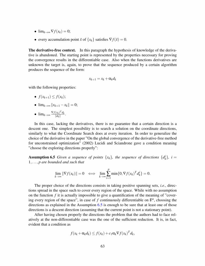
• limk→∞ ∇ f (xk) = 0;

• every accumulation point x of xk satisfies ∇ f (x) = 0.

The derivative-free context. In this paragraph the hypothesis of knowledge of the deriva-tive is abandoned. The starting point is represented by the properties necessary for provingthe convergence results in the differentiable case. Also when the functions derivatives areunknown the target is, again, to prove that the sequence produced by a certain algorithmproduces the sequence of the form:

xk+1 = xk +αkdk

with the following properties:

• f (xk+1)≤ f (xk);

• limk→∞ ‖xk+1− xk‖= 0;

• limk→∞∇ f (xk)

T dk‖dk‖ .

In this case, lacking the derivatives, there is no guarantee that a certain direction is adescent one. The simplest possibility is to search a solution on the coordinate directions,similarly to what the Coordinate Search does at every iteration. In order to generalize thechoice of the derivative in the paper ”On the global convergence of the derivative-free methodfor unconstrained optimization” (2002) Lucidi and Sciandrone gave a condition meaning”choose the exploring directions properly”:

Assumption 6.5 Given a sequence of points xk, the sequence of directions dik, i =

1, . . . , p are bounded and such that

limk→∞‖∇ f (xk)‖= 0 ⇐⇒ lim

k→∞

p

∑i=1

min0,∇ f (xk)T di

k= 0.

The proper choice of the directions consists in taking positive spanning sets, i.e., direc-tions spread in the space such to cover every region of the space. While with no assumptionon the function f it is actually impossible to give a quantification of the meaning of ”cover-ing every region of the space”, in case of f continuously differentiable on Rn, choosing thedirections as explained in the Assumption 6.5 is enough to be sure that at least one of thosedirections is a descent direction (assuming that the current point is not a stationary point).

After having chosen properly the directions the problem that the authors had to face rel-atively at the non-differentiable case was the one of the sufficient reduction. It is, in fact,evident that a condition as

f (xk +αkdk)≤ f (xk)+ c1αk∇ f (xk)T dk,

63

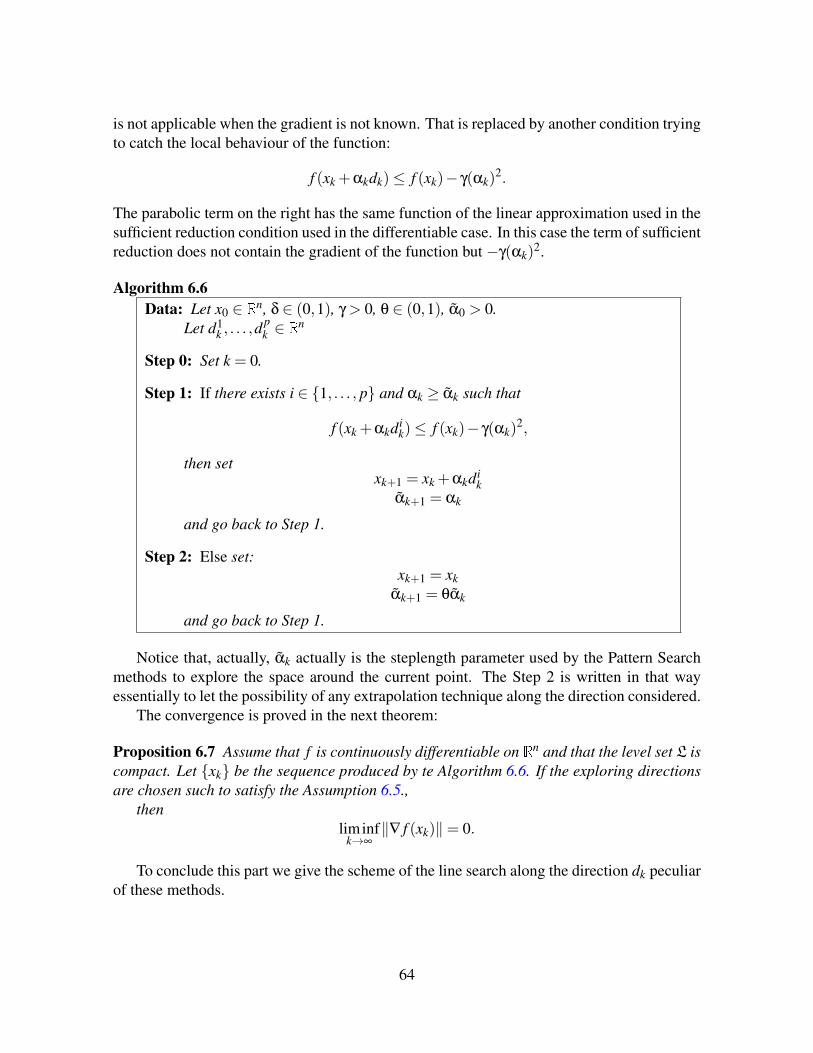
is not applicable when the gradient is not known. That is replaced by another condition tryingto catch the local behaviour of the function:

f (xk +αkdk)≤ f (xk)− γ(αk)2.

The parabolic term on the right has the same function of the linear approximation used in thesufficient reduction condition used in the differentiable case. In this case the term of sufficientreduction does not contain the gradient of the function but −γ(αk)

2.

Algorithm 6.6Data: Let x0 ∈ Rn, δ ∈ (0,1), γ > 0, θ ∈ (0,1), α0 > 0.

Let d1k , . . . ,d

pk ∈ R

n

Step 0: Set k = 0.

Step 1: If there exists i ∈ 1, . . . , p and αk ≥ αk such that

f (xk +αkdik)≤ f (xk)− γ(αk)

2,

then setxk+1 = xk +αkdi

kαk+1 = αk

and go back to Step 1.

Step 2: Else set:xk+1 = xk

αk+1 = θαk

and go back to Step 1.

Notice that, actually, αk actually is the steplength parameter used by the Pattern Searchmethods to explore the space around the current point. The Step 2 is written in that wayessentially to let the possibility of any extrapolation technique along the direction considered.

The convergence is proved in the next theorem:

Proposition 6.7 Assume that f is continuously differentiable on Rn and that the level set L iscompact. Let xk be the sequence produced by te Algorithm 6.6. If the exploring directionsare chosen such to satisfy the Assumption 6.5.,

thenliminf

k→∞‖∇ f (xk)‖= 0.

To conclude this part we give the scheme of the line search along the direction dk peculiarof these methods.

64

Algorithm 6.8 (LS procedure)Compute αi

i = minδ− jαk : j = 0,1, . . . such that

f (xk +αikdi

k)≤ f (xk)− γ(αik)

2,

f(xk +

αik

δdi

k

)≥max

[f (xi

k +αikdi

k), f (xik)− γ

(αi

kδ

)].

65

7 Linesearch inserted into a GPS approach: a possible al-gorithm.

The Generalized Pattern Search and a scheme of the Linesearch algorithms have been pre-sented in the previous two chapters as two different approaches of the DFO. This section isdedicated to an interesting parallel between the two different worlds with the purpose of putthem together in an algorithm being able to exploit both their strong points. In order to dothat it is first necessary to understand their weaknesses.The GPS algorithm at every iteration explore the points on the poll, i.e., the points lying nearthe current one. In the basic implementations, once a better point was found in the poll alongthe direction dk ∈ Dk the GPS moved in the new point incresing the parameter ∆k. Althoughit made sense considering that direction dk as a promising one in the first implementations theGPS methods just started again the search from the new point considering a static orderingof the poll directions. In that way there was not a direct satisfying exploitation of the promis-ing directions. Successively it was probably the Linesearch branch that influenced the GPSand it was introduced a simple little forsesight: storing and then considering the last successdirection wk as the first one to explore at iteration k. That rule, together with considering thegeneralize updating rule of ∆k allowing exponential increases in case of successful iterations,actually brought into the GPS context a line search. Notice that we use ”line search” insteadof ”Linesearch” to mark the difference between the exploitation of a direction and the branchof the DFO relying on the concept of line search with all its different implementations and itsconvergence theory.

In particular the main assumption of that convergence theory represents also its principalweakness: the sufficient decrease of the objective function. Summarizing, while the conver-gence price of the Pattern Search methods is that all the iterates have to lie on a mesh of points(whom refinement can be set nevertheless without limitations by the user), a Linesearch it-erate can be accepted as a new solution only if its function value is ”sufficiently” better thanthe last one. This represents also a practical limit: in fact it would result hard to explain toa generic user that a certain target cannot be considered because, though it is better than thecurrent one, it is not ”sufficiently” better.

For this reason it has been decided to describe a method that basically is a Pattern Searchmethod and that uses a module implementing a line search, different from the Linesearchprocedure first of all for the simple decrease criterion. The second important difference is theslighly difference of the parameter γ used by the line search, being a rational value and not areal one. Although this is conceptually necessary to prove that the iterations of the Algorithm7.1 still lie on a mesh, it does not really change anything in the practice implementation.

66

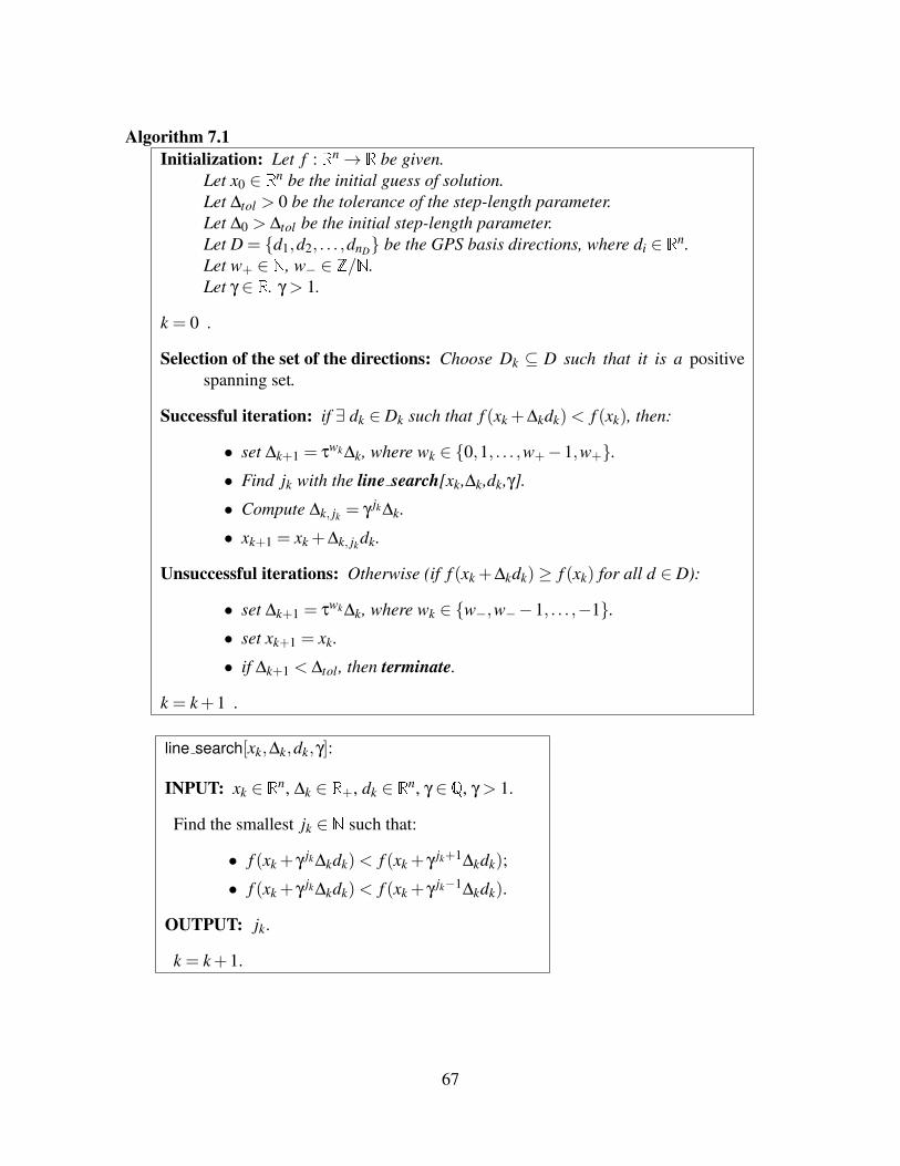
Algorithm 7.1Initialization: Let f : Rn→ R be given.

Let x0 ∈ Rn be the initial guess of solution.Let ∆tol > 0 be the tolerance of the step-length parameter.Let ∆0 > ∆tol be the initial step-length parameter.Let D = d1,d2, . . . ,dnD be the GPS basis directions, where di ∈ Rn.Let w+ ∈ N, w− ∈ Z/N.Let γ ∈ R. γ > 1.

k = 0 .

Selection of the set of the directions: Choose Dk ⊆ D such that it is a positivespanning set.

Successful iteration: if ∃ dk ∈ Dk such that f (xk +∆kdk)< f (xk), then:

• set ∆k+1 = τwk∆k, where wk ∈ 0,1, . . . ,w+−1,w+.• Find jk with the line search[xk,∆k,dk,γ].

• Compute ∆k, jk = γ jk∆k.

• xk+1 = xk +∆k, jkdk.

Unsuccessful iterations: Otherwise (if f (xk +∆kdk)≥ f (xk) for all d ∈ D):

• set ∆k+1 = τwk∆k, where wk ∈ w−,w−−1, . . . ,−1.• set xk+1 = xk.

• if ∆k+1 < ∆tol , then terminate.

k = k+1 .

line search[xk,∆k,dk,γ]:

INPUT: xk ∈ Rn, ∆k ∈ R+, dk ∈ Rn, γ ∈ Q, γ > 1.

Find the smallest jk ∈ N such that:

• f (xk + γ jk∆kdk)< f (xk + γ jk+1∆kdk);

• f (xk + γ jk∆kdk)< f (xk + γ jk−1∆kdk).

OUTPUT: jk.

k = k+1.

67

As previously anticipated in the line search module the concept of sufficient decrease intothe stopping criteria condition lacks and is substituted by the simple decrease.

In order to rewrite the generic iterate we introduce a little notation: it has been saidthat it is possible to write the generic steplength parameter related to the initial steplength:∆k = τrk∆0, where τ ∈ R is such that τ > 1 and rk is an integer number depending on theoutcome of the iterates until the iteration k. The greater is the number of successes amongthe first k iterates the greater is rk; the lower is the number of unsuccessful iterations until k,the lower is rk. Depending on the version used rk can be augmented or not at every k ∈ S but,for sure, it is decreased at every k ∈U .

Ensuring that the reason will be clear in the following rows, two measures are fixed:

rLBk = min

0≤i≤kri,

rUBk = max

0≤i≤kri.

It follows that rLBk ≤ rUB

k for every k = 0,1,2, . . ..Repeating the same reasoning for k→+∞, we write:

rLB = min0≤i<+∞

ri

rUB = max0≤i<+∞

ri<+∞

A priori nothing can be said on the lower bound of rk while, for the upper bound we recall thatall the iterates lie on a bounded set. Since the norm of the longer direction is fixed, it meansthat ∆k has to be bounded above (∆k = τrk∆0 ≤ ∆M). Being ∆0 fixed it becomes a conditionon the upper bound of τrk , hence on rk: rUB < +∞, i.e., it exists a finite upper bound on rk.About the lower bound rLB it will be important on the convergence proof in the following.

Here the parameter ∆k is not the only one of interest. Another parameter strictly con-nected with the first one is introduced inside the module Linesearch[xk,∆k,dk], the elongedsteplength parameter ∆k, jk ∈ R+. It is detected thanks to the constant γ ∈ Q:

∆k, jk = γjk∆k.

Remark 7.2 In the classical linesearch approach, the costant of elongation is γ ∈ R. In thepresent approach it is stated that γ ∈ Q simply for a convergence reason. It is, in fact, usedinside the proof of the theorem 7.3. If it had been γ ∈ Q it would have been impossible to saythat xk lies on a certain mesh for all the k.

The first aspect to point out from the algorithm is that the elonged step at k depends on ∆kbut, at the contrary, ∆k+1 does not depend on ∆k, jk . Hence, the elonged steplength is createdfrom the normal steplength at every iteration but does not influence the next steplength ∆k.Also in this case it is possible to detect two measures:

jLBk = min

0≤i≤k ji,

68

jUBk = max

0≤i≤k ji.

The main difference with the previous case on rk is that now there exist finite both the upperand the lower bounds:

jLB = min0≤i<+∞

ji ≥ 0,

jUB = max0≤i<+∞

ji<+∞.

This is true because the linesearch is activated just if a better point respect with the currentsolution is found. In that case the interesting direction is analyzed and, if no other interestingpoints are found along that, it is fixed jk = 0 and ∆k, jk = γ0∆k = ∆k. About the upper boundit is sufficient to consider the assumption that all the iterates have to belong to a bounded set.It also means that jk cannot be arbitrately great: jUB is a finite value.

It is also possible to write the elonged step respect with ∆0:

∆k, jk = γjk∆k = γ

jkτrk∆0,

where the parameter rk can be computed relying on ∆0,∆1,∆2, . . . ,∆k−1, while it does notdepend at all on ∆1, j1 ,∆2, j2, . . . ,∆k, jk and where jk depends on the single iteration k (henceon xk,dk,∆k) besides γ.

It is now introduced an important theorem that is necessary to prove the convergence in7.5.

Theorem 7.3 The generic point at iteration k+1 can be written as

xk+1 = x0 +(βrLB

k1 α

−rUBk

1 )(βjLBk

2 α− jUB

k2 )∆0D

k

∑i=1

ui,

where

• x0 ∈ Rn is the initial guess;

• ∆0 ∈ R+;

• D ∈ Rn×nD;

• β1,α1 ∈ N relatively prime, with β1 > α1 such that τ≡ β1α1

(hence τ ∈ Q);

• β2,α2 ∈ N relatively prime, with β2 > α2 such that γ≡ β2α2

(hence γ ∈ Q);

• ui ∈ NnD , for each i = 1,2, . . . ,k.

Proof. We start writing the generic iterate.

xk+1 = xk +∆k, jkdk= xk−1 +∆k−1, jk−1dk−1 +∆k, jkdk= xk−2 +∆k−2, jk−2dk−2 +∆k−1, jk−1dk−1 +∆k, jkdk= x0 +∑

ki=1 ∆i, jidi.

69

Considering that dk = Duk, where uk ∈NnD is a vector with all zeros and 1 correspondingto the chosen direction (it would not be right to speak of ”coordinate direction” because uk isnD-dimension, and not n):

xk+1 = x0 +∑ki=1 ∆i, jiDui.

It is now necessary to decompose ∆i, ji into the original and linesearch components, i.e.,relatively at iteration k, ∆k, jk = γ jk∆k. Using, in addition, the expression of ∆k related to itsinitial value ∆0: ∆k, jk = γ jkτrk∆0. Again, the expression of xk becomes:

xk+1 = x0 +k

∑i=1

γjkτ

rk∆0Dui.

To understand what we are going to do in the next rows, let see xk+1 in another way:

xk+1 = x0 +∆0D( k

∑i=1

γjkτ

rkui

).

Between parenthesis there is a vector. If it was an integer vector that would be the typicalexpression of points lying on a mesh. Unfortunately, it is evident that, being γ and τ notinteger also that amount cannot be integer. We cannot say that xk+1 belongs to the meshdefined by the columns of D scaled of ∆0. Nvertheless, there is another mesh containing theiterates untile k+1.

We use the fact that γ and τ are fractional:

xk+1 = x0 +∆0D[ k

∑i=1

(β2

α2

) ji(β1

α1

)ri

ui

]=

= x0 +∆0D[ k

∑i=1

((β2)

ji(α2)− ji)(

(β1)ri(α1)

−ri

)ui

].

Here the quantities rLBk , rUB

k , jLBk , jUB

k are used to isolate a part inside the sum.

xk+1 = x0+∆0

(β

jLBk

2 α− jUB

k2 β

rLBk

1 α−rUB

k1

)D[ k

∑i=1

((β2)

ji− jLBk (α2)

jUBk − ji

)((β1)

ri−rLBk (α1)

rUBk −ri

)ui

].

To understand the reason of this mathematical trick, notice that β1, β2, α1, α2 are allinteger positive numbers, raised to the power of natural numbers ( ji− jLB

k , jUBk − ji, ri− rLB

k ,rUB

k − ri ∈ N).It follows that, for every i ∈ 0,1, . . . ,k,(

(β2)ji− jLB

k (α2)jUBk − ji

)((β1)

ri−rLBk (α1)

rUBk −ri

)∈ N,

and the quantity between the square parenthesis is an integer positive vector u. It followsthat:

70

xk+1 = x0 +∆0

(β

jLBk

2 α− jUB

k2 β

rLBk

1 α−rUB

k1

)D

k

∑i=1

ui.

Also if it could seem counterintuitive the meaning of this theorem is extremely simple:at every finite iteration k the iterate xk lies on a mesh. In fact, being ui ∈ ZnD , it results∑

ki=1 ui = u. Then it is possible to write the generic iterate as

xk+1 = x0 +

[(β

rLBk

1 α−rUB

k1 )(β

jLBk

2 α− jUB

k2 )∆0

]Du,

with u ∈ ZnD , meaning that the iterate xk+1 belongs to a mesh generated by the directions

contained in the columns od D and scaled by the factor βrLB

k1 α

−rUBk

1 βjLBk

2 α− jUB

k2 ∆0. For finite k it

results: rLB ≤ rLB

k ≤ rUBk ≤ rUB ,for every k.

jLB ≤ jLBk ≤ jUB

k ≤ jUB ,for every k

While it is easy the reasoning for a finite iteration k, nothing can be said for k→+∞. Asit has been said, in fact, we cannot say that rLB has a lower bound.

Remark 7.4 For a moment suppose that rLB is a finite value. Intuitively, analyzing the mul-tipliers of ∆0D, it results: (

βrLB

1 βjLB

2

αrUB

1 αjUB

2

)<

(β

rLBk

1 βjLBk

2

αrUBk

1 αjUBk

2

).

That means that the final mesh on which all the iterates have to lie is a finer mesh.

Theorem 7.5 If the iterates of the algorithm 7.1 lie all in a bounded set, then

liminfk→+∞

∆k, jk = 0.

Proof. What has been said until now is that:

• jLBk ≥ 0, jUB

k <+∞ for each k;

• jLB ≥ 0, jUB <+∞;

• rUBk <+∞ since the assumption of a bounded set containing all the iterates.

• rUB <+∞ since the assumption of a bounded set containing all the iterates.

71

Nothing has been said about the lower bounds relative rLBk and absolute rLB

k . It dependson the value of ∆k and hence on ∆k, jk . Proceeding by contradiction suppose that ∆k, jk has alower bound: 0 < ∆LB ≤ ∆k ≤ ∆k, jk .Moreover, since all the iterates have to lie in a bounded set, ∆k, jk (and hence also ∆k) has tobe limited above: ∆k ≤ ∆k, jk ≤ ∆UB <+∞.Summarizing:

0 < ∆LB ≤ ∆k ≤ ∆k, jk ≤ ∆

UB <+∞.

The previous condition can be conceptually transferred to the parameter rk re-writing thedisequality:

0 < ∆LB ≤ τ

rk∆0 ≤ γjkτ

rk∆0 ≤ ∆UB <+∞.

Noticing that γ jk is a finite amount for every k it is possible to write:

0 < τLB ≤ τ

rk ≤ τUB <+∞.

The bounds ∆LB and ∆UB can be conveniently chosen such that ∆LB = τrLB∆0 and ∆UB =

τrUB∆0. Being that so it is possible to transfer the limits on the steplength (it is convenient to

remember that one of the two is given by th absurd hypothesis) to limits on rk:

rk ∈ rLB,rLB +1, . . . ,rUB−1,rUB.

Coming back to the previous theorem 7.3, we see that the generic iteration xk+1 can bewritten as:

xk+1 = x0 +(βrLBk

1 α−rUB

k1 β

jLBk

2 α− jUB

k2 )∆0Duk, (17)

where uk ∈ NnD . It means that at iteration k + 1 the points found so far have to lie on amesh centered in x0 and generated by the directions contained in D scaled by the quantity

(βrLB

k1 α

−rUBk

1 βjLBk

2 α− jUB

k2 )∆0.

What happens for k→+∞? Having stated that

rLB = min0≤k<+∞

rk >−∞

it is possible to substitute the global value for the minimum and maximum of rk concludingthat the whole sequence xk has to belong to the mesh centered in x0 and generated by thedirections contained in D and scaled by the factor (βrLB

1 α−rUB

1 βjLB

2 α− jUB

2 )∆0. Note that withoutsetting the upper bound on rk it would have been impossible to ensure that tha scaled factorof the mesh was a finite value.

So it exist a mesh M(x0;D;βrLB

1 α−rUB

1 βjLB

2 α− jUB

2 ∆0) that contains all the iterates of thesequence xk generated by the algorithm 7.1. Obviously, since all the iterates have to lieon a bounded set and at the same time on the particular mesh showed above, and sincethe intersection of the two sets is a finite set of points, it follows that infinite points of thesequence xk have to correspond to a point of this finite set of points:

xk = x, for an infinite subset k ∈ K ⊂U.

72

Then, looking at the updating rule of the steplength parameter ∆k, we see that ∆k is increaseda finite number of times and decreased infinitey many times (for k ∈ U). It would result∆k → 0. At the same way , since ∆k, jk = γ jk∆k and γ jk is a finite number it follows that∆k, jk → 0. Both these results are a constradiction respect with the initial hypothesis.

73

8 The Mesh Adaptive Direct Search (MADS) algorithmsThe Mesh Adaptive Direct Search algorithms come at the end of the evolutive path trackedin this thesis, as the last version of the Pattern Search methods. As suggested by the name itis a Direct Search approach, since it uses exclusively the function values.

Being an evolution of the GPS methods seen in the previous chapter a lot of features arein common. The first and most important one is the presence of a conceptual mesh, generatedby the basis directions analogous to the previous ones, underlying all the iterations produced.In this sense we can say that Mk is a pattern on which new points are explored, though we willsee it is a different one respect with the pattern defined for CS and GPS. The real differencewill be in the set of directions generated at each iteration.

Thanks to this different approach it is possible to deal with functions with different de-grees of differentiability. So, although a MADS approach is completely applicable to a prob-lem in a differentiable context it has been thought to deal with harder problems in which onlythe Lipschitzianity of the function f can be supposed. Considering the Lipschitzianity a dif-ferent theory is developed relying on the generalized Clarke derivative instead of the classicalfirst derivative.

As it has been done until now, also for presenting the MADS approach the constrainedcase will be ignored. We are confident that here, more than for the previous cases, it isimportant because the exploring way in MADS is sufficiently more complicated respect withthe others, so it is important to focus the attetion on the fewer concept possible. Anyway, togive an anticipation, we will see in the part ?? that the MADS approach will be crucial alsoin solving theoretical issues in the constrained case.

8.1 Mesh Adaptive Direct Search: the basic conceptsGoing from the Coordinate Search to the Generalized Pattern Search cases it has been seenas the number of basis directions passed from 2n to a generic p ≥ n+ 1 while the rule fordetecting the polling directions that was Dk = D,∀k for the CS became then Dk ⊆D for GPS.The basis directions are again defined as D = GZ, by the nonsingular matrix G ∈ Rn×n andby the integer matrix Z ∈ Zn×nD . An important common point of these approaches is the factthat both the number of the basis directions D and the number of directions chosen at eachiteration Dk are chosen in a finite set, hence

∞⋃k=1

Dk ⊆ D,

where for the CS the equality always holds, while in the GPS case it can be both an equalityor a strict inclusion depending on the choice of the directions along the whole run of themethod. Anyway, the infinite union of the exploring directions produces a set of directionsthat still is finite. That is not a problem in the unconstrained differentiable case (it would beenough to consider the constrained differentiable case to see the first problem arising) but itactually produces convergence issues when that condition is relaxed.

74

In order to ”solve” the previous problem Dennis and Audet a trick for obtaining an infi-nite number of candidates to explore at the poll phase. The first step to do that is splittingthe parameter ∆k on which both the mesh Mk and the frame Pk were built in two differentsteplength parameters:

• ∆mk : the mesh size parameter;

• ∆pk : the poll size parameter;

It will be also necessary to put a relationship between them. Anyway the parameter ∆mk ∈ R

+

actually is the steplength parameter associated to the pattern. Similarly it can be used todefine the mesh:

Definition 8.1 The current mesh is defined at iteration k as the union:

Mk =⋃

x∈Vk

M(x;∆mk ) = x+∆

mk Du : u ∈ NnD ,x ∈Vk. (18)

So, being the mesh defined by the parameter ∆mk , we have to see the role played by the poll

size parameter ∆pk . As the name suggests, the poll size parameter detects the set of candidate

directions to be inserted in Dk: it is important to understand how. It has been said that thetarget is to create a set of polling directions growing dense for k→∞. To understand the wayin which this is obtained it is necessary to define a new concept of polling direction.

Definition 8.2 The points composing the MADS frame at iteration k is defined as the set:

Pk = xk∪xk +∆mk d : d ∈ Dk ⊂Mk, (19)

where the set of directions Dk is such that for each d ∈ Dk two results are verified:

• the direction d 6= 0 is such that d = Du, where u ∈ NnD may depend on the iterationnumber k;

• the exploration step related to the direction d is bounded above by a quantity dependingon the poll size parameter:

∆mk ||d|| ≤ ∆

pk max

∣∣∣∣d′∣∣∣∣ : d′ ∈ D. (20)

Depending on the values of ∆pk respect with ∆

pk , considering the second bullet of the

Definition 8.2 it results that actually the poll research region can be extended or reduced.That makes necessary to set a condition on this new parameter ∆

pk such that the poll region

does not lose its meaning of set of points near the current point. In other words we want thatfor k→ ∞ the trial points xk +∆m

k d, with d ∈ Dk still collapse to xk.It is necessary to fix the relation between ∆m

k and ∆pk in order to state some important

properties of the poll set of points.

75

The mesh size parameter is exactly the same seen in the GPS approach. So, equivalently, itwill be updated in the usual generalized way:

∆mk+1 = τ

wk∆mk ,

where τ ∈ Q, τ > 1 and wk is an integer satisfying the following properties:

wk ∈1,2, . . . ,w+−1,w+ , with wk integer negative , for k ∈ Sw−,w−+1, . . . ,0 , with wk integer non-negative , for k ∈U.

(21)

The poll size parameter ∆pk , instead, is chosen dependently on ∆m

k , such that:

• ∆mk ≤ ∆

pk , for all the k;

• for any infinite subset of indices K it has to result :

limk∈K

∆mk = 0 ⇐⇒ lim

k∈K∆

pk = 0. (22)

Remark 8.3 To prove that the MADS is a generalization of the GPS case, it is necessary toprove that the GPS are a particular case of the MADS. To do that it is enough to set ∆m

k =∆

pk = ∆k and u the vector with all zeros and a component equals to one in corrispondence

with the column containing the desired direction.

76

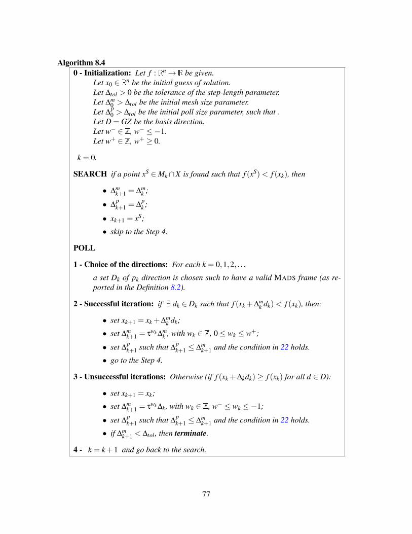
Algorithm 8.40 - Initialization: Let f : Rn→ R be given.

Let x0 ∈ Rn be the initial guess of solution.Let ∆tol > 0 be the tolerance of the step-length parameter.Let ∆m

0 > ∆tol be the initial mesh size parameter.Let ∆

p0 > ∆tol be the initial poll size parameter, such that .

Let D = GZ be the basis direction.Let w− ∈ Z, w− ≤−1.Let w+ ∈ Z, w+ ≥ 0.

k = 0.

SEARCH if a point xS ∈Mk∩X is found such that f (xS)< f (xk), then

• ∆mk+1 = ∆m

k ;

• ∆pk+1 = ∆

pk ;

• xk+1 = xS;

• skip to the Step 4.

POLL

1 - Choice of the directions: For each k = 0,1,2, . . .

a set Dk of pk direction is chosen such to have a valid MADS frame (as re-ported in the Definition 8.2).

2 - Successful iteration: if ∃ dk ∈ Dk such that f (xk +∆mk dk)< f (xk), then:

• set xk+1 = xk +∆mk dk;

• set ∆mk+1 = τwk∆m

k , with wk ∈ Z, 0≤ wk ≤ w+;

• set ∆pk+1 such that ∆

pk+1 ≤ ∆m

k+1 and the condition in 22 holds.

• go to the Step 4.

3 - Unsuccessful iterations: Otherwise (if f (xk +∆kdk)≥ f (xk) for all d ∈ D):

• set xk+1 = xk;

• set ∆mk+1 = τwk∆k, with wk ∈ Z, w− ≤ wk ≤−1;

• set ∆pk+1 such that ∆

pk+1 ≤ ∆m

k+1 and the condition in 22 holds.

• if ∆mk+1 < ∆tol , then terminate.

4 - k = k+1 and go back to the search.

77

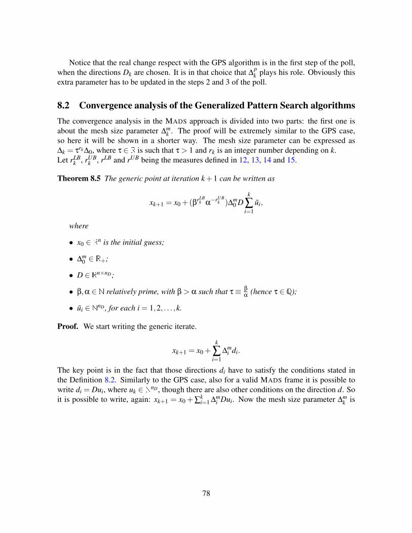
Notice that the real change respect with the GPS algorithm is in the first step of the poll,when the directions Dk are chosen. It is in that choice that ∆

pk plays his role. Obviously this

extra parameter has to be updated in the steps 2 and 3 of the poll.

8.2 Convergence analysis of the Generalized Pattern Search algorithmsThe convergence analysis in the MADS approach is divided into two parts: the first one isabout the mesh size parameter ∆m

k . The proof will be extremely similar to the GPS case,so here it will be shown in a shorter way. The mesh size parameter can be expressed as∆k = τrk∆0, where τ ∈ R is such that τ > 1 and rk is an integer number depending on k.Let rLB

k , rUBk , rLB and rUB being the measures defined in 12, 13, 14 and 15.

Theorem 8.5 The generic point at iteration k+1 can be written as

xk+1 = x0 +(βrLBk α−rUB

k )∆m0 D

k

∑i=1

ui,

where

• x0 ∈ Rn is the initial guess;

• ∆m0 ∈ R+;

• D ∈ Rn×nD;

• β,α ∈ N relatively prime, with β > α such that τ≡ β

α(hence τ ∈ Q);

• ui ∈ NnD , for each i = 1,2, . . . ,k.

Proof. We start writing the generic iterate.

xk+1 = x0 +k

∑i=1

∆mi di.

The key point is in the fact that those directions di have to satisfy the conditions stated inthe Definition 8.2. Similarly to the GPS case, also for a valid MADS frame it is possible towrite di = Dui, where uk ∈ NnD , though there are also other conditions on the direction d. Soit is possible to write, again: xk+1 = x0 +∑

ki=1 ∆m

i Dui. Now the mesh size parameter ∆mk is

78

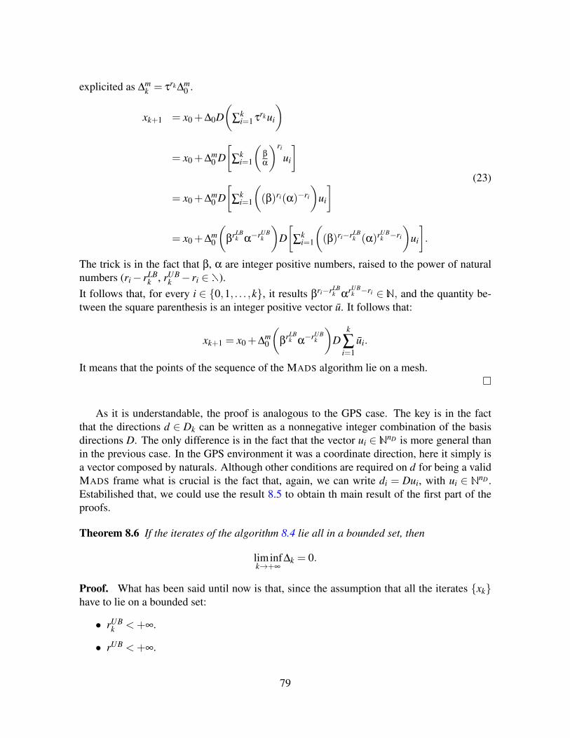
explicited as ∆mk = τrk∆m

0 .

xk+1 = x0 +∆0D(

∑ki=1 τrkui

)

= x0 +∆m0 D[

∑ki=1

(β

α

)ri

ui

]

= x0 +∆m0 D[

∑ki=1

((β)ri(α)−ri

)ui

]

= x0 +∆m0

(βrLB

k α−rUB

k

)D[

∑ki=1

((β)ri−rLB

k (α)rUBk −ri

)ui

].

(23)

The trick is in the fact that β, α are integer positive numbers, raised to the power of naturalnumbers (ri− rLB

k , rUBk − ri ∈ N).

It follows that, for every i ∈ 0,1, . . . ,k, it results βri−rLBk α

rUBk −ri ∈ N, and the quantity be-

tween the square parenthesis is an integer positive vector u. It follows that:

xk+1 = x0 +∆m0

(β

rLBk α−rUB

k

)D

k

∑i=1

ui.

It means that the points of the sequence of the MADS algorithm lie on a mesh.

As it is understandable, the proof is analogous to the GPS case. The key is in the factthat the directions d ∈ Dk can be written as a nonnegative integer combination of the basisdirections D. The only difference is in the fact that the vector ui ∈ NnD is more general thanin the previous case. In the GPS environment it was a coordinate direction, here it simply isa vector composed by naturals. Although other conditions are required on d for being a validMADS frame what is crucial is the fact that, again, we can write di = Dui, with ui ∈ NnD .Estabilished that, we could use the result 8.5 to obtain th main result of the first part of theproofs.

Theorem 8.6 If the iterates of the algorithm 8.4 lie all in a bounded set, then

liminfk→+∞

∆k = 0.

Proof. What has been said until now is that, since the assumption that all the iterates xkhave to lie on a bounded set:

• rUBk <+∞.

• rUB <+∞.

79

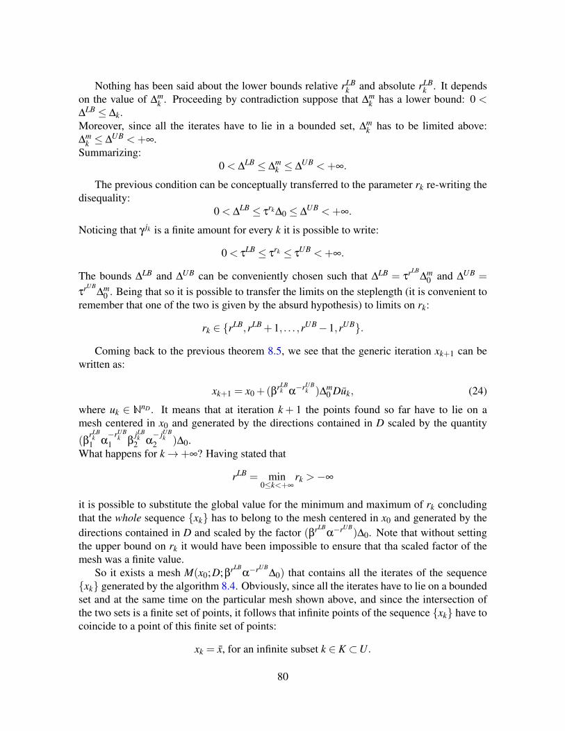
Nothing has been said about the lower bounds relative rLBk and absolute rLB

k . It dependson the value of ∆m

k . Proceeding by contradiction suppose that ∆mk has a lower bound: 0 <

∆LB ≤ ∆k.Moreover, since all the iterates have to lie in a bounded set, ∆m

k has to be limited above:∆m

k ≤ ∆UB <+∞.Summarizing:

0 < ∆LB ≤ ∆

mk ≤ ∆

UB <+∞.

The previous condition can be conceptually transferred to the parameter rk re-writing thedisequality:

0 < ∆LB ≤ τ

rk∆0 ≤ ∆UB <+∞.

Noticing that γ jk is a finite amount for every k it is possible to write:

0 < τLB ≤ τ

rk ≤ τUB <+∞.

The bounds ∆LB and ∆UB can be conveniently chosen such that ∆LB = τrLB∆m

0 and ∆UB =

τrUB∆m

0 . Being that so it is possible to transfer the limits on the steplength (it is convenient toremember that one of the two is given by the absurd hypothesis) to limits on rk:

rk ∈ rLB,rLB +1, . . . ,rUB−1,rUB.

Coming back to the previous theorem 8.5, we see that the generic iteration xk+1 can bewritten as:

xk+1 = x0 +(βrLBk α−rUB

k )∆m0 Duk, (24)

where uk ∈ NnD . It means that at iteration k + 1 the points found so far have to lie on amesh centered in x0 and generated by the directions contained in D scaled by the quantity

(βrLB

k1 α

−rUBk

1 βjLBk

2 α− jUB

k2 )∆0.

What happens for k→+∞? Having stated that

rLB = min0≤k<+∞

rk >−∞

it is possible to substitute the global value for the minimum and maximum of rk concludingthat the whole sequence xk has to belong to the mesh centered in x0 and generated by thedirections contained in D and scaled by the factor (βrLB

α−rUB)∆0. Note that without setting

the upper bound on rk it would have been impossible to ensure that tha scaled factor of themesh was a finite value.

So it exists a mesh M(x0;D;βrLBα−rUB

∆0) that contains all the iterates of the sequencexk generated by the algorithm 8.4. Obviously, since all the iterates have to lie on a boundedset and at the same time on the particular mesh shown above, and since the intersection ofthe two sets is a finite set of points, it follows that infinite points of the sequence xk have tocoincide to a point of this finite set of points:

xk = x, for an infinite subset k ∈ K ⊂U.

80

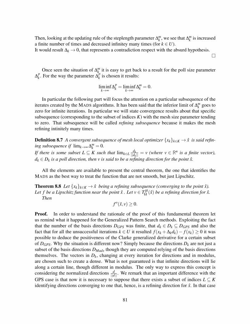
Then, looking at the updating rule of the steplength parameter ∆mk , we see that ∆m

k is increaseda finite number of times and decreased infinitey many times (for k ∈U).It would result ∆k→ 0, that represents a contradiction respect with the absurd hypothesis.

Once seen the situation of ∆mk it is easy to get back to a result for the poll size parameter

∆pk . For the way the parameter ∆

pk is chosen it results:

liminfk→∞

∆pk = liminf

k→∞∆

mk = 0.

In particular the following part will focus the attention on a particular subsequence of theiterates created by the MADS algorithms. It has been said that the inferior limit of ∆m

k goes tozero for infinite iterations. In particular we will state convergence results about that specificsubsequence (corresponding to the subset of indices K) with the mesh size parameter tendingto zero. That subsequence will be called refining subsequence because it makes the meshrefining intinitely many times.

Definition 8.7 A convergent subsequence of mesh local optimizer xkk∈K→ x is said refin-ing subsequence if limk→∞ ∆m

k = 0.If there is some subset L ⊆ K such that limk∈L

dk||dk|| = v (where v ∈ Rn is a finite vector),

dk ∈ Dk is a poll direction, then v is said to be a refining direction for the point x.

All the elements are available to present the central theorem, the one that identifies theMADS as the best way to treat the function that are not smooth, but just Lipschitz.

Theorem 8.8 Let xkk∈K → x being a refining subsequence (converging to the point x).Let f be a Lipschitz function near the point x . Let v ∈ T H

Ω(x) be a refining direction for x.

Thenf o(x,v)≥ 0.

Proof. In order to understand the rationale of the proof of this fundamental theorem letus remind what it happened for the Generalized Pattern Search methods. Exploiting the factthat the number of the basis directions DGPS was finite, that dk ∈ Dk ⊆ DGPS and also thefact that for all the unsuccessful iterations k ∈U it resulted f (xk +∆kdk)− f (xk) ≥ 0 it waspossible to deduce the positiveness of the Clarke generalized derivative for a certain subsetof DGPS. Why the situation is different now? Simply because the directions Dk are not just asubset of the basis directions DMads though they are computed relying of the basis directionsthemselves. The vectors in Dk, changing at every iteration for directions and in modulus,are chosen such to create a dense. What is not guaranteed is that infinite directions will liealong a certain line, though different in modulus. The only way to express this concept isconsidering the normalized directions d

||d|| . We remark that an important difference with theGPS case is that now it is necessary to suppose that there exists a subset of indices L ⊆ Kidentifying directions converging to one that, hence, is a refining direction for x. In that case

81

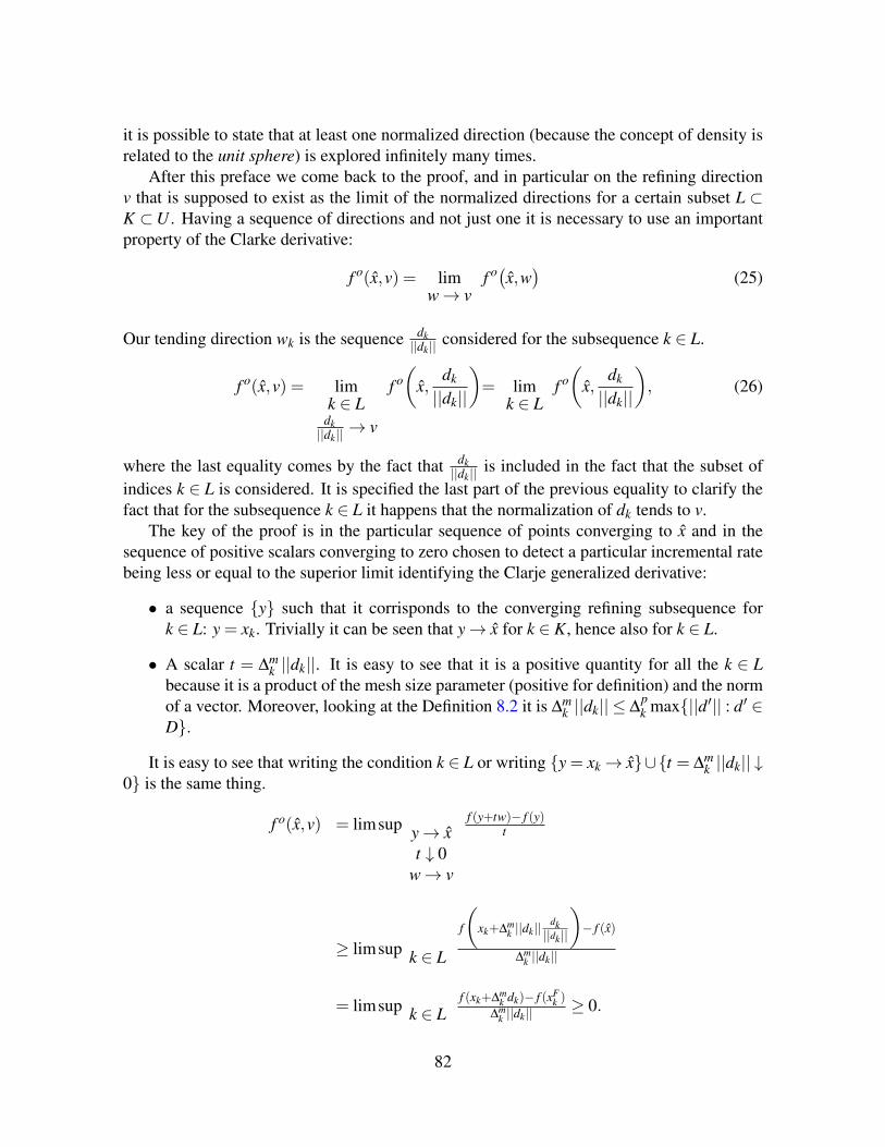
it is possible to state that at least one normalized direction (because the concept of density isrelated to the unit sphere) is explored infinitely many times.

After this preface we come back to the proof, and in particular on the refining directionv that is supposed to exist as the limit of the normalized directions for a certain subset L ⊂K ⊂U . Having a sequence of directions and not just one it is necessary to use an importantproperty of the Clarke derivative:

f o(x,v) = limw→ v

f o(x,w) (25)

Our tending direction wk is the sequence dk||dk|| considered for the subsequence k ∈ L.

f o(x,v) = limk ∈ L

dk||dk|| → v

f o(

x,dk

||dk||

)= lim

k ∈ Lf o(

x,dk

||dk||

), (26)

where the last equality comes by the fact that dk||dk|| is included in the fact that the subset of

indices k ∈ L is considered. It is specified the last part of the previous equality to clarify thefact that for the subsequence k ∈ L it happens that the normalization of dk tends to v.

The key of the proof is in the particular sequence of points converging to x and in thesequence of positive scalars converging to zero chosen to detect a particular incremental ratebeing less or equal to the superior limit identifying the Clarje generalized derivative:

• a sequence y such that it corrisponds to the converging refining subsequence fork ∈ L: y = xk. Trivially it can be seen that y→ x for k ∈ K, hence also for k ∈ L.

• A scalar t = ∆mk ||dk||. It is easy to see that it is a positive quantity for all the k ∈ L

because it is a product of the mesh size parameter (positive for definition) and the normof a vector. Moreover, looking at the Definition 8.2 it is ∆m

k ||dk|| ≤ ∆pk max||d′|| : d′ ∈

D.

It is easy to see that writing the condition k ∈ L or writing y = xk→ x∪t = ∆mk ||dk|| ↓

0 is the same thing.

f o(x,v) = limsup y→ xt ↓ 0

w→ v

f (y+tw)− f (y)t

≥ limsup k ∈ L

f

(xk+∆m

k ||dk||dk||dk||

)− f (x)

∆mk ||dk||

= limsup k ∈ Lf (xk+∆m

k dk)− f (xFk )

∆mk ||dk|| ≥ 0.

82

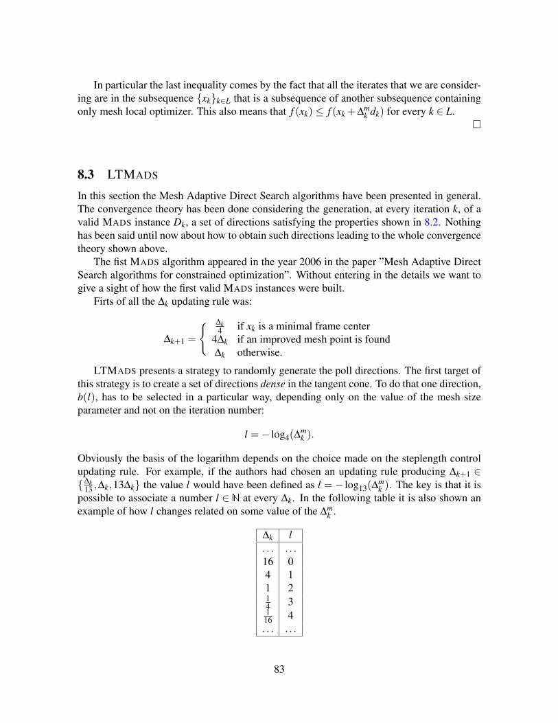
In particular the last inequality comes by the fact that all the iterates that we are consider-ing are in the subsequence xkk∈L that is a subsequence of another subsequence containingonly mesh local optimizer. This also means that f (xk)≤ f (xk +∆m

k dk) for every k ∈ L.

8.3 LTMADS

In this section the Mesh Adaptive Direct Search algorithms have been presented in general.The convergence theory has been done considering the generation, at every iteration k, of avalid MADS instance Dk, a set of directions satisfying the properties shown in 8.2. Nothinghas been said until now about how to obtain such directions leading to the whole convergencetheory shown above.

The fist MADS algorithm appeared in the year 2006 in the paper ”Mesh Adaptive DirectSearch algorithms for constrained optimization”. Without entering in the details we want togive a sight of how the first valid MADS instances were built.

Firts of all the ∆k updating rule was:

∆k+1 =

∆k4 if xk is a minimal frame center

4∆k if an improved mesh point is found∆k otherwise.

LTMADS presents a strategy to randomly generate the poll directions. The first target ofthis strategy is to create a set of directions dense in the tangent cone. To do that one direction,b(l), has to be selected in a particular way, depending only on the value of the mesh sizeparameter and not on the iteration number:

l =− log4(∆mk ).

Obviously the basis of the logarithm depends on the choice made on the steplength controlupdating rule. For example, if the authors had chosen an updating rule producing ∆k+1 ∈∆k

13 ,∆k,13∆k the value l would have been defined as l = − log13(∆mk ). The key is that it is

possible to associate a number l ∈ N at every ∆k. In the following table it is also shown anexample of how l changes related on some value of the ∆m

k .

∆k l. . . . . .16 04 11 214 31

16 4. . . . . .

83

Once computed the value l ∈ N associated to a certain mesh it is necessary to computethe direction related to l following three steps:

• Verify that the vector b(l) related to l has not been already computed. In that casereturns the existing vector b(l).

• Choose randomly one element i of b(l):

i ∈ 1,2, . . . ,n.

• Construct the vector b(l) separating conceptually the i-th element for the others n−1:

– set randomly one of the two values for the i-th element:

bi(l) =

+2l

−2l ,

– choose randomly

bi(l) ∈ −2l +1,−2l +2, . . . ,+2l−2,+2l−1

for every remaining i ∈ 1,2, . . . , i−1, i+1, . . . ,N.

Until now we started from the mesh size ∆mk to obtain a vector b(l) ∈ Zn:

∆mk −→ l ∈ N−→ b(l) ∈ Zn.

Now a lower triangular matrix (from here the name of LTMADS as a ”lower triangular MADS

”) L ∈ Z(n−1)×(n−1) is taken such that:

• Li,i ∈ +2l,−2l, for every i = 1,2, . . . ,n−1.

• Li, j ∈ −2l +1, . . . ,2l−1, for every i = 1,2, . . . ,n−1, j < i.

This lower triangular matrix is a basis in the Rn−1 such that |det(L)|= 2l(n−1).The lines of L are permuted and the vector b(l) is added to the permuted matrix to obtain

a basis in Rn. So, given a permutation p1, . . . , pn−1 of the set 1,2, . . . , i−1, i+1, . . . ,n,the new matric B is computed in the following way:

B =

Bpi, j = Li, j , i, j ∈ 1,2, . . . ,n−1Bi, j = 0 ,

Bi,n , i ∈ 1,2, . . . ,n.

It is possible to compute that B is a basis of Rn and its determinant is |det(B)|= 2ln.The last step is simply to permute the columns of B. So, given a generic permutation

q1,q2. . . . ,qn of the set 1,2, . . . ,n the last basis is computed:

84

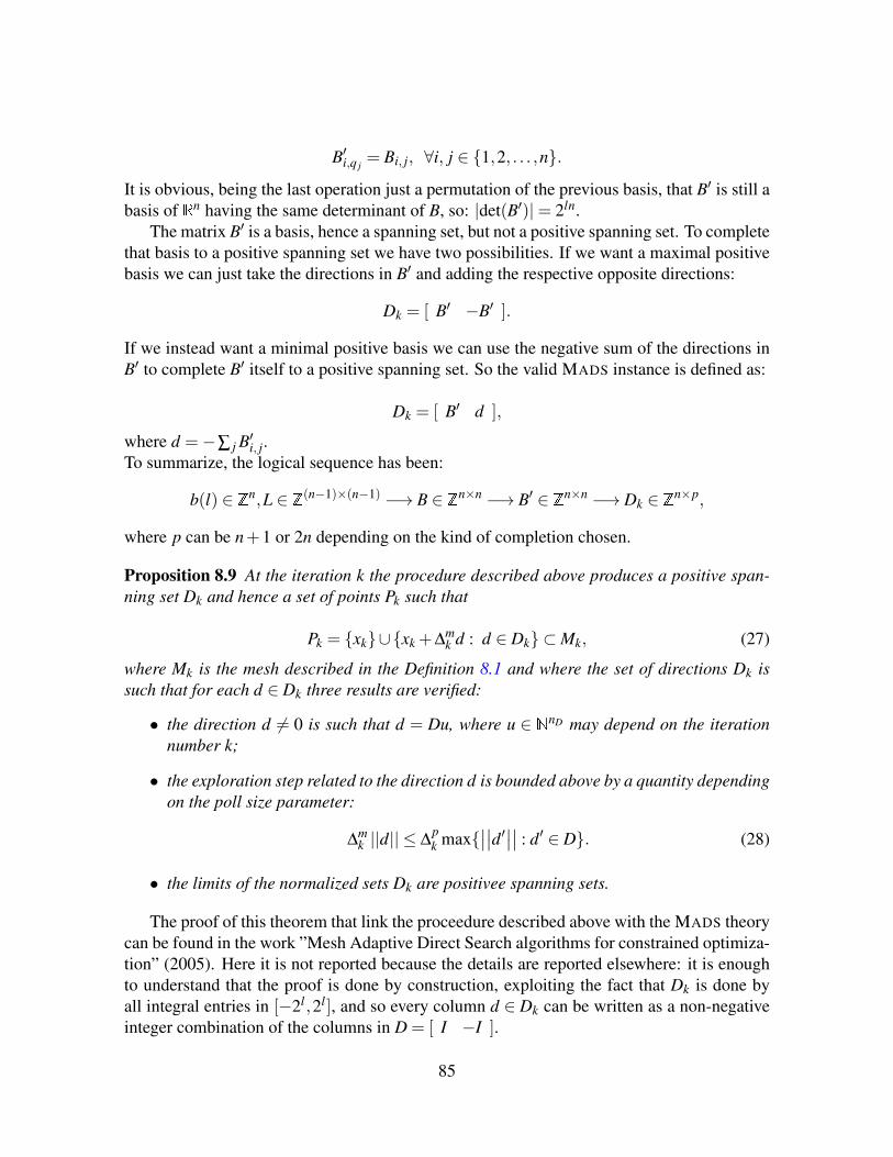
B′i,q j= Bi, j, ∀i, j ∈ 1,2, . . . ,n.

It is obvious, being the last operation just a permutation of the previous basis, that B′ is still abasis of Rn having the same determinant of B, so: |det(B′)|= 2ln.

The matrix B′ is a basis, hence a spanning set, but not a positive spanning set. To completethat basis to a positive spanning set we have two possibilities. If we want a maximal positivebasis we can just take the directions in B′ and adding the respective opposite directions:

Dk = [ B′ −B′ ].

If we instead want a minimal positive basis we can use the negative sum of the directions inB′ to complete B′ itself to a positive spanning set. So the valid MADS instance is defined as:

Dk = [ B′ d ],

where d =−∑ j B′i, j.To summarize, the logical sequence has been:

b(l) ∈ Zn,L ∈ Z(n−1)×(n−1) −→ B ∈ Zn×n −→ B′ ∈ Zn×n −→ Dk ∈ Zn×p,

where p can be n+1 or 2n depending on the kind of completion chosen.

Proposition 8.9 At the iteration k the procedure described above produces a positive span-ning set Dk and hence a set of points Pk such that

Pk = xk∪xk +∆mk d : d ∈ Dk ⊂Mk, (27)

where Mk is the mesh described in the Definition 8.1 and where the set of directions Dk issuch that for each d ∈ Dk three results are verified:

• the direction d 6= 0 is such that d = Du, where u ∈ NnD may depend on the iterationnumber k;

• the exploration step related to the direction d is bounded above by a quantity dependingon the poll size parameter:

∆mk ||d|| ≤ ∆

pk max

∣∣∣∣d′∣∣∣∣ : d′ ∈ D. (28)

• the limits of the normalized sets Dk are positivee spanning sets.

The proof of this theorem that link the proceedure described above with the MADS theorycan be found in the work ”Mesh Adaptive Direct Search algorithms for constrained optimiza-tion” (2005). Here it is not reported because the details are reported elsewhere: it is enoughto understand that the proof is done by construction, exploiting the fact that Dk is done byall integral entries in [−2l,2l], and so every column d ∈ Dk can be written as a non-negativeinteger combination of the columns in D = [ I −I ].

85

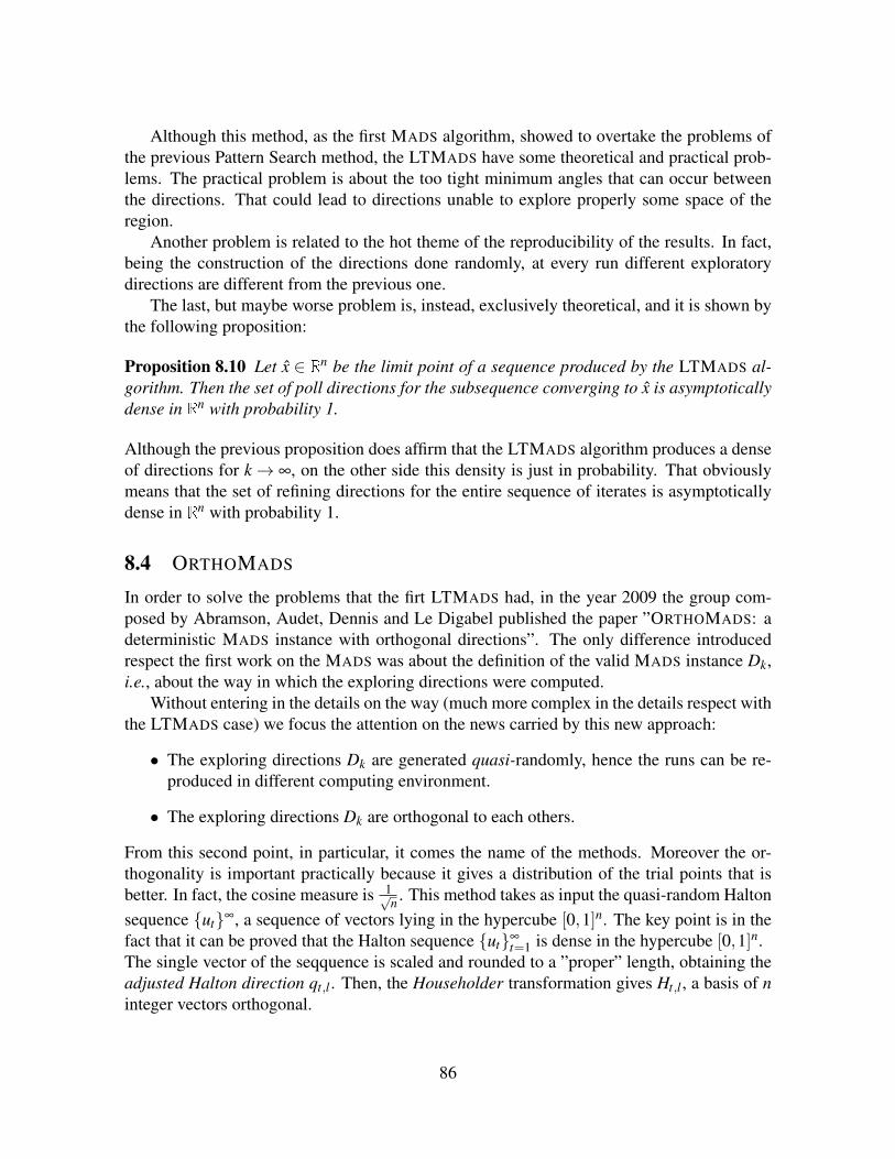
Although this method, as the first MADS algorithm, showed to overtake the problems ofthe previous Pattern Search method, the LTMADS have some theoretical and practical prob-lems. The practical problem is about the too tight minimum angles that can occur betweenthe directions. That could lead to directions unable to explore properly some space of theregion.

Another problem is related to the hot theme of the reproducibility of the results. In fact,being the construction of the directions done randomly, at every run different exploratorydirections are different from the previous one.

The last, but maybe worse problem is, instead, exclusively theoretical, and it is shown bythe following proposition:

Proposition 8.10 Let x ∈ Rn be the limit point of a sequence produced by the LTMADS al-gorithm. Then the set of poll directions for the subsequence converging to x is asymptoticallydense in Rn with probability 1.

Although the previous proposition does affirm that the LTMADS algorithm produces a denseof directions for k→ ∞, on the other side this density is just in probability. That obviouslymeans that the set of refining directions for the entire sequence of iterates is asymptoticallydense in Rn with probability 1.

8.4 ORTHOMADS

In order to solve the problems that the firt LTMADS had, in the year 2009 the group com-posed by Abramson, Audet, Dennis and Le Digabel published the paper ”ORTHOMADS: adeterministic MADS instance with orthogonal directions”. The only difference introducedrespect the first work on the MADS was about the definition of the valid MADS instance Dk,i.e., about the way in which the exploring directions were computed.

Without entering in the details on the way (much more complex in the details respect withthe LTMADS case) we focus the attention on the news carried by this new approach:

• The exploring directions Dk are generated quasi-randomly, hence the runs can be re-produced in different computing environment.

• The exploring directions Dk are orthogonal to each others.

From this second point, in particular, it comes the name of the methods. Moreover the or-thogonality is important practically because it gives a distribution of the trial points that isbetter. In fact, the cosine measure is 1√

n . This method takes as input the quasi-random Haltonsequence ut∞, a sequence of vectors lying in the hypercube [0,1]n. The key point is in thefact that it can be proved that the Halton sequence ut∞

t=1 is dense in the hypercube [0,1]n.The single vector of the seqquence is scaled and rounded to a ”proper” length, obtaining theadjusted Halton direction qt,l . Then, the Householder transformation gives Ht,l , a basis of ninteger vectors orthogonal.

86

Once a basis is at disposal the procedure continues identically to the LTMADS case: thebasis is completed to obtain a minimal or a maximal positive basis

Dk = [ Ht,l −Ht,l ].

In addition of proving that the ORTHOMADS still produces valid MADS instances, in theabove mentioned paper it is also shown the following proposition:

Proposition 8.11 The set of normalized directions

qt,l‖qt,l‖

∞

t=1are dense on the unit sphere.

In this way it is evident that ORTHOMADS inherits the whole structure of the MADS

convergence deterministically and not probabilistically.

87

Part II

ORTHOMADS (n+1)

88

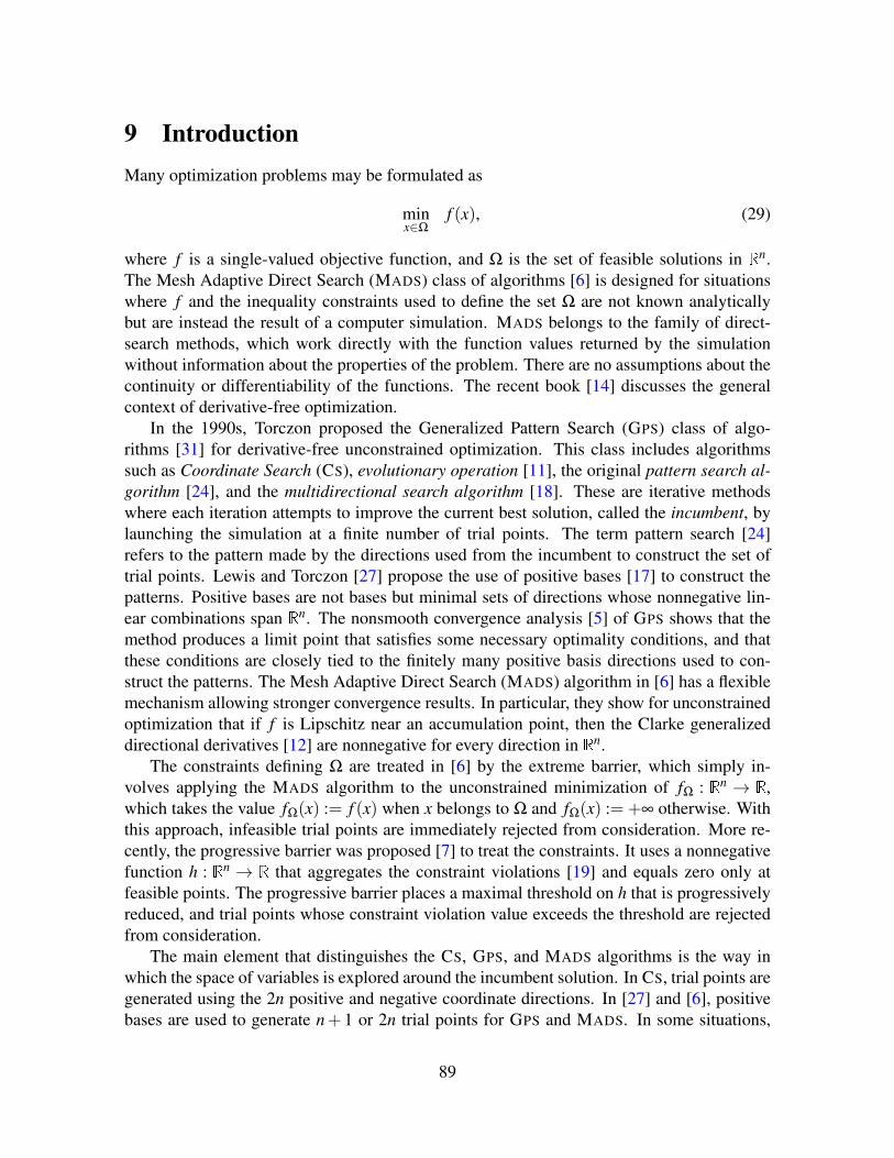
9 IntroductionMany optimization problems may be formulated as

minx∈Ω

f (x), (29)

where f is a single-valued objective function, and Ω is the set of feasible solutions in Rn.The Mesh Adaptive Direct Search (MADS) class of algorithms [6] is designed for situationswhere f and the inequality constraints used to define the set Ω are not known analyticallybut are instead the result of a computer simulation. MADS belongs to the family of direct-search methods, which work directly with the function values returned by the simulationwithout information about the properties of the problem. There are no assumptions about thecontinuity or differentiability of the functions. The recent book [14] discusses the generalcontext of derivative-free optimization.

In the 1990s, Torczon proposed the Generalized Pattern Search (GPS) class of algo-rithms [31] for derivative-free unconstrained optimization. This class includes algorithmssuch as Coordinate Search (CS), evolutionary operation [11], the original pattern search al-gorithm [24], and the multidirectional search algorithm [18]. These are iterative methodswhere each iteration attempts to improve the current best solution, called the incumbent, bylaunching the simulation at a finite number of trial points. The term pattern search [24]refers to the pattern made by the directions used from the incumbent to construct the set oftrial points. Lewis and Torczon [27] propose the use of positive bases [17] to construct thepatterns. Positive bases are not bases but minimal sets of directions whose nonnegative lin-ear combinations span Rn. The nonsmooth convergence analysis [5] of GPS shows that themethod produces a limit point that satisfies some necessary optimality conditions, and thatthese conditions are closely tied to the finitely many positive basis directions used to con-struct the patterns. The Mesh Adaptive Direct Search (MADS) algorithm in [6] has a flexiblemechanism allowing stronger convergence results. In particular, they show for unconstrainedoptimization that if f is Lipschitz near an accumulation point, then the Clarke generalizeddirectional derivatives [12] are nonnegative for every direction in Rn.

The constraints defining Ω are treated in [6] by the extreme barrier, which simply in-volves applying the MADS algorithm to the unconstrained minimization of fΩ : Rn → R,which takes the value fΩ(x) := f (x) when x belongs to Ω and fΩ(x) :=+∞ otherwise. Withthis approach, infeasible trial points are immediately rejected from consideration. More re-cently, the progressive barrier was proposed [7] to treat the constraints. It uses a nonnegativefunction h : Rn → R that aggregates the constraint violations [19] and equals zero only atfeasible points. The progressive barrier places a maximal threshold on h that is progressivelyreduced, and trial points whose constraint violation value exceeds the threshold are rejectedfrom consideration.

The main element that distinguishes the CS, GPS, and MADS algorithms is the way inwhich the space of variables is explored around the incumbent solution. In CS, trial points aregenerated using the 2n positive and negative coordinate directions. In [27] and [6], positivebases are used to generate n+ 1 or 2n trial points for GPS and MADS. In some situations,

89

numerical experiments show that it is better to reduce the number of evaluations at everyiteration from 2n to n + 1 [3, 21, 30]. The numerical results of Section 14 confirm thisobservation of some other test set.

The objective of the present paper is to improve the efficiency of MADS algorithms byreducing the maximal number of trial points at each iteration without impacting the qualityof the solution. We devise various strategies, embedded in a generic algorithmic framework,that order the trial points in such a way that the promising points are evaluated first, and theunpromising points are discarded and replaced by a single point. A crucial element is thatthe proposed methods retain the hierarchical nonsmooth convergence analysis. A differentapproach is proposed in [1] in a context where the signs of some directional derivatives of theobjective exist and are known: the set of directions is reduced to a single promising direction.

This paper is organized as follows. Section 10 gives a general overview of the MADS

class of algorithms, with an emphasis on the rules that govern how the trial points are gener-ated. Section 18.1 describes a first framework for the reduction of the number of trial points ata given iteration and proposes a concrete implementation to reduce the 2n ORTHOMADS [2]directions to exactly n+ 1. A second and more elaborate framework is then presented inSection 12, applicable to any MADS instance. This second framework uses models of theoptimization problem to reduce the number of directions. Section 13 shows that the proposedframeworks constitute valid MADS instantiations, and it gives a simple algorithmic rule en-suring that the strongest convergence results of MADS hold. Finally, Section 14 illustrates theperformance of the various strategies on a set of academic problems from the derivative-freeoptimization literature and on an engineering blackbox simulator.

10 The MADS class of algorithmsThe content of this section is mainly extracted from [6] where the MADS class of algorithmsis introduced.

10.1 A brief summary of MADS

MADS is a generic class of algorithms and to date two practical implementations exist. LT-MADS was defined in the original MADS article [6]. It is based on random lower triangularmatrices, hence the name LT. A more recent implementation, ORTHOMADS, was introducedin [2] and possesses many advantages over LTMADS: it is deterministic and uses sets ofdirections with a better spread, and its convergence theory is not based on a probabilisticargument as in LTMADS. In addition, numerical tests suggest that ORTHOMADS is superiorto LTMADS on most problems [9].

At each iteration of these methods, we generate and compare a finite number of trialpoints. Each of these trial points lies on a conceptual mesh, constructed from a finite set ofnD directions D⊂ Rn scaled by a mesh size parameter ∆m

k ∈ Rn+. The subscript k denotes the

iteration number. The superscript m is a label referring to the mesh and is used to distinguishit from ∆

pk , the poll size parameter to be introduced later. For convenience, the set D is also

90

viewed as a real n×nD matrix. The mesh is defined as follows, and it is central to the practicalapplications and the theoretical analysis of MADS.

Definition 10.1 At iteration k, the current mesh is defined to be the following union:

Mk =⋃

x∈Vk

x+∆mk Dz : z ∈ NnD,

where Vk is the set of points where the objective function has been evaluated by the start ofiteration k, and ∆m

k > 0 is the mesh size parameter that dictates the coarseness of the mesh.

In the above definition the mesh is defined to be the union of sets over the cache Vk.Defining the mesh in this way ensures that all previously visited points trivially belong to themesh, and that new trial points can be selected around any of them using the directions in D.To verify that a trial point x+∆m

k Dz belongs to the mesh, it suffices to check that x belongsto the cache Vk and that z is an integer vector.

In addition to being a finite set of Rn, the set D must satisfy two requirements:

• D must be a positive spanning set, i.e., nonnegative linear combinations of its elementsmust span Rn;

• Each direction d j ∈ D, for j ∈ 1,2, . . . ,nD, must be the product Gz j of some fixednonsingular generating matrix G ∈ Rn×n by an integer vector z j ∈ Zn.

In the LTMADS and ORTHOMADS instantiations of MADS, this set is simply defined asD = [I − I], the 2n positive and negative standard coordinate directions.

In the situation where the union of all trial points over all iterations belongs to a boundedsubset of Rn, MADS produces a limit point x that satisfies some optimality conditions thatdepend on the degree of smoothness of the objective and constraints near x. These optimalityconditions are also tied to the directions used to generate new trial points.

Each iteration of a MADS algorithm is divided into two steps. Both of them generate alist of tentative points that lie on the mesh Mk at which the functions defining problem (53)are evaluated. The first step, the search, requires only that finitely many mesh points areevaluated. This allows users to exploit knowledge of the problem in order to propose newcandidates. The second step, the poll, performs a local exploration near the current incumbentsolution. An iteration is called successful when either the search or the poll generates a trialpoint that is better than the previous best point. Otherwise, no better solution is found andthe iteration is said to be unsuccessful.

In addition to the set of mesh directions D, there are a few other parameters that are fixedthroughout the algorithm. A rational number τ > 1 and two integers w− ≤ 0 and w+ ≥ 0define how the mesh size parameter is updated. When an iteration succeeds in generating anew incumbent solution, the mesh size parameter is allowed to increase as follows:

∆mk+1 = τ

wk∆mk

where wk ∈ 0,1, . . . ,w+; otherwise wk ∈ w−,w−+1, . . . ,−1. In ORTHOMADS the gen-eral rule is to multiply the mesh size parameter by four on successful iterations and to divideit by four otherwise. A detailed analysis of the rules imposed on τ and D can be found in [4].

91

10.2 The polling directionsThe MADS class of algorithms introduces the poll size parameter ∆

pk to indicate the distance

from the trial points generated by the poll step to the current incumbent solution xk. In GPS

there is a single parameter called ∆k that represents both the poll size parameter ∆pk and the

mesh size parameter ∆mk used in the definition of the mesh Mk: ∆k = ∆

pk = ∆m

k .Decoupling the mesh- and poll size parameters allows MADS to explore the space of

variables using a richer set of directions. In fact, the GPS poll directions are confined to afixed finite subset of D, but in MADS these normalized directions can be asymptotically densein the unit sphere as the number of iterations k goes to infinity. The strategy for updating ∆

pk

must be such that ∆mk ≤ ∆

pk for all k, and moreover, it must satisfy

limk∈K

∆mk = 0 if and only if lim

k∈K∆

pk = 0 for any infinite subset of indices K.

While the set D and the parameter ∆mk define the mesh Mk, the poll size parameter ∆

pk

defines the region in which the tentative poll points will lie. The set of trial points consideredduring the poll step is called the poll set, and it is constructed using the current incumbentsolution xk and the parameters ∆m

k and ∆pk to obtain a positive spanning set of directions

denoted by Dk.

Definition 10.2 At iteration k, the MADS poll set is:

Pk = xk +∆mk d : d ∈ Dk ⊂Mk,

where Dk is a positive spanning set of nDk directions such that 0 /∈ Dk and for each d ∈ Dk:

• d can be written as a nonnegative integer combination of the directions in D:

d = Du

for some vector u ∈ NnDk that may depend on the iteration number k;

• The distance from the frame center xk to a frame point xk +∆mk d ∈ Pk is bounded by a

constant times the poll size parameter:

∆mk ‖d‖ ≤ ∆

pk max‖d′‖ : d′ ∈ D;

• The limits (as defined in Coope and Price [15]) of the normalized sets Dk are positivespanning sets.

The third condition of Definition 10.2 plays an important role in the framework presentedin the next section. The condition requires that the limits of Dk are positive spanning sets.This requirement precludes positive bases such as

Dk =

[11k

],

[1−1

k

],

[−1

0

]→[

10

],

[−1

0

]92

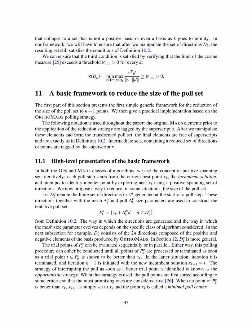
that collapse to a set that is not a positive basis or even a basis as k goes to infinity. Inour framework, we will have to ensure that after we manipulate the set of directions Dk, theresulting set still satisfies the conditions of Definition 10.2.

We can ensure that the third condition is satisfied by verifying that the limit of the cosinemeasure [25] exceeds a threshold κmin > 0 for every k:

κ(Dk) = minv∈Rn

maxd∈Dk

vT d‖v‖‖d‖

≥ κmin > 0.

11 A basic framework to reduce the size of the poll setThe first part of this section presents the first simple generic framework for the reduction ofthe size of the poll set to n+1 points. We then give a practical implementation based on theORTHOMADS polling strategy.

The following notation is used throughout the paper: the original MADS elements prior tothe application of the reduction strategy are tagged by the superscript o. After we manipulatethese elements and form the transformed poll set, the final elements are free of superscriptsand are exactly as in Definition 10.2. Intermediate sets, containing a reduced set of directionsor points are tagged by the superscript r.

11.1 High-level presentation of the basic frameworkIn both the GPS and MADS classes of algorithms, we use the concept of positive spanningsets iteratively: each poll step starts from the current best point xk, the incumbent solution,and attempts to identify a better point by exploring near xk using a positive spanning set ofdirections. We now propose a way to reduce, in some situations, the size of the poll set.

Let Dok denote the finite set of directions in Rn generated at the start of a poll step. These

directions together with the mesh ∆mk and poll ∆

pk size parameters are used to construct the

tentative poll setPo

k = xk +∆mk d : d ∈ Do

k

from Definition 10.2. The way in which the directions are generated and the way in whichthe mesh size parameter evolves depends on the specific class of algorithm considered. In thenext subsection for example, Do

k consists of the 2n directions composed of the positive andnegative elements of the basis produced by ORTHOMADS. In Section 12, Do

k is more general.The trial points of Po

k can be evaluated sequentially or in parallel. Either way, this pollingprocedure can either be conducted until all points of Po

k are processed or terminated as soonas a trial point t ∈ Po

k is shown to be better than xk. In the latter situation, iteration k isterminated, and iteration k + 1 is initiated with the new incumbent solution xk+1 = t. Thestrategy of interrupting the poll as soon as a better trial point is identified is known as theopportunistic strategy. When that strategy is used, the poll points are first sorted according tosome criteria so that the most promising ones are considered first [26]. When no point of Po

kis better than xk, xk+1 is simply set to xk and the point xk is called a minimal poll center.

93

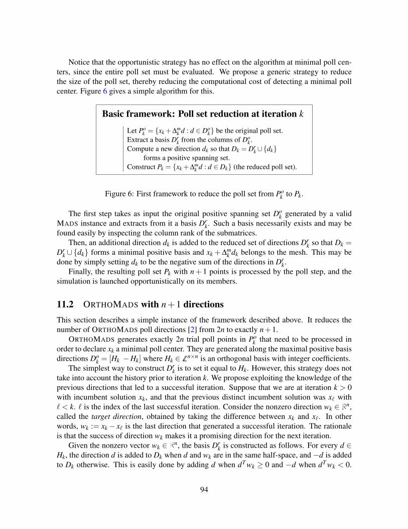
Notice that the opportunistic strategy has no effect on the algorithm at minimal poll cen-ters, since the entire poll set must be evaluated. We propose a generic strategy to reducethe size of the poll set, thereby reducing the computational cost of detecting a minimal pollcenter. Figure 6 gives a simple algorithm for this.

Basic framework: Poll set reduction at iteration k

Let Pok = xk +∆m

k d : d ∈ Dok be the original poll set.

Extract a basis Drk from the columns of Do

k .Compute a new direction dk so that Dk = Dr

k∪dkforms a positive spanning set.

Construct Pk = xk +∆mk d : d ∈ Dk (the reduced poll set).

Figure 6: First framework to reduce the poll set from Pok to Pk.

The first step takes as input the original positive spanning set Dok generated by a valid

MADS instance and extracts from it a basis Drk. Such a basis necessarily exists and may be

found easily by inspecting the column rank of the submatrices.Then, an additional direction dk is added to the reduced set of directions Dr

k so that Dk =Dr

k ∪dk forms a minimal positive basis and xk +∆mk dk belongs to the mesh. This may be

done by simply setting dk to be the negative sum of the directions in Drk.

Finally, the resulting poll set Pk with n+ 1 points is processed by the poll step, and thesimulation is launched opportunistically on its members.

11.2 ORTHOMADS with n+1 directionsThis section describes a simple instance of the framework described above. It reduces thenumber of ORTHOMADS poll directions [2] from 2n to exactly n+1.

ORTHOMADS generates exactly 2n trial poll points in Pok that need to be processed in

order to declare xk a minimal poll center. They are generated along the maximal positive basisdirections Do

k = [Hk −Hk] where Hk ∈ Zn×n is an orthogonal basis with integer coefficients.The simplest way to construct Dr

k is to set it equal to Hk. However, this strategy does nottake into account the history prior to iteration k. We propose exploiting the knowledge of theprevious directions that led to a successful iteration. Suppose that we are at iteration k > 0with incumbent solution xk, and that the previous distinct incumbent solution was x` with` < k. ` is the index of the last successful iteration. Consider the nonzero direction wk ∈ Rn,called the target direction, obtained by taking the difference between xk and x`. In otherwords, wk := xk− x` is the last direction that generated a successful iteration. The rationaleis that the success of direction wk makes it a promising direction for the next iteration.

Given the nonzero vector wk ∈ Rn, the basis Drk is constructed as follows. For every d ∈

Hk, the direction d is added to Dk when d and wk are in the same half-space, and −d is addedto Dk otherwise. This is easily done by adding d when dT wk ≥ 0 and −d when dT wk < 0.

94

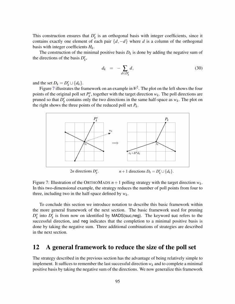
This construction ensures that Drk is an orthogonal basis with integer coefficients, since it

contains exactly one element of each pair d,−d where d is a column of the orthogonalbasis with integer coefficients Hk.

The construction of the minimal positive basis Dk is done by adding the negative sum ofthe directions of the basis Dr

k,

dk = − ∑d∈Dr

k

d, (30)

and the set Dk = Drk∪dk.

Figure 7 illustrates the framework on an example in R2. The plot on the left shows the fourpoints of the original poll set Po

k , together with the target direction wk. The poll directions arepruned so that Dr

k contains only the two directions in the same half-space as wk. The plot onthe right shows the three points of the reduced poll set Pk.

Pokr

r

rHH

HHH

H

rHHHH

HH

2n directions Dok .

1wk

rxk =⇒

Pk

rHHHH

HH

rxk

xk+∆mdkr

r

n+1 directions Dk = Drk∪dk.

Figure 7: Illustration of the ORTHOMADS n+1 polling strategy with the target direction wk.In this two-dimensional example, the strategy reduces the number of poll points from four tothree, including two in the half-space defined by wk.

To conclude this section we introduce notation to describe this basic framework withinthe more general framework of the next section. The basic framework used for pruningDo

k into Drk is from now on identified by MADS(suc,neg). The keyword suc refers to the

successful direction, and neg indicates that the completion to a minimal positive basis isdone by taking the negative sum. Three additional combinations of strategies are describedin the next section.

12 A general framework to reduce the size of the poll setThe strategy described in the previous section has the advantage of being relatively simple toimplement. It suffices to remember the last successful direction wk and to complete a minimalpositive basis by taking the negative sum of the directions. We now generalize this framework

95

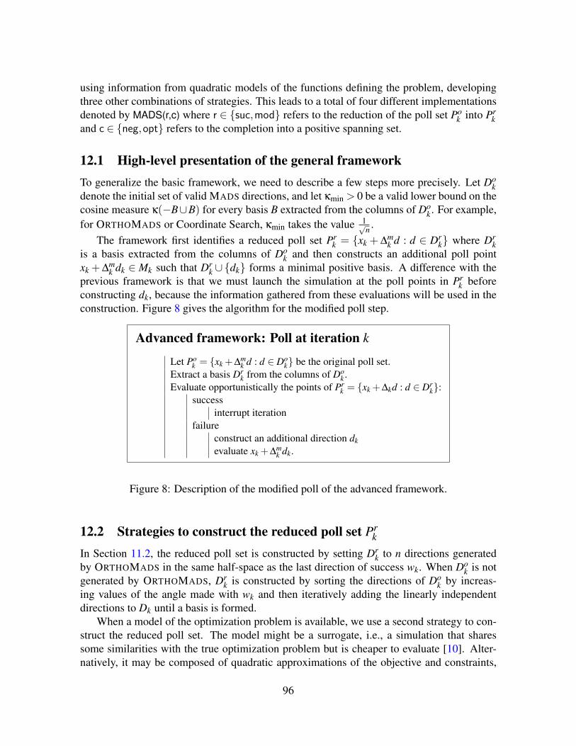
using information from quadratic models of the functions defining the problem, developingthree other combinations of strategies. This leads to a total of four different implementationsdenoted by MADS(r,c) where r ∈ suc,mod refers to the reduction of the poll set Po

k into Prk

and c ∈ neg,opt refers to the completion into a positive spanning set.

12.1 High-level presentation of the general frameworkTo generalize the basic framework, we need to describe a few steps more precisely. Let Do

kdenote the initial set of valid MADS directions, and let κmin > 0 be a valid lower bound on thecosine measure κ(−B∪B) for every basis B extracted from the columns of Do

k . For example,for ORTHOMADS or Coordinate Search, κmin takes the value 1√

n .The framework first identifies a reduced poll set Pr

k = xk +∆mk d : d ∈ Dr

k where Drk

is a basis extracted from the columns of Dok and then constructs an additional poll point

xk +∆mk dk ∈ Mk such that Dr

k ∪dk forms a minimal positive basis. A difference with theprevious framework is that we must launch the simulation at the poll points in Pr

k beforeconstructing dk, because the information gathered from these evaluations will be used in theconstruction. Figure 8 gives the algorithm for the modified poll step.

Advanced framework: Poll at iteration k

Let Pok = xk +∆m

k d : d ∈ Dok be the original poll set.

Extract a basis Drk from the columns of Do

k .Evaluate opportunistically the points of Pr

k = xk +∆kd : d ∈ Drk:

successinterrupt iteration

failureconstruct an additional direction dkevaluate xk +∆m

k dk.

Figure 8: Description of the modified poll of the advanced framework.

12.2 Strategies to construct the reduced poll set Prk

In Section 11.2, the reduced poll set is constructed by setting Drk to n directions generated

by ORTHOMADS in the same half-space as the last direction of success wk. When Dok is not

generated by ORTHOMADS, Drk is constructed by sorting the directions of Do

k by increas-ing values of the angle made with wk and then iteratively adding the linearly independentdirections to Dk until a basis is formed.

When a model of the optimization problem is available, we use a second strategy to con-struct the reduced poll set. The model might be a surrogate, i.e., a simulation that sharessome similarities with the true optimization problem but is cheaper to evaluate [10]. Alter-natively, it may be composed of quadratic approximations of the objective and constraints,

96

as presented in [13] or in [16] in the unconstrained case. Regardless of the type of model,the second strategy consists of ordering the directions of Do

k according to the model valuesat the tentative poll points in Po

k . We then sort the feasible points by their objective functionvalues. To handle the infeasible points, we use the constraint aggregation function [20] inconjunction with the progressive barrier [7]. Using these tools, we order the directions of Do

kas proposed in [13]. Finally, we iteratively add to Dk the linearly independent directions ofDo

k until a basis is formed. The models used in the numerical tests of Section 14 are quadraticmodels.

In the numerical experiments, these two strategies will be tagged with the labels sucand mod, which stand for ordering by the angle made with the last successful direction orby the model values, respectively. Notice that both strategies can be applied for both theunconstrained case and the constrained case.

12.3 Completion to a positive basisHaving constructed the reduced poll set, we evaluate the blackbox functions defining prob-lem (53) at the trial points in Pr

k = xk + ∆mk d : d ∈ Dr

k. The process is opportunistic,meaning that it terminates either when a new incumbent solution is found or when it cannotfind a better solution than xk. In the latter case, we construct an additional direction dk. Toease the presentation, let d1,d2, . . . ,dn denote the n directions forming the basis Dr

k. Theadditional direction dk must be chosen so that

dk ∈ int(cone−d1,−d2, . . . ,−dn) (31)

and the new poll candidate must belong to the mesh: xk +∆mk dk ⊆Mk.

When constructing the positive basis, we must consider an important algorithmic aspect.Even if Dr

k ∪ dk forms a positive spanning set for all values of k, the limit in the senseof [15] might collapse to a nonpositive spanning set, as illustrated by the example at theend of Section 10.2. To address this potential problem, we introduce a minimal threshold0 < ε < 1, a scalar fixed throughout the algorithm, and we require the added direction dk tosatisfy

dk = −n

∑i=1

αidi (32)

where ε < αi ≤ 1 for i = 1,2, . . . ,n. Notice that under these conditions, the requirements ofEq. (31) are satisfied. Notice also that Eq. (32) is consistent with Eq. (30) where dk is simplythe negative sum of the directions.

The solution of a model or surrogate of the optimization problem restricted to the region

Cε =

xk−∆

mk

n

∑i=1

αidi : αi ∈ [ε,1], i = 1,2, . . . ,n

is needed to generate a trial point yk ∈Cε. We describe in the next subsection a way to performthis suboptimization using quadratic models.

97

Finally, it is unlikely that the resulting candidate yk belongs to the mesh. The last stepconsists of rounding yk to some point xk +∆m

k dk on the mesh Mk. In the LTMADS or OR-THOMADS framework, where the mesh is constructed from the positive and negative coordi-nate directions, it suffices to set the jth coordinate of dk to

(dk) j =

dv je if v j ≤−∑

pi=1 di

j

bv jc if v j >−∑pi=1 di

j,

where d.e and b.c are the ceiling and floor operators respectively and vk ∈ Rn satisfies theequality yk = xk +∆m

k vk. This approach rounds the trial point toward xk−∆mk ∑

pi=1 di and en-

sures that Drk∪dk forms a positive spanning set (these assertions are formally demonstrated

in Section 13).This strategy of completion to a positive basis via a suboptimization is called the opt

strategy.

12.4 Completion using quadratic modelsThis section gives the technical details of the construction of the candidate yk ∈Cε generatedby considering quadratic models of the objective and constraints.

We build one quadratic model for the objective function and one for each constraint. Moreprecisely, the feasible region Ω defined in (53) is described as the following set of inequalityconstraints:

Ω =

x ∈ Rn : c j(x)≤ 0 for all j ∈ J

with J = 1,2, . . . ,nJ and c j : Rn → R∪ ∞, j ∈ J. The infinity value is used for trialpoints where at least one function failed to evaluate in practice, due to some hidden constraintembedded in the simulator associated with this function.

First, we collect data points where the function values are available and finite. Thesepoints form the data set Y ⊂ Rn and are taken within a neighborhood of the poll center:

Y =

y ∈Vk : ‖y− xk‖∞ ≤ ρ∆pk , f (y)< ∞ and g j(y)< ∞ for all j ∈ J

where the parameter ρ≥ 2 is called the radius factor and is typically set to 2 as in [13]. Theconstraint ρ ≥ 2 ensures that the recently evaluated poll points of Pr

k belong to Y . Further-more, this choice of ρ also ensures that the previously visited trial points in the region Cε

are contained in Y . Note that cache points from previous iterations may also be found in Y ,which enriches the models.

Consider the nonsingular linear transformation T : Rn → Rn that maps the region Cε tothe unit hypercube [0,1]n, as illustrated in Fig. 9. The motivation for this transformation is toreplace linear constraints by simple bounds to construct the model optimization problem (33).For y ∈ Rn and λ ∈ Rn the expressions for T (y) and its inverse T−1(λ) are:

T (y) =(Dr

k)−1

∆mk (1− ε)

(xk− y−∆mk Dr

k1ε)

and T−1(λ) = xk +∆mk Dr

k((ε−1)λ− ε1).

98

Indeed, it can readily be verified that T (xk−∆mk Dr

k1) = 1, T−1(1) = xk−∆mk Dr

k1 and thatT (xk− ε∆m

k Drk1) = 0, T−1(0) = xk− ε∆m

k Drk1.

The shaded area on the left of Fig. 9 represents the set Cε, and the open circle representsthe candidate yk.

.

..............................................

.............................................

............................................

...........................................

...................................................................................

....................................... ...................................... ....................................... ........................................ .........................................................................

..........

..........................................

...........................................

......................................

......

..................................

...........

T (Cε)

0

1j

.

........................

................

........................

.............

........................

...........

..........................

.......

..............................

...

.................................

..................................

..................................

..................................

.................................. ................................... ................................... .................................... ...............................................................................

...........................................

.............................................

...............................................

.................................................

...................................................

T−1([0,1]n)

][0,1]n

•

•

•

•

••

•

•

xk

xk+∆mk d1

xk+∆mk d2

Cε

yk

?PPq

xk+∆mk dk

Figure 9: The T transformation applied to Cε gives the unit hypercube.

The next step consists of building the nJ + 1 models by considering the scaled points of[0,1]n. Depending on the size nY of the data set Y , there are two possible strategies. First, ifnY < (n+1)(n+2)/2, which is more likely to happen, we consider minimum Frobenius normmodels; otherwise we use least-squares regression. See [13] for the computational details.

Let m f be the model constructed from f and mg j the model associated with g j for allj ∈ J. We expect these models to be good representations of the original functions in thezone of interest:

m f (T (x))' f (x) and mg j(T (x))' g j(x) for all x ∈Cε.

In Fig. 9, the shaded region represents Cε. The solid outline on the left represents the regionin which ‖y− xk‖ ≤ ρ∆

pk with a value of ρ = 2. The eight points of Y represented by bullets

are used to construct the models. The right part of the figure represents the hypercube onwhich the following quadratic model is minimized:

minλ∈[0,1]n

m f (λ) subject to mg j(λ)≤ 0 for all j ∈ J. (33)

Any method, heuristic or otherwise, can be applied to solve Problem (33) since the conver-gence of the framework does not rely on the quality of this optimization. However, in practicebetter solutions should improve the overall quality of the method. Currently, and similarly

99

to [13], we use the MADS algorithm for the sake of simplicity. Future work will include thereplacement of MADS by a dedicated bound-constrained quadratic solver.

The point obtained when solving Problem (33) is denoted λk ∈ [0,1]n and can be feasibleor infeasible with respect to the model constraints. Regardless of feasibility, the solution istransformed into the original space via the inverse transformation: set yk = T−1(λk) ∈Cε.

13 Convergence analysis of the general frameworkWe now show that the general framework is a valid MADS instance. The analysis does notdepend on the order in which the poll points are evaluated, and it therefore holds for the basicframework of Section 18.1. Next, we give a detailed example in which the set of normalizedrefined directions does not grow asymptotically dense in the unit sphere. To circumvent thisundesirable behavior, we add a rule to decide whether or not the polling reduction should beapplied.

13.1 A valid MADS instanceTo show that the general framework produces a valid MADS instance, we must prove that theconditions of Definition 10.2 are satisfied. To achieve this, we must redefine the set D of di-rections used to construct the polling directions to take into account the fact that the directiondk produced by Eq. (32) lies in the cone generated by the negative of d1,d2, . . . ,dn.

Let Do be the original set used to construct the set Dok at every iteration, and consider the

direction with the largest norm: dmax ∈ argmax‖d′‖ : d′ ∈ Do. Now, replace Do by

D =−Do∪Do∪n dmax

as the new finite set of directions. The addition of −Do ensures that the added direction dkfrom Eq. (32) belongs to the cone of negative directions. It also ensures that the strategy thatrounds yk generates a mesh point successfully, because Cε contains at least one mesh point,namely xk−∆m

k ∑ni=1 di. The addition of n dmax does not introduce any point into the mesh. It

simply ensures that dk belongs to the poll frame and increases the maximal norm used in thesecond condition of Definition 10.2, thereby allowing poll points to lie further from the pollcenter. Figure 7 illustrates the fact that the norm of the added direction dk may exceed that ofthe directions in the original set Do

k .The following proof is independent of the construction of the reduced poll set Pr

k and ofthe method used for the completion to a positive spanning set, provided Dr

k is a basis extractedfrom Do

k and dk satisfies Eq. (32).

Lemma 13.1 If Drk = d1,d2, . . . ,dn is a basis of Rn extracted from the columns of Do

k anddk = −∑

ni=1 αidi with 0 < ε ≤ αi ≤ 1 for i ∈ 1,2, . . . ,n then Dk = Dr

k ∪dk is a minimalpositive basis and

κ(Dk)≥ε

nκ(−Dr

k∪Drk).

100

Proof. Let Drk and Dk satisfy the conditions in the statement. To show that Dk is a posi-

tive spanning set, we let v be a nonzero vector in Rn such that vT di ≤ 0 for i = 1,2, . . . ,n.Then, since Dr

k is a basis and v 6= 0, vT di < 0 for at least one index i. Therefore, vT dk =−∑

ni=1 αivT di ≥−ε∑

ni=1 vT di > 0 and consequently v is in the same half-space as dk. Since

Dk contains exactly n elements, it follows that it is a minimal positive basis [17].The cosine measure is invariant with respect to the length of the vectors, since the vectors

are normalized, so let us introduce λ = dk‖dk‖ and δi = di

‖di‖ for i = 1,2, . . . ,n. The cosinemeasure can be obtained by solving the following optimization problem:

κ(Dk∪dk) = mint∈R,v∈Rn

t

s.t. t ≥ vT δi i = 1,2, . . .nt ≥ vT λ

vT v = 1.

There exists an optimal solution (t,v) such that n of the inequality constraints are satisfied atequality and t = κ(Dk∪dk). Two cases must be considered:

Case 1. If vT δi = κ(Dk ∪ dk) for every index i = 1,2, . . . ,n, then κ(Dk ∪ dk) = vT δi,which implies that κ(Dk∪dk) = κ(−Dr

k∪Drk)≥ κ(−Dr

k∪Drk).

Case 2. Otherwise, renaming the indices if necessary, vT δi = κ(Dk ∪dk) for every indexi = 1,2, . . . ,n−1 and vT λ = κ(Dk∪dk). By the definition of λ and Eq. (32), we have

κ(Dk∪dk) = vTλ = −

n

∑i=1

αivTδ

i

= −

(κ(Dk∪dk)

n−1

∑i=1

αi +αnvTδ

n

)≥ −κ(Dk∪dk)(n−1)+αnvT (−δ

n).

Observe that vT (−δn) ≥ 0, since otherwise all directions of the positive basis Drk ∪ dk

would lie in the same half-space, which is impossible. Reordering the terms, dividing by n,and using the fact that αn ≥ ε yields κ(Dk∪dk)≥ ε

nvT (−δn).Next, consider the cosine measure of the maximal positive basis −Dr

k∪Drk:

κ(−Drk∪Dr

k) ≤ maxi=1,2,...,n

|vTδ

i|

= maxκ(Dk∪dk),vT (−δn).

It follows that either κ(Dk∪dk)≥ κ(−Drk∪Dr

k) or vT (−δn)≥ κ(−Drk∪Dr

k). In both casesthe inequality κ(Dr

k∪dk)≥ ε

nκmin holds.

The following theorem ensures that this strategy yields a valid MADS instance by showingthat the conditions of Definition 10.2 are satisfied.

101

Theorem 13.2 Let Dok be the original spanning set. The poll set formed by the directions in

Dk = Drk ∪dk, where Dr

k is a basis formed of n columns of Dok and xk +∆m

k dk belongs toMk∩Cε, yields a valid MADS instance.

Proof. Since Dok is a valid set of polling directions and xk + ∆m

k dk belongs to the mesh,xk +∆m

k d ∈Mk for every d ∈ Dk and the first condition of Definition 10.2 is satisfied.Since Dr

k ⊂ Dok and Do ⊂ D, the second condition is trivially satisfied for every direction

d ∈ Dk. For the additional direction,

∆mk ‖dk‖ ≤ ∆

mk

n

∑i=1

αi‖di‖ ≤ n∆mk dmax = ∆

pk max‖d′‖ : d′ ∈ D

since αi ≤ 1 and dmax is the direction of D with the largest norm. This shows that the secondcondition of the definition is satisfied.

The previous lemma showed that Dk is a minimal positive basis and that its cosine mea-sure is bounded below by the strictly positive value ε

nκmin. This ensures that the third condi-tion of the definition is satisfied.

All the conditions of Definition 10.2 are satisfied, and therefore this strategy defines avalid instance of MADS.

13.2 An example that does not cover all directionsSatisfying the requirements of Definition 10.2 is not sufficient to ensure that the set of normal-ized polling directions grows asymptotically dense in the unit sphere. Indeed, the CoordinateSearch and GPS are both instantiations of MADS, but the set of polling directions is limitedto a fixed finite number.

We now give an example for which reducing the size of the poll set at every iteration doesnot produce a dense set of directions. In the next subsection, we propose a slight modificationof the method that guarantees density in the unit sphere. The following example illustratesthis issue.

Example 13.3 Consider the unconstrained minimization of the continuous piecewise linearfunction f : R2→ R defined as

f (a,b) = maxa,min−a+b,−a−b

whose graph is plotted on the left of Fig. 10 and whose level sets are represented on the rightof the figure.

Now, suppose that the initial point is x0 = (−1,0)T with f (x0) = 1, and that the first trialpoint proposed by a MADS instance is the origin. The iteration is successful and terminatesat x1 = (0,0)T with f (x1) = 0. The direction of success is w1 = (1,0)T .

Now consider any iteration k ≥ 1 with xk = (0,0) and let Dok = [Hk −Hk] be a maximal

positive basis obtained using an orthogonal basis Hk. Construct the basis Drk by taking

directions in Dok that are in the same half-space as the target direction wk. Dr

k contains

102

Figure 10: Graphical representation and level sets of a continuous piecewise linear function.

exactly two directions in the half-space V = v = (v1,v2) ∈ R2 : v1 ≥ 0 and any trial pointgenerated in that subspace xk +∆m

k v = ∆mk v will have a nonnegative objective function value

equal to ∆mk v1.

Therefore, the additional direction dk will need to be computed. But since Drk forms an

orthogonal basis, the direction dk will necessarily belong to the cone W = v ∈ R2 : v1 <0, |v1| ≥ |v2|. However, any trial point generated in that cone also possesses a nonnegativeobjective function value because f (v) = −v1− |v2| = |v1| − |v2| ≥ 0 for every v ∈W. Itfollows that iteration k ≥ 1 is unsuccessful and xk = (0,0)T for every k ≥ 1.

In this example, even if the sets of normalized directions of Dok generated by a valid

MADS instance grow asymptotically dense in the unit sphere, the normalized sets of pollingdirections Dk = Dr

k ∪dk are never generated in the full-dimensional cone v ∈ R2 : v1 <0, |v2|> |v1|.

13.3 Asymptotically dense normalized polling directionsThe previous example shows that the poll reduction strategy cannot be systematically ap-plied at every iteration. A similar difficulty was encountered n the development of the OR-THOMADS 2n algorithm (see the management of the index tk in Section 3.4 of [2]). Thesituation was handled by making different algorithmic decisions based on whether or not thecurrent poll size parameter is the smallest so far, i.e., if ∆

pk ≤ ∆

pj for every integer j ≤ k. The

same treatment is applied to the present context.To formalize the presentation, we give the definition of a refining direction for a MADS

algorithm.

Definition 13.4 (from [6]) A subsequence of the MADS iterates consisting of minimal framecenters (i.e., unsuccessful iterations) xkk∈K for some subset of indices K is said to be a

103

refining subsequence if ∆pkk∈K converges to zero.

Let x be the limit of a convergent refining subsequence. If the limit limk∈Ldk‖dk‖ exists for

some subset L⊆K with poll direction dk ∈Dk, and if xk+∆mk dk ∈Ω for infinitely many k ∈ L,

then this limit is said to be a refining direction for x.

Theorem 13.5 Suppose that the strategy for generating the set of original polling directionsDo

k∞k=0 is rich enough that the set of normalized refining directions grows asymptotically

dense in the unit sphere. At iteration k, define the poll set:

Dk =

Do

k if ∆pk ≤ ∆

pj for every integer j ≤ k

Drk∪dk otherwise.

Then the set of refining directions with Dk grows asymptotically dense in the unit sphere.

Proof. Consider the subset of indices of unsuccessful iterations

U = k1,k2, . . . = k : iteration k is unsuccessful and ∆pk ≤ ∆

pj ∀ j = 0,1, ...k.

This subset is infinite because liminfk ∆mk = 0 for any valid MADS instance. The mesh size

is reduced only at unsuccessful iterations, and therefore there exists a refining subsequencewith indices in U . However, the construction of the poll set is such that at all iterations inU , the set of poll directions is Dk = Do

k . Therefore, the normalized directions are constructedwith elements of Do

k , which grow dense by assumption. The previous result ensures that the proposed method inherits the convergence results of

MADS. More precisely, let x be a feasible limit of a refining subsequence generated by anORTHOMADS instantiation that reduces to n+1 polling directions, as prescribed by the pre-vious theorem. Then, the analyses of [6, 7] ensure that the Clarke directional derivatives arenonnegative for every direction in the Clarke tangent cone, provided f is Lipschitz near x andthe hypertangent cone at x is not empty. For directionally Lipschitz functions, the Rockafellargeneralized directional derivatives are nonnegative along the refining directions [32].

14 Numerical resultsThe numerical tests are conducted using the NOMAD [26] software publicly available athttp://www.gerad.ca/nomad. The tests compare the performance of the new frameworkswith the default version. All tests are conducted with the ORTHOMADS strategy: the originalset of directions Do

k at iteration k is the orthogonal maximal positive basis introduced in [2].In our implementation, the default value of the parameter ε from Section 12.3 is 1%.

The default version of the algorithm is denoted MADS 2n, and the basic framework pre-sented in Section 11.2 is denoted MADS(suc,neg) where suc stands for a successful directionas the target direction, and neg for the sum of negative directions for the positive basis com-pletion.

The combination of strategies where Prk is obtained not by considering the target direction

but by ordering the model values is denoted MADS(mod,neg). The keyword mod stands

104

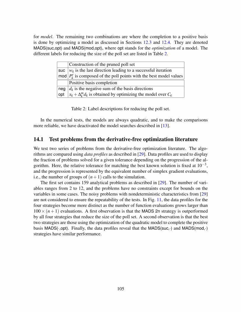
for model. The remaining two combinations are where the completion to a positive basisis done by optimizing a model as discussed in Sections 12.3 and 12.4. They are denotedMADS(suc,opt) and MADS(mod,opt), where opt stands for the optimization of a model. Thedifferent labels for reducing the size of the poll set are listed in Table 2.

Construction of the pruned poll setsuc wk is the last direction leading to a successful iterationmod Pr

k is composed of the poll points with the best model valuesPositive basis completion

neg dk is the negative sum of the basis directionsopt xk +∆m

k dk is obtained by optimizing the model over Cε

Table 2: Label descriptions for reducing the poll set.

In the numerical tests, the models are always quadratic, and to make the comparisonsmore reliable, we have deactivated the model searches described in [13].

14.1 Test problems from the derivative-free optimization literatureWe test two series of problems from the derivative-free optimization literature. The algo-rithms are compared using data profiles as described in [29]. Data profiles are used to displaythe fraction of problems solved for a given tolerance depending on the progression of the al-gorithm. Here, the relative tolerance for matching the best known solution is fixed at 10−3,and the progression is represented by the equivalent number of simplex gradient evaluations,i.e., the number of groups of (n+1) calls to the simulation.

The first set contains 159 analytical problems as described in [29]. The number of vari-ables ranges from 2 to 12, and the problems have no constraints except for bounds on thevariables in some cases. The noisy problems with nondeterministic characteristics from [29]are not considered to ensure the repeatability of the tests. In Fig. 11, the data profiles for thefour strategies become more distinct as the number of function evaluations grows larger than100× (n+ 1) evaluations. A first observation is that the MADS 2n strategy is outperformedby all four strategies that reduce the size of the poll set. A second observation is that the besttwo strategies are those using the optimization of the quadratic model to complete the positivebasis MADS(·,opt). Finally, the data profiles reveal that the MADS(suc,·) and MADS(mod,·)strategies have similar performance.

105

20 40 60 80 100 120 1400

10

20

30

40

50

60

70

80

90

100

Groups of n + 1 evaluations

Fra

ctio

nofpro

ble

ms

solv

ed(%

)

uT

uT

uT

uTuT

uTuT

uT

lD

lD

lD

lDlD

lD lDlD

rS

rS

rS

rSrS

rSrS

rS

qP

qP

qP

qPqP

qPqP qP

bC

bC

bCbC

bC

bCbC

bC

uT MADS 2nlD MADS(suc,neg)rS MADS(suc,opt)qP MADS(mod,neg)bC MADS(mod,opt)

1Figure 11: Data profiles with a relative tolerance of 10−3 for 159 problems from [29].

106

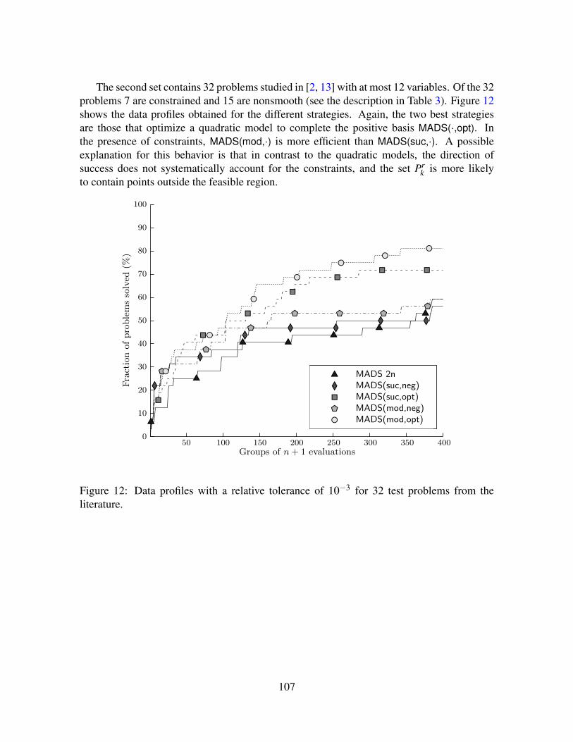
The second set contains 32 problems studied in [2, 13] with at most 12 variables. Of the 32problems 7 are constrained and 15 are nonsmooth (see the description in Table 3). Figure 12shows the data profiles obtained for the different strategies. Again, the two best strategiesare those that optimize a quadratic model to complete the positive basis MADS(·,opt). Inthe presence of constraints, MADS(mod,·) is more efficient than MADS(suc,·). A possibleexplanation for this behavior is that in contrast to the quadratic models, the direction ofsuccess does not systematically account for the constraints, and the set Pr

k is more likelyto contain points outside the feasible region.

50 100 150 200 250 300 350 4000

10

20

30

40

50

60

70

80

90

100

Groups of n + 1 evaluations

Fra

ctio

nofpro

ble

ms

solv

ed(%

)

uT

uT

uT uTuT

uTuT

lD

lD

lDlD lD

lD lD

rS

rS

rS

rSrS

rS rS

qP

qP

qPqP qP qP

qP

bC

bC

bC

bCbC

bCbC

uT MADS 2nlD MADS(suc,neg)rS MADS(suc,opt)qP MADS(mod,neg)bC MADS(mod,opt)

1Figure 12: Data profiles with a relative tolerance of 10−3 for 32 test problems from theliterature.

107

# Name Source n nJ Bnds Smth f ∗

1 ARWHEAD [22] 10 0 no yes 0.02 BDQRTIC [22] 10 0 no yes 18.28123 BIGGS6 [22] 6 0 no yes 6.97074 ·10−5

4 BRANIN [23] 2 0 yes yes 0.3978875 BROWNAL [22] 10 0 no yes 0.06 CRESCENT10 [7] 10 2 no yes −9.07 DIFF2 [13] 2 0 yes no 2 ·10−4

8 DISK10 [7] 10 1 no yes −17.32059 ELATTAR [28] 6 0 no no 0.561139

10 EVD61 [28] 6 0 no no 3.51212 ·10−2

11 FILTER [28] 9 0 no no 8.40648 ·10−3

12 G2 [8] 10 2 yes no −0.74046613 GRIEWANK [23] 10 0 yes yes 0.014 HS78 [28] 5 0 no no −2.4911115 HS114 [28] 9 6 yes no −1429.3416 MAD6 [28] 5 7 no no 0.10183117 OSBORNE2 [28] 11 0 no no 9.43876 ·10−2

18 PBC1 [28] 5 0 no no 8.90604 ·10−2

19 PENALTY1 [22] 10 0 no yes 7.08765 ·10−5

20 PENALTY2 [22] 10 0 no yes 2.95665 ·10−4

21 PENTAGON [28] 6 15 no no −1.8596222 POLAK2 [28] 10 0 no no 54.598223 POWELLSG [22] 12 0 no yes 0.024 RASTRIGIN [23] 2 0 yes yes 0.025 SHOR [28] 5 0 no no 22.602326 SNAKE [7] 2 2 no yes 0.027 SROSENBR [22] 10 0 no yes 0.028 TRIDIA [22] 10 0 no yes 0.029 VARDIM [22] 10 0 no yes 0.030 WONG1 [28] 7 0 no no 680.70731 WONG2 [28] 10 0 no no 24.945832 WOODS [22] 12 0 no yes 0.0

Table 3: Description of the set of 32 analytical problems. Those for which nJ > 0 haveconstraints other than bounds. The column Bnds indicates whether a problem has boundconstraints, the column Smth indicates whether the problem is smooth, and the column f ∗

gives the best known solution.

108

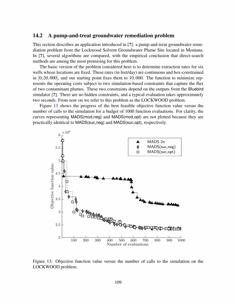
14.2 A pump-and-treat groundwater remediation problemThis section describes an application introduced in [?]: a pump-and-treat groundwater reme-diation problem from the Lockwood Solvent Groundwater Plume Site located in Montana.In [?], several algorithms are compared, with the empirical conclusion that direct-searchmethods are among the most promising for this problem.

The basic version of the problem considered here is to determine extraction rates for sixwells whose locations are fixed. These rates (in feet/day) are continuous and box-constrainedin [0;20,000], and our starting point fixes them to 10,000. The function to minimize rep-resents the operating costs subject to two simulation-based constraints that capture the fluxof two contaminant plumes. These two constraints depend on the outputs from the Bluebirdsimulator [?]. There are no hidden constraints, and a typical evaluation takes approximatelytwo seconds. From now on we refer to this problem as the LOCKWOOD problem.

Figure 13 shows the progress of the best feasible objective function value versus thenumber of calls to the simulation for a budget of 1000 function evaluations. For clarity, thecurves representing MADS(mod,neg) and MADS(mod,opt) are not plotted because they arepractically identical to MADS(suc,neg) and MADS(suc,opt), respectively.

100 200 300 400 500 600 700 800 900 10002

2.5

3

3.5

4

4.5

5

5.5

6×104

Number of evaluations

Obje

ctiv

efu

nct

ion

valu

e

uT

uTuT

uT uT uT uT uT uT uT uT uT uT uT uT uT uT uT uT uT uT uT uT uT uT uT uT uT uTuTuTuT uT uT uT uT uT uT uT uT uT uT uT uT uT uT uT uT uT uT uT

lD

lDlD

lD

lDlD lD lD

lD lD lD lD lD lD lD lD lD lD lD lD lD lD lD lD lD lD lD lD lD lD lD lD lD lD lD lD lD lD lD lD lD lD lD lD lD lD lD lD lD lD lD lD lD lD lD lD lD lD lD lD lD lD lD lD lD lD lD lD lD

rS

rSrS

rS

rS

rS

rS rS rS rS rS rS rS rS rS rS rS rS rS rS rS rS rS rS rS rS rS rS rS rS rS rS rS rS rS rS rS rS rS rS rS rS rS rS rS rS rS rS rS rS rS rS rS rS rS rS rS rS rS rS rS rS rS

uT MADS 2nlD MADS(suc,neg)rS MADS(suc,opt)

1Figure 13: Objective function value versus the number of calls to the simulation on theLOCKWOOD problem.

109

The MADS 2n algorithm gets stuck at local solutions, and the runs in which the numberof polling directions is reduced to n+ 1 all have similar behavior and converge rapidly to amuch better solution.

15 DiscussionThe MADS algorithm is composed of two main steps: the global search and the local poll.We have focused on reducing the number of poll points. In previous instantiations of MADS,the poll set was constructed by considering the 2n directions of a maximal positive basis. Wehave proposed four combinations of strategies to reduce that number to n+ 1, which is theminimal number required for the theory to hold. The reduction is applied at every iterationwhere the mesh is not the finest so far.

The next release of the NOMAD software will allow the reduction of the size of the pollset as we have described. To make the software package easily usable by a wide community,we try to limit the number of user-defined parameters. Numerical experiments in which thevalue of ε was varied led to minor changes in the solutions. Therefore, we chose to fix ε to1%.

Guided by our numerical results, we have set the default strategy for generating thepolling directions in NOMAD to MADS(suc,neg) when the user does not use the option tobuild quadratic models and when no surrogates are used; to MADS(mod,opt) when quadraticmodels are used; and to MADS(mod,neg) when a surrogate optimization problem is supplied.These options are enabled in NOMAD by setting the DIRECTION TYPE parameter to ORTHON+1 and may be overruled by setting it to e.g., ORTHO N+1 SUC OPT.

110

16 ORTHOMADS n+1 vs ORTHOMADS 2n:Numerical Results on two real problems

Previously we introduced the ORTHOMADS-(n+ 1) algorithm and in particular two phasesof the MADS algorithms were focused:

• the dynamic ordering of the trial points Pk;

• the completion of the Halton basis to a positive spanning set.

Two target directions have been considered as reference to order all the others: the directionof the last success (suc) or a direction computed through approximation models (mod).In parallel two methods have been studied to complete a basis (the Halton basis has beenconsidered) to a positive spanning set of directions: the first was simply adding the negativesum of the n directions forming the basis to the base itself (neg), while the second, morecomplicated, considered the use of a quadratic model to detect the ”best” completion (opt).So the numerical results about test problems contained in the literature have been studied onthe classical ORTHOMADS (with the 2n exploring directions) the four cases shown in theTable 4:

In this additional numerical part the target will be a little different: testing the innovationbrought by the introduction of the n+1 directions instead of the classical 2n directions of theexisting ORTHOMADS.

For this purpose it has been decided to compare the classical ORTHOMADS with just oneof the four algorithms described in the ORTHOMADS n+1:

(suc,neg).

The reason is simple: study the effect on te reduction of the exploring directions without the”help” of the surrogate fuctions. In this way we are pretty confident to be able to see theeffective power of the two methods.

Before analyzing the results the two real problems are briefly presented.

111

poll ordering pss completionsuc negsuc optmod negmod opt

Table 4: The four cases of the ORTHOMADS n+1.

16.1 MDOWith MDO a particular muldisciplinary design optimization problem about the design of anaricraft (a problem from the mechanical engineering literature) is meant. The name is referredto the kind of the problem more than to the specific problem itsefl because of the importancethat those kind of problems gained in the last 20 years. In particular a lot of applicationswere on the aircraft designs and on the wings shaping because these kind of problems areextremely challenging. The main reason is the combination of three different disciplinesnecessary to compute the measures of interest on the aircraft: structure, aerodynamics andpropulsion. The fourth one is the performance that is conceptually separate from the others:it just receives the informations from the others three and evaluate the range performance ofthe design.

The coupling of the different disciplines is due to the fact that aerodynamics loads causechanges in aircraft structural deflection that, in turn, changes the aerodynamics characteristicsof the aircraft. Moreover the thrust required is dependent on the total aircraft weight, hencealso on the eengine weight which in turn is function of the thrust.

In order to do that a simplified aircraft model with 10 variables is studied. The target is tomaximize (or minimize the opposite of) the aircraft range being subect to bounds constraintsand 10 open constraints. From our point of view we have a black-box using an iterativefixed point method through the three disciplines mentioned above that returns the value ofthe aircraft range.

Remark 16.1 Algorithms designed specifically for the MDO problems exist and, banally,gives results better than the one obtained by the Pattern Search methods. Since the PatternSearch algorithms, and hence also the MADS algorithms, are intended for a much more wideuse, here the target is not to have performances better than the ”proper” MDO algorithms.

16.2 STYRENEThe chemical industry has undergone significant changes during the past 25 years becauseof the increased cost of energy, the increasingly stringent environmental regulations and theglobal competition in product pricing and quality. For this reason the optimization has be-come very important in this field recently: modifications in plant designs, implementation ofoperating procedures to reduce costs and satisfying constraints, improvements on efficiency.

One example is the styrene (a derivative of benzene) production process simulation. It isproduced in large scale from the ethylbenzene, followinf 4 steps:

112

• the reactants preparation, with the pressure rise and the evaporation;

• the catalytic reactions;

• the styrene recovery, that represents the first distillation;

• the benzene recovery, representing the second distillation.

The Sequential Modular Simulation (SMS) paradigm was used to develop a chemical pro-cess simulator. The problem is such that each block can compute its output only after havingcomputed its input. Unfortunately the first block of the sequence requires the evaluations ofthe last ones and that is one of the reason of the high cost of the function evaluations.

The target is to maximize a variable said Net Present Value (NPV) related to the styreneproduction process project, satisfying also regulations both industrial and environmental.

In this case our black-box includes common methods as Runge-Kutta, Newton, the fixedpoints, secant, bisection and also chemical engineering related solvers.

17 Numerical ResultsThe numerical parts in the Optimization context often deal with the classical test functions asseen in the previous numerical part. If the wide literature and a strong tradition about thesekind of functions affect such choice, one of the main reasons is the lack of real problems totest. The Derivative-Free branch is not an exception in this sense, though there have been alot of new simulation-based codes developed in the last years. Needless to say that testingan algorithm on a real problem does not give results necessarily similar to tests on standardfactitious problems in general. For this reason this section has been inserted in addition tothe previous numerical part, because, after having tested the efficiency on the problems in theliterature, we want to test the reduction of the directions procedure ”off-road”. Moreover wedo not have to forget that the innovations present in this work, as the most of the innovationsin the DFO context, is intended to be a massive applicability. From that the importance ofhaving some real testing problems, as MDO and STYRENE.

Considering the MADS evolution, ORTHOMADS (2n) has been taken as benchmark tobe compared with the new ORTHOMADS (n+1). Usually, when a large set of problems isnot available, the algorithms are tested on a certain launching the runs from various startingpoints. So, in our case, the reduced number of problems has been balanced with a muchlarger number of considered starting points. The results are represented with the data profilescorrelating the number of ”solved” (respect with a certain precision degree) problems withthe number of iterations performed. The algorithm ORTHOMADS (n+1) represents a pollmodification in the MADS structure. For this reason here it has been isolated the contributionof the surrogates used in the ORTHOMADS (n+1), (neither in the Search nor in ordering thetrial points within the Poll phase) relying exclusively on the poll phase.

The MDO problem has a more robust function code respect with STYRENE, so it resultsbetter defined. That simply means that a generic STYRENE computation has a higher proba-

113

bility to fail. Moreover the MDO function evaluation is also much less costly. For this reasonit has been possible to fulfill a deeper analysis about it. MDO has been the first prototype.

MDO. The first step as been giving a measure of the robustness of MDO function: the twoORTHOMADS algorithms have been tested for 10 different sets of starting points, each onewith 100 elements, in order to verify how much the results feel the effects of the initial dis-tribution itself. The results, reported from the figure 14 to 23, show different data profiles,but with the same well-defined trend. It is easy to see that happens because having consid-ered large enough sets of starting points. At limit, sets of ∞ starting points would be all thesame. Anyway from sufficiently numerous sets of starting points MDO the results are not tooaffected by the used distribution. As a subresult it is important to notice that after 1000 itera-tions ORTHOMADS (n+1) solves an average of 89.3% of the problems, while ORTHOMADS

(2n) just 44.9% of the total, for an average difference of 44.4%. For the third distribution ofthe points (26) there is the minimum difference (83%−49% = 34.0%), while for the fifth one(28) the maximum one (93%−42% = 51%). These first results agree with the intuition aboutthe possibility of an increase of the speed of the convergence of the method ORTHOMADS

(n+1).A particular mention is necessary for two parameters: τ and the maximum number of iter-

ations. Setting the parameters of optimization algorithms is often a very tricky problem. ThePenalty function approach in the constrained environment is just one of the several literaturecases. Too often the problem of setting the parameters is liquidated without underlining thecriticism of that point. Though the MADS algorithm are a category not affected by this ”curseof setting the right parameters” and the only parameters to set are about the data representa-tions, here it is specified how it has been done to remark the not-criticality of this point andto the advantage of the reader; the will, in fact, is to give a very general modality of work.

In particular τ simply concern the data representations, with the only effect to modifythe data profiles. It is strictly related to the maximum number of iterations, for which thediscussion is very simple: Ideally we could need an infinite number of iterations to find thereal solution. Despite of that this work concerns an increase of the rate of the convergence. Itis easy to think that it will be applied to contexts where the time is a critical factor, so performa too great number of iterations could be counter-productive. The very high cost of many ofthe functions of interest make that argument also more critical.

To apply what has been said to MDO, a particular distribution of points (that one for theparameter SEED set to 5) has been fixed. The classical ORTHOMADS with the negative-sum approach have been tested for 10, 50, 80, 100, 200, 300 and 500 sets of starting points,varying the value of τ for each one. Usually, with a short time at disposal, the biggest possiblenumber of starting points (at limit infinite starting points) has to be chosen to have the bestrepresentative data profiles. In this case, instead, taking advantage of the low cost of theMDO objective function, different sizes of sets and different values of τ have been studiedto analyze the behaviour of the algorithm in addition of finding the optimum point. Seeingthe results it is possible to say that 10 starting points are too few to produce a well dataprofile (figure 24). The graph becomes smoother already for 50 starting points, though it ispossible to notice yet some differences with the graph obtained for 80 starting points. From

114

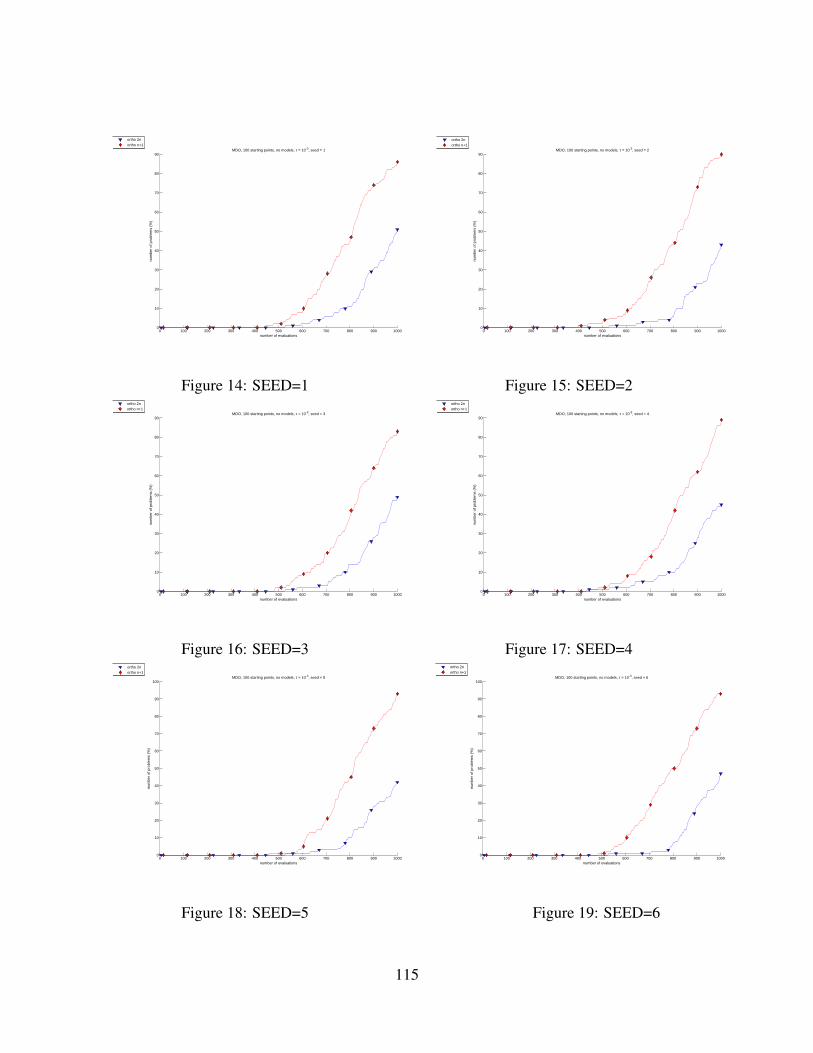
0 100 200 300 400 500 600 700 800 900 10000

10

20

30

40

50

60

70

80

90MDO, 100 starting points, no models, τ = 10-3, seed = 1

number of evaluations

num

ber

of p

robl

ems

(%)

ortho 2northo n+1

Figure 14: SEED=1

0 100 200 300 400 500 600 700 800 900 10000

10

20

30

40

50

60

70

80

90MDO, 100 starting points, no models, τ = 10-3, seed = 2

number of evaluations

num

ber

of p

robl

ems

(%)

ortho 2northo n+1

Figure 15: SEED=2

0 100 200 300 400 500 600 700 800 900 10000

10

20

30

40

50

60

70

80

90MDO, 100 starting points, no models, τ = 10-3, seed = 3

number of evaluations

num

ber

of p

robl

ems

(%)

ortho 2northo n+1

Figure 16: SEED=3

0 100 200 300 400 500 600 700 800 900 10000

10

20

30

40

50

60

70

80

90MDO, 100 starting points, no models, τ = 10-3, seed = 4

number of evaluations

num

ber

of p

robl

ems

(%)

ortho 2northo n+1

Figure 17: SEED=4

0 100 200 300 400 500 600 700 800 900 10000

10

20

30

40

50

60

70

80

90

100MDO, 100 starting points, no models, τ = 10-3, seed = 5

number of evaluations

num

ber

of p

robl

ems

(%)

ortho 2northo n+1

Figure 18: SEED=5

0 100 200 300 400 500 600 700 800 900 10000

10

20

30

40

50

60

70

80

90

100MDO, 100 starting points, no models, τ = 10-3, seed = 6

number of evaluations

num

ber

of p

robl

ems

(%)

ortho 2northo n+1

Figure 19: SEED=6

115

0 100 200 300 400 500 600 700 800 900 10000

10

20

30

40

50

60

70

80

90MDO, 100 starting points, no models, τ = 10-3, seed = 7

number of evaluations

num

ber

of p

robl

ems

(%)

ortho 2northo n+1

Figure 20: SEED=7

0 100 200 300 400 500 600 700 800 900 10000

10

20

30

40

50

60

70

80

90MDO, 100 starting points, no models, τ = 10-3, seed = 8

number of evaluations

num

ber

of p

robl

ems

(%)

ortho 2northo n+1

Figure 21: SEED=8

0 100 200 300 400 500 600 700 800 900 10000

10

20

30

40

50

60

70

80

90

100MDO, 100 starting points, no models, τ = 10-3, seed = 9

number of evaluations

num

ber

of p

robl

ems

(%)

ortho 2northo n+1

Figure 22: SEED=9

0 100 200 300 400 500 600 700 800 900 10000

10

20

30

40

50

60

70

80

90MDO, 100 starting points, no models, τ = 10-3, seed = 10

number of evaluations

num

ber

of p

robl

ems

(%)

ortho 2northo n+1

Figure 23: SEED=10

116

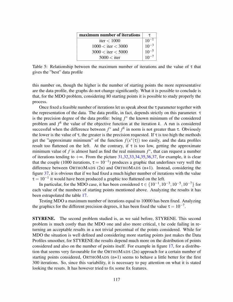
maximum number of iterations τ

iter < 1000 10−1

1000 < iter < 3000 10−3

3000 < iter < 5000 10−5

5000 < iter 10−7

Table 5: Relationship between the maximum number of iterations and the value of τ thatgives the ”best” data profile

this number on, though the higher is the number of starting points the more representativeare the data profile, the graphs do not change significantly. What it is possible to conclude isthat, for the MDO problem, considering 80 starting points it is possible to study properly theprocess.

Once fixed a feasible number of iterations let us speak about the τ parameter together withthe representation of the data. The data profile, in fact, depends strictly on this parameter. τ

is the precision degree of the data profile: being f ∗ the known minimum of the consideredproblem and f k the value of the objective function at the iteration k. A run is consideredsuccessful when the difference between f ∗ and f k in norm is not greater than τ. Obviouslythe lower is the value of τ, the greater is the precision requested. If τ is too high the methodsget the ”approximate minimum” of the function f (x∗(τ)) too easily, and the data profilesresult too flattened on the left. At the contrary, if τ is too low, getting the approximateminimum value of f is almost hard as find the real minimum f ∗, that can request a numberof iterations tending to +∞. From the picture 31,32,33,34,35,36,37, for example, it is clearthat the couple (1000 iterations, τ = 10−1) produces a graphic that underlines very well thedifference between ORTHOMADS (2n) and ORTHOMADS (n+1). Instead, considering thefigure 37, it is obvious that if we had fixed a much higher number of iterations with the valueτ = 10−1 it would have been produced a graphic too flattened on the left.

In particular, for the MDO case, it has been considered τ ∈ 10−1,10−3,10−5,10−7 foreach value of the numbers of starting points mentioned above. Analyzing the results it hasbeen estrapolated the table 17.

Testing MDO a maximum number of iterations equal to 10000 has been fixed. Analyzingthe graphics for the different precision degrees, it has been fixed the value τ = 10−7.

STYRENE. The second problem studied is, as we said before, STYRENE. This secondproblem is much costly than the MDO one and also more critical, t he code failing in re-turning an acceptable results in a not trivial percentual of the points considered. While forMDO the situation is well defined and considering more starting points just makes the DataProfiles smoother, for STYRENE the results depend much more on the distribution of pointsconsidered and also on the number of points itself. For example in figure 17, for a distribu-tion that seems very favourable for the ORTHOMADS (2n) approach for a certain number ofstarting points considered, ORTHOMADS (n+1) seems to behave a little better for the first300 iterations. So, since this variability, it is necessary to pay attention on what it is statedlooking the resuts. It has however tried to fix some fix features.

117

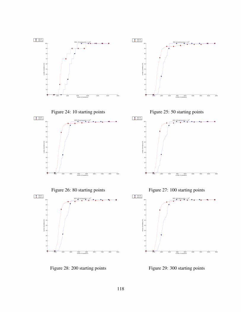
0 1000 2000 3000 4000 5000 6000 70000

10

20

30

40

50

60

70

80

90

100MDO, 10 starting points, τ = 10-5

number of evaluations

num

ber

of p

robl

ems

(%)

ortho 2northo n+1

Figure 24: 10 starting points

0 1000 2000 3000 4000 5000 6000 7000 8000 90000

10

20

30

40

50

60

70

80

90

100MDO, 50 starting points, τ = 10-5

number of evaluations

num

ber

of p

robl

ems

(%)

ortho 2northo n+1

Figure 25: 50 starting points

0 1000 2000 3000 4000 5000 6000 7000 8000 90000

10

20

30

40

50

60

70

80

90

100MDO, 80 starting points, τ = 10-5

number of evaluations

num

ber

of p

robl

ems

(%)

ortho 2northo n+1

Figure 26: 80 starting points

0 1000 2000 3000 4000 5000 6000 7000 8000 90000

10

20

30

40

50

60

70

80

90

100MDO, 100 starting points, τ = 10-5

number of evaluations

num

ber

of p

robl

ems

(%)

ortho 2northo n+1

Figure 27: 100 starting points

0 1000 2000 3000 4000 5000 6000 7000 8000 90000

10

20

30

40

50

60

70

80

90

100MDO, 200 starting points, τ = 10-5

number of evaluations

num

ber

of p

robl

ems

(%)

ortho 2northo n+1

Figure 28: 200 starting points

0 1000 2000 3000 4000 5000 6000 7000 8000 90000

10

20

30

40

50

60

70

80

90

100MDO, 300 starting points, τ = 10-5

number of evaluations

num

ber

of p

robl

ems

(%)

ortho 2northo n+1

Figure 29: 300 starting points

118

0 1000 2000 3000 4000 5000 6000 7000 8000 90000

10

20

30

40

50

60

70

80

90

100MDO, 500 starting points, τ = 10-5

number of evaluations

num

ber

of p

robl

ems

(%)

ortho 2northo n+1

Figure 30: 500 starting points

119

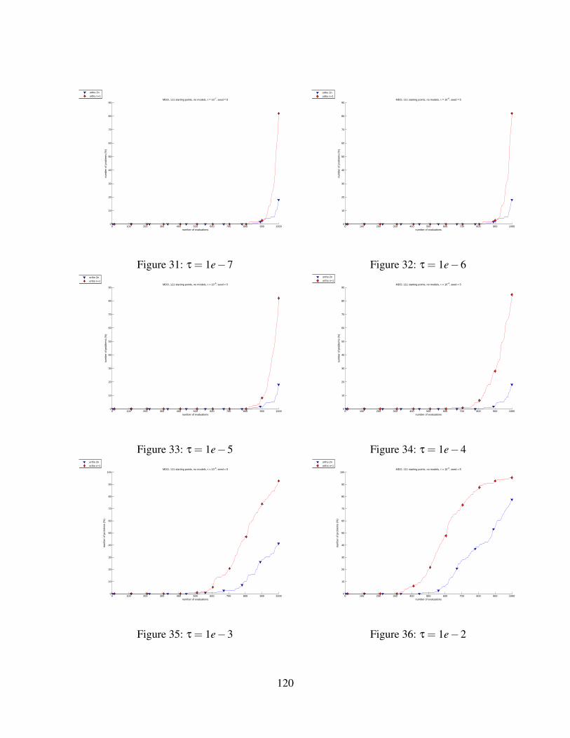
0 100 200 300 400 500 600 700 800 900 10000

10

20

30

40

50

60

70

80

90MDO, 111 starting points, no models, τ = 10-7, seed = 5

number of evaluations

num

ber

of p

robl

ems

(%)

ortho 2northo n+1

Figure 31: τ = 1e−7

0 100 200 300 400 500 600 700 800 900 10000

10

20

30

40

50

60

70

80

90MDO, 111 starting points, no models, τ = 10-6, seed = 5

number of evaluations

num

ber

of p

robl

ems

(%)

ortho 2northo n+1

Figure 32: τ = 1e−6

0 100 200 300 400 500 600 700 800 900 10000

10

20

30

40

50

60

70

80

90MDO, 111 starting points, no models, τ = 10-5, seed = 5

number of evaluations

num

ber

of p

robl

ems

(%)

ortho 2northo n+1

Figure 33: τ = 1e−5

0 100 200 300 400 500 600 700 800 900 10000

10

20

30

40

50

60

70

80

90MDO, 111 starting points, no models, τ = 10-4, seed = 5

number of evaluations

num

ber

of p

robl

ems

(%)

ortho 2northo n+1

Figure 34: τ = 1e−4

0 100 200 300 400 500 600 700 800 900 10000

10

20

30

40

50

60

70

80

90

100MDO, 111 starting points, no models, τ = 10-3, seed = 5

number of evaluations

num

ber

of p

robl

ems

(%)

ortho 2northo n+1

Figure 35: τ = 1e−3

0 100 200 300 400 500 600 700 800 900 10000

10

20

30

40

50

60

70

80

90

100MDO, 111 starting points, no models, τ = 10-2, seed = 5

number of evaluations

num

ber

of p

robl

ems

(%)

ortho 2northo n+1

Figure 36: τ = 1e−2

120

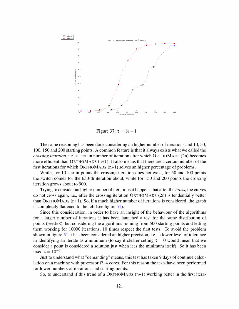
0 100 200 300 400 500 600 700 800 900 10000

10

20

30

40

50

60

70

80

90

100MDO, 111 starting points, no models, τ = 10-1, seed = 5

number of evaluations

num

ber

of p

robl

ems

(%)

ortho 2northo n+1

Figure 37: τ = 1e−1

The same reasoning has been done considering an higher number of iterations and 10, 50,100, 150 and 200 starting points. A common feature is that it always exists what we called thecrossing iteration, i.e., a certain number of iteration after which ORTHOMADS (2n) becomesmore efficient than ORTHOMADS (n+1). It also means that there are a certain number of thefirst iterations for which ORTHOMADS (n+1) solves an higher percentage of problems.

While, for 10 startin points the crossing iteration does not exist, for 50 and 100 pointsthe switch comes for the 650-th iteration about, while for 150 and 200 points the crossingiteration grows about to 900.

Trying to consider an higher number of iterations it happens that after the cross, the curvesdo not cross again, i.e., after the crossing iteration ORTHOMADS (2n) is tendentially betterthan ORTHOMADS (n+1). So, if a much higher number of iterations is considered, the graphis completely flattened to the left (see figure 51).

Since this consideration, in order to have an insight of the behaviour of the algorithmsfor a larger number of iterations it has been launched a test for the same distribution ofpoints (seed=8), but considering the algorithms running from 500 starting points and lettingthem working for 10000 iterations, 10 times respect the first tests. To avoid the problemshown in figure 51 it has been considered an higher precision, i.e., a lower level of tolerancein identifying an iterate as a minimum (to say it clearer setting τ = 0 would mean that weconsider a point is considered a solution just when it is the minimum itself). So it has beenfixed τ = 10−7.

Just to understand what ”demanding” means, this test has taken 9 days of continue calcu-lation on a machine with processor i7, 4 cores. For this reason the tests have been performedfor lower numbers of iterations and starting points.

So, to understand if this trend of a ORTHOMADS (n+1) working better in the first itera-

121

0 1000 2000 3000 4000 5000 6000 70000

10

20

30

40

50

60

70

80

90

100MDO, 10 starting points, τ = 10-7

number of evaluations

num

ber

of p

robl

ems

(%)

ortho 2northo n+1

Figure 38: 10 starting points

0 1000 2000 3000 4000 5000 6000 7000 8000 90000

10

20

30

40

50

60

70

80

90

100MDO, 80 starting points, τ = 10-7

number of evaluations

num

ber

of p

robl

ems

(%)

ortho 2northo n+1

Figure 39: 80 starting points

0 1000 2000 3000 4000 5000 6000 7000 8000 90000

10

20

30

40

50

60

70

80

90

100MDO, 500 starting points, τ = 10-7

number of evaluations

num

ber

of p

robl

ems

(%)

ortho 2northo n+1

Figure 40: 500 starting points

122

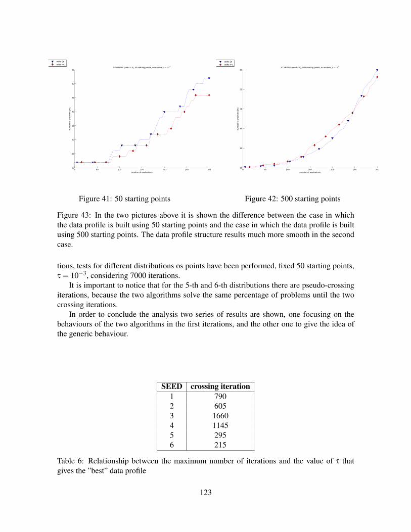
0 50 100 150 200 250 30050

55

60

65

70

75

80

85STYRENE (seed = 5), 50 starting points, no models, τ = 10-2

number of evaluations

num

ber

of p

robl

ems

(%)

ortho 2northo n+1

Figure 41: 50 starting points

0 50 100 150 200 250 30055

60

65

70

75

80STYRENE (seed = 5), 500 starting points, no models, τ = 10-2

number of evaluations

num

ber

of p

robl

ems

(%)

ortho 2northo n+1

Figure 42: 500 starting points

Figure 43: In the two pictures above it is shown the difference between the case in whichthe data profile is built using 50 starting points and the case in which the data profile is builtusing 500 starting points. The data profile structure results much more smooth in the secondcase.

tions, tests for different distributions os points have been performed, fixed 50 starting points,τ = 10−3, considering 7000 iterations.

It is important to notice that for the 5-th and 6-th distributions there are pseudo-crossingiterations, because the two algorithms solve the same percentage of problems until the twocrossing iterations.

In order to conclude the analysis two series of results are shown, one focusing on thebehaviours of the two algorithms in the first iterations, and the other one to give the idea ofthe generic behaviour.

SEED crossing iteration1 7902 6053 16604 11455 2956 215

Table 6: Relationship between the maximum number of iterations and the value of τ thatgives the ”best” data profile

123

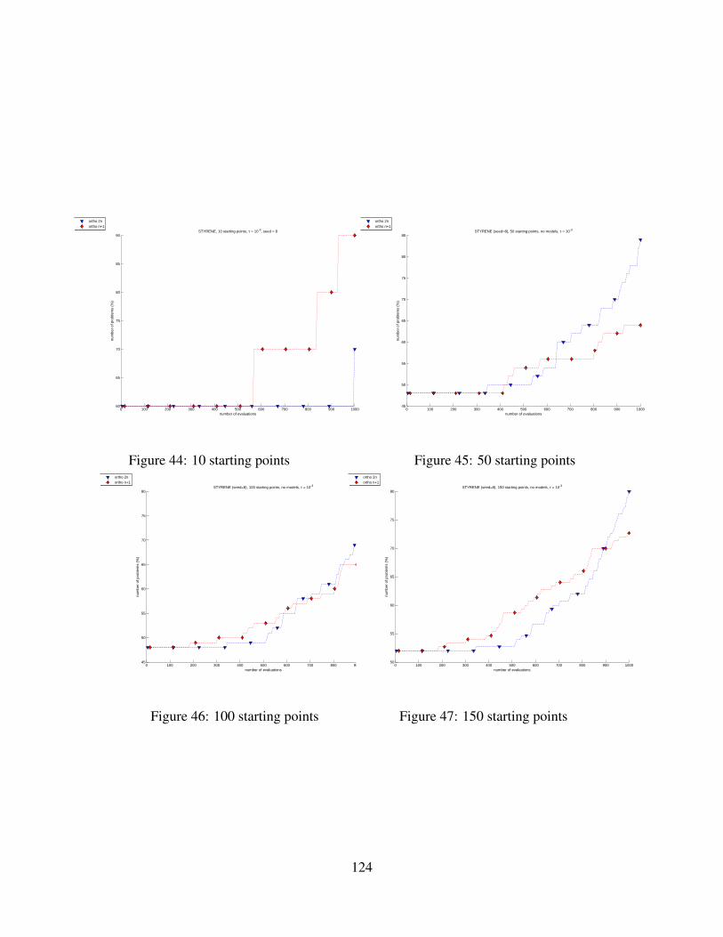
0 100 200 300 400 500 600 700 800 900 100060

65

70

75

80

85

90STYRENE, 10 starting points, τ = 10-3, seed = 8

number of evaluations

num

ber

of p

robl

ems

(%)

ortho 2northo n+1

Figure 44: 10 starting points

0 100 200 300 400 500 600 700 800 900 100045

50

55

60

65

70

75

80

85STYRENE (seed=8), 50 starting points, no models, τ = 10-3

number of evaluations

num

ber

of p

robl

ems

(%)

ortho 2northo n+1

Figure 45: 50 starting points

0 100 200 300 400 500 600 700 800 900 100045

50

55

60

65

70

75

80STYRENE (seed=8), 100 starting points, no models, τ = 10-3

number of evaluations

num

ber

of p

robl

ems

(%)

ortho 2northo n+1

Figure 46: 100 starting points

0 100 200 300 400 500 600 700 800 900 100050

55

60

65

70

75

80STYRENE (seed=8), 150 starting points, no models, τ = 10-3

number of evaluations

num

ber

of p

robl

ems

(%)

ortho 2northo n+1

Figure 47: 150 starting points

124

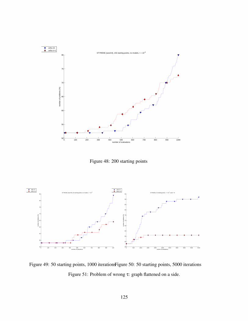
0 100 200 300 400 500 600 700 800 900 100050

55

60

65

70

75

80STYRENE (seed=8), 150 starting points, no models, τ = 10-3

number of evaluations

num

ber

of p

robl

ems

(%)

ortho 2northo n+1

Figure 48: 200 starting points

0 100 200 300 400 500 600 700 800 900 100045

50

55

60

65

70

75

80

85STYRENE (seed=8), 50 starting points, no models, τ = 10-3

number of evaluations

num

ber

of p

robl

ems

(%)

ortho 2northo n+1

Figure 49: 50 starting points, 1000 iterations

0 500 1000 1500 2000 2500 3000 3500 4000 4500 500045

50

55

60

65

70

75

80

85

90

95STYRENE, 50 starting points, τ = 10-3, seed = 8

number of evaluations

num

ber

of p

robl

ems

(%)

ortho 2northo n+1

Figure 50: 50 starting points, 5000 iterations

Figure 51: Problem of wrong τ: graph flattened on a side.

125

0 1000 2000 3000 4000 5000 6000 7000 8000 9000 1000050

55

60

65

70

75

80

85STYRENE, 500 starting points, no models, τ = 10-7, seed = 8

number of evaluations

num

ber

of p

robl

ems

(%)

ortho 2n

ortho n+1

Figure 52: Demanding test

126

0 100 200 300 400 500 600 700 800 900 100050

55

60

65

70

75

80

85STYRENE, 150 starting points, no models, τ = 10-3, seed = 3

number of evaluations

num

ber

of p

robl

ems

(%)

ortho 2northo n+1

Figure 53: SEED 3

0 100 200 300 400 500 600 700 800 900 100050

55

60

65

70

75

80

85STYRENE, 150 starting points, no models, τ = 10-3, seed = 5

number of evaluations

num

ber

of p

robl

ems

(%)

ortho 2n

ortho n+1

Figure 54: SEED 5

0 100 200 300 400 500 600 700 800 900 100050

55

60

65

70

75

80STYRENE (seed=8), 150 starting points, no models, τ = 10-3

number of evaluations

num

ber

of p

robl

ems

(%)

ortho 2northo n+1

Figure 55: SEED 8

0 100 200 300 400 500 600 700 800 900 100050

55

60

65

70

75

80

85STYRENE, 150 starting points, no models, τ = 10-3, seed = 10

number of evaluations

num

ber

of p

robl

ems

(%)

ortho 2northo n+1

Figure 56: SEED 10

Figure 57: Data Profiles for for high precision: τ = 10−3.

127

0 1000 2000 3000 4000 5000 6000 700050

55

60

65

70

75

80

85STYRENE, 150 starting points, no models, τ = 10-7, seed = 3

number of evaluations

num

ber

of p

robl

ems

(%)

ortho 2n

ortho n+1

Figure 58: SEED 3

0 1000 2000 3000 4000 5000 6000 700050

55

60

65

70

75

80

85

90STYRENE, 150 starting points, no models, τ = 10-7, seed = 5

number of evaluations

num

ber

of p

robl

ems

(%)

ortho 2n

ortho n+1

Figure 59: SEED 5

0 1000 2000 3000 4000 5000 6000 700050

55

60

65

70

75

80STYRENE, 150 starting points, no models, τ = 10-7, seed = 8

number of evaluations

num

ber

of p

robl

ems

(%)

ortho 2n

ortho n+1

Figure 60: SEED 8

0 1000 2000 3000 4000 5000 6000 700050

55

60

65

70

75

80

85STYRENE, 150 starting points, no models, τ = 10-7, seed = 10

number of evaluations

num

ber

of p

robl

ems

(%)

ortho 2n

ortho n+1

Figure 61: SEED 10

Figure 62: Data Profiles for for high precision: τ = 10−7.

128

18 Backtracking: the Unconstrained CaseUntil now a digression has been done on a branch of the Direct Search methods, the PatternSearch methods. Starting from the ancestor, the Coordinate Search method, it has been stud-ied its progressive evolution that arrived to the last Mesh Adaptive Direct Search methodspassing through the Generalized Pattern Search ones. Then the attention has been focused onthe MADS considering, in particular, the new part, named briefly ORTHOMADS (n+ 1), onreducing the set of the poll directions of the single iteration k. Coming back to the generalstructure of the MADS agorithms it has been said that they are conceptually divided in twomain steps:

• the poll phase;

• the search phase.

The ORTHOMADS (n+ 1) focused the attention on the first phase, working on the poll di-rections Dk generated at every mesh local optimizer xk. The search phase, at the contrary,has only been mentioned. The reason of this lack of consideration lies in the fact that intothis phase the user has a complete freedom of choice. Bringing to the extreme this rationaleone could just choose a casual point x in Rn and evaluating the function vaue in that point. Iff (x) < f (xk), then it would possible to take xk+1 = x, otherwise xk+1 = xk. Obviously, alsoconsidering the cost of evaluating the function value in a point, this is never actually done.What happens is practise is that surrogate models are used to have an idea of the real functionand that the surrogates themselves are minimized to find a mathematically promising pointto evaluate.

Although conceptually the search phase can be ignored theoretically speaking (since allthe convergence properties lie exclusively on the poll phase), computationally it is extremelyimportant to increase the rate of convergence of the methods.

In the following part the Back-tracking search will be introduced as an implementation ofthe search phase in the MADS context, making additional convergence results not necessary.

18.1 From the Coordinate Search to the MADS algorithms: the impor-tance of the Speculative Search [2006]

Two are the basic expedients that have been used to improve the convergence speed since thearising of the first Pattern Search methods:the first one is to consider a target vector wk representing some information a priori on apossible interesting direction for the function (that often coincides with the last direction ofsuccess dk−1) in order to promote some directions on the top of the list for the next Poll phase(this approach is also known as dynamic ordering of the polling directions).The second expedient concerns a possible modification of the updating rule of ∆

pk in the suc-

cessful cases (k ∈ S) such to have ∆pk+1 > ∆

pk , i.e., leading larger steps when they are neces-

sary. A typical choice is to double the size of the mesh (∆pk+1 = 2∆

pk ), but in the derivative-free

129

literature a more general possibility is allowed:

∆pk+1 = γM∆

pk ,

where γM ∈N/0,1 represents the amount of the exploring step along the considered direc-tion.

Combining these two tricks both the Coordinate Search (1960) and the successive Gener-alized Pattern Search (GPS) methods putted in practise a line search (the word Linesearch isintentionally not used to avoid confusion with what follows) along the successful directions.In fact, considering the finite number of directions in CS and GPS, at every iteration the targetdirection wk has necessarily to coincide with one of the directions in Dk and, in particular,with the one related to the last success. That being so, if dk is a successful direction with pollparameter ∆

pk , i.e. if f (xk +∆

pk dk) < f (xk), it follows that wk = dk, hence dk+1 = dk, with

∆pk+1 = γM∆

pk . So the successive points

xk + γjkM∆

pk dk

(where jk = 0,1, . . . ,J+1 and γM > 1) are evaluated until a J ∈ N is found such that:

f (xk + γJ+1M ∆

pk dk)> f (xk + γ

JM∆

pk dk).

Remark 18.1 The search along dk ends when we do not have a successive reduction. Herethere is no mention of sufficient reduction, dealing just with the simple objective functionreductions.

Now the discussion about the Pattern Search methods is left aside for a moment, becauseit is interesting to analyse the parallelism with another important branch of methods dealingwith the derivative-free problems: The Linesearch methods (Armijo, Grippo, Lucidi, Scian-drone). In that case, for jk = 0,1,2, . . . ,J, the successive points

xk + γjkLSαdk,

(where dk ∈ Rn was a descent direction, α > 0 was the initial step and where, in particular,γLS ∈ R, γLS > 1) were evaluated.

Except the fact that theoretically the Linesearch methods use the concept of sufficientdecrease (and not the mesh) to prove the convergence and that the difference between γMand γLS is significant (not just theoretically but also practically), there is one important ba-sic concept in common: they both try to exploit the promising direction dk in depth beforegenerating points along other directions.

It is easy to verify that the same rationale cannot be used analyzing the MADS methods. Inthe standard implementation of the NOMAD algorithm at every step a set of poll directions iscreated. Nevertheless, when the incumbent best solution is achieved, a new set of directionsis created, starting the search from the point detected by the direction that creates the smallestangle with the last success direction w. This is the way the last promising direction at k affectsthe k+1 one. It was observed that, in this way, a direction could not be entirely exploited.

130

In order to repair to that an option (setted as default in NOMAD) has been introduced(see [6]) giving the possibility of exponentially increasing the steplength parameter lettingthe direction unchanged at successful points: that is the Speculative Search. Using a valueγM = 3 the option forces NOMAD to keep the successful directions for more than a singleevaluation, as long as simple reductions of the objective functions are obtained.

As a result a sequence of points is evaluated until a worse point C is found, and theprevious-to-the-worse, B, is set as incumbent. The question is: what about the interval be-tween A and C? The target of the present paper is to explore that space, looking for a pointlying on the mesh that could be promising, considering that this interval can be hopefullyvery large respect with the dimensions of the examined problem (depending on how manytimes the steplength parameter is exponentially increased).

At the first the unconstrained case is presented in 18.2 in order to give a clear idea ofthe purpose of the paper. Successively the same is done for the constrained case, where theconstraints will be supposed to be managed with the Progressive Barrier (PB) approach. Itwill be also shown that this choice is critical respect with the implementation of the algorithm.

Dealing exclusively with a MADS approach, in order to simplify the notation, for thefollowing, with γ we will refer to γM.

18.2 The Unconstrained Back-tracking searchThe entire Pattern Search discussion presented until now has been conducted into the uncon-strained context. Along the same line this section, that is the last one of this first part, dealswith the classical unconstrained problem:

minx∈Rn

f (x) . (34)

Suppose also that, at the current point xk, a set of poll directions Dk has been created, andone of them, dk, has been identified as a descent one in combination with the parameter ∆

pk . So

it results: f (xk+∆pk dk)< f (xk). Without other informations we can say that dk is a promising

direction: it makes sense to go further along the points xk + γ j∆pk dk, where j = 1,2, . . ., with

the Speculative Search, possibly finding better function values than the incumbent one.Although, as it has been said previously, this phase does not affect the convergence theory,

nevertheless there is a property that is necessary to guarantee: this exploration along a singledirection has necessariyl to be a finite process in order to avoid that the method does not havean end. In order to guarantee that the next assumption is supposed:

Assumption 18.2 All trial points considered by the algorithm lie in a bounded set.

This assumption may be reformulated in our notation as follows: there exists somebounded set in Rn containing Vk for every k. In the constrained case it is simple: by itsdefinition, Vk does not contain any points that violate any of the unrelaxable constraints.Thus, it is easy to ensure that 18.2 is satisfied when there is a bounded set of unrelaxableconstraints (it will be seen in the next part in the constrained context). Nevertheless, in the

131

unconstrained case, lacking unrelaxable constraints, it is necessary to introduce some stan-dard assumption as the boundedness of the level sets of the objective function f . Anyways,engineering problems often have bounds on all the optimization variables.

Combining Assumption 18.2 with the mesh structure was shown in [6] to be enough toensure that

liminfk

∆mk = 0,

that is extremely important in the MADS context.Summarizing, the assumption 18.2, standard in the derivative-free context, ensures that

the line search along the direction dk ends in a finite number of steps. It means that it existsan integer value J ≥ 1 such that:

f (xk + γJ∆pk dk)< f (xk + γJ−1∆

pk dk)< .. . < f (xk + γ0∆

pk dk) = f (xk +∆

pk dk)< f (xk)

f (xk + γJ∆pk dk)< f (xk + γJ+1∆

pk dk).

Starting from the point xk, along the direction dk, this procedure evaluates J+2 points (whereJ+2 ∈ N, J+2 < ∞): one is the poll point xk + γ0∆

pk dk = xk +∆

pk dk and the other J+1 ones

are the points generated further that along dk.For semplicity, being interested in particular on the last three points, they are renamed:

• f (xk + γJ−1∆pk dk) = f (A)

• f (xk + γJ∆pk dk) = f (B)

• f (xk + γJ+1∆pk dk) = f (C).

Remark 18.3 Conceptually the first point detected for the Back-tracking procedure is C (theinteger J+1 is found). Then B and A are detected as:

• B = xk +γJ+1

γ∆

pk dk;

• A = xk +γJ+1

γ2 ∆pk dk

The notation A,B,C is used exclusively to give a sight of the crescent distances of thepoints from xk.

So it is possible to write:f (B)≤ f (A)≤ f (xk + γs2∆

pk dk)≤ . . .≤ f (xk +∆

pk dk)≤ f (xk)

f (C)≥ f (B).

After having introduced a clear notification of what the Speculative Search is alreadyable to do in NOMAD, in the next subsection it is presented its evolution, the Back-trackingsearch. That will be divided into two parts: the construction of the quadratic model of f (inthe constrained case obviously it will not be the only one) in order to detect the promisingpoint along dk, and the successive Rounding of the point to the mesh, in order to let all theMADS analysis working as well.

132

Figure 63: In this example γ = 3. Also for a so small value of γ it is evident that the distancebetween B and C could be much larger than the distance between A and B. This schemerepresents the classic starting situation for the Back-tracking. In the next chapters we will seethat an accepted point, in general, can be infeasible or feasible and the same for a rejectedpoint.

133

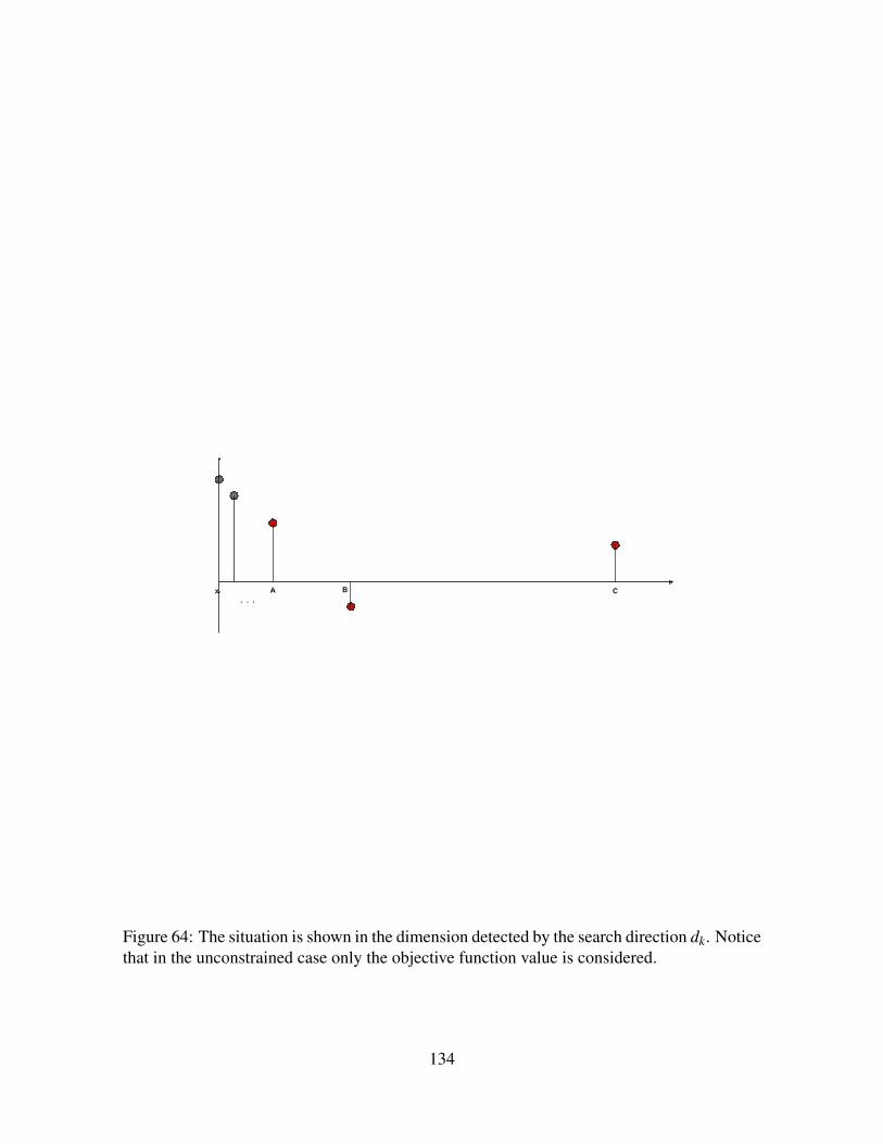
Figure 64: The situation is shown in the dimension detected by the search direction dk. Noticethat in the unconstrained case only the objective function value is considered.

134

18.2.1 The Back-tracking

In this part the focus is on the space between xk + γJ−1∆pk dk and xk + γJ+1∆

pk dk.

Depending on the value chosen for γ and on the value of J (it expresses the times the line-search has produced successful points along dk) the interval

∆pk dk(γ

s+1− γs)

could also be a very large space.

Remark 18.4 In this remark we want just compare the dimensions of the interval includedbetween A and B with the one between B and C. Intuitively they have to be different. Mathe-matically:

dist(B,C) = ∆pk dk(γ

s+1− γs) = γ

[∆

pk dk(γ

s− γs−1)

]= γ dist(A,B),

meaning that the interval between B and C is γ -times respect with the one between A and B.

The Speculative Search identifies an approximation of the minimum of f along dk, that isthe point B.Referring to the remark 18.4 it stands to reason that the greater J is, the worse the approxi-mation B could be, i.e., the greater the distance between B and the real minimum could be.To ride over this malfunctioning behaviour it is necessary trying to explore better the one-dimensional space between xk and C (notice that xk could coincide with A but, in general, itresults xk 6= A) to detect a new promising point L using the only informations available:

f (xk),

f (xk + γ jk∆pk dk), where jk = (0,1,2, . . . ,J−2),

f (A),f (B),f (C).

The simplest idea is to build a surrogate model Q f (α) from the evaluated points withan additional cost given by the construction of a model based on the function values in theevaluated points and by an additional function evaluation (in the new proposed point).

About the additional computation of f it is enough to consider that the point is a promisingone, so the evaluation effort is repaid from the mathematical likelihood of obtaining a betterpoint than B. That likelihood depends obviously on the regularity of f and on the chosenmodel to use as the surrogate (in general B is not the minimum of f along dk but it is notpossible to ensure that f (L)< f (B)). Besides, the functions considered in the derivative-freeapproach are costy, usually much more respect with the construction of a generic surrogatemodel. So it is possible to say that the cost to construct a surrogate for obtaining L and thecost to evaluate the function in L is referable to the cost of the single evaluation.

A first possibility to construct the model considering all the points evaluated along dk is touse the Kriging approximation. It has the property to pass exactly for all the points evaluated

135

between xk and C. Another interesting property of this kind of approximation is that the morepoints are added along dk the more similar is the kriging function to the real function.

A possible critic to move to a surrogate like that is that it is not possible to know apriori where the minimum of the surrogate lies. Different is the situation if a quadraticapproximation is considered. Let us explore this possibility.

The Quadratic model. Consider to construct a quadratic model skf (x) passing for the three

points A, B and C. So it will result: skf (A) = f (A), sk

f (B) = f (B) and skf (C) = f (C). Since

the analytic structure of the quadratic function is known skf (x) is minimized in place of f (x)

to identify the most ”promising” point.Considering the values of sk

f (x) on A, B and C it is possible to state that the minimum ofthe surrogate of f will lie between xk + γs−1∆

pk dk and xk + γs+1∆

pk dk.

So it is possible to write the problem as in 35:

minx∈[xk+γs−1∆

pk dk,xk+γs+1∆

pk dk]

skf (x)≡minx∈[xk+αdk] sk

f (x) , (35)

where α > 0. The next theorem ensures that a point is marked as promising into the segmentlying between the points A and C.

Theorem 18.5 Suppose that, at the iteration k, dk ∈ Rn is the search direction, ∆pk ∈ R is

the step parameter, s ∈ N is the integer detected by the linesearch and γ ∈ Q, γ > 1 is thelinesearch parameter.

Then if xks f

is the minimal value of the problem 35 it results

xks f∈[xk + γ

s−1∆

pk dk , xk + γ

s+1∆

pk dk].

Rounding to the mesh. Once obtained the promising point, what we do throught theRounding to the mesh-phases is to obtain the promising-mesh point. In this case, in whichthere is only f , this phase is very simple both to explain and to code. It is sufficient to findthe point as nearer as possible to the promising point lying on the mesh.

What it is obtained at the end of the quadratic model construction and the rounding-to-the-mesh phase is a point lying extremely near (it depends on the refinement of the mesh Mk)to a point that results mathematically promising.

Remark 18.6 As last observation we notice that, in order to obtain points along the linesearch with the property of lying on a mesh it is necessary that the elongation parameter isγ ∈ Q. The Speculative Search was introduced considering a value γ = 3. We suggest, for themoment in which this implementation of the search will be tested, to consider different valuesof γ, and not just the one fixed in the year 2006 by Audet and Dennis.

In the next part it will be seen how to adapt the back-tracking search to the constrained case.

136

Part III

Introducing the constraints

137

19 IntroductionAfter having studied the process that transformed the way in which the space was explored,in this section the constraints are introduced to see how the different approaches presenteduntil now work on the general optimization problem described in 36. min f (x)

x ∈ Xx ∈Ω

(36)

This section is not intended just for exposing the results that are scattered in the literature butalso for making clear why the different algorithms produce certain theoretical results. Wewant to link the results themselves to the different way in which the different Pattern Searchmethods explore the space. In particular we want to highlight the difference between thepre-MADS methods, generating a finite number of directions and the MADS approach thatintroduced the concept of a dense of directions generated along the infinitely many iterations.The theoretical results will be massively affected by this feature of the MADS.

In the section 20 some additional mathematical tool is presented. Then, in section 21 afirst algorithm managing the constrained case is shown. The target is becoming familiar withthe constrained context and, again, showing the main limits given having at disposal a finitenumber of directions.

In section 22 it will be recalled the concept of conforming. A new notation is here in-troduced splitting the previously existing concept of conforming in three aspects: the global,the sufficient and the standard conforming. We are pretty confident that this distinction isextremely useful to present the results in a more elegant and simple way.

In the sections 23, 24 and 25 the problem is seen from the perspective of the complexityof the constraints, starting from the simplest ones, the bound constraints and ending withthe general constraints, passing through the linear ones. Fixing the types of the constraintsit has been found the Pattern Search algorithms able to find a point with a certain level ofstationarity. In section 26 it is instead described the way in which actually the constraints aremanaged starting from the extreme barrier to arrive to the progressive barrier.

At the end the Back-tracking search, previously introduced in the unconstrained case asa new implementation of the search phase of the MADS, is now adapted for managing theconstraints.

20 Mathematical toolsIn what follows we will refer to the costrained problem described in 36.

In order to study the portions of the space containing feasible points the concept of coneis used. It is formally described in the following definition:

Definition 20.1 A subset K ⊆ Rn is called cone when, for every scalar λ > 0, if d ∈ K, thenλd ∈ K.

138

As inferable by the expression K ⊆ Rn we can notice that K = Rn is a cone as well as theother extreme case: K =∅.An additional useful tool is the polar cone defined as:

Definition 20.2 The polar of a cone K ⊆ Rn is the set K∗ = d ∈ Rn : dT v≤ 0,∀v ∈ K.

In the constrained case one has to pay attention not only to the distribution of the set ofthe directions in the space, but also on the kind of the directions themselves. In fact, whilepreviously the main point was to detect descent directions, now we have to pay attention tosomething more. The next definition clarifies this point.

Definition 20.3 The direction d ∈ Rn is said feasible for the set Ω ⊆ Rn at x ∈ Ω if thereexists some scalar ε > 0 such that x+ td ∈ Ω for all the t ∈ [0,ε]. Otherwise they are calledinfeasible.

It goes without saying that we will be interested in the feasible directions that possibly willgenerate feasible points that, at the end, are the target to every optimization algorithm.

The concept of cone has been introduced in order to present a particular cone useful forour analysis, i.e. the cone of the directions satisfying a condition of feasibility.

Definition 20.4 The set of the feasible directions to Ω at x ∈Ω is called T FΩ(x).

Being T FΩ(x) a cone it is called the cone of feasible directions to Ω at x and it is computed

relying on those two elements. The ”F” as superscript is to remember its meaning of feasi-bility.

Through the cone of the feasible directions it is possible to deduce the necessary optimal-ity condition:

Proposition 20.5 (Necessary optimality condition) Let x∈Ω⊆Rn a local minimizer of thefunction f over the set Ω.Suppose that all the directional derivatives of f at x∗ exist.Then:

f ′(x∗;d)≥ 0 for all d ∈ T FΩ (x∗).

Notice that the condition on the existence of the derivatives is necessary to be able towrite them. Obviously it is a milder condition than requiring the function f differentiable inx∗. In that case also the gradient ∇ f (x∗) exists and the directional derivatives can be writtenas f ′(x∗;d) = ∇ f (x∗)T d. That very important property will be used when a generic directionin a subspace will be written as a positive linear combination of the directions of a spanningset of the subspace itself. It is important because when the directional derivatives along thedirections spanning the subspace are positive, it will be possible to say that the directionalderivative is positive also for all the infinitely many other directions in that subspace. Ob-viously that subspace can also coincide with Rn, as for the unconstrained case or when theconsidered point is an internal point. It is easy to prove the necessary optimality conditionshown in the Theorem 20.5.

139

Proof. Suppose that d ∈ T FΩ(x∗), it means that x∗+ td ∈ Ω for t ∈ [0,ε]. Writing the

directional derivative along the feasible direction d it results:

f ′(x∗;d) = limt↓0

f (x∗+ td)− f (x∗)t

≥ 0,

where the last inequality comes by the fact that x∗ is a local minimizer, so there exists an ε

small enough to make the inequality true.

21 Constrained exploratory moves: an adapted Pattern Searchalgorithm

In this section we describe a first simple algorithm using a finite number of exploring direc-tions being able to manage the presence of contraints. In other words we describe a genericGeneralized Pattern Search method adapted to the constrained case.At this point one could wonder: why do not use the MADS approach? The purpose is tofocus the attention on what using a finite number of directions actually means in presence ofconstraints and on the theoretical consequences.

Let xk being a sequence generated by a not well specified Pattern Search algorithm.Suppose that a refining subsequence xkK exists. So, being Dk the matrix of the directionsgenerated at the iteration k, and being D the basis directions specific of the Pattern Searchmethods, it is possible to say that, if d ∈ Dk:

• d is a direction in D: d ∈ D.

• Dk is a positive spanning set of directions.

140

Algorithm 21.1Initialization: Let f : Rn→ R be given.

Let x0 ∈ X be the initial guess of solution.Let ∆tol > 0 be the tolerance of the step-length parameter.Let ∆0 > ∆tol be the initial step-length parameter.Let D = d1,d2, . . . ,dnD be the basis directions, where di ∈ Rn.

k = 0.

Selection of the set of the feasible directions: Create a set Dk ⊆D through a Pat-tern Search method, such that it is a positive spanning set.

Successful iteration: if ∃ dk ∈ Dk such that

(i) f (xk +∆kdk)< f (xk)(ii) xk +∆kdk ∈ X

then:

• set ∆k+1 ≥ ∆k.

• xk+1 = xk +∆kdk.

Unsuccessful iterations: Otherwise:

• set ∆k+1 < ∆k.

• set xk+1 = xk.

• if ∆k+1 < ∆tol , then terminate.

k = k+1.

The conceptual difference respect with what it has been seen in the unconstrained case isin the search of an improving point. Two are the conditions necessary to satisfy to consider apoint of the poll frame as better respect with the incumbent xk. The first one is the same ofthe uncontrained case: the function of the proposed point has to be lower than the incumbentone. The second one is the peculiarity of the constrained case: the point has to be feasible.

Theorem 21.2 Let xk be a sequence produced by 21.1. Then there always exists a refiningsubsequence xkK , i.e.,

liminfk→∞

∆k = 0.

The proof of the previous theorem is not reported because it is analogous to the uncon-tstrained case. In particular the difference is in the fact that it is not necessary to assume thatthe iterations of the sequence xk lie in a bounded set, because every point of the sequencexk ∈ X , where X estabilishes a natural bound for them. The limit point of a generic refiningsubsequence is called x.

141

The following theorem consider the differentiable case. Then that condition is relaxed,considering the function f Lipschitz continuos.

Theorem 21.3 ( f smooth) Let xkK be a refining subsequence produced by the algorithm21.1 converging to the point x. Let D being the directions explored infinitely many times inthe point x. Let f being continuously differentiable on Rn.

Then:f ′(x;d)≥ 0, for each d ∈ DF(x),

where DF(x) is the subset of D composed by the directions that are feasible in the point x.

Proof. The generic Pattern Search algorithm produces the sequence xk. The theorem 21.2states that there exists at least a subsequence xkK converging to a point x. It also meansthat the set of indices K is also a set of unsuccessful iterations (K ⊆U).

For k ∈ K ⊆U :

0≤ f (xk +∆kd)− f (xk) = f (xk)+∆kdT∇ f (xk +α∆kd),

for every d ∈DFk (xk) (the subset of the directions in Dk that are also feasible) and where α

is a certain real value between 0 and 1. For the equality on the right of the previous expressionthe classical mean value theorem has been used, for which it is used the property of continuityof the function f . Being ∆k > 0 it is also possible to write:

dT∇ f (xk +α∆kd)≥ 0,

for each d ∈ DFk (xk).

In order to give some property on the limit point of the refining subsequence the behaviourof the algorithm for k ∈ K,k→ ∞ is analyzed. The fact that the gradient is continuous let usbring the limit at the argument of the gradient of f . In particular limk∈K α∆kd = 0, sincethe refining subsequence is, for definition, a subsequence for which the limit of ∆k goes tozero, and both α and d are bounded values. In addition xk→ x. It follows that the directionalderivative is:

f ′(x;d) = dT∇ f (x)≥ 0, ∀d ∈ DF(x),

where DF(x) are the feasible directions in x explored infinitely many times.

Now the hypotheses on the function f are relaxed: it is considered a function Lipschitzcontinuous near the convergence point of the refining subsequence (that exists for what saidin the Theorem 21.2).

Theorem 21.4 ( f Lipschitz continuous) Let xkK be a refining subsequence produced bythe algorithm 21.1 converging to the point x. Let D being the directions explored infinitelymany times in the point x. Let f being Lipschitz continuous near the point x.

Then:f O(x;d)≥ 0, for each d ∈ DF(x).

142

Proof.The generic Pattern Search algorithm produces the sequence xk. The theorem ?? states

that there exists at least a subsequence xkK converging to a point x. It also means that theset of indices K is also a set of unsuccessful iterations (K ⊆U).

For k ∈ K ⊆U :0≤ f (xk +∆kd)− f (xk),

for every d ∈ DFk (xk). In this case, for the lack of continuity of the function f , the mean

value theorem cannot be used. On the other hand the Lipschitzianity of the function near xallows us to write the generalized Clarke derivative f O(x;d). For what follows it is enoughto consider the fact that xk is a particular sequence converging to the point x and ∆k is aparticular sequence of positive scalars converging to zero.Then:

limsupy→x,t↓0

f (y+ td)− f (y)t

≥ limk∈K

f (xk +∆kd)− f (xk)

∆k≥ 0,

for every d ∈ DFk (xk).

It follows that:f O(x;d)≥ 0, ∀d ∈ DF(x).

The result of the theorem 21.3 is obviously stronger than the result of the theorem 21.4,because the first one requires f continuously differentiable, while the second one requires fLipshitz continuous just in the neighborhood of the limit point of the sequence. Although,in addition to the kid of the derivative on which the results are given, there is also an hiddenresult relatively to the theorem 21.3 that will take a great importance for what it will be saidin the following part. The positiveness of the directional derivative can be guaranteed notonly along the directions d ∈ DF(x), but also along the diirections contained in the convexcone generated by the directions in DF(x). This can be assured through a way of writingthe directional derivative in the point X along the direction d thanks to the gradient of f :f ′(x;d) = dT ∇ f (x). It is easy to see that:

f ′(x;d) = dT∇ f (x) = ∑

i∈FλidT

i ∇ f (x)≥ 0,

where it has been used the fact that every direction d internal on the convex cone cc(DF(x))generated by the feasible refining directions of x can be written as a positive linear combina-tion of those directions themselves: if d ∈ cc(DF(x)), then d = ∑i∈F λidi, where di ∈ DF(x)and λi ∈ R,λi > 0.

This last consideration leads us to the conclusion that the differentiability of f has adouble merit: that lets us giving a result on the directional derivatives f ′(x;d) with d ∈DF(x) but also on all the directions contained in the convex cone formed by those directionsthemselves.

143

Figure 65: f continuously differentiable.

An important observation is on the refining directions considered. While, in the non-smooth case, an infinite number of directions are necessary to explore in order to give someinteresting information about the point x, in the differentiable case the situation is signifi-cantly different. In fact if the refining directions are properly chosen, it is possible to statethat the limit point x has a stationarity property. To understand what ”proper” means in thiscase, in the next chapter will be introduced the concept of conforming. To give an anticipa-tion we will define a way to choose the pattern directions such that the directions are suitableto explore the feasible region around the generic iteration xk and around the limit point x too.

Remark 21.5 To be thorough, it is important to notice that, in the non-smooth case, althoughthe theorem 21.4 gives an information on all the feasible refining directions in the case inwhich f is a Lipschitz continuous function near x, nothing can actually be said about otherdirections on Rn. That also means that in order to give some stationarity property to the limitpoint x is necessary to explore an infinite number of directions. That recalls what it has beensaid about the MADS algorithms and their capacity to generate a dense of directions.

144

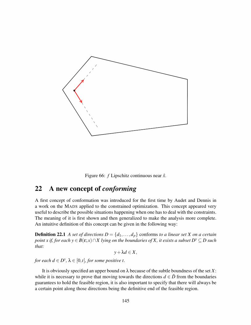
Figure 66: f Lipschitz continuous near x.

22 A new concept of conformingA first concept of conformation was introduced for the first time by Audet and Dennis ina work on the MADS applied to the constrained optimization. This concept appeared veryuseful to describe the possible situations happening when one has to deal with the constraints.The meaning of it is first shown and then generalized to make the analysis more complete.An intuitive definition of this concept can be given in the following way:

Definition 22.1 A set of directions D = d1, . . . ,dp conforms to a linear set X on a certainpoint x if, for each y∈ B(ε;x)∩X lying on the boundaries of X, it exists a subset Dy ⊆D suchthat:

y+λd ∈ X ,

for each d ∈ Dy, λ ∈ [0, t], for some positive t.

It is obviously specified an upper bound on λ because of the subtle boundness of the set X :while it is necessary to prove that moving towards the directions d ∈ D from the boundariesguarantees to hold the feasible region, it is also important to specify that there will always bea certain point along those directions being the definitive end of the feasible region.

145

If the classical definition 22.1 gives a quick idea of the conformation, nevertheless, for whatfollows it is necessary a concept of conforming slightly different, using the theoretical con-struct of the feasible cone of directions T F

X (x) to define what the first concept really means.

Definition 22.2 A set of directions D = d1, . . . ,dp conforms to a linear set X on a certainpoint x if, for each y∈ B(ε;x)∩X lying on the boundaries of X, it exists a subset Dy ⊆D suchthat:the cones of the feasible directions T F

X (y) is generated by a non-negative linear combinationf the columns of a subset Dy ⊆ D.

Since this last definition it is clear as the the conformation actually is an adhere to, speak-ing of the generated cones (the one of the feasible directions and the one generated by thedirections in Dy).

This definition was used, in particular, referring to the single iteration k of a run of thewhole algorithm. That being so, it was said that a choice of the pattern Dk was conformingto the feasible set X respect with the current point xk if the hypotheses in 22.2 were true forDk, xk.

Remark 22.3 The case in which the current point xk is sufficiently internal respect with thefeasible set is a particular case leading to a simple consideration. If B(ε;xk) does not containpoints on the boundaries of X, in fact, it results:

T FX (xk)≡ Rn.

This would mean that Dk conforms to X on the point xk if T FX (xk) is generated by a non-

negative linear combination of a subset Dyk ⊆ Dk. It follows that Dy

k has to be a positivespanning set of directions, i.e., also Dk has to be a positive spanning set of directions.Fortunately both the Coordinate Search and the Generalized Pattern Search methods andthe MADS algorithms produce at every iteration k a set of directions Dk being a positivespanning set.

So, for internal points far enough from the boundaries of the feasible region the directionsDk generated at every iteration by a generic Pattern Search method banally conforms to Xon the point xk itself.

In the three classes of Pattern Search methods analyzed in this work (CS, GPS and MADS)two types of directions are always separated conceptually and practically: the basis directionsD and the directions created at every iteration Dk. It has been seen that the relation betweenD and Dk changes at every considered method.The next two definitions diverge from 22.2 first of all because they are introduced to estabilishproperties on the basis directions D. The first one is the more demanding assumption:

Definition 22.4 The set of directions D globally conforms to the set X iffor every x ∈ X the set T F

X (x) is generated by a subset Dx ⊆ D.

146

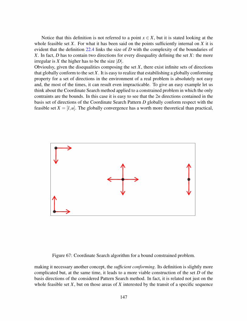
Notice that this definition is not referred to a point x ∈ X , but it is stated looking at thewhole feasible set X . For what it has been said on the points sufficiently internal on X it isevident that the definition 22.4 links the size of D with the complexity of the boundaries ofX . In fact, D has to contain two directions for every disequality defining the set X : the moreirregular is X the higher has to be the size |D|.Obvioulsy, given the disequalities composing the set X , there exist infinite sets of directionsthat globally conform to the set X . It is easy to realize that estabilishing a globally conformingproperty for a set of directions in the environment of a real problem is absolutely not easyand, the most of the times, it can result even impracticable. To give an easy example let usthink about the Coordinate Search method applied to a constrained problem in which the onlycontraints are the bounds. In this case it is easy to see that the 2n directions contained in thebasis set of directions of the Coordinate Search Pattern D globally conform respect with thefeasible set X = [l,u]. The globally convergence has a worth more theoretical than practical,

Figure 67: Coordinate Search algorithm for a bound constrained problem.

making it necessary another concept, the sufficient conforming. Its definition is slightly morecomplicated but, at the same time, it leads to a more viable construction of the set D of thebasis directions of the considered Pattern Search method. In fact, it is related not just on thewhole feasible set X , but on those areas of X interested by the transit of a specific sequence

147

xk (see definition 22.5).

Definition 22.5 The set of directions D sufficiently conforms to the set X respect with thesequence xk entirely contained into the set X if for each y ∈ B(ε;xk) on the boundary ofX all the feasible cones T F

X (y) are generated by a non-negative linear combination of thecolumns of a subset Dy ⊆ D.

Remark 22.6 The sufficient conforming is referred to all those sequences entirely containedinside the set X. It is the case in which the Extreme Barrier approach is used to manage thecontraints.

The reason why more general sequences of points are not considered is in the fact that theconcept of conforming that will be introduced in the following part deals with points xk ∈ X,i.e. with points internal to the feasible set.

Notice that, while the global conformation is related to the whole set X , the sufficientconformation takes into account also the specific sequence xk produced by the specific al-gorithm. It can be said that, while the global conforming is related exclusively to the feasibleset considered, for the sufficient conforming it is necessary to fix a certain sequence of pointsproduced by a certain method. The utility of this relaxation actually is in the fact that the re-quirement of sufficient conforming is, as it is explained by the word itself, sufficient to ensureconvergence properties related to a specific sequence of convergent points xk. Neverthelessthe sufficient conforming is a less restrictive requirement and, depending on the consideredsubsequence and on the complexity (i.e., the number of the constraints, since the constraintshave all the same complexity, being all linear) of the feasible region, it can be also much lessrestrictive. The restriction is about the basis directions D of the considered method.

As last the classical definition of conforming is recalled. It appeared for the first time withTorczon and Lewis in 1999 and is referred to the set of directions Dk composing the frame atthe iteration k. Then it is not a condition on the basis directions but, depending on the methodchosen, it could become also a condition of that type. For example in the Coordinate Searchcase setting a condition on the basis directions means setting a condition on all the framedirections built at the various iterations k (since Dk = D, for each k).

Definition 22.7 Fixed a point xk ∈ X, the set of directions Dk conforms to the set X respectwith a positive scalar ε > 0 if, for each y ∈ B(ε;xk) on the boundary of X, all the feasiblecones T F

X (y) are generated by a non-negative linear combination of the columns of a subsetDy ⊆ D.

This last definition is related to a single point of a certain subsequence.

Theorem 22.8 If a set of basis directions D globally conforms to a set X, then D sufficientlyconforms to the set X respect with all the possible sequences xk produced by the specificDerivative-Free algorithm.

148

Proof. If D globally conforms to the set X it means that for all the points x ∈ X the coneof feasible directions T F

X (x) is generated by a subset of the direcctions contained in D. Thatbeing so, it is also possible to generate the cones T F

X (xk) through the directions contained inD. That leads to the result.

Theorem 22.9 Let xkK be a refining subsequence produced by a specific DFO methodand let Dk being the set of directions produced at every iteration k ∈ K. If a set of basisdirections D sufficiently conforms to a set X respect with xkK , then Dk can be chosen suchto conforming to the set X for each k ∈ K.

Proof. If D sufficiently conforms to the set X respect with the refining subsequence xkK itmeans that for each xk of the subsequence it exists a subset of D generating the cone T F

X (xk).This simply means that

Remark 22.10 What does it means that Dk can be chosen such to conform to X as written inthe theorem 22.9? Saying that D sufficiently conforms to X respect with the sequence xkmeans saying that the set D is rich enough to contain at least all the directions generating thecones of feasible directions related to those boundaries sufficiently near to the path of xk.Now let us transfer the reasoning on the algorithm that generates the sequence xk and thedirections Dk at every iteration. Although D contains enough directions to conform to X, Dk,depending on how it is chosen, could not have this property. So, unless Dk = D for each k, itis necessary to specify that the rule of selecting Dk is such that Dk conforms to X in the pointxk.

Theorem 22.11 If a set of basis directions D globally conforms to a set X and if Dk is theset of the polling directions at iteration k then at the current point xk the frame directions Dkcan be chosen by the specific algorithm such to conform to the set X.

Proof. If D globally conforms to the set X it means that for all the points x ∈ X the coneof feasible directions T F

X (x) is generated by a subset of the directions contained in D. Beingxk ∈ X , it is possible to generate the cone T F

X (xk) through a subset of directions contained inD. It is obvious, again, that a wrong choice of directions could lead to a Dk not conformingto X in xk. In order to solve this problem the second assumption on a proper choice of Dkleads to the result.

23 X: Bounded constraintsIn this section the target will be the simplest case of constrained problem: a situation in whichthe feasible set Ω ≡ X is detected by the bounds on the problem variables. The number of

149

constraints is here m = 2n. min f (x)

x ∈ X (37)

where X = x ∈ Rn : li ≤ x≤ ui, i = 1, . . . ,n.To deal with this case let us consider the Coordinate Search algorithm as first. Despite of

its semplicity, and paradoxically also thanks to its semplicity, the Coordinate Search methodresults completely suitable for this particular constrained case. The next theorem shows theinteresting property for the convergence points of the refining subsequences produced by theCoordinate Search algorithm.

Theorem 23.1 Let xk the sequence produced by the Coordinate Search algorithm to theproblem 37. Let x ∈ X the converging point of a refining subsequence xkK . If the ExtremeBarrier approach is used in order to manage the constraints and if the function f is continu-ously differentiable on Rn,then

f ′(x;d)≥ 0, ∀d ∈ T FX (x).

Proof. Let xk being the sequence of points produced by the Coordinate Search algorithm.The use of the Extreme Barrier approach to manage the constraints ensures that the sequenceis contained in the feasible set X , hence it makes true the classical assumption that the wholesequence xk has to belong to a bounded set. That assumption satisfying also ensures thatthere exists at least a refining subsequence xkK , i.e., a subsequence for which the parameterlimk∈K ∆k = 0. That being so it makes sense to speak about x, the limit point of the covergingrefining subsequence.

Since the refining subsequence xkK is composed by only unsuccessful iterations (K ⊆U), for each k ∈ K it is possible to write:

0≤ f (xk +∆kd)− f (xk), ∀d ∈ DF(x).

In order to relate that amount with the gradient the continuity of f is used though the MeanValue Theorem:

f (xk +∆kd)− f (xk) = ∆kdT∇ f (xk +α∆kd),

where α ∈ [0,1]. Considering that ∆k ≥ 0 for each k it is possible to divide all for ∆k keepingthe sign. Then it is sufficient to consider that limk∈K xk = x and that limk∈K α∆kd = 0 to write:

0≤ limk∈K

[dT

∇ f (xk +α∆kd)]= dT

∇[limk∈K

(xk +α∆kd)]= dT

∇ f (x) = f ′(x;d).

That results does not hold for all the directions d ∈ D as happened in the unconstrained case,because nothing can be said on the amounts f (xk +∆kd)− f (xk) for d ∈ D/DF(x), i.e., whenxk +∆kd /∈ X . So it results:

f ′(x;d)≥ 0, ∀d ∈ DF(x).

150

To conclude the proof an important observation is necessary for explaining why the Coor-dinate Search is that suitable for the bounded constrained case. It is a property that is naturallysatisfied in this case but that will be necessary to put in the assumptions for the following re-sults: For each y in the boundary of X the feasible cone T F

X (x) is generated by a non-negativelinear combination of the columns of a subset of the finite set DCS containing the coordinatedirections. The last property can be translated though the notation presented in the previouschapter: the basis directions of the Coordinate Search algorithm DCS globally conform tothe feasible set X . In other words the directions d ∈ DF(x) envelop the cone of the feasibledirections T F

X (x). That means that for the external directions of T FX (x) we have proved that

the directional derivative is non-negative. What about the infinite internal directions?The key for the proof is in the fact that a generic d ∈ T F

X (x) can be actually written as aninteger positive combination of the feasible limit directions in x:

d ∈ T FX (x)⇒ d = ∑

i∈Fλidi, (38)

with λi ≥ 0 and not all zeros. The equation is 38 is used to compute the sign of the genericdirectional derivative f ′(x;d) for all the d ∈ T F

X (x), in the following way:

f ′(x;d) = dT∇ f (x) = ∑

i∈FλidT

i ∇ f (x) = ∑i∈F

λi f ′(x;di)≥ 0,

where the last disequality derives by the fact that the scalar λi are all non-negative and thatit has been shown previously that f ′(x;di) ≥ 0 for all the d ∈ DF(x). That being so, it ispossible to write

f ′(x;d)≥ 0, ∀d ∈ T FX (x),

that concludes the proof.

The discussion needs some specification in the case in which the simple CoordinateSearch method is generalized with the Generalized Pattern Search method. It is possibleto adapt the previous theorem for this case:

Theorem 23.2 Let xk the sequence produced by the Generalized Pattern Search algorithmto the problem 37 and suppose that DGPS contains DCS. Let x ∈ X the converging point of arefining subsequence xkK . If the Extreme Barrier approach is used in order to manage theconstraints and if the function f is continuously differentiable on Rn,then

f ′(x;d)≥ 0, ∀d ∈ T FX (x).

The proof is analogous to the one of the theorem 23.1. The real difference is in thestatement ”and suppose that DGPS contains DCS”. Notice that the notation introduced on thechapter on the ”conformation” could be used to do another assumption for which the resultcould be proved. It would have been sufficient to write: suppose that DGPS globally conformsto X . If that is true, in fact, DGPS has necessarily to contain DCS. Nevertheless it has been

151

decided not to use the structure of the conformation in this part to make the concept simple.It will be esplicited in the next part, when giving that assumption without the concept ofconforming would have complicated the discussion.Proof. Since DGPS contains DCS, whatever x, it is possible to state that cc[DF(x)] = T F

X (x)(condition that was naturally satisfied using the Coordinate Search algorithm). The rest ofthe proof is identical to the one of the theorem 23.1.

For completion let also introduce a corresponding theorem for the MADS algorithm. Nowthe discussion is different because it is not necessary to give assumptions on the basis direc-tions DMads.

Theorem 23.3 Let xk the sequence produced by the MADS algorithm to the problem 37.Let x ∈ X the converging point of a refining subsequence xkK . If the Extreme Barrierapproach is used in order to manage the constraints and if the function f is continuouslydifferentiable on Rn,then

f ′(x;d)≥ 0, ∀d ∈ T FX (x).

Proof. In the previous part of this work it has been shown that the MADS algorithms generatea dense of directions in the limit point of any refining subsequence xkK (that is guaranteedto exist). So, coming back to the notation introduced in this chapter: both D and DF(x) growdense in the unit sphere for k ∈K,k→∞. So it results T F

X (x)⊂ cc[D] and cc[DF(x)] = T FX (x).

Again, the rest of the proof is identical of the one of the theorem 23.1.

Notice that the MADS algorithm work even for a simple problem as the bound constrainedone, although in this case the simple Coordinate Search algorithm work as well. Notice alsothat the definition of conforming given previously are thought for the Generalized Patternsearch environment. The effort to generalize to the MADS case is not necessary because theMADS algorithms do not need any.

This section is concluded with a consideration on the evident limits of the CoordinateSearch method for constrained problem slightly more complex respect with those one pre-sented in this part. Let us take the case in which the feasible set X and the starting pointx0 of the method are the one shown in the example of figure 68. Also in a case like that inwhich the feasible set is very simple, there is no coordinate direction that is also feasible.All the points produced, hence, will be unfeasible points, also for ∆k → 0. What makes theprevious theorems failing is the fact that in this case the Coordnate Search basis directions donot conform globally to the set X , and, in particular, in the point x0 the directions D0 = DCSdo not conform to the set X for all the possible ε > 0.

24 X: Linear constraintsIn this section a more complex situation will be analyzed. The feasible set is still a polyedron,but it is a general one. To see the concept in R = 2, the feasible set is not necessarily a

152

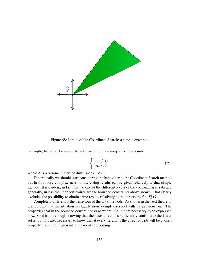
Figure 68: Limits of the Coordinate Search: a simple example.

rectangle, but it can be every shape formed by linear inequality constraints.min f (x)Ax≤ b (39)

where A is a rational matrix of dimensions n×m.Theoretically we should start considering the behaviour ot the Coordinate Search method

but in this more complex case no interesting results can be given relatively to that simplemethod. It is evident, in fact, that no one of the different levels of the conforming is satisfiedgenerally, unless the liner constraints are the bounded constraints above shown. That clearlyexcludes the possibility to obtain some results relatively to the directions d ∈ T F

X (x).Completely different is the behaviour of the GPS methods. As shown in the next theorem,

it is evident that the situation is slightly more complex respect with the previous one. Theproperties that in the bounded constrained case where implicit are necessary to be expressednow. So it is not enough knowing that the basis directions sufficiently conform to the linearset X , but it is also necessary to know that at every iterations the directions Dk will be chosenproperly, i.e., such to guarantee the local conforming.

153

Theorem 24.1 Let xk being the sequence produced by a Generalized Pattern Search algo-rithm applied to the problem 39. Suppose the Extreme Barrier procedure is used to managethe constraints. Let f being strictly differentiable at x. If the basis directions DGPS sufficientlyconform to the feasible set X respect with the sequence xk and if the rule for selecting Dkconforms to X for an ε > 0, then

f ′(x;d)≥ 0, ∀d ∈ T FX (x).

Proof. Since the Extreme Barrier approach is used to manage the constraints of the problemit is possible to state that the whole sequence produced by the Generalized Pattern Searchmethod xk lies inside the feasible set X , i.e., it lies on a bounded set. That is necessary tosay that there exists a refining subsequence xkK converging to a point x that is the maincarachter of the theorem. Let D being the positive spanning set composed by the refining di-rections of x and let DF(x) being the subset of D composed by the feasible refining directionsof x.

Suppose initially that the limit point x is an internal point respect to X (hence DF(x) = D).In this case, exploiting the Mean Value theorem as it has been done previously it is possibleto say that f ′(x;d)≥ 0 for all the directions d ∈ Rn, hence that ∇ f (x) = 0.

Once seen that the theorem works in the trivial case, we focus the attention on the casein which the limit point x lies on the boundary of X . Let us consider the fact that it has beensupposed that DGPS sufficiently conforms to X , meaning that for each xk of the sequenceproduced by the algorithm the corresponding directions d ∈ Dk conform to the set X for acertain ε ∈ [0,1]. Being x a limit point but still a point of the sequence xk (consider thatfor a finite value k of the parameter k, it results xk = x,∀k ≥ k) , the corresponding directionsD have to conform to the set X . That being so the cone of the feasible directions in x can bewritten as the convex cone of a subset of D composed by the feasible directions in the pointx:

cc(DF(x)

)≡ T F

X (x).

At this point is enough to show that f ′(x;d) ≥ 0 for all the directions d ∈ DF(x) to getthe theorem similarly to the previous case. Again, the way is to consider that the set ofindices K is a subset of the unsuccessful iterations U : so it is possible to write that for everyk ∈ K ⊂ U : f (xk + ∆kd) ≥ f (xk) for every d ∈ DF

k . Using the mean value theorem it ispossible to conclude that f ′(x;d)≥ 0 for each d ∈ DF(x). The result of the theorem followsfrom that considering the differentiability of the function f .

Remark 24.2 Saying that f is strictly differentiable at a point x is equivalent than sayingthat f is differentiable in the neighborhood of the point x.

The MADS behaviour results similar to the previous case, not being affected by the par-ticular form of the feasible set.

154

Theorem 24.3 Let xk being the sequence produced by a MADS algorithm applied to theproblem 39. Suppose the Extreme Barrier procedure is used to manage the constraints. Letf being strictly differentiable at x.

Thenf ′(x;d)≥ 0, ∀d ∈ T F

X (x).

Proof. The proof is completely analogous to the one of the Theorem 23.3, relying on thefact that the MADS algorithms generate a dense of directions.

25 Ω: general constraintsIn the previous sections the constrained problem has been seen in its simplest version: in factthe constraints were always supposed being linear. Unfortunately this semplification does notfit with a pletora of real cases. It is necessary to consider the general problem:

min f (x)x ∈Ω

(40)

where the feasible set, defined as Ω = x∈ Rn : c j(x)≤ 0, j = 1, . . . ,m, is defined by generalconstraints.

Again, different degrees of smoothness can be supposed for the objective function f :in this paper less common cases as the lower continuity will not be studied. In particularit will be seen the differentiable case and, as the non-smooth case, it will be supposed theLipschitzianity of f as the weakest hypothesis. Indipendently from the hypotheses on theobjective function, what there really changes is the number of directions necessary to explorea more general feasible region as the one presented in the problem 40.

The first task is to re-consider the concept of conforming for this general case. Let uspresent a very simple case, in which the feasible set is a simple sphere. In the space R2 it is:

Ω = (x1,x2) ∈ R2 : x21 + x2

2 ≤ 0.

The only set of directions D that globally conforms to the set Ω is composed by infinitedirections spread uniformly on the entire unitary space. That being so, it is evident thatneither the Coordinate Search nor its generalization, the Generalize Pattern Search algorithm,can globally converge to the set Ω.

What about the sufficient conforming? Suppose an extremely simple implementation ofa Generalized Pattern Search method. Suppose the starting point is x0 = (0,0)T and that theglobal minimum is on the point x∗ = (−10,0)T . Suppose that the sequence produced by theCoordinate Search algorithm collapses on the point x= (−1,0)T . In a certain sense one couldbe sufficiently convinced that the directions ”north, east and south” conform to Ω in the point(−1,0)T , since the north and the south represent the limit feasible directions in that pointfor the ∆k → 0. Consider that, also in a very simple case like this there would be a trivial

155

problem: all the points considered towards the north and the south will result infeasible. Ifthe Extreme Barrier approach is used to manage the constraints, the only theoretical resultthat could be given would be: f ′(x;deast)≥ 0 for only one direction, the one pointing towardseast (d = (a,o), with a > 0). This example helps us to understand that adapting the conceptof the conforming in the general case is not of easy implementation. In order to answer tothis more challenging case the dense of directions created by the MADS algorithms will beexploited.

In the previous cases the concept of feasible cone T FΩ(x) was all we needed to represent

the feasible directions in the generic point x. Now two tanget cones have to be introduced toanalyze what happens on the boundary of the feasible set Ω. The first one, the HypertangentCone, defined for a certain set at a certain point, is the fundamental one to state the mainresults about the MADS algorithms applied to these kind of problems.

Definition 25.1 A vector is said to be an hypertangent vector to the set Ω ⊂ Rn at the pointx ∈Ω if there exists a scalar ε > 0 such that:

y+ tw

for all the points y ∈ Ω∩Bε(x) and for every direction w ∈ Bε(v), with 0 < t < ε. The set ofthe hypertangent vectors to Ω at x is called hypertangent cone to Ω at x and it is denoted byT (

Ωx).

The hypertangent cone, by definition is both convex and open. Moreover, if Ω is a fulldimentional polytope defined by linear constraints, then every direction in int

[T F

Ω(x)]

is anhypertangent vector. In general, for every point x ∈Ω it is:

T HΩ (x)⊆ T F

Ω (x), (41)

i.e., all the hypertangent vectors are feasible directions. The hypertangent cone is also used todefine a concept of regularity on the feasible set Ω, a sort of constraints qualification: in thenext main theorems it is supposed that the hypertangent cone at the limit point of the refiningsubsequence produced by the algorithm is not-null:

T HΩ (x) 6= 0. (42)

It is easy to see that it results T HΩ(x) = 0 just for strange configurations of the feasible set Ω,

as in presence of cusps.The property in 41 makes evident the fact that it is not possible using the hypertangent

cone to define a concept of conforming. At this purpose it is presented another type of tangentcone:

Definition 25.2 A vector v ∈ Rn is said to be a Clarke tangent vector to the set Ω ⊂ Rn atthe point x in the closure of Ω if, for every sequence yk of elements of Ω that convergesto x and for every sequence of positive real numbers tk converging to zero, there exists asequence of vectors wk converging to v such that

yk + tkwk ∈Ω.

156

The set of all the Clarke tangent vectors to Ω at x is called the Clarke tangent cone to Ω at xand it is denoted by TCl

Ω(x).

In case of regularity it can be estabilished a relation between the two types of tangentcones:

Proposition 25.3 If T HΩ(x) 6= 0, then T H

Ω(x) = int

[TCl

Ω(x)]

The cones introduced make possible to define a different concept of conforming relativelyto the directions generated at the iteration k for this more general case.

Definition 25.4 Suppose that T HΩ(x) 6= 0 for each point x ∈Ω (Ω is regular). The directions

Dk associated at xk conform to the set Ω if, for each point y ∈ Bε(xk) (where Bε(xk) is a openneighborhood of the point xk) there exists a subset of directions D(y)⊂ Dk such that

cc(D(y)) = TClΩ (y).

That is a generalization of the definition given previously on the simple conforming, sincein the case in which the feasible set is a polytope defined by linear constraints it resultsTCl

Ω(y) = T F

Ω(y) for each y ∈ Ω. An important consideration is that in the definition 25.4 it

is not possible to use the concept of feasible direction alone. The condition is given, thistime, on the Clarke cone TCl

Ω(x) relying on an important property connected to another cone,

the contingent cone TCoΩ

(x) whom definition is not given here to avoid complications. It isenough to know that, if the feasible set Ω is regular, the contingent cone coincides with theClarke cone. To summarize what it has been said:

Corollary 25.5 If the feasible set Ω is regular, then

T FΩ (x)⊆ TCl

Ω (x).

The previous corollary allows to use the Clarke cone to give properties on the cone ofthe feasible directions. To prove that the definition 25.4 is a generalization of the previousdefinition of the one is 22.7, the next corollary has to be considered.

Corollary 25.6 If the feasible set Ω is a polyedron defined by linear inequality constraints,then

T FΩ (x) = TCl

Ω (x).

Anyways, the generalized definition of conforming in 25.4 is not useful practically for asimple reason: until this point just the extreme barrier approach has been considered to man-age the constraints. That technique does not consider infeasible directions and, unfortunately,the directions contained in TCl

Ω(x) are not always feasible. Summarizing, in presence of the

general constraints the concept of conforming will be used, but just broadley speaking, as itwill be shown in the follow.

The obstacle given by the additional complication can be overtaken considering the MADS

approach. The key of the speech is here the possibility to create a dense of directions. Howcan a dense of direction guaranteee the convergence towards stationary points is the topic ofthe next propositions.

157

Proposition 25.7 Let f be strictly differentiable at a limit x ∈ Ω of a refining subsequence.Suppose that T H

Ω(x) 6= 0. If the set of the refining directions for x is dense in T H

Ω(x), then x is

a Clarke KKT stationary point of f over Ω.

Proof. Similarly to previous proofs, notice that the indices detecting the refining subse-quence xkK is a subset of the index detecting the unsuccessful iterations: K ⊂U . Then,f (xk) ≤ f (xk +∆m

k dk) for each k ∈ K. Exploiting the differentiability of the function f themean value theorem is used to say that f (xk)− f (xk+∆m

k dk) =∆k∇ f (xk+αk∆kdk)T dk, where

α ∈ R is a value between 0 and 1 that detects a certain point lying on the segment includedbetween xk and xk +∆kdk. Considering k ∈ K,k→ ∞ it results that f ′(x;d) ≥ 0 , for all therefining directions such that d ∈ T H

Ω(x). Being the refining directions a dense of directions it

is possible to modify the result in this way:

f ′(x;d)≥ 0, ∀d ∈ T HΩ (x).

Nevertheless, the result of the theorem is obtain only partially, because nothing has beensaid about the directions d ∈ TCl

Ω(x)/T H

Ω(x), i.e.. those directions contained in the Clarke

tangent cone but not in the hypertangent cone. Those directions have to exist because thehypertangent cone is an open cone included in the Clarke tangent cone that, instead, is aclosed one. To see what happens for those kind of directions a proposition is given withoutproof because it is very technical and it is not of interest for the purposes of this work:

Proposition 25.8 Let f be Lipschitz near x ∈Ω. If T HΩ(x) 6= 0 and if v ∈ TCl

Ω(x), then

f o(x;v) = limw→ v

w ∈ T HΩ(x)

f o(x;w). (43)

Applying the previous theorem it results f ′(x;d)≥ 0 also for the directions d ∈TClΩ(x)/T H

Ω(x).

It follows that:f ′(x;d)≥ 0, ∀d ∈ TCl

Ω (x).

That result is equivalent to say that x is a Clarke KKT stationary point for f on Ω.

Proposition 25.9 Let f be Lipschitz near a limit x ∈ Ω of a refining subsequence. Supposethat T H

Ω(x) 6= 0. If the set of the refining directions for x is dense in T H

Ω(x), then x is a Clarke

stationary point of f over Ω.

Proof. Being xkK the refining subsequence, for each K ⊂U it is

f (xk)− f (xk +∆mk dk)

∆k≥ 0.

Exploiting the Lipschitzianity of the function f , it is possible to deduce the Clarke directionalderivative exploiting the previous disequality:

158

f o(x;d) = limsupy→ xw→ dt ↓ 0

f (y)− f (y+ tw)∆k

≥ limk∈K

f (xk)− f (xk +∆mk dk)

∆k≥ 0.

Considering k ∈ K,k→ ∞ it results that f o(x;d)≥ 0 , for all the refining directions such thatd ∈ T H

Ω(x).

Being the refining directions a dense of directions it is possible to modify the result in thisway:

f ′(x;d)≥ 0, ∀d ∈ T HΩ (x).

Nevertheless, the result of the theorem is to obtain only partially, because nothing has beensaid about the directions d ∈ TCl

Ω(x)/T H

Ω(x), i.e., those directions contained in the Clarke

tangent cone but not in the hypertangent cone. Those directions have to exist because thehypertangent cone is an open cone included in the Clarke tangent cone that, instead, is aclosed one. Applying the proposition 25.8 it results f o(x;d) ≥ 0 also for the directions d ∈TCl

Ω(x)/T H

Ω(x). It follows that:

f o(x;d)≥ 0, ∀d ∈ TClΩ (x).

That being so, it can be stated that the point x is a Clarke stationary point of f over Ω.

In order to give the previous results on the constrained case an assumption has been doneon the approach used to manage the infeasible points. In particular the simplest idea waspresented: consider the points lying in the feasible region discarding the others. The practicalway to implement that idea is to consider a slightly more sophisticated objective function:

fΩ(x) = f (x), ∀x ∈Ω

+∞, ∀x /∈Ω

The effect produced by considering the function fΩ in place of f is to create an out-and-out barrier coinciding with the boundary of Ω evaluating the function values only forthe feasible points and rejecting the infeasible ones without ever considering their objectivefunction values. In the following part it will be presented a scheme of the different ways inwhich the constraints are managed nowdays.

A remark to conclude this part: analyzing the various ways to manage the constraints it isimportant to take into account the fact that it does not change the way in which the space isexplored. What it really changes is the value obtained respect with every point of the space.

159

26 How to manage the constraints: from the EB to the PB

26.1 A mention to the Penalty FunctionsBefore continuing on the successive sophistications of the extreme barrier approach, a men-tion is reserved to the parallel branch dealing with the constraints management: the Penalty.As their name suggests the methods using the penalty function assign a certain utility to everypoint depending on two features: the objective function value and the level of infeasibility.The constraints c j(x) are enveloped together f in an unique function, called the penalty func-tion P(x). In this way in a single function both the objective function and the constraints areconsidered and the penalty function P(x) is then minimized over Rn. The key point is howweight the constraints respect the function value in the penalty function: this is done througha parameter p ∈ R+ that is chosen by the user. Hence the penalty function results:

P(x) = f (x)+ p∑j[max(0,c j(x))]2.

That being so the minimization of P(x) is not guaranteed to converge to a feasible point,unless the penalty p is progressively increased to infinity. This consideration suggests acomparison with the barriers approaach that will be treated in this chapter: in fact, notice thatthe Extreme Barrier can be explained as a particular penalty function for which the penaltyparameter has been set to ∞.

This kind of approaches present a drawback that, although it is not theoretical, representsa very annoying practical problem: the setting of the initial penalty parameter p.

26.2 The barriersUntil now the MADS algorithms has been shown to be the last and the more sophisticatedversion of the Pattern Search methods. There have been shown the theoretical results also forthe most general constrained case. In particular all the results have been given considering theconstraintss managed with the extreme barrier (EB) approach: we can refer to that algorithmas to the MADS-EB. Although it has been shown the convergence of the MADS-EB algorithm,there are a couple of consideration explaining why an evolution of the first barrier approachhas been thought.

• The first consideration, very practical, is likely also the most important: in order for theMADS-EB approach to work it is necessary a feasible starting point x0 that the user hasto provide. The problem underlying this point is that very often in real problems findinga starting feasible point has the same complexity than finding a local solution. Thatbeing so, it is necessary to present a method with such a flexibility to allow infeasiibleiterates.

• In real problems there are constraints that are naturally relaxable. Let us think to a casein which a certain budget has been priced in order to realize a certain work. Even-tually that budget can be grown up and, in general, it can be useful for the users to

160

know what are the possible changes on the realization of the work for increases in theavailable moneys. The MADS-EB method would not be able to interpret the flexibilityincidental to the over explained constraint. If there exists an amazing solution providedfor the maximum budget increased of an ε that solution would not be considered. TheProgressive Barrier will be shown to be a ”less drastic alternatiive than the EB for therelaxable constraints”.

• In the non linear optimization the feasible region can be disjoint. In a case like thatallowing infeasible iterates can drive the algorithm towards better local minima and atthe same time can enable one to solve the problem with fewer function evaluations.

• Sometimes the feasible region has a thin shape. In cases like that a very great numberof evaluation can be necessary just to remain on the feasible region.

The Progressive Barrier uses the concept of dominance proper of the Filter methods.Disgroup the feasible region conceptually in two entities: the relaxable region Ω and the

unrelaxable region X .A second function is put beside the objective one f , representing a measure of the con-

straint violation respect with every point x ∈ Rn. One example of this

h(x) =

∑ j∈J(max(c j(x),0)

)2, x ∈ X

+∞, otherwise(44)

This representation of the constraint violation had the advantage not to introduce differentia-bility.

h(x) x ∈Ω

0 < h(x)<+∞ x ∈ X/Ω

h(x) = +∞ x /∈ X

In the MADS-EB algorithm the user had to provide a feasible point x0 for which −∞ <f (x0)<+∞. In this case thee basilar assumption is less strict than previously:

Assumption 26.1 There exists some point x0 provided by the user into the set V0 such thatx0 ∈ X, f (x0) and h(x0) are both finite and h(x0)≤ hMAX

0 .

It is to understand how it is possible to take advantage of this new structure. The first idea,that is also the simplest one, is to implement an algorithm composed of two phases.

Algorithm 26.2 (Two-phases method)

161

Phase I:

• Run the MADS-EB algorithm for the set of points defined by V0∩X tosolve the problem:

minx∈X

h(x)

UNTIL a feasible point x ∈Ω is found.

• if MADS-EB ends without generating a feasible point, conclude that Ω

is empty.

Phase II: Run the MADS-EB algorithm from the feasible starting point x.

The algorithm 26.9 is actually a masked MADS-EB algorithm that is applied to an uncon-trained minimization before and to a constrained problem in the second phase, that is the realconstrained problem. It is interesting explaining what happens at the end of the Phase I: ifthat phase ends without finding a feasible point it is concluded that the the feasible set Ω onwhich we are looking for the best solution is actually empty. This conclusion is, in general, asemplification. It would be true if another assumption is done previously:

Assumption 26.3 The constraints violation function h(x) referred to the problem 40 doesnot have local minima.

Considering the assumption 26.3 it is possible to say that, if the Phase I ends withoutfinding any feasible point, it is possible to properly conclude that Ω is empty.

The good point of this two-phases approach is that it is a very simple idea to explain.Then, which is the main limitation of the Two-Phases approach? It can be focused in a singleconsideration: in the Phase II the objective function f is totally not considered. This maylead toward regions relatively far from local minima of the functions and making necessary agreat number of iterations in the second phase to get one.

Another aspect can be considered, speaking about the quality of the minima. Dependingon the particular structure of the considered problem, in fact, there could be a lot of localminima or, again, the feasible set could be disjoint. Not considering the objective function inthe first iterations could bring a double problem:

It is evident that if there are few local minima (or, going to the extreme, if there is aunique global minimum) or if the feasible set is not disjoint and also regular (it would affectthe regularity of the function h(x)) a very simple method like the Two-Phases one could workvery efficiently. Although the progressive barrier approach that we are going to present ismuch more sophisticated, in the cases in which that additional sophistication is not necessaryto deal with the effective problem structure, the Two-Phases could get better results than aprogressive barrier based method. Since very often the test problems set is built with artificialproblems it happens that the Two-Phases approach is preferred.

162

26.3 Notation to handle the infeasibilitySpeaking of extreme barrier a particular subsequence was taken into account: the refiningsubsequence xkK . All the theoretical results were given on that particular subsequencehaving, above all, the particularity that ∆k went to zero in corrispondence of the subsequenceitself. With the progressive barrier the focus is set on two refining subsequences: the feasibleand the infeasible ones. This distinction reflects the fact that infeasible iterates are allowednow. Similarly not just an incumbent solution is defined, but two, being aware of one fact: ingeneral a point is better than another one when it has a better function (a lower f value) anda better infeasibility (so, a lower h).Hence, at first, let us define the set of the feasible incumbent points.

Definition 26.4 The set of the feasible incumbent at iteration k is defined to be

Fk = arg minxk∈Vk

f (x) : h(x) = 0

.

The points (possibly more than one) contained in this set have, obviously, the infeasibilitymeasure at zero (see the table at chapter 26.2). The definition 26.4 is moreover very simplebecause it can be reconducted to how it has been said in the previous sections.

In order to present the infeasible incumbent, instead, a concept has to be taken by the filterenvironment: the domination. A subset of the infeasible visited points having the feature ”notto be worse than any other point” are defined:

Definition 26.5 At iteration k, the set of infeasible undominated points is defined to be

Uk =

x ∈Vk/Ω : @ y ∈Vk/Ω such that y≺ x,

where y≺ x means that h(y)< h(x) and f (y)≤ f (x), or that h(y)≤ h(x) and f (y)< f (x).

These are those points that are not worse than (i.e. not dominated by) any other visited point.Uk coincides with a single point when that point has both the best f and the best h. Intu-itively the infeasible incumbent points have to belong to the previous set of point. When thefirst filter-approached constrained problem was introduced by C.Audet and J.Dennis in 2004the infeasible incumbent point was defined as the undominated point (if one) nearest to thefeasible region. That nearess to the feasible set was the grant that the infeasible incumbenteventually would converge to the feasible region. Then something has been changed intro-ducing a more- f -oriented approach. The infeasible incumbent was defined (2009) in thisway:

Definition 26.6 At iteration k the set of infeasible incumbent solutions is defined to be:

Ik = arg minxk∈Uk

f (x) : h(x) = 0

.

Choosing everytime the farest possible infeasible point, in order to avoid that point going farerand farer away from Ω a limitation on the violability was introduced: the barrier threshold

163

hmaxk . This threshold represent tha confidence we have respect the contraints violation. If hmax

kis very high we are considering in our analysis also points very far from the feasible region.All the points y such that h(y) > hmax

k are simply rejected and their f values are not evencomputed. How can this threshold forcing the infeasible incumbents towards the feasibleregion Ω? Simply implementing the progressive barrier algorithm such that hmax

k → 0, i.e.,allowing infeasible iterates gradually nearer to Ω.

Now we have at our disposal the elements necessary to define the incumbent values of thefunctions f and h at iteration k. In the feasible case only the f value has to be defind becausethe constraints violation function h is banally h(xF

k ) = 0:

f Fk =

∞ if Fk = /0,f (x) for any x ∈ Fk, otherwise. (45)

So the feasible incumbent funcion value is set to ∞ if no points are available inside the set Fk.Similarly, if the set of the infeasible incumbent is zero (that is a much less likely situation), theincumbent is supposed to have the worst objective function and constraint violation values,both set at infinity:

(hIk, f I

k ) = (∞,∞) if Ik = /0,

(h(x), f (x)) for any x ∈ Ik, otherwise. (46)

26.4 The generalized pollWhen we had to deal just with the simple extreme barrier (EB) approach the classical pollframe of the MADS was taken into account. With the progressive barrier (PB) approach amore complex definition of the poll set is necessary. Previously Pk was simply a particularset of values relatively near to the incumbent xk. Now the same concept is only adaptedto the new definition of incumbent points. In case Ik = /0 the definition of the poll frame isexactly the one given previously (with xF

k substituting conceptually xk). At the contrary, ifonly infeasible incumbent are defined (Fk = /0), the poll frame is defined as a particular set ofpoints near the infeasible incumbent point. The two results are put together in the case boththe incumbents exist (Fk, Ik 6= /0). All is summarized in the following definition:

Definition 26.7 At iteration k, the poll set Pk is defined to be:

Pk =

Pk(xFk ) for some xF

k ∈ Fk, if Ik = /0

Pk(xIk) for some xI

k ∈ Fk, if Fk = /0

Pk(xFk )∪Pk(xI

k) for some xFk ∈ Fk and xI

k ∈ Fk, if Ik 6= /0∩Fk 6= /0

.

In particular, in the case in which both the incumbents are defined, one has to face the questionof which one favouring. That question is important since very often the poll is opportunistic(it is stopped as soon as a better point is found) in order to try to avoid function computations.How do we choice one of them considering that xF

k is remarkable specially because of itsfeasibility and xI

k is remarkable for its low function value? Who can be considered better?The comparison is done on the basis of the objective function values, and the infeasibleincumbent is favoured just in case itss function value f I

k is ”sufficiently better” than f Fk . This

”sufficience” is actualized through a parameter ρ.

164

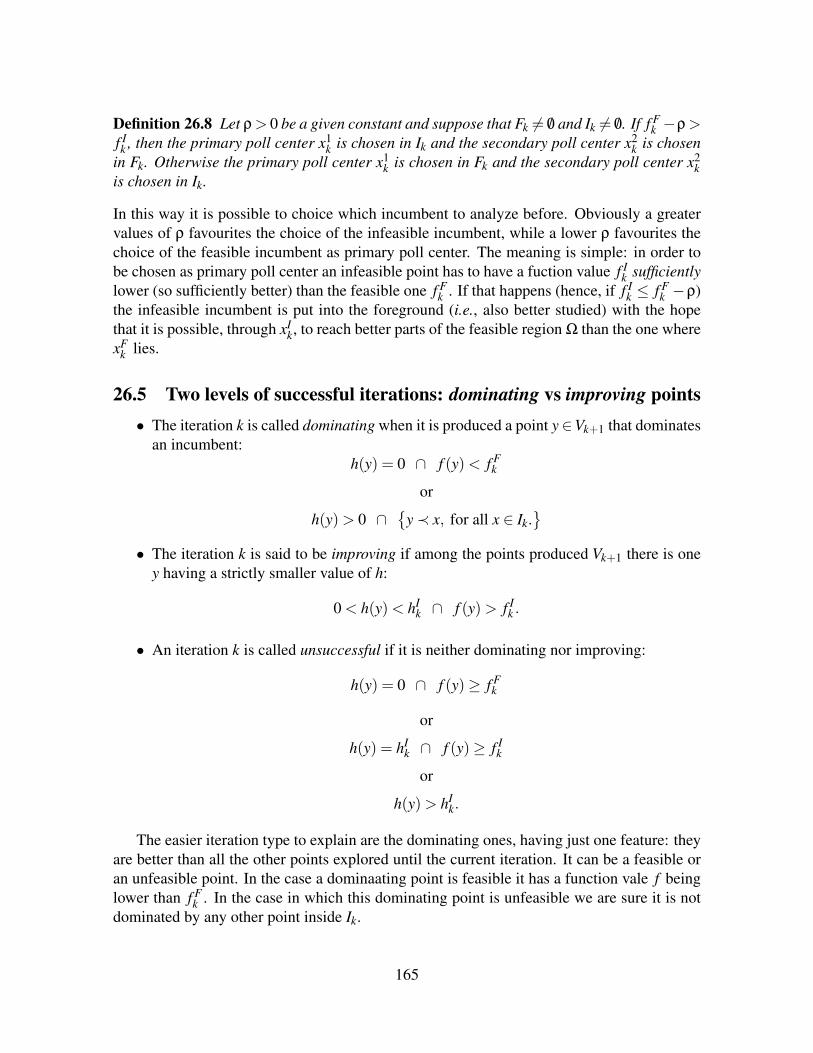
Definition 26.8 Let ρ> 0 be a given constant and suppose that Fk 6= /0 and Ik 6= /0. If f Fk −ρ>

f Ik , then the primary poll center x1

k is chosen in Ik and the secondary poll center x2k is chosen

in Fk. Otherwise the primary poll center x1k is chosen in Fk and the secondary poll center x2

kis chosen in Ik.

In this way it is possible to choice which incumbent to analyze before. Obviously a greatervalues of ρ favourites the choice of the infeasible incumbent, while a lower ρ favourites thechoice of the feasible incumbent as primary poll center. The meaning is simple: in order tobe chosen as primary poll center an infeasible point has to have a fuction value f I

k sufficientlylower (so sufficiently better) than the feasible one f F

k . If that happens (hence, if f Ik ≤ f F

k −ρ)the infeasible incumbent is put into the foreground (i.e., also better studied) with the hopethat it is possible, through xI

k, to reach better parts of the feasible region Ω than the one wherexF

k lies.

26.5 Two levels of successful iterations: dominating vs improving points• The iteration k is called dominating when it is produced a point y∈Vk+1 that dominates

an incumbent:h(y) = 0 ∩ f (y)< f F

k

or

h(y)> 0 ∩

y≺ x, for all x ∈ Ik.

• The iteration k is said to be improving if among the points produced Vk+1 there is oney having a strictly smaller value of h:

0 < h(y)< hIk ∩ f (y)> f I

k .

• An iteration k is called unsuccessful if it is neither dominating nor improving:

h(y) = 0 ∩ f (y)≥ f Fk

or

h(y) = hIk ∩ f (y)≥ f I

k

or

h(y)> hIk.

The easier iteration type to explain are the dominating ones, having just one feature: theyare better than all the other points explored until the current iteration. It can be a feasible oran unfeasible point. In the case a dominaating point is feasible it has a function vale f beinglower than f F

k . In the case in which this dominating point is unfeasible we are sure it is notdominated by any other point inside Ik.

165

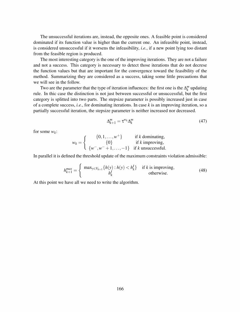
The unsuccessful iterations are, instead, the opposite ones. A feasible point is considereddominated if its function value is higher than the current one. An infeasible point, instead,is considered unsuccessful if it worsens the infeasibility, i.e., if a new point lying too distantfrom the feasible region is produced.

The most interesting category is the one of the improving iterations. They are not a failureand not a success. This category is necessary to detect those iterations that do not decresethe function values but that are important for the convergence toward the feasibility of themethod. Summarizing they are considered as a success, taking some little precautions thatwe will see in the follow.

Two are the parameter that the type of iteration influences: the first one is the ∆mk updating

rule. In thic case the distinction is not just between successful or unsuccessful, but the firstcategory is splitted into two parts. The stepsize parameter is possibly increased just in caseof a complete success, i.e., for dominating iterations. In case k is an improving iteration, so apartially successful iteration, the stepsize parameter is neither increased nor decreased.

∆mk+1 = τ

wk∆mk (47)

for some wk:

wk =

0,1, . . . ,w+ if k dominating,0 if k improving,

w−,w−+1, . . . ,−1 if k unsuccessful.

In parallel it is defined the threshold update of the maximum constraints violation admissible:

hmaxk+1 =

maxy∈Vk+1h(y) : h(y)< hI

k if k is improving,hI

k otherwise. (48)

At this point we have all we need to write the algorithm.

166

Algorithm 26.9 (MADS-PB)INITIALIZATION:

Given:

• Let V0 be a set of initial points satisfying the Assumption 26.10.

• Let D = GZ be a positive spanning set such that:

– G ∈ Rn×n is a non-singular matrix;– Z ∈ Zn×nD

defining a mesh on Rn: M0.

• Let ρ > 0 a frame trigger as defined in 26.8.

• Let the counter k = 0.

INCUMBENTS DEFINITION: Define:

• the incumbent sets Fk and Ik as in Definitions 26.4 and 26.6;

• the incumbent values f Fk and ( f I

k ,hIk) as in Definitions 45 and 46.

SEARCH AND POLL STEP: Performing the search (optionally) and the pollsteps stopping if an improving or a dominating point xk+1 is found.

• search: evaluate f and h on a finite number of trial points lying on themesh Mk, as described in the previous chapter.

• poll: evaluate f and h on the poll set Pk∩X

PARAMETER UPDATE:

• Classify the iteration k as: dominating, improving or unsuccessful;

• update the mesh size parameter ∆mk+1 in accord with the 47 and the poll

size paramter ∆pk+1 such that

limk→∞

∆pk = 0⇔ lim

k→∞∆

mk = 0;

• update the barrier threshold hmaxk+1 following the rule in 48;

• k = k+1 and go back to the INCUMBENT DEFINITION phase.

Also for the Progressive Barrier approach the user has a total freedom in the choice of themethod used in the search to detect promising points on the mesh Mk. We remember that thepoll set is defined as

Pk(x1k) = x1

k∪x1k +∆

mk d : d ∈ Dk,

where Dk is a positive spanning set, not necessarily a subset of D. Practically the key pointis that a well-defined poll frame has to be defined around the primary poll center. In fact one

167

can decide to create a Pk(x2k) useful only to have a look at the neighborhood of the secondary

poll center. In fact it will be better analyzed as soon as it will become the primary poll center.Nevertheless, it is up to the user deciding to do a greater effort creating a well defined pollframe also around the secondary poll center (it does not affect the convergence analysis).Moreover it is possible to jump the poll phase wherever a point better than the incumbent isfound in the search.

26.6 Convergence theoryBefore concentrating on the results of the progressive barrier approach we take this first partto summarizing the two basic assumptions that are necessary to build the theory structure.They are present previously but the choice of the author here is to present them here ex-plicitly to avoid the common problem of jumping pages back and forward to understand theproves. That being so, to make it as clearer as possible the two basic assumptions are in thefollow:

Assumption 26.10 (A1) There exists some point x0 provided by theuser into the set V0 such that x0 ∈ X, f (x0) and h(x0) are both finiteand h(x0)≤ hMAX

0 .

Assumption 26.11 (A2) All trial points considered by the algorithm liein a bounded set.

The necessity of the assumption 26.10 is very easy to explain: we have to be sure that there isat least one point inside the relaxed region X from which it is possible to start the progressivebarrier algorithm. Moreover this point has to have an acceptable constraints violation (respectwith how estabilished at the beginning, hmax

0 ) and a finite value of the objective function ftoo.The second assumption (26.11), instead, is the classical assumption always done in this work,either in the unconstrained or in the constrained case. This second assumption importance liesin the possibility to ensure, together with the mesh structure (always supposed, also implicitlyas in the Coordinate Search method) that:

liminfk

∆mk = 0.

Roughly speaking the previous inferior limit means that there exists at least one subsequenceof the sequence produced by the MADS-PB for which the corresponding mesh size parameterconverges to zero. That subsequence, defined previoulsy refining subsequence, is the one onwhich it is possible to state the convergence results. For this reason everytime we say ”letxkk∈K → x be a refining subsequence”, the assumption 26.11 guarantees us the existenceof that particular subsequence.

The main difference with the extreme barrier case is that now not a single result is given,but the proof is divided in two parts: the sequence produced by the MADS-PB algorithmoscillating between feasible and infeasible points is analyzed in the feasible and the infeasiblesubsequence.

168

Feasible sequence: xFk The first part that we are going to analyze is the feasible part, be-

cause it is the most similar to the previous case. The following theorem results as an adapta-tion of the etreme barrier case:

Theorem 26.12 Let xFk k∈K → x be a refining subsequence, with xF

k ∈ Fk (converging tothe point xF ∈Ω).Let f be a Lipschitz function near the point xF . If v ∈ T H

Ω(x) is a refining direction for xF .

Thenf o(xF ,v)≥ 0.

Proof. This proof is similar to the one of the central theorem of the MADS algorithms.Instead of the only previous refining subsequence the feasible refining subsequence is takeninto account: xF

k k∈K . The existence of a refining direction is defined through the normalizeddirections: v = limk∈L

dk||dk|| . As said previously it is used the following property:

f o(xF ,v) = limw→ v

f o(x,w) (49)

Our tending direction wk is the sequence dk||dk|| considered for the subsequence k ∈ L.

f o(x,v) = limk ∈ L

dk||dk|| → v

f o(

x,dk

||dk||

)= lim

k ∈ Lf o(

x,dk

||dk||

), (50)

where the last equality comes by the fact that dk||dk|| is included in the fact that the subset of

indices k ∈ L is considered. It is specified the last part of the previous equality to clarify thefact that for the subsequence k ∈ L it happens that the normalization of dk tends to v.

The key of the proof is in the particular sequence of points converging to x and in thesequence of positive scalars converging to zero chosen to detect a particular incremental ratebeing less or equal to the superior limit identifying the Clarke generalized derivative:

• a sequence yk such that it corrisponds to the converging refining subsequence fork ∈ L:

yk = xFk + tk

( dk

||d||k− v).

Tending of k to ∞ it results yk→ xF for k ∈ K, hence also for k ∈ L.

• A scalar tk = ∆mk ||dk||. It is a positive quantity for all the k being a product of the mesh

size parameter and the norm of a vector. Moreover, looking at the Definition 8.2 it is∆m

k ||dk|| ≤ ∆pk max||d′|| : d′ ∈ D, where the second term goes infinitely to zero.

Before computing the value of the generalized Clarke derivative described by the theoremwe give a result about the amount yk we will need along this proof. For this purpose let usconsider the lipschitzianity of the function f :∣∣ f (xF

k )− f (yk)∣∣≤ λ

∣∣∣∣xFk − yk

∣∣∣∣= λ

∣∣∣∣∣∣∣∣−tk( dk

||dk||− v)∣∣∣∣∣∣∣∣≤ λ ||tk||

∣∣∣∣∣∣∣∣( dk

||dk||− v)∣∣∣∣∣∣∣∣

169

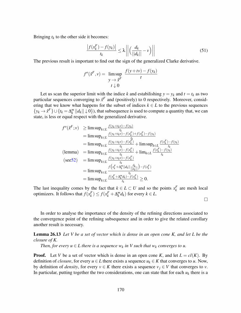
Bringing tk to the other side it becomes:∣∣ f (xFk )− f (yk)

∣∣tk

≤ λ

∣∣∣∣∣∣∣∣( dk

||dk||− v)∣∣∣∣∣∣∣∣ (51)

The previous result is important to find out the sign of the generalized Clarke derivative.

f o(xF ,v) = limsupy→ xF

t ↓ 0

f (y+ tv)− f (yk)

t

Let us scan the superior limit with the indice k and estabilishing y = yk and t = tk as twoparticular sequences converging to xF and (positively) to 0 respectively. Moreover, consid-ering that we know what happens for the subset of indices k ∈ L to the previous sequencesyk→ xF∪tk = ∆m

k ||dk|| ↓ 0), that subsequence is used to compute a quantity that, we canstate, is less or equal respect with the generalized derivative.

f o(xF ;v) ≥ limsupk∈Lf (yk+tkv)− f (yk)

tk

= limsupk∈Lf (yk+tkv)− f (xF

k )+ f (xFk )− f (yk)

tk

= limsupk∈Lf (yk+tkv)− f (xF

k )tk

+ limsupk∈Lf (xF

k )− f (yk)tk

(lemma) = limsupk∈Lf (yk+tkv)− f (xF

k )tk

+ limk∈Lf (xF

k )− f (yk)tk

(see52) = limsupk∈Lf (yk+tkv)− f (xF

k )tk

= limsupk∈L

f(

xFk +∆m

k ||dk||dk||dk||)− f (xF

k )

tk

= limsupk∈Lf (xF

k +∆mk dk)− f (xF

k )tk

≥ 0.

The last inequality comes by the fact that k ∈ L ⊂ U and so the points xFk are mesh local

optimizers. It follows that f (xFk )≤ f (xF

k +∆mk dk) for every k ∈ L.

In order to analyse the importance of the density of the refining directions associated tothe convergence point of the refining subsequence and in order to give the related corollaryanother result is necessary.

Lemma 26.13 Let V be a set of vector which is dense in an open cone K, and let L be theclosure of K.

Then, for every u ∈ L there is a sequence wk in V such that wk converges to u.

Proof. Let V be a set of vector which is dense in an open cone K, and let L = cl(K). Bydefinition of closure, for every u ∈ L there exists a sequence uk ∈ K that converges to u. Now,by definition of density, for every v ∈ K there exists a sequence v j ∈ V that converges to v.In particular, putting together the two considerations, one can state that for each uk there is a

170

sequence vk j in V converging to uk.Finally, for every k one can choose one vk j (and call it wk) such that

|vk j−uk|< 1/k.

It follows that the sequence wk converges to u since:

|wk−u|< |vk j−uk|+ |uk−u|< 1/k+ |uk−u| → 0

.In conclusion, for every u ∈ L there is a sequence wk ∈V such that wk converges to u.

The previous lemma is fundamental to obtain the result completing the analysis on thefeasible refining subsequences. In fact, this corollary introduces the density typical of theMADS algorithms.

Corollary 26.14 Let xFk k∈K → xF be a refining subsequence, with xF

k ∈ Fk (converging tothe point xF ∈ Ω). Let f be a Lipschitz function near the point xF . If the set of refiningdirections for xF is dense in T H

Ω(xF) 6= /0, then xF is a Clarke stationary point for the original

problem.

Proof. Since the assumptions, the Proposition 26.12 ensures that

f o(xF ,v)≥ 0,

for a set of directions v which is dense in the open cone K = T HΩ(xF). We also know that,

under the constraint qualification assumption that T HΩ(xF) 6= /0, there exist a precise relation

between the hypertangent and the Clarke tangent cone:

TClΩ (xF) = cl[T H

Ω (xF)].

The cone L = TClΩ(xF) is a close one. We notice that the situation is the one presented at

Lemma 26.13, then for every u ∈ TClΩ(xF) there is a sequence wk in the set of the refining

directions such that wk converges to u. This is also true for those u belonging to the Clarkecone but not to the hypertangent cone. What we do not know is the generalized Clarkederivative for those directions u ∈ cl[T H

Ω(xF)]/T H

Ω(xF), since the results of the Proposition

26.12 is only on the directions lying on the hypertangent cone. At this purpose comes to aidthe Proposition 25.8 (given without proof). In fact, considering that f Lipschitz near xF , thatT H

Ω(xF) 6= /0 and analyzing the directions u ∈ TCl

Ω(xF), it is possible to say that:

f o(x;u) = limwk→ u

wk ∈ T HΩ(xF)

f o(xF ;wk)≥ 0.

Finally, if f o(x;v)≥ 0 for all the directions contained in the Clarke tangent cone TClΩ(xF) it

is possible to conclude that xF is a Clarke stationary point of the constrained general problem.

171

Infeasible sequence: xIk

Theorem 26.15 Let xIkk∈K→ x be a refining subsequence, with xI

k ∈ Fk (converging to thepoint xI ∈ X/Ω).Let f be a Lipschitz function near the point xF . If v ∈ T H

X (xI) is a refining direction for xI .Then

ho(xI,v)≥ 0.

Proof. This proof is absolutely analogous to the one 26.12. Instead of the sequence xFk k∈K ,

the infeasible refining subsequence is taken into account: xIkk∈K . The existence of a refining

direction is defined through the normalized directions: v = limk∈Ldk||dk|| . This direction is

supposed to belong to the feasible directions for the relaxed set X : v ∈ T HX (xI).

Similarly with the feasible case two quantities are taken into account to detect the sign ofthe generalized Clarke derivative:

• a sequence yk such that it corrisponds to the converging refining subsequence fork ∈ L:

yk = xIk + tk

( dk

||d||k− v)→k∈L xI.

• A scalar tk = ∆mk ||dk|| ↓k∈L 0.

Again, the pre-result (computed similarly to the previous case) is computed:∣∣h(xIk)−h(yk)

∣∣tk

≤ λ

∣∣∣∣∣∣∣∣( dk

||dk||− v)∣∣∣∣∣∣∣∣ (52)

The generalized Clarke derivative of the constraints violation function h is written simi-larly to the one for f . It results:

ho(xI,v) = limsupy→ xI

t ↓ 0

h(y+ tv)−h(yk)

t

Then the previous quantities y = yk and t = tk are specified. Moreover, considering thatwe know what happens for the subset of indices k ∈ L to the previous sequences yk →xI∪tk = ∆m

k ||dk|| ↓ 0), we can compute the sign of the ho(xI;v) in the following manner:

ho(xI;v) ≥ limsupk∈Lh(yk+tkv)−h(yk)

tk

= limsupk∈Lh(yk+tkv)−h(xI

k)+h(xIk)−h(yk)

tk

= limsupk∈Lh(yk+tkv)−h(xI

k)tk

+ limsupk∈Lh(xI

k)−h(yk)tk

(lemma) = limsupk∈Lh(yk+tkv)−h(xI

k)tk

+ limk∈Lh(xI

k)−h(yk)tk

(see52) = limsupk∈Lh(yk+tkv)−h(xI

k)tk

= limsupk∈L

h(

xIk+∆m

k ||dk||dk||dk||)−h(xI

k)

tk

= limsupk∈Lh(xI

k+∆mk dk)−h(xI

k)tk

≥ 0.

172

The last inequality comes by the fact that k ∈ L ⊂ U and so the points xIk are mesh local

optimizers. It follows that h(xIk)≤ h(xI

k +∆mk dk) for every k ∈ L.

Corollary 26.16 Let xIkk∈K→ xI be a refining subsequence, with xI

k ∈ Ik (converging to thepoint xI ∈ X). Let h be a Lipschitz function near the point xI . If the set of refining directionsfor xI is dense in T H

X (xI) 6= /0, then xI is a Clarke stationary point for the original problem.

Proof. Since the assumptions, the Proposition 26.15 ensures that

ho(xI,v)≥ 0,

for a set of directions v which is dense in the open cone K = T HX (xI). We also know that,

under the constraint qualification assumption that T HX (xI) 6= /0, there exist a precise relation

between the hypertangent and the Clarke tangent cone:

TClX (xI) = cl[T H

X (xI)].

The cone L = TClX (xI) is a close one. We notice that the situation is the one presented at

Lemma 26.13, then for every u ∈ TClX (xI) there is a sequence wk in the set of the refining

directions such that wk converges to u. This is also true for those u belonging to the Clarkecone but not to the hypertangent cone. What we do not know is the generalized Clarkederivative for those directions u ∈ cl[T H

X (xI)]/T HX (xI), since the results of the Proposition

26.12 is only on the directions lying on the hypertangent cone. At this purpose comes to aidthe Proposition 25.8 (given without proof). In fact, considering that f Lipschitz near xI , thatT H

X (xI) 6= /0 and analyzing the directions u ∈ TClX (xI), it is possible to say that:

ho(x;u) = limwk→ u

wk ∈ T HX (xI)

ho(xI;wk)≥ 0.

Finally, if ho(x;v)≥ 0 for all the directions contained in the Clarke tangent cone TClX (xI) it

is possible to conclude that xI is a Clarke stationary point of the constrained general problem.

Putting together xFk and xI

k Until now two discussions have been done separately. It isnormal to wonder if there is a way to put them together in order to obtain a total result. In thisway we come to a crucial point of the constrained problems in the Derivative-free context.

Central result It is not possible to state that an infeasible sequence will convergen to afeasible point.

We give however a result that is possible to obtain under a certain constraint qualificationassumption:

173

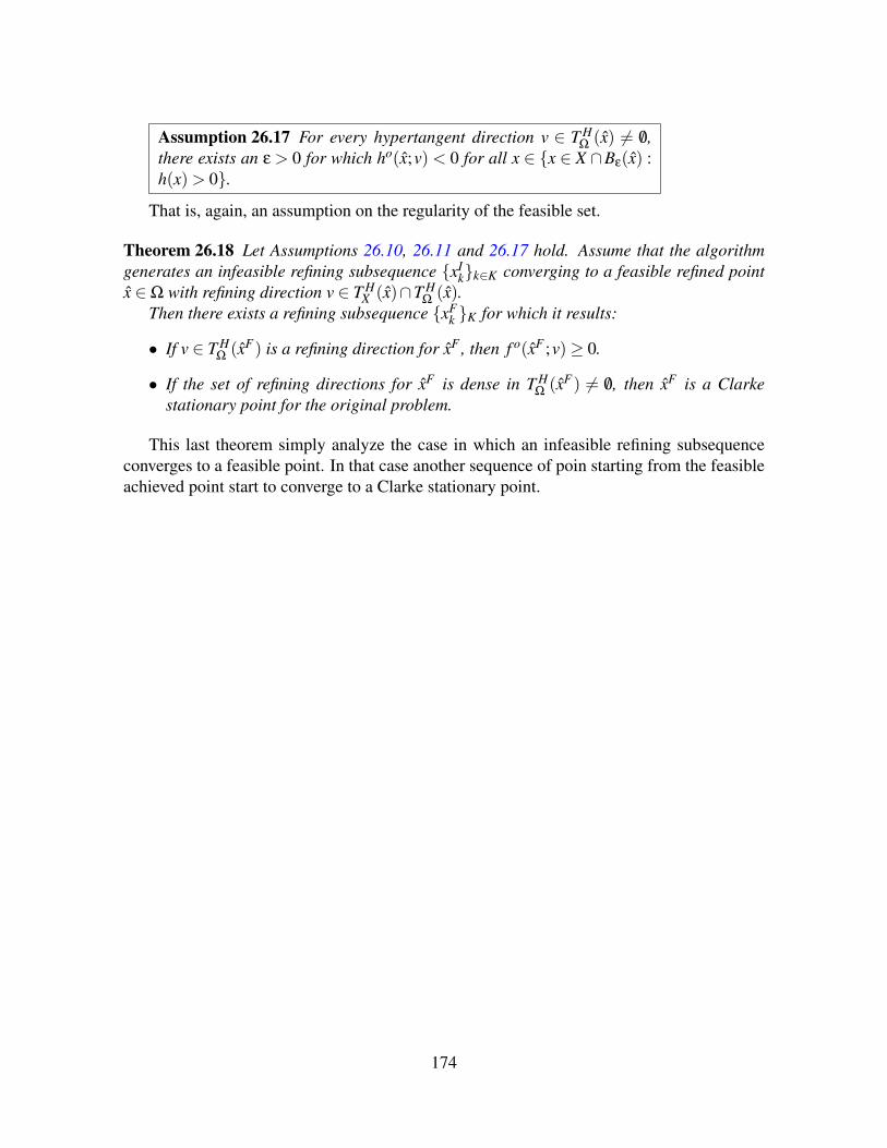
Assumption 26.17 For every hypertangent direction v ∈ T HΩ(x) 6= /0,

there exists an ε > 0 for which ho(x;v) < 0 for all x ∈ x ∈ X ∩Bε(x) :h(x)> 0.

That is, again, an assumption on the regularity of the feasible set.

Theorem 26.18 Let Assumptions 26.10, 26.11 and 26.17 hold. Assume that the algorithmgenerates an infeasible refining subsequence xI

kk∈K converging to a feasible refined pointx ∈Ω with refining direction v ∈ T H

X (x)∩T HΩ(x).

Then there exists a refining subsequence xFk K for which it results:

• If v ∈ T HΩ(xF) is a refining direction for xF , then f o(xF ;v)≥ 0.

• If the set of refining directions for xF is dense in T HΩ(xF) 6= /0, then xF is a Clarke

stationary point for the original problem.

This last theorem simply analyze the case in which an infeasible refining subsequenceconverges to a feasible point. In that case another sequence of poin starting from the feasibleachieved point start to converge to a Clarke stationary point.

174

27 Back-tracking search: the Constrained caseIn this last part the particular implementation of the search phase of the MADS algorithmsnamed Back-tracking search is taken again into account to be generalized to the constrainedcase. As said it does not affect the convergence theory already proved for the MADS.

Let us briefly remember that the Back-tracking search is an evolution of the so calledSpeculative Search that, together with the conceept of the dynamic ordering of the pollingdirections relying on a target direction w and with the generalized updating rule ∆

pk+1 = γm∆

pk ,

with γm ∈ N (allowing larger steps in case of successful iterations) introduced the concept ofsearch along a line also for the MADS algorithms. It is important to notice that this line searchdid not present any concept of sufficient reduction of the objective function values.

The concept in the unconstrained case was very simple: evaluating points along dk untila worse point (named C) was found.Obviously, at that point, it is not C the point we will be interested to, but to the previous-to-the-worse point, i.e. B.. In particular three are the function values on which we focused theattention:

• f (xk + γJ−1∆pk dk) = f (A)

• f (xk + γJ∆pk dk) = f (B)

• f (xk + γJ+1∆pk dk) = f (C).

We are interested in all the mesh points contained in the interval [A,C]: in which way? Thepurpose of the Backtracking procedure had already be shown in the unconstrained case: usingsome mathematical approximation (the quadratic approximation can work properly for ouruse) finding a promising point among the ones on the mesh contained in the segment [A,C]. Inthat simple case explaining the rationale leading us to take a point as promising was extremelysimple because the discussion was entirely focused on the objective function f values. Nowthat procedure is generalized dealing with the constraints. Then the referential problem is,again:

minx∈Ω

f (x) , (53)

It is now necessary to understand what ”worse” means respect with the consideration ofa certain point.

Previously it was presented the quadratic approximations use and the way in which thepoints were rounded to the mesh. Now, instead, we will have another point of view studyingall the possible cases that can happen in the constrained context separating the different cases.

Algorithmically the method will simply have to recognize which are the points A, B andC every time and to find a new promising point in some way. Obviouvlsy, this ”way” has toconsider both the objective function and the constraints values.

In particular, to identify the three points A, B and C two letters will be used, F and I,identifying the feasibility (F) or not of the point itself.

175

Figure 69: In this example it is set τ = 3. Also for a so small value of τ it is evident thatthe distance between B and C could be much larger than the distance between A and B. Thisscheme represents the classic starting situation for the Back-tracking. In the following partwe will see that an accepted point, in general, can be infeasible or feasible and the same fora rejected point.

176

27.1 The simplest cases: F F F and I I IThe first case presented is probably the simplest ones because it is possible to connect them tothe unconstrained case that has been already studied. The real situation are actually different,because now the problem is constrained, but the way in which they are treated practically isexactly the same of the unconstrained case.

Remark 27.1 It is trivial to notice that the case FFF in the constrained case is not thesame of the FFF of the unconstrained case, though it is treated in the same way. To easilyunderstand the difference betweeen the different cases let us compare an unconstrained caseFFF with a constrained case FFF. In the first case every point is feasible, not just A, B and Cbut also all the points into the segment [A,C] and outside. In the constrained case, also whenA, B and C are all feasible, nothing can be say for sure about all the other points. In fact, ingeneral, there could be infinite infeasible points between A and B and/or infinite infeasiblepoints between B and C. Otherwise all the points contained between A and C could be allfeasible. The point is that we cannot know what really happens in the non-evaluated points.Nevertheless, the purpose of this paper is to find a certain point that has a good probabilityto be a good point. The best we could find is a feasible point (because, at the very end, whatwe want to find is always a feasible point) having a as lower as possible objective function f .For this purpose, relying on the situation that is possible to observe, the smoothest situationwill be supposed, because that is the situation representing the reality in the most of cases innature.

So, if in a constrained situation A, B and C results all feasible, what it will be assumed isthat all the points between A and C are feasible. The target of this remark is to point out thefact that this fact is just an assumption, and this is the reason for which the constrained caseFFF is treated as the unconstrained case.

The case III is comparable to the FFF one: although we have not just f (A), f (B) andf (C), but also h(A), h(B) and h(C) the rule of the EB approach forces the algorithm not toconsider the objective function as long as the feasibility is not reached. So method to dealwith the case III is the same used in FFF replacing f with the constraints c j. This is sobecause in this case the values of h are all positive. If one of those had been equal to zero thecumulative measure of the violation would have not being enough to find the right point.

27.2 The constrained case (F F I)This is the first case in which it is actually necessary to deal with both the objective functionf and the constraints g j, for j = 1, . . . ,m. The constraints violation in the three point is:

• h(A) = 0;

• h(B) = 0;

• h(C)> 0;

177

Figure 70:

Figure 71:

178

Figure 72:

Since the point B is accepted and h(B) = h(A), it has necessarily to be: f (B)< f (A). Atthe contrary, since h(C)> h(B), the discussion about the rejection of C is more complicated.In fact, in order to detect a promising search point, it is necessary to understand if the pointC is rejected because both a worse function value and the infeasibility or just because theinfeasibility. So that, two are the possible cases:

• f (C)< f (B);

• f (C)≥ f (B);

The first one is also the simplest: if f (C) < f (B), in fact, it is not necessary to build thequadratic model Q(α), being that always decreasing between A and C. That means that C isthe minimum of f between A and C. Even though only what happens in A, B and C is known,quadratic models are used to predict what happens in the other infinite points on the segmentbetween A and C. Being h(C)> 0 at least one of the constraints g j(x), j = 1, . . . ,m has to bepositive in the point C.

A quadratic model is built for each j such that g j(C)> 0, in order to obtain the points inwhich the quadratic models of the constraints become positive. In particular we are interestedin detecting the point P in which the first constraint becomes positive, that corresponds to thepoint in which the infeasibility is reached.

It is important to distinguish the model from the reality: the fact that B is feasible and C isinfeasible does not mean that along that segment it exists a single point in which there is theswitch between feasibility and infeasibility. It could be possible that the functions are verydiscontinuous such that there are a lot of switching points between B and C. Nevertheless, the

179

aim is to detect a point having a good probability to be a feasible point whith a lower functionthan the current one. To do that it is necessary to suppose an underlying smoothness of thefunctions. Following this rationale, it is more likely to suppose that there is only a point in asegment in which one passes from feasibility to infeasibility if the beginning of the segmentis feasible and its end is infeasible.

Coming back to the case f (C)< f (B), once the switching point P has been detected it isalso the feasible minimum of the quaratic model of the function f . The point P itself cannotbe taken as a new iterate because P is not a mesh point. Hence, it is necessary to round iton the mesh. Considering that the target is to get a feasible point and that the point P is theprediction of the boundary of the first violated constraint, without any other informations,one can say P has 50% of possibilities to be a feasible point. In order to avoid this drawbacka proper projection on the mesh is used: the point P is rounded on the nearest to P mesh pointon the left of P itself, i.e., on the first mesh point along the semi-line P−dk. For semplicityone can say that the rounding of P is toward A.

It is clear that using a Progressive Barrier approach is a probabilisticly better choice thanusing the Extreme Barrier approach. In fact, though the smarter rounding, there is a signifi-cant probability that the new search point X is infeasible. In that case, with the Extreme Bar-rier approach, X is simply rejected. At the contrary, with the Progressive Barrier approach,even if the new point is infesible, it will likely be a not-dominated point.

The second case, f (C) ≥ f (B) is more complicated, because it is necessary to computenot just the point P that is the approximation of the boundary of the first violated constraint,but also the point L in which the predicted f in the lowest along dk. In general the point Lwill lie between A and B or between B and C depending on the values f (A), f (B) and f (C).After having computed the points L and P through quadratic models based on the values ofthe objective function and the constraints, it is necessary to understand the distribution of thepoints in order to create the new search point X . If L ∈ (P,C) it means that the predictedminimum of f is outside the feasible region. That also means that the feasible minimumpredicted point is P. Following the same reasoning it is possible give the promising pointback as X = Roundleft(P).

If L ∈ (A,B)∪ (B,P), at the contrary, the predicted minimum point is inside the predictedfeasible region. In this case: X = Round(L), i.e., the minimum is simply rounded on themesh.

Remark 27.2 It should be noted that a conservative strategy would make sense: do not passa new search point to the mesh when L ∈ (A,B).

27.3 The constrained case (F I I)Constraints values: h(A) = 0, h(B)> 0, h(C)> 0.

There exist two ways for searching a new point to evaluate: to reason about the disequal-ities among the function values of A, B and C or to reason about the placements of the pointsP and L.

180

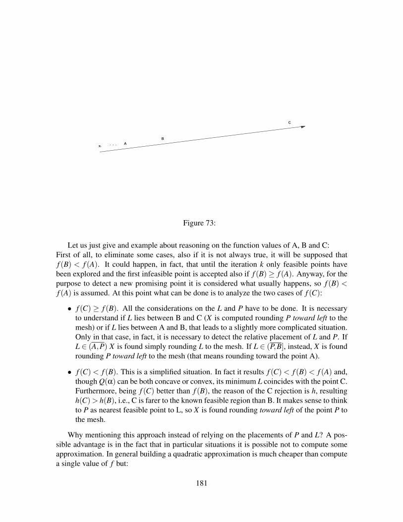
Figure 73:

Let us just give and example about reasoning on the function values of A, B and C:First of all, to eliminate some cases, also if it is not always true, it will be supposed thatf (B) < f (A). It could happen, in fact, that until the iteration k only feasible points havebeen explored and the first infeasible point is accepted also if f (B)≥ f (A). Anyway, for thepurpose to detect a new promising point it is considered what usually happens, so f (B) <f (A) is assumed. At this point what can be done is to analyze the two cases of f (C):

• f (C) ≥ f (B). All the considerations on the L and P have to be done. It is necessaryto understand if L lies between B and C (X is computed rounding P toward left to themesh) or if L lies between A and B, that leads to a slightly more complicated situation.Only in that case, in fact, it is necessary to detect the relative placement of L and P. IfL ∈ (A,P) X is found simply rounding L to the mesh. If L ∈ (P,B], instead, X is foundrounding P toward left to the mesh (that means rounding toward the point A).

• f (C)< f (B). This is a simplified situation. In fact it results f (C)< f (B)< f (A) and,though Q(α) can be both concave or convex, its minimum L coincides with the point C.Furthermore, being f (C) better than f (B), the reason of the C rejection is h, resultingh(C)> h(B), i.e., C is farer to the known feasible region than B. It makes sense to thinkto P as nearest feasible point to L, so X is found rounding toward left of the point P tothe mesh.

Why mentioning this approach instead of relying on the placements of P and L? A pos-sible advantage is in the fact that in particular situations it is possible not to compute someapproximation. In general building a quadratic approximation is much cheaper than computea single value of f but:

181

• there could exist problems in which f is not that costly and the cost of building thequadratic approximation is comparable to the cost of the single evaluation of f itself.

• although a quadratic approximation is here used it could be possible implementing amethod that uses other more advanced or simply more suitable approximations. In thatcase it could be smarter to avoid some model computation.

Different is the case in which the function evaluations are immeasurably more costlythan constructing the surrogate model (hypothesis that is often satisfied when the quadraticapproximation is used as surrogate of the functions) in the derivative-free context. In this caseit is easier to compute the points L and P using the approximations of the objective functionand of the constraints. First of all the point P lies between A and B. The proceding of themethod depends on the location of L. All depends on L. So L and P are computed.

• If L ∈ (−∞,A). Since no informations are supposed to exists a priori on the functionvalues here it is specified that L can lie also to the left of A. It is important to considerthat actually the successive points are being computed from the left, so it is most likelythat in this case the information given by the quadratic model is not reliable, or howevernot that significant. Since it makes sense to take X ≡ A the Search phase does notreceive any proposal.

• If L∈ (A,P). If the minimum of the quadratic function lies inside the predicted feasibleregion it is simply rounded to the mesh to detect X . It is done though it is important toconsider that being the space between A and B much smaller than the region betweenB and C (for construction) it is also a less promising zone to analyze.X = Round(L).

• If L ∈ (P,B]∪ (B,C]∪ (C,+∞). The minimum of the quadratic approximation of fis far away from the predicted feasible area, so the rounding is done toward the pointsA and B along the direction dk.X = Roundleft(P).

27.4 The constrained case (F I F)In this case the constraints values are:

h(A) = 0,h(B)> 0,h(C) = 0,

and the function values:f (C)≥ f (A).

It can be stated that f (C) ≥ f (A) considering the rejection of the point C. Being A andC both feasible, the only reason for C to be rejected is up to the function value f . In orderto estabilish a promising point it is necessary to discern two cases about the relation between

182

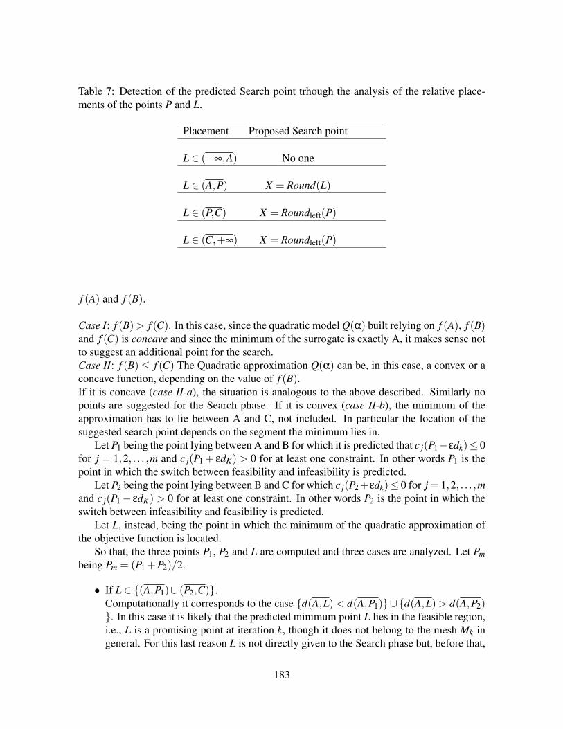
Table 7: Detection of the predicted Search point trhough the analysis of the relative place-ments of the points P and L.

Placement Proposed Search point

L ∈ (−∞,A) No one

L ∈ (A,P) X = Round(L)

L ∈ (P,C) X = Roundleft(P)

L ∈ (C,+∞) X = Roundleft(P)

f (A) and f (B).

Case I: f (B)> f (C). In this case, since the quadratic model Q(α) built relying on f (A), f (B)and f (C) is concave and since the minimum of the surrogate is exactly A, it makes sense notto suggest an additional point for the search.Case II: f (B)≤ f (C) The Quadratic approximation Q(α) can be, in this case, a convex or aconcave function, depending on the value of f (B).If it is concave (case II-a), the situation is analogous to the above described. Similarly nopoints are suggested for the Search phase. If it is convex (case II-b), the minimum of theapproximation has to lie between A and C, not included. In particular the location of thesuggested search point depends on the segment the minimum lies in.

Let P1 being the point lying between A and B for which it is predicted that c j(P1−εdk)≤ 0for j = 1,2, . . . ,m and c j(P1 + εdK) > 0 for at least one constraint. In other words P1 is thepoint in which the switch between feasibility and infeasibility is predicted.

Let P2 being the point lying between B and C for which c j(P2+εdk)≤ 0 for j = 1,2, . . . ,mand c j(P1− εdK) > 0 for at least one constraint. In other words P2 is the point in which theswitch between infeasibility and feasibility is predicted.

Let L, instead, being the point in which the minimum of the quadratic approximation ofthe objective function is located.

So that, the three points P1, P2 and L are computed and three cases are analyzed. Let Pmbeing Pm = (P1 +P2)/2.

• If L ∈ (A,P1)∪ (P2,C).Computationally it corresponds to the case d(A,L)< d(A,P1)∪d(A,L)> d(A,P2). In this case it is likely that the predicted minimum point L lies in the feasible region,i.e., L is a promising point at iteration k, though it does not belong to the mesh Mk ingeneral. For this last reason L is not directly given to the Search phase but, before that,

183

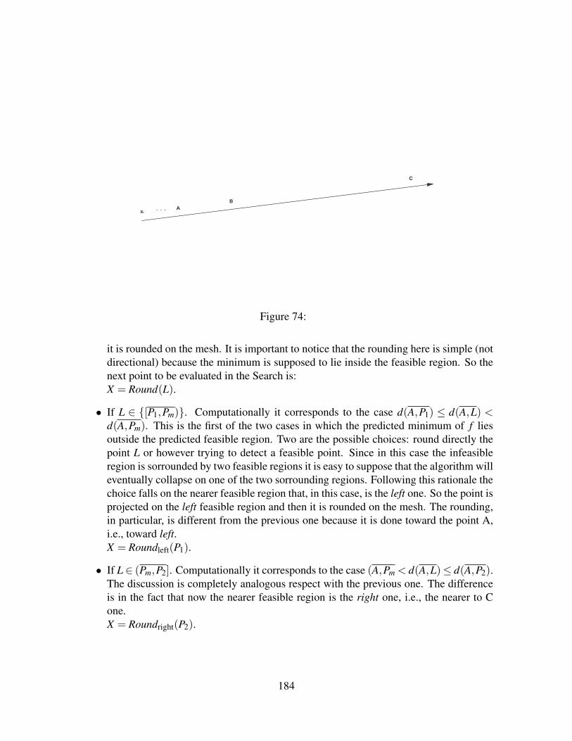
Figure 74:

it is rounded on the mesh. It is important to notice that the rounding here is simple (notdirectional) because the minimum is supposed to lie inside the feasible region. So thenext point to be evaluated in the Search is:X = Round(L).

• If L ∈ [P1,Pm). Computationally it corresponds to the case d(A,P1) ≤ d(A,L) <d(A,Pm). This is the first of the two cases in which the predicted minimum of f liesoutside the predicted feasible region. Two are the possible choices: round directly thepoint L or however trying to detect a feasible point. Since in this case the infeasibleregion is sorrounded by two feasible regions it is easy to suppose that the algorithm willeventually collapse on one of the two sorrounding regions. Following this rationale thechoice falls on the nearer feasible region that, in this case, is the left one. So the point isprojected on the left feasible region and then it is rounded on the mesh. The rounding,in particular, is different from the previous one because it is done toward the point A,i.e., toward left.X = Roundleft(P1).

• If L∈ (Pm,P2]. Computationally it corresponds to the case (A,Pm < d(A,L)≤ d(A,P2).The discussion is completely analogous respect with the previous one. The differenceis in the fact that now the nearer feasible region is the right one, i.e., the nearer to Cone.X = Roundright(P2).

184

Table 8: Detection of the predicted Search point trhough the analysis of the relative place-ments of the points P and L in the case Q(α) convex.

Placement for Q(α) convex Proposed Search point

L ∈ (A,P1) X = Round(L)

L ∈ [P1,Pm) X = Roundleft(P1)

L ∈ (Pm,P2] X = Roundright(P2)

L ∈ (P2,C) X = Round(L)

27.5 The constrained case (I F F)In this case the constraints values are:

h(A)> 0,h(B) = 0,h(C) = 0,

while the function values isf (C)≥ f (B).

It can be stated that B is the feasible incumbent solution since it is accepted. It means thatthere are not feasible evaluated points better than B. At the contrary, being the feasible pointC rejected there is the certainty that f (C) ≥ f (B). So the search proposed point depends onthe relative value of f (A).

When Q(α) is concave (it can happens only when f (A)< f (B)< f (C)), in this case, theminimum of f on (A,C) coincides with A. Unfortunately the contrary is not true, i.e., if alsof (A)< f (B)< f (C) the Q(α) can be concave or convex, so it is impossible to consider justthe objective function disequalities to eliminate some cases without building the surrogatemodels. Two are the possible choices when L coincides with one of the explored point:simply not to do anything and going to the next iteration or making the algorithm collapsingon a boundary of the feasible region, trying to detect the point P. In this case it would result:X = Roundright(P).

While nothing can be said a priori on the point L, P ∈ (A,B]. So it is not necessary todistinguish between the cases f (A)> f (B) and f (A)≤ f (B) but one has to see the respectiveplacement of P and L.

So, at the first the two points P and L are computed, the approximations of the objectivefunction and of the constraints violated in A are built, and the relative positioning of L and Pis analyzed:

• If L∈ [A,P]. The predicted minimum L lies on a region that is predicted to be infeasible.As it has been written above, the orientation is detecting interesting feasible points, so

185

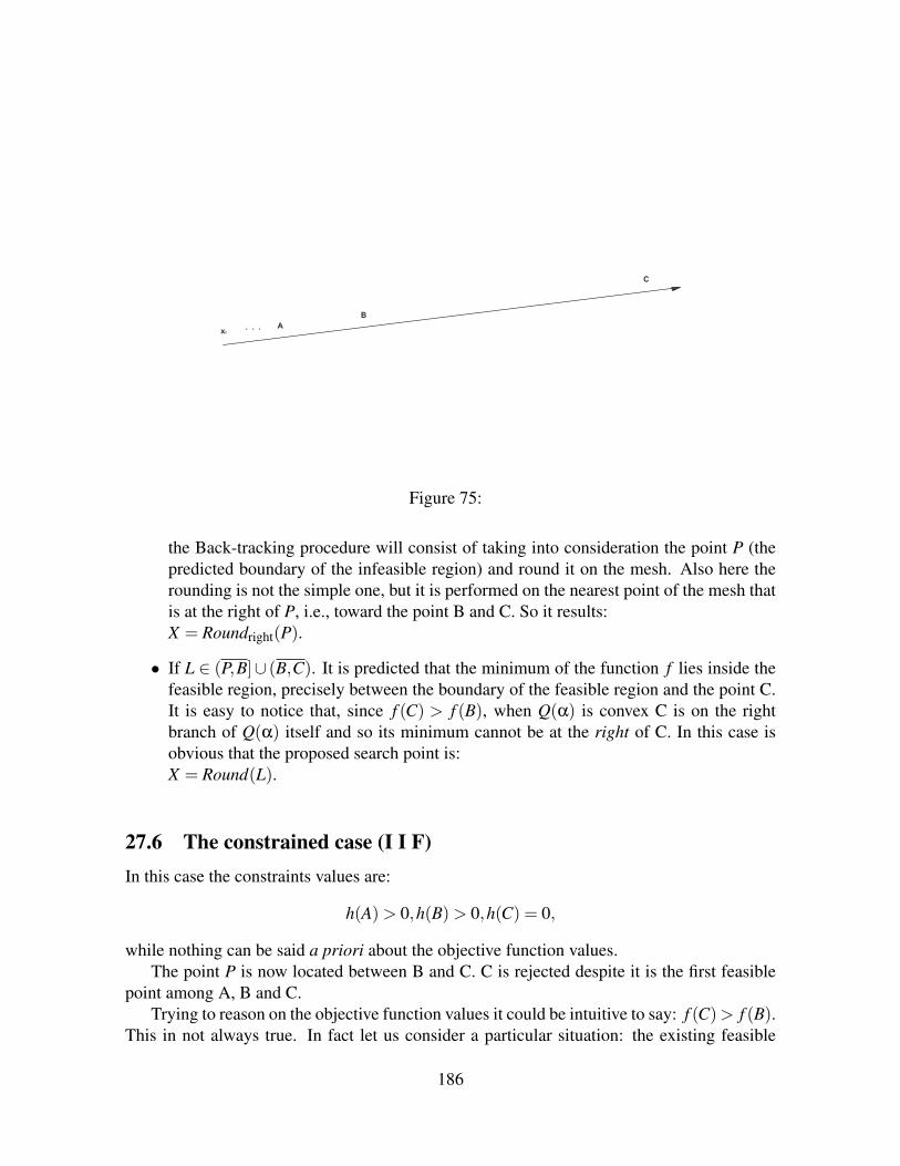
Figure 75:

the Back-tracking procedure will consist of taking into consideration the point P (thepredicted boundary of the infeasible region) and round it on the mesh. Also here therounding is not the simple one, but it is performed on the nearest point of the mesh thatis at the right of P, i.e., toward the point B and C. So it results:X = Roundright(P).

• If L ∈ (P,B]∪ (B,C). It is predicted that the minimum of the function f lies inside thefeasible region, precisely between the boundary of the feasible region and the point C.It is easy to notice that, since f (C) > f (B), when Q(α) is convex C is on the rightbranch of Q(α) itself and so its minimum cannot be at the right of C. In this case isobvious that the proposed search point is:X = Round(L).

27.6 The constrained case (I I F)In this case the constraints values are:

h(A)> 0,h(B)> 0,h(C) = 0,

while nothing can be said a priori about the objective function values.The point P is now located between B and C. C is rejected despite it is the first feasible

point among A, B and C.Trying to reason on the objective function values it could be intuitive to say: f (C)> f (B).

This in not always true. In fact let us consider a particular situation: the existing feasible

186

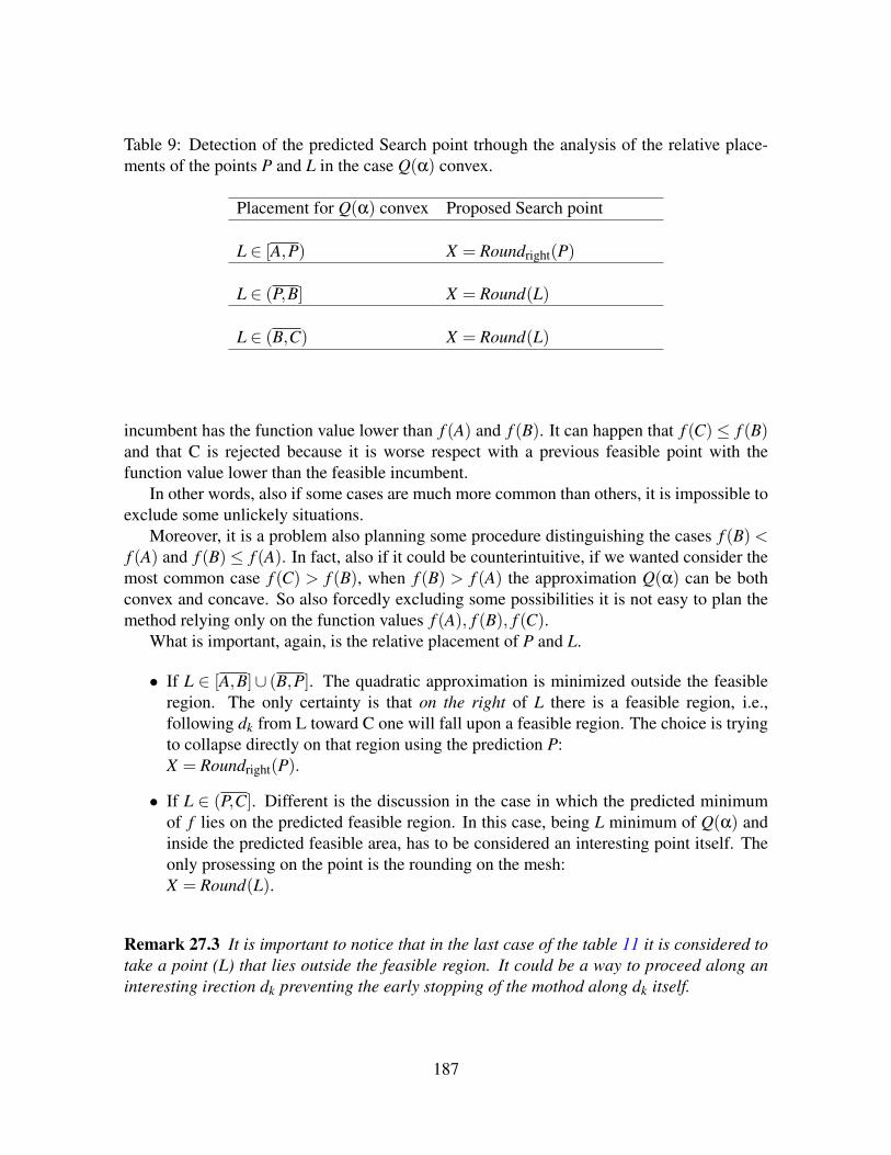
Table 9: Detection of the predicted Search point trhough the analysis of the relative place-ments of the points P and L in the case Q(α) convex.

Placement for Q(α) convex Proposed Search point

L ∈ [A,P) X = Roundright(P)

L ∈ (P,B] X = Round(L)

L ∈ (B,C) X = Round(L)

incumbent has the function value lower than f (A) and f (B). It can happen that f (C)≤ f (B)and that C is rejected because it is worse respect with a previous feasible point with thefunction value lower than the feasible incumbent.

In other words, also if some cases are much more common than others, it is impossible toexclude some unlickely situations.

Moreover, it is a problem also planning some procedure distinguishing the cases f (B)<f (A) and f (B)≤ f (A). In fact, also if it could be counterintuitive, if we wanted consider themost common case f (C) > f (B), when f (B) > f (A) the approximation Q(α) can be bothconvex and concave. So also forcedly excluding some possibilities it is not easy to plan themethod relying only on the function values f (A), f (B), f (C).

What is important, again, is the relative placement of P and L.

• If L ∈ [A,B]∪ (B,P]. The quadratic approximation is minimized outside the feasibleregion. The only certainty is that on the right of L there is a feasible region, i.e.,following dk from L toward C one will fall upon a feasible region. The choice is tryingto collapse directly on that region using the prediction P:X = Roundright(P).

• If L ∈ (P,C]. Different is the discussion in the case in which the predicted minimumof f lies on the predicted feasible region. In this case, being L minimum of Q(α) andinside the predicted feasible area, has to be considered an interesting point itself. Theonly prosessing on the point is the rounding on the mesh:X = Round(L).

Remark 27.3 It is important to notice that in the last case of the table 11 it is considered totake a point (L) that lies outside the feasible region. It could be a way to proceed along aninteresting irection dk preventing the early stopping of the mothod along dk itself.

187

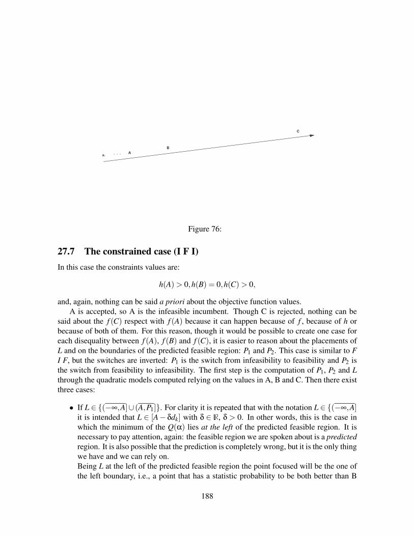
Figure 76:

27.7 The constrained case (I F I)In this case the constraints values are:

h(A)> 0,h(B) = 0,h(C)> 0,

and, again, nothing can be said a priori about the objective function values.A is accepted, so A is the infeasible incumbent. Though C is rejected, nothing can be

said about the f (C) respect with f (A) because it can happen because of f , because of h orbecause of both of them. For this reason, though it would be possible to create one case foreach disequality between f (A), f (B) and f (C), it is easier to reason about the placements ofL and on the boundaries of the predicted feasible region: P1 and P2. This case is similar to FI F, but the switches are inverted: P1 is the switch from infeasibility to feasibility and P2 isthe switch from feasibility to infeasibility. The first step is the computation of P1, P2 and Lthrough the quadratic models computed relying on the values in A, B and C. Then there existthree cases:

• If L ∈ (−∞,A]∪ (A,P1]. For clarity it is repeated that with the notation L ∈ (−∞,A]it is intended that L ∈ [A− δdk] with δ ∈ R, δ > 0. In other words, this is the case inwhich the minimum of the Q(α) lies at the left of the predicted feasible region. It isnecessary to pay attention, again: the feasible region we are spoken about is a predictedregion. It is also possible that the prediction is completely wrong, but it is the only thingwe have and we can rely on.Being L at the left of the predicted feasible region the point focused will be the one ofthe left boundary, i.e., a point that has a statistic probability to be both better than B

188

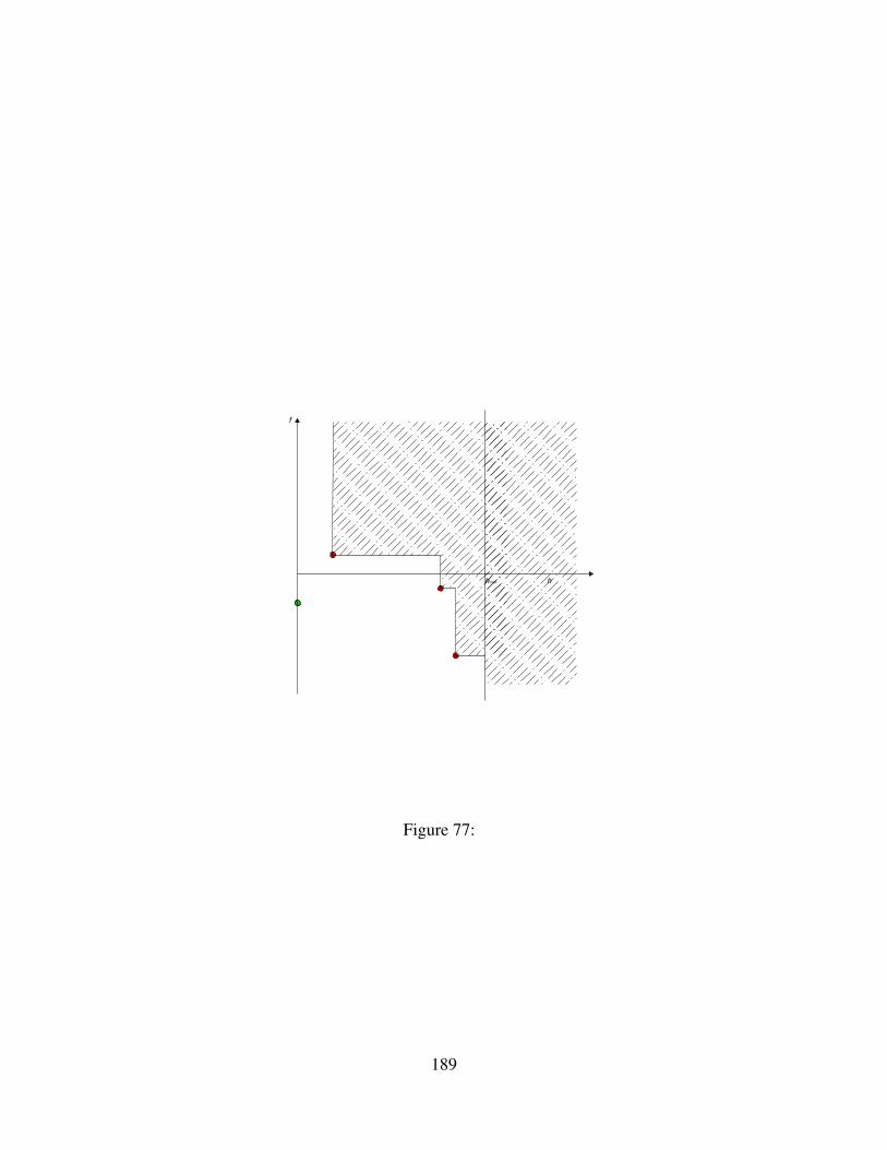
Figure 77:

189

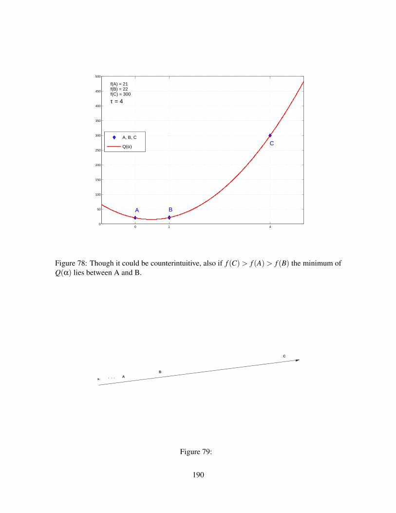
0 1 40

50

100

150

200

250

300

350

400

450

500

A, B, C

Q(α)

BA

C

f(A) = 21f(B) = 22f(C) = 300

τ = 4

Figure 78: Though it could be counterintuitive, also if f (C)> f (A)> f (B) the minimum ofQ(α) lies between A and B.

Figure 79:

190

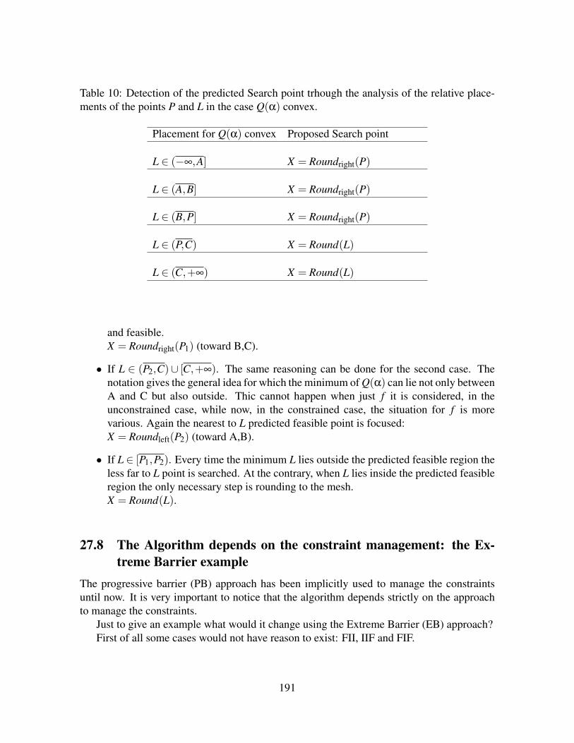
Table 10: Detection of the predicted Search point trhough the analysis of the relative place-ments of the points P and L in the case Q(α) convex.

Placement for Q(α) convex Proposed Search point

L ∈ (−∞,A] X = Roundright(P)

L ∈ (A,B] X = Roundright(P)

L ∈ (B,P] X = Roundright(P)

L ∈ (P,C) X = Round(L)

L ∈ (C,+∞) X = Round(L)

and feasible.X = Roundright(P1) (toward B,C).

• If L ∈ (P2,C)∪ [C,+∞). The same reasoning can be done for the second case. Thenotation gives the general idea for which the minimum of Q(α) can lie not only betweenA and C but also outside. Thic cannot happen when just f it is considered, in theunconstrained case, while now, in the constrained case, the situation for f is morevarious. Again the nearest to L predicted feasible point is focused:X = Roundleft(P2) (toward A,B).

• If L ∈ [P1,P2). Every time the minimum L lies outside the predicted feasible region theless far to L point is searched. At the contrary, when L lies inside the predicted feasibleregion the only necessary step is rounding to the mesh.X = Round(L).

27.8 The Algorithm depends on the constraint management: the Ex-treme Barrier example

The progressive barrier (PB) approach has been implicitly used to manage the constraintsuntil now. It is very important to notice that the algorithm depends strictly on the approachto manage the constraints.

Just to give an example what would it change using the Extreme Barrier (EB) approach?First of all some cases would not have reason to exist: FII, IIF and FIF.

191

Table 11: Detection of the predicted Search point trhough the analysis of the relative place-ments of the points P and L in the case Q(α) convex.

Placement for Q(α) convex Proposed Search point

L ∈ (−∞,A] X = Roundright(P1)

L ∈ (A,P1] X = Roundright(P1)

L ∈ (P1,P2] X = Round(L)

L ∈ (P2,C) X = Roundleft(P2)

L ∈ (C,+∞) X = Roundleft(P2)

• FII: after having accepted the feasible point A, the infeasible point B is accepted aswell. the contradiction is in the fact that in the EB approach infeasible points areaccepted just when no feasible points have been produced so far. Since A ∈ Vk andh(A) = 0, the Extreme Barrier would not let B being accepted.

• IIF: Since A and B are accepted it means that no feasible points have been explored sofar. So C is the first feasible point found by the algorithm, and for this reason it wouldbe accepted, no matter how high is f (C).

• FIF: A is a feasible point. It means that infeasible points after A (B is one of those)cannot be accepted.

192

References[1] M.A. Abramson, C. Audet, and J.E. Dennis, Jr. Generalized pattern searches with derivative

information. Mathematical Programming, Series B, 100:3–25, 2004.

[2] M.A. Abramson, C. Audet, J.E. Dennis, Jr., and S. Le Digabel. OrthoMADS: A deterministicMADS instance with orthogonal directions. SIAM Journal on Optimization, 20(2):948–966,2009.

[3] P. Alberto, F. Nogueira, H. Rocha, and L.N. Vicente. Pattern search methods for user-provided points: application to molecular geometry problems. SIAM Journal on Optimization,14(4):1216–1236, 2004.

[4] C. Audet. Convergence results for pattern search algorithms are tight. Optimization and Engi-neering, 5(2):101–122, 2004.

[5] C. Audet and J.E. Dennis, Jr. Analysis of generalized pattern searches. SIAM Journal on Opti-mization, 13(3):889–903, 2003.

[6] C. Audet and J.E. Dennis, Jr. Mesh adaptive direct search algorithms for constrained optimiza-tion. SIAM Journal on Optimization, 17(1):188–217, 2006.

[7] C. Audet and J.E. Dennis, Jr. A progressive barrier for derivative-free nonlinear programming.SIAM Journal on Optimization, 20(4):445–472, 2009.

[8] C. Audet, J.E. Dennis, Jr., and S. Le Digabel. Parallel space decomposition of the mesh adaptivedirect search algorithm. SIAM Journal on Optimization, 19(3):1150–1170, 2008.

[9] C. Audet, J.E. Dennis, Jr., and S. Le Digabel. Globalization strategies for mesh adaptive directsearch. Computational Optimization and Applications, 46(2):193–215, 2010.

[10] A.J. Booker, J.E. Dennis, Jr., P.D. Frank, D.B. Serafini, V. Torczon, and M.W. Trosset. A rigor-ous framework for optimization of expensive functions by surrogates. Structural and Multidis-ciplinary Optimization, 17(1):1–13, 1999.

[11] G.E.P. Box. Evolutionary operation: A method for increasing industrial productivity. AppliedStatistics, 6(2):81–101, 1957.

[12] F.H. Clarke. Optimization and Nonsmooth Analysis. John Wiley & Sons, New York, 1983.Reissued in 1990 by SIAM Publications, Philadelphia, as Vol. 5 in the series Classics in AppliedMathematics.

[13] A.R. Conn and S. Le Digabel. Use of quadratic models with mesh adaptive direct search forconstrained black box optimization. Technical Report G-2011-11, Les cahiers du GERAD, 2011.To appear in Optimization Methods and Software.

[14] A.R. Conn, K. Scheinberg, and L.N. Vicente. Introduction to Derivative-Free Optimization.MOS/SIAM Series on Optimization. SIAM, Philadelphia, 2009.

[15] I.D. Coope and C.J. Price. Frame-based methods for unconstrained optimization. Journal ofOptimization Theory and Applications, 107(2):261–274, 2000.

193

[16] A.L. Custodio, H. Rocha, and L.N. Vicente. Incorporating minimum Frobenius norm models indirect search. Computational Optimization and Applications, 46(2):265–278, 2010.

[17] C. Davis. Theory of positive linear dependence. American Journal of Mathematics, 76:733–746,1954.

[18] J.E. Dennis, Jr. and V. Torczon. Direct search methods on parallel machines. SIAM Journal onOptimization, 1(4):448–474, 1991.

[19] R. Fletcher and S. Leyffer. Nonlinear programming without a penalty function. MathematicalProgramming, Series A, 91:239–269, 2002.

[20] R. Fletcher, S. Leyffer, and Ph.L. Toint. On the global convergence of an SLP–filter algorithm.Technical Report NA/183, Dundee University, Department of Mathematics, 1998.

[21] K.R. Fowler, J.P. Reese, C.E. Kees, J.E. Dennis Jr., C.T. Kelley, C.T. Miller, C. Audet, A.J.Booker, G. Couture, R.W. Darwin, M.W. Farthing, D.E. Finkel, J.M. Gablonsky, G. Gray, andT.G. Kolda. Comparison of derivative-free optimization methods for groundwater supply andhydraulic capture community problems. Advances in Water Resources, 31(5):743–757, 2008.

[22] N.I.M. Gould, D. Orban, and Ph.L. Toint. CUTEr (and SifDec): a constrained and unconstrainedtesting environment, revisited. ACM Transactions on Mathematical Software, 29(4):373–394,2003.

[23] A. Hedar. Global optimization test problems. http://www-optima.amp.i.kyoto-u.ac.jp/member/student/hedar/Hedar_files/TestGO.htm.

[24] R. Hooke and T.A. Jeeves. Direct search solution of numerical and statistical problems. Journalof the Association for Computing Machinery, 8(2):212–229, 1961.

[25] T.G. Kolda, R.M. Lewis, and V. Torczon. Optimization by direct search: new perspectives onsome classical and modern methods. SIAM Review, 45(3):385–482, 2003.

[26] S. Le Digabel. Algorithm 909: NOMAD: Nonlinear optimization with the MADS algorithm.ACM Transactions on Mathematical Software, 37(4):44:1–44:15, 2011.

[27] R.M. Lewis and V. Torczon. Rank ordering and positive bases in pattern search algorithms.Technical Report 96–71, Institute for Computer Applications in Science and Engineering, MailStop 132C, NASA Langley Research Center, Hampton, Virginia 23681–2199, 1996.

[28] L. Luksan and J. Vlcek. Test problems for nonsmooth unconstrained and linearly constrainedoptimization. Technical Report V-798, ICS AS CR, 2000.

[29] J.J. More and S.M. Wild. Benchmarking derivative-free optimization algorithms. SIAM Journalon Optimization, 20(1):172–191, 2009.

[30] D. Orban. Templating and automatic code generation for performance with python. TechnicalReport G-2011-30, Les cahiers du GERAD, 2011.

[31] V. Torczon. On the convergence of pattern search algorithms. SIAM Journal on Optimization,7(1):1–25, 1997.

194

[32] L.N. Vicente and A.L. Custodio. Analysis of direct searches for discontinuous functions. Math-ematical Programming, 2010.

195