Density-functional-theory study of the electric-field-inducedsecond harmonic generation (EFISHG) of push–pull phenylpolyenes

in solution

Lara Ferrighi a, Luca Frediani a,*, Chiara Cappelli b, Pawe! Sa!ek c, Hans Agren c,Trygve Helgaker d, Kenneth Ruud a

a Department of Chemistry, University of Tromsø, N-9037 Tromsø, Norwayb PolyLab-CNR-INFM, c/o Dipartimento di Chimica e Chimica Industriale, Universita di Pisa, Via Risorgimento 35, 56126 Pisa, Italy

c Laboratory of Theoretical Chemistry, AlbaNova University Center, Royal Institute of Technology, S-10691 Stockholm, Swedend Department of Chemistry, University of Oslo, P.O.B. 1033 Blindern, N-0315 Oslo, Norway

Received 20 January 2006; in final form 21 April 2006Available online 10 May 2006

Abstract

Density-functional theory and the polarizable continuum model have been used to calculate the electric-field-induced second har-monic generation of a series of push–pull phenylpolyenes in chloroform solution. The calculations have been performed using boththe Becke 3-parameter Lee–Yang–Parr functional and the recently developed Coulomb-attenuated method functional. Solvation hasbeen investigated by examining the e"ects of the reaction field, non-equilibrium solvation, geometry relaxation, and cavity field. Theinclusion of solvent e"ects leads to significantly better agreement with experimental observations.! 2006 Elsevier B.V. All rights reserved.

1. Introduction

Second harmonic generation (SHG) is studied by mea-suring the signal produced by a solution containing thedye under investigation. The experimental findings are thenconverted from macroscopic to microscopic quantities[1,2], which are correlated with molecular structure bycomparing the results obtained for di"erent dyes [3].

Although molecular properties such as SHG can usuallybe studied rather straightforwardly by carrying out calcula-tions on isolated molecules, such calculations ignore thee"ects of the environment. When these e"ects are impor-tant, they are most e#ciently included by means of contin-uum solvation models [4], which are capable of reproducingthe environmental e"ect on the solute by introducing anadditional field acting on the molecule. To be successful,

these models must account for several distinct e"ects arisingfrom the solute–solvent interaction. The most importantone is the electrostatic reaction-field or ‘direct’ solvatione"ect, arising from the polarization of the solute electrondensity by the solvent [5]. Closely related is the ‘indirect’ sol-vation e"ect, arising from the geometry relaxation of thesolute caused by the solvent polarization [6]. Finally, whendealing with field-induced properties, we must also include‘cavity-field’ e"ects, arising from the deviation of the fieldexperienced by the molecule (local field) from the appliedmacroscopic Maxwell field [2]. This problem is normallysolved by resorting to the Onsager–Lorentz theory of dielec-tric polarization, treating the solute as a polarizable pointdipole located inside a spherical cavity in the dielectric[7,8]. Within the polarizable continuum model (PCM), aquantum-mechanical approach to the local field problemhas recently been formulated for (hyper)polarizabilities [9]and extended to several optical and spectroscopic properties[2,10–16].

0009-2614/$ - see front matter ! 2006 Elsevier B.V. All rights reserved.doi:10.1016/j.cplett.2006.04.112

* Corresponding author.E-mail address: luca@chem.uit.no (L. Frediani).

www.elsevier.com/locate/cplett

Chemical Physics Letters 425 (2006) 267–272

The basis of the PCM approach to the local fieldproblem is the assumption that the e"ective field experi-enced by the molecule in the cavity can be viewed as thesum of a reaction-field term and a cavity-field term. Thereaction field is connected to the response (polarization)of the dielectric to the solute charge distribution,whereas the cavity field depends on the polarization ofthe dielectric induced by the applied field once the cavityhas been created. Moreover, since the external fields ofSHG are time-dependent, we must account for solventdynamics by introducing a non-equilibrium formalism[17,18]. All these e"ects have successfully been developedwithin the framework of the PCM [19] and also in othercontinuum models, based on a simpler description of thecavity [20].

To model optical properties, we must also choose thelevel of theory to be used in the description of the electronicstructure of the solute. An e#cient and flexible method isthat of density-functional-theory (DFT), provided that anappropriate functional for the systems under investigationis available. Here, we used the popular Becke-3-parameterLee–Yang–Parr (B3LYP) functional [21,22] together withthe newly developed Coulomb-attenuated-method B3LYP(CAM-B3LYP) functional [23,24]. The CAM-B3LYPfunctional is included since B3LYP is quite reliable forsmall and medium-sized systems but it fails for states dom-inated by a long-range charge-transfer (CT) character [25],such as those studied here. The B3LYP functional o"ers agood description of the training-set molecules and proper-ties for which it was optimized but does not properlydescribe certain long-range processes. The CAM-B3LYPfunctional improves on this behavior by varying theamount of exact exchange used for short- and long-rangeinteractions.

The Letter is organized as follows: the theoreticalmethod and computational details are outlined in Section2, the results are presented and discussed in Section 3,and some concluding remarks are given in Section 4.

2. Methodology and computational details

2.1. Methodology

In EFISHG gas-phase measurements, the observedquantity is l Æ b(!2x;x,x), where l is the molecular dipolemoment and where the elements of b are related to theCartesian components of the first hyperpolarizability ten-sor bijk(!2x;x,x) as follows:

bi"!2x;x;x# $ 1

5

X

j

"bijj % bjji % bjij# "1#

The hyperpolarizability elements can be expressed in termsof a quadratic response function with a proper choice ofoperators: [26]

bijk"!2x;x;x# $ !hhli; lj; lkiix;x "2#

In the condensed phase, the corresponding microscopicquantity to be calculated and compared with experimentis l& ' eb"!2x;x;x#, see Ref. [2]. In the PCM, the e"ectivedipole moment is obtained as [15]

l& $ oGoE

; "3#

where G is the solute free energy and E the Maxwell electricfield in the continuum dielectric. By analogy with Eq. (1),the elements of eb"!2x;x;x# are defined as

ebi"!2x;x;x# $ 1

5

X

j

"ebijj % ebjji % ebjij#; "4#

in terms of the e"ective first hyperpolarizability tensorcomponents of Ref. [2]:

ebijk"!2x;x;x# $ !hhlk; eli; eljiix;x: "5#

The PCM definition of el has been discussed elsewhere[10,15]. It is expressed in terms of a suitable set of pointcharges (the external charges) qexl , each associated with aportion (tessera) of the cavity surface

el $ !X

l

V "sl#oqexloE

; "6#

where V(sl) is the electric potential associated with themolecular charge density, measured at the center of thelth tessera sl. The charges are obtained from the usualPCM relation

qex $ !D!1en; "7#where D is calculated from the optical dielectric constant ofthe medium so as to include the non-equilibrium responseof the solvent to the external electric field [18], and en con-tains the components of the external electric field normal tothe cavity surface [9]. The e"ective electric dipole momentl* and the hyperpolarizability eb contain both reactionand cavity-field contributions [9,10], representing thein situ response of the solute to variations in the Maxwellfields in the medium.

2.2. Computational details

The ground-state structures of the molecules investi-gated were fully optimized in the gas phase at the HF/6-31G* level and both in gas-phase and chloroform at theB3LYP/6-31G* level of theory. For the hyperpolarizabilitycalculations, we used HF, B3LYP, and CAM-B3LYP. ForCAM-B3LYP, two di"erent parameterizations of the func-tionals have been investigated: using the same notation asin Ref. [24] the two following sets of parameters have beenemployed: a = 0.19, b = 0.46, l = 0.33 and a = 0.19,b = 0.81, l = 0.30 (for the sake of brevity we will refer tothem as CAM-B3LYP(1) and CAM-B3LYP(2) in the fol-lowing). The former parametrization is the original oneproposed in Ref. [23], which was found to give the smallestatomization energy errors for the set of molecules tested.This parametrization does however not have a fully correct

268 L. Ferrighi et al. / Chemical Physics Letters 425 (2006) 267–272

asymptotic behavior. The latter parametrization which wasused in Ref. [24] addresses this deficiency. The parametersa, b and l are however not fully optimized and this param-etrization cannot be recommended for common use. For allhyperpolarizability calculations the cc-pVDZ basis set [27]has been used, based on a previous study of solvent e"ectson the SHG [28].

The chloroform calculations were carried out with thequadratic response implementation [28] of the integral-equation formalism PCM (IEF-PCM) method [29] in theDalton program [30] using the static and optical dielectricconstants !0 = 4.90 and !opt = 2.085. The molecule-shapedcavity surrounding the solute was built from a set of inter-locking spheres placed on the heavy atoms having the fol-lowing radii: RC = 2.28 A (for the sp2 carbons), RC = 2.4 A(for the sp3 carbons), and RC,N = 2.4 A (for the carbonsand nitrogens in the cyano group). The vector b(!2x;x,x)was calculated at a frequency x corresponding to a wave-length of 1.907 lm. All l Æ b values are reported in unitsof 1048 esu.

Although the measurements were carried out on ana-logues where the donor methyl groups were replaced bybutyl groups [31], this should not a"ect the hyperpolariz-ability since the electronic structure of the chromophoreis not substantially modified by the longer aliphatic chain.The accuracy of the measurements is 5%–10%.

3. Results and discussion

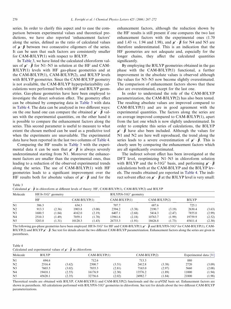
In Fig. 1, the structures of the five molecules studiedhere are shown. For brevity, we shall refer to these asN1, N2, N3, N4, and N5, with reference to the numberof double bonds in the polyene chain.

One important parameter in the resulting hyperpolariz-ability is the so-called bond length alternation (BLA) whichcan be defined as the di"erence between the average lengthsof single and double bonds in the chain. The BLA valuesfor N3, N4, and N5, calculated from the (–CH@CH–)n!1

part of the polyene chain, are reported in Table 1. It canbe noted that there exists a significant di"erence betweenthe obtained BLA values at the HF level in comparisonto the B3LYP analogues. Namely, the HF BLAs show asubstantially higher localization of the double bonds,whereas the B3LYP BLAs indicate that a higher degreeof conjugation is observed. Another significant di"erence

between HF and B3LYP, which will play an important rolein the future discussion of the hyperpolarizability results, isthe trend along the series: the HF BLAs increase along theN3–N5 series wheres the B3LYP BLAs is almost constantshowing a very limited decrease. For what concerns theCAM-B3LYP functional, geometry optimization is notyet available. It is worth noticing that whereas HF isknown to yield too localized geometries (higher BLAs),B3LYP displays the opposite behavior, overestimatingthe delocalization [32] (smaller BLAs). It is reasonable toexpect that CAM-B3LYP would yield somewhat interme-diate geometries. For a discussion about this aspect in con-nection to solvation e"ects see, e.g. Ref [32] and referencestherein.

Concerning the solvent e"ect, which has been investi-gated at the B3LYP level we have observed a decrease ofaround 0.014 A in the BLA for all molecules with respectto the gas-phase values, showing a further delocalizationdue to solvation, as would be expected. Moreover, in solu-tion the trend along the series is opposite to that observedin the gas phase. The full set of HF optimizations in solventhas not been carried out, but a test calculation on N4shows a similar qualitative solvation behavior as forB3LYP with a decrease of the BLA of 0.008 A.

In Table 2, we have listed the calculated l Æ b gas-phasevalues of the five molecules. A significant amplification ofthe SHG signal along the series is observed. Moreover,the total increase in l Æ b from N1 to N5 is 47 times forthe B3LYP functional and 34 times for the CAM-B3LYP(1) functional, in agreement with the limitationsof B3LYP in reproducing polarizabilities of extended con-jugated molecules, especially CT systems, because of itsincorrect long-range behavior [33,34]. As expected, the dif-ference between the functionals is negligible for the smallestsystem N1 but significant for N5, where we observe a 30%lowering of the SHG signal from B3LYP to CAM-B3LYP(1). This behavior is consistent throughout the

CH3

H3C CN

CN

N

n 1

Fig. 1. Molecular structure of the push–pull phenylpolyenes investigatedin the present work (n = 1,5).

Table 1BLA values calculated at the HF/6-31G* level in gas-phase and at theB3LYP/6-31G* level in gas-phase and in chloroform solution

Molecule HF gas-phase B3LYP gas-phase B3LYP chloroform

N3 0.1042 0.0554 0.0407N4 0.1083 0.0547 0.0409N5 0.1112 0.0541 0.0413

Table 2Gas-phase values of l Æ b phase calculated at B3LYP/cc-pVDZ and CAM-B3LYP(1)/cc-pVDZ levels

Molecule B3LYP CAM-B3LYP(1)

N1 249.2 248.9N2 876.8 (3.52) 826.0 (3.32)N3 2425.5 (2.77) 2114.6 (2.56)N4 5633.5 (2.34) 4475.4 (2.12)N5 11842.3 (2.10) 8412.3 (1.88)

Geometries optimized in the gas phase at the B3LYP/6-31G* level.Enhancement factors (l Æ b)n/(l Æ b)n!1 are given in parentheses.

L. Ferrighi et al. / Chemical Physics Letters 425 (2006) 267–272 269

series. In order to clarify this aspect and to ease the com-parison between experimental values and theoretical pre-dictions, we have also reported ‘enhancement factors’along the series, defined as the ratio of calculated valuesof l Æ b between two consecutive oligomers of the series.It can be seen that such factors are consistently smallerfor CAM-B3LYP(1) with respect to B3LYP.

In Table 3, we have listed the calculated chloroform val-ues of l& ' eb for N1–N5 in solution at the HF and CAM-B3LYP(1) levels with HF gas-phase geometries and atthe CAM-B3LYP(1), CAM-B3LYP(2), and B3LYP levelswith B3LYP geometries. Since the CAM-B3LYP geometryis not available, the CAM-B3LYP hyperpolarizability cal-culations were performed both with HF and B3LYP geom-etries. Gas-phase geometries have here been employed toinvestigate the direct solvation e"ect. The geometry e"ectcan be obtained by comparing data in Table 3 with datain Table 4. The data can be analyzed in two di"erent ways:on the one hand one can compare the obtained l& ' eb val-ues with the experimental quantities, on the other hand itis possible to compare the enhancement factors along theseries. This second parameter is useful to measure to whatextent the chosen method can be used as a predictive toolwhen the experiments are unavailable. The experimentaldata have been reported in the last two columns of Table 4.

Comparing the HF results in Table 3 with the experi-mental data it can be seen that l& ' eb is always severelyunderestimated starting from N1. Moreover the enhance-ment factors are smaller than the experimental ones, thusleading to a reduction of the observed experimental trendsalong the series. The use of CAM-B3LYP(1) with HFgeometries leads to a significant improvement over theHF results both for absolute values of l& ' eb and for the

enhancement factors, although the reduction shown bythe HF results is still present if one compares the two lastenhancement factors with the experimental ones (1.70and 1.43 vs. 1.94 and 1.98), and l& ' eb for N4 and N5 aretherefore underestimated. This is an indication that theHF geometries are not adequate and, especially for thelonger chains, they a"ect the calculated quantitiessignificantly.

By employing the B3LYP geometries obtained in the gasphase with the CAM-B3LYP(1) functional, a furtherimprovement in the absolute values is observed althoughthe values for N3–N5 now become slightly overestimated.The comparison of enhancement factors shows that thesealso are overestimated, except for the last one.

In order to understand the role of the CAM-B3LYPparametrization, the CAM-B3LYP(2) has also been tested.The resulting absolute values are improved compared toCAM-B3LYP(1) and are in good agreement with theexperimental quantities. The factors along the series areon average improved compared to CAM-B3LYP(1), apartfrom the last one which is now slightly underestimated. Inorder to complete this series of calculations, the B3LYPl& ' eb have also been included. Although the values forN1 and N2 are here well reproduced, the trend along theseries leads to a severe overestimation of l& ' eb. This isclearly seen by comparing the enhancement factors whichare all significantly overestimated.

The indirect solvent e"ect has been investigated at theDFT level, reoptimizing N1–N5 in chloroform solutionwith B3LYP and the 6-31G* basis, and performing l& ' ebcalculations both at the CAM-B3LYP and the B3LYP lev-els. The results obtained are reported in Table 4. The indi-rect solvent e"ect on l& ' eb at the B3LYP level is very small:

Table 3Calculated l& ' eb in chloroform at di"erent levels of theory: HF, CAM-B3LYP(1), CAM-B3LYP(2) and B3LYP

Molecule HF/6-31G* geometry B3LYP/6-31G* geometry

HF CAM-B3LYP(1) CAM-B3LYP(1) CAM-B3LYP(2) B3LYP

N1 386.3 634.3 707.7 687.6 725.1N2 913.3 (2.36) 1903.8 (3.00) 2394.2 (3.38) 2190.7 (3.19) 2630.4 (3.63)N3 1680.5 (1.84) 4162.0 (2.19) 6407.1 (2.68) 5414.3 (2.47) 7855.0 (2.99)N4 2510.3 (1.49) 7059.1 (1.70) 13961.6 (2.18) 10763.7 (1.99) 19759.9 (2.52)N5 3283.8 (1.31) 10120.3 (1.43) 26733.3 (1.91) 18626.8 (1.73) 45411.4 (2.30)

The following gas-phase geometries have been employed: HF/6-31G* for HF and CAM-B3LYP(1) l& ' eb and B3LYP/6-31G* for CAM-B3LYP(1), CAM-B3LYP(2) and B3LYP l& ' eb. See text for details about the two di"erent CAM-B3LYP parametrization. Enhancement factors along the series are given inparentheses.

Table 4Calculated and experimental values of l& ' eb in chloroform

Molecule B3LYP CAM-B3LYP(1) CAM-B3LYP(2) Experimental data [31]

N1 694.6 712.6 713.3 880N2 2516.4 (3.62) 2500.7 (3.51) 2412.8 (3.38) 2720 (3.09)N3 7603.5 (3.02) 7035.3 (2.81) 7165.0 (2.97) 5660 (2.08)N4 19418.1 (2.55) 16176.9 (2.30) 13576.2 (1.89) 11000 (1.94)N5 45620.1 (2.35) 32756.6 (2.02) 24982.7 (1.84) 21800 (1.98)

Theoretical results are obtained with B3LYP, CAM-B3LYP(1) and CAM-B3LYP(2) functionals and the cc-pVDZ basis set. Enhancement factors areshown in parenthesis. All calculations performed with B3LYP/6-31G* geometries in chloroform. See text for details about the two di"erent CAM-B3LYPparameterizations.

270 L. Ferrighi et al. / Chemical Physics Letters 425 (2006) 267–272

the absolute values are only slightly modified and theenhancement factors are overestimated even further.CAM-B3LYP(1) results are improved over B3LYP resultsalong the whole series, although the indirect solvent e"ecthere leads to a worse agreement with experiment: fromN3 to N5 we observe an overestimation of the experimentalresults and moreover all enhancement factors are worsethan their counterparts obtained using the gas-phase geom-etries. By changing the parametrization of CAM-B3LYPfrom (1) to (2) a better agreement with experiment is againobserved, confirming the better behavior of CAM-B3LYP(2). It must be noted that also in this case theindirect solvent e"ect leads to an overestimation of theproperty for N3–N5.

From the comparison of the calculated data in Tables 3and 4 we can conclude that the DFT results in general aresuperior to HF values as expected, both for the l& ' eb val-ues and the trends along the series. Moreover, B3LYPgeometries are better than HF: this can for instance be seenby comparing the CAM-B3LYP(1) results obtained withthe HF and B3LYP gas-phase geometries where a signifi-cant improvement on the calculated absolute values andenhancement factors is clearly observed. Another impor-tant aspect is shown by the comparison of the two CAM-B3LYP parameterizations: namely, parametrization (2)performs better than parametrization (1) both with gas-phase geometries and with chloroform solution geometries.

The indirect solvent e"ect must be analyzed with specialcare. The pure B3LYP l& ' eb show almost no secondarysolvation e"ect: this surprising behavior can be rationalizedby examining l* and eb separately. The dipole momentincreases of about 4% from N1 to N5 upon geometry relax-ation whereas the hyperpolarizability partly cancels thechanges arising from l*. The CAM-B3LYP functionalsgive an increase of both l* and eb upon geometry relaxationalong the series which is in better agreement with theexpected variation of the hyperpolarizabilities due to thereduction of BLA upon solvation.

One important point connected to the indirect solvente"ect concerns the apparent deterioration of the calculatedl& ' eb at the CAM-B3LYP level upon geometry relaxation.For both parameterizations, slightly worse results than withgas-phase geometries are observed. We propose the follow-ing rationalization of the observed behavior: the solvente"ect leads to a reduction of the BLA, but the starting gas-phase B3LYP geometries are already underestimating thecorrect values, and therefore the calculated l& ' eb at theCAM-B3LYP level with B3LYP gas-phase geometries ben-efit from a fortuitous cancellation of errors, thus leading tobetter values with respect to solvent-optimized geometries.

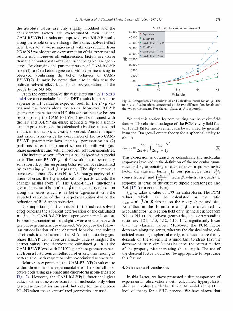
Relative to experiment, the CAM-B3LYP(2) values arewithin three times the experimental error bars for all mol-ecules both using gas-phase and chloroform geometries (seeFig. 2). However, the CAM-B3LYP(1) functional givesvalues within three error bars for all molecules only whengas-phase geometries are used, but only for the moleculeN1–N3 when the solvent-relaxed geometries are used.

We end this section by commenting on the cavity-fieldfactors. The classical analogue of the PCM cavity field fac-tor for EFISHG measurement can be obtained by general-izing the Onsager–Lorentz theory for a spherical cavity toobtain

lons–lor $3!0

2!0 % 1

3!opt2!opt % 1

! "2

"8#

This expression is obtained by considering the molecularresponses involved in the definition of the molecular quan-tities and by associating to each of them a proper cavityfactor (in classical terms). In our particular case, 3!0

2!0%1

comes from l* and 3!opt2!opt%1

# $2

from eb, which is a quadratic

response in terms of the e"ective dipole operator (see alsoRef. [15] for a comparison).

lons–lor takes a value of 1.99 for chloroform. The PCMvalues, which can be calculated as the ratiolPCM $ l& ' eb=l ' b depend on the cavity shape and size.Note that in this formula l and b are calculated byaccounting for the reaction field only. In the sequence fromN1 to N5 at the solvent geometries, the correspondingratios are 1.21, 1.15, 1.12, 1.10, 1.09, significantly lowerthan the classical values. Moreover, the PCM factordecreases along the series, whereas the classical value, cal-culated assuming a spherical cavity, is constant since it onlydepends on the solvent. It is important to stress that thedecrease of the cavity factors balances the overestimationof the property with increasing chain length. The use ofthe classical factor would not be appropriate to reproducethis feature.

4. Summary and conclusions

In this Letter, we have presented a first comparison ofexperimental observations with calculated hyperpolariz-abilities in solvent with the IEF-PCM model at the DFTlevel of theory for a SHG process. We have shown that

Fig. 2. Comparison of experimental and calculated result for l& ' eb. Thefour sets of calculations correspond to the two di"erent functionals andthe two environments. For the gas-phase, l Æ b is reported.

L. Ferrighi et al. / Chemical Physics Letters 425 (2006) 267–272 271

the solvent e"ects are important and must be included toobtain a satisfactory agreement with experiments. Ourmodel takes into account direct solvation e"ects throughthe solvent reaction field, indirect solvation e"ects due togeometry relaxation, and cavity-field e"ects to reproducethe local variation of the fields experienced by the moleculebecause of the presence of the surrounding environment.The observed experimental trends have been satisfactorilyreproduced with the CAM-B3LYP functional, which per-forms significantly better than the B3LYP functional, espe-cially for the bigger oligomers. However, there are stillsome issues to be addressed: we refer in particular to therole of CAM-B3LYP optimized geometries which are notavailable at present and to the validity and reliability ofthe di"erent CAM-B3LYP parameterizations. For whatconcerns the former, based on the obtained results we haveinferred that B3LYP gas-phase geometries could be used asa good guess for CAM-B3LYP solvent-optimizedgeometries, hence explaining the better agreement withexperiment observed with CAM-B3LYP using B3LYPgas-phase geometries compared to the ones using B3LYPsolvent-geometries. For the latter, we stress that CAM-B3LYP functional has not been thoroughly tested yet,therefore an ‘optimal’ commonly accepted parametrizationis still under discussion requiring dedicated work which isbeyond the scope of this Letter.

Acknowledgments

This work has been supported by the Norwegian Re-search Council through a Strategic University Program inQuantum Chemistry (Grant No. 154011/420), a YFF grant(Grant No. 162746/V00), and a Ph.D. grant to L. Ferrighithrough the Nanomat program (Grant No. 158538/431). Agrant of computer time from the Norwegian Supercomput-ing Program is also acknowledged. This work is part of,and is supported by, the EU-STREP project ODEONfounded by the European Community’s Sixth FrameworkProgramme. Support from NorFa (Grant No. 030262) isalso gratefully acknowledged.

References

[1] R. Wortmann, D.M. Bishop, J. Chem. Phys. 108 (1998) 1001.[2] R. Cammi, B. Mennucci, J. Tomasi, J. Phys. Chem. A 104 (2000)

4690.

[3] D.R. Kanis, M.A. Ratner, T.J. Marks, Chem. Rev. 94 (1994) 195.[4] J. Tomasi, M. Persico, Chem. Rev. 94 (1994) 2027.[5] S. Miertus, E. Scrocco, J. Tomasi, Chem. Phys. 55 (1981) 117.[6] E. Cances, B. Mennucci, J. Chem. Phys. 109 (1998) 249.[7] L. Onsager, J. Am. Chem. Soc. 58 (1936) 1486.[8] C.J.F. Bottcher, P. Bordewijk, Dielectric in time–dependent

fieldsTheory of Electric Polarization, vol. II, Elsevier, Amsterdam,1978.

[9] R. Cammi, B. Mennucci, J. Tomasi, J. Phys. Chem. A 102 (1998) 870.[10] R. Cammi, C. Cappelli, S. Corni, J. Tomasi, J. Phys. Chem. A 104

(2000) 9874.[11] S. Corni, C. Cappelli, R. Cammi, J. Tomasi, J. Phys. Chem. A 105

(2001) 8310.[12] C. Cappelli, S. Corni, B. Mennucci, R. Cammi, J. Tomasi, J. Phys.

Chem. A 106 (2002) 12331.[13] C. Cappelli, B. Mennucci, J. Tomasi, R. Cammi, A. Rizzo, G.

Rikken, R. Mathevet, C. Rizzo, J. Chem. Phys. 118 (2003) 10712.[14] C. Cappelli, S. Corni, B. Mennucci, R. Cammi, J. Tomasi, Int. J.

Quantum Chem. 104 (2005) 716.[15] C. Cappelli, B. Mennucci, R. Cammi, A. Rizzo, J. Phys. Chem. B 109

(2005) 18706.[16] M. Pecul, E. Lamparska, C. Cappelli, L. Frediani, K. Ruud, J. Phys.

Chem. B 110 (2006) 2807.[17] H. Kim, J.T. Hynes, J. Chem. Phys. 93 (1990) 5194.[18] R. Cammi, J. Tomasi, Int. J. Quantum Chem. 29 (1995) 465.[19] J. Tomasi, B. Mennucci, R. Cammi, Chem. Rev. 105 (2005) 2999.[20] K.V. Mikkelsen, K.O. Sylvester-Hvid, J. Phys. Chem. 100 (1996)

9116.[21] A.D. Becke, J. Chem. Phys. 98 (1993) 5648.[22] P.J. Stephens, F.J. Devlin, C.F. Chabalowski, M.J. Frisch, J. Phys.

Chem. 98 (1994) 11623.[23] T. Yanai, D. Tew, N.C. Handy, Chem. Phys. Lett. 393 (2004) 51.[24] M.J.G. Peach, T. Helgaker, P. Sa!ek, T.W. Keal, O.B. Lutnæs, D.J.

Tozer, N.C. Handy, Phys. Chem. Chem. Phys. 8 (2006) 558.[25] A. Dreuw, J.L. Weisman, M. Head-Gordon, J. Chem. Phys. 119

(2003) 2943.[26] J. Olsen, P. Jørgensen, in: D.R. Yarkony (Ed.), Modern Electronic

Structure Theory, Part II, p. 857, World Scientific, Singapore, 1995.[27] D.E. Woon, T.H. Dunning jr., J. Chem. Phys. 100 (1994) 2975.[28] L. Frediani, H. Agren, L. Ferrighi, K. Ruud, J. Chem. Phys. 123

(2005) 144117.[29] E. Cances, B. Mennucci, J. Math. Chem. 23 (1998) 309.[30] dalton, a molecular electronic structure program, Release 2.0, 2005.

Available from: <http://www.kjemi.uio.no/software/dalton/dalton.html>.

[31] V. Alain, L. Thouin, M. Blanchard-Desce, U. Gubler, C. Bosshard, P.Gunter, J. Muller, A. Fort, M. Barzoukas, Adv. Mater. 11 (1999)1210.

[32] S. Corni, C. Cappelli, M.D. Zoppo, J. Tomasi, J. Phys. Chem. A 107(2003) 10261.

[33] B. Champagne, E.A. Perpete, D. Jacquemin, S.J.A. van Gisbergen,E.J. Baerends, C. Soubra-Ghaoui, K.A. Robins, B. Kirtman, J. Phys.Chem. A 104 (2000) 4755.

[34] D.P. Tew, T. Yanai, N.C. Handy, Chem. Phys. Lett. 393 (2004) 51.

272 L. Ferrighi et al. / Chemical Physics Letters 425 (2006) 267–272