a comparative study of pull and push production methods for supply chain resilience

International Journal of Operations and Logistics Management www.absronline.org/journals p-ISSN: 2310-4945; e-ISSN: 2309-8023 Volume: 3, Issue: 1, Pages: 1-15 (March 2014) © Academy of Business & Scientific Research

*Corresponding author: Chih-Hung Tsai, PhD, Department of Information Management, Yuanpei University, No. 306, Yuanpei Street, Hsin-Chu, Taiwan.

E-Mail: [email protected], [email protected]

1

A Comparative Study of Pull and Push Production Methods for Supply Chain Resilience

Chia-Ling Huang1, Rong-Kwei Li2, Chih-Hung Tsai3*, Yi-Chan Chung4, and Chun-Hsien Shih2

1. Department of Logistics and Shipping Management Kainan University, Taoyuan, Taiwan 2. Department of Industrial Engineering and Management, National Chiao-Tung University, Hsin-Chu,

Taiwan 3. Department of Information Management, Yuanpei University, Hsin-Chu, Taiwan 4. Department and Graduate Institute of Business Administration, Yuanpei University, Hsin-Chu, Taiwan

The earthquake of March 11, 2011, seriously affected the production of electronic parts in Japan. This disruptive event highlights the challenge that businesses face in how to manage and mitigate this type of risk. Resilient supply chains and emerging disciplines of supply chain management (SCM) that incorporate event readiness can provide an efficient response, and often are capable of recovering to their original state after the disruptive event. There are generally two methods of managing a supply chain in current supply chain management practice: a pull system or a push system. Based on the characteristics of resilient supply chains and general prescriptions of pull supply chain system, the pull supply chain system can provide better resilience than the push supply chain system. This study designs an experiment to evaluate the ability of both management methods to provide resilience ability. Experiments results reveal that two main findings: (1) during the disruption period, if the initial system inventory of both systems is enough to cover the demand during the disruption period, the actual damage is far less than expected for the period. If most of the inventory can be cleared while maintaining sales, financial performance will be better than normal; (2) the pull system outperforms the push system for its ability to restore the system to stable operation after the disruption. This is because the pull system uses the precious capacity to produce only those goods with insufficient or no inventory. Thus, the pull system can efficiently use limited capacity after the disruption. If goods that are not needed now are produced, they will turn into inventory that will eat up the limited capacity of production and eventually prevent manufacturers from producing what is truly needed now.

Keywords: Supply Chain Management, Resilient Supply Chain Management, Pull and

Push

Pull and Push Production Methods for Supply Chain Resilience Huang et al.

2

INTRODUCTION

The earthquake of March 11, 2011, seriously affected the production of electronic parts in Japan. The electronic components manufacturers in Japan worked hard to recover their capabilities, and resumed operation within mere weeks of the earthquake. The resulting component shortage was so serious that some analysts say it may affect the global economic. This disruptive event highlights the challenges that businesses face in how to build supply chains that are resilient enough to withstand unexpected disruptions and help the organization to excel. Resilience is a concept borrowed from the materials sciences, and represents the ability of a material to recover its original shape following a deformation. For companies, resilience measures their ability to return to a normal performance level (production, services, fill rate, etc.) following a disruption (Sheffi, 2006). In supply chains, resilience represents the adaptive capacity of the supply chain to prepare for unexpected events, respond to disruptions, and recover from events by maintaining continuity of operations at the desired level of connectedness and control over structure and function (Ponomarov and Holcomb, 2009; Makharia et al., 2012).

According to Sheffi (2006), resilience can be achieved either through redundancy or through building flexibility into supply chains. The standard use of redundancy includes either underutilized production capacity or a safety stock of material and finished goods. This excess inventory can give a company time to plan its recovery following a disruption. Indeed, many companies increase their inventories when preparing for a disruption. Redundancy, however, is expensive, and particularly when preparing for large, infrequent disruptions. In contrast, increasing supply chain flexibility can help a company not only withstand disruptions, but also better respond to the day-to-day vagaries of the market place. To build in flexibility for resilience, companies must involve many facets of the supply chain design. They must (1) develop the ability to use interchangeable and generic parts in many products, (2) design products and processes for maximum postponement of as many operations

and decisions as possible in the supply chain, and (3) align their procurement strategy with their supplier relationships.

Christopher and Peck (2004) proposed that a resilient supply chain should consist of four principles that underpin resilience. First, the resilience should be designed. This means that there are certain features that, if engineered into a supply chain, can improve its resilience. The second principle is that because supply chains generally extend across different corporate links, there will need to be a high level of collaboration if risk is to be identified and managed. Third, resilience implies agility. Being able to react quickly to unpredictable events is a distinct advantage in an uncertain environment. Finally, the creation of a risk management culture in the organization will enhance, and is required to achieve, resilience in the supply chain. The message that needs to be understood and acted upon is that the biggest risk to the business continuity may well come from the wider supply chain rather than from within the business.

Ponomarov and Holcomb (2009) proposed that the dynamic integration of logistics capabilities enables supply chain resilience and leads to a sustainable competitive advantage. They also developed a conceptual framework of the relationship between logistics capabilities and supply chain resilience. Their framework results in six research propositions: (1) The better the dynamic integration of logistic capabilities, the greater the supply chain resilience; (2) The greater the resilience of the supply chain, the better it maintains control of logistics capabilities when disruptions occur; (3) The greater the resilience of the supply chain, the better it maintains coherence of logistics capabilities when disruptions occur; (4) The greater the resilience of the supply chain, the higher the levels of integration (connectedness) across logistics capabilities when dealing with disruptions; (5) The greater the level of risk sharing in a supply chain (based on continual risk analysis, assessment, and top management support) the stronger the relationship between logistics capabilities and supply chain resilience;

Int. j. oper. logist. manag. p-ISSN: 2310-4945; e-ISSN: 2309-8023 Volume: 3, Issue: 1, Pages: 1-15

3

(6) The greater the supply chain resilience, the better the sustainable competitive advantage.

SUPPLY CHAIN MANAGEMENT—PULL OR PUSH SYSTEM

Manufacturers, distributors, and retailers of supply chain participators must choose the approach they hope will make them the most profit. Is it producing and making goods available to forecast expected consumer demand, or by reacting to what consumers have already bought? Most companies use the former approach. In a “push system,” product availability is based on forecasts. Companies forecast to feel confident that the goods they buy, sometimes many months in advance, will both find willing buyers and not run out unexpectedly. In the push world, decision points occur at every reorder. How much should be purchased? How often is it necessary to consider buying each item? In their attempts to prevent stock-outs and protect sales, managers end up with fewer inventory turns than they wish. Pushing inventory downstream through the links of the supply chain is a response to the natural desire to reduce inventory over-investment and record sales today rather than tomorrow.

In contrast, a “pull system” controls the flow of products by automatically adjusting inventory levels based on actual consumption. Pull systems simply respond to what consumers buy. A pull system manages time buffers of inventory for each item. These buffers act as shock absorbers that are compressed as inventory is consumed until replenishment can occur. For each product consumed, an equivalent order is placed. This approach lends itself to automatic electronic processing. Replenishments are frequent, and made in the smallest economical batches. Decision points in pull systems are triggered only occasionally to resize buffers when on-hand inventory levels consistently correspond to too little or too much protection time. Many successful cases demonstrate that switching from a push to pull system reduces the inventory by half, leads to less shortage, and increases sales (Aben, 2006; Camp, 2006; Krishan and Kothekar, 2007; Ploss, 2008; Grant, 2008).

Push supply chain system

Supply chain problems such as high carrying costs, discounting, disposals, missed sales, weak customer loyalty, shortages, high debt loads, inventory disposals (or returns), emergency shipments, rescheduled production, and attenuated profits all stem from three common root causes (Camp, 2006): inaccurate forecasts, significant replenishment times, and variability in both demand and replenishment times. Perhaps the worst of the three causes of problems in push environments is that forecasts are almost always wrong. Despite billions spent annually in the US for the best computers and most sophisticated software, actual demand varies from forecasts. Forecasting does not make the end consumer react more rationally or predictably (Kendall, 2005). No matter how sophisticated its algorithm, a forecast is only a guess. Wrong guesses mean excess inventory and lower profits because of missed sales.

The bullwhip effect in supply chain (Lee et al., 1997a/1997b; Chin et al., 2012) is a phenomenon of forecast-driven push systems. It refers to the trend of larger and larger swings in inventory in response to changes in demand, as one looks at firm further back in the supply chain for a product. The problem with the bullwhip effect is that even if we have inventory and excess capacity, it can lead to either insufficient stock during the disruption period or insufficient production after the disruption. Despite safety stocks and excess capacity, there is still the hazard of stock-outs and a delay in returning to its original state, which results in poor customer service. Another bullwhip effect is that during the recovery time, when the orders are inflated to reflect the need to increase inventories, the demand is higher than the capacity available, creating manufacturer’s bottleneck. When a manufacturer has a bottleneck, any upward fluctuation in demand translates into a longer lead time to satisfy client orders. Any increase in supply lead time causes the client to realize that it should further increase its inventories. This phenomena often leads to inflated internal demand (orders from assembly to components) when the external demand (purchases by consumers) is relatively stable.


4

The major problem of a push system is that the demand is not real. It is not a demand driven by the consumer purchases, because consumer purchases have remained relatively stable during the disruption and recover periods. Instead, it is a demand driven by internal adjustments in the supply chain. Once again, companies that are participating in the supply chain ignore the most fundamental rule: As long as the end consumer hasn’t bought a product, no one in the supply chain has really sold a product. If not stopped right away, this mistake will have much graver and longer lasting ramifications.

Pull supply chain system

The bullwhip effect (Lee et al., 1997a/1997b) will theoretically not occur if all orders exactly meet the demand of each period. This is consistent with the findings of supply chain experts who have recognized that the bullwhip effect is a problem in forecast-driven push supply chains. Careful management of the bullwhip effect is an important goal for supply chain managers. Therefore, it is necessary to extend the visibility of customer demand as far as possible. One way to achieve this is to establish a market demand-pull supply chain that reacts to actual customer orders. Applying pull to a supply chain is analogous to (but more straightforward than) adapting the Toyota Production System (TPS) to manufacturing (Goldratt, 2008a). Even though it seems counterintuitive to behave reactively than proactively by choice, this may be a viable approach for supply chains. The general prescriptions of pull supply chain include the following points (Camp, 2006):

1. Push inventory as far as possible back upstream in the supply chain toward the production operation. This puts the largest amount of inventory where the forecast error is least and helps minimize excess inventory.

2. Size inventory buffers based on variation and forecasting error. If a distribution center can expect replenishment at regular, shorter intervals, its inventory buffer need not be larger than required to cover exceptionally high demand during the short period between replenishments.

3. Use actual demand data to drive both replenishment and production. Only draw immediate customer requirements from the protective inventories upstream.

4. Focus each link in a pull supply chain on improving speed of replenishment and ordering smaller batches more frequently. The majority of supply chain replenishment time is typically consumed in waiting. Shipping smaller batches more frequently shortens replenishment time.

5. Activate the information system capability of each upstream link in the supply chain so actual demand is visible as it occurs—in real time or near real time—at each downstream link. With effective information technology in place, actual consumption at each retail outlet is visible daily to the upstream distribution center. The aggregate consumption of the distribution center is visible daily to the manufacturing facility. As a result, the manufacturing facility can schedule production in near real time, especially if it, too, is operating on a just-in-time basis. Real time demand then pulls inventory through the system, preventing undue accumulation anywhere along the supply chain. The result is that each link in the chain is essentially filling holes in inventory buffers caused by actual consumption.

6. Realign performance metrics throughout the supply chain to reinforce “just-in-time” behavior. Metrics that emphasize minimizing the time value of inventory must replace measures that reinforce “efficiency” behavior. Inventory value alone is an insufficient indicator of system efficiency. A more effective indicator is inventory value combined with the length of time it stays in the system. Ultimately, cash flow and throughput, instead of costs, should dictate inventory transfer and storage decisions.

7. Build a protective capacity and institute mechanisms to guard protective capacity while fully supporting sales growth. This is because there is no flexibility in time of delivery (delivery is immediate upon demand) and the quantities required may increase without warning.

Acting on actual demand dampens rather than magnifies statistical variations, steadying on-hand inventory levels at every stocking location. There


5

is a very nice consequence of less fluctuation in the level of inventory on-hand. The lower limits of the on-hand fluctuations are similar to those in a push system, fixed by the need to hold prudent safety stock. However, there is less variation on the high side in pull systems, resulting in significantly lower average inventory. There is another effect on the supply chain as a whole. Because goods only flow downstream to cover immediate need, the bulk of the inventory remains further up the supply chain. The demand variations of a store are greater than that of a region because the region’s sales are the aggregated sales of all it stores. The same is true at a central production location compared to the regions it serves. The greater the aggregation, the more statistical highs and lows offset each other. As a result, variability is proportionally lower where demand is aggregated, and safety stocks are sized to protect against variability. Thus, safety stocks are proportionally less when they are closer to the source, where pull supply chain hold most of their inventory.

How can market demand-pull provide supply chain resilience? When a disruption occurs at the manufacturers of a consumer goods supply chain, a check of the finished goods at the manufacturer’s central warehouse, regional warehouses (or wholesalers), and retailers will reveal that the whole supply chain carries a few months of inventory. For example, if the supply chain carries two months of inventory, it would theoretically have no trouble providing products to retailers for (an average of) two months. Therefore, it is likely that there are enough inventories to supply end users during disruption periods. In this case, the actual damage may be far less than expected for the period covered by the inventory. If most of the inventory can be cleared while maintaining sales, corporate financial performance can be far better than normal.

During the disruption period (for example, a month), the regional warehouse, and not just the retailers, reduces inventory as well. When the disruption is over and companies (retailers and regional warehouse) have adjusted to the new reality, they naturally want to gradually restore their inventories to the proper level. Their orders reflect not just their current consumption, but also

the quantities needed to return to normal inventory levels. Increasing back inventories is governed by the amount of excess capacity the vendor has. Because of the policy of protective capacity (average 20%) in market demand-pull supply chain, manufacturers often have excess capacity (Schragenheim, 2009). With this amount of excess capacity, the time it takes to refill inventory back to its original level depends on the disruption period and excess capacity. For example, if the disruption time is one month and the excess capacity is 20%, it will take 5 months to refill the inventory consumed during the disruption period. This means the supply chain will need five months to return to its original state.

Of course, there are fast movers with little inventory and slow movers with excess inventory. Since a product is sold in different retailers, manufacturers can check inventory and sales trends in the market for each stock keeping unit (SKU) and then use the precious capacity (after the disruption is recovered) only for the goods with insufficient or no inventory. While making sure to supply fast movers to the market to avoid shortage, if slow movers are not produced, the amount of slow movers will gradually decrease according to the rate of consumption. Wholesalers and retailers should also inform their manufacturers what they really need now. This allows manufacturers to effectively use their limited capacity. If goods that are not needed now are produced, they will turn into inventory that will eat up the limited capacity of manufacturers and eventually prevent them from producing what is truly needed now. Manufacturers, wholesalers, and retailers must take a mutually holistic approach across the board, using limited inventory and capacity to provide the goods that are needed now in the market. Efforts invested in buying items that are unnecessary right now will likely be considered a waste in the future. In other words, goods that are needed now can be produced by not producing goods that are not needed now. Goods should simply be produced according to the pace of consumption in the market—a market demand-pull supply chain system. Thus, a market demand-pull supply chain operation mode meets the principles of resilient supply chain proposed by


6

Christopher and Peck (2004) and Ponomarov and Holcomb (2009).

RESEARCH’S ASSUMPTION AND OBJECTIVE

Based on the characteristics of resilient supply chains and general prescriptions of pull supply chain, we assume that the market demand-pull supply chain advocated by Goldratt (2004, 2006, 2008a, 2008b, 2009a), Schragenheim (2006, 2007, 2009), Ptak and Smith (2008), and successfully implemented in Wal-Mart's distribution system and other companies (Aben, 2006; Camp, 2006; Krishan and Kothekar, 2007; Ploss, 2008; Grant, 2008) can provide better resilience than push system for supply chains. To validate this assumption, this study uses a supply chain simulation developed by Goldratt (2006) to simulate a disruptive event and compare the ability of pull and push systems to provide an efficient response during disruptive periods and their ability to recover to their original state after being disrupted.

SUPPLY CHAIN SIMULATION SYSTEM

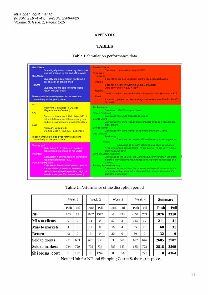
The supply chain simulations in this study deal with situations typical of a network of regional warehouse and retail clients that in turn sells it to the final consumers. Figure 1 illustrates the simulation environment. In this simulation, a company (with one production line) supplies 6 products to 5 regional warehouses. In turn, each regional warehouse serves 4 retail clients. Each week, retail clients place orders with the regional warehouses, and expect delivery within one week. Clients consume an average of 6 units per product per week. Peak consumption can be as high as 6.5 times weekly demand (39 units per product). Regional warehouses consume an average of 24 units per product per week. Peak consumption can be as high as 2.5 times weekly demand (60 units per product). Based on the above, the company’s production requirement is an average of 120 units per product per week.

FIGURE 1 HERE

The company production line can produce 6 units of a product per hour. The set-up time to change from one product to another is 24 hours. The

production line runs 24 hours per day, 7 days per week, and there are no breakdowns, strikes, material shortages, etc. There are daily transfers from the production factory to the regional warehouses in truckload quantities of 6 units/truck, and can be any mix of products. Transportation from the production factory to the regional warehouses costs $5 per truck per day on the road. Transfers happen automatically according to the following rules: (1) If the factory has enough inventories, all regional warehouse orders are shipped; (2) If the factory does not have enough inventory, then each regional warehouse gets ½ of what it ordered prioritized by distance from the factory; (3) If there is remaining company inventory, it is divided between regional warehouses in units of 6 until the inventory is gone. The regional warehouses with the largest difference between existing inventory (plus inventory in transit) and maximum inventory receives the shipment.

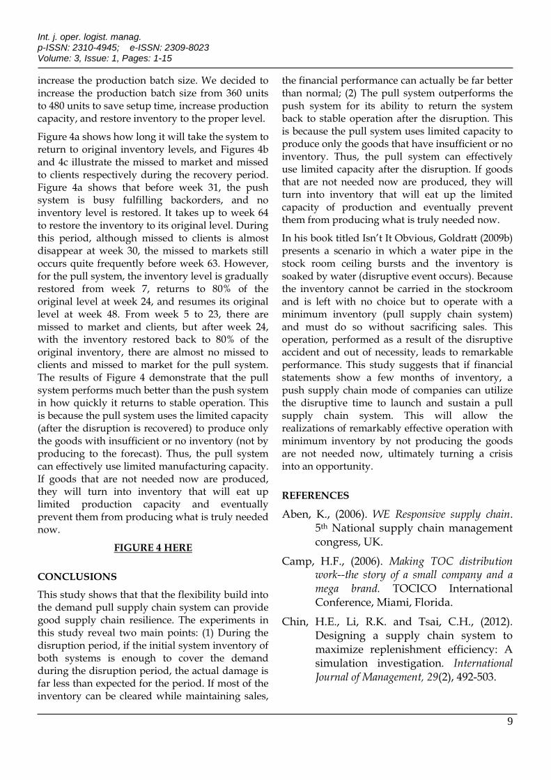
The product selling price is $35 per unit, and the raw material cost is $20 per unit. Therefore, throughput is $15 per unit ($35 - $20). Fixed expenses are $8,000 per week, and interest is approximately $600 per week. Using an average demand/product of 120 units per week and factory capacity, it is possible to calculate an ideal production cycle time and determine the recommended batch sizes. Total production hours required 120 hours for 1 week’s average sales ((120 units × 6 products)/ 6 units per hour) and total hours available per week is 168 hours (24 hours × 7 days). Therefore, the excess available for setups is 48 hours (168 hours - 120 hours), allow 2 setups per week (48 hours/24 hours per setup). Therefore, we can produce 2 products per week. This means there is a 3-week production cycle for the 6 products. It also means that we need to run, on average, three week’s sales (360 units) per production run, as these units will be sold during the next production cycle. At the end of each week, the system generates all the performance data shown in Table 1.

TABLE 1 HERE

Push simulation system This study models the push simulation system with no central warehouse, so consequently, the


7

company depends on 5 regional warehouses to store and distribute the bulk of its products. Regional warehouses are designed to hold a maximum of 10 weeks (240 units) and a minimum of 4 weeks (96 units) of average demand per product. The company has 2~3 days staging and shipping inventory. Clients are designed to hold inventory a maximum of 10 weeks (60 units) and a minimum of 4 weeks (24 units) of average demand per product. The weekly orders for each client are based on the new average computed by the simulation and adjusted by real-to-whole number. However, some extreme cases are checked: (1) if the inventory level is more than 1.7 of the max, the order value will be 0; (2) If the inventory level is more than 1.3 of the max, the order value will be 75% of the computed average; (3) If the inventory level plus the open orders is less than the minimum, a special order is immediately issued to cover the difference. Regional warehouses place demands on the production-plants. These demands are similar to orders, but do not have an order time. The weekly demand is based on the computed average. However, the inventory level compared to the max-min level may change it. If the inventory level is lower than 0.66 of the max, the weekly demand will be 1.3 of the average. If the inventory level is very high (more than 1.7 of the max level), the weekly demand will be zero. If the inventory level is between 1.2 and 1.7 of the max level, the weekly demand will be 0.75 of the average.

Pull simulation system

The difference between pull and push is that a pull system has a plant central warehouse and the plant central warehouse holds enough stock to cover demand during the time it takes to reliably replenish. How much inventory should the plant central warehouse hold? It depends on the replenishment time from the production line. The 3-week production cycle in this simulation means the average replenishment time is 3 weeks. Because this is an average, we should add a safety factor, say 50% of the average replenishment time. Thus, the replenishment is 4.5 weeks. The average demand of each week is 120 units per product, so the inventory level the plant central warehouse should hold 540 units per product. The plant only

produces products to replace products that have been shipped to the regional warehouses.

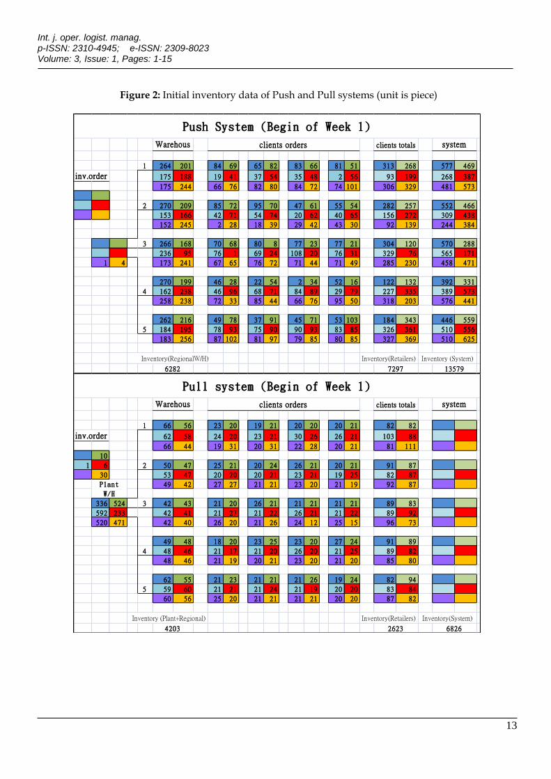
The replenishment time from the plant central warehouse to regional warehouses is shipping time only. The shipping time from the plant central warehouse to regional warehouses #1 and #5 is 7 days, to regional warehouses #2 and #4 is 6 days, and to regional warehouses #3 is 5 days. Because the average week demand is 24 units per product and the peak demand is 2.5 of the average demand which is 60 units per week. Therefore, the inventory is approximately 60 units per product for regional warehouses #1 and #5, approximately 48 units for regional warehouses #2 and #4, and approximately 42 units for regional warehouse #3. The regional warehouses order from the plant only to replace products that have been shipped to their clients. The replenishment time from the regional warehouse to client is shipping time only. The shipping time from the regional warehouse to clients is 3 days. Because the average week demand is 6 units per product and the peak demand is 6 times the average demand which is 36 units per week (6 units per day). Therefore, the inventory for clients is approximately 20 units. The clients order only to replenish what was sold. Figure 2 summarizes both systems’ initial data. Total inventory for push system is 13,579 units (7,292 units in 20 retailers and 6,282 units in 5 regional warehouses, with no inventory for plant warehouse) and total inventory for pull system is 6,826 units in 20 retailers and 4,203 units in plant and regional warehouses. The push system carries almost twice the inventory of the pull system.

FIGURE 2 HERE

Experimental Design

This study uses two experiments to collect data for further analysis. In these simulations, both systems’ production lines are shut down for 4 weeks (no production action, but demand from market still comes in). Comparing the results of each week reveals the effects of the disruption on both systems. Experiment two simulates the recovery period after disruption. When the disruption is over and companies (retailers and regional warehouse) adjust to the new reality, they naturally want to gradually return their


8

inventories to the proper level. Thus, their orders reflect not only their current consumption, but also the quantities needed to restore inventory. Increasing inventories is governed by the amount of excess capacity the vendor has. Since no capacity can be added for both systems, the only way to increase capacity is to save setup time, which means increasing production batch size. Since the production batch size is 360 units, we decided to increase the production batch size to 480 units to save setup time to increase production capacity to restore inventory to the proper level. Both systems run 30 runs to collect the data for further analysis and each run takes simulation time of 64 weeks.

RESULTS OF ANALYSIS

During the disruption period

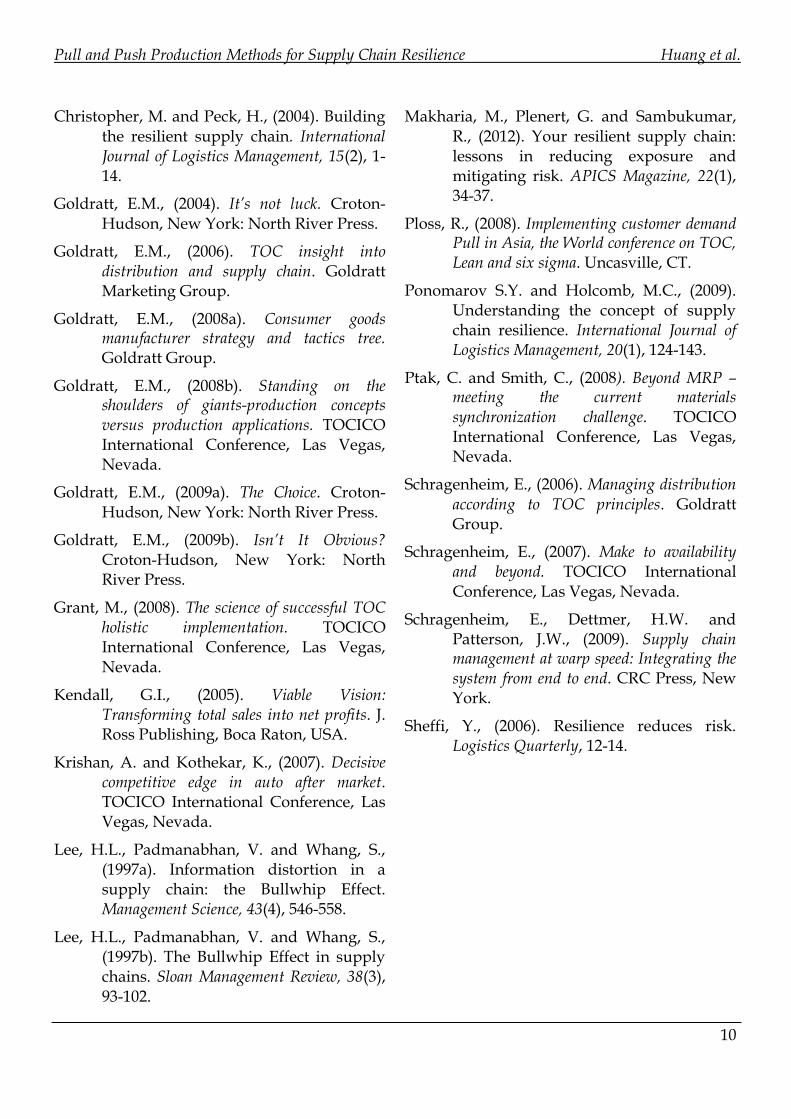
Table 2 shows the performance of the disruption period. Since the disruption period is 4 weeks, the average demand is 2,880 units. From the initial inventory of both systems shown in Figure 2, both systems have enough inventories to cover the demand during the disruption period. The results of the simulation confirm this (pull system sold out 2,869 units and push system 2,818 units), and the actual damage is far less than expected during the disruption period. Comparing the net profits, the missed to retail clients, missed to market, and returns for both systems, the push system has worse performance than the pull system. This is not because of the disruption, but because of the operational model of the pull system, which can provide much less inventory at the right time and right place to meet market demand.

TABLE 2 HERE

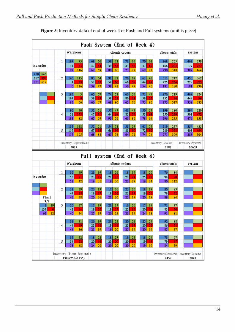
Figure 3 illustrates the inventory status of both systems at the end of week four. The total inventory both systems decreased because of no production during the disruption period. The total inventory of the 20 retailers at the end of week four reveals that their inventory levels are almost unchanged (compared to the initial inventory status). This is because they still get their order delivery from their regional warehouses. However, comparing the inventory status for each retailer shows that for the pull system, the

inventory status in the first week and at the end of week four is almost the same. For the push system, however, the inventory status for the first week and at the end of week four has changed a lot. This change causes the push system to achieve higher missed to market than the pull system. At the end of week four, the pull system shows that except for blue, red, and brown products (which have almost no inventory in the plant central warehouse), the inventory status for the other three products remains almost unchanged. This is because they still get enough replenishment from the plant central warehouse. Despite the shortage of blue, red, and brown proucts from the plant central warehouse, the total inventory level of regional warehouses decreases only 392 units (from 1,527 units to 1,135 units). However, for the push system, the total inventory level of the regional warehouse decreases 3,254 units (from 6,282 units to 3,028 units).

FIGURE 3 HERE

Table 3 shows that for the push system, the backorder for the production plant at the end of week four is 3,956 units, which is much higher than the actual units sold to the market (2,818 units). This is caused by the bullwhip effect. However, for the pull system, the backorder is 2,869 units which are the same as the number sold to the market.

TABLE 3 HERE

During the recovery period

The inventory status shows that both systems have enough inventories to cover sales during a four week disruption period. Therefore, the actual damage is far less than expected for the period. If most of the inventory can be cleared while maintaining sales, corporate financial performance can actually be far better than normal. The key factor is the speed of restoring the system to its original state. During the restore period, the production plant reflected not just their current consumption, but also the quantities needed to raise their inventory levels. Increasing inventory is governed by the amount of excess capacity the production line has. Since no capacity can be added for both systems, the only way to increase capacity is to save setup time, which means to


9

increase the production batch size. We decided to increase the production batch size from 360 units to 480 units to save setup time, increase production capacity, and restore inventory to the proper level.

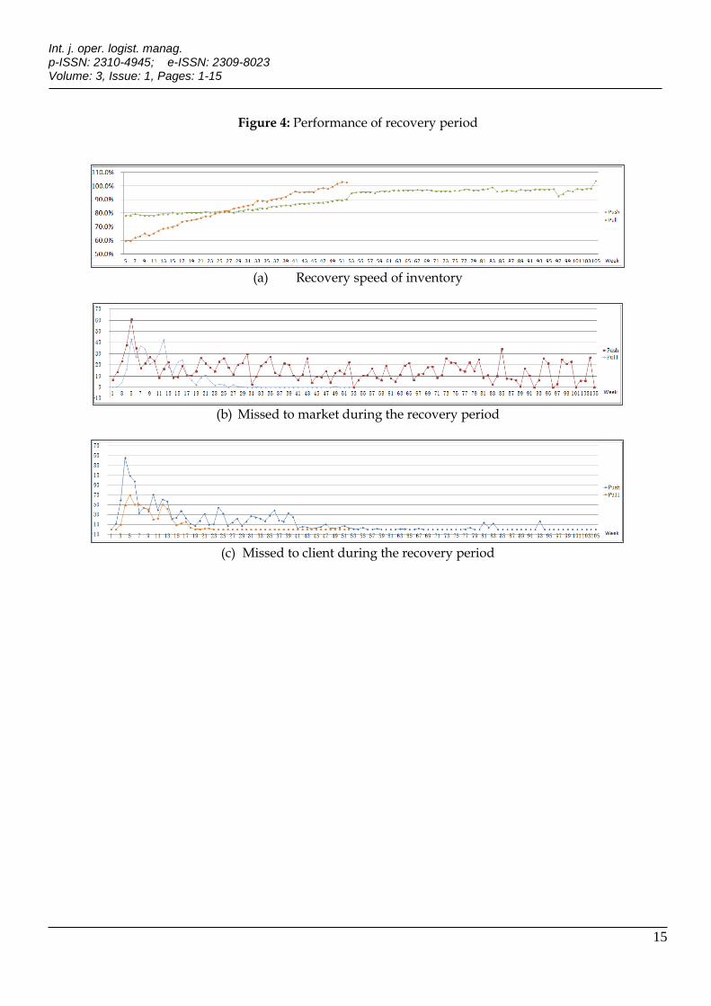
Figure 4a shows how long it will take the system to return to original inventory levels, and Figures 4b and 4c illustrate the missed to market and missed to clients respectively during the recovery period. Figure 4a shows that before week 31, the push system is busy fulfilling backorders, and no inventory level is restored. It takes up to week 64 to restore the inventory to its original level. During this period, although missed to clients is almost disappear at week 30, the missed to markets still occurs quite frequently before week 63. However, for the pull system, the inventory level is gradually restored from week 7, returns to 80% of the original level at week 24, and resumes its original level at week 48. From week 5 to 23, there are missed to market and clients, but after week 24, with the inventory restored back to 80% of the original inventory, there are almost no missed to clients and missed to market for the pull system. The results of Figure 4 demonstrate that the pull system performs much better than the push system in how quickly it returns to stable operation. This is because the pull system uses the limited capacity (after the disruption is recovered) to produce only the goods with insufficient or no inventory (not by producing to the forecast). Thus, the pull system can effectively use limited manufacturing capacity. If goods that are not needed now are produced, they will turn into inventory that will eat up limited production capacity and eventually prevent them from producing what is truly needed now.

FIGURE 4 HERE

CONCLUSIONS

This study shows that that the flexibility build into the demand pull supply chain system can provide good supply chain resilience. The experiments in this study reveal two main points: (1) During the disruption period, if the initial system inventory of both systems is enough to cover the demand during the disruption period, the actual damage is far less than expected for the period. If most of the inventory can be cleared while maintaining sales,

the financial performance can actually be far better than normal; (2) The pull system outperforms the push system for its ability to return the system back to stable operation after the disruption. This is because the pull system uses limited capacity to produce only the goods that have insufficient or no inventory. Thus, the pull system can effectively use limited capacity after the disruption. If goods that are not needed now are produced, they will turn into inventory that will eat up the limited capacity of production and eventually prevent them from producing what is truly needed now.

In his book titled Isn’t It Obvious, Goldratt (2009b) presents a scenario in which a water pipe in the stock room ceiling bursts and the inventory is soaked by water (disruptive event occurs). Because the inventory cannot be carried in the stockroom and is left with no choice but to operate with a minimum inventory (pull supply chain system) and must do so without sacrificing sales. This operation, performed as a result of the disruptive accident and out of necessity, leads to remarkable performance. This study suggests that if financial statements show a few months of inventory, a push supply chain mode of companies can utilize the disruptive time to launch and sustain a pull supply chain system. This will allow the realizations of remarkably effective operation with minimum inventory by not producing the goods are not needed now, ultimately turning a crisis into an opportunity.

REFERENCES

Aben, K., (2006). WE Responsive supply chain. 5th National supply chain management congress, UK.

Camp, H.F., (2006). Making TOC distribution work--the story of a small company and a mega brand. TOCICO International Conference, Miami, Florida.

Chin, H.E., Li, R.K. and Tsai, C.H., (2012). Designing a supply chain system to maximize replenishment efficiency: A simulation investigation. International Journal of Management, 29(2), 492-503.


10

Christopher, M. and Peck, H., (2004). Building the resilient supply chain. International Journal of Logistics Management, 15(2), 1-14.

Goldratt, E.M., (2004). It’s not luck. Croton-Hudson, New York: North River Press.

Goldratt, E.M., (2006). TOC insight into distribution and supply chain. Goldratt Marketing Group.

Goldratt, E.M., (2008a). Consumer goods manufacturer strategy and tactics tree. Goldratt Group.

Goldratt, E.M., (2008b). Standing on the shoulders of giants-production concepts versus production applications. TOCICO International Conference, Las Vegas, Nevada.

Goldratt, E.M., (2009a). The Choice. Croton-Hudson, New York: North River Press.

Goldratt, E.M., (2009b). Isn’t It Obvious? Croton-Hudson, New York: North River Press.

Grant, M., (2008). The science of successful TOC holistic implementation. TOCICO International Conference, Las Vegas, Nevada.

Kendall, G.I., (2005). Viable Vision: Transforming total sales into net profits. J. Ross Publishing, Boca Raton, USA.

Krishan, A. and Kothekar, K., (2007). Decisive competitive edge in auto after market. TOCICO International Conference, Las Vegas, Nevada.

Lee, H.L., Padmanabhan, V. and Whang, S., (1997a). Information distortion in a supply chain: the Bullwhip Effect. Management Science, 43(4), 546-558.

Lee, H.L., Padmanabhan, V. and Whang, S., (1997b). The Bullwhip Effect in supply chains. Sloan Management Review, 38(3), 93-102.

Makharia, M., Plenert, G. and Sambukumar, R., (2012). Your resilient supply chain: lessons in reducing exposure and mitigating risk. APICS Magazine, 22(1), 34-37.

Ploss, R., (2008). Implementing customer demand Pull in Asia, the World conference on TOC, Lean and six sigma. Uncasville, CT.

Ponomarov S.Y. and Holcomb, M.C., (2009). Understanding the concept of supply chain resilience. International Journal of Logistics Management, 20(1), 124-143.

Ptak, C. and Smith, C., (2008). Beyond MRP – meeting the current materials synchronization challenge. TOCICO International Conference, Las Vegas, Nevada.

Schragenheim, E., (2006). Managing distribution according to TOC principles. Goldratt Group.

Schragenheim, E., (2007). Make to availability and beyond. TOCICO International Conference, Las Vegas, Nevada.

Schragenheim, E., Dettmer, H.W. and Patterson, J.W., (2009). Supply chain management at warp speed: Integrating the system from end to end. CRC Press, New York.

Sheffi, Y., (2006). Resilience reduces risk. Logistics Quarterly, 12-14.


11

APPENDIX

TABLES

Table 1: Simulation performance data

Table 2: Performance of the disruption period

Note: *Unit for NP and Shipping Cost is $, the rest is piece.

Push Pull Push Pull Push Pull Push Pull Push Pull

903 71 1637 1577 -7 893 -657 769 1876 3310

0 0 11 0 57 3 143 39 211 41

4 0 12 0 16 4 35 28 68 31

43 0 9 0 30 0 50 0 132 0

731 653 697 739 630 669 627 646 2685 2707

744 729 705 734 685 683 685 723 2818 2869

0 1391 0 1246 0 956 0 771 0 4364

Week_1 Week_2 Week_3 Week_4 Summary

NP

Miss to clients

Miss to markets

Returns

Sold to clients

Sold to markets

Shipping cost


12

Table 3: Back order of disruption period (unit is piece)

FIGURES

Figure 1: Supply chain simulation environment

Push Pull Push Pull Push Pull Push Pull Push Pull

Blue 145 134 218 138 341 121 438 93 438 486

Green 234 126 343 113 497 123 646 147 646 509

Cyan 224 110 412 114 489 111 657 129 657 463

Red 284 136 448 112 656 112 897 120 897 481

Magenta 215 119 358 122 668 109 701 121 701 471

broWn 252 108 382 128 478 116 617 125 617 477

Total 1354 733 2160 727 3129 691 3956 734 3956 2885

o

r

d

e

r

Week_1 Week_2 Week_3 Week_4 Summary


13

Figure 2: Initial inventory data of Push and Pull systems (unit is piece)

1 264 201 84 69 65 82 83 66 81 51 313 268 577 469

175 188 19 41 37 54 35 48 2 56 93 199 268 387

175 244 66 76 82 80 84 72 74 101 306 329 481 573

2 270 209 85 72 95 70 47 61 55 54 282 257 552 466

153 166 42 71 54 74 20 62 40 65 156 272 309 438

152 245 2 28 18 39 29 42 43 30 92 139 244 384

3 266 168 70 68 80 8 77 23 77 21 304 120 570 288

236 95 76 1 69 24 108 20 76 31 329 76 565 171

1 4 173 241 67 65 76 72 71 44 71 49 285 230 458 471

270 199 46 28 22 54 2 34 52 16 122 132 392 331

4 162 238 46 96 68 71 84 89 29 79 227 335 389 573

258 238 72 33 85 44 66 76 95 50 318 203 576 441

262 216 49 78 37 91 45 71 53 103 184 343 446 559

5 184 195 78 93 75 90 90 93 83 85 326 361 510 556

183 256 87 102 81 97 79 85 80 85 327 369 510 625

Inventory(Retailers) Inventory (System)

6282 7297 13579

Push System (Begin of Week 1)

Warehous

es

clients orders clients totals system

totals

inv.order

Inventory(RegionalW/H)

1 66 56 23 20 19 21 20 20 20 21 82 82

62 58 24 20 23 21 30 26 26 21 103 88

66 44 19 31 20 31 22 28 20 21 81 111

10

1 6 2 50 47 25 21 20 24 26 21 20 21 91 87

30 53 47 20 20 20 21 23 21 19 25 82 87

49 42 27 27 21 21 23 20 21 19 92 87

336 524 3 42 43 21 20 26 21 21 21 21 21 89 83

592 233 42 41 21 27 21 22 26 21 21 22 89 92

520 471 42 40 26 20 21 26 24 12 25 15 96 73

49 48 18 20 23 25 23 20 27 24 91 89

4 48 46 21 17 21 20 26 20 21 25 89 82

48 46 21 19 20 21 23 20 21 20 85 80

62 55 21 23 21 21 21 26 19 24 82 94

5 59 60 21 21 21 24 21 19 20 20 83 84

60 56 25 20 21 21 21 21 20 20 87 82

Inve

Inventory(System)

Plant

W/H

Pull system (Begin of Week 1)

Warehous

es


totals

inv.order

Inventory (Plant+Regional) Inventory(Retailers)

4203 2623 6826


14

Figure 3: Inventory data of end of week 4 of Push and Pull systems (unit is piece)

1 199 75 68 66 58 72 71 65 70 62 268 265 467 339

11 73 47 44 39 53 43 46 37 60 166 204 177 277

97 146 69 69 80 86 73 72 69 91 290 318 387 464

438 646

657 897 2 140 115 83 64 91 72 76 62 61 48 311 247 450 362

701 617 4 69 57 67 58 60 66 59 44 68 225 254 229 323

0 116 39 47 38 41 50 47 54 46 181 180 181 296

3 193 5 65 67 74 52 66 53 71 47 276 219 469 224

194 0 59 19 58 25 80 21 59 32 255 96 449 96

85 66 66 77 68 90 65 70 73 80 273 317 358 383

96 40 52 51 57 49 41 44 50 37 199 180 294 220

4 51 173 47 91 64 64 85 76 53 68 250 299 301 472

183 82 65 69 93 56 61 86 78 64 296 275 479 358

135 158 52 71 54 72 53 57 61 77 219 277 354 435

5 119 91 67 93 66 99 85 90 72 90 289 373 408 464

117 195 68 88 65 76 64 72 74 74 271 309 388 504

3028 7582 10609

Push System (End of Week 4)

Warehous

es


totals

inv.order

Inventory(RegionalW/H) Inventory(Retailers) Inventory (System)

1 36 49 23 19 18 26 18 19 18 20 76 84

53 21 23 15 21 16 29 21 25 18 98 70

52 42 19 31 19 30 22 27 19 24 80 112

2 31 39 23 19 17 26 23 20 18 19 80 83

44 18 19 17 19 16 23 17 19 21 79 72

45 38 26 26 21 20 22 19 20 19 89 84

3 39 3 20 37 17 19 21 19 16 20 17 19 71 77

137 0 42 14 19 20 19 17 25 16 20 18 83 70

62 12 40 34 25 19 20 25 23 19 24 18 91 81

31 41 26 19 21 25 20 21 25 24 92 88

4 44 19 23 16 19 16 25 17 20 22 86 71

44 36 21 19 19 20 25 19 20 19 85 77

35 52 18 22 18 27 19 25 18 24 73 97

5 54 22 20 16 20 20 20 16 19 15 79 67

53 48 24 20 20 20 20 20 19 19 84 79

1388(253+1135)

Inventory(Retailers) Inventory(System)

inv.order

Plant

W/H

Pull system (End of Week 4)

Warehous

es


totals

2459 3847

Inventory (Plant+Regional)


15

Figure 4: Performance of recovery period

(a) Recovery speed of inventory

(b) Missed to market during the recovery period

(c) Missed to client during the recovery period

a comparative study of pull and push production methods for supply chain resilience

Documents