demographics of newspaper readership: predictors and patterns of u.s. consumption

Copyright © 2006 Journal of Media Business Studies. Edward C. Malthouse and Bobby Calder, “Demographics of Newspaper Readership: Predictors and Patterns of U.S. Consumption,” 3(1):1-18 (2006).

Demographics of Newspaper Readership:

Predictors and Patterns of U.S. Consumption

Edward C. Malthouse

Medill School of Journalism, Northwestern University

Bobby J. Calder

Kellogg School of Management, Northwestern University

ABSTRACT This study of 101 newspapers and markets finds that the

strongest predictors of readership are length of residence and age in most

markets, although the effect sizes vary across newspapers and markets.

Income also has a highly significant positive overall effect. The effect of

education is small, but varies considerably across newspapers/markets.

The fraction of variation in readership accounted for by demographics is

small, indicating that newspapers have a broad reach across

demographic groups.

KEY WORDS: Audiences, newspapers, demographics, readership

Who reads the newspaper? This question is of interest to businesses,

journalists, and society at large, prompted by professional, marketing,

and civic concerns. The answer is often sought in demographics. Studies

have found that income has a positive correlation with readership. Age is

also related to readership, although there is some evidence that this

relationship may be curvilinear in that both younger and older people are

more likely to be nonreaders (Burgoon and Burgoon 1980). Education is

consistently found to have a positive correlation with readership

(Burgoon and Burgoon 1980). Length of residence is sometimes found to

have a positive relationship with readership, but other studies have not

found it significant (Burgoon and Burgoon 1980). Gender is unrelated to

2 Malthouse and Calder-Newspaper Readership

readership in several studies (Burgoon and Burgoon 1980; Schoenbach,

et al. 1999; Loges and Ball-Rokeach 1993; Lain 1986). Overall, readers

have been characterized as established. “Reading in the US can be

described to some extent as determined by one's lifestyle: a higher

income, a good education, being male and of an age indicating a state in

life that may be called `established' (Schoenbach, et al. 1999, p. 237).” At

the societal level, research seems consistent with Bourdieu's observation

that newspapers in the United States serve to separate some social

groups from others, particularly from the lower strata of society.

While this picture of who reads seems clear, four important issues

need to be addressed. Three of these are methodological and have to do

with the way readership is measured, how the relationship with

readership is statistically modeled, and whether the relationship

between readership and demographics is different across markets. This

study addresses these issues to obtain a more complete picture of

readership. The fourth issue is empirical. Demographics seem to be

important in explaining readership. But just how important they are is

unclear. This study seeks to determine whether demographics, taken as

a whole, are a major determinant of readership or only a small part of

the story.

FOUR ISSUES

Readership as a Latent Variable

In the past, industry has relied on measures of readership such as paid

circulation or the number who read the newspaper yesterday. Previous

academic research studies have considered readership in terms of a

single aspect of reading the newspaper and measured this, most often,

with a single question. Usually this question has been about the

frequency of reading the newspaper, for example the number of times

read during the previous week. The limitations of using a single aspect of

readership have recently been pointed-up by Calder and Malthouse

(2003).

Calder and Malthouse (2003) argue that readership should be

measured as a latent variable. What we observe (ask questions about)

are manifestations of readership. No single manifestation is adequate to

characterize a person's level of readership. Reading the paper twice in

one week is one manifestation. Reading it for ten minutes each time,

versus twenty, is another. Both should be taken into account to measure

readership. Single manifestations will have poorer validity and lower

reliability than a composite measure. The Calder and Malthouse (2003)

analysis indicated that it is necessary to consider at least six

manifestations of readership. These are the frequency of reading, the

time spent reading, and the completeness of reading the paper for

Journal of Media Business Studies 3

weekdays and, separately, for Sundays. These variables can be combined

into a single score on a unidimensional scale of readership.1

This score can be computed with respect to readership for a single

target newspaper. In this case it is called RBS (the Reader Behavior

Score) and is appropriate for studying the readership of individual

newspapers. The score can also be computed over all of the newspapers a

person reads. We refer to this as TRBS, the Total Reader Behavior Score.

For the details of computing RBS and TRBS, and information about the

reliability and validity of these measures, see Calder and Malthouse

(2003).

Both RBS and TRBS are used in this study. By relating

demographics to these measures of readership we can obtain a better

picture of the role of demographics. It is well known that using any single

measure can have a smaller correlation with other variables than a more

reliable composite variable; this is often called attenuation and is due to

measurement error in the individual measure (Everitt 1984, pp. 6-8).

Moreover, we are likely to avoid limited and even spurious results by

using a measure such as RBS or TRBS that has greater validity. The

newspaper and advertising industries are also considering more

comprehensive definitions of readership (Fitzgerald 2000; Wilson 1999).

Nonlinear relationships

The second methodological issue involves how the relationship between a

demographic variable and readership, either RBS or TRBS, is specified

in the statistical model. All studies of such questions necessarily entail

the use of a model. Linear regression models are generally preferred, but

we need a more flexible model to capture potentially important features

of the relationship. One such feature is nonlinearity. There is no reason

to expect, and several studies have noted, that demographic variables

will always relate to readership in a linear way. Other researchers have

approached this by introducing transformations of predictor variables

into their linear models. We use additive models with smoothing splines.

The details are provided later.

Modeling Heterogeneity across Markets

The third methodological issue is that the relationship between a

demographic variable and readership may be different for different

newspapers. It is well known that statistical relationships can be

dependent on the units in which the relationship occurs. For example,

education could be a strong predictor of readership in one market, but

not in another. A previous study has found evidence of differences across

newspapers: “Correlates of readership do differ from one market to the

next. However, there are factors common to two or more markets. …

1 Also see http://www.medill.nwu.edu/faculty/malthouse/ftp/rbsdemo.html for computational details.


Income and age appear in all four models, but the patterns of the

relationships are not always the same (Burgoon and Burgoon 1980, p.

595).” Education enters some of their models, but not others. Their study

is limited in that it based on a convenience sample of four Gannett

newspapers and the methodology they use, separate stepwise regressions

for each newspaper, does not allow for a systematic quantification of the

heterogeneity across markets.

Another example of heterogeneity across units is children's

homework (Kreft and de Leeuw 1998). What is the relationship between

the time spent on homework and test results? If one simply correlates the

two variables across a national sample, a picture of the relationship

emerges. But if one takes into account that any student is a member of a

unit, some school, a different picture may emerge. Specifically different

relationships may exist for different schools. Newspapers are analogous

to schools in this way, as units, and should be explicitly considered in the

analysis.

It is necessary to do two things to incorporate newspapers, as a

higher unit of analysis, as well as readers, as a lower unit of analysis,

into our study. The first is to examine a random sample of newspapers,

and a random sample of potential readers of the different newspapers. In

this study we use a stratified sample of 101 newspapers drawn from the

universe of U.S. daily newspapers. A random sample of potential readers

is drawn from each of the 101 newspaper markets. This necessitates a

very large sample of potential readers. The second is to use a statistical

analysis that can explicitly model heterogeneity across newspapers such

as a random coefficient model.

So in addition to using the additive models mentioned above to

modeling nonlinearities, we also use random coefficient models to handle

differences in the relationship between demographic variables and

readership due to differences among newspapers. In the case of RBS,

which considers an individual newspaper, these differences are due to

specific individual newspapers. In the case of TRBS, which considers all

of the newspapers a person reads, they are due to different newspaper

markets. Note that the stimuli to which people are exposed, the available

newspapers, vary across market.

We should point out that in our view these three issues are not

methodological niceties. Each represents a potentially vital issue if the

demographics of readership are to be fully understood.

Fraction of Variation in Readership Explained by Demographics

The fourth question we address is to what extent is readership accounted

for by demographics? If demographics account for a large percentage of

readership, then certain demographic groups must read newspapers

heavily while others do not. This suggests that newspapers are a

targeted medium. If demographics do not account for a large percentage


of readership, then newspapers have a broad reach across demographic

groups.

METHOD

Sampling

We use data from a multi-stage probability sample of the general U.S.

population. The data were collected as part of the IMPACT study

conducted by the Readership Institute at Northwestern University. The

sample was designed to be representative of both the population and of

newspapers. Technical details of the sampling procedures are given

below.

The first step of the sampling process was to select a representative

sample of daily newspapers in the United States. We compiled a

sampling frame using lists of newspapers from the Newspaper

Association of America, the Audit Bureau of Circulation (ABC), and

Editor and Publisher. We dropped newspapers with the following

characteristics: (1) average daily circulation under 10,000; (2) non-

English language; (3) specialty newspapers such as Investor's Business

Daily; (4) national newspapers (i.e., New York Times, Wall Street

Journal, or USA Today). In total, the sampling frame consisted of 846

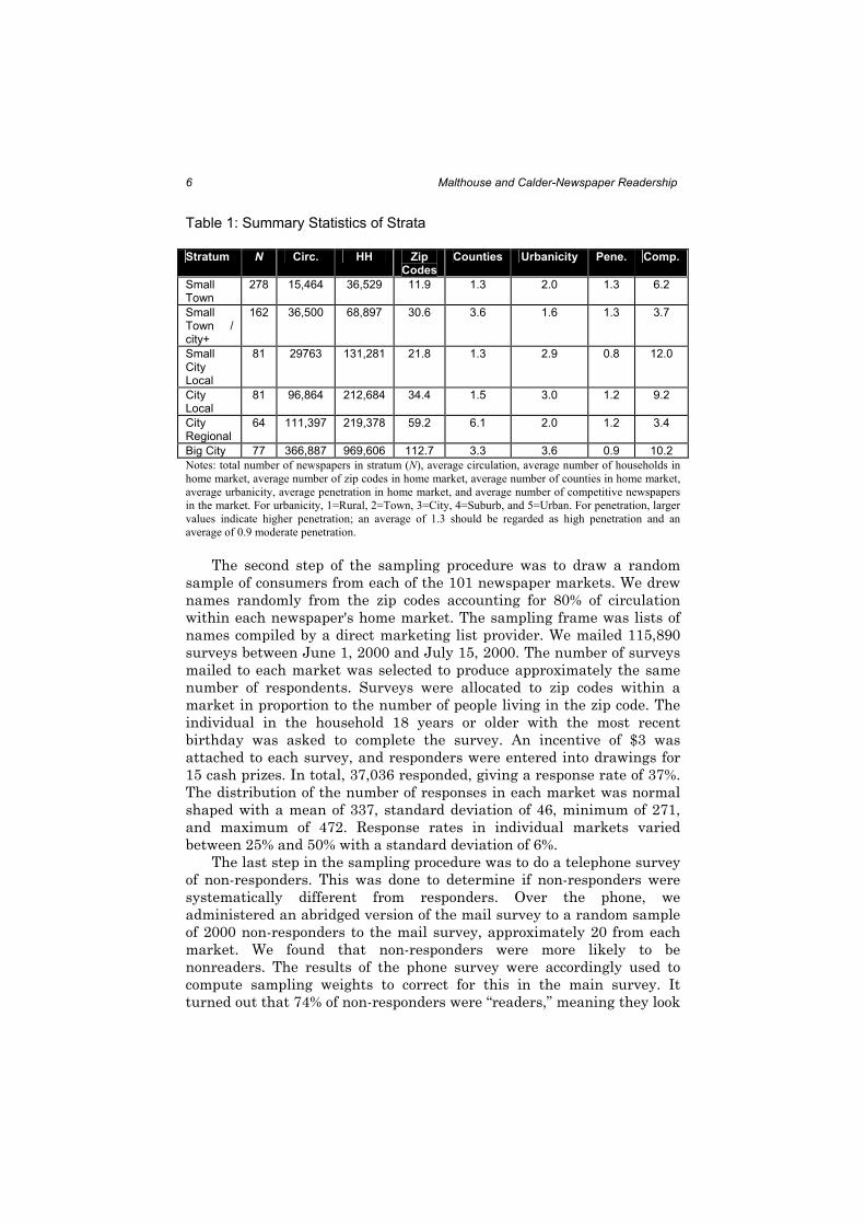
newspapers. We first drew a stratified random sample of 101 U.S. daily

newspapers, stratifying on market and newspaper characteristics such as

circulation, urbanicity, competition, market penetration, and the

geographical extent of distribution. We stratified the sampling frame into

six strata by applying K-means clustering to circulation data from ABC,

household counts from the US Postal Service, and demographic data

from Claritas and the US Census. In defining the strata we needed to

identify the “market” for each newspaper. We defined home counties as

those counties that make up 80% of total circulation. The strata were

defined using the average daily circulation, number of households in the

home counties, number of zip codes in the home counties, number of

home counties, Claritas' measure of urbanicity averaged over the home

counties, number of competitive daily newspapers in the DMA, and a

measure of market penetration in the home counties. Characteristics of

six strata are summarized in Table 1.

We drew simple random samples without replacement from each

stratum so that we would have approximately the same number of

newspapers from each stratum. In total, 101 out of 104 newspapers

agreed to participate in the study, giving a response rate of 97%. The

final list of participating newspapers included 18 from small town, 20

from small town/city+, 14 from small city local, 17 from city local, 15 from

city regional, and 17 from big city.


Table 1: Summary Statistics of Strata

Stratum N Circ. HH Zip

Codes Counties Urbanicity Pene. Comp.

Small Town

278 15,464 36,529 11.9 1.3 2.0 1.3 6.2

Small Town / city+

162 36,500 68,897 30.6 3.6 1.6 1.3 3.7

Small City Local

81 29763 131,281 21.8 1.3 2.9 0.8 12.0

City Local

81 96,864 212,684 34.4 1.5 3.0 1.2 9.2

City Regional

64 111,397 219,378 59.2 6.1 2.0 1.2 3.4

Big City 77 366,887 969,606 112.7 3.3 3.6 0.9 10.2

Notes: total number of newspapers in stratum (N), average circulation, average number of households in

home market, average number of zip codes in home market, average number of counties in home market,

average urbanicity, average penetration in home market, and average number of competitive newspapers

in the market. For urbanicity, 1=Rural, 2=Town, 3=City, 4=Suburb, and 5=Urban. For penetration, larger

values indicate higher penetration; an average of 1.3 should be regarded as high penetration and an

average of 0.9 moderate penetration.

The second step of the sampling procedure was to draw a random

sample of consumers from each of the 101 newspaper markets. We drew

names randomly from the zip codes accounting for 80% of circulation

within each newspaper's home market. The sampling frame was lists of

names compiled by a direct marketing list provider. We mailed 115,890

surveys between June 1, 2000 and July 15, 2000. The number of surveys

mailed to each market was selected to produce approximately the same

number of respondents. Surveys were allocated to zip codes within a

market in proportion to the number of people living in the zip code. The

individual in the household 18 years or older with the most recent

birthday was asked to complete the survey. An incentive of $3 was

attached to each survey, and responders were entered into drawings for

15 cash prizes. In total, 37,036 responded, giving a response rate of 37%.

The distribution of the number of responses in each market was normal

shaped with a mean of 337, standard deviation of 46, minimum of 271,

and maximum of 472. Response rates in individual markets varied

between 25% and 50% with a standard deviation of 6%.

The last step in the sampling procedure was to do a telephone survey

of non-responders. This was done to determine if non-responders were

systematically different from responders. Over the phone, we

administered an abridged version of the mail survey to a random sample

of 2000 non-responders to the mail survey, approximately 20 from each

market. We found that non-responders were more likely to be

nonreaders. The results of the phone survey were accordingly used to

compute sampling weights to correct for this in the main survey. It

turned out that 74% of non-responders were “readers,” meaning they look


into a newspaper during a typical 7-day week, while 93% of responders

were readers.

Respondents to the mail survey were also weighted based on age and

sex to make the sample more representative. Weights were computed to

reflect a random sample from the United States using data from phone

survey, Claritas, and the 1990 Census.

The Questionnaire

RBS (reader behavior scores) and TRBS (total RBS) are the dependent

variables of our analyses. RBS measures an individual's readership of a

particular newspaper and TRBS measures readership of all daily

newspaper. Respondents were also asked their sex, birth date (recoded to

age as of 2000), education, household income, and years of residence in

their town or community. Details on question wording are available at

the Readership Institute’s web site.2

RESULTS

The analysis is divided into two sections. The first uses additive models

to examine nonlinear relationships and establish an upper bound for the

fraction of variation in readership that can be “explained” by five

demographic variables. The second uses random coefficient models to

examine differences due to newspapers and markets.

The analysis examines effects on two dependent variables, RBS and

TRBS. RBS is a measure of the readership of a specific paper and the

results of regressions involving RBS should be thought of as a study of

what affects readership of the “local paper.” Recall that only people living

in the primary market of the newspaper were included in the sample.

TRBS is a measure of readership of any newspaper.

Let )',...,( 51 ijij xx denote the values of income (variable 1), education

(2), age (3), residence (4), and female (5), respectively, for respondent i of

newspaper j=1, …, 101. The variable female takes the value 1 if the

respondent is female and 0 otherwise; thus, a positive slope coefficient for

female would indicate that females read more than males. Hereafter, the

variable i indexes respondents, j newspapers, and k variables.

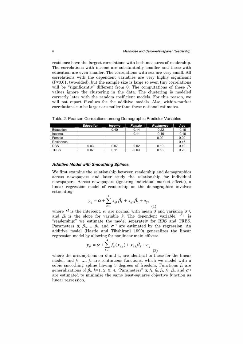
We first provide pair-wise correlations in Table 2 among variables to

assess the extent of multicollinearity. None of the correlations are

alarmingly large, with the largest being between age and length of

residence and between education and income; all other correlations are

small. The condition number is 3.5, indicating no serious problem with

multicollinearity (Montgomery and Peck 1982, p.301). The table also

gives correlations with the two dependent variables. Age and length of

2 See http://www.readership.org/consumers/survey/data/consumer_survey.pdf for the complete question-

naire. See http://www.medill.nwu.edu/faculty/malthouse/ftp/rbsdemo.html for details of this analysis.


residence have the largest correlations with both measures of readership.

The correlations with income are substantially smaller and those with

education are even smaller. The correlations with sex are very small. All

correlations with the dependent variables are very highly significant

(P<0.01, two-sided), but the sample size is large so even tiny correlations

will be “significantly” different from 0. The computations of these P-

values ignore the clustering in the data. The clustering is modeled

correctly later with the random coefficient models. For this reason, we

will not report P-values for the additive models. Also, within-market

correlations can be larger or smaller than these national estimates.

Table 2: Pearson Correlations among Demographic Predictor Variables

Education Income Female Residence Age

Education 0.40 -0.14 -0.22 -0.16

Income -0.11 -0.16 -0.16

Female 0.02 0.00

Residence 0.46

RBS 0.03 0.07 -0.02 0.19 0.19

TRBS 0.07 0.11 -0.03 0.18 0.23

Additive Model with Smoothing Splines

We first examine the relationship between readership and demographics

across newspapers and later study the relationship for individual

newspapers. Across newspapers (ignoring individual market effects), a

linear regression model of readership on the demographics involves

estimating

∑=

+++=4

1

55 ,k

ijijkijkij exxy ββα (1)

where α is the intercept, eij are normal with mean 0 and variance σ 2, and βk is the slope for variable k. The dependent variable, ijy is

“readership;” we estimate the model separately for RBS and TRBS.

Parameters α, β1,…, β5, and σ 2 are estimated by the regression. An additive model (Hastie and Tibshirani 1990) generalizes the linear

regression model by allowing for nonlinear main effects:

∑=

+++=4

1

55)(k

ijijijkkij exxfy βα (2)

where the assumptions on α and eij are identical to those for the linear model, and f1, …, f4 are continuous functions, which we model with a

cubic smoothing spline having 3 degrees of freedom. Functions fk are

generalizations of βk, k=1, 2, 3, 4. “Parameters” α, f1, f2, f3, f4, β5, and σ 2 are estimated to minimize the same least-squares objective function as

linear regression,


∑ ∑∑=

−−−j k

ijijkkij

i

xxfy .))(( 24

1

55βα (3)

We estimated the models specified in equations (1) and (2) using the

S-plus software package after dropping cases where any of the variables

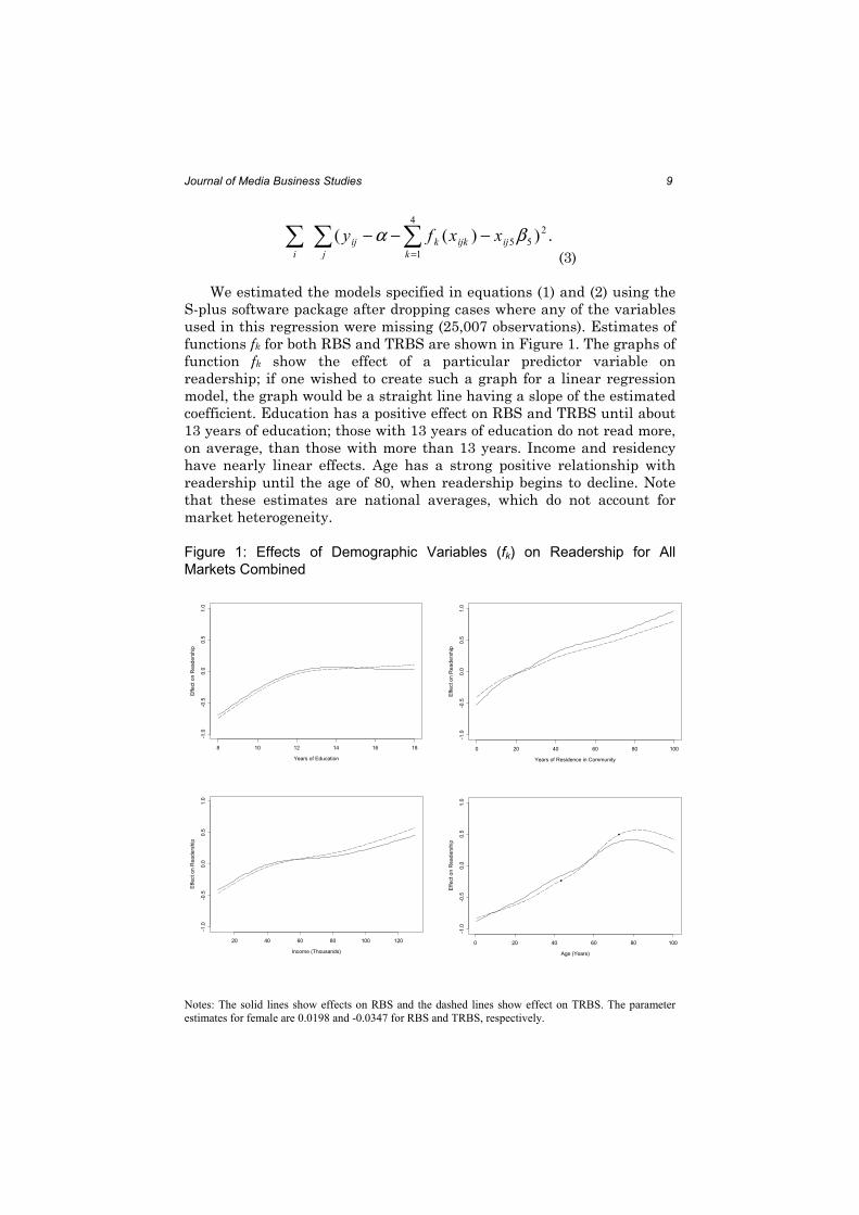
used in this regression were missing (25,007 observations). Estimates of

functions fk for both RBS and TRBS are shown in Figure 1. The graphs of

function fk show the effect of a particular predictor variable on

readership; if one wished to create such a graph for a linear regression

model, the graph would be a straight line having a slope of the estimated

coefficient. Education has a positive effect on RBS and TRBS until about

13 years of education; those with 13 years of education do not read more,

on average, than those with more than 13 years. Income and residency

have nearly linear effects. Age has a strong positive relationship with

readership until the age of 80, when readership begins to decline. Note

that these estimates are national averages, which do not account for

market heterogeneity.

Figure 1: Effects of Demographic Variables (fk) on Readership for All

Markets Combined

Years of Education

Effect on Readership

8 10 12 14 16 18

-1.0

-0.5

0.0

0.5

1.0

Income (Thousands)


20 40 60 80 100 120

-1.0

-0.5

0.0

0.5

1.0

Years of Residence in Community


0 20 40 60 80 100

-1.0

-0.5

0.0

0.5

1.0

Age (Years)


0 20 40 60 80 100

-1.0

-0.5

0.0

0.5

1.0

Notes: The solid lines show effects on RBS and the dashed lines show effect on TRBS. The parameter

estimates for female are 0.0198 and -0.0347 for RBS and TRBS, respectively.


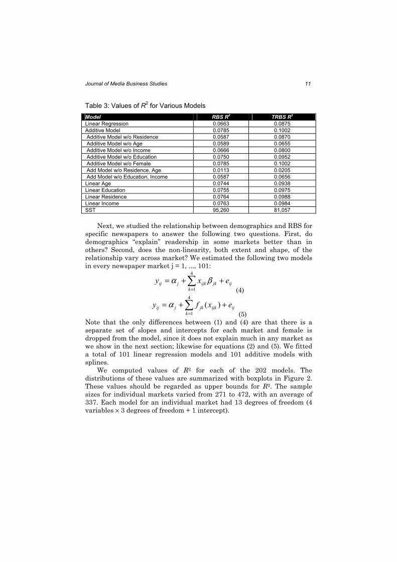
We can examine how much readership is explained by the various

demographics by noting the difference in R2 with a variable in and

without it. Table 3 compares the values of R2 for several models. Note the

following:

1. The demographics considered here are weak predictors of

readership. Even after modeling for nonlinear main effects with

an additive model, these demographics only account for 10% of

the variation in readership. Readership must be determined by

other factors.

2. The relationships between readership and these demographics is

somewhat nonlinear. For RBS, R2 improves from 6.63% to 7.85%,

or 18% = (0.0785-0.0663)/0.0663 by adding the nonlinear terms;

for TRBS, R2 improves by 15%. With the large sample size, this

improvement is highly significant.

3. Length of residence and age are the most important predictors of

readership. When both of these variables are dropped from the

RBS and TRBS models, R2 decreases to 1.13% and 2.05%

respectively. Income, education, and sex only explain 1-2% of the

variation in readership. When age or residence is dropped from

the model, R2 decreases by a substantial amount; age and

residence are moderately correlated (0.46) and thus can serve as

surrogates for each other to some extent.

4. Age seems to be a more important predictor of TRBS than of

RBS. When age is dropped from the RBS model, R2 decreases

from 7.85% to 5.89%, a 25% decrease. When age is dropped from

the TRBS model, R2 decreased from 10.02% to 6.65%, a 34%

decrease. The difference between the RBS and TRBS models is

not as great for length of residence.

5. Income and education explain some variation in readership, but

not as much as years of residence or age.

6. Sex has very little effect on readership. The coefficient is not

significantly different from 0 (P=0.1345, two-sided) even with the

very large sample size. R2, when rounded to four decimal places,

does not change when sex is dropped from the model.

7. We also quantified the amount of non-linearity by replacing the

smoothing terms with linear terms. If the model with the linear

term has essentially the same R2 value as the model with the

smoother, we conclude that the relationship is essentially linear.

R2 decreases the most for age.


Table 3: Values of R2 for Various Models

Model RBS R2 TRBS R

2

Linear Regression 0.0663 0.0875

Additive Model 0.0785 0.1002

Additive Model w/o Residence 0.0587 0.0870

Additive Model w/o Age 0.0589 0.0655

Additive Model w/o Income 0.0666 0.0800

Additive Model w/o Education 0.0750 0.0952

Additive Model w/o Female 0.0785 0.1002

Add Model w/o Residence, Age 0.0113 0.0205

Add Model w/o Education, Income 0.0587 0.0656

Linear Age 0.0744 0.0938

Linear Education 0.0755 0.0975

Linear Residence 0.0764 0.0988

Linear Income 0.0763 0.0984

SST 95,260 81,057

Next, we studied the relationship between demographics and RBS for

specific newspapers to answer the following two questions. First, do

demographics “explain” readership in some markets better than in

others? Second, does the non-linearity, both extent and shape, of the

relationship vary across market? We estimated the following two models

in every newspaper market j = 1, ..., 101:

∑=

++=4

1k

ijjkijkjij exy βα (4)

∑=

++=4

1

)(k

ijijkjkjij exfy α (5)

Note that the only differences between (1) and (4) are that there is a

separate set of slopes and intercepts for each market and female is

dropped from the model, since it does not explain much in any market as

we show in the next section; likewise for equations (2) and (5). We fitted

a total of 101 linear regression models and 101 additive models with

splines.

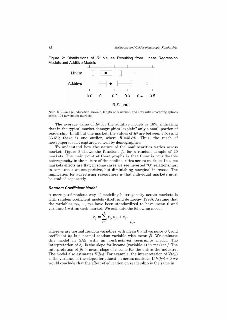
We computed values of R2 for each of the 202 models. The

distributions of these values are summarized with boxplots in Figure 2.

These values should be regarded as upper bounds for R2. The sample

sizes for individual markets varied from 271 to 472, with an average of

337. Each model for an individual market had 13 degrees of freedom (4

variables × 3 degrees of freedom + 1 intercept).


Figure 2: Distributions of R

2 Values Resulting from Linear Regression

Models and Additive Models

Note. RBS on age, education, income, length of residence, and sex) with smoothing splines

across 101 newspaper markets

The average value of R2 for the additive models is 18%, indicating

that in the typical market demographics “explain” only a small portion of

readership. In all but one market, the values of R2 are between 7.5% and

33.6%; there is one outlier, where R2=45.8%. Thus, the reach of

newspapers is not captured so well by demographics.

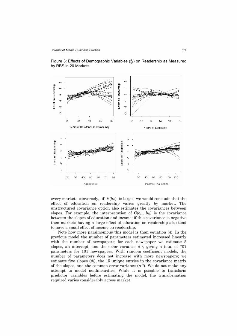
To understand how the nature of the nonlinearities varies across

market, Figure 3 shows the functions fjk for a random sample of 20

markets. The main point of these graphs is that there is considerable

heterogeneity in the nature of the nonlinearities across markets. In some

markets effects are flat; in some cases we see inverted "U" relationships;

in some cases we see positive, but diminishing marginal increases. The

implication for advertising researchers is that individual markets must

be studied separately.

Random Coefficient Model

A more parsimonious way of modeling heterogeneity across markets is

with random coefficient models (Kreft and de Leeuw 1998). Assume that

the variables xij1, ..., xij5 have been standardized to have mean 0 and

variance 1 within each market. We estimate the following model:

∑=

+=5

1

,k

ijjkijkij ebxy

(6)

where eij are normal random variables with mean 0 and variance σ 2, and coefficient bjk is a normal random variable with mean βk. We estimate this model in SAS with an unstructured covariance model. The

interpretation of bj1 is the slope for income (variable 1) in market j. The

interpretation of β1 is mean slope of income for the entire the industry. The model also estimates V(bjk). For example, the interpretation of V(bj2)

is the variance of the slopes for education across markets. If V(bj2) ≈ 0 we would conclude that the effect of education on readership is the same in


Figure 3: Effects of Demographic Variables (fjk) on Readership as Measured

by RBS in 20 Markets

every market; conversely, if V(bj2) is large, we would conclude that the

effect of education on readership varies greatly by market. The

unstructured covariance option also estimates the covariances between

slopes. For example, the interpretation of C(bj1, bj2) is the covariance

between the slopes of education and income; if this covariance is negative

then markets having a large effect of education on readership also tend

to have a small effect of income on readership.

Note how more parsimonious this model is than equation (4). In the

previous model the number of parameters estimated increased linearly

with the number of newspapers; for each newspaper we estimate 5

slopes, an intercept, and the error variance σ 2, giving a total of 707 parameters for 101 newspapers. With random coefficient models, the

number of parameters does not increase with more newspapers; we

estimate five slopes (βk), the 15 unique entries in the covariance matrix of the slopes, and the common error variance (σ 2). We do not make any attempt to model nonlinearities. While it is possible to transform

predictor variables before estimating the model, the transformation

required varies considerably across market.


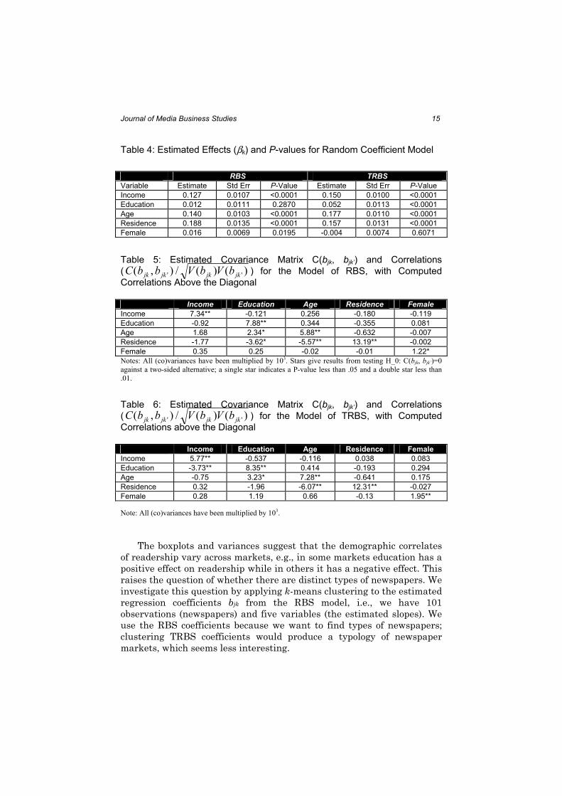
We estimated the model using proc mixed in SAS with the default

estimation method, restricted maximum likelihood (REML). Estimates of

slopes for individual newspapers were made using empirical best linear

unbiased predictors (EBLUPs). Estimates of βk and the covariances of the slopes are given in Tables 4, 5, and 6. The marginal distributions of bk

are shown in Figure 4. The residual variance (σ 2) is estimated as 0.9135 (standard error 0.0082) for RBS and 0.9051 (0.0081) for TRBS. Note the

following:

1. Length of residence has the largest effect (βk=0.188) for both RBS and TRBS, confirming the conclusion from the additive model

that this is an important variable. The variance of the residence

slopes across newspapers V(bj4) is also by far the largest (.01319

for RBS and .01231 for TRBS), suggesting that it is not equally

important in all markets. The boxplots reveal that the slope

estimates are close 0 or negative for up to a quarter of the

markets.

2. Education is not significantly different from 0 for RBS, and has a

small, but highly significant, effect for TRBS. We also estimated

this model without income. When income is dropped from the

RBS model, the effect for education is 0.065 and has a P-value

less than 00001. Recall that education and income have a positive

correlation and thus can serve as surrogates for one another to

some extent. The variance of the slopes across newspaper V(bj2),

however, is large. The boxplots show clearly that in some

markets education has a positive effect on readership while in

others the effect is negative. Negative effects are particularly

common when RBS is the dependent variable. Thus, for some

newspapers, the more educated a person is, the less likely the

person reads the particular paper.

3. Age and Income have similar effects on readership. Both have

substantial positive effect sizes that vary across markets.

4. Sex has little effect on readership in any market. With TRBS as

the dependent variable, the slope for sex, βk = −0.005, is not significantly different from 0; the overall slope for when RBS is

the dependent variable is also small. The variances are the

smallest of the predictor variables, which is reflected by the short

box plots. This indicates that sex has little effect on readership in

any market.

5. Covariances. There are several significant covariances, which are

likely related to the correlations among predictor variables. For

example, the covariance between the slopes of age and residence

with RBS as the dependent variable is −5.57, but these two variables have a positive correlation (0.46) and both have positive

overall correlations with readership.


Table 4: Estimated Effects (βk) and P-values for Random Coefficient Model

RBS TRBS

Variable Estimate Std Err P-Value Estimate Std Err P-Value

Income 0.127 0.0107 <0.0001 0.150 0.0100 <0.0001

Education 0.012 0.0111 0.2870 0.052 0.0113 <0.0001

Age 0.140 0.0103 <0.0001 0.177 0.0110 <0.0001

Residence 0.188 0.0135 <0.0001 0.157 0.0131 <0.0001

Female 0.016 0.0069 0.0195 -0.004 0.0074 0.6071

Table 5: Estimated Covariance Matrix C(bjk, bjk’) and Correlations

( )()(/),( '' jkjkjkjk bVbVbbC ) for the Model of RBS, with Computed

Correlations Above the Diagonal

Income Education Age Residence Female

Income 7.34** -0.121 0.256 -0.180 -0.119

Education -0.92 7.88** 0.344 -0.355 0.081

Age 1.68 2.34* 5.88** -0.632 -0.007

Residence -1.77 -3.62* -5.57** 13.19** -0.002

Female 0.35 0.25 -0.02 -0.01 1.22*

Notes: All (co)variances have been multiplied by 103. Stars give results from testing H_0: C(bjk, bjk’)=0

against a two-sided alternative; a single star indicates a P-value less than .05 and a double star less than

.01.

Table 6: Estimated Covariance Matrix C(bjk, bjk’) and Correlations

( )()(/),( '' jkjkjkjk bVbVbbC ) for the Model of TRBS, with Computed

Correlations above the Diagonal

Income Education Age Residence Female

Income 5.77** -0.537 -0.116 0.038 0.083

Education -3.73** 8.35** 0.414 -0.193 0.294

Age -0.75 3.23* 7.28** -0.641 0.175

Residence 0.32 -1.96 -6.07** 12.31** -0.027

Female 0.28 1.19 0.66 -0.13 1.95**

Note: All (co)variances have been multiplied by 103.

The boxplots and variances suggest that the demographic correlates

of readership vary across markets, e.g., in some markets education has a

positive effect on readership while in others it has a negative effect. This

raises the question of whether there are distinct types of newspapers. We

investigate this question by applying k-means clustering to the estimated

regression coefficients bjk from the RBS model, i.e., we have 101

observations (newspapers) and five variables (the estimated slopes). We

use the RBS coefficients because we want to find types of newspapers;

clustering TRBS coefficients would produce a typology of newspaper

markets, which seems less interesting.


We selected the 4-cluster solution, which has a cubic clustering

criterion of 1.434, indicating that it is a reasonable cluster solution.

Table 7 summarizes the distributions of slopes by cluster.

• Cluster 1 (19/101 newspapers). Age has the strongest effect; the

older a person, the higher readership is on average. Income also

has a strong effect. Length of residence has little effect.

• Cluster 2 (14/101 newspapers). Large residence and income

effects, negative education effects.

• Cluster 3 (40/101 newspapers). Average newspaper: moderate

residence, age, and income effects.

• Cluster 4 (28/101 newspapers). Large residence effects, small

negative education effects, small positive income effects.

A newspaper could determine which cluster it is in by estimating the

regression model described above to arrive at slopes. It would then

compute the Euclidean distance between the slope estimates and each of

the four cluster centroid given in Table 7. The newspaper is assigned to

the cluster with the closest centroid, just as the K-mean algorithm

operates.

Table 7: Cluster Means Grouping Newspapers by the Estimated Effect of

Five Demographic Variables on RBS

Variable Cluster 1 Cluster 2 Cluster 3 Cluster 4

Income 0.15 0.18 0.14 0.07

Education 0.08 -0.06 0.03 -0.02

Age 0.20 0.10 0.16 0.08

Residence 0.04 0.30 0.16 0.27

Female 0.01 0.01 0.02 0.01

CONCLUSIONS

The main contribution of this article is to examine how readership

depends on demographic variables across different newspapers and

markets. We find that there is considerable heterogeneity across both

newspapers and markets for length of residence, education, income, and

age, e.g., in some markets the effect of education on readership is positive

while in others it is negative. The non-linearity of the relationship also

varies considerably across markets. We suggest four types of newspapers

based on which demographics drives readership of the newspaper.

Of these five demographics, length of residence and age have the

strongest effects, which are positive overall and for most individual

newspapers/markets. Income also has a positive effect on readership. The

effect of education is very small overall, but varies considerably across

newspapers/markets. Sex has little effect anywhere. The overall effect of

age is somewhat nonlinear, with readership declining after the age of 75-


80. The overall effect of education is also nonlinear; it is positive for less

than 12 years of and flat thereafter.

Our analysis also provides estimates of national effects of

demographics, averaging over newspaper/markets. The fraction of

readership variation explained by these demographic variables is small,

suggesting that readership is better determined by factors other than

these five demographics. This also indicates that newspapers can be used

to reach all ages. If the fraction of variation in readership explained by

demographics had been large, we would have concluded that newspapers

were finely targeted towards a particular demographic segment, but this

is not the case. Researchers and practitioners must look beyond

demographics to explain newspaper readership.

Future research should propose variables that can better explain

readership. We hypothesize that the consumer experience – what

consumers think and feel when they read a newspaper – will be more

predictive of readership and more actionable to the practitioner than

demographics. Our research has identified such experiences (Calder and

Malthouse 2004) and related experiences to usage.

REFERENCES

Judee K. Burgoon and Michael Burgoon (1980). Predictors of newspaper readership.

Journalism Quarterly, 57(4):589-596.

Bobby J. Calder and Edward C. Malthouse (2003). The behavioral score approach to

conceptualizing and measuring dependent variables. Journal of Consumer Psychology,

16(4): 37-50.

Bobby J. Calder and Edward C. Malthouse (2004), "Qualitative Media Measures:

Newspaper Experiences, International Journal on Media Management, 6(1&2) pp.124-

131.

B.S. Everitt (1984). An Introduction to Latent Variable Models. Chapman and Hall, London.

Mark Fitzgerald (2000). ABC audit seek `critical mass'. Editor and Publisher, 133:9.

Trevor Hastie and Robert Tibshirani (1990). Generalized Additive Models. Chapman and

Hall, London.

Ita Kreft and Jan de Leeuw (1998). Introduction to Multilevel Modeling. Sage, London.

Laurence B. Lain (1986). Steps toward a comprehensive model of newspaper readership.

Journalism Quarterly, 63(1):69-74.

William E. Loges and Sandra J. Ball-Rokeach (1993). Dependency relations and newspaper

readership. Journalism Quarterly, 70(3):602-614.


D.C. Montgomery and E.A. Peck (1982). Introduction to Linear Regression Analysis. Wiley,

New York.

Klaus Schoenbach, Edmund Lauf, Jack M. McLeod, and Dietram A. Scheufele (1999).

Sociodemographic determinants of newspaper reading in the USA and Germany, 1974-

96. European Journal of Communication, 14(2):225-239.

Steve Wilson (1999). Newspaper profile service making sense to buyers: `intangible'

readership number taking on shape. Advertising Age, page S12.

demographics of newspaper readership: predictors and patterns of u.s. consumption

Documents