1

BUSN79—Business Administration:

Degree Project in Accounting and

Finance.

Financial Leverage and Market Return: Empirical Evidence from US Market Indices.

Author: Ernest Agyei

Supervisor: Håkan Jankensgård

Date: 28th May 2020

2

Contents Acknowledgement ........................................................................................................................................ 3

Section 1.0: Abstract ..................................................................................................................................... 5

Section 1.2: Introduction: ............................................................................................................................. 6

Section 2: Literature Review ......................................................................................................................... 9

Section 3: Theoretical background ............................................................................................................. 13

Section 4: Empirical Framework and Methodology .................................................................................... 18

Section 5: Data and Descriptive Statistics ................................................................................................... 27

Section 6: Empirical Analysis ....................................................................................................................... 28

Section 7: Conclusion .................................................................................................................................. 32

Section 8: Tables and Figures ...................................................................................................................... 34

Section 9: References: ................................................................................................................................ 58

Section 10: Appendix ................................................................................................................................. 72

3

Acknowledgement The author really wishes to thank his supervisor, Håkan Jankensgård, for his advice and guidelines

not forgetting Reda Mousli. The author is grateful to his Mother, Afia Chiaa, Family and friends,

Derek Asuman, the Ghanaian Community in Lund, Swedish Institute, and Lund University. I really

appreciate their extraordinary support in this thesis process.

4

5

Section 1.0: Abstract Purpose

The purpose of this paper is to empirically investigate the relationship between leverage and firm

performance if any exists, “what is the direction of the relation?” as well as test the possibility of

non-monotonic relationship. This is a central issue in corporate finance and there is a huge gap in

existing literature since there is no generally accepted conclusion on their relationship status, thus,

the findings of this paper will underpin literature and enhance efficient decisions and policies of

corporate agents like managers, investors, and government. Also, the notion that the relation of

leverage and firm performance has a lot to do with its measurement will be comprehensively

studied to robust the results.

Design/methodology/approach

Panel regression analysis is used for this study. This relationship is, tested empirically, robustly

tested with other factors like control variables, standard robust, lagging to address reverse causality

and serial correlation, the use of a variable instrument like asset tangibility, using dummy variables

for industry, regional and year effect, the use of Hausman V test to choose a fixed effect, use of a

white test for homoscedasticity to test good fit, and test also quadratic function. Later, a further

robust test by comparing the results with other measurements of both the firm performance and

leverage. Leverage is proxied by debt to asset and firm performance is measured by market return.

Findings

The results reveal that an increase in financial leverage has a negative, statistically significant

impact on market return after introducing an instrumental variable to deal with potential

endogeneity issues to make the results very robust, at the 10% level. The effect is linear and has a

lot to do with measurement choices since some measures did not find significant pronouncement.

The first null hypothesis is rejected while the second is accepted, with regards to this paper. This

is to underpin literature and assist corporate decisions.

Originality/value

This is the ‘first study’ that examines the relationship between financial leverage and market return

of companies considered into the top U.S market indices including S&P 500 Index, Dow Jones

Industrial Average, NASDAQ Composite, and NYSE Composite Index, together known to be part

of the Security Market Indicator Series (SMIS). This approach is considered to give us exposure

to leverage and market return of companies internationally listed from other countries together

6

with companies already in the US (and dual-listed companies), so, this study will have a new look

as it deals with the US market which is efficient according to literature. According to Ebaid (2009,

p. 478) and Kyereboah-Coleman (2007, p. 57), most of leverage and market return relation studies

consider developing markets (countries), thus, there are limited studies of developed markets like

the US. Also, this paper uses market return as the measurement of firm performance and compare

with other firm performance measurements like ROA and Tobin’s Q as well as uses leverage as

debt to assets compare with debt to equity (gearing) measurement to robust the results and aids our

understanding and our approach to financial leverage decisions and mechanisms. It also considers

different robust testing levels like the use of instrumental variables to address the endogeneity

issue. I use dividend (%) plus stock return (%) as the formula for market return, to make my studies

different from existing works of literature that use CAPM’s formula and the Fama-French three-

factor model which is an extension of the CAPM, as it is comprised of market risk, the

outperformance of small-value cap firms relative to large-valued firms, and outperformance of

high book-to-market value firms relative to low book-to-market value firms. 𝐸(𝑅𝑖) = 𝑅𝑓 +

𝐵𝑖[𝐸(𝑅𝑀) – 𝑅𝑓], for market return, 𝐸(𝑅𝑖) = 𝑅𝑓 + 𝐵1[𝐸(𝑅𝑀) – 𝑅𝑓] + 𝐵2 (𝑆𝑀𝐵) +

𝐵3 (𝐻𝑀𝐿).

Keywords: Firm Performance, Market return, Leverage, Debt Overhang theory, Irrelevance

theory, US stock indices, Free cash flow theory

Section 1.2: Introduction: Managerial performance and responsibility to maximize shareholders' value are administered and

enhanced by literature covering corporate governance. The maximization of the shareholders'

wealth largely depends on the betterment of managerial performance, and corporate literature tries

to give a better understanding of management to improve their decision makings to favor growth.

Thus, making corporate governance literature vital to corporate finance. One central issue in

corporate finance is leverage influence on firm performance (Modigliani and Miller, 1958),

deciding on capital structure is one of the most important and challenging decisions managers face

in the corporate world, and a change in the financing mix determines, arguably, firm’s financing

capacity, firms risk exposure, cost of external financing, investment capacities, strategic decisions,

and eventually shareholders wealth. Irrespective of how valuable this topic is to the corporate

world, few empirical studies are being examined to verify and clarify the long-debated issue of the

relationship between market return and leverage financing (Dimitrov and Jain 2007, George and

7

Hwang, 2009). Since Modigliani and Miller (1958) work on irrelevance theory, much literature

has been focused on the capital structure of corporations. Some pieces of literature claim capital

structure explain market return, others say it does not. Even if the former holds, there are also

conflicting findings as to the direction of the effect. Sides of the relation’s arguments have been

studied and reported on. First, leverage has a positive explanation for firm performance. It’s argued

by Jensen (1986) that leverage spills positive effect on firm performance by raising pressure on

managers to perform to meet debt servicing obligation in a way to reduce free cash flow to control

management moral hazard of misuse or overuse of the cash (Gill et al., 2011, Ahmad et al., 2013,

Yang et al., 2004). Second, literature also found there is a negative relationship that exists between

leverage and firm performance (Dawar, 2014, Yang et al., 2010). The Authors argue that higher

leverage firms are prone to higher agency costs since debtholders’ interests come in conflict with

existing shareholders’ interest, of which moral hazard gives rise to inverse relation (Jensen and

Meckling, 1976, Myers, 1977). Moreover, the work of literature argues that mixed relationship

exists between leverage and firm performance (Graham, 2000, Opler and Titman, 1994, Mourillo,

2005, and Arthur, 2010). The financial crises and boom and bust are argued by Adami et al. (2015)

to have exposed firms of not managing the issue of financial leverage well, there is a lack of

empirical consensus when it comes to this topic, firm performance and leverage relation (Laurent,

2007). The author stated that the lack of consensus can be ascribed to the various measurements,

both the dependent and the independent variables, implying different results are derived from

different measurements, thus, deductively, the measurement indicators play a role.

So, to analyze to contribute and enhance evidence of the true underlying relationship between

leverage and firm performance, I used market return as the measurement of firm performance,

since the dataset is full of public listed firms. I also use an efficient market, thus, considered

companies included in the top market indices: S&P 500 Index, Dow Jones Industrial Average,

NASDAQ Composite, and NYSE Composite Index since these indices house the companies that

can be a representation of the USA and other international markets. This relationship is robustly

tested, empirically, with factors like control variables, lagging to address reverse causality and

serial correlation, comparing with other measurements of both the firm performance and leverage,

the use of an instrumental variable, quadratic function testing, using dummy variables for industry,

regional (local or foreign company) and year effect, the use of Hausman test to choose between

fixed effect and random effects, a test of a good fit. I then proceeded to use other measurements of

8

leverage and firm performance to check further if indeed the relationship this paper has found will

pronounce in those measurements with this same dataset, and the same methods as the

aforementioned but only differ in the measurements. The models’ robustness was tested with the

same approach as the one used for the main measurement models, and both hypotheses,

irrespective of the measurement, except for the models which have gearing as the variable of

interest since gearing has no positive significant relation with asset tangibility, thus, I cannot use

the instrumental variable to address endogeneity.

The results reveal that an increase in leverage financing has a negatively statistically significant

impact on market return. The instrumental variable gave a negative statistically significant (at the

10% significant level) results and an economically significant relation in line with literature and

theories. Indicating the results is negatively significant even after introducing an instrumental

variable to deal with potential endogeneity issues, that there is a negative sensitivity of firm

performance with regards to leverage financing which is in line with work of literature and debt

overhang theory, financial distress cost and so forth. This implies that a percentage increase

(decrease) in leverage financing will cause a mean percentage decrease (increase) in market return,

statistically significant because it is at the 10% significant level. The relation between firm

performance and leverage depends on the measurement in line with the work of literature (like

Laurent, 2007, Ling and Chang 2011). After robust testing, only market return relation with

leverage is negatively, statistically significant. Also, aside from market return and gearing, and

Tobin’s Q and leverage, all other relations based on the base models are statistically and

economically significant, when regress independent variables and the dependent variable, without

further robust testing for endogeneity, considering the base model for the first hypothesis (H1).

Also, only ROA and leverage, ROA and Gearing, and Tobin’s Q and Gearing results found

significant support for non-monotonic relation, considering the base model for the second

hypothesis (H2). Also, none of the models has a non-monotonic function pronounced in it when

the base model is robustly tested. This makes us not find support for the non-linear function that

enables the trade-off theory to be applied in this study. The effect is linear and has a lot to do with

measurement choices. The results indicate an efficient market uses less leverage financing

consistent with the pecking order. These findings are also consistent with Myers’ (1976)

underinvestment problem with leverage financing, Opler and Titman’s (1994) shareholders

problems with debt, thus a high level of leverage is detrimental to firm performance, market return

9

and in contrast against Modigliani and Miller’s irrelevance theory and agency theory. The inverse

relation pronounced is also consistent with the works of literature [such as Abor (2005)—firms on

Ghana stock exchange; Ardatti (1967)—who used railroad firms; Adami et al. (2015)—with listed

firms on London Stock Exchange; Acheampong, Shibu, and Agalega (2013)—who studied the

Ghana Stock Exchange firms]. While on the other hand, it is in contrast with literature which found

positive relation [such as Gonzalez (2002); (Jensen, 1986 and Stulz, 1990); (Graham & Harvey,

2001); (Jensen, 1986 and Stulz, 1990); Khalid et al (2014), Almajali et al (2012)]. The study did

not find support for non-monotonic relation between leverage and market return which contrasts

with literature [such as Ganiyu et al.’s (2019)] study of capital structure and firm performance in

Nigeria. The inability to reject the second null hypothesis that there is a monotonic relationship

can attributes to this paper not considering firm characteristics and it is in line with Ibhagui and

Olokoyo (2018) argument that work of literature on the relationship between leverage and market

return reports a monotonic relationship without a qualitative analysis of firm characteristics like

size, and leverage level. The first null hypothesis is rejected while the second is accepted, with

regards to this paper. This is to underpin literature and assist corporate decisions.

Research question:

1. Is market return sensitive to financial leverage?

2. How a market return is affected by financial leverage, considering companies listed on the

top-notch US market indices for 2010 to the 2019-time horizon if the question (1) holds?

3. Does the relation depend on measurements?

4. Does leverage has a non-monotonic effect on the market return?

The remainder of this paper is organized in this way: section 2 is of literature review, section 3 has

the theoretical framework and empirical review, section 4 is made of empirical framework and

methodology, section 5 is data and descriptive statistics, section 6 is made of empirical analysis,

section 7 is the conclusion and section 8 and 9 are made of tables and figures, reference lists and

further included with section 10, appendices.

Section 2: Literature Review There are diverse findings from previous studies that try to find the relationship between leverage

and firm performance (I use market returns as a proxy), one of corporate finance central questions

(Modigliani and Miller, 1963). These findings come in different arguments, some studies find no

10

relation, others find relation, but there are also conflicting arguments to the latter, as some works

of literature find a positive relationship, others find a negative relationship while there is also a

mixed relationship between leverage and firm performance. The literature review is organized in

such a way of various arguments respective works of literature have covered. It starts with no

relation argument, then positive relation, negative and mixed relation.

No or insignificant relationship between Leverage and market return

Modigliani and Miller (1958) argue that under perfect market return, financial leverage does not

affect the market value of a firm, thus, its performance. These findings caused greater concern for

the corporate world to take a critical look if indeed the use of leverage financing does not affect

firm performance, which made literature to channel resources in this vital corporate finance issue,

for instance, Ling and Chang (2011) argue that there is no evidence of firm performance being

sensitive to leverage when leverage is high, using Taiwanese listed firms, and using Tobin’s Q as

a proxy for firms’ performance. Toraman, Kihc, and Reis (2013) also did not find evidence of firm

performance having any relationship with financial leverage, using the return on assets (ROA) as

a proxy for firm performance measurement. Cole, Yan, Hemley, (2015) study support the no

relevance theory introduced by Modigliani and Miller, as their study results showed that leverage

and firm performance are indifference to each other in the three US sectors the paper focused on

just as Philips and Sipahioglu (2004), Kovenock and Philips (1997) found insignificance results

as well Velnampy and Anojan (2014).

The positive relationship between leverage and market return.

Gonzalez (2002) holds the underlying point that debt financing influences managers to make value

maximization decisions and policies. It is also argued that leverage financing provides a

disciplinary mechanism against problematic perquisite and value destruction investment managers

who get influenced by excess cashflow undertake (Jensen, 1986 and Stulz, 1990). This study gives

the impression that leverage financing is a mechanism that deters managers from the misuse of

available cash since they have the commitment to pay off the debt’s principal and interest that

comes along to reduce the propensity for the firm to default. The direct and indirect costs that are

accompanied by default cannot be undermined. The agency of free cash flow is handled by the

need to service debt obligations, to reduce chances of free cash flow available to be squandered by

management irresponsible spending including perks. Also, the threat of defaulting on debt’s

principal and interests influence firms’ management to be efficient in their dealings. Gonzalez

11

(2002) suggests there are benefits of financial distress like revenue and cost restructuring,

corporate operational structure, organizational strategies, and corporate governance restructuring.

There is a consistent view that general rating and leverage are positively statistically correlated

(Graham & Harvey, 2001), as even together determined, thus, highly levered firms will be

downgraded to junk rating whiles low levered will be given investment rating, which will affect

the cost of external financing including the high cost of capital, credit rationing, terms of debt

covenants (which can be unbearable and profit draining). Financial distress is found by several

authors to have distressed firms’ Executives lose their jobs compared to their not distressed

counterparts. Khalid et al (2014), Fosu (2013), Almajali et al (2012) found a positive relationship

between leverage and firm performance, using profit as a proxy.

The negative relationship between leverage and market return.

On the other hand, leverage financing becomes an impediment for firms to undertake positive NPV

investment opportunities, this is consistent with what Myers (1977) refers to as “debt overhung”.

If firms are forced to forego some available positive NPV Investment Projects, it reduces the

growth rate of the firm since it’s not making either organic investment or inorganic investments

that cause the firm’s performance, on average, to be explained by the leverage on a negative basis

(Varouj, Ying, and Jiaping, 2003, Aivazian et al., 2005 & Ahn et al., 2006). Firms cannot have

access to new underlying assets that could increase the cash flow, thus, there will be negative

implications on such a firm’s performance, and eventually, the firm’s value. Varouj, Ying, Jiaping

(2003) argue that the disciplinary mechanism of agency cost theory is usually not maintained in a

firm with many opportunities to take NPV investment projects, so, only firms with few positive

NPV investment opportunities’ managers can be disciplined with leverage financing. Gonzalez

(2002) says evidence from the studies of Warner (1977) and many other studies established that

direct financial distress cost is comparatively low, including the survey that was done by Altman

and Hotchkiss (2006). Empirically, it is known from Bris et al. (2006) study that on average, there

is an 8.1% direct financial distress cost for smaller firms’ samples on pre-bankruptcy assets. On

the other hand, there are Indirect costs like debt overhung, underinvestment, policies like fire sales

due to being financially constrained and it is on the urge of defaulting and has many illiquid assets,

lost sales (loss customers), lost employees (loss experts), divided attention of the management

(Gonzalez, 2002). Adding to the distress cost, decision-makers are coerced to make even harmful

decisions against their partners and other stakeholders of the business life-cycle, not to rule out

12

that competitors will have competitive advantages and aggressive behaviors like a long purse and

cutthroat competition to obtain a greater market share portion (Gonzalez, 2002). However, Carlos

(2005) use an instrumental variable to find that leverage has a great impact on firm’s probability

to default while Arthur (2010) argues that on average companies are under-leveraged irrespective

of the supposed benefits that leverage financing comes along with, which can be inferred that, the

cost outweighs the benefit that is why the corporate world chooses to be under-levered.

.

The mixed relationship between leverage and market return.

The positive effect that comes with the mechanism of leverage financing, also, at a point becomes

a burden when a firm gets carried away with the positive “implications” from the leverage

(Graham, 2000). Opler and Titman (1994) even argue that in a financial or economic downturn,

firms that use greater leverage ratios are highly hit by such economic shocks, they tend to lose a

greater portion of the market share and eventually experience lower operating profits than their

competitors who use low leverage ratios, ceteris paribus, thus, indicating at such moments, the

cost of leverage write off the benefits of leverage and so, the benefit of leverage financing does

not come near the cost that high leverage can bring forth to firms. Arthur (2010) argues that when

firms increase their leverage position, firms with lower leverage levels increase their market

returns more than firms that are already highly levered. Mourillo's (2005) finding is also in support

of the work that debt financing can in a way boost firm performance and at the same time hurt the

firm badly. We think it is intuitive to imagine that the final effect of a firm’s leverage position on

its economic performance (Gonzalez, 2002) will be determined by which of the two sides of the

economic points will have a larger effect. The author argues that in the end if leverage cost exceeds

the benefit of leverage, the highly levered firm will poorly perform compared to the lowly levered

firms. On the other hand, the author highlights that, in the opposite scenario where the benefits

from leverage enable greater changes than the costs of the leverage, the high levered firms will

perform better than the less levered. Empirical evidence from Opler and Titman (1994) for US

firms also provide the support that highly leveraged firms lose market share and operating profits

to their competitors or peers with less leverage. Some other side of leverage and firm performance

relationship significance can be regarded which is part of the mixed argument, for instance, J. Cai

(2011) empirical study found that leverage ratio has no significant rotation with a firm’s future

13

R&D spending and the effect of the leverage ratio on a firm’s stock price depends on the size of

the firm’s leverage. A firm with lower leverage ratio experience weaker statistically significant

effect, consistent with Matsa (2011) work as well as Mura and Marchica (2010) which also find

support for lower leveraged firms’ significant positive relation with positive NPV investment

projects. By so, J. Cai (2011) findings of the negative relation leverage has with the stock price

also is in agreement with the findings of Myers (1977) theory of debt overhang’s prediction that

firms with greater possibility and probability to experience debt overhung has the stronger impact

of their stock price from leverage ratio scenarios. (J. Cai, 2011) also has an empirical finding that

outrightly supports that a change in leverage has a stronger negative effect on relatively highly

leveraged firms’ stock price. So, leverage the negative effect is lower when firms are not “over-

leveraged”.

Albeit the costs and benefits that the different schools of thought have established will vary to

different companies and other factors, it is still worthwhile to analyze the corporate operating and

economic performance response to leverage. This paper builds on the analyses of leverage and

market return of companies in the USA's top-notch indices.

Section 3: Theoretical background The theoretical and empirical background of the relationship between leverage and corporate

performance is thoroughly analyzed in this section and based on capital structure and financing

mix theories. Corporate Finance has different theories that try to find meanings into corporate

financial leverage preferences. These theories include, first, the trade-off theory, which establishes

an argument for optimal capital structure, by relaxing most assumptions from Modigliani and

Miller (1958) hypothesis, apart from assumptions of market efficiency and symmetric information.

Although financial leverage increment might create an avenue for firms to increase their value, by

profiting from debt tax shields (Modigliani and Miller, 1963), on the other hand, the firm value

gets diminished from both financial direct costs and financial indirect costs expected from leverage

increment (Ross et al., 2002). According to the tradeoff theory, the optimum level of capital

structure is when the benefits and the costs of financial leverage balance out exactly. The trade-off

theory of leverage makes us believe that until the optimal capital structure is attained, we assume

it is beneficial to increase leverage financing. The trade-off theory identifies that debt interest is

subjected to tax deductibility which reduces the amount of a firm’s income taxable, thus, reduces

the firm’s tax liability by tax shield. The trade-off between the bankruptcy cost and tax advantage

14

of debt financing determines the firm’s optimal leverage level and it is realized at the level when

the marginal present value of the debt tax shield on marginal debt is equal to the increase in the

present value of financial distress costs (Owalobi and Anyang, 2013).

Secondly, pecking order explains the decision for firms’ capital structure choice and mix that

internal financing is preferred to external financing, ceteris paribus. The pecking order hypothesis

argues that firms’ choice of order of capital structure mix is dependent on the relative availability

and relative cost of the external finance type (Myers and Majluf, 1984). This ‘theory’ considers

financial position, historical profitability, and the need for additional capital for investment

opportunities at a point in time. This theory explains why internal finance is preferred to external

finance and why debt is considered the best option for firms compared to equity when internal

financing is exclusive, thus external financing is on board or is the last resort. Debt financing is

deemed interestingly appealing, relatively inexpensive, and flexible. Pecking order theory has a

lot to do with information asymmetry. A sect of parties involved in the transaction sometimes has

more information than other parties (who are less or poorly informed) which increases information

costs to the less informed or uninformed parties. Pecking order explains that managers will first

use internally generated funds for their capital needs. If the internally generated funds do not

suffice to their investments, cash commitment or operational capital needs, then the firm will

consider cheap debt, and make equity the last resort in financing the firm's activities because it’s

costly and not appealing because of the right and control equity subscribers gain by diluting the

equity position of already existing shareholders (Myers and Majluf, 1984 and Popescu, 2009).

Moreover, Irrelevancy theory, put forward by Modigliani and Miller (1958), based on perfect

market assumptions like no transaction cost, no taxes, no bankruptcy cost, and so forth. The theory

posits that firm value is independent of the capital structure mix of a firm in a perfect market.

Modigliani and Miller (theory) emphasized that the market value of a firm is determined by its

ability to increase cash flow and reduce its underlying assets exposure to risks, for that matter, the

weighted average cost of capital is expected to be constant. Modigliani and Miller state that a

firm’s value is not influenced by the capital structure mix but by the earning qualities of its

underlying assets. Unfortunately, these emphases do not apply in the real world. These

assumptions do not hold when put to a test in our real world, and previous researches have

indicated they do not.

15

Also, market timing theory (Baker and Wurgler, 2002) argues that firms prefer equity to debt when

a booming economy or the market situation makes the cost of equity financing low, otherwise debt

finance would still be preferred as indicated by the pecking order theory. Firms exercise market

timing for their equity issues and buybacks. New shares are issued when the stock price is deemed

to be overvalued and the firm also, on the other hand, exercises stock buyback from the firm’s

shares when they are deemed to be undervalued. So, firms use equity financing when the market

is favorable to do so.

Besides, free cash flow theory postulates that managers must pay excess cash to equity investors

as dividends and interest to debt holders (investors) to reduce the excess cash to mitigate against

the misuse of cash and overuse of cash. High debt ratio which correlates with high-interest

payments disciplines managers and reduces their ability to invest in value destruction NPVs

projects and the use of free cash for perking activities. Jensen (1976) argues that increasing

leverage is a disciplinary mechanism to managers as they will tread carefully not to make the firm

insolvent (Owadabi and Anyang, 2013).

Debt Overhang theory of Myers (1977) argues that firms higher leverage level induces the

increasing probability of firms to forego the availability of positive NPV projects in the future

because after shareholders have made initial investments in the projects, the debt holders have

their obligations to be fulfilled first before shareholders will be considered for any residual amount

that will be left which might be lower even than their initial investment for that project, so, they’re

discouraged to go on that tangent. The foregoing of such investment opportunities reduces the

earning stream of the firm underlying assets that causes the firm performance to be below ideal or

that causes an increase in leverage to cause a negative mean explanation of firm performance,

ceteris paribus. So, from this theory, it can be inferred that an increase in leverage causes lower

investments that cause lower earnings and lower firm performance.

There are Empirical studies on this issue with different findings which include:

No Relation Between Leverage and Market return

Ling and Chang (2011) argue that there is no evidence of firm performance being sensitive to

leverage when leverage is high, using Taiwanese listed firms, and using Tobin’s Q as a proxy for

firms’ performance. Toraman, Kihc, and Reis (2013) also did not find evidence of firm

performance having any relationship with financial leverage, using the return on assets (ROA) as

a proxy for firm performance measurement. Cole, Yan, Hemley, (2015) study supports the no

16

relevance theory introduced by Modigliani and Miller, as their study results showed that leverage

and firm performance are indifference to each other in the three US sectors the paper focused on.

The positive relationship between capital structure and market return.

Wippern (1966), Holz (2002), Dessi and Robertson, (2003), Margrates and Psillaki, (2010) studies

of financial leverage and firm value relationship on some industries found positive relationship

when the studies used debt to equity ratio as a measurement of financial leverage and earnings to

a market value of the common stock as a measurement of performance. Implying shareholders add

up value to their wealth by using external (debt) financing. Managers finance their projects with

more debt and manage the fund optimally to improve and sustain performance. Hamanda (1969)

study also underpin the positive relation arguments as the study found that rate of return is

positively related with leverage financing which is in line with Baker & Martin (2011) empirical

study of United States of America firms, as well as the study of Masulis (1983) who also used

changes in leverage to support a positive relationship with market returns. Considering the market

returns monthly, Bhandari (1988) found the support of a positive relationship with annual leverage

ratios. Matsa's (2011) work as well as Mura and Marchica's (2010) work also finds support for

lower leveraged firms’ significant positive relation with positive NPV investment projects.

The negative relationship between capital structure and market return.

On the other hand, some previous studies also indicate that financial leverage relates negatively to

corporate performance. Majumdar and Chhibber (1997), Ghosh's (2007) study found the same

relation as found by Abor (2005), who argues that debt financing associates inversely with

corporate financial performance with listed firms on Ghana stock exchange as a dataset with

regards to Abor’s study. The authors argue that highly leveraged firms are faced with unfavorable

conditions imposed by debt holders’ covenants that interfere, in some sense, even against actions

that will increase earning and firm performance. This could be motivated by the fact that some

covenants might restrict firms from paying out dividends to shareholders or not undertaking

positive NPV projects. Highly leveraged firms are prone to the high cost of debt financing which

will cause a firm to focus on how to pay the debt burden (principal and interest) and leave small

room for focusing on achieving earnings. Firms' habit of extreme financial leverage level would

not allow for the firm to enjoy tax shields, and then it leads to an increase in debt distress cost of

which the firm becomes exposed to bankruptcy risks and reduces the firm’s performance. The

17

negative explanation of the mean change in firm performance is consistent with the costs of debt

theories like debt overhang (Myers, 1977). Muradoglu & Sivaprasad (2012) also have empirical

support for low leverage and high market returns. Moreover, Rao, Hamed, Al-yahee and Syed,

(2007), Krishnan and Moyer (1997), Gleason, Mathur, and Mathur (2000), Simerly and Li (2000),

King and Santor (2008) and Onalapo and Kajola (2010) provide the support that capital structure

also relates negatively with firm performance. Ardatti (1967), although found evidence of inverse

relationship leverage and market returns, for railroad firms, was not statistically significant, which

the author ascribed to omitted factors that relate differently with leverage and market returns.

Adami et al. (2015) analyses of listed firms on the London stock exchange also found there is a

statistically significant inverse relationship between leverage and market returns. Not forgetting

that Penman, Richardson, and Tuna (2007) found evidence that measurement errors in leverage,

misprices, and unrecognition of important risk factors cause an inverse relationship between

leverage and market returns. From the Ghana stock exchange, Acheampong, Shibu, and Agalega

(2013) found the support of a negative relationship between leverage and market return. George

and Hwang (2009) found support for a negative relationship between leverage and market return.

Ogebe et al. (2013) found a negative relation between leverage and firm performance for a 10

years’ time horizon dataset-study, using variables including GDP and inflation as a key influence

on firm performance. The authors empirically classified the considered firms into low leverage

firms and high leverage firms based on a baseline of above 10% as being a high leverage firm.

Mixed results of capital structure and market return.

Hurdle (1974) empirical study showed that financial leverage explains a negative mean change in

firm performance when two-stage least squares (2SLS) is applied and explain positively when

ordinary least squares (OLS) is applied instead. McConnell and Servaes (1995), Agarwal and

Zhao(2007), Weill (2007), Cheng, Liu and Chien (2010) and Li Meng, Wang and Zhou(2008)

presented additional evidence that support leverage has a positive effect on firm performance from

one situation and negative effect on firm performance on others. These situations range from using

firm size (small and large), the institutional basis for different countries, and so forth. Also, Ozdagli

(2012) empirically found that it is not market leverage rather operating leverage that explains stock

return based on tax deductibility.

Hypothesis

18

The hypotheses are based on both the theories and empirical studies. There are two (2) hypotheses

to be studied. The null hypothesis will be rejected or not rejected due to the p-value that comes out

from the regressions. The first null hypothesis is that there is no relationship between market

returns and financial leverage, inspired by theories and literature. A second hypothesis will be

investigated by observing the quadratic function of leverage to analyze if there is support for non-

monotonic relation arguments. The underlying base model is based on the research question: does

the leverage level explain market return?

Hypothesis 1 (H1) states t0hat financial leverage explains, on average, changes in market return.

This is motivated to either find support for the Modigliani and Miller (1958) irrelevance theory or

provide support of relation and further clarify the relationship between leverage and market issue,

as there are still different results with different contexts, but no specific result, which can be

generalized. So, this hypothesis will enable this paper to analyze if there is an inverse relationship

between leverage financing and market return, thus, an increase in leverage will cause a decrease

in market return which is related to financial distress cost and debt overhang theory. Or, there is a

direct or positive relation as the free cash flow theory that disciplines managers to be responsible

for financial management.

Hypothesis 2 (H2) there is a non-linear relation between leverage and market return. As literature

argues that leverage and market return relation take a U-turn based on factors like economic, firm

size, and leverage levels. If there is an economic downturn, leverage impact differently on different

firms and different leverage level of firms as well as the test of possibility of non-monotonic

relationship based on the excessive use of financial leverage argument.

H1 = Financial leverage explains, on average, changes in market return.

H2 = Financial leverage and market return have non-monotonic relationship.

Section 4: Empirical Framework and Methodology Methodology

This paper focuses on an empirical study of the sensitivity of market return by leverage financing

with regards to companies in the top market indices in the US. Since the dataset is a panel, that it

combines both time series and cross-section, thus provides unbiased estimators. Demsetz and Lehn

(1985) and Himmelberg et al. (1999) stated that leverage and firm performance are influenced by

similar characteristics, some of which cannot be observed on economic grounds, following their

study, I address this using panel regression, multivariate regression technique for this study. Vong

19

and Chan (2009), and Baltagi (2013) advocate for panel regression technique, since it gives more

information, reduces collinearities, and gives efficient estimations. The authors also argue that the

data individual variability and dynamic adjustment are easily traced in a panel data regression

aside accounting for the heterogeneity that is found in the individual data units. At the descriptive

analysis, the relevant aspects of leverage financing and the market return is provided with detailed

information about each variable considered for the analysis. The correlation matrix is applied to

measure the degree of connection between the variables under consideration. Regression analysis

examines the relationship between the independent variables and the dependent variable, to know

the effect of selected independent variables on market return. This regression method enables to

identification the statistical and economic significant of each independent variable and their

respective coefficient to the model and the significance of the overall model. The model used for

the first regression is simple regression (only one variable), and the others were multiple

regressions (more than one independent variable) including the base model. Here I follow Berger

and di Patti (2006) as well as Margaritis and Psillaki (2007, 2010).

Following the literature, I use fixed effects (FE) model specification because some of our variables

of interest are constant over time such as the industry dummy, regional dummy and the results

from Hausman V test, I use a fixed effect specification because the statistically significant p-value

of 0.0000 and chi2 of 88,09 from Hausman V test gives us strong chance to reject the null

hypothesis that random effect is preferable, after I run both the random effect (RE) and fixed effect

(FE) models. The test of fixed effect and random effect will be the same if the error is uncorrelated

with the regressors. Consequently, I consider both fixed effect and standard robust errors for the

economical and statistical significance estimation and include year dummies to account for any

time effect together with the industry and regional dummies. I examine the impact of leverage

financing on firm performance using different proxies for the dependent variable and the

independent variable of interest. Moreover, the linear function of leverage and firm performance

does not make room for the trade-off theory. To address these issues, leverage squared is added to

investigate the possibility of a U-shape (non-monotonic) relationship between leverage and market

return. The research design adopted for the study is quantitative. The quantitative research design

is appropriate because it measures figures and observed facts (Cooper and Schindler, 2006).

The study design under the quantitative research design is a panel. The population of this study is

companies under the stock indices considered. The study focuses on a target population of 1899

20

companies included for the stock indices in the US. This study uses active, publicly-traded, non-

financial firms included in the top-notch market index in the USA, namely, S&P 500 Index, Dow

Jones Industrial Average, NASDAQ Composite, and NYSE Composite Index with a time horizon

between 2010 and 2019 from Orbis database which ‘houses’ financial information of over 20

million companies. The dataset from exhibit 1.0 had 1899 number of non-financial companies,

and 24 number of industries and I had to combine some industries to increase the sample size used

in this study to enhance the robustness of the results (Brooks, 2008). I had to re-classify the

industry into retail, electronic, transport, education, manufacturing, communication, properties,

mining, products, commercial and the rests were transferred to others. Exhibit 2.0 and 2.1 provides

the distribution of the considered industry sample. The results are robust to different

methodologies. Eventually, I based on the Hausman V test to apply fixed effect methodology on

the model and the white test to test homoscedasticity, and further use standard robust.

I tested for H1 by regressing the firm performance (market return) function on the explanatory

variable (leverage) and control for other firm characteristics (firm size, EBIT margin, growth rate,

Cashflow volatility, and investment rate), thus, consider the explanation’s significance and

directions if any. I then proceeded to test H2 using the same method for H1 to test for leverage and

firm performance non-monotonic relation. I used instrumental variables of asset tangibility

(Aivazian et al. 2005, Lang et al.,1996, Firth et al., 2008) to test the robustness of the results of the

relationship that exists between leverage and market return and address possible endogeneity issue.

Asset tangibility is the ratio of the sum of fixed assets and inventories (Net Fixed Assets) to total

assets for firm x in year t (see Aivazian et al., 2005). He argues that bankruptcy cost has a

relationship with leverage ratio, and so is the firm’s assets tangibility. So, bankruptcy costs

influence the managers' decision to increase leverage or reduce leverage. On the other hand,

tangible assets reduce bankruptcy costs, and that motivates managers to levered up. I used the

ivreg2 since it takes the 2 stage least square (2SLS), the GMM, and the LIML. Assets tangibility

is a relevant predictor of the endogenous variables, it satisfies the exogeneous requirement and

does not appear as an explanatory variable.

Based on the rule of thumb that if the pair-wise correlation coefficient between two explanatory

variables is more than 0.8 (Gujarati, 2004) then we expect multicollinearity. From Fig., B, the

pairwise correlations between the explanatory variables are low. The negative relationship

between leverage and Investment rate, unlike the rests which are positively related, is consistent

21

with debt overhang theory, as it indicates, highly leverage reduces the opportunity to even access

debt capital to finance a positive NPV project, since, senior debt holders will have the first claim

of proceeds, and also, because of information asymmetry, creditors will not trust the claim of

positive NPV not forgetting that even shareholders will not invest in such available positive NPV

projects since debt holders have first claims of interest.

Variables Measurement

Firm performance measurement is arguably a key factor in the varying results in this corporate

finance issue. Literature uses different measurement indicators as a proxy for firm performance,

from accounting measurements (Majumdar and Chhibber, 1999; Abor, 200) including Return on

Equity (ROE), Return on Assets (ROA), and market measurements (Welch, 2004) like Market

return, Volatility, and the mixture of both market and accounting measurements like Market

capitalization to total Assets (Tobin’s Q). This study will use market measurement’s market return

as the main proxy for firm performance, considering publicly listed companies of the market

indices, and later robust test the results with other measurements or proxies. So, in addition to the

Market return as the dependent variable for the main models, I use ROA and Tobin’s Q as other

dependent variables for other models. King and Santor (2008) argue that Tobin’s Q is a forward-

looking measure that is an indicator of the valuation of firms’ future growth opportunities while

ROA is a backward-looking measure.

The dependent variable, firm performance, is proxied by Market return (%), which is derived from

the available annual stock prices (%) and the dividend yield (%). The difference in the current and

the previous prices and the dividend yield (%), divided by the previous price (%) derive market

return (%). Annual stock return is not as volatile and noisy as the monthly and quarterly stock

prices, so, I use the annual data since at least it will comparatively be a good reflection of a “true”

stock performance: price and returns movement”. There is a popular measurement of market return

in the situation of capital asset pricing model (CAPM) which recognizes return as the addition of

risk-free and beta rate multiplied by market risk premium, I decided to use the other measurement

of dividend and stock return, to make my studies different from existing literature that uses CAPM,

𝐸(𝑅𝑖) = 𝑅𝑓 + 𝐵𝑖[𝐸(𝑅𝑀) – 𝑅𝑓], as the market return formula, and also the Fama-French three-

factor model which is an extension of the CAPM, comprises of market risk, the outperformance

of small-value cap firms relative to large-valued firms, and outperformance of high book-to-market

22

value firms relative to low book-to-market value firms, is another measurement of the market

return.

𝑅𝑖𝑠𝑘 − 𝐹𝑟𝑒𝑒 % + 𝐵𝑒𝑡𝑎 % ∗ 𝑀𝑎𝑟𝑘𝑒𝑡 𝑟𝑖𝑠𝑘 𝑝𝑟𝑒𝑚𝑖𝑢𝑚 % = 𝑀𝑎𝑟𝑘𝑒𝑡 𝑟𝑒𝑡𝑢𝑛 % 𝑒𝑞𝑢(1.0)

𝑅𝑖𝑠𝑘 − 𝐹𝑟𝑒𝑒 % + 𝐵𝑒𝑡𝑎 % ∗ 𝑀𝑎𝑟𝑘𝑒𝑡 𝑟𝑖𝑠𝑘 𝑝𝑟𝑒𝑚𝑖𝑢𝑚 % + 𝑆𝑚𝑎𝑙𝑙 𝑚𝑖𝑛𝑢𝑠 𝑏𝑖𝑔 % +

𝐻𝑖𝑔ℎ 𝑚𝑖𝑛𝑢𝑠 𝐿𝑜𝑤 % = 𝑀𝑎𝑟𝑘𝑒𝑡 𝑟𝑒𝑡𝑢𝑛 % 𝑒𝑞𝑢 (1.1)

So, for the market return formula for this model, Total (simple) market returns Rt includes

dividends and is calculated as follows: dividends and is calculated as follows:

MReturn % =(𝑝𝑡 − 𝑝𝑡 − 1) + 𝐷

𝑝𝑡 − 1= 𝑆𝑡𝑜𝑐𝑘 𝑟𝑒𝑡𝑢𝑟𝑛 % + 𝐷𝑖𝑣𝑖𝑑𝑒𝑛𝑑 %

= 𝑀𝑎𝑟𝑘𝑒𝑡 𝑟𝑒𝑡𝑢𝑛 % 𝑒𝑞𝑢 (1.2)

Leverage also has book value and market value measurements. The book value measurement is

such that the firm’s total book value of assets in relation to the total book value of debt. On the

other hand, the market value is the book value of debt together with the market value of equity in

relation to the total book value of debt. In this study, book leverage will be the focus (Barclay,

Morellec & Smith Jr, 2003, J Cai, 2011), since market value might cause spurious correlation with

other variables and can even be related to stock prices. With regards to the interesting independent

variable, that is, Leverage, there are different forms of measurement in corporate finance and its

previous literature. For instance, Debt to Equity ratio, Debt to capital, and Debt to Assets. Aside

from that, the debt component also comes in different measurements including Non-current debt,

Long-term debt, Total Long-Term Interest-Bearing Debt, Long-term, and Short-Term Interest-

Bearing Debts, and so forth. The study will first use leverage as a measurement of Debt to Assets

as the main leverage basis but will consider leverage as Debt to Equity to test for robustness, also.

As seen in literature, when it comes to definitions of leverage ratios (Graham and Leary, 2010;

Lemmon, Roberts, and Zender, 2008; Leary and Roberts, 2010; Lemmon and Zender, 2010;

Gonzalez, 2002; Titman & Wessels 1988; Rajan & Zingales 1995).

Leverage(BV) =𝑇𝑜𝑡𝑎𝑙 𝐷𝑒𝑏𝑡(BV)

𝑇𝑜𝑡𝑎𝑙 𝐴𝑠𝑠𝑒𝑡𝑠(BV) 𝑒𝑞𝑢 (1.3)

23

Here, I control for firm characteristics that explain market returns also, so the control variables

include firm size (which is measured by the natural log of Assets), revenue growth (g) [that is the

percentage change in revenue], cash flow volatility (lCF) [as a proxy of log cash flow] and

Investment rate (linv) [as a proxy of log investment] Chong & Kim, 2018. The consideration of

these control variables are motivated by prior literature, for instance (Banz, 1981; Acheampong et

al, 2014) for firm size, (Yang et al., 2010; Rezaei and Habashi, 2012; Hermuningsih, 2013; Quang

and Xin, 2014) for growth, for EBIT, literature like Ahmad et al., 2013. In addition to these control

variables, I also use year and industry (effect) dummies, following the Fama and French (1997).

The dependent variable and the interested independent variables are already “naturally logged”,

indicating an “elasticity”; that is a percentage change in leverage explains a percentage change, on

average, of the market return. This enables all exposure to be put on an equal footing since it is

relatively better for communication and comparisons of the coefficient of the relationship that

exists between leverage and market returns. So, the included control variables including the natural

log of total assets as a proxy of firm size, cashflow logged to get volatility, which influences firms’

ability to meet its cash commitments; EBIT margin which is also about the profitability of the firm,

since it has a lot to do with even the ability to sustain and maintain operations, as Ahmad et al.

(2013) indicates it’s an indicator of good economic fundamentals, that influences investors and

market return in the long run; investment also logged to get the rate is also considered since the

investment rate gives new asset bases that can help give new returns from new assets together with

those provided with the already existing asset base, revenue growth also helps firm performance.

I have considered these variables as control variables since they are firm characteristics that can

explain the market return of the observed companies.

Market Return relationship with leverage

Yxt = Market Return, b1xt = Leverage

I estimate an equation to examine the sensitivity of market return to leverage financing. I used

similar specifications as that of Lang et al. (1996) but this paper uses panel data. The relationship

between leverage and a firm’s performance is tested by the necessary regression models and further

robust tested. Where the respective models will be based on these measurements below, which

explains the model characteristics. Where: Yxt = Dependent variable of the company. Xxt =

Independent variable of company, b0 = Intercept for X variable of x company for time t. (That is

the expected mean value of Y when all X equals to 0), b1 – b6 = Coefficient for the independent

24

variables X of companies, denoting the nature of the relationship with dependent variable Y (or

parameters), b7 to b9 = dummy variables, ɛxt = The error term Specially, where: LEV (%) =

Leverage rate, M_Return (%) = Market return rate, TobinsQ = Tobin’s Q = Market capitalization

/ Total assets, , Gearing = Gearing rate = Debt-Equity, EBIT (%) = EBIT Margin, lTA = log of

Total Asset (Firm Size), lCF=Cash Flow volatility, Iinv=Investment rate, g = Revenue growth

rate, ɛ xt = Error term.

Simple Regression

I run a simple regression model for the relationship between financial leverage and market return:

M_Return 𝑥𝑡 = 𝑏𝑜 + 𝑏1LEV𝑥𝑡 + ɛ𝑥𝑡 𝑒𝑞𝑢 (2.0)

Which regresses the dependent variable, market return function on the regressor, leverage, to test

if there is a relationship between market return and financial leverage, ‘and if there exists a

relationship, what is the direction of the relationship between leverage and market return?’.

The first hypothesis (H1)

However, the main base model is the market return regressed on the regressors comprising of the

independent variable of interest and other firm characteristics that influence market return, as used

as control variables. The H1 baseline model is estimated by:

M_Return 𝑥𝑡 = 𝑏𝑜 + 𝑏1LEV𝑥𝑡 + 𝑏2lTA𝑥𝑡 + 𝑏3lCF𝑥𝑡 + 𝑏4EBIT𝑥𝑡 + 𝑏5Iinv𝑥𝑡

+ 𝑏6g𝑥𝑡 + ɛ𝑥𝑡 𝑒𝑞𝑢 (2.1)

So, I tested the possibility of omitted variables, by including these control variables to the simple

regression model to estimate the base model. I included firm size, growth rate, cash flow volatility,

investment rate, and EBIT margin because they are characteristics that are more likely to cause

more or less market return, thus one must control for these sorts of characteristics in any empirical

model that examines the effect of leverage on market return.

Second Hypothesis (H2)

I further tested the second hypothesis that the trade-off theory and other literature posit that

leverage has a non-monotonic relation with the market return. For instance, there is both a positive

25

and negative explanation of market return by leverage. I included leverage square to the base model

of the first hypothesis (equ 2.1). The H2 baseline model is estimated by:

MReturn𝑥𝑡 = 𝑏𝑜 + 𝑏1LEV𝑥𝑡 + 𝑏2LEV𝑥𝑡2 + 𝑏3lTA𝑥𝑡 + 𝑏4lCF𝑥𝑡 + 𝑏5EBIT𝑥𝑡

+ 𝑏6Iinv𝑥𝑡 + 𝑏7g𝑥𝑡 + ɛ𝑥𝑡 𝑒𝑞𝑢(2.2)

I tested to estimate if I consider the quadratic function of leverage variable, will leverage

explanation of market return have a U-turn or switch in between negative and positive since there

are economic arguments that leverage has a mixed relationship with the market return. That, the

relationship, or the explanation changes either with more leverage financing, during an economic

downturn or the size of the firm changes.

Robust Test

First Robust without instrumental Variable (IV)

Hypothesis 1 (H1)

I used different methods to make sure the results are robust and endogeneity possibilities have

been reduced to the minimum. So, I put the results through these robust testing methods. I corrected

regression error for residual clustering and homoscedasticity using the white test, the white results

mean I fail to reject the null hypothesis that there is homoscedasticity in the model. Since, from

Fig. A white test was insignificant with a chi2 of 0.92 and a p-value of 0.63. I still considered

standard robust although the model residual variables have the same scatter. I also consider the

fact that the previous rates of both the market return and leverage can influence the market return

sensitivity to leverage financing, so, both the market return and leverage are lagged by one year to

be able to control for reverse causality in the model to address endogeneity. I then added dummy

variables to purge idiosyncratic effects to the baseline model such as an industry, region, and year

dummies to make the results more robust.

MReturn𝑥𝑡 − 1

= 𝑏𝑜 + 𝑏1LEV𝑥𝑡 − 1 + 𝑏2LEV𝑥𝑡2 + 𝑏3lTA𝑥𝑡 + 𝑏4lCF𝑥𝑡 + 𝑏5EBIT𝑥𝑡

+ 𝑏6Iinv𝑥𝑡 + 𝑏7g𝑥𝑡 + 𝑏8𝑖. 𝐼𝑁𝐷 + 𝑏9𝑖. 𝑟𝑒𝑔 + 𝑏10𝑖. 𝑌𝑟 + 𝑎𝑥𝑡

+ ɛ𝑥𝑡 𝑒𝑞𝑢(2.3)

I did Hausman V test to consider either to use fixed effect (fe) or random effect (re) to test the

robustness of the model, so by removing the mean regional industry-year fixed effect to deal with

26

each year effect together with respective industry and regional effect. For attributing the respective

idiosyncratic effects among the explanatory variables to expunge all the specifics, being its

regional effects, industry effects, and time effects, and to be able to interpret the estimates.

Hypothesis Two (H2)

I also consider the fact that the previous rates of both the market return and leverage can influence

the market return sensitivity to leverage in other periods, so, both the market return and leverage

will be lagged by one year to be able to control for reverse causality in the model to address

endogeneity. I did Hausman V test to consider either to use fixed effect (fe) or random effect (re)

to test the robustness of the model.

𝑀𝑅𝑒𝑡𝑢𝑟𝑛𝑥𝑡 − 1

= 𝑏𝑜 + 𝑏1𝐿𝐸𝑉𝑥𝑡 − 1 + 𝑏2𝐿𝐸𝑉𝑥𝑡^2 + 𝑏2𝑙𝑇𝐴𝑥𝑡 + 𝑏3𝑙𝐶𝐹𝑥𝑡

+ 𝑏4𝐸𝐵𝐼𝑇𝑥𝑡 + 𝑏5𝐼𝑖𝑛𝑣𝑥𝑡 + 𝑏6𝑔𝑥𝑡 + 𝑏7𝑖. 𝐼𝑁𝐷 + 𝑏8𝑖. 𝑟𝑒𝑔 + 𝑏9𝑖. 𝑌𝑟

+ 𝑎𝑥𝑡 + ɛ𝑥𝑡 𝑒𝑞𝑢 (2.4)

So, I used a fixed effect for the model, I then added dummy variables to the model. An industry,

region, and year dummies to make the results more robust.

Robust with instrumental Variable (IV)

Instrumental Variable

Hypothesis One (H1)

I find asset tangibility as a good instrumental variable (iv) for this main model, it meets the

requirements of a good instrument, that is, it satisfies the exogeneous requirement and does not

appear as an explanatory variable, and it is also statistically significant from the empirical analysis

of leverage and asset tangibility relation.

MReturn𝑥𝑡 𝑖𝑣^2

= 𝑏𝑜 + (𝑏1 LEV𝑥𝑡 = 𝑇𝑇𝐴) + 𝑏2lTA𝑥𝑡 + 𝑏3 lCF𝑥𝑡 + 𝑏4EBIT𝑥𝑡

+ 𝑏5Iinv𝑥𝑡 + 𝑏6g𝑥𝑡 + 𝑎 𝑥𝑡 + ɛ𝑥𝑡 (𝑓𝑖𝑟𝑠𝑡) 𝑒𝑞𝑢 (2.5)

Hypothesis 2 (H2)

Just as I instrumented the first hypothesis model, I instrumented this second hypothesis model also.

MReturn𝑥𝑡 𝑖𝑣^2

= 𝑏𝑜 + (𝑏1 LEV𝑥𝑡 = 𝑇𝑇𝐴) + 𝑏1LEV𝑥𝑡2 + 𝑏2lTA𝑥𝑡 + 𝑏3 lCF𝑥𝑡

+ 𝑏4EBIT𝑥𝑡 + 𝑏5Iinv𝑥𝑡 + 𝑏6g𝑥𝑡 + 𝑎 𝑥𝑡 + ɛ𝑥𝑡 (𝑓𝑖𝑟𝑠𝑡) 𝑒𝑞𝑢 (2.6)

27

Section 5: Data and Descriptive Statistics Data

I had a weakly balanced data set when I reshaped the panel data from wide to long shape and sorted

the panel data by Id (firmID) and year. This study uses active, publicly-traded non-financial firms

included in the top-notch market indices in the USA namely, S&P 500 Index, Dow Jones Industrial

Average, NASDAQ Composite, and NYSE Composite Index with a time horizon between 2010

and 2019 from Orbis database which ‘houses’ financial information of over 20 million companies.

I had 2169 companies when I selected active companies on Orbis and chose those indices. I filtered

the companies down to 1899 by limiting it to publicly listed and excluded financial and financial

related companies like Insurance companies since literature argues that they have different

regulations with regards to their financial mix or capital structure.

Exhibit 1.0 contains summary statistics for the data on the variables: market return, leverage, firm

size (as a natural logarithm of the asset), growth rate, cash flow volatility, investment rate, and

EBIT margin.

I have these variations for firm performance and the regressors. The Overall variation indicates the

variation over time and individual companies. The between variation indicates variation between

the individual companies. The within variation indicates variation within individual companies

over time. The Market return, as a proxy for firm performance, of the observed firms’ variation on

average is a ratio of 6.46 over the 10 years and the 1899 companies observed. There are 28 different

sectors considering US SIC 3-digit codes (from exhibit 1.2), of which I brought it down to 10

industries. Which include (from exhibit 2.0) Retail (1800), Electronic (3390), Education (3100),

Manufacturing (1250), Communication (910), Properties (790), Mining (2860), Production (790),

Commercial (930) and the rest in others (2340). I observed that the maximum return of 4290.335

was too far away from the average return of 6.46, so, the dataset of the variable has outliers, thus,

they must be removed. Tobin’s Q ratio ranges between 0 and 1250 ratio with a mean ratio of 1.13.

ROA also ranges between a ratio of -98 and 99 with 9.89 standard deviation and averages at 3.01.

The leverage ratio ranged between 0 and 3.85, overall, but averages at 2.5. The gearing is averaged

at 100.85 with a standard deviation of 1.34. Firm size has a standard deviation of 1.77 overall and

1.76 and 0.52 between and within, respectively. The growth rate is 2.63 ratio on average and EBIT

margin falling between -98.87 and 100. With cash flow volatility ranging between a ratio of 4.75

and 18.07. Investment rate also averages at 11.78.

28

The market return, Tobin’s Q, growth rate, and leverage have outliers that make the dataset kind

of spurious. The data is also winsorized at the 1% and 99% levels to ensure outliers do not affect

the results. After the outliers were removed, on average the ratio of market return of the companies

is 5.70 and at maximum, 34.47 of return. Tobin’s Q ratio ranges between 0 and 3.85 ratios with a

mean ratio of 0.25. Leverage ranges between 0 and 21.98, overall, but averages at 15.12, a growth

rate of 4.75 to 18.07, and 7.48 on average. However, some companies do not use leverage at all,

so, minimum leverage of 0. From exhibit 3.0, the respective countries from which companies

considered into the indices which are used for this paper are from. Since some of these market

indices are of global standard, companies from various countries which meet the requirement for

international listening of a company per the standard of the respective index can be on board of

the market index. So, there are 24 countries, thus, 23 non-US countries and the US, so, divided

into two categories of regions, with all the 23 countries categorized into the non-US region

(foreign) and then US (domestic) (Exhibit 3.1). Also, region, industry, and year dummies,

following the Fama and French (1997), can be found in Exhibit 1.0. The choice of variables and

proxies were motivated by literature.

Section 6: Empirical Analysis Simple Regression Results

When I run the OLS regression for the model, the results from Fig. 1 column (1) indicates a

negative insignificant coefficient of -0.07 with an individual p-value that is more than the any of

the significant levels, which indicates leverage and market have no relationship using simple

regression. This result is in line with literature that market return is not sensitive to financial

leverage and it is consistent with Modigliani and Miller’s irrelevant theory, in a perfect market.

Results of the First Hypothesis

The result also became significant, unlike the simple regression model, at a p-value at 10%

statistically significant level. This also has an economic significance, that a percent (%) increase

in the leverage level will have an adverse effect by causing the market return to decrease, on

average, by -28.9 percent (%), Fig 1., column (2). This results rather conflicts with no relationship

literature and Modigliani and Miller’s irrelevant theory, rather, it is in line with debt overhang

theory and literature. The base model regression significant results indicate leverage’s value-

relevant information conveyed to the market is beyond that of other firm characteristics. Since

leverage is statistically and economically significant after controlling for other firm characteristics

29

(Dimitrov and Jain, 2008, J Cai, 2011) and even support the study of Myers and Majluf (1984), a

firm with good prospects or good cash position will use their internal funding before soliciting for

external financing like leverage financing.

Result for Second Hypothesis

Fig. 7, column (1), the coefficients of the leverage is in a negative direction, that is -4.94 and

leverage square is -0.037. Although the main leverage has a p-value at the 1% level, the leverage

square is neither significant nor changes direction, indicating an insignificant relationship and even

there is no evidence to support a switch of the direction of the estimated coefficient. This goes

contrary to literature about leverage U-shape characteristics.

Robust Test

First Robust without instrumental Variable (IV)

Hypothesis 1 (H1)

I had a statistically significant Prob>Chi2=0.0000 and Chi of 29.91, from fig. A, which gives us a

strong chance to reject the null hypothesis that random effect is preferable, from the Hausman v

test. So, I used a fixed effect for the model aside motivation by literature. I had a coefficient of -

5.77, statistically insignificant at the individual level with a p-value higher than any of the

statistically significant levels, from Fig. 3, column (1). I did this to compare the other

measurements that do not take asset tangibility as an instrumental variable. None of these models

found support for statistical significance when we limit it to this robust level without instrumenting

it yet, for all the hypothesis.

Hypothesis two (H2)

When I regressed market return and the regressors, I had a negative insignificant result, because it

has a p-value which is higher than any of the statistically significant levels, from fig. 8.

Robust with Instrumental Variable (IV)

Hypothesis 1 (H1)

The regression results, from Fig. 5, column (1), I find leverage to explain market return with a

statistically significant coefficient of -101.1 with an individual p-value of 0.072, which is at the

10% significant level. Before that, the relationship between leverage and asset tangibility has

positive relation (that is coefficient of 1.37 and a p-value of 0.003), in line with literature that, it is

a good instrumental variable. This implies that a percentage increase (decrease) in leverage

financing will cause a mean decrease (increase) in market return. The result is statistically

significant because it is at the 10% significance level.

30

Hypothesis 2 (H2)

Fig. 6, column (1), both coefficients are negative, the coefficient of the leverage is in a negative

direction, -55.20 and leverage square is -0.212. Indicating they are all negatively statistically

significant at the 10% significant level, and there is no support for a U-turn shape since only

negative direction and no positive direction at a point. This goes contrary to literature about

leverage U-shape characteristics. I instrumented in both the linear model and the non-linear model

in the explanatory variable of interest. Before that, I checked the relationship between leverage

and tangible assets, and it has a positive relationship (that is coefficient of 1.73 and a p-value of

0.000), underpinning the literature that it is a good instrumental variable. This implies that a

percentage increase (decrease) in leverage financing will cause a mean decrease (increase) in

market return.

Other Measurements.

Methods

I then proceeded to use other measurements of Leverage and firm performance to check if indeed

the relationship this paper has found will be pronounced in those measurements with this same

dataset, and the same methods as the aforementioned but only differ in the measurements. The

models’ robustness was tested with the same approach as the one used for the main measurement’s

models, and both hypotheses, irrespective of the measurement, except the models which have a

gearing rate as the variable of interest since gearing has no positive significant relation with asset

tangibility, thus, I cannot use the instrumental variable to address endogeneity. So, before I

instrumented the models with leverage as the explanatory variable of interest because it is a good

instrument, I initially tested with the other methods including lagging both dependent and

explanatory variables of interest, adding dummy variables, robust standard, fixed effect to further

address endogeneities. I instrumented those models with leverage as the variable of interest with

tangible assets since they meet the criteria for an instrumental variable.

Discussion of Results

The equations from 2.1 to 2.6 are for the main measurements and main models while those

equations from 3.1 to 7.4 (at the appendix) are models for the other measurements. The results for

all base models have a significant explanation of leverage and firm performance except market

return and gearing together with Tobin’s Q and leverage base model relations, when I regress

independent variables and the dependent variable, without further robust testing for endogeneity,

31

considering the base model for the first hypothesis (H1), irrespective of the measurement (Fig. 1

& 2). I had insignificant results for all the models irrespective of the measurements when they

were robustly tested without instrumental variables with regards to the first hypotheses (Fig. 3 &

4). Moreover, considering the instrumented model for the first hypotheses (H1), the results, from

fig. 5, show only Leverage and market return have negatively significant relation pronounced in

it, while Tobin’s Q and leverage have positive insignificant relation, and ROA and leverage have

negatively insignificant relation. When it comes to the second hypotheses (H2), only ROA and

leverage, ROA and Gearing, and Tobin’s Q and Gearing results found significant support for U-

shape or non-monotonic relation, considering the base model, from fig. 7. There is also no support

for the non-monotonic relationship between leverage and market return nor any other measurement

model after the baseline model had further robust tests, as the method used for the first hypotheses

(from Fig. 8). The formulas can be found in the appendix. This makes us not find support for the

non-linear function that enables the trade-off theory to be applied in this study. Because of the

negative implications, they tend to use more of internal financing as suggested by pecking order

theory, so, they do not use much of leverage financing for it to reach a point where it can have

positive consequences. Thus, it is linear throughout. Also, the base models with significant

negative explanation indicate leverage conveys value-relevant information to the market beyond

other firm characteristics (Dimitrov and Jain (2008), J Cai, 2011).

I think these indices give us exposure to multiple region firms to facilitate the analysis to reduce

regional bias. Market indices have different standards and different coverages, these indices are of

global exposure, implying companies from different countries apply to be considered if they meet

the requirements of the respective market index. Some companies are part of more than one market

index, so, the Orbis data automatically recognizes and considers only one, the company appears

once when multiple indices are selected. These markets have good performing companies and

some indices also go beyond only monetary performance to consider the non-monetary

performance of the companies. I believe the developed market indices will give us developed and

efficient companies and efficient market information. These indices considered include the “blue-

chip stocks”, the largest companies in the U.S. by market cap, and most of the significant U.S. and

non-US companies, and it is a good proxy for the representation of the overall stock market. An

index is a barometer of markets.

32

Section 7: Conclusion This paper finds support for a negative relationship between market return and leverage even after

the robust test, using data of companies included in the US top market indices, at a 10% significant

level. Also, aside from market return and gearing, Tobin’s Q and leverage, all other relations based

on the base models are statistically and economically significant, without further robust testing for

endogeneity, considering the base models for the first hypotheses (H1). Also, only ROA and

leverage, ROA and Gearing, and Tobin’s Q and Gearing results found significant support for non-

monotonic relation, considering the base models for the second hypotheses (H2). The models’

robustness was tested with the same approach irrespective of the measurement, except the models

which have gearing as the variable of interest since gearing has no positive significant relationship

with a tangible asset when empirically tested, hence, I did not use an instrumental variable to

address endogeneity. So, before I instrumented the models that have leverage as it meets the

instrumenting requirement, I had insignificant results for all the models and their respective

measurements when I robust tested with the other methods such as standard robust, lag the

dependent and independent variables for autocorrelation, also Industry, regional dummy variables,

and year fixed effects were activated. Those models with leverage as the variable of interest were

subjected to an instrumental variable of asset tangibility, the results show leverage and market

return have negative significant relation pronounced in it.

This implies that a percentage increase (decrease) in leverage financing will cause a mean decrease

(increase) in market return, and it is statistically significant at the 10% significant level. Which has

an economic significance in line with the literature, that a (highly) levered firm might not undertake

positive NPV investment projects if more of the proceeds will go to debt holders, instead. The

effect is linear and has a lot to do with measurement choices. The results indicate an efficient

market uses less leverage financing. These findings are consistent with Myers’ (1977)

underinvestment problem with leverage financing, Opler and Titman’s (1994) shareholders

problems with debt, and in contrast against Modigliani and Miller’s irrelevance theory and agency

theory. The inverse relationship is also consistent with the literature [such as Abor (2005)—firms

on Ghana stock exchange; Ardatti (1967)—who used railroad firms; Adami et al. (2015)—with

listed firms on London Stock Exchange; Acheampong, Shibu, and Agalega (2013)—who studied

the Ghana Stock Exchange firms]. While on the other hand, it is in contrast with literature which

found positive relation [such as Gonzalez (2002); (Jensen, 1986 and Stulz, 1990); (Graham &

33

Harvey, 2001); (Jensen, 1986 and Stulz, 1990); Khalid et al (2014)]. The study did not find support

for non-monotonic relation between leverage and market return which contrasts with literature

[such as Ganiyu et al.’s (2019)] study of capital structure and firm performance in Nigeria. The

inability to reject the second null hypothesis that there is a monotonic relationship can attributes

to this paper not considering firm characteristics and it is in line with Ibhagui and Olokoyo (2018)

argument that work of literature on the relationship between leverage and market return reports a

monotonic relationship without a qualitative analysis of firm characteristics like size, and leverage

level. The first null hypothesis is rejected while the second is accepted, with regards to this paper.

This is to underpin literature and assist corporate decisions.

Limitation

The study is limited by focusing on well-performing companies in the top-notch indices. Also,

this paper is limited to the 2010-2019-time horizon. This paper is also limited to literature

accessible. The financial companies are excluded due to different regulations and measurements

regarding capital structure (Alves & Francisco 2014), so this paper focus is on non-financial

companies in the market indices, as well as few industries are considered due to insufficient data

availability. This paper did not consider firm and economic characteristics that can explain well of

monotonic or non-monotonic relationship and it is in line with Ibhagui and Olokoyo (2018)

argument that work of literature on the relationship between leverage and market return reports a

monotonic relationship without a qualitative analysis of firm characteristics like size, and leverage

level. Lastly, apart from internal firm variables, there are also external market factors and

macroeconomic factors that affect firms’ performance that were not considered.

Further Studies

There is an opportunity to base on the categorization of the company’s original domicile that brings

regional levels, that is US companies and Internationally listed companies (non-US), to consider

the pronouncement of market return sensitivity with regards to locally and internationally listed

firms. Thus, assign a dummy variable for the region with the US (locally listed) companies to take

1 and those non-US (internationally listed) companies, to take 0. To find out how companies in

the US are affected by leverage financing compared to their counterparts who are internationally

listed in the US market from other countries. Further studies can use the median of the firm size

(natural logarithm of Total Assets) to categorize the companies into a larger size firm and a smaller

34

size firm to enable the second hypothesis of market return and leverage non-monotonic relation to

be further tested. Also, further research can use the Leverage median to categorize the firms into

highly levered and lowly levered firms and analyze if the firms considered in the US top-notch

market indices also experience U-shape when levered firm increases its leverage position and what

if it decreases its leverage position.

Section 8: Tables and Figures

Exhibit 1.0 Summary Statistics

Variable

Mean Std. Dev. Min Max

Observation

s

countr~s overall

19.5639

8 5.751584 1 24

N = 18990

betwee

n

5.752947 1 24

n = 1899

within

0 19.56398

19.5639

8

T = 10

35

region overall

1.69773

6 0.459251 1 2

N = 18990

betwee

n

0.45936 1 2

n = 1899

within

0 1.697736

1.69773

6

T = 10

company overall 950 548.2084 1 1899

N = 18990

betwee

n

548.3384 1 1899

n = 1899

within

0 950 950

T = 10

sector overall 14.2882 7.442328 1 28

N = 18980

betwee

n

7.444093 1 28

n = 1898

within

0 14.2882 14.2882

T = 10

IND overall

4.94151

7 2.84619 1 10

N = 18980

betwee

n

2.846866 1 10

n = 1898

within

0 4.941517

4.94151

7

T = 10

M_Return

(%) overall 6.45608 34.17496 0

4290.33

5

N = 18990

betwee

n

11.42969 0

430.349

8

n = 1899

within

32.20795 -423.894

3866.44

1

T = 10

36

1

IND overall

4.94151

7 2.84619 1 10

N = 18980

betwee

n

2.846866 4.941517 10

n = 1898

within

0

4.94151

7

T = 10

0

TobinsQ overall

1.13012

8 9.523042 0 1250

N = 18990

betwee

n

3.911407 -124.067

125.196

7

n = 1899

within

8.683114

1125.93

3

T = 10

-98.043

ROA overall

3.00952

8 9.890203 -38.7807 99.213

N = 18990

betwee

n

6.569932 -82.209 58.7825

n = 1899

within

7.394091

96.7703

3

T = 10

0

LEV (%) overall

0.25166

7 0.226612 0

3.85248

9

N = 16812

betwee

n

0.203256 -0.51486

3.10320

9

n = 1893

within

0.104732

2.16957

1 T

bar =

8.88114

0

Gearing

(%) overall

100.850

4 134.4441 0 999.916

N = 18990

37

betwee

n

96.40627 -474.487

696.661

8

n = 1899

within

93.73079

978.912

T = 10

0

log (TA) overall

15.1235

8 1.774811 4.906025 21.9828

N = 16812

betwee

n

1.758048 2.503571

21.7338

6

n = 1893

within

0.517416

20.7354

3 T

bar =

8.88114

-87.7664

g (%) overall

2.63379

5 216.77 -10.0863

24851.6

4

N = 15305

betwee

n

82.18217 -2759.43

2761.32

9

n = 1846

within

202.7762

22092.9

4 T

bar =

8.2909

-98.867

EBIT (%) overall

10.2705

6 17.66995 -35.8622 100

N = 18990

betwee

n

13.37607 -91.6153 94.991

n = 1899

within

11.54957

113.614

6

T = 10

4.75359

CF (%) overall 12.7185 1.677679 7.280697

18.0701

9

N = 15194

betwee

n

1.649975 6.62669

17.6327

2

n = 1767

within

0.58629

15.6996

7 T

bar =

8.59875

38

0

INV (%) overall

11.7797

9 2.368466 0

19.0870

4

N = 6359

betwee

n

2.382263 3.250022

18.4773

2

n = 970

within

0.8116

16.1577

2 T

bar =

6.55567

Exhibi

t 1.1

The Winsorized

Statistics

overall

0

M_Retur

n (%)

overall 5.70887

7

6.06928

2

0 34.473

N = 18990

betwee

n

3.94901 0 28.2959

n =

1899

within

4.60965

2

-22.587 36.7345

8

T =

10

overall

0

TobinsQ

betwee

n

0.25166

7

0.22661

2 0

3.85248

9

N = 16812

within

0.20325

6 -0.51486

3.10320

9

n =

1893

0.10473

2

2.16957

1 T bar = 8.88114

overall

0

LEV (%)

betwee

n

15.1235

8

1.77481

1

4.90602

5 21.9828

N = 16812

39

within

1.75804

8

2.50357

1

21.7338

6

n =

1893

0.51741

6

20.7354

3 T bar = 8.88114

overall

4.75359

g (%)

betwee

n 12.7185

1.67767

9

7.28069

7

18.0701

9

N = 15194

within

1.64997

5 6.62669

17.6327

2

n =

1767

0.58629 T bar = 8.59875

Exhibit 2.0 The Industries

1. Agriculture, Horticulture &

Livestoc

40 0.21 0.21

2. commercial Servi 930 4.9 5.11

3. Biotechnology and Life Sciences 70 0.37 5.48

4. Business Services 940 4.95 10.43

5. Chemicals, Petroleum, Rubber &

Plast

1,630 8.59 19.02

6. Communications 440 2.32 21.34

7. Computer Hardware 140 0.74 22.08

8. Computer Software 490 2.58 24.66

9. Construction 520 2.74 27.4

10. Food & Tobacco Manufacturing 610 3.21 30.61

11. Industrial, Electric & Electronic

M

2,760 14.54 45.15

12. Leather, Stone, Clay & Glass

produc

130 0.68 45.84

40

13. Media & Broadcasting 470 2.48 48.31

14. Metals & Metal Products 660 3.48 51.79

15. Mining & Extraction 1,230 6.48 58.27

16. Miscellaneous Manufacturing 120 0.63 58.9

17. Printing & Publishing 210 1.11 60.01

18. Property Services 1,560 8.22 68.23

19. Public Administration,

Education, H

420 2.21 70.44

20. Retail 1,130 5.95 76.4

21. Textiles & Clothing

Manufacturing

230 1.21 77.61

22. Transport Manufacturing 710 3.74 81.35

23. Transport, Freight & Storage 950 5.01 86.35

24. Travel, Personal & Leisure 690 3.64 89.99

25. Utilities 770 4.06 94.05

26. Waste Management & Treatment 50 0.26 94.31

27. Wholesale 670 3.53 97.84

28. Wood, Furniture & Paper

Manufacturi

410 2.16 100

Exhibit 2.1 The Reviewed Industries

Overall Between Within

IND Freq. Percent Freq. Percent Percent

1. Retai 1800 9.48 180 9.48 100

2. Elect 3390 17.86 339 17.86 100

3. Educa 3100 16.33 310 16.33 100

4. manuf 1250 6.59 125 6.59 100

41

5. commu 910 4.79 91 4.79 100

6. Prope 1610 8.48 161 8.48 100

7. Minin 2860 15.07 286 15.07 100

8. Produ 790 4.16 79 4.16 100

9. other 2340 12.33 234 12.33 100

10. Comm 930 4.90 93 4.90 100

Exhibit 3.0

Overall

Betwee

n

Wit

hin

count

ries

Freq.

Percent

Freq.

Percent

Perc

ent

1. AR

10

0.05

1

0.05 100

2. BE

10

0.05

1

0.05 100

3.

BM

310

1.63

31

1.63 100

4. CA

680

3.58

68

3.58 100

5. CH

60

0.32

6

0.32 100

6.

CW

10

0.05

1

0.05 100

7. DE

30

0.16

3

0.16 100

Count

ries

42

8. FR

10

0.05

1

0.05 100

9. GB

200

1.05

20

1.05 100

10. IE

140

0.74

14

0.74 100

11. IL

60

0.32

6

0.32 100

12. IT

10

0.05

1

0.05 100

13. JP

3010

15.85

301

15.85 100

14.

KY

660

3.48

66

3.48 100

15.

LR

10

0.05

1

0.05 100

16.

LU

120

0.63

12

0.63 100

17.

MH

170

0.90

17

0.90 100

18.

MU

10

0.05

1

0.05 100

19.

MX

10

0.05

1

0.05 100

20.

NL

110

0.58

11

0.58 100

21.

PA

20

0.11

2

0.11 100

22.

SG

10

0.05

1

0.05 100

43

23.

US

13250

69.77

1325

69.77 100

24.

VG

80

0.42

8

0.42 100

Total

18990

100.00

1899

100.00 100

(

n = 1899)

Exhibit 3.1 Region

Overal

l

Betwe

en

With

in

region Freq. Percent

Freq.

Perce

nt

Perce

nt

1. non-U 5740 30.23

574

30.23 100

2. USA 13250 69.77

1325

69.77 100

Total

18990

100.00

1899

100.0

0 100

(n = 1899)

Fig. 1

(1) (2) (3) (4)

44

VARIABLES M_Return M_Return ROA TobinsQ

LEV -0.0706 -2.899* -2.832*** -0.0200

(1.869) (1.683) (0.415) (0.103)

lTA -4.599*** -4.660*** -0.347***

(0.520) (0.127) (0.0313)

lCF 5.579*** 4.155*** 0.249***

(0.348) (0.0934) (0.0219)

EBIT 0.0354* 0.166*** 0.00805***

(0.0188) (0.00493) (0.00117)

linv -0.00842 0.159*** -0.00422

(0.183) (0.0457) (0.0112)

g 2.524*** 0.258*** 0.00813

(0.347) (0.0966) (0.0221)

Constant 7.470*** 8.208 20.15*** 3.233***

(0.751) (5.845) (1.235) (0.333)

Observations 16,812 5,236 5,236 5,236

Number of firmID 1,893 893 893 893

Standard errors in parentheses

*** p<0.01, ** p<0.05, * p<0.1

Fig 2

(1) (2) (3)

VARIABLES M_Return ROA TobinsQ

Gearing -0.000730 -0.00371*** -0.000327**

(0.00217) (0.000575) (0.000136)

lTA -4.694*** -4.669*** -0.337***

(0.520) (0.127) (0.0313)

lCF 5.638*** 4.159*** 0.243***

45

(0.348) (0.0934) (0.0218)

EBIT 0.0356* 0.165*** 0.00809***

(0.0188) (0.00493) (0.00117)

linv 0.0160 0.190*** -0.00417

(0.182) (0.0455) (0.0111)

g 2.536*** 0.272*** 0.00859

(0.347) (0.0966) (0.0221)

Constant 8.052 19.64*** 3.180***

(5.859) (1.242) (0.333)

Observations 5,236 5,236 5,236

Number of firmID 893 893 893

Standard errors in parentheses

*** p<0.01, ** p<0.05, * p<0.1

Fig 3

(1) (2) (3)

VARIABLES M_Return_lag1 ROA_lag1 TobinsQ_lag1

LEV_lag1 -5.769 0.00230 -0.00258

(6.298) (0.00237) (0.00200)

lTA -0.152 -0.00147 -0.000861

(0.894) (0.00147) (0.000719)

lCF -0.652 -4.45e-05 0.000151

(0.719) (6.56e-05) (0.000124)

EBIT 0.0331 1.20e-06 3.73e-06

(0.0278) (2.51e-06) (4.60e-06)

linv 0.184 4.76e-05 0.000314

(0.151) (5.27e-05) (0.000231)

g -3.262* -6.49e-05 -5.46e-05

46

(1.970) (9.29e-05) (6.11e-05)

2o.IND - - -

3o.IND - - -

4o.IND - - -

5o.IND - - -

6o.IND - - -

7o.IND - - -

8o.IND - - -

9o.IND - - -

10o.IND - - -

2o.region - - -

o.Y_1 - - -

Y_2 -2.075** -0.000269 0.000100

(0.863) (0.000281) (0.00107)

Y_3 -2.345*** 0.00141 -0.00160

(0.830) (0.00141) (0.00114)

Y_4 -1.970** -0.000243 -0.000737

(0.892) (0.000253) (0.000672)

Y_5 -2.807*** -0.000228 -0.000731

(0.821) (0.000237) (0.000654)

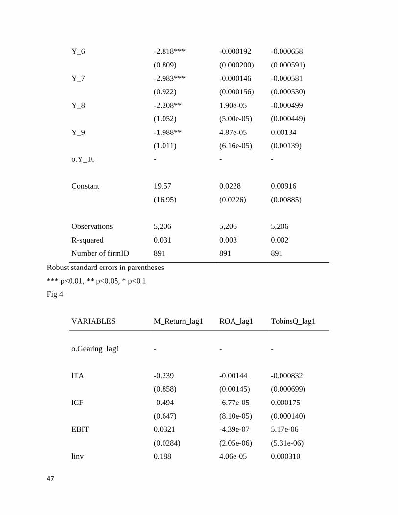
47

Y_6 -2.818*** -0.000192 -0.000658

(0.809) (0.000200) (0.000591)

Y_7 -2.983*** -0.000146 -0.000581

(0.922) (0.000156) (0.000530)

Y_8 -2.208** 1.90e-05 -0.000499

(1.052) (5.00e-05) (0.000449)

Y_9 -1.988** 4.87e-05 0.00134

(1.011) (6.16e-05) (0.00139)

o.Y_10 - - -

Constant 19.57 0.0228 0.00916

(16.95) (0.0226) (0.00885)

Observations 5,206 5,206 5,206

R-squared 0.031 0.003 0.002

Number of firmID 891 891 891

Robust standard errors in parentheses

*** p<0.01, ** p<0.05, * p<0.1

Fig 4

VARIABLES M_Return_lag1 ROA_lag1 TobinsQ_lag1

o.Gearing_lag1 - - -

lTA -0.239 -0.00144 -0.000832

(0.858) (0.00145) (0.000699)

lCF -0.494 -6.77e-05 0.000175

(0.647) (8.10e-05) (0.000140)

EBIT 0.0321 -4.39e-07 5.17e-06

(0.0284) (2.05e-06) (5.31e-06)

linv 0.188 4.06e-05 0.000310

48

(0.150) (4.62e-05) (0.000228)

g -3.242* -5.37e-05 -5.78e-05

(1.963) (8.59e-05) (6.15e-05)

2o.IND - - -

3o.IND - - -

4o.IND - - -

5o.IND - - -

6o.IND - - -

7o.IND - - -

8o.IND - - -

9o.IND - - -

10o.IND - - -

2o.region - - -

o.Y_1 - - -

Y_2 -2.013** -0.000350 0.000201

(0.861) (0.000357) (0.00104)

Y_3 -2.277*** 0.00132 -0.00149

(0.843) (0.00133) (0.00107)

Y_4 -1.927** -0.000310 -0.000637

(0.910) (0.000316) (0.000599)

49

Y_5 -2.816*** -0.000297 -0.000625

(0.852) (0.000302) (0.000576)

Y_6 -2.776*** -0.000245 -0.000580

(0.833) (0.000250) (0.000533)

Y_7 -3.058*** -0.000173 -0.000528

(0.967) (0.000180) (0.000491)

Y_8 -2.194** -1.80e-05 -0.000441

(1.108) (4.58e-05) (0.000406)

Y_9 -1.938* 1.33e-05 0.00139

(1.032) (3.74e-05) (0.00142)

o.Y_10 - - -

Constant 17.48 0.0233 0.00774

(15.57) (0.0232) (0.00789)

Observations 5,236 5,236 5,236

R-squared 0.028 0.003 0.002

Number of firmID 893 893 893

Robust standard errors in parentheses

*** p<0.01, ** p<0.05, * p<0.1

Fig 5

(1) (2) (3)

VARIABLES M_Return ROA TobinsQ

LEV -101.0* -7.376 0.106

(54.29) (12.16) (2.699)

lTA -0.813 -4.334*** -0.216**

(1.716) (0.384) (0.0853)

lCF 3.898*** 3.828*** 0.195***

(1.209) (0.271) (0.0601)

50

EBIT -0.0281 0.178*** 0.00760***

(0.0362) (0.00811) (0.00180)

Linv -0.460 0.0214 -0.0223

(0.355) (0.0795) (0.0176)

G 1.950*** 0.366*** 0.0135

(0.510) (0.114) (0.0253)

Observations 5,142 5,142 5,142

R-squared -0.488 0.459 0.036

Number of firmID 799 799 799

Fig 6

(1) (2) (3)

VARIABLES M_Return ROA TobinsQ

LEV -55.20* -3.241 3.401*

(30.64) (9.550) (1.976)

LEVsq -0.212* 0.0271 0.0140*

(0.118) (0.0368) (0.00761)

lTA -4.727*** -4.107*** -0.311***

(0.670) (0.209) (0.0432)

lCF 4.797*** 3.489*** 0.224***

(0.598) (0.186) (0.0386)

EBIT 0.000207 0.179*** 0.00745***

(0.0219) (0.00682) (0.00141)

linv -0.414* 0.0307 0.00698

(0.238) (0.0743) (0.0154)

g 0.348 0.496*** 0.0390

(0.409) (0.128) (0.0264)

51

Observations 4,588 4,588 4,588

R-squared -0.088 0.451 -0.166

Number of firmID 732 732 732

Standard errors in parentheses

*** p<0.01, ** p<0.05, * p<0.1

Fig 7

(1) (2) (3) (4) (5) (6)

VARIABLES M_Return ROA TobinsQ M_Return ROA TobinsQ

LEV -4.942*** -2.252*** 0.213**

(1.389) (0.453) (0.0961)

LEVsq -0.0368 0.0334*** 0.00365**

(0.0229) (0.00767) (0.00155)

lTA -5.169*** -4.122*** -0.338*** -4.767*** -4.593*** -0.326***

(0.413) (0.134) (0.0291) (0.526) (0.128) (0.0316)

lCF 5.179*** 3.743*** 0.219*** 5.660*** 4.135*** 0.240***

(0.283) (0.0957) (0.0189) (0.349) (0.0936) (0.0219)

EBIT 0.0156 0.166*** 0.00639*** 0.0358* 0.165*** 0.00809***

(0.0152) (0.00507) (0.00102) (0.0188) (0.00492) (0.00117)

linv 0.00978 0.168*** 0.00503 0.0291 0.176*** -0.00619

(0.146) (0.0475) (0.0101) (0.183) (0.0455) (0.0112)

g 0.841*** 0.308*** 0.0181 2.535*** 0.271*** 0.00862

(0.309) (0.106) (0.0203) (0.347) (0.0966) (0.0221)

Gearing 0.00351 -0.00799*** -0.00103***

(0.00509) (0.00134) (0.000317)

Gearingsq -6.27e-06 6.52e-06*** 1.04e-06**

(6.81e-06) (1.83e-06) (4.28e-07)

Constant 22.78*** 16.50*** 3.263*** 8.462 19.22*** 3.120***

(4.459) (1.368) (0.335) (5.877) (1.239) (0.333)

52

Observations 4,688 4,688 4,688 5,236 5,236 5,236

Number of firmID 832 832 832 893 893 893

Standard errors in parentheses

*** p<0.01, ** p<0.05, * p<0.1

(Robust) (Robust) (Robust)

Fig 8

(1) (2) (3)

VARIABLES M_Return_lag1 ROA_lag1 TobinsQ_lag1

LEV_lag1 -6.030 0.00218 -0.00261

(6.662) (0.00228) (0.00200)

LEVsq -0.0241 -2.18e-06 1.84e-05

(0.0215) (4.23e-06) (2.13e-05)

lTA 0.413 -0.00201 -0.000961

(0.729) (0.00201) (0.000805)

lCF -0.667 -2.64e-05 0.000173

(0.727) (6.45e-05) (0.000143)

EBIT 0.0505* 1.96e-06 3.80e-06

(0.0276) (3.50e-06) (4.53e-06)

linv 0.168 3.75e-05 0.000369

(0.138) (4.76e-05) (0.000272)

g -1.299*** -0.000115 -9.33e-05

(0.397) (0.000141) (8.37e-05)

2o.IND - - -

3o.IND - - -

4o.IND - - -

53

5o.IND - - -

6o.IND - - -

7o.IND - - -

8o.IND - - -

9o.IND - - -

10o.IND - - -

2o.region - - -

o.Y_1 - - -

Y_2 -1.956** -0.000334 0.000132

(0.846) (0.000347) (0.00118)

Y_3 -2.091*** 0.00153 -0.00176

(0.781) (0.00153) (0.00126)

Y_4 -1.829** -0.000291 -0.000812

(0.874) (0.000304) (0.000737)

Y_5 -2.643*** -0.000281 -0.000807

(0.765) (0.000292) (0.000715)

Y_6 -2.788*** -0.000248 -0.000734

(0.744) (0.000257) (0.000654)

Y_7 -2.357*** -0.000188 -0.000650

(0.752) (0.000199) (0.000589)

Y_8 -1.835** 1.20e-05 -0.000561

(0.934) (5.85e-05) (0.000500)

54

Y_9 -2.604*** 3.69e-05 0.00154

(0.958) (6.00e-05) (0.00159)

o.Y_10 - - -

Constant 11.03 0.0314 0.00995

(15.04) (0.0312) (0.00980)

Observations 4,667 4,667 4,667

R-squared 0.018 0.003 0.003

Number of firmID 829 829 829

Robust standard errors in parentheses

*** p<0.01, ** p<0.05, * p<0.1

Fig 9

(1) (2) (3)

VARIABLES M_Return_lag1 ROA_lag1 TobinsQ_lag1

o.Gearing_lag1 - - -

Gearingsq -8.32e-06*** 8.80e-10 1.07e-10

(1.98e-06) (9.38e-10) (3.02e-10)

lTA -0.175 -0.00145 -0.000833

(0.856) (0.00145) (0.000700)

lCF -0.551 -6.16e-05 0.000176

(0.649) (7.58e-05) (0.000141)

EBIT 0.0327 -5.08e-07 5.16e-06

(0.0284) (2.13e-06) (5.30e-06)

linv 0.212 3.80e-05 0.000310

(0.149) (4.41e-05) (0.000228)

g -3.236* -5.43e-05 -5.78e-05

(1.961) (8.59e-05) (6.15e-05)

55

2o.IND - - -

3o.IND - - -

4o.IND - - -

5o.IND - - -

6o.IND - - -

7o.IND - - -

8o.IND - - -

9o.IND - - -

10o.IND - - -

2o.region - - -

o.Y_1 - - -

Y_2 -2.072** -0.000344 0.000201

(0.859) (0.000351) (0.00104)

Y_3 -2.306*** 0.00133 -0.00149

(0.842) (0.00133) (0.00107)

Y_4 -1.999** -0.000302 -0.000636

(0.907) (0.000309) (0.000597)

Y_5 -2.876*** -0.000291 -0.000624

(0.851) (0.000296) (0.000575)

Y_6 -2.834*** -0.000239 -0.000579

56

(0.832) (0.000245) (0.000532)

Y_7 -3.102*** -0.000168 -0.000527

(0.966) (0.000175) (0.000490)

Y_8 -2.292** -7.66e-06 -0.000440

(1.107) (4.35e-05) (0.000404)

Y_9 -2.026** 2.25e-05 0.00139

(1.032) (4.20e-05) (0.00142)

o.Y_10 - - -

Constant 17.23 0.0233 0.00775

(15.56) (0.0232) (0.00790)

Observations 5,236 5,236 5,236

R-squared 0.030 0.003 0.002

Number of firmID 893 893 893

Robust standard errors in parentheses

*** p<0.01, ** p<0.05, * p<0.1

Fig. A

(1)

VARIABLES M_Return

LEV 1.147

(1.233)

Constant 6.997***

(0.418)

Observations 16,812

R-squared 0.000

Standard errors in parentheses

*** p<0.01, ** p<0.05, * p<0.1

The white test gives a chi2 of 0.92 and a p-value of 063.

57

Fig. B

Correlation matrix

LEV lTA lCF EBIT linv g

LEV 1

lTA 0.1557 1

lCF 0.0597 0.8964 1

EBIT 0.1493 -0.0189 0.0822 1

linv -0.0945 0.5806 0.492 -0.0208 1

g 0.0165 -0.1514 -0.1352 0.1546 -0.102 1

Graph 1.0

58

Section 9: References: Wippern, R.1966. Financial Structure and The Value of The Firm. The Journal of

Finance,21(4):615-633. Available from: https://onlinelibrary.wiley.com/doi/abs/10.1111/j.1540-

6261.1966.tb00270.x [Accessed: 20 May 2020]

Holz,Carsten A.2002. The Impact of The Liability-Asset Ratio on Profitability in China's

Industrial State-Owned Enterprises, China Economic Review,13: 1-26. Available from:

https://www.sciencedirect.com/science/article/abs/pii/S1043951X01000542 [Accessed: 20 May

2020]

Majumdar and Chhibber (1997). Capital structure and performance: Evidence from a

transition economy on an aspect of corporate governance. Capital structure and

performance: Evidence from a transition economy on an aspect of corporate governance.

https://www.coursehero.com/file/p2dfh9l/Majumdar...

Marchica, M.T. and Mura, R. (2010) Financial Flexibility, Investment Ability and Firm Value

Evidence from Firms with Space Debt Capacity. Financial Management, 39, 1339-1365.

https://www.scirp.org/reference/ReferencesPapers.aspx?ReferenceID=2434881

59

Gormley, T. A., & Matsa, D. A. (2011). Growing Out of Trouble? Corporate Responses to Liability

Risk.Review of Financial Studies,24 (8), 2781-2821.http://dx.doi.org/10.1093/rfs/hhr011

Gormley, Todd A.; Matsa, David A.; Milbourn, Todd. Journal of Accounting & Economics.

Dec2013 Supplement, Vol. 56, p79-101. 23p. DOI: 10.1016/j.jacceco.2013.08.001.

Fosu, S 2013, 'Capital structure, product market competition and firm performance: Evidence

from South Africa' The Quarterly Review of Economics and Finance, vol. 53, no. 2, pp. 140 -

151. DOI: 10.1016/j.qref.2013.02.004

Velnampy, T. and Anojan, V. (2014). Capital Structure, Liquidity Position and Their Impact

on Profitability: A study of Listed Telecommunication Firms in Colombo Stock Exchange, Sri

Lanka. Research Journal of Finance and Accounting, 5 (9), 131-139

https://www.iiste.org/Journals/index.php/RJFA/article/download/13046/13433

Hamada, R S 1969, Portfolio Analysis, Market Equilibrium and Corporate Finance, pp. 13-

31, The Journal of Finance Vol. 24, Available from: http://ecsocman.hse.

ru/data/856/126/1231/hamada_-_cs_1969.pdf [Accessed: 20 May 2020]

Baker, H K & Martin, G S 2011, Capital Structure and Corporate Financing Decision:

Theory, Evidence and Practise, pp. 75-90, John Wiley & Sons, Inc, New Jersey. Available

from: https://www.sciencedirect.com/science/article/abs/pii/S1043951X01000542 [Accessed:

20 May 2020]

Malcolm Baker, Jeffrey Wurgler (2002). Market Timing and Capital Structure. The Journal

of FinanceVolume 57, Issue 1. https://doi.org/10.1111/1540-6261.00414

Masulis, R W 1983, The Impact of Capital Structure Change on Firms Value: Some Estimates,

pp. 107-126, The American Finance Association, Available from: http:

//citeseerx.ist.psu.edu/viewdoc/download?doi=10.1.1.477.4201&rep=rep1&type=pdf

[Accessed: 20 May 2020]

Modigliani, F. and Miller, M.H. (1958). The Cost of Capital, Corporation Finance and the

Theory of Investment. The American Economic Review, Vol. 48, No. 3, pp. 261-297. Available

from https://www.jstor.org/stable/1812919 [Accessed: 20 May 2020]

60

Abor, J. (2005), "The effect of capital structure on profitability: an empirical analysis of listed

firms in Ghana", Journal of Risk Finance, Vol. 6 No. 5, pp. 438-445. Available from:

https://doi.org/10.1108/15265940510633505 Accessed by: 20th May 2020

Modigliani, F. and Miller, M.H. (1963). Corporation Income Taxes and the cost of capital; A

Correction. The American Economic Review, Vol. 53, No. 3, pp. 433-443. Available from

https://www.sciencedirect.com/science/article/pii/S2212567115008643 [Accessed: 20 May

2020]

Bris A, Welch I, Zhu N (2006). The Costs of Bankruptcy: Chapter 7 Liquidation versus

Chapter 11 Reorganization. The Journal of FinanceVolume 61, Issue 3.

https://doi.org/10.1111/j.1540-6261.2006.00872.x

Baltagi, B. H., (2013). Econometrics Analysis of Panel Data. 5th Edition, New York, John

Wiley & Sons Ltd. Available from: bcs.wiley.com/he-

bcs/Books?action=index&bcsId=4338&itemId=1118672321 [Accessed: 20 May 2020]

Masulis, R W & Korwar, A N 1986, Seasoned Equity Offerings: an Empirical Investigation,

pp. 91-118, Journal of Finance Economics 15, Available from: http://219.

219.114.96/cufe/upload_files/file/20140522/3_20140522_32%20Seasoned%20equity%

20offeringsAn%20empirical%20investigationOriginal%20Research%20Article. pdf

[Accessed: 20 May 2020]

Miller, M H1988, The Modigliani-Miller Propositions after Thirty Years, pp. 99-120, Journal

of Economic Perspectives Vol. 2, Available from: http://vip.opload.ir/ vipdl/94/4/zohreh/The-

Modigliani-Miller-Propositions-After-Thirty-Years. [Accessed: 20 May 2020]

Bhandari, LC1988, Debt/Equity Ratio and Expected Common Stock Returns: Empirical

evidence, The Journal of Finance vol. XLIII, Available from: Lund University Libraries.

[Accessed: 20 April 2020]

Shyam-Sunder, L & Myers, S C 1999, Testing Static Trade-off against Pecking Order Models

of Capital Structure, pp. 219-244, Journal of Finance Economics 51, Available from:

http://pages.stern.nyu.edu/~eofek/PhD/papers/SM_Testing_ JFE.pdf [Accessed: 18 May

2020]

61

Kinsman M. and Newman J. [1999]: "Debt Level and Corporate performance: An Empirical

Analysis", Proceedings of the 28th Annual Meeting of the Western Decision Sciences Institute,

April 6-10, 1999, Puerto Vallarta, Mexico. Available from:

https://www.researchgate.net/publication/228253634... [Accessed: 18 May 2020]

Altman, E. I., & Hotchkiss, E. S. (2006). Corporate financial distress and bankruptcy (3rd

edition). Hoboken, NJ: John Wiley & Sons1. Available from:

https://onlinelibrary.wiley.com/doi/book/10.1002/9781118267806 [Accessed: 18 May 2020]

Mwangi, L. W., Muathe, S.K., and Kosimbei, G. (2014). Relationship between Capital

Structure and Performance of Non-Financial Companies Listed in the Nairobi Securities

Exchange, Kenya. Global Journal of Contemporary Research in Accounting, Auditing and

Business Ethics, Vol.1 Issue 2. 72-90. Available from:

https://oapub.org/soc/index.php/EJEFR/article/view/412 [Accessed: 18 May 2020]

Booth, L., Aivazian, V., Demirguc-Kunt, A., & Maksimovic, V. (2001). Capital structure in

developing countries. Journal of Finance, 56, 87. Available from:

https://onlinelibrary.wiley.com/doi/abs/10.1111/0022-1082.00320 [Accessed: 10 May 2020]

Author(s): Carlos A. Molina Source: The Journal of Finance, Vol. 60, No. 3 (Jun., 2005), pp.

1427-1459 Published by: Wiley for the American Finance Association Stable Available from:

https://www.jstor.org/stable/3694931 [Accessed: 20 May 2020]

Tim C. Opler and Sheridan (1994). Titman Financial Distress and Corporate Performance.

The Journal of Finance, Vol. 49, No. 3, Papers and Proceedings Fifty-Fourth Annual Meeting

of the American Finance Association, Boston, Massachusetts, pp. 1015-1040 Published by:

Wiley for the American Finance Association Stable Available from :

https://www.jstor.org/stable/2329214. [Accessed: 20 May 2020]

Dhaliwal, D. S., Heitzman S., & Zhen Li, O. (2006). Taxes, leverage, and the cost of equity

capital. Journal of Accounting Research, 44(4), 691–723. Available from:

http://dx.doi.org/10.1111/j.1475-679X.2006.00214.x [Accessed: 10 May 2020]

Dimitrov, V., & Jain, P. C. (2008). The Value Relevance of Changes in Financial Leverage

beyond Growth in Assets and GAAP Earnings. Journal of Accounting, Auditing and Finance.

62

Available from: https://journals.sagepub.com/doi/full/10.1177/0972652715601910 [Accessed:

10 May 2020]

Arthur Korteweg (2010). The Net Benefits to Leverage. The Journal of Finance, Vol. 65, No.

6, pp. 2137-2170 Published by: Wiley for the American Finance Association Stable. Available

from: https://www.jstor.org/stable/23324407 [Accessed: 20 May 2020]

Gonzalez m. Gonzalez, (2012). Leverage and corporate performance: International evidence.

International Review of Economics and Finance. Available from:

https://www.researchgate.net/publication/271883261... [Accessed: 15 April 2020]

Denis Davydov (2016). Debt structure and corporate performance in emerging markets.

Research in International Business and Finance (Journal). Available from:

https://www.sciencedirect.com/science/article/pii/S0275531916300691 [Accessed: 15 April

2020]

Michael R. King & Eric Santor (2008). Family values: Owner structure, performance, and

capital structure of Canadian Firms. Journal of Banking & Finance. Available from:

https://papers.ssrn.com/sol3/Delivery.cfm/SSRN_ID... [Accessed: 15 April 2020]

Ahn, S., Denis, D.J., Denis, D.K., 2006. “Leverage and investment in diversified firms.”

Journal of Financial Economics 79, 317-337.

https://www.sciencedirect.com/science/article/pii/S0304405X05001510

Aivazian, V.A., Ge, Y., Qiu, J.P., 2005. “The impact of leverage on firm investment: Canadian

evidence,” Journal of Corporate Finance 11, 277-291.

https://www.onlinelibrary.wiley.com/doi/abs/10.1111/j.1755-053X.2005.tb00120.x

Chen Lin; Yue Ma; Paul Malatesta, & Yuhai Xuan. Corporate ownership structure and the

choice between bank debt and public debt. Journal of Financial Economics. Available from:

https://papers.ssrn.com/sol3/papers.cfm?abstract_id=2024308 [Accessed: 15 April 2020]

Carlos A. Molina, 2005,” Are Firms Underleveraged? An Examination of the Effect of

Leverage on Default Probabilities”, The Journal of Finance, pp. 1427-1459. Available from:

https://onlinelibrary.wiley.com/doi/abs/10.1111/j.1540-6261.2005.00766.x [Accessed: 15 April

2020]

63

Booth, Aivazian, Asli and Maksimovic, 2001,” Capital structure in developing countries”,

The Journal of Finance, pp. 87-130. Available from:

https://onlinelibrary.wiley.com/doi/abs/10.1111/0022-1082.00320 [Accessed: 15 April 2020]

Varouj A. Aivazian, Ying Geb, Jiaping Qiuc, 2005,” The impact of leverage on firm

investment: Canadian evidence”, Journal of Corporate Finance pp. 277-291. Available from:

pdfsr.com/pdf/the-impact-of-leverage-on-firm-investment-canadian-evidence [Accessed: 29

March 2020]

Corey Cole, Ying Yan and David Hemley (2015). Does Capital Structure Impact Firm

Performance: An Empirical. Journal of Accounting and Finance Vol. 15(6).

digitalcommons.www.na-businesspress.com/JAF/ColeC_Web15_6_.pdf

O.W. Ibhagui, F.O. Olokoyo. Leverage and firm performance: New evidence on the role of

firm size North American Journal of Economics and Finance 45 (2018) 57–82 58. Available

from: DOI: 10.1016/j.najef.2018.02.002 ... [Accessed: 29 March 2020]

Valentin Mitrov, Premc. Jaw, 2007,” The Value-Relevance of Changes in Financial Leverage

Beyond Growth in Assets and GAAP Earnings”, pp. 191-222. Available from:

https://www.emerald.com/insight/content/doi/10... [Accessed: 29 March 2020]

Murillo Campello, 2006,” Debt financing: Does it boost or hurt firm performance in product

markets?”, Journal of Financial Economics pp. 135-172. Available from:

https://www.sciencedirect.com/science/article/pii/S0304405X05001777 [Accessed: 29 March

2020]

Rao, Hamed, Al-yahee and Syed, (2007). Capital Structure and Financial Performance:

Evidence from Oman. Indian Journal of Economics and Business.

https://www.questia.com/library/journal/1G1...

Muradoglu, G. and S. Sivaprasad. 2009. Leverage, stock returns, taxes and industry

concentration. Retrieved on December 19, 2016, from http://ssrn.com/abstract=1031987.

Muradoglu, G. and S. Sivaprasad. 2012. Capital structure and abnormal returns.

International Business Review 21(3): 328–341.

https://www.sciencedirect.com/science/article/pii/S0969593111000473

64

Khalid, Ata et al. (2014) Terahertz oscillations in an In0.53Ga0.47As submicron planar gunn

diode. Journal of Applied Physics, 115 . p. 114502. Available from: ISSN 0021-897

[Accessed: 29 March 2020] http://eprints.gla.ac.uk/93202/

Hurdle, G.L., “Leverage Risk, Market Structure and Profitability”, Review of Economics and

Statistics, Vol.56, pp. 478-85, 1974.

Arthur Korteweg, 2010,” The Net Benefits to Leverage”, The Journal of Finance, pp. 2137 -

2170. Available from: https://onlinelibrary.wiley.com/doi/abs/10.1111/j.1540-

6261.2010.01612.x [Accessed: 29 March 2020]

Altman, E. I., & Hotchkiss, E. (2006). Corporate Financial Distress and Bankruptcy. John

Wiley & Sons. https://onlinelibrary.wiley.com/doi/book/10.1002/9781118267806

Jie Cai a, Zhe Zhang, 2011,” Leverage change, debt overhang, and stock prices”, journal of

Corporate Finance, pp. 391–402. Available from:

https://www.sciencedirect.com/science/article/pii/S0929119910001082 [Accessed: 29 March

2020]

A.Y Almajali, S. A Alamro, Yahya Z. Al-Soub. (2012). Factors Affecting the Financial

Performance of Jordanian Insurance Companies Listed at Amman Stock Exchange. Journal

of Management. Available from: DOI: https://doi.org/10.5296/jmr.v4i2.1482 Accessed: 29 March

2020]

Stulz, R.M. (1990) Managerial Discretion and Optimal Financing Policies. Journal of

financial Economics, 26, 3-27. Available from:

https://www.scirp.org/reference/ReferencesPapers.aspx?ReferenceID=2201699.

S0304405X05001777 [Accessed: 29 March 2020]

Dawar V. (2014). Agency theory, capital structure and firm performance: some Indian evidence.

Managerial Finance 40(12):1190-1206. Available from: DOI: 10.1108/MF-10-2013-0275.

Accessed: 29-04-2020 10:46

Marco Pagano, Ailsa A. Röell and Josef Zechner (2002). The Geography of Equity Listing:

Why Do Companies List Abroad? Source: The Journal of Finance, Vol. 57, No., 6 pp. 2651-

65

2694 Published by: Wiley for the American Finance Association Stable. Available from:

https://www.jstor.org/stable/3094540 Accessed: 29-04-2020 10:46

Acheampong, P, Agalega E & Shibu, A K 2013, The Effect of Financial Leverage and Market

Size on Stock Return on the Ghana Stock Exchange: Evidence from Selected Stocks in the

Manufacturing Sector, Pp. 125-134, International Journal Of Financial Research, Available

from: Www.sciedupress.com/journal/index.php/ijfr/article/viewFile/3973/2344 [Accessed:

29 March 2020]

John R. Graham and Campbell R. Harvey (2012). The Theory and Practice of Corporate

Finance: Evidence from the Field. Journal of Financial Economics. Available from:

https://faculty.fuqua.duke.edu/~charvey/Research/... Accessed: 29-04-2020

Ross S. [1977]. "The Determination of Financial Structure: The Incentive Signalling

Approach", Bell Journal of Economics 8, 23-40 Available from:

https://www.jstor.org/stable/3003485 [Accessed: 5 May 2020]

Ross, Stephen A., and Westerfield, Randolph W., and Jaffe, Jeffrey, (2002), “Corporate

Finance”, 6th edition, McGraw-Hill. https://www.mheducation.com/highered/product/...

Aivazian V., Ge Y., Qiu J., 2005. The impact of leverage on firm investment: Canadian

evidence. Journal of Corporate Finance 11, 277–291. Available from:

https://www.sciencedirect.com/science/article/pii/S0929119903000622 [Accessed: 5 May 2020]

Fred D. Ardatti 1967, The Effect of Financial Leverage and Market Size on Stock Returns on

the Karachi Stock Exchange: Evidence from Selected Stocks in the Non-Financial Sector of

Pakistan. The International Journal Of Business & Management, Vol. 5, Issue 10 Available

from: https://www.researchgate.net/publication/202329264.. [Accessed: 5 May 2020]

Adami, R, Gough, O, Muradoglu, Y G & Sivaprasad, S. 2015, How does a Firm’s Capital

Structure affect Stock Performance? Available from: Lund University Libraries. [Accessed:

10 April 2020]

Michael C. Jensen (1986). Agency Costs of Free Cash Flow, Corporate Finance, and

Takeovers. The American Economic Review, Vol. 76, No. 2, Papers and Proceedings of the

66

Ninety-Eighth Annual Meeting of the American Economic Association (May, 1986), pp. 323-

329. https://www.jstor.org/stable/1818789 .. [Accessed: 5 May 2020]

Penman, S H, Richardson S A & Tuna, 2007, The Book-to-price Effect in Stock Returns:

Accounting for Leverage, Journal of Accounting Research vol. 45, Available from:

http://citeseerx.ist.psu.edu/viewdoc/download?doi=10.1.1.421. 4711&rep=rep1&type=pdf

[Accessed: 5 May 2020]

Lang L., Ofek E., Stulz R.M., 1996. Leverage, investment and firm growth, Journal of

Financial Economics 40, 3–29. Available from:

https://papers.ssrn.com/sol3/papers.cfm?abstract_id=1669104 [Accessed: 5 May 2020]

. Stulz R.M., 1990. Managerial discretion and optimal financing policies. Journal of Financial

Economics 26, 3– 27. Available from:

https://www.sciencedirect.com/science/article/abs/pii/0304405X9090011N [Accessed: 5 May

2020]

Muradoglu, G., & Sivaprasad, S. (2008). An Empirical Analysis of Capital Structure and

Abnormal Returns. Retrieved from http://ssrn.com/abstract=948393. [Accessed: 5 May 2020]

Myers, S. (1977). Determinants of Corporate Borrowing. Journal of Financial Economics.

Available from: https://www.sciencedirect.com/science/article/pii/0304405X77900150

[Accessed: 5 May 2020]

Rajan, R., & Zingales, L. (1995). What Do We Know about Capital Structure? Some Evidence

from International Data. Journal of Finance, 50(5), 1421-1460. Available from:

https://www.sciencedirect.com/science/article/pii/0304405X77900150 [Accessed: 5 May 2020]

Ganiyu Y.O, Adelopo I, Rodionova Y (2019). Capital Structure and Firm Performance in

Nigeria. African Journal of Economic Review. Available from:

https://www.ajol.info/index.php/ajer/article/view/182550 [Accessed: 20 April 2020]

Kyereboah‐Coleman A. (2007). Corporate Governance and Shareholder Value Maximization: An

African Perspective. African Development Review. Available from:

https://doi.org/10.1111/j.1467-8268.2007.00165.x [Accessed: 20 April 2020]

67

Oyakhilome W. IbhaguiFelicia Omowunmi Olokoyo (2018). Leverage and firm performance:

New evidence on the role of firm size. The North American Journal of Economics and Finance.

Available from: DOI: 10.1016/j.najef.2018.02.002. [Accessed: 20 April 2020]

Psillaki, M., Tsolas, I.E. and Margaritis, D. (2010). Evaluation of Credit Risk Based on Firm

Performance. European Journal of Operational Research, 201(3), 873-888.

https://www.coursehero.com/file/p4falc0s/Psillaki...

Psillaki, M., Tsolas, I.E. and Margaritis, D. (2007). Capital Structure and Firm Efficiency.

Journal of Business Finance & AccountingVolume 34, Issue 9‐10.

https://doi.org/10.1111/j.1468-5957.2007.02056.x

George and Hwang (2009). A resolution of the distress risk and leverage puzzles in the cross

section of returns. Journal of Financial Economics 96(1):56-79. Available from: DOI:

10.1016/j.jfineco.2009.11.003. [Accessed: 20 April 2020]

Ibrahim El‐Sayed Ebaid (2009). The impact of capital-structure choice on firm performance:

empirical evidence from Egypt. Journal of Risk Finance. Available from:

https://econpapers.repec.org/RePEc:eme:jrfpps:v:10:y:2009:i:5:p:477-487 [Accessed: 20 April

2020]

Feng-Li Lin & T sangyao Chang (2011): Does debt affect firm value in T aiwan? A panel

threshold regression analysis, Applied Economics, 43:1, 117-128, Available from:

https://www.researchgate.net/publication/227606411_Does_debt_affect... [Accessed: 20 April

2020]

Roberta DessÌ & Donald Robertson, 2003. "Debt, Incentives and Performance: Evidence

from UK Panel Data," Economic Journal, Royal Economic Society, vol. 113.

https://ideas.repec.org/a/ecj/econjl/v113y2003i490p903-919.html

George, T J & Hwang, C Y 2009, A Resolution of the Distress Risk and Leverage Puzzles in

the Cross Section of Stock Returns, The Journal of Financial Economics, Available from:

http://citeseerx.ist.psu.edu/viewdoc/download?doi=10.1.1.452.8994&rep=rep1&type=pdf

[Accessed: 20 April 2020]

68

J.J McConnell, H Servaes (1995). Equity ownership and the two faces of debt. Journal of

Financial Economics, 39 (1995), pp. 131-157. https://doi.org/10.1016/0304-405X(95)00824-X

Kovenock, D., and G. Phillips, 1997, "Capital Structure and Product Market Behavior: An

Examination of Plant Exit and Investment Decisions," Review of Financial Studies, 10, 767-

803. https://pdfs.semanticscholar.org/b570/fe39bedd7f97d48aa164dba5c0ce9e234562.pdf

Owolabi, S. & inyang,U (2013). International Pragmatic Review and Assessment of Capital

Structure Determinants. Kuwait Chapter of Arabian Journal of Business and Management

Review Vol. 2, No.6. https://www.arabianjbmr.com/pdfs/KD_VOL_2_6/10.pdf

Myers, S C 1984, The Capital Structure Puzzle, pp. 575-592, Journal of Finance 39.

http://lib.cufe.edu.cn/upload_files/file/20140522/3_20140522_35%20Myers,%20Stewart%2

0C.,%201984,%20The%20capital%20structure% 20puzzle.pdf [Accessed: 20 April 2020]

https://us.spindices.com/documents/methodologies/methodology-dj-global-indices.pdf

[Accessed: 20 April 2020]

Phillips, P. A., & Sipahioglu, M. A. (2004). Performance implications of capital structure;

evidence from quoted U. K. organisations with hotel interests. The Services Industry Journal,

24(5), 1–21. https://www.tandfonline.com/doi/abs/10.1080/0264206042000276829

Toraman, C., Kihc, Y., & Reis, S.G. (2013). “The Effects of Capital Structure Decisions on

Firm Performance: Evidence from Turkey”. International Conference on Economic and

Social Studies. 10-11 May, 2013. Sarajevo. 137-145.

https://www.researchgate.net/publication/328916442...

Abor, J. (2005). The effect of capital structure on profitability: An empirical analysis of listed

firms in Ghana. Journal of Risk Finance, 6(5), 16–30. Akinlo, O., & Asaolu, T. (2012).

Profitability and leverage: Evidence from Nigerian firms. Global Journal of Business

Research, 6(1), 17–25. Brick, I. E., & Ravid, S. A. (1985). On the relevance of debt maturity

structure. Journal of Finance, 40, 1423–1437. Chandrakumarmangalam, S., & Govindasamy,

69

P. (2010). Leverage- an analysis and its impact on profitability with reference to selected

cement companies in India. European Journal of Economics, Finance and Administrative

Sciences, 27, 1450–2275.

Chen, J. J. (2004). Determinants of capital structure of chinese listed companies. Journal of

Business Research, 57, 1341–1351.

Cheng, Y., Liu, Y., & Chien, C. (2010). Capital structure and firm value in china panel

threshold regression analysis. African Journal of Business Management, 4(12), 2500–2507.

Fama, E. F., & French, K. R. (1998). Taxes, financing decision and firm value. The Journal

of Finance, 53.

Hansen, B. E. (1999). Threshold effects in non-dynamic panels: estimation, testing, and

inference. Journal of Econometrics, 93, 345–368.

Jeleel, A., & Olayiwola, B. (2017). Effect of leverage on firm performance in nigeria: A case

of listed chemicals and paints firms in Nigeria. Global Journal of Management and Business

Research: Accounting and Auditing.

Jensen, M. (1986). Agency costs of free cash flow, corporate finance and takeovers. American

Economic Review, 76(2), 323–329.

Kebewar, M. (2013). The effect of debt on corporate profitability: Evidence from French

service sector. Brussels Economic Review, 56(1), 43–59.

Klapper, L. F., & Love, I. (2004). Corporate governance, investor protection, and

performance in emerging markets. Journal of Corporate Finance, 10(5), 703–728.

Lin, F., & Chang, T. (2011). Does debt affect firm value in taiwan? a panel threshold

regression analysis. Applied Economics, 43, 117–128.

Mashayekhi, B., & Bazaz, M. S. (2008). Corporate governance and firm performance in Iran.

Journal of Contemporary Accounting and Economics, 4(2), 156–172.

Modigliani, F., & Miller, M. (1958). The cost of capital, corporate finance and the theory of

investment. American Economic Review, 48, 261–297.

70

Negash, M. (2001). Debt, Tax shield and bankruptcy costs: some evidence from johannesburg

stock exchange. Investment Analysis Journal, 54(3), 114–128. Nwankwo, Odi (2014). Effect

of capital structure of nigeria firms on economic growth. Mediterranean Journal of Social

Sciences, 5(1), 515–519.

Olokoyo, F. O. (2013). Capital structure and corporate performance of nigerian quoted firms:

A panel data approach. African Development Review, 25(3), 358–369.

Olokoyo, F. O. (2012). Capital structure and corporate performance of nigerian quoted

firms: A panel data approach. African Development Review, 25(3), 358–369.

Onaolapo, A., & Kajola, S. (2010). Capital structure and firm performance: evidence from

Nigeria. European Journal of Economics, Finance and Administrative Sciences ISSN 1450.

Patrick. O., & Ogebe, J. O. (2013), The Impact of Capital Structure on Firms’ Performance

in Nigeria. http://mpra.ub.uni-muenchen.de/45986/.

Pratheepkanth, P. (2011). Capital structure and financial performance: evidence from

selected business companies in colombo stock exchange Sri Lanka. Journal of Arts, Science

and Commerce, 23.

Pratomo, W. A., & Ismail, A. G. (2006) Islamic bank performance and capital structure.

MPRA Paper No 6012.

Robb, A., & Robinson, D. T. (2009), The capital structure decision of new firms [Online]

Available: http://papers.ssrn.com/so13/papers.cfm?abstract-id=1345895 [Accesssed: 17

October 2009].

Ruland, W., & Zhou, P. (2005). Debt, diversification and valuation. Review of Quantitative.

Financial. Accounting, 25(3), 277–291.

Salawu, R. O. (2007). An empirical analysis of the capital structure of selected quoted

companies in Nigeria. The International Journal of Applied Economics and Finance, 1(1),

16–28.

Simon-Oke, O. O., & Afolabi, B. (2011). Capital structure and industrial performance in

Nigeria (1997–2007). International Business and Management, 2(1), 100–106.

71

Tian, G.G., & Zeitun, R. (2007). Capital structure andcorporate performance: Evidence from

Jordan. Australasian Accounting Business and Finance Journal, 1(4), 40–61.

Further reading

Cuong, N. T. (2012). Threshold effect of capital structure on firm value: evidence from

seafood processing enterprises in the south-central region of Vietnam. International Journal

of Finance and Banking Studies, 3(3), 14–29.

Vo, D., & Phan, T. (2013). Corporate governance and firm performance: Empirical evidence

from Vietnam. http://www.murdoch.edu.au/School-of-

ManagementandGovernance/_document/Australian-Conference-ofEconomists/Corporate-

governance-and-firm-performance.pdf, 03.12.2013.

O.

72

Section 10: Appendix

ROA relationship with leverage

Yxt = ROA, b1xt = leverage

Hypothesis 1 (H1)

ROA𝑥𝑡 = 𝑏𝑜 + 𝑏1LEV𝑥𝑡 + 𝑏2lTA𝑥𝑡 + 𝑏3lCF𝑥𝑡 + 𝑏4EBIT𝑥𝑡 + 𝑏5Iinv𝑥𝑡 + 𝑏6g𝑥𝑡

+ ɛ𝑥𝑡 𝑒𝑞𝑢 (3.1)

Robust Test

𝑅𝑂𝐴𝑥𝑡 − 1 = 𝑏𝑜 + 𝑏1LEV𝑥𝑡 − 1 + 𝑏2lTA𝑥𝑡 + 𝑏3lCF𝑥𝑡 + 𝑏4EBIT𝑥𝑡 + 𝑏5Iinv𝑥𝑡

+ 𝑏6g𝑥𝑡 + 𝑏7𝑖. 𝐼𝑁𝐷 + 𝑏8𝑖. 𝑟𝑒𝑔 + 𝑏9𝑖. 𝑌𝑟 + 𝑎𝑥𝑡 + ɛ𝑥𝑡 𝑒𝑞𝑢(3.2)

ROA𝑥𝑡𝑖𝑣^2 = 𝑏𝑜 + (𝑏1 LEV𝑥𝑡 = 𝑇𝑇𝐴) + 𝑏2lTA𝑥𝑡 + 𝑏3 lCF𝑥𝑡 + 𝑏4EBIT𝑥𝑡

+ 𝑏5Iinv𝑥𝑡 + 𝑏6g𝑥𝑡 + 𝑎 𝑥𝑡 + ɛ𝑥𝑡 (𝑓𝑖𝑟𝑠𝑡) 𝑒𝑞𝑢 (3.3)

Second Hypothesis (H2)

𝑅𝑂𝐴𝑥𝑡 = 𝑏𝑜 + 𝑏1LEV𝑥𝑡 + 𝑏1𝐿𝐸𝑉𝑥𝑡2 + 𝑏2lTA𝑥𝑡 + 𝑏3lCF𝑥𝑡 + 𝑏4EBIT𝑥𝑡 + 𝑏5Iinv𝑥𝑡

+ 𝑏6g𝑥𝑡 + ɛ𝑥𝑡 𝑒𝑞𝑢(3.4)

Robust Test

ROA𝑥𝑡𝑖𝑣2 = 𝑏𝑜 + (𝑏1 LEV𝑥𝑡 = 𝑇𝑇𝐴) + 𝑏1𝐿𝐸𝑉𝑥𝑡2 + 𝑏2lTA𝑥𝑡 + 𝑏3 lCF𝑥𝑡 + 𝑏4EBIT𝑥𝑡

+ 𝑏5Iinv𝑥𝑡 + 𝑏6g𝑥𝑡 + 𝑎 𝑥𝑡 + ɛ𝑥𝑡 (𝑓𝑖𝑟𝑠𝑡) 𝑒𝑞𝑢 (3.5)

73

Tobin’s Q relationship with leverage

Yxt = Tobin’s Q, b1xt = Leverage

H1: base model

TobinsQ𝑥𝑡 = 𝑏𝑜 + 𝑏1LEV𝑥𝑡 + 𝑏2lTA𝑥𝑡 + 𝑏3lCF𝑥𝑡 + 𝑏4EBIT𝑥𝑡 + 𝑏5Iinv𝑥𝑡 + 𝑏6g𝑥𝑡

+ ɛ𝑥𝑡 𝑒𝑞𝑢 (4.1)

Robust Test

TobinsQ𝑥𝑡 = 𝑏𝑜 + 𝑏1LEV𝑥𝑡 + 𝑏2lTA𝑥𝑡 + 𝑏3lCF𝑥𝑡 + 𝑏4EBIT𝑥𝑡 + 𝑏5Iinv𝑥𝑡 + 𝑏6g𝑥𝑡

+ 𝑏7𝑖. 𝐼𝑁𝐷 + 𝑏8𝑖. 𝑟𝑒𝑔 + 𝑏9𝑖. 𝑌𝑟 + 𝑎𝑥𝑡 + ɛ𝑥𝑡 𝑒𝑞𝑢(4.2)

TobinsQ𝑥𝑡𝑖𝑣^2

= 𝑏𝑜 + (𝑏1 LEV𝑥𝑡 = 𝑇𝑇𝐴) + 𝑏2lTA𝑥𝑡 + 𝑏3 lCF𝑥𝑡 + 𝑏4EBIT𝑥𝑡

+ 𝑏5Iinv𝑥𝑡 + 𝑏6g𝑥𝑡 + 𝑎 𝑥𝑡 + ɛ𝑥𝑡 (𝑓𝑖𝑟𝑠𝑡) 𝑒𝑞𝑢 (4.3)

Second Hypothesis (H2)

TobinsQ𝑥𝑡𝑖𝑣^2 = 𝑏𝑜 + (𝑏1 LEV𝑥𝑡 = 𝑇𝑇𝐴) + 𝑏1𝐿𝐸𝑉𝑥𝑡2 + 𝑏2lTA𝑥𝑡 + 𝑏3 lCF𝑥𝑡 +

𝑏4EBIT𝑥𝑡 + 𝑏5Iinv𝑥𝑡 + 𝑏6g𝑥𝑡 + 𝑎 𝑥𝑡 + ɛ𝑥𝑡 𝑒𝑞𝑢 (4.4)

Market Return relationship with Gearing

Yxt = Market Return, b1xt = Gearing

H1

M_Return 𝑥𝑡 = 𝑏𝑜 + 𝑏1Gearing𝑥𝑡 + 𝑏2lTA𝑥𝑡 + 𝑏3lCF𝑥𝑡 + 𝑏4EBIT𝑥𝑡 + 𝑏5Iinv𝑥𝑡

+ 𝑏6g𝑥𝑡 + ɛ𝑥𝑡 𝑒𝑞𝑢 (5.1)

Robust Test

MReturn𝑥𝑡 − 1

= 𝑏𝑜 + 𝑏1Gearing𝑥𝑡 − 1 + 𝑏2lTA𝑥𝑡 + 𝑏3lCF𝑥𝑡 + 𝑏4EBIT𝑥𝑡 + 𝑏5Iinv𝑥𝑡

+ 𝑏6g𝑥𝑡 + 𝑏7𝑖. 𝐼𝑁𝐷 + 𝑏8𝑖. 𝑟𝑒𝑔 + 𝑏9𝑖. 𝑌𝑟 + 𝑎𝑥𝑡 + ɛ𝑥𝑡 𝑒𝑞𝑢(5.2)

Second Hypothesis (H2)

MReturn𝑥𝑡 = 𝑏𝑜 + 𝑏1Gearing𝑥𝑡 + 𝑏1Gearing𝑥𝑡𝑥𝑡2 + 𝑏2lTA𝑥𝑡 + 𝑏3lCF𝑥𝑡 + 𝑏4EBIT𝑥𝑡

+ 𝑏5Iinv𝑥𝑡 + 𝑏6g𝑥𝑡 + ɛ𝑥𝑡 𝑒𝑞𝑢 (5.3)

74

Robust Test

MReturn𝑥𝑡 − 1

= 𝑏𝑜 + 𝑏1Gearing𝑥𝑡 − 1 + 𝑏1Gearing𝑥𝑡𝑥𝑡2 + 𝑏2lTA𝑥𝑡 + 𝑏3lCF𝑥𝑡

+ 𝑏4EBIT𝑥𝑡 + 𝑏5Iinv𝑥𝑡 + 𝑏6g𝑥𝑡 + 𝑏7𝑖. 𝐼𝑁𝐷 + 𝑏8𝑖. 𝑟𝑒𝑔 + 𝑏9𝑖. 𝑌𝑟 + 𝑎𝑥𝑡

+ ɛ𝑥𝑡 𝑒𝑞𝑢(5.4)

ROA relationship with Gearing

Yxt = ROA, b1xt = Gearing

H1

ROA 𝑥𝑡 = 𝑏𝑜 + 𝑏1Gearing𝑥𝑡 + 𝑏2lTA𝑥𝑡 + 𝑏3lCF𝑥𝑡 + 𝑏4EBIT𝑥𝑡 + 𝑏5Iinv𝑥𝑡

+ 𝑏6g𝑥𝑡 + ɛ𝑥𝑡 𝑒𝑞𝑢 (6.1)

Robust Test

ROA 𝑥𝑡 − 1 = 𝑏𝑜 + 𝑏1Gearing𝑥𝑡 − 1 + 𝑏2lTA𝑥𝑡 + 𝑏3lCF𝑥𝑡 + 𝑏4EBIT𝑥𝑡 + 𝑏5Iinv𝑥𝑡

+ 𝑏6g𝑥𝑡 + 𝑏7𝑖. 𝐼𝑁𝐷 + 𝑏8𝑖. 𝑟𝑒𝑔 + 𝑏9𝑖. 𝑌𝑟 + 𝑎𝑥𝑡 + ɛ𝑥𝑡 𝑒𝑞𝑢(6.2)

Second hypothesis

ROA 𝑥𝑡 = 𝑏𝑜 + 𝑏1Gearing𝑥𝑡 + 𝑏1Gearing𝑥𝑡2 + 𝑏2lTA𝑥𝑡 + 𝑏3lCF𝑥𝑡 + 𝑏4EBIT𝑥𝑡

+ 𝑏5Iinv𝑥𝑡 + 𝑏6g𝑥𝑡 + ɛ𝑥𝑡 𝑒𝑞𝑢 (6.3)

Robust Test

ROA 𝑥𝑡 − 1 = 𝑏𝑜 + 𝑏1Gearing𝑥𝑡 − 1 + 𝑏1Gearing𝑥𝑡2 + 𝑏2lTA𝑥𝑡 + 𝑏3lCF𝑥𝑡

+ 𝑏4EBIT𝑥𝑡 + 𝑏5Iinv𝑥𝑡 + 𝑏6g𝑥𝑡 + 𝑏7𝑖. 𝐼𝑁𝐷 + 𝑏8𝑖. 𝑟𝑒𝑔 + 𝑏9𝑖. 𝑌𝑟 + 𝑎𝑥𝑡

+ ɛ𝑥𝑡 𝑒𝑞𝑢(6.4)

Tobin’s Q relationship with Gearing

Yxt = Tobin’s Q, b1xt = Gearing

H1

TobinsQ𝑥𝑡 = 𝑏𝑜 + 𝑏1Gearing𝑥𝑡 + 𝑏2lTA𝑥𝑡 + 𝑏3lCF𝑥𝑡 + 𝑏4EBIT𝑥𝑡 + 𝑏5Iinv𝑥𝑡

+ 𝑏6g𝑥𝑡 + ɛ𝑥𝑡 𝑒𝑞𝑢 (7.1)

75

Robust Test

TobinsQ𝑥𝑡 − 1

= 𝑏𝑜 + 𝑏1Gearing𝑥𝑡 − 1 + 𝑏2lTA𝑥𝑡 + 𝑏3lCF𝑥𝑡 + 𝑏4EBIT𝑥𝑡

+ 𝑏5Iinv𝑥𝑡 + 𝑏6g𝑥𝑡 + 𝑏7𝑖. 𝐼𝑁𝐷 + 𝑏8𝑖. 𝑟𝑒𝑔 + 𝑏9𝑖. 𝑌𝑟 + 𝑎𝑥𝑡

+ ɛ𝑥𝑡 𝑒𝑞𝑢(7.2)

Second Hypothesis (H2)

TobinsQ𝑥𝑡 = 𝑏𝑜 + 𝑏1Gearing𝑥𝑡 + 𝑏1Gearing𝑥𝑡2 + 𝑏2lTA𝑥𝑡 + 𝑏3lCF𝑥𝑡 + 𝑏4EBIT𝑥𝑡

+ 𝑏5Iinv𝑥𝑡 + 𝑏6g𝑥𝑡 + ɛ𝑥𝑡 𝑒𝑞𝑢 (7.3)

Robust Test

TobinsQ𝑥𝑡 − 1

= 𝑏𝑜 + 𝑏1Gearing𝑥𝑡 − 1 + 𝑏1Gearing𝑥𝑡2 + 𝑏2lTA𝑥𝑡 + 𝑏3lCF𝑥𝑡

+ 𝑏4EBIT𝑥𝑡 + 𝑏5Iinv𝑥𝑡 + 𝑏6g𝑥𝑡 + 𝑏7𝑖. 𝐼𝑁𝐷 + 𝑏8𝑖. 𝑟𝑒𝑔 + 𝑏9𝑖. 𝑌𝑟 + 𝑎𝑥𝑡

+ ɛ𝑥𝑡 𝑒𝑞𝑢(7.4)