PHYSICAL REVIEW B 84, 125433 (2011)

Decoupling conservative and dissipative forces in frequency modulation atomic force microscopy

Aleksander Labuda,* Yoichi Miyahara, Lynda Cockins, and Peter H. GrutterDepartment of Physics, McGill University, 3600 University, Montreal, Canada, H3A 2T8

(Received 1 June 2011; published 15 September 2011)

Experiments and theoretical calculations of conservative forces measured by frequency modulation atomicforce microscopy (FM-AFM) in vacuum are generally in reasonable agreement. This contrasts with dissipativeforces, where experiment and theory often disagree by several orders of magnitude. These discrepancies haverepeatedly been attributed to instrumental artifacts, the cause of which remains elusive. We demonstrate thatthe frequency response of the piezoacoustic cantilever excitation system, traditionally assumed flat, can actuallylead to surprisingly large apparent damping by the coupling of the frequency shift to the drive-amplitude signal,typically referred to as the “dissipation” signal. Our theory predicts large quantitative and qualitative variabilityobserved in dissipation spectroscopy experiments, contrast inversion at step edges and in atomic-scale dissipationimaging, as well as changes in the power-law relationship between the drive signal and bias voltage in dissipationspectroscopy. The magnitude of apparent damping can escalate by more than an order of magnitude at cryogenictemperatures. We present a simple nondestructive method for correcting this source of apparent damping, whichwill allow dissipation measurements to be reliably and quantitatively compared to theoretical models.

DOI: 10.1103/PhysRevB.84.125433 PACS number(s): 68.37.Ps, 07.79.Lh

I. INTRODUCTION

Since its invention in 1991, frequency modulation atomicforce microscopy1 (FM-AFM) has proven to be an indispens-able method for probing forces at the atomic scale in vacuumenvironments. The heart of the instrument is a cantilever thatis self-excited at its natural frequency, which shifts upon inter-action with a sample under study. The cantilever oscillationamplitude is kept constant by an automatic-gain-controller(AGC), which adjusts the amplitude of the drive signal usedto actuate the cantilever by piezoacoustic excitation. Onenominal advantage of FM-AFM over other techniques is thedecoupling of conservative and dissipative forces: the shiftof the self-excited oscillation frequency is proportional to theeffective interaction stiffness,2 while the drive amplitude ofthe AGC directly relates to the interaction damping with negli-gible coupling between both signals.3,4 This situation shouldgreatly simplify the interpretation of data acquired by FM-AFM.

The unprecedented understanding and control of tip-sampleconservative forces in FM-AFM has enabled impressiveroom-temperature manipulation of single atoms5 and chemicalidentification of individual surface atoms,6 for example. On theother hand, the poorly understood dissipation measurementsusing FM-AFM have mainly been the source of questions7 andcontroversies.8,9

Dissipation contrast mechanisms in FM-AFM havebeen extensively studied from both experimental10–17 andtheoretical18–28 perspectives. Although most postulated dis-sipation mechanisms have been experimentally verified, thevariability in the data often exceeds theoretical predictionsby orders of magnitude.29,30 The large discrepancies betweentheory and experiment have led to the notion of “apparentdamping”—also known as “apparent dissipation.”31 It refersto any change in the drive amplitude that is not related totip-sample dissipative forces; rather, it is assumed to be causedby nonideal behavior of the instrument. Despite numerousinvestigations,11,29,32 the large variability in experimentalobservations remains elusive.

At the forefront of nanoscience, many experimentsperformed at cryogenic temperatures identify theoreticallypredicted physical processes with FM-AFM dissipation mea-surements. The degenerate energy-level structure in quantumdots was identified by measuring the amplitude dependenceof dissipation.33–35 The suppression of electronic frictionon Nb films in the superconducting state was identified bya change in the power law between the dissipation andbias voltage (V 2 → V 4).36 The chemical identification oftip-apex termination37 and recognition of atomic speciesat semiconductor surfaces38 are aided by measurements ofsingle atomic-contact adhesion studied by dissipation-distancespectroscopy.

Our detailed analysis of FM-AFM clearly demonstrates thatdrawing robust conclusions from dissipation experiments re-quires an accurate measurement of the transfer function of thepiezoacoustic excitation system used to oscillate the cantilever.Omitting this measurement can lead to false interpretation ofchanges in the drive signal, which relate to the physics ofthe FM-AFM system as opposed to tip-sample physics. Forexample, the piezoacoustic transfer function can cause contrastinversion at step edges or in atomic contrast in dissipationimages, as well as change the dependence between the drivesignal and bias voltage from quadratic to quartic, or com-pletely distort dissipation-distance spectroscopy results bothquantitatively and qualitatively. Notably, although the piezoa-coustic transfer function affects measurements performed atany temperature, it becomes exceedingly problematic at cryo-genic temperatures at which sensitive dissipation experimentare being performed.

In this study, we discuss the apparent damping causedby the piezoacoustic excitation transfer function. Recentcommunications39,40 have derived theories and methods foreliminating this source of apparent damping in air andliquid environments. Here, we present a theory tailored forvacuum environments, demonstrate a noninvasive method forits implementation, and assess its impact on a wide range ofdissipation experiments at different temperatures.

125433-11098-0121/2011/84(12)/125433(11) ©2011 American Physical Society

LABUDA, MIYAHARA, COCKINS, AND GRUTTER PHYSICAL REVIEW B 84, 125433 (2011)

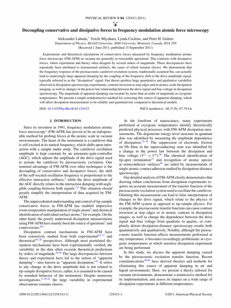
FIG. 1. (Color online) The amplitude |X | and phase θX compo-nents of the piezoacoustic excitation transfer function X (ω) acquiredat two different temperatures. This measurement was obtained bypiezoacoustically driving a cantilever well below its resonancefrequency (∼160 kHz) and detecting its response with a lock-inamplifier across [70, 100] kHz. The mechanical cantilever transferfunction is approximately flat within this frequency range. Both |X |and θX are much more corrugated at lower temperatures as the qualityfactors of mechanical components of the AFM increase. Assumingthat X (ω) is flat leads to a false interpretation of the drive signalacquired during an experiment. Our choice for using a logarithmicscale for |X | is important and justified elsewhere (see supplementarymaterial, Sec. 244).

II. MOTIVATION

Figure 1 displays a measurement of the transfer functionof the piezoacoustic excitation system X (ω), which describeshow the piezoelectric transducer converts the drive voltage ofthe AGC into an effective force felt by the cantilever tip. Thismeasurement was acquired by piezoacoustically driving thecantilever well below resonance where its transfer function isnearly flat and the driven cantilever response reflects changesin X (ω). Figure 1 demonstrates that X (ω) is far from flatin vacuum environments: hardware components mechanicallycoupled to the cantilever and piezoelectric transducer causespurious resonances. In fact X (ω) can be more corrugatedin vacuum than in liquid environments, where it is typicallyreferred to as the “forest of peaks” (see supplementarymaterial, Sec. 141). Furthermore, cooling the vacuum AFM to77 K greatly accentuates features inX (ω), as seen in Fig. 1; justas the cantilever quality factor Q increases, the quality factor ofeach spurious resonance also increases. These measurementsof the phase θX and amplitude |X | components ofX (ω) clearlydemonstrate that both carry a strong frequency dependence.This has profound effects on FM-AFM measurements, asdescribed in the following paragraphs.

The frequency dependence of θX , commonly assumednegligible, affects the tracking of the cantilever resonancefrequency and thus modifies the measured frequency shift �ω

caused by conservative interactions with the sample.42,43 Thisproblem disappears as Q → ∞ (see supplementary material,

Sec. 244), such that the effect of θX can usually be neglectedwhen the conservative force is calculated from �ω in vacuumexperiments where Q is large. However, it is important to notethat the cantilever phase is not kept constant in the presence ofa nonflat θX , regardless of Q. This is explained by the fact thatthe cantilever self-oscillates by positive feedback, such that thetotal phase around the self-excitation loop is always an integermultiple of −360◦. If θX varies by 10◦ upon some frequencyshift, the cantilever phase will change by −10◦ to compensate.This fact holds even if the phase spectrum of the self-excitationelectronics is flat compared to θX , as was verified on our system(see supplementary material, Sec. 445). Driving a cantileveroff resonance is less efficient, resulting in an increase of thedrive amplitude necessary to maintain a constant oscillationamplitude. Importantly, this increase in drive amplitude isnot related to tip-sample dissipative processes—it is purelyinstrumental.

The amplitude spectrum |X | does not affect the tracking ofthe cantilever resonance, however, it determines the efficiencyfor driving the cantilever at any given frequency. If |X |increases by 10% upon some frequency shift �ω, the driveamplitude will decrease by 10% simply to maintain a constantcantilever amplitude. Again, this decrease in drive amplitudeis not related to tip-sample dissipative processes.

These heuristic explanations suggest that θX and |X | mustbe considered when deriving the relationship between the driveamplitude and the damping due to tip-sample interaction. Inother words, the drive-amplitude signal is expected to have afrequency dependence which must be corrected.

III. THEORY

This section presents the derivation which relates thedrive amplitude to the tip-sample damping in FM-AFM invacuum environments. Alternatively, this derivation can alsobe performed in the time-domain based on the approach ofHolscher et al.;46 see supplementary material, Sec. 3.47

To high accuracy, a cantilever in vacuum environments canbe modeled as a damped harmonic oscillator with a transferfunction C(ω) in units of m/N, which describes the responseof the cantilever to a driving force exerted by the piezoacousticexcitation system. The amplitude component of C(ω) is definedby (see Appendix)

|C(ω)| = − sin θC(ω)

ω × γ, (1)

where θC(ω) is the phase spectrum of the cantilever, and γ

is the damping (in Ns/m). Although this form of the transferfunction is mathematically identical to the more conventionalform, it provides a more useful way to describe the cantileverin the context of FM-AFM as it allows us to directly distinguishhow changes in phase, drive frequency, and damping affect thecantilever amplitude response.

With this definition, the cantilever response before any tip-sample interaction is simply

|C(ωs)| = − sin θCs

ωs × γs

, (2)

where θCs , ωs , and γs are the phase of the cantilever,the self-excited oscillation frequency, and the damping; the

125433-2

DECOUPLING CONSERVATIVE AND DISSIPATIVE . . . PHYSICAL REVIEW B 84, 125433 (2011)

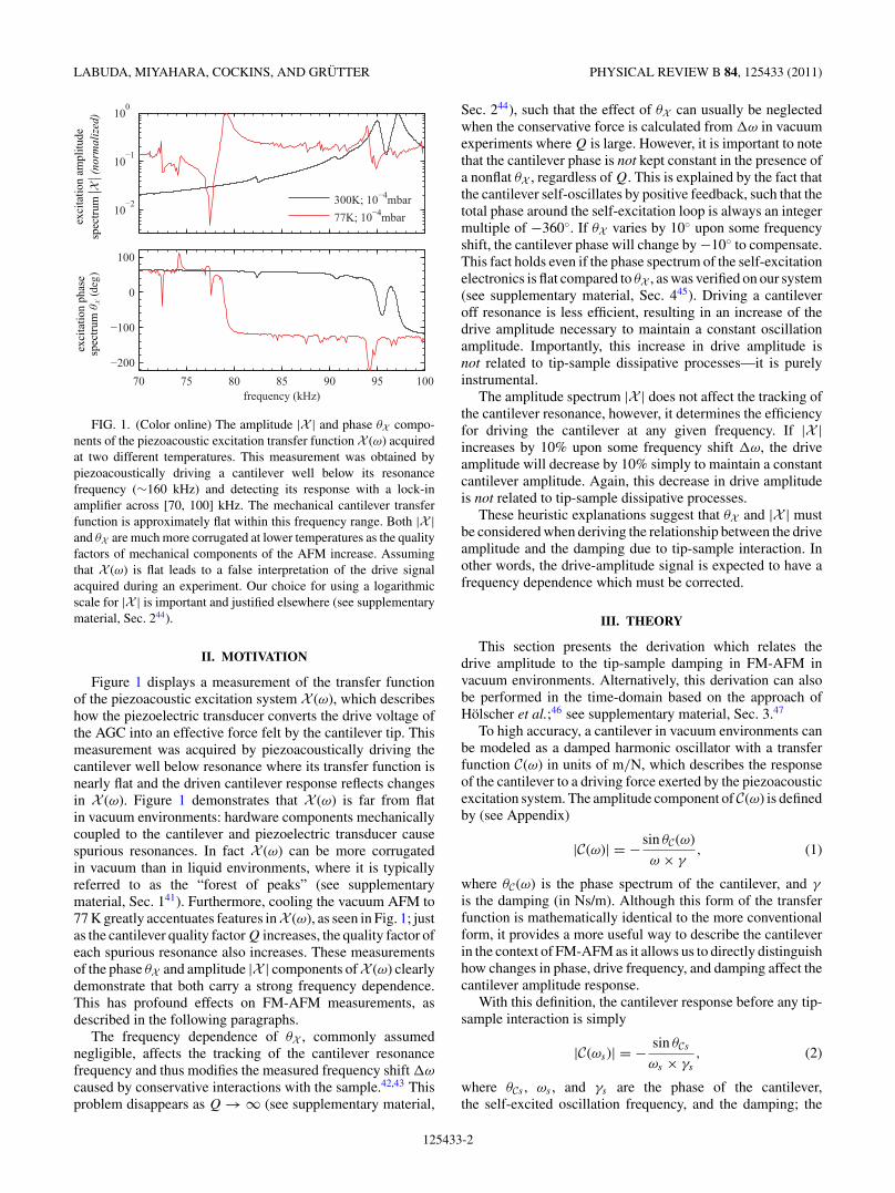
FIG. 2. The transfer functions comprising the self-excitationloop are represented as four grey boxes. The evolution of theself-excitation signal is described within the loop, along withunits. The cantilever tip interacts with the sample; the bias voltageVb between the two is adjustable. The AGC maintains a constantcantilever amplitude A by modulating the drive amplitude Vd ; thisis valid if the amplitude response of the detection system |D| isflat, as assumed through this article (dropping this assumption leadsto a more complicated derivation40). The derivation in this articlealso assumes that self-excitation electronics (θD + θS ) have flat phasespectra, where θD is the phase spectrum of the detection system.

subscript “s” denotes measurements taken at the start of theexperiment before any tip-sample interaction occurs. Theintrinsic cantilever damping γs is typically estimated byγs ≈ k/Qωs , where k and Q are the stiffness and quality factorof the unperturbed cantilever.

During the experiment, the cantilever transfer function (seeFig. 2) undergoes perturbation due to tip-sample conservativeinteractions, causing the self-excited oscillation frequency ω

to vary. Also, the perturbed cantilever damping becomes γ =γs + γtip, where the additional damping γtip relates to the tip-sample dissipative interactions. As described in the previoussection, the phase of the cantilever θC(ω) varies to compensatefor changes in the excitation system phase response �θX (ω). Inthe limit that the self-excitation electronics respond instantly,the cantilever phase is θC(ω) = θCs − �θX (ω), where theconvention �θX (ωs) = 0◦ is adopted for simplicity. Finally,from Eq. (1), the resulting perturbed cantilever amplitudetransfer function becomes

|C∗(ω,γtip)| = − sin (θCs − �θX (ω))ω × (γs + γtip)

. (3)

Note that θCs , θX , γs can be measured before the experiment,and the self-excited oscillation frequency ω is measured duringthe experiment; therefore, γtip is the only unknown variableremaining to fully define |C∗(ω,γtip)|.

In order to maintain a constant cantilever oscillationamplitude, the AGC adjusts the drive amplitude to accountfor changes in the amplitude response of the piezoacousticallydriven cantilever |X | × |C∗(ω,γtip)|. Measuring the drive

amplitude during the experiment allows determining γtip asfollows.

For a given drive amplitude Vd , the resulting cantileveroscillation amplitude A can be calculated by

A = Vd × |X | × |C|, (4)

as can be understood from Fig. 2. This equation holdsunder the approximation that the detection system, whichconverts the cantilever displacement into a measurable voltage,has a frequency independent (flat) transfer function. Thisapproximation is usually valid in vacuum environments48 andis assumed herein. Throughout the whole experiment, A iskept constant by the AGC such that

Vd × |X (ω)| × |C∗(ω,γtip)|︸ ︷︷ ︸during the experiment

= Vs × |X (ωs)| × |C(ωs)|︸ ︷︷ ︸start of the experiment

, (5)

where Vs is the drive amplitude measured at the start of theexperiment. Rearranging Eq. (5) results in

� = Vd

Vs

=∣∣∣∣X (ωs)

X (ω)

∣∣∣∣ ×∣∣∣∣ C(ωs)

C∗(ω,γtip)

∣∣∣∣, (6)

where the normalized drive-amplitude signal � is defined forthe convenience of avoiding units of volts. Notice that the drivesignal � changes as a function of |X |, which can be measuredbefore or after the experiment, as will be thoroughly describedin the next section. Both |C|s are defined by Eqs. (2) and (3)with γtip as the only remaining unknown variable. SolvingEq. (6) allows us to infer the tip-sample damping γtip from themeasured drive signal � by

γtip = γs

(� − 1

), (7)

where [the Japanese katakana symbol pronounced “ne”] isdefined as

(ω) =∣∣∣∣ sin(θCs − �θx(ω))

sin(θCs)

∣∣∣∣︸ ︷︷ ︸θ−f actor

−1 ∣∣∣∣ X (ω)

X (ωs)

∣∣∣∣︸ ︷︷ ︸x−f actor

−1 (ω

ωs

)︸ ︷︷ ︸

˜1

. (8)

As can be understood from Eq. (7), is the unitlesscalibration factor that corrects for the frequency dependenceof the drive signal �, which otherwise can be mistakenfor tip-sample damping. Note that for a purely conservativeinteraction, the drive-amplitude signal varies as � = , whichcorrectly results in γtip = 0 if processed by Eq. (7). Incorrectlyassuming a constant X (ω) by omitting in Eq. (7) results innonzero damping γs

( −1), which is designated as “apparent

damping.” In other words, apparent damping in the contextof this article refers to the interpretation of the frequencydependence ( ) of the drive signal using standard FM-AFMtheory4,32,49 rather than Eq. (7).

In Eq. (8) is broken down into the θ -factor (“phasefactor”) and X -factor (“excitation factor”), which describehow the drive-signal calibration is affected by a nonflat θXand |X |, respectively. These two factors were heuristicallydescribed in the Motivation section. Finally, we henceforth

125433-3

LABUDA, MIYAHARA, COCKINS, AND GRUTTER PHYSICAL REVIEW B 84, 125433 (2011)

omit the ω/ωs factor from the discussion because it is usuallytwo to three orders of magnitude smaller than the X -factor invacuum environments.

In most FM-AFM experiments, the accuracy in determiningγtip is limited by the accuracy and precision in measuring ,consisting of |X |, θX , and θCs . This will be investigated in thefollowing sections.

Before proceeding, we note that tip-sample dissipatedpower Ptip is proportional to γtip within the approximationω/ωs ∼ 1, such that

Ptip = Ps

(� − 1

), (9)

where the starting cantilever dissipated power Ps is typicallyapproximated by Ps ≈ 1

2kωoA2/Q.

IV. CHARACTERIZING THE EXCITATION SYSTEM

This section presents the protocol used to measure thepiezoacoustic excitation transfer function X , which is subse-quently used to determine the starting phase of the cantileverθCs .

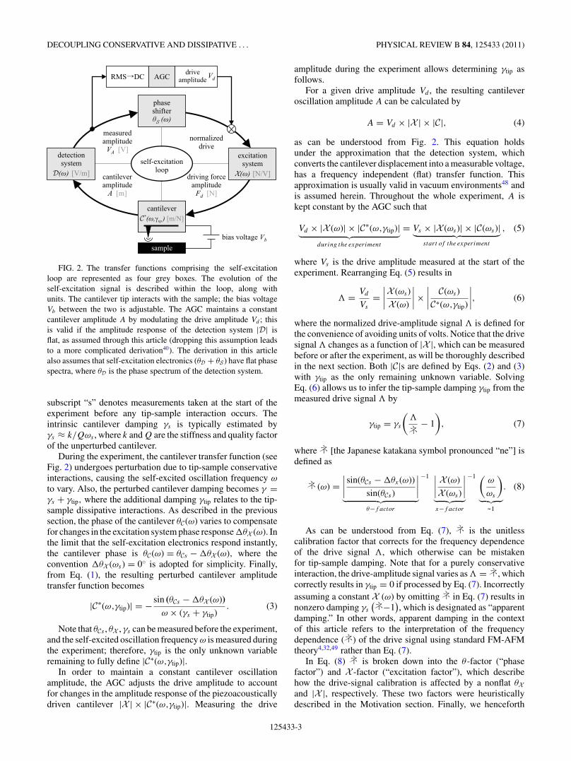
Piezoacoustically driving the cantilever and recording itsresponse inevitably leads to the combined transfer functionXC of the cantilever and the excitation system, as can beunderstood from Fig. 2. However, by independently measuringthe cantilever transfer function C, the X can be isolated bydivision. Applying a small amplitude AC bias voltage betweenthe cantilever and sample results in an electrostatic drivingforce.50 By sweeping the frequency of this AC bias, thetransfer function of the cantilever C can be measured acrossany desired frequency range. This independent measurementof C allows the isolation of X , as shown in Fig. 3. Note thatthe electrostatic excitation transfer function is assumed flat forthis measurement.

For technical clarity, the exact protocol used to obtain thedata in Fig. 3 is now explicitly outlined:

(i) Self-excite the cantilever with an AGC amplitude setpoint of 1.6 nm and adjust the phase shifter to minimize thedrive amplitude (the self-excited oscillation frequency becomes156.30 kHz).

(ii) Engage the tip-sample distance feedback controller witha frequency shift set point of −10 Hz after applying a 2 Vtip-sample DC bias (this approaches the tip to 10–20 nm abovethe sample).

(iii) Disable the tip-sample distance feedback to fix the tip-sample distance.

(iv) Set the tip-sample bias to 10 V, thereby shiftingthe self-excited oscillation frequency to 155.92 kHz. (Thisoptional step reduces the necessary dynamic range necessaryto perform the measurements in steps vi and vii and may reducethe effects of tip-sample drift on the estimation of X in stepviii.)

(v) Disable cantilever self-excitation.(vi) Measure the transfer function XC by piezoacoustically

driving the cantilever (Vd ) and measuring the cantileverresponse (VA) across [156.00 kHz, 156.33 kHz] (this frequencyrange was selected to cover the frequency range used through-out the actual experiment).

FIG. 3. (Color online) On the primary axes (black), the driventransfer functions of the cantilever for both the piezoacoustic (XC)and the electrostatic (C) methods of excitation are plotted in their(a) amplitude and (b) phase components. For this measurement, a∼10 V bias was applied to the cantilever to shift the resonancefrequency to below 156 kHz, whereas this measurement was onlytaken above 156 kHz: this reduces the necessary dynamic range formeasuring C and XC because the measurement is taken where C isflatter. The dotted lines are extrapolated and only plotted for clarity.Dividing these transfer functions results in the piezoacoustic transferfunction X = XC/C, plotted on the secondary axes (blue/gray). Theresonance frequency at the zero contact potential difference is labeledfo, which corresponds to a null frequency shift in Fig. 4.

(vii) Measure the transfer function C by driving the cantileverwith a tip-sample AC bias (Vb) and measuring the cantileverresponse (VA) across [156.00 kHz, 156.33 kHz].(viii) Infer the excitation transfer function byX = XC/C andcalculate its magnitude |X | and phase θX .

This protocol was performed before and after the exper-iment, which is described in the next section, to verify thatthe transfer function X remained constant throughout theexperiment. Linearity of the cantilever response was verifiedby acquiring both transfer functions at double the drive voltage.

Now, this measurement of X will be used to determine thestarting phase of the cantilever θCs . Typically, the AFM userminimizes the drive amplitude at the start of the experimentby adjusting the phase shifter in an attempt to drive thecantilever on resonance. However, this method locates themaximum of |XC|—not |C|. Solving for ∂ |XC| /∂f = 0 (seesupplementary material, Sec. 551) returns a starting cantileverphase

θCs = atan2Q

(αXfo − 1), (10)

where the normalized slope of the amplitude spectrum αX =|X |−1 ∂ |X | /∂f is evaluated at the resonance frequency fo.Applying Eq. (10) to the data from Fig. 3 results in θCs =−90.8◦ ± 0.5◦. Note the Q dependence in Eq. (10); thecommonly used drive-minimization method can misidentify

125433-4

DECOUPLING CONSERVATIVE AND DISSIPATIVE . . . PHYSICAL REVIEW B 84, 125433 (2011)

the true cantilever resonance by more than 10◦ in situationswhere Q ∼ 1000 (see supplementary material, Sec. 551).

Now |X |, θX , and θCs can be used to determine , accordingto Eq. (8), allowing an accurate recovery of the damping signalin the following experiment.

V. EXPERIMENT

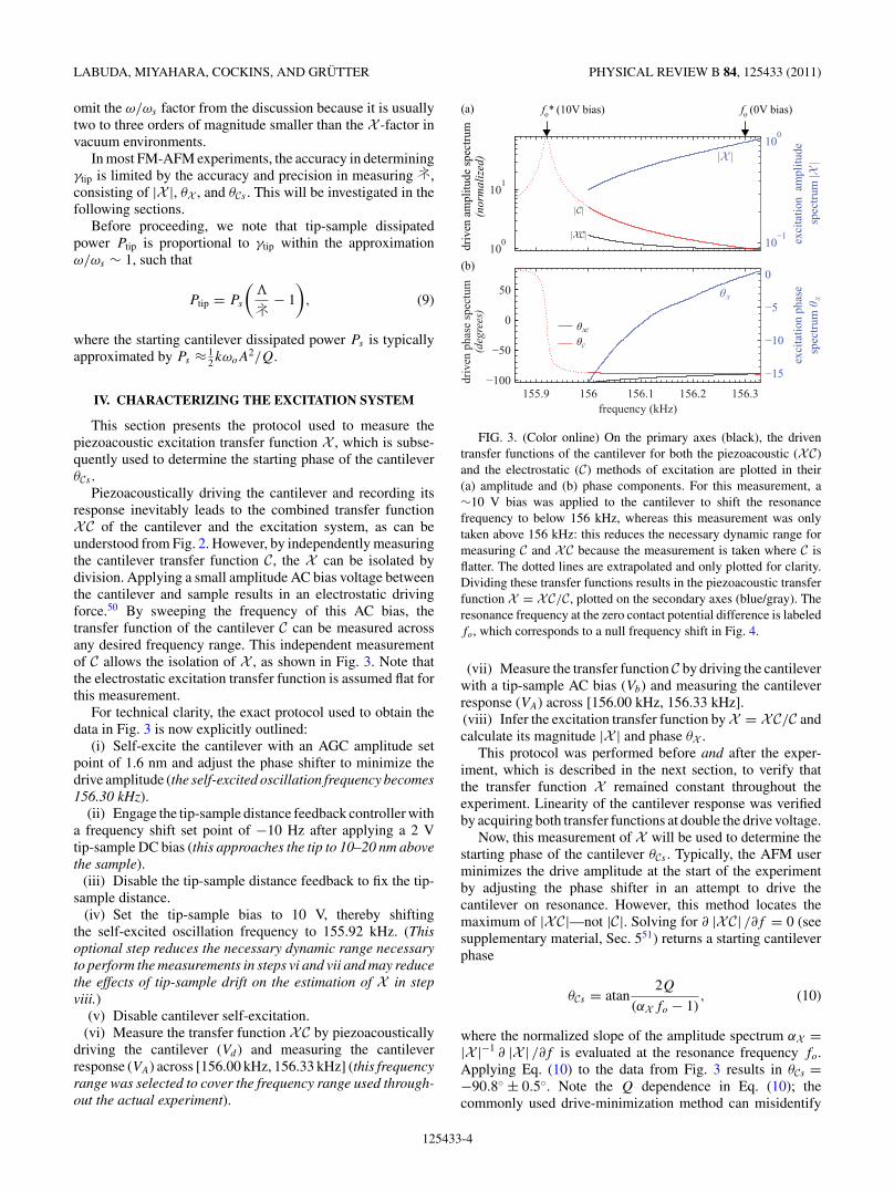
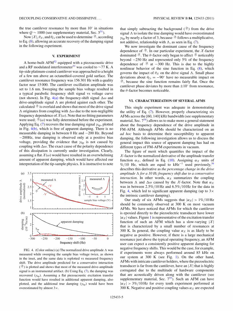
A home-built AFM52 equipped with a piezoacoustic driveand a RF modulated interferometer53 was cooled to ∼77 K. Atip-side platinum-coated cantilever was approached to a heightof a few nm above an octanethiol-covered gold surface. Thecantilever resonance frequency was 156 301 Hz with a qualityfactor near 15 000. The cantilever oscillation amplitude wasset to 1.6 nm. Sweeping the sample bias voltage resulted ina typical parabolic frequency shift signal vs voltage curve(not shown). In Fig. 4(a) the frequency-shift signal �ω anddrive-amplitude signal � are plotted against each other. Thecalculated is overlaid and shows that most of the drive signal� originates from coupling with �ω due to the non-negligiblefrequency dependence ofX (ω). Note that no fitting parameterswere used; (ω) was fully determined before the experiment.Applying Eq. (7) recovers the true damping signal γtip, plottedin Fig. 4(b), which is free of apparent damping. There is nomeasurable damping in between 0 Hz and −200 Hz. Beyond−200Hz, true damping is observed only at a positive biasvoltage, providing the evidence that γtip is not caused bycoupling with �ω. The exact cause of the polarity dependenceof this dissipation is currently under investigation. Clearly,assuming a flat X (ω) would have resulted in an overwhelmingamount of apparent damping, which would have affected ourinterpretation of the tip-sample physics. It is instructive to note

FIG. 4. (Color online) (a) The normalized drive amplitude � wasmeasured while sweeping the sample bias voltage twice, as shownin the inset, and the same data is replotted vs measured frequencyshift. The drive amplitude predicted for a conservative interaction( ) is plotted and shows that most of the measured drive-amplitudesignal is an instrumental artifact. (b) Using Eq. (7), the damping wasrecovered (γtip). Assuming a flat piezoacoustic excitation transferfunction would have resulted in additional apparent damping, alsoplotted, and the additional true damping (γtip) would have beenoverestimated by almost 3×.

that simply subtracting the background ( ) from the drivesignal � to isolate the true damping would have overestimatedγtip by nearly a factor of 3, because follows a multiplicative,not additive, relationship with �, as seen in Eq. (7).

We now investigate the dominant cause of the frequencydependence of . In our particular experiment, the X -factordominated . The θ -factor only began to affect noticeablybeyond −250 Hz and represented only 5% of the frequencydependence of at −300 Hz. This is due to the highlynonlinear behavior of the sine function in Eq. (8), whichgoverns the impact of θX on the drive signal �. Small phasedeviations about θCs = −90◦ have no measurable impact on

, because the sine function remains fairly flat. Once thecantilever phase deviates by more than ±10◦ from resonance,the θ -factor becomes noticeable.

VI. CHARACTERIZATION OF SEVERAL AFMS

This single experiment was adequate in demonstratingthe utility of Eq. (7). However, properly characterizing sixAFMs across the [60, 140] kHz bandwidth (see supplementarymaterial, Sec. 754) allows us to make more a general statementabout the frequency dependence of the drive amplitude inFM-AFM. Although AFMs should be characterized on anad hoc basis to determine their susceptibility to apparentdamping, the following investigation allows us to discuss thegeneral impact this source of apparent damping has had ondifferent types of FM-AFM experiments in vacuum.

The figure of merit which quantifies the impact of theX -factor is the normalized derivative of the amplitude transferfunction αX , defined in Eq. (10). Assigning αX units of%/10 Hz, which are equal to kHz−1 used previously,39

describes this derivative as the percentage change in the driveamplitude � for a 10 Hz frequency shift due to a conservativeinteraction. In other words, αX summarizes the couplingbetween � and �ω caused by the X -factor. Note that αXwas in between 2.5%/10 Hz and 6.5%/10 Hz for the data inFig. 4, which led to significant apparent damping (up to 3×the intrinsic cantilever damping).

Our study of six AFMs suggests that |αX | > 1%/10 Hzshould be commonly observed at 300 K on most vacuumAFMs. We have noticed that AFMs for which the cantileveris epoxied directly to the piezoelectric transducer have lower|αX | values. Figure 1 is representative of the excitation transferfunction of such an AFM which has a slow-varying |X |that is characterized by a small number of resonances at300 K. In general, the coupling value αX is as likely to benegative as positive. However, if there is a large mechanicalresonance just above the typical operating frequency, an AFMuser can expect a consistently positive apparent damping fornegative frequency shifts. This would be the case, for example,if experiments were always performed around 85 kHz onour system at 300 K (see Fig. 1). On the other hand,AFMs with intricate cantilever holders, where the piezoelectrictransducer is far from the cantilever, have an |X | that is highlycorrugated due to the multitude of hardware componentsthat are acoustically driven along with the cantilever (seesupplementary material, Sec. 755). Such an AFM can have|αX | > 3%/10 Hz for every tenth experiment performed at300 K. Negative and positive coupling values αX are expected

125433-5

LABUDA, MIYAHARA, COCKINS, AND GRUTTER PHYSICAL REVIEW B 84, 125433 (2011)

to be equally likely, even between cantilevers with similarresonant frequencies.

The magnitude of the θ -factor depends on the slope of thephase transfer function βX , in units of ◦/10 Hz. The discussionabout αX in the previous paragraph qualitatively applies to βX ,although typically the value of βX (in ◦/10 Hz) is roughly halfthe value of αX (in %/10 Hz). Whereas the previous discussionconcerning αX was independent of βX , the reverse is not true:a nonzero αX causes the starting phase of the cantilever θCs �=−90◦ and affects the impact that βX has on the θ -factor, ascan be understood from Eq. (8). The quantitative effects of anonzero βX on the drive signal are highly nonlinear, far fromintuitive, and should be assessed on an ad hoc basis.

As shown in Fig. 1, the excitation transfer functionX (ω) hasa strong temperature dependence. The X (ω) of our home-builtAFM was tested at 300, 77, and 4 K, with |αX | values largerthan 0.4, 2.6, and 10%/10 Hz, respectively, affecting one tenthof the studied frequency range. The corresponding values of|βX | were 0.2, 1.3, 5◦/10 Hz. Roughly speaking, the problemof apparent damping is 25× larger at 4 K than it is at 300 K onour system. These observations are consistent with previousreports of exceedingly large apparent dissipation occurring atlow temperatures.29

VII. SIMULATIONS

In this section, we discuss different experiments performedusing FM-AFM to gauge the impact of the piezoacousticexcitation transfer function characterized in the previoussection. The first subsection elaborates on the quantitative andqualitative effects of apparent damping in force spectroscopy.The second subsection deals with apparent damping observedin constant frequency shift FM-AFM imaging.

A. Force spectroscopy

The difference in apparent damping between room temper-atures and cryogenic temperatures is not only quantitative.Whereas αX and βX , defined in the previous section, aretypically fairly constant for a single experiment performed at300 K, they can change dramatically as a function of frequencyduring a single experiment at 77 K, and especially at 4 K,because X (ω) can be highly corrugated within a frequencywindow as small as 100 Hz.

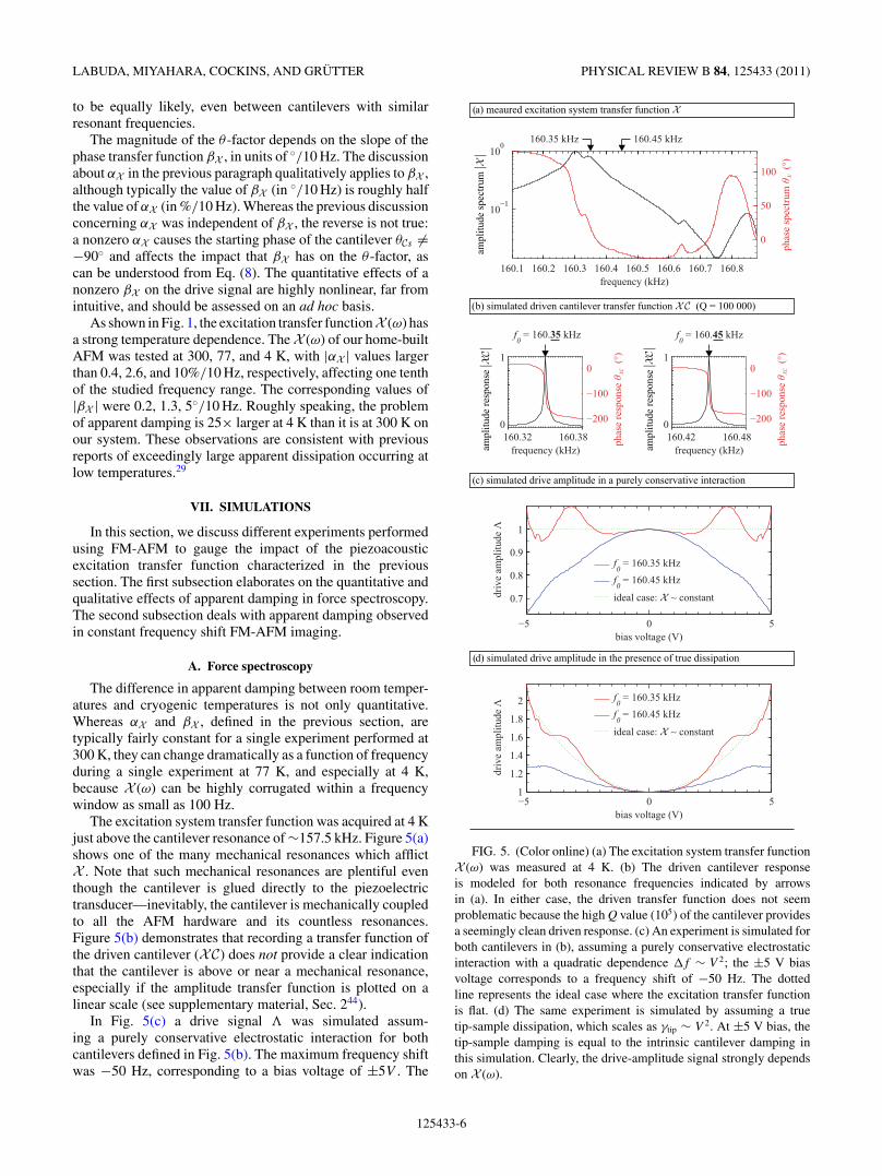
The excitation system transfer function was acquired at 4 Kjust above the cantilever resonance of ∼157.5 kHz. Figure 5(a)shows one of the many mechanical resonances which afflictX . Note that such mechanical resonances are plentiful eventhough the cantilever is glued directly to the piezoelectrictransducer—inevitably, the cantilever is mechanically coupledto all the AFM hardware and its countless resonances.Figure 5(b) demonstrates that recording a transfer function ofthe driven cantilever (XC) does not provide a clear indicationthat the cantilever is above or near a mechanical resonance,especially if the amplitude transfer function is plotted on alinear scale (see supplementary material, Sec. 244).

In Fig. 5(c) a drive signal � was simulated assum-ing a purely conservative electrostatic interaction for bothcantilevers defined in Fig. 5(b). The maximum frequency shiftwas −50 Hz, corresponding to a bias voltage of ±5V . The

FIG. 5. (Color online) (a) The excitation system transfer functionX (ω) was measured at 4 K. (b) The driven cantilever responseis modeled for both resonance frequencies indicated by arrowsin (a). In either case, the driven transfer function does not seemproblematic because the high Q value (105) of the cantilever providesa seemingly clean driven response. (c) An experiment is simulated forboth cantilevers in (b), assuming a purely conservative electrostaticinteraction with a quadratic dependence �f ∼ V 2; the ±5 V biasvoltage corresponds to a frequency shift of −50 Hz. The dottedline represents the ideal case where the excitation transfer functionis flat. (d) The same experiment is simulated by assuming a truetip-sample dissipation, which scales as γtip ∼ V 2. At ±5 V bias, thetip-sample damping is equal to the intrinsic cantilever damping inthis simulation. Clearly, the drive-amplitude signal strongly dependson X (ω).

125433-6

DECOUPLING CONSERVATIVE AND DISSIPATIVE . . . PHYSICAL REVIEW B 84, 125433 (2011)

large variations and multiple peaks in the drive signal arerepresentative of what we observe most of the time in ourexperiments at 4 K. Combined with Fig. 4, this simulationillustrates that the frequency dependent calibration ( ) of thedrive amplitude can increase, decrease, or be highly corrugatedas a function of frequency.

In the simulated data starting at 160.45 kHz, wasdominated by the X -factor (by >98%). However, for the datastarting at 160.35 kHz, the θ -factor exceeded the X -factor atfrequency shifts beyond −45 Hz. The high Q-factor of thecantilever (105) ensured that the drive-minimization methodaccurately set the starting cantilever phase near −90◦ within1◦, but the steep phase spectrum of the excitation system(〈βX 〉avg = −8.4◦/10 Hz) caused the cantilever phase to reachθC = −132.0◦ at a frequency shift of −50 Hz. Operating thecantilever off resonance, at −132.0◦, results in a θ -factorequal to 1.35. Note that measuring the phase response ofthe driven cantilever using a lock-in amplifier56 would notidentify the problem. In fact, a lock-in amplifier measuresthe combined phase response of the excitation system andthe cantilever θXC such that θX and θC can vary wildlyduring an experiment despite an ideal phase-locked loop (PLL)maintaining a constant θXC .

On many systems, “negative apparent damping” corre-sponding to � < 1, seen in Fig. 5(c), is rarely or neverobserved. The reason for this is demonstrated by the followingsimulation. Figure 5(d) represents the same simulation of anelectrostatic interaction as shown in Fig. 5(c), however anonzero tip-sample damping γtip was modeled as γtip ∼ V 2,where V is the bias voltage (Joule heating, for example,follows this quadratic dependence36,57). The magnitude of thetrue damping was arbitrarily adjusted such that γtip = γs at±5V bias voltage. For these conditions, the drive amplituderemains above 1; nevertheless, affects the drive amplitudeby the same factor as in the absence of true damping. Thiscan severely distort the drive-amplitude signal by introducingfeatures that do not relate to tip-sample physics or by skewingthe power-law behavior between (� − 1) and the bias voltageV , for example. The power-law behavior within the ±3V biasrange in Fig. 5(d) is closer to V 4 than to V 2 by virtue of .

B. Imaging

FM-AFM is most often used for acquiring images by rasterscanning the sample and maintaining a constant frequencyshift set point �fset by adjusting the tip-sample distanceaccordingly. In the ideal case where �fset remains perfectlyconstant throughout the experiment, will remain constantand therefore apparent damping will affect the entire drive-amplitude image by a constant factor. However, the idealcondition of a constant �fset is usually not fulfilled in practice,even if the PLL and AGC parameters are set to their optimalvalues (PLL locking time = 0.35 ms; AGC response time =2 ms as defined in Ref. 29).

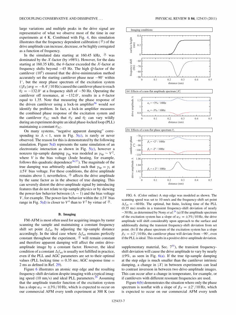
Figure 6 illustrates an atomic step edge and the resultingfrequency-shift deviation despite imaging with a typical imag-ing speed (10 nm/s) and ideal PLL parameters.29 Assumingthat the amplitude transfer function of the excitation systemhas a slope αX = ±3%/10 Hz, which is expected to occur onour commercial AFM every tenth experiment at 300 K (see

FIG. 6. (Color online) A step edge was modeled as shown. Thescanning speed was set to 10 nm/s and the frequency-shift set point�fset = −60 Hz. The optimal, but finite, locking time of the PLL(0.35 ms) results in a transient frequency-shift deviation of nearly−30 Hz, as determined by Nony et al.29 (a) If the amplitude spectrumof the excitation system has a slope of αX = ±3%/10 Hz, the driveamplitude will shift considerably upon approach to the surface andadditionally during the transient frequency-shift deviation from setpoint. (b) If the phase spectrum of the excitation system has a slopeβX = ±2◦/10 Hz, the cantilever phase will deviate from −90◦, evenif the PLL is ideal. This results in a positive drive-amplitude deviation.

supplementary material, Sec. 755), the transient frequency-shift deviation will cause the drive amplitude to vary by nearly±9%, as seen in Fig. 6(a). If the true tip-sample dampingat the step edge is much smaller than the cantilever intrinsicdamping, a change in |X | in between experiments can leadto contrast inversion in between two drive-amplitude images.This can occur after a change in temperature, for example, orif cantilevers with different resonant frequencies are used.

Figure 6(b) demonstrates the situation where only the phasespectrum is nonflat with a slope of βX = ±2◦/10 Hz, whichis expected to occur on our commercial AFM every tenth

125433-7

LABUDA, MIYAHARA, COCKINS, AND GRUTTER PHYSICAL REVIEW B 84, 125433 (2011)

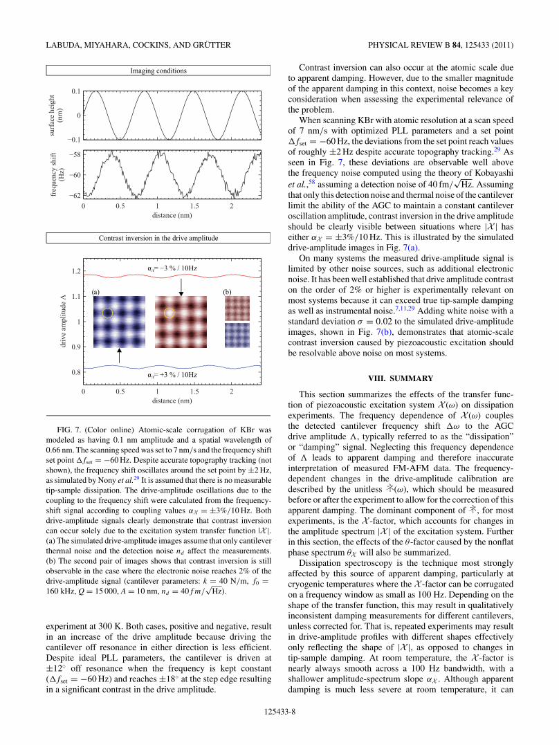
FIG. 7. (Color online) Atomic-scale corrugation of KBr wasmodeled as having 0.1 nm amplitude and a spatial wavelength of0.66 nm. The scanning speed was set to 7 nm/s and the frequency shiftset point �fset = −60 Hz. Despite accurate topography tracking (notshown), the frequency shift oscillates around the set point by ±2 Hz,as simulated by Nony et al.29 It is assumed that there is no measurabletip-sample dissipation. The drive-amplitude oscillations due to thecoupling to the frequency shift were calculated from the frequency-shift signal according to coupling values αX = ±3%/10 Hz. Bothdrive-amplitude signals clearly demonstrate that contrast inversioncan occur solely due to the excitation system transfer function |X |.(a) The simulated drive-amplitude images assume that only cantileverthermal noise and the detection noise nd affect the measurements.(b) The second pair of images shows that contrast inversion is stillobservable in the case where the electronic noise reaches 2% of thedrive-amplitude signal (cantilever parameters: k = 40 N/m, f0 =160 kHz, Q = 15 000, A = 10 nm, nd = 40f m/

√Hz).

experiment at 300 K. Both cases, positive and negative, resultin an increase of the drive amplitude because driving thecantilever off resonance in either direction is less efficient.Despite ideal PLL parameters, the cantilever is driven at±12◦ off resonance when the frequency is kept constant(�fset = −60 Hz) and reaches ±18◦ at the step edge resultingin a significant contrast in the drive amplitude.

Contrast inversion can also occur at the atomic scale dueto apparent damping. However, due to the smaller magnitudeof the apparent damping in this context, noise becomes a keyconsideration when assessing the experimental relevance ofthe problem.

When scanning KBr with atomic resolution at a scan speedof 7 nm/s with optimized PLL parameters and a set point�fset = −60 Hz, the deviations from the set point reach valuesof roughly ±2 Hz despite accurate topography tracking.29 Asseen in Fig. 7, these deviations are observable well abovethe frequency noise computed using the theory of Kobayashiet al.,58 assuming a detection noise of 40 fm/

√Hz. Assuming

that only this detection noise and thermal noise of the cantileverlimit the ability of the AGC to maintain a constant cantileveroscillation amplitude, contrast inversion in the drive amplitudeshould be clearly visible between situations where |X | haseither αX = ±3%/10 Hz. This is illustrated by the simulateddrive-amplitude images in Fig. 7(a).

On many systems the measured drive-amplitude signal islimited by other noise sources, such as additional electronicnoise. It has been well established that drive amplitude contraston the order of 2% or higher is experimentally relevant onmost systems because it can exceed true tip-sample dampingas well as instrumental noise.7,11,29 Adding white noise with astandard deviation σ = 0.02 to the simulated drive-amplitudeimages, shown in Fig. 7(b), demonstrates that atomic-scalecontrast inversion caused by piezoacoustic excitation shouldbe resolvable above noise on most systems.

VIII. SUMMARY

This section summarizes the effects of the transfer func-tion of piezoacoustic excitation system X (ω) on dissipationexperiments. The frequency dependence of X (ω) couplesthe detected cantilever frequency shift �ω to the AGCdrive amplitude �, typically referred to as the “dissipation”or “damping” signal. Neglecting this frequency dependenceof � leads to apparent damping and therefore inaccurateinterpretation of measured FM-AFM data. The frequency-dependent changes in the drive-amplitude calibration aredescribed by the unitless (ω), which should be measuredbefore or after the experiment to allow for the correction of thisapparent damping. The dominant component of , for mostexperiments, is the X -factor, which accounts for changes inthe amplitude spectrum |X | of the excitation system. Furtherin this section, the effects of the θ -factor caused by the nonflatphase spectrum θX will also be summarized.

Dissipation spectroscopy is the technique most stronglyaffected by this source of apparent damping, particularly atcryogenic temperatures where the X -factor can be corrugatedon a frequency window as small as 100 Hz. Depending on theshape of the transfer function, this may result in qualitativelyinconsistent damping measurements for different cantilevers,unless corrected for. That is, repeated experiments may resultin drive-amplitude profiles with different shapes effectivelyonly reflecting the shape of |X |, as opposed to changes intip-sample damping. At room temperature, the X -factor isnearly always smooth across a 100 Hz bandwidth, with ashallower amplitude-spectrum slope αX . Although apparentdamping is much less severe at room temperature, it can

125433-8

DECOUPLING CONSERVATIVE AND DISSIPATIVE . . . PHYSICAL REVIEW B 84, 125433 (2011)

significantly affect sensitive dissipation experiments wherethe tip-sample damping is much smaller than the cantileverintrinsic damping.

For applications using constant frequency shifts with someset point �fset, such as typical FM-AFM topography imaging,apparent damping can appear in two ways. Each cantilever willhave a different drive-amplitude calibration at identical �fset

because of differences in theirX -factor; if left uncorrected, thiscan lead to quantitatively variable-dissipation measurementstaken at identical �fset with different cantilevers and mayprevent drawing conclusions about dissipative mechanismsunder study. In the second scenario, transient deviationsfrom a constant set point �fset, due to the finite responsetime of the PLL or distance regulation feedback, may causeexperimentally significant apparent damping, for example,at step edges. This can cause inconsistent results betweencantilevers, or even for the same cantilever if operated at adifferent �fset. Atomic-scale contrast inversion in the driveamplitude is also likely to occur because coupling constantson the order of ±3%/10 Hz, which can be observed on mostAFMs even at room temperature, cause apparent damping,which exceeds the true tip-sample damping and instrumentalnoise.

Although the θ -factor rarely dominates the X -factor intypical experiments (see supplementary material, Sec. 654), theformer should not be neglected. At cryogenic temperatures,a very corrugated phase spectrum θX implies that carefullysetting the cantilever on resonance away from the surface(at �f = 0 Hz) does not ensure proper resonance trackingduring the experiment; once �fset �= 0 Hz, the cantilever willbe driven off resonance and even small modulations of thecantilever phase may significantly enhance apparent dampingby a large θ -factor contribution. At room temperature, themuch shallower phase spectrum reduces the magnitude of thisproblem. However, the drive-minimization method is morelikely to fail because of a lower cantilever Q-factor which canmisidentify the true cantilever resonance by more than 10◦ incertain situations. This could lead to a significant θ -factor evenfor small frequency shifts.

IX. CONCLUSION

In FM-AFM operated with a piezoacoustically excitedcantilever, the AGC drive-amplitude signal can only beaccurately converted into a damping or dissipation signal aftermeasuring the transfer function X (ω) of the piezoacousticexcitation system. This measurement allows the decouplingof conservative and dissipative forces by correcting for thefrequency dependence of the drive amplitude, which doesnot relate to tip-sample damping. Using standard FM-AFMtheory leads to apparent damping in force spectroscopy aswell as topography imaging, thereby potentially altering thequantitative and qualitative interpretation of the tip-samplephysics. We have demonstrated a nondestructive and robustmethod which enables measuring X (ω), thereby eliminatingapparent damping which can dominate the true tip-sampledamping signal.

The impact of apparent damping depends on numerousparameters, such as frequency shift, Q-factor, temperature,feedback parameters, and most importantly the details of the

mechanical construction of the AFM. Due to the complexityof the problem, the impact of apparent damping must beconsidered on an ad hoc basis for any particular experimentperformed at any temperature. Conclusive statements aboutqualitative and quantitative FM-AFM dissipation studies(using a piezoacoustically excited cantilever) rely on a properinvestigation of the piezoacoustic excitation system, as pre-sented in this paper.

Whereas we are not denying that other studied sourcesof apparent damping can be significant, we have shown thatthe transfer function of the piezoacoustic excitation systemaccounts for a large part of the observed variability in reporteddissipation experiments to date. Applying the methodologypresented in this paper can reconcile many discrepanciesbetween theory and experiment, which have thus far preventedadvancement in FM-AFM dissipation applications and studies.

ACKNOWLEDGMENTS

A.L. would like to acknowledge the help and valuablediscussions with Jeffrey Bates, Sarah Burke, Philip Egberts,Monserratt Lopez-Ayon, William Paul, Antoine Roy-Gobeil,Antoni Tekiel, and Jessica Topple, as well as guidance fromRoland Bennewitz through existing literature. A.L. also greatlyacknowledges his memorable stay in Kyoto, Japan, wherethe study of FM-AFM in liquid environments with HirofumiYamada, Kei Kobayashi, and Daniel Kiracofe was an indis-pensable ingredient for this study in vacuum environments.Funding from NSERC, FQRNT and CIfAR are gratefullyacknowledged.

APPENDIX : REPARAMETRIZING THE CANTILEVERTRANSFER FUNCTION

A cantilever interacting with a sample can be describedas a damped harmonic oscillator with two time-varyingparameters. The choice of these parameters is somewhatarbitrary. Typically, the amplitude transfer function is definedby the resonance frequency ω0 and the quality factor Q as in

|C(ω|ωo,Q)| = 1

k

√1

[1 − (ω/ωo)2]2 + (ω/ωoQ)2, (A1)

with its associated phase transfer function

θC(ω) = tan−1

{− ω/ωo

Q[(1 − (ω/ωo)2]

}, (A2)

where k is the cantilever stiffness, which remains constant.This is not a very useful parameterization of the cantilevertransfer function in FM-AFM because the perturbed cantileverresonance due to tip-sample interaction is unknown to theAFM user during the experiment. Furthermore the qualityfactor Q carries an intrinsic dependence on the variableresonance frequency.

Using the rules of trigonometry, Eq. (A2) can be rewrittenas

sin θC(ω) = − ω/ωoQ√[(1 − (ω/ωo)2]2 + (ω/ωoQ)2

, (A3)

125433-9

LABUDA, MIYAHARA, COCKINS, AND GRUTTER PHYSICAL REVIEW B 84, 125433 (2011)

which, combined with Eq. (A1), results in

|C (ω|ωo,Q)| = −ωoQ

k

sin θC (ω)

ω. (A4)

Using the well-known relations

Q = mωo

γand k = mω2

o, (A5)

the cantilever amplitude transfer function can bereparametrized to

|C (ω|θC,γ )| = − sin θC (ω)

ω × γ. (A6)

Note that Eq. (A6) is mathematically identical to Eq. (A1).This reparametrized version of the cantilever transfer functionis useful for FM-AFM applications because it directly relateschanges in phase, frequency, and damping to the amplituderesponse |C|.

*aleks.labuda@gmail.com1T. R. Albrecht, P. Grutter, D. Horne, and D. Rugar, J. Appl. Phys.69, 668 (1991).

2U. Durig, O. Zuger, and A. Stalder, J. Appl. Phys. 72, 1778 (1992).3U. Durig, H. R. Steinauer, and N. Blanc, J. Appl. Phys. 82, 3641(1997).

4H. Holscher, B. Gotsmann, W. Allers, U. Schwarz, H. Fuchs, andR. Wiesendanger, Phys. Rev. B 64, 075402 (2001).

5Y. Sugimoto, M. Abe, S. Hirayama, N. Oyabu, O. Custance, andS. Morita, Nat. Mater. 4, 156 (2005).

6Y. Sugimoto, S. Innami, M. Abe, Oscar. Custance, and S. Morita,Appl. Phys. Lett. 91, 093120 (2007).

7T. Trevethan, L. Kantorovich, J. Polesel-Maris, and S. Gauthier,Nanotechnology 18, 084017 (2007).

8H. Holscher, B. Gotsmann, W. Allers, U. Schwarz, H. Fuchs, andR. Wiesendanger, Phys. Rev. Lett. 88, 019601 (2001).

9S. A. Burke and P. Grutter, Nanotechnology 19, 398001 (2008).10Ch. Loppacher, M. Bammerlin, M. Guggisberg, S. Schar,

R. Bennewitz, A. Baratoff, E. Meyer, and H.-J. Guntherodt, Phys.Rev. B 62, 16944 (2000).

11M. Gauthier, R. Perez, T. Arai, M. Tomitori, and M. Tsukada, Phys.Rev. Lett. 89, 146104 (2002).

12T. Kunstmann, A. Schlarb, M. Fendrich, D. Paulkowski, Th.Wagner, and R. Moller, Appl. Phys. Lett. 88, 153112 (2006).

13M. Guggisberg, Surf. Sci. 461, 255 (2000).14S. Molitor, P. Guthner, and T. Berghaus, Appl. Surf. Sci. 140, 276

(1999).15M. Fendrich, T. Kunstmann, D. Paulkowski, and R. Moller,

Nanotechnology 18, 084004 (2007).16R. Hoffmann, M. Lantz, H. Hug, P. van Schendel, P. Kappenberger,

S. Martin, A. Baratoff, and H.-J. Guntherodt, Phys. Rev. B 67,085402 (2003).

17R. Garcia, C. Gomez, N. Martinez, S. Patil, C. Dietz, andR. Magerle, Phys. Rev. Lett. 97, 016103 (2006).

18T. Trevethan, Surf. Sci. 540, 497 (2003).19T. Trevethan and L. Kantorovich, Nanotechnology 16, S79 (2005).20T. Trevethan and L. Kantorovich, Nanotechnology 17, S205

(2006).21L. Kantorovich and T. Trevethan, Phys. Rev. Lett. 93, 236102

(2004).22S. Ghasemi, Stefan Goedecker, Alexis Baratoff, Thomas Lenosky,

Ernst Meyer, and Hans Hug, Phys. Rev. Lett. 100, 236106(2008).

23M. Gauthier and M. Tsukada, Phys. Rev. B 60, 11716(1999).

24A Abdurixit, A. Baratoff, and E. Meyer, Appl. Surf. Sci. 157, 355(2000).

25T. Trevethan and L. Kantorovich, Nanotechnology 15, S44(2004).

26M. Gauthier and M. Tsukada, Phys. Rev. Lett. 85, 5348 (2000).27L. Kantorovich, Surf. Sci. 521, 117 (2002).28L. Kantorovich, Phys. Rev. B 64, 245409 (2001).29L. Nony, A. Baratoff, D. Schar, O. Pfeiffer, A. Wetzel, and

E. Meyer, Phys. Rev. B 74, 235439 (2006).30G. Langewisch, H. Fuchs, and A. Schirmeisen, Nanotechnology 21,

345703 (2010).31S. Morita, R. Wiesendanger, and E. Meyer, Noncontact Atomic

Force Microscopy (Springer, Berlin, 2002), p. 399.32J. P. Cleveland, B. Anczykowski, A. E. Schmid, and V. B. Elings,

Appl. Phys. Lett. 72, 2613 (1998).33L. Cockins, Y. Miyahara, S. D Bennett, A. A Clerk, S. Studenikin,

P. Poole, A. Sachrajda, and P. Grutter, PNAS 107, 9496 (2010).34S. D. Bennett, L. Cockins, Y. Miyahara, P. Grutter, and A. A. Clerk,

Phys. Rev. Lett. 104, 017203 (2010).35L. Cockins, Y. Miyahara, S. D. Bennett, A. A. Clerk, and P. Grutter,

submitted (2011).36M. Kisiel, E. Gnecco, U. Gysin, L. Marot, S. Rast, and E. Meyer,

Nat. Mater. 10, 119 (2011).37M. Ternes, C. Gonzalez, C. Lutz, P. Hapala, F. Giessibl, P. Jelınek,

and A. Heinrich, Phys. Rev. Lett. 106, 016802 (2011).38N. Oyabu, P. Pou, Y. Sugimoto, P. Jelinek, M. Abe, S. Morita,

R. Perez, and O. Custance, Phys. Rev. Lett. 96, 106101 (2006).39R. Proksch and S. V Kalinin, Nanotechnology 21, 455705 (2010).40A. Labuda, K. Kobayashi, D. Kiracofe, K. Suzuki, P. H. Grutter,

and H. Yamada, AIP Adv. 1, 022136 (2011).41See Supplemental Material at http://link.aps.org/supplemental/

10.1103/PhysRevB.84.125433 in Sec. 1 for the “forest of peaks.”42K. Kobayashi, H. Yamada, and K. Matsushige, Rev. Sci. Instrum.

82, 033702 (2011).43W. Hofbauer, Scanning Probe Microscopy—Dynamic Force Mi-

croscopy in Liquid Media, (World Scientific, Singapore, 2010),Chapter 7, pp. 137–163.

44See Supplemental Material at http://link.aps.org/supplemental/10.1103/PhysRevB.84.125433 in Sec. 2 for the illusory nature ofthe “forest of peaks.”

45See Supplemental Material at http://link.aps.org/supplemental/10.1103/PhysRevB.84.125433 in Sec. 4 for the investigation ofelectronic phase shifts.

46H. Holscher, B. Gotsmann, W. Allers, U. Schwarz, H. Fuchs, andR. Wiesendanger, Phys. Rev. B 64, 075402 (2001).

125433-10

DECOUPLING CONSERVATIVE AND DISSIPATIVE . . . PHYSICAL REVIEW B 84, 125433 (2011)

47See Supplemental Material at http://link.aps.org/supplemental/10.1103/PhysRevB.84.125433 in Sec. 3 for the derivation ofFM-AFM dissipation theory in the time-domain.

48In vacuum environments, cantilever frequency shifts are typicallymuch smaller than in liquid environments, and band-pass filters aretypically not necessary to obtain stable self-excitation. Therefore,the frequency dependence of the detection electronics is usuallynegligible. Dropping this assumption leads to a more elaboratederivation.40

49U. Durig, Surf. Interface Anal. 27, 467 (1999).50B. Terris, J. Stern, D. Rugar, and H. Mamin, Phys. Rev. Lett. 63,

2669 (1989).51See Supplemental Material at http://link.aps.org/supplemental/

10.1103/PhysRevB.84.125433 in Sec. 5 for the bias in the drive-minimization method.

52M. Roseman and P. Grutter, Rev. Sci. Instrum. 71, 3782 (2000).53D. Rugar, H. J. Mamin, and P. Guethner, Appl. Phys. Lett. 55, 2588

(1989).54See Supplemental Material at http://link.aps.org/supplemental/

10.1103/PhysRevB.84.125433 in Sec. 6 for the X-factor Vs �-factor.

55See Supplemental Material at http://link.aps.org/supplemental/10.1103/PhysRevB.84.125433 in Sec. 7 for the “forest of peaks”growing larger in vacuum.

56A. E. Gildemeister, T. Ihn, C. Barengo, P. Studerus, and K. Ensslin,Rev. Sci. Instrum. 78, 013704 (2007).

57O. Pfeiffer, L. Nony, R. Bennewitz, A. Baratoff, and E. Meyer,Nanotechnology 15, S101 (2004).

58K. Kobayashi, H. Yamada, and K. Matsushige, Rev. Sci. Instrum.80, 043708 (2009).

125433-11