UNIVERSITY OF BREMEN

DOCTORAL THESIS

Deciphering past and present ice flowpatterns from radar reflections

Author:Steven FRANKE

Supervisors:Dr. Daniela JANSENProf. Dr. Olaf EISEN

Referees:Prof. Dr. Olaf EISEN

Dr. Christoph MAYER

A thesis submitted in fulfillment of the requirementsfor the degree of Doctor Rerum Naturalium

in the

Department of Geosciences

Date of submission: May 27, 2021

Date of defense: September 22, 2021

i

Versicherung an Eides Stattgem. § 5 Abs. 5 der Promotionsordnung vom 18.06.2018

Ich, Steven FRANKE (Matr. Nr.: 3164006),versichere an Eides Statt durch meine Unterschrift, dass ich die vorstehende Arbeit,“Deciphering past and present ice flow patterns from radar reflections” selbständigund ohne fremde Hilfe angefertigt und alle Stellen, die ich wörtlich dem Sinne nachaus Veröffentlichungen entnommen habe, als solche kenntlich gemacht habe, michauch keiner anderen als der angegeben Literatur oder sonstiger Hilfsmittel bedienthabe.

Ich versichere an Eides Statt, dass ich die vorgenannten Angaben nach bestem Wissenund Gewissen gemacht habe und dass die Angaben der Wahrheit entsprechen undich nichts verschwiegen habe.

Die Strafbarkeit einer falschen eidesstattlichen Versicherung ist mir bekannt, na-mentlich die Strafandrohung gemäß § 156 StGB bis zu drei Jahren Freiheitsstrafe oderGeldstrafe bei vorsätzlicher Begehung der Tat bzw. gemäß § 161 Abs. 1 StGB bis zueinem Jahr Freiheits-strafe oder Geldstrafe bei fahrlässiger Begehung.

Signed:

Date:

ii

“Respect the old but break new ground too.”

Madball - A band based in NYC

iii

UNIVERSITY OF BREMEN

AbstractDepartment of Geosciences

Doctor Rerum Naturalium

Deciphering past and present ice flow patterns from radar reflections

by Steven FRANKE

The large ice sheets on Earth respond to changes in the global climate. Ice mass lossincreases with rising global mean temperature and thus is a major contributor tosea-level rise. In order to reduce the uncertainty to predict the contributions to sea-level rise of ice sheets, it is crucial to study how the ice sheets‘ fast-flowing drainagepathways (so-called ice streams) have evolved over the last thousand to millions ofyears. In this thesis, a contribution to the understanding of the flow characteristicsof large ice streams in Greenland and Antarctica is performed by an analysis of (ice-penetrating) radar reflections within the ice column and at the ice base. My focus lieson the question how these data can be used to obtain information about present andpaleo ice-flow regimes. I concentrate on radar data acquired in Northeast Greenlandin the upstream regions of the North East Greenland Ice Stream (NEGIS) and in theupstream catchment of the Nioghalvfjerdsbrae (79° N Glacier) as well as on datarecorded at the onset of the Jutulstraumen Glacier in Antarctica. In my studies, I showthat the NEGIS in its present form is a relatively young feature and that its geometryand flow characteristics are intertwined with the subglacial topography. I also foundindications for a re-organization of ice stream activity in the NEGIS catchment duringthe Holocene. This suggests that ice streams are probably are less persistent thanpreviously thought and adapt in their entire length to the changing geometry of theice sheet on short time scales. In Antarctica, I investigate past ice flow patterns over aperiod of millions of years, as in the example of the Jutulstraumen Glacier basin inAntarctica. Many of the glacial and fluvial landscapes, which developed since theglaciation of Antarctica, have been mostly preserved under the contemporary thickice sheet, and some even serve as basins for active subglacial lakes today.

iv

UNIVERSITÄT BREMEN

ZusammenfassungFachbereich Geowissenschaften | FB5

Doctor Rerum Naturalium

Deciphering past and present ice flow patterns from radar reflections

von Steven FRANKE

Die großen Eisschilde der Erde reagieren auf Veränderungen des globalen Klimas.Der Eismassenverlust nimmt mit steigender globaler Mitteltemperatur zu und trägtsomit wesentlich zum Meeresspiegelanstieg bei. Um die Unsicherheiten bei derVorhersage der Beiträge von Eisschilden zum Meeresspiegelanstieg zu reduzieren,ist es von entscheidender Bedeutung zu untersuchen, wie sich Eisschilde und ihreschnell fließenden “Förderbänder” (sogenannte Eisströme) in den letzten Tausendenbis Millionen von Jahren entwickelt haben. Diese Arbeit ist ein Beitrag zum Verständ-nis des Fließverhaltens der großen Eisschilde in Grönland und der Antarktis anhandeiner Analyse von Radarreflexionen innerhalb der Eissäule und an der Eisbasis. MeinSchwerpunkt liegt auf der Darstellung der Möglichkeiten, wie diese Daten genutztwerden können, um Informationen über gegenwärtige und vergangene Fließkonfigu-rationen zu erhalten. Ich konzentriere mich auf Radardaten, die in Nordostgrönlandin den stromaufwärts gelegenen Regionen des Nordostgrönländischen Eisstroms(NEGIS) und im stromaufwärts gelegenen Einzugsgebiet des Nioghalvfjerdsbrae(79° N Gletscher) gewonnen wurden, sowie auf Daten, die am Onset des Jutulstrau-men Gletschers in der Antarktis erhoben wurden. In meinen Studien zeige ich, dassder NEGIS in seiner heutigen Form ein relativ junger Eisstrom ist und dass seine Ge-ometrie und Fließeigenschaften mit der subglazialen Topographie zusammenhängen.Ich zeige auch, dass sich die Eisströmungsbedingungen in Nordgrönland von einemweit ins Landesinnere reichenden, lokalisierten Strömungsregime zu dem heutigenFließregime verschoben haben. Dies deutet darauf hin, dass Eisströme wahrschein-lich viel kurzlebiger sind als bisher angenommen und sich im Laufe der Zeit an dieveränderte Geometrie des Eisschildes anpassen. In der Antarktis untersuche ichvergangene Eisflussmuster über einen Zeitraum von Millionen von Jahren, wie amBeispiel des Jutulstraumen-Gletscherbeckens im Dronning Maud Land. Viele derGletscher- und Flusslandschaften, die sich seit der Vergletscherung der Antarktisentwickelt haben, sind größtenteils unter dem heutigen dicken Eisschild erhaltengeblieben und einige dienen heute sogar als Becken für aktive subglaziale Seen.

v

AcknowledgementsAbove all, I want to thank my supervisor and mentor Daniela Jansen as well as myco-supervisors Olaf Eisen and Ilka Weikusat. They created an environment in whichI could be myself. I truly believe that interpersonal respect and mutual acceptance ofone’s own and the other’s strengths and weaknesses are the most important qualitiesof a supervisor for a successful doctoral period. Daniela, you are a wonderful person.I was lucky to be at the right moment at the right place. You gave me the chanceto work on a great project, visit phenomenal places, and I am very thankful foreverything you did for me. Olaf, thanks for being so reliable and supporting all theway. You had the right ideas at the right time. Our paths did not cross so many timesin person, but still after all this time, I have to say that I am a big fan of you. AndIlka, thanks for letting me be a tiny part of the ice crystal world. All the things youdo for your colleagues at work are immensely important. I will never forget the timewith you and David in the PP-(rave)-cave.

I consider myself lucky to have met Jölund Asseng, already before I started myPhD. I appreciate him as a wonderful colleague, a true friend and a person who hasprobably influenced me the most during the last years. We share a passion for badjokes, coffee breaks, V1 at Bao Mi and the creation of GIS maps.

I have benefited immensely from my colleagues: Ole, Nico, Alex (all three greatoffice mates), Hannah, Hannes, Emma, Remi, Ursel, Jakob, Jan, Damien, Nico (theone with the afro), Nils (the tall one) at AWI, and also Julien and Tamara at Universityof Copenhagen, it was a pleasure to have you guys around me. The person I haveto thank the most during the last one and a half years is Niklas Neckel. Not onlythat we share a passion for climbing, chilli-cheese burger menus and Python, we alsobecame good friends and found some subglacial water in Antarctica.

A special thanks goes to John Paden, who is an extraordinary human being. Atthe end of my PhD, I revealed to him than I am starting to understand tiny first bits ofthe radar system I was working with. He made me feel so much better when he toldme, that he is still beginning to understand glaciology after 20 years. John, thanks forteaching me these tiny bits! In respect to ice-penetrating radar, I haven’t met anyonewho knows as many details about radars and radioglaciology as Daniel Steinhage.He is a modest, hard-working and extremely valuable colleague with a good sense ofhumor. I also want to thank Veit Helm, just for being Veit Helm. He might be theonly person I know who might be able to solve just everything. But most of all, I havenot forgotten all the work of Tobias Binder. Because of him, I was lucky to be able towork with incredible radar data.

Frank Wilhelms is a magnificent leader of the glaciology department. His com-mitment to the doctoral students is characterized by prompt assistance regarding anysubject. He always supported me on my way in administrative and personal mattersand took care of my concerns. The same accounts for Heinz Miller. Some of hisfascination for glaciology and radar data has jumped over to me. And what wouldbe AWI Glaciology without Constance. Thank you for all your invaluable help.

vi

One of the most memorable and saddest moments during my PhD was when NilsDörr left Bremerhaven. I truly believe that he is one of the smartest geophysicists Ihave ever met. I could always count on him and he is still the person I contact when Iam not sure what is going on with the UWB radar data processing.

From Paul Bons, I learned a good deal of scientific practice. Although it issometimes difficult to keep up with him and to follow his ideas, he was an inspirationfor me and will be even more for the whole glaciological community. And I will keepin mind the following sentence you once said: "It doesn’t mean that I’m right, it’s justan idea...".

Like many other PhD students, I really appreciated all the help and support fromthe Claudias (POLMAR) and in this context I would also like to thank GuntherTress for his many valuable courses on paper writing. That being said, I want tomention Nick Holschuh, who reviewed one of my manuscripts (he is aware that heis mentioned here) and from whom I learned so much during the review process. Ihad the feeling that he was even more interested in the study than I was.

I want to thank Kinga and Ruth from AWI K&M. Every time I spend my freetime helping out AWI on a public event as a volunteer, I did it because they are justfun to be around.

Finally, a big thank goes to Sarah, my home office mate for the last year. Thankyou for being so patient with me, for selecting the appropriate colors for my figuresin this thesis and for making me stay in Bremen. And of course, I have not forgottenall the things my family has done for me. Thank you for creating an environment forme that has made everything possible so far.

vii

Contents

Abstract iii

Acknowledgements v

1 Introduction 11.1 Scope of the thesis . . . . . . . . . . . . . . . . . . . . . . . . . . . . . . . 11.2 Structure of the thesis . . . . . . . . . . . . . . . . . . . . . . . . . . . . . 21.3 Background . . . . . . . . . . . . . . . . . . . . . . . . . . . . . . . . . . 3

1.3.1 Ice sheets and glaciers . . . . . . . . . . . . . . . . . . . . . . . . 41.3.2 The flow and deformation of ice . . . . . . . . . . . . . . . . . . 61.3.3 Ice-sheet bed and internal processes . . . . . . . . . . . . . . . . 8

1.4 Ultra-wideband radar . . . . . . . . . . . . . . . . . . . . . . . . . . . . 121.4.1 Radioglaciology . . . . . . . . . . . . . . . . . . . . . . . . . . . . 121.4.2 UWB radar data . . . . . . . . . . . . . . . . . . . . . . . . . . . . 13

1.5 Methods for radar data analysis . . . . . . . . . . . . . . . . . . . . . . . 171.6 Study sites and regional overview . . . . . . . . . . . . . . . . . . . . . 21

2 Summary of scientific contributions 24Paper I NEGIS Onset Bed Topography . . . . . . . . . . . . . . . . . . 24Paper II NEGIS Onset Basal Conditions . . . . . . . . . . . . . . . . . . 25Paper III Jutulstraumen Geomorphology . . . . . . . . . . . . . . . . . . 26Paper IV Jutulstraumen Subglacial Hydrology . . . . . . . . . . . . . . . 27Paper V EGRIP-NOR-2018 Radar Data . . . . . . . . . . . . . . . . . . . 28Paper VI Deciphering NEGIS’ folds . . . . . . . . . . . . . . . . . . . . . 29Paper VII Ice Stream Regime Shift in NE Greenland . . . . . . . . . . . . 30Paper VIII A 3D View on Folded Radar Stratigraphy . . . . . . . . . . . . 31

3 Discussion and outlook 323.1 Ice flow and its imprint in the subglacial environment . . . . . . . . . . 32

3.1.1 Subglacial geomorphology and its link to the ice dynamics oflocalised ice flow . . . . . . . . . . . . . . . . . . . . . . . . . . . 32

3.1.2 Reconstruction and modification of the ice base by former iceflow . . . . . . . . . . . . . . . . . . . . . . . . . . . . . . . . . . . 33

3.2 Past ice-flow patterns captured in the englacial deformationhistory . . . . . . . . . . . . . . . . . . . . . . . . . . . . . . . . . . . . . 34

3.3 Perspectives . . . . . . . . . . . . . . . . . . . . . . . . . . . . . . . . . . 37

Bibliography 38

Contents viii

A UWB radar: theoretical background 49A.1 Electromagnetic wave

propagation . . . . . . . . . . . . . . . . . . . . . . . . . . . . . . . . . . 49A.2 AWI UWB radar system . . . . . . . . . . . . . . . . . . . . . . . . . . . 52A.3 UWB radar data acquisition . . . . . . . . . . . . . . . . . . . . . . . . . 53A.4 UWB radar data processing . . . . . . . . . . . . . . . . . . . . . . . . . 54

B UWB radar: acquisition and processing tests 61B.1 Data acquisition tests . . . . . . . . . . . . . . . . . . . . . . . . . . . . . 61B.2 Data processing tests . . . . . . . . . . . . . . . . . . . . . . . . . . . . . 61B.3 Image mode . . . . . . . . . . . . . . . . . . . . . . . . . . . . . . . . . . 65B.4 Recommendations . . . . . . . . . . . . . . . . . . . . . . . . . . . . . . 67

C Software, data and documentation 70

D Further contributions 73

E Paper I NEGIS Onset Bed Topography (published) 75

F Paper II NEGIS Onset Basal Conditions (published) 92

G Paper III Jutulstraumen Geomorphology (published) 119

H Paper IV Jutulstraumen Subgl. Hydrology (in review) 140

I Paper V EGRIP-NOR-2018 Radar Data (in review) 151

J Paper VI Deciphering NEGIS’ folds (in prep.) 169

K Paper VII Ice Stream Regime Shift (in prep.) 180

L Paper VIII A 3D View on Folded Radar Stratigraphy (in prep.) 191

ix

List of Figures

1.1 Glacial cycles in atmospheric CO2 concentration . . . . . . . . . . . . . . . . . 41.2 Overview of the polar regions . . . . . . . . . . . . . . . . . . . . . . . . . . . . 51.3 The flow of ice . . . . . . . . . . . . . . . . . . . . . . . . . . . . . . . . . . . . . 61.4 Ice stream locations of the Laurentide Ice Sheet . . . . . . . . . . . . . . . . . . 71.5 Schematic illustration of subglacial landscapes . . . . . . . . . . . . . . . . . . 91.6 Folds in ice sheets on different spatial scales . . . . . . . . . . . . . . . . . . . . 101.7 Illustration of the general principle in radioglaciology. . . . . . . . . . . . . . . 121.8 AWI UWB setup on Polar 6 . . . . . . . . . . . . . . . . . . . . . . . . . . . . . 131.9 AWI UWB radar data workflow. . . . . . . . . . . . . . . . . . . . . . . . . . . 151.10 Diagram explaining the analysis of basal properties from radar data . . . . . . 181.11 3D surface reconstruction from IRHs . . . . . . . . . . . . . . . . . . . . . . . . 191.12 Full workflow for 3D surface construction on the basis of radar data . . . . . 201.13 Overview of the locations of the two radar survey in Greenland . . . . . . . . 211.14 Overview of the locations of the two radar survey in Antarctica . . . . . . . . 22

3.1 Cartoon illustration of subglacial environments in Greenland and Antarctica 333.2 Ice-flow reconstruction methods based on radar stratigraphy . . . . . . . . . . 36

A.1 Crystal orientation fabric distribution in ice. . . . . . . . . . . . . . . . . . . . . 50A.2 Sloping layer effect on radar processing. . . . . . . . . . . . . . . . . . . . . . . 52A.3 AWI UWB radar system on Polar6. . . . . . . . . . . . . . . . . . . . . . . . . . 52A.4 Schematic illustration of chirped waveforms and reflections. . . . . . . . . . . 53A.5 Amplitude, time and phase correction. . . . . . . . . . . . . . . . . . . . . . . . 53A.6 CReSIS radar data processing. . . . . . . . . . . . . . . . . . . . . . . . . . . . . 54A.7 SAR coordinate system. . . . . . . . . . . . . . . . . . . . . . . . . . . . . . . . 54A.8 Combination of waveform images. . . . . . . . . . . . . . . . . . . . . . . . . . 56A.9 Principle of 3D swath tomography. . . . . . . . . . . . . . . . . . . . . . . . . . 56

B.1 Radargrams showing four different acquisition modes. . . . . . . . . . . . . . 62B.2 Comparison between two different processing methods. . . . . . . . . . . . . 63B.3 Sketch showing the principle of sub-aperture processing. . . . . . . . . . . . . 64B.4 Bed topography imaging with 3D swath processing. . . . . . . . . . . . . . . . 66B.5 UWB acquisition modes over different glaciological settings . . . . . . . . . . 67

E.1 Paper 1: Overview of the survey area. . . . . . . . . . . . . . . . . . . . . . . . 78E.2 Paper 1: Map of ice thickness distribution at the NEGIS onset. . . . . . . . . . 80E.3 Paper 1: Comparison of BMv3 and EGRIP-NOR-2018 bed topography. . . . . 81E.4 Paper 1: Echogram from profile 20180508_06_003. . . . . . . . . . . . . . . . . 82E.5 Paper 1: Radargrams showing off-nadir reflection patterns. . . . . . . . . . . . 83E.6 Paper 1: Sketch of the interpretation of off-nadir bed reflections. . . . . . . . . 84

F.1 Paper 2: Overview of the survey area . . . . . . . . . . . . . . . . . . . . . . . . 96F.2 Paper 2: Vertical roughness profiles in along- and cross-flow . . . . . . . . . . 99F.3 Paper 2: Flux gate analysis at the onset of the NEGIS . . . . . . . . . . . . . . . 101F.4 Paper 2: NEGIS’ basal and englacial properties’ evolution. . . . . . . . . . . . 102

List of Figures x

F.5 Paper 2: Bed and flow properties in the downstream survey region. . . . . . . 103F.6 Paper 2: Bed return power and waveform abruptness . . . . . . . . . . . . . . 104F.7 Paper 2: Radar cross-sections with BRP and waveform abruptness . . . . . . . 105F.8 Paper 2: Basal routing pathways calculates with different DEMs . . . . . . . . 107F.9 Paper 2: Histograms showing the roughness anisotropy . . . . . . . . . . . . . 108F.10 Paper 2: Summary of basal properties at the onset of the NEGIS . . . . . . . . 110

G.1 Paper 3: Distribution of geological units within Gondwana . . . . . . . . . . . 120G.2 Paper 3: Geographical and glaciological setting of the JG drainage basin. . . . 121G.3 Paper 3: Flight tracks in the Jutulstraumen drainage basin. . . . . . . . . . . . 122G.4 Paper 3: Sketch of parameters used to describe the geometries of valleys . . . 124G.5 Paper 3: Bed topography in survey area. . . . . . . . . . . . . . . . . . . . . . . 125G.6 Paper 3: JURAS-2018 radargrams. . . . . . . . . . . . . . . . . . . . . . . . . . . 126G.7 Paper 3: Analysis of valley geometries. . . . . . . . . . . . . . . . . . . . . . . . 127G.8 Paper 3: Basal roughness, water flow routing and hypsometric analyses. . . . 128G.9 Paper 3: Landscape interpretation for the JG drainage system. . . . . . . . . . 133

H.1 Paper 4: Subglacial lake locations at the onset of the Jutulstraumen Glacier . . 142H.2 Paper 4: Ice surface displacements derived from DInSAR and ICESat-2 . . . . 144H.3 Paper 4: Propagation of ice surface uplift and subsidence events . . . . . . . . 145

I.1 Paper 5: Location of the EGRPI-NOR-2018 survey area in NE Greenland. . . . 152I.2 Paper 5: EGRIP-NOR-2018, flow parallel radar profile. . . . . . . . . . . . . . 156I.3 Paper 5: EGRIP-NOR-2018, flow perpendicular radar profiles. . . . . . . . . . 158I.4 Paper 5: EGRIP-NOR-2018 data products. . . . . . . . . . . . . . . . . . . . . . 159I.5 Paper 5: EGRIP-NOR-2018 waveforms. . . . . . . . . . . . . . . . . . . . . . . 160I.6 Paper 5: EGRIP-NOR-2018 segment overview. . . . . . . . . . . . . . . . . . . 163

J.1 Paper 6: Overview map of survey area and radar lines . . . . . . . . . . . . . . 170J.2 Paper 6: Fold amplitude vs depth plots . . . . . . . . . . . . . . . . . . . . . . 172J.3 Paper 6: Situation before localisation of strain . . . . . . . . . . . . . . . . . . . 173

K.1 Paper 7: Study site overview and key radar observations . . . . . . . . . . . . 181K.2 Paper 7: Folded radiostratigraphy in NE Greenland . . . . . . . . . . . . . . . 183K.3 Paper 7: Ice-dynamic reconstruction from folds in NE Greenland . . . . . . . 184

L.1 Paper 8: 3D englacial stratigraphy horizons in northern Greenland . . . . . . 192L.2 Paper 8: Workflow sequence for 3D horizon construction. . . . . . . . . . . . . 194L.3 Paper 8: Individual 3D horizons. . . . . . . . . . . . . . . . . . . . . . . . . . . 196

xi

List of Tables1.1 AWI UWB processing and acquisition parameters. . . . . . . . . . . . . . . . . 13

A.1 Reflectivity values for subglacial materials . . . . . . . . . . . . . . . . . . . . 51

E.1 Acquisition parameters of AWI’s UWB radar campaign in Greenland 2018. . . 77

I.1 Paper 5: Acquisition parameters of the EGRIP-NOR-2018 radar campaign. . . 154I.2 Paper 5: Data record properties. . . . . . . . . . . . . . . . . . . . . . . . . . . . 156I.3 Paper 5: EGRIP-NOR-2018 segment specifications. . . . . . . . . . . . . . . . . 161

L.1 Paper 8: Radar data used for 3D horizon construction. . . . . . . . . . . . . . . 193L.2 Paper 8: 3D horizon specifications of the three survey regions. . . . . . . . . . 197L.3 Paper 8: Data format specifications, description and usage. . . . . . . . . . . . 197

1

Chapter 1

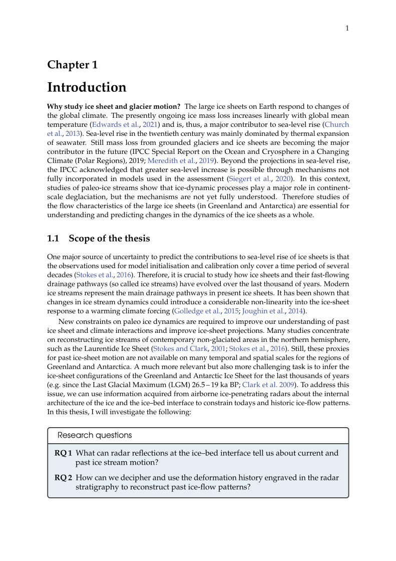
IntroductionWhy study ice sheet and glacier motion? The large ice sheets on Earth respond to changes ofthe global climate. The presently ongoing ice mass loss increases linearly with global meantemperature (Edwards et al., 2021) and is, thus, a major contributor to sea-level rise (Churchet al., 2013). Sea-level rise in the twentieth century was mainly dominated by thermal expansionof seawater. Still mass loss from grounded glaciers and ice sheets are becoming the majorcontributor in the future (IPCC Special Report on the Ocean and Cryosphere in a ChangingClimate (Polar Regions), 2019; Meredith et al., 2019). Beyond the projections in sea-level rise,the IPCC acknowledged that greater sea-level increase is possible through mechanisms notfully incorporated in models used in the assessment (Siegert et al., 2020). In this context,studies of paleo-ice streams show that ice-dynamic processes play a major role in continent-scale deglaciation, but the mechanisms are not yet fully understood. Therefore studies ofthe flow characteristics of the large ice sheets (in Greenland and Antarctica) are essential forunderstanding and predicting changes in the dynamics of the ice sheets as a whole.

1.1 Scope of the thesis

One major source of uncertainty to predict the contributions to sea-level rise of ice sheets is thatthe observations used for model initialisation and calibration only cover a time period of severaldecades (Stokes et al., 2016). Therefore, it is crucial to study how ice sheets and their fast-flowingdrainage pathways (so called ice streams) have evolved over the last thousand of years. Modernice streams represent the main drainage pathways in present ice sheets. It has been shown thatchanges in ice stream dynamics could introduce a considerable non-linearity into the ice-sheetresponse to a warming climate forcing (Golledge et al., 2015; Joughin et al., 2014).

New constraints on paleo ice dynamics are required to improve our understanding of pastice sheet and climate interactions and improve ice-sheet projections. Many studies concentrateon reconstructing ice streams of contemporary non-glaciated areas in the northern hemisphere,such as the Laurentide Ice Sheet (Stokes and Clark, 2001; Stokes et al., 2016). Still, these proxiesfor past ice-sheet motion are not available on many temporal and spatial scales for the regions ofGreenland and Antarctica. A much more relevant but also more challenging task is to infer theice-sheet configurations of the Greenland and Antarctic Ice Sheet for the last thousands of years(e.g. since the Last Glacial Maximum (LGM) 26.5 – 19 ka BP; Clark et al. 2009). To address thisissue, we can use information acquired from airborne ice-penetrating radars about the internalarchitecture of the ice and the ice–bed interface to constrain todays and historic ice-flow patterns.In this thesis, I will investigate the following:

Research questions

RQ 1 What can radar reflections at the ice–bed interface tell us about current andpast ice stream motion?

RQ 2 How can we decipher and use the deformation history engraved in the radarstratigraphy to reconstruct past ice-flow patterns?

Chapter 1. Introduction 2

1.2 Structure of the thesis

I present my research as a cumulative dissertation. Hence, this thesis is composed of a collectionof publications in recognised scientific journals. Some of the publications are already published,and others are currently in review or close to submission. In the central part of my thesis(Chapter 1 – 3), I explain the scientific background and the data and methods I use for myresearch. Then, I focus on the summary and key messages of my publications and discuss myfindings within the scope of the current state of the science.

The common thread running through the publications is the radar-based analysis of ice-internal and bed structures, which provide information about the past and present ice-flowcharacteristics. Further details of the background in radar data and all publications in full lengthare provided in the appendix. This results in the following structure of my thesis:

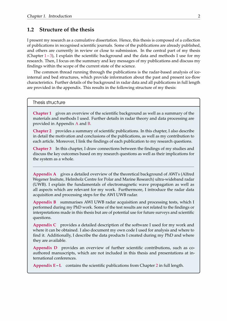
Thesis structure

Chapter 1 gives an overview of the scientific background as well as a summary of thematerials and methods I used. Further details in radar theory and data processing areprovided in Appendix A and B.

Chapter 2 provides a summary of scientific publications. In this chapter, I also describein detail the motivation and conclusions of the publications, as well as my contribution toeach article. Moreover, I link the findings of each publication to my research questions.

Chapter 3 In this chapter, I draw connections between the findings of my studies anddiscuss the key outcomes based on my research questions as well as their implications forthe system as a whole.

Appendix A gives a detailed overview of the theoretical background of AWI’s (AlfredWegener Insitute, Helmholz Centre for Polar and Marine Research) ultra-wideband radar(UWB). I explain the fundamentals of electromagnetic wave propagation as well asall aspects which are relevant for my work. Furthermore, I introduce the radar dataacquisition and processing steps for the AWI UWB radar.

Appendix B summarises AWI UWB radar acquisition and processing tests, which Iperformed during my PhD work. Some of the test results are not related to the findings orinterpretations made in this thesis but are of potential use for future surveys and scientificquestions.

Appendix C provides a detailed description of the software I used for my work andwhere it can be obtained. I also document my own code I used for analysis and where tofind it. Additionally, I describe the data products I created during my PhD and wherethey are available.

Appendix D provides an overview of further scientific contributions, such as co-authored manuscripts, which are not included in this thesis and presentations at in-ternational conferences.

Appendix E – L contains the scientific publications from Chapter 2 in full length.

Chapter 1. Introduction 3

1.3 Background

"The polar regions are losing ice, and their oceans are changing rapidly. Theconsequences of this polar transition extend to the whole planet, and are affect-ing people in multiple ways."

IPCC - Special Report on the Ocean and Cryosphere in a ChangingClimate (Polar Regions), 2019, Meredith et al. (2019)

Around 71 % of the Earth surface are covered by the ocean, and another 10 % of the land areaby glaciers and ice sheets. Both systems are responsible for the distribution and storage of heatand carbon dioxide (CO2). The ice sheets of Antarctica and Greenland hold a respective waterequivalent to raise global sea level by 58 m (Fretwell et al., 2013) and 7.4 m (Morlighem et al.,2017). The fate of coastal cities as well as the heritage of many ecosystems depend on theirlong-term stability. In order to predict the changes in the polar regions due to a warming climateas well as their consequences for the entire Earth system, we have to understand the processesgoverning the dynamics of polar ice sheets.

99 % of all ice mass on Earth is stored in the Greenland (11 %) and Antarctic (88 %) IceSheet (Allison et al., 2009). Mass and energy are constantly exchanged between glaciers, oceans,the atmosphere, biosphere and the solid Earth and thus, play a central role in the globalhydrological system. Ice mass loss occurs due to meltwater runoff at the ice base and surfaceas well via calving at marine-terminating outlet glaciers. The regrowth of the collapse ofmarine ice sheets would require more than ten thousand years, considering the current rates ofaccumulation (Michael Oppenheimer, 1998). However, when global warming exceeds criticaltemperature thresholds, substantial ice loss is irreversible and ice masses would not regrow toits contemporary extent, even if the increase of the global mean temperature is reversed (Garbeet al., 2020).

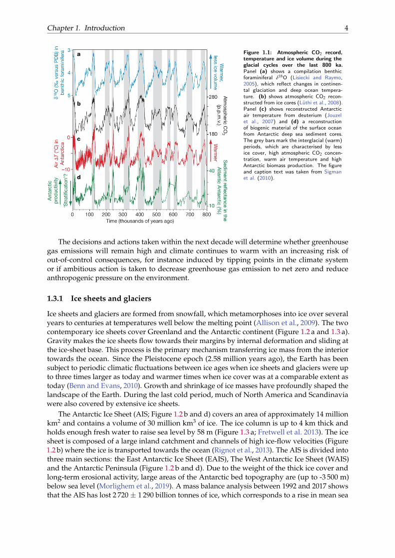
The importance and potential of sea level fluctuations is revealed by ocean sediment andice core records. For the last several million years (Pleistocene epoch) the Earth is experiencingcycles of extensive glaciation and warmer times called glacial and interglacial periods. Thesecycles currently last approximately 100 000 years, where the interglacial periods like the presentHolocene (with high sea level and low ice volume) make up around 10 % of the time (Allenet al., 2005). Changes between glacial and interglacial periods correlate with variations inthe atmospheric CO2 concentration (Figure 1.1), which causes a substantial fraction of ice-agecooling and helps to explain why the climate forcing is distributed globally (Sigman et al.,2010). Variations in sea level over the glacial cycles are mainly caused by the accretion or meltof continental ice (in contrast to sea ice) with a small contribution from thermal expansion ofocean water. In the past glacial periods, two additional large ice sheet covered Northern Europe(the Fennoscandian Ice Sheet) and North America (the Laurentide Ice Sheet). The maximumextension during the last glacial period occurred around 21 000 years ago. During the pastinterglacials, the extent of the Greenland and Antarctic Ice Sheet decreased but the ice sheetsnever fully disappeared. In this respect, it is timely to remember that simulations based on theRCP 8.5 scenario (Representative Concentration Pathway on greenhouse gas concentration; seeIPCC AR5; IPCC 2013), suggest that the Greenland Ice Sheet will potentially disappear within amillennium (Aschwanden et al., 2019).

Chapter 1. Introduction 4

Figure 1.1: Atmospheric CO2 record,temperature and ice volume during theglacial cycles over the last 800 ka.Panel (a) shows a compilation benthicforaminiferal δ18O (Lisiecki and Raymo,2005), which reflect changes in continen-tal glaciation and deep ocean tempera-ture. (b) shows atmospheric CO2 recon-structed from ice cores (Lüthi et al., 2008).Panel (c) shows reconstructed Antarcticair temperature from deuterium (Jouzelet al., 2007) and (d) a reconstructionof biogenic material of the surface oceanfrom Antarctic deep sea sediment cores.The grey bars mark the interglacial (warm)periods, which are characterised by lessice cover, high atmospheric CO2 concen-tration, warm air temperature and highAntarctic biomass production. The figureand caption text was taken from Sigmanet al. (2010).

The decisions and actions taken within the next decade will determine whether greenhousegas emissions will remain high and climate continues to warm with an increasing risk ofout-of-control consequences, for instance induced by tipping points in the climate systemor if ambitious action is taken to decrease greenhouse gas emission to net zero and reduceanthropogenic pressure on the environment.

1.3.1 Ice sheets and glaciers

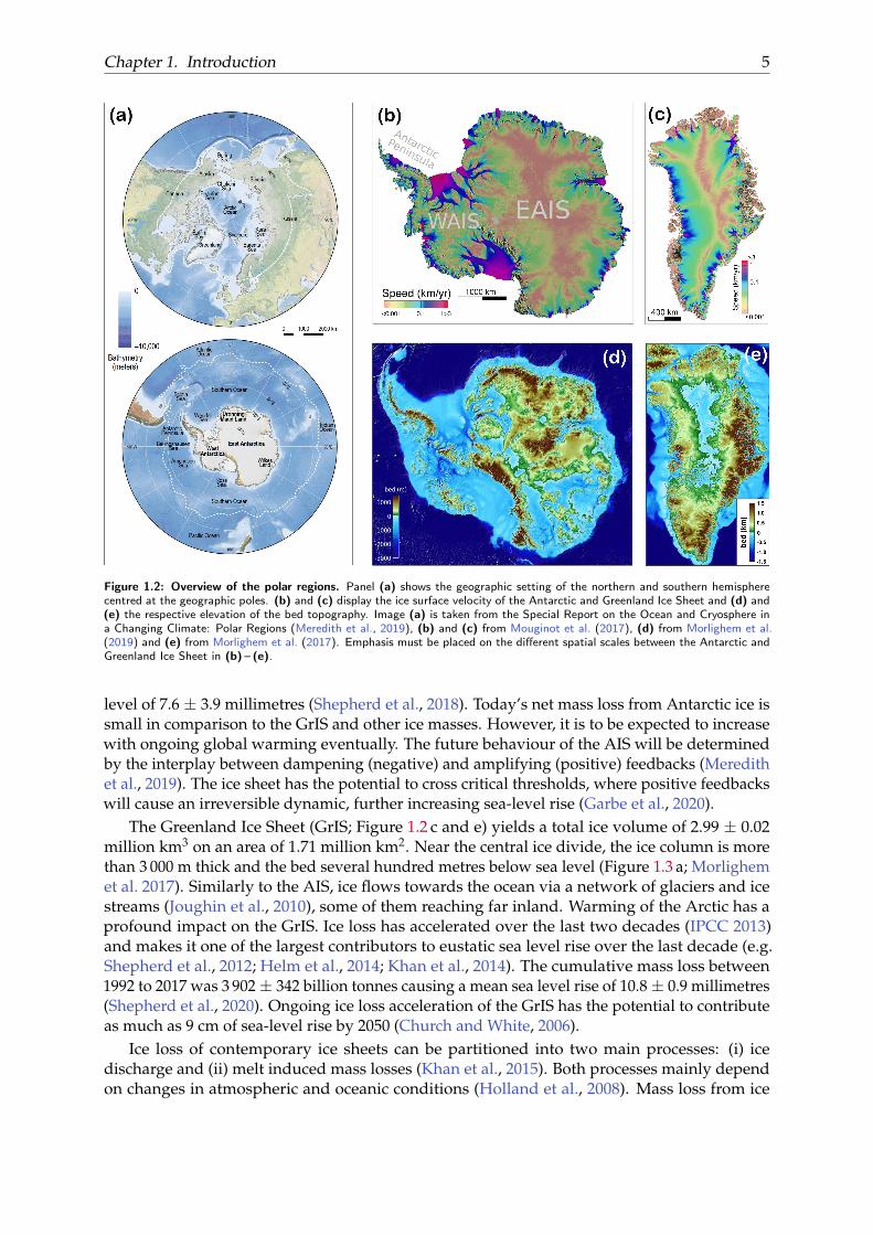
Ice sheets and glaciers are formed from snowfall, which metamorphoses into ice over severalyears to centuries at temperatures well below the melting point (Allison et al., 2009). The twocontemporary ice sheets cover Greenland and the Antarctic continent (Figure 1.2 a and 1.3 a).Gravity makes the ice sheets flow towards their margins by internal deformation and sliding atthe ice-sheet base. This process is the primary mechanism transferring ice mass from the interiortowards the ocean. Since the Pleistocene epoch (2.58 million years ago), the Earth has beensubject to periodic climatic fluctuations between ice ages when ice sheets and glaciers were upto three times larger as today and warmer times when ice cover was at a comparable extent astoday (Benn and Evans, 2010). Growth and shrinkage of ice masses have profoundly shaped thelandscape of the Earth. During the last cold period, much of North America and Scandinaviawere also covered by extensive ice sheets.

The Antarctic Ice Sheet (AIS; Figure 1.2 b and d) covers an area of approximately 14 millionkm2 and contains a volume of 30 million km3 of ice. The ice column is up to 4 km thick andholds enough fresh water to raise sea level by 58 m (Figure 1.3 a; Fretwell et al. 2013). The icesheet is composed of a large inland catchment and channels of high ice-flow velocities (Figure1.2 b) where the ice is transported towards the ocean (Rignot et al., 2013). The AIS is divided intothree main sections: the East Antarctic Ice Sheet (EAIS), The West Antarctic Ice Sheet (WAIS)and the Antarctic Peninsula (Figure 1.2 b and d). Due to the weight of the thick ice cover andlong-term erosional activity, large areas of the Antarctic bed topography are (up to -3 500 m)below sea level (Morlighem et al., 2019). A mass balance analysis between 1992 and 2017 showsthat the AIS has lost 2 720 ± 1 290 billion tonnes of ice, which corresponds to a rise in mean sea

Chapter 1. Introduction 5

Figure 1.2: Overview of the polar regions. Panel (a) shows the geographic setting of the northern and southern hemispherecentred at the geographic poles. (b) and (c) display the ice surface velocity of the Antarctic and Greenland Ice Sheet and (d) and(e) the respective elevation of the bed topography. Image (a) is taken from the Special Report on the Ocean and Cryosphere ina Changing Climate: Polar Regions (Meredith et al., 2019), (b) and (c) from Mouginot et al. (2017), (d) from Morlighem et al.(2019) and (e) from Morlighem et al. (2017). Emphasis must be placed on the different spatial scales between the Antarctic andGreenland Ice Sheet in (b) – (e).

level of 7.6 ± 3.9 millimetres (Shepherd et al., 2018). Today’s net mass loss from Antarctic ice issmall in comparison to the GrIS and other ice masses. However, it is to be expected to increasewith ongoing global warming eventually. The future behaviour of the AIS will be determinedby the interplay between dampening (negative) and amplifying (positive) feedbacks (Meredithet al., 2019). The ice sheet has the potential to cross critical thresholds, where positive feedbackswill cause an irreversible dynamic, further increasing sea-level rise (Garbe et al., 2020).

The Greenland Ice Sheet (GrIS; Figure 1.2 c and e) yields a total ice volume of 2.99 ± 0.02million km3 on an area of 1.71 million km2. Near the central ice divide, the ice column is morethan 3 000 m thick and the bed several hundred metres below sea level (Figure 1.3 a; Morlighemet al. 2017). Similarly to the AIS, ice flows towards the ocean via a network of glaciers and icestreams (Joughin et al., 2010), some of them reaching far inland. Warming of the Arctic has aprofound impact on the GrIS. Ice loss has accelerated over the last two decades (IPCC 2013)and makes it one of the largest contributors to eustatic sea level rise over the last decade (e.g.Shepherd et al., 2012; Helm et al., 2014; Khan et al., 2014). The cumulative mass loss between1992 to 2017 was 3 902 ± 342 billion tonnes causing a mean sea level rise of 10.8 ± 0.9 millimetres(Shepherd et al., 2020). Ongoing ice loss acceleration of the GrIS has the potential to contributeas much as 9 cm of sea-level rise by 2050 (Church and White, 2006).

Ice loss of contemporary ice sheets can be partitioned into two main processes: (i) icedischarge and (ii) melt induced mass losses (Khan et al., 2015). Both processes mainly dependon changes in atmospheric and oceanic conditions (Holland et al., 2008). Mass loss from ice

Chapter 1. Introduction 6

discharge is dynamically induced and related to changes in the ice movement (e.g. increasein ice flow due to a reduction of marine ice shelf buttressing (see Dupont and Alley, 2005;Gagliardini et al., 2010) or a reduction of the resistance at the glacier bed). Melt induced iceloss is expressed by changes in the surface mass balance (SMB), which represents the differencebetween accumulation (via snow deposition and refreezing rain) and ablation (via sublimation,meltwater runoff and snow erosion).

1.3.2 The flow and deformation of ice

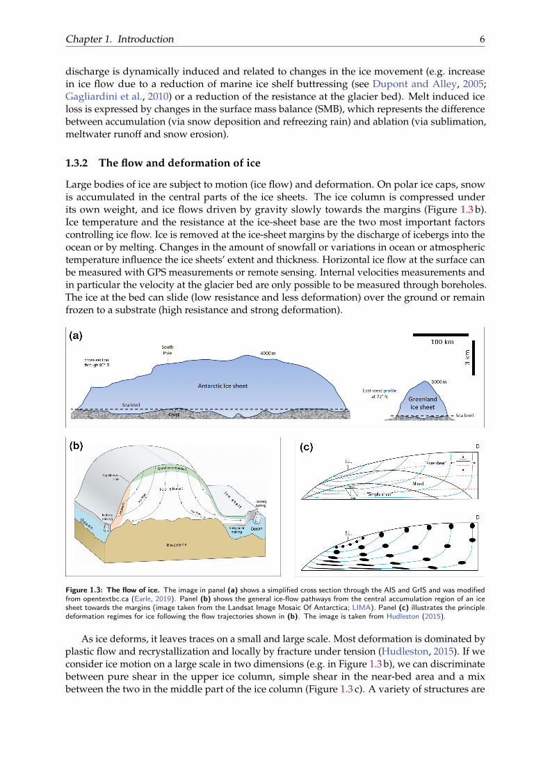
Large bodies of ice are subject to motion (ice flow) and deformation. On polar ice caps, snowis accumulated in the central parts of the ice sheets. The ice column is compressed underits own weight, and ice flows driven by gravity slowly towards the margins (Figure 1.3 b).Ice temperature and the resistance at the ice-sheet base are the two most important factorscontrolling ice flow. Ice is removed at the ice-sheet margins by the discharge of icebergs into theocean or by melting. Changes in the amount of snowfall or variations in ocean or atmospherictemperature influence the ice sheets’ extent and thickness. Horizontal ice flow at the surface canbe measured with GPS measurements or remote sensing. Internal velocities measurements andin particular the velocity at the glacier bed are only possible to be measured through boreholes.The ice at the bed can slide (low resistance and less deformation) over the ground or remainfrozen to a substrate (high resistance and strong deformation).

Figure 1.3: The flow of ice. The image in panel (a) shows a simplified cross section through the AIS and GrIS and was modifiedfrom opentextbc.ca (Earle, 2019). Panel (b) shows the general ice-flow pathways from the central accumulation region of an icesheet towards the margins (image taken from the Landsat Image Mosaic Of Antarctica; LIMA). Panel (c) illustrates the principledeformation regimes for ice following the flow trajectories shown in (b). The image is taken from Hudleston (2015).

As ice deforms, it leaves traces on a small and large scale. Most deformation is dominated byplastic flow and recrystallization and locally by fracture under tension (Hudleston, 2015). If weconsider ice motion on a large scale in two dimensions (e.g. in Figure 1.3 b), we can discriminatebetween pure shear in the upper ice column, simple shear in the near-bed area and a mixbetween the two in the middle part of the ice column (Figure 1.3 c). A variety of structures are

Chapter 1. Introduction 7

the result of cumulative deformation. For instance, foliation or folding can be identified in icesheets because new layers of snow are deposited horizontally on the ice sheet representing anundisturbed horizon. Variations in ice flow over time or inhomogeneities in the flow associatedwith shear zones (Hudleston, 2015) are one possible mechanism for ice deformation. A typicalregime in an ice sheet where strong deformations are occurring are so-called ice streams.

In the AIS and GrIS, ice streams are commonly referred to as corridors of fast ice flow withinan ice sheet, responsible for discharging the majority of the ice and sediment within them(Bennett, 2003). Ice streams were first defined by Swithinbank (1954) as a part of an inland icesheet that flows faster than the surrounding ice. Six decades ago, Henri Bader provided anotherdefinition for an ice stream (Bader, 1961): An "ice stream" is something akin to a mountain glacierconsisting of a broad accumulation basin and a narrower outlet valley glacier: but a mountain glacier islaterally hemmed in by rock slopes, while the ice stream is contained by slower moving surrounding ice.

Ice streams play a key role in the stability of ice sheets. As all ice from the AIS and GrIS isdischarged into the ocean, ice streams provide a link between the cryosphere and the ocean.Today, ice streams discharge over 90 % of all the ice and sediment of the the AIS (Bamber et al.,2000). Episodes of intensive ice streaming have been suggested to trigger a climate responseof a global extent (Broecker, 1994). Therefore, it is important to understand the mechanics offast ice flow and to investigate the controlling factors for ice stream initiation and shut down todecode past glacial activity as well as to predict the future evolution of an ice sheet (Bennett,2003). Winsborrow et al. (2010) identified potential controls on ice stream locations in theliterature, such as topographic focusing, topographic steps, topographic roughness, calvingmargin, subglacial geology, geothermal heat flux and subglacial meltwater routing. Wheninvestigating the controls on ice stream geometry and location, it can be difficult to distinguishthe cause and effect of ice stream activity. E.g. does a smooth bed initiate or favour ice streaminitiation, or is a smooth bed the result of ice stream activity?

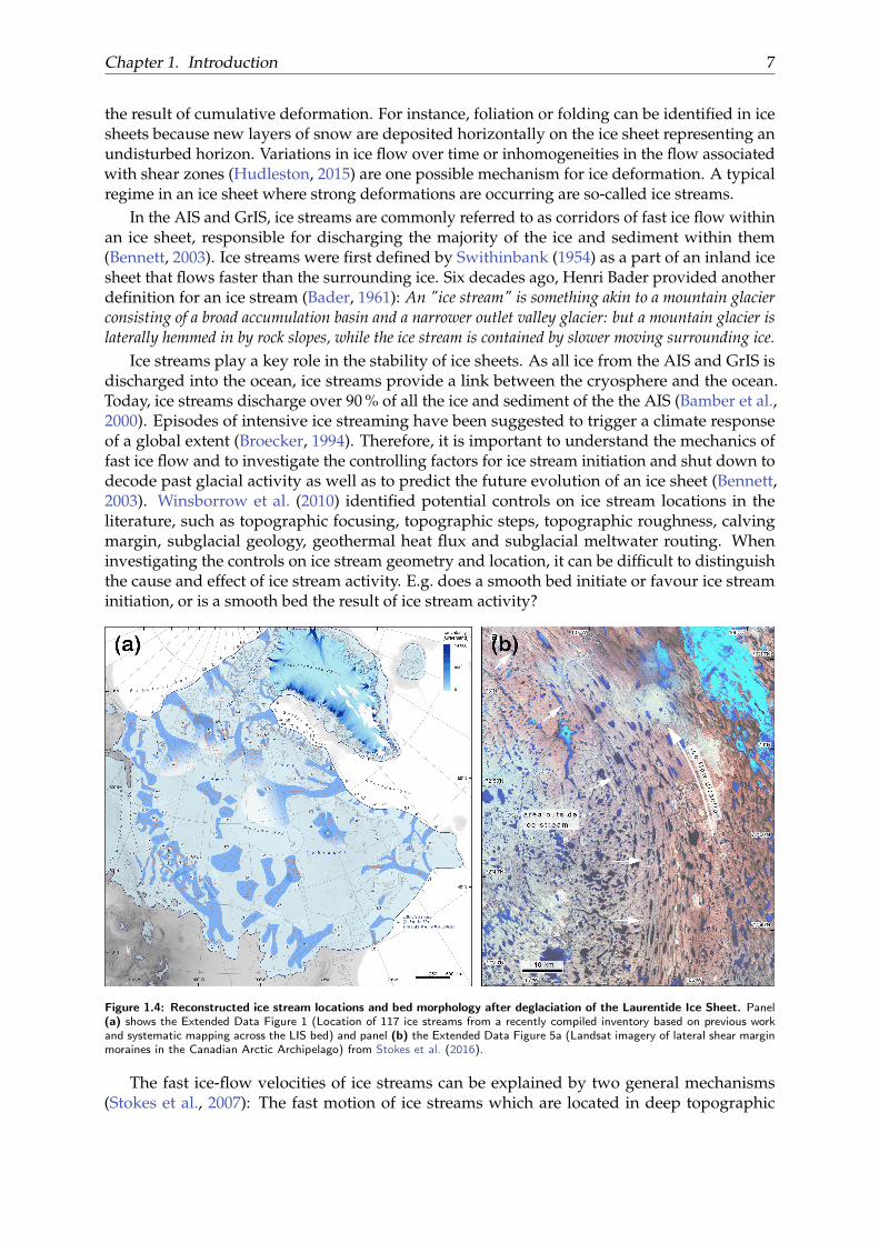
Figure 1.4: Reconstructed ice stream locations and bed morphology after deglaciation of the Laurentide Ice Sheet. Panel(a) shows the Extended Data Figure 1 (Location of 117 ice streams from a recently compiled inventory based on previous workand systematic mapping across the LIS bed) and panel (b) the Extended Data Figure 5a (Landsat imagery of lateral shear marginmoraines in the Canadian Arctic Archipelago) from Stokes et al. (2016).

The fast ice-flow velocities of ice streams can be explained by two general mechanisms(Stokes et al., 2007): The fast motion of ice streams which are located in deep topographic

Chapter 1. Introduction 8

troughs is enabled by the so-called creep instability (Clarke et al., 1977). Ice streams that are notconstrained by a subglacial valley require a layer where sliding is facilitated, such as a lubricatedbed or soft and deformable sediment (Anandakrishnan and Alley, 1997). Furthermore, it wasshown that ice streams can be highly dynamic and are subject to rapid changes. Changes in theice-sheet configuration, such as continuing thinning or thicknening are presumably responsiblefor a switch in flow direction of the Whillans ice stream (Conway et al., 2002). Also, numerous icestreams show a decrease or increase in ice-flow velocity over time (Stephenson and Bindschadler,1988; Joughin et al., 2003). Changes in ice stream behaviour are either driven by external forcing(e.g., changes in the atmosphere or ocean) or internal forcing at the ice stream bed Margold et al.(2015).

In contrast to atmospheric and oceanic measurements, it is far more challenging to investigatethe glacier bed. Only a few single borehole locations in Greenland and Antarctica give insightinto the in-situ physical and material properties. However, the bed characteristics of paleo icestreams can be reconstructed from sedimentary records and the analysis of former subglaciallandforms (Stokes and Clark, 2001). A large number of former ice streams of the LaurentideIce Sheet (LIS; former largest of the Northern Hemisphere ice sheets during the last ice ages)have been reconstructed and described by Margold et al. (2015) (Figure 1.4). Stokes et al. (2016)investigated the potential impact of ice streams of the former LIS during deglaciation afterits maximum extent approximately 22 000 years ago. The drainage network of the LIS hada comparable extent as the AIS and GrIS. The authors find evidence that depending on theice-sheet scale, its drainage network adjusted to the changes in ice-sheet volume. It is possiblethat ice streams had a less severe impact on the ice-sheet mass balance during the retreat ofthe LIS as hypothesised for modern ice streams. However, it is unclear if these findings can betranslated to modern ice sheets (Stokes et al., 2016).

1.3.3 Ice-sheet bed and internal processes

Processes at the ice-sheet bed ice-flow patterns can be complex and the basal propertiesrender one of the most important parametrisations in ice-flow modelling, such as bed type andstructure and availability of liquid water (Wilkens et al., 2015). The ice base (also referred toas the interface between ice and the underlying material) of glaciers and ice sheets is one ofthe most difficult to access parts of an ice sheet. The way the ice sheet behaves depends on theconditions underneath the ice. In particular, the geometry of the bed topography, the physicalconditions (e.g. temperature, softness of the bed and liquid water content and subglacial waterpressure) and material properties of the basal ice influence ice flow. At the same time, ice flowaffects the ice-underlying material. For example the removal of material of material at the icebase contributes to the sculpting of the subglacial environment and transportation of materialdownstream. Furthermore, increased sliding increases the temperature at the ice base, which inturn plays a major role in respect to the availability of subglacial water.

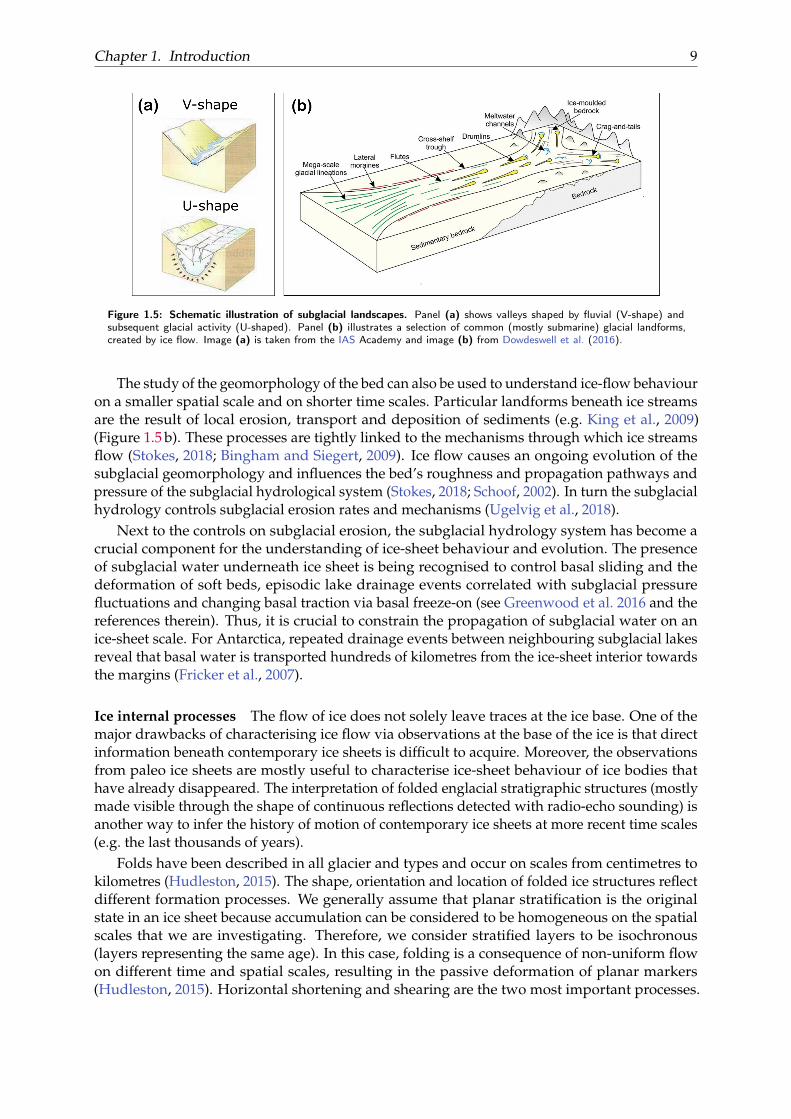
Glacial erosion has contributed to the creation of alpine landscapes, scouring of areasand transportation and deposition of sediments (Cook and Swift, 2012). Formerly glaciatedregions give insight into the evolution of glacial landscapes. The distribution of large erosionallandforms, such as U-shaped valleys, scoured areas, cirques and overdeepenings can be usedto reconstruct the paleo-glaciological conditions (Glasser and Bennett, 2004). In this context,geomorphological observations of the bed can also be used to infer the glacial history beneathcontemporary ice sheets (Bingham et al., 2010). In particular, the widening and deepening ofsubglacial valleys, starting from pre-glacial fluvial erosion with successive glacial cycles (Figure1.5 a), have the potential to constrain the evolution, dynamics and ice extent of former andcontemporary ice sheets (e.g. Cook and Swift, 2012; Taylor et al., 2004; Kessler et al.; Kaplanet al., 2009).

Chapter 1. Introduction 9

Figure 1.5: Schematic illustration of subglacial landscapes. Panel (a) shows valleys shaped by fluvial (V-shape) andsubsequent glacial activity (U-shaped). Panel (b) illustrates a selection of common (mostly submarine) glacial landforms,created by ice flow. Image (a) is taken from the IAS Academy and image (b) from Dowdeswell et al. (2016).

The study of the geomorphology of the bed can also be used to understand ice-flow behaviouron a smaller spatial scale and on shorter time scales. Particular landforms beneath ice streamsare the result of local erosion, transport and deposition of sediments (e.g. King et al., 2009)(Figure 1.5 b). These processes are tightly linked to the mechanisms through which ice streamsflow (Stokes, 2018; Bingham and Siegert, 2009). Ice flow causes an ongoing evolution of thesubglacial geomorphology and influences the bed’s roughness and propagation pathways andpressure of the subglacial hydrological system (Stokes, 2018; Schoof, 2002). In turn the subglacialhydrology controls subglacial erosion rates and mechanisms (Ugelvig et al., 2018).

Next to the controls on subglacial erosion, the subglacial hydrology system has become acrucial component for the understanding of ice-sheet behaviour and evolution. The presenceof subglacial water underneath ice sheet is being recognised to control basal sliding and thedeformation of soft beds, episodic lake drainage events correlated with subglacial pressurefluctuations and changing basal traction via basal freeze-on (see Greenwood et al. 2016 and thereferences therein). Thus, it is crucial to constrain the propagation of subglacial water on anice-sheet scale. For Antarctica, repeated drainage events between neighbouring subglacial lakesreveal that basal water is transported hundreds of kilometres from the ice-sheet interior towardsthe margins (Fricker et al., 2007).

Ice internal processes The flow of ice does not solely leave traces at the ice base. One of themajor drawbacks of characterising ice flow via observations at the base of the ice is that directinformation beneath contemporary ice sheets is difficult to acquire. Moreover, the observationsfrom paleo ice sheets are mostly useful to characterise ice-sheet behaviour of ice bodies thathave already disappeared. The interpretation of folded englacial stratigraphic structures (mostlymade visible through the shape of continuous reflections detected with radio-echo sounding) isanother way to infer the history of motion of contemporary ice sheets at more recent time scales(e.g. the last thousands of years).

Folds have been described in all glacier and types and occur on scales from centimetres tokilometres (Hudleston, 2015). The shape, orientation and location of folded ice structures reflectdifferent formation processes. We generally assume that planar stratification is the originalstate in an ice sheet because accumulation can be considered to be homogeneous on the spatialscales that we are investigating. Therefore, we consider stratified layers to be isochronous(layers representing the same age). In this case, folding is a consequence of non-uniform flowon different time and spatial scales, resulting in the passive deformation of planar markers(Hudleston, 2015). Horizontal shortening and shearing are the two most important processes.

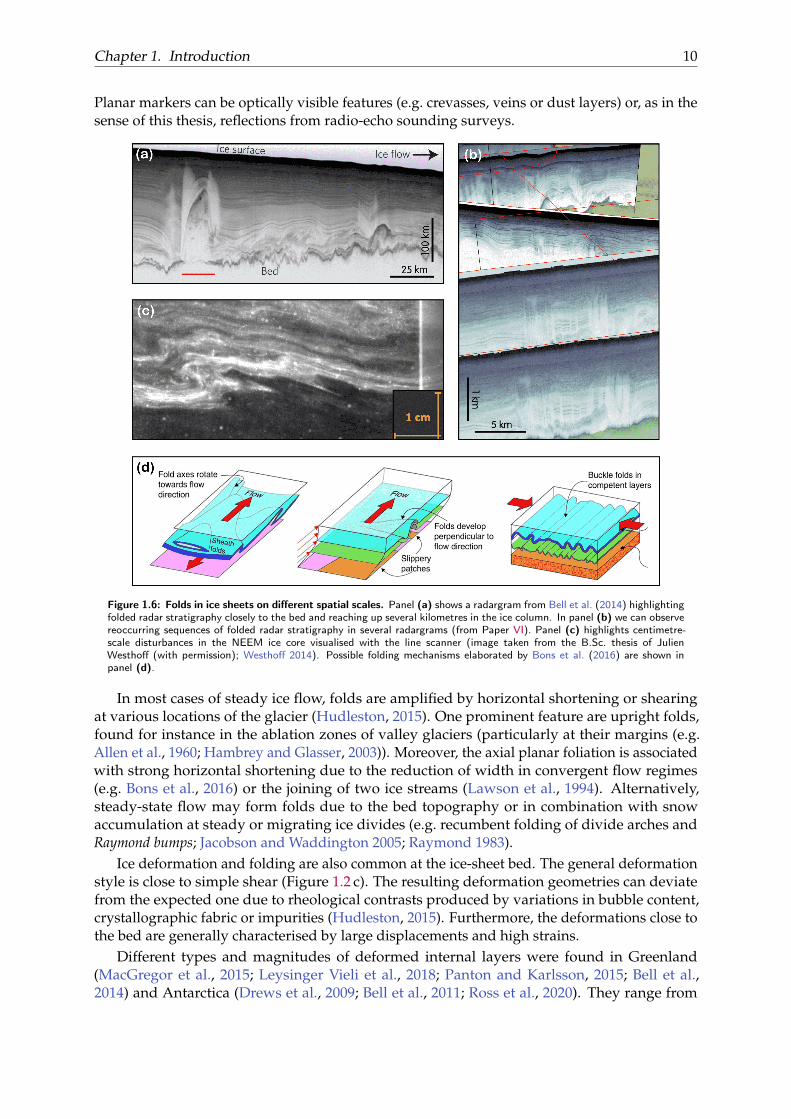
Chapter 1. Introduction 10

Planar markers can be optically visible features (e.g. crevasses, veins or dust layers) or, as in thesense of this thesis, reflections from radio-echo sounding surveys.

Figure 1.6: Folds in ice sheets on different spatial scales. Panel (a) shows a radargram from Bell et al. (2014) highlightingfolded radar stratigraphy closely to the bed and reaching up several kilometres in the ice column. In panel (b) we can observereoccurring sequences of folded radar stratigraphy in several radargrams (from Paper VI). Panel (c) highlights centimetre-scale disturbances in the NEEM ice core visualised with the line scanner (image taken from the B.Sc. thesis of JulienWesthoff (with permission); Westhoff 2014). Possible folding mechanisms elaborated by Bons et al. (2016) are shown inpanel (d).

In most cases of steady ice flow, folds are amplified by horizontal shortening or shearingat various locations of the glacier (Hudleston, 2015). One prominent feature are upright folds,found for instance in the ablation zones of valley glaciers (particularly at their margins (e.g.Allen et al., 1960; Hambrey and Glasser, 2003)). Moreover, the axial planar foliation is associatedwith strong horizontal shortening due to the reduction of width in convergent flow regimes(e.g. Bons et al., 2016) or the joining of two ice streams (Lawson et al., 1994). Alternatively,steady-state flow may form folds due to the bed topography or in combination with snowaccumulation at steady or migrating ice divides (e.g. recumbent folding of divide arches andRaymond bumps; Jacobson and Waddington 2005; Raymond 1983).

Ice deformation and folding are also common at the ice-sheet bed. The general deformationstyle is close to simple shear (Figure 1.2 c). The resulting deformation geometries can deviatefrom the expected one due to rheological contrasts produced by variations in bubble content,crystallographic fabric or impurities (Hudleston, 2015). Furthermore, the deformations close tothe bed are generally characterised by large displacements and high strains.

Different types and magnitudes of deformed internal layers were found in Greenland(MacGregor et al., 2015; Leysinger Vieli et al., 2018; Panton and Karlsson, 2015; Bell et al.,2014) and Antarctica (Drews et al., 2009; Bell et al., 2011; Ross et al., 2020). They range from

Chapter 1. Introduction 11

overturned and sheath folds as well as plume-like structures associated with large units ofdisrupted stratigraphy at the ice base (see MacGregor et al. 2015; Bell et al. 2014; Bons et al. 2016;Leysinger Vieli et al. 2018 and Figure 1.6 a), over tight folds that extend almost over the entireice column with a fold axis oriented parallel to the shear margins of ice streams (see Franke et al.2020, Paper VI – VII and Figure 1.6 b), to small folds visible in ice cores (Figure 1.6 c), such ascentimetre-scale undulations observed in the visual stratigraphy of ice cores (NEEM communitymembers, 2013; Jansen et al., 2016; Westhoff et al., 2020).

The overview given here, of course, represents only a fraction of the background informationthat is important for ice-dynamic processes in ice sheets. More detailed information can befound in the individual manuscripts. The majority of the studies (Papers I, II and V – VIII) focuson the Greenland Ice Sheet. Studies III and IV, on the other hand, analyse data from Antarctica.The exact survey areas are described in Section 1.6. The manuscripts are basically divided intotwo groups, with papers I – IV dealing with processes and findings from the base of the ice sheetand papers V – VIII dealing with processes within the ice.

Chapter 1. Introduction 12

1.4 Ultra-wideband radar

The results of this thesis are based on radio-echo sounding (radar) data acquired with a multi-channel ultra wideband (UWB) radar system mounted on AWI’s polar research aircraft Polar 6.In this section, I introduce the radar based measurement principle to investigate ice sheets andglaciers (radioglaciology), the acquisition system, data processing steps as well as the methods Iuse to analyse the data. More specific information can be found in the Appendix A and B and inthe method sections in the scientific publications.

1.4.1 Radioglaciology

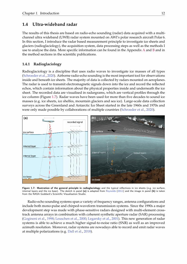
Radioglaciology is a discipline that uses radio waves to investigate ice masses of all types(Schroeder et al., 2020). Airborne radio-echo sounding is the most important tool for observationsinside and beneath ice sheets. The majority of data is collected by radars mounted on aeroplanes.The radar is used to transmit electromagnetic signals down into the ice and record the reflectedechos, which contain information about the physical properties inside and underneath the icesheet. The recorded data are visualised in radargrams, which are vertical profiles through theice column (Figure 1.7). Radar waves have been used for more than five decades to sound icemasses (e.g. ice sheets, ice shelfes, mountain glaciers and sea ice). Large-scale data collectionsurveys across the Greenland and Antarctic Ice Sheet started in the late 1960s and 1970s andwere only made possible by collaborations of multiple countries (Schroeder et al., 2020).

Figure 1.7: Illustration of the general principle in radioglaciology and the typical reflections in ice sheets (e.g. ice surface,internal layers and the ice base). The sketch in panel (a) is adapted from Reynolds (2011) and the image in panel (b) is takenfrom the NASA Goddard’s Scientific Visualisation Studio.

Radio-echo sounding systems span a variety of frequency ranges, antenna configurations andinclude both mono-pulse and chirped-waveform transmission systems. Since the 1990s a majordevelopment step was made with phase-sensitive radars designed with multi-element cross-track antenna arrays in combination with coherent synthetic aperture radar (SAR) processing(Gogineni et al., 1998; Leuschen et al., 2000; Legarsky et al., 2001). This new generation of radarsystems is able to achieve a much higher signal-to-noise ratio (SNR) as well as an improvedazimuth resolution. Moreover, radar systems are nowadays able to record and emit radar wavesat multiple polarizations (e.g. Dall et al., 2018).

Chapter 1. Introduction 13

Regardless of the type of radar system, the analysis of the data is based on the same physicalprinciples. Radar waves travelling through the ice get reflected at every interface separatingmaterials of contrasting electromagnetic properties (in particular, the dielectric properties).These reflections are referred to as internal reflection horizons IRHs and their geometry containsinformation about the history of the ice sheet. In combination with ice core dating, IRHs can beused to reconstruct accumulation rates or historic ice flow (e.g. Paren and Robin, 1975; Jacobeland Hodge, 1995; Cavitte et al., 2016). Next to the analysis of englacial properties, the primaryobjective of the vast majority of radar soundings was to locate the bed reflection and obtaininformation about the ice thickness (Bailey et al., 1964; Bamber et al., 2013; Fretwell et al., 2013).

In this thesis, I build my analysis on radar data, which has been acquired with one of themost modern airborne radio-echo sounding systems at the present time. The radar system anddata, as well as the survey regions are introduced in the upcoming sections. Details about thespecific survey and acquisition can be found in the respective manuscripts. Two sections in theAppendix provide further details on the theoretical background of the radar system (AppendixA) and on acquisition and processing tests I performed during my PhD work (Appendix B).

1.4.2 UWB radar data

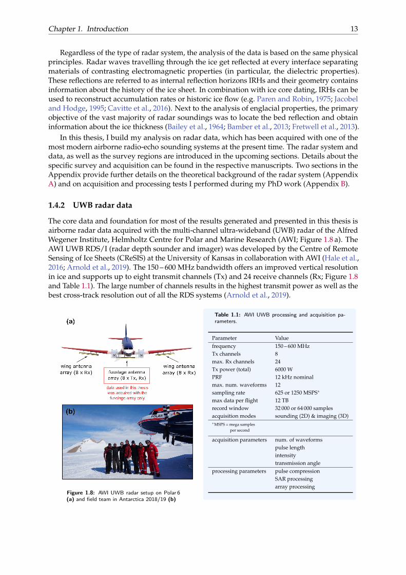
The core data and foundation for most of the results generated and presented in this thesis isairborne radar data acquired with the multi-channel ultra-wideband (UWB) radar of the AlfredWegener Institute, Helmholtz Centre for Polar and Marine Research (AWI; Figure 1.8 a). TheAWI UWB RDS/I (radar depth sounder and imager) was developed by the Centre of RemoteSensing of Ice Sheets (CReSIS) at the University of Kansas in collaboration with AWI (Hale et al.,2016; Arnold et al., 2019). The 150 – 600 MHz bandwidth offers an improved vertical resolutionin ice and supports up to eight transmit channels (Tx) and 24 receive channels (Rx; Figure 1.8and Table 1.1). The large number of channels results in the highest transmit power as well as thebest cross-track resolution out of all the RDS systems (Arnold et al., 2019).

Figure 1.8: AWI UWB radar setup on Polar 6(a) and field team in Antarctica 2018/19 (b)

Table 1.1: AWI UWB processing and acquisition pa-rameters.

Parameter Valuefrequency 150 – 600 MHzTx channels 8max. Rx channels 24Tx power (total) 6000 WPRF 12 kHz nominalmax. num. waveforms 12sampling rate 625 or 1250 MSPS∗

max data per flight 12 TBrecord window 32 000 or 64 000 samplesacquisition modes sounding (2D) & imaging (3D)∗MSPS = mega samples

per second

acquisition parameters num. of waveformspulse lengthintensitytransmission angle

processing parameters pulse compressionSAR processingarray processing

Chapter 1. Introduction 14

The radar can resolve details of the lower ice stratigraphy, which allow new possibilities for theinterpretation of englacial structures. In my thesis, I used data from three different surveys ofthe Greenland campaign 2018 and from one survey in Antarctica in austral summer 2018/19:

1. EGRIP-NOR-2018: A survey in the vicinity of the EastGRIP (East Greenland Ice-CoreProject) drill site on the Northeast Greenland Ice Stream (NEGIS) (Figure 1.13 a and c).The focus of this survey was to image the ice thickness and bed properties as well as thestratigraphy of the whole ice column, in particular at the ice streams shear margins.

2. FINEGIS: A survey in Northern Greenland upstream of the 79°NG (Figure 1.13 a and b).The survey lines cover a set of cylindrical folds, and the aim of the survey was to imagethe deformation structures of the folds.

3. JURAS: A survey at the onset of the Jutulstraumen Glacier, Dronning Maud Land, Antarc-tica (Figure 1.14). The survey area is located between Troll (Norway) and Kohnen (Ger-many) station. The focus of the survey was to map the radar stratigraphy perpendicularto ice flow as well as close substantial gaps in the bed topography data.

In the following, I will (i) show how the radar data is acquired and processed to generatehigh-resolution radargrams, (ii) introduce the methods used to infer the physical conditions anderosional activity at the ice base and (iii) the procedure for the construction and analysis of 3Dsurfaces of englacial layers.

General workflow of radar data acquisition and processing

Figure 1.9 illustrates the complete workflow starting with the radar data acquisition in the fielduntil the generation of data products, which are used for scientific analysis. The raw radardata as well as GPS positioning data is initially saved on a large raid set of SSD disks on theacquisition server. A backup is created after every flight, either on a second set of SSD disks oron HDD disks. A first so-called qlook processing is applied to check the quality and generate firstradargrams. Complete SAR processing in the field is usually too time consuming and requiresfurther computational resources.

After a field season, the AWI aircraft team stores all GPS/INS and metadata as well as thedata from other instruments (e.g. Laserscanner data) in the DMS archive. UWB raw radar datacan be transferred to the AWI servers via the Ground 3 server. A compressed version of the rawdata is transferred to the AWI HSM server and stored at the WORM (write once read many)file system. This has the advantage that the raw data is highly protected and cannot be deletedeasily. The uncompressed raw data is transferred to the HPC (High Performance Computation)server Ollie for full data processing.

The option for parallel processing of the radar data reduces the time needed to generateresults. For the processing, we use the CReSIS Toolbox (CReSIS-Toolbox, 2019), developed bythe team of John Paden from the Centre for Remote Sensing of Ice Sheets at the Universityof Kansas. The toolbox generates various types of high-resolution radargrams in the form ofmatfiles (hdf5 format). We can consider three typical types of results:

1. The qlook data product, which is an efficiently produced output and only performsstacking (averaging followed by decimation) in the along-track dimension without anykind of migration/focusing in the along-track.

2. The SAR data product uses fk-migration to focus scattered energy back to their reflectionorigin (Leuschen et al., 2000).

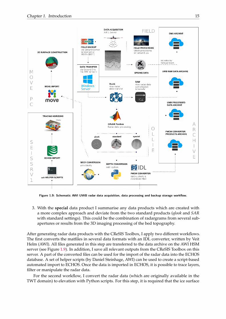
Chapter 1. Introduction 15

Figure 1.9: Schematic AWI UWB radar data acquisition, data processing and backup storage workflow.

3. With the special data product I summarise any data products which are created witha more complex approach and deviate from the two standard products (qlook and SARwith standard settings). This could be the combination of radargrams from several sub-apertures or results from the 3D imaging processing of the bed topography.

After generating radar data products with the CReSIS Toolbox, I apply two different workflows.The first converts the matfiles in several data formats with an IDL converter, written by VeitHelm (AWI). All files generated in this step are transferred to the data archive on the AWI HSMserver (see Figure 1.9). In addition, I save all relevant outputs from the CReSIS Toolbox on thisserver. A part of the converted files can be used for the import of the radar data into the ECHOSdatabase. A set of helper scripts (by Daniel Steinhage, AWI) can be used to create a script-basedautomated import to ECHOS. Once the data is imported in ECHOS, it is possible to trace layers,filter or manipulate the radar data.

For the second workflow, I convert the radar data (which are originally available in theTWT domain) to elevation with Python scripts. For this step, it is required that the ice surface

Chapter 1. Introduction 16

reflection is available and correct. After that, I convert the data to the SEGY format to importthe files to the Move software. Move is afterwards used to generate 3D surfaces of englacialstructures.

Chapter 1. Introduction 17

1.5 Methods for radar data analysis

In this section, I introduce the methods I apply and describe how they are used to gain infor-mation on ice-sheet motion. The focus lies on their general description and how I use them toanswer my research questions. For an in-depth description, I refer to the manuscripts in whichthey are used, as well as to other literature.

Methods

1. Analysis of the geometry/geomorphology of the bed

2. Analysis of reflection patterns and intensities at the bed

3. Analysis of subglacial water transport and ice mass flux

4. Two- and three-dimensional analysis of radar stratigraphy

1. Analysis of the geometry/geomorphology of the ice-sheet bed

The base of a glacier is the most difficult part of an ice sheet to access. At the same time, itcontains many of the most important parameters to understand ice flow, such as the geologicaltype of the bed, its ability to deform, the temperature regime and the availability of subglacialwater. Next to seismic surveys and in-situ information acquired by drilling through the ice,radar surveys are the most effective way to infer the physical properties of the base.

We use the reflection of the ice surface and ice–bed interface in our radar data to calculate theice thickness and the elevation of the bed topography. As a result, we obtain the bed topographyalong the flight path of our instrument. I use this purely geometric information to:

(A) Create and analyse a digital elevation model (DEM) of bed topography elevation (seePaper I, III). The bedrock topography is an essential boundary condition for numericalmodelling studies of the Greenland and Antarctic Ice Sheet (Bamber et al., 2001). Further-more, it provides essential information on the large-scale morphology of the bed. Airborneradar data provide bed elevation measurements directly beneath the flight trajectory.Hence, depending on the flight line coverage, major data gaps remain. Therefore, weextrapolate the point measurements to a two-dimensional DEM. The actual resolutiondepends on the measurement density, which can introduce errors (Morlighem et al., 2019).

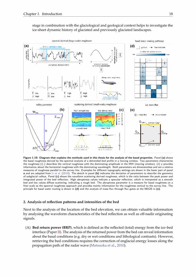
(B) Analyse the roughness of the bed topography (see Paper II, III and Figure 1.10 a), whichis a geomorphological parametrisation of the undulations of the bed beneath an ice mass(Lindbäck and Pettersson, 2015). It can be determined via statistical analysis of verticalvariation in along-track bed topography (e.g. Siegert et al., 2005; Cooper et al., 2019).Basal roughness has become an indicator of subglacial conditions for past ice-flow activityand potential control for current ice-sheet dynamics (Rippin et al., 2014). For this study,we employ a spectral method to analyse the vertical and horizontal roughness with theapplication of fast Furier transforms (FFT; Hubbard et al. 2000).

(C) Analyse specific subglacial structures, such as subglacial valleys (Paper III and Figure1.10 b). Knowledge of their location, extend, and geometry is important to determine thedevelopmental stage for a glacial valley (Hirano and Aniya, 1988). The developmental

Chapter 1. Introduction 18

stage in combination with the glaciological and geological context helps to investigate theice-sheet dynamic history of glaciated and previously glaciated landscapes.

Figure 1.10: Diagram that explains the methods used in this thesis for the analysis of the basal properties. Panel (a) showsthe basal roughness derived by the spectral analysis of a detrended bed profile in a moving window. Two parameters characterisethe roughness (i) ξ describes the vertical roughness with the dominating amplitude in the MW (moving window), (ii) η providesinformation about the horizontal roughness with the dominating wavelength. Both parameters are dimensionless and are a relativemeasures of roughness parallel to the survey line. Examples for different topography settings are shown in the lower part of panela and are adapted from Li et al. (2010). The sketch in panel (b) indicates the deviation of parameters to describe the geometryof subglacial valleys. Panel (c) shows the waveform scattering derived roughness, which is the ratio between the peak power andintegrated power of the bed reflection. High abruptness values indicate a specular reflection, which is interpreted as a smoothbed and low values diffuse scattering, indicating a rough bed. The abruptness parameter is a measure for basal roughness on afiner scale as the spectral roughness approach and provides mainly information for the roughness vertical to the survey line. Theprinciple for basal water routing is shown in (d) and the analysis of mass flux through flux gates at the NEGIS in (e).

2. Analysis of reflection patterns and intensities of the bed

Next to the analysis of the location of the bed elevation, we can obtain valuable informationby analysing the waveform characteristics of the bed reflection as well as off-nadir originatingsignals.

(A) Bed return power (BRP), which is defined as the reflected (total) energy from the ice–bedinterface (Paper II). The analysis of the returned power from the bed can reveal informationabout the basal conditions (e.g. dry or wet conditions and lithological contrasts). However,retrieving the bed conditions requires the correction of englacial energy losses along thepropagation path of the radar wave (Matsuoka et al., 2010).

Chapter 1. Introduction 19

(B) Roughness derived from waveform scattering (Paper II) describes the relative spreadof the bed-echo waveform return (Cooper et al., 2019). The characteristics of the returnsignal are related to the electromagnetic scattering from the ice–bed interface and thereforeprovides information about the roughness of the illuminated area (Oswald and Gogineni,2008; Jordan et al., 2017). Sharp return signals (high abruptness) are in general associatedwith specular reflections from a smooth interface and diffuse scattered signals (low abrupt-ness) with a rougher interface (see Figure 1.10 c). An important piece of information inthis context is the shape of the emitted radar beam. Together with the direction of theroughness of the bed, it is useful to determine the main direction from which we expectscattering reflections.

(C) Off-nadir bed reflections (Paper I). If the shape and width of the radar transmissionbeam is known, we can use this information to interpret off-nadir reflections. It has tobe noted that the direction of signals from along-track will reduce after SAR processing.Hence for the UWB radar system, most off-nadir scatter will arise from cross-track. Thisinformation enables us to make further interpretations from, e.g. intersecting radar profilesor continuous off-nadir reflections. Moreover, cross-track off-nadir reflections from theice-sheet bed can be used to reconstruct strips of ~ 5 km bed topography in high resolutionalong the flight path. This method is not part of the manuscripts presented here and stillunder development. An extended description of this method is to be found in AppendixA and B.

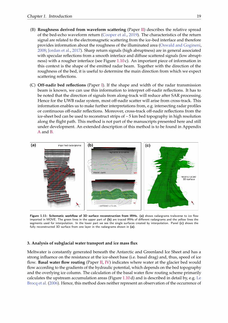
Figure 1.11: Schematic workflow of 3D surface reconstruction from IRHs. (a) shows radargrams tralsverse to ice flowimported in MOVE. The green lines in the upper part of (b) are traced IRHs of different radargrams and the yellow lines thesegments used for interpolation. In the lower part we see the single surfaces created by interpolation. Panel (c) shows thefully reconstructed 3D surface from one layer in the radargrams shown in (a).

3. Analysis of subglacial water transport and ice mass flux

Meltwater is constantly generated beneath the Antarctic and Greenland Ice Sheet and has astrong influence on the resistance at the ice-sheet base (i.e. basal drag) and, thus, speed of iceflow. Basal water flow routing (Paper II, IV) indicates where water at the glacier bed wouldflow according to the gradients of the hydraulic potential, which depends on the bed topographyand the overlying ice column. The calculation of the basal water flow routing scheme primarilycalculates the upstream accumulation areas (Figure 1.10 d) and is described in detail by, e.g. LeBrocq et al. (2006). Hence, this method does neither represent an observation of the occurrence of

Chapter 1. Introduction 20

subglacial water, nor does it provide information on quantities of volume or flux. Nonetheless,we can use this information to make extended interpretations of the subglacial environment.

In Paper II we calculate the ice mass flux through the trunk and the shear margins of theNEGIS (Figure 1.10 e). The estimation of ice flux through a flow-cross-sectional area (flux gate)depends on the ice surface velocity and an assumption on the vertical ice density and velocityprofile. The vertical velocity profile is a valuable parameter and difficult to derive withoutborehole observations. At the NEGIS, we analyse the thickness evolution of internal layerpatches parallel to ice flow and find indications for a decrease of the ice-flow velocity near theice base, where the bed is rougher (see Figure F.4). Hence, ice flux is not directly a parameterthat describes the properties of the bed. However, it relates our findings at the ice base withthe ice dynamics of the ice stream. For the ice mass flux calculation, we follow the approachdescribed in Neckel et al. (2012).

4. Two- and three-dimensional analysis of radar stratigraphy

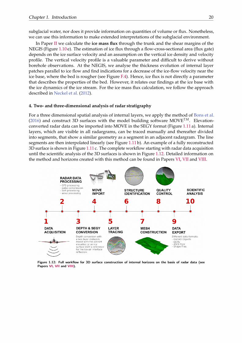
For a three dimensional spatial analysis of internal layers, we apply the method of Bons et al.(2016) and construct 3D surfaces with the model building software MOVETM. Elevation-converted radar data can be imported into MOVE in the SEGY format (Figure 1.11 a). Internallayers, which are visible in all radargrams, can be traced manually and thereafter dividedinto segments, that show a similar geometry as a segment in an adjacent radargram. The linesegments are then interpolated linearly (see Figure 1.11 b). An example of a fully reconstructed3D surface is shown in Figure 1.11 c. The complete workflow starting with radar data acquisitionuntil the scientific analysis of the 3D surfaces is shown in Figure 1.12. Detailed information onthe method and horizons created with this method can be found in Papers VI, VII and VIII.

Figure 1.12: Full workflow for 3D surface construction of internal horizons on the basis of radar data (seePapers VI, VII and VIII).

Chapter 1. Introduction 21

1.6 Study sites and regional overview

The radar data I use in my thesis were obtained from two different regions on the GrIS and onelocation on the AIS:

1. Upstream region of the 79NG (FINEGIS; Figure 1.13 b). The data in this region are includedin Paper VII and VIII.

2. The onset region of the North East Greenland Ice Stream (EGRIP-NOR-2018; Figure 1.13 c).The data of this survey are included in Paper I, II and V – VIII.

3. The onset region of the Jutulstraumen Glacier drainage basin in western Dronning MaudLand, Antarctica (JuRaS; Figure 1.14 b and d). This data set is included in Paper III and IV.

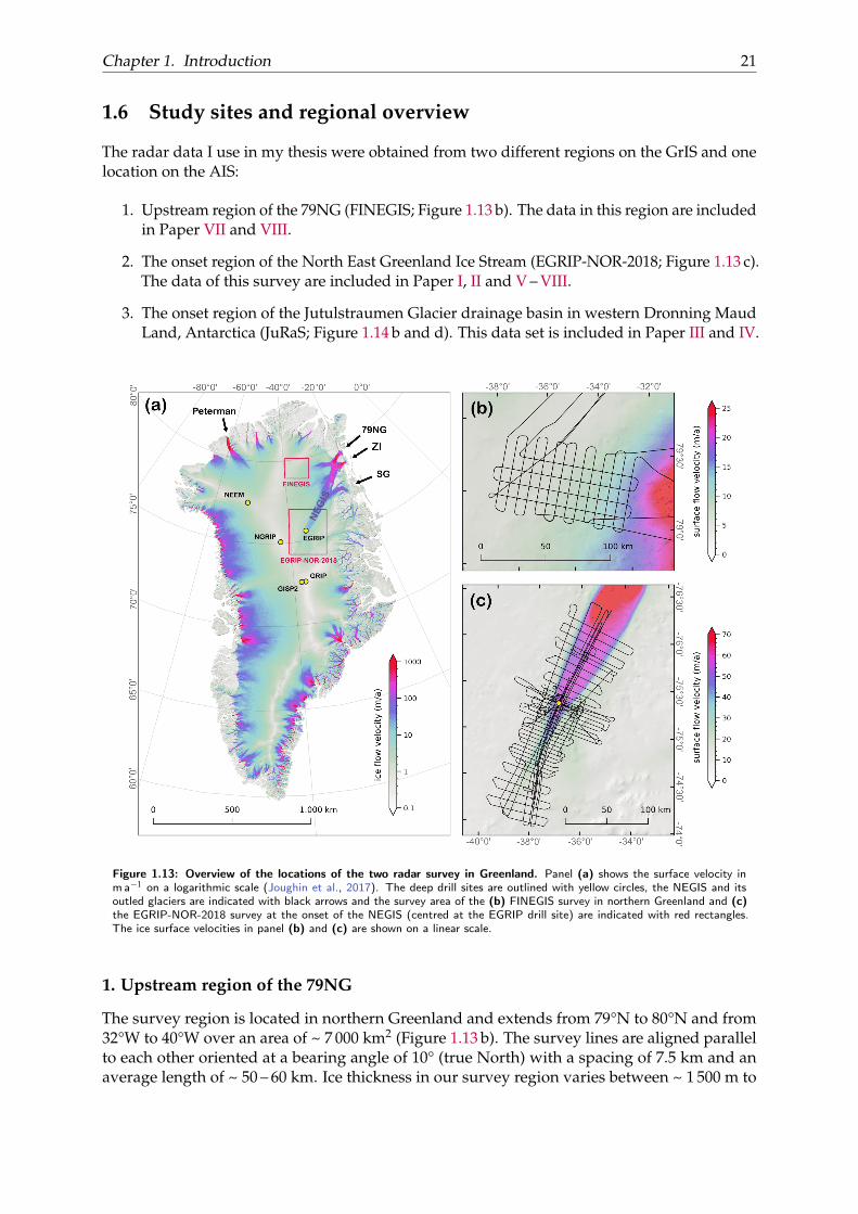
Figure 1.13: Overview of the locations of the two radar survey in Greenland. Panel (a) shows the surface velocity inm a−1 on a logarithmic scale (Joughin et al., 2017). The deep drill sites are outlined with yellow circles, the NEGIS and itsoutled glaciers are indicated with black arrows and the survey area of the (b) FINEGIS survey in northern Greenland and (c)the EGRIP-NOR-2018 survey at the onset of the NEGIS (centred at the EGRIP drill site) are indicated with red rectangles.The ice surface velocities in panel (b) and (c) are shown on a linear scale.

1. Upstream region of the 79NG

The survey region is located in northern Greenland and extends from 79°N to 80°N and from32°W to 40°W over an area of ~ 7 000 km2 (Figure 1.13 b). The survey lines are aligned parallelto each other oriented at a bearing angle of 10° (true North) with a spacing of 7.5 km and anaverage length of ~ 50 – 60 km. Ice thickness in our survey region varies between ~ 1 500 m to

Chapter 1. Introduction 22

~ 2250 m, is largest in the Southwest and becomes thinner towards East-Northeast. The bedtopography varies between ~ −100 m and 300 m elevation but shows no clear trend in theimmediate surrounding of our survey grid. Ice-flow velocity is almost zero in the western partof our survey area at the ice divide and increases up to 15 m a−1 in the East (Figure 1.13 b). Thehorizontal gradient in surface velocity is in general very small and ranges between 0 and 0.1 %.

2. Onset region of the NEGIS

The NEGIS is a prominent feature in northern Greenland and drains ~12 % of the ice mass of theGrIS Rignot and Mouginot (2012). The ice stream is more than 600 km long and extends almostup to the ice divide. Ice surface flow velocities range from 10 m a−1 at its onset to more than2 000 m a−1 at the grounding line of the marine-terminating glaciers (Mouginot et al., 2017). Theice entering the NEGIS is passing through the well-developed shear margins (Fahnestock, 2001).

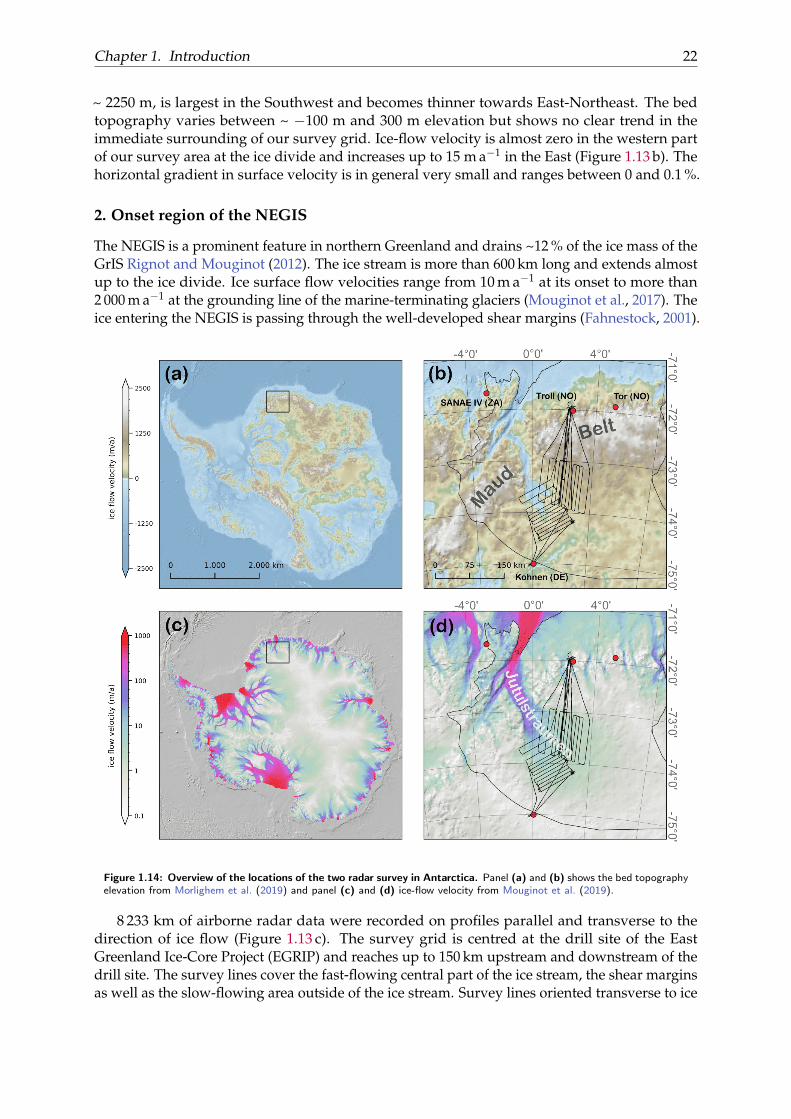
Figure 1.14: Overview of the locations of the two radar survey in Antarctica. Panel (a) and (b) shows the bed topographyelevation from Morlighem et al. (2019) and panel (c) and (d) ice-flow velocity from Mouginot et al. (2019).

8 233 km of airborne radar data were recorded on profiles parallel and transverse to thedirection of ice flow (Figure 1.13 c). The survey grid is centred at the drill site of the EastGreenland Ice-Core Project (EGRIP) and reaches up to 150 km upstream and downstream of thedrill site. The survey lines cover the fast-flowing central part of the ice stream, the shear marginsas well as the slow-flowing area outside of the ice stream. Survey lines oriented transverse to ice

Chapter 1. Introduction 23

flow have a spacing of 5 km in the centre of the survey area and 10 km further upstream anddownstream. Parallel to flow profiles follow the ice surface flow paths, which were calculatedon the basis of the current surface velocity field.

3. Jutulstraumen drainage basin

The Antarctic Jutulstraumen Glacier (JG) is located within a prominent graben system, whichseparates the geologic provinces of DML. The JG is the largest glacier in DML draining an areaof approximately 100 000 km2 through the 40 – 50 km wide Jutulstraumen Graben (Figure 1.14 b).The Graben cuts deep into the Maud Belt through the DML escarpment and reaches down to 1.6km below present sea level (Fretwell et al., 2013). Ice flow accelerates to up to 760 m a−1 at thegrounding line where the JG feeds the Fimbul Ice Shelf (Figure 1.14 d). This part of the DMLhas been extensively mapped by RES, gravity and magnetic surveys (e.g. Steinhage et al., 2001;Riedel et al., 2012). The survey lines of the UWB survey are located at the onset of JG where iceflow accelerates from 5 to 50 m a−1 (Fig. 1.14 d). The survey lines are divided into two sets andoriented approximately perpendicular to ice flow.

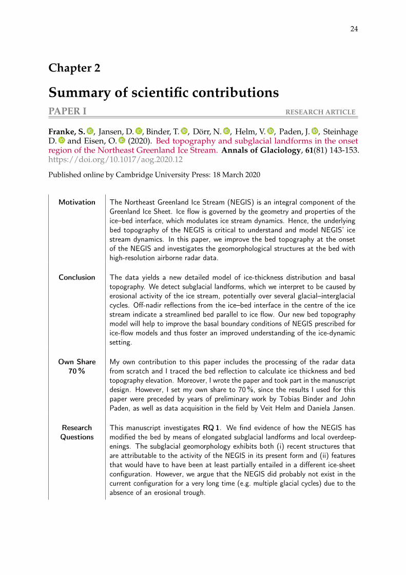
24

Chapter 2

Summary of scientific contributionsPAPER I RESEARCH ARTICLE

Franke, S. , Jansen, D. , Binder, T. , Dörr, N. , Helm, V. , Paden, J. , SteinhageD. and Eisen, O. (2020). Bed topography and subglacial landforms in the onsetregion of the Northeast Greenland Ice Stream. Annals of Glaciology, 61(81) 143-153.https://doi.org/10.1017/aog.2020.12

Published online by Cambridge University Press: 18 March 2020

Motivation The Northeast Greenland Ice Stream (NEGIS) is an integral component of theGreenland Ice Sheet. Ice flow is governed by the geometry and properties of theice–bed interface, which modulates ice stream dynamics. Hence, the underlyingbed topography of the NEGIS is critical to understand and model NEGIS’ icestream dynamics. In this paper, we improve the bed topography at the onsetof the NEGIS and investigates the geomorphological structures at the bed withhigh-resolution airborne radar data.

Conclusion The data yields a new detailed model of ice-thickness distribution and basaltopography. We detect subglacial landforms, which we interpret to be caused byerosional activity of the ice stream, potentially over several glacial–interglacialcycles. Off-nadir reflections from the ice–bed interface in the centre of the icestream indicate a streamlined bed parallel to ice flow. Our new bed topographymodel will help to improve the basal boundary conditions of NEGIS prescribed forice-flow models and thus foster an improved understanding of the ice-dynamicsetting.

Own Share70 %

My own contribution to this paper includes the processing of the radar datafrom scratch and I traced the bed reflection to calculate ice thickness and bedtopography elevation. Moreover, I wrote the paper and took part in the manuscriptdesign. However, I set my own share to 70%, since the results I used for thispaper were preceded by years of preliminary work by Tobias Binder and JohnPaden, as well as data acquisition in the field by Veit Helm and Daniela Jansen.

ResearchQuestions

This manuscript investigates RQ 1. We find evidence of how the NEGIS hasmodified the bed by means of elongated subglacial landforms and local overdeep-enings. The subglacial geomorphology exhibits both (i) recent structures thatare attributable to the activity of the NEGIS in its present form and (ii) featuresthat would have to have been at least partially entailed in a different ice-sheetconfiguration. However, we argue that the NEGIS did probably not exist in thecurrent configuration for a very long time (e.g. multiple glacial cycles) due to theabsence of an erosional trough.

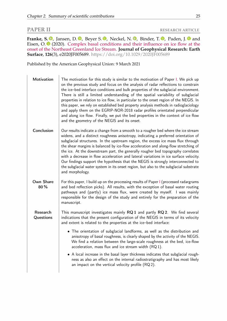
Chapter 2. Summary of scientific contributions 25

PAPER II RESEARCH ARTICLE

Franke, S. , Jansen, D. , Beyer S. , Neckel, N. , Binder, T. , Paden, J. andEisen, O. (2020). Complex basal conditions and their influence on ice flow at theonset of the Northeast Greenland Ice Stream. Journal of Geophysical Research: EarthSurface, 126(3), e2020JF005689. https://doi.org/10.1029/2020JF005689

Published by the American Geophysical Union: 9 March 2021

Motivation The motivation for this study is similar to the motivation of Paper I. We pick upon the previous study and focus on the analysis of radar reflections to constrainthe ice–bed interface conditions and bulk properties of the subglacial environment.There is still a limited understanding of the spatial variability of subglacialproperties in relation to ice flow, in particular to the onset region of the NEGIS. Inthis paper, we rely on established bed property analysis methods in radioglaciologyand apply them on the EGRIP-NOR-2018 radar profiles orientated perpendicularand along ice flow. Finally, we put the bed properties in the context of ice flowand the geometry of the NEGIS and its onset.

Conclusion Our results indicate a change from a smooth to a rougher bed where the ice streamwidens, and a distinct roughness anisotropy, indicating a preferred orientation ofsubglacial structures. In the upstream region, the excess ice mass flux throughthe shear margins is balanced by ice-flow acceleration and along-flow stretching ofthe ice. At the downstream part, the generally rougher bed topography correlateswith a decrease in flow acceleration and lateral variations in ice surface velocity.Our findings support the hypothesis that the NEGIS is strongly interconnected tothe subglacial water system in its onset region, but also to the subglacial substrateand morphology.

Own Share80 %

For this paper, I build up on the processing results of Paper I (processed radargramsand bed reflection picks). All results, with the exception of basal water routingpathways and (partly) ice mass flux, were created by myself. I was mainlyresponsible for the design of the study and entirely for the preparation of themanuscript.

ResearchQuestions

This manuscript investigates mainly RQ 1 and partly RQ 2. We find severalindications that the present configuration of the NEGIS in terms of its velocityand extent is related to the properties at the ice–bed interface:

• The orientation of subglacial landforms, as well as the distribution andanisotropy of basal roughness, is clearly shaped by the activity of the NEGIS.We find a relation between the large-scale roughness at the bed, ice-flowacceleration, mass flux and ice stream width (RQ 1).

• A local increase in the basal layer thickness indicates that subglacial rough-ness as also an effect on the internal radiostratigraphy and has most likelyan impact on the vertical velocity profile (RQ2).

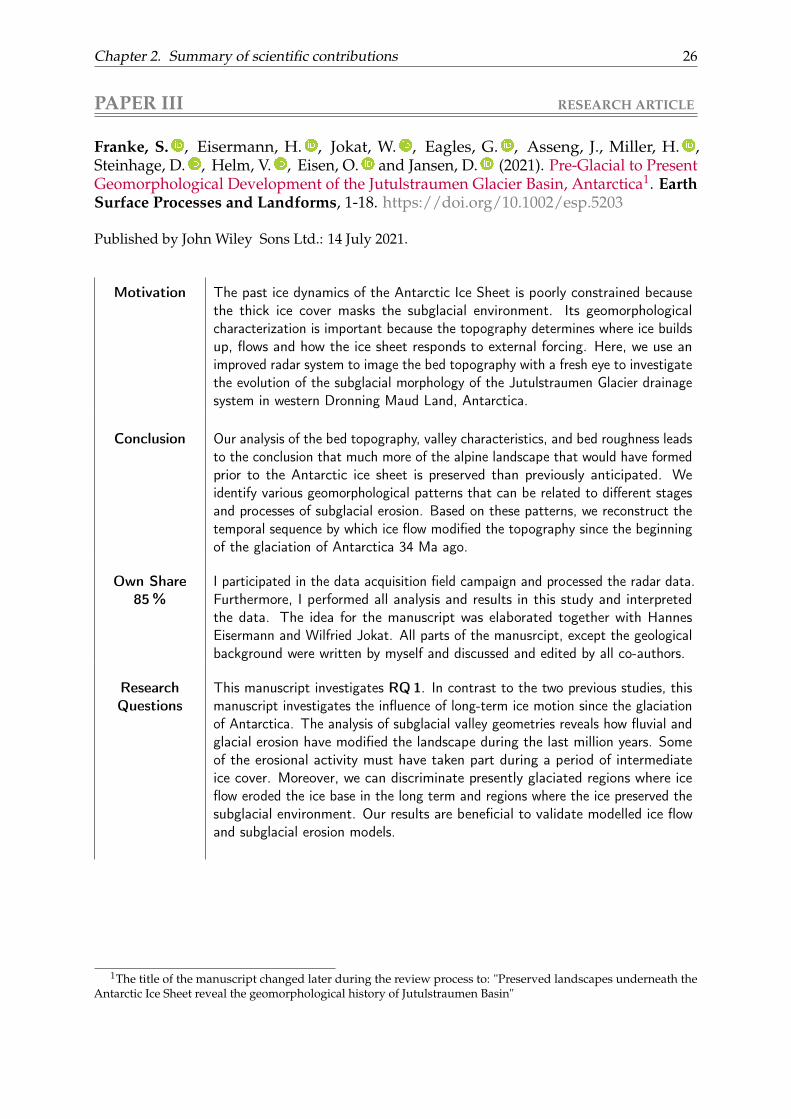
Chapter 2. Summary of scientific contributions 26

PAPER III RESEARCH ARTICLE

Franke, S. , Eisermann, H. , Jokat, W. , Eagles, G. , Asseng, J., Miller, H. ,Steinhage, D. , Helm, V. , Eisen, O. and Jansen, D. (2021). Pre-Glacial to PresentGeomorphological Development of the Jutulstraumen Glacier Basin, Antarctica1. EarthSurface Processes and Landforms, 1-18. https://doi.org/10.1002/esp.5203

Published by John Wiley Sons Ltd.: 14 July 2021.

Motivation The past ice dynamics of the Antarctic Ice Sheet is poorly constrained becausethe thick ice cover masks the subglacial environment. Its geomorphologicalcharacterization is important because the topography determines where ice buildsup, flows and how the ice sheet responds to external forcing. Here, we use animproved radar system to image the bed topography with a fresh eye to investigatethe evolution of the subglacial morphology of the Jutulstraumen Glacier drainagesystem in western Dronning Maud Land, Antarctica.

Conclusion Our analysis of the bed topography, valley characteristics, and bed roughness leadsto the conclusion that much more of the alpine landscape that would have formedprior to the Antarctic ice sheet is preserved than previously anticipated. Weidentify various geomorphological patterns that can be related to different stagesand processes of subglacial erosion. Based on these patterns, we reconstruct thetemporal sequence by which ice flow modified the topography since the beginningof the glaciation of Antarctica 34 Ma ago.

Own Share85 %

I participated in the data acquisition field campaign and processed the radar data.Furthermore, I performed all analysis and results in this study and interpretedthe data. The idea for the manuscript was elaborated together with HannesEisermann and Wilfried Jokat. All parts of the manusrcipt, except the geologicalbackground were written by myself and discussed and edited by all co-authors.

ResearchQuestions

This manuscript investigates RQ 1. In contrast to the two previous studies, thismanuscript investigates the influence of long-term ice motion since the glaciationof Antarctica. The analysis of subglacial valley geometries reveals how fluvial andglacial erosion have modified the landscape during the last million years. Someof the erosional activity must have taken part during a period of intermediateice cover. Moreover, we can discriminate presently glaciated regions where iceflow eroded the ice base in the long term and regions where the ice preserved thesubglacial environment. Our results are beneficial to validate modelled ice flowand subglacial erosion models.

1The title of the manuscript changed later during the review process to: "Preserved landscapes underneath theAntarctic Ice Sheet reveal the geomorphological history of Jutulstraumen Basin"

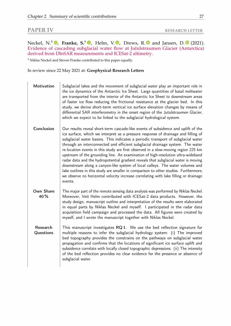
Chapter 2. Summary of scientific contributions 27

PAPER IV RESEARCH LETTER

Neckel, N.† , Franke, S.† , Helm, V. , Drews, R. and Jansen, D. (2021).Evidence of cascading subglacial water flow at Jutulstraumen Glacier (Antarctica)derived from DInSAR measurements and ICESat-2 altimetry.† Niklas Neckel and Steven Franke contributed to this paper equally.

In review since 22 May 2021 at: Geophysical Research Letters

Motivation Subglacial lakes and the movement of subglacial water play an important role inthe ice dynamics of the Antarctic Ice Sheet. Large quantities of basal meltwaterare transported from the interior of the Antarctic Ice Sheet to downstream areasof faster ice flow reducing the frictional resistance at the glacier bed. In thisstudy, we derive short-term vertical ice surface elevation changes by means ofdifferential SAR interferometry in the onset region of the Jutulstraumen Glacier,which we expect to be linked to the subglacial hydrological system.

Conclusion Our results reveal short-term cascade-like events of subsidence and uplift of theice surface, which we interpret as a pressure response of drainage and filling ofsubglacial water basins. This indicates a periodic transport of subglacial waterthrough an interconnected and efficient subglacial drainage system. The waterre-location events in this study are first observed in a slow-moving region 225 kmupstream of the grounding line. An examination of high-resolution ultra-widebandradar data and the hydropotential gradient reveals that subglacial water is movingdownstream along a canyon-like system of local valleys. The water volumes andlake outlines in this study are smaller in comparison to other studies. Furthermore,we observe no horizontal velocity increase correlating with lake filling or drainageevents.

Own Share40 %

The major part of the remote sensing data analysis was performed by Niklas Neckel.Moreover, Veit Helm contributed with ICESat-2 data products. However, thestudy design, manuscript outline and interpretation of the results were elaboratedin equal parts by Niklas Neckel and myself. I participated in the radar dataacquisition field campaign and processed the data. All figures were created bymyself, and I wrote the manuscript together with Niklas Neckel.

ResearchQuestions

This manuscript investigates RQ 1. We use the bed reflection signature formultiple reasons to infer the subglacial hydrology system: (i) The improvedbed topography provides the constrains on the pathways on subglacial waterpropagation and confirms that the locations of significant ice surface uplift andsubsidence correlate with locally closed topographic depressions. (ii) The intensityof the bed reflection provides no clear evidence for the presence or absence ofsubglacial water.

Chapter 2. Summary of scientific contributions 28

PAPER V DATA DESCRIPTION ARTICLE

Franke, S. , Jansen, D. , Binder, T. , Paden, J. , Dörr N. , Gerber T. , Miller,H. , Dahl-Jensen, D. , Helm V. , Steinhage D. , Weikusat, I. , Wilhelm, F. andEisen, O. (2021). Airborne ultra-wideband radar sounding over the shear marginsand along flow lines at the onset region of the Northeast Greenland Ice Stream. EarthSystem Science Data Discussion. https://doi.org/10.5194/essd-2021-91

In review since 31 March 2021 at: Earth System Science Data.

Motivation This manuscript is motivated by our interest in making the radar data used inPaper I, II, VI and VII available to the scientific community. We present variousdata products and describe their characteristics and processing chain in detail.The prospect that parts of the ice core can be rotated back into their correctgeographic direction (Westhoff et al., 2020) is a unique possibility for a systematicanalysis of ice crystal orientation fabric together with radar data.

Conclusion This radar data set provides essential observations of internal and bed reflections todetermine the spatial distribution of ice thickness, internal layering and reflectivity.These observations constitute boundary conditions and elucidate the propertiesand processes of the NEGIS.

Own Share90 %

I developed the outline for the manuscript and wrote the major part with contribu-tions from Nils Dörr and Tamara Gerber. Furthermore, I processed and compiledthe data products for publication and created all results and figures. To be trans-parent, I would like to note that I am not including the data acquisition by DanielaJansen, John Paden and the Polar 6 Team, as well as the years of preparatorywork by Tobias Binder in the scope of work here. These were completed for sometime, but it has to be acknowledged that the work on this manuscript builds ontheir efforts.

ResearchQuestions

Due to the fact that this is a data description paper, we do not answer any ofthe research questions. However, this manuscript presents SAR processed radardata with a wider angular range, which helps to visualize the radar stratigraphyof steeply inclined reflectors. Using this data greatly facilitates answering RQ 2,since more of the internal layers are resolved than in the standard product.Furthermore, the idea behind the manuscript and data release is to answer theresearch questions in my thesis and more jointly with the scientific community.

Chapter 2. Summary of scientific contributions 29

PAPER VI RESEARCH ARTICLE

Jansen, D. , Franke, S. , Bauer, C. C., Binder, T. , Dahl-Jensen, D. , de Riese, T. ,Eisen, O. , Llorens, M-G. , Miller, H. , Neckel, N. , Paden, J. D. , Sachau, T.Weikusat, I. Zhang, Y. and Bons, P. (2021). Interior of the North East Greenland Icestream reveals that NEGIS-type ice streams may come and go.

Draft.

Motivation Localized ice streams drain large portions of the entire Greenland Ice Sheet. Itis therefore essential to understand their formation, behaviour, and temporalvariability, especially with respect to predicting future sea-level rise. The NortheastGreenland Ice Stream (NEGIS) is by far the longest and largest ice stream inGreenland. Its present ice dynamics are well constrained via remote sensing data.However, it is unclear what processes triggered and control ice flow this far inland.In this study, we present the first 3D analysis of stratigraphic layers from anextensive airborne radar survey at the onset of the NEGIS and show how thedeformation history of the ice is recorded in the internal stratigraphy.

Conclusion The deformation history archived in the ice suggests that the folded layers withinthe NEGIS system are initiated by convergence and subsequently sheared. Byusing a novel method for dating folding sequences, we are able to show thatthe shear margins at the onset of the NEGIS were established ∼ 2 500 yearsago, which markes the timing for the onset of fast flow. Our results lead to theconclusion that, contrary to previous assumptions, the NEGIS has not been stablein its present configuration throughout the Holocene. Our study further showsthat ice streams can appear and decay within relatively short periods of time,which has a large impact on ice-sheet stability.

Own Share25 %

My share in this study includes the processing of radar data from the EGRIP-NOR-2018 campaign (see Paper V) and provided high-resolution radargrams to PaulBons for the application of the fold-dating scheme. I also created a standardizedworkflow to efficiently import radar data into the 3D structural geology softwareMOVE. Furthermore, I traced the stratigraphic layers in the radar data and createdthe 3D model of the stratigraphic horizons with contributions by Daniela Jansen.

ResearchQuestions

This paper addresses RQ 2. We use two key aspects of the radar stratigraphyto understand the temporal evolution of the NEGIS: (i) The 3D construction ofa stratigraphic horizon. Using this information, we can observe the advectionbehaviour of existing folds in the NEGIS. (ii) By applying the fold dating methodin individual radar profiles, we can estimate when the folds were initially formedand when their growth stopped. From the fact that the folds inside the presentshear zone and outside both started to grow at the same time and the folds insidethe shear zone stopped growing around 2 500 years ago but continued to growoutside the ice stream, we can reconstruct when the NEGIS started to flow in itspresent configuration.

Chapter 2. Summary of scientific contributions 30

PAPER VII RESEARCH ARTICLE

Franke, S. , Bons P. , Westhoff J. , Binder, T. , Streng K., Helm V. , SteinhageD. , Eisen, O. , Paden, J. , Weikusat I. and Jansen, D. (2021). Indication ofice-stream regime shift in Northereast Greenland.

Draft.

Motivation Ice streams are known to exhibit complex spatiotemporal dynamics, which islargely not well understood. A major challenge is the lack of observations onthe variability of the temporal dynamics of ice streams of the last thousands ofyears on contemporary glaciated regions. Here we make use of the geometryof the internal stratigraphy of the Greenland ice sheet, which yields valuableconstraints upon its temporal evolution. The stratigraphic record of isochronouslayers is shaped by the cumulative deformation sequence of initially surface parallelradar reflectors. Decoding the formation history of these structures offers anexcellent possibility to reconstruct past ice movements and draw conclusionsabout processes on the Earth’s surface. Here we use the radiostratigraphic layersfrom newly acquired and existing radar data in northeastern Greenland to deciphertheir deformation history.

ConclusionOur results reveal a deformation sequence pointing to two paleo ice streamsreaching far inland into the Greenland ice sheet that nowadays show no icestream signature in the surface velocity. We propose that (1) a switch froma convergent ice-flow regime to the present surface flow regime with parallelstreamlines, including a change in flow direction and (2) a former NEGIS-typeice stream with sharp shear margins, are the most likely scenarios to create theobserved structures.

Own Share70 %

I wrote the main part of the paper and prepared the manuscript with contributionsfrom all co-authors. Furthermore, I processed the ultra-wideband radar dataand performed all analyses. All figures in the main document and supplementwere generated by myself except for Figure 3, which was generated by JulienWesthoff. I adapted the concept of estimating the timing of the onset of uprightfold shearing from Paul Bons and Daniela Jansen and applied it to this data set.

ResearchQuestions

This manuscript addresses RQ 2. We are able to relate the deformations in theradar stratigraphy of two passive settings to deformation sequences found in twodifferent active ice-dynamic settings: the onset region of the NEGIS, with its sharpshear margins and the convergent ice-flow regime at the onset of the PetermanGlacier. The fold sequences allow further constraints on the approximate timeperiod where changes in the ice-dynamic setting occurred.

Chapter 2. Summary of scientific contributions 31

PAPER VIII DATA DESCRIPTION ARTICLE

Franke, S. , Bons P. D. , Mundel F., Sachau, T., Streng K., Weikusat I. , Miller, H. ,Binder, T. , Helm V. , Paden, J. , Steinhage D. , Dörr, N. , Eisen, O. , Jansen,D. (2021). A 3D view on folded radar stratigraphy in northern Greenland.

Draft.

Motivation Englacial stratigraphic layers are interpreted as isochrones (i.e. layers deposited assnow at the same time) and provide insight into the ice-sheet deformation history.During the last decades, continuous progress in the quality and coverage of high-resolution radar data improved the understanding of the englacial stratigraphicarchitecture of the Greenlandic and Antarctic Ice Sheet. In this manuscript, wepublish three data sets of 3D englacial stratigraphic horizons in northern Greenland.The data covers three different ice-dynamic settings in northern Greenland: (i)the onset of the Peterman Glacier (Bons et al., 2016), (ii) a region of deformedstratigraphy close to the ice divide in Northern Greenland (Paper VI) and (iii) theonset of the Northeast Greenland Ice Stream (Paper VII).

Conclusion Our 3D horizons allow an extended interpretation of fold formation mechanisms,past ice-flow patterns as well as processes at the shear margins of ice streams. Weprovide an overview of locations and glaciological setting of the 3D stratigraphichorizons, a detailed workflow on how the data were created and data formats.

Own Share70 %

I created two of the three data sets myself with contributions of Daniela Jansen.The processing includes radar data processing, conversion and import into astructural geology software MOVE, structure identification and 3D horizon con-struction (see Figure 1.12 and 1.11). The data set at the Peterman Glacier wascreated by Felicitas Mundel and the team of Paul Bons. I developed the outlineof the manuscript, wrote the manuscript and compiled the data set and usageopportunities.

ResearchQuestions

The data presented in this manuscript has been used to analyze RQ 2. A keyoutcome of this thesis is that a 3D analysis and interpretation of englacial foldsin a glaciological context is an important consideration for a comprehensiveunderstanding of present and past ice flow.

32

Chapter 3

Discussion and outlookThe recent advances in radar data acquisition and processing made it possible to image previ-ously invisible structures in the ice column and in particular details in the near-bed environmentof the Greenland and Antarctic Ice Sheet. The studies presented here illustrate the possibilities ofhow these data can be used to obtain information about the present and paleo ice-flow regimes.

3.1 Ice flow and its imprint in the subglacial environment

The ice sheet bed is difficult to access, yet possibly the most important of all glacier environments.Many decades of research provided an understanding of the main ice-dynamic and subglacialprocesses responsible for forming the landscape and its relation to erosion and deposition ofsediments. In my studies, I use ice-penetrating radar data to obtain information about thesubglacial environment and address two key aspects of RQ 1: (i) The imprints of ice flow atthe onset of the largest ice stream in Greenland (NEGIS) on the ice base and the links betweensubglacial bed features and ice-flow dynamics of the ice stream. (ii) The modification of the icebase by past ice motion and its reconstruction over several glacial cycles at the Jutulstraumendrainage basin in Antarcticas Dronning Maud Land.

3.1.1 Subglacial geomorphology and its link to the ice dynamics of localised iceflow

Sediments are eroded, transported and deposited beneath ice streams, which creates subglaciallandforms (Stokes, 2018). Most of the observations concentrate on nowadays deglaciated regionson- and offshore (e.g. Clark, 1993; Arndt et al., 2020) and only a few on the environmentunderneath contemporary ice sheets located closely to the glacier terminus (e.g. at the RutfordIce Stream, Pine Island Glacier or Thwaites Glacier; King et al., 2009; Bingham et al., 2017;Holschuh et al., 2020). In Paper I and II, I find evidence in radar reflections at the ice basethat elongated subglacial landforms are present underneath the NEGIS at its onset. ice-flowvelocity in this region is lower in comparison to the previously mentioned studies in Antarctica.Furthermore, they appear almost in the centre of the GrIS more than 600 km upstream of theoutlet glaciers. The spatial analysis basal roughness in Paper II shows that streamlining of thebed is restricted to the central part of the NEGIS and is particularly pronounced at moderate ice-flow velocities (30 – 70 m a−1). Together with the seismic analysis of bed properties performed byChristianson et al. (2014), this leads to the assumption that the subglacial landforms must havebeen formed by the NEGIS in its present configuration over a longer time period (e.g. hundredsto thousands of years) and that they were formed on a deformable bed. Due to the limitedresolution of the bed geometry, it is unfortunately not possible to determine the exact geometryand type (e.g. MSGL, drumlins, crag-and-tails) of the subglacial landforms, as well as estimatesof their formation time (Clark, 1993).

A unique feature of the NEGIS is that its onset extends very far towards the interior or theGrIS (Joughin et al., 2001) and its shear zones show no relation to the bed topography in largeparts (Morlighem et al., 2017). The analysis of the improved topography of Paper I also showsvarious large-scale erosion structures. These can be explained by a variable lithology within theice stream and potentially indicate which regions are covered with sediments. How the location

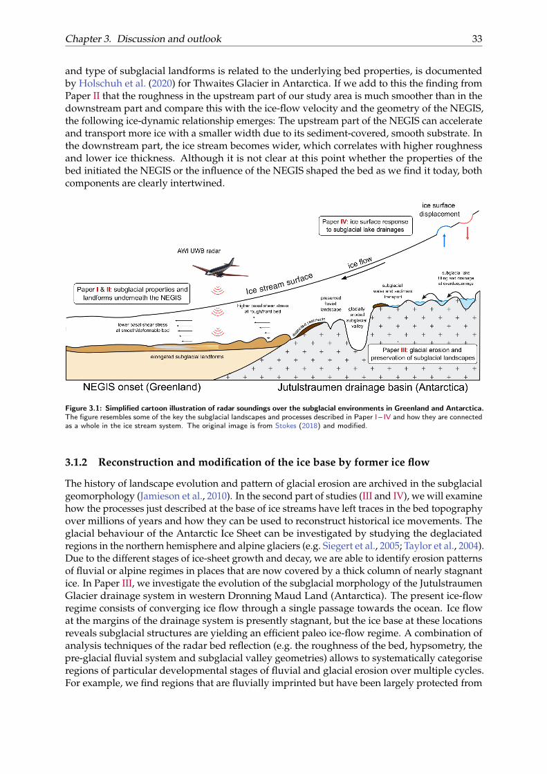
Chapter 3. Discussion and outlook 33

and type of subglacial landforms is related to the underlying bed properties, is documentedby Holschuh et al. (2020) for Thwaites Glacier in Antarctica. If we add to this the finding fromPaper II that the roughness in the upstream part of our study area is much smoother than in thedownstream part and compare this with the ice-flow velocity and the geometry of the NEGIS,the following ice-dynamic relationship emerges: The upstream part of the NEGIS can accelerateand transport more ice with a smaller width due to its sediment-covered, smooth substrate. Inthe downstream part, the ice stream becomes wider, which correlates with higher roughnessand lower ice thickness. Although it is not clear at this point whether the properties of thebed initiated the NEGIS or the influence of the NEGIS shaped the bed as we find it today, bothcomponents are clearly intertwined.

Figure 3.1: Simplified cartoon illustration of radar soundings over the subglacial environments in Greenland and Antarctica.The figure resembles some of the key the subglacial landscapes and processes described in Paper I – IV and how they are connectedas a whole in the ice stream system. The original image is from Stokes (2018) and modified.

3.1.2 Reconstruction and modification of the ice base by former ice flow

The history of landscape evolution and pattern of glacial erosion are archived in the subglacialgeomorphology (Jamieson et al., 2010). In the second part of studies (III and IV), we will examinehow the processes just described at the base of ice streams have left traces in the bed topographyover millions of years and how they can be used to reconstruct historical ice movements. Theglacial behaviour of the Antarctic Ice Sheet can be investigated by studying the deglaciatedregions in the northern hemisphere and alpine glaciers (e.g. Siegert et al., 2005; Taylor et al., 2004).Due to the different stages of ice-sheet growth and decay, we are able to identify erosion patternsof fluvial or alpine regimes in places that are now covered by a thick column of nearly stagnantice. In Paper III, we investigate the evolution of the subglacial morphology of the JutulstraumenGlacier drainage system in western Dronning Maud Land (Antarctica). The present ice-flowregime consists of converging ice flow through a single passage towards the ocean. Ice flowat the margins of the drainage system is presently stagnant, but the ice base at these locationsreveals subglacial structures are yielding an efficient paleo ice-flow regime. A combination ofanalysis techniques of the radar bed reflection (e.g. the roughness of the bed, hypsometry, thepre-glacial fluvial system and subglacial valley geometries) allows to systematically categoriseregions of particular developmental stages of fluvial and glacial erosion over multiple cycles.For example, we find regions that are fluvially imprinted but have been largely protected from

Chapter 3. Discussion and outlook 34

successive selective glacial erosion or scouring. In another region, we find signs of selectivelinear erosion, indicating an ice-dynamic regime with much lower ice thickness and differentice-flow direction than today.

My previous work focused exclusively on the analysis of ice-penetrating radar data. How-ever, there is also the possibility to include other remote sensing methods in order to studysubglacial processes. In Paper IV, we use differential InSAR to detect vertical displacementsof the ice surface. In combination with the information about the bed topography from theradar data, we conclude that the surface motions are caused by a pressure response due to thetransport of subglacial meltwater (Gray et al., 2000). From the data, we can infer where thewater flows along and that it pools in topographically closed depressions (also referred to asoverdeepenings) before being transported further. Subglacial water transport in itself is notnecessarily responsible for deep erosion but for the movement of sediments below the ice (Alleyet al., 2019). However, a much more interesting aspect emerges when the situation is viewedfrom a certain distance. The depressions in which the subglacial water collects and causes aparticularly strong uplift and subsidence of the ice surface must have been formed by erosionalprocesses at some point in the past. For these specific locations, we can therefore assume thatmost likely alpine glaciers under a much thinner ice layer have caused these depressions.

The results presented in Paper I – IV provide significant insights for the detection andinterpretation of contemporary and paleo ice-flow landforms and their relation to the icedynamics. I show that landform location, size, shape and distribution are either related to thepresent ice-flow regime or the consequence of historic ice-flow activity. Investigating ice streambeds at higher resolution is an important step towards developing an understanding of the timescales and what processes generate subglacial landforms.

3.2 Past ice-flow patterns captured in the englacial deformationhistory

High-resolution radar data do provide not only a detailed image of the glacier base but alsoinsight into the internal layering architecture of an ice sheet. Deformed internal layers are anindicator for past ice-flow activity and reveal large perturbations with no apparent link to theunderlying bed geometry (Bons et al., 2016). This section investigates RQ 2 and consists of twomanuscripts focusing on the derivation and reconstruction of ice-flow patterns in NortheastGreenland (Papers VI and VII) and the implications for the future of the Greenland Ice Sheet.In addition, two further manuscripts are included that publish the data from these and otherstudies (following the FAIR data principles; Wilkinson et al. 2016) and address both the methodsbehind the creation of the data sets and their description and value to the scientific community(Papers V and VIII).

Contemporary ice-flow regimes are very well captured by satellite remote sensing data (e.g.Joughin et al., 2017), but less is know about the temporal evolution of ice streams. To reconstructthe former evolution of ice-flow regimes, we consider folded radar isochrones as passive tracesfor cumulative deformation. The range of studies on the mechanisms that cause large-scale foldsin ice sheets has become more abundant in the past decade (Wolovick et al., 2014; LeysingerVieli et al., 2018; Bons et al., 2016). This is mainly due to the improved coverage and quality ofradar data from Operation Ice Bridge by NASA and the Center for Remote Sensing of Ice Sheets(CReSIS) at the University of Kansas (see MacGregor et al.; Leuschen et al., 2010; Li et al., 2013),and is being complemented by data from AWI in the studies presented here. Overall, three basicprocesses can be hypothesised for the formation of large-scale folds in the ice:

1. Variations in basal sliding: The development of large complex stratigraphic folds has

Chapter 3. Discussion and outlook 35

been investigated by Wolovick et al. (2014). According to their simulations, the genesisof large folded and overturned structures in the radar stratigraphy are governed bydeformation caused by heterogeneous and time-variable basal sliding.

2. Basal freeze-on and ice flow: Leysinger Vieli et al. (2018) simulated the genesis of largeplume-like internal structures by basal freeze-on and ice-flow modelling. The authors finda good agreement between their simulations and the radar observations and highlightthat the height of the folds is primarily a function of ice-flux and secondarily depends onfreeze-on processes.

3. Convergent ice flow: Bons et al. (2016) established a conceptual model for the formationprocesses of cylindrical folds sub-parallel to ice flow. Their modelling shows that thesefolds can be formed by lateral compression, where mechanical anisotropy plays a majorrole.

Each of the three mechanisms presented produces folds under a specific glaciological settingand depends on, e.g. the conditions at the glacier bed and ice-flow characteristics. In Paper VII, Idiscuss all three variants and evaluate the arguments for and against creating the fold structurespresented. While Leysinger Vieli et al. (2018) shows that the generation of large plume-like foldsis possible with basal freeze-on and ice flow, it seems unlikely that freeze-on would raise thelocalised areas where we observe the cylindrical anticlines. Moreover, freeze-on cannot explainsynclines. However, since freeze-on still can happen, it might be a contributing mechanismfor the elevation of anticlines. Therefore, we argue that mechanical folding due to horizontalshortening (due to convergent flow) is the most likely mechanism for initial fold formation (seeFigure 3.2 a) for the features shown in Paper VII in northern Greenland.

It has been proven that to have a three-dimensional idea of the location and orientation of thefold axis and the direction of overturning is of particular importance. This information, togetherwith an estimate of the basal conditions and how the ice flow would have been organised overthe past thousands of years, was the ultimate reason why we considered that it most likely thatconvergent flow in the direction of the major outlets in northeast Greenland must have been thecause of the initiation of the folds (Figure 3.2 a).

For the interpretation of deformations in the radar stratigraphy, three different approachesemerge (see Figure 3.2):

(a) For the case of large overturned folds as in Paper VII, we can divide the deformationprocess into two subprocesses, assuming the past ice-flow direction is parallel to thefold axis. In the first stage, upright folds are created by convergent flow (e.g. as in thecurrent ice-flow regime at Peterman Glacier; Bons et al. 2016). A change in the flow regimesubsequently shears the radar layers, as long as a component of the flow field is orientedperpendicular to the fold axis (Figure 3.2 a).

(b) For the second case in Paper VII, I do not use a direct reconstruction based on radarstratigraphy. In principle, I only use the recurring pattern of densely folded radar layers inradargrams and compare them with those of an existing active ice stream (the NEGIS; seefindings in Paper VI and Figure 3.2 b).

(c) For the third approach, we return to the folds in the shear zone, but not to concludethat there was once an ice stream. The approach essentially builds on approach (a) bysubsequent shearing of folds initiated by convergent flow due to increasing flow velocityto such an extent that their amplitude does not increase further, but the wavelength isgreatly reduced (Figure 3.2 c).

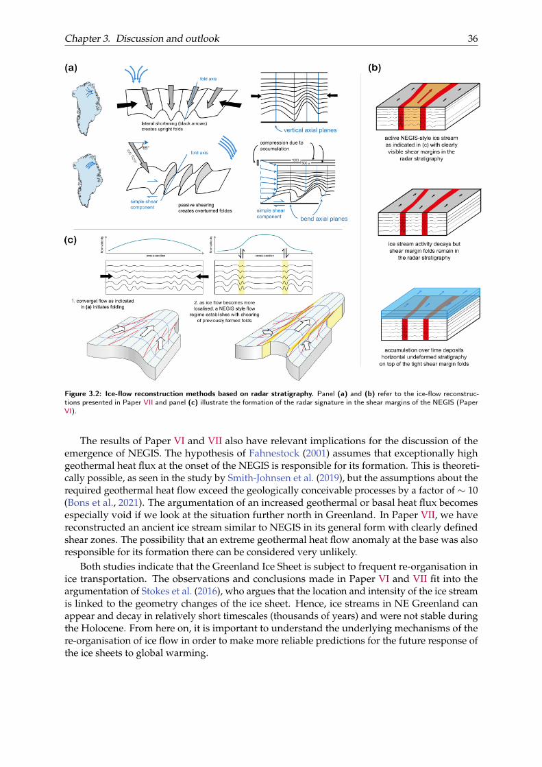
Chapter 3. Discussion and outlook 36

Figure 3.2: Ice-flow reconstruction methods based on radar stratigraphy. Panel (a) and (b) refer to the ice-flow reconstruc-tions presented in Paper VII and panel (c) illustrate the formation of the radar signature in the shear margins of the NEGIS (PaperVI).

The results of Paper VI and VII also have relevant implications for the discussion of theemergence of NEGIS. The hypothesis of Fahnestock (2001) assumes that exceptionally highgeothermal heat flux at the onset of the NEGIS is responsible for its formation. This is theoreti-cally possible, as seen in the study by Smith-Johnsen et al. (2019), but the assumptions about therequired geothermal heat flow exceed the geologically conceivable processes by a factor of ∼ 10(Bons et al., 2021). The argumentation of an increased geothermal or basal heat flux becomesespecially void if we look at the situation further north in Greenland. In Paper VII, we havereconstructed an ancient ice stream similar to NEGIS in its general form with clearly definedshear zones. The possibility that an extreme geothermal heat flow anomaly at the base was alsoresponsible for its formation there can be considered very unlikely.

Both studies indicate that the Greenland Ice Sheet is subject to frequent re-organisation inice transportation. The observations and conclusions made in Paper VI and VII fit into theargumentation of Stokes et al. (2016), who argues that the location and intensity of the ice streamis linked to the geometry changes of the ice sheet. Hence, ice streams in NE Greenland canappear and decay in relatively short timescales (thousands of years) and were not stable duringthe Holocene. From here on, it is important to understand the underlying mechanisms of there-organisation of ice flow in order to make more reliable predictions for the future response ofthe ice sheets to global warming.

Chapter 3. Discussion and outlook 37

3.3 Perspectives

Rapidly flowing and far-inland reaching ice streams are a key component of the Greenland andAntarctic Ice Sheet. Their importance is increasingly being recognised in the ice-sheet massbalance and their subsequent impacts on sea-level changes (Choi et al., 2021). It has becomeclear that the internal structure within and the geomorphology beneath ice streams is uniqueand that their flow characteristics are governed by ice-internal mechanisms and processes atthe ice–bed interface (Stokes, 2018; Schoof and Mantelli, 2021). Understanding where, why, andhow ice streams and their geomorphology originate and evolve is critical to understanding andcomprehensively modelling ice flow.

Although there is a detailed knowledge of the subglacial morphology underneath ice streamsand an improved knowledge on the distribution of sediments, basal water and shear stresses, ourunderstanding of the processes at the ice-sheet bed is still limited (Stokes, 2018). Furthermore,there is uncertainty about accurate subglacial erosion rates, which is one of the key processes,which shaped the Earth’s surface. Cook et al. (2020) started to establish an empirical relationbetween glacier sliding and erosion rates from a compilation of 38 glaciers. In this context, wemust keep in mind that the possibilities for studying these alpine glaciers are limited. Today theyare the laboratories to study fundamental glaciological processes, but soon they will disappearcompletely, depending on the development of the global climate. As for ice streams, the futureusage of much more efficient and high-resolution ice-sheet bed mapping techniques such as viaradar swath tomography (see Holschuh et al. (2020) and Appendix B) is a promising methodthat will greatly improve the resolution at the ice base.

From the findings presented in this thesis, it is clear that radar reflections in ice sheets canbe used in a variety of ways to reconstruct and characterize ice flow. In Greenland, althoughmany large-scale folds have been mapped by radar surveys (see Leysinger Vieli et al., 2018), it isunclear for most of them how these structures are related to each other. Further efforts such asthose in Paper VI and VII and the work of Bons et al. (2016) and Streng (2019) are the first stepstoward a coherent understanding of deformations in Greenland’s Ice Sheet. In addition, there isa major effort to model localised ice streams (e.g. Schoof and Mantelli, 2021), which are mostlikely a major driver of folding (Bons et al., 2016). In this context, the comparison of modellingresults and the underlying processes and input parameters with geophysical observations willplay a central role. Another important factor will be the integration of these results into theoverall Earth system to evaluate how plausible these results are in a different context (see thestudy of Fahnestock (2001), Smith-Johnsen et al. (2019) and the comment of Bons et al. (2021)regarding the proposed exceptionally high geothermal heat flux).

38

39

BibliographyAllen, C. R., Kamb, W. B., Meier, M. F., and Sharp, R. P. Struc-

ture of the lower blue glacier, washington. The Journal ofGeology, 68(6):601–625, 1960. doi: 10.1086/626700. URLhttps://doi.org/10.1086/626700.

Allen, C. T., Mozaffar, S. N., and Akins, T. L. Suppress-ing coherent noise in radar applications with long dwelltimes. IEEE Geoscience and Remote Sensing Letters, 2(3):284–286, July 2005. doi: 10.1109/LGRS.2005.847931. URLhttp://dx.doi.org/10.1109/LGRS.2005.847931.

Alley, R. B., Cuffey, K. M., and Zoet, L. K. Glacial erosion:status and outlook. Annals of Glaciology, 60(80):1–13, 2019.doi: 10.1017/aog.2019.38.

Allison, I., Alley, R., Fricker, H., Thomas, R., and Warner, R.Ice sheet mass balance and sea level. Antarctic Science, 21(5):413–426, 2009. doi: 10.1017/S0954102009990137. URLhttps://doi.org/10.1017/S0954102009990137.

Anandakrishnan, S. and Alley, R. B. Tidal forcing ofbasal seismicity of ice stream c, west antarctica, ob-served far inland. Journal of Geophysical Research: SolidEarth, 102(B7):15183–15196, 1997. doi: https://doi.org/10.1029/97JB01073. URL https://agupubs.onlinelibrary.wiley.com/doi/abs/10.1029/97JB01073.

Arndt, J. E., Larter, R. D., Hillenbrand, C.-D., Sørli, S. H., For-wick, M., Smith, J. A., and Wacker, L. Past ice sheet–seabedinteractions in the northeastern weddell sea embayment,antarctica. The Cryosphere, 14(6):2115–2135, 2020. doi:10.5194/tc-14-2115-2020. URL https://tc.copernicus.org/articles/14/2115/2020/.

Arnold, E., Leuschen, C., Rodriguez-Morales, F., Li, J., Paden,J., Hale, R., and Keshmiri, S. CReSIS airborne radars andplatforms for ice and snow sounding. Annals of Glaciology,pages 1–10, nov 2019. doi: 10.1017/aog.2019.37. URLhttps://doi.org/10.1017%2Faog.2019.37.

Aschwanden, A., Fahnestock, M. A., Truffer, M., Brinker-hoff, D. J., Hock, R., Khroulev, C., Mottram, R., andKhan, S. A. Contribution of the Greenland Ice Sheetto sea level over the next millennium. Science Advances,5(6), 2019. doi: 10.1126/sciadv.aav9396. URL https://advances.sciencemag.org/content/5/6/eaav9396.

Bader, H. The greenland ice sheet. Hanover, NH, U.S. ArmyCold Regions Research and Engineering Laboratory., (1), 1961.URL https://erdc-library.erdc.dren.mil/jspui/bitstream/11681/2674/1/CRREL-Mono-1-B2.pdf.

Bailey, J. T., Evans, S., and Robin, G. d. Q. Radio EchoSounding of Polar Ice Sheets. Nature, 204(4957):420–421,1964. ISSN 1476-4687. doi: 10.1038/204420a0. URLhttps://doi.org/10.1038/204420a0.

Bamber, J. L., Vaughan, D. G., and Joughin, I. Widespreadcomplex flow in the interior of the antarctic ice sheet.Science, 287(5456):1248–1250, 2000. ISSN 00368075. doi:10.1126/science.287.5456.1248. URL http://dx.doi.org/10.1126/science.287.5456.1248.

Bamber, J. L., Layberry, R. L., and Gogineni, S. P. Anew ice thickness and bed data set for the greenlandice sheet: 1. measurement, data reduction, and er-rors. Journal of Geophysical Research: Atmospheres, 106(D24):33773–33780, 2001. doi: https://doi.org/10.1029/2001JD900054. URL https://agupubs.onlinelibrary.wiley.com/doi/abs/10.1029/2001JD900054.

Bamber, J. L., Griggs, J. A., Hurkmans, R. T. W. L.,Dowdeswell, J. A., Gogineni, S. P., Howat, I., Mouginot,J., Paden, J., Palmer, S., Rignot, E., and Steinhage, D. Anew bed elevation dataset for Greenland. Cryosphere, 7(2):499–510, 2013. ISSN 19940416. doi: 10.5194/tc-7-499-2013.URL http://dx.doi.org/10.5194/tc-7-499-2013.

Bell, R. E., Ferraccioli, F., Creyts, T. T., Braaten, D., Corr, H.,Das, I., Damaske, D., Frearson, N., Jordan, T., Rose, K.,Studinger, M., and Wolovick, M. Widespread PersistentThickening of the East Antarctic Ice Sheet by Freezingfrom the Base. Science, 331(6024):1592–1595, mar 2011.doi: 10.1126/science.1200109. URL https://doi.org/10.1126%2Fscience.1200109.

Bell, R. E., Tinto, K., Das, I., Wolovick, M., Chu, W., Creyts,T. T., Frearson, N., Abdi, A., and Paden, J. D. Deforma-tion warming and softening of Greenland’s ice by refreez-ing meltwater. Nature Geoscience, 7(7):497–502, jun 2014.doi: 10.1038/ngeo2179. URL https://doi.org/10.1038%2Fngeo2179.

Benn, D. and Evans, D. Glaciers and glaciation, 2nd edi-tion. Routledge, 2010. doi: 10.4324/9780203785010. URLhttps://doi.org/10.4324/9780203785010.

Bennett, M. R. Ice streams as the arteries of an icesheet: their mechanics, stability and significance.Earth-Science Reviews, 61(3):309–339, 2003. ISSN 0012-8252. doi: 10.1016/S0012-8252(02)00130-7. URLhttps://www.sciencedirect.com/science/article/pii/S0012825202001307.

Bingham, R. G. and Siegert, M. J. Quantifying subglacial bedroughness in Antarctica: implications for ice-sheet dynam-ics and history. Quaternary Science Reviews, 28(3-4):223–236,

BIBLIOGRAPHY 40

feb 2009. doi: 10.1016/j.quascirev.2008.10.014. URL https://doi.org/10.1016%2Fj.quascirev.2008.10.014.

Bingham, R. G., King, E. C., Smith, A. M., and Pritchard,H. D. Glacial geomorphology: Towards a convergenceof glaciology and geomorphology. Progress in Physical Ge-ography: Earth and Environment, 34(3):327–355, 2010. doi:10.1177/0309133309360631. URL https://doi.org/10.1177/0309133309360631.

Bingham, R. G., Vaughan, D. G., King, E. C., Davies, D.,Cornford, S. L., Smith, A. M., Arthern, R. J., Brisbourne,A. M., Rydt, J. D., Graham, A. G. C., Spagnolo, M., Marsh,O. J., and Shean, D. E. Diverse landscapes beneath PineIsland Glacier influence ice flow. Nature Communications,8(1), nov 2017. doi: 10.1038/s41467-017-01597-y. URLhttps://doi.org/10.1038%2Fs41467-017-01597-y.

Bons, P. D., Jansen, D., Mundel, F., Bauer, C. C., Binder, T.,Eisen, O., Jessell, M. W., Llorens, M.-G., Steinbach, F.,Steinhage, D., and Weikusat, I. Converging flow andanisotropy cause large-scale folding in Greenland's icesheet. Nature Communications, 7(1), apr 2016. doi: 10.1038/ncomms11427. URL https://doi.org/10.1038%2Fncomms11427.

Bons, P. D., de Riese, T., Franke, S., Llorens, M.-G., Sachau,T., Stoll, N., Weikusat, I., Westhoff, J., and Zhang, Y. Com-ment on “exceptionally high heat flux needed to sustainthe northeast greenland ice stream” by smith-johnsen etal. (2020). The Cryosphere, 15(5):2251–2254, 2021. doi:10.5194/tc-15-2251-2021. URL https://tc.copernicus.org/articles/15/2251/2021/.

Broecker, W. Massive iceberg discharges as triggersfor global climate change. Nature, 372(6505):421–424, 1994. URL http://www.nature.com/articles/372421a0%0Apapers3://publication/doi/10.1038/372421a0.

Cavitte, M. G. P., Blankenship, D. D., Young, D. A., Schroeder,D. M., Parrenin, F., Lemeur, E., MacGregor, J. A., andSiegert, M. J. Deep radiostratigraphy of the east antarc-tic plateau: connecting the dome c and vostok ice coresites. Journal of Glaciology, 62(232):323–334, 2016. doi:10.1017/jog.2016.11. URL https://doi.org/10.1017/jog.2016.11.

Choi, Y., Morlighem, M., Rignot, E., and Wood, M. Ice dy-namics will remain a primary driver of greenland ice sheetmass loss over the next century. Communications Earth& Environment, 2(1):26, Feb 2021. ISSN 2662-4435. doi:10.1038/s43247-021-00092-z. URL https://doi.org/10.1038/s43247-021-00092-z.

Christianson, K., Peters, L. E., Alley, R. B., Anandakrish-nan, S., Jacobel, R. W., Riverman, K. L., Muto, A., andKeisling, B. A. Dilatant till facilitates ice-stream flow innortheast Greenland. Earth and Planetary Science Letters,401:57–69, sep 2014. doi: 10.1016/j.epsl.2014.05.060. URLhttps://doi.org/10.1016%2Fj.epsl.2014.05.060.

Church, J. A. and White, N. J. A 20th century accel-eration in global sea-level rise. Geophysical ResearchLetters, 33(1), 2006. doi: https://doi.org/10.1029/2005GL024826. URL https://agupubs.onlinelibrary.wiley.com/doi/abs/10.1029/2005GL024826.

Church, J. A., Clark, P., Cazenave, A., Gregory, J., Jevrejeva,S., Levermann, A., Merrifield, M., Milne, G., Nerem, R.,Nunn, P., Payne, A., Pfeffer, W., Stammer, D., and Unnikr-ishnan, A. 2013: Sea level change. In Climate Change 2013:The Physical Science Basis. Contribution of Working Group Ito the Fifth Assessment Report of the Intergovernmental Panelon Climate Change, pages 1137–1216. 2013. ISBN ISBN 978-1-107-66182-0. doi: 10.1017/CB09781107415315.026. URLhttp://dx.doi.org/10.1017/CB09781107415315.026.

Clark, C. D. Mega-scale glacial lineations and cross-cuttingice-flow landforms. Earth Surface Processes and Land-forms, 18(1):1–29, 1993. doi: https://doi.org/10.1002/esp.3290180102. URL https://onlinelibrary.wiley.com/doi/abs/10.1002/esp.3290180102.

Clark, P. U., Dyke, A. S., Shakun, J. D., Carlson, A. E., Clark,J., Wohlfarth, B., Mitrovica, J. X., Hostetler, S. W., and Mc-Cabe, A. M. The last glacial maximum. Science, 325(5941):710–714, 2009. doi: 10.1126/science.1172873. URL https://science.sciencemag.org/content/325/5941/710.

Clarke, G. K. C., Nitsan, U., and Paterson, W. S. B.Strain heating and creep instability in glaciers andice sheets. Reviews of Geophysics, 15(2):235–247, 1977.doi: https://doi.org/10.1029/RG015i002p00235. URLhttps://agupubs.onlinelibrary.wiley.com/doi/abs/10.1029/RG015i002p00235.

Conway, H., Catania, G., Raymond, C. F., Gades, A. M., Scam-bos, T. A., and Engelhardt, H. Switch of flow directionin an Antarctic ice stream. Nature, 419(6906):465–467, oct2002. ISSN 0028-0836. doi: 10.1038/nature01081. URLhttp://www.nature.com/articles/nature01081.

Cook, S. J. and Swift, D. A. Subglacial basins: Their ori-gin and importance in glacial systems and landscapes.Earth-Science Reviews, 115(4):332 – 372, 2012. ISSN 0012-8252. doi: https://doi.org/10.1016/j.earscirev.2012.09.009. URL http://www.sciencedirect.com/science/article/pii/S0012825212001286.

BIBLIOGRAPHY 41

Cook, S. J., Swift, D. A., Kirkbride, M. P., Knight, P. G., andWaller, R. I. The empirical basis for modelling glacial ero-sion rates. Nature Communications, 11(1):759, Feb 2020.ISSN 2041-1723. doi: 10.1038/s41467-020-14583-8. URLhttps://doi.org/10.1038/s41467-020-14583-8.

Cooper, M. A., Jordan, T. M., Schroeder, D. M., Siegert, M. J.,Williams, C. N., and Bamber, J. L. Subglacial roughnessof the Greenland Ice Sheet: relationship with contem-porary ice velocity and geology. The Cryosphere, 13(11):3093–3115, nov 2019. doi: 10.5194/tc-13-3093-2019. URLhttps://doi.org/10.5194%2Ftc-13-3093-2019.

CReSIS-Toolbox. J Paden, URL:https://ops.cresis.ku.edu/wiki/index.php/Main_Page,acessed: 2019-06-01, 2019. URL https://ops.cresis.ku.edu/wiki/index.php/Main_Page.

Dall, J., Corr, H. F. J., Walker, N., Rommen, B., and Lin,C. Sounding the antarctic ice sheet from space: a fea-sibility study based on airborne p-band radar data. InIGARSS 2018 - 2018 IEEE International Geoscience and Re-mote Sensing Symposium, pages 4142–4145, 2018. doi:10.1109/IGARSS.2018.8518826. URL https://doi.org/10.1109/IGARSS.2018.8518826.

Dowdeswell, J. A., Canals, M., Jakobsson, M., Todd, B. J.,Dowdeswell, E. K., and Hogan, K. A. The variety anddistribution of submarine glacial landforms and implica-tions for ice-sheet reconstruction. Geological Society, Lon-don, Memoirs, 46(1):519–552, 2016. ISSN 0435-4052. doi:10.1144/M46.183. URL https://mem.lyellcollection.org/content/46/1/519.

Drews, R., Eisen, O., Weikusat, I., Kipfstuhl, S., Lam-brecht, A., Steinhage, D., Wilhelms, F., and Miller, H.Layer disturbances and the radio-echo free zone in icesheets. The Cryosphere, 3(2):195–203, aug 2009. doi:10.5194/tc-3-195-2009. URL https://doi.org/10.5194%2Ftc-3-195-2009.

Dupont, T. K. and Alley, R. B. Assessment of the importanceof ice-shelf buttressing to ice-sheet flow. Geophysical Re-search Letters, 32(4), 2005. doi: https://doi.org/10.1029/2004GL022024. URL https://agupubs.onlinelibrary.wiley.com/doi/abs/10.1029/2004GL022024.

Earle. Physical geology - 2nd edition, 2019.URL https://opentextbc.ca/geology/chapter/16-2-how-glaciers-work/.

Edwards, T. L., Nowicki, S., Marzeion, B., Hock, R., Goelzer,H., Seroussi, H., Jourdain, N. C., Slater, D. A., Turner, F. E.,Smith, C. J., McKenna, C. M., Simon, E., Abe-Ouchi, A.,Gregory, J. M., Larour, E., Lipscomb, W. H., Payne, A. J.,

Shepherd, A., Agosta, C., Alexander, P., Albrecht, T., An-derson, B., Asay-Davis, X., Aschwanden, A., Barthel, A.,Bliss, A., Calov, R., Chambers, C., Champollion, N., Choi,Y., Cullather, R., Cuzzone, J., Dumas, C., Felikson, D., Fet-tweis, X., Fujita, K., Galton-Fenzi, B. K., Gladstone, R.,Golledge, N. R., Greve, R., Hattermann, T., Hoffman, M. J.,Humbert, A., Huss, M., Huybrechts, P., Immerzeel, W.,Kleiner, T., Kraaijenbrink, P., Le clec’h, S., Lee, V., Leguy,G. R., Little, C. M., Lowry, D. P., Malles, J.-H., Martin,D. F., Maussion, F., Morlighem, M., O’Neill, J. F., Nias,I., Pattyn, F., Pelle, T., Price, S. F., Quiquet, A., Radic,V., Reese, R., Rounce, D. R., Rückamp, M., Sakai, A.,Shafer, C., Schlegel, N.-J., Shannon, S., Smith, R. S., Stra-neo, F., Sun, S., Tarasov, L., Trusel, L. D., Van Breedam,J., van de Wal, R., van den Broeke, M., Winkelmann, R.,Zekollari, H., Zhao, C., Zhang, T., and Zwinger, T. Pro-jected land ice contributions to twenty-first-century sealevel rise. Nature, 593(7857):74–82, 2021. ISSN 0028-0836,1476-4687. doi: 10.1038/s41586-021-03302-y. URL http://www.nature.com/articles/s41586-021-03302-y.

Fahnestock, M. High Geothermal Heat Flow Basal Melt,and the Origin of Rapid Ice Flow in Central Green-land. Science, 294(5550):2338–2342, dec 2001. doi: 10.1126/science.1065370. URL https://doi.org/10.1126%2Fscience.1065370.

Franke, S., Jansen, D., Binder, T., Dörr, N., Helm, V., Paden,J., Steinhage, D., and Eisen, O. Bed topography andsubglacial landforms in the onset region of the North-east Greenland Ice Stream. Annals of Glaciology, pages1–11, mar 2020. doi: 10.1017/aog.2020.12. URL https://doi.org/10.1017%2Faog.2020.12.

Fretwell, P., Pritchard, H. D., Vaughan, D. G., Bamber, J. L.,Barrand, N. E., Bell, R., Bianchi, C., Bingham, R. G.,Blankenship, D. D., Casassa, G., Catania, G., Callens,D., Conway, H., Cook, A. J., Corr, H. F. J., Damaske, D.,Damm, V., Ferraccioli, F., Forsberg, R., Fujita, S., Gim, Y.,Gogineni, P., Griggs, J. A., Hindmarsh, R. C. A., Holm-lund, P., Holt, J. W., Jacobel, R. W., Jenkins, A., Jokat,W., Jordan, T., King, E. C., Kohler, J., Krabill, W., Riger-Kusk, M., Langley, K. A., Leitchenkov, G., Leuschen, C.,Luyendyk, B. P., Matsuoka, K., Mouginot, J., Nitsche, F. O.,Nogi, Y., Nost, O. A., Popov, S. V., Rignot, E., Rippin,D. M., Rivera, A., Roberts, J., Ross, N., Siegert, M. J.,Smith, A. M., Steinhage, D., Studinger, M., Sun, B., Tinto,B. K., Welch, B. C., Wilson, D., Young, D. A., Xiangbin,C., and Zirizzotti, A. Bedmap2: improved ice bed surfaceand thickness datasets for Antarctica. The Cryosphere, 7(1):375–393, feb 2013. doi: 10.5194/tc-7-375-2013. URLhttps://doi.org/10.5194%2Ftc-7-375-2013.

BIBLIOGRAPHY 42

Fricker, H. A., Scambos, T., Bindschadler, R., and Padman,L. An active subglacial water system in west antarc-tica mapped from space. Science, 315(5818):1544–1548,2007. ISSN 0036-8075. doi: 10.1126/science.1136897.URL https://science.sciencemag.org/content/315/5818/1544.

Gagliardini, O., Durand, G., Zwinger, T., Hindmarsh, R. C. A.,and Le Meur, E. Coupling of ice-shelf melting and buttress-ing is a key process in ice-sheets dynamics. Geophysical Re-search Letters, 37(14), 2010. doi: https://doi.org/10.1029/2010GL043334. URL https://agupubs.onlinelibrary.wiley.com/doi/abs/10.1029/2010GL043334.

Garbe, J., Albrecht, T., Levermann, A., Donges, J. F., andWinkelmann, R. The hysteresis of the Antarctic Ice Sheet.Nature, 585(7826):538–544, 2020. ISSN 14764687. doi:10.1038/s41586-020-2727-5. URL http://dx.doi.org/10.1038/s41586-020-2727-5.

Glasser, N. F. and Bennett, M. R. Glacial erosional landforms:origins and significance for palaeoglaciology. Progressin Physical Geography: Earth and Environment, 28(1):43–75, 2004. doi: 10.1191/0309133304pp401ra. URL https://doi.org/10.1191/0309133304pp401ra.

Gogineni, S., Chuah, T., Allen, C., Jezek, K., and Moore,R. K. An improved coherent radar depth sounder. Jour-nal of Glaciology, 44(148):659–669, 1998. doi: 10.3189/S0022143000002161. URL https://doi.org/10.3189/S0022143000002161.

Golledge, N. R., Kowalewski, D. E., Naish, T. R., Levy,R. H., Fogwill, C. J., and Gasson, E. G. The multi-millennial Antarctic commitment to future sea-level rise.Nature, 526(7573):421–425, 2015. ISSN 14764687. doi:10.1038/nature15706. URL https://www.nature.com/articles/nature15706.

Gray, A. L., Mattar, K. E., and Sofko, G. Influence of iono-spheric electron density fluctuations on satellite radar in-terferometry. Geophysical Research Letters, 27(10):1451–1454,2000. ISSN 1944-8007. doi: 10.1029/2000GL000016. URLhttp://dx.doi.org/10.1029/2000GL000016.

Greenwood, S. L., Clason, C. C., Helanow, C., and Margold,M. Theoretical, contemporary observational and palaeo-perspectives on ice sheet hydrology: Processes and prod-ucts. Earth-Science Reviews, 155:1–27, 2016. ISSN 0012-8252. doi: https://doi.org/10.1016/j.earscirev.2016.01.010. URL https://www.sciencedirect.com/science/article/pii/S0012825216300095.

Hale, R., Miller, H., Gogineni, S., Yan, J. B., Leuschen,C., Paden, J., and Li, J. Multi-channel ultra-wideband

radar sounder and imager. 2016 IEEE International Geo-science and Remote Sensing Symposium (IGARSS), pages2112–2115, 2016. doi: 10.1109/IGARSS.2016.7729545. URLhttp://dx.doi.org/10.1109/IGARSS.2016.7729545.

Hambrey, M. J. and Glasser, N. F. The role of folding and fo-liation development in the genesis of medial moraines:Examples from svalbard glaciers. The Journal of Geol-ogy, 111(4):471–485, 2003. doi: 10.1086/375281. URLhttps://doi.org/10.1086/375281.

Helm, V., Humbert, A., and Miller, H. Elevation and ele-vation change of Greenland and Antarctica derived fromCryoSat-2. Cryosphere, 8(4):1539–1559, aug 2014. ISSN19940424. doi: 10.5194/tc-8-1539-2014. URL https://tc.copernicus.org/articles/8/1539/2014/.

Hirano, M. and Aniya, M. A rational explanation of cross-profile morphology for glacial valleys and of glacial val-ley development. Earth Surface Processes and Landforms,13(8):707–716, 1988. doi: https://doi.org/10.1002/esp.3290130805. URL https://onlinelibrary.wiley.com/doi/abs/10.1002/esp.3290130805.

Holland, D. M., Thomas, R. H., De Young, B., Ribergaard,M. H., and Lyberth, B. Acceleration of Jakobshavn Isbr trig-gered by warm subsurface ocean waters. Nature Geoscience,1(10):659–664, 2008. ISSN 17520894. doi: 10.1038/ngeo316.URL http://dx.doi.org/.

Holschuh, N., Christianson, K., Paden, J., Alley, R., andAnandakrishnan, S. Linking postglacial landscapes toglacier dynamics using swath radar at Thwaites GlacierAntarctica. Geology, jan 2020. doi: 10.1130/g46772.1. URLhttps://doi.org/10.1130%2Fg46772.1.

Hubbard, B., Siegert, M. J., and McCarroll, D. Spectralroughness of glaciated bedrock geomorphic surfaces: Im-plications for glacier sliding. Journal of Geophysical Re-search: Solid Earth, 105(B9):21295–21303, sep 2000. doi:10.1029/2000jb900162. URL https://doi.org/10.1029%2F2000jb900162.

Hudleston, P. J. Structures and fabrics in glacial ice: A review,2015. ISSN 01918141. URL https://www.sciencedirect.com/science/article/pii/S0191814115300365.

IAS. Ias preparation. URL http://officersiasacademy.blogspot.com/2016/04/landforms-created-by-glacier.html.

IPCC 2013. IPCC, 2013: Climate Change 2013: The PhysicalScience Basis. Contribution of Working Group I to the FifthAssessment Report of the Intergovernmental Panel on ClimateChange [Stocker, T.F., D. Qin, G.-K. Plattner, M. Tignor, S.K.

BIBLIOGRAPHY 43

Allen, J. Boschung, A. Nauels, Y. Xia, V. Bex and P.M. Midgley(eds.)]. . Cambridge University Press, Cambridge, UnitedKingdom and New York, NY, USA. ISBN 9789291691517.

Jacobel, R. W. and Hodge, S. M. Radar internal layersfrom the greenland summit. Geophysical Research Let-ters, 22(5):587–590, 1995. doi: https://doi.org/10.1029/95GL00110. URL https://agupubs.onlinelibrary.wiley.com/doi/abs/10.1029/95GL00110.

Jacobson, H. P. and Waddington, E. D. Recumbent foldingof divide arches in response to unsteady ice-divide mi-gration. Journal of Glaciology, 51(173):201–209, 2005. doi:10.3189/172756505781829412. URL https://doi.org/10.3189/172756505781829412.

Jamieson, S. S., Sugden, D. E., and Hulton, N. R. The evo-lution of the subglacial landscape of Antarctica. Earthand Planetary Science Letters, 293(1-2):1–27, 2010. ISSN0012821X. doi: 10.1016/j.epsl.2010.02.012. URL http://dx.doi.org/10.1016/j.epsl.2010.02.012.

Jansen, D., Llorens, M.-G., Westhoff, J., Steinbach, F., Kipf-stuhl, S., Bons, P. D., Griera, A., and Weikusat, I. Small-scale disturbances in the stratigraphy of the NEEMice core: observations and numerical model simula-tions. The Cryosphere, 10(1):359–370, feb 2016. doi: 10.5194/tc-10-359-2016. URL https://doi.org/10.5194%2Ftc-10-359-2016.

Jordan, T. M., Cooper, M. A., Schroeder, D. M., Williams,C. N., Paden, J. D., Siegert, M. J., and Bamber, J. L.Self-affine subglacial roughness: consequences for radarscattering and basal water discrimination in northernGreenland. The Cryosphere, 11(3):1247–1264, may 2017.doi: 10.5194/tc-11-1247-2017. URL https://doi.org/10.5194%2Ftc-11-1247-2017.

Joughin, I., Fahnestock, M., MacAyeal, D., Bamber, J. L., andGogineni, P. Observation and analysis of ice flow in thelargest Greenland ice stream. Journal of Geophysical Re-search: Atmospheres, 106(D24):34021–34034, dec 2001. doi:10.1029/2001jd900087. URL https://doi.org/10.1029%2F2001jd900087.

Joughin, I., Rignot, E., Rosanova, C. E., Lucchitta,B. K., and Bohlander, J. Timing of recent accel-erations of pine island glacier, antarctica. 30(13),2003. ISSN 1944-8007. doi: https://doi.org/10.1029/2003GL017609. URL https://agupubs.onlinelibrary.wiley.com/doi/abs/10.1029/2003GL017609.

Joughin, I., Smith, B. E., Howat, I. M., Scambos, T., and Moon,T. Greenland flow variability from ice-sheet-wide veloc-ity mapping. Journal of Glaciology, 56(197):415–430, 2010.

ISSN 0022-1430. doi: 10.3189/002214310792447734. URLhttp://dx.doi.org/10.3189/002214310792447734.

Joughin, I., Smith, B. E., and Medley, B. Marine ice sheet col-lapse potentially under way for the thwaites glacier basin,west antarctica. Science, 344(6185):735–738, 2014. ISSN0036-8075. doi: 10.1126/science.1249055. URL https://science.sciencemag.org/content/344/6185/735.

Joughin, I., Smith, B. E., and Howat, I. M. A completemap of Greenland ice velocity derived from satellitedata collected over 20 years. Journal of Glaciology, 64(243):1–11, nov 2017. doi: 10.1017/jog.2017.73. URLhttps://doi.org/10.1017%2Fjog.2017.73.

Jouzel, J., Masson-Delmotte, V., Cattani, O., Dreyfus, G.,Falourd, S., Hoffmann, G., Minster, B., Nouet, J., Barnola,J. M., Chappellaz, J., Fischer, H., Gallet, J. C., Johnsen,S., Leuenberger, M., Loulergue, L., Luethi, D., Oerter, H.,Parrenin, F., Raisbeck, G., Raynaud, D., Schilt, A., Schwan-der, J., Selmo, E., Souchez, R., Spahni, R., Stauffer, B., Stef-fensen, J. P., Stenni, B., Stocker, T. F., Tison, J. L., Werner, M.,and Wolff, E. W. Orbital and millennial antarctic climatevariability over the past 800,000 years. Science, 317(5839):793–796, 2007. doi: 10.1126/science.1141038. URL https://science.sciencemag.org/content/317/5839/793.

Kaplan, M. R., Hein, A. S., Hubbard, A., and Lax,S. M. Can glacial erosion limit the extent of glacia-tion? Geomorphology, 103(2):172–179, 2009. ISSN 0169-555X. doi: https://doi.org/10.1016/j.geomorph.2008.04.020. URL https://www.sciencedirect.com/science/article/pii/S0169555X08001578.

Kessler, M. A., Anderson, R. S., and Briner, J. P. Fjord in-sertion into continental margins driven by topographicsteering of ice. Nature Geoscience, 1(6):365–369. ISSN 1752-0908. doi: 10.1038/ngeo201. URL https://www.nature.com/articles/ngeo201.

Khan, S. A., Kjær, K. H., Bevis, M., Bamber, J. L., Wahr, J.,Kjeldsen, K. K., Bjørk, A. A., Korsgaard, N. J., Stearns,L. A., Van Den Broeke, M. R., Liu, L., Larsen, N. K.,and Muresan, I. S. Sustained mass loss of the northeastGreenland ice sheet triggered by regional warming. Na-ture Climate Change, 4(4):292–299, 2014. ISSN 17586798.doi: 10.1038/nclimate2161. URL http://dx.doi.org/10.1038/nclimate2161.

Khan, S. A., Aschwanden, A., Bjørk, A. A., Wahr, J., Kjeld-sen, K. K., and Kjær, K. H. Greenland ice sheet massbalance: a review. Reports on Progress in Physics, 78(4):046801, 2015. doi: 10.1088/0034-4885/78/4/046801. URLhttps://doi.org/10.1088/0034-4885/78/4/046801.

BIBLIOGRAPHY 44

King, E. C., Hindmarsh, R. C. A., and Stokes, C. R. Formationof mega-scale glacial lineations observed beneath a WestAntarctic ice stream. Nature Geoscience, 2(8):585–588, jul2009. doi: 10.1038/ngeo581. URL https://doi.org/10.1038%2Fngeo581.

Lawson, W. J., Sharp, M. J., and Hambrey, M. J. Thestructural geology of a surge-type glacier. Journalof Structural Geology, 16(10):1447–1462, 1994. ISSN0191-8141. doi: 10.1016/0191-8141(94)90008-6. URLhttps://www.sciencedirect.com/science/article/pii/0191814194900086.

Le Brocq, A. M., Payne, A. J., and Siegert, M. J. WestAntarctic balance calculations: Impact of flux-routingalgorithm smoothing algorithm and topography. Com-puters & Geosciences, 32(10):1780–1795, dec 2006. doi:10.1016/j.cageo.2006.05.003. URL https://doi.org/10.1016%2Fj.cageo.2006.05.003.

Legarsky, J. J., Gogineni, S. P., and Akins, T. L. Focusedsynthetic aperture radar processing of ice-sounder datacollected over the greenland ice sheet. IEEE Transactions onGeoscience and Remote Sensing, 39(10):2109–2117, 2001. doi:10.1109/36.957274. URL http://dx.doi.org/10.1109/36.957274.

Leuschen, C., Gogineni, S., and Tammana, D. SAR processingof radar echo sounder data. pages 2570–2572, 2000. doi:10.1109/igarss.2000.859643. URL http://dx.doi.org/10.1109/igarss.2000.859643.

Leuschen, C., Gogineni, P. S., Allen, C., Paden, J. D., Hale,R., Rodriguez-Morales, F., Harish, A., Seguin, S., Arnold,E., Blake, W., Byers, K., Crowe, R., Lewis, C., Panzer, B.,Patel, A., and Shi, L. The CReSIS Radar Suite for Measure-ments of the Ice Sheets and Sea Ice during Operation IceBridge. In AGU Fall Meeting Abstracts, volume 2010, pagesC44A–02, Dec. 2010. URL https://ui.adsabs.harvard.edu/abs/2010AGUFM.C44A..02L.

Leysinger Vieli, G. J.-M. C., Martín, C., Hindmarsh, R.C. A., and Lüthi, M. P. Basal freeze-on generates com-plex ice-sheet stratigraphy. Nature Communications, 9(1), nov 2018. doi: 10.1038/s41467-018-07083-3. URLhttps://doi.org/10.1038%2Fs41467-018-07083-3.

Li, J., Paden, J., Leuschen, C., Rodriguez-Morales, F., Hale,R. D., Arnold, E. J., Crowe, R., Gomez-Garcia, D., andGogineni, P. High-altitude radar measurements of icethickness over the antarctic and greenland ice sheets as apart of operation icebridge. IEEE Transactions on Geoscienceand Remote Sensing, 51(2):742–754, 2013. ISSN 0196-2892.doi: 10.1109/TGRS.2012.2203822.

Li, X., Sun, B., Siegert, M. J., Bingham, R. G., Tang, X.,Zhang, D., Cui, X., and Zhang, X. Characterization ofsubglacial landscapes by a two-parameter roughness in-dex. Journal of Glaciology, 56(199):831–836, 2010. doi:10.3189/002214310794457326. URL https://doi.org/10.3189%2F002214310794457326.

LIMA. Landsat image mosaic of antarctica (lima). URLhttps://lima.usgs.gov/.

Lindbäck, K. and Pettersson, R. Spectral roughness andglacial erosion of a land-terminating section of the Green-land Ice Sheet. Geomorphology, 238:149–159, jun 2015. doi:10.1016/j.geomorph.2015.02.027. URL https://doi.org/10.1016%2Fj.geomorph.2015.02.027.

Lisiecki, L. E. and Raymo, M. E. A pliocene-pleistocenestack of 57 globally distributed benthic 18o records. Pale-oceanography, 20(1), 2005. doi: https://doi.org/10.1029/2004PA001071. URL https://agupubs.onlinelibrary.wiley.com/doi/abs/10.1029/2004PA001071.

Lüthi, D., Le Floch, M., Bereiter, B., Blunier, T., Barnola, J.-M., Siegenthaler, U., Raynaud, D., Jouzel, J., Fischer, H.,Kawamura, K., and Stocker, T. F. High-resolution car-bon dioxide concentration record 650,000–800,000 yearsbefore present. Nature, 453(7193):379–382, May 2008. doi:10.1038/nature06949. URL https://doi.org/10.1038/nature06949.

MacGregor, J. A., Boisvert, L. N., Medley, B., Petty, A. A., Har-beck, J. P., Bell, R. E., Blair, J. B., Blanchard-Wrigglesworth,E., Buckley, E. M., Christoffersen, M. S., Cochran, J. R.,Csathó, B. M., De Marco, E. L., Dominguez, R. T., Fahne-stock, M. A., Farrell, S. L., Gogineni, S. P., Greenbaum,J. S., Hansen, C. M., Hofton, M. A., Holt, J. W., Jezek,K. C., Koenig, L. S., Kurtz, N. T., Kwok, R., Larsen,C. F., Leuschen, C. J., Locke, C. D., Manizade, S. S., Mar-tin, S., Neumann, T. A., Nowicki, S. M., Paden, J. D.,Richter-Menge, J. A., Rignot, E. J., Rodríguez-Morales,F., Siegfried, M. R., Smith, B. E., Sonntag, J. G., Studinger,M., Tinto, K. J., Truffer, M., Wagner, T. P., Woods, J. E.,Young, D. A., and Yungel, J. K. The scientific legacy ofnasa’s operation icebridge. Reviews of Geophysics, n/a(n/a):e2020RG000712. doi: https://doi.org/10.1029/2020RG000712. URL https://agupubs.onlinelibrary.wiley.com/doi/abs/10.1029/2020RG000712.

MacGregor, J. A., Fahnestock, M. A., Catania, G. A., Paden,J. D., Gogineni, S. P., Young, S. K., Rybarski, S. C., Mabrey,A. N., Wagman, B. M., and Morlighem, M. Radios-tratigraphy and age structure of the Greenland Ice Sheet.Journal of Geophysical Research: Earth Surface, 120(2):212–241, feb 2015. doi: 10.1002/2014jf003215. URL https://doi.org/10.1002%2F2014jf003215.

BIBLIOGRAPHY 45

Margold, M., Stokes, C. R., and Clark, C. D. Ice streamsin the Laurentide Ice Sheet: Identification characteristicsand comparison to modern ice sheets. Earth-Science Re-views, 143:117–146, apr 2015. doi: 10.1016/j.earscirev.2015.01.011. URL https://doi.org/10.1016%2Fj.earscirev.2015.01.011.

Matsuoka, K., Morse, D., and Raymond, C. F. Esti-mating englacial radar attenuation using depth pro-files of the returned power, central west antarc-tica. Journal of Geophysical Research: Earth Sur-face, 115(F2), 2010. doi: https://doi.org/10.1029/2009JF001496. URL https://agupubs.onlinelibrary.wiley.com/doi/abs/10.1029/2009JF001496.

Meredith, M., Sommerkorn, M., Cassotta, S., Derksen, C.,Ekaykin, A., Hollowed, A., Kofinas, G., Mackintosh,A., Melbourne-Thomas, J., Muelbert, M., Ottersen, G.,Pritchard, H., , and Schuur, E. Polar regionss. IPCCSpecial Report on the Ocean and Cryosphere in a ChangingClimate [H.-O. Pörtner, D.C. Roberts, V. Masson-Delmotte, P.Zhai, M. Tignor, E. Poloczanska, K. Mintenbeck, A. Alegría, M.Nicolai, A. Okem, J. Petzold, B. Rama, N.M. Weyer (eds.)]. Inpress, 2019. URL https://www.ipcc.ch/srocc/chapter/chapter-3-2/.

Michael Oppenheimer. Global warming and the stabilityof the West Antarctic Ice Sheet. Nature, 393:325–332,1998. doi: 10.1038/30661. URL https://www.nature.com/articles/30661.

Morlighem, M., Williams, C. N., Rignot, E., An, L., Arndt,J. E., Bamber, J. L., Catania, G., Chauché, N., Dowdeswell,J. A., Dorschel, B., Fenty, I., Hogan, K., Howat, I., Hubbard,A., Jakobsson, M., Jordan, T. M., Kjeldsen, K. K., Millan,R., Mayer, L., Mouginot, J., Noël, B. P. Y., O'Cofaigh, C.,Palmer, S., Rysgaard, S., Seroussi, H., Siegert, M. J., Slabon,P., Straneo, F., van den Broeke, M. R., Weinrebe, W., Wood,M., and Zinglersen, K. B. BedMachine v3: Complete BedTopography and Ocean Bathymetry Mapping of Green-land From Multibeam Echo Sounding Combined WithMass Conservation. Geophysical Research Letters, 44(21):11,051–11,061, nov 2017. doi: 10.1002/2017gl074954. URLhttps://doi.org/10.1002%2F2017gl074954.

Morlighem, M., Rignot, E., Binder, T., Blankenship, D.,Drews, R., Eagles, G., Eisen, O., Ferraccioli, F., Forsberg,R., Fretwell, P., Goel, V., Greenbaum, J. S., Gudmundsson,H., Guo, J., Helm, V., Hofstede, C., Howat, I., Humbert,A., Jokat, W., Karlsson, N. B., Lee, W. S., Matsuoka, K.,Millan, R., Mouginot, J., Paden, J., Pattyn, F., Roberts, J.,Rosier, S., Ruppel, A., Seroussi, H., Smith, E. C., Stein-hage, D., Sun, B., van den Broeke, M. R., van Ommen,T. D., van Wessem, M., and Young, D. A. Deep glacial

troughs and stabilizing ridges unveiled beneath the mar-gins of the Antarctic ice sheet. Nature Geoscience, 13(2):132–137, dec 2019. doi: 10.1038/s41561-019-0510-8. URLhttps://doi.org/10.1038%2Fs41561-019-0510-8.

Mouginot, J., Rignot, E., Scheuchl, B., and Millan, R. Compre-hensive annual ice sheet velocity mapping using Landsat-8, Sentinel-1, and RADARSAT-2 data. Remote Sensing, 9(4),apr 2017. ISSN 20724292. doi: 10.3390/rs9040364. URLhttp://dx.doi.org/10.3390/rs9040364.

Mouginot, J., Rignot, E., Bjørk, A. A., van den Broeke,M., Millan, R., Morlighem, M., Noël, B., Scheuchl, B.,and Wood, M. Forty-six years of Greenland Ice Sheetmass balance from 1972 to 2018. Proceedings of the Na-tional Academy of Sciences, 116(19):9239–9244, apr 2019.doi: 10.1073/pnas.1904242116. URL https://doi.org/10.1073%2Fpnas.1904242116.

Neckel, N., Drews, R., Rack, W., and Steinhage, D. Basal melt-ing at the Ekström Ice Shelf, Antarctica, estimated frommass flux divergence. Annals of Glaciology, 53(60):294–302,2012. ISSN 0260-3055. doi: 10.3189/2012aog60a167. URLhttps://doi.org/10.3189/2012aog60a167.

NEEM community members. Eemian interglacial recon-structed from a Greenland folded ice core. Nature, 493(7433):489–494, jan 2013. doi: 10.1038/nature11789. URLhttps://doi.org/10.1038%2Fnature11789.

Oswald, G. and Gogineni, S. Recovery of subglacial wa-ter extent from Greenland radar survey data. Jour-nal of Glaciology, 54(184):94–106, 2008. doi: 10.3189/002214308784409107. URL https://doi.org/10.3189%2F002214308784409107.

Panton, C. and Karlsson, N. B. Automated mapping ofnear bed radio-echo layer disruptions in the GreenlandIce Sheet. Earth and Planetary Science Letters, 432:323–331, dec 2015. doi: 10.1016/j.epsl.2015.10.024. URLhttps://doi.org/10.1016%2Fj.epsl.2015.10.024.

Paren, J. G. and Robin, G. d. Q. Internal reflections inpolar ice sheets. Journal of Glaciology, 14(71):251–259,1975. doi: 10.3189/S0022143000021730. URL https://doi.org/10.3189/S0022143000021730.

Raymond, C. F. Deformation in the vicinity of ice di-vides. Journal of Glaciology, 29(103):357–373, 1983. doi:10.3189/S0022143000030288. URL https://doi.org/10.3189/S0022143000030288.

Reynolds, J. M. An Introduction to Applied and Environ-mental Geophysics (2nd Edition). Wiley-Blackwell, 2011.

BIBLIOGRAPHY 46

Riedel, S., Jokat, W., and Steinhage, D. Mapping tec-tonic provinces with airborne gravity and radar data inDronning Maud Land, East Antarctica. Geophysical Jour-nal International, 189(1):414–427, 2012. ISSN 0956540X.doi: 10.1111/j.1365-246X.2012.05363.x. URL https://doi.org/10.1111/j.1365-246X.2012.05363.x.

Rignot, E. and Mouginot, J. Ice flow in Greenland for theInternational Polar Year 2008-2009. Geophysical ResearchLetters, 39(11):n/a–n/a, jun 2012. ISSN 00948276. doi:10.1029/2012GL051634. URL http://doi.wiley.com/10.1029/2012GL051634.

Rignot, E., Jacobs, S., Mouginot, J., and Scheuchl, B. Ice-Shelf Melting Around Antarctica. Science, 341(6143):266–270, 2013. ISSN 0036-8075. doi: 10.1126/science.1235798.URL https://science.sciencemag.org/content/341/6143/266.

Rippin, D., Bingham, R., Jordan, T., Wright, A., Ross, N., Corr,H., Ferraccioli, F., Brocq, A. L., Rose, K., and Siegert, M.Basal roughness of the Institute and Möller Ice StreamsWest Antarctica: Process determination and landscape in-terpretation. Geomorphology, 214:139–147, jun 2014. doi:10.1016/j.geomorph.2014.01.021. URL https://doi.org/10.1016%2Fj.geomorph.2014.01.021.

Ross, N., Corr, H., and Siegert, M. Large-scale englacialfolding and deep-ice stratigraphy within the West Antarc-tic Ice Sheet. The Cryosphere, 14(6):2103–2114, jun 2020.doi: 10.5194/tc-14-2103-2020. URL https://doi.org/10.5194%2Ftc-14-2103-2020.

Schoof, C. Basal perturbations under ice streams: formdrag and surface expression. Journal of Glaciology, 48(162):407–416, 2002. doi: 10.3189/172756502781831269. URLhttps://doi.org/10.3189/172756502781831269.

Schoof, C. and Mantelli, E. The role of sliding inice stream formation. Proceedings of the Royal Soci-ety A: Mathematical, Physical and Engineering Sciences,477(2248):20200870, 2021. doi: 10.1098/rspa.2020.0870.URL https://royalsocietypublishing.org/doi/abs/10.1098/rspa.2020.0870.

Schroeder, D. M., Bingham, R. G., Blankenship, D. D., Chris-tianson, K., Eisen, O., Flowers, G. E., Karlsson, N. B.,Koutnik, M. R., Paden, J. D., Siegert, M. J., and et al.Five decades of radioglaciology. Annals of Glaciology, 61(81):1–13, 2020. doi: 10.1017/aog.2020.11. URL https://doi.org/10.1017/aog.2020.11.

Shepherd, A., Ivins, E. R., Geruo, A., Barletta, V. R., Bent-ley, M. J., Bettadpur, S., Briggs, K. H., Bromwich, D. H.,Forsberg, R., Galin, N., Horwath, M., Jacobs, S., Joughin,

I., King, M. A., Lenaerts, J. T., Li, J., Ligtenberg, S. R.,Luckman, A., Luthcke, S. B., McMillan, M., Meister, R.,Milne, G., Mouginot, J., Muir, A., Nicolas, J. P., Paden, J.,Payne, A. J., Pritchard, H., Rignot, E., Rott, H., Sørensen,L. S., Scambos, T. A., Scheuchl, B., Schrama, E. J., Smith,B., Sundal, A. V., Van Angelen, J. H., Van De Berg, W. J.,Van Den Broeke, M. R., Vaughan, D. G., Velicogna, I.,Wahr, J., Whitehouse, P. L., Wingham, D. J., Yi, D., Young,D., and Zwally, H. J. A reconciled estimate of ice-sheetmass balance. Science, 338(6111):1183–1189, nov 2012.ISSN 10959203. doi: 10.1126/science.1228102. URLhttps://doi.org/10.1126/science.1228102.

Shepherd, A., Ivins, E., Rignot, E., Smith, B., Van Den Broeke,M., Velicogna, I., Whitehouse, P., Briggs, K., Joughin, I.,Krinner, G., Nowicki, S., Payne, T., Scambos, T., Schlegel,N., Geruo, A., Agosta, C., Ahlstrøm, A., Babonis, G., Bar-letta, V., Blazquez, A., Bonin, J., Csatho, B., Cullather, R.,Felikson, D., Fettweis, X., Forsberg, R., Gallee, H., Gardner,A., Gilbert, L., Groh, A., Gunter, B., Hanna, E., Harig, C.,Helm, V., Horvath, A., Horwath, M., Khan, S., Kjeldsen,K. K., Konrad, H., Langen, P., Lecavalier, B., Loomis, B.,Luthcke, S., McMillan, M., Melini, D., Mernild, S., Mo-hajerani, Y., Moore, P., Mouginot, J., Moyano, G., Muir,A., Nagler, T., Nield, G., Nilsson, J., Noel, B., Otosaka, I.,Pattle, M. E., Peltier, W. R., Pie, N., Rietbroek, R., Rott,H., Sandberg-Sørensen, L., Sasgen, I., Save, H., Scheuchl,B., Schrama, E., Schröder, L., Seo, K. W., Simonsen, S.,Slater, T., Spada, G., Sutterley, T., Talpe, M., Tarasov, L.,Van De Berg, W. J., Van Der Wal, W., Van Wessem, M., Vish-wakarma, B. D., Wiese, D., and Wouters, B. Mass balanceof the Antarctic Ice Sheet from 1992 to 2017. 558(7709):219–222, 2018. doi: 10.1038/s41586-018-0179-y. URL https://www.nature.com/articles/s41586-018-0179-y.

Shepherd, A., Ivins, E., Rignot, E., Smith, B., van den Broeke,M., Velicogna, I., Whitehouse, P., Briggs, K., Joughin, I.,Krinner, G., Nowicki, S., Payne, T., Scambos, T., Schlegel,N., A, G., Agosta, C., Ahlstrøm, A., Babonis, G., Barletta,V. R., Bjørk, A. A., Blazquez, A., Bonin, J., Colgan, W.,Csatho, B., Cullather, R., Engdahl, M. E., Felikson, D.,Fettweis, X., Forsberg, R., Hogg, A. E., Gallee, H., Gard-ner, A., Gilbert, L., Gourmelen, N., Groh, A., Gunter,B., Hanna, E., Harig, C., Helm, V., Horvath, A., Hor-wath, M., Khan, S., Kjeldsen, K. K., Konrad, H., Langen,P. L., Lecavalier, B., Loomis, B., Luthcke, S., McMillan,M., Melini, D., Mernild, S., Mohajerani, Y., Moore, P.,Mottram, R., Mouginot, J., Moyano, G., Muir, A., Na-gler, T., Nield, G., Nilsson, J., Noël, B., Otosaka, I., Pat-tle, M. E., Peltier, W. R., Pie, N., Rietbroek, R., Rott, H.,Sandberg Sørensen, L., Sasgen, I., Save, H., Scheuchl, B.,Schrama, E., Schröder, L., Seo, K. W., Simonsen, S. B.,Slater, T., Spada, G., Sutterley, T., Talpe, M., Tarasov, L.,van de Berg, W. J., van der Wal, W., van Wessem, M.,

BIBLIOGRAPHY 47

Vishwakarma, B. D., Wiese, D., Wilton, D., Wagner, T.,Wouters, B., and Wuite, J. Mass balance of the GreenlandIce Sheet from 1992 to 2018. Nature, 579(7798):233–239,2020. ISSN 14764687. doi: 10.1038/s41586-019-1855-2.URL https://doi.org/10.1038/s41586-019-1855-2.

Siegert, M., Alley, R. B., Rignot, E., Englander, J., andCorell, R. Twenty-first century sea-level rise could ex-ceed ipcc projections for strong-warming futures. OneEarth, 3(6):691–703, 2020. ISSN 2590-3322. doi: 10.1016/j.oneear.2020.11.002. URL https://www.sciencedirect.com/science/article/pii/S2590332220305923.

Siegert, M. J., Taylor, J., and Payne, A. J. Spectral rough-ness of subglacial topography and implications for formerice-sheet dynamics in East Antarctica. Global and Plan-etary Change, 45(1-3):249–263, feb 2005. doi: 10.1016/j.gloplacha.2004.09.008. URL https://doi.org/10.1016%2Fj.gloplacha.2004.09.008.

Sigman, D. M., Hain, M. P., and Haug, G. H. The polarocean and glacial cycles in atmospheric CO2 concentra-tion. Nature, 466(7302):47–55, 2010. ISSN 00280836. doi:10.1038/nature09149. URL https://www.nature.com/articles/nature09149.

Smith-Johnsen, S., de Fleurian, B., Schlegel, N., Seroussi,H., and Nisanciolgu, K. Exceptionally High GeothermalHeat Flux Needed to Sustain the Northeast Greenland IceStream. The Cryosphere, sep 2019. doi: 10.5194/tc-2019-212.URL https://doi.org/10.5194%2Ftc-2019-212.

Steinhage, D., Nixdorf, U., Meyer, U., and Miller, H. An-nals of Glaciology. doi: 10.3189/172756499781821409. URLhttps://doi.org/10.3189/172756499781821409.

Steinhage, D., Nixdorf, U., Meyer, U., and Miller, H. Sub-glacial topography and internal structure of Central andWestern Dronning Maud Land, Antarctica, determinedfrom airborne radio echo sounding. Journal of AppliedGeophysics, 47(3-4):183–189, jul 2001. ISSN 09269851. doi:10.1016/S0926-9851(01)00063-5. URL https://doi.org/10.1016/S0926-9851(01)00063-5.

Stephenson, S. N. and Bindschadler, R. A. Observed velocityfluctuations on a major antarctic ice stream. Nature, 334:695–697, 1988. ISSN 1476-4687. doi: 10.1038/334695a0.URL https://www.nature.com/articles/334695a0.

Stokes, C. R. Geomorphology under ice streams: Mov-ing from form to process. Earth Surface Processes andLandforms, 43(1):85–123, 2018. doi: https://doi.org/10.1002/esp.4259. URL https://onlinelibrary.wiley.com/doi/abs/10.1002/esp.4259.

Stokes, C. R. and Clark, C. D. Palaeo-ice streams. QuaternaryScience Reviews, 20(13):1437–1457, 2001. ISSN 0277-3791.doi: https://doi.org/10.1016/S0277-3791(01)00003-8.URL https://www.sciencedirect.com/science/article/pii/S0277379101000038.

Stokes, C. R., Clark, C. D., Lian, O. B., and Tulaczyk, S.Ice stream sticky spots: A review of their identifica-tion and influence beneath contemporary and palaeo-ice streams. Earth-Science Reviews, 81(3-4):217–249, apr2007. doi: 10.1016/j.earscirev.2007.01.002. URL https://doi.org/10.1016%2Fj.earscirev.2007.01.002.

Stokes, C. R., Margold, M., Clark, C. D., and Tarasov, L.Ice stream activity scaled to ice sheet volume duringLaurentide Ice Sheet deglaciation. Nature, 530(7590):322–326, feb 2016. doi: 10.1038/nature16947. URL https://doi.org/10.1038%2Fnature16947.

Streng, K. Characterisation of folds in the northern greenlandice sheet. BSc Thesis, Eberhard Karls Universität Tübingen,2019.

Swithinbank, C. W. M. “ice streams”. Polar Record, 7(48):185–186, 1954. doi: 10.1017/S0032247400043746. URLhttps://doi.org/10.1017/S0032247400043746.

Taylor, J., Siegert, M., Payne, A., Hambrey, M., O’Brien, P.,Cooper, A., and Leitchenkov, G. Topographic controlson post-Oligocene changes in ice-sheet dynamics, PrydzBay region, East Antarctica. Geology, 32(3):197–200, 032004. ISSN 0091-7613. doi: 10.1130/G20275.1. URLhttps://doi.org/10.1130/G20275.1.

Ugelvig, S. V., Egholm, D. L., Anderson, R. S., and Iverson,N. R. Glacial erosion driven by variations in meltwaterdrainage. Journal of Geophysical Research: Earth Surface,123(11):2863–2877, 2018. doi: https://doi.org/10.1029/2018JF004680. URL https://agupubs.onlinelibrary.wiley.com/doi/abs/10.1029/2018JF004680.

Westhoff, J. Small scale folding in neem ice core. BSc Thesis,Eberhard Karls Universität Tübingen, 2014.

Westhoff, J., Stoll, N., Franke, S., Weikusat, I., Bons, P.,Kerch, J., Jansen, D., Kipfstuhl, S., and Dahl-Jensen, D.A stratigraphy-based method for reconstructing ice coreorientation. Annals of Glaciology, page 1–12, 2020. doi:10.1017/aog.2020.76. URL https://doi.org/10.1017/aog.2020.76.

Wilkens, N., Behrens, J., Kleiner, T., Rippin, D., Rückamp,M., and Humbert, A. Thermal structure and basal slidingparametrisation at Pine Island Glacier – a 3-D full-Stokesmodel study. The Cryosphere, 9(2):675–690, apr 2015. doi:10.5194/tc-9-675-2015. URL https://doi.org/10.5194%2Ftc-9-675-2015.

BIBLIOGRAPHY 48

Wilkinson, M. D., Dumontier, M., Aalbersberg, I. J., Apple-ton, G., Axton, M., Baak, A., Blomberg, N., Boiten, J.-W., da Silva Santos, L. B., Bourne, P. E., Bouwman, J.,Brookes, A. J., Clark, T., Crosas, M., Dillo, I., Dumon,O., Edmunds, S., Evelo, C. T., Finkers, R., Gonzalez-Beltran, A., Gray, A. J., Groth, P., Goble, C., Grethe,J. S., Heringa, J., ’t Hoen, P. A., Hooft, R., Kuhn, T.,Kok, R., Kok, J., Lusher, S. J., Martone, M. E., Mons, A.,Packer, A. L., Persson, B., Rocca-Serra, P., Roos, M., vanSchaik, R., Sansone, S.-A., Schultes, E., Sengstag, T., Slater,T., Strawn, G., Swertz, M. A., Thompson, M., van derLei, J., van Mulligen, E., Velterop, J., Waagmeester, A.,Wittenburg, P., Wolstencroft, K., Zhao, J., and Mons, B.The fair guiding principles for scientific data manage-ment and stewardship. Scientific Data, 3(1):160018, Mar

2016. ISSN 2052-4463. doi: 10.1038/sdata.2016.18. URLhttps://doi.org/10.1038/sdata.2016.18.

Winsborrow, M. C., Clark, C. D., and Stokes, C. R.What controls the location of ice streams? Earth-Science Reviews, 103(1):45–59, 2010. ISSN 0012-8252. doi: https://doi.org/10.1016/j.earscirev.2010.07.003. URL https://www.sciencedirect.com/science/article/pii/S0012825210000838.

Wolovick, M. J., Creyts, T. T., Buck, W. R., and Bell, R. E.Traveling slippery patches produce thickness-scale foldsin ice sheets. Geophysical Research Letters, 41(24):8895–8901, dec 2014. doi: 10.1002/2014gl062248. URL https://doi.org/10.1002%2F2014gl062248.

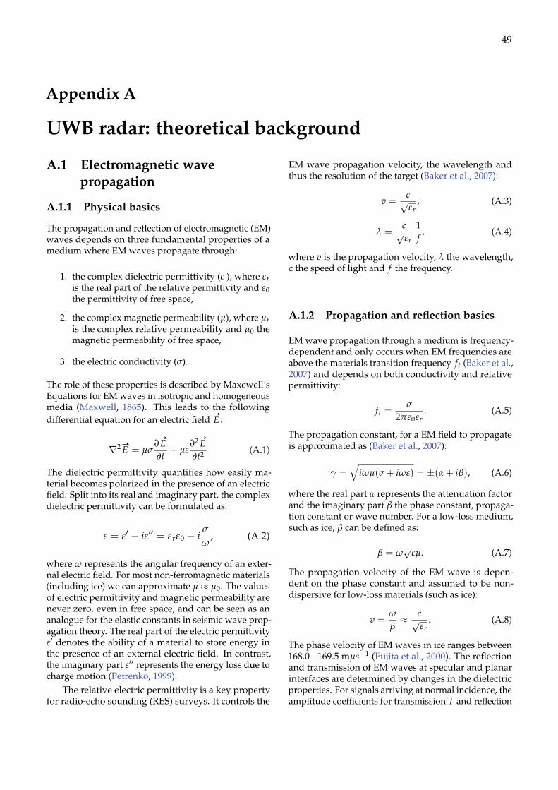
49

Appendix A

UWB radar: theoretical background

A.1 Electromagnetic wavepropagation

A.1.1 Physical basics

The propagation and reflection of electromagnetic (EM)waves depends on three fundamental properties of amedium where EM waves propagate through:

1. the complex dielectric permittivity (ε ), where εris the real part of the relative permittivity and ε0the permittivity of free space,

2. the complex magnetic permeability (µ), where µris the complex relative permeability and µ0 themagnetic permeability of free space,

3. the electric conductivity (σ).

The role of these properties is described by Maxewell’sEquations for EM waves in isotropic and homogeneousmedia (Maxwell, 1865). This leads to the followingdifferential equation for an electric field

#»

E :

∇2 #»

E = µσ∂

#»

E∂t

+ µε∂2 #»

E∂t2 (A.1)

The dielectric permittivity quantifies how easily ma-terial becomes polarized in the presence of an electricfield. Split into its real and imaginary part, the complexdielectric permittivity can be formulated as:

ε = ε′ − iε′′ = εrε0 − iσ

ω, (A.2)

where ω represents the angular frequency of an exter-nal electric field. For most non-ferromagnetic materials(including ice) we can approximate µ ≈ µ0. The valuesof electric permittivity and magnetic permeability arenever zero, even in free space, and can be seen as ananalogue for the elastic constants in seismic wave prop-agation theory. The real part of the electric permittivityε′ denotes the ability of a material to store energy inthe presence of an external electric field. In contrast,the imaginary part ε′′ represents the energy loss due tocharge motion (Petrenko, 1999).

The relative electric permittivity is a key propertyfor radio-echo sounding (RES) surveys. It controls the

EM wave propagation velocity, the wavelength andthus the resolution of the target (Baker et al., 2007):

v =c√εr

, (A.3)

λ =c√εr

1f

, (A.4)

where v is the propagation velocity, λ the wavelength,c the speed of light and f the frequency.

A.1.2 Propagation and reflection basics

EM wave propagation through a medium is frequency-dependent and only occurs when EM frequencies areabove the materials transition frequency ft (Baker et al.,2007) and depends on both conductivity and relativepermittivity:

ft =σ

2πε0εr. (A.5)

The propagation constant, for a EM field to propagateis approximated as (Baker et al., 2007):

γ =√

iωµ(σ + iωε) = ±(α + iβ), (A.6)

where the real part α represents the attenuation factorand the imaginary part β the phase constant, propaga-tion constant or wave number. For a low-loss medium,such as ice, β can be defined as:

β = ω√

εµ. (A.7)

The propagation velocity of the EM wave is depen-dent on the phase constant and assumed to be non-dispersive for low-loss materials (such as ice):

v =ω

β≈ c√

εr. (A.8)

The phase velocity of EM waves in ice ranges between168.0 – 169.5 mµs−1 (Fujita et al., 2000). The reflectionand transmission of EM waves at specular and planarinterfaces are determined by changes in the dielectricproperties. For signals arriving at normal incidence, theamplitude coefficients for transmission T and reflection

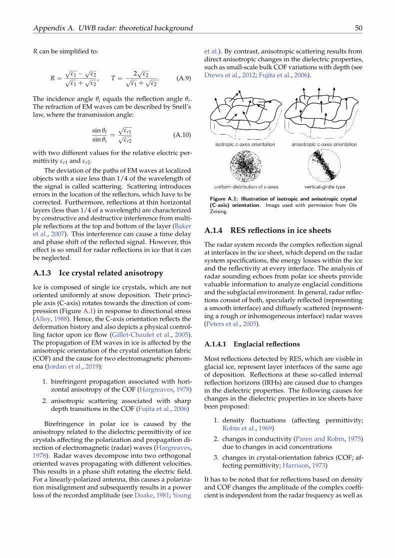
Appendix A. UWB radar: theoretical background 50

R can be simplified to:

R =

√ε1 −

√ε2√

ε1 +√

ε2, T =

2√

ε2√ε1 +

√ε2

. (A.9)

The incidence angle θi equals the reflection angle θr.The refraction of EM waves can be described by Snell’slaw, where the transmission angle:

sin θt

sin θi=

√εr1√εr2

(A.10)

with two different values for the relative electric per-mittivity εr1 and εr2.

The deviation of the paths of EM waves at localizedobjects with a size less than 1/4 of the wavelength ofthe signal is called scattering. Scattering introduceserrors in the location of the reflectors, which have to becorrected. Furthermore, reflections at thin horizontallayers (less than 1/4 of a wavelength) are characterizedby constructive and destructive interference from multi-ple reflections at the top and bottom of the layer (Bakeret al., 2007). This interference can cause a time delayand phase shift of the reflected signal. However, thiseffect is so small for radar reflections in ice that it canbe neglected.

A.1.3 Ice crystal related anisotropy

Ice is composed of single ice crystals, which are notoriented uniformly at snow deposition. Their princi-ple axis (C-axis) rotates towards the direction of com-pression (Figure A.1) in response to directional stress(Alley, 1988). Hence, the C-axis orientation reflects thedeformation history and also depicts a physical control-ling factor upon ice flow (Gillet-Chaulet et al., 2005).The propagation of EM waves in ice is affected by theanisotropic orientation of the crystal orientation fabric(COF) and the cause for two electromagnetic phenom-ena (Jordan et al., 2019):

1. birefringent propagation associated with hori-zontal anisotropy of the COF (Hargreaves, 1978)

2. anisotropic scattering associated with sharpdepth transitions in the COF (Fujita et al., 2006)

Birefringence in polar ice is caused by theanisotropy related to the dielectric permittivity of icecrystals affecting the polarization and propagation di-rection of electromagnetic (radar) waves (Hargreaves,1978). Radar waves decompose into two orthogonaloriented waves propagating with different velocities.This results in a phase shift rotating the electric field.For a linearly-polarized antenna, this causes a polariza-tion misalignment and subsequently results in a powerloss of the recorded amplitude (see Doake, 1981; Young

et al.). By contrast, anisotropic scattering results fromdirect anisotropic changes in the dielectric properties,such as small-scale bulk COF variations with depth (seeDrews et al., 2012; Fujita et al., 2006).

Figure A.1: Illustration of isotropic and anisotropic crystal(C-axis) orientation. Image used with permission from OleZeising.

A.1.4 RES reflections in ice sheets

The radar system records the complex reflection signalat interfaces in the ice sheet, which depend on the radarsystem specifications, the energy losses within the iceand the reflectivity at every interface. The analysis ofradar sounding echoes from polar ice sheets providevaluable information to analyze englacial conditionsand the subglacial environment. In general, radar reflec-tions consist of both, specularly reflected (representinga smooth interface) and diffusely scattered (represent-ing a rough or inhomogeneous interface) radar waves(Peters et al., 2005).

A.1.4.1 Englacial reflections

Most reflections detected by RES, which are visible inglacial ice, represent layer interfaces of the same ageof deposition. Reflections at these so-called internalreflection horizons (IRHs) are caused due to changesin the dielectric properties. The following causes forchanges in the dielectric properties in ice sheets havebeen proposed:

1. density fluctuations (affecting permittivity;Robin et al., 1969)

2. changes in conductivity (Paren and Robin, 1975)due to changes in acid concentrations

3. changes in crystal-orientation fabrics (COF; af-fecting permittivity; Harrison, 1973)

It has to be noted that for reflections based on densityand COF changes the amplitude of the complex coeffi-cient is independent from the radar frequency as well as

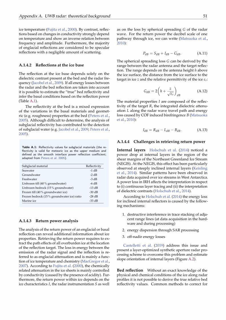
Appendix A. UWB radar: theoretical background 51

ice temperature (Fujita et al., 2000). By contrast, reflec-tions based on changes in conductivity strongly dependon temperature and show an inverse relation betweenfrequency and amplitude. Furthermore, the majorityof englacial reflections are considered to be specularreflections with a negligible amount of scattering.

A.1.4.2 Reflections at the ice base

The reflection at the ice base depends solely on thedielectric contrast present at the bed and the radar fre-quency (Jacobel et al., 2009). If all energy losses betweenthe radar and the bed reflection are taken into accountit is possible to estimate the “true” bed reflectivity andinfer the basal conditions based on the reflection power(Table A.1).

The reflectivity at the bed is a mixed expressionof the variations in the basal materials and geomet-ric (e.g. roughness) properties at the bed (Peters et al.,2005). Although difficult to determine, the analysis ofsubglacial reflectivity has contributed to the detectionof subglacial water (e.g. Jacobel et al., 2009; Peters et al.,2005).

Table A.1: Reflectivity values for subglacial materials (the re-flectivity is valid for meteoric ice as the upper medium anddefined as the smooth interface power reflection coefficient;adapted from Peters et al. 2005).

Subglacial material ReflectivitySeawater -1 dBGroundwater -2 dBFreshwater -3 dBUnfrozen till (40 % groundwater) -6 dBUnfrozen bedrock (15 % groundwater) -13 dBFrozen till (40 % groundwater ice) -30 dBFrozen bedrock (15 % groundwater ice) ratio -28 dBMarine ice -33 dB

A.1.4.3 Return power analysis

The analysis of the return power of an englacial or basalreflection can reveal additional information about iceproperties. Retrieving the return power requires to ex-tract the path effects of all overburden ice at the locationof the reflection target. The loss in energy between theemission of the radar signal and the reflection is re-ferred to as englacial attenuation and is mainly a func-tion of ice temperature and chemistry (MacGregor et al.,2007). According to Fujita et al. (2000), the chemicallyrelated attenuation in the ice sheets is mainly controlledby conductivity (caused by the presence of acidity). Fur-thermore, the return power within ice depends on theice characteristics I, the radar instrumentation S as well

as on the loss by spherical spreading G of the radarwave. For the return power the decibel scale of onepathway through ice, we can write (Matsuoka et al.,2010):

PdB = SdB + IdB − GdB. (A.11)

The spherical spreading loss G can be derived by therange between the radar antenna and the target reflec-tion. The range depends on the antenna height h abovethe ice surface, the distance from the ice surface to thetarget in ice z and the relative permittivity of the ice εr:

GdB = 2(

h +z√εr

)dB

(A.12)

The material properties I are composed of the reflec-tivity of the target R, the integrated dielectric attenu-ation L along the radar wave travel path and energyloss caused by COF induced birefringence B (Matsuokaet al., 2010):

IdB = RdB − LdB − BdB. (A.13)

A.1.4.4 Challenges in retrieving return power

Internal layers Holschuh et al. (2014) noticed apower drop at internal layers in the region of theshear margins of the Northeast Greenland Ice Stream(NEGIS). At the NEGIS, this effect has been particularlyobserved at steeply inclined internal layers (Keislinget al., 2014). Similar patterns have been observed inradar data acquired over ice streams in West Antarctica.A power loss in IRH affects the interpretation in respectto (i) continuous layer tracing and (ii) the interpretationof dielectric contrasts (Holschuh et al., 2014).

According to Holschuh et al. (2014) the energy lossfor inclined internal reflectors is caused by the follow-ing mechanisms:

1. destructive interference in trace stacking of adja-cent range lines (at data acquisition in the hard-ware and during processing)

2. energy dispersion through SAR processing

3. off-nadir energy losses

Castelletti et al. (2019) address this issue andpresent a layer-optimized synthetic aperture radar pro-cessing scheme to overcome this problem and estimateslope orientation of internal layers (Figure A.2).

Bed reflection Without an exact knowledge of thephysical and chemical conditions of the ice along radarprofiles it is not possible to derive the true relative bedreflectivity values. Common methods to correct for

Appendix A. UWB radar: theoretical background 52

englacial attenuation are based on ice sheet modellingor obtained by empirical methods. The weakness be-hind both approaches is that they either depend onassumptions or do not capture the horizontal hetero-geneity of changes in ice velocity, temperature, andsurface roughness at critical glaciological settings, suchas ice stream shear margins (Matsuoka et al., 2010; Mat-suoka, 2011; Schroeder et al., 2015).

Figure A.2: Sloping layer effect on radar processing. Compar-ison of radar data processing on flat and sloping internal layers(image obtained from Castelletti et al. (2019)).

A.1.5 Real and synthetic aperture radar

Along-track resolution for traditional radars is deter-mined by the beamwidth of the antenna, which in turndepends on the length of the antenna (so-called realaperture radars; RAR). The along-track resolution isproportional to the aperture length and in this case theantenna dimensions. Hence, obtaining a high along-track resolution requires very long antennas, which isin many cases unfeasible and has the disadvantage toreduce the resolution in range. A synthetic apertureradar (SAR) overcomes this problem by using a smallantenna, which is moved while taking the measure-ment. The recorded data can be combined to obtain asynthesized longer aperture,

A.2 AWI UWB radar system

In my thesis I use radar data from AWI’s (AlfredWegener Institute) ultra-wideband radar (UWB). The

radar was developed at the Centrer for Remote Sens-ing of Ice Sheets (CReSIS) at the university of Kansas,is a MCoRDS (Multichannel Coherent Radar DepthSounder) type radar (Arnold et al., 2019) and designedto image a full vertical profile of the ice column.

Figure A.3: AWI UWB radar system on Polar6 . Schematicillustration and photograph of the antenna arrays. The 3D an-imation was kindly provided by University of Kansas and thephotograph by Sepp Kipfstuhl.

Multi-element antenna arrays in combination withSAR techniques overcome typical limitations in radio-glaciology. SAR algorithms improve the azimuth reso-lution and the usage of beam-steering techniques can re-duce surface clutter and allow the detection of off-nadiroriented reflectors. Moreover, an increased bandwidthin combination with pulse compression techniques al-low the sounding of thick ice in high resolution. Fur-thermore, multiple waveforms are emitted to sounddifferent parts of the ice column. After processing thewaveform images are combined to increase the overallresolution of the entire ice column. The system canoperate in two different modes:

1. Sounding mode: The “traditional” 2D acquisi-tion mode of a nadir section of the ice below theradar.

2. Image mode: Also referred to as “swath tomog-raphy” mode, which uses off-nadir scatteringreflections from the ice-base to create a high-resolution DEM of the bed topography for awidth of ~ 5 km along the radar transect.

The radar system comprises an eight-element an-tenna array, which is mounted underneath the fuselageof the AWI Basler BT-67 Polar 6 aircraft and two furthereight-antenna arrays, which can be mounted under-neath the wings (Hale et al., 2016). The centre array canalternate between transmission and reception, whereasboth wing antenna-arrays only represent receivers. Thedata I used in my thesis were acquired during surveys,where only the centre array has been used.

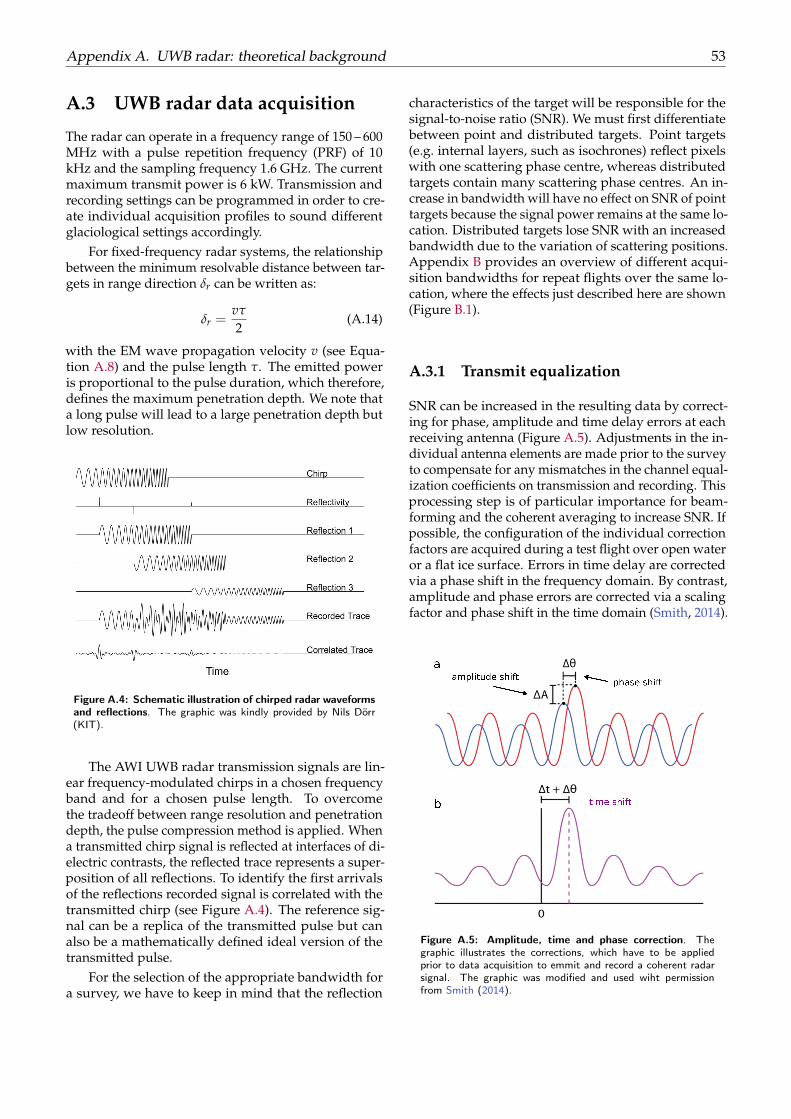
Appendix A. UWB radar: theoretical background 53

A.3 UWB radar data acquisition

The radar can operate in a frequency range of 150 – 600MHz with a pulse repetition frequency (PRF) of 10kHz and the sampling frequency 1.6 GHz. The currentmaximum transmit power is 6 kW. Transmission andrecording settings can be programmed in order to cre-ate individual acquisition profiles to sound differentglaciological settings accordingly.

For fixed-frequency radar systems, the relationshipbetween the minimum resolvable distance between tar-gets in range direction δr can be written as:

δr =vτ

2(A.14)

with the EM wave propagation velocity v (see Equa-tion A.8) and the pulse length τ. The emitted poweris proportional to the pulse duration, which therefore,defines the maximum penetration depth. We note thata long pulse will lead to a large penetration depth butlow resolution.

Figure A.4: Schematic illustration of chirped radar waveformsand reflections. The graphic was kindly provided by Nils Dörr(KIT).

The AWI UWB radar transmission signals are lin-ear frequency-modulated chirps in a chosen frequencyband and for a chosen pulse length. To overcomethe tradeoff between range resolution and penetrationdepth, the pulse compression method is applied. Whena transmitted chirp signal is reflected at interfaces of di-electric contrasts, the reflected trace represents a super-position of all reflections. To identify the first arrivalsof the reflections recorded signal is correlated with thetransmitted chirp (see Figure A.4). The reference sig-nal can be a replica of the transmitted pulse but canalso be a mathematically defined ideal version of thetransmitted pulse.

For the selection of the appropriate bandwidth fora survey, we have to keep in mind that the reflection

characteristics of the target will be responsible for thesignal-to-noise ratio (SNR). We must first differentiatebetween point and distributed targets. Point targets(e.g. internal layers, such as isochrones) reflect pixelswith one scattering phase centre, whereas distributedtargets contain many scattering phase centres. An in-crease in bandwidth will have no effect on SNR of pointtargets because the signal power remains at the same lo-cation. Distributed targets lose SNR with an increasedbandwidth due to the variation of scattering positions.Appendix B provides an overview of different acqui-sition bandwidths for repeat flights over the same lo-cation, where the effects just described here are shown(Figure B.1).

A.3.1 Transmit equalization

SNR can be increased in the resulting data by correct-ing for phase, amplitude and time delay errors at eachreceiving antenna (Figure A.5). Adjustments in the in-dividual antenna elements are made prior to the surveyto compensate for any mismatches in the channel equal-ization coefficients on transmission and recording. Thisprocessing step is of particular importance for beam-forming and the coherent averaging to increase SNR. Ifpossible, the configuration of the individual correctionfactors are acquired during a test flight over open wateror a flat ice surface. Errors in time delay are correctedvia a phase shift in the frequency domain. By contrast,amplitude and phase errors are corrected via a scalingfactor and phase shift in the time domain (Smith, 2014).

Figure A.5: Amplitude, time and phase correction. Thegraphic illustrates the corrections, which have to be appliedprior to data acquisition to emmit and record a coherent radarsignal. The graphic was modified and used wiht permissionfrom Smith (2014).

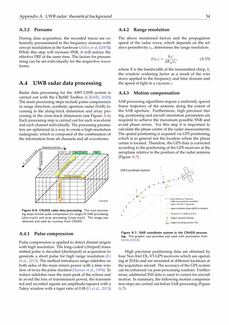
Appendix A. UWB radar: theoretical background 54

A.3.2 Presums

During data acquisition, the recorded traces are co-herently presummend in the frequency domain withzero-pi modulation in the hardware (Allen et al. (2005)).While this step will increase SNR, it will reduce theeffective PRF at the same time. The factors for presum-ming can be set individually for the respective wave-forms.

A.4 UWB radar data processing

Radar data processing for the AWI UWB system iscarried out with the CReSIS Toolbox (CReSIS, 2020).The main processing steps include pulse compressionin range direction, synthetic aperture radar (SAR) fo-cussing in the along-track dimension and array pro-cessing in the cross-track dimension (see Figure A.6).Each processing step is carried out for each waveformand each channel individually. The processing parame-ters are optimized in a way to create a high-resolutionradargram, which is composed of the combination ofthe information from all channels and all waveforms.

Figure A.6: CReSIS radar data processing. The main process-ing steps include pulse compression (in range) fk SAR processing(alon-track) and array processing (cross-track). The image wasobtained and used by courtesy from CReSIS.

A.4.1 Pulse compression

Pulse compression is applied to detect distant targetswith high resolution. The long-coded (chirped) trans-mitted pulse is decoded (dechirped) at acquisition togenerate a short pulse for high range resolution (Liet al., 2013). The method introduces range sidelobes onboth sides of the main return power with a time win-dow of twice the pulse duration (Tanner et al., 1994). Toreduce sidelobes near the main peak of the echoes andto avoid the loss of transmission power, the transmit-ted and recorded signals are amplitude-tapared with aTukey window with a taper ratio of 0.08 (Li et al., 2013).

A.4.2 Range resolution

The above mentioned factors and the propagationspeed of the radar wave, which depends on the rel-ative permittivity εr, determines the range resolution:

δ(εr) =kic

2B√

εr, (A.15)

where B is the bandwidth of the transmitted chirp, kithe window widening factor as a result of the win-dows applied to the frequency and time domain andthe speed of light in a vacuum c.

A.4.3 Motion compensation

SAR processing algorithms require a uniformly spacedlinear trajectory of the antenna along the extent ofthe SAR aperture. Furthermore, high precision tim-ing, positioning and aircraft orientation parameters arerequired to achieve the maximum possible SNR andavoid phase errors. For this step it is important tocalculate the phase centre of the radar measurements.The spatial positioning is acquired via GPS positioning,which is in general not the location where the phasecentre is located. Therefore, the GPS data is correctedaccording to the positioning of the GPS receivers at theaeroplane relative to the position of the radar antenna(Figure A.7).

Figure A.7: SAR coordinate system in the CReSIS process-ing. The graphic was provided and used with permission fromSmith (2014).

High precision positioning data are obtained byfour NovAtel DL-V3 GPS receivers which are operat-ing at 20 Hz and are mounted at different locations atthe acquisition aircraft. The accuracy of the GPS systemcan be enhanced via post-processing routines. Further-more, additional INS data is used to correct for aircraftmotion. In summary, the following motion compensa-tion steps are carried out before SAR processing (FigureA.7):

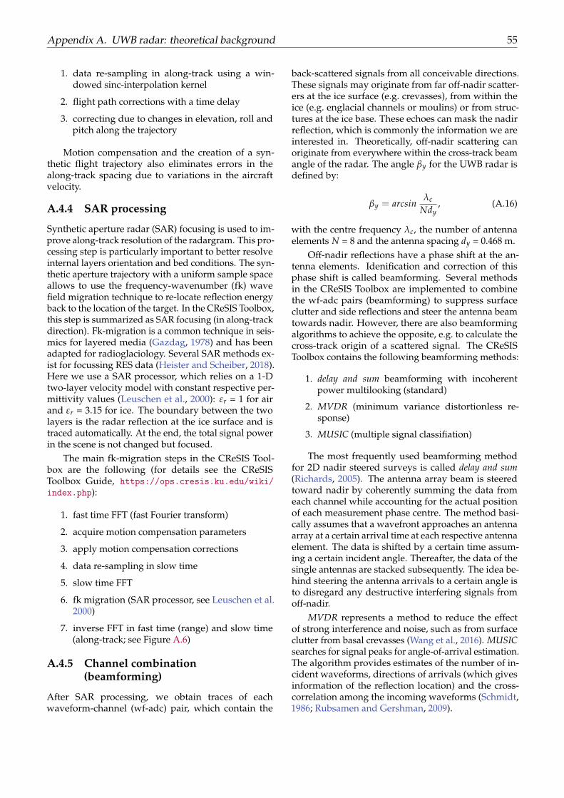
Appendix A. UWB radar: theoretical background 55

1. data re-sampling in along-track using a win-dowed sinc-interpolation kernel

2. flight path corrections with a time delay

3. correcting due to changes in elevation, roll andpitch along the trajectory

Motion compensation and the creation of a syn-thetic flight trajectory also eliminates errors in thealong-track spacing due to variations in the aircraftvelocity.

A.4.4 SAR processing

Synthetic aperture radar (SAR) focusing is used to im-prove along-track resolution of the radargram. This pro-cessing step is particularly important to better resolveinternal layers orientation and bed conditions. The syn-thetic aperture trajectory with a uniform sample spaceallows to use the frequency-wavenumber (fk) wavefield migration technique to re-locate reflection energyback to the location of the target. In the CReSIS Toolbox,this step is summarized as SAR focusing (in along-trackdirection). Fk-migration is a common technique in seis-mics for layered media (Gazdag, 1978) and has beenadapted for radioglaciology. Several SAR methods ex-ist for focussing RES data (Heister and Scheiber, 2018).Here we use a SAR processor, which relies on a 1-Dtwo-layer velocity model with constant respective per-mittivity values (Leuschen et al., 2000): εr = 1 for airand εr = 3.15 for ice. The boundary between the twolayers is the radar reflection at the ice surface and istraced automatically. At the end, the total signal powerin the scene is not changed but focused.

The main fk-migration steps in the CReSIS Tool-box are the following (for details see the CReSISToolbox Guide, https://ops.cresis.ku.edu/wiki/index.php):

1. fast time FFT (fast Fourier transform)

2. acquire motion compensation parameters

3. apply motion compensation corrections

4. data re-sampling in slow time

5. slow time FFT

6. fk migration (SAR processor, see Leuschen et al.2000)

7. inverse FFT in fast time (range) and slow time(along-track; see Figure A.6)

A.4.5 Channel combination(beamforming)

After SAR processing, we obtain traces of eachwaveform-channel (wf-adc) pair, which contain the

back-scattered signals from all conceivable directions.These signals may originate from far off-nadir scatter-ers at the ice surface (e.g. crevasses), from within theice (e.g. englacial channels or moulins) or from struc-tures at the ice base. These echoes can mask the nadirreflection, which is commonly the information we areinterested in. Theoretically, off-nadir scattering canoriginate from everywhere within the cross-track beamangle of the radar. The angle βy for the UWB radar isdefined by:

βy = arcsinλc

Ndy, (A.16)

with the centre frequency λc, the number of antennaelements N = 8 and the antenna spacing dy = 0.468 m.

Off-nadir reflections have a phase shift at the an-tenna elements. Idenification and correction of thisphase shift is called beamforming. Several methodsin the CReSIS Toolbox are implemented to combinethe wf-adc pairs (beamforming) to suppress surfaceclutter and side reflections and steer the antenna beamtowards nadir. However, there are also beamformingalgorithms to achieve the opposite, e.g. to calculate thecross-track origin of a scattered signal. The CReSISToolbox contains the following beamforming methods:

1. delay and sum beamforming with incoherentpower multilooking (standard)

2. MVDR (minimum variance distortionless re-sponse)

3. MUSIC (multiple signal classifiation)

The most frequently used beamforming methodfor 2D nadir steered surveys is called delay and sum(Richards, 2005). The antenna array beam is steeredtoward nadir by coherently summing the data fromeach channel while accounting for the actual positionof each measurement phase centre. The method basi-cally assumes that a wavefront approaches an antennaarray at a certain arrival time at each respective antennaelement. The data is shifted by a certain time assum-ing a certain incident angle. Thereafter, the data of thesingle antennas are stacked subsequently. The idea be-hind steering the antenna arrivals to a certain angle isto disregard any destructive interfering signals fromoff-nadir.

MVDR represents a method to reduce the effectof strong interference and noise, such as from surfaceclutter from basal crevasses (Wang et al., 2016). MUSICsearches for signal peaks for angle-of-arrival estimation.The algorithm provides estimates of the number of in-cident waveforms, directions of arrivals (which givesinformation of the reflection location) and the cross-correlation among the incoming waveforms (Schmidt,1986; Rubsamen and Gershman, 2009).

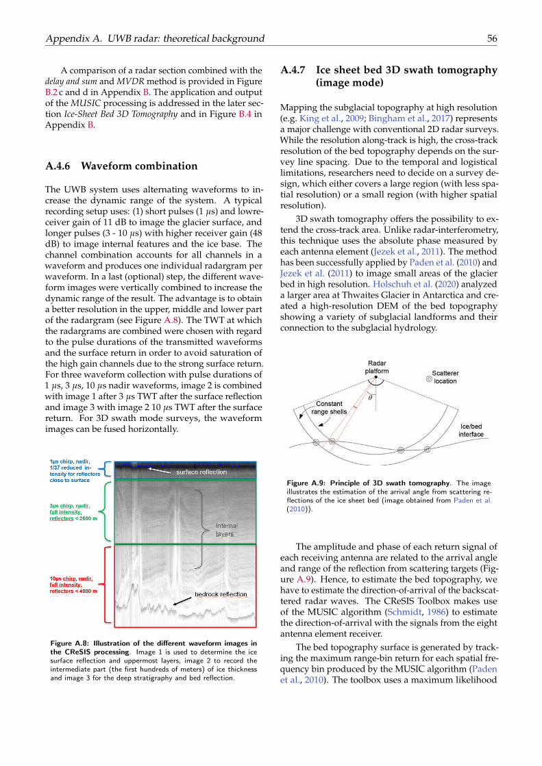
Appendix A. UWB radar: theoretical background 56

A comparison of a radar section combined with thedelay and sum and MVDR method is provided in FigureB.2 c and d in Appendix B. The application and outputof the MUSIC processing is addressed in the later sec-tion Ice-Sheet Bed 3D Tomography and in Figure B.4 inAppendix B.

A.4.6 Waveform combination

The UWB system uses alternating waveforms to in-crease the dynamic range of the system. A typicalrecording setup uses: (1) short pulses (1 µs) and lowre-ceiver gain of 11 dB to image the glacier surface, andlonger pulses (3 - 10 µs) with higher receiver gain (48dB) to image internal features and the ice base. Thechannel combination accounts for all channels in awaveform and produces one individual radargram perwaveform. In a last (optional) step, the different wave-form images were vertically combined to increase thedynamic range of the result. The advantage is to obtaina better resolution in the upper, middle and lower partof the radargram (see Figure A.8). The TWT at whichthe radargrams are combined were chosen with regardto the pulse durations of the transmitted waveformsand the surface return in order to avoid saturation ofthe high gain channels due to the strong surface return.For three waveform collection with pulse durations of1 µs, 3 µs, 10 µs nadir waveforms, image 2 is combinedwith image 1 after 3 µs TWT after the surface reflectionand image 3 with image 2 10 µs TWT after the surfacereturn. For 3D swath mode surveys, the waveformimages can be fused horizontally.

Figure A.8: Illustration of the different waveform images inthe CReSIS processing. Image 1 is used to determine the icesurface reflection and uppermost layers, image 2 to record theintermediate part (the first hundreds of meters) of ice thicknessand image 3 for the deep stratigraphy and bed reflection.

A.4.7 Ice sheet bed 3D swath tomography(image mode)

Mapping the subglacial topography at high resolution(e.g. King et al., 2009; Bingham et al., 2017) representsa major challenge with conventional 2D radar surveys.While the resolution along-track is high, the cross-trackresolution of the bed topography depends on the sur-vey line spacing. Due to the temporal and logisticallimitations, researchers need to decide on a survey de-sign, which either covers a large region (with less spa-tial resolution) or a small region (with higher spatialresolution).

3D swath tomography offers the possibility to ex-tend the cross-track area. Unlike radar-interferometry,this technique uses the absolute phase measured byeach antenna element (Jezek et al., 2011). The methodhas been successfully applied by Paden et al. (2010) andJezek et al. (2011) to image small areas of the glacierbed in high resolution. Holschuh et al. (2020) analyzeda larger area at Thwaites Glacier in Antarctica and cre-ated a high-resolution DEM of the bed topographyshowing a variety of subglacial landforms and theirconnection to the subglacial hydrology.

Figure A.9: Principle of 3D swath tomography. The imageillustrates the estimation of the arrival angle from scattering re-flections of the ice sheet bed (image obtained from Paden et al.(2010)).

The amplitude and phase of each return signal ofeach receiving antenna are related to the arrival angleand range of the reflection from scattering targets (Fig-ure A.9). Hence, to estimate the bed topography, wehave to estimate the direction-of-arrival of the backscat-tered radar waves. The CReSIS Toolbox makes useof the MUSIC algorithm (Schmidt, 1986) to estimatethe direction-of-arrival with the signals from the eightantenna element receiver.

The bed topography surface is generated by track-ing the maximum range-bin return for each spatial fre-quency bin produced by the MUSIC algorithm (Padenet al., 2010). The toolbox uses a maximum likelihood

Appendix A. UWB radar: theoretical background 57

method to calculate signal amplitude and the direction-of-arrival for the left and right side along the flight tra-jectory (Jezek et al., 2011). Together with an estimationof the refraction index for ice, the ice thickness and bedtopography can be calculated. The approach assumesthat there is little or no volume scattering occurringalong the EM wave path. Furthermore, it is assumedthat scattering at internal layers can be neglected dueto the anticipated specular reflectivity of internal layers(Paren and Robin, 1975).

The results from the first bed topography DEM onthe basis of AWI UWB swath radar data are shown inFigure B.4 Appendix B in the section Swath Mode (3DImaging Mode).

58

BibliographyAllen, C. T., Mozaffar, S. N., and Akins, T. L. Suppress-

ing coherent noise in radar applications with longdwell times. IEEE Geoscience and Remote Sensing Let-ters, 2(3):284–286, July 2005. doi: 10.1109/LGRS.2005.847931. URL http://dx.doi.org/10.1109/LGRS.2005.847931.

Alley, R. B. Fabrics in polar ice sheets: De-velopment and prediction. Science, 240(4851):493–495, 1988. doi: 10.1126/science.240.4851.493.URL https://science.sciencemag.org/content/240/4851/493.

Arnold, E., Leuschen, C., Rodriguez-Morales, F., Li,J., Paden, J., Hale, R., and Keshmiri, S. CReSIS air-borne radars and platforms for ice and snow sound-ing. Annals of Glaciology, pages 1–10, nov 2019.doi: 10.1017/aog.2019.37. URL https://doi.org/10.1017%2Faog.2019.37.

Baker, G. S., Jordan, T. E., and Pardy, J. An intro-duction to ground penetrating radar (GPR). InStratigraphic Analyses Using GPR. Geological Soci-ety of America, 01 2007. ISBN 9780813724324. doi:10.1130/2007.2432(01). URL https://doi.org/10.1130/2007.2432(01).

Bingham, R. G., Vaughan, D. G., King, E. C., Davies,D., Cornford, S. L., Smith, A. M., Arthern, R. J.,Brisbourne, A. M., Rydt, J. D., Graham, A. G. C.,Spagnolo, M., Marsh, O. J., and Shean, D. E. Di-verse landscapes beneath Pine Island Glacier influ-ence ice flow. Nature Communications, 8(1), nov2017. doi: 10.1038/s41467-017-01597-y. URL https://doi.org/10.1038%2Fs41467-017-01597-y.

Castelletti, D., Schroeder, D. M., Mantelli, E., and Hilger,A. Layer optimized sar processing and slope estima-tion in radar sounder data. Journal of Glaciology, 65(254):983–988, 2019. doi: 10.1017/jog.2019.72. URLhttps://doi.org/10.1017/jog.2019.72.

CReSIS. CReSIS Toolbox [computer software],Lawrence, Kansas, USA. Retrieved fromhttps://github.com/CReSIS/., 2020.

Doake, C. S. M. Polarization of radio waves in icesheets. Geophysical Journal International, 64(2):539–558,02 1981. ISSN 0956-540X. doi: 10.1111/j.1365-246X.1981.tb02682.x. URL https://doi.org/10.1111/j.1365-246X.1981.tb02682.x.

Drews, R., Eisen, O., Steinhage, D., Weikusat, I., Kipf-stuhl, S., and Wilhelms, F. Potential mechanisms

for anisotropy in ice-penetrating radar data. Jour-nal of Glaciology, 58(209):613–624, sep 2012. ISSN0022-1430. doi: 10.3189/2012JoG11J114. URL http://dx.doi.org/.

Fujita, S., Matsuoka, T., Ishida, T., Matsuoka, K.,and Mae, S. A summary of the complex dielec-tric permittivity of ice in the megahertz range andits applications for radar sounding of polar icesheets. Physics of Ice Core Records, pages 185–212,2000. URL https://eprints.lib.hokudai.ac.jp/dspace/bitstream/2115/32469/1/P185-212.pdf.

Fujita, S., Maeno, H., and Matsuoka, K. Radio-wave depolarization and scattering within ice sheets:a matrix-based model to link radar and ice-coremeasurements and its application. Journal ofGlaciology, 52(178):407–424, 2006. doi: 10.3189/172756506781828548. URL https://doi.org/10.3189/172756506781828548.

Gazdag, J. Wave equation migration with the phase-shift method. Geophysics, 43(7):1342–1351, 1978. ISSN0016-8033. doi: 10.1190/1.1440899. URL http://dx.doi.org/10.1190/1.1440899.

Gillet-Chaulet, F., Gagliardini, O., Meyssonnier, J.,Montagnat, M., and Castelnau, O. A user-friendlyanisotropic flow law for ice-sheet modeling. Jour-nal of Glaciology, 51(172):3–14, 2005. doi: 10.3189/172756505781829584.

Hale, R., Miller, H., Gogineni, S., Yan, J. B., Rodriguez-Morales, F., Leuschen, C., Paden, J., Li, J., Binder,T., Steinhage, D., Gehrmann, M., and Braaten, D.Multi-channel ultra-wideband radar sounder andimager. In 2016 IEEE International Geoscience and Re-mote Sensing Symposium (IGARSS). IEEE, jul 2016.doi: 10.1109/igarss.2016.7729545. URL https://doi.org/10.1109%2Figarss.2016.7729545.

Hargreaves, N. D. The Radio-Frequency Birefrin-gence of Polar Ice. Journal of Glaciology, 21(85):301–313, 1978. ISSN 0022-1430. doi: 10.3189/s0022143000033499. URL https://doi.org/10.3189/s0022143000033499.

Harrison, C. H. Radio echo sounding of horizontallayers in ice. Journal of Glaciology, 12(66):383–397,1973. doi: 10.3189/S0022143000031804. URL https://doi.org/10.3189/S0022143000031804.

Heister, A. and Scheiber, R. Coherent large beamwidthprocessing of radio-echo sounding data. TheCryosphere, 12(9):2969–2979, 2018. doi: 10.5194/tc-12-2969-2018. URL https://tc.copernicus.org/articles/12/2969/2018/.

BIBLIOGRAPHY 59

Holschuh, N., Christianson, K., and Anandakrishnan,S. Power loss in dipping internal reflectors imagedusing ice-penetrating radar. Annals of Glaciology, 55(67):49–56, 2014. doi: 10.3189/2014aog67a005. URLhttps://doi.org/10.3189%2F2014aog67a005.

Holschuh, N., Christianson, K., Paden, J., Alley, R.,and Anandakrishnan, S. Linking postglacial land-scapes to glacier dynamics using swath radar atThwaites Glacier Antarctica. Geology, jan 2020. doi:10.1130/g46772.1. URL https://doi.org/10.1130%2Fg46772.1.

Jacobel, R. W., Welch, B. C., Osterhouse, D., Petters-son, R., and MacGregor, J. A. Spatial variation ofradar-derived basal conditions on kamb ice stream,west antarctica. Annals of Glaciology, 50(51):10–16,2009. doi: 10.3189/172756409789097504. URL https://doi.org/10.3189/172756409789097504.

Jezek, K., Wu, X., Gogineni, P., Rodríguez, E., Free-man, A., Rodriguez-Morales, F., and Clark, C. D.Radar images of the bed of the Greenland Ice Sheet.Geophysical Research Letters, 38(1):1–5, 2011. ISSN00948276. doi: 10.1029/2010GL045519. URL http://dx.doi.org/10.1029/2010GL045519.

Jordan, T. M., Schroeder, D. M., Castelletti, D., Li,J., and Dall, J. A polarimetric coherence methodto determine ice crystal orientation fabric fromradar sounding: Application to the neem ice coreregion. IEEE Transactions on Geoscience and Re-mote Sensing, 57(11):8641–8657, 2019. doi: 10.1109/TGRS.2019.2921980. URL https://ieeexplore.ieee.org/document/8755860.

Keisling, B. A., Christianson, K., Alley, R. B., Peters,L. E., Christian, J. E., Anandakrishnan, S., River-man, K. L., Muto, A., and Jacobel, R. W. Basalconditions and ice dynamics inferred from radar-derived internal stratigraphy of the northeast Green-land ice stream. Annals of Glaciology, 55(67):127–137,2014. doi: 10.3189/2014aog67a090. URL https://doi.org/10.3189%2F2014aog67a090.

King, E. C., Hindmarsh, R. C. A., and Stokes, C. R. For-mation of mega-scale glacial lineations observed be-neath a West Antarctic ice stream. Nature Geoscience,2(8):585–588, jul 2009. doi: 10.1038/ngeo581. URLhttps://doi.org/10.1038%2Fngeo581.

Leuschen, C., Gogineni, S., and Tammana, D. SAR pro-cessing of radar echo sounder data. pages 2570–2572,2000. doi: 10.1109/igarss.2000.859643. URL http://dx.doi.org/10.1109/igarss.2000.859643.

Li, J., Paden, J., Leuschen, C., Rodriguez-Morales,F., Hale, R. D., Arnold, E. J., Crowe, R., Gomez-Garcia, D., and Gogineni, P. High-altitude radar

measurements of ice thickness over the antarcticand greenland ice sheets as a part of operation ice-bridge. IEEE Transactions on Geoscience and RemoteSensing, 51(2):742–754, 2013. ISSN 0196-2892. doi:10.1109/TGRS.2012.2203822.

MacGregor, J. A., Winebrenner, D. P., Conway, H.,Matsuoka, K., Mayewski, P. A., and Clow, G. D. Mod-eling englacial radar attenuation at siple dome, westantarctica, using ice chemistry and temperature data.Journal of Geophysical Research: Earth Surface, 112(F3),2007. doi: https://doi.org/10.1029/2006JF000717.URL https://agupubs.onlinelibrary.wiley.com/doi/abs/10.1029/2006JF000717.

Matsuoka, K. Pitfalls in radar diagnosis of ice-sheetbed conditions: Lessons from englacial attenuationmodels. Geophysical Research Letters, 38(5):n/a–n/a,mar 2011. doi: 10.1029/2010gl046205. URL https://doi.org/10.1029%2F2010gl046205.

Matsuoka, K., Morse, D., and Raymond, C. F. Estimat-ing englacial radar attenuation using depth profilesof the returned power, central west antarctica.Journal of Geophysical Research: Earth Surface, 115(F2),2010. doi: https://doi.org/10.1029/2009JF001496.URL https://agupubs.onlinelibrary.wiley.com/doi/abs/10.1029/2009JF001496.

Maxwell, J. C. Viii. a dynamical theory of the electro-magnetic field. Philosophical Transactions of the RoyalSociety of London, 155:459–512, 1865. doi: 10.1098/rstl.1865.0008. URL https://royalsocietypublishing.org/doi/abs/10.1098/rstl.1865.0008.

Paden, J., Akins, T., Dunson, D., Allen, C., and Gogi-neni, P. Ice-sheet bed 3-D tomography. Journalof Glaciology, 56(195):3–11, 2010. doi: 10.3189/002214310791190811. URL https://doi.org/10.3189%2F002214310791190811.

Paren, J. G. and Robin, G. d. Q. Internal reflections inpolar ice sheets. Journal of Glaciology, 14(71):251–259,1975. doi: 10.3189/S0022143000021730.

Peters, M. E., Blankenship, D. D., and Morse, D. L.Analysis techniques for coherent airborne radarsounding: Application to west antarctic ice streams.Journal of Geophysical Research: Solid Earth, 110(B6),2005. doi: https://doi.org/10.1029/2004JB003222.URL https://agupubs.onlinelibrary.wiley.com/doi/abs/10.1029/2004JB003222.

Petrenko, V. F. und Whitworth, R. W. Physics of ice.Oxford University Press, Oxford, New York, 1999.

Richards, M. Fundamentals of Radar Signal Process-ing. Professional Engineering, New York: McGraw-HillEducation, 2005.

BIBLIOGRAPHY 60

Robin, G. D. Q., Evans, S., Bailey, J. T., and Bullard, E. C.Interpretation of radio echo sounding in polar icesheets. Philosophical Transactions of the Royal Societyof London. Series A, Mathematical and Physical Sciences,265(1166):437–505, 1969. doi: 10.1098/rsta.1969.0063.URL https://royalsocietypublishing.org/doi/abs/10.1098/rsta.1969.0063.

Rubsamen, M. and Gershman, A. B. Direction-of-arrival estimation for nonuniform sensor arrays:From manifold separation to fourier domain mu-sic methods. IEEE Transactions on Signal Process-ing, 57(2):588–599, 2009. doi: 10.1109/TSP.2008.2008560. URL https://ieeexplore.ieee.org/document/4663945.

Schmidt, R. Multiple emitter location and signal pa-rameter estimation. IEEE Transactions on Antennasand Propagation, 34(3):276–280, 1986. doi: 10.1109/TAP.1986.1143830. URL https://ieeexplore.ieee.org/document/1143830.

Schroeder, D. M., Grima, C., and Blankenship, D. D.Evidence for variable grounding-zone and shear-margin basal conditions across Thwaites Glacier,West Antarctica. Geophysics, 81(1):WA35–WA43, 2015.ISSN 0016-8033. doi: 10.1190/geo2015-0122.1. URLhttps://doi.org/10.1190/geo2015-0122.1.

Smith, L. Validation of CReSIS synthetic apertureradar processor and optimal processing parameters.Master’s thesis, University of Kansas, 2014. URLhttps://kuscholarworks.ku.edu/handle/1808/18381(lastaccess:1December2020).

Tanner, A., Durden, S., Denning, R., Im, E., Li, F., Rick-etts, W., and Wilson, W. Pulse compression with verylow sidelobes in an airborne rain mapping radar.IEEE Transactions on Geoscience and Remote Sensing, 32(1):211–213, 1994. doi: 10.1109/36.285205.

Wang, Z., Gogineni, S., Rodriguez-Morales, F., Yan, J. B.,Paden, J., Leuschen, C., Hale, R. D., Li, J., Caraba-jal, C. L., Gomez-Garcia, D., Townley, B., Willer,R., Stearns, L., Child, S., and Braaten, D. Mul-tichannel Wideband Synthetic Aperture Radar forIce Sheet Remote Sensing: Development and theFirst Deployment in Antarctica. IEEE Journal of Se-lected Topics in Applied Earth Observations and RemoteSensing, 9(3):980–993, 2016. ISSN 21511535. doi:10.1109/JSTARS.2015.2403611. URL http://dx.doi.org/10.1109/JSTARS.2015.2403611.

Young, T. J., Schroeder, D. M., Jordan, T. M., Christof-fersen, P., Tulaczyk, S. M., Culberg, R., andBienert, N. L. Inferring ice fabric from birefrin-gence loss in airborne radargrams: Applicationto the eastern shear margin of thwaites glacier,west antarctica. Journal of Geophysical Research:

Earth Surface, n/a(n/a):e2020JF006023. doi:https://doi.org/10.1029/2020JF006023. URLhttps://agupubs.onlinelibrary.wiley.com/doi/abs/10.1029/2020JF006023.

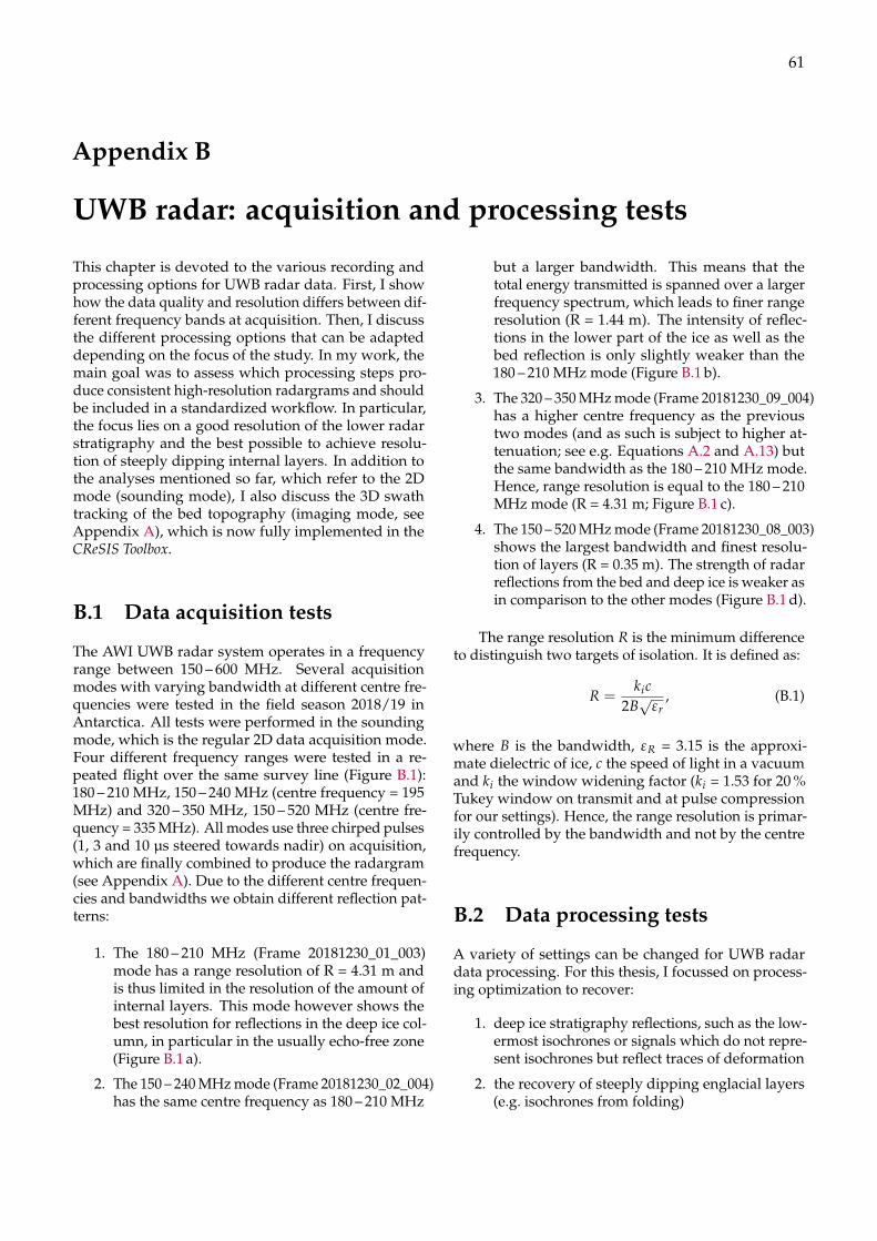
61

Appendix B

UWB radar: acquisition and processing tests

This chapter is devoted to the various recording andprocessing options for UWB radar data. First, I showhow the data quality and resolution differs between dif-ferent frequency bands at acquisition. Then, I discussthe different processing options that can be adapteddepending on the focus of the study. In my work, themain goal was to assess which processing steps pro-duce consistent high-resolution radargrams and shouldbe included in a standardized workflow. In particular,the focus lies on a good resolution of the lower radarstratigraphy and the best possible to achieve resolu-tion of steeply dipping internal layers. In addition tothe analyses mentioned so far, which refer to the 2Dmode (sounding mode), I also discuss the 3D swathtracking of the bed topography (imaging mode, seeAppendix A), which is now fully implemented in theCReSIS Toolbox.

B.1 Data acquisition tests

The AWI UWB radar system operates in a frequencyrange between 150 – 600 MHz. Several acquisitionmodes with varying bandwidth at different centre fre-quencies were tested in the field season 2018/19 inAntarctica. All tests were performed in the soundingmode, which is the regular 2D data acquisition mode.Four different frequency ranges were tested in a re-peated flight over the same survey line (Figure B.1):180 – 210 MHz, 150 – 240 MHz (centre frequency = 195MHz) and 320 – 350 MHz, 150 – 520 MHz (centre fre-quency = 335 MHz). All modes use three chirped pulses(1, 3 and 10 µs steered towards nadir) on acquisition,which are finally combined to produce the radargram(see Appendix A). Due to the different centre frequen-cies and bandwidths we obtain different reflection pat-terns:

1. The 180 – 210 MHz (Frame 20181230_01_003)mode has a range resolution of R = 4.31 m andis thus limited in the resolution of the amount ofinternal layers. This mode however shows thebest resolution for reflections in the deep ice col-umn, in particular in the usually echo-free zone(Figure B.1 a).

2. The 150 – 240 MHz mode (Frame 20181230_02_004)has the same centre frequency as 180 – 210 MHz

but a larger bandwidth. This means that thetotal energy transmitted is spanned over a largerfrequency spectrum, which leads to finer rangeresolution (R = 1.44 m). The intensity of reflec-tions in the lower part of the ice as well as thebed reflection is only slightly weaker than the180 – 210 MHz mode (Figure B.1 b).

3. The 320 – 350 MHz mode (Frame 20181230_09_004)has a higher centre frequency as the previoustwo modes (and as such is subject to higher at-tenuation; see e.g. Equations A.2 and A.13) butthe same bandwidth as the 180 – 210 MHz mode.Hence, range resolution is equal to the 180 – 210MHz mode (R = 4.31 m; Figure B.1 c).

4. The 150 – 520 MHz mode (Frame 20181230_08_003)shows the largest bandwidth and finest resolu-tion of layers (R = 0.35 m). The strength of radarreflections from the bed and deep ice is weaker asin comparison to the other modes (Figure B.1 d).

The range resolution R is the minimum differenceto distinguish two targets of isolation. It is defined as:

R =kic

2B√

εr, (B.1)

where B is the bandwidth, εR = 3.15 is the approxi-mate dielectric of ice, c the speed of light in a vacuumand ki the window widening factor (ki = 1.53 for 20 %Tukey window on transmit and at pulse compressionfor our settings). Hence, the range resolution is primar-ily controlled by the bandwidth and not by the centrefrequency.

B.2 Data processing tests

A variety of settings can be changed for UWB radardata processing. For this thesis, I focussed on process-ing optimization to recover:

1. deep ice stratigraphy reflections, such as the low-ermost isochrones or signals which do not repre-sent isochrones but reflect traces of deformation

2. the recovery of steeply dipping englacial layers(e.g. isochrones from folding)

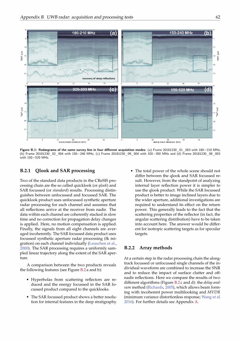
Appendix B. UWB radar: acquisition and processing tests 62

Figure B.1: Radargrams of the same survey line in four different acquisition modes: (a) Frame 20181230_01_003 with 180 – 210 MHz,(b) Frame 20181230_02_004 with 150 – 240 MHz, (c) Frame 20181230_09_004 with 320 – 350 MHz and (d) Frame 20181230_08_003with 150 – 520 MHz.

B.2.1 Qlook and SAR processing

Two of the standard data products in the CReSIS pro-cessing chain are the so called quicklook (or qlook) andSAR focussed (or standard) results. Processing distin-guishes between unfocussed and focussed SAR. Thequicklook product uses unfocussed synthetic apertureradar processing for each channel and assumes thatall reflections arrive at the receiver from nadir. Thedata within each channel are coherently stacked in slowtime and no correction for propagation delay changesis applied. Here, no motion compensation is applied.Finally, the signals from all eight channels are aver-aged incoherently. The SAR focussed data product usesfocussed synthetic aperture radar processing (fk mi-gration) on each channel individually (Leuschen et al.,2000). The SAR processing requires a uniformly sam-pled linear trajectory along the extent of the SAR aper-ture.

A comparison between the two products revealsthe following features (see Figure B.2 a and b):

• Hyperbolas from scattering reflectors are re-duced and the energy focussed in the SAR fo-cussed product compared to the quicklooks.

• The SAR focussed product shows a better resolu-tion for internal features in the deep stratigraphy.

• The total power of the whole scene should notdiffer between the qlook and SAR focussed re-sult. However, from the standpoint of analyzinginternal layer reflection power it is simpler touse the qlook product. While the SAR focussedproduct is better to image inclined layers due tothe wider aperture, additional investigations arerequired to understand its effect on the returnpower. This generally leads to the fact that thescattering properties of the reflector (in fact, theangular scattering distribution) have to be takeninto account here. The answer would be differ-ent for isotropic scattering targets as for speculartargets.

B.2.2 Array methods

At a certain step in the radar processing chain the along-track focussed or unfocussed single channels of the in-dividual waveform are combined to increase the SNRand to reduce the impact of surface clutter and off-nadir reflections. Here we compare the results of twodifferent algorithms (Figure B.2 c and d): the delay-and-sum method (Richards, 2005), which allows beam form-ing with incoherent power multilooking and MVDR(minimum variance distortionless response; Wang et al.2016). For further details see Appendix A.

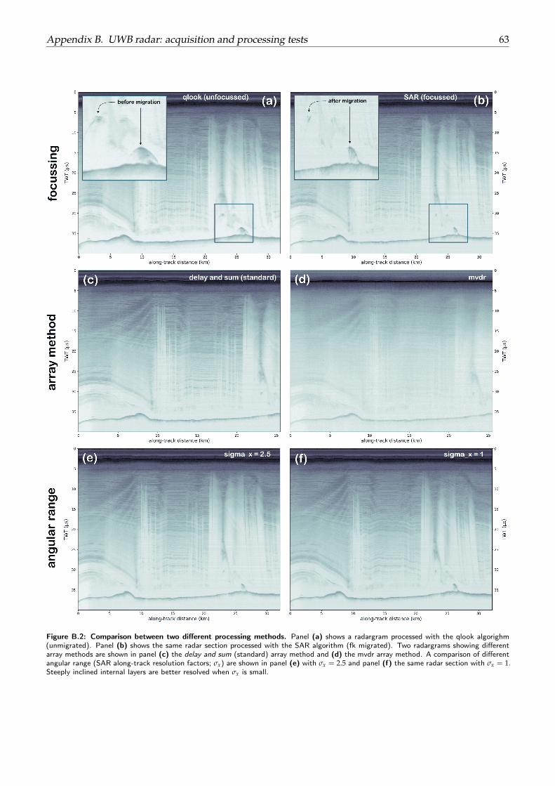
Appendix B. UWB radar: acquisition and processing tests 63

Figure B.2: Comparison between two different processing methods. Panel (a) shows a radargram processed with the qlook algorighm(unmigrated). Panel (b) shows the same radar section processed with the SAR algorithm (fk migrated). Two radargrams showing differentarray methods are shown in panel (c) the delay and sum (standard) array method and (d) the mvdr array method. A comparison of differentangular range (SAR along-track resolution factors; σx) are shown in panel (e) with σx = 2.5 and panel (f) the same radar section with σx = 1.Steeply inclined internal layers are better resolved when σx is small.

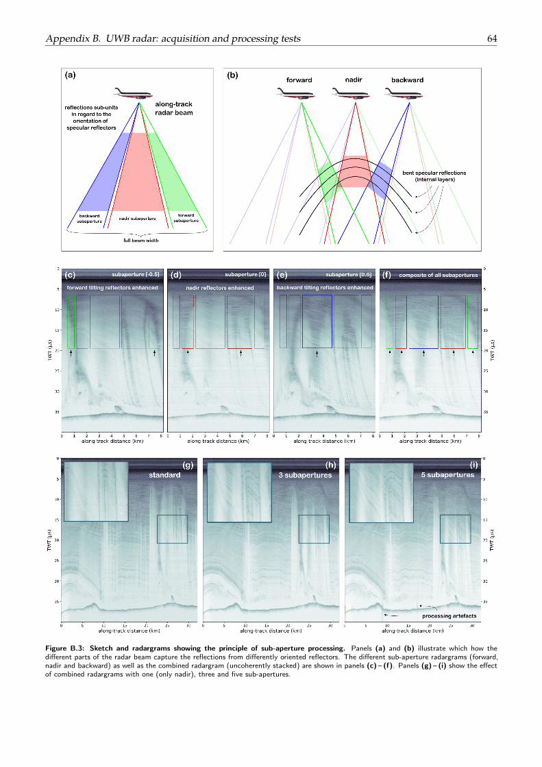
Appendix B. UWB radar: acquisition and processing tests 64

Figure B.3: Sketch and radargrams showing the principle of sub-aperture processing. Panels (a) and (b) illustrate which how thedifferent parts of the radar beam capture the reflections from differently oriented reflectors. The different sub-aperture radargrams (forward,nadir and backward) as well as the combined radargram (uncoherently stacked) are shown in panels (c) – (f). Panels (g) – (i) show the effectof combined radargrams with one (only nadir), three and five sub-apertures.

Appendix B. UWB radar: acquisition and processing tests 65

I compared several radar sections with the MVDRand delay-and-sum method and I can clearly state thatdelay-and-sum shows always the better results. Thiscan most likely be explained that we did not surveyice where the signal was interfered by severe surfaceclutter.

B.2.3 SAR with wider angular range

I tested several settings to increase the return powerfor steeply dipping internal reflections. One possibilityoffers the parameter sigma_x (σx), which performs theSAR focussing with a wider angular range. By process-ing at a finer SAR resolution, the SAR processor usesscattered energy from a wider angular range aroundnadir to form the image. Since the angle of scatteredreturns from a specular internal layer is proportional tothe internal layer slope, the SAR processor’s increasedsensitivity to larger angle returns translates to an in-creased sensitivity to layers with larger slopes. Weachieve a better resolution of steeply inclined internalreflectors by changing the along-track resolution beforeSAR processing to 1 m (σx = 1), whereas the defaultsetting is σx = 2.5). 1 m is not the smallest possiblevalue for processing, but is on the limit to achieve asufficiently high SNR. The SNR is smaller for larger an-gles because the range to the target increases for greaterangles, which leads to additional signal loss (sphericalspreading loss and additional signal attenuation in ice).

Figure B.2 e and f show a comparison between thesame radar section processed with σx = 2.5 and σx = 1,respectively. The results generated with σx = 1 recoversome portion of the steeply dipping internal reflections,particularly in the upper part of the ice column withoutcausing any SNR loss in other parts of the scene. Dueto the increase in along-track samples, the data amountincreases significantly in comparison to the σx = 2.5result.

B.2.4 Sub-apertures

Another method to enhance the reflection power ofsteeply inclined reflectors via sub-aperture processing.Hereby we can create several radargrams of the samescene from defined sub-apertures, which are partialsections of the full aperture (Figure B.3). For regularprocessing, only the nadir sub-aperture is used. Theworking principle is shown in Figure B.3 c – f. For ex-ample, the forward steered sub-aperture will producea radargram where only signals from internal layersinclined towards the airplane are resolved in the radar-gram.

One radargram is produced for each sub-aperture.It has been proven to be best to create three, five or ninesub-apertures. Because it is not very useful to work

with a single sub-aperture radargram, we can stack allsub-aperture radargrams to obtain the desired informa-tion for the whole scene. However, this step is subjectto two issues: (i) the return power and amplitude infor-mation is not very useful for further analysis and (ii) theSNR for the whole scene reduces due to the incoherentstacking.

A comparison or a radar scene with (a) the regularnadir sub-aperture, (b) the combination of three and (c)five sub-apertures is presented in Figure B.3 g – i. Wenote the advantage of a better resolution for dipping re-flectors but also the disadvantages of a reduced SNR ofthe nadir reflections and the appearance of processingartefacts.

B.3 Image mode

In addition to the data recorded in the (2D) soundingmode, the EGRIP-NOR-2018 data set also contains twosegments recorded in the (3D) image mode. The acqui-sition settings of these segments are slightly differentsince the transmission signals are composed of fourinstead of three pulses: 1 µs and 3 µs waveforms withnadir directed transmit beam followed by two 10 µswaveforms, one with the transmit beam directed tothe left and one with it directed to the right (left andright in respect to the flight direction) to increase theimaged swath width at the ice bottom (Figure B.4 a).The processing consists of three steps:

1. Generating 3D images. In this step, we generatea cross-track snapshot of the off-nadir return sig-nals with an estimate of the data covariance ma-trix, which depends on the number of off-nadircross-track multilooks. A high number of lookswill reduce the resolution but increase the accu-racy. For our 8-channel system, a number of 33looks usually provides an acceptable trade-off.

2. 3D surface/bed tracking. In this step, the ice sur-face and bed topography is automatically tracked(in the direction-of-arrival vs depth diagram; seeFigure B.4 c). Both surfaces are needed for theprocessing, but finally the reconstruction of thebed is the ultimate output. The nadir bed reflec-tion can be set as ground truth, which increasesthe accuracy of the autotracker. Moreover, it ispossible to manually fix the surface tracking.

3. DEM Generation. Based on the ice surface andbed topography tracking data, a gridded DEMwill be produced.

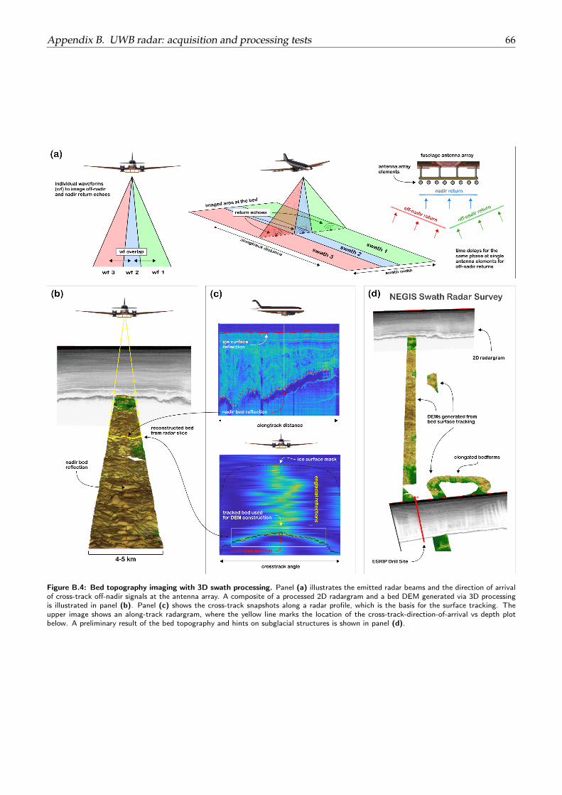
Appendix B. UWB radar: acquisition and processing tests 66

Figure B.4: Bed topography imaging with 3D swath processing. Panel (a) illustrates the emitted radar beams and the direction of arrivalof cross-track off-nadir signals at the antenna array. A composite of a processed 2D radargram and a bed DEM generated via 3D processingis illustrated in panel (b). Panel (c) shows the cross-track snapshots along a radar profile, which is the basis for the surface tracking. Theupper image shows an along-track radargram, where the yellow line marks the location of the cross-track-direction-of-arrival vs depth plotbelow. A preliminary result of the bed topography and hints on subglacial structures is shown in panel (d).

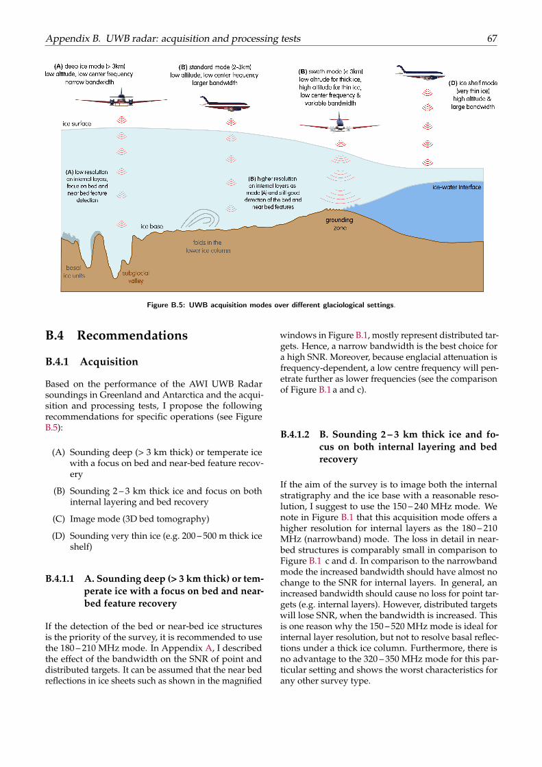
Appendix B. UWB radar: acquisition and processing tests 67

Figure B.5: UWB acquisition modes over different glaciological settings.

B.4 Recommendations

B.4.1 Acquisition

Based on the performance of the AWI UWB Radarsoundings in Greenland and Antarctica and the acqui-sition and processing tests, I propose the followingrecommendations for specific operations (see FigureB.5):

(A) Sounding deep (> 3 km thick) or temperate icewith a focus on bed and near-bed feature recov-ery

(B) Sounding 2 – 3 km thick ice and focus on bothinternal layering and bed recovery

(C) Image mode (3D bed tomography)

(D) Sounding very thin ice (e.g. 200 – 500 m thick iceshelf)

B.4.1.1 A. Sounding deep (> 3 km thick) or tem-perate ice with a focus on bed and near-bed feature recovery

If the detection of the bed or near-bed ice structuresis the priority of the survey, it is recommended to usethe 180 – 210 MHz mode. In Appendix A, I describedthe effect of the bandwidth on the SNR of point anddistributed targets. It can be assumed that the near bedreflections in ice sheets such as shown in the magnified

windows in Figure B.1, mostly represent distributed tar-gets. Hence, a narrow bandwidth is the best choice fora high SNR. Moreover, because englacial attenuation isfrequency-dependent, a low centre frequency will pen-etrate further as lower frequencies (see the comparisonof Figure B.1 a and c).

B.4.1.2 B. Sounding 2 – 3 km thick ice and fo-cus on both internal layering and bedrecovery

If the aim of the survey is to image both the internalstratigraphy and the ice base with a reasonable reso-lution, I suggest to use the 150 – 240 MHz mode. Wenote in Figure B.1 that this acquisition mode offers ahigher resolution for internal layers as the 180 – 210MHz (narrowband) mode. The loss in detail in near-bed structures is comparably small in comparison toFigure B.1 c and d. In comparison to the narrowbandmode the increased bandwidth should have almost nochange to the SNR for internal layers. In general, anincreased bandwidth should cause no loss for point tar-gets (e.g. internal layers). However, distributed targetswill lose SNR, when the bandwidth is increased. Thisis one reason why the 150 – 520 MHz mode is ideal forinternal layer resolution, but not to resolve basal reflec-tions under a thick ice column. Furthermore, there isno advantage to the 320 – 350 MHz mode for this par-ticular setting and shows the worst characteristics forany other survey type.

Appendix B. UWB radar: acquisition and processing tests 68

B.4.1.3 C. Image mode (3D bed tomography)

Theoretically, any 2D survey could be designed to mapthe desired 2D features in combination with a 3D swath.However, we have to keep in mind that the best resultsare most likely obtained with the low-frequency, nar-rowband mode, which produces the strongest bed re-turns. While the sounding mode is important, we alsohave to consider englacial attenuation caused by the icethickness and the chemical and thermal conditions ofthe ice. Hence, a setting with thinner ice, or where lessenglacial attenuation is expected, would allow either touse a larger bandwidth (to increase range resolution)or to fly at a higher altitude (to increase the area of bedtopography mapped along the flight profile).

B.4.1.4 D. Sounding very thin ice(e.g. 200 – 500 m thick ice shelf)

For the investigation of very thin ice or ice shelves, the150 – 520 MHz mode is the most suitable. On the onehand, it resolves the internal stratigraphy with highestresolution without losing much energy due to the thickice column. Second, the expected dielectric contraston the ice-water/ice-bed interface at the ice shelf ornear the grounding line is most likely so strong thatit can be expected to be clearly detected. The profi-ciency of this mode has been demonstrated by Bessetteet al. (2021) at the large impact crater beneath HiawathaGlacier, Greenland. For soundings near the groundingline (whether on the grounded or floating ice site, it iscertainly also helpful to use the 3D mode. The basalcrevasses or basal terraces (Dutrieux et al., 2014) shouldbe suitable refractors for the 3D mode.

Special attention should be paid to the flight alti-tude. In particular, if it is likely that the ice surfaceand also the underlying layers will produce a strongreflection, it should be flown at an elevation that thefirst multiple reflection of the ice top is located belowthe bed reflection. One expected advantage of thismethod is that the footprint of the 3D swath will belarger, i.e. more (bed topography) area can be mappedalong the flight profile.

B.4.2 Processing

In addition to the standard processing settings andproducts (qlook and SAR focussed), it is worth to gen-erate additional standardized data products for partic-ular campaigns. The SAR processed product with awider angular range (where σx = 1) is useful for mostpurposes. The only limitation is that much larger datasets are generated. The supaperture processing is prob-ably not suitable for routine processing in my opinionbut can be used for certain individual profiles.

69

BibliographyBessette, J. T., Schroeder, D. M., Jordan, T. M.,

and MacGregor, J. A. Radar-sounding charac-terization of the subglacial groundwater tablebeneath hiawatha glacier, greenland. GeophysicalResearch Letters, 48(10):e2020GL091432, 2021. doi:https://doi.org/10.1029/2020GL091432. URLhttps://agupubs.onlinelibrary.wiley.com/doi/abs/10.1029/2020GL091432.

Dutrieux, P., Stewart, C., Jenkins, A., Nicholls, K. W.,Corr, H. F. J., Rignot, E., and Steffen, K. Basal terraceson melting ice shelves. Geophysical Research Letters,41(15):5506–5513, 2014. doi: 10.1002/2014GL060618.URL https://agupubs.onlinelibrary.wiley.com/doi/abs/10.1002/2014GL060618.

Leuschen, C., Gogineni, S., and Tammana, D. SAR pro-cessing of radar echo sounder data. pages 2570–2572,2000. doi: 10.1109/igarss.2000.859643. URL http://dx.doi.org/10.1109/igarss.2000.859643.

Richards, M. Fundamentals of Radar Signal Process-ing. Professional Engineering, New York: McGraw-HillEducation, 2005.

Wang, Z., Gogineni, S., Rodriguez-Morales, F., Yan, J. B.,Paden, J., Leuschen, C., Hale, R. D., Li, J., Caraba-jal, C. L., Gomez-Garcia, D., Townley, B., Willer,R., Stearns, L., Child, S., and Braaten, D. Mul-tichannel Wideband Synthetic Aperture Radar forIce Sheet Remote Sensing: Development and theFirst Deployment in Antarctica. IEEE Journal of Se-lected Topics in Applied Earth Observations and RemoteSensing, 9(3):980–993, 2016. ISSN 21511535. doi:10.1109/JSTARS.2015.2403611. URL http://dx.doi.org/10.1109/JSTARS.2015.2403611.

70

Appendix C

Software, data and documentation

Software

CReSIS toolbox

I used the CReSIS Toolbox for the processing of AWIUWB MCoRDS depth sounder radar data. The tool-box is a collection of software routines, most of themwritten in Matlab. The toolbox is designed for dataprocessing of raw radar data as well as GPS/INS data(metadata) and produces support files, calibration files,radar image files as well as layer tracking files. TheCReSIS Toolbox can be downloaded from the follow-ing Git repository: https://github.com/CReSIS/. Asetup guide as well as the full documentation is avail-able via the CReSIS Wiki page: https://ops.cresis.ku.edu/wiki/index.php. The contact person for theCReSIS Toolbox is John D. Paden from the Universityof Kansas: paden@ku.edu.

Python

I used Python3 (https://www.python.org), includingstandard Python Libraries for the major part of the dataanalysis as well as for data conversion. Moreover, allfigures and plots (excluding geographic maps and 3Dimages) were created with Python. Furthermore, I usedthe following non-standard libraries:

Data handling: h5py, scipy, obspy

Geo-tools: geopandas, shapely, pyoroj, geopy, rasterio,rioxarray, xarray, pygmt, gdal

Data processing: numpy, pandas, obspy, scipy

Visualization: matplotlib, seaborn

GIS

QGIS is a free and open-source geographic informa-tion system (GIS) and was used in this thesis to per-form numerous spatial calculations, for the generalhandling of geo-data and geo-data files as well as forthe generation of 2D maps. In addition, I used QGISfor data interpretation. QGIS can be downloaded here:https://www.qgis.org

SAGA GIS algorithms are implemented within QGISand I used several algorithms for terrain analysis such

as: flow accumulation, hypsometry as well as rastertools for gridding (http://www.saga-gis.org).

GDAL/OGR geo-algorithms were used to for the ma-nipulation and conversion of (geo) raster and vectordata (https://gdal.org/). GDAL can be used in astand-alone command-line interface or within QGIS.

ECHOS

Emerson’s E&P EchosTM is a commercial software suitefor seismic processing. For this work, I used the soft-ware to trace the ice surface, internal layers as wellas the bed reflection of the radar data. The resultswere used for instance to calculate ice and individ-ual layer thickness or to perform the roughness anal-ysis of the bed topography. For more information seehttps://www.pdgm.com/products/echos/.

MOVE

I used the 3D model building software MOVETMtoconstruct 3D surfaces of internal stratigraphic hori-zons in the radar data. Furthermore, many of the3D figures in this thesis and the manuscripts werecreated with Move. Further information at https://www.petex.com/products/move-suite/move/.

Inkscape

Inkscape is an open-source vector graphics editor tocreate and modify vector images (https://inkscape.org). I used this software to create sketches and toassemble and annotate figures.

GMT

I used several functions of the GMT (Generic Map-ping Tools) toolbox for gridding and other geographicdata manipulations. GMT is an open-source col-lection of command-line tools for manipulating geo-graphic data sets (further information at: https://www.generic-mapping-tools.org/).

Appendix C. Software, data and documentation 71

IDL toolbox

A part of the radar data processing routine is per-formed with an IDL toolbox written by Veit Helm(AWI; veit.helm@awi.de). I used his tools to post-process GPS data and for data conversion. IDL(Interactive Data Language) is commonly used inthe scientific community for processing of largeamounts of data (https://www.l3harrisgeospatial.com/Software-Technology/IDL).

Code

The Python scripts and methods I used to processthe data are stored in the Strata (Small Toolbox forRAdar daTa Processing and Analysis) Github reposi-tory: https://github.com/stvnfrnk/Strata.git.

• Functions for radar data processing are avail-able at: https://github.com/stvnfrnk/uwb_radar_library.git

• A collection of scripts is available at: https://github.com/stvnfrnk/Kangaroo.git

Data

Ultra-wideband radar data

The data of the UWB system is stored at different loca-tions. The following paragraphs describe where to findacquisition settings, the parameter spreadsheets, rawdata (waveform data) and the processing outputs.

MCoRDS acquisition XML files store all relevantinformation used for data acquisition, e.g. number ofwaveforms, pulse durations, receiver gains, numberof individual presums, etc. Each acquisition settinghas an individual name and is divided into one filecontaining the transmission settings and another filecontaining the receiver settings. We learned during the2019 field season in Antarctica (antr2019) that the usageof the wrong transmission/receceiver files leads towaveform data which cannot be used for analysis. Thefiles for the arkr2018 campaign are available at: /hs/gsys/p_radar/arkr2018/CSARP_2018_Greenland_Polar6_rds/waveforms and for the antr2019 cam-paign at: /hs/gsys/p_radar/arkr2018/CSARP_2018_Greenland_Polar6_rds/waveforms. Note that bothwaveform folders have the same file content. Totrack which setting has been used in a survey, seethe parameter spreadsheet.

Parameter spreadsheets (for processing) The so-called ct_params parameter spreadsheet controls theprocessing settings for the CReSIS toolbox. It containsradar and processing settings. A full documentationfor is available under: https://ops.cresis.ku.edu/wiki/index.php/Parameter_Spreadsheet_Guide. Pa-rameter spreadsheets for completed campaigns shouldbe added to the ct_params Git repository: https://github.com/CReSIS/ct_params.

Raw data In this thesis I used AWI UWB data fromthe summer 2018 field season in Greenland (FINEGISand EGRIP-NOR-2018) and austral summer season2018/19 in Antarctica (JuRaS). The raw data is atthe moment (September 27, 2021) stored at the AWIHSM Server in the WORM (Write Once Read Many)file system: /hs/platforms/WORM/aircraft/polar6/uwb/exdata/ in the following two campaigns:

• P6-211_RESURV79_2018 (FINEGIS)

• P6-211_EGRIP-NOR_2018 (NEGIS)

• P6-215_UWB_2018 (JuRaS)

Processed data The processing results of the radardata processing, which I created among others for thefield season 2018 in Greenland, are also stored on theAWI HSM Server System (last access September 27,2021):

• /hs/gsys/p_radar/arkr2018/CSARP_2018_Greenland_Polar6_rds

• /hs/gsys/p_radar/antr2019/CSARP_2019_Antarctica_Polar6_rds

Internal layers

Traced internal layers of the work presented in this the-sis are stored in the ECHOS database in the arkr2018and antr2019 project.

Data products generated during my PhD

• Ice thickness in TWT at the onset of the NEGIS(point data)https://doi.org/10.1594/PANGAEA.907917

• Bed topography and ice thickness in meters atthe onset of the NEGIS (gridded data)https://doi.org/10.1594/PANGAEA.907916

• Bed return power (BRP) and waveform abrupt-ness of the onset of the NEGIS (point data)https://doi.pangaea.de/10.1594/PANGAEA.915135

Appendix C. Software, data and documentation 72

• Spectral subglacial bed roughness of the onset ofthe NEGIS (point data)https://doi.pangaea.de/10.1594/PANGAEA.915133

• Hydropotential and subglacial water routing ofthe onset of the NEGIS (gridded data)https://doi.pangaea.de/10.1594/PANGAEA.915134

• Ice thickness from the northern catchment regionof Greenland’s 79 North Glacier (point data)https://doi.pangaea.de/10.1594/PANGAEA.913193

• Locations and outlines of active lakes at the onsetof the Jutulstraumen Glacier (Antarctica) derivedfrom DInSAR measurements. (shapefiles)https://doi.pangaea.de/10.1594/PANGAEA.927120

• Ice thickness from Jutulstraumen Glacierrecorded with the airborne AWI UWB radarsystem, Antarctica. (point data)https://doi.pangaea.de/10.1594/PANGAEA.911475

• Ice thickness and bedrock topography of the icedivide, South of Sør Rondane Mountains (DML),Antarctica. (point data)https://doi.org/10.1594/PANGAEA.910019

• Ice thickness from the coast of Dronning MaudLand (Antarctica), recorded 2018/19 with the

AWI UWB radar system. (point data)https://doi.pangaea.de/10.1594/PANGAEA.911868

• Ultra-wideband radar data over the shear mar-gins and along flow lines at the onset region ofthe Northeast Greenland Ice Stream. (radar data)https://doi.org/10.1594/PANGAEA.928569

Documentation

I documented everything I found useful and mightbe useful to others working with AWI UWB data inthe AWI Confluence Wiki: https://spaces.awi.de/display/Glaziologie/Aero-UWB. Furthermore, thereis information available regarding the radar usage inMOVE and ECHOS. You will find useful informationthere if you have one of the following questions:

1. Where are the individual raw data and data prod-ucts stored?

2. How do I import the UWB data to ECHOS?

3. Is there a translation table from UWB Frame IDsto ECHOS Line IDs?

4. How do I import and use the radar data inMOVE?

73

Appendix D

Further contributions

Co-authored manuscriptsThe following manuscripts where I am a co-author are not included in this dissertation:

Westhoff, J., Stoll, N., Franke, S., Weikusat, I., Bons, P., Kerch, J., Jansen, D., Kipfstuhl, S. and Dahl-Jensen(2020). A stratigraphy Based Method for Reconstructing Ice Core Orientation. Annals of Glaciology,61(83) 1-12. https://doi.org/10.1017/aog.2020.76

Bons, P., de Riese, T., Franke, S., Llorens, M-G., Sachau, T., Westhoff, J., Stoll, N., Weikusat, I. and Zhang,Y. (2021). Comment on ’Exceptionally high heat flux needed to sustain the Northeast Greenland IceStream’ by S. Smith-Johnsen et al., The Cryosphere, 14, 841-854, 2020. The Cryosphere, 15, 2251–2254,https://doi.org/10.5194/tc-15-2251-2021

Gerber, T . A., Hvidberg, C., Rasmussen, S. O., Franke, S., Sinnl, G., Grinsted, A., Jansen, D. and Dahl-Jensen, D. (2021; in review). Upstream flow effects revealed in the EastGRIP ice core using a Monte-Carloinversion of a 2D ice flow model. The Cryosphere,15, 3655–3679, https://doi.org/10.5194/tc-15-3655-2021

Mojtabavi, S., Eisen, O., Franke, S., Jansen, D., Steinhage, D., Paden, J., Dahl-Jensen, D., Weikusat, I.,Eichler, J. and Wilhelms, F. (2021; in review). Physical properties of the Greenland Ice Sheet from linkingradar surveys to three deep ice cores by synthetic radar modelling. In review for: Journal of Glaciology

Conference contributionsI presented my research at the following conferences:

Franke, S., Jansen, D. Beyer, S., Neckel, N., Binder, T., Paden, J., Dörr, N., Helm, V., Steinhage, D.Eisen, O. (2020). Ice flow and the conditions of the ice-bed interface at the onset of the NortheastGreenland Ice Stream. Online iPoster: AGU Fall Meeting 2020, Online Everywhere (December 1-17,2020). https://epic.awi.de/id/eprint/53403/

Franke, S., Jansen, D. Beyer, S., Binder, T., Paden, J. Eisen, O. (2020). Radar derived basal conditions atthe onset of the Northeast Greenland Ice Stream. Online Presentation: NEGIS Symposium 2020, EGRIPOnline Seminars (September 13-November 3, 2020). https://epic.awi.de/id/eprint/53120/

Franke, S., Jansen, D. Westhoff, J., Weikusat, I., Bons, P., Binder, T. Eisen, O. (2020). Foldedice stratigraphy in North East Greenland: A three dimensional structural analysis. Online Pre-sentation (Video): ESA 2020 European Polar Science Week, Virtual Event (October 26-30, 2020).

Appendix D. Further contributions 74

https://epic.awi.de/id/eprint/53185/

Franke, S., Stoll, N., Jansen, D. Koldtoft, I. (2020). Understanding an ice stream in Greenlandat the EastGRIP camp: An international-multidisciplinary effort and knowledge transfer amongscientists. Online Presentation: 6th annual APECS International Online Conference (May 19-21, 2020).https://epic.awi.de/id/eprint/52032/ Honors: 3rd prize for best Arctic presentation

Franke, S., Jansen, D., Paden, J. Eisen, O. (2020). Complex basal conditions influence flow at the onsetof the North East Greenland Ice Stream. Online Presentation: EGU General Assembly 2020, SharingGeosciences (Vienna, Austria, May 3-9, 2020). https://doi.org/10.5194/egusphere-egu2020-1173

Franke, S., Jansen, D., Binder, T., Dörr, N., Helm, V., Paden, J., Steinhage, D. Eisen, O. (2019). Bedrocktopography and subglacial landforms of the Northeast Greenland Ice Stream. Oral Presentation: NEGISSymposium, EastGRIP Steering Committee Meeting (Copenhagen, Denmark, November 11-15, 2019).https://epic.awi.de/id/eprint/50856/

Franke, S., Jansen, D., Binder, T., Helm, V., Steinhage, D., Dörr, N., Paden, J. Eisen, O. (2019). IceThickness and Bed Conditions of the North East Greenland Ice Stream. Poster Presentation: AWI PhDDays (Potsdam, Germany, July 4-7, 2019).

Franke, S., Jansen, D., Binder, T., Helm, V., Steinhage, D., Dörr, N., Paden, J., Weikusat, I., Bons, P. Eisen,O. (2019). Detailed bedrock topography in the vicinity of the EGRIP ice-core drill site. Poster Presentation:IGS Symposium Five Decades of Radioglaciology (Stanford, USA, July 8-12, 2019). (Presented byDaniela Jansen) https://epic.awi.de/id/eprint/50861/

Franke, S., Jansen, D., Binder, T., Helm, V., Steinhage, D., Paden, J., Weikusat, I. Eisen, O. (2018).First results of the AWI-Polar6 airborne radio echo sounding survey around the EGRIP drill site. OralPresentation: NEGIS Symposium, EastGRIP Steering Committee Meeting (Copenhagen, Denmark,November 12-16, 2018). https://epic.awi.de/id/eprint/49976/

75

Appendix E

PAPER I RESEARCH ARTICLE

Bed topography and subglacial landforms in the onset region of theNortheast Greenland Ice StreamSteven Franke1 , Daniela Jansen1 , Tobias Binder1 , Nils Dörr1 , Veit Helm1 , John Paden2 ,Daniel Steinhage1 and Olaf Eisen1,3

1 Alfred Wegener Institute, Helmholtz Centre for Polar and Marine Research, Bremerhaven, Germany2 Center for Remote Sensing of Ice Sheets (CReSIS), University of Kansas, Lawrence, KS, USA3 Department of Geosciences, University of Bremen, Bremen, Germany

Published on 18 March 2020 in Annals of Glaciology https://doi.org/10.1017/aog.2020.12

AbstractThe North East Greenland Ice Stream (NEGIS) is an important dynamic component for the total mass balance of theGreenland Ice Sheet, as it reaches up to the central divide and drains 12 % of the ice sheet. The geometric boundaryconditions and in particular the nature of the subglacial bed of the NEGIS are essential to understand its ice flowdynamics. We present a record of more than 8,000 km of radar survey lines of multi-channel, ultra-widebandradio echo sounding data covering an area of 24,000 km2, centered on the drill site for the East Greenland Ice-coreProject (EGRIP), in the upper part of the NEGIS catchment. Our data yield a new detailed model of ice-thicknessdistribution and basal topography in the region. The enhanced resolution of our bed topography model showsfeatures which we interpret to be caused by erosional activity, potentially over several glacial-interglacial cycles. Off-nadir reflections from the ice–bed interface in the center of the ice stream indicate a streamlined bed with elongatedsubglacial landforms. Our new bed topography model will help to improve the basal boundary conditions ofNEGIS prescribed for ice-flow models and thus foster an improved understanding of the ice-dynamic setting.

Received: 3 October 2019 - Revised 26 February 2020 - Accepted: 27 February 2020

Introduction

The Greenland Ice Sheet (GrIS) is the second largestland ice mass on Earth and one of the largest contrib-utors to global sea-level rise (Khan et al., 2014a; Gard-ner et al., 2013; Rignot et al., 2011). Observations indi-cate that its contribution increased from 0.09 mm a−1

for the period 1992–2001 to 0.68 mm a−1 for 2012–2016(IPCC, 2019, Section 4.2.2). Apart from a negative sur-face mass balance due to melting, this contributionto sea level rise is driven by speed-up and retreat ofmarine-terminating glaciers, leading to ice thinning(Howat et al., 2007; Rignot et al., 2011; Gillet-Chauletet al., 2012; IPCC, 2019). Of particular importance forsea-level predictions are observations of ice streamsthat transport ice from the interior of the ice sheet tothe margin, where it either melts or calves into ice-bergs. Dynamic processes of ice sheets in Greenlandand Antarctica have been progressively included in nu-merical models to project sea-level changes (Robinson

et al., 2012; Church et al., 2013; Rückamp et al., 2020;Goelzer et al., 2020). To simulate present ice streamflow and determine its contribution to the mass balanceof ice sheets, we have to understand the natural vari-ability of ice stream dynamics on time scales of tens tothousands of years (Robel et al., 2013). For an accurateassessment of the dynamic component of mass loss,ice-sheet flow requires high-resolution observations ofthe kinematic properties and the geometry conditions.

Ice stream characteristics vary in their geographicalsettings and thus boundary conditions, for instanceice thickness, subglacial topography, resistive prop-erties of the underlying substrate, subglacial hydrol-ogy, as well as atmospheric and oceanic forcing (As-chwanden et al., 2016; Khan et al., 2014b; Robel et al.,2013). In contrast to flow of outlet glaciers, which of-ten drain ice through bedrock channels or valleys, thehigh flow velocities of ice streams extend further into

Appendix E. Paper I NEGIS Onset Bed Topography (published) 76

the interior of the ice sheet. In some cases their loca-tion is not controlled by the bed topography and theirboundaries are characterized by narrow shear zones(Truffer and Echelmeyer, 2003). Basal properties of icestreams in Greenland have been mostly investigatedat the (now sub-marine) ice sheet margins of paleoglacier beds with multi-beam bathymetry and marinesediment cores (e. g. Dowdeswell et al., 2014; Hoganet al., 2016; Newton et al., 2017). The beds of paleoice streams can be hard or soft and often show a largenumber of streamlined bedforms, mostly parallel to iceflow (Roberts et al., 2010). Streamlined bedforms un-derneath contemporary ice streams in Antarctica havebeen analyzed by King et al. (2009) and Bingham et al.(2017) and classified as mega-scale glacial lineations(MSGL) (Stokes and Clark, 2002). As subglacial struc-tures may have formed over multiple glaciations, theirinterpretion is often challenging (Roberts and Long,2005). Little is known about the current conditions ofice stream beds in the central regions of the GrIS, at theonset of streaming ice flow, because data acquisitionas well as determination of the geometry and composi-tion of the bed is much more difficult to elaborate thanon the continental shelf. For central Greenland it wasgenerally assumed until recently that the ice sheet isunderlain by lithified sediment or a crystalline base-ment. However, a detailed study of Christianson et al.(2014) identifies deformable and water saturated sedi-ment several meters thick at the onset zone of the NorthEast Greenland Ice Stream (NEGIS), which indicatesthat deformation of the basal substrate could influencesliding at the ice-bed interface and probably also limitsubglacial erosion. Furthermore, Jezek et al. (2011) de-tect elongated landforms probably formed by erosionat the base of the southern flank of the Jakobshavn icestream. Both interpretations indicate a more complexinterplay of basal conditions and ice dynamics thanpresent in the case of a simply hard-based ice sheet inGreenland’s interior.

The NEGIS is one of the most prominent featuresof the GrIS. With a length of ∼ 600 km it drains ∼ 12 %of the Greenland ice sheet via fast-flowing marine-terminating glaciers (Rignot and Mouginot, 2012). Sur-face ice flow velocities vary from 10 m a−1 at the on-set to more than 2000 m a−1 at the grounding line ofthe outlet glaciers (Mouginot et al., 2017). The NEGISdiffers from all other marine-terminating glaciers inGreenland with its catchment of fast streaming ice flowalmost reaching the central ice divide (Joughin et al.,2018). This configuration provides a possible mecha-nism to transmit forcing from the marine area far inland(Christianson et al., 2014) and several studies have as-sessed potential changes in the stability of the NEGISand the ice dynamics in North-East Greenland (Joughinet al., 2010; Fahnestock et al., 2001; Bamber et al., 2013;Khan et al., 2014a).

To fully understand the dominating processes andbasal boundary conditions driving NEGIS ice flow, inparticular in its onset region, on-site measurementsare most useful. So far, geophysical surveys investi-gating the upstream part of the NEGIS concentratedon the immediate surroundings of the EGRIP drill site(Figure E.1 b), where the ice stream widens (Vallelongaet al., 2014; Keisling et al., 2014). High basal melt ratescaused by higher continental geothermal heat flux closeto the ice divide, as a remnant of the passing of the Ice-landic hot spot, are assumed to cause the onset of the icestream (Fahnestock et al., 2001; Rogozhina et al., 2016;Martos et al., 2018). Further downstream, accelerationis likely caused by subglacial water routing and thepresence of high porosity, water-saturated deformablesubglacial till, which lubricates the ice stream (Chris-tianson et al., 2014). The geophysical data of Christian-son et al. (2014) suggest that subglacial till is distributedin the center of our survey region, across the entire icestream, and is dilatant in the fast-flowing part of the icestream. The source and routing of till is not yet fullyunderstood. The presence of unconsolidated sedimentinside and outside of the NEGIS suggest that sedimentsare funnelled into the NEGIS from the upstream catch-ment (Christianson et al., 2014). Overall it is difficult toassess which processes dominate the different regionsof the ice stream and how they interact (Schlegel et al.,2015).

The most important factors controlling ice streamsare their basal properties, ice thickness and bed topog-raphy, especially as studies of subglacial hydrology aredependent upon bed and surface slope and thus thevariation in ice thickness on a local to regional scale(Wright et al., 2008). Without a sufficient spatial datacoverage also at the onset of ice streams, it is not pos-sible to assess the nature of the ice stream bed and itsproperties. Over the last five decades, most radio-echosounding campaigns have concentrated on ice divides,domes or fast flowing outlet glaciers (Bamber et al.,2013; Fretwell et al., 2013). To date, several bed ele-vation models for Greenland exist (e. g. Bamber et al.,2013; Morlighem et al., 2017) with variable resolutionand data coverage. Furthermore, modelling studies re-veal that an interpretation of isochrones of ice streamsis challenging without a detailed knowledge of the bedtopography (Leysinger Vieli et al., 2007). These exist-ing limitations motivated the acquisition of new highresolution ice thickness data to improve available bedtopographies around NEGIS, in order to help interpretbasal structures and thereby determine ice-substrateinteraction within NEGIS and in its vicinity (Vallelongaet al., 2014; Keisling et al., 2014).

In this paper, we use airborne radio-echo sound-ing data to extend previous geophysical surveys of icethickness and internal layering around the EGRIP drillsite. We provide a new high-resolution bed topography

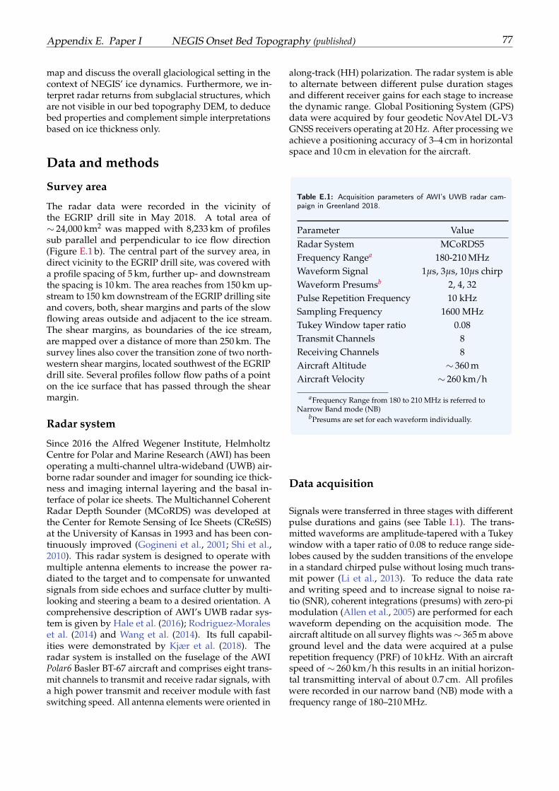
Appendix E. Paper I NEGIS Onset Bed Topography (published) 77

map and discuss the overall glaciological setting in thecontext of NEGIS’ ice dynamics. Furthermore, we in-terpret radar returns from subglacial structures, whichare not visible in our bed topography DEM, to deducebed properties and complement simple interpretationsbased on ice thickness only.

Data and methods

Survey area

The radar data were recorded in the vicinity ofthe EGRIP drill site in May 2018. A total area of∼ 24,000 km2 was mapped with 8,233 km of profilessub parallel and perpendicular to ice flow direction(Figure E.1 b). The central part of the survey area, indirect vicinity to the EGRIP drill site, was covered witha profile spacing of 5 km, further up- and downstreamthe spacing is 10 km. The area reaches from 150 km up-stream to 150 km downstream of the EGRIP drilling siteand covers, both, shear margins and parts of the slowflowing areas outside and adjacent to the ice stream.The shear margins, as boundaries of the ice stream,are mapped over a distance of more than 250 km. Thesurvey lines also cover the transition zone of two north-western shear margins, located southwest of the EGRIPdrill site. Several profiles follow flow paths of a pointon the ice surface that has passed through the shearmargin.

Radar system

Since 2016 the Alfred Wegener Institute, HelmholtzCentre for Polar and Marine Research (AWI) has beenoperating a multi-channel ultra-wideband (UWB) air-borne radar sounder and imager for sounding ice thick-ness and imaging internal layering and the basal in-terface of polar ice sheets. The Multichannel CoherentRadar Depth Sounder (MCoRDS) was developed atthe Center for Remote Sensing of Ice Sheets (CReSIS)at the University of Kansas in 1993 and has been con-tinuously improved (Gogineni et al., 2001; Shi et al.,2010). This radar system is designed to operate withmultiple antenna elements to increase the power ra-diated to the target and to compensate for unwantedsignals from side echoes and surface clutter by multi-looking and steering a beam to a desired orientation. Acomprehensive description of AWI’s UWB radar sys-tem is given by Hale et al. (2016); Rodriguez-Moraleset al. (2014) and Wang et al. (2014). Its full capabil-ities were demonstrated by Kjær et al. (2018). Theradar system is installed on the fuselage of the AWIPolar6 Basler BT-67 aircraft and comprises eight trans-mit channels to transmit and receive radar signals, witha high power transmit and receiver module with fastswitching speed. All antenna elements were oriented in

along-track (HH) polarization. The radar system is ableto alternate between different pulse duration stagesand different receiver gains for each stage to increasethe dynamic range. Global Positioning System (GPS)data were acquired by four geodetic NovAtel DL-V3GNSS receivers operating at 20 Hz. After processing weachieve a positioning accuracy of 3–4 cm in horizontalspace and 10 cm in elevation for the aircraft.

Table E.1: Acquisition parameters of AWI’s UWB radar cam-paign in Greenland 2018.

Parameter ValueRadar System MCoRDS5Frequency Rangea 180-210 MHzWaveform Signal 1µs, 3µs, 10µs chirpWaveform Presumsb 2, 4, 32Pulse Repetition Frequency 10 kHzSampling Frequency 1600 MHzTukey Window taper ratio 0.08Transmit Channels 8Receiving Channels 8Aircraft Altitude ∼ 360 mAircraft Velocity ∼ 260 km/h

aFrequency Range from 180 to 210 MHz is referred toNarrow Band mode (NB)

bPresums are set for each waveform individually.

Data acquisition

Signals were transferred in three stages with differentpulse durations and gains (see Table I.1). The trans-mitted waveforms are amplitude-tapered with a Tukeywindow with a taper ratio of 0.08 to reduce range side-lobes caused by the sudden transitions of the envelopein a standard chirped pulse without losing much trans-mit power (Li et al., 2013). To reduce the data rateand writing speed and to increase signal to noise ra-tio (SNR), coherent integrations (presums) with zero-pimodulation (Allen et al., 2005) are performed for eachwaveform depending on the acquisition mode. Theaircraft altitude on all survey flights was ∼ 365 m aboveground level and the data were acquired at a pulserepetition frequency (PRF) of 10 kHz. With an aircraftspeed of ∼ 260 km/h this results in an initial horizon-tal transmitting interval of about 0.7 cm. All profileswere recorded in our narrow band (NB) mode with afrequency range of 180–210 MHz.

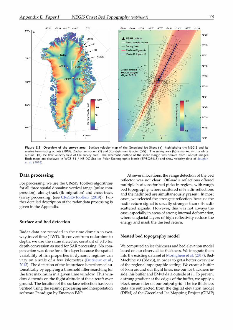
Appendix E. Paper I NEGIS Onset Bed Topography (published) 78

Figure E.1: Overview of the survey area. Surface velocity map of the Greenland Ice Sheet (a), highlighting the NEGIS and itsmarine terminating outlets (79NG, Zachariae Isbrae (ZI) and Storstrømmen Glacier (SG)). The survey area (b) is marked with a whiteoutline. (b) Ice flow velocity field of the survey area. The schematic outline of the shear margin was derived from Landsat images.Both maps are displayed in WGS 84 / NSIDC Sea Ice Polar Stereographic North (EPSG:3413) and show velocity data of Joughinet al. (2018).

Data processing

For processing, we use the CReSIS Toolbox algorithmsfor all three spatial domains: vertical range (pulse com-pression), along-track (fk migration) and cross track(array processing) (see CReSIS-Toolbox (2019)). Fur-ther detailed description of the radar data processing isgiven in the Appendix.

Surface and bed detection

Radar data are recorded in the time domain in two-way travel time (TWT). To convert from radar time todepth, we use the same dielectric constant of 3.15 fordepth-conversion as used for SAR processing. No com-pensation was done for a firn layer because the spatialvariability of firn properties in dynamic regimes canvary on a scale of a few kilometres (Dutrieux et al.,2013). The detection of the ice surface is performed au-tomatically by applying a threshold filter searching forthe first maximum in a given time window. This win-dow depends on the flight altitude of the aircraft overground. The location of the surface reflection has beenverified using the seismic processing and interpretationsoftware Paradigm by Emerson E&P.

At several locations, the range detection of the bedreflector was not clear. Off-nadir reflections offeredmultiple horizons for bed picks in regions with roughbed topography, where scattered off-nadir reflectionsand the nadir bed are simultaneously present. In mostcases, we selected the strongest reflection, because thenadir return signal is usually stronger than off-nadirscattered signals. However, this was not always thecase, especially in areas of strong internal deformation,where englacial layers of high reflectivity reduce theenergy and mask the the bed return.

Nested bed topography model

We computed an ice thickness and bed elevation modelbased on our observed ice thickness. We integrate theminto the existing data set of Morlighem et al. (2017), Bed-Machine v3 (BMv3), in order to get a better overviewof the regional topographic setting. We create a bufferof 5 km around our flight lines, use our ice thickness in-side this buffer and BMv3 data outside of it. To preventa strong gradient at the edges of the buffer, we apply ablock mean filter on our output grid. The ice thicknessdata are subtracted from the digital elevation model(DEM) of the Greenland Ice Mapping Project (GIMP)

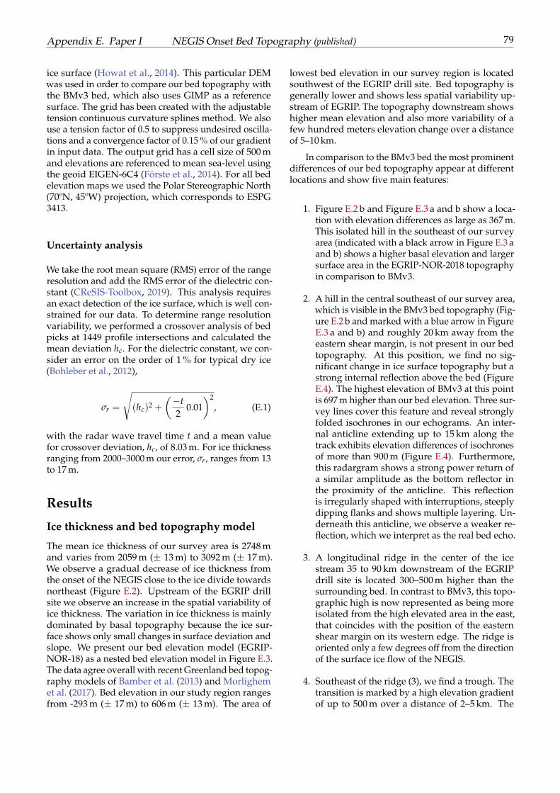
Appendix E. Paper I NEGIS Onset Bed Topography (published) 79

ice surface (Howat et al., 2014). This particular DEMwas used in order to compare our bed topography withthe BMv3 bed, which also uses GIMP as a referencesurface. The grid has been created with the adjustabletension continuous curvature splines method. We alsouse a tension factor of 0.5 to suppress undesired oscilla-tions and a convergence factor of 0.15 % of our gradientin input data. The output grid has a cell size of 500 mand elevations are referenced to mean sea-level usingthe geoid EIGEN-6C4 (Förste et al., 2014). For all bedelevation maps we used the Polar Stereographic North(70ºN, 45ºW) projection, which corresponds to ESPG3413.

Uncertainty analysis

We take the root mean square (RMS) error of the rangeresolution and add the RMS error of the dielectric con-stant (CReSIS-Toolbox, 2019). This analysis requiresan exact detection of the ice surface, which is well con-strained for our data. To determine range resolutionvariability, we performed a crossover analysis of bedpicks at 1449 profile intersections and calculated themean deviation hc. For the dielectric constant, we con-sider an error on the order of 1 % for typical dry ice(Bohleber et al., 2012),

σr =

√(hc)2 +

(−t2

0.01)2

, (E.1)

with the radar wave travel time t and a mean valuefor crossover deviation, hc, of 8.03 m. For ice thicknessranging from 2000–3000 m our error, σr, ranges from 13to 17 m.

Results

Ice thickness and bed topography model

The mean ice thickness of our survey area is 2748 mand varies from 2059 m (± 13 m) to 3092 m (± 17 m).We observe a gradual decrease of ice thickness fromthe onset of the NEGIS close to the ice divide towardsnortheast (Figure E.2). Upstream of the EGRIP drillsite we observe an increase in the spatial variability ofice thickness. The variation in ice thickness is mainlydominated by basal topography because the ice sur-face shows only small changes in surface deviation andslope. We present our bed elevation model (EGRIP-NOR-18) as a nested bed elevation model in Figure E.3.The data agree overall with recent Greenland bed topog-raphy models of Bamber et al. (2013) and Morlighemet al. (2017). Bed elevation in our study region rangesfrom -293 m (± 17 m) to 606 m (± 13 m). The area of

lowest bed elevation in our survey region is locatedsouthwest of the EGRIP drill site. Bed topography isgenerally lower and shows less spatial variability up-stream of EGRIP. The topography downstream showshigher mean elevation and also more variability of afew hundred meters elevation change over a distanceof 5–10 km.

In comparison to the BMv3 bed the most prominentdifferences of our bed topography appear at differentlocations and show five main features:

1. Figure E.2 b and Figure E.3 a and b show a loca-tion with elevation differences as large as 367 m.This isolated hill in the southeast of our surveyarea (indicated with a black arrow in Figure E.3 aand b) shows a higher basal elevation and largersurface area in the EGRIP-NOR-2018 topographyin comparison to BMv3.

2. A hill in the central southeast of our survey area,which is visible in the BMv3 bed topography (Fig-ure E.2 b and marked with a blue arrow in FigureE.3 a and b) and roughly 20 km away from theeastern shear margin, is not present in our bedtopography. At this position, we find no sig-nificant change in ice surface topography but astrong internal reflection above the bed (FigureE.4). The highest elevation of BMv3 at this pointis 697 m higher than our bed elevation. Three sur-vey lines cover this feature and reveal stronglyfolded isochrones in our echograms. An inter-nal anticline extending up to 15 km along thetrack exhibits elevation differences of isochronesof more than 900 m (Figure E.4). Furthermore,this radargram shows a strong power return ofa similar amplitude as the bottom reflector inthe proximity of the anticline. This reflectionis irregularly shaped with interruptions, steeplydipping flanks and shows multiple layering. Un-derneath this anticline, we observe a weaker re-flection, which we interpret as the real bed echo.

3. A longitudinal ridge in the center of the icestream 35 to 90 km downstream of the EGRIPdrill site is located 300–500 m higher than thesurrounding bed. In contrast to BMv3, this topo-graphic high is now represented as being moreisolated from the high elevated area in the east,that coincides with the position of the easternshear margin on its western edge. The ridge isoriented only a few degrees off from the directionof the surface ice flow of the NEGIS.

4. Southeast of the ridge (3), we find a trough. Thetransition is marked by a high elevation gradientof up to 500 m over a distance of 2–5 km. The

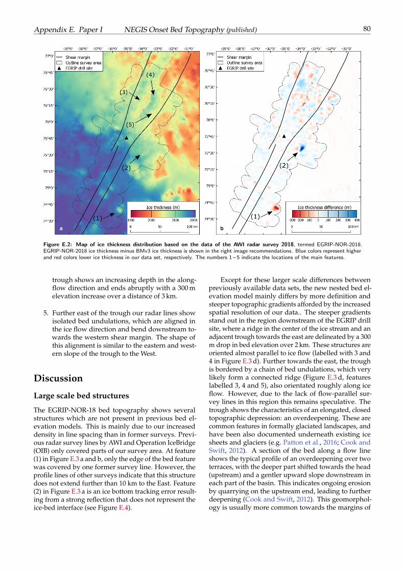
Appendix E. Paper I NEGIS Onset Bed Topography (published) 80

Figure E.2: Map of ice thickness distribution based on the data of the AWI radar survey 2018, termed EGRIP-NOR-2018.EGRIP-NOR-2018 ice thickness minus BMv3 ice thickness is shown in the right image recommendations. Blue colors represent higherand red colors lower ice thickness in our data set, respectively. The numbers 1 – 5 indicate the locations of the main features.

trough shows an increasing depth in the along-flow direction and ends abruptly with a 300 melevation increase over a distance of 3 km.

5. Further east of the trough our radar lines showisolated bed undulations, which are aligned inthe ice flow direction and bend downstream to-wards the western shear margin. The shape ofthis alignment is similar to the eastern and west-ern slope of the trough to the West.

Discussion

Large scale bed structures

The EGRIP-NOR-18 bed topography shows severalstructures which are not present in previous bed el-evation models. This is mainly due to our increaseddensity in line spacing than in former surveys. Previ-ous radar survey lines by AWI and Operation IceBridge(OIB) only covered parts of our survey area. At feature(1) in Figure E.3 a and b, only the edge of the bed featurewas covered by one former survey line. However, theprofile lines of other surveys indicate that this structuredoes not extend further than 10 km to the East. Feature(2) in Figure E.3 a is an ice bottom tracking error result-ing from a strong reflection that does not represent theice-bed interface (see Figure E.4).

Except for these larger scale differences betweenpreviously available data sets, the new nested bed el-evation model mainly differs by more definition andsteeper topographic gradients afforded by the increasedspatial resolution of our data.. The steeper gradientsstand out in the region downstream of the EGRIP drillsite, where a ridge in the center of the ice stream and anadjacent trough towards the east are delineated by a 300m drop in bed elevation over 2 km. These structures areoriented almost parallel to ice flow (labelled with 3 and4 in Figure E.3 d). Further towards the east, the troughis bordered by a chain of bed undulations, which verylikely form a connected ridge (Figure E.3 d, featureslabelled 3, 4 and 5), also orientated roughly along iceflow. However, due to the lack of flow-parallel sur-vey lines in this region this remains speculative. Thetrough shows the characteristics of an elongated, closedtopographic depression: an overdeepening. These arecommon features in formally glaciated landscapes, andhave been also documented underneath existing icesheets and glaciers (e.g. Patton et al., 2016; Cook andSwift, 2012). A section of the bed along a flow lineshows the typical profile of an overdeepening over twoterraces, with the deeper part shifted towards the head(upstream) and a gentler upward slope downstream ineach part of the basin. This indicates ongoing erosionby quarrying on the upstream end, leading to furtherdeepening (Cook and Swift, 2012). This geomorphol-ogy is usually more common towards the margins of

Appendix E. Paper I NEGIS Onset Bed Topography (published) 81

Figure E.3: Bed topography of a) BedMachine v3 (Morlighem et al. (2017) and b) the EGRIP-NOR-2018 bed topographyderived from our ice thickness data. A magnified view for the area upstream of the EGRIP drill site for both models (a) and(b) is shown on the two lower images (c) and (d), respectively). Two locations with strong elevation differences are markedwith a blue arrow. In the magnified sections, (c) and (d), we show the location of features 3 – 5.

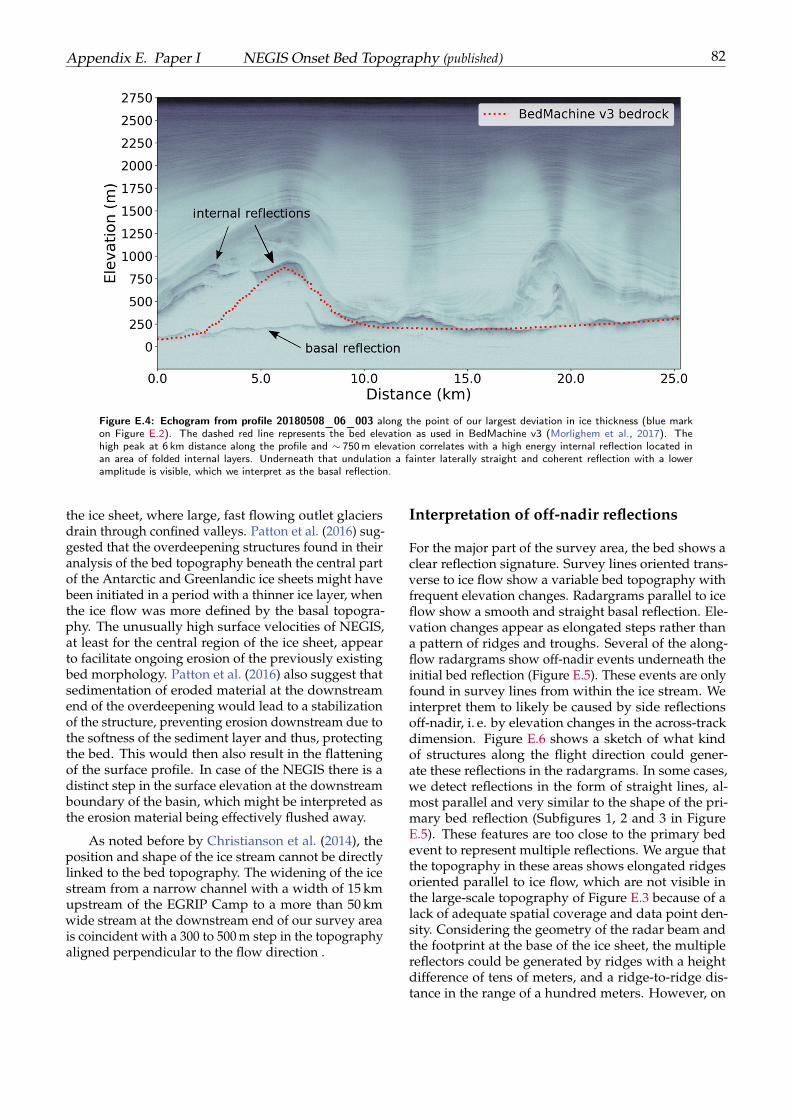
Appendix E. Paper I NEGIS Onset Bed Topography (published) 82

Figure E.4: Echogram from profile 20180508_06_003 along the point of our largest deviation in ice thickness (blue markon Figure E.2). The dashed red line represents the bed elevation as used in BedMachine v3 (Morlighem et al., 2017). Thehigh peak at 6 km distance along the profile and ∼ 750m elevation correlates with a high energy internal reflection located inan area of folded internal layers. Underneath that undulation a fainter laterally straight and coherent reflection with a loweramplitude is visible, which we interpret as the basal reflection.

the ice sheet, where large, fast flowing outlet glaciersdrain through confined valleys. Patton et al. (2016) sug-gested that the overdeepening structures found in theiranalysis of the bed topography beneath the central partof the Antarctic and Greenlandic ice sheets might havebeen initiated in a period with a thinner ice layer, whenthe ice flow was more defined by the basal topogra-phy. The unusually high surface velocities of NEGIS,at least for the central region of the ice sheet, appearto facilitate ongoing erosion of the previously existingbed morphology. Patton et al. (2016) also suggest thatsedimentation of eroded material at the downstreamend of the overdeepening would lead to a stabilizationof the structure, preventing erosion downstream due tothe softness of the sediment layer and thus, protectingthe bed. This would then also result in the flatteningof the surface profile. In case of the NEGIS there is adistinct step in the surface elevation at the downstreamboundary of the basin, which might be interpreted asthe erosion material being effectively flushed away.

As noted before by Christianson et al. (2014), theposition and shape of the ice stream cannot be directlylinked to the bed topography. The widening of the icestream from a narrow channel with a width of 15 kmupstream of the EGRIP Camp to a more than 50 kmwide stream at the downstream end of our survey areais coincident with a 300 to 500 m step in the topographyaligned perpendicular to the flow direction .

Interpretation of off-nadir reflections

For the major part of the survey area, the bed shows aclear reflection signature. Survey lines oriented trans-verse to ice flow show a variable bed topography withfrequent elevation changes. Radargrams parallel to iceflow show a smooth and straight basal reflection. Ele-vation changes appear as elongated steps rather thana pattern of ridges and troughs. Several of the along-flow radargrams show off-nadir events underneath theinitial bed reflection (Figure E.5). These events are onlyfound in survey lines from within the ice stream. Weinterpret them to likely be caused by side reflectionsoff-nadir, i. e. by elevation changes in the across-trackdimension. Figure E.6 shows a sketch of what kindof structures along the flight direction could gener-ate these reflections in the radargrams. In some cases,we detect reflections in the form of straight lines, al-most parallel and very similar to the shape of the pri-mary bed reflection (Subfigures 1, 2 and 3 in FigureE.5). These features are too close to the primary bedevent to represent multiple reflections. We argue thatthe topography in these areas shows elongated ridgesoriented parallel to ice flow, which are not visible inthe large-scale topography of Figure E.3 because of alack of adequate spatial coverage and data point den-sity. Considering the geometry of the radar beam andthe footprint at the base of the ice sheet, the multiplereflectors could be generated by ridges with a heightdifference of tens of meters, and a ridge-to-ridge dis-tance in the range of a hundred meters. However, on

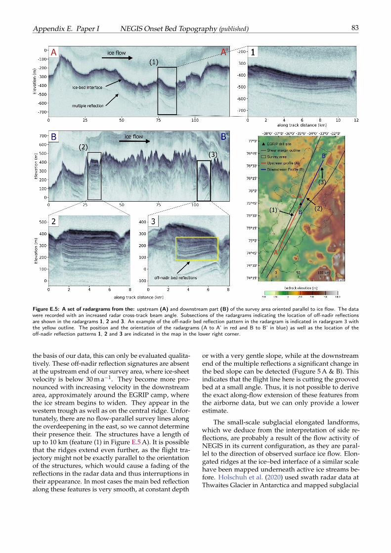
Appendix E. Paper I NEGIS Onset Bed Topography (published) 83

Figure E.5: A set of radargrams from the: upstream (A) and downstream part (B) of the survey area oriented parallel to ice flow. The datawere recorded with an increased radar cross-track beam angle. Subsections of the radargrams indicating the location of off-nadir reflectionsare shown in the radargrams 1, 2 and 3. An example of the off-nadir bed reflection pattern in the radargram is indicated in radargram 3 withthe yellow outline. The position and the orientation of the radargrams (A to A’ in red and B to B’ in blue) as well as the location of theoff-nadir reflection patterns 1, 2 and 3 are indicated in the map in the lower right corner.

the basis of our data, this can only be evaluated qualita-tively. These off-nadir reflection signatures are absentat the upstream end of our survey area, where ice-sheetvelocity is below 30 m a−1. They become more pro-nounced with increasing velocity in the downstreamarea, approximately around the EGRIP camp, wherethe ice stream begins to widen. They appear in thewestern trough as well as on the central ridge. Unfor-tunately, there are no flow-parallel survey lines alongthe overdeepening in the east, so we cannot determinetheir presence their. The structures have a length ofup to 10 km (feature (1) in Figure E.5 A). It is possiblethat the ridges extend even further, as the flight tra-jectory might not be exactly parallel to the orientationof the structures, which would cause a fading of thereflections in the radar data and thus interruptions intheir appearance. In most cases the main bed reflectionalong these features is very smooth, at constant depth

or with a very gentle slope, while at the downstreamend of the multiple reflections a significant change inthe bed slope can be detected (Fugure 5 A & B). Thisindicates that the flight line here is cutting the groovedbed at a small angle. Thus, it is not possible to derivethe exact along-flow extension of these features fromthe airborne data, but we can only provide a lowerestimate.

The small-scale subglacial elongated landforms,which we deduce from the interpretation of side re-flections, are probably a result of the flow activity ofNEGIS in its current configuration, as they are paral-lel to the direction of observed surface ice flow. Elon-gated ridges at the ice–bed interface of a similar scalehave been mapped underneath active ice streams be-fore. Holschuh et al. (2020) used swath radar data atThwaites Glacier in Antarctica and mapped subglacial

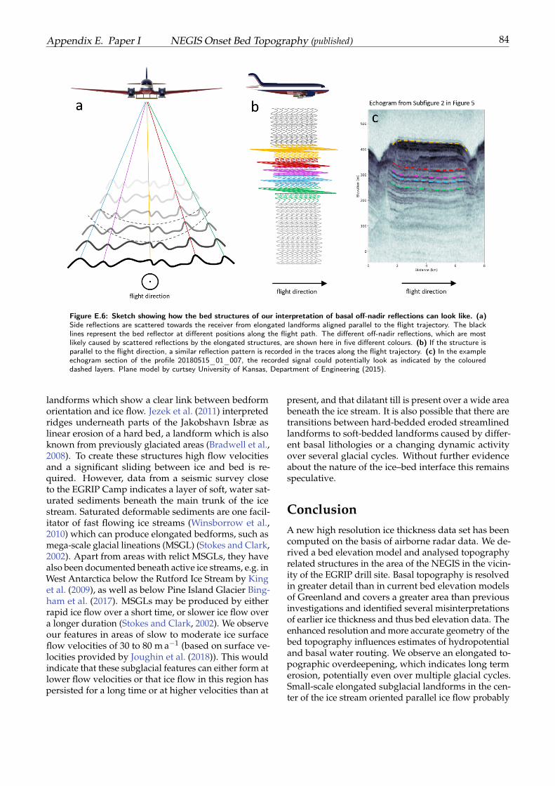
Appendix E. Paper I NEGIS Onset Bed Topography (published) 84

Figure E.6: Sketch showing how the bed structures of our interpretation of basal off-nadir reflections can look like. (a)Side reflections are scattered towards the receiver from elongated landforms aligned parallel to the flight trajectory. The blacklines represent the bed reflector at different positions along the flight path. The different off-nadir reflections, which are mostlikely caused by scattered reflections by the elongated structures, are shown here in five different colours. (b) If the structure isparallel to the flight direction, a similar reflection pattern is recorded in the traces along the flight trajectory. (c) In the exampleechogram section of the profile 20180515_01_007, the recorded signal could potentially look as indicated by the coloureddashed layers. Plane model by curtsey University of Kansas, Department of Engineering (2015).

landforms which show a clear link between bedformorientation and ice flow. Jezek et al. (2011) interpretedridges underneath parts of the Jakobshavn Isbræ aslinear erosion of a hard bed, a landform which is alsoknown from previously glaciated areas (Bradwell et al.,2008). To create these structures high flow velocitiesand a significant sliding between ice and bed is re-quired. However, data from a seismic survey closeto the EGRIP Camp indicates a layer of soft, water sat-urated sediments beneath the main trunk of the icestream. Saturated deformable sediments are one facil-itator of fast flowing ice streams (Winsborrow et al.,2010) which can produce elongated bedforms, such asmega-scale glacial lineations (MSGL) (Stokes and Clark,2002). Apart from areas with relict MSGLs, they havealso been documented beneath active ice streams, e.g. inWest Antarctica below the Rutford Ice Stream by Kinget al. (2009), as well as below Pine Island Glacier Bing-ham et al. (2017). MSGLs may be produced by eitherrapid ice flow over a short time, or slower ice flow overa longer duration (Stokes and Clark, 2002). We observeour features in areas of slow to moderate ice surfaceflow velocities of 30 to 80 m a−1 (based on surface ve-locities provided by Joughin et al. (2018)). This wouldindicate that these subglacial features can either form atlower flow velocities or that ice flow in this region haspersisted for a long time or at higher velocities than at

present, and that dilatant till is present over a wide areabeneath the ice stream. It is also possible that there aretransitions between hard-bedded eroded streamlinedlandforms to soft-bedded landforms caused by differ-ent basal lithologies or a changing dynamic activityover several glacial cycles. Without further evidenceabout the nature of the ice–bed interface this remainsspeculative.

ConclusionA new high resolution ice thickness data set has beencomputed on the basis of airborne radar data. We de-rived a bed elevation model and analysed topographyrelated structures in the area of the NEGIS in the vicin-ity of the EGRIP drill site. Basal topography is resolvedin greater detail than in current bed elevation modelsof Greenland and covers a greater area than previousinvestigations and identified several misinterpretationsof earlier ice thickness and thus bed elevation data. Theenhanced resolution and more accurate geometry of thebed topography influences estimates of hydropotentialand basal water routing. We observe an elongated to-pographic overdeepening, which indicates long termerosion, potentially even over multiple glacial cycles.Small-scale elongated subglacial landforms in the cen-ter of the ice stream oriented parallel ice flow probably

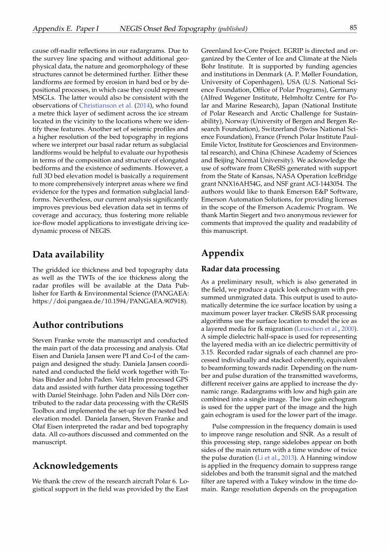
Appendix E. Paper I NEGIS Onset Bed Topography (published) 85

cause off-nadir reflections in our radargrams. Due tothe survey line spacing and without additional geo-physical data, the nature and geomorphology of thesestructures cannot be determined further. Either theselandforms are formed by erosion in hard bed or by de-positional processes, in which case they could representMSGLs. The latter would also be consistent with theobservations of Christianson et al. (2014), who founda metre thick layer of sediment across the ice streamlocated in the vicinity to the locations where we iden-tify these features. Another set of seismic profiles anda higher resolution of the bed topography in regionswhere we interpret our basal radar return as subglaciallandforms would be helpful to evaluate our hypothesisin terms of the composition and structure of elongatedbedforms and the existence of sediments. However, afull 3D bed elevation model is basically a requirementto more comprehensively interpret areas where we findevidence for the types and formation subglacial land-forms. Nevertheless, our current analysis significantlyimproves previous bed elevation data set in terms ofcoverage and accuracy, thus fostering more reliableice-flow model applications to investigate driving ice-dynamic process of NEGIS.

Data availability

The gridded ice thickness and bed topography dataas well as the TWTs of the ice thickness along theradar profiles will be available at the Data Pub-lisher for Earth & Environmental Science (PANGAEA:https://doi.pangaea.de/10.1594/PANGAEA.907918).

Author contributions

Steven Franke wrote the manuscript and conductedthe main part of the data processing and analysis. OlafEisen and Daniela Jansen were PI and Co-I of the cam-paign and designed the study. Daniela Jansen coordi-nated and conducted the field work together with To-bias Binder and John Paden. Veit Helm processed GPSdata and assisted with further data processing togetherwith Daniel Steinhage. John Paden and Nils Dörr con-tributed to the radar data processing with the CReSISToolbox and implemented the set-up for the nested bedelevation model. Daniela Jansen, Steven Franke andOlaf Eisen interpreted the radar and bed topographydata. All co-authors discussed and commented on themanuscript.

Acknowledgements

We thank the crew of the research aircraft Polar 6. Lo-gistical support in the field was provided by the East

Greenland Ice-Core Project. EGRIP is directed and or-ganized by the Center of Ice and Climate at the NielsBohr Institute. It is supported by funding agenciesand institutions in Denmark (A. P. Møller Foundation,University of Copenhagen), USA (U.S. National Sci-ence Foundation, Office of Polar Programs), Germany(Alfred Wegener Institute, Helmholtz Centre for Po-lar and Marine Research), Japan (National Instituteof Polar Research and Arctic Challenge for Sustain-ability), Norway (University of Bergen and Bergen Re-search Foundation), Switzerland (Swiss National Sci-ence Foundation), France (French Polar Institute Paul-Emile Victor, Institute for Geosciences and Environmen-tal research), and China (Chinese Academy of Sciencesand Beijing Normal University). We acknowledge theuse of software from CReSIS generated with supportfrom the State of Kansas, NASA Operation IceBridgegrant NNX16AH54G, and NSF grant ACI-1443054. Theauthors would like to thank Emerson E&P Software,Emerson Automation Solutions, for providing licensesin the scope of the Emerson Academic Program. Wethank Martin Siegert and two anonymous reviewer forcomments that improved the quality and readability ofthis manuscript.

Appendix

Radar data processing

As a preliminary result, which is also generated inthe field, we produce a quick look echogram with pre-summed unmigrated data. This output is used to auto-matically determine the ice surface location by using amaximum power layer tracker. CReSIS SAR processingalgorithms use the surface location to model the ice asa layered media for fk migration (Leuschen et al., 2000).A simple dielectric half-space is used for representingthe layered media with an ice dielectric permittivity of3.15. Recorded radar signals of each channel are pro-cessed individually and stacked coherently, equivalentto beamforming towards nadir. Depending on the num-ber and pulse duration of the transmitted waveforms,different receiver gains are applied to increase the dy-namic range. Radargrams with low and high gain arecombined into a single image. The low gain echogramis used for the upper part of the image and the highgain echogram is used for the lower part of the image.

Pulse compression in the frequency domain is usedto improve range resolution and SNR. As a result ofthis processing step, range sidelobes appear on bothsides of the main return with a time window of twicethe pulse duration (Li et al., 2013). A Hanning windowis applied in the frequency domain to suppress rangesidelobes and both the transmit signal and the matchedfilter are tapered with a Tukey window in the time do-main. Range resolution depends on the propagation

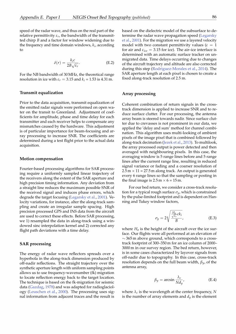
Appendix E. Paper I NEGIS Onset Bed Topography (published) 86

speed of the radar wave, and thus on the real part of therelative permittivity εr, the bandwidth of the transmit-ted chirp B and a factor for window widening due tothe frequency and time domain windows, ki, accordingto

δ(r) =kic

2B√

εr. (E.2)

For the NB bandwidth of 30 MHz, the theoretical rangeresolution in ice with εr = 3.15 and ki = 1.53 is 4.31 m.

Transmit equalization

Prior to the data acquisition, transmit equalization ofthe emitted radar signals were performed on open wa-ter on the transit to Greenland. Adjustment of coef-ficients for amplitude, phase and time delay for eachtransmitter and each receiver helps to compensate anymismatches caused by the hardware. This adjustmentis of particular importance for beam-focusing and ar-ray processing to increase SNR. The coefficients aredetermined during a test flight prior to the actual dataacquisition.

Motion compensation

Fourier-based processing algorithms for SAR process-ing require a uniformly sampled linear trajectory ofthe receivers along the extent of the SAR aperture andhigh precision timing information. Any deviation froma straight line reduces the maximum possible SNR ofthe received signal and induces phase errors, whichdegrade the target focusing (Legarsky et al., 2001). Ve-locity variations, for instance, alter the along-track sam-pling and create an irregular sample spacing. Highprecision processed GPS and INS data from the aircraftare used to correct these effects. Before SAR processing,we 1) resampled the data in along-track using a win-dowed sinc interpolation kernel and 2) corrected anyflight path deviations with a time delay.

SAR processing

The energy of radar wave reflectors spreads over ahyperbola in the along-track dimension produced byoff-nadir reflections. The straight trajectory over thesynthetic aperture length with uniform sampling pointsallows us to use frequency-wavenumber (fk) migrationto locate reflection energy back to the target location.The technique is based on the fk-migration for seismicdata (Gazdag, 1978) and was adapted for radioglaciol-ogy (Leuschen et al., 2000). The processing uses sig-nal information from adjacent traces and the result is

based on the dielectric model of the subsurface to de-termine the radar wave propagation speed (Legarskyet al., 2001). For the migration we use a layered velocitymodel with two constant permittivity values (ε = 1for air and εice = 3.15 for ice). The air–ice interface isdetermined with an automatic surface tracker on un-migrated data. Time delays occurring due to changesof the aircraft trajectory and altitude are also correctedduring this step (Rodriguez-Morales et al., 2014). TheSAR aperture length at each pixel is chosen to create afixed along-track resolution of 2.5 m.

Array processing

Coherent combination of return signals in the cross-track dimension is applied to increase SNR and to re-duce surface clutter. For our processing, the antennaarray beam is steered towards nadir. Since surface clut-ter due to crevasses is not prominent in our data, weapplied the ’delay and sum’ method for channel combi-nation. This algorithm uses multi-looking of ambientpixels of the image pixel that is combined followed byalong-track decimation (Jezek et al., 2013). To multilook,the array processed output is power detected and thenaveraged with neighbouring pixels. In this case, theaveraging window is 5 range lines before and 5 rangelines after the current range line, resulting in reducedsignal variance or fading and a coarser resolution of2.5 m× 11 = 27.5 m along track. An output is generatedevery 6 range lines so that the sampling or posting inthe final image is 2.5 m× 6 = 15 m.

For our bed return, we consider a cross-track resolu-tion for a typical rough surface σy, which is constrainedby the pulse-limited footprint and is dependent on Han-ning and Tukey window factors,

σy = 2

√Ha√

εrcki

B, (E.3)

where Ha is the height of the aircraft over the ice sur-face. Our flights were all performed at an elevation of∼ 365 m above ground, which corresponds to a cross-track footprint of 300–350 m for an ice column of 2000–3000 m in our survey region. The bed return, however,is in some cases characterized by layover signals fromoff-nadir due to topography. In this case, cross-trackresolution depends on the full beam width, βy, of theantenna array,

βy = arcsinλc

Ndy, (E.4)

where λc is the wavelength at the center frequency, Nis the number of array elements and dy is the element

Appendix E. Paper I NEGIS Onset Bed Topography (published) 87

spacing of 46.8 cm. Cross-track resolution can now becalculated as

σy = 2Ha + T√

εtan

βykt

2. (E.5)

Considering Equation (I.5) with a beam angle of ∼ 21

corresponds to a cross-track resolution for the bed layerof 800 m to 1100 m for an ice thickness range of 2000–3000 m.

88

BibliographyAllen, C. T., Mozaffar, S. N., and Akins, T. L. Suppress-

ing coherent noise in radar applications with long dwelltimes. IEEE Geoscience and Remote Sensing Letters, 2(3):284–286, July 2005. doi: 10.1109/LGRS.2005.847931. URLhttp://dx.doi.org/10.1109/LGRS.2005.847931.

Aschwanden, A., Fahnestock, M. A., and Truffer, M. Com-plex Greenland outlet glacier flow captured. NatureCommunications, 7(May 2015):1–8, 2016. ISSN 20411723.doi: 10.1038/ncomms10524. URL http://dx.doi.org/10.1038/ncomms10524.

Bamber, J. L., Griggs, J. A., Hurkmans, R. T. W. L.,Dowdeswell, J. A., Gogineni, S. P., Howat, I., Mouginot,J., Paden, J., Palmer, S., Rignot, E., and Steinhage, D. Anew bed elevation dataset for Greenland. Cryosphere, 7(2):499–510, 2013. ISSN 19940416. doi: 10.5194/tc-7-499-2013.URL http://dx.doi.org/10.5194/tc-7-499-2013.

Bingham, R. G., Vaughan, D. G., King, E. C., Davies, D.,Cornford, S. L., Smith, A. M., Arthern, R. J., Brisbourne,A. M., De Rydt, J., Graham, A. G. C., Spagnolo, M.,Marsh, O. J., and Shean, D. E. Diverse landscapes be-neath Pine Island Glacier influence ice flow. Nature Com-munications, 8(1):1618, dec 2017. ISSN 2041-1723. doi:10.1038/s41467-017-01597-y. URL http://www.nature.com/articles/s41467-017-01597-y.

Bohleber, P., Wagner, N., and Eisen, O. Permittivity of ice atradio frequencies: Part II. Artificial and natural polycrys-talline ice. Cold Regions Science and Technology, 83-84:13–19,dec 2012. ISSN 0165-232X. doi: 10.1016/J.COLDREGIONS.2012.05.010. URL https://www.sciencedirect.com/science/article/pii/S0165232X12001103.

Bradwell, T., Stoker, M., and Krabbendam, M. Megagroovesand streamlined bedrock in NW Scotland: The role of icestreams in landscape evolution. Geomorphology, 97(1-2):135–156, 2008. ISSN 0169555X. doi: 10.1016/j.geomorph.2007.02.040. URL http://dx.doi.org/10.1016/j.geomorph.2007.02.040.

Christianson, K., Peters, L. E., Alley, R. B., Anandakrishnan,S., Jacobel, R. W., Riverman, K. L., Muto, A., and Keisling,B. A. Dilatant till facilitates ice-stream flow in northeastGreenland. Earth and Planetary Science Letters, 401:57–69,2014. ISSN 0012821X. doi: 10.1016/j.epsl.2014.05.060. URLhttp://dx.doi.org/10.1016/j.epsl.2014.05.060.

Church, J. A., Clark, P., Cazenave, A., Gregory, J., Jevrejeva,S., Levermann, A., Merrifield, M., Milne, G., Nerem, R.,Nunn, P., Payne, A., Pfeffer, W., Stammer, D., and Unnikr-ishnan, A. 2013: Sea level change. In Climate Change 2013:The Physical Science Basis. Contribution of Working Group Ito the Fifth Assessment Report of the Intergovernmental Panelon Climate Change, pages 1137–1216. 2013. ISBN ISBN 978-1-107-66182-0. doi: 10.1017/CB09781107415315.026. URLhttp://dx.doi.org/10.1017/CB09781107415315.026.

Cook, S. J. and Swift, D. A. Subglacial basins: Their ori-gin and importance in glacial systems and landscapes.Earth-Science Reviews, 115(4):332 – 372, 2012. ISSN0012-8252. doi: https://doi.org/10.1016/j.earscirev.2012.09.009. URL http://www.sciencedirect.com/science/article/pii/S0012825212001286.

CReSIS-Toolbox. J Paden, URL:https://ops.cresis.ku.edu/wiki/index.php/Main_Page,acessed: 2019-06-01, 2019. URL https://ops.cresis.ku.edu/wiki/index.php/Main_Page.

Dowdeswell, J. A., Hogan, K. A., Ó Cofaigh, C., Fugelli, E. M.,Evans, J., and Noormets, R. Late Quaternary ice flowin a West Greenland fjord and cross-shelf trough system:Submarine landforms from Rink Isbrae to Uummannaqshelf and slope. Quaternary Science Reviews, 2014. ISSN02773791. doi: 10.1016/j.quascirev.2013.09.007. URL http://dx.doi.org/10.1016/j.quascirev.2013.09.007.

Dutrieux, P., Vaughan, D. G., Corr, H. F. J., Jenkins, A.,Holland, P. R., Joughin, I., and Fleming, A. H. Pine Is-land glacier ice shelf melt distributed at kilometre scales.The Cryosphere, 7(5):1543–1555, 2013. ISSN 19940416.doi: 10.5194/tc-7-1543-2013. URL http://dx.doi.org/10.5194/tc-7-1543-2013.

Fahnestock, M., Abdalati, W., Joughin, I., Brozena, J., andGogineni, P. High geothermal heat flow, basal melt, andthe origin of rapid ice flow in central Greenland. Sci-ence, 294(5550):2338–2342, 2001. ISSN 00368075. doi:10.1126/science.1065370. URL http://dx.doi.org/10.1126/science.1065370.

Förste, C., Bruinsma, S., Abrikosov, O., Flechtner, F., Marty,J.-C., Lemoine, J.-M., Dahle, C., Neumayer, H., Barthelmes,F., König, R., and Biancale, R. EIGEN-6C4 - The latestcombined global gravity field model including GOCE dataup to degree and order 1949 of GFZ Potsdam and GRGSToulouse. EGU General Assembly 2014, held 27 April - 2May, 2014 in Vienna, Austria, id.3707, 16, 2014. URL http://adsabs.harvard.edu/abs/2014EGUGA..16.3707F.

Fretwell, P., Pritchard, H. D., Vaughan, D. G., Bamber, J. L.,Barrand, N. E., Bell, R., Bianchi, C., Bingham, R. G.,Blankenship, D. D., Casassa, G., Catania, G., Callens, D.,Conway, H., Cook, A. J., Corr, H. F. J., Damaske, D., Damm,V., Ferraccioli, F., Forsberg, R., Fujita, S., Gim, Y., Gogi-neni, P., Griggs, J. A., Hindmarsh, R. C. A., Holmlund,P., Holt, J. W., Jacobel, R. W., Jenkins, A., Jokat, W., Jor-dan, T., King, E. C., Kohler, J., Krabill, W., Riger-Kusk, M.,Langley, K. A., Leitchenkov, G., Leuschen, C., Luyendyk,B. P., Matsuoka, K., Mouginot, J., Nitsche, F. O., Nogi,Y., Nost, O. A., Popov, S. V., Rignot, E., Rippin, D. M.,Rivera, A., Roberts, J., Ross, N., Siegert, M. J., Smith, A. M.,Steinhage, D., Studinger, M., Sun, B., Tinto, B. K., Welch,B. C., Wilson, D., Young, D. A., Xiangbin, C., and Zirizzotti,A. Bedmap2: improved ice bed, surface and thicknessdatasets for Antarctica. The Cryosphere, 7(1):375–393, feb2013. ISSN 1994-0424. doi: 10.5194/tc-7-375-2013. URLhttps://www.the-cryosphere.net/7/375/2013/.

BIBLIOGRAPHY 89

Gardner, A. S., Moholdt J.G., G., Wouters, B., Arendt, A. A.,Wahr, J., Berthier, E., Hock, R., Pfeffer, W. T., Kaser,G., Ligtenberg, S. R. M., Bolch, T., Sharp, M. J., Ha-gen, J. O., van den Broeke, M. R., and Paul, F. A Rec-onciled Estimate of Glacier Contributions to Sea LevelRise: 2003 to 2009. Science, 340(May):852–857, 2013. doi:10.1126/science.1234532. URL http://dx.doi.org/10.1126/science.1234532.

Gazdag, J. Wave equation migration with the phase-shiftmethod. Geophysics, 43(7):1342–1351, 1978. ISSN 0016-8033. doi: 10.1190/1.1440899. URL http://dx.doi.org/10.1190/1.1440899.

Gillet-Chaulet, F., Gagliardini, O., Seddik, H., Nodet, M.,Durand, G., Ritz, C., Zwinger, T., and Greve, R. TheCryosphere Greenland ice sheet contribution to sea-levelrise from a new-generation ice-sheet model. The Cryosphere,6(6):1561–1576, 2012. doi: 10.5194/tc-6-1561-2012. URLhttp://dx.doi.org/10.5194/tc-6-1561-2012.

Goelzer, H., Nowicki, S., Payne, A., Larour, E., Seroussi,H., Lipscomb, W. H., Gregory, J., Abe-Ouchi, A., Shep-herd, A., Simon, E., Agosta, C., Alexander, P., Aschwan-den, A., Barthel, A., Calov, R., Chambers, C., Choi, Y.,Cuzzone, J., Dumas, C., Edwards, T., Felikson, D., Fet-tweis, X., Golledge, N. R., Greve, R., Humbert, A., Huy-brechts, P., Le clec’h, S., Lee, V., Leguy, G., Little, C., Lowry,D. P., Morlighem, M., Nias, I., Quiquet, A., Rückamp, M.,Schlegel, N.-J., Slater, D., Smith, R., Straneo, F., Tarasov, L.,van de Wal, R., and van den Broeke, M. The future sea-level contribution of the greenland ice sheet: a multi-modelensemble study of ismip6. The Cryosphere Discussions,2020:1–43, 2020. doi: 10.5194/tc-2019-319. URL https://www.the-cryosphere-discuss.net/tc-2019-319/.

Gogineni, S., Tammana, D., Braaten, D., Leuschen, C., Akins,T., Legarsky, J., Kanagaratnam, P., Stiles, J., Allen, C.,and Jezek, K. Coherent radar ice thickness measure-ments over the Greenland ice sheet. Journal of GeophysicalResearch, 106(D24):33,761–33,772, 2001. ISSN 0148-0227.doi: 10.1029/2001JD900183. URL http://dx.doi.org/10.1029/2001JD900183.

Hale, R., Miller, H., Gogineni, S., Yan, J. B., Leuschen, C.,Paden, J., and Li, J. Multi-channel ultra-wideband radarsounder and imager. 2016 IEEE International Geoscienceand Remote Sensing Symposium (IGARSS), pages 2112–2115,2016. doi: 10.1109/IGARSS.2016.7729545. URL http://dx.doi.org/10.1109/IGARSS.2016.7729545.

Hogan, K. A., Ó Cofaigh, C., Jennings, A. E., Dowdeswell,J. A., and Hiemstra, J. F. Deglaciation of a major palaeo-ice stream in Disko Trough, West Greenland. Quater-nary Science Reviews, 2016. ISSN 02773791. doi: 10.1016/j.quascirev.2016.01.018. URL http://dx.doi.org/10.1016/j.quascirev.2016.01.018.

Holschuh, N., Christianson, K., Paden, J., Alley, R., and Anan-dakrishnan, S. Linking postglacial landscapes to glacier dy-namics using swath radar at Thwaites Glacier, Antarctica.Geology, jan 2020. ISSN 0091-7613. doi: 10.1130/g46772.1.URL http://dx.doi.org/10.1130/g46772.1.

Howat, I. M., Joughin, I., and Scambos, T. A. Rapid Changesin Ice Discharge from. Science, 315(5818):1559–1561, 2007.doi: 10.1126/science.1138478. URL http://dx.doi.org/10.1126/science.1138478.

Howat, I. M., Negrete, A., and Smith, B. E. The Green-land Ice Mapping Project (GIMP) land classification andsurface elevation data sets. Cryosphere, 8(4):1509–1518,2014. ISSN 19940424. doi: 10.5194/tc-8-1509-2014. URLhttp://dx.doi.org/10.5194/tc-8-1509-2014.

IPCC. IPCC Special Report on the Ocean and Cryospherein a Changing Climate [H.-O. Pörtner, Roberts, D. C.,Masson-Delmotte, V., Zhai, P., Tignor, M., Poloczanska, E.,Mintenbeck, K., Nicolai, M., Okem, A., Petzold, J. Rama,B. Weyer, N. (eds.)]. Technical report, 2019. URL https://www.ipcc.ch/srocc/chapter/technical-summary/.

Jezek, K., Wu, X., Gogineni, P., Rodríguez, E., Freeman, A.,Rodriguez-Morales, F., and Clark, C. D. Radar imagesof the bed of the Greenland Ice Sheet. Geophysical Re-search Letters, 38(1):1–5, 2011. ISSN 00948276. doi: 10.1029/2010GL045519. URL http://dx.doi.org/10.1029/2010GL045519.

Jezek, K., Wu, X., Paden, J., and Leuschen, C. Radar map-ping of isunnguata Sermia, Greenland. Journal of Glaciol-ogy, 59(218):1135–1146, 2013. ISSN 00221430. doi: 10.3189/2013JoG12J248. URL http://dx.doi.org/10.3189/2013JoG12J248.

Joughin, I., Smith, B. E., Howat, I. M., Scambos, T., and Moon,T. Greenland flow variability from ice-sheet-wide veloc-ity mapping. Journal of Glaciology, 56(197):415–430, 2010.ISSN 0022-1430. doi: 10.3189/002214310792447734. URLhttp://dx.doi.org/10.3189/002214310792447734.

Joughin, I., Smith, B. E., and Howat, I. M. A complete map ofGreenland ice velocity derived from satellite data collectedover 20 years. Journal of Glaciology, 64(243):1–11, feb 2018.ISSN 0022-1430. doi: 10.1017/jog.2017.73. URL https://www.cambridge.org/core/product/identifier/S0022143017000739/type/journal_article.

Keisling, B. A., Christianson, K., Alley, R. B., Peters, L. E.,Christian, J. E., Anandakrishnan, S., Riverman, K. L.,Muto, A., and Jacobel, R. W. Basal conditions and icedynamics inferred from radar-derived internal stratigra-phy of the northeast Greenland ice stream. Annals ofGlaciology, 55(67):127–137, 2014. ISSN 02603055. doi:10.3189/2014AoG67A090. URL http://dx.doi.org/10.3189/2014AoG67A090.

Khan, S. A., Kjær, K. H., Bevis, M., Bamber, J. L., Wahr, J.,Kjeldsen, K. K., Bjørk, A. A., Korsgaard, N. J., Stearns,L. A., Van Den Broeke, M. R., Liu, L., Larsen, N. K.,and Muresan, I. S. Sustained mass loss of the northeastGreenland ice sheet triggered by regional warming. Na-ture Climate Change, 4(4):292–299, 2014a. ISSN 17586798.doi: 10.1038/nclimate2161. URL http://dx.doi.org/10.1038/nclimate2161.

BIBLIOGRAPHY 90

Khan, S. A., Kjeldsen, K. K., Kjær, K. H., Bevan, S., Luckman,A., Bjørk, A. A., Korsgaard, N. J., Box, J. E., Van Den Broeke,M., Van Dam, T. M., and Fitzner, A. Glacier dynamics atHelheim and Kangerdlugssuaq glaciers, southeast Green-land, since the Little Ice Age. Cryosphere, 8(4):1497–1507,2014b. ISSN 19940424. doi: 10.5194/tc-8-1497-2014. URLhttp://dx.doi.org/10.5194/tc-8-1497-2014.

King, E. C., Hindmarsh, R. C. A., and Stokes, C. R. Forma-tion of mega-scale glacial lineations observed beneath aWest Antarctic ice stream. Nature Geoscience, 2(8):585–588,aug 2009. ISSN 1752-0894. doi: 10.1038/ngeo581. URLhttp://www.nature.com/articles/ngeo581.

Kjær, K. H., Larsen, N. K., Binder, T., Bjørk, A. A., Eisen, O.,Fahnestock, M. A., Funder, S., Garde, A. A., Haack, H.,Helm, V., Houmark-Nielsen, M., Kjeldsen, K. K., Khan,S. A., Machguth, H., McDonald, I., Morlighem, M., Moug-inot, J., Paden, J. D., Waight, T. E., Weikusat, C., Willerslev,E., and MacGregor, J. A. A large impact crater beneath Hi-awatha Glacier in northwest Greenland. Science Advances,4(11):eaar8173, nov 2018. ISSN 2375-2548. doi: 10.1126/sciadv.aar8173. URL http://advances.sciencemag.org/lookup/doi/10.1126/sciadv.aar8173.

Legarsky, J. J., Gogineni, S. P., and Akins, T. L. Focusedsynthetic aperture radar processing of ice-sounder datacollected over the greenland ice sheet. IEEE Transactions onGeoscience and Remote Sensing, 39(10):2109–2117, 2001. doi:10.1109/36.957274. URL http://dx.doi.org/10.1109/36.957274.

Leuschen, C., Gogineni, S., and Tammana, D. SAR processingof radar echo sounder data. pages 2570–2572, 2000. doi:10.1109/igarss.2000.859643. URL http://dx.doi.org/10.1109/igarss.2000.859643.

Leysinger Vieli, G.-M., Hindmarsh, R. C. a., and Siegert,M. J. Three-dimensional flow influences on radar layersstratigraphy. Annals of Glaciology, pages 22–28, 2007. doi:10.3189/172756407782871729. URL http://dx.doi.org/10.3189/172756407782871729.

Li, J., Paden, J., Leuschen, C., Rodriguez-Morales, F., Hale,R. D., Arnold, E. J., Crowe, R., Gomez-Garcia, D., and Gogi-neni, P. High-altitude radar measurements of ice thicknessover the antarctic and greenland ice sheets as a part ofoperation icebridge. IEEE Transactions on Geoscience andRemote Sensing, 51(2):742–754, 2013. ISSN 0196-2892. doi:10.1109/TGRS.2012.2203822.

Martos, Y. M., Jordan, T. A., Catalán, M., Jordan, T. M.,Bamber, J. L., and Vaughan, D. G. Geothermal HeatFlux Reveals the Iceland Hotspot Track UnderneathGreenland. Geophysical Research Letters, 45(16):8214–8222, aug 2018. ISSN 0094-8276. doi: 10.1029/2018GL078289. URL https://onlinelibrary.wiley.com/doi/abs/10.1029/2018GL078289.

Morlighem, M., Williams, C. N., Rignot, E., An, L., Arndt,J. E., Bamber, J. L., Catania, G., Chauché, N., Dowdeswell,J. A., Dorschel, B., Fenty, I., Hogan, K., Howat, I., Hubbard,A., Jakobsson, M., Jordan, T. M., Kjeldsen, K. K., Millan, R.,

Mayer, L., Mouginot, J., Noël, B. P., O’Cofaigh, C., Palmer,S., Rysgaard, S., Seroussi, H., Siegert, M. J., Slabon, P., Stra-neo, F., van den Broeke, M. R., Weinrebe, W., Wood, M.,and Zinglersen, K. B. BedMachine v3: Complete Bed To-pography and Ocean Bathymetry Mapping of GreenlandFrom Multibeam Echo Sounding Combined With MassConservation. Geophysical Research Letters, 44(21):11,051–11,061, 2017. ISSN 19448007. doi: 10.1002/2017GL074954.URL http://dx.doi.org/10.1002/2017GL074954.

Mouginot, J., Rignot, E., Scheuchl, B., and Millan, R. Compre-hensive annual ice sheet velocity mapping using Landsat-8,Sentinel-1, and RADARSAT-2 data. Remote Sensing, 9(4),apr 2017. ISSN 20724292. doi: 10.3390/rs9040364. URLhttp://dx.doi.org/10.3390/rs9040364.

Newton, A. M. W., Knutz, P. C., Huuse, M., Gannon, P., Brock-lehurst, S. H., Clausen, O. R., and Gong, Y. Ice streamreorganization and glacial retreat on the northwest Green-land shelf. Geophysical Research Letters, 44(15):7826–7835,aug 2017. ISSN 00948276. doi: 10.1002/2017GL073690.URL http://doi.wiley.com/10.1002/2017GL073690.

Patton, H., Swift, D. A., Clark, C. D., Livingstone, S. J., andCook, S. J. Distribution and characteristics of overdeep-enings beneath the Greenland and Antarctic ice sheets:Implications for overdeepening origin and evolution. Qua-ternary Science Reviews, 2016. ISSN 02773791. doi: 10.1016/j.quascirev.2016.07.012. URL http://dx.doi.org/10.1016/j.quascirev.2016.07.012.

Rignot, E. and Mouginot, J. Ice flow in Greenland for theInternational Polar Year 2008-2009. Geophysical ResearchLetters, 39(11):n/a–n/a, jun 2012. ISSN 00948276. doi:10.1029/2012GL051634. URL http://doi.wiley.com/10.1029/2012GL051634.

Rignot, E., Velicogna, I., Van Den Broeke, M. R., Monaghan,A., and Lenaerts, J. Acceleration of the contribution ofthe Greenland and Antarctic ice sheets to sea level rise.Geophysical Research Letters, 38(5):1–5, 2011. ISSN 00948276.doi: 10.1029/2011GL046583. URL http://dx.doi.org/10.1029/2011GL046583.

Robel, A. A., Degiuli, E., Schoof, C., and Tziperman, E. Dy-namics of ice stream temporal variability: Modes, scales,and hysteresis. Journal of Geophysical Research: Earth Surface,118(2):925–936, 2013. ISSN 21699011. doi: 10.1002/jgrf.20072. URL http://dx.doi.org/10.1002/jgrf.20072.

Roberts, D. H. and Long, A. J. Streamlined bedrock terrainand fast ice flow, Jakobshavns Isbrae, West Greenland: im-plications for ice stream and ice sheet dynamics. Boreas, 34(1):25–42, jun 2005. doi: 10.1111/j.1502-3885.2005.tb01002.x. URL http://doi.wiley.com/10.1111/j.1502-3885.2005.tb01002.x.

Roberts, D. H., Long, A. J., Davies, B. J., Simpson, M. J. R.,and Schnabel, C. Ice stream influence on West Green-land Ice Sheet dynamics during the Last Glacial Maxi-mum. Journal of Quaternary Science, 25(6):850–864, sep2010. ISSN 02678179. doi: 10.1002/jqs.1354. URL http://doi.wiley.com/10.1002/jqs.1354.

BIBLIOGRAPHY 91

Robinson, A., Calov, R., and Ganopolski, A. Multistabilityand critical thresholds of the Greenland ice sheet. Na-ture Climate Change, 2(6):429–432, 2012. ISSN 1758678X.doi: 10.1038/nclimate1449. URL http://dx.doi.org/10.1038/nclimate1449.

Rodriguez-Morales, F., Gogineni, S., Leuschen, C. J., Paden,J. D., Li, J., Lewis, C. C., Panzer, B., Gomez-GarciaAlvestegui, D., Patel, A., Byers, K., Crowe, R., Player,K., Hale, R. D., Arnold, E. J., Smith, L., Gifford, C. M.,Braaten, D., and Panton, C. Advanced multifrequencyradar instrumentation for polar Research. IEEE Trans-actions on Geoscience and Remote Sensing, 52(5):2824–2842,2014. ISSN 01962892. doi: 10.1109/TGRS.2013.2266415.URL http://dx.doi.org/10.1109/TGRS.2013.2266415.

Rogozhina, I., Petrunin, A. G., Vaughan, A. P., Steinberger, B.,Johnson, J. V., Kaban, M. K., Calov, R., Rickers, F., Thomas,M., and Koulakov, I. Melting at the base of the Greenlandice sheet explained by Iceland hotspot history. Nature Geo-science, 9(5):366–369, 2016. ISSN 17520908. doi: 10.1038/ngeo2689. URL http://dx.doi.org/10.1038/ngeo2689.

Rückamp, M., Goelzer, H., and Humbert, A. Sensitivityof greenland ice sheet projections to spatial resolution inhigher-order simulations: the awi contribution to ismip6-greenland using issm. The Cryosphere Discussions, 2020:1–26, 2020. doi: 10.5194/tc-2019-329. URL https://www.the-cryosphere-discuss.net/tc-2019-329/.

Schlegel, N. J., Larour, E., Seroussi, H., Morlighem, M.,and Box, J. E. Ice discharge uncertainties in North-east Greenland from boundary conditions and climateforcing of an ice flow model. Journal of Geophysical Re-search: Earth Surface, 120(1):29–54, 2015. ISSN 21699011.doi: 10.1002/2014JF003359. URL http://dx.doi.org/10.1002/2014JF003359.

Shi, L., Allen, C. T., Ledford, J. R., Rodriguez-Morales, F.,Blake, W. A., Panzer, B. G., Prokopiack, S. C., Leuschen,C. J., and Gogineni, S. Multichannel coherent radar depthsounder for NASA operation ice bridge. International Geo-science and Remote Sensing Symposium (IGARSS), pages1729–1732, 2010. doi: 10.1109/IGARSS.2010.5649518. URLhttp://dx.doi.org/10.1109/IGARSS.2010.5649518.

Stokes, C. R. and Clark, C. D. Are long subglacialbedforms indicative of fast ice flow? Boreas, 31(3):239–249, 2002. doi: 10.1111/j.1502-3885.2002.tb01070.x. URL https://onlinelibrary.wiley.com/doi/abs/10.1111/j.1502-3885.2002.tb01070.x.

Truffer, M. and Echelmeyer, K. A. Of isbræ and ice streams.Annals of Glaciology, 36:66–72, 2003. ISSN 02603055. doi:10.3189/172756403781816347. URL http://dx.doi.org/10.3189/172756403781816347.

Vallelonga, P., Christianson, K., Alley, R. B., Anandakrishnan,S., Christian, J. E., Dahl-Jensen, D., Gkinis, V., Holme, C.,Jacobel, R. W., Karlsson, N. B., Keisling, B. A., Kipfstuhl, S.,Kjær, H. A., Kristensen, M. E., Muto, A., Peters, L. E., Popp,T., Riverman, K. L., Svensson, A. M., Tibuleac, C., Vinther,B. M., Weng, Y., and Winstrup, M. Initial results fromgeophysical surveys and shallow coring of the NortheastGreenland Ice Stream (NEGIS). Cryosphere, 8(4):1275–1287,2014. ISSN 19940424. doi: 10.5194/tc-8-1275-2014. URLhttp://dx.doi.org/10.5194/tc-8-1275-2014.

Wang, Z., Gogineni, S., Rodriguez-Morales, F., Yan, J. B.,Hale, R., Paden, J., Leuschen, C., Carabajal, C., Gomez-Garcia, D., Townley, B., Willer, R., Stearns, L., Child, S.,and Braaten, D. Wideband imaging radar for cryosphericremote sensing. International Geoscience and Remote Sens-ing Symposium (IGARSS), pages 4026–4029, 2014. doi:10.1109/IGARSS.2014.6947369. URL http://dx.doi.org/10.1109/IGARSS.2014.6947369.

Winsborrow, M. C., Clark, C. D., and Stokes, C. R. Whatcontrols the location of ice streams? Earth-Science Re-views, 103(1-2):45–59, 2010. ISSN 00128252. doi: 10.1016/j.earscirev.2010.07.003. URL http://dx.doi.org/10.1016/j.earscirev.2010.07.003.

Wright, A. P., Siegert, M. J., Le Brocq, A. M., and Gore, D. B.High sensitivity of subglacial hydrological pathways inAntarctica to small ice-sheet changes. Geophysical ResearchLetters, 35(17):L17504, sep 2008. ISSN 0094-8276. doi:10.1029/2008GL034937. URL http://doi.wiley.com/10.1029/2008GL034937.

92

Appendix F

PAPER II RESEARCH ARTICLE

Complex basal conditions and their influence on ice flow at the onset ofthe Northeast Greenland Ice StreamSteven Franke1 , Daniela Jansen1 , Sebastian Beyer1,2 , Niklas Neckel1 , Tobias Binder1 , JohnD. Paden3 and Olaf Eisen1,4

1 Alfred Wegener Institute, Helmholtz Centre for Polar and Marine Research, Bremerhaven, Germany2 MARUM - Center for Marine Environmental Sciences, University of Bremen, Bremen, Germany3 Center for Remote Sensing of Ice Sheets (CReSIS), University of Kansas, Lawrence, KS, USA4 Department of Geosciences, University of Bremen, Bremen, Germany

Published on 9 March 2021 in JGR: Earth Surface https://doi.org/10.1029/2020JF005689

AbstractThe ice stream geometry and large ice surface velocities at the onset region of the Northeast Greenland Ice Stream(NEGIS) are not yet well reproduced by ice sheet models. The quantification of basal sliding and a parametrisationof basal conditions remains a major gap. In this study, we assess the basal conditions of the onset region of theNEGIS in a systematic analysis of airborne ultra-wideband radar data. We evaluate basal roughness and basalreturn echoes in the context of the current ice stream geometry and ice surface velocity. We observe a changefrom a smooth to a rougher bed where the ice stream widens, and a distinct roughness anisotropy, indicating apreferred orientation of subglacial structures. In the upstream region, the excess ice mass flux through the shearmargins is evacuated by ice flow acceleration and along-flow stretching of the ice. At the downstream part, thegenerally rougher bed topography correlates with a decrease in flow acceleration and lateral variations in icesurface velocity. Together with basal water routing pathways, this hints to two different zones in this part of theNEGIS: the upstream region collecting water, with a reduced basal traction and downstream, where the ice streamis slowing down and is widening on a rougher bed, with a distribution of basal water towards the shear margins.Our findings support the hypothesis that the NEGIS is strongly interconnected to the subglacial water system in itsonset region, but also to the subglacial substrate and morphology.

Received: 14 May 2020 - Revised 5 December 2020 - Accepted: 8 December 2020

Plain Language SummaryThe Northeast Greenland Ice Stream (NEGIS) transports a large amount of ice mass from the interior of theGreenland Ice Sheet (GrIS) towards the ocean. The extent and geometry of the NEGIS are difficult to reproduce incurrent ice sheet models because many boundary conditions, such as the properties of the ice base, are not wellknown. In this study, we present new characteristics of the ice base from the onset region of the NEGIS derived byairborne radio-echo sounding data. Our data yield a smooth and increasingly lubricated bed in the upstream partof our survey area, which enables the ice to accelerate. Our results confirm the hypothesis that the position of theice stream boundaries are coupled to the subglacial hydrology system.

Appendix F. Paper II NEGIS Onset Basal Conditions (published) 93

Introduction

The lack of high-resolution bed topography and knowl-edge about the subglacial conditions in Greenland andAntarctica is one of the largest sources of uncertaintyin present ice sheet projections (Morlighem et al., 2019)and higher resolution bed topography is needed to im-prove the accuracy of ice sheet models (Durand et al.,2011). The subglacial environment of the Antarctic andGreenland Ice Sheet (AIS, GrIS) is only poorly knownfrom direct observations. The technical and logisticalefforts for an analysis of the base underneath ice, oftenseveral kilometres thick, is much more challenging thanobservations on paleo-glaciated areas on land or theseafloor through remote sensing techniques (e.g. Stokeset al. (2013); Clark and Meehan (2001)) or marine swathbathymetry (e.g. Arndt et al. (2020); Dowdeswell et al.(2004)). Most of the knowledge about the ice coveredbathymetry, bed topography and basal properties arededuced from the analysis and interpretation of indi-rect observations like radio-echo sounding (Fretwellet al., 2013; Humbert et al., 2018; Morlighem et al., 2017,2019; Schroeder et al., 2020, 2019; Winter et al., 2017),seismic (Brisbourne et al., 2014; Dow et al., 2013; Hofst-ede et al., 2018; Kulessa et al., 2017; Rosier et al., 2018;Smith et al., 2020) as well as magnetic and gravimet-ric surveys combined with modelling approaches (Anet al., 2019; Cochran and Bell, 2012; Muto et al., 2013;Eisermann et al., 2020).

In the central regions of the AIS and GrIS, lit-tle is known about the distribution and properties ofbedrock, lithified and unlithified sediments, liquid wa-ter quantity, hydromechanical processes and the ther-mal and mechanical properties of ice (Clarke, 2005).Variations of these parameters over time can influencethe spatial and temporal behaviour of the ice sheetsand their streams, by altering the fast flow dynamicsor the mobilisation of subglacial sediments. It is as-sumed that parts of the base of the GrIS are coveredby mechanically weak sediments, which facilitate basalsliding (Christianson et al., 2014; Dow et al., 2013). Fur-thermore, an analysis of the thermal state of the basereveals large areas of a thawed bed and high melt ratesat the interior of the GrIS (Fahnestock, 2001; MacGregoret al., 2016; Jordan et al., 2018). However, the responseof changes at the glacier base to the ice surface dynam-ics can vary on several time scales (Ryser et al., 2014).

In Greenland, one feature causing the most signifi-cant discrepancies between numerically modelled andobserved ice surface velocities is the Northeast Green-land Ice Stream (NEGIS) (Aschwanden et al., 2016),which therefore represents one of the largest uncertain-ties for ice flow predictions. Several studies assessedthe genesis as well as the positioning and geometryof the NEGIS in its onset region close to the ice divide(Fahnestock, 2001; Fahnestock et al., 1993; Joughin et al.,

2001). The ice stream is constrained by its 400-km-longshear margins, and their locations at its onset regionshow no apparent indications for a topographic control(Holschuh et al., 2019; Franke et al., 2020b). Christian-son et al. (2014) established an extended hypothesis onthe initiation and development of the NEGIS based onthese studies and an analysis of data from an extensivegeophysical survey at the onset of the ice stream, cen-tred at the drill site of the EGRIP ice core where the icestream widens (Vallelonga et al., 2014). The ice streamis most likely initiated by anomalous high geothermalheat flux (GHF) close to the ice divide (Fahnestock,2001). The GHF is the primary control on the gen-eration of basal meltwater and the sensitivity of thehydrology system (Smith-Johnsen et al., 2020). In theabsence of cross-marginal ice flow, acceleration alongthe trunk of NEGIS should lead to the developmentof a surface trough. However, the lack of an observedtrough must mean acceleration is compensated by aninflux of ice through the shear margins (Christiansonet al., 2014). The increasing ice flow velocity of the onsetof the NEGIS in its current geometry would lead to thedevelopment a surface trough, which is not consistentwith observations.

In present ice-sheet models, the NEGIS is repro-duced through estimating basal-shear stress from in-verse methods informed by surface velocities (Larouret al., 2014; Smith-Johnsen et al., 2019). Estimatesof basal resistance are not accurate enough to suffi-ciently reproduce geometry and surface velocities ofice streams by ice-flow models, as our understandingof processes and conditions is still very limited. In thisregard, the analysis of the basal roughness has becomeimportant for glacial geomorphological research andis an increasingly accepted attribute to describe sub-glacial conditions and to derive a controlling factor forthe dynamics of ice-sheets (Smith et al., 2013). Basalroughness parameters can thus help us to discriminatewhether the ice is underlain by softer sediments orharder rock, to reveal traces of former ice dynamics,to constrain the thermal regime and identify potentialprocesses of subglacial erosion and deposition of sed-iments (Bingham and Siegert, 2009). They are key pa-rameters for the ice–bed coupling (Hughes et al., 2011),to model basal sliding (Wilkens et al., 2015) as well as aparameter for subglacial hydrology studies Meyer et al.(2018). At present, the roughness of the bed topogra-phy is typically analyzed by spectral analysis of verticaland horizontal topography variations, based on the ap-proaches of Shepard et al. (2001); Taylor et al. (2004)and Li et al. (2010). In many studies, basal roughnessshows a clear correlation to basal drag and ice sheetvelocity (Smith et al., 2013). In radio-echo soundingmeasurements, the roughness of the subglacial topogra-phy on different scales also influences the scattering ofreflected radar waves (Jordan et al., 2017) and thus, the

Appendix F. Paper II NEGIS Onset Basal Conditions (published) 94

reflectivity of the bed (Jacobel et al., 2010). Furthermore,the intensity and reflection pattern of the bed returninforms us about the reflection properties of the base,thus complementing inferences made by the roughnessparameter. Jordan et al. (2017), for example, analyzethe radar scattering in combination with the topograph-ically derived roughness to evaluate the relationshipbetween basal roughness and the basal thermal state.The study concludes that frozen regions are relativelysmooth and many thawed regions are relatively rough.

The majority of subglacial roughness studies inAntarctica focus on outlet glaciers (Bingham andSiegert, 2007, 2009; Diez et al., 2018; MacGregor et al.,2013; Rippin et al., 2006, 2011, 2014; Taylor et al., 2004)with only a few studies extending over large areas (e.g.Eisen et al. (2020) in East Antarctica). In a study tomodel the surface flow field of Pine Island Glacier,Wilkens et al. (2015) related basal sliding to a bed rough-ness parameter and were able to reproduce some essen-tial flow features, like the location of the fast-flowingcentral stream and various tributaries. One of the firststudies of basal roughness in Greenland was conductedby Layberry and Bamber (2001) using the residual bedelevation deviation to quantify basal roughness. Anestimate of the basal roughness distribution based ona spectral approach for those part of GrIS covered byradio-echo sounding data was given by Rippin (2013).A recent study by Cooper et al. (2019) indicates dif-ferent relationships between ice flow and basal rough-ness parameters. They conclude that in certain regionsof slow ice flow, coinciding with low vertical rough-ness (i.e. smooth topography), a mechanism other thanbasal sliding must control ice flow. The relation be-tween basal traction and sliding is still under debateand varies for different glaciological settings. For ex-ample, the study of Stearns and van der Veen (2018),observed that bed friction, which should control basalsliding, does not control the rapid flow of a large num-ber of glaciers in Greenland. (For a full account of thediscussion also see the subsequent replies to the study(Minchew et al., 2019; Stearns and van der Veen, 2019).)Furthermore, the inverse correlation between basalroughness and ice-sheet flow velocity (slow-flowing ar-eas are mostly smooth, while increased ice flow showsrougher beds) encouraged the authors of more recentstudies to rethink the influence of basal roughness tobasal traction (Rippin, 2013). Possible mechanisms thatcontrol basal traction could be the thermal state at thebase, subglacial hydrology and the rates of erosion anddeformation of sediments.

In this paper, we use airborne radar data fromAWI’s ultra-wideband radar system to analyze thebasal conditions of the onset of the NEGIS. We performa spectral roughness analysis to characterize the patternof the bed return signals and investigate the subglacialroughness parallel and perpendicular to ice flow. For

the basal roughness analysis on finer spatial scales, weanalyze the scattering pattern of the bed return echoes.Based on an improved bed elevation model, we investi-gate subglacial water pathways. We then combine thesedata with an analysis of ice mass flux at the ice stream.This should ultimately give a consistent picture of theprocesses at the base, which control ice flow dynamics.Finally, we use our larger-scale data set to discuss theextended hypothesis of Christianson et al. (2014) of theinitiation and development of the NEGIS as well as thepositioning of the shear margins in its onset region.

Our results reveal a regional change in basal rough-ness and the pattern and intensity of the basal returnecho from the upstream towards the downstream partin our study area on the NEGIS (Figure F.2). Further-more, we detect a bed roughness anisotropy concerningthe ice flow direction, indicating streamlining parallelto ice flow. The analysis of water flow paths on the basisof a better resolved bed topography confirms the hy-pothesis that the subglacial hydrology and the positionof the shear margins are tightly coupled.

Data and methods

Survey area and data acquisition

We use airborne radar data of the EGRIP-NOR-2018survey in the onset area of the NEGIS (Figure F.1). Thedata were collected with the AWI multi-channel ultra-wideband (UWB) airborne radar sounder (for detailssee Hale et al. (2016); Arnold et al. (2019); Franke et al.(2020b)) and recorded at a centre frequency of 195 MHzand a bandwidth of 30 MHz. The transmit signals arechirp waveforms transmitted at three stages with differ-ent pulse durations and gains to obtain high signal-to-noise ratio (SNR) in all parts of the radargrams. Radardata processing comprises pulse compression, along-track SAR processing (fk-migration) and cross-track ar-ray processing. A complete methodological descriptionof the radar data processing and uncertainty estimationis described in Franke et al. (2020b). In the study area,the NEGIS accelerates from ∼ 10 to 80 m/a over a dis-tance of roughly 300 km and widens from ∼ 20 km inthe upstream boundary of our survey area to ∼ 65 kmfurther downstream (Figure F.1). More than 8000 kmof survey profiles are distributed over an area of morethan 250 km along ice flow direction and 50 to 100 kmacross, covering the interior of the ice stream, the shearmargins and the slow-flowing area in the vicinity ofthe NEGIS (Figure F.1). The profile spacing of across-flow profiles is 5 km in the central part of the surveyarea, near the drill site of the East Greenland Ice-coreProject (EGRIP; http://eastgrip.org), and 10 km fur-ther upstream and downstream. Along-flow profilesare mostly aligned along calculated pathways of ice

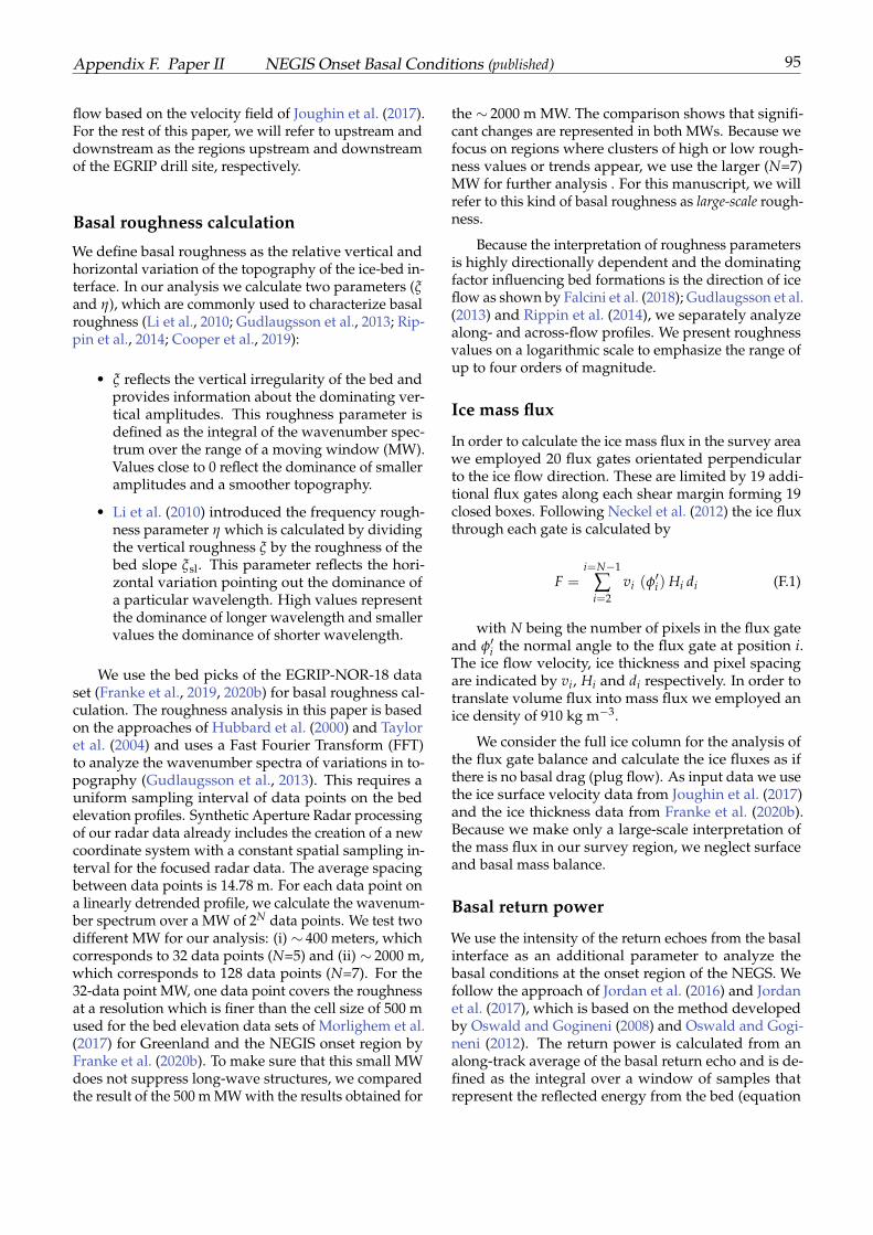
Appendix F. Paper II NEGIS Onset Basal Conditions (published) 95

flow based on the velocity field of Joughin et al. (2017).For the rest of this paper, we will refer to upstream anddownstream as the regions upstream and downstreamof the EGRIP drill site, respectively.

Basal roughness calculation

We define basal roughness as the relative vertical andhorizontal variation of the topography of the ice-bed in-terface. In our analysis we calculate two parameters (ξand η), which are commonly used to characterize basalroughness (Li et al., 2010; Gudlaugsson et al., 2013; Rip-pin et al., 2014; Cooper et al., 2019):

• ξ reflects the vertical irregularity of the bed andprovides information about the dominating ver-tical amplitudes. This roughness parameter isdefined as the integral of the wavenumber spec-trum over the range of a moving window (MW).Values close to 0 reflect the dominance of smalleramplitudes and a smoother topography.

• Li et al. (2010) introduced the frequency rough-ness parameter η which is calculated by dividingthe vertical roughness ξ by the roughness of thebed slope ξsl. This parameter reflects the hori-zontal variation pointing out the dominance ofa particular wavelength. High values representthe dominance of longer wavelength and smallervalues the dominance of shorter wavelength.

We use the bed picks of the EGRIP-NOR-18 dataset (Franke et al., 2019, 2020b) for basal roughness cal-culation. The roughness analysis in this paper is basedon the approaches of Hubbard et al. (2000) and Tayloret al. (2004) and uses a Fast Fourier Transform (FFT)to analyze the wavenumber spectra of variations in to-pography (Gudlaugsson et al., 2013). This requires auniform sampling interval of data points on the bedelevation profiles. Synthetic Aperture Radar processingof our radar data already includes the creation of a newcoordinate system with a constant spatial sampling in-terval for the focused radar data. The average spacingbetween data points is 14.78 m. For each data point ona linearly detrended profile, we calculate the wavenum-ber spectrum over a MW of 2N data points. We test twodifferent MW for our analysis: (i) ∼ 400 meters, whichcorresponds to 32 data points (N=5) and (ii) ∼ 2000 m,which corresponds to 128 data points (N=7). For the32-data point MW, one data point covers the roughnessat a resolution which is finer than the cell size of 500 mused for the bed elevation data sets of Morlighem et al.(2017) for Greenland and the NEGIS onset region byFranke et al. (2020b). To make sure that this small MWdoes not suppress long-wave structures, we comparedthe result of the 500 m MW with the results obtained for

the ∼ 2000 m MW. The comparison shows that signifi-cant changes are represented in both MWs. Because wefocus on regions where clusters of high or low rough-ness values or trends appear, we use the larger (N=7)MW for further analysis . For this manuscript, we willrefer to this kind of basal roughness as large-scale rough-ness.

Because the interpretation of roughness parametersis highly directionally dependent and the dominatingfactor influencing bed formations is the direction of iceflow as shown by Falcini et al. (2018); Gudlaugsson et al.(2013) and Rippin et al. (2014), we separately analyzealong- and across-flow profiles. We present roughnessvalues on a logarithmic scale to emphasize the range ofup to four orders of magnitude.

Ice mass flux

In order to calculate the ice mass flux in the survey areawe employed 20 flux gates orientated perpendicularto the ice flow direction. These are limited by 19 addi-tional flux gates along each shear margin forming 19closed boxes. Following Neckel et al. (2012) the ice fluxthrough each gate is calculated by

F =i=N−1

∑i=2

vi (ϕ′i) Hi di (F.1)

with N being the number of pixels in the flux gateand ϕ′

i the normal angle to the flux gate at position i.The ice flow velocity, ice thickness and pixel spacingare indicated by vi, Hi and di respectively. In order totranslate volume flux into mass flux we employed anice density of 910 kg m−3.

We consider the full ice column for the analysis ofthe flux gate balance and calculate the ice fluxes as ifthere is no basal drag (plug flow). As input data we usethe ice surface velocity data from Joughin et al. (2017)and the ice thickness data from Franke et al. (2020b).Because we make only a large-scale interpretation ofthe mass flux in our survey region, we neglect surfaceand basal mass balance.

Basal return power

We use the intensity of the return echoes from the basalinterface as an additional parameter to analyze thebasal conditions at the onset region of the NEGS. Wefollow the approach of Jordan et al. (2016) and Jordanet al. (2017), which is based on the method developedby Oswald and Gogineni (2008) and Oswald and Gogi-neni (2012). The return power is calculated from analong-track average of the basal return echo and is de-fined as the integral over a window of samples thatrepresent the reflected energy from the bed (equation

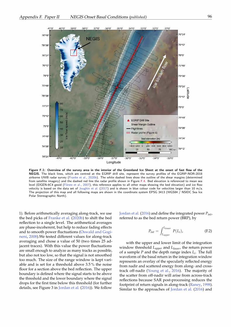
Appendix F. Paper II NEGIS Onset Basal Conditions (published) 96

Figure F.1: Overview of the survey area in the interior of the Greenland Ice Sheet at the onset of fast flow of theNEGIS. The black lines, which are centred at the EGRIP drill site, represent the survey profiles of the EGRIP-NOR-2018airborne UWB radar survey (Franke et al., 2020b). The white dashed lines show the outline of the shear margins (determinedfrom satellite imagery) and the dashed red line the radar profile shown in Figure F.4. Bed elevation is referenced to mean sealevel (EIGEN-6C4 geoid (Förste et al., 2007), this reference applies to all other maps showing the bed elevation) and ice flowvelocity is based on the data set of Joughin et al. (2017) and is shown in blue colour code for velocities larger than 10 m/a.The projection of this map and all following maps are shown in the coordinate system EPSG 3413 (WGS84 / NSIDC Sea IcePolar Stereographic North).

1). Before arithmetically averaging along-track, we usethe bed picks of Franke et al. (2020b) to shift the bedreflection to a single level. The arithmetical averagesare phase-incoherent, but help to reduce fading effectsand to smooth power fluctuations (Oswald and Gogi-neni, 2008).We tested different values for along-trackaveraging and chose a value of 50 (two times 25 ad-jacent traces). With this value the power fluctuationsare small enough to analyze as many tracks as possible,but also not too low, so that the signal is not smoothedtoo much. The size of the range window is kept vari-able and is set for a threshold above 3.5 % the noisefloor for a section above the bed reflection. The upperboundary is defined where the signal starts to be abovethe threshold and the lower boundary where the signaldrops for the first time below this threshold (for furtherdetails, see Figure 3 in Jordan et al. (2016)). We follow

Jordan et al. (2016) and define the integrated power Pint,referred to as the bed return power (BRP), by

Pint =∫ Llower

LupperP(Li), (F.2)

with the upper and lower limit of the integrationwindow threshold Lupper and Llower, the return powerof a sample P and the depth range index Li. The fullwaveform of the basal return in the integration windowrepresents an overlay of the specularly reflected energyfrom nadir and scattered energy from along- and cross-track off-nadir (Young et al., 2016). The majority ofthe scatter from off-nadir will arise from across-trackreflections because SAR post-processing reduces thefootprint of return signals in along-track (Raney, 1998).Similar to the approaches of Jordan et al. (2016) and

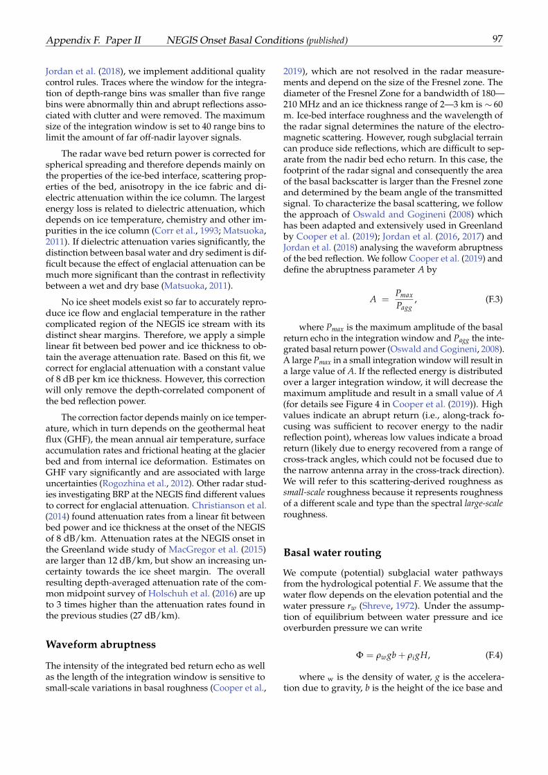
Appendix F. Paper II NEGIS Onset Basal Conditions (published) 97

Jordan et al. (2018), we implement additional qualitycontrol rules. Traces where the window for the integra-tion of depth-range bins was smaller than five rangebins were abnormally thin and abrupt reflections asso-ciated with clutter and were removed. The maximumsize of the integration window is set to 40 range bins tolimit the amount of far off-nadir layover signals.

The radar wave bed return power is corrected forspherical spreading and therefore depends mainly onthe properties of the ice-bed interface, scattering prop-erties of the bed, anisotropy in the ice fabric and di-electric attenuation within the ice column. The largestenergy loss is related to dielectric attenuation, whichdepends on ice temperature, chemistry and other im-purities in the ice column (Corr et al., 1993; Matsuoka,2011). If dielectric attenuation varies significantly, thedistinction between basal water and dry sediment is dif-ficult because the effect of englacial attenuation can bemuch more significant than the contrast in reflectivitybetween a wet and dry base (Matsuoka, 2011).

No ice sheet models exist so far to accurately repro-duce ice flow and englacial temperature in the rathercomplicated region of the NEGIS ice stream with itsdistinct shear margins. Therefore, we apply a simplelinear fit between bed power and ice thickness to ob-tain the average attenuation rate. Based on this fit, wecorrect for englacial attenuation with a constant valueof 8 dB per km ice thickness. However, this correctionwill only remove the depth-correlated component ofthe bed reflection power.

The correction factor depends mainly on ice temper-ature, which in turn depends on the geothermal heatflux (GHF), the mean annual air temperature, surfaceaccumulation rates and frictional heating at the glacierbed and from internal ice deformation. Estimates onGHF vary significantly and are associated with largeuncertainties (Rogozhina et al., 2012). Other radar stud-ies investigating BRP at the NEGIS find different valuesto correct for englacial attenuation. Christianson et al.(2014) found attenuation rates from a linear fit betweenbed power and ice thickness at the onset of the NEGISof 8 dB/km. Attenuation rates at the NEGIS onset inthe Greenland wide study of MacGregor et al. (2015)are larger than 12 dB/km, but show an increasing un-certainty towards the ice sheet margin. The overallresulting depth-averaged attenuation rate of the com-mon midpoint survey of Holschuh et al. (2016) are upto 3 times higher than the attenuation rates found inthe previous studies (27 dB/km).

Waveform abruptness

The intensity of the integrated bed return echo as wellas the length of the integration window is sensitive tosmall-scale variations in basal roughness (Cooper et al.,

2019), which are not resolved in the radar measure-ments and depend on the size of the Fresnel zone. Thediameter of the Fresnel Zone for a bandwidth of 180—210 MHz and an ice thickness range of 2—3 km is ∼ 60m. Ice-bed interface roughness and the wavelength ofthe radar signal determines the nature of the electro-magnetic scattering. However, rough subglacial terraincan produce side reflections, which are difficult to sep-arate from the nadir bed echo return. In this case, thefootprint of the radar signal and consequently the areaof the basal backscatter is larger than the Fresnel zoneand determined by the beam angle of the transmittedsignal. To characterize the basal scattering, we followthe approach of Oswald and Gogineni (2008) whichhas been adapted and extensively used in Greenlandby Cooper et al. (2019); Jordan et al. (2016, 2017) andJordan et al. (2018) analysing the waveform abruptnessof the bed reflection. We follow Cooper et al. (2019) anddefine the abruptness parameter A by

A =Pmax

Pagg, (F.3)

where Pmax is the maximum amplitude of the basalreturn echo in the integration window and Pagg the inte-grated basal return power (Oswald and Gogineni, 2008).A large Pmax in a small integration window will result ina large value of A. If the reflected energy is distributedover a larger integration window, it will decrease themaximum amplitude and result in a small value of A(for details see Figure 4 in Cooper et al. (2019)). Highvalues indicate an abrupt return (i.e., along-track fo-cusing was sufficient to recover energy to the nadirreflection point), whereas low values indicate a broadreturn (likely due to energy recovered from a range ofcross-track angles, which could not be focused due tothe narrow antenna array in the cross-track direction).We will refer to this scattering-derived roughness assmall-scale roughness because it represents roughnessof a different scale and type than the spectral large-scaleroughness.

Basal water routing

We compute (potential) subglacial water pathwaysfrom the hydrological potential F. We assume that thewater flow depends on the elevation potential and thewater pressure rw (Shreve, 1972). Under the assump-tion of equilibrium between water pressure and iceoverburden pressure we can write

Φ = ρwgb + ρigH, (F.4)

where w is the density of water, g is the accelera-tion due to gravity, b is the height of the ice base and

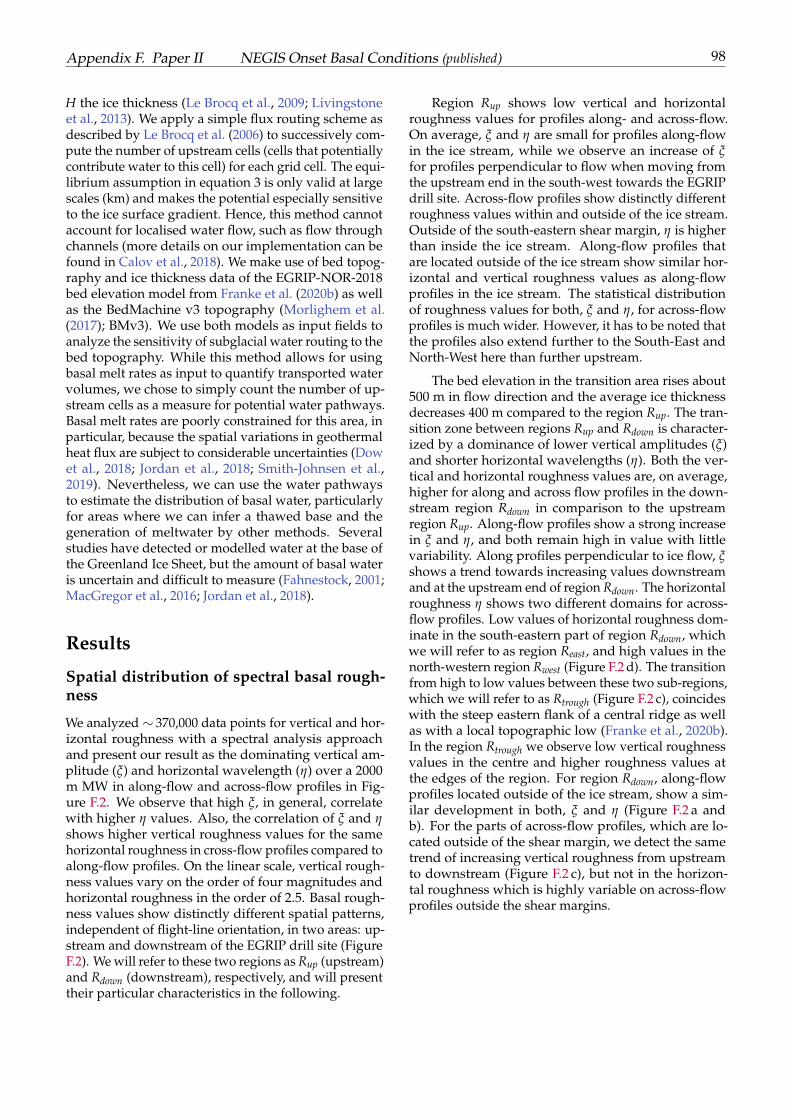
Appendix F. Paper II NEGIS Onset Basal Conditions (published) 98

H the ice thickness (Le Brocq et al., 2009; Livingstoneet al., 2013). We apply a simple flux routing scheme asdescribed by Le Brocq et al. (2006) to successively com-pute the number of upstream cells (cells that potentiallycontribute water to this cell) for each grid cell. The equi-librium assumption in equation 3 is only valid at largescales (km) and makes the potential especially sensitiveto the ice surface gradient. Hence, this method cannotaccount for localised water flow, such as flow throughchannels (more details on our implementation can befound in Calov et al., 2018). We make use of bed topog-raphy and ice thickness data of the EGRIP-NOR-2018bed elevation model from Franke et al. (2020b) as wellas the BedMachine v3 topography (Morlighem et al.(2017); BMv3). We use both models as input fields toanalyze the sensitivity of subglacial water routing to thebed topography. While this method allows for usingbasal melt rates as input to quantify transported watervolumes, we chose to simply count the number of up-stream cells as a measure for potential water pathways.Basal melt rates are poorly constrained for this area, inparticular, because the spatial variations in geothermalheat flux are subject to considerable uncertainties (Dowet al., 2018; Jordan et al., 2018; Smith-Johnsen et al.,2019). Nevertheless, we can use the water pathwaysto estimate the distribution of basal water, particularlyfor areas where we can infer a thawed base and thegeneration of meltwater by other methods. Severalstudies have detected or modelled water at the base ofthe Greenland Ice Sheet, but the amount of basal wateris uncertain and difficult to measure (Fahnestock, 2001;MacGregor et al., 2016; Jordan et al., 2018).

Results

Spatial distribution of spectral basal rough-ness

We analyzed ∼ 370,000 data points for vertical and hor-izontal roughness with a spectral analysis approachand present our result as the dominating vertical am-plitude (ξ) and horizontal wavelength (η) over a 2000m MW in along-flow and across-flow profiles in Fig-ure F.2. We observe that high ξ, in general, correlatewith higher η values. Also, the correlation of ξ and ηshows higher vertical roughness values for the samehorizontal roughness in cross-flow profiles compared toalong-flow profiles. On the linear scale, vertical rough-ness values vary on the order of four magnitudes andhorizontal roughness in the order of 2.5. Basal rough-ness values show distinctly different spatial patterns,independent of flight-line orientation, in two areas: up-stream and downstream of the EGRIP drill site (FigureF.2). We will refer to these two regions as Rup (upstream)and Rdown (downstream), respectively, and will presenttheir particular characteristics in the following.

Region Rup shows low vertical and horizontalroughness values for profiles along- and across-flow.On average, ξ and η are small for profiles along-flowin the ice stream, while we observe an increase of ξfor profiles perpendicular to flow when moving fromthe upstream end in the south-west towards the EGRIPdrill site. Across-flow profiles show distinctly differentroughness values within and outside of the ice stream.Outside of the south-eastern shear margin, η is higherthan inside the ice stream. Along-flow profiles thatare located outside of the ice stream show similar hor-izontal and vertical roughness values as along-flowprofiles in the ice stream. The statistical distributionof roughness values for both, ξ and η, for across-flowprofiles is much wider. However, it has to be noted thatthe profiles also extend further to the South-East andNorth-West here than further upstream.

The bed elevation in the transition area rises about500 m in flow direction and the average ice thicknessdecreases 400 m compared to the region Rup. The tran-sition zone between regions Rup and Rdown is character-ized by a dominance of lower vertical amplitudes (ξ)and shorter horizontal wavelengths (η). Both the ver-tical and horizontal roughness values are, on average,higher for along and across flow profiles in the down-stream region Rdown in comparison to the upstreamregion Rup. Along-flow profiles show a strong increasein ξ and η, and both remain high in value with littlevariability. Along profiles perpendicular to ice flow, ξshows a trend towards increasing values downstreamand at the upstream end of region Rdown. The horizontalroughness η shows two different domains for across-flow profiles. Low values of horizontal roughness dom-inate in the south-eastern part of region Rdown, whichwe will refer to as region Reast, and high values in thenorth-western region Rwest (Figure F.2 d). The transitionfrom high to low values between these two sub-regions,which we will refer to as Rtrough (Figure F.2 c), coincideswith the steep eastern flank of a central ridge as wellas with a local topographic low (Franke et al., 2020b).In the region Rtrough we observe low vertical roughnessvalues in the centre and higher roughness values atthe edges of the region. For region Rdown, along-flowprofiles located outside of the ice stream, show a sim-ilar development in both, ξ and η (Figure F.2 a andb). For the parts of across-flow profiles, which are lo-cated outside of the shear margin, we detect the sametrend of increasing vertical roughness from upstreamto downstream (Figure F.2 c), but not in the horizon-tal roughness which is highly variable on across-flowprofiles outside the shear margins.

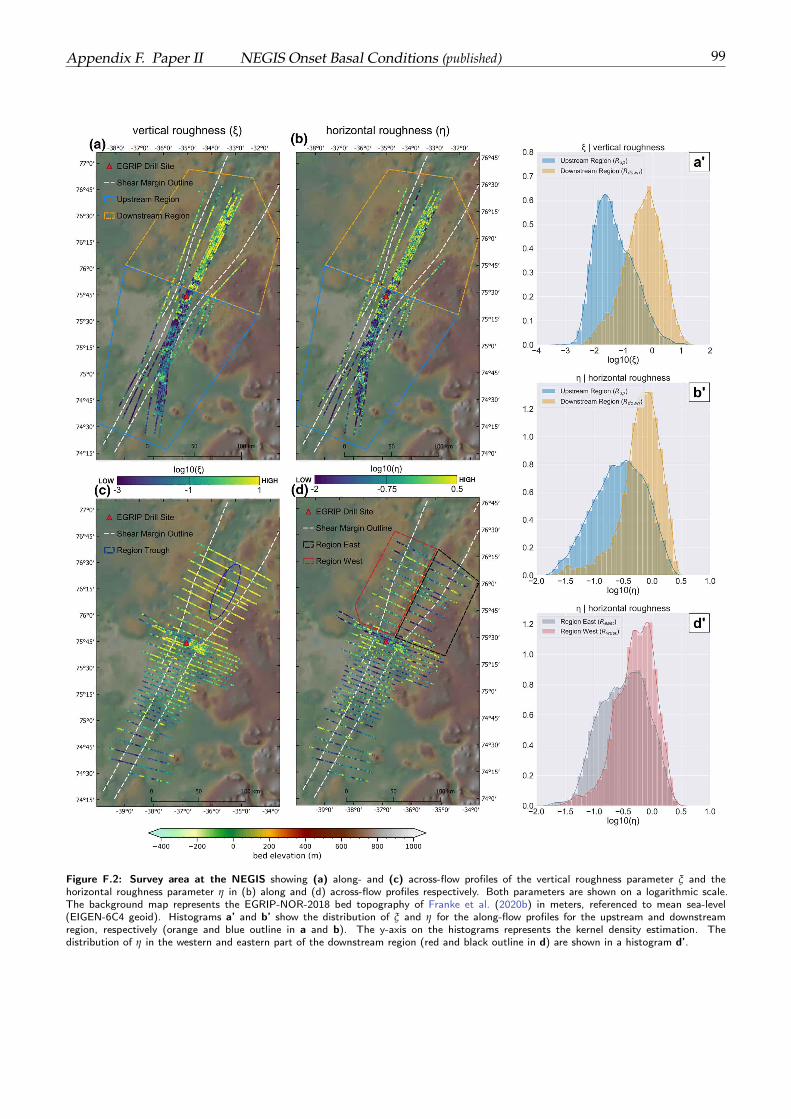
Appendix F. Paper II NEGIS Onset Basal Conditions (published) 99

Figure F.2: Survey area at the NEGIS showing (a) along- and (c) across-flow profiles of the vertical roughness parameter ξ and thehorizontal roughness parameter η in (b) along and (d) across-flow profiles respectively. Both parameters are shown on a logarithmic scale.The background map represents the EGRIP-NOR-2018 bed topography of Franke et al. (2020b) in meters, referenced to mean sea-level(EIGEN-6C4 geoid). Histograms a’ and b’ show the distribution of ξ and η for the along-flow profiles for the upstream and downstreamregion, respectively (orange and blue outline in a and b). The y-axis on the histograms represents the kernel density estimation. Thedistribution of η in the western and eastern part of the downstream region (red and black outline in d) are shown in a histogram d’.

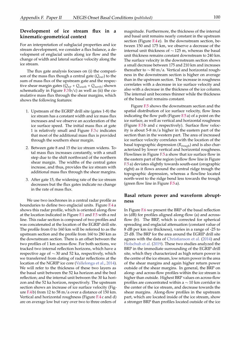
Appendix F. Paper II NEGIS Onset Basal Conditions (published) 100

Development of ice stream flux in akinematic-geometrical context

For an interpretation of subglacial properties and icestream development, we consider a flux balance, a de-velopment of englacial units along ice flow and thechange of width and lateral surface velocity along theice stream.

The flux gate analysis focuses on (i) the compari-son of the mass flux though a central gate (Qout) to thesum of mass flux of the upstream gate and the respec-tive shear margin gates (Qup + Qsouth + Qnorth; shownschematically in Figure F.3 b/c) as well as (ii) the cu-mulative mass flux through the shear margins, whichshows the following features:

1. Upstream of the EGRIP drill site (gates 1-8) theice stream has a constant width and ice mass fluxincreases and we observe an acceleration of theice surface speed. The initial mass flux at gate1 is relatively small and Figure F.3 c indicatesthat most of the additional mass flux is providedthrough the southern shear margin.

2. Between gate 8 and 15 the ice stream widens. To-tal mass flux increases constantly, with a smallstep due to the shift northward of the northernshear margin. The widths of the central gatesincrease, and thus, provides the ice stream withadditional mass flux through the shear margins.

3. After gate 15, the widening rate of the ice streamdecreases but the flux gates indicate no changein the rate of mass flux.

We use two isochrones in a central radar profile asboundaries to define two englacial units. Figure F.4 ashows this radar profile, which is oriented along-flowat the location indicated in Figure F.1 and F.5 with a redline. This radar section is composed of two profiles andwas concatenated at the location of the EGRIP drill site.The profile from 0 to 160 km will be referred to as theupstream section and the profile from 160 to 280 km asthe downstream section. There is an offset between thetwo profiles of 1 km across-flow. For both sections, wetracked two internal reflection horizons, which have arespective age of ∼ 30 and 52 ka, respectively, whichwe transferred from dating of radar reflections at thelocation of the NGRIP ice core (Vallelonga et al., 2014).We will refer to the thickness of these two layers asthe basal unit between the 52 ka horizon and the bedreflection; and the internal unit between the 30 ka hori-zon and the 52 ka horizon, respectively. The upstreamsection shows an increase of ice surface velocity (Fig-ure F.4 b) from 12 to 58 m/a over a distance of 150 km.Vertical and horizontal roughness (Figure F.4 c and d)are on average low but vary over two to three orders of

magnitude. Furthermore, the thickness of the internaland basal unit remains nearly constant in the upstreamsection (Figure F.4 e). In the downstream section, be-tween 150 and 175 km, we observe a decrease of theinternal unit thickness of ∼ 125 m, whereas the basalunit thickness remains constant downstream to 240 km.The surface velocity in the downstream section showsa small decrease between 175 and 210 km and increasesthereafter to ∼ 80 m/a. Vertical and horizontal rough-ness in the downstream section is higher on averagethan in the upstream section. The increase in roughnesscorrelates with a decrease in ice surface velocity andalso with a decrease in the thickness of the ice column.The internal unit becomes thinner while the thicknessof the basal unit remains constant.

Figure F.5 shows the downstream section and thespatial distribution of ice surface velocity, flow linesindicating the flow path (Figure F.5 a) of a point on theice surface, as well as vertical and horizontal roughness(Figure F.5 b and c respectively). Surface flow veloc-ity is about 5-8 m/a higher in the eastern part of thesection than in the western part. The area of increasedice surface velocity correlates with the location of thebasal topographic depression (Rtrough) and is also char-acterized by lower vertical and horizontal roughness.Flowlines in Figure F.5 a show that ice surface flow inthe eastern part of the region (yellow flow line in FigureF.5 a) deviates slightly towards south-east (orographicright) as it flows around the central ridge trough thetopographic depression, whereas a flowline locatednorth-west to the ridge bend less towards the trough(green flow line in Figure F.5 a).

Basal return power and waveform abrupt-ness

In Figure F.6 we present the BRP of the basal reflectionin (dB) for profiles aligned along-flow (a) and across-flow (b). The BRP, which is corrected for sphericalspreading and englacial attenuation (constant value of8 dB per km ice thickness), varies in a range of -25 to25 dB. The BRP for the area around the EGRIP drill siteagrees with the data of Christianson et al. (2014) andHolschuh et al. (2019). These two studies analyzed theBRP in the immediate surrounding of the EGRIP drillsite, which they characterized as high return power inthe centre of the ice stream, low return power in the areaof the shear margins and again higher return poweroutside of the shear margins. In general, the BRP onalong- and across-flow profiles within the ice stream ishigher than outside. Highest BRP values on across-flowprofiles are concentrated within a ∼ 10 km corridor inthe center of the ice stream, and decrease towards theshear margins. Along-flow profiles in the upstreampart, which are located inside of the ice stream, showa stronger BRP than profiles located outside of the ice

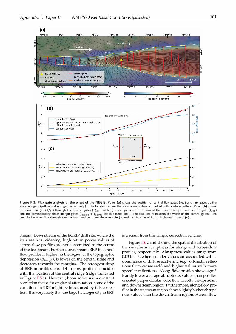
Appendix F. Paper II NEGIS Onset Basal Conditions (published) 101

Figure F.3: Flux gate analysis of the onset of the NEGIS. Panel (a) shows the position of central flux gates (red) and flux gates at theshear margins (yellow and orange, respectively). The location where the ice stream widens is marked with a white outline. Panel (b) showsthe mass flux (in Gt/yr) through the central gates (Qout; red line) in comparison to the sum of the respective upstream central gate (Qup)and the corresponding shear margin gates (Qsouth + Qnorth; black dashed line). The blue line represents the width of the central gates. Thecumulative mass flux through the northern and southern shear margin (as well as the sum of both) is shown in panel (c).

stream. Downstream of the EGRIP drill site, where theice stream is widening, high return power values ofacross-flow profiles are not constrained to the centreof the ice stream. Further downstream, BRP in across-flow profiles is highest in the region of the topographicdepression (Rtrough), is lower on the central ridge anddecreases towards the margins. The strongest dropof BRP in profiles parallel to flow profiles coincideswith the location of the central ridge (ridge indicatedin Figure F.5 a). However, because we use a constantcorrection factor for englacial attenuation, some of thevariations in BRP might be introduced by this correc-tion. It is very likely that the large heterogeneity in BRP

is a result from this simple correction scheme.

Figure F.6 c and d show the spatial distribution ofthe waveform abruptness for along- and across-flowprofiles, respectively. Abruptness values range from0.03 to 0.6, where smaller values are associated with adominance of diffuse scattering (e.g. off-nadir reflec-tions from cross-track) and higher values with morespecular reflections. Along-flow profiles show signif-icantly lower average abruptness values than profilesoriented perpendicular to ice flow in both, the upstreamand downstream region. Furthermore, along-flow pro-files in the upstream region show slightly higher abrupt-ness values than the downstream region. Across-flow

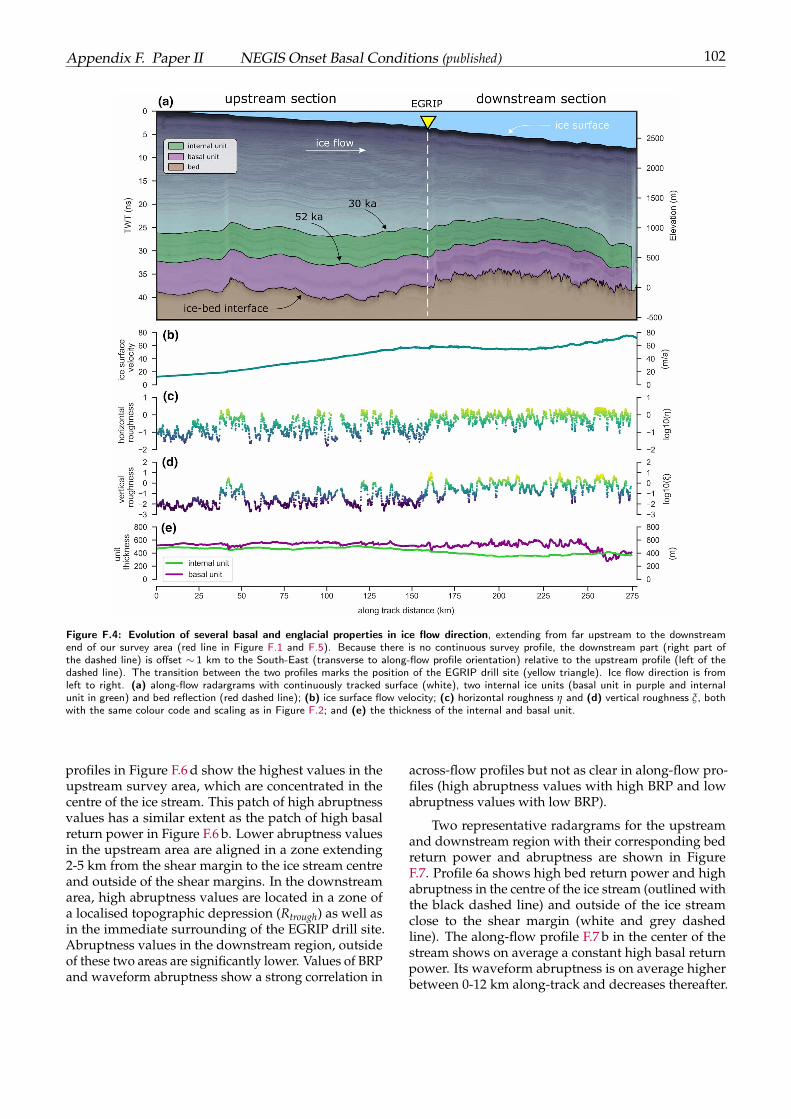
Appendix F. Paper II NEGIS Onset Basal Conditions (published) 102

Figure F.4: Evolution of several basal and englacial properties in ice flow direction, extending from far upstream to the downstreamend of our survey area (red line in Figure F.1 and F.5). Because there is no continuous survey profile, the downstream part (right part ofthe dashed line) is offset ∼ 1 km to the South-East (transverse to along-flow profile orientation) relative to the upstream profile (left of thedashed line). The transition between the two profiles marks the position of the EGRIP drill site (yellow triangle). Ice flow direction is fromleft to right. (a) along-flow radargrams with continuously tracked surface (white), two internal ice units (basal unit in purple and internalunit in green) and bed reflection (red dashed line); (b) ice surface flow velocity; (c) horizontal roughness η and (d) vertical roughness ξ, bothwith the same colour code and scaling as in Figure F.2; and (e) the thickness of the internal and basal unit.

profiles in Figure F.6 d show the highest values in theupstream survey area, which are concentrated in thecentre of the ice stream. This patch of high abruptnessvalues has a similar extent as the patch of high basalreturn power in Figure F.6 b. Lower abruptness valuesin the upstream area are aligned in a zone extending2-5 km from the shear margin to the ice stream centreand outside of the shear margins. In the downstreamarea, high abruptness values are located in a zone ofa localised topographic depression (Rtrough) as well asin the immediate surrounding of the EGRIP drill site.Abruptness values in the downstream region, outsideof these two areas are significantly lower. Values of BRPand waveform abruptness show a strong correlation in

across-flow profiles but not as clear in along-flow pro-files (high abruptness values with high BRP and lowabruptness values with low BRP).

Two representative radargrams for the upstreamand downstream region with their corresponding bedreturn power and abruptness are shown in FigureF.7. Profile 6a shows high bed return power and highabruptness in the centre of the ice stream (outlined withthe black dashed line) and outside of the ice streamclose to the shear margin (white and grey dashedline). The along-flow profile F.7 b in the center of thestream shows on average a constant high basal returnpower. Its waveform abruptness is on average higherbetween 0-12 km along-track and decreases thereafter.

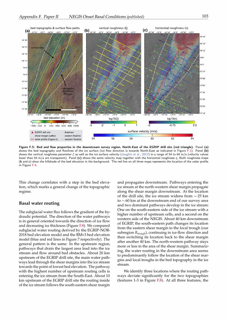
Appendix F. Paper II NEGIS Onset Basal Conditions (published) 103

Figure F.5: Bed and flow properties in the downstream survey region, North-East of the EGRIP drill site (red triangle). Panel (a)shows the bed topography and flowlines of the ice surface (ice flow direction is towards North-East as indicated in Figure F.1). Panel (b)shows the vertical roughness parameter ξ as well as the ice surface velocity (Joughin et al., 2017) in a range of 54 to 64 m/a (velocity valueslower than 54 m/a are transparent). Panel (c) shows the same velocity map together with the horizontal roughness η, Both roughness maps(b and c) show the hillshade of the bed elevation in the background. The red line on all three maps represents the location of the radar profilein Figure F.4.

This change correlates with a step in the bed eleva-tion, which marks a general change of the topographicregime.

Basal water routing

The subglacial water flux follows the gradient of the hy-draulic potential. The direction of the water pathwaysis in general oriented towards the direction of ice flowand decreasing ice thickness (Figure F.8). We comparedsubglacial water routing derived by the EGRIP-NOR-2018 bed elevation model and the BMv3 bed elevationmodel (blue and red lines in Figure 7 respectively). Thegeneral pattern is the same: In the upstream region,pathways that drain the largest area lead into the icestream and flow around bed obstacles. About 20 kmupstream of the EGRIP drill site, the main water path-ways lead through the shear margins into the ice streamtowards the point of lowest bed elevation. The pathwaywith the highest number of upstream routing cells isentering the ice stream from the South-East. About 10km upstream of the EGRIP drill site the routing insideof the ice stream follows the south-eastern shear margin

and propagates downstream. Pathways entering theice stream at the north-western shear margin propagatealong the shear margin downstream. At the locationof the drill site, the ice stream widens from ∼ 25 kmto ∼ 60 km at the downstream end of our survey areaand two dominant pathways develop in the ice stream:One on the south-eastern side of the ice stream with ahigher number of upstream cells, and a second on thewestern side of the NEGIS. About 40 km downstreamof EGRIP, the south-eastern path changes its locationfrom the eastern shear margin to the local trough (oursubregion Rtrough), continuing in ice-flow direction andthen switching its location back to the shear marginafter another 40 km. The north-western pathway staysmore or less in the area of the shear margin. Summariz-ing, the water routing in the downstream area seemsto predominantly follow the location of the shear mar-gins and local troughs in the bed topography in the icestream.

We identify three locations where the routing path-ways deviate significantly for the two topographies(features 1-3 in Figure F.8). At all three features, the

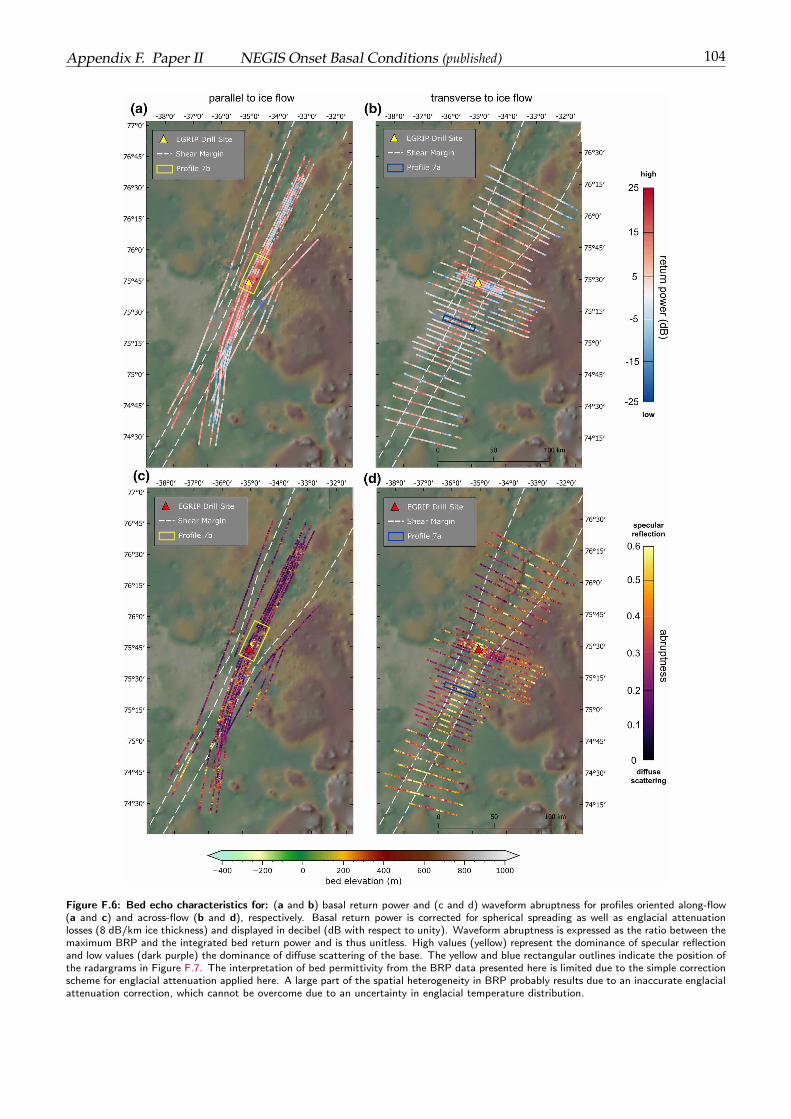
Appendix F. Paper II NEGIS Onset Basal Conditions (published) 104

Figure F.6: Bed echo characteristics for: (a and b) basal return power and (c and d) waveform abruptness for profiles oriented along-flow(a and c) and across-flow (b and d), respectively. Basal return power is corrected for spherical spreading as well as englacial attenuationlosses (8 dB/km ice thickness) and displayed in decibel (dB with respect to unity). Waveform abruptness is expressed as the ratio between themaximum BRP and the integrated bed return power and is thus unitless. High values (yellow) represent the dominance of specular reflectionand low values (dark purple) the dominance of diffuse scattering of the base. The yellow and blue rectangular outlines indicate the position ofthe radargrams in Figure F.7. The interpretation of bed permittivity from the BRP data presented here is limited due to the simple correctionscheme for englacial attenuation applied here. A large part of the spatial heterogeneity in BRP probably results due to an inaccurate englacialattenuation correction, which cannot be overcome due to an uncertainty in englacial temperature distribution.

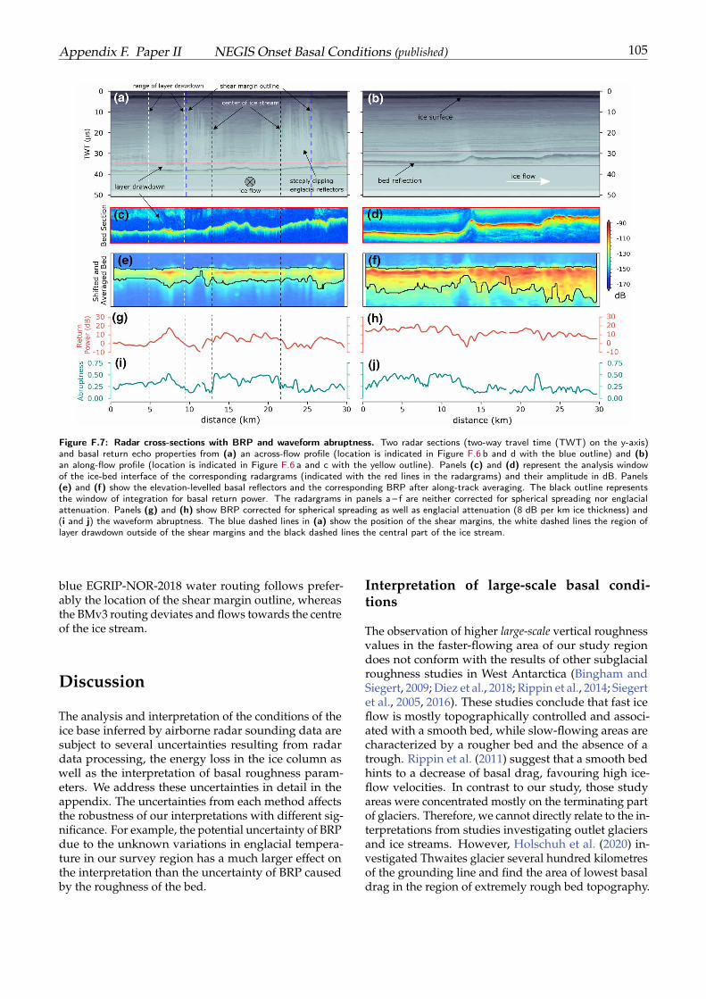
Appendix F. Paper II NEGIS Onset Basal Conditions (published) 105

Figure F.7: Radar cross-sections with BRP and waveform abruptness. Two radar sections (two-way travel time (TWT) on the y-axis)and basal return echo properties from (a) an across-flow profile (location is indicated in Figure F.6 b and d with the blue outline) and (b)an along-flow profile (location is indicated in Figure F.6 a and c with the yellow outline). Panels (c) and (d) represent the analysis windowof the ice-bed interface of the corresponding radargrams (indicated with the red lines in the radargrams) and their amplitude in dB. Panels(e) and (f) show the elevation-levelled basal reflectors and the corresponding BRP after along-track averaging. The black outline representsthe window of integration for basal return power. The radargrams in panels a – f are neither corrected for spherical spreading nor englacialattenuation. Panels (g) and (h) show BRP corrected for spherical spreading as well as englacial attenuation (8 dB per km ice thickness) and(i and j) the waveform abruptness. The blue dashed lines in (a) show the position of the shear margins, the white dashed lines the region oflayer drawdown outside of the shear margins and the black dashed lines the central part of the ice stream.

blue EGRIP-NOR-2018 water routing follows prefer-ably the location of the shear margin outline, whereasthe BMv3 routing deviates and flows towards the centreof the ice stream.

Discussion

The analysis and interpretation of the conditions of theice base inferred by airborne radar sounding data aresubject to several uncertainties resulting from radardata processing, the energy loss in the ice column aswell as the interpretation of basal roughness param-eters. We address these uncertainties in detail in theappendix. The uncertainties from each method affectsthe robustness of our interpretations with different sig-nificance. For example, the potential uncertainty of BRPdue to the unknown variations in englacial tempera-ture in our survey region has a much larger effect onthe interpretation than the uncertainty of BRP causedby the roughness of the bed.

Interpretation of large-scale basal condi-tions

The observation of higher large-scale vertical roughnessvalues in the faster-flowing area of our study regiondoes not conform with the results of other subglacialroughness studies in West Antarctica (Bingham andSiegert, 2009; Diez et al., 2018; Rippin et al., 2014; Siegertet al., 2005, 2016). These studies conclude that fast iceflow is mostly topographically controlled and associ-ated with a smooth bed, while slow-flowing areas arecharacterized by a rougher bed and the absence of atrough. Rippin et al. (2011) suggest that a smooth bedhints to a decrease of basal drag, favouring high ice-flow velocities. In contrast to our study, those studyareas were concentrated mostly on the terminating partof glaciers. Therefore, we cannot directly relate to the in-terpretations from studies investigating outlet glaciersand ice streams. However, Holschuh et al. (2020) in-vestigated Thwaites glacier several hundred kilometresof the grounding line and find the area of lowest basaldrag in the region of extremely rough bed topography.

Appendix F. Paper II NEGIS Onset Basal Conditions (published) 106

The generally higher values of vertical roughnessin across-flow profiles in comparison to along-flow pro-files of ξ and η (Figure F.9 a and b) is an indication thatthe bed has been modified by ice flow. In the upstreamregion Rup, we find a trend towards higher verticalroughness in across-flow profiles inside and outsideof the ice stream. A higher ξ in across-flow profilescould be an indication for streamlining of the bed in iceflow direction. The formation of elongated subglaciallandforms with increasing ice flow velocities cannot beinterpreted by our large-scale roughness values alonebut is supported by the observations of Franke et al.(2020b), who interpret off-nadir side reflections as anindication for the presence of elongated subglacial land-forms oriented parallel to ice flow.

Further downstream the ice stream slows down onits northern side due to a step in the bed topographyand a general change of the terrain, which might bedue to a change in bedrock type, and thus a highermean vertical roughness, which is probably not relatedto ice flow. The analysis of flux gates shows that theadditional incoming ice mass through the shear mar-gins is evacuated by two different mechanisms. Inthe upstream regime we observe that flowlines con-verge (Figure F.3), which is compensated by along-flowstretching due to ice stream acceleration. Downstreamof flux gate 8, ice flow acceleration decreases, the icestream widens and flowlines do neither converge ordiverge. Hence, the widening of the ice stream hastwo interdependent effects: (i) excess ice mass can beevacuated without ice stream acceleration but also (ii)more ice is added to the system on a shorter distancedue to the widening. Disregarding the initial cause forice stream widening we observe a strong interdepen-dence between the roughness of the bed, ice surfaceflow velocity and the geometry of the ice stream.

In contrast to the large-scale roughness, the small-scale roughness is defined by the reflection pattern andenergy distribution of the bed echo. The resolution of asingle point can range from ∼ 60 m, which is the foot-print of the Fresnel zone, to several 100s of meters ifoff-nadir side reflections interfere with the nadir returnsignal. For the analysis of the small-scale roughness,it is assumed that the energy reflected from a diffusereflector in a large integration window should be pro-portional to the reflected energy of a specular target ina small window. The waveform abruptness is a mea-sure for bed roughness in the across-track dimensionof a radar profile. Low abruptness values indicate arather diffuse reflection and high values a rather spec-ular reflection transverse to the flight trajectory. If anintersection of two profiles shows a high value of A inan across-flow profile and a low A on an along-flowprofile, we can infer a geomorphologic anisotropy, thatindicates streamlining in ice flow direction (Figure F.9 c).This anisotropy is significant in the centre of the ice

stream in the upstream region (Figure F.6 c and d) andsupports the hypothesis of a streamlined bed.

Unlike the pattern in the waveform abruptness, wefind no significant directional anisotropy in basal returnpower (Figure F.9 d). The basal return power can beinfluenced either by the scattering characteristics of thebase, englacial energy loss due to folded internal layersor scattering, the thermal state of the ice as well as theavailability and amount of liquid water at the base or acombination of these factors.

Englacial attenuation should be higher in the icestream than in the surrounding ice (Matsuoka et al.,2012) and probably highest at the shear margin dueto an increase in ice temperature by internal shear. Itis likely that elevated temperatures in the margins doaffect the BRP (see Holschuh et al. 2019). However, wehave no evidence in our data to state if the increase intemperature is substantial to indicate temperate ice orthe production of basal melt water. The existence oftemperate ice in some regions would agree with a sub-glacial hydrology modelling study by Riverman et al.(2019). They suggested that subglacial bedforms inthe shear margins are created by melt out of sedimentwithin the ice column. The phenomenon described byKeisling et al. (2014) and Holschuh et al. (2014) of weakinternal reflections at steeply dipping englacial reflec-tors in the shear margin area, as indicated in FigureF.7 a, does most likely have no effect on the BRP.

We find several indications that the BRP is influ-enced by the roughness of the bed. Within the icestream area, we find higher BRP associated with highabruptness values in across-track profiles (see FigureF.6 b and d) as well as with low vertical roughness val-ues (see Figure F.2 c). Low BRP on the central ridge inthe downstream area is associated with low abruptnessand high vertical roughness values in both along- andacross-flow profiles. From this relationship we can in-terpret that the bed roughness can explain many of thechanges in BRP inside of the ice stream. This intercon-nection was also observed by MacGregor et al. (2013)at the eastern shear margin at Thwaites Glacier.

The high BRP and low large- and small-scale rough-ness values in across-flow profiles in the centre of re-gion Rup could be interpreted as an indication for weak,porous, water saturated sediment, following similarinterpretations of Rippin et al. (2011). As the modeledsubglacial water routes suggest, it is possible that wateris continuously channelled towards the ice stream andweakens the subglacial sediments, which could have apotential stabilising effect on the ice flow (Bougamontet al., 2014). Our routing paths indicate that basal waterdoes not leave the ice stream. Consequently, the basecould become increasingly lubricated, reducing basalshear stress and facilitating basal slip.

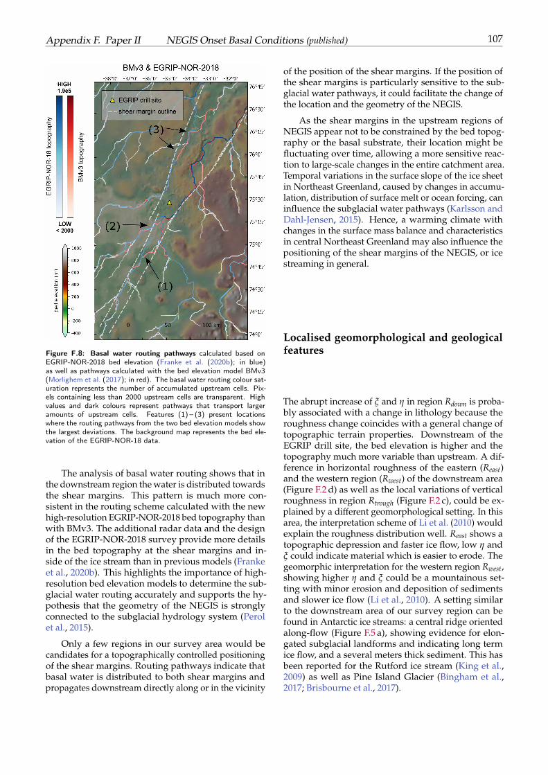
Appendix F. Paper II NEGIS Onset Basal Conditions (published) 107

Figure F.8: Basal water routing pathways calculated based onEGRIP-NOR-2018 bed elevation (Franke et al. (2020b); in blue)as well as pathways calculated with the bed elevation model BMv3(Morlighem et al. (2017); in red). The basal water routing colour sat-uration represents the number of accumulated upstream cells. Pix-els containing less than 2000 upstream cells are transparent. Highvalues and dark colours represent pathways that transport largeramounts of upstream cells. Features (1) – (3) present locationswhere the routing pathways from the two bed elevation models showthe largest deviations. The background map represents the bed ele-vation of the EGRIP-NOR-18 data.

The analysis of basal water routing shows that inthe downstream region the water is distributed towardsthe shear margins. This pattern is much more con-sistent in the routing scheme calculated with the newhigh-resolution EGRIP-NOR-2018 bed topography thanwith BMv3. The additional radar data and the designof the EGRIP-NOR-2018 survey provide more detailsin the bed topography at the shear margins and in-side of the ice stream than in previous models (Frankeet al., 2020b). This highlights the importance of high-resolution bed elevation models to determine the sub-glacial water routing accurately and supports the hy-pothesis that the geometry of the NEGIS is stronglyconnected to the subglacial hydrology system (Perolet al., 2015).

Only a few regions in our survey area would becandidates for a topographically controlled positioningof the shear margins. Routing pathways indicate thatbasal water is distributed to both shear margins andpropagates downstream directly along or in the vicinity

of the position of the shear margins. If the position ofthe shear margins is particularly sensitive to the sub-glacial water pathways, it could facilitate the change ofthe location and the geometry of the NEGIS.

As the shear margins in the upstream regions ofNEGIS appear not to be constrained by the bed topog-raphy or the basal substrate, their location might befluctuating over time, allowing a more sensitive reac-tion to large-scale changes in the entire catchment area.Temporal variations in the surface slope of the ice sheetin Northeast Greenland, caused by changes in accumu-lation, distribution of surface melt or ocean forcing, caninfluence the subglacial water pathways (Karlsson andDahl-Jensen, 2015). Hence, a warming climate withchanges in the surface mass balance and characteristicsin central Northeast Greenland may also influence thepositioning of the shear margins of the NEGIS, or icestreaming in general.

Localised geomorphological and geologicalfeatures

The abrupt increase of ξ and η in region Rdown is proba-bly associated with a change in lithology because theroughness change coincides with a general change oftopographic terrain properties. Downstream of theEGRIP drill site, the bed elevation is higher and thetopography much more variable than upstream. A dif-ference in horizontal roughness of the eastern (Reast)and the western region (Rwest) of the downstream area(Figure F.2 d) as well as the local variations of verticalroughness in region Rtrough (Figure F.2 c), could be ex-plained by a different geomorphological setting. In thisarea, the interpretation scheme of Li et al. (2010) wouldexplain the roughness distribution well. Reast shows atopographic depression and faster ice flow, low η andξ could indicate material which is easier to erode. Thegeomorphic interpretation for the western region Rwest,showing higher η and ξ could be a mountainous set-ting with minor erosion and deposition of sedimentsand slower ice flow (Li et al., 2010). A setting similarto the downstream area of our survey region can befound in Antarctic ice streams: a central ridge orientedalong-flow (Figure F.5 a), showing evidence for elon-gated subglacial landforms and indicating long termice flow, and a several meters thick sediment. This hasbeen reported for the Rutford ice stream (King et al.,2009) as well as Pine Island Glacier (Bingham et al.,2017; Brisbourne et al., 2017).

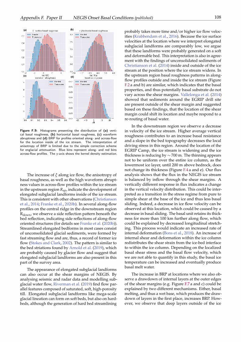
Appendix F. Paper II NEGIS Onset Basal Conditions (published) 108

Figure F.9: Histograms presenting the distribution of (a) verti-cal basal roughness, (b) horizontal basal roughness, (c) waveformabruptness and (d) BRP for profiles oriented along- and across-flowfor the location inside of the ice stream. The interpretation ofanisotropy of BRP is limited due to the simple correction schemefor englacial attenuation. Blue bins represent along- and red binsacross-flow profiles. The y-axis shows the kernel density estimation.

The increase of ξ along ice flow, the anisotropy ofbasal roughness, as well as the high waveform abrupt-ness values in across-flow profiles within the ice streamin the upstream region Rup, indicate the development ofelongated subglacial landforms inside of the ice stream.This is consistent with other observations (Christiansonet al., 2014; Franke et al., 2020b). In several along-flowprofiles on the central ridge in the downstream regionRdown, we observe a side reflection pattern beneath thebed reflection, indicating side reflections of along-floworiented structures (for details see Franke et al. (2020b)).Streamlined elongated bedforms in most cases consistof unconsolidated glacial sediments, were formed byfast streaming flow and are, thus, a record of former iceflow (Stokes and Clark, 2002). The pattern is similar tothe bed striations found by Arnold et al. (2019), whichare probably caused by glacier flow and suggest thatelongated subglacial landforms are also present in thispart of the survey area.

The appearance of elongated subglacial landformscan also occur at the shear margins of NEGIS. Byanalysing seismic and radar data and modelling sub-glacial water flow, Riverman et al. (2019) find flow par-allel features composed of saturated, soft, high-porositytill. Elongated subglacial landforms like mega-scaleglacial lineation can form on soft beds, but also on hard-beds, although the generation of hard bed streamlining

probably takes more time and/or higher ice flow veloc-ities (Krabbendam et al., 2016). Because the ice surfacevelocities at the location where we interpret elongatedsubglacial landforms are comparably low, we arguethat these landforms were probably generated on a softand deformable bed. This interpretation is also in agree-ment with the findings of unconsolidated sediments ofChristianson et al. (2014) inside and outside of the icestream at the position where the ice stream widens. Inthe upstream region basal roughness patterns in along-flow profiles outside and inside the ice stream (FigureF.2 a and b) are similar, which indicates that the basalproperties, and thus potentially basal substrate do notvary across the shear margins. Vallelonga et al. (2014)showed that sediments around the EGRIP drill siteare present outside of the shear margin and suggestedbased on these findings, that the location of the shearmargin could shift its location and maybe respond to are-routing of basal water.

In the downstream region we observe a decreasein velocity of the ice stream. Higher average verticalroughness contributes to an increase basal resistanceand a slope in the bed topography decreases the localdriving stress in this region. Around the location of theEGRIP Camp, the ice stream is widening and the icethickness is reducing by ∼ 700 m. The thinning appearsnot to be uniform over the entire ice column, as thelowermost ice layer, until 200 m above bedrock, doesnot change its thickness (Figure F.4 a and e). Our fluxanalysis shows that the flux in the NEGIS ice streamis balanced by inflow through the shear margins. Avertically different response in flux indicates a changein the vertical velocity distribution. This could be inter-preted as a transition in the stress regime from pure tosimple shear at the base of the ice and thus less basalsliding. Indeed, a decrease in ice flow velocity can beobserved at this location, which could be caused by adecrease in basal sliding. The basal unit retains its thick-ness for more than 100 km further along flow, whichcould be explained by decreased longitudinal stretch-ing. This process would indicate an increased rate ofinternal deformation (Bons et al., 2018). An increase ofinternal shear and deformation within the ice columnredistributes the shear strain from the ice-bed interfaceto within the ice column. Depending on the localizedbasal shear stress and the basal flow velocity, whichwe are not able to quantify in this study, the basal icetemperature can be increased and eventually producebasal melt water.

The increase in BRP at locations where we also ob-serve a drawdown of internal layers at the outer edgesof the shear margins (e.g. Figure F.7 a and c) could beexplained by two different mechanisms. Either, basalmelting, and thus a wet base, which produces the draw-down of layers in the first place, increases BRP. How-ever, we observe that deep layers outside of the ice

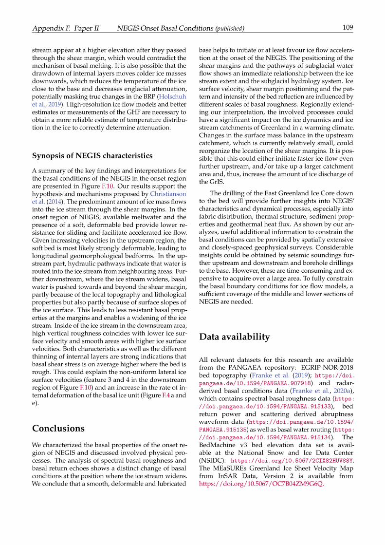
Appendix F. Paper II NEGIS Onset Basal Conditions (published) 109

stream appear at a higher elevation after they passedthrough the shear margin, which would contradict themechanism of basal melting. It is also possible that thedrawdown of internal layers moves colder ice massesdownwards, which reduces the temperature of the iceclose to the base and decreases englacial attenuation,potentially masking true changes in the BRP (Holschuhet al., 2019). High-resolution ice flow models and betterestimates or measurements of the GHF are necessary toobtain a more reliable estimate of temperature distribu-tion in the ice to correctly determine attenuation.

Synopsis of NEGIS characteristics

A summary of the key findings and interpretations forthe basal conditions of the NEGIS in the onset regionare presented in Figure F.10. Our results support thehypothesis and mechanisms proposed by Christiansonet al. (2014). The predominant amount of ice mass flowsinto the ice stream through the shear margins. In theonset region of NEGIS, available meltwater and thepresence of a soft, deformable bed provide lower re-sistance for sliding and facilitate accelerated ice flow.Given increasing velocities in the upstream region, thesoft bed is most likely strongly deformable, leading tolongitudinal geomorphological bedforms. In the up-stream part, hydraulic pathways indicate that water isrouted into the ice stream from neighbouring areas. Fur-ther downstream, where the ice stream widens, basalwater is pushed towards and beyond the shear margin,partly because of the local topography and lithologicalproperties but also partly because of surface slopes ofthe ice surface. This leads to less resistant basal prop-erties at the margins and enables a widening of the icestream. Inside of the ice stream in the downstream area,high vertical roughness coincides with lower ice sur-face velocity and smooth areas with higher ice surfacevelocities. Both characteristics as well as the differentthinning of internal layers are strong indications thatbasal shear stress is on average higher where the bed isrough. This could explain the non-uniform lateral icesurface velocities (feature 3 and 4 in the downstreamregion of Figure F.10) and an increase in the rate of in-ternal deformation of the basal ice unit (Figure F.4 a ande).

Conclusions

We characterized the basal properties of the onset re-gion of NEGIS and discussed involved physical pro-cesses. The analysis of spectral basal roughness andbasal return echoes shows a distinct change of basalconditions at the position where the ice stream widens.We conclude that a smooth, deformable and lubricated

base helps to initiate or at least favour ice flow accelera-tion at the onset of the NEGIS. The positioning of theshear margins and the pathways of subglacial waterflow shows an immediate relationship between the icestream extent and the subglacial hydrology system. Icesurface velocity, shear margin positioning and the pat-tern and intensity of the bed reflection are influenced bydifferent scales of basal roughness. Regionally extend-ing our interpretation, the involved processes couldhave a significant impact on the ice dynamics and icestream catchments of Greenland in a warming climate.Changes in the surface mass balance in the upstreamcatchment, which is currently relatively small, couldreorganize the location of the shear margins. It is pos-sible that this could either initiate faster ice flow evenfurther upstream, and/or take up a larger catchmentarea and, thus, increase the amount of ice discharge ofthe GrIS.

The drilling of the East Greenland Ice Core downto the bed will provide further insights into NEGIS’characteristics and dynamical processes, especially intofabric distribution, thermal structure, sediment prop-erties and geothermal heat flux. As shown by our an-alyzes, useful additional information to constrain thebasal conditions can be provided by spatially extensiveand closely-spaced geophysical surveys. Considerableinsights could be obtained by seismic soundings fur-ther upstream and downstream and borehole drillingsto the base. However, these are time-consuming and ex-pensive to acquire over a large area. To fully constrainthe basal boundary conditions for ice flow models, asufficient coverage of the middle and lower sections ofNEGIS are needed.

Data availability

All relevant datasets for this research are availablefrom the PANGAEA repository: EGRIP-NOR-2018bed topography (Franke et al. (2019); https://doi.pangaea.de/10.1594/PANGAEA.907918) and radar-derived basal conditions data (Franke et al., 2020a),which contains spectral basal roughness data (https://doi.pangaea.de/10.1594/PANGAEA.915133), bedreturn power and scattering derived abruptnesswaveform data (https://doi.pangaea.de/10.1594/PANGAEA.915135) as well as basal water routing (https://doi.pangaea.de/10.1594/PANGAEA.915134). TheBedMachine v3 bed elevation data set is avail-able at the National Snow and Ice Data Center(NSIDC): https://doi.org/10.5067/2CIX82HUV88Y.The MEaSUREs Greenland Ice Sheet Velocity Mapfrom InSAR Data, Version 2 is available fromhttps://doi.org/10.5067/OC7B04ZM9G6Q.

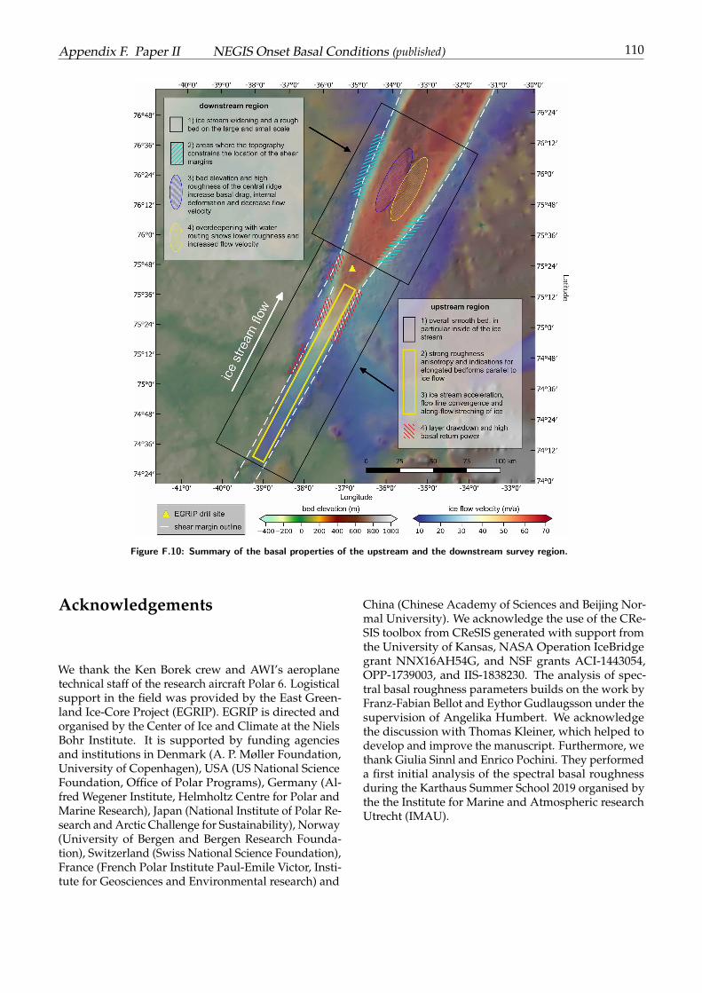
Appendix F. Paper II NEGIS Onset Basal Conditions (published) 110

Figure F.10: Summary of the basal properties of the upstream and the downstream survey region.

Acknowledgements

We thank the Ken Borek crew and AWI’s aeroplanetechnical staff of the research aircraft Polar 6. Logisticalsupport in the field was provided by the East Green-land Ice-Core Project (EGRIP). EGRIP is directed andorganised by the Center of Ice and Climate at the NielsBohr Institute. It is supported by funding agenciesand institutions in Denmark (A. P. Møller Foundation,University of Copenhagen), USA (US National ScienceFoundation, Office of Polar Programs), Germany (Al-fred Wegener Institute, Helmholtz Centre for Polar andMarine Research), Japan (National Institute of Polar Re-search and Arctic Challenge for Sustainability), Norway(University of Bergen and Bergen Research Founda-tion), Switzerland (Swiss National Science Foundation),France (French Polar Institute Paul-Emile Victor, Insti-tute for Geosciences and Environmental research) and

China (Chinese Academy of Sciences and Beijing Nor-mal University). We acknowledge the use of the CRe-SIS toolbox from CReSIS generated with support fromthe University of Kansas, NASA Operation IceBridgegrant NNX16AH54G, and NSF grants ACI-1443054,OPP-1739003, and IIS-1838230. The analysis of spec-tral basal roughness parameters builds on the work byFranz-Fabian Bellot and Eythor Gudlaugsson under thesupervision of Angelika Humbert. We acknowledgethe discussion with Thomas Kleiner, which helped todevelop and improve the manuscript. Furthermore, wethank Giulia Sinnl and Enrico Pochini. They performeda first initial analysis of the spectral basal roughnessduring the Karthaus Summer School 2019 organised bythe the Institute for Marine and Atmospheric researchUtrecht (IMAU).

Appendix F. Paper II NEGIS Onset Basal Conditions (published) 111

Author contributions

Steven Franke designed and wrote the manuscript, con-ducted the radar data processing, performed the mainpart of the data analysis and created all figures. OlafEisen and Daniela Jansen were PI and Co-I of the air-borne radar campaign and designed the study. Sebas-tian Beyer computed the hydraulic potential and basalwater pathways. Niklas Neckel and Steven Frankecalculated ice mass flux. Tobias Binder acquired theairborne radar data together with Daniela Jansen andJohn Paden. Tobias Binder contributed to the radardata processing and John Paden to the analysis of bedreturn echoes. Daniela Jansen, Steven Franke, NiklasNeckel, Sebastian Beyer and Olaf Eisen interpreted thedata. All co-authors discussed and commented on themanuscript.

Appendix

Uncertainties

Several uncertainties can influence the results and in-terpretation of the spectral bed roughness parameters.This accounts in particular for small values of ξ in con-junction with η, A major uncertainty arises from miss-ing or ambiguous bed reflections and how continuousthe tracking of the basal event is applied. In rough ter-rains, automatic trackers, e.g. of reflection power, oftencreate zigzag or step patterns whereas manual pickingis often characterized by straight lines. A combinationof both methods may represent the best possible wayto pick the bed geometry efficiently. Still, it will havean impact on both vertical and horizontal roughnessvalues, in particular when ξ is small. The uncertaintydecreases if larger vertical amplitudes come into play.Li et al. (2010) introduced schematic interpretationsfor geomorphic settings based on the combination of ξand η, which we will refer to as cases in the following.For example, low ξ and high η (case 1) can refer to amarine setting with intensive deposition of sediments.Low ξ and low η (case 2) could imply a continentalsetting after intensive erosion. For minimal values ofξ, this categorisation is accompanied with a high un-certainty based on the radar data or bed topographyproduct and the method of the ice-bed interface detec-tion. For example, automatic or semiautomatic pickingwith a maximum power tracker might lead to a high-frequency zigzag pattern leading to case 2 (erosion).Manual picking at locations where a tracker is not use-ful can smooth the surface and would favour case 1(deposition). Therefore, we argue that an interpreta-tion of subglacial landscapes with low ξ are difficult tointerpret in combination with η, even though the bedreflection is quality checked and picked very accurately.A robust interpretation of small ξ, regardless of high or

low η, is that the base is smooth. Without additionaldata like radar wave scattering properties, seismic in-formation about the basal substrate’s lithology, or anindication for the presence of water at the base, furtherinterpretations have low confidence. Another sourceof uncertainty are off-nadir/side reflections that aredifficult to distinguish from nadir reflections. Only co-herent and phase-sensitive radar depth sounders withmultiple cross-track antenna elements and appropriate3D processing algorithms can compute the directionangle of the reflected signal (Paden et al., 2010). A bet-ter estimate of the effect of cross-track roughness isthe scattering-derived waveform abruptness (Oswaldand Gogineni, 2008; Jordan et al., 2017; Cooper et al.,2019). However, this method does not consider sidereflections from far off-nadir angles.

Several uncertainties in the BRP result from themostly unobserved physical bulk properties of the icecolumn and their lateral variation, mainly across the icestream. We anticipate an effect of ice crystal anisotropyon the basal return signal due to a different expectedpreferred orientation in the crystal fabric in the icestream, outside of the ice stream and in the area ofthe shear margins. However, overall we consider it asa negligible effect on the BRP Matsuoka (2011), giventhe magnitude of other uncertainties. The most signifi-cant uncertainty will arise from the unknown dielectricattenuation of the ice column from impurity loadingand temperature, which is difficult to estimate for anice stream. It is challenging to estimate the effect ofenglacial attenuation in our survey area because icetemperature has not been sufficiently constrained yet.For an ice stream, we have to consider three differentlateral domains, with unknown dielectric attenuation:the fast-flowing central part of streaming ice, the slow-flowing part outside of the ice stream and the shearmargins. Finally, in general, a layer of temperate ice offinite thickness might be present above the bed (Hum-bert et al., 2018). As we cannot constrain its presencefurther because of missing measurements, we do notconsider it in our evaluation. An additional feature, in-fluencing the bed return intensity can be internal layersof altered ice or containing entrainments of basal mate-rial which reduce the return energy of the bed. We findareas of large folds south-west of the EGRIP drill siteoutside of the ice stream. Therefore, we excluded thisregion because the strong internal deformation and bedentrainments appear to disturb the reflection power ofthe base significantly.

Further uncertainties are related to data acquisitionand processing. Another source of uncertainty for theBRP can arise during SAR processing of the radar data.Focusing of scattered signals effectively shifts energyfrom multiple unfocused pixels into a single pixel. Asa consequence, poor focusing due to position errors ordirectional scattering may cause the return power to

Appendix F. Paper II NEGIS Onset Basal Conditions (published) 112

deviate from the ideal case. Furthermore, the steeplydipping reflectors due to englacial layer folding in thevicinity of the shear margins will most likely reducethe reflected energy from the ice-basal interface under-neath this zone. The energy loss probably occurs dueto destructive interference in trace stacking, energy dis-persion through SAR processing and off-nadir ray pathlosses (see Holschuh et al. 2014 for details).

113

BibliographyAn, L., Rignot, E., Chauche, N., Holland, D. M., Holland, D.,

Jakobsson, M., Kane, E., Wood, M., Klaucke, I., Morlighem,M., Velicogna, I., Weinrebe, W., and Willis, J. K. Bathymetryof Southeast Greenland From Oceans Melting Greenland(OMG) Data. Geophysical Research Letters, 46(20):11197–11205, oct 2019. doi: 10.1029/2019gl083953. URL https://doi.org/10.1029%2F2019gl083953.

Arndt, J. E., Larter, R. D., Hillenbrand, C.-D., Sørli, S. H.,Forwick, M., Smith, J. A., and Wacker, L. Past ice sheet–seabed interactions in the northeastern weddell sea embay-ment, antarctica. The Cryosphere, 14(6):2115–2135, 2020. doi:10.5194/tc-14-2115-2020. URL https://tc.copernicus.org/articles/14/2115/2020/.

Arnold, E., Leuschen, C., Rodriguez-Morales, F., Li, J., Paden,J., Hale, R., and Keshmiri, S. CReSIS airborne radars andplatforms for ice and snow sounding. Annals of Glaciol-ogy, pages 1–10, nov 2019. doi: 10.1017/aog.2019.37. URLhttps://doi.org/10.1017%2Faog.2019.37.

Aschwanden, A., Fahnestock, M. A., and Truffer, M. ComplexGreenland outlet glacier flow captured. Nature Communi-cations, 7(1), feb 2016. doi: 10.1038/ncomms10524. URLhttps://doi.org/10.1038%2Fncomms10524.

Bingham, R. G. and Siegert, M. J. Radar-derived bed rough-ness characterization of Institute and Möller ice streamsWest Antarctica, and comparison with Siple Coast icestreams. Geophysical Research Letters, 34(21), nov 2007. doi:10.1029/2007gl031483. URL https://doi.org/10.1029%2F2007gl031483.

Bingham, R. G. and Siegert, M. J. Quantifying subglacial bedroughness in Antarctica: implications for ice-sheet dynam-ics and history. Quaternary Science Reviews, 28(3-4):223–236,feb 2009. doi: 10.1016/j.quascirev.2008.10.014. URL https://doi.org/10.1016%2Fj.quascirev.2008.10.014.

Bingham, R. G., Vaughan, D. G., King, E. C., Davies, D., Corn-ford, S. L., Smith, A. M., Arthern, R. J., Brisbourne, A. M.,Rydt, J. D., Graham, A. G. C., Spagnolo, M., Marsh, O. J.,and Shean, D. E. Diverse landscapes beneath Pine Is-land Glacier influence ice flow. Nature Communications,8(1), nov 2017. doi: 10.1038/s41467-017-01597-y. URLhttps://doi.org/10.1038%2Fs41467-017-01597-y.

Bons, P. D., Kleiner, T., Llorens, M.-G., Prior, D. J., Sachau,T., Weikusat, I., and Jansen, D. Greenland Ice Sheet:Higher Nonlinearity of Ice Flow Significantly Reduces Es-timated Basal Motion. Geophysical Research Letters, 45(13):6542–6548, jul 2018. doi: 10.1029/2018gl078356. URLhttps://doi.org/10.1029%2F2018gl078356.

Bougamont, M., Christoffersen, P., Hubbard, A. L., Fitz-patrick, A. A., Doyle, S. H., and Carter, S. P. Sensitive re-sponse of the Greenland Ice Sheet to surface melt drainageover a soft bed. Nature Communications, 5(1), sep 2014. doi:

10.1038/ncomms6052. URL https://doi.org/10.1038%2Fncomms6052.

Brisbourne, A. M., Smith, A. M., King, E. C., Nicholls, K. W.,Holland, P. R., and Makinson, K. Seabed topography be-neath Larsen C Ice Shelf from seismic soundings. TheCryosphere, 8(1):1–13, jan 2014. doi: 10.5194/tc-8-1-2014.URL https://doi.org/10.5194%2Ftc-8-1-2014.

Brisbourne, A. M., Smith, A. M., Vaughan, D. G., King, E. C.,Davies, D., Bingham, R. G., Smith, E. C., Nias, I. J., andRosier, S. H. R. Bed conditions of Pine Island Glacier WestAntarctica. Journal of Geophysical Research: Earth Surface,122(1):419–433, jan 2017. doi: 10.1002/2016jf004033. URLhttps://doi.org/10.1002%2F2016jf004033.

Calov, R., Beyer, S., Greve, R., Beckmann, J., Willeit, M.,Kleiner, T., Rückamp, M., Humbert, A., and Ganopolski,A. Simulation of the future sea level contribution of Green-land with a new glacial system model. The Cryosphere,12(10):3097–3121, oct 2018. doi: 10.5194/tc-12-3097-2018.URL https://doi.org/10.5194%2Ftc-12-3097-2018.

Christianson, K., Peters, L. E., Alley, R. B., Anandakrishnan,S., Jacobel, R. W., Riverman, K. L., Muto, A., and Keis-ling, B. A. Dilatant till facilitates ice-stream flow in north-east Greenland. Earth and Planetary Science Letters, 401:57–69, sep 2014. doi: 10.1016/j.epsl.2014.05.060. URLhttps://doi.org/10.1016%2Fj.epsl.2014.05.060.

Clark, C. D. and Meehan, R. T. Subglacial bedform geomor-phology of the Irish Ice Sheet reveals major configurationchanges during growth and decay. Journal of QuaternaryScience, 16(5):483–496, 2001. doi: 10.1002/jqs.627. URLhttps://doi.org/10.1002%2Fjqs.627.

Clarke, G. K. SUBGLACIAL PROCESSES. AnnualReview of Earth and Planetary Sciences, 33(1):247–276,may 2005. doi: 10.1146/annurev.earth.33.092203.122621. URL https://doi.org/10.1146%2Fannurev.earth.33.092203.122621.

Cochran, J. R. and Bell, R. E. Inversion of IceBridge grav-ity data for continental shelf bathymetry beneath theLarsen Ice Shelf Antarctica. Journal of Glaciology, 58(209):540–552, 2012. doi: 10.3189/2012jog11j033. URL https://doi.org/10.3189%2F2012jog11j033.

Cooper, M. A., Jordan, T. M., Schroeder, D. M., Siegert, M. J.,Williams, C. N., and Bamber, J. L. Subglacial roughnessof the Greenland Ice Sheet: relationship with contem-porary ice velocity and geology. The Cryosphere, 13(11):3093–3115, nov 2019. doi: 10.5194/tc-13-3093-2019. URLhttps://doi.org/10.5194%2Ftc-13-3093-2019.

Corr, H., Moore, J. C., and Nicholls, K. W. Radar absorptiondue to impurities in Antarctic ice. Geophysical Research Let-ters, 20(11):1071–1074, jun 1993. doi: 10.1029/93gl01395.URL https://doi.org/10.1029%2F93gl01395.

Diez, A., Matsuoka, K., Ferraccioli, F., Jordan, T. A., Corr,H. F., Kohler, J., Olesen, A. V., and Forsberg, R. Basal Set-tings Control Fast Ice Flow in the Recovery/Slessor/BaileyRegion East Antarctica. Geophysical Research Letters, 45(6):

BIBLIOGRAPHY 114

2706–2715, mar 2018. doi: 10.1002/2017gl076601. URLhttps://doi.org/10.1002%2F2017gl076601.

Dow, C., Hubbard, A., Booth, A., Doyle, S., Gusmeroli,A., and Kulessa, B. Seismic evidence of mechanicallyweak sediments underlying Russell Glacier West Green-land. Annals of Glaciology, 54(64):135–141, 2013. doi: 10.3189/2013aog64a032. URL https://doi.org/10.3189%2F2013aog64a032.

Dow, C. F., Werder, M. A., Babonis, G., Nowicki, S.,Walker, R. T., Csatho, B., and Morlighem, M. Dynam-ics of Active Subglacial Lakes in Recovery Ice Stream.Journal of Geophysical Research: Earth Surface, 123(4):837–850, 2018. doi: https://doi.org/10.1002/2017JF004409.URL https://agupubs.onlinelibrary.wiley.com/doi/abs/10.1002/2017JF004409.

Dowdeswell, J. A., Cofaigh, C. Ó., and Pudsey, C. J. Thicknessand extent of the subglacial till layer beneath an Antarcticpaleo–ice stream. Geology, 32(1):13, 2004. doi: 10.1130/g19864.1. URL https://doi.org/10.1130%2Fg19864.1.

Durand, G., Gagliardini, O., Favier, L., Zwinger, T., andle Meur, E. Impact of bedrock description on model-ing ice sheet dynamics. Geophysical Research Letters, 38(20):n/a–n/a, oct 2011. doi: 10.1029/2011gl048892. URLhttps://doi.org/10.1029%2F2011gl048892.

Eisen, O., Winter, A., Steinhage, D., Kleiner, T., and Humbert,A. Basal roughness of the east antarctic ice sheet in relationto flow speed and basal thermal state. Annals of Glaciol-ogy, 61(81):162–175, 2020. doi: 10.1017/aog.2020.47. URLhttps://doi.org/10.1017/aog.2020.47.

Eisermann, H., Eagles, G., Ruppel, A., Smith, E. C., andJokat, W. Bathymetry beneath ice shelves of westerndronning maud land, east antarctica, and implicationson ice shelf stability. Geophysical Research Letters, 47(12):e2019GL086724, 2020. doi: https://doi.org/10.1029/2019GL086724. URL https://agupubs.onlinelibrary.wiley.com/doi/abs/10.1029/2019GL086724.

Fahnestock, M. High Geothermal Heat Flow Basal Melt,and the Origin of Rapid Ice Flow in Central Green-land. Science, 294(5550):2338–2342, dec 2001. doi: 10.1126/science.1065370. URL https://doi.org/10.1126%2Fscience.1065370.

Fahnestock, M., Bindschadler, R., Kwok, R., and Jezek, K.Greenland Ice Sheet Surface Properties and Ice Dynam-ics from ERS-1 SAR Imagery. Science, 262(5139):1530–1534, dec 1993. doi: 10.1126/science.262.5139.1530. URLhttps://doi.org/10.1126%2Fscience.262.5139.1530.

Falcini, F. A., Rippin, D. M., Krabbendam, M., and Selby,K. A. Quantifying bed roughness beneath contempo-rary and palaeo-ice streams. Journal of Glaciology, 64(247):822–834, sep 2018. doi: 10.1017/jog.2018.71. URLhttps://doi.org/10.1017%2Fjog.2018.71.

Franke, S., Jansen, D., Binder, T., Dörr, N., Paden, J., Helm,V., Steinhage, D., and Eisen, O. Bedrock topographyand ice thickness in the onset region of the Northeast

Greenland Ice Stream recorded with the airborne AWIUltra-Wideband radar (UWB) in 2018, 2019. URL https://doi.pangaea.de/10.1594/PANGAEA.907918.

Franke, S., Jansen, D., Beyer, S., Paden, J., and Eisen, O. Basalconditions of the onset zone of the Northeast GreenlandIce Stream derived from airborne ultra-wideband radardata. PANGAEA, 2020a. doi: 10.1594/PANGAEA.915136.URL https://doi.org/10.1594/PANGAEA.915136.

Franke, S., Jansen, D., Binder, T., Dörr, N., Helm, V., Paden,J., Steinhage, D., and Eisen, O. Bed topography andsubglacial landforms in the onset region of the North-east Greenland Ice Stream. Annals of Glaciology, pages1–11, mar 2020b. doi: 10.1017/aog.2020.12. URL https://doi.org/10.1017%2Faog.2020.12.

Fretwell, P., Pritchard, H. D., Vaughan, D. G., Bamber, J. L.,Barrand, N. E., Bell, R., Bianchi, C., Bingham, R. G.,Blankenship, D. D., Casassa, G., Catania, G., Callens, D.,Conway, H., Cook, A. J., Corr, H. F. J., Damaske, D., Damm,V., Ferraccioli, F., Forsberg, R., Fujita, S., Gim, Y., Gogi-neni, P., Griggs, J. A., Hindmarsh, R. C. A., Holmlund,P., Holt, J. W., Jacobel, R. W., Jenkins, A., Jokat, W., Jor-dan, T., King, E. C., Kohler, J., Krabill, W., Riger-Kusk, M.,Langley, K. A., Leitchenkov, G., Leuschen, C., Luyendyk,B. P., Matsuoka, K., Mouginot, J., Nitsche, F. O., Nogi,Y., Nost, O. A., Popov, S. V., Rignot, E., Rippin, D. M.,Rivera, A., Roberts, J., Ross, N., Siegert, M. J., Smith,A. M., Steinhage, D., Studinger, M., Sun, B., Tinto, B. K.,Welch, B. C., Wilson, D., Young, D. A., Xiangbin, C.,and Zirizzotti, A. Bedmap2: improved ice bed surfaceand thickness datasets for Antarctica. The Cryosphere, 7(1):375–393, feb 2013. doi: 10.5194/tc-7-375-2013. URLhttps://doi.org/10.5194%2Ftc-7-375-2013.

Förste, C., Schmidt, R., Stubenvoll, R., Flechtner, F., Meyer,U., König, R., Neumayer, H., Biancale, R., Lemoine, J.-M., Bruinsma, S., Loyer, S., Barthelmes, F., and Essel-born, S. The GeoForschungsZentrum Potsdam/Groupede Recherche de Gèodésie Spatiale satellite-only and com-bined gravity field models: EIGEN-GL04S1 and EIGEN-GL04C. Journal of Geodesy, 82(6):331–346, oct 2007. doi:10.1007/s00190-007-0183-8. URL https://doi.org/10.1007%2Fs00190-007-0183-8.

Gudlaugsson, E., Humbert, A., Winsborrow, M., and An-dreassen, K. Subglacial roughness of the former BarentsSea ice sheet. Journal of Geophysical Research: Earth Sur-face, 118(4):2546–2556, dec 2013. doi: 10.1002/2013jf002714.URL https://doi.org/10.1002%2F2013jf002714.

Hale, R., Miller, H., Gogineni, S., Yan, J. B., Rodriguez-Morales, F., Leuschen, C., Paden, J., Li, J., Binder, T.,Steinhage, D., Gehrmann, M., and Braaten, D. Multi-channel ultra-wideband radar sounder and imager. In2016 IEEE International Geoscience and Remote Sensing Sym-posium (IGARSS). IEEE, jul 2016. doi: 10.1109/igarss.2016.7729545. URL https://doi.org/10.1109%2Figarss.2016.7729545.

Hofstede, C., Christoffersen, P., Hubbard, B., Doyle, S. H.,Young, T. J., Diez, A., Eisen, O., and Hubbard, A. Phys-ical Conditions of Fast Glacier Flow: 2. Variable Extent

BIBLIOGRAPHY 115

of Anisotropic Ice and Soft Basal Sediment From SeismicReflection Data Acquired on Store Glacier West Green-land. Journal of Geophysical Research: Earth Surface, 123(2):349–362, feb 2018. doi: 10.1002/2017jf004297. URLhttps://doi.org/10.1002%2F2017jf004297.

Holschuh, N., Christianson, K., and Anandakrishnan, S.Power loss in dipping internal reflectors imaged usingice-penetrating radar. Annals of Glaciology, 55(67):49–56,2014. doi: 10.3189/2014aog67a005. URL https://doi.org/10.3189%2F2014aog67a005.

Holschuh, N., Christianson, K., Anandakrishnan, S., Alley,R. B., and Jacobel, R. W. Constraining attenuation uncer-tainty in common midpoint radar surveys of ice sheets.Journal of Geophysical Research: Earth Surface, 121(10):1876–1890, oct 2016. ISSN 21699011. doi: 10.1002/2016JF003942.URL http://doi.wiley.com/10.1002/2016JF003942.

Holschuh, N., Lilien, D., and Christianson, K. ThermalWeakening, Convergent Flow, and Vertical Heat Trans-port in the Northeast Greenland Ice Stream Shear Mar-gins. Geophysical Research Letters, 46:8184–8193, 2019. doi:10.1029/2019GL083436. URL https://doi.org/10.1029/2019GL083436.

Holschuh, N., Christianson, K., Paden, J., Alley, R., and Anan-dakrishnan, S. Linking postglacial landscapes to glacierdynamics using swath radar at Thwaites Glacier Antarc-tica. Geology, jan 2020. doi: 10.1130/g46772.1. URLhttps://doi.org/10.1130%2Fg46772.1.

Hubbard, B., Siegert, M. J., and McCarroll, D. Spectralroughness of glaciated bedrock geomorphic surfaces: Im-plications for glacier sliding. Journal of Geophysical Re-search: Solid Earth, 105(B9):21295–21303, sep 2000. doi:10.1029/2000jb900162. URL https://doi.org/10.1029%2F2000jb900162.

Hughes, T., Sargent, A., and Fastook, J. Ice-bed couplingbeneath and beyond ice streams: Byrd Glacier Antarc-tica. Journal of Geophysical Research, 116(F3), jul 2011. doi:10.1029/2010jf001896. URL https://doi.org/10.1029%2F2010jf001896.

Humbert, A., Steinhage, D., Helm, V., Beyer, S., and Kleiner,T. Missing Evidence of Widespread Subglacial Lakes atRecovery Glacier Antarctica. Journal of Geophysical Re-search: Earth Surface, 123(11):2802–2826, nov 2018. doi:10.1029/2017jf004591. URL https://doi.org/10.1029%2F2017jf004591.

Jacobel, R. W., Lapo, K. E., Stamp, J. R., Youngblood, B. W.,Welch, B. C., and Bamber, J. L. A comparison of basal re-flectivity and ice velocity in East Antarctica. The Cryosphere,4(4):447–452, oct 2010. doi: 10.5194/tc-4-447-2010. URLhttps://doi.org/10.5194%2Ftc-4-447-2010.

Jordan, T. M., Bamber, J. L., Williams, C. N., Paden, J. D.,Siegert, M. J., Huybrechts, P., Gagliardini, O., and Gillet-Chaulet, F. An ice-sheet-wide framework for englacial at-tenuation from ice-penetrating radar data. The Cryosphere,10(4):1547–1570, jul 2016. doi: 10.5194/tc-10-1547-2016.URL https://doi.org/10.5194%2Ftc-10-1547-2016.

Jordan, T. M., Cooper, M. A., Schroeder, D. M., Williams,C. N., Paden, J. D., Siegert, M. J., and Bamber, J. L.Self-affine subglacial roughness: consequences for radarscattering and basal water discrimination in northernGreenland. The Cryosphere, 11(3):1247–1264, may 2017.doi: 10.5194/tc-11-1247-2017. URL https://doi.org/10.5194%2Ftc-11-1247-2017.

Jordan, T. M., Williams, C. N., Schroeder, D. M., Martos,Y. M., Cooper, M. A., Siegert, M. J., Paden, J. D., Huy-brechts, P., and Bamber, J. L. A constraint upon the basalwater distribution and thermal state of the GreenlandIce Sheet from radar bed echoes. The Cryosphere, 12(9):2831–2854, sep 2018. doi: 10.5194/tc-12-2831-2018. URLhttps://doi.org/10.5194%2Ftc-12-2831-2018.

Joughin, I., Fahnestock, M., MacAyeal, D., Bamber, J. L., andGogineni, P. Observation and analysis of ice flow in thelargest Greenland ice stream. Journal of Geophysical Re-search: Atmospheres, 106(D24):34021–34034, dec 2001. doi:10.1029/2001jd900087. URL https://doi.org/10.1029%2F2001jd900087.

Joughin, I., Smith, B. E., and Howat, I. M. A completemap of Greenland ice velocity derived from satellite datacollected over 20 years. Journal of Glaciology, 64(243):1–11, nov 2017. doi: 10.1017/jog.2017.73. URL https://doi.org/10.1017%2Fjog.2017.73.

Karlsson, N. B. and Dahl-Jensen, D. Response of the large-scale subglacial drainage system of Northeast Greenlandto surface elevation changes. The Cryosphere, 9(4):1465–1479, aug 2015. doi: 10.5194/tc-9-1465-2015. URL https://doi.org/10.5194%2Ftc-9-1465-2015.

Keisling, B. A., Christianson, K., Alley, R. B., Peters, L. E.,Christian, J. E., Anandakrishnan, S., Riverman, K. L., Muto,A., and Jacobel, R. W. Basal conditions and ice dynamicsinferred from radar-derived internal stratigraphy of thenortheast Greenland ice stream. Annals of Glaciology, 55(67):127–137, 2014. doi: 10.3189/2014aog67a090. URLhttps://doi.org/10.3189%2F2014aog67a090.

King, E. C., Hindmarsh, R. C. A., and Stokes, C. R. Formationof mega-scale glacial lineations observed beneath a WestAntarctic ice stream. Nature Geoscience, 2(8):585–588, jul2009. doi: 10.1038/ngeo581. URL https://doi.org/10.1038%2Fngeo581.

Krabbendam, M., Eyles, N., Putkinen, N., Bradwell, T., andArbelaez-Moreno, L. Streamlined hard beds formed bypalaeo-ice streams: A review. Sedimentary Geology, 338:24–50, jun 2016. doi: 10.1016/j.sedgeo.2015.12.007. URLhttps://doi.org/10.1016%2Fj.sedgeo.2015.12.007.

Kulessa, B., Hubbard, A. L., Booth, A. D., Bougamont,M., Dow, C. F., Doyle, S. H., Christoffersen, P., Lind-bäck, K., Pettersson, R., Fitzpatrick, A. A. W., and Jones,G. A. Seismic evidence for complex sedimentary con-trol of Greenland Ice Sheet flow. Science Advances, 3(8):e1603071, aug 2017. doi: 10.1126/sciadv.1603071. URLhttps://doi.org/10.1126%2Fsciadv.1603071.

BIBLIOGRAPHY 116

Larour, E., Utke, J., Csatho, B., Schenk, A., Seroussi, H.,Morlighem, M., Rignot, E., Schlegel, N., and Khazendar,A. Inferred basal friction and surface mass balance of theNortheast Greenland Ice Stream using data assimilation ofICESat (Ice Cloud and land Elevation Satellite) surface al-timetry and ISSM (Ice Sheet System Model). The Cryosphere,8(6):2335–2351, dec 2014. doi: 10.5194/tc-8-2335-2014.URL https://doi.org/10.5194%2Ftc-8-2335-2014.

Layberry, R. L. and Bamber, J. L. A new ice thicknessand bed data set for the Greenland ice sheet: 2. Rela-tionship between dynamics and basal topography. Jour-nal of Geophysical Research: Atmospheres, 106(D24):33781–33788, dec 2001. doi: 10.1029/2001jd900053. URL https://doi.org/10.1029%2F2001jd900053.

Le Brocq, A. M., Payne, A. J., and Siegert, M. J. WestAntarctic balance calculations: Impact of flux-routingalgorithm smoothing algorithm and topography. Com-puters & Geosciences, 32(10):1780–1795, dec 2006. doi:10.1016/j.cageo.2006.05.003. URL https://doi.org/10.1016%2Fj.cageo.2006.05.003.

Le Brocq, A. M., Payne, A., Siegert, M., and Alley, R. Asubglacial water-flow model for West Antarctica. Jour-nal of Glaciology, 55(193):879–888, 2009. doi: 10.3189/002214309790152564. URL https://doi.org/10.3189%2F002214309790152564.

Li, X., Sun, B., Siegert, M. J., Bingham, R. G., Tang, X.,Zhang, D., Cui, X., and Zhang, X. Characterization ofsubglacial landscapes by a two-parameter roughness in-dex. Journal of Glaciology, 56(199):831–836, 2010. doi:10.3189/002214310794457326. URL https://doi.org/10.3189%2F002214310794457326.

Livingstone, S. J., Clark, C. D., Woodward, J., and Kingslake,J. Potential subglacial lake locations and meltwaterdrainage pathways beneath the Antarctic and Greenlandice sheets. The Cryosphere, 7(6):1721–1740, nov 2013. doi:10.5194/tc-7-1721-2013. URL https://doi.org/10.5194%2Ftc-7-1721-2013.

MacGregor, J. A., Catania, G. A., Conway, H., Schroeder,D. M., Joughin, I., Young, D. A., Kempf, S. D., and Blanken-ship, D. D. Weak bed control of the eastern shear marginof Thwaites Glacier West Antarctica. Journal of Glaciology,59(217):900–912, 2013. doi: 10.3189/2013jog13j050. URLhttps://doi.org/10.3189%2F2013jog13j050.

MacGregor, J. A., Fahnestock, M. A., Catania, G. A., Paden,J. D., Gogineni, S. P., Young, S. K., Rybarski, S. C., Mabrey,A. N., Wagman, B. M., and Morlighem, M. Radios-tratigraphy and age structure of the Greenland Ice Sheet.Journal of Geophysical Research: Earth Surface, 120(2):212–241, feb 2015. doi: 10.1002/2014jf003215. URL https://doi.org/10.1002%2F2014jf003215.

MacGregor, J. A., Fahnestock, M. A., Catania, G. A., As-chwanden, A., Clow, G. D., Colgan, W. T., Gogineni, S. P.,Morlighem, M., Nowicki, S. M. J., Paden, J. D., Price,S. F., and Seroussi, H. A synthesis of the basal thermalstate of the Greenland Ice Sheet. Journal of Geophysical

Research: Earth Surface, 121(7):1328–1350, jul 2016. doi:10.1002/2015jf003803. URL https://doi.org/10.1002%2F2015jf003803.

Matsuoka, K. Pitfalls in radar diagnosis of ice-sheet bedconditions: Lessons from englacial attenuation models.Geophysical Research Letters, 38(5):n/a–n/a, mar 2011. doi:10.1029/2010gl046205. URL https://doi.org/10.1029%2F2010gl046205.

Matsuoka, K., Pattyn, F., Callens, D., and Conway, H. Radarcharacterization of the basal interface across the groundingzone of an ice-rise promontory in East Antarctica. Annals ofGlaciology, 53(60):29–34, 2012. doi: 10.3189/2012aog60a106.URL https://doi.org/10.3189%2F2012aog60a106.

Meyer, C. R., Yehya, A., Minchew, B., and Rice, J. R. AModel for the Downstream Evolution of Temperate Iceand Subglacial Hydrology Along Ice Stream Shear Mar-gins. Journal of Geophysical Research: Earth Surface, 123(8):1682–1698, aug 2018. doi: 10.1029/2018jf004669. URLhttps://doi.org/10.1029%2F2018jf004669.

Minchew, B. M., Meyer, C. R., Pegler, S. S., Lipovsky, B. P.,Rempel, A. W., Gudmundsson, G. H., and Iverson, N. R.Comment on “friction at the bed does not control fastglacier flow”. Science, 363(6427), 2019. ISSN 0036-8075.doi: 10.1126/science.aau6055. URL https://science.sciencemag.org/content/363/6427/eaau6055.

Morlighem, M., Williams, C. N., Rignot, E., An, L., Arndt,J. E., Bamber, J. L., Catania, G., Chauché, N., Dowdeswell,J. A., Dorschel, B., Fenty, I., Hogan, K., Howat, I., Hubbard,A., Jakobsson, M., Jordan, T. M., Kjeldsen, K. K., Millan,R., Mayer, L., Mouginot, J., Noël, B. P. Y., O'Cofaigh, C.,Palmer, S., Rysgaard, S., Seroussi, H., Siegert, M. J., Slabon,P., Straneo, F., van den Broeke, M. R., Weinrebe, W., Wood,M., and Zinglersen, K. B. BedMachine v3: Complete BedTopography and Ocean Bathymetry Mapping of Green-land From Multibeam Echo Sounding Combined WithMass Conservation. Geophysical Research Letters, 44(21):11,051–11,061, nov 2017. doi: 10.1002/2017gl074954. URLhttps://doi.org/10.1002%2F2017gl074954.

Morlighem, M., Rignot, E., Binder, T., Blankenship, D., Drews,R., Eagles, G., Eisen, O., Ferraccioli, F., Forsberg, R.,Fretwell, P., Goel, V., Greenbaum, J. S., Gudmundsson,H., Guo, J., Helm, V., Hofstede, C., Howat, I., Humbert,A., Jokat, W., Karlsson, N. B., Lee, W. S., Matsuoka, K.,Millan, R., Mouginot, J., Paden, J., Pattyn, F., Roberts, J.,Rosier, S., Ruppel, A., Seroussi, H., Smith, E. C., Stein-hage, D., Sun, B., van den Broeke, M. R., van Ommen,T. D., van Wessem, M., and Young, D. A. Deep glacialtroughs and stabilizing ridges unveiled beneath the mar-gins of the Antarctic ice sheet. Nature Geoscience, 13(2):132–137, dec 2019. doi: 10.1038/s41561-019-0510-8. URLhttps://doi.org/10.1038%2Fs41561-019-0510-8.

Muto, A., Anandakrishnan, S., and Alley, R. B. Subglacialbathymetry and sediment layer distribution beneath thePine Island Glacier ice shelf West Antarctica, modeledusing aerogravity and autonomous underwater vehicledata. Annals of Glaciology, 54(64):27–32, 2013. doi: 10.

BIBLIOGRAPHY 117

3189/2013aog64a110. URL https://doi.org/10.3189%2F2013aog64a110.

Neckel, N., Drews, R., Rack, W., and Steinhage, D. Basal melt-ing at the Ekström Ice Shelf, Antarctica, estimated frommass flux divergence. Annals of Glaciology, 53(60):294–302,2012. ISSN 0260-3055. doi: 10.3189/2012aog60a167. URLhttps://doi.org/10.3189/2012aog60a167.

Oswald, G. and Gogineni, S. Recovery of subglacial wa-ter extent from Greenland radar survey data. Jour-nal of Glaciology, 54(184):94–106, 2008. doi: 10.3189/002214308784409107. URL https://doi.org/10.3189%2F002214308784409107.

Oswald, G. K. A. and Gogineni, S. P. Mapping Basal MeltUnder the Northern Greenland Ice Sheet. IEEE Trans-actions on Geoscience and Remote Sensing, 50(2):585–592,feb 2012. doi: 10.1109/tgrs.2011.2162072. URL https://doi.org/10.1109%2Ftgrs.2011.2162072.

Paden, J., Akins, T., Dunson, D., Allen, C., and Gogineni, P.Ice-sheet bed 3-D tomography. Journal of Glaciology, 56(195):3–11, 2010. doi: 10.3189/002214310791190811. URLhttps://doi.org/10.3189%2F002214310791190811.

Perol, T., Rice, J. R., Platt, J. D., and Suckale, J. Subglacialhydrology and ice stream margin locations. Journal ofGeophysical Research: Earth Surface, 120(7):1352–1368, jul2015. doi: 10.1002/2015jf003542. URL https://doi.org/10.1002%2F2015jf003542.

Raney, R. The delay/Doppler radar altimeter. IEEE Trans-actions on Geoscience and Remote Sensing, 36(5):1578–1588,1998. doi: 10.1109/36.718861. URL https://doi.org/10.1109%2F36.718861.

Rippin, D., Bamber, J., Siegert, M., Vaughan, D., andCorr, H. Basal conditions beneath enhanced-flowtributaries of Slessor Glacier East Antarctica. Jour-nal of Glaciology, 52(179):481–490, 2006. doi: 10.3189/172756506781828467. URL https://doi.org/10.3189%2F172756506781828467.

Rippin, D., Vaughan, D., and Corr, H. The basal roughness ofPine Island Glacier West Antarctica. Journal of Glaciology, 57(201):67–76, 2011. doi: 10.3189/002214311795306574. URLhttps://doi.org/10.3189%2F002214311795306574.

Rippin, D., Bingham, R., Jordan, T., Wright, A., Ross, N., Corr,H., Ferraccioli, F., Brocq, A. L., Rose, K., and Siegert, M.Basal roughness of the Institute and Möller Ice StreamsWest Antarctica: Process determination and landscape in-terpretation. Geomorphology, 214:139–147, jun 2014. doi:10.1016/j.geomorph.2014.01.021. URL https://doi.org/10.1016%2Fj.geomorph.2014.01.021.

Rippin, D. M. Bed roughness beneath the Greenland icesheet. Journal of Glaciology, 59(216):724–732, 2013. doi:10.3189/2013jog12j212. URL https://doi.org/10.3189%2F2013jog12j212.

Riverman, K. L., Anandakrishnan, S., Alley, R. B., Holschuh,N., Dow, C. F., Muto, A., Parizek, B. R., Christianson,K., and Peters, L. E. Wet subglacial bedforms of the NEGreenland Ice Stream shear margins. Annals of Glaciology,60(80):91–99, dec 2019. doi: 10.1017/aog.2019.43. URLhttps://doi.org/10.1017%2Faog.2019.43.

Rogozhina, I., Hagedoorn, J. M., Martinec, Z., Fleming,K., Soucek, O., Greve, R., and Thomas, M. Effectsof uncertainties in the geothermal heat flux distribu-tion on the greenland ice sheet: An assessment of ex-isting heat flow models. Journal of Geophysical Research:Earth Surface, 117(F2), 2012. doi: 10.1029/2011JF002098.URL https://agupubs.onlinelibrary.wiley.com/doi/abs/10.1029/2011JF002098.

Rosier, S. H. R., Hofstede, C., Brisbourne, A. M., Hattermann,T., Nicholls, K. W., Davis, P. E. D., Anker, P. G. D., Hil-lenbrand, C.-D., Smith, A. M., and Corr, H. F. J. A NewBathymetry for the Southeastern Filchner-Ronne Ice Shelf:Implications for Modern Oceanographic Processes andGlacial History. Journal of Geophysical Research: Oceans, 123(7):4610–4623, jul 2018. doi: 10.1029/2018jc013982. URLhttps://doi.org/10.1029%2F2018jc013982.

Ryser, C., Lüthi, M. P., Andrews, L. C., Catania, G. A.,Funk, M., Hawley, R., Hoffman, M., and Neumann,T. A. Caterpillar-like ice motion in the ablation zoneof the Greenland ice sheet. Journal of Geophysical Re-search: Earth Surface, 119(10):2258–2271, oct 2014. doi:10.1002/2013jf003067. URL https://doi.org/10.1002%2F2013jf003067.

Schroeder, D. M., Dowdeswell, J. A., Siegert, M. J., Bingham,R. G., Chu, W., MacKie, E. J., Siegfried, M. R., Vega, K. I.,Emmons, J. R., and Winstein, K. Multidecadal observa-tions of the Antarctic ice sheet from restored analog radarrecords. Proceedings of the National Academy of Sciences, 116(38):18867–18873, sep 2019. doi: 10.1073/pnas.1821646116.URL https://doi.org/10.1073%2Fpnas.1821646116.

Schroeder, D. M., Bingham, R. G., Blankenship, D. D., Chris-tianson, K., Eisen, O., Flowers, G. E., Karlsson, N. B.,Koutnik, M. R., Paden, J. D., and Siegert, M. J. Fivedecades of radioglaciology. Annals of Glaciology, pages1–13, mar 2020. doi: 10.1017/aog.2020.11. URL https://doi.org/10.1017%2Faog.2020.11.

Shepard, M. K., Campbell, B. A., Bulmer, M. H., Farr, T. G.,Gaddis, L. R., and Plaut, J. J. The roughness of nat-ural terrain: A planetary and remote sensing perspec-tive. Journal of Geophysical Research: Planets, 106(E12):32777–32795, dec 2001. doi: 10.1029/2000je001429. URLhttps://doi.org/10.1029%2F2000je001429.

Shreve, R. L. Movement of Water in Glaciers. Journal of Glaciol-ogy, 11(62):205–214, 1972. doi: 10.3189/s002214300002219x.URL https://doi.org/10.3189%2Fs002214300002219x.

Siegert, M. J., Taylor, J., and Payne, A. J. Spectral rough-ness of subglacial topography and implications for formerice-sheet dynamics in East Antarctica. Global and Plan-etary Change, 45(1-3):249–263, feb 2005. doi: 10.1016/j.

BIBLIOGRAPHY 118

gloplacha.2004.09.008. URL https://doi.org/10.1016%2Fj.gloplacha.2004.09.008.

Siegert, M. J., Ross, N., Li, J., Schroeder, D. M., Rippin, D.,Ashmore, D., Bingham, R., and Gogineni, P. Subglacialcontrols on the flow of Institute Ice Stream West Antarc-tica. Annals of Glaciology, 57(73):19–24, may 2016. doi:10.1017/aog.2016.17. URL https://doi.org/10.1017%2Faog.2016.17.

Smith, A. M., Jordan, T. A., Ferraccioli, F., and Bingham, R. G.Influence of subglacial conditions on ice stream dynamics:Seismic and potential field data from Pine Island GlacierWest Antarctica. Journal of Geophysical Research: Solid Earth,118(4):1471–1482, apr 2013. doi: 10.1029/2012jb009582.URL https://doi.org/10.1029%2F2012jb009582.

Smith, E. C., Hattermann, T., Kuhn, G., Gaedicke, C.,Berger, S., Drews, R., Ehlers, T. A., Franke, D., Gromig,R., Hofstede, C., Lambrecht, A., Läufer, A., Mayer,C., Tiedemann, R., Wilhelms, F., and Eisen, O. De-tailed seismic bathymetry beneath ekström ice shelf,antarctica: Implications for glacial history and ice-ocean interaction. Geophysical Research Letters, 47(10):e2019GL086187, 2020. doi: 10.1029/2019GL086187.URL https://agupubs.onlinelibrary.wiley.com/doi/abs/10.1029/2019GL086187. e2019GL08618710.1029/2019GL086187.

Smith-Johnsen, S., de Fleurian, B., Schlegel, N., Seroussi,H., and Nisanciolgu, K. Exceptionally High GeothermalHeat Flux Needed to Sustain the Northeast Greenland IceStream. The Cryosphere, sep 2019. doi: 10.5194/tc-2019-212.URL https://doi.org/10.5194%2Ftc-2019-212.

Smith-Johnsen, S., Schlegel, N.-J., Fleurian, B., and Nisan-cioglu, K. H. Sensitivity of the Northeast Greenland IceStream to Geothermal Heat. Journal of Geophysical Research:Earth Surface, 125(1), jan 2020. doi: 10.1029/2019jf005252.URL https://doi.org/10.1029%2F2019jf005252.

Stearns, L. A. and van der Veen, C. Response to commenton “friction at the bed does not control fast glacier flow”.Science, 363(6427), 2019. ISSN 0036-8075. doi: 10.1126/science.aau8375. URL https://science.sciencemag.org/content/363/6427/eaau8375.

Stearns, L. A. and van der Veen, C. J. Friction at the beddoes not control fast glacier flow. Science, 361(6399):273–277, jun 2018. doi: 10.1126/science.aat2217. URLhttps://doi.org/10.1126%2Fscience.aat2217.

Stokes, C., Spagnolo, M., Clark, C., Cofaigh, C. Ó., Lian,O., and Dunstone, R. Formation of mega-scale glacial

lineations on the Dubawnt Lake Ice Stream bed: 1. sizeshape and spacing from a large remote sensing dataset.Quaternary Science Reviews, 77:190–209, oct 2013. doi:10.1016/j.quascirev.2013.06.003. URL https://doi.org/10.1016%2Fj.quascirev.2013.06.003.

Stokes, C. R. and Clark, C. D. Are long subglacialbedforms indicative of fast ice flow? Boreas, 31(3):239–249, 2002. doi: 10.1111/j.1502-3885.2002.tb01070.x. URL https://onlinelibrary.wiley.com/doi/abs/10.1111/j.1502-3885.2002.tb01070.x.

Taylor, J., Siegert, M., Payne, A., Hambrey, M., O’Brien, P.,Cooper, A., and Leitchenkov, G. Topographic controlson post-Oligocene changes in ice-sheet dynamics, PrydzBay region, East Antarctica. Geology, 32(3):197–200, 032004. ISSN 0091-7613. doi: 10.1130/G20275.1. URLhttps://doi.org/10.1130/G20275.1.

Vallelonga, P., Christianson, K., Alley, R. B., Anandakrishnan,S., Christian, J. E. M., Dahl-Jensen, D., Gkinis, V., Holme,C., Jacobel, R. W., Karlsson, N. B., Keisling, B. A., Kipfstuhl,S., Kjær, H. A., Kristensen, M. E. L., Muto, A., Peters, L. E.,Popp, T., Riverman, K. L., Svensson, A. M., Tibuleac, C.,Vinther, B. M., Weng, Y., and Winstrup, M. Initial resultsfrom geophysical surveys and shallow coring of the North-east Greenland Ice Stream (NEGIS). The Cryosphere, 8(4):1275–1287, jul 2014. doi: 10.5194/tc-8-1275-2014. URLhttps://doi.org/10.5194%2Ftc-8-1275-2014.

Wilkens, N., Behrens, J., Kleiner, T., Rippin, D., Rückamp,M., and Humbert, A. Thermal structure and basal slidingparametrisation at Pine Island Glacier – a 3-D full-Stokesmodel study. The Cryosphere, 9(2):675–690, apr 2015. doi:10.5194/tc-9-675-2015. URL https://doi.org/10.5194%2Ftc-9-675-2015.

Winter, A., Steinhage, D., Arnold, E. J., Blankenship, D. D.,Cavitte, M. G. P., Corr, H. F. J., Paden, J. D., Urbini,S., Young, D. A., and Eisen, O. Comparison of mea-surements from different radio-echo sounding systemsand synchronization with the ice core at Dome C Antarc-tica. The Cryosphere, 11(1):653–668, mar 2017. doi: 10.5194/tc-11-653-2017. URL https://doi.org/10.5194%2Ftc-11-653-2017.

Young, D. A., Schroeder, D. M., Blankenship, D. D., Kempf,S. D., and Quartini, E. The distribution of basal waterbetween Antarctic subglacial lakes from radar sounding.Philosophical Transactions of the Royal Society A: MathematicalPhysical and Engineering Sciences, 374(2059):20140297, jan2016. doi: 10.1098/rsta.2014.0297. URL https://doi.org/10.1098%2Frsta.2014.0297.

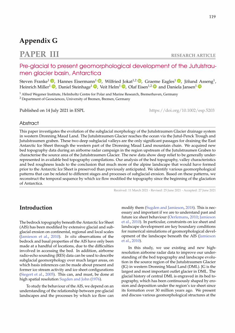
119

Appendix G

PAPER III RESEARCH ARTICLE

Pre-glacial to present geomorphological development of the Jutulstrau-men glacier basin, AntarcticaSteven Franke1 , Hannes Eisermann1 , Wilfried Jokat1,2 , Graeme Eagles1 , Jölund Asseng1,Heinrich Miller1 , Daniel Steinhage1 , Veit Helm1 , Olaf Eisen1,2 and Daniela Jansen1

1 Alfred Wegener Institute, Helmholtz Centre for Polar and Marine Research, Bremerhaven, Germany2 Department of Geosciences, University of Bremen, Bremen, Germany

Published on 14 July 2021 in ESPL https://doi.org/10.1002/esp.5203

AbstractThis paper investigates the evolution of the subglacial morphology of the Jutulstraumen Glacier drainage systemin western Dronning Maud Land. The Jutulstraumen Glacier reaches the ocean via the Jutul-Penck Trough andJutulstraumen graben. These two deep subglacial valleys are the only significant passages for draining the EastAntarctic Ice Sheet through the western part of the Dronning Maud Land mountain chain. We acquired newbed topography data during an airborne radar campaign in the region upstream of the Jutulstraumen Graben tocharacterise the source area of the Jutulstraumen Glacier. The new data show deep relief to be generally under-represented in available bed topography compilations. Our analysis of the bed topography, valley characteristicsand bed roughness leads to the conclusion that much more of the alpine landscape that would have formedprior to the Antarctic Ice Sheet is preserved than previously anticipated. We identify various geomorphologicalpatterns that can be related to different stages and processes of subglacial erosion. Based on these patterns, wereconstruct the temporal sequence by which ice flow modified the topography since the beginning of the glaciationof Antarctica.

Received: 11 March 2021 - Revised: 25 June 2021 - Accepted: 27 June 2021

Introduction

The bedrock topography beneath the Antarctic Ice Sheet(AIS) has been modified by extensive glacial and sub-glacial erosion on continental, regional and local scales(Jamieson et al., 2010). In situ observations of thebedrock and basal properties of the AIS have only beenmade at a handful of locations, due to the difficultiesinvolved in accessing the bed. In addition, airborneradio-echo sounding (RES) data can be used to describesubglacial geomorphology over much larger areas, onwhich basis inferences can be made about present andformer ice stream activity and ice sheet configurations(Siegert et al., 2005). This can, and must, be done athigh spatial resolution Sugden and John (1976).

To study the behaviour of the AIS, we depend on anunderstanding of the relationship between pre-glaciallandscapes and the processes by which ice flow can

modify them (Sugden and Jamieson, 2018). This is nec-essary and important if we are to understand past andfuture ice sheet behaviour (Oerlemans, 2010; Jamiesonet al., 2010). In particular, constraints on ice sheet andlandscape development are key boundary conditionsfor numerical simulations of geomorphological devel-opment of the landscape beneath the AIS (Jamiesonet al., 2010).

In this study, we use existing and new high-resolution airborne radar data to improve our under-standing of the bed topography and landscape evolu-tion in the source region of the Jutulstraumen Glacier(JG) in western Dronning Maud Land (DML). JG is thelargest and most important outlet glacier in DML. Theglacial history of central DML is engraved in its bed to-pography, which has been continuously shaped by ero-sion and deposition under the region’s ice sheet sinceits formation over 30 million years ago. We presentand discuss various geomorphological structures at the

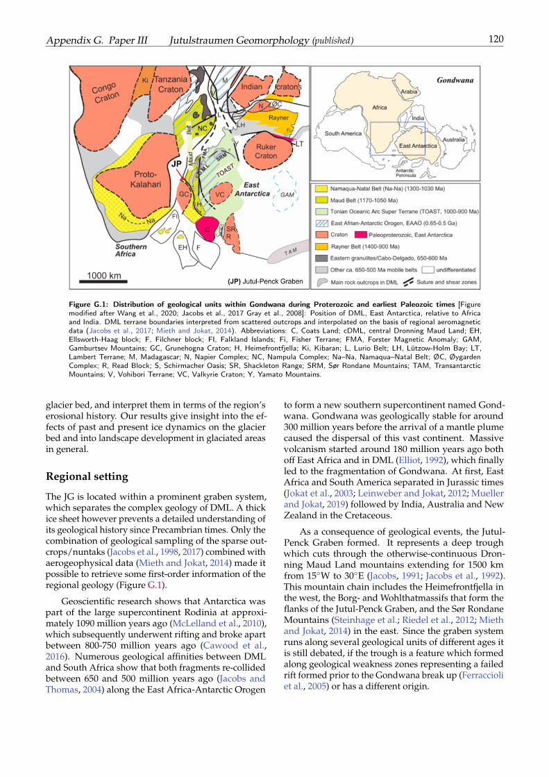
Appendix G. Paper III Jutulstraumen Geomorphology (published) 120

Figure G.1: Distribution of geological units within Gondwana during Proterozoic and earliest Paleozoic times [Figuremodified after Wang et al., 2020; Jacobs et al., 2017 Gray et al., 2008]: Position of DML, East Antarctica, relative to Africaand India. DML terrane boundaries interpreted from scattered outcrops and interpolated on the basis of regional aeromagneticdata (Jacobs et al., 2017; Mieth and Jokat, 2014). Abbreviations: C, Coats Land; cDML, central Dronning Maud Land; EH,Ellsworth-Haag block; F, Filchner block; FI, Falkland Islands; Fi, Fisher Terrane; FMA, Forster Magnetic Anomaly; GAM,Gamburtsev Mountains; GC, Grunehogna Craton; H, Heimefrontfjella; Ki, Kibaran; L, Lurio Belt; LH, Lützow-Holm Bay; LT,Lambert Terrane; M, Madagascar; N, Napier Complex; NC, Nampula Complex; Na–Na, Namaqua–Natal Belt; ØC, ØygardenComplex; R, Read Block; S, Schirmacher Oasis; SR, Shackleton Range; SRM, Sør Rondane Mountains; TAM, TransantarcticMountains; V, Vohibori Terrane; VC, Valkyrie Craton; Y, Yamato Mountains.

glacier bed, and interpret them in terms of the region’serosional history. Our results give insight into the ef-fects of past and present ice dynamics on the glacierbed and into landscape development in glaciated areasin general.

Regional setting

The JG is located within a prominent graben system,which separates the complex geology of DML. A thickice sheet however prevents a detailed understanding ofits geological history since Precambrian times. Only thecombination of geological sampling of the sparse out-crops/nuntaks (Jacobs et al., 1998, 2017) combined withaerogeophysical data (Mieth and Jokat, 2014) made itpossible to retrieve some first-order information of theregional geology (Figure G.1).

Geoscientific research shows that Antarctica waspart of the large supercontinent Rodinia at approxi-mately 1090 million years ago (McLelland et al., 2010),which subsequently underwent rifting and broke apartbetween 800-750 million years ago (Cawood et al.,2016). Numerous geological affinities between DMLand South Africa show that both fragments re-collidedbetween 650 and 500 million years ago (Jacobs andThomas, 2004) along the East Africa-Antarctic Orogen

to form a new southern supercontinent named Gond-wana. Gondwana was geologically stable for around300 million years before the arrival of a mantle plumecaused the dispersal of this vast continent. Massivevolcanism started around 180 million years ago bothoff East Africa and in DML (Elliot, 1992), which finallyled to the fragmentation of Gondwana. At first, EastAfrica and South America separated in Jurassic times(Jokat et al., 2003; Leinweber and Jokat, 2012; Muellerand Jokat, 2019) followed by India, Australia and NewZealand in the Cretaceous.

As a consequence of geological events, the Jutul-Penck Graben formed. It represents a deep troughwhich cuts through the otherwise-continuous Dron-ning Maud Land mountains extending for 1500 kmfrom 15W to 30E (Jacobs, 1991; Jacobs et al., 1992).This mountain chain includes the Heimefrontfjella inthe west, the Borg- and Wohlthatmassifs that form theflanks of the Jutul-Penck Graben, and the Sør RondaneMountains (Steinhage et al.; Riedel et al., 2012; Miethand Jokat, 2014) in the east. Since the graben systemruns along several geological units of different ages itis still debated, if the trough is a feature which formedalong geological weakness zones representing a failedrift formed prior to the Gondwana break up (Ferraccioliet al., 2005) or has a different origin.

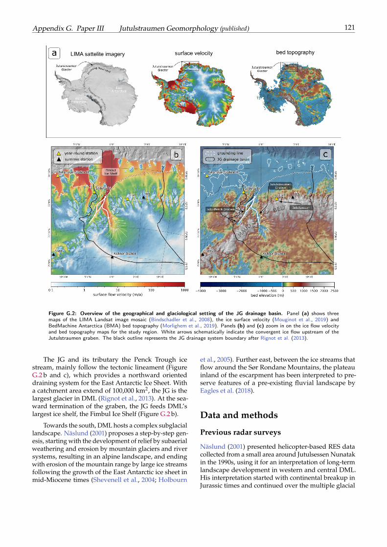
Appendix G. Paper III Jutulstraumen Geomorphology (published) 121

Figure G.2: Overview of the geographical and glaciological setting of the JG drainage basin. Panel (a) shows threemaps of the LIMA Landsat image mosaic (Bindschadler et al., 2008), the ice surface velocity (Mouginot et al., 2019) andBedMachine Antarctica (BMA) bed topography (Morlighem et al., 2019). Panels (b) and (c) zoom in on the ice flow velocityand bed topography maps for the study region. White arrows schematically indicate the convergent ice flow upstream of theJutulstraumen graben. The black outline represents the JG drainage system boundary after Rignot et al. (2013).

The JG and its tributary the Penck Trough icestream, mainly follow the tectonic lineament (FigureG.2 b and c), which provides a northward orienteddraining system for the East Antarctic Ice Sheet. Witha catchment area extend of 100,000 km2, the JG is thelargest glacier in DML (Rignot et al., 2013). At the sea-ward termination of the graben, the JG feeds DML’slargest ice shelf, the Fimbul Ice Shelf (Figure G.2 b).

Towards the south, DML hosts a complex subglaciallandscape. Näslund (2001) proposes a step-by-step gen-esis, starting with the development of relief by subaerialweathering and erosion by mountain glaciers and riversystems, resulting in an alpine landscape, and endingwith erosion of the mountain range by large ice streamsfollowing the growth of the East Antarctic ice sheet inmid-Miocene times (Shevenell et al., 2004; Holbourn

et al., 2005). Further east, between the ice streams thatflow around the Sør Rondane Mountains, the plateauinland of the escarpment has been interpreted to pre-serve features of a pre-existing fluvial landscape byEagles et al. (2018).

Data and methods

Previous radar surveys

Näslund (2001) presented helicopter-based RES datacollected from a small area around Jutulsessen Nunatakin the 1990s, using it for an interpretation of long-termlandscape development in western and central DML.His interpretation started with continental breakup inJurassic times and continued over the multiple glacial

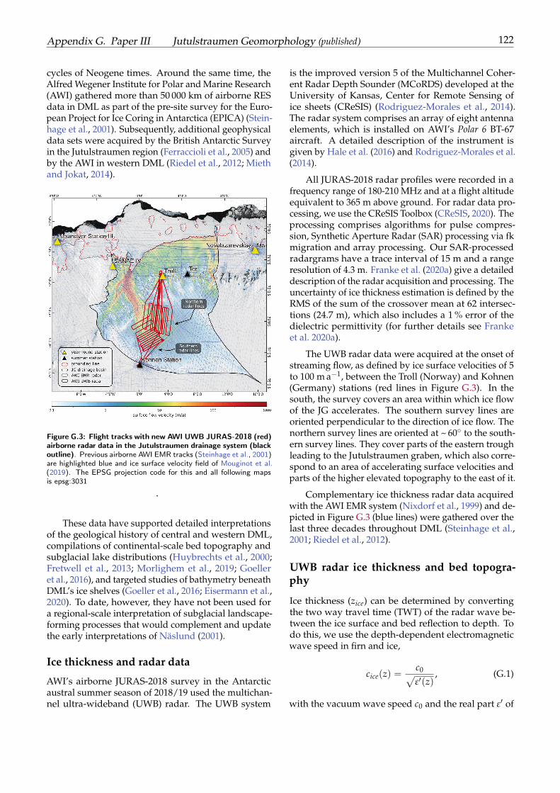
Appendix G. Paper III Jutulstraumen Geomorphology (published) 122

cycles of Neogene times. Around the same time, theAlfred Wegener Institute for Polar and Marine Research(AWI) gathered more than 50 000 km of airborne RESdata in DML as part of the pre-site survey for the Euro-pean Project for Ice Coring in Antarctica (EPICA) (Stein-hage et al., 2001). Subsequently, additional geophysicaldata sets were acquired by the British Antarctic Surveyin the Jutulstraumen region (Ferraccioli et al., 2005) andby the AWI in western DML (Riedel et al., 2012; Miethand Jokat, 2014).

Figure G.3: Flight tracks with new AWI UWB JURAS-2018 (red)airborne radar data in the Jutulstraumen drainage system (blackoutline). Previous airborne AWI EMR tracks (Steinhage et al., 2001)are highlighted blue and ice surface velocity field of Mouginot et al.(2019). The EPSG projection code for this and all following mapsis epsg:3031

.

These data have supported detailed interpretationsof the geological history of central and western DML,compilations of continental-scale bed topography andsubglacial lake distributions (Huybrechts et al., 2000;Fretwell et al., 2013; Morlighem et al., 2019; Goelleret al., 2016), and targeted studies of bathymetry beneathDML’s ice shelves (Goeller et al., 2016; Eisermann et al.,2020). To date, however, they have not been used fora regional-scale interpretation of subglacial landscape-forming processes that would complement and updatethe early interpretations of Näslund (2001).

Ice thickness and radar data

AWI’s airborne JURAS-2018 survey in the Antarcticaustral summer season of 2018/19 used the multichan-nel ultra-wideband (UWB) radar. The UWB system

is the improved version 5 of the Multichannel Coher-ent Radar Depth Sounder (MCoRDS) developed at theUniversity of Kansas, Center for Remote Sensing ofice sheets (CReSIS) (Rodriguez-Morales et al., 2014).The radar system comprises an array of eight antennaelements, which is installed on AWI’s Polar 6 BT-67aircraft. A detailed description of the instrument isgiven by Hale et al. (2016) and Rodriguez-Morales et al.(2014).

All JURAS-2018 radar profiles were recorded in afrequency range of 180-210 MHz and at a flight altitudeequivalent to 365 m above ground. For radar data pro-cessing, we use the CReSIS Toolbox (CReSIS, 2020). Theprocessing comprises algorithms for pulse compres-sion, Synthetic Aperture Radar (SAR) processing via fkmigration and array processing. Our SAR-processedradargrams have a trace interval of 15 m and a rangeresolution of 4.3 m. Franke et al. (2020a) give a detaileddescription of the radar acquisition and processing. Theuncertainty of ice thickness estimation is defined by theRMS of the sum of the crossover mean at 62 intersec-tions (24.7 m), which also includes a 1 % error of thedielectric permittivity (for further details see Frankeet al. 2020a).

The UWB radar data were acquired at the onset ofstreaming flow, as defined by ice surface velocities of 5to 100 m a−1, between the Troll (Norway) and Kohnen(Germany) stations (red lines in Figure G.3). In thesouth, the survey covers an area within which ice flowof the JG accelerates. The southern survey lines areoriented perpendicular to the direction of ice flow. Thenorthern survey lines are oriented at ~ 60 to the south-ern survey lines. They cover parts of the eastern troughleading to the Jutulstraumen graben, which also corre-spond to an area of accelerating surface velocities andparts of the higher elevated topography to the east of it.

Complementary ice thickness radar data acquiredwith the AWI EMR system (Nixdorf et al., 1999) and de-picted in Figure G.3 (blue lines) were gathered over thelast three decades throughout DML (Steinhage et al.,2001; Riedel et al., 2012).

UWB radar ice thickness and bed topogra-phy

Ice thickness (zice) can be determined by convertingthe two way travel time (TWT) of the radar wave be-tween the ice surface and bed reflection to depth. Todo this, we use the depth-dependent electromagneticwave speed in firn and ice,

cice(z) =c0√ε′(z)

, (G.1)

with the vacuum wave speed c0 and the real part ε′ of

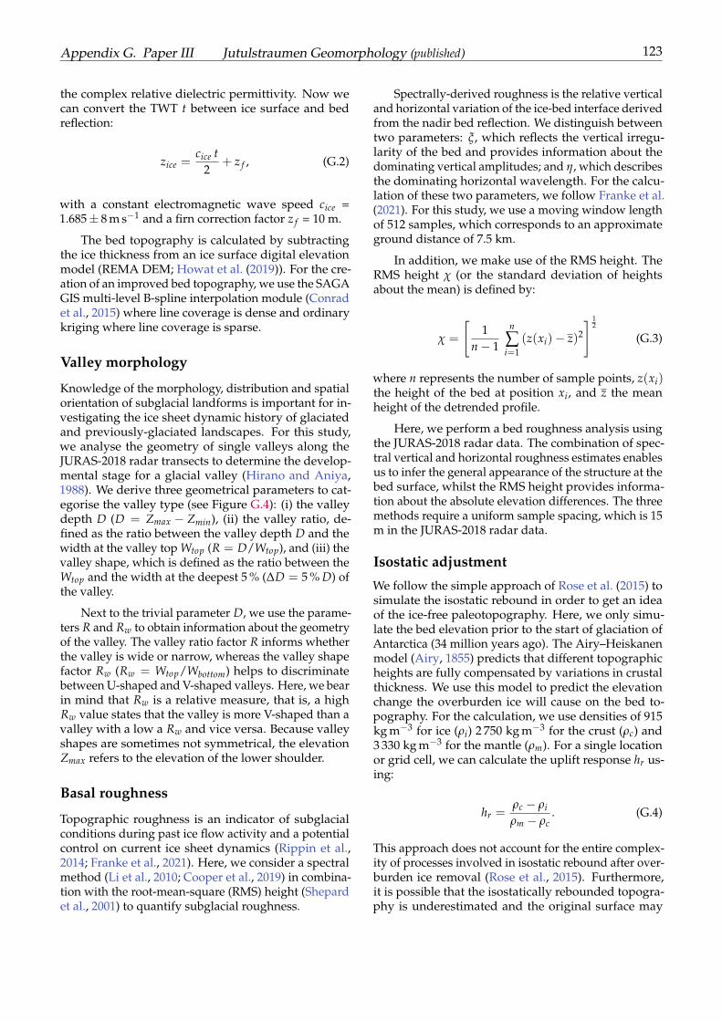
Appendix G. Paper III Jutulstraumen Geomorphology (published) 123

the complex relative dielectric permittivity. Now wecan convert the TWT t between ice surface and bedreflection:

zice =cice t

2+ z f , (G.2)

with a constant electromagnetic wave speed cice =1.685± 8 m s−1 and a firn correction factor z f = 10 m.

The bed topography is calculated by subtractingthe ice thickness from an ice surface digital elevationmodel (REMA DEM; Howat et al. (2019)). For the cre-ation of an improved bed topography, we use the SAGAGIS multi-level B-spline interpolation module (Conradet al., 2015) where line coverage is dense and ordinarykriging where line coverage is sparse.

Valley morphology

Knowledge of the morphology, distribution and spatialorientation of subglacial landforms is important for in-vestigating the ice sheet dynamic history of glaciatedand previously-glaciated landscapes. For this study,we analyse the geometry of single valleys along theJURAS-2018 radar transects to determine the develop-mental stage for a glacial valley (Hirano and Aniya,1988). We derive three geometrical parameters to cat-egorise the valley type (see Figure G.4): (i) the valleydepth D (D = Zmax − Zmin), (ii) the valley ratio, de-fined as the ratio between the valley depth D and thewidth at the valley top Wtop (R = D/Wtop), and (iii) thevalley shape, which is defined as the ratio between theWtop and the width at the deepest 5 % (∆D = 5 % D) ofthe valley.

Next to the trivial parameter D, we use the parame-ters R and Rw to obtain information about the geometryof the valley. The valley ratio factor R informs whetherthe valley is wide or narrow, whereas the valley shapefactor Rw (Rw = Wtop/Wbottom) helps to discriminatebetween U-shaped and V-shaped valleys. Here, we bearin mind that Rw is a relative measure, that is, a highRw value states that the valley is more V-shaped than avalley with a low a Rw and vice versa. Because valleyshapes are sometimes not symmetrical, the elevationZmax refers to the elevation of the lower shoulder.

Basal roughness

Topographic roughness is an indicator of subglacialconditions during past ice flow activity and a potentialcontrol on current ice sheet dynamics (Rippin et al.,2014; Franke et al., 2021). Here, we consider a spectralmethod (Li et al., 2010; Cooper et al., 2019) in combina-tion with the root-mean-square (RMS) height (Shepardet al., 2001) to quantify subglacial roughness.

Spectrally-derived roughness is the relative verticaland horizontal variation of the ice-bed interface derivedfrom the nadir bed reflection. We distinguish betweentwo parameters: ξ, which reflects the vertical irregu-larity of the bed and provides information about thedominating vertical amplitudes; and η, which describesthe dominating horizontal wavelength. For the calcu-lation of these two parameters, we follow Franke et al.(2021). For this study, we use a moving window lengthof 512 samples, which corresponds to an approximateground distance of 7.5 km.

In addition, we make use of the RMS height. TheRMS height χ (or the standard deviation of heightsabout the mean) is defined by:

χ =

[1

n − 1

n

∑i=1

(z(xi)− z)2

] 12

(G.3)

where n represents the number of sample points, z(xi)the height of the bed at position xi, and z the meanheight of the detrended profile.

Here, we perform a bed roughness analysis usingthe JURAS-2018 radar data. The combination of spec-tral vertical and horizontal roughness estimates enablesus to infer the general appearance of the structure at thebed surface, whilst the RMS height provides informa-tion about the absolute elevation differences. The threemethods require a uniform sample spacing, which is 15m in the JURAS-2018 radar data.

Isostatic adjustment

We follow the simple approach of Rose et al. (2015) tosimulate the isostatic rebound in order to get an ideaof the ice-free paleotopography. Here, we only simu-late the bed elevation prior to the start of glaciation ofAntarctica (34 million years ago). The Airy–Heiskanenmodel (Airy, 1855) predicts that different topographicheights are fully compensated by variations in crustalthickness. We use this model to predict the elevationchange the overburden ice will cause on the bed to-pography. For the calculation, we use densities of 915kg m−3 for ice (ρi) 2 750 kg m−3 for the crust (ρc) and3 330 kg m−3 for the mantle (ρm). For a single locationor grid cell, we can calculate the uplift response hr us-ing:

hr =ρc − ρiρm − ρc

. (G.4)

This approach does not account for the entire complex-ity of processes involved in isostatic rebound after over-burden ice removal (Rose et al., 2015). Furthermore,it is possible that the isostatically rebounded topogra-phy is underestimated and the original surface may

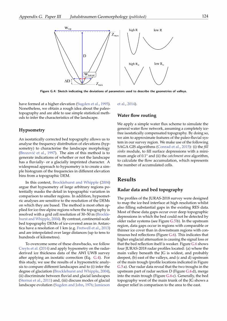
Appendix G. Paper III Jutulstraumen Geomorphology (published) 124

Figure G.4: Sketch indicating the deviations of parameters used to describe the geometries of valleys.

have formed at a higher elevation (Sugden et al., 1995).Nonetheless, we obtain a rough idea about the paleo-topography and are able to use simple statistical meth-ods to infer the characteristics of the landscape.

Hypsometry

An isostatically corrected bed topography allows us toanalyse the frequency distribution of elevations (hyp-sometry) to characterise the landscape morphology(Brozovic et al., 1997). The aim of this method is togenerate indications of whether or not the landscapehas a fluvially- or a glacially imprinted character. Awidespread approach to hypsometry is to create a sim-ple histogram of the frequencies in different elevationbins from a topographic DEM.

In this context, Brocklehurst and Whipple (2004)argue that hypsometry of large arbitrary regions po-tentially masks the detail in topographic variation incomparison to smaller regions. In addition, hypsomet-ric analyses are sensitive to the resolution of the DEMson which they are based. The method is most often ap-plied for ice-free alpine regions where the topography isresolved with a grid cell resolution of 30–50 m (Brockle-hurst and Whipple, 2004). By contrast, continental-scalebed topography DEMs of ice-covered areas in Antarc-tica have a resolution of 1 km (e.g. Fretwell et al., 2013)and are interpolated over large distances (up to tens tohundreds of kilometres).

To overcome some of these drawbacks, we followCreyts et al. (2014) and apply hypsometry on the radar-derived ice thickness data of the AWI UWB surveyafter applying an isostatic correction (Eq. G.4). Forthis study, we use the results of a hypsometric analy-sis to compare different landscapes and to (i) infer thedegree of glaciation (Brocklehurst and Whipple, 2004),(ii) discriminate between fluvial and glacial landscapes(Sternai et al., 2011) and, (iii) discuss modes of glaciallandscape evolution (Sugden and John, 1976; Jamieson

et al., 2014).

Water flow routing

We apply a simple water flux scheme to simulate thegeneral water flow network, assuming a completely ice-free isostatically compensated topography. By doing so,we aim to approximate features of the paleo-fluvial sys-tem in our survey region. We make use of the followingSAGA GIS algorithms (Conrad et al., 2015): (i) the fillsinks module, to fill surface depressions with a mini-mum angle of 0.1° and (ii) the catchment area algorithm,to calculate the flow accumulation, which representsthe number of accumulated cells.

Results

Radar data and bed topography

The profiles of the JURAS-2018 survey were designedto map the ice-bed interface at high resolution whilstalso filling substantial gaps in the existing RES data.Most of these data gaps occur over deep topographicdepressions in which the bed could not be detected byolder radar systems (see Figure G.5 b). In the upstreamregion, data gaps occur in regions with comparable orthinner ice cover than in downstream regions with con-tinuous bed reflections (Figure G.6). This indicates thathigher englacial attenuation is causing the signal loss orthat the bed reflection itself is weaker. Figure G.6 showsfour JURAS-2018 radar profiles located: (a) where themain valley beneath the JG is widest, and probablydeepest, (b) east of the valleys, and (c and d) upstreamof the main trough (profile locations indicated in FigureG.5 a). Our radar data reveal that the two troughs in theupstream part of radar section D (Figure G.6 d), mergeinto the main trough (Figure G.6 c). Generally, the bedtopography west of the main trunk of the JG shows adeeper relief in comparison to the area to the east.

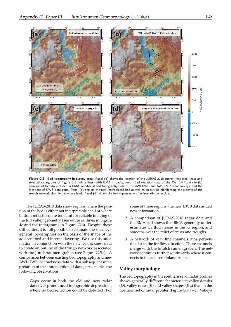
Appendix G. Paper III Jutulstraumen Geomorphology (published) 125

Figure G.5: Bed topography in survey area: Panel (a) shows the location of the JURAS-2018 survey lines (red lines) andselected radargrams of Figure G.6 (white lines) with BMA in background. Bed elevation data of the AWI EMR data in (b)correspond to data included in BMA, additional bed topography data of the AWI UWB and AWI EMR radar surveys, and thelocations of UWB data gaps. Panel (c) depicts the new interpolated bed as well as an outline highlighting the extents of thetrough network that lie below sea level. Panel (d) shows the bed topography after isostatic correction.

The JURAS-2018 data show regions where the posi-tion of the bed is either not interpretable at all or wherebottom reflections are too faint for reliable imaging ofthe full valley geometry (see white outlines in Figure4c and the radargrams in Figure G.6). Despite thesedifficulties, it is still possible to estimate these valleys’general topographies on the basis of the shape of theadjacent bed and internal layering. We use this infor-mation in conjunction with the new ice thickness datato create an outline of the trough network associatedwith the Jutulstraumen graben (see Figure G.5 c). Acomparison between existing bed topography and newAWI UWB ice thickness data with a subsequent inter-pretation of the aforementioned data gaps enables thefollowing observations:

1. Gaps occur in both the old and new radardata over pronounced topographic depressions,where no bed reflection could be detected. For

some of these regions, the new UWB data addednew information.

2. A comparison of JURAS-2018 radar data andthe BMA bed shows that BMA generally under-estimates ice thicknesses in the JG region, andsmooths over the relief of crests and troughs.

3. A network of very fine channels runs perpen-dicular to the ice flow direction. These channelsmerge with the Jutulstraumen graben. The net-work continues further southwards where it con-nects to the adjacent inland basin.

Valley morphology

The bed topography in the southern set of radar profilesshows generally different characteristic valley depths(D), valley ratios (R) and valley shapes (Rw) than in thenorthern set of radar profiles (Figure G.7 a – c). Valleys

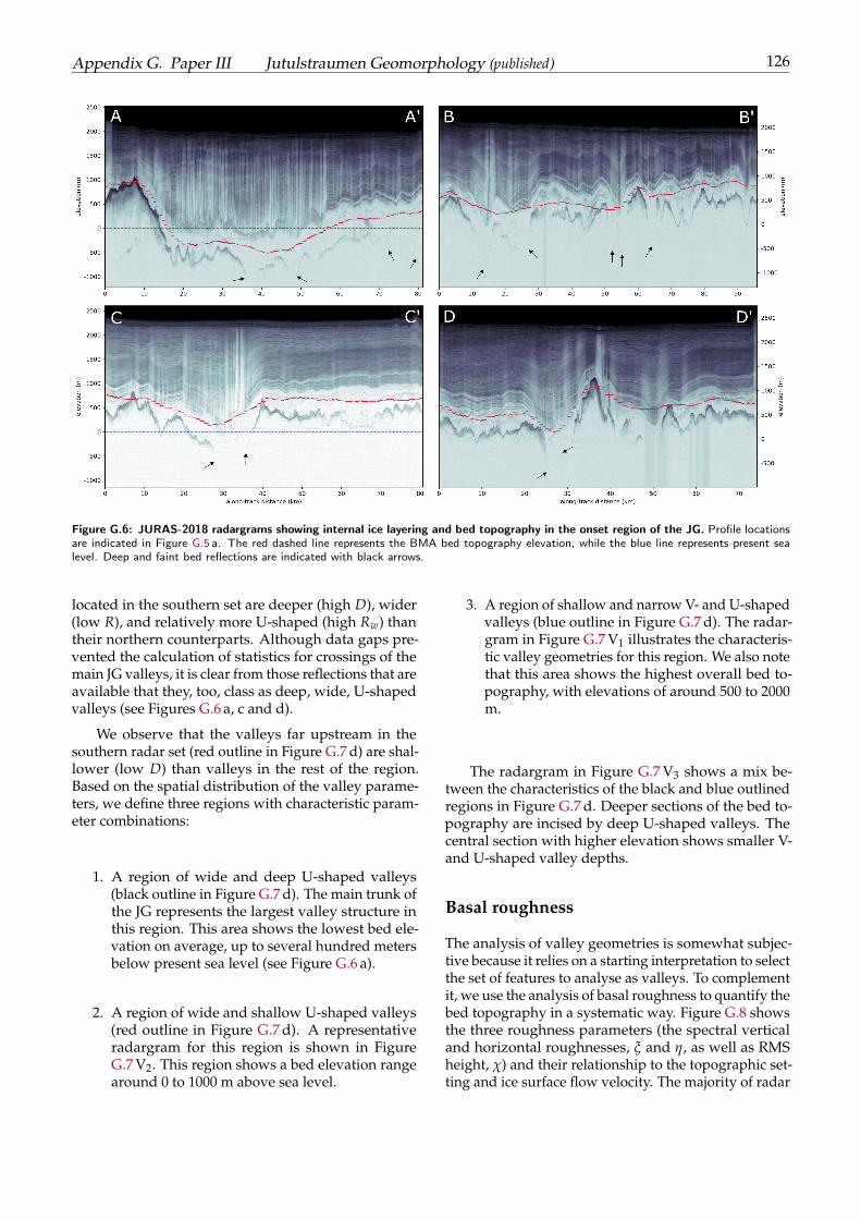
Appendix G. Paper III Jutulstraumen Geomorphology (published) 126

Figure G.6: JURAS-2018 radargrams showing internal ice layering and bed topography in the onset region of the JG. Profile locationsare indicated in Figure G.5 a. The red dashed line represents the BMA bed topography elevation, while the blue line represents present sealevel. Deep and faint bed reflections are indicated with black arrows.

located in the southern set are deeper (high D), wider(low R), and relatively more U-shaped (high Rw) thantheir northern counterparts. Although data gaps pre-vented the calculation of statistics for crossings of themain JG valleys, it is clear from those reflections that areavailable that they, too, class as deep, wide, U-shapedvalleys (see Figures G.6 a, c and d).

We observe that the valleys far upstream in thesouthern radar set (red outline in Figure G.7 d) are shal-lower (low D) than valleys in the rest of the region.Based on the spatial distribution of the valley parame-ters, we define three regions with characteristic param-eter combinations:

1. A region of wide and deep U-shaped valleys(black outline in Figure G.7 d). The main trunk ofthe JG represents the largest valley structure inthis region. This area shows the lowest bed ele-vation on average, up to several hundred metersbelow present sea level (see Figure G.6 a).

2. A region of wide and shallow U-shaped valleys(red outline in Figure G.7 d). A representativeradargram for this region is shown in FigureG.7 V2. This region shows a bed elevation rangearound 0 to 1000 m above sea level.

3. A region of shallow and narrow V- and U-shapedvalleys (blue outline in Figure G.7 d). The radar-gram in Figure G.7 V1 illustrates the characteris-tic valley geometries for this region. We also notethat this area shows the highest overall bed to-pography, with elevations of around 500 to 2000m.

The radargram in Figure G.7 V3 shows a mix be-tween the characteristics of the black and blue outlinedregions in Figure G.7 d. Deeper sections of the bed to-pography are incised by deep U-shaped valleys. Thecentral section with higher elevation shows smaller V-and U-shaped valley depths.

Basal roughness

The analysis of valley geometries is somewhat subjec-tive because it relies on a starting interpretation to selectthe set of features to analyse as valleys. To complementit, we use the analysis of basal roughness to quantify thebed topography in a systematic way. Figure G.8 showsthe three roughness parameters (the spectral verticaland horizontal roughnesses, ξ and η, as well as RMSheight, χ) and their relationship to the topographic set-ting and ice surface flow velocity. The majority of radar

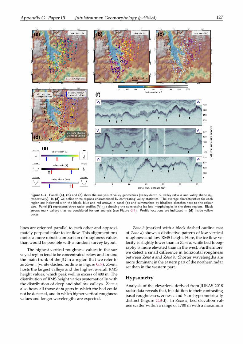
Appendix G. Paper III Jutulstraumen Geomorphology (published) 127

Figure G.7: Panels (a), (b) and (c) show the analysis of valley geometries (valley depth D, valley ratio R and valley shape Rw,respectively). In (d) we define three regions characterised by contrasting valley statistics. The average characteristics for eachregion are indicated with the black, blue and red arrows in panel (e) and summarized by idealized sketches next to the colourbars. Panel (f) represents three radar profiles (V1,2,3) showing the contrasting ice bed morphologies in the three regions. Blackarrows mark valleys that we considered for our analysis (see Figure G.4). Profile locations are indicated in (d) inside yellowboxes.

lines are oriented parallel to each other and approxi-mately perpendicular to ice flow. This alignment pro-motes a more robust comparison of roughness valuesthan would be possible with a random survey layout.

The highest vertical roughness values in the sur-veyed region tend to be concentrated below and aroundthe main trunk of the JG in a region that we refer toas Zone a (white dashed outline in Figure G.8). Zone ahosts the largest valleys and the highest overall RMSheight values, which peak well in excess of 400 m. Thedistribution of RMS height varies systematically withthe distribution of deep and shallow valleys. Zone aalso hosts all those data gaps in which the bed couldnot be detected, and in which higher vertical roughnessvalues and longer wavelengths are expected.

Zone b (marked with a black dashed outline eastof Zone a) shows a distinctive pattern of low verticalroughness and low RMS height. Here, the ice flow ve-locity is slightly lower than in Zone a, while bed topog-raphy is more elevated than in the west. Furthermore,we detect a small difference in horizontal roughnessbetween Zone a and Zone b. Shorter wavelengths aremore dominant in the eastern part of the northern radarset than in the western part.

Hypsometry

Analysis of the elevations derived from JURAS-2018radar data reveals that, in addition to their contrastingbasal roughnesses, zones a and b are hypsometricallydistinct (Figure G.8 d). In Zone a, bed elevation val-ues scatter within a range of 1700 m with a maximum

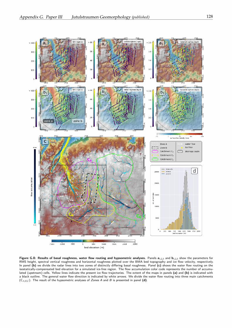
Appendix G. Paper III Jutulstraumen Geomorphology (published) 128

Figure G.8: Results of basal roughness, water flow routing and hypsometric analyses. Panels a1,2,3 and b1,2,3 show the parameters forRMS height, spectral vertical roughness and horizontal roughness plotted over the BMA bed topography and ice flow velocity, respectively.In panel (b) we divide the radar lines into two zones of distinctly differing basal roughness. Panel (c) shows the water flow routing on theisostatically-compensated bed elevation for a simulated ice-free region. The flow accumulation color code represents the number of accumu-lated (upstream) cells. Yellow lines indicate the present ice flow trajectories. The extent of the maps in panels (a) and (b) is indicated witha black outline. The general water flow direction is indicated by white arrows. We divide the water flow routing into three main catchments(CA,B,C). The result of the hypsometric analyses of Zones A and B is presented in panel (d).

Appendix G. Paper III Jutulstraumen Geomorphology (published) 129

at 1000–1400 m elevation. Hence, the data are asym-metrically concentrated towards high elevations. Thisdistribution does not include those low elevations thatwould have been encountered over gaps in the UWBdata. The distribution of bed elevations in Zone b isnarrower and, on average, higher. Its shape is approxi-mately normal, with a slightly higher concentration ofcounts on its low-elevation flank. Analysis of combinedelevations from both zones shows a similar patternoverall to that in Zone a.

Water flow routing

The water flow routing analysis aims to simulate the po-tential pre-glacial surface hydrology of the paleo-fluviallandscape. The calculations of water flow routing andthe analysis of the hydrologic system was performedover the isostatically-compensated bed topography. Inthis study, we only show the water routing for thedrainage basin of the JG. Most of the water originatesfrom high-elevation regions within the DML mountainchain and is distributed towards three main catchments(Figure G.8 c):

1. Catchment CA leads into the main trough belowwhat is now the JG and covers the north-easternpart of the present-day ice drainage basin. Mostof the routing pathways of this catchment arelocated within Zone a.

2. The second catchment, CB, leads towards a topo-graphic depression in the south of the present-day ice drainage basin. Most of the radar surveylines of Zone b are located in this catchment. Fur-thermore, the EPICA ice core is located at thesouth-western tip of this catchment.

3. Catchment CC is located in the eastern part ofthe drainage basin where ice flow velocity is low-est. The flow routing indicates a flow directiontowards the east.

The water routing pathways of catchment CA cor-respond approximately to the present-day ice flow di-rection and propagation of subglacial water. The flowdirections of CB and CC, however, lead towards regionsof higher present-day ice thicknesses and therefore inthe opposite direction to that of present ice flow. Thus,the direction of water flow may in part correspond tothe current subglacial hydrology (Livingstone et al.,2013) which is not parallel to the direction of presentice flow.

Interpretation and discussion

Bed topography and valley morphology

Bed topography construction via simple interpolationtechniques such as those used to generate Bedmap2(Fretwell et al., 2013) relies for its resolution on the spa-tial data density of ice thickness measurements alone.Hence, the deep bed relief at the onset of the maintrunk of the JG, where the bed could not be detectedwith radar techniques, is biased to shallower values inBedmap2.

U-shaped valleys are distinctive features that sug-gest selective linear erosion on a local to regional scale,and thus an indication for the presence of warm basedice at the time of erosion (Sugden and John, 1976). Thedeepest troughs in the JG drainage area are locatedwhere present-day ice flow velocity and accelerationare highest. This suggests the region (black outline inFigure G.7 d) has experienced erosion over a long pe-riod. The wide but shallow U-shaped valleys in theupstream region (red outline in Figure G.7 d) are lo-cated close to the ice divide, where the ice column isthickest and current ice flow velocities are low. This in-dicates that the troughs of these valleys were probablynot eroded under the present ice sheet configuration.The locations, shapes and sizes of these valleys sug-gest they most likely formed in regions of tectonic orlithologic weakness, or by the exploitation of valleys ina pre-existing fluvial network (e.g. Jordan et al., 2013;Baroni et al., 2005; Rose et al., 2015).

As an ice sheet grows to an intermediate size overa pre-existing fluvial landscape, selective linear erosionwill deepen existing river valleys whilst sparing theirflanks (Sugden, 1968, 1978). Ongoing ice sheet growthmay lead to the development of a cold base, concomi-tant with a reduction of sliding and increase in ice-bedcoupling (Jamieson et al., 2010). As a consequence, iceflow will be dominated by internal deformation andice flow velocity will reduce (Creyts et al., 2014). Atthe base of the ice sheet, the consequence of all thismay be a change from an erosive alpine environmentto a passive setting, in which the bed undergoes littlefurther modification. This kind of evolution may haveoccurred rapidly over the upstream part of the northernradar data set (blue outline in Figure G.7 d), which re-flects the lowest degree of glacial erosion in its averagehigh elevation and the dominance of shallow, V-shapedvalleys.

The relative orientation of the radar line to the val-ley pathways is the largest source of uncertainty inthe valley geometry analysis. Oblique crossings willmake valleys appear artefactually too wide (a poten-tial candidate could be the rightmost valley in Figure

Appendix G. Paper III Jutulstraumen Geomorphology (published) 130

G.7 V2). Artefacts like this will affect the determina-tions of valley ratio (R) and valley shape (Rw) but notof valley depth (D). Therefore, narrow and V-shapedvalleys could potentially be underrepresented in Fig-ures G.7 b – c. The potential discrepancy between valleypathway and optimum radar line orientation mainlydepends on the ice flow direction at the time of valleyformation. Following this assumption, we can hypothe-sise under which scenarios the valleys have been mostlikely formed and can constrain the potential impact ofthe radar survey layout on the valley geometry calcula-tions.

Basal roughness

Eisen et al. (2020) analysed basal roughness parame-ters for AWI EMR radar data on a continental scale inAntarctica. They observed low vertical roughness inthe region east of our northern survey grid. This isconsistent with low vertical roughness in Zone b (FigureG.8) and indicates that similar low vertical roughnessvalues are to be expected further east. Eisen et al. (2020)show that basal roughness in this region is on averageanisotropic in respect to the orientation of the radarlines to the direction of ice flow. The interpretation ofbasal roughness is thus limited and restricted to pro-files perpendicular to ice flow. Similar to Rose et al.(2015), we note that the interpretation of low verticalroughness regions as indicative of fast ice flow and un-derlying marine sediments (e.g. Bingham and Siegert,2007) is not valid in this area. In our study area, iceflow is fastest at the locations close to deeply incisedtroughs.

Most importantly, the analysis of spectral verticalroughness and RMS height confirms and supports theresults of the valley geometry analysis, increasing therobustness of their interpretation. The spatial clustersof deep valleys correlate with high vertical roughnessand RMS height, whereas the locations of shallow val-leys correlate with low vertical roughness and RMSheight. Furthermore, we observe that in Zone b the com-bination of narrow, V-shaped valleys is consistent withthe dominance of short horizontal wavelengths.

Hypsometry

The main differences in the hypsometric curves for Zonea and Zone b (Figure G.8 d) are in the location of thepeak and the absolute distributions of bed elevations.Jamieson et al. (2014) relate hypsometric patterns to thetopographic classifications of Sugden and John (1976).According to Jamieson et al. (2014), the broad distribu-tion of bed elevation values and the maximum towardshigher values (as we observe in Zone a) is characteristicof a landscape formed under selective linear erosion.The high mean bed elevation values in Zone b, in con-trast, most likely point to a mainly alpine setting that

has been slightly modified by erosion. The relativelyhigh mean elevations of both zones also suggest thatthe survey area has not been subject to areal scour orlong-term denudation.

Brocklehurst and Whipple (2004) analysed differ-ent ice-free mountain regimes and found a relationshipbetween the degree of glaciation and their hypsometriccurves. Their analysis shows that hypsometric curveswith maxima near higher elevations are indicative offully glaciated landscapes, whereas maxima at lowerelevations tend to characterise curves for non-glaciatedlandscapes. In this context, Zone a, which shows a totalrange of 0-2000 m elevation and a maximum towardshigher elevations (1000-1500 m), can be interpreted asa more fully glaciated landscape than Zone b, whichshows a slight trend towards a lower-elevation maxi-mum (1400 m) with a total elevation range of 1000-1800m (Figure G.8).

Landscape classification

Using the isostatically corrected bed topography (Fig-ure G.5 d) as an approximation of the pre-glacial sur-face, we note that the deepest and widest U-shapedvalleys extend down to present sea level (Figure G.5 d).The Jutulstraumen graben is of tectonic origin, datingback to the ice-free Jurassic, and so must have beensubject to a long period of fluvial erosion after its for-mation (Näslund, 2001). This suggests that the bed inZone a would have been subsequently modified by se-lective linear glacial erosion (Sugden and John, 1976).The subglacial troughs in Zone a are likely candidatesfor pre-glacial fluvial activity and subsequent selectiveerosion after the onset of glaciation (Sugden and John,1976). Hence, the U-shaped valleys of Zone a are likelyto follow the pre-existing fluvial system. It is likely that,regardless of the regional evolution in the extent andthickness of ice and the location of ice divides, someportion of the region’s ice has always flowed throughthe Jutulstraumen graben towards the margin. Suchlongevity could explain the deeply-incised relief.

The analysis of basal roughness and hypsometryfor the area east of the main trunk of the JG (Zone b inFigure G.8) points towards a largely preserved fluviallandscape whose origin precedes extensive glaciation.This is supported by the predominant appearance ofshallow and narrow valleys at the glacier bed and theless variable and generally more elevated topography(and the resulting hypsometry). The mix of V- and U-shaped valleys suggests that the bed has been locallymodified by glacial erosion at some point in the past,but that the degree of modification was probably lim-ited due to the slow-flowing environment, such as acold ice base (Sugden and John, 1976). Erosion undercold-based ice is several orders of magnitude slowerthan under temperate ice (Cuffey and Paterson, 2010).

Appendix G. Paper III Jutulstraumen Geomorphology (published) 131

Jacobs et al. (1995) suggest that intensive denuda-tion by weathering and fluvial erosion were importantlandforming processes in western DML during the up-lift that followed continental breakup in the middle andlate Mesozoic. The fluvial landscape preserved east ofthe JG may have originated in this period. The flowregime calculated for that landscape, in catchments CBand CC, does not correlate with that of the drainagebasin of the modern-day JG (Figure G.8 d). Today, themountains of DML prevent the ice from flowing di-rectly towards the margin, whilst the thicker inland icein the interior of the AIS prevents southwards flow.

The present ice sheet configuration likely causesonly selective linear erosion in the deep troughs con-nected to the Jutulstraumen graben and JutulsessenNunatak, where basal temperatures are probably abovethe pressure melting point. Elevated basal ice tempera-tures would increase englacial attenuation, consistentwith the fact that the locations where we are unable todetect a bed reflection all lie in the deepest parts of thedeepest troughs with fastest-flowing ice.

Basal thermal regime

Geothermal heat flow (GHF) at the base of the AntarcticIce Sheet is a parameter which is subject to substantialuncertainty because it is difficult to measure in situwhilst geophysical models diverge greatly. Van Lief-feringe et al. (2018) compare existing GHF data sets(Shapiro and Ritzwoller, 2004; Maule et al., 2005; Anet al., 2015; Martos et al., 2017) to predict the probabledistribution of basal ice that has been frozen over thelast 1.5 million years. Their modelled area includesthe ice divides at the upstream part of the JG drainagebasin. Based on the individual GHF data sets, theirmodelling reveals it to be likely that the ice base hasreached the pressure melting point at least once overthe last 1.5 million years. Moreover, it has been shownthat measured GHF in eastern DML is locally muchhigher than predicted by geophysical methods (Talalayet al., 2020), consistent with evidence for temperate bedconditions from subglacial water (Wilhelms et al., 2014;Weikusat et al., 2017).

Modelling results and borehole observations indi-cate that large parts of the JG drainage basin’s ice bedare likely to be temperate. In combination with ice flow,this should lead to subglacial erosion. What remainsopen to question is exactly how temperate conditionsaffect processes at the glacier bed under slow flow ve-locities and near the ice divides. In view of the apparentpreservation of fluvial landscapes in the basin, it canbe suggested that erosion in such settings may be lim-ited to subglacial fluvial action with relatively limitedconsequences for landscapes.

Landscape erosion and preservation

The bed morphology of the JG drainage system showspatterns of three successive and/or separate stages oflandscape modification (Figure G.9). We regionallyextend our interpretation of the structures we have clas-sified in our study and define the following interpreta-tion for landscape erosion and preservation: (1) a pre-glacial landscape shaped by fluvial erosion, minimalglacial erosion and preserved thereafter, (2) a fluviallandscape, which was more strongly modified by selec-tive linear erosion at some time in the past, and (3) anintensively selectively-eroded trough system, in whichthe erosion has been long-lived and is still ongoing.

The glacial landscape close to the trough system ofthe JG and further upstream (black and red outlines inFigure G.9) was probably formed by a local alpine-likeglacier system during a period when Antarctica wasinfluenced by a warmer climate than present (Holm-lund and Näslund, 1994; Young et al., 2011). A formerice divide may have separated the two regions duringthis period (yellow dashed line in Figure G.9). At somepoint, as ice coverage increased (Holmlund and Näs-lund, 1994), erosion terminated in the U-shaped valleysin the south and west (red dashed arrows in Figure G.9),but continued further north where ice surface velocitiesare still fast today (black dashed arrows in Figure G.9).At locations where the ice sheet grows beyond a criticalsize, we expect basal melting and the development ofa subglacial water network (Creyts et al., 2014). In thestudy area, this might explain the increased erosionrates that locally formed exceptionally deep valleys.Erosion mechanisms, such as plucking and abrasion,are mainly controlled by basal sliding, which requiresin turn a lubricated bed (Hallet, 1996). By contrast, re-freezing of subglacial water in cold-based areas witha thinner ice thickness (Creyts et al., 2014) is probablyalso a factor in the preservation of the fluvial landscapein the east.

Jamieson et al. (2010) use an ice sheet and erosionmodel to investigate the subglacial landscape evolutionof Antarctica since the Oligocene (34 million years ago).Those authors use three different stages for their sim-ulations (see Table 1 in Jamieson et al. (2010)) where:(a) ice sheets grow and shrink at similar scales to north-ern hemisphere Pleistocene ice sheets (34–14 millionyears before present), (b) cooling shifts the system to-wards development of a continental polar ice sheet(14-13.6 million years ago) and (c) the continental po-lar ice sheet stabilises and subsequently experiencesonly minor changes (13.6 million years ago to present).In order to establish a rough timing for the landscapeevolution in the JG drainage system, we compare theerosion rates modelled by Jamieson et al. (2010) withour landscape classification. For the comparison, wemainly rely on the results shown in Figure 6 in Jamieson

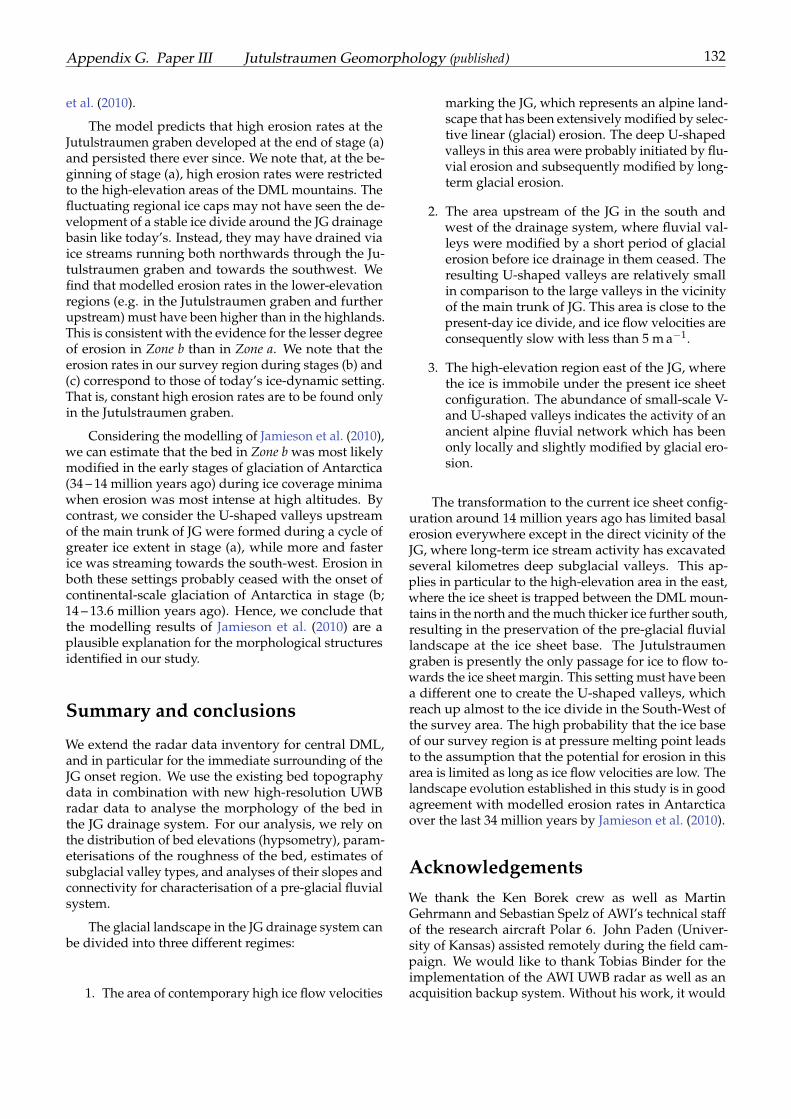
Appendix G. Paper III Jutulstraumen Geomorphology (published) 132

et al. (2010).

The model predicts that high erosion rates at theJutulstraumen graben developed at the end of stage (a)and persisted there ever since. We note that, at the be-ginning of stage (a), high erosion rates were restrictedto the high-elevation areas of the DML mountains. Thefluctuating regional ice caps may not have seen the de-velopment of a stable ice divide around the JG drainagebasin like today’s. Instead, they may have drained viaice streams running both northwards through the Ju-tulstraumen graben and towards the southwest. Wefind that modelled erosion rates in the lower-elevationregions (e.g. in the Jutulstraumen graben and furtherupstream) must have been higher than in the highlands.This is consistent with the evidence for the lesser degreeof erosion in Zone b than in Zone a. We note that theerosion rates in our survey region during stages (b) and(c) correspond to those of today’s ice-dynamic setting.That is, constant high erosion rates are to be found onlyin the Jutulstraumen graben.

Considering the modelling of Jamieson et al. (2010),we can estimate that the bed in Zone b was most likelymodified in the early stages of glaciation of Antarctica(34 – 14 million years ago) during ice coverage minimawhen erosion was most intense at high altitudes. Bycontrast, we consider the U-shaped valleys upstreamof the main trunk of JG were formed during a cycle ofgreater ice extent in stage (a), while more and fasterice was streaming towards the south-west. Erosion inboth these settings probably ceased with the onset ofcontinental-scale glaciation of Antarctica in stage (b;14 – 13.6 million years ago). Hence, we conclude thatthe modelling results of Jamieson et al. (2010) are aplausible explanation for the morphological structuresidentified in our study.

Summary and conclusions

We extend the radar data inventory for central DML,and in particular for the immediate surrounding of theJG onset region. We use the existing bed topographydata in combination with new high-resolution UWBradar data to analyse the morphology of the bed inthe JG drainage system. For our analysis, we rely onthe distribution of bed elevations (hypsometry), param-eterisations of the roughness of the bed, estimates ofsubglacial valley types, and analyses of their slopes andconnectivity for characterisation of a pre-glacial fluvialsystem.

The glacial landscape in the JG drainage system canbe divided into three different regimes:

1. The area of contemporary high ice flow velocities

marking the JG, which represents an alpine land-scape that has been extensively modified by selec-tive linear (glacial) erosion. The deep U-shapedvalleys in this area were probably initiated by flu-vial erosion and subsequently modified by long-term glacial erosion.

2. The area upstream of the JG in the south andwest of the drainage system, where fluvial val-leys were modified by a short period of glacialerosion before ice drainage in them ceased. Theresulting U-shaped valleys are relatively smallin comparison to the large valleys in the vicinityof the main trunk of JG. This area is close to thepresent-day ice divide, and ice flow velocities areconsequently slow with less than 5 m a−1.

3. The high-elevation region east of the JG, wherethe ice is immobile under the present ice sheetconfiguration. The abundance of small-scale V-and U-shaped valleys indicates the activity of anancient alpine fluvial network which has beenonly locally and slightly modified by glacial ero-sion.

The transformation to the current ice sheet config-uration around 14 million years ago has limited basalerosion everywhere except in the direct vicinity of theJG, where long-term ice stream activity has excavatedseveral kilometres deep subglacial valleys. This ap-plies in particular to the high-elevation area in the east,where the ice sheet is trapped between the DML moun-tains in the north and the much thicker ice further south,resulting in the preservation of the pre-glacial fluviallandscape at the ice sheet base. The Jutulstraumengraben is presently the only passage for ice to flow to-wards the ice sheet margin. This setting must have beena different one to create the U-shaped valleys, whichreach up almost to the ice divide in the South-West ofthe survey area. The high probability that the ice baseof our survey region is at pressure melting point leadsto the assumption that the potential for erosion in thisarea is limited as long as ice flow velocities are low. Thelandscape evolution established in this study is in goodagreement with modelled erosion rates in Antarcticaover the last 34 million years by Jamieson et al. (2010).

AcknowledgementsWe thank the Ken Borek crew as well as MartinGehrmann and Sebastian Spelz of AWI’s technical staffof the research aircraft Polar 6. John Paden (Univer-sity of Kansas) assisted remotely during the field cam-paign. We would like to thank Tobias Binder for theimplementation of the AWI UWB radar as well as anacquisition backup system. Without his work, it would

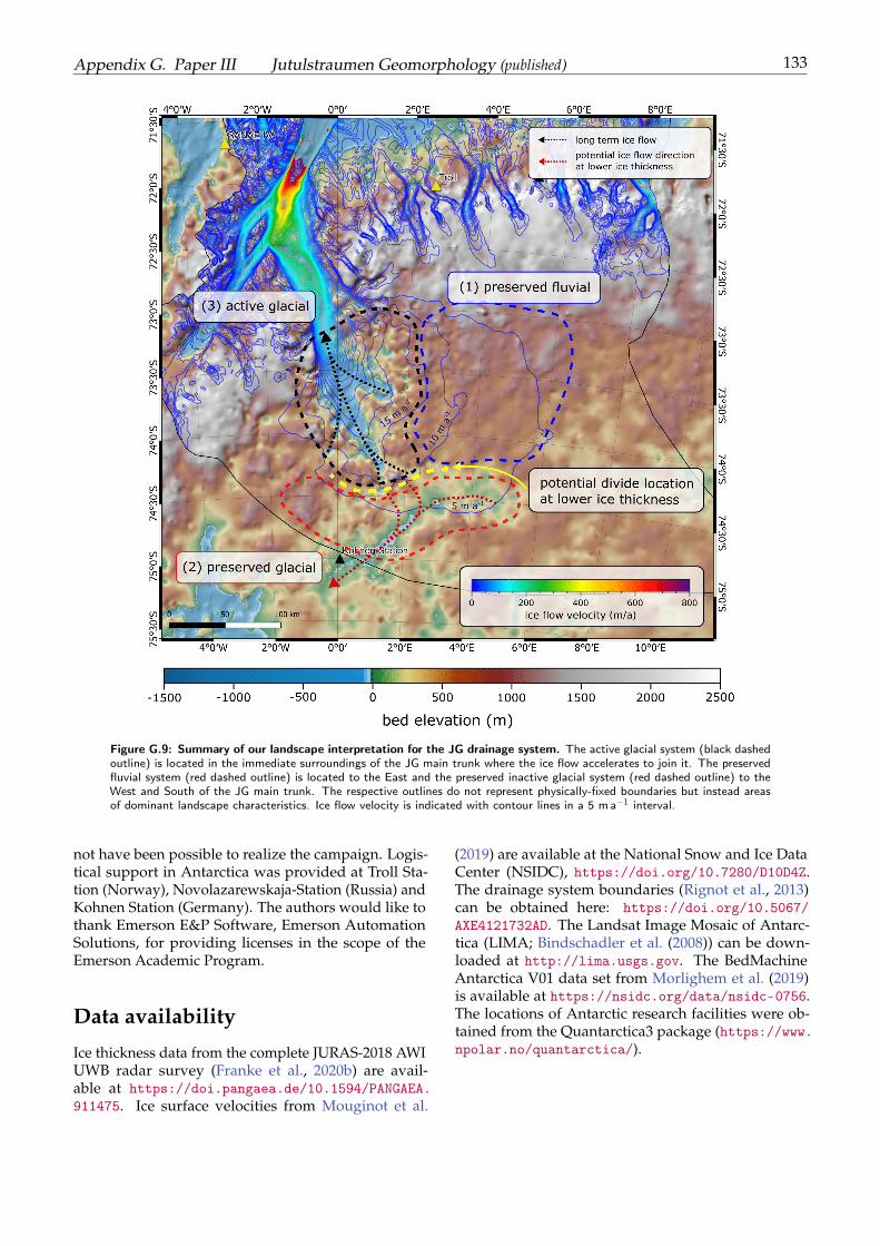
Appendix G. Paper III Jutulstraumen Geomorphology (published) 133

Figure G.9: Summary of our landscape interpretation for the JG drainage system. The active glacial system (black dashedoutline) is located in the immediate surroundings of the JG main trunk where the ice flow accelerates to join it. The preservedfluvial system (red dashed outline) is located to the East and the preserved inactive glacial system (red dashed outline) to theWest and South of the JG main trunk. The respective outlines do not represent physically-fixed boundaries but instead areasof dominant landscape characteristics. Ice flow velocity is indicated with contour lines in a 5 ma−1 interval.

not have been possible to realize the campaign. Logis-tical support in Antarctica was provided at Troll Sta-tion (Norway), Novolazarewskaja-Station (Russia) andKohnen Station (Germany). The authors would like tothank Emerson E&P Software, Emerson AutomationSolutions, for providing licenses in the scope of theEmerson Academic Program.

Data availability

Ice thickness data from the complete JURAS-2018 AWIUWB radar survey (Franke et al., 2020b) are avail-able at https://doi.pangaea.de/10.1594/PANGAEA.911475. Ice surface velocities from Mouginot et al.

(2019) are available at the National Snow and Ice DataCenter (NSIDC), https://doi.org/10.7280/D10D4Z.The drainage system boundaries (Rignot et al., 2013)can be obtained here: https://doi.org/10.5067/AXE4121732AD. The Landsat Image Mosaic of Antarc-tica (LIMA; Bindschadler et al. (2008)) can be down-loaded at http://lima.usgs.gov. The BedMachineAntarctica V01 data set from Morlighem et al. (2019)is available at https://nsidc.org/data/nsidc-0756.The locations of Antarctic research facilities were ob-tained from the Quantarctica3 package (https://www.npolar.no/quantarctica/).

Appendix G. Paper III Jutulstraumen Geomorphology (published) 134

Author contributionsSteven Franke, Hannes Eisermann, Daniela Jansen andWilfried Jokat designed the study with contributionsof Heinz Miller and Olaf Eisen. Steven Franke andHannes Eisermann wrote the manuscript. DanielaJansen designed the JURAS-2018 radar survey and ac-quired the data together with Steven Franke. StevenFranke performed the data processing and generatedthe results with contributions from Daniela Jansen, VeitHelm and Daniel Steinhage and Jölund Asseng. Allauthors discussed and commented the manuscript.

135

BibliographyAiry, G. B. III. On the computation of the effect of

the attraction of mountain-masses, as disturbing theapparent astronomical latitude of stations in geodeticsurveys. Philosophical Transactions of the Royal Societyof London, 145:101–104, 1855. doi: 10.1098/rstl.1855.0003. URL https://royalsocietypublishing.org/doi/abs/10.1098/rstl.1855.0003.

An, M., Wiens, D. A., Zhao, Y., Feng, M., Nyblade, A., Kanao,M., Li, Y., Maggi, A., and Lévêque, J.-J. Temperature,lithosphere-asthenosphere boundary, and heat flux be-neath the Antarctic Plate inferred from seismic velocities.Journal of Geophysical Research: Solid Earth, 120(12):8720–8742, 2015. doi: https://doi.org/10.1002/2015JB011917.URL https://agupubs.onlinelibrary.wiley.com/doi/abs/10.1002/2015JB011917.

Baroni, C., Noti, V., Ciccacci, S., Righini, G., and Salva-tore, M. C. Fluvial origin of the valley system in north-ern Victoria Land (Antarctica) from quantitative geomor-phic analysis. Bulletin of the Geological Society of Amer-ica, 117(1-2):212–228, 2005. ISSN 00167606. doi: 10.1130/B25529.1. URL https://pubs.geoscienceworld.org/gsabulletin/article-lookup/117/1-2/212.

Bindschadler, R., Vornberger, P., Fleming, A., Fox, A., Mullins,J., Binnie, D., Paulsen, S. J., Granneman, B., and Gorodet-zky, D. The Landsat Image Mosaic of Antarctica. Re-mote Sensing of Environment, 112(12):4214 – 4226, 2008.ISSN 0034-4257. doi: https://doi.org/10.1016/j.rse.2008.07.006. URL http://www.sciencedirect.com/science/article/pii/S003442570800223X.

Bingham, R. G. and Siegert, M. J. Radar-derived bed rough-ness characterization of Institute and Möller ice streamsWest Antarctica, and comparison with Siple Coast icestreams. Geophysical Research Letters, 34(21), nov 2007. doi:10.1029/2007gl031483. URL https://doi.org/10.1029%2F2007gl031483.

Brocklehurst, S. H. and Whipple, K. X. Hypsometry ofglaciated landscapes. Earth Surface Processes and Landforms,29(7):907–926, 2004. ISSN 01979337. doi: 10.1002/esp.1083.URL https://doi.org/10.1002/esp.1083.

Brozovic, N., Burbank, D. W., and Meigs, A. J. Climaticlimits on landscape development in the northwestern Hi-malaya. Science, 276(5312):571–574, 1997. ISSN 00368075.doi: 10.1126/science.276.5312.571. URL https://science.sciencemag.org/content/276/5312/571.abstract.

Cawood, P. A., Strachan, R. A., Pisarevsky, S. A., Glad-kochub, D. P., and Murphy, J. B. Linking collisionaland accretionary orogens during rodinia assembly andbreakup: Implications for models of supercontinent cy-cles. Earth and Planetary Science Letters, 449:118–126, 2016.ISSN 0012-821X. doi: https://doi.org/10.1016/j.epsl.2016.05.049. URL https://www.sciencedirect.com/science/article/pii/S0012821X16302746.

Conrad, O., Bechtel, B., Bock, M., Dietrich, H., Fischer, E.,Gerlitz, L., Wehberg, J., Wichmann, V., and Böhner, J.System for Automated Geoscientific Analyses (SAGA)v. 2.1.4. Geoscientific Model Development, 8(7):1991–2007,2015. doi: 10.5194/gmd-8-1991-2015. URL https://gmd.copernicus.org/articles/8/1991/2015/.

Cooper, M. A., Jordan, T. M., Schroeder, D. M., Siegert, M. J.,Williams, C. N., and Bamber, J. L. Subglacial roughnessof the Greenland Ice Sheet: relationship with contem-porary ice velocity and geology. The Cryosphere, 13(11):3093–3115, nov 2019. doi: 10.5194/tc-13-3093-2019. URLhttps://doi.org/10.5194%2Ftc-13-3093-2019.

CReSIS. CReSIS Toolbox [computer software], Lawrence,Kansas, USA. Retrieved from https://github.com/CReSIS,2020. URL https://ops.cresis.ku.edu/wiki/index.php/Main_Page.

Creyts, T. T., Ferraccioli, F., Bell, R. E., Wolovick, M., Corr,H., Rose, K. C., Frearson, N., Damaske, D., Jordan, T.,Braaten, D., and Finn, C. Freezing of ridges and waternetworks preserves the Gamburtsev Subglacial Mountainsfor millions of years. Geophysical Research Letters, 41(22):8114–8122, nov 2014. doi: 10.1002/2014gl061491. URLhttps://doi.org/10.1002%2F2014gl061491.

Cuffey, K. and Paterson, W. S. B. The Physics of Glaciers 4thEdition. Elsivier, Academic Press, 2010.

Eagles, G., Karlsson, N. B., Ruppel, A., Steinhage, D., Jokat,W., and Läufer, A. Erosion at extended continental mar-gins: Insights from new aerogeophysical data in easterndronning maud land. Gondwana Research, 63:105–116, 2018.ISSN 1342-937X. doi: https://doi.org/10.1016/j.gr.2018.05.011. URL https://www.sciencedirect.com/science/article/pii/S1342937X18301655.

Eisen, O., Winter, A., Steinhage, D., Kleiner, T., and Hum-bert, A. Basal roughness of the East Antarctic Ice Sheet inrelation to flow speed and basal thermal state. Annals ofGlaciology, 61(81):162–175, apr 2020. ISSN 0260-3055. doi:10.1017/aog.2020.47.

Eisermann, H., Eagles, G., Ruppel, A., Smith, E. C., andJokat, W. Bathymetry beneath ice shelves of westerndronning maud land, east antarctica, and implicationson ice shelf stability. Geophysical Research Letters, 47(12):e2019GL086724, 2020. doi: https://doi.org/10.1029/2019GL086724. URL https://agupubs.onlinelibrary.wiley.com/doi/abs/10.1029/2019GL086724.

Elliot, D. H. Jurassic magmatism and tectonism associ-ated with Gondwanaland break-up: an Antarctic perspec-tive. Geological Society, London, Special Publications, 68(1):165–184, 1992. doi: 10.1144/GSL.SP.1992.068.01.11. URLhttps://doi.org/10.1144/GSL.SP.1992.068.01.11.

Ferraccioli, F., Jones, P. C., Curtis, M. L., and Leat, P. T. Sub-glacial imprints of early Gondwana break-up as identi-fied from high resolution aerogeophysical data over west-ern Dronning Maud Land, East Antarctica. Terra Nova,17(6):573–579, dec 2005. ISSN 09544879. doi: 10.1111/j.1365-3121.2005.00651.x. URL https://doi.org/10.1111/j.1365-3121.2005.00651.x.

BIBLIOGRAPHY 136

Franke, S., Jansen, D., Binder, T., Dörr, N., Helm, V., Paden,J., Steinhage, D., and Eisen, O. Bed topography andsubglacial landforms in the onset region of the North-east Greenland Ice Stream. Annals of Glaciology, pages1–11, mar 2020a. doi: 10.1017/aog.2020.12. URL https://doi.org/10.1017%2Faog.2020.12.

Franke, S., Jansen, D., and Helm, V. Ice Thickness fromJutulstraumen Glacier recorded with the airborne AWIUWB radar system, Antarctica. 2020b. doi: 10.1594/PANGAEA.911475. URL https://doi.pangaea.de/10.1594/PANGAEA.911475.

Franke, S., Jansen, D., Beyer, S., Neckel, N., Binder, T., Paden,J., and Eisen, O. Complex basal conditions and their in-fluence on ice flow at the onset of the northeast greenlandice stream. Journal of Geophysical Research: Earth Surface,126(3):e2020JF005689, 2021. doi: 10.1029/2020JF005689.URL https://agupubs.onlinelibrary.wiley.com/doi/abs/10.1029/2020JF005689.

Fretwell, P., Pritchard, H. D., Vaughan, D. G., Bamber, J. L.,Barrand, N. E., Bell, R., Bianchi, C., Bingham, R. G.,Blankenship, D. D., Casassa, G., Catania, G., Callens, D.,Conway, H., Cook, A. J., Corr, H. F. J., Damaske, D., Damm,V., Ferraccioli, F., Forsberg, R., Fujita, S., Gim, Y., Gogi-neni, P., Griggs, J. A., Hindmarsh, R. C. A., Holmlund,P., Holt, J. W., Jacobel, R. W., Jenkins, A., Jokat, W., Jor-dan, T., King, E. C., Kohler, J., Krabill, W., Riger-Kusk, M.,Langley, K. A., Leitchenkov, G., Leuschen, C., Luyendyk,B. P., Matsuoka, K., Mouginot, J., Nitsche, F. O., Nogi,Y., Nost, O. A., Popov, S. V., Rignot, E., Rippin, D. M.,Rivera, A., Roberts, J., Ross, N., Siegert, M. J., Smith,A. M., Steinhage, D., Studinger, M., Sun, B., Tinto, B. K.,Welch, B. C., Wilson, D., Young, D. A., Xiangbin, C.,and Zirizzotti, A. Bedmap2: improved ice bed surfaceand thickness datasets for Antarctica. The Cryosphere, 7(1):375–393, feb 2013. doi: 10.5194/tc-7-375-2013. URLhttps://doi.org/10.5194%2Ftc-7-375-2013.

Goeller, S., Steinhage, D., Thoma, M., and Grosfeld, K. As-sessing the subglacial lake coverage of Antarctica. Annalsof Glaciology, 57(72):109–117, jul 2016. ISSN 02603055. doi:10.1017/aog.2016.23. URL http://creativecommons.

Hale, R., Miller, H., Gogineni, S., Yan, J. B., Rodriguez-Morales, F., Leuschen, C., Paden, J., Li, J., Binder, T.,Steinhage, D., Gehrmann, M., and Braaten, D. Multi-channel ultra-wideband radar sounder and imager. In2016 IEEE International Geoscience and Remote Sensing Sym-posium (IGARSS). IEEE, jul 2016. doi: 10.1109/igarss.2016.7729545. URL https://doi.org/10.1109%2Figarss.2016.7729545.

Hallet, B. Glacial quarrying: a simple theoretical model.Annals of Glaciology, 22:1–8, 1996. doi: 10.3189/1996AoG22-1-1-8.

Hirano, M. and Aniya, M. A rational explanation of cross-profile morphology for glacial valleys and of glacial val-ley development. Earth Surface Processes and Landforms,13(8):707–716, 1988. doi: https://doi.org/10.1002/esp.3290130805. URL https://onlinelibrary.wiley.com/doi/abs/10.1002/esp.3290130805.

Holbourn, A., Kuhnt, W., Schulz, M., and Erlenkeuser, H.Impacts of orbital forcing and atmospheric carbon diox-ide on Miocene ice-sheet expansion. Nature, 438(7067):483–487, 2005. doi: 10.1038/nature04123. URL https://www.nature.com/articles/nature04123.

Holmlund, P. and Näslund, J.-O. Antarctica , formed bywet-based mountain glaciation and not by the present icesheet. Boreas, 23:139–148, 1994. ISSN 0300-9483. doi:10.1111/j.1502-3885.1994.tb00594.x. URL https://doi.org/10.1111/j.1502-3885.1994.tb00594.x.

Howat, I. M., Porter, C., Smith, B. E., Noh, M.-J., andMorin, P. The Reference Elevation Model of Antarc-tica. The Cryosphere, 13(2):665–674, feb 2019. ISSN 1994-0424. doi: 10.5194/tc-13-665-2019. URL https://www.the-cryosphere.net/13/665/2019/.

Huybrechts, P., Steinhage, D., Wilhelms, F., and Bamber, J.Balance velocities and measured properties of the Antarc-tic ice sheet from a new compilation of gridded datafor modelling. Annals of Glaciology, 30(1996):52–60, 2000.ISSN 02603055. doi: 10.3189/172756400781820778. URLhttps://doi.org/10.3189/172756400781820778.

Jacobs, J. Strukturelle Entwicklung und Abkühlungs-geschichte der Heimefrontfjella (Westliches DronningMaud Land/Antarktika)= Structural evolution and cool-ing history of the Heimefrontfjella (western DronningMaud Land/Antarctica). Berichte zur Polarforschung (Re-ports on Polar Research), 97, 1991. URL https://epic.awi.de/id/eprint/26274/1/BerPolarforsch199197.pdf.

Jacobs, J. and Thomas, R. J. Himalayan-type indenter-escape tectonics model for the southern part of the lateNeoproterozoic–early Paleozoic East African–Antarcticorogen. Geology, 32(8):721–724, 2004. doi: 10.1130/G20516.1. URL https://doi.org/10.1130/G20516.1.

Jacobs, J., Hejl, E., Wagner, G., and Weber, K. Apatite fissiontrack evidence for contrasting thermal and uplift histo-ries of metamorphic basement blocks in western DronningMaud Land. Recent Progress in Antarctic Earth Science, Ter-rapub, Tokyo, pages 323–330, 1992.

Jacobs, J., Ahrendt, H., Kreutzer, H., and Weber, K. K-Ar.40Ar-19Ar and apatite fission-track evidence for Neopro-terozoic and Mesozoic basement rejuvenation event inthe Heimefrontfjella and Mannefallknausane (East Antarc-tica). Precambrian Research, 75:251–262, 1995. doi: 10.1016/0301-9268(95)80009-7. URL https://doi.org/10.1016/0301-9268(95)80009-7.

Jacobs, J., Fanning, C. M., Henjes-Kunst, F., Olesch, M., andPaech, H.-J. Continuation of the Mozambique Belt into EastAntarctica: Grenville-age metamorphism and polyphasePan-African high-grade events in central Dronning MaudLand. The Journal of Geology, 106(4):385–406, 1998.

Jacobs, J., Opås, B., Elburg, M., Läufer, A., Estrada, S., Ksien-zyk, A. K., Damaske, D., and Hofmann, M. Cryptic sub-icegeology revealed by a U-Pb zircon study of glacial tillin Dronning Maud Land, East Antarctica. Precambrian Re-search, 294:1–14, 2017. doi: 10.1016/j.precamres.2017.03.012.

BIBLIOGRAPHY 137

URL https://doi.org/10.1016/j.precamres.2017.03.012.

Jamieson, S. S., Sugden, D. E., and Hulton, N. R. The evo-lution of the subglacial landscape of Antarctica. Earthand Planetary Science Letters, 293(1-2):1–27, 2010. ISSN0012821X. doi: 10.1016/j.epsl.2010.02.012. URL http://dx.doi.org/10.1016/j.epsl.2010.02.012.

Jamieson, S. S., Stokes, C. R., Ross, N., Rippin, D. M., Bing-ham, R. G., Wilson, D. S., Margold, M., and Bentley,M. J. The glacial geomorphology of the Antarctic icesheet bed. Antarctic Science, 26(6):724–741, 2014. doi:10.1017/S0954102014000212. URL https://doi.org/10.1017/S0954102014000212.

Jokat, W., Boebel, T., König, M., and Meyer, U. Tim-ing and geometry of early Gondwana breakup. Journalof Geophysical Research: Solid Earth, 108(B9), 2003. doi:10.1029/2002JB001802. URL https://doi.org/10.1029/2002JB001802.

Jordan, T. A., Ferraccioli, F., Ross, N., Corr, H. F., Leat, P. T.,Bingham, R. G., Rippin, D. M., le Brocq, A., and Siegert,M. J. Inland extent of the Weddell Sea Rift imaged by newaerogeophysical data. Tectonophysics, 585:137 – 160, 2013.ISSN 0040-1951. doi: https://doi.org/10.1016/j.tecto.2012.09.010. URL http://www.sciencedirect.com/science/article/pii/S0040195112005689.

Leinweber, V. T. and Jokat, W. The Jurassic history of theAfrica–Antarctica corridor—new constraints from mag-netic data on the conjugate continental margins. Tectono-physics, 530:87–101, 2012. doi: 10.1016/j.tecto.2011.11.008.URL https://doi.org/10.1016/j.tecto.2011.11.008.

Li, X., Sun, B., Siegert, M. J., Bingham, R. G., Tang, X.,Zhang, D., Cui, X., and Zhang, X. Characterization ofsubglacial landscapes by a two-parameter roughness in-dex. Journal of Glaciology, 56(199):831–836, 2010. doi:10.3189/002214310794457326. URL https://doi.org/10.3189%2F002214310794457326.

Livingstone, S. J., Clark, C. D., Woodward, J., and Kingslake,J. Potential subglacial lake locations and meltwaterdrainage pathways beneath the Antarctic and Greenlandice sheets. The Cryosphere, 7(6):1721–1740, nov 2013. doi:10.5194/tc-7-1721-2013. URL https://doi.org/10.5194%2Ftc-7-1721-2013.

Martos, Y. M., Catalán, M., Jordan, T. A., Golynsky, A., Golyn-sky, D., Eagles, G., and Vaughan, D. G. Heat Flux Distri-bution of Antarctica Unveiled. Geophysical Research Letters,44(22):11,417–11,426, 2017. doi: https://doi.org/10.1002/2017GL075609. URL https://agupubs.onlinelibrary.wiley.com/doi/abs/10.1002/2017GL075609.

Maule, C. F., Purucker, M. E., Olsen, N., and Mosegaard, K.Heat Flux Anomalies in Antarctica Revealed by SatelliteMagnetic Data. Science, 309(5733):464–467, 2005. ISSN0036-8075. doi: 10.1126/science.1106888. URL https://science.sciencemag.org/content/309/5733/464.

McLelland, J. M., Selleck, B. W., Bickford, M., Tollo, R.,Bartholomew, M., Hibbard, J., and Karabinos, P. Reviewof the Proterozoic evolution of the Grenville Province, itsAdirondack outlier, and the Mesoproterozoic inliers of theAppalachians. From Rodinia to Pangea: The LithotectonicRecord of the Appalachian Region: Geological Society of Amer-ica Memoir, 206:21–49, 2010.

Mieth, M. and Jokat, W. New aeromagnetic view of thegeological fabric of southern dronning maud land andcoats land, east antarctica. Gondwana Research, 25(1):358 –367, 2014. ISSN 1342-937X. doi: https://doi.org/10.1016/j.gr.2013.04.003. URL http://www.sciencedirect.com/science/article/pii/S1342937X13001226.

Morlighem, M., Rignot, E., Binder, T., Blankenship, D., Drews,R., Eagles, G., Eisen, O., Ferraccioli, F., Forsberg, R.,Fretwell, P., Goel, V., Greenbaum, J. S., Gudmundsson,H., Guo, J., Helm, V., Hofstede, C., Howat, I., Humbert,A., Jokat, W., Karlsson, N. B., Lee, W. S., Matsuoka, K.,Millan, R., Mouginot, J., Paden, J., Pattyn, F., Roberts, J.,Rosier, S., Ruppel, A., Seroussi, H., Smith, E. C., Stein-hage, D., Sun, B., van den Broeke, M. R., van Ommen,T. D., van Wessem, M., and Young, D. A. Deep glacialtroughs and stabilizing ridges unveiled beneath the mar-gins of the Antarctic ice sheet. Nature Geoscience, 13(2):132–137, dec 2019. doi: 10.1038/s41561-019-0510-8. URLhttps://doi.org/10.1038%2Fs41561-019-0510-8.

Mouginot, J., Rignot, E., Bjørk, A. A., van den Broeke,M., Millan, R., Morlighem, M., Noël, B., Scheuchl, B.,and Wood, M. Forty-six years of Greenland Ice Sheetmass balance from 1972 to 2018. Proceedings of the Na-tional Academy of Sciences, 116(19):9239–9244, apr 2019.doi: 10.1073/pnas.1904242116. URL https://doi.org/10.1073%2Fpnas.1904242116.

Mueller, C. O. and Jokat, W. The initial Gondwana break-up: a synthesis based on new potential field data ofthe Africa-Antarctica Corridor. Tectonophysics, 750:301–328, 2019. doi: 10.1016/j.tecto.2018.11.008. URL https://doi.org/10.1016/j.tecto.2018.11.008.

Näslund, J. O. Landscape development in western andcentral Dronning Maud Land, East Antarctica. Antarc-tic Science, 13(3):302–311, 2001. ISSN 09541020. doi:10.1017/S0954102001000438. URL https://doi.org/10.1017/S0954102001000438.

Nixdorf, U., Steinhage, D., Meyer, U., Hempel, L., Jenett,M., Wachs, P., and Miller, H. The newly developed air-borne radio-echo sounding system of the AWI as a glacio-logical tool. Annals of Glaciology, 29:231–238, 1999. doi:10.3189/172756499781821346. URL https://doi.org/10.3189%2F172756499781821346.

Oerlemans, J. Numerical Experiments on Large Scale GlacialErosion. Zeitschrift für Gletscherkunde und Glaziologie,20:107–126, 2010. URL https://dspace.library.uu.nl/bitstream/handle/1874/21026/oerlemans_84_numericalexperimentsonglacialerosion.pdf.

BIBLIOGRAPHY 138

Riedel, S., Jokat, W., and Steinhage, D. Mapping tectonicprovinces with airborne gravity and radar data in Dron-ning Maud Land, East Antarctica. Geophysical Journal In-ternational, 189(1):414–427, 2012. ISSN 0956540X. doi:10.1111/j.1365-246X.2012.05363.x. URL https://doi.org/10.1111/j.1365-246X.2012.05363.x.

Rignot, E., Jacobs, S., Mouginot, J., and Scheuchl, B.Ice-Shelf Melting Around Antarctica. Science, 341(6143):266–270, 2013. ISSN 0036-8075. doi: 10.1126/science.1235798. URL https://science.sciencemag.org/content/341/6143/266.

Rippin, D., Bingham, R., Jordan, T., Wright, A., Ross, N., Corr,H., Ferraccioli, F., Brocq, A. L., Rose, K., and Siegert, M.Basal roughness of the Institute and Möller Ice StreamsWest Antarctica: Process determination and landscape in-terpretation. Geomorphology, 214:139–147, jun 2014. doi:10.1016/j.geomorph.2014.01.021. URL https://doi.org/10.1016%2Fj.geomorph.2014.01.021.

Rodriguez-Morales, F., Gogineni, S., Leuschen, C. J., Paden,J. D., Li, J., Lewis, C. C., Panzer, B., Gomez-GarciaAlvestegui, D., Patel, A., Byers, K., Crowe, R., Player,K., Hale, R. D., Arnold, E. J., Smith, L., Gifford, C. M.,Braaten, D., and Panton, C. Advanced multifrequencyradar instrumentation for polar Research. IEEE Trans-actions on Geoscience and Remote Sensing, 52(5):2824–2842,2014. ISSN 01962892. doi: 10.1109/TGRS.2013.2266415.URL https://doi.org/10.1109/TGRS.2013.2266415.

Rose, K. C., Ross, N., Jordan, T. A., Bingham, R. G., Corr,H. F. J., Ferraccioli, F., Le Brocq, A. M., Rippin, D. M.,and Siegert, M. J. Ancient pre-glacial erosion surfacespreserved beneath the West Antarctic Ice Sheet. EarthSurface Dynamics, 3(1):139–152, 2015. doi: 10.5194/esurf-3-139-2015. URL https://esurf.copernicus.org/articles/3/139/2015/.

Shapiro, N. M. and Ritzwoller, M. H. Inferring sur-face heat flux distributions guided by a global seismicmodel: particular application to antarctica. Earth andPlanetary Science Letters, 223(1):213 – 224, 2004. ISSN0012-821X. doi: https://doi.org/10.1016/j.epsl.2004.04.011. URL http://www.sciencedirect.com/science/article/pii/S0012821X0400247X.

Shepard, M. K., Campbell, B. A., Bulmer, M. H., Farr, T. G.,Gaddis, L. R., and Plaut, J. J. The roughness of nat-ural terrain: A planetary and remote sensing perspec-tive. Journal of Geophysical Research: Planets, 106(E12):32777–32795, dec 2001. doi: 10.1029/2000je001429. URLhttps://doi.org/10.1029%2F2000je001429.

Shevenell, A. E., Kennett, J. P., and Lea, D. W. Middle Miocenesouthern ocean cooling and Antarctic cryosphere expan-sion. Science, 305(5691):1766–1770, 2004.

Siegert, M. J., Taylor, J., and Payne, A. J. Spectral rough-ness of subglacial topography and implications for formerice-sheet dynamics in East Antarctica. Global and Plan-etary Change, 45(1-3):249–263, feb 2005. doi: 10.1016/j.gloplacha.2004.09.008. URL https://doi.org/10.1016%2Fj.gloplacha.2004.09.008.

Steinhage, D., Nixdorf, U., Meyer, U., and Miller, H. An-nals of Glaciology. doi: 10.3189/172756499781821409. URLhttps://doi.org/10.3189/172756499781821409.

Steinhage, D., Nixdorf, U., Meyer, U., and Miller, H. Sub-glacial topography and internal structure of Central andWestern Dronning Maud Land, Antarctica, determinedfrom airborne radio echo sounding. Journal of Applied Geo-physics, 47(3-4):183–189, jul 2001. ISSN 09269851. doi:10.1016/S0926-9851(01)00063-5. URL https://doi.org/10.1016/S0926-9851(01)00063-5.

Sternai, P., Herman, F., Fox, M. R., and Castelltort, S. Hyp-sometric analysis to identify spatially variable glacial ero-sion. Journal of Geophysical Research: Earth Surface, 116(F3), 2011. doi: https://doi.org/10.1029/2010JF001823.URL https://agupubs.onlinelibrary.wiley.com/doi/abs/10.1029/2010JF001823.

Sugden, D. E. The Selectivity of Glacial Erosion in theCairngorm Mountains, Scotland. Transactions of the In-stitute of British Geographers, 45:79–92, 1968. ISSN 00202754,14755661. URL http://www.jstor.org/stable/621394.

Sugden, D. E. Glacial Erosion by the Laurentide Ice Sheet.Journal of Glaciology, 20(83):367–391, 1978. doi: 10.3189/S0022143000013915.

Sugden, D. E. and Jamieson, S. S. R. The pre-glacial land-scape of Antarctica. Scottish Geographical Journal, 134(3-4):203–223, 2018. doi: 10.1080/14702541.2018.1535090. URLhttps://doi.org/10.1080/14702541.2018.1535090.

Sugden, D. E. and John, B. S. Glaciers and Landscape: AGeomorphological Approach. Edward Arnold, A member ofthe Hodder Headline Group, 1976.

Sugden, D. E., Denton, G. H., and Marchant, D. R. Landscapeevolution of the Dry Valleys, Transantarctic Mountains:Tectonic implications. Journal of Geophysical Research: SolidEarth, 100(B6):9949–9967, 1995. doi: https://doi.org/10.1029/94JB02895. URL https://agupubs.onlinelibrary.wiley.com/doi/abs/10.1029/94JB02895.

Talalay, P., Li, Y., Augustin, L., Clow, G. D., Hong, J., Lefeb-vre, E., Markov, A., Motoyama, H., and Ritz, C. Geother-mal heat flux from measured temperature profiles in deepice boreholes in Antarctica. The Cryosphere, 14(11):4021–4037, 2020. doi: 10.5194/tc-14-4021-2020. URL https://tc.copernicus.org/articles/14/4021/2020/.

Van Liefferinge, B., Pattyn, F., Cavitte, M. G. P., Karlsson,N. B., Young, D. A., Sutter, J., and Eisen, O. PromisingOldest Ice sites in East Antarctica based on thermodynam-ical modelling. The Cryosphere, 12(8):2773–2787, 2018. doi:10.5194/tc-12-2773-2018. URL https://tc.copernicus.org/articles/12/2773/2018/.

Weikusat, I., Jansen, D., Binder, T., Eichler, J., Faria, S. H.,Wilhelms, F., Kipfstuhl, S., Sheldon, S., Miller, H., Dahl-Jensen, D., and Kleiner, T. Physical analysis of an Antarc-tic ice core—towards an integration of micro- andmacrodynamics of polar ice*. Philosophical Transactions ofthe Royal Society A: Mathematical, Physical and Engineering

BIBLIOGRAPHY 139

Sciences, 375(2086):20150347, 2017. doi: 10.1098/rsta.2015.0347. URL https://royalsocietypublishing.org/doi/abs/10.1098/rsta.2015.0347.

Wilhelms, F., Miller, H., Gerasimoff, M. D., Drücker, C., Fren-zel, A., Fritzsche, D., Grobe, H., Hansen, S. B., Hilmars-son, S. , Hoffmann, G., and et al. The EPICA DronningMaud Land deep drilling operation. Annals of Glaciology,55(68):355–366, 2014. doi: 10.3189/2014AoG68A189. URLhttps://doi.org/10.3189/2014AoG68A189.

Young, D. A., Wright, A. P., Roberts, J. L., Warner, R. C., Young,N. W., Greenbaum, J. S., Schroeder, D. M., Holt, J. W., Sug-den, D. E., Blankenship, D. D., Van Ommen, T. D., andSiegert, M. J. A dynamic early East Antarctic Ice Sheet sug-gested by ice-covered fjord landscapes. Nature, 474(7349):72–75, 2011. ISSN 00280836. doi: 10.1038/nature10114.URL https://doi.org/10.1038/nature10114.

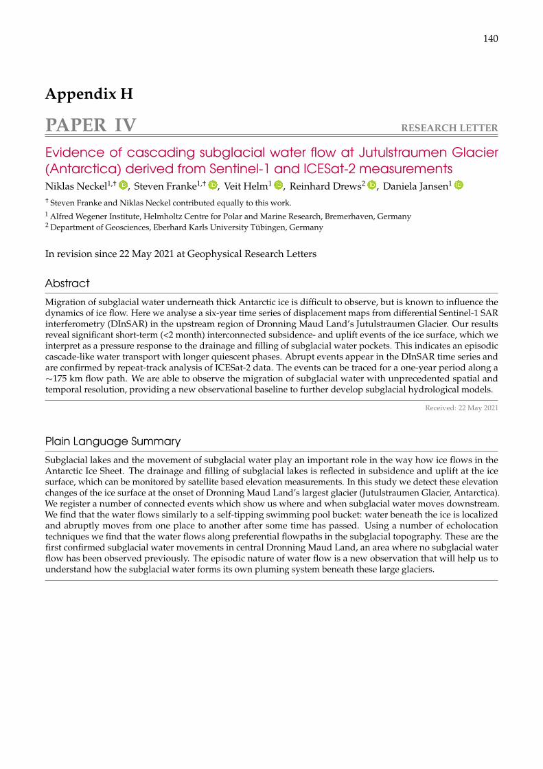
140

Appendix H

PAPER IV RESEARCH LETTER

Evidence of cascading subglacial water flow at Jutulstraumen Glacier(Antarctica) derived from Sentinel-1 and ICESat-2 measurementsNiklas Neckel1,† , Steven Franke1,† , Veit Helm1 , Reinhard Drews2 , Daniela Jansen1

† Steven Franke and Niklas Neckel contributed equally to this work.1 Alfred Wegener Institute, Helmholtz Centre for Polar and Marine Research, Bremerhaven, Germany2 Department of Geosciences, Eberhard Karls University Tübingen, Germany

In revision since 22 May 2021 at Geophysical Research Letters

AbstractMigration of subglacial water underneath thick Antarctic ice is difficult to observe, but is known to influence thedynamics of ice flow. Here we analyse a six-year time series of displacement maps from differential Sentinel-1 SARinterferometry (DInSAR) in the upstream region of Dronning Maud Land’s Jutulstraumen Glacier. Our resultsreveal significant short-term (<2 month) interconnected subsidence- and uplift events of the ice surface, which weinterpret as a pressure response to the drainage and filling of subglacial water pockets. This indicates an episodiccascade-like water transport with longer quiescent phases. Abrupt events appear in the DInSAR time series andare confirmed by repeat-track analysis of ICESat-2 data. The events can be traced for a one-year period along a∼175 km flow path. We are able to observe the migration of subglacial water with unprecedented spatial andtemporal resolution, providing a new observational baseline to further develop subglacial hydrological models.

Received: 22 May 2021

Plain Language SummarySubglacial lakes and the movement of subglacial water play an important role in the way how ice flows in theAntarctic Ice Sheet. The drainage and filling of subglacial lakes is reflected in subsidence and uplift at the icesurface, which can be monitored by satellite based elevation measurements. In this study we detect these elevationchanges of the ice surface at the onset of Dronning Maud Land’s largest glacier (Jutulstraumen Glacier, Antarctica).We register a number of connected events which show us where and when subglacial water moves downstream.We find that the water flows similarly to a self-tipping swimming pool bucket: water beneath the ice is localizedand abruptly moves from one place to another after some time has passed. Using a number of echolocationtechniques we find that the water flows along preferential flowpaths in the subglacial topography. These are thefirst confirmed subglacial water movements in central Dronning Maud Land, an area where no subglacial waterflow has been observed previously. The episodic nature of water flow is a new observation that will help us tounderstand how the subglacial water forms its own pluming system beneath these large glaciers.

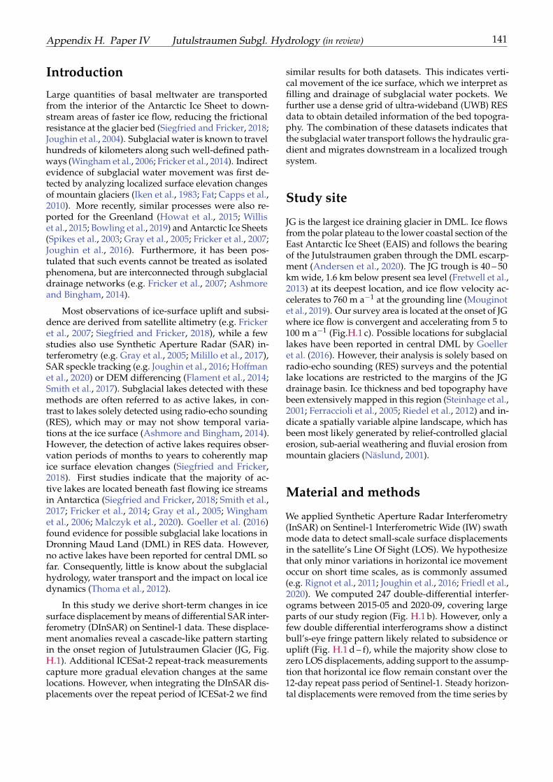
Appendix H. Paper IV Jutulstraumen Subgl. Hydrology (in review) 141

Introduction

Large quantities of basal meltwater are transportedfrom the interior of the Antarctic Ice Sheet to down-stream areas of faster ice flow, reducing the frictionalresistance at the glacier bed (Siegfried and Fricker, 2018;Joughin et al., 2004). Subglacial water is known to travelhundreds of kilometers along such well-defined path-ways (Wingham et al., 2006; Fricker et al., 2014). Indirectevidence of subglacial water movement was first de-tected by analyzing localized surface elevation changesof mountain glaciers (Iken et al., 1983; Fat; Capps et al.,2010). More recently, similar processes were also re-ported for the Greenland (Howat et al., 2015; Williset al., 2015; Bowling et al., 2019) and Antarctic Ice Sheets(Spikes et al., 2003; Gray et al., 2005; Fricker et al., 2007;Joughin et al., 2016). Furthermore, it has been pos-tulated that such events cannot be treated as isolatedphenomena, but are interconnected through subglacialdrainage networks (e.g. Fricker et al., 2007; Ashmoreand Bingham, 2014).

Most observations of ice-surface uplift and subsi-dence are derived from satellite altimetry (e.g. Frickeret al., 2007; Siegfried and Fricker, 2018), while a fewstudies also use Synthetic Aperture Radar (SAR) in-terferometry (e.g. Gray et al., 2005; Milillo et al., 2017),SAR speckle tracking (e.g. Joughin et al., 2016; Hoffmanet al., 2020) or DEM differencing (Flament et al., 2014;Smith et al., 2017). Subglacial lakes detected with thesemethods are often referred to as active lakes, in con-trast to lakes solely detected using radio-echo sounding(RES), which may or may not show temporal varia-tions at the ice surface (Ashmore and Bingham, 2014).However, the detection of active lakes requires obser-vation periods of months to years to coherently mapice surface elevation changes (Siegfried and Fricker,2018). First studies indicate that the majority of ac-tive lakes are located beneath fast flowing ice streamsin Antarctica (Siegfried and Fricker, 2018; Smith et al.,2017; Fricker et al., 2014; Gray et al., 2005; Winghamet al., 2006; Malczyk et al., 2020). Goeller et al. (2016)found evidence for possible subglacial lake locations inDronning Maud Land (DML) in RES data. However,no active lakes have been reported for central DML sofar. Consequently, little is know about the subglacialhydrology, water transport and the impact on local icedynamics (Thoma et al., 2012).

In this study we derive short-term changes in icesurface displacement by means of differential SAR inter-ferometry (DInSAR) on Sentinel-1 data. These displace-ment anomalies reveal a cascade-like pattern startingin the onset region of Jutulstraumen Glacier (JG, Fig.H.1). Additional ICESat-2 repeat-track measurementscapture more gradual elevation changes at the samelocations. However, when integrating the DInSAR dis-placements over the repeat period of ICESat-2 we find

similar results for both datasets. This indicates verti-cal movement of the ice surface, which we interpret asfilling and drainage of subglacial water pockets. Wefurther use a dense grid of ultra-wideband (UWB) RESdata to obtain detailed information of the bed topogra-phy. The combination of these datasets indicates thatthe subglacial water transport follows the hydraulic gra-dient and migrates downstream in a localized troughsystem.

Study site

JG is the largest ice draining glacier in DML. Ice flowsfrom the polar plateau to the lower coastal section of theEast Antarctic Ice Sheet (EAIS) and follows the bearingof the Jutulstraumen graben through the DML escarp-ment (Andersen et al., 2020). The JG trough is 40 – 50km wide, 1.6 km below present sea level (Fretwell et al.,2013) at its deepest location, and ice flow velocity ac-celerates to 760 m a−1 at the grounding line (Mouginotet al., 2019). Our survey area is located at the onset of JGwhere ice flow is convergent and accelerating from 5 to100 m a−1 (Fig.H.1 c). Possible locations for subglaciallakes have been reported in central DML by Goelleret al. (2016). However, their analysis is solely based onradio-echo sounding (RES) surveys and the potentiallake locations are restricted to the margins of the JGdrainage basin. Ice thickness and bed topography havebeen extensively mapped in this region (Steinhage et al.,2001; Ferraccioli et al., 2005; Riedel et al., 2012) and in-dicate a spatially variable alpine landscape, which hasbeen most likely generated by relief-controlled glacialerosion, sub-aerial weathering and fluvial erosion frommountain glaciers (Näslund, 2001).

Material and methods

We applied Synthetic Aperture Radar Interferometry(InSAR) on Sentinel-1 Interferometric Wide (IW) swathmode data to detect small-scale surface displacementsin the satellite’s Line Of Sight (LOS). We hypothesizethat only minor variations in horizontal ice movementoccur on short time scales, as is commonly assumed(e.g. Rignot et al., 2011; Joughin et al., 2016; Friedl et al.,2020). We computed 247 double-differential interfer-ograms between 2015-05 and 2020-09, covering largeparts of our study region (Fig. H.1 b). However, only afew double differential interferograms show a distinctbull’s-eye fringe pattern likely related to subsidence oruplift (Fig. H.1 d – f), while the majority show close tozero LOS displacements, adding support to the assump-tion that horizontal ice flow remain constant over the12-day repeat pass period of Sentinel-1. Steady horizon-tal displacements were removed from the time series by

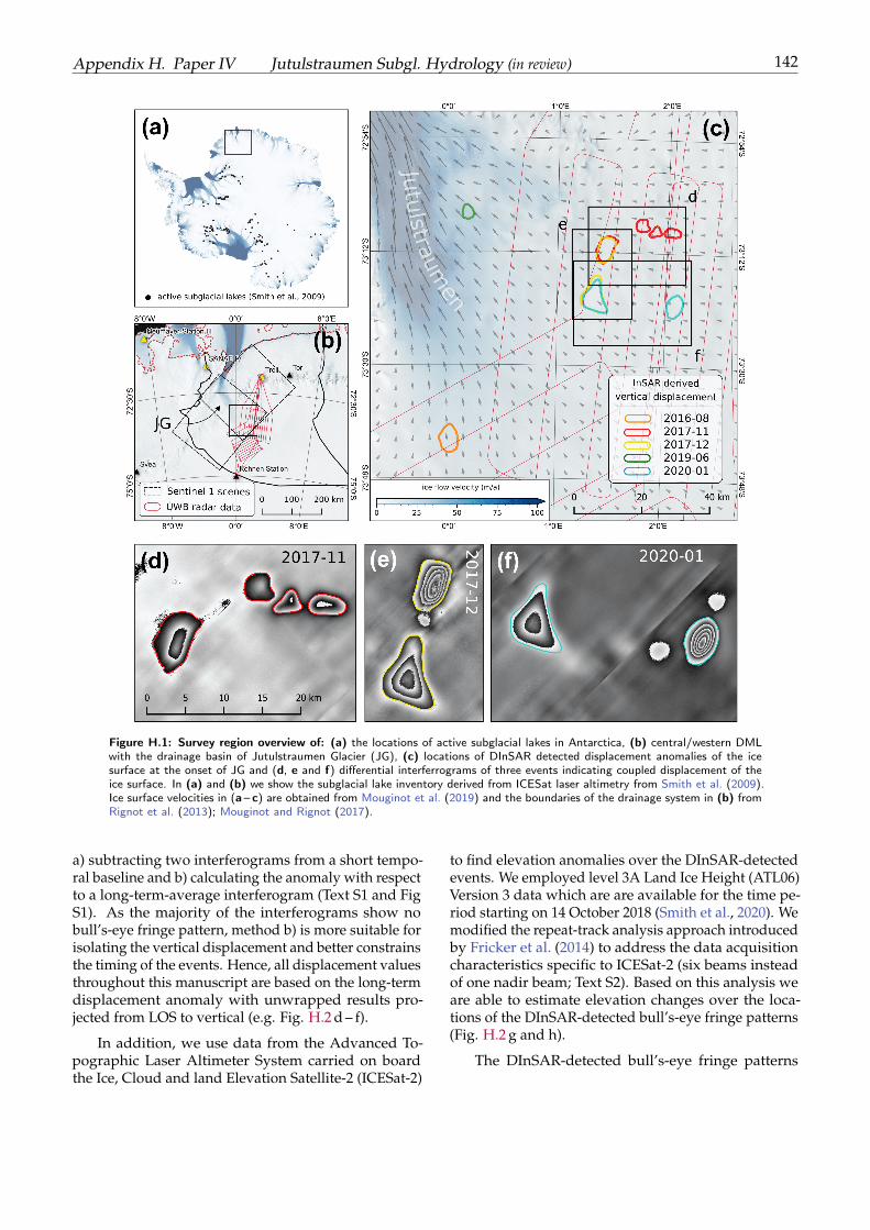
Appendix H. Paper IV Jutulstraumen Subgl. Hydrology (in review) 142

Figure H.1: Survey region overview of: (a) the locations of active subglacial lakes in Antarctica, (b) central/western DMLwith the drainage basin of Jutulstraumen Glacier (JG), (c) locations of DInSAR detected displacement anomalies of the icesurface at the onset of JG and (d, e and f) differential interferrograms of three events indicating coupled displacement of theice surface. In (a) and (b) we show the subglacial lake inventory derived from ICESat laser altimetry from Smith et al. (2009).Ice surface velocities in (a – c) are obtained from Mouginot et al. (2019) and the boundaries of the drainage system in (b) fromRignot et al. (2013); Mouginot and Rignot (2017).

a) subtracting two interferograms from a short tempo-ral baseline and b) calculating the anomaly with respectto a long-term-average interferogram (Text S1 and FigS1). As the majority of the interferograms show nobull’s-eye fringe pattern, method b) is more suitable forisolating the vertical displacement and better constrainsthe timing of the events. Hence, all displacement valuesthroughout this manuscript are based on the long-termdisplacement anomaly with unwrapped results pro-jected from LOS to vertical (e.g. Fig. H.2 d – f).

In addition, we use data from the Advanced To-pographic Laser Altimeter System carried on boardthe Ice, Cloud and land Elevation Satellite-2 (ICESat-2)

to find elevation anomalies over the DInSAR-detectedevents. We employed level 3A Land Ice Height (ATL06)Version 3 data which are are available for the time pe-riod starting on 14 October 2018 (Smith et al., 2020). Wemodified the repeat-track analysis approach introducedby Fricker et al. (2014) to address the data acquisitioncharacteristics specific to ICESat-2 (six beams insteadof one nadir beam; Text S2). Based on this analysis weare able to estimate elevation changes over the loca-tions of the DInSAR-detected bull’s-eye fringe patterns(Fig. H.2 g and h).

The DInSAR-detected bull’s-eye fringe patterns

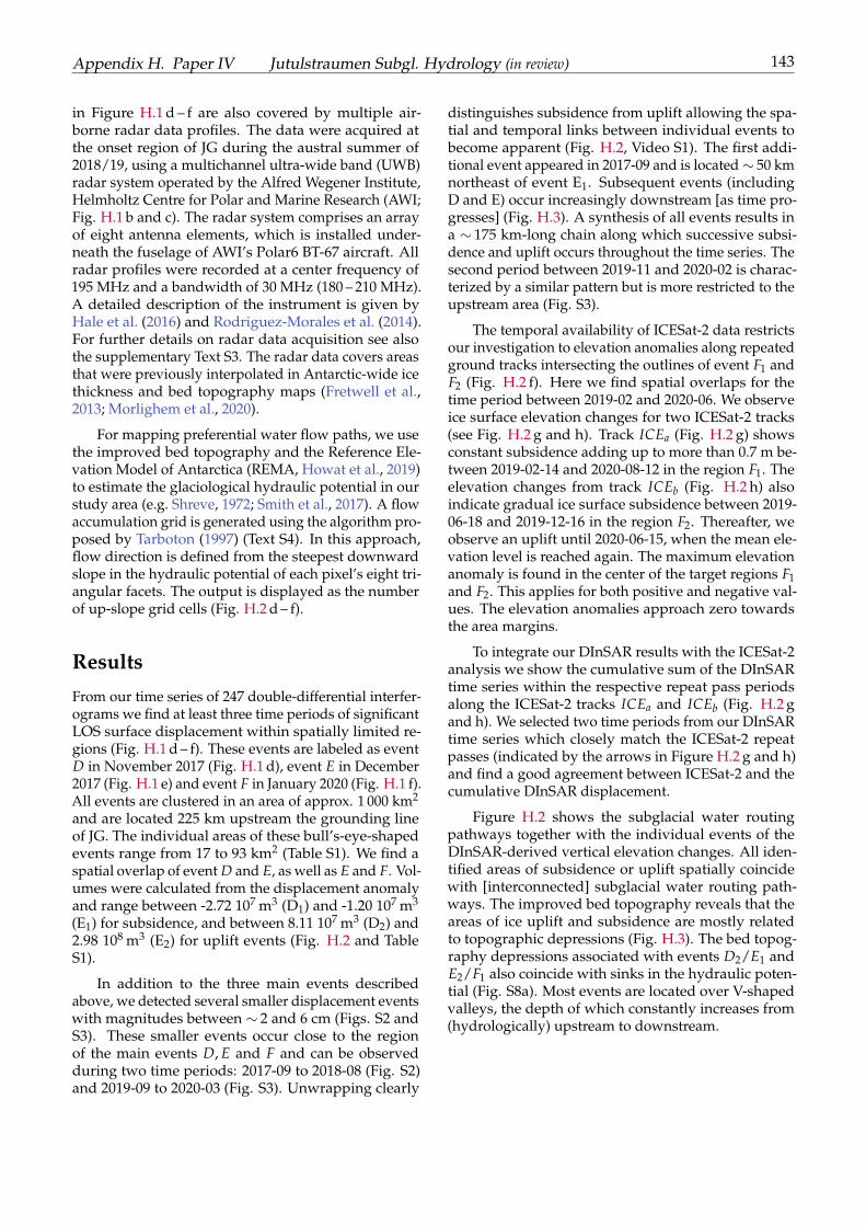
Appendix H. Paper IV Jutulstraumen Subgl. Hydrology (in review) 143

in Figure H.1 d – f are also covered by multiple air-borne radar data profiles. The data were acquired atthe onset region of JG during the austral summer of2018/19, using a multichannel ultra-wide band (UWB)radar system operated by the Alfred Wegener Institute,Helmholtz Centre for Polar and Marine Research (AWI;Fig. H.1 b and c). The radar system comprises an arrayof eight antenna elements, which is installed under-neath the fuselage of AWI’s Polar6 BT-67 aircraft. Allradar profiles were recorded at a center frequency of195 MHz and a bandwidth of 30 MHz (180 – 210 MHz).A detailed description of the instrument is given byHale et al. (2016) and Rodriguez-Morales et al. (2014).For further details on radar data acquisition see alsothe supplementary Text S3. The radar data covers areasthat were previously interpolated in Antarctic-wide icethickness and bed topography maps (Fretwell et al.,2013; Morlighem et al., 2020).

For mapping preferential water flow paths, we usethe improved bed topography and the Reference Ele-vation Model of Antarctica (REMA, Howat et al., 2019)to estimate the glaciological hydraulic potential in ourstudy area (e.g. Shreve, 1972; Smith et al., 2017). A flowaccumulation grid is generated using the algorithm pro-posed by Tarboton (1997) (Text S4). In this approach,flow direction is defined from the steepest downwardslope in the hydraulic potential of each pixel’s eight tri-angular facets. The output is displayed as the numberof up-slope grid cells (Fig. H.2 d – f).

Results

From our time series of 247 double-differential interfer-ograms we find at least three time periods of significantLOS surface displacement within spatially limited re-gions (Fig. H.1 d – f). These events are labeled as eventD in November 2017 (Fig. H.1 d), event E in December2017 (Fig. H.1 e) and event F in January 2020 (Fig. H.1 f).All events are clustered in an area of approx. 1 000 km2

and are located 225 km upstream the grounding lineof JG. The individual areas of these bull’s-eye-shapedevents range from 17 to 93 km2 (Table S1). We find aspatial overlap of event D and E, as well as E and F. Vol-umes were calculated from the displacement anomalyand range between -2.72 107 m3 (D1) and -1.20 107 m3

(E1) for subsidence, and between 8.11 107 m3 (D2) and2.98 108 m3 (E2) for uplift events (Fig. H.2 and TableS1).

In addition to the three main events describedabove, we detected several smaller displacement eventswith magnitudes between ∼ 2 and 6 cm (Figs. S2 andS3). These smaller events occur close to the regionof the main events D, E and F and can be observedduring two time periods: 2017-09 to 2018-08 (Fig. S2)and 2019-09 to 2020-03 (Fig. S3). Unwrapping clearly

distinguishes subsidence from uplift allowing the spa-tial and temporal links between individual events tobecome apparent (Fig. H.2, Video S1). The first addi-tional event appeared in 2017-09 and is located ∼ 50 kmnortheast of event E1. Subsequent events (includingD and E) occur increasingly downstream [as time pro-gresses] (Fig. H.3). A synthesis of all events results ina ∼ 175 km-long chain along which successive subsi-dence and uplift occurs throughout the time series. Thesecond period between 2019-11 and 2020-02 is charac-terized by a similar pattern but is more restricted to theupstream area (Fig. S3).

The temporal availability of ICESat-2 data restrictsour investigation to elevation anomalies along repeatedground tracks intersecting the outlines of event F1 andF2 (Fig. H.2 f). Here we find spatial overlaps for thetime period between 2019-02 and 2020-06. We observeice surface elevation changes for two ICESat-2 tracks(see Fig. H.2 g and h). Track ICEa (Fig. H.2 g) showsconstant subsidence adding up to more than 0.7 m be-tween 2019-02-14 and 2020-08-12 in the region F1. Theelevation changes from track ICEb (Fig. H.2 h) alsoindicate gradual ice surface subsidence between 2019-06-18 and 2019-12-16 in the region F2. Thereafter, weobserve an uplift until 2020-06-15, when the mean ele-vation level is reached again. The maximum elevationanomaly is found in the center of the target regions F1and F2. This applies for both positive and negative val-ues. The elevation anomalies approach zero towardsthe area margins.

To integrate our DInSAR results with the ICESat-2analysis we show the cumulative sum of the DInSARtime series within the respective repeat pass periodsalong the ICESat-2 tracks ICEa and ICEb (Fig. H.2 gand h). We selected two time periods from our DInSARtime series which closely match the ICESat-2 repeatpasses (indicated by the arrows in Figure H.2 g and h)and find a good agreement between ICESat-2 and thecumulative DInSAR displacement.

Figure H.2 shows the subglacial water routingpathways together with the individual events of theDInSAR-derived vertical elevation changes. All iden-tified areas of subsidence or uplift spatially coincidewith [interconnected] subglacial water routing path-ways. The improved bed topography reveals that theareas of ice uplift and subsidence are mostly relatedto topographic depressions (Fig. H.3). The bed topog-raphy depressions associated with events D2/E1 andE2/F1 also coincide with sinks in the hydraulic poten-tial (Fig. S8a). Most events are located over V-shapedvalleys, the depth of which constantly increases from(hydrologically) upstream to downstream.

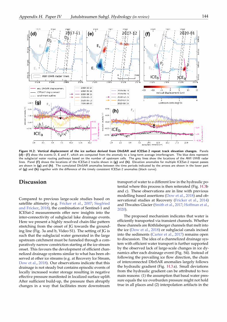
Appendix H. Paper IV Jutulstraumen Subgl. Hydrology (in review) 144

Figure H.2: Vertical displacement of the ice surface derived from DInSAR and ICESat-2 repeat track elevation changes. Panels(d) – (f) show the events D, E and F, which are computed from the anomaly to a long-term average interferogram. The blue dots representthe subglacial water routing pathways based on the number of upstream cells. The grey lines show the locations of the AWI UWB radarlines. Panel (f) shows the locations of the ICESat-2 tracks shown in (g) and (h). Elevation anomalies for multiple ICESat-2 repeat passesare shown in (g) and (h). The cumulated DInSAR anomalies between the time periods indicated by the arrows are shown in the lower partof (g) and (h) together with the difference of the timely consistent ICESat-2 anomalies (black curve).

Discussion

Compared to previous large-scale studies based onsatellite altimetry (e.g. Fricker et al., 2007; Siegfriedand Fricker, 2018), the combination of Sentinel-1 andICESat-2 measurements offer new insights into theinter-connectivity of subglacial lake drainage events.Here we present a highly resolved chain-like patternstretching from the onset of JG towards the ground-ing line (Fig. 3a and b, Video S1). The setting of JG issuch that the subglacial water generated in the largeupstream catchment must be funneled through a com-paratively narrow constriction starting at the ice-streamonset. This favours the development of efficient chan-nelized drainage systems similar to what has been ob-served at other ice streams (e.g. at Recovery Ice Stream,Dow et al., 2018). Our observations indicate that thisdrainage is not steady but contains episodic events oflocally increased water storage resulting in negativeeffective pressure manifested in localized surface uplift.After sufficient build-up, the pressure then abruptlychanges in a way that facilitates more downstream

transport of water to a different low in the hydraulic po-tential where this process is then reiterated (Fig. H.3band c). These observations are in line with previousmodelling based assertions (Dow et al., 2018) and ob-servational studies at Recovery (Fricker et al., 2014)and Thwaites Glacier (Smith et al., 2017; Hoffman et al.,2020).

The proposed mechanism indicates that water isefficiently transported via transient channels. Whetherthese channels are Röthlisberger channels that melt intothe ice (Dow et al., 2018) or subglacial canals incisedinto the sediments (Carter et al., 2017) remains opento discussion. The idea of a channelized drainage sys-tem with efficient water transport is further supportedby the observed lack of large-scale changes in ice dy-namics after each drainage event (Fig. S4). Instead offollowing the prevailing ice flow direction, the chainof interconnected DInSAR anomalies largely followsthe hydraulic gradient (Fig. H.3 a). Small deviationsfrom the hydraulic gradient can be attributed to twomain reasons: (1) the assumption that basal water pres-sure equals the ice overburden pressure might not holdtrue in all places and (2) interpolation artifacts in the

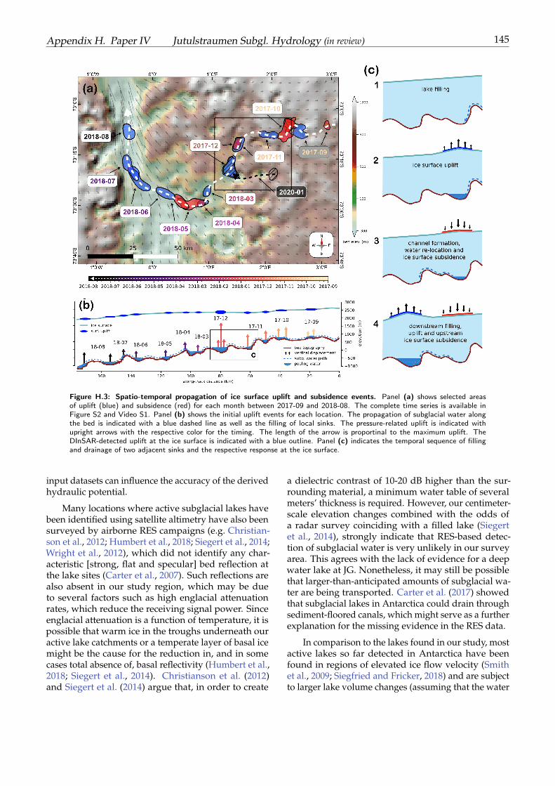
Appendix H. Paper IV Jutulstraumen Subgl. Hydrology (in review) 145

Figure H.3: Spatio-temporal propagation of ice surface uplift and subsidence events. Panel (a) shows selected areasof uplift (blue) and subsidence (red) for each month between 2017-09 and 2018-08. The complete time series is available inFigure S2 and Video S1. Panel (b) shows the initial uplift events for each location. The propagation of subglacial water alongthe bed is indicated with a blue dashed line as well as the filling of local sinks. The pressure-related uplift is indicated withupright arrows with the respective color for the timing. The length of the arrow is proportinal to the maximum uplift. TheDInSAR-detected uplift at the ice surface is indicated with a blue outline. Panel (c) indicates the temporal sequence of fillingand drainage of two adjacent sinks and the respective response at the ice surface.

input datasets can influence the accuracy of the derivedhydraulic potential.

Many locations where active subglacial lakes havebeen identified using satellite altimetry have also beensurveyed by airborne RES campaigns (e.g. Christian-son et al., 2012; Humbert et al., 2018; Siegert et al., 2014;Wright et al., 2012), which did not identify any char-acteristic [strong, flat and specular] bed reflection atthe lake sites (Carter et al., 2007). Such reflections arealso absent in our study region, which may be dueto several factors such as high englacial attenuationrates, which reduce the receiving signal power. Sinceenglacial attenuation is a function of temperature, it ispossible that warm ice in the troughs underneath ouractive lake catchments or a temperate layer of basal icemight be the cause for the reduction in, and in somecases total absence of, basal reflectivity (Humbert et al.,2018; Siegert et al., 2014). Christianson et al. (2012)and Siegert et al. (2014) argue that, in order to create

a dielectric contrast of 10-20 dB higher than the sur-rounding material, a minimum water table of severalmeters’ thickness is required. However, our centimeter-scale elevation changes combined with the odds ofa radar survey coinciding with a filled lake (Siegertet al., 2014), strongly indicate that RES-based detec-tion of subglacial water is very unlikely in our surveyarea. This agrees with the lack of evidence for a deepwater lake at JG. Nonetheless, it may still be possiblethat larger-than-anticipated amounts of subglacial wa-ter are being transported. Carter et al. (2017) showedthat subglacial lakes in Antarctica could drain throughsediment-floored canals, which might serve as a furtherexplanation for the missing evidence in the RES data.

In comparison to the lakes found in our study, mostactive lakes so far detected in Antarctica have beenfound in regions of elevated ice flow velocity (Smithet al., 2009; Siegfried and Fricker, 2018) and are subjectto larger lake volume changes (assuming that the water

Appendix H. Paper IV Jutulstraumen Subgl. Hydrology (in review) 146

volume change is proportional to the subsidence anduplift volume; Smith et al. 2009). To our knowledge,this is the first study which finds active lakes in centralDML. However, this might be attributed to the fact thatcompared to the altimetry measurements of previousstudies, InSAR is not restricted to sparse repeat tracksand is capable of detecting surface elevation changes atthe wavelength scale of the sensor. When we considerthe history of subglacial lake identification in Antarc-tica since the 1960s (Wright et al., 2012) it becomes clearthat many lake locations could be identified due to theincreasing availability of space-borne data productsand analysis techniques. The lake areas and the surfacedisplacement magnitudes in this study are relativelysmall and could only be confirmed using a combinationof remote sensing methods, which have been continu-ously developed in recent years. Hence, it is very likelythat many more small lakes with short-term drainageand filling events will be identified in the future.

ConclusionsWe identified a subglacial hydrologic network at Ju-tulstraumen Glacier in which subglacial water is pe-riodically trapped and released. We are able to tracethe propagation of subglacial water over a distanceof ∼175 km within one year using a combinationof different remote sensing methods. DInSAR esti-mates from Sentinel-1 data reveal abrupt, localizedevents occurring between 12 days and two month. In-dividual events are interconnected in a cascade-likepattern of short-term surface uplift and subsidencefollowing lows in the hydraulic potential indicatingepisodic transport of excess water across subglaciallakes. ICESat-2 repeat-tracks capture the long-term lakedrainage patterns and match with the cumulated DIn-SAR displacements, but undersample the short term dy-namics. Additional airborne radar data constrains thehydraulic potential and shows that the inter-connectedchain of subsidence and uplift events occurs along pro-jected pathways of subglacial water flux. The subglacialwater is not apparent in the bed reflection amplitudeseither because of the transient nature or because of alack in system sensitivity. Despite the widely discussedinfluence of subglacial water on local ice flow variabil-ity, we find no evidence of changes in downstreamice velocities in connection with the detected drainageevents.

AcknowledgementsWe thank the Ken Borek crew as well as MartinGehrmann and Sebastian Spelz of AWI’s technical staffof the research aircraft Polar 6. John Paden (Universityof Kansas) assisted remotely during the field campaign.

We would like to thank Tobias Binder for the implemen-tation of an entire backup system for UWB radar dataacquisition. Without his work we would not have beenable to realize the campaign. We acknowledge fruit-ful discussions with Angelika Humbert. Furthermore,logistical support in Antarctica was provided at TrollStation (Norway), Novolazarewskaja-Station (Russia)and Kohnen Station (Germany). Steven Franke andDaniela Jansen were funded by the AWI strategy fund.R. Drews was supported by an Emmy Noether Grantof the Deutsche Forschungsgemeinschaft (DR 822/3-1).

Data availabilitySentinel-1 SAR data are freely available from https://scihub.copernicus.eu. ICESat-2 level 3A land iceheight data are freely available from https://nsidc.org/data/atl06/versions/3. The center coordinatesof active lake locations derived in this study are avail-able in the Supplementary Material. The outlines of thelakes will be made available at the PANGAEA reposi-tory. Ice thickness from the complete AWI UWB radarsurvey (Franke et al., 2020) is available at https://doi.pangaea.de/10.1594/PANGAEA.911475. Ice sur-face velocities from Mouginot et al. (2019) are availableat the National Snow and Ice Data Center (NSIDC),https://doi.org/10.7280/D10D4Z. The REMA icesurface DEM (Howat et al., 2019) is available fromthe U.S. Polar Geospatial Center at https://www.pgc.umn.edu/data/rema/. The drainage system bound-aries (Rignot et al., 2013) can be obtained here: https://doi.org/10.5067/AXE4121732AD.

Author contributionsNiklas Neckel and Steven Franke wrote the manuscriptand designed the study. Veit Helm processed ICESat-2laser altimetry data. Daniela Jansen was PI of the UWBradar campaign and acquired the radar data togetherwith Steven Franke. Niklas Neckel performed the DIn-SAR processing of Sentinel-1 SAR data and derivedthe hydraulic parameters. Steven Franke processedUWB radar data and calculated the ice thickness andbed topography elevation. All authors discussed andcommented the manuscript.

147

BibliographyInsar observations of the 1993–95 bering glacier (alaska,

u.s.a.) surge and a surge hypothesis. 48. doi: 10.3189/172756502781831296. URL https://doi.org/10.3189/172756502781831296.

Andersen, J., Newall, J., Blomdin, R., Sams, S., Fabel, D.,Koester, A., Lifton, N., Fredin, O., Caffee, M., Glasser,N. F., Rogozhina, I., Suganuma, Y., Harbor, J., andStroeven, A. Ice surface changes during recent glacialcycles along the Jutulstraumen and Penck Trough icestreams in western Dronning Maud Land, East Antarc-tica. Quaternary Science Reviews, 249:106636, 2020. ISSN0277-3791. doi: https://doi.org/10.1016/j.quascirev.2020.106636. URL http://www.sciencedirect.com/science/article/pii/S0277379120305989.

Ashmore, D. and Bingham, R. G. Antarctic subglacialhydrology: Current knowledge and future challenges.Antarctic Science, 26:758–773, 12 2014. doi: 10.1017/S0954102014000546. URL https://doi.org/10.1017/S0954102014000546.

Bowling, J. S., Livingstone, S. J., Sole, A. J., and Chu, W. Dis-tribution and dynamics of Greenland subglacial lakes. Na-ture Communications, 10(1):2810, June 2019. ISSN 2041-1723.URL https://doi.org/10.1038/s41467-019-10821-w.

Capps, D. M., Rabus, B., Clague, J. J., and Shugar, D. H. Iden-tification and characterization of alpine subglacial lakesusing interferometric synthetic aperture radar (InSAR):Brady Glacier, Alaska, USA. Journal of Glaciology, 56(199):861–870, 2010. doi: 10.3189/002214310794457254. URLhttps://doi.org/10.3189/002214310794457254.

Carter, S. P., Blankenship, D. D., Peters, M. E., Young, D. A.,Holt, J. W., and Morse, D. L. Radar-based subglaciallake classification in antarctica. Geochemistry, Geophysics,Geosystems, 8(3):1–20, 2007. doi: https://doi.org/10.1029/2006GC001408. URL https://agupubs.onlinelibrary.wiley.com/doi/abs/10.1029/2006GC001408.

Carter, S. P., Fricker, H. A., and Siegfried, M. R. Antarcticsubglacial lakes drain through sediment-floored canals:theory and model testing on real and idealized do-mains. The Cryosphere, 11(1):381–405, 2017. doi: 10.5194/tc-11-381-2017. URL https://tc.copernicus.org/articles/11/381/2017/.

Christianson, K., Jacobel, R. W., Horgan, H. J., Anandakr-ishnan, S., and Alley, R. B. Subglacial lake whillans— ice-penetrating radar and gps observations of a shal-low active reservoir beneath a west antarctic ice stream.Earth and Planetary Science Letters, 331-332:237 – 245, 2012.ISSN 0012-821X. doi: https://doi.org/10.1016/j.epsl.2012.03.013. URL http://www.sciencedirect.com/science/article/pii/S0012821X12001276.

Dow, C. F., Werder, M. A., Babonis, G., Nowicki, S.,Walker, R. T., Csatho, B., and Morlighem, M. Dynam-ics of Active Subglacial Lakes in Recovery Ice Stream.Journal of Geophysical Research: Earth Surface, 123(4):837–850, 2018. doi: https://doi.org/10.1002/2017JF004409.URL https://agupubs.onlinelibrary.wiley.com/doi/abs/10.1002/2017JF004409.

Ferraccioli, F., Jones, P. C., Curtis, M. L., and Leat, P. T. Sub-glacial imprints of early Gondwana break-up as identi-fied from high resolution aerogeophysical data over west-ern Dronning Maud Land, East Antarctica. Terra Nova,17(6):573–579, dec 2005. ISSN 09544879. doi: 10.1111/j.1365-3121.2005.00651.x. URL https://doi.org/10.1111/j.1365-3121.2005.00651.x.

Flament, T., Berthier, E., and Rémy, F. Cascading water under-neath Wilkes Land, East Antarctic ice sheet, observed usingaltimetry and digital elevation models. The Cryosphere,8(2):673–687, 2014. doi: 10.5194/tc-8-673-2014. URLhttps://tc.copernicus.org/articles/8/673/2014/.

Franke, S., Jansen, D., and Helm, V. Ice Thickness fromJutulstraumen Glacier recorded with the airborne AWIUWB radar system, Antarctica. 2020. doi: 10.1594/PANGAEA.911475. URL https://doi.pangaea.de/10.1594/PANGAEA.911475.

Fretwell, P., Pritchard, H. D., Vaughan, D. G., Bamber, J. L.,Barrand, N. E., Bell, R., Bianchi, C., Bingham, R. G.,Blankenship, D. D., Casassa, G., Catania, G., Callens, D.,Conway, H., Cook, A. J., Corr, H. F. J., Damaske, D., Damm,V., Ferraccioli, F., Forsberg, R., Fujita, S., Gim, Y., Gogi-neni, P., Griggs, J. A., Hindmarsh, R. C. A., Holmlund,P., Holt, J. W., Jacobel, R. W., Jenkins, A., Jokat, W., Jor-dan, T., King, E. C., Kohler, J., Krabill, W., Riger-Kusk, M.,Langley, K. A., Leitchenkov, G., Leuschen, C., Luyendyk,B. P., Matsuoka, K., Mouginot, J., Nitsche, F. O., Nogi,Y., Nost, O. A., Popov, S. V., Rignot, E., Rippin, D. M.,Rivera, A., Roberts, J., Ross, N., Siegert, M. J., Smith,A. M., Steinhage, D., Studinger, M., Sun, B., Tinto, B. K.,Welch, B. C., Wilson, D., Young, D. A., Xiangbin, C.,and Zirizzotti, A. Bedmap2: improved ice bed surfaceand thickness datasets for Antarctica. The Cryosphere, 7(1):375–393, feb 2013. doi: 10.5194/tc-7-375-2013. URLhttps://doi.org/10.5194%2Ftc-7-375-2013.

Fricker, H. A., Scambos, T., Bindschadler, R., and Padman,L. An active subglacial water system in west antarcticamapped from space. Science, 315(5818):1544–1548, 2007.ISSN 0036-8075. doi: 10.1126/science.1136897. URL https://science.sciencemag.org/content/315/5818/1544.

Fricker, H. A., Carter, S. P., Bell, R. E., and Scambos, T. Activelakes of recovery ice stream, east antarctica: a bedrock-controlled subglacial hydrological system. Journal of Glaciol-ogy, 60(223):1015–1030, 2014. doi: 10.3189/2014JoG14J063.URL https://doi.org/10.3189/2014JoG14J063.

Friedl, P., Weiser, F., Fluhrer, A., and Braun, M. H. Re-mote sensing of glacier and ice sheet grounding lines:A review. Earth-Science Reviews, 201:102948, 2020. ISSN0012-8252. doi: https://doi.org/10.1016/j.earscirev.2019.

BIBLIOGRAPHY 148

102948. URL http://www.sciencedirect.com/science/article/pii/S0012825219300832.

Goeller, S., Steinhage, D., Thoma, M., and Grosfeld, K. As-sessing the subglacial lake coverage of Antarctica. Annalsof Glaciology, 57(72):109–117, jul 2016. ISSN 02603055. doi:10.1017/aog.2016.23. URL http://creativecommons.

Gray, L., Joughin, I., Tulaczyk, S., Spikes, V. B., Bindschadler,R., and Jezek, K. Evidence for subglacial water transport inthe West Antarctic Ice Sheet through three-dimensionalsatellite radar interferometry. Geophysical Research Let-ters, 32(3):1–4, feb 2005. ISSN 00948276. doi: 10.1029/2004GL021387. URL https://agupubs.onlinelibrary.wiley.com/doi/abs/10.1029/2004GL021387.

Hale, R., Miller, H., Gogineni, S., Yan, J. B., Rodriguez-Morales, F., Leuschen, C., Paden, J., Li, J., Binder, T.,Steinhage, D., Gehrmann, M., and Braaten, D. Multi-channel ultra-wideband radar sounder and imager. In2016 IEEE International Geoscience and Remote Sensing Sym-posium (IGARSS). IEEE, jul 2016. doi: 10.1109/igarss.2016.7729545. URL https://doi.org/10.1109%2Figarss.2016.7729545.

Hoffman, A. O., Christianson, K., Shapero, D., Smith, B. E.,and Joughin, I. Brief communication: Heterogenous thin-ning and subglacial lake activity on Thwaites Glacier, WestAntarctica. The Cryosphere, 14(12):4603–4609, 2020. doi:10.5194/tc-14-4603-2020. URL https://tc.copernicus.org/articles/14/4603/2020/.

Howat, I. M., Porter, C., Noh, M. J., Smith, B. E., and Jeong, S.Brief Communication: Sudden drainage of a subglaciallake beneath the Greenland Ice Sheet. The Cryosphere,9(1):103–108, 2015. doi: 10.5194/tc-9-103-2015. URLhttps://tc.copernicus.org/articles/9/103/2015/.

Howat, I. M., Porter, C., Smith, B. E., Noh, M.-J., andMorin, P. The Reference Elevation Model of Antarc-tica. The Cryosphere, 13(2):665–674, 2019. doi: 10.5194/tc-13-665-2019. URL https://tc.copernicus.org/articles/13/665/2019/.

Humbert, A., Steinhage, D., Helm, V., Beyer, S., andKleiner, T. Missing evidence of widespread sub-glacial lakes at recovery glacier, antarctica. Jour-nal of Geophysical Research: Earth Surface, 123(11):2802–2826, 2018. doi: https://doi.org/10.1029/2017JF004591.URL https://agupubs.onlinelibrary.wiley.com/doi/abs/10.1029/2017JF004591.

Iken, A., Röthlisberger, H., Flotron, A., and Haeberli, W.The uplift of unteraargletscher at the beginning of themelt season—a consequence of water storage at the bed?Journal of Glaciology, 29(101):28–47, 1983. doi: 10.3189/S0022143000005128. URL https://doi.org/10.3189/S0022143000005128.

Joughin, I., Tulaczyk, S., MacAyeal, D. R., and Engelhardt,H. Melting and freezing beneath the ross ice streams,antarctica. Journal of Glaciology, 50(168):96–108, 2004. doi:10.3189/172756504781830295. URL https://doi.org/10.3189/172756504781830295.

Joughin, I., Shean, D. E., Smith, B. E., and Dutrieux, P. Ground-ing line variability and subglacial lake drainage on PineIsland Glacier, Antarctica. Geophysical Research Letters,43(17):9093–9102, Sep 2016. ISSN 0094-8276. doi: 10.1002/2016gl070259. URL http://dx.doi.org/10.1002/2016GL070259.

Malczyk, G., Gourmelen, N., Goldberg, D., Wuite, J.,and Nagler, T. Repeat subglacial lake drainageand filling beneath thwaites glacier. Geophysi-cal Research Letters, 47(23):e2020GL089658, 2020.doi: https://doi.org/10.1029/2020GL089658. URLhttps://agupubs.onlinelibrary.wiley.com/doi/abs/10.1029/2020GL089658. e2020GL089658 2020GL089658.

Milillo, P., Rignot, E., Mouginot, J., Scheuchl, B., Morlighem,M., Li, X., and Salzer, J. T. On the Short-termGrounding Zone Dynamics of Pine Island Glacier, WestAntarctica, Observed With COSMO-SkyMed Interfero-metric Data. Geophysical Research Letters, 44(20):10,436–10,444, 2017. doi: https://doi.org/10.1002/2017GL074320.URL https://agupubs.onlinelibrary.wiley.com/doi/abs/10.1002/2017GL074320.

Morlighem, M., Rignot, E., Binder, T., Blankenship, D., Drews,R., Eagles, G., Eisen, O., Ferraccioli, F., Forsberg, R.,Fretwell, P., Goel, V., Greenbaum, J. S., Gudmundsson,H., Guo, J., Helm, V., Hofstede, C., Howat, I., Humbert, A.,Jokat, W., Karlsson, N. B., Lee, W. S., Matsuoka, K., Millan,R., Mouginot, J., Paden, J., Pattyn, F., Roberts, J., Rosier, S.,Ruppel, A., Seroussi, H., Smith, E. C., Steinhage, D., Sun,B., Broeke, M. R. v. d., Ommen, T. D. v., Wessem, M. v., andYoung, D. A. Deep glacial troughs and stabilizing ridgesunveiled beneath the margins of the Antarctic ice sheet. Na-ture Geoscience, 13(2):132–137, 2020. ISSN 1752-0908. URLhttps://doi.org/10.1038/s41561-019-0510-8.

Mouginot, J., B. S. and Rignot, E. MEaSUREs AntarcticBoundaries for IPY 2007-2009 from Satellite Radar, Ver-sion 2. 2017. doi: 10.5067/AXE4121732AD. URL https://doi.org/10.5067/AXE4121732AD.

Mouginot, J., Rignot, E., and Scheuchl, B. Continent-Wide, Interferometric SAR Phase, Mapping of Antarc-tic Ice Velocity. Geophysical Research Letters, 46(16):9710–9718, 2019. doi: 10.1029/2019GL083826.URL https://agupubs.onlinelibrary.wiley.com/doi/abs/10.1029/2019GL083826.

Näslund, J. O. Landscape development in western andcentral Dronning Maud Land, East Antarctica. Antarc-tic Science, 13(3):302–311, 2001. ISSN 09541020. doi:10.1017/S0954102001000438. URL https://doi.org/10.1017/S0954102001000438.

Riedel, S., Jokat, W., and Steinhage, D. Mapping tectonicprovinces with airborne gravity and radar data in Dron-ning Maud Land, East Antarctica. Geophysical Journal In-ternational, 189(1):414–427, 2012. ISSN 0956540X. doi:10.1111/j.1365-246X.2012.05363.x. URL https://doi.org/10.1111/j.1365-246X.2012.05363.x.

BIBLIOGRAPHY 149

Rignot, E., Velicogna, I., Van Den Broeke, M. R., Monaghan,A., and Lenaerts, J. Acceleration of the contribution ofthe Greenland and Antarctic ice sheets to sea level rise.Geophysical Research Letters, 38(5):1–5, 2011. ISSN 00948276.doi: 10.1029/2011GL046583. URL http://dx.doi.org/10.1029/2011GL046583.

Rignot, E., Jacobs, S., Mouginot, J., and Scheuchl, B.Ice-Shelf Melting Around Antarctica. Science, 341(6143):266–270, 2013. ISSN 0036-8075. doi: 10.1126/science.1235798. URL https://science.sciencemag.org/content/341/6143/266.

Rodriguez-Morales, F., Gogineni, S., Leuschen, C. J., Paden,J. D., Li, J., Lewis, C. C., Panzer, B., Gomez-GarciaAlvestegui, D., Patel, A., Byers, K., Crowe, R., Player,K., Hale, R. D., Arnold, E. J., Smith, L., Gifford, C. M.,Braaten, D., and Panton, C. Advanced multifrequencyradar instrumentation for polar Research. IEEE Trans-actions on Geoscience and Remote Sensing, 52(5):2824–2842,2014. ISSN 01962892. doi: 10.1109/TGRS.2013.2266415.URL https://doi.org/10.1109/TGRS.2013.2266415.

Shreve, R. L. Movement of Water in Glaciers. Jour-nal of Glaciology, 11(62):205–214, 1972. doi: 10.3189/S002214300002219X. URL https://doi.org/10.3189/S002214300002219X.

Siegert, M. J., Ross, N., Corr, H., Smith, B., Jordan, T., Bing-ham, R. G., Ferraccioli, F., Rippin, D. M., and Le Brocq,A. Boundary conditions of an active west antarctic sub-glacial lake: implications for storage of water beneaththe ice sheet. The Cryosphere, 8(1):15–24, 2014. doi:10.5194/tc-8-15-2014. URL https://tc.copernicus.org/articles/8/15/2014/.

Siegfried, M. R. and Fricker, H. A. Thirteen years of subglaciallake activity in antarctica from multi-mission satellite al-timetry. Annals of Glaciology, 59(76pt1):42–55, 2018. doi:10.1017/aog.2017.36. URL https://doi.org/10.1017/aog.2017.36.

Smith, B., Fricker, H., Gardner, A., Siegfried, M., S., A.,Csathó, B., Holschuh, N., Nilsson, J., Paolo, F., and theICESat-2 Science Team. ATLAS/ICESat-2 L3A Land IceHeight, Version 3. Boulder, Colorado USA. NASA NationalSnow and Ice Data Center Distributed Active ArchiveCenter. 2020. doi: 10.5067/ATLAS/ATL06.003. URLhttps://doi.org/10.5067/ATLAS/ATL06.003.

Smith, B. E., Fricker, H. A., Joughin, I. R., and Tulaczyk, S.An inventory of active subglacial lakes in antarctica de-tected by icesat (2003–2008). Journal of Glaciology, 55(192):573–595, 2009. doi: 10.3189/002214309789470879. URLhttps://doi.org/10.3189/002214309789470879.

Smith, B. E., Gourmelen, N., Huth, A., and Joughin, I. Con-nected subglacial lake drainage beneath thwaites glacier,

west antarctica. The Cryosphere, 11(1):451–467, 2017. doi:10.5194/tc-11-451-2017. URL https://tc.copernicus.org/articles/11/451/2017/.

Spikes, V. B., Csatho, B. M., Hamilton, G. S., and Whillans,I. M. Thickness changes on whillans ice stream andice stream c, west antarctica, derived from laser altime-ter measurements. Journal of Glaciology, 49(165):223–230,2003. doi: 10.3189/172756503781830683. URL https://doi.org/10.3189/172756503781830683.

Steinhage, D., Nixdorf, U., Meyer, U., and Miller, H. An-nals of Glaciology. doi: 10.3189/172756499781821409. URLhttps://doi.org/10.3189/172756499781821409.

Steinhage, D., Nixdorf, U., Meyer, U., and Miller, H. Sub-glacial topography and internal structure of Central andWestern Dronning Maud Land, Antarctica, determinedfrom airborne radio echo sounding. Journal of Applied Geo-physics, 47(3-4):183–189, jul 2001. ISSN 09269851. doi:10.1016/S0926-9851(01)00063-5. URL https://doi.org/10.1016/S0926-9851(01)00063-5.

Tarboton, D. G. A new method for the determinationof flow directions and upslope areas in grid digital el-evation models. Water Resources Research, 33(2):309–319, 1997. doi: https://doi.org/10.1029/96WR03137.URL https://agupubs.onlinelibrary.wiley.com/doi/abs/10.1029/96WR03137.

Thoma, M., Grosfeld, K., Mayer, C., and Pattyn, F. Ice-flow sensitivity to boundary processes: a coupled modelstudy in the vostok subglacial lake area, antarctica.Annals of Glaciology, 53(60):173–180, 2012. doi: 10.3189/2012AoG60A009. URL https://doi.org/10.3189/2012AoG60A009.

Willis, M. J., Herried, B. G., Bevis, M. G., and Bell, R. E.Recharge of a subglacial lake by surface meltwater innortheast Greenland. Nature, 518(7538):223–227, Feb.2015. ISSN 1476-4687. URL https://doi.org/10.1038/nature14116.

Wingham, D. J., Siegert, M. J., Shepherd, A., and Muir, A. S.Rapid discharge connects Antarctic subglacial lakes. Na-ture, 440(7087):1033–1036, 2006. ISSN 14764687. doi:10.1038/nature04660. URL https://www.nature.com/articles/nature04660.

Wright, A. P., Young, D. A., Roberts, J. L., Schroeder, D. M.,Bamber, J. L., Dowdeswell, J. A., Young, N. W., Le Brocq,A. M., Warner, R. C., Payne, A. J., Blankenship, D. D., vanOmmen, T. D., and Siegert, M. J. Evidence of a hydrologicalconnection between the ice divide and ice sheet margin inthe aurora subglacial basin, east antarctica. Journal of Geo-physical Research: Earth Surface, 117(F1), 2012. doi: 10.1029/2011JF002066. URL https://agupubs.onlinelibrary.wiley.com/doi/abs/10.1029/2011JF002066.

BIBLIOGRAPHY 150

PAPER IV SUPPLEMENTARY INFORMATION

Supplementary Information:Evidence of cascading subglacial water flow at Jutulstraumen Glacier(Antarctica) derived from Sentinel-1 and ICESat-2 measurementsNiklas Neckel1,† , Steven Franke1,† , Veit Helm1 , Reinhard Drews2 , Daniela Jansen1

† Steven Franke and Niklas Neckel contributed equally to this work.1 Alfred Wegener Institute, Helmholtz Centre for Polar and Marine Research, Bremerhaven, Germany2 Department of Geosciences, Eberhard Karls University Tübingen, Germany

The supplemantary information for Paper IV is provided on the USB stick submittedalongside the thesis as well as in a private online repository (see below).

Supplementary Information of Paper IV:

1. Text S1 – S4, Table S1 and Figures S1 – S8 (pdf):https://storage.luckycloud.de/f/07ca816931cf45ed9d94/

2. Video S1 (mp4): https://storage.luckycloud.de/f/ab445e7af39b48ffa87f/

151

Appendix I

PAPER V DATA DESCRIPTION ARTICLE

Airborne ultra-wideband radar sounding over the shear margins andalong flow lines at the onset region of the Northeast Greenland IceStreamSteven Franke1 , Daniela Jansen1 , Tobias Binder1,∗ , John D. Paden2 , Nils Dörr1,3 , TamaraA. Gerber4 , Heinrich Miller1 , Dorthe Dahl-Jensen4,5 , Veit Helm1 , Daniel Steinhage1 , IlkaWeikusat1,6 , Frank Wilhelm1,7 and Olaf Eisen1,8

1 Alfred Wegener Institute, Helmholtz Centre for Polar and Marine Research, Bremerhaven, Germany2 Centre for Remote Sensing of Ice Sheets (CReSIS), University of Kansas, Lawrence, KS, USA3 Institute of Photogrammetry and Remote Sensing, Karlsruhe Institute of Technology, Karlsruhe, Germany4 Physics of Ice, Climate, and Earth, Niels Bohr Institute, University of Copenhagen, Denmark5 Centre for Earth Observation Science, University of Manitoba, Winnipeg, Canada6 Department of Geosciences, Eberhard Karls University Tübingen, Germany7 Department of Crystallography, Geoscience Centre, University of Göttingen, Germany8 Department of Geosciences, University of Bremen, Bremen, Germany∗ now at Ibeo Automotive Systems, Hamburg, Germany

In review since 31 March 2021 at Earth System Science Data. https://doi.org/10.5194/essd-2021-91

AbstractWe present a high-resolution airborne radar data set (EGRIP-NOR-2018) for the onset region of the NortheastGreenland Ice Stream (NEGIS). The radar data were acquired in May 2018 with Alfred Wegener Institute’smultichannel ultra-wideband (UWB) radar mounted on the Polar6 aircraft. Radar profiles cover an area of ~ 24 000km2 and extend over the well-defined shear margins of the NEGIS. The survey area is centred at the location of thedrill site of the East Greenland Ice-Core Project (EastGRIP) and several radar lines intersect at this location. Thesurvey layout was designed to: (i) map the stratigraphic signature of the shear margins with radar profiles alignedperpendicular to ice flow, (ii) trace the radar stratigraphy along several flow lines and (iii) provide spatial coverageof ice thickness and basal properties. While we are able to resolve radar reflections in the deep stratigraphy, wecan not fully resolve the steeply inclined reflections at the tightly folded shear margins in the lower part of the icecolumn. The NEGIS is causing the most significant discrepancies between numerically modelled and observed icesurface velocities. Given the high likelihood of future climate and ocean warming, this extensive data set of newhigh-resolution radar data in combination with the EastGRIP ice core will be a key contribution to understandthe past and future dynamics of the NEGIS. The EGRIP-NOR-2018 radar data products can be obtained at thePANGAEA Data Publisher (https://doi.pangaea.de/10.1594/PANGAEA.928569; Franke et al. 2021a).

Received: 17 Mar 2021 – Accepted for review: 31 Mar 2021 – Discussion started: 6 Apr 2021

Introduction

The Northeast Greenland Ice Stream (NEGIS) effi-ciently drains a large area of the Greenland Ice Sheetand is a crucial component of the ice sheet mass bal-ance (Fahnestock et al., 1993; Rignot and Mouginot,2012). It extends from the central ice divide over morethan 600 km towards the northeastern coast, where it

discharges ice through the three marine-terminatingglaciers (79 N Glacier, Zachariae Isbræ and Storstrøm-men Glacier). The currently prevailing hypothesis isthat an anomaly of elevated geothermal heat flux (GHF)leads to extensive basal melting (Fahnestock et al., 2001)and induces ice flow.

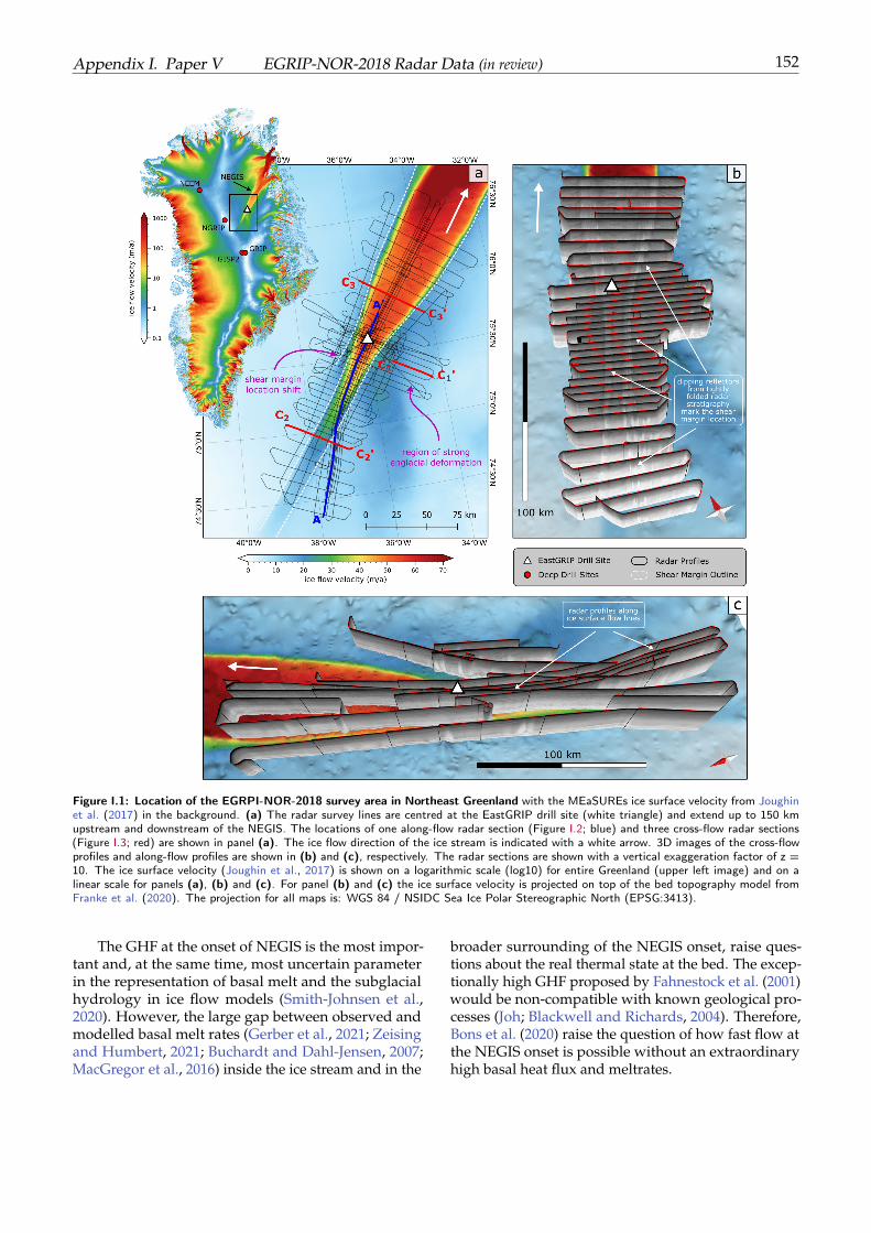
Appendix I. Paper V EGRIP-NOR-2018 Radar Data (in review) 152

Figure I.1: Location of the EGRPI-NOR-2018 survey area in Northeast Greenland with the MEaSUREs ice surface velocity from Joughinet al. (2017) in the background. (a) The radar survey lines are centred at the EastGRIP drill site (white triangle) and extend up to 150 kmupstream and downstream of the NEGIS. The locations of one along-flow radar section (Figure I.2; blue) and three cross-flow radar sections(Figure I.3; red) are shown in panel (a). The ice flow direction of the ice stream is indicated with a white arrow. 3D images of the cross-flowprofiles and along-flow profiles are shown in (b) and (c), respectively. The radar sections are shown with a vertical exaggeration factor of z =10. The ice surface velocity (Joughin et al., 2017) is shown on a logarithmic scale (log10) for entire Greenland (upper left image) and on alinear scale for panels (a), (b) and (c). For panel (b) and (c) the ice surface velocity is projected on top of the bed topography model fromFranke et al. (2020). The projection for all maps is: WGS 84 / NSIDC Sea Ice Polar Stereographic North (EPSG:3413).

The GHF at the onset of NEGIS is the most impor-tant and, at the same time, most uncertain parameterin the representation of basal melt and the subglacialhydrology in ice flow models (Smith-Johnsen et al.,2020). However, the large gap between observed andmodelled basal melt rates (Gerber et al., 2021; Zeisingand Humbert, 2021; Buchardt and Dahl-Jensen, 2007;MacGregor et al., 2016) inside the ice stream and in the

broader surrounding of the NEGIS onset, raise ques-tions about the real thermal state at the bed. The excep-tionally high GHF proposed by Fahnestock et al. (2001)would be non-compatible with known geological pro-cesses (Joh; Blackwell and Richards, 2004). Therefore,Bons et al. (2020) raise the question of how fast flow atthe NEGIS onset is possible without an extraordinaryhigh basal heat flux and meltrates.

Appendix I. Paper V EGRIP-NOR-2018 Radar Data (in review) 153

Unlike other ice streams in Greenland, the NEGISlacks an extensive overdeepened bed, and thus lateraltopographic constraints (Joughin et al., 2001b; Frankeet al., 2020). The ice stream more or less symmetricallybroadens along flow, as more ice is dragged throughthe shear margins (Fahnestock et al., 2001; Joughinet al., 2001a). Subglacial water routing in combinationwith subglacial till deformation seems to be a furthercontrolling mechanism of ice flow at the onset of theNEGIS (Keisling et al., 2014; Christianson et al., 2014).The outlet area is characterised by an overdeepenedbasin covered with unconsolidated sediments (Joughinet al., 2001a; Bamber et al., 2013). Ice thinning as aconsequence of increasing oceanic water temperaturesaround Greenland, could thus potentially be transmit-ted far upstream (Christianson et al., 2014), and changesin the hydropotential might have significant effects onthe ice stream geometry. The high susceptibility ofNEGIS to marine-triggered discharge and the expectedincrease in ocean water temperatures in the years tocome (Yin et al., 2011; Straneo et al., 2012) raises ques-tions about the future ice stream stability and its effecton the Greenland Ice Sheet mass balance.

Large scale ice flow models are essential tools topredict the future behaviour of glaciers and ice sheetsand are necessary to estimate future sea-level rise. Un-til today, these models fail to successfully simulate theNEGIS due to insufficient understanding of the key pro-cesses responsible for ice flow dynamics (Mottram et al.,2019; Shepherd et al., 2020), limiting the prediction ac-curacy. The East Greenland Ice-Core project (EastGRIP;https://eastgrip.org) aims to drill a deep ice corein the upstream area of the NEGIS, providing valuableinsights into the climate record, basal properties andice flow history at the drill site. Ice cores provide insitu information on physical and chemical properties athigh resolution but are limited as being a spatial pointmeasurement. Hence, further geophysical techniquesare required to extrapolate this information to obtain acomplete picture of the ice dynamic properties.

Radio-echo sounding (RES) has long become a stan-dard method in glaciology. The polar ice sheets aswell as low-latitude glaciers and ice caps have exten-sively been covered by airborne (e.g. Steinhage et al.;Schroeder et al., 2020) or ground-based (e.g. Pälli et al.,2002) RES surveys. The transmitted electromagneticwaves are sensitive to changes in dielectric permittivityand electrical conductivity and get reflected, scatteredor refracted at interfaces of dielectric contrasts in themedium they propagate (Fujita et al., 1999). The mostcommon glaciological application is the sounding ofice thickness and bedrock topography (e.g. Hempeland Thyssen, 1992; Dahl-Jensen et al., 1997; Steinhageet al., 1999; Nixdorf and Göktas, 2001; Kanagaratnamet al., 2001). Reflections within the ice column, orso-called internal reflection horizons (IRH), are often

caused by impurity layers of volcanic origin represent-ing isochronous horizons (Millar, 1981). These pro-vide valuable information on the ice flow regime andstrain history (Vaughan et al., 1999; Jacobel et al., 1993;Hodgkins et al.) and can be used to reconstruct pastaccumulation rates (e.g. Richardson et al., 1997; Nere-son et al., 2000; Siegert and Hodgkins, 2000; Pälli et al.,2002; Nereson and Raymond, 2001), to match ice coresfrom different locations (e.g. Jacobel and Hodge, 1995;Siegert et al., 1998; Hempel et al., 2000) and to vali-date numerical ice flow models (e.g. Huybrechts et al.,2000; Baldwin et al., 2003). Further applications of RESinclude the detection of crevasses (e.g. Zamora et al.,2007; Eder et al., 2008; Williams et al., 2014), mapping ofsubglacial lakes and basal hydrology (e.g. Carter et al.,2007; Palmer et al., 2013; Young et al., 2016), identifyingthermal regimes (e.g. Murray et al., 2000; Copland andSharp, 2001), determining snow and firn genesis (e.g.Frezzotti et al.) and obtaining information on the crys-tal orientation fabric (e.g. Matsuoka et al., 2003; Eisenet al., 2007; Jordan et al., 2020).

We present unique airborne radar data of the onsetregion of NEGIS recorded in 2018 by a multichannelultra-wideband radar system. The data set consists ofprofiles oriented parallel and perpendicular to the iceflow direction. The high along-track and range reso-lution allows consistent isochrone tracing, providinginsights into the three-dimensional structure of the icestream. In combination with the EastGRIP ice core, thisdataset contributes to a better understanding of ice flowdynamics of the NEGIS. In our manuscript, we intro-duce the study site and survey design. Furthermore,we describe the radar data processing and the respec-tive data products. The data are freely available at thePANGAEA data publisher (https://doi.pangaea.de/10.1594/PANGAEA.928569).

Survey region and previous work

In May 2018, we recorded radar data in the vicinityof the drill site of the EastGRIP ice core. An area of~ 24,000 km2 was mapped with 7494 km of radar pro-files along flow lines and perpendicular to ice flow(Figure 1). The survey region extends ~ 150 km up-stream and downstream of the EastGRIP drill site andranges from the central part of the ice stream up to 50km beyond the shear margins. In our survey region,the ice stream accelerates from ~ 10 to more than 80m a−1 and widens from ~15 to ~55 km. The radar dataalso covers the transition in the position of the shearmargin as well as strongly folded internal stratigraphyoutside of the ice stream (see Figure 1). Figure 1b andc show the locations of radar profiles in relation to theice surface velocity. Profiles extending perpendicularto ice flow have a spacing of 5 km in the region close

Appendix I. Paper V EGRIP-NOR-2018 Radar Data (in review) 154

to the drill site and 10 km further up- and downstream.Along-flow profiles either follow flowlines, which insome cases pass through the shear margins, or are con-stantly located inside the ice stream. Other profilesare oriented parallel to ice flow of the NEGIS but arelocated outside of the ice stream.

The ice thickness in our survey region ranges from2059 m to 3092 m and shows, on average, a gradualdecrease in thickness from the upstream to the down-stream part (Franke et al., 2020, 2019). An analysis ofthe bed topography, basal roughness and bed returnechoes by Franke et al. (2021b) shows that our surveyarea can be divided into two different morphologicalregimes. The upstream part (upstream of EastGRIP) ischaracterised by a narrow ice stream width with accel-erating ice flow velocity, a smooth bed with elongatedflow-parallel subglacial landforms and a soft till layerat the base (Christianson et al., 2014). Downstreamof EastGRIP, the ice stream widens, and we note anoverall change to a rougher and more variable bed geo-morphology. The ice stream widens up to 57 km andice flow velocity keeps constant and decreases locally(Franke et al., 2021b).

In the 2012 summer field season, a scientific con-sortium collected ground-based geophysical data (RESand seismic survey) as well as a shallow ice core (Valle-longa et al., 2014). Christianson et al. (2014) examinedthe ice-bed interface by means of radar and seismic dataanalysis. They found high-porosity, water-saturated till,which lubricates the ice stream base and most likely fa-cilitates ice stream flow. Keisling et al. (2014) used thesame radar data to analyse the internal radar stratig-raphy and suggest that the basal hydrology controlsthe upstream portion of the NEGIS. By contrast, thedownstream part is rather confined by the bed topog-raphy. Riverman et al. (2019) and ? analysed the shearmargins in particular and observed an increased accu-mulation and enhanced firn densification in the upperice column as well as wet elongated subglacial land-forms at the bed. Furthermore Holschuh et al. (2019)use RES data to evaluate 3-D thermomechanical modelsof the NEGIS. The authors highlight the complexity ofthe stagnant to streaming ice flow transition and pro-vide insights into the englacial heat transport. Finally,a comprehensive chemical analysis of a 67 m deep firncore was conducted by Vallelonga et al. (2014). Theresults demonstrated that a deep ice core at this loca-tion has the potential to retrieve a reliable record of theHolocene and last-glacial cycle.

Methods

Radar data acquisition

The ultra-wideband (UWB) airborne radar is a Mul-tichannel Coherent Radar Depth Sounder (MCoRDS,version 5) which was developed at the centre for Re-mote Sensing of Ice Sheets (CReSIS) at the University ofKansas (Hale et al., 2016). It has an improved hardwaredesign compared to predecessor radar depth soundersby CReSIS (Gogineni et al., 1998; Wang et al., 2016).The radar configuration deployed in 2018 consists of aneight-element radar array mounted under the Polar 6Basler BT-67 aircraft’s fuselage. The eight antenna ele-ments function as transmit and receive channels usinga transmit-receive switch. The total transmit power is6 kW, the radar can be operated within the frequencyband of 150 – 600 MHz. The pulse repetition frequency(PRF) is 10 kHz, and the sampling frequency is 1.6 GHz.The characteristics of the transmitted waveform as wellas the recording settings can be manually adjusted. Werefer to the combined transmission/reception settingsas waveforms in the following.

Table I.1: Acquisition parameters of the EGRIP-NOR-2018radar campaign.

Parameter ValueRadar system MCoRDS5Frequency range 180-210 MHzWaveform signal 1, 3, 10µs chirpWaveform presumsa 2, 4, 32Pulse Repetition Frequency 10 kHzSampling frequency 1600 MHzTukey window taper ratio 0.08Transmit channels 8Receiving channels 8Aircraft altitude above ground ∼ 360 mAircraft velocity ∼ 260 km h−1

aPresums are set for each waveform individually.

All profiles were recorded using linear frequency-modulated chirps in the frequency band of 180-210 MHz, antenna elements oriented with the E-planealigned with the along-track (HH polarisation), and thetransmit antenna beam pointed toward nadir. We usedthree alternating waveforms to increase the dynamicrange of the system (see Table I.1). Short pulses (1 µs)and low receiver gain of 11 dB to image the glacier sur-face, and longer pulses (3 - 10 µs) with higher receivergain (48 dB) to image internal features and the ice base.

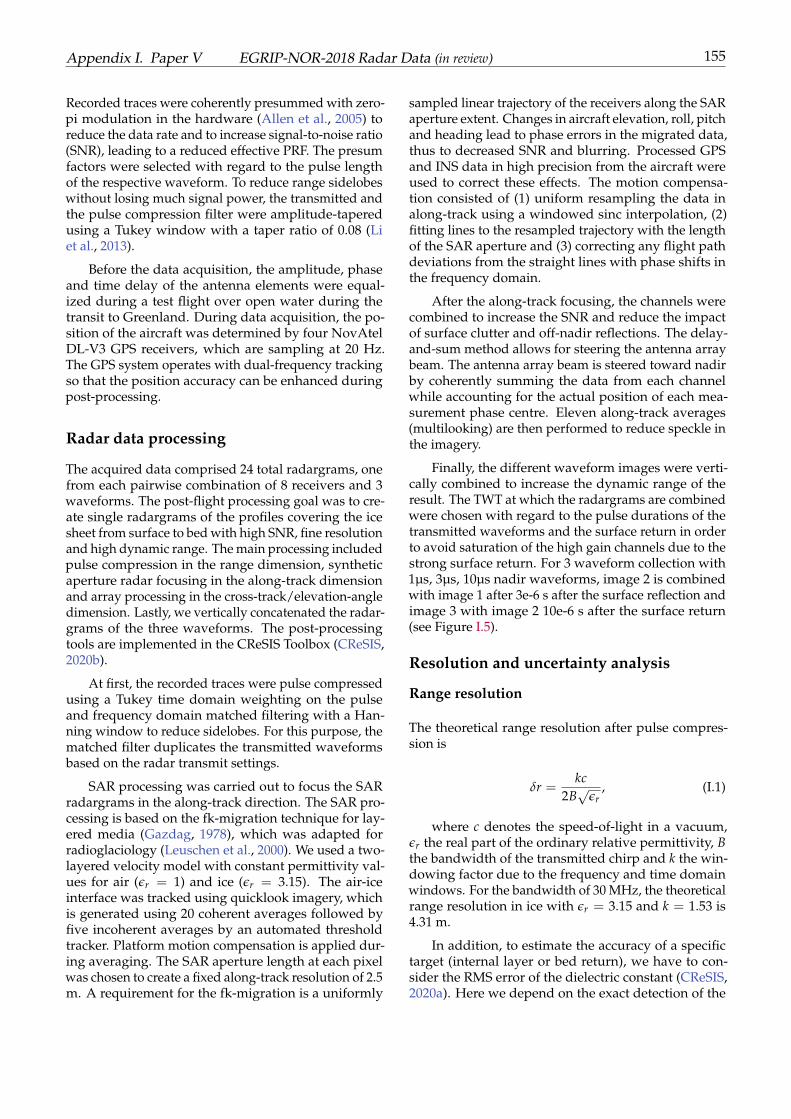
Appendix I. Paper V EGRIP-NOR-2018 Radar Data (in review) 155

Recorded traces were coherently presummed with zero-pi modulation in the hardware (Allen et al., 2005) toreduce the data rate and to increase signal-to-noise ratio(SNR), leading to a reduced effective PRF. The presumfactors were selected with regard to the pulse lengthof the respective waveform. To reduce range sidelobeswithout losing much signal power, the transmitted andthe pulse compression filter were amplitude-taperedusing a Tukey window with a taper ratio of 0.08 (Liet al., 2013).

Before the data acquisition, the amplitude, phaseand time delay of the antenna elements were equal-ized during a test flight over open water during thetransit to Greenland. During data acquisition, the po-sition of the aircraft was determined by four NovAtelDL-V3 GPS receivers, which are sampling at 20 Hz.The GPS system operates with dual-frequency trackingso that the position accuracy can be enhanced duringpost-processing.

Radar data processing

The acquired data comprised 24 total radargrams, onefrom each pairwise combination of 8 receivers and 3waveforms. The post-flight processing goal was to cre-ate single radargrams of the profiles covering the icesheet from surface to bed with high SNR, fine resolutionand high dynamic range. The main processing includedpulse compression in the range dimension, syntheticaperture radar focusing in the along-track dimensionand array processing in the cross-track/elevation-angledimension. Lastly, we vertically concatenated the radar-grams of the three waveforms. The post-processingtools are implemented in the CReSIS Toolbox (CReSIS,2020b).

At first, the recorded traces were pulse compressedusing a Tukey time domain weighting on the pulseand frequency domain matched filtering with a Han-ning window to reduce sidelobes. For this purpose, thematched filter duplicates the transmitted waveformsbased on the radar transmit settings.

SAR processing was carried out to focus the SARradargrams in the along-track direction. The SAR pro-cessing is based on the fk-migration technique for lay-ered media (Gazdag, 1978), which was adapted forradioglaciology (Leuschen et al., 2000). We used a two-layered velocity model with constant permittivity val-ues for air (ϵr = 1) and ice (ϵr = 3.15). The air-iceinterface was tracked using quicklook imagery, whichis generated using 20 coherent averages followed byfive incoherent averages by an automated thresholdtracker. Platform motion compensation is applied dur-ing averaging. The SAR aperture length at each pixelwas chosen to create a fixed along-track resolution of 2.5m. A requirement for the fk-migration is a uniformly

sampled linear trajectory of the receivers along the SARaperture extent. Changes in aircraft elevation, roll, pitchand heading lead to phase errors in the migrated data,thus to decreased SNR and blurring. Processed GPSand INS data in high precision from the aircraft wereused to correct these effects. The motion compensa-tion consisted of (1) uniform resampling the data inalong-track using a windowed sinc interpolation, (2)fitting lines to the resampled trajectory with the lengthof the SAR aperture and (3) correcting any flight pathdeviations from the straight lines with phase shifts inthe frequency domain.

After the along-track focusing, the channels werecombined to increase the SNR and reduce the impactof surface clutter and off-nadir reflections. The delay-and-sum method allows for steering the antenna arraybeam. The antenna array beam is steered toward nadirby coherently summing the data from each channelwhile accounting for the actual position of each mea-surement phase centre. Eleven along-track averages(multilooking) are then performed to reduce speckle inthe imagery.

Finally, the different waveform images were verti-cally combined to increase the dynamic range of theresult. The TWT at which the radargrams are combinedwere chosen with regard to the pulse durations of thetransmitted waveforms and the surface return in orderto avoid saturation of the high gain channels due to thestrong surface return. For 3 waveform collection with1µs, 3µs, 10µs nadir waveforms, image 2 is combinedwith image 1 after 3e-6 s after the surface reflection andimage 3 with image 2 10e-6 s after the surface return(see Figure I.5).

Resolution and uncertainty analysis

Range resolution

The theoretical range resolution after pulse compres-sion is

δr =kc

2B√

ϵr, (I.1)

where c denotes the speed-of-light in a vacuum,ϵr the real part of the ordinary relative permittivity, Bthe bandwidth of the transmitted chirp and k the win-dowing factor due to the frequency and time domainwindows. For the bandwidth of 30 MHz, the theoreticalrange resolution in ice with ϵr = 3.15 and k = 1.53 is4.31 m.

In addition, to estimate the accuracy of a specifictarget (internal layer or bed return), we have to con-sider the RMS error of the dielectric constant (CReSIS,2020a). Here we depend on the exact detection of the

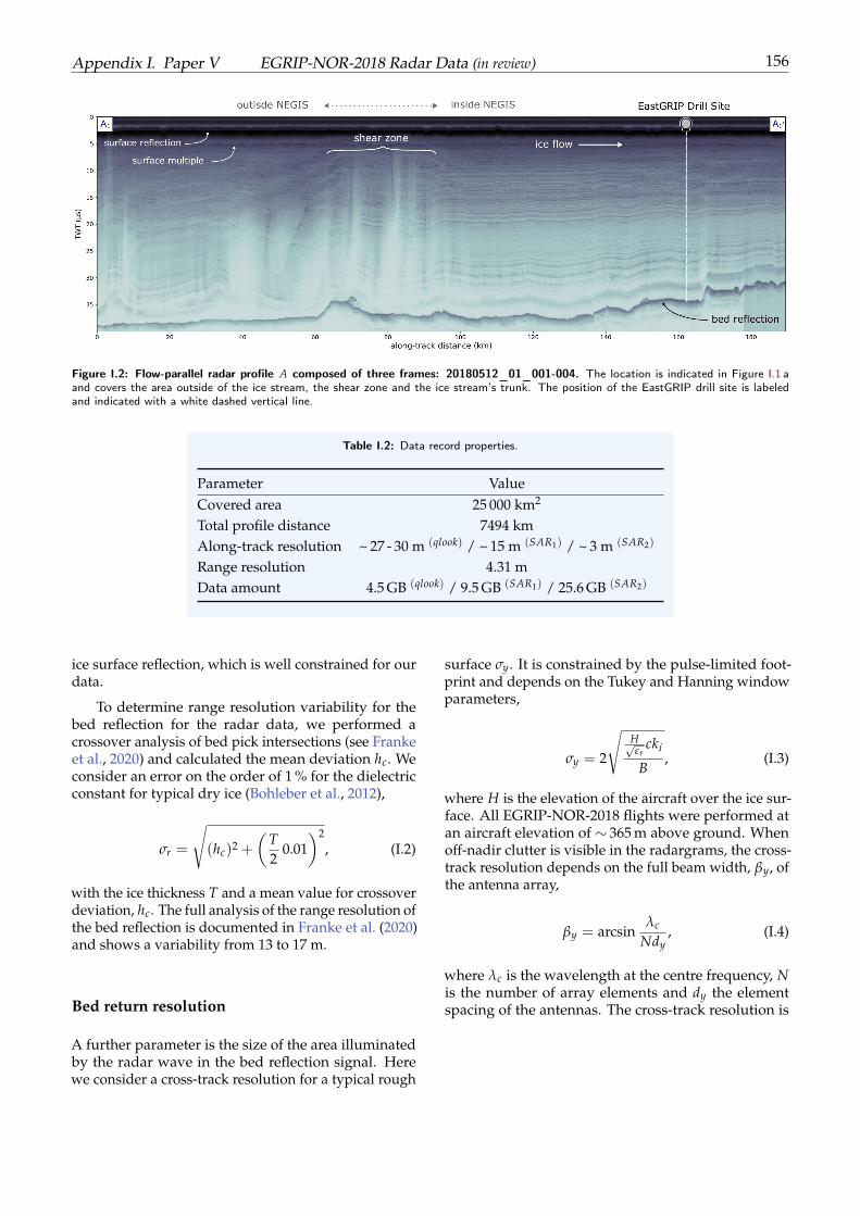
Appendix I. Paper V EGRIP-NOR-2018 Radar Data (in review) 156

Figure I.2: Flow-parallel radar profile A composed of three frames: 20180512_01_001-004. The location is indicated in Figure I.1 aand covers the area outside of the ice stream, the shear zone and the ice stream’s trunk. The position of the EastGRIP drill site is labeledand indicated with a white dashed vertical line.

Table I.2: Data record properties.

Parameter ValueCovered area 25 000 km2

Total profile distance 7494 kmAlong-track resolution ~ 27 - 30 m (qlook) / ~ 15 m (SAR1) / ~ 3 m (SAR2)

Range resolution 4.31 mData amount 4.5 GB (qlook) / 9.5 GB (SAR1) / 25.6 GB (SAR2)

ice surface reflection, which is well constrained for ourdata.

To determine range resolution variability for thebed reflection for the radar data, we performed acrossover analysis of bed pick intersections (see Frankeet al., 2020) and calculated the mean deviation hc. Weconsider an error on the order of 1 % for the dielectricconstant for typical dry ice (Bohleber et al., 2012),

σr =

√(hc)2 +

(T2

0.01)2

, (I.2)

with the ice thickness T and a mean value for crossoverdeviation, hc. The full analysis of the range resolution ofthe bed reflection is documented in Franke et al. (2020)and shows a variability from 13 to 17 m.

Bed return resolution

A further parameter is the size of the area illuminatedby the radar wave in the bed reflection signal. Herewe consider a cross-track resolution for a typical rough

surface σy. It is constrained by the pulse-limited foot-print and depends on the Tukey and Hanning windowparameters,

σy = 2

√H√εr

cki

B, (I.3)

where H is the elevation of the aircraft over the ice sur-face. All EGRIP-NOR-2018 flights were performed atan aircraft elevation of ∼ 365 m above ground. Whenoff-nadir clutter is visible in the radargrams, the cross-track resolution depends on the full beam width, βy, ofthe antenna array,

βy = arcsinλc

Ndy, (I.4)

where λc is the wavelength at the centre frequency, Nis the number of array elements and dy the elementspacing of the antennas. The cross-track resolution is

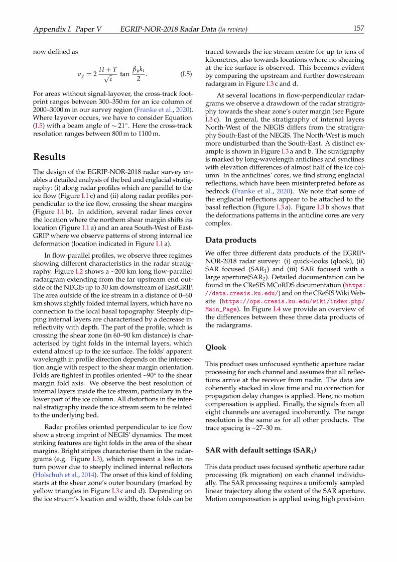
Appendix I. Paper V EGRIP-NOR-2018 Radar Data (in review) 157

now defined as

σy = 2H + T√

εtan

βykt

2. (I.5)

For areas without signal-layover, the cross-track foot-print ranges between 300–350 m for an ice column of2000–3000 m in our survey region (Franke et al., 2020).Where layover occurs, we have to consider Equation(I.5) with a beam angle of ∼ 21. Here the cross-trackresolution ranges between 800 m to 1100 m.

ResultsThe design of the EGRIP-NOR-2018 radar survey en-ables a detailed analysis of the bed and englacial stratig-raphy: (i) along radar profiles which are parallel to theice flow (Figure I.1 c) and (ii) along radar profiles per-pendicular to the ice flow, crossing the shear margins(Figure I.1 b). In addition, several radar lines coverthe location where the northern shear margin shifts itslocation (Figure I.1 a) and an area South-West of East-GRIP where we observe patterns of strong internal icedeformation (location indicated in Figure I.1 a).

In flow-parallel profiles, we observe three regimesshowing different characteristics in the radar stratig-raphy. Figure I.2 shows a ~200 km long flow-parallelradargram extending from the far upstream end out-side of the NEGIS up to 30 km downstream of EastGRIP.The area outside of the ice stream in a distance of 0–60km shows slightly folded internal layers, which have noconnection to the local basal topography. Steeply dip-ping internal layers are characterised by a decrease inreflectivity with depth. The part of the profile, which iscrossing the shear zone (in 60–90 km distance) is char-acterised by tight folds in the internal layers, whichextend almost up to the ice surface. The folds’ apparentwavelength in profile direction depends on the intersec-tion angle with respect to the shear margin orientation.Folds are tightest in profiles oriented ~90° to the shearmargin fold axis. We observe the best resolution ofinternal layers inside the ice stream, particulary in thelower part of the ice column. All distortions in the inter-nal stratigraphy inside the ice stream seem to be relatedto the underlying bed.

Radar profiles oriented perpendicular to ice flowshow a strong imprint of NEGIS’ dynamics. The moststriking features are tight folds in the area of the shearmargins. Bright stripes characterise them in the radar-grams (e.g. Figure I.3), which represent a loss in re-turn power due to steeply inclined internal reflectors(Holschuh et al., 2014). The onset of this kind of foldingstarts at the shear zone’s outer boundary (marked byyellow triangles in Figure I.3 c and d). Depending onthe ice stream’s location and width, these folds can be

traced towards the ice stream centre for up to tens ofkilometres, also towards locations where no shearingat the ice surface is observed. This becomes evidentby comparing the upstream and further downstreamradargram in Figure I.3 c and d.

At several locations in flow-perpendicular radar-grams we observe a drawdown of the radar stratigra-phy towards the shear zone’s outer margin (see FigureI.3 c). In general, the stratigraphy of internal layersNorth-West of the NEGIS differs from the stratigra-phy South-East of the NEGIS. The North-West is muchmore undisturbed than the South-East. A distinct ex-ample is shown in Figure I.3 a and b. The stratigraphyis marked by long-wavelength anticlines and synclineswith elevation differences of almost half of the ice col-umn. In the anticlines’ cores, we find strong englacialreflections, which have been misinterpreted before asbedrock (Franke et al., 2020). We note that some ofthe englacial reflections appear to be attached to thebasal reflection (Figure I.3 a). Figure I.3 b shows thatthe deformations patterns in the anticline cores are verycomplex.

Data products

We offer three different data products of the EGRIP-NOR-2018 radar survey: (i) quick-looks (qlook), (ii)SAR focused (SAR1) and (iii) SAR focused with alarge aperture(SAR2). Detailed documentation can befound in the CReSIS MCoRDS documentation (https://data.cresis.ku.edu/) and on the CReSIS Wiki Web-site (https://ops.cresis.ku.edu/wiki/index.php/Main_Page). In Figure I.4 we provide an overview ofthe differences between these three data products ofthe radargrams.

Qlook

This product uses unfocused synthetic aperture radarprocessing for each channel and assumes that all reflec-tions arrive at the receiver from nadir. The data arecoherently stacked in slow time and no correction forpropagation delay changes is applied. Here, no motioncompensation is applied. Finally, the signals from alleight channels are averaged incoherently. The rangeresolution is the same as for all other products. Thetrace spacing is ~27–30 m.

SAR with default settings (SAR1)

This data product uses focused synthetic aperture radarprocessing (fk migration) on each channel individu-ally. The SAR processing requires a uniformly sampledlinear trajectory along the extent of the SAR aperture.Motion compensation is applied using high precision

Appendix I. Paper V EGRIP-NOR-2018 Radar Data (in review) 158

Figure I.3: Radar profiles C1,2,3 (frames 20180508_06_003, 20180511_01_007 and 20180514_01_011-012, respectively). Thecorresponding locations are shown in Figure I.1 a. Panel (a) shows a profile located outside of the NEGIS, SE of EastGRIP. A close up ofan anticline and other patterns of deformation are shown in panel (b), resembling the skeleton of a dead penguin. A slice through the icestream in the upstream region is shown in panel (c) and a radar section further downstream in (d). The position of the shear margins (themaximum in the surface velocity gradient) are indicated with a yellow triangle and the folds in the shear margin areas with purple lines. Theice flow direction is out of the page.

processed GPS and INS data from the aircraft. The di-rection of arrival is estimated by delay-and-sum beam-forming to combine the channels. A Hanning windowis applied in the frequency domain to suppress side-lobes. This product is comparable to the CReSIS stan-dard data product. The trace spacing is ~15 m.

SAR with wider angular range (SAR2)

By processing at a finer SAR resolution, the SAR proces-sor uses scattered energy from a wider angular rangearound nadir to form the image. Since the angle of scat-tered returns from a specular internal layer is propor-tional to the internal layer slope, the SAR processor’sincreased sensitivity to larger angle returns translates toan increased sensitivity to layers with larger slopes. We

achieve a better resolution of steeply inclined internalreflectors by changing the along-track resolution beforeSAR processing to 1 m (≈ σx = 1, whereas the defaultsetting is σx = 2.5). 1 m is not the smallest possiblevalue for processing, but is on the limit to achieve asufficiently high SNR. The SNR is smaller for larger an-gles because the range to the target increases for greaterangles, which leads to additional signal loss (sphericalspreading loss and additional signal attenuation in ice).The differences between radargrams processed withσx = 1 and 2.5 are shown in Figure I.4. The final tracespacing is ~3 m.

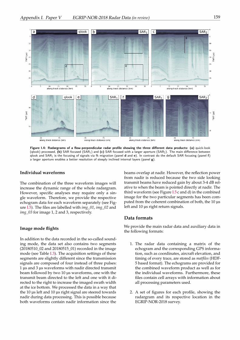
Appendix I. Paper V EGRIP-NOR-2018 Radar Data (in review) 159

Figure I.4: Radargrams of a flow-perpendicular radar profile showing the three different data products: (a) quick-look(qlook) processed, (b) SAR focused (SAR1) and (c) SAR focused with a larger aperture (SAR2). The main difference betweenqlook and SAR1 is the focusing of signals via fk migration (panel d and e). In contrast do the default SAR focusing (panel f)a larger aperture enables a better resolution of steeply inclined internal layers (panel g).

Individual waveforms

The combination of the three waveform images willincrease the dynamic range of the whole radargram.However, specific analyses may require only a sin-gle waveform. Therefore, we provide the respectiveechogram data for each waveform separately (see Fig-ure I.5). The files are labelled with img_01, img_02 andimg_03 for image 1, 2 and 3, respectively.

Image mode flights

In addition to the data recorded in the so-called sound-ing mode, the data set also contains two segments(20180510_02 and 20180515_01) recorded in the imagemode (see Table I.3). The acquisition settings of thesesegments are slightly different since the transmissionsignals are composed of four instead of three pulses:1 µs and 3 µs waveforms with nadir directed transmitbeam followed by two 10 µs waveforms, one with thetransmit beam directed to the left and one with it di-rected to the right to increase the imaged swath widthat the ice bottom. We processed the data in a way thatthe 10 µs left and 10 µs right signal are steered towardsnadir during data processing. This is possible becauseboth waveforms contain nadir information since the

beams overlap at nadir. However, the reflection powerfrom nadir is reduced because the two side lookingtransmit beams have reduced gain by about 3-4 dB rel-ative to when the beam is pointed directly at nadir. Thethird waveform (see Figure I.5 c and d) in the combinedimage for the two particular segments has been com-puted from the coherent combination of both, the 10 µsleft and 10 µs right return signals.

Data formats

We provide the main radar data and auxiliary data inthe following formats:

1. The radar data containing a matrix of theechogram and the corresponding GPS informa-tion, such as coordinates, aircraft elevation, andtiming of every trace, are stored as matfiles (HDF-5 based format). The echograms are provided forthe combined waveform product as well as forthe individual waveforms. Furthermore, thesefiles contain cell arrays with information aboutall processing parameters used.

2. A set of figures for each profile, showing theradargram and its respective location in theEGRIP-NOR-2018 survey.

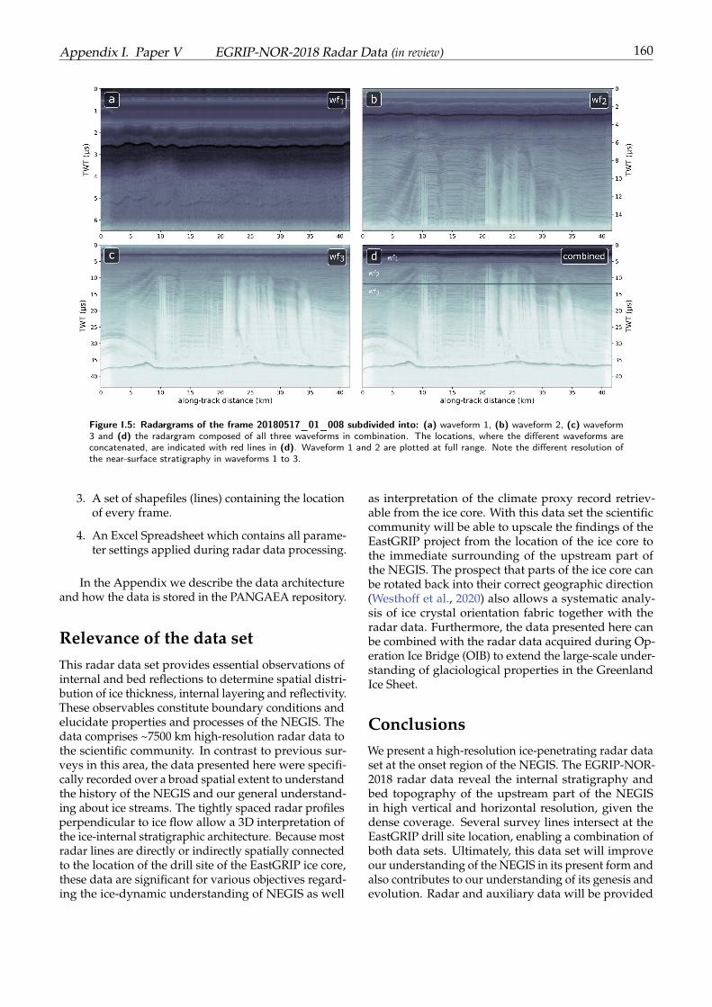
Appendix I. Paper V EGRIP-NOR-2018 Radar Data (in review) 160

Figure I.5: Radargrams of the frame 20180517_01_008 subdivided into: (a) waveform 1, (b) waveform 2, (c) waveform3 and (d) the radargram composed of all three waveforms in combination. The locations, where the different waveforms areconcatenated, are indicated with red lines in (d). Waveform 1 and 2 are plotted at full range. Note the different resolution ofthe near-surface stratigraphy in waveforms 1 to 3.

3. A set of shapefiles (lines) containing the locationof every frame.

4. An Excel Spreadsheet which contains all parame-ter settings applied during radar data processing.

In the Appendix we describe the data architectureand how the data is stored in the PANGAEA repository.

Relevance of the data setThis radar data set provides essential observations ofinternal and bed reflections to determine spatial distri-bution of ice thickness, internal layering and reflectivity.These observables constitute boundary conditions andelucidate properties and processes of the NEGIS. Thedata comprises ~7500 km high-resolution radar data tothe scientific community. In contrast to previous sur-veys in this area, the data presented here were specifi-cally recorded over a broad spatial extent to understandthe history of the NEGIS and our general understand-ing about ice streams. The tightly spaced radar profilesperpendicular to ice flow allow a 3D interpretation ofthe ice-internal stratigraphic architecture. Because mostradar lines are directly or indirectly spatially connectedto the location of the drill site of the EastGRIP ice core,these data are significant for various objectives regard-ing the ice-dynamic understanding of NEGIS as well

as interpretation of the climate proxy record retriev-able from the ice core. With this data set the scientificcommunity will be able to upscale the findings of theEastGRIP project from the location of the ice core tothe immediate surrounding of the upstream part ofthe NEGIS. The prospect that parts of the ice core canbe rotated back into their correct geographic direction(Westhoff et al., 2020) also allows a systematic analy-sis of ice crystal orientation fabric together with theradar data. Furthermore, the data presented here canbe combined with the radar data acquired during Op-eration Ice Bridge (OIB) to extend the large-scale under-standing of glaciological properties in the GreenlandIce Sheet.

ConclusionsWe present a high-resolution ice-penetrating radar dataset at the onset region of the NEGIS. The EGRIP-NOR-2018 radar data reveal the internal stratigraphy andbed topography of the upstream part of the NEGISin high vertical and horizontal resolution, given thedense coverage. Several survey lines intersect at theEastGRIP drill site location, enabling a combination ofboth data sets. Ultimately, this data set will improveour understanding of the NEGIS in its present form andalso contributes to our understanding of its genesis andevolution. Radar and auxiliary data will be provided

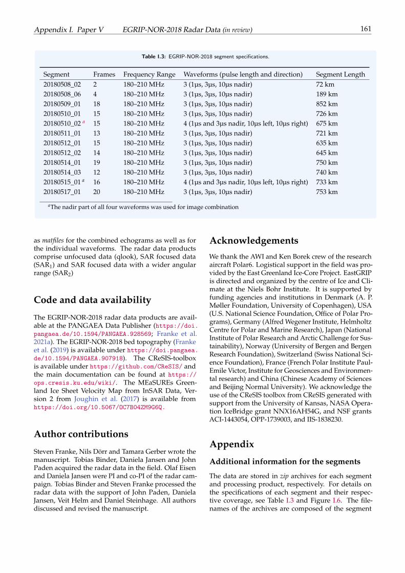
Appendix I. Paper V EGRIP-NOR-2018 Radar Data (in review) 161

Table I.3: EGRIP-NOR-2018 segment specifications.

Segment Frames Frequency Range Waveforms (pulse length and direction) Segment Length20180508_02 2 180–210 MHz 3 (1µs, 3µs, 10µs nadir) 72 km20180508_06 4 180–210 MHz 3 (1µs, 3µs, 10µs nadir) 189 km20180509_01 18 180–210 MHz 3 (1µs, 3µs, 10µs nadir) 852 km20180510_01 15 180–210 MHz 3 (1µs, 3µs, 10µs nadir) 726 km20180510_02 a 15 180–210 MHz 4 (1µs and 3µs nadir, 10µs left, 10µs right) 675 km20180511_01 13 180–210 MHz 3 (1µs, 3µs, 10µs nadir) 721 km20180512_01 15 180–210 MHz 3 (1µs, 3µs, 10µs nadir) 635 km20180512_02 14 180–210 MHz 3 (1µs, 3µs, 10µs nadir) 645 km20180514_01 19 180–210 MHz 3 (1µs, 3µs, 10µs nadir) 750 km20180514_03 12 180–210 MHz 3 (1µs, 3µs, 10µs nadir) 740 km20180515_01 a 16 180–210 MHz 4 (1µs and 3µs nadir, 10µs left, 10µs right) 733 km20180517_01 20 180–210 MHz 3 (1µs, 3µs, 10µs nadir) 753 km

aThe nadir part of all four waveforms was used for image combination

as matfiles for the combined echograms as well as forthe individual waveforms. The radar data productscomprise unfocused data (qlook), SAR focused data(SAR1) and SAR focused data with a wider angularrange (SAR2)

Code and data availability

The EGRIP-NOR-2018 radar data products are avail-able at the PANGAEA Data Publisher (https://doi.pangaea.de/10.1594/PANGAEA.928569; Franke et al.2021a). The EGRIP-NOR-2018 bed topography (Frankeet al. (2019) is available under https://doi.pangaea.de/10.1594/PANGAEA.907918). The CReSIS-toolboxis available under https://github.com/CReSIS/ andthe main documentation can be found at https://ops.cresis.ku.edu/wiki/. The MEaSUREs Green-land Ice Sheet Velocity Map from InSAR Data, Ver-sion 2 from Joughin et al. (2017) is available fromhttps://doi.org/10.5067/OC7B04ZM9G6Q.

Author contributions

Steven Franke, Nils Dörr and Tamara Gerber wrote themanuscript. Tobias Binder, Daniela Jansen and JohnPaden acquired the radar data in the field. Olaf Eisenand Daniela Jansen were PI and co-PI of the radar cam-paign. Tobias Binder and Steven Franke processed theradar data with the support of John Paden, DanielaJansen, Veit Helm and Daniel Steinhage. All authorsdiscussed and revised the manuscript.

Acknowledgements

We thank the AWI and Ken Borek crew of the researchaircraft Polar6. Logistical support in the field was pro-vided by the East Greenland Ice-Core Project. EastGRIPis directed and organized by the centre of Ice and Cli-mate at the Niels Bohr Institute. It is supported byfunding agencies and institutions in Denmark (A. P.Møller Foundation, University of Copenhagen), USA(U.S. National Science Foundation, Office of Polar Pro-grams), Germany (Alfred Wegener Institute, HelmholtzCentre for Polar and Marine Research), Japan (NationalInstitute of Polar Research and Arctic Challenge for Sus-tainability), Norway (University of Bergen and BergenResearch Foundation), Switzerland (Swiss National Sci-ence Foundation), France (French Polar Institute Paul-Emile Victor, Institute for Geosciences and Environmen-tal research) and China (Chinese Academy of Sciencesand Beijing Normal University). We acknowledge theuse of the CReSIS toolbox from CReSIS generated withsupport from the University of Kansas, NASA Opera-tion IceBridge grant NNX16AH54G, and NSF grantsACI-1443054, OPP-1739003, and IIS-1838230.

Appendix

Additional information for the segments

The data are stored in zip archives for each segmentand processing product, respectively. For details onthe specifications of each segment and their respec-tive coverage, see Table I.3 and Figure I.6. The file-names of the archives are composed of the segment

Appendix I. Paper V EGRIP-NOR-2018 Radar Data (in review) 162

and the data product (e.g. 20180508_02_qlook.zip,20180508_02_sar1.zip and 20180508_02_sar2.zip for thequick-look, SAR with default settings (SAR1) and SARwith larger angular range data product (SAR2), respec-tively). Each zip archive contains the individual framesin the matfile format.

Appendix I. Paper V EGRIP-NOR-2018 Radar Data (in review) 163

Figure I.6: Radar profiles locations of the 12 segments shown in Table I.3 of the EGRIP-NOR-2018 data set. The respectivesegments are highlighted with a white line and the radar profiles of the complete survey with a finer black line. The backgroundmap represents ice surface velocity from Joughin et al. (2017). The shear margin is indicated with a white dashed outline andthe location of EastGRIP with a red dot.

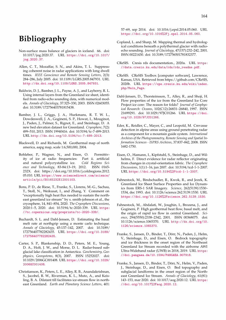
164

BibliographyNon-surface mass balance of glaciers in iceland. 66. doi:

10.1017/jog.2020.37. URL https://doi.org/10.1017/jog.2020.37.

Allen, C. T., Mozaffar, S. N., and Akins, T. L. Suppress-ing coherent noise in radar applications with long dwelltimes. IEEE Geoscience and Remote Sensing Letters, 2(3):284–286, July 2005. doi: 10.1109/LGRS.2005.847931. URLhttp://dx.doi.org/10.1109/LGRS.2005.847931.

Baldwin, D. J., Bamber, J. L., Payne, A. J., and Layberry, R. L.Using internal layers from the Greenland ice sheet, identi-fied from radio-echo sounding data, with numerical mod-els. Annals of Glaciology, 37:325–330, 2003. ISSN 02603055.doi: 10.3189/172756403781815438.

Bamber, J. L., Griggs, J. A., Hurkmans, R. T. W. L.,Dowdeswell, J. A., Gogineni, S. P., Howat, I., Mouginot,J., Paden, J., Palmer, S., Rignot, E., and Steinhage, D. Anew bed elevation dataset for Greenland. Cryosphere, 7(2):499–510, 2013. ISSN 19940416. doi: 10.5194/tc-7-499-2013.URL http://dx.doi.org/10.5194/tc-7-499-2013.

Blackwell, D. and Richards, M. Geothermal map of northamerica, aapg map, scale 1:6,500,000, 2004.

Bohleber, P., Wagner, N., and Eisen, O. Permittiv-ity of ice at radio frequencies: Part ii. artificialand natural polycrystalline ice. Cold Regions Sci-ence and Technology, 83-84:13–19, 2012. ISSN 0165-232X. doi: https://doi.org/10.1016/j.coldregions.2012.05.010. URL https://www.sciencedirect.com/science/article/pii/S0165232X12001103.

Bons, P. D., de Riese, T., Franke, S., Llorens, M.-G., Sachau,T., Stoll, N., Weikusat, I., and Zhang, Y. Comment on“exceptionally high heat flux needed to sustain the north-east greenland ice stream” by s. smith-johnson et al., thecryosphere, 14, 841–854, 2020. The Cryosphere Discussions,2020:1–5, 2020. doi: 10.5194/tc-2020-339. URL https://tc.copernicus.org/preprints/tc-2020-339/.

Buchardt, S. L. and Dahl-Jensen, D. Estimating the basalmelt rate at northgrip using a monte carlo technique.Annals of Glaciology, 45:137–142, 2007. doi: 10.3189/172756407782282435. URL https://doi.org/10.3189/172756407782282435.

Carter, S. P., Blankenship, D. D., Peters, M. E., Young,D. A., Holt, J. W., and Morse, D. L. Radar-based sub-glacial lake classification in Antarctica. Geochemistry, Geo-physics, Geosystems, 8(3), 2007. ISSN 15252027. doi:10.1029/2006GC001408. URL https://doi.org/10.1029/2006GC001408.

Christianson, K., Peters, L. E., Alley, R. B., Anandakrishnan,S., Jacobel, R. W., Riverman, K. L., Muto, A., and Keis-ling, B. A. Dilatant till facilitates ice-stream flow in north-east Greenland. Earth and Planetary Science Letters, 401:

57–69, sep 2014. doi: 10.1016/j.epsl.2014.05.060. URLhttps://doi.org/10.1016%2Fj.epsl.2014.05.060.

Copland, L. and Sharp, M. Mapping thermal and hydrolog-ical conditions beneath a polythermal glacier with radio-echo sounding. Journal of Glaciology, 47(157):232–242, 2001.ISSN 00221430. doi: 10.3189/172756501781832377.

CReSIS. Cresis rds documentation., 2020a. URL https://data.cresis.ku.edu/data/rds/rds_readme.pdf.

CReSIS. CReSIS Toolbox [computer software], Lawrence,Kansas, USA. Retrieved from https://github.com/CReSIS,2020b. URL https://ops.cresis.ku.edu/wiki/index.php/Main_Page.

Dahl-Jensen, D., Thorsteinsson, T., Alley, R., and Shoji, H.Flow properties of the ice from the Greenland Ice CoreProject ice core: The reason for folds? Journal of Geophys-ical Research: Oceans, 102(C12):26831–26840, 1997. ISSN21699291. doi: 10.1029/97JC01266. URL https://doi.org/10.1029/97JC01266.

Eder, K., Reidler, C., Mayer, C., and Leopold, M. Crevassedetection in alpine areas using ground penetrating radaras a component for a mountain guide system. InternationalArchives of the Photogrammetry, Remote Sensing and Spatial In-formation Sciences - ISPRS Archives, 37:837–842, 2008. ISSN1682-1750.

Eisen, O., Hamann, I., Kipfstuhl, S., Steinhage, D., and Wil-helms, F. Direct evidence for radar reflector originatingfrom changes in crystal-orientation fabric. The CryosphereDiscussions, 1(1):1–16, jun 2007. doi: 10.5194/tcd-1-1-2007.URL https://doi.org/10.5194%2Ftcd-1-1-2007.

Fahnestock, M., Bindschadler, R., Kwok, R., and Jezek, K.Greenland Ice Sheet Surface Properties and Ice Dynam-ics from ERS-1 SAR Imagery. Science, 262(5139):1530–1534, dec 1993. doi: 10.1126/science.262.5139.1530. URLhttps://doi.org/10.1126%2Fscience.262.5139.1530.

Fahnestock, M., Abdalati, W., Joughin, I., Brozena, J., andGogineni, P. High geothermal heat flow, basal melt, andthe origin of rapid ice flow in central Greenland. Sci-ence, 294(5550):2338–2342, 2001. ISSN 00368075. doi:10.1126/science.1065370. URL http://dx.doi.org/10.1126/science.1065370.

Franke, S., Jansen, D., Binder, T., Dörr, N., Paden, J., Helm,V., Steinhage, D., and Eisen, O. Bedrock topographyand ice thickness in the onset region of the NortheastGreenland Ice Stream recorded with the airborne AWIUltra-Wideband radar (UWB) in 2018, 2019. URL https://doi.pangaea.de/10.1594/PANGAEA.907918.

Franke, S., Jansen, D., Binder, T., Dörr, N., Helm, V., Paden,J., Steinhage, D., and Eisen, O. Bed topography andsubglacial landforms in the onset region of the North-east Greenland Ice Stream. Annals of Glaciology, 61(81):143–153, mar 2020. doi: 10.1017/aog.2020.12. URL https://doi.org/10.1017%2Faog.2020.12.

BIBLIOGRAPHY 165

Franke, S., Binder, T., Jansen, D., Paden, J. D., Dörr, N., Ger-ber, T., Miller, H., Dahl-Jensen, D., Helm, V., Steinhage, D.,Weikusat, I., Wilhelms, F., and Eisen, O. [DATASET] Ultra-wideband radar data over the shear margins and alongflow lines at the onset region of the Northeast GreenlandIce Stream (NEGIS), 2021a. URL https://doi.pangaea.de/10.1594/PANGAEA.928569.

Franke, S., Jansen, D., Beyer, S., Neckel, N., Binder, T., Paden,J., and Eisen, O. Complex basal conditions and their in-fluence on ice flow at the onset of the northeast greenlandice stream. Journal of Geophysical Research: Earth Surface,126(3):e2020JF005689, 2021b. doi: 10.1029/2020JF005689.URL https://agupubs.onlinelibrary.wiley.com/doi/abs/10.1029/2020JF005689.

Frezzotti, M., Gandolfi, S., and Urbini, S. doi: 10.1029/2001JD000673. URL https://doi.org/10.1029/2001JD000673.

Fujita, S., Maeno, H., Uratsuka, S., Furukawa, T., Mae, S.,Fujii, Y., and Watanabe, O. Nature of radio echo layering inthe Antarctic Ice Sheet detected by a two-frequency experi-ment. Journal of Geophysical Research: Solid Earth, 104(B6):13013–13024, jun 1999. doi: 10.1029/1999jb900034. URLhttps://doi.org/10.1029%2F1999jb900034.

Gazdag, J. Wave equation migration with the phase-shiftmethod. Geophysics, 43(7):1342–1351, 1978. ISSN 0016-8033. doi: 10.1190/1.1440899. URL http://dx.doi.org/10.1190/1.1440899.

Gerber, T. A., Hvidberg, C. S., Rasmussen, S. O., Franke, S.,Sinnl, G., Grinsted, A., Jansen, D., and Dahl-Jensen, D.Upstream flow effects revealed in the eastgrip ice core us-ing a monte carlo inversion of a two-dimensional ice-flowmodel. The Cryosphere Discussions, 2021:1–32, 2021. doi:10.5194/tc-2021-63. URL https://tc.copernicus.org/preprints/tc-2021-63/.

Gogineni, S., Chuah, T., Allen, C., Jezek, K., and Moore,R. K. An improved coherent radar depth sounder. Jour-nal of Glaciology, 44(148):659–669, 1998. doi: 10.3189/S0022143000002161. URL https://doi.org/10.3189/S0022143000002161.

Hale, R., Miller, H., Gogineni, S., Yan, J. B., Leuschen, C.,Paden, J., and Li, J. Multi-channel ultra-wideband radarsounder and imager. 2016 IEEE International Geoscienceand Remote Sensing Symposium (IGARSS), pages 2112–2115,2016. doi: 10.1109/IGARSS.2016.7729545. URL http://dx.doi.org/10.1109/IGARSS.2016.7729545.

Hempel, L. and Thyssen, F. Deep radio echo soundingsin the vicinity of GRIP and GISP2 drill sites, Greenland.Polarforschung, 62(1):11–16, 1992. ISSN 00322490. URLhttps://epic.awi.de/id/eprint/28321/.

Hempel, L., Thyssen, F., Gundestrup, N., Clausen, H. B., andMiller, H. A comparison of radio-echo sounding dataand electrical conductivity of the GRIP ice core. Journalof Glaciology, 46(154):369–374, 2000. ISSN 00221430. doi:10.3189/172756500781833070. URL https://doi.org/10.3189/172756500781833070.

Hodgkins, R., Siegert, M. J., and Dowdeswell, J. A. doi:10.3189/172756500781833223. URL https://doi.org/10.3189/172756500781833223.

Holschuh, N., Christianson, K., and Anandakrishnan, S.Power loss in dipping internal reflectors imaged usingice-penetrating radar. Annals of Glaciology, 55(67):49–56,2014. doi: 10.3189/2014aog67a005. URL https://doi.org/10.3189%2F2014aog67a005.

Holschuh, N., Lilien, D., and Christianson, K. ThermalWeakening, Convergent Flow, and Vertical Heat Trans-port in the Northeast Greenland Ice Stream Shear Mar-gins. Geophysical Research Letters, 46:8184–8193, 2019. doi:10.1029/2019GL083436. URL https://doi.org/10.1029/2019GL083436.

Huybrechts, P., Steinhage, D., Wilhelms, F., and Bamber, J.Balance velocities and measured properties of the Antarc-tic ice sheet from a new compilation of gridded datafor modelling. Annals of Glaciology, 30(1996):52–60, 2000.ISSN 02603055. doi: 10.3189/172756400781820778. URLhttps://doi.org/10.3189/172756400781820778.

Jacobel, R. W. and Hodge, S. M. Radar internal layers fromthe greenland summit. Geophysical Research Letters, 22(5):587–590, 1995. doi: https://doi.org/10.1029/95GL00110.URL https://agupubs.onlinelibrary.wiley.com/doi/abs/10.1029/95GL00110.

Jacobel, R. W., Gades, A. M., Gottschling, D. L., Hodge, S. M.,and Wright, D. L. Interpretation of radar-detected inter-nal layer folding in West Antarctic ice streams. Journalof Glaciology, 39(133):528–537, 1993. ISSN 00221430. doi:10.1017/s0022143000016427. URL https://doi.org/10.1017/s0022143000016427.

Jordan, T. M., Schroeder, D. M., Elsworth, C. W., and Siegfried,M. R. Estimation of ice fabric within Whillans Ice Streamusing polarimetric phase-sensitive radar sounding. An-nals of Glaciology, 61(81):74–83, 2020. ISSN 02603055. doi:10.1017/aog.2020.6. URL https://doi.org/10.1017/aog.2020.6.

Joughin, I., Fahnestock, M., MacAyeal, D., Bamber, J. L., andGogineni, P. Observation and analysis of ice flow in thelargest Greenland ice stream. Journal of Geophysical ResearchAtmospheres, 106(D24):34021–34034, 2001a. ISSN 01480227.doi: 10.1029/2001JD900087.

Joughin, I., Fahnestock, M., MacAyeal, D., Bamber, J. L., andGogineni, P. Observation and analysis of ice flow in thelargest Greenland ice stream. Journal of Geophysical Re-search: Atmospheres, 106(D24):34021–34034, dec 2001b. doi:10.1029/2001jd900087. URL https://doi.org/10.1029%2F2001jd900087.

Joughin, I., Smith, B. E., and Howat, I. M. A completemap of Greenland ice velocity derived from satellite datacollected over 20 years. Journal of Glaciology, 64(243):1–11, nov 2017. doi: 10.1017/jog.2017.73. URL https://doi.org/10.1017%2Fjog.2017.73.

BIBLIOGRAPHY 166

Kanagaratnam, P., Gogineni, S. P., Gundestrup, N., andLarsen, L. High-resolution radar mapping of internallayers at the North Greenland Ice Core Project. Journalof Geophysical Research Atmospheres, 106(D24):33799–33811,2001. ISSN 01480227. doi: 10.1029/2001JD900191. URLhttps://doi.org/10.1029/2001JD900191.

Keisling, B. A., Christianson, K., Alley, R. B., Peters, L. E.,Christian, J. E., Anandakrishnan, S., Riverman, K. L., Muto,A., and Jacobel, R. W. Basal conditions and ice dynamicsinferred from radar-derived internal stratigraphy of thenortheast Greenland ice stream. Annals of Glaciology, 55(67):127–137, 2014. doi: 10.3189/2014aog67a090. URLhttps://doi.org/10.3189%2F2014aog67a090.

Leuschen, C., Gogineni, S., and Tammana, D. SAR processingof radar echo sounder data. pages 2570–2572, 2000. doi:10.1109/igarss.2000.859643. URL http://dx.doi.org/10.1109/igarss.2000.859643.

Li, J., Paden, J., Leuschen, C., Rodriguez-Morales, F., Hale,R. D., Arnold, E. J., Crowe, R., Gomez-Garcia, D., and Gogi-neni, P. High-altitude radar measurements of ice thicknessover the antarctic and greenland ice sheets as a part ofoperation icebridge. IEEE Transactions on Geoscience andRemote Sensing, 51(2):742–754, 2013. ISSN 0196-2892. doi:10.1109/TGRS.2012.2203822.

MacGregor, J. A., Fahnestock, M. A., Catania, G. A., As-chwanden, A., Clow, G. D., Colgan, W. T., Gogineni, S. P.,Morlighem, M., Nowicki, S. M. J., Paden, J. D., Price,S. F., and Seroussi, H. A synthesis of the basal thermalstate of the Greenland Ice Sheet. Journal of GeophysicalResearch: Earth Surface, 121(7):1328–1350, jul 2016. doi:10.1002/2015jf003803. URL https://doi.org/10.1002%2F2015jf003803.

Matsuoka, K., Furukawa, T., Fujita, S., Maeno, H., Urat-suka, S., Naruse, R., and Watanabe, O. Crystal orien-tation fabrics within the Antarctic ice sheet revealed bya multipolarization plane and dual-frequency radar sur-vey. Journal of Geophysical Research: Solid Earth, 108(B10),2003. ISSN 0148-0227. doi: 10.1029/2003jb002425. URLhttps://doi.org/10.1029/2003jb002425.

Millar, D. H. Radio-echo layering in polar ice sheets andpast volcanic activity. Nature, 292(5822):441–443, 1981.ISSN 00280836. doi: 10.1038/292441a0. URL https://www.nature.com/articles/292441a0.

Mottram, R., Simonsen, S. B., Svendsen, S. H., Barletta, V. R.,Sørensen, L. S., Nagler, T., Wuite, J., Groh, A., Horwath,M., Rosier, J., Solgaard, A., Hvidberg, C. S., and Forsberg,R. An integrated view of greenland ice sheet mass changesbased on models and satellite observations. Remote Sensing,11(12):1–26, 2019. ISSN 20724292. doi: 10.3390/rs11121407.URL https://doi.org/10.3390/rs11121407.

Murray, T., Stuart, G. W., Miller, P. J., Woodward, J., Smith,A. M., Porter, P. R., and Jiskoot, H. Glacier surge prop-agation by thermal evolution at the bed. Journal of Geo-physical Research: Solid Earth, 105(B6):13491–13507, 2000.ISSN 21699356. doi: 10.1029/2000jb900066. URL https://doi.org/10.1029/2000jb900066.

Nereson, N. A. and Raymond, C. F. The elevation historyof ice streams and the spatial accumulation pattern alongthe Siple Coast of West Antarctica inferred from ground-based radar data from three inter-ice-stream ridges. Journalof Glaciology, 47(157):303–313, 2001. ISSN 00221430. doi:10.3189/172756501781832197. URL https://doi.org/10.3189/172756501781832197.

Nereson, N. A., Raymond, C. F., Jacobel, R. W., and Wadding-ton, E. D. The accumulation pattern across Siple Dome,West Antarctica, inferred from radar-detected internallayers. Journal of Glaciology, 46(152):75–87, 2000. ISSN00221430. doi: 10.3189/172756500781833449. URL https://doi.org/10.3189/172756500781833449.

Nixdorf, U. and Göktas, F. Spatial depth distribution ofthe subglacial bed and internal layers in the ice aroundNGRIP, Greenland, derived with airborne RES. Jour-nal of Applied Geophysics, 47(3-4):175–182, 2001. ISSN09269851. doi: 10.1016/S0926-9851(01)00062-3. URLhttps://doi.org/10.1016/S0926-9851(01)00062-3.

Pälli, A., Kohler, J. C., Isaksson, E., Moore, J. C., Pinglot,J. F., Pohjola, V. A., and Samuelsson, H. Spatial andtemporal variability of snow accumulation using ground-penetrating radar and ice cores on a Svalbard glacier. Jour-nal of Glaciology, 48(162):417–424, 2002. ISSN 00221430. doi:10.3189/172756502781831205. URL https://doi.org/10.3189/172756502781831205.

Palmer, S. J., Dowdeswell, J. A., Christoffersen, P., Young,D. A., Blankenship, D. D., Greenbaum, J. S., Benham, T.,Bamber, J., and Siegert, M. J. Greenland subglacial lakesdetected by radar. Geophysical Research Letters, 40(23):6154–6159, 2013. ISSN 00948276. doi: 10.1002/2013GL058383.URL https://doi.org/10.1002/2013GL058383.

Richardson, C., Aarholt, E., Hamran, S.-E., Holmlund, P.,and Isaksson, E. Spatial distribution of snow in west-ern Dronning Maud Land, East Antarctica, mapped by aground-based snow radar. Journal of Geophysical Research,102(B9):20343–20353, 1997. doi: 10.1029/97JB01441. URLhttps://doi.org/10.1029/97JB01441.

Rignot, E. and Mouginot, J. Ice flow in Greenland for theInternational Polar Year 2008-2009. Geophysical ResearchLetters, 39(11):n/a–n/a, jun 2012. ISSN 00948276. doi:10.1029/2012GL051634. URL http://doi.wiley.com/10.1029/2012GL051634.

Riverman, K. L., Alley, R. B., Anandakrishnan, S., Chris-tianson, K., Holschuh, N. D., Medley, B., Muto, A.,and Peters, L. E. Enhanced Firn Densification in High-Accumulation Shear Margins of the NE Greenland IceStream. Journal of Geophysical Research: Earth Surface, 124(2):365–382, feb 2019. ISSN 2169-9003. doi: 10.1029/2017JF004604. URL https://onlinelibrary.wiley.com/doi/abs/10.1029/2017JF004604.

Schroeder, D. M., Bingham, R. G., Blankenship, D. D., Chris-tianson, K., Eisen, O., Flowers, G. E., Karlsson, N. B.,Koutnik, M. R., Paden, J. D., and Siegert, M. J. Fivedecades of radioglaciology. Annals of Glaciology, pages

BIBLIOGRAPHY 167

1–13, mar 2020. doi: 10.1017/aog.2020.11. URL https://doi.org/10.1017%2Faog.2020.11.

Shepherd, A., Ivins, E., Rignot, E., Smith, B., van den Broeke,M., Velicogna, I., Whitehouse, P., Briggs, K., Joughin, I.,Krinner, G., Nowicki, S., Payne, T., Scambos, T., Schlegel,N., A, G., Agosta, C., Ahlstrøm, A., Babonis, G., Bar-letta, V. R., Bjørk, A. A., Blazquez, A., Bonin, J., Col-gan, W., Csatho, B., Cullather, R., Engdahl, M. E., Felik-son, D., Fettweis, X., Forsberg, R., Hogg, A. E., Gallee,H., Gardner, A., Gilbert, L., Gourmelen, N., Groh, A.,Gunter, B., Hanna, E., Harig, C., Helm, V., Horvath, A.,Horwath, M., Khan, S., Kjeldsen, K. K., Konrad, H., Lan-gen, P. L., Lecavalier, B., Loomis, B., Luthcke, S., McMil-lan, M., Melini, D., Mernild, S., Mohajerani, Y., Moore,P., Mottram, R., Mouginot, J., Moyano, G., Muir, A., Na-gler, T., Nield, G., Nilsson, J., Noël, B., Otosaka, I., Pat-tle, M. E., Peltier, W. R., Pie, N., Rietbroek, R., Rott, H.,Sandberg Sørensen, L., Sasgen, I., Save, H., Scheuchl, B.,Schrama, E., Schröder, L., Seo, K. W., Simonsen, S. B.,Slater, T., Spada, G., Sutterley, T., Talpe, M., Tarasov, L.,van de Berg, W. J., van der Wal, W., van Wessem, M.,Vishwakarma, B. D., Wiese, D., Wilton, D., Wagner, T.,Wouters, B., and Wuite, J. Mass balance of the GreenlandIce Sheet from 1992 to 2018. Nature, 579(7798):233–239,2020. ISSN 14764687. doi: 10.1038/s41586-019-1855-2.URL https://doi.org/10.1038/s41586-019-1855-2.

Siegert, M. J. and Hodgkins, R. A stratigraphic link across1100 km of the antarctic ice sheet between the Vostok ice-core site and Titan Dome (near South Pole). GeophysicalResearch Letters, 27(14):2133–2136, 2000. ISSN 00948276.doi: 10.1029/2000GL008479. URL https://doi.org/10.1029/2000GL008479.

Siegert, M. J., Hodgkins, R., and Dowdeswell, J. A. A chronol-ogy for the Dome C deep ice-core site through radio-echo layer correlation with the Vostok ice core, Antarctica.Geophysical Research Letters, 25(7):1019–1022, 1998. ISSN00948276. doi: 10.1029/98GL00718.

Smith-Johnsen, S., Schlegel, N.-J., de Fleurian, B., and Nisan-cioglu, K. H. Sensitivity of the northeast greenland icestream to geothermal heat. Journal of Geophysical Research:Earth Surface, 125(1):e2019JF005252, 2020. doi: 10.1029/2019JF005252. URL https://agupubs.onlinelibrary.wiley.com/doi/abs/10.1029/2019JF005252.

Steinhage, D., Nixdorf, U., Meyer, U., and Miller, H. An-nals of Glaciology. doi: 10.3189/172756499781821409. URLhttps://doi.org/10.3189/172756499781821409.

Steinhage, D., Nixdorf, U., Meyer, U., and Miller, H. Newmaps of the ice thickness and subglacial topographyin Dronning Maud Land, Antarctica, determined bymeans of airborne radio-echo sounding. Annals of Glaciol-ogy, 29:267–272, 1999. ISSN 02603055. doi: 10.3189/172756499781821409.

Straneo, F., Sutherland, D. A., Holland, D., Gladish, C.,Hamilton, G. S., Johnson, H. L., Rignot, E., Xu, Y., andKoppes, M. Characteristics of ocean waters reachingGreenland’s glaciers. Annals of Glaciology, 53(60):202–210,

2012. ISSN 02603055. doi: 10.3189/2012AoG60A059. URLhttps://doi.org/10.3189/2012AoG60A059.

Vallelonga, P., Christianson, K., Alley, R. B., Anandakrishnan,S., Christian, J. E. M., Dahl-Jensen, D., Gkinis, V., Holme,C., Jacobel, R. W., Karlsson, N. B., Keisling, B. A., Kipfstuhl,S., Kjær, H. A., Kristensen, M. E. L., Muto, A., Peters, L. E.,Popp, T., Riverman, K. L., Svensson, A. M., Tibuleac, C.,Vinther, B. M., Weng, Y., and Winstrup, M. Initial resultsfrom geophysical surveys and shallow coring of the North-east Greenland Ice Stream (NEGIS). The Cryosphere, 8(4):1275–1287, jul 2014. doi: 10.5194/tc-8-1275-2014. URLhttps://doi.org/10.5194%2Ftc-8-1275-2014.

Vaughan, D. G., Corr, H. F., Doake, C. S., and Wadding-ton, E. D. Distortion of isochronous layers in ice re-vealed by ground-penetrating radar. Nature, 398(6725):323–326, 1999. ISSN 00280836. doi: 10.1038/18653. URLhttps://www.nature.com/articles/18653.

Wang, Z., Gogineni, S., Rodriguez-Morales, F., Yan, J. B.,Paden, J., Leuschen, C., Hale, R. D., Li, J., Carabajal, C. L.,Gomez-Garcia, D., Townley, B., Willer, R., Stearns, L.,Child, S., and Braaten, D. Multichannel Wideband Syn-thetic Aperture Radar for Ice Sheet Remote Sensing: De-velopment and the First Deployment in Antarctica. IEEEJournal of Selected Topics in Applied Earth Observations andRemote Sensing, 9(3):980–993, 2016. ISSN 21511535. doi:10.1109/JSTARS.2015.2403611. URL http://dx.doi.org/10.1109/JSTARS.2015.2403611.

Westhoff, J., Stoll, N., Franke, S., Weikusat, I., Bons, P.,Kerch, J., Jansen, D., Kipfstuhl, S., and Dahl-Jensen, D.A stratigraphy-based method for reconstructing ice coreorientation. Annals of Glaciology, page 1–12, 2020. doi:10.1017/aog.2020.76. URL https://doi.org/10.1017/aog.2020.76.

Williams, R. M., Ray, L. E., Lever, J. H., and Burzynski,A. M. Crevasse detection in ice sheets using groundpenetrating radar and machine learning. IEEE Journalof Selected Topics in Applied Earth Observations and RemoteSensing, 7(12):4836–4848, 2014. ISSN 21511535. doi:10.1109/JSTARS.2014.2332872. URL https://doi.org/10.1109/JSTARS.2014.2332872.

Yin, J., Overpeck, J. T., Griffies, S. M., Hu, A., Russell, J. L.,and Stouffer, R. J. Different magnitudes of projected sub-surface ocean warming around Greenland and Antarctica.Nature Geoscience, 4:524–528, 2011. ISSN 17452481. doi:10.1038/nphys1189. URL http://dx.doi.org/10.1038/nphys1189.

Young, D. A., Schroeder, D. M., Blankenship, D. D., Kempf,S. D., and Quartini, E. The distribution of basalwater between Antarctic subglacial lakes from radarsounding. Philosophical Transactions of the Royal SocietyA: Mathematical, Physical and Engineering Sciences, 374(2059), 2016. ISSN 1364503X. doi: 10.1098/rsta.2014.0297. URL https://royalsocietypublishing.org/doi/abs/10.1098/rsta.2014.0297.

Zamora, R., Casassa, G., Rivera, A., Ordenes, F.,Neira, G., Araya, L., Mella, R., and Bunster, C.

BIBLIOGRAPHY 168

Crevasse detection in glaciers of southern Chileand Antarctica by means of ground penetratingradar. (318):153–162, 2007. ISSN 01447815. URLhttp://citeseerx.ist.psu.edu/viewdoc/download?doi=10.1.1.544.8213&rep=rep1&type=pdf.

Zeising, O. and Humbert, A. Indication of high basal melt-ing at eastgrip drill site on the northeast greenland icestream. The Cryosphere Discussions, 2021:1–15, 2021. doi:10.5194/tc-2021-37. URL https://tc.copernicus.org/preprints/tc-2021-37/.

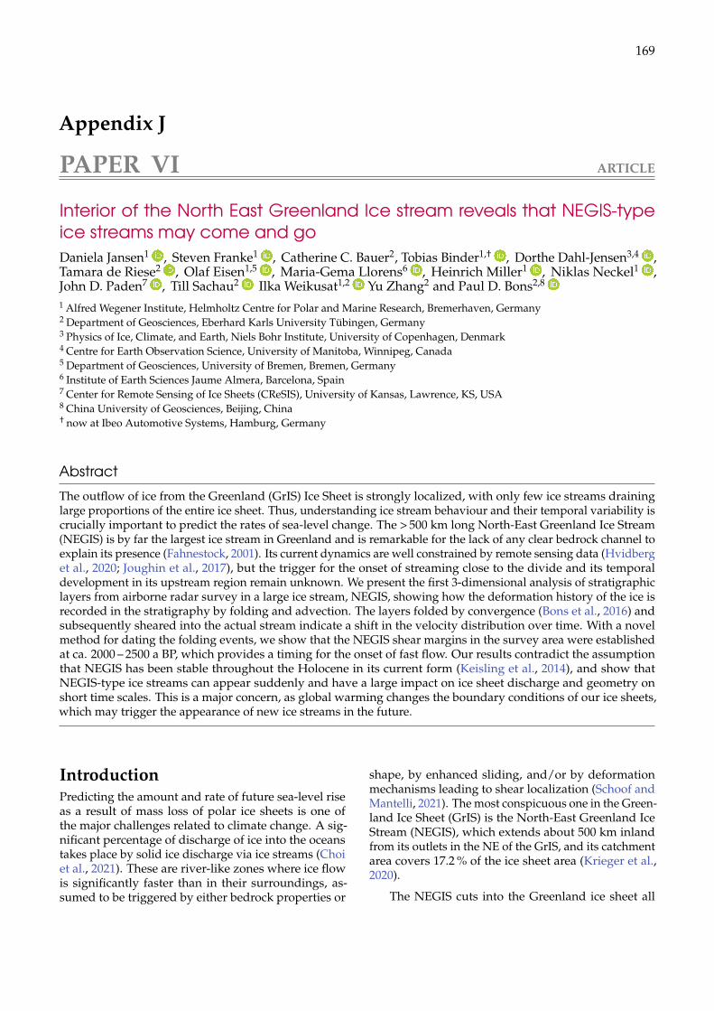
169

Appendix J

PAPER VI ARTICLE

Interior of the North East Greenland Ice stream reveals that NEGIS-typeice streams may come and goDaniela Jansen1 , Steven Franke1 , Catherine C. Bauer2, Tobias Binder1,† , Dorthe Dahl-Jensen3,4 ,Tamara de Riese2 , Olaf Eisen1,5 , Maria-Gema Llorens6 , Heinrich Miller1 , Niklas Neckel1 ,John D. Paden7 , Till Sachau2 Ilka Weikusat1,2 Yu Zhang2 and Paul D. Bons2,8

1 Alfred Wegener Institute, Helmholtz Centre for Polar and Marine Research, Bremerhaven, Germany2 Department of Geosciences, Eberhard Karls University Tübingen, Germany3 Physics of Ice, Climate, and Earth, Niels Bohr Institute, University of Copenhagen, Denmark4 Centre for Earth Observation Science, University of Manitoba, Winnipeg, Canada5 Department of Geosciences, University of Bremen, Bremen, Germany6 Institute of Earth Sciences Jaume Almera, Barcelona, Spain7 Center for Remote Sensing of Ice Sheets (CReSIS), University of Kansas, Lawrence, KS, USA8 China University of Geosciences, Beijing, China† now at Ibeo Automotive Systems, Hamburg, Germany

AbstractThe outflow of ice from the Greenland (GrIS) Ice Sheet is strongly localized, with only few ice streams draininglarge proportions of the entire ice sheet. Thus, understanding ice stream behaviour and their temporal variability iscrucially important to predict the rates of sea-level change. The > 500 km long North-East Greenland Ice Stream(NEGIS) is by far the largest ice stream in Greenland and is remarkable for the lack of any clear bedrock channel toexplain its presence (Fahnestock, 2001). Its current dynamics are well constrained by remote sensing data (Hvidberget al., 2020; Joughin et al., 2017), but the trigger for the onset of streaming close to the divide and its temporaldevelopment in its upstream region remain unknown. We present the first 3-dimensional analysis of stratigraphiclayers from airborne radar survey in a large ice stream, NEGIS, showing how the deformation history of the ice isrecorded in the stratigraphy by folding and advection. The layers folded by convergence (Bons et al., 2016) andsubsequently sheared into the actual stream indicate a shift in the velocity distribution over time. With a novelmethod for dating the folding events, we show that the NEGIS shear margins in the survey area were establishedat ca. 2000 – 2500 a BP, which provides a timing for the onset of fast flow. Our results contradict the assumptionthat NEGIS has been stable throughout the Holocene in its current form (Keisling et al., 2014), and show thatNEGIS-type ice streams can appear suddenly and have a large impact on ice sheet discharge and geometry onshort time scales. This is a major concern, as global warming changes the boundary conditions of our ice sheets,which may trigger the appearance of new ice streams in the future.

IntroductionPredicting the amount and rate of future sea-level riseas a result of mass loss of polar ice sheets is one ofthe major challenges related to climate change. A sig-nificant percentage of discharge of ice into the oceanstakes place by solid ice discharge via ice streams (Choiet al., 2021). These are river-like zones where ice flowis significantly faster than in their surroundings, as-sumed to be triggered by either bedrock properties or

shape, by enhanced sliding, and/or by deformationmechanisms leading to shear localization (Schoof andMantelli, 2021). The most conspicuous one in the Green-land Ice Sheet (GrIS) is the North-East Greenland IceStream (NEGIS), which extends about 500 km inlandfrom its outlets in the NE of the GrIS, and its catchmentarea covers 17.2 % of the ice sheet area (Krieger et al.,2020).

The NEGIS cuts into the Greenland ice sheet all

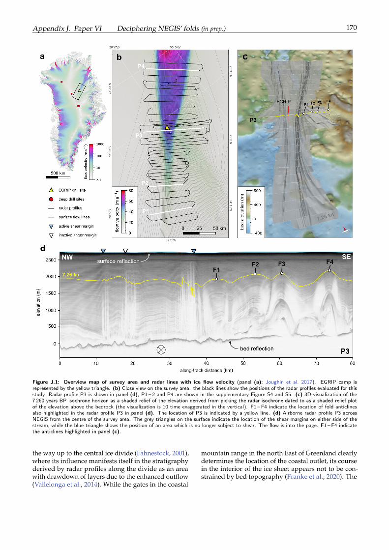
Appendix J. Paper VI Deciphering NEGIS’ folds (in prep.) 170

Figure J.1: Overview map of survey area and radar lines with ice flow velocity (panel (a); Joughin et al. 2017). EGRIP camp isrepresented by the yellow triangle. (b) Close view on the survey area. the black lines show the positions of the radar profiles evaluated for thisstudy. Radar profile P3 is shown in panel (d), P1 – 2 and P4 are shown in the supplementary Figure S4 and S5. (c) 3D-visualization of the7 260 years BP isochrone horizon as a shaded relief of the elevation derived from picking the radar isochrone dated to as a shaded relief plotof the elevation above the bedrock (the visualization is 10 time exaggerated in the vertical). F1 – F4 indicate the location of fold anticlinesalso highlighted in the radar profile P3 in panel (d). The location of P3 is indicated by a yellow line. (d) Airborne radar profile P3 acrossNEGIS from the centre of the survey area. The grey triangles on the surface indicate the location of the shear margins on either side of thestream, while the blue triangle shows the position of an area which is no longer subject to shear. The flow is into the page. F1 – F4 indicatethe anticlines highlighted in panel (c).

the way up to the central ice divide (Fahnestock, 2001),where its influence manifests itself in the stratigraphyderived by radar profiles along the divide as an areawith drawdown of layers due to the enhanced outflow(Vallelonga et al., 2014). While the gates in the coastal

mountain range in the north East of Greenland clearlydetermines the location of the coastal outlet, its coursein the interior of the ice sheet appears not to be con-strained by bed topography (Franke et al., 2020). The

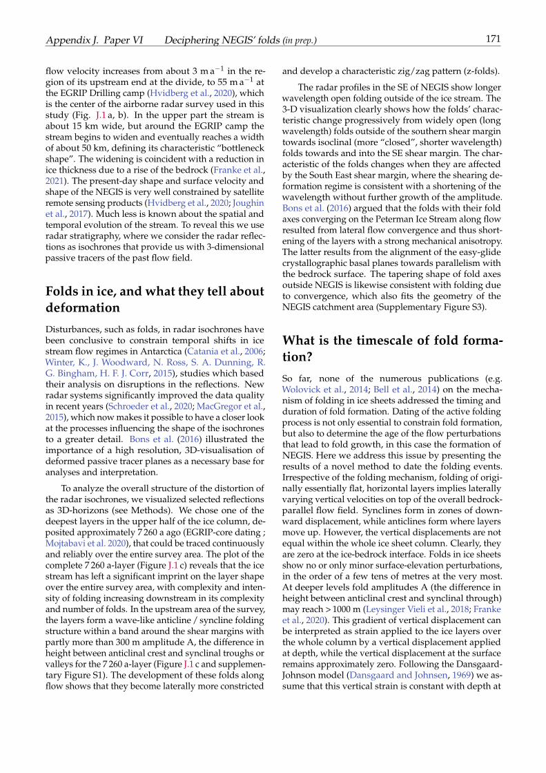
Appendix J. Paper VI Deciphering NEGIS’ folds (in prep.) 171

flow velocity increases from about 3 m a−1 in the re-gion of its upstream end at the divide, to 55 m a−1 atthe EGRIP Drilling camp (Hvidberg et al., 2020), whichis the center of the airborne radar survey used in thisstudy (Fig. J.1 a, b). In the upper part the stream isabout 15 km wide, but around the EGRIP camp thestream begins to widen and eventually reaches a widthof about 50 km, defining its characteristic “bottleneckshape”. The widening is coincident with a reduction inice thickness due to a rise of the bedrock (Franke et al.,2021). The present-day shape and surface velocity andshape of the NEGIS is very well constrained by satelliteremote sensing products (Hvidberg et al., 2020; Joughinet al., 2017). Much less is known about the spatial andtemporal evolution of the stream. To reveal this we useradar stratigraphy, where we consider the radar reflec-tions as isochrones that provide us with 3-dimensionalpassive tracers of the past flow field.

Folds in ice, and what they tell aboutdeformation

Disturbances, such as folds, in radar isochrones havebeen conclusive to constrain temporal shifts in icestream flow regimes in Antarctica (Catania et al., 2006;Winter, K., J. Woodward, N. Ross, S. A. Dunning, R.G. Bingham, H. F. J. Corr, 2015), studies which basedtheir analysis on disruptions in the reflections. Newradar systems significantly improved the data qualityin recent years (Schroeder et al., 2020; MacGregor et al.,2015), which now makes it possible to have a closer lookat the processes influencing the shape of the isochronesto a greater detail. Bons et al. (2016) illustrated theimportance of a high resolution, 3D-visualisation ofdeformed passive tracer planes as a necessary base foranalyses and interpretation.

To analyze the overall structure of the distortion ofthe radar isochrones, we visualized selected reflectionsas 3D-horizons (see Methods). We chose one of thedeepest layers in the upper half of the ice column, de-posited approximately 7 260 a ago (EGRIP-core dating ;Mojtabavi et al. 2020), that could be traced continuouslyand reliably over the entire survey area. The plot of thecomplete 7 260 a-layer (Figure J.1 c) reveals that the icestream has left a significant imprint on the layer shapeover the entire survey area, with complexity and inten-sity of folding increasing downstream in its complexityand number of folds. In the upstream area of the survey,the layers form a wave-like anticline / syncline foldingstructure within a band around the shear margins withpartly more than 300 m amplitude A, the difference inheight between anticlinal crest and synclinal troughs orvalleys for the 7 260 a-layer (Figure J.1 c and supplemen-tary Figure S1). The development of these folds alongflow shows that they become laterally more constricted

and develop a characteristic zig/zag pattern (z-folds).

The radar profiles in the SE of NEGIS show longerwavelength open folding outside of the ice stream. The3-D visualization clearly shows how the folds’ charac-teristic change progressively from widely open (longwavelength) folds outside of the southern shear margintowards isoclinal (more “closed”, shorter wavelength)folds towards and into the SE shear margin. The char-acteristic of the folds changes when they are affectedby the South East shear margin, where the shearing de-formation regime is consistent with a shortening of thewavelength without further growth of the amplitude.Bons et al. (2016) argued that the folds with their foldaxes converging on the Peterman Ice Stream along flowresulted from lateral flow convergence and thus short-ening of the layers with a strong mechanical anisotropy.The latter results from the alignment of the easy-glidecrystallographic basal planes towards parallelism withthe bedrock surface. The tapering shape of fold axesoutside NEGIS is likewise consistent with folding dueto convergence, which also fits the geometry of theNEGIS catchment area (Supplementary Figure S3).

What is the timescale of fold forma-tion?

So far, none of the numerous publications (e.g.Wolovick et al., 2014; Bell et al., 2014) on the mecha-nism of folding in ice sheets addressed the timing andduration of fold formation. Dating of the active foldingprocess is not only essential to constrain fold formation,but also to determine the age of the flow perturbationsthat lead to fold growth, in this case the formation ofNEGIS. Here we address this issue by presenting theresults of a novel method to date the folding events.Irrespective of the folding mechanism, folding of origi-nally essentially flat, horizontal layers implies laterallyvarying vertical velocities on top of the overall bedrock-parallel flow field. Synclines form in zones of down-ward displacement, while anticlines form where layersmove up. However, the vertical displacements are notequal within the whole ice sheet column. Clearly, theyare zero at the ice-bedrock interface. Folds in ice sheetsshow no or only minor surface-elevation perturbations,in the order of a few tens of metres at the very most.At deeper levels fold amplitudes A (the difference inheight between anticlinal crest and synclinal through)may reach > 1000 m (Leysinger Vieli et al., 2018; Frankeet al., 2020). This gradient of vertical displacement canbe interpreted as strain applied to the ice layers overthe whole column by a vertical displacement appliedat depth, while the vertical displacement at the surfaceremains approximately zero. Following the Dansgaard-Johnson model (Dansgaard and Johnsen, 1969) we as-sume that this vertical strain is constant with depth at

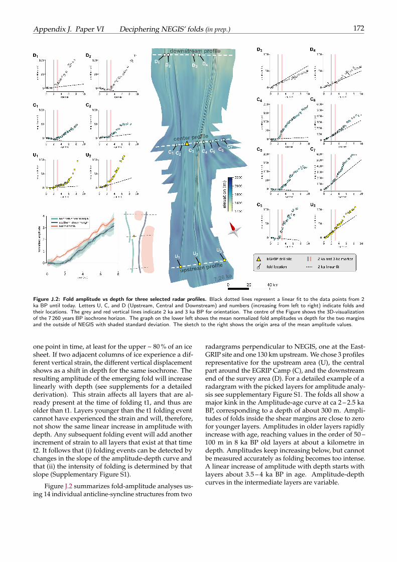
Appendix J. Paper VI Deciphering NEGIS’ folds (in prep.) 172

Figure J.2: Fold amplitude vs depth for three selected radar profiles. Black dotted lines represent a linear fit to the data points from 2ka BP until today. Letters U, C, and D (Upstream, Central and Downstream) and numbers (increasing from left to right) indicate folds andtheir locations. The grey and red vertical lines indicate 2 ka and 3 ka BP for orientation. The centre of the Figure shows the 3D-visualizationof the 7 260 years BP isochrone horizon. The graph on the lower left shows the mean normalized fold amplitudes vs depth for the two marginsand the outside of NEGIS with shaded standard deviation. The sketch to the right shows the origin area of the mean amplitude values.

one point in time, at least for the upper ~ 80 % of an icesheet. If two adjacent columns of ice experience a dif-ferent vertical strain, the different vertical displacementshows as a shift in depth for the same isochrone. Theresulting amplitude of the emerging fold will increaselinearly with depth (see supplements for a detailedderivation). This strain affects all layers that are al-ready present at the time of folding t1, and thus areolder than t1. Layers younger than the t1 folding eventcannot have experienced the strain and will, therefore,not show the same linear increase in amplitude withdepth. Any subsequent folding event will add anotherincrement of strain to all layers that exist at that timet2. It follows that (i) folding events can be detected bychanges in the slope of the amplitude-depth curve andthat (ii) the intensity of folding is determined by thatslope (Supplementary Figure S1).

Figure J.2 summarizes fold-amplitude analyses us-ing 14 individual anticline-syncline structures from two

radargrams perpendicular to NEGIS, one at the East-GRIP site and one 130 km upstream. We chose 3 profilesrepresentative for the upstream area (U), the centralpart around the EGRIP Camp (C), and the downstreamend of the survey area (D). For a detailed example of aradargram with the picked layers for amplitude analy-sis see supplementary Figure S1. The folds all show amajor kink in the Amplitude-age curve at ca 2 – 2.5 kaBP, corresponding to a depth of about 300 m. Ampli-tudes of folds inside the shear margins are close to zerofor younger layers. Amplitudes in older layers rapidlyincrease with age, reaching values in the order of 50 –100 m in 8 ka BP old layers at about a kilometre indepth. Amplitudes keep increasing below, but cannotbe measured accurately as folding becomes too intense.A linear increase of amplitude with depth starts withlayers about 3.5 – 4 ka BP in age. Amplitude-depthcurves in the intermediate layers are variable.

Appendix J. Paper VI Deciphering NEGIS’ folds (in prep.) 173

Figure J.3: (a) Situation before localisation of strain in distinct shear zones. Red lines indicate fold hinges, white arrows indicate directionof flow (b) after the establishment of shear zones (highlighted in yellow): Inside of the stream the fold hinges are rotated towards the shearmargins due to the velocity gradient. (c) Folded layer with shear strain rates, the blue frame highlights the area which is described in panel(d). The image is distorted to exaggerate the angles relative to the shear zones, which are very small. (d) Sketch to illustrate the developmentof an apparent shorter wavelength of folds within the shear zone.

What can the folds reveal about thehistory of NEGIS?

Bons et al. (2016) argued that the folds with their foldaxes converging on the Peterman Ice Stream along flowresulted from lateral flow convergence and thus short-ening of the layers with a strong mechanical anisotropy.The tapering shape of fold axes outside NEGIS is like-wise consistent with folding due to convergence, whichalso fits the geometry of the NEGIS catchment area(Figure S3). This type of folding can occur withoutstrong localisation of shear and a distributed compres-sive regime throughout the catchment area.

A conceptual model for the development of thestructures in NEGIS that we see today in our radar hori-zon is summarized in Figure J.3: in the upstream region

of NEGIS convergent folding occurred as a “first defor-mation phase” (time period t1) due to the mechanicalanisotropy typical in flowing ice (Bons et al., 2016). Thestrong localization of shear deformation in the margins,that is today apparent in the observed surface velocityfield, has not yet developed. Thus, the strike of thefold hinges was orientated roughly towards the outletgate (Figure J.3 a). Due to enhanced drawdown of icealong the evolving stream, probably triggered at theoutlet of NEGIS , the shear margins then intensified. Tocompensate the local mass loss caused by this draw-down, the ice stream has two ways how to providethe material without substantial thinning of the streamarea: by widening or elongating. As the formation ofshear zones quickly results in reorientation of the me-chanical anisotropy (vertical to horizontal CPO), theshear zones’ lateral position and thus the width of the

Appendix J. Paper VI Deciphering NEGIS’ folds (in prep.) 174

stream is pinned/fixed and thus shear zones are likelyto travelled upwards, a behavior which is common inrock deformation. The fold trains which then were cutby a new shear margin experienced a “secondary de-formation phase” (time period t2), due to the stronglateral velocity gradient in the shear margin. This leadsto a rotation of the fold hinges towards the marginsof the stream, as the ice in the center is moving faster,which is apparent in the isochrone horizon shown infig. 1c and center panel of fig. 2, but becomes evenmore obvious when the horizon is shortened along theflow direction (Fig. J.3 c). The rotation of the hingesis connected to a shortening of the wavelengths of thefolds (Fig. J.3 c, d), but not to further growth of theamplitudes as it would be expected for the geometry ofa simply progressing first deformation phase. The stag-nation of amplitude growth within the shear marginis also consistent with the expected change in CPO instrong horizontal shearing, which very likely producesa horizontal single maximum. Thus, the horizontalshortening is effectively resolved by glide along thebasal planes and rotation.

In the mapped layers folding relicts are visible in-side the stream, which must have been part of conver-gent fold structures which formed in the area before theestablishment of the shear margins happened (FigureJ.3 c). The connection of these fold hinges to their coun-terpart on the outside of the stream provides a meansto estimate the duration of the current “secondary” de-formation phase by calculating the angle of rotationassuming today’s shearing, and also by evaluating thedistance between the “breaking points” of the inner andouter folds. From this, our first estimate of the timingof shear zone establishment is approximately 2.3 ka BP(see supplementary material for details).

This age estimation from the offset of the folds dis-rupted by the shear margin is consistent with the eval-uation of the amplitude-age graphs of the picked folds.The graph in Figure J.2 on the lower left shows nor-malized fold amplitudes for the three different regions,both shear margins and the outside of the stream. A no-ticeable difference between folds in the shear marginsand those outside NEGIS is that the outside folds am-plitudes are distinctly non-zero in the youngest layersas well. This means that these folds were still growinguntil recently, possibly up to the present day. Kinks inthe amplitude-age curves are also present at ca 2 – 2.5ka and/or 3.5 – 4 ka BP.

The constructed isochrone surfaces show that foldsoutside and inside the shear margins are the same foldsinitiated during t1, with the latter ones being shearedinto the margins during t2. A common feature is thatthey all show bends in their ampltitude-age curves atabout 3.5 – 4 ka BP, below which the curves tend to

straighten. This strongly suggests that all folds initi-ated around that time (t1). Sections of the folds thatwere caught in the strong shearing at the margins essen-tially stopped growing at 2 – 2.5 ka BP, while sectionsoutside NEGIS did not. The intensification of foldingin a two-stage process could be interpreted as a resultof increasing discharge from the NEGIS catchment area.The first stage, around 3.5 to 4 ka BP, is coincident withthe end of the ice sheet re-advance during the Holocene.

Larsen et al. (2018) summarized geological evi-dence from the north east Greenland coast and showedthat the three major outlets of NEGIS, the Nioghalvf-jerdsfjord Gletscher (NG), the Zachariae Isstrom (ZI),and the Storstrommen Gletscher (SG) have been re-treating beyond their current extent and re-advancingagain at least twice during the last 45 ka. In theHolocene Thermal Maximum (HTM) in the early tomiddle Holocene, temperatures in the Arctic wherehigher than today, caused by orbital forcing, whichresulted in a change of insolation, and thus mainly in-fluenced the summer temperature (Miller et al., 2010).This had a large effect on the sea ice conditions andalso on Greenland ice volume and frontal positions ofoutlet glaciers (Axford et al., 2021). The onset and end-ing of this warm period was regionally different, andthere is evidence from geological data that in the area ofthe three major outlets of the NEGIS, warming startedaround 8 000 years ago, and ended approximately 4 000years ago (Miller et al., 2010). Accordingly, NG wassmaller than today in its extension at least until 4.6 kaago (Bennike and Weidick, 2001).

Our observed intensification of folding in the up-stream NEGIS area in a two-stage process could beinterpreted as a result of increasing discharge from theNEGIS catchment area following the readvance of theice front after the HTM. This would fit into the line ofargument of Stokes et al. (2016), who concluded, thatice stream activity is linked to the geometry changesof the ice sheet, with increasing intensity of streamingfor higher ice volume. The first stage, around 3.5 to4 ka BP, could be a consequence of a still distributedincrease of the outflow, leading to a drawdown of icefrom the flanks and a confluent flow regime due to thegeometry of the catchment and the bedrock. The local-ization effect of shear in narrow shear margin as we seethem today is, if similar to processes in other geologicmaterials, initiated closer to the margin of the ice sheetand travelling upwards in time, thus reaching our sur-vey area at a significantly later time around 2 300 BP.Our results thus indicate how and on which time scaleschanges at the front are translated into the inner icesheet, and that processes at the calving front of NEGISare much more likely to trigger formation and inten-sification of streaming than local heatflow anomalies(Bons et al., 2021).

Appendix J. Paper VI Deciphering NEGIS’ folds (in prep.) 175

Methods

Airborne Radar

The data presented in this study have been derivedfrom an airborne radar survey in May 2018 using anultra-wide-band radar system (AWI UWB, detailed de-scription see Rodriguez-Morales et al. 2014; Frankeet al. 2020) with an array of 8 transmitters and re-ceivers mounted beneath the fuselage of the AWI air-craft Polar 6. The layout of the survey was designedfor mapping radar stratigraphy and bedrock proper-ties in the vicinity of the EGRIP drilling camp, with anarea stretching along flow from 150 km upstream ofthe camp to 150 km downstream. The profiles used inthis study were recorded in narrow-band mode, withthe Frequency range set to 180 – 210 MHz. Due to thefocus on stratigraphy, the radar lines are mostly per-pendicular to ice flow in order to best reproduce thedeformation pattern in the shear margins. Here weonly use data from across-flow profiles (Figure J.1 b).The distance between the profiles is 5 km in the centralpart of the survey region, in the outer area the distanceis 10 km. Bedrock reflections from this data set havebeen used to produce a high-resolution bedrock dataset in the vicinity of EGRIP camp (Franke et al., 2020),as well as for bed properties and roughness (Frankeet al., 2021).

Move 3D

In order to assess the distortion of the radar isochronesin terms of their deformation history to deter-mine the dynamic setting of the ice stream, the 2-dimensional profiles have to be combined to produce a3-dimensional model of the folded isochrone surfaces(Bons et al., 2016). For this purpose, we picked selectedinternal reflections, which are detectable throughoutmost of the survey area. To ensure spatial continuity,we restrict our analysis to reflections from the upperhalf of the ice column. By manually assigning profilesections from two neighboring lines to each other, a sur-face can be generated in a half-automated way. For thisstep of the analysis, we used the software MOVETM,a tool for structural analysis and 3-D visualization ingeosciences. The isochrones are dated by tying themin the depth domain to the age dating of the EGRIPice core (Mojtabavi et al., 2020) and transferring age ina particular depth to the respective isochrone at thatdepth. The absolute age and its uncertainty is of minorimportance in our study, as we focus on the overalldeformation of the initial flat shape of the consideredisochrones.

Dating of folding events

To determine the amplitude-depth curves, as many lay-ers in a radargram as possible are manually traced foranticline-syncline pairs. Axial planes are constructedas lines that connect the fold hinges. Near the ice sur-face folds may die out upwards, in which case the ax-ial planes are extended vertically towards the surface.Depth (z) of a stratigraphic layer is now defined as thevertical distance between a hinge of that layer and theheight of the ice surface at the point where it is inter-sected by the axial planes. For each anticline-synclinepair, referred to as a fold, this results in a set of zanti(i)and zsyn(i) data for each layer (i) that was deposited ata(i). The fold amplitude is now defined as A(i)=zsyn(i)-zanti(i), with associated depth z(i)=(zsyn(i)+zanti(i))/2.Ages of layers are derived from tracing or correlatingof layers with known ages from the EastGRIP drill site.This results in a set of layers with known depositionalages. Over half of the traceable layers within one foldcannot be traced all the way to the drill site or can berecognised in the radargram at that site. Their agesare estimated by interpolating between nearest layersabove and below the layer of unknown age, assumingthat within the age window the relation between heightof the layer above the bedrock (h) and age (a) is givenby: h=H-z=exp(k·a). Details on error analysis and re-duction are provided in supplementary information.

Strain rates

In order to describe the overall dynamic setting of thesurvey area, we used two different velocity products.The velocity data from the Measures Project (Joughinet al. 2017, Figure J.1) with a resolution of 250 m wasused to characterize the present-day surface velocitymagnitude and flow direction, which we also used tocalculate advection and distortion of stratigraphic fea-tures. As the picked isochrones are located in the upperhalf of the ice column throughout our survey area, weassume that the surface velocity field is still a valid ap-proximation at the depth of the horizon. This velocityfield has been also used to calculate principal strainrates and strain rates in flow and across the flow di-rection for each pixel. For this purpose, the data wasfiltered with a Lee filter over a window of 10×10 pixelsto reduce the noise. A high-resolution velocity productbased on TerraSAR-X data is available in a limited areaaround the EastGRIP camp (Hvidberg et al., 2020). Al-though this data set shows significantly less noise thanMeasures, we also deployed a Lee filter with a 5×5pixel window before calculating strain rates. Strainrates and projections were calculated following Pater-son (the textbook).

Appendix J. Paper VI Deciphering NEGIS’ folds (in prep.) 176

AcknowledgementsWe thank the Ken Borek crew of the research aircraftPolar 6 and system engineer Lukas Kandora. Logisticalsupport in the field was provided by the East Green-land Ice-Core Project (EGRIP). EGRIP is directed andorganized by the Center of Ice and Climate at the NielsBohr Institute. It is supported by funding agenciesand institutions in Denmark (A. P. Møller Foundation,University of Copenhagen), USA (US National ScienceFoundation, Office of Polar Programs), Germany (Al-fred Wegener Institute, Helmholtz Centre for Polar andMarine Research), Japan (National Institute of Polar Re-search and Arctic Challenge for Sustainability), Norway(University of Bergen and Bergen Research Founda-tion), Switzerland (Swiss National Science Foundation),France (French Polar Institute Paul-Emile Victor, Insti-tute for Geosciences and Environmental research) andChina (Chinese Academy of Sciences and Beijing Nor-mal University).We acknowledge the use of the CRe-SIS toolbox from CReSIS generated with support fromthe University of Kansas, NASA Operation IceBridgegrant NNX16AH54G, and NSF grants ACI-1443054,OPP-1739003, and IIS-1838230. The advection of thefolds have been calculated with the tool Grd2Stream de-veloped by Thomas Kleiner. Steven Franke was fundedby the AWI Strategy fund, Daniela Jansen was fundedby the AWI Strategy funds and the Helmholtz Younginvestigator group HGF YIG VH-NG-802.

177

BibliographyAxford, Y., de Vernal, A., and Osterberg, E. C. Past

warmth and its impacts during the holocene thermalmaximum in greenland. Annual Review of Earth andPlanetary Sciences, 49(1):null, 2021. doi: 10.1146/annurev-earth-081420-063858. URL https://doi.org/10.1146/annurev-earth-081420-063858.

Bell, R. E., Tinto, K., Das, I., Wolovick, M., Chu, W., Creyts,T. T., Frearson, N., Abdi, A., and Paden, J. D. Deforma-tion warming and softening of Greenland’s ice by refreez-ing meltwater. Nature Geoscience, 7(7):497–502, jun 2014.doi: 10.1038/ngeo2179. URL https://doi.org/10.1038%2Fngeo2179.

Bennike, O. and Weidick, A. Late quaternary his-tory around nioghalvfjerdsfjorden and jøkelbugten,north-east greenland. Boreas, 30(3):205–227, 2001.doi: https://doi.org/10.1111/j.1502-3885.2001.tb01223.x. URL https://onlinelibrary.wiley.com/doi/abs/10.1111/j.1502-3885.2001.tb01223.x.

Bons, P. D., Jansen, D., Mundel, F., Bauer, C. C., Binder, T.,Eisen, O., Jessell, M. W., Llorens, M.-G., Steinbach, F., Stein-hage, D., and Weikusat, I. Converging flow and anisotropycause large-scale folding in Greenland's ice sheet. NatureCommunications, 7(1), apr 2016. doi: 10.1038/ncomms11427.URL https://doi.org/10.1038%2Fncomms11427.

Bons, P. D., de Riese, T., Franke, S., Llorens, M.-G., Sachau,T., Stoll, N., Weikusat, I., Westhoff, J., and Zhang, Y. Com-ment on “exceptionally high heat flux needed to sustainthe northeast greenland ice stream” by smith-johnsen etal. (2020). The Cryosphere, 15(5):2251–2254, 2021. doi:10.5194/tc-15-2251-2021. URL https://tc.copernicus.org/articles/15/2251/2021/.

Catania, G. A., Scambos, T. A., Conway, H., and Ray-mond, C. F. Sequential stagnation of kamb ice stream,west antarctica. Geophysical Research Letters, 33(14),2006. doi: https://doi.org/10.1029/2006GL026430.URL https://agupubs.onlinelibrary.wiley.com/doi/abs/10.1029/2006GL026430.

Choi, Y., Morlighem, M., Rignot, E., and Wood, M. Ice dy-namics will remain a primary driver of greenland ice sheetmass loss over the next century. Communications Earth& Environment, 2(1):26, Feb 2021. ISSN 2662-4435. doi:10.1038/s43247-021-00092-z. URL https://doi.org/10.1038/s43247-021-00092-z.

Dansgaard, W. and Johnsen, S. J. A flow model and atime scale for the ice core from camp century, green-land. Journal of Glaciology, 8(53):215–223, 1969. doi:10.3189/S0022143000031208.

Fahnestock, M. High Geothermal Heat Flow Basal Melt,and the Origin of Rapid Ice Flow in Central Green-land. Science, 294(5550):2338–2342, dec 2001. doi: 10.

1126/science.1065370. URL https://doi.org/10.1126%2Fscience.1065370.

Franke, S., Jansen, D., Binder, T., Dörr, N., Helm, V., Paden,J., Steinhage, D., and Eisen, O. Bed topography andsubglacial landforms in the onset region of the North-east Greenland Ice Stream. Annals of Glaciology, pages1–11, mar 2020. doi: 10.1017/aog.2020.12. URL https://doi.org/10.1017%2Faog.2020.12.

Franke, S., Jansen, D., Beyer, S., Neckel, N., Binder, T., Paden,J., and Eisen, O. Complex basal conditions and their in-fluence on ice flow at the onset of the northeast greenlandice stream. Journal of Geophysical Research: Earth Surface,126(3):e2020JF005689, 2021. doi: 10.1029/2020JF005689.URL https://agupubs.onlinelibrary.wiley.com/doi/abs/10.1029/2020JF005689.

Hvidberg, C. S., Grinsted, A., Dahl-Jensen, D., Khan, S. A.,Kusk, A., Andersen, J. K., Neckel, N., Solgaard, A., Karls-son, N. B., Kjær, H. A., and Vallelonga, P. Surface ve-locity of the northeast greenland ice stream (negis): as-sessment of interior velocities derived from satellite databy gps. The Cryosphere, 14(10):3487–3502, 2020. doi:10.5194/tc-14-3487-2020. URL https://tc.copernicus.org/articles/14/3487/2020/.

Joughin, I., Smith, B. E., and Howat, I. M. A completemap of Greenland ice velocity derived from satellite datacollected over 20 years. Journal of Glaciology, 64(243):1–11, nov 2017. doi: 10.1017/jog.2017.73. URL https://doi.org/10.1017%2Fjog.2017.73.

Keisling, B. A., Christianson, K., Alley, R. B., Peters, L. E.,Christian, J. E., Anandakrishnan, S., Riverman, K. L., Muto,A., and Jacobel, R. W. Basal conditions and ice dynamicsinferred from radar-derived internal stratigraphy of thenortheast Greenland ice stream. Annals of Glaciology, 55(67):127–137, 2014. doi: 10.3189/2014aog67a090. URLhttps://doi.org/10.3189%2F2014aog67a090.

Krieger, L., Floricioiu, D., and Neckel, N. Drainage basindelineation for outlet glaciers of Northeast Greenlandbased on Sentinel-1 ice velocities and TanDEM-X eleva-tions. Remote Sensing of Environment, 237:111483, 2020.ISSN 0034-4257. doi: https://doi.org/10.1016/j.rse.2019.111483. URL http://www.sciencedirect.com/science/article/pii/S0034425719305024.

Larsen, N. K., Levy, L. B., Carlson, A. E., Buizert, C., Olsen,J., Strunk, A., Bjørk, A. A., and Skov, D. S. Instabil-ity of the Northeast Greenland Ice Stream over the last45,000 years. Nature Communications, 9(1):3–10, 2018.ISSN 20411723. doi: 10.1038/s41467-018-04312-7. URLhttp://dx.doi.org/10.1038/s41467-018-04312-7.

Leysinger Vieli, G. J.-M. C., Martín, C., Hindmarsh, R. C. A.,and Lüthi, M. P. Basal freeze-on generates complex ice-sheet stratigraphy. Nature Communications, 9(1), nov 2018.doi: 10.1038/s41467-018-07083-3. URL https://doi.org/10.1038%2Fs41467-018-07083-3.

MacGregor, J. A., Fahnestock, M. A., Catania, G. A., Paden,J. D., Gogineni, S. P., Young, S. K., Rybarski, S. C., Mabrey,

BIBLIOGRAPHY 178

A. N., Wagman, B. M., and Morlighem, M. Radios-tratigraphy and age structure of the Greenland Ice Sheet.Journal of Geophysical Research: Earth Surface, 120(2):212–241, feb 2015. doi: 10.1002/2014jf003215. URL https://doi.org/10.1002%2F2014jf003215.

Miller, G., Brigham-Grette, J., Alley, R., Anderson, L., Bauch,H., Douglas, M., Edwards, M., Elias, S., Finney, B., Fitz-patrick, J., Funder, S., Herbert, T., Hinzman, L., Kauf-man, D., MacDonald, G., Polyak, L., Robock, A., Ser-reze, M., Smol, J., Spielhagen, R., White, J., Wolfe, A.,and Wolff, E. Temperature and precipitation history ofthe arctic. Quaternary Science Reviews, 29(15):1679–1715,2010. doi: https://doi.org/10.1016/j.quascirev.2010.03.001. URL https://www.sciencedirect.com/science/article/pii/S0277379110000673.

Mojtabavi, S., Wilhelms, F., Cook, E., Davies, S. M., Sinnl, G.,Skov Jensen, M., Dahl-Jensen, D., Svensson, A., Vinther,B. M., Kipfstuhl, S., Jones, G., Karlsson, N. B., Faria,S. H., Gkinis, V., Kjær, H. A., Erhardt, T., Berben, S.M. P., Nisancioglu, K. H., Koldtoft, I., and Rasmussen,S. O. A first chronology for the east greenland ice-coreproject (egrip) over the holocene and last glacial termi-nation. Climate of the Past, 16(6):2359–2380, 2020. doi:10.5194/cp-16-2359-2020. URL https://cp.copernicus.org/articles/16/2359/2020/.

Rodriguez-Morales, F., Byers, K., Crowe, R., Player, K., Hale,R. D., Arnold, E. J., Smith, L., Gifford, C. M., Braaten,D., Panton, C., Gogineni, S., Leuschen, C. J., Paden,J. D., Li, J., Lewis, C. C., Panzer, B., Alvestegui, D. G.-G., and Patel, A. Advanced Multifrequency Radar In-strumentation for Polar Research. IEEE Transactions onGeoscience and Remote Sensing, 52(5):2824–2842, may 2014.doi: 10.1109/tgrs.2013.2266415. URL https://doi.org/10.1109%2Ftgrs.2013.2266415.

Schoof, C. and Mantelli, E. The role of sliding inice stream formation. Proceedings of the Royal Soci-ety A: Mathematical, Physical and Engineering Sciences,477(2248):20200870, 2021. doi: 10.1098/rspa.2020.

0870. URL https://royalsocietypublishing.org/doi/abs/10.1098/rspa.2020.0870.

Schroeder, D. M., Bingham, R. G., Blankenship, D. D., Chris-tianson, K., Eisen, O., Flowers, G. E., Karlsson, N. B.,Koutnik, M. R., Paden, J. D., and Siegert, M. J. Fivedecades of radioglaciology. Annals of Glaciology, pages1–13, mar 2020. doi: 10.1017/aog.2020.11. URL https://doi.org/10.1017%2Faog.2020.11.

Stokes, C. R., Margold, M., Clark, C. D., and Tarasov, L.Ice stream activity scaled to ice sheet volume duringLaurentide Ice Sheet deglaciation. Nature, 530(7590):322–326, feb 2016. doi: 10.1038/nature16947. URL https://doi.org/10.1038%2Fnature16947.

Vallelonga, P., Christianson, K., Alley, R. B., Anandakrishnan,S., Christian, J. E. M., Dahl-Jensen, D., Gkinis, V., Holme,C., Jacobel, R. W., Karlsson, N. B., Keisling, B. A., Kipfstuhl,S., Kjær, H. A., Kristensen, M. E. L., Muto, A., Peters, L. E.,Popp, T., Riverman, K. L., Svensson, A. M., Tibuleac, C.,Vinther, B. M., Weng, Y., and Winstrup, M. Initial resultsfrom geophysical surveys and shallow coring of the North-east Greenland Ice Stream (NEGIS). The Cryosphere, 8(4):1275–1287, jul 2014. doi: 10.5194/tc-8-1275-2014. URLhttps://doi.org/10.5194%2Ftc-8-1275-2014.

Winter, K., J. Woodward, N. Ross, S. A. Dunning, R. G.Bingham, H. F. J. Corr, a. J. S. Airborne radar evidencefor tributary flow switching in Institute Ice Stream, WestAntarctica: Implications for ice sheet configuration anddynamics. Journal of Geophysical Research: Earth Sur-face, 120(9):2498–2528, 2015. doi: 10.1002/2015JF003518.URL https://agupubs.onlinelibrary.wiley.com/doi/full/10.1002/2015JF003518.

Wolovick, M. J., Creyts, T. T., Buck, W. R., and Bell, R. E.Traveling slippery patches produce thickness-scale foldsin ice sheets. Geophysical Research Letters, 41(24):8895–8901, dec 2014. doi: 10.1002/2014gl062248. URL https://doi.org/10.1002%2F2014gl062248.

BIBLIOGRAPHY 179

PAPER VI SUPPLEMENTARY INFORMATION

Supplementary Information:Interior of the North East Greenland Ice stream reveals that NEGIS-typeice streams may come and goDaniela Jansen1 , Steven Franke1 , Catherine C. Bauer2, Tobias Binder1,† , Dorthe Dahl-Jensen3,4 ,Tamara de Riese2 , Olaf Eisen1,5 , Maria-Gema Llorens6 , Heinrich Miller1 , Niklas Neckel1 ,John D. Paden7 , Till Sachau2 Ilka Weikusat1,2 Yu Zhang2 and Paul D. Bons2,8

1 Alfred Wegener Institute, Helmholtz Centre for Polar and Marine Research, Bremerhaven, Germany2 Department of Geosciences, Eberhard Karls University Tübingen, Germany3 Physics of Ice, Climate, and Earth, Niels Bohr Institute, University of Copenhagen, Denmark4 Centre for Earth Observation Science, University of Manitoba, Winnipeg, Canada5 Department of Geosciences, University of Bremen, Bremen, Germany6 Institute of Earth Sciences Jaume Almera, Barcelona, Spain7 Center for Remote Sensing of Ice Sheets (CReSIS), University of Kansas, Lawrence, KS, USA8 China University of Geosciences, Beijing, China† now at Ibeo Automotive Systems, Hamburg, Germany

The supplemantary information for Paper VI is provided on the USB stick submittedalongside the thesis as well as in a private online repository (see below).

Supplementary Information of Paper VI:

1. Figures S1 – S5 and Equations S1 – S9 (pdf):https://storage.luckycloud.de/f/ec67a445dad54ed98e4b/

180

Appendix K

PAPER VII RESEARCH ARTICLE

Indication of ice-stream regime shift in Northereast GreenlandSteven Franke1 , Paul Bons2,3 , Julien Westhoff4 , Tobias Binder1,† , Kyra Streng2, Veit Helm1 ,Daniel Steinhage1 , Olaf Eisen1,5 , John Paden6 , Ilka Weikusat1,2 and Daniela Jansen1

1 Alfred Wegener Institute, Helmholtz Centre for Polar and Marine Research, Bremerhaven, Germany2 Department of Geosciences, Eberhard Karls University Tübingen, Germany3 China University of Geosciences, Beijing, China4 Physics of Ice, Climate, and Earth, Niels Bohr Institute, University of Copenhagen, Denmark5 Department of Geosciences, University of Bremen, Bremen, Germany6 Centre for Remote Sensing of Ice Sheets (CReSIS), University of Kansas, Lawrence, KS, USA† now at Ibeo Automotive Systems, Hamburg, Germany

AbstractIce penetrating radar reveals the geometry of internal stratigraphy of the Greenland Ice Sheet and thus constrainsits evolution. The record of radar reflectors is shaped by the cumulative deformation of initially surface-parallelisochronous stratigraphic layers. Decoding the deformation history of these structures offers an excellent possibilityto reconstruct past ice movements and draw conclusions about processes on the Earth’s surface. Here we use theradiostratigraphic layers from newly acquired and older radar data from northeastern Greenland to decipher theirdeformation history. We apply a three-dimensional construction of isochronous surfaces and connect recurringpatterns in the radar signature. Our results reveal a deformation sequence pointing to two former ice streamsreaching far inland in the northeastern Greenland Ice Sheet that nowadays show no trace in the surface velocity.We propose that the observed fold geometries are best explained by (1) the former presence of a Peterman-typeice stream with convergent flow that subsequently changed to the present-day surface flow field and (2) a ceasedformer localized NEGIS-type ice stream with sharp shear margins.

Introduction

Despite the continuous increase in in-situ and remotesensing data of the polar ice sheets, we find a large gapof observations that are necessary to reconstruct pastice motion. Satellite observations of ice surface flow ofthe Greenland (GrIS) and Antarctic (AIS) reach backto the 1970s (Rosenau et al., 2015; Rignot et al., 2019;Mouginot et al., 2019). The reconstruction of ice streamactivity at formerly glaciated regions is limited to theend of the last glacial (Margold et al., 2015; Stokes et al.,2016) but shows that ice streams operated at differenttimes during deglaciation of the (22 ka – 7 ka ago) andwere activated and deactivated in different locationsand periods. A way to close this observational gap isprovided by high-quality radio-echo sounding (RES)data (Rodriguez-Morales et al., 2014; Gogineni et al.,2001; MacGregor et al., 2015; Bell et al., 2014) that showdetails of the sometimes disturbed or folded englacial

stratigraphic architecture of internal reflection horizons(IRHs) of the GrIS and AIS. Most IRHs are assumed tobe isochrones (Fujita et al., 1999), representing the hori-zons of buried former ice-sheet surfaces (Siegert, 1999).Englacial deformation can disturb the conformity andcontinuity of IRHs and lead to a non-monotonicallyincreasing age distribution with depth, which is a chal-lenge for ice-core analysis (Waddington et al., 2001).

Disturbances of different types and magnitudes ofinternal layers were found in Greenland (MacGregoret al., 2015; Leysinger Vieli et al., 2018; Panton andKarlsson, 2015; Bell et al., 2014) and Antarctica (Drewset al., 2009; Bell et al., 2011; Wrona et al., 2018). Theyrange from small folds on a centimetre-scale found inice cores (e.g. Dahl-Jensen et al., 2013; Westhoff et al.,2020; Jansen et al., 2016) to tight folds that extend al-most over the entire ice column with a fold axis ori-ented parallel to the shear margins of ice streams (e.g.

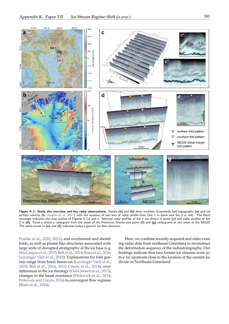
Appendix K. Paper VII Ice Stream Regime Shift (in prep.) 181

Figure K.1: Study site overview and key radar observations. Panels (a) and (b) show northern Greenlands bed topography (a) and icesurface velocity (b; Joughin et al. 2017) with the location of two sets of radar profile lines (Set 1 in black and Set 2 in red). The blackrectangle indicates the map outline of Figures K.2 d and e. Selected radar profiles of Set 1 are shown in panel (c) and radar profiles of Set2 in (d). Panel e shows a radargram from the onset of the Peterman Glacier and panel (f) and (g) radargrams at the onset of the NEGIS.The white arrow in (e) and (f) indicates today’s general ice flow direction.

Franke et al., 2020, 2021), and overturned and sheathfolds, as well as plume-like structures associated withlarge units of disrupted stratigraphy at the ice base (e.g.MacGregor et al., 2015; Bell et al., 2014; Bons et al., 2016;Leysinger Vieli et al., 2018). Explanations for fold gen-esis range from basal freeze-on (Leysinger Vieli et al.,2018; Bell et al., 2014, 2011; Creyts et al., 2014), overdifferences in the ice rheology (Dahl-Jensen et al., 2013),changes in the basal resistance (Wolovick et al., 2014;Wolovick and Creyts, 2016) to convergent flow regimes(Bons et al., 2016).

Here, we combine recently acquired and older exist-ing radar data from northeast Greenland to reconstructthe deformation sequence of the radiostratigraphy. Ourfindings indicate that two former ice streams were ac-tive far upstream close to the location of the current icedivide in Northeast Greenland.

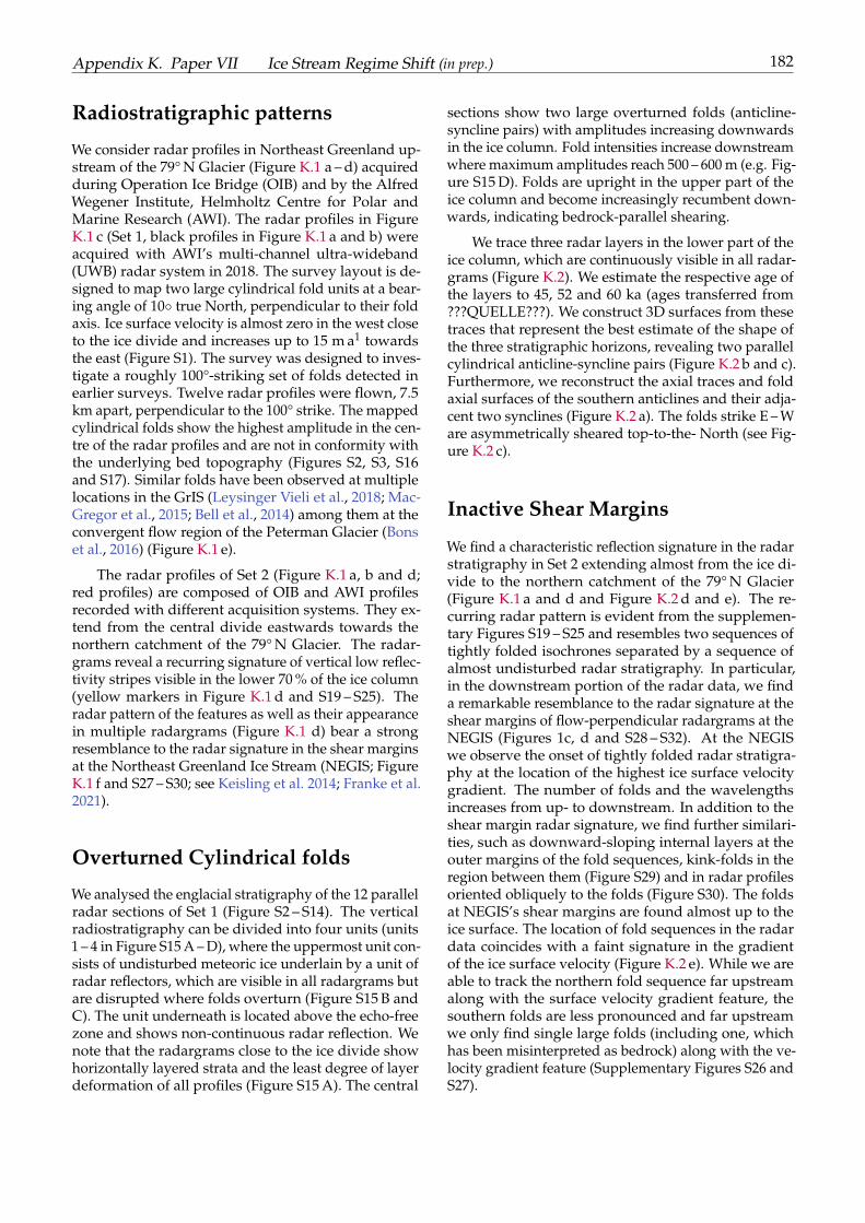
Appendix K. Paper VII Ice Stream Regime Shift (in prep.) 182

Radiostratigraphic patterns

We consider radar profiles in Northeast Greenland up-stream of the 79° N Glacier (Figure K.1 a – d) acquiredduring Operation Ice Bridge (OIB) and by the AlfredWegener Institute, Helmholtz Centre for Polar andMarine Research (AWI). The radar profiles in FigureK.1 c (Set 1, black profiles in Figure K.1 a and b) wereacquired with AWI’s multi-channel ultra-wideband(UWB) radar system in 2018. The survey layout is de-signed to map two large cylindrical fold units at a bear-ing angle of 10 true North, perpendicular to their foldaxis. Ice surface velocity is almost zero in the west closeto the ice divide and increases up to 15 m a1 towardsthe east (Figure S1). The survey was designed to inves-tigate a roughly 100°-striking set of folds detected inearlier surveys. Twelve radar profiles were flown, 7.5km apart, perpendicular to the 100° strike. The mappedcylindrical folds show the highest amplitude in the cen-tre of the radar profiles and are not in conformity withthe underlying bed topography (Figures S2, S3, S16and S17). Similar folds have been observed at multiplelocations in the GrIS (Leysinger Vieli et al., 2018; Mac-Gregor et al., 2015; Bell et al., 2014) among them at theconvergent flow region of the Peterman Glacier (Bonset al., 2016) (Figure K.1 e).

The radar profiles of Set 2 (Figure K.1 a, b and d;red profiles) are composed of OIB and AWI profilesrecorded with different acquisition systems. They ex-tend from the central divide eastwards towards thenorthern catchment of the 79° N Glacier. The radar-grams reveal a recurring signature of vertical low reflec-tivity stripes visible in the lower 70 % of the ice column(yellow markers in Figure K.1 d and S19 – S25). Theradar pattern of the features as well as their appearancein multiple radargrams (Figure K.1 d) bear a strongresemblance to the radar signature in the shear marginsat the Northeast Greenland Ice Stream (NEGIS; FigureK.1 f and S27 – S30; see Keisling et al. 2014; Franke et al.2021).

Overturned Cylindrical folds

We analysed the englacial stratigraphy of the 12 parallelradar sections of Set 1 (Figure S2 – S14). The verticalradiostratigraphy can be divided into four units (units1 – 4 in Figure S15 A – D), where the uppermost unit con-sists of undisturbed meteoric ice underlain by a unit ofradar reflectors, which are visible in all radargrams butare disrupted where folds overturn (Figure S15 B andC). The unit underneath is located above the echo-freezone and shows non-continuous radar reflection. Wenote that the radargrams close to the ice divide showhorizontally layered strata and the least degree of layerdeformation of all profiles (Figure S15 A). The central

sections show two large overturned folds (anticline-syncline pairs) with amplitudes increasing downwardsin the ice column. Fold intensities increase downstreamwhere maximum amplitudes reach 500 – 600 m (e.g. Fig-ure S15 D). Folds are upright in the upper part of theice column and become increasingly recumbent down-wards, indicating bedrock-parallel shearing.

We trace three radar layers in the lower part of theice column, which are continuously visible in all radar-grams (Figure K.2). We estimate the respective age ofthe layers to 45, 52 and 60 ka (ages transferred from???QUELLE???). We construct 3D surfaces from thesetraces that represent the best estimate of the shape ofthe three stratigraphic horizons, revealing two parallelcylindrical anticline-syncline pairs (Figure K.2 b and c).Furthermore, we reconstruct the axial traces and foldaxial surfaces of the southern anticlines and their adja-cent two synclines (Figure K.2 a). The folds strike E – Ware asymmetrically sheared top-to-the- North (see Fig-ure K.2 c).

Inactive Shear Margins

We find a characteristic reflection signature in the radarstratigraphy in Set 2 extending almost from the ice di-vide to the northern catchment of the 79° N Glacier(Figure K.1 a and d and Figure K.2 d and e). The re-curring radar pattern is evident from the supplemen-tary Figures S19 – S25 and resembles two sequences oftightly folded isochrones separated by a sequence ofalmost undisturbed radar stratigraphy. In particular,in the downstream portion of the radar data, we finda remarkable resemblance to the radar signature at theshear margins of flow-perpendicular radargrams at theNEGIS (Figures 1c, d and S28 – S32). At the NEGISwe observe the onset of tightly folded radar stratigra-phy at the location of the highest ice surface velocitygradient. The number of folds and the wavelengthsincreases from up- to downstream. In addition to theshear margin radar signature, we find further similari-ties, such as downward-sloping internal layers at theouter margins of the fold sequences, kink-folds in theregion between them (Figure S29) and in radar profilesoriented obliquely to the folds (Figure S30). The foldsat NEGIS’s shear margins are found almost up to theice surface. The location of fold sequences in the radardata coincides with a faint signature in the gradientof the ice surface velocity (Figure K.2 e). While we areable to track the northern fold sequence far upstreamalong with the surface velocity gradient feature, thesouthern folds are less pronounced and far upstreamwe only find single large folds (including one, whichhas been misinterpreted as bedrock) along with the ve-locity gradient feature (Supplementary Figures S26 andS27).

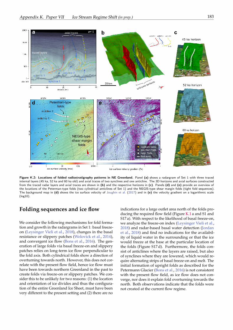
Appendix K. Paper VII Ice Stream Regime Shift (in prep.) 183

Figure K.2: Locations of folded radiostratigraphy patterns in NE Greenland. Panel (a) shows a radargram of Set 1 with three tracedinternal layers (45 ka, 52 ka and 60 ka old) and axial traces of two synclines and one anticline. The 3D horizons and axial surfaces constructedfrom the traced radar layers and axial traces are shown in (b) and the respective horizons in (c). Panels (d) and (e) provide an overview ofthe locations of the Peterman-type folds (two cylindrical anticlines of Set 1) and the NEGIS-type shear margin folds (tight fold sequences).The background map in (d) shows the ice surface velocity of Joughin et al. (2017) and in (e) the velocity gradient on a logarithmic scale(log10).

Folding sequences and ice flow

We consider the following mechanisms for fold forma-tion and growth in the radargrams in Set 1: basal freeze-on (Leysinger Vieli et al., 2018), changes in the basalresistance or slippery patches (Wolovick et al., 2014),and convergent ice flow (Bons et al., 2016). The gen-eration of large folds via basal freeze-on and slipperypatches relies on long-term ice flow perpendicular tothe fold axis. Both cylindrical folds show a direction ofoverturning towards north. However, this does not cor-relate with the present flow field, hence ice flow musthave been towards northern Greenland in the past tocreate folds via freeze-on or slippery patches. We con-sider this to be unlikely for two reasons: (1) the locationand orientation of ice divides and thus the configura-tion of the entire Greenland Ice Sheet, must have beenvery different to the present setting and (2) there are no

indications for a large outlet area north of the folds pro-ducing the required flow field (Figure K.1 a and S1 andS17 a). With respect to the likelihood of basal freeze-on,we analyze the freeze-on index (Leysinger Vieli et al.,2018) and radar-based basal water detection (Jordanet al., 2018) and find no indications for the availabil-ity of liquid water in the surrounding or that the icewould freeze at the base at the particular location ofthe folds (Figure S17 d). Furthermore, the folds con-sist of anticlines where the layers are raised, but alsoof synclines where they are lowered, which would re-quire alternating strips of basal freeze-on and melt. Theinitial formation of upright folds as described for thePetermann Glacier (Bons et al., 2016) is not consistentwith the present flow field, as ice flow does not con-verge, nor does it explain fold overturning towards thenorth. Both observations indicate that the folds werenot created at the current flow regime.

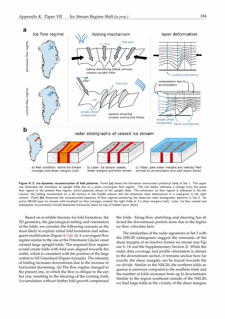
Appendix K. Paper VII Ice Stream Regime Shift (in prep.) 184

Figure K.3: Ice-dynamic reconstruction of fold patterns. Panel (a) shows the formation overturned cylindrical folds of Set 1. The upperrow illustrates the formation of upright folds due to a paleo convergent flow regime. The row below indicates a change from the paleoflow regime to the present flow regime, which passively shears of the upright folds. The schematic ice flow regime is indicated in the leftcolumn, the folding mechanisms on a 3D horizon in the middle column and the schematic layer deformation in a radargram in the rightcolumn. Panel (b) illustrates the reconstructed sequence of flow regimes producing the observed radar stratigraphy patterns in Set 2. Anactive NEGIS-type ice stream with localized ice flow (orange) created the tight folds at it’s shear margins (red). Later, ice flow ceased andsubsequent accumulation buried deposited horizontal layers on top of folded layers (blue).

Based on available theories for fold formation, the3D geometry, the glaciological setting and orientationof the folds, we consider the following scenario as themost likely to explain initial fold formation and subse-quent modification (Figure K.3 a): (i) A convergent flowregime similar to the one at the Petermann Glacier onsetcreated large upright folds. The required flow regimewould create folds with fold axes aligned towards theoutlet, which is consistent with the position of the largeoutlets in NE Greenland (Figure 4 purple). The intensityof folding increases downstream due to the increase inhorizontal shortening. (ii) The flow regime changed tothe present one, in which the flow is oblique to the ear-lier one, resulting in the shearing of the existing folds.Accumulation without further fold growth compressed

the folds. Along-flow stretching and shearing has af-fected the downstream portion more due to the higherice flow velocities here.

The similarities of the radar signatures in Set 2 withthe NEGIS radargrams suggest the remnants of theshear margins of an inactive former ice stream (see Fig-ure K.3 b and the Supplementary Section 2). While theradar data coverage and profile orientation is denserin the downstream section, it remains unclear how farexactly the shear margins can be traced towards theice divide. Similar to the NEGIS, the northern folds se-quence is narrower compared to the southern folds andthe number of folds increases from up to downstream.Similar to the region southeast outside of the NEGIS,we find large folds in the vicinity of the shear margins

Appendix K. Paper VII Ice Stream Regime Shift (in prep.) 185

of the inactive ice stream. The fold locations coincidewith the small signature in the velocity gradient (FigureK.2 e and S26). Whether the folds mark the location ofthe former shear margin or not is unclear. A furthersimilarity is that (if the folds mark the shear marginlocation) the ice stream is wider at its very onset asfurther downstream. An analysis of the isochrones inthe upper part of the ice column shows that the imprintof the downstream folds in Set 2 reaches almost up tothe ice surface (~ 90 %), similar to the signature in theNEGIS. By contrast the fold imprint in the upstreamisochrones in Set 2 is lost at ~ 70 % of the ice column.

All this points to the fact that the fold sequences inSet 2 were created by a former ice-flow regime similarto the present one at the upstream part of the NEGIS.The downstream portion most likely persisted longerand is not buried by long-term accumulation in contrastto the upstream portion. Since we find only a marginalindication of the required flow regime in the surfacevelocity gradient, we argue that a paleo ice-flow regime,similar to the present one at the onset of the NEGIS,but different to the present one created these structures(Figure 4 red).

Ice streams come and go

Numerical modelling results for the flow field of therecent Greenland Ice Sheet poorly represent the stronglocalisation of ice drawdown from the central ice sheetby the NEGIS. Results from Aschwanden et al. (2019)show a more distributed outflow within the catch-ment north eastern catchment area, towards the threemain outlets, the Nioghalvfjerdsfjord Gletscher (79° NGlacier), the Zachariae Isstrom (ZI), and the Storstrom-men Gletscher (SG). Our findings suggest that the ac-tivity of ice streams or flow regimes in this catchmenthas been shifting over time, and possibly faster thanpreviously anticipated. Changes in past flow regimeswere so far detected at Antarctic ice streams closely tothe outlets (e.g. Conway et al., 2002; Anandakrishnanand Alley, 1997; Jacobel et al., 1996; Payne and Don-gelmans, 1997) as a result to localized thinning in thedrainage system and formerly glaciated regions (e.g.Dowdeswell et al., 2006) due to long-term modifica-tions of glacial erosion and deposition of sedimentsover multiple glacial cycles. For the outlets of NEGISthere is geological evidence that at least their extent alsovaried in the past as a reaction to the varying climateconditions during the Holocene Thermal maximum.

For Antarctica, Payne and Dongelmans (1997) pro-pose that the cause for the switching behaviour appearsto arise from a competition of ice discharge betweenthe adjacent drainage basins. The authors suggest thatlocalized thickening might be responsible for the ini-tiation of a new ice stream at a different location. A

similar line of Argument is followed by Stokes et al.(2016), who describe the ice stream activity in the Lau-rentide ice stream in relation to its volume. They sug-gest that streaming is triggered if ice volume is large,but could also cease rapidly if volume is reduced. Thus,ice streams are much more likely to be initiated at thebeginning of deglaciation, and might be less importantlater on . For Greenland, geologic evidence (e.g. Larsenet al., 2018), and also modelling studies (Lecavalieret al., 2014) indicate that the geometry and elevationof the ice sheet has changed significantly during theHolocene. We earlier showed in Paper VI (Jansen et al.,2021; in prep.) the upstream part of NEGIS as it is todayhas very likely been activated around 3 500 years ago,following the onset of the re-advance of the front of the79° N Glacier. We suggest that after the HTM retreat,the geometry of the catchment area and especially theelevation did not support streaming any more in itsnorthern part, which then shifted further south to theposition of the current NEGIS. It also has to be notedthat a shift in the ice divide following the opening of theNares Straight around 8k a ago (England, 1999) couldbe one possible explanation for the shift.

The fact that a NEGIS-type ice stream was active atanother location in the Greenland ice sheet again raisesthe fundamental question of how such ice streams areformed. It is questionable whether the theory of Fahne-stock (2001), that an extremely high geothermal heatflux (GHF) determines the location and formation of theNEGIS, was also responsible for this ice stream furthernorth in the past. That such a high GHF is geologicallyrealistic and is responsible for the formation and con-tinuation of the NEGIS is widely discussed (see Smithet al. 2019 and the comment of Bons et al. 2021) andsuggests that a combination of various ice-dynamic andthe conditions at the glacier base determine the appear-ance of this ice stream type. Another striking feature ofthe location of the past NEGIS-type ice stream is thatits relics lie in an area where ice is still draining rapidlytoday. Furthermore, as we show, the downstream por-tion of this ice stream was active longer as the upstreamportion. We take that as an indication that the ice flowregime changed gradually from a far-inland reachinglocalized ice stream to the present flow regime. Themodeling of Schoof and Mantelli (2021) shows that icestreams with highly localized shear zones can simply becreated by self-reinforcing processes. This mechanismfits our observations and suggests that past strongerrunoff led to strong localization and rapid ice flow andweakened over time.

Appendix K. Paper VII Ice Stream Regime Shift (in prep.) 186

Methods

AWI UWB Radar Data Profiles

In April and April and May 2018, we collected radardata upstream of the 79° N Glacier and at the onset ofthe Northeast Greenland Ice Stream (NEGIS) with themulti-channel ultra-wideband (UWB) airborne radarsounder of the Alfred Wegener Institute, HelmholtzCentre for Polar and Marine Research (AWI; black linesof Set 1 and purple lines at the NEGIS in Figure K.1 a,b,c and f). The system comprises an antenna array witheight channels (HH polarization), and the data wererecorded at a frequency range of 180- 210 MHz. For acomprehensive description of AWI’s UWB radar sys-tem and the survey design of the NEGIS survey (seeFranke et al., 2020, 2021; Hale et al., 2016; Rodriguez-Morales et al., 2014). We used the CReSIS Toolbox (CRe-SIS, 2020) for radar data processing, which includessynthetic aperture radar (SAR) and array processing(for further details see the appendix in Franke et al.(2020, 2021). For the geometrical analysis of the IRHswe translate the two-way travel time (TWT) radar datainto an elevation domain with a two dimensional di-electric constant (ε) model for air with ε = 1 and icewith ε = 3.15. The boundary between the two dielectricconstants is the ice surface radar reflection.

3D Horizon Construction

For a three-dimensional analysis of the IRHs, we buildup on the approach of Bons et al. (2016) and use the3D model building software MOVETM (MOVE CoreApplication, Version 2019). The elevation-convertedradargrams were converted to the SEGY format withthe ObsPy Python toolbox (Beyreuther et al., 2010) andimported in MOVE. Internal layers, which could beclearly identified in all radar sections, were traced man-ually. The traced layers were split into fragments whichshow a similar geometry (e.g. anticlines and synclines)as a fragment of the same IRH in the adjacent radar-gram. Supplementary Figure S35 a shows how the linefragments are interpolated between two radargrams.

Fold axial surfaces

We construct three axial surfaces (one anticline and twosynclines) of the northern cylindrical folds upstreamof the 79° N Glacier (Figure K.1 c and 2. The method isanalogous to the construction of the 3D horizons (seeFigure K.2 a,Y and SX). We trace the points of maximumcurvature in the radargrams for two synclines and theanticline of the cylindrical fold to create a line segmentand interpolate between the lines of each radargram.

Ice flow reconstruction from axial traces

Due to the curvature of the fold axial traces, we definea minimum and a maximum distance for a measure thedisplacement of the ice column (dSmin and dSmax) forfive profiles for syncline 1 and 2, respectively. At eachposition we use the absolute ice flow velocity (vS) tocalculate the velocity component parallel to the direc-tion of shearing with the offset angle α: vy = vS cos(α)(see Figure S36). We assume that the ice flow velocitydoes not change over time and only changes very littlein space. Then we calculate the time needed for thedisplacement of the upper ice column tS assuming thatthe deepest end of the axial trace is immobile: tS = dS.The vector components of the velocity field are shownin supplementary Figure S36a.

AcknowledgementsWe thank the crew of the research aircraft Polar 6. Weacknowledge the use of radar data from CReSIS gener-ated with support from the University of Kansas, NASAOperation IceBridge grant NNX16AH54G, NSF grantsACI-1443054, OPP-1739003, and IIS-1838230, Lilly En-dowment Incorporated, and Indiana METACyt Initia-tive. Steven Franke and Daniela Jansen were fundedby the AWI strategy fund.

Data AvailabilityThe CReSIS radio-echo sounding data used in thisstudy are available under CReSIS data products https://data.cresis.ku.edu/data/rds/. The list of profilesis provided in the supplementary material. AWI UWBice thickness data from Jansen et al. (2020) are avail-able at the PANGAEA data publisher https://doi.pangaea.de/10.1594/PANGAEA.913193.

Author ContributionsSF wrote the manuscript, processed the radar data, con-structed the 3D horizons, and performed all calcula-tions and analyses. DJ designed the study and devel-oped the scientific idea with contributions of PB, IWand SF. DJ was PI on the airborne radar survey and TBand VH collected the data. DS provided additional icethickness data and VH assisted with GPS post process-ing. JW developed the idea for the visualization forthe fold deformation stages and developed the foldinghypothesis together with PB, DJ, IW, KS and SF. OE, DS,VH and IW provided detailed feedback on the analyses.All authors discussed and reviewed the manuscript.

187

BibliographyAnandakrishnan, S. and Alley, R. B. Tidal forcing of basal seis-

micity of ice stream c, west antarctica, observed far inland.Journal of Geophysical Research: Solid Earth, 102(B7):15183–15196, 1997. doi: https://doi.org/10.1029/97JB01073.URL https://agupubs.onlinelibrary.wiley.com/doi/abs/10.1029/97JB01073.

Aschwanden, A., Fahnestock, M. A., Truffer, M., Brinker-hoff, D. J., Hock, R., Khroulev, C., Mottram, R., andKhan, S. A. Contribution of the Greenland Ice Sheet tosea level over the next millennium. Science Advances,5(6), 2019. doi: 10.1126/sciadv.aav9396. URL https://advances.sciencemag.org/content/5/6/eaav9396.

Bell, R. E., Ferraccioli, F., Creyts, T. T., Braaten, D., Corr, H.,Das, I., Damaske, D., Frearson, N., Jordan, T., Rose, K.,Studinger, M., and Wolovick, M. Widespread PersistentThickening of the East Antarctic Ice Sheet by Freezingfrom the Base. Science, 331(6024):1592–1595, mar 2011.doi: 10.1126/science.1200109. URL https://doi.org/10.1126%2Fscience.1200109.

Bell, R. E., Tinto, K., Das, I., Wolovick, M., Chu, W., Creyts,T. T., Frearson, N., Abdi, A., and Paden, J. D. Deforma-tion warming and softening of Greenland’s ice by refreez-ing meltwater. Nature Geoscience, 7(7):497–502, jun 2014.doi: 10.1038/ngeo2179. URL https://doi.org/10.1038%2Fngeo2179.

Beyreuther, M., Barsch, R., Krischer, L., Megies, T., Behr, Y.,and Wassermann, J. ObsPy: A Python Toolbox for Seis-mology. Seismological Research Letters, 81(3):530–533, may2010. doi: 10.1785/gssrl.81.3.530. URL https://doi.org/10.1785%2Fgssrl.81.3.530.

Bons, P. D., Jansen, D., Mundel, F., Bauer, C. C., Binder, T.,Eisen, O., Jessell, M. W., Llorens, M.-G., Steinbach, F., Stein-hage, D., and Weikusat, I. Converging flow and anisotropycause large-scale folding in Greenland's ice sheet. NatureCommunications, 7(1), apr 2016. doi: 10.1038/ncomms11427.URL https://doi.org/10.1038%2Fncomms11427.

Bons, P. D., de Riese, T., Franke, S., Llorens, M.-G., Sachau,T., Stoll, N., Weikusat, I., Westhoff, J., and Zhang, Y. Com-ment on “exceptionally high heat flux needed to sustainthe northeast greenland ice stream” by smith-johnsen etal. (2020). The Cryosphere, 15(5):2251–2254, 2021. doi:10.5194/tc-15-2251-2021. URL https://tc.copernicus.org/articles/15/2251/2021/.

Conway, H., Catania, G., Raymond, C. F., Gades, A. M., Scam-bos, T. A., and Engelhardt, H. Switch of flow directionin an Antarctic ice stream. Nature, 419(6906):465–467, oct2002. ISSN 0028-0836. doi: 10.1038/nature01081. URLhttp://www.nature.com/articles/nature01081.

CReSIS. CReSIS Toolbox [computer software], Lawrence,Kansas, USA. Retrieved from https://github.com/CReSIS,

2020. URL https://ops.cresis.ku.edu/wiki/index.php/Main_Page.

Creyts, T. T., Ferraccioli, F., Bell, R. E., Wolovick, M., Corr,H., Rose, K. C., Frearson, N., Damaske, D., Jordan, T.,Braaten, D., and Finn, C. Freezing of ridges and waternetworks preserves the Gamburtsev Subglacial Mountainsfor millions of years. Geophysical Research Letters, 41(22):8114–8122, nov 2014. doi: 10.1002/2014gl061491. URLhttps://doi.org/10.1002%2F2014gl061491.

Dahl-Jensen, D., Albert, M. R., Aldahan, A., Azuma, N.,Balslev-Clausen, D., Baumgartner, M., Berggren, A. M.,Bigler, M., Binder, T., Blunier, T., Bourgeois, J. C., Brook,E. J., Buchardt, S. L., Buizert, C., Capron, E., Chappellaz,J., Chung, J., Clausen, H. B., Cvijanovic, I., Davies, S. M.,Ditlevsen, P., Eicher, O., Fischer, H., Fisher, D. A., Fleet,L. G., Gfeller, G., Gkinis, V., Gogineni, S., Goto-Azuma, K.,Grinsted, A., Gudlaugsdottir, H., Guillevic, M., Hansen,S. B., Hansson, M., Hirabayashi, M., Hong, S., Hur, S. D.,Huybrechts, P., Hvidberg, C. S., Iizuka, Y., Jenk, T., Johnsen,S. J., Jones, T. R., Jouzel, J., Karlsson, N. B., Kawamura, K.,Keegan, K., Kettner, E., Kipfstuhl, S., Kjær, H. A., Kout-nik, M., Kuramoto, T., Köhler, P., Laepple, T., Landais,A., Langen, P. L., Larsen, L. B., Leuenberger, D., Leuen-berger, M., Leuschen, C., Li, J., Lipenkov, V., Martinerie,P., Maselli, O. J., Masson-Delmotte, V., McConnell, J. R.,Miller, H., Mini, O., Miyamoto, A., Montagnat-Rentier,M., Mulvaney, R., Muscheler, R., Orsi, A. J., Paden, J.,Panton, C., Pattyn, F., Petit, J. R., Pol, K., Popp, T., Poss-nert, G., Prié, F., Prokopiou, M., Quiquet, A., Rasmussen,S. O., Raynaud, D., Ren, J., Reutenauer, C., Ritz, C., Röck-mann, T., Rosen, J. L., Rubino, M., Rybak, O., Samyn, D.,Sapart, C. J., Schilt, A., Schmidt, A. M., Schwander, J.,Schüpbach, S., Seierstad, I., Severinghaus, J. P., Sheldon,S., Simonsen, S. B., Sjolte, J., Solgaard, A. M., Sowers, T.,Sperlich, P., Steen-Larsen, H. C., Steffen, K., Steffensen,J. P., Steinhage, D., Stocker, T. F., Stowasser, C., Sture-vik, A. S., Sturges, W. T., Sveinbjörnsdottir, A., Svens-son, A., Tison, J. L., Uetake, J., Vallelonga, P., Van DeWal, R. S., Van Der Wel, G., Vaughn, B. H., Vinther, B.,Waddington, E., Wegner, A., Weikusat, I., White, J. W., Wil-helms, F., Winstrup, M., Witrant, E., Wolff, E. W., Xiao,C., and Zheng, J. Eemian interglacial reconstructed froma Greenland folded ice core. Nature, 493(7433):489–494,2013. ISSN 00280836. doi: 10.1038/nature11789. URLhttp://dx.doi.org/10.1038/nature11789.

Dowdeswell, J. A., Ottesen, D., and Rise, L. Flow switchingand large-scale deposition by ice streams draining formerice sheets. Geology, 34(4):313–316, 2006. doi: 10.1130/G22253.1. URL https://doi.org/10.1130/G22253.1.

Drews, R., Eisen, O., Weikusat, I., Kipfstuhl, S., Lam-brecht, A., Steinhage, D., Wilhelms, F., and Miller, H.Layer disturbances and the radio-echo free zone in icesheets. The Cryosphere, 3(2):195–203, aug 2009. doi:10.5194/tc-3-195-2009. URL https://doi.org/10.5194%2Ftc-3-195-2009.

England, J. Coalescent greenland and innuitian ice duringthe last glacial maximum: revising the quaternary of thecanadian high arctic. Quaternary Science Reviews, 18(3):

BIBLIOGRAPHY 188

421–456, 1999. doi: 10.1016/S0277-3791(98)00070-5. URLhttps://www.sciencedirect.com/science/article/pii/S0277379198000705.

Fahnestock, M. High Geothermal Heat Flow Basal Melt,and the Origin of Rapid Ice Flow in Central Green-land. Science, 294(5550):2338–2342, dec 2001. doi: 10.1126/science.1065370. URL https://doi.org/10.1126%2Fscience.1065370.

Franke, S., Jansen, D., Binder, T., Dörr, N., Helm, V., Paden,J., Steinhage, D., and Eisen, O. Bed topography andsubglacial landforms in the onset region of the North-east Greenland Ice Stream. Annals of Glaciology, pages1–11, mar 2020. doi: 10.1017/aog.2020.12. URL https://doi.org/10.1017%2Faog.2020.12.

Franke, S., Jansen, D., Binder, T., Paden, J. D., Dörr, N., Ger-ber, T., Miller, H., Dahl-Jensen, D., Helm, V., Steinhage,D., Weikusat, I., Wilhelms, F., and Eisen, O. Airborneultra-wideband radar sounding over the shear marginsand along flow lines at the onset region of the northeastgreenland ice stream. Earth System Science Data Discussions,2021:1–24, 2021. doi: 10.5194/essd-2021-91. URL https://essd.copernicus.org/preprints/essd-2021-91/.

Fujita, S., Maeno, H., Uratsuka, S., Furukawa, T., Mae, S.,Fujii, Y., and Watanabe, O. Nature of radio echo layering inthe Antarctic Ice Sheet detected by a two-frequency experi-ment. Journal of Geophysical Research: Solid Earth, 104(B6):13013–13024, jun 1999. doi: 10.1029/1999jb900034. URLhttps://doi.org/10.1029%2F1999jb900034.

Gogineni, S., Tammana, D., Braaten, D., Leuschen, C., Akins,T., Legarsky, J., Kanagaratnam, P., Stiles, J., Allen, C., andJezek, K. Coherent radar ice thickness measurementsover the Greenland ice sheet. Journal of Geophysical Re-search: Atmospheres, 106(D24):33761–33772, dec 2001. doi:10.1029/2001jd900183. URL https://doi.org/10.1029%2F2001jd900183.

Hale, R., Miller, H., Gogineni, S., Yan, J. B., Rodriguez-Morales, F., Leuschen, C., Paden, J., Li, J., Binder, T.,Steinhage, D., Gehrmann, M., and Braaten, D. Multi-channel ultra-wideband radar sounder and imager. In2016 IEEE International Geoscience and Remote Sensing Sym-posium (IGARSS). IEEE, jul 2016. doi: 10.1109/igarss.2016.7729545. URL https://doi.org/10.1109%2Figarss.2016.7729545.

Jacobel, R. W., Scambos, T. A., Raymond, C. F., andGades, A. M. Changes in the configuration of icestream flow from the west antarctic ice sheet. Jour-nal of Geophysical Research: Solid Earth, 101(B3):5499–5504, 1996. doi: https://doi.org/10.1029/95JB03735.URL https://agupubs.onlinelibrary.wiley.com/doi/abs/10.1029/95JB03735.

Jansen, D., Llorens, M.-G., Westhoff, J., Steinbach, F.,Kipfstuhl, S., Bons, P. D., Griera, A., and Weikusat,I. Small-scale disturbances in the stratigraphy of theNEEM ice core: observations and numerical model sim-ulations. The Cryosphere, 10(1):359–370, feb 2016. doi:

10.5194/tc-10-359-2016. URL https://doi.org/10.5194%2Ftc-10-359-2016.

Jansen, D., Franke, S., Binder, T., Helm, V., and Paden,J. D. Ice thickness from the northern catchment regionof Greenland's 79 North Glacier, recorded with the air-borne AWI UWB radar system [DATA SET], 2020. URLhttps://doi.org/10.1594/PANGAEA.913193.

Jordan, T. M., Williams, C. N., Schroeder, D. M., Martos,Y. M., Cooper, M. A., Siegert, M. J., Paden, J. D., Huy-brechts, P., and Bamber, J. L. A constraint upon the basalwater distribution and thermal state of the GreenlandIce Sheet from radar bed echoes. The Cryosphere, 12(9):2831–2854, sep 2018. doi: 10.5194/tc-12-2831-2018. URLhttps://doi.org/10.5194%2Ftc-12-2831-2018.

Joughin, I., Smith, B. E., and Howat, I. M. A completemap of Greenland ice velocity derived from satellite datacollected over 20 years. Journal of Glaciology, 64(243):1–11, nov 2017. doi: 10.1017/jog.2017.73. URL https://doi.org/10.1017%2Fjog.2017.73.

Keisling, B. A., Christianson, K., Alley, R. B., Peters, L. E.,Christian, J. E., Anandakrishnan, S., Riverman, K. L., Muto,A., and Jacobel, R. W. Basal conditions and ice dynamicsinferred from radar-derived internal stratigraphy of thenortheast Greenland ice stream. Annals of Glaciology, 55(67):127–137, 2014. doi: 10.3189/2014aog67a090. URLhttps://doi.org/10.3189%2F2014aog67a090.

Larsen, N. K., Levy, L. B., Carlson, A. E., Buizert, C., Olsen,J., Strunk, A., Bjørk, A. A., and Skov, D. S. Instabil-ity of the Northeast Greenland Ice Stream over the last45,000 years. Nature Communications, 9(1):3–10, 2018.ISSN 20411723. doi: 10.1038/s41467-018-04312-7. URLhttp://dx.doi.org/10.1038/s41467-018-04312-7.

Lecavalier, B. S., Milne, G. A., Simpson, M. J., Wake, L., Huy-brechts, P., Tarasov, L., Kjeldsen, K. K., Funder, S., Long,A. J., Woodroffe, S., Dyke, A. S., and Larsen, N. K. A modelof greenland ice sheet deglaciation constrained by observa-tions of relative sea level and ice extent. Quaternary ScienceReviews, 102:54–84, 2014. ISSN 0277-3791. doi: 10.1016/j.quascirev.2014.07.018. URL https://www.sciencedirect.com/science/article/pii/S0277379114003011.

Leysinger Vieli, G. J.-M. C., Martín, C., Hindmarsh, R. C. A.,and Lüthi, M. P. Basal freeze-on generates complex ice-sheet stratigraphy. Nature Communications, 9(1), nov 2018.doi: 10.1038/s41467-018-07083-3. URL https://doi.org/10.1038%2Fs41467-018-07083-3.

MacGregor, J. A., Fahnestock, M. A., Catania, G. A., Paden,J. D., Gogineni, S. P., Young, S. K., Rybarski, S. C., Mabrey,A. N., Wagman, B. M., and Morlighem, M. Radios-tratigraphy and age structure of the Greenland Ice Sheet.Journal of Geophysical Research: Earth Surface, 120(2):212–241, feb 2015. doi: 10.1002/2014jf003215. URL https://doi.org/10.1002%2F2014jf003215.

Margold, M., Stokes, C. R., and Clark, C. D. Ice streamsin the Laurentide Ice Sheet: Identification characteristics

BIBLIOGRAPHY 189

and comparison to modern ice sheets. Earth-Science Re-views, 143:117–146, apr 2015. doi: 10.1016/j.earscirev.2015.01.011. URL https://doi.org/10.1016%2Fj.earscirev.2015.01.011.

Mouginot, J., Rignot, E., Bjørk, A. A., van den Broeke,M., Millan, R., Morlighem, M., Noël, B., Scheuchl, B.,and Wood, M. Forty-six years of Greenland Ice Sheetmass balance from 1972 to 2018. Proceedings of the Na-tional Academy of Sciences, 116(19):9239–9244, apr 2019.doi: 10.1073/pnas.1904242116. URL https://doi.org/10.1073%2Fpnas.1904242116.

Payne, A. J. and Dongelmans, P. W. Self-organizationin the thermomechanical flow of ice sheets. Jour-nal of Geophysical Research: Solid Earth, 102(B6):12219–12233, 1997. doi: https://doi.org/10.1029/97JB00513.URL https://agupubs.onlinelibrary.wiley.com/doi/abs/10.1029/97JB00513.

Rignot, E., Mouginot, J., Scheuchl, B., van den Broeke, M.,van Wessem, M. J., and Morlighem, M. Four decades ofAntarctic Ice Sheet mass balance from 1979–2017. Pro-ceedings of the National Academy of Sciences, 116(4):1095–1103, jan 2019. doi: 10.1073/pnas.1812883116. URLhttps://doi.org/10.1073%2Fpnas.1812883116.

Rodriguez-Morales, F., Byers, K., Crowe, R., Player, K., Hale,R. D., Arnold, E. J., Smith, L., Gifford, C. M., Braaten,D., Panton, C., Gogineni, S., Leuschen, C. J., Paden,J. D., Li, J., Lewis, C. C., Panzer, B., Alvestegui, D. G.-G., and Patel, A. Advanced Multifrequency Radar In-strumentation for Polar Research. IEEE Transactions onGeoscience and Remote Sensing, 52(5):2824–2842, may 2014.doi: 10.1109/tgrs.2013.2266415. URL https://doi.org/10.1109%2Ftgrs.2013.2266415.

Rosenau, R., Scheinert, M., and Dietrich, R. A process-ing system to monitor Greenland outlet glacier veloc-ity variations at decadal and seasonal time scales utiliz-ing the Landsat imagery. Remote Sensing of Environment,169:1–19, nov 2015. doi: 10.1016/j.rse.2015.07.012. URLhttps://doi.org/10.1016%2Fj.rse.2015.07.012.

Schoof, C. and Mantelli, E. The role of sliding inice stream formation. Proceedings of the Royal Soci-ety A: Mathematical, Physical and Engineering Sciences,477(2248):20200870, 2021. doi: 10.1098/rspa.2020.0870. URL https://royalsocietypublishing.org/doi/abs/10.1098/rspa.2020.0870.

Siegert, M. On the origin nature and uses of Antarc-tic ice-sheet radio-echo layering. Progress in Physi-cal Geography, 23(2):159–179, jun 1999. doi: 10.1191/

030913399671124903. URL https://doi.org/10.1191%2F030913399671124903.

Smith, E. C., Hattermann, T., Kuhn, G., Gaedicke, C., Berger,S., Drews, R., Ehlers, T. A., Franke, D., Gromig, R., Hof-stede, C., Lambrecht, A., Läufer, A., Mayer, C., Tiede-mann, R., Wilhelms, F., and Eisen, O. Detailed seismicbathymetry beneath Ekstroem Ice Shelf Antarctica: Im-plications for glacial history and ice-ocean interaction.nov 2019. doi: 10.1002/essoar.10501125.1. URL https://doi.org/10.1002%2Fessoar.10501125.1.

Stokes, C. R., Margold, M., Clark, C. D., and Tarasov, L.Ice stream activity scaled to ice sheet volume duringLaurentide Ice Sheet deglaciation. Nature, 530(7590):322–326, feb 2016. doi: 10.1038/nature16947. URL https://doi.org/10.1038%2Fnature16947.

Waddington, E. D., Bolzan, J. F., and Alley, R. B. Poten-tial for stratigraphie folding near ice-sheet centers. Jour-nal of Glaciology, 47(159):639–648, 2001. doi: 10.3189/172756501781831756. URL https://doi.org/10.3189%2F172756501781831756.

Westhoff, J., Stoll, N., Franke, S., Weikusat, I., Bons, P.,Kerch, J., Jansen, D., Kipfstuhl, S., and Dahl-Jensen, D.A stratigraphy-based method for reconstructing ice coreorientation. Annals of Glaciology, page 1–12, 2020. doi:10.1017/aog.2020.76. URL https://doi.org/10.1017/aog.2020.76.

Wolovick, M. J. and Creyts, T. T. Overturned folds in icesheets: Insights from a kinematic model of traveling stickypatches and comparisons with observations. Journal ofGeophysical Research: Earth Surface, 121(5):1065–1083, may2016. doi: 10.1002/2015jf003698. URL https://doi.org/10.1002%2F2015jf003698.

Wolovick, M. J., Creyts, T. T., Buck, W. R., and Bell, R. E.Traveling slippery patches produce thickness-scale foldsin ice sheets. Geophysical Research Letters, 41(24):8895–8901, dec 2014. doi: 10.1002/2014gl062248. URL https://doi.org/10.1002%2F2014gl062248.

Wrona, T., Wolovick, M. J., Ferraccioli, F., Corr, H., Jordan,T., and Siegert, M. J. Position and variability of com-plex structures in the central east antarctic ice sheet. Geo-logical Society, London, Special Publications, 461(1):113–129,2018. ISSN 0305-8719. doi: 10.1144/SP461.12. URL https://sp.lyellcollection.org/content/461/1/113.

BIBLIOGRAPHY 190

PAPER VII SUPPLEMENTARY INFORMATION

Supplementary Information:Indication of ice-stream regime shift in Northereast GreenlandSteven Franke1 , Paul Bons2,3 , Julien Westhoff4 , Tobias Binder1,† , Kyra Streng2, Veit Helm1 ,Daniel Steinhage1 , Olaf Eisen1,5 , John Paden6 , Ilka Weikusat1,2 and Daniela Jansen1

1 Alfred Wegener Institute, Helmholtz Centre for Polar and Marine Research, Bremerhaven, Germany2 Department of Geosciences, Eberhard Karls University Tübingen, Germany3 China University of Geosciences, Beijing, China4 Physics of Ice, Climate, and Earth, Niels Bohr Institute, University of Copenhagen, Denmark5 Department of Geosciences, University of Bremen, Bremen, Germany6 Centre for Remote Sensing of Ice Sheets (CReSIS), University of Kansas, Lawrence, KS, USA† now at Ibeo Automotive Systems, Hamburg, Germany

The supplemantary information for Paper VII is provided on the USB stick submittedalongside the thesis as well as in a private online repository (see below).

Supplementary Information of Paper VII:

1. Figures S1 – S36 and Tables S1 – S2 (pdf):https://storage.luckycloud.de/f/b4b3bc2457a740a68e3c/

191

Appendix L

PAPER VIII DATA DESCRIPTION ARTICLE

A 3D view on folded radar stratigraphy in northern GreenlandSteven Franke1 , Paul D. Bons2,3 , Felicitas Mundel2, Till Sachau2, Kyra Streng2, Ilka Weikusat1,2 ,Heinrich Miller1 , Tobias Binder1,∗ , Veit Helm1 , John D. Paden4 , Daniel Steinhage1 , NilsDörr1,5 , Olaf Eisen1,6 , Daniela Jansen1

1 Alfred Wegener Institute, Helmholtz Centre for Polar and Marine Research, Bremerhaven, Germany2 Department of Geosciences, Eberhard Karls University Tübingen, Germany3 China University of Geosciences, Beijing, China4 Centre for Remote Sensing of Ice Sheets (CReSIS), University of Kansas, Lawrence, KS, USA5 Institute of Photogrammetry and Remote Sensing, Karlsruhe Institute of Technology, Karlsruhe, Germany6 Department of Geosciences, University of Bremen, Bremen, Germany∗ now at Ibeo Automotive Systems, Hamburg, Germany

Draft to be submitted to Scientific Data.

AbstractWe present a data set of reconstructed three-dimensional (3D) englacial stratigraphic horizons in northern Greenlandand explain how 3D horizons provide an improved basis for the interpretation of deformed radar stratigraphy. Thedata covers three different survey regions, which represent crucial ice-dynamic settings in Greenland: (a) the onsetof the Peterman Glacier, (b) a region of deformed stratigraphy close to the ice divide in Northern Greenland and (c)the onset of the North East Greenland Ice Stream (NEGIS). We provide the data in different formats to enable awide range of applications and reproduction of the results. The data set will be made available for download fromPANGAEA.

Background

The Greenland Ice Sheet (GrIS) is one of the largest icemasses and holds 11 % of all ice on Earth (Allison et al.,2009). Over the last two decades, ice mass loss of theGrIS has accelerated and caused sea level to rise about10.8 ± 0.9 millimetres (Shepherd et al., 2020). If ice massloss continues as predicted by Church and White (2006),it has the potential to contribute as much as 9 cm of sealevel rise by 2050. At the same time, the interior of theGrIS is thickening, partly as an ongoing dynamic re-sponse to the last deglaciation (MacGregor et al., 2016).This suggests that the behavior of the Greenland icesheet is complex, and at the same time we see that cli-matic and dynamic effects of the past are preserved inthe ice.

Ice flows from the centre towards the ocean viaa network of glaciers and ice streams (Joughin et al.,2010). These corridors of fast ice flow are responsible

of discharging large amounts of ice and sediment (Ben-nett, 2003) and are thus considered to play a key rolein the stability of the GrIS. The geometry, flow velocityand location of ice streams are controlled by a variety offactors, which can be difficult to identify (Winsborrowet al., 2010). Furthermore, it has been shown that icestream behaviour can be highly dynamic and subject ofrapid changes (Conway et al., 2002). As ice flows it de-forms and as it deforms it leaves traces in the ice on thelarge and small scale. We are able to visualize a varietyof structures in ice sheets are the result of cumulativedeformation. Many are the result of inhomogenities inice flow and the structures can be preserved or over-printed over time.

For instance, folding in ice sheets can be identifiedwith ice-penetrating radar data. The depth-varyingreflections of radar waves by englacial layers are in-terpreted as isochrones (i.e. layers depostied as snowat the same time; e.g. Cavitte et al. 2016) and provide

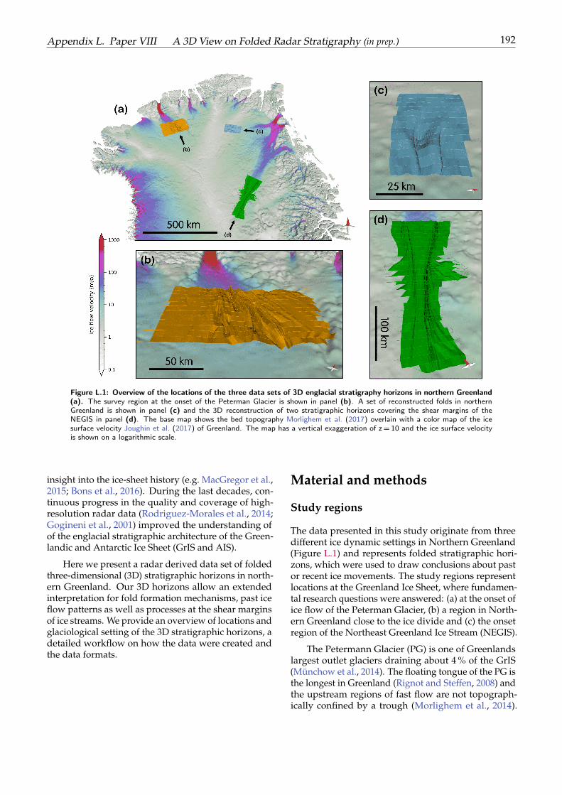
Appendix L. Paper VIII A 3D View on Folded Radar Stratigraphy (in prep.) 192

Figure L.1: Overview of the locations of the three data sets of 3D englacial stratigraphy horizons in northern Greenland(a). The survey region at the onset of the Peterman Glacier is shown in panel (b). A set of reconstructed folds in northernGreenland is shown in panel (c) and the 3D reconstruction of two stratigraphic horizons covering the shear margins of theNEGIS in panel (d). The base map shows the bed topography Morlighem et al. (2017) overlain with a color map of the icesurface velocity Joughin et al. (2017) of Greenland. The map has a vertical exaggeration of z= 10 and the ice surface velocityis shown on a logarithmic scale.

insight into the ice-sheet history (e.g. MacGregor et al.,2015; Bons et al., 2016). During the last decades, con-tinuous progress in the quality and coverage of high-resolution radar data (Rodriguez-Morales et al., 2014;Gogineni et al., 2001) improved the understanding ofof the englacial stratigraphic architecture of the Green-landic and Antarctic Ice Sheet (GrIS and AIS).

Here we present a radar derived data set of foldedthree-dimensional (3D) stratigraphic horizons in north-ern Greenland. Our 3D horizons allow an extendedinterpretation for fold formation mechanisms, past iceflow patterns as well as processes at the shear marginsof ice streams. We provide an overview of locations andglaciological setting of the 3D stratigraphic horizons, adetailed workflow on how the data were created andthe data formats.

Material and methods

Study regions

The data presented in this study originate from threedifferent ice dynamic settings in Northern Greenland(Figure L.1) and represents folded stratigraphic hori-zons, which were used to draw conclusions about pastor recent ice movements. The study regions representlocations at the Greenland Ice Sheet, where fundamen-tal research questions were answered: (a) at the onset ofice flow of the Peterman Glacier, (b) a region in North-ern Greenland close to the ice divide and (c) the onsetregion of the Northeast Greenland Ice Stream (NEGIS).

The Petermann Glacier (PG) is one of Greenlandslargest outlet glaciers draining about 4 % of the GrIS(Münchow et al., 2014). The floating tongue of the PG isthe longest in Greenland (Rignot and Steffen, 2008) andthe upstream regions of fast flow are not topograph-ically confined by a trough (Morlighem et al., 2014).

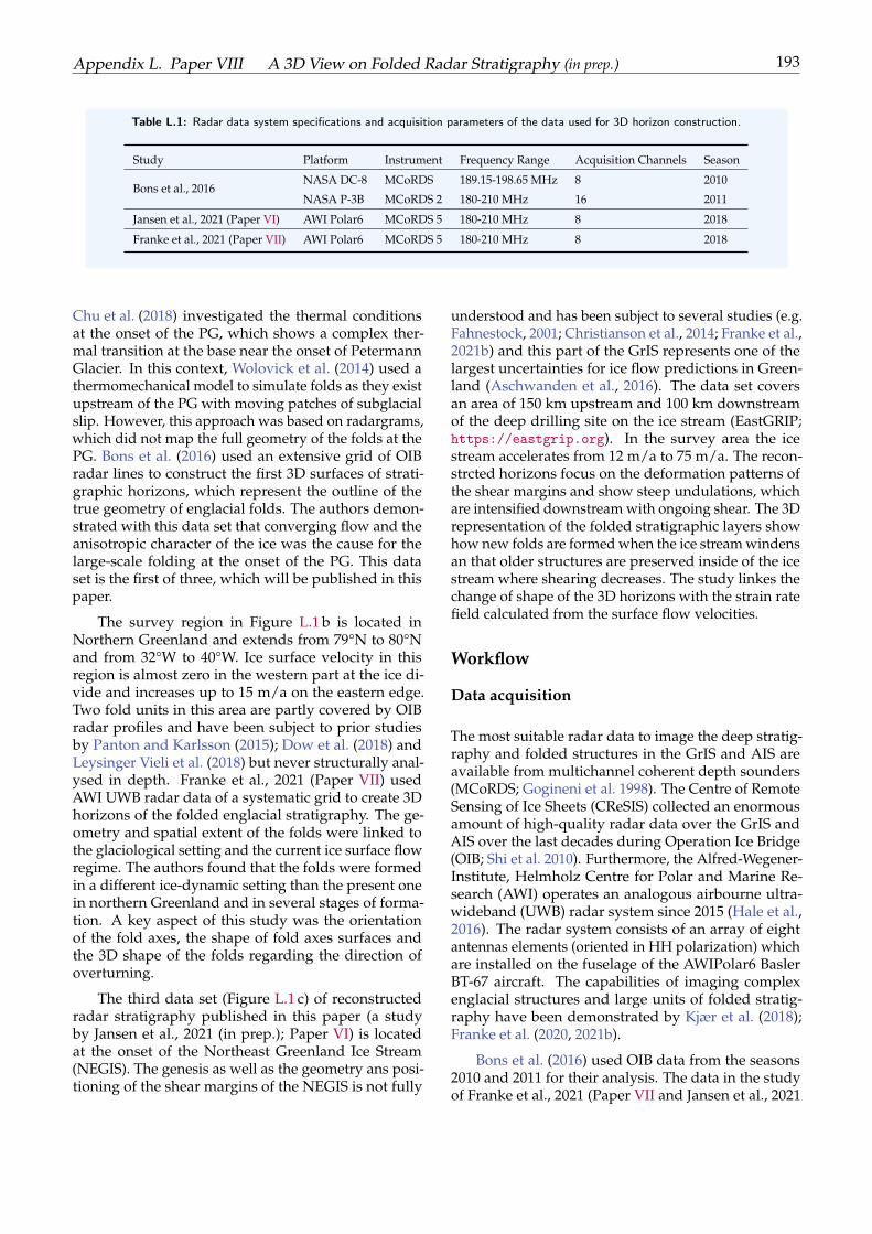
Appendix L. Paper VIII A 3D View on Folded Radar Stratigraphy (in prep.) 193

Table L.1: Radar data system specifications and acquisition parameters of the data used for 3D horizon construction.

Study Platform Instrument Frequency Range Acquisition Channels Season

Bons et al., 2016NASA DC-8 MCoRDS 189.15-198.65 MHz 8 2010

NASA P-3B MCoRDS 2 180-210 MHz 16 2011

Jansen et al., 2021 (Paper VI) AWI Polar6 MCoRDS 5 180-210 MHz 8 2018

Franke et al., 2021 (Paper VII) AWI Polar6 MCoRDS 5 180-210 MHz 8 2018

Chu et al. (2018) investigated the thermal conditionsat the onset of the PG, which shows a complex ther-mal transition at the base near the onset of PetermannGlacier. In this context, Wolovick et al. (2014) used athermomechanical model to simulate folds as they existupstream of the PG with moving patches of subglacialslip. However, this approach was based on radargrams,which did not map the full geometry of the folds at thePG. Bons et al. (2016) used an extensive grid of OIBradar lines to construct the first 3D surfaces of strati-graphic horizons, which represent the outline of thetrue geometry of englacial folds. The authors demon-strated with this data set that converging flow and theanisotropic character of the ice was the cause for thelarge-scale folding at the onset of the PG. This dataset is the first of three, which will be published in thispaper.

The survey region in Figure L.1 b is located inNorthern Greenland and extends from 79°N to 80°Nand from 32°W to 40°W. Ice surface velocity in thisregion is almost zero in the western part at the ice di-vide and increases up to 15 m/a on the eastern edge.Two fold units in this area are partly covered by OIBradar profiles and have been subject to prior studiesby Panton and Karlsson (2015); Dow et al. (2018) andLeysinger Vieli et al. (2018) but never structurally anal-ysed in depth. Franke et al., 2021 (Paper VII) usedAWI UWB radar data of a systematic grid to create 3Dhorizons of the folded englacial stratigraphy. The ge-ometry and spatial extent of the folds were linked tothe glaciological setting and the current ice surface flowregime. The authors found that the folds were formedin a different ice-dynamic setting than the present onein northern Greenland and in several stages of forma-tion. A key aspect of this study was the orientationof the fold axes, the shape of fold axes surfaces andthe 3D shape of the folds regarding the direction ofoverturning.

The third data set (Figure L.1 c) of reconstructedradar stratigraphy published in this paper (a studyby Jansen et al., 2021 (in prep.); Paper VI) is locatedat the onset of the Northeast Greenland Ice Stream(NEGIS). The genesis as well as the geometry ans posi-tioning of the shear margins of the NEGIS is not fully

understood and has been subject to several studies (e.g.Fahnestock, 2001; Christianson et al., 2014; Franke et al.,2021b) and this part of the GrIS represents one of thelargest uncertainties for ice flow predictions in Green-land (Aschwanden et al., 2016). The data set coversan area of 150 km upstream and 100 km downstreamof the deep drilling site on the ice stream (EastGRIP;https://eastgrip.org). In the survey area the icestream accelerates from 12 m/a to 75 m/a. The recon-strcted horizons focus on the deformation patterns ofthe shear margins and show steep undulations, whichare intensified downstream with ongoing shear. The 3Drepresentation of the folded stratigraphic layers showhow new folds are formed when the ice stream windensan that older structures are preserved inside of the icestream where shearing decreases. The study linkes thechange of shape of the 3D horizons with the strain ratefield calculated from the surface flow velocities.

Workflow

Data acquisition

The most suitable radar data to image the deep stratig-raphy and folded structures in the GrIS and AIS areavailable from multichannel coherent depth sounders(MCoRDS; Gogineni et al. 1998). The Centre of RemoteSensing of Ice Sheets (CReSIS) collected an enormousamount of high-quality radar data over the GrIS andAIS over the last decades during Operation Ice Bridge(OIB; Shi et al. 2010). Furthermore, the Alfred-Wegener-Institute, Helmholz Centre for Polar and Marine Re-search (AWI) operates an analogous airbourne ultra-wideband (UWB) radar system since 2015 (Hale et al.,2016). The radar system consists of an array of eightantennas elements (oriented in HH polarization) whichare installed on the fuselage of the AWIPolar6 BaslerBT-67 aircraft. The capabilities of imaging complexenglacial structures and large units of folded stratig-raphy have been demonstrated by Kjær et al. (2018);Franke et al. (2020, 2021b).

Bons et al. (2016) used OIB data from the seasons2010 and 2011 for their analysis. The data in the studyof Franke et al., 2021 (Paper VII and Jansen et al., 2021

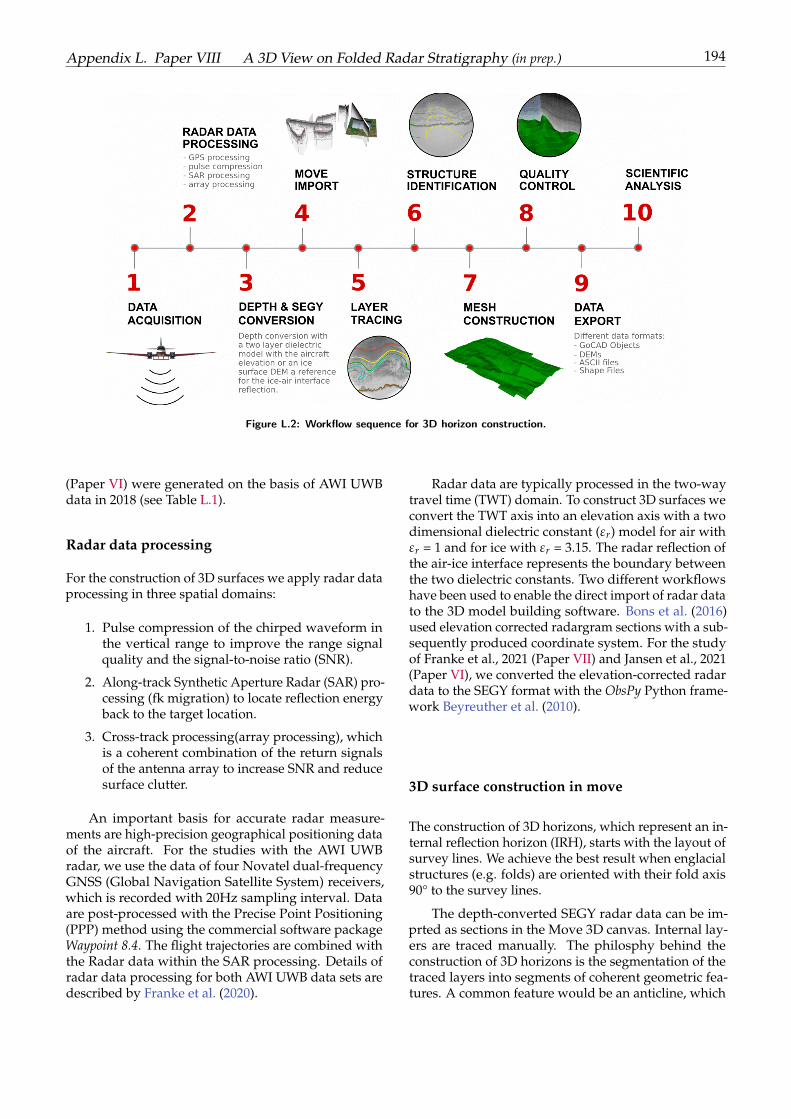
Appendix L. Paper VIII A 3D View on Folded Radar Stratigraphy (in prep.) 194

Figure L.2: Workflow sequence for 3D horizon construction.

(Paper VI) were generated on the basis of AWI UWBdata in 2018 (see Table L.1).

Radar data processing

For the construction of 3D surfaces we apply radar dataprocessing in three spatial domains:

1. Pulse compression of the chirped waveform inthe vertical range to improve the range signalquality and the signal-to-noise ratio (SNR).

2. Along-track Synthetic Aperture Radar (SAR) pro-cessing (fk migration) to locate reflection energyback to the target location.

3. Cross-track processing(array processing), whichis a coherent combination of the return signalsof the antenna array to increase SNR and reducesurface clutter.

An important basis for accurate radar measure-ments are high-precision geographical positioning dataof the aircraft. For the studies with the AWI UWBradar, we use the data of four Novatel dual-frequencyGNSS (Global Navigation Satellite System) receivers,which is recorded with 20Hz sampling interval. Dataare post-processed with the Precise Point Positioning(PPP) method using the commercial software packageWaypoint 8.4. The flight trajectories are combined withthe Radar data within the SAR processing. Details ofradar data processing for both AWI UWB data sets aredescribed by Franke et al. (2020).

Radar data are typically processed in the two-waytravel time (TWT) domain. To construct 3D surfaces weconvert the TWT axis into an elevation axis with a twodimensional dielectric constant (εr) model for air withεr = 1 and for ice with εr = 3.15. The radar reflection ofthe air-ice interface represents the boundary betweenthe two dielectric constants. Two different workflowshave been used to enable the direct import of radar datato the 3D model building software. Bons et al. (2016)used elevation corrected radargram sections with a sub-sequently produced coordinate system. For the studyof Franke et al., 2021 (Paper VII) and Jansen et al., 2021(Paper VI), we converted the elevation-corrected radardata to the SEGY format with the ObsPy Python frame-work Beyreuther et al. (2010).

3D surface construction in move

The construction of 3D horizons, which represent an in-ternal reflection horizon (IRH), starts with the layout ofsurvey lines. We achieve the best result when englacialstructures (e.g. folds) are oriented with their fold axis90° to the survey lines.

The depth-converted SEGY radar data can be im-prted as sections in the Move 3D canvas. Internal lay-ers are traced manually. The philosphy behind theconstruction of 3D horizons is the segmentation of thetraced layers into segments of coherent geometric fea-tures. A common feature would be an anticline, which

Appendix L. Paper VIII A 3D View on Folded Radar Stratigraphy (in prep.) 195

is visible in several adjacent radargrams. These seg-ments can then be combined to form a coherent struc-ture, such as the anticline of a fold. An apropriate wayto check if the geometry of the interpolarted is correct,it is possible to compare the 3D horizon with a radarprofile which is oriented perpendicular to the actualradar sections.

Data records

Peterman Glacier

Four 3D horizons are provided for the onset region ofthe PG. Horizon P1 is 11.7 ka old and represents thetransition from the glacial to the holocene and is located~ 1 km below the ice surface. The horizon is mainlycharacterized by open cylindrical folds with the foldaxis oriented parallel to ice flow. Horizons P2 and P3are located deeper and show asymetric and overturnedfolds with respective ages of 37.5 ka and 87.0 ka. Hori-zon P4 represents strongly disturbed ice stratigraphyof the basal unit.

Northern Greenland

The data set in Northern Greenland represents two foldunits, which are located close to the ice divide andare oriented towards the main glacier outlet system inNortheast Greenland. Three 3D horizons (F1, F2 and F3;labelled from young to old) were constructed to outlinethe geometry and extension of the folds as well as todisplay the deformation of stratigraphic horizons withincreasing depth. The horizons have a respective ageof 45.5 ka, 52.2 ka as well as 60 ka and extend 85 km inthe direction parallel to the fold axis and 50 – 60 km in90° to the fold axis. Horizon F3 is smaller than the twoyounger horizons because the radar horizon could notbe traced in all radargrams.

NEGIS onset

The data set at the onset of the NEGIS comprises two 3Dhorizons extending ~250 km in the direction of ice flowand between 30 – 70 km and ZZ km across ice flow. Thetwo horizons have a respective age of 7.3 ka and 12.8ka and are labelled N1 (for the younger horizon) andN2 (for the older horizon). The main characteristic ofthese horizons is the representation of the deformationstructure at the shear margins.

Technical validationThe 3D horizons of the three data sets were createdon the basis of parallel radar profiles between whichthe individual structures were linearly interpolated. In

addition, the radar profiles are oriented perpendicu-lar to the fold axis, as this produces the best results.In order to check whether the interpolated geometriesare as consistent as possible, they are compared withobliquely oriented radar profiles, if these are available.This was performed for all three data sets and no signif-icant deviations of the 3D geometries were found. Nosignificant deviations of the 3D geometries were found.

Data formats and usage notes3D horizons are provided in different data formats (seeTable L.3). Some of the data formats can be used withstandard and open source software (e.g. GeoTIFFs orASCII xyz files) but others require specialised and oftenalso commercial software (e.g. GoCAD Objects or CADformat). In the following, we discuss the possible ap-plications, advantages, and disadvantages of the dataformats:

1. GoCAD (Geological Objects) is a common fileformat for (mostly) commercial geological mod-eling software. The 3D horizons can be exportedand imported directly in the TSURF (.ts) format,which stores the shape as well as meta-data ofthe horizon. A great advantage of many com-mercial geology software with a 3D canvas is thesimultaneous use and display of different dataformats like radar sections, geo-coded raster files,shapefiles as well as well-data. Another advan-tage to pure 3D software is the incorporation of3D structures and the georeferenced canvas. Forthe data presented in this paper, we provide the3D horizons in the TSURF format and as a pointset, where the surface is represented by a pointcloud with xyz coordinates in EPSG:3413. Fur-thermore, the single radar layers, which are thebasis for the 3D reconstruction are provided asxyz data.

2. CAD (Computer Aided Design) files in theDrawing Exchange Format (.dxf). CAD surfaceobjects preserve the 3D nature of the horizonspresented here as triangulated objects and can behandled by several commercial and open-sourceCAD software. One disadvantage in compari-son to the GoCAD format is that geographicalinformation is lost and that the file size is larger.

3. Digital Elevation Models (DEMs) are providedin the GeoTIFF and .nc format in the EPSG:3413coordinate system. DEMs are not exported di-rectly but interpolated from the xyz point datawith a cell size of 100m. Because it is not possi-ble to represent overturning structures (such asin Figure L.3 e), we only provide DEMs for 3D

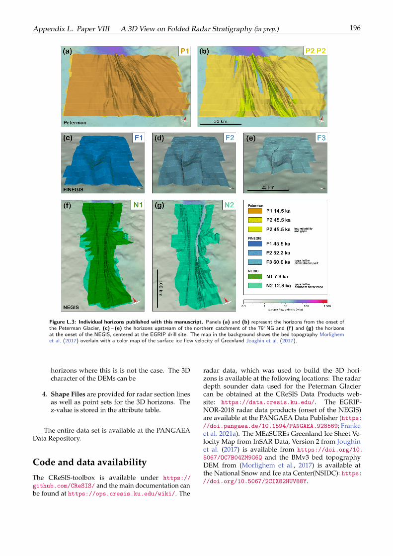
Appendix L. Paper VIII A 3D View on Folded Radar Stratigraphy (in prep.) 196

Figure L.3: Individual horizons published with this manuscript. Panels (a) and (b) represent the horizons from the onset ofthe Peterman Glacier, (c) – (e) the horizons upstream of the northern catchment of the 79° NG and (f) and (g) the horizonsat the onset of the NEGIS, centered at the EGRIP drill site. The map in the background shows the bed topography Morlighemet al. (2017) overlain with a color map of the surface ice flow velocity of Greenland Joughin et al. (2017).

horizons where this is is not the case. The 3Dcharacter of the DEMs can be

4. Shape Files are provided for radar section linesas well as point sets for the 3D horizons. Thez-value is stored in the attribute table.

The entire data set is available at the PANGAEAData Repository.

Code and data availabilityThe CReSIS-toolbox is available under https://github.com/CReSIS/ and the main documentation canbe found at https://ops.cresis.ku.edu/wiki/. The

radar data, which was used to build the 3D hori-zons is available at the following locations: The radardepth sounder data used for the Peterman Glaciercan be obtained at the CReSIS Data Products web-site: https://data.cresis.ku.edu/. The EGRIP-NOR-2018 radar data products (onset of the NEGIS)are available at the PANGAEA Data Publisher (https://doi.pangaea.de/10.1594/PANGAEA.928569; Frankeet al. 2021a). The MEaSUREs Greenland Ice Sheet Ve-locity Map from InSAR Data, Version 2 from Joughinet al. (2017) is available from https://doi.org/10.5067/OC7B04ZM9G6Q and the BMv3 bed topographyDEM from (Morlighem et al., 2017) is available atthe National Snow and Ice ata Center(NSIDC): https://doi.org/10.5067/2CIX82HUV88Y.

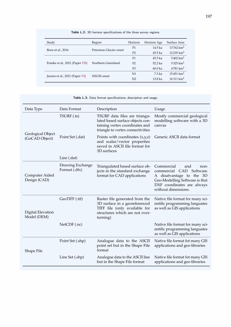
197

Table L.2: 3D horizon specifications of the three survey regions.

Study Region Horizon Horizon Age Surface Area

Bons et al., 2016 Peterman Glacier onsetP1 14.5 ka 13 762 km2

P2 45.5 ka 12 235 km2

Franke et al., 2021 (Paper VII) Northern Greenland

F1 45.5 ka 5 402 km2

F2 52.2 ka 5 325 km2

F3 60.0 ka 4 781 km2

Jansen et al., 2021 (Paper VI) NEGIS onsetN1 7.3 ka 15 451 km2

N2 12.8 ka 16 311 km2

Table L.3: Data format specifications, description and usage.

Data Type Data Format Description Usage

Geological Object(GoCAD Object)

TSURF (.ts) TSURF data files are triangu-lated based surface objects con-taining vertex coordinates andtriangle to vertex connectivities

Mostly commercial geologicalmodelling software with a 3Dcanvas

Point Set (.dat) Points with coordinates (x,y,z)and scalar/vector propertiessaved in ASCII file format for3D surfaces

Generic ASCII data format

Line (.dat)

Computer AidedDesign (CAD)

Drawing ExchangeFormat (.dfx)

Triangulated based surface ob-jects in the standard exchangeformat for CAD applications

Commercial and non-commercial CAD Software.A disatvantage to the 3DGeo-Modelling Software is thatDXF coordinates are alwayswithout dimensions.

Digital ElevationModel (DEM)

GeoTIFF (.tif) Raster file generated from the3D surface in a georeferencedTIFF file (only available forstructures which are not over-turning)

Native file format for many sci-entific programming languatesas well as GIS applications

NetCDF (.nc) Native file format for many sci-entific programming languatesas well as GIS applications

Shape File

Point Set (.shp) Analogue data to the ASCIIpoint set but in the Shape Fileformat

Native file format fot many GISapplications and geo-libraries

Line Set (.shp) Analogue data to the ASCII linebut in the Shape File format

Native file format fot many GISapplications and geo-libraries

BIBLIOGRAPHY 198

BibliographyAllison, I., Alley, R., Fricker, H., Thomas, R., and Warner, R.

Ice sheet mass balance and sea level. Antarctic Science, 21(5):413–426, 2009. doi: 10.1017/S0954102009990137. URLhttps://doi.org/10.1017/S0954102009990137.

Aschwanden, A., Fahnestock, M. A., and Truffer, M. ComplexGreenland outlet glacier flow captured. Nature Communi-cations, 7(1), feb 2016. doi: 10.1038/ncomms10524. URLhttps://doi.org/10.1038%2Fncomms10524.

Bennett, M. R. Ice streams as the arteries of an icesheet: their mechanics, stability and significance.Earth-Science Reviews, 61(3):309–339, 2003. ISSN 0012-8252. doi: 10.1016/S0012-8252(02)00130-7. URLhttps://www.sciencedirect.com/science/article/pii/S0012825202001307.

Beyreuther, M., Barsch, R., Krischer, L., Megies, T., Behr, Y.,and Wassermann, J. ObsPy: A Python Toolbox for Seis-mology. Seismological Research Letters, 81(3):530–533, may2010. doi: 10.1785/gssrl.81.3.530. URL https://doi.org/10.1785%2Fgssrl.81.3.530.

Bons, P. D., Jansen, D., Mundel, F., Bauer, C. C., Binder, T.,Eisen, O., Jessell, M. W., Llorens, M.-G., Steinbach, F., Stein-hage, D., and Weikusat, I. Converging flow and anisotropycause large-scale folding in Greenland's ice sheet. NatureCommunications, 7(1), apr 2016. doi: 10.1038/ncomms11427.URL https://doi.org/10.1038%2Fncomms11427.

Cavitte, M. G. P., Blankenship, D. D., Young, D. A., Schroeder,D. M., Parrenin, F., Lemeur, E., MacGregor, J. A., andSiegert, M. J. Deep radiostratigraphy of the east antarc-tic plateau: connecting the dome c and vostok ice coresites. Journal of Glaciology, 62(232):323–334, 2016. doi:10.1017/jog.2016.11. URL https://doi.org/10.1017/jog.2016.11.

Christianson, K., Peters, L. E., Alley, R. B., Anandakrishnan,S., Jacobel, R. W., Riverman, K. L., Muto, A., and Keis-ling, B. A. Dilatant till facilitates ice-stream flow in north-east Greenland. Earth and Planetary Science Letters, 401:57–69, sep 2014. doi: 10.1016/j.epsl.2014.05.060. URLhttps://doi.org/10.1016%2Fj.epsl.2014.05.060.

Chu, W., Schroeder, D. M., Seroussi, H., Creyts, T. T., andBell, R. E. Complex Basal Thermal Transition Near theOnset of Petermann Glacier Greenland. Journal of Geophysi-cal Research: Earth Surface, 123(5):985–995, may 2018. doi:10.1029/2017jf004561. URL https://doi.org/10.1029%2F2017jf004561.

Church, J. A. and White, N. J. A 20th century accelerationin global sea-level rise. Geophysical Research Letters, 33(1), 2006. doi: https://doi.org/10.1029/2005GL024826.URL https://agupubs.onlinelibrary.wiley.com/doi/abs/10.1029/2005GL024826.

Conway, H., Catania, G., Raymond, C. F., Gades, A. M., Scam-bos, T. A., and Engelhardt, H. Switch of flow directionin an Antarctic ice stream. Nature, 419(6906):465–467, oct2002. ISSN 0028-0836. doi: 10.1038/nature01081. URLhttp://www.nature.com/articles/nature01081.

Dow, C. F., Werder, M. A., Babonis, G., Nowicki, S.,Walker, R. T., Csatho, B., and Morlighem, M. Dynam-ics of Active Subglacial Lakes in Recovery Ice Stream.Journal of Geophysical Research: Earth Surface, 123(4):837–850, 2018. doi: https://doi.org/10.1002/2017JF004409.URL https://agupubs.onlinelibrary.wiley.com/doi/abs/10.1002/2017JF004409.

Fahnestock, M. High Geothermal Heat Flow Basal Melt,and the Origin of Rapid Ice Flow in Central Green-land. Science, 294(5550):2338–2342, dec 2001. doi: 10.1126/science.1065370. URL https://doi.org/10.1126%2Fscience.1065370.

Franke, S., Jansen, D., Binder, T., Dörr, N., Helm, V., Paden,J., Steinhage, D., and Eisen, O. Bed topography andsubglacial landforms in the onset region of the North-east Greenland Ice Stream. Annals of Glaciology, pages1–11, mar 2020. doi: 10.1017/aog.2020.12. URL https://doi.org/10.1017%2Faog.2020.12.

Franke, S., Binder, T., Jansen, D., Paden, J. D., Dörr, N., Ger-ber, T., Miller, H., Dahl-Jensen, D., Helm, V., Steinhage, D.,Weikusat, I., Wilhelms, F., and Eisen, O. [DATASET] Ultra-wideband radar data over the shear margins and alongflow lines at the onset region of the Northeast GreenlandIce Stream (NEGIS), 2021a. URL https://doi.pangaea.de/10.1594/PANGAEA.928569.

Franke, S., Jansen, D., Beyer, S., Neckel, N., Binder, T., Paden,J., and Eisen, O. Complex basal conditions and their in-fluence on ice flow at the onset of the northeast greenlandice stream. Journal of Geophysical Research: Earth Surface,126(3):e2020JF005689, 2021b. doi: 10.1029/2020JF005689.URL https://agupubs.onlinelibrary.wiley.com/doi/abs/10.1029/2020JF005689.

Gogineni, S., Chuah, T., Allen, C., Jezek, K., and Moore,R. K. An improved coherent radar depth sounder. Jour-nal of Glaciology, 44(148):659–669, 1998. doi: 10.3189/S0022143000002161. URL https://doi.org/10.3189/S0022143000002161.

Gogineni, S., Tammana, D., Braaten, D., Leuschen, C., Akins,T., Legarsky, J., Kanagaratnam, P., Stiles, J., Allen, C., andJezek, K. Coherent radar ice thickness measurementsover the Greenland ice sheet. Journal of Geophysical Re-search: Atmospheres, 106(D24):33761–33772, dec 2001. doi:10.1029/2001jd900183. URL https://doi.org/10.1029%2F2001jd900183.

Hale, R., Miller, H., Gogineni, S., Yan, J. B., Rodriguez-Morales, F., Leuschen, C., Paden, J., Li, J., Binder, T.,Steinhage, D., Gehrmann, M., and Braaten, D. Multi-channel ultra-wideband radar sounder and imager. In2016 IEEE International Geoscience and Remote Sensing Sym-posium (IGARSS). IEEE, jul 2016. doi: 10.1109/igarss.

BIBLIOGRAPHY 199

2016.7729545. URL https://doi.org/10.1109%2Figarss.2016.7729545.

Joughin, I., Smith, B. E., Howat, I. M., Scambos, T., and Moon,T. Greenland flow variability from ice-sheet-wide veloc-ity mapping. Journal of Glaciology, 56(197):415–430, 2010.ISSN 0022-1430. doi: 10.3189/002214310792447734. URLhttp://dx.doi.org/10.3189/002214310792447734.

Joughin, I., Smith, B. E., and Howat, I. M. A completemap of Greenland ice velocity derived from satellite datacollected over 20 years. Journal of Glaciology, 64(243):1–11, nov 2017. doi: 10.1017/jog.2017.73. URL https://doi.org/10.1017%2Fjog.2017.73.

Kjær, K. H., Larsen, N. K., Binder, T., Bjørk, A. A., Eisen, O.,Fahnestock, M. A., Funder, S., Garde, A. A., Haack, H.,Helm, V., Houmark-Nielsen, M., Kjeldsen, K. K., Khan,S. A., Machguth, H., McDonald, I., Morlighem, M., Moug-inot, J., Paden, J. D., Waight, T. E., Weikusat, C., Willerslev,E., and MacGregor, J. A. A large impact crater beneath Hi-awatha Glacier in northwest Greenland. Science Advances, 4(11):eaar8173, nov 2018. doi: 10.1126/sciadv.aar8173. URLhttps://doi.org/10.1126%2Fsciadv.aar8173.

Leysinger Vieli, G. J.-M. C., Martín, C., Hindmarsh, R. C. A.,and Lüthi, M. P. Basal freeze-on generates complex ice-sheet stratigraphy. Nature Communications, 9(1), nov 2018.doi: 10.1038/s41467-018-07083-3. URL https://doi.org/10.1038%2Fs41467-018-07083-3.

MacGregor, J. A., Fahnestock, M. A., Catania, G. A., Paden,J. D., Gogineni, S. P., Young, S. K., Rybarski, S. C., Mabrey,A. N., Wagman, B. M., and Morlighem, M. Radios-tratigraphy and age structure of the Greenland Ice Sheet.Journal of Geophysical Research: Earth Surface, 120(2):212–241, feb 2015. doi: 10.1002/2014jf003215. URL https://doi.org/10.1002%2F2014jf003215.

MacGregor, J. A., Colgan, W. T., Fahnestock, M. A.,Morlighem, M., Catania, G. A., Paden, J. D., and Gogi-neni, S. P. Holocene deceleration of the greenland icesheet. Science, 351(6273):590–593, 2016. ISSN 0036-8075.doi: 10.1126/science.aab1702. URL https://science.sciencemag.org/content/351/6273/590.

Morlighem, M., Rignot, E., Mouginot, J., Seroussi, H., andLarour, E. Deeply incised submarine glacial valleys be-neath the Greenland ice sheet. Nature Geoscience, 7(6):418–422, may 2014. doi: 10.1038/ngeo2167. URL https://doi.org/10.1038%2Fngeo2167.

Morlighem, M., Williams, C. N., Rignot, E., An, L., Arndt,J. E., Bamber, J. L., Catania, G., Chauché, N., Dowdeswell,J. A., Dorschel, B., Fenty, I., Hogan, K., Howat, I., Hubbard,A., Jakobsson, M., Jordan, T. M., Kjeldsen, K. K., Millan,R., Mayer, L., Mouginot, J., Noël, B. P. Y., O'Cofaigh, C.,Palmer, S., Rysgaard, S., Seroussi, H., Siegert, M. J., Slabon,P., Straneo, F., van den Broeke, M. R., Weinrebe, W., Wood,M., and Zinglersen, K. B. BedMachine v3: Complete BedTopography and Ocean Bathymetry Mapping of Green-land From Multibeam Echo Sounding Combined WithMass Conservation. Geophysical Research Letters, 44(21):

11,051–11,061, nov 2017. doi: 10.1002/2017gl074954. URLhttps://doi.org/10.1002%2F2017gl074954.

Münchow, A., Padman, L., and Fricker, H. A. Interannualchanges of the floating ice shelf of Petermann GletscherNorth Greenland, from 2000 to 2012. Journal of Glaciology,60(221):489–499, 2014. doi: 10.3189/2014jog13j135. URLhttps://doi.org/10.3189%2F2014jog13j135.

Panton, C. and Karlsson, N. B. Automated mapping ofnear bed radio-echo layer disruptions in the GreenlandIce Sheet. Earth and Planetary Science Letters, 432:323–331, dec 2015. doi: 10.1016/j.epsl.2015.10.024. URLhttps://doi.org/10.1016%2Fj.epsl.2015.10.024.

Rignot, E. and Steffen, K. Channelized bottom melting andstability of floating ice shelves. Geophysical Research Let-ters, 35(2), jan 2008. doi: 10.1029/2007gl031765. URLhttps://doi.org/10.1029%2F2007gl031765.

Rodriguez-Morales, F., Byers, K., Crowe, R., Player, K., Hale,R. D., Arnold, E. J., Smith, L., Gifford, C. M., Braaten,D., Panton, C., Gogineni, S., Leuschen, C. J., Paden,J. D., Li, J., Lewis, C. C., Panzer, B., Alvestegui, D. G.-G., and Patel, A. Advanced Multifrequency Radar In-strumentation for Polar Research. IEEE Transactions onGeoscience and Remote Sensing, 52(5):2824–2842, may 2014.doi: 10.1109/tgrs.2013.2266415. URL https://doi.org/10.1109%2Ftgrs.2013.2266415.

Shepherd, A., Ivins, E., Rignot, E., Smith, B., van den Broeke,M., Velicogna, I., Whitehouse, P., Briggs, K., Joughin, I.,Krinner, G., Nowicki, S., Payne, T., Scambos, T., Schlegel,N., A, G., Agosta, C., Ahlstrøm, A., Babonis, G., Bar-letta, V. R., Bjørk, A. A., Blazquez, A., Bonin, J., Col-gan, W., Csatho, B., Cullather, R., Engdahl, M. E., Felik-son, D., Fettweis, X., Forsberg, R., Hogg, A. E., Gallee,H., Gardner, A., Gilbert, L., Gourmelen, N., Groh, A.,Gunter, B., Hanna, E., Harig, C., Helm, V., Horvath, A.,Horwath, M., Khan, S., Kjeldsen, K. K., Konrad, H., Lan-gen, P. L., Lecavalier, B., Loomis, B., Luthcke, S., McMil-lan, M., Melini, D., Mernild, S., Mohajerani, Y., Moore,P., Mottram, R., Mouginot, J., Moyano, G., Muir, A., Na-gler, T., Nield, G., Nilsson, J., Noël, B., Otosaka, I., Pat-tle, M. E., Peltier, W. R., Pie, N., Rietbroek, R., Rott, H.,Sandberg Sørensen, L., Sasgen, I., Save, H., Scheuchl, B.,Schrama, E., Schröder, L., Seo, K. W., Simonsen, S. B.,Slater, T., Spada, G., Sutterley, T., Talpe, M., Tarasov, L.,van de Berg, W. J., van der Wal, W., van Wessem, M.,Vishwakarma, B. D., Wiese, D., Wilton, D., Wagner, T.,Wouters, B., and Wuite, J. Mass balance of the GreenlandIce Sheet from 1992 to 2018. Nature, 579(7798):233–239,2020. ISSN 14764687. doi: 10.1038/s41586-019-1855-2.URL https://doi.org/10.1038/s41586-019-1855-2.

Shi, L., Allen, C. T., Ledford, J. R., Rodriguez-Morales, F.,Blake, W. A., Panzer, B. G., Prokopiack, S. C., Leuschen,C. J., and Gogineni, S. Multichannel coherent radar depthsounder for NASA operation ice bridge. International Geo-science and Remote Sensing Symposium (IGARSS), pages1729–1732, 2010. doi: 10.1109/IGARSS.2010.5649518. URLhttp://dx.doi.org/10.1109/IGARSS.2010.5649518.

BIBLIOGRAPHY 200

Winsborrow, M. C., Clark, C. D., and Stokes, C. R.What controls the location of ice streams? Earth-Science Reviews, 103(1):45–59, 2010. ISSN 0012-8252. doi: https://doi.org/10.1016/j.earscirev.2010.07.003. URL https://www.sciencedirect.com/science/article/pii/S0012825210000838.

Wolovick, M. J., Creyts, T. T., Buck, W. R., and Bell, R. E.Traveling slippery patches produce thickness-scale foldsin ice sheets. Geophysical Research Letters, 41(24):8895–8901, dec 2014. doi: 10.1002/2014gl062248. URL https://doi.org/10.1002%2F2014gl062248.