decentralizing centralized matching markets - hal-shs
TRANSCRIPT

HAL Id: halshs-02146792https://halshs.archives-ouvertes.fr/halshs-02146792v2
Preprint submitted on 1 Jul 2021 (v2), last revised 3 May 2022 (v3)
HAL is a multi-disciplinary open accessarchive for the deposit and dissemination of sci-entific research documents, whether they are pub-lished or not. The documents may come fromteaching and research institutions in France orabroad, or from public or private research centers.
L’archive ouverte pluridisciplinaire HAL, estdestinée au dépôt et à la diffusion de documentsscientifiques de niveau recherche, publiés ou non,émanant des établissements d’enseignement et derecherche français ou étrangers, des laboratoirespublics ou privés.
Decentralizing Centralized Matching Markets:Implications from Early Offers in University Admissions
Julien Grenet, Yinghua He, Dorothea Kübler
To cite this version:Julien Grenet, Yinghua He, Dorothea Kübler. Decentralizing Centralized Matching Markets: Impli-cations from Early Offers in University Admissions. 2021. �halshs-02146792v2�

WORKING PAPER N° 2019 – 24
Decentralizing Centralized Matching Markets: Implications from Early Offers in University Admissions
Julien Grenet YingHua He
Dorothea Kübler
JEL Codes: C78, D47, I23, D81, D83. Keywords: Centralized Matching Market, Gale-Shapley Algorithm, Deferred Acceptance Mechanism, University Admissions, Early Offers, Information Acquisition.

Decentralizing Centralized Matching Markets:Implications from Early Offers in University Admissions∗
Julien Grenet YingHua He Dorothea Kübler
June 2021
Abstract
The matching literature often recommends market centralization under the assumptionthat agents know their own preferences and that their preferences are fixed. We findcounterevidence to this assumption in a quasi-experiment. In Germany’s universityadmissions, a clearinghouse implements the early stages of the Gale-Shapley algorithmin real time. We show that early offers made in this decentralized phase, although notmore desirable, are accepted more often than later ones. These results, together withsurvey evidence and a theoretical model, are consistent with students’ costly learningabout universities. We propose a hybrid mechanism to combine the advantages ofdecentralization and centralization.
JEL Codes: C78, D47, I23, D81, D83Keywords: Centralized Matching Market, Gale-Shapley Algorithm, Deferred Accep-tance Mechanism, University Admissions, Early Offers, Information Acquisition
∗First version: May 31, 2019. Grenet: CNRS and Paris School of Economics, 48 boulevard Jour-dan, 75014 Paris, France (e-mail: [email protected]); He: Rice University and Toulouse Schoolof Economics, Department of Economics MS-22, Houston, TX 77251 (e-mail: [email protected]);Kübler: WZB Berlin Social Science Center, Reichpietschufer 50, D-10785 Berlin, Germany (e-mail:[email protected]) and Technical University Berlin. For constructive comments, we thank InácioBó, Caterina Calsamiglia, Estelle Cantillon, Laura Doval, Tobias Gamp, Rustamdjan Hakimov, Thilo Klein,as well as seminar and conference participants at CREST/Polytechnique, Econometric Society/BocconiUniversity Virtual World Congress 2020, Matching in Practice (2017 Brussels), Gothenburg, Stanford, andZEW Mannheim. Jennifer Rontganger provided excellent copy editing service. The authors are gratefulto the Stiftung für Hochschulzulassung, in particular Matthias Bode, for invaluable assistance. Financialsupport from the National Science Foundation through grant no. SES-1730636, the French National ResearchAgency (Agence Nationale de la Recherche) through project ANR-14-FRAL-0005 FDA and EUR grantANR-17-EURE-0001, and the German Research Foundation (Deutsche Forschungsgemeinschaft) throughprojects KU 1971/3-1 and CRC TRR 190 is gratefully acknowledged.
1

Introduction
Research on the design of matching markets has been a success story, not least because it
has resulted in improved designs for school choice, university admissions, and entry-level
labor markets (Roth and Peranson, 1999; Abdulkadiroğlu et al., 2009; Pathak, 2011).
Centralization has been a common contributor to this success (see, e.g., Roth, 1990). In a
standard centralized market, each agent is required to inform a clearinghouse of how she
ranks her potential matching partners. Then, a matching algorithm uses the rank-order
lists to generate at most one match offer for every agent.1
This trend toward centralization is often guided by market design research, and aims
at improving efficiency, e.g., by reducing congestion and the unraveling of markets. In
this paper, we focus on one important distinction between centralized and decentralized
markets: A centralized market allows an agent to hold at most one offer, while holding
multiple offers is possible in a decentralized market. As a centralized market forms the
benchmark of our analysis, we assume that a decentralized market also has a clearinghouse
to facilitate the interactions between agents.
When studying centralized designs for a market, the literature commonly assumes
that an agent knows her own preferences upon participation and has fixed preferences
throughout the matching process (e.g., Roth and Sotomayor, 1990; Abdulkadiroğlu and
Sönmez, 2003). This known-and-fixed-preference assumption implies that the market
design itself, such as the degree of decentralization or centralization, has no effect on agent
preferences.2
The first contribution of our study is to provide unambiguous empirical evidence
against the known-and-fixed-preference assumption. In an administrative data set on
university admissions in Germany, we identify a quasi-experiment in which the arrival
time of admission offers is exogenous to student preferences. We show that a student is
more likely to accept an early offer relative to later offers, despite the fact that an offer
cannot be rescinded.1In many-to-one matching such as school choice and college admissions, an agent who can accept
multiple matching partners, such as a school or a college, will receive multiple match offers. However, anagent on the other side, who can accept at most one match partner, will obtain at most one offer.
2An exception are models with externalities such as peer effects. For example, in Calsamiglia et al.(2021), student preferences over schools depend on the composition of the post-match student body.Market design can influence who goes to which school and thereby affect student preferences.
2

This finding, which cannot be reconciled with the known-and-fixed-preference assump-
tion, is instead consistent with students’ learning about university qualities at a cost. This
interpretation, which is corroborated by evidence from a survey of students, is plausible
in reality. To be able to form preferences over universities, a student must consider many
aspects of every university, including academic quality, courses offered, and quality of life.
Moreover, as more and more market segments are integrated in a centralized design,3 the
number of potential matching partners can be overwhelming. Therefore, when agents
enter a market, they may not know their preferences over all options, and market design
can influence the agents’ learning decisions.
Our second contribution is to propose a novel solution, the Hybrid mechanism, that
integrates elements of decentralization into a centralized market to facilitate agents’
learning. Specifically, in a decentralized phase of the Hybrid mechanism, an agent can
hold multiple offers, thereby know for sure the availability of these matches, and thus
learn more efficiently. The advantages of this new mechanism are shown in a theoretical
model and in simulations based on the German data set.
Our empirical investigation takes advantage of a unique centralized matching pro-
cedure with features of a decentralized market. It is called DoSV, Dialogorientiertes
Serviceverfahren (literally, “dialogue-oriented service procedure”), and is used for ad-
missions to over-demanded university programs in Germany. The procedure is based
on the program-proposing Gale-Shapley (GS) algorithm, but differs from the standard
implementation in that students can defer their commitment to rank-order lists (ROLs)
of programs. Specifically, the DoSV “decentralizes” the first stages of the GS algorithm.
For a decentralized phase of 34 days, students and programs interact as if in a decentral-
ized market although all offers and acceptances are communicated via a clearinghouse.
Programs make admission offers to their preferred students in real time; offers cannot be
rescinded; and students can decide to accept an offer and exit the procedure, to retain all
offers, or to keep only a subset of their offers, also in real time.
At the end of the decentralized phase, students who have not yet accepted an offer are
required to finalize their ROLs and to participate in the GS algorithm. In this centralized
phase, the computerized GS algorithm is run for the remaining students and seats.4 For a3For instance, charter school and traditional public school admissions are unified in a single-offer
centralized design in Denver (Abdulkadiroğlu et al., 2017) and New Orleans (Abdulkadiroğlu et al., 2020).4The sequential filling of seats is also a feature of the previous system for medical programs in Germany
(Westkamp, 2013; Braun et al., 2010, 2014). There, quotas are filled one after the other, each quota with
3

student with offers from the decentralized phase, the highest-ranked offer in her final ROL
is kept and will not be taken away from her unless she receives an offer from a program
that is ranked higher in her final ROL.
We analyze a comprehensive administrative data set that contains every event during
the admission process as well as its exact timing. We define a program as being feasible to
a student if the student has applied to the program and would receive its admission offer
if she does not exit the procedure early. There are 21, 711 students in our data set who
have at least two feasible programs and have accepted one of them. We find that, relative
to offers arriving in the centralized phase, an offer that arrives during the decentralized
phase—which we define as an early offer—is more likely to be accepted.
The early-offer effect is sizable when we calculate its impact on offer acceptance. In
our sample, the average probability of a feasible program being accepted is 0.385. An early
offer that is not the first one raises the acceptance probability by 8.7 percentage points—a
27.9 percent increase. More significantly, the first early offer increases the acceptance
probability by 11.8 percentage points—a 38.3 percent jump.5
We rule out a range of possible explanations of the early-offer effect through additional
data analyses. The effect is unlikely to be driven by students’ preferences for being ranked
high by a program, their intuitive reaction, pessimism about future offers, need of a head
start in housing search, or dislike of being assigned by a computerized algorithm.
Our preferred explanation is that the early-offer effect is driven by students’ learning
about university and program qualities. From a student survey, we find direct evidence
that, at the start of the procedure, many students have not yet formed preferences over
the programs. Further, they tend to invest more time learning about universities that have
made them an early offer, and early offers influence their perceptions of the programs.
To formalize the above evidence, we develop a model of university admissions with
learning. A student can learn her valuation of a university only after paying a cost. She
applies to two universities and has access to an outside option of a known value. In
expectation, each university makes her an offer with some probability, which determines
its own ROLs and matching algorithm (Boston or GS). In contrast, the DoSV is based on one algorithm(GS) for all seats but its early stages resemble a decentralized market.
5Another way to gauge the magnitude of the effect is to use distance from a student’s home to theuniversity where the program is located as a “numeraire.” At the sample mean of 126 kilometers, an earlyoffer amounts to reducing the distance to the corresponding program by 61 kilometers. The first earlyoffer has an even larger effect, equivalent to a reduction of 79 kilometers.
4

the student’s endogenous learning decision. An early offer from a university, which leads
the student to update the corresponding offer probability to one, increases her incentive to
learn about this university. Finally, learning about a university increases the probability
that its offer is accepted, leading to the early-offer effect.
These results provide novel insights for market design, especially the benefits of
incorporating features of decentralization into a centralized market. Generalizing the model
with learning, we evaluate three mechanisms: (i) the Deferred-Acceptance mechanism
(DA), which is the most common single-offer, centralized design wherein students finalize
their ROLs before receiving any offer, (ii) the DoSV mechanism, and (iii) our proposed
Hybrid mechanism that is similar to the DoSV but with early offers arriving on a pre-
determined day. The model shows that the Hybrid dominates the other two mechanisms
in terms of student welfare. The reason is that, by informing her of the availability of
certain universities, early offers help the student better target her learning. Moreover, we
find that the student can do worse under the DoSV than under the DA, because an early
offer from an ex-ante low quality university may still sub-optimally increase its acceptance
probability.
The comparison of the three mechanisms is further quantified in a set of simulations
that use the same German data set. Relative to the DA, the Hybrid mechanism makes
72.2 percent of the students better off, and only 20.8 percent of them worse off. Further,
the Hybrid also improves upon the DoSV by making 41.7 percent of the students better
off and 37.1 percent worse off.
Other related literature. Violations of the assumption of known-and-fixed preferences
have received little attention in the market-design literature. As an exception, Narita
(2018) finds that students reveal contradictory preferences in the main round and the
subsequent round of school choice in New York City. Unlike our model, he considers
preference changes that are exogenous to the matching mechanism. Moreover, in the
admissions to German medicine programs, Dwenger et al. (2018) document results implying
a more complex process of preference formation than is commonly assumed.
Costly acquisition of information about preferences is a recent topic in the matching
literature. For example, Chen and He (2018a,b) investigate theoretically and experimen-
tally students’ incentives to acquire information about their own and others’ preferences
in school choice. They study the canonical DA and the Boston Immediate-Acceptance
5

mechanisms. Similar to our work, Immorlica et al. (2020) investigate how advising students
on their admission chances can facilitate information acquisition, although the authors
consider centralized mechanisms such as iterative implementations of the DA and the
provision of historic information.
Sequential learning in our model is related to the theoretical literature on consumer
search (Weitzman, 1979; Ke et al., 2016; Doval, 2018; Dzyabura and Hauser, 2019; Ke and
Villas-Boas, 2019). Unlike in our setting, agents in that literature hold “offers” from all
programs at the outset. The early-offer effect that we document resembles the increased
demand for the item that is made salient in the model by Gossner et al. (forthcoming),
although an early offer in our model changes an agent’s behavior by informing her that
the corresponding program is available.
Our study complements the recent literature on dynamic implementations of single-
offer, centralized procedures. Under the known-and-fixed-preference assumption, a series
of papers, some of them inspired by college admission procedures in practice (Gong and
Liang, 2017; Bó and Hakimov, 2018), investigate dynamic, or iterative, versions of the
DA mechanism (Echenique et al., 2016; Klijn et al., 2019; Bó and Hakimov, 2020).6
Our paper is also related to the literature on mechanism design with transferable utility
where, in an initial stage, agents acquire information (e.g., Bergemann and Välimäki,
2002), make investments (e.g., Hatfield et al., 2014; Nöldeke and Samuelson, 2015), or face
a surplus sharing rule (e.g., Dizdar and Moldovanu, 2016). The sequential information
updates due to early offers in our setup resemble those in open versus closed auctions (see,
e.g., Compte and Jehiel, 2007).
Preference formation has been studied outside the market design literature. For
example, Elster (1983) considers agents adjusting their preferences according to what is
available to them, for which Alladi (2018) provides experimental evidence.
There is a large empirical literature on the determinants of college choice (see, e.g.,
Manski and Wise, 1983, for an early contribution), which investigates the determinants of
preferences rather than the process of preference formation. Early admission offers play
an important role in college admissions in the U.S. (Avery et al., 2003; Avery and Levin,6One of the main findings in this literature is that agents are more likely to report their true preferences
under a dynamic DA than under a static one. There is a growing literature showing that under thestatic DA, many agents do not report their true preferences in the laboratory (Chen and Sönmez, 2006;Rees-Jones and Skowronek, 2018; for a survey, see Hakimov and Kübler, 2019) and in the field (Artemovet al., 2017; Shorrer and Sóvágó, 2017; Hassidim et al., 2021).
6

2010). Colleges want to admit students who are enthusiastic about attending, and early
admission systems give students an opportunity to signal this enthusiasm.
Organization of the paper. After introducing the institutional background of Ger-
many’s university admissions in Section 1, we proceed to the data analysis and present
the results as well as robustness checks in Section 2. To explain the findings, Section 3
discusses several hypotheses and shows evidence from a survey. Section 4 develops a
model of university admissions with learning that can explain the observed early-offer
effect. We present the Hybrid mechanism and use the model as well as simulations to
compare the DA, DoSV, and the Hybrid mechanisms. Finally, Section 5 concludes.
1 Institutional Background
1.1 University Admissions in Germany
Access to higher education in Germany is based on the principle that every student who
completes the school track leading to the university entrance qualification (Abitur) should
be given the opportunity to study at a university in the program of her choice. However,
starting in the 1960s, a steep increase in the number of applicants created an overdemand
for seats in programs such as medicine, and selection based on the final grade in the Abitur
(Numerus clausus) was introduced. In response to court cases brought forward against the
universities, a central clearinghouse, the Zentralstelle für die Vergabe von Studienplätzen
(ZVS), was established in 1972 to guarantee “orderly procedures.”
In the 1990s and early 2000s, the number of programs administered through the ZVS
clearinghouse steadily declined. The main reasons were that universities wanted to gain
control of their admission process, and new bachelor and master’s programs were created
as part of the Bologna reforms that did not fit into the broad categories of programs that
the clearinghouse used for its central allocation mechanism. By 2005, the only programs
administered by the ZVS were medicine, pharmacy, dental medicine, veterinary medicine,
and psychology (the latter only until 2010–11). Seats for these programs are allocated
according to a procedure involving quotas that is regulated by law.7 At the same time,
severe congestion for many other programs appeared.7For analyses of the ZVS procedure, see Braun et al. (2010), Westkamp (2013), and Braun et al.
(2014).
7

A re-organization and re-naming of the clearinghouse from ZVS to Stiftung für Hoch-
schulzulassung (literally, Foundation for University Admission) was completed in 2008,
and the DoSV, a new admission procedure for programs other than medicine and medicine-
related subjects, was implemented in 2012. Universities have the option to participate in
the DoSV, and they can do so for a subset of their programs. Since 2012, the number of
programs participating in this procedure has increased steadily.8
1.2 The DoSV Procedure: Integrating Decentralization and
Centralization
The DoSV procedure has multiple phases. The early phases extend over several weeks and
allow for student-university interactions that resemble those in a decentralized market.
Each student applies to up to 12 programs and forms a rank-order list (ROL), without
the possibility of later adding other programs to this list. Importantly, a student is not
required to finalize her ROL until a later date by which she may have received some offers
from the programs to which she applied. With the finalized ROLs, the program-proposing
Gale-Shapley algorithm (Gale and Shapley, 1962; Roth, 1982) is run to determine the
matching. This procedure provides us with a unique data set of offers to students, their
re-ranking of programs, and offer acceptances and rejections in real time. It allows us to
measure the effects of early offers on the final admission outcome.
Figure 1 describes the timeline of the DoSV. The dates indicated are relevant for
the winter term and are the same every year. We use data from the winter term, since
admission for the summer term is only possible for a small number of programs.
Preparation Phase (March 15–April 14): The participating university programs register
with the clearinghouse.
Application Phase (April 15–July 15): Students apply to at most 12 programs by
directly submitting their application to the universities. The universities transmit to
the clearinghouse the applications they have received for their programs. A student’s
initial ROL of programs is based on the time her applications arrive at the clearinghouse,8For the winter term of 2015–16, 89 universities with 465 programs participated, compared to
17 universities with 22 programs in the first year in which the DoSV was implemented (winter term of2012–13). The total number of students who were assigned to a program through the DoSV in 2015–16was 80,905, relative to a total of 432,000 students who started university in Germany that year.
8

ApplicationPhase
(92 days)
Coordination Phase 1(31 days)
DecisionPhase(3 days)
Coordination Phase 2(11 days)
Clearing Procedures1 & 2
(37 days)
PreparationPhase
(31 days)
Phase 1(early offers)
Phase 2(GS)
March 15 April 15 July 16 August 16 August 19 August 30 October 5
Final ROL
InitialROL
Figure 1 – Timeline of the DoSV Procedure (Winter Term)Notes: This figure shows the different phases of the DoSV procedure. Our main interest is in Phase 1, consisting ofCoordination Phase 1 and the Decision Phase, where early offers are made, and in Phase 2, consisting of CoordinationPhase 2, where the GS algorithm is run.
although she may actively change it at any time during this phase. No new applications
can be submitted after this phase and no program will consider a student who did not
apply to it.
Coordination Phase 1 (July 16–August 15): For each program, the university admission
office creates rankings over its applicants, one for each quota, following a set of pre-specified
criteria for that quota (Abitur grade, waiting time since high school graduation, etc.)
and transmits them to the clearinghouse. Every applicant is considered and ranked for
every quota.9 Universities cannot manipulate their rankings of applicants although they
may have some scope as to when the lists are transmitted.10 Via automated emails, the
clearinghouse sends admission offers for a program to the top students on its ranking
up to the program’s capacity. We define these offers as early offers. Note that an early
offer cannot be rescinded and does not expire before August 29 (the end of Coordination
Phase 2). A student with one or more offers may accept one of them and leave the
procedure, or she can choose to hold on to these offers (either all of them or a subset).
If an offer is rejected, a new offer to the next applicant in that program’s ranking is
automatically generated. Students are informed about how a program ranks them in each
quota, the total number of seats available in the program, and the number of students
ranked above them in each quota who are no longer competing for a seat.
Decision Phase (August 16–18): Starting on August 16, universities can no longer submit
their rankings of applicants to the clearinghouse. However, early offers continue to be9For this reason, we sometimes consider a student’s most favorable quota at a program under which
she has the highest probability of receiving an offer. A student cannot receive two offers from a programeven if they are from different quotas.
10Details on the process through which universities rank applicants and the role of quotas are providedin Appendix A.1.
9

generated until August 18 because students may still reject offers received in Coordination
Phase 1. Students are informed that they are entering the last days of the decentralized
phase and are encouraged to finalize their ROL.
Coordination Phase 2 (August 19–29): At the beginning of this phase, a program may
have (a) seats taken by students who have accepted its early offer and left the procedure,
(b) seats/offers tentatively held by students who have kept their early offer from this
program but have chosen to stay on, and (c) seats available because of its rejected early
offers. Meanwhile, a student may have (i) left the procedure by accepting an early offer,
(ii) kept an early offer and chosen to stay on with her final ROL, (iii) received no offer
and stayed on with her final ROL, or (iv) exited the procedure, thereby rejecting all
offers. Taking the remaining students and the seats available or tentatively held, the
clearinghouse runs a program-proposing GS algorithm as follows:
(A) Following the ranking of its applicants provided in Coordination Phase 1, a program
sends admission offers to students ranked at the top of its ranking up to the number
of available seats that are not tentatively held. However, the students who previously
received an offer from the program can never receive the same offer again.
(B) Students with multiple offers keep the the highest-ranked one according to their
final ROLs and reject all other offers. All other students are inactive.
(C) Steps (A) and (B) are repeated until every program either has no seats left or has
no more students to make offers to. Then, each student is assigned to the program
she holds, if any.
This phase uses the program-proposing GS algorithm where students start out with
their highest-ranked offer from previous phases. They can never do worse than this offer,
while a better offer may arrive. Also, note that we define the GS algorithm as a computer
code that uses information on students and programs to calculate a matching outcome.
Importantly, the GS algorithm is silent about how students and programs provide such
information. See Appendix B.1 for more details and the definition of the GS algorithm.
Clearing Phases 1 and 2 (August 30–September 4; September 30–October 5): A
random serial dictatorship is run to allocate the remaining seats to students who have not
yet been admitted.
10

For the analysis of students’ choices, we focus on Coordination Phase 1 and the
Decision Phase. Since the two phases do not differ from the students’ perspective, we
group them together and call them Phase 1 (see Figure 1). Coordination Phase 2 is also
of interest, and we call it Phase 2. Recall that offers in Phase 1 are early offers. We define
as the initial ROL the ROL over programs that the clearinghouse has recorded for each
student at the beginning of Phase 1, while the one at the end of Phase 1 is defined as the
final ROL. A program is defined as feasible for a student if the student applied to the
program and was ranked higher than the lowest-ranked student who received an offer from
the program in Coordination Phase 2.11 A student may not actually receive an offer from
a feasible program, as she might have left the procedure before she could receive the offer.
In contrast to centralized markets that typically deliver at most one offer to a student,
a student may hold multiple offers in Phase 1 of the DoSV. Because of this feature, we
call it the decentralized phase although, just as Phase 2, it is administered centrally by
the clearinghouse.
1.3 Data
Our data set covers the DoSV procedure for the winter term of 2015–16. There are
183,088 students who applied to 465 programs at 89 universities in total. The data
contain students’ socio-demographic information (gender, age, postal code) and their
Abitur grade.12 Further, we observe students’ ROLs at any point in time, programs’
rankings of applicants, the offers made by the programs throughout the procedure, the
acceptance and rejection of offers by students, and the final admission outcome.
We exclude students with missing socio-demographic information as well as students
who apply to specific programs with complex ranking rules. These are mostly students
who want to become teachers and who have to choose multiple subjects (e.g., math and
English). For our analysis, we focus on the subsample of students who apply to at least
two feasible programs and accept an offer. This leaves us with 21,771 students.11Our definition of feasibility is conditional on a student applying to a program. By contrast, the
definition of feasibility in other papers on school choice and university admissions (e.g., Fack et al., 2019)extends to the programs that a student did not apply to. This alternative is less appropriate in oursetting, because not all programs participate in the clearinghouse and our analysis is conditional on theprograms to which each student has applied.
12In the data, the Abitur grade is missing for about half of the students, but we can infer it forapproximately two thirds of applicants with a missing grade based on how students are ranked under theprograms’ Abitur quota. See Appendix A.1 for details.
11

Table 1 – Summary Statistics of DoSV Application Data for 2015-16 (Winter Term)
Sample
All applicantsto standardprograms
Applied tomore than
one program
Applied to at leasttwo feasibleprograms and
accepted an offer(1) (2) (3)
A. StudentsFemale 0.579 0.596 0.558Age 20.8 20.5 20.7
(3.2) (2.6) (3.1)Abitur percentile rank (between 0 and 1) 0.50 0.51 0.65
(0.29) (0.29) (0.28)B. ApplicationsLength of initial ROL (on July 15) 2.9 4.2 4.7
(2.6) (2.7) (2.9)Re-ranked programs before Phase 1a 0.547 0.226 0.320Re-ranked programs during Phase 1b 0.178 0.305 0.419Fraction of programs located in student’s municipality 0.205 0.153 0.184
(0.379) (0.311) (0.342)Fraction of programs located in student’s region (Land) 0.623 0.610 0.583
(0.446) (0.420) (0.417)Average distance to ranked programs (km)c 111 120 126
(127) (119) (122)Top-ranked program (on July 15): field of studyd
Economics and Business Administration 0.368 0.397 0.427Psychology 0.197 0.204 0.138Social work 0.121 0.110 0.044Law 0.110 0.125 0.170Math/Engineering/Computer science 0.065 0.052 0.097Natural sciences 0.055 0.046 0.059Other 0.085 0.065 0.066
C. Feasible programs and offers receivedAt least one feasible program 0.505 0.581 1.000Received one or more early offers in Phase 1 0.475 0.549 0.989
D. Admission outcomeCanceled application before Phase 2 0.054 0.042 0.000Accepted an early offer in Phase 1 0.220 0.247 0.554
of which: not initially top ranked 0.262 0.399 0.369Participated in Phase 2 0.725 0.711 0.446Accepted an offer in Phase 1 or Phase 2 0.448 0.518 1.000Number of days between offer arrival and acceptancee 9.19 9.62 9.11
(8.73) (8.75) (8.30)
Number of students 110,781 64,876 21,711
Notes: The summary statistics are computed from the DoSV data for the winter term of 2015–16. The main sample(column 1) is restricted to students with non-missing values and who applied to standard programs only, i.e., after excludingstudents who applied to specific “multiple course” programs (Mehrfachstudiengang), which consist of two or more sub-programs with complex assignment rules. Column 2 further restricts the sample to students who applied to two programsor more. Column 3 considers students who applied to at least two feasible programs and who either actively accepted anearly offer during Phase 1 or were assigned to a program through the computerized algorithm in Phase 2. a A student isconsidered as having re-ranked programs before Phase 1 if she only applied to one program or if she manually altered theordering of her applications before July 15, which by default is from the oldest to the most recent program included in herROL. b A student is considered as having re-ranked her choices during Phase 1 if either the final ROL is different fromthe initial ROL or if the student accepted an early offer from a program that she did not initially rank in first position.c The distance between a student’s home and a program is computed as the cartesian distance between the centroid ofthe student’s postcode and the geographic coordinates of the university in which the program is located. d For programscombining multiple fields of study, each field is assigned a weight equal to 1{k, where k is the number of fields. e Thenumber of days elapsed between offer arrival and acceptance is the number of days between the date the offer that wasultimately accepted was made to a student and the date it was accepted; for students who were automatically assigned totheir best offer in Phase 2, the acceptance date is set to the first day of Phase 2, i.e., August 19, 2015.
12

Table 1 provides summary statistics. On average, applicants to standard programs
apply to 2.9 programs (column 1). The corresponding figure is 4.2 among the students
who apply to more than one program (column 2), and 4.7 among those who apply to
at least two feasible programs and accept an offer (column 3). Panel C reveals that
58.1 percent of students who apply to at least two programs (column 2) have at least
one feasible program, that is, they would have received at least one offer in the course of
the procedure if they did not leave the procedure before Phase 2. Importantly for our
analysis, more than half the students who apply to more than one program receive one or
more offers in Phase 1, and around a quarter (24.7 percent) accept an offer in Phase 1
(Panel D). Among them, almost 40 percent accept an offer that was not their first choice
in their initial ROL. Table 1 also indicates that only half of the students end up accepting
an offer from a program in either Phase 1 or Phase 2.13 The rest may have accepted offers
from programs that did not participate in the DoSV procedure.
1.4 Timing of Activities in the DoSV 2015–16
Figure 2 presents an overview of the activities in the DoSV procedure for 2015–16. It
displays the points in time when students register with the clearinghouse, when they
submit an ROL that is not changed any more (“finalize their ROL”), when they receive
their first offers from programs (“receive an offer”), and when they exit the procedure.
An important takeaway is that the first offers received by students are spread out over
Phase 1 (see also Figure C1 in the Appendix). It is exactly this dispersed arrival of offers
that allows us to identify the effect of early offers on offer acceptance. We will show below
that the offer arrival is not correlated with students’ initial ROLs and that early offers are
not, on average, made by more selective or desirable programs. Instead, the time at which
programs submit their rankings to the clearinghouse is determined by administrative
processes within the universities.14
Almost all student exits from the DoSV take place in Phases 1 and 2. During Phase 1,
students leave when they either accept an offer or cancel all applications. The number of13Throughout the analysis, a student is defined as having accepted an offer when she either actively
accepts an early offer in Phase 1 or is assigned by the computerized algorithm in Phase 2.14According the Stiftung für Hochschulzulassung, the time point when the rankings are transmitted to
the clearinghouse depends on the number of personnel available in an admission office, the number ofprograms a university administers through the DoSV, the number of incomplete applications received,internal processes to determine the amount of overbooking for each program, and a university’s policy asto whether to check all applications for completeness or instead to accept applicants conditionally.
13

Application Phase Phase 1 Phase 2
0.0
0.2
0.4
0.6
0.8
1.0
Apr 15 Apr 22 Apr 29 May 6 May 13 May 20 May 27 Jun 3 Jun 10 Jun 17 Jun 24 Jul 1 Jul 8 Jul 15 Jul 22 Jul 29 Aug 5 Aug 12 Aug 19 Aug 26 Sep 2
Date
register with the clearinghousefinalize their ROLreceive an offerexit the procedure
Cumulative fraction of students who
Figure 2 – Activities during the DoSV Procedure (Winter Term of 2015–16)Notes: This figure displays the evolution of several key indicators throughout the DoSV procedure for the winter termof 2015–16: (i) cumulative fraction of students who register with the clearinghouse during each phase (dash-dot line);(ii) cumulative fraction of students who finalize their rank-order list (ROL) of programs (short-dashed line); (iii) cumulativefraction of students who receive at least one offer (long-dashed line); and (iv) cumulative fraction of students who exit theprocedure due to one of the following motives: active acceptance of an early offer during Phase 1, automatic acceptance ofthe best offer during Phase 2, cancellation of application, rejection due to application errors, or rejection in the final stagefor students who participate in Phase 2 but receive no offer (solid line).
Application Phase Phase 1 Phase 2
0.0
0.2
0.4
0.6
0.8
1.0
Jul 1 Jul 8 Jul 15 Jul 22 Jul 29 Aug 5 Aug 12 Aug 19 Aug 26 Sep 2
Date
All exits
Actively accept an early offer in Phase 1
Automatically assigned to best offer in Phase 2
Cancel all applications
Participate in Phase 2 but receive no offer
Figure 3 – Reasons for exiting the DoSV Procedure (Winter Term of 2015–16)Notes: This figure shows the cumulative admission outcomes of students throughout the DoSV procedure for the winterterm of 2015–16: (i) cumulative fraction of students who actively accept an early offer received during Phase 1 (area withhorizontal hatching); (ii) cumulative fraction of students on whose behalf the clearinghouse accepts their best offer duringPhase 2 (area with diagonal hatching); (iii) cumulative fraction of students who cancel all applications (dotted area); and(iv) cumulative fraction of students who participate in Phase 2 but receive no offer (area with vertical hatching).
14

exits peaks at the beginning of Phase 2 when the clearinghouse automatically accepts an
early offer from the top-ranked program of students who have not actively accepted the
offer. The second spike occurs at the end of this phase, indicating that around half of the
students do not receive any offer and therefore stay in the procedure until the very end.
Next, we disaggregate the exits by their reason for leaving the procedure. Figure 3
shows that 22 percent of students actively accept an offer during Phase 1, 22 percent
receive their best offer during Phase 2 when the GS algorithm is run (of which two thirds
are automatically removed on the first day because they have an offer from their top-
ranked program), 14 percent cancel their applications at some point, while the remaining
41 percent participate in Phase 2 but receive no offer.
2 Accepting Early Offers: Empirical Results
We now turn to the question of whether a program’s offer to a student is more likely to
be accepted when it is an early offer. Our analysis is restricted to a student’s feasible
programs. Recall that a program is feasible to a student if the student applied to the
program and would have received its offer, provided that she remained in the procedure
until Phase 2 while holding other students’ behavior constant. Infeasible programs are
irrelevant to a student’s offer acceptance decision. Conceptually, if offers from the feasible
programs arrive in an exogenous sequence, common matching models predict no early-offer
effect on acceptance because of the known-and-fixed-preference assumption.
2.1 Empirical Approach
We adopt a logit model to assess if students are more likely to accept early offers. Let Fibe student i’s set of feasible programs (indexed by k). For i and k in Fi:
Ui,k � Zi,kβ � εi,k,
where Ui,k is how student i values feasible program k at the time of making the ranking
or acceptance decision (i.e., conditional on all her information at that time), Zi,k is a row
vector of student-program-specific characteristics, and εi,k is i.i.d. type I extreme value
(Gumbel) distributed.
Students accept the offer from their most-preferred feasible program. Therefore, we
15

can write i’ choice probability for k P Fi as follows:
Ppi accepts program k’s offer | Fi, tZi,kukPFiq �PpUi,k ¥ Ui,k1 , @k1 P Fi | Fi, tZi,kukPFiq
� exp pZi,kβq°k1PFi exp pZi,k1βq . (1)
In effect, our analysis assumes that a student ranks her most preferred feasible program
above all other feasible programs in her final ROL, conditional on the set of applications
that has already been finalized in the Application Phase.15 By focusing on feasible
programs, we allow for the possibility that a student arbitrarily ranks an infeasible
program without any payoff consequences (Artemov et al., 2017; Fack et al., 2019).
To investigate whether receiving an early offer from program k in Phase 1 (as opposed
to receiving it in Phase 2) increases the probability that i accepts k’s offer, the model is
specified as follows:
Ui,k � θk � δ EarlyOffer i,k�γdi,k �Xi,kλ� εi,k, (2)
where θk is the fixed effect of program k, di,k is the distance between student i’s postal
code and the address of the university where the program is located. EarlyOffer i,k is a
dummy variable that equals one if i receives a potential early offer from program k during
Phase 1 (i.e., up to August 18) rather than in Phase 2. A potential early offer is defined
as either an offer that was actually received by the student in Phase 1 or—if the student
cancelled her application to the program before Phase 2—an offer that the student would
have received in Phase 1.16 The row vector Xi,k includes other student-program-specific
controls. The coefficient of interest, δ, is thus identified by the within-student variation in
the timing of offer arrival, conditional on programs’ observed heterogeneity and unobserved
average quality.15As the DoSV is based on the program-proposing GS algorithm, it is not strategy-proof for students.
A student can misreport her preferences in an ROL by “reversal” (i.e., reversing the true preferenceorder of two programs) and “dropping” (i.e., dropping programs from the true preference order). Toidentify profitable misreports, a student usually needs rich information on other students’ and programs’preferences. In a low-information environment, Roth and Rothblum (1999) show that reversals are notprofitable. Dropping does not create an issue for our analysis, because we focus on the programs rankedin an ROL.
16Our focus on potential rather than actual early offers ensures that our definition of an early offerdoes not depend on the student’s acceptance decision. In the data, 90 percent of potential early offerswere actually received by students.
16

2.2 Identifying Assumption: Exogenous Arrival of Offers
One potential concern is that early offers might be more attractive than those arriving
later for reasons unrelated to their arrival time. The specification in Equation (2) requires
that EarlyOffer i,k is independent of shocks (εi,k) conditional on other controls. To test
this identifying assumption, we examine whether the average “quality” of potential offers
varies over time using two measures of a program’s selectivity and desirability. After
calculating these measures for every program, we take the average over all offers that are
sent out on a given day (weighted by the number of offers made by each program).
A. Program selectivity: Abitur percentileof last admitted applicant
Phase 1 Phase 2
0.0
0.2
0.4
0.6
0.8
1.0
Average selectivity
05,
000
10,0
0015
,000
Num
ber o
f (po
tent
ial)
offe
rs
Jul 16 Jul 21 Jul 26 Jul 31 Aug 5 Aug 10 Aug 15 Aug 20 Aug 25
Date
Number of (potential) offersAbitur percentile of last admitted student95% confidence intervals
B. Program desirability: based on stu-dents’ acceptance decisions
Phase 1 Phase 2
-1.0
-0.5
0.0
0.5
1.0
Average unobersved quality
05,
000
10,0
0015
,000
Num
ber o
f (po
tent
ial)
offe
rs
Jul 16 Jul 21 Jul 26 Jul 31 Aug 5 Aug 10 Aug 15 Aug 20 Aug 25
Date
Number of (potential) offersStandardized program fixed effects (conditional logit)95% confidence intervals
Figure 4 – Offer Arrival, Program Selectivity, and Program DesirabilityNotes: The vertical bars indicate the number of potential offers sent out by programs on a given day throughout the DoSVprocedure (winter term of 2015–16). Potential offers are defined as either actual offers that were sent out to students, oroffers that a student would have received had she not canceled her application to the program. The jagged line shows theaverage selectivity/desirability of programs sending out offers on a given day, with 95 percent confidence intervals denotedby vertical T bars. In Panel A, a program’s selectivity is proxied by the Abitur percentile (between 0 and 1) of the laststudent admitted to the program in Phase 2. In Panel B, a program’s desirability is proxied by the program fixed-effectestimates (standardized to have a mean of zero and a unit variance across programs) from the conditional logit modelwhose results are shown in column 3 of Table 3. The selectivity/desirability of potential offers made on a given day iscomputed as the average over the programs making these offers on a given day (weighted by the number of offers madeby each program). The measures are not shown for days in which less than 150 potential offers were made, which mostlycoincide with weekends (denoted by gray shaded areas).
In Panel A of Figure 4, the selectivity measure is the Abitur percentile (between 0
and 1) of the last student admitted to the program in Phase 2, with the percentile
computed among all DoSV applicants. A higher value on this measure indicates a higher
degree of selectivity. In Panel B, similar to Avery et al. (2013), a program’s desirability is
inferred from students’ acceptance decisions among their feasible programs. Specifically,
we estimate the conditional logit model described by Equation (2) and use the program
fixed-effect estimates (standardized to have a mean of zero and a unit variance across
17

programs) as a proxy for program desirability.17,18
In either of the two panels, there is no clear pattern over time, which is consistent with
the timing of offers being mostly determined by the universities’ administrative processes
rather than by strategic considerations. If anything, the very early offers tend to come
from slightly less selective or less desirable programs.
We further investigate time trends in offers based on regression analyses. Column 1 of
Table 2 (Panel A), shows an insignificant correlation between the selectivity measure on
each day and the number of days that have elapsed since the start of Phase 1. Column 3
repeats the same regression for the desirability measure. The correlation is positive
and significant, implying that earlier offers are from marginally less desirable programs.
Columns 2 and 4 regress the selectivity measures on week dummies. Indeed, the results
show that the very early offers are less desirable. Panel B further investigates time trends
in the variance of the selectivity/desirability of offers, since the higher acceptance rate
of early offers may be caused by their more dispersed quality relative to later offers
(even though the average quality is the same). We find no evidence of such trends: the
coefficients on days elapsed or week dummies are almost never statistically significant.
Additionally, in Table 4 (columns 1–3) we show that early offers are not correlated with
how students rank feasible programs in their initial ROLs. Taken together, the results
indicate that programs from which students receive early offers are not more attractive
and that they were initially not ranked higher by students.
2.3 Empirical Results on the Early-Offer Effect
We use the sample of students who applied to at least two feasible programs and either
actively accepted an early offer in Phase 1 or were automatically assigned in Phase 2. In
the empirical analysis, we refer to these students as having accepted a program’s offer. In
total, there are 21,711 such students. Together, they applied to 66,263 feasible programs.
We start with the specification in Equation (2) to study the impact of early offers on17We use the results in column 3 of Table 3 below, in which we control for a quadratic function of
distance to the program, whether the program is in the student’s region (Land), and how the programranks the student. We also considered an alternative measure of program desirability based on students’initial ROLs rather than on their acceptance decisions, using a larger sample of students who applied toat least two programs (not necessarily feasible). The results (available upon request) are very similar tothose based on students’ acceptance decisions.
18Although positive and statistically significant, the correlation between the two measures of programselectivity and desirability is small (0.17), suggesting that these proxies capture different dimensions.
18

Table 2 – Offer Arrival, Program Selectivity and Program Desirability: RegressionAnalyses
Program selectivity:Abitur percentileof last admitted
applicant
Program desirability:Based on students’
acceptancedecisions
(1) (2) (3) (4)
A. Dependent variable: average selectivity/desirability of programs making offers on a given day
Days since start of Phase 1 0.0038 0.0133���p0.0024q p0.0028q
Week of (potential) offer arrival
Week 1 (July 16–22) �0.110 �0.294���p0.104q p0.061q
Week 2 (July 23–29) �0.052 �0.248���p0.116q p0.088q
Week 3 (July 30–August 5) ref. ref.
Week 4 (August 6–12) �0.028 0.090p0.119q p0.088q
Week 5 (August 13–19) 0.027 0.053p0.103q p0.064q
Week 6 (August 20–25) 0.066 0.011p0.101q p0.056q
B. Dependent variable: variance of selectivity/desirability of programs making offers on a given day
Days since start of Phase 1 0.0008 0.0029p0.0006q p0.0034q
Week of (potential) offer arrival
Week 1 (July 16–22) �0.020 �0.198p0.020q p0.119q
Week 2 (July 23–29) �0.008 �0.199p0.017q p0.119q
Week 3 (July 30–August 5) ref. ref.
Week 4 (August 6–12) 0.005 �0.008p0.024q p0.197q
Week 5 (August 13–19) �0.005 �0.158p0.018q p0.118q
Week 6 (August 20–25) 0.067��� �0.199p0.023q p0.118q
N (days in Phase 1) 39 39 39 39Number of potential offers 192,840 192,840 192,840 192,840
Notes: This table reports linear regressions estimates to test whether the timing of offers is correlated with the selectivity(columns 1–2) or desirability (columns 3–4) of the programs sending out these offers. The sample includes all potentialoffers, i.e., offers that was either sent out to students or that could have been sent out had the students not canceled theirapplication to the program. The day of arrival of each (potential) offer is identified as the day it became feasible to thestudent. In columns 1–2, a program’s selectivity is proxied by the Abitur percentile (between 0 and 1) of the last studentadmitted to the program in Phase 2. In columns 3–4, a program’s desirability is proxied by the program fixed-effectestimates (standardized to have a mean of zero and a unit variance across programs) from the conditional logit modelwhose results are shown in column 3 of Table 3, using the restricted sample of students who applied to at least two feasibleprograms and who accepted an offer. After calculating the selectivity/desirability measures for every program, we computethe mean and variance of each measure over all offers that were sent out on a given day (weighted by the number of offersmade by each program). In Panel A, the dependent variable is the average selectivity/desirability of the programs sendingout offers on a given day. In panel B, the dependent variable is the variance of the selectivity/desirability of programssending out offers on a given day. In odd-numbered columns, the program selectivity/desirability measures are regressedon a linear time trend; in even-numbered columns, they are regressed on a vector of week dummies, with the third week ofthe DoSV procedure (July 30–August 5) as the omitted category. Standard errors clustered at the day level are shown inparentheses. *: p 0.1; **: p 0.05: ***: p 0.01.
19

the acceptance of offers. The regression results are reported in Table 3. Column 1 includes
the early offer dummy (EarlyOffer) and program fixed effects. The program fixed effects
capture observed and unobserved program-specific characteristics, such as selectivity or
faculty quality, which might be correlated with students’ offer acceptance decisions. The
coefficient on EarlyOffer is positive and significant, suggesting that having received an
early offer increases the probability of a student accepting that offer. Column 2 adds
another dummy variable that is equal to one for the first early offer (FirstEarlyOffer).19
Students are even more likely to accept the first offer, while all early offers remain more
likely to be accepted than other offers. The results are qualitatively similar when we add
further controls, such as a quadratic function of distance to the program and whether the
program is in the student’s region (Land) (column 3), how the program ranks the student
(column 4),20 and the chances of a student not receiving an offer from the program in
Phase 2 (column 5). We proxy the last control variable by the ratio between a student’s
rank and the rank of the last student who received an offer from the program in Phase 1.
The variable is zero if a student has an early from the program. We thus allow for the
possibility that a student accepts an early offer because she does not expect to receive
other offers in Phase 2.
All these results show a positive early-offer effect on offer acceptance and a larger
effect for the first early offer. To quantify the effects, we calculate the impact of an early
offer on the probability of offer acceptance (Panel B of Table 3). On average, a feasible
program is accepted by a student with a probability of 0.385. An early offer that is not the
first one increases the acceptance probability by 8.7 percentage points, or a 27.9 percent
increase, based on the estimates in column 5.21 This is of the same order of magnitude as
the estimates from other specifications (columns 1–4). The first early offer has a larger
marginal effect. It increases the acceptance probability by 11.8 percentage points, or a
38.3 percent increase, based on the estimates in column 5.19In our sample, the average time between the first and second early offers is 4.89 days among the
17,351 students who received two or more early offers. When we consider the 19,582 students who receivedor could have received two or more early offers, the average time between the first and second (potential)early offers is 5.38 days.
20We compute how a student is ranked by a given program using the student’s percentile (between 0and 1) among all applicants to the program under the Abitur quota.
21This marginal effect is the difference between the following two predictions on offer acceptance: Whilekeeping all other variables at their original values, we let (i) EarlyOffer � 1 and FirstEarlyOffer � 0, and(ii) EarlyOffer � FirstEarlyOffer � 0. The baseline probability is the average of the second predictionacross students, while the reported marginal effect is the average difference between the two predictionsacross students. The marginal effect of the first early offer is calculated in a similar manner.
20

Table 3 – Early Offer and Acceptance among Feasible Programs: Conditional Logit
(1) (2) (3) (4) (5)
A. Estimates
EarlyOffer : Potential offer from program in Phase 1 0.484��� 0.410��� 0.411��� 0.404��� 0.424���p0.041q p0.043q p0.044q p0.044q p0.108q
FirstEarlyOffer : First offer in Phase 1 0.133��� 0.147��� 0.147��� 0.147���p0.022q p0.023q p0.023q p0.023q
Distance to university (in thousand km) �9.36��� �9.37��� �9.37���p0.33q p0.33q p0.33q
Distance to university (in thousand km) – squared 12.52��� 12.54��� 12.54���p0.55q p0.55q p0.55q
Program in student’s region (Land) �0.005 �0.006 �0.006p0.039q p0.039q p0.039q
Program’s ranking of student (between 0 and 1) 0.439� 0.442�p0.227q p0.227q
Chances of not receiving an offer from program in Phase 2 0.016p0.076q
Program fixed effects (376 programs) Yes Yes Yes Yes Yes
Number of students 21,711 21,711 21,711 21,711 21,711Total number of feasible programs 66,263 66,263 66,263 66,263 66,263
B. Marginal effects on acceptance probability of feasible programsa
Baseline (no early offer) acceptance probability: 38.5%
Non-first early offer (percentage points) 10.4 8.7 8.4 8.3 8.7(1.5) (1.4) (1.6) (1.5) (1.6)
Non-first early offer (%) 31.9 26.7 27.0 26.5 27.9(8.6) (6.9) (6.9) (6.8) (7.2)
First early offer (percentage points) 11.6 11.5 11.3 11.8(1.7) (2.0) (2.0) (2.1)
First early offer (%) 35.9 37.4 36.8 38.3(10.0) (10.3) (10.1) (10.7)
C. Marginal effects on utility (measured in distance)b
Average distance to ranked programs: 126 km
Non-first early offer (in km) �59 �58 �61First early offer (in km) �78 �77 �79Notes: This table reports estimates from a conditional logit model for the probability of accepting a program amongfeasible programs. The sample only includes students who applied to at least two feasible programs and who either activelyaccepted an early offer during Phase 1 or were automatically assigned to their best offer in Phase 2. Each student’s choiceset is restricted to the feasible programs that she included in her initial ROL, i.e., the programs from which she could havereceived an offer by the end of Phase 2. EarlyOffer is a dummy variable, equal to one if the program became feasible tothe student during Phase 1 and zero if it became feasible in Phase 2. FirstEarlyOffer is a dummy variable, equal to oneif the program is the first to have become feasible to the student during Phase 1. A program’s ranking of the student iscomputed as the student’s percentile (between 0 and 1) among all applicants to the program under the Abitur quota. Thechances of not receiving an offer from a program in Phase 2 are proxied by the ratio between the student’s rank and therank of the last student who received an offer from the program in Phase 1; the variable is zero if the student has an earlyfrom the program. *: p 0.1; **: p 0.05: ***: p 0.01.a For the marginal effect of a non-first early offer on offer acceptance probability, we measure the difference between thefollowing two predictions on offer acceptance behavior: While keeping all other variables at their original values, we let(i) EarlyOffer � 1 and FirstEarlyOffer � 0, and (ii) EarlyOffer � FirstEarlyOffer � 0. The baseline probability is theaverage of the second prediction across students, while the reported marginal effect is the average of the difference betweenthe two predictions across students. The marginal effect of the first early offer is calculated in a similar manner.b The marginal effect of a non-first early offer measured in distance is calculated as the reduction in distance from 126 kmthat is needed to equalize the effect on utility of switching EarlyOffer from one to zero. A similar calculation is performedfor the marginal effect of the very first offer.
21

Another way to evaluate the magnitude of the early-offer effect is to use distance as a
“numeraire” (Panel C of Table 3). At the sample mean of distance (126 km, as shown in
column 3 of Table 1), an early offer that is not the first offer gives the program a boost in
utility equivalent to reducing the distance by 61 km, based on the results in column 5.22
The first early offer has an even larger effect, amounting to a reduction of 79 km.
We explored the heterogeneity of the early-offer effect by adding interactions between
student characteristics and the EarlyOffer and FirstEarlyOffer dummies. The results are
shown in Appendix Table C1. They indicate that female students respond less to early
offers, although there is no additional heterogeneity in the effect of the first early offer.
Students with a better Abitur grade are less responsive to the first early offer, but do not
behave differently for other early offers. The number of feasible programs that a student
has does not change the early-offer and first-early-offer effects.
Early-offer effect on students’ re-ranking behavior. We extend the above analyses
to students’ re-ranking behavior, which is feasible because our data set tracks all changes
in a student’s ROL. Specifically, we use the initial and final ROLs of each student to
investigate whether the ranking of programs is influenced by early offers.
As justified in Section 2.1, we restrict our attention to feasible programs and extract
information from a final ROL as follows. (i) For a student who actively accepted an early
offer during Phase 1, we only code that she prefers the accepted offer to all other feasible
programs in her ROL. Clearly, we do not have credible information on the relative rank
order among all the feasible programs. (ii) For a student who was assigned to a program
in Phase 2, we use the rank order among the feasible programs in her final ROL up to the
first program that has made her an early offer in Phase 1. Programs ranked below this
highest-ranked early offer are only coded to be less preferred than those ranked above.
Their relative rank order is ignored because it is payoff-irrelevant for the student.
Using a rank-ordered logit (or exploded logit), we obtain the results in Panel A of
Table 4. Columns 1–3 are “placebo tests” in which we use a student’s initial ROL as the
outcome variable. The results show that there is no significant correlation between the
initial rank order of a program and receiving an early offer from that program, which is22To calculate the marginal effect of this non-first early offer, we calculate the reduction in distance
from 126 km that is needed to equalize the effect on utility of switching EarlyOffer from one to zero. Asimilar calculation is performed for the marginal effect of the first early offer.
22

Table 4 – Initial vs. Final Ranking of Feasible Programs: Rank-Ordered Logit
Rank-order list
Initial ROL Final ROL(at start of Phase 1) (at end of Phase 1)
(1) (2) (3) (4) (5) (6)
A. Estimates
EarlyOffer : Potential offer from program in Phase 1 �0.033 �0.028 �0.071 0.453��� 0.387��� 0.405���p0.028q p0.028q p0.078q p0.040q p0.042q p0.105q
FirstEarlyOffer : First offer in Phase 1 �0.012 �0.003 0.118��� 0.131���p0.016q p0.016q p0.022q p0.023q
Distance to university (in thousand km) �5.44��� �9.15���p0.21q p0.32q
Distance to university (in thousand km) – squared 7.21��� 12.17���p0.36q p0.53q
Program is in student’s region (Land) 0.004 0.002p0.026q p0.038q
Program’s ranking of student (between 0 and 1) 0.130 0.448��p0.155q p0.224q
Chances of not receiving an offer from program in Phase 2 �0.018 0.019p0.056q p0.074q
Program fixed effects (376 programs) Yes Yes Yes Yes Yes Yes
Number of students 21,711 21,711 21,711 21,711 21,711 21,711Total number of feasible programs 66,263 66,263 66,263 66,263 66,263 66,263
B. Marginal effects on probability of ranking feasible program as top choicea
Baseline (no early offer) acceptance probability: 38.5%
Non-first early offer (percentage points) 9.7 8.3 8.3(1.5) (1.3) (1.5)
Non-first early offer (%) 29.7 25.2 26.6(7.9) (6.4) (6.8)
First early offer (percentage points) 10.8 11.1(1.6) (1.9)
First early offer (%) 33.3 35.8(9.1) (9.8)
C. Marginal effects on utility (measured in distance)b
Average distance to ranked programs: 126 km
Non-first early offer (in km) �60
First early offer (in km) �76
Notes: This table reports estimates from a rank-ordered logit model for the probability of observing a student’s initial andfinal rank-order lists (ROL) of feasible programs. The sample only includes students who applied to at least two feasibleprograms and who actively accepted an early offer during Phase 1 or were automatically assigned to their best offer inPhase 2. Each student’s choice set is restricted to the feasible programs that she included in her initial ROL, i.e., theprograms from which she could have received an offer by the end of Phase 2. Columns 1–3 consider students’ initial ROLswhile columns 4–6 consider their final ROLs. We take as a student’s initial ROL the partial order of feasible programs thatshe ranked at the beginning of Phase 1. The final ROL is constructed as follows: (i) when a student actively accepted anearly offer during Phase 1, we only assume that she prefers the accepted offer to all other feasible programs in her ROL;(ii) when a student was assigned to a program in Phase 2, we use the rank order among the feasible programs in her finalROL up to the first program that had made her an early offer in Phase 1—programs ranked below this highest-ranked earlyoffer are only assumed to be less preferred than those ranked above (their relative rank order is ignored). EarlyOffer is adummy variable, equal to one if the program became feasible to the student during Phase 1 and zero if it became feasiblein Phase 2. FirstEarlyOffer is a dummy variable, equal to one if the program is the first to have become feasible to thestudent during Phase 1. *: p 0.1; **: p 0.05: ***: p 0.01.a For the marginal effect of a non-first early offer on top-ranking probability, we measure the difference between the followingtwo predictions on top-ranking behavior: While keeping all other variables at their original values, we let (i) EarlyOffer � 1and FirstEarlyOffer � 0, and (ii) EarlyOffer � FirstEarlyOffer � 0. The baseline probability is the average of the secondprediction across students, while the reported marginal effect is the average of the difference between the two predictionsacross students. The marginal effect of the first early offer is calculated in a similar manner.b The marginal effect of a non-first early offer measured in distance is calculated as the reduction in distance from 126 kmthat is needed to equalize the effect on utility of switching EarlyOffer from one to zero. A similar calculation is performedfor the marginal effect of the first early offer.
23

consistent with the finding that early offers are not from more attractive programs.
Columns 4–6 of Panel A reveal that receiving an early offer induces a student to rank
that program higher in her final ROL. Similarly, the first early offer enjoys a premium.
Using the estimation results, we further quantify the effect of receiving an early offer
and find results that are almost identical to those for acceptance probability (Table 3).
Panel B of Table 4 presents the marginal early-offer effects on the probability of top ranking
the program in one’s ROL among feasible programs. A non-first early offer increases the
top-ranking probability by 8–10 percentage points, or a 25–30 percent increase (columns 4–
6).23 The first early offer has a larger effect. It increases the top-ranking probability by
11 percentage points, or a 33–36 percent increase (columns 5–6).
In Panel C of Table 4, at the sample mean of distance (126 km), the first early offer
gives the program a boost in utility that is equivalent to reducing the distance by 76 km,
while the distance-equivalent utility of other early offers is a reduction of 60 km on average.
Robustness checks. Our results are robust to a number of sensitivity tests.
First, we consider a more restrictive definition of program feasibility, to account for
the possibility that students who barely cleared a program’s admission cutoff in Phase 2
may have considered this program infeasible ex ante. We relabel as “infeasible” any
program k that a student included in her initial ROL such that the ratio rik between
the student’s rank under the program’s most favorable quota and the rank of the last
student who received an offer from the program under that quota is between a pre-specified
value r ( 1) and 1.24 The sample selection and the dummy for offer acceptance are
adjusted according to the new feasibility (see detailed notes of Table C2 in the Appendix).
Table C2 summarizes the results from the conditional logit model when we vary the ratio r
between 0.5 and 1. The early-offer and first-early-offer effects are very similar to the
baseline estimates across the values of r. We also assess the robustness of our estimates to
artificially expanding students’ feasible sets (see Appendix Table C3). Again, the results
are similar to those from the baseline specification.
Second, we consider the possibly heterogeneous effect of early offers during the first
two weeks of Phase 1, since there is some evidence that the very early offers are from23The calculations are similar to those on offer acceptance probability. See the details in footnote 21.24Note that this ratio is the same as the one we use to proxy a student’s chances of not receiving an
offer from the program in Phase 2 (Table 3, column 5).
24

slightly less selective programs. Table C4 in the Appendix shows that our main results
are not driven by these very early offers.
How a student ranks her feasible programs in the initial ROL may reflect her preferences.
In the investigation of the early-offer effect on offer acceptance, we further control for
how the student ranks each program. Table C5 in the Appendix reveals that this further
control does not change our results.
In the analysis of student ranking behavior, one may be concerned that some students’
initial ROLs may not be meaningful because students know that they can change them
until the end of Phase 1. In Table C6 in the Appendix, we restrict the sample to students
who submitted an initial ROL that they had re-ranked in the Application Phase. For a
student in this subsample, her initial ROL is more likely to reflect her initial preferences.
The results in the table are very similar to those based on the full sample.
Finally, as additional evidence for our main findings, we implement an alternative
empirical design to estimate the early-offer effect. We take advantage of the discontinuity
around the cutoff rank that allows students to receive an offer in Phase 1 (i.e., an early offer)
rather than in Phase 2, and compare the probability that a (potential) offer is accepted
by students on either side of the cutoff. While intuitively appealing, this regression
discontinuity (RD) design has several limitations in our setting, leading to our decision of
not using it as our main empirical strategy.25 Bearing in mind these limitations, we apply
a fuzzy RD design to estimate the impact of receiving a (potential) early offer from a
program on the acceptance probability of students who were ranked just above versus just
below the program’s Phase-1 cutoff rank (see Appendix D for details). Reassuringly, the
results from this approach are very similar to those from the conditional logit model. The
RD estimates indicate that receiving an early offer from a program increases the probability
of accepting that program by 8 to 9 percentage points (see Appendix Table D1).25First, in the context of the DoSV procedure, the RD design is fuzzy rather than sharp because
students are ranked under multiple quotas for any given program (an average program has six quotas).Namely, a student who fails to clear the Phase-1 cutoff under a program’s quota q can receive an earlyoffer from the same program under a different quota q1, thus reducing the discontinuity in the early-offerprobability at the Phase-1 cutoff. Second, the RD design only allows us to estimate the early-offer effecton offer acceptance but not to compare the effects of the first versus subsequent early offers nor to analyzestudents’ re-ranking behavior. Third, the RD design only identifies the early-offer effect for the subgroupof students who barely cleared or barely missed the cutoff, whereas we are interested in estimating thiseffect for a broader population of applicants.
25

3 Explanations of the Early-Offer Effect
In this section, we test and rule out several possible explanations of the early-offer effect.
Further, we report on survey data showing that students learn about their preferences
over programs in the course of the procedure. Based on these findings, we develop a model
with learning in Section 4 that can explain the early-offer effect.
3.1 Alternative Explanations
Below, we discuss alternative explanations of the early-offer effect.
Preference for being ranked high by a program. A student may respond positively
to an early offer if she thinks that a program reveals its appreciation or a high match
quality by making her an early offer.26 This implies that students care about how a
program ranks them. If the early-offer effect is driven by students’ preferences for being
ranked high by a program, the effect would disappear or decrease when we control for how
a program ranks a student (which is observable to her in the DoSV). With this additional
control, column 4 of Table 3 shows that the early-offer effect remains the same.27
System-1 (intuitive) reaction. The early-offer effect can be driven by an intuitive
reaction, e.g., a feeling of relief. Theories of dual selves posit that decisions are influenced
by an intuitive system, System 1, that performs automated or emotion-driven choices,
and a deliberative system, System 2, responsible for more reflective decisions.28 Under
the influence of System 1, a student would tend to immediately accept an early offer,
especially the first one, upon its arrival. However, we find some counter-evidence. First,
a non-first early offer is also more likely to be accepted than non-early offers (Table 3).
Second, students do not immediately accept an offer upon its arrival (Figure C2 and
Table C7 in Appendix C), with the average waiting time before accepting an offer being26Relatedly, Antler (2019) studies a model in which workers experience a disutility when they are
ranked low on the employer’s preference list.27Appendix Table C8 further shows that our results are robust to controlling for potential non-linearities
in the relationship between a student’s rank and her acceptance probability (e.g., students dislike being atthe bottom of their class). We perform this test either by including a second/fourth-order polynomial of astudent’s rank (between 0 and 1) or by splitting each program’s ranking of applicants into quartiles/decilesand including these indicators as controls. Our estimates remain essentially unchanged.
28See, e.g., Kahneman (2003, 2011), Loewenstein and O’Donoghue (2004), Fudenberg and Levine (2006),and Evans (2008).
26

nine days. Lastly, the distributions of offers and acceptances on each day of the week
differ markedly (Appendix Figure C5). A significant fraction of acceptances occur on
weekends during which almost no offers are made; most acceptances occur on Mondays
and Tuesdays, while the number of offers tends to increase over the week and peaks on
Fridays.
Pessimism about future offers. Students may accept early offers if they assign a
close to zero probability to receiving a better offer later. However, given the information
provided by the DoSV, it is likely that students have a reasonably accurate assessment
of the offer probabilities. Taking a student’s initial ROL as a proxy of her preferences,
we find evidence that the probability of receiving a better offer in Phase 2 is substantial.
Among the students who have at least one (potential) offer in Phase 2,29 almost half
ranked a Phase-2 offer above all early offers in their initial ROLs. These students could
have received better offers in Phase 2 had they stayed in the system. Moreover, among all
students in our sample, 65 percent have at least one potential offer in either phase that is
ranked above their first early offer in their initial ROLs. Therefore, given the information
available and the actual possibility to receive better offers in the future, it seems unlikely
that the early-offer effect would be driven by students’ pessimistic beliefs.30
Head start in the housing market. A student may accept an offer early to have
a head start when searching for housing.31 However, this incentive does not exist for
students who attend a university in their own municipality and thus often stay with
their parents. We can therefore test this housing-demand hypothesis by checking if the
early-offer effect is also observed in the subsample of students who only applied to local
programs. The results are summarized in Appendix Table C9. Despite the relatively small
size of this subsample (11.3 percent of the full sample), the early-offer and first-early-offer
effects are statistically significant and similar in magnitude to our baseline estimates.32
29Those who do not have a (potential) Phase 2 offer do not contribute to identifying the early-offereffect, although they do contribute to identifying the first-early-offer effect if they have multiple earlyoffers.
30Consistent with this interpretation, our earlier results show that the early-offer and first-early-offereffects are robust to adopting a more restrictive definition of program feasibility (see Appendix Table C2),which excludes programs that students may not have considered as feasible.
31Student dormitories are scarce in Germany and can only accommodate a small fraction of students.32As additional evidence, we show in Appendix Table C10 that our results are robust to restricting the
sample to students who did not accept an early offer until at least halfway through Phase 1 (i.e., August 2)and hence who are less likely to have accepted an early offer in order to start looking for housing as soon
27

We thus conclude that housing concerns are unlikely to explain the early-offer effect.
Aversion to the computerized assignment. Some students may dislike being as-
signed by a computerized algorithm in Phase 2 and therefore actively accept an offer in
Phase 1. We document two pieces of evidence to show that this is unlikely to drive our
findings. First, almost half of the students actively choose to participate in a computerized
assignment in Phase 2 by top ranking an early offer when entering Phase 2 (see Figure 3).
Second, the effect of the first early offer is larger than that of other early offers, which
cannot be explained by an aversion to the computerized assignment.
Beyond the possible explanations discussed so far, we cannot rule out that early offers
create an endowment effect that might cause students to value programs with early offers
more than other programs (Kahneman et al., 1990). Our model in Section 4 shows that
such a behavioral factor is not necessary to explain the early-offer effect. Moreover, we
have direct evidence for our model from a survey. It is presented below and documents
that students learn about universities in the course of the DoSV procedure.
3.2 Evidence from a Survey
To obtain direct information on students’ decision-making, we conducted a survey. It was
administered by the Stiftung für Hochschulzulassung as part of an official survey that was
accessible through a link on the website of the DoSV. Around 9,000 students completed it
in our sample period (the year 2015). Information about the setup of the survey and the
complete list of questions are provided in Appendix A.2.
Table 5 considers three different groups of survey respondents in Panels A–C. Re-
spondents in Panel A are those who applied to more than one program, accounting for
66 percent of all the respondents. Among them, 30 percent report that they did not
have a clear ranking over programs at the time of application, because they needed more
research to form their preferences; 25 percent agree that coming up with a preference
ranking was very difficult and that they wanted to delay the decision as long as possible.
Among respondents who applied to more than one program, 84 percent had received
at least one offer at the time of the survey, including offers from programs not in theas possible. The estimated early-offer effects are comparable to those using the full sample, while thefirst-early-offer effects are only slightly smaller when expressed in terms of marginal effect on acceptanceprobability.
28
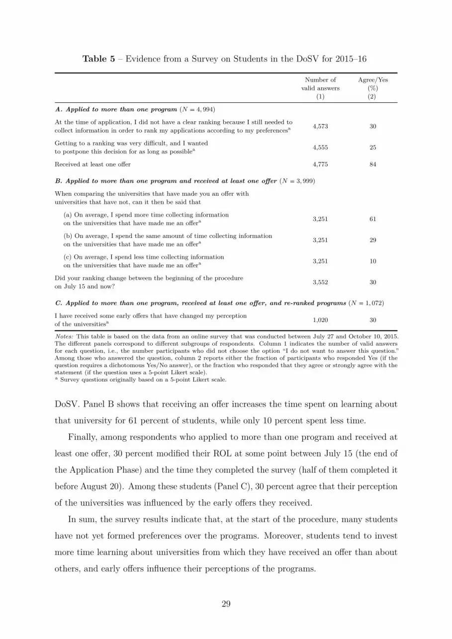
Table 5 – Evidence from a Survey on Students in the DoSV for 2015–16
Number ofvalid answers
Agree/Yes(%)
(1) (2)
A. Applied to more than one program (N � 4, 994)
At the time of application, I did not have a clear ranking because I still needed to 4,573 30collect information in order to rank my applications according to my preferencesa
Getting to a ranking was very difficult, and I wanted 4,555 25to postpone this decision for as long as possiblea
Received at least one offer 4,775 84
B. Applied to more than one program and received at least one offer (N � 3, 999)
When comparing the universities that have made you an offer withuniversities that have not, can it then be said that
(a) On average, I spend more time collecting information 3,251 61on the universities that have made me an offera
(b) On average, I spend the same amount of time collecting information 3,251 29on the universities that have made me an offera
(c) On average, I spend less time collecting information 3,251 10on the universities that have made me an offera
Did your ranking change between the beginning of the procedure 3,552 30on July 15 and now?
C. Applied to more than one program, received at least one offer, and re-ranked programs (N � 1, 072)
I have received some early offers that have changed my perception 1,020 30of the universitiesa
Notes: This table is based on the data from an online survey that was conducted between July 27 and October 10, 2015.The different panels correspond to different subgroups of respondents. Column 1 indicates the number of valid answersfor each question, i.e., the number participants who did not choose the option “I do not want to answer this question.”Among those who answered the question, column 2 reports either the fraction of participants who responded Yes (if thequestion requires a dichotomous Yes/No answer), or the fraction who responded that they agree or strongly agree with thestatement (if the question uses a 5-point Likert scale).a Survey questions originally based on a 5-point Likert scale.
DoSV. Panel B shows that receiving an offer increases the time spent on learning about
that university for 61 percent of students, while only 10 percent spent less time.
Finally, among respondents who applied to more than one program and received at
least one offer, 30 percent modified their ROL at some point between July 15 (the end of
the Application Phase) and the time they completed the survey (half of them completed it
before August 20). Among these students (Panel C), 30 percent agree that their perception
of the universities was influenced by the early offers they received.
In sum, the survey results indicate that, at the start of the procedure, many students
have not yet formed preferences over the programs. Moreover, students tend to invest
more time learning about universities from which they have received an offer than about
others, and early offers influence their perceptions of the programs.
29

4 A University-Admissions Model with Learning
Below, we develop a model of university admissions. Consistent with the findings from
the survey in Section 3.2, it allows students to learn about programs at a cost. The
sequential arrival of early offers under the DoSV influences a student’s learning behavior
and leads to the documented early-offer effect. Further, we compare the DoSV with the
canonical DA and a new mechanism—called Hybrid—that improves upon the DoSV. For
ease of exposition, we assume in the following that students apply to universities, instead
of programs, and that each university admits students.
4.1 The Mechanisms: DoSV, DA, and Hybrid
We start by formally defining the mechanisms. Abstracting from the German context, the
DoSV mechanism is defined to have the following stages:
(i) Applications: Through a clearinghouse, students apply to a set of universities
without committing to an ROL of these universities.
(ii) Ranking applicants: Every university ranks the students who have applied to it
and submits the ranking to the clearinghouse.
(iii) Continuous offers and rejections: Through the clearinghouse, each university
extends admission offers to its top-ranked applicants up to its capacity. Students can
reject any offers that they have received. Whenever a university’s offer is rejected
by a student, the clearinghouse automatically makes a new offer to the top-ranked
applicant among those who have not received its offer.
(iv) Final ROLs: Every student commits to an ROL of the universities that she has
applied to (and has not rejected offers from).
(v) Final match: With the rankings from students and universities as well as the
remaining seats at each university, the clearinghouse runs the university-proposing
GS algorithm (Appendix B.1) and finalizes the matching.
In contrast to the DoSV, the university-proposing DA mechanism asks students to commit
to an ROL of universities in stage (i) and proceeds to stages (ii) and (v), while skipping all
30

others. Recall that the GS algorithm is a set of computer codes that calculate a matching
from information on students and universities, while a mechanism in our setting includes
an algorithm and how relevant information is collected from students and universities
(Appendix B.1).
A potential concern about the DoSV mechanism is that the sequential arrival of offers
may lead students to accept sub-optimal offers. We thus propose the Hybrid mechanism
that has a common date for every university to send out its early offers. Specifically, it
replaces stage (iii) of the DoSV with stage (iii)’, while keeping everything else the same:
(iii)’ Offers on a common date: On a pre-specified date, every program extends
admission offers through the clearinghouse to its top-ranked applicants up to its
capacity. Students can reject any offers that they have received.33
Recall that we call a market decentralized if a student can hold multiple offers for
some time; otherwise, it is centralized. By this definition, a market that uses the DA is
completely centralized, while the DoSV and the Hybrid both have a decentralized stage
and a centralized stage. However, in the decentralized stage, the offer arrival under the
Hybrid is more structured than that under the DoSV.
4.2 Model Setup and Welfare Comparison
In the model, there is a student in a finite time horizon of J � 2 (J ¥ 2) periods,
t P t0, 1, . . . , J, J � 1u.34 We focus on two time points in each period, the beginning and
the end, implying that actions can be taken during a period. There is no time discounting.
At the beginning of period 0, the student has applied to a set of universities, J
(|J | � J). In period 0, the student has the belief that she will receive an offer from j P J
in period J � 1 with probability p0j P p0, 1q. Let p0 � pp0
1, . . . , p0Jq. As we shall clarify
shortly, the student does not update her belief about offer probabilities unless she receives
an offer before period J � 1. Admission decisions are independent across universities.
University j’s quality is a random variable, Xj, whose distribution function is Fj. Xj
and Xj1 are independent for any j � j1. Let F �±j Fj be the joint distribution.33In some cases, it can be helpful to have multiple rounds of offers. We provide a discussion in Section 5.34Unlike the matching literature, we study a single-agent model to highlight the learning dynamics.
The comparison among the mechanisms therefore ignores equilibrium effects that other students’ behaviormay cause. Our simulations in Section 4.4 provide some idea about the magnitude of these equilibriumeffects and reveal that the results from the single-agent problem still hold.
31

The student values a university at upXjq, where upXjq is weakly concave, implying
that she can be risk neutral or risk averse. She has access to an outside option that can
be an admission offer from another university outside of the system. This outside option
gives her zero utility and is forfeited if she accepts an offer from any j P J .
At the beginning of period 0, the student only knows the distribution of Xj, Fj. The
student can pay a cost, k, to learn about a university’s (realized) quality.
Remark 1. Our model deviates from the common assumption in the matching literature
that agents know their own ordinal preferences (Roth and Sotomayor, 1990; Bogomolnaia
and Moulin, 2001). Under this assumption, Appendix B.2 shows that the early-offer effect
documented in Section 2 cannot emerge. Intuitively, conditional on her applications J ,
the student only needs information on ordinal preferences to make an optimal decision.
Throughout periods 1 to J , there can be at most one early offer arriving at the beginning
of each period. No offer can be rescinded. Let O � pO1, . . . , OJq P t1, . . . , J, J � 1uJ be an
offer arrival such that Oj � t for 1 ¤ t ¤ J if the student receives an offer from university j
in period t and that Oj � J � 1 if she does not receive an offer from university j before
period J � 1. Note that Oj � J � 1 does not imply that she will necessarily receive an
offer from j in period J � 1. There is no early offer in period 0.
Timeline under the DA: The student is required to rank the J universities at the
end of period 0. Therefore, her learning activities, if any, are in period 0.
Timeline under the Hybrid: The student must rank the J universities at the end
of period J . At the beginning of period J , she observes all early offers given O. The offer
probabilities are updated from p0 to pJpOq such that (i) pJj pOq � p0j if Oj � J � 1, and
(ii) pJj pOq � 1 if Oj J � 1. She makes a learning decision given pJpOq.Timeline under the DoSV: The student must submit an ROL of the J universities
at the end of period J , but her learning decision is made “myopically” period by period
as follows. Define t � mintmintOu, Ju such that t is the period when her first early
offer arrives, if any, or period J if there is no early offer. The student does not learn
anything in period t for all t t. At the beginning of period t, for t ¤ t ¤ J , the
student updates her offer probabilities according to offer arrival O from ppt�1qpOq to
ptpOq � ppt1pOq, . . . , ptJpOqq such that (i) ptjpOq � p0j if Oj ¡ t (i.e., no offer from j up to
period t), and (ii) ptjpOq � 1 if Oj ¤ t (i.e., an offer from j has arrived in period t or
earlier). Conditional on ptpOq and what has been learned up until period (t � 1), the
32

student decides whether to learn more, assuming (incorrectly) that there would be no
more offers before period pJ � 1q. If mintOu � J � 1 (i.e., no early offer at all), she makes
a learning decision in period J given that pJpOq � p0.
We assume that the student under the DoSV ignores the possibility of receiving more
early offers in later periods. We conjecture that a student under the real-life DoSV is
somewhere between the above description and full rationality. If the student is fully
rational, she would not make her learning decision until she has received all early offers,
making the DoSV equivalent to the Hybrid (conditional on offer arrival). In this case,
there would be no difference between the first and later early offers, provided that offers
arrive randomly. However, Section 2.3 shows that the first early offer has a larger effect
than later early offers. Additionally, without the assumption of myopia, in the setting in
Section 4.3 below, we can still show the early-offer effect under the DoSV (Lemma 2) but
not the first-early-offer effect (i.e., Lemma 3 no longer holds).
Remark 2. As shown below, depending on the mechanism in place, the student learns
about the universities. Given her information set at the time of ROL finalization, each
mechanism has the same properties as the university-proposing DA: it is stable with respect
to reported ordinal preferences and non-strategy-proof for students and universities.35
4.2.1 Learning Strategy in a Given Period
We now consider the student’s learning strategy in a given period with up-to-date offer
probabilities p P p0, 1sJ . This is precisely what she does under the DA or Hybrid, because
learning happens only in one period. We will extend the derivation to learning in multiple
periods under the DoSV.
Let U � J be the set of universities whose qualities have not yet been learned by the
student, and U � J zU . Also let lpUq � tpj, xjqjPUu P pJ � Rq|U | be the realized university
qualities already learned by the student, paired with their identities.
Given a state (U , l) and offer probabilities p, the student’s learning strategy is
ψpU , l | pq P t0uYU such that ψ � 0 when the student stops learning and ψ P U indicates
which university to learn next. With this definition, we only consider pure strategies.36
35Under the assumption that student preferences evolve over time exogenously, Narita (2018) investigatesthe properties of alternative mechanisms.
36A mixed strategy implies that in some state, the student is indifferent between two different actions.This may happen for a measure zero set of pU , lq when Fj admits a continuous density function for all j.
33

Given (U , l, p), if ψ � 0, the student then submits an ROL. The expected utility
from an ROL is calculated as follows. For j P U , define vj � maxt0, upxjqu in which
xj is the realized value of Xj; for j P U , vj � maxt0, ³ upxqdFjpxqu. Recall that the
outside option yields zero utility. Given her information, it is optimal for the student
to submit a truthful ROL of all acceptable universities (i.e., vj ¡ 0).37 Not taking into
account the learning costs that are already sunk, the expected utility from this ROL is
vpU , l, pq � pj1vj1 �°Jk�2 pjkvjk
±k�1k1�1p1� pjk1 q, where vjk ¥ vjk1 whenever k k1.
If the student adopts strategy ψ, her expected utility given (U , l, p) is:
V pU , l, p | ψq �1pψpU ,l|pq�0q � vpU , l, pq
�¸jPU
1pψpU ,l|pq�jq
�»V pUztju, l Y tpj, xjqu, p | ψqdFjpxjq � k
,
where 1p�q is an indicator function. Thus, V pJ ,H, p | ψq is the student’s expected payoff
from adopting strategy ψ before she starts learning.
An optimal strategy, ψ�, solves the following problem for every state (U , l) given p:
V pU , l, p | ψ�q � max"vpU , l, pq,max
jPUt»V pUztju, l Y tpj, xjqu, p | ψ�qdFjpxjq � ku
*,
In other words, ψ�pU , l | pq � 0 if vpU , l, pq ¥ ³V pUztju, l Y tpj, xjqu, p|ψ�qdFjpxjq � k
for all j P U ; otherwise, ψ�pU , l | pq � arg maxjPUt³V pUztju, lY tpj, xjqu, p | ψ�qdFjpxjqu.
By definition, V pJ ,H, p | ψ�q ¥ V pJ ,H, p | ψq for all ψ.Learning under the DA: The student learns about the universities in period 0.
That is, she starts learning given pJ ,H, p0q. Let ψDAp�, � | p0q be an optimal strategy.
Learning under the Hybrid: The student learns about the universities in period J
after receiving all early offers as prescribed by offer arrival O. Hence, she starts learning
given pJ ,H, pJpOqq. Let ψHp�, � | pJpOqq be an optimal strategy.
4.2.2 Learning under the DoSV
We now extend the analysis to the DoSV under which the student’s learning can be
updated upon the arrival of an early offer. Recall that t � mintmintOu, Ju. In each
period t � t, . . . , J , given ptpOq, the student has a myopic strategy, ψtp�, � | ptpOqq, leading37We assume that including a university in a submitted ROL is a commitment to accepting the
university’s offer if it is the highest-ranked offer. Equivalently, we may assume there is a cost to reject anunacceptable offer that is included in the student’s ROL.
34

to (subjective) expected utility V tpU pt�1q, lpt�1q, ptpOq | ψtp�, � | ptpOqqq, where U pt�1q and
lpt�1q are the learning outcomes at the end of period pt�1q and U pt�1q � J and lpt�1q � H.
Hence, ψt P arg maxψ V tpU pt�1q, lpt�1q, ptpOq | ψq, for t � t, . . . , J .
The DoSV thus leads to a sequence of learning strategies, tψtuJt�t. Importantly, the
learning technology is such that the student cannot “unlearn” what has been learned. We
show in Appendix B.4 that under an assumption of no-learning on off-equilibrium paths
(Assumption B1), for any state, there is at most one strategy in the sequence tψtuJt�trequiring the student to learn more (Lemma B1). Therefore, we can define ψDoSV pU , l |pJpOqq � maxtPtt,...,Ju ψtpU , l | ptpOqq for all pU , lq. By Lemma B1, ψDoSV pU , l | pJpOqq isequivalent to applying tψtuJt�t sequentially.
4.2.3 Welfare Dominance of the Hybrid over the DA and DoSV
For each mechanism, we study the student’s welfare in period 0 (i.e., before any learning)
conditional on offer arrival O. Thus, we do not need to specify a distribution for O.
Under the DA, the expected utility in period 0 is evaluated at pJpOq, resulting in
V pJ ,H, pJpOq | ψDAp�, � | p0qq. Notice that the learning strategy is determined based
on p0 without knowing offer arrival O, a source of inefficiency. Under the DoSV, it is
V pJ ,H, pJpOq | ψDoSV p�, � | pJpOqqq; and it is V pJ ,H, pJpOq | ψHp�, � | pJpOqqq underthe Hybrid. We then have the following result.
Proposition 1. Conditional on offer arrival O, in terms of the student’s expected utility
in period 0,
(i) the Hybrid mechanism dominates both the DoSV and DA mechanisms:
V�J ,H, pJpOq | ψHp�, � | pJpOqq� ¥ V
�J ,H, pJpOq | ψDoSV p�, � | pJpOqq� ,
V�J ,H, pJpOq | ψHp�, � | pJpOqq� ¥ V
�J ,H, pJpOq | ψDAp�, � | p0qq� ,
with each inequality being strict for some (J , p0, O, F, k); and
(ii) the welfare ranking between the DoSV and the DA is ambiguous.
For an arbitrary distribution of O, part (i) still holds in terms of the student’s
unconditional expected utility in period 0, because it is satisfied for all possible O.
35

4.3 Costly Learning and Early-offer Effect: An Example
Our empirical analysis documents that an early offer increases the probability that the
offer is accepted and that the effect is larger for the first offer. We now present a simple
setting to highlight how these effects can be caused by the student’s learning about
university qualities.38 Moreover, we clarify a disadvantage of the DoSV: If a low-quality
university makes an offer first, this may sub-optimally increase the probability that the
student accepts its offer. We show that this inefficiency is avoided by the Hybrid.
The student is risk neutral, upXq � X. There are two universities, J � t1, 2u. Thequality of university j is an i.i.d. draw from Uniformpµj � 0.5, µj � 0.5q. Suppose that
0 µj 0.5, and that, without loss of generality, µ1 ¡ µ2. Everything else in the model
is the same as in Section 4.2. For instance, there is an outside option whose value is zero.
There are five different types of offer arrivals, OH (no early offer), Ot1u (an early
offer from university 1), Ot2u (an early offer from university 2), Ot1,2u (early offers
from university 1 and then university 2), Ot2,1u (early offers from university 2 and then
university 1).
To make this problem non-trivial, we impose the following assumption.
Assumption 1. For any offer probabilities, the student has an “interior solution” to the
dynamic learning problem: she has incentives to learn at least one university and to learn the
second if and only if the realized quality of the first university is below a threshold that is in-
terior in its support. Specifically, the parameters, (p01, p
02, µ1, µ2, k), are such that k k k,
where k � max
$&%maxp1Ptp01,1u,p2Ptp0
2,1ut12p1� p1qp2pµ2 � 1
2q2u,maxp1Ptp0
1,1u,p2Ptp02,1ut1
2p1� p2qp1pµ1 � 12q2 � 1
2p1p2pµ2 � µ1q2u
,.- and k �
min!
minp2Ptp02,1ut1
2p2pµ2 � 12q2u,minp1Ptp0
1,1ut12p1pµ1 � 1
2q2u).
As shown in Appendix B.6, most of the results can be derived for general values of the
parameter vector, (p01, p
02, µ1, µ2, k). However, many results would involve long expressions
such as those in Assumption 1. To make the results more readable, we consider a specific
numerical example.
Assumption 2. µ1 � 116 , µ2 � 1
32 , p01 � 9
16 , and p02 � 9
16 .38We note that the positive early-offer effect on offer acceptance may not hold in some cases. Ap-
pendix B.3 provides an example in which an early offer from a university reduces the likelihood that theoffer is accepted. Besides, there is no first-offer effect. The main feature of that example is that thestudent never has any incentive to learn about one of the two universities.
36

Assumptions 1 and 2 imply that k � 157532768 , k � 1764
32768 , and thus we can have
k P p 157532768 ,
176432768q. We allow k to be in a range to show that (i) this is not a knife-edge case
and (ii) the expressions are already long even with just one free parameter.
Below, we investigate optimal learning behavior (Section 4.3.1), ranking behavior
(Section 4.3.2), and efficiency of the mechanisms (Section 4.3.3).
4.3.1 Learning Behavior
The student’s learning strategy under a given mechanism has two parts: which university
to learn first and, depending on what has been learned, whether to learn about the other
university. We solve her optimization problem by backward induction.
Suppose that the offer arrival is OH (no early offer). If the student first learns
X1, the decision of whether to learn X2 is depicted in Panel A of Figure 5. When
the realization of X1, x1, is below the threshold (the dashed vertical line on the right),
X�1 pp0
1, p02q � µ2 � 1
2 �c
2k�p1�p01qp0
2pµ2� 12 q
p01p
02
P r0, µ1 � 12s, the student learns X2; otherwise,
she stops learning. Intuitively, with a higher value of x1, the incentive to learn X2 is lower,
because she can stop learning and top rank university 1 to guarantee herself a payoff of
p01x1 � p1 � p0
1qp02µ2. Similar thresholds are derived in Appendix B.6 when the student
learns X2 first and/or when there are one or two early offers.
We now consider which university to learn first. For j, j1 P t1, 2u, let Xj–then–Xj1
denote that the student first learns Xj and then, depending on the realization of Xj
and the thresholds, possibly learns Xj1 . It involves pairwise welfare comparisons among
X1–then–X2, X2–then–X1, and no learning. Let us take offer arrival OH as an example.
We calculate the welfare difference between learning X1 first and X2–then–X1, as well as
the difference between X1–then–X2 and no learning. Appendix B.6 shows that both are
greater than zero for all k P p 157532768 ,
176432768q. Therefore, given OH, it is optimal to learn X1
first, as depicted in Panel A of Figure 5
The following lemma summarizes the optimal learning sequences.
Lemma 1. Suppose that the offer arrival is O. Given Assumptions 1 and 2, the student’s
optimal learning sequence is as follows:
(i) if O � OH, X1–then–X2 under the DoSV or the Hybrid;
(ii) if O � Ot1u, X1–then–X2 under the DoSV or the Hybrid;
(iii) if O � Ot2u, X2–then–X1 under the DoSV or the Hybrid;
37

A. No early offer: offer arrival OH
B. Early offer from university 1: offer arrival Ot1u
Figure 5 – Learning & Ranking Behaviors w/ & w/o an Early Offer from University 1Notes: This figure applies to both the DoSV and the Hybrid. We set µ1 � 1
16 , µ2 � 132 , p
01 � 9
16 , p02 � 9
16 , andk � 3339
65536 (the mid-point of the interval of all admissible k), although k can be any value in p 157532768 ,
176432768 q. In Panel A,
the student receives no early offer. She learns X1 first and continues to learn X2 if and only if the realization of X1, x1,
is below X�1 pp0
1, p02q � µ2 � 1
2 �c
2k�p1�p01qp
02pµ2� 1
2 q2
p01p
02
. If x1 P rX�1 pp0
1, p02q, µ1 � 1
2 s, the student submits ROL 1–2. If
x1 P r0, X�1 pp0
1, p02qq, she will learn X2 and submits a truthful ROL among 1–2, 2–1, and 1–0. If x1 P rµ1 � 1
2 , 0q, shewill learn X2 and submits a truthful ROL, either 2–0 or 0–0 (an empty ROL). In Panel B, the student receives an earlyoffer from university 1, and it is still optimal to learn X1 first. The probability of learning X2 decreases, because thethreshold decreases from X�
1 pp01, p
02q to X�
1 p1, p02q � µ2 � 1
2 �c
2kp0
2. The probability of top-ranking university 1 increases:
for x1 P rX�1 p1, p0
2q, X�1 pp0
1, p02qs, she now always submits ROL 1–2 instead of one of the ROLs 1–2, 2–1, and 1–0 after
learning X2.
(iv) if O � Ot1,2u, X1–then–X2 under the DoSV or the Hybrid;
(v) if O � Ot2,1u, X2–then–X1 under the DoSV, but X1–then–X2 under the Hybrid.
Under the DA, since the student has to learn before receiving any early offer, the
optimal sequence is always X1–then–X2.
For the DoSV, Lemma 1 considers the learning sequence in the period when the
first offer arrives, provided that O � OH. Due to Assumption 1, the student will learn
38

Table 6 – Learning, Ranking & Welfare Given Offer Arrival with k � 333965536
Mechanism Learning OH: No Ot1u: early offer Ot2u: early offer Ot1,2u: early offers Ot2,1u: early offersprobability early offer from univ. 1 from univ. 2 from 1 & then 2 from 2 & then 1
(1) (2) (3) (4) (5)A. Learning probabilities (multiplied by 100)
DA P(learning X1) 100 100 100 100 100P(learning X2) 58.0 58.0 58.0 58.0 58.0
DoSV P(learning X1) 100 100 60.6 100 71.2P(learning X2) 58.0 54.3 100 65.0 100
Hybrid P(learning X1) 100 100 60.6 100 100P(learning X2) 58.0 54.3 100 65.0 65.0
B. Top ranking probabilities (multiplied by 100)
DA P(top rank univ. 1) 49.7 49.7 49.7 49.7 49.7P(top rank univ. 2) 29.8 29.8 29.8 29.8 29.8
DoSV P(top rank univ. 1) 49.7 51.2 33.1 47.2 37.1P(top rank univ. 2) 29.8 28.3 46.4 32.3 42.4
Hybrid P(top rank univ. 1) 49.7 51.2 33.3 47.2 47.2P(top rank univ. 2) 29.8 28.3 46.4 32.3 32.3
C. Welfare conditional on offer arrival (multiplied by 1000)DA 56.2 121.0 93.3 154.6 154.6
DoSV 56.2 121.1 110.5 155.5 152.3
Hybrid 56.2 121.1 110.5 155.5 155.5
Notes: These results are calculated for µ1 � 116 , µ2 � 1
32 , p01 � 9
16 , p02 � 9
16 , and, specifically, k � 333965536 (the mid-point of
the interval of all admissible k). The results are qualitatively the same for any k P p 157532768 ,
176432768 q as shown in Table B3.
about at least one of the universities. The lemma shows that offer arrival determines
the optimal learning sequence. In turn, it affects the probability of a university’s quality
being learned: when the optimal sequence is Xj–then–Xj1 , Xj is learned for sure while
Xj1 is only learned with some probability. This is illustrated in Panel A of Table 6 for
k � 333965536 . In column (1), given OH, the probability of X1 being learned is one under the
DoSV or Hybrid, but it decreases to 60.6 percent under the DoSV or Hybrid when there
is an early offer from university 2 (column 3). This is because the early offer changes the
optimal learning sequence.
Even when the optimal sequence remains the same, the learning probability can change
for the university that is learned second. In column (2) of Table 6, when the student
receives an early offer from university 1 and thus the offer arrival changes from OH to
Ot1u, the probability of X2 being learned decreases from 58.0 percent to 54.3 percent
under either the DoSV or the Hybrid. This is depicted in Figure 5: the threshold of X1,
X�1 , below which the student does not learn X2 is lower given Ot1u (Panel B) than given
OH (Panel A).
39

4.3.2 Ranking Behavior under the DoSV
We now explore how early offers affect the student’s ROL of the universities. Investigat-
ing the student’s ranking behavior amounts to studying her offer acceptance, because
conditional on receiving offers from both universities, the top-ranked university will be
accepted by the student. This is similar to our empirical analysis of offer acceptance in
which we focus on a student’s ex-post feasible universities that would make her an offer.
Panel A of Figure 5 shows that given OH and if x1 ¡ X�1 pp0
1, p02q, the student stops
learning and submits ROL 1–2. If 0 x1 ¤ X�1 pp0
1, p02q, she learns X2 and submits a
truthful ROL, 1–2, 2–1, or 1–0. If x1 0, she learns X2 and submits a truthful ROL,
2–0 or 0–0 (an empty ROL). However, when the offer arrival becomes Ot1u (Panel B),
for X�1 p1, p0
2q x1 X�1 pp0
1, p02q, the optimal strategy is to stop learning and submit
ROL 1–2, while there is no change for other values of x1. This increases the probability
that university 1 is top ranked, from 49.7 percent to 51.2 percent under the DoSV as
shown in columns 1 and 2 in Panel B of Table 6. Panel B of Table 6 provides more
examples.
The following lemma shows that this early-offer effect holds more generally.
Lemma 2. Given Assumptions 1 and 2, receiving an offer from one of the universities,
either as the first or as the second early offer, strictly increases the probability that this
university is top ranked in the student’s submitted ROL under the DoSV, ceteris paribus.
Lemma 2 describes the effect of receiving an early offer from j, holding everything else
constant. For example, it calculates the difference in the probability of university 1 being
top ranked between Ot1u and OH, between Ot1,2u and Ot2u, or between Ot2,1u and Ot2u.
When there are two early offers, offer arrival matters under the DoSV. The following
lemma shows the first-early-offer effect on ranking behavior under the DoSV.
Lemma 3. Suppose that Assumptions 1 and 2 hold and that there are two early offers.
Under the DoSV, the probability of a university being top ranked in the student’s submitted
ROL is higher when its offer is the first one than when it is the second.
Lemma 3 focuses on the difference in the probability of university 1 being top ranked
between Ot1,2u and Ot2,1u; a similar comparison is also done for university 2. For example,
when we move from column 4 to column 5 in Panel B of Table 6, the early offer from
40

university 2 becomes the first offer, and the probability that university 2 is top ranked
increases from 32.3 percent to 42.4 percent under DoSV.
Lemmata 2 and 3 are consistent with our empirical findings in Section 2.
4.3.3 Welfare Dominance of the Hybrid and Welfare Loss under the DoSV
We now compare student welfare under the three mechanisms. With the assumptions on
the parameters, we show that some of the weak inequalities in Proposition 1 are strict. In
particular, we highlight that the DoSV can result in a welfare loss when a low-quality
offer arrives first.
Lemma 4. Suppose that the offer arrival is O and that Assumptions 1 and 2 are satisfied.
We have the following results on student welfare:
(i) Dominance of the Hybrid: Conditional on O, the Hybrid dominates the DA,
and the dominance is strict if O � OH (i.e., there is at least one early offer); the Hybrid
also dominates the DoSV, and the dominance is strict when O � Ot2,1u (i.e., early offers
from university 2 and then university 1).
(ii) Comparison between the DA and the DoSV: Conditional on O, the DoSV
is equivalent to the DA if O � OH; the DA strictly dominates the DoSV if O � Ot2,1u; the
DoSV strictly dominates the DA if O � OH and O � Ot2,1u.
Lemma 4 is illustrated in Panel C of Table 6 for k � 333965536 . Specifically, given O � Ot2,1u
(column 5), the DoSV leads to a welfare loss relative to both the DA and Hybrid. Under
the DoSV, the student’s optimal learning sequence is X2–then–X1, starting with the
ex-ante low-quality university (Panel A). As Lemma 3 shows, the student has a higher
probability of top ranking university 2 (Panel B), often without learning X1. As a result,
the student misses some chances of being assigned to university 1. This inefficiency is
avoided by the Hybrid under which the optimal learning sequence is X1–then–X2.
4.4 Simulation Results
To gauge the relative performance of the DA, DoSV, and Hybrid mechanisms in a real-life
setting, we calibrate a set of simulations with the same data used in Section 2. Due to
the data limitations and the lack of a fully-fledged empirical model, certain simplifying
41

assumptions are needed in the simulations. We highlight these assumptions below, while
the details of the simulation procedure are in Appendix E.
Setup. We construct a stylized market based on the DoSV data. As in Section 2, we use
the 21,711 students who applied to at least two feasible programs and accepted an offer.
In every simulation, student i always applies to the same set of programs, Ai, including
those in her initial ROL and an outside option.39 A program’s capacity is set equal to
the number of students in the simulation sample who accepted its offer in reality. Each
program ranks its applicants by the average of their Abitur percentile rank (between 0
and 1) and a program-specific Uniformp0, 1q random variable.
The timeline is as follows: (i) under the DA, students submit their ROL before
receiving any offer; (ii) under the DoSV, each program, at a random time, sends out a
single batch of early offers to its highest-ranked applicants up to its capacity and the ROL
submission is after the arrival of early offers; (iii) under the Hybrid, the timing is the same
as under the DoSV, except that all early offers are sent out on the same date. Under any
mechanism, the matching is determined by the program-proposing GS algorithm, using as
inputs the submitted ROLs and the programs’ capacities and rankings of students.
Learning. As in our theoretical model, students are uncertain about their preferences
over programs and can only learn them at a cost. If student i pays the cost, she learns
her true utility from program k, UFullInfoi,k ; otherwise, she values k at its expected utility,
UNoInfoi,k . At the time of submitting her ROL, student i’s perceived utility from program k
under mechanism m is specified as follows:
Umi,k � λmi,k � UFullInfo
i,k � p1� λmi,kqUNoInfoi,k @i, k P Ai, (3)
where λmi,k P t0, 1u is an indicator for whether i has learned her true utility from k.
Further, UFullInfoi,k � V FullInfo
i,k � εFullInfoi,k , where V FullInfoi,k depends on observable student-
program-specific characteristics and εFullInfoi,k is i.i.d. type I extreme value distributed. To
calculate V FullInfoi,k , we rely on the same sample as in Section 2.40 Under the assumption
39This outside option accounts for the possibility that students may apply to programs outside theDoSV procedure and devote some time learning about them. Since all students in our sample acceptedan offer from the clearinghouse, we make the simplifying assumption that this outside option is neverfeasible.
40We estimate a rank-ordered logit model that is an augmented version of the specification in column 3
42

that a student always learns her preference for her first early offer, V FullInfoi,k is computed by
imposing that k is her first early offer. Similarly, we assume that UNoInfoi,k � V NoInfo
i,k �εNoInfoi,k ,
where V NoInfoi,k is drawn from a normal distribution with mean V FullInfo
i,k and εNoInfoi,k is a
type I extreme value such that εNoInfoi,k K εFullInfoi,k .
Lacking an estimate of learning costs, we assume that under any mechanism, student i
learns her true preferences for half of the programs in Ai. Further deviating from the
endogenous learning in Section 4.2, we impose the following assumptions. Under the DA,
the programs learned by i (i.e., λDAi,k � 1) are randomly selected. Under the DoSV, we
emulate the myopic learning behavior in Section 4.2 by assuming that i always learns her
first early offer and then alternates between (i) learning a randomly chosen program from
the ones in Ai she has not learned yet and (ii) learning her early offers (if any) in their
arrival order. Under the Hybrid, early offers are learned before other programs.
Results. The simulations generate students’ submitted ROLs and matching outcomes
under the three mechanisms in 10,000 samples. As a benchmark, we also simulate the
matching that would be observed under full information.
Panel A of Figure 6 contrasts the mechanisms by students’ preference discovery. The
simulations confirm that in terms of learning, (i) the DoSV and the Hybrid mechanisms
are both more efficient than the DA and (ii) the Hybrid slightly outperforms the DoSV.
On average across the simulation samples, 44.0 percent of students rank ex-post feasible
programs in the order of their full information preferences under the Hybrid, relative to
43.3 and 40.6 percent under the DoSV and the DA, respectively.41
As for student welfare, we compute each student’s expected utility as the average utility
(UFullInfoi,k ) from her matches across the simulation samples. We then perform pairwise
comparisons of the mechanisms based on the shares of students whose expected utility
is (i) strictly higher under one mechanism than under the other, (ii) strictly lower, or
(iii) equal. These comparisons incorporate equilibrium effects since a student’s match
depends not only on her submitted ROL but also on other students’ behavior. As shown
in Panel B of Figure 6, the majority of students (over 70 percent) are strictly better off
of Table 3, in which we fully interact the early-offer and first-early-offer dummies with university fixedeffects, field-of-study fixed effects, distance, distance squared, and a dummy for whether the program is inthe student’s region. This model is estimated using the information extracted from a student’s final ROL.
41The comparisons are restricted to ex-post feasible programs since it is payoff-irrelevant for a studentto rank an infeasible program arbitrarily.
43

A. Submitted ROLs B. Expected utility
5.8%21.0% 20.8%
37.1%
0.5%
7.1% 7.0%
21.3%93.6%
71.9% 72.2%
41.7%
0
20%
40%
60%
80%
100%
Shar
e of
stu
dent
s
Full infovs.DA
DoSVvs.DA
Hybridvs.DA
Hybridvs.
DoSV
Strictly higher EqualStrictly lower
Expected utility of matching outcome:
Figure 6 – Comparing the DA, DoSV, and Hybrid Mechanisms: Simulation ResultsNotes: Using the simulations described in Appendix E, this figure compares the DA, DoSV, and Hybrid mechanismsalong two dimensions: students’ submitted ROLs (Panel A) and their expected utility of the matching outcome (Panel B).There are 21,711 students. Panel A compares the share of students who, under each mechanism, rank the ex-post feasibleprograms to which they applied in the order of their full-information preferences, averaged across 10,000 simulation samples.Panel B performs pairwise comparisons of mechanisms based on the shares of students whose expected utility is (i) strictlyhigher under the first mechanism than under the second; (ii) strictly lower; (iii) equal. A student’s expected utility is theaverage of the full information utility of her matches across the 10,000 simulation samples.
under the DoSV and the Hybrid than under the DA. Moreover, the Hybrid outperforms
the DoSV, as 41.7 percent of students are strictly better off under the Hybrid than under
the DoSV, while only 37.1 percent are worse off.
Overall, these simulations provide suggestive evidence that the DoSV and the Hybrid
can generate sizable welfare gains relative to the DA. Furthermore, the bundling of early
offers in the Hybrid mechanism is found to yield a small yet meaningful improvement
upon the DoSV.
5 Concluding Remarks
It is a recent trend in market design that matching markets are more and more centralized
into single-offer procedures. The trend is especially prominent in school choice and
university admissions where it requires students to rank a large number of schools or
universities from the outset. Theoretical justifications for centralization are usually based
on the assumption that agents know their own preferences and that their preferences are
fixed over time.
44

Relying on a unique data set from Germany’s university admissions, we identify a
quasi-experiment in which the arrival time of admission offers is exogenous to student
preferences. We show that a student is more likely to accept an early offer relative to
later offers, despite the fact that offers cannot be rescinded. This finding, which cannot
be reconciled with the known-and-fixed-preference assumption, is instead consistent with
students’ learning about university qualities at a cost, which is corroborated by survey
evidence.
In the midst of increasing centralization, our results highlight the advantages of
incorporating elements of decentralization into a centralized market. Specifically, we make
a case for a decentralized phase before the single-offer centralized phase in a matching
mechanism. When students are allowed to hold multiple offers in the decentralized
phase, the arrival of offers helps students optimize their learning. Our proposed Hybrid
mechanism, which is an improvement over the DoSV mechanism used in Germany, captures
such efficiency gains and dominates the DA, the most commonly used mechanism in
centralized markets.
The Hybrid mechanism can be implemented through an online clearinghouse, similar
to the DoSV in Germany and Parcoursup in France for university admissions. When
implementing the Hybrid mechanism in practice, it is important to pay attention to the
details of its design. For example, the choice of the number of rounds with offers in the
decentralized phase should be guided by the specific context. The more time consuming
the learning is, the more time students should have between rounds, ceteris paribus,
which implies fewer rounds of offers if the total length of the decentralized phase is fixed.
Moreover, highly homogenous preferences of both students and programs imply that offers
in each round are concentrated on a small group of students. Having more rounds of offers
may benefit students who are ranked low by the programs. We leave the formal analysis
of such considerations to future research.
45

ReferencesAbdulkadiroğlu, Atila, Joshua D. Angrist, Yusuke Narita, and Parag A.Pathak, “Research Design Meets Market Design: Using Centralized Assignment forImpact Evaluation,” Econometrica, 2017, 85 (5), 1373–1432.
Abdulkadiroğlu, Atila and Tayfun Sönmez, “School Choice: A Mechanism DesignApproach,” American Economic Review, 2003, 93 (3), 729–747., Parag A. Pathak, and Alvin E. Roth, “Strategyproofness versus Effciency inMatching with Indifferences: Redesigning the NYC High School Match,” AmericanEconomic Review, 2009, 99 (5), 1954–1978., Yeon-Koo Che, Parag A. Pathak, Alvin E. Roth, and Olivier Tercieux,“Efficiency, Justified Envy, and Incentives in Priority-Based Matching,” AmericanEconomic Review: Insights, 2020, 2 (4), 425–442.
Alladi, Vinayak, “Sour Grapes in the Lab and Field: A Test of Access-Based Beliefs,”2018. Manuscript.
Antler, Yair, “No One Likes To Be Second Choice,” Economic Journal, 2019, 129 (619),1119–1138.
Artemov, Georgy, Yeon-Koo Che, and Yinghua He, “Strategic ‘Mistakes’: Impli-cations for Market Design Research,” 2017. Manuscript.
Avery, Christopher and Jonathan Levin, “Early Admissions at Selective Colleges,”American Economic Review, 2010, 100 (5), 2125–2156., Andrew Fairbanks, and Richard J. Zeckhauser, The Early Admissions Game:Joining the Elite, Harvard University Press, 2003.
Avery, Christopher N., Mark E. Glichman, Caroline M. Hoxby, and AndrewMetrick, “A Revealed Preference Ranking of U.S. Colleges and Universities,” QuarterlyJournal of Economics, 2013, 128 (1), 425–467.
Bergemann, Dirk and Juuso Välimäki, “Information Acquisition and Efficient Mech-anism Design,” Econometrica, 2002, 70 (3), 1007–1033.
Bó, Inació and Rustamdjan Hakimov, “The Iterative Deferred Acceptance Mecha-nism,” 2018. Manuscript.and , “Iterative versus Standard Deferred Acceptance: Experimental Evidence,”Economic Journal, 2020, 130 (626), 356–392.
Bogomolnaia, Anna and Hervé Moulin, “A New Solution to the Random AssignmentProblem,” Journal of Economic Theory, 2001, 100 (2), 295–328.
Braun, Sebastian, Nadja Dwenger, and Dorothea Kübler, “Telling the Truth MayNot Pay Off: An Empirical Study of Centralized University Admissions in Germany,”The B.E. Journal of Economic Analysis & Policy (Advances), 2010, 10 (1), 1–38., , , and Alexander Westkamp, “Implementing Quotas in University Admissions:An Experimental Analysis,” Games and Economic Behavior, 2014, 85 (C), 232–251.
Calsamiglia, Caterina, Francisco Martínez-Mora, and Antonio Miralles,“School Choice Design, Risk Aversion and Cardinal Segregation,” Economic Journal,2021, 131 (635), 1081–1104.
Chen, Yan and Tayfun Sönmez, “School Choice: An Experimental Study,” Journalof Economic Theory, 2006, 127 (1), 202–231.
46

and Yinghua He, “Information Acquisition and Provision in School Choice: ATheoretical Investigation,” 2018. Manuscript.and , “Information Acquisition and Provision in School Choice: An ExperimentalStudy,” 2018. Manuscript.
Compte, Olivier and Philippe Jehiel, “Auctions and Information Acquisition: SealedBid or Dynamic Formats?,” RAND Journal of Economics, 2007, 38 (2), 355–372.
Dizdar, Deniz and Benny Moldovanu, “On the Importance of Uniform Sharing Rulesfor Efficient Matching,” Journal of Economic Theory, 2016, 165 (C), 106–123.
Doval, Laura, “Whether or Not to Open Pandora’s Box,” Journal of Economic Theory,2018, 175 (C), 127–158.
Dwenger, Nadja, Dorothea Kübler, and Georg Weizsäcker, “Flipping a Coin:Evidence from University Applications,” Journal of Public Economics, 2018, 167,240–250.
Dzyabura, Daria and John R. Hauser, “Recommending Products when ConsumersLearn their Preferences,” Marketing Science, 2019, 38 (3), 417–441.
Echenique, Federico, Alistair. J. Wilson, and Leeat Yariv, “Clearinghouses forTwo-Sided Matching: An Experimental Study,” Quantitative Economics, 2016, 7 (2),449–482.
Elster, Jon, Sour Grapes: Studies in the Subversion of Rationality, Cambridge UniversityPress, 1983.
Evans, Jonathan St. B. T., “Dual-Processing Accounts of Reasoning, Judgment, andSocial Cognition,” Annual Review of Psychology, 2008, 59, 255–278.
Fack, Gabrielle, Julien Grenet, and Yinghua He, “Beyond Truth-Telling: Prefer-ence Estimation with Centralized School Choice and College Admissions,” AmericanEconomic Review, 2019, 109 (4), 1486–1529.
Fudenberg, Drew and David K. Levine, “A Dual-Self Model of Impulse Control,”American Economic Review, 2006, 96 (5), 1449–1476.
Gale, David E. and Lloyd S. Shapley, “College Admissions and the Stability ofMarriage,” American Mathematical Monthly, 1962, 69 (1), 9–15.
Gong, Binglin and Yingzhi Liang, “A Dynamic College Admission Mechanism inInner Mongolia: Theory and Experiment,” 2017. Manuscript.
Gossner, Olivier, Jakub Steiner, and Colin Stewart, “Attention Please!,” Econo-metrica, forthcoming.
Hakimov, Rustamdjan and Dorothea Kübler, “Experiments on Matching Markets:A Survey,” 2019. Manuscript.
Hassidim, Avinatan, Assaf Romm, and Ran I. Shorrer, “The Limits of Incentivesin Economic Matching Procedures,” Management Science, 2021, 67 (2).
Hatfield, John William, Fuhito Kojima, and Scott Duke Kominers, “InvestmentIncentives in Labor Market Matching,” American Economic Review, 2014, 104 (5),436–441.
Immorlica, Nicole S., Jacob D. Leshno, Irene Y. Lo, and Brendan J. Lucier,“Information Acquisition in Matching Markets: The Role of Price Discovery,” 2020.Manuscript.
47

Kahneman, Daniel, “Maps of Bounded Rationality: Psychology for Behavioral Eco-nomics,” American Economic Review, 2003, 93 (5), 1449–1475., Thinking, Fast and Slow, New York: Farrar, Straus and Giroux, 2011., Jack L. Knetsch, and Richard H. Thaler, “Experimental Tests of the EndowmentEffect and the Coase Theorem,” Journal of Political Economy, 1990, 98(6), 1325–1348.
Ke, T. Tony and J. Miguel Villas-Boas, “Optimal Learning before Choice,” Journalof Economic Theory, 2019, 180, 383–437., Zuo-Jun Max Shen, and J. Miguel Villas-Boas, “Search for Information onMultiple Products,” Management Science, 2016, 62 (12), 3576–3603.
Klijn, Flip, Joana Pais, and Marc Vorsatz, “Static versus Dynamic Deferred Ac-ceptance in School Choice: Theory and Experiment,” Games and Economic Behavior,2019, 113, 147–163.
Loewenstein, George and Ted O’Donoghue, “Animal Spirits: Affective and Delib-erative Processes in Economic Behavior,” 2004. Manuscript.
Manski, Charles F. and David A. Wise, College Choice in America, Harvard Uni-versity Press, 1983.
Narita, Yusuke, “Match or Mismatch? Learning and Inertia in School Choice,” 2018.Manuscript.
Nöldeke, Georg and Larry Samuelson, “Investment and Competitive Matching,”Econometrica, 2015, 83 (3), 835–896.
Pathak, Parag A., “The Mechanism Design Approach to Student Assignment,” AnnualReview of Economics, 2011, 3 (1), 513–536.
Rees-Jones, Alex and Samuel Skowronek, “An Experimental Investigation of Prefer-ence Misrepresentation in the Residency Match,” Proceedings of the National Academyof Sciences, 2018, 115 (45), 11471–11476.
Roth, Alvin E., “The Economics of Matching: Stability and Incentives,” Mathematicsof Operations Research, 1982, 7 (4), 617–628., “New Physicians: A Natural Experiment in Market Organization,” Science, 1990, 250,1524–1528.and Elliott Peranson, “The Redesign of the Matching Market for American Physi-cians: Some Engineering Aspects of Economic Design,” American Economic Review,1999, 89 (4), 748–780.and Marilda A. Oliveira Sotomayor, Two-Sided Matching: A Study in Game-
Theoretic Modeling and Analysis, Econometric Society Monograph Series, CambridgeUniversity Press, 1990.and Uriel G. Rothblum, “Truncation Strategies in Matching Markets–in Search ofAdvice for Participants,” Econometrica, 1999, 67 (1), 21–43.
Shorrer, Ran I. and Sándor Sóvágó, “Obvious Mistakes in a Strategically SimpleCollege Admissions Environment,” 2017. Tinbergen Institute Discussion Papers No. 2017-107/V.
Weitzman, Martin L., “Optimal Search for the Best Alternative,” Econometrica, 1979,47 (3), 641–654.
Westkamp, Alexander, “An Analysis of the German University Admissions System,”Economic Theory, 2013, 53 (3), 561–589.
48

(For Online Publication)
Appendix to
Decentralizing Centralized Matching Markets:Implications from Early Offers in University Admissions
Julien Grenet YingHua He Dorothea Kübler
June 2021
List of Appendices
A Data A-2
B Additional Definitions, Proofs, and Results A-7
C Supplementary Figures and Tables A-17
D Early-Offer Effect: Regression Discontinuity Estimates A-30
E Simulation-Based Comparison of Mechanisms A-35
Appendix References A-45
A-1

A DataThis appendix provides additional information about the data sets used in the empiricalanalysis.
A.1 DoSV DataThe Dialogorientierten Serviceverfahren (DoSV) data for the winter term of 2015–16 ismanaged by the Stiftung für Hochschulzulassung. It consists of several files, all of whichcan be linked using encrypted identifiers for students and programs.
A.1.1 Data Files
Applicants. A specific file provides information on applicants’ basic socio-demographiccharacteristics (gender, year of birth, postal code), their Abitur grade, and their finaladmission outcome, i.e., the reason for exit, the date and time of exit, and (when relevant)the accepted program. The Abitur grade is only available for approximately 50 percentof the applicants but, as explained below (Section A.1.2), it can be inferred for a largefraction of those for whom the information is missing. Possible reasons for exit include(i) the active acceptance of an early offer; (ii) the automatic acceptance of the best offerduring Phase 2; (iii) the cancellation of applications; and (iv) rejection due to applicationerrors or rejection in the final stage for students who participated in Phase 2 but receivedno offer.
Programs. For each of the 465 programs that participated in the DoSV procedure in2015–16, information is provided on the program’s field of study and the university whereit is located.
Applicants’ rank-order lists of programs. Applicants’ ROLs of programs are recordedon a daily basis throughout the duration of the DoSV procedure, i.e., between April 15and October 5, 2015. During the Application Phase, students can apply to at most 12university programs. By default, applications are ranked by their arrival time at the clear-inghouse but students may actively change the ordering at any time before Phase 2—withthe information recorded in the data.
Programs’ rankings of applicants. In general, the ranking of applicants by theprograms follows a quota system. The size, number, and nature of the quotas aredetermined by state laws and regulations, and by the universities themselves. For eachquota, applicants are ranked according to quota-specific criteria. We make use of thecomplete rankings of applicants by the programs, including all quotas. So-called pre-selection quotas are filled before other quotas and are typically applied to 10–20 percentof a program’s seats. They are open to, e.g., foreign students, applicants with professionalqualifications, cases of special hardship, and minors. One of the main quotas is the Abiturquota (Abiturbestenquote) where the ranking is based on a student’s average Abitur gradeand typically applies to 20 percent of the seats. The Waiting Time Quota (Wartezeitquote)is devoted to applicants who have waited for the greatest number of semesters sinceobtaining the Abitur, and typically applies to 20 percent of the seats as well. Finally,the University Selection Quota (Auswahlverfahren der Hochschulen) tends to apply to
A-2

around 60 percent of seats and employs criteria that are determined by the programsthemselves. However, the ranking under the University Selection Quota is almost entirelydetermined by the students’ Abitur grade, with an average correlation coefficient betweenthe rankings submitted by programs and the Abitur grade of 0.86 across programs. Theorder in which the quotas are processed is specific to each university.
Program offers. The exact date and time at which offers are made by programs toapplicants are recorded in a separate file.
A.1.2 Additional Information
Based on the data from the DoSV procedure, we computed a number of auxiliary variables.
Abitur grades. In the data, the Abitur grade is only available for 49.6 percent ofapplicants. However, this information can be inferred for a large fraction of the otherapplicants based on how they are ranked under programs’ Abitur quota, because theserankings are strictly determined by an applicant’s Abitur grade. The grade is given on a6-point scale to one place after the decimal and ranges between 1.0 (highest grade) and6.0 (lowest grade). Since the lowest passing grade is 4.0, all applicants in the data haveAbitur grades between 1.0 and 4.0. Due to the discreteness of the Abitur, missing gradescan be imputed without error in the following cases: (i) an applicant is ranked above anyapplicant with a grade of 1.0 (in which case the assigned grade is 1.0); (ii) an applicant isranked below any applicant with a grade equal to s and above any applicant with thesame grade s (in which case the assigned grade is s); and (iii) an applicant is rankedbelow any applicant with a grade of 4.0 (in which case the assigned grade is 4.0). Usingthis procedure, we were able to impute the Abitur grade for approximately two thirds ofapplicants with a missing grade in the data, bringing the overall proportion of studentswith a non-missing Abitur grade to 83 percent.
Distance to university. To measure the distance between a student’s home and theuniversity of each of the programs she applied to, we geocoded students’ postal codes anduniversity addresses, and computed the cartesian distance between the centroid of thestudent’s postal code and the geographic coordinates of each university.
Feasible programs. A program is defined as being ex-post feasible for a student if thestudent was ranked above the last applicant to have received an offer from the programunder any of the quota-specific rankings in which the student appears. The date theprogram became feasible to the student i is determined as the first day when i, or anystudent ranked below i, received an offer from the program under any of the quota-specificrankings in which i appears.
A.1.3 Sample Restrictions
The DoSV data contain 183,028 students applying to university programs for the winterterm of 2015–16. We exclude 31,066 students for whom the Abitur grade is missing andcannot be inferred using the procedure described above, as well as 2,252 students withmissing socio-demographic or postal code information. We further remove from the sample4,097 students who registered to the clearinghouse after the start of Phase 1. Finally, we
A-3

exclude 34,832 students who applied to specific programs with complex ranking rules,these students being mostly those wanting to become teachers and who have to choosemultiple subjects (e.g., math and English). This leaves us with a sample of 110,781students.
Table 1 in the main text provides summary statistics for this sample, as well as forthe subsample of students who applied to at least two programs (64,876 students). Toestimate the impact of early offers on the acceptance of offers, we only consider studentswho applied to two feasible programs and who either actively accepted an early offer inPhase 1 or were automatically assigned to their best offer in Phase 2. In total, there are21,711 such students in the sample.
A.2 SurveyWe conducted an online survey between July 27 and October 10, 2015, among studentswho participated in the DoSV procedure for the winter term of 2015–16. All visitors ofthe application website were invited to participate in the survey. We collected around9,000 responses. Of all respondents, 52 percent completed the survey in July and Augustwhile 48 percent completed it in September and October. The survey formed part ofan official survey conducted by the Stiftung für Hochschulzulassung, which was aimed atcollecting feedback on the DoSV procedure and its website.
Our survey questions focus on the general understanding of the procedure as well asthe process of preference formation, including the effect of early offers and the acquisitionof information. Since students were able to participate in the survey over a long period oftime, we also asked questions regarding the status of their applications, including offersreceived, rejected, etc. For every question, we included the option “I do not want to answerthis question.” In the following, we document the complete list of questions (translatedfrom German).
1. How many programs did you apply for through the DoSV? Please provide thenumber.
2. How many programs did you apply for outside the DoSV? Please provide the number.3. Which subjects did you apply for through the DoSV? [The list of all subjects grouped
in clusters was shown.]4. Did you apply to some universities in the hope of going there with your friends?
[Yes/no]5. How many offers have you already received? Please consider both offers inside the
DoSV and outside of it. Please provide the number.6. If you have already received an offer, please answer questions 7, 8, 9, and 10. If not,
please proceed with question 11.7. Regarding the offers that you have received up to now [Rate on a Likert scale]
• Did you talk to your parents about these universities?• Did you talk to your friends about these universities?• Did you talk to your friends about the possibility of accepting offers at the
same university or at universities that are located close to each other?8. When comparing universities that have made you an offer with universities that
have not, can it then be said that [Choose one option]
A-4

• On average, I spend more time collecting information on the universities thathave made me an offer.
• On average, I spend the same amount of time collecting information on theuniversities that have made me an offer.
• On average, I spend less time collecting information on the universities thathave made me an offer.
9. Regarding the universities that have already made you an offer, which of the followingstatements best describes your situation? [Choose one option]
• On average, I find these universities better than before receiving their offers.• I find some of these universities better and some worse than before receiving
their offers.• On average, I find these universities worse than before receiving their offers.• The offers did not influence my evaluation of the universities.
10. What is your opinion regarding the acceptance of one of the offers that you havealready received?
• I will accept (or have already accepted) one of the offers since it is from mymost preferred university.
• I will accept (or have already accepted) one of the offers in order to be able tostart planning future activities as soon as possible.
• I will take my time since I want to find out more about the universities.• I will take my time since I want to find out where my friends are going to study.• I will take my time since I have not received an offer from my preferred
university yet.11. Have any of your friends already received an offer? [Yes/no]12. If yes, did any of your friends... [Rate on a Likert scale]
• ... talk to you about the advantages and disadvantages of these universities?• ... talk to you about accepting one of these offers?• ... consider the possibility of accepting one of the offers from the same or a
nearby university together with you or some other friends?13. Please remember the situation when you submitted your applications to the uni-
versities in the DoSV. We would like to know how well you knew at this point howto rank your applications, that is, which application was your most preferred, yoursecond preferred, etc. How accurate are the following statements regarding yoursituation back then with respect to your preference ranking over the programs?[Rate on a Likert scale]
• I had a clear preference ranking over the programs.• I did not have a clear ranking because I still needed to collect information in
order to rank my applications according to my preferences.• I did not have a clear ranking because I did not know where my friends were
going.• Getting to a ranking was very difficult, and I wanted to postpone this decision
for as long as possible.14. Did you actively change your ranking in the DoSV (that is, submitted a new ranking
or actively prioritized the applications)? [Yes/no]15. If no, please provide us with the reasons. [Rate on a Likert scale]
A-5

• I did not know that it was possible to change the ranking.• I was happy with the initial ranking of the DoSV.• I missed the deadline before which it was possible to change the ranking.• I did not have a clear ranking of my applications.• I assume that the ranking has no effect on the likelihood of being admitted.
16. Has your ranking changed between the beginning of the procedure on July 15 andnow? [Yes/no]
17. If yes, what were the reasons for changing your ranking? [Rate on a Likert scale]• I did not have a ranking at the beginning of the procedure when I submitted
my applications.• I have received new information during this time period.• Now I know where my friends are going.• I have received some early offers that have changed my perception of the
universities.18. Have you tried to collect information about the universities during the procedure,
in particular... [Rate on a Likert scale]• ... via the internet?• ... from students of these universities?• ... from your school teachers?• ... from your parents or other members of your family?• ... from your friends?
19. Which of the following reasons have played a role for your selection of programs anduniversities and for your ranking of them? [Rate on a Likert scale]
• The fit between the program offered by the university and my own interests.• The geographical proximity to my parents.• The geographical proximity to my friends.• Job market considerations.• Whether my application has a chance of being successful at this university.• Other reasons.
20. Please tell us your gender. [Female/male]
A-6

B Additional Definitions, Proofs, and ResultsThis appendix first defines the Gale-Shapley algorithm (Section B.1). Then, it providesadditional results and proofs for Section 4. Specifically, Section B.2 considers a specialcase in which the student knows her own ordinal preferences, an assumption that is oftenimposed in the matching literature. Under this assumption, we show that there are noearly-offer effects. Section B.3 provides an example in which the early-offer effect on offeracceptance is negative.
Section B.4 proves that the sequence of optimal strategies under the DoSV can besummarized into one strategy. Thus, it provides a theoretical foundation for Section 4.2.2.The rest of this appendix includes various proofs and derivations. Section B.5 provesProposition 1, and Section B.6 presents detailed derivations and proofs for Section 4.3.
B.1 The Gale-Shapley AlgorithmWe distinguish between a “mechanism” and an “algorithm.” Let us consider the casethat students apply to universities and that each university admits students. In oursetting, a university-admissions mechanism, such as the DoSV, is a complete procedurethat specifies how students and universities exchange information with the mechanismand how a matching outcome is determined. In contrast, an algorithm is a computer codethat takes as inputs information from applicants and universities and delivers a matchingoutcome; importantly, it is silent on how relevant information is collected. Therefore, analgorithm is always one of the multiple components of a mechanism.
The Gale-Shapley algorithm can be either student-proposing or university-proposing.We focus on the latter. Specifically, taking as inputs university capacities, universities’ranking over applicants, and students’ rank-order lists of universities (ROLs), it proceedsas follows:
Round 1. Every university with capacity qk and n1k applicants extends an admission
offer to its top-mintqk, n1ku applicants in its ranking over applicants. Each student who
receives multiple offers keeps the highest-ranked offer according to her ROL and rejectsthe rest.
Generally, in:Round (r ¡ 1). Every university withmpr�1q
k of its previous offers rejected in round r�1and nrk applicants who have never received its offer extends offers to the top-mintmpr�1q
k , nrkuapplicants among those who have not received its offer. Each student who has multipleoffers keeps the highest-ranked offers according to her ROL and rejects the rest.
The process terminates after any round r in which no offers are rejected by students.Each university is then matched with the students that are currently holding its offer.
B.2 Ordinally Informed StudentWe now investigate if the early-offer effect in Section 2 can emerge when we impose thefollowing assumption that is common in the matching literature: agents know their ownordinal preferences (Roth and Sotomayor, 1990; Bogomolnaia and Moulin, 2001).
We call the student ordinally informed if tFjuj is such that with probability one,(i) either upXjq ¡ upXj1q or upXjq upXj1q for any j � j1, and (ii) either upXjq ¡ 0or upXjq 0 for any j. In other words, the student knows her ordinal preferences andwhether a university is (ex-post) acceptable without any further learning. Importantly,
A-7

this assumption includes the following as a special case: there is no uncertainty aboutuniversity quality and there are no ties in the student’s cardinal preferences.
Proposition B1. If the student is ordinally informed, she does not learn about universityquality and submits the same ROL for all O, p0, and k under the DA, the DoSV or theHybrid. Her expected utility is constant across the mechanisms.
This proposition is straightforward, and we therefore only sketch the proof here. Sincethe optimal strategy for the student is to submit an ROL respecting her true ordinalpreferences, which are known to her without additional learning, the marginal benefit oflearning more about the universities is zero under any mechanism. Since her submittedROL is constant across mechanisms, her expected utility is constant.
Proposition B1 also leads to the following corollary.
Corollary B1. If the student is ordinally informed, for all O, p0, and k, there is noearly-offer effect on offer acceptance under the DoSV.
In contrast to Corollary B1, our empirical study documents a sizable early-offer effecton offer acceptance; it therefore implies that students being ordinally informed may notbe plausible in our empirical setting.
B.3 Ambiguous Effects of Early Offers on Offer AcceptanceOur empirical analysis finds that an early offer increases the probability that the offer isaccepted. This result does not hold in some cases. Below, we provide an example in whichan early offer from a university reduces the likelihood that the offer is accepted on average;moreover, there is no first-early-offer effect. One of the key features of this example isthat the student never has any incentives to learn about one of the two universities.
Suppose that the student is risk neutral and applies to two universities, j � 1, 2.The offer probabilities (as seen in period 0) are p0
1 and p02, while 0 p0
1 p02 1. The
distribution of X1 is Uniformpµ1 � δ, µ1 � δq with µ1 P p1{2, 1q; importantly, 0 δ k{2and thus it never pays to learn about X1. Moreover, X2 � Uniformp0, 1q, and there is anoutside option whose value is zero.
When there is no learning, the student submits ROL 1–2 (the first choice is university 1and the second choice is university 2) with an expected payoff V0pp1, p2q � p1µ1 � p1 �p1qp2{2, for p1 P tp0
1, 1u and p2 P tp02, 1u. If the student learns X2, the expected payoff is:
V1pp1, p2q �» 1
µ1
pp2x2 � p1� p2qp1µ1qdx2 �» µ1
0pp1µ1 � p1� p1qp2x2qdx2 � k
�V0pp1, p2q � p1p2
2 p1� µ1q2 � k.
Suppose that k is such that p012 p1� µ1q2 k p0
22 p1� µ1q2. Therefore, when there is
no early offer or only one early offer from university 2, the student will not learn aboutX2 and thus always submit ROL 1–2.
When the student receives only one early offer from university 1, she will learn aboutX2 and ex ante (before learning) submit ROL 1–2 with probability µ1. When there are twoearly offers, regardless of the arrival order, the student’s learning and ranking behaviorsare the same as when she receives an early offer from university 1.
A-8

We calculate the early-offer effects as follows (similar to Lemma 2):
Prptop rank univ. 1 | early offer from 1q � Prptop rank univ. 1 | no early offerq � µ1 � 1,Prptop rank univ. 1 | two early offersq � Prptop rank univ. 1 | early offer from 2q � µ1 � 1,
Prptop rank univ. 2 | early offer from 2q � Prptop rank univ. 2 | no early offerq � 0,Prptop rank univ. 2 | two early offersq � Prptop rank univ. 2 | early offer from 1q � 0.
If early offers arrive randomly, the average early-offer effect on offer acceptance is aweighted average of the above four effects, while each weight is strictly positive. Thus, itleads to a negative average effect.
We also calculate the first-early-offer effects as follows (similar to Lemma 3):
Prptop rank univ. 1 | offers from 1 then 2q � Prptop rank univ. 1 | offers from 2 then 1q � 0,Prptop rank univ. 2 | offers from 2 then 1q � Prptop rank univ. 1 | offers from 1 then 2q � 0.
Therefore, there is no first-early-offer effect.
B.4 Optimal Learning Strategy under the DoSVRecall that t � mintmintOu, Ju. In each period t � t, . . . , J , given ptpOq, the stu-dent has a myopic strategy, ψtp�, � | ptpOqq, leading to (subjective) expected utilityV tpU pt�1q, lpt�1q, ptpOq | ψtp�, � | ptpOqqq, where U pt�1q and lpt�1q are the learning out-comes at the end of period pt � 1q with U pt�1q � J and lpt�1q � H. Hence, ψt Parg maxψ V tpU pt�1q, lpt�1q, ptpOq | ψq, for t � t, . . . , J . Below, we show that this sequenceof strategies is equivalent to one single strategy.
Suppose that the student adopts the sequence of strategies tψtuJt�t. In a given period t,only ψt is applied, and at the end of the period, the student must reach a state, pU , lq,such that ψtpU , l | ptpOqq � 0 (i.e., the student stops learning).
We say that a state pU , lq that is not pJ ,Hq is never reached in period t if thereis no learning sequence, tj1, ..., jnu � U � J zU and tpj1, xj1q, . . . , pjn, xjnqu � l, suchthat ψtpJ ,H | ptpOqq � j1 and ψtpJ ztj1, . . . , jmu, tpj1, xj1q, . . . , pjm, xjmquq � jm�1 form � 1, . . . , n� 1. Let N Rpt, tψtuJt�tq be the collection of states that are never reached inperiod t given tψtuJt�t. We can sequentially define N Rpt, tψtuJt�tq for t � t� 1, . . . , J .
For a state that is never reached in a period, a strategy can prescribe an arbitraryaction without affecting the student’s payoff. We impose a no-learning assumption onsuch off-equilibrium paths:
Assumption B1. The student’s strategy does not require her to learn anything in a neverreached state, i.e., ψtpU , l | ptpOqq � 0 if pU , lq P N Rpt, tψtuJt�tq.
Further, we let T pt, tψtuJt�tq be the collection of terminal states that can be reachedat the end of period t, such that ψtpU , l | ptpOqq � 0, @pU , lq P T pt, tψtuJt�tq. It must bethat T pt, tψtuJt�tq XN Rpt, tψtuJt�tq � H.
We can sequentially define T pt, tψtuJt�tq for t � t� 1, . . . , J by noting that a possibleinitial state in period t must be in T pt� 1, tψtuJt�tq.Lemma B1. Under Assumption B1, for any pU , lq, if ψtpU , l | ptpOqq � 0 for some t ¥ t,then ψt1pU , l | pt1pOqq � 0 for all t1 P tt, . . . , Juzttu.
A-9

Proof. Suppose that ψtpU , l | ptpOqq � 0 for some t ¥ t.First, we consider t � t. With the off-equilibrium restriction in Assumption B1 and
ψtpU , l | ptpOqq being a pure strategy, ψtpU , l | ptpOqq � 0 implies that there existsa unique learning sequence, tj1, ..., jnu � U � J zU and tpj1, xj1q, . . . , pjn, xjnqu � l,such that ψtpJ ,H | ptpOqq � j1 and ψtpJ ztj1, . . . , jmu, tpj1, xj1q, . . . , pjm, xjmquq � jm�1for m � 1, . . . , n � 1. Uniqueness is because we consider pure strategies. Moreover,pU , lq R T pt, tψtuJt�tq; that is, pU , lq is not a possible terminal state in period t. Thismeans that pU , lq P N Rpt1, tψtuJt�tq for t1 ¡ t and thus ψt1pU , l | pt1pOqq � 0 (by theoff-equilibrium restriction).
Second, a similar argument can be made for t � t�1. We note the following observation:ψtpU , l | ptpOqq � 0 implies that there exists a unique state pU pt�1q, lpt�1qq P T pt�1, tψtuJt�tqand a unique learning sequence tj1, ..., jnu � U pt�1qzU and tpj1, xj1q, . . . , pjn, xjnqu �lzlpt�1q such that ψtpU pt�1q, lpt�1q | ptpOqq � j1 and, for m � 1, . . . , n� 1,
ψt�U pt�1qztj1, . . . , jmu, lpt�1q Y tpj1, xj1q, . . . , pjm, xjmqu
� � jm�1.
Therefore, pU , lq is either in N Rpt, tψtuJt�tq or T pt, tψtuJt�tq, and thus ψtpU , l | ptpOqq � 0.Moreover, pU , lq P N Rpt1, tψtuJt�tq for t1 ¡ t and thus ψt1pU , l | pt1pOqq � 0.
By continuing this argument, we can show that if ψtpU , l | ptpOqq � 0 for t ¥ t, thenψt
1pU , l | pt1pOqq � 0 for all t1 P tt, . . . , Juzttu. �
By Lemma B1, we can define a single strategy that is equivalent to applying tψtuJt�tsequentially, as we do in Section 4.2.2.
B.5 Proof of Proposition 1Proof. The weak inequalities in part (i) are implied by the fact that ψHp�, � | pJpOqq Parg maxψ V pJ ,H, pJpOq | ψq, while ψDAp�, � | p0q and ψDoSV p�, � | pJpOqq may not maxi-mize V pJ ,H, pJpOq | ψq.
Furthermore, Lemma 4 gives an example of pJ , p0, O, F, kq such that the dominanceof the Hybrid is strict.
For part (ii), we notice that the Hybrid and the DoSV are equivalent when there is onlyone early offer (i.e., there is a unique university j such that Oj J � 1 and Oj1 � J � 1 ifj1 � j). In this case, the DoSV achieves a higher expected utility than the DA, as impliedby part (i). The opposite can be true in cases where the DoSV is not equivalent to theHybrid. Lemma 4 gives a concrete example. �
B.6 Derivations and Proofs for Section 4.3This section provides the derivations of the results in Section 4.3. We consider the student’slearning strategy in a given period with up-to-date offer probabilities p P p0, 1s2. This isprecisely what the student does under the DA or Hybrid, as she only learns in one period.Recall that the student makes myopic decisions under the DoSV as if there would be nomore early offers. The following discussion holds under the DoSV in each period after anearly offer arrives.
We start without assuming specific values of the parameters (i.e., without imposingAssumption 2) and calculate the expected utility given a learning sequence in two steps.
First, conditional on a learning sequence, Xj–then–Xj1 , and what has been learnedabout Xj, we derive the expected payoffs if the student does or does not learn about Xj1 .
A-10

The results are summarized in Tables B1 and B2 in which p1 P tp01, 1u and p2 P tp0
2, 1u.That is, the results are satisfied for all possible offer arrivals under all mechanisms.A.1
Table B1 – Expected Payoff Conditional on Having Learned X1 � x1
Expected Payoff Difference b/tw/ learning X2 w/o learning X2 (1) and (2)
(1) (2) (3)
Case 1: x1 ¤ 0 12p2pµ2 �
12 q
2 � k p2µ212p2pµ2 �
12 q
2 � k
Case 2: x1 P p0, µ2s
p2µ2 � p1 � p2qp1x1� 1
2 p1 � p1qp2pµ2 �12 q
2
� 12p1p2px1 � µ2 �
12 q
2
�k
p2µ2�p1 � p2qp1x1
12 p1 � p1qp2pµ2 �
12 q
2
� 12p1p2px1 � µ2 �
12 q
2
�k
Case 3: x1 P pµ2,12 � µ2s
p1x1 � p1 � p1qp2µ2� 1
2 p1 � p1qp2pµ2 �12 q
2
� 12p1p2px1 � µ2 �
12 q
2
�k
p1x1�p1 � p1qp2µ2
12 p1 � p1qp2pµ2 �
12 q
2
� 12p1p2px1 � µ2 �
12 q
2
�k
Case 4: x1 P p12 � µ2,
12 � µ1s
p1x1 � p1 � p1qp2µ2� 1
2 p1 � p1qp2pµ2 �12 q
2
�k
p1x1�p1 � p1qp2µ2
12 p1 � p1qp2pµ2 �
12 q
2
�k
Notes: In this table, the learning sequence is fixed at X2–then–X1; moreover, p1 P tp01, 1u and p2 P tp0
2, 1u.
Table B2 – Expected Payoff Conditional on Having Learned X2 � x2
Expected Payoff Difference b/tw/ learning X1 w/o learning X1 (1) and (2)
(1) (2) (3)
Case 1: x2 ¤ 0 12p1pµ1 �
12 q
2 � k p1µ112p1pµ1 �
12 q
2 � k
Case 2: x2 P p0, µ1s
p1µ1 � p1 � p1qp2x2� 1
2 p1 � p2qp1pµ1 �12 q
2
� 12p1p2px2 � µ1 �
12 q
2
�k
p1µ1�p1 � p1qp2x2
12 p1 � p2qp1pµ1 �
12 q
2
� 12p1p2px2 � µ1 �
12 q
2
�k
Case 3: x2 P pµ1,12 � µ2s
p2x2 � p1 � p2qp1µ1� 1
2 p1 � p2qp1pµ1 �12 q
2
� 12p1p2px2 � µ1 �
12 q
2
�k
p2x2�p1 � p2qp1µ1
12 p1 � p2qp1pµ1 �
12 q
2
� 12p1p2px2 � µ1 �
12 q
2
�k
Notes: In this table, the learning sequence is fixed at X2–then–X1; moreover, p1 P tp01, 1u and p2 P tp0
2, 1u.
Conditional on X1–then–X2 and the realization of X1, say x1 P rµ1 � 12 , µ1 � 1
2s, thereare four cases to be considered as depicted in Table B1. Case 1 is x1 ¤ 0, or university 1turns out to be unacceptable. Therefore, the student will exclude university 1 from herROL. If she learns X2, she will submit ROL 2–0 if university 2 is acceptable and, otherwise,ROL 0–0 (an empty ROL). This leads to the expected payoffs in column 1. If she does notlearn X2, she submits ROL 2–0 (column 2). We perform a similar calculation for Case 2(x1 P p0, µ2s), Case 3 (x1 P pµ2,
12 � µ2s), and Case 4 (x1 P p1
2 � µ2,12 � µ1s).
A.1For the DoSV, learning decisions are made in each period. These results hold for the period in whichthe first offer arrives and for period 2 if the student does not receive any early offer. The learning decisionupon the arrival of the second offer is analyzed below in Section B.6.1.
A-11

Column 3 shows that the payoff difference between learning and not learning X2 isindependent of x1 in Cases 1 and 4, is increasing in x1 in Case 2, and is decreasing inx1 in Case 3. Assumption 1 is motivated by the following observation: this “interiorsolution” assumption ensures that the student learns X2 in Cases 1 and 2 and somelow x1 values in Case 3, but never in Case 4. Specifically, we find X�
1 � X�1 pp1, p2q �
µ2 � 12 �
b2k�p1�p1qp2pµ2� 1
2 q2
p1p2P p0, µ2 � 1
2q under Assumption 1. Conditional on havinglearned X1 and x1 � X�
1 , the student is indifferent between learning and not learning X2.For all x1 X�
1 , the student learns X2, but not when x1 ¡ X�1 .
Similarly, we derive the results for three cases conditional on X2–then–X1 and therealization of X2 (Table B2). The table shows that Assumption 1 ensures an “interiorsolution.” We find X�
2 � X�2 pp1, p2q � µ1 � 1
2 �b
2k�p1�p2qp1pµ1� 12 q2
p1p2P p0, µ1 � 1
2q underAssumption 1. Conditional on having learned X2 and x2 � X�
2 , the student is indifferentbetween learning and not learning X1. For all x2 X�
2 , the student learns X1, but notwhen x2 ¡ X�
2 .Second, based on the results in Tables B1 and B2 as well as Assumption 1, we
can compute the expected utility conditional on Xj–then–Xj1 but before learning therealization of Xj. Specifically, the expected utility given X1–then–X2 is:
p2µ2 � p1p2µ2pX�1 � µ1q � kp32 �X�
1 � µ1q � p1p2X�1
3
6 � p2X�1
8 � p1pµ1 � 12q2
2 � p2µ22X
�1
2
�p1p2µ2
2 � p2µ2X�1
2 � p2pµ1 � 12qpµ2 � 1
2q22 X�
12 � p1p2µ2X
�1
2
2 � p1p2X�2
2
4 . (A.1)
The expected utility given X2–then–X1 is:
p1µ1 � p1p2µ1pX�2 � µ2q � kp32 �X�
2 � µ2q � p1p2X�2
3
6 � p1X�2
8 � p2pµ2 � 12q2
2 � p1µ21X
�2
2
�p1p2µ1
2 � p1µ1X�2
2 � p1pµ1 � 12q2pµ2 � 1
2q2 � p1p2µ1X
�2
2
2 � p1p2X�2
2
4 . (A.2)
The expected utility when the student does not learn either X1 or X2 is:
µ1p1 � µ2p2p1� p1q. (A.3)
Equations (A.1) and (A.2) highlight the complexity of the results when we do notrestrict the values of µ1, µ2, p0
1, and p02. To make the results more readable, we impose
Assumption 2 in the following analysis.
B.6.1 Results with Restricted Parameter Values (Assumption 2)
Assumption 2 states that µ1 � 116 , µ2 � 1
32 , p01 � 9
16 , and p02 � 9
16 . Therefore, Assumption 1implies that k P p 1575
32768 ,176432768q. In the main text, Figure 5 and Table 6 are constructed
with k � 333965536 , the mid-point of the interval of all admissible k.
Below, we show the effects of early offers on the student’s optimal learning behavior(Lemma 1), ranking behavior (Lemmata 2 and 3), and welfare (Lemma 4).
We start with the investigation of learning behavior under the DoSV upon the arrivalof a second offer. Due to the myopic decision-making, a new offer may induce the studentto adjust her learning decision, although she can only choose to learn more or nothing, aswhat has been learned cannot be unlearned.
A-12

Learning behavior under the DoSV upon the arrival of a second early offer.Suppose that the offer arrival is Ot1,2u, i.e., university 2 extends the second early offer.Once the first early offer from university 1 has arrived, the student decides upon the“optimal” learning, assuming there would be no more early offer. Suppose that her learningsequence is X1–then–X2.
After her leaning activities, if both universities’ qualities have been learned in period 1,the student cannot do anything upon the arrival of the second offer. However, thereis a difference when X�
1 p1, p02q x1 X�
1 p1, 1q, where X�1 p1, p0
2q � µ2 � 12 �
b2kp0
2(the
optimal threshold for learning X2 conditional on X1 having been learned when there isonly one early offer from university 1) and X�
1 p1, 1q � µ2� 12 �
?2k (the optimal threshold
for learning X2 conditional on X1 having been learned when there are two early offers).Specifically, for these values, the student does not learn X2 without the second offer butwill learn X2 after the second offer’s arrival.
Similarly, when the offer arrival is Ot2,1u, if the sequence under the DoSV isX2–then–X1,for X�
2 pp01, 1q x2 X�
2 p1, 1q, with X�2 pp0
1, 1q � µ1� 12�b
2kp0
1and X�
2 p1, 1q � µ1� 12�
?2k,
the student does not learn X1 without the second offer but will learn X1 after its arrival.In sum, consistent with Lemma B1, the learning decision under the DoSV given Otj,j1u
can be characterized by the learning sequence, Xj–then–Xj1 , which is optimal for Otju,and a threshold for learning Xj1 , X�
j p1, 1q.A.2
Optimal learning behavior. Optimal learning behavior has two parts. The first is tochoose among X1–then–X2, X2–then–X1, or learning nothing; the second is whether ornot to learn the other university conditional on what has been learned about the first.
In the second part of the learning decision, given Xj–then–Xj1 , what has been learned(xj), and Assumption 1, the optimal learning decision is that the student learns Xj1 if andonly if xj X�
j pp1, p2q, with X�j pp1, p2q � µj1 � 1
2 �b
2k�p1�pjqpj1 pµj1� 12 q2
p1p2P p0, µj1 � 1
2q forp1 P tp0
1, 1u and p2 P tp02, 1u. This is what we have found at the beginning of this section
(Appendix B.6), in particular, Tables B1 and B2.The first part, the choice among X1–then–X2, X2–then–X1, and learning nothing, is
summarized in Lemma 1 in the main text.
Proof of Lemma 1. The proof for each part of the lemma consists of pairwise welfarecomparisons among X1–then–X2, X2–then–X1, and no learning. We plug the parametervalues in Assumption 2 into equations (A.1), (A.2), and (A.3) and then check the sign ofeach difference for all k P p 1575
32768 ,176432768q.
Part (i): When O � OH, the welfare difference between X1–then–X2 and X2–then–X1
first is k16 � p524288k�14175q?524288k�14175�358425
226492416 � p131072k�3087q?131072k�308728311552 . The difference
between X1–then–X2 and no learning is p524288k�14175q?524288k�14175�24340095226492416 � 63k
32 . Bothdifferences are greater than zero for all k P p 1575
32768 ,176432768q. Therefore, if O � OH, the
optimal sequence is X1–then–X2 under all three mechanisms, because all mechanisms areequivalent when O � OH.
Part (ii): When O � Ot1u, the welfare difference between X1–then–X2 and X2–then–X1 is k
16 � 8k?
2k9 � p8192k�343q?8192k�343
589824 � 13751048576 . The difference between X1–then–X2
A.2To be more precise, the student may decide not to learn anything when she only has the first offer andto start learning upon receiving the second offer. However, Assumption 1 guarantees that not learninganything when she has one offer is not optimal.
A-13

and no learning is 8k?
2k9 � 63k
32 � 1515051048576 . Both differences are greater than zero for all
k P p 157532768 ,
176432768q. Therefore, if O � Ot1u, the optimal sequence is X1–then–X2 under the
DoSV and Hybrid.Part (iii): When O � Ot2u, the welfare difference between X2–then–X1 and X1–then–
X2 is 8k?
2k9 � k
16 � p32768k�1575q?32768k�15754718592 � 789
524288 . The difference between X2–then–X1
and no learning is 8k?
2k9 � 65k
32 � 39501262144 . Both are positive for all k P p 1575
32768 ,176432768q. Therefore,
if O � Ot2u, the optimal sequence is X2–then–X1 under DoSV and Hybrid.Part (iv): Under the DoSV, the learning sequence is finalized when the first early offer
arrives under the incorrect assumption that no more early offer would arrive. Therefore,by part (ii), the learning sequence is X1–then–X2 under DoSV when O � Ot1,2u.
Under the Hybrid, the welfare difference between learning X1 first and learning X2 firstis k
16� 1196608 . The difference between learning X1 first and no learning is 2k
?2k
3 � 63k32 � 35867
196608 .Both are positive for all k P p 1575
32768 ,176432768q. Therefore, if O � Ot1,2u, the optimal sequence
is X1–then–X2 under the Hybrid.Part (v): Under the DoSV, the learning sequence is X2–then–X1, as implied by
part (iii), when O � Ot2,1u. Under the Hybrid, the learning sequence given O � Ot2,1u
is the same as that given O � Ot1,2u, because the arrival sequence of offers does notmatter. �
Based on the equilibrium learning behavior, Table B3 shows learning and rankingbehaviors as well as student welfare given each offer arrival.
Table B3 – Welfare, Ranking, & Learning Behaviors Given Offer Arrival & k Pp 1575
32768 ,176432768q
Mechanism Learning OH: No Ot1u: early offer Ot2u: early offer Ot1,2u: early offers Ot2,1u: early offersprobability early offer from univ. 1 from univ. 2 from 1 & then 2 from 2 & then 1
(1) (2) (3) (4) (5)A. Learning probabilities
DA P(learning X1) 1 1 1 1 1P(learning X2)
45�?
3p4096k�49q48 = DA in col. 1 = DA in col. 1 = DA in col. 1 = DA in col. 1
DoSV P(learning X1) 1 1 1716 � 2
?6k
3 1 1�?2k
P(learning X2) = DA in col. 1 1516 � 2
?k 1 15
16 �?
2k 1
Hybrid P(learning X1) 1 1 = DoSV in col. 3 1 1P(learning X2) = DA in col. 1 = DoSV in col. 2 1 = DoSV in col. 4 15
16 �?
2k
B. Top ranking probabilities
DA P(top rank univ. 1) 256k81 � 43
128 = DA in col. 1 = DA in col. 1 = DA in col. 1 = DA in col. 1P(top rank univ. 2) 235
512 � 256k81 = DA in col. 1 = DA in col. 1 = DA in col. 1 = DA in col. 1
DoSV P(top rank univ. 1) = DA in col. 1 16k9 � 863
20482764 � 16k
9 k � 8632048
2764 � k
P(top rank univ. 2) = DA in col. 1 7652048 � 16k
916k9 � 191
5127652048 � k k � 191
512
Hybrid P(top rank univ. 1) = DA in col. 1 = DoSV in col. 2 = DoSV in col. 3 = DoSV in col. 4 k � 8632048
P(top rank univ. 2) = DA in col. 1 = DoSV in col. 2 = DoSV in col. 3 = DoSV in col. 4 7652048 � k
C. Welfare conditional on offer arrival
DAk?
524288k�14175432
�525?
524288k�141758388608
�63k32 � 1260909
8388608
k?
524288k�14175288
� p524288k�14175q3{2
254803968�63k
32 � 2170411048576
11k?
524288k�141757776
�175?
524288k�141751572864
�63k32 � 103813
524288
k?
524288k�14175288
� p524288k�14175q3{2
143327232�63k
32 � 48155196608
= DA in col. 4
DoSV = DA in col. 18k?
2k9 � 63k
32� 217041
1048576
8k?
2k9 � 65k
32� 52301
262144
2k?
2k3 � 63k
32� 48155
196608
2k?
2k3 � 65k
32� 4013
16384
Hybrid = DA in col. 1 = DoSV in col. 2 = DoSV in col. 3 = DoSV in col. 4 = Hybrid in col. 4
Notes: The results are for the configuration with µ1 � 116 , µ2 � 1
32 , p01 � 9
16 , and p02 � 9
16 . The results hold for allk P p 1575
32768 ,1764
32768 q. A numerical example of this table with is Table 6 with k � 333965536 , the mid-point of the interval of all
admissible k.
A-14

Ranking behavior. We now derive the probability of top ranking each university,assuming k P p 1575
32768 ,176432768q. Let Pj � Prpuniversity j is top rankedq.
Suppose that the student’s learning sequence is X1–then–X2. Using the results inTable B1, we consider the student’s ranking behavior in three cases:
(i) x1 ¤ 0: P1 � 0 and P2 � µ2 � 0.5.
(ii) 0 x1 ¤ X�1 : P1 � x1 � 0.5� µ2 and P2 � µ2 � 0.5� x1.
(iii) X�1 x1 ¤ 0.5� µ1: P1 � 1 and P2 � 0.
Ex ante, before X1 is learned, P1 � X�1
2
2 �X�1 pµ2� 1
2q�pµ1� 12q and P2 � pµ2� 1
2qp12 �
µ1 � X�1 q � X�
12
2 , where X�1 � X�
1 pp1, p2q � µ2 � 12 �
b2k�p1�p1qp2pµ2� 1
2 q2
p1p2for p1 P tp0
1, 1uand p2 P tp0
2, 1u.Suppose that the student’s learning sequence is X2–then–X1. In the same manner,
using the results in Table B2, we consider the student’s ranking behavior in three cases:
(i) x2 ¤ 0: P2 � 0 and P1 � µ1 � 0.5.
(ii) 0 x2 ¤ X�2 : P2 � x2 � µ1 � 0.5 and P1 � µ1 � 0.5� x2.
(iii) X�2 x2 ¤ 0.5� µ2: P2 � 1 and P1 � 0.
Ex ante, before X2 is learned, P1 � pµ1 � 12qp1
2 � µ2 � X�2 q � X�
22
2 and P2 � X�2
2
2 �p1
2 � µ1qX�2 � pµ2 � 1
2 �X�2 q, where X�
2 � X�2 pp1, p2q � µ1 � 1
2 �b
2k�p1�p2qp1pµ1� 12 q2
p1p2for
p1 P tp01, 1u and p2 P tp0
2, 1u.Plugging in the parameter values in Assumption 2 and using the results on learning
behavior in Lemma 1, we get the ranking probabilities in Panel B of Table B3. We arenow ready to prove Lemma 2.
Proof of Lemma 2. For university 1, we calculate the following three differences by usingthe results for the DoSV in Panel B of Table B3:
Prptop rank univ. 1 | Ot1uq � Prptop rank univ. 1 | OHq � 1752048 �
112k81 ,
Prptop rank univ. 1 | Ot1,2uq � Prptop rank univ. 1 | Ot2uq � 25k9 � 1
2048 ,
Prptop rank univ. 1 | Ot2,1uq � Prptop rank univ. 1 | Ot2uq � 7k9 .
All are positive for k P p 157532768 ,
176432768q.
Similarly, for university 2, we calculate the following three differences by using theresults for the DoSV in Panel B of Table B3:
Prptop rank univ. 2 | Ot2uq � Prptop rank univ. 2 | OHq � 400k81 � 44
512 ,
Prptop rank univ. 2 | Ot1,2uq � Prptop rank univ. 2 | Ot1uq � 7k9 ,
Prptop rank univ. 2 | Ot2,1uq � Prptop rank univ. 2 | Ot1uq � 25k9 � 1
2048 .
Again, all are positive for k P p 157532768 ,
176432768q. �
A-15

Lemma 3 can be proven in the same manner.
Proof of Lemma 3. We calculate the following differences by using the results for theDoSV in Panel B of Table B3:
Prptop rank univ. 1 | Ot1,2uq � Prptop rank univ. 1 | Ot2,1uq � 2k � 12048 ,
Prptop rank univ. 2 | Ot2,1uq � Prptop rank univ. 2 | Ot1,2uq � 2k � 12048 .
Both are positive for k P p 157532768 ,
176432768q. �
Student welfare in equilibrium With the student’s learning and ranking behavior,we can calculate her welfare for each offer arrival. Plugging in the parameter values inAssumption 2, we obtain the results in Panel C of Table B3. We are now ready to proveLemma 4.
Proof of Lemma 4. We first notice two facts in Panel C of Table B3: (a) When O � OH,all three mechanisms are equivalent, and (b) when O � Ot2,1u, the DoSV and the Hybridare equivalent.
(i) Dominance of the HybridWe first calculate the welfare differences between the Hybrid and the DA conditional
on O such that O � OH.If O � Ot1u, the welfare difference is 8k
?2k
9 � k?
524288k�14175288 � p524288k�14175q3{2
254803968 .IfO � Ot2u, the welfare difference is 8k
?2k
9 � k16� 789
524288�11k?
524288k�141757776 �175
?524288k�141751572864 .
If O � Ot1,2u or Ot2,1u, the welfare difference is 2k?
2k3 � k
?524288k�14175
288 � p524288k�14175q3{2
143327232 .All are positive for k P p 1575
32768 ,176432768q.
The welfare difference between the Hybrid and the DoSV conditional on O � Ot2,1u isk16 � 1
196608 , which is also positive for all k P p 157532768 ,
176432768q.
(ii) Comparison between the DA and the DoSVWhenO � Ot2,1u, the welfare difference between the DA and the DoSV is k
?524288k�14175
288 �p524288k�14175q3{2
143327232 � 2k?
2k3 � k
16 � 1196608 , which is positive for k P p 1575
32768 ,176432768q.
When O � Ot2,1u and O � OH, the DoSV is equivalent to the Hybrid but not equivalentto the DA, and thus part (i) implies that the DoSV strictly dominates the DA. �
A-16

C Supplementary Figures and Tables
Phase 1 Phase 2
050
100
150
200
250
300
350
400
Cum
ulat
ive
num
ber o
f pro
gram
s
16-07 21-07 26-07 31-07 05-08 10-08 15-08 20-08 25-08
Date of first batch of offers
Figure C1 – First Batch of Offers Sent Out by ProgramsNotes: This figure shows the cumulative number of programs that have made their first round of offers throughout Phase 1of the DoSV procedure, i.e., between July 16 and August 18, 2105, based on data from the winter term of 2015–16.Weekends—during which no first round of offers are sent by universities—are denoted by gray shaded areas.
A-17

Average waiting time among students who accepted an offer: 9.1 days
0.0
0.2
0.4
0.6
0.8
1.0
Cum
ulat
ive
prob
abilit
y
0 10 20 30 40Accepted offer: days elapsed between offer and acceptance
All accepted offersAccepted offers that wereinitially top rankedAccepted offers that werenot initially top ranked
Figure C2 – Accepted Offer: Cumulative Distribution of Number of Days Elapsedbetween Offer and AcceptanceNotes: This figure shows the cumulative empirical distribution of the number of days elapsed between the date an offeris received by a student and the date it is accepted. The sample is restricted to students who applied to at least twofeasible programs and who either actively accepted an early offer during Phase 1 or were automatically assigned to theirbest offer in Phase 2. The different lines correspond to different subsets of accepted offers: (i) all accepted offers (solidline); (ii) accepted offers that were initially top ranked by students (long-dashed line); and (iii) accepted offers that werenot initially top ranked by students (short-dashed line).
A-18

17.2 16.7
12.0
18.119.8
15.5
21.2
14.4
27.7
15.9
1.4
10.0
0.6
9.4
010
2030
Perc
ent
Monday Tuesday Wednesday Thursday Friday Saturday Sunday
Day of the week
Early offersAcceptances
Figure C3 – Distribution of Early Offers and Acceptances across the Days of the WeekNotes: This figure shows the distribution of early offers and acceptances during Phase 1 of the DoSV procedure (i.e.,between Thursday, July 16 and Tuesday, August 18, 2015), across the days of the week. The proportions are adjusted toaccount for the fact that the distribution of days of the week is not balanced during the period (all days but Wednesdayhave 5 occurrences each whereas Wednesday has 4 occurrences).
A-19

Table C1 – Early Offer and Acceptance among Feasible Programs: Heterogeneity Analysis
(1) (2) (3) (4) (5)
EarlyOffer : Potential offer from program in Phase 1 0.424��� 0.568��� 0.529��� 0.432��� 0.592���p0.108q p0.122q p0.162q p0.115q p0.164q
� female student �0.202�� �0.196��p0.081q p0.084q
� Abitur percentile (between 0 and 1) �0.109 �0.022p0.155q p0.165q
� number of feasible programs (in excess of two) �0.005 0.004p0.024q p0.025q
FirstEarlyOffer : First offer in Phase 1 0.147��� 0.176��� 0.326��� 0.152��� 0.339���p0.023q p0.031q p0.051q p0.026q p0.054q
� female student �0.051 �0.029p0.036q p0.036q
� Abitur percentile (between 0 and 1) �0.268��� �0.258���p0.068q p0.069q
� number of feasible programs (in excess of two) �0.007 �0.002p0.013q p0.013q
ControlsDistance to university (quadratic) Yes Yes Yes Yes YesProgram in student’s region (Land) Yes Yes Yes Yes YesProgram’s ranking of student (between 0 and 1) Yes Yes Yes Yes YesChances of not receiving an offer from program in Phase 2 Yes Yes Yes Yes YesProgram fixed effects (376 programs) Yes Yes Yes Yes Yes
Number of students 21,711 21,711 21,711 21,711 21,711Total number of feasible programs 66,263 66,263 66,263 66,263 66,263
Notes: This table reports estimates from a conditional logit model for the probability of accepting a program amongfeasible programs. The sample only includes students who applied to at least two feasible programs and who either activelyaccepted an early offer during Phase 1 or were automatically assigned to their best offer in Phase 2. Each student’s choiceset is restricted to the feasible programs that she included in her initial ROL, i.e., to the programs from which she couldhave received an offer by the end of Phase 2. EarlyOffer is a dummy variable, equal to one if the program became feasibleto the student during Phase 1 and zero if it became feasible in Phase 2. FirstEarlyOffer is a dummy variable, equal to oneif the program is the first to have become feasible to the student during Phase 1. A program’s ranking of the student iscomputed as the student’s percentile (between 0 and 1) among all applicants to the program under the Abitur quota. Thechances of not receiving an offer from a program in Phase 2 are proxied by the ratio between the student’s rank and therank of the last student who received an offer from the program in Phase 1; the variable is zero if the student has an earlyfrom the program. *: p 0.1; **: p 0.05: ***: p 0.01.
A-20

Table C2 – Early Offer and Acceptance among Feasible Programs: Robustness toContracting Students’ Feasible Sets
Contracted feasible sets: a program is considered as feasible ifthe student’s rank ¤ r � admission cutoff rank (with r ¤ 1)
r � 1.0 r � 0.9 r � 0.8 r � 0.7 r � 0.6 r � 0.5(1) (2) (3) (4) (5) (6)
A. Estimates
EarlyOffer : Potential offer from program in Phase 1 0.404��� 0.459��� 0.465��� 0.460��� 0.478��� 0.681���p0.044q p0.053q p0.069q p0.097q p0.154q p0.239q
FirstEarlyOffer : First offer in Phase 1 0.147��� 0.137��� 0.134��� 0.131��� 0.127��� 0.125���p0.023q p0.023q p0.024q p0.024q p0.024q p0.024q
Distance to university (in thousand km) �9.37��� �9.35��� �9.31��� �9.39��� �9.42��� �9.40���p0.33q p0.34q p0.34q p0.34q p0.35q p0.35q
Distance to university (in thousand km) – squared 12.54��� 12.53��� 12.41��� 12.42��� 12.49��� 12.45���p0.55q p0.56q p0.56q p0.57q p0.57q p0.57q
Program in student’s region (Land) �0.006 �0.004 0.011 �0.008 �0.017 �0.021p0.039q p0.040q p0.040q p0.041q p0.041q p0.041q
Program’s ranking of student (between 0 and 1) 0.439� 0.440� 0.492�� 0.361 0.402� 0.407�p0.227q p0.231q p0.236q p0.239q p0.240q p0.241q
Program fixed effects (376) Yes Yes Yes Yes Yes Yes
Number of students 21,711 20,911 20,300 19,925 19,713 19,627Total number of feasible programs 66,263 63,523 61,358 59,986 59,218 58,925
B. Marginal effects on acceptance probability of feasible programs
Baseline (no early offer) acceptance probability 0.385 0.386 0.387 0.388 0.388 0.389
Non-first early offer (percentage points) 8.3 9.4 9.5 9.4 9.8 14.1(1.5) (1.7) (1.7) (1.7) (1.8) (2.4)
Non-first early offer (%) 26.5 30.3 30.6 30.2 31.5 46.0(6.8) (7.9) (8.0) (7.9) (8.3) (13.4)
First early offer (percentage points) 11.3 12.3 12.3 12.2 12.5 16.6(2.0) (2.1) (2.1) (2.1) (2.2) (2.7)
First early offer (%) 36.8 40.0 40.2 39.5 40.4 55.2(10.1) (11.2) (11.3) (11.0) (11.3) (17.0)
Notes: See notes of Table 3 in the main text. This table shows the results based on the specification in column 4 ofTable 3 when we artificially contract students’ sets of feasible programs. We proceed by relabelling as “infeasible” fromthe student’s perspective any program that a student included in her initial ROL and whose cutoff was barely cleared bythe student in Phase 2. Starting from the main analysis sample, i.e., students who applied to at least two feasible programsand who either accepted an early offer during Phase 1 or were automatically assigned to their best offer in Phase 2, wemodify students’ feasible sets and acceptance decisions as follows: (i) We relabel as “infeasible” any program that becamefeasible to the student in Phase 2 and for which the ratio r between the student’s rank under the most favorable quotaand the rank of the last student who received an offer from the program under that quota is between r and 1, with r 1(the most favorable quota is the quota under which the program first became feasible to the student); (ii) we restrict thesample to students who applied to at least two feasible programs under the new definition of program feasibility; (iii) if thestudent accepted an offer from a program that became feasible in Phase 2 but is no longer feasible under the new definition,we modify the student’s acceptance decision by considering that the student accepted the highest-ranked offer among theprograms that she ranked upon entering Phase 2 and that remain feasible under the new definition of feasibility. Thebaseline estimates obtained using the observed (ex-post) feasible sets of programs are reported in column 1. The resultsusing the contracted feasible sets are shown in columns 2–6 for various choices of the upper limit r between 0.5 and 0.9.*: p 0.1; **: p 0.05: ***: p 0.01.
A-21

Table C3 – Early Offer and Acceptance among Feasible Programs: Robustness toExpanding Students’ Feasible Sets
Expanded feasible sets: a program is considered as feasible ifthe student’s rank ¤ r � admission cutoff rank (with r ¥ 1)
r � 1.0 r � 1.1 r � 1.2 r � 1.3 r � 1.4 r � 1.5(1) (2) (3) (4) (5) (6)
A. Estimates
EarlyOffer : Potential offer from program in Phase 1 0.404��� 0.564��� 0.654��� 0.711��� 0.752��� 0.768���p0.044q p0.034q p0.030q p0.029q p0.027q p0.027q
FirstEarlyOffer : First offer in Phase 1 0.147��� 0.152��� 0.145��� 0.130��� 0.117��� 0.116���p0.023q p0.022q p0.021q p0.021q p0.021q p0.020q
Distance to university (in thousand km) �9.37��� �9.36��� �9.09��� �9.05��� �8.90��� �8.83���p0.33q p0.31q p0.30q p0.29q p0.28q p0.28q
Distance to university (in thousand km) – squared 12.54��� 12.52��� 12.05��� 12.00��� 11.83��� 11.70���p0.55q p0.52q p0.50q p0.49q p0.47q p0.46q
Program in student’s region (Land) �0.006 0.008 0.021 0.026 0.021 0.033p0.039q p0.037q p0.036q p0.034q p0.033q p0.033q
Program’s ranking of student (between 0 and 1) 0.439� 0.463�� 0.490�� 0.568��� 0.545��� 0.531���p0.227q p0.217q p0.209q p0.203q p0.197q p0.192q
Program fixed effects (376) Yes Yes Yes Yes Yes Yes
Number of students 21,711 23,513 25,101 26,590 27,915 29,159Total number of feasible programs 66,263 72,521 78,508 84,154 89,610 94,677
B. Marginal effects on acceptance probability of feasible programs
Baseline (no early offer) acceptance probability 0.385 0.382 0.379 0.376 0.373 0.370
Non-first early offer (percentage points) 8.3 11.7 13.5 14.8 15.6 15.9(1.5) (2.0) (2.3) (2.4) (2.5) (2.5)
Non-first early offer (%) 26.5 38.0 44.9 49.4 52.8 54.3(6.8) (10.6) (13.1) (14.9) (16.3) (16.9)
First early offer (percentage points) 11.3 14.8 16.6 17.5 18.1 18.4(2.0) (2.4) (2.6) (2.7) (2.7) (2.8)
First early offer (%) 36.8 49.1 55.8 59.3 61.8 63.4(10.1) (14.7) (17.4) (19.0) (20.2) (20.9)
Notes: See notes of Table 3 in the main text. This table shows the results based on the specification in column 4 of Table 3when we artificially expand students’ sets of feasible programs. We proceed by relabelling as “feasible” from the student’sperspective any program that a student included in her initial ROL and whose cutoff was barely missed by the studentin Phase 2. Starting from the sample of students who applied to at least two programs (not necessarily feasible) andwho did not cancel their application at some point during the procedure, we modify students’ feasible sets and acceptancedecisions as follows: (i) We relabel as “feasible” any program for which the ratio r between the student’s rank under themost favorable quota and the rank of the last student who received an offer from the program under that quota is atmost r, with r ¡ 1 (the most favorable quota is approximated as the quota under which the ratio r is he smallest for thestudent); (ii) we restrict the sample to students who applied to at least two feasible programs under the new definition ofprogram feasibility; (iii) if the student participated in Phase 2 and would have been assigned to program k under the newdefinition of feasibility, i.e., if program k is the highest-ranked feasible program in the student’s final ROL, the student isconsidered as having accepted an offer from that program. The baseline estimates using the observed (ex-post) feasible setsof programs are reported in column 1. The results using the expanded feasible sets are shown in columns 2–6 for variouschoices of the upper limit r between 1.1 and 1.5. *: p 0.1; **: p 0.05: ***: p 0.01.
A-22

Table C4 – Early Offer and Acceptance among Feasible Programs: By Week in whichProgram Became Feasible
(1) (2) (3) (4) (5)
EarlyOffer : Potential offer from program in Phase 1
� Weeks 1-2 0.790��� 0.838��� 0.817��� 0.810��� 0.800���p0.060q p0.075q p0.076q p0.076q p0.123q
� Weeks 3–5 0.434��� 0.372��� 0.375��� 0.367��� 0.356���p0.042q p0.044q p0.044q p0.044q p0.109q
FirstEarlyOffer : First offer in Phase 1
� Weeks 1-2 �0.111�� �0.090� �0.090� �0.090�p0.047q p0.048q p0.048q p0.048q
� Weeks 3–5 0.152��� 0.169��� 0.168��� 0.168���p0.028q p0.029q p0.029q p0.029q
Distance to university (in thousand km) �9.35��� �9.36��� �9.36���p0.33q p0.33q p0.33q
Distance to university (in thousand km) – squared 12.51��� 12.53��� 12.53���p0.55q p0.55q p0.55q
Program in student’s region (Land) �0.007 �0.008 �0.008p0.039q p0.039q p0.039q
Program’s ranking of student (between 0 and 1) 0.445� 0.444�p0.227q p0.227q
Chances of not receiving an offer from program in Phase 2 �0.009p0.076q
Program fixed effects (376 programs) Yes Yes Yes Yes Yes
Number of students 21,711 21,711 21,711 21,711 21,711Total number of feasible programs 66,263 66,263 66,263 66,263 66,263
Notes: This table reports estimates from a conditional logit model for the probability of accepting an offer from a feasibleprogram. The sample only includes students who applied to at least two feasible programs and who either actively acceptedan early offer during Phase 1 or were automatically assigned to their best offer in Phase 2. Each student’s choice set isrestricted to the feasible programs that she included in her initial ROL, i.e., to the programs from which she could havereceived an offer by the end of Phase 2. EarlyOffer is a dummy variable, equal to one if the program became feasible tothe student during Phase 1 and zero if it became feasible in Phase 2. FirstEarlyOffer is a dummy variable, equal to oneif the program is the first to have become feasible to the student during Phase 1. A program’s ranking of the student iscomputed as the student’s percentile (between 0 and 1) among all applicants to the program under the Abitur quota. Thechances of not receiving an offer from a program in Phase 2 are proxied by the ratio between the student’s rank and therank of the last student who received an offer from the program in Phase 1; the variable is zero if the student has an earlyfrom the program. *: p 0.1; **: p 0.05: ***: p 0.01.
A-23

Table C5 – Acceptance among Feasible Programs and Final ROLs: Controlling for HowStudents Initially Rank Programs
Acceptance among feasible Final ROL(conditional logit) (rank-ordered logit)
(1) (2)
EarlyOffer : Potential offer from program in Phase 1 0.707��� 0.653���p0.134q p0.130q
FirstEarlyOffer : First offer in Phase 1 0.189��� 0.169���p0.028q p0.027q
Distance to university (in thousand km) �6.54��� �6.35���p0.39q p0.38q
Distance to university (in thousand km) – squared 8.55��� 8.23���p0.66q p0.64q
Program in student’s region (Land) �0.032 �0.021p0.047q p0.046q
Program’s ranking of student (between 0 and 1) 0.534� 0.549��p0.274q p0.271q
Chances of not receiving an offer from program in Phase 2 0.050 0.052p0.095q p0.092q
Student’s initial ranking of program (ref.: rank�1)rank�2 �1.422��� �1.410���
p0.022q p0.022qrank�3 �2.043��� �2.039���
p0.032q p0.031qrank�4 �2.358��� �2.362���
p0.041q p0.040qrank�5 or above �3.051��� �3.068���
p0.042q p0.041qProgram fixed effects (376 programs) Yes Yes
Number of students 21,711 21,711Total number of feasible programs 66,263 66,263
Notes: Column 1 reports estimates from a conditional logit model for the probability of accepting an offer from a feasibleprogram. Column 2 reports estimates from a rank-ordered logit model for the probability of observing a student’s finalrank-order list (ROL) of feasible programs. The sample only includes students who applied to at least two feasible programsand who actively accepted an early offer during Phase 1 or were automatically assigned to their best offer in Phase 2. Eachstudent’s choice set is restricted to the feasible programs that she included in her initial ROL, i.e., to the programs fromwhich she could have received an offer by the end of Phase 2. Final ROLs are constructed as follows: (i) when a studentactively accepted an early offer during Phase 1, we only assume that she prefers the accepted offer to all other feasibleprograms in her ROL; (ii) when a student was assigned to a program in Phase 2, we use the rank order among the feasibleprograms in her final ROL up to the first program that made her an early offer in Phase 1—programs ranked belowthis highest-ranked early offer are only assumed to be less preferred than those ranked above (their relative rank order isignored). EarlyOffer is a dummy variable, equal to one if the program became feasible to the student during Phase 1 andzero if it became feasible in Phase 2. FirstEarlyOffer is a dummy variable, equal to one if the program is the first to havebecome feasible to the student during Phase 1. A program’s ranking of the student is computed as the student’s percentile(between 0 and 1) among all applicants to the program under the Abitur quota. The chances of not receiving an offer froma program in Phase 2 are proxied by the ratio between the student’s rank and the rank of the last student who received anoffer from the program in Phase 1; the variable is zero if the student has an early from the program. *: p 0.1; **: p 0.05:***: p 0.01.
A-24

Table C6 – Initial vs. Final Ranking of Feasible Programs: Students who Submitted anInitial ROL that they Re-Ranked in the Application Phase
Rank-order list
Initial ROL Final ROL(at start of Phase 1) (at end of Phase 1)
(1) (2) (3) (4) (5) (6)
EarlyOffer : Potential offer from program in Phase 1 �0.083�� �0.068 �0.073 0.476��� 0.437��� 0.499���p0.041q p0.042q p0.119q p0.065q p0.068q p0.178q
FirstEarlyOffer : First offer in Phase 1 �0.041 �0.027 0.076� 0.104���p0.026q p0.026q p0.039q p0.040q
Distance to university (in thousand km) �5.03��� �9.50���p0.32q p0.53q
Distance to university (in thousand km) – squared 6.35��� 11.84���p0.53q p0.87q
Program is in student’s region (Land) 0.010 0.033p0.041q p0.063q
Program’s ranking of student (between 0 and 1) �0.021 0.106p0.266q p0.431q
Chances of not receiving an offer from program in Phase 2 0.018 0.057p0.086q p0.126q
Program fixed effects (366) Yes Yes Yes Yes Yes Yes
Number of students 6,953 6,953 6,953 6,953 6,953 6,953Total number of feasible programs 24,724 24,724 24,724 24,724 24,724 24,724
Notes: This table reports estimates from a rank-ordered logit model for the probability of observing a student’s initial andfinal rank-order list (ROL) of feasible programs. The sample only includes students who applied to at least two feasibleprograms, who submitted an initial ROL that they re-ranked in the Application Phase (i.e., before Phase 1), and whoactively accepted an early offer during Phase 1 or were automatically assigned to their best offer in Phase 2. Each student’schoice set is restricted to the feasible programs that she included in her initial ROL, i.e., to the programs from which shecould have received an offer by the end of Phase 2. Columns 1–3 consider students’ initial ROL while columns 4–6 considertheir final ROL. We take as a student’s initial ROL the partial order of feasible programs that she ranked at the beginningof Phase 1. The final ROL is constructed as follows: (i) when a student actively accepted an early offer during Phase 1, weonly assume that she prefers the accepted offer to all other feasible programs in her ROL; (ii) when a student was assignedto a program in Phase 2, we use the rank order among the feasible programs in her final ROL up to the first programthat made her an early offer in Phase 1—programs ranked below this highest-ranked early offer are only assumed to beless preferred than those ranked above (their relative rank order is ignored). EarlyOffer is a dummy variable, equal to oneif the program became feasible to the student during Phase 1 and zero if it became feasible in Phase 2. FirstEarlyOfferis a dummy variable, equal to one if the program is the first to have become feasible to the student during Phase 1. Aprogram’s ranking of the student is computed as the student’s percentile (between 0 and 1) among all applicants to theprogram under the Abitur quota. The chances of not receiving an offer from a program in Phase 2 are proxied by theratio between the student’s rank and the rank of the last student who received an offer from the program in Phase 1; thevariable is zero if the student has an early from the program. *: p 0.1; **: p 0.05: ***: p 0.01.
A-25

Table C7 – How Long do Students Wait before Accepting an Offer?
Dependent variable: number of daysbetween offer arrival and acceptance
Sample 1: Sample 2:Students with a least Sample 1 + students
two feasible programs who who were automaticallyactively accepted an offer assigned to a program
in Phase 1 in Phase 2
(1) (2)
Intercepta 11.17��� 18.17���p0.17q p0.15q
Female �0.228� 0.004p0.100q p0.088q
Abitur percentile (between 0 and 1) 0.270 �0.369�p0.182q p0.162q
Distance to university (in thousand km) 4.99��� 15.91���p1.31q p1.10q
Distance to university (in thousand km) – squared �8.02��� �24.40���p2.41q p1.98q
Program is not in student’s region (Land) 0.032 0.365��p0.138q p0.121q
Student’s initial ranking of program (ref.: rank�1)rank = 2 2.637��� 1.150���
p0.125q p0.113qrank = 3 2.855��� 1.615���
p0.176q p0.155qrank = 4 3.590��� 1.841���
p0.229q p0.202qrank�5 or above 3.566��� 2.166���
p0.212q p0.183qNumber of days between start of Phase 1 and date of offer arrival �0.419��� �0.597���
p0.006q p0.005qNumber of programs in initial ROL (in excess of 2) 0.086��� 0.046�
p0.024q p0.021qNumber of other offers held when accepting offer 0.659��� 0.579���
p0.039q p0.036q
Number of observations 12,025 21,711
Adjusted R-squared 0.343 0.435
Mean waiting time before accepting offer (in days) 6.67 9.11p6.50q p8.30q
Notes: This table reports estimates from a regression where the dependent variable is the number of days between the datean offer was received by a student and the date it was accepted. The sample in column 1 includes students who appliedto at least two feasible programs and who actively accepted an early offer in Phase 1. The sample in column 2 furtherincludes students who were automatically assigned to their best offer in Phase 2 (with an acceptance date set to the firstday of Phase 2, i.e., August 19, 2015). Standard errors are shown in parentheses. *: p 0.1; **: p 0.05: ***: p 0.01.a The regression intercept can be interpreted as the mean waiting time before accepting an offer that was received by amale student at the lowest percentile of the Abitur grade distribution, from a program located in the student’s region, thatwas initially ranked in first position in a two-choice rank-order list, when the offer arrives on the first day of Phase 1 andno other offers are held.
A-26

Table C8 – Early Offer and Acceptance among Feasible Programs: Using FlexibleControls for a Program’s Ranking of the Student
(1) (2) (3) (4) (5)
A. Estimates
EarlyOffer : Potential offer from program in Phase 1 0.424��� 0.455��� 0.454��� 0.436��� 0.443���p0.108q p0.109q p0.109q p0.108q p0.109q
FirstEarlyOffer : First offer in Phase 1 0.147��� 0.153��� 0.154��� 0.148��� 0.151���p0.023q p0.023q p0.023q p0.023q p0.023q
Distance to university (in thousand km) �9.37��� �9.41��� �9.41��� �9.39��� �9.39���p0.33q p0.33q p0.33q p0.33q p0.33q
Distance to university (in thousand km) – squared 12.54��� 12.60��� 12.60��� 12.57��� 12.58���p0.55q p0.55q p0.55q p0.55q p0.55q
Program in student’s region (Land) �0.006 �0.006 �0.005 �0.005 �0.005p0.039q p0.039q p0.039q p0.039q p0.039q
Chances of not receiving an offer from program in Phase 2 0.016 0.024 0.022 0.018 0.021p0.076q p0.076q p0.076q p0.076q p0.076q
Program’s ranking of student (between 0 and 1) Linear Quadratic Quartic Quartiles Deciles
Program fixed effects (376) Yes Yes Yes Yes Yes
Number of students 21,711 21,711 21,711 21,711 21,711Total number of feasible programs 66,263 66,263 66,263 66,263 66,263
B. Marginal effects on acceptance probability of feasible programs
Baseline (no early offer) acceptance probability: 38.5%
Non-first early offer (percentage points) 8.7 9.3 9.3 8.9 9.1(1.6) (1.7) (1.7) (1.7) (1.7)
Non-first early offer (%) 27.9 30.0 30.0 28.8 29.2(7.2) (7.9) (7.9) (7.5) (7.6)
First early offer (percentage points) 11.8 12.5 12.5 12.0 12.2(2.1) (2.2) (2.2) (2.1) (2.1)
First early offer (%) 38.3 40.9 41.0 39.3 40.0(10.7) (11.6) (11.6) (11.0) (11.2)
Notes: See notes of Table 3 in the main text. This table shows the results obtained when using alternative ways ofcontrolling for a program’s ranking of the student, which is measured as the student percentile (between 0 and 1) amongall applicants under the Abitur quota: a linear control (column 1, which replicates column 5 of Table 3 in the main text);a quartic (column 2) or quadratic (column 3) function; dummies for quartiles of this variable (column 4); and dummies fordeciles of this variable (column 5). *: p 0.1; **: p 0.05: ***: p 0.01.
A-27

Table C9 – Early Offer and Acceptance among Feasible Programs: Students who onlyApplied to Programs Located in their Municipality of Residence
(1) (2) (3)
A. Estimates
EarlyOffer : Potential offer from program in Phase 1 0.661��� 0.466��� 0.461���p0.121q p0.131q p0.131q
FirstEarlyOffer : First offer in Phase 1 0.312��� 0.307���p0.079q p0.079q
Program’s ranking of student (between 0 and 1) 0.289p0.649q
Program fixed effects (273 programs) Yes Yes Yes
Number of students 2,459 2,459 2,459Total number of feasible programs 6,612 6,612 6,612
B. Marginal effects on acceptance probability of feasible programsa
Baseline (no early offer) acceptance probability: 41.5%
Non-first early offer (percentage points) 13.7 9.6 9.5(3.3) (2.4) (2.4)
Non-first early offer (%) 41.9 28.0 28.6(11.4) (8.8) (7.0)
First early offer (percentage points) 16.0 15.7(3.9) (3.9)
First early offer (%) 47.9 49.2(16.6) (14.0)
Notes: This table reports estimates from a conditional logit model for the probability of accepting a program among feasibleprograms. The sample is the same as that used in Table 3 in the main text but is restricted to students who only appliedto programs located in their municipality of residence. Each student’s choice set is restricted to the feasible programs thatshe included in her initial ROL, i.e., those from which she could have received an offer by the end of Phase 2. EarlyOffer isa dummy variable, equal to one if the program became feasible to the student during Phase 1 and zero if it became feasiblein Phase 2. FirstEarlyOffer is a dummy variable, equal to one if the program is the first to have become feasible to thestudent during Phase 1. A program’s ranking of the student is computed as the student’s percentile (between 0 and 1)among all applicants to the program under the Abitur quota. We do not control for distance nor for the program being inthe student’s region (Land) since, by construction, all programs considered in this subsample are located in the student’shometown. *: p 0.1; **: p 0.05: ***: p 0.01.a For the marginal effect of a non-first early offer on offer acceptance probability, we measure the difference between thefollowing two predictions on offer acceptance behavior: While keeping all other variables at their original values, we let(i) EarlyOffer � 1 and FirstEarlyOffer � 0, and (ii) EarlyOffer � FirstEarlyOffer � 0. The baseline probability is theaverage of the second prediction across students, while the reported marginal effect is the average of the difference betweenthe two predictions across students. The marginal effect of the first early offer is calculated in a similar manner.
A-28

Table C10 – Early Offer and Acceptance among Feasible Programs: Students who Didnot Accept an Early Offer until at least Halfway Through Phase 1
(1) (2) (3) (4) (5)
A. Estimates
EarlyOffer : Potential offer from program in Phase 1 0.446��� 0.411��� 0.410��� 0.405��� 0.412���p0.042q p0.044q p0.045q p0.045q p0.109q
FirstEarlyOffer : First offer in Phase 1 0.063��� 0.078��� 0.077��� 0.077���p0.023q p0.024q p0.024q p0.024q
Distance to university (in thousand km) �8.77��� �8.78��� �8.78���p0.34q p0.34q p0.34q
Distance to university (in thousand km) – squared 11.62��� 11.63��� 11.63���p0.56q p0.56q p0.56q
Program in student’s region (Land) �0.002 �0.003 �0.003p0.04q p0.04q p0.04q
Program’s ranking of student (between 0 and 1) 0.346 0.347p0.237q p0.237q
Chances of not receiving an offer from program in Phase 2 0.006p0.076q
Program fixed effects (273 programs) Yes Yes Yes Yes Yes
Number of students 19,693 19,693 19,693 19,693 19,693Total number of feasible programs 60,394 60,394 60,394 60,394 60,394
B. Marginal effects on acceptance probability of feasible programsa
Baseline (no early offer) acceptance probability: 38.4%
Non-first early offer (percentage points) 9.5 8.7 8.4 8.3 8.4(1.5) (1.4) (1.6) (1.5) (1.6)
Non-first early offer (%) 29.3 26.9 27.0 26.6 27.1(7.7) (7.0) (6.9) (6.8) (7.0)
First early offer (percentage points) 10.1 10.0 9.9 10.1(1.5) (1.8) (1.8) (1.8)
First early offer (%) 31.3 32.5 32.0 32.6(8.4) (8.7) (8.5) (8.7)
Notes: This table reports estimates from a conditional logit model for the probability of accepting a program among feasibleprograms. The sample is the same as that used in Table 3 in the main text but is further restricted to students who didnot accept an early offer until at least halfway through Phase 1, i.e., until August 2 (Phase 1 lasted 34 days, from July 16to August 18). Each student’s choice set is restricted to the feasible programs that she included in her initial ROL, i.e., tothe programs from which she could have received an offer by the end of Phase 2. EarlyOffer is a dummy variable, equal toone if the program became feasible to the student during Phase 1 and zero if it became feasible in Phase 2. FirstEarlyOfferis a dummy variable, equal to one if the program is the first to have become feasible to the student during Phase 1. Aprogram’s ranking of the student is computed as the student’s percentile (between 0 and 1) among all applicants to theprogram under the Abitur quota. The chances of not receiving an offer from a program in Phase 2 are proxied by theratio between the student’s rank and the rank of the last student who received an offer from the program in Phase 1; thevariable is zero if the student has an early from the program. *: p 0.1; **: p 0.05: ***: p 0.01.a For the marginal effect of a non-first early offer on offer acceptance probability, we measure the difference between thefollowing two predictions on offer acceptance behavior: While keeping all other variables at their original values, we let(i) EarlyOffer � 1 and FirstEarlyOffer � 0, and (ii) EarlyOffer � FirstEarlyOffer � 0. The baseline probability is theaverage of the second prediction across students, while the reported marginal effect is the average of the difference betweenthe two predictions across students. The marginal effect of the first early offer is calculated in a similar manner.
A-29

D Early-Offer Effect: Regression Discontinuity Esti-mates
This appendix uses a regression discontinuity (RD) design to provide supplementaryevidence that early offers are accepted more often than later ones. This design exploitsthe fact that a student’s receipt of an early offer during Phase 1 of the DoSV procedure isdetermined by the student’s position in the program’s ranking of its applicants. The effectof early offers on the acceptance probability can therefore be estimated by comparing theacceptance behavior of students ranked just above versus just below a program’s Phase-1cutoff rank, i.e., the rank of the last student who received an early offer from the programin Phase 1.
Limitations of the RD design in the DoSV setting. The reason why we do notadopt an RD design as our main empirical strategy is that it has a number of limitationsin our setting.
A first limitation comes from the fact that in the DoSV procedure, each programhas several quotas (an average program has six) and an applicant appears on multiplerankings of the same program, e.g., the one for the Abitur quota (Abiturbestenquote) andthe one for the Waiting time quota (Wartezeitquote). An undesirable consequence of thesemultiple rankings is that a student who missed a program’s Phase-1 cutoff under quota qcan receive an early offer from the program under a different quota q1 provided that sheclears this other quota’s cutoff by the end of Phase 1. As a result, the RD design is fuzzyrather than sharp—the observed discontinuity in the probability of receiving a potentialearly offer at the Phase-1 cutoff of a program’s quota is less than one.
A second limitation of the RD design is that the comparison of students’ acceptancedecisions around the Phase-1 cutoffs only allows us to estimate the early-offer effect onthe probability of accepting a program but not to compare the effects of the first versussubsequent early offers nor to analyze students’ re-ranking behavior.
A third limitation is that the RD design only identifies the early-offer effect for thesubgroup of students who barely cleared or barely missed the cutoff to receive an earlyoffer, whereas we are interested in estimating this effect for a broader population ofapplicants.
Sample restrictions. Bearing in mind these limitations, we implement a fuzzy RDdesign by restricting the sample to the subset of students and programs for which thisapproach can be applied. We start by considering all programs that made offers in bothPhase 1 and Phase 2 and keep only the relevant quotas, i.e., those under which offers weremade in both phases. Let R1
k,q denote the rank of the last student who received an offerfrom program k under quota q by the end of Phase 1, and let R2
k,q denote the rank of thelast applicant who received an offer from program k under quota q by the end of Phase 2.By construction, R2
k,q ¥ R1k,q. We restrict the set of program quotas pk, qq to those having
at least 10 applicants ranked above the Phase-1 cutoff (R1k,q) and at least 10 applicants
ranked between the Phase-1 and Phase-2 cutoffs (i.e., between R1k,q and R
2k,q). To ensure
consistency with our main empirical results, we only consider students who applied to atleast two feasible programs and accepted an offer.
A-30

Empirical specification. Our RD estimates of the early-offer effect are based on thefollowing empirical specification:
Accepti,k,q � δ EarlyOffer i,k,q �fpR1i,k,qq � εi,k,q, (A.4)
EarlyOffer i,k,q � π1tR1i,k,q ¤ 0u � gpR1
i,k,qq � νi,k,q, (A.5)
where Accepti,k,q is an indicator that equals one if student i, ranked under programquota pk, qq, accepted an offer (in Phase 1 or Phase 2) from program k under any quota;EarlyOffer i,k,q is an indicator that takes the value one if the student had a potentialearly offer (i.e., before the end of Phase 1) from program k under any quota; the forcingvariable R1
i,k,q � Ri,k,q�R1k,q is the distance between the student’s rank under the program
quota pk, qq and the rank of the last student who received an offer in Phase 1 underthat quota; 1tR1
i,k,q ¤ 0u is an indicator that is equal to one if the student cleared thePhase-1 cutoff for program k under quota q, and hence was eligible to receive an earlyoffer from the program under that quota; fp�q and gp�q are polynomial functions of theforcing variable R1
i,k,q.The RD instrumental variable estimator using 1tR1
i,k,q ¤ 0u as an instrument forEarlyOffer i,k,q identifies the local average treatment effect of early offers on the accep-tance probability under two main assumptions: (i) Epεi,k,q|R1
i,k,qq and Epνi,k,q|R1i,k,qq are
continuous, i.e., the assignment of students on either side of Phase-1 cutoff is as good asrandom; (ii) crossing the cutoff affects students’ acceptance probability only through theincreased probability of receiving an early offer.
We implemented this fuzzy RD design using the statistical package rdrobust describedin Calonico et al. (2017). We present estimates from data-driven bandwidths that aremean square error (MSE)-optimal as proposed by Imbens and Kalyanaraman (2012) aswell as the bias-corrected estimates and robust standard errors proposed by Calonico et al.(2014). Since a student can be ranked under multiple program quotas, standard errors areclustered at the individual level using the nearest neighbor variance estimation methodproposed by Calonico et al. (2014).
The linear reduced-form specifications for observations within a distance h of thePhase-1 cutoff are as follows:
EarlyOffer i,k,q � π1tR1i,k,q ¤ 0u � ρ0 � ρ1R
1i,k,q � ρ2R
1i,k,q � 1tR1
i,k,q ¤ 0u � ηi,k,q, (A.6)Accepti,k,q � γ1tR1
i,k,q ¤ 0u � λ0 � λ1R1i,k,q � λ2R
1i,k,q � 1tR1
i,k,q ¤ 0u � ξi,k,q, (A.7)
where γ � δ � π.Note that, by construction, the probability of receiving an early offer is equal to one
for the last student who received an offer in Phase 1. To mitigate concerns arising fromthis endogenous stopping rule, we follow the recommendation in de Chaisemartin andBehaghel (2020) of dropping the last applicant who received an offer in Phase 1.A.3
Graphical evidence. Figure D1 plots the density of applicants on either side of thePhase-1 cutoffs, after pooling all program quotas and centering their cutoffs at 0. Themanipulation testing procedure is implemented using the local polynomial density estima-tors proposed by Cattaneo et al. (2020). The results show no statistical evidence against
A.3The authors consider the closely related problem of estimating treatment effects allocated by ran-domized waiting lists.
A-31

the null hypothesis that the density is smooth around the Phase 1 cutoff.A.4Panel A of Figure D2 provides graphical evidence of the first stage, i.e., the discontinuity
in the probability of receiving a potential early offer when crossing the Phase-1 cutoff of aprogram’s quota. The x-axis represents the distance between a student’s rank under theprogram’s quota and the Phase-1 cutoff rank for this quota. The graphical evidence showsthat the early-offer probability increases discontinuously for students who barely clearedthe Phase-1 cutoff. The induced discontinuity is smaller than one because some studentswho barely missed the cutoff for the considered program quota were ranked above thePhase-1 cutoff for a different quota of the same program, and hence could receive an earlyoffer from that program.
Panel B of Figure D2 presents graphical evidence of the discontinuity in the probabilityof accepting program k at the Phase-1 cutoff for a quota of the program. There is clearevidence that the acceptance probability increases discontinuously for students who barelycleared the cutoff.
RD estimates of the early-offer effect. Table D1 presents the results. The specifi-cations in columns 1 and 2 do not include covariates whereas those in columns 3 and 4include program-quota fixed effects. Columns 1 and 3 uses the mean-squared-error-optimalbandwidth following Imbens and Kalyanaraman (2012). Columns 2 and 4 in additionreport bias-corrected estimates and robust standard errors following Calonico et al. (2014).Standard errors are clustered at the student level using the nearest neighbor varianceestimation method proposed by Calonico et al. (2014).
Panel A reports first-stage RD estimates of the discontinuity in the probability ofreceiving an early offer from a program when crossing the Phase-1 cutoff of a program’squotas. The results indicate that the early-offer probability increases significantly at thecutoff, by 76.2 to 76.4 percentage points from a baseline of 26.8 percent for studentsranked below the Phase-1 cutoff.
Panel B reports reduced-form RD estimates of the corresponding discontinuity in theprobability of accepting a program’s offer. Consistent with an early-offer effect, the resultsindicate that the probability of accepting a program’s offer increases significantly at thecutoff, by 6.2 to 7.0 percentage points from a baseline of 25.8 percent for students rankedbelow the Phase-1 cutoff.
Panel C reports RD IV estimates of the impact of receiving an early offer from aprogram on the probability of ultimately accepting that program, where the estimand ofinterest is the ratio between the estimand from the reduced-form equation (discontinuityin acceptance probability) and the estimand from the first-stage equation (discontinuityin the early-offer probability). The results indicate that receiving an early offer from aprogram significantly increases the probability of accepting that program’s offer by 8.2to 9.1 percentage points. These RD estimates are remarkably similar to those we obtainusing the conditional logit model: in our preferred specification (Table 3, column 5), anearly offer is estimated to increase the acceptance probability by 8.7 percentage points.
A.4The reason why the density exhibits a spike at the Phase-1 cutoff is that we pool together all programquotas and center their cutoffs. Some program quotas have many students ranked above and below thePhase-1 cutoff whereas others have few.
A-32

p-value: 0.936
0.00
00.
001
0.00
20.
003
0.00
4D
ensi
ty
-200 -100 0 100 200Rank distance to Phase-1 cutoff of program quota
Density estimate 95% C.I.
Figure D1 – Phase-1 Cutoff: Density TestNotes: This figure implements a manipulation testing procedure using the local polynomial density estimators proposedin Cattaneo et al. (2020) (Stata command rddensity). The solid line indicates the density estimate and the shaded areashows the 95 percent confidence interval. The program quotas considered are those under which offers were made in bothPhase 1 and Phase 2, with at least 10 students ranked above the Phase-1 cutoff rank and at least 10 students ranked belowthe Phase-1 cutoff and above the Phase-2 cutoff. The sample consists of all students who applied to at least two feasibleprograms and whose rank under one of the selected program quotas was above the quota’s Phase-2 cutoff.
A. Probability of a (potential) early offerfrom program
0.0
0.2
0.4
0.6
0.8
1.0
Prob
. of r
ecei
ving
ear
ly o
ffer f
rom
pro
gram
-100 -50 0 50 100Rank distance to Phase-1 cutoff of program quota
Sample average within bin 95% C.I. for sample mean Polynomial fit of order 4
B. Probability of accepting an offer fromprogram
0.0
0.1
0.2
0.3
0.4
0.5
0.6
Prob
abilit
y of
acc
eptin
g pr
ogra
m
-100 -50 0 50 100Rank distance to Phase-1 cutoff of program quota
Sample average within bin 95% C.I. for sample mean Polynomial fit of order 4
Figure D2 – Probability of Receiving and Accepting an Early Offer at a Program’sPhase-1 CutoffNotes: This figure shows the probability of receiving a (potential) early offer (Panel A) and the probability of accepting anoffer (Panel B) from a program as a function of the student’s rank-distance to the Phase-1 cutoff of one of the program’squotas. The Phase-1 cutoff is the rank of the last student who received an early offer from the program under the consideredquota in Phase 1. We restrict program quotas to those under which offers were made in both Phase 1 and Phase 2, withat least 10 students ranked above the Phase-1 cutoff rank and at least 10 students ranked below the Phase-1 cutoff andabove the Phase-2 cutoff. The sample pools together all students who applied to at least two feasible programs and whoserank under one of the considered program quotas was above the quota’s Phase-2 cutoff. Following de Chaisemartin andBehaghel (2020), the last student to receive an early offer under any program quota is removed. The plots are obtainedusing the Stata command rdplot described in Calonico et al. (2017). The dots represent early-offer probabilities (Panel A)and acceptance probabilities (Panel B) averaged within bins. The bins are selected to balance squared-bias and variance sothat the integrated mean squared error is approximately minimized. The solid lines represent kernel-weighted fourth-orderpolynomial fits using a uniform kernel. The shaded area represents the 95 percent confidence intervals for local meanswithin each bin.
A-33

Table D1 – Impact of (Potential) Early Offers on Acceptance Probability: RD Estimates
(1) (2) (3) (4)
A. First Stage: Discontinuity in probability of (potential) early offer from program
1tRank ¤ Phase-1 cutoffu 0.764��� 0.762��� 0.762��� 0.763���p0.009q p0.010q p0.008q p0.009q
Baseline mean (Rank ¡ Phase 1 cutoff) 0.268 0.268 0.268 0.268
B. Reduced Form: Discontinuity in probability of accepting a program’s offer
1tRank ¤ Phase-1 cutoffu 0.066��� 0.070��� 0.062��� 0.066���p0.012q p0.014q p0.012q p0.013q
Baseline mean (Rank ¡ Phase-1 cutoff) 0.258 0.258 0.258 0.258
C. RD IV: Impact of early offer on acceptance probability
EarlyOffer 0.086��� 0.091��� 0.082��� 0.087���p0.016q p0.018q p0.016q p0.017q
Number of observations 40,103 40,103 40,103 40,103Number of students 19,659 19,659 19,659 19,659RD estimation method Conventional Bias-corrected Conventional Bias-correctedBandwidth (rank-distance to Phase-1 cutoff) �124.5 �124.5 �125.7 �125.7Spline Linear Linear Linear LinearProgram-quota fixed effects (208) No No Yes Yes
Notes: Panel A reports the first-stage RD estimates of the discontinuity in the probability of a (potential) offer from aprogram when crossing the Phase-1 cutoff of a program’s quota. The Phase-1 cutoff of a program quota is the rank of thelast student who received an early offer from the program under that quota in Phase 1. Panel B reports the reduced-formRD estimates of the corresponding discontinuity in the probability of accepting a program’s offer. Panel C reports theRD IV estimates of the impact of an early offer from a program on the probability of accepting the program’s offer. Theprogram quotas considered in the analysis are those under which offers were made in both Phase 1 and Phase 2, with atleast 10 students ranked above the Phase-1 cutoff rank and at least 10 students ranked below the Phase-1 cutoff and abovethe Phase-2 cutoff. The sample pools together all students who applied to at least two feasible programs and whose rankunder one of the considered program quotas was above the quota’s Phase-2 cutoff. Following de Chaisemartin and Behaghel(2020), the last student to receive an early offer under any program quota is removed. The estimates are obtained usingthe rdrobust package described in Calonico et al. (2017). The specifications in columns 1 and 2 do not include covariateswhereas those in columns 3 and 4 include program-quota fixed effects. Columns 1 and 3 use the mean-squared-error-optimalbandwidth following Imbens and Kalyanaraman (2012). Columns 2 and 4 in addition report bias-corrected estimates androbust standard errors following Calonico et al. (2014). Standard errors are clustered at the student level using the nearestneighbor variance estimation method proposed by Calonico et al. (2014).
A-34

E Simulation-Based Comparison of MechanismsThis appendix describes the simulations we carry out to compare the welfare propertiesof the three mechanisms studied in Section 4: the DA, the DoSV, and the Hybrid. Inkeeping with our theoretical model (Section 4) whenever possible, we construct a stylized,closed market in which student behavior can be simulated under each mechanism usingour empirical estimates based on the DoSV data, which makes it possible to compare thewelfare properties of these mechanisms.
E.1 SetupWe use the same data set as for the main empirical analysis, namely the data from theDoSV procedure for 2015–16, to construct a market in which students are matched withuniversity programs under the DA, DoSV, and Hybrid mechanisms.
E.1.1 The Market
Students. As in the main empirical analysis, we use the set of 21,711 students whoapplied to at least two feasible programs and accepted an offer.
Students’ applications and programs. Throughout the simulations, we keep fixedthe set of programs that each student i applies to, which we denote by Ai. This set includesan outside option as well as all programs that are in the student’s initial rank-order list(ROL) in the DoSV procedure for 2015–16. Introducing this outside option accounts forthe possibility that participants may have applied to programs outside the platform anddevoted some time learning about them. Since all students in our sample accepted anoffer from the platform, we make the simplifying assumption that this outside optionis never feasible. We denote by Ai � |Ai| the number of programs in Ai including theoutside option.
The union of Ai across all students in the simulation,�i Ai, is the set of programs in
the simulated market. In total, there are 376 programs.
Program capacities. For each program k, the number of available seats, denoted byqk, is set equal to the number of students in the simulation sample who accepted an offerfrom the program in reality.
Programs’ ranking over students. To simplify the analysis, we depart from theGerman setting by imposing that each program ranks its applicants under a single ranking(instead of the multiple-quota system). We generate the programs’ rankings on the basis ofa student-program-specific priority score, denoted scorei,k (higher is better), which is theaverage of the student’s Abitur percentile rank and a program-specific random component:
scorei,k � Abituri � νi,k2 , @i, k, (A.1)
whereAbituri is student i’s Abitur percentile rank (between 0 and 1) and νi,k � Uniformp0, 1q.To ensure that our analyses are performed on a subset of programs for which student
preferences can be estimated, while allowing for some variation in feasible sets acrosssimulations, we put some restrictions on the programs that can ever be feasible to a
A-35

student. We define an extended feasible set for each student. It includes the programs inAi that were ex-post feasible to the student in reality and the non-feasible program inAi (if any) that was the closest to being feasible under the most favorable quota to thestudent. In the simulations, a student who applies to programs outside of this extendedfeasible set is considered unacceptable to the corresponding programs (i.e., she neverreceives offers from those programs).
E.1.2 Timeline under the Three Mechanisms
We assume that the following components are constant across the three mechanisms:(i) each student always applies to the same subset of programs in Ai; (ii) program capacities;and (iii) programs’ rankings over students.
As described in Section 4, the three mechanisms differ in terms of the existence andtiming of early offers as well as the timing for students to submit their ROL.
DA. Students submit their ROL without having received early offers. The matchingis determined by the program-proposing Gale-Shapley (GS) algorithm, using as inputsthe students’ submitted ROLs, the programs’ rankings of students, and the programs’capacities.
DoSV. Each program sends out a single batch of early offers to its highest-rankedapplicants up to its capacity. We assume that early offers are sent out on different datesand that the order of offer arrival is random for every student. Students are required tosubmit an ROL of programs after all early offers have been sent out. The matching isthen determined by the program-proposing GS algorithm.
Hybrid. The timing is the same as under the DoSV mechanism, except that all earlyoffers are sent out to students on the same date.
E.2 Learning, Rank-Order Lists, and Matching OutcomeStudents’ preferences, their learning behavior under the three mechanisms, and thedetermination of their submitted ROL and matching outcome are simulated using a modelwhose parameters are estimated based on the DoSV data.
E.2.1 Utility under Full Information and No Information
As in Section 4, a student’s preferences over programs are unknown and can only belearned at a cost. Student i’s true utility from program k (i.e., conditional on havinglearned her preferences for this program) is UFullInfo
i,k , while UNoInfoi,k is her expected, or
perceived, utility without learning.
Utility under full information. Student i’s utility from program k under full infor-mation, UFullInfo
i,k , takes the following form:
UFullInfoi,k � V FullInfo
i,k � εFullInfoi,k , @i, k P Ai, (A.2)
where V FullInfoi,k is the deterministic component of the student’s utility, which depends on
observable student-program-specific characteristics (e.g., field of study and distance), and
A-36

εFullInfoi,k is the (random) idiosyncratic component, which is unobserved and i.i.d. type Iextreme value (Gumbel) distributed.
To quantify V FullInfoi,k , we rely on the same sample as in the main empirical analysis of
the early-offer effect, i.e., those students who applied to at least two feasible programs andwho accepted an offer. Under the assumption that a student always learns her preferencefor the program from which she has received her first early offer, V FullInfo
i,k is calculated byassuming that i receives her first early offer from program k.
We use students’ final ROLs. After restricting each student’s choice set to the ex-post feasible programs that she included in her initial ROL, we estimate the followingspecification using a rank-ordered logit to extract information from students’ final ROLsas described in Section 2.3:
Ui,k � Vi,kpXi,k,Wi,k,EOi,k,FEOi,kq � ηi,k
� Xi,kβ � δ1 EOi,k�δ2 FEOi,k�pEOi,k �Wi,kqγ1 � pFEOi,k �Wi,kqγ2 � ηi,k, @i, k(A.3)
where Xi,k and Wi,k are row vectors of student-program-specific characteristics; Xi,k
includes program fixed effects, distance, distance squared, and a dummy for whetherthe program is in the student’s region (Land); Wi,k includes university fixed effects,field-of-study fixed effects,A.5 distance, distance squared, and a dummy for whether theprogram is in the student’s region; EOi,k is an indicator for whether student i has receivedan early offer from program k; FEOi,k is an indicator for whether the first early offerreceived by student i was from program k; and ηi,k is a type I extreme value.
In this specification, the coefficients γ1 and γ2 on the interaction terms between theindicators for early offer/first early offer and the student-program-specific characteris-tics Wi,k capture indirectly the learning effects induced by early offers. They measurehow early offers modify the weights that students place on the observable characteristicsof the programs from which they received such offers.
We then compute V FullInfoi,k as follows:
V FullInfoi,k � pVi,kpXi,k,Wi,k,EOi,k � 1,FEOi,k � 1q
� Zi,kpβ � pδ1 � pδ2 �Wi,kppγ1 � pγ2q, @i, k, (A.4)
where ppβ, pδ1, pδ2, pγ1, pγ2q are the parameter estimates from Equation (A.3).
Utility under no information. Similar to UFullInfoi,k , we assume that student i’s utility
from program k without learning, UNoInfoi,k , takes the following form:
UNoInfoi,k � V NoInfo
i,k � εNoInfoi,k , @i, k P Ai, (A.5)
where V NoInfoi,k and εNoInfoi,k are the deterministic and idiosyncratic components, respectively;
εNoInfoi,k is assumed to be i.i.d. type I extreme value distributed and εNoInfoi,k K εFullInfoi,k .We further assume that V NoInfo
i,k is drawn from a normal distribution centered atA.5The programs are grouped into 12 fields of study (architecture and design, business and economics,
engineering, language and culture, law, mathematics and computer science, medicine, natural sciences,psychology, social sciences, social work, and teaching programs) and a residual group for other fields.
A-37

V FullInfoi,k :
V NoInfoi,k � N
�V FullInfoi,k ,
�s.e.pV FullInfo
i,k q�2 �, @i, k P Ai. (A.6)
where s.e.pV FullInfoi,k q is the standard error of the predicted value in Equation (A.4).
E.2.2 Student Learning under the Three Mechanisms
As in Section 4, for each mechanism, we assume that the learning technology is such thata student either learns her true utility from program k, UFullInfo
i,k , or learns nothing beyondUNoInfoi,k . We denote by λmi,k an indicator that takes the value of one if student i learns her
true utility from program k under mechanism m, and zero otherwise.
Learning costs. We do not have an estimate of learning costs. Therefore, we impose thesimplifying assumption that under any mechanism, a students learns her true preferencesfor half of the programs in Ai (which may include learning the outside option). Whilethis assumption neglects any potential effects of a matching mechanism on the amountof learning, it allows us to ignore the learning costs when comparing welfare betweenmechanisms.
Learning under the DA. Under the DA mechanism, we assume that each studentlearns her true preferences for a random half (rounded up to the next lower integer) of theprograms to which she has applied. Let ωDA
i : Ai Ñ t1, 2, ..., Aiu denote a function suchthat ωDA
i pkq returns the order of program k at which it might be learned by student i. Inthe simulations, ωDA
i pkq is chosen randomly. Student i’s learning outcome for program kunder the DA is:
λDAi,k �#
1 if ωDAi pkq ¤ XAi2 \
0 if ωDAi pkq ¡ XAi2 \ , @i, k P Ai, (A.7)
where t�u is the floor function.
Learning under the DoSV. Under the DoSV mechanism, a student may receive earlyoffers at different dates before submitting her ROL. As in our theoretical model, an earlyoffer may change a student’s learning behavior. Compared to the DA, students’ learningunder the DoSV is modified by taking into account early offers and the order in whichthey are received.
Specifically, we assume that a student always learns her first early offer and thenalternates between (i) learning a randomly chosen program from the ones in Ai she hasnot learned yet (including those from which she may later receive an early offer) and(ii) learning her early offers (if any) in the order in which they arrive. Similar to Section 4,the underlying assumption is that under the DoSV, a student’s learning decision is made“myopically” period by period: each time a student receives an early offer, she learns herutility from this program (unless she has already learned her true preferences for half ofthe programs in Ai); during the time interval between two consecutive early offers (or ifthe students has already learned her preferences for all early offers), she learns at randomone of the programs that have not yet been learned.
Define ei : t1, 2, . . . , Aiu Ñ Ai
�H such that student i’s jth early offer is fromprogram eipjq if eipjq � H and such that i has no more than j�1 early offers if eipjq � H.
A-38

Further, we define ωDoSVi : Ai Ñ t1, 2, ..., Aiu such that ωDoSV
i pkq is the (potential) learningorder of program k under the DoSV. Specifically, if the student does not receive any earlyoffers, ωDoSV
i � ωDAi . If the student receives one or more early offers, ωDoSV
i is constructedin Ai steps as follows:
(1) We define L as the latest early offer and set L � 1. Let ωDoSVi peipLqq � 1, i.e., the
first early offer is learned first.
(l) (2 ¤ l ¤ Ai) There are two different cases:
(a) ωDoSVi peipLqq � l� 1; i.e., the latest early offer, eipLq, was chosen to be learned
in step l � 1 because it was the latest early offer then. In this case, we letωDoSVi pkq � l where k � arg mink1PAi: ωDoSV
i pk1qRt1,...,l�1u ωDAi pk1q. That is, the
student learns in step l the earliest program, as determined by ωDAi , among
those that have not been learned.(b) ωDoSV
i peipLqq l � 1; i.e., the latest early offer, eipLq, was chosen to belearned in a step earlier than l � 1 (or, equivalently, the program learnedin step l � 1 was not an early offer then). Let L � L � 1, i.e., the nextearly offer becomes the latest early offer. If eipLq � H and ωDoSV
i peipLqq Rt1, . . . , l � 1u, we let ωDoSV
i peipLqq � l; otherwise, ωDoSVi pkq � l where k �
arg mink1PAi: ωDoSVi pk1qRt1,...,l�1u ω
DAi pk1q. That is, the student learns either the
latest early offer (if any and if it has not been learned) or the earliest program,as determined by ωDA
i , among those that have not been learned.
Student i’s learning outcome for program k under the DoSV is then defined as
λDoSVi,k �
#1 if ωDoSV
i pkq ¤ XAi2 \0 if ωDoSV
i pkq ¡ XAi2 \ , @i, k P Ai. (A.8)
By construction, if a student does not receive early offers, her learning outcomes under theDoSV are the same as under the DA, i.e., λDoSV
i,k � λDAi,k for all k P Ai. We maintain sucha correlation between λDoSV
i,k and λDAi,k (or, equivalently, between ωDoSVi and ωDA
i ) so thatthe differences between the two mechanisms are only driven by the arrival of early offers.
Example: Suppose that Ai � tk1, k2, k3, k4u and that student i’s potential learning sequenceunder the DA is pk1, k2, k3, k4q. If the student receives early offers from three of theseprograms in the order pk4, k2, k1q, the learning sequence under the DoSV is pk4, k1, k2, k3q,implying that the student first learns k4 and then k1.A.6 If instead the arrival order of theearly offers is pk2, k1, k4q, the learning sequence under the DoSV is pk2, k1, k3, k4q, so thestudent first learns k2 and then k1.A.7
A.6The learning sequence under the DoSV is determined as follows: (i) the first program in the sequenceis the student’s first early offer, i.e., k4; (ii) the next program is the first one in the learning sequenceunder the DA that has not yet been learned, i.e., k1; (iii) then comes the second early offer (k2), as it hasnot been learned in the previous step; (iv) the last program is the one in the learning sequence under theDA that has not yet been learned, i.e., k3.
A.7The learning sequence under the DoSV is determined as follows: (i) the first program in the sequenceis the student’s first early offer, i.e., k2; (ii) the next program is the first one in the learning sequenceunder the DA that has not yet been learned, i.e., k1; (iii) since the second early offer (k1) has beenlearned in the previous step, the next program to be learned is the first program in the learning sequenceunder the DA that has not yet been learned, i.e., k3; (iv) the last program is the next one in the learningsequence under the DA that has not yet been learned, i.e., k4.
A-39

Learning under the Hybrid. Under the Hybrid mechanism, each student receivesher early offers on a single date before submitting her ROL. In contrast to the DoSV, weassume that a student always learns her early offers before learning other programs, up tothe point where she has learned half of the programs to which she has applied.
Define ωHybridi : Ai Ñ t1, 2, ..., Aiu such that ωHybrid
i pkq returns the (potential) learningorder of program k under the Hybrid mechanism. If the student does not receive earlyoffers, we assume that the learning order is the same as under the DA and the DoSV,i.e., ωHybrid
i � ωDoSVi � ωDA
i . If instead the student receives one or more early offers, wemake the following assumptions: (i) programs that made an early offer to the studentare learned before programs that did not; (ii) the relative learning order of early offers isgiven by ωDA
i ; and (iii) programs that did not extend an early offer to the student arelearned in the same relative order as under the DA (as given by ωDA
i ).Under the Hybrid mechanism, student i’s learning outcome for program k is then
defined as
λHybridi,k �#
1 if ωHybridi pkq ¤ XAi2 \
0 if ωHybridi pkq ¡ XAi2 \ , @i, k P Ai. (A.9)
If a student does not receive early offers, her learning outcomes under the Hybrid mech-anism are the same as under the DA and the DoSV, i.e., λHybridi,k � λDAi,k � λDoSV
i,k forall k P Ai. Again, we maintain such correlations among λHybridi,k , λDoSV
i,k , and λDAi,k (or,equivalently, among ωHybrid
i , ωDoSVi , and ωDA
i ) so that the differences between any twomechanisms are only driven by the arrival of early offers.
E.2.3 Determination of Submitted ROL and Matching Outcome
Perceived utility. At the time of submitting her final ROL (i.e., conditional on all herinformation at that time), student i’s perceived utility from program k under mechanismm,Umi,k, depends on whether or not she has learned her preferences for that program:
Umi,k � λmi,k � UFullInfo
i,k � p1� λmi,kqUNoInfoi,k @i, k P Ai. (A.10)
Submitted ROL. Each student is assumed to submit a complete and truthful (w.r.t.Umi,k) ranking of the programs in Ai.
Matching outcome. For each mechanism, the program-proposing GS algorithm isused to match the students and programs. We assume that after the matching takes place,students always experience their true preference for the program to which they have beenmatched. A student’s utility of her matching outcome, µpiq, can therefore be evaluated atUFullInfoi,µpiq .
E.3 Monte Carlo SimulationsThe simulations are performed among the same S Monte Carlo samples under each of thethree mechanisms. We set S �10,000.
A-40

E.3.1 Components Fixed across Simulation Samples
Across the simulation samples, the following components are held fixed as specified inSection E.1.1:
Market participants. Student characteristics and program attributes are fixed. Theset of students is I � t1, ..., Iu while the set of programs is K � t1, ..., Ku. In thesimulations, I �21,711 and K=376.
Student Applications. Each student i applies to all programs in Ai. On average,students in the simulation sample apply to 5.7 programs (including the outside option).
Program capacities. The programs’ capacities are tqkuKk�1.
Programs’ rankings of students. Each program ranks its applicants based on thestudent-program specific score defined by Equation (A.1). If the program does not belongto the student’s extended feasible set as defined in Section E.1.1, the student is assumedto be unacceptable to the program.
Early offers. Under the DoSV and Hybrid mechanisms, early offers are made to eachprogram’s top-ranked applicants up to the program’s capacity. The set of early offers isthe same under both mechanisms.
Utility under full information. For each student i and program k P Ai, the determin-istic component of the student’s utility from the program under full information, V FullInfo
i,k ,is calculated using Equation (A.4) and is stored together with the standard error of theprediction, s.e.pV FullInfo
i,k q.
E.3.2 Simulation Steps
Other than those in Section E.3.1, a component in general is independently drawn in eachsimulation sample. This includes idiosyncratic utility shocks, utility without learning,early offer arrival orders, and potential learning orders. Note that in a given simulationsample, we have the same market for each of the three mechanisms.
The S independent Monte Carlo samples are generated as follows:
Step 1: Utility functions with and without learning. Let UFullInfoi,k,s denote stu-
dent i’s utility from program k in sample s under full information and UNoInfoi,k,s her utility
without learning. For each student i in sample s:
(i) Draw a set of “true” and “false” i.i.d. type I extreme values εFullInfoi,k,s and εNoInfoi,k,s forall k P Ai.
(ii) Use Equation (A.2) to compute the student’s true utility from program k in sample s,UFullInfoi,k,s :
UFullInfoi,k,s � V FullInfo
i,k � εFullInfoi,k,s @i, k P Ai.
Note that V FullInfoi,k is constant across simulation samples.
A-41

(ii) Use Equation (A.5) to compute the student’s utility from program k in sample swithout learning, UNoInfo
i,k,s :
UNoInfoi,k,s � V NoInfo
i,k,s � εNoInfoi,k,s @i, k P Ai,
where V NoInfoi,k,s � N
�V FullInfoi,k ,
�s.e.pV FullInfo
i,k q�2 � as specified in Equation (A.6).
Step 2: Early offer arrival and learning order. For each student i in sample s:
(i) Draw an arrival order ei,s of i’s early offers under the DoSV mechanism. Recall thatthe set of i’s early offers is fixed across simulation samples.
(ii) Generate the (potential) learning sequences ωDAi,s , ωDoSV
i,s , and ωHybridi,s as specified in
Section E.2.2.
Step 3: Learning outcomes. Let λmi,k,s be an indicator for whether student i learnsher true preferences for program k in sample s under mechanism m P tDA, DoSV, Hybridu.The learning outcomes λDAi,k,s, λDoSV
i,k,s , and λHybridi,k,s are computed from the learning sequencesωDAi,s , ωDoSV
i,s , and ωHybridi,s as specified in Equations (A.7), (A.8), and (A.9).
Step 4: Submitted ROLs. Let Umi,k,s denote student i’s perceived utility from pro-
gram k in sample s under mechanism m P tDA, DoSV, Hybridu. For each student i insample s under mechanism m:
(i) Use Equation (A.10) to compute
Umi,k,s � λmi,k,s � UFullInfo
i,k,s � p1� λmi,k,sqUNoInfoi,k,s @i, k P Ai.
(ii) Let each student submit a complete ranking of the programs in Ai, truthful w.r.t.Umi,k,s.
Step 5: Matching. For each sample s and mechanism m P tDA, DoSV, Hybridu, theprogram-proposing GS algorithm is used to match the students and programs based on(i) students’ submitted ROLs, (ii) the programs’ rankings of applicants, and (iii) theprograms’ capacities. Note that the last two components are constant across s. Letµpi, s,mq denote student i’s match in sample s under mechanism m.
As a benchmark, we also simulate the match that would be observed under fullinformation. Specifically, we let each student rank the programs in her ROL by UFullInfo
i,k,s ,and then only Step 5 is needed to be run.
E.4 Comparisons between the MechanismsWe compare the DA, DoSV, and Hybrid mechanisms along two dimensions: students’submitted ROLs and the utility that students derive from the matching outcome.
A-42

Submitted ROLs. To contrast the different mechanisms in terms of how they affectstudents’ preference discovery, we compare in each simulation the ROL that a studentsubmits under each of the three mechanisms to the ROL that she would submit underfull information (her “true” preferences).
Because it is payoff-irrelevant how an infeasible program is ranked, these comparisonsare restricted to the programs that are ex-post feasible to the student under the consideredmechanism. Specifically, the ex-post feasible programs are those to which the studentapplied that either did not fill their capacity or for which the student was ranked abovethe lowest-ranked student who was admitted to the program.
We compute the following statistic for each mechanism m P tDA, DoSV, Hybrid}:
θm � 1S � I
S
S�1
I
i�11
�student i’s ex-post feasible programs in sample s undermechanism m are ranked in order of full info preferences
,
where 1p�q is an indicator function. In other words, θm is the fraction of students who,under mechanism m, rank ex-post feasible programs in the order of their true preferences,averaged across the simulation samples.
Expected utility of students. To compare student welfare across mechanisms, weadopt an “ex-ante” perspective by taking an average across the simulation samples. Asdetailed in Section E.3.2, sample-specific components include idiosyncratic utility shocks,utility without learning, early offer arrival orders, and potential learning sequences. As aresult, a student’s match may change across the samples.
Recall that each student learns her true preferences for the same number of programsunder the DA, DoSV, and Hybrid mechanisms (see the discussion in Section E.2.2). Thus,learning costs can be ignored in the welfare comparison.
For each student, her expected utility is the average of the student’s full informationutility of her matches across the simulation samples. We then perform pairwise comparisonsof mechanisms, say between m1 and m2, based on the shares of students whose expectedutility is (i) strictly higher under mechanism m1 than under mechanism m2; (ii) strictlylower; (iii) equal.
Formally, let Ui,µpi,m,sq,s denote student i’s utility from µpi,m, sq, her match in sample sunder mechanism m. If the student is assigned to a program (i.e., µpi, s,mq � ∅),Ui,µpi,m,sq,s is evaluated as the student’s utility from the program under full information,i.e., Ui,µpi,s,mq,s � UFullInfo
i,µpi,s,mq,s. If the student is unmatched (i.e., µpi, s,mq � ∅), we assumethat her utility is below that of the least preferred program in her extended feasible set(as defined in Section E.1.1), which we denote by Fi. Specifically, this utility is equal tothe utility of the student’s least preferred program in Fi minus the standard deviation ofεFullInfoi,k :
Ui,∅,s ��
minkPFi
UFullInfoi,k,s
� π?
6.
Therefore, student i’s expected utility under mechanism m, denoted by EUmi , is:
EUmi � 1
S
S
s�1Ui,µpi,s,mq,s.
To compare students’ expected utility under two mechanisms m1 and m2, we compute
A-43

the following statistics:
(i) πpm1¡m2q: Share of students whose expected utility is strictly higher under mecha-nism m1 than under mechanism m2:
πpm1¡m2q �1I
I
i�11pEUm1
i ¡ EUm2i q.
(ii) πpm2¡m1q: Share of students whose expected utility is strictly lower under mecha-nism m1 than under mechanism m2:
πpm2¡m1q �1I
I
i�11pEUm1
i EUm2i q.
(iii) πpm1�m2q: Share of students whose expected utility is the same under both mecha-nisms m1 and m2:
πpm1�m2q �1I
I
i�11pEUm1
i � EUm2i q.
In Section 4.4 of the main text, we use the above statistics to compare student welfareunder (1) Full information versus the DA; (2) The DoSV versus the DA; (3) The Hybridversus the DA; and (4) The Hybrid versus the DoSV.
A-44

Appendix ReferencesBogomolnaia, Anna and Hervé Moulin, “A New Solution to the Random AssignmentProblem,” Journal of Economic Theory, 2001, 100 (2), 295–328.
Calonico, Sebastian, Matias D. Cattaneo, and Rocco Titiunik, “Robust Non-parametric Confidence Intervals for Regression-Discontinuity Designs,” Econometrica,2014, 82 (6), 2295–2326., , Max H. Farrell, and Rocco Titiunik, “rdrobust: Software for RegressionDiscontinuity Designs,” Stata Journal, 2017, 14 (4), 909–946.
Cattaneo, Matias D., Michael Jansson, and Xinwei Ma, “Simple Local PolynomialDensity Estimators,” Journal of the American Statistical Association, 2020, 115 (531),1449–1455.
de Chaisemartin, Clément and Luc Behaghel, “Estimating the Effect of TreatmentsAllocated by Randomized Waiting Lists,” Econometrica, 2020, 88 (4), 1453–147.
Imbens, Guido and Karthik Kalyanaraman, “Optimal Bandwidth Choice for theRegression Discontinuity Estimator,” Review of Economic Studies, 2012, 79 (3), 933–959.
Roth, Alvin E. and Marilda A. Oliveira Sotomayor, Two-Sided Matching: AStudy in Game-Theoretic Modeling and Analysis, Econometric Society MonographSeries, Cambridge University Press, 1990.
A-45