Credit Constraints, Firm Dynamics, and the Transmission ofExternal Financial Shocks1

Sangeeta Pratap Carlos UrrutiaHunter College & Graduate Center, CUNY

New YorkCIE and Dept. of Economics, ITAM

Mexico

Preliminary and Incomplete - Comments Welcome

This Draft: January 2007

Abstract.-We build a two sector, dynamic general equilibrium model of a smallopen economy with traded an non-traded goods, heterogeneous �rms and credit con-straints. Firms face a working capital constraint in order to purchase intermediategoods, and face a borrowing limit for investment depending on their net worth. Themodel combines a �nancial accelerator mechanism with sectoral allocation of resourcesand balance sheet e¤ects. We calibrate the model using data from Mexico, from 1989to 2000, and analyze the e¤ect of the 1994 crisis modeled as an unexpected suddenstop of foreign loans. The model predicts: (i) a current account reversal, (ii) a realexchange rate depreciation, (iii) a drop in output and TFP, and (iv) a large declinein investment. Moreover, the model predicts a deeper recession and a slower recoveryfor the non-traded sector. These real e¤ects are consistent with the evidence for the1994 Mexican crisis.

1We are grateful to Roberto Chang, Tim Kehoe and Kim Ruhl for helpful comments. We arealso grateful for comments from participants at the Latin American Meetings of the EconometricsSociety in 2006, Econometric Society Winter Meetings in 2007 and seminars at Drexel Universityand ITAM. We also acknowledge the valuable help provided by Jessica Serrano, Jose Luis Negrin,Lorenza Martinez, Julio Santaella and Vivian Yue in assembling our data and the research assistanceprovided by Raul Escorza. We are responsible for all errors.

1 Introduction

Financial crises, such as the ones a¤ecting Latin American and East Asian countriesin the last decade, can be used as valuable natural experiments to understand theconnections between the real and �nancial sectors of the economy. In these episodes, asudden stop of new loans from abroad is accompanied by several real e¤ects, including(i) a large fall in output, mostly accounted for a drop in total factor productivity(TFP); (ii) an even larger drop in investment; (iii) a current account reversal; and(iv) an important real exchange rate depreciation.2

There is a large body of literature attempting to explain what caused the crisisin the �rst place. In particular, models with self-ful�lling prophecies provide anexplanation of the phenomenon that economies with solid fundamentals are subjectto speculative attacks, which might evolve into �nancial crises.3 The episodes inLatin America and East Asia in the 1990s seem to �t this characterization: countrieswith reasonable fundamentals and sound polices suddenly lose access to international�nancial markets, with painful and long lasting real consequences. Recently, the focusof the literature has shifted from explaining the origins of crises towards analyzingthe propagation mechanisms through which such a crisis a¤ects the behavior of realvariables in subsequent years.The observed pattern of evolution of real variables after a �nancial crisis creates a

challenge for dynamic general equilibrium, RBC-like, models. Consider, for example,the prototype one-sector, small open economy, growth model. There a sudden stopof foreign loans is associated with an increase in GDP instead of a recession, as theeconomy needs to produce previously imported goods domestically (Chari, Kehoe andMcGrattan 2005). Alternatively, if the crisis is modelled as a negative TFP shock,then the model would predict a deterioration of the current account, as individualswould borrow abroad to smooth consumption over time. The standard model is thenunable to explain a drop in output and the current account reversal simultaneously.Two sector growth models, in particular models with a traded sector and a non-

traded sector, seem more promising in order to account for these facts. As Kehoeand Ruhl (2006) show, a sudden stop can generate important reallocation e¤ectsfrom non-traded to traded sectors which increase the relative price of traded goodsand are responsible for the depreciation of the real exchange rate. Unlike the onesector model, their model does not deliver an increase in output following the suddenstop, but a substitution of traded goods for non-traded goods in production. However,their model is still unable to generate a drop in aggregate output and investment. Themain issue is that in a frictionless environment, as the one used by Kehoe and Ruhl,

2For instance, in the year following the December 1994 crisis, Mexico experienced a GDP dropof more than 6%, a fall in investment of about 29%, and a real exchange rate depreciation of 55%.The sudden stop translated in to a sharp current account reversal, starting from a de�cit of about5% of GDP in 1994 to a surplus of 4% in 1995.

3See among others, Schneider and Tornell (2004), Aghion, Bachetta and Banerjee (2000), Coleand Kehoe (2000), Obstfeld (1998) and Cole and Kehoe (1996).

1

sudden stops are not the same thing as a fall in TFP. To explain the real exchangerate depreciation and output and investment drops simultaneously, we either need toassume an exogenous fall in TFP or to specify frictions which would make the suddenstop look like a negative TFP shock.In this paper, we follow the second route. We test the ability of a two sector,

dynamic general equilibrium model with heterogeneous �rms and credit constraintsto account for the four facts listed at the beginning (fall in GDP and TFP, drop ininvestment, current account reversal and real exchange rate depreciation) as a result ofa sudden stop only. In particular, we do not assume an exogenous TFP shock, but letthe model account for the observed drop in measured TFP as an endogenous responseof the economy to the �nancial crisis. As in the �nancial accelerator literature, creditconstraints act as a transmission mechanism of �nancial shocks to productivity andother real variables. We measure the strength of this mechanism using a quantitativeversion of our model calibrated to the Mexican economy around the 1994 crisis.Our model features two sectors, traded and non-traded. Firms in each sector

produce one homogeneous good each and di¤er in their idiosyncratic random pro-ductivity, capital stock, and stock of foreign debt. They produce according to adecreasing returns to scale production function which depends on the �rm speci�ccapital stock, the amount of labor hired and intermediate goods (a composite of thetraded and non-traded goods bought in the market). Firms choose how much to pro-duce and invest, subject to the following credit constraints: (i) they need to borrowin order to purchase a fraction of the intermediate goods (working capital constraint),and (ii) they need to �nance investment out of current pro�ts and borrowing, whichcannot exceed a fraction of the �rm�s net worth (investment constraint). In addition,all borrowing is one period and denominated in traded goods. In the open economy,the interest rate for such loans is given by the world interest rate, plus an exogenous(and constant) premium re�ecting monitoring costs.We model the conditions previous to the �nancial crisis as the �rst T periods of a

transitional path for the model, starting from the steady state of the closed economyand after an unexpected opening of the economy at date 0. This transition pathexhibits growth in output, large investment in the traded sector, an increase in �rm�sdebt, a current account de�cit and a real exchange rate depreciation, which correspondto the conditions prior to the 1994 Mexican crisis. At date T , an unexpected suddenstop occurs, meaning that for two years no new loans are received from abroad andall borrowing must be �nanced from consumer�s savings at a domestic interest ratedetermined in equilibrium. We compute the equilibrium response of the model to suchan unexpected shock, assuming that after the sudden stop the model keeps transitingtowards the steady state of the open economy.After the sudden stop the model generates an increase in the relative price of

traded goods (which are required to pay back old loans through a current accountsurplus) and an increase in the domestic interest rate (to provide incentives to con-sumers to sustain �rms� borrowing). These two price e¤ects trigger the �nancial

2

constraints in the model, generating important real e¤ects. First, the rise in theinterest rate increase the cost of intermediate goods for �rms, generating a misal-location of resources which reduces current TFP (working capital e¤ects). Second,the cost of investment also increases and the credit constraint binds for more �rms(investment e¤ects). Third, due to the real exchange rate depreciation, the net worthof �rms decrease (balance sheet e¤ects), amplifying the two previous e¤ects for thissector. The model is then consistent with the main stylized facts of �nancial crisis,including the di¤erent recovery path of the traded and non-traded sectors.Our paper is closely related to Gertler, Gilchrist and Natalucci (2003), who also

analyze the real e¤ects of a �nancial crisis (their background is the 1997 Korean crisis)in a model with �nancial frictions. They are able to generate large drops in outputand investment in a �nancial accelerator model. There are a few di¤erences betweenthis paper and ours. First, they model the crisis as an increase in the exogenouscountry risk premium, instead of a sudden stop of foreign loans. Second, their modelhas heterogeneous �rms but only one sector, hence cannot account for the changein relative price of traded over non-traded goods, as well as sectoral reallocation ofresources and balance sheet e¤ects. Finally, the fall in output and measured TFPin their model is due to a decrease in the rate of capital utilization, instead of amisallocation of intermediate goods as in our model.We also borrow from Mendoza and Smith (2004) and Mendoza (2006), which

include �nancial frictions to investment and working capital in an open economy,RBC-like model. They show that credit constraints magnify the impact of exogenousTFP shocks, so that a large crisis can be the result of a sequence of bad realizationsof normal-size TFP shocks. Even though the mechanisms are related, their thoughtexperiment is very di¤erent from ours. We do not see episodes like the 1994 Mexicancrisis as business cycle phenomena, but as an unexpected reversal in a country�sprocess of structural transformation following a capital account liberalization. Hence,our e¤ort to model initial conditions so that they closely resemble what was actuallyobserved in the years previous to the crisis. In particular, we do not rely on a badsequence of TFP shocks before the crisis, as we �nd no evidence of these.Finally, our work also relates to Benjamin and Meza (2007), who analyze the real

e¤ects of Korea�s 1997 sudden stop. They also attempt to obtain TFP e¤ects out ofa purely �nancial sudden stop. Their mechanism is not �nancial frictions, though,but reallocation of resources towards low-productivity sectors, which in their modelcorrespond to non-tradable, consumption goods. We do not observe such a patternbut the opposite reallocation, from non-traded towards traded goods, in the Mexicancase. Moreover, their TFP e¤ects coming out the reallocation mechanism are small.To amplify it, they add other shocks (as a decrease in the demand for exports, or anincrease in the world interest rate) and a working capital requirement to �nance thewage bill, à la Neumeyer and Perri (2004). Our �nancial frictions are di¤erent, andwe are able to obtain large TFP e¤ects without relying on additional shocks.

3

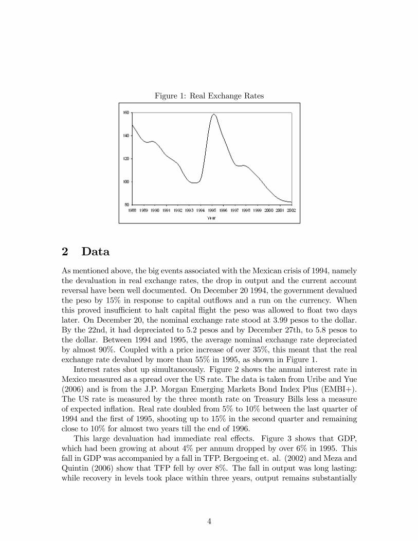
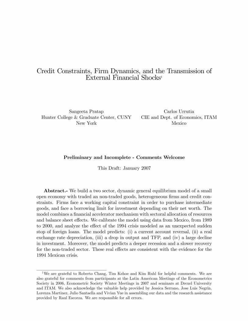
Figure 1: Real Exchange Rates

2 Data

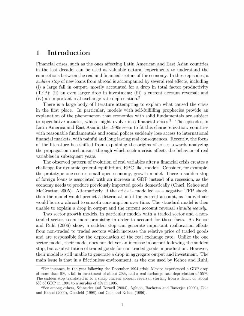
As mentioned above, the big events associated with the Mexican crisis of 1994, namelythe devaluation in real exchange rates, the drop in output and the current accountreversal have been well documented. On December 20 1994, the government devaluedthe peso by 15% in response to capital out�ows and a run on the currency. Whenthis proved insu¢ cient to halt capital �ight the peso was allowed to �oat two dayslater. On December 20, the nominal exchange rate stood at 3.99 pesos to the dollar.By the 22nd, it had depreciated to 5.2 pesos and by December 27th, to 5.8 pesos tothe dollar. Between 1994 and 1995, the average nominal exchange rate depreciatedby almost 90%. Coupled with a price increase of over 35%, this meant that the realexchange rate devalued by more than 55% in 1995, as shown in Figure 1.Interest rates shot up simultaneously. Figure 2 shows the annual interest rate in

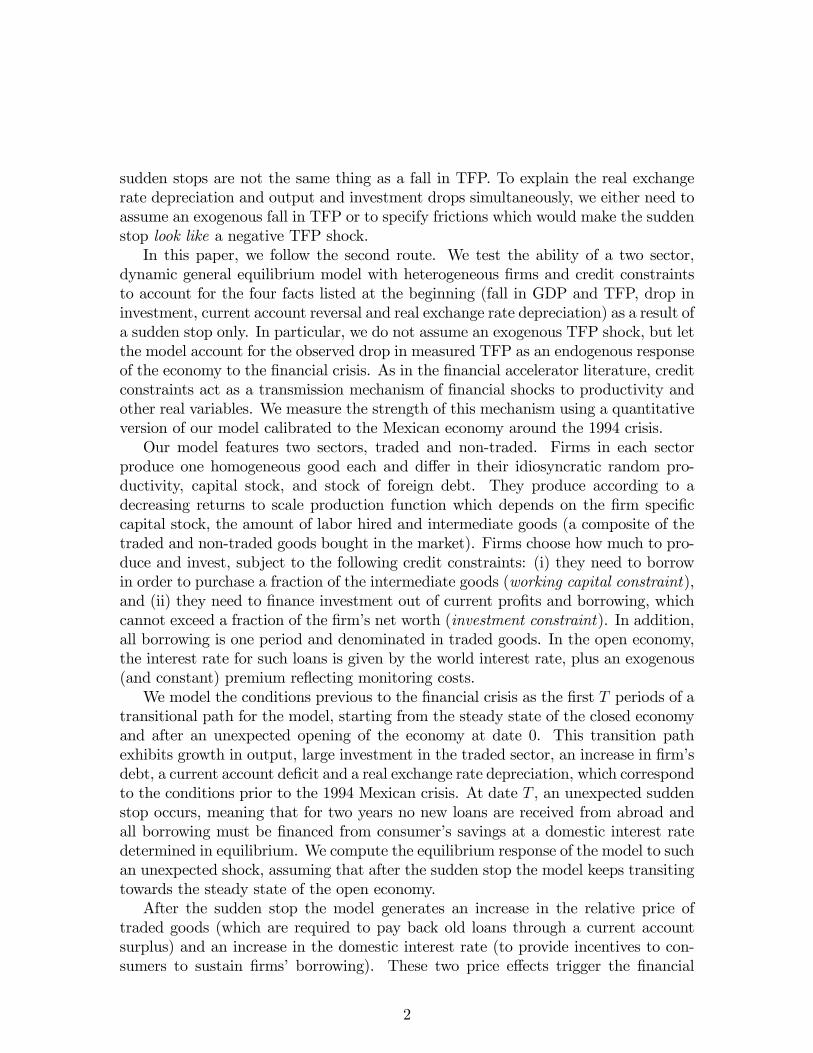
Mexico measured as a spread over the US rate. The data is taken from Uribe and Yue(2006) and is from the J.P. Morgan Emerging Markets Bond Index Plus (EMBI+).The US rate is measured by the three month rate on Treasury Bills less a measureof expected in�ation. Real rate doubled from 5% to 10% between the last quarter of1994 and the �rst of 1995, shooting up to 15% in the second quarter and remainingclose to 10% for almost two years till the end of 1996.This large devaluation had immediate real e¤ects. Figure 3 shows that GDP,

which had been growing at about 4% per annum dropped by over 6% in 1995. Thisfall in GDP was accompanied by a fall in TFP. Bergoeing et. al. (2002) and Meza andQuintin (2006) show that TFP fell by over 8%. The fall in output was long lasting:while recovery in levels took place within three years, output remains substantially

4

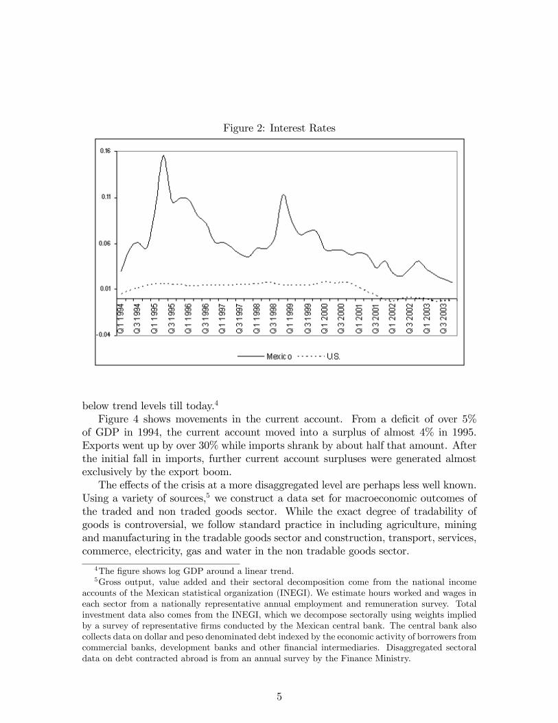
Figure 2: Interest Rates

below trend levels till today.4

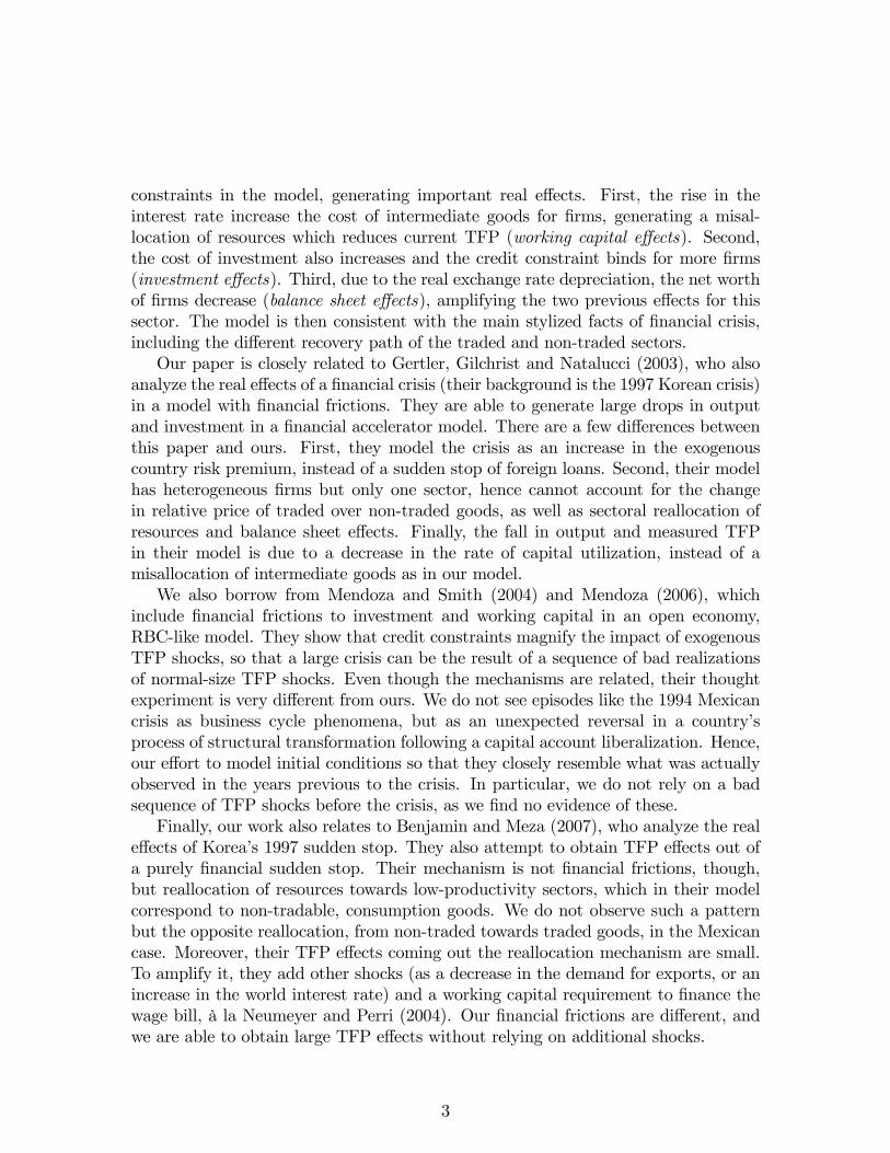
Figure 4 shows movements in the current account. From a de�cit of over 5%of GDP in 1994, the current account moved into a surplus of almost 4% in 1995.Exports went up by over 30% while imports shrank by about half that amount. Afterthe initial fall in imports, further current account surpluses were generated almostexclusively by the export boom.The e¤ects of the crisis at a more disaggregated level are perhaps less well known.

Using a variety of sources,5 we construct a data set for macroeconomic outcomes ofthe traded and non traded goods sector. While the exact degree of tradability ofgoods is controversial, we follow standard practice in including agriculture, miningand manufacturing in the tradable goods sector and construction, transport, services,commerce, electricity, gas and water in the non tradable goods sector.

4The �gure shows log GDP around a linear trend.5Gross output, value added and their sectoral decomposition come from the national income

accounts of the Mexican statistical organization (INEGI). We estimate hours worked and wages ineach sector from a nationally representative annual employment and remuneration survey. Totalinvestment data also comes from the INEGI, which we decompose sectorally using weights impliedby a survey of representative �rms conducted by the Mexican central bank. The central bank alsocollects data on dollar and peso denominated debt indexed by the economic activity of borrowers fromcommercial banks, development banks and other �nancial intermediaries. Disaggregated sectoraldata on debt contracted abroad is from an annual survey by the Finance Ministry.

5

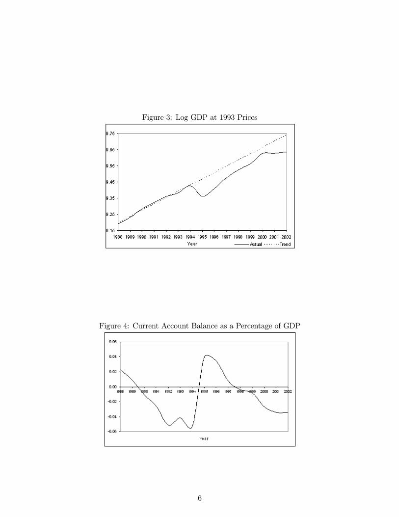
Figure 3: Log GDP at 1993 Prices

Figure 4: Current Account Balance as a Percentage of GDP

6

Figure 5: Log GDP in the Traded Goods Sector

Our discussion is organized around three key facts: (a) The traded goods sectorsu¤ered a smaller drop in output and recovered faster than the non traded goodssector. This was accompanied by a reallocation of labor from the non traded tothe traded sector. (b) While borrowing in both sectors declined, the traded goodssector had substantially more access to credit from abroad than the non traded goodssector. (c) Although the recovery from the crisis was essentially a recovery of thetraded goods sector, the export boom petered out and both sectors stagnated in themedium term.Figure 5 and 6 illustrate these facts. Output in the T sector, which was growing

at around 3.2% before the devaluation, declined initially by 3% in 1995. In 1996,the T sector made a strong recovery and output not only recovered, but surpassedtrend growth within the next two years. The N sector on the other hand, faced aninitial output decline of more than 7% after the devaluation. While growth resumedin 1996, output grew slower than in the T sector has been below trend levels for theentire period.As Figure 7 shows, the immediate aftermath of the crisis involved a reallocation of

production from the N to the T sector. Prior to the devaluation, the ratio of T sectoroutput to N sector declined from 0.37 in 1990 to 0.34 in 1994, re�ecting the worldwidetrend of a decline in manufacturing relative to the service sector. The devaluationreversed this trend and in 1995 the ratio increased to 0.36 and to 0.39 in 1998.The change in the sectoral composition of output was also re�ected in the reallo-

cation of labor. Figure 8 shows the ratio of hours worked in T sector relative to theN sector.Prior to the devaluation, the ratio of T sector output to N sector declined from 0.37

in 1990 to 0.34 in 1994, re�ecting the worldwide trend of a decline in manufacturing

7

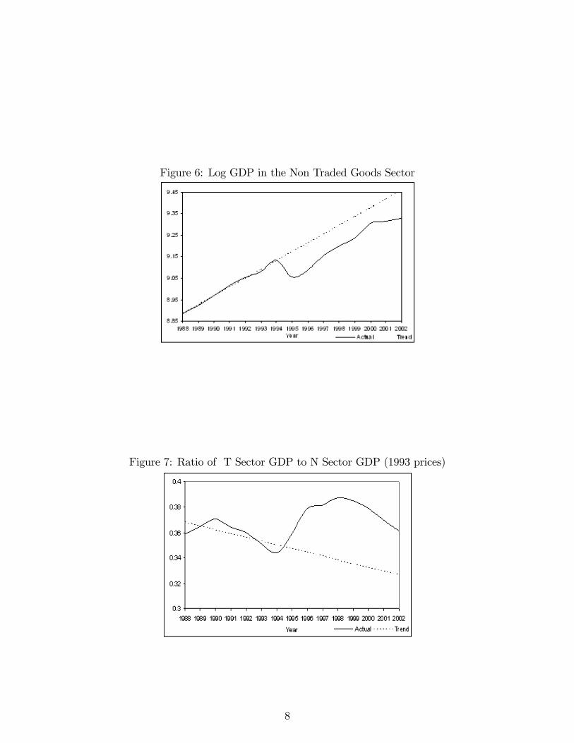
Figure 6: Log GDP in the Non Traded Goods Sector

Figure 7: Ratio of T Sector GDP to N Sector GDP (1993 prices)

8

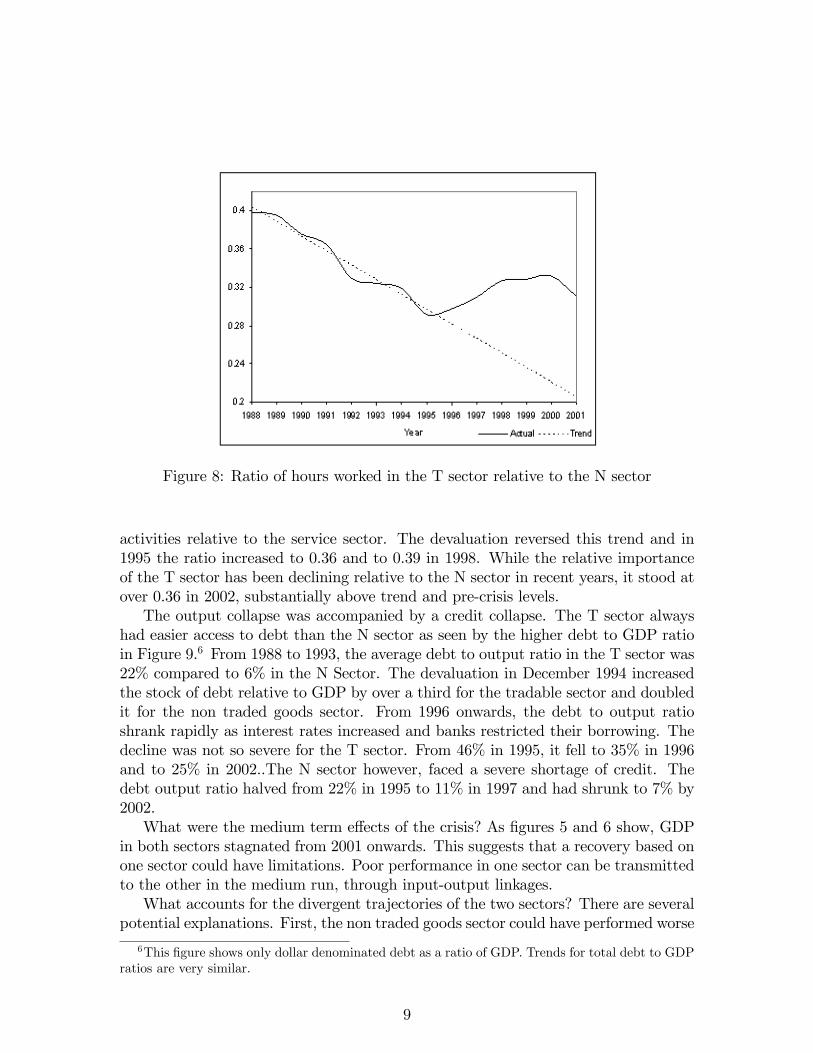
Figure 8: Ratio of hours worked in the T sector relative to the N sector

activities relative to the service sector. The devaluation reversed this trend and in1995 the ratio increased to 0.36 and to 0.39 in 1998. While the relative importanceof the T sector has been declining relative to the N sector in recent years, it stood atover 0.36 in 2002, substantially above trend and pre-crisis levels.The output collapse was accompanied by a credit collapse. The T sector always

had easier access to debt than the N sector as seen by the higher debt to GDP ratioin Figure 9.6 From 1988 to 1993, the average debt to output ratio in the T sector was22% compared to 6% in the N Sector. The devaluation in December 1994 increasedthe stock of debt relative to GDP by over a third for the tradable sector and doubledit for the non traded goods sector. From 1996 onwards, the debt to output ratioshrank rapidly as interest rates increased and banks restricted their borrowing. Thedecline was not so severe for the T sector. From 46% in 1995, it fell to 35% in 1996and to 25% in 2002..The N sector however, faced a severe shortage of credit. Thedebt output ratio halved from 22% in 1995 to 11% in 1997 and had shrunk to 7% by2002.What were the medium term e¤ects of the crisis? As �gures 5 and 6 show, GDP

in both sectors stagnated from 2001 onwards. This suggests that a recovery based onone sector could have limitations. Poor performance in one sector can be transmittedto the other in the medium run, through input-output linkages.What accounts for the divergent trajectories of the two sectors? There are several

potential explanations. First, the non traded goods sector could have performed worse

6This �gure shows only dollar denominated debt as a ratio of GDP. Trends for total debt to GDPratios are very similar.

9

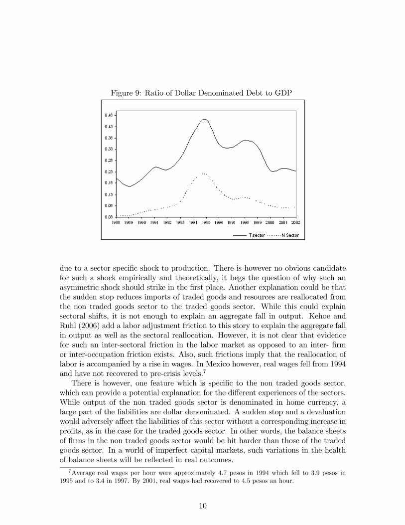
Figure 9: Ratio of Dollar Denominated Debt to GDP

due to a sector speci�c shock to production. There is however no obvious candidatefor such a shock empirically and theoretically, it begs the question of why such anasymmetric shock should strike in the �rst place. Another explanation could be thatthe sudden stop reduces imports of traded goods and resources are reallocated fromthe non traded goods sector to the traded goods sector. While this could explainsectoral shifts, it is not enough to explain an aggregate fall in output. Kehoe andRuhl (2006) add a labor adjustment friction to this story to explain the aggregate fallin output as well as the sectoral reallocation. However, it is not clear that evidencefor such an inter-sectoral friction in the labor market as opposed to an inter- �rmor inter-occupation friction exists. Also, such frictions imply that the reallocation oflabor is accompanied by a rise in wages. In Mexico however, real wages fell from 1994and have not recovered to pre-crisis levels.7

There is however, one feature which is speci�c to the non traded goods sector,which can provide a potential explanation for the di¤erent experiences of the sectors.While output of the non traded goods sector is denominated in home currency, alarge part of the liabilities are dollar denominated. A sudden stop and a devaluationwould adversely a¤ect the liabilities of this sector without a corresponding increase inpro�ts, as in the case for the traded goods sector. In other words, the balance sheetsof �rms in the non traded goods sector would be hit harder than those of the tradedgoods sector. In a world of imperfect capital markets, such variations in the healthof balance sheets will be re�ected in real outcomes.

7Average real wages per hour were approximately 4.7 pesos in 1994 which fell to 3.9 pesos in1995 and to 3.4 in 1997. By 2001, real wages had recovered to 4.5 pesos an hour.

10

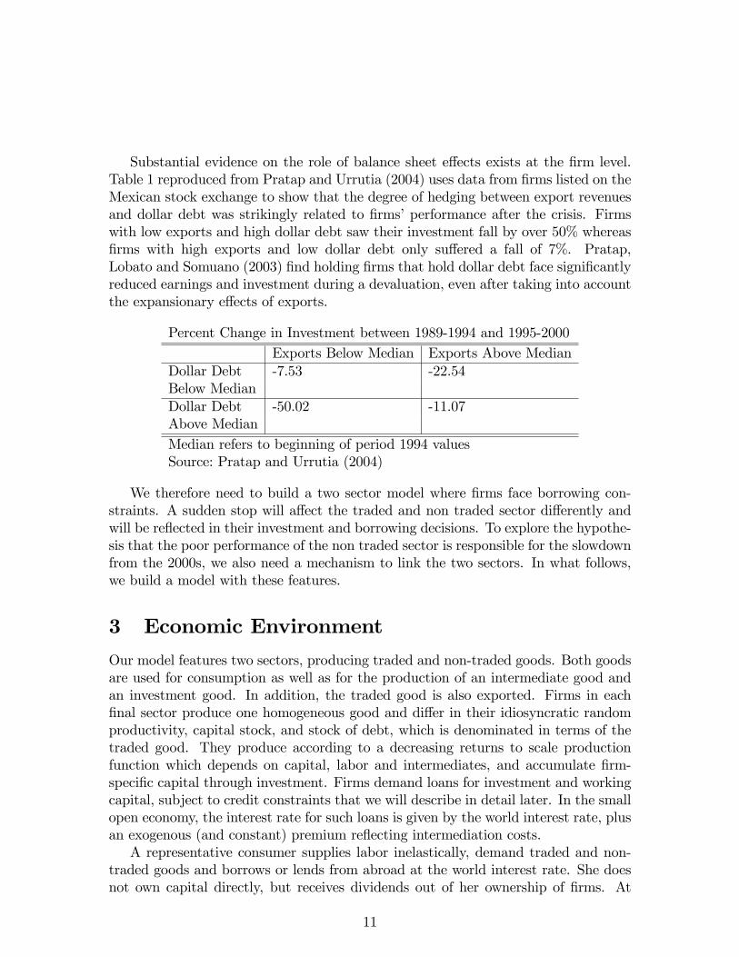
Substantial evidence on the role of balance sheet e¤ects exists at the �rm level.Table 1 reproduced from Pratap and Urrutia (2004) uses data from �rms listed on theMexican stock exchange to show that the degree of hedging between export revenuesand dollar debt was strikingly related to �rms�performance after the crisis. Firmswith low exports and high dollar debt saw their investment fall by over 50% whereas�rms with high exports and low dollar debt only su¤ered a fall of 7%. Pratap,Lobato and Somuano (2003) �nd holding �rms that hold dollar debt face signi�cantlyreduced earnings and investment during a devaluation, even after taking into accountthe expansionary e¤ects of exports.

Percent Change in Investment between 1989-1994 and 1995-2000Exports Below Median Exports Above Median

Dollar Debt -7.53 -22.54Below MedianDollar Debt -50.02 -11.07Above MedianMedian refers to beginning of period 1994 valuesSource: Pratap and Urrutia (2004)

We therefore need to build a two sector model where �rms face borrowing con-straints. A sudden stop will a¤ect the traded and non traded sector di¤erently andwill be re�ected in their investment and borrowing decisions. To explore the hypothe-sis that the poor performance of the non traded sector is responsible for the slowdownfrom the 2000s, we also need a mechanism to link the two sectors. In what follows,we build a model with these features.

3 Economic Environment

Our model features two sectors, producing traded and non-traded goods. Both goodsare used for consumption as well as for the production of an intermediate good andan investment good. In addition, the traded good is also exported. Firms in each�nal sector produce one homogeneous good and di¤er in their idiosyncratic randomproductivity, capital stock, and stock of debt, which is denominated in terms of thetraded good. They produce according to a decreasing returns to scale productionfunction which depends on capital, labor and intermediates, and accumulate �rm-speci�c capital through investment. Firms demand loans for investment and workingcapital, subject to credit constraints that we will describe in detail later. In the smallopen economy, the interest rate for such loans is given by the world interest rate, plusan exogenous (and constant) premium re�ecting intermediation costs.A representative consumer supplies labor inelastically, demand traded and non-

traded goods and borrows or lends from abroad at the world interest rate. She doesnot own capital directly, but receives dividends out of her ownership of �rms. At

11

each period, markets for the traded good, non-traded good, as well as for labor, theintermediate good and the investment good clear. We now describe this economy indetail.

3.1 Consumers

The representative consumer is endowed with one unit of labor which she suppliesinelastically. She consumes the traded (T ) and the non traded (N) sector goods withCobb Douglas preferences. She can lend or borrow at the risk-free world interest rater�, measured in units of the traded good. Her optimization problem can be writtenas:

maxfCTt ;CNt ;st+1g1t=0

1Xt=0

�t� log

�CTt�+ (1� ) log

�CNt��

s.to CTt + pnt CNt + st+1 = wt + (1 + rt) st + �t

where st are consumer�s savings and �t represents aggregate dividends. We use theprice of traded goods as numeraire, so that pnt is the price of non-traded goods overtraded goods (the inverse of the real exchange rate) and wt is the wage in period t,also in terms of the traded good.

3.2 Intermediate Good Sector

The representative �rm in this sector combines traded good and non traded goods toproduce intermediate goods, according to the production function

M = Am�MT

�� �MN

�1��The problem of the representative �rm can be written as

maxfMt;MT

t ;MNt g

�pmt Mt �MT

t � pntMNt

s.to Mt = Am

�MTt

�� �MNt

�1��Notice that, since production is constant returns to scale: (i) pro�ts are zero in thissector; and (ii) we cannot pin down the output of the intermediate goods sector fromthe supply side, but from market clearing conditions.

3.3 Investment Good Sector

There is also a representative �rm in this sector, combining traded good and nontraded goods to produce the investment good. The problem of this representative�rm can be written as

maxfXt;XT

t ;XNt g

�pxtXt �XT

t � pntXNt

12

s.to Xt = Ax�XTt

�� �XNt

�1��This sector also exhibits zero-pro�ts.

3.4 Traded Good Sector

There is a continuum of ex-ante equal �rms in this sector. To produce traded goods,these �rms combine capital, labor and intermediate goods according to the productionfunction:

Y = AT �i��k�T l1��T

�"T m1�"T��

with �T ; "T ; v 2 (0; 1). �i is a discrete, i.i.d., idiosyncratic shock with supportf�L; �M ; �Hg and probability function � (�i). Sector-speci�c capital is owned by the�rm and it is accumulated through investment xt according to the law of motion:

kt+1 = (1� �) kt + xt

Each period, �rms face an exogenous probability of bankruptcy �:Firms face two constraints: (i) they need to purchase intermediate goods at the

beginning of the period before production using within period loans, in units of thesame traded good; and (ii) in order to �nance investment, �rms must rely on currentpro�ts and/or between period loans, subject to a borrowing constraint depending onits net worth. They also cannot issue equity to �nance investment (dividends mustbe always non-negative). Both types of loans are contracted at the interest rate

brt+1 = 1 + rt+1 + �

1� �� 1

where � > 0 is an exogenous �nancial intermediation cost and the denominatoraccounts for the (exogenous) risk of default.The �rm�s problem can be divided into static and dynamic decisions.

Static DecisionsGiven �i, k and prices, �rms must choose the level of labor and intermediate goods

to maximize within-period pro�ts

�Tt (�i; k) = maxfY;l;mg

fY � wtl � (1 + brt+1) pmt mgs.to Y = AT �i

��k�T l1��T

�"T m1�"T��

Notice that the cost of credit brt+1 a¤ects the e¤ective price of intermediate goodsfor the �rm. This problem delivers static decision rules for input demands: laborlTt (�i; k) and intermediate goods m

Tt (�i; k), and gross output y

Tt (�i; k) and within-

period pro�ts �Tt (�i; k) as functions of the state variables.Dynamic Decisions

13

To �nance investment, �rms must rely on current pro�ts and/or loans (in unitsof the same traded good), contracted at the rate brt+1:

pxt x � �Tt (�i; k) + b0 � (1 + brt) bwhere b0 is new borrowing and x is investment. This constraint implies that divi-dends must be always non-negative. We also impose the restriction that �rms canonly borrow up to a fraction of the value of their net worth (current pro�ts plusundepreciated capital minus current liabilities):

b0 � ��Tt (�i; k) + (1� �) pxt k � (1 + brt) b�

Since in equilibirum brt+1 > r�, �rms would never want to borrow more than theamount strictly required for investment. In particular, �rms would not borrow fundsjust to redistribute them as dividends. We also assume that �rms cannot not save inthe �nancial market, i.e., b0 � 0. The �rm�s dynamic problem can then be writtenrecursively as

V Tt (�i; k; b) = max

fk0;b0g

��Tt (�i; k) + (1� �) pxt k � pxt k

0 + b0 � (1 + brt) b+

�1� �

1 + r�

� P�j2f�L;�M ;�Hg

� (�j)VTt+1 (�j; k

0; b0)

)subject to

pxt k0 � (1 + )

��Tt (�i; k) + (1� �) pxt k � (1 + brt) b�

andb0 = max

�pxt k

0 ���Tt (�i; k) + (1� �) pxt k � (1 + brt) b� ; 0

The solution to this problem delivers decision rules k0Tt (�i; k; b), b0Tt (�i; k; b) and div-

idends

�Tt (�i; k; b) = �Tt (�i; k) + (1� �) pxt k � pxt k

0Tt (�ik; b) + b0Tt (�i; k; b)� (1 + brt) b

3.5 Non-Traded Goods Sector

Firms in this sector make analogous decisions. The static decision (in units of thetraded good) is represented by the problem:

�Nt (�i; k) = maxfY;l;mg

fpnt Y � wtl � (1 + brt+1) pmt mgs.to Y = AN�i

��k�N l1��N

�"N m1�"N��

Notice that the cost of credit brt+1 also a¤ects the e¤ective price of intermediate goodsfor these �rms. The problem delivers static decision rules for labor lNt (�i; k), demand

14

for intermediate goods mNt (�i; k), gross output y

Nt (�i; k) and within-period pro�ts

�Nt (�i; k).The dynamic decision can be written recursively as

V Nt (�i; k; b) = max

fk0;b0g

��Nt (�i; k) + (1� �) pxt k � pxt k

0 + b0 � (1 + brt) b+

�1� �

1 + r�

� P�j2f�L;�M ;�Hg

� (�j)VNt+1 (�j; k

0; b0)

)subject to

pxt k0 � (1 + )

��Nt (�i; k) + (1� �) pxt k � (1 + brt) b�

andb0 = max

�pxt k

0 ���Nt (�i; k) + (1� �) pxt k � (1 + brt) b� ; 0

The solution to this problem delivers decision rules k0Nt (�i; k; b), b0Nt (�i; k; b) anddividends

�Nt (�i; k; b) = �Nt (�i; k) + (1� �) pxt k � pxt k

0Nt (�ik; b) + b0Nt (�i; k; b)� (1 + brt) b

Notice that the pro�ts in the non traded sector are in units of the non-tradedgood, but borrowing is in units of the traded good. This will be responsible for thedi¤erential performance of each sector in the recovery.Notice also that we assume a common process for productivity (�), returns to

scale parameter (�), depreciation rate (�), banktrupcy probability (�), cost of credit(brt+1), and borrowing constraint tightness ( ) for all �rms in the two sectors.3.6 Entry, Exit and Distribution of Firms

We denote the distribution of operating �rms in the traded sector by �Tt (�i; k; b), andby �N (�i; k; b) in the non-traded sector. At each period, some �rms in both sectors aredestroyed by the bankruptcy shock. We assume for simplicity that each �rm destroyedis replaced by a new �rm with the lowest level of capital, average productivity andno debt. Together with the decision rules for investment and borrowing, these entryconditions de�ne the laws of motion of the distribution of �rms in the traded sector:

�Tt+1 (�M ; kmin; 0) = �

and

�Tt+1 (�j; k0; b0) = (1� �) � (�j)

Z(�i;k;b)

I[k0Tt (xTt (�i;k;b))=k0]I[b0Tt (xTt (�i;k;b))=b0]

d�Tt (�i; k; b)

where I is the indicator function. Similarly, for the non-traded sector

�Nt+1 (�M ; kmin; 0) = �

15

and

�Nt+1 (�j; k0; b0) = (1� �) � (�j)

Z(�i;k;b)

I[k0Nt (xNt (�i;k;b))=k0]I[b0Nt (xNt (�i;k;b))=b0]

d�Nt (�i; k; b)

Given these distributions, we can compute aggregate demand for labor and inter-mediate goods as well as output in traded sector:

lTt =

Z(�i;k;b)

lTt (�i; k) d�Tt (�i; k; b)

mTt =

Z(�i;k;b)

lTt (�i; k) d�Tt (�i; k; b)

yTt =

Z(�i;k;b)

yTt (�i; k) d�Tt (�i; k; b)

The stock of capital and outstanding debt in each sector is given by

kTt =

Z(�i;k;b)

kd�Tt (�i; k; b)

bTt =

Z(�i;k;b)

kd�Tt (�i; k; b)

The distribution of �rms as well as the other quantities are calculated analogouslyfor the non traded sector.

3.7 Equilibrium in the Open Economy

The model is closed by imposing the following market clearing conditions: (i) for theintermediate good:

mTt +mN

t =Mt

(ii) for the investment good:xTt + xNt = Xt

(iii) for the traded good:

CTt +NXt = yTt �MTt �XT

t

where NXt are net exports; (iv) for the non-traded good:

CNt = yNt �MNt �XN

t

and (v) for labor:lTt + lNt = 1

Notice that, in equilibrium, the balance of payments identity (net exports equalsnet capital out�ows) always holds

NXt = r�pmt�mTt +mN

t

�+�st+1 � bTt+1 � bNt+1

�� (1 + r�)

�st � bTt � bNt

�16

4 Calibration

We calibrate the model to match key features of the Mexican economy in the pre-crisis period from 1988-1994. Since our model is multisectoral, we need informationabout the interaction of sectors in the economy. While input output tables would bea valuable resource, the last input output table for Mexico was constructed in 1970and recent versions consist of updates using the RAS method. Since this method isunlikely to be able to capture the large structural changes in the Mexican economyover the past 30 years, we use input output tables as little as possible, relying insteadon National Income and Product Accounts (NIPA) wherever feasible. The parameterscalibrated and the statistics they match are summarized in Table 1.

Consumption The consumption parameter can be calculated from the ratioof consumption of traded and non traded goods. The model implies that

CTtpnt C

Nt

=

�

1�

�Since our model does not include a role for the government, total consumption in eachsector is calculated by aggregating private and government consumption for each year.This implies a value of of 0.45. The discount factor � is calibrated to the worldinterest rate of 5%.

Intermediate Goods Producers Similarly, the demand for traded and nontraded goods by intermediate goods producers problem gives us

MTt

pntMNt

=

��

1� �

�From the NIPA we can back out the amount of gross output of each sector used asintermediate goods. These are used to construct �:

Capital goods producers: The demand for traded and non traded goods bycapital goods producers also follows the ratio

XTt

pntXNt

=

��

1� �

�Since we know the amount of each good used in capital formation, we can use theirratio to back out �:

17

Production Function Parameters The share of intermediate goods in grossoutput can be assessed from the ratio of sectoral value added to gross output. Thenwe have �

Value AddedGross Output

�J

= 1� (1� "J) � where J = T;N

Taking � = 0:9 for both sectors, this implies a value of "T = 0:32 and "N = 0:78:The share of labor in GDP from the NIPA is about 33% and its lack of conformity

with other countries has long been a source of puzzlement. Using household surveydata, Garcia-Verdu (2005) estimates labor share in aggregate GDP to be closer to theshares in the U.S. and other countries with estimates ranging from 57% to 73%. Wecalibrate labor share in each sector to match the average of these estimates (66%) inthe aggregate. We know that aggregate labor shares must be a weighted average ofthe sectoral labor shares. In other words

Labor IncomeGDP

=

�Labor Income

GDP

�T

�GDPTGDP

�+

�Labor Income

GDP

�N

�GDPNGDP

�Using the proportion of labor income to GDP between the T and sector implied bythe NIPA each year (about 0.80), we calculate the sectoral labor share in GDP. Inthe context of our model,�

Labor IncomeGDP

�J

=(1� �J) "J�

1� (1� "J) �where J = T;N

Given values for �J and "J calibrated previously we get 1� �T = 0:75 and 1� �N =0:80:8

Calibrated ParametersStatistic Target Parameter ValueRatio of T to N consumption 0.83 0.45World risk free rate 0.05 r� 0.05Ratio of T to N intermediate goods 2.99 � 0.75Ratio of T to N investment goods 0.98 � 0.49Returns to Scale Parameter � 0.9Ratio of value added to GDP in T sector 0.38 "T 0.32Ratio of value added to GDP in N sector 0.40 "N 0.79Ratio of labor share in GDP between T and N sector (1� �T ) 0.74(Aggregate Labor Share in GDP=0.66) (1� �N) 0.80

8For robustness, we also checked the proportionality between labor share in the two sectors frominput-output tables and scaled them to match an aggregate labor share of 0.66. The results werevery similar: (1� �T ) = 0:76 and (1� �N ) = 0:79:

18

Additional Parameters: In a preliminary calibration attempt, we normal-ized AT = 1 and chose the scale parameters Ax, Am and AN , plus the strength of theborrowing constraint for investment , in order to reproduce in the stationary equi-librium of the model an investment rate of 25% for the traded sector, of 15% for thenon-traded sector, a debt-to output ratio of about 10% in each sector. We also chosea depreciation rate of 5% per year, a turnover rate of 10%, a small intermediation costof 1% and an arbitrary stochastic process for �rms�productivities. A more carefulcalibration procedure will choose these parameters as to reproduce some patterns ofthe pre-crisis transition for Mexico, like the speed of convergence (in progress).

Additional ParametersAT AN Ax Am � � �1 0.62 1.15 1.21 0.15 0.05 0.01 0.1

Stochastic Process�L �M �H � (�L) � (�M) � (�H)0.8 1 1.2 0.25 0.5 0.25

5 Preliminary Results

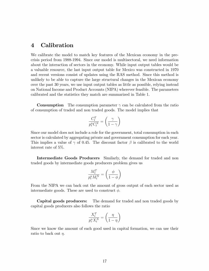
We perform the following experiment: Starting from the stationary equilibrium ofthe model calibrated in the previous section, we shock the model with an unexpectedsudden stop. At date T , corresponding to the year 1995 in Mexico, no new loansarrive from abroad, so �rms must rely on consumer�s savings in order to �nanceworking capital and investment. The sudden stop lasts for two periods (years), andthis is perfectly anticipated by agents. At date T + 2, the economy can borrow/saveagain unlimited amounts at the world interest rate r�. The response of the main realvariables of the model to the sudden stop is illustrated in Figures 10 and 11.During the sudden stop, the risk free rate for loans is given by the domestic

interest rate which equilibrates the domestic credit market. As a result, the interestrate increases from 5% before the crisis to about 21% while the sudden stop lasts.We do observe such an increase in domestic interest rates in Mexico after the crisis,although the magnitude of the change is a bit smaller (a domestic interest rate closeto16% in 1995). Moreover, as in the model, the domestic interest rate in Mexico cameback to the pre-crisis level in two years.The cut in foreign loans re�ects directly in the current account. In the model,

the ratio of net exports over GDP goes form a 0.5% de�cit before the crisis to a5% superavit in the year where the sudden stop occurs. A similar current accountreversal is observed in the Mexican experience. Again, in the data and in the model,the improvement in the current account is short-lived and comes back to a smallde�cit in the following years. The reallocation required to sustain the current account

19

Figure 10: Time Series Generated by the Model as a Response to a Sudden Stop (I)

20

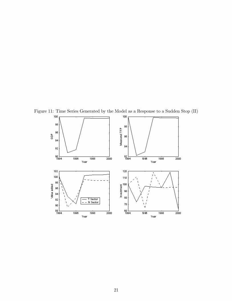
Figure 11: Time Series Generated by the Model as a Response to a Sudden Stop (II)

21

superavit generates also important e¤ects in the relative price of traded vs. non-tradedgoods, which increase by 10% in the model. This is short of the 50% depreciation ofthe real exchange rate observed in the Mexican case, but it accounts for the observedchange in relative prices of traded over non-traded goods (about 8.5% from 1994 to1995). The model also predicts a 15% drop in real wages.So far, the model is consistent with: (i) the rise in interest rates; (ii) the current

account reversal; and (iii) the real exchange rate depreciation (or, at least, the changein relative prices between the traded and non-traded goods). Kehoe and Ruhl (2007)obtained a similar set of results, based on the same sectoral reallocation mechanism.However, in their frictionless model this reallocation does not have neither outputnor TFP e¤ects, and the predictions for investment are ambiguous (an increase ininvestment for the traded sector, and a decrease for the non�traded sector).In our model, the �nancial frictions amplify the e¤ects of the sudden stop to

aggregate quantities, as Figure 11 shows. The model predicts a drop in GDP ofabout 9% after the crisis, from which most of it is accounted for a 7% fall in TFP.This overestimates the drop in Mexican GDP in 1995, which was only 6%. Therecovery, at least in levels, takes two-three years in the model, as well as in the data.The fall in TFP, which is key to explain the real e¤ects of the sudden stop, is due tothe working capital constraint and the misallocation of inputs following the increasein interest rates, which generate a wedge between the price of intermediate goodspaid by users and received by producers.However, this pattern of aggregate recovery masks important di¤erences across

sectors. In the model, as well as in the data, the recession a¤ects both the tradedand non-traded sectors. However, the fall in GDP is bigger in the non-traded sector,and the recovery takes longer. Also, investment falls more in the non-traded sector,although with a one year lag.9 These patterns match very well the stylized factsobserved in the case of Mexico, and highlight the role of balance sheet e¤ects inpropagating the �nancial crisis.For now, we should interpret these results as a set of impulse-response functions,

providing some intuition about what the model can deliver. The experiment that wewant to perform (in progress) di¤ers in two key aspects: (i) we want to start notfrom the stationary equilibrium, but a transition path re�ecting the opening of theeconomy in the years prior to the crisis; and (ii) we want to add uncertainty aboutthe sudden stop itself. Still, we believe the main results that we obtained will carryon to the more sophisticated experiments.

9In general, the model generates too much volatility in investment over time, suggesting that�nancial frictions might not completely replace adjustment costs in capital in terms of delivering asmooth adjustment in the aggregate.

22

6 Conclusions

(to be written)

23

References

[1] Aghion, P., Bacchetta P., and Banerjee, A., (2000) �A Simple Model of MonetaryPolicy and Currency Crises�, European Economic Review, 44, pp. 728-738.

[2] Benjamin, D.M. and Meza, F., (2007) �Total Factor Productivity and LaborReallocation: The Case of the Korean 1997 Crisis�, mimeo.

[3] Bergoeing, R., Kehoe, P., Kehoe, T., Soto, R. (2002) �Decades Lost and Found:Mexico and Chile Since 1980�. Federal Reserve Bank of Minneapolis QuarterlyReview, Winter.

[4] Chari, V.V, Kehoe, P.J., and McGrattan, E., (2005). �Sudden Stops and OutputDrops�, American Economic Association Papers and Proceedings, 95, pp.381-387.

[5] Chari, V.V, Kehoe, P.J., and McGrattan, E., (2006). �Business Cycle Account-ing�, Econometrica, forthcoming.

[6] Cole, H.L. and Kehoe, T.J. (2000). �Self Ful�lling Debt Crises�, Review of Eco-nomic Studies, 67, pp. 91-116.

[7] Cole, H.L. and Kehoe, T.J. (1996).�A Self-Ful�lling Model of Mexico�s 1994-�95Debt Crisis�, Journal of International Economics, 41, pp. 309-330.

[8] Garcia-Verdu, R., (2005). �Factor Shares from Household Survey Data�, mimeo.

[9] Gertler, M., Gilchrist, S., and Natalucci, F.M., �External Constraints on Mone-tary Policy and the Financial Accelerator�, Journal of Money, Credit and Bank-ing, forthcoming.

[10] Kehoe, T.J., and Ruhl, K.J., (2006) �Sudden Stops, Sectoral Reallocations andthe Real Exchange Rate�, mimeo.

[11] Obstfeld, M., (1998) �Financial Shocks and Business Cycles: Lessons from Out-side the United States�, in J.C. Fuhrer and S.Schuh (eds).What Causes BusinessCycles, Federal Reserve of Boston, Conference Series.

[12] Mendoza, E.G. and Smith, K.A. (2005). �Quantitative Implications of a DebtDe�ation Theory of Sudden Stops and Asset Prices�, Journal of InternationalEconomics, forthcoming.

[13] Mendoza, E.G.(2006).�Endogenous Sudden Stops in a Business Cycle Model withCollateral Constraints: A Fisherian De�ation of Tobin�s Q�, mimeo.

[14] Meza, F., and Quintin, E., (2006). �Financial Crises and Total Factor Produc-tivity�, mimeo.

24

[15] Neumeyer, P.A. and Perri, F., (2005). �Business Cycles in Emerging Economies:the Role of Interest Rates�, Journal of Monetary Economics, 52, pp. 345-380.

[16] Pratap, S., Lobato I.N., and Somuano, A. (2003). �Debt Composition and Bal-ance Sheet E¤ects of Exchange Rate Volatility in Mexico: A Firm Level Analy-sis�, Emerging Markets Review, 450-471.

[17] Pratap, S., and Urrutia, C., (2004). �Firm Dynamics, Investment and CurrencyComposition of Debt: Accounting for the Real E¤ects of the Mexican Crisis of1994�, Journal of Development Economics, 75, 535-563.

[18] Schneider, M., and A. Tornell (2004). �Balance Sheet E¤ects, Bailout Guaran-tees, and Financial Crisis�, Review of Economic Studies, 71, pp. 883-913.

[19] Uribe, M., and Yue, V.Z. (2006). �Country Spreads and Emerging Countries:Who Drives Whom?�Journal of International Economics, 69, pp. 6-36.

25