cranfield university françois pierrel phd. thesis
TRANSCRIPT
CRANFIELD UNIVERSITY
François Pierrel
PhD. Thesis
School of Engineering
This thesis is submitted in partial fulfilment of the requirements
for the Degree of Doctor of Philosophy
CRANFIELD UNIVERSITY
SCHOOL OF ENGINEERING
PhD
Academic Year 1998−2003
François Pierrel
Examination of Heat Transfer in Baking using a Thermal Performance Research Oven
Supervisor: Prof M Newborough
This thesis is submitted in partial fulfillment of the requirementsfor the Degree of Doctor of Philosophy

To my parents, brother and sister and Ratna for her patience, understanding and unconditional support throughout.
Mens sana in corpore sano.......Juvenal
TABLE OF CONTENTS
i
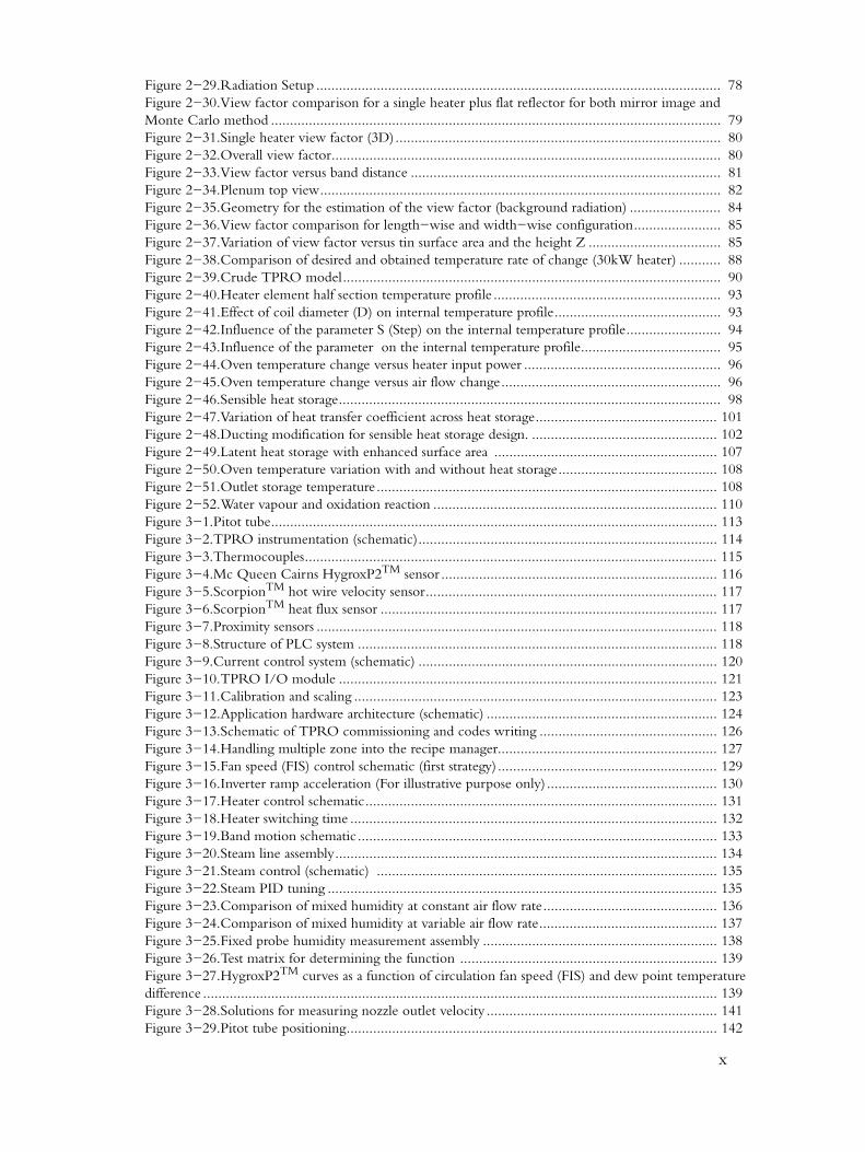
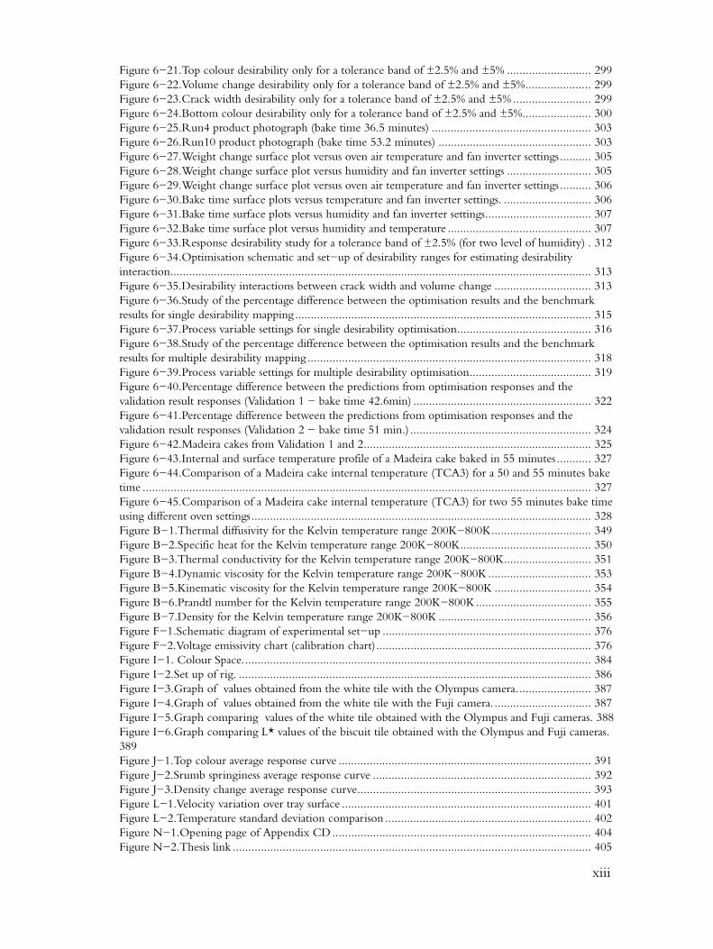
LIST OF FIGURES .................................................................................................... IX
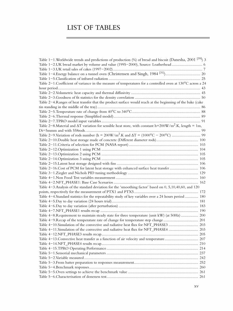
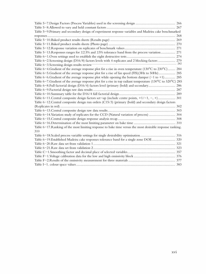
LIST OF TABLES .....................................................................................................XV
LIST OF ABBREVIATIONS .................................................................................XVII
ACKNOWLEDGEMENTS ....................................................................................XXV
ABSTRACT ................................................................................................................. 1
CHAPTER 1 : LITERATURE REVIEW.................................................................... 2
1.1 Introduction ............................................................................................................ 21.2 Trends in the baked products market ....................................................................... 3
1.2.1 The world .........................................................................................................31.2.2 The European Market .......................................................................................41.2.2.1 Bread ............................................................................................................41.2.2.2 Cakes and pastries .........................................................................................71.2.2.3 Biscuits .........................................................................................................9
1.2.3 Industrial travelling oven market ......................................................................101.2.3.1 APV Baker industrial baking ovens .............................................................111.2.3.2 APV oven design family tree .......................................................................15
1.3 From micro to macro heat transfer mechanism ....................................................... 161.3.1 Micro heat transfer mechanism ........................................................................161.3.2 Macro heat transfer mechanism .......................................................................19
1.4 Objectives of investigation ..................................................................................... 30
CHAPTER 2 : CONCEPTS AND DESIGN OF TPRO RIG .................................. 31
2.1 Rig history ............................................................................................................ 312.2 Rig description ...................................................................................................... 32
2.2.1 Air circulation .................................................................................................322.2.2 Methods of heating and humidifying ...............................................................352.2.3 Working ranges ...............................................................................................362.2.4 Changeable parameters within the TPRO .......................................................36
2.3 The TPRO: A Thermal System ............................................................................. 392.3.1 Understanding the TPRO as a thermal system .................................................392.3.1.1 Extra heat load ............................................................................................392.3.1.2 Steady state and transient mode ...................................................................422.3.1.3 Sources of heat loss .....................................................................................462.3.1.4 TPRO Energy balance ...............................................................................47
2.4 Flow and heat transfer solutions ............................................................................. 482.4.1 Properties ........................................................................................................492.4.2 Flow calculations .............................................................................................512.4.2.1 Main feed flow: ..........................................................................................51

TABLE OF CONTENTS
ii
2.4.2.2 Top and bottom nozzle: .............................................................................522.4.2.3 Extraction flow: ..........................................................................................532.4.2.4 Re−circulated flow: ....................................................................................532.4.2.5 Air leakages and infiltration: ........................................................................542.4.2.5.1 ‘Plenum air loss’ .....................................................................................542.4.2.5.2 TPRO chamber air loss .........................................................................552.4.2.5.3 Return duct air loss ................................................................................56
2.4.3 Thermal process energy balance .......................................................................562.4.3.1 Generated energy .......................................................................................562.4.3.1.1 Duct and radiant heaters .........................................................................572.4.3.1.2 Circulation and extraction fans ...............................................................57
2.4.3.2 Energy loss .................................................................................................582.4.3.2.1 Wall convective equivalent heat losses ....................................................582.4.3.2.2 Radiative heat loss .................................................................................612.4.3.2.3 Air losses ................................................................................................622.4.3.2.4 Equivalent thermal bridges .....................................................................64
2.4.3.3 Energy storage ............................................................................................662.5 Real time energy balance ....................................................................................... 68
2.5.1 Real time conflict ............................................................................................692.5.2 Energy terms ...................................................................................................702.5.2.1 Energy input ..............................................................................................702.5.2.2 Energy loss .................................................................................................712.5.2.3 Energy stored .............................................................................................72
2.6 Defining steady−state conditions ............................................................................ 722.7 Heat flux to product surface ................................................................................... 74
2.7.1 Convective heat flux .......................................................................................752.7.1.1 Validity of Reynolds number ......................................................................76
2.7.2 Radiative heat flux ..........................................................................................772.7.2.1 Direct radiation ..........................................................................................792.7.2.2 Background radiation .................................................................................81
2.8 Design challenge .................................................................................................... 872.8.1 Air heater design problem ...............................................................................882.8.2 Heater mass and reaction time .........................................................................89
2.9 TPRO mathematical model ................................................................................... 892.9.1 Prediction tool ................................................................................................902.9.2 Driver for advanced heat transfer method ........................................................902.9.3 Approach to Modelling ...................................................................................902.9.3.1 Changeable parameters within TPRO model ..............................................912.9.3.2 Results of model .........................................................................................922.9.3.2.1 Coil parametric analysis ..........................................................................922.9.3.2.2 Power variation and optimum flow rate .................................................94
2.9.4 Thermal storage modelling ..............................................................................972.9.4.1 Sensible−heat storage ..................................................................................972.9.4.1.1 Feasibility considerations ...................................................................... 100
TABLE OF CONTENTS
iii
2.9.4.2 Conclusion of sensible heat storage ........................................................... 1022.9.4.3 Latent heat storage .................................................................................... 1022.9.4.3.1 Latent storage model ............................................................................ 103
2.9.5 Overall conclusion on heat storage feasibility ................................................. 1082.9.6 Final decision ................................................................................................ 109
CHAPTER 3 : COMPUTER AIDED CONTROL SYSTEM ................................ 111
3.1 Aim and philosophy of the control system ............................................................ 1113.2 Choice of instrumentation ................................................................................... 112
3.2.1 Process instrumentation ................................................................................. 1123.2.1.1 Flow measurement ................................................................................... 1123.2.1.2 Temperature measurement ....................................................................... 1133.2.1.3 Humidity measurement ............................................................................ 1153.2.1.4 Velocity measurement .............................................................................. 1163.2.1.5 Heat flux measurement ............................................................................. 1173.2.1.6 Proximity measurement ............................................................................ 117
3.3 Choice of control system ..................................................................................... 1183.4 Current control system ........................................................................................ 120
3.4.1 DeviceNet Network communication ............................................................ 1203.4.2 I/O module .................................................................................................. 1213.4.3 TPRO commissioning .................................................................................. 1223.4.3.1 Addressing ................................................................................................ 122
3.4.4 Mapping ....................................................................................................... 1223.4.5 Calibration and sensor scaling ........................................................................ 1223.4.6 Global variables ............................................................................................. 1243.4.7 Software capabilities ...................................................................................... 1243.4.7.1 InControlTM ..................................................................................................................... 124
3.4.7.2 InTouchTM ....................................................................................................................... 125
3.4.8 Control routine design .................................................................................. 1273.4.8.1 Recipe Manager ....................................................................................... 1273.4.8.2 Fan speed (FIS) control ............................................................................. 1283.4.8.2.1 First strategy ......................................................................................... 1283.4.8.2.1 Second strategy .................................................................................... 130
3.4.8.3 Heater control .......................................................................................... 1313.4.8.4 Band speed control ................................................................................... 1323.4.8.4.1 Band movement .................................................................................. 132
3.4.8.5 Humidity control ..................................................................................... 1333.4.8.5.1 Strategy of control ............................................................................... 1353.4.8.5.2 Steam measurement ............................................................................. 138
3.4.8.6 Heat flux measurement ............................................................................. 1403.4.8.6.1 Measurement issues in convective heat transfer determination .............. 1403.4.8.6.2 Measurement issues in radiative heat transfer determination .................. 1423.4.8.6.3 Conclusion on method of measuring heat transfer to the product surface 144
TABLE OF CONTENTS
iv
3.4.8.7 Control handling of alarms ....................................................................... 1453.4.8.7.1 Monitoring alarms ................................................................................ 1453.4.8.7.2 Preventing alarms ................................................................................. 1453.4.8.7.3 Protecting alarms ................................................................................. 146
3.4.8.8 Program execution ................................................................................... 1463.4.9 Human machine interface (HMI) .................................................................. 1463.4.10 Design of TPRO GUI ................................................................................ 1483.4.10.1 Pivot screen ............................................................................................ 1483.4.10.2 Input screen ............................................................................................ 1493.4.10.3 Action screen .......................................................................................... 1493.4.10.4 Status and display .................................................................................... 1513.4.10.5 Help Screen ............................................................................................ 1523.4.10.6 Trending and data acquisition ................................................................. 1523.4.10.7 Data management ................................................................................... 157
CHAPTER 4 : TPRO COMMISSIONING AND PERFORMANCE ENVELOPE158
4.1 Objectives and pathways ...................................................................................... 1584.2 Definition of test setup and variable measured ...................................................... 159
4.2.1 NFT_PHASE0 .............................................................................................. 1604.2.1.1 Objective ................................................................................................. 1604.2.1.2 Test setup ................................................................................................. 160
4.2.2 NFT_PHASE1 .............................................................................................. 1614.2.2.1 Objectives ................................................................................................ 1614.2.2.2 Test setup ................................................................................................. 162
4.2.3 NFT_PHASE2 .............................................................................................. 1634.2.3.1 Objectives ................................................................................................ 1634.2.3.2 Test setup ................................................................................................. 163
4.2.4 NFT_PHASE3 .............................................................................................. 1644.2.4.1 Objectives ................................................................................................ 1644.2.4.2 Test setup ................................................................................................. 165
4.2.5 NFT_PHASE4 .............................................................................................. 1664.2.5.1 Objectives ................................................................................................ 1664.2.5.2 Test Setup ................................................................................................ 166
4.2.6 NFT_PHASE5 .............................................................................................. 1674.2.6.1 Objectives ................................................................................................ 1674.2.6.2 Test setup ................................................................................................. 167
4.3 Sensitivity study ................................................................................................... 1684.3.1 Data processing technique ............................................................................. 1694.3.1.1 Data filtering ............................................................................................ 170
4.3.2 Results of sensitivity study ............................................................................. 1714.3.2.1 Temperature measurement ....................................................................... 1714.3.2.2 Pressure measurement ............................................................................... 1714.3.2.3 Air loss ..................................................................................................... 173
TABLE OF CONTENTS
v
4.3.2.4 Heat transfer coefficient ............................................................................ 1744.3.2.5 Establishing the steady state, transient regime of the TPRO ...................... 1754.3.2.5.1 Threshold determination for steady state and transient regime .............. 1754.3.2.5.2 Reaction to disturbance ....................................................................... 176
4.3.3 Results of repeatability .................................................................................. 1784.3.3.1 Repeatability over 24 hours period ........................................................... 1784.3.3.2 Repeatability after perturbation ................................................................ 182
4.4 NFT_PHASE0 results .......................................................................................... 1834.5 NFT_PHASE1 results .......................................................................................... 184
4.5.1 Base case ....................................................................................................... 1844.5.1.1 NFT_PHASE1 test T1 ............................................................................. 1844.5.1.2 NFT_PHASE1 test T2 ............................................................................. 1854.5.1.3 NFT_PHASE1 test T3 ............................................................................. 1864.5.1.4 NFT_PHASE1 test T5 ............................................................................. 1864.5.1.5 NFT_PHASE1 test T8 ............................................................................. 1874.5.1.6 NFT_PHASE1 test T11 ........................................................................... 1894.5.1.7 Conclusions of base case scenarios ............................................................. 189
4.5.2 Advanced cases .............................................................................................. 1904.5.2.1 NFT_PHASE1 test T13 ........................................................................... 1904.5.2.2 NFT_PHASE1 test T14 ........................................................................... 191
4.6 NFT_PHASE2 results .......................................................................................... 1934.6.1 First Section .................................................................................................. 1934.6.2 Requirement to maintain steady state ............................................................ 2004.6.3 Second section .............................................................................................. 200
4.7 NFT_PHASE3 and NFT_PHASE4 results ........................................................... 2024.7.1 Simulation results .......................................................................................... 2024.7.2 NFT_PHASE3 results ................................................................................... 2044.7.3 NFT_PHASE3 results recap .......................................................................... 2054.7.4 Convective coefficient comparison ................................................................ 207
4.8 NFT_PHASE4 results .......................................................................................... 2084.8.1 NFT_PHASE4 results recap .......................................................................... 2094.8.2 Conclusion on heat flux measurement ........................................................... 210
4.9 NFT_PHASE5 results .......................................................................................... 2124.10 TPRO technical specifications ........................................................................... 213
CHAPTER 5 : CONCEPT OF BAKING COMFORT ZONE AND SETTING UP OF EXPERIMENTAL DESIGN ..................................................................................... 216
5.1 Baking Comfort Zone ......................................................................................... 2165.1.1 Thermal comfort and baking comfort zone analogy ....................................... 2165.1.2 Theoretical concept of BCZ .......................................................................... 2175.1.3 Empirical BCZ .............................................................................................. 223
5.2 Baking optimisation process methodology ............................................................ 2235.2.1 Sensory evaluation of baked goods ................................................................. 224
TABLE OF CONTENTS
vi
5.2.2 Instrumentation and measurements in use for the Madeira cake baking optimisation process ........................................................................................................................ 226
5.2.2.1 Incoming ingredients measurements ......................................................... 2275.2.2.2 On−line product measurement ................................................................. 2295.2.2.3 Post Process measurement ......................................................................... 231
5.2.3 Definitions of measured responses related to batter transformation ................. 2445.2.3.1 Measured responses for product analysis .................................................... 246
5.2.4 Test procedures ............................................................................................. 2475.2.4.1 Managing resources and flow of data ......................................................... 2475.2.4.2 From batter preparation to responses measurement ................................... 2515.2.4.3 Recording and processing data .................................................................. 257
5.2.5 Establish a benchmark ................................................................................... 2595.2.6 Characterisation of ‘doneness’ ........................................................................ 261
5.3 Design of experiment ........................................................................................... 2645.3.1 Method of approach to DOE ........................................................................ 2655.3.1.1 Problem statement and objectives: ............................................................ 2655.3.1.2 Choice of factors levels and ranges ............................................................ 266
5.3.2 Responses variables ....................................................................................... 2675.3.3 Response tolerance band ............................................................................... 2705.3.4 Methodology of the DOE ............................................................................. 272
CHAPTER 6 : ANALYSIS OF RESULTS............................................................... 274
6.1 Destructive tests ................................................................................................... 2746.2 Screening design .................................................................................................. 278
6.2.1 Response analysis .......................................................................................... 2806.3 Factorial design .................................................................................................... 286
6.3.1 Raw data results ............................................................................................ 2876.3.2 Response analysis .......................................................................................... 2886.3.3 Sensitivity study of most desirable responses ................................................... 298
6.4 Central composite design ..................................................................................... 3006.4.1 Central composite raw data results ................................................................. 3026.4.2 Response analysis .......................................................................................... 3046.4.3 Desirability methodology for baking optimisation .......................................... 3096.4.3.1 Determination of most limiting response to bake time .............................. 3096.4.3.2 Single desirability sensitivity study ............................................................. 3116.4.3.3 Multiple response sensitivity study ............................................................ 316
6.5 Validation of results and discussions ...................................................................... 3216.5.1 Validation ...................................................................................................... 3216.5.2 Discussion ..................................................................................................... 325
CHAPTER 7 : CONCLUSIONS AND RECOMMENDATIONS......................... 329
7.1 Conclusions ......................................................................................................... 3297.1.1 Rig design ..................................................................................................... 329

TABLE OF CONTENTS
vii
7.1.2 Preliminary tests ............................................................................................ 3307.1.3 Experimental findings .................................................................................... 332
7.2 Recommendations ............................................................................................... 3347.2.1 TPRO design improvements ......................................................................... 3347.2.2 Measurement issues ....................................................................................... 3357.2.3 Multiple zone optimisation and scaling up ..................................................... 3367.2.4 Product measurement issue ............................................................................ 336
REFERENCES ........................................................................................................ 338
APPENDIX A : SCORPION HEAT FLUX LOGGER............................................ 346
A.1 Heat flux sensors specifications ............................................................................ 346A.2 Basic heat balance equations ................................................................................ 346
APPENDIX B : THERMAL PROPERTIES OF DRY AIR AND CORRELATIONS IN USE FOR THE TEMPERATURE RANGE [200−800 K]....................................... 348
APPENDIX C : SMOOTHING FACTOR AND DECIMAL PRECISION OF SELECTED VARIABLES.............................................................................................................. 357
APPENDIX D : PRESSURE CALIBRATION AND FLOW MEASUREMENT COR−RECTION FACTORS ............................................................................................. 358
D.1 Calibration certificates for averaging and straight Pitot tube ................................. 358D.2 Wilson flow grid calibration ................................................................................ 360D.3 Wilson flow grid technical specifications ............................................................. 362
APPENDIX E : FLEXIFLAME GAS BURNER TECHNICAL SPECIFICATIONS 374
APPENDIX F : EMISSIVITY MEASUREMENT .................................................... 375
F.1 Emissivity determination by experiment ............................................................... 375
APPENDIX G : STATISTICAL DEFINITIONS...................................................... 378
G.1 Mean .................................................................................................................. 378G.2 Standard deviation .............................................................................................. 378G.3 Coefficient of variance ........................................................................................ 378
APPENDIX H : REPEATABILITY STUDY AFTER PERTURBATION.............. 379
H.1 Day1 repeats ....................................................................................................... 379H.2 Day2 repeats ....................................................................................................... 380H.3 Day3 repeats ....................................................................................................... 381H.4 Results summary ................................................................................................. 381H.5 Overall result variations ...................................................................................... 382
TABLE OF CONTENTS
viii
APPENDIX I : COLOUR RESEARCH .................................................................. 383
I.1 Colour definition ................................................................................................. 383I.2 Colour measurement ............................................................................................ 384I.3 Digital cameras ..................................................................................................... 385I.4 Errors with results ................................................................................................. 389
APPENDIX J : DOE / SCREENING DESIGN........................................................ 390
I.1 Additional screening design results ........................................................................ 390J.1.1 Top colour average response curve ................................................................. 391J.1.2 Crumb springiness average response curve ...................................................... 392J.1.3 Density change average response curve ........................................................... 393
APPENDIX K : INPUT AND OUPUT LIST .......................................................... 394
APPENDIX L : VELOCITY VARIATION INVESTIGATION .............................. 401
APPENDIX M : INDUSTRIAL OVEN DESIGN RULES OF THUMBS............... 403
APPENDIX N : APPENDIX CD.............................................................................. 404
N.1 Content of the Appendix CD ............................................................................. 404

ix
LIST OF FIGURES
Figure 1−1.World map of biscuit and bread production for the year 1999. .......................................... 5Figure 1−2.European bakery market analysis by volume, product types and bakery types .................... 8Figure 1−3.UK retail sales of Sweet and Non−Sweet biscuit for the year 1996−2001 ....................... 10Figure 1−4.APV Direct Gas Fired schematic (top heating system only)............................................. 12Figure 1−5.Modular oven photograph (courtesy of APV Baker: South American biscuit oven) ........ 12Figure 1−6.APV direct convection schematic (top heating system only)............................................ 13Figure 1−7.APV Indirect convection schematic (top heating system only) ........................................ 13Figure 1−8.APV Convecto−radiant schematic (top and bottom heating system) ............................... 14Figure 1−9.APV Turbo−radiant schematic (top heating system only)................................................ 14Figure 1−10.APV Impingement schematic (top heating system only) ............................................... 15Figure 1−11.Current and on−sale APV oven design......................................................................... 16Figure 1−12.Single and double sided bubble..................................................................................... 17Figure 1−13.Crumb structure before and after the baking process..................................................... 18Figure 1−14.Heat pipe phenomenon inside gas cell under the effect of heat ..................................... 19Figure 1−15.Micro and macro heat transfer transport for a baking porous body ................................ 20Figure 1−16.Macroscopic heat transfer to baking product schematic into an industrial oven.............. 21Figure 1−17.Condensation and evaporation occurrence ................................................................... 23Figure 1−18.Effect of stagnant boundary layer under the effect of impingement ............................... 24Figure 1−19.Absorption of infra−red radiation by a 3 mm thick layer of water superimposed with the energy distribution curve of a radiant heater peaking at 0.9 mm ....................................................... 26Figure 2−1.Explanation of TPRO rig .............................................................................................. 33Figure 2−2.Conveyor band .............................................................................................................. 34Figure 2−3.Heating methods schematic within the TPRO ............................................................... 35Figure 2−4.The TPRO today .......................................................................................................... 38Figure 2−5.Fan heat load ................................................................................................................. 41Figure 2−6.Fan assembly .................................................................................................................. 41Figure 2−7.External factors .............................................................................................................. 43Figure 2−8.Transient response time of the TPRO ........................................................................... 44Figure 2−9.Controlled oven situation ............................................................................................... 45Figure 2−10.Inlet duct cover plate.................................................................................................... 46Figure 2−11.Sources of heat loss ...................................................................................................... 47Figure 2−12.Air density correlation.................................................................................................. 50Figure 2−13.Nodal network of measurement points in the TPRO ................................................... 51Figure 2−14.Thermal imaging: Duct Heater 1 ................................................................................. 55Figure 2−15.Predicted absorbed power curves for CFAN based on computed pressure drop for TPRO 58Figure 2−16.Thermal imaging: wall 1 temperature .......................................................................... 59Figure 2−17.TPRO oven wall surfaces ............................................................................................. 61Figure 2−18.Air loss of the control volume ...................................................................................... 62Figure 2−19.Thermal bridges (A−D) ............................................................................................... 65Figure 2−20.Thermal bridges (E−F) ................................................................................................ 66Figure 2−21.Steady steady wall temperature profile .......................................................................... 67Figure 2−22.Wall temperature measurement points .......................................................................... 68Figure 2−23.Cumulative calculations................................................................................................ 71Figure 2−24.C1 criterion (Screen shot from TPRO control software) .............................................. 73Figure 2−25.C2 criterion (Screen shot from TPRO control software) .............................................. 73Figure 2−26.Heat fluxes to product surface ...................................................................................... 74Figure 2−27.Nozzle arrangement..................................................................................................... 75Figure 2−28.Slot nozzle of equivalent round nozzle surface area ....................................................... 76
x
Figure 2−29.Radiation Setup ........................................................................................................... 78Figure 2−30.View factor comparison for a single heater plus flat reflector for both mirror image and Monte Carlo method ....................................................................................................................... 79Figure 2−31.Single heater view factor (3D)...................................................................................... 80Figure 2−32.Overall view factor....................................................................................................... 80Figure 2−33.View factor versus band distance .................................................................................. 81Figure 2−34.Plenum top view.......................................................................................................... 82Figure 2−35.Geometry for the estimation of the view factor (background radiation) ........................ 84Figure 2−36.View factor comparison for length−wise and width−wise configuration....................... 85Figure 2−37.Variation of view factor versus tin surface area and the height Z ................................... 85Figure 2−38.Comparison of desired and obtained temperature rate of change (30kW heater) ........... 88Figure 2−39.Crude TPRO model.................................................................................................... 90Figure 2−40.Heater element half section temperature profile ............................................................ 93Figure 2−41.Effect of coil diameter (D) on internal temperature profile............................................ 93Figure 2−42.Influence of the parameter S (Step) on the internal temperature profile......................... 94Figure 2−43.Influence of the parameter on the internal temperature profile..................................... 95Figure 2−44.Oven temperature change versus heater input power .................................................... 96Figure 2−45.Oven temperature change versus air flow change.......................................................... 96Figure 2−46.Sensible heat storage..................................................................................................... 98Figure 2−47.Variation of heat transfer coefficient across heat storage................................................ 101Figure 2−48.Ducting modification for sensible heat storage design. ................................................. 102Figure 2−49.Latent heat storage with enhanced surface area ........................................................... 107Figure 2−50.Oven temperature variation with and without heat storage.......................................... 108Figure 2−51.Outlet storage temperature.......................................................................................... 108Figure 2−52.Water vapour and oxidation reaction ........................................................................... 110Figure 3−1.Pitot tube...................................................................................................................... 113Figure 3−2.TPRO instrumentation (schematic)............................................................................... 114Figure 3−3.Thermocouples............................................................................................................. 115Figure 3−4.Mc Queen Cairns HygroxP2TM sensor ......................................................................... 116Figure 3−5.ScorpionTM hot wire velocity sensor............................................................................. 117Figure 3−6.ScorpionTM heat flux sensor ......................................................................................... 117Figure 3−7.Proximity sensors .......................................................................................................... 118Figure 3−8.Structure of PLC system ............................................................................................... 118Figure 3−9.Current control system (schematic) ............................................................................... 120Figure 3−10.TPRO I/O module .................................................................................................... 121Figure 3−11.Calibration and scaling ................................................................................................ 123Figure 3−12.Application hardware architecture (schematic) ............................................................. 124Figure 3−13.Schematic of TPRO commissioning and codes writing ............................................... 126Figure 3−14.Handling multiple zone into the recipe manager.......................................................... 127Figure 3−15.Fan speed (FIS) control schematic (first strategy) .......................................................... 129Figure 3−16.Inverter ramp acceleration (For illustrative purpose only) ............................................. 130Figure 3−17.Heater control schematic............................................................................................. 131Figure 3−18.Heater switching time ................................................................................................. 132Figure 3−19.Band motion schematic ............................................................................................... 133Figure 3−20.Steam line assembly..................................................................................................... 134Figure 3−21.Steam control (schematic) .......................................................................................... 135Figure 3−22.Steam PID tuning ....................................................................................................... 135Figure 3−23.Comparison of mixed humidity at constant air flow rate.............................................. 136Figure 3−24.Comparison of mixed humidity at variable air flow rate............................................... 137Figure 3−25.Fixed probe humidity measurement assembly .............................................................. 138Figure 3−26.Test matrix for determining the function .................................................................... 139Figure 3−27.HygroxP2TM curves as a function of circulation fan speed (FIS) and dew point temperature difference ........................................................................................................................................ 139Figure 3−28.Solutions for measuring nozzle outlet velocity ............................................................. 141Figure 3−29.Pitot tube positioning.................................................................................................. 142

xi
Figure 3−30.Convective heat transfer coefficient comparison (semi−theoretical, logger, corrected) .. 143Figure 3−31.Pressure transducers assembly ...................................................................................... 143Figure 3−32.Product and logger temperature surface difference (Illustrative purpose only) ............... 144Figure 3−33.Pivot screen (TPRO main menu screen)...................................................................... 150Figure 3−34.Input screen (Recipe Manager) ................................................................................... 151Figure 3−35.Action screen: Conveyor Band Motion screen ............................................................. 151Figure 3−36.Status and display screen: Control Room screen displaying the rig’s devices status ....... 153Figure 3−37.Help screen: for the ‘Main Menu Help’ screen ............................................................ 154Figure 3−38.Current Zone screen displaying real−time trend and other oven status......................... 155Figure 3−39.Trending and Data Acquisition screen: historical trend for oven temperatures .............. 156Figure 3−40.Data Management screen ............................................................................................ 157Figure 4−1.Thermocouple positioning............................................................................................ 161Figure 4−2.NFT_PHASE2 setup (Illustrative purpose only) ............................................................ 164Figure 4−3.NFT_PHASE3 (Illustrative purpose only) ..................................................................... 166Figure 4−4.NFT_PHASE4 (Illustrative purpose only) ..................................................................... 167Figure 4−5.NFT_PHASE5 (Illustrative purpose only) ..................................................................... 168Figure 4−6.Data capture.................................................................................................................. 170Figure 4−7.‘Smoothing factor’ for the nozzle temperature based on 5 and 40 points........................ 172Figure 4−8.Influence of the ‘smoothing factor’ number of points for PTX1, PTX5......................... 173Figure 4−9.Influence of the ‘smoothing factor’ number of points for QPLEN................................. 174Figure 4−10.Influence of the ‘smoothing factor’ number of points for HNOZT ............................. 175Figure 4−11.Estimation of the TPRO thermal steady state and transient threshold........................... 177Figure 4−12.Reaction to disturbance .............................................................................................. 177Figure 4−13.Repeatability over a 24hour period (for illustrative purpose only) ................................ 178Figure 4−14.Variation of key variables over the steady state period .................................................. 179Figure 4−15.Pitot tube attachment.................................................................................................. 181Figure 4−16.Repeatability study after perturbation.......................................................................... 182Figure 4−17.Analysis of NFT test T1 .............................................................................................. 185Figure 4−18.Analysis of NFT test T2 .............................................................................................. 186Figure 4−19.Analysis of NFT test T3 .............................................................................................. 187Figure 4−20.Analysis of NFT test T5 .............................................................................................. 188Figure 4−21.Analysis of NFT test T8 .............................................................................................. 188Figure 4−22.Analysis of NFT test T11 ............................................................................................ 189Figure 4−23.Analysis of NFT test T13 ............................................................................................ 191Figure 4−24.Analysis of NFT test T14 ............................................................................................ 192Figure 4−25.Request time for the duct heater switching rate........................................................... 194Figure 4−26.Verification of the energy balance for a TPRO set−point of 160oC ............................. 195Figure 4−27.Wall temperature profile assumption for the energy storage term ................................. 195Figure 4−28.Energy balance over time for a set−point temperature of 160oC .................................. 197Figure 4−29.Energy balance (distribution of the cumulative gain) temperature set−point = 160oC .. 198Figure 4−30.Energy balance (distribution of the cumulative loss and store) for set−point temperature of 160oC............................................................................................................................................. 199Figure 4−31.Temperature rate of change for a step change from 160oC to 200oC............................ 201Figure 4−32.Heat flux simulation to FTE Scorpion heat flux logger................................................ 202Figure 4−33.Heat flux profile at different air velocity for a temperature set−point of 160oC ............ 205Figure 4−34.Oven temperature log for NFT_PHASE3 (oven set−point 160oC).............................. 206Figure 4−35.Average convective heat transfer coefficient ................................................................. 207Figure 4−36.Heat flux profile (oven settings = 160oC, all radiant heater on at 525oC) ..................... 209Figure 4−37.Top radiant output percentage during the control of 300oC (surface temperature) ...... 211Figure 4−38.Controlled mixed humidity profile at 400g/kg (Oven set−point temperature = 160oC, fan inverter settings= 20Hz) .................................................................................................................. 212Figure 4−39.Controlled mixed humidity profile at 1200g/kg (oven set−point temperature = 160oC) 213Figure 5−1.Concept of heat flux map.............................................................................................. 218Figure 5−2.Starting and final shape of the heat flux map as it can be imagined in traditional oven baking profile ............................................................................................................................................. 219

xii
Figure 5−3..Two possible heat flux paths for achieving final heat flux map....................................... 219Figure 5−4.Feasible heat flux map that would give a satisfactory (edible) product............................. 220Figure 5−5.Concept of Baking Comfort Zone and optimised comfort zone.................................... 221Figure 5−6.Process variables and product responses for the BCZ concept ........................................ 222Figure 5−7.Optimisation of multiple responses process methodology ............................................... 224Figure 5−8.Dipix Qualivision system .............................................................................................. 226Figure 5−9.Density cup .................................................................................................................. 227Figure 5−10.Viscosimeter VT−04 ................................................................................................... 228Figure 5−11.Moisture analyser ........................................................................................................ 228Figure 5−12.Scale ........................................................................................................................... 229Figure 5−13.Tin thermocouple assembly (Not scaled) ..................................................................... 230Figure 5−14.Surface temperature measurement solutions................................................................. 231Figure 5−15.Computer scale ........................................................................................................... 232Figure 5−16. Colour space.............................................................................................................. 233Figure 5−17.Digital camera test rig colour measurement ................................................................. 235Figure 5−18.Minolta photo spectrometer CM−508d....................................................................... 235Figure 5−19.Measurement of different crack types........................................................................... 236Figure 5−20.QTS25 CNS Farnell texture analyser .......................................................................... 238Figure 5−21.Madeira cake test site for firmness and hardness measurement ...................................... 239Figure 5−22.Cutting template (jig).................................................................................................. 240Figure 5−23.Cake tin bench positioning ......................................................................................... 240Figure 5−24.Analytical scale............................................................................................................ 241Figure 5−25.Brushing and cutting tools........................................................................................... 241Figure 5−26.Tin positioning onto conveyor band............................................................................ 242Figure 5−27.PC architecture for performing food process optimisation with the TPRO.................. 247Figure 5−28.Task for Baker ............................................................................................................. 248Figure 5−29.Task for Operator........................................................................................................ 249Figure 5−30.Task for Manager / Analyst ......................................................................................... 250Figure 5−31.Task for Lab Technician .............................................................................................. 251Figure 5−32.Data Management....................................................................................................... 258Figure 5−33.Benchmark product..................................................................................................... 260Figure 5−34.Transient temperature mapping of Madeira cake (Degree of doneness)......................... 263Figure 5−35.Internal and surface temperature of a madeira cake baked in 55 minutes ...................... 264Figure 5−36.Tolerance band and accepted process variation............................................................. 271Figure 6−1.Destructive tests ............................................................................................................ 277Figure 6−2.Madeira cake shape comparison between baking with and without grease paper ............ 281Figure 6−3.Thermal barrier created by the grease−proof paper ....................................................... 281Figure 6−4.Day1(1) product photograph (bake time 82.5 minutes) .................................................. 288Figure 6−5.Day2(5) product photograph (bake time 28.6 minutes) .................................................. 288Figure 6−6.Full factorial design average response plot for top colour ............................................... 290Figure 6−7.Top colour response interaction plot of fan speed (FIS) and top radiation....................... 290Figure 6−8.Full factorial design average response plot for bottom colour ......................................... 291Figure 6−9.Bottom colour response interaction plot of fan speed (FIS) and bottom damper............. 292Figure 6−10.Full factorial design average response plot for crust hardness ........................................ 292Figure 6−11.Crust hardness interaction plot of fan speed (FIS) and top radiation ............................. 293Figure 6−12.Transient weight loss (actual unit = g) contour plot of top radiation temperature versus fan inverter settings ............................................................................................................................... 294Figure 6−13.Weight change contour plot of fan speed (FIS) versus oven air temperature ................. 294Figure 6−14.Density change contour plot of fan speed (FIS) versus oven air temperature................. 295Figure 6−15.Full factorial design average response plot for crack width ........................................... 296Figure 6−16.Crack width interaction plot of top radiation temperature and oven air temperature .... 296Figure 6−17.Full factorial design average response plot for bake time............................................... 297Figure 6−18.Bake time contour plot of fan speed (FIS) versus oven air temperature......................... 297Figure 6−19.Desirability map ......................................................................................................... 298Figure 6−20.Top colour desirability (±2.5% tolerance band)............................................................ 299
xiii
Figure 6−21.Top colour desirability only for a tolerance band of ±2.5% and ±5% ........................... 299Figure 6−22.Volume change desirability only for a tolerance band of ±2.5% and ±5%..................... 299Figure 6−23.Crack width desirability only for a tolerance band of ±2.5% and ±5% ......................... 299Figure 6−24.Bottom colour desirability only for a tolerance band of ±2.5% and ±5%...................... 300Figure 6−25.Run4 product photograph (bake time 36.5 minutes) ................................................... 303Figure 6−26.Run10 product photograph (bake time 53.2 minutes) ................................................. 303Figure 6−27.Weight change surface plot versus oven air temperature and fan inverter settings.......... 305Figure 6−28.Weight change surface plot versus humidity and fan inverter settings ........................... 305Figure 6−29.Weight change surface plot versus oven air temperature and fan inverter settings.......... 306Figure 6−30.Bake time surface plots versus temperature and fan inverter settings. ............................ 306Figure 6−31.Bake time surface plots versus humidity and fan inverter settings.................................. 307Figure 6−32.Bake time surface plot versus humidity and temperature .............................................. 307Figure 6−33.Response desirability study for a tolerance band of ±2.5% (for two level of humidity) . 312Figure 6−34.Optimisation schematic and set−up of desirability ranges for estimating desirability interaction....................................................................................................................................... 313Figure 6−35.Desirability interactions between crack width and volume change ............................... 313Figure 6−36.Study of the percentage difference between the optimisation results and the benchmark results for single desirability mapping ............................................................................................... 315Figure 6−37.Process variable settings for single desirability optimisation........................................... 316Figure 6−38.Study of the percentage difference between the optimisation results and the benchmark results for multiple desirability mapping ........................................................................................... 318Figure 6−39.Process variable settings for multiple desirability optimisation....................................... 319Figure 6−40.Percentage difference between the predictions from optimisation responses and the validation result responses (Validation 1 − bake time 42.6min) ......................................................... 322Figure 6−41.Percentage difference between the predictions from optimisation responses and the validation result responses (Validation 2 − bake time 51 min.) .......................................................... 324Figure 6−42.Madeira cakes from Validation 1 and 2......................................................................... 325Figure 6−43.Internal and surface temperature profile of a Madeira cake baked in 55 minutes ........... 327Figure 6−44.Comparison of a Madeira cake internal temperature (TCA3) for a 50 and 55 minutes bake time ................................................................................................................................................ 327Figure 6−45.Comparison of a Madeira cake internal temperature (TCA3) for two 55 minutes bake time using different oven settings............................................................................................................. 328Figure B−1.Thermal diffusivity for the Kelvin temperature range 200K−800K................................ 349Figure B−2.Specific heat for the Kelvin temperature range 200K−800K.......................................... 350Figure B−3.Thermal conductivity for the Kelvin temperature range 200K−800K............................ 351Figure B−4.Dynamic viscosity for the Kelvin temperature range 200K−800K ................................. 353Figure B−5.Kinematic viscosity for the Kelvin temperature range 200K−800K ............................... 354Figure B−6.Prandtl number for the Kelvin temperature range 200K−800K..................................... 355Figure B−7.Density for the Kelvin temperature range 200K−800K ................................................. 356Figure F−1.Schematic diagram of experimental set−up ................................................................... 376Figure F−2.Voltage emissivity chart (calibration chart)..................................................................... 376Figure I−1. Colour Space................................................................................................................ 384Figure I−2.Set up of rig. ................................................................................................................. 386Figure I−3.Graph of values obtained from the white tile with the Olympus camera........................ 387Figure I−4.Graph of values obtained from the white tile with the Fuji camera................................ 387Figure I−5.Graph comparing values of the white tile obtained with the Olympus and Fuji cameras. 388Figure I−6.Graph comparing L* values of the biscuit tile obtained with the Olympus and Fuji cameras. 389Figure J−1.Top colour average response curve ................................................................................. 391Figure J−2.Srumb springiness average response curve ...................................................................... 392Figure J−3.Density change average response curve........................................................................... 393Figure L−1.Velocity variation over tray surface ................................................................................ 401Figure L−2.Temperature standard deviation comparison .................................................................. 402Figure N−1.Opening page of Appendix CD ................................................................................... 404Figure N−2.Thesis link ................................................................................................................... 405

xiv
Figure N−3.Appendix CD.............................................................................................................. 405
xv
LIST OF TABLES
Table 1−1.Worldwide trends and predictions of production (%) of bread and biscuit (Danesha, 2001 [39]) 3Table 1−2.UK bread market by volume and value (1995−2000), Source: Leatherhead .............................. 6Table 1−3.UK retail sales of cakes (1997−2002)........................................................................................ 7Table 1−4.Energy balance on a tunnel oven (Christensen and Singh, 1984 [31]).................................. 20Table 1−5.Classification of infrared radiation .......................................................................................... 25Table 2−1.Coefficient of variance in the measure of temperatures for a controlled oven at 130oC across a 24 hour period............................................................................................................................................ 43Table 2−2.Volumetric heat capacity and thermal diffusivity .................................................................... 45Table 2−3.Goodness of fit statistics for the density correlation ................................................................ 50Table 2−4.Ranges of heat transfer that the product surface would reach at the beginning of the bake (cake tin standing in the middle of the tray)..................................................................................................... 86Table 2−5.Temperature rate of change from 40oC to 340oC................................................................... 88Table 2−6.Thermal response (Simplified model)..................................................................................... 89Table 2−7.TPRO model input variables ................................................................................................. 91Table 2−8.Material and ∆T variation for sensible heat store, with constant h=200W/m2.K, length = 1m, Di=5mmm and with 558rods. ................................................................................................................ 99Table 2−9.Variation of rods number (h = 200W/m2.K and ∆T = (1000oC − 200oC) ............................ 99Table 2−10.Double heat storage made of concrete (Different diameter rods)......................................... 100Table 2−11.Criteria of selection for PCM (NASA report) .................................................................... 103Table 2−12.Optimization 1 using PCM ............................................................................................... 104Table 2−13.Optimization 2 using PCM ............................................................................................... 105Table 2−14.Optimization 3 using PCM ............................................................................................... 105Table 2−15.Latent heat storage designed with fins ................................................................................ 106Table 2−16.Cost of PCM for latent heat storage with enhanced surface heat transfer ............................ 106Table 3−1.Ziegler and Nichols PID tuning methodology ..................................................................... 129Table 4−1.Non Food Test variables measurement ................................................................................. 160Table 4−2.NFT_PHASE1: Base Case Scenarios ................................................................................... 162Table 4−3.Analysis of the standard deviation for the ‘smoothing factor’ based on 0, 5,10,40,60, and 120 points, respectively for the measurement of PTX1 and PTX5............................................................... 172Table 4−4.Standard statistics for the repeatability study of key variables over a 24 hours period ............. 180Table 4−5.Day to day variation (24 hours trial)..................................................................................... 181Table 4−6.Day to day variation (after perturbation) .............................................................................. 183Table 4−7.NFT_PHASE1 results recap ................................................................................................ 190Table 4−8.Requirement to maintain steady state for three temperature (unit kW) (at 50Hz) ................. 200Table 4−9.Recap of the temperature rate of change for temperature step change .................................. 201Table 4−10.Simulation of the convective and radiative heat flux for NFT_PHASE3 ............................. 203Table 4−11.Simulation of the convective and radiative heat flux for NFT_PHASE4 ............................. 203Table 4−12.NFT_PHASE3 results recap............................................................................................... 205Table 4−13.Convective heat transfer as a function of air velocity and temperature................................. 207Table 4−14.NFT_PHASE4 results recap............................................................................................... 210Table 4−15.TPRO Operating Performance.......................................................................................... 214Table 5−1.Sensorial mechanical parameters .......................................................................................... 237Table 5−2.Variable measured ................................................................................................................ 242Table 5−3.From batter preparation to responses measurement............................................................... 252Table 5−4.Benchmark responses........................................................................................................... 260Table 5−5.Oven settings to achieve the benchmark value ..................................................................... 261Table 5−6.Characterisation of doneness test.......................................................................................... 261
xvi
Table 5−7.Design Factors (Process Variables) used in the screening design ............................................ 266Table 5−8.Allowed to vary and held constant factors ............................................................................ 267Table 5−9.Primary and secondary design of experiment response variables and Madeira cake benchmarked responses .............................................................................................................................................. 268Table 5−10.Baked product results sheets (Results page) ........................................................................ 269Table 5−11.Baked product results sheets (Photo page) .......................................................................... 270Table 5−12.Response variation on replicates of benchmark values ........................................................ 271Table 5−13.Responses ranges for ±2.5% and ±5% tolerance band from the process variation................ 271Table 6−1.Oven settings used to establish the eight destructive tests...................................................... 274Table 6−2.Screening design (D16/8) factors levels with 4 replicates and 2 blocking factors ................... 279Table 6−3.Screening design results review..................................................................................................................... 282
Table 6−4.Gradient of the average response plot for a rise in oven temperature (130oC to 230oC) ........ 284Table 6−5.Gradient of the average response plot for a rise of fan speed (FIS)(3Hz to 50Hz) .................. 285Table 6−6.Gradient of the average response plot while opening the bottom damper (−1 to +1)............ 285Table 6−7.Gradient of the average response plot for a rise in top radiant temperature (130oC to 520oC) 285Table 6−8.Full factorial design (D16/4) factors level (primary (bold) and secondary.............................. 286Table 6−9.Factorial design raw data results ........................................................................................... 287Table 6−10.Summary table for the D16/4 full factorial design .............................................................. 289Table 6−11.Central composite design factors set−up (include centre points, +1/−1, −, +) ................... 301Table 6−12.Central composite design run orders (C15/3) (primary (bold) and secondary design factors (Replicates in red). ............................................................................................................................... 302Table 6−13.Central composite design raw data results........................................................................... 303Table 6−14.Variation study of replicates for the CCD (Natural variation of process) ............................. 304Table 6−15.Central composite design response analysis recap................................................................ 308Table 6−16.Determination of the most limiting parameter on bake time .............................................. 310Table 6−17.Ranking of the most limiting response to bake time versus the most desirable response ranking. 310Table 6−18.Scaled process variable settings for single desirability optimisation....................................... 316Table 6−19.Established Madeira cake responses tolerance band for a single zone DOE.......................... 320Table 6−20.Raw data set from validation 1........................................................................................... 321Table 6−21.Raw data set from validation 2........................................................................................... 323Table C−1.Smoothing factor and decimal place of selected variables..................................................... 357Table F−1.Voltage calibration data for the low and high emissivity block .............................................. 376Table F−2.Results of the emissivity measurement for three materials .................................................... 377Table I−1. colour space values .............................................................................................................. 383
xvii
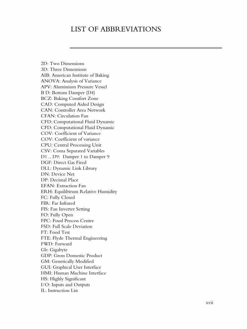
LIST OF ABBREVIATIONS
2D: Two Dimensions3D: Three DimensionsAIB: American Institute of BakingANOVA: Analysis of VarianceAPV: Aluminium Pressure VesselB D: Bottom Damper (D4)BCZ: Baking Comfort ZoneCAD: Computed Aided DesignCAN: Controller Area NetworkCFAN: Circulation FanCFD: Computational Fluid DynamicCFD: Computational Fluid DynamicCOV: Coefficient of VarianceCOV: Coefficient of varianceCPU: Central Processing UnitCSV: Coma Separated VariablesD1 .. D9: Damper 1 to Damper 9DGF: Direct Gas FiredDLL: Dynamic Link LibraryDN: Device NetDP: Decimal PlaceEFAN: Extraction FanERH: Equilibirum Relative HumidityFC: Fully ClosedFIR: Far InfraredFIS: Fan Inverter SettingFO: Fully OpenFPC: Food Process CentreFSD: Full Scale DeviationFT: Food TestFTE: Flyde Thermal EngineeringFWD: ForwardGb: GigabyteGDP: Gross Domestic ProductGM: Genetically ModifiedGUI: Graphical User InterfaceHMI: Human Machine InterfaceHS: Highly SignificantI/O: Inputs and OutputsIL: Instruction List
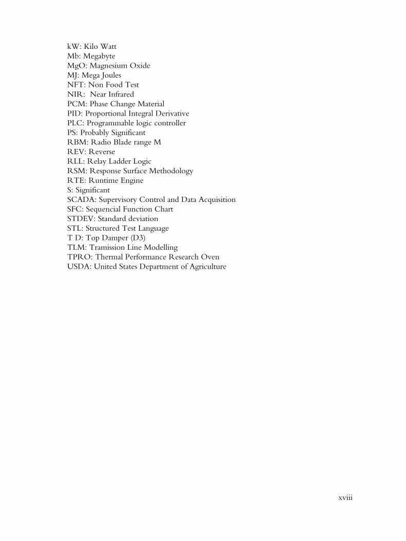
xviii
kW: Kilo WattMb: MegabyteMgO: Magnesium OxideMJ: Mega JoulesNFT: Non Food TestNIR: Near InfraredPCM: Phase Change MaterialPID: Proportional Integral DerivativePLC: Programmable logic controllerPS: Probably SignificantRBM: Radio Blade range MREV: ReverseRLL: Relay Ladder LogicRSM: Response Surface MethodologyRTE: Runtime EngineS: SignificantSCADA: Supervisory Control and Data Acquisition SFC: Sequencial Function ChartSTDEV: Standard deviationSTL: Structured Test LanguageT D: Top Damper (D3)TLM: Tramission Line ModellingTPRO: Thermal Performance Research OvenUSDA: United States Department of Agriculture
xix
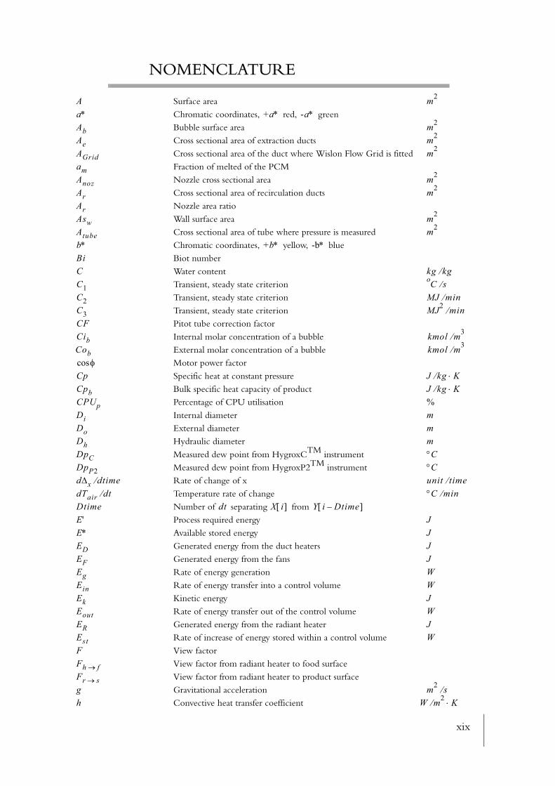
NOMENCLATURE
Surface areaChromatic coordinates, red, greenBubble surface areaCross sectional area of extraction ductsCross sectional area of the duct where Wislon Flow Grid is fittedFraction of melted of the PCMNozzle cross sectional areaCross sectional area of recirculation ductsNozzle area ratioWall surface areaCross sectional area of tube where pressure is measuredChromatic coordinates, yellow, blueBiot number Water contentTransient, steady state criterionTransient, steady state criterionTransient, steady state criterionPitot tube correction factorInternal molar concentration of a bubbleExternal molar concentration of a bubbleMotor power factorSpecific heat at constant pressureBulk specific heat capacity of productPercentage of CPU utilisationInternal diameterExternal diameterHydraulic diameterMeasured dew point from HygroxCTM instrumentMeasured dew point from HygroxP2TM instrumentRate of change of xTemperature rate of changeNumber of separating from Process required energyAvailable stored energyGenerated energy from the duct heatersGenerated energy from the fansRate of energy generationRate of energy transfer into a control volume Kinetic energyRate of energy transfer out of the control volumeGenerated energy from the radiant heaterRate of increase of energy stored within a control volumeView factorView factor from radiant heater to food surfaceView factor from radiant heater to product surfaceGravitational accelerationConvective heat transfer coefficient
A m2
a∗ +a∗ -a∗Ab m2
Ae m2
AGrid m2
amAnoz m2
Ar m2
ArAsw m2
Atube m2
b∗ +b∗ -b∗BiC kg kg⁄C1 Co s⁄C2 MJ min⁄C3 MJ2 min⁄CFCib kmol m3⁄Cob kmol m3⁄
φcosCp J kg K⋅⁄Cpb J kg K⋅⁄CPUp %Di mDo mDh mDpC °CDpP2 °Cd∆x dtime⁄ unit time⁄dTair dt⁄ °C min⁄Dtime dt X i[ ] Y i Dtime–[ ]E' JE∗ JED JEF JEg WEin WEk JEout WER JEst WFFh f→Fr s→g m2 s⁄h W m2⁄ K⋅

xx
NOMENCLATURE
Nozzle heightLatent heat of evaporation Mean nozzle heat transfer coefficient (top plenum nozzle)Mean equivalent heat transfer coefficient Electrical current Dissipated current by the duct heaterDissipated current by the radiant heaterConductivityMass transfer coefficient of a bubble Proportional gainBulk thermal conductivity of productCharacteristic lengthLightnessMass of airMagnification factor for flow gridMeasured mixed humidity from HygroxP2TM instrumentMass flow to the control volume Mass flow out of the control volume Storage massTotal mass of air extractedTotal mass of air from both plenumsMass flow at a node Number of radiant heaterNumber of nozzleNumber of rows of nozzleNusselt number (applied to characteristic length)Mean Nusselt numberAvailable energy after charging heat storePerimeterPressure within a bubbleWater vapour pressure at product surfacePressure surrounding a bubbleInput pressureOutput pressureEnergy remaining in the heat store after 15 secondsPrandtl numberStatic pressureSaturation partial vapour pressure of water Total pressureMeasured pressure at a node Stored energyFan volume flowCumulative energy into air Cumulative energy loss from air leakagesTotal rate of air energy loss from the TPROMolar rate of mass transfer to/from a bubbleCumulative energy from circulation fan
H mhfg J kg⁄hnozT W m2⁄ K⋅hv h, W m2⁄ K⋅I AIDH AIRH Ak W m⁄ K⋅kb m2 s⁄KCUkp W m⁄ K⋅L mL∗ma kgMaMHP2 gH2O kgdryair⁄Min kg s⁄Mout kg s⁄ms kgMT e, kg s⁄MT p, kg s⁄Mx x kg s⁄nhNnozNrowNuLNuP JP mPb NPequ atmP∞ NPi PaPo PaP0 JPrPs PaPsat atmPT PaPTXx x PaQs JQ· m3 s⁄QAIR_CUMUL JQAIRL_CUMUL JQa l, WQb kmol s m2⋅⁄QCFAN_CUMUL J
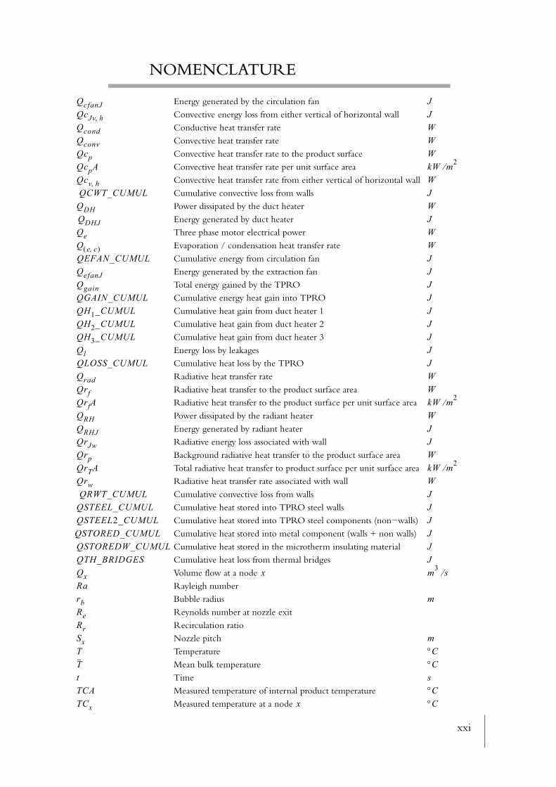
xxi
NOMENCLATURE
Energy generated by the circulation fanConvective energy loss from either vertical of horizontal wallConductive heat transfer rateConvective heat transfer rateConvective heat transfer rate to the product surfaceConvective heat transfer rate per unit surface areaConvective heat transfer rate from either vertical of horizontal wallCumulative convective loss from walls Power dissipated by the duct heaterEnergy generated by duct heaterThree phase motor electrical power Evaporation / condensation heat transfer rateCumulative energy from circulation fanEnergy generated by the extraction fanTotal energy gained by the TPROCumulative energy heat gain into TPROCumulative heat gain from duct heater 1Cumulative heat gain from duct heater 2Cumulative heat gain from duct heater 3Energy loss by leakagesCumulative heat loss by the TPRORadiative heat transfer rateRadiative heat transfer to the product surface areaRadiative heat transfer to the product surface per unit surface areaPower dissipated by the radiant heaterEnergy generated by radiant heaterRadiative energy loss associated with wallBackground radiative heat transfer to the product surface areaTotal radiative heat transfer to product surface per unit surface areaRadiative heat transfer rate associated with wallCumulative convective loss from walls Cumulative heat stored into TPRO steel walls Cumulative heat stored into TPRO steel components (non−walls)Cumulative heat stored into metal component (walls + non walls)Cumulative heat stored in the microtherm insulating materialCumulative heat loss from thermal bridgesVolume flow at a node Rayleigh numberBubble radiusReynolds number at nozzle exitRecirculation ratio Nozzle pitchTemperatureMean bulk temperatureTimeMeasured temperature of internal product temperatureMeasured temperature at a node
QcfanJ JQcJv h, JQcond WQconv WQcp WQcpA kW m2⁄Qcv h, WQCWT_CUMUL J
QDH WQDHJ JQe WQ e c,( ) WQEFAN_CUMUL JQefanJ JQgain JQGAIN_CUMUL JQH1_CUMUL JQH2_CUMUL JQH3_CUMUL JQl JQLOSS_CUMUL JQrad WQrf WQrfA kW m2⁄QRH WQRHJ JQrJw JQrp WQrTA kW m2⁄Qrw WQRWT_CUMUL J
QSTEEL_CUMUL JQSTEEL2_CUMUL JQSTORED_CUMUL JQSTOREDW_CUMUL JQTH_BRIDGES JQx x m3 s⁄Rarb mReRrSx mT °CT °Ct sTCA °CTCx x °C
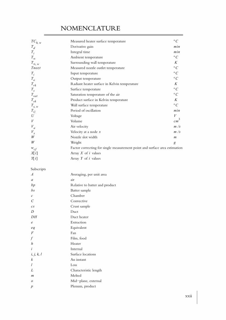
xxii
NOMENCLATURE
Measured heater surface temperature Derivative gainIntegral timeAmbient temperature Surrounding wall temperature
Measured nozzle outlet temperatureInput temperatureOutput temperatureRadiant heater surface in Kelvin temperatureSurface temperatureSaturation temperature of the airProduct surface in Kelvin temperatureWall surface temperaturePeriod of oscillationVoltageVolumeAir velocityVelocity at a node Nozzle slot widthWeight Factor correcting for single measurement point and surface area estimationArray of valuesArray of values
SubscriptsAveraging, per unit areaairRelative to batter and productBatter sampleChamberConvectiveCrust sampleDuctDuct heaterExtractionEquivalentFanFilm, foodHeaterInternalSurface locationsAn instantLossCharacteristic lengthMeltedMid−plane, externalPlenum, product
TCh w, °CTd minTi minT∞ °CT∞ w, KTnozt °CTi °CTo °CTrk KTs °CTsat °CTsk KTs w, °CTU minU VV cm3
Va m s⁄Vx x m s⁄W mW gwcfX i[ ] X iY i[ ] Y i
AabpbscCcsDDHeeqFfhii j k l, , ,klLmop

xxiii
NOMENCLATURE
RecirculationRadiativeRadiantRadiant heaterReturnSurfaceStoredSteelTotalWallA point of measurementCartesian coordinate axes
Greek lettersCorrection factor for an averaging Pitot tubeCorrection factor for a straight Pitot tube (Non−averaging)Product thermal diffusivityInverse film temperatureStored energy in the wallStored energy in the steel wallHeat of fusion of PCM per unit mass Rate of mass flow change of a control volumeChamber air lossReturn duct air lossTotal plenum air lossRate of energy loss from the oven chamberEnergy loss from the return ductRate of energy loss by leakagesRate of energy loss from the plenum chamberRate of energy loss from the return ductStored energy in the air Density changeTime intervalVolume changeWeight changeTransient weight loss over a 60 minute periodRelative moisture changeEmissivityIsentropic compression factorDynamic viscosityImpeller efficiency (total efficiency)DensityBulk density of productDensity of liquidDerived density from measurement of temperature at a node Stephan−Boltzman constant Bubble surface tension
rrRRHrtSsstTwxx y ζ η, , ,
αAαNαp m2 s⁄β K 1–
∆Es w, J∆Es w st, , J∆hm kJ kg⁄∆M kg s⁄∆Mc L, kg s⁄∆Mret L, kg s⁄∆MT p L, , kg s⁄∆Qc l, W∆QJrt l, J∆Ql W∆Qp l, W∆Qrt l, W∆Qs a, J∆ρ %∆t s∆V %∆W %∆Wp 60( ) g∆χ %εγµ kg s⁄ m⋅ηTρ kg m3⁄ρb kg m3⁄ρl kg m3⁄ρTCx
x kg m3⁄σ W m2⁄ K4⋅σb N m⁄

xxiv
NOMENCLATURE
Temperature differenceThermal time constantKinematic viscosity Relative moisture
θ °Cτt sν m2 s⁄χ %
xxv
Acknowledgements
I would like to thank,
The sponsor of this project APV Baker, for their long term investment in this project and their trust and belief in the work that could be achieved by me and the TPRO. A special
thank to the Director of development Peter Smith for his enthusiasm and continuous sup−port during both the testing and the writing up period.
My supervisor Professor Newborough for his pertinent technical expertise and advice throughout. For his mental support during the ups and downs and mostly to have taught
me a great deal of people handling skills.
John Miller and Rory Millard, which I would like to express my extreme gratitude for having spent long hours during both the commissioning but especially the food testing
program which would not haven been possible without them.
Graham Andrews for passing me a little bite of his knowledge in the cake baking process.
Dr. Bryan Shaughnessy for his advise in thermal radiation.
Henry Clark for his sound technical expertise and support throughout. Clive Mountain, Peter Daines, Jim Shaw and Paul Vjestica for their help on the control side and electrical
section of this project.
Kaye Burling for help with the Design of Experiment.
Stephen St. Clair Thompson and Ken Barras for passing their experience and knowledge in oven design and functioning.
Edie Newton and Alan Rutford for their mechanical know how. All the engineers that I have not mention which worked on maintaining and repairing the TPRO night and day.
All the MIS team for their continuous hardware support.
Although we have never met I would like to thank Rob Van der Woude for his uncondi−tional help on NT Batch Scritping, Scott Keiser & Carrol Sparks for their expertise in the
Wonderware products (InControl™ Development California). Peter Ebel (fan consul−tancy). All the people from the Framemaker newsgroup (comp.text.frame and the Adobe
User forum.)

1
________________________________________________________________________
Abstract
Industrial baking oven design follows long−established rules of thumb, but the boundaries for effective heat transfer, which provide minimum baking time and high quality food prod−ucts are not well understood. With a view to reducing bake time, the overall aim of this research was to examine increased rates of heat transfer in baking by means of a Thermal Performance Research Oven (TPRO). If a reduction in bake time of only 10% was achiev−able, a major benefit would exist for both the sponsor of this project and for bakeries (increased throughput per hour or reduced oven footprint per number of products baked).
Chapter 1 highlights the current and past trends in the baking industry with respect to bread, biscuit and cakes. It also discusses the two basic methods for approaching this research (the−oretical, empirical). In Chapter 2 the design and function of the TPRO are described, where the main objective was to explore existing heat transfer conditions as they exist in current baking ovens, and to permit baking beyond these conventional limits. One of the challenges was to attempt to give the TPRO the capability to reproduce existing temperature and humidity conditions as occur in the adjacent and separately controlled zones of existing trav−elling ovens. This was explored in Chapter 2 via a mathematical model which was designed to provide a first order indication of the heating conditions within the TPRO. The outcome of this analysis as well as the development of a unique computer aided control system (Chapter 3) provided the platform for subsequent tests. A series of preliminary (non−food) tests were undertaken to examine the thermal performance envelope of the TPRO under different sets of conditions (Chapter 4). An energy balance was derived from measured results of the entire process and was generated to depict in real time (from transient to steady state), the energy distribution in the various components of the oven. The operating performance of the TPRO are described in Chapter 4. Chapter 5 proposes a ‘baking comfort zone’ con−cept (similar to the 'thermal comfort' concept in buildings) as an approach to baking opti−misation analysis. Then a design of experiments approach (DOE) was developed for undertaking the food tests and the various measurements and analysis developed for the experimental approach for Madeira cake are described in Chapter 6. This chaper presents the results emerging from the three−stage DOE (screening, factorial, central composite) employed for analysing the baking process. The influence of each of the main design factors (temperature, humidity etc.) affecting the product responses (colour, crust hardness, etc.) is discussed statistically in terms of significance. Interactions between design factors and responses and their relationships are identified. A desirability analysis based on the product responses identified which of the responses were a greater constraint on achieving a reduced bake time. The statistical model built upon the DOE identified a bake time reduction of up to 16% (relative to the benchmark) while maintaining acceptable values for the other product responses. This has been validated experimentally with success. The future translation of this achievement to full scale industrial baking ovens would permit significant savings in bake time, oven footprint and/or energy consumption to be achieved.
Introduction 2
Chapter 1/ Literature Review________________________________________________________________________
CHAPTER 1
LITERATURE REVIEW
1.1 Introduction
The history of baking process dates from about 10,000 B.C when man first started to eat a crude form of flat bread, which was a combination of water and flour. In 150 B.C, the first baker’s guild was formed in Rome. Roman bakeries were producing a variety of breads, which were distributed to the poor in times of need. In 1202 A.D, King John of England adopted laws to regulate the price of bread and limit their profit. In the 1850’s, the United States had 2,017 bakeries employing over 6,700 workers. In the early days of the twentieth century, gas ovens replaced the wood and coal burning brick ovens, producing a more even coloured product. Plant automation started for continuous production. In the 1930’s com−mercial bread−slicers were used in large bakeries. Sliced bread appeared in England under the name of Wonderbread. In 1941, calcium was added to the flour for women who joined the land army. The Bread and Flour regulations were introduced in 1963, to govern the composition and additives permitted in bread and flour. In 1974, a large sliced white loaf was controlled at 14.5p to the consumer with baker receiving an additional 0.5p from the UK government. In the UK alone, 9%106 large loave (Bakers Federation, 1999 [14]) are produced every day and consumers can choose from hundreds of varieties of bread rolls, buns, and other speciality breads. With a world population of 6.25 billions (US census estimate, 2002) the need for high production rates is obvious. Large bakery plant can produce today in the region of 8000 bread loaves an hour, which works out about 67%106 loaves a year. With such a staggering production, baking plant has to be efficient if low production costs, energy costs and product unit costs are to be kept low.
Although baking has been there for centuries, compared with more recent technologies, such as aeronautics, the baking process has remained more of an art than a science. Most of the entire production of the baking sector, is associated with bread, biscuit and cake. Through product and oven market research, Section 1.2 shows the current tendencies in the European, and worldwide market for these three products. Heat transfer is reviewed (Section 1.2.3) for the broad collection of oven designs that is currently used by the project’s sponsor (APV Baker) to impose their strength on the worldwide market. In order to explain why baking is still considered more as an art than a science, Section 1.3) reviews the heat transfer occurring during the baking and the complexities related with quantifying the dif−
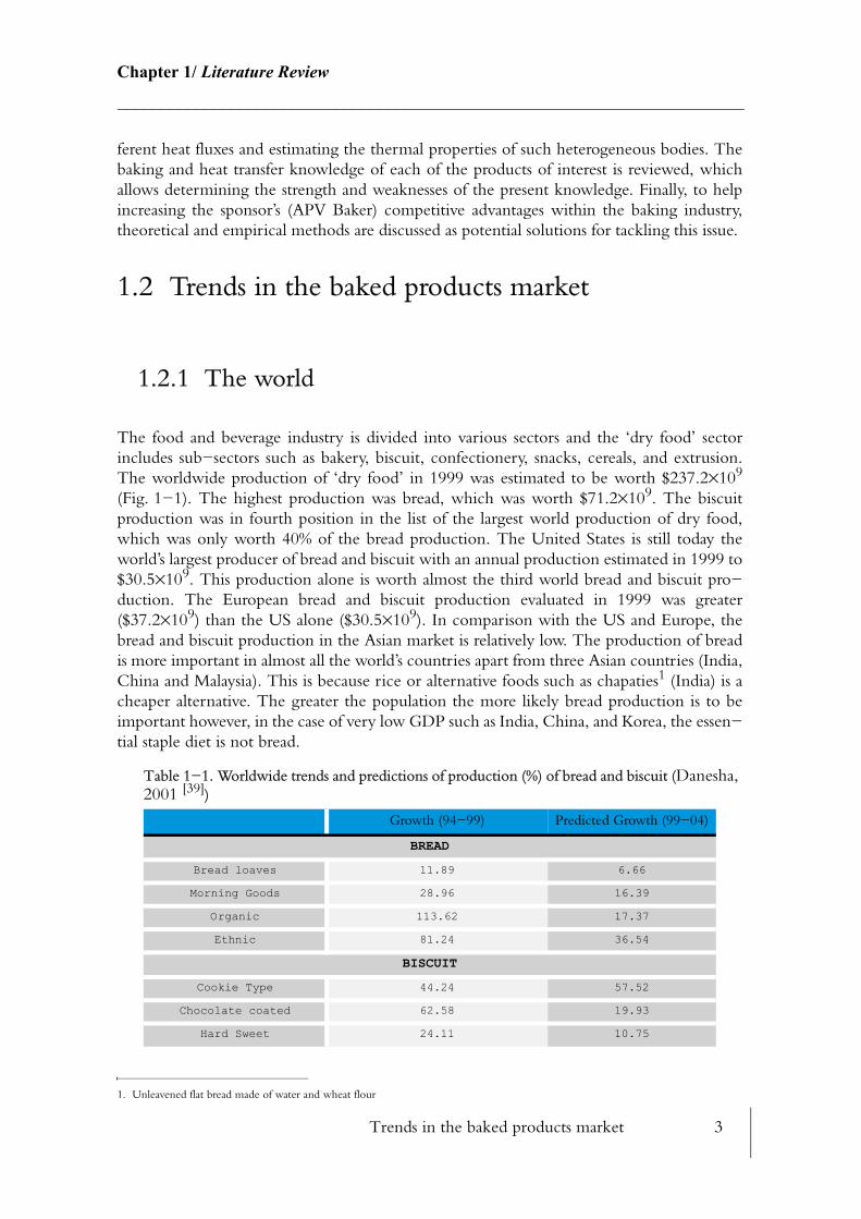
Trends in the baked products market 3
Chapter 1/ Literature Review________________________________________________________________________
ferent heat fluxes and estimating the thermal properties of such heterogeneous bodies. The baking and heat transfer knowledge of each of the products of interest is reviewed, which allows determining the strength and weaknesses of the present knowledge. Finally, to help increasing the sponsor’s (APV Baker) competitive advantages within the baking industry, theoretical and empirical methods are discussed as potential solutions for tackling this issue.
1.2 Trends in the baked products market
1.2.1 The world
The food and beverage industry is divided into various sectors and the ‘dry food’ sector includes sub−sectors such as bakery, biscuit, confectionery, snacks, cereals, and extrusion. The worldwide production of ‘dry food’ in 1999 was estimated to be worth $237.2%109
(Fig. 1−1). The highest production was bread, which was worth $71.2%109. The biscuit production was in fourth position in the list of the largest world production of dry food, which was only worth 40% of the bread production. The United States is still today the world’s largest producer of bread and biscuit with an annual production estimated in 1999 to $30.5%109. This production alone is worth almost the third world bread and biscuit pro−duction. The European bread and biscuit production evaluated in 1999 was greater ($37.2%109) than the US alone ($30.5%109). In comparison with the US and Europe, the bread and biscuit production in the Asian market is relatively low. The production of bread is more important in almost all the world’s countries apart from three Asian countries (India, China and Malaysia). This is because rice or alternative foods such as chapaties1 (India) is a cheaper alternative. The greater the population the more likely bread production is to be important however, in the case of very low GDP such as India, China, and Korea, the essen−tial staple diet is not bread.
1. Unleavened flat bread made of water and wheat flour
Table 1−1. Worldwide trends and predictions of production (%) of bread and biscuit (Danesha, 2001 [39])
Growth (94−99) Predicted Growth (99−04)
BREAD
Bread loaves 11.89 6.66
Morning Goods 28.96 16.39
Organic 113.62 17.37
Ethnic 81.24 36.54
BISCUIT
Cookie Type 44.24 57.52
Chocolate coated 62.58 19.93
Hard Sweet 24.11 10.75
Trends in the baked products market 4
Chapter 1/ Literature Review________________________________________________________________________
The cultural background of a country as well as its GDP can determine whether the country is more likely to use industrial processed food or not. Table 1−1 shows the trends (1994−1999) and predictions (1999−2004) of bread and biscuit worldwide. The value indicated in this table were taken as the average of 22 countries.
During the 1994−1999 period, the bakery market has been largely dominated by new gen−eration of product which highlights a change of consumer’s mentality. The growth produc−tion of organic bread (113%) during this period is the best example to illustrate this change. With the emergence of GM1 crops, consumers choice has drifted to a more healthier and ‘organic’ diet. According to a USDA2 study (2000), organic crop−land has doubled from 1992 to 1997, nowadays, the organic foods industry is growing by 20 to 24% annually. The more traditional bread loaves production has been declining and has been predicted to decrease by half by 2004. The production of ethnic or speciality bread such as ciabatta, pitta, naan, baguette, rye, has also become very popular mostly in Europe especially in Germany, France, UK and Italy during the period 94−99 with a growth production of almost 82%. This increase in ethnic bread emphasise the increase in cosmopolitan eating habit and the need for a more diverse bread diet.
Production information in the baking industry is difficult to obtain and often data are very costly. Information from one source to another can differ, which usually is explained by a different definitions of baking product. For instance, the UK bread market for the United Kingdom was valued in 2000 by the British Baker (Bread and Bakery Products, 2001 [20]) at £2.4%109 while Leatherhead Food Research Association (Danesha, 2001 [39]) estimated at £2.2%109. This discrepancy is caused by both market research which uses different defini−tions for what the ‘bread family’ contains. While Leatherhead Food Research Association specified that bread contained white, brown and all other rolls, vienna, pre−packed sand−wiches, the British Baker data does not give any specific definition.
1.2.2 The European Market
The European bakery market was estimated in 1999 by Leatherhead Food Research Asso−ciation (Danesha, 2001 [39]) to 30.2%106 tonnes worth a $73%109, including all types of bread, biscuits and cakes. The bread which is still today a staple part of a European’s diet is dominating the bakery market, in comparison with biscuit and cake which are usually con−sidered as regular snacking foods.
1.2.2.1 Bread
Fig. 1−2 represents the European bakery product market map by volume produced for bread, biscuit and cakes. The Germans are by far the biggest bread eaters in Europe with an average of 98.5 kg per capita. This translates to 6.9%106 tonnes of bread produced in 2000 amounting the second biggest producer worldwide. The Belgians are second biggest ‘bread eater’ with 90.7kg per capita. The average consumption in the European market is 78kg per year. Bread takes the lead of largest volume sold in the European bakery market with 81%.
1. Genetically Modified
2. United States Department of Agriculture
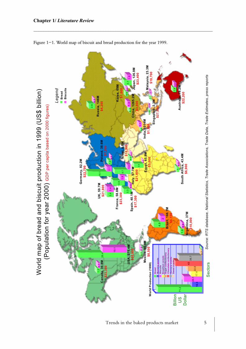
Trends in the baked products market 5
Chapter 1/ Literature Review________________________________________________________________________
Figure 1−1. World map of biscuit and bread production for the year 1999.
1.2
0.7
Can
ada,
30.
8M$2
3,30
0
2.6
0.3
Rus
sia,
146
M$4
,200
20.4
10.1
US
A, 2
75.4
M$3
3,90
0
4.9
2B
razi
l, 16
6.1M
$6,1
50
0.1
0.1
Mex
ico,
98.
9M$8
,500
4.8
1.8
Fran
ce, 5
8.8M
$23,
300
2.4
2.4
UK
, 59.
7M$2
1,80
010
.1
2.1
Ger
man
y, 8
2.2M
$22,
700
3.3
0.6
Spai
n, 4
0.1M
$17,
300
6.7
1.3
Italy
, 57.
7M$2
1,40
0
1.4
0.3
Pola
nd, 3
8.6M
$7,2
00
1.6
0.9
Arg
entin
a, 3
7M$1
0,00
0
0.7
0.2
Isra
el, 6
.1M
$18,
300
3.9
0.2
Egyp
t, 65
.8M
$3,0
00
10.
5S
outh
Afr
ica,
43.
4M$6
,900
1.4
0.9
Aus
tral
ia, 1
9.2M
$22,
200
Mal
aysi
a, 2
3.3M
$10,
700
0.2
1.1
Indi
a, 1
014M
$1,8
00S
inga
pore
, 3.3
M$2
7,80
0
0.8
0.4
Kor
ea, 6
9M$1
,000
3.1
1.9
Japa
n, 1
26.9
M$2
3,40
0
0.3
1.3
Chi
na, 1
265.
2M$3
,800
Wor
ld m
ap o
f bre
ad a
nd b
iscu
it pr
oduc
tion
in 1
999
(US
$ bi
llion
)(P
opul
atio
n fo
r yea
r 200
0) G
DP
per
cap
ita b
ased
on
2000
figu
res)
Lege
nd
Sec
tors
71.2
16.3
29.1
17.4
22.8
4336
.7
0.7
0.06
0.06
0.13
0.1
Sou
rce:
RTS
dat
abas
e, N
atio
nal S
tatis
tics,
Tra
de A
ssoc
iatio
ns, T
rade
Dat
a, T
rade
Est
imat
es, p
ress
repo
rts
Mor
ning
goo
dsB
iscu
itsB
reak
fast
cer
eals
Suga
r con
fect
ione
ryC
hoco
late
con
fect
ione
rySa
vour
y sn
acks
Swee
t sna
cks
Bre
ad
Bis
cuits
Bre
ad
Bill
ion
US
Dol
larW
orld
Pro
duct
ion
(199
9)
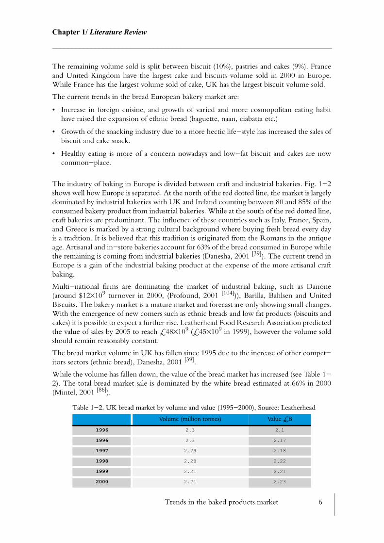
Trends in the baked products market 6
Chapter 1/ Literature Review________________________________________________________________________
The remaining volume sold is split between biscuit (10%), pastries and cakes (9%). France and United Kingdom have the largest cake and biscuits volume sold in 2000 in Europe. While France has the largest volume sold of cake, UK has the largest biscuit volume sold.
The current trends in the bread European bakery market are:
• Increase in foreign cuisine, and growth of varied and more cosmopolitan eating habit have raised the expansion of ethnic bread (baguette, naan, ciabatta etc.)
• Growth of the snacking industry due to a more hectic life−style has increased the sales of biscuit and cake snack.
• Healthy eating is more of a concern nowadays and low−fat biscuit and cakes are now common−place.
The industry of baking in Europe is divided between craft and industrial bakeries. Fig. 1−2shows well how Europe is separated. At the north of the red dotted line, the market is largely dominated by industrial bakeries with UK and Ireland counting between 80 and 85% of the consumed bakery product from industrial bakeries. While at the south of the red dotted line, craft bakeries are predominant. The influence of these countries such as Italy, France, Spain, and Greece is marked by a strong cultural background where buying fresh bread every day is a tradition. It is believed that this tradition is originated from the Romans in the antique age. Artisanal and in−store bakeries account for 63% of the bread consumed in Europe while the remaining is coming from industrial bakeries (Danesha, 2001 [39]). The current trend in Europe is a gain of the industrial baking product at the expense of the more artisanal craft baking.
Multi−national firms are dominating the market of industrial baking, such as Danone (around $12%109 turnover in 2000, (Profound, 2001 [104])), Barilla, Bahlsen and United Biscuits. The bakery market is a mature market and forecast are only showing small changes. With the emergence of new comers such as ethnic breads and low fat products (biscuits and cakes) it is possible to expect a further rise. Leatherhead Food Research Association predicted the value of sales by 2005 to reach £48%109 (£45%109 in 1999), however the volume sold should remain reasonably constant.
The bread market volume in UK has fallen since 1995 due to the increase of other compet−itors sectors (ethnic bread), Danesha, 2001 [39].
While the volume has fallen down, the value of the bread market has increased (see Table 1−2). The total bread market sale is dominated by the white bread estimated at 66% in 2000 (Mintel, 2001 [86]).
Table 1−2. UK bread market by volume and value (1995−2000), Source: Leatherhead
Volume (million tonnes) Value £B
1996 2.3 2.1
1996 2.3 2.17
1997 2.29 2.18
1998 2.28 2.22
1999 2.21 2.21
2000 2.21 2.23
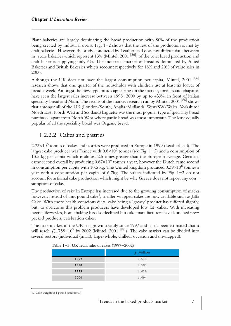
Trends in the baked products market 7
Chapter 1/ Literature Review________________________________________________________________________
Plant bakeries are largely dominating the bread production with 80% of the production being created by industrial ovens. Fig. 1−2 shows that the rest of the production is met by craft bakeries. However, the study conducted by Leatherhead does not differentiate between in−store bakeries which represent 13% (Mintel, 2001 [86]) of the total bread production and craft bakeries supplying only 6%. The industrial market of bread is dominated by Allied Bakeries and British Bakeries which account respectively for 18% and 20% of value sales in 2000.
Although the UK does not have the largest consumption per capita, Mintel, 2001 [86]
research shows that one quarter of the households with children use at least six loaves of bread a week. Amongst the new type breads appearing on the market, tortillas and chapaties have seen the largest sales increase between 1998−2000 by up to 433%, in front of italian speciality bread and Naan. The results of the market research run by Mintel, 2001 [86] shows that amongst all of the UK (London/South, Anglia/Midlands, West/SW/Wales, Yorkshire/North East, North West and Scotland) baguette was the most popular type of speciality bread purchased apart from North West where garlic bread was most important. The least equally popular of all the speciality bread was Organic bread.
1.2.2.2 Cakes and pastries
2.73%106 tonnes of cakes and pastries were produced in Europe in 1999 (Leatherhead). The largest cake producer was France with 0.8%106 tonnes (see Fig. 1−2) and a consumption of 13.5 kg per capita which is almost 2.5 times greater than the European average. Germans came second overall by producing 0.67%106 tonnes a year, however the Dutch came second in consumption per capita with 10.5 kg. The United kingdom produced 0.39%106 tonnes a year with a consumption per capita of 6.7kg. The values indicated by Fig. 1−2 do not account for artisanal cake production which might be why Greece does not report any con−sumption of cake.
The production of cake in Europe has increased due to the growing consumption of snacks however, instead of unit pound cake1, smaller wrapped cakes are now available such as Jaffa Cake. With more health conscious diets, cake being a ‘greasy’ product has suffered slightly, but, to overcome this problem producers have developed low fat−cakes. With increasing hectic life−styles, home baking has also declined but cake manufacturers have launched pre−packed products, celebration cakes.
The cake market in the UK has grown steadily since 1997 and it has been estimated that it will reach £1.758%109 by 2002 (Mintel, 2001 [87]). The cake market can be divided into several sectors (individual (small), large/whole, chilled, occasion and unwrapped).
1. Cake weighting 1 pound (traditional)
Table 1−3. UK retail sales of cakes (1997−2002)
£ Million
1997 1.515
1998 1.587
1999 1.629
2000 1.694

Trends in the baked products market 8
Chapter 1/ Literature Review________________________________________________________________________
Figure 1−2. European bakery market analysis by volume, product types and bakery types
Amongst these, small individual wrapped cakes account for 50% of the total UK retail sales followed by large/whole cakes. The UK retail sales in the large/whole cake sector has fallen by nearly 2% between 1999 and 2001 at the expense of small wrapped cakes which are
2001 1.718
2002 (estimate) 1.758
Table 1−3. UK retail sales of cakes (1997−2002)
£ Million
3.2
0.8 0.5France, 58.8M
70%
18% 12%
2.2
0.4 0.6UK, 59.7M
69%
12% 19%
0.3 0 0Ireland, 3.8M
82% 4% 14%
2.2
0.2 0.2Spain, 40.1M
86%
6% 8%4
0.3 0.4Italy, 57.7M
85%
7% 8%
6.9
0.7 0.6
Germany, 82.2M
18% 12%
0.70.1
Greece, 10.7M
93%7%
0.6 0 0.1Sweden, 8.9M
82%12%6%
0.70 0
Portugal, 10M
92%2% 6%
0.6 0 0Austria, 8M
89%2% 9%
0 0 0
Finland, 5.2M81% 9% 10%
0 0 0Norway, 4.5M
87% 6% 7%
European bakery products market by volumeby product type (Sales Volume in million tonnes for 2000
and by bakeries type (Year data was collected indicated in red)
Legend
Source:The European Bakery Products Market (Leatherhead Food research Association UK), Bakersfederation
85%
23 %
77 %1998
80 %
20 %85 %
15 %
1998
1995
92 %8 %
1997
0 0 0
Switzerland7.2M
84% 4% 12%
80 %
20 %
1993
50 %
50 %1993
56 %
44 %
0.90.2 0.1
TheNeterhlands
15.9M1998
92 %8 %
1998
35 %
65 %1998
54 %
46 %1998
0 0 0
Danemark, 5.3M84% 7% 9%
77%
14% 9%
75 %
25 %1998
0.70 0.2Belgium, 10.2M
78%5% 17%
90 %10 %
1998
Bread
Biscuits
Bar chart
Cake and pastries
Craft bakeries
Pie chartIndustrial bakeries
(Population for year 2000)
95 % 5 %
1999
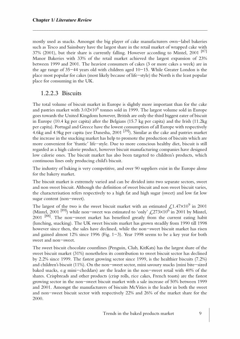
Trends in the baked products market 9
Chapter 1/ Literature Review________________________________________________________________________
mostly used as snacks. Amongst the big player of cake manufacturers own−label bakeries such as Tesco and Sainsbury have the largest share in the retail market of wrapped cake with 37% (2001), but their share is currently falling. However according to Mintel, 2001 [87]
Manor Bakeries with 33% of the retail market achieved the largest expansion of 23% between 1999 and 2001. The heaviest consumers of cakes (3 or more cakes a week) are in the age range of 35−44 years old with children aged 10−15. While Greater London is the place most popular for cakes (most likely because of life−style) the North is the least popular place for consuming in the UK.
1.2.2.3 Biscuits
The total volume of biscuit market in Europe is slightly more important than for the cake and pastries market with 3.02%106 tonnes sold in 1999. The largest volume sold in Europe goes towards the United Kingdom however, British are only the third biggest eater of biscuit in Europe (10.4 kg per capita) after the Belgians (15.7 kg per capita) and the Irish (11.2kg per capita). Portugal and Greece have the lowest consumption of all Europe with respectively 4.6kg and 4.9kg per capita (see Danesha, 2001 [39]). Similar as the cake and pastries market the increase in the snacking market has help to promote the production of biscuits which are more convenient for ‘frantic’ life−style. Due to more conscious healthy diet, biscuit is still regarded as a high calorie product, however biscuit manufacturing companies have designed low calorie ones. The biscuit market has also been targeted to children’s products, which continuous lines only producing child’s biscuit.
The industry of baking is very competitive, and over 90 suppliers exist in the Europe alone for the bakery market.
The biscuit market is extremely varied and can be divided into two separate sectors, sweet and non sweet biscuit. Although the definition of sweet biscuit and non sweet biscuit varies, the characterisation refers respectively to a high fat and high sugar (sweet) and low fat low sugar content (non−sweet).
The largest of the two is the sweet biscuit market with an estimated £1.47%109 in 2001 (Mintel, 2001 [89]) while non−sweet was estimated to ‘only’ £273%106 in 2001 by Mintel, 2001 [88]. The non−sweet market has benefited greatly from the current eating habit (lunching, snacking). The UK sweet biscuits market has grown steadily from 1990 till 1998 however since then, the sales have declined, while the non−sweet biscuit market has risen and gained almost 12% since 1996 (Fig. 1−3). Year 1998 seems to be a key year for both sweet and non−sweet.
The sweet biscuit chocolate countlines (Penguin, Club, KitKats) has the largest share of the sweet biscuit market (31%) nonetheless its contribution to sweet biscuit sector has declined by 2.2% since 1999. The fastest growing sector since 1999, is the healthier biscuits (7.2%) and children’s biscuit (11%). On the non−sweet sector, mini savoury snacks (mini bite−sized baked snacks, e.g mini−cheddars) are the leader in the non−sweet retail with 40% of the shares. Crispbreads and other products (crisp rolls, rice cakes, French toasts) are the fastest growing sector in the non−sweet biscuit market with a sale increase of 50% between 1999 and 2001. Amongst the manufacturers of biscuits McVities is the leader in both the sweet and non−sweet biscuit sector with respectively 22% and 26% of the market share for the 2000.
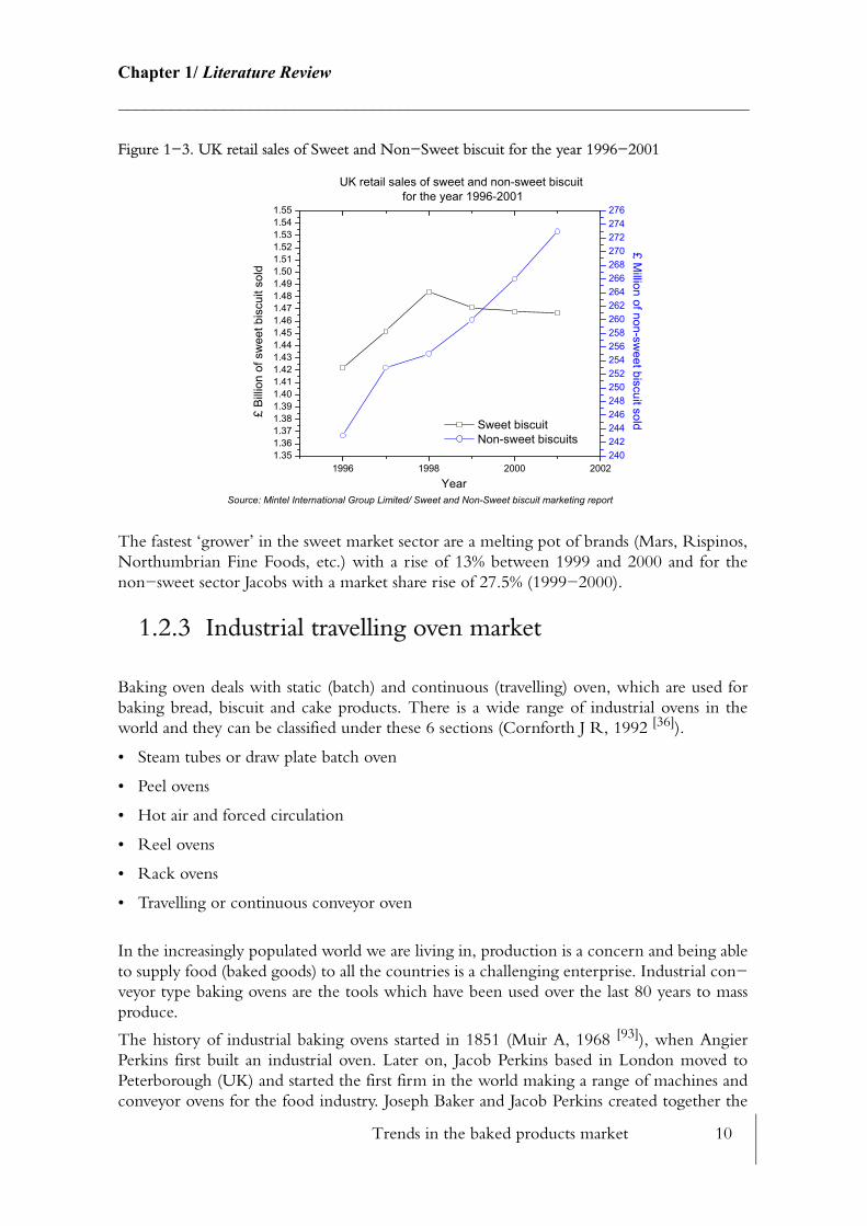
Trends in the baked products market 10
Chapter 1/ Literature Review________________________________________________________________________
Figure 1−3. UK retail sales of Sweet and Non−Sweet biscuit for the year 1996−2001
The fastest ‘grower’ in the sweet market sector are a melting pot of brands (Mars, Rispinos, Northumbrian Fine Foods, etc.) with a rise of 13% between 1999 and 2000 and for the non−sweet sector Jacobs with a market share rise of 27.5% (1999−2000).
1.2.3 Industrial travelling oven market
Baking oven deals with static (batch) and continuous (travelling) oven, which are used for baking bread, biscuit and cake products. There is a wide range of industrial ovens in the world and they can be classified under these 6 sections (Cornforth J R, 1992 [36]).
• Steam tubes or draw plate batch oven
• Peel ovens
• Hot air and forced circulation
• Reel ovens
• Rack ovens
• Travelling or continuous conveyor oven
In the increasingly populated world we are living in, production is a concern and being able to supply food (baked goods) to all the countries is a challenging enterprise. Industrial con−veyor type baking ovens are the tools which have been used over the last 80 years to mass produce.
The history of industrial baking ovens started in 1851 (Muir A, 1968 [93]), when Angier Perkins first built an industrial oven. Later on, Jacob Perkins based in London moved to Peterborough (UK) and started the first firm in the world making a range of machines and conveyor ovens for the food industry. Joseph Baker and Jacob Perkins created together the
1996 1998 2000 20021.351.361.371.381.391.401.411.421.431.441.451.461.471.481.491.501.511.521.531.541.55
Source: Mintel International Group Limited/ Sweet and Non-Sweet biscuit marketing report
UK retail sales of sweet and non-sweet biscuit for the year 1996-2001
Sweet biscuit Non-sweet biscuits
Year
£ Bi
llion
of s
wee
t bis
cuit
sold
240242244246248250252254256258260262264266268270272274276
£ Million of non-sw
eet biscuit sold

Trends in the baked products market 11
Chapter 1/ Literature Review________________________________________________________________________
Baker Perkins company which has led the baking industry for almost half a century. Since 1943, Baker Perkins acquired Forgrove Machinery Co, Steel and Cowlishaw, Douglas Rownson, Rose Brothers, Jaxons, Werner Lehara, Tweedy and Lanham. Dr. R Seligman created the company Aluminium Pressure Vessels (APV) in 1910, and invented the flat plate heat exchanger in 1923. 50 years later APV acquired Baker Perkins (1987). And today, APV is part of the large group Invensys and is in direct competition with other industrial oven manufacturer such as Imaforni (Italy), Sasib Spooner (Italian group owing Spooner Vicars (UK), Meincke (Denmark) and Orlandi (Italy)), Stewart (from Sasib group), Baketech (USA), Kaak (Holland), and Gouet (France).
APV Baker has designed over 31 different baking ovens since the early days, and today 25 of these designs are still operational worldwide and some are almost 60 years old. Today, to compete with its rivals, APV Baker has around 13 oven designs which are on sale. Long−established rules of thumb (Appendix M) are still driving industrial oven design today.
1.2.3.1 APV Baker industrial baking ovens
The baking industry has adopted jargon to describe ovens and their heat transfer function−ing/heat input, which is slightly different to the heat transfer terminology that is generally adopted in engineering. The name given to an oven family always refers to the methods of heating.
The methods of heating in industrial baking ovens are divided into direct and indirect firing. In the case of direct gas firing, the gas burner fires directly into the baking chamber and the products of combustion are in contact with the product being baked, while in the case of indirect firing the burner fires through an air to air heat exchanger which is used indirectly to transfer heat to the product.
These definitions can be slightly mis−leading with the well established heat transfer defini−tions. For instance, it is possible to have an indirect radiation oven, which, in the jargon of baking industry means that the products of combustion are not in contact with the product however, in heat transfer terms, indirect radiation can have a very different meaning. It sig−nifies that radiation emitted by either the heating elements (gas burner or electric elements) or the enclosure walls that experiences one or more reflections within the enclosure before intercepting the load (baking product) (Shaughnessy, 1996 [119]).
Amongst, the two basic types of heating system, all APV oven designs fall into 6 different sub−categories which are ‘direct gas fired’ (DGF), ‘direct convection’, ‘indirect convection’, ‘convecto radiant’, ‘turbo radiant’ and ‘impingement’.
1. Direct Gas Fired design (DGF): DGF ovens use gas which is fired through gas burners, (ribbon burners). Fig. 1−4 shows a simplified schematic whose purpose is only to show the principle of the DGF top heat modules. As the products of combustion are directly in contact with the baking product this heating method is ‘direct’ as previously defined. The air is usually extracted from the chamber via a set of dampers and an extraction duct, and re−fed through a series of pierced tube or nozzles to promote some air flow movement (turbulence system) around the product. Air from the chamber, is also removed via extraction hoods (ducts) to the flue. Flexiflame® (Appendix E) ribbon burners are commonly used in DGF ovens as they are versatile and can be control to give uniform heat balance across the width of the oven. The flame radiating from them is

Trends in the baked products market 12
Chapter 1/ Literature Review________________________________________________________________________
directed to the product surface. However, in some cases the gas burner heats up a metal plate which promotes a more uniform radiant heating medium, but is not as responsive as gas burner control.
The DGF section relies mostly on radiation to the product surface which has been used successfully for crackers and biscuits baking. The turbulence system helps moisture removal of the product. Conduction is also present through the steel or meshed band.
Nowadays, hybrid ovens are fairly common and consist of modular sections of the dif−ferent design type such as DGF and direct convection section. These allow easier con−struction as each modules are transportable and easy to assemble, but also a more appropriate variation of the different type of heating system that is required to bake the product in the best conditions.
Figure 1−4. APV Direct Gas Fired schematic (top heating system only)
Travelling ovens can be as long as 140m (Plasmon Italy).
Figure 1−5. Modular oven photograph (courtesy of APV Baker: South American biscuit oven)
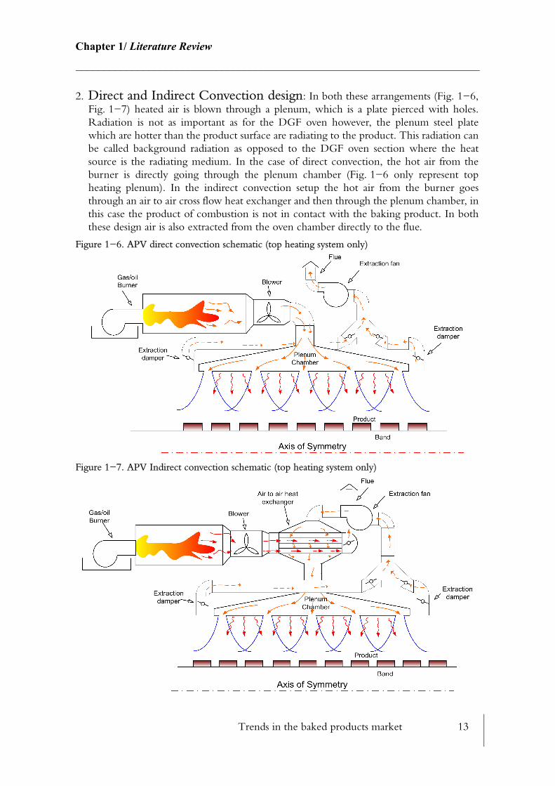
Trends in the baked products market 13
Chapter 1/ Literature Review________________________________________________________________________
2. Direct and Indirect Convection design: In both these arrangements (Fig. 1−6, Fig. 1−7) heated air is blown through a plenum, which is a plate pierced with holes. Radiation is not as important as for the DGF oven however, the plenum steel plate which are hotter than the product surface are radiating to the product. This radiation can be called background radiation as opposed to the DGF oven section where the heat source is the radiating medium. In the case of direct convection, the hot air from the burner is directly going through the plenum chamber (Fig. 1−6 only represent top heating plenum). In the indirect convection setup the hot air from the burner goes through an air to air cross flow heat exchanger and then through the plenum chamber, in this case the product of combustion is not in contact with the baking product. In both these design air is also extracted from the oven chamber directly to the flue.
Figure 1−6. APV direct convection schematic (top heating system only)
Figure 1−7. APV Indirect convection schematic (top heating system only)
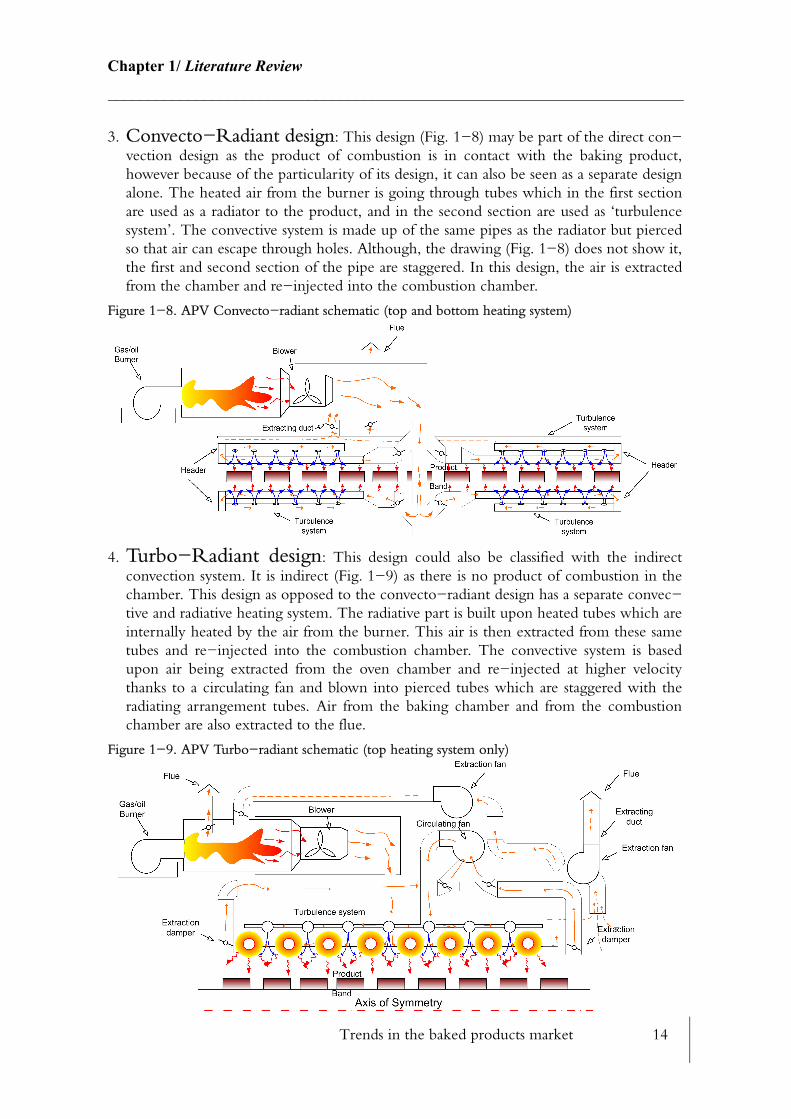
Trends in the baked products market 14
Chapter 1/ Literature Review________________________________________________________________________
3. Convecto−Radiant design: This design (Fig. 1−8) may be part of the direct con−vection design as the product of combustion is in contact with the baking product, however because of the particularity of its design, it can also be seen as a separate design alone. The heated air from the burner is going through tubes which in the first section are used as a radiator to the product, and in the second section are used as ‘turbulence system’. The convective system is made up of the same pipes as the radiator but pierced so that air can escape through holes. Although, the drawing (Fig. 1−8) does not show it, the first and second section of the pipe are staggered. In this design, the air is extracted from the chamber and re−injected into the combustion chamber.
Figure 1−8. APV Convecto−radiant schematic (top and bottom heating system)
4. Turbo−Radiant design: This design could also be classified with the indirect convection system. It is indirect (Fig. 1−9) as there is no product of combustion in the chamber. This design as opposed to the convecto−radiant design has a separate convec−tive and radiative heating system. The radiative part is built upon heated tubes which are internally heated by the air from the burner. This air is then extracted from these same tubes and re−injected into the combustion chamber. The convective system is based upon air being extracted from the oven chamber and re−injected at higher velocity thanks to a circulating fan and blown into pierced tubes which are staggered with the radiating arrangement tubes. Air from the baking chamber and from the combustion chamber are also extracted to the flue.
Figure 1−9. APV Turbo−radiant schematic (top heating system only)

Trends in the baked products market 15
Chapter 1/ Literature Review________________________________________________________________________
5. Impingement design: The impingement design (also called Enerjet) is only manu−factured in the United Stated (APV Goldsboro) and has not been sold in the United Kingdom. The impingement design is part of the direct firing ‘family’ as the product of combustion is in contact with the product. The particularity of its design is to achieve ‘very high’ velocity of the order of 35m/s which impinge to the product surface. The air is extracted from between each of the impingement section of the plenum chamber via an extraction fan. It is then re−circulating to a duct which is connected to the combus−tion chamber. Air is also extracted from the main oven chamber to the flue.
Figure 1−10. APV Impingement schematic (top heating system only)
1.2.3.2 APV oven design family tree
The flow chart (Fig. 1−11) represents the APV oven design family classified by product range (bread, biscuit and cake) and by type of heating system. Each oven has a specific coded number. This flow chart shows the different ovens that are still today on−sale in the industrial baking market, while the rest are still in operation today. The market sale of ovens for APV Baker has been declining in recent years and today the sales trend for most of these ovens (Fig. 1−11) is down. This is due to the increasing number of competitors in this fast growing market and the current fragile economic climate.
This chapter has so far indicated the worldwide market of baked products and highlighted the different types of existing oven design applied by the sponsor APV Baker. Although industrial ovens have been used for the last 100 years few major design changes have been applied in their heat transfer function, which indicates how conservative the baking industry really is. So, why so little change? Is the current baking process optimised so no changes are required? Baking process is still considered today as more of art than a science, but what are the reasons for this belief?
The next paragraphs hope to clarify the heat transfer mechanism occurring during the baking process and give some answers via reviewing literature, to the questions which are at the origin of this project.
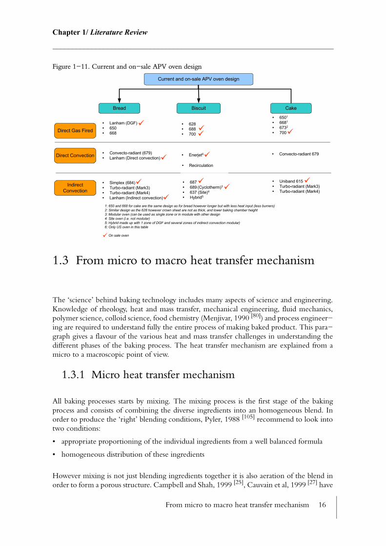
From micro to macro heat transfer mechanism 16
Chapter 1/ Literature Review________________________________________________________________________
Figure 1−11. Current and on−sale APV oven design
1.3 From micro to macro heat transfer mechanism
The ‘science’ behind baking technology includes many aspects of science and engineering. Knowledge of rheology, heat and mass transfer, mechanical engineering, fluid mechanics, polymer science, colloid science, food chemistry (Menjivar, 1990 [80]) and process engineer−ing are required to understand fully the entire process of making baked product. This para−graph gives a flavour of the various heat and mass transfer challenges in understanding the different phases of the baking process. The heat transfer mechanism are explained from a micro to a macroscopic point of view.
1.3.1 Micro heat transfer mechanism
All baking processes starts by mixing. The mixing process is the first stage of the baking process and consists of combining the diverse ingredients into an homogeneous blend. In order to produce the ‘right’ blending conditions, Pyler, 1988 [105] recommend to look into two conditions:
• appropriate proportioning of the individual ingredients from a well balanced formula
• homogeneous distribution of these ingredients
However mixing is not just blending ingredients together it is also aeration of the blend in order to form a porous structure. Campbell and Shah, 1999 [25], Cauvain et al, 1999 [27] have
Current and on-sale APV oven design
Bread Biscuit Cake
Direct Convection
Direct Gas Fired
IndirectConvection
Lanham (DGF)650668
628688700
6501
6681
6732
700
Simplex (684)Turbo-radiant (Mark3)Turbo-radiant (Mark4)Lanham (Indirect convection)
Enerjet6Convecto-radiant (679)Lanham (Direct convection)
687689 (Cyclotherm)3
637 (Site)4
Hybrid5
Convecto-radiant 679
Uniband 615Turbo-radiant (Mark3)Turbo-radiant (Mark4)
1: 650 and 668 for cake are the same design as for bread however longer but with less heat input (less burners)2: Similar design as the 628 however crown sheet are not as thick, and lower baking chamber height3: Modular oven (can be used as single zone or in module with other design4: Site oven (i.e. not modular)5: Hybrid made up with 1 zone of DGF and several zones of indirect convection modular)6: Only US oven in this table
On sale oven
Recirculation
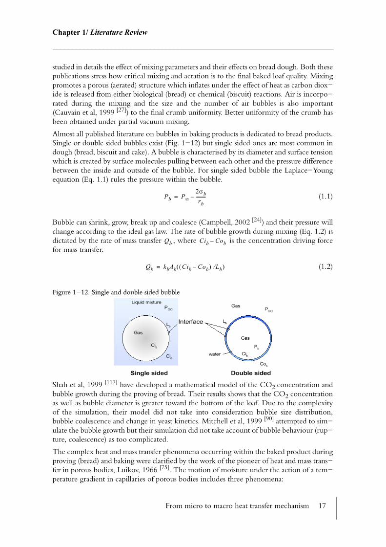
From micro to macro heat transfer mechanism 17
Chapter 1/ Literature Review________________________________________________________________________
studied in details the effect of mixing parameters and their effects on bread dough. Both these publications stress how critical mixing and aeration is to the final baked loaf quality. Mixing promotes a porous (aerated) structure which inflates under the effect of heat as carbon diox−ide is released from either biological (bread) or chemical (biscuit) reactions. Air is incorpo−rated during the mixing and the size and the number of air bubbles is also important (Cauvain et al, 1999 [27]) to the final crumb uniformity. Better uniformity of the crumb has been obtained under partial vacuum mixing.
Almost all published literature on bubbles in baking products is dedicated to bread products. Single or double sided bubbles exist (Fig. 1−12) but single sided ones are most common in dough (bread, biscuit and cake). A bubble is characterised by its diameter and surface tension which is created by surface molecules pulling between each other and the pressure difference between the inside and outside of the bubble. For single sided bubble the Laplace−Young equation (Eq. 1.1) rules the pressure within the bubble.
(1.1)
Bubble can shrink, grow, break up and coalesce (Campbell, 2002 [24]) and their pressure will change according to the ideal gas law. The rate of bubble growth during mixing (Eq. 1.2) is dictated by the rate of mass transfer , where is the concentration driving force for mass transfer.
(1.2)
Figure 1−12. Single and double sided bubble
Shah et al, 1999 [117] have developed a mathematical model of the CO2 concentration and bubble growth during the proving of bread. Their results shows that the CO2 concentration as well as bubble diameter is greater toward the bottom of the loaf. Due to the complexity of the simulation, their model did not take into consideration bubble size distribution, bubble coalescence and change in yeast kinetics. Mitchell et al, 1999 [90] attempted to sim−ulate the bubble growth but their simulation did not take account of bubble behaviour (rup−ture, coalescence) as too complicated.
The complex heat and mass transfer phenomena occurring within the baked product during proving (bread) and baking were clarified by the work of the pioneer of heat and mass trans−fer in porous bodies, Luikov, 1966 [75]. The motion of moisture under the action of a tem−perature gradient in capillaries of porous bodies includes three phenomena:
Pb P∞2σbrb
---------–=
Qb Cib Cob–
Qb kbAb Cib Cob–( ) Lb⁄( )=

From micro to macro heat transfer mechanism 18
Chapter 1/ Literature Review________________________________________________________________________
1. Molecular thermal diffusion of moisture
2. Capillary diffusion
3. Movement of the moisture under the action of entrapped air (Darcy flow)
These three transport mechanism were more recently used by Datta and Zhang, 1999 [41] in their approach to model heat and mass transfer in solid foods.
Luikov was the first to notice the phenomena of evaporation zone in soils which is also present in the baking of wet product. Many authors use Luikov’s equation which rules the heat and mass transport for simulating porous baking products. De Vries et al, 1988 [42] have performed extensive work in the modelling of bread baking, and their heat and mass trans−port model includes conduction in the continuous liquid phase and evaporation−conden−sation in the gas phase. In a more recent publication, Boukadida and Ben Nasrallah, 2002[16] considered a rigid solid phase, liquid phase (pure water) and a gaseous phase which con−tained both air and water vapour. Their model used the generalized Darcy’ s law for two phase flow, gas and liquid.
As pressure increases under the effect of temperature the fine porous body present after the mixing process becomes more aerated and the overall volume of the product increases (see Fig. 1−13).
Figure 1−13. Crumb structure before and after the baking process
Heat pipe phenomenon in the gas cells where evaporation and condensation occurs simul−taneously has been acknowledged by several authors, (De Vries et al, 1988 [42], Hallström et al, 1988 [56], Wiggins, 1998 [139]). The pores are formed with water and water vapour (CO2mainly) that results from the chemical transformation (biscuit) or biological reaction (bread) during the baking (proving). The water contained within these cells is evaporated at the warmest end of the bubble (T1) (see Fig. 1−14) thereby absorbing the latent heat of vapor−isation, but some of it is transferred to the outside by mass transport (conduction and diffu−sion) through the cell membrane to the warmer side of the next gas cell, while the rest flows towards the centre at the coldest side of the gas cell (T2) where its latent heat is released.
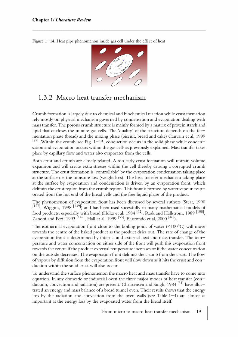
From micro to macro heat transfer mechanism 19
Chapter 1/ Literature Review________________________________________________________________________
Figure 1−14. Heat pipe phenomenon inside gas cell under the effect of heat
1.3.2 Macro heat transfer mechanism
Crumb formation is largely due to chemical and biochemical reaction while crust formation rely mostly on physical mechanism governed by condensation and evaporation dealing with mass transfer. The porous crumb structure is mainly formed by a matrix of protein starch and lipid that encloses the minute gas cells. The ‘quality’ of the structure depends on the fer−mentation phase (bread) and the mixing phase (biscuit, bread and cake) Cauvain et al, 1999[27]. Within the crumb, see Fig. 1−15, conduction occurs in the solid phase while conden−sation and evaporation occurs within the gas cells as previously explained. Mass transfer takes place by capillary flow and water also evaporates from the cells.
Both crust and crumb are closely related. A too early crust formation will restrain volume expansion and will create extra stresses within the cell thereby causing a corrupted crumb structure. The crust formation is ‘controllable’ by the evaporation condensation taking place at the surface i.e. the moisture loss (weight loss). The heat transfer mechanism taking place at the surface by evaporation and condensation is driven by an evaporation front, which delimits the crust region from the crumb region. This front is formed by water vapour evap−orated from the hot end of the bread cells and the free liquid phase of the product.
The phenomenon of evaporation front has been discussed by several authors (Stear, 1990[127], Wiggins, 1998 [139]) and has been used sucessfully in many mathematical models of food products, especially with bread (Holtz et al, 1984 [62], Rask and Hallström, 1989 [108], Zanoni and Peri, 1993 [142], Hall et al, 1999 [55], Elustondo et al, 2000 [46]).
The isothermal evaporation front close to the boiling point of water (<100oC) will move towards the centre of the baked product as the product dries out. The rate of change of the evaporation front is determined by internal and external heat and mass transfer. The tem−perature and water concentration on either side of the front will push this evaporation front towards the centre if the product external temperature increases or if the water concentration on the outside decreases. The evaporation front delimits the crumb from the crust. The flow of vapour by diffusion from the evaporation front will slow down as it hits the crust and con−duction within the solid crust will also occur.
To understand the surface phenomenon the macro heat and mass transfer have to come into equation. In any domestic or industrial oven the three major modes of heat transfer (con−duction, convection and radiation) are present. Christensen and Singh, 1984 [31] have illus−trated an energy and mass balance of a bread tunnel oven. Their results shows that the energy loss by the radiation and convection from the oven walls (see Table 1−4) are almost as important as the energy loss by the evaporated water from the bread itself.
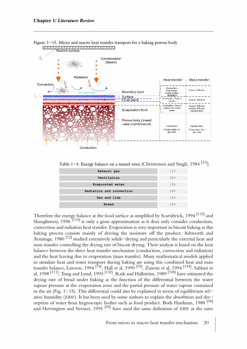
From micro to macro heat transfer mechanism 20
Chapter 1/ Literature Review________________________________________________________________________
Figure 1−15. Micro and macro heat transfer transport for a baking porous body
Therefore the energy balance at the food surface as simplified by Scarisbrick, 1994 [115] and Shaughnessy, 1996 [119] is only a gross approximation as it does only consider conduction, convection and radiation heat transfer. Evaporation is very important in biscuit baking as this baking process consists mainly of driving the moisture off the product. Ashworth and Armitage, 1980 [12] studied extensively solids−drying and particularly the external heat and mass transfer controlling the drying rate of biscuit drying. Their analysis is based on the heat balance between the three heat transfer mechanism (conduction, convection and radiation) and the heat leaving due to evaporation (mass transfer). Many mathematical models applied to simulate heat and water transport during baking are using this combined heat and mass transfer balance, Lawson, 1994 [74], Hall et al, 1999 [55], Zanoni et al, 1994 [144], Sablani et al, 1998 [111], Tong and Lund, 1993 [132]. Rask and Hallström, 1989 [108] have estimated the drying rate of bread under baking as the function of the differential between the water vapour pressure at the evaporation zone and the partial pressure of water vapour contained in the air (Fig. 1−15). This differential could also be explained in terms of equilibrium rel−ative humidity ( ). It has been used by some authors to explain the absorbtion and des−orption of water from hygroscopic bodies such as food product. Both Hardman, 1988 [58]
and Herrington and Vernier, 1995 [59] have used the same definition of as the ratio
Table 1−4. Energy balance on a tunnel oven (Christensen and Singh, 1984 [31])
Exhaust gas 11%
Ventilation 20%
Evaporated water 15%
Radiation and convection 20%
Pan and lids 16%
Bread 18%
ERH
ERH
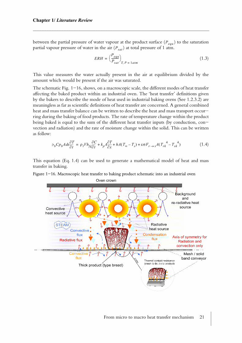
From micro to macro heat transfer mechanism 21
Chapter 1/ Literature Review________________________________________________________________________
between the partial pressure of water vapour at the product surface ( ) to the saturation partial vapour pressure of water in the air ( ) at total pressure of 1 atm.
(1.3)
This value measures the water actually present in the air at equilibrium divided by the amount which would be present if the air was saturated.
The schematic Fig. 1−16, shows, on a macroscopic scale, the different modes of heat transfer affecting the baked product within an industrial oven. The ‘heat transfer’ definitions given by the bakers to describe the mode of heat used in industrial baking ovens (See 1.2.3.2) are meaningless as far as scientific definitions of heat transfer are concerned. A general combined heat and mass transfer balance can be written to describe the heat and mass transport occur−ring during the baking of food products. The rate of temperature change within the product being baked is equal to the sum of the different heat transfer inputs (by conduction, con−vection and radiation) and the rate of moisture change within the solid. This can be written as follow:
(1.4)
This equation (Eq. 1.4) can be used to generate a mathematical model of heat and mass transfer in baking.
Figure 1−16. Macroscopic heat transfer to baking product schematic into an industrial oven
PequPsat
ERHPequPsat-----------
T P, 1atm==
ρbCpbA xdt∂
∂T ρlVhfg t∂∂C kpA
x∂∂T hA T∞ Ts–( ) εσFr s→ A Trk
4 Tsk4
–( )+ + +=
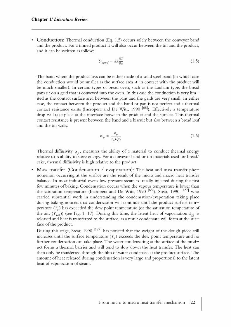
From micro to macro heat transfer mechanism 22
Chapter 1/ Literature Review________________________________________________________________________
• Conduction: Thermal conduction (Eq. 1.5) occurs solely between the conveyor band and the product. For a tinned product it will also occur between the tin and the product, and it can be written as follow:
(1.5)
The band where the product lays can be either made of a solid steel band (in which case the conduction would be smaller as the surface area in contact with the product will be much smaller). In certain types of bread oven, such as the Lanham type, the bread pans sit on a grid that is conveyed into the oven. In this case the conduction is very lim−ited as the contact surface area between the pans and the grids are very small. In either case, the contact between the product and the band or pan is not perfect and a thermal contact resistance exists (Incropera and De Witt, 1990 [68]). Effectively a temperature drop will take place at the interface between the product and the surface. This thermal contact resistance is present between the band and a biscuit but also between a bread loaf and the tin walls.
(1.6)
Thermal diffusivity , measures the ability of a material to conduct thermal energy relative to is ability to store energy. For a conveyor band or tin materials used for bread/cake, thermal diffusivity is high relative to the product.
• Mass transfer (Condensation / evaporation): The heat and mass transfer phe−nomenon occurring at the surface are the result of the micro and macro heat transfer balance. In most industrial ovens low pressure steam is usually injected during the first few minutes of baking. Condensation occurs when the vapour temperature is lower than the saturation temperature (Incropera and De Witt, 1990 [68]). Stear, 1990 [127] who carried substantial work in understanding the condensation/evaporation taking place during baking noticed that condensation will continue until the product surface tem−perature ( ) has exceeded the dew point temperature (or the saturation temperature of the air, ( )) (see Fig. 1−17). During this time, the latent heat of vaporisation is released and heat is transferred to the surface, as a result condensate will form at the sur−face of the product.
During this stage, Stear, 1990 [127] has noticed that the weight of the dough piece still increases until the surface temperature ( ) exceeds the dew point temperature and no further condensation can take place. The water condensating at the surface of the prod−uct forms a thermal barrier and will tend to slow down the heat transfer. The heat can then only be transferred through the film of water condensed at the product surface. The amount of heat released during condensation is very large and proportional to the latent heat of vaporisation of steam.
Qcond kAx∂
∂T=
A
αpkp
ρpCpb----------------=
αp
TsTsat hfg
Ts
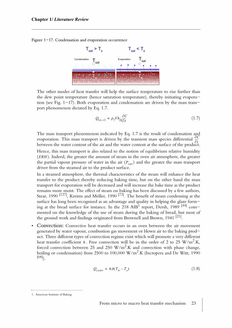
From micro to macro heat transfer mechanism 23
Chapter 1/ Literature Review________________________________________________________________________
Figure 1−17. Condensation and evaporation occurrence
The other modes of heat transfer will help the surface temperature to rise further than the dew point temperature (hence saturation temperature), thereby initiating evapora−tion (see Fig. 1−17). Both evaporation and condensation are driven by the mass trans−port phenomenon dictated by Eq. 1.7.
(1.7)
The mass transport phenomenon indicated by Eq. 1.7 is the result of condensation and evaporation. This mass transport is driven by the transient mass species differential between the water content of the air and the water content at the surface of the product.
Hence, this mass transport is also related to the notion of equilibrium relative humidity ( ). Indeed, the greater the amount of steam in the oven air atmosphere, the greater the partial vapour pressure of water in the air ( ) and the greater the mass transport driver from the steamed air to the product surface.
In a steamed atmosphere, the thermal characteristics of the steam will enhance the heat transfer to the product thereby reducing baking time, but on the other hand the mass transport for evaporation will be decreased and will increase the bake time as the product remains more moist. The effect of steam on baking has been discussed by a few authors, Stear, 1990 [127], Kreims and Möller, 1990 [72]. The benefit of steam condensing at the surface has long been recognised as an advantage and quality in helping the glaze form−ing at the bread surface for instance. In the 218 AIB1 report, Dersh, 1989 [44] com−mented on the knowledge of the use of steam during the baking of bread, but most of the ground work and findings originated from Brownell and Brown, 1941 [21].
• Convection: Convective heat transfer occurs in an oven between the air movement generated by water vapour, combustion gas movement or blown air to the baking prod−uct. Three different types of convection regime exist which will promote a very different heat transfer coefficient . Free convection will be in the order of 2 to 25 W/m2.K, forced convection between 25 and 250 W/m2.K and convection with phase change, boiling or condensation) from 2500 to 100,000 W/m2.K (Incropera and De Witt, 1990[68]).
(1.8)
1. American Institute of Baking
Condensation Evaporation
Ts
TsatTsat
Ts
Tsat > Ts Tsat < Ts
Q e c,( ) ρlVhfg t∂∂C
=
t∂∂C
ERHPsat
h
Qconv hA T∞ Ts–( )=
From micro to macro heat transfer mechanism 24
Chapter 1/ Literature Review________________________________________________________________________
The higher the heat transfer coefficient and the greater the temperature difference between the crust temperature and the oven air, the greater the convective flux will be become to the product. A boundary layer is created when a fluid flows over a solid. Mil−son and Kirk, 1980 [83] have discussed the critical effect of this boundary and its effect on heat transfer during baking. They concluded that the heat transfer coefficient is inversely proportional to the boundary layer thickness. The thickness of this boundary layer tends to be minimal at the leading edge of plate (type biscuit) and often causes edge burning. Many authors have discussed the benefit and detriment of convection during baking. In their optimisation of the baking process, both Christensen et al, 1984 [30], Mälkki et al, 1984 [94] have concluded that more uniform coloured bread could be obtained using convection, and bake time was also reduced as the weight loss (water loss) was greater.
Amongst heat transfer enhancement convection technique, recirculation of air in ovens has been used for decades, which allows to produce more uniform temperature distri−bution all around products and improve product quality uniformity (shape colour). More radical enhancement technique has also been used with great success in more recent years. Walker, 1987 [136], Walker and Sparman, 1989 [137], Ovadia and Walker, 1997 [99]
have described the effects and the usage of impingement technology in the baking. Thanks to its high velocity air flow and directed perpendicularly to the product surface, impingement jets allow to reduce the thickness of stagnant air boundary layer (see Fig. 1−18) and promote better moisture removal, i.e. evaporation.
Although it has been used for many years, impingement has recently been investigated by Wählby et al, 1999 [135] to understand its effect on cooking time and food quality. They concluded that the cooking time was similar as traditional oven but at a much lower air temperature. For relatively large meat products overall browning was uniform. However, they concluded that impingement did not influence significantly the browning of bun although it was achieved in a faster time.
Figure 1−18. Effect of stagnant boundary layer under the effect of impingement
• Radiation: In a domestic or industrial oven, all the surfaces are emitting, absorbing and reflecting thermal radiation. Radiation does not require a transfer medium (as opposed to convection and conduction) and can be propagated through vacuum (Incropera and De Witt, 1990 [68]). The rate of thermal radiation transferred between a hot surface at ( ) to a colder surface at ( ) is expressed by the Kelvin temperature difference to the fourth power (Eq. 1.9). The view factor represent the fraction of the energy leav−ing the radiating surface ( ) to the product skin surface ( ).
Trk TskFr s→
r s
From micro to macro heat transfer mechanism 25
Chapter 1/ Literature Review________________________________________________________________________
(1.9)
The definition of indirect and direct firing in the baking industry refers to the methods of heating but has nothing in common with the direct and indirect radiation as far as heat transfer is concerned. Direct radiation refers to the emitting surfaces, either radiat−ing surface (heater, flame, or oven walls) that strikes the product directly, while indirect radiation refers to the emitted radiation that encountered one or more reflections from the walls before being absorbed by the product (Shaughnessy, 1996 [119]). The emissivity of the background walls is therefore important to be kept as low as possible to improve the radiating to product efficiency. Shaughnessy and Newborough, 1998 [120], have per−formed extensive practical and modelling work to improve the thermal radiation exchange between sheathed electrical elements and the thermal load(s). By reducing the oven linings emissivity to 0.1 they managed to bring the absorbed radiant energy to the load to 88% of the total heat transfer, which is twice as much as what Milson and Kirk, 1980 [83] discussed. This resulted in a much improved thermal response for their oven.
The radiant thermal energy is transmitted by electromagnetic waves which can be of different wavelength. The higher the temperature of the radiator and the shorter the wavelength. These wavelength are traditionally separated into short medium and long wave:
The most efficient wavelength for baking bread according to Pyler, 1988 [105] is between 3 to 6µm. Skjöldebrand and Anderson, 1987 [124] as well as Horace and Smith, 1960 [65]
have discussed the absorption of radiant heat from different wavelength. Pyler, 1988 [105]
who found that 3 to 6µm was an adequate wavelength for bread baking is not entirely wrong as colour will be better overall, however leading to a longer bake time than using NIR.
Baked products are relatively moist and as discussed previously a film of water usually occur during the first minutes of the bake if steam is condensing at the surface of the product. Later on during the bake, evaporation from the product will also leave a thinner water layer on the surface. The absorptivity curve of water merits consideration in order to understand how much of the radiant energy is absorbed by the product. From the absorption curve for a water layer of 3mm (Fig. 1−19), it can be seen that the water will absorb most of the radiant energy in the medium wave infra−red (1.4 − 2.6µm) while below 1.4µm, water will only absorb a very small amount. If a short−wave radiator with a peak radiation of 0.9µm then some of its radiation would be absorbed by the water (see Fig. 1−19, intersection between energy distribution curve from radiator and water absorption curve for a 3mm water layer) and some will penetrate into the baking prod−uct. However, due to their reflectivity properties, Skjöldebrand and Anderson, 1987 [124]
estimated that 50% of the infrared heat would be reflected in the short wave, while only 10% will be reflected in the long wave.
Table 1−5. Classification of infrared radiation
Short wave 0.78 - 1.4µm Near Infrared (NIR) >1500oC
Medium Wave 1.4 - 3µm Mid Infrared (mid-IR)
Long Wave 3 - 1000µm Far INfrared (FIR) <400oC
Qrad εσFr s→ A Trk4 Tsk
4–( )=
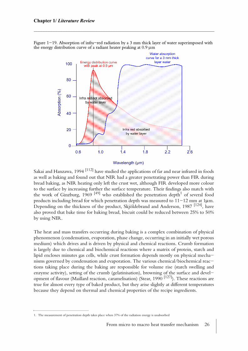
From micro to macro heat transfer mechanism 26
Chapter 1/ Literature Review________________________________________________________________________
Figure 1−19. Absorption of infra−red radiation by a 3 mm thick layer of water superimposed with the energy distribution curve of a radiant heater peaking at 0.9 µm
Sakai and Hanzawa, 1994 [112] have studied the applications of far and near infrared in foods as well as baking and found out that NIR had a greater penetrating power than FIR during bread baking, as NIR heating only left the crust wet, although FIR developed more colour to the surface by increasing further the surface temperature. Their findings also match with the work of Ginzburg, 1969 [49] who established the penetration depth1 of several food products including bread for which penetration depth was measured to 11−12 mm at 1µm. Depending on the thickness of the product, Skjöldebrand and Anderson, 1987 [124], have also proved that bake time for baking bread, biscuit could be reduced between 25% to 50% by using NIR.
The heat and mass transfers occurring during baking is a complex combination of physical phenomenon (condensation, evaporation, phase change, occurring in an initially wet porous medium) which drives and is driven by physical and chemical reactions. Crumb formation is largely due to chemical and biochemical reactions where a matrix of protein, starch and lipid encloses minutes gas cells, while crust formation depends mostly on physical mecha−nisms governed by condensation and evaporation. The various chemical/biochemical reac−tions taking place during the baking are responsible for volume rise (starch swelling and enzyme activity), setting of the crumb (gelatinisation), browning of the surface and devel−opment of flavour (Maillard reaction, caramelisation) (Stear, 1990 [127]). These reactions are true for almost every type of baked product, but they arise slightly at different temperatures because they depend on thermal and chemical properties of the recipe ingredients.
1. The measurement of penetration depth takes place when 37% of the radiation energy is unabsorbed
From micro to macro heat transfer mechanism 27
Chapter 1/ Literature Review________________________________________________________________________
Heat and mass transfer in baking usually takes place simultaneously and mathematical sim−ulation and theoretical analysis becomes challenging. For well defined substances, mathe−matical simulation is difficult and general solutions do not necessarily exist. The problem becomes even more problematical when it concerns foods whose thermal and engineering properties are difficult to predict.
Many authors and research associations are spending considerable effort in determining thermal properties of foodstuff for improving the mathematical simulation, and the literature reveals that there has been an increasing trend in determining these properties with the emergence of more affordable and powerful computers. Short et al, 1942 [121] were the pio−neers in the determination of specific heat capacities for foodstuffs, although there is some previous record of measurement of heat capacity and latent heat of fish muscle in 1928. Christenson et al, 1989 [32] have determined experimentally the physical properties of baked products as functions of moisture in the temperature range of 20oC to 85oC. Moisture con−tent, desorption, density, heat capacity and thermal capacity were determined for white bread, muffin and biscuit. Mellor, 1983 [79] has identified areas which are; data estimations using freezing points, instantaneous measurements using probes, data banking, smoothing data, and high temperature data, where special attention should be drawn in order to improve the development of thermophysical properties. Started in 1978, a three year project called COST90 (Meffert, 1983 [78]) was initiated by a voluntary team of scientist and research groups, in the European Economic Community by ten members (Belgium, Denmark, Eire, Federal German Republic, France Greece, Italy Luxembourg, The Netherlands, United Kingdom). This project target was to establish procedures to constitute a database of physical properties of foodstuffs. Those procedures were verified by experts in the field. To help in building simultaneous heat and mass transfer models of foodstuffs, Saravacos, 1994 [113] has studied the mass transfer of foodstuffs with special attention to the important properties driving mass transfer. He also collected from previous work diffusivities and permeabilites of several food properties. Sweat, 1994 [128] has contributed to this field by focusing on the estimation technique to evaluate thermal properties and by helping to understand the mean−ing of each of the useful thermal properties (specific heat, enthalpy, thermal conductivity, thermal diffusivity, and surface heat transfer coefficient). Zanoni et al, 1995 [143] have carried out experiments to determine thermal diffusivity and apparent density of bread crust and crumb and predicted that both these properties were a linear relationship of porosity. A mathematical model for simulating internal temperature profile using their experimental data demonstrated that their methods for measuring thermal properties was accurate. Other properties such as dielectric loss were investigated by Calay et al, 1995 [23] for helping in modelling microwave heating. To date, some considerable efforts have been made to collect and assemble foodstuff properties to build up databases (e.g. National Physical Laboratory, 2002 [95], Nelfood, 2002 [96], Singh, 2002 [123]).
The baking industry has been and still is today a very conservative industry especially in the development of new ovens. This is understandable when looking at the size and the replace−ment cost of new ovens (a tunnel oven costs approximately £500,000). Manufacturers of ovens are not willing to invest a large amount of research and development unless high turn−over can be achieved, that is why effort tends to be directed to improving manufacturing efficiencies only. The science involved behind the baking process is complex (heat and mass transfer, chemistry, fluids mechanics, rheology...) so, the persons responsible for operating the
From micro to macro heat transfer mechanism 28
Chapter 1/ Literature Review________________________________________________________________________
baking process rely very much on the experience gained over generations of bakers. The application of their knowledge is considered an art.
For the first time the sponsor of this research, APV Baker, has invested significant effort in trying to investigate heat transfer for optimising the baking process, thereby transforming the art of baking into a more scientific approach. Although it is possible to build mathematical models, and specific thermal properties might be available, they are product specific (models for bread baking will not be the same as biscuit for instance). For this reason the experimental avenue was considered to represent a better strategy. To help achieve this challenge, APV Baker and Cranfield University (Urrutia, 1997 [133], Pierrel, 1998 [101]) started the devel−opment and construction of a Thermal Performance Research Oven which has been designed to investigate baking while respecting the traditional industrial oven based on an impingement, and recirculation.
Three products (bread, biscuit and cake) were candidates for this investigation. It is obvious, that bread and biscuit have conveyed significantly more interest in the research field because they are the main focus of the baking market. A cake (Madeira cake) product was chosen as the subject for investigating process optimisation. Cake is relatively unexplored. The baking time of a cake product is relatively long (~ 60min) compared with bread (~ 20min) and bis−cuit (~5 min.) so variation on the product characteristics can be noticed more easily and the energy implications of baking cake are substantial per item.
The first research in cakes was directed into the fat content and its evolution into the batter under the influence of heat (Carlin, 1944 [26]). Carlin conducted a microscopic study of cake batters and found out that the ‘fat globules’ were affecting the stability of cake structure hence cake shrinkage. He also determined that the end of the baking could be established microscopically using a polarized light. Hood and Lowe, 1948 [63] have also looked in the influence of fat with regards to volume increase. Their study concluded that the volume of cakes directly related to the effectiveness of carbon dioxide evolution which, was the greatest when using hydrogenated lard as opposed to oil or butter. Other criteria for scoring the cakes were also used (texture, eating quality). From the 1950’s onward, the literature reports that most of the research concerns improving the quality of the baking changing every possible variables, from pan material, recipe ingredients, oven settings. Charley (Charley, 1950 [29], Charley, 1956 [28]) studied the effect of pan material on the heat penetration during the baking of cake and observed the changes in quality. Materials such as aluminium, anodized aluminium, tinned iron, japanned iron, steel, copper, stainless steel and glass were used for her study. The penetration was measured with the help of a mercury−glass thermometer. The faster bake was obtained with the tins which were dark or dull (steel, japanned iron, anodized aluminium and iron) and produced the larger volume and better crumb quality however, the overall appearance was poor. Elgidaily et al, 1969 [45] studied the effect of dif−ferent baking temperature on quality of angel cakes. Four temperatures were studied and the quality aspects of the cakes were bake loss, cake moisture content, compressibilty, colour and volume. A jury panel was also assessing the overall quality of the product. The main finding of this research was the discovery of a relationship between the temperature and the volume. Lower temperature (177oC, 191oC) led to higher quality scores than those which were baked at 204oC and 218oC, as a result the compressibilty on the cakes baked at higher temperature were harder. They reported that the weight loss was not influenced by the oven temperature. In their experimental research, Gordon et al, 1979 [50] have shown that a relationship exists between the moisture loss and the internal temperature profile. Their study was also oriented
From micro to macro heat transfer mechanism 29
Chapter 1/ Literature Review________________________________________________________________________
to change the starch content of the recipe and study the moisture loss according to these dif−ferent levels of starch. They indicated that the water loss mechanism was linked to the pro−portion of starch in their recipe.
The experimental work conducted by Garrison and Peart, 1986 [48] was to estimate the effect of radiant heat transfer in a conventional electric oven during the baking of cake. The irradiation to the product was measured with a cake−pan radiometer, and altered by treating the oven wall surfaces with different reflectance materials. Browning was measured using a browning scale (1 to 10) and moisture loss was also measured. Their final results revealed that browning of the top and bottom surfaces were positively correlated with the increase of radiation by using foil on the internal oven wall surfaces. The increase of irradiation on the lower cake surface resulted in the increase of both bottom surface browning and increase in moisture loss. They also concluded that cake volume was not significantly related to irradi−ation levels. A small convective oven was used in the research of Sato et al, 1987 [114] to esti−mate the effect of air velocity and temperature (oven convective heat transfer) on the cake volume and cohesiveness. Four different air velocities between 0 m/sec to 1.5 m/sec, and temperatures of 180oC, 220oC, and 220oC were used in the experiments. Their findings shows that velocity and/or temperature could shorten the bake time. Increasing the air and /or temperature resulted in a dryer sponge cake with a darker colour. The firmness of the product was only affected by air velocity. Increase in air velocity resulted in a firmer cake. Change in temperature affected more the volume more than change in velocity. Baik et al, 1999 [13] looked into measuring the heat transfer coefficient with a h−monitor on cake over the length of an industrial tunnel type oven. The ranges of temperature were from 186−225oC, relative air velocities from 0.02−0.437 m/s and absolute humidities between 0.0267−0.0428kg H2O/Kg dry air.
From the literature it is clear that a method for establishing whether the baked product can be produced more rapidly and more energy efficiently is required. In particular the lack of previous work on cake products requires further research attention.
The data reported by literature whether it is an oven operating performance or a baked product characteristics is difficult to compare with other similar information as the methods of monitoring or measuring are often not mentioned and not comparable. It is therefore important to set a method for measuring and monitoring real data within a known accuracy and repeatability. Human judgement for assessing product quality is very subjective and the literature shows a lack of established method. The literature only reports few attempts of optimising baking process, and the methods for achieving this are very much a field for research.
Objectives of investigation 30
Chapter 1/ Literature Review________________________________________________________________________
1.4 Objectives of investigation
The objectives of this research were:
1. To complete the development of a batch research oven which achieve much greater rates of heat transfer than traditional baking ovens with a view to proving its reliability and capability for simulating an industrial travelling type oven.
2. To equip this Thermal Performance Research Oven with sufficient and reliable meas−urement devices and control systems, for measuring and controlling baking in a repeata−ble and accurate manner.
3. To undertake experimental testing to identify the thermal performance characteristics of this oven and define the boundaries of the operating parameters.
4. To develop testing procedures using accurate measurement techniques so that an exper−imental investigation of baking can be performed, measuring the product characteristics without using a jury panel.
5. To carry out a design of experiment to optimise the baking process of a Madeira cake and establish how to decrease bake time while keeping the product characteristics within an acceptable tolerance band.
6. To validate the design of experiments model to authenticate the methodology and con−firm results of the optimised process.
7. To make recommendations for the enhanced baking of Madeira cake and improvements to the oven and the experimental approach.
Rig history 31
Chapter 2/ Concepts and Design of TPRO Rig________________________________________________________________________
CHAPTER 2
CONCEPTS AND DESIGN OF TPRO RIG
The Thermal Performance Research Oven (TPRO) is the name given by APV Baker Ltd. to a novel research oven which was designed to simulate the operation of a full scale tunnel oven. It offers a basis for investigating very high rates of heat transfer relative to those obtained in conventional baking ovens. This chapter deals with the main aspects of the mechanical, electrical and thermal design of the TPRO.
2.1 Rig history
The foremost driving concept behind this project is to investigate heat transfer enhancement to reduce baking time by replicating baking profiles as they exist in long−travelling ovens. The rig for exploring this concept is the Thermal Performance Research Oven, TPRO. As a result, the challenge of this project is to simulate ovens (100 to 300m) with temperature and humidity controlled zones, into a single zone of one meter long. The TPRO has been specifically designed to achieve rates of heat transfer well in excess of those in current baking ovens.
The Thermal performance research oven is part of an on−going project which started in 1996 with the communion of Cranfield University and APV Baker Ltd. as a sponsorship. It was first design and conceived by the MSc student Urrutia, 1997 [133] and was further devel−oped by the MSc student Pierrel, 1998 [101] before this PhD work started. The construction of the TPRO (mechanical and electrical) was covered by engineers at APV Baker. The total cost of the TPRO is estimated to be £400,000 of which on third is allocated to parts. Although the TPRO was physically conceived in the first year of this PhD project, several commissioning problems arose and were solved during the second year of this work. Numerous design changes were required to produce what the TPRO is today. Some major re−design was undertaken during the core of this work and the most relevant aspects will be covered in the description of the rig in this chapter.

Rig description 32
Chapter 2/ Concepts and Design of TPRO Rig________________________________________________________________________
2.2 Rig description
The TPRO has been built on the concept of an APV Baker impingement, direct gas fired and recirculation type ovens. The TPRO today (Figure 2−1) is build with walls of 1.3 mm thick stainless steel (316) and covered with 25mm to 50mm (Urrutia, 1997 [133]) of micro−therm insulation, of conductivity 58% less than of glass fiber insulating material. Today three electrical heaters of a total power of 130kW are used for convection (radiation) heating sys−tem, however it was originally designed with 1 single 30kW heater. 6 Radiant heaters posi−tioned (top and bottom, Fig. 2−1) on each ends of the top and bottom plenums are radiating to the product surface giving up a total of 5.7kW. With the two fans, (circulation fan, CFAN) 5.5kW and (recirculation fan) 4.5kW, the oven requires 250 amps to run. This oven was originally designed by Urrutia, 1997 [133] to operate at maximum temperature of 500oC and specific details can be found in Urrutia, 1997 [133] and Pierrel, 1998 [101]. Chapter 2describes the hardware used in the TPRO while Chapter 3 defines the software Wonderware (Wonderware, 2002 [141]) InControl™ and InTouch™.
2.2.1 Air circulation
The skeleton of the TPRO during the first year of this research project is represented by Fig. 2−1. In the situation where D1 if fully open, the ambient air is drawn in the inlet duct via the circulation fan. At the junction between the inlet duct and the recirculation duct, the inlet air can be mixed with recirculated (pre−heated) air. The ratio of recirculation is con−trolled mostly by dampers 8 (D8),9 (D9) and 1 (D1).
The functions of D8 and D1 are to select between total, partial or no recirculation mode. The functioning of D9 is to adjust the amount of air recirculated, i.e. either partial, full or none. The key issues in recirculation are to homogenize the mixing, allow faster heating time and also reduce energy consumption. After the circulation fan the air meets a honeycomb grid which encourages laminar flow in that portion before it enters the duct heater. Both fans are speed controlled but D2 and D7 were designed in for fine adjustment. Injection of steam is made straight after the heater before the splitting duct.
The humid mixture is then fed equally to the top and bottom ducts. Assuring the equality of top and bottom air flow was studied by both experimentally and by computational fluid dynamics (CFD) Pierrel, 1998 [101]. A half size perspex model of the plenum chamber was constructed and smoke was introduced by means of a smoke machine, into the chamber so that the flow can be visualized. Results from this experiments revealed the creation of vor−tices inside the plenum chamber. Higher velocities could also be observed in the top bend of the plenum. The creation of a CFD model helped to visualise both velocity and pressure profile within the plenum and also to position flow guides (vanes) to promote an homoge−neous velocity profile coming out of the nozzle outlets.
The functions of D8 and D1 are to select between total, partial or no recirculation mode. The functioning of D9 is to adjust the amount of air recirculated, i.e. either partial, full or none.
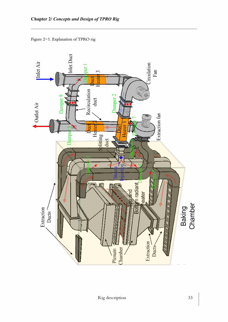
Rig description 33
Chapter 2/ Concepts and Design of TPRO Rig________________________________________________________________________
Figure 2−1. Explanation of TPRO rig
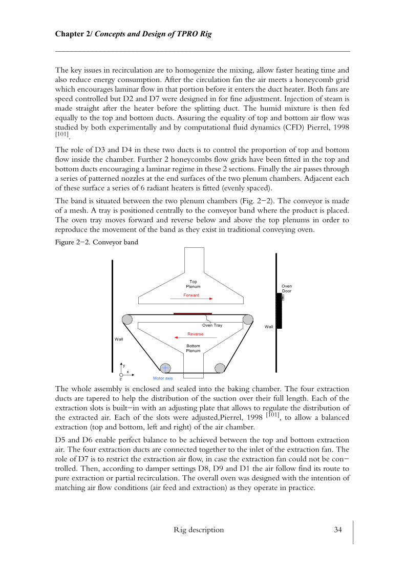
Rig description 34
Chapter 2/ Concepts and Design of TPRO Rig________________________________________________________________________
The key issues in recirculation are to homogenize the mixing, allow faster heating time and also reduce energy consumption. After the circulation fan the air meets a honeycomb grid which encourages laminar flow in that portion before it enters the duct heater. Both fans are speed controlled but D2 and D7 were designed in for fine adjustment. Injection of steam is made straight after the heater before the splitting duct. The humid mixture is then fed equally to the top and bottom ducts. Assuring the equality of top and bottom air flow was studied by both experimentally and by computational fluid dynamics (CFD) Pierrel, 1998[101].
The role of D3 and D4 in these two ducts is to control the proportion of top and bottom flow inside the chamber. Further 2 honeycombs flow grids have been fitted in the top and bottom ducts encouraging a laminar regime in these 2 sections. Finally the air passes through a series of patterned nozzles at the end surfaces of the two plenum chambers. Adjacent each of these surface a series of 6 radiant heaters is fitted (evenly spaced).
The band is situated between the two plenum chambers (Fig. 2−2). The conveyor is made of a mesh. A tray is positioned centrally to the conveyor band where the product is placed. The oven tray moves forward and reverse below and above the top plenums in order to reproduce the movement of the band as they exist in traditional conveying oven.
Figure 2−2. Conveyor band
The whole assembly is enclosed and sealed into the baking chamber. The four extraction ducts are tapered to help the distribution of the suction over their full length. Each of the extraction slots is built−in with an adjusting plate that allows to regulate the distribution of the extracted air. Each of the slots were adjusted,Pierrel, 1998 [101], to allow a balanced extraction (top and bottom, left and right) of the air chamber.
D5 and D6 enable perfect balance to be achieved between the top and bottom extraction air. The four extraction ducts are connected together to the inlet of the extraction fan. The role of D7 is to restrict the extraction air flow, in case the extraction fan could not be con−trolled. Then, according to damper settings D8, D9 and D1 the air follow find its route to pure extraction or partial recirculation. The overall oven was designed with the intention of matching air flow conditions (air feed and extraction) as they operate in practice.
TopPlenum
xy
z
Wall
Wall
OvenDoor
Reverse
Oven Tray
BottomPlenum
Forward
Motor axis
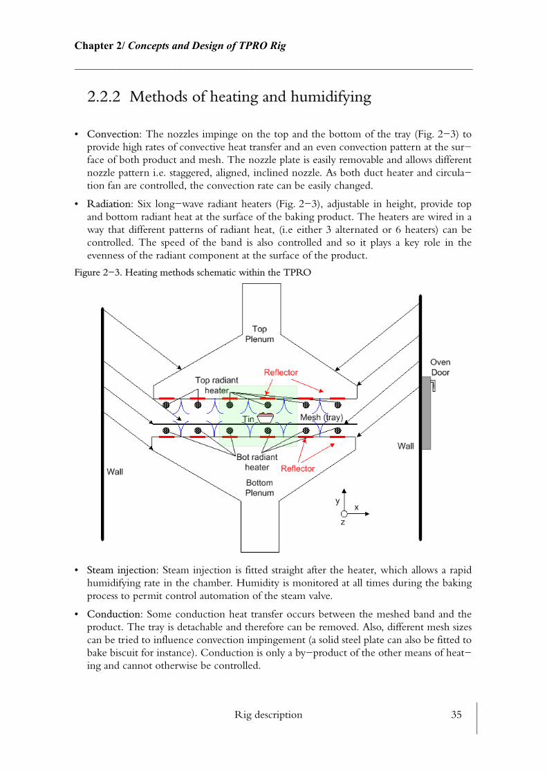
Rig description 35
Chapter 2/ Concepts and Design of TPRO Rig________________________________________________________________________
2.2.2 Methods of heating and humidifying
• Convection: The nozzles impinge on the top and the bottom of the tray (Fig. 2−3) to provide high rates of convective heat transfer and an even convection pattern at the sur−face of both product and mesh. The nozzle plate is easily removable and allows different nozzle pattern i.e. staggered, aligned, inclined nozzle. As both duct heater and circula−tion fan are controlled, the convection rate can be easily changed.
• Radiation: Six long−wave radiant heaters (Fig. 2−3), adjustable in height, provide top and bottom radiant heat at the surface of the baking product. The heaters are wired in a way that different patterns of radiant heat, (i.e either 3 alternated or 6 heaters) can be controlled. The speed of the band is also controlled and so it plays a key role in the evenness of the radiant component at the surface of the product.
Figure 2−3. Heating methods schematic within the TPRO
• Steam injection: Steam injection is fitted straight after the heater, which allows a rapid humidifying rate in the chamber. Humidity is monitored at all times during the baking process to permit control automation of the steam valve.
• Conduction: Some conduction heat transfer occurs between the meshed band and the product. The tray is detachable and therefore can be removed. Also, different mesh sizes can be tried to influence convection impingement (a solid steel plate can also be fitted to bake biscuit for instance). Conduction is only a by−product of the other means of heat−ing and cannot otherwise be controlled.
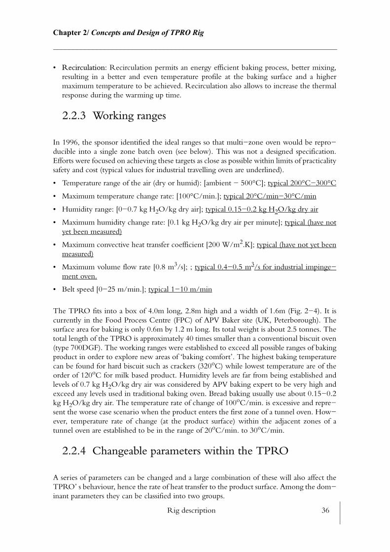
Rig description 36
Chapter 2/ Concepts and Design of TPRO Rig________________________________________________________________________
• Recirculation: Recirculation permits an energy efficient baking process, better mixing, resulting in a better and even temperature profile at the baking surface and a higher maximum temperature to be achieved. Recirculation also allows to increase the thermal response during the warming up time.
2.2.3 Working ranges
In 1996, the sponsor identified the ideal ranges so that multi−zone oven would be repro−ducible into a single zone batch oven (see below). This was not a designed specification. Efforts were focused on achieving these targets as close as possible within limits of practicality safety and cost (typical values for industrial travelling oven are underlined).
• Temperature range of the air (dry or humid): [ambient − 500°C]; typical 200°C−300°C
• Maximum temperature change rate: [100°C/min.]; typical 20°C/min−30°C/min
• Humidity range: [0−0.7 kg H2O/kg dry air]; typical 0.15−0.2 kg H2O/kg dry air
• Maximum humidity change rate: [0.1 kg H2O/kg dry air per minute]; typical (have not yet been measured)
• Maximum convective heat transfer coefficient [200 W/m2.K]; typical (have not yet been measured)
• Maximum volume flow rate [0.8 m3/s]; ; typical 0.4−0.5 m3/s for industrial impinge−ment oven.
• Belt speed [0−25 m/min.]; typical 1−10 m/min
The TPRO fits into a box of 4.0m long, 2.8m high and a width of 1.6m (Fig. 2−4). It is currently in the Food Process Centre (FPC) of APV Baker site (UK, Peterborough). The surface area for baking is only 0.6m by 1.2 m long. Its total weight is about 2.5 tonnes. The total length of the TPRO is approximately 40 times smaller than a conventional biscuit oven (type 700DGF). The working ranges were established to exceed all possible ranges of baking product in order to explore new areas of ‘baking comfort’. The highest baking temperature can be found for hard biscuit such as crackers (320oC) while lowest temperature are of the order of 120oC for milk based product. Humidity levels are far from being established and levels of 0.7 kg H2O/kg dry air was considered by APV baking expert to be very high and exceed any levels used in traditional baking oven. Bread baking usually use about 0.15−0.2 kg H2O/kg dry air. The temperature rate of change of 100oC/min. is excessive and repre−sent the worse case scenario when the product enters the first zone of a tunnel oven. How−ever, temperature rate of change (at the product surface) within the adjacent zones of a tunnel oven are established to be in the range of 20oC/min. to 30oC/min.
2.2.4 Changeable parameters within the TPRO
A series of parameters can be changed and a large combination of these will also affect the TPRO’ s behaviour, hence the rate of heat transfer to the product surface. Among the dom−inant parameters they can be classified into two groups.

Rig description 37
Chapter 2/ Concepts and Design of TPRO Rig________________________________________________________________________
1. Manual controla) Recirculation rate adjusting D1, D8 and D9.
b) Main feed flow rate adjusting D2.
c) Ratio of top and bottom plenum air flow by adjusting D3 and D4.
d) Food product top surface and nozzle exit distance by adjusting the top plenum height.
e) Top and bottom, left, right extraction adjusting D5 and D6.
g) Extraction flow modifying D7.
i) Convection pattern and rate by changing the nozzle plates for both top and bottom ple−nums.
j) Height between the product surface and the radiation heater can be modified manually, hence changing the amount of radiation power to the product surface.
2. Computer controlleda) Feed flow, by adjusting both circulation and extraction fans.
b) Air temperature within the oven chamber.
c) Radiant heater surface temperature.
d) Speed of the baking tray.
e) Rate of steam injection in the chamber by adjusting motorised pneumatic valve.
f) Baking time can be adjusted for each zone modelled.
g) Number of zones modelled can vary between 1 and 10.
Control is a major issue as there is a large number of parameters and sub−parameters that can be controlled and monitored. Control and instrumentation in use are treated independently in this chapter.
Prior to starting the non−food test phases (4.1) a large amount of preliminary test work was undertaken, to discover thermal limitations of the TPRO rig, to establish robust and reliable control algorithm, and to assess the reliability of the various instrumentation in use. The TPRO was treated as thermal system and an energy balance was constructed to define the thermal performance envelope of the TPRO (See 2.4.3, 4.6).
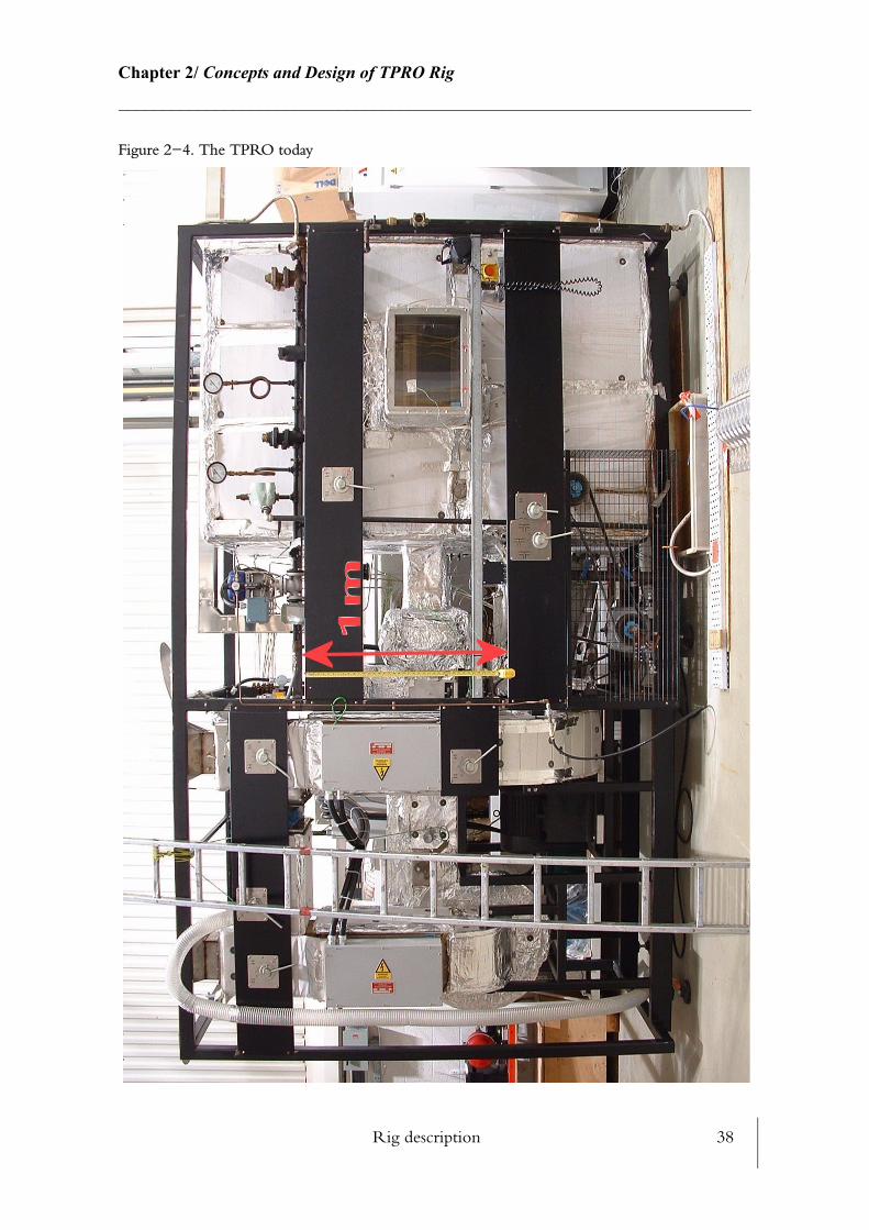
Rig description 38
Chapter 2/ Concepts and Design of TPRO Rig________________________________________________________________________
Figure 2−4. The TPRO today

The TPRO: A Thermal System 39
Chapter 2/ Concepts and Design of TPRO Rig________________________________________________________________________
2.3 The TPRO: A Thermal System
Industrial baking ovens operate days and nights seven days a week and most of the days of the year apart from the days allocated for maintenance and cleaning. Each of the oven zones is controlled independently and the temperature, humidity profile remains the same over the year within each zone. Industrial baking ovens performs similarly as furnaces but at lower temperatures and behaves as thermal steady state system. The only non steady−state regime operates during the warm up phase which can take up to several hours due to the enormous mass of real oven. The advantage of having large masses makes these thermal systems extremely stable and day to day temperature variation is very unlikely. This is of particular importance when trying to produce the same product again and again to tight tolerances. The down−side of having a heavy thermal system is its inability to respond quickly to control changes. The challenge of building a batch oven capable of reproducing such profiles is more complex than building a standard industrial oven. Indeed, the TPRO must react to changes rapidly in order to replicate the step changes from one zone to another, but it must also remain in thermal steady state as much as possible thereafter, so as to avoid product variation and keep close product tolerances.
2.3.1 Understanding the TPRO as a thermal system
The target of the commissioning phase (NFT_PHASE0) was to allow a better understanding of the TPRO as a thermal system. Numerous aspects of the design (hardware and software) were assessed to check for robustness and reliability. For this matter, the test rig was initially run for several days without interruption at full fan speed (FIS1) and in the full re−circulating mode with no heat load applied. One aspect of the non food test phase was to comprehend how the TPRO respond in the transient regime. The analysis of transient regime can give very useful information. Understanding how the structure warms up and which of the oven components is heating up the quickest or the slowest can be used to re−design the oven structure and choose better material to optimise the oven thermal response time. Investiga−tion of the breakdown of the energy balance from transient to steady state regime allows to visualize which of the heat losses is pre−dominant during both phases and answer the ques−tion: where does the energy go?
2.3.1.1 Extra heat load
The first unexpected result (Fig. 2−5), was that the oven air temperature had reached 95.2oC after 13h in those conditions. This was the time required to achieve a thermal steady state by both the air and the rig structure (wall insulation, steel, and internal uncovered steel mass). The temperature rate of change during the first 25 minutes (See zoom, Fig. 2−5) of the test
1. The fan speed is controlled by inverter settings. The values quoted in this thesis are Fan Inverter Settings (FIS) which could be meas−ured in Hertz and which are proportional to the fan speed in RPM.
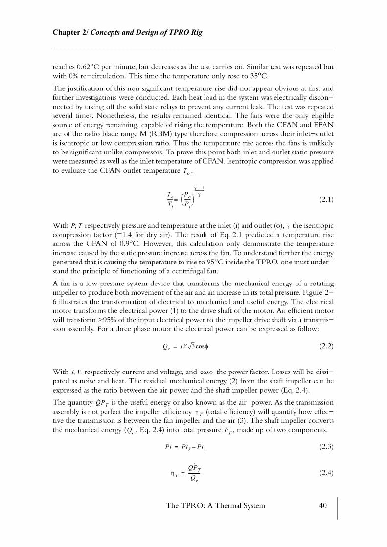
The TPRO: A Thermal System 40
Chapter 2/ Concepts and Design of TPRO Rig________________________________________________________________________
reaches 0.62oC per minute, but decreases as the test carries on. Similar test was repeated but with 0% re−circulation. This time the temperature only rose to 35oC.
The justification of this non significant temperature rise did not appear obvious at first and further investigations were conducted. Each heat load in the system was electrically discon−nected by taking off the solid state relays to prevent any current leak. The test was repeated several times. Nonetheless, the results remained identical. The fans were the only eligible source of energy remaining, capable of rising the temperature. Both the CFAN and EFAN are of the radio blade range M (RBM) type therefore compression across their inlet−outlet is isentropic or low compression ratio. Thus the temperature rise across the fans is unlikely to be significant unlike compressors. To prove this point both inlet and outlet static pressure were measured as well as the inlet temperature of CFAN. Isentropic compression was applied to evaluate the CFAN outlet temperature .
(2.1)
With respectively pressure and temperature at the inlet (i) and outlet (o), the isentropic compression factor (=1.4 for dry air). The result of Eq. 2.1 predicted a temperature rise across the CFAN of 0.9oC. However, this calculation only demonstrate the temperature increase caused by the static pressure increase across the fan. To understand further the energy generated that is causing the temperature to rise to 95oC inside the TPRO, one must under−stand the principle of functioning of a centrifugal fan.
A fan is a low pressure system device that transforms the mechanical energy of a rotating impeller to produce both movement of the air and an increase in its total pressure. Figure 2−6 illustrates the transformation of electrical to mechanical and useful energy. The electrical motor transforms the electrical power (1) to the drive shaft of the motor. An efficient motor will transform >95% of the input electrical power to the impeller drive shaft via a transmis−sion assembly. For a three phase motor the electrical power can be expressed as follow:
(2.2)
With respectively current and voltage, and the power factor. Losses will be dissi−pated as noise and heat. The residual mechanical energy (2) from the shaft impeller can be expressed as the ratio between the air power and the shaft impeller power (Eq. 2.4).
The quantity is the useful energy or also known as the air−power. As the transmission assembly is not perfect the impeller efficiency (total efficiency) will quantify how effec−tive the transmission is between the fan impeller and the air (3). The shaft impeller converts the mechanical energy ( , Eq. 2.4) into total pressure , made up of two components.
(2.3)
(2.4)
To
ToTi-----
PoPi------
γ 1–γ
-----------
=
P T, γ
Qe IV 3 φcos=
I V, φcos
Q· PTηT
Qe PT
Pt Pt2 Pt1–=
ηTQPT
·
Qe-----------=

The TPRO: A Thermal System 41
Chapter 2/ Concepts and Design of TPRO Rig________________________________________________________________________
The first component is the static pressure which depends mainly on the aerodynamics of the blade, and the second is the dynamic pressure which is developed due to velocity or kinetic energy.
Figure 2−5. Fan heat load
Figure 2−6. Fan assembly
The remaining energy is consumed by irreversible losses across the impeller and in the fan casing but also produce an additional increase in temperature of the air due to isentropic compression. If the fan was blowing out in the open air, this energy would be lost, however in a ducting system, thanks to the law of energy conservation, this useful energy (absorbed power), works to overcome pressure loss and is entirely used to increase the internal energy of the air, which is physically translated to a temperature rise. The energy given by the fans to the air is not as insignificant as it might first appear and this energy input term was latter considered in the whole energy balance of the this thermal system. The quantifying of this energy term is expressed latter in this chapter.
PsPv
Centrifugal FanMotor
Electrical Mechanical Flow
1 2 3
Pt1 Pt2
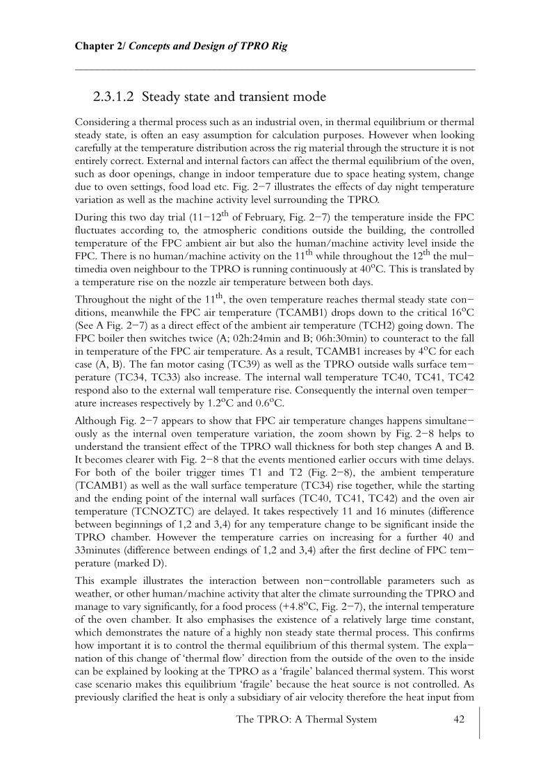
The TPRO: A Thermal System 42
Chapter 2/ Concepts and Design of TPRO Rig________________________________________________________________________
2.3.1.2 Steady state and transient mode
Considering a thermal process such as an industrial oven, in thermal equilibrium or thermal steady state, is often an easy assumption for calculation purposes. However when looking carefully at the temperature distribution across the rig material through the structure it is not entirely correct. External and internal factors can affect the thermal equilibrium of the oven, such as door openings, change in indoor temperature due to space heating system, change due to oven settings, food load etc. Fig. 2−7 illustrates the effects of day night temperature variation as well as the machine activity level surrounding the TPRO.
During this two day trial (11−12th of February, Fig. 2−7) the temperature inside the FPC fluctuates according to, the atmospheric conditions outside the building, the controlled temperature of the FPC ambient air but also the human/machine activity level inside the FPC. There is no human/machine activity on the 11th while throughout the 12th the mul−timedia oven neighbour to the TPRO is running continuously at 40oC. This is translated by a temperature rise on the nozzle air temperature between both days.
Throughout the night of the 11th, the oven temperature reaches thermal steady state con−ditions, meanwhile the FPC air temperature (TCAMB1) drops down to the critical 16oC (See A Fig. 2−7) as a direct effect of the ambient air temperature (TCH2) going down. The FPC boiler then switches twice (A; 02h:24min and B; 06h:30min) to counteract to the fall in temperature of the FPC air temperature. As a result, TCAMB1 increases by 4oC for each case (A, B). The fan motor casing (TC39) as well as the TPRO outside walls surface tem−perature (TC34, TC33) also increase. The internal wall temperature TC40, TC41, TC42 respond also to the external wall temperature rise. Consequently the internal oven temper−ature increases respectively by 1.2oC and 0.6oC.
Although Fig. 2−7 appears to show that FPC air temperature changes happens simultane−ously as the internal oven temperature variation, the zoom shown by Fig. 2−8 helps to understand the transient effect of the TPRO wall thickness for both step changes A and B. It becomes clearer with Fig. 2−8 that the events mentioned earlier occurs with time delays. For both of the boiler trigger times T1 and T2 (Fig. 2−8), the ambient temperature (TCAMB1) as well as the wall surface temperature (TC34) rise together, while the starting and the ending point of the internal wall surfaces (TC40, TC41, TC42) and the oven air temperature (TCNOZTC) are delayed. It takes respectively 11 and 16 minutes (difference between beginnings of 1,2 and 3,4) for any temperature change to be significant inside the TPRO chamber. However the temperature carries on increasing for a further 40 and 33minutes (difference between endings of 1,2 and 3,4) after the first decline of FPC tem−perature (marked D).
This example illustrates the interaction between non−controllable parameters such as weather, or other human/machine activity that alter the climate surrounding the TPRO and manage to vary significantly, for a food process (+4.8oC, Fig. 2−7), the internal temperature of the oven chamber. It also emphasises the existence of a relatively large time constant, which demonstrates the nature of a highly non steady state thermal process. This confirms how important it is to control the thermal equilibrium of this thermal system. The expla−nation of this change of ‘thermal flow’ direction from the outside of the oven to the inside can be explained by looking at the TPRO as a ‘fragile’ balanced thermal system. This worst case scenario makes this equilibrium ‘fragile’ because the heat source is not controlled. As previously clarified the heat is only a subsidiary of air velocity therefore the heat input from
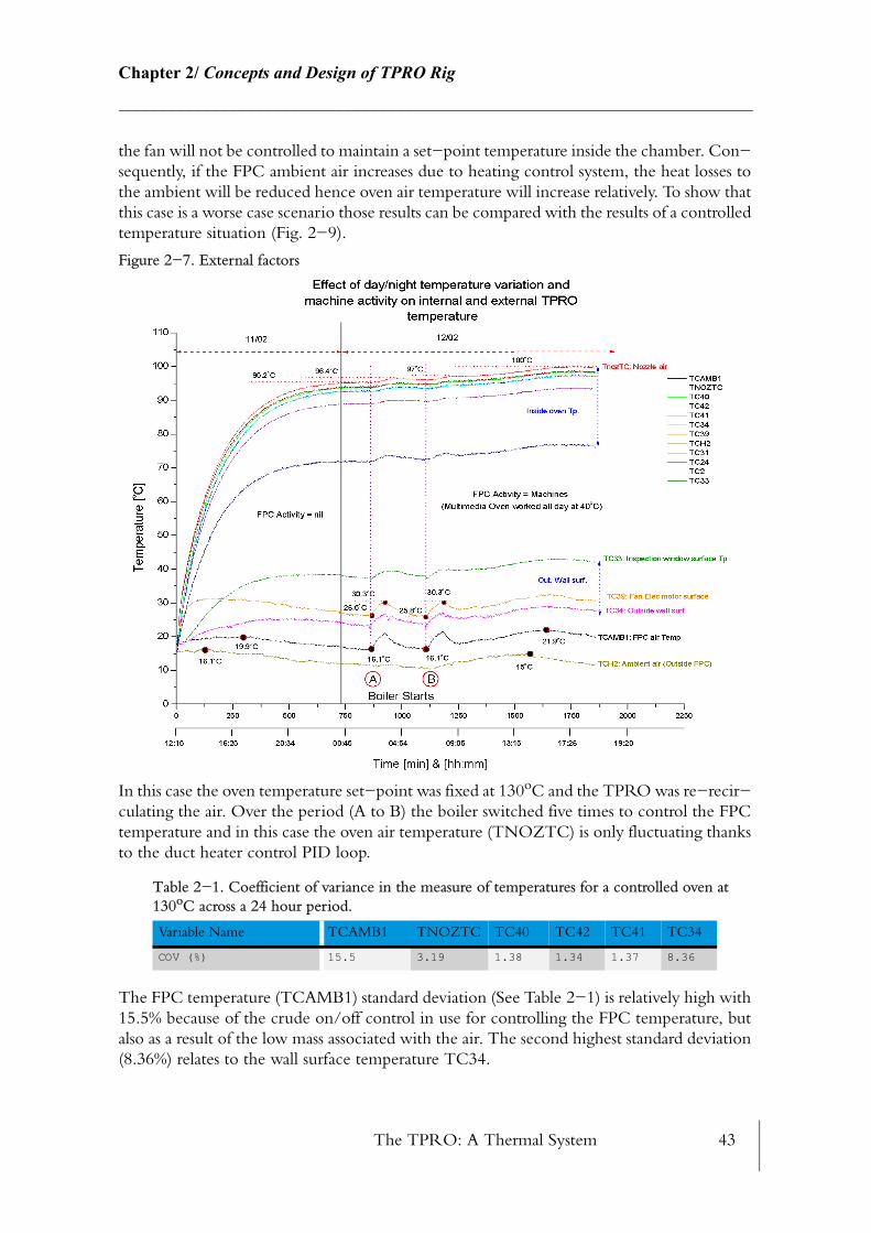
The TPRO: A Thermal System 43
Chapter 2/ Concepts and Design of TPRO Rig________________________________________________________________________
the fan will not be controlled to maintain a set−point temperature inside the chamber. Con−sequently, if the FPC ambient air increases due to heating control system, the heat losses to the ambient will be reduced hence oven air temperature will increase relatively. To show that this case is a worse case scenario those results can be compared with the results of a controlled temperature situation (Fig. 2−9).
Figure 2−7. External factors
In this case the oven temperature set−point was fixed at 130oC and the TPRO was re−recir−culating the air. Over the period (A to B) the boiler switched five times to control the FPC temperature and in this case the oven air temperature (TNOZTC) is only fluctuating thanks to the duct heater control PID loop.
The FPC temperature (TCAMB1) standard deviation (See Table 2−1) is relatively high with 15.5% because of the crude on/off control in use for controlling the FPC temperature, but also as a result of the low mass associated with the air. The second highest standard deviation (8.36%) relates to the wall surface temperature TC34.
Table 2−1. Coefficient of variance in the measure of temperatures for a controlled oven at 130oC across a 24 hour period.
Variable Name TCAMB1 TNOZTC TC40 TC42 TC41 TC34
COV (%) 15.5 3.19 1.38 1.34 1.37 8.36

The TPRO: A Thermal System 44
Chapter 2/ Concepts and Design of TPRO Rig________________________________________________________________________
Figure 2−8. Transient response time of the TPRO
It is relatively lower than TCAMB1 as the measurement is assigned to the mass of the insulant which dampers the variation of TCAMB1. The relatively low standard deviation (3.19%) of the oven air temperature (TNOZTC) is greater still than those for the internal wall temper−atures (TC40, TC41, TC42) is partly due to the PID loop controlling the duct heater. The interesting point to mention is the order of the COV for the three internal wall surface measurement. Their low COV’s is entirely due to the mass of the metal and insulant asso−ciated with the point of measurement which reduces the temperature oscillation. The lowest of the three is TC42 which sees the thickest layer of steel and insulant on either side of the measurement point. TC41 is slightly more dampened than TC40 most likely because of the 1.6 mm steel wall separating TC40 and TC41.
Two crucial thermal characteristics, volumetric heat capacity and the thermal diffusivity, are of particular importance when designing oven walls, and their consideration clarifies the previous result.
(2.5)ρCp
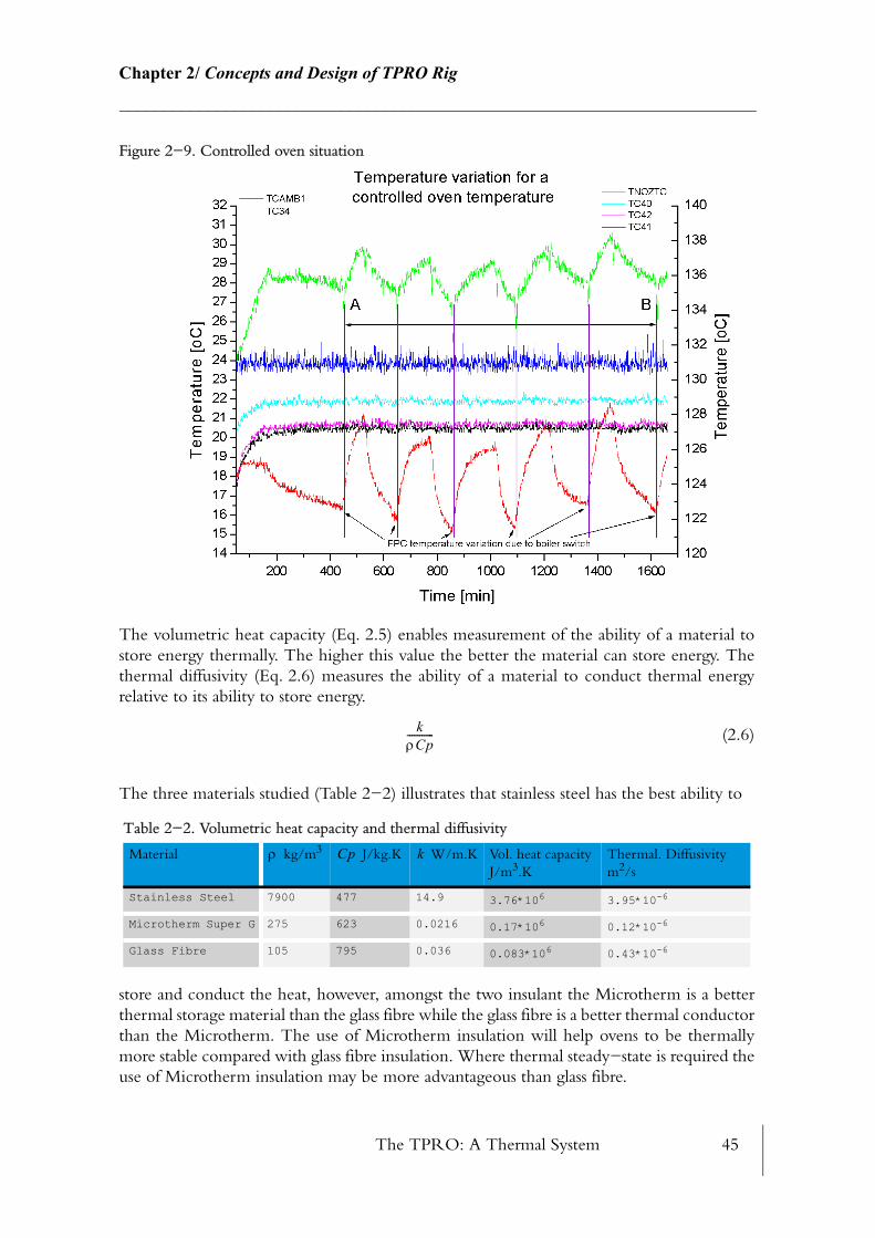
The TPRO: A Thermal System 45
Chapter 2/ Concepts and Design of TPRO Rig________________________________________________________________________
Figure 2−9. Controlled oven situation
The volumetric heat capacity (Eq. 2.5) enables measurement of the ability of a material to store energy thermally. The higher this value the better the material can store energy. The thermal diffusivity (Eq. 2.6) measures the ability of a material to conduct thermal energy relative to its ability to store energy.
(2.6)
The three materials studied (Table 2−2) illustrates that stainless steel has the best ability to
store and conduct the heat, however, amongst the two insulant the Microtherm is a better thermal storage material than the glass fibre while the glass fibre is a better thermal conductor than the Microtherm. The use of Microtherm insulation will help ovens to be thermally more stable compared with glass fibre insulation. Where thermal steady−state is required the use of Microtherm insulation may be more advantageous than glass fibre.
Table 2−2. Volumetric heat capacity and thermal diffusivity
Material kg/m3 J/kg.K W/m.K Vol. heat capacity J/m3.K
Thermal. Diffusivity m2/s
Stainless Steel 7900 477 14.9 3.76*106 3.95*10-6
Microtherm Super G 275 623 0.0216 0.17*106 0.12*10-6
Glass Fibre 105 795 0.036 0.083*106 0.43*10-6
kρCp-----------
ρ Cp k

The TPRO: A Thermal System 46
Chapter 2/ Concepts and Design of TPRO Rig________________________________________________________________________
2.3.1.3 Sources of heat loss
Fig. 2−5 shows the existence of an energy balance within the TPRO. A thermal equilibrium is reached after 13 hours at zero heat input, therefore at this point in time, the heat losses must equal heat gains. During this steady state regime the temperatures of the external TPRO wall surfaces are greater than the ambient air temperature, indicating the presence of convective and radiative losses from the TPRO wall to the ambient air. When analysing temperature differences of the network nodes for the TPRO ducting system (see Fig. 2−11), temperature variation can help to understand better the sources of heat losses.
Fig. 2−11 shows a positive temperature gradient from wall surface to the ambient air (TC34−TCAMB1), indicating external convective and radiative losses. Three other tem−perature difference are of particular importance and their analysis demonstrate another type of heat loss. The difference (TCEXTRAC−TC24) shows that the average temperature coming out of the extraction is always hotter than the re−circulated temperature TC24, which proves that losses exist between the two nodes. The ductings are well insulated between the extraction point and the re−circulation section therefore heat losses from the wall by convection, radiation should be minimal. However, D8 and the outlet sealing plate are between these two nodes and may well impart this temperature variation due to air leak−age through the outlet duct sealed cover plate. For the temperature difference (TC1−TCH3), TCH3 is always hotter than TC1, in the thermal steady state region. TC1 is posi−tioned between the damper D1 (see Fig. 2−10) and the inlet duct sealed cover plate. The lower temperature TC1 could be explained by the inlet duct entry being un−insulated and also due to air infiltrating through the teflon seal of the inlet sealed cover plate.
Figure 2−10. Inlet duct cover plate
The study of the temperature decay difference (TCNOZTC−TC40) between the two period, transient and thermal steady state, reflects that heat travels through the wall and is absorbed and stored by the wall until a thermal equilibrium is achieved within the wall depth between the internal and outside wall surfaces.
The constant positive difference of 3oC between (TCNOZTC−TCEXTRAC) during both transient and steady state demonstrates that heat is loss through the oven chamber and absorbed through the material (insulation, steel) within the TPRO chamber vicinity.
Clamp systemHinge
Teflon seal
Wing-nut
TC1
TCH3
Damper
Inlet duct sealed cover plate
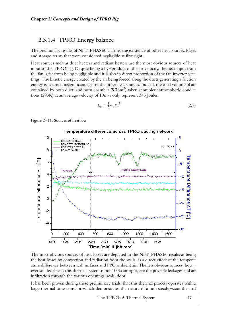
The TPRO: A Thermal System 47
Chapter 2/ Concepts and Design of TPRO Rig________________________________________________________________________
2.3.1.4 TPRO Energy balance
The preliminary results of NFT_PHASE0 clarifies the existence of other heat sources, losses and storage terms that were considered negligible at first sight.
Heat sources such as duct heaters and radiant heaters are the most obvious sources of heat input to the TPRO rig. Despite being a by−product of the air velocity, the heat input from the fan is far from being negligible and it is also in direct proportion of the fan inverter set−tings. The kinetic energy created by the air being forced along the ducts generating a friction energy is assumed insignificant against the other heat sources. Indeed, the total volume of air contained by both ducts and oven chamber (5.76m3) taken at ambient atmospheric condi−tions (293K) at an average velocity of 10m/s only represent 345 Joules.
(2.7)
Figure 2−11. Sources of heat loss
The most obvious sources of heat losses are depicted in the NFT_PHASE0 results as being the heat losses by convection and radiation from the walls, as a direct effect of the temper−ature difference between wall surfaces and FPC ambient air. The less obvious sources, how−ever still feasible as this thermal system is not 100% air tight, are the possible leakages and air infiltration through the various openings, seals, door.
It has been proven during these preliminary trials, that this thermal process operates with a large thermal time constant which demonstrates the nature of a non steady−state thermal
Ek12---maVa
2=
Flow and heat transfer solutions 48
Chapter 2/ Concepts and Design of TPRO Rig________________________________________________________________________
process. The most obvious explanation finds itself in the designed structure of the TPRO. A simple analysis of thermal diffusivity and thermal heat capacity of the materials used, seems to show some evidence and believes for the materials to act as good thermal storage, which implies directly on the transient process of the TPRO.
An energy balance can be drawn by applying the law of conservation of energy on the con−trol volume (TPRO), Incropera and De Witt, 1990 [68]. Over a time interval , ‘the amount of thermal and mechanical energy which enters the TPRO volume, plus the amount of thermal energy which is generated within the TPRO volume, minus the amount of ther−mal and mechanical energy which leaves the TPRO volume must equal the increase in the amount of energy stored in the control volume’. Over the time interval this law can be translated to:
(2.8)
A direct implication of the above equation means that the sum of inflow and generated energy will rise the quantity of stored energy within the TPRO volume while the
outflow energy will reduce it.
At any instant the inflow and outflow rate are considered respectively as energy gain and energy loss. The radiation and convection losses will go under this category as well as the air infiltration and leakages. The rate of energy generated from the duct heaters, radiant heaters and heat dissipated by the fans to the air will be quantified by the generated energy
. Finally, the rate of energy stored into the different materials, such as the composite walls and the uncovered steel mass inside the chamber will be covered by the rate of energy stored
. In addition of the first law of thermodynamics this thermal system must also obey the law of mass conservation which simply states that mass cannot be created or destroyed. Over a time interval this law can be translated into:
(2.9)
As no chemical reactions takes place inside the TPRO chamber vicinity, the above equation (Eq. 2.9) applies at any time. The pressure inside the TPRO chamber is believed to be equal to the atmospheric pressure and to be controlled by the equilibrium of Eq. 2.9. The change in mass of the system over a time interval must equal the mass inflow which is caused by air infiltration (or fresh air input) and mass outflow generated by air leakages through the different TPRO apertures. The above equation is valid for any oven damper set−tings, i.e. full or partial re−circulation. The mass inflow and outflow are taking into consid−eration the possible hot air leakages or cold air infiltration (2.4.2 for details).
2.4 Flow and heat transfer solutions
In order to demonstrate the different aspects of the TPRO transient responses, the interpre−tation of both the energy and mass balance must be expressed in a particular fashion so they
∆t
∆t
Est Ein Eg Eout–+=
EinEg Est
Eout
t E· in E· out
E· g
E· st
∆t
∆M Min Mout– 0= =
∆M ∆t MinMout
Flow and heat transfer solutions 49
Chapter 2/ Concepts and Design of TPRO Rig________________________________________________________________________
can be time dependent and characterise accurately this transient process. The particularity of real time calculations is that they are already embedded inside a time loop which is connected to the process while non real time programming have no relation with the current clock and are completely time independent. Not only the latest release of InControl™ allows to carry out data acquisition and handles PLC programming but it can also perform as a true pro−gramming language as it integrates structured text which resembles to the Pascal language. This allows to build user defined functions and sub−routines as any other programming lan−guage of which can be executed in a real time. Hundreds of line of codes can be executed within a fraction of seconds and can perfectly run as fast as the scantime of the data acqui−sition card (e.g 50msec). Nonetheless, if runs1 are skipped during the scantime, this can lead to tiny errors which can build up and cause erroneous calculations. Missed scantime can be initiated by a CPU overload which leads to an impossibility to cope with the demanded scantime. Therefore the scantime must be calculated accurately to avoid this sort of random error possibility.
2.4.1 Properties
While the TPRO is heating up, both the air and the material properties are likely to change over time. The best approach for integrating those changes is to correlate the appropriate properties as a function of temperature. For each run (scan) the temperature will evolve and the real−time functions will update the properties with the new temperature.
• Air properties:Air properties such as density, specific heat, thermal conductivity, thermal diffusivity, Prandtl number, dynamic viscosity, and kinematic viscosity were correlated by using the data from the heat transfer text book, Incropera and De Witt, 1990 [68]. The software SPSS table curve 2D (release5) was used for estimating the best fitting equation for each data set (Appendix B). A series of 188 equations were fitted through each data set. The fitted equation which gave the highest (goodness of fit factor, 0 represent a complete lack of fit) was used. The range of temperature for estimating the correlation was taken between 200K and 800K which overlap the band of oven air temperature studied. Once correlated, see Fig. 2−12, the correlation had to be translated into an InControl™ function. For the air density for instance, the best fitted equation was of the form (Appendix N):
(2.10)
which can be translated into: FUNCT := a+b*Tk**c; DECIM_PLACE := 4;
with and the constant defined by the air density correlation. As the air density data were given with four decimal place in the reference text book (Incropera and De Witt, 1990[68]), the InControl™ function was set to the same format. Goodness of fit statistics is com−puted for each model. The statistics for the model of the air density are given by Table 2−3. The definitions of all the statistical terms (Appendix G for definitions) shows that the air
1. entire program ran once
r2
y a b Tk( )c+=
a b, c
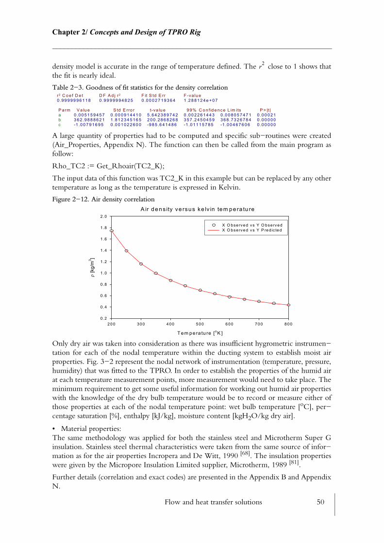
Flow and heat transfer solutions 50
Chapter 2/ Concepts and Design of TPRO Rig________________________________________________________________________
density model is accurate in the range of temperature defined. The close to 1 shows that the fit is nearly ideal.
Table 2−3. Goodness of fit statistics for the density correlation
A large quantity of properties had to be computed and specific sub−routines were created (Air_Properties, Appendix N). The function can then be called from the main program as follow:
Rho_TC2 := Get_Rhoair(TC2_K);
The input data of this function was TC2_K in this example but can be replaced by any other temperature as long as the temperature is expressed in Kelvin.
Figure 2−12. Air density correlation
Only dry air was taken into consideration as there was insufficient hygrometric instrumen−tation for each of the nodal temperature within the ducting system to establish moist air properties. Fig. 3−2 represent the nodal network of instrumentation (temperature, pressure, humidity) that was fitted to the TPRO. In order to establish the properties of the humid air at each temperature measurement points, more measurement would need to take place. The minimum requirement to get some useful information for working out humid air properties with the knowledge of the dry bulb temperature would be to record or measure either of those properties at each of the nodal temperature point: wet bulb temperature [oC], per−centage saturation [%], enthalpy [kJ/kg], moisture content [kgH2O/kg dry air].
• Material properties: The same methodology was applied for both the stainless steel and Microtherm Super G insulation. Stainless steel thermal characteristics were taken from the same source of infor−mation as for the air properties Incropera and De Witt, 1990 [68]. The insulation properties were given by the Micropore Insulation Limited supplier, Microtherm, 1989 [81].
Further details (correlation and exact codes) are presented in the Appendix B and Appendix N.
r2
r2 C o e f D e t D F A d j r2 F it S td E rr F -va lu e 0 .9 9 9 9 9 9 6 1 1 8 0 .9 9 9 9 9 9 4 8 2 5 0 .0 0 0 2 7 1 9 3 6 4 1 .2 8 8 1 2 4 e + 0 7 P a rm V a lu e S td E rro r t-va lu e 9 9 % C o n fid e n c e L im its P > |t | a 0 .0 0 5 1 5 9 4 5 7 0 .0 0 0 9 1 4 4 1 0 5 .6 4 2 3 8 9 7 4 2 0 .0 0 2 2 6 1 4 4 3 0 .0 0 8 0 5 7 4 7 1 0 .0 0 0 2 1 b 3 6 2 .9 8 8 8 6 2 1 1 .8 1 2 3 4 5 1 6 5 2 0 0 .2 8 6 8 2 6 8 3 5 7 .2 4 5 0 4 5 9 3 6 8 .7 3 2 6 7 8 4 0 .0 0 0 0 0 c -1 .0 0 7 9 1 6 9 5 0 .0 0 1 0 2 2 6 0 0 -9 8 5 .6 4 1 4 8 6 -1 .0 1 1 1 5 7 8 5 -1 .0 0 4 6 7 6 0 6 0 .0 0 0 0 0
A ir den s ity ve rsus ke lv in tem pe ra tu re
T e m pe ra tu re [oK ]
2 00 30 0 4 00 50 0 6 00 70 0 80 0
ρ [k
g/m
3 ]
0 .2
0 .4
0 .6
0 .8
1 .0
1 .2
1 .4
1 .6
1 .8
2 .0
X O bse rve d vs Y O bse rve d X O bse rve d v s Y P re d ic te d
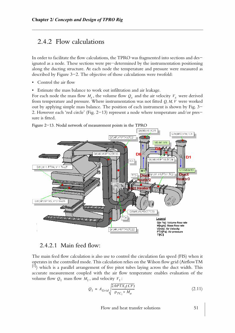
Flow and heat transfer solutions 51
Chapter 2/ Concepts and Design of TPRO Rig________________________________________________________________________
2.4.2 Flow calculations
In order to facilitate the flow calculations, the TPRO was fragmented into sections and des−ignated as a node. These sections were pre−determined by the instrumentation positioning along the ducting structure. At each node the temperature and pressure were measured as described by Figure 3−2. The objective of those calculations were twofold:
• Control the air flow
• Estimate the mass balance to work out infiltration and air leakage.For each node the mass flow , the volume flow and the air velocity were derived from temperature and pressure. Where instrumentation was not fitted were worked out by applying simple mass balance. The position of each instrument is shown by Fig. 3−2. However each ‘red circle’ (Fig. 2−13) represent a node where temperature and/or pres−sure is fitted.
Figure 2−13. Nodal network of measurement points in the TPRO
2.4.2.1 Main feed flow:
The main feed flow calculation is also use to control the circulation fan speed (FIS) when it operates in the controlled mode. This calculation relies on the Wilson flow grid (AirflowTM[1]) which is a parallel arrangement of five pitot tubes laying across the duct width. This accurate measurement coupled with the air flow temperature enables evaluation of the volume flow mass flow , and velocity :
(2.11)
Mx Qx VxQ M V, ,
Q1 M1 V1
Q1 AGrid2.0PTX1 CF( )ρTC2
Ma×-----------------------------------=

Flow and heat transfer solutions 52
Chapter 2/ Concepts and Design of TPRO Rig________________________________________________________________________
(2.12)
(2.13)
(2.14)
is the temperature correction factor and is a magnification factor specifically use with this particular flow grid. was evaluated by using an abacus provided by the flow grid sup−plier and was evaluated to 2.1. (see Appendix D for more precision) is the cross sec−tional area of the duct considered where the flow grid is positioned.
2.4.2.2 Top and bottom nozzle:
As explained byFigure 4−15 the measurement of equivalent nozzle pressure was established using a bell shape tubing and a pitot tube which gave comparable velocity readings as meas−urement operated with a pitot tube placed 10 mm away from the nozzle. The explanation of the velocity similarity originates from analogous flow pattern between the two setup. For the top nozzle the equivalent nozzle volume flow can be estimated as follow:
(2.15)
where, is the pressure to the point of measurement, is a correction factor for the Pitot tube. In this case this correction factor equals unity as the Pitot tube is a 90o angle as opposed to a straight Pitot tube (averaging pitot tube). is the cross sectional area of the bell shape tubing considered. For a single nozzle, the velocity can be deduced from Eq. 2.15:
(2.16)
The total volume flow for the top plenum is related to the top nozzle velocity and the geometry of the nozzles.
(2.17)
with respectively, , , nozzle area, number of nozzle per row and row of nozzle for the entire plenum area. The total mass flow for the plenum is related to the volume flow by the air density at the point of measurement:
(2.18)
Similarly as for the top plenum variables, , , , can be worked out for the bottom plenum.
M1 Q1 ρTC2×=
V1Q1
Agrid-------------=
CFTC2
293.0-------------=
CF MaMa
Agrid
Q11A Atube2.0PTX4ρTnoztαN-----------------------=
PTX4 αN
Atube
V11Q11AAtube-------------=
Q11 V11
Q11 V11AnozNnozNrow=
Anoz Nnoz NrowM11
ρTnozt
M11 Q11ρTnozt=
Q12A V12 Q12 M12
Flow and heat transfer solutions 53
Chapter 2/ Concepts and Design of TPRO Rig________________________________________________________________________
2.4.2.3 Extraction flow:
(2.19)
(2.20)
(2.21)
(2.22)
is the correction factor in use with the averaging Pitot tube. for the four extrac−tion ducts were calculated as above. Averaging Pitot tube were used in the extraction duct elbow where the flow pattern is complex. The error induced in such a setup can be large (up to 15%) and the variation from one duct to another can also be important. Therefore the average pressure of the four extracting duct was used instead of individual pressures.
The total mass of air extracted is the sum of the four individual air mass for each extraction ducts:
(2.23)
2.4.2.4 Re−circulated flow:
Similarly as the extraction flow the re−circulation flow was evaluated with an averaging Pitot tube as the flow in this duct section was altered by D9 and could be turbulent.
(2.24)
(2.25)
(2.26)
With the cross sectional area of the re−circulation duct where the averaging Pitot tube is fitted.
The two inlet and outlet mass flow and were estimated applying the Kirshoff law respectively at the damper (node) D8 and D1. For the outlet flow, the sum of the mass flow leaving the node D8, is equal to the total extracted mass flow .
(2.27)
Q4 Ae2.0PTXavgρTC22
αA×---------------------------=
M4Q4ρTC22
------------=
V4Q4Ae------=
PTXAPTX2 PTX3 PTX6 PTX7+ + +
4.0---------------------------------------------------------------------------=
αA Q M V, ,
PTXA
MT e,
MT e, M4 M5 M6 M7+ ++=
Q8 Ar2.0PTX8ρTC24
αA×--------------------------=
M8 Q8ρTC24=
V8Q8Ar------=
Ar
M9 M10
M9 M8+ MT e,
M9 MT e, M8–=
Flow and heat transfer solutions 54
Chapter 2/ Concepts and Design of TPRO Rig________________________________________________________________________
Hence, volume flow rate and velocity at this point can be written as follow:
(2.28)
(2.29)
Re−circulation and extraction duct have the same cross sectional area (Eq. 2.29).
The same law can be applied to the node D1.
(2.30)
(2.31)
With the ambient air temperature in the FPC.
(2.32)
Depending on the mass flow difference of Eq. 2.27 and Eq. 2.30 the inflow and outflow could become either positive or negative, which means that both mass flows could either be considered as a infiltration or a leakage.
The re−circulation ratio Eq. 2.33, was defined to reflect the overall air loss in this process. The definition of this ratio is the percentage of air mass re−circulated referenced to the main air mass flow . In an ideal situation, if the mass is conserved and the system is 100% seal proof then the re−circulation ratio should be 1. However if this percentage drops to 96% it means that 4% of the main mass flow has been loss in the ductings by leakages.
(2.33)
2.4.2.5 Air leakages and infiltration:
The air loss is subdivided into three main sources: ‘plenum air loss’, chamber, and return loss.
2.4.2.5.1 ‘Plenum air loss’
‘Plenum air loss’ is a broad term given to the air loss (leak or infiltration) in the section defined from the outlet of CFAN to the splitting duct separating the air flow between the two plenum chambers nozzle outlets. As there was no instrument fitted in the splitting region section, it was assumed that the sum of both the nozzle outlets plenums is equal to the mass flow in the splitting duct section.
(2.34)
Q9M9ρTC31
------------=
V9Q9
Arecirc-----------------=
M10 M1 M8–=
Q10M10ρTC∞
------------=
TC∞
V10M10Ae
----------=
M9 M10,
RrM8
M1
Rr 100M8M1------- =
MT p, M11 M12+=
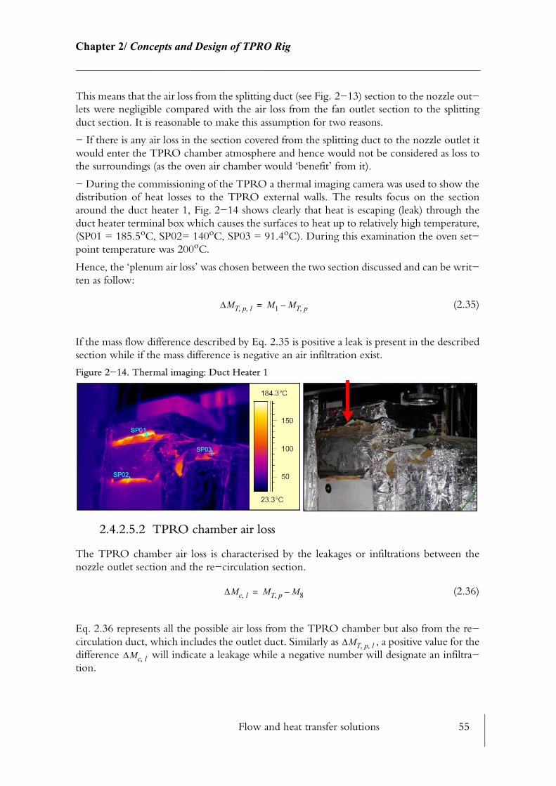
Flow and heat transfer solutions 55
Chapter 2/ Concepts and Design of TPRO Rig________________________________________________________________________
This means that the air loss from the splitting duct (see Fig. 2−13) section to the nozzle out−lets were negligible compared with the air loss from the fan outlet section to the splitting duct section. It is reasonable to make this assumption for two reasons.
− If there is any air loss in the section covered from the splitting duct to the nozzle outlet it would enter the TPRO chamber atmosphere and hence would not be considered as loss to the surroundings (as the oven air chamber would ‘benefit’ from it).
− During the commissioning of the TPRO a thermal imaging camera was used to show the distribution of heat losses to the TPRO external walls. The results focus on the section around the duct heater 1, Fig. 2−14 shows clearly that heat is escaping (leak) through the duct heater terminal box which causes the surfaces to heat up to relatively high temperature, (SP01 = 185.5oC, SP02= 140oC, SP03 = 91.4oC). During this examination the oven set−point temperature was 200oC.
Hence, the ‘plenum air loss’ was chosen between the two section discussed and can be writ−ten as follow:
(2.35)
If the mass flow difference described by Eq. 2.35 is positive a leak is present in the described section while if the mass difference is negative an air infiltration exist.
Figure 2−14. Thermal imaging: Duct Heater 1
2.4.2.5.2 TPRO chamber air loss
The TPRO chamber air loss is characterised by the leakages or infiltrations between the nozzle outlet section and the re−circulation section.
(2.36)
Eq. 2.36 represents all the possible air loss from the TPRO chamber but also from the re−circulation duct, which includes the outlet duct. Similarly as , a positive value for the difference will indicate a leakage while a negative number will designate an infiltra−tion.
∆MT p l, , M1 MT p,–=
∆Mc l, MT p, M8–=
∆MT p l, ,∆Mc l,
Flow and heat transfer solutions 56
Chapter 2/ Concepts and Design of TPRO Rig________________________________________________________________________
2.4.2.5.3 Return duct air loss
This section is defined from the re−circulation point to the CFAN outlet . It incor−porates the possible losses from the inlet duct. This loss can be expressed simply as:
(2.37)
Yet again will be considered as a leak if its sign is positive and negative for an infil−tration.
If the law of mass conservation is confirmed the sum of the air loss must equal zero, therefore the Eq. 2.38 is true:
(2.38)
In order to achieve the mass balance of the TPRO system and confirm the equality of Eq. 2.38, several factors were treated with great care. Cross sectional area of the duct and pressure measurement were the most important parameters to consider. Duct cross sectional area were read from the CAD drawing issued with the TPRO. As for pressure measurement (See 3.2.1.1), each Pitot tube and pressure transmitter were calibrated using benchmarked instrument (see calibration sheet Appendix D). The accuracy of the pressure measurements was checked on a weekly basis over the entire test period as part of a maintenance routine.
2.4.3 Thermal process energy balance
As previously explained an energy balance was constructed around this thermal process in order to get a better understanding of the energy flow but also as a mean of answering and defining the thermal performance envelope of the TPRO. The law of energy conservation (Eq. 2.8) summarises the energy balance of any thermal system. The next paragraphs will treat how each of those terms were translated with respect to the TPRO.
2.4.3.1 Generated energy
The generated energy is composed of three terms. The first heat generation term is the the energy generated from the duct heater , which is the dominant source of energy during the transient process as the three duct heaters are switched on at all times and generate 130kW. During the entire trial period the three heaters were used at all times to control the temperature of the oven chamber. The second heat generation term comes from the radiant heaters inside the TPRO chamber. There are six rod heaters on each plenum and each emitting 475W. These were not used specifically during the estimation of the overall energy balance (NFT_PHASE2) as unused during this phase, however they were utilised for NFT_PHASE3. Finally the third heat generation term which acts at all times as long as one fan is running, is the heat generated from both the circulation and extraction fan .
(2.39)
Q8 Q1
∆Mret l, M8 M1–=
∆Mret L,
∆MT p l, , ∆Mc L, ∆Mret L,+ + 0=
EgED
ER
EF
Eg ED ER EF+ +=
Flow and heat transfer solutions 57
Chapter 2/ Concepts and Design of TPRO Rig________________________________________________________________________
2.4.3.1.1 Duct and radiant heaters
The power dissipated from the duct heaters in three phase wiring (see details of wiring diagram in Appendix N) can be written as follow:
(2.40)
where, and are respectively the voltage and the current through the duct heater. The same equation would apply for the three duct heaters, however the current would vary according to the heat load. Assuming a constant circuit voltage of 415V the current would be 41.7A and 68.5A for respectively duct heater 1 ( ) and duct heater 2 and 3 ( ). A variation up to ±6% in the mains voltage is not uncommon. This error is also taken into consideration and introduced as an error term on the voltage. The current is measured in real time via a Paladin Unit (253−TAL) Crompton, 2001 [38] which transmits the current information to the I/O module and is then transformed to a real number inside InControl™. The formulation of the power dissipated from the radiant heater is not much different than Eq. 2.40 however the current is only one phase (110V).
(2.41)
2.4.3.1.2 Circulation and extraction fans
Earlier on in this chapter various explanations proved the existence of generated heat from the fans and initial trials illustrates that this heat quantity is not negligible. In order to incor−porate this quantity as a heat generation term one must understand what makes it vary.
One way of approaching this problem is to understand the fan law principles. Osborne and Turner, 1960 [98] describe the different variables acting on the absorbed power quantity. Among those, two are directly applicable to this problem.
− The absorbed power varies as speed of rotation to the third power
− The absorbed power varies directly with change in density or is inversely proportional to the temperature.
The absorbed power can be worked out experimentally for various speed and temperature however the number of experiment to conduct might be large to get good accuracy. The ordinary fan curve from the fan supplier are restricted to a single temperature and do not provide enough information to correlate the absorbed power as a function of temperature and fan inverter settings. Hence the fan curve had to be computed. The fan curve was com−puted for five temperature ranges for both the CFAN and EFAN, with the Apovent software from Piller, 2001 [102] provided by the fan supplier.
Fig. 2−15 illustrates the results of the computed values for the CFAN. The fan curves were computed for a system resistance of 3.6kPa based on the pressure drop calculation of Urrutia, 1997 [133]. Each of the curves were correlated as a function of the inlet volume flow at a specific air temperature . A specific function was built within InControl™ (Appendix N) for both CFAN and EFAN to interpolate between curves of different temperatures and flow rate. This graph pictures one of the fan laws as the absorbed power decreases when temper−
QDH
QDH UIDH 3.0=
U IDH
IDH1IDH2 IDH3,
QRH
QRH UIRH=
QT

Flow and heat transfer solutions 58
Chapter 2/ Concepts and Design of TPRO Rig________________________________________________________________________
ature rises (at constant fan inverter settings). Different fan curves were computed for EFAN as the fans were not identical. Within, the main calculation sub−routine, the calculation of the absorbed power as a heat generation term was reduced to call a function (Appendix N).
To evaluate the total generated energy, both the CFAN and EFAN absorbed power were added to the previous generated energy terms from the duct heater.
(2.42)
All the terms of Eq. 2.42 are assigned with the letter (Joules) which indicates that the energy quantity term is evaluated over a time . It is clarified, later in this chapter (2.5.2.1), how these energy quantities are evaluated.
Figure 2−15. Predicted absorbed power curves for CFAN based on computed pressure drop for TPRO
2.4.3.2 Energy loss
The energy loss is sub−divided into three terms, convection, radiation and air loss.
2.4.3.2.1 Wall convective equivalent heat losses
The accuracy in evaluating wall losses depends mainly on the surface area evaluation but also on the wall surface temperature measurement. The TPRO surfaces were disctretized into eleven single surfaces (see Fig. 2−17). On each of these surfaces a thermocouple was fitted at the most descriptive point representing the surface temperature (e.g. central wall position). However a thermal imaging camera analysis of oven wall surfaces showed that a single tem−
Qgain QDH1J QDH2J QDH3J QRH4J QRH5J QcfanJ QefanJ+ + + + + +=
Jdt
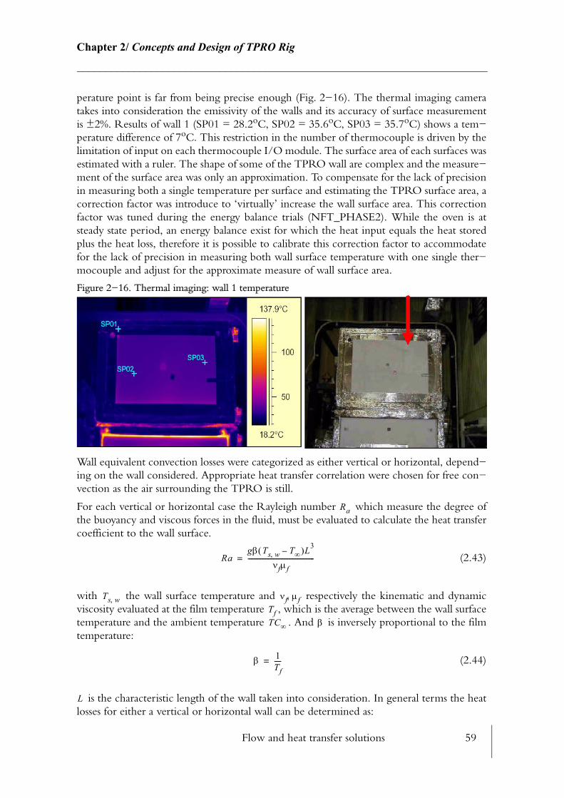
Flow and heat transfer solutions 59
Chapter 2/ Concepts and Design of TPRO Rig________________________________________________________________________
perature point is far from being precise enough (Fig. 2−16). The thermal imaging camera takes into consideration the emissivity of the walls and its accuracy of surface measurement is ±2%. Results of wall 1 (SP01 = 28.2oC, SP02 = 35.6oC, SP03 = 35.7oC) shows a tem−perature difference of 7oC. This restriction in the number of thermocouple is driven by the limitation of input on each thermocouple I/O module. The surface area of each surfaces was estimated with a ruler. The shape of some of the TPRO wall are complex and the measure−ment of the surface area was only an approximation. To compensate for the lack of precision in measuring both a single temperature per surface and estimating the TPRO surface area, a correction factor was introduce to ‘virtually’ increase the wall surface area. This correction factor was tuned during the energy balance trials (NFT_PHASE2). While the oven is at steady state period, an energy balance exist for which the heat input equals the heat stored plus the heat loss, therefore it is possible to calibrate this correction factor to accommodate for the lack of precision in measuring both wall surface temperature with one single ther−mocouple and adjust for the approximate measure of wall surface area.
Figure 2−16. Thermal imaging: wall 1 temperature
Wall equivalent convection losses were categorized as either vertical or horizontal, depend−ing on the wall considered. Appropriate heat transfer correlation were chosen for free con−vection as the air surrounding the TPRO is still.
For each vertical or horizontal case the Rayleigh number which measure the degree of the buoyancy and viscous forces in the fluid, must be evaluated to calculate the heat transfer coefficient to the wall surface.
(2.43)
with the wall surface temperature and respectively the kinematic and dynamic viscosity evaluated at the film temperature , which is the average between the wall surface temperature and the ambient temperature . And is inversely proportional to the film temperature:
(2.44)
is the characteristic length of the wall taken into consideration. In general terms the heat losses for either a vertical or horizontal wall can be determined as:
Ra
Ragβ Ts w, T∞–( )L3
νfµf------------------------------------------=
Ts w, νf µf,TfTC∞ β
β 1Tf----=
L
Flow and heat transfer solutions 60
Chapter 2/ Concepts and Design of TPRO Rig________________________________________________________________________
(2.45)
is the surface area of the wall and is the correction factor which compensate for the lack of precision in measuring both a single temperature per surface and for the wall surface area estimation. This correction factor wall applied to the eleventh single wall surface area.
is the mean equivalent convective heat transfer coefficient for either a vertical or hor−izontal configuration.
To obtain greater accuracy in the estimation of the heat transfer coefficient the Nusselt number was estimated for two possible ranges of Rayleigh number for both the vertical and horizontal arrangement.
(a) Vertical walls.
If then the average Nusselt number applied to characteristic length :
(2.46)
If the average Nusselt number applied to characteristic length :
(2.47)
The equivalent heat transfer coefficient for a vertical wall can then be considered as such:
(2.48)
where is the conductivity of the air taken at the film temperature.
(b) Horizontal walls.
Yet again two correlation were used to cover a wider range of .
If then the Nusselt number is obtained by using:
(2.49)
If then the Nusselt number is obtained by using:
(2.50)
In that case the characteristic length is defined as the surface area to perimeter ratio:
(2.51)
The previous correlation used for estimating the wall convective losses were embedded inside built in function within InControl™ so that real time calculation can be possible.
Qcv h, hv h, Aswwcf Ts w, T∞–( )=
Asw wcf
hv h,
Ra 109< L
NuL 0.68 0.670Ra1 4⁄
1 0.492 Pr⁄( )9 16⁄+[ ]
4 9⁄-------------------------------------------------------------+=
Ra 109> L
NuL 0.825 0.387Ra1 6⁄
1 0.492 Pr⁄( )9 16⁄+[ ]
8 27⁄----------------------------------------------------------------+
2=
hvkNuL
L-------------=
k
Ra
104 Ra 107≤ ≤
NuL 0.54RaL1 4⁄
=
107 Ra 1011≤ ≤
NuL 0.15RaL1 3⁄
=
LAs w,
P-----------=
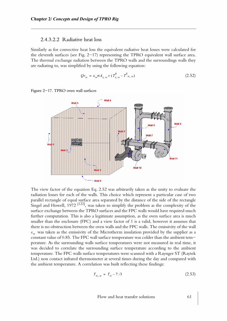
Flow and heat transfer solutions 61
Chapter 2/ Concepts and Design of TPRO Rig________________________________________________________________________
2.4.3.2.2 Radiative heat loss
Similarly as for convective heat loss the equivalent radiative heat losses were calculated for the eleventh surfaces (see Fig. 2−17) representing the TPRO equivalent wall surface area. The thermal exchange radiation between the TPRO walls and the surroundings walls they are radiating to, was simplified by using the following equation:
(2.52)
Figure 2−17. TPRO oven wall surfaces
The view factor of the equation Eq. 2.52 was arbitrarily taken as the unity to evaluate the radiation losses for each of the walls. This choice which represent a particular case of two parallel rectangle of equal surface area separated by the distance of the side of the rectangle Siegel and Howell, 1972 [122], was taken to simplify the problem as the complexity of the surface exchange between the TPRO surfaces and the FPC walls would have required much further computation. This is also a legitimate assumption, as the oven surface area is much smaller than the enclosure (FPC) and a view factor of 1 is a valid, however it assumes that there is no obstruction between the oven walls and the FPC walls. The emissivity of the wall
was taken as the emissivity of the Microtherm insulation provided by the supplier as a constant value of 0.85. The FPC wall surface temperature was colder than the ambient tem−perature. As the surrounding walls surface temperatures were not measured in real time, it was decided to correlate the surrounding surface temperature according to the ambient temperature. The FPC walls surface temperatures were scanned with a Raynger ST (Raytek Ltd.) non contact infrared thermometer at several times during the day and compared with the ambient temperature. A correlation was built reflecting these findings:
(2.53)
Qrw εwσAs w, Ts w,4 T4
∞ w,–( )×=
εw
T∞ w, T∞ 7 3⁄–=

Flow and heat transfer solutions 62
Chapter 2/ Concepts and Design of TPRO Rig________________________________________________________________________
in Eq. 2.52 is the Stephan Boltzman constant ( )
2.4.3.2.3 Air losses
A pressure gauge was fitted inside the TPRO and results upon this measurement demon−strated that the TPRO chamber operates approximately at atmospheric pressure. Therefore any mass leaking should be replaced by an equivalent mass of infiltrated air. This finding is in agreement with the law of mass conservation. As previously explained in this chapter an arbitrary sign convention was set, which defines a leakage as a positive mass of air flowing out from the TPRO envelope while an infiltration is assigned a negative sign to represent a mass of ambient air leaking into the TPRO envelope. This sign convention is (Eq. 2.54):
(2.54)
There are two possible approaches for estimating the heat loss associated with the air leak or infiltration. The first approach is to consider the absolute energy content attributed to the mass of air for the section considered. This value uses the mean bulk temperature of the flow . The enthalpy represents the energy value of the air while represents the quantity of energy losses over a time .
(2.55)
Figure 2−18. Air loss of the control volume
The second approach is to refer to a datum temperature. Although, the energy quantity does not refer to any datum temperature it could refer to the absolute zero temperature or any temperature. To stay in agreement with the rest of the heat losses, (wall losses) the ambi−ent temperature was taken as the datum temperature. At the section considered, the term
of Eq. 2.56 assumes that the mass of air leaving and entering are equal. This assumption was made as it is not feasible to measure the mass of air entering the TPRO envelope through gaps. The equation governing the air loss Eq. 2.56 also assumes that the mean bulk temperature of the section considered is representative of the air leaking out over the entire section. This air loss estimation also assumes that the controlled volume assigned to the section considered is adiabatic.
(2.56)
σ 5.67 8–×10 W m2K4⁄,
∆M 0> leak∆M 0< infiltration
∆MT CpT Ql
dt
Ql ∆MCpTdt=
Ql
∆Ql ∆M
∆Ql ∆M CpT Cp∞T∞–( )=

Flow and heat transfer solutions 63
Chapter 2/ Concepts and Design of TPRO Rig________________________________________________________________________
Indeed, the temperature drop across the section considered is not entirely due to the energy loss coupled with the air loss but also the energy loss from the wall by convection, radiation and the energy stored inside the walls.
In a transient problem like this one, the major temperature fall within this controlled volume will be caused by the energy stored into the walls and the energy loss from the leakages during the transient phase, while throughout the steady state regime the fall in temperature across the section will be mainly caused by convection, radiation losses from the walls and the air loss. This hypothesis considers that the temperature fall from the entry of the con−trolled volume to the outlet is only due to the air loss. The error incurred by this assumption is small if the control volume is small. The other alternative to estimate the air loss would be to differentiate the control volume into several smaller control sub−volume and apply an energy balance on each sub−volume, then work out the heat loss by air leakage/infiltration by differentiation. This can only be done if enough instrumentation is available along the ductings. This technique of differentiation fits more the modelling approach than the exper−imental one.
The two driving forces of Eq. 2.56 are the and the temperature difference . Four cases can be envisaged, where heat gain heat loss is relative to the ambient temperature.
(a) if then
(a1) − if then : heat loss to the controlled volume
(a2) − if then : heat gain to the controlled volume(b) if then
(b1) − if then : heat gain to the controlled volume
(b2) − if then : heat loss to the controlled volume
Three quantities were estimated to evaluate the total energy loss by air leak/infiltration.
• Heat loss associated with plenum ‘chamber air loss’:
(2.57)
is taken as the average between and (see nodal network of measurement points in the TPRO, Fig. 2−13) and considered to be a representative temperature within this section.
• Heat loss associated with ‘chamber air loss’:
(2.58)
• Heat loss associated with the ‘return air loss’:
(2.59)
∆M T TC∞–( )
T TC∞>
∆M 0> ∆Ql 0>
∆M 0< ∆Ql 0<T TC∞<
∆M 0> ∆Ql 0<
∆M 0< ∆Ql 0>
∆Qp l, ∆MTp l, Cp53TC53 Cp∞TC∞–( )=
TC53 TC3 TC5
∆Qc l, ∆Mc l, CpcTCc Cp∞TC∞–( )=
∆Qrt l, ∆Mrt l, CprTCr Cp∞TC∞–( )=
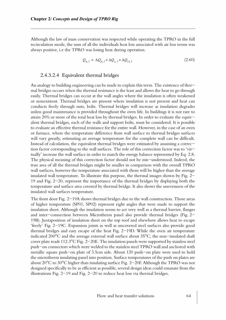
Flow and heat transfer solutions 64
Chapter 2/ Concepts and Design of TPRO Rig________________________________________________________________________
Although the law of mass conservation was respected while operating the TPRO in the full recirculation mode, the sum of all the individuals heat loss associated with air loss terms was always positive, i.e the TPRO was losing heat during operation.
(2.60)
2.4.3.2.4 Equivalent thermal bridges
An analogy to building engineering can be made to explain this term. The existence of ther−mal bridges occurs when the thermal resistance is the least and allows the heat to go through easily. Thermal bridges can occur at the wall angles where the insulation is often weakened or nonexistent. Thermal bridges are present where insulation is not present and heat can conducts freely through nuts, bolts. Thermal bridges will increase as insulation degrades unless good maintenance is provided throughout the oven life. In buildings it is not rare to attain 20% or more of the total heat loss by thermal bridges. In order to evaluate the equiv−alent thermal bridges, each of the walls and support bolts, must be considered. It is possible to evaluate an effective thermal resistance for the entire wall. However, in the case of an oven or furnace, where the temperature difference from wall surface to thermal bridges surfaces will vary greatly, estimating an average temperature for the complete wall can be difficult. Instead of calculation, the equivalent thermal bridges were estimated by assuming a correc−tion factor corresponding to the wall surfaces. The role of this correction factor was to ‘vir−tually’ increase the wall surface in order to match the energy balance represented by Eq. 2.8. The physical meaning of this correction factor should not be mis−understood. Indeed, the true area of all the thermal bridges might be smaller in comparison with the overall TPRO wall surfaces, however the temperature associated with them will be higher than the average insulated wall temperature. To illustrate this purpose, the thermal images shown by Fig. 2−19 and Fig. 2−20, represent the importance of the thermal bridges by displaying both the temperature and surface area covered by thermal bridge. It also shows the unevenness of the insulated wall surfaces temperature.
The front door Fig. 2−19A shows thermal bridges due to the wall construction. Those areas of higher temperature (SP01, SP02) represent right angles that were made to support the insulation sheet. Although the insulation seems to act very well as a thermal barrier, flanges and inter−connection between Microtherm panel also provide thermal bridges (Fig. 2−19B). Juxtaposition of insulation sheet on the top roof and elsewhere allows heat to escape ‘freely’ Fig. 2−19C. Expansion joints as well as uncovered steel surfaces also provide good thermal bridges and easy escape of the heat Fig. 2−19D. While the oven air temperature indicated 200oC and the average external wall surface about 35oC, the non−insulated shaft cover plate reads 112.3oC Fig. 2−20E. The insulation panels were supported by stainless steel push−on connectors which were welded to the stainless steel TPRO wall and anchored with metallic square push−on plate of 3.5cm side. About 120 push−on plate were used to hold the microtherm insulating panel into position. Surface temperatures of the push on plates are about 20oC to 30oC higher than insulating surface Fig. 2−20F. Although the TPRO was not designed specifically to be as efficient as possible, several design ideas could emanate from the illustrations Fig. 2−19 and Fig. 2−20 to reduce heat loss via thermal bridges.
Qa l, ∆Qp l, ∆Qc l, ∆Qrt l,+ +=
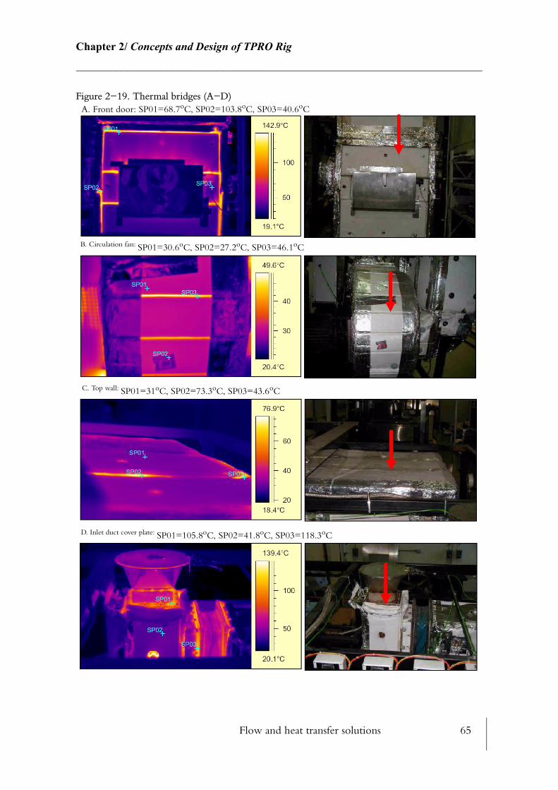
Flow and heat transfer solutions 65
Chapter 2/ Concepts and Design of TPRO Rig________________________________________________________________________
Figure 2−19. Thermal bridges (A−D)A. Front door: SP01=68.7oC, SP02=103.8oC, SP03=40.6oC
B. Circulation fan: SP01=30.6oC, SP02=27.2oC, SP03=46.1oC
C. Top wall: SP01=31oC, SP02=73.3oC, SP03=43.6oC
D. Inlet duct cover plate: SP01=105.8oC, SP02=41.8oC, SP03=118.3oC
Flow and heat transfer solutions 66
Chapter 2/ Concepts and Design of TPRO Rig________________________________________________________________________
Figure 2−20. Thermal bridges (E−F)
2.4.3.3 Energy storage
The energy stored is the last term of the energy balance Eq. 2−6. The storage term was sub−divided into two storage terms.
• AirA very small fraction of the total energy goes to heat the air up. As the mass of air is very little (6.85kg at ambient temperature) compared to the mass of the rig, (several hundred kilos) one can understand that the energy stored within the TPRO air volume will rise rel−atively quickly compared with the rest of the energy stored in the oven mass. To be able to follow transiently the energy stored in the air, Eq. 2.61 was established:
(2.61)
The quantity represents the energy that is contained at the instant within the air while the quantity is the energy contained in the air at the pre−vious instant . The energy contained within the air during the time is quantified by
.
• SolidThe energy contained within solids such as insulation, steel wall and other masses of steel inside the TPRO chamber can be evaluated by integrating the volumetric heat capacity of a section of solid wall. Assuming a steady state scenario whereby the temperature falls, within
E. Conveyor band shaft cover plate: SP01=112.3oC, SP02=60.2oC, SP03=137.4oC
F. Insulation push on: SP01=45.6oC, SP02=61.2oC, SP03=55.3oC
∆Qs a, M1CpTC2
k 1+ TC2k 1+ M1CpTC2
k TC2k
–( )dt=
M1CpTC2
k 1+ TC2k 1+ k 1+
M1CpTC2k TC2
k
k dt∆Qs a,
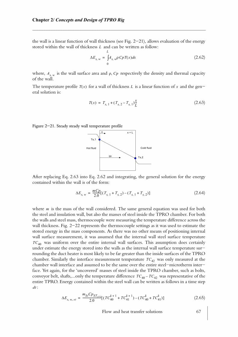
Flow and heat transfer solutions 67
Chapter 2/ Concepts and Design of TPRO Rig________________________________________________________________________
the wall is a linear function of wall thickness (see Fig. 2−21), allows evaluation of the energy stored within the wall of thickness and can be written as follow:
(2.62)
where, is the wall surface area and respectively the density and thermal capacity of the wall.
The temperature profile for a wall of thickness is a linear function of and the gen−eral solution is:
(2.63)
Figure 2−21. Steady steady wall temperature profile
After replacing Eq. 2.63 into Eq. 2.62 and integrating, the general solution for the energy contained within the wall is of the form:
(2.64)
where is the mass of the wall considered. The same general equation was used for both the steel and insulation wall, but also the masses of steel inside the TPRO chamber. For both the walls and steel mass, thermocouple were measuring the temperature difference across the wall thickness. Fig. 2−22 represents the thermocouple settings as it was used to estimate the stored energy in the mass components. As there was no other means of positioning internal wall surface measurement, it was assumed that the internal wall steel surface temperature
was uniform over the entire internal wall surfaces. This assumption does certainly under estimate the energy stored into the walls as the internal wall surface temperature sur−rounding the duct heater is most likely to be far greater than the inside surfaces of the TPRO chamber. Similarly the interface measurement temperature was only measured at the chamber wall interface and assumed to be the same over the entire steel−microtherm inter−face. Yet again, for the ‘uncovered’ masses of steel inside the TPRO chamber, such as bolts, conveyor belt, shafts,...only the temperature difference was representative of the entire TPRO. Energy contained within the steel wall can be written as follows in a time step
:
(2.65)
L
∆Es w, As w, ρCpT x( ) xd0
L
∫=
As w, ρ Cp,
T x( ) L x
T x( ) Ts 1, Ts 2, Ts 1,–( ) xL---+=
x x = L
Ts,2
Ts,1
qx
Hot fluid Cold fluid
∆Es w,mCp2.0
------------ Ts 1, Ts 2,+( ) Ts 1, Ts 2,+( )–[ ]=
m
TC40
TC42
TC40 TC42–
dt
∆Es w st, ,
mStCpSTAVG
2.0---------------------------- TC40
k 1+ TC41k 1+
+( ) TC40k TC41
k+( )–[ ]=
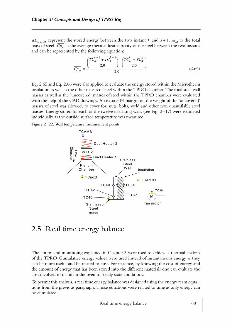
Real time energy balance 68
Chapter 2/ Concepts and Design of TPRO Rig________________________________________________________________________
represent the stored energy between the two instant and . is the total mass of steel. is the average thermal heat capacity of the steel between the two instants and can be represented by the following equation:
(2.66)
Eq. 2.65 and Eq. 2.66 were also applied to evaluate the energy stored within the Microtherm insulation as well as the other masses of steel within the TPRO chamber. The total steel wall masses as well as the ‘uncovered’ masses of steel within the TPRO chamber were evaluated with the help of the CAD drawings. An extra 30% margin on the weight of the ‘uncovered’ masses of steel was allowed, to cover for, nuts, bolts, weld and other non quantifiable steel masses. Energy stored for each of the twelve insulating walls (see Fig. 2−17) were estimated individually as the outside surface temperature was measured.
Figure 2−22. Wall temperature measurement points
2.5 Real time energy balance
The contol and montiroing explained in Chapter 3 were used to achieve a thermal analysis of the TPRO. Cumulative energy values were used instead of instantaneous energy as they can be more useful and be related to cost. For instance, by knowing the cost of energy and the amount of energy that has been stored into the different materials one can evaluate the cost involved to maintain the oven to steady state conditions.
To permit this analysis, a real time energy balance was designed using the energy term equa−tions from the previous paragraph. Those equations were related to time as only energy can be cumulated.
∆Es w st, , k k 1+ mStCpst
Cpst
TC40k 1+ TC41
k 1++
2.0----------------------------------------- TC40
k TC41k
+
2.0-------------------------------
+
2.0-------------------------------------------------------------------------------------------=
TC39
M
Fan motor
PlenumChamber
TCAMB
TC2
TCnozt
TC40 TC34TCAMB1
TC41
insulation
StainlessSteelW all
StainlessSteelmass
TC42
TC40
Duct Heater 3
Duct Heater 1Flow
Direction

Real time energy balance 69
Chapter 2/ Concepts and Design of TPRO Rig________________________________________________________________________
2.5.1 Real time conflict
The cumulative energy represent the integration of all the energy terms during a time . The smaller the , the more accurate the summation. During the estimation of the cumu−lative energy that is related to the duct heater, it was noticed that integration of number inside InControl™ contained a growing error term. The 30 kW duct heater was switched on for 1 minute. The time increment was set to 1 second within an InControl™ built in function, therefore the expected cumulative energy should have been equal to , however the calculated value was larger. The error between the expected cumulative energy and the calculated one increased as the experiment was repeated for a longer period. This error term was also increasing in a non linear fashion. Eventually an explanation arose for this difference. Timer Function within the ‘Real−Time Control Component’ InControl™, were believed to be true real time function however after investigation with the Wonder−ware™ programmers (S Keiser and C Sparks California) the time base used inside InCon−trol™ uses the Microsoft DLL which relates to the CPU and not the PC clock. The CPU is far less precise than the PC clock and it can also be altered by the usage of the CPU itself. Usually there are two possible ways of handling timer inside InControl™, standard timer and pulse timer, however none of them is a true real timer. A real timer which uses the PC clock was created into a built−in function. This function uses the InControl™ system variable RTE. The class variable RTE.RelativeTime issued from the system variable RTE contains the length of the time that the runtime engine has been running since the system was booted. This value is independent of the CPU clock and was used inside this true real timer. The code associated with this function is described below:IF (Enable) THEN(* Update Snapshot on starting of timer *) IF NOT(TimerRun) THEN LastTime := RTEngine.RelativeTime ; TimerRun := TRUE; END_IF; (* Get Elasped Time *) ET := RTEngine.RelativeTime - LastTime;
(* When ET exceeds PT, then generate a PULSE *)(* Then, subrtract off any residue of overshot *)(* and create next snapshot. *)IF (ET > Preset) THEN
Q := TRUE; LastTime := RTEngine.RelativeTime - (ET - Preset); (* Don't allow timer to get behind by more that the preset *) (* This could occur if the scan time exceeds the preset *) (* or project/program is paused. *) IF (ET > Preset) THEN ET := RTEngine.RelativeTime; END_IF; ELSE (* Turn off pulse *) Q := FALSE; END_IF;ELSE (* The Timer is not enabled. Turn off output *) Q := FALSE; (* Clear Timer Run *) TimerRun := FALSE; END_IF;
dtdt
dt1.8 6×10 J
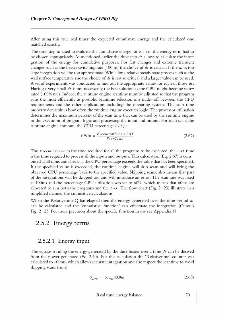
Real time energy balance 70
Chapter 2/ Concepts and Design of TPRO Rig________________________________________________________________________
After using this true real timer the expected cumulative energy and the calculated one matched exactly.
The time step used to evaluate the cumulative energy for each of the energy term had to be chosen appropriately. As mentioned earlier the time step allows to calculate the inte−gration of the energy for cumulative purposes. For fast changes and extreme transient changes such as the heater switching rate (100ms) the choice of is crucial. If the is too large integration will be too approximate. While for a relative steady state process such as the wall surface temperature rise the choice of is not so critical and a larger value can be used. A set of experiments was conducted to find out the appropriate values for each of those . Having a very small is not necessarily the best solution as the CPU might become satu−rated (100% use). Indeed, the runtime engine scantime must be adjusted so that the program runs the most efficiently as possible. Scantime selection is a trade−off between the CPU requirements and the other applications including the operating system. The scan time property determines how often the runtime engine executes logic. The processor utilisation determines the maximum percent of the scan time that can be used by the runtime engine in the execution of program logic and processing the input and output. For each scan, the runtime engine compute the CPU percentage :
(2.67)
The is the time required for all the programs to be executed, the time is the time required to process all the inputs and outputs. This calculation (Eq. 2.67) is com−puted at all time, and checks if the CPU percentage exceeds the value that has been specified. If the specified value is exceeded, the runtime engine will skip scans and will bring the observed CPU percentage back to the specified value. Skipping scans, also means that part of the integrations will be skipped too and will introduce an error. The scan rate was fixed at 100ms and the percentage CPU utilisation was set to 60%, which means that 60ms are allocated to run both the programs and the . The flow chart (Fig. 2−23) illustrate in a simplified manner the cumulative calculations.
When the Relativetime.Q has elapsed then the energy generated over the time period can be calculated and the ‘cumulative function’ can effectuate the integration (Cumul) Fig. 2−23. For more precision about the specific function in use see Appendix N.
2.5.2 Energy terms
2.5.2.1 Energy input
The equation ruling the energy generated by the duct heater over a time can be derived from the power generated (Eq. 2.40). For this calculation the ‘Relativetime’ counter was calculated to 100ms, which allows accurate integration and also respect the scantime to avoid skipping scans (runs).
(2.68)
dtdt
dt dt
dtdt
dt
CPUp
CPUp ExecutionTime I O⁄+ScanTime
---------------------------------------------------------=
ExecutionTime I O⁄
I O⁄
dt
dt
QDHJ UIDH 3.0dt=
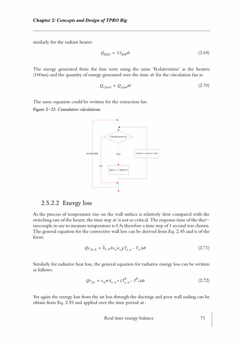
Real time energy balance 71
Chapter 2/ Concepts and Design of TPRO Rig________________________________________________________________________
similarly for the radiant heater:
(2.69)
The energy generated from the fans were using the same ‘Relativetime’ as the heaters (100ms) and the quantity of energy generated over the time for the circulation fan is:
(2.70)
The same equation could be written for the extraction fan.
Figure 2−23. Cumulative calculations
2.5.2.2 Energy loss
As the process of temperature rise on the wall surface is relatively slow compared with the switching rate of the heater, the time step is not so critical. The response time of the ther−mocouple in use to measure temperature is 0.5s therefore a time step of 1 second was chosen. The general equation for the convective wall loss can be derived from Eq. 2.45 and is of the form:
(2.71)
Similarly for radiative heat loss, the general equation for radiative energy loss can be written as follows:
(2.72)
Yet again the energy loss from the air loss through the ductings and poor wall sealing can be obtain from Eq. 2.59 and applied over the time period :
QRHJ UIRHdt=
dt
QcfanJ Qcfandt=
If Relativetime.Q
QDH_J = QDH*dt
YES Cumul = Cumul + ValSCANTIME
NO
dt
QcJv h, hv h, Aswwcf Ts w, T∞–( )dt=
QrJw εwσAs w, Ts w,4 T4
r–( )dt×=
dt
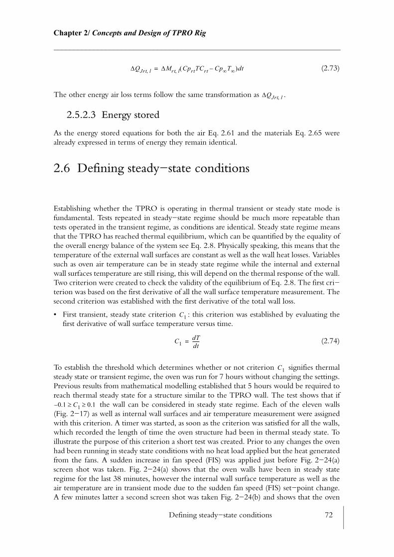
Defining steady−state conditions 72
Chapter 2/ Concepts and Design of TPRO Rig________________________________________________________________________
(2.73)
The other energy air loss terms follow the same transformation as .
2.5.2.3 Energy stored
As the energy stored equations for both the air Eq. 2.61 and the materials Eq. 2.65 were already expressed in terms of energy they remain identical.
2.6 Defining steady−state conditions
Establishing whether the TPRO is operating in thermal transient or steady state mode is fundamental. Tests repeated in steady−state regime should be much more repeatable than tests operated in the transient regime, as conditions are identical. Steady state regime means that the TPRO has reached thermal equilibrium, which can be quantified by the equality of the overall energy balance of the system see Eq. 2.8. Physically speaking, this means that the temperature of the external wall surfaces are constant as well as the wall heat losses. Variables such as oven air temperature can be in steady state regime while the internal and external wall surfaces temperature are still rising, this will depend on the thermal response of the wall. Two criterion were created to check the validity of the equilibrium of Eq. 2.8. The first cri−terion was based on the first derivative of all the wall surface temperature measurement. The second criterion was established with the first derivative of the total wall loss.
• First transient, steady state criterion : this criterion was established by evaluating the first derivative of wall surface temperature versus time.
(2.74)
To establish the threshold which determines whether or not criterion signifies thermal steady state or transient regime, the oven was run for 7 hours without changing the settings. Previous results from mathematical modelling established that 5 hours would be required to reach thermal steady state for a structure similar to the TPRO wall. The test shows that if
the wall can be considered in steady state regime. Each of the eleven walls (Fig. 2−17) as well as internal wall surfaces and air temperature measurement were assigned with this criterion. A timer was started, as soon as the criterion was satisfied for all the walls, which recorded the length of time the oven structure had been in thermal steady state. To illustrate the purpose of this criterion a short test was created. Prior to any changes the oven had been running in steady state conditions with no heat load applied but the heat generated from the fans. A sudden increase in fan speed (FIS) was applied just before Fig. 2−24(a) screen shot was taken. Fig. 2−24(a) shows that the oven walls have been in steady state regime for the last 38 minutes, however the internal wall surface temperature as well as the air temperature are in transient mode due to the sudden fan speed (FIS) set−point change. A few minutes latter a second screen shot was taken Fig. 2−24(b) and shows that the oven
∆QJrt l, ∆Mrt l, CprtTCrt Cp∞T∞–( )dt=
∆QJrt l,
C1
C1dTdt------=
C1
0.1– C1 0.1≥ ≥
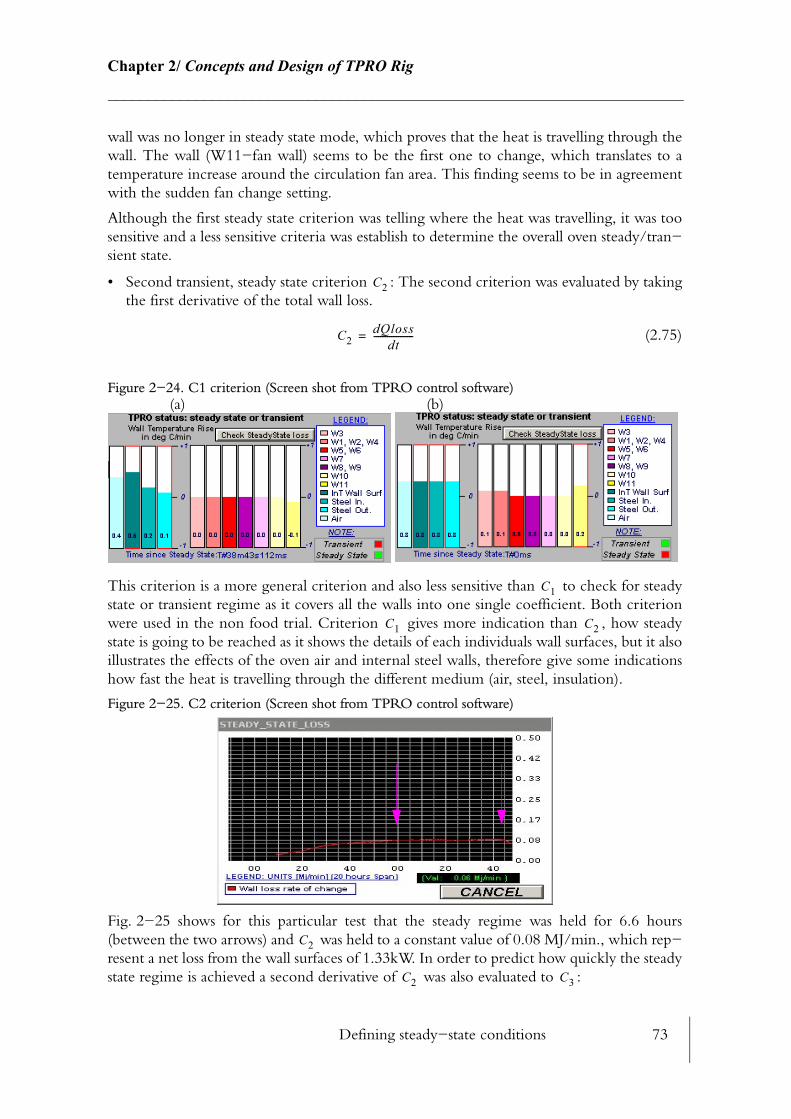
Defining steady−state conditions 73
Chapter 2/ Concepts and Design of TPRO Rig________________________________________________________________________
wall was no longer in steady state mode, which proves that the heat is travelling through the wall. The wall (W11−fan wall) seems to be the first one to change, which translates to a temperature increase around the circulation fan area. This finding seems to be in agreement with the sudden fan change setting.
Although the first steady state criterion was telling where the heat was travelling, it was too sensitive and a less sensitive criteria was establish to determine the overall oven steady/tran−sient state.
• Second transient, steady state criterion : The second criterion was evaluated by taking the first derivative of the total wall loss.
(2.75)
Figure 2−24. C1 criterion (Screen shot from TPRO control software)
This criterion is a more general criterion and also less sensitive than to check for steady state or transient regime as it covers all the walls into one single coefficient. Both criterion were used in the non food trial. Criterion gives more indication than , how steady state is going to be reached as it shows the details of each individuals wall surfaces, but it also illustrates the effects of the oven air and internal steel walls, therefore give some indications how fast the heat is travelling through the different medium (air, steel, insulation).
Figure 2−25. C2 criterion (Screen shot from TPRO control software)
Fig. 2−25 shows for this particular test that the steady regime was held for 6.6 hours (between the two arrows) and was held to a constant value of 0.08 MJ/min., which rep−resent a net loss from the wall surfaces of 1.33kW. In order to predict how quickly the steady state regime is achieved a second derivative of was also evaluated to :
C2
C2dQloss
dt------------------=
(a) (b)
C1
C1 C2
C2
C2 C3

Heat flux to product surface 74
Chapter 2/ Concepts and Design of TPRO Rig________________________________________________________________________
(2.76)
represents the ‘acceleration’ of the total wall heat loss. Theoretically, when reaches almost 0, steady regime is obtained. In reality tests revealed (See Figure 4−11) that when
then the TPRO can be considered in steady state.
The TPRO energy balance was formulated to estimate the efficiency of the TPRO and to assess the performance envelope. The analysis of these results (See 4.2.3) will help to develop a better understanding of how the efficiency of ovens can in general be improved.
2.7 Heat flux to product surface
Although it is recognized that heat flux measurement at the product surface would be very beneficial in the baking industry, heat flux measurement in ovens is still very much a future possibility. No instrument yet exists to measure the direct heat flux to the product surface. However, several heat flux loggers can be found on the market, which will estimate what the heat flux is at the point of measurement at elevated temperatures.
The baking product receives up to four sources of heat fluxes within the TPRO (Fig. 2−26) but only three are concerning the product surface:
a) convection from nozzle impingement (product surface)
b) radiation from radiant heater and background radiation (product surface)
c) condensation from steam injection (product surface)
d) conduction through the pan
Figure 2−26. Heat fluxes to product surface
C3dC2dt
---------=
C3 C3
0.01– C3 0.01≤ ≤
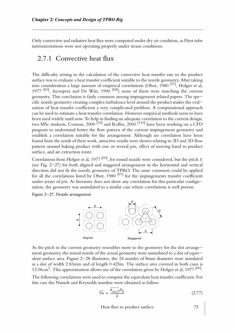
Heat flux to product surface 75
Chapter 2/ Concepts and Design of TPRO Rig________________________________________________________________________
Only convective and radiative heat flux were computed under dry air condition, as Pitot tube instrumentations were not operating properly under steam conditions.
2.7.1 Convective heat flux
The difficulty arising in the calculation of the convective heat transfer rate to the product surface was to evaluate a heat transfer coefficient suitable to the nozzle geometry. After taking into consideration a large amount of empirical correlations (Obot, 1980 [97], Holger et al, 1977 [60], Incropera and De Witt, 1990 [68]) none of them were matching the current geometry. This conclusion is fairly common among impingement related papers. The spe−cific nozzle geometry creating complex turbulence level around the product makes the eval−uation of heat transfer coefficient a very complicated problem. A computational approach can be used to estimate a heat transfer correlation. However empirical methods seem to have been used widely until now. To help in finding an adequate correlation to the current design, two MSc students, Connan, 2000 [34] and Rollin, 2000 [110] have been working on a CFD program to understand better the flow pattern of the current impingement geometry and establish a correlation suitable for the arrangement. Although no correlation have been found from the result of their work, attractive results were shown relating to 2D and 3D flow pattern around baking product with one or several jets, effect of moving band to product surface, and air extraction route.
Correlations from Holger et al, 1977 [60], for round nozzle were considered, but the pitch (see Fig. 2−27) for both aligned and staggered arrangement in the horizontal and vertical direction did not fit the nozzle geometry of TPRO. The same comment could be applied for all the correlations listed by Obot, 1980 [97] for the impingements transfer coefficient under arrays of jets. As literature does not show any correlation for this particular configu−ration, the geometry was assimilated to a similar case where correlations is well proven.
Figure 2−27. Nozzle arrangement
As the pitch in the current geometry resembles more to the geometry for the slot arrange−ment geometry, the round nozzle of the actual geometry were assimilated to a slot of equiv−alent surface area. Figure 2−28 illustrates, the 24 nozzles of 8mm diameter were simulated as a slot of width 2.83mm and of length 0.425m. The surface area covered in both cases is 12.06cm2. This approximation allows use of the correlation given by Holger et al, 1977 [60].
The following correlations were used to compute the equivalent heat transfer coefficient. For this case the Nusselt and Reynolds number were obtained as follow:
(2.77)
S
D
S
S
S
S
Aligned Staggered
NuhnozTDh
k---------------------=

Heat flux to product surface 76
Chapter 2/ Concepts and Design of TPRO Rig________________________________________________________________________
Figure 2−28. Slot nozzle of equivalent round nozzle surface area
where, is the hydraulic diameter for a slot arrangement which is twice the slot width:
(2.78)
(2.79)
where, is the velocity at the nozzle exit and the kinematic viscosity function of the nozzle outlet air temperature. For an array of slot nozzle the Nusselt can also be expressed as a function of the nozzle area ratio :
(2.80)
where, and are the nozzle area ratio and can be defined as follow:
(2.81)
(2.82)
where, is the centre slot distance (nozzle pitch) see Fig. 2−27. The above equations are valid for the following conditions:
; ; ;
With the current geometry, the conditions 1, 3 and 4 are verified, however, condition 2 is a function of nozzle outlet exit velocity and requires to be checked at all time.
2.7.1.1 Validity of Reynolds number
During the commissioning phase, the TPRO was run at low fan velocity and the Reynolds number was estimated to be lower than 1,500. Below this regime the air flow is considered to be laminar. The air flow was measured close to the product surface and was estimated at 1 m.s−1. Correlations for laminar and free convection were used to compare numerically the
L = 42
5mm
H = 220 mm
W = 2.83 mmS= 139.5 mm
SlotNozzle
NozzlePlate
Round nozzlediameter
Equivalent slotsurface area
Drawings for illustrativepurpose only
Dh
Dh 2W=
ReVeDhν
-------------=
Ve ν
Ar o,
Nu 23---Ar o,
3 4⁄ 2.0ReAr Ar o, Ar o, Ar⁄+⁄-----------------------------------------------
2 3⁄=
Ar o, Ar
Ar o, 60.0 4.0 H2.0W------------ 2.0– 2
+1 2⁄–
=
ArWSx-----=
Sx
SxH( ) WL( )⁄ 1≥ 1 500, Re 40 000,≤ ≤ 2 HW----- 80≤ ≤ 0.008 Ar 2.5Ar o,≤ ≤
Heat flux to product surface 77
Chapter 2/ Concepts and Design of TPRO Rig________________________________________________________________________
results of the heat transfer coefficient for the low range of Reynolds for the above equations (Eq. 2.77, Eq. 2.80). The following assumptions were considered:
− Constant product surface temperature: 20oC (Initial state)
− Constant nozzle air temperature (air temperature): 165oC
For free convection the Rayleigh and Nusselt number were estimated respectively using correlations Eq. 2.43 and Eq. 2.46. For free convection and for the above conditions, the heat transfer coefficient is equal to 6.6 W/m2.K. In the case of laminar flow, the Nusselt number was estimated using the flat plate in parallel flow situation (Incropera and De Witt, 1990 [68]):
(2.83)
For laminar flow the heat transfer coefficient was slightly higher than for the free convection scenario, and equal to 9.0 W/m2.K. The value computed by the impingement correlation for the same temperature and flow conditions as for the free and laminar conditions is 7.0 W/m2.K. This value is computed with a nozzle outlet velocity of 3 m.s−1. As the impinge−ment results for low Reynolds number (in this case ) is close to both free and lam−inar flow results, the impingement correlation was assumed to apply below the threshold of
. In the literature it is difficult to find valid impingement correlation below this limit of , as impingement is usually used for high air speed jets, i.e. high Reynolds number.
The temperature of the nozzle was taken as the average of five nozzle outlet temperature measurement. The total convection heat flux to the product surface can be obtained by Eq. 2.84:
(2.84)
where, is the product surface area, assumed to be equivalent to the top surface of the tin, the nozzle exit temperature is the average of five nozzle outlet measurement points. The surface temperature of the product was measured at all time during the bake using .
2.7.2 Radiative heat flux
The radiation heat flux at the product surface is a function of the fourth power temperature difference between the product surface temperature and the radiating surfaces (heater ele−ments, walls). It is also proportional to the view factor between the load and the radiating surfaces and the various emissivities involved, radiant heater, walls, and the food surface. During the baking of the product, the band oscillates forward and reverse between the posi−tion A and B (Fig. 2−29), therefore the view factor will not be a constant value but a func−tion of the tin position hence speed of the band. While the product bakes, its emissivity varies in proportion with the moisture removed and it might not be homogeneous over the entire surface. Its surface area also changes as the product surface deforms and grows. Several
Nu 0.664Re1 2⁄ Pr
1 3⁄=
Re 953=
Re 1 500,<Re 1 500,<
Qcp hnozTAs f, TCnozT TCA8–( )×=
As f,TCnozT
TCA8
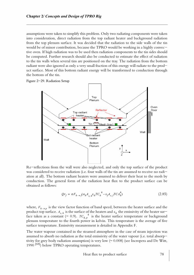
Heat flux to product surface 78
Chapter 2/ Concepts and Design of TPRO Rig________________________________________________________________________
assumptions were taken to simplify this problem. Only two radiating components were taken into consideration, direct radiation from the top radiant heater and background radiation from the top plenum surface. It was decided that the radiation to the side walls of the tin would be of minor contribution, because the TPRO would be working in a highly convec−tive oven. If high radiation was to be used then radiation components to the tin sides should be computed. Further research should also be conducted to estimate the effect of radiation to the tin walls when several tins are positioned on the tray. The radiation from the bottom radiant were also ignored as only a very small fraction of this energy will radiate to the prod−uct surface. Most of this bottom radiant energy will be transformed to conduction through the bottom of the tin.
Figure 2−29. Radiation Setup
Re−reflections from the wall were also neglected, and only the top surface of the product was considered to receive radiation (i.e. four walls of the tin are assumed to receive no radi−ation at all). The bottom radiant heaters were assumed to deliver their heat to the mesh by conduction. The general form of the radiation heat flux to the product surface can be obtained as follows:
(2.85)
where, is the view factor function of band speed, between the heater surface and the product top surface. is the surface of the heaters and the emissivity of the heater sur−face taken as a constant (= 0.9). is the heater surface temperature or background plenum temperature to the fourth power in kelvin. This temperature is the average of five surface temperature. Emissivity measurement is detailed in Appendix F.
The water wapour contained in the steamed atmosphere in the case of steam injection was assumed to absorb no radiation as the total emissivity of the water vapour (i.e. total absorp−tivity for grey body radiation assumption) is very low (~ 0.008) (see Incropera and De Witt, 1990 [68]) below TPRO operating temperatures.
Qrf σFh f→ nhAs h, εhTCh4 εfAs f, TCA8
4–( )=
Fh p→As h, εh
TCh p,4
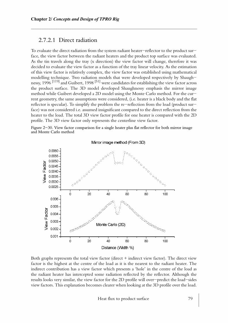
Heat flux to product surface 79
Chapter 2/ Concepts and Design of TPRO Rig________________________________________________________________________
2.7.2.1 Direct radiation
To evaluate the direct radiation from the system radiant heater−reflector to the product sur−face, the view factor between the radiant heaters and the product top surface was evaluated. As the tin travels along the tray (x direction) the view factor will change, therefore it was decided to evaluate the view factor as a function of the tray linear velocity. As the estimation of this view factor is relatively complex, the view factor was established using mathematical modelling technique. Two radiation models that were developed respectively by Shaugh−nessy, 1996 [119] and Guibert, 1998 [51] were candidates for establishing the view factor across the product surface. The 3D model developed Shaughnessy emphasis the mirror image method while Guibert developed a 2D model using the Monte Carlo method. For the cur−rent geometry, the same assumptions were considered, (i.e. heater is a black body and the flat reflector is specular). To simplify the problem the re−reflection from the load (product sur−face) was not considered i.e. assumed insignificant compared to the direct reflection from the heater to the load. The total 3D view factor profile for one heater is compared with the 2D profile. The 3D view factor only represents the centerline view factor.
Figure 2−30. View factor comparison for a single heater plus flat reflector for both mirror image and Monte Carlo method
Both graphs represents the total view factor (direct + indirect view factor). The direct view factor is the highest at the centre of the load as it is the nearest to the radiant heater. The indirect contribution has a view factor which presents a ‘hole’ in the centre of the load as the radiant heater has intercepted some radiation reflected by the reflector. Although the results looks very similar, the view factor for the 2D profile will over−predict the load−sides view factors. This explanation becomes clearer when looking at the 3D profile over the load.

Heat flux to product surface 80
Chapter 2/ Concepts and Design of TPRO Rig________________________________________________________________________
The view factor is maximum near the centerline, however it decreases as distance increase from the heater centerline Fig. 2−31.
Figure 2−31. Single heater view factor (3D)
6 of the above profile were overlapped using the view factor summation rule, Incropera and De Witt, 1990 [68] to estimate the overall view factor for the full width and length covered by the six radiant heaters (Fig. 2−32).
Figure 2−32. Overall view factor
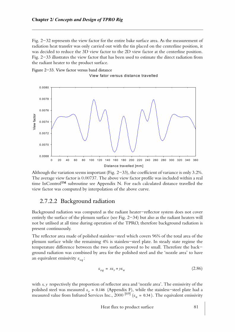
Heat flux to product surface 81
Chapter 2/ Concepts and Design of TPRO Rig________________________________________________________________________
Fig. 2−32 represents the view factor for the entire bake surface area. As the measurement of radiation heat transfer was only carried out with the tin placed on the centerline position, it was decided to reduce the 3D view factor to the 2D view factor at the centerline position. Fig. 2−33 illustrates the view factor that has been used to estimate the direct radiation from the radiant heater to the product surface.
Figure 2−33. View factor versus band distance
Although the variation seems important (Fig. 2−33), the coefficient of variance is only 3.2%. The average view factor is 0.00737. The above view factor profile was included within a real time InControl™ subroutine see Appendix N. For each calculated distance travelled the view factor was computed by interpolation of the above curve.
2.7.2.2 Background radiation
Background radiation was computed as the radiant heater−reflector system does not cover entirely the surface of the plenum surface (see Fig. 2−34) but also as the radiant heaters will not be utilised at all time during operation of the TPRO, therefore background radiation is present continuously.
The reflector area made of polished stainless−steel which covers 96% of the total area of the plenum surface while the remaining 4% is stainless−steel plate. In steady state regime the temperature difference between the two surfaces proved to be small. Therefore the back−ground radiation was combined by area for the polished steel and the ‘nozzle area’ to have an equivalent emissivity :
(2.86)
with respectively the proportion of reflector area and ‘nozzle area’. The emissivity of the polished steel was measured (Appendix F), while the stainless−steel plate had a measured value from Infrared Services Inc., 2000 [69] ( ). The equivalent emissivity
View fator versus distance travelled
Distance travelled [mm]
20 60 100 140 180 220 260 300 3400 40 80 120 160 200 240 280 320 360
View
fact
or
0.0068
0.0070
0.0072
0.0074
0.0076
0.0078
0.0080
εeq
εeq xεr yεn+=
x y,εr 0.146=
εn 0.34=
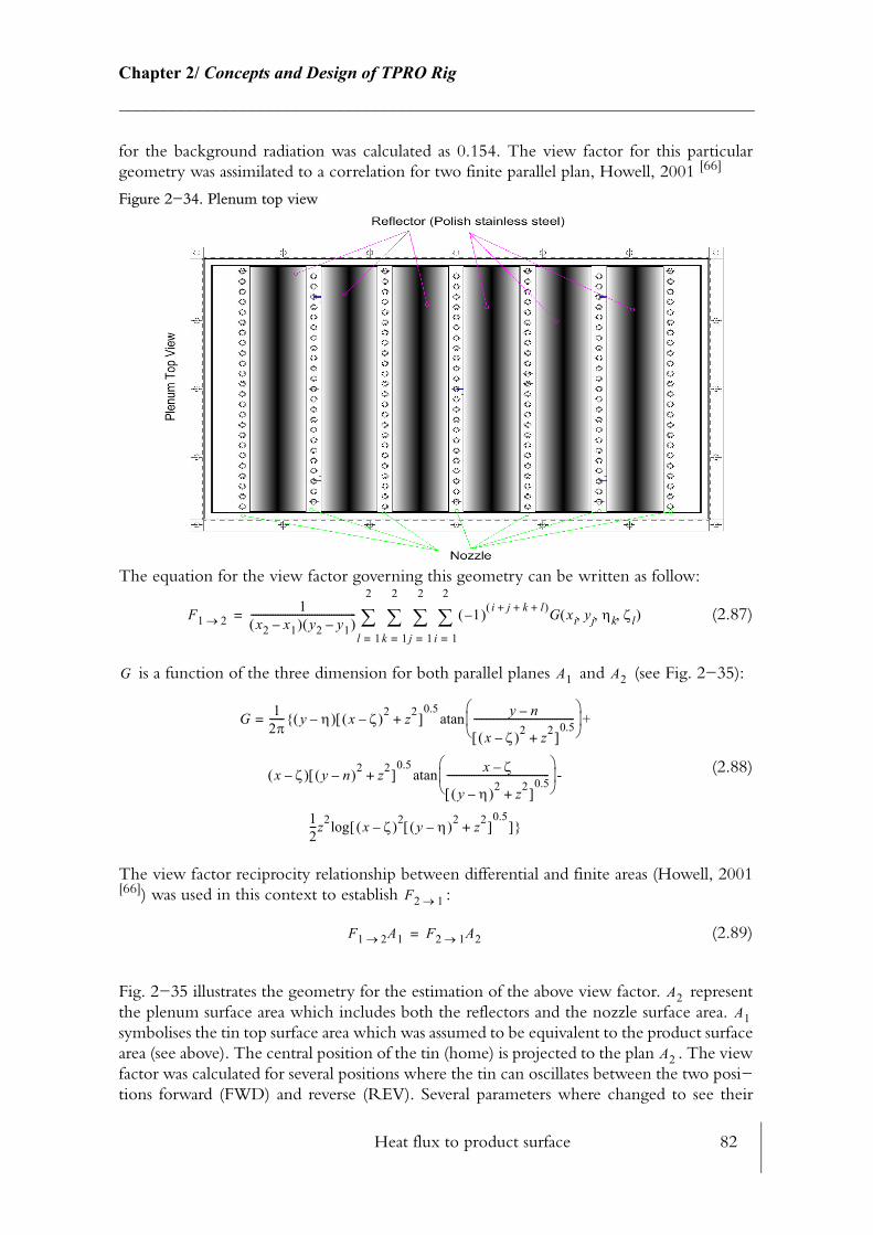
Heat flux to product surface 82
Chapter 2/ Concepts and Design of TPRO Rig________________________________________________________________________
for the background radiation was calculated as 0.154. The view factor for this particular geometry was assimilated to a correlation for two finite parallel plan, Howell, 2001 [66]
Figure 2−34. Plenum top view
The equation for the view factor governing this geometry can be written as follow:
(2.87)
is a function of the three dimension for both parallel planes and (see Fig. 2−35):
(2.88)
The view factor reciprocity relationship between differential and finite areas (Howell, 2001[66]) was used in this context to establish :
(2.89)
Fig. 2−35 illustrates the geometry for the estimation of the above view factor. represent the plenum surface area which includes both the reflectors and the nozzle surface area. symbolises the tin top surface area which was assumed to be equivalent to the product surface area (see above). The central position of the tin (home) is projected to the plan . The view factor was calculated for several positions where the tin can oscillates between the two posi−tions forward (FWD) and reverse (REV). Several parameters where changed to see their
F1 2→1
x2 x1–( ) y2 y1–( )------------------------------------------- 1–( ) i j k l+ + +( )G xi yj ηk ζl, , ,( )
i 1=
2
∑j 1=
2
∑k 1=
2
∑l 1=
2
∑=
G A1 A2
G 12π------ y η–( ) x ζ–( )2 z2
+[ ]0.5 y n–
x ζ–( )2 z2+[ ]
0.5-----------------------------------------
+atan=
x ζ–( ) y n–( )2 z2+[ ]
0.5 x ζ–
y η–( )2 z2+[ ]
0.5------------------------------------------
-atan
12---z2 x ζ–( )2 y η–( )2 z2
+[ ]0.5
[ ]log
F2 1→
F1 2→ A1 F2 1→ A2=
A2A1
A2

Heat flux to product surface 83
Chapter 2/ Concepts and Design of TPRO Rig________________________________________________________________________
influence on the total view factor. Fig. 2−36 shows the difference of view factor between a tin positioned along its width and its length for the complete oscillation of the band (between REV and FWD position). As the tin moves from its centerline position, the view factor decreases. Nevertheless, the overall view factor is smoother for a tin positioned along its length, however the peak view factor in the case of a tin positioned along its width is higher. For these reasons, the background radiation will be more effective if the tin is placed along its length.
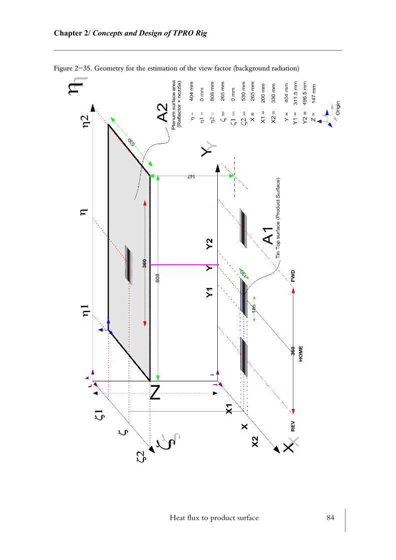
Heat flux to product surface 84
Chapter 2/ Concepts and Design of TPRO Rig________________________________________________________________________
Figure 2−35. Geometry for the estimation of the view factor (background radiation)
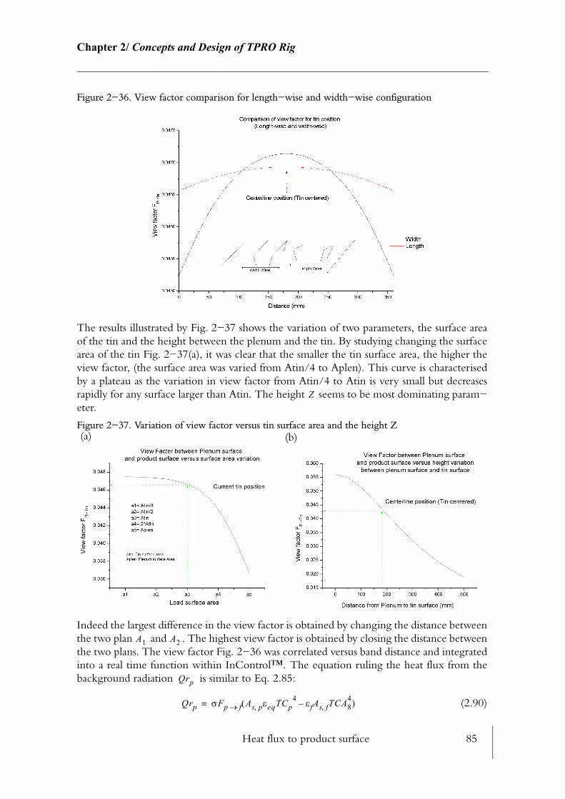
Heat flux to product surface 85
Chapter 2/ Concepts and Design of TPRO Rig________________________________________________________________________
Figure 2−36. View factor comparison for length−wise and width−wise configuration
The results illustrated by Fig. 2−37 shows the variation of two parameters, the surface area of the tin and the height between the plenum and the tin. By studying changing the surface area of the tin Fig. 2−37(a), it was clear that the smaller the tin surface area, the higher the view factor, (the surface area was varied from Atin/4 to Aplen). This curve is characterised by a plateau as the variation in view factor from Atin/4 to Atin is very small but decreases rapidly for any surface larger than Atin. The height seems to be most dominating param−eter.
Figure 2−37. Variation of view factor versus tin surface area and the height Z
Indeed the largest difference in the view factor is obtained by changing the distance between the two plan and . The highest view factor is obtained by closing the distance between the two plans. The view factor Fig. 2−36 was correlated versus band distance and integrated into a real time function within InControl™. The equation ruling the heat flux from the background radiation is similar to Eq. 2.85:
(2.90)
Z
(b)(a)
A1 A2
Qrp
Qrp σFp f→ As p, εeqTCp4 εfAs f, TCA8
4–( )=
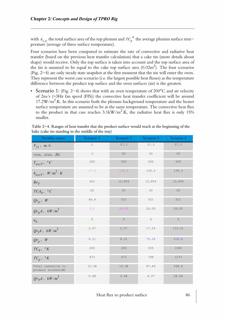
Heat flux to product surface 86
Chapter 2/ Concepts and Design of TPRO Rig________________________________________________________________________
with the total surface area of the top plenum and the average plenum surface tem−perature (average of three surface temperature).
Four scenarios have been computed to estimate the rate of convective and radiative heat transfer (based on the previous heat transfer calculation) that a cake tin (more details about shape) would receive. Only the top surface is taken into account and the top surface area of the tin is assumed to be equal to the cake top surface area (0.02m2). The four scenarios (Fig. 2−4) are only steady state snapshot at the first moment that the tin will enter the oven. They represent the worst case scenario (i.e. the largest possible heat fluxes) as the temperature difference between the product top surface and the oven surfaces (air) is the greatest.
• Scenario 1: (Fig. 2−4) shows that with an oven temperature of 200oC and air velocity of 2m/s (~3Hz fan speed (FIS)) the convective heat transfer coefficient will be around 17.2W/m2.K. In this scenario both the plenum background temperature and the heater surface temperature are assumed to be at the same temperature. The convective heat flux to the product in that case reaches 3.1kW/m2.K, the radiative heat flux is only 15% smaller.
Table 2−4. Ranges of heat transfer that the product surface would reach at the beginning of the bake (cake tin standing in the middle of the tray)
Variables names Scenario 1 Scenario 2 Scenario 3 Scenario 4
, 2 57.3 57.3 57.3
CFAN, EFAN, 3 50 50 50
, 200 200 200 200
, 17.2 134.3 134.3 134.3
601 12,854 12,854 12,854
, 20 20 20 20
, 66.4 521 521 521
, 3.1 26.05 26.05 26.05
6 6 6 6
, 2.07 2.07 17.24 112.01
, 8.31 8.31 70.24 456.8
, 200 200 525 1000
, 473 473 798 1273
Total radiation to product surface(W)
10.38 10.38 87.49 568.8
, 0.48 0.48 4.37 28.44
As p, TCp4
V11 m s⁄
Hz
TnozT °C
hnozT W m2⁄ K⋅
ReT
TCA8 °C
Qcp W
QcpA kW m2⁄
nh
QrfA kW m2⁄
Qrp W
TC9 °K
TCp °K
QrTA kW m2⁄
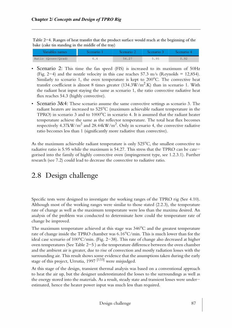
Design challenge 87
Chapter 2/ Concepts and Design of TPRO Rig________________________________________________________________________
• Scenario 2: This time the fan speed (FIS) is increased to its maximum of 50Hz (Fig. 2−4) and the nozzle velocity in this case reaches 57.3 m/s (Reynolds = 12,854). Similarly to scenario 1, the oven temperature is kept to 200oC. The convective heat transfer coefficient is almost 8 times greater (134.3W/m2.K) than in scenario 1. With the radiant heat input staying the same as scenario 1, the ratio convective radiative heat flux reaches 54.3 (highly convective).
• Scenario 3&4: These scenario assume the same convective settings as scenario 3. The radiant heaters are increased to 525oC (maximum achievable radiant temperature in the TPRO) in scenario 3 and to 1000oC in scenario 4. It is assumed that the radiant heater temperature achieve the same as the reflector temperature. The total heat flux becomes respectively 4.37kW/m2 and 28.44kW/m2. Only in scenario 4, the convective radiative ratio becomes less than 1 (significantly more radiative than convective).
As the maximum achievable radiant temperature is only 525oC, the smallest convective to radiative ratio is 5.95 while the maximum is 54.27. This stress that the TPRO can be cate−gorised into the family of highly convective oven (impingement type, see 1.2.3.1). Further research (see 7.2) could lead to decrease the convective to radiative ratio.
2.8 Design challenge
Specific tests were designed to investigate the working ranges of the TPRO rig (See 4.10). Although most of the working ranges were similar to those stated (2.2.3), the temperature rate of change as well as the maximum temperature were less than the maxima desired. An analysis of the problem was conducted to determinate how could the temperature rate of change be improved.
The maximum temperature achieved at this stage was 346oC and the greatest temperature rate of change inside the TPRO chamber was 6.16oC/min. This is much lower than for the ideal case scenario of 100°C/min. (Fig. 2−38). This rate of change also decreased at higher oven temperatures (See Table 2−5 ) as the temperature difference between the oven chamber and the ambient air is greater, due to rise of convection and mostly radiation losses with the surrounding air. This result shows some evidence that the assumptions taken during the early stage of this project, Urrutia, 1997 [133] were misjudged.
At this stage of the design, transient thermal analysis was based on a conventional approach to heat the air up, but the designer underestimated the losses to the surroundings as well as the energy stored into the materials. As a result, steady state and transient losses were under−estimated, hence the heater power input was much less than required.
Ratio (Qconv/Qrad) 6.4 54.27 5.95 0.92
Table 2−4. Ranges of heat transfer that the product surface would reach at the beginning of the bake (cake tin standing in the middle of the tray)
Variables names Scenario 1 Scenario 2 Scenario 3 Scenario 4
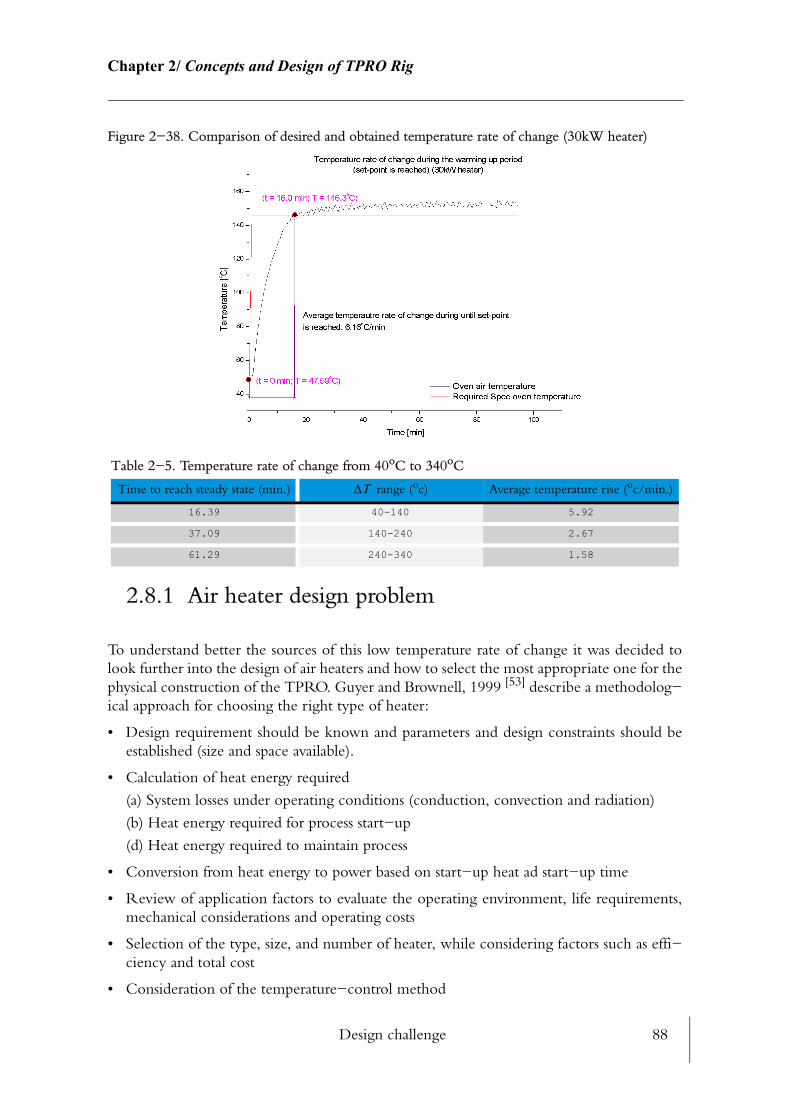
Design challenge 88
Chapter 2/ Concepts and Design of TPRO Rig________________________________________________________________________
Figure 2−38. Comparison of desired and obtained temperature rate of change (30kW heater)
2.8.1 Air heater design problem
To understand better the sources of this low temperature rate of change it was decided to look further into the design of air heaters and how to select the most appropriate one for the physical construction of the TPRO. Guyer and Brownell, 1999 [53] describe a methodolog−ical approach for choosing the right type of heater:
• Design requirement should be known and parameters and design constraints should be established (size and space available).
• Calculation of heat energy required
(a) System losses under operating conditions (conduction, convection and radiation)
(b) Heat energy required for process start−up
(d) Heat energy required to maintain process
• Conversion from heat energy to power based on start−up heat ad start−up time
• Review of application factors to evaluate the operating environment, life requirements, mechanical considerations and operating costs
• Selection of the type, size, and number of heater, while considering factors such as effi−ciency and total cost
• Consideration of the temperature−control method
Table 2−5. Temperature rate of change from 40oC to 340oC
Time to reach steady state (min.) range (oc) Average temperature rise (oc/min.)
16.39 40-140 5.92
37.09 140-240 2.67
61.29 240-340 1.58
∆T
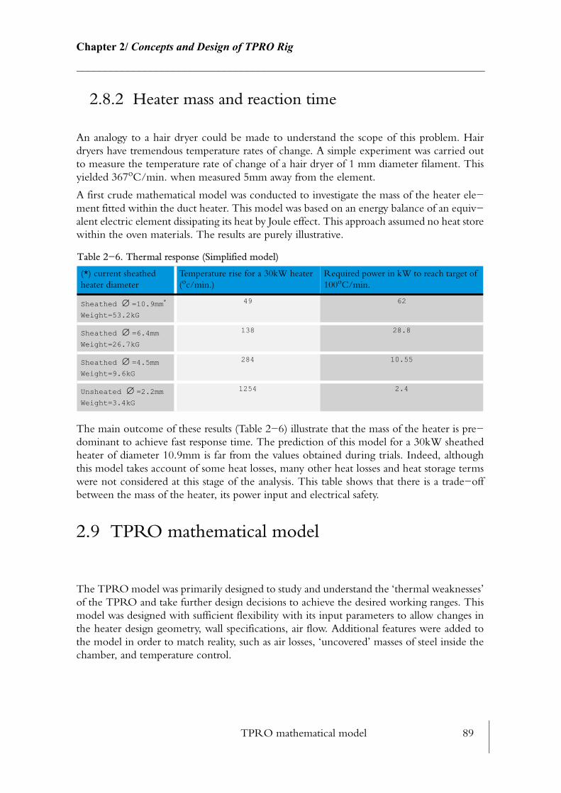
TPRO mathematical model 89
Chapter 2/ Concepts and Design of TPRO Rig________________________________________________________________________
2.8.2 Heater mass and reaction time
An analogy to a hair dryer could be made to understand the scope of this problem. Hair dryers have tremendous temperature rates of change. A simple experiment was carried out to measure the temperature rate of change of a hair dryer of 1 mm diameter filament. This yielded 367oC/min. when measured 5mm away from the element.
A first crude mathematical model was conducted to investigate the mass of the heater ele−ment fitted within the duct heater. This model was based on an energy balance of an equiv−alent electric element dissipating its heat by Joule effect. This approach assumed no heat store within the oven materials. The results are purely illustrative.
The main outcome of these results (Table 2−6) illustrate that the mass of the heater is pre−dominant to achieve fast response time. The prediction of this model for a 30kW sheathed heater of diameter 10.9mm is far from the values obtained during trials. Indeed, although this model takes account of some heat losses, many other heat losses and heat storage terms were not considered at this stage of the analysis. This table shows that there is a trade−off between the mass of the heater, its power input and electrical safety.
2.9 TPRO mathematical model
The TPRO model was primarily designed to study and understand the ‘thermal weaknesses’ of the TPRO and take further design decisions to achieve the desired working ranges. This model was designed with sufficient flexibility with its input parameters to allow changes in the heater design geometry, wall specifications, air flow. Additional features were added to the model in order to match reality, such as air losses, ‘uncovered’ masses of steel inside the chamber, and temperature control.
Table 2−6. Thermal response (Simplified model)
(*) current sheathed heater diameter
Temperature rise for a 30kW heater (oc/min.)
Required power in kW to reach target of 100oC/min.
Sheathed =10.9mm*
Weight=53.2kG
49 62
Sheathed =6.4mm
Weight=26.7kG
138 28.8
Sheathed =4.5mm
Weight=9.6kG
284 10.55
Unsheated =2.2mm
Weight=3.4kG
1254 2.4
∅
∅
∅
∅
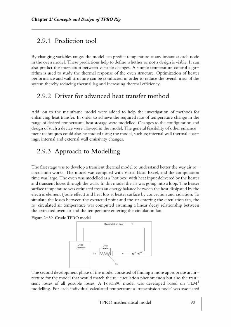
TPRO mathematical model 90
Chapter 2/ Concepts and Design of TPRO Rig________________________________________________________________________
2.9.1 Prediction tool
By changing variables ranges the model can predict temperature at any instant at each node in the oven model. These predictions help to define whether or not a design is viable. It can also predict the interaction between variable changes. A simple temperature control algo−rithm is used to study the thermal response of the oven structure. Optimization of heater performance and wall structure can be conducted in order to reduce the overall mass of the system thereby reducing thermal lag and increasing thermal efficiency.
2.9.2 Driver for advanced heat transfer method
Add−on to the mainframe model were added to help the investigation of methods for enhancing heat transfer. In order to achieve the required rate of temperature change in the range of desired temperature, heat storage were modelled. Changes to the configuration and design of such a device were allowed in the model. The general feasibility of other enhance−ment techniques could also be studied using the model, such as; internal wall thermal coat−ings, internal and external wall emissivity changes.
2.9.3 Approach to Modelling
The first stage was to develop a transient thermal model to understand better the way air re−circulation works. The model was compiled with Visual Basic Excel, and the computation time was large. The oven was modelled as a ‘hot box’ with heat input delivered by the heater and transient losses through the walls. In this model the air was going into a loop. The heater surface temperature was estimated from an energy balance between the heat dissipated by the electric element (Joule effect) and heat loss at heater surface by convection and radiation. To simulate the losses between the extracted point and the air entering the circulation fan, the re−circulated air temperature was computed assuming a linear decay relationship between the extracted oven air and the temperature entering the circulation fan.
Figure 2−39. Crude TPRO model
The second development phase of the model consisted of finding a more appropriate archi−tecture for the model that would match the re−circulation phenomenon but also the tran−sient losses of all possible losses. A Fortan90 model was developed based on TLM1
modelling. For each individual calculated temperature a ‘transmission node’ was associated
Ts
To
OvenChamber
Recirculation duct
DuctHeater
Ti ,n
Tin+1
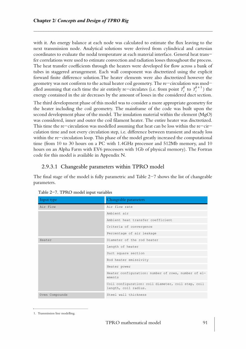
TPRO mathematical model 91
Chapter 2/ Concepts and Design of TPRO Rig________________________________________________________________________
with it. An energy balance at each node was calculated to estimate the flux leaving to the next transmission node. Analytical solutions were derived from cylindrical and cartesian coordinates to evaluate the nodal temperature at each material interface. General heat trans−fer correlations were used to estimate convection and radiation losses throughout the process. The heat transfer coefficients through the heaters were developed for flow across a bank of tubes in staggered arrangement. Each wall component was disctretized using the explicit forward finite difference solution.The heater elements were also disctretized however the geometry was not conform to the actual heater coil geometry. The re−circulation was mod−elled assuming that each time the air entirely re−circulates (i.e. from point to ) the energy contained in the air decreases by the amount of losses in the considered duct section.
The third development phase of this model was to consider a more appropriate geometry for the heater including the coil geometry. The mainframe of the code was built upon the second development phase of the model. The insulation material within the element (MgO) was considered, inner and outer the coil filament heater. The entire heater was disctretized. This time the re−circulation was modelled assuming that heat can be loss within the re−cir−culation time and not every circulation step, i.e. difference between transient and steady loss within the re−circulation loop. This phase of the model greatly increased the computational time (from 10 to 30 hours on a PC with 1.4GHz processor and 512Mb memory, and 10 hours on an Alpha Farm with EV6 processors with 1Gb of physical memory). The Fortran code for this model is available in Appendix N.
2.9.3.1 Changeable parameters within TPRO model
The final stage of the model is fully parametric and Table 2−7 shows the list of changeable parameters.
1. Transmission line modelling.
Table 2−7. TPRO model input variables
Input type Changeable parameters
Air Flow Air flow rate
Ambient air
Ambient heat transfer coefficient
Criteria of convergence
Percentage of air leakage
Heater Diameter of the rod heater
Length of heater
Duct square section
Rod heater emissivity
Heater power
Heater configuration: number of rows, number of el-ements
Coil configuration: coil diameter, coil step, coil length, coil radius.
Oven Compounds Steel wall thickness
Tik Ti
k 1+

TPRO mathematical model 92
Chapter 2/ Concepts and Design of TPRO Rig________________________________________________________________________
The model was used to establish a first order understanding. It required some calibration using real test rig parameters. Some parameters of this model are well known but some others were assumed.
Model certitudes: Wall characteristics, Heater power, min.−max flow rate.
Model assumptions: Coil characteristics, heater characteristics, mass of steel in the chamber, convection coefficient inside the chamber, flow pattern inside the chamber, flow pattern around heaters.
With the data gathered by the non food test (See 4.10), this model could be extended and fed with useful informations.
2.9.3.2 Results of model
The duct heater elements have been modelled taking into consideration their internal geometry. The heater element supplier (Watlow and Industrial Electric Element) refused to give the internal geometry of the coil (heated filament). A parametric study of the internal coil geometry shows that external surface temperature of the heater element is extremely sensitive to coil geometry and demonstrates how confidential these parameters are, from a supplier and designer point of view.
2.9.3.2.1 Coil parametric analysis
The internal temperature profile of the heater element shows well the three different ‘layers’ which correspond respectively to MgO electrical insulation + coil, MgO insulation and stainless steel sheath. Fig. 2−40 represent the temperature profile for half section of the ele−ment (i.e. node 0 correspond to the centre).
Insulation chamber/duct wall thickness
Insulation emissivity walls
Steel emissivity
Coefficient of convection from wall and from noz-zles
Mass of steel in the chamber: each disctretized mass affected by a different convective heat trans-fer coefficient (Reason: oven chamber flow pattern unknown).
Table 2−7. TPRO model input variables
Input type Changeable parameters
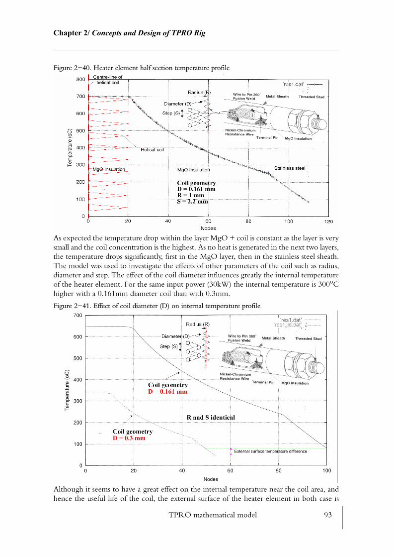
TPRO mathematical model 93
Chapter 2/ Concepts and Design of TPRO Rig________________________________________________________________________
Figure 2−40. Heater element half section temperature profile
As expected the temperature drop within the layer MgO + coil is constant as the layer is very small and the coil concentration is the highest. As no heat is generated in the next two layers, the temperature drops significantly, first in the MgO layer, then in the stainless steel sheath. The model was used to investigate the effects of other parameters of the coil such as radius, diameter and step. The effect of the coil diameter influences greatly the internal temperature of the heater element. For the same input power (30kW) the internal temperature is 300oC higher with a 0.161mm diameter coil than with 0.3mm.
Figure 2−41. Effect of coil diameter (D) on internal temperature profile
Although it seems to have a great effect on the internal temperature near the coil area, and hence the useful life of the coil, the external surface of the heater element in both case is
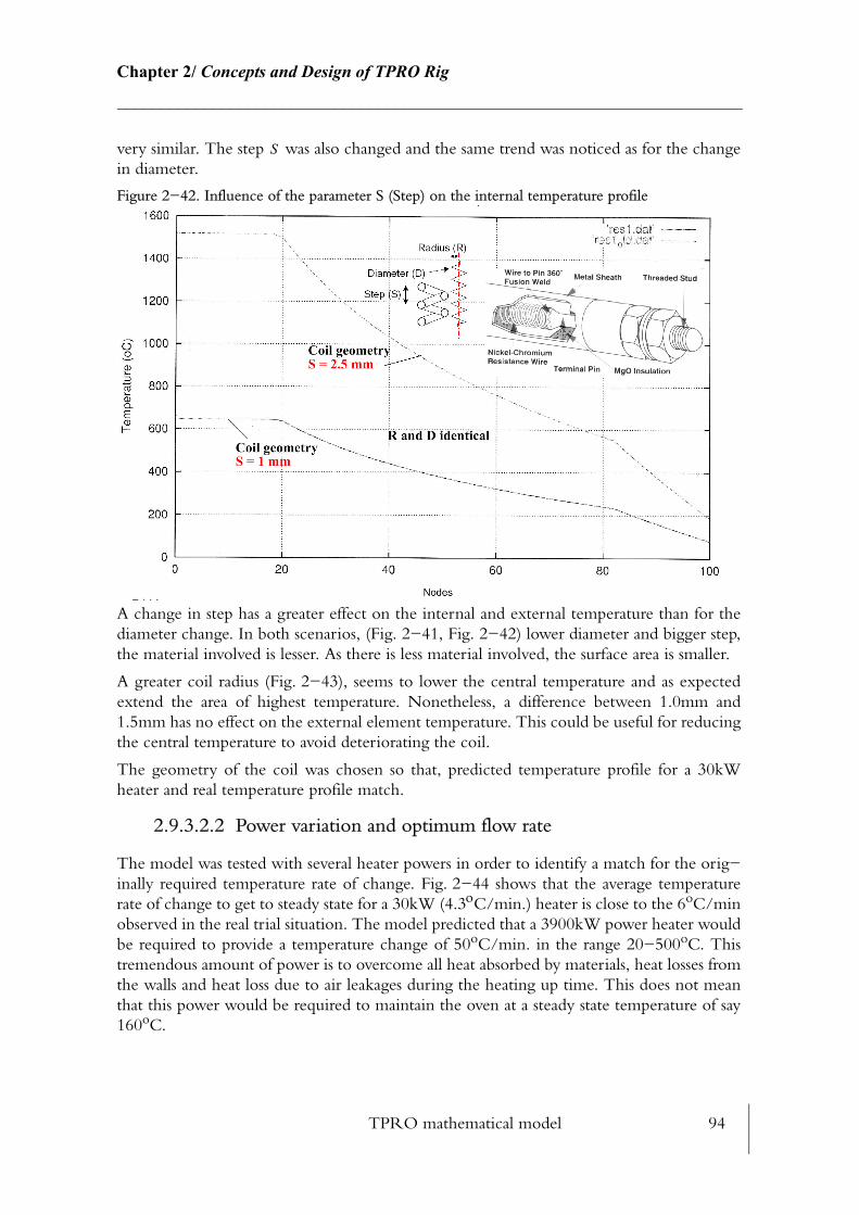
TPRO mathematical model 94
Chapter 2/ Concepts and Design of TPRO Rig________________________________________________________________________
very similar. The step was also changed and the same trend was noticed as for the change in diameter.
Figure 2−42. Influence of the parameter S (Step) on the internal temperature profile
A change in step has a greater effect on the internal and external temperature than for the diameter change. In both scenarios, (Fig. 2−41, Fig. 2−42) lower diameter and bigger step, the material involved is lesser. As there is less material involved, the surface area is smaller.
A greater coil radius (Fig. 2−43), seems to lower the central temperature and as expected extend the area of highest temperature. Nonetheless, a difference between 1.0mm and 1.5mm has no effect on the external element temperature. This could be useful for reducing the central temperature to avoid deteriorating the coil.
The geometry of the coil was chosen so that, predicted temperature profile for a 30kW heater and real temperature profile match.
2.9.3.2.2 Power variation and optimum flow rate
The model was tested with several heater powers in order to identify a match for the orig−inally required temperature rate of change. Fig. 2−44 shows that the average temperature rate of change to get to steady state for a 30kW (4.3οC/min.) heater is close to the 6oC/min observed in the real trial situation. The model predicted that a 3900kW power heater would be required to provide a temperature change of 50oC/min. in the range 20−500oC. This tremendous amount of power is to overcome all heat absorbed by materials, heat losses from the walls and heat loss due to air leakages during the heating up time. This does not mean that this power would be required to maintain the oven at a steady state temperature of say 160oC.
S
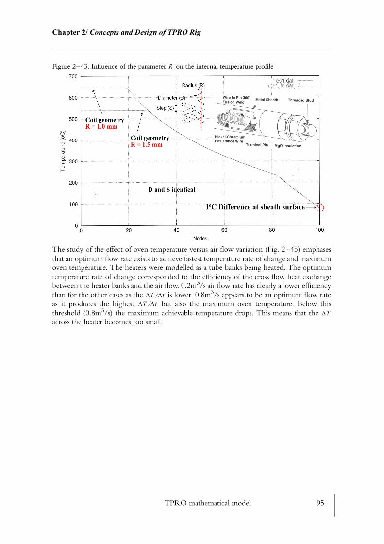
TPRO mathematical model 95
Chapter 2/ Concepts and Design of TPRO Rig________________________________________________________________________
Figure 2−43. Influence of the parameter on the internal temperature profile
The study of the effect of oven temperature versus air flow variation (Fig. 2−45) emphases that an optimum flow rate exists to achieve fastest temperature rate of change and maximum oven temperature. The heaters were modelled as a tube banks being heated. The optimum temperature rate of change corresponded to the efficiency of the cross flow heat exchange between the heater banks and the air flow. 0.2m3/s air flow rate has clearly a lower efficiency than for the other cases as the is lower. 0.8m3/s appears to be an optimum flow rate as it produces the highest but also the maximum oven temperature. Below this threshold (0.8m3/s) the maximum achievable temperature drops. This means that the across the heater becomes too small.
R
∆T ∆t⁄∆T ∆t⁄
∆T
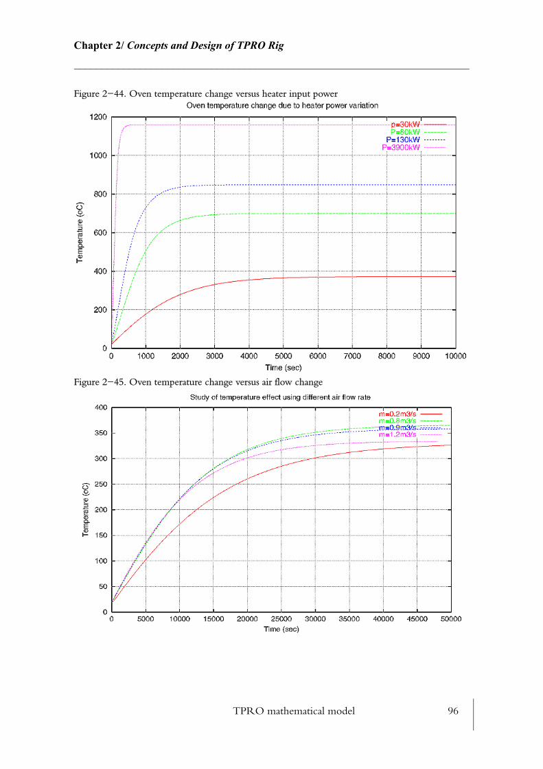
TPRO mathematical model 96
Chapter 2/ Concepts and Design of TPRO Rig________________________________________________________________________
Figure 2−44. Oven temperature change versus heater input power
Figure 2−45. Oven temperature change versus air flow change
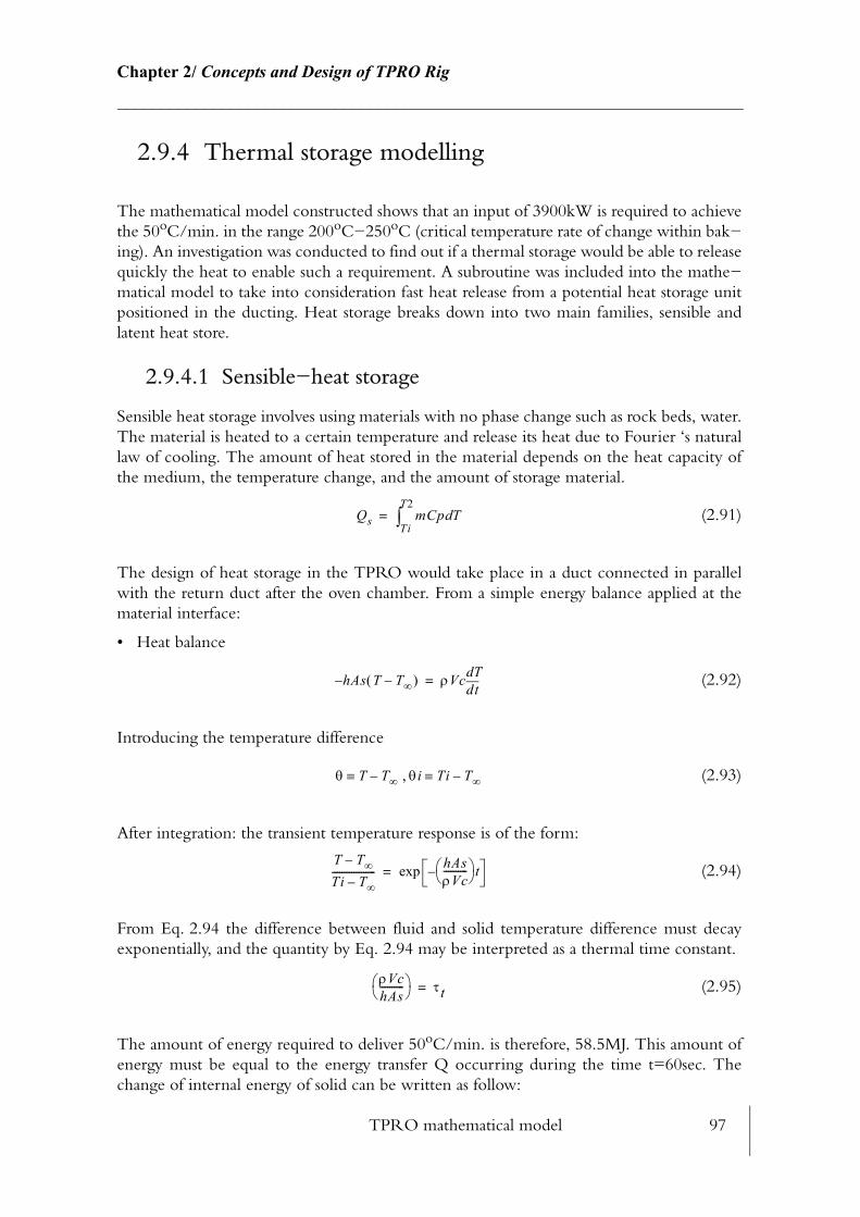
TPRO mathematical model 97
Chapter 2/ Concepts and Design of TPRO Rig________________________________________________________________________
2.9.4 Thermal storage modelling
The mathematical model constructed shows that an input of 3900kW is required to achieve the 50oC/min. in the range 200oC−250oC (critical temperature rate of change within bak−ing). An investigation was conducted to find out if a thermal storage would be able to release quickly the heat to enable such a requirement. A subroutine was included into the mathe−matical model to take into consideration fast heat release from a potential heat storage unit positioned in the ducting. Heat storage breaks down into two main families, sensible and latent heat store.
2.9.4.1 Sensible−heat storage
Sensible heat storage involves using materials with no phase change such as rock beds, water. The material is heated to a certain temperature and release its heat due to Fourier ‘s natural law of cooling. The amount of heat stored in the material depends on the heat capacity of the medium, the temperature change, and the amount of storage material.
(2.91)
The design of heat storage in the TPRO would take place in a duct connected in parallel with the return duct after the oven chamber. From a simple energy balance applied at the material interface:
• Heat balance
(2.92)
Introducing the temperature difference
, (2.93)
After integration: the transient temperature response is of the form:
(2.94)
From Eq. 2.94 the difference between fluid and solid temperature difference must decay exponentially, and the quantity by Eq. 2.94 may be interpreted as a thermal time constant.
(2.95)
The amount of energy required to deliver 50oC/min. is therefore, 58.5MJ. This amount of energy must be equal to the energy transfer Q occurring during the time t=60sec. The change of internal energy of solid can be written as follow:
Qs mCp TdTi
T2∫=
hAs T T∞–( )– ρVctd
dT=
θ T T∞–≡ θi Ti T∞–≡
T T∞–
Ti T∞–------------------ hAs
ρVc---------- t–exp=
ρVchAs---------- τt=
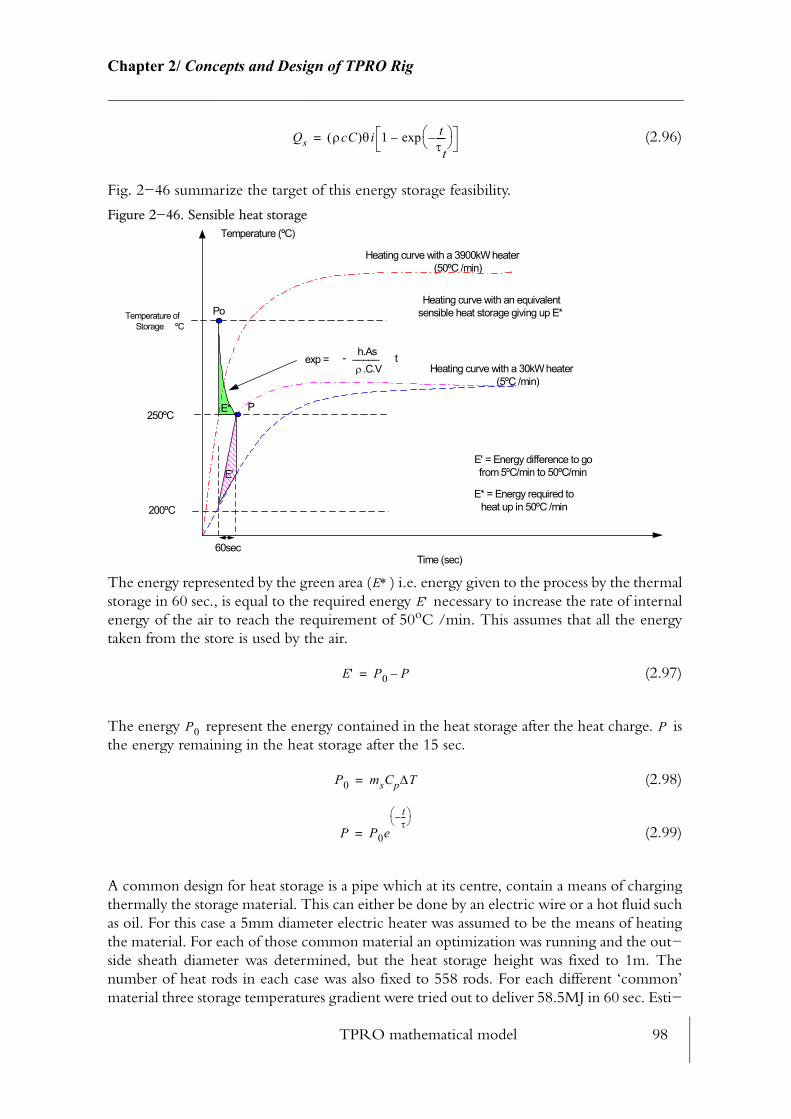
TPRO mathematical model 98
Chapter 2/ Concepts and Design of TPRO Rig________________________________________________________________________
(2.96)
Fig. 2−46 summarize the target of this energy storage feasibility.
Figure 2−46. Sensible heat storage
The energy represented by the green area ( ) i.e. energy given to the process by the thermal storage in 60 sec., is equal to the required energy necessary to increase the rate of internal energy of the air to reach the requirement of 50oC /min. This assumes that all the energy taken from the store is used by the air.
(2.97)
The energy represent the energy contained in the heat storage after the heat charge. is the energy remaining in the heat storage after the 15 sec.
(2.98)
(2.99)
A common design for heat storage is a pipe which at its centre, contain a means of charging thermally the storage material. This can either be done by an electric wire or a hot fluid such as oil. For this case a 5mm diameter electric heater was assumed to be the means of heating the material. For each of those common material an optimization was running and the out−side sheath diameter was determined, but the heat storage height was fixed to 1m. The number of heat rods in each case was also fixed to 558 rods. For each different ‘common’ material three storage temperatures gradient were tried out to deliver 58.5MJ in 60 sec. Esti−
Qs ρcC( )θi 1 tτt----–
exp–=
Time (sec)
Temperature (ºC)
200ºC
250ºC
60sec
Heating curve with a 3900kW heater(50ºC /min)
Heating curve with a 30kW heater(5ºC /min)
E* = Energy required toheat up in 50ºC /min
E*
exp = _____h.As-ρ .C.V
t
Heating curve with an equivalentsensible heat storage giving up E*
E' = Energy difference to gofrom 5ºC/min to 50ºC/min
Temperature ofStorage ºC
Po
P
E'
E∗E'
E' P0 P–=
P0 P
P0 msCp∆T=
P P0e
tτ--–
=
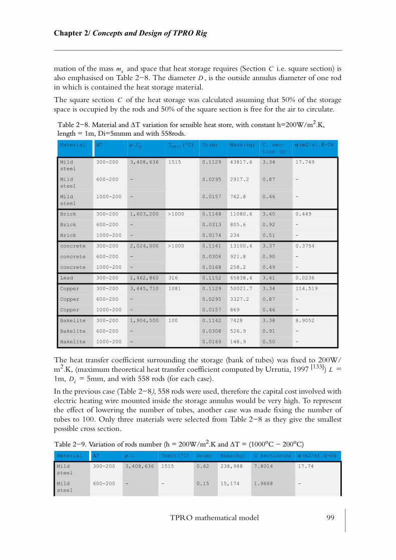
TPRO mathematical model 99
Chapter 2/ Concepts and Design of TPRO Rig________________________________________________________________________
mation of the mass and space that heat storage requires (Section i.e. square section) is also emphasised on Table 2−8. The diameter , is the outside annulus diameter of one rod in which is contained the heat storage material.
The square section of the heat storage was calculated assuming that 50% of the storage space is occupied by the rods and 50% of the square section is free for the air to circulate.
The heat transfer coefficient surrounding the storage (bank of tubes) was fixed to 200W/m2.K, (maximum theoretical heat transfer coefficient computed by Urrutia, 1997 [133]) = 1m, = 5mm, and with 558 rods (for each case).
In the previous case (Table 2−8), 558 rods were used, therefore the capital cost involved with electric heating wire mounted inside the storage annulus would be very high. To represent the effect of lowering the number of tubes, another case was made fixing the number of tubes to 100. Only three materials were selected from Table 2−8 as they give the smallest possible cross section.
Table 2−8. Material and ∆T variation for sensible heat store, with constant h=200W/m2.K, length = 1m, Di=5mmm and with 558rods.
Material ∆T ρ.Cp Tmelt(ºC) Do(m) Mass(kg) C. sec-tion (m)
α(m2/s).E-06
Mild steel
300-200 3,408,636 1515 0.1129 43817.6 3.34 17.749
Mild steel
600-200 - 0.0295 2917.2 0.87 -
Mild steel
1000-200 - 0.0157 762.8 0.46 -
Brick 300-200 1,603,200 >1000 0.1148 11080.6 3.40 0.449
Brick 600-200 - 0.0313 805.6 0.92 -
Brick 1000-200 - 0.0174 234 0.51 -
concrete 300-200 2,024,000 >1000 0.1141 13100.4 3.37 0.3754
concrete 600-200 - 0.0306 921.8 0.90 -
concrete 1000-200 - 0.0168 258.2 0.49 -
Lead 300-200 1,462,860 316 0.1152 65838.4 3.41 0.0236
Copper 300-200 3,445,710 1081 0.1129 50021.7 3.34 114.519
Copper 600-200 - 0.0295 3327.2 0.87 -
Copper 1000-200 - 0.0157 869 0.46 -
Bakelite 300-200 1,904,500 100 0.1142 7428 3.38 8.9052
Bakelite 600-200 - 0.0308 526.9 0.91 -
Bakelite 1000-200 - 0.0169 148.9 0.50 -
Table 2−9. Variation of rods number (h = 200W/m2.K and ∆T = (1000oC − 200oC)
Material ∆T ρ.C Tmelt(ºC) Do(m) Mass(kg) C section(m) α(m2/s).E-06
Mild steel
300-200 3,408,636 1515 0.62 238,988 7.8014 17.74
Mild steel
600-200 - - 0.15 15,174 1.9668 -
ms CD
C
LDi
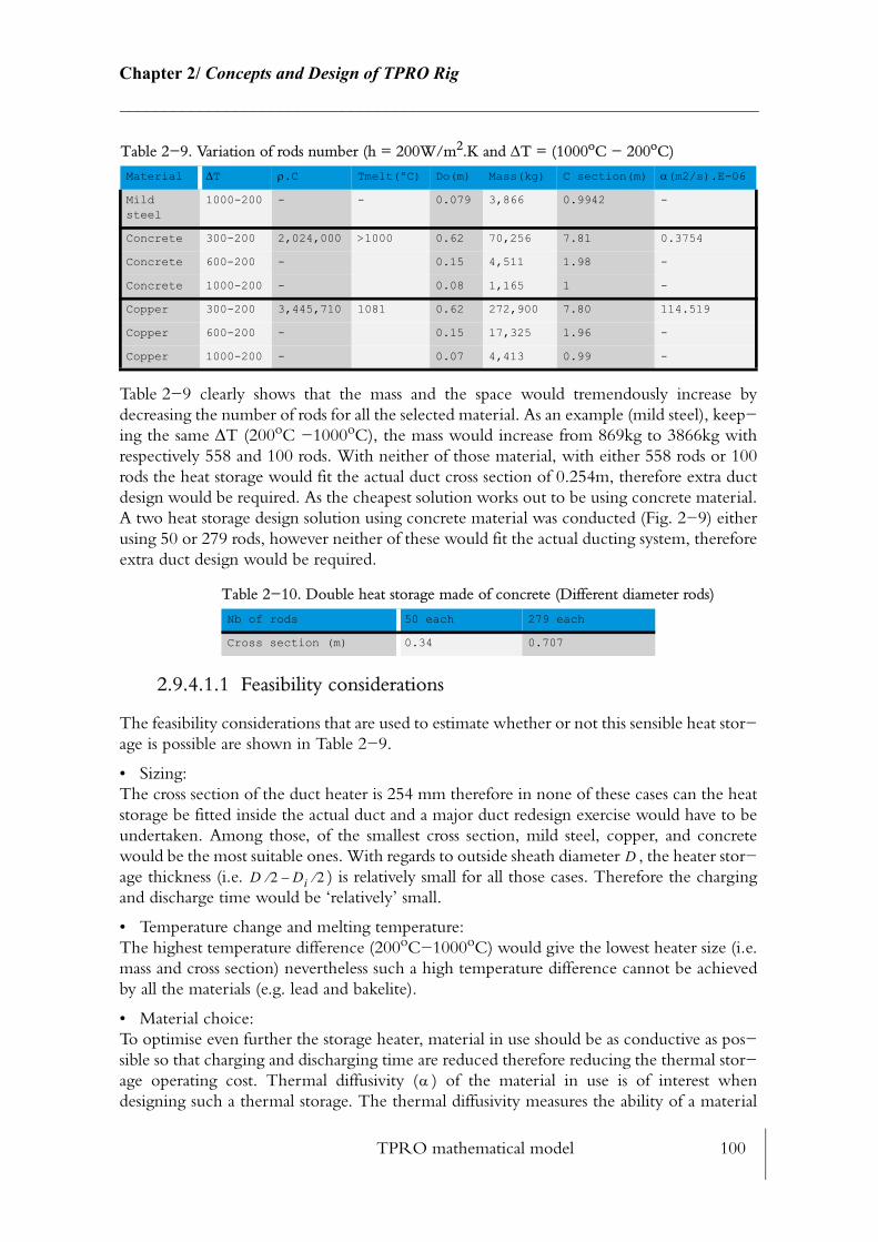
TPRO mathematical model 100
Chapter 2/ Concepts and Design of TPRO Rig________________________________________________________________________
Table 2−9 clearly shows that the mass and the space would tremendously increase by decreasing the number of rods for all the selected material. As an example (mild steel), keep−ing the same ∆T (200oC −1000oC), the mass would increase from 869kg to 3866kg with respectively 558 and 100 rods. With neither of those material, with either 558 rods or 100 rods the heat storage would fit the actual duct cross section of 0.254m, therefore extra duct design would be required. As the cheapest solution works out to be using concrete material. A two heat storage design solution using concrete material was conducted (Fig. 2−9) either using 50 or 279 rods, however neither of these would fit the actual ducting system, therefore extra duct design would be required.
2.9.4.1.1 Feasibility considerations
The feasibility considerations that are used to estimate whether or not this sensible heat stor−age is possible are shown in Table 2−9.
• Sizing: The cross section of the duct heater is 254 mm therefore in none of these cases can the heat storage be fitted inside the actual duct and a major duct redesign exercise would have to be undertaken. Among those, of the smallest cross section, mild steel, copper, and concrete would be the most suitable ones. With regards to outside sheath diameter , the heater stor−age thickness (i.e. ) is relatively small for all those cases. Therefore the charging and discharge time would be ‘relatively’ small.
• Temperature change and melting temperature:The highest temperature difference (200oC−1000oC) would give the lowest heater size (i.e. mass and cross section) nevertheless such a high temperature difference cannot be achieved by all the materials (e.g. lead and bakelite).
• Material choice:To optimise even further the storage heater, material in use should be as conductive as pos−sible so that charging and discharging time are reduced therefore reducing the thermal stor−age operating cost. Thermal diffusivity ( ) of the material in use is of interest when designing such a thermal storage. The thermal diffusivity measures the ability of a material
Mild steel
1000-200 - - 0.079 3,866 0.9942 -
Concrete 300-200 2,024,000 >1000 0.62 70,256 7.81 0.3754
Concrete 600-200 - 0.15 4,511 1.98 -
Concrete 1000-200 - 0.08 1,165 1 -
Copper 300-200 3,445,710 1081 0.62 272,900 7.80 114.519
Copper 600-200 - 0.15 17,325 1.96 -
Copper 1000-200 - 0.07 4,413 0.99 -
Table 2−10. Double heat storage made of concrete (Different diameter rods)
Nb of rods 50 each 279 each
Cross section (m) 0.34 0.707
Table 2−9. Variation of rods number (h = 200W/m2.K and ∆T = (1000oC − 200oC)
Material ∆T ρ.C Tmelt(ºC) Do(m) Mass(kg) C section(m) α(m2/s).E-06
DD 2⁄ Di 2⁄–
α

TPRO mathematical model 101
Chapter 2/ Concepts and Design of TPRO Rig________________________________________________________________________
to conduct thermal energy relative to its ability to store thermal energy. Therefore materials of large will respond quickly to changes in their thermal environment, while materials of small will take longer to reach a new thermal equilibrium. For this reason copper would be ideal (Table 2−9). The mass of the storage using copper would still be large (3327 kg for 200oC−600oC, and = 29mm). Another way of reducing its size would be to increase the rate of heat transfer inside the heat storage system (increase ).
From mathematical modelling the maximum achievable rate of heat transfer across the heat storage would be around 300 W/m2.K with a 1.2 m3/s air flow (i.e. above the requirements) and 235 W/m2.K with 0.8m3/s (requirement). Fig. 2−47 shows that square section and the mass of the heater would reduce subsequently by increasing the rate of heat transfer across the thermal storage. If increased from 200 to 300 W/m2.K with a across heat storage of (1000oC − 200oC) then the mass would reduce from 869kg to 462kg (half) (Fig. 2−47).
There will be a difference in the heat transfer coefficient prediction (from model) and the real value, therefore heat transfer convection variation across heat storage could lead to a wrong design e.g. not enough storage mass. If the mass is overestimated this could lead in slowing down the heat storage thermal response.
Figure 2−47. Variation of heat transfer coefficient across heat storage
• Rod number: By reducing the number of rods from 558 to 100, i.e. reducing the capital cost, results from the model shows that the total mass would increase by a factor of 4.5. Also the cross section would be twice as large.
• Cost of material:Comparing the three sensible heat storage (100 tubes) in the range of temperature (1000oC−200oC) can drive to a straight conclusion. A mild−steel heat storage would cost £3,175, a copper one would cost £14,650 while a concrete sensible heat storage would only cost £15 pounds (cost only included price of material). The two sensible heat storage made of metals
αα
Dh
h ∆T
0 50 10 0 1 50 20 0 25 0 3 000. 0
0. 1
0. 2
0. 3
0. 4
0. 5
0. 6
0. 7
Materia l: C opperHeat s to rage l en tgh: 1 mCons tan t ∆T : 200-1000 oC
Varia tion o f heat transfer coefficie n t versusheat storage m ass and heat storage cross sec tion
C .Section M ass
C onvection he at trans fer c oefficien t (W /m 2.K )
Cro
ss S
ectio
n (m
)
0
10 00
20 00
30 00
40 00
50 00
60 00
70 00
80 00
90 00
10 00 0
11 00 0
12 00 0
13 00 0
Mass of heat storage (kg)
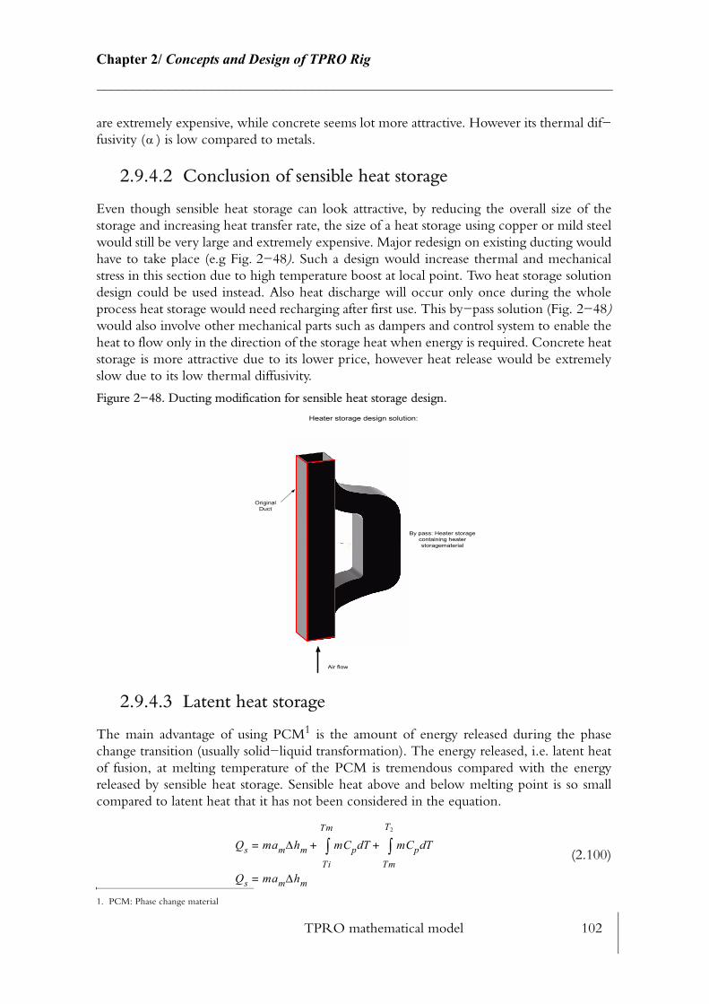
TPRO mathematical model 102
Chapter 2/ Concepts and Design of TPRO Rig________________________________________________________________________
are extremely expensive, while concrete seems lot more attractive. However its thermal dif−fusivity ( ) is low compared to metals.
2.9.4.2 Conclusion of sensible heat storage
Even though sensible heat storage can look attractive, by reducing the overall size of the storage and increasing heat transfer rate, the size of a heat storage using copper or mild steel would still be very large and extremely expensive. Major redesign on existing ducting would have to take place (e.g Fig. 2−48). Such a design would increase thermal and mechanical stress in this section due to high temperature boost at local point. Two heat storage solution design could be used instead. Also heat discharge will occur only once during the whole process heat storage would need recharging after first use. This by−pass solution (Fig. 2−48) would also involve other mechanical parts such as dampers and control system to enable the heat to flow only in the direction of the storage heat when energy is required. Concrete heat storage is more attractive due to its lower price, however heat release would be extremely slow due to its low thermal diffusivity.
Figure 2−48. Ducting modification for sensible heat storage design.
2.9.4.3 Latent heat storage
The main advantage of using PCM1 is the amount of energy released during the phase change transition (usually solid−liquid transformation). The energy released, i.e. latent heat of fusion, at melting temperature of the PCM is tremendous compared with the energy released by sensible heat storage. Sensible heat above and below melting point is so small compared to latent heat that it has not been considered in the equation.
(2.100)
1. PCM: Phase change material
α
Heater storage design solution:
By pass: Heater storagecontaining heaterstoragematerial
Air flow
OriginalDuct
Qs mam∆hm mCp TdTi
Tm
∫ mCp TdTm
T2
∫+ +=
Qs mam∆hm=
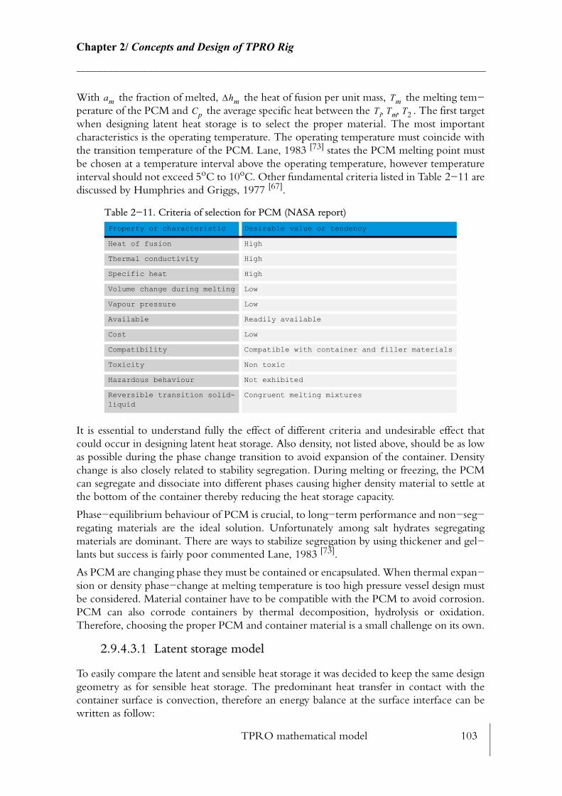
TPRO mathematical model 103
Chapter 2/ Concepts and Design of TPRO Rig________________________________________________________________________
With the fraction of melted, the heat of fusion per unit mass, the melting tem−perature of the PCM and the average specific heat between the . The first target when designing latent heat storage is to select the proper material. The most important characteristics is the operating temperature. The operating temperature must coincide with the transition temperature of the PCM. Lane, 1983 [73] states the PCM melting point must be chosen at a temperature interval above the operating temperature, however temperature interval should not exceed 5oC to 10oC. Other fundamental criteria listed in Table 2−11 are discussed by Humphries and Griggs, 1977 [67].
It is essential to understand fully the effect of different criteria and undesirable effect that could occur in designing latent heat storage. Also density, not listed above, should be as low as possible during the phase change transition to avoid expansion of the container. Density change is also closely related to stability segregation. During melting or freezing, the PCM can segregate and dissociate into different phases causing higher density material to settle at the bottom of the container thereby reducing the heat storage capacity.
Phase−equilibrium behaviour of PCM is crucial, to long−term performance and non−seg−regating materials are the ideal solution. Unfortunately among salt hydrates segregating materials are dominant. There are ways to stabilize segregation by using thickener and gel−lants but success is fairly poor commented Lane, 1983 [73].
As PCM are changing phase they must be contained or encapsulated. When thermal expan−sion or density phase−change at melting temperature is too high pressure vessel design must be considered. Material container have to be compatible with the PCM to avoid corrosion. PCM can also corrode containers by thermal decomposition, hydrolysis or oxidation. Therefore, choosing the proper PCM and container material is a small challenge on its own.
2.9.4.3.1 Latent storage model
To easily compare the latent and sensible heat storage it was decided to keep the same design geometry as for sensible heat storage. The predominant heat transfer in contact with the container surface is convection, therefore an energy balance at the surface interface can be written as follow:
Table 2−11. Criteria of selection for PCM (NASA report)
Property or characteristic Desirable value or tendency
Heat of fusion High
Thermal conductivity High
Specific heat High
Volume change during melting Low
Vapour pressure Low
Available Readily available
Cost Low
Compatibility Compatible with container and filler materials
Toxicity Non toxic
Hazardous behaviour Not exhibited
Reversible transition solid-liquid
Congruent melting mixtures
am ∆hm TmCp Ti Tm T2, ,
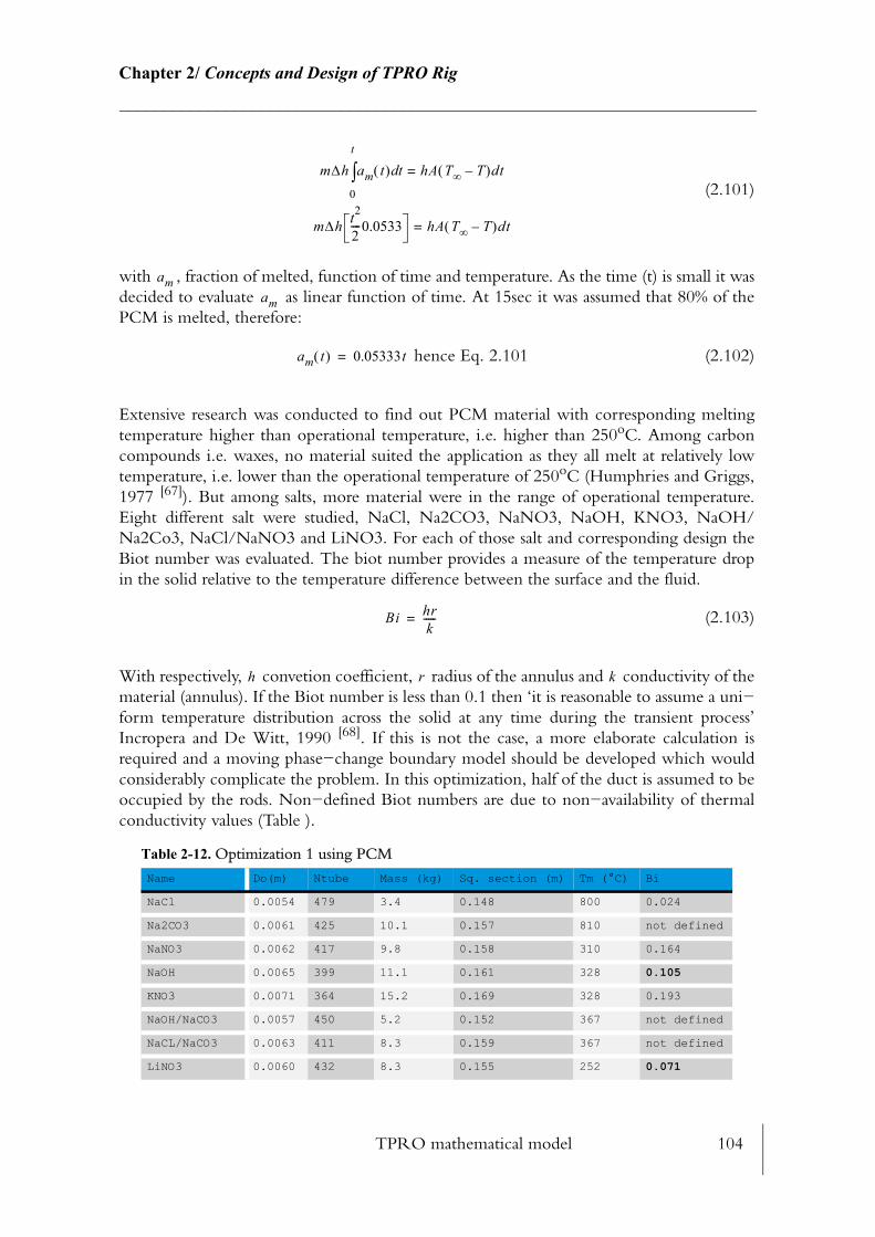
TPRO mathematical model 104
Chapter 2/ Concepts and Design of TPRO Rig________________________________________________________________________
(2.101)
with , fraction of melted, function of time and temperature. As the time (t) is small it was decided to evaluate as linear function of time. At 15sec it was assumed that 80% of the PCM is melted, therefore:
hence Eq. 2.101 (2.102)
Extensive research was conducted to find out PCM material with corresponding melting temperature higher than operational temperature, i.e. higher than 250oC. Among carbon compounds i.e. waxes, no material suited the application as they all melt at relatively low temperature, i.e. lower than the operational temperature of 250oC (Humphries and Griggs, 1977 [67]). But among salts, more material were in the range of operational temperature. Eight different salt were studied, NaCl, Na2CO3, NaNO3, NaOH, KNO3, NaOH/Na2Co3, NaCl/NaNO3 and LiNO3. For each of those salt and corresponding design the Biot number was evaluated. The biot number provides a measure of the temperature drop in the solid relative to the temperature difference between the surface and the fluid.
(2.103)
With respectively, convetion coefficient, radius of the annulus and conductivity of the material (annulus). If the Biot number is less than 0.1 then ‘it is reasonable to assume a uni−form temperature distribution across the solid at any time during the transient process’ Incropera and De Witt, 1990 [68]. If this is not the case, a more elaborate calculation is required and a moving phase−change boundary model should be developed which would considerably complicate the problem. In this optimization, half of the duct is assumed to be occupied by the rods. Non−defined Biot numbers are due to non−availability of thermal conductivity values (Table ).
Table 2-12. Optimization 1 using PCM
Name Do(m) Ntube Mass (kg) Sq. section (m) Tm (°C) Bi
NaCl 0.0054 479 3.4 0.148 800 0.024
Na2CO3 0.0061 425 10.1 0.157 810 not defined
NaNO3 0.0062 417 9.8 0.158 310 0.164
NaOH 0.0065 399 11.1 0.161 328 0.105
KNO3 0.0071 364 15.2 0.169 328 0.193
NaOH/NaCO3 0.0057 450 5.2 0.152 367 not defined
NaCL/NaCO3 0.0063 411 8.3 0.159 367 not defined
LiNO3 0.0060 432 8.3 0.155 252 0.071
m∆h am t( ) td0
t
∫ hA T∞ T–( )dt=
m∆h t2
2----0.0533 hA T∞ T–( )dt=
amam
am t( ) 0.05333t=
Bi hrk
-----=
h r k

TPRO mathematical model 105
Chapter 2/ Concepts and Design of TPRO Rig________________________________________________________________________
In the optimization 1 (Table ) two parameters were fixed, (inside annulus diam−eter) and length of rods . The total surface area was fixed = 8.125m2
For the same reason as sensible heat storage the number of rods being too important (large capital cost) another optimization was completed using only 100 rods. Only three material (i.e. design) can be trusted as the biot number is below or equal to 0.1 (bold).
The second optimization (Table 2−13) has a constant number of rods (100) which lower the
capital cost. The same assumptions as for optimization 1 were considered to establish its dimensions. Comparing to the first PCM optimization the total length of heat storage has increased but the cross sectional area has reduced. This time only, two materials have a Biot number under the 0.1 target (bold). As compared to sensible heat storage it seems possible to fit one of this storage into an existing duct. The third optimization is looking at fitting one of these latent heat storage inside the existing duct. In this optimization the inside annu−lus diameter was free to vary but the same assumptions was made as optimization no2.
In this optimization the design constraints were, 100 rods, total storage surface area = 8.125m2 and square section = 0.254. The optimization reveals that the total length of heat storage is 1.27 m and the outside rod diameter is 20 mm in each scenarios. This time again, only two materials are in competition as far as Biot number is concerned. In all these opti−mization the gap between the inner and outer diameter is not sufficient enough to make this solution feasible i.e. 0.3 mm. For this reason, a fourth optimization was carried out using enhanced surface area (fins). For the three products with a biot number in the range of
Table 2−13. Optimization 2 using PCM
Name Do(m) Mass (kg) Sq. section (m) Tm (°C) Bi length
NaCl 0.0054 3.40 0.0677 800 0.009 4.78
Na2CO3 0.0061 10.16 0.0763 810 - 4.24
NaNO3 0.0062 9.82 0.0775 310 0.200 4.17
NaOH 0.0065 11.19 0.0810 328 0.158 3.99
KNO3 0.0071 15.25 0.0889 328 0.417 3.64
NaOH/NaCO3 0.0057 5.20 0.0718 367 - 4.50
NaCL/NaCO3 0.0063 8.34 0.0786 367 - 4.11
LiNO3 0.0055 4.75 0.0690 252 0.039 4.69
Table 2−14. Optimization 3 using PCM
Name Do(m) Di (m) Mass (kg) Tm (°C) Bi Length
NaCl 0.020 0.0189 11.42 800 0.033 1.27
Na2CO3 - 0.0192 10.16 810 - -
NaNO3 - 0.0191 9.82 310 0.186 -
NaOH - 0.0189 11.19 328 0.145 -
KNO3 - 0.0183 15.25 328 0.373 -
NaOH/NaCO3 - 0.0195 5.20 367 - -
NaCL/NaCO3 - 0.0190 8.34 367 - -
LiNO3 - 0.0197 4.75 252 0.038 -
Di 5mm=
L 1m=
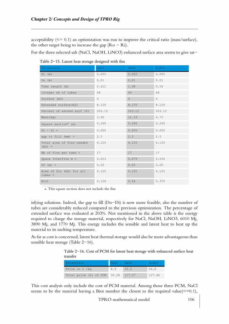
TPRO mathematical model 106
Chapter 2/ Concepts and Design of TPRO Rig________________________________________________________________________
acceptability (<= 0.1) an optimization was run to improve the critical ratio (mass/surface), the other target being to increase the gap (Ro − Ri).
For the three selected salt (NaCl, NaOH, LiNO3) enhanced surface area seems to give sat−
isfying solutions. Indeed, the gap to fill (Do−Di) is now more feasible, also the number of tubes are considerably reduced compared to the previous optimization. The percentage of extended surface was evaluated at 203%. Not mentioned in the above table is the energy required to charge the storage material, respectively for NaCl, NaOH, LiNO3, 6010 Mj, 3890 Mj, and 1770 Mj. This energy includes the sensible and latent heat to heat up the material to its melting temperature.
As far as cost is concerned, latent heat thermal storage would also be more advantageous than sensible heat storage (Table 2−16).
This cost analysis only include the cost of PCM material. Among those three PCM, NaCl seems to be the material having a Biot number the closest to the required value(<=0.1),
Table 2−15. Latent heat storage designed with fins
Parameters NaCl NaOH LiNO3
Di (m) 0.005 0.005 0.005
Do (m) 0.01 0.01 0.01
Tube length (m) 0.411 1.38 0.54
Integer nb of tubes 64 64 64
Surface (m2) 4 4 4
Extended surface(m2) 8.125 8.125 8.125
Percent of extend surf (%) 203.12 203.12 203.12
Mass(kg) 3.40 11.19 4.75
Square sectiona (m)
a. This square section does not include the fins
0.265 0.265 0.265
Do - Di = 0.005 0.005 0.005
gap to fill (mm) = 2.5 2.5 2.5
Total area of fins needed (m2) =
4.125 4.125 4.125
Nb of fins per tube = 17 17 17
Space Interfins m = 0.023 0.079 0.030
Df (m) = 0.05 0.05 0.05
Area of fin (m2) for all tubes =
4.125 4.125 4.125
Biot 0.124 0.54 0.370
Table 2−16. Cost of PCM for latent heat storage with enhanced surface heat transfer
Parameters NaCl NaOH LiNO3
Price in £ /kg 8.9 10.5 26.8
Total price (£) of PCM 30.28 117.57 127.46
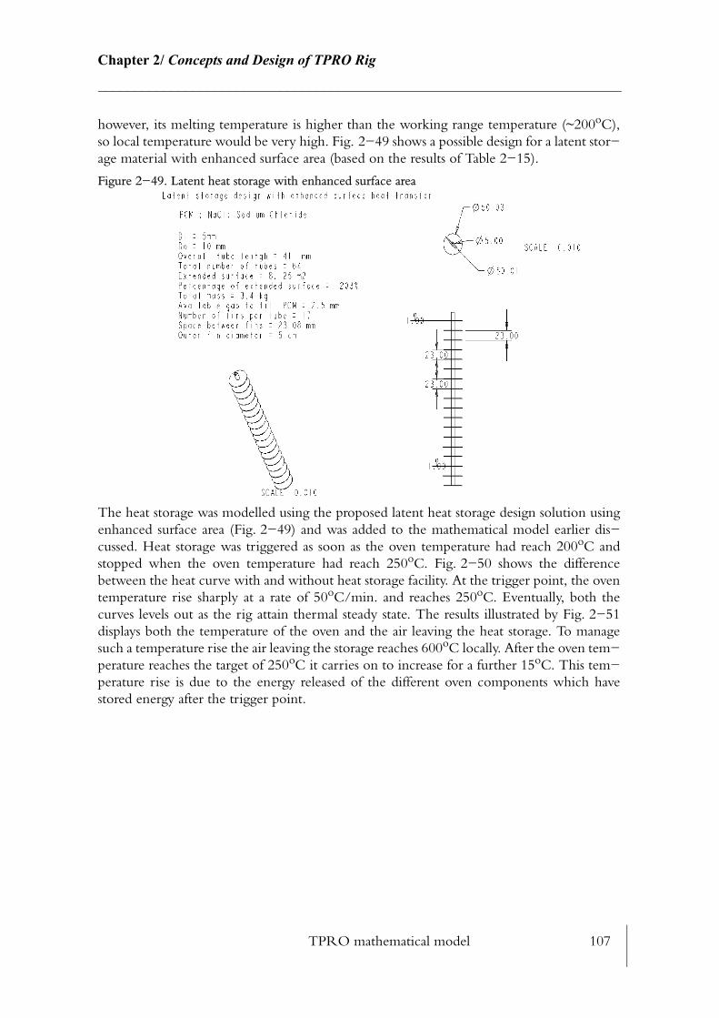
TPRO mathematical model 107
Chapter 2/ Concepts and Design of TPRO Rig________________________________________________________________________
however, its melting temperature is higher than the working range temperature (~200oC), so local temperature would be very high. Fig. 2−49 shows a possible design for a latent stor−age material with enhanced surface area (based on the results of Table 2−15).
Figure 2−49. Latent heat storage with enhanced surface area
The heat storage was modelled using the proposed latent heat storage design solution using enhanced surface area (Fig. 2−49) and was added to the mathematical model earlier dis−cussed. Heat storage was triggered as soon as the oven temperature had reach 200oC and stopped when the oven temperature had reach 250oC. Fig. 2−50 shows the difference between the heat curve with and without heat storage facility. At the trigger point, the oven temperature rise sharply at a rate of 50oC/min. and reaches 250oC. Eventually, both the curves levels out as the rig attain thermal steady state. The results illustrated by Fig. 2−51displays both the temperature of the oven and the air leaving the heat storage. To manage such a temperature rise the air leaving the storage reaches 600oC locally. After the oven tem−perature reaches the target of 250oC it carries on to increase for a further 15oC. This tem−perature rise is due to the energy released of the different oven components which have stored energy after the trigger point.

TPRO mathematical model 108
Chapter 2/ Concepts and Design of TPRO Rig________________________________________________________________________
Figure 2−50. Oven temperature variation with and without heat storage
Figure 2−51. Outlet storage temperature
2.9.5 Overall conclusion on heat storage feasibility
Sensible heat storage has the advantage of being relatively simple to manufacture compared to latent heat storage. Nevertheless, in all studied scenarios, all different material tried out at various convection rate, shows that size of sensible heat storage would require a major mod−ification of the duct work. Cost wise, sensible heat storage is not attractive for metals (£3,715: mild−steel; £14,650: copper) while for concrete it is lot more appealing (£15), However the thermal diffusivity (α) of concrete is very low and this would considerably slow down the charge and discharge process unless configured as very thin rods.
Latent heat storage looks more promising in terms of size and cost (NaCl = £30; NaOH = £117; LiNO3 = £127), however, PCM’s melting temperature are not a good match (a part
TPRO mathematical model 109
Chapter 2/ Concepts and Design of TPRO Rig________________________________________________________________________
from LINO3) for the required operating temperature, so local air temperature will be very high, therefore more research should be made to find out specific PCM material. For these relatively non−corrosive salts, such as NaCl, NaOH, and LiNO3, copper or stainless steel container could be used without risking corrosion to occur at condition that salt have been stored without any water particles. As PCM melts thermal expansion would occur in the encapsulation container therefore, container design should be studied with more care in order to avoid high stress and deformation that would cause fissures.
Latent heat storage calculations were based on non−encapsulated storage, therefore overall conductivity values should be increased. The convection rate at thermal storage surface would vary markedly if fins were used. To predict more accurately the thermal storage reac−tion time, heat transfer model should be made through container.
In both latent and sensible heat storage, high temperature would occur at the duct junction that would result in high thermo−mechanical stress. A solution would be to divide the number storage rooms in many to lower high peak of temperature.
Using heat storage material has its own drawback for this process as the energy required for charging the heat storage would be tremendous (e.g 6010 Mj for NaCl) and charging time might be a lengthy protocol.
2.9.6 Final decision
Although there was some real interest in looking into thermal storage the solution was left for further research. A more practical and conventional solution was chosen as the function−ality of the heating system was not oriented for research experimentation but to perform reliability. Effort was made to find out a more powerful duct heater solution. Unsheated and sheathed heater were taken into consideration. Unsheated heater element would have the advantage of fast response time however under high moisture atmosphere some problem related to oxidation and hydrogen embrittlement may occur.
At high temperature, a film or scale of oxide is formed at the metal surface in presence with oxygen (Eq. 2.104).
, with metal and (2.104)
The oxidation behaviour depends also on whether the scales are compact or porous. Metallic oxidation resistant material must be able to build a stable oxide layer at high temperature that will protect the heater from further oxidation. Kostfad P compares three multi−component alloys at 1000°C (surface temperature). Ni with 31% Aluminium seems to have a constant and stable weight gain and also the lowest weight gain compare to Co with 31% chrome. More generally, under 900°C the rate of oxidation hence the weight gain of scale is relatively low.
• Effect of water vapour on oxidation behaviour: Holmes and Rahmel, 1978 [61] have tested the unalloyed iron and found no effects of water vapour on the oxidation rate below 750°C, but at 950°C marked effect was observed. They also report that hydrogen content in the metal core had increased after reaction in moist
Me b2---O2 MeaOb→+
aMe O2
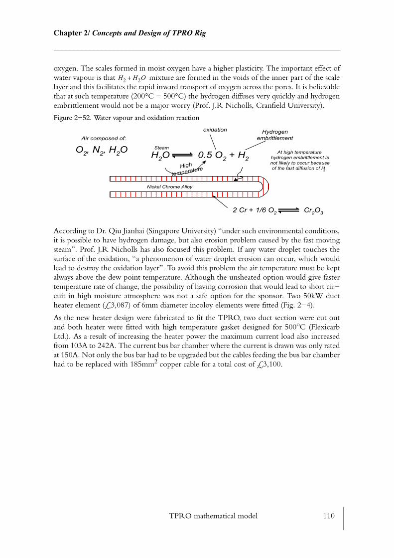
TPRO mathematical model 110
Chapter 2/ Concepts and Design of TPRO Rig________________________________________________________________________
oxygen. The scales formed in moist oxygen have a higher plasticity. The important effect of water vapour is that mixture are formed in the voids of the inner part of the scale layer and this facilitates the rapid inward transport of oxygen across the pores. It is believable that at such temperature (200°C − 500°C) the hydrogen diffuses very quickly and hydrogen embrittlement would not be a major worry (Prof. J.R Nicholls, Cranfield University).
Figure 2−52. Water vapour and oxidation reaction
According to Dr. Qiu Jianhai (Singapore University) “under such environmental conditions, it is possible to have hydrogen damage, but also erosion problem caused by the fast moving steam”. Prof. J.R Nicholls has also focused this problem. If any water droplet touches the surface of the oxidation, “a phenomenon of water droplet erosion can occur, which would lead to destroy the oxidation layer”. To avoid this problem the air temperature must be kept always above the dew point temperature. Although the unsheated option would give faster temperature rate of change, the possibility of having corrosion that would lead to short cir−cuit in high moisture atmosphere was not a safe option for the sponsor. Two 50kW duct heater element (£3,087) of 6mm diameter incoloy elements were fitted (Fig. 2−4).
As the new heater design were fabricated to fit the TPRO, two duct section were cut out and both heater were fitted with high temperature gasket designed for 500oC (Flexicarb Ltd.). As a result of increasing the heater power the maximum current load also increased from 103A to 242A. The current bus bar chamber where the current is drawn was only rated at 150A. Not only the bus bar had to be upgraded but the cables feeding the bus bar chamber had to be replaced with 185mm2 copper cable for a total cost of £3,100.
H2 H2O+
High
temperature
Nickel Chrome Alloy
O2, N2, H2O H2O 0.5 O2 + H2
Air composed of:
Steam
2 Cr + 1/6 O2 Cr2O3
oxidation Hydrogenembrittlement
At high temperaturehydrogen embrittlement isnot likely to occur becauseof the fast diffusion of H2
Aim and philosophy of the control system 111
Chapter 3/ Computer Aided Control System________________________________________________________________________
CHAPTER 3
COMPUTER AIDED CONTROL SYSTEM
A computer aided control system was design to perform the communication between the various devices to control, monitor and carry out data acquisition. This automation sys−tem uses the latest technology in terms of process control software and hardware, DeviceNet technology protocol for the communication mechanism and Wonderware, 2002 [141] InControl™ and InTouch™ product were used to build a fully automated test rig and its human machine interface.
3.1 Aim and philosophy of the control system
Control is a major issue when transferring heat in an oven to a moving food product, espe−cially because baked products can be extremely sensitive to operating conditions (heat flux, temperatures, air speed, humidity). Preliminary tests on cake baking demonstrated that a few degrees rise above the set−point during the baking process would cause a fast rise of the cake height and would eventually burst the cake surface. Similarly when too much steam was injected inside the oven, the initial rate of heat transfer to surface increased significantly and a similar problem occurred. Other parameters have a great importance in the control logic, such as band speed, top and bottom heat, fan inverter settings. A too slow band speed in a biscuit tunnel oven can cause too much browning for instance.
As long as ovens have existed, they have always had a limited amount of instrumentation to monitor and control the baking process. Even today, baking relies mostly on visual checking, rules of thumb and process knowledge gained over years of experience by bakers. Things have changed slightly with the development of multi−purpose instruments such as the Qualivision Inspection System (APV Baker, 2002 [5]). However it seems difficult to persuade baking companies with strong knowledge of their process to use such technologies. Most often, air temperature is the only parameter that is measured and used to adjust control loops so that gas burners can be adjusted. One of the ambitions of the TPRO rig was to monitor
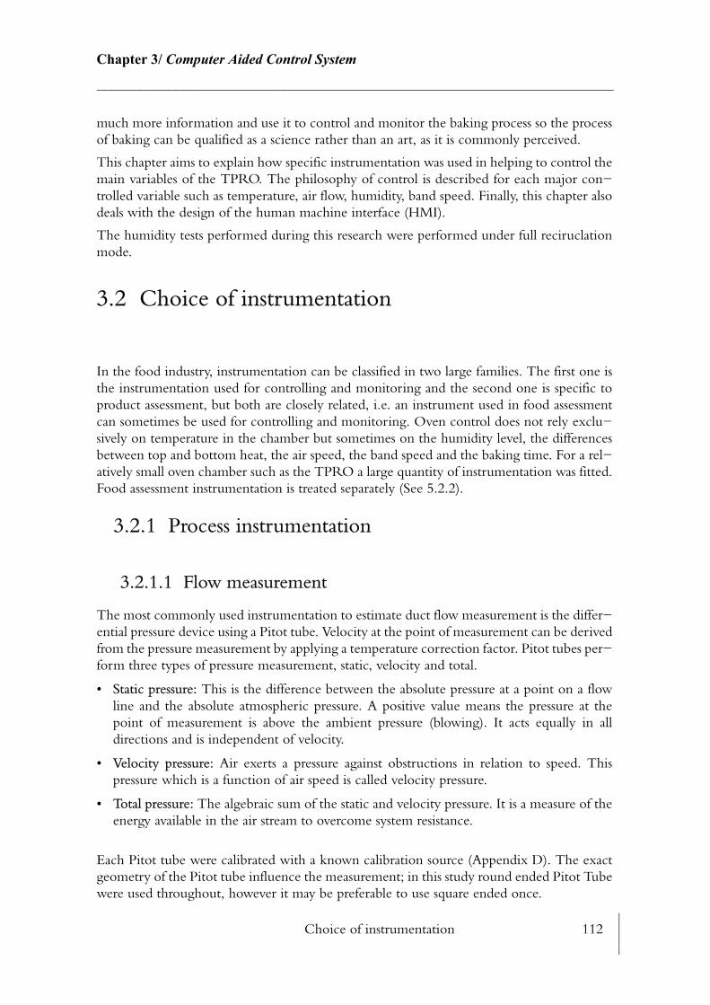
Choice of instrumentation 112
Chapter 3/ Computer Aided Control System________________________________________________________________________
much more information and use it to control and monitor the baking process so the process of baking can be qualified as a science rather than an art, as it is commonly perceived.
This chapter aims to explain how specific instrumentation was used in helping to control the main variables of the TPRO. The philosophy of control is described for each major con−trolled variable such as temperature, air flow, humidity, band speed. Finally, this chapter also deals with the design of the human machine interface (HMI).
The humidity tests performed during this research were performed under full reciruclation mode.
3.2 Choice of instrumentation
In the food industry, instrumentation can be classified in two large families. The first one is the instrumentation used for controlling and monitoring and the second one is specific to product assessment, but both are closely related, i.e. an instrument used in food assessment can sometimes be used for controlling and monitoring. Oven control does not rely exclu−sively on temperature in the chamber but sometimes on the humidity level, the differences between top and bottom heat, the air speed, the band speed and the baking time. For a rel−atively small oven chamber such as the TPRO a large quantity of instrumentation was fitted. Food assessment instrumentation is treated separately (See 5.2.2).
3.2.1 Process instrumentation
3.2.1.1 Flow measurement
The most commonly used instrumentation to estimate duct flow measurement is the differ−ential pressure device using a Pitot tube. Velocity at the point of measurement can be derived from the pressure measurement by applying a temperature correction factor. Pitot tubes per−form three types of pressure measurement, static, velocity and total.
• Static pressure: This is the difference between the absolute pressure at a point on a flow line and the absolute atmospheric pressure. A positive value means the pressure at the point of measurement is above the ambient pressure (blowing). It acts equally in all directions and is independent of velocity.
• Velocity pressure: Air exerts a pressure against obstructions in relation to speed. This pressure which is a function of air speed is called velocity pressure.
• Total pressure: The algebraic sum of the static and velocity pressure. It is a measure of the energy available in the air stream to overcome system resistance.
Each Pitot tube were calibrated with a known calibration source (Appendix D). The exact geometry of the Pitot tube influence the measurement; in this study round ended Pitot Tube were used throughout, however it may be preferable to use square ended once.
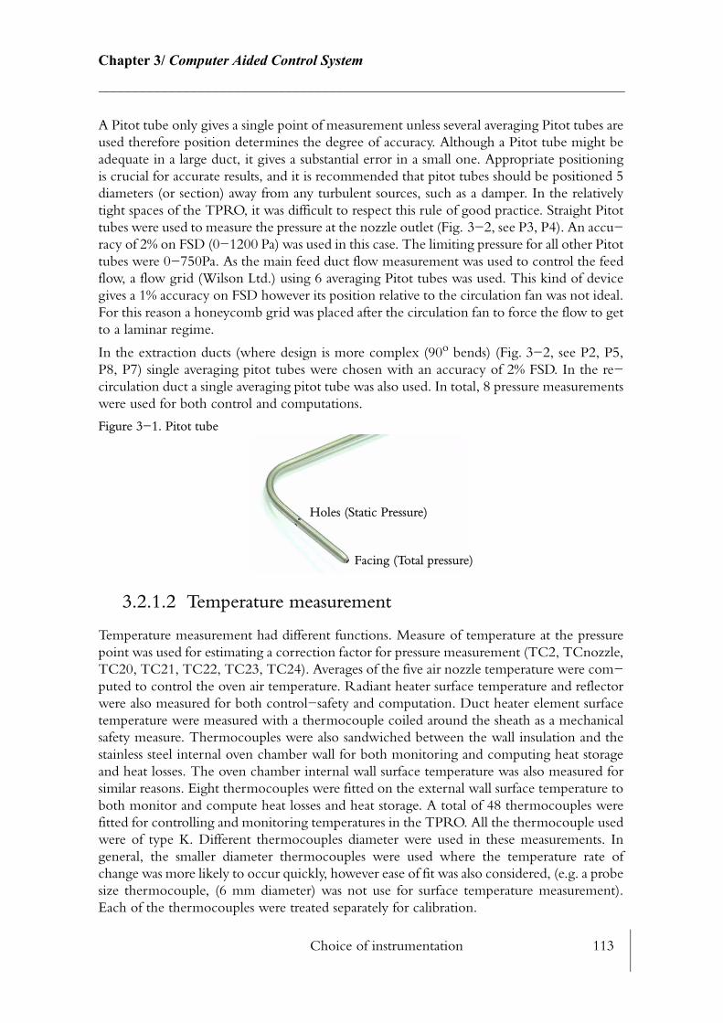
Choice of instrumentation 113
Chapter 3/ Computer Aided Control System________________________________________________________________________
A Pitot tube only gives a single point of measurement unless several averaging Pitot tubes are used therefore position determines the degree of accuracy. Although a Pitot tube might be adequate in a large duct, it gives a substantial error in a small one. Appropriate positioning is crucial for accurate results, and it is recommended that pitot tubes should be positioned 5 diameters (or section) away from any turbulent sources, such as a damper. In the relatively tight spaces of the TPRO, it was difficult to respect this rule of good practice. Straight Pitot tubes were used to measure the pressure at the nozzle outlet (Fig. 3−2, see P3, P4). An accu−racy of 2% on FSD (0−1200 Pa) was used in this case. The limiting pressure for all other Pitot tubes were 0−750Pa. As the main feed duct flow measurement was used to control the feed flow, a flow grid (Wilson Ltd.) using 6 averaging Pitot tubes was used. This kind of device gives a 1% accuracy on FSD however its position relative to the circulation fan was not ideal. For this reason a honeycomb grid was placed after the circulation fan to force the flow to get to a laminar regime.
In the extraction ducts (where design is more complex (90o bends) (Fig. 3−2, see P2, P5, P8, P7) single averaging pitot tubes were chosen with an accuracy of 2% FSD. In the re−circulation duct a single averaging pitot tube was also used. In total, 8 pressure measurements were used for both control and computations.
Figure 3−1. Pitot tube
3.2.1.2 Temperature measurement
Temperature measurement had different functions. Measure of temperature at the pressure point was used for estimating a correction factor for pressure measurement (TC2, TCnozzle, TC20, TC21, TC22, TC23, TC24). Averages of the five air nozzle temperature were com−puted to control the oven air temperature. Radiant heater surface temperature and reflector were also measured for both control−safety and computation. Duct heater element surface temperature were measured with a thermocouple coiled around the sheath as a mechanical safety measure. Thermocouples were also sandwiched between the wall insulation and the stainless steel internal oven chamber wall for both monitoring and computing heat storage and heat losses. The oven chamber internal wall surface temperature was also measured for similar reasons. Eight thermocouples were fitted on the external wall surface temperature to both monitor and compute heat losses and heat storage. A total of 48 thermocouples were fitted for controlling and monitoring temperatures in the TPRO. All the thermocouple used were of type K. Different thermocouples diameter were used in these measurements. In general, the smaller diameter thermocouples were used where the temperature rate of change was more likely to occur quickly, however ease of fit was also considered, (e.g. a probe size thermocouple, (6 mm diameter) was not use for surface temperature measurement). Each of the thermocouples were treated separately for calibration.
Facing (Total pressure)
Holes (Static Pressure)
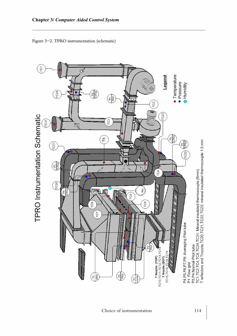
Choice of instrumentation 114
Chapter 3/ Computer Aided Control System________________________________________________________________________
Figure 3−2. TPRO instrumentation (schematic)

Choice of instrumentation 115
Chapter 3/ Computer Aided Control System________________________________________________________________________
Small diameter thermocouples can be more noisy electrically than larger ones and data ‘smoothing correction factors’ were applied case by case (See 4.3.2).
Thermocouple accuracy depends on their calibration but for non specific calibration sup−pliers advise using the following rule to establish the accuracy of the measure.
or ± (3.1)
Temperature range measurement were expected to be between ambient to 600oC (duct heater sheath temperature). Repeatability test conducted over a 24 hour period during four consecutive days revealed that temperatures were accurate to ±0.5oC (See 4.3.3.1). In this investigation the thermocouple internal to the oven chamber were not shielded from radi−ation as the TPRO environement was highly convectif. For test involving high radiation temperature it would be necessary to shield the exposed thermocouple. In this situation the mean temperature would be overestimated compared to the real temperature. The discre−pency would be of the order of 1 to 5oC. Only nozzle temperature measurement points were protected from the radiant heater by inserting the thermocouple further in the plenum chamber.
Figure 3−3. Thermocouples
3.2.1.3 Humidity measurement
Humidity measurement was performed with devices from Mc Queen Cairns Ltd. Real time humidity measurement was performed with a HygroxCTM positioned closed to the top extraction duct, while HygroxP2TM (portable) was used to collect data closed to the prod−uct. Two Zirconia sensor are fitted within the head of both devices. One of the sensors is used to measure the oxygen in the air while the other one measures both the oxygen in the air and the oxygen in the water molecules contained in the air. The difference between the two gives a measure of the humidity. Terminology to quantify humidity level varies from user to user. Bakers for instance will use dew point temperature while ‘engineers’ will use any−thing from moisture content, specific, mixed or absolute humidity. The definition which was used in this context was the mixed humidity, also known as the water vapour content or mixing ratio. It is the ratio of the mass of the water vapour to the mass of the dry air sample. Normal operating values in bread ovens are in the range of 150−300g/kg. A maximum humidity of 400g/kg may be used for glazing product surface, however there is not much information available which defines the upper limit. The TPRO was able to control up to 1200g/kg of steam (See 4.9). Maximum operating temperature for both these devices is
error 0.0075T= 2.5oC

Choice of instrumentation 116
Chapter 3/ Computer Aided Control System________________________________________________________________________
300oC. The fixed probe (HygroxCTM) was fitted with a cooling unit which cools the sensor head. The manufacturer indicates that accuracy in the measurement of the mixed humidity is 1% of FSD, however it can vary depending on where it is sensing the air flow. This sensor works better where the air is well mixed.
Figure 3−4. Mc Queen Cairns HygroxP2TM sensor
3.2.1.4 Velocity measurement
Hand−held pitot tube with anemometer AF200 from Digitron was used to cross check the results obtained from the fixed pitot tube inside the TPRO. Logger velocity sensor from ScorpionTM was also used to map the entire surface of the band as the product travel (Appendix L). This logger is made of 10 miniature hot wire anemometers along a meter wide carriage. Each element is individually calibrated over a range of 0−8 m/s and gives a response proportional to the total resultant velocity, which is the sum of velocity components in all directions. Each element is made of two thermocouples which one is heated above the ambient temperature using a small electrical coil. The other is not heated and used as a ref−erence temperature. The different between the two sensors is proportional to the air velocity. This sensor was only used to check the uniformity of the air at low velocity across the band as the maximum air velocity from the TPRO was far above the capacities of this instrument. The error on the measure is ±5%. The response time t601 in air at 1 m/s is 3 s.
1. 60% of the response
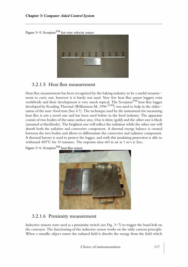
Choice of instrumentation 117
Chapter 3/ Computer Aided Control System________________________________________________________________________
Figure 3−5. ScorpionTM hot wire velocity sensor
3.2.1.5 Heat flux measurement
Heat flux measurement has been recognized by the baking industry to be a useful measure−ment to carry out, however it is barely not used. Very few heat flux sensor loggers exist worldwide and their development is very much topical. The ScorpionTM heat flux logger developed by Reading Thermal (Williamson M, 1996 [140]) was used to help in the elabo−ration of the non−food tests (See 4.7). The technique used by the instrument for measuring heat flux is not a novel one and has been used before in the food industry. The apparatus consist of two bodies of the same surface area. One is shiny (gold) and the other one is black (assumed as blackbody). The brightest one will reflect the radiation while the other one will absorb both the radiative and convective component. A thermal energy balance is created between the two bodies and allows to differentiate the convective and radiative component. A thermal barrier is used to protect the logger, and with this insulating protection is able to withstand 450oC for 10 minutes. The response time t60 in air at 1 m/s is 2sec.
Figure 3−6. ScorpionTM heat flux sensor
3.2.1.6 Proximity measurement
Inductive sensors were used as a proximity switch (see Fig. 3−7) to trigger the band belt on the conveyor. The functioning of the inductive sensor works on the eddy current principle. When a metallic object enters the radiated field it absorbs the energy from the field which
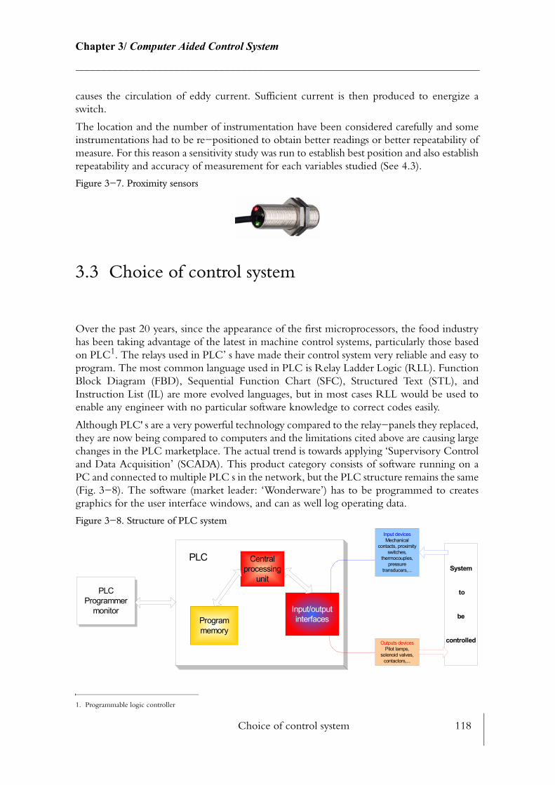
Choice of control system 118
Chapter 3/ Computer Aided Control System________________________________________________________________________
causes the circulation of eddy current. Sufficient current is then produced to energize a switch.
The location and the number of instrumentation have been considered carefully and some instrumentations had to be re−positioned to obtain better readings or better repeatability of measure. For this reason a sensitivity study was run to establish best position and also establish repeatability and accuracy of measurement for each variables studied (See 4.3).
Figure 3−7. Proximity sensors
3.3 Choice of control system
Over the past 20 years, since the appearance of the first microprocessors, the food industry has been taking advantage of the latest in machine control systems, particularly those based on PLC1. The relays used in PLC’ s have made their control system very reliable and easy to program. The most common language used in PLC is Relay Ladder Logic (RLL). Function Block Diagram (FBD), Sequential Function Chart (SFC), Structured Text (STL), and Instruction List (IL) are more evolved languages, but in most cases RLL would be used to enable any engineer with no particular software knowledge to correct codes easily.
Although PLC' s are a very powerful technology compared to the relay−panels they replaced, they are now being compared to computers and the limitations cited above are causing large changes in the PLC marketplace. The actual trend is towards applying ‘Supervisory Control and Data Acquisition’ (SCADA). This product category consists of software running on a PC and connected to multiple PLC s in the network, but the PLC structure remains the same (Fig. 3−8). The software (market leader: ‘Wonderware’) has to be programmed to creates graphics for the user interface windows, and can as well log operating data.
Figure 3−8. Structure of PLC system
1. Programmable logic controller
Centralprocessing
unit
Programmemory
Input/outputinterfaces
Input devicesMechanical
contacts, proximityswitches,
thermocouples,pressure
transducers,...
Outputs devicesPilot lamps,
solenoid valves,contactors,...
System
to
be
controlled
PLCProgrammer
monitor
PLC
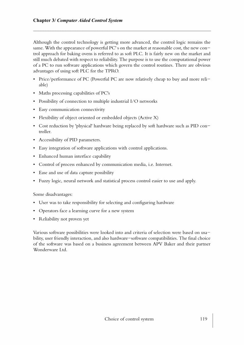
Choice of control system 119
Chapter 3/ Computer Aided Control System________________________________________________________________________
Although the control technology is getting more advanced, the control logic remains the same. With the appearance of powerful PC' s on the market at reasonable cost, the new con−trol approach for baking ovens is referred to as soft PLC. It is fairly new on the market and still much debated with respect to reliability. The purpose is to use the computational power of a PC to run software applications which govern the control routines. There are obvious advantages of using soft PLC for the TPRO.
• Price/performance of PC (Powerful PC are now relatively cheap to buy and more reli−able)
• Maths processing capabilities of PC's
• Possibility of connection to multiple industrial I/O networks
• Easy communication connectivity
• Flexibility of object oriented or embedded objects (Active X)
• Cost reduction by 'physical' hardware being replaced by soft hardware such as PID con−troller.
• Accessibility of PID parameters.
• Easy integration of software applications with control applications.
• Enhanced human interface capability
• Control of process enhanced by communication media, i.e. Internet.
• Ease and use of data capture possibility
• Fuzzy logic, neural network and statistical process control easier to use and apply.
Some disadvantages:
• User was to take responsibility for selecting and configuring hardware
• Operators face a learning curve for a new system
• Reliability not proven yet
Various software possibilities were looked into and criteria of selection were based on usa−bility, user friendly interaction, and also hardware−software compatibilities. The final choice of the software was based on a business agreement between APV Baker and their partner Wonderware Ltd.
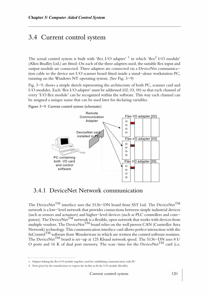
Current control system 120
Chapter 3/ Computer Aided Control System________________________________________________________________________
3.4 Current control system
The actual control system is built with ‘flex I/O adapter’ 1 in which ‘flex2 I/O module’ (Allen Bradley Ltd.) are fitted. On each of the three adapters used, the suitable flex input and output module are connected. Three adapters are connected via a DeviceNet communica−tion cable to the device net I/O scanner board fitted inside a stand−alone workstation PC, running on the Windows NT operating system. (See Fig. 3−9)
Fig. 3−9, shows a simple sketch representing the architecture of both PC, scanner card and I/O modules. Each ‘flex I/O adapter’ must be addressed (02, 03, 00) so that each channel of every ‘I/O flex module’ can be recognized within the software. This way each channel can be assigned a unique name that can be used later for declaring variables.
Figure 3−9. Current control system (schematic)
3.4.1 DeviceNet Network communication
The DeviceNetTM interface uses the 5136−DN board from SST Ltd. The DeviceNetTM
network is a low−level network that provides connections between simple industrial devices (such as sensors and actuators) and higher−level devices (such as PLC controllers and com−puters). The DeviceNetTM network is a flexible, open network that works with devices from multiple vendors. The DeviceNetTM board relies on the well proven CAN (Controller Area Network) technology. This communication interface card allows perfect interaction with the InControlTM software from Wonderware in which are written the control software routines. The DeviceNetTM board is set−up at 125 Kbaud network speed. The 5136−DN uses 8 I/O ports and 16 K of dual port memory. The scan−time for the DeviceNetTM card (i.e.
1. Adapter linking the flex I/O module together, used for establishing communication with PC
2. Term given by the manufacturer to express the facility to fit the I/O module (flexible)
RemoteCommunication
Adapter
DeviceNet cardinstalled in PC
PC containingboth I/O card
and controlsoftware
Flex I/O adapter [02]
Flex I/O adapter [03]
Flex I/O adapter [00]
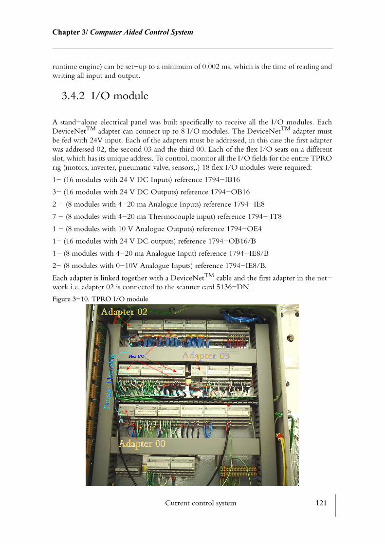
Current control system 121
Chapter 3/ Computer Aided Control System________________________________________________________________________
runtime engine) can be set−up to a minimum of 0.002 ms, which is the time of reading and writing all input and output.
3.4.2 I/O module
A stand−alone electrical panel was built specifically to receive all the I/O modules. Each DeviceNetTM adapter can connect up to 8 I/O modules. The DeviceNetTM adapter must be fed with 24V input. Each of the adapters must be addressed, in this case the first adapter was addressed 02, the second 03 and the third 00. Each of the flex I/O seats on a different slot, which has its unique address. To control, monitor all the I/O fields for the entire TPRO rig (motors, inverter, pneumatic valve, sensors,.) 18 flex I/O modules were required:
1− (16 modules with 24 V DC Inputs) reference 1794−IB16
3− (16 modules with 24 V DC Outputs) reference 1794−OB16
2 − (8 modules with 4−20 ma Analogue Inputs) reference 1794−IE8
7 − (8 modules with 4−20 ma Thermocouple input) reference 1794− IT8
1 − (8 modules with 10 V Analogue Outputs) reference 1794−OE4
1− (16 modules with 24 V DC outputs) reference 1794−OB16/B
1− (8 modules with 4−20 ma Analogue Input) reference 1794−IE8/B
2− (8 modules with 0−10V Analogue Inputs) reference 1794−IE8/B.
Each adapter is linked together with a DeviceNetTM cable and the first adapter in the net−work i.e. adapter 02 is connected to the scanner card 5136−DN.
Figure 3−10. TPRO I/O module

Current control system 122
Chapter 3/ Computer Aided Control System________________________________________________________________________
3.4.3 TPRO commissioning
The commissioning of the TPRO was a crucial stage in establishing communication between hardware and software. This consisted of a three stages process: adressing, mapping and calibrating.
3.4.3.1 Addressing
Addressing is a very important feature when controlling such a system. Addressing means that for each physical input and output (sensors, motors, inverter,...) connected to the flex I/O, a virtual input and output name is attributed. In this case the address refers to the adapter, slot (i.e. flex I/O) and channel number. For instance, the addressing of the emer−gency stop relay is: N2_S0_CH0, which means in word:
adapter 2, slot 0, in channel 0. (Appendix K)
3.4.4 Mapping
Mapping is similar to addressing, but the difference is that mapping is used by the software and has a real meaning to the software user. For any input and output addressed a virtual name is given inside the InControlTM software. For instance, mapping N2_S0_CH0:= ESR_STS; means that the address N2_S0_CH0 (Adapter 02, Slot 0 channel 0) is attributed with the tag1 ESR_STS (Emergency Stop Relay Status).
All Addressing and mapping are tabled in Appendix K. The flowchart Fig. 3−8 summarises the goal of commissioning and codes writing.
3.4.5 Calibration and sensor scaling
For each of the analogue inputs and outputs a calibration was applied using the DeviceN−etTM Manager software from Allen Bradley and the process calibrator model X86 − 8036C from Ronan Ltd. (Fig. 3−11). For each of these analogue inputs and outputs the min./max voltage or current was applied on the flex I/O channel. For thermocouples a 0−75 mV cur−rent was send to the flex I/O using the process calibrator, then from Allen Bradley Device−NetTM manager software, real data (in °C) were obtained. For a type K thermocouple, a 0 mV input from the calibrator should give the minimum bit number corresponding to −232°C. For a 75 mV input from the process calibrator the results from the software should give the maximum bit number corresponding to +1372°C. For a given thermocouple type, the software estimates automatically correction factors to fit the linear relationship between mV and temperature. As well as using this calibration factors which is automatically run when the thermocouples are connected to the modules, another calibration factor was applied for temperature measurement. Thermocouples were assigned if needed with a cor−
1. A tag is any name given to a physical or virtual I/O used in the software
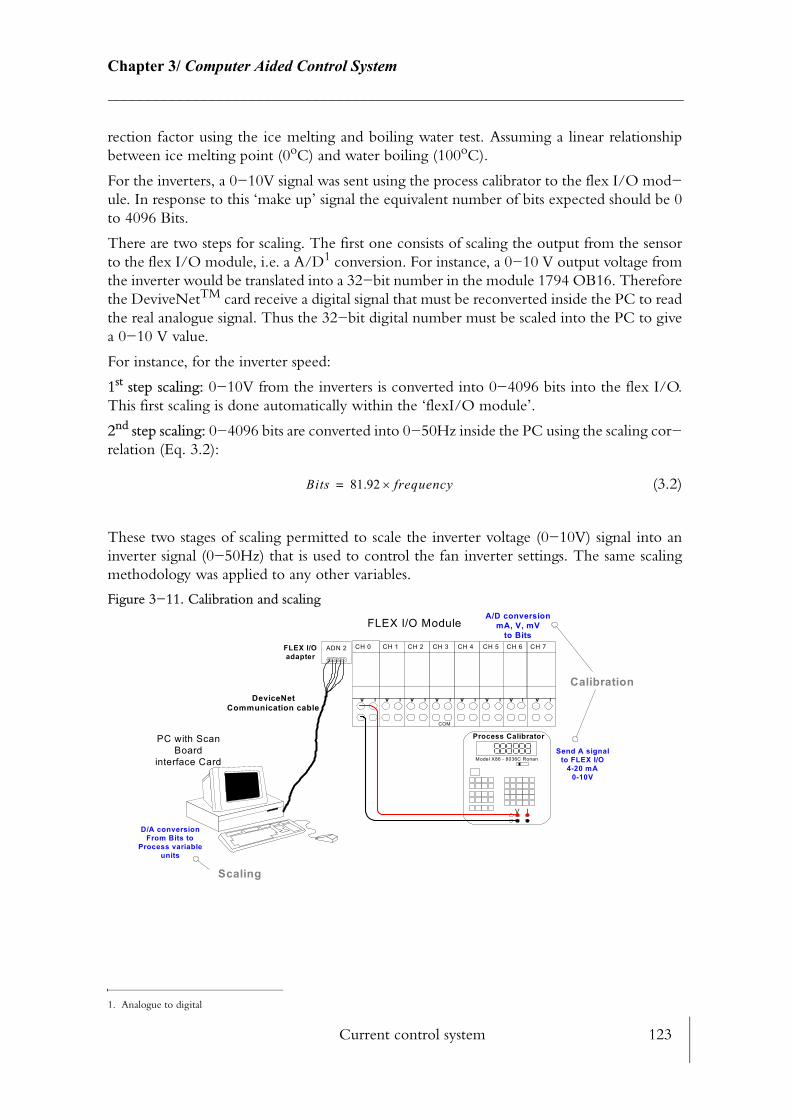
Current control system 123
Chapter 3/ Computer Aided Control System________________________________________________________________________
rection factor using the ice melting and boiling water test. Assuming a linear relationship between ice melting point (0oC) and water boiling (100oC).
For the inverters, a 0−10V signal was sent using the process calibrator to the flex I/O mod−ule. In response to this ‘make up’ signal the equivalent number of bits expected should be 0 to 4096 Bits.
There are two steps for scaling. The first one consists of scaling the output from the sensor to the flex I/O module, i.e. a A/D1 conversion. For instance, a 0−10 V output voltage from the inverter would be translated into a 32−bit number in the module 1794 OB16. Therefore the DeviveNetTM card receive a digital signal that must be reconverted inside the PC to read the real analogue signal. Thus the 32−bit digital number must be scaled into the PC to give a 0−10 V value.
For instance, for the inverter speed:
1st step scaling: 0−10V from the inverters is converted into 0−4096 bits into the flex I/O. This first scaling is done automatically within the ‘flexI/O module’.
2nd step scaling: 0−4096 bits are converted into 0−50Hz inside the PC using the scaling cor−relation (Eq. 3.2):
(3.2)
These two stages of scaling permitted to scale the inverter voltage (0−10V) signal into an inverter signal (0−50Hz) that is used to control the fan inverter settings. The same scaling methodology was applied to any other variables.
Figure 3−11. Calibration and scaling
1. Analogue to digital
Bits 81.92 frequency×=
V I
CH 0 CH 1 CH 2 CH 3 CH 4 CH 5 CH 6 CH 7
COM
v I v I v I v I v I v I v I v I
ADN 2
FLEX I/O Module
Process Calibrator
DeviceNetCommunication cable
PC with ScanBoard
interface CardSend A signal
to FLEX I/O4-20 mA
0-10V
A/D conversionmA, V, mV
to Bits
D/A conversionFrom Bits to
Process variableunits
FLEX I/Oadapter
Model X86 - 8036C Ronan
Calibration
Scaling
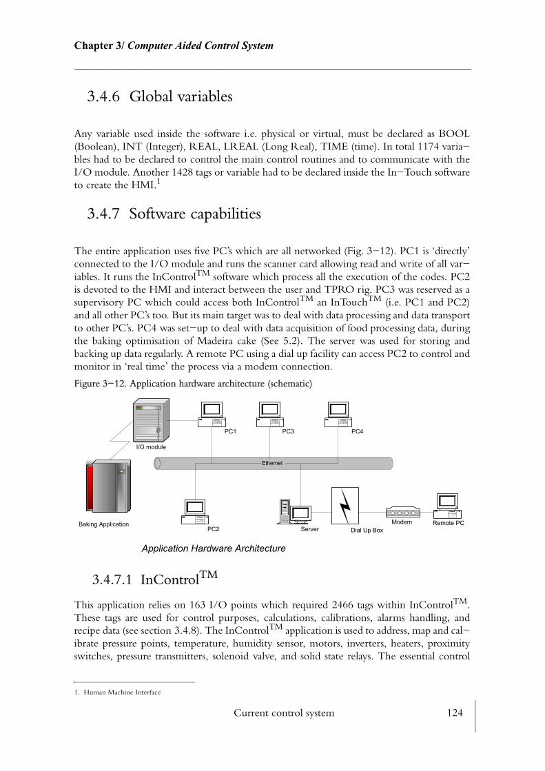
Current control system 124
Chapter 3/ Computer Aided Control System________________________________________________________________________
3.4.6 Global variables
Any variable used inside the software i.e. physical or virtual, must be declared as BOOL (Boolean), INT (Integer), REAL, LREAL (Long Real), TIME (time). In total 1174 varia−bles had to be declared to control the main control routines and to communicate with the I/O module. Another 1428 tags or variable had to be declared inside the In−Touch software to create the HMI.1
3.4.7 Software capabilities
The entire application uses five PC’s which are all networked (Fig. 3−12). PC1 is ‘directly’ connected to the I/O module and runs the scanner card allowing read and write of all var−iables. It runs the InControlTM software which process all the execution of the codes. PC2 is devoted to the HMI and interact between the user and TPRO rig. PC3 was reserved as a supervisory PC which could access both InControlTM an InTouchTM (i.e. PC1 and PC2) and all other PC’s too. But its main target was to deal with data processing and data transport to other PC’s. PC4 was set−up to deal with data acquisition of food processing data, during the baking optimisation of Madeira cake (See 5.2). The server was used for storing and backing up data regularly. A remote PC using a dial up facility can access PC2 to control and monitor in ‘real time’ the process via a modem connection.
Figure 3−12. Application hardware architecture (schematic)
3.4.7.1 InControlTM
This application relies on 163 I/O points which required 2466 tags within InControlTM. These tags are used for control purposes, calculations, calibrations, alarms handling, and recipe data (see section 3.4.8). The InControlTM application is used to address, map and cal−ibrate pressure points, temperature, humidity sensor, motors, inverters, heaters, proximity switches, pressure transmitters, solenoid valve, and solid state relays. The essential control
1. Human Machine Interface
Ethernet
PC2 Server Remote PC
PC1 PC3 PC4
Dial Up BoxModem
I/O module
Application Hardware Architecture
Baking Application
Current control system 125
Chapter 3/ Computer Aided Control System________________________________________________________________________
coding of this application has been written in RLL language (Relay Ladder Logic) while calculations and recipe handling, were defined in functions and function blocks and were written in STL language (Structured Text Language). ActiveX object such as PID’s were also used for the control of heaters, and steam injection. Specific control algorithms were used for control purposes. Results of mathematical modelling were integrated into define func−tions to evaluate for instance air and material properties versus temperature, view factor, and convection heat transfer coefficient. The usage of defined functions has tremendously reduced and simplify the amount of coding within InControlTM.
3.4.7.2 InTouchTM
The HMI created by InTouchTM is playing a key role in the success of this application. 3220 tags were created to design 73 screens1. The target of creating an interface was to help the user to communicate better and easily with the TPRO. The sponsor requirements for this interface were to elaborate an interface that could be used by skilled operative users but also people with no necessarily understanding of the software. The purpose of these screens can be summarised under four different categories: control, display, data acquisition and data management.
Control screens were used for moving the band to oscillate, starting or stopping a baking trial, manually controlling a fan, changing PID settings etc. Display screens were used to dis−play real−time: heat transfer calculation, energy consumption, flow correlation, modelling results, statistics, internal product temperature, rates of change. Data acquisition screens using ActiveX historical logging trend object and additional InTouchTM scripts were written to save useful data as CSV files and update graphs. The data management screen allows to create a directory structured architecture to save and organise the data, backup and compress data into the company server. The recipe manager within InTouchTM was also used to define data−recipe to load the baking application. 190 items were used to build this template def−inition. The recipe manager interacts perfectly with InControlTM by exchanging informa−tion for each recipe definition.
Integration of other application into ActiveX control were also used such as AdobeTM
Acrobat Reader to display help file of the entire application as well as mechanical and elec−trical drawings. Other data acquisition software working with remote devices can also be launched from InTouchTM software such as heat flux, velocity and humidity logger. Two MicrosoftTM Excel Visual Basic application are executed via batch command process inside InTouchTM in order to download, analyse and save data.
Other Visual Basic applications can be launched from InTouchTM to generate ‘food test report’. In order to compress historical trend data into self executable files Winrar command line application was integrated into Windows NT batch command within InTouchTM
(Appendix N). The graphical interface of this application was designed by using InTouchTM
templates to keep the overall look uniform and easy for the user to navigate through. Help screens are provided on each of the screens to aid understanding individual screen contents. The schematic structure of the TPRO software and hardware application is illustrated by Fig. 3−13.
1. Windows type graphical interfaces
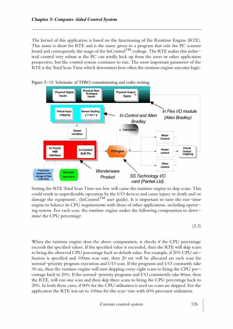
Current control system 126
Chapter 3/ Computer Aided Control System________________________________________________________________________
The kernel of this application is based on the functioning of the Runtime Engine (RTE). This name is short for RTE and is the name given to a program that rule the PC scanner board and consequently the usage of the InControlTM codings. The RTE makes this indus−trial control very robust as the PC can totally lock up from the users or other application perspective, but the control system continues to run. The most important parameter of the RTE is the Total Scan Time which determines how often the runtime engine executes logic.
Figure 3−13. Schematic of TPRO commissioning and codes writing
Setting the RTE Total Scan Time too low will cause the runtime engine to skip scans. This could result in unpredictable operation by the I/O devices and cause injury or death and/or damage the equipment’, (InControlTM user guide). It is important to tune the run−time engine to balance its CPU requirements with those of other applications, including operat−ing system. For each scan, the runtime engine makes the following computation to deter−mine the CPU percentage:
(3.3)
When the runtime engine does the above computation, it checks if the CPU percentage exceeds the specified values. If the specified value is exceeded, then the RTE will skip scans to bring the observed CPU percentage back to default value. For example, if 20% CPU uti−lisation is specified and 100ms scan rate, then 20 ms will be allocated on each scan for normal−priority program execution and I/O scan. If the programs and I/O constantly take 30 ms, then the runtime engine will start skipping every eight scans to bring the CPU per−centage back to 20%. If the normal−priority programs and I/O consistently take 80ms, then the RTE, will run one scan and then skip three scans to bring the CPU percentage back to 20%. In both these cases, if 80% for the CPU utilisation is used no scans are skipped. For the application the RTE was set to 100ms for the scan−rate with 60% processor utilisation.
Globalvariables
Trend DataAquistion and
storage of Data(CSV files)
Real dataAquisition
Calculation
MotorControl
Heatercontrol
Othercontrol
Physical DigitalInputs
Physical RealAnalogueInputs
Physical OutputDigital
Sensor Scalingy = mx + p
Virtual Inputmapping
RTEngineVirtualOutputmapping
In-ControlSoft Plc
In-TouchHMI
interface
In Flex I/O module(Allen Bradley)
WonderwareProduct
In-Control and AllenBradley
SS Technology I/Ocard (Pantek Ltd)

Current control system 127
Chapter 3/ Computer Aided Control System________________________________________________________________________
3.4.8 Control routine design
The software has been built and developed over a three years period. Over this time, changes were made to the software to improve the control routines and to enable a ‘bug free’ software so that an operator having limited knowledge in heat transfer and the baking process can make use of the TPRO rig.
3.4.8.1 Recipe Manager
The name recipe in this context has a different terminology than a ‘food recipe’ to bake a product. As the ultimate goal of the TPRO is to simulate profiles of a real tunnel oven, the control must also handle the zone changes. The recipe manager supervises just that, as it acts as a database of information for each zone that can be simulated and distribute the informa−tion to the different cores devices. It is usually divided into four sections:
• The database: composed with all the items from the recipe, tags, number, content.
• The interface: recipe user input for all the zones (HMI).
• The current zone: Buffer zone which holds the data for as long as it is required.
• The codes: allows the change over from one recipe to another when a certain condition is fulfilled.
Figure 3−14. Handling multiple zone into the recipe manager
The items that compose the recipe are the following:
Recipe nRecipe ....
Recipe n. 3Recipe n. 2
Recipe n. 1
Item 3
Item n
Item ...
Item 2Item 1
Zone 0
Zone 1 Zone 2 Zone 3 Zone 4 Zone 5 Zone 6 Zone 7 Zone 8 Zone 9 Zone 10Item 1Item 2
Item n
Item ...
Current zone
Hum an m achine interface HMI (data input)
RecipeDatabase
Current control system 128
Chapter 3/ Computer Aided Control System________________________________________________________________________
Bake time, band speed, oven air temperature, top and bottom radiant heat temperature, radi−ant heat configuration (half or full), feed flow rate, specific humidity, and all the damper set−ting from 1 to 9.
The current zone or zone 0 see Fig. 3−14 is the 'buffer zone'. Only data in the buffer zone are distributed to the various devices and control loops. After the baking time of the first zone has elapsed then the content of zone 2 is copied inside the zone 0 and the bake time of zone 2 is counting down. If the bake time of the next zone does not have any input for its bake time or a maximum of ten zones is achieved then the TPRO returns to the first zone in a warming up conditions. With the interaction of the HMI screens TPRO user can load create or delete recipes. This way the database keeps the information for any profile and can be loaded into the TPRO at a later date.
3.4.8.2 Fan speed (FIS) control
In the majority of industrial baking ovens the air flow is ‘controlled’ with a fixed fan speed (FIS) and manual dampers acts as a fine control. In the more modern ovens, the fan speed (FIS) is varied and controlled via an inverter, and the dampers only act as fine tuning devices. In either case the air flow rate is not measured and the control relies completely on trial and error methods and process knowledge from the bakers. Two strategies were adopted to con−trol the air flow inside the TPRO. Compared with current ‘control’ of baking ovens the developed strategy offers accurate control of flow and correction for density difference but also the possibility of monitoring flow variation.
3.4.8.2.1 First strategy
As a first trial to control the feed flow, a simple close loop control was used. Both inputs sig−nals, temperature and pressure were converted into real numbers so they can be used to compute the volume of air flow (Fig. 3−15). The measured value and the set−point are compared and the PID algorithm establish an error term which is used to correct the fan speed (FIS) accordingly, via the inverter. The advantage of using this logic compared with other traditional fan control is that it compensates for density change due to temperature change. This is particularly significant when rapid changes of temperature occur. This way the volume of air can remain constant at any temperature, as the inverter will adjust respec−tively for density difference.
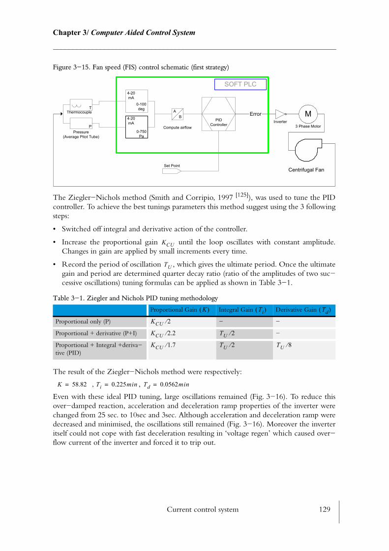
Current control system 129
Chapter 3/ Computer Aided Control System________________________________________________________________________
Figure 3−15. Fan speed (FIS) control schematic (first strategy)
The Ziegler−Nichols method (Smith and Corripio, 1997 [125]), was used to tune the PID controller. To achieve the best tunings parameters this method suggest using the 3 following steps:
• Switched off integral and derivative action of the controller.
• Increase the proportional gain until the loop oscillates with constant amplitude. Changes in gain are applied by small increments every time.
• Record the period of oscillation , which gives the ultimate period. Once the ultimate gain and period are determined quarter decay ratio (ratio of the amplitudes of two suc−cessive oscillations) tuning formulas can be applied as shown in Table 3−1.
The result of the Ziegler−Nichols method were respectively:
, ,
Even with these ideal PID tuning, large oscillations remained (Fig. 3−16). To reduce this over−damped reaction, acceleration and deceleration ramp properties of the inverter were changed from 25 sec. to 10sec and 3sec. Although acceleration and deceleration ramp were decreased and minimised, the oscillations still remained (Fig. 3−16). Moreover the inverter itself could not cope with fast deceleration resulting in ‘voltage regen’ which caused over−flow current of the inverter and forced it to trip out.
Table 3−1. Ziegler and Nichols PID tuning methodology
Proportional Gain Integral Gain Derivative Gain
Proportional only (P) − −
Proportional + derivative (P+I) −
Proportional + Integral +deriva−tive (PID)
PPressure
(Average Pitot Tube)
TThermocouple
PIDController
Set Point
AB
Compute airflowInverter
M3 Phase Motor
Centrifugal Fan
Error
SOFT PLC4-20mA
0-100deg
4-20mA
0-750Pa
KCU
TU
K( ) Ti( ) Td( )
KCU 2⁄
KCU 2.2⁄ TU 2⁄
KCU 1.7⁄ TU 2⁄ TU 8⁄
K 58.82= Ti 0.225min= Td 0.0562min=

Current control system 130
Chapter 3/ Computer Aided Control System________________________________________________________________________
Figure 3−16. Inverter ramp acceleration (For illustrative purpose only)
3.4.8.2.1 Second strategy
Two solutions were proposed to reduce the over damped reaction of the fan and ‘voltage regen’. Two break resistors (36Ω each) were fitted on the inverter terminals so that the surge of energy, i.e. ‘voltage regen’ is dissipated into the resistors. Nevertheless, this does not mean that oscillations would disappear entirely, moreover if oscillations remain, over heating of the inverter would surely occur in the long term. The other alternative was to use a ‘dead band controller’ to avoid using P, I and D actions. The second solution was preferred as no cost was involved, just few lines of codes.
‘Voltage regen’ will also occur when process variables change dramatically and the PID con−troller integrates up to 100% to counteract this effect. Because there is still an error in the process loop, the controller will try to correct for it by further increasing (integrating the error) even though the fan is running at very high speed already. As a result the control loop can become out of control, and causing ‘voltage regen’. This scenario is most likely to occur where time lag is important. In this case the PID controller was totally suppressed and a ‘dead−band controller’ algorithm was written and 'tuned' (see further details in Appendix N). The ‘dead−band controller’ was set to run at a certain time interval (every 250ms). Sim−ilarly as a PID an error term ‘FEED_FAN_ERROR’ was computed between the set−point and the measured value.The ‘Feed_Fan_Rate’ is the rate at which the inverter will increment its speed to. A set of five rules were created based on a trial and error method. When the measured value exceed the set−point the rules are the following:
IF (Fan_Calc_Timer_Done = TRUE) THEN Feed_Fan_Error := Zone0.FeedFlow - Q1C;(* WHEN Q1C > Set-Point *) IF (Q1C < Zone0.FeedFlow) THEN IF ABS(Feed_Fan_Error) > 0.08 THEN Feed_Fan_Rate := 1.0; ELSEIF ABS(Feed_Fan_Error) > 0.05 THEN Feed_Fan_Rate := 0.4; ELSEIF ABS(Feed_Fan_Error) > 0.03 THEN Feed_Fan_Rate := 0.3; ELSEIF ABS(Feed_Fan_Error) > 0.01 THEN Feed_Fan_Rate := 0.2; ELSE Feed_Fan_Rate := 0.0;
TIME (Min)
Flow Rate (m3/s)
Set Point
Inverter ramp = 10 sec
Inverter ramp = 3 secIdeal

Current control system 131
Chapter 3/ Computer Aided Control System________________________________________________________________________
Feed_Fan_Error := 0; END_IF; CFAN.SPEED := CFAN.SPEED + Feed_Fan_Rate; ELSE
The result of this second strategy was very successful and accurate and repeatable flow control was achieved (See 4.3.3).
For low volume flow control (below 0.06m3/s) the measurement of pressure in the main duct was not stable (low range of operation of the flow grid instrument) and had to be con−trolled manually. A different algorithm as the one shown above was built to enable manual operation of the fan without creating ‘voltage regen’. In this scenario all information regard−ing the main flow rate were unusable as not accurate.
3.4.8.3 Heater control
A single strategy was adopted to build a control loop to actuate the heaters (duct heater and radiant heaters). The heater set point is compared to the measured temperature (Fig. 3−17). An error term is generated from the PID which is proportional to the heat demand to bring the process temperature as close as possible to the set−point.
The output value from the PID is compared to a dummy value from a pulse counter inside the InControlTM software. For instance, on a 100 units time basis, if the PID error term is 80%, the off time will be 20 units and the on time the remaining 80 units (Fig. 3−18). The heater counter was based on a 1000ms (1s) time base, which allows a very accurate control of the heat delivered, (e.g. if 5% heat is on demand the heat will be on for 50 ms).
Figure 3−17. Heater control schematic
All heaters were equipped with solid state relays (no moving parts), which allows very high rates of switching. This strategy was adopted so that switching of individual heaters will not necessarily occur at the same time, to avoid current surge.
TThermocouple PID
Controller
Set Point
SOFT PLC
4-20mA
0-100deg
Pulse Counter
Error term
Solid State Relay
HeaterI
Input
Calc
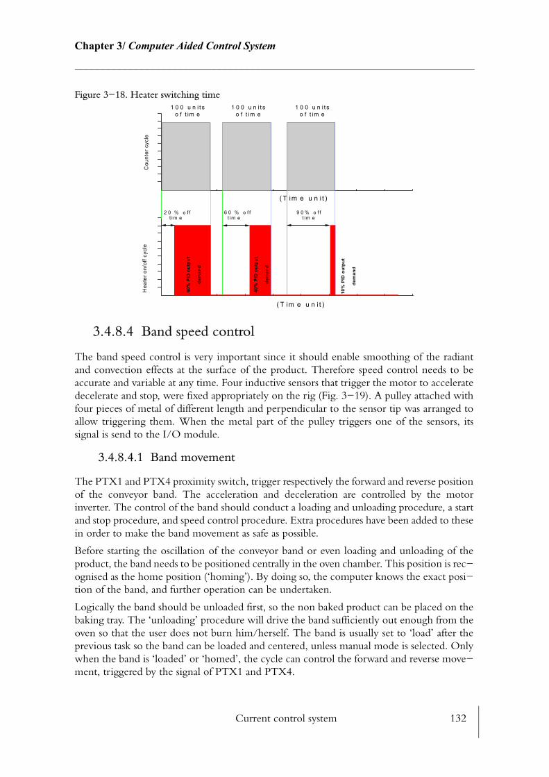
Current control system 132
Chapter 3/ Computer Aided Control System________________________________________________________________________
Figure 3−18. Heater switching time
3.4.8.4 Band speed control
The band speed control is very important since it should enable smoothing of the radiant and convection effects at the surface of the product. Therefore speed control needs to be accurate and variable at any time. Four inductive sensors that trigger the motor to accelerate decelerate and stop, were fixed appropriately on the rig (Fig. 3−19). A pulley attached with four pieces of metal of different length and perpendicular to the sensor tip was arranged to allow triggering them. When the metal part of the pulley triggers one of the sensors, its signal is send to the I/O module.
3.4.8.4.1 Band movement
The PTX1 and PTX4 proximity switch, trigger respectively the forward and reverse position of the conveyor band. The acceleration and deceleration are controlled by the motor inverter. The control of the band should conduct a loading and unloading procedure, a start and stop procedure, and speed control procedure. Extra procedures have been added to these in order to make the band movement as safe as possible.
Before starting the oscillation of the conveyor band or even loading and unloading of the product, the band needs to be positioned centrally in the oven chamber. This position is rec−ognised as the home position (‘homing’). By doing so, the computer knows the exact posi−tion of the band, and further operation can be undertaken.
Logically the band should be unloaded first, so the non baked product can be placed on the baking tray. The ‘unloading’ procedure will drive the band sufficiently out enough from the oven so that the user does not burn him/herself. The band is usually set to ‘load’ after the previous task so the band can be loaded and centered, unless manual mode is selected. Only when the band is ‘loaded’ or ‘homed’, the cycle can control the forward and reverse move−ment, triggered by the signal of PTX1 and PTX4.
Hea
ter o
n/of
f cyc
le
( T im e u n i t )
Cou
nter
cyc
le
( T im e u n i t )80
% P
ID o
utpu
t
dem
and
40%
PID
out
put
dem
and
10%
PID
out
put
dem
and
9 0 % o f ft im e
6 0 % o f ft im e
2 0 % o f ft im e
1 0 0 u n i t so f t im e
1 0 0 u n i t so f t im e
1 0 0 u n i t so f t im e
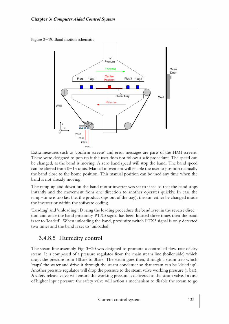
Current control system 133
Chapter 3/ Computer Aided Control System________________________________________________________________________
Figure 3−19. Band motion schematic
Extra measures such as 'confirm screens' and error messages are parts of the HMI screens. These were designed to pop up if the user does not follow a safe procedure. The speed can be changed, as the band is moving. A zero band speed will stop the band. The band speed can be altered from 0−15 units. Manual movement will enable the user to position manually the band close to the home position. This manual position can be used any time when the band is not already moving.
The ramp up and down on the band motor inverter was set to 0 sec so that the band stops instantly and the movement from one direction to another operates quickly. In case the ramp−time is too fast (i.e. the product slips out of the tray), this can either be changed inside the inverter or within the software coding.
‘Loading’ and ‘unloading’: During the loading procedure the band is set in the reverse direc−tion and once the band proximity PTX3 signal has been located three times then the band is set to ‘loaded’. When unloading the band, proximity switch PTX3 signal is only detected two times and the band is set to ‘unloaded’.
3.4.8.5 Humidity control
The steam line assembly Fig. 3−20 was designed to promote a controlled flow rate of dry steam. It is composed of a pressure regulator from the main steam line (boiler side) which drops the pressure from 10bars to 3bars. The steam goes then, through a steam trap which ‘traps’ the water and drive it through the steam condenser so that steam can be ‘dried up’. Another pressure regulator will drop the pressure to the steam valve working pressure (1 bar). A safety release valve will ensure the working pressure is delivered to the steam valve. In case of higher input pressure the safety valve will action a mechanism to disable the steam to go
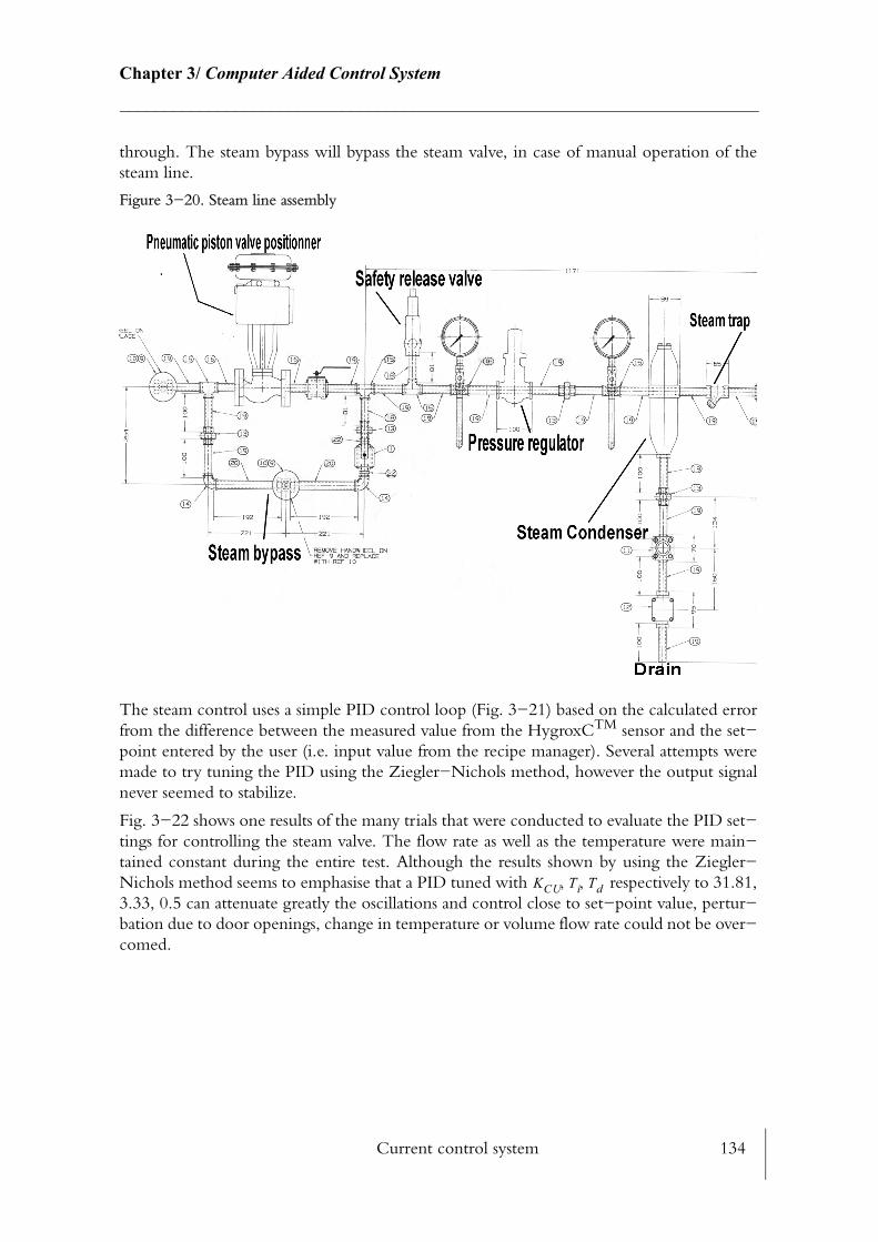
Current control system 134
Chapter 3/ Computer Aided Control System________________________________________________________________________
through. The steam bypass will bypass the steam valve, in case of manual operation of the steam line.
Figure 3−20. Steam line assembly
The steam control uses a simple PID control loop (Fig. 3−21) based on the calculated error from the difference between the measured value from the HygroxCTM sensor and the set−point entered by the user (i.e. input value from the recipe manager). Several attempts were made to try tuning the PID using the Ziegler−Nichols method, however the output signal never seemed to stabilize.
Fig. 3−22 shows one results of the many trials that were conducted to evaluate the PID set−tings for controlling the steam valve. The flow rate as well as the temperature were main−tained constant during the entire test. Although the results shown by using the Ziegler−Nichols method seems to emphasise that a PID tuned with respectively to 31.81, 3.33, 0.5 can attenuate greatly the oscillations and control close to set−point value, pertur−bation due to door openings, change in temperature or volume flow rate could not be over−comed.
KCU Ti Td, ,
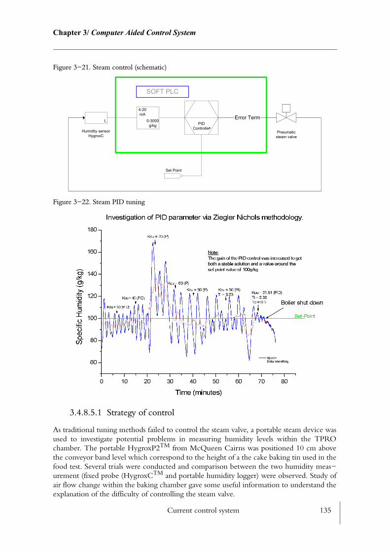
Current control system 135
Chapter 3/ Computer Aided Control System________________________________________________________________________
Figure 3−21. Steam control (schematic)
Figure 3−22. Steam PID tuning
3.4.8.5.1 Strategy of control
As traditional tuning methods failed to control the steam valve, a portable steam device was used to investigate potential problems in measuring humidity levels within the TPRO chamber. The portable HygroxP2TM from McQueen Cairns was positioned 10 cm above the conveyor band level which correspond to the height of a the cake baking tin used in the food test. Several trials were conducted and comparison between the two humidity meas−urement (fixed probe (HygroxCTM and portable humidity logger) were observed. Study of air flow change within the baking chamber gave some useful information to understand the explanation of the difficulty of controlling the steam valve.
PIDController
Set Point
SOFT PLC
`L
Humidity sensorHygroxC
Pneumaticsteam valve
Error Term4-20mA
0-3000g/kg

Current control system 136
Chapter 3/ Computer Aided Control System________________________________________________________________________
Fig. 3−23 highlights the comparison between the measurement of mixed humidity between the HygroxCTM and the HygroxP2TM. The oscillations in the mixed humidity for both the traces is due to the PID trying to control the mixed humidity. The delay between the two traces shows a time lag of about 2.3 minutes. The portable instrument picks up the changes more rapidly than the fixed probe does. As well as being delayed the value of the peaks is also different for both traces; the fixed probe gives higher values than the portable probe.
By varying the flow rate from 0.15m3/s to 0.6m3/s, Fig. 3−24 reveals that oscillation dimin−ishes between the two measuring instruments, however a fixed difference between the two traces remains (about 15 g/kg).
Figure 3−23. Comparison of mixed humidity at constant air flow rate
From the result of both, constant and variable flow rate study, it proves that the air flow around the fixed probe influences greatly the response of the humidity. Consequently, fur−ther investigation were carried out on the fixed probe humidity assembly.
The HygroxCTM probe was fitted in with a cooling unit to drop down the temperature and protect the probe head (i.e. Zirconium sensor) which can only withstand 300oC. This unit was required and made specially as the maximum required oven temperature was 500oC.
Fig. 3−25 shows the design problems created by trying to cool this unit. Air slots in the cooling unit end plate are very small and did not allow enough air flow to the zirconium sensor which works better with relatively high air flow as the previous results revealed. Gap between insulation walls and HygroxCTM is very small (1mm), and the air flow movement to the humidity sensor head slots is therefore reduced. The probe tail end is not in contact (air contact) with outside ambient air therefore cooling fan heat sink are only used to cool the oven wall cavity surface and the end of the probe tail (i.e. where the electronics is fitted). With this arrangement the HygroxCTM head cannot be cooled by air movement.
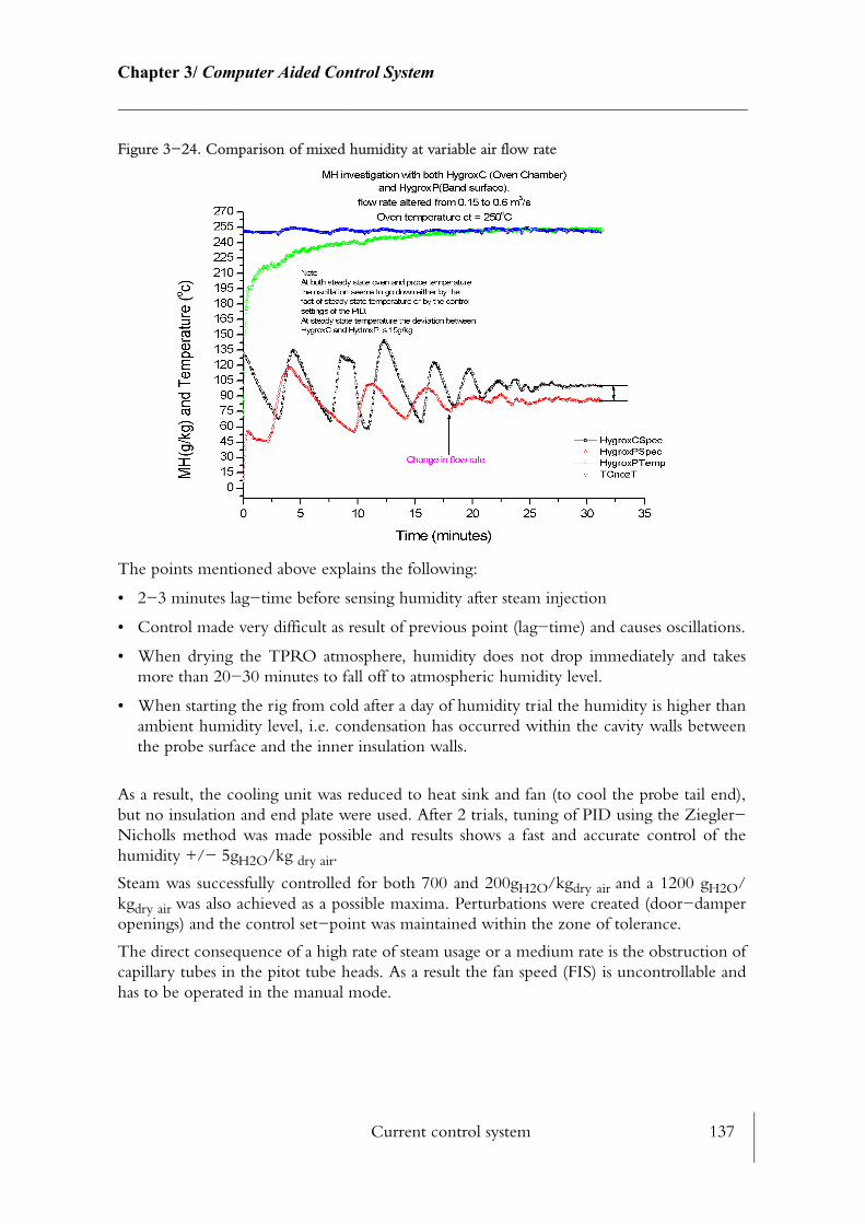
Current control system 137
Chapter 3/ Computer Aided Control System________________________________________________________________________
Figure 3−24. Comparison of mixed humidity at variable air flow rate
The points mentioned above explains the following:
• 2−3 minutes lag−time before sensing humidity after steam injection
• Control made very difficult as result of previous point (lag−time) and causes oscillations.
• When drying the TPRO atmosphere, humidity does not drop immediately and takes more than 20−30 minutes to fall off to atmospheric humidity level.
• When starting the rig from cold after a day of humidity trial the humidity is higher than ambient humidity level, i.e. condensation has occurred within the cavity walls between the probe surface and the inner insulation walls.
As a result, the cooling unit was reduced to heat sink and fan (to cool the probe tail end), but no insulation and end plate were used. After 2 trials, tuning of PID using the Ziegler−Nicholls method was made possible and results shows a fast and accurate control of the humidity +/− 5gH2O/kg dry air.
Steam was successfully controlled for both 700 and 200gH2O/kgdry air and a 1200 gH2O/kgdry air was also achieved as a possible maxima. Perturbations were created (door−damper openings) and the control set−point was maintained within the zone of tolerance.
The direct consequence of a high rate of steam usage or a medium rate is the obstruction of capillary tubes in the pitot tube heads. As a result the fan speed (FIS) is uncontrollable and has to be operated in the manual mode.
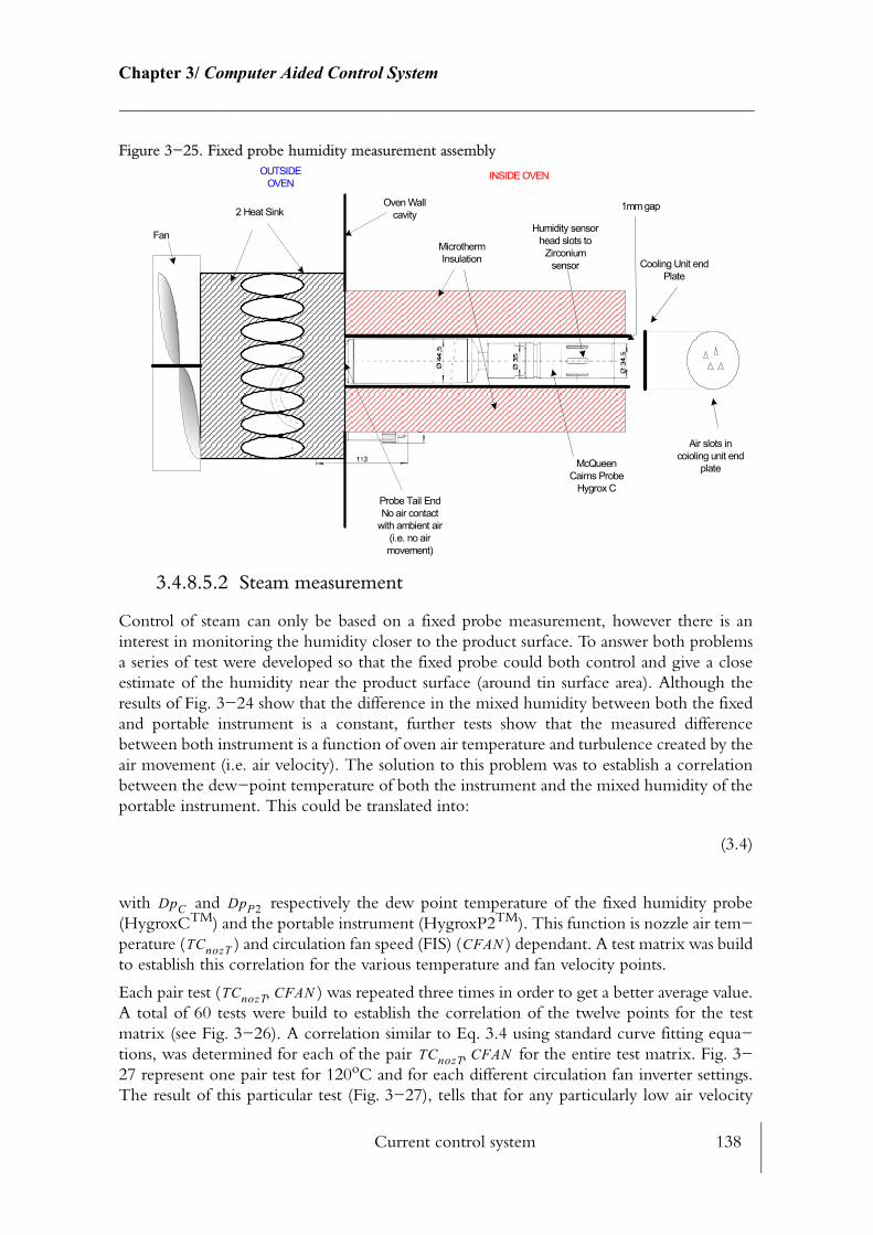
Current control system 138
Chapter 3/ Computer Aided Control System________________________________________________________________________
Figure 3−25. Fixed probe humidity measurement assembly
3.4.8.5.2 Steam measurement
Control of steam can only be based on a fixed probe measurement, however there is an interest in monitoring the humidity closer to the product surface. To answer both problems a series of test were developed so that the fixed probe could both control and give a close estimate of the humidity near the product surface (around tin surface area). Although the results of Fig. 3−24 show that the difference in the mixed humidity between both the fixed and portable instrument is a constant, further tests show that the measured difference between both instrument is a function of oven air temperature and turbulence created by the air movement (i.e. air velocity). The solution to this problem was to establish a correlation between the dew−point temperature of both the instrument and the mixed humidity of the portable instrument. This could be translated into:
(3.4)
with and respectively the dew point temperature of the fixed humidity probe (HygroxCTM) and the portable instrument (HygroxP2TM). This function is nozzle air tem−perature ( ) and circulation fan speed (FIS) ( ) dependant. A test matrix was build to establish this correlation for the various temperature and fan velocity points.
Each pair test ( ) was repeated three times in order to get a better average value. A total of 60 tests were build to establish the correlation of the twelve points for the test matrix (see Fig. 3−26). A correlation similar to Eq. 3.4 using standard curve fitting equa−tions, was determined for each of the pair for the entire test matrix. Fig. 3−27 represent one pair test for 120oC and for each different circulation fan inverter settings. The result of this particular test (Fig. 3−27), tells that for any particularly low air velocity
MicrothermInsulation
McQueenCairns Probe
Hygrox C
Cooling Unit endPlate
Air slots incoioling unit end
plate
Probe Tail EndNo air contact
with ambient air(i.e. no airmovement)
2 Heat SinkOven Wall
cavityHumidity sensor
head slots toZirconium
sensor
INSIDE OVENOUTSIDEOVEN
Fan
1mm gap
DpC DpP2
TCnozT CFAN
TCnozT CFAN,
TCnozT CFAN,
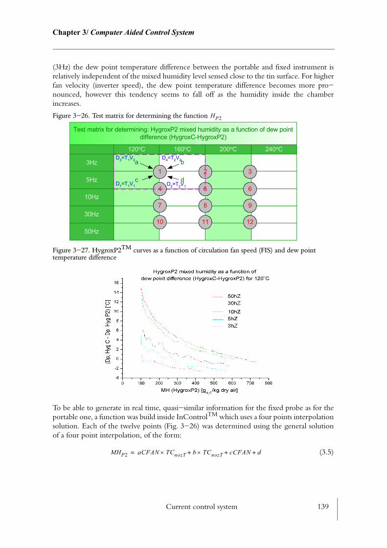
Current control system 139
Chapter 3/ Computer Aided Control System________________________________________________________________________
(3Hz) the dew point temperature difference between the portable and fixed instrument is relatively independent of the mixed humidity level sensed close to the tin surface. For higher fan velocity (inverter speed), the dew point temperature difference becomes more pro−nounced, however this tendency seems to fall off as the humidity inside the chamber increases.
Figure 3−26. Test matrix for determining the function
Figure 3−27. HygroxP2TM curves as a function of circulation fan speed (FIS) and dew point temperature difference
To be able to generate in real time, quasi−similar information for the fixed probe as for the portable one, a function was build inside InControlTM which uses a four points interpolation solution. Each of the twelve points (Fig. 3−26) was determined using the general solution of a four point interpolation, of the form:
(3.5)
HP2
50Hz
30Hz
10Hz
dc5Hz
ba3Hz
240oC200oC160oC120oC
Test matrix for determining: HygroxP2 mixed humidity as a function of dew pointdifference (HygroxC-HygroxP2)
1 2 3
4 5 6
7 8 9
10 11 12
D3=T1V2 D4=T2V2
D2=T2V1D1=T1V1
MHP2 aCFAN TCnozT× b TCnozT× cCFAN d+ + +=
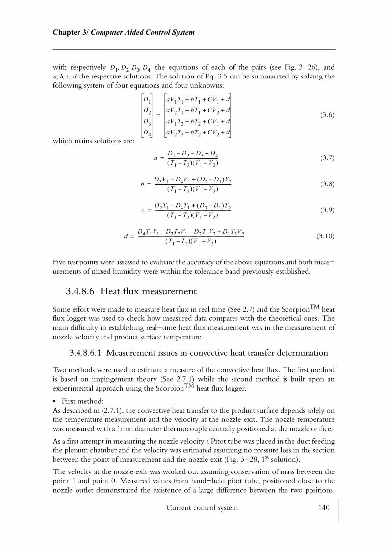
Current control system 140
Chapter 3/ Computer Aided Control System________________________________________________________________________
with respectively the equations of each of the pairs (see Fig. 3−26), and the respective solutions. The solution of Eq. 3.5 can be summarized by solving the
following system of four equations and four unknowns:
(3.6)
which mains solutions are:
(3.7)
(3.8)
(3.9)
(3.10)
Five test points were assessed to evaluate the accuracy of the above equations and both meas−urements of mixed humidity were within the tolerance band previously established.
3.4.8.6 Heat flux measurement
Some effort were made to measure heat flux in real time (See 2.7) and the ScorpionTM heat flux logger was used to check how measured data compares with the theoretical ones. The main difficulty in establishing real−time heat flux measurement was in the measurement of nozzle velocity and product surface temperature.
3.4.8.6.1 Measurement issues in convective heat transfer determination
Two methods were used to estimate a measure of the convective heat flux. The first method is based on impingement theory (See 2.7.1) while the second method is built upon an experimental approach using the ScorpionTM heat flux logger.
• First method:As described in (2.7.1), the convective heat transfer to the product surface depends solely on the temperature measurement and the velocity at the nozzle exit. The nozzle temperature was measured with a 1mm diameter thermocouple centrally positioned at the nozzle orifice.
As a first attempt in measuring the nozzle velocity a Pitot tube was placed in the duct feeding the plenum chamber and the velocity was estimated assuming no pressure loss in the section between the point of measurement and the nozzle exit (Fig. 3−28, 1st solution).
The velocity at the nozzle exit was worked out assuming conservation of mass between the point 1 and point 0. Measured values from hand−held pitot tube, positioned close to the nozzle outlet demonstrated the existence of a large difference between the two positions.
D1 D2 D3 D4, , ,a b c d, , ,
D1
D2
D3
D4
aV1T1 bT1 CV1 d+ + +
aV2T1 bT1 CV2 d+ + +
aV1T2 bT2 CV1 d+ + +
aV2T2 bT2 CV2 d+ + +
=
aD1 D2– D3– D4+
T1 T2–( ) V1 V2–( )----------------------------------------------=
bD3V1 D4V1– D2 D1–( )V2+
T1 T2–( ) V1 V2–( )-----------------------------------------------------------------------=
cD2T1 D4T1– D3 D1–( )T2+
T1 T2–( ) V1 V2–( )----------------------------------------------------------------------=
dD4T1V1 D3T2V1– D2T1V2– D1T2V2+
T1 T2–( ) V1 V2–( )--------------------------------------------------------------------------------------------------=

Current control system 141
Chapter 3/ Computer Aided Control System________________________________________________________________________
This difference was not constant over the full velocity range, moreover results using this technique did not repeat very well. It is usually advised to placed Pitot tubes away from any flow disturbance (5 to 10 section away from bends, dampers...). The damper arrangement in this duct section was affecting the flow measurement. As a result the complete measurement assembly (Pitot tubes, fittings and piping) was moved, so that measurement could occur closer to the nozzle (Fig. 3−28, 2nd solution). To avoid turbulence at the edge of the nozzle exit, a bell shaped tube was built specifically to help laminar flow line to develop and to enhance the accuracy and repeatability of measurement. A test was conducted to understand how the Pitot tube should be positioned with respect to the nozzle outlet. Three different measurement techniques were compared to the benchmark instrument values. Fig. 3−29shows the various volume flow rate at a constant oven air temperature (150oC).
Figure 3−28. Solutions for measuring nozzle outlet velocity
In the lowest region of volume flow (0.2−0.5m3/s), the measurement technique using the bell shaped tube arrangement is close to the measurement, where the Pitot head is 10mm away from the nozzle exit. This indicate that the flow pattern is similar for both arrangement. However in region of higher volume flow rate (0.5−0.8m3/s) the difference accentuates, which might be caused by higher rate of turbulence. The sudden maxima (at 0.65m3/s) reached by the bell shaped arrangement technique is due to the limitation of the Pitot tube pressure transducer (FC0322 transmitter) which cannot stretch further than 750Pa. To over−come this problem a larger range transmitter was fitted (0−1200Pa).
• Second method:The ScorpionTM heat flux logger was used to evaluate the convective heat transfer coeffi−cient and investigate how it would compare to the nozzle impingement theory. The logger placed 10 cm above the band, conveyed in an oscillation movement to simulate the band movement of a tunnel oven. Results obtained were plotted against the semi−theoretical values from the first method (Fig. 3−30). During this test the fan inverter speed was increased in three phases (5Hz, 30Hz and 50Hz). The graph plotted on Fig. 3−30 are the average of five tests repeated in the exact same conditions.
Flow direction
Pitot tube
BSP fitting
Pressure Transducer0-750pa To 4-20ma
I/O moduleA/D converter
Plenum ChamberNozzle impingement
PCOutput scaling
+Conversion D/A
1
34
5 6
0
Damper
2
Pressure Transducer0-1200pa To 4-20ma
1st Solution
2nd SolutionI/O module
A/D converter
7
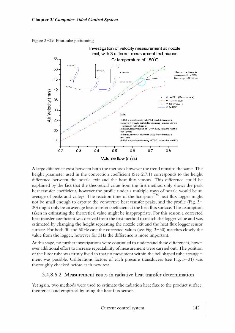
Current control system 142
Chapter 3/ Computer Aided Control System________________________________________________________________________
Figure 3−29. Pitot tube positioning
A large difference exist between both the methods however the trend remains the same. The height parameter used in the convection coefficient (See 2.7.1) corresponds to the height difference between the nozzle exit and the heat flux sensors. This difference could be explained by the fact that the theoretical value from the first method only shows the peak heat transfer coefficient, however the profile under a multiple rows of nozzle would be an average of peaks and valleys. The reaction time of the ScorpionTM heat flux logger might not be small enough to capture the convective heat transfer peaks, and the profile (Fig. 3−30) might only be an average heat transfer coefficient at the heat flux surface. The assumption taken in estimating the theoretical value might be inappropriate. For this reason a corrected heat transfer coefficient was derived from the first method to match the logger value and was estimated by changing the height separating the nozzle exit and the heat flux logger sensor surface. For both 30 and 50Hz case the corrected values (see Fig. 3−30) matches closely the value from the logger, however for 5Hz the difference is more important.
At this stage, no further investigations were continued to understand these differences, how−ever additional effort to increase repeatability of measurement were carried out. The position of the Pitot tube was firmly fixed so that no movement within the bell shaped tube arrange−ment was possible. Calibrations factors of each pressure transducers (see Fig. 3−31) was thoroughly checked before each new test.
3.4.8.6.2 Measurement issues in radiative heat transfer determination
Yet again, two methods were used to estimate the radiation heat flux to the product surface, theoretical and empirical by using the heat flux sensor.
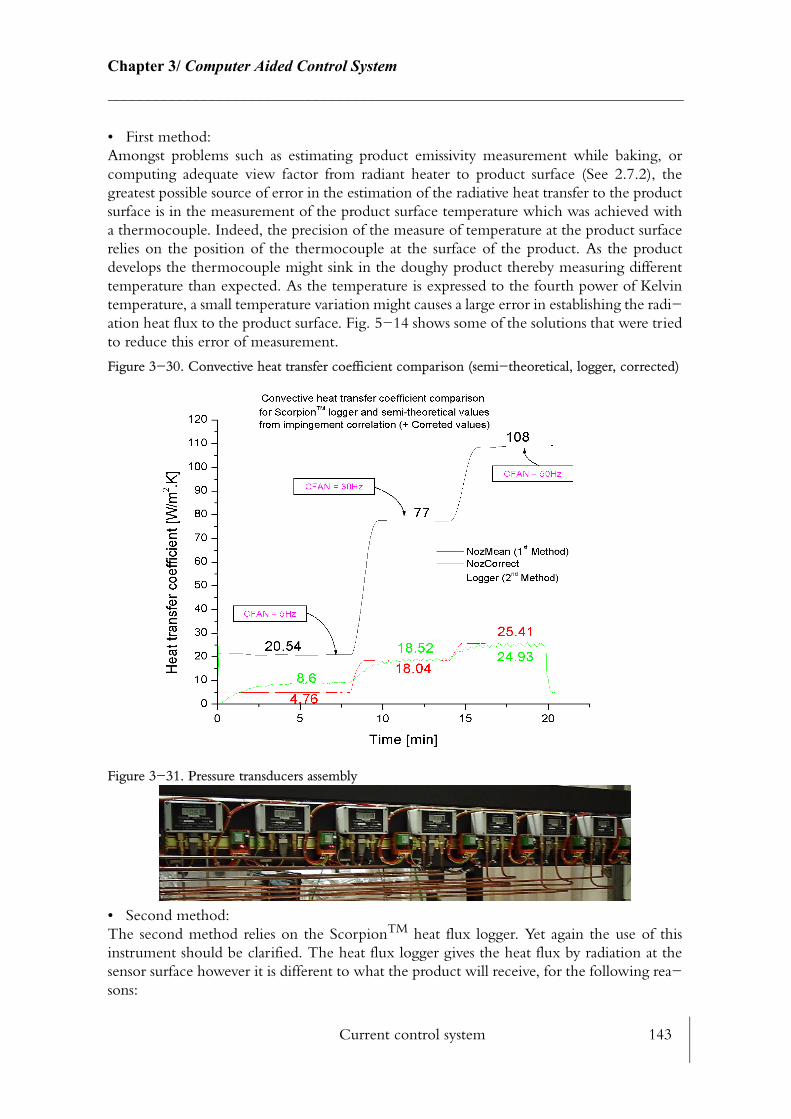
Current control system 143
Chapter 3/ Computer Aided Control System________________________________________________________________________
• First method:Amongst problems such as estimating product emissivity measurement while baking, or computing adequate view factor from radiant heater to product surface (See 2.7.2), the greatest possible source of error in the estimation of the radiative heat transfer to the product surface is in the measurement of the product surface temperature which was achieved with a thermocouple. Indeed, the precision of the measure of temperature at the product surface relies on the position of the thermocouple at the surface of the product. As the product develops the thermocouple might sink in the doughy product thereby measuring different temperature than expected. As the temperature is expressed to the fourth power of Kelvin temperature, a small temperature variation might causes a large error in establishing the radi−ation heat flux to the product surface. Fig. 5−14 shows some of the solutions that were tried to reduce this error of measurement.
Figure 3−30. Convective heat transfer coefficient comparison (semi−theoretical, logger, corrected)
Figure 3−31. Pressure transducers assembly
• Second method:The second method relies on the ScorpionTM heat flux logger. Yet again the use of this instrument should be clarified. The heat flux logger gives the heat flux by radiation at the sensor surface however it is different to what the product will receive, for the following rea−sons:
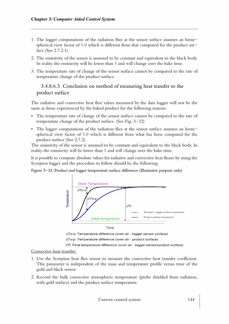
Current control system 144
Chapter 3/ Computer Aided Control System________________________________________________________________________
1. The logger computations of the radiation flux at the sensor surface assumes an hemi−spherical view factor of 1.0 which is different from that computed for the product sur−face (See 2.7.2.1).
2. The emissivity of the sensor is assumed to be constant and equivalent to the black body. In reality the emissivity will be lower than 1 and will change over the bake time.
3. The temperature rate of change of the sensor surface cannot be compared to the rate of temperature change of the product surface.
3.4.8.6.3 Conclusion on method of measuring heat transfer to the product surface
The radiative and convective heat flux values measured by the data logger will not be the same as those experienced by the baked product for the following reasons:
• The temperature rate of change of the sensor surface cannot be compared to the rate of temperature change of the product surface. (See Fig. 3−32)
• The logger computations of the radiation flux at the sensor surface assumes an hemi−spherical view factor of 1.0 which is different from what has been computed for the product surface (See 2.7.2).
The emissivity of the sensor is assumed to be constant and equivalent to the black body. In reality the emissivity will be lower than 1 and will change over the bake time.
It is possible to compute absolute values for radiative and convective heat fluxes by using the Scorpion logger and the procedure to follow should be the following:
Figure 3−32. Product and logger temperature surface difference (Illustrative purpose only)
Convective heat transfer:
1. Use the Scorpion heat flux sensor to measure the convective heat transfer coefficient. This parameter is independent of the mass and temperature profile versus time of the gold and black sensor.
2. Record the bulk convective atmospheric temperature (probe shielded from radiation, with gold surface) and the product surface temperature.
Current control system 145
Chapter 3/ Computer Aided Control System________________________________________________________________________
3. Calculate the convective heat flux versus time profile with traditional formulation for convective flux heat transfer.
Radiative heat transfer:
1. Use the Scorpion heat flux logger to measure the perceived radiation temperature . This parameter is independent of the mass and temperature profile versus time of the gold and black sensor. It does however assumes an hemispherical view factor of 1.
2. Use the product surface temperature profile together with the emissivity of the product surface.
3. Compute the radiative heat flux profile versus time with conventional radiative heat flux correlation.
For the reason cited above, the heat flux logger was only used to record the convective heat transfer coefficient and the perceived radiation for comparison purposes.
3.4.8.7 Control handling of alarms
Control handling of the alarms was designed to make sure the use of the TPRO is 100% safe. Several types of alarms were created with three major purposes; monitor, prevent and pro−tect.
3.4.8.7.1 Monitoring alarms
These types of alarms are intended specifically to inform the user of the TPRO rig that cer−tain conditions have been reached. They were used for all the different control loops. A ‘Hi’ alarm in the usage of the temperature control loops inform the user that the controlled tem−perature has reached 5% above its set−point. Monitoring alarms are not considered to be critical and the user can either take a decision manually or leave it. Similar alarms were used in the control of humidity, and volume flow rate control. Monitoring alarms were also employed to inform that a specific event occurred, for instance:
− Thermal steady state achieved
− Bake time finished
− Band homing (band being centred)
These message can only be granted and there is nothing to do but acknowledging that the event has occurred.
3.4.8.7.2 Preventing alarms
This family of alarms can be differentiated from the previous ones as a choice is offered to the user of the TPRO. A decision can be taken immediately so that change can occur quickly. A ‘Hi−Hi’ alarm is used when the actual controlled variable reaches 10% above the set−point. Some advises will guide the user of the TPRO what to do to overcome this prob−lem. In the case of the duct heater sheath surface over−temperature, preventing alarms will guide the user of the TPRO to cool the surface temperature down to avoid burning the heater elements.
Tr
Current control system 146
Chapter 3/ Computer Aided Control System________________________________________________________________________
3.4.8.7.3 Protecting alarms
A large number of protecting alarms were coded to protect the user of the TPRO to be in danger. Often when a serious problem occur decision have to be taken immediately and human actions are usually too slow to avoid disaster. Protecting alarms were build upon cat−astrophic, what if scenarios.
• What if none is present around the oven and something goes wrong?
• What if someone has done something wrong?
• What if the duct heater sheath temperature goes beyond its operating limit?
When the duct heater sheath surface reaches 15% above their working temperature (460oC), an alarm will perform to trip the circuit−breaker which feeds the solid state relay operating the heater in order to avoid any electrical current to flow through.
Some procedure which cannot be called alarms were also used without warning the user of the TPRO. While shutting down the TPRO is it important to dry out any moisture remain−ing inside the TPRO ductings, in order to prevent the various heater element to corrode. For this reason a shut down procedure has been written which maintains both the fans to their maximum speed while the hot air is extracted until the temperature within the chamber has dropped to 35oC, for this reason shut down procedure could take up to several hours.
3.4.8.8 Program execution
A total of 63 separate files were created to build the entire control system of the TPRO rig. For the code to execute without fault these files were arranged in a logical manner. As a gen−eral rule of programming, the declaration of variables, the mapping and the sensor scaling were highly prioritised were be positioned before any other codings.
3.4.9 Human machine interface (HMI)
The human machine interface (HMI) has become increasingly more important over the years. HMI is where people and technology meet. Nowadays humans interact more with computer−based technology than with hammers and drills. The task of an HMI is to make the function of a technology self−evident. Much like a well−designed hammer fits the user's hand and makes a physical task easy, a well−designed HMI must fit the user's idea of the task that needs to be carried out. The design of the TPRO HMI allows the user to communicate with the various devices and to have entire control of the process. HMI effectiveness is measured by a number of components, such as learnability and productivity. These compo−nents are sometimes brought together under the title of ‘usability’ also known as quality of use (Cortes, 1997 [37]).
• Effectiveness: does the product do what the users require?
• Efficiency: can the users learn the HMI quickly? Can they carry out their tasks with minimum effort, including a minimum of errors? Does it improve the productivity?

Current control system 147
Chapter 3/ Computer Aided Control System________________________________________________________________________
• Satisfaction: Do users express satisfaction with the product? Does the new product reduce stress? Do the end users now have a more satisfying job?
Ease of use is a real user need and most product reviews, whether in consumer magazines or professional journals, usually compare products based on their usability. Research also shows (Cortes, 1997 [37]) that about 50 percent of the code in new software applications is devoted to the user interface. Although pure text interfaces are still appropriate for some applications, nowadays most Windows, Mac and Unix programmers use the more popular and versatile graphical user interfaces (GUI).
In the field of process engineering, Wonderware InTouchTM, is the world's leading HMI software. It enables engineers, supervisors, managers and operators to view and interact with the workings of an entire operation through graphical representations of their production processes. Additionally, the network application development environment allows systems to be developed for use in large PC−based networks. InTouch is a powerful, view−only node, that enables supervisors and managers to view real−time plant floor data from a desktop PC anywhere on the network. This way it reduces the cost and time associated with maintaining operator interface/HMI systems.
Cortes, 1997 [37] describes ten principles for designing a good quality GUI.1. Consistent style for a better anticipation of the various widget’s (button, menu, check
box, scroll bars.)
2. Consistency of the widgets with other programs will help to reduce the learning curve of computer literate users.
3. Error and help dialogue should be used to help without over taking the rest of the screens and should only be shown when required.
4. Provide adequate user feedback (e.g. start or end of process), when selecting or un−selecting options.
5. ‘Good’ interfaces invite exploration and should be attractive and easy to use without fearing (Undo and redo capabilities are usually used for this purpose).
6. ‘Good’ applications comes with user guide and user manuals, but ‘great’ applications are those which novice users rarely need to refer to the manuals.
7. Appropriate and conventional colour code should be used when required so that user is not confused (e.g: Alarms = Yellow, Water = blue, Stop = red, Start = green).
8. Customize and preserve preferred work environment when it is possible (help the con−sistency).
9. Modal behaviour should be avoided when possible. Modal behaviour forces the user to perform tasks in a specific order or otherwise modify the user’s expected responses. Modal behaviours generally feel uncomfortable if used by any other person apart from the programmers. Movement of the conveyor band in the TPRO had to be ruled by modal behaviour, otherwise safety of the user could be put in danger.
10.Interface should be designed so that the user can accomplish their task while being minimally aware of the interface itself. Interface transparency occurs when the user’s attention is drawn away from the interface and naturally directed at the task itself.
Current control system 148
Chapter 3/ Computer Aided Control System________________________________________________________________________
3.4.10 Design of TPRO GUI
A total of 84 screens were designed to help the user to interact with the TPRO. The design of screens can be a time consuming task and most of the screens were first designed on paper. The variables (tag) from InControlTM can easily be transferred to InTouchTM which is only there to display the values/status. Most of the calculation were performed with InControlTM
and displayed on the InTouchTM GUI, however, InTouchTM can also be used for compu−tation purposes as it has its own scripting languages. Minor ‘conditions script’ were written within InTouchTM to alter screen display. For instance, a menu or warning can pop up on a screen when a particular condition is reached so that the user has to take an immediate action to solve the problem.
Each of the screens has a specific functionality, and the totality of the screen designed can be classified under six families:
• Pivot screen: allows to communicate with other screens, acts as a platform where multi−ple choice is possible.
• Input screen: are designed only to receive input data than can be stored or changed inside a database.
• Action Screen: have direct connection with the process applications (valve, motor, con−trol) which can be seen as ‘the arms and the legs’ of the process.
• Status and Display Screen: display useful information so that decision taking is easier. Can monitor in real−time process values.
• Help screen: display help with regards to a particular area of the screen that is not neces−sary self−explanatory.
• Trending and data acquisition screen: there are two sorts of trends; real−time and histor−ical. Historical trends are the trends which have the capability to record a number of variable over a time period and save its contents to the hard disk, while real−time trends only display data in real time without the capacity of saving data.
Although screens can be grouped into the six above categories some of the screen can belong to two or more category at a time.
3.4.10.1 Pivot screen
Several pivot screen were created, however ‘TPRO MAIN MENU’ (see Fig. 3−33) is the principal one. From this screen any other screen can be accessed by the click of a button. This screen displays at its centre, a sketch of the skeleton of the TPRO with all temperature and pressure points. Fans, heaters as well as steam line will change colour depending on their status.
The top of the screen only displays informations. The current recipe ‘demo’ can be changed by simply clicking on the word and loading a pre−existing recipe. The current zone number is also displayed and will increment as the baking starts. The operator name, the level and the key allow the user to logon and check its security level. The security level is an important
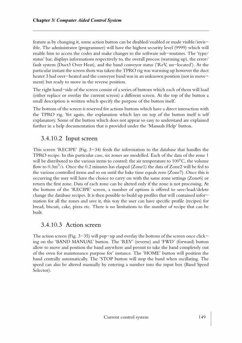
Current control system 149
Chapter 3/ Computer Aided Control System________________________________________________________________________
feature as by changing it, some action button can be disabled/enabled or made visible/invis−ible. The administrator (programmer) will have the highest security level (9999) which will enable him to access the codes and make changes to the software sub−routines. The ‘type/status’ bar, displays informations respectively to, the overall process (warming up), the error/fault system (Duct3 Over Heat), and the band conveyor status (‘ReV, un−located’). At the particular instant the screen shots was taken the TPRO rig was warming up however the duct heater 3 had over−heated and the conveyor band was in an unknown position (not in move−ment) but ready to move in the reverse position.
The right hand−side of the screen consist of a series of buttons which each of them will load (either replace or overlay the current screen) a different screen. At the top of the button a small description is written which specify the purpose of the button itself.
The bottom of the screen is reserved for actions buttons which have a direct interaction with the TPRO rig. Yet again, the explanation which lays on top of the button itself is self explanatory. Some of the button which does not appear so easy to understand are explained further in a help documentation that is provided under the ‘Manuals Help’ button.
3.4.10.2 Input screen
This screen ‘RECIPE’ (Fig. 3−34) feeds the information to the database that handles the TPRO recipe. In this particular case, six zones are modelled. Each of the data of the zone 1 will be distributed to the various items to control: the air temperature to 100oC, the volume flow to 0.3m3/s. Once the 0.2 minutes has elasped (Zone1) the data of Zone2 will be fed to the various controlled items and so on until the bake time equals zero (Zone7). Once this is occurring the user will have the choice to carry on with the same zone settings (Zone6) or return the first zone. Data of each zone can be altered only if the zone is not processing. At the bottom of the ‘RECIPE’ screen, a number of options is offered to save/load/delete change the database recipes. It is then possible to build up profiles that will contained infor−mation for all the zones and save it, this way the user can have specific profile (recipes) for bread, biscuit, cake, pizza etc. There is no limitations to the number of recipe that can be built.
3.4.10.3 Action screen
The action screen (Fig. 3−35) will pop−up and overlay the bottom of the screen once click−ing on the ‘BAND MANUAL’ button. The ‘REV’ (reverse) and ‘FWD’ (forward) button allow to move and position the band anywhere and permit to take the band completely out of the oven for maintenance purpose for’ instance. The ‘HOME’ button will position the band centrally automatically. The ‘STOP button will stop the band when oscillating. The speed can also be altered manually by entering a number into the input box (Band Speed Selector).
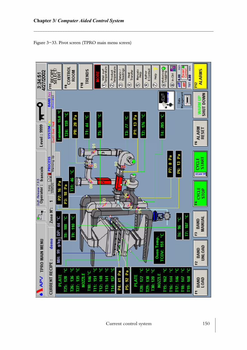
Current control system 150
Chapter 3/ Computer Aided Control System________________________________________________________________________
Figure 3−33. Pivot screen (TPRO main menu screen)
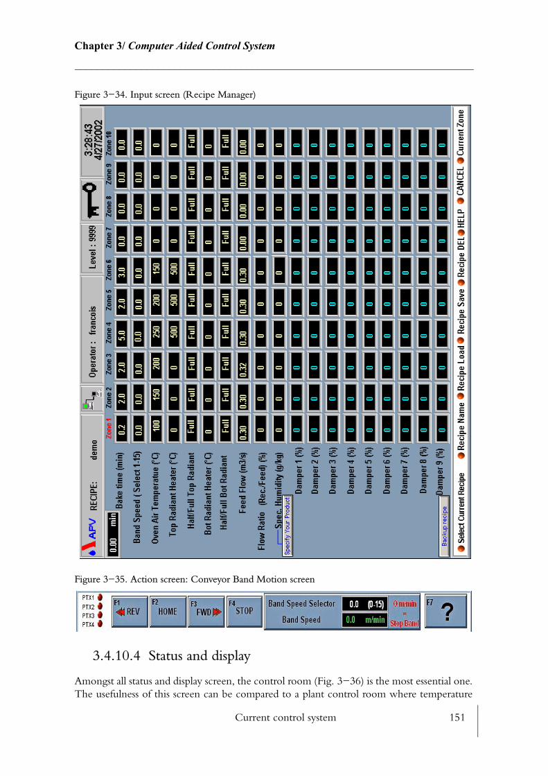
Current control system 151
Chapter 3/ Computer Aided Control System________________________________________________________________________
Figure 3−34. Input screen (Recipe Manager)
Figure 3−35. Action screen: Conveyor Band Motion screen
3.4.10.4 Status and display
Amongst all status and display screen, the control room (Fig. 3−36) is the most essential one. The usefulness of this screen can be compared to a plant control room where temperature
Current control system 152
Chapter 3/ Computer Aided Control System________________________________________________________________________
gauge, meter readings can be overview and the functioning of the process can be verified (Fig. 3−36). The two sliders on the left hand−side of the screen as well as the button ‘FAN MOTOR STATUS’ permits total control of the two fan motor inverters. The two fan inverters can be controlled manually to allow low air flow set−up where the pressure instru−mentations is not stable or when high rate of humidity is used and condensates inside the Pitot tubings. The next two screens (Heaters PID control and Steam Valve PID control) are two ActiveX control that acts similarly as a hard PID control. P, I, D, control gain Kd and derivative time Tc can be changed manually, however their values have been optimised within InControlTM. The damper settings have also been programmed so they could be actuated through this interface, however they are still operated manually today. The feed flow rate is displayed at the centre of this screen and indicates in real−time the feed flow rate in the main feed duct. Five thermometers indicates the sheath temperature of the duct heater and the radiant heater. The coloured status indicator below the thermometer displays how critical the temperature of the sheath is (blue is fine, red is critical). The squared coloured indicator below the status indicator displays the power delivered in real time. At the time this screenshot was taken 132kW were used. The other menu buttons are similar to the ‘MAIN MENU’ screen.
3.4.10.5 Help Screen
Numerous help screen were created to help the user to understand how to make the best of this interface and how to commute information between the various screens. Fig. 3−37shows the help screen that is used to assist the user with the ‘MAIN MENU’ screen. Each of the major screen had a help screen such as this one. However, more details could be found by clicking the button 5 of the ‘MAIN MENU’ screen (Manuals Help). The manual con−tains the instructions for maintenance and repairs of the various parts of the oven and also how to operate the software and understand the meaning and the interpretation of the data that have been logged. The various strategy established for the control of fan, humidity, tem−perature are explained and the main governing heat transfer equations are also highlighted.
3.4.10.6 Trending and data acquisition
Real time trending is one of the most important graphing features as it allows to understand in real time how things are changing, when a set−point is altered for instance. This tech−nology is a breakthrough for the future of baking as internal product temperature can be logged and related to events and changes in the oven settings. The ‘CURRENT ZONE’ screen (Fig. 3−38) permits to follow in real time trends of the process variables compared to set−points. On the left hand−side of this screen the input box will change directly the cur−rent settings of the oven, i.e. it will overwrite the settings of the current zone. These real−time trends were found extremely useful for the optimisation of the PID settings in order to establish the tuning coefficients of the Ziegler−Nichols methodology.
Historical trending (Fig. 3−39) were used heavily in the screen design. Historical trend pro−vide a ‘snapshot’ of data from a time a date in the past. They are not dynamic. As opposed to real−time trends, historical trends will not update until it is required. Up to eight tagnames (pens) can be trended at one time.
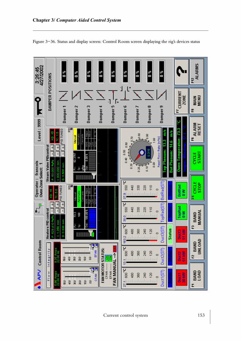
Current control system 153
Chapter 3/ Computer Aided Control System________________________________________________________________________
Figure 3−36. Status and display screen: Control Room screen displaying the rig’s devices status
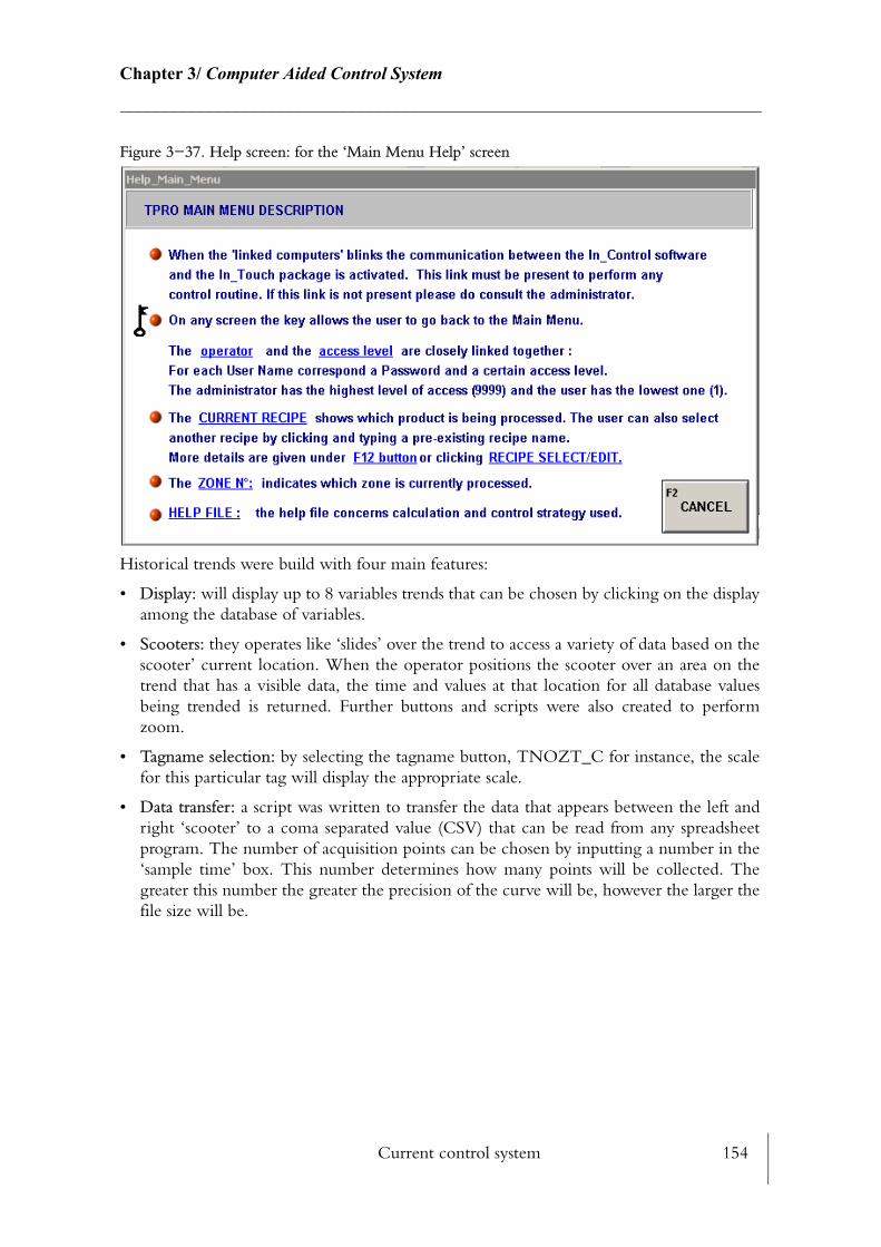
Current control system 154
Chapter 3/ Computer Aided Control System________________________________________________________________________
Figure 3−37. Help screen: for the ‘Main Menu Help’ screen
Historical trends were build with four main features:
• Display: will display up to 8 variables trends that can be chosen by clicking on the display among the database of variables.
• Scooters: they operates like ‘slides’ over the trend to access a variety of data based on the scooter’ current location. When the operator positions the scooter over an area on the trend that has a visible data, the time and values at that location for all database values being trended is returned. Further buttons and scripts were also created to perform zoom.
• Tagname selection: by selecting the tagname button, TNOZT_C for instance, the scale for this particular tag will display the appropriate scale.
• Data transfer: a script was written to transfer the data that appears between the left and right ‘scooter’ to a coma separated value (CSV) that can be read from any spreadsheet program. The number of acquisition points can be chosen by inputting a number in the ‘sample time’ box. This number determines how many points will be collected. The greater this number the greater the precision of the curve will be, however the larger the file size will be.
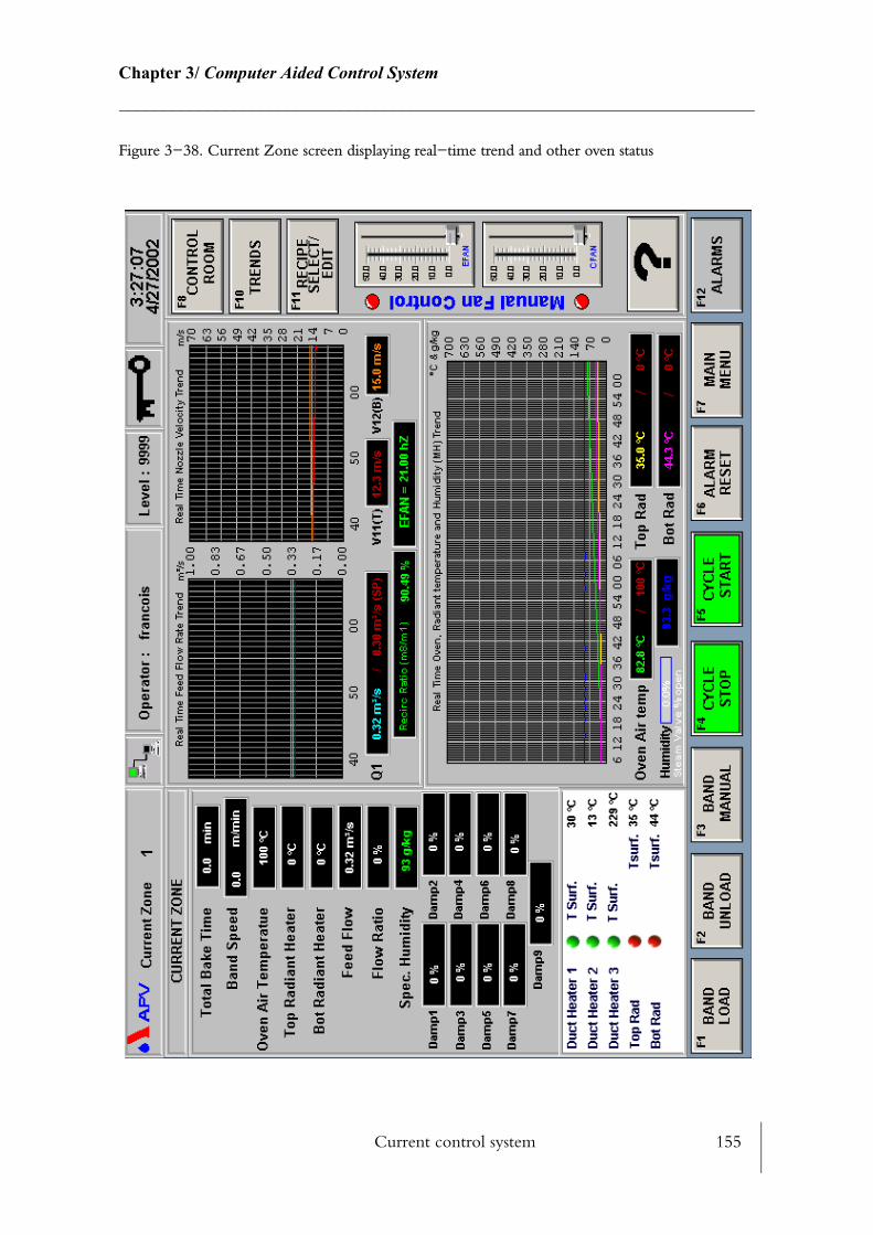
Current control system 155
Chapter 3/ Computer Aided Control System________________________________________________________________________
Figure 3−38. Current Zone screen displaying real−time trend and other oven status
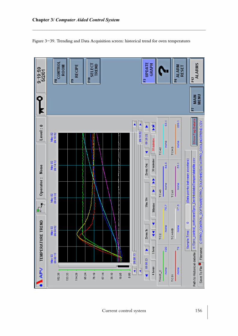
Current control system 156
Chapter 3/ Computer Aided Control System________________________________________________________________________
Figure 3−39. Trending and Data Acquisition screen: historical trend for oven temperatures

Current control system 157
Chapter 3/ Computer Aided Control System________________________________________________________________________
3.4.10.7 Data management
Data management played a great role in the non food test (NFT) and food test (FT) organ−isation. A total of 12Gb of data were collected during both these test phases. Not only files had to be saved on a regular basis but they also had to be organised in a structured way and backed up. The data management platform (Fig. 3−40) was constructed to help this organ−isation. On the left hand−side of this screen each machines is monitored for hard disk space. This is especially critical for the server which performs the data backup. A menu button selection (Test Type and Medium Used) creates the appropriate architecture of data on the PC hard disk and permits the classification of the collected data. When data is categorised the server can effectuate the backup of the data. For each set of test the InTouchTM raw data were compressed and backed up to the server.
Figure 3−40. Data Management screen
Objectives and pathways 158
Chapter 4/ TPRO Commissioning and Performance Envelope________________________________________________________________________
CHAPTER 4
TPRO COMMISSIONING AND PERFORMANCE ENVELOPE
This chapter describes the experimental setup as well as the results of the preliminary tests that were required during the commissioning phase of this project and six test phases whose purpose was to quantify the TPRO performance envelope. These non−food tests (NFT) did not involve bak−ing food product and their main objective was to establish the TPRO performance envelope and reveal how well the TPRO compares to the ‘preliminary requirements’.
4.1 Objectives and pathways
A series of preliminary tests were undertaken, the non−food tests (NFT) to establish the TPRO operating performance. In this context, the ‘performance envelope’ is defined as series of six test phases which quantified the thermal performance of the test rig over the achievable process variables (oven air temperature, air velocity, radiant heater surface tem−perature, humidity and band speed).
Ultimately performance curves generated for the TPRO enable comparing with full scale travelling ovens. Analogous curves are required for APV’s full−scale ovens. In reality, very little accurate information exists for APV’ s full scale ovens, and experimental data would have to be collected to enable accurate comparisons. This translation issue (from TPRO to full−scale oven) was not included in the scope of this work, but will be an important part for further work (See 7.2).
Two main families of data were collected; (i) to reveal how close preliminary requirements were respected, and (ii) to provide a basic understanding of the TPRO functionality. Data collection could take several days or just a few minutes, so the test phases were planned in a careful manner so that as much information could be collected per test. As rates of change (temperature, humidity) were most likely to differ from one range of baking temperature to
Definition of test setup and variable measured 159
Chapter 4/ TPRO Commissioning and Performance Envelope________________________________________________________________________
another, three different temperature ranges were studied which are representative of a wide range of baking temperature; 160oC, 220oC, and 280oC. To compare the rate of temperature change that a full scale travelling oven would perform from one zone to another, the TPRO was submitted to set−point temperature change of 40oC from 160oC to 200oC; 220oC to 260oC; and 280oC to 320oC. These set−point changes were within established baking pro−files for most common food product, where zone temperature changes are of the order of 20−30oC.
For accuracy of post processed data, a sensitivity study was conducted. An examination of repeatability was also carried out on controlled variables in order to understand variability and establish a tolerance band for each variable. Instrumentation calibration was an issue during this phase and great care was taken to achieve optimum accuracy by: (i) re−position−ing sensors and instruments, (ii) modifying hardware, (iii) and calibrating instrumentation with established sources of measurement (See 3.4.5). The findings of these investigations were used directly in the InControl™ sub−routines for software calibration and data filtering purposes such as data smoothing and decimal precision.
To ease data capturing and analysis, a specific software platform were created to enable fast and reliable data transport between PC’s but also to format data in a usable and friendly way. As data could be logged for several days therefore generating a large amount of disk space (up to 1Gb per trial) automation of archives was a safe option. In order to facilitate the data analysis post processing was made in real time and derived data were calculated within InControl™ in specific sub−routines (See 3.4.7).
4.2 Definition of test setup and variable measured
The non−food tests were designed to provide a family of curves that would represent accu−rately the performance envelope of the TPRO. Each of the test phase were constructed to study a particular aspect of the TPRO. The non food test phase 0 (NFT_PHASE0) was built with the intention to understand and tackle the heat generation problem caused by both the fans. NFT_PHASE1 was created with the only purpose to figure out how to reach the fastest temperature rate of change inside the TPRO chamber. NFT_PHASE2 was built to develop a thermal energy balance of the TPRO and comprehend how and where the energy was dis−tributed in the TPRO rig. This thermal transient study would enable to picture which com−ponent of the rig is using most of the energy during both transient and steady state and also compute the total energy required to maintain the TPRO in thermal steady state. NFT_PHASE3 and NFT_PHASE4 were designed to study the influence of process variable parameters particularly with concerns with convective and radiative heat transfer to the product surface. Finally the goal of NFT_PHASE5 was to evaluate the maximum humidity rate of change and also control humidity level as preliminary desired.

Definition of test setup and variable measured 160
Chapter 4/ TPRO Commissioning and Performance Envelope________________________________________________________________________
Each of these test were repeated a number of times to enable to compute a ‘good’ average. The list of variable measured for each of these test phase is summarised by (Table 4−1).
4.2.1 NFT_PHASE0
4.2.1.1 Objective
During the phase of commissioning, the TPRO was tested over several days in full re−cir−culation mode at maximum fan speed (FIS) and without any heat input. The purpose was to test the reliability and robustness of the hardware and software. After thirteen hours run−ning in these conditions a thermal steady state regime was reached by both the air and the oven walls where the oven air temperature reached 95.2oC. In order to prove that the heat was not generated by current leakage from the heaters, the solid state relays controlling both duct heaters and radiant heaters were disconnected. The test was repeated several times to verify steady state results. The goal of this test was to understand, these incidental heat gain.
4.2.1.2 Test setup
As the only moving part during this test was the circulation and extraction fans, their speed was varied across their operating range to see the effect on the internal and external wall sur−face temperature. Temperatures were measured at different points within the ducts and wall surfaces (Fig. 4−1).
The thermocouple arrangement was the same as previously discussed in (See Fig. 2−17), but more thermocouples were fitted to sense the temperature at the internal wall surface , and between the walls , , in order to view the transient evolution of temperature across the wall (Fig. 4−1). The ‘stainless steel mass’ represents internal masses of steel such as reinforcement bars which are up to 30mm thick. was fitted on the external wall surface
Table 4−1. Non Food Test variables measurement
Test Phase Test target Variable measured and computed (derived)
NFT_PHASE0 Heat generation performance - temperatures (measured)
NFT_PAHSE1 Fastest temperature rate of change
- temperatures (measured)- temperature rates of change (derived)
NFT_PAHSE2 Develop an energy balance of the TPRO under both tran-sient and steady state
- energy (derived)- cumulated energy (derived)
NFT_PAHSE3 Study the effects of proc-ess variables on convection measurement
- convection heat transfer (measured and derived)- convective heat flux (measured)- radiation heat flux (measured)
NFT_PAHSE4 Study the effects of proc-ess variables on radiation measurement
- convection heat transfer (measured and derived)- convective heat flux (measured)- radiation heat flux (measured)
NFT_PAHSE5 Evaluation of maximum hu-midity rate of change and controlled humidity levels
- mixed humidity (measured)- mixed humidity rate of change (derived)
TC40TC42 TC41
TC39
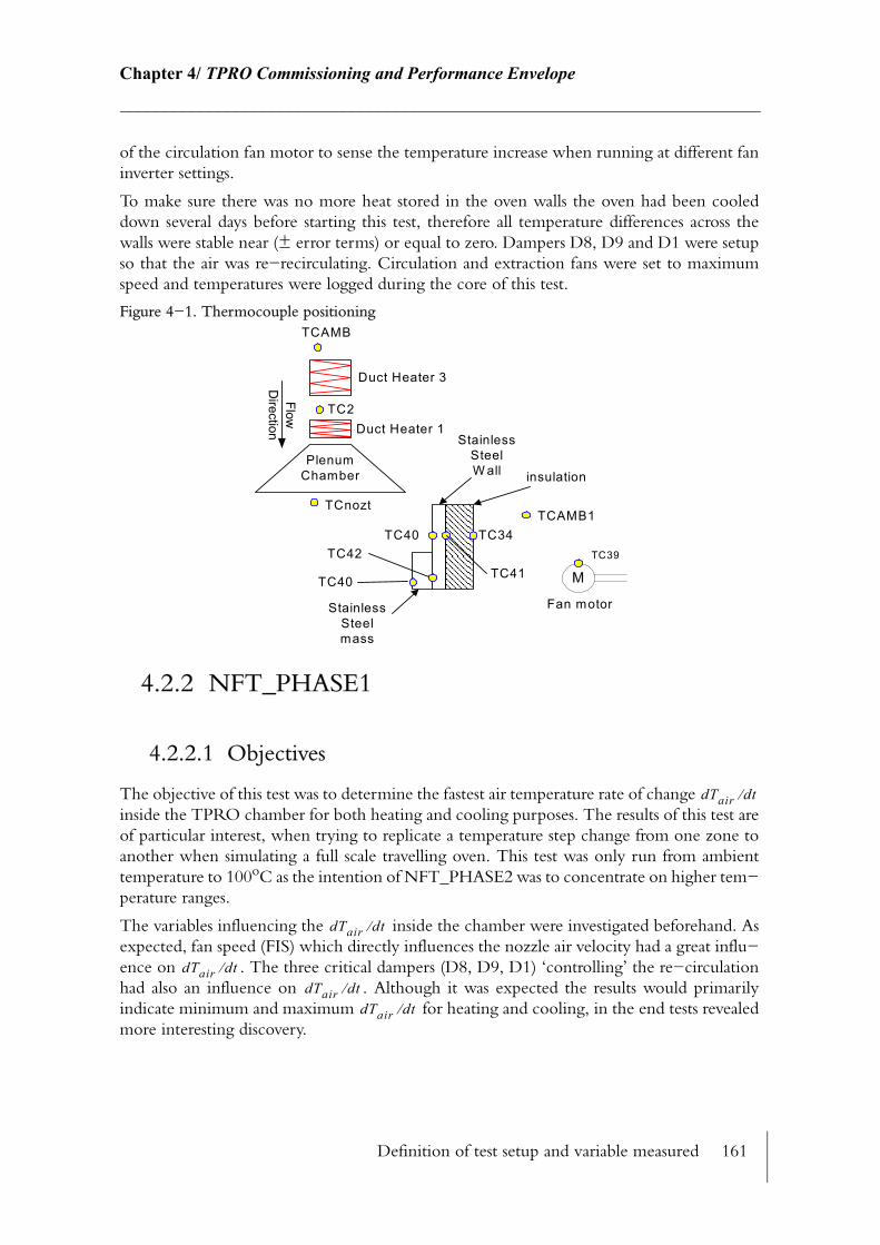
Definition of test setup and variable measured 161
Chapter 4/ TPRO Commissioning and Performance Envelope________________________________________________________________________
of the circulation fan motor to sense the temperature increase when running at different fan inverter settings.
To make sure there was no more heat stored in the oven walls the oven had been cooled down several days before starting this test, therefore all temperature differences across the walls were stable near (± error terms) or equal to zero. Dampers D8, D9 and D1 were setup so that the air was re−recirculating. Circulation and extraction fans were set to maximum speed and temperatures were logged during the core of this test.
Figure 4−1. Thermocouple positioning
4.2.2 NFT_PHASE1
4.2.2.1 Objectives
The objective of this test was to determine the fastest air temperature rate of change inside the TPRO chamber for both heating and cooling purposes. The results of this test are of particular interest, when trying to replicate a temperature step change from one zone to another when simulating a full scale travelling oven. This test was only run from ambient temperature to 100oC as the intention of NFT_PHASE2 was to concentrate on higher tem−perature ranges.
The variables influencing the inside the chamber were investigated beforehand. As expected, fan speed (FIS) which directly influences the nozzle air velocity had a great influ−ence on . The three critical dampers (D8, D9, D1) ‘controlling’ the re−circulation had also an influence on . Although it was expected the results would primarily indicate minimum and maximum for heating and cooling, in the end tests revealed more interesting discovery.
TC39
M
Fan motor
PlenumChamber
TCAMB
TC2
TCnozt
TC40 TC34TCAMB1
TC41
insulation
StainlessSteelW all
StainlessSteelmass
TC42
TC40
Duct Heater 3
Duct Heater 1
FlowD
irection
dTair dt⁄
dTair dt⁄
dTair dt⁄dTair dt⁄
dTair dt⁄

Definition of test setup and variable measured 162
Chapter 4/ TPRO Commissioning and Performance Envelope________________________________________________________________________
4.2.2.2 Test setup
The starting points of each test were similar as for NFT_PHASE0. The oven was let to cool naturally or using assisting cooling using a flexible conduit connected to the inlet duct, thereby, drawing cold air from the outside of the FPC. Dampers (D8, D9, D1) were set at a fixed settings during the entire test. After the fans speed (FIS) had risen to their maximum controlled frequency the TPRO temperature set−point was instantly changed to 100oC.
After the top nozzle temperature had reached the target, the set−point was dropped to 0oC in order to cut−out the heater power. The oven was allowed to cool down in order to meas−ure the during the cooling section. The appropriate temperatures were logged during both the heating and the cooling phases and their were computed in real−time. Base case were established beforehand, however the findings during testing raised the interest in building other scenarios, (see Table 4.2.3 and results). A test matrix was designed for two variables, fan speed (FIS) and dampers settings.
Three fan speed (FIS) were used respectively 5, 30 and 50Hz and dampers were only allowed to vary between fully open (FO) or fully closed (FC) settings. This choice was to reduce the number of experiments as the aim was to understand the trends, and not to understand behaviours at intermediate damper settings.
Another expectation of these results was to understand how dampers and flow could be automated together to give the fastest . During pre−trials it was discovered that par−ticular settings (fan speed (FIS) = 5Hz, D8=FC, D9=FO, D1=FO) (Table 4.2.3) were not able to produce the required 100oC limit. Before reaching the targeted set−point, the duct heater solid state relays tripped as the heaters were over heating locally due to a lack of air flow across the duct heater elements. This indicates that a minimum air flow has to be main−tained across the duct heater elements in order to function properly. A continuous use of these heaters in this regime would have damaged them and reduced their lifetime signifi−cantly.
Table 4−2. NFT_PHASE1: Base Case Scenarios
NFT_PHASE1: Optimum Temperature Rate of Change (Base Case)
5Hz 30Hz 50HZ
D8D9D1
FOFCFO
T1
FOFCFO
T2
FOFCFO
T3
D8D9D1
FOFOFO
T4
FOFOFO
T5
FOFOFO
T6
D8D9D1
FCFOFC
T7
FCFOFC
T8
FCFOFC
T9
D8D9D1
NONEFCFOFO
T10
FCFOFO
T11
dTair dt⁄dTair dt⁄
dTair dt⁄
Definition of test setup and variable measured 163
Chapter 4/ TPRO Commissioning and Performance Envelope________________________________________________________________________
4.2.3 NFT_PHASE2
4.2.3.1 Objectives
This test had two major objectives; (i) to assess the from ambient to respectively 160oC, 220oC and 280oC and for a temperature step change from 160oC to 200oC, 220oC to 260oC and 280oC to 320oC; and (ii) to study the energy balance of the TPRO rig during the same temperature step change (both transient and steady state).
An energy balance was computed in real time for both transient and steady state conditions with the intention to study; (i) the distribution of heat into the different location of the framework, (ii) the useful energy to keep the air at constant temperature, and (iii) the heat losses from the wall and air leakages.
Not only was it expected to see the different oven components (steel wall, insulation wall, uncovered steel masses within chamber) and their ‘heat allocation’ but also to show the dif−ferent type of heat losses due to leakages, convection and radiation. The total and cumulated energy was also computed transiently and for thermal steady state. Cumulated values have a particular interest when associated to cost, as they can highlight which part of the rig takes most of the energy i.e. which is the most expensive to run. During the second section data were collected to compute the for both heating and cooling. To allow a good aver−age of the temperature rate of changes five repeats were performed (Fig. 4−2).
4.2.3.2 Test setup
The test set−up were following exact procedures to enable an easy data comparison. In the first section (Fig. 4−2) the TPRO rig had to be cooled down to ambient conditions and the preparation were identical as explained in NFT_PHASE1. Dampers D8, D9, D1 were set respectively to FC, FO, FO with respect to the result of the previous test phase. After the temperature had reached its targeted set−point the dampers were set to full recirculation mode.
In order to compare the energy distribution and the cumulated energy, for each of the heat−ing section of the first section (Fig. 4−2) at the different studied temperature, the counters dealing with cumulated calculations were set to zero to start the test. Data were recorded as long as needed so that the TPRO system achieved thermal equilibrium. Once this equilib−rium was reached, the counters were turned off and the logging stopped. Thereafter, data were stored and compressed for latter analysis. The pie charts (Fig. 4−2) is only for illustrative purposes, however, each sector represent the percentage of the total energy cumulated of an individual items of the energy balance, (e.g. percentage of energy stored in the insulation wall, leakages...).
During the second section the oven had already been heated up and care was taken to make sure that the oven remained in thermal steady state, i.e. that the balance at the end of first section was still in equilibrium. In the case where the thermal equilibrium had been dis−rupted (door, damper opening), sufficient time (t0) was left so that the TPRO reach thermal steady state before starting the second test section. The settings of the second section were identical to the first section.
dTair dt⁄
dTair dt⁄
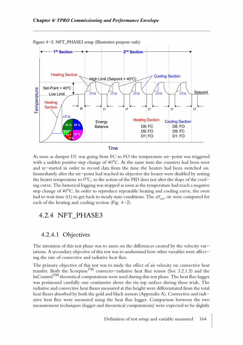
Definition of test setup and variable measured 164
Chapter 4/ TPRO Commissioning and Performance Envelope________________________________________________________________________
Figure 4−2. NFT_PHASE2 setup (Illustrative purpose only)
As soon as damper D1 was going from FC to FO the temperature set−point was triggered with a sudden positive step change of 40oC. At the same time the counters had been reset and re−started in order to record data from the time the heaters had been switched on. Immediately after the set−point had reached its objective the heater were disabled by setting the heater temperature to 0oC, so the action of the PID does not alter the slope of the cool−ing curve. The historical logging was stopped as soon as the temperature had reach a negative step change of 40oC. In order to reproduce repeatable heating and cooling curve, the oven had to wait time (t1) to get back to steady state conditions. The were computed for each of the heating and cooling section (Fig. 4−2).
4.2.4 NFT_PHASE3
4.2.4.1 Objectives
The intention of this test phase was to assess on the differences created by the velocity var−iations. A secondary objective of this test was to understand how other variables were affect−ing the rate of convective and radiative heat flux.
The primary objective of this test was to study the effect of air velocity on convective heat transfer. Both the ScorpionTM convecto−radiative heat flux sensor (See 3.2.1.5) and the InControlTM theoretical computations were used during this test phase. The heat flux logger was positioned carefully one centimetre above the tin top surface during these trials. The radiative and convective heat fluxes measured at this height were differentiated from the total heat fluxes absorbed by both the gold and black sensors (Appendix A). Convective and radi−ative heat flux were measured using the heat flux logger. Comparison between the two measurement techniques (logger and theoretical computations) were expected to be slightly
Tem
pera
ture
Time
High Limit (Setpoint + 40oC)
Low Limit
∆T/∆t
∆T/∆t ∆T/∆t ∆T/∆t ∆T/∆t ∆T/∆t
25 % 25 %
25 %10 %
10 %5 %
t1 t1 t1 t1 t1
D8: FCD9: FOD1: FO
Set-Point + 40oC
HeatingSection
Heating Section Cooling Section
EnergyBalance
Heating Section Cooling Section
1St Section 2nd Section
D8: FOD9: FCD1: FO
t0
Setpoint
dTair dt⁄

Definition of test setup and variable measured 165
Chapter 4/ TPRO Commissioning and Performance Envelope________________________________________________________________________
different. As far as convection is concerned, theoretical computations are evaluating the static peak heat transfer coefficient, which is assumed for a given height and straight below the nozzle, however the logger measures a dynamic average heat transfer coefficient that is meas−ured at a given height but underneath several rows of nozzle (forward and reverse movement of the conveyor band). For these reasons the projected heat transfer coefficient from the logger (non static) should be lower in absolute value than in the theoretical computations (static). Due its mass and slow response time convective heat transfer peaks should also be more even. For radiation, the mathematical model used to estimate the view factor was taking consideration of both direct radiation from the radiant heater surfaces but also the indirect radiation from he reflector surface and background from plenums. However, every other oven wall surfaces were ignored in these theoretical computations (side, top bottom walls of the baking chamber as well as the plenums surfaces).
4.2.4.2 Test setup
Before starting this test the oven had to settle down at the same air velocity and temperature in order to achieve thermal steady state. Internal wall surface temperatures as well as oven air temperature fluctuations were logged. Steady state conditions were monitored so that each start were achieved in the same thermal conditions every time. The band was then moved forward and the oven door was closed. Subsequently the door was opened and the logger was positioned rapidly on the tray and centered on the conveyor band. At the same instance as the door was shut, the band was triggered to travel backwards and forwards at a constant speed (2 on the software selection). Heat flux logger and InTouch™ were not exactly in phase while recording data however this gap was latter adjusted in the data post processing phase. Three different fan speed (FIS) were used during this trial, respectively 5, 30 and 50Hz. As perturbations were established while opening and positioning the heat flux logger onto the conveyor band, the sensor was allowed to stay longer (eight minutes) at the 5Hz fan speed (FIS) as it would take longer for its temperature to reach steady state (Fig. 4−3). After 8 minutes had elapsed, the fan speed (FIS) was set to 30Hz for 6 minutes then the fan speed (FIS) were set to 50Hz for 6 minutes. Afterwards, the band was stopped and the logger was removed from the conveyor band. Data acquisitions were then stopped.
The logger was extracted from its thermal barrier and two fans were blowing onto both the logger and the thermal barrier to facilitate the cooling process and get ready for the next trial. Data were downloaded from the heat flux logger and were added to the InTouch™data for compression and latter analysis.
Throughout this test the oven temperature remained constant and was controlled via PID The three steady state temperatures were tested, 160oC, 220oC, ad 280oC (Fig. 4−3).
Five repeats were established for each of the three temperatures studied to achieve a ‘good’ average.
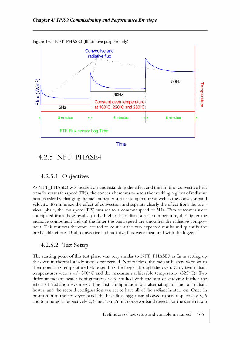
Definition of test setup and variable measured 166
Chapter 4/ TPRO Commissioning and Performance Envelope________________________________________________________________________
Figure 4−3. NFT_PHASE3 (Illustrative purpose only)
4.2.5 NFT_PHASE4
4.2.5.1 Objectives
As NFT_PHASE3 was focused on understanding the effect and the limits of convective heat transfer versus fan speed (FIS), the concern here was to assess the working regions of radiative heat transfer by changing the radiant heater surface temperature as well as the conveyor band velocity. To minimize the effect of convection and separate clearly the effect from the pre−vious phase, the fan speed (FIS) was set to a constant speed of 5Hz. Two outcomes were anticipated from these results; (i) the higher the radiant surface temperature, the higher the radiative component and (ii) the faster the band speed the smoother the radiative compo−nent. This test was therefore created to confirm the two expected results and quantify the predictable effects. Both convective and radiative flux were measured with the logger.
4.2.5.2 Test Setup
The starting point of this test phase was very similar to NFT_PHASE3 as far as setting up the oven in thermal steady state is concerned. Nonetheless, the radiant heaters were set to their operating temperature before sending the logger through the oven. Only two radiant temperatures were used, 300oC and the maximum achievable temperature (525oC). Two different radiant heater configurations were studied with the aim of studying further the effect of ‘radiation evenness’. The first configuration was alternating on and off radiant heater, and the second configuration was set to have all of the radiant heaters on. Once in position onto the conveyor band, the heat flux logger was allowed to stay respectively 8, 6 and 6 minutes at respectively 2, 8 and 15 m/min. conveyor band speed. For the same reason
Flux
(W/m
2 )
Time
Temperature
5Hz
30Hz
50Hz
Convective andradiative flux
Constant oven temperatureat 160oC, 220oC and 280oC
8 minutes 6 minutes 6 minutes
FTE Flux sensor Log Time

Definition of test setup and variable measured 167
Chapter 4/ TPRO Commissioning and Performance Envelope________________________________________________________________________
as explained before the test was repeated five times at both 300oC and the maximum radiant temperature 525oC
Figure 4−4. NFT_PHASE4 (Illustrative purpose only)
After each trial the oven was allowed to return into thermal steady state before starting the next trial. Internal wall surface temperature as well as radiant surface temperature were mon−itored to help take this decision. Before starting this test phase preliminary trials were com−pleted and revealed that the maximum achievable radiant heater surface temperature under low air flow movement was 525oC.
4.2.6 NFT_PHASE5
4.2.6.1 Objectives
The main intention of NFT_PHASE5 was to determine the fastest humidity rate of change close to the product surface and to discover the maximum achievable humidity rate of change inside the chamber. As described in Chapter 3 (See 3.4.8.5.2), the TPRO was fitted with a humidity probe (HygroxCTM) to help perform the control decisions, however, this sensor was away from the food surface and was only indicating the humidity level in the higher areas (near the extraction points) of the TPRO chamber. A portable humidity (HygroxP2TM) sensor was used to estimate mixed humidity levels closer to the product.
4.2.6.2 Test setup
In order to establish a correction factor that could be applied to the HygroxCTM real time data, for any particular fan speed (FIS) and temperature, so that HygroxCTM data matches HygroxP2TM data, a test matrix was created for four different temperatures, respectively, 120, 160, 200, 240oC, and five fan speed (FIS): 3, 5, 10, 30, and 50Hz. With the purpose of
Flux
(W/m
2 )
Time
Radiant elem
ent surfaceTemperature
300oC 1/2 or full
Max Tp 1/2 or full
BandSpeed2m/min
8m/min
2m/min
8m/min
15m/min15m/min
8 minutes
FTE Flux sensor Log Time
6 minutes 6 minutes 8 minutes 6 minutes 6 minutes
Time

Sensitivity study 168
Chapter 4/ TPRO Commissioning and Performance Envelope________________________________________________________________________
creating a reliable, repeatable and precise correction factor, each of these tests were repeated three times.
The oven was set in thermal steady state before starting this test. During this time the logger was configured to be sent in the oven. Once ready both InTouch™ historical logging and HygroxP2TM logger were recording data. The steam was injected straight after the logger had been positioned onto the conveyor band. During these trials the mixed humidity set−point was set to 700g/kg which is well above traditional mixed humidity level encountered in conventional baking ovens. The instant the mixed humidity level had reached its objective, the set−point was dropped to zero and the dampers D8, D9, D1 were set for full extraction to respectively FO, FC, FO. The data were recorded until the mixed humidity concentration had reached starting level for dry air. The oven was let to settle for a time (t1) and reach ther−mal steady state before starting the next trial.
Figure 4−5. NFT_PHASE5 (Illustrative purpose only)
Several days were required to conduct this test phase as a total of twelve tests were processed for each set of five fan speed (FIS) (Fig. 4−5).
4.3 Sensitivity study
A ‘Sensitivity Study’ was conducted to examine the degree of responsiveness of measured and derived variables submitted or not to changes in ‘environmental’ conditions. The pur−pose of conducting such a study was primarily to establish precision levels for the measuring variables and derived variables. It is particularly important to determine how precise meas−urements are, as the lower the precision, the more difficult the data interpretation. Under−standing how ‘noisy’ the data are is crucial and data ‘noise treatment’ by data filtering can help to significantly improve the accuracy of data capture. Precise measurement is charac−terised by good repeatability and reproducibility. The two concepts, can also be found under
Mix
ed H
umid
ity (g
/kg)
T ime
Mc Queen Cairns Humidity Sensor Log Time
120oC
160oC
240oC
W aiting time for steady state conditions
220oC
t1 t1 t1 t1
Sensitivity study 169
Chapter 4/ TPRO Commissioning and Performance Envelope________________________________________________________________________
the name of validity and reliability. The repeatability (validity) measures how close successive measurements results of the same instrument carried out under the same conditions. The definition of reproducibility (reliability) is similar as it measures the closeness of measure−ments of the same instruments however the conditions of measurements are carried out under changed conditions of measurements. Taylor and Kuyatt, 1994 [131] have defined the repeatability and reproducibility conditions in those terms:
• Repeatability conditions (validity) implies:− Same measurement procedure
− Same observer
− Same measuring instrument used under the same conditions
− Same location
− Repetition over a short period of time
• Reproducibility conditions (reliability) implies:− Principle of measurement
− Method of measurement
− Observer
− Measuring instrument
− Reference standard
− Location
− Condition of use
− Time
True value of the measurement is not as important as repeatability and reproducibility. Indeed, a value can be very accurate to five significant figures, however if the same meas−urement is varying greatly from day to day or changes within the same test, comparison and interpretation of result is made very difficult. In the world of industrial baking, instrumen−tation fitted in ovens are often not calibrated and overall maintenance of instrumentation is very poor. However, as each zones operates in steady state regime, temperature, pressure variation are more likely to be very small and the overall product results is repeatable enough to be profitable on the market.
Only repeatability was investigated in the core of this sensitivity study. It is common to accept repeatability values within 5%.
4.3.1 Data processing technique
In order to pursue this study, instruments were calibrated (See 3.4.5), and data had to be pre−processed. In this case pre−processing means that data were collected in a certain fashion and treated adequately for precision and noise reduction.
As the calculation indicated earlier only involves transient computation, data were captured and distributed into two arrays which respectively represent the instant and the instant
. k
k 1+
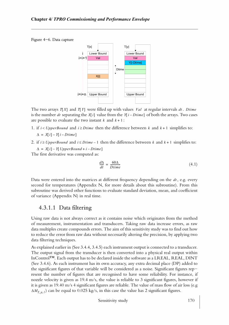
Sensitivity study 170
Chapter 4/ TPRO Commissioning and Performance Envelope________________________________________________________________________
Figure 4−6. Data capture
The two arrays and were filled up with values at regular intervals . is the number separating the value from the of both the arrays. Two cases are possible to evaluate the two instant and :
1. if and then the difference between and simplifies to:
2. if and then the difference between and simplifies to:
The first derivative was computed as:
(4.1)
Data were entered into the matrices at different frequency depending on the , e.g. every second for temperatures (Appendix N, for more details about this subroutine). From this subroutine was derived other functions to evaluate standard deviation, mean, and coefficient of variance (Appendix N) in real time.
4.3.1.1 Data filtering
Using raw data is not always correct as it contains noise which originates from the method of measurement, instrumentation and transducers. Taking raw data increase errors, as raw data multiples create compounds errors. The aim of this sensitivity study was to find out how to reduce the error from raw data without necessarily altering the precision, by applying two data filtering techniques.
As explained earlier in (See 3.4.4, 3.4.5) each instrument output is connected to a transducer. The output signal from the transducer is then converted into a physical real output within InControl™. Each output has to be declared inside the software as a LREAL, REAL, DINT (See 3.4.6). As each instrument has its own accuracy, any extra decimal place (DP) added to the significant figures of that variable will be considered as a noise. Significant figures rep−resent the number of figures that are recognised to have some reliability. For instance, if nozzle velocity is given as 19.4 m/s, the value is reliable to 3 significant figures, however if it is given as 19.40 m/s 4 significant figures are reliable. The value of mass flow of air loss (e.g
) can be equal to 0.025 kg/s, in this case the value has 2 significant figures.
T[x] T[y]
Upper Bound Upper Bound
Lower BoundLower Bound
Dtime
Vali
i=i+1
i=i+n
ValY[i-Dtime]
X[i]
T X[ ] T Y[ ] Val dt Dtimedt X i[ ] Y i Dtime–[ ]
k k 1+
i UpperBound< i Dtime≥ k k 1+
∆ X i[ ] Y i Dtime–[ ]–=
i UpperBound≥ i Dtime 1–≤ k k 1+
∆ X i[ ] Y UpperBound i Dtime–+[ ]–=
d∆dt------- 60∆
Dtime----------------=
dt
∆MT p l, ,

Sensitivity study 171
Chapter 4/ TPRO Commissioning and Performance Envelope________________________________________________________________________
The other data filtering technique applied to the data was a ‘smoothing factor’ to even out the numbers. This factor was based on a moving average of the set of data considered. For instance a value collected every second and assigned with a ‘smoothing factor’ of 10 would be represented by an averaged value over the last 10 seconds (‘smoothing factor’ based on 10 points). (See Appendix N).
Accuracy of devices were taken as a reference to help choose the right number of significant figures. For thermocouples, one dp is advisable and any extra dp would add noise to the sig−nal, as accuracy was given from the supplier to 1 dp as well. For pressure measurement, each instrument was calibrated separately, with benchmarked instruments. Pitot tube at nozzle measurement were given as ±0.48Pa (See pressure calibration Appendix D). However the accuracy for an averaging or a straight Pitot tube might be altered depending on the sensor position in the flow.
4.3.2 Results of sensitivity study
4.3.2.1 Temperature measurement
‘Smoothing factors’ applied to temperature measurement were treated case by case. Depending on the measurement purpose of specific temperature, an appropriate ‘smoothing factor’ was applied. The decision for choosing a small or large ‘smoothing factor’ was related to the thermal regime that the temperature measurement is representing. The nozzle tem−perature for instance is more likely to vary accordingly to the heaters switching rate, therefore the ‘smoothing factor’ should be small in order to characterise fast changes, however the ‘smoothing factor’ used for the measurement of external wall surface temperature should be high in order to avoid unwanted variation, as it is a slow transient process. Even small vari−ations due to noisy signal can have a significant effect on the long term cumulative energy balance.
The two graphs represented by Fig. 4−7 show the top plenum nozzle temperature TNOZTC, the filtered nozzle temperature TNOZTCM (computed) and the duct heater 3 power input. The energy cumulated by the duct heater 3 is the integration of all the power input peaks over the entire test period. This test was performed under steady state conditions, although the nozzle temperature varies slightly (1.5oC). This small variation is entirely due to the heater switching rate as it matches the switching time of the duct heater. With 5 points smoothing Fig. 4−7(a), all the temperature peaks seems to match exactly with the heater switching rate. As expected with more points for the smoothing factor Fig. 4−7(b) the tem−perature response is attenuated. As the nozzle temperature rate of change was one of the critical requirement, ‘smoothing factor’ based on 5 points were chosen.
4.3.2.2 Pressure measurement
All pressure points were rounded to 1 decimal place after an investigation was carried out to prove there was very little difference on the pressure measurement standard error between 1 dp and more. Moreover the largest fall in standard error occurred between 0 dp and 1 dp. This test was carried out under controlled temperature settings and fixed fan inverter settings.

Sensitivity study 172
Chapter 4/ TPRO Commissioning and Performance Envelope________________________________________________________________________
Six different ‘smoothing factors’ were tried out and an analysis of the standard deviation allowed to conclude which factor was most adequate for this measurement.
Figure 4−7. ‘Smoothing factor’ for the nozzle temperature based on 5 and 40 points
The standard deviation between both the pressure measurement PTX1 and PTX5 (Table 4−3) are very different. Pressure measurement (PTX1) consists of five averaging Pitot tubes across the main feed duct width. From this average pressure is derived the air flow in the main feed duct where the flow is most likely to be laminar as a honeycomb grid allows to straighten the flow lines. However, the larger deviation in the measure of nozzle pressure outlet (PTX5) relates to a more complex flow pattern around this Pitot tube.
‘Smoothing factor’ based on 40 points was used for both pressure measurement as the stand−ard deviation did not decrease greatly for either 60 or 120 points.
Table 4−3. Analysis of the standard deviation for the ‘smoothing factor’ based on 0, 5,10,40,60, and 120 points, respectively for the measurement of PTX1 and PTX5
Smoothing factor based on x points 0 5 10 40 60 120
STDEV (PTX1) 0.38 0.24 0.18 0.09 0.09 0.05
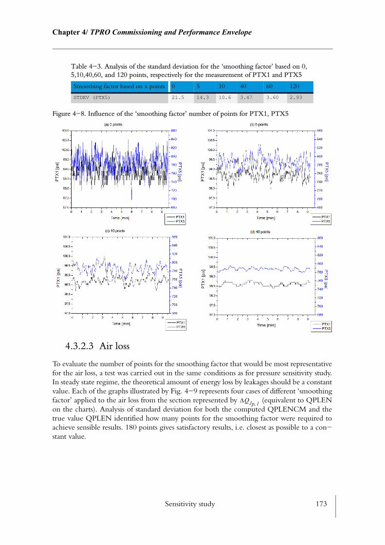
Sensitivity study 173
Chapter 4/ TPRO Commissioning and Performance Envelope________________________________________________________________________
Figure 4−8. Influence of the ‘smoothing factor’ number of points for PTX1, PTX5
4.3.2.3 Air loss
To evaluate the number of points for the smoothing factor that would be most representative for the air loss, a test was carried out in the same conditions as for pressure sensitivity study. In steady state regime, the theoretical amount of energy loss by leakages should be a constant value. Each of the graphs illustrated by Fig. 4−9 represents four cases of different ‘smoothing factor’ applied to the air loss from the section represented by (equivalent to QPLEN on the charts). Analysis of standard deviation for both the computed QPLENCM and the true value QPLEN identified how many points for the smoothing factor were required to achieve sensible results. 180 points gives satisfactory results, i.e. closest as possible to a con−stant value.
STDEV (PTX5) 21.5 14.3 10.6 3.47 3.60 2.93
Table 4−3. Analysis of the standard deviation for the ‘smoothing factor’ based on 0, 5,10,40,60, and 120 points, respectively for the measurement of PTX1 and PTX5
Smoothing factor based on x points 0 5 10 40 60 120
∆QJp l,

Sensitivity study 174
Chapter 4/ TPRO Commissioning and Performance Envelope________________________________________________________________________
Figure 4−9. Influence of the ‘smoothing factor’ number of points for QPLEN
4.3.2.4 Heat transfer coefficient
Convective heat transfer coefficient for both the wall surfaces heat losses and the nozzle outlet heat transfer coefficient were also assigned with a ‘smoothing factor’ in order to obtain a better average. Yet again, the choice of the ‘smoothing factor’ for both of them was driven by the prediction of the results. Although the standard deviation for the raw heat transfer calculation HNOZT is already low (STDEV = 0.5), 40 points were taken for evaluating the computed average HNOZTMEAN. This ‘smoothing factor’ was applied to counteract the effect of nozzle velocity variation.
During the course of this test (10 minutes), the surrounding conditions were unchanged as well as the external surface temperature, so expected theoretical convective heat transfer at the external wall surface should be constant. Thus, 120 points were used for smoothing the curve as it reflects theoretical belief.
The same approach was followed for all other variables. Appendix C shows a summary of ‘smoothing factor’ and decimal place in use with other variables. Not every variable was attributed with a ‘smoothing factor’, and a few variables had to be declared twice for specific reasons. Indeed, nozzle outlet temperature, for instance had to be declared twice as it had ‘double usage’, control and calculation. In this particular case, as the oven temperature rate of change based on the nozzle outlet temperature had to be the highest, a different variable without ‘smoothing factor’ and using the same temperature measurement was chosen to effectuate the control of this temperature. As the moving average algorithm is applied in real time it can slow down the reaction of the true measurement (Fig. 4−10).

Sensitivity study 175
Chapter 4/ TPRO Commissioning and Performance Envelope________________________________________________________________________
Figure 4−10. Influence of the ‘smoothing factor’ number of points for HNOZT
4.3.2.5 Establishing the steady state, transient regime of the TPRO
In order to facilitate repeatable results it is essential to determine whether or not the rig operate in thermal steady state. Two experiments were conducted to establish the threshold of both first and second derivative of the total wall heat loss in order to decide when the rig was considered to be in steady state or transient regime. The first derivative of the total wall heat loss gives an estimate of the amount of energy which the rig is losing heat. The second derivative determines how quickly the heat is loss. Further experimentations were developed to study the effect of opening the door over a five minute period to destabilise the steady state regime and establish how long it would take to return to initial conditions.
4.3.2.5.1 Threshold determination for steady state and transient regime
To establish this threshold the oven was set to 120oC in full recirculation mode. The volume flow was controlled to 0.4 m3/s. First and second derivatives were logged as well as the sur−rounding air temperature and the total wall heat loss. Fig. 4−11 only relates to the data logged after the heat−up period.
Sensitivity study 176
Chapter 4/ TPRO Commissioning and Performance Envelope________________________________________________________________________
From 0 to 700 minutes, both the first and second derivative are stable. During this phase the the first derivative is averaging 0.275 MJ/min which represent about 4.6kW (Qloss) of total wall heat loss (includes, convection and radiation). The value of the second derivative is averaging around zero, which proves that the oven is losing heat at a constant rate, hence demonstrating steady state regime. The variation of the second derivative indicates the limit of the steady state regime (±0.005MJ2/min). During this phase the surrounding temperature (i.e the FPC temperature) is decreasing as a result of the ambient temperature decreasing due to nightfall. During this period the FPC battery heater control is switched off until the FPC temperature falls to 14oC.
From t = 700minutes onwards, the surrounding temperature increases from 14oC to 22oC in response to the FPC on/off temperature control. The reaction of the first derivative to this ambient condition change is almost instantaneous, however the second derivative takes longer to respond. The time delay between the first and the second derivative is caused by a large ‘smoothing factor’ which slows down the reaction time of this variable.
At 880 min. the FPC heater control switches off and the FPC temperature falls to 17oC. Eventually both the first and second derivative return to constant values.
As the temperature difference between the wall surfaces and the surrounding air decreases, the total heat loss from the wall decreases by 17% (from 4.6kW to 3.8kW). During this phase the duct heaters switching rate drops as a reaction of the increase in surrounding temperature.
4.3.2.5.2 Reaction to disturbance
The purpose of this test was to estimate the time it takes for the oven to ‘recover’ from fre−quent everyday disturbance such as door openings. To increase the chances to perform repeatable results, initial thermal test conditions had to be identical. This test was started in steady−state thermal conditions and the oven door was opened for five minutes then closed. Both total wall heat loss first derivative and internal wall surface temperature were plotted in order to judge the thermal state of the TPRO rig. This operation was repeated three times.
The starting point of Fig. 4−12 starts at the first door opening. As soon as the door is opened the internal wall surface temperature drops almost immediately, which causes the total wall losses to counteract and increase up to 5738W as a direct response of the PID duct heater control reactions.
As the door opens, the amount of cold air coming in, forces the oven air temperature to come down. The duct heater PID control algorithm reacts fast enough to cope with this new heat loss and maintains the oven temperature to its set−point.
Following the closing of the door, the total wall heat loss rate of change carries on increasing for a further 2 minutes. For each of the repeated test, it takes about the same amount of time (20 minutes) to recover completely from this disturbance.
In this situation, determining whether the TPRO rig operates in thermal steady state can be judged by the total heat loss first derivative. When this value oscillates around 0.28MJ/min ±0.005MJ/min2 the oven can be considered in thermal steady state. The stability of the internal wall surface temperature can also complement this analysis.
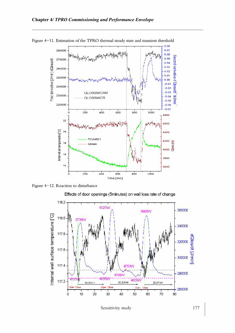
Sensitivity study 177
Chapter 4/ TPRO Commissioning and Performance Envelope________________________________________________________________________
Figure 4−11. Estimation of the TPRO thermal steady state and transient threshold
Figure 4−12. Reaction to disturbance
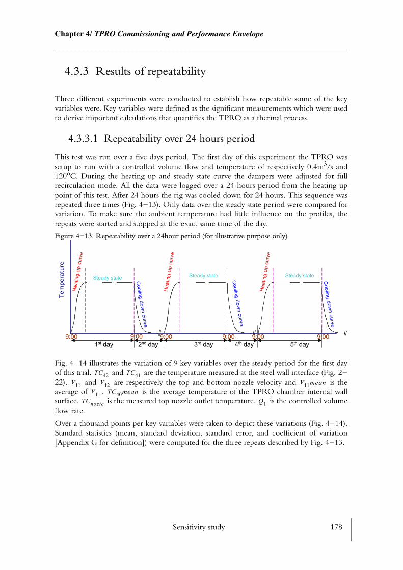
Sensitivity study 178
Chapter 4/ TPRO Commissioning and Performance Envelope________________________________________________________________________
4.3.3 Results of repeatability
Three different experiments were conducted to establish how repeatable some of the key variables were. Key variables were defined as the significant measurements which were used to derive important calculations that quantifies the TPRO as a thermal process.
4.3.3.1 Repeatability over 24 hours period
This test was run over a five days period. The first day of this experiment the TPRO was setup to run with a controlled volume flow and temperature of respectively 0.4m3/s and 120oC. During the heating up and steady state curve the dampers were adjusted for full recirculation mode. All the data were logged over a 24 hours period from the heating up point of this test. After 24 hours the rig was cooled down for 24 hours. This sequence was repeated three times (Fig. 4−13). Only data over the steady state period were compared for variation. To make sure the ambient temperature had little influence on the profiles, the repeats were started and stopped at the exact same time of the day.
Figure 4−13. Repeatability over a 24hour period (for illustrative purpose only)
Fig. 4−14 illustrates the variation of 9 key variables over the steady period for the first day of this trial. and are the temperature measured at the steel wall interface (Fig. 2−22). and are respectively the top and bottom nozzle velocity and is the average of . is the average temperature of the TPRO chamber internal wall surface. is the measured top nozzle outlet temperature. is the controlled volume flow rate.
Over a thousand points per key variables were taken to depict these variations (Fig. 4−14). Standard statistics (mean, standard deviation, standard error, and coefficient of variation [Appendix G for definition]) were computed for the three repeats described by Fig. 4−13.
Tem
pera
ture
Hea
ting
up c
urve
Hea
ting
up c
urve
Hea
ting
up c
urve
Cooling dow
n curve
Cooling dow
n curve
Cooling dow
n curve
1st day
Steady state Steady state Steady state
2nd day 3rd day 4th day 5th day9:00 9:00 9:00 9:00 9:00 9:00
TC42 TC41V11 V12 V11mean
V11 TC40meanTCnoztc Q1
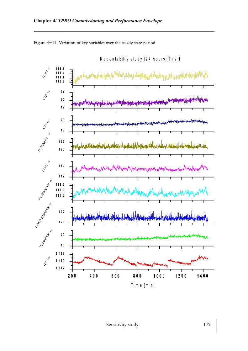
Sensitivity study 179
Chapter 4/ TPRO Commissioning and Performance Envelope________________________________________________________________________
Figure 4−14. Variation of key variables over the steady state period
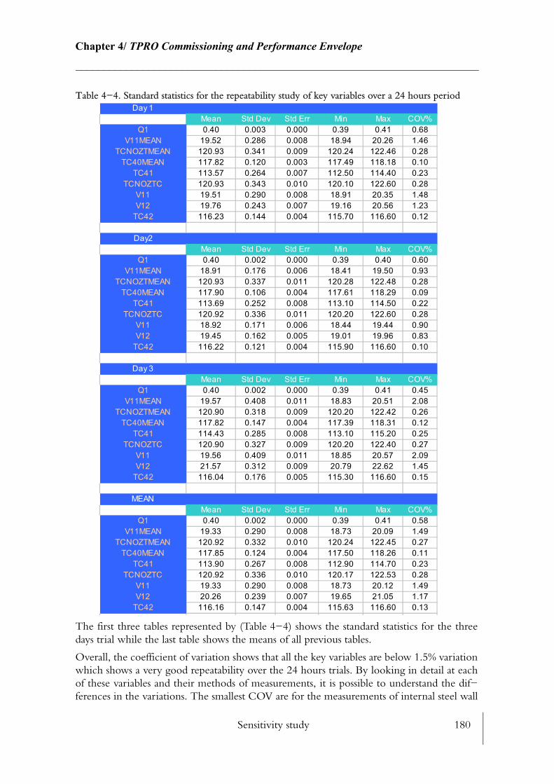
Sensitivity study 180
Chapter 4/ TPRO Commissioning and Performance Envelope________________________________________________________________________
Table 4−4. Standard statistics for the repeatability study of key variables over a 24 hours period
The first three tables represented by (Table 4−4) shows the standard statistics for the three days trial while the last table shows the means of all previous tables.
Overall, the coefficient of variation shows that all the key variables are below 1.5% variation which shows a very good repeatability over the 24 hours trials. By looking in detail at each of these variables and their methods of measurements, it is possible to understand the dif−ferences in the variations. The smallest COV are for the measurements of internal steel wall
Day 1Mean Std Dev Std Err Min Max COV%
Q1 0.40 0.003 0.000 0.39 0.41 0.68V11MEAN 19.52 0.286 0.008 18.94 20.26 1.46
TCNOZTMEAN 120.93 0.341 0.009 120.24 122.46 0.28TC40MEAN 117.82 0.120 0.003 117.49 118.18 0.10
TC41 113.57 0.264 0.007 112.50 114.40 0.23TCNOZTC 120.93 0.343 0.010 120.10 122.60 0.28
V11 19.51 0.290 0.008 18.91 20.35 1.48V12 19.76 0.243 0.007 19.16 20.56 1.23
TC42 116.23 0.144 0.004 115.70 116.60 0.12
Day2Mean Std Dev Std Err Min Max COV%
Q1 0.40 0.002 0.000 0.39 0.40 0.60V11MEAN 18.91 0.176 0.006 18.41 19.50 0.93
TCNOZTMEAN 120.93 0.337 0.011 120.28 122.48 0.28TC40MEAN 117.90 0.106 0.004 117.61 118.29 0.09
TC41 113.69 0.252 0.008 113.10 114.50 0.22TCNOZTC 120.92 0.336 0.011 120.20 122.60 0.28
V11 18.92 0.171 0.006 18.44 19.44 0.90V12 19.45 0.162 0.005 19.01 19.96 0.83
TC42 116.22 0.121 0.004 115.90 116.60 0.10
Day 3Mean Std Dev Std Err Min Max COV%
Q1 0.40 0.002 0.000 0.39 0.41 0.45V11MEAN 19.57 0.408 0.011 18.83 20.51 2.08
TCNOZTMEAN 120.90 0.318 0.009 120.20 122.42 0.26TC40MEAN 117.82 0.147 0.004 117.39 118.31 0.12
TC41 114.43 0.285 0.008 113.10 115.20 0.25TCNOZTC 120.90 0.327 0.009 120.20 122.40 0.27
V11 19.56 0.409 0.011 18.85 20.57 2.09V12 21.57 0.312 0.009 20.79 22.62 1.45
TC42 116.04 0.176 0.005 115.30 116.60 0.15
MEANMean Std Dev Std Err Min Max COV%
Q1 0.40 0.002 0.000 0.39 0.41 0.58V11MEAN 19.33 0.290 0.008 18.73 20.09 1.49
TCNOZTMEAN 120.92 0.332 0.010 120.24 122.45 0.27TC40MEAN 117.85 0.124 0.004 117.50 118.26 0.11
TC41 113.90 0.267 0.008 112.90 114.70 0.23TCNOZTC 120.92 0.336 0.010 120.17 122.53 0.28
V11 19.33 0.290 0.008 18.73 20.12 1.49V12 20.26 0.239 0.007 19.65 21.05 1.17
TC42 116.16 0.147 0.004 115.63 116.60 0.13
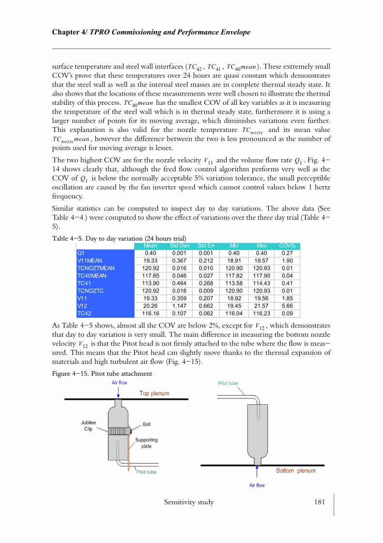
Sensitivity study 181
Chapter 4/ TPRO Commissioning and Performance Envelope________________________________________________________________________
surface temperature and steel wall interfaces ( , , ). These extremely small COV’s prove that these temperatures over 24 hours are quasi constant which demonstrates that the steel wall as well as the internal steel masses are in complete thermal steady state. It also shows that the locations of these measurements were well chosen to illustrate the thermal stability of this process. has the smallest COV of all key variables as it is measuring the temperature of the steel wall which is in thermal steady state, furthermore it is using a larger number of points for its moving average, which diminishes variations even further. This explanation is also valid for the nozzle temperature and its mean value
, however the difference between the two is less pronounced as the number of points used for moving average is lesser.
The two highest COV are for the nozzle velocity and the volume flow rate . Fig. 4−14 shows clearly that, although the feed flow control algorithm performs very well as the COV of is below the normally acceptable 5% variation tolerance, the small perceptible oscillation are caused by the fan inverter speed which cannot control values below 1 hertz frequency.
Similar statistics can be computed to inspect day to day variations. The above data (See Table 4−4 ) were computed to show the effect of variations over the three day trial (Table 4−5).
Table 4−5. Day to day variation (24 hours trial)
As Table 4−5 shows, almost all the COV are below 2%, except for , which demonstrates that day to day variation is very small. The main difference in measuring the bottom nozzle velocity is that the Pitot head is not firmly attached to the tube where the flow is meas−ured. This means that the Pitot head can slightly move thanks to the thermal expansion of materials and high turbulent air flow (Fig. 4−15).
Figure 4−15. Pitot tube attachment
TC42 TC41 TC40mean
TC40mean
TCnoztcTCnoztcmean
V11 Q1
Q1
Mean Std Dev Std Err Min Max COV%Q1 0.40 0.001 0.001 0.40 0.40 0.27V11MEAN 19.33 0.367 0.212 18.91 19.57 1.90TCNOZTMEAN 120.92 0.016 0.010 120.90 120.93 0.01TC40MEAN 117.85 0.046 0.027 117.82 117.90 0.04TC41 113.90 0.464 0.268 113.58 114.43 0.41TCNOZTC 120.92 0.016 0.009 120.90 120.93 0.01V11 19.33 0.359 0.207 18.92 19.56 1.85V12 20.26 1.147 0.662 19.45 21.57 5.66TC42 116.16 0.107 0.062 116.04 116.23 0.09
V12
V12
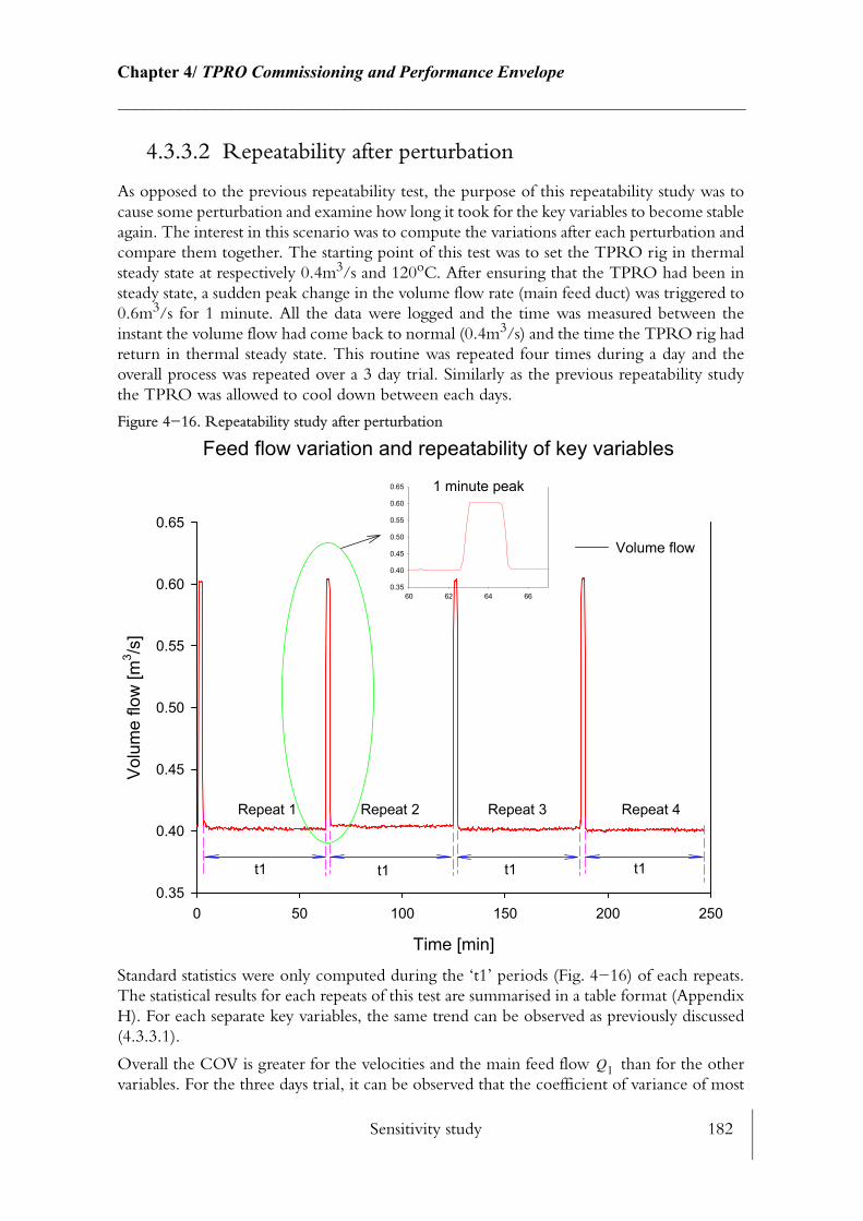
Sensitivity study 182
Chapter 4/ TPRO Commissioning and Performance Envelope________________________________________________________________________
4.3.3.2 Repeatability after perturbation
As opposed to the previous repeatability test, the purpose of this repeatability study was to cause some perturbation and examine how long it took for the key variables to become stable again. The interest in this scenario was to compute the variations after each perturbation and compare them together. The starting point of this test was to set the TPRO rig in thermal steady state at respectively 0.4m3/s and 120oC. After ensuring that the TPRO had been in steady state, a sudden peak change in the volume flow rate (main feed duct) was triggered to 0.6m3/s for 1 minute. All the data were logged and the time was measured between the instant the volume flow had come back to normal (0.4m3/s) and the time the TPRO rig had return in thermal steady state. This routine was repeated four times during a day and the overall process was repeated over a 3 day trial. Similarly as the previous repeatability study the TPRO was allowed to cool down between each days.
Figure 4−16. Repeatability study after perturbation
Standard statistics were only computed during the ‘t1’ periods (Fig. 4−16) of each repeats. The statistical results for each repeats of this test are summarised in a table format (Appendix H). For each separate key variables, the same trend can be observed as previously discussed (4.3.3.1).
Overall the COV is greater for the velocities and the main feed flow than for the other variables. For the three days trial, it can be observed that the coefficient of variance of most
Feed flow variation and repeatability of key variables
Time [min]
0 50 100 150 200 250
Volu
me
flow
[m3 /s
]
0.35
0.40
0.45
0.50
0.55
0.60
0.65
Volume flow
60 62 64 660.35
0.40
0.45
0.50
0.55
0.60
0.65 1 minute peak
t1 t1 t1 t1
Repeat 1 Repeat 2 Repeat 3 Repeat 4
Q1

NFT_PHASE0 results 183
Chapter 4/ TPRO Commissioning and Performance Envelope________________________________________________________________________
of the key variables of the first repeat are smaller than the variations of the following repeats. However, after the first repeat the variation still remain higher than for the first one but sta−bilises. Even if the TPRO was in thermal steady state before starting each new repeats, the first repeat seems to act as a ‘catalyst’ in bringing the TPRO in slightly higher variations mode. This was taken into consideration when performing both NFT and FT. Before start−ing any of these tests the door was opened for few minutes to perturb slightly the TPRO environment, thereafter sufficient time was left to bring the TPRO in thermal steady state.
Comparing with the previous repeatability study (over 24hours period − Table 4−5) the study of COV’s shows less of a variation in this case than for the perturbation over a 24 hours period. Variations over a 24 hours period are more likely to occur than over a 70 minutes period. Temperature surrounding the TPRO over a 24 hours period will also change and may also help to produce slightly higher variations on the key variables.
Table 4−6. Day to day variation (after perturbation)
Overall, the TPRO shows that it can reproduce very repeatable trials either over a 24 hours period or in a successive repeated test separated by sufficient time to allow the rig to return in thermal steady state conditions. This is the results of a careful positioning of instrumen−tation and adequate calibrations and methodological approach.
4.4 NFT_PHASE0 results
The results of NFT_PHASE0 have been described in Chapter 2 (See 2.3.1.1). The objective in running this test was to understand the heat rise behaviour when running the TPRO with zero heating inputs and estimate where the heat was coming from, in which quantities, and how could it be controlled. To do so, both the fans were working at full speed and the oven was set−up in the full recirculation mode. 13 hours were necessary to reach an internal oven air temperature of 95.2oC, (Fig. 2−5). By changing both the fans to a lower speed the inter−nal oven air temperature decreased, which proved the direct relation between the heating effect and the fans. However there was an important lag time until the oven structure returned to thermal steady state.
External activity also had an influence on the evolution of the temperature within the cham−ber. During the night time the drop in external temperature due to night fall was causing the external wall surface and the internal temperature of the rig to drop. The overall structure and internal air temperature of the TPRO rig followed the same trend as the surrounding FPC building, but with a time delay. Energy inputs from the fans were correlated with inlet
Mean Std Dev Std Err Min Max COV%Q1 0.40 0.001 0.000 0.40 0.40 0.20V11MEAN 19.24 0.151 0.087 19.13 19.41 0.78TCNOZTMEAN 120.93 0.020 0.012 120.91 120.95 0.02TC40MEAN 117.98 0.030 0.017 117.95 118.01 0.03TC41 114.01 0.067 0.039 113.93 114.06 0.06TNOZTC 120.93 0.021 0.012 120.91 120.95 0.02V11 19.26 0.170 0.098 19.13 19.45 0.88V12 19.50 0.189 0.109 19.30 19.68 0.97TC42 116.31 0.093 0.054 116.20 116.37 0.08

NFT_PHASE1 results 184
Chapter 4/ TPRO Commissioning and Performance Envelope________________________________________________________________________
air temperature and fan inverter settings. The temperature rise due to the fan input power is proportional to the speed of the fan and there is no other possible ways of controlling this temperature apart from varying the fan inverter settings. As this energy input is far from neg−ligible it was taken into consideration for the computation of the energy balance of the TPRO rig. It could be envisaged that in these conditions (zero heat input) that if the TPRO rig was better insulated and the air leaks were minimised the resultant internal temperature of the TPRO could be even greater than 95.2oC, i.e it might then be possible to bake with only the heat provided from the fans.
With no heat input but the fans, the temperature within the TPRO chamber can vary in an non controlled manner, however this finding is irrelevant for the baking process. Indeed, it has been demonstrated earlier on (4.3.3) that oven temperature and thermal steady state could be maintained to very close tolerances when the TPRO uses its computer control sys−tem.
4.5 NFT_PHASE1 results
The intention with this test was to understand how the fastest could be achieved at the nozzle exit. Fan speed (FIS) and dampers D8, D9 and D1 are the main driver for achiev−ing this goal. Eleven base case scenarios, varying both the fan speed (FIS) and the damper settings, were established to study how the fastest could be achieved. The base case scenarios are summarised by Table 4.2.3. For each of these base case, both the fan speed (FIS) and the damper settings are fixed until the set−point temperature of 100oC is obtained. Then, the oven is cooled rapidly until it returns in thermal steady state. To make easy com−parison between tests, statistics were computed over the first 90 second period (during the heating up period) for the . All the results from the base case scenario are summa−rised by Table 4−7.
4.5.1 Base case
4.5.1.1 NFT_PHASE1 test T1
Before starting any of the base case tests of NFT_PHASE1, the TPRO was primarily cooled with ambient air. The inlet duct is connected with a flexible pipe that is sucking fresh air from the outside of the FPC. During this cooling phase of the test both fans were running at 10Hz and the dampers D8, D9 and D1 were set respectively to FO, FC and FO to enable faster cooling. At this speed, the amount of heat added to the air is minimum which allows to maintain the oven at a constant ambient temperature. Once the TPRO had reached steady state the dampers were set to their ‘test’ positions, in this case: D8=FO, D9=FO and D1=FC, and the temperature is set to 150oC. The temperature was set higher than the 100oC limit so that the temperature PID controller did not interact to slow down the tem−perature response. When the oven temperature had reached its target set−point, the shut down procedure was loaded into the soft PLC and the following oven setting was applied:
dTair dt⁄
dTair dt⁄
dTair dt⁄

NFT_PHASE1 results 185
Chapter 4/ TPRO Commissioning and Performance Envelope________________________________________________________________________
• CFAN and EFAN set to 50Hz.
• Oven temperature PID set point is set to 0oC.The dampers are set manually to:
• D8 = FO; D9 = FC; D1 = FOThe flexible pipe is reconnected to the inlet duct to ensure the inlet air is cool. Both mean nozzle temperature (TCNOZTMEAN) and temperature rate of change (TCNOZTRISE) were logged.
Figure 4−17. Analysis of NFT test T1
During the first phase (heating phase) the mean is 19.8oC/min. over the first 90 seconds. As soon the target is achieved the shut down procedure is loaded (second phase) and almost immediately the oven temperature rise sharply to 125oC which is translated by a
of 216oC/min. Shortly after this peak rise, the temperature comes down and reaches a negative peak ( ) of −40oC/min. During the second phase the fans velocity is reduced to 10Hz. To start the next test the oven was cooled down until the whole of the TPRO had returned to thermal steady state.
4.5.1.2 NFT_PHASE1 test T2
The main difference between T1 and T2 is the fan speed (FIS). In the second case the fan speed (FIS) is increased to 30Hz. At this air flow regime the mean (32.25oC/min.) (Fig. 4−18) is 38.6% greater than for the previous test (Fig. 4−18). This shows that the duct heaters are more efficient at this air flow regime than at the lower air flow. With this air flow regime, it can also be noticed that the mean decreases as the air temperature increases, while it is near constant in the case of T1.
dTair dt⁄
dTair dt⁄dTair dt⁄
dTair dt⁄
dTair dt⁄
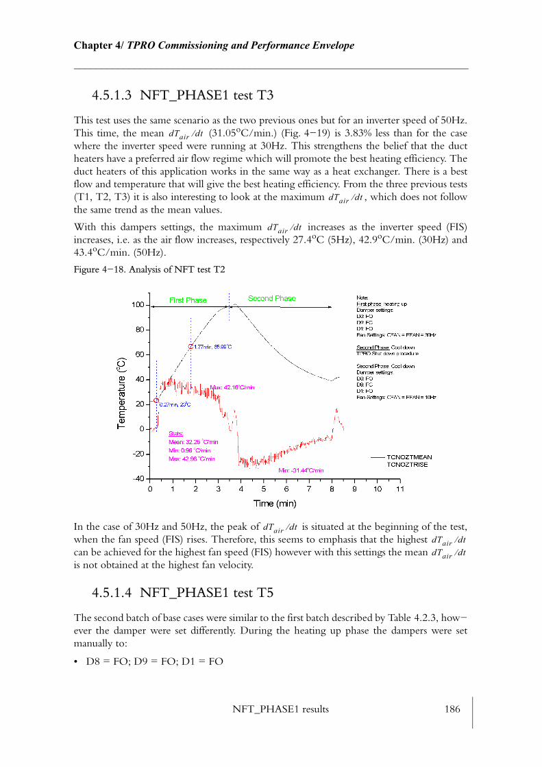
NFT_PHASE1 results 186
Chapter 4/ TPRO Commissioning and Performance Envelope________________________________________________________________________
4.5.1.3 NFT_PHASE1 test T3
This test uses the same scenario as the two previous ones but for an inverter speed of 50Hz. This time, the mean (31.05oC/min.) (Fig. 4−19) is 3.83% less than for the case where the inverter speed were running at 30Hz. This strengthens the belief that the duct heaters have a preferred air flow regime which will promote the best heating efficiency. The duct heaters of this application works in the same way as a heat exchanger. There is a best flow and temperature that will give the best heating efficiency. From the three previous tests (T1, T2, T3) it is also interesting to look at the maximum , which does not follow the same trend as the mean values.
With this dampers settings, the maximum increases as the inverter speed (FIS) increases, i.e. as the air flow increases, respectively 27.4oC (5Hz), 42.9oC/min. (30Hz) and 43.4oC/min. (50Hz).
Figure 4−18. Analysis of NFT test T2
In the case of 30Hz and 50Hz, the peak of is situated at the beginning of the test, when the fan speed (FIS) rises. Therefore, this seems to emphasis that the highest can be achieved for the highest fan speed (FIS) however with this settings the mean is not obtained at the highest fan velocity.
4.5.1.4 NFT_PHASE1 test T5
The second batch of base cases were similar to the first batch described by Table 4.2.3, how−ever the damper were set differently. During the heating up phase the dampers were set manually to:
• D8 = FO; D9 = FO; D1 = FO
dTair dt⁄
dTair dt⁄
dTair dt⁄
dTair dt⁄dTair dt⁄dTair dt⁄
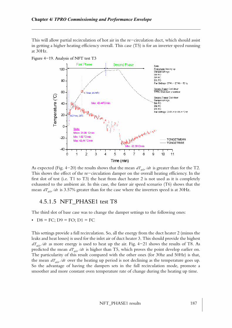
NFT_PHASE1 results 187
Chapter 4/ TPRO Commissioning and Performance Envelope________________________________________________________________________
This will allow partial recirculation of hot air in the re−circulation duct, which should assist in getting a higher heating efficiency overall. This case (T5) is for an inverter speed running at 30Hz.
Figure 4−19. Analysis of NFT test T3
As expected (Fig. 4−20) the results shows that the mean is greater than for the T2. This shows the effect of the re−circulation damper on the overall heating efficiency. In the first slot of test (i.e. T1 to T3) the heat from duct heater 2 is not used as it is completely exhausted to the ambient air. In this case, the faster air speed scenario (T6) shows that the mean is 3.57% greater than for the case where the inverters speed is at 30Hz.
4.5.1.5 NFT_PHASE1 test T8
The third slot of base case was to change the damper settings to the following ones:
• D8 = FC; D9 = FO; D1 = FC
This settings provide a full recirculation. So, all the energy from the duct heater 2 (minus the leaks and heat losses) is used for the inlet air of duct heater 3. This should provide the highest
as more energy is used to heat up the air. Fig. 4−21 shows the results of T8. As predicted the mean is higher than T5, which proves the point develop earlier on. The particularity of this result compared with the other ones (for 30hz and 50Hz) is that, the mean over the heating up period is not declining as the temperature goes up. So the advantage of having the dampers sets in the full recirculation mode, promote a smoother and more constant oven temperature rate of change during the heating up time.
dTair dt⁄
dTair dt⁄
dTair dt⁄dTair dt⁄
dTair dt⁄
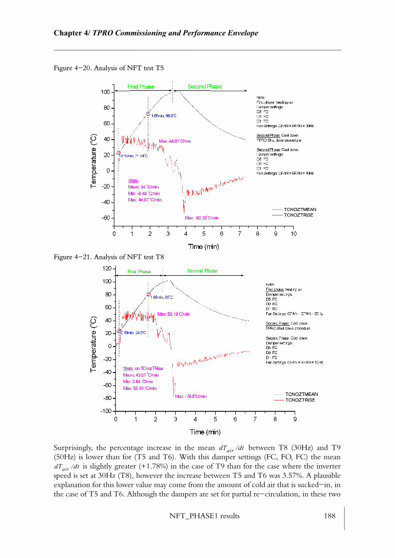
NFT_PHASE1 results 188
Chapter 4/ TPRO Commissioning and Performance Envelope________________________________________________________________________
Figure 4−20. Analysis of NFT test T5
Figure 4−21. Analysis of NFT test T8
Surprisingly, the percentage increase in the mean between T8 (30Hz) and T9 (50Hz) is lower than for (T5 and T6). With this damper settings (FC, FO, FC) the mean
is slightly greater (+1.78%) in the case of T9 than for the case where the inverter speed is set at 30Hz (T8), however the increase between T5 and T6 was 3.57%. A plausible explanation for this lower value may come from the amount of cold air that is sucked−in, in the case of T5 and T6. Although the dampers are set for partial re−circulation, in these two
dTair dt⁄
dTair dt⁄

NFT_PHASE1 results 189
Chapter 4/ TPRO Commissioning and Performance Envelope________________________________________________________________________
cases (T5 and T6), the temperature difference across the duct heater 3 is greater than in the case (T8 and T9) and might be responsible for the higher percentage increase from 30Hz to 50Hz.
4.5.1.6 NFT_PHASE1 test T11
The fourth base case scenario (T10 to T11) is yet again similar as far as the fan settings are concerned however, during the heating curve, the damper were set as following:
• D8 = FC; D9 = FO; D1 = FOThis damper setting means that the TPRO is recirculating at 100% with some fresh air inputs. The results of T11 (Fig. 4−22) shows a mean of 45.97oC/min. which is the highest amongst all the base case test.
In comparison with the pair test (T2, T3), (T5,T6), (T8,T9) the biggest increase for the is for (T10,T11) with 5.96%. With this particular damper setting and for the max−
imum fan inverter settings, the mean as well as the peak are maximum. This results reinforce the findings between the pair test (T2, T3), (T5,T6).
Figure 4−22. Analysis of NFT test T11
4.5.1.7 Conclusions of base case scenarios
Table 4−7 summarises the different cases discussed in the above paragraphs. When compar−ing , the differences between the three different studied air flow (i.e for fan inverter speed 5Hz, 30Hz and 50Hz) shows that the largest variation exist between the 5Hz and 30Hz while between 30Hz and 50Hz the variation are much smaller and in one case negative (T3). This signifies that there is an optimum inverter speed for both CFAN and EFAN (i.e. air flow) which gives the maximum heating efficiency. Although the fastest inverter speed seems
dTair dt⁄
dTair dt⁄dTair dt⁄ dTair dt⁄
dTair dt⁄
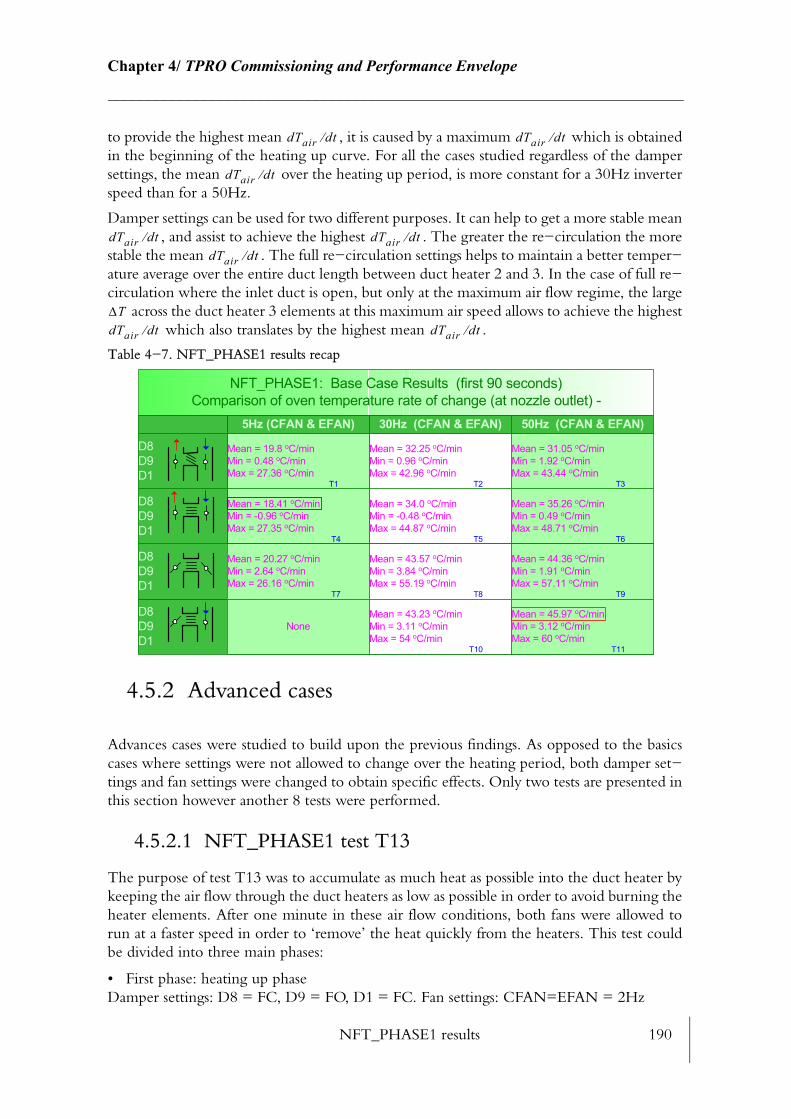
NFT_PHASE1 results 190
Chapter 4/ TPRO Commissioning and Performance Envelope________________________________________________________________________
to provide the highest mean , it is caused by a maximum which is obtained in the beginning of the heating up curve. For all the cases studied regardless of the damper settings, the mean over the heating up period, is more constant for a 30Hz inverter speed than for a 50Hz.
Damper settings can be used for two different purposes. It can help to get a more stable mean , and assist to achieve the highest . The greater the re−circulation the more
stable the mean . The full re−circulation settings helps to maintain a better temper−ature average over the entire duct length between duct heater 2 and 3. In the case of full re−circulation where the inlet duct is open, but only at the maximum air flow regime, the large
across the duct heater 3 elements at this maximum air speed allows to achieve the highest which also translates by the highest mean .
Table 4−7. NFT_PHASE1 results recap
4.5.2 Advanced cases
Advances cases were studied to build upon the previous findings. As opposed to the basics cases where settings were not allowed to change over the heating period, both damper set−tings and fan settings were changed to obtain specific effects. Only two tests are presented in this section however another 8 tests were performed.
4.5.2.1 NFT_PHASE1 test T13
The purpose of test T13 was to accumulate as much heat as possible into the duct heater by keeping the air flow through the duct heaters as low as possible in order to avoid burning the heater elements. After one minute in these air flow conditions, both fans were allowed to run at a faster speed in order to ‘remove’ the heat quickly from the heaters. This test could be divided into three main phases:
• First phase: heating up phaseDamper settings: D8 = FC, D9 = FO, D1 = FC. Fan settings: CFAN=EFAN = 2Hz
dTair dt⁄ dTair dt⁄
dTair dt⁄
dTair dt⁄ dTair dt⁄dTair dt⁄
∆TdTair dt⁄ dTair dt⁄
D8D9D1
D8D9D1
Mean = 35.26 oC/minMin = 0.49 oC/minMax = 48.71 oC/min
Mean = 34.0 oC/minMin = -0.48 oC/minMax = 44.87 oC/min
Mean = 18.41 oC/minMin = -0.96 oC/minMax = 27.35 oC/min
D8D9D1
Mean = 31.05 oC/minMin = 1.92 oC/minMax = 43.44 oC/min
Mean = 32.25 oC/minMin = 0.96 oC/minMax = 42.96 oC/min
Mean = 19.8 oC/minMin = 0.48 oC/minMax = 27.36 oC/min
D8D9D1
50Hz (CFAN & EFAN)30Hz (CFAN & EFAN)5Hz (CFAN & EFAN)
NFT_PHASE1: Base Case Results (first 90 seconds)Comparison of oven temperature rate of change (at nozzle outlet) -
Mean = 20.27 oC/minMin = 2.64 oC/minMax = 26.16 oC/min
Mean = 44.36 oC/minMin = 1.91 oC/minMax = 57.11 oC/min
Mean = 43.57 oC/minMin = 3.84 oC/minMax = 55.19 oC/min
T1 T2
T5
T8T7
T4
T3
T6
T9
NoneMean = 45.97 oC/minMin = 3.12 oC/minMax = 60 oC/min
Mean = 43.23 oC/minMin = 3.11 oC/minMax = 54 oC/min
T10 T11
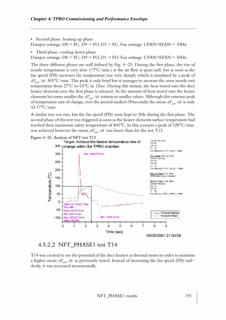
NFT_PHASE1 results 191
Chapter 4/ TPRO Commissioning and Performance Envelope________________________________________________________________________
• Second phase: heating up phaseDamper settings: D8 = FC, D9 = FO, D1 = FC. Fan settings: CFAN=EFAN = 30Hz
• Third phase: cooling down phaseDamper settings: D8 = FC, D9 = FO, D1 = FO. Fan settings: CFAN=EFAN = 50Hz
The three different phases are well defined by Fig. 4−23. During the first phase, the rise of nozzle temperature is very slow (~7oC/min.) as the air flow is quasi null, but as soon as the fan speed (FIS) increases the temperature rise very sharply which is translated by a peak of
305oC/min. This peak is only brief but it manages to increase the oven nozzle exit temperature from 27oC to 65oC in 12sec. During this instant, the heat stored into the duct heater elements over the first phase is released. As the amount of heat stored into the heater elements becomes smaller the returns to smaller values. Although this extreme peak of temperature rate of change, over the period studied (90seconds) the mean is only 43.17oC/min.
A similar test was run, but the fan speed (FIS) were kept to 5Hz during the first phase. The second phase of this test was triggered as soon as the heater elements surface temperature had reached their maximum safety temperature of 460oC. In this scenario a peak of 328oC/min. was achieved however the mean was lower than for the test T13.
Figure 4−23. Analysis of NFT test T13
4.5.2.2 NFT_PHASE1 test T14
T14 was created to use the potential of the duct heaters as thermal stores in order to maintain a higher mean as previously tested. Instead of increasing the fan speed (FIS) sud−denly, it was increased incrementally.
dTair dt⁄
dTair dt⁄dTair dt⁄
dTair dt⁄
dTair dt⁄

NFT_PHASE1 results 192
Chapter 4/ TPRO Commissioning and Performance Envelope________________________________________________________________________
Figure 4−24. Analysis of NFT test T14
In this scenario the maximum peak of is not as high as for test T13 however the mean is the greatest amongst all the test performed.
T14 shows that it is possible to use the heater as thermal heat storage in order to maintain a relatively high mean .
Overall, the NFT_PHASE1 tests have revealed that the TPRO can achieve high temperature rates of change within the chamber in a very short time by using the duct heater elements as thermal stores. However it involves increasing the fan speed (FIS) to very high rates in order to remove the heat quickly from the duct heater elements. Although it is possible to reach very high temperature rate of change, it would be difficult to maintain a relatively high temperature after reaching high . Nonetheless, it was also discovered during the advanced test cases that the average temperature rate of change can be kept relatively high by incrementally rising the fan inverter settings. Therefore to control the temperature rate of change within the TPRO chamber a trade off exist between the fan settings and the amount of heat that can be released from the duct heater. Further development work could be done to find out the best fan/damper settings and/or a control algorithm could be created to esti−mate how to obtain the highest and maintaining a high temperature thereafter.
The temperature rates of change explored during this test phase are only for low temperature (20oC−100oC). These value will go down as the temperature of the oven increases, as the heat loss increases. NFT_PHASE2 deals with the temperature rate of change for higher oven temperature.
dTair dt⁄dTair dt⁄
dTair dt⁄
dTair dt⁄
dTair dt⁄
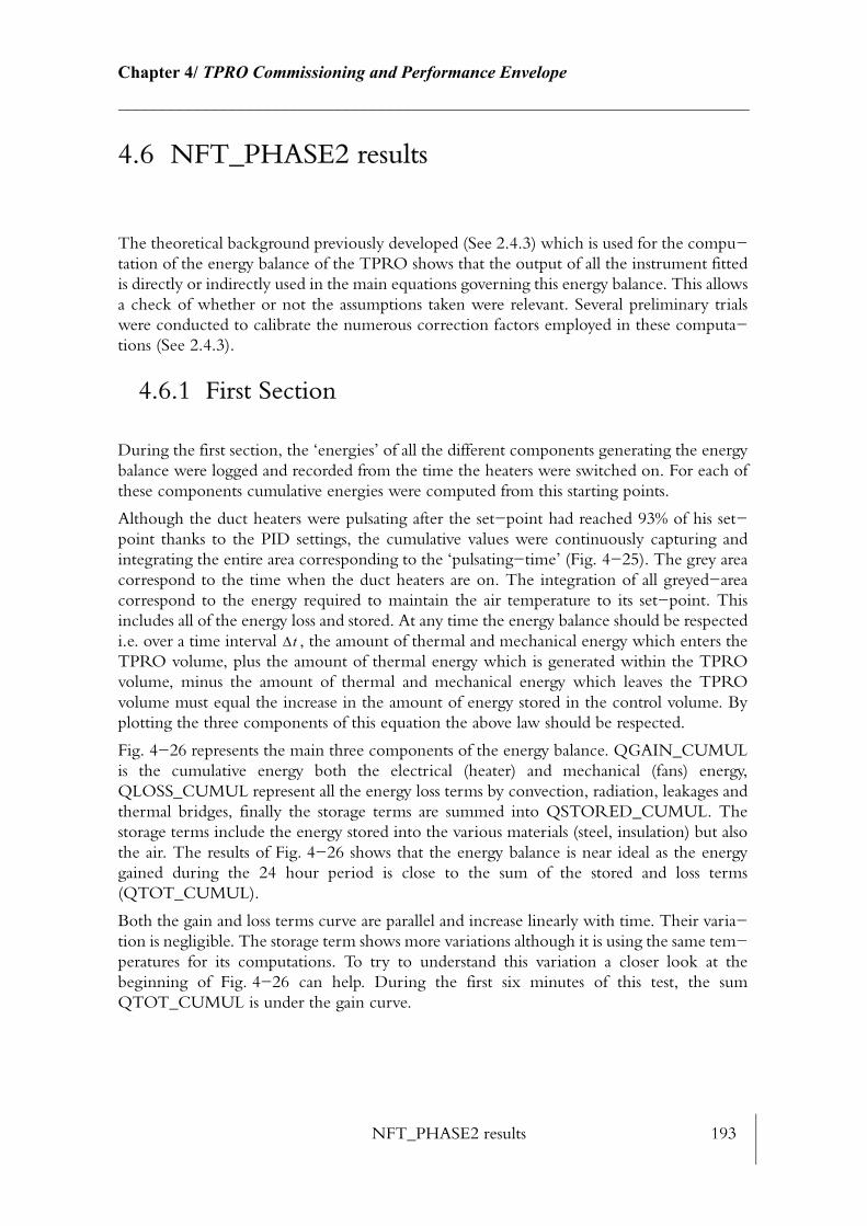
NFT_PHASE2 results 193
Chapter 4/ TPRO Commissioning and Performance Envelope________________________________________________________________________
4.6 NFT_PHASE2 results
The theoretical background previously developed (See 2.4.3) which is used for the compu−tation of the energy balance of the TPRO shows that the output of all the instrument fitted is directly or indirectly used in the main equations governing this energy balance. This allows a check of whether or not the assumptions taken were relevant. Several preliminary trials were conducted to calibrate the numerous correction factors employed in these computa−tions (See 2.4.3).
4.6.1 First Section
During the first section, the ‘energies’ of all the different components generating the energy balance were logged and recorded from the time the heaters were switched on. For each of these components cumulative energies were computed from this starting points.
Although the duct heaters were pulsating after the set−point had reached 93% of his set−point thanks to the PID settings, the cumulative values were continuously capturing and integrating the entire area corresponding to the ‘pulsating−time’ (Fig. 4−25). The grey area correspond to the time when the duct heaters are on. The integration of all greyed−area correspond to the energy required to maintain the air temperature to its set−point. This includes all of the energy loss and stored. At any time the energy balance should be respected i.e. over a time interval , the amount of thermal and mechanical energy which enters the TPRO volume, plus the amount of thermal energy which is generated within the TPRO volume, minus the amount of thermal and mechanical energy which leaves the TPRO volume must equal the increase in the amount of energy stored in the control volume. By plotting the three components of this equation the above law should be respected.
Fig. 4−26 represents the main three components of the energy balance. QGAIN_CUMUL is the cumulative energy both the electrical (heater) and mechanical (fans) energy, QLOSS_CUMUL represent all the energy loss terms by convection, radiation, leakages and thermal bridges, finally the storage terms are summed into QSTORED_CUMUL. The storage terms include the energy stored into the various materials (steel, insulation) but also the air. The results of Fig. 4−26 shows that the energy balance is near ideal as the energy gained during the 24 hour period is close to the sum of the stored and loss terms (QTOT_CUMUL).
Both the gain and loss terms curve are parallel and increase linearly with time. Their varia−tion is negligible. The storage term shows more variations although it is using the same tem−peratures for its computations. To try to understand this variation a closer look at the beginning of Fig. 4−26 can help. During the first six minutes of this test, the sum QTOT_CUMUL is under the gain curve.
∆t
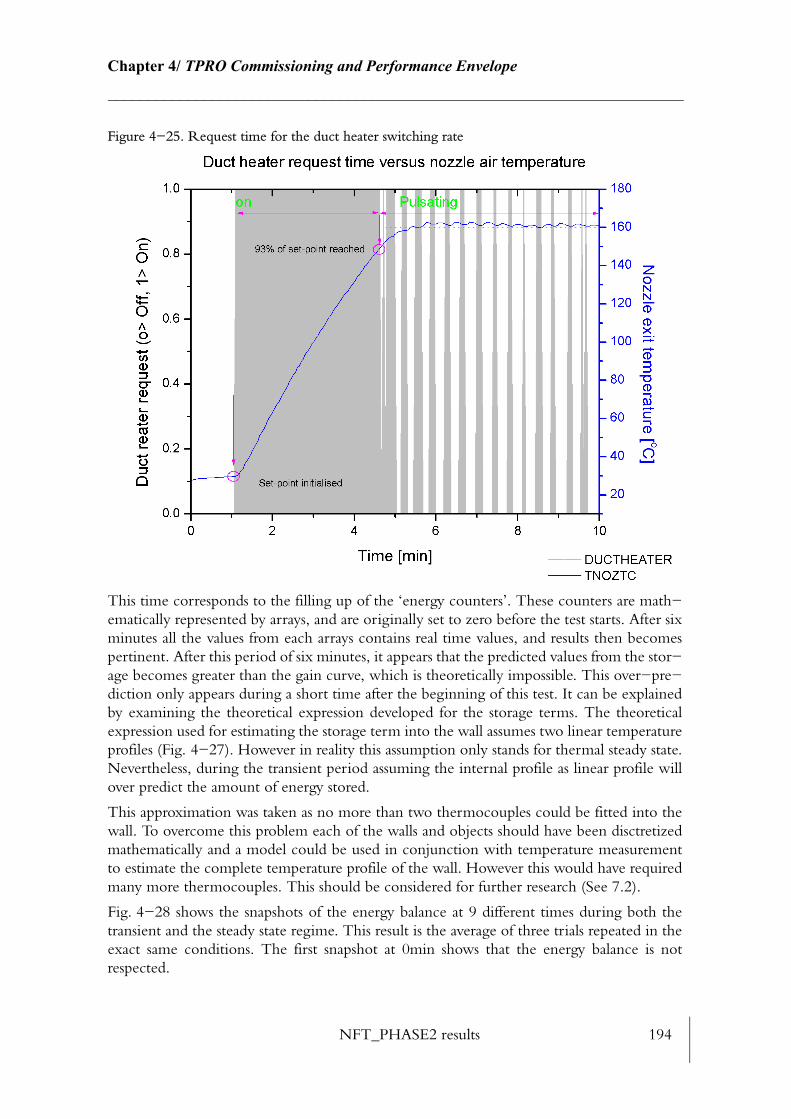
NFT_PHASE2 results 194
Chapter 4/ TPRO Commissioning and Performance Envelope________________________________________________________________________
Figure 4−25. Request time for the duct heater switching rate
This time corresponds to the filling up of the ‘energy counters’. These counters are math−ematically represented by arrays, and are originally set to zero before the test starts. After six minutes all the values from each arrays contains real time values, and results then becomes pertinent. After this period of six minutes, it appears that the predicted values from the stor−age becomes greater than the gain curve, which is theoretically impossible. This over−pre−diction only appears during a short time after the beginning of this test. It can be explained by examining the theoretical expression developed for the storage terms. The theoretical expression used for estimating the storage term into the wall assumes two linear temperature profiles (Fig. 4−27). However in reality this assumption only stands for thermal steady state. Nevertheless, during the transient period assuming the internal profile as linear profile will over predict the amount of energy stored.
This approximation was taken as no more than two thermocouples could be fitted into the wall. To overcome this problem each of the walls and objects should have been disctretized mathematically and a model could be used in conjunction with temperature measurement to estimate the complete temperature profile of the wall. However this would have required many more thermocouples. This should be considered for further research (See 7.2).
Fig. 4−28 shows the snapshots of the energy balance at 9 different times during both the transient and the steady state regime. This result is the average of three trials repeated in the exact same conditions. The first snapshot at 0min shows that the energy balance is not respected.
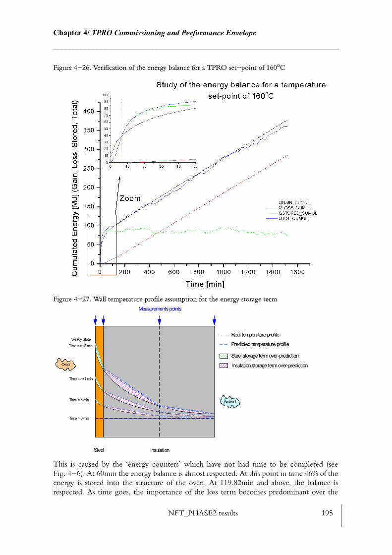
NFT_PHASE2 results 195
Chapter 4/ TPRO Commissioning and Performance Envelope________________________________________________________________________
Figure 4−26. Verification of the energy balance for a TPRO set−point of 160oC
Figure 4−27. Wall temperature profile assumption for the energy storage term
This is caused by the ‘energy counters’ which have not had time to be completed (see Fig. 4−6). At 60min the energy balance is almost respected. At this point in time 46% of the energy is stored into the structure of the oven. At 119.82min and above, the balance is respected. As time goes, the importance of the loss term becomes predominant over the
Steel Insulation
Measurements points
Time = 0 min
Time = n min
Time = n+1 min
Steady StateTime = n+2 min
Real temperature profile
Predicted temperature profile
Steel storage term over-prediction
Insulation storage term over-prediction
Ambient
Oven
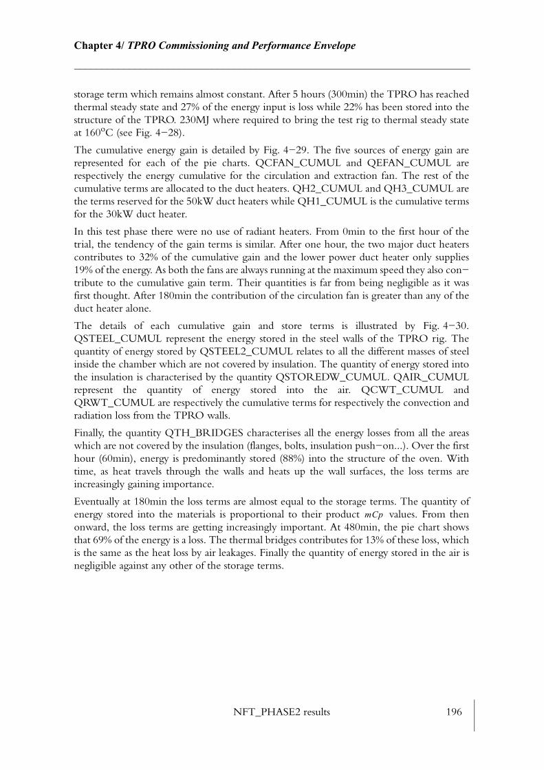
NFT_PHASE2 results 196
Chapter 4/ TPRO Commissioning and Performance Envelope________________________________________________________________________
storage term which remains almost constant. After 5 hours (300min) the TPRO has reached thermal steady state and 27% of the energy input is loss while 22% has been stored into the structure of the TPRO. 230MJ where required to bring the test rig to thermal steady state at 160oC (see Fig. 4−28).
The cumulative energy gain is detailed by Fig. 4−29. The five sources of energy gain are represented for each of the pie charts. QCFAN_CUMUL and QEFAN_CUMUL are respectively the energy cumulative for the circulation and extraction fan. The rest of the cumulative terms are allocated to the duct heaters. QH2_CUMUL and QH3_CUMUL are the terms reserved for the 50kW duct heaters while QH1_CUMUL is the cumulative terms for the 30kW duct heater.
In this test phase there were no use of radiant heaters. From 0min to the first hour of the trial, the tendency of the gain terms is similar. After one hour, the two major duct heaters contributes to 32% of the cumulative gain and the lower power duct heater only supplies 19% of the energy. As both the fans are always running at the maximum speed they also con−tribute to the cumulative gain term. Their quantities is far from being negligible as it was first thought. After 180min the contribution of the circulation fan is greater than any of the duct heater alone.
The details of each cumulative gain and store terms is illustrated by Fig. 4−30. QSTEEL_CUMUL represent the energy stored in the steel walls of the TPRO rig. The quantity of energy stored by QSTEEL2_CUMUL relates to all the different masses of steel inside the chamber which are not covered by insulation. The quantity of energy stored into the insulation is characterised by the quantity QSTOREDW_CUMUL. QAIR_CUMUL represent the quantity of energy stored into the air. QCWT_CUMUL and QRWT_CUMUL are respectively the cumulative terms for respectively the convection and radiation loss from the TPRO walls.
Finally, the quantity QTH_BRIDGES characterises all the energy losses from all the areas which are not covered by the insulation (flanges, bolts, insulation push−on...). Over the first hour (60min), energy is predominantly stored (88%) into the structure of the oven. With time, as heat travels through the walls and heats up the wall surfaces, the loss terms are increasingly gaining importance.
Eventually at 180min the loss terms are almost equal to the storage terms. The quantity of energy stored into the materials is proportional to their product values. From then onward, the loss terms are getting increasingly important. At 480min, the pie chart shows that 69% of the energy is a loss. The thermal bridges contributes for 13% of these loss, which is the same as the heat loss by air leakages. Finally the quantity of energy stored in the air is negligible against any other of the storage terms.
mCp
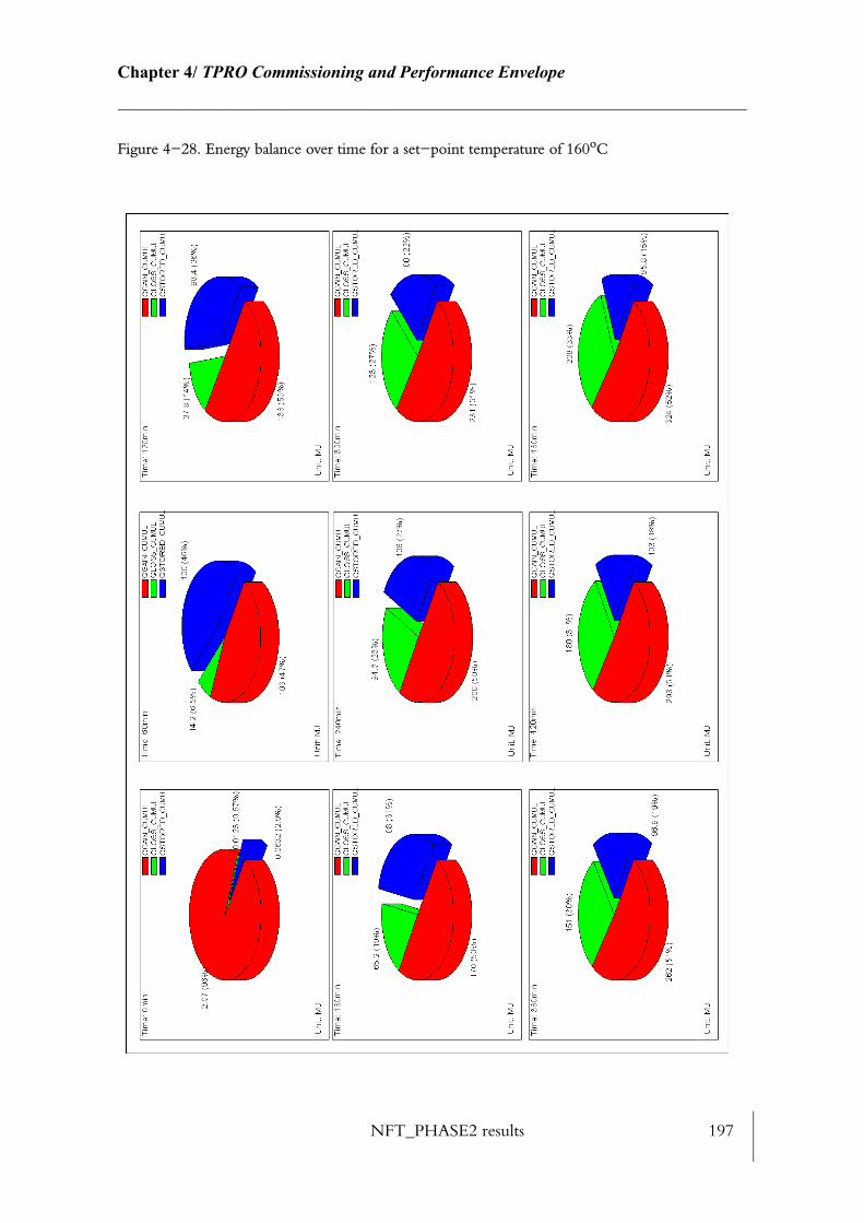
NFT_PHASE2 results 197
Chapter 4/ TPRO Commissioning and Performance Envelope________________________________________________________________________
Figure 4−28. Energy balance over time for a set−point temperature of 160oC
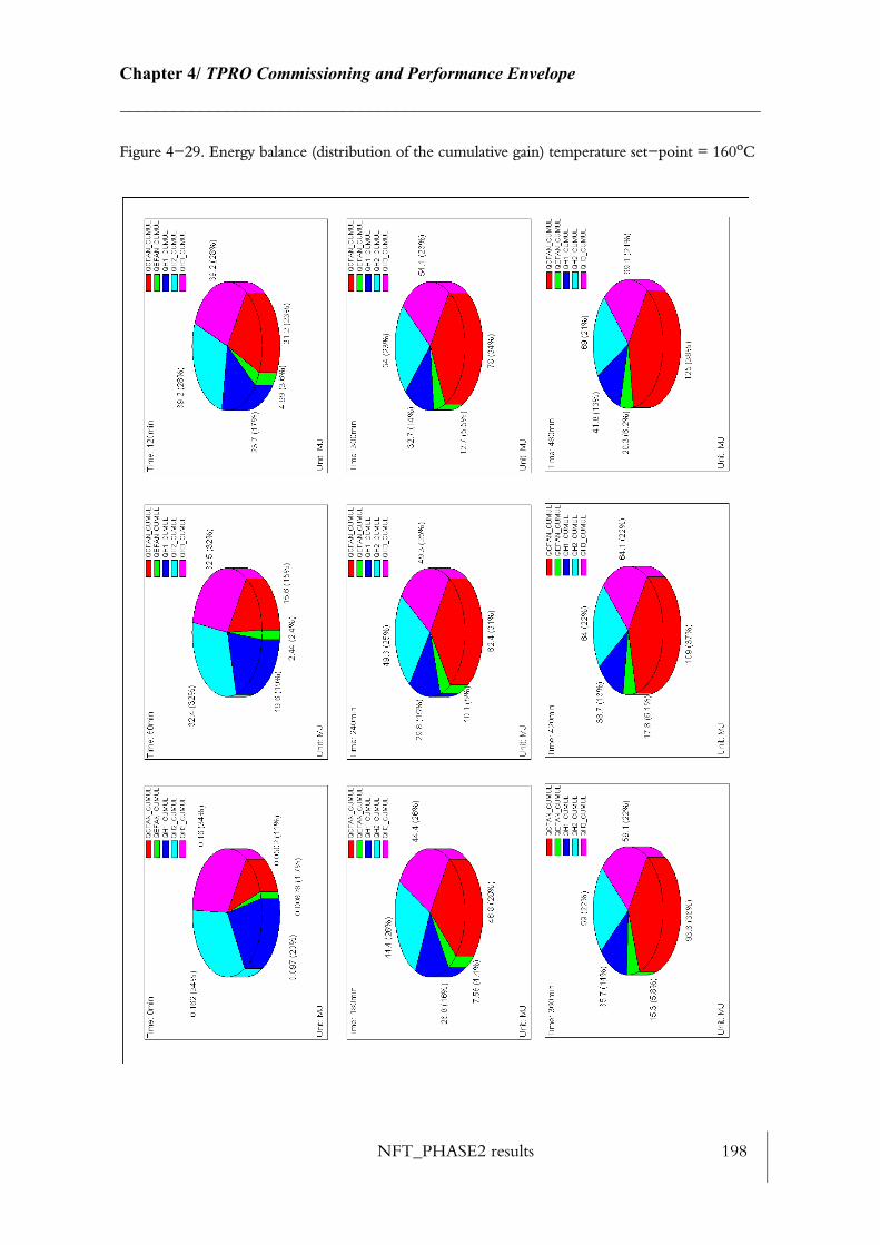
NFT_PHASE2 results 198
Chapter 4/ TPRO Commissioning and Performance Envelope________________________________________________________________________
Figure 4−29. Energy balance (distribution of the cumulative gain) temperature set−point = 160oC

NFT_PHASE2 results 199
Chapter 4/ TPRO Commissioning and Performance Envelope________________________________________________________________________
Figure 4−30. Energy balance (distribution of the cumulative loss and store) for set−point temperature of 160oC
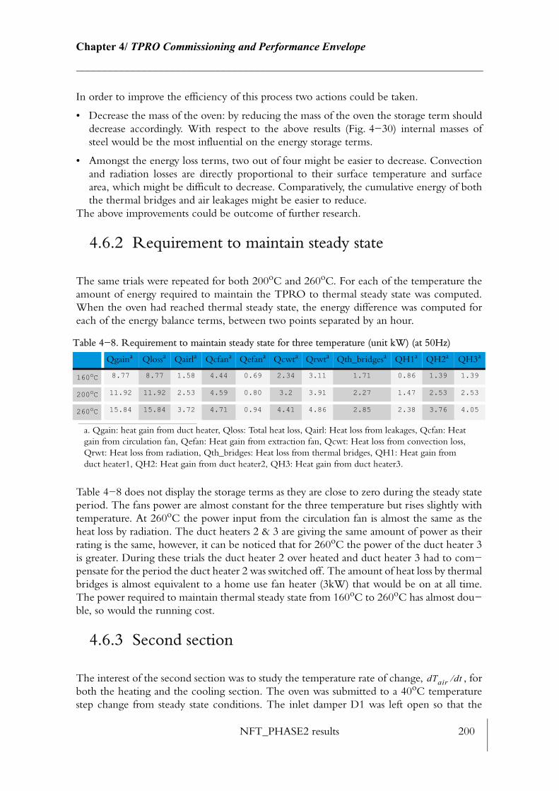
NFT_PHASE2 results 200
Chapter 4/ TPRO Commissioning and Performance Envelope________________________________________________________________________
In order to improve the efficiency of this process two actions could be taken.
• Decrease the mass of the oven: by reducing the mass of the oven the storage term should decrease accordingly. With respect to the above results (Fig. 4−30) internal masses of steel would be the most influential on the energy storage terms.
• Amongst the energy loss terms, two out of four might be easier to decrease. Convection and radiation losses are directly proportional to their surface temperature and surface area, which might be difficult to decrease. Comparatively, the cumulative energy of both the thermal bridges and air leakages might be easier to reduce.
The above improvements could be outcome of further research.
4.6.2 Requirement to maintain steady state
The same trials were repeated for both 200oC and 260oC. For each of the temperature the amount of energy required to maintain the TPRO to thermal steady state was computed. When the oven had reached thermal steady state, the energy difference was computed for each of the energy balance terms, between two points separated by an hour.
Table 4−8 does not display the storage terms as they are close to zero during the steady state period. The fans power are almost constant for the three temperature but rises slightly with temperature. At 260oC the power input from the circulation fan is almost the same as the heat loss by radiation. The duct heaters 2 & 3 are giving the same amount of power as their rating is the same, however, it can be noticed that for 260oC the power of the duct heater 3 is greater. During these trials the duct heater 2 over heated and duct heater 3 had to com−pensate for the period the duct heater 2 was switched off. The amount of heat loss by thermal bridges is almost equivalent to a home use fan heater (3kW) that would be on at all time. The power required to maintain thermal steady state from 160oC to 260oC has almost dou−ble, so would the running cost.
4.6.3 Second section
The interest of the second section was to study the temperature rate of change, , for both the heating and the cooling section. The oven was submitted to a 40oC temperature step change from steady state conditions. The inlet damper D1 was left open so that the
Table 4−8. Requirement to maintain steady state for three temperature (unit kW) (at 50Hz)
Qgaina
a. Qgain: heat gain from duct heater, Qloss: Total heat loss, Qairl: Heat loss from leakages, Qcfan: Heat gain from circulation fan, Qefan: Heat gain from extraction fan, Qcwt: Heat loss from convection loss, Qrwt: Heat loss from radiation, Qth_bridges: Heat loss from thermal bridges, QH1: Heat gain from duct heater1, QH2: Heat gain from duct heater2, QH3: Heat gain from duct heater3.
Qlossa Qairla Qcfana Qefana Qcwta Qrwta Qth_bridgesa QH1a QH2a QH3a
160oC 8.77 8.77 1.58 4.44 0.69 2.34 3.11 1.71 0.86 1.39 1.39
200oC 11.92 11.92 2.53 4.59 0.80 3.2 3.91 2.27 1.47 2.53 2.53
260oC 15.84 15.84 3.72 4.71 0.94 4.41 4.86 2.85 2.38 3.76 4.05
dTair dt⁄
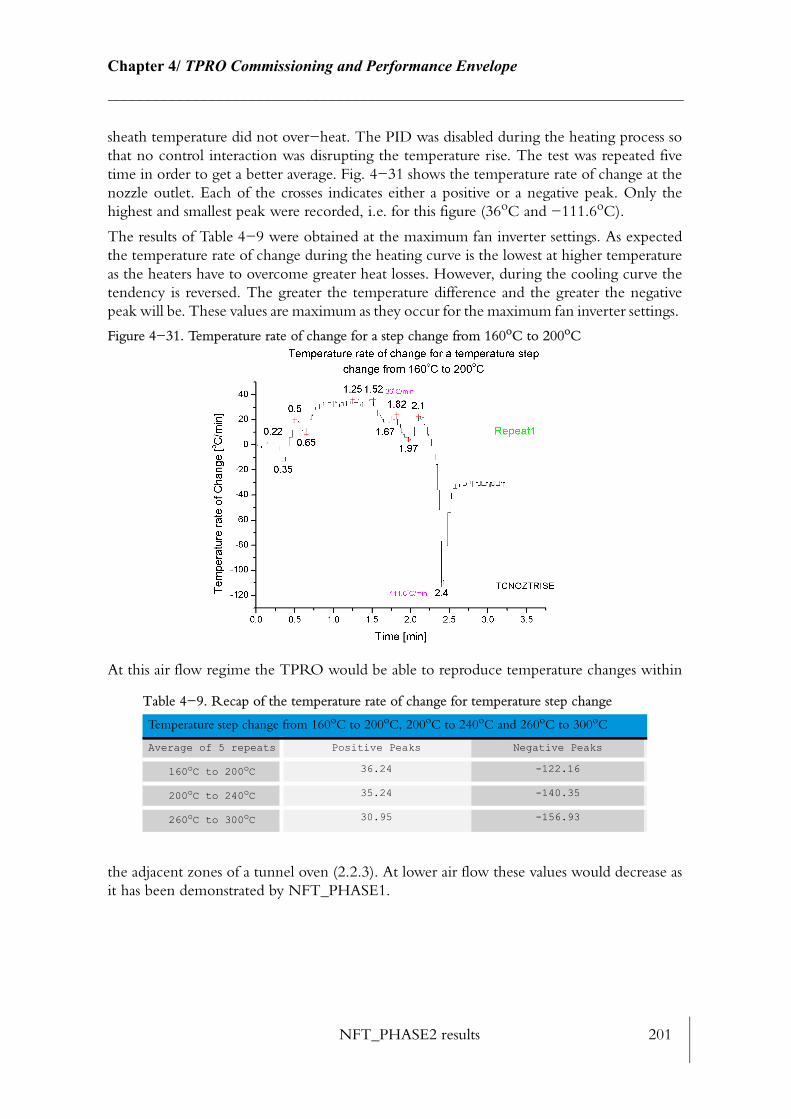
NFT_PHASE2 results 201
Chapter 4/ TPRO Commissioning and Performance Envelope________________________________________________________________________
sheath temperature did not over−heat. The PID was disabled during the heating process so that no control interaction was disrupting the temperature rise. The test was repeated five time in order to get a better average. Fig. 4−31 shows the temperature rate of change at the nozzle outlet. Each of the crosses indicates either a positive or a negative peak. Only the highest and smallest peak were recorded, i.e. for this figure (36oC and −111.6oC).
The results of Table 4−9 were obtained at the maximum fan inverter settings. As expected the temperature rate of change during the heating curve is the lowest at higher temperature as the heaters have to overcome greater heat losses. However, during the cooling curve the tendency is reversed. The greater the temperature difference and the greater the negative peak will be. These values are maximum as they occur for the maximum fan inverter settings.
Figure 4−31. Temperature rate of change for a step change from 160oC to 200oC
At this air flow regime the TPRO would be able to reproduce temperature changes within
the adjacent zones of a tunnel oven (2.2.3). At lower air flow these values would decrease as it has been demonstrated by NFT_PHASE1.
Table 4−9. Recap of the temperature rate of change for temperature step change
Temperature step change from 160oC to 200oC, 200oC to 240oC and 260oC to 300oC
Average of 5 repeats Positive Peaks Negative Peaks
160oC to 200oC 36.24 -122.16
200oC to 240oC 35.24 -140.35
260oC to 300oC 30.95 -156.93

NFT_PHASE3 and NFT_PHASE4 results 202
Chapter 4/ TPRO Commissioning and Performance Envelope________________________________________________________________________
4.7 NFT_PHASE3 and NFT_PHASE4 results
The FTE Scorpion heat flux sensor (Williamson M, 1996 [140]) was used for both NFT_PHASE3 and NFT_PHASE4 trials. Because the rates of temperature change for the heat flux logger are not the same as the food being baked, and also because the surface emis−sivity of the product changes slighlty as moisture is driven of the product, the prediction of the convective and radiative heat flux made by this instrument only gives a relative appreci−ation of heat flux values (3.4.8.6 for discussion of the methods of measuring the heat transfer to the food product). These measures are relative to a sink temperature which is placed inside the heat flux logger (Fig. 4−32). At the start of the trial the heat sink temperature should be close to the ambient temperature, however the whole temperature of the heat sink will rise relatively to the total heat flux surrounding the logger casings. Therefore the heat−sink tem−perature will not remain constant and the heat flux values will change as the heat sink tem−perature heats up. The TPRO InControlTM software has been built with heat transfer correlation equations (See 2.7.1, 2.7.2) which have been used to estimate the ranges of the convective and radiative heat flux that the product would go to. The equations variables are taking into consideration the possibility of changing the heat sink temperature .
Figure 4−32. Heat flux simulation to FTE Scorpion heat flux logger
4.7.1 Simulation results
The heat transfer coefficient used in the simulation of the NFT_PHASE3 trials (Table 4−10) were estimated from real trials for the range of temperature simulated. The results illus−
Tsink
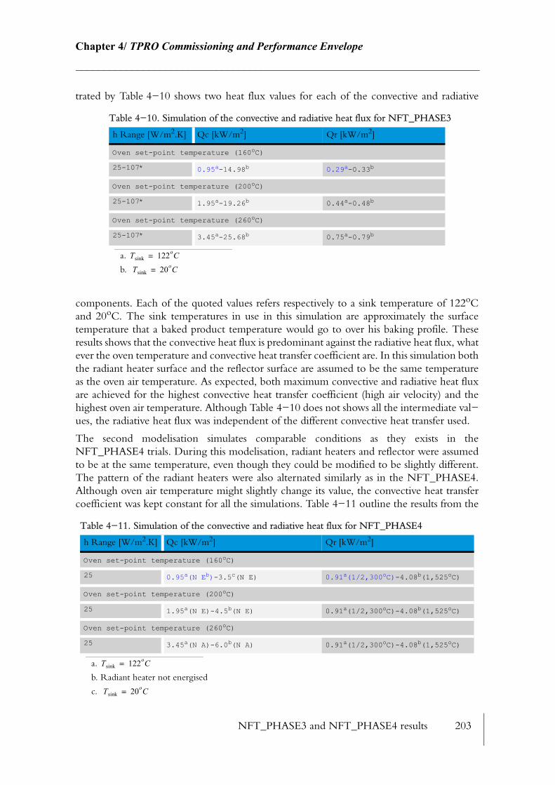
NFT_PHASE3 and NFT_PHASE4 results 203
Chapter 4/ TPRO Commissioning and Performance Envelope________________________________________________________________________
trated by Table 4−10 shows two heat flux values for each of the convective and radiative
components. Each of the quoted values refers respectively to a sink temperature of 122oC and 20oC. The sink temperatures in use in this simulation are approximately the surface temperature that a baked product temperature would go to over his baking profile. These results shows that the convective heat flux is predominant against the radiative heat flux, what ever the oven temperature and convective heat transfer coefficient are. In this simulation both the radiant heater surface and the reflector surface are assumed to be the same temperature as the oven air temperature. As expected, both maximum convective and radiative heat flux are achieved for the highest convective heat transfer coefficient (high air velocity) and the highest oven air temperature. Although Table 4−10 does not shows all the intermediate val−ues, the radiative heat flux was independent of the different convective heat transfer used.
The second modelisation simulates comparable conditions as they exists in the NFT_PHASE4 trials. During this modelisation, radiant heaters and reflector were assumed to be at the same temperature, even though they could be modified to be slightly different. The pattern of the radiant heaters were also alternated similarly as in the NFT_PHASE4. Although oven air temperature might slightly change its value, the convective heat transfer coefficient was kept constant for all the simulations. Table 4−11 outline the results from the
Table 4−10. Simulation of the convective and radiative heat flux for NFT_PHASE3
h Range [W/m2.K] Qc [kW/m2] Qr [kW/m2]
Oven set-point temperature (160oC)
25-107* 0.95a-14.98b
a.
b.
0.29a-0.33b
Oven set-point temperature (200oC)
25-107* 1.95a-19.26b 0.44a-0.48b
Oven set-point temperature (260oC)
25-107* 3.45a-25.68b 0.75a-0.79b
Table 4−11. Simulation of the convective and radiative heat flux for NFT_PHASE4
h Range [W/m2.K] Qc [kW/m2] Qr [kW/m2]
Oven set-point temperature (160oC)
25 0.95a(N Eb)-3.5c(N E)
a.
b. Radiant heater not energised
c.
0.91a(1/2,300oC)-4.08b(1,525oC)
Oven set-point temperature (200oC)
25 1.95a(N E)-4.5b(N E) 0.91a(1/2,300oC)-4.08b(1,525oC)
Oven set-point temperature (260oC)
25 3.45a(N A)-6.0b(N A) 0.91a(1/2,300oC)-4.08b(1,525oC)
Tsink 122oC=
Tsink 20oC=
Tsink 122oC=
Tsink 20oC=
NFT_PHASE3 and NFT_PHASE4 results 204
Chapter 4/ TPRO Commissioning and Performance Envelope________________________________________________________________________
simulation of NFT_PHASE4. Next to each radiant heat flux measurement, the radiation pattern is indicated (1 = full, 1/2 = half) and also the temperature of the radiant surface and reflector temperature. For the convective heat flux, the radiant heater pattern as well as the temperature of the radiant/reflector does not influence the convective heat flux measure−ment (theoretically). Both convective and radiative heat flux are affected in a similar manner by the radiant heater and reflector temperature. The greater the heater and reflector tem−perature, the larger the temperature difference between the heated surface and the sink tem−perature, hence the greater the heat fluxes. For high oven temperature (260oC), the convective heat flux is still predominant. In order for the radiant heat flux to reach similar levels achieved for highest convective heat flux of 25.7kW/m2, the radiant heater as well as the reflector temperature would need to get to 1000oC (sink temperature between 20oC −122oC).
4.7.2 NFT_PHASE3 results
During this test phase, convection and radiation fluxes were measured using the Scorpion heat flux logger. For each tested temperature (160oC, 200oC, 260oC) five repeats were per−formed to get better average values. The heater surface temperature were not controlled and therefore the assumptions from the models were different. Convective heat transfer coeffi−cient values were compared to the computed values from InControlTM. Fig. 4−33 is one of the NFT_PHASE3 repeats, for an oven temperature set−point of 160oC. This graphs dif−ferentiate the convective and radiative flux. The total heat flux is also plotted.
The three phases of the test appears clearly. During the first phase of this test, both fans speed run at 5Hz which provides a constant nozzle outlet air velocity of 3.6m/s. The logger is left purposely 2 minutes longer than for the other two phases as it is started from cold and the relatively ‘heavy weight’ sensors needs to reach steady temperature. Approaching 8 minutes, the second phase is started and the graph follows well the fan speed (FIS) step change. During this phase the nozzle air velocity reaches 25.5m/s. Finally the third phase is started just before the 14 minutes mark and the nozzle exit velocity reaches 42.4m/s. It appears clearly on this graph that the convective flux is predominant comparatively to the radiative heat flux.
The convective flux features some recurring oscillation all along its profile. Between two minutes (marked A and B) four peaks are present. At the speed (2) at which the band was travelling during this trial (0.276 m/min.) the logger would see 4 times a row of nozzle. This indication seems to match with the number of peaks described between the interval A and B. From the second phase onward the radiative component decreases.

NFT_PHASE3 and NFT_PHASE4 results 205
Chapter 4/ TPRO Commissioning and Performance Envelope________________________________________________________________________
Figure 4−33. Heat flux profile at different air velocity for a temperature set−point of 160oC
4.7.3 NFT_PHASE3 results recap
45 trials similar to the one shown by Fig. 4−33 were performed. Three categories of tem−perature were studied, 160oC, 200oC, and 260oC.
For every set of oven temperature set−point (Table 4−12), the trend of Qc and Qr is iden−tical. The convective heat flux increases as fan speed (FIS) increases. Air temperature also affect positively the convective heat flux however its effects is not as great as the effect of the increase in air velocity. For a controlled oven set−point temperature, one would expect the radiation flux to remain constant over the fan velocity (FIS) range (as previously mentioned by Table 4−10). Theoretically, the radiative heat flux should be independent of the change in air velocity, i.e. convective heat flux. The results of Table 4−12 seems to go against this belief. By examining the temperature profile in the TPRO during this trials, it becomes clearer that radiative heat flux is affected by the rate of convective heat flux. The nozzle exit
Table 4−12. NFT_PHASE3 results recap
Qc [kW/m2] Qr [kW/m2]
Oven set-point temperature (160oC)
5Hz (3.6m/s) 0.441(43.7oC) 0.100(43.7oC)
50Hz (42.4m/s) 0.848(59.9oC) 0.004(59.9oC)
Oven set-point temperature (200oC)
5Hz (3.6m/s) 0.582(47.2oC) 0.100(47.2oC)
50Hz (42.4m/s) 1.093(68.8oC) 0.021(68.8oC)
Oven set-point temperature (260oC)
5Hz (3.6m/s) 0.706(76.3oC) 0.186(76.3oC)
50Hz (42.4m/s) 1.313(100.7oC) 0.086(100.7oC)
Trend
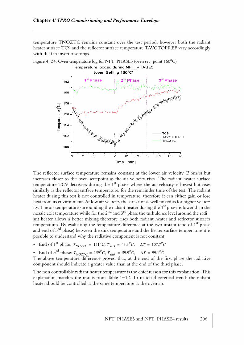
NFT_PHASE3 and NFT_PHASE4 results 206
Chapter 4/ TPRO Commissioning and Performance Envelope________________________________________________________________________
temperature TNOZTC remains constant over the test period, however both the radiant heater surface TC9 and the reflector surface temperature TAVGTOPREF vary accordingly with the fan inverter settings.
Figure 4−34. Oven temperature log for NFT_PHASE3 (oven set−point 160oC)
The reflector surface temperature remains constant at the lower air velocity (3.6m/s) but increases closer to the oven set−point as the air velocity rises. The radiant heater surface temperature TC9 decreases during the 1st phase where the air velocity is lowest but rises similarly as the reflector surface temperature, for the remainder time of the test. The radiant heater during this test is not controlled in temperature, therefore it can either gain or lose heat from its environment. At low air velocity the air is not as well mixed as for higher veloc−ity. The air temperature surrounding the radiant heater during the 1st phase is lower than the nozzle exit temperature while for the 2nd and 3rd phase the turbulence level around the radi−ant heater allows a better mixing therefore rises both radiant heater and reflector surfaces temperatures. By evaluating the temperature difference at the two instant (end of 1st phase and end of 3rd phase) between the sink temperature and the heater surface temperature it is possible to understand why the radiative component is not constant.
• End of 1st phase:
• End of 3rd phase: The above temperature difference proves, that, at the end of the first phase the radiative component should indicate a greater value than at the end of the third phase.
The non controllable radiant heater temperature is the chief reason for this explanation. This explanation matches the results from Table 4−12. To match theoretical trends the radiant heater should be controlled at the same temperature as the oven air.
TNOZTC 151oC, T ksin 43.3oC, ∆T 107.7oC= = =
TNOZTC 159oC, T ksin 59.9oC, ∆T 99.1oC= = =
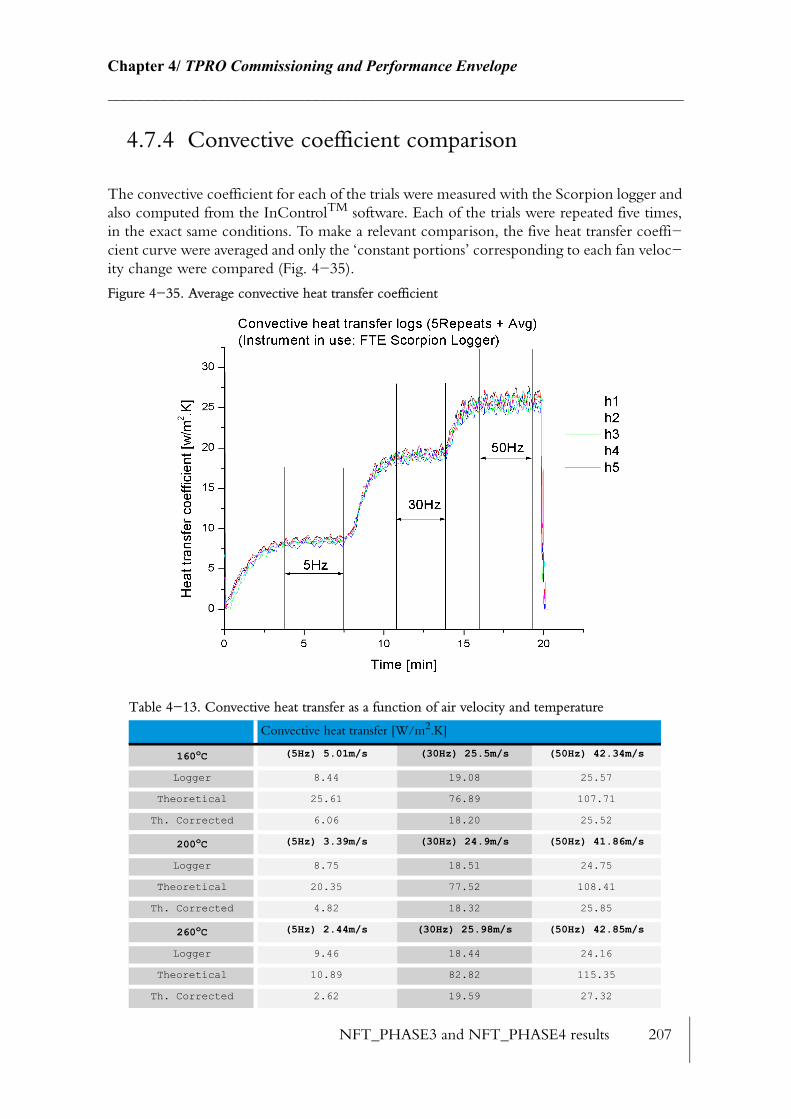
NFT_PHASE3 and NFT_PHASE4 results 207
Chapter 4/ TPRO Commissioning and Performance Envelope________________________________________________________________________
4.7.4 Convective coefficient comparison
The convective coefficient for each of the trials were measured with the Scorpion logger and also computed from the InControlTM software. Each of the trials were repeated five times, in the exact same conditions. To make a relevant comparison, the five heat transfer coeffi−cient curve were averaged and only the ‘constant portions’ corresponding to each fan veloc−ity change were compared (Fig. 4−35).
Figure 4−35. Average convective heat transfer coefficient
Table 4−13. Convective heat transfer as a function of air velocity and temperature
Convective heat transfer [W/m2.K]
160oC (5Hz) 5.01m/s (30Hz) 25.5m/s (50Hz) 42.34m/s
Logger 8.44 19.08 25.57
Theoretical 25.61 76.89 107.71
Th. Corrected 6.06 18.20 25.52
200oC (5Hz) 3.39m/s (30Hz) 24.9m/s (50Hz) 41.86m/s
Logger 8.75 18.51 24.75
Theoretical 20.35 77.52 108.41
Th. Corrected 4.82 18.32 25.85
260oC (5Hz) 2.44m/s (30Hz) 25.98m/s (50Hz) 42.85m/s
Logger 9.46 18.44 24.16
Theoretical 10.89 82.82 115.35
Th. Corrected 2.62 19.59 27.32

NFT_PHASE4 results 208
Chapter 4/ TPRO Commissioning and Performance Envelope________________________________________________________________________
For each temperature and fan velocity, three heat transfer coefficients were computed. The first value (logger) is the value logged directly from the FTE Scorpion logger. The second value (theoretical) is the value computed issued from the nozzle outlet velocity and temper−ature measurement. The third value (theoretical corrected) is the theoretical value corrected to ‘match’ the readings of the logger value. As the difference between the logger value and theoretical value were far apart the theoretical values were adjusted by virtually increasing the distance separating the nozzle outlet and the logger surface.
By analysing the data of Table 4−13 in rows, the three computed heat transfer coefficients, follows the same trend, i.e. the greater the air velocity the greater the convective heat transfer coefficient. Without taking into consideration the effect of temperature, the theoretical value is almost 4 times greater than the logger for every velocity change. The corrected theoretical values are almost equal to the logger values a part for the lowest air velocities.
A large difference in the convective heat transfer coefficient exists between the logger and the theoretical value. From a single round nozzle theory (Holger et al, 1977 [60]) a simple computation was performed to evaluate the heat transfer coefficient for a given nozzle exit temperature of 160oC. For the air nozzle velocity of 5, 25.5 and 42.4 m/s the respective convective coefficient were computed at, 19.3, 50.2 and 69 W/m2.K. For both cases (single or multiple nozzle impingement) the values from the FTE Scorpion logger are under esti−mated compared to the theoretical values.
For the lowest fan speed (FIS) (5Hz) the air velocity did change at the various temperature studied. This phenomenon, was proven to be a weakness in the measurement of the velocity. In these conditions, the support of the pitot tube undergo higher thermal stress and often deforms, hence the pitot head moves off−centre with the nozzle outlet. This phenomenon was not observable at higher velocities.
4.8 NFT_PHASE4 results
This test phase consisted of 3 repeats for each 4 scenarios at 3 different oven air temperature. A total of 36 tests were conducted to establish the effects of:
• having half of the radiant heaters on, in an alternate pattern, as opposed to having them all on.
• running the band at different speed in order to observe the effect on the radiant heat flux.
The results shown by Fig. 4−36 illustrate the three different phases of this trial. During this trial all the radiant heaters were switched on at their maximum surface temperature of 525oC. Over a two minutes period, at the band speed of the first phase, the number of peak
expected by both convective and radiative flux should be respectively 4 and 4.6. Although the peaks of the convective curve appear more clearly than for the radiative curve, they match the expected number of peaks for this band speed. For the second and third phase for both convective and radiative heat flux the peaks appears a lot less clearly and a zoom on the graph does not show a matching number of peak with the phases respective to the band speed. The
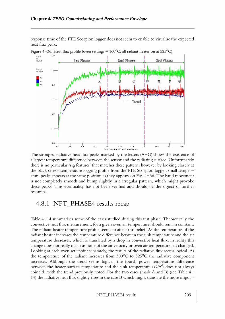
NFT_PHASE4 results 209
Chapter 4/ TPRO Commissioning and Performance Envelope________________________________________________________________________
response time of the FTE Scorpion logger does not seem to enable to visualise the expected heat flux peak.
Figure 4−36. Heat flux profile (oven settings = 160oC, all radiant heater on at 525oC)
The strongest radiative heat flux peaks marked by the letters (A−G) shows the existence of a largest temperature difference between the sensor and the radiating surface. Unfortunately there is no particular ‘rig features’ that matches these pattern, however by looking closely at the black sensor temperature logging profile from the FTE Scorpion logger, small temper−ature peaks appears at the same position as they appears on Fig. 4−36. The band movement is not completely smooth and bump slightly in a irregular pattern, which might provoke these peaks. This eventuality has not been verified and should be the object of further research.
4.8.1 NFT_PHASE4 results recap
Table 4−14 summarises some of the cases studied during this test phase. Theoretically the convective heat flux measurement, for a given oven air temperature, should remain constant. The radiant heater temperature profile seems to affect this belief. As the temperature of the radiant heater increases the temperature difference between the sink temperature and the air temperature decreases, which is translated by a drop in convective heat flux, in reality this change does not really occur as none of the air velocity or oven air temperature has changed. Looking at each oven set−point separately, the results of the radiative flux seems logical. As the temperature of the radiant increases from 300oC to 525oC the radiative component increases. Although the trend seems logical, the fourth power temperature difference between the heater surface temperature and the sink temperature (Diff4) does not always coincide with the trend previously noted. For the two cases (mark A and B) (see Table 4−14) the radiative heat flux slightly rises in the case B which might translate the more impor−
Trend
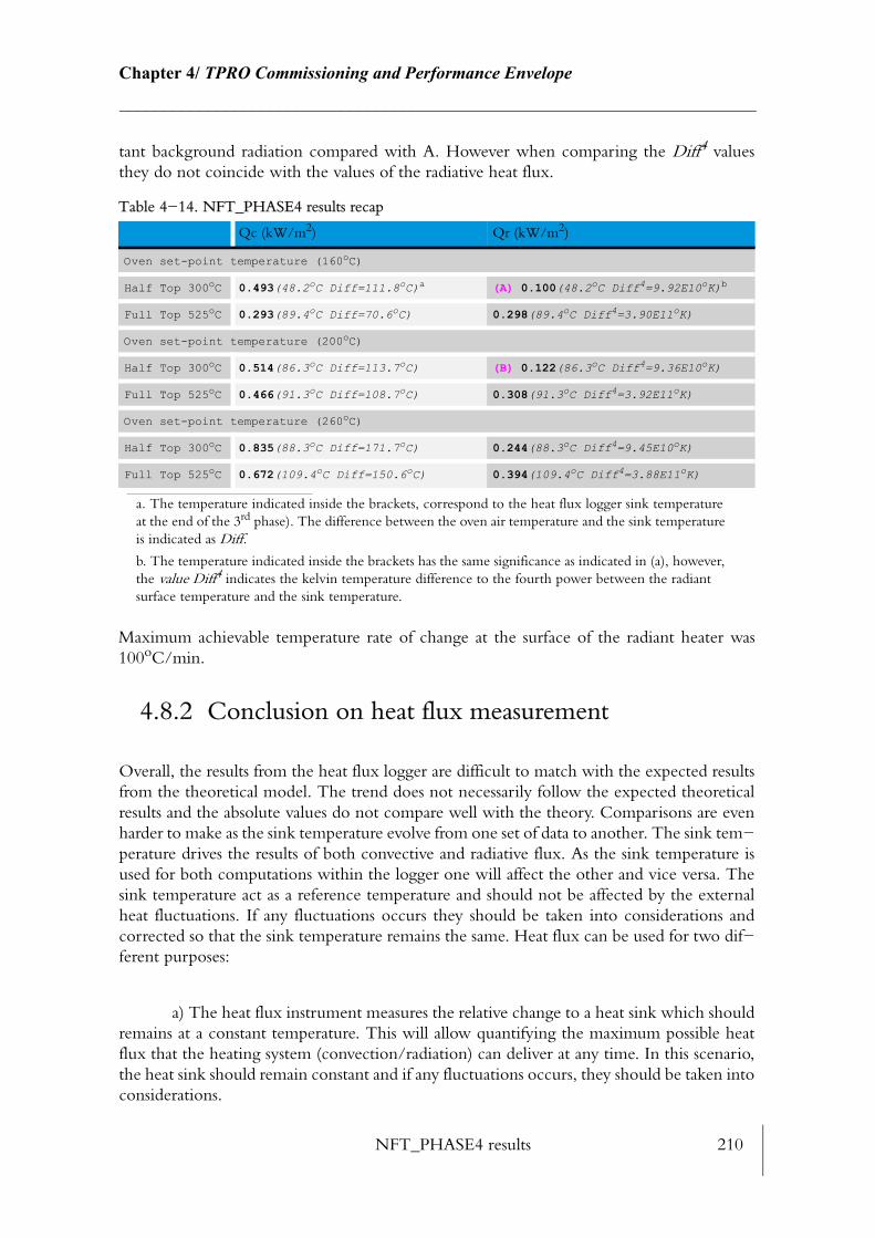
NFT_PHASE4 results 210
Chapter 4/ TPRO Commissioning and Performance Envelope________________________________________________________________________
tant background radiation compared with A. However when comparing the Diff4 values they do not coincide with the values of the radiative heat flux.
4.8.2 Conclusion on heat flux measurement
Overall, the results from the heat flux logger are difficult to match with the expected results from the theoretical model. The trend does not necessarily follow the expected theoretical results and the absolute values do not compare well with the theory. Comparisons are even harder to make as the sink temperature evolve from one set of data to another. The sink tem−perature drives the results of both convective and radiative flux. As the sink temperature is used for both computations within the logger one will affect the other and vice versa. The sink temperature act as a reference temperature and should not be affected by the external heat fluctuations. If any fluctuations occurs they should be taken into considerations and corrected so that the sink temperature remains the same. Heat flux can be used for two dif−ferent purposes:
a) The heat flux instrument measures the relative change to a heat sink which should remains at a constant temperature. This will allow quantifying the maximum possible heat flux that the heating system (convection/radiation) can deliver at any time. In this scenario, the heat sink should remain constant and if any fluctuations occurs, they should be taken into considerations.
Table 4−14. NFT_PHASE4 results recap
Qc (kW/m2) Qr (kW/m2)
Oven set-point temperature (160oC)
Half Top 300oC 0.493(48.2oC Diff=111.8oC)a
a. The temperature indicated inside the brackets, correspond to the heat flux logger sink temperature at the end of the 3rd phase). The difference between the oven air temperature and the sink temperature is indicated as Diff.
(A) 0.100(48.2oC Diff4=9.92E10oK)b
b. The temperature indicated inside the brackets has the same significance as indicated in (a), however, the value Diff4 indicates the kelvin temperature difference to the fourth power between the radiant surface temperature and the sink temperature.
Maximum achievable temperature rate of change at the surface of the radiant heater was 100oC/min.
Full Top 525oC 0.293(89.4oC Diff=70.6oC) 0.298(89.4oC Diff4=3.90E11oK)
Oven set-point temperature (200oC)
Half Top 300oC 0.514(86.3oC Diff=113.7oC) (B) 0.122(86.3oC Diff4=9.36E10oK)
Full Top 525oC 0.466(91.3oC Diff=108.7oC) 0.308(91.3oC Diff4=3.92E11oK)
Oven set-point temperature (260oC)
Half Top 300oC 0.835(88.3oC Diff=171.7oC) 0.244(88.3oC Diff4=9.45E10oK)
Full Top 525oC 0.672(109.4oC Diff=150.6oC) 0.394(109.4oC Diff4=3.88E11oK)
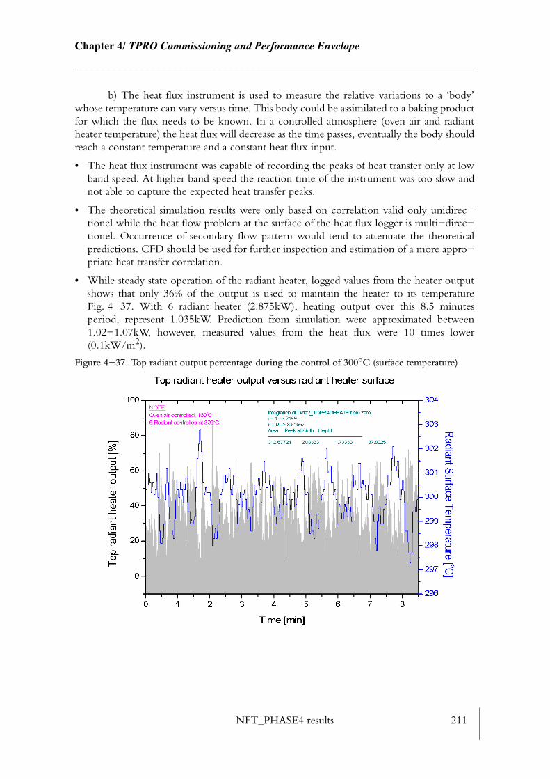
NFT_PHASE4 results 211
Chapter 4/ TPRO Commissioning and Performance Envelope________________________________________________________________________
b) The heat flux instrument is used to measure the relative variations to a ‘body’ whose temperature can vary versus time. This body could be assimilated to a baking product for which the flux needs to be known. In a controlled atmosphere (oven air and radiant heater temperature) the heat flux will decrease as the time passes, eventually the body should reach a constant temperature and a constant heat flux input.
• The heat flux instrument was capable of recording the peaks of heat transfer only at low band speed. At higher band speed the reaction time of the instrument was too slow and not able to capture the expected heat transfer peaks.
• The theoretical simulation results were only based on correlation valid only unidirec−tionel while the heat flow problem at the surface of the heat flux logger is multi−direc−tionel. Occurrence of secondary flow pattern would tend to attenuate the theoretical predictions. CFD should be used for further inspection and estimation of a more appro−priate heat transfer correlation.
• While steady state operation of the radiant heater, logged values from the heater output shows that only 36% of the output is used to maintain the heater to its temperature Fig. 4−37. With 6 radiant heater (2.875kW), heating output over this 8.5 minutes period, represent 1.035kW. Prediction from simulation were approximated between 1.02−1.07kW, however, measured values from the heat flux were 10 times lower (0.1kW/m2).
Figure 4−37. Top radiant output percentage during the control of 300oC (surface temperature)
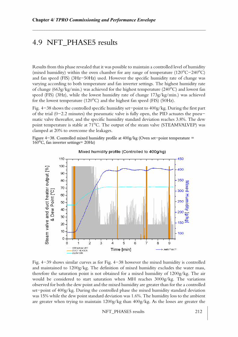
NFT_PHASE5 results 212
Chapter 4/ TPRO Commissioning and Performance Envelope________________________________________________________________________
4.9 NFT_PHASE5 results
Results from this phase revealed that it was possible to maintain a controlled level of humidity (mixed humidity) within the oven chamber for any range of temperature (120oC−240oC) and fan speed (FIS) (3Hz−50Hz) used. However the specific humidity rate of change was varying according to both temperature and fan inverter settings. The highest humidity rate of change (663g/kg/min.) was achieved for the highest temperature (240oC) and lowest fan speed (FIS) (3Hz), while the lowest humidity rate of change 173g/kg/min.) was achieved for the lowest temperature (120oC) and the highest fan speed (FIS) (50Hz).
Fig. 4−38 shows the controlled specific humidity set−point to 400g/kg. During the first part of the trial (0−2.2 minutes) the pneumatic valve is fully open, the PID actuates the pneu−matic valve thereafter, and the specific humidity standard deviation reaches 3.8%. The dew point temperature is stable at 71oC. The output of the steam valve (STEAMVALVEP) was clamped at 20% to overcome the leakages.
Figure 4−38. Controlled mixed humidity profile at 400g/kg (Oven set−point temperature = 160oC, fan inverter settings= 20Hz)
Fig. 4−39 shows similar curves as for Fig. 4−38 however the mixed humidity is controlled and maintained to 1200g/kg. The definition of mixed humidity excludes the water mass, therefore the saturation point is not obtained for a mixed humidity of 1200g/kg. The air would be considered to start saturation when MH reaches 3000g/kg. The variations observed for both the dew point and the mixed humidity are greater than for the a controlled set−point of 400g/kg. During the controlled phase the mixed humidity standard deviation was 15% while the dew point standard deviation was 1.6%. The humidity loss to the ambient are greater when trying to maintain 1200g/kg than 400g/kg. As the losses are greater the

TPRO technical specifications 213
Chapter 4/ TPRO Commissioning and Performance Envelope________________________________________________________________________
PID tends to counteract quicker the humidity loss and cause a slight overshoot. Both the PID controlling the temperature and the humidity are acting in phase. Indeed, as humidity is loss from the oven chamber, the energy contained by the hot vapour adds up as an energy loss and the duct heater PID controller counteract quickly to this thermal loss. As both steam and heating acts in phase the amount of energy added is greater than what is actually requested, hence the overshoot. One solution to avoid large overshoot, would be to avoid these two PID to act in phase, however this issue is left for further research.
Figure 4−39. Controlled mixed humidity profile at 1200g/kg (oven set−point temperature = 160oC)
4.10 TPRO technical specifications
The measured technical specifications of the TPRO are summarised in Table 4−15. This table indicates the ranges of operations that the TPRO has been tested to. These ranges rep−resents minimum and maximum achievable values.
Power ratings are often used in the baking industry to compare the maximum achievable power that can be delivered by the heating source. Often these values mislead. A more sci−entific terminology would be the maximum achievable ‘baking area total heat flux’ which represents the maximum heating power available divided by the area of the baking area. Only a fraction of this baking area total heat flux will be used to bake the product, and the rest is used to heat up and maintain the oven to temperature. For comparison, the total convective and radiative baking area heat flux of the TPRO was evaluated to 565.5kW/m2 of which 95.8% was convective heat flux and 4.1% was radiative heat flux.
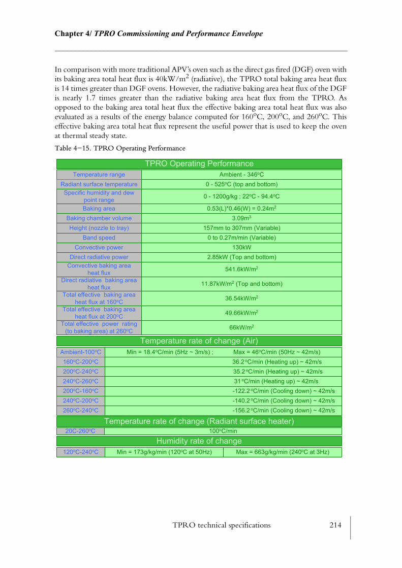
TPRO technical specifications 214
Chapter 4/ TPRO Commissioning and Performance Envelope________________________________________________________________________
In comparison with more traditional APV’s oven such as the direct gas fired (DGF) oven with its baking area total heat flux is 40kW/m2 (radiative), the TPRO total baking area heat flux is 14 times greater than DGF ovens. However, the radiative baking area heat flux of the DGF is nearly 1.7 times greater than the radiative baking area heat flux from the TPRO. As opposed to the baking area total heat flux the effective baking area total heat flux was also evaluated as a results of the energy balance computed for 160oC, 200oC, and 260oC. This effective baking area total heat flux represent the useful power that is used to keep the oven at thermal steady state.
Table 4−15. TPRO Operating Performance
TPRO Operating PerformanceTemperature range Ambient - 346oC
Radiant surface temperature 0 - 525oC (top and bottom)
Baking area 0.53(L)*0.46(W) = 0.24m2
Baking chamber volume 3.09m3
Height (nozzle to tray) 157mm to 307mm (Variable)Band speed 0 to 0.27m/min (Variable)
Convective power 130kWDirect radiative power 2.85kW (Top and bottom)
Convective baking areaheat flux 541.6kW/m2
Direct radiative baking areaheat flux 11.87kW/m2 (Top and bottom)
Total effective baking areaheat flux at 160oC 36.54kW/m2
Total effective baking areaheat flux at 200oC 49.66kW/m2
Total effective power rating(to baking area) at 260oC 66kW/m2
Specific humidity and dewpoint range 0 - 1200g/kg ; 22oC - 94.4oC
Temperature rate of change (Air)
Temperature rate of change (Radiant surface heater)
Humidity rate of change120oC-240oC Min = 173g/kg/min (120oC at 50Hz) Max = 663g/kg/min (240oC at 3Hz)
Ambient-100oC Min = 18.4oC/min (5Hz ~ 3m/s) ; Max = 46oC/min (50Hz ~ 42m/s)160oC-200oC 36.2 oC/min (Heating up) ~ 42m/s200oC-240oC 35.2 oC/min (Heating up) ~ 42m/s240oC-260oC 31 oC/min (Heating up) ~ 42m/s200oC-160oC -122.2 oC/min (Cooling down) ~ 42m/s
260oC-240oC -156.2 oC/min (Cooling down) ~ 42m/s240oC-200oC -140.2 oC/min (Cooling down) ~ 42m/s
20C-260oC 100oC/min

TPRO technical specifications 215
Chapter 4/ TPRO Commissioning and Performance Envelope________________________________________________________________________
Power requirement to maintain thermal steady state (kW)Temperature Qgain*
200oC 11.92260oC 15.84
160oC 8.77Qloss*
8.7711.9215.84
Qefan*
0.690.800.94
Qairl*
1.582.533.72
Qcfan*
4.444.594.71
Qcwt*
2.343.2
4.41
Qrwt*
3.113.914.86
Qth_Bridges*
1.712.272.85
QH1*
0.861.472.38
QH2*
1.392.533.76
QH3*
1.392.534.05
* Qgain: Heat gain from heaters, fans; Qloss: Heat loss from convection, radiation, leakages, thermal bridges;
Qairl: Heat loss from leakages; Qcfan: Heat gain from circulation fan; Qefan: Heat gain from extraction fan;
Qcwt: Heat loss from convective loss; Qrwt: Heat loss from radiative loss; Qth_Bridges: Heat loss from thermal
bridges; QH1(2,3): Heat gain from duct heater (1, 2, 3)
Effect of convective heating on convective and radiative heat flux (kW/m2)*: Sink temperatue in bracket
160oC - 5Hz(3.6m/s) 0.441(43.7oC) 0.1(43.7oC)160oC - 50Hz(42.4m/s) 0.848(59.9oC) 0.004(59.9oC)200oC - 5Hz(3.6m/s) 0.582(59.9oC) 0.1(59.9oC)200oC - 5Hz(42.4m/s) 1.093(59.9oC) 0.021(59.9oC)
0.95(122oC)14.98(20oC)1.95(122oC)19.26(20oC)
0.29(122oC)0.33(20oC)
0.44(43.7oC)0.48(20oC)
260oC - 5Hz(3.6m/s) 0.706(59.9oC) 0.186(59.9oC) 3.45(122oC) 0.75(122oC)260oC - 5Hz(42.4m/s) 1.313(59.9oC) 0.086(59.9oC) 25.68(20oC) 0.79(20oC)
Heat Flux Qc (logger) Qr (logger) Qc (model) Qr (model)
Effect of radiant heating on convective and radiative heat flux (kW/m2)
160oC - ½ Top 300oC 0.493(48.2oC) 0.1(48.2oC)160oC - 1 Top 525oC 0.293(89.4oC) 0.298(89.4oC)200oC - ½ Top 300oC 0.514(86.3oC) 0.122(86.3oC)200oC - 1 Top 525oC 0.466(91.3oC) 0.308(91.3oC)
0.95(122oC)3.5(20oC)
1.95(122oC)4.5(20oC)
0.91(122oC)4.08(20oC)
0.91(43.7oC)4.08(20oC)
260oC - ½ Top 300oC 0.835(88.3oC) 0.244(88.3oC) 3.45(122oC) 0.91(122oC)260oC - 1 Top 525oC 0.672(109.4oC) 0.394(109.4oC) 6.0(20oC) 4.08(20oC)
Heat Flux Qc (logger) Qr (logger) Qc (model) Qr (model)
Baking Comfort Zone 216
Chapter 5/ Concept of Baking Comfort Zone and Setting up of Experimental Design________________________________________________________________________
CHAPTER 5
CONCEPT OF BAKING COMFORT ZONE AND SETTING UP OF EXPERIMENTAL DESIGN
The study of heterogeneous products (foods) is a challenge and ensuring repeatability is difficult. This chapter proposes ‘baking comfort zones’ for optimising the baking process of Madeira cake. A design of experiments was developed to optimise the experimental programme and the methodology employed is described in detail.
5.1 Baking Comfort Zone
As opposed to the TPRO performance envelope, baking performance curves were devel−oped in an attempt to establish the ‘Baking Comfort Zone’ (BCZ) for a Madeira cake prod−uct. The term ‘BCZ’ is not used in the baking industry but has been adopted here as an analogy with the defined thermal comfort zone for indoor comfort in buildings. Significantly more research work has been undertaken on bread and biscuit, as these products alone rep−resent a large proportion of the world wide bakery production (1.2). Comparatively, very little has been done on cake products. Madeira cake product was chosen as the subject of this baking optimisation process for this reason, but also because its bake time is relatively long compared to biscuit and bread and therefore changes can be noticed more easily.
5.1.1 Thermal comfort and baking comfort zone analogy
Thermal comfort has been defined by the ISO 7730, 1995 [70], standard as being that ‘con−dition of mind which express satisfaction with the thermal environment’, Fanger, 1973 [47]. This notion can be difficult to translate into physical parameters, as for instance, a person can feel thermally comfortable in two different environments. The two conditions defining
Baking Comfort Zone 217
Chapter 5/ Concept of Baking Comfort Zone and Setting up of Experimental Design________________________________________________________________________
thermal comfort are the control of both core and skin temperature to respectively 37oC and 34oC and the maintenance of the body’s energy balance between heat gain (heat produced by the metabolism) and heat loss (by convection, conduction, radiation and evapo/conden−sation). This fragile energy balance is controlled by vertical air temperature difference, floor temperature, draughts, clothing, humidity, body activity level, and asymmetry of thermal radiation. A multitude of combinations exist between these parameters which provide ther−mally comfortable conditions in a building.
The baking scenario is different but by analogy a well baked product can be achieved by a number of combinations of heat fluxes (convective, radiative, conductive, condensation) and baking times. By baking a product within its comfort zone the baker can seek to reduce time and energy requirements, while achieving an acceptable product. Although the term baking comfort does not yet exist in the jargon of bakers, the concept should influence baking oven designers. For years, the baking process has remained a ‘black art’ and knowledge has been passed over between generations of bakers. Oven settings have been used without necessarily questioning the effectiveness of the baking process itself. Although it is not easy to quantify how ‘good’ a baked product is, as it refers to people’ s judgement and is very much a sub−jective notion, the target of this work was to quantify as much as possible the baking process and the product under study so that this ‘black art’ can become more of a defined science.
5.1.2 Theoretical concept of BCZ
For the traditional baking process, it has been defined (1.3) that four flux components can define the energy exchange between the product and the oven. In the case of a product baked in a tin (bread, cake), conduction occurs between the bottom surface of the product and the tray or band (support) where the product lays. The conduction flux is driven by the temperature difference across the tin thickness and the bottom surface temperature of the product to be baked and their conductivities. Convection is predominant at the top surface of the product where the temperature difference between the product top surface temper−ature and the air temperature. The convective flux is largely influenced by the air velocity. Radiation exchange is proportional to the temperature difference in Kelvin to the fourth power between the radiant heat source (radiant heater surface in this case) and the product surface. The view factor between the radiant/reflector and the product surface governs how much of the radiant energy strikes the product surface. The emissivity of the product is also of importance and will change slightly during the baking process as the product darkens. The evapo/condensation flux is closely linked to the convection flux, however it is driven by the wet bulb temperature of the product surface and the gas (dry bulb) temperature of the gas stream. During the early stage of the baking process when steam is injected and water con−denses onto surface of the product, a large quantity of heat is transferred to the baking prod−uct thanks to the latent heat of vaporisation. Later in the bake, the product dries out and the water vapour is released from the product surface by evaporation.
The four fluxes as defined above, can be plotted on four radii of a cylinder with the height axis representing the elapsed bake time Fig. 5−1, (A). The points plotted on each radius, at the base of this cylinder, represent the four fluxes as one can imagine they would be at the start on the baking Fig. 5−1, (A). The parallelogram Fig. 5−1, (B) represented by these four points represents the oven conditions at the early stage of the baking. This imaginary quad−
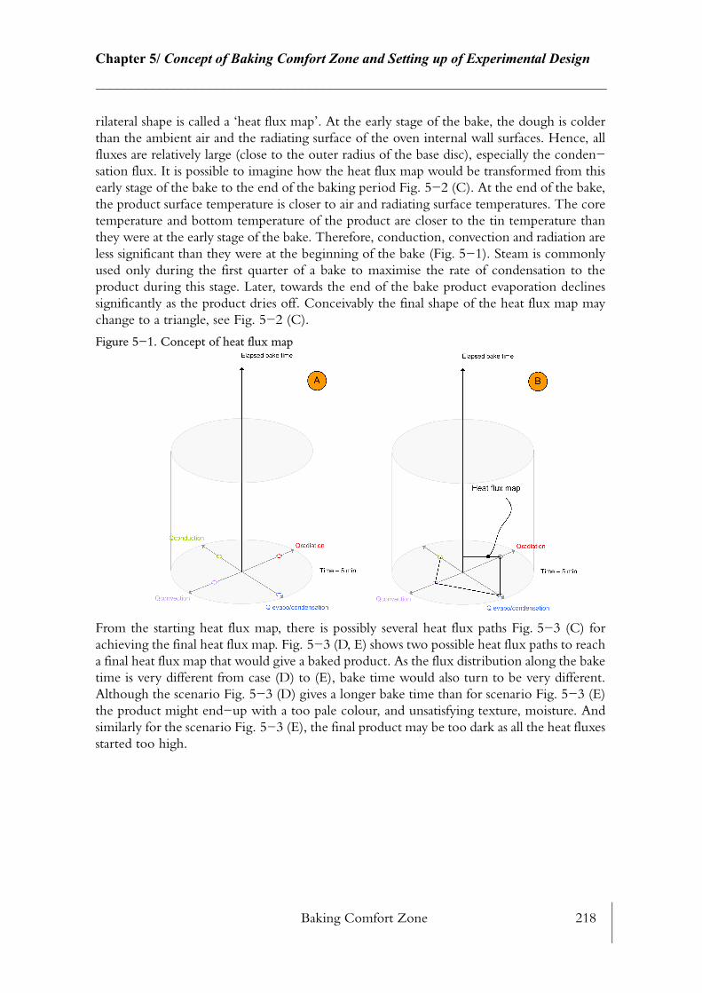
Baking Comfort Zone 218
Chapter 5/ Concept of Baking Comfort Zone and Setting up of Experimental Design________________________________________________________________________
rilateral shape is called a ‘heat flux map’. At the early stage of the bake, the dough is colder than the ambient air and the radiating surface of the oven internal wall surfaces. Hence, all fluxes are relatively large (close to the outer radius of the base disc), especially the conden−sation flux. It is possible to imagine how the heat flux map would be transformed from this early stage of the bake to the end of the baking period Fig. 5−2 (C). At the end of the bake, the product surface temperature is closer to air and radiating surface temperatures. The core temperature and bottom temperature of the product are closer to the tin temperature than they were at the early stage of the bake. Therefore, conduction, convection and radiation are less significant than they were at the beginning of the bake (Fig. 5−1). Steam is commonly used only during the first quarter of a bake to maximise the rate of condensation to the product during this stage. Later, towards the end of the bake product evaporation declines significantly as the product dries off. Conceivably the final shape of the heat flux map may change to a triangle, see Fig. 5−2 (C).
Figure 5−1. Concept of heat flux map
From the starting heat flux map, there is possibly several heat flux paths Fig. 5−3 (C) for achieving the final heat flux map. Fig. 5−3 (D, E) shows two possible heat flux paths to reach a final heat flux map that would give a baked product. As the flux distribution along the bake time is very different from case (D) to (E), bake time would also turn to be very different. Although the scenario Fig. 5−3 (D) gives a longer bake time than for scenario Fig. 5−3 (E) the product might end−up with a too pale colour, and unsatisfying texture, moisture. And similarly for the scenario Fig. 5−3 (E), the final product may be too dark as all the heat fluxes started too high.
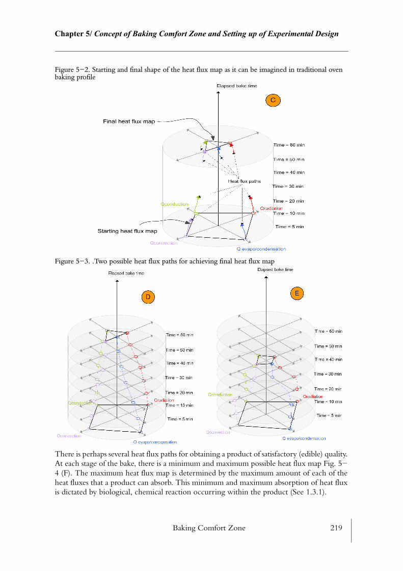
Baking Comfort Zone 219
Chapter 5/ Concept of Baking Comfort Zone and Setting up of Experimental Design________________________________________________________________________
Figure 5−2. Starting and final shape of the heat flux map as it can be imagined in traditional oven baking profile
Figure 5−3. .Two possible heat flux paths for achieving final heat flux map
There is perhaps several heat flux paths for obtaining a product of satisfactory (edible) quality. At each stage of the bake, there is a minimum and maximum possible heat flux map Fig. 5−4 (F). The maximum heat flux map is determined by the maximum amount of each of the heat fluxes that a product can absorb. This minimum and maximum absorption of heat flux is dictated by biological, chemical reaction occurring within the product (See 1.3.1).
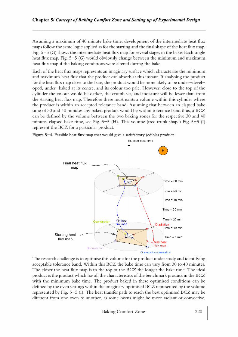
Baking Comfort Zone 220
Chapter 5/ Concept of Baking Comfort Zone and Setting up of Experimental Design________________________________________________________________________
Assuming a maximum of 40 minute bake time, development of the intermediate heat flux maps follow the same logic applied as for the starting and the final shape of the heat flux map. Fig. 5−5 (G) shows the intermediate heat flux map for several stages in the bake. Each single heat flux map, Fig. 5−5 (G) would obviously change between the minimum and maximum heat flux map if the baking conditions were altered during the bake.
Each of the heat flux maps represents an imaginary surface which characterise the minimum and maximum heat flux that the product can absorb at this instant. If analysing the product for the heat flux map close to the base, the product would be more likely to be under−devel−oped, under−baked at its centre, and its colour too pale. However, close to the top of the cylinder the colour would be darker, the crumb set, and moisture will be lesser than from the starting heat flux map. Therefore there must exists a volume within this cylinder where the product is within an accepted tolerance band. Assuming that between an elapsed bake time of 30 and 40 minutes any baked product would be within tolerance band thus, a BCZ can be defined by the volume between the two baking zones for the respective 30 and 40 minutes elapsed bake time, see Fig. 5−5 (H). This volume (tree trunk shape) Fig. 5−5 (I) represent the BCZ for a particular product.
Figure 5−4. Feasible heat flux map that would give a satisfactory (edible) product
The research challenge is to optimise this volume for the product under study and identifying acceptable tolerance band. Within this BCZ the bake time can vary from 30 to 40 minutes. The closer the heat flux map is to the top of the BCZ the longer the bake time. The ideal product is the product which has all the characteristics of the benchmark product in the BCZ with the minimum bake time. The product baked in these optimised conditions can be defined by the oven settings within the imaginary optimised BCZ represented by the volume represented by Fig. 5−5 (I). The heat transfer path to reach the best optimised BCZ may be different from one oven to another, as some ovens might be more radiant or convective,

Baking Comfort Zone 221
Chapter 5/ Concept of Baking Comfort Zone and Setting up of Experimental Design________________________________________________________________________
however it should be within each of the heat flux map represented by Fig. 5−5 (H). What−ever heat flux path has been followed, the optimised heat flux map may be represented by the flux map represented by Fig. 5−5 (J).
If the heat fluxes to the product were easily measurable in real time, it would be possible to develop a real−time graphic imaging interface that would show how the heat flux maps are changing during the bake. Further control algorithm might help to control their shape to reach optimum BCZ. The heat flux map paths displayed by Fig. 5−3 could be altered at any−time. For instance, more radiation might be required half way through the bake, hence the shape of the overall heat flux map would be altered. The best heat transfer BCZ profiles for any baking product could be established either by experimentation (Design of Experi−ments techniques) or by more sophisticated feedback control system using the Qualivision system and appropriate control algorithm such as fuzzy logic or neural networks. This way, BCZ profiles for any baking product could be established and entered into a database that would be used as a control reference, so that the current profile would match the optimised reference. To do so, the thermal response of the oven would have to be altered very quickly which obviously has limitations in practice.
Figure 5−5. Concept of Baking Comfort Zone and optimised comfort zone
To estimate the optimised BCZ, hence the best heat flux path, it is important to relate the process variable changes (heat fluxes) to responses changes such as product colour, crumb moisture, height, etc. The optimised heat flux map Fig. 5−5 (J) is considered to be optimised if the product responses are within the tolerance band. For any heat flux map (variables) a corresponding product zone (responses) exists, see Fig. 5−6. A heat flux map is accepted as part of the BCZ if and only if, the response zone is within the tolerance band. At any instant

Baking Comfort Zone 222
Chapter 5/ Concept of Baking Comfort Zone and Setting up of Experimental Design________________________________________________________________________
during the bake there is an optimum range of conditions defined by the four fluxes that will promote the final optimised product.
To optimise the baking process, one can imagine a control system linked to the process var−iables that would adjust the heat flux maps in order to attain the response zone within the tolerance band in the fastest time. This way, an ideal profile (variables/responses) versus time could be built for any individual product, thereby forming a unique mapping. The shape of the responses would be constrained by the maximum energy that the product can absorb at any time and hence relate to its thermal properties and geometry. The BCZ concept applies irrespective of oven type for a given product. BCZ concept also allows to purposely exper−iment to see if a greater input by one flux is a good method, or whether 2 or more fluxes need to be increased to get lower bake time. This concept is an idea for helping research objective, more than the baker in practice, mainly to help designing more efficient ovens.
Measurement of heat flux at the product surface in real time cannot be done easily and accu−racy can be difficult to estimate so it is more appropriate to measure the final product responses. In any experiment, measurements must be reliable and repeatable in any condi−tions. Chapter 4 (See 4.3.3) demonstrated the repeatability as well as the accuracy of the measured variables in the TPRO were of a high standard, but, the measurement of the prod−uct surface temperature was difficult to establish repeatedly. The use of a high humidity for long time period showed that condensation occurred in the Pitot tubes which made the reading of air velocity inaccurate. As yet, the BCZ is difficult to apply in practice, because of various measurement issues and so this concept is recommended for further research (See 7.2).
Figure 5−6. Process variables and product responses for the BCZ concept

Baking optimisation process methodology 223
Chapter 5/ Concept of Baking Comfort Zone and Setting up of Experimental Design________________________________________________________________________
5.1.3 Empirical BCZ
The four fluxes defining the concept of baking comfort were not measured with the TPRO. The following oven variables were measured to help defining the BCZ for Madeira cake:
• Oven temperature: air temperature in the vicinity of where the product bakes
• Fan speed (FIS): both circulation and re−circulation fan were kept the same
• Top damper position: the exact position of the top damper allows adjustment of the air velocity blowing at the top of the product
• Bottom damper position: the exact position of the bottom damper allows adjustment of the air velocity blowing at the bottom of the product
• Top radiation: top radiation element surface temperature
• Bottom radiation: bottom radiation element surface temperature
• Humidity: air specific humidity at the product surface
• Band speed: linear speed of the band during the baking
It is advantageous to measure heat fluxes as their absolute values can be compared with other ovens. Oven settings on the TPRO cannot be compared with any other industrial travelling ovens settings unless a scaling up is performed (See 7.2). The above eight measurements were proven to be easily reproducible in the TPRO.
5.2 Baking optimisation process methodology
The optimisation of a process can be difficult depending on the number of variable to be studied. A methodological approach is essential. The key question is to recognize what needs to be optimised and understand fully what are the process variables and the responses to be studied (Fig. 5−7). The process variables have to be accurately measured and repeatability is the most fundamental asset. Minimum day to day variations and improved repeatability of the test method will help to determine the possible correlations between the cause (process variable) and effects (responses). Ensuring adequacy of instrumentation and methods of measuring the product response seems obvious however in practice it is not straight forward. An important step must be taken during this methodology to determine the degree of accu−racy of all the process variables and the responses and ensure they can be measured repeatedly at all times.
Indeed, it is a necessity before performing an experimental design to ensure that all the process variables and responses can be recorded at all times. If it is not the case the entire experimental design cannot carry on as the result will become meaningless. This method−ology of process optimisation is at the heart of process performance improvement. This methodology can be applied to a full baking plant for instance where the core problems are to improve the production capacity and to reduce downtime, APV Baker, 2002 [7].

Baking optimisation process methodology 224
Chapter 5/ Concept of Baking Comfort Zone and Setting up of Experimental Design________________________________________________________________________
Figure 5−7. Optimisation of multiple responses process methodology
5.2.1 Sensory evaluation of baked goods
Sensory evaluation is a key aspect in the baking optimisation methodology. The aim of this evaluation is to measure characteristics of baked foods which humans are related to:
• smell: odour−flavour
• feel: texture
• visual: colour
• taste: flavour
• sound: noise
• appearance (mixture of colour and shape)
Suitable sensory evaluation is crucial in the world of food process engineering as it helps to ‘trouble−shoot’ in the market place and to ensure products are more likely to succeed than fail, Setser, 1993 [116]. In the early days sensory evaluation instrumentation did not exist therefore, sensory evaluation was based on sensory methods which relied on jury panel. Then, two types of test were in used, affective and analytical tests. The affective test measures the degree of preference (like/dislike) while the analytical test is more descriptive. Trained panellist are more involved in the analytical method while un−trained panellist will focus more on the cruder affective measures. Ranking or quantitative tests are very subjective because each individual is influenced by its own background (food habits, cultural back−ground etc.). Analytical questionnaires are a lot less subjective like the affectives one, as their answer have to be quantitative and accurate. Panellist are still present nowadays but the method of approach can be more radical. Often, eye check compared with dummy product can be used to judge of the quality of the final baked product.
Baking optimisation process methodology 225
Chapter 5/ Concept of Baking Comfort Zone and Setting up of Experimental Design________________________________________________________________________
Over the years sensory instrumentation has been developed to measure these characteristics as close as possible to represents the human senses. Measurement of volume and crumb firmness in bread and cake were reported by Cornford, 1969 [35]. Although the method of measuring volume seems crude by using a measuring box filled up with barley seeds, this approach is still very much in use today. Crumb firmness was measured with a compressim−eter which was originated from the 1950’s. This device was made of a circular brass plate where the weight was applied and a platform to dispose the baked product which was linked to a scale. The cone indenter device was build to try to overcome the limitations of the com−pressimeter for crumb which fractured.
In the 1980’s, on−line monitoring sensors were developed. With the advances in micro−technology and computing, on−line sensors and closed−loop control were developed to evaluate ‘better’ product with less variation, Mc Farlane, 1986 [77]. Whaley and Ellis, 1986[138], developed a two stage program to assess and control incoming ingredients and the fin−ished product. On−line sensor were allowing deviations to be identified quickly and inform operators, or an automated control system, to make adjustments to the product prior to it exceeding the process tolerances. In their attempt to increase flexibility and profit, near infrared on line moisture analyser was used to measure and control the key oven process var−iables. Pleass, 1986 [103] studied the advantages of using radio frequency dielectric techniques compared with the infra−red reflectance measurement which, only penetrates about 1 mm into the material being inspected. Infra red sensors are used where the surface moisture measured by the reflection can be related to the bulk moisture content, whereas dielectric sensors measure the entire amount of water present in the product. On line internal tem−perature measurement of the baking product is one of the key measurements to perform as it relates to chemical transformation and gives a good idea of the state of the bake. Ultrasonic temperature measurement were performed successfully by Richardson, 1986 [109] to measure the bulk temperature of food being processed.
The current trend in on−line monitoring is a vision system which can measure more than one parameter at a time such as colour, dimension, surface area, volume. The leader in this field is the Dipix instrument (Fig. 5−8).
The Dipix is a complex instrument which continuously views the product, thanks to a sensor head with laser profiling system. The Qualivision inspection software allows it to compute several aspect of the product such as diameters, heights, slopes, bake colour (lightness only), fissures, length, surface area and volume, APV Baker, 2002 [5]. These characteristics are most representative of the human sensory evaluation criteria. Very specific instrumentation has been developed for specific tasks. For instance the on−line bulk density meter from Three Sigma Ltd., APV Baker, 2002 [9], has been build for measuring on−line bulk density as the main criteria of cereals product rejection is based on the bulk density.
In today’s world still very few instrumentation are used on−line, and the Dipix and bulk density are one the few. Comparatively, there is more after bake measurement as more easy to preform (colour (Dipix), temperature, moisture, sizes).
Much of the literature seems to concentrate on the on−line measurement equipment because of its direct application in the industry. However, nowadays effort also tends to con−centrate on more microscopic instrumentations which are designed for very specific needs. Denys and Hendrickx, 1999 [43] used the line heat source probe method to estimate the thermal conductivity of food stuff. There has been a large increase in this types of instru−
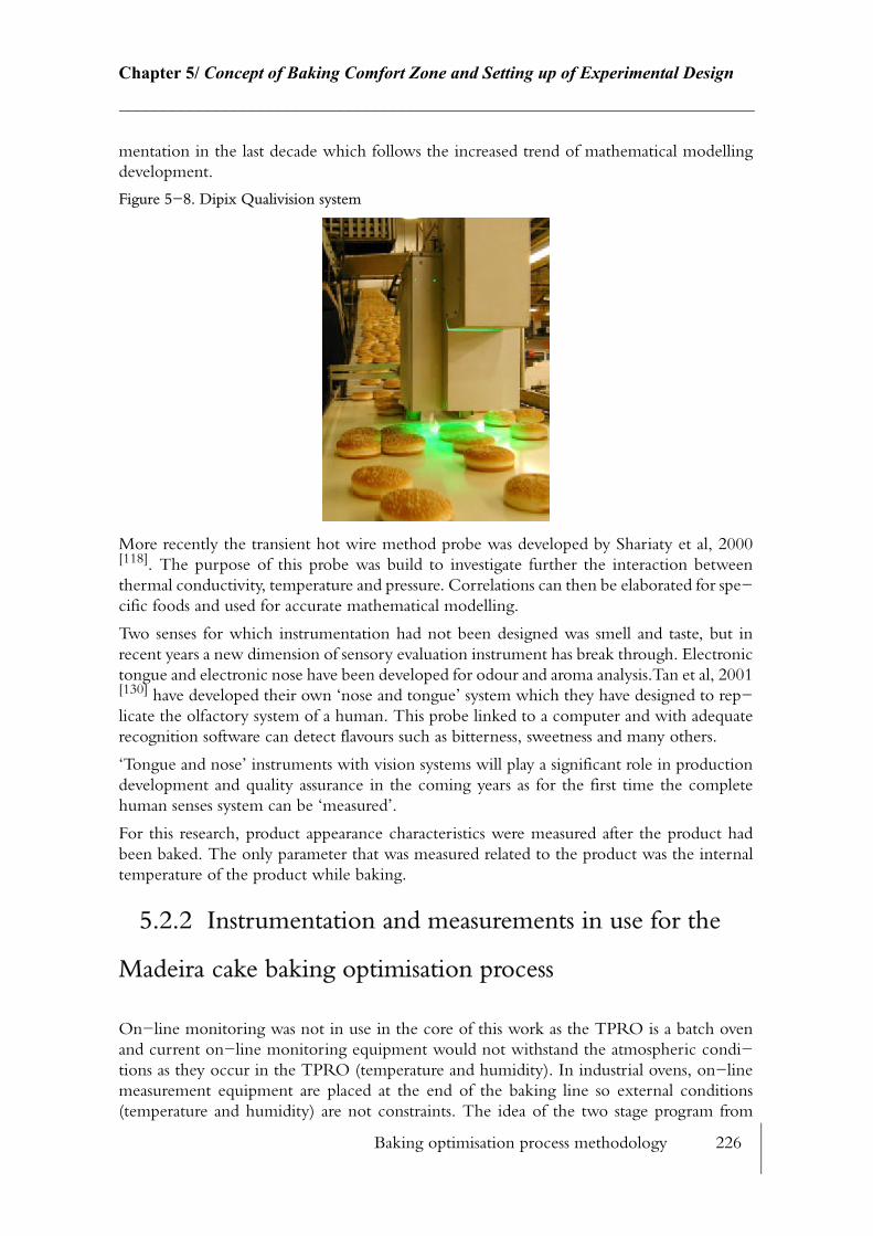
Baking optimisation process methodology 226
Chapter 5/ Concept of Baking Comfort Zone and Setting up of Experimental Design________________________________________________________________________
mentation in the last decade which follows the increased trend of mathematical modelling development.
Figure 5−8. Dipix Qualivision system
More recently the transient hot wire method probe was developed by Shariaty et al, 2000[118]. The purpose of this probe was build to investigate further the interaction between thermal conductivity, temperature and pressure. Correlations can then be elaborated for spe−cific foods and used for accurate mathematical modelling.
Two senses for which instrumentation had not been designed was smell and taste, but in recent years a new dimension of sensory evaluation instrument has break through. Electronic tongue and electronic nose have been developed for odour and aroma analysis.Tan et al, 2001[130] have developed their own ‘nose and tongue’ system which they have designed to rep−licate the olfactory system of a human. This probe linked to a computer and with adequate recognition software can detect flavours such as bitterness, sweetness and many others.
‘Tongue and nose’ instruments with vision systems will play a significant role in production development and quality assurance in the coming years as for the first time the complete human senses system can be ‘measured’.
For this research, product appearance characteristics were measured after the product had been baked. The only parameter that was measured related to the product was the internal temperature of the product while baking.
5.2.2 Instrumentation and measurements in use for the
Madeira cake baking optimisation process
On−line monitoring was not in use in the core of this work as the TPRO is a batch oven and current on−line monitoring equipment would not withstand the atmospheric condi−tions as they occur in the TPRO (temperature and humidity). In industrial ovens, on−line measurement equipment are placed at the end of the baking line so external conditions (temperature and humidity) are not constraints. The idea of the two stage program from
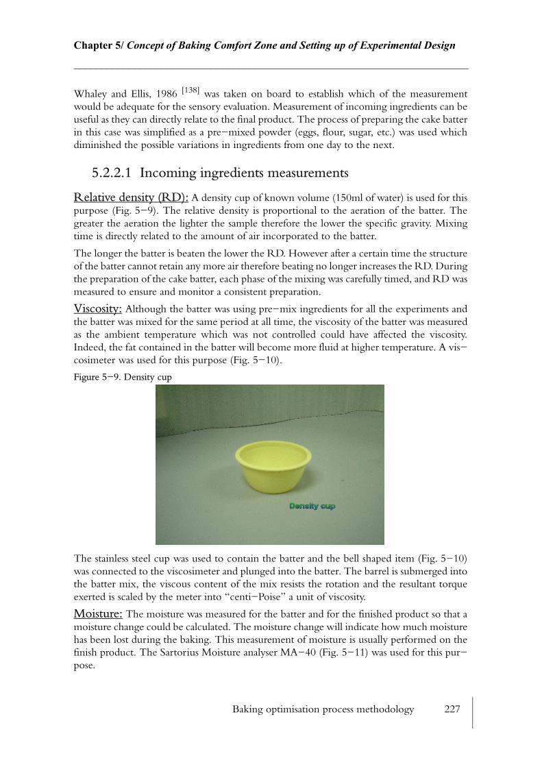
Baking optimisation process methodology 227
Chapter 5/ Concept of Baking Comfort Zone and Setting up of Experimental Design________________________________________________________________________
Whaley and Ellis, 1986 [138] was taken on board to establish which of the measurement would be adequate for the sensory evaluation. Measurement of incoming ingredients can be useful as they can directly relate to the final product. The process of preparing the cake batter in this case was simplified as a pre−mixed powder (eggs, flour, sugar, etc.) was used which diminished the possible variations in ingredients from one day to the next.
5.2.2.1 Incoming ingredients measurements
Relative density (RD): A density cup of known volume (150ml of water) is used for this purpose (Fig. 5−9). The relative density is proportional to the aeration of the batter. The greater the aeration the lighter the sample therefore the lower the specific gravity. Mixing time is directly related to the amount of air incorporated to the batter.
The longer the batter is beaten the lower the RD. However after a certain time the structure of the batter cannot retain any more air therefore beating no longer increases the RD. During the preparation of the cake batter, each phase of the mixing was carefully timed, and RD was measured to ensure and monitor a consistent preparation.
Viscosity: Although the batter was using pre−mix ingredients for all the experiments and the batter was mixed for the same period at all time, the viscosity of the batter was measured as the ambient temperature which was not controlled could have affected the viscosity. Indeed, the fat contained in the batter will become more fluid at higher temperature. A vis−cosimeter was used for this purpose (Fig. 5−10).
Figure 5−9. Density cup
The stainless steel cup was used to contain the batter and the bell shaped item (Fig. 5−10) was connected to the viscosimeter and plunged into the batter. The barrel is submerged into the batter mix, the viscous content of the mix resists the rotation and the resultant torque exerted is scaled by the meter into “centi−Poise” a unit of viscosity.
Moisture: The moisture was measured for the batter and for the finished product so that a moisture change could be calculated. The moisture change will indicate how much moisture has been lost during the baking. This measurement of moisture is usually performed on the finish product. The Sartorius Moisture analyser MA−40 (Fig. 5−11) was used for this pur−pose.
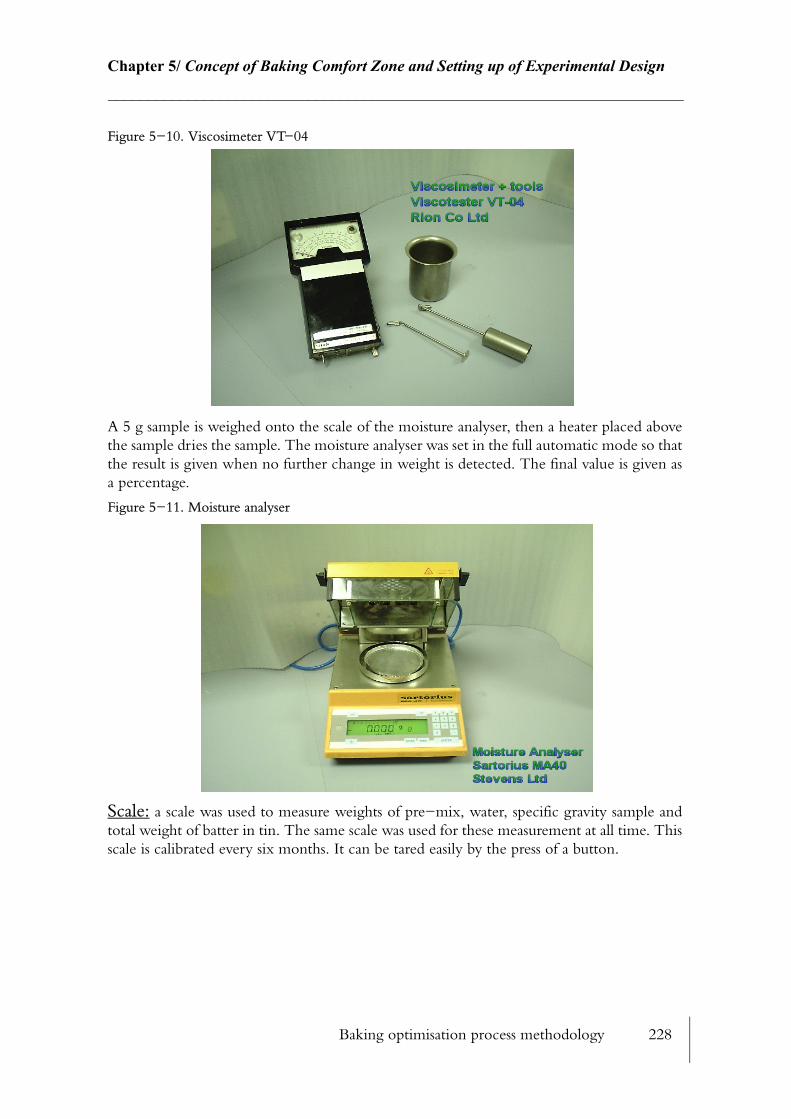
Baking optimisation process methodology 228
Chapter 5/ Concept of Baking Comfort Zone and Setting up of Experimental Design________________________________________________________________________
Figure 5−10. Viscosimeter VT−04
A 5 g sample is weighed onto the scale of the moisture analyser, then a heater placed above the sample dries the sample. The moisture analyser was set in the full automatic mode so that the result is given when no further change in weight is detected. The final value is given as a percentage.
Figure 5−11. Moisture analyser
Scale: a scale was used to measure weights of pre−mix, water, specific gravity sample and total weight of batter in tin. The same scale was used for these measurement at all time. This scale is calibrated every six months. It can be tared easily by the press of a button.
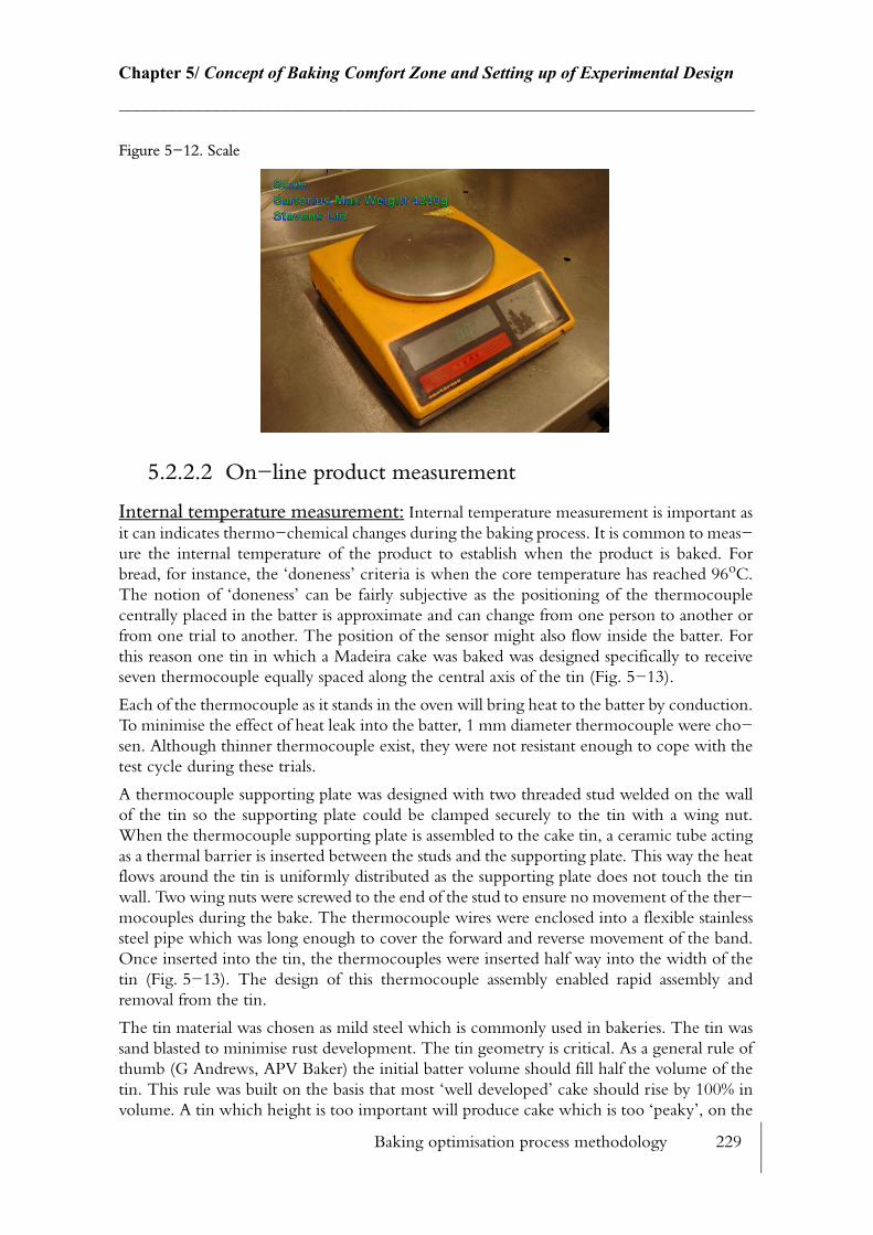
Baking optimisation process methodology 229
Chapter 5/ Concept of Baking Comfort Zone and Setting up of Experimental Design________________________________________________________________________
Figure 5−12. Scale
5.2.2.2 On−line product measurement
Internal temperature measurement: Internal temperature measurement is important as it can indicates thermo−chemical changes during the baking process. It is common to meas−ure the internal temperature of the product to establish when the product is baked. For bread, for instance, the ‘doneness’ criteria is when the core temperature has reached 96oC. The notion of ‘doneness’ can be fairly subjective as the positioning of the thermocouple centrally placed in the batter is approximate and can change from one person to another or from one trial to another. The position of the sensor might also flow inside the batter. For this reason one tin in which a Madeira cake was baked was designed specifically to receive seven thermocouple equally spaced along the central axis of the tin (Fig. 5−13).
Each of the thermocouple as it stands in the oven will bring heat to the batter by conduction. To minimise the effect of heat leak into the batter, 1 mm diameter thermocouple were cho−sen. Although thinner thermocouple exist, they were not resistant enough to cope with the test cycle during these trials.
A thermocouple supporting plate was designed with two threaded stud welded on the wall of the tin so the supporting plate could be clamped securely to the tin with a wing nut. When the thermocouple supporting plate is assembled to the cake tin, a ceramic tube acting as a thermal barrier is inserted between the studs and the supporting plate. This way the heat flows around the tin is uniformly distributed as the supporting plate does not touch the tin wall. Two wing nuts were screwed to the end of the stud to ensure no movement of the ther−mocouples during the bake. The thermocouple wires were enclosed into a flexible stainless steel pipe which was long enough to cover the forward and reverse movement of the band. Once inserted into the tin, the thermocouples were inserted half way into the width of the tin (Fig. 5−13). The design of this thermocouple assembly enabled rapid assembly and removal from the tin.
The tin material was chosen as mild steel which is commonly used in bakeries. The tin was sand blasted to minimise rust development. The tin geometry is critical. As a general rule of thumb (G Andrews, APV Baker) the initial batter volume should fill half the volume of the tin. This rule was built on the basis that most ‘well developed’ cake should rise by 100% in volume. A tin which height is too important will produce cake which is too ‘peaky’, on the
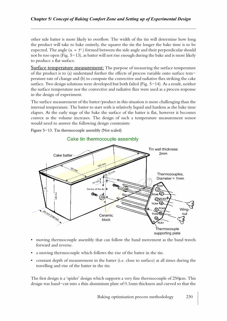
Baking optimisation process methodology 230
Chapter 5/ Concept of Baking Comfort Zone and Setting up of Experimental Design________________________________________________________________________
other side batter is more likely to overflow. The width of the tin will determine how long the product will take to bake entirely, the squarer the tin the longer the bake time is to be expected. The angle ( ) formed between the side angle and their perpendicular should not be too open (Fig. 5−13), as batter will not rise enough during the bake and is more likely to produce a flat surface.
Surface temperature measurement: The purpose of measuring the surface temperature of the product is to (a) understand further the effects of process variable onto surface tem−perature rate of change and (b) to compute the convective and radiative flux striking the cake surface. Two design solutions were developed but both failed (Fig. 5−14). As a result, neither the surface temperature nor the convective and radiative flux were used as a process response in the design of experiment.
The surface measurement of the batter/product in this situation is more challenging than the internal temperature. The batter to start with is relatively liquid and hardens as the bake time elapses. At the early stage of the bake the surface of the batter is flat, however it becomes convex as the volume increases. The design of such a temperature measurement sensor would need to answer the following design constraints:
Figure 5−13. Tin thermocouple assembly (Not scaled)
• moving thermocouple assembly that can follow the band movement as the band travels forward and reverse.
• a moving thermocouple which follows the rise of the batter in the tin.
• constant depth of measurement in the batter (i.e. close to surface) at all times during the travelling and rise of the batter in the tin.
The first design is a ‘spider’ design which supports a very fine thermocouple of 250µm. This design was hand−cut into a thin aluminium plate of 0.1mm thickness and curved so that the
α 5°=

Baking optimisation process methodology 231
Chapter 5/ Concept of Baking Comfort Zone and Setting up of Experimental Design________________________________________________________________________
‘legs’ sat on top of the batter product surface. The thin thermocouple was inserted into the body of the ‘spider’ design so that the ‘legs’ acted as a floater and the tip of the thermocouple touches the product surface without sinking. The thermocouple was guided by a copper pipe fixed a the top of the tin to guide the ‘spider’ thermocouple centrally to the tin. Several trials were conducted very successfully, however the thermocouple wire stiffened as the number of trials carried on. Thermal conditions arising in the TPRO caused high thermal stress which hardens the thermocouples (wire, sheath). The assembly got deeper in batter as the thermocouple got more rigid. Eventually, the thermocouple became brittle and rup−tured.
As the first solution failed a second solution was elaborated (Fig. 5−14). The ‘boat’ design, was built with a much larger surface area to ensure that the thermocouple was applied to the surface at all times. However, the drawback with this solution was that the much thicker thermocouple could not follow well the movement of the batter rising. No further attempt was made to measure the surface temperature of the product but further research attention should be given to this in the future.
Figure 5−14. Surface temperature measurement solutions
5.2.2.3 Post Process measurement
All the post process measurements were used to establish the product responses to the changes in the process variables.
Transient weight loss after bake: The first measurement that the product was subjected to after leaving the oven was the transient weight loss measurement. This was completed with a digital weight scale linked to a computer (Fig. 5−15). The cake was left for an hour and its weight was recorded every three seconds. As the product leaves the oven its internal temperature is approaching nearly 100oC, therefore the moisture contained inside the crumb will be driven off in the same direction as the temperature gradient between the crumb and the atmospheric temperature. The shape of the curve can give an estimation of how quickly the moisture is removed and therefore is related to the porosity of the crust. A highly porous crust will allow moisture to be driven off quicker compared with a less porous one. The presence of a crack at the surface can also change the rate at which moisture is driven off. The atmospheric temperature and humidity surrounding the cake in the process of cooling were not controlled and might have changed the transient weight loss. However the cake being cooled, was left every time in the FPC whose temperature during the day time did not vary a great deal.
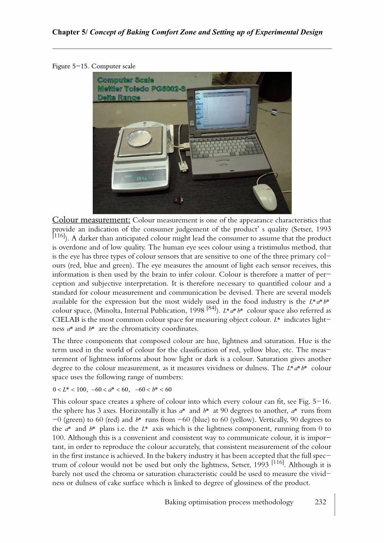
Baking optimisation process methodology 232
Chapter 5/ Concept of Baking Comfort Zone and Setting up of Experimental Design________________________________________________________________________
Figure 5−15. Computer scale
Colour measurement: Colour measurement is one of the appearance characteristics that provide an indication of the consumer judgement of the product’ s quality (Setser, 1993[116]). A darker than anticipated colour might lead the consumer to assume that the product is overdone and of low quality. The human eye sees colour using a tristimulus method, that is the eye has three types of colour sensors that are sensitive to one of the three primary col−ours (red, blue and green). The eye measures the amount of light each sensor receives, this information is then used by the brain to infer colour. Colour is therefore a matter of per−ception and subjective interpretation. It is therefore necessary to quantified colour and a standard for colour measurement and communication be devised. There are several models available for the expression but the most widely used in the food industry is the colour space, (Minolta, Internal Publication, 1998 [84]). colour space also referred as CIELAB is the most common colour space for measuring object colour. indicates light−ness and are the chromaticity coordinates.
The three components that composed colour are hue, lightness and saturation. Hue is the term used in the world of colour for the classification of red, yellow blue, etc. The meas−urement of lightness informs about how light or dark is a colour. Saturation gives another degree to the colour measurement, as it measures vividness or dulness. The colour space uses the following range of numbers:
This colour space creates a sphere of colour into which every colour can fit, see Fig. 5−16. the sphere has 3 axes. Horizontally it has and at 90 degrees to another, runs from −0 (green) to 60 (red) and runs from −60 (blue) to 60 (yellow). Vertically, 90 degrees to the and plans i.e. the axis which is the lightness component, running from 0 to 100. Although this is a convenient and consistent way to communicate colour, it is impor−tant, in order to reproduce the colour accurately, that consistent measurement of the colour in the first instance is achieved. In the bakery industry it has been accepted that the full spec−trum of colour would not be used but only the lightness, Setser, 1993 [116]. Although it is barely not used the chroma or saturation characteristic could be used to measure the vivid−ness or dulness of cake surface which is linked to degree of glossiness of the product.
L∗a∗b∗L∗a∗b∗
L∗a∗ b∗
L∗a∗b∗
0 L∗ 100, 60– a∗ 60, 60– b∗ 60< << << <
a∗ b∗ a∗b∗
a∗ b∗ L∗
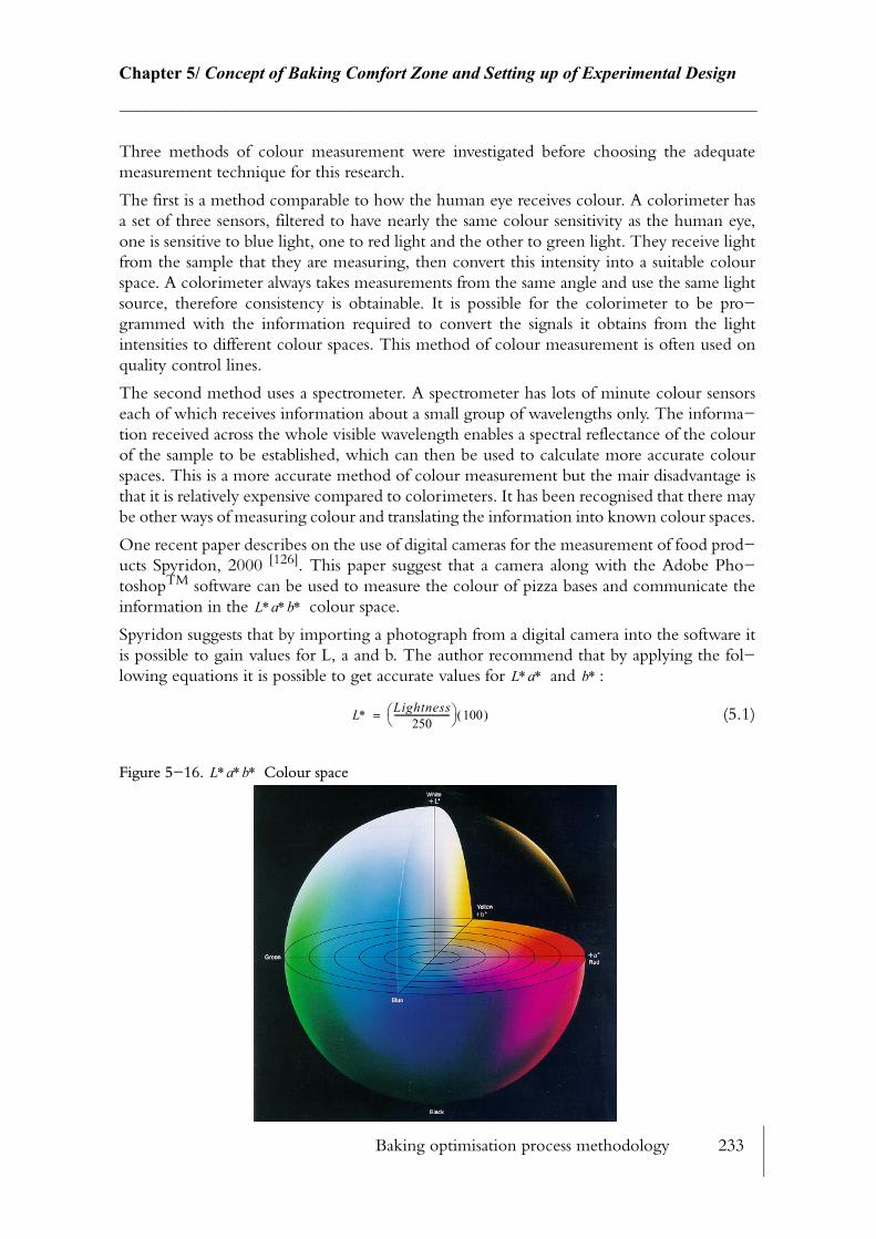
Baking optimisation process methodology 233
Chapter 5/ Concept of Baking Comfort Zone and Setting up of Experimental Design________________________________________________________________________
Three methods of colour measurement were investigated before choosing the adequate measurement technique for this research.
The first is a method comparable to how the human eye receives colour. A colorimeter has a set of three sensors, filtered to have nearly the same colour sensitivity as the human eye, one is sensitive to blue light, one to red light and the other to green light. They receive light from the sample that they are measuring, then convert this intensity into a suitable colour space. A colorimeter always takes measurements from the same angle and use the same light source, therefore consistency is obtainable. It is possible for the colorimeter to be pro−grammed with the information required to convert the signals it obtains from the light intensities to different colour spaces. This method of colour measurement is often used on quality control lines.
The second method uses a spectrometer. A spectrometer has lots of minute colour sensors each of which receives information about a small group of wavelengths only. The informa−tion received across the whole visible wavelength enables a spectral reflectance of the colour of the sample to be established, which can then be used to calculate more accurate colour spaces. This is a more accurate method of colour measurement but the mair disadvantage is that it is relatively expensive compared to colorimeters. It has been recognised that there may be other ways of measuring colour and translating the information into known colour spaces.
One recent paper describes on the use of digital cameras for the measurement of food prod−ucts Spyridon, 2000 [126]. This paper suggest that a camera along with the Adobe Pho−toshopTM software can be used to measure the colour of pizza bases and communicate the information in the colour space.
Spyridon suggests that by importing a photograph from a digital camera into the software it is possible to gain values for L, a and b. The author recommend that by applying the fol−lowing equations it is possible to get accurate values for and :
(5.1)
Figure 5−16. Colour space
L∗a∗b∗
L∗a∗ b∗
L∗ Lightness250
------------------------- 100( )=
L∗a∗b∗
Baking optimisation process methodology 234
Chapter 5/ Concept of Baking Comfort Zone and Setting up of Experimental Design________________________________________________________________________
(5.2)
(5.3)
By using a digital camera it is immediately possible to obtain information about the colour of the sample and values for . However as the method of colour measurement is sim−ilar to the way that a colorimeter works and it is recognised that colorimeters obtain con−sistency through always having the same lighting conditions, (often standard or if not standard, accounted for) it is crucial that the lighting of the sample is always the same.
To ensure that there were no variations in the lighting conditions a test rig was built (Fig. 5−17) which employed a proper light source for the illuminating the sample. The light source used dictates the appearance of the sample to the human eye and to the camera. The colour perceived by the human eye is the component of the incident light that is reflected by the sample called the diffuse reflection. Different light sources have different incident spectrum and therefore different diffused reflections and different appearances. The CIE (commission Internationale d’ Eclairage) has set standard light sources that should be used for food research. These standard light sources emit a spectrum of light similar to that of day light. and are characterised by their colour temperatures; A (2856K), C(6774K), D65(6500K) and D(7500K).
At present it is still uncertain as to the effect of several variables on the values for lightness that can be obtained by digital photography, and precision and accuracy of colour measure−ment by digital photography was not mentioned in the work performed by Spyridon, 2000[126]. These variables are:
• different digital camera
• different bulb in the lighting rig
• resolution of the camera
• output file to the computer
To establish reliability of the lighting rig and the camera, tests were carried out, which involved using different cameras, different light sources and different samples to understand what consistency could be established. Detailed results are shown in Appendix I. Due to poor consistency between the two cameras and the colour variations between the different file size, the digital imaging camera for measuring colour was left aside for further develop−ment.
The final decision on colour measurement system was helped by the joint venue of the IED group from APV Baker (Industrial Extrusion Division) which possessed a photo spectrom−eter Minolta CM−508d (Fig. 5−18).
a∗ 240a255
------------ 120–=
b∗ 240b255
------------ 120–=
L∗a∗b∗
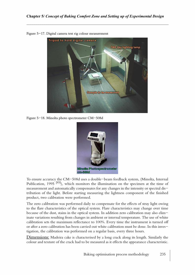
Baking optimisation process methodology 235
Chapter 5/ Concept of Baking Comfort Zone and Setting up of Experimental Design________________________________________________________________________
Figure 5−17. Digital camera test rig colour measurement
Figure 5−18. Minolta photo spectrometer CM−508d
To ensure accuracy the CM−508d uses a double−beam feedback system, (Minolta, Internal Publication, 1995 [85]), which monitors the illumination on the specimen at the time of measurement and automatically compensates for any changes in the intensity or spectral dis−tribution of the light. Before starting measuring the lightness component of the finished product, two calibration were performed.
The zero calibration was performed daily to compensate for the effects of stray light owing to the flare characteristics of the optical system. Flare characteristics may change over time because of the dust, stains in the optical system. In addition zero calibration may also elim−inate variations resulting from changes in ambient or internal temperature. The use of white calibration sets the maximum reflectance to 100%. Every time the instrument is turned off or after a zero calibration has been carried out white calibration must be done. In this inves−tigation, the calibration was performed on a regular basis, every three hours.
Dimensions: Madeira cake is characterised by a long crack along its length. Similarly the colour and texture of the crack had to be measured as it effects the appearance characteristic.
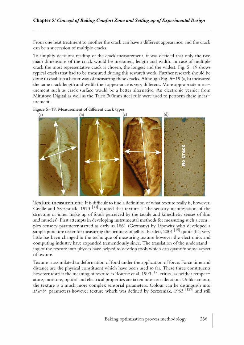
Baking optimisation process methodology 236
Chapter 5/ Concept of Baking Comfort Zone and Setting up of Experimental Design________________________________________________________________________
From one heat treatment to another the crack can have a different appearance, and the crack can be a succession of multiple cracks.
To simplify decisions reading of the crack measurement, it was decided that only the two main dimensions of the crack would be measured, length and width. In case of multiple crack the most representative crack is chosen, the longest and the widest. Fig. 5−19 shows typical cracks that had to be measured during this research work. Further research should be done to establish a better way of measuring these cracks. Although Fig. 5−19 (a, b) measured the same crack length and width their appearance is very different. More appropriate meas−urement such as crack surface would be a better alternative. An electronic vernier from Mitutoyo Digital as well as the Talco 300mm steel rule were used to perform these meas−urement.
Figure 5−19. Measurement of different crack types
Texture measurement: It is difficult to find a definition of what texture really is, however, Civille and Szczesniak, 1973 [33] quoted that texture is ‘the sensory manifestation of the structure or inner make up of foods perceived by the tactile and kinesthetic senses of skin and muscles’. First attempts in developing instrumental methods for measuring such a com−plex sensory parameter started as early as 1861 (Germany) by Lipowitz who developed a simple puncture tester for measuring the firmness of jellies. Bartlett, 2001 [15] quote that very little has been changed in the technique of measuring texture however the electronics and computing industry have expanded tremendously since. The translation of the understand−ing of the texture into physics have helped to develop tools which can quantify some aspect of texture.
Texture is assimilated to deformation of food under the application of force. Force time and distance are the physical constituent which have been used so far. These three constituents however restrict the meaning of texture as Bourne et al, 1993 [17] critics, as neither temper−ature, moisture, optical and electrical properties are taken into consideration. Unlike colour, the texture is a much more complex sensorial parameters. Colour can be distinguish into
parameters however texture which was defined by Szczesniak, 1963 [129] and still
(a) (b) (c) (d)
L∗a∗b∗
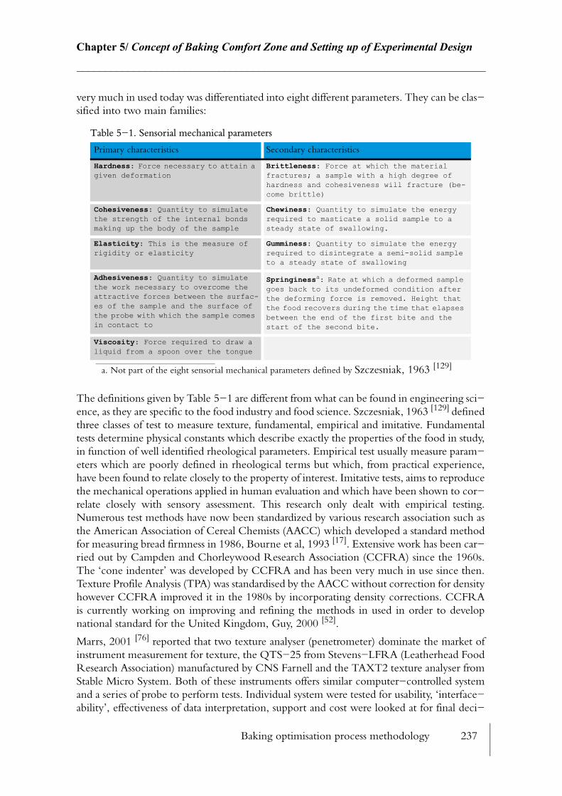
Baking optimisation process methodology 237
Chapter 5/ Concept of Baking Comfort Zone and Setting up of Experimental Design________________________________________________________________________
very much in used today was differentiated into eight different parameters. They can be clas−sified into two main families:
The definitions given by Table 5−1 are different from what can be found in engineering sci−ence, as they are specific to the food industry and food science. Szczesniak, 1963 [129] defined three classes of test to measure texture, fundamental, empirical and imitative. Fundamental tests determine physical constants which describe exactly the properties of the food in study, in function of well identified rheological parameters. Empirical test usually measure param−eters which are poorly defined in rheological terms but which, from practical experience, have been found to relate closely to the property of interest. Imitative tests, aims to reproduce the mechanical operations applied in human evaluation and which have been shown to cor−relate closely with sensory assessment. This research only dealt with empirical testing. Numerous test methods have now been standardized by various research association such as the American Association of Cereal Chemists (AACC) which developed a standard method for measuring bread firmness in 1986, Bourne et al, 1993 [17]. Extensive work has been car−ried out by Campden and Chorleywood Research Association (CCFRA) since the 1960s. The ‘cone indenter’ was developed by CCFRA and has been very much in use since then. Texture Profile Analysis (TPA) was standardised by the AACC without correction for density however CCFRA improved it in the 1980s by incorporating density corrections. CCFRA is currently working on improving and refining the methods in used in order to develop national standard for the United Kingdom, Guy, 2000 [52].
Marrs, 2001 [76] reported that two texture analyser (penetrometer) dominate the market of instrument measurement for texture, the QTS−25 from Stevens−LFRA (Leatherhead Food Research Association) manufactured by CNS Farnell and the TAXT2 texture analyser from Stable Micro System. Both of these instruments offers similar computer−controlled system and a series of probe to perform tests. Individual system were tested for usability, ‘interface−ability’, effectiveness of data interpretation, support and cost were looked at for final deci−
Table 5−1. Sensorial mechanical parameters
Primary characteristics Secondary characteristics
Hardness: Force necessary to attain a given deformation
Brittleness: Force at which the material fractures; a sample with a high degree of hardness and cohesiveness will fracture (be-come brittle)
Cohesiveness: Quantity to simulate the strength of the internal bonds making up the body of the sample
Chewiness: Quantity to simulate the energy required to masticate a solid sample to a steady state of swallowing.
Elasticity: This is the measure of rigidity or elasticity
Gumminess: Quantity to simulate the energy required to disintegrate a semi-solid sample to a steady state of swallowing
Adhesiveness: Quantity to simulate the work necessary to overcome the attractive forces between the surfac-es of the sample and the surface of the probe with which the sample comes in contact to
Springinessa: Rate at which a deformed sample goes back to its undeformed condition after the deforming force is removed. Height that the food recovers during the time that elapses between the end of the first bite and the start of the second bite.
a. Not part of the eight sensorial mechanical parameters defined by Szczesniak, 1963 [129]
Viscosity: Force required to draw a liquid from a spoon over the tongue
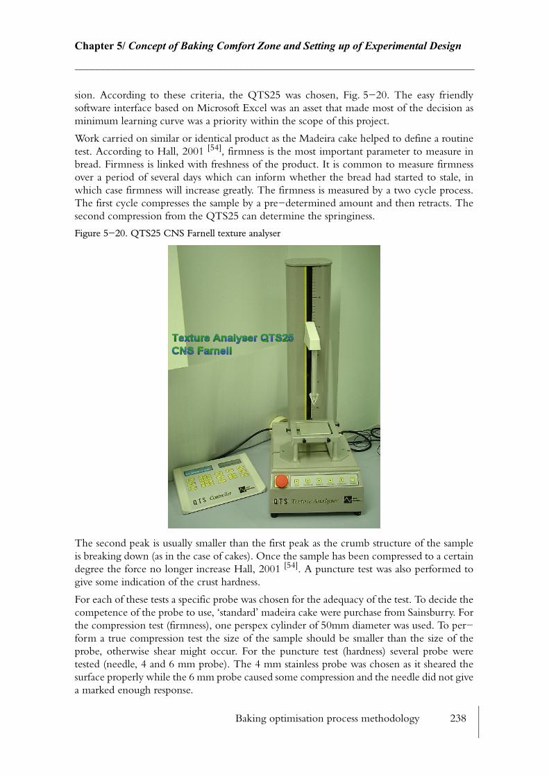
Baking optimisation process methodology 238
Chapter 5/ Concept of Baking Comfort Zone and Setting up of Experimental Design________________________________________________________________________
sion. According to these criteria, the QTS25 was chosen, Fig. 5−20. The easy friendly software interface based on Microsoft Excel was an asset that made most of the decision as minimum learning curve was a priority within the scope of this project.
Work carried on similar or identical product as the Madeira cake helped to define a routine test. According to Hall, 2001 [54], firmness is the most important parameter to measure in bread. Firmness is linked with freshness of the product. It is common to measure firmness over a period of several days which can inform whether the bread had started to stale, in which case firmness will increase greatly. The firmness is measured by a two cycle process. The first cycle compresses the sample by a pre−determined amount and then retracts. The second compression from the QTS25 can determine the springiness.
Figure 5−20. QTS25 CNS Farnell texture analyser
The second peak is usually smaller than the first peak as the crumb structure of the sample is breaking down (as in the case of cakes). Once the sample has been compressed to a certain degree the force no longer increase Hall, 2001 [54]. A puncture test was also performed to give some indication of the crust hardness.
For each of these tests a specific probe was chosen for the adequacy of the test. To decide the competence of the probe to use, ‘standard’ madeira cake were purchase from Sainsburry. For the compression test (firmness), one perspex cylinder of 50mm diameter was used. To per−form a true compression test the size of the sample should be smaller than the size of the probe, otherwise shear might occur. For the puncture test (hardness) several probe were tested (needle, 4 and 6 mm probe). The 4 mm stainless probe was chosen as it sheared the surface properly while the 6 mm probe caused some compression and the needle did not give a marked enough response.
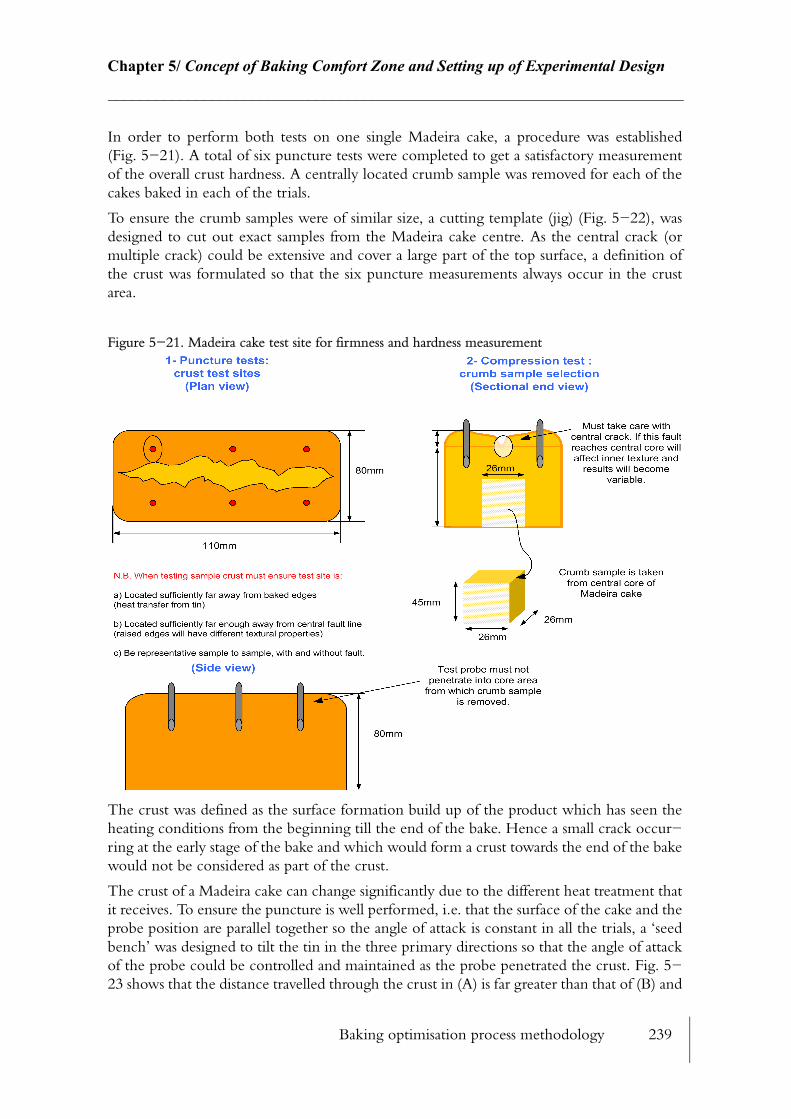
Baking optimisation process methodology 239
Chapter 5/ Concept of Baking Comfort Zone and Setting up of Experimental Design________________________________________________________________________
In order to perform both tests on one single Madeira cake, a procedure was established (Fig. 5−21). A total of six puncture tests were completed to get a satisfactory measurement of the overall crust hardness. A centrally located crumb sample was removed for each of the cakes baked in each of the trials.
To ensure the crumb samples were of similar size, a cutting template (jig) (Fig. 5−22), was designed to cut out exact samples from the Madeira cake centre. As the central crack (or multiple crack) could be extensive and cover a large part of the top surface, a definition of the crust was formulated so that the six puncture measurements always occur in the crust area.
Figure 5−21. Madeira cake test site for firmness and hardness measurement
The crust was defined as the surface formation build up of the product which has seen the heating conditions from the beginning till the end of the bake. Hence a small crack occur−ring at the early stage of the bake and which would form a crust towards the end of the bake would not be considered as part of the crust.
The crust of a Madeira cake can change significantly due to the different heat treatment that it receives. To ensure the puncture is well performed, i.e. that the surface of the cake and the probe position are parallel together so the angle of attack is constant in all the trials, a ‘seed bench’ was designed to tilt the tin in the three primary directions so that the angle of attack of the probe could be controlled and maintained as the probe penetrated the crust. Fig. 5−23 shows that the distance travelled through the crust in (A) is far greater than that of (B) and

Baking optimisation process methodology 240
Chapter 5/ Concept of Baking Comfort Zone and Setting up of Experimental Design________________________________________________________________________
would introduce errors into the data. The steel tin can be tilted within the plastic container to align the surface of the crust so that it is perpendicular to the texture analyser probe.
Crumb density: Crumb density might be related to crumb firmness, i.e. the denser the crumb the firmer it will be. However, the density of the crumb was also used to evaluate the difference in density between the batter and finished product. The difference in densities is entirely caused by the air entrapped in the crumb. The central crumb sample used for the compression test was used for this measurement as well. The weight of the sample was meas−ured with an analytical scale which gives a three decimal place precision (Fig. 5−24). The volume of the crumb sample was calculated with the three dimensions of the crumb sample measured with an electronic vernier.
Figure 5−22. Cutting template (jig)
Figure 5−23. Cake tin bench positioning

Baking optimisation process methodology 241
Chapter 5/ Concept of Baking Comfort Zone and Setting up of Experimental Design________________________________________________________________________
Crumb and crust moisture: Crumb and crust moisture will vary versus time as soon as the cake has been removed from the oven. As soon as the product comes out from the oven, the bread crust for instance is fairly dry compared with its crumb. With time, moisture will gradually migrate towards the crust, i.e. making the crust more moist and the crumb less moist. Although cake ingredients contains more sugar and fat, bread and cake have relatively similar crumb structures so similar moisture migration phenomenon should be observed. The moisture analyser previously described was also used in the determination of crust and moisture. The work involved in measuring the crust moisture was tedious as it consisted of removing the crust without leaving any crumb attached to it.
Figure 5−24. Analytical scale
Almost ‘surgical’ methods were employed to achieve this task. Brush, scalpel and scrapper were used for this meticulous and lengthy process (Fig. 5−25).
Figure 5−25. Brushing and cutting tools
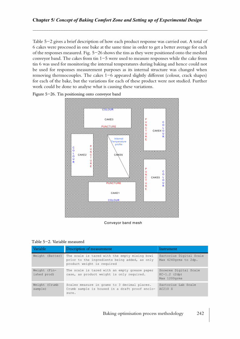
Baking optimisation process methodology 242
Chapter 5/ Concept of Baking Comfort Zone and Setting up of Experimental Design________________________________________________________________________
Table 5−2 gives a brief description of how each product response was carried out. A total of 6 cakes were processed in one bake at the same time in order to get a better average for each of the responses measured. Fig. 5−26 shows the tins as they were positioned onto the meshed conveyor band. The cakes from tin 1−5 were used to measure responses while the cake from tin 6 was used for monitoring the internal temperatures during baking and hence could not be used for responses measurement purposes as its internal structure was changed when removing thermocouples. The cakes 1−6 appeared slightly different (colour, crack shapes) for each of the bake, but the variations for each of these product were not studied. Further work could be done to analyse what is causing these variations.
Figure 5−26. Tin positioning onto conveyor band
Table 5−2. Variable measured
Variable Description of measurement Instrument
Weight (Batter) The scale is tared with the empty mixing bowl prior to the ingredients being added, as only product weight is required
Sartorius Digital ScaleMax 4240grms to 2dp.
Weight (Fin-ished prod)
The scale is tared with an empty grease paper case, as product weight is only required.
Snowrex Digital ScaleKC-1.2 (2dp)Max 1200grms
Weight (Crumb sample)
Scales measure in grams to 3 decimal places. Crumb sample is housed in a draft proof enclo-sure.
Sartorius Lab ScaleAC210 S
CAKE6
CAKE1
CAKE5
CAKE4
CAKE3
CAKE2
PUNCTURE
COLOUR
COLOUR
COLOUR
COLOUR
COLOUR
PUNCTURE
PUNCTURE
PUNCTURE
PUNCTURE
InternalTemperature
profile
Conveyor band mesh
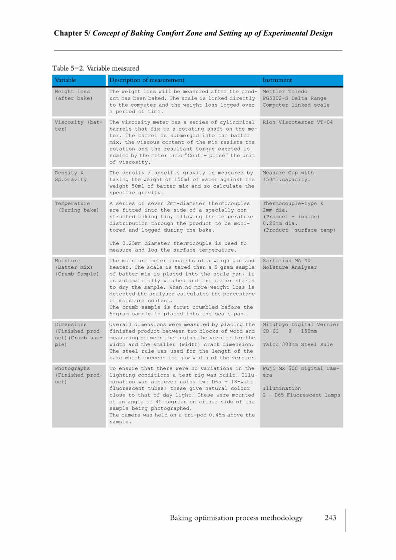
Baking optimisation process methodology 243
Chapter 5/ Concept of Baking Comfort Zone and Setting up of Experimental Design________________________________________________________________________
Weight loss (after bake)
The weight loss will be measured after the prod-uct has been baked. The scale is linked directly to the computer and the weight loss logged over a period of time.
Mettler ToledoPG5002-S Delta RangeComputer linked scale
Viscosity (bat-ter)
The viscosity meter has a series of cylindrical barrels that fix to a rotating shaft on the me-ter. The barrel is submerged into the batter mix, the viscous content of the mix resists the rotation and the resultant torque exerted is scaled by the meter into “Centi- poise” the unit of viscosity.
Rion Viscotester VT-04
Density & Sp.Gravity
The density / specific gravity is measured by taking the weight of 150ml of water against the weight 50ml of batter mix and so calculate the specific gravity.
Measure Cup with 150ml.capacity.
Temperature (During bake)
A series of seven 2mm-diameter thermocouples are fitted into the side of a specially con-structed baking tin, allowing the temperature distribution through the product to be moni-tored and logged during the bake.
The 0.25mm diameter thermocouple is used to measure and log the surface temperature.
Thermocouple-type k2mm dia.(Product - inside)0.25mm dia.(Product -surface temp)
Moisture(Batter Mix)(Crumb Sample)
The moisture meter consists of a weigh pan and heater. The scale is tared then a 5 gram sample of batter mix is placed into the scale pan, it is automatically weighed and the heater starts to dry the sample. When no more weight loss is detected the analyser calculates the percentage of moisture content.The crumb sample is first crumbled before the 5-gram sample is placed into the scale pan.
Sartorius MA 40Moisture Analyser
Dimensions(Finished prod-uct)(Crumb sam-ple)
Overall dimensions were measured by placing the finished product between two blocks of wood and measuring between them using the vernier for the width and the smaller (width) crack dimension. The steel rule was used for the length of the cake which exceeds the jaw width of the vernier.
Mitutoyo Digital VernierCD-6C 0 – 150mm
Talco 300mm Steel Rule
Photographs(Finished prod-uct)
To ensure that there were no variations in the lighting conditions a test rig was built. Illu-mination was achieved using two D65 – 18-watt fluorescent tubes; these give natural colour close to that of day light. These were mounted at an angle of 45 degrees on either side of the sample being photographed.The camera was held on a tri-pod 0.45m above the sample.
Fuji MX 500 Digital Cam-era
Illumination2 – D65 Fluorescent lamps
Table 5−2. Variable measured
Variable Description of measurement Instrument
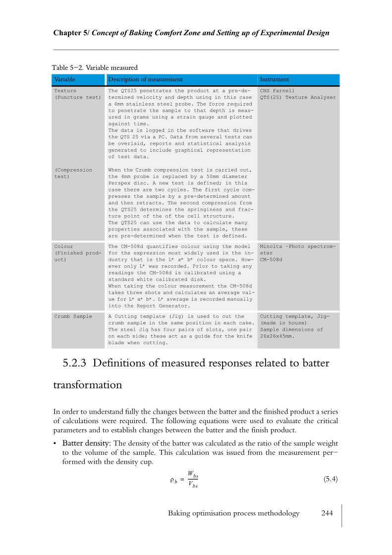
Baking optimisation process methodology 244
Chapter 5/ Concept of Baking Comfort Zone and Setting up of Experimental Design________________________________________________________________________
5.2.3 Definitions of measured responses related to batter
transformation
In order to understand fully the changes between the batter and the finished product a series of calculations were required. The following equations were used to evaluate the critical parameters and to establish changes between the batter and the finish product.
• Batter density: The density of the batter was calculated as the ratio of the sample weight to the volume of the sample. This calculation was issued from the measurement per−formed with the density cup.
(5.4)
Texture(Puncture test)
(Compression test)
The QTS25 penetrates the product at a pre-de-termined velocity and depth using in this case a 4mm stainless steel probe. The force required to penetrate the sample to that depth is meas-ured in grams using a strain gauge and plotted against time.The data is logged in the software that drives the QTS 25 via a PC. Data from several tests can be overlaid, reports and statistical analysis generated to include graphical representation of test data.
When the Crumb compression test is carried out, the 4mm probe is replaced by a 50mm diameter Perspex disc. A new test is defined; in this case there are two cycles. The first cycle com-presses the sample by a pre-determined amount and then retracts. The second compression from the QTS25 determines the springiness and frac-ture point of the of the cell structure.The QTS25 can use the data to calculate many properties associated with the sample, these are pre-determined when the test is defined.
CNS FarnellQTS(25) Texture Analyser
Colour(Finished prod-uct)
The CM-508d quantifies colour using the model for the expression most widely used in the in-dustry that is the L* a* b* colour space. How-ever only L* was recorded. Prior to taking any readings the CM-508d is calibrated using a standard white calibrated disk.When taking the colour measurement the CM-508d takes three shots and calculates an average val-ue for L* a* b*. L* average is recorded manually into the Report Generator.
Minolta –Photo spectrom-eterCM-508d
Crumb Sample A Cutting template (Jig) is used to cut the crumb sample in the same position in each cake.The steel Jig has four pairs of slots, one pair on each side; these act as a guide for the knife blade when cutting.
Cutting template, Jig- (made in house)Sample dimensions of 26x26x45mm.
Table 5−2. Variable measured
Variable Description of measurement Instrument
ρbWbsVbs--------- =

Baking optimisation process methodology 245
Chapter 5/ Concept of Baking Comfort Zone and Setting up of Experimental Design________________________________________________________________________
• Product density (crumb): The product density was based on the central crumb sample extracted from each cake (using the cutting template). Therefore, this density only refers to the crumb density. In order to estimate the total product density a fixed weight of crust and crumb should be taken, however this is not practical.
(5.5)
• Total cake batter volume: The total cake batter volume represents the volume of batter that was used in each cake tin. The batter was laid into appropriate baking grease paper. This volume can be expressed as the ratio of batter density to batter weight (without grease paper).
(5.6)
• Total baked product volume: The total baked product volume was estimated by taking the ratio of the total cake weight to the product density. This calculation assumes that the density of the crumb is the same for the entire product which might not be entirely true. However, the density of the total product might be very close to the density of the entire product as the crust of the baked product is in most cases, only represent few percent of the total finished product.
(5.7)
• Product relative weight change: The relative weight change is the expression of the difference between the batter product and the final product expressed as a percentage of the batter weight. In this case, as the product weight will always be lighter than the batter weight, this relative weight change can be considered as a percentage weight loss. A pos−itive 10% value would mean that the product is lighter by 10% compared to the batter weight.
(5.8)
• Product relative density change: The relative change in the density is expressed as the density difference between the product and the batter relative to the product density. The product was taken as the ‘reference’ in this case as the density of the product will be lower than the batter density, therefore the expected value should be negative. A nega−tive value in this case means the product has become less dense.
(5.9)
• Product relative moisture change: Similarly as Eq. 5.9 the relative moisture change is expressed as the moisture difference between the product (crumb) and the batter, relative to the product moisture. A negative value is expected from this relative change as the product under heating treatment will loose moisture.
ρpWcsVcs--------- =
Vbpρb
Wbp---------- =
VpWpρp------- =
∆WbpWbp Wp–( )100
Wbp-------------------------------------- =
∆ρpbρp ρb–( )100
ρp-------------------------------- =
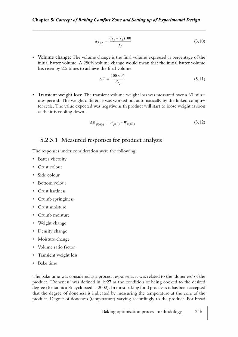
Baking optimisation process methodology 246
Chapter 5/ Concept of Baking Comfort Zone and Setting up of Experimental Design________________________________________________________________________
(5.10)
• Volume change: The volume change is the final volume expressed as percentage of the initial batter volume. A 250% volume change would mean that the initial batter volume has risen by 2.5 times to achieve the final volume.
(5.11)
• Transient weight loss: The transient volume weight loss was measured over a 60 min−utes period. The weight difference was worked out automatically by the linked compu−ter scale. The value expected was negative as th product will start to loose weight as soon as the it is cooling down.
(5.12)
5.2.3.1 Measured responses for product analysis
The responses under consideration were the following:
• Batter viscosity
• Crust colour
• Side colour
• Bottom colour
• Crust hardness
• Crumb springiness
• Crust moisture
• Crumb moisture
• Weight change
• Density change
• Moisture change
• Volume ratio factor
• Transient weight loss
• Bake time
The bake time was considered as a process response as it was related to the ‘doneness’ of the product. ‘Doneness’ was defined in 1927 as the condition of being cooked to the desired degree (Britannica Encyclopaedia, 2002). In most baking food processes it has been accepted that the degree of doneness is indicated by measuring the temperature at the core of the product. Degree of doneness (temperature) varying accordingly to the product. For bread
∆χpbχp χb–( )100
χp--------------------------------=
∆V100 Vp×
Vbp--------------------- =
∆Wp 60( ) Wp 0( ) Wp 60( ) –=
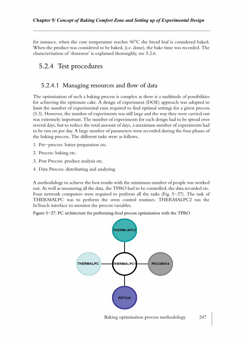
Baking optimisation process methodology 247
Chapter 5/ Concept of Baking Comfort Zone and Setting up of Experimental Design________________________________________________________________________
for instance, when the core temperature reaches 96oC the bread loaf is considered baked. When the product was considered to be baked, (i.e. done), the bake time was recorded. The characterisation of ‘doneness’ is explained thoroughly, see 5.2.6.
5.2.4 Test procedures
5.2.4.1 Managing resources and flow of data
The optimisation of such a baking process is complex as there is a multitude of possibilities for achieving the optimum cake. A design of experiment (DOE) approach was adopted to limit the number of experimental runs required to find optimal settings for a given process (5.3). However, the number of experiments was still large and the way they were carried out was extremely important. The number of experiments for each design had to be spread over several days, but to reduce the total amount of days, a maximum number of experiments had to be run on per day. A large number of parameters were recorded during the four phases of the baking process. The different tasks were as follows.
1. Pre−process: batter preparation etc.
2. Process: baking etc.
3. Post Process: product analysis etc.
4. Data Process: distributing and analysing
A methodology to achieve the best results with the minimum number of people was worked out. As well as measuring all the data, the TPRO had to be controlled, the data recorded etc. Four network computers were required to perform all the tasks (Fig. 5−27). The task of THERMALPC was to perform the oven control routines. THERMALPC2 ran the InTouch interface to monitor the process variables.
Figure 5−27. PC architecture for performing food process optimisation with the TPRO
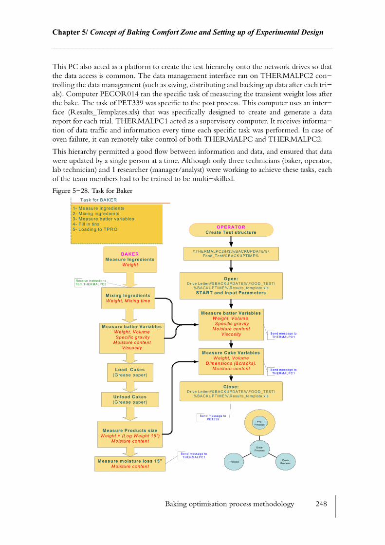
Baking optimisation process methodology 248
Chapter 5/ Concept of Baking Comfort Zone and Setting up of Experimental Design________________________________________________________________________
This PC also acted as a platform to create the test hierarchy onto the network drives so that the data access is common. The data management interface ran on THERMALPC2 con−trolling the data management (such as saving, distributing and backing up data after each tri−als). Computer PECOR014 ran the specific task of measuring the transient weight loss after the bake. The task of PET339 was specific to the post process. This computer uses an inter−face (Results_Templates.xls) that was specifically designed to create and generate a data report for each trial. THERMALPC1 acted as a supervisory computer. It receives informa−tion of data traffic and information every time each specific task was performed. In case of oven failure, it can remotely take control of both THERMALPC and THERMALPC2.
This hierarchy permitted a good flow between information and data, and ensured that data were updated by a single person at a time. Although only three technicians (baker, operator, lab technician) and 1 researcher (manager/analyst) were working to achieve these tasks, each of the team members had to be trained to be multi−skilled.
Figure 5−28. Task for Baker
1- Measure ingredients2- M ixing ingredients3- Measure batter variables4- Fill in tins5- Loading to TPRO
Task for BAKER
BAKERMeasure Ingredients
W eight
Mixing IngredientsW eight, M ixing time
Measure batter VariablesW eight, Volume Specific gravityMoisture content
Viscosity
Load Cakes(Grease paper)
Unload Cakes(Grease paper)
Open:Drive Letter:\%BACKUPDATE%\FOOD_TEST\
%BACKUPTIME%\Results_template.xlsSTART and Input Parameters
OPERATORCreate Test structure
\\THERMALPC2\H$\%BACKUPDATE%\Food_Test\%BACKUPTIM E%
Measure Products sizeW eight + (Log W eight 15")
Moisture content
Measure batter VariablesW eight, Volume, Specific gravityMoisture content
Viscosity
Close:Drive Letter:\%BACKUPDATE%\FOOD_TEST\
%BACKUPTIME%\Results_template.xls
Send message toTHERMALPC1
Measure Cake VariablesW eight, Volume
Dimensions (&cracks),Moisture content Send message to
THERMALPC1
Receive instructionsfrom THERMALPC2
Send message toPET339
Measure moisture loss 15"Moisture content
Send message toTHERMALPC1
Process P ost-Process
Pre-P rocess
D ata-P rocess
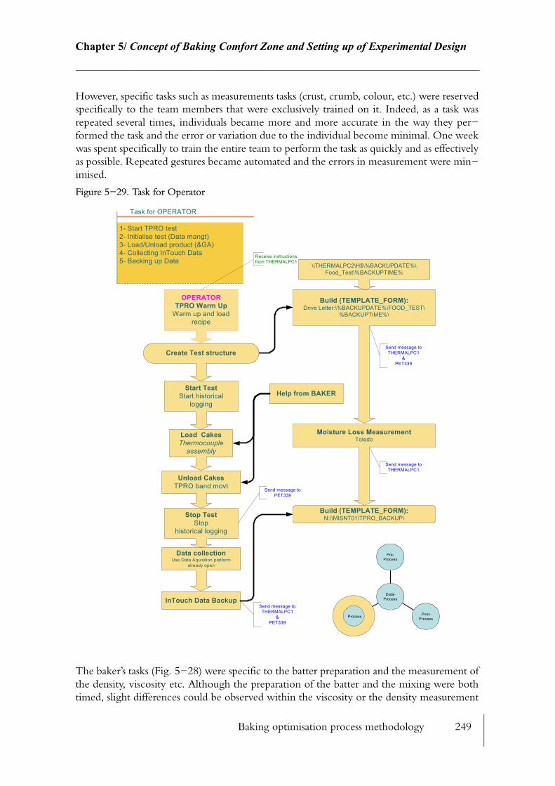
Baking optimisation process methodology 249
Chapter 5/ Concept of Baking Comfort Zone and Setting up of Experimental Design________________________________________________________________________
However, specific tasks such as measurements tasks (crust, crumb, colour, etc.) were reserved specifically to the team members that were exclusively trained on it. Indeed, as a task was repeated several times, individuals became more and more accurate in the way they per−formed the task and the error or variation due to the individual become minimal. One week was spent specifically to train the entire team to perform the task as quickly and as effectively as possible. Repeated gestures became automated and the errors in measurement were min−imised.
Figure 5−29. Task for Operator
The baker’s tasks (Fig. 5−28) were specific to the batter preparation and the measurement of the density, viscosity etc. Although the preparation of the batter and the mixing were both timed, slight differences could be observed within the viscosity or the density measurement
1- Start TPRO test2- Initialise test (Data mangt)3- Load/Unload product (&GA)4- Collecting InTouch Data5- Backing up Data
Task for OPERATOR
Create Test structure
Start TestStart historical
logging
OPERATORTPRO Warm Up
Warm up and loadrecipe
Send message toTHERMALPC1
Load CakesThermocouple
assembly
Unload CakesTPRO band movt
Data collectionUse Data Aquisition platform
already open
Send message toTHERMALPC1
&PET339
Help from BAKER
\\THERMALPC2\H$\%BACKUPDATE%\Food_Test\%BACKUPTIME%
Build (TEMPLATE_FORM):Drive Letter:\%BACKUPDATE%\FOOD_TEST\
%BACKUPTIME%\
Build (TEMPLATE_FORM):N:\\MISNT01\TPRO_BACKUP\
Process Post-Process
Pre-Process
Data-ProcessInTouch Data Backup
Moisture Loss MeasurementToledo
Send message toTHERMALPC1
&PET339
Receive instructionsfrom THERMALPC1
Stop TestStop
historical logging
Send message toPET339
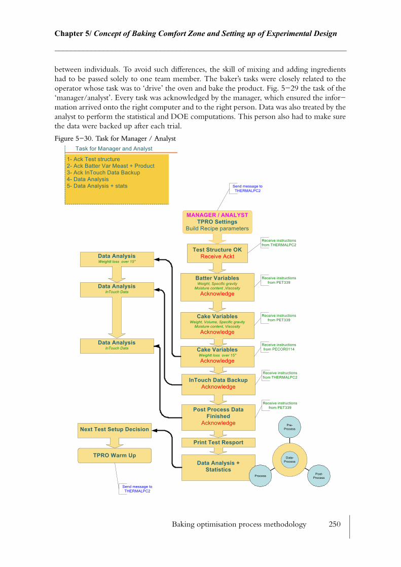
Baking optimisation process methodology 250
Chapter 5/ Concept of Baking Comfort Zone and Setting up of Experimental Design________________________________________________________________________
between individuals. To avoid such differences, the skill of mixing and adding ingredients had to be passed solely to one team member. The baker’s tasks were closely related to the operator whose task was to ‘drive’ the oven and bake the product. Fig. 5−29 the task of the ‘manager/analyst’. Every task was acknowledged by the manager, which ensured the infor−mation arrived onto the right computer and to the right person. Data was also treated by the analyst to perform the statistical and DOE computations. This person also had to make sure the data were backed up after each trial.
Figure 5−30. Task for Manager / Analyst
1- Ack Test structure2- Ack Batter Var Meast + Product3- Ack InTouch Data Backup4- Data Analysis5- Data Analysis + stats
Task for Manager and Analyst
MANAGER / ANALYSTTPRO Settings
Build Recipe parameters
Send message toTHERMALPC2
Test Structure OKReceive Ackt
Receive instructionsfrom THERMALPC2
Receive instructionsfrom PET339
Batter VariablesWeight, Specific gravity
Moisture content ,ViscosityAcknowledge
Cake VariablesWeight, Volume, Specific gravity
Moisture content, ViscosityAcknowledge
Receive instructionsfrom PET339
Cake VariablesWeightt loss over 15"Acknowledge
Receive instructionsfrom PECOR0114
Data AnalysisWeightt loss over 15"
InTouch Data BackupAcknowledge
Data AnalysisInTouch Data
Receive instructionsfrom THERMALPC2
Post Process DataFinished
Acknowledge
Receive instructionsfrom PET339
Data AnalysisInTouch Data
Print Test Resport
Data Analysis +Statistics
Next Test Setup Decision
TPRO Warm Up
Send message toTHERMALPC2
Process Post-Process
Pre-Process
Data-Process

Baking optimisation process methodology 251
Chapter 5/ Concept of Baking Comfort Zone and Setting up of Experimental Design________________________________________________________________________
The lab technician (Fig. 5−31) tasks were the one which required most skills. Ways of meas−uring the product size, shape, crack dimensions, colour, texture, crust moisture, etc. were closely related to the eye and hand checks to ensure the measures were performed in the best conditions.
Figure 5−31. Task for Lab Technician
5.2.4.2 From batter preparation to responses measurement
A cake pre−mix powder was used with no extra additives but water. No colourings nor fla−vourings were added to the batter. Madeira & Genova Mix from Whitworth Bros. from Friars Pride Ltd. (Peterborough) were ordered sufficiently in advance to cover a full week of tests. Enough batter was made at once to bake six cakes of 400g at a time. Batter was never
1- Collect product2- Product photo3- Product colour measurement4- Product texture measurement5- Packaging 6- Statistics
Task for Lab technician
Process Post-Process
Pre-Process
Data-Process
Receive instructionsfrom THERMALPC2
LAB TECHNICIANTest Structure
EstablishedOnly edit concerned section
Product Ready forCollection
Receive instructionsfrom THERMALPC2
Ready to Open:Drive Letter:\%BACKUPDATE%\FOOD_TEST\
%BACKUPTIME%\Results_template.xls
Open:Drive Letter:\%BACKUPDATE%\FOOD_TEST\
%BACKUPTIME%\Results_template.xlsSTART and Input Parameters
Product Measurment: PhotoTake 3 product samples photo:
Top/Side/Bottom
Receive instructionsfrom PET339
Product Measurment: ColourTake colour measurement on each
samples + enter values
Product Measurment: TextureMeasure texture and record traces
save to appropriate directory
Open:Drive Letter:\%BACKUPDATE%\FOOD_TEST\
%BACKUPTIME%\Form_template.xlsSave Data Sheets
Send instructionsTo THERMALPC1
Sample PackagingPack samples with sample stick
informations:Test name/Date/
StatisticsDesign of experiments
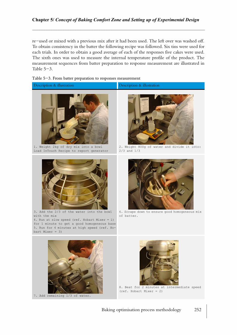
Baking optimisation process methodology 252
Chapter 5/ Concept of Baking Comfort Zone and Setting up of Experimental Design________________________________________________________________________
re−used or mixed with a previous mix after it had been used. The left over was washed off. To obtain consistency in the batter the following recipe was followed. Six tins were used for each trials. In order to obtain a good average of each of the responses five cakes were used. The sixth ones was used to measure the internal temperature profile of the product. The measurement sequences from batter preparation to response measurement are illustrated in Table 5−3.
Table 5−3. From batter preparation to responses measurement
Description & illustration Description & illustration
1. Weight 2kg of dry mix into a bowlLoad InTouch Recipe to report generator
2. Weight 800g of water and divide it into: 2/3 and 1/3
3. Add the 2/3 of the water into the bowl with the mix4. Run at slow speed (ref. Hobart Mixer = 1) for 1 minute to get a good homogeneous base5. Run for 4 minutes at high speed (ref. Ho-bart Mixer = 3)
6. Scrape down to ensure good homogeneous mix of batter.
7. Add remaining 1/3 of water.
8. Beat for 2 minutes at intermediate speed (ref. Hobart Mixer = 2)
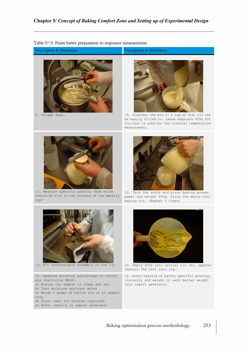
Baking optimisation process methodology 253
Chapter 5/ Concept of Baking Comfort Zone and Setting up of Experimental Design________________________________________________________________________
9. Scrape down. 10. Transfer the mix to a jug so that tin can be easily filled in. Leave separate 450g for tin that is used for the internal temperature measurement.
11. Measure specific gravity (the knife should be flat to the surface of the density cup)
12. Tare the scale and place baking grease paper and weight 400g. Place the whole into baking tin. (Repeat 5 times)
13. Fit thermocouple assembly to the tin 14. Empty 400g into central tin (6), approx-imately 50g left into jug.
15. Measure moisture percentage of batter mix (Sartorius MA40).a) Ensure the sample is clean and dryb) Tare moisture analyser meterc) Weigh 5 grams of batter mix on to sample trayd) Start test (10 minutes required)e) Enter results in report generator
16. Enter results of batter specific gravity, viscosity and weight of each batter weight into report generator.
Table 5−3. From batter preparation to responses measurement
Description & illustration Description & illustration
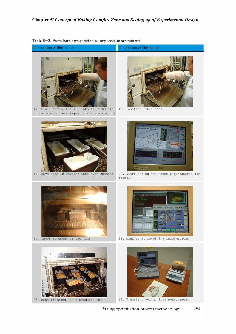
Baking optimisation process methodology 254
Chapter 5/ Concept of Baking Comfort Zone and Setting up of Experimental Design________________________________________________________________________
17. Place centre tin (6) into the TPRO (In-ternal and surface temperature measurements)
18. Position other tins
19. Move band in reverse into oven chamber 20. Start baking and check temperatures (in-ternal)
21. Check movement of the tins 22. Manager PC receiving informations
23. Bake finished, take products out 24. Transient weight loss measurement
Table 5−3. From batter preparation to responses measurement
Description & illustration Description & illustration
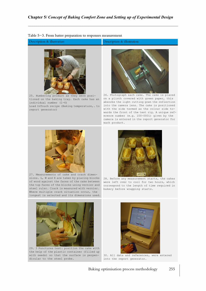
Baking optimisation process methodology 255
Chapter 5/ Concept of Baking Comfort Zone and Setting up of Experimental Design________________________________________________________________________
25. Numbering product as they were posi-tioned on the baking tray. Each cake has an individual number (1-6)Load InTouch recipe (Baking temperature,. to report generator)
26. Photograph each cake. The cake is placed on a plinth covered with green paper, this absorbs the light cutting gown the reflection into the camera lens. The cake is positioned with the side termed as the colour side to-wards the front of the test rig. A unique ref-erence number (e.g. 100-0001) given by the camera is entered in the report generator for each product.
27. Measurements of cake and crack dimen-sions. L, W and H are taken by placing blocks of wood against the faces of the cake between the top faces of the blocks using vernier and steel ruler. Crack is measured with vernier. Where multiple crack situation occur, the longest is selected and its dimensions used.
28. Before any measurement starts, the cakes were left over to cool for two hours, which correspond to the length of time required in bakery before wrapping starts.
29. 3 Punctures test: position the cake with the help of the plastic container (filled up with seeds) so that the surface is perpen-dicular to the steel probe.
30. All data and references, were entered into the report generator.
Table 5−3. From batter preparation to responses measurement
Description & illustration Description & illustration

Baking optimisation process methodology 256
Chapter 5/ Concept of Baking Comfort Zone and Setting up of Experimental Design________________________________________________________________________
31. Colour measurement: Carefully remove the grease paper from the cake and ensure the surface is not damaged. Ensure the cake is free if loose crumb using a fine brush. Clean the optical lens with appropriate cloth and spray. Measure colour on the top surface ‘colour side’ (Unified approach for measur-ing colour (ensure pressure is applied to the sample to guarantee good contact).
32. Crust moisture analysis: Slice up the crust of the cake with a scalpel and remove the crumb from the sample with a scraper. En-sure consistency of the removal of the crumb. Place the whole crust (skin) into an electric grinder and use 5 grams for the moisture an-alyser. If the moisture analyser is already in use, place the whole sample into a sealed container, writing the name and number of the trial and cake.
32(bis). Brushing the crust sample to remove the loose crumb.
33. Tare scale with closed door. Weigh crumb sample and record into report generator. Us-ing a vernier, take two measurements of each dimension (L, W, H) this is to allow for any tapering of the surfaces. These dimensions are crucial as they will be used for volumet-ric and density calculations within the re-port generator. Place the sample into marked plastic sealed contained (to avoid moisture loss)
34. Compression test: the crumb standardise sample of dimension (45*26*26) where 45 is the height. Fit 50 mm compression disk to texture ana-lyser, position get prepared test sample onto the analyser platform and align cen-trally with the compression disk, make sure the 45mm length is the vertical axis. Per-form the compression test. Once finish place the sample into a sealed container (avoid moisture loss) to perform the crumb moisture measurement.
35. Crust and crumb moisture measurement
Table 5−3. From batter preparation to responses measurement
Description & illustration Description & illustration

Baking optimisation process methodology 257
Chapter 5/ Concept of Baking Comfort Zone and Setting up of Experimental Design________________________________________________________________________
5.2.4.3 Recording and processing data
For each trial a large amount of information had to be processed. Timing was crucial so each of the individual tasks were timed. On average, four to five trials could be performed per day, which provided a total of 24 to 30 cakes. Before any measurement could be carried out a batch of cakes were left to cool for two hours, which is the required cooling time in use by cake manufacturers before packaging takes place.
Although measurements such as puncture, compression or moisture measurement could not be started, a series of tasks such as colour, dimensions, were allowed to start after 45 minutes, therefore it was assumed that baked colour and dimensions would not vary after this time. Allowing data to be recorded before two hours permitted to perform measurement in par−allel for different batches, hence, reducing the overall data processing time. Being able to classify and order data without losing any was the biggest challenge. In order to achieve such a task, several interfaces were created to ease repetitive tasks (Fig. 5−32).
1. Collect, distribute and archive: The first interface was designed as part of the InTouchTM Wonderware application. The Data Management Centre screen was designed with the purpose of selecting the type of test to be processed and the instru−mentations in use. Once this primary information is selected the computer will create the directory structure in every computer that is required for the chosen test. The batch script is used to complete this tasks and create a logical tree structure using time settings at which the test occurs. This scripts also send messages to all other users within this mini−network (Fig. 5−27) to ensure that each user is informed that the data has arrived. When trial is finished the data is compressed and backed up onto the main server.
2. Data formatting form: this interface keeps a consistent format throughout data capture and allows easy data comparison.
3. Report generator form: the report generator allows to enter all the informations col−lected for an entire bake. Computations are updated automatically. All the useful infor−mations are collected and arranged to build the final report for the concerning bake.
4. Specific forms: several other platform were created to link the different instrument in use (texture analyser, colour measurement tool). This way the report generator becomes the only form of concern for the user.
5. Comments form: specific comments can be added by each user to the report.
6. Printing: once all information have been entered in the report (including photos) the complete report can be printed, either to a file (PDF format) or on paper.
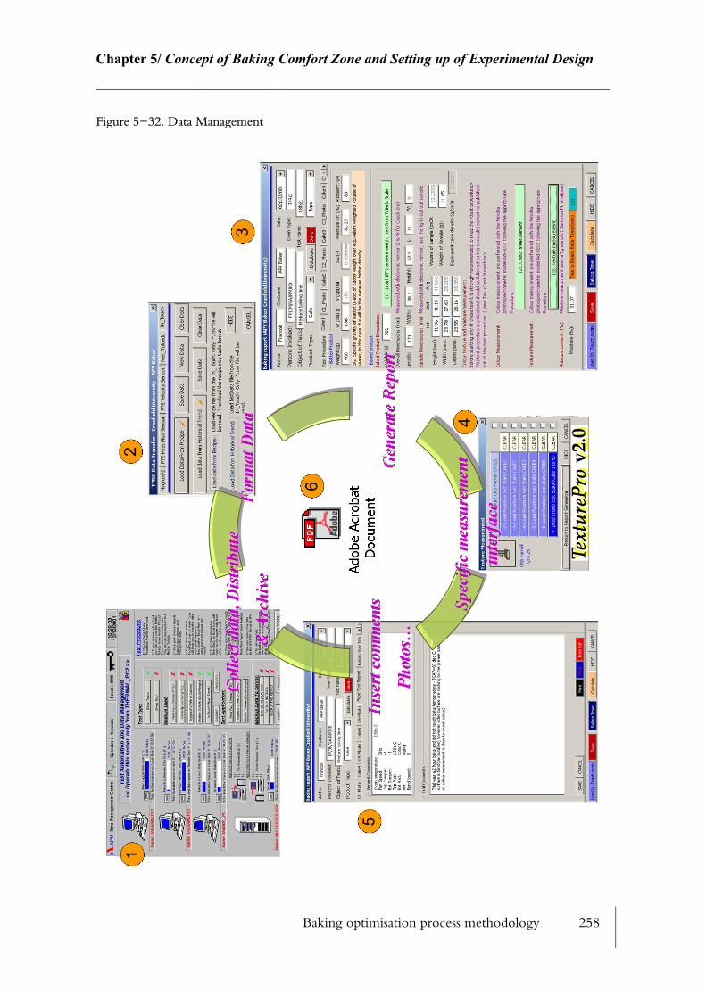
Baking optimisation process methodology 258
Chapter 5/ Concept of Baking Comfort Zone and Setting up of Experimental Design________________________________________________________________________
Figure 5−32. Data Management

Baking optimisation process methodology 259
Chapter 5/ Concept of Baking Comfort Zone and Setting up of Experimental Design________________________________________________________________________
5.2.5 Establish a benchmark
The reference or benchmark, is the standard product that serves as a basis for evaluation or comparison. In the food industry establishing a benchmark is usually based upon sensory evaluation by a test panel. The product which is ranked the highest in terms of quality becomes the reference. A trained panel was not readily available but each business section in APV has an experienced specialist who was used as a test panel. Graham Andrews from APV Baker Ltd. has 25 years of experience in the bakery industry and has specialised in the cake baking process. The benchmark was established with his help. Intuitively, a specialist can establish by trial and error methodology how to get close to an acceptable product that would be saleable on the market. Twelve trials were performed to achieve the benchmark product. For each trials, the product was left to cool then sliced and tasted. The acceptance of the product was based on the following criteria:
• Colour appearance: Overall colour is important. Bakers usually work with a benchmark guide (photographs) of colour ranges. Photographs of tolerance band are usually taken to show the limits of acceptability of the product. For the Madeira cake the colour should be evenly distributed over the top and bottom surfaces. It should appear as a slightly shaded pine−wood colour. The side colour is not so much important in this case as Madeira cake is usually sold within grease proof paper.
• Volume appearance: This parameter is constrained by the side of the packaging, which is usually a manufacturer’s choice. The volume of the Madeira cake should have a rounded appearance with a ‘crown’ feature. The side wall height should be even and the overall volume should be consistent along the length of the cake. The decline of the shape towards the ends of the cake should be low rather than abrupt.
• Crack appearance: Crack appearance is different for different cake types. A slab cake is blind (no crack) while Madeira cake features a relatively long crack along its length. Criteria for selecting a ‘good’ crack dimension are based on a simple rule, which states that a crack width should be half of the width of the cake. The crack should also be shallow but not deep. The crack formation is defined by surface phenomena. The sur−face of the cake usually sets while the internal core of the cake is still liquid. However, during this early stage the liquid phase is still expanding and forming its way through the surface, forming eruption and developing crust as the heat transfer to surface hardens the surface. Excessive crack structure is often a sign of too much top heat.
• Internal appearance: The crumb should be even with no large holes which shows the possibility of fast baking powder release. The crust should be even and finely defined all over.
• Taste and texture: The taste should not be acidic, which emphases the effect of baking powder but should be rather sweet. The bite should be short, i.e. not hard. The crumb should be holding together when cut. The crumb should be ‘fibrous’ and break up easily in the mouth (almost like melting) and low chewing should be necessary to eat it.
Many manufacturers base their benchmark on photographs and an eye check is performed to establish whether the product is acceptable or not. Although the benchmark was photo−graphed (Fig. 5−33), the photos were not used for checking the acceptability of the product, because a more rigorous approach based on measurement was chosen. Three repeats of the
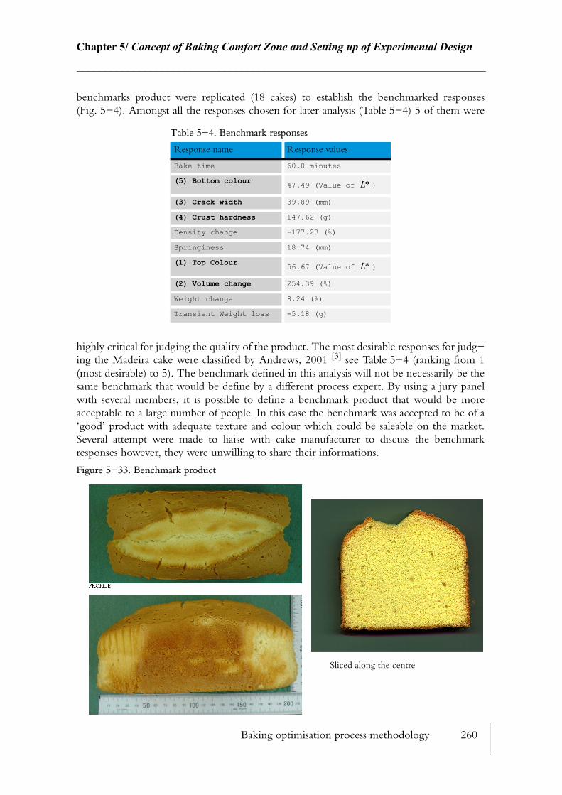
Baking optimisation process methodology 260
Chapter 5/ Concept of Baking Comfort Zone and Setting up of Experimental Design________________________________________________________________________
benchmarks product were replicated (18 cakes) to establish the benchmarked responses (Fig. 5−4). Amongst all the responses chosen for later analysis (Table 5−4) 5 of them were
highly critical for judging the quality of the product. The most desirable responses for judg−ing the Madeira cake were classified by Andrews, 2001 [3] see Table 5−4 (ranking from 1 (most desirable) to 5). The benchmark defined in this analysis will not be necessarily be the same benchmark that would be define by a different process expert. By using a jury panel with several members, it is possible to define a benchmark product that would be more acceptable to a large number of people. In this case the benchmark was accepted to be of a ‘good’ product with adequate texture and colour which could be saleable on the market. Several attempt were made to liaise with cake manufacturer to discuss the benchmark responses however, they were unwilling to share their informations.
Figure 5−33. Benchmark product
Table 5−4. Benchmark responses
Response name Response values
Bake time 60.0 minutes
(5) Bottom colour47.49 (Value of )
(3) Crack width 39.89 (mm)
(4) Crust hardness 147.62 (g)
Density change -177.23 (%)
Springiness 18.74 (mm)
(1) Top Colour 56.67 (Value of )
(2) Volume change 254.39 (%)
Weight change 8.24 (%)
Transient Weight loss -5.18 (g)
L∗
L∗
Sliced along the centre
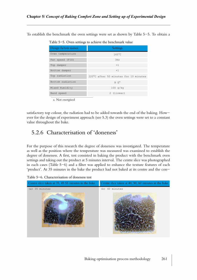
Baking optimisation process methodology 261
Chapter 5/ Concept of Baking Comfort Zone and Setting up of Experimental Design________________________________________________________________________
To establish the benchmark the oven settings were set as shown by Table 5−5. To obtain a
satisfactory top colour, the radiation had to be added towards the end of the baking. How−ever for the design of experiment approach (see 5.3) the oven settings were set to a constant value throughout the bake.
5.2.6 Characterisation of ‘doneness’
For the purpose of this research the degree of doneness was investigated. The temperature as well as the position where the temperature was measured was examined to establish the degree of doneness. A first, test consisted in baking the product with the benchmark oven settings and taking out the product at 5 minutes interval. The centre slice was photographed in each cases (Table 5−6) and a filter was applied to enhance the texture features of each ‘product’. At 35 minutes in the bake the product had not baked at its centre and the con−
Table 5−5. Oven settings to achieve the benchmark value
Design factors names Settings
Oven temperature 165oC
Fan speed (FIS) 3Hz
Top damper +1
Bottom damper +1
Top radiation 220oC after 50 minutes for 10 minutes
Bottom radiation N Ea
a. Not energised
Mixed Humidity 100 g/kg
Band speed 2 (linear)
Table 5−6. Characterisation of doneness test
Centre slice taken at 35, 45 55 minutes in the bake Centre slice taken at 40, 50, 60 minutes in the bake
(a) 35 minutes (b) 40 minutes
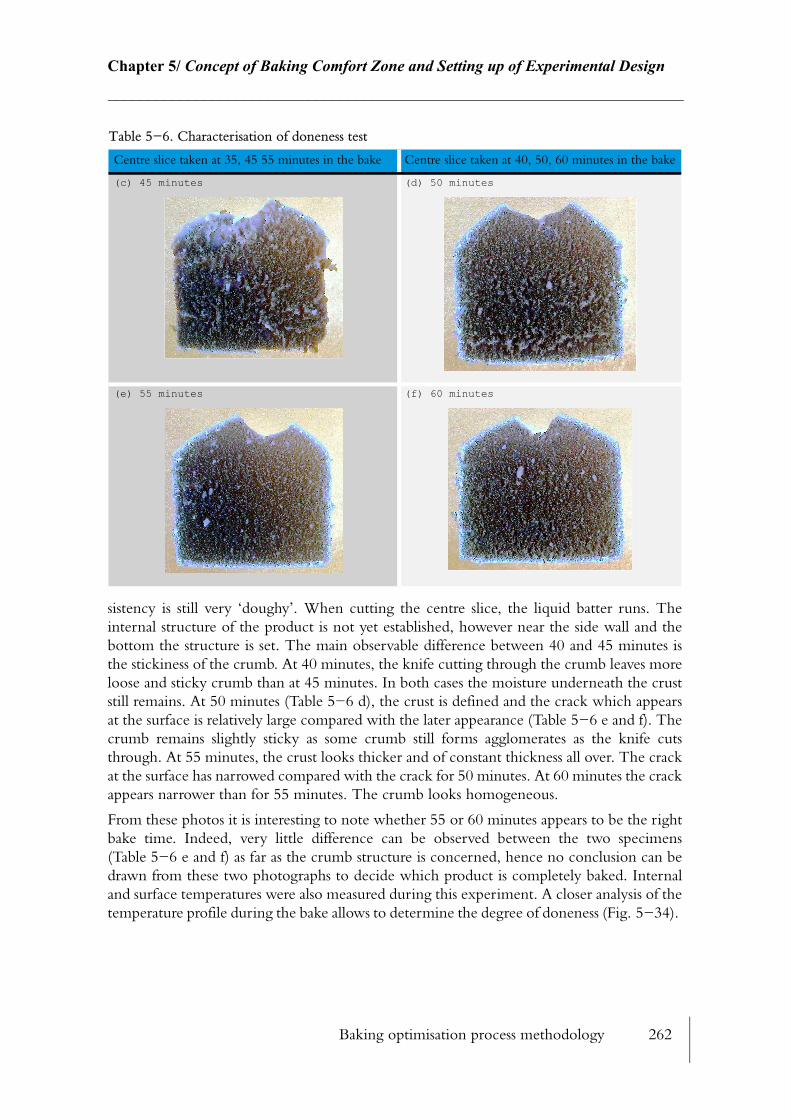
Baking optimisation process methodology 262
Chapter 5/ Concept of Baking Comfort Zone and Setting up of Experimental Design________________________________________________________________________
sistency is still very ‘doughy’. When cutting the centre slice, the liquid batter runs. The internal structure of the product is not yet established, however near the side wall and the bottom the structure is set. The main observable difference between 40 and 45 minutes is the stickiness of the crumb. At 40 minutes, the knife cutting through the crumb leaves more loose and sticky crumb than at 45 minutes. In both cases the moisture underneath the crust still remains. At 50 minutes (Table 5−6 d), the crust is defined and the crack which appears at the surface is relatively large compared with the later appearance (Table 5−6 e and f). The crumb remains slightly sticky as some crumb still forms agglomerates as the knife cuts through. At 55 minutes, the crust looks thicker and of constant thickness all over. The crack at the surface has narrowed compared with the crack for 50 minutes. At 60 minutes the crack appears narrower than for 55 minutes. The crumb looks homogeneous.
From these photos it is interesting to note whether 55 or 60 minutes appears to be the right bake time. Indeed, very little difference can be observed between the two specimens (Table 5−6 e and f) as far as the crumb structure is concerned, hence no conclusion can be drawn from these two photographs to decide which product is completely baked. Internal and surface temperatures were also measured during this experiment. A closer analysis of the temperature profile during the bake allows to determine the degree of doneness (Fig. 5−34).
(c) 45 minutes (d) 50 minutes
(e) 55 minutes (f) 60 minutes
Table 5−6. Characterisation of doneness test
Centre slice taken at 35, 45 55 minutes in the bake Centre slice taken at 40, 50, 60 minutes in the bake
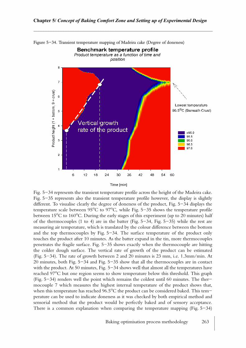
Baking optimisation process methodology 263
Chapter 5/ Concept of Baking Comfort Zone and Setting up of Experimental Design________________________________________________________________________
Figure 5−34. Transient temperature mapping of Madeira cake (Degree of doneness)
Fig. 5−34 represents the transient temperature profile across the height of the Madeira cake. Fig. 5−35 represents also the transient temperature profile however, the display is slightly different. To visualise clearly the degree of doneness of the product, Fig. 5−34 displays the temperature scale between 95oC to 97oC, while Fig. 5−35 shows the temperature profile between 15oC to 160oC. During the early stages of this experiment (up to 20 minutes) half of the thermocouples (1 to 4) are in the batter (Fig. 5−34, Fig. 5−35) while the rest are measuring air temperature, which is translated by the colour difference between the bottom and the top thermocouples by Fig. 5−34. The surface temperature of the product only touches the product after 10 minutes. As the batter expand in the tin, more thermocouples penetrates the fragile surface. Fig. 5−35 shows exactly when the thermocouple are hitting the colder dough surface. The vertical rate of growth of the product can be estimated (Fig. 5−34). The rate of growth between 2 and 20 minutes is 23 mm, i.e. 1.3mm/min. At 20 minutes, both Fig. 5−34 and Fig. 5−35 show that all the thermocouples are in contact with the product. At 50 minutes, Fig. 5−34 shows well that almost all the temperatures have reached 97oC but one region seems to show temperature below this threshold. This graph (Fig. 5−34) renders well the point which remains the coldest until 60 minutes. The ther−mocouple 7 which measures the highest internal temperature of the product shows that, when this temperature has reached 96.5oC the product can be considered baked. This tem−perature can be used to indicate doneness as it was checked by both empirical method and sensorial method that the product would be perfectly baked and of sensory acceptance. There is a common explanation when comparing the temperature mapping (Fig. 5−34)
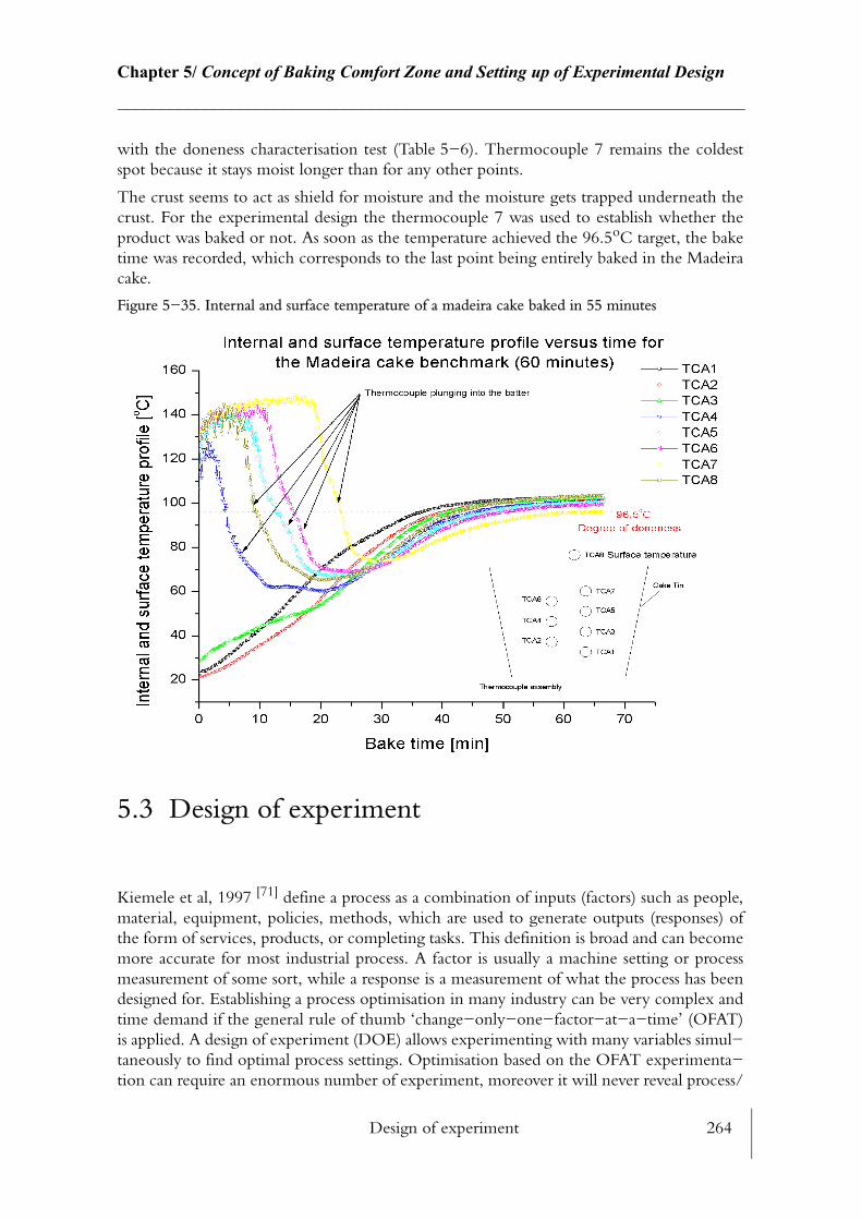
Design of experiment 264
Chapter 5/ Concept of Baking Comfort Zone and Setting up of Experimental Design________________________________________________________________________
with the doneness characterisation test (Table 5−6). Thermocouple 7 remains the coldest spot because it stays moist longer than for any other points.
The crust seems to act as shield for moisture and the moisture gets trapped underneath the crust. For the experimental design the thermocouple 7 was used to establish whether the product was baked or not. As soon as the temperature achieved the 96.5oC target, the bake time was recorded, which corresponds to the last point being entirely baked in the Madeira cake.
Figure 5−35. Internal and surface temperature of a madeira cake baked in 55 minutes
5.3 Design of experiment
Kiemele et al, 1997 [71] define a process as a combination of inputs (factors) such as people, material, equipment, policies, methods, which are used to generate outputs (responses) of the form of services, products, or completing tasks. This definition is broad and can become more accurate for most industrial process. A factor is usually a machine setting or process measurement of some sort, while a response is a measurement of what the process has been designed for. Establishing a process optimisation in many industry can be very complex and time demand if the general rule of thumb ‘change−only−one−factor−at−a−time’ (OFAT) is applied. A design of experiment (DOE) allows experimenting with many variables simul−taneously to find optimal process settings. Optimisation based on the OFAT experimenta−tion can require an enormous number of experiment, moreover it will never reveal process/
Design of experiment 265
Chapter 5/ Concept of Baking Comfort Zone and Setting up of Experimental Design________________________________________________________________________
response interactions. DOE is a methodology that allows manipulating many variables at once to interpret the results. If well designed, a DOE uses the smallest possible number of experimental runs to find optimum settings for a given process. DOE is seen today as the tool for increasing market share, decreasing costs and increasing profit, Anderson and Kraber, 1999 [2].
Both Montgomery, 2001 [91] and Anderson and Kraber, 1999 [2] have given guidelines and objectives for designing experiments. Those objectives were taken on board in the design of this process optimisation.
5.3.1 Method of approach to DOE
Some industrial processes are relatively easy to optimise as the number of variables (factors) is relatively low, however in the baking, the number of factors can be large and so a method of approach had to be assembled before starting the experiments. This method consisted of:
1. Stating the problem and the objectives
2. Choosing the factors and their levels
3. Choosing the responses defining the benchmark Madeira cake, and establish zones of tolerance
4. Ensuring viability of measurement for the range of tests
5. Deciding the different experiment design required and executing the different runs1
(trials)
6. Validating the results predicted from the optimisation
5.3.1.1 Problem statement and objectives:
Anderson and Kraber, 1999 [2] assert three possible risk in defining badly the objectives of the problem:
• trying to study too many or too few factors
• not measuring the correct responses
• arriving at conclusions that are already known
Problem statement: The relationship between responses and process variables are still very much unknown for Madeira cake. Literature does not report significant findings for the Madeira cake product and for baking product in general. The optimisation process still relies very much on one One Factor At the Time (OFAT) techniques which can be very costly and inefficient. Usually, bakers believe that their baking process is already close to optimum and cannot be optimised further. This study was intended to establish a new starting point in the baking optimisation process for Madeira cake.
1. Runs: terminology used in DOE to define an experiment with know ranges of factors
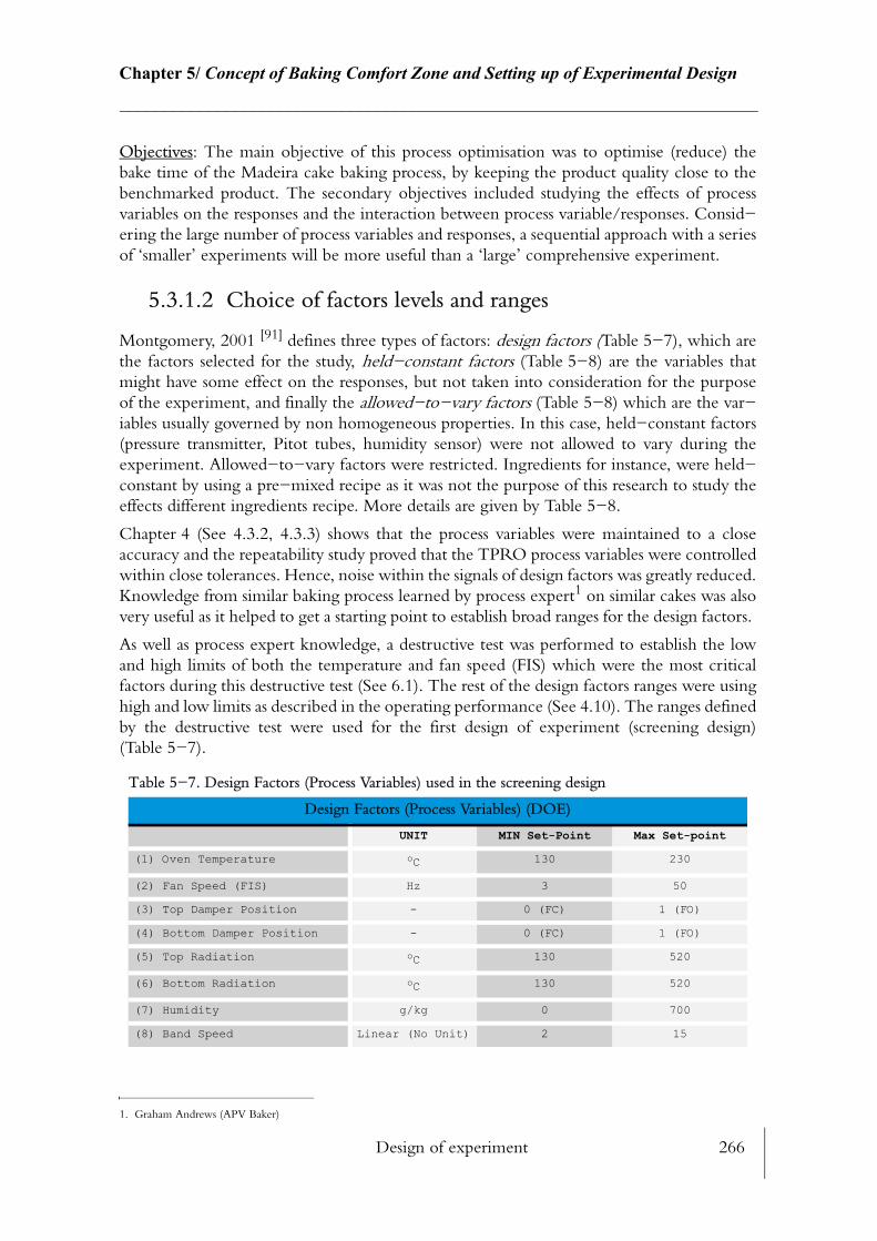
Design of experiment 266
Chapter 5/ Concept of Baking Comfort Zone and Setting up of Experimental Design________________________________________________________________________
Objectives: The main objective of this process optimisation was to optimise (reduce) the bake time of the Madeira cake baking process, by keeping the product quality close to the benchmarked product. The secondary objectives included studying the effects of process variables on the responses and the interaction between process variable/responses. Consid−ering the large number of process variables and responses, a sequential approach with a series of ‘smaller’ experiments will be more useful than a ‘large’ comprehensive experiment.
5.3.1.2 Choice of factors levels and ranges
Montgomery, 2001 [91] defines three types of factors: design factors (Table 5−7), which are the factors selected for the study, held−constant factors (Table 5−8) are the variables that might have some effect on the responses, but not taken into consideration for the purpose of the experiment, and finally the allowed−to−vary factors (Table 5−8) which are the var−iables usually governed by non homogeneous properties. In this case, held−constant factors (pressure transmitter, Pitot tubes, humidity sensor) were not allowed to vary during the experiment. Allowed−to−vary factors were restricted. Ingredients for instance, were held−constant by using a pre−mixed recipe as it was not the purpose of this research to study the effects different ingredients recipe. More details are given by Table 5−8.
Chapter 4 (See 4.3.2, 4.3.3) shows that the process variables were maintained to a close accuracy and the repeatability study proved that the TPRO process variables were controlled within close tolerances. Hence, noise within the signals of design factors was greatly reduced. Knowledge from similar baking process learned by process expert1 on similar cakes was also very useful as it helped to get a starting point to establish broad ranges for the design factors.
As well as process expert knowledge, a destructive test was performed to establish the low and high limits of both the temperature and fan speed (FIS) which were the most critical factors during this destructive test (See 6.1). The rest of the design factors ranges were using high and low limits as described in the operating performance (See 4.10). The ranges defined by the destructive test were used for the first design of experiment (screening design) (Table 5−7).
1. Graham Andrews (APV Baker)
Table 5−7. Design Factors (Process Variables) used in the screening design
Design Factors (Process Variables) (DOE)
UNIT MIN Set-Point Max Set-point
(1) Oven Temperature oC 130 230
(2) Fan Speed (FIS) Hz 3 50
(3) Top Damper Position - 0 (FC) 1 (FO)
(4) Bottom Damper Position - 0 (FC) 1 (FO)
(5) Top Radiation oC 130 520
(6) Bottom Radiation oC 130 520
(7) Humidity g/kg 0 700
(8) Band Speed Linear (No Unit) 2 15
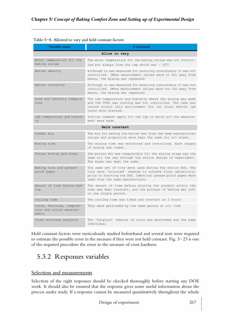
Design of experiment 267
Chapter 5/ Concept of Baking Comfort Zone and Setting up of Experimental Design________________________________________________________________________
Held constant factors were meticulously studied beforehand and several tests were required to estimate the possible error in the measure if they were not held constant. Fig. 5−23 is one of the required procedure the error in the measure of crust hardness.
5.3.2 Responses variables
Selection and measurements
Selection of the right responses should be checked thoroughly before starting any DOE work. It should also be ensured that the response gives some useful information about the process under study. If a response cannot be measured quantitatively throughout the whole
Table 5−8. Allowed to vary and held constant factors
Variable name Comments
Allow to vary
Water temperature for the baking recipe
The water temperature for the baking recipe was not control-
led but always from the tap which was ~ 16oC
Batter density Although is was measured for ensuring consistency it was not controlled. (When measurement values were to far away from means, the mixing was repeated)
Batter viscosity Although is was measured for ensuring consistency it was not controlled. (When measurement values were too far away from means, the mixing was repeated)
Room and humidity tempera-ture
The lab temperature and humidity where the mixing was made and the TPRO was running was not controlled. The cake was cooled within this environment for two hours before lab tests were started.
Lab temperature and humidi-ty
Similar comment apply for the lab in which all the measure-ment were made.
Held constant
Powder mix The mix for making the batter was from the same manufacturer recipe and proportion were kept the same for all mixes.
Mixing time The mixing time was monitored and controlled. Each stages of mixing was timed.
Person mixing and mixer The person who was responsible for the mixing stage was the same all the way through the entire design of experiment. The mixer was kept the same.
Baking tins and grease-proof paper
The same set of tins were used during the entire DOE. The tins were ‘coloured’ (heated to achieve final emissivity) prior to starting the DOE. Identical grease proof paper were used from the same manufacturer.
Amount of time before bak-ing
The amount of time before placing the product within the oven was kept constant, and the process of baking was left to one single person.
Cooling time The cooling time was timed and constant at 2 hours
Crack, Puncture, compres-sion and colour measure-ments
They were performed by the same person at all time
Crust moisture analysis The ‘surgical’ removal of crust was performed was the same individual
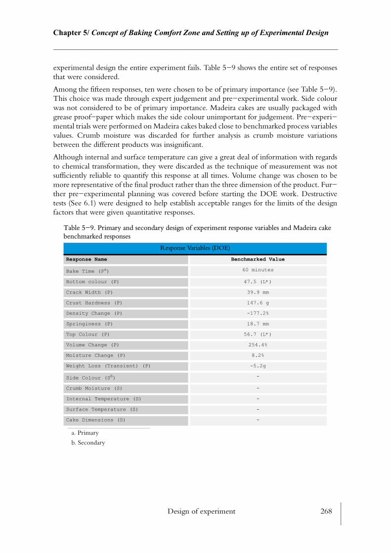
Design of experiment 268
Chapter 5/ Concept of Baking Comfort Zone and Setting up of Experimental Design________________________________________________________________________
experimental design the entire experiment fails. Table 5−9 shows the entire set of responses that were considered.
Among the fifteen responses, ten were chosen to be of primary importance (see Table 5−9). This choice was made through expert judgement and pre−experimental work. Side colour was not considered to be of primary importance. Madeira cakes are usually packaged with grease proof−paper which makes the side colour unimportant for judgement. Pre−experi−mental trials were performed on Madeira cakes baked close to benchmarked process variables values. Crumb moisture was discarded for further analysis as crumb moisture variations between the different products was insignificant.
Although internal and surface temperature can give a great deal of information with regards to chemical transformation, they were discarded as the technique of measurement was not sufficiently reliable to quantify this response at all times. Volume change was chosen to be more representative of the final product rather than the three dimension of the product. Fur−ther pre−experimental planning was covered before starting the DOE work. Destructive tests (See 6.1) were designed to help establish acceptable ranges for the limits of the design factors that were given quantitative responses.
Table 5−9. Primary and secondary design of experiment response variables and Madeira cake benchmarked responses
Response Variables (DOE)
Response Name Benchmarked Value
Bake Time (Pa)
a. Primary
60 minutes
Bottom colour (P) 47.5 (L*)
Crack Width (P) 39.9 mm
Crust Hardness (P) 147.6 g
Density Change (P) -177.2%
Springiness (P) 18.7 mm
Top Colour (P) 56.7 (L*)
Volume Change (P) 254.4%
Moisture Change (P) 8.2%
Weight Loss (Transient) (P) -5.2g
Side Colour (Sb)
b. Secondary
-
Crumb Moisture (S) -
Internal Temperature (S) -
Surface Temperature (S) -
Cake Dimensions (S) -
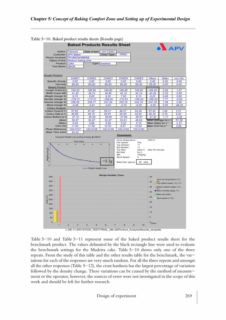
Design of experiment 269
Chapter 5/ Concept of Baking Comfort Zone and Setting up of Experimental Design________________________________________________________________________
Table 5−10. Baked product results sheets (Results page)
Table 5−10 and Table 5−11 represent some of the baked product results sheet for the benchmark product. The values delimited by the black rectangle line were used to evaluate the benchmark settings for the Madeira cake. Table 5−10 shows only one of the three repeats. From the study of this table and the other results table for the benchmark, the var−iations for each of the responses are very much random. For all the three repeats and amongst all the other responses (Table 5−12), the crust hardness has the largest percentage of variation followed by the density change. These variations can be caused by the method of measure−ment or the operator, however, the sources of error were not investigated in the scope of this work and should be left for further research.
Baked Products Results Sheet
Author: Francois Date of test: 10/11/2001
Customer: APV Baker Oven Type: TPRO
Person Involved: FP/JM/GA/RM/KB
Object of test: Reduce baking time
Product: Cake Type: madeira
Test Name: 08h28
Dough Product:
CAKE1 CAKE2 CAKE3 CAKE4 CAKE5 Mean Stdev cov (%)
Specific Gravity 0.92 0.92 0.92 0.92 0.92 0.92 0.00 0.00
Viscosity 85.00 85.00 85.00 85.00 85.00 85.00 0.00 0.00
Baked Product
Length Crack (L) 154.00 146.80 146.80 149.40 149.40 149.28 2.94 1.97
Width Crack (W) 41.20 39.10 36.90 42.10 42.10 40.28 2.25 5.59
Weight change % 8.15 8.85 8.30 7.55 8.15 8.20 0.46 5.65
Density change % -178.77 -172.27 -159.04 -172.81 -164.24 -169.43 7.77 -4.59
Volume change % 256.05 248.17 237.54 252.22 242.70 247.34 7.38 2.98
Moist.change % -9.49 -3.41 -5.67 -3.15 -6.05 -5.55 2.55 -46.00
Colour Analysis
Colour Crust (L*) 57.62 57.42 59.31 58.27 54.38 57.40 1.84 3.21
Colour Side (L*) 46.68 49.15 50.81 55.46 44.62 49.34 4.16 8.42
Colour Bottom (L*) 47.72 46.04 48.80 47.98 46.57 47.42 1.11 2.34
Mean 50.67 50.87 52.97 53.91 48.52 Main average for L* 51.39
StDev 6.04 5.88 5.58 5.32 5.16 Main Stdev for L* 2.37
COV (%) 11.92 11.56 10.53 9.87 10.64 Main COV for L* 4.66
Photo Reference 100-0157 100-0158 100-0159 100-0162 100-0160
Bake Time (min) 60.00
Comments:
Recipe Variable / Zone
0
50
100
150
200
250
300
350
400
450
500
1 2 3 4 5 6 7 8 9 10Zone
Units
(Y
1)
0
5
10
15
20
25
30
35
40
45
Oven air temperature (°C) -
Y1-Top radient heater (°C) -Y1-
Bottom radient heater (°C) -
Y1-Spec humidity (g/kg) -Y1-
Bake time (Min)
Band speed (1-15)
Oven temperature : 165o C
Fan Speed: 3Hz
Top Damper: +1
Bot Damper: +1
Top Rad: 220o C af ter 50 minutes
Bot Rad: 0o C
MH: 100g/kg
Band Speed: 0
Bake time: approx 60 mins
Transient Weight Loss during Cooling @ 200oC
-6
-5
-4
-3
-2
-1
0
0 10 20 30 40 50 60 70
Time (min)
We
igh
t L
oss
(g
)
Weight weight Loss
L:\08-11-2001\FOOD_TEST\TRIAL_08h-28\Product_Analysis\Results_template
−5.1g
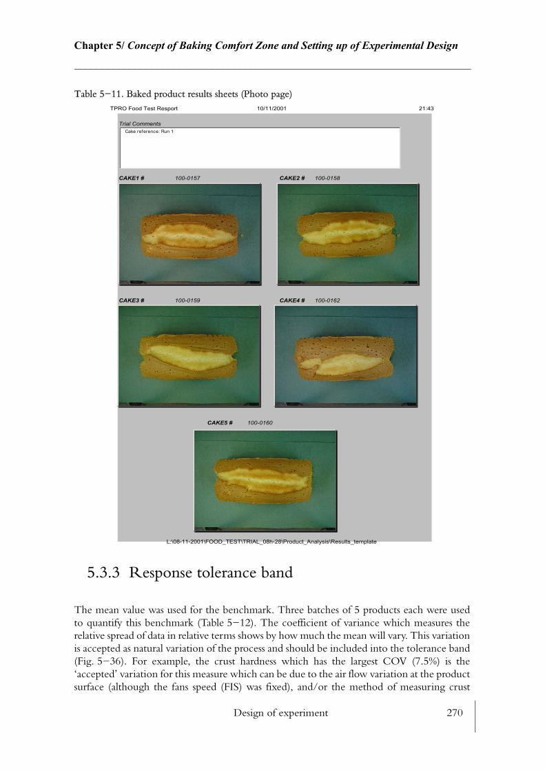
Design of experiment 270
Chapter 5/ Concept of Baking Comfort Zone and Setting up of Experimental Design________________________________________________________________________
Table 5−11. Baked product results sheets (Photo page)
5.3.3 Response tolerance band
The mean value was used for the benchmark. Three batches of 5 products each were used to quantify this benchmark (Table 5−12). The coefficient of variance which measures the relative spread of data in relative terms shows by how much the mean will vary. This variation is accepted as natural variation of the process and should be included into the tolerance band (Fig. 5−36). For example, the crust hardness which has the largest COV (7.5%) is the ‘accepted’ variation for this measure which can be due to the air flow variation at the product surface (although the fans speed (FIS) was fixed), and/or the method of measuring crust
TPRO Food Test Resport 10/11/2001 21:43
Trial Comments
CAKE1 # 100-0157 CAKE2 # 100-0158
CAKE3 # 100-0159 CAKE4 # 100-0162
CAKE5 # 100-0160
Cake reference: Run 1
L:\08-11-2001\FOOD_TEST\TRIAL_08h-28\Product_Analysis\Results_template
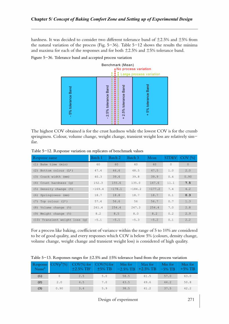
Design of experiment 271
Chapter 5/ Concept of Baking Comfort Zone and Setting up of Experimental Design________________________________________________________________________
hardness. It was decided to consider two different tolerance band of ±2.5% and ±5% from the natural variation of the process (Fig. 5−36). Table 5−12 shows the results the minima and maxima for each of the responses and for both ±2.5% and ±5% tolerance band.
Figure 5−36. Tolerance band and accepted process variation
The highest COV obtained is for the crust hardness while the lowest COV is for the crumb springiness. Colour, volume change, weight change, transient weight loss are relatively sim−ilar.
For a process like baking, coefficient of variance within the range of 5 to 10% are considered to be of good quality, and every responses which COV is below 5% (colours, density change, volume change, weight change and transient weight loss) is considered of high quality.
Table 5−12. Response variation on replicates of benchmark values
Response name Batch 1 Batch 2 Batch 3 Mean STDEV COV [%]
(1) Bake time (min) 60 60 60 60 0 0
(2) Bottom colour (L*) 47.4 46.6 48.5 47.5 1.0 2.0
(3) Crack width (mm) 40.3 39.6 39.8 39.9 0.4 0.90
(4) Crust hardness (g) 152.3 155.6 135.0 147.6 11.1 7.5
(5) Density change (%) -169.4 -178.1 -184.2 -177.2 7.4 4.2
(6) Springiness (mm) 18.7 18.8 18.7 18.7 0.1 0.3
(7) Top colour (L*) 57.4 56.6 56 56.7 0.7 1.3
(8) Volume change (%) 261.4 254.4 247.3 254.4 7.0 2.8
(9) Weight change (%) 8.2 8.5 8.0 8.2 0.2 2.9
(10) Transient weight loss (g) -5.1 -5.1 -5.3 -5.2 0.1 2.2
Table 5−13. Responses ranges for ±2.5% and ±5% tolerance band from the process variation
Response Namea
COVpb(%) COV(%) for ±2.5% TBc
COV(%) for ±5% TB
Min for −2.5% TB
Max for +2.5% TB
Min for −5% TB
Max for +5% TB
(1) 0 2.5 5.0 58.5 61.5 57.0 63.0
(2) 2.0 4.5 7.0 43.5 49.6 44.2 50.8
(3) 0.90 3.4 5.9 38.5 41.2 37.5 42.2
Benchmark (Mean)No process variation
- 2.5
% to
lera
nce
Band
- 5%
tole
ranc
e Ba
nd
+ 2.
5% to
lera
nce
Band
+ 5%
tole
ranc
e Ba
nd
Large process variation
Design of experiment 272
Chapter 5/ Concept of Baking Comfort Zone and Setting up of Experimental Design________________________________________________________________________
5.3.4 Methodology of the DOE
The terminology used in DOE is specific and some clarification must be given. There are three basics principles in designing experiments, which are: replication, randomization and blocking. Replication means to repeat an entire run. Replicating allows increasing the pre−cision of the response measurement and improves the chance of detecting a statistically sig−nificant effect in the middle of natural process variation. Randomising the run order of the experiments allows to minimise the effect of uncontrolled variables (time related variables) such as ambient air temperature or humidity, which would influence the moisture loss of the product being cooled for instance. Because it was not possible to conduct all the runs on the same day a blocking was introduced to account for potential day to day variations. The experiments is then divided into uniform blocks which increase the sensitivity of the design.
(4) 7.5 10.0 12.5 132.9 162.4 129.2 166.0
(5) 4.2 6.7 9.2 -165.4 -189.1 -160.9 -193.5
(6) 0.3 2.8 5.3 18.2 19.3 17.7 19.7
(7) 1.3 3.8 6.3 54.5 58.8 53.1 60.2
(8) 2.8 5.3 7.8 241.0 267.8 234.6 274.1
(9) 2.9 5.4 7.9 7.8 8.7 7.6 8.9
(10) 2.2 4.7 7.2 -4.9 -5.4 -4.8 -5.6
a. Numbering of response name is identical to Table 5−12
b. COVp: Variation caused by process
c. TB: Tolerance Band
It is uncertain how the desirability should best be applied to each response, however by using the tolerance band previously established (see 5.3.3) for each response the optimisation proc−ess might be simplified. The notion of a tolerance band is fundamental for estimating the baking optimum. A response tolerance band means that a percentage variation on the benchmarked response can be accepted. Knowledge of the product tolerance band means that it is easier to define the ranges of product response in which the product is acceptable. The tolerance band may be different for each of the responses under study.
Some products such as biscuit have a very sharp tolerance band on their size, as it becomes an issue for packaging. However, for most of the bakery products, tolerance appear to be undefined and a visual check is the main means of controlling tolerance. This rule applies for the Madeira cake product. The only known control technique today for Madeira cake (Park Cakes (Liverpool), 2001 [100]) is to check between a reference photograph and the product to be controlled. For these reasons, tolerance bands were not available for the Madeira cake product. However, for future research a close link should be established between the baking manufacturers to estimate closely the tolerance band for the primary product responses (Chapter 7).
Table 5−13. Responses ranges for ±2.5% and ±5% tolerance band from the process variation
Response Namea
COVpb(%) COV(%) for ±2.5% TBc
COV(%) for ±5% TB
Min for −2.5% TB
Max for +2.5% TB
Min for −5% TB
Max for +5% TB
Design of experiment 273
Chapter 5/ Concept of Baking Comfort Zone and Setting up of Experimental Design________________________________________________________________________
There are many DOE software packages available and they all seem to cover the complete range of designs features. MaxSuite was used as it was the company standard at the time the DOE work started. There are three main families of designs:
• Screening (SD)
• Factorial (FD)
• Central Composite Design (CCD)
The designs performed to conduct this optimisation were used in a strategic order. Knowl−edge of each design was used to choose the appropriate design to be run next. Each run con−sisted of one set of temperature/humidity/fan speed (FIS) etc. which could be assimilated to one single zone of a travelling oven. Multi zone oven spectrum was beyond the scope of this research but it is recommended for study in a future DOE (Chapter 7).
Each of the designs has a specific functionality. SD is usually employed to assess the impor−tance of the main effect of a variable when there are a large number of design factors (usually more than 5) and a need to study them in as few experiments as possible, BTR, 1995 [22].The drawback with this sort of design is that interaction between the design factors and the responses cannot be looked at with precision. Screening design is commonly used to decrease the number of variables under study by eliminating the less significant ones, so more pow−erful design can be used to establish interactions and process optimum. In this research the use of screening design allowed to decreased the number of design factors from 8 (Table 5−7) to 4. FD are more interesting in the fact that they provide more informations than screen−ing’s. The strategy of FD is resumed by the fact that design factors are varied together. The most common factorial design is called the factorial design with the number of design factors studied. There are many variation in this sort of design, and fractional factorial design is part of it. Fractional factorial minimise even further the number of runs. All the possible interactions between the design factors and the responses were studied thanks to this design. Contour plots which plots interactions in a 2D format between one design factor and one response were used to study the gradient of the interaction. On the basis of these analysis the the number of design factors were reduced to three significant factors.
The output of CCD is usually a mathematical ‘statistical’ model that can find areas of the design factors in which the process can be optimised. Confirmation runs are advised to be performed so that the model built with the DOE can be assessed for accurate predictions. Confirmation runs are similar to validation for mathematical modelling. Optimisation is usually characterised by central composite design which allows to plot response surface. Response surface allows to establish regions between two design factors and one response. As opposed to screenings’s and factional’ s, the mathematical model issued from central composite design can study potential curvatures in the models and used to compute specific points on a curve. All possible interactions and response surface were computed.
Because of the complexity of the response surfaces, a methodology has been developed and applied in Chapter 6 which allows to estimate the process optimum (shortest bake time) with full filling the most desirable responses within the tolerance band. This method is based on the desirability study of the most constraining responses to the bake time.
2k k
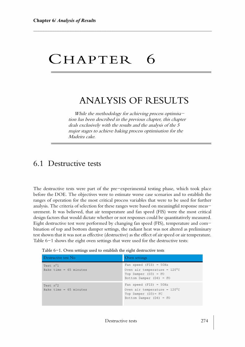
Destructive tests 274
Chapter 6/ Analysis of Results________________________________________________________________________
CHAPTER 6
ANALYSIS OF RESULTSWhile the methodology for achieving process optimisa−
tion has been described in the previous chapter, this chapter deals exclusively with the results and the analysis of the 5 major stages to achieve baking process optimisation for the Madeira cake.
6.1 Destructive tests
The destructive tests were part of the pre−experimental testing phase, which took place before the DOE. The objectives were to estimate worse case scenarios and to establish the ranges of operation for the most critical process variables that were to be used for further analysis. The criteria of selection for these ranges were based on meaningful response meas−urement. It was believed, that air temperature and fan speed (FIS) were the most critical design factors that would dictate whether or not responses could be quantitatively measured. Eight destructive test were performed by changing fan speed (FIS), temperature and com−bination of top and bottom damper settings, the radiant heat was not altered as preliminary test shown that it was not as effective (destructive) as the effect of air speed or air temperature. Table 6−1 shows the eight oven settings that were used for the destructive tests:
Table 6−1. Oven settings used to establish the eight destructive tests
Destructive test No Oven settings
Test no1Bake time = 65 minutes
Fan speed (FIS) = 50Hz
Oven air temperature = 120oCTop Damper (D3) = FOBottom Damper (D4) = FO
Test no2Bake time = 65 minutes
Fan speed (FIS) = 50Hz
Oven air temperature = 120oCTop Damper (D3)= FCBottom Damper (D4) = FO

Destructive tests 275
Chapter 6/ Analysis of Results________________________________________________________________________
The results from this test are illustrated by the photographs shown in Fig. 6−1. The eight cakes produced under these conditions show very different features, indicating the influence of different rates of heat transfer.
• Test no1: The cake produced with these settings was almost entirely baked. However there was still a slight sign of moisture trap underneath the crust. The volume was rela−tively homogeneous and the colour was uniform on the top surface. A crack is apparent but not really pronounced compared with the benchmarked product. The crumb struc−ture is relatively uniform.
• Test no2: The volume of this product was similar to the cake produced with test no1. This cake was blind (i.e. no crack) and the top colour was slightly paler than for test no1. The crumb underneath the crust was under−baked. The top velocity was reduced com−pared with settings of Test no1 (top damper FC), and it had a direct effect on the final product. The heat transfer by convection to the product surface seems to help in remov−ing moisture and also colouring the product.
• Test no3: The shape of this cake was very particular and shows well the effect of high air velocity air−flow to the top surface. In this case the bottom damper was closed which minimised the heat transfer to the bottom surface compared with Test no1 & 2. The caramelised surface was very hard and shows signs of a ‘tormented’ baking. The crumb
Test no3Bake time = 65 minutes
Fan speed (FIS) = 50Hz
Oven air temperature = 120oCTop Damper (D3) = FOBottom Damper (D4) = FC
Test no4Bake time = 65 minutes
Fan speed (FIS) = 3Hz
Oven air temperature = 120oCTop Damper (D3) = FOBottom Damper (D4) = FO
Test no5Bake time = 7 minutes
Fan speed (FIS) = 50Hz
Oven air temperature = 300oCTop Damper (D3) = FOBottom Damper (D4) = FO
Test no6Bake time = 10 minutes
Fan speed (FIS) = 3Hz
Oven air temperature = 300oCTop Damper (D3) = FOBottom Damper (D4) = FO
Test no7Bake time = 30 minutes
Fan speed (FIS) = 3Hz
Oven air temperature = 260oCTop Damper (D3) = FOBottom Damper (D4) = FO
Test no8Bake time = 18 minutes
Fan speed (FIS) = 50Hz
Oven air temperature = 255oCTop Damper (D3) = FCBottom Damper (D4) = FO
Table 6−1. Oven settings used to establish the eight destructive tests
Destructive test No Oven settings
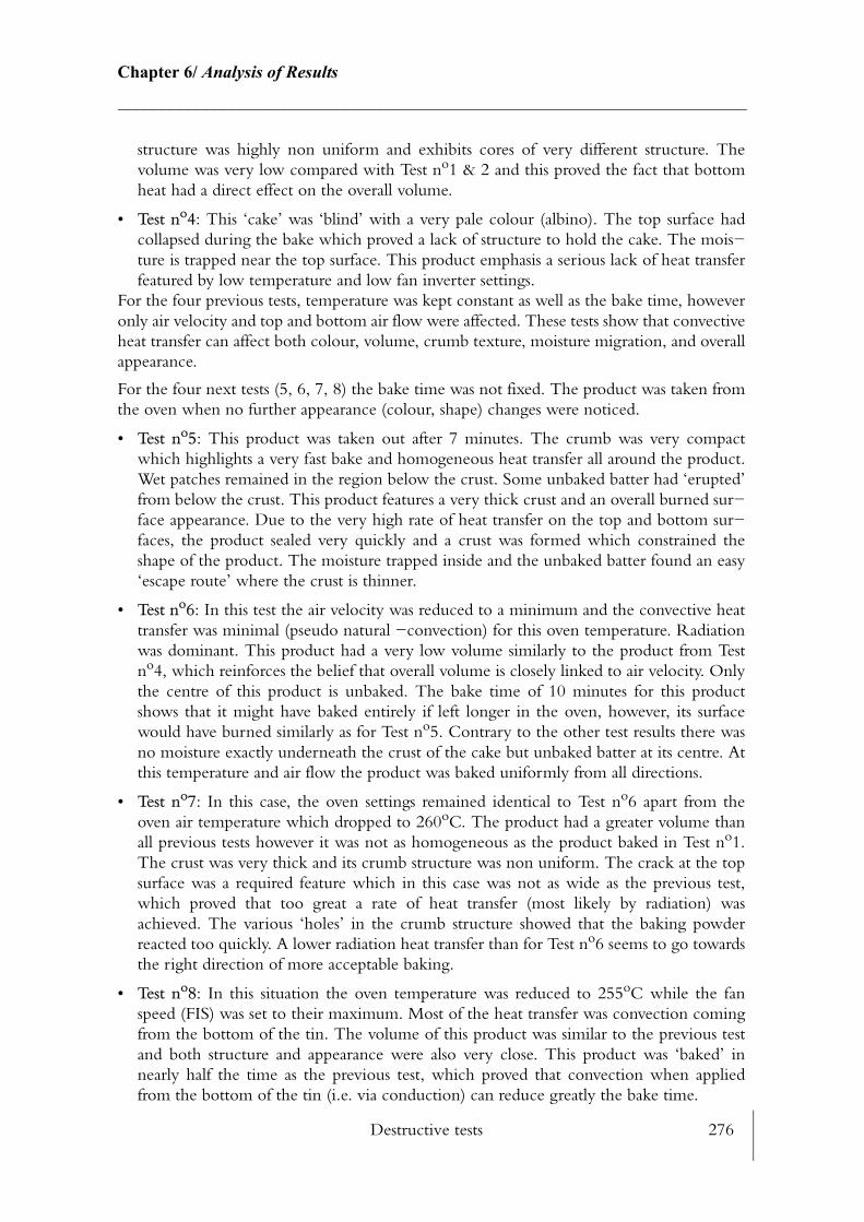
Destructive tests 276
Chapter 6/ Analysis of Results________________________________________________________________________
structure was highly non uniform and exhibits cores of very different structure. The volume was very low compared with Test no1 & 2 and this proved the fact that bottom heat had a direct effect on the overall volume.
• Test no4: This ‘cake’ was ‘blind’ with a very pale colour (albino). The top surface had collapsed during the bake which proved a lack of structure to hold the cake. The mois−ture is trapped near the top surface. This product emphasis a serious lack of heat transfer featured by low temperature and low fan inverter settings.
For the four previous tests, temperature was kept constant as well as the bake time, however only air velocity and top and bottom air flow were affected. These tests show that convective heat transfer can affect both colour, volume, crumb texture, moisture migration, and overall appearance.
For the four next tests (5, 6, 7, 8) the bake time was not fixed. The product was taken from the oven when no further appearance (colour, shape) changes were noticed.
• Test no5: This product was taken out after 7 minutes. The crumb was very compact which highlights a very fast bake and homogeneous heat transfer all around the product. Wet patches remained in the region below the crust. Some unbaked batter had ‘erupted’ from below the crust. This product features a very thick crust and an overall burned sur−face appearance. Due to the very high rate of heat transfer on the top and bottom sur−faces, the product sealed very quickly and a crust was formed which constrained the shape of the product. The moisture trapped inside and the unbaked batter found an easy ‘escape route’ where the crust is thinner.
• Test no6: In this test the air velocity was reduced to a minimum and the convective heat transfer was minimal (pseudo natural −convection) for this oven temperature. Radiation was dominant. This product had a very low volume similarly to the product from Test no4, which reinforces the belief that overall volume is closely linked to air velocity. Only the centre of this product is unbaked. The bake time of 10 minutes for this product shows that it might have baked entirely if left longer in the oven, however, its surface would have burned similarly as for Test no5. Contrary to the other test results there was no moisture exactly underneath the crust of the cake but unbaked batter at its centre. At this temperature and air flow the product was baked uniformly from all directions.
• Test no7: In this case, the oven settings remained identical to Test no6 apart from the oven air temperature which dropped to 260oC. The product had a greater volume than all previous tests however it was not as homogeneous as the product baked in Test no1. The crust was very thick and its crumb structure was non uniform. The crack at the top surface was a required feature which in this case was not as wide as the previous test, which proved that too great a rate of heat transfer (most likely by radiation) was achieved. The various ‘holes’ in the crumb structure showed that the baking powder reacted too quickly. A lower radiation heat transfer than for Test no6 seems to go towards the right direction of more acceptable baking.
• Test no8: In this situation the oven temperature was reduced to 255oC while the fan speed (FIS) was set to their maximum. Most of the heat transfer was convection coming from the bottom of the tin. The volume of this product was similar to the previous test and both structure and appearance were also very close. This product was ‘baked’ in nearly half the time as the previous test, which proved that convection when applied from the bottom of the tin (i.e. via conduction) can reduce greatly the bake time.

Destructive tests 277
Chapter 6/ Analysis of Results________________________________________________________________________
Figure 6−1. Destructive tests

Screening design 278
Chapter 6/ Analysis of Results________________________________________________________________________
For both Test no4 and Test no6 all of the responses could not be measured (texture, moisture). For these destructive tests, the air temperature seemed to be more critical than fan speed (FIS) (air velocity) and the range of temperature was reduced to 130oC−230oC for the start−ing point of the DOE.
This range of study confirmed the practical temperature range. Indeed, the majority of cake baking ovens are direct gas fired which operate in temperature ranges from 150oC (first zone) to 220oC (final zone).
6.2 Screening design
Considering the design factors under study (see Table 5−7) the most appropriate design proposed by the DOE software Maximize was a D16/8. This design suggest that 16 exper−iments should be run for the 8 design factors. Four partial replicates were chosen as it is strongly recommended to run replicates in order to compute an estimate of standard error which tells whether or not the observed variations are statistically significant. Runs were also randomized from the proposed design. The final design was made up of 20 runs including the repeats.
It is normally advised to randomise fully the whole design. However due to the time required for the TPRO to reach steady state, the changes of temperature from 130oC to 230oC could have taken far too much time and therefore increased significantly the overall time of the runs. For this reason, similar temperatures were grouped together forming two separate blocks. The runs of each of the separate groups were randomized. Two blocking factors were created to reflect the specification of the design. The first blocking factor (BK1) was created to reflect the possible variation of high and low temperature and the second blocking factor (BK2) was placed to understand the possible day to day variations. These blocking factors were used to improve the precision of the responses of interest. Table 6−2 summarises the complete SD.
Some proposed runs by the software were slightly modified as they were not physically viable for the TPRO settings (e.g. Run 2 on Day1 and Run 5 on Day 3). In both these cases, the fan speeds (FIS) cannot run at full speed if the top and bottom dampers are closed, for this reason these settings were dropped to the minimum.
Results given by the software were of two forms; table, composed of ANOVA (Analysis of Variance), regression coefficients and average response plots. An example of these results for the top colour response is given in Appendix J. The regression coefficients were the coeffi−cients used by the statistical model from the software. In order to judge whether the design factors was to be kept for further analysis three criteria were chosen from the DOE software results:
• Percentage contribution: This expresses the relative influence of each response for con−tributing to the overall variation in the results. In many cases more than one variable is important and the percentage contribution can help to rank which of the variables is the most important.
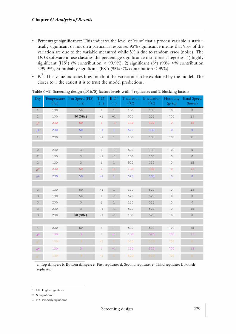
Screening design 279
Chapter 6/ Analysis of Results________________________________________________________________________
• Percentage significance: This indicates the level of ‘trust’ that a process variable is statis−tically significant or not on a particular response. 95% significance means that 95% of the variation are due to the variable measured while 5% is due to random error (noise). The DOE software in use classifies the percentage significance into three categories: 1) highly significant (HS1) (% contribution > 99.9%), 2) significant (S2) (99% <% contribution <99.9%), 3) probably significant (PS3) (95% <% contribution < 99%).
• R2: This value indicates how much of the variation can be explained by the model. The closer to 1 the easiest it is to trust the model predictions.
1. HS: Highly significant
2. S: Significant
3. P S: Probably significant
Table 6−2. Screening design (D16/8) factors levels with 4 replicates and 2 blocking factors
Day Temperature (oC)
Fan Speed (FIS)(Hz)
T Da
(−)
a. Top damper; b. Bottom damper; c. First replicate; d. Second replicate; e. Third replicate; f. Fourth replicate;
B Db
(−)T radiation
(oC)B radiation
(oC)Humidity
(g/kg)Band Speed
(linear)
1 130 50 1 1 130 130 700 0
1 130 50(3Hz) -1 -1 520 130 700 15
1c 230 50 1 -1 130 130 0 15
1d 230 50 -1 1 520 130 0 0
1 230 3 -1 1 130 130 700 15
2 240 3 1 -1 520 130 700 0
2 130 3 -1 -1 130 130 0 0
2 130 3 1 1 520 130 0 15
2c 230 50 1 -1 130 130 0 15
2d 230 50 -1 1 520 130 0 0
3 130 50 -1 1 130 520 0 15
3 130 50 1 -1 520 520 0 0
3 230 3 1 1 130 520 0 0
3 230 3 -1 -1 520 520 0 15
3 230 50(3Hz) -1 -1 130 520 700 0
4 230 50 1 1 520 520 700 15
4e 130 3 1 -1 130 520 700 15
4f 130 3 -1 1 520 520 700 0
4e 130 3 1 -1 130 520 700 15
4f 130 3 -1 1 520 520 700 0

Screening design 280
Chapter 6/ Analysis of Results________________________________________________________________________
6.2.1 Response analysis
Table 6−3 shows a summary of all the three criteria of selection for all the responses. A code of colour for the percentage of significance was used to aid understanding the decision taken; 1) highly significant (HS) = red, 2) significant (S) = orange, 3) probably significant (PS) = yellow). The other ‘design factors’ included in this table are the estimate factor interactions, E6, E7, E8, E9 and E10. For instance E6 can be any interaction between the design factors X1X3 (temperature and top damper), X2X5 (fan speed (FIS) and top radiation), X3X6 (top damper and bottom radiation), or X2X8 (fan speed (FIS) and band speed). Average response analysis, and average plots were also used in this design to compare the average value of the responses at each level of each design factors (Table 6−2). The examination of the slopes of each statistically significant average plots was also computed to help in this analysis.
An analysis of the correlation coefficient (R2) values indicates that the model constructed for the bake time is the most accurate one. This means that amongst all the responses under study the variations in bake time can be relatively well explained by the model. The transient weight loss comes second on this ranking analysis, then, the density change.
• Moisture change: None of the factors nor interaction contribute in the explanation of the crumb moisture change (see Table 6−3). This result means that the oven settings conditions did not affect the moisture change. This result can appear surprising at first sight, however there is a feasible explanation. As the degree of doneness was used as a basis to remove the product from the oven, the internal conditions of the product when baked were almost identical for all the trials, therefore very little variation should have been expected.
By looking at the actual measurement values, very little variation exists between the batter moisture and the crumb moisture. Moisture is essentially lost from the crust and not the crumb. The cake baking process is to create an aerated crumb, i.e. with much lower density than the batter. Although the findings are of interest for characterising this baking process, this analysis proves that this criteria was not of primary importance here.
• Top colour: This response can be explained to a major extent (54.3%) by the change of oven temperature (see Table 6−3). As expected, the second biggest player was the top radiation temperature. Fan speed (FIS) and humidity also contribute to 5% for this response, however they are only statistically significant or probably significant (Table 6−3). The HS figure from both the oven temperature and the radiation temperature proves that these results can be trusted statistically.
The computed slope (see Table 6−4) of the average response shows that temperature, fan speed (FIS) and top radiation have a tendency to darkens the product (negative coeffi−cient) while humidity tends to brighten the cake surface.
Top Colour is related to the caramelisation of sugar, which is temperature dependent. At 140oC, sugar will start caramelising therefore colour will start developing, so the sooner the surface reaches this threshold temperature the darker the temperature will become. Hence, the hotter the temperature (oven air, top radiation) the darker the surface will be.
• Bottom colour: The greatest contribution in bottom colour by a large margin is the oven air temperature (68.4%) (see Table 6−3). The temperature contribution to explain the bottom colour variation is 22 times greater than fan speed (FIS) and almost 10 times
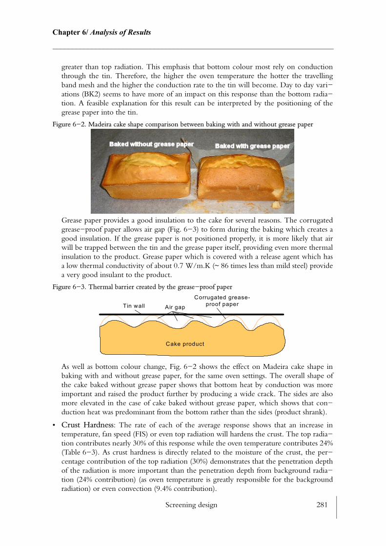
Screening design 281
Chapter 6/ Analysis of Results________________________________________________________________________
greater than top radiation. This emphasis that bottom colour most rely on conduction through the tin. Therefore, the higher the oven temperature the hotter the travelling band mesh and the higher the conduction rate to the tin will become. Day to day vari−ations (BK2) seems to have more of an impact on this response than the bottom radia−tion. A feasible explanation for this result can be interpreted by the positioning of the grease paper into the tin.
Figure 6−2. Madeira cake shape comparison between baking with and without grease paper
Grease paper provides a good insulation to the cake for several reasons. The corrugated grease−proof paper allows air gap (Fig. 6−3) to form during the baking which creates a good insulation. If the grease paper is not positioned properly, it is more likely that air will be trapped between the tin and the grease paper itself, providing even more thermal insulation to the product. Grease paper which is covered with a release agent which has a low thermal conductivity of about 0.7 W/m.K (~ 86 times less than mild steel) provide a very good insulant to the product.
Figure 6−3. Thermal barrier created by the grease−proof paper
As well as bottom colour change, Fig. 6−2 shows the effect on Madeira cake shape in baking with and without grease paper, for the same oven settings. The overall shape of the cake baked without grease paper shows that bottom heat by conduction was more important and raised the product further by producing a wide crack. The sides are also more elevated in the case of cake baked without grease paper, which shows that con−duction heat was predominant from the bottom rather than the sides (product shrank).
• Crust Hardness: The rate of each of the average response shows that an increase in temperature, fan speed (FIS) or even top radiation will hardens the crust. The top radia−tion contributes nearly 30% of this response while the oven temperature contributes 24% (Table 6−3). As crust hardness is directly related to the moisture of the crust, the per−centage contribution of the top radiation (30%) demonstrates that the penetration depth of the radiation is more important than the penetration depth from background radia−tion (24% contribution) (as oven temperature is greatly responsible for the background radiation) or even convection (9.4% contribution).
Tin wallCorrugated grease-
proof paper
Cake product
Air gap
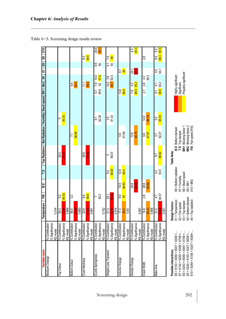
Screening design 282
Chapter 6/ Analysis of Results________________________________________________________________________
Table 6−3. Screening design results reviewV
aria
ble
nam
eT
emp
erat
ure
FIS
B D
T D
To
p R
adia
tio
nB
ot
Rad
iati
on
Hu
mid
ity
Ban
d s
pee
dB
K1
Bk2
E6
E7
E8
E9
E10
Moi
stur
e C
hang
e%
Con
trib
utio
n
% S
igni
fican
ce
R2
mod
el0.
314
Top
Col
our
% C
ontr
ibut
ion
54.3
5.2
20.4
5
% S
igni
fican
ce99
.96
95.6
399
.91
95.3
5
R2
mod
el0.
869
Bot
tom
Col
our
% C
ontr
ibut
ion
68.4
3.2
7.1
9.4
% S
igni
fican
ce99
.96
98.8
899
.5
R2
mod
el0.
883
Cru
st H
ardn
ess
% C
ontr
ibut
ion
23.9
9.4
29.8
11.1
9.3
% S
igni
fican
ce99
.95
98.6
99.9
899
.298
.6
R2
mod
el0.
861
Cru
mb
Spr
ingi
ness
% C
ontr
ibut
ion
78.
16.
77.
914
.49.
520
.8
% S
igni
fican
ce90
.292
.36
89.6
9297
.694
99.1
R2
mod
el0.
752
Wei
ght L
oss
Tra
nsie
nt%
Con
trib
utio
n21
.324
.19.
23
3.5
14.5
3.8
4.1
7.4
% S
igni
fican
ce99
.91
99.9
498
.83
89.0
791
.43
99.7
92.4
9398
R2
mod
el0.
914
Vol
ume
Cha
nge
% C
ontr
ibut
ion
17.3
9.9
14.5
12.9
5.9
13.6
8.7
% S
igni
fican
ce99
.397
98.8
398
.491
.69
98.6
96
R2
mod
el0.
83
Den
sity
Cha
nge
% C
ontr
ibut
ion
34.6
13.6
7.6
4.2
24.1
4.3
% S
igni
fican
ce99
.96
99.7
898
.895
.299
.995
.3
R2
mod
el0.
887
Cra
ck W
idth
% C
ontr
ibut
ion
16.9
2.8
28.6
9.9
14.9
2.7
2.8
4.3
2.8
% S
igni
fican
ce99
.43
99.8
997
.67
99.1
889
.3
R2
mod
el0.
856
Bak
e tim
e%
Con
trib
utio
n37
.24.
74.
29.
73.
75.
26.
14.
14.
58.
45.
2
% S
igni
fican
ce99
.98
94.5
793
.598
.82
92.0
795
.53
96.6
93.2
94.1
98.3
95.5
R2
mod
el0.
921
Po
ssib
le in
tera
ctio
ns:
Des
ign
Fac
tors
: T
able
No
te:
E6
= X
1X3
+ X
4X6
+ X
5X7
+ X
2X8
+…
X1
= T
empe
ratu
reX
6 = B
otto
m r
adia
tion
B D
B
otto
m d
ampe
r H
ighl
y si
gnifi
cant
E7
= X
1X4
+ X
2X5
+ X
3X6
+ X
7X8
+…
X2
= F
an s
peed
X7
= H
umid
ityT
D
Top
dam
per
Sig
nific
ant
E8
= X
2X3
+ X
5X6
+ X
4X7
+ X
1X8
+…
X3
= T
op d
ampe
rX
8 = B
and
spee
dB
K1
Blo
ckin
g fa
ctor
1 P
ropa
bly
sign
ifica
nt
E9
= X
2X4
+ X
1X5
+ X
3X7
+ X
6X8
+…
X4
= B
otto
m d
ampe
rX
9 = B
K1
BK
2 B
lock
ing
fact
or 2
E10
= X
3X4
+ X
1X6
+ X
2X7
+ X
5X8+
…X
5 = T
op r
adia
tion
X10
= B
K2
FIS
F
an s
peed
(F
IS)

Screening design 283
Chapter 6/ Analysis of Results________________________________________________________________________
Day to day variation as well as interaction between fan speed (FIS) and bottom damper position also contributes respectively to 11% and 9.4% to crust hardness variation. However it is more difficult to make a decisive judgement upon them.
• Crumb springiness: Two possible interactions seems to stand out of the list of factors contributing to the variation in crumb springiness. The most plausible interaction for the E10 factor could be X2X7 (fan speed (FIS) and humidity) (see Table 6−3). Indeed, the fan speed (FIS) and humidity are the only two factors on the average plots (See Appendix J) which seem to have some influence on the variations of the crumb spring−iness. So the interaction E10, might be a possible interaction. The physical explanation behind this interaction is more probable than for the other interaction proposed by the design (see Table 6−3). The humidity helps to promote a softer and more aerated crumb (i.e. higher springiness), as opposed to the higher fan speed (FIS) which can constrain the volume development of the product (i.e. lower springiness). Another way of explaining the significance of the interaction between the humidity and the fan speed (FIS) is to look at springiness related to the crumb moisture content. The rate of starch gelatinisation will be higher using high convective rate than using high humidity that will keep the overall crumb more moist and softer. Hence, a product baked with high convective rate will be more resilient, (i.e. lower springiness) than for a cake baked with a higher humidity rate. The proposed interaction for E6 does not seem to have any physically feasible explanations.
• Transient weight loss: This parameter measures the ability of the moisture to migrate during the cooling. It measures the amount of water that is loss during the first hour after the bake. Two of the factors are markedly contributing to this response (Table 6−3), the fan speed (FIS) and the temperature. Both of them are statistically significant. The transient weight loss may be related to the porosity of the crust and both oven air tem−perature and fan speed (FIS) will affect the crust formation. The larger the moisture dif−ferential between the crumb and crust structure the greater the potential of releasing moisture during the cooling section. Moisture will diffuse naturally driven by moisture gradient and temperature gradient. Analysis of the gradients of all statistically significant average responses shows that an increase in fan speed (FIS) will increase the transient weight loss, while opening the top damper further will tend to decrease the transient weight loss. Average response shows also that opening the top damper hardens the sur−face of the product greatly, therefore moisture will get trapped inside the product and transient weight loss will be greater comparatively.
• Volume change: Many factors contribute to the volume change response (see Table 6−3). The temperature yet again is the predominant one (17.3% contribution). The other factors are also contributing however, they are only probably ‘significant’. The volume change is affected by the crust formation, the amount of gases trapped during the aera−tion of the batter, and the CO2 released by the baking powder. If the crust is formed too quickly, it will inhibit the expansion of the cake, i.e. low volume change. This is shown by these results as the higher the oven air temperature/top radiation temperature the lower the volume. All of the process variables that are connected to promoting a higher heat flux to the top surface of the product (oven air temperature, top radiation tempera−ture, fan speed (FIS), top damper have a negative effect upon volume development. However all the fluxes, which are promoting indirectly a higher conduction flux to the tin (bottom damper, bottom radiation), have a positive effect to increasing the final vol−
Screening design 284
Chapter 6/ Analysis of Results________________________________________________________________________
ume of the cake. The final volume measurement of the product relies on the crumb−density sample measurement, which is not truly representative of the product for each run. Some products might have more crust than other depending on their ‘baking his−tory’.
• Density change: Two factors are clearly contributing to the density change variation: the bottom damper position and the estimated interaction E7. The bottom damper has the highest contribution percentage of the two (34.6%). Its explanation was to be expected. Indeed, the bottom damper positioning will vary the amount of air flow to the bottom of the tin, i.e. heat transfer. The average response plot reinforce this belief (see Appendix J). The greater the bottom damper is open and the less dense the product becomes, which means that the product structure is more open. The most plausible interaction of E7 can be between X3X6 (bottom damper and bottom radiation). Fol−lowing a similar explanation as the previous one, both these factors would tend to increase the conduction to the bottom of the tin.
• Crack width: Although the percentage significance is only ‘significant’, three factors contribute largely to the crack variation. These are: bottom damper (28.6%), tempera−ture (16.9%) and humidity (14.9%) (see Table 6−3). According to the average response curve, all of these factors have a positive effect on crack width response, i.e the higher the wider the crack. These three factors are directly proportional to the flux delivered. The results of this analysis emphasis that crack width control is driven mainly by a tin conduction problem. By letting more air flow from the bottom damper, the conduction through to the tin will increase, the higher the oven air temperature the higher back−ground radiation and convection flux will be. As for humidity the higher the humidity level the greater the heat transfer will be (especially at the start of the bake). If setting of the products surface can be slowed down, a less ‘dramatic’ eruption should occur and the crack width should be minimised.
• Bake time: A large number of factors and possible interactions seem to play a contribu−tion to the variation in bake time. However oven air temperature has the largest per−centage contribution of all factors (37.2%) (see Table 6−3). The top radiation is the second greatest factors (9.7%) in reducing the bake time. Humidity and fan speed (FIS) play equal role in reducing the bake time although only humidity is probably significant.
When analysing the gradient of each of the average response plot, oven air temperature shows that it has the largest positive influence on crust hardness (Table 6−4). This gradient is about 10 times greater than for all the other responses. The effect of increasing the oven
air temperature has almost the same effect (same gradient) for top colour, bottom colour, and bake time. According to Table 6−4, a large increase would be required to modify the volume change. The effect of the fan speed (FIS) influence the responses in the same way as tem−
Table 6−4. Gradient of the average response plot for a rise in oven temperature (130oC to 230oC)
Top colour[1]a
a. [1,2,.] represent the ranking number establish by Andrews, 2001 [3]
Bottom colour[5] Crust hardness[4] Bake time Volume change[2] Crack width[3]
-0.27 -0.26 2.76 -0.29 -0.09 0.16
Screening design 285
Chapter 6/ Analysis of Results________________________________________________________________________
perature does (gradient have same sign). Comparatively to temperature, fan speed (Table 6−
5) has even more influence on crust hardness than for top or bottom colour (20 to 30 times). The most significant change compared with oven air temperature is the volume change. Indeed, increasing the fan speed will have almost 2 times more effect for reducing the volume change than oven air temperature. Bottom damper (Table 6−6) has the greatest effect on
crust hardness and crack width. Contrarily to temperature and fan speed bottom damper will brighten the top colour surface and increase the overall volume of the cake. Increasing the
top radiant temperature (Table 6−7) from 130oC to 520oC has the greatest impact on crust hardness and has no influence at all on the volume change, crack width and bottom colour. The effect on crust hardness is 19 times greater on darkening the cake top surface. The effect of increasing the top radiation temperature on bake reduction is very small (−0.01).
The results of the SD have pin pointed the factors that are contributing greatly to some of the responses under study and also determined which of the responses could be discarded for the following design study. This analysis was based on the findings of the SD but also on the time constraint for running trials. Four design factors were chosen:
1. Temperature
2. Fan speed (FIS)
3. Bottom damper
4. Top radiation temperature
This choice was based on the analysis of the percentage contribution (Table 6−3) identified as the highest for the most desirable responses. As well as contributing to the responses, the percentage significance also had to be within the acceptable limits defined (HS, S, or PS). The design factor selected have a least one response which is highly significant. These design factors were also the factors for which the gradient of the average response analysis had the greatest influence. Although it did not appear to contribute highly significantly to any of the
Table 6−5. Gradient of the average response plot for a rise of fan speed (FIS)(3Hz to 50Hz)
Top colour[1] Bottom colour[5] Crust hardness[4] Bake time Volume change[2] Crack width[3]
-0.18 -0.12 3.68 -0.22 -0.14 0.14
Table 6−6. Gradient of the average response plot while opening the bottom damper (−1 to +1)
Top colour[1] Bottom colour[5] Crust hardness[4] Bake time Volume change[2] Crack width[3]
2.21 -2.18 24.63 -3.01 4.10 10.51
Table 6−7. Gradient of the average response plot for a rise in top radiant temperature (130oC to 520oC)
Top colour[1] Bottom colour[5] Crust hardness[4] Bake time Volume change[2] Crack width[3]
-0.04 0.01 0.79 -0.01 0 0
Factorial design 286
Chapter 6/ Analysis of Results________________________________________________________________________
responses, the humidity could have been kept for the next stage of the design, as it is of inter−est to be studied. However the cost of running a factorial design with five factors (32 exper−iments required plus replicates) was much greater than with only four factors (16 experiments plus replicates). As far as the responses are concerned, moisture change as well as volume change were not measured for the next design stage. This choice was based on the number of highly contributing factors.
6.3 Factorial design
A two level full factorial (D16/4) design was performed without replicates. No replicates were carried out this time as the design itself without replicates could predict standard errors accurately, thereby giving a good estimate of the possible interactions. Full factorial design is a very powerful tool as it provides an average response plot, an interaction plot which indi−cates when one factor on a response depends on the level of another factor, and a contour plot which gives a more accurate mapping of two factor interactions. Contour plotting is a tool of the Response Surface Methodology (RSM). RSM is useful for the modelling and analysis of problems in which a response of interest is influenced by several variables and the objective is to optimise this response.
The main design factors ranges (see Table 6−10) were set up as for the previous design (see Table 6−8). The secondary factors (design factors discarded from the previous design) were set up to minimise their likely effects on the desirable responses. The top damper was set to be fully open as fully closed would have given to much importance on conduction through the bottom of the tin. The bottom radiation temperature was kept constant to 130oC which is the minimum oven air temperature, hence the effect of bottom radiation should be min−imum. Crack width is one of the most important features for the appearance of the Madeira cake, and SD results have shown previously that temperature and humidity had almost equal contribution (Table 6−3) to this response, hence humidity was set fixed to the average between the lowest and highest value of the range i.e. 350g/kg. As band speed had no influ−ence on any of the responses it was fixed to the lowest speed.
Table 6−8. Full factorial design (D16/4) factors level (primary (bold) and secondary
Day Temperaturea (oC) (X1)
Fan Speed (FIS)(Hz) (X2)
T Db
(−)B Db
(−) (X3)T radiation(oC) (X4)
B radiation(oC)
Humidity(g/kg)
Band Speed(linear)
1 130 50 1 -1 130 130 350 2
1 130 50 1 1 520 130 350 2
1 230 3 1 1 520 130 350 2
1 230 50 1 1 130 130 350 2
1 230 50 1 -1 520 130 350 2
2 130 50 1 -1 130 130 350 2
2 230 50 1 1 520 130 350 2
2 130 3 1 1 520 130 350 2

Factorial design 287
Chapter 6/ Analysis of Results________________________________________________________________________
6.3.1 Raw data results
The DOE software requires the raw data of each run before processing further computation. Table 6−9 shows the raw data set of the FD. The average of every runs for each responses is calculated and the percentage difference for two runs, Day1 (1) (%Diff D1 − Benchmark) and Day2(5) (%Diff D2 − Bench) is computed (see Table 6−9). For these two runs a top view photograph of each of the product is shown by Fig. 6−4 and Fig. 6−5. From Table 6−9 results it can be seen that for the run Day1(1) only top colour, bottom colour are relatively close to the benchmark values, i.e. within the ±2.5% and ±5% tolerance band established (see 5.3.3).
Table 6−9. Factorial design raw data results
2 230 3 1 -1 520 130 350 2
2 230 50 1 -1 130 130 350 2
3 130 3 1 -1 520 130 350 2
3 130 50 1 1 130 130 350 2
3 130 50 1 -1 520 130 350 2
3 230 3 1 1 130 130 350 2
3 230 3 1 -1 130 130 350 2
4 240 3 1 1 130 130 350 2
a. Temperature, Fan speed (FIS), B D and top radiation are primary design factors (allow to vary)
b. Top damper; b. Bottom damper; c. First replicate; d. Second replicate; e. Third replicate; f. Fourth replicate;
Table 6−8. Full factorial design (D16/4) factors level (primary (bold) and secondary
Day Temperaturea (oC) (X1)
Fan Speed (FIS)(Hz) (X2)
T Db
(−)B Db
(−) (X3)T radiation(oC) (X4)
B radiation(oC)
Humidity(g/kg)
Band Speed(linear)
Day Top Colour Bottom Colour Crust Hard. Weight Ch. Trans Weight. Density Ch. Bake Time Crack Width Volume Ch.1* 58.33 50.78 596.13 9.85 -3.88 -158.89 82.45 31.88 233.391 32.61 41.95 530.86 8.76 -6.81 -149.59 27.73 55.08 227.791 46.39 62.90 1418.80 12.59 -3.68 -141.42 36.80 37.38 211.141 22.20 22.56 581.13 14.23 -5.42 -152.34 18.06 62.22 216.501 67.34 58.56 287.40 8.27 -4.71 -155.87 97.20 22.33 234.722 45.22 42.62 263.13 8.23 -7.76 -165.01 29.93 70.40 243.222 52.87 52.54 211.33 9.12 -5.07 -149.88 41.50 69.40 227.222 22.40 19.23 1385.46 18.61 -5.10 -161.01 28.50 62.84 212.502 42.53 50.06 453.13 8.03 -6.43 -162.96 39.78 55.06 241.882* 26.18 35.76 1155.07 11.98 -6.45 -142.48 28.60 48.20 213.463 37.60 53.78 857.20 13.26 -3.62 -138.28 38.20 74.20 206.733 20.51 19.73 857.40 17.86 -4.65 -155.27 21.50 65.88 209.743 45.01 59.86 819.80 8.31 -5.61 -155.73 52.25 42.20 234.503 27.22 39.88 739.20 9.81 -5.93 -161.78 27.23 52.84 236.113 48.56 50.98 291.63 9.77 -4.99 -144.14 42.70 62.52 220.314 22.80 18.41 475.46 12.64 -5.80 -151.67 18.36 53.28 219.92
Average 38.61 42.48 682.70 11.33 -5.37 -152.90 39.42 54.11 224.32Benchmark 56.70 47.50 147.60 8.20 -5.20 -177.20 60.00 39.90 254.40
% Diff D1 - Bench 2.87 6.91 303.88 20.12 25.38 10.33 37.42 20.10 8.26% Diff D2 - Bench 53.83 24.72 682.57 46.10 24.04 19.59 52.33 20.80 16.09
+/-2.5% tolerance band Day 1(1) in out out out out out na out out+/- 5% tolerance band Day1(1) in in out out out out na out out

Factorial design 288
Chapter 6/ Analysis of Results________________________________________________________________________
From an eye analysis of the photograph Fig. 6−4, only the crack width and the colour appears to be different from the benchmark Fig. 5−33, although a top view might not be give enough information to judge the other response criteria. However there is no doubt for Fig. 6−4 which has clearly a non edible appearance. Overall colour (53.8% out of bench−mark specification), shape, hardness (682.6% out of benchmark specification). The only design factor that changed between Day(1) and Day2(5) run is the oven air temperature (see Table 6−8). The bake time difference between these two runs is 54 minutes, which is almost the bake time of the benchmark.
Figure 6−4. Day1(1) product photograph (bake time 82.5 minutes)
Figure 6−5. Day2(5) product photograph (bake time 28.6 minutes)
6.3.2 Response analysis
In this design each of the responses can be built as an equation which is composed of the main factors (X1 = temperature, X2 = fan inverter settings, X3 = bottom damper, X4 = top radiation), the linear regression coefficients for each responses associated to the main factors (A1, A2, A3, A4) and the interactions coefficients (A12, A13, A14 etc.). Interactions in this design are ‘direct’ and not based on hypothesis as a computed error terms allows to predict them relatively well (specific to FD). This means for instance that A12 is an interaction between temperature and fan speed (FIS). The general response equation is of the form:
(6.1)Y A0 A1X1 A2X2 A3X3 A4X4 A12X1X2 A13X1X3 A14X1X4 A23X2X3 A24X2X4 A34X3X4+ + + + + + + + + +=
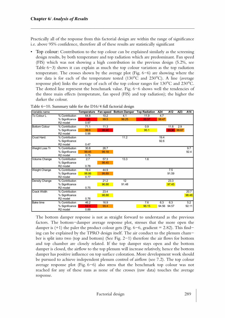
Factorial design 289
Chapter 6/ Analysis of Results________________________________________________________________________
Practically all of the response from this factorial design are within the range of significance i.e. above 95% confidence, therefore all of these results are statistically significant
• Top colour: Contribution to the top colour can be explained similarly as the screening design results, by both temperature and top radiation which are predominant. Fan speed (FIS) which was not showing a high contribution in the previous design (5.2%, see Table 6−3) shows it can explain as much the top colour variation as the top radiation temperature. The crosses shown by the average plot (Fig. 6−6) are showing where the raw data is for each of the temperature tested (130oC and 230oC). A line (average response plot) links the average of each of the top colour ranges for 130oC and 230oC. The dotted line represent the benchmark value. Fig. 6−6 shows well the tendencies of the three main effects (temperature, fan speed (FIS) and top radiation); the higher the darker the colour.
Table 6−10. Summary table for the D16/4 full factorial design
The bottom damper response is not as straight forward to understand as the previous factors. The bottom−damper average response plot, stresses that the more open the damper is (+1) the paler the product colour gets (Fig. 6−6, gradient = 2.82). This find−ing can be explained by the TPRO design itself. The air conduct to the plenum cham−ber is split into two (top and bottom) (See Fig. 2−1) therefore the air flows for bottom and top chamber are closely related. If the top damper stays open and the bottom damper is closed, the airflow to the top plenum will increase relatively, hence the bottom damper has positive influence on top surface coloration. More development work should be pursued to achieve independent plenum control of airflow (see 7.2). The top colour average response plot (Fig. 6−6) also stress that the benchmark top colour was not reached for any of these runs as none of the crosses (raw data) touches the average response.
Variable name Temperature Fan speed Bottom Damper Top Radiation A24 A12 A23 A14To Colour L % Contribution 64.8 10.2 4.1 11.9 4.7
% Significance 100 99.5 99.25 99.97 99.47R2 model 0.97
Bottom Colour % Contribution 71.1 11.3 0.9 11.8 2.9% Significance 99.6 99.96 95.1 99.96 99.67R2 model 0.98
Crust Hard. % Contribution 11.2 19.4% Significance 92.6R2 model 0.47
Weight Loss Tr % Contribution 30.8 26.7 9.7% Significance 99.45 99.18 92.4R2 model 0.75
Volume Change % Contribution 2.7 57.3 13.3 1.6% Significance 98.45R2 model 0.78
Weight Change % Contribution 19.4 44.9 7.5% Significance 98.86 99.89 91.59R2 model 0.77
Density Change % Contribution 21.2 12 23.3% Significance 96.88 91.48 97.45R2 model 0.75
Crack Width % Contribution 23.4 20.7% Significance 98.88 98.48R2 model 0.76
Bake time % Contribution 46.2 16.9 7.6 6.3 6.3 5.2% Significance 99.9 99.4 96.15 94.56 94.57 92.11R2 model 0.88
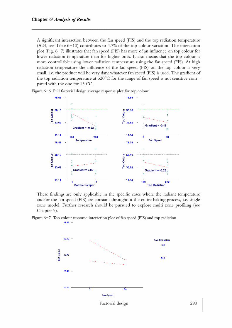
Factorial design 290
Chapter 6/ Analysis of Results________________________________________________________________________
A significant interaction between the fan speed (FIS) and the top radiation temperature (A24, see Table 6−10) contributes to 4.7% of the top colour variation. The interaction plot (Fig. 6−7) illustrates that fan speed (FIS) has more of an influence on top colour for lower radiation temperature than for higher ones. It also means that the top colour is more controllable using lower radiation temperature using the fan speed (FIS). At high radiation temperature the influence of the fan speed (FIS) on the top colour is very small, i.e. the product will be very dark whatever fan speed (FIS) is used. The gradient of the top radiation temperature at 520oC for the range of fan speed is not sensitive com−pared with the one for 130oC.
Figure 6−6. Full factorial design average response plot for top colour
These findings are only applicable in the specific cases where the radiant temperature and/or the fan speed (FIS) are constant throughout the entire baking process, i.e. single zone model. Further research should be pursued to explore multi zone profiling (see Chapter 7).
Figure 6−7. Top colour response interaction plot of fan speed (FIS) and top radiation

Factorial design 291
Chapter 6/ Analysis of Results________________________________________________________________________
• Bottom colour: The oven air temperature contributes greatly (71.1%) to the change in bottom colour of the product (Table 6−10). Contribution of fan speed (FIS) alone (11.3%) and the interaction between the air temperature and the fan speed (FIS) (A12 = 11.8%) contribute almost equally to this response variation. Fig. 6−8 shows that the bottom colour benchmark value could be reached, if the oven temperature was set up to 160oC (intersection between the dotted line (benchmark) and the average response line) and the fan speed (FIS) was running at 3Hz. Bottom colour is more sensitive to air tem−perature than fan speed (gradient comparison).
Figure 6−8. Full factorial design average response plot for bottom colour
Although its contribution is lesser than for the other factors, fan speed (FIS) and bottom damper are interacting (A23, see Table 6−10) in the variation of bottom colour (Fig. 6−8). This interaction (A23) was to be expected however the shape of the interaction is of interest (Fig. 6−8) as for low oven temperature the fan speed (FIS) has no influence on the bottom colour. Nonetheless, as the oven air temperature increases the fan speed (FIS) has more ‘weight’ on the bottom colour. The coloration of the bottom is directly linked to the conduction through the tin, which is indirectly correlated to the convection flux. As the temperature and velocity increase, the convective heat transfer coefficient must increase too.
As the ‘travelling’ band is a mesh, some of the convective heat, is transferred by conduc−tion through the mesh and to the bottom of tin, thereby increasing the overall amount of conduction through the bottom of the tin, i.e. darkening the bottom of the cake. The results from this experiment does not allow to distinguish between the amount of con−vection conduction to the bottom of the tin. The gradient of both the average response of temperature and fan speed are close to the gradient obtained by the SD.
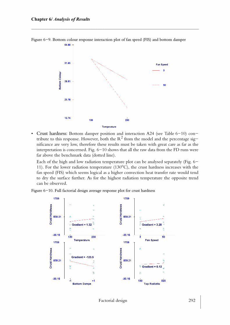
Factorial design 292
Chapter 6/ Analysis of Results________________________________________________________________________
Figure 6−9. Bottom colour response interaction plot of fan speed (FIS) and bottom damper
• Crust hardness: Bottom damper position and interaction A24 (see Table 6−10) con−tribute to this response. However, both the R2 from the model and the percentage sig−nificance are very low, therefore these results must be taken with great care as far as the interpretation is concerned. Fig. 6−10 shows that all the raw data from the FD runs were far above the benchmark data (dotted line).
Each of the high and low radiation temperature plot can be analysed separately (Fig. 6−11). For the lower radiation temperature (130oC), the crust hardness increases with the fan speed (FIS) which seems logical as a higher convection heat transfer rate would tend to dry the surface further. As for the highest radiation temperature the opposite trend can be observed.
Figure 6−10. Full factorial design average response plot for crust hardness
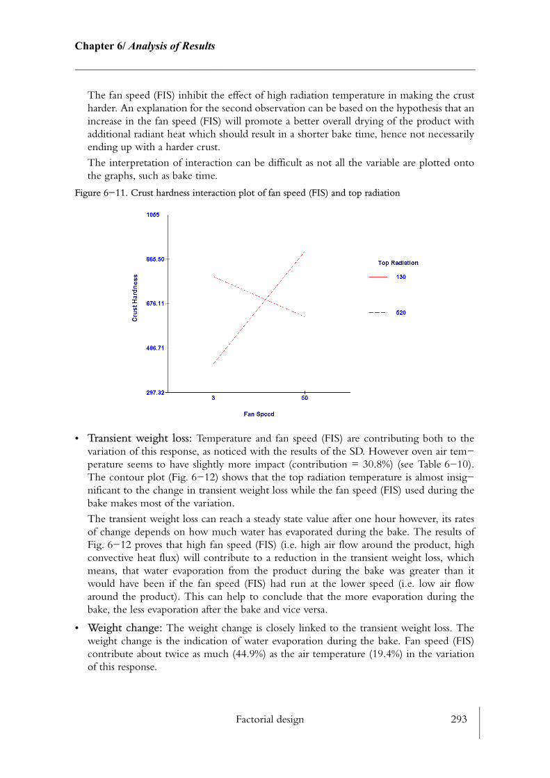
Factorial design 293
Chapter 6/ Analysis of Results________________________________________________________________________
The fan speed (FIS) inhibit the effect of high radiation temperature in making the crust harder. An explanation for the second observation can be based on the hypothesis that an increase in the fan speed (FIS) will promote a better overall drying of the product with additional radiant heat which should result in a shorter bake time, hence not necessarily ending up with a harder crust.
The interpretation of interaction can be difficult as not all the variable are plotted onto the graphs, such as bake time.
Figure 6−11. Crust hardness interaction plot of fan speed (FIS) and top radiation
• Transient weight loss: Temperature and fan speed (FIS) are contributing both to the variation of this response, as noticed with the results of the SD. However oven air tem−perature seems to have slightly more impact (contribution = 30.8%) (see Table 6−10). The contour plot (Fig. 6−12) shows that the top radiation temperature is almost insig−nificant to the change in transient weight loss while the fan speed (FIS) used during the bake makes most of the variation.
The transient weight loss can reach a steady state value after one hour however, its rates of change depends on how much water has evaporated during the bake. The results of Fig. 6−12 proves that high fan speed (FIS) (i.e. high air flow around the product, high convective heat flux) will contribute to a reduction in the transient weight loss, which means, that water evaporation from the product during the bake was greater than it would have been if the fan speed (FIS) had run at the lower speed (i.e. low air flow around the product). This can help to conclude that the more evaporation during the bake, the less evaporation after the bake and vice versa.
• Weight change: The weight change is closely linked to the transient weight loss. The weight change is the indication of water evaporation during the bake. Fan speed (FIS) contribute about twice as much (44.9%) as the air temperature (19.4%) in the variation of this response.
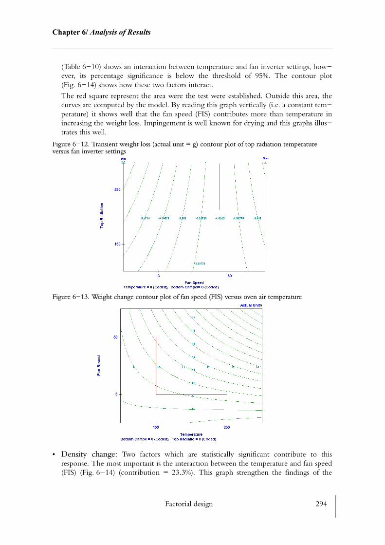
Factorial design 294
Chapter 6/ Analysis of Results________________________________________________________________________
(Table 6−10) shows an interaction between temperature and fan inverter settings, how−ever, its percentage significance is below the threshold of 95%. The contour plot (Fig. 6−14) shows how these two factors interact.
The red square represent the area were the test were established. Outside this area, the curves are computed by the model. By reading this graph vertically (i.e. a constant tem−perature) it shows well that the fan speed (FIS) contributes more than temperature in increasing the weight loss. Impingement is well known for drying and this graphs illus−trates this well.
Figure 6−12. Transient weight loss (actual unit = g) contour plot of top radiation temperature versus fan inverter settings
Figure 6−13. Weight change contour plot of fan speed (FIS) versus oven air temperature
• Density change: Two factors which are statistically significant contribute to this response. The most important is the interaction between the temperature and fan speed (FIS) (Fig. 6−14) (contribution = 23.3%). This graph strengthen the findings of the
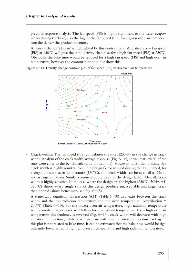
Factorial design 295
Chapter 6/ Analysis of Results________________________________________________________________________
previous response analysis. The fan speed (FIS) is highly significant to the water evapo−ration during the bake, also the higher the fan speed (FIS) for a given oven air tempera−ture the denser the product becomes.
A density change ‘plateau’ is highlighted by this contour plot. A relatively low fan speed (FIS) at 130oC will give the same density change as for a high fan speed (FIS) at 230oC. Obviously the bake time would be reduced for a high fan speed (FIS) and high oven air temperature, however the contour plot does not show this.
Figure 6−14. Density change contour plot of fan speed (FIS) versus oven air temperature
• Crack width: The fan speed (FIS) contributes the most (23.4%) to the change in crack width. Analysis of the crack width average response (Fig. 6−15) shows that several of the runs were close to the benchmark value (dotted line). However, it also demonstrate that crack width is highly sensitive to all the design factor in used during the FD. Indeed, for a single constant oven temperature (130oC), the crack width can be as small as 22mm and as large as 74mm. Similar comment apply to all of the design factor. Overall, crack width is highly sensitive. In the case where the design are the highest (230oC, 50Hz, +1, 520oC) almost every single runs of this design produce unacceptable and larger crack than desired (above benchmark see Fig. 6−15).
A statistically significant interaction (A14) (Table 6−10) also exist between the crack width and the top radiation temperature and the oven temperature (contribution = 20.7%) (Table 6−10). For the lowest oven air temperature, high radiation temperature will promote a larger crack width than for low radiant temperature. For a high oven air temperature this tendency is reversed (Fig. 6−16), crack width will decrease with high radiation temperature, while it will increase with low radiation temperature. Yet again, this plot is not related to bake time. It can be estimated that the bake time would be sig−nificantly lower when using high oven air temperature and high radiation temperature.

Factorial design 296
Chapter 6/ Analysis of Results________________________________________________________________________
Figure 6−15. Full factorial design average response plot for crack width
Figure 6−16. Crack width interaction plot of top radiation temperature and oven air temperature
• Bake time: 46.2% of this response can be explained by the oven air temperature. This seems an obvious conclusion, that the higher the oven air temperature the more likely the bake is to be shortened. The fan speed (FIS) is the second most important contribu−tor (16.9%) in reducing the bake time, then the top radiation (7.6%). There are three interactions which contribute almost equally to this response however their significance is below the threshold of 95%. Similar to crack width, bake time is very sensitive as data spread is very large in the lower range design factors (Fig. 6−17), while the spread of data is much reduced for the higher range.
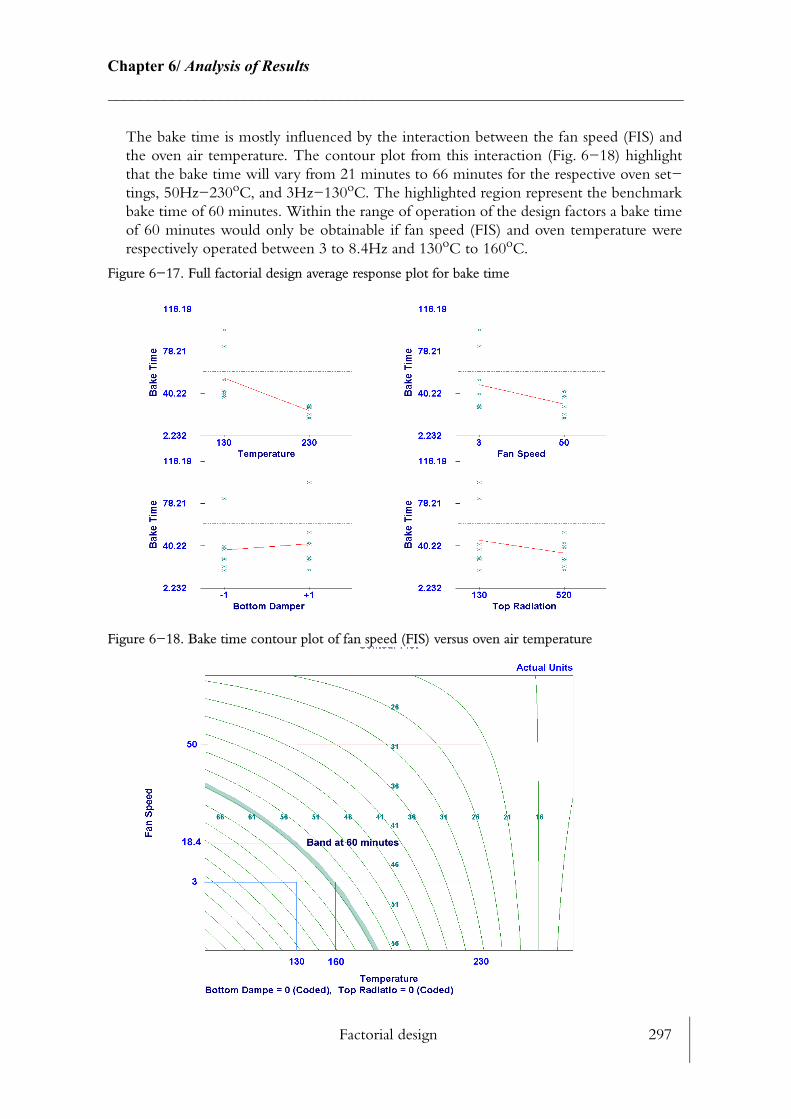
Factorial design 297
Chapter 6/ Analysis of Results________________________________________________________________________
The bake time is mostly influenced by the interaction between the fan speed (FIS) and the oven air temperature. The contour plot from this interaction (Fig. 6−18) highlight that the bake time will vary from 21 minutes to 66 minutes for the respective oven set−tings, 50Hz−230oC, and 3Hz−130oC. The highlighted region represent the benchmark bake time of 60 minutes. Within the range of operation of the design factors a bake time of 60 minutes would only be obtainable if fan speed (FIS) and oven temperature were respectively operated between 3 to 8.4Hz and 130oC to 160oC.
Figure 6−17. Full factorial design average response plot for bake time
Figure 6−18. Bake time contour plot of fan speed (FIS) versus oven air temperature
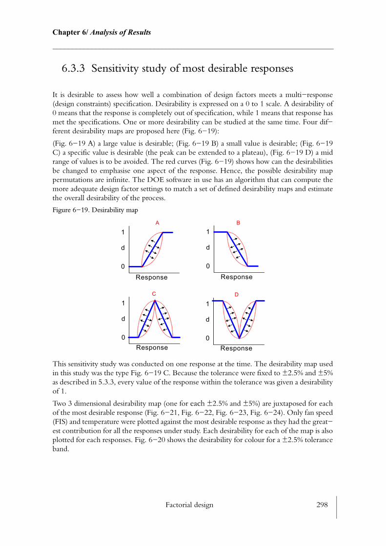
Factorial design 298
Chapter 6/ Analysis of Results________________________________________________________________________
6.3.3 Sensitivity study of most desirable responses
It is desirable to assess how well a combination of design factors meets a multi−response (design constraints) specification. Desirability is expressed on a 0 to 1 scale. A desirability of 0 means that the response is completely out of specification, while 1 means that response has met the specifications. One or more desirability can be studied at the same time. Four dif−ferent desirability maps are proposed here (Fig. 6−19):
(Fig. 6−19 A) a large value is desirable; (Fig. 6−19 B) a small value is desirable; (Fig. 6−19C) a specific value is desirable (the peak can be extended to a plateau), (Fig. 6−19 D) a mid range of values is to be avoided. The red curves (Fig. 6−19) shows how can the desirabilities be changed to emphasise one aspect of the response. Hence, the possible desirability map permutations are infinite. The DOE software in use has an algorithm that can compute the more adequate design factor settings to match a set of defined desirability maps and estimate the overall desirability of the process.
Figure 6−19. Desirability map
This sensitivity study was conducted on one response at the time. The desirability map used in this study was the type Fig. 6−19 C. Because the tolerance were fixed to ±2.5% and ±5% as described in 5.3.3, every value of the response within the tolerance was given a desirability of 1.
Two 3 dimensional desirability map (one for each ±2.5% and ±5%) are juxtaposed for each of the most desirable response (Fig. 6−21, Fig. 6−22, Fig. 6−23, Fig. 6−24). Only fan speed (FIS) and temperature were plotted against the most desirable response as they had the great−est contribution for all the responses under study. Each desirability for each of the map is also plotted for each responses. Fig. 6−20 shows the desirability for colour for a ±2.5% tolerance band.
0
1
Response
d
0
1
Response
d
0
1
Response
d
0
1
Response
d
A B
C D
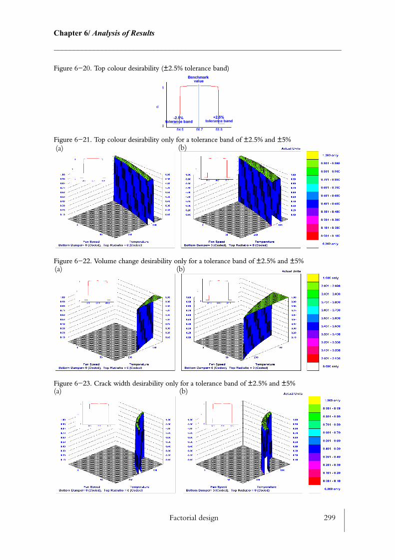
Factorial design 299
Chapter 6/ Analysis of Results________________________________________________________________________
Figure 6−20. Top colour desirability (±2.5% tolerance band)
Figure 6−21. Top colour desirability only for a tolerance band of ±2.5% and ±5%
Figure 6−22. Volume change desirability only for a tolerance band of ±2.5% and ±5%
Figure 6−23. Crack width desirability only for a tolerance band of ±2.5% and ±5%
(a) (b)
(a) (b)
(a) (b)

Central composite design 300
Chapter 6/ Analysis of Results________________________________________________________________________
Figure 6−24. Bottom colour desirability only for a tolerance band of ±2.5% and ±5%
All the above graphs were computed for a constant top radiation temperature of 325oC and the bottom damper set to 0 (half open). To understand how sensitive is the response to a change in fan speed and temperature three criteria can be looked at: the surface area of each map, the change in surface area from ±2.5% and ±5% and the direction of the map. A small surface area such as Fig. 6−23 (a) indicates that the response is highly sensitive to fan speed and temperature as it is not completely horizontal or vertical. The change of surface area between Fig. 6−22 (a) and Fig. 6−22 (b) points that the volume change is specifically sen−sitive as the change between he two areas is relatively large compared with the other responses. The direction of the map Fig. 6−21 (a & b) shows that top colour is highly sen−sitive to fan speed (FIS) compared to temperature. While the bottom colour is sensitive to fan speed between 3Hz and about 16Hz but less to temperature, however it becomes more sensitive to temperature as the fan speed increase from 16Hz and above.
The factorial design has helped to understand the various interaction between the design factors (process variables) and the responses under study. These results have made clearer to comprehend how one response can be increased or decreased by varying one or two factors. Nonetheless, from this design it is still difficult to estimate precisely how the design factors could be varied, in order to achieve responses close to the benchmark values. This can be caused by the highly sensitive response and also by the design factor ranges which could have been too narrow.
6.4 Central composite design
A central composite design was chosen to pursue further analysis and help in optimising the bake time. The mathematical model built so far with the previous designs assumed that the response surface was planar and no curvature could be established. CCD is commonly used to generate models in which response surfaces may be curved. The curvature can be obtained by including extra terms into the response equations. More experiments are required in order to include these extra terms into the equations. As resources and time were limited at the time of this experiment a CCD C15/3 (15 runs with three design factors) design with
(a) (b)
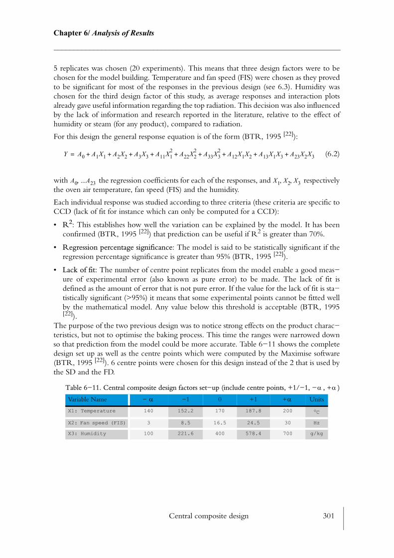
Central composite design 301
Chapter 6/ Analysis of Results________________________________________________________________________
5 replicates was chosen (20 experiments). This means that three design factors were to be chosen for the model building. Temperature and fan speed (FIS) were chosen as they proved to be significant for most of the responses in the previous design (see 6.3). Humidity was chosen for the third design factor of this study, as average responses and interaction plots already gave useful information regarding the top radiation. This decision was also influenced by the lack of information and research reported in the literature, relative to the effect of humidity or steam (for any product), compared to radiation.
For this design the general response equation is of the form (BTR, 1995 [22]):
(6.2)
with the regression coefficients for each of the responses, and respectively the oven air temperature, fan speed (FIS) and the humidity.
Each individual response was studied according to three criteria (these criteria are specific to CCD (lack of fit for instance which can only be computed for a CCD):
• R2: This establishes how well the variation can be explained by the model. It has been confirmed (BTR, 1995 [22]) that prediction can be useful if R2 is greater than 70%.
• Regression percentage significance: The model is said to be statistically significant if the regression percentage significance is greater than 95% (BTR, 1995 [22]).
• Lack of fit: The number of centre point replicates from the model enable a good meas−ure of experimental error (also known as pure error) to be made. The lack of fit is defined as the amount of error that is not pure error. If the value for the lack of fit is sta−tistically significant (>95%) it means that some experimental points cannot be fitted well by the mathematical model. Any value below this threshold is acceptable (BTR, 1995[22]).
The purpose of the two previous design was to notice strong effects on the product charac−teristics, but not to optimise the baking process. This time the ranges were narrowed down so that prediction from the model could be more accurate. Table 6−11 shows the complete design set up as well as the centre points which were computed by the Maximise software (BTR, 1995 [22]). 6 centre points were chosen for this design instead of the 2 that is used by the SD and the FD.
Table 6−11. Central composite design factors set−up (include centre points, +1/−1, − , + )
Variable Name − −1 0 +1 + Units
X1: Temperature 140 152.2 170 187.8 200 oC
X2: Fan speed (FIS) 3 8.5 16.5 24.5 30 Hz
X3: Humidity 100 221.6 400 578.4 700 g/kg
Y A0 A1X1 A2X2 A3X3 A11X12 A22X2
2 A33X32 A12X1X2 A13X1X3 A23X2X3+ + + + + + + + +=
A0 ...A23, X1 X2 X3, ,
α α
α α

Central composite design 302
Chapter 6/ Analysis of Results________________________________________________________________________
This time the top and bottom damper were left open and top and bottom radiation tem−perature were not energised
6.4.1 Central composite raw data results
The raw data set from Table 6−13 shows that overall, the results from CCD have more response values closer to the benchmark than had the FD. This was to be expected as the design factor ranges were narrower as for the previous designs. The two example taken from Table 6−13 (Run4 and Run10) are the extreme of this data set. Run10 photograph illus−trated by Fig. 6−26 shows that the cake baked in these conditions is closer to the benchmark than for the Run4. Indeed, two of the responses are within ±2.5% and 6 are within ±5%
Table 6−12. Central composite design run orders (C15/3) (primary (bold) and secondary design factors (Replicates in red).
Day Temperature [oC]
Fan speed FIS [Hz]
Humidity [g/kg]
T Da
a. T D: Top Damper; B D: Bottom Damper; B R: Bottom Radiant; T R: Top Radiant
B Da T Ra B Ra Band Speed (linear)
1 140 16.5 400 1 1 N Eb
b. Not energised
N E 2
1 152.16 8.474 221.64 1 1 N E N E 2
1 170 30 400 1 1 N E N E 2
1 187.84 8.474 578.36 1 1 N E N E 2
1 152.16 24.53 578.36 1 1 N E N E 2
2 170 16.5 400 1 1 N E N E 2
2 187.54 8.474 221.64 1 1 N E N E 2
2 152.16 8.474 578.36 1 1 N E N E 2
2 170 16.5 400 1 1 N E N E 2
2 170 16.5 400 1 1 N E N E 2
3 187.84 24.53 578.36 1 1 N E N E 2
3 170 3 400 1 1 N E N E 2
3 170 16.5 100 1 1 N E N E 2
3 170 16.5 400 1 1 N E N E 2
3 170 16.5 400 1 1 N E N E 2
4 152.16 24.53 221.64 1 1 N E N E 2
4 170 16.5 400 1 1 N E N E 2
4 187.84 24.53 221.64 1 1 N E N E 2
4 170 16.5 400 1 1 N E N E 2
4 200 16.5 400 1 1 N E N E 2
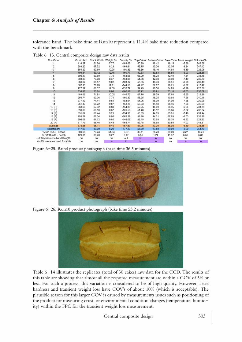
Central composite design 303
Chapter 6/ Analysis of Results________________________________________________________________________
tolerance band. The bake time of Run10 represent a 11.4% bake time reduction compared with the benchmark.
Table 6−13. Central composite design raw data results
Figure 6−25. Run4 product photograph (bake time 36.5 minutes)
Figure 6−26. Run10 product photograph (bake time 53.2 minutes)
Table 6−14 illustrates the replicates (total of 30 cakes) raw data for the CCD. The results of this table are showing that almost all the response measurement are within a COV of 5% or less. For such a process, this variation is considered to be of high quality. However, crust hardness and transient weight loss have COV’s of about 10% (which is acceptable). The plausible reason for this larger COV is caused by measurements issues such as positioning of the product for measuring crust, or environmental condition changes (temperature, humid−ity) within the FPC for the transient weight loss measurement.
Run Order Crust Hard. Crack Width Weight Ch. Density Ch. Top Colour Bottom Colour Bake Time Trans Weight. Volume Ch.1 114.27 51.26 7.77 -169.62 50.99 48.42 48.15 -5.86 248.682 208.20 67.52 8.23 -169.61 52.75 45.26 42.05 -8.34 247.423 354.20 60.60 10.28 -150.83 53.36 45.16 44.93 -6.39 225.084 709.34 69.12 12.45 -160.77 39.63 33.83 36.55 -5.03 228.355 300.47 63.60 7.70 -158.05 66.09 48.28 42.40 -7.31 238.186 308.33 73.08 8.37 -153.95 54.36 42.98 29.98 -7.49 232.707 366.67 68.57 9.02 -163.17 55.65 46.43 36.31 -6.99 239.488 662.13 70.70 11.11 -144.58 44.97 37.07 29.71 -5.37 217.429 727.27 66.37 12.69 -155.77 34.29 28.50 34.93 -6.29 223.3610 338.46 55.74 8.96 -160.42 58.72 46.91 53.18 -5.53 237.0911 489.66 71.91 10.05 -146.73 47.70 39.79 37.68 -5.65 219.9812 294.74 60.06 7.74 -160.33 58.95 48.75 40.68 -7.66 240.1613 377.13 71.41 9.81 -153.94 54.06 45.09 34.00 -7.55 229.0514 261.47 66.22 9.87 -158.15 53.33 44.48 38.46 -7.66 232.69
15 [R] 363.60 67.32 8.88 -154.38 52.25 44.49 36.95 -6.94 231.7916 [R] 390.86 68.10 8.67 -161.50 51.40 43.12 35.66 -7.22 238.8417 [R] 331.07 68.44 9.21 -154.91 53.89 44.09 35.81 -7.46 231.4418 [R] 295.27 66.04 8.86 -163.32 51.90 44.01 37.65 -5.03 239.9819 [R] 306.06 67.72 9.80 -146.09 52.15 43.65 35.70 -6.92 221.9720 [R] 317.79 68.46 8.45 -165.74 52.48 45.65 30.85 -7.02 243.31
Average 375.85 66.11 9.40 -157.59 51.95 43.30 38.08 -6.69 233.35Benchmark 147.60 39.90 8.20 -177.20 56.70 47.50 60.00 -5.20 254.40
% Diff Run4 - Bench 380.58 73.23 51.83 9.27 30.11 28.78 39.08 3.27 10.24% Diff Run10 - Bench 129.31 39.70 9.27 9.47 3.56 1.24 11.37 6.35 6.80
+/-2.5% tolerance band Run(10) out out out out in in na out out+/- 5% tolerance band Run(10) out out in in in in na in in

Central composite design 304
Chapter 6/ Analysis of Results________________________________________________________________________
Table 6−14. Variation study of replicates for the CCD (Natural variation of process)
6.4.2 Response analysis
It is desirable to predict what needs to change in order to reduce or increase the effect upon one response, and to understand how sensitive the response is. A 3D mapping representation for each of the responses under study was plotted for respectively 3 interactions: tempera−ture−fan inverter settings, temperature−humidity and fan inverter settings−humidity. If a 3−D map is flat or near symmetrical around the benchmark value it shows insensitivity, if not it shows sensitivity to that design factor(s) and suggest a narrower range is desirable. Each of the 10 responses were plotted for these 3 interactions. The most interesting are discussed below.
• Weight change: The three graphs (Fig. 6−27, Fig. 6−28, Fig. 6−29) represent the contour mapping of the weight change response versus the three design factors under study. The weight change contour plot (Fig. 6−27) demonstrates that the fan speed (FIS) does not affect greatly the weight change of the product if the oven air temperature is between 130oC and about 170oC. However, beyond this limit the interactions between the two factors becomes critical to the weight change. It is interesting to notice the cur−vature of this response. The minimum weight change is not obtained at the lowest tem−perature as expected, but somewhere near 170oC. The peak value seems to confirm what has been previously described (high temperature, high fan speed (FIS) will lead to high weight change). The benchmarked value would be represented by the pink area (Fig. 6−27). On this graph, the benchmark value can be obtained with a large combi−nation of both fan speed and temperature (i.e. all the design factor (fan speed (FIS) and humidity) leading to weight change within benchmark value).
The results of Fig. 6−28 shows the response plot versus humidity and fan speed (FIS) (temperature is kept constant at 170oC). High fan speed (FIS) and low humidity yield to high weight change. For any given temperature increasing the fan speed (FIS) will increase the weight change. For most of the fan speed (FIS) range (9Hz and above), the rise in humidity has a tendency to decrease the weight change. By adding extra humid−ity, the cake seems to retain more moisture, which is true for fan speed (FIS) of 9Hz and above, nonetheless for the lower fan speed (FIS) range, weight change is becoming greater as the humidity increase. In the benchmark area (see Fig. 6−28, range from 8.1 to 8.8) the weight change is almost non−sensitive to humidity but sensitive to fan speed.
The results of Fig. 6−29 (temperature and humidity varying but fan speed (FIS) fixed at 16.5Hz) shows a plateau area (red) which stress that weight change is non−sensitive to humidity and temperature from 140oC to 170oC and within 221−578 g/kg. The benchmark cannot be reached within the temperature range and humidity range com−puted by Fig. 6−29.
Run Order Crust Hard. Crack Width Weight Ch. Density Ch. Top Colour Bottom Colour Bake Time Trans Weight. Volume Ch.15 [R] 363.60 67.32 8.88 -154.38 52.25 44.49 36.95 -6.94 231.7916 [R] 390.86 68.10 8.67 -161.50 51.40 43.12 35.66 -7.22 238.8417 [R] 331.07 68.44 9.21 -154.91 53.89 44.09 35.81 -7.46 231.4418 [R] 295.27 66.04 8.86 -163.32 51.90 44.01 37.65 -5.03 239.9819 [R] 306.06 67.72 9.80 -146.09 52.15 43.65 35.70 -6.92 221.9720 [R] 317.79 68.46 8.45 -165.74 52.48 45.65 30.85 -7.02 243.31Mean 334.11 67.68 8.98 -157.66 52.35 44.17 35.44 -6.77 234.56Stdev 33.32 0.83 0.43 6.64 0.77 0.79 2.18 0.80 7.07
COV (%) 9.97 1.23 4.83 4.21 1.47 1.78 6.15 11.79 3.02
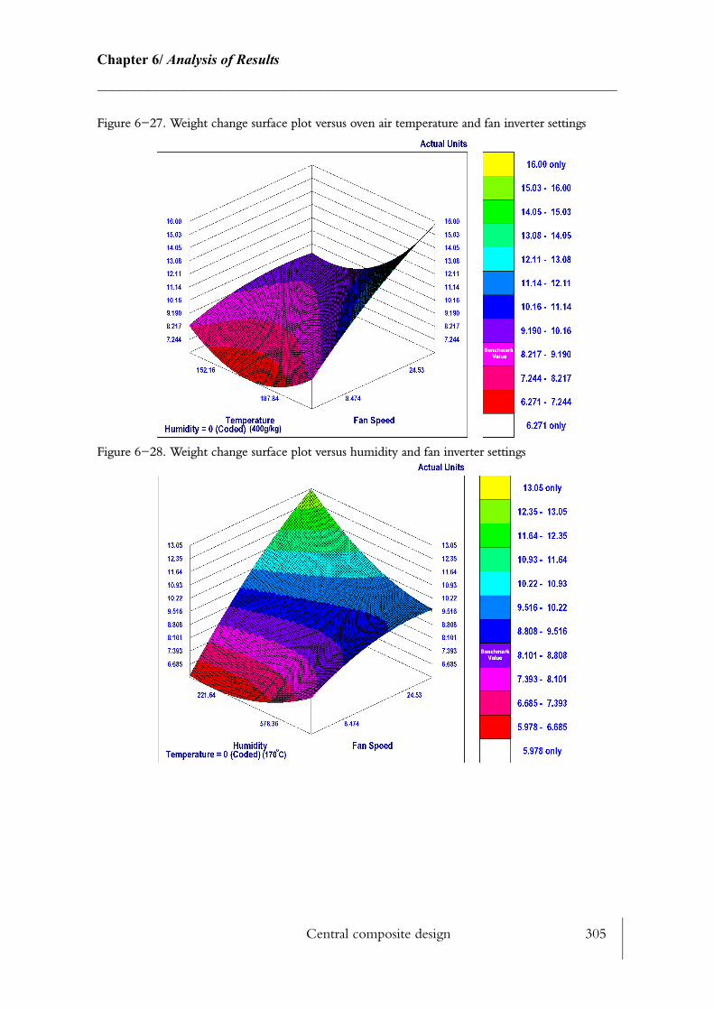
Central composite design 305
Chapter 6/ Analysis of Results________________________________________________________________________
Figure 6−27. Weight change surface plot versus oven air temperature and fan inverter settings
Figure 6−28. Weight change surface plot versus humidity and fan inverter settings
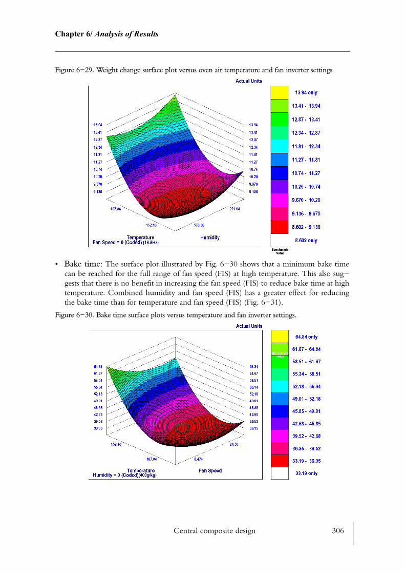
Central composite design 306
Chapter 6/ Analysis of Results________________________________________________________________________
Figure 6−29. Weight change surface plot versus oven air temperature and fan inverter settings
• Bake time: The surface plot illustrated by Fig. 6−30 shows that a minimum bake time can be reached for the full range of fan speed (FIS) at high temperature. This also sug−gests that there is no benefit in increasing the fan speed (FIS) to reduce bake time at high temperature. Combined humidity and fan speed (FIS) has a greater effect for reducing the bake time than for temperature and fan speed (FIS) (Fig. 6−31).
Figure 6−30. Bake time surface plots versus temperature and fan inverter settings.
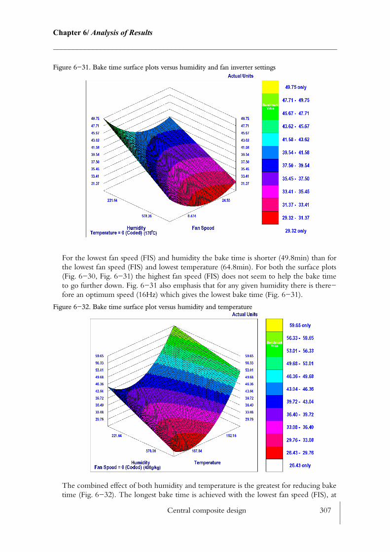
Central composite design 307
Chapter 6/ Analysis of Results________________________________________________________________________
Figure 6−31. Bake time surface plots versus humidity and fan inverter settings
For the lowest fan speed (FIS) and humidity the bake time is shorter (49.8min) than for the lowest fan speed (FIS) and lowest temperature (64.8min). For both the surface plots (Fig. 6−30, Fig. 6−31) the highest fan speed (FIS) does not seem to help the bake time to go further down. Fig. 6−31 also emphasis that for any given humidity there is there−fore an optimum speed (16Hz) which gives the lowest bake time (Fig. 6−31).
Figure 6−32. Bake time surface plot versus humidity and temperature
The combined effect of both humidity and temperature is the greatest for reducing bake time (Fig. 6−32). The longest bake time is achieved with the lowest fan speed (FIS), at
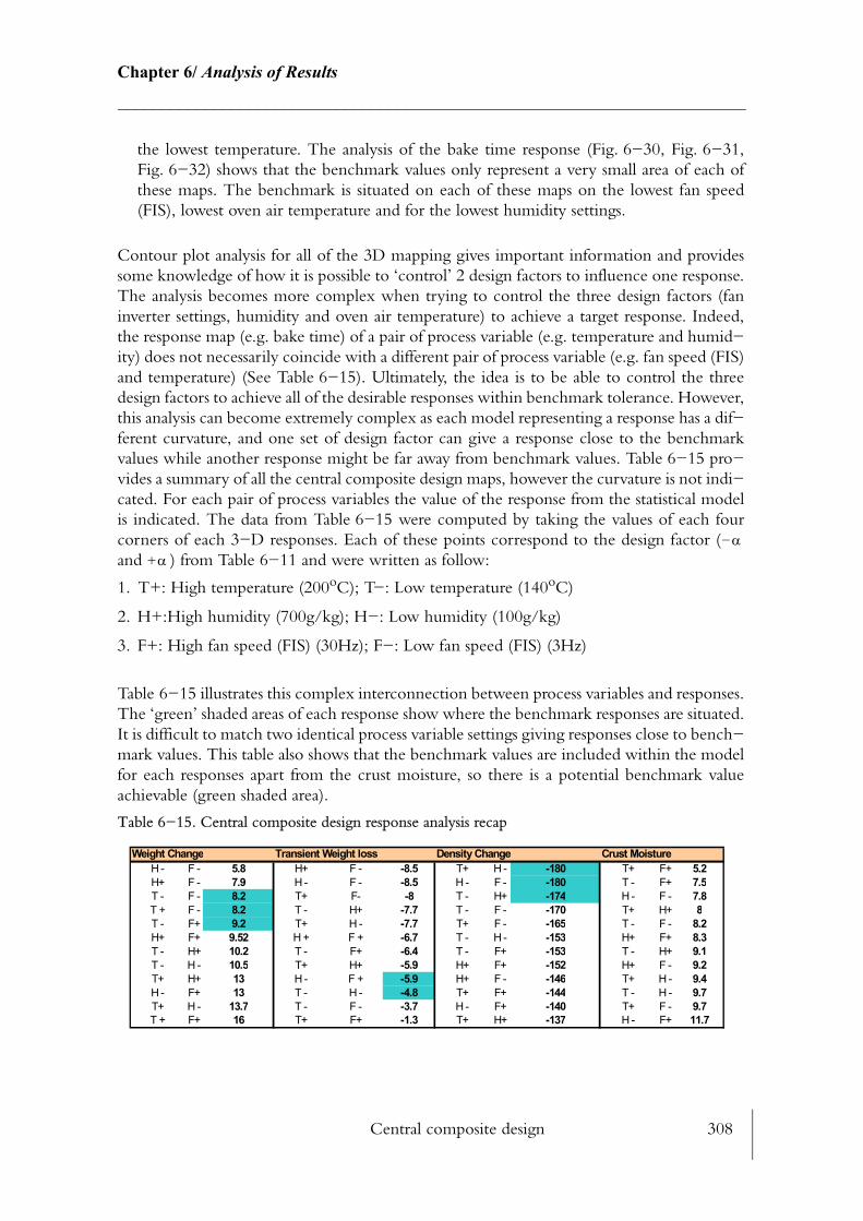
Central composite design 308
Chapter 6/ Analysis of Results________________________________________________________________________
the lowest temperature. The analysis of the bake time response (Fig. 6−30, Fig. 6−31, Fig. 6−32) shows that the benchmark values only represent a very small area of each of these maps. The benchmark is situated on each of these maps on the lowest fan speed (FIS), lowest oven air temperature and for the lowest humidity settings.
Contour plot analysis for all of the 3D mapping gives important information and provides some knowledge of how it is possible to ‘control’ 2 design factors to influence one response. The analysis becomes more complex when trying to control the three design factors (fan inverter settings, humidity and oven air temperature) to achieve a target response. Indeed, the response map (e.g. bake time) of a pair of process variable (e.g. temperature and humid−ity) does not necessarily coincide with a different pair of process variable (e.g. fan speed (FIS) and temperature) (See Table 6−15). Ultimately, the idea is to be able to control the three design factors to achieve all of the desirable responses within benchmark tolerance. However, this analysis can become extremely complex as each model representing a response has a dif−ferent curvature, and one set of design factor can give a response close to the benchmark values while another response might be far away from benchmark values. Table 6−15 pro−vides a summary of all the central composite design maps, however the curvature is not indi−cated. For each pair of process variables the value of the response from the statistical model is indicated. The data from Table 6−15 were computed by taking the values of each four corners of each 3−D responses. Each of these points correspond to the design factor (−and + ) from Table 6−11 and were written as follow:
1. T+: High temperature (200oC); T−: Low temperature (140oC)
2. H+:High humidity (700g/kg); H−: Low humidity (100g/kg)
3. F+: High fan speed (FIS) (30Hz); F−: Low fan speed (FIS) (3Hz)
Table 6−15 illustrates this complex interconnection between process variables and responses. The ‘green’ shaded areas of each response show where the benchmark responses are situated. It is difficult to match two identical process variable settings giving responses close to bench−mark values. This table also shows that the benchmark values are included within the model for each responses apart from the crust moisture, so there is a potential benchmark value achievable (green shaded area).
Table 6−15. Central composite design response analysis recap
αα
Weight Change Transient Weight loss Density Change Crust MoistureH - F - 5.8 H+ F - -8.5 T+ H - -180 T+ F+ 5.2H+ F - 7.9 H - F - -8.5 H - F - -180 T - F+ 7.5T - F - 8.2 T+ F- -8 T - H+ -174 H - F - 7.8T + F - 8.2 T - H+ -7.7 T - F - -170 T+ H+ 8T - F+ 9.2 T+ H - -7.7 T+ F - -165 T - F - 8.2H+ F+ 9.52 H + F + -6.7 T - H - -153 H+ F+ 8.3T - H+ 10.2 T - F+ -6.4 T - F+ -153 T - H+ 9.1T - H - 10.5 T+ H+ -5.9 H+ F+ -152 H+ F - 9.2T+ H+ 13 H - F + -5.9 H+ F - -146 T+ H - 9.4H - F+ 13 T - H - -4.8 T+ F+ -144 T - H - 9.7T+ H - 13.7 T - F - -3.7 H - F+ -140 T+ F - 9.7T + F+ 16 T+ F+ -1.3 T+ H+ -137 H - F+ 11.7
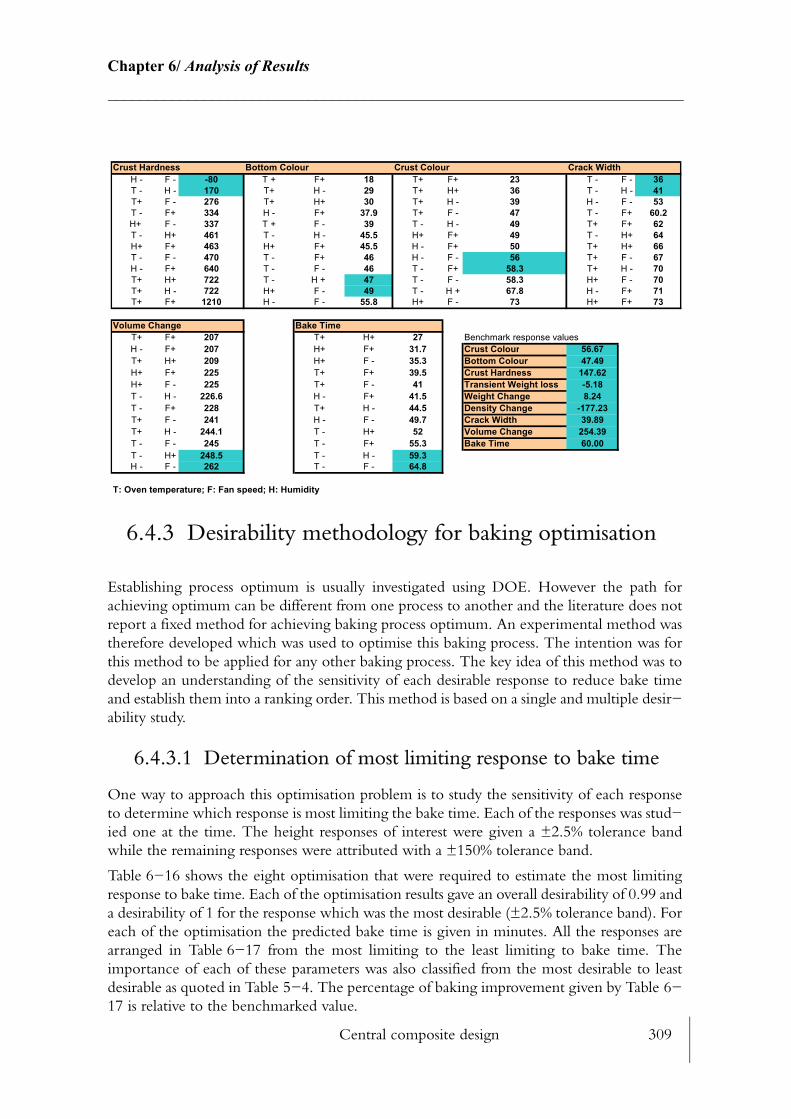
Central composite design 309
Chapter 6/ Analysis of Results________________________________________________________________________
6.4.3 Desirability methodology for baking optimisation
Establishing process optimum is usually investigated using DOE. However the path for achieving optimum can be different from one process to another and the literature does not report a fixed method for achieving baking process optimum. An experimental method was therefore developed which was used to optimise this baking process. The intention was for this method to be applied for any other baking process. The key idea of this method was to develop an understanding of the sensitivity of each desirable response to reduce bake time and establish them into a ranking order. This method is based on a single and multiple desir−ability study.
6.4.3.1 Determination of most limiting response to bake time
One way to approach this optimisation problem is to study the sensitivity of each response to determine which response is most limiting the bake time. Each of the responses was stud−ied one at the time. The height responses of interest were given a ±2.5% tolerance band while the remaining responses were attributed with a ±150% tolerance band.
Table 6−16 shows the eight optimisation that were required to estimate the most limiting response to bake time. Each of the optimisation results gave an overall desirability of 0.99 and a desirability of 1 for the response which was the most desirable (±2.5% tolerance band). For each of the optimisation the predicted bake time is given in minutes. All the responses are arranged in Table 6−17 from the most limiting to the least limiting to bake time. The importance of each of these parameters was also classified from the most desirable to least desirable as quoted in Table 5−4. The percentage of baking improvement given by Table 6−17 is relative to the benchmarked value.
Crust Hardness Bottom Colour Crust Colour Crack WidthH - F - -80 T + F+ 18 T+ F+ 23 T - F - 36T - H - 170 T+ H - 29 T+ H+ 36 T - H - 41T+ F - 276 T+ H+ 30 T+ H - 39 H - F - 53T - F+ 334 H - F+ 37.9 T+ F - 47 T - F+ 60.2H+ F - 337 T + F - 39 T - H - 49 T+ F+ 62T - H+ 461 T - H - 45.5 H+ F+ 49 T - H+ 64H+ F+ 463 H+ F+ 45.5 H - F+ 50 T+ H+ 66T - F - 470 T - F+ 46 H - F - 56 T+ F - 67H - F+ 640 T - F - 46 T - F+ 58.3 T+ H - 70T+ H+ 722 T - H + 47 T - F - 58.3 H+ F - 70T+ H - 722 H+ F - 49 T - H + 67.8 H - F+ 71T+ F+ 1210 H - F - 55.8 H+ F - 73 H+ F+ 73
Volume Change Bake TimeT+ F+ 207 T+ H+ 27 Benchmark response valuesH - F+ 207 H+ F+ 31.7 Crust Colour 56.67T+ H+ 209 H+ F - 35.3 Bottom Colour 47.49H+ F+ 225 T+ F+ 39.5 Crust Hardness 147.62H+ F - 225 T+ F - 41 Transient Weight loss -5.18T - H - 226.6 H - F+ 41.5 Weight Change 8.24T - F+ 228 T+ H - 44.5 Density Change -177.23T+ F - 241 H - F - 49.7 Crack Width 39.89T+ H - 244.1 T - H+ 52 Volume Change 254.39T - F - 245 T - F+ 55.3 Bake Time 60.00T - H+ 248.5 T - H - 59.3H - F - 262 T - F - 64.8
T: Oven temperature; F: Fan speed; H: Humidity
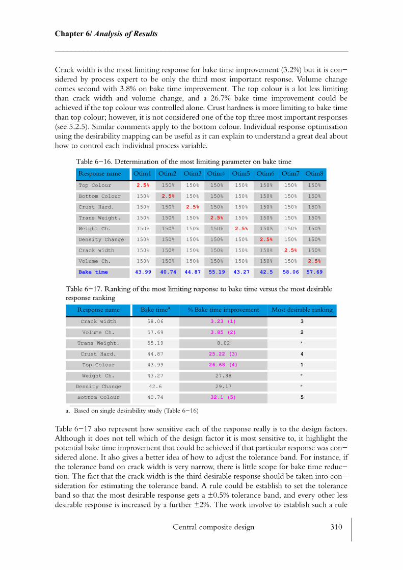
Central composite design 310
Chapter 6/ Analysis of Results________________________________________________________________________
Crack width is the most limiting response for bake time improvement (3.2%) but it is con−sidered by process expert to be only the third most important response. Volume change comes second with 3.8% on bake time improvement. The top colour is a lot less limiting than crack width and volume change, and a 26.7% bake time improvement could be achieved if the top colour was controlled alone. Crust hardness is more limiting to bake time than top colour; however, it is not considered one of the top three most important responses (see 5.2.5). Similar comments apply to the bottom colour. Individual response optimisation using the desirability mapping can be useful as it can explain to understand a great deal about how to control each individual process variable.
Table 6−17 also represent how sensitive each of the response really is to the design factors. Although it does not tell which of the design factor it is most sensitive to, it highlight the potential bake time improvement that could be achieved if that particular response was con−sidered alone. It also gives a better idea of how to adjust the tolerance band. For instance, if the tolerance band on crack width is very narrow, there is little scope for bake time reduc−tion. The fact that the crack width is the third desirable response should be taken into con−sideration for estimating the tolerance band. A rule could be establish to set the tolerance band so that the most desirable response gets a ±0.5% tolerance band, and every other less desirable response is increased by a further ±2%. The work involve to establish such a rule
Table 6−16. Determination of the most limiting parameter on bake time
Response name Otim1 Otim2 Otim3 Otim4 Otim5 Otim6 Otim7 Otim8
Top Colour 2.5% 150% 150% 150% 150% 150% 150% 150%
Bottom Colour 150% 2.5% 150% 150% 150% 150% 150% 150%
Crust Hard. 150% 150% 2.5% 150% 150% 150% 150% 150%
Trans Weight. 150% 150% 150% 2.5% 150% 150% 150% 150%
Weight Ch. 150% 150% 150% 150% 2.5% 150% 150% 150%
Density Change 150% 150% 150% 150% 150% 2.5% 150% 150%
Crack width 150% 150% 150% 150% 150% 150% 2.5% 150%
Volume Ch. 150% 150% 150% 150% 150% 150% 150% 2.5%
Bake time 43.99 40.74 44.87 55.19 43.27 42.5 58.06 57.69
Table 6−17. Ranking of the most limiting response to bake time versus the most desirable response ranking
Response name Bake timea
a. Based on single desirability study (Table 6−16)
% Bake time improvement Most desirable ranking
Crack width 58.06 3.23 (1) 3
Volume Ch. 57.69 3.85 (2) 2
Trans Weight. 55.19 8.02 *
Crust Hard. 44.87 25.22 (3) 4
Top Colour 43.99 26.68 (4) 1
Weight Ch. 43.27 27.88 *
Density Change 42.6 29.17 *
Bottom Colour 40.74 32.1 (5) 5
Central composite design 311
Chapter 6/ Analysis of Results________________________________________________________________________
would require much further test and optimisation work and should be left for further research (see 7.2).
6.4.3.2 Single desirability sensitivity study
A sensitivity study was performed to establish the effect of humidity onto the various responses. To do so, desirabilities identical to the one described in 6.3.3 were used for each of the most desirable response under study. A ±2.5% tolerance band was chosen. The graphs situated on the left side of Fig. 6−33 (a, c, e, g, i) show all the desirability maps of each responses versus fan speed (FIS) and temperature for a given humidity of 400g/kg, while the graphs on the right hand−side of Fig. 6−33 (b, d, f, h, j) are for a set humidity of 221g/kg. Crack width, volume change and crust hardness desirability map surface area increases as the humidity drops from 400 to 221g/kg. This means that there is more fans speed (FIS) and temperature settings that will give a crack width, volume change and crust hardness within the ±2.5% tolerance band if the air is dryer. Opposite comments apply to top and bottom colour. From Fig. 6−33 it can be seen that both crack width and crust hardness are extremely sensitive to fan speed and temperature but even more sensitive at higher humidity (Fig. 6−33 (a) & (e)) than at lower humidity (Fig. 6−33 (b) & (f)).
All of the desirability maps are continuous a part from the top colour. At a humidity of 221g/kg this map shows that fan speed (FIS) between about 15Hz to 23Hz will not promote a desirable top colour. However, below and above this threshold the top colour can be achieved (highly desirable) within the ±2.5% tolerance band. Is this map truly representative or can this be caused by a lack of data over this fan speed (FIS) range, which stops the software algorithm to compute top colour values for this humidity setting. Much further test work should be carried out to establish why this map ‘separates’ at lower humidity.
The graphs illustrated by Fig. 6−33 sows how complex the analysis gets when several responses have to be optimised. It is difficult to imagine a temperature and fan speed (FIS) that give a desirability of 0.99 for all of these responses. There might be an intersection between the maps Fig. 6−33(b) (crack width) Fig. 6−33(d) (volume change) and Fig. 6−33(h) (Top colour) but Fig. 6−33(j) (bottom colour) might only intersect with Fig. 6−33(d) (volume change).
To illustrate further this idea of desirability maps intersection, 16 optimisations were com−puted for crack width and volume change. The idea of these optimisation were to produce a graph displaying the different crack width and volume change and the resultant bake time achievable. In order to achieve such a graph the desirabilities of the studied responses (crack width and volume change) had to be set up as desirability ranges (see Fig. 6−34). For each optimisation an optimum bake time (shortest) could be computed. But in some cases, there was no optimisation possible, that is why the total number of points of Fig. 6−35 does not match the number of optimisation.
Fig. 6−35 shows the results of these optimisations for both crack width and volume change. It highlights that there is no interaction possible around the benchmark value. The volume change benchmark (254.4%) (see Fig. 6−35) intersect with the crack width at 65 mm. Intersection could occur if the tolerance band of one or the other of the response was increased, or if the benchmarked values were different.
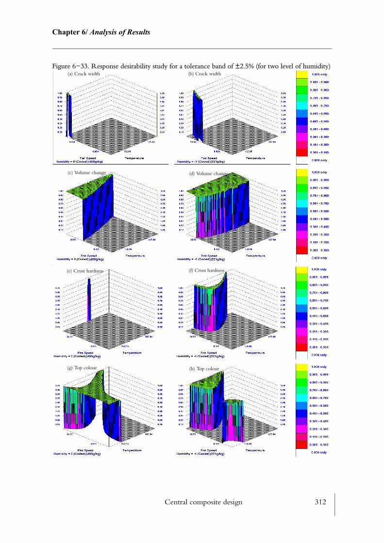
Central composite design 312
Chapter 6/ Analysis of Results________________________________________________________________________
Figure 6−33. Response desirability study for a tolerance band of ±2.5% (for two level of humidity)(a) Crack width (b) Crack width
(c) Volume change (d) Volume change
(e) Crust hardness (f) Crust hardness
(g) Top colour (h) Top colour
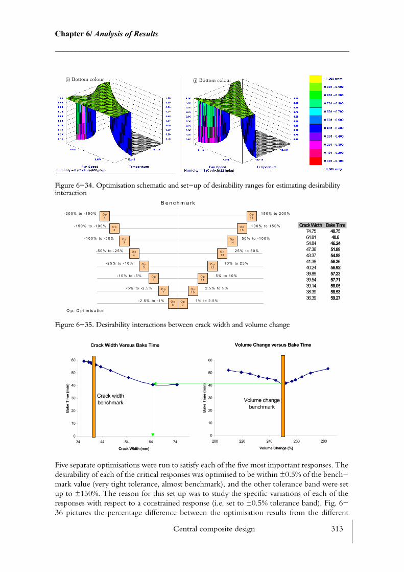
Central composite design 313
Chapter 6/ Analysis of Results________________________________________________________________________
Figure 6−34. Optimisation schematic and set−up of desirability ranges for estimating desirability interaction
Figure 6−35. Desirability interactions between crack width and volume change
Five separate optimisations were run to satisfy each of the five most important responses. The desirability of each of the critical responses was optimised to be within ±0.5% of the bench−mark value (very tight tolerance, almost benchmark), and the other tolerance band were set up to ±150%. The reason for this set up was to study the specific variations of each of the responses with respect to a constrained response (i.e. set to ±0.5% tolerance band). Fig. 6−36 pictures the percentage difference between the optimisation results from the different
(i) Bottom colour (j) Bottom colour
Crack Width Bake Time74.75 40.7564.81 40.854.84 46.2447.36 51.8943.37 54.8841.38 56.3640.24 56.9239.89 57.2339.54 57.7139.14 58.0538.39 58.5336.39 59.27
O p8
-2 .5 % to -1 %
O p1
O p2
O p3
O p4
O p5
O p6
O p7
-2 0 0 % to -1 5 0 %
-1 5 0 % to -1 0 0 %
-1 0 0 % to -5 0 %
-5 0 % to -2 5 %
-2 5 % to -1 0 %
-1 0 % to -5 %
-5 % to -2 .5 %
O p1 5
O p1 4
O p1 3
O p1 2
O p1 1
O p1 0
O p9
1 0 0 % to 1 5 0 %
5 0 % to -1 0 0 %
2 5 % to 5 0 %
1 0 % to 2 5 %
5 % to 1 0 %
2 .5 % to 5 %
1 % to 2 .5 %
O p1 6
1 5 0 % to 2 0 0 %
B e n c h m a rk
O p : O p tim is a tio n
Volume Change versus Bake Time
0
10
20
30
40
50
60
200 220 240 260 280
Volume Change (%)
Bak
e Ti
me
(min
)
Crack Width Versus Bake Time
0
10
20
30
40
50
60
34 44 54 64 74
Crack Width (mm)
Bak
e Ti
me
(min
)
Crack width benchmark Volume change
benchmark
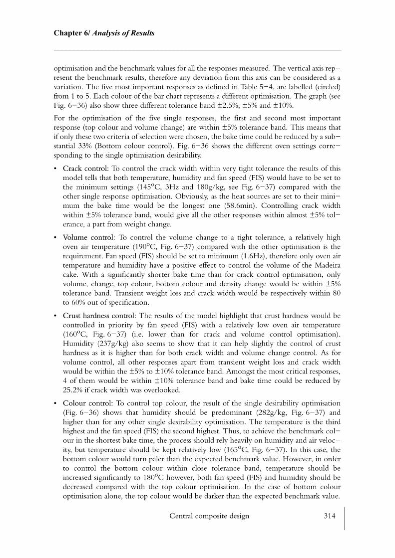
Central composite design 314
Chapter 6/ Analysis of Results________________________________________________________________________
optimisation and the benchmark values for all the responses measured. The vertical axis rep−resent the benchmark results, therefore any deviation from this axis can be considered as a variation. The five most important responses as defined in Table 5−4, are labelled (circled) from 1 to 5. Each colour of the bar chart represents a different optimisation. The graph (see Fig. 6−36) also show three different tolerance band ±2.5%, ±5% and ±10%.
For the optimisation of the five single responses, the first and second most important response (top colour and volume change) are within ±5% tolerance band. This means that if only these two criteria of selection were chosen, the bake time could be reduced by a sub−stantial 33% (Bottom colour control). Fig. 6−36 shows the different oven settings corre−sponding to the single optimisation desirability.
• Crack control: To control the crack width within very tight tolerance the results of this model tells that both temperature, humidity and fan speed (FIS) would have to be set to the minimum settings (145oC, 3Hz and 180g/kg, see Fig. 6−37) compared with the other single response optimisation. Obviously, as the heat sources are set to their mini−mum the bake time would be the longest one (58.6min). Controlling crack width within ±5% tolerance band, would give all the other responses within almost ±5% tol−erance, a part from weight change.
• Volume control: To control the volume change to a tight tolerance, a relatively high oven air temperature (190oC, Fig. 6−37) compared with the other optimisation is the requirement. Fan speed (FIS) should be set to minimum (1.6Hz), therefore only oven air temperature and humidity have a positive effect to control the volume of the Madeira cake. With a significantly shorter bake time than for crack control optimisation, only volume, change, top colour, bottom colour and density change would be within ±5% tolerance band. Transient weight loss and crack width would be respectively within 80 to 60% out of specification.
• Crust hardness control: The results of the model highlight that crust hardness would be controlled in priority by fan speed (FIS) with a relatively low oven air temperature (160oC, Fig. 6−37) (i.e. lower than for crack and volume control optimisation). Humidity (237g/kg) also seems to show that it can help slightly the control of crust hardness as it is higher than for both crack width and volume change control. As for volume control, all other responses apart from transient weight loss and crack width would be within the ±5% to ±10% tolerance band. Amongst the most critical responses, 4 of them would be within ±10% tolerance band and bake time could be reduced by 25.2% if crack width was overlooked.
• Colour control: To control top colour, the result of the single desirability optimisation (Fig. 6−36) shows that humidity should be predominant (282g/kg, Fig. 6−37) and higher than for any other single desirability optimisation. The temperature is the third highest and the fan speed (FIS) the second highest. Thus, to achieve the benchmark col−our in the shortest bake time, the process should rely heavily on humidity and air veloc−ity, but temperature should be kept relatively low (165oC, Fig. 6−37). In this case, the bottom colour would turn paler than the expected benchmark value. However, in order to control the bottom colour within close tolerance band, temperature should be increased significantly to 180oC however, both fan speed (FIS) and humidity should be decreased compared with the top colour optimisation. In the case of bottom colour optimisation alone, the top colour would be darker than the expected benchmark value.
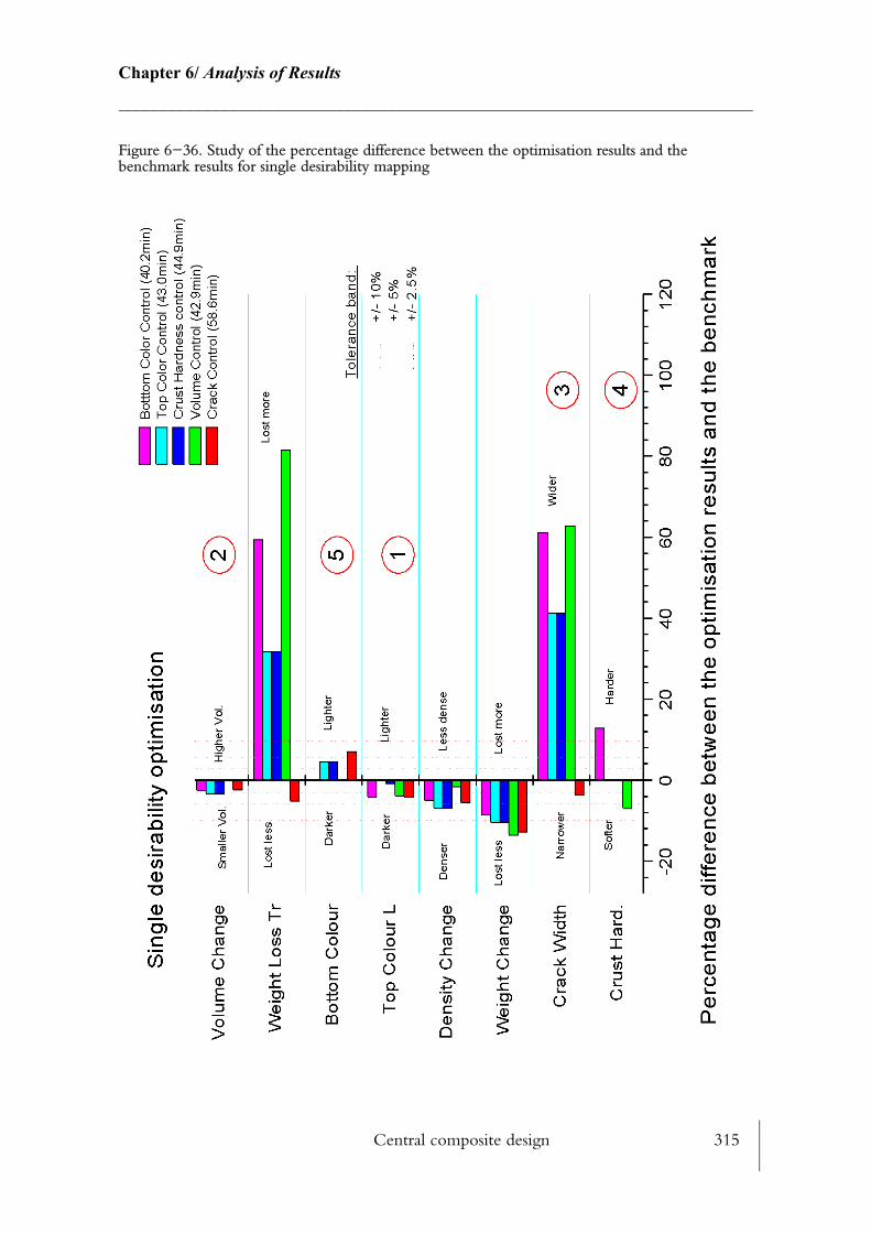
Central composite design 315
Chapter 6/ Analysis of Results________________________________________________________________________
Figure 6−36. Study of the percentage difference between the optimisation results and the benchmark results for single desirability mapping

Central composite design 316
Chapter 6/ Analysis of Results________________________________________________________________________
Figure 6−37. Process variable settings for single desirability optimisation
The results of Fig. 6−36 and Fig. 6−37 have been simplified to Table 6−18 which shows a ranking classifications of the process variable settings. So, from this table it can be concluded that to achieve volume and bottom colour close to benchmark values, oven air temperature should be set relatively high, however, temperature in the case of volume control should be greater than for bottom colour control.
6.4.3.3 Multiple response sensitivity study
It is most probable that the majority of bakery products have at least two desirable criteria (height and colour; weight loss and dimension; etc.). For this more conventional judgement similar optimisations were run as for the single response optimisations (see 6.4.3.2) but this time several desirability criteria were given as input to the DOE software. An algorithm was used which allowed to look for the process variable settings that will give the most desirable
Table 6−18. Scaled process variable settings for single desirability optimisation
Temperaturea
a. Temperature scaled from 1 to 5
Fan speed (FIS)b
b. Fan speed (FIS) and humidity scaled from 1 to 4
Humidity
Crack width control 1 1 1
Volume change control 5 1 2
Crust hardness control 2 4 3
Top colour control 3 3 4
Bottom colour control 4 2 3

Central composite design 317
Chapter 6/ Analysis of Results________________________________________________________________________
map overall. Fig. 6−38 and Fig. 6−39 show the outputs of respectively the responses and process variables settings for the four optimsations using multiple desirability mapping.
• (a) Top colour and volume change control optimisation: The first optimisation was to match within a very tight ±0.5% tolerance band, both of the most important responses, top colour and volume change response. This was achieved with success with a predicted bake time of 43.4min (Fig. 6−38), which means a 27.6% bake time reduc−tion. This is a very significant improvement and this proves that top colour and volume together are not restricting the bake time reduction. Nonetheless, two of the most important responses were out of the ±10% tolerance band set−up (crack width (+54%), crust hardness (−53%). For this optimisation (Fig. 6−39) temperature has to be set to 180oC and the humidity to 220g/kg.
• (b) Volume, top colour and crack width control optimisation: The second optimi−sation was based on (a), but the crack width was added to be controlled within a ±0.5% tolerance band. No optimisation points were found, and the crack width constraints was relaxed until an optimum was found. The optimum point was achieved for +6.2% of the crack width benchmark value. The predicted bake time (55.7min) was still a reduction from the benchmark value by 7.2%. The temperature as well as the humidity should be reduced considerably from the previous optimisation. The fan speed (FIS) should be as closed to zero as possible (Fig. 6−39), but unfortunately unsafe for the TPRO heaters to run at such air flow conditions. As already mentioned in the previous optimisation (see 6.4.3.2), crack width is highly limiting bake time reduction.
• (c) Volume, top colour and crust hardness control optimisation: Instead of keeping crack width for this optimisation, only crust hardness was added to top colour and vol−ume change. −25.7% difference between the benchmark crust hardness and the predic−tion had to be set to keep both the top colour and volume change within the ±0.5% tolerance band. To achieve this optimisation both oven air temperature and humidity would be predominant (190oC, 269g/kg see Fig. 6−39). In this situation the crack width would be above +50% tolerance. The bake time in this case was similar to the optimisation of both top colour and volume change. Although it has not been con−ducted, both top colour and volume control constrained could have been relaxed until crust hardness achieve values within ±10% to ±5% tolerance band.
• (d) Best compromise optimisation: The top colour as well as the volume change tol−erance band were slightly increased from ±0.5% to ±1.5%. The crack desirability was also affected to be less restrictive (+50%). As well as changing the desirability map, the process variable constraints were altered so that the fan speed (FIS) should be operated strictly above the 3Hz threshold (the lowest operating fan speed (FIS) which promotes sufficient air movement around the duct heater elements). The forecasted bake time from this optimisation was 50 min., which is a bake time reduction compared with the benchmark of 16.6%. The Percentage difference for top colour and volume change were slightly higher than the previous optimisations, however still within the ±5% tolerance band. Although, the percentage crack width predicted was the second best of all the four optimisation (+24.7%), the predicted fan speed (FIS) was within acceptable ranges of operation (3Hz, see Fig. 6−39).
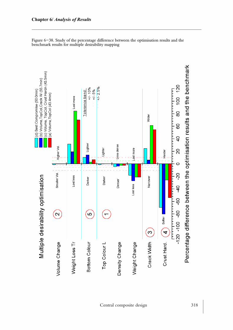
Central composite design 318
Chapter 6/ Analysis of Results________________________________________________________________________
Figure 6−38. Study of the percentage difference between the optimisation results and the benchmark results for multiple desirability mapping
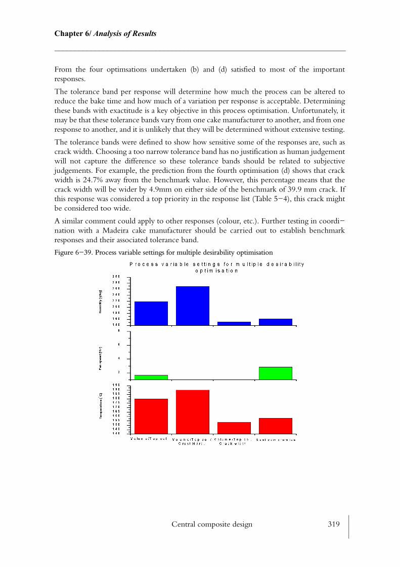
Central composite design 319
Chapter 6/ Analysis of Results________________________________________________________________________
From the four optimsations undertaken (b) and (d) satisfied to most of the important responses.
The tolerance band per response will determine how much the process can be altered to reduce the bake time and how much of a variation per response is acceptable. Determining these bands with exactitude is a key objective in this process optimisation. Unfortunately, it may be that these tolerance bands vary from one cake manufacturer to another, and from one response to another, and it is unlikely that they will be determined without extensive testing.
The tolerance bands were defined to show how sensitive some of the responses are, such as crack width. Choosing a too narrow tolerance band has no justification as human judgement will not capture the difference so these tolerance bands should be related to subjective judgements. For example, the prediction from the fourth optimisation (d) shows that crack width is 24.7% away from the benchmark value. However, this percentage means that the crack width will be wider by 4.9mm on either side of the benchmark of 39.9 mm crack. If this response was considered a top priority in the response list (Table 5−4), this crack might be considered too wide.
A similar comment could apply to other responses (colour, etc.). Further testing in coordi−nation with a Madeira cake manufacturer should be carried out to establish benchmark responses and their associated tolerance band.
Figure 6−39. Process variable settings for multiple desirability optimisation
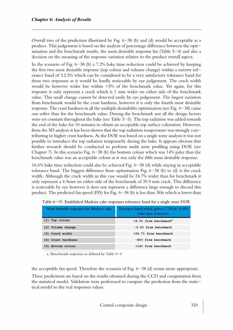
Central composite design 320
Chapter 6/ Analysis of Results________________________________________________________________________
Overall two of the prediction illustrated by Fig. 6−38 (b) and (d) would be acceptable as a product. This judgement is based on the analysis of percentage difference between the opti−misation and the benchmark results, the most desirable response list (Table 5−4) and also a decision on the meaning of the response variation relative to the product overall aspect.
In the scenario of Fig. 6−38 (b) a 7.2% bake time reduction could be achieved by keeping the first two most desirable response (top colour and volume change) within a narrow tol−erance band of ±2.5% which can be considered to be a very satisfactory tolerance band for these two responses as it would be hardly noticeable by eye judgement. The crack width would be however wider but within +5% of the benchmark value. Yet again, for this response it only represent a crack which is 1 mm wider on either side of the benchmark value. This small change cannot be detected easily by eye judgement. The largest variation from benchmark would be the crust hardness, however it is only the fourth most desirable response. The crust hardness in all the multiple desirability optimisation (see Fig. 6−38) came out softer than for the benchmark value. During the benchmark not all the design factors were set constant throughout the bake (see Table 5−5). The top radiation was added towards the end of the bake for 10 minutes to obtain an acceptable top surface coloration. However, from the SD analysis it has been shown that the top radiation temperature was strongly con−tributing to higher crust hardness. As the DOE was based on a single zone analysis it was not possible to introduce the top radiation temporarily during the bake. It appears obvious that further research should be conducted to perform multi zone profiling using DOE (see Chapter 7). In this scenario Fig. 6−38 (b) the bottom colour which was 14% paler than the benchmark value was an acceptable colour as it was only the fifth most desirable response.
16.6% bake time reduction could also be achieved Fig. 6−38 (d) while staying in acceptable tolerance band. The biggest difference from optimisation Fig. 6−38 (b) to (d) is the crack width. Although the crack width in this case would be 24.7% wider than for benchmark it only represent a 4.9mm on either side of the benchmark of 39.9 mm crack. This difference is noticeable by eye however it does not represent a difference large enough to discard this product. The predicted fan speed (FIS) for Fig. 6−38 (b) is less than 3Hz which is lower than
the acceptable fan speed. Therefore the scenario of Fig. 6−38 (d) seems more appropriate.
These predictions are based on the results obtained during the CCD and computation from the statistical model. Validation were performed to compare the prediction from the statis−tical model to the real responses values.
Table 6−19. Established Madeira cake responses tolerance band for a single zone DOE
Most desirable responses for Madeira cake Tolerance band which gives a 7.2% to 16.6% bake time reduction
(1) Top colour +2.5% from benchmarka
a. Benchmark responses as defined by Table 5−4
(2) Volume change -2.5% from benchmark
(3) Crack width +24.7% from benchmark
(4) Crust hardness -80% from benchmark
(5) Bottom colour +14% from benchmark
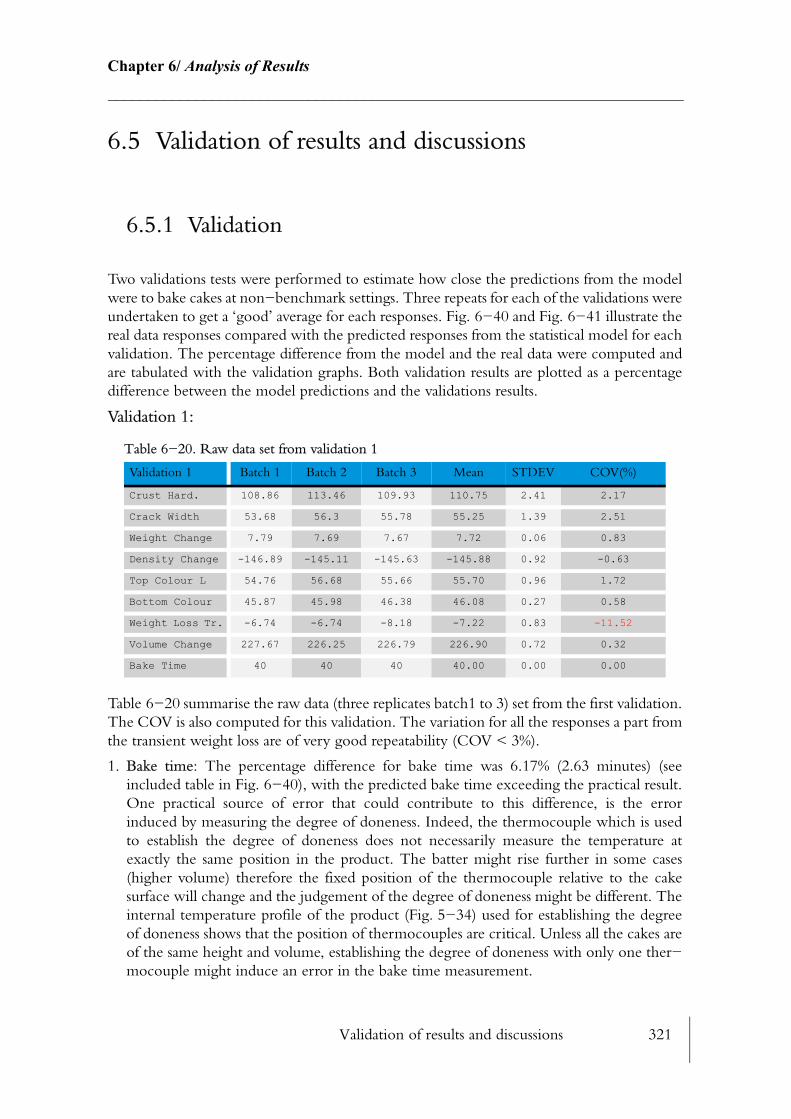
Validation of results and discussions 321
Chapter 6/ Analysis of Results________________________________________________________________________
6.5 Validation of results and discussions
6.5.1 Validation
Two validations tests were performed to estimate how close the predictions from the model were to bake cakes at non−benchmark settings. Three repeats for each of the validations were undertaken to get a ‘good’ average for each responses. Fig. 6−40 and Fig. 6−41 illustrate the real data responses compared with the predicted responses from the statistical model for each validation. The percentage difference from the model and the real data were computed and are tabulated with the validation graphs. Both validation results are plotted as a percentage difference between the model predictions and the validations results.
Validation 1:
Table 6−20 summarise the raw data (three replicates batch1 to 3) set from the first validation. The COV is also computed for this validation. The variation for all the responses a part from the transient weight loss are of very good repeatability (COV < 3%).
1. Bake time: The percentage difference for bake time was 6.17% (2.63 minutes) (see included table in Fig. 6−40), with the predicted bake time exceeding the practical result. One practical source of error that could contribute to this difference, is the error induced by measuring the degree of doneness. Indeed, the thermocouple which is used to establish the degree of doneness does not necessarily measure the temperature at exactly the same position in the product. The batter might rise further in some cases (higher volume) therefore the fixed position of the thermocouple relative to the cake surface will change and the judgement of the degree of doneness might be different. The internal temperature profile of the product (Fig. 5−34) used for establishing the degree of doneness shows that the position of thermocouples are critical. Unless all the cakes are of the same height and volume, establishing the degree of doneness with only one ther−mocouple might induce an error in the bake time measurement.
Table 6−20. Raw data set from validation 1
Validation 1 Batch 1 Batch 2 Batch 3 Mean STDEV COV(%)
Crust Hard. 108.86 113.46 109.93 110.75 2.41 2.17
Crack Width 53.68 56.3 55.78 55.25 1.39 2.51
Weight Change 7.79 7.69 7.67 7.72 0.06 0.83
Density Change -146.89 -145.11 -145.63 -145.88 0.92 -0.63
Top Colour L 54.76 56.68 55.66 55.70 0.96 1.72
Bottom Colour 45.87 45.98 46.38 46.08 0.27 0.58
Weight Loss Tr. -6.74 -6.74 -8.18 -7.22 0.83 -11.52
Volume Change 227.67 226.25 226.79 226.90 0.72 0.32
Bake Time 40 40 40 40.00 0.00 0.00

Validation of results and discussions 322
Chapter 6/ Analysis of Results________________________________________________________________________
2. Crack width: The percentage difference for the crack width was 13.73% (i.e. 8.8 mm or 4.4 mm on either side of the benchmark crack). The crack is narrower than the pre−dicted value from the model. A slightly longer bake time as predicted by the model might have widened the crack. However, this difference might not even be noticed by customers. This shows how important it is to establish a benchmark and tolerance band for each response. The tolerance band will also be different from one customer to another. For instance Madeira cake from Sainsbury is different from the Madeira cake from Tesco, although they are both of Madeira type cake.
Figure 6−40. Percentage difference between the predictions from optimisation responses and the validation result responses (Validation 1 − bake time 42.6min)
3. Weight change and transient weight loss: The percentage difference for weight change was 6.88% (0.5g) With the expected bake time being longer than the validation results the expected weight change from the validation should have been lower than for the prediction however this was not the case. The percentage difference for transient weight loss was 20% (2g) which is the largest percentage difference between the validation and predicted values. This could be explained partially by different ambient and atmospheric conditions in which the product was cooling down (not monitored). It has been proven in the various design stage that both weight change and transient weight loss were closely related. However the percentage discrepancies between the prediction and the results are difficult to explain fully. Because of the heterogeneous properties of the prod−uct, the chemical reaction releasing gases to the porous structure creates variation in the process. Weight change (water evaporation) during baking is governed by heat and mass transfer within the product which are not controlled. Therefore, the acceptable variation may be ±10% or more.
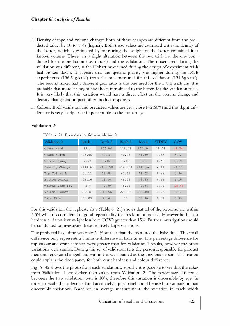
Validation of results and discussions 323
Chapter 6/ Analysis of Results________________________________________________________________________
4. Density change and volume change: Both of these changes are different from the pre−dicted value, by 10 to 16% (higher). Both these values are estimated with the density of the batter, which is estimated by measuring the weight of the batter contained in a known volume. There was a slight alteration between the two trials i.e. the one con−ducted for the prediction (i.e. model) and the validation. The mixer used during the validation was different, as the Hobart mixer used during the design of experiment trials had broken down. It appears that the specific gravity was higher during the DOE experiments (136.5 g/cm3) from the one measured for this validation (131.5g/cm3). The second mixer had a different gear ratio as the one used for the DOE trials and it is probable that more air might have been introduced to the batter, for the validation trials. It is very likely that this variation would have a direct effect on the volume change and density change and impact other product responses.
5. Colour: Both validation and predicted values are very close (−2.60%) and this slight dif−ference is very likely to be imperceptible to the human eye.
Validation 2:
For this validation the replicate data (Table 6−21) shows that all of the response are within 5.5% which is considered of good repeatability for this kind of process. However both crust hardness and transient weight loss have COV’s greater than 15%. Further investigation should be conducted to investigate these relatively large variations.
The predicted bake time was only 2.1% smaller than the measured the bake time. This small difference only represents a 1 minute difference in bake time. The percentage difference for top colour and crust hardness were greater than for Validation 1 results, however the other variations were similar. During this set of validation tests the person responsible for product measurement was changed and was not as well trained as the previous person. This reason could explain the discrepancy for both crust hardness and colour difference.
Fig. 6−42 shows the photo from each validations. Visually it is possible to see that the cakes from Validation 1 are darker than cakes from Validation 2. The percentage difference between the two validations tests is 10%, therefore this variation is discernible by eye. In order to establish a tolerance band accurately a jury panel could be used to estimate human discernible variations. Based on an average measurement, the variation in crack width
Table 6−21. Raw data set from validation 2
Validation 2 Batch 1 Batch 2 Batch 3 Mean STDEV COV
Crust Hard. 82.2 107.06 111.46 100.24 15.78 15.74
Crack Width 42.96 40.18 40.46 41.20 1.53 3.72
Weight Change 7.69 8.46 8.48 8.21 0.45 5.49
Density Change -144.65 -136.58 -143.68 -141.64 4.41 -3.11
Top Colour L 61.11 61.08 61.48 61.22 0.22 0.36
Bottom Colour 48.16 48.46 49.34 48.65 0.61 1.26
Weight Loss Tr. -5.8 -8.89 -5.88 -6.86 1.76 -25.69
Volume Change 225.83 216.56 223.02 221.80 4.75 2.14
Bake Time 51.83 49.4 55 52.08 2.81 5.39
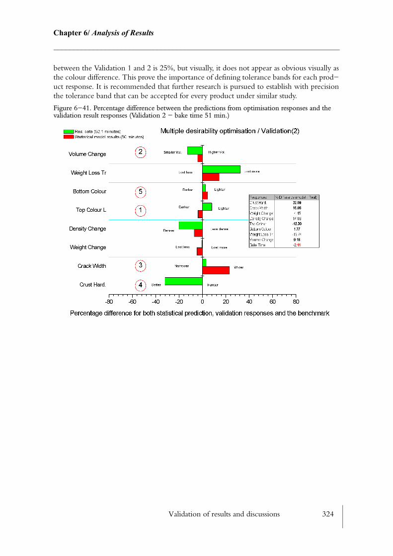
Validation of results and discussions 324
Chapter 6/ Analysis of Results________________________________________________________________________
between the Validation 1 and 2 is 25%, but visually, it does not appear as obvious visually as the colour difference. This prove the importance of defining tolerance bands for each prod−uct response. It is recommended that further research is pursued to establish with precision the tolerance band that can be accepted for every product under similar study.
Figure 6−41. Percentage difference between the predictions from optimisation responses and the validation result responses (Validation 2 − bake time 51 min.)
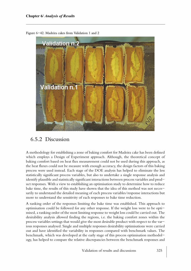
Validation of results and discussions 325
Chapter 6/ Analysis of Results________________________________________________________________________
Figure 6−42. Madeira cakes from Validation 1 and 2
6.5.2 Discussion
A methodology for establishing a zone of baking comfort for Madeira cake has been defined which employs a Design of Experiment approach. Although, the theoretical concept of baking comfort based on heat flux measurement could not be used during this approach, as the heat fluxes could not be measure with enough accuracy, the design factors of this baking process were used instead. Each stage of the DOE analysis has helped to eliminate the less statistically significant process variables, but also to undertake a single response analysis and identify plausible and statistically significant interactions between process variables and prod−uct responses. With a view to establishing an optimisation study to determine how to reduce bake time, the results of this study have shown that the idea of this method was not neces−sarily to understand the detailed meaning of each process variables/response interactions but more to understand the sensitivity of each responses to bake time reduction.
A ranking order of the responses limiting the bake time was established. This approach to optimisation could be followed for any other response. If the weight loss were to be opti−mised, a ranking order of the most limiting response to weight loss could be carried out. The desirability analysis allowed finding the regions, i.e. the baking comfort zones within the process variables settings that would give the most desirable product with respect to the var−ious responses analysed. Single and multiple responses desirability optimisations were carried out and have identified the variability in responses compared with benchmark values. The benchmark, which was developed at the early stage of this process optimisation methodol−ogy, has helped to compare the relative discrepancies between the benchmark responses and
Validation of results and discussions 326
Chapter 6/ Analysis of Results________________________________________________________________________
the various optimisations. Quantitative tolerance bands for this particular product and for baking products in general were non−existent and it was difficult to ascertain which opti−misation was best. However, the most important responses (see Table 5−4) were prioritised and were optimised to within low variation percentage of the benchmark. The Madeira cake baking process was successfully optimised, showing that bake time could be reduced from 7.2% to 16.6% depending on the tolerance band that were used. This optimisation work could be taken on board by a Madeira cake manufacturer to establish adequate tolerance band.
The two validation results have demonstrated that bake time can be predicted to within 6%. The results of both validations and the observed discrepancies are related to how well the measurements were taken and in which conditions, but also due to uncontrolled phenom−ena. Indeed, internal phenomena, chemical transformation, gas formation, cell structure and internal heat and mass transfer are likely to be vary a little due to the complex heterogeneous characteristics of the product. Therefore tolerance bands for responses such as weight change, transient weight loss are unlikely to be within ±5% but more to be within likely ±10%. In order to help understand the mass transfer phenomena that is controlling the bake time, transient weight loss during baking should be measured.
The concept of degree of doneness, which was used to establish the final bake time, could be re−designed, as the possible error in the temperature measurement could be responsible for the benchmark−validation variation noticed. Only a single thermocouple in a position fixed relative to the tin was used to establish the degree of doneness. If the volume of the product increases, the relative position of this single thermocouple to the product top surface will change and the temperature development in the later stage of the process will be dif−ferent. Several closely positioned thermocouples could be used instead of a single one for judging the degree of doneness. Maybe the entire internal temperature profile could be used instead. Fig. 6−43 shows the internal and the surface temperature profile during the 55 minutes baking of a Madeira cake. TCA4−7 are not covered by the batter during the early stages of the baking, but as the batter rises the thermocouples are plunging into the product being formed. During the whole baking process for this trial, the bottom temperature meas−urement (TCA1) close to the tin bottom is almost identical to the surface temperature meas−urement (TCA8). As expected, as the bake time is closing up to 55 minutes, all the internal temperature measurement apart from TCA1 are getting close to each other.
Fig. 6−44 illustrates two internal profiles for the Madeira cake for respectively 50 and 55 minutes bake. The oven settings were slightly different however both the internal profile (TCA3) are represented by a distinctive ‘S’ shape curve. This specific profile is marked by three main chemical phenomenon. During the first 20 minutes, the heat penetrates through the batter which rise the temperature slowly to 50oC. Then, the chemical release of CO2helps to promote a fast temperature rise which will also promote an increase in overall vol−ume. From almost 70oC to 80oC, coagulation starts and the temperature rate of change drops which is marked by an inflection point. These phenomena occur but only CO2 and gelat−inisation are discernible from Fig. 6−44 and Fig. 6−45. The slope of the curve is markedly change from 90oC onwards where gelatinisation starts. Although the oven settings of the 50 minutes bake profile are slightly higher than for the 55 minutes ones, the internal tempera−ture profile for the first 20 minutes is unexpected as the fastest bake time profile is below the longest bake time profile. However, at 25 minutes within the bake, the tendencies are reversed. The results of Fig. 6−45 shows that two different oven settings can end up with

Validation of results and discussions 327
Chapter 6/ Analysis of Results________________________________________________________________________
identical bake time but different internal temperature profiles and different product. The high humidity and fan speed (FIS) setting shows clearly how it influences the first 15 minutes of the internal temperature profile.
Figure 6−43. Internal and surface temperature profile of a Madeira cake baked in 55 minutes
Figure 6−44. Comparison of a Madeira cake internal temperature (TCA3) for a 50 and 55 minutes bake time
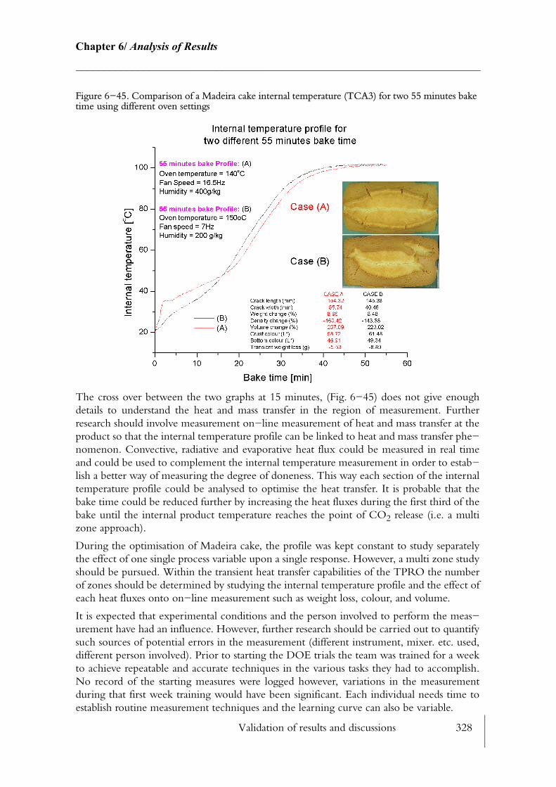
Validation of results and discussions 328
Chapter 6/ Analysis of Results________________________________________________________________________
Figure 6−45. Comparison of a Madeira cake internal temperature (TCA3) for two 55 minutes bake time using different oven settings
The cross over between the two graphs at 15 minutes, (Fig. 6−45) does not give enough details to understand the heat and mass transfer in the region of measurement. Further research should involve measurement on−line measurement of heat and mass transfer at the product so that the internal temperature profile can be linked to heat and mass transfer phe−nomenon. Convective, radiative and evaporative heat flux could be measured in real time and could be used to complement the internal temperature measurement in order to estab−lish a better way of measuring the degree of doneness. This way each section of the internal temperature profile could be analysed to optimise the heat transfer. It is probable that the bake time could be reduced further by increasing the heat fluxes during the first third of the bake until the internal product temperature reaches the point of CO2 release (i.e. a multi zone approach).
During the optimisation of Madeira cake, the profile was kept constant to study separately the effect of one single process variable upon a single response. However, a multi zone study should be pursued. Within the transient heat transfer capabilities of the TPRO the number of zones should be determined by studying the internal temperature profile and the effect of each heat fluxes onto on−line measurement such as weight loss, colour, and volume.
It is expected that experimental conditions and the person involved to perform the meas−urement have had an influence. However, further research should be carried out to quantify such sources of potential errors in the measurement (different instrument, mixer. etc. used, different person involved). Prior to starting the DOE trials the team was trained for a week to achieve repeatable and accurate techniques in the various tasks they had to accomplish. No record of the starting measures were logged however, variations in the measurement during that first week training would have been significant. Each individual needs time to establish routine measurement techniques and the learning curve can also be variable.
Conclusions 329
Chapter 7/ Conclusions and Recommendations________________________________________________________________________
CHAPTER 7
CONCLUSIONS AND RECOMMENDATIONS
7.1 Conclusions
For generations, bakers have been applying relatively crude methods to find out the best oven settings for baking biscuits, bread and cake products. Today, there is a need to optimise baking processes to reduce baking time and energy requirements hence reduce CO2 emis−sions. This involves defining improved designs of ovens and enhanced control for achieving increased rates of heat transfer to food products. For these reasons a research oven was designed, instrumented and used in this investigation to analyse the baking of one product − Madeira cake.
7.1.1 Rig design
This thermal Performance Research Oven (TPRO) was designed to provide the facilities to perform industrial baking research beyond the conventional heat transfer limits baking con−ditions existing in conveyor type tunnel ovens. The TPRO provides the facility of testing the most important variables affecting the rate of convective and radiative heat transfer to the baking product (nozzle size and shape, air velocity, distance separating the plenum chamber to the food product, radiant electric element temperature, diameter. See 2.7.1, 2.7.2). Con−veyor travelling ovens are divided into zones which are independently controlled (temper−ature, air speed, radiant heat). Although this research rig is a batch oven, a computer aided control system has been successfully designed which can reproduce atmospheric conditions for the different zones of a travelling oven and up to 10 zones can be simulated.
The main focus of the rig design phase was to achieve fast rates of change, so rapid change can occur between the different zones modelled. Temperature was the most critical param−eter. A theoretical mathematical model has been developed to help find how to achieve the highest temperature rate of change. The electrical duct cartridge heater resistance coil was the most critical design feature, however air flow around the cartridge heater was also a lim−
Conclusions 330
Chapter 7/ Conclusions and Recommendations________________________________________________________________________
iting parameter for the maximum temperature rate of change. Subsequently alternative methods were investigated for achieving even higher rates of change using heat stores but, these methods were discarded as they were impractical. The rates of change for the various temperature ranges tested, proved that the TPRO would be suitable for reproducing multi zone capability as they exist in conveyor type ovens.
The TPRO has been designed so it can outperform existing travelling ovens. Its convective power rating of 541kW/m2 is far greater than normal. For example the 25.2kW/m2 from the APV 687 indirect convection oven, or the 7.6kW/m2 from the APV 700 DGF oven. The TPRO can achieve impinging convective heat transfer value well above 100W/m2.K (see Table 2−4), which is higher than any impinging coefficient, reported by the literature for baking ovens of 60W/m2.K. The TPRO is merely a convective batch oven however its total radiative power rating of 23.75kW/m2 is still much greater than the power ratings of the APV 687 indirect convection with 6.3 kW/m2 or the APV 689 Cylcotherm oven (19.2kW/m2). The steam injection system allows control of humidity levels up to 1200g/kg (see 4.9) which is well above common levels used in the baking industry (150 to 300 g/kg). The TPRO has been designed to outperform any known baking conditions so that ‘baking profiles boundaries’ could be pushed further.
7.1.2 Preliminary tests
The research rig is an energy efficient oven with a very low thermal conductivity insulation. Some preliminary tests have shown that a temperature of 98oC could be maintained without any heat load when both the fans are running at full speed and recirculating the air. The non food tests carried out during this research have defined the performance characteristics of this research oven. An energy balance was constructed which emphasised the distribution of the heat sources and losses during both the transient and the steady state phase. Real time computations involved in the evaluation of this energy balance accounted for the different heat sources (heaters and fans), the various heat storage terms (insulation, steel wall and diverse internal steel masses) and the multiple heat loss terms (convection, radiation, air leak−ages, and thermal bridges).
During the early stages of the transient phase, the heat storage terms were over predicted as not enough measurement points were taken inside the walls. Further research should be car−ried out to get a better estimate of the energy storage terms. More accurate computation using a finite difference model could be used in conjunction with real temperature meas−urement. Amongst the heat losses during the steady state operation of TPRO, both the energy losses by air leakages through the system and the heat dissipated through thermal bridges accounted for 26% of the total energy loss. Future research could concentrate on reducing both heat storage terms and the overall heat losses, which could improve signifi−cantly the overall efficiency of this process. From these computations it was also concluded that the energy required to heat up and maintain the air to temperature set point was less than 1% of the total energy use. Estimation of the real−time energy stored in the baked product could also be included into this energy balance, however the difficulty with this par−ticular computation remains in the accurate measurement of the heat flux to the product surface. To achieve this, further research should be pursued in the heat transfer measurement at the product surface.
Conclusions 331
Chapter 7/ Conclusions and Recommendations________________________________________________________________________
Convective and radiative heat flux were measured at the same position of the Madeira cake tin top surface with the Scorpion heat flux logger, however absolute values did not match theoretical values (see Table 2−4 and Table 4−13). Values reported from literature for similar configurations were closer to theoretical computations than values measured with the Scor−pion logger. Although the measurement of heat flux in the oven is of interest, its measure−ment remains a challenge. The measurement of heat flux to the product surface could help greatly in the estimation of the ‘baking comfort zone’, however its measurement is relative to surface temperature, surface emissivity, radiation view factor between the radiant heat source and the product to be baked and the air flow pattern at the product surface, which are difficult to estimate (see 3.4.8.6.3).
Unless the heat flux sensor can mimic the exact same surface properties (temperature, mass, emissivity) as the product, the heat flux measured with current heat flux logger will not be a measure of what the product actually receives. Further development should be followed to minimise the size of the logger so that it can fit on the product surface, so the temperature rate of change between the logger and the real product are identical. Impingement convec−tive correlation were used (see 2.7.1) for a similar geometry as for the one in used in the TPRO, however accuracy of such correlations will vary accordingly with the air flow pattern at the product surface. Either an empirical approach or CFD should be used to establish the air flow at the product surface and get a more accurate estimate of the heat transfer coefficient as a function of air speed and air temperature. Attempts to measure the surface temperature of the product being baked, which surface rises, were successful in the short term using a 250 µm thermocouple mounted onto a supporting plate (see Fig. 5−14), however the extreme thermal conditions within the TPRO yielded to the break down of this thermo−couple. Alternative measurement using a thicker thermocouple was used (see Fig. 5−14), but was not as successful as far as depth of measurement is concerned. Further effort should be carried out to develop effective measurement of heat transfer measurement to the product surface.
Accuracy and repeatability of all the measurements played a great part in obtaining the results of this research programme (sensitivity study see 4.3). The TPRO was designed to have a strong software architecture which allowed comprehensive analysis of the measurements and accuracy assessments (Chapter 3). A sensitivity and repeatability study were carried out to establish for each of the measured variables (52 temperature points, 8 pressure points, 1 humidity point) and derived variables (325), the number of accurate decimal places and noise reduction factors, ‘smoothing factor’. A repeatability study over a 24 hour period (see 4.3.3.1) demonstrated that results from the various measurements could be obtained with a COV of less than 1.5% while operating the TPRO in the steady state periods of this study. This very low degree of variance was also achieved by accurately controlling each of the major oven process variables (oven temperature, fan speed (FIS), radiation temperature, humidity). Real time computations based on the first and second derivative of the wall heat losses have also demonstrated when the oven had reached steady state (see 2.6). Estimation of the heat losses during door openings were useful to determine the time for the oven to return to steady state mode (see 4.3.3.2). Specific control routines were developed to min−imise variation around set−points. As well as controlling the oven, several software interfaces (84) were created to operate the oven; log, record and graph data; change the zone profiles and generate reports (see 3.4.9).
Conclusions 332
Chapter 7/ Conclusions and Recommendations________________________________________________________________________
7.1.3 Experimental findings
The TPRO has not been designed for a particular type of baking product, and any baking product size can be baked inside the TPRO chamber as the height between the plenum chamber and the product surface is adjustable. Much of the literature in this area concerns modelling heat and mass transfers on a microscopic or macroscopic level but this is prob−lematic due to the complexities of food products which undergo thermo−chemical changes during baking. An experimental approach is preferable as the assumptions taken are less crude. There is significantly more research work on bread and biscuit than on any other baked product as their production alone represents a large proportion (30%, see Fig. 1−1) of the world wide bakery production. Comparatively, very little has been done on cake prod−ucts. Hence the Madeira cake product was chosen as the subject of this baking optimisation process but also because its bake time is relatively long compared to biscuit and bread, there−fore changes could be noticed with greater ease.
The ranges of operations of the TPRO were designed far in excess of what typical ovens are capable of achieving so that the zones of baking comfort could be explored (Table 4−15). The ‘baking comfort zone’ is proposed as a theoretical concept (analogous to thermal com−fort zones in building engineering) which represents an area of product ‘comfort’ defined by the four heat transfer fluxes at the product surface, (conduction, convection, radiation and condensation/evaporation) (see 5.1). At any time during the bake, this imaginary area can be optimised to get the best quality product in the shortest bake time. This concept could be used to understand the measure of each of these heat flux components in real time during the baking, and deduce when the product is absorbing more convection, than radiation etc. This concept could then be used to control the oven process variable precisely to ensure that the product receives the right quantity of each of these flux at the right time to give the best quality output product. A database of baking comfort zone profiles could be estimated for any baking product and fed into a control system.
Nonetheless, the optimisation approach for the Madeira cake baking process was rather dif−ferent. A methodological approach based around a design of experiments (DOE) was devel−oped, which consisted of five stages:
• benchmarking
• destructive test
• DOE screening design
• DOE full factorial design
• DOE central composite design
The DOE was applied to establish how to bake the product in the shortest time while main−taining product quality close to the product benchmark values. The process optimisation research presented in Chapter 6 was based upon eight design factors (see Table 5−7) (oven temperature, fan speed (FIS), top and bottom damper position, top and bottom radiation heater surface temperature, humidity inside the chamber and band speed) and ten product responses (see Table 5−9) (bake time, top and bottom colour, crack width, crust hardness, density change, springiness, volume change, moisture change, and transient weight loss).
Conclusions 333
Chapter 7/ Conclusions and Recommendations________________________________________________________________________
Unlike some other processes (textiles) there was no tolerance band established for the Madeira cake product. This is often the case in the baking industry and quality control check are often based on an eye judgement between photographic sources, however there is very little or no knowledge of the product quality measure (colour, crack width etc.). This thesis proposes a novel DOE methodology which is used to discover the limits of tolerance band that gives acceptable product responses which are as close as possible to benchmark values within the shortest bake time. This method investigated bake time reduction as the optimised response however, any other responses could have been used instead. This method consisted of:
(a) Establishing a Madeira cake benchmark which gives responses of a satisfactory level based on cake process expert judgement, and identify the most desirable responses.
(b) Defining a destructive test which allows to estimate the broad ranges of the design factors in which each of the responses have a measurement value.
(c) Identifying the design factors of the screening design and factorial design (this applies for a design which has a large number of initial design factor >8) which are contributing and are significant to the most desirable responses. The analysis of these two design results also allows to improve the knowledge and understanding of the responses and design factors interactions.
(d) Estimating a ranking of the most limiting responses to bake time reduction by conducting optimisation of each of the desirable responses using a central composite design.
(e) Establishing a single and multiple desirability optimisation by including each of the most desirable response. The ranking of the most limiting responses to bake time reduction helps to set−up the different tolerance limits of each of the desirable response. The output of these desirability optimisations is a set of tolerance limits which demonstrates of much the responses can stretch around the benchmark values. The associated design factors are used to set the baking process to achieve the shortest bake time.
By following these steps the baking process of Madeira cake could be reduced by 7.2% by keeping the tolerance limit of both top colour and volume change within 0 to 2.5%, crack width would be +6.2% out of benchmark values (which only represent a 1.2 mm on either side of the benchmark crack width, Fig. 6−38). A 16.6% bake time reduction could also be achieved keeping top colour and volume change within 0 to 2.5% of benchmark, crack width would be out of benchmark by 24.7% (4.9mm on either side of the benchmark crack), which is noticeable by eye however is still considered as an acceptable variation. This very significant bake time reduction could easily lead to very large savings. This saving can provide an increase in production and/or a reduction in the energy per unit produced. A better con−trol of the process variable/responses also means a better consistency on the process which directly lead to less scrap. A reduction in the energy bill will also result in a reduction in greenhouse gas emissions. For the manufacturer, this research could lead to the development of more efficient generation of ovens, which are smaller, i.e. more energy efficient and cost less to produce. The fruit of this research will inevitably help understanding the baking proc−ess in a more scientific manner and will help to seek new heat transfer enhancement methods to improve the baking process.
Although analysis of a single process variable was interesting it is crucial to understand the sensitivity of the entire process. Most limiting process response to bake time was a successful approach for this optimisation study and could be repeated with other bake product. Estab−

Recommendations 334
Chapter 7/ Conclusions and Recommendations________________________________________________________________________
lishing a benchmark is also important and should further work be pursued, benchmark and tolerance bands should be ascertained by the product manufacturer.
7.2 Recommendations
• Further work should be conducted to increase the rate of change of temperature in the oven chamber and decrease the response time of the TPRO.
• Experimental design using similar method with other baked product could be per−formed to find out if similar bake time reduction as for Madeira Cake can be achieved.
• Further research analysis should be performed on Madeira using multi−zone profile to estimate if a further bake time reduction can be achieved.
• Further research should be performed on internal temperature baking measurement to help sub−diving zonal profile for multi−zone DOE.
• Research should be carried on to find out the transferability of the TPRO results into real ovens.
7.2.1 TPRO design improvements
The TPRO was designed with one single inlet duct which is separated into top and bottom plenum chambers. Current travelling ovens have separate control of top and bottom heat, which gives an extra flexibility to the process. Interaction analysis from the result of Madeira baking process optimisation emphasised this design weakness. Ultimately there should be two inlet ducts with two separate heat sources and fans which feed separately the top and bottom plenums chambers. Although costly, independent control is desirable.
Dampers were manually controlled, though to model a multi zone oven, rapid changes (temperature, humidity, etc.) have to occur, which cannot be achieved with manual control. The only three recirculation dampers to automate in order to perform rapid changes to model a multi zone oven would be D1, D8 and D9. Extra control features could be added so that these three dampers operate concurrently in order to regulate the recirculation of fresh air.
An increase in radiant heat power is recommended to analyse highly radiative heating (e.g. 50kW/m2).
Thermal bridges were also non−negligible (11% of the total heat loss and heat store). Improvement could be made to reduce air leakages by using a different wall sealing technique and design should be made to reduce/avoid thermal bridging. In order to improve the overall temperature response of this rig and reduce the time to reach steady state the overall mass of the rig could be reduced, by decreasing the wall thickness of both steel and insulation. To decrease the heat losses further, a thin layer of insulation (ceramic coating) might be used inside the chamber to lower the temperature difference between the steel wall internal sur−face and the external insulation wall surface, similar to furnaces. Computation could take

Recommendations 335
Chapter 7/ Conclusions and Recommendations________________________________________________________________________
place to optimise the insulation and steel wall thickness, to keep the heat losses as well as the masses as small as possible. The results from the mathematical model have demonstrated that the heater coil design as well as the heater mass was critical in achieving the fastest temper−ature rate of change. The solution used was conservative and sheathed heaters were chosen, as the test rig was subjected to high steam rates and possible risks of hydrogen embrittlement may have occurred with an unsheathed heater. However, it is plausible that a different design could use unsheathed heaters could reach a very fast temperature rate of change.
7.2.2 Measurement issues
Pressure: pressure measurements are vital to the operation of the TPRO, but tend to become susceptible to breaking down when subjected to high humidity levels via the injec−tion of steam. Failure of the pressure readings cause both velocities and air flow computation to fail, as they are closely related. This problem is currently under investigation and it has been possible to identify the cause, which lies with condensation in the copper piping, con−necting the pitot tube to the pressure transmitter. Several design features have been tried to eliminate this problem. If they are satisfactory and pass tests of accuracy and reliability, nozzle velocity will be used instead of fan speed (FIS) in the baking process otpimisation.
Heat flux: heat flux sensing has become the centre of interest of many industries and being able to measure heat flux would give more information than temperature or velocity alone. There are a few of heat flux sensors and the Scorpion heat flux logger used in this research only showed trends, and absolute values were far away from theoretical computations. The surface measurement of the product being baked is crucial for the computation of heat flux to the product. However, it is a measurement challenge itself. The solution of having a thin and light thermocouple floating to the surface has shown some interesting results, neverthe−less, this solution was abandoned as not reliable enough. Non surface measurement might be a possible solution; however the temperature and humidity within the TPRO might prevent any measurement device from operating. Infrared measurement using optic fibre as the signal transmitter might be a feasible solution but it could be costly.
More recently United Biscuit Ltd. has patented (Rolston, 2001 [106]) a single and twin heat flux device which can measure both radiative and convective flux. Each of these heat flux loggers were tested inside the TPRO and gave results almost matching both trends and abso−lute values from the theoretical computations. This instrument could be used to establish the complete range of heat flux for any air flow/oven air temperature/radiant surface tempera−ture settings so prediction can be given in real time. However, further computations coupled with these measurements would be necessary to derive the heat flux to the product surface. Heat flux measurement to the product surface is the ultimate requirement for establishing the baking comfort zones. Although the heat flux logger would tell the heat flux received by the logger, a knowledge of the product surface temperature measurement during the bake would help to derive the flux quantity to the product surface. Further investigation should be carried out to measure product surface with accuracy and derive from the heat flux logger the quantity of heat flux to the product surface. Ultimately, real time computation of heat flux to the product surface should be possible. Heat flux measurement is central to the ‘bak−ing comfort zone’ concept, and developing further heat flux measurement/derivation is important.
Recommendations 336
Chapter 7/ Conclusions and Recommendations________________________________________________________________________
7.2.3 Multiple zone optimisation and scaling up
Further work is highly recommended for studying the baking optimisation of multiple baking zones. Current travelling ovens are multi zone and a multiple zone optimisation would improve understanding of the entire baking profile of industrial travelling ovens. Output from this further research would lead to design optimisation as well as process opti−misation of each baking zone, which would be an invaluable help for designing the next generation of oven. The result of this research would indicate when to apply the heat and what sort of heat the product would require to bake in the fastest bake time whilst keeping quality output within tolerance bands. It is strongly suggested that a link should be estab−lished between the product manufacturer and the sponsor of this project so that product responses tolerance bands can be defined with accuracy.
The scaling up issue is the next stage of this project. The findings from the process optimi−sation should be able to be transferred to any ‘long’ travelling baking ovens. For this partic−ular matter the heat flux sensor should be used to help to estimate scaling up factors so that the TPRO can replicate exactly profile as they exist in travelling ovens and vice versa. The TPRO could then become a very powerful tool for analysing baking errors.
7.2.4 Product measurement issue
There are a number of product measurement improvements which could apply to other products than for Madeira cake, such as, crust hardness, transient weight loss, top colour, bake time. However, crack width is very specific to Madeira cake as a longitudinal crack is the desired feature.
• Crack width: measuring the width of the product at the widest point of the crack could be slightly subjective. Indeed, if the crack is not very well defined i.e. not an oval shape, but more of a random crack, it makes the choice very complicated. A measure−ment based on the surface area of the crack would be more accurate. Moreover the sur−face area is more likely to relate to the evaporation and could latterly correlate to the transient weight loss and the total weight loss. To establish the surface area of the crack, a digital photograph could be used and appropriate software could help to estimate the crack surface area.
• Crust hardness: the possible sources of errors could come from the position of the penetration probe to the product surface. It was proven that the angle between the two can cause some large variation. The tin was positioned so that the surface of the product would be perpendicular to the penetrating probe. However this is only based on an vis−ual check and there could error induced by poor positioning. In addition, the position−ing to the edge of the product is making an influence, i.e. the corner of the cake have a larger crust than the centred position. More points should be chosen to have a better average of the crust hardness or a different probe should be chosen.
Recommendations 337
Chapter 7/ Conclusions and Recommendations________________________________________________________________________
• Transient weight loss: the transient weight loss of the final product is proportional and relative to the ambient conditions in which the product has been cooled. To decrease the error incurred by this measure, the product should be cooled in a known and controlled environment conditions (temperature and humidity).
• Top colour: the measures of colours (top and bottom) are in relatively good agree−ment with the predictions and the human eye might not even be sensitive to the relative difference. The reason for this success is due in great parts by the accuracy of the instru−ment, and the contact between the sample and the lens. Nevertheless, the ‘good’ contact is only present for a well−defined crust. For surface highly non homogeneous it is rec−ommended to use a different instrument such as non contact surface measurement (Dipix).
• Bake time: thermocouple positioning in the tin is an issue. The thermocouples are usually bent while the cake is extracted from the tin and for the next trial the thermo−couple could be slightly offset, thereby not measuring the temperature at the same posi−tion. Looking at a single temperature to estimate the ‘doneness’ of the product is not accurate enough and variations might occur in the estimation of the bake time. Several thermocouples could be used to take a better average of this ‘critical’ temperature for establishing the degree of doneness. More criteria could be festered to automate the time measurement process of the baking. The contact between the thermocouples and the porous dough might cause erroneous readings; air trapped could play the role of an insulant and slightly modify the temperature. Further research work should be involved to establish appropriate instrumentation and techniques for accurate and repeatable measurement of the degree of ‘doneness’.
• Composite sample of multiple samples: The moisture tends to migrate as time passes; therefore, the measure of crust moisture is time dependant. Instead of taking crust samples one after the other a composite sample could be taken from the five different crusts, mixed, and measured at the time of measurement.
• Other measurements: The squareness of the product is of importance as it is one of the visual check that is currently conducted by cake manufacturer.

338
References
[1] AirflowTM, The WILSON FLOWGRID (instructions for installation and use). http://www.air−flow.co.uk/contact/manuals.htm.
[2] Anderson M J and Kraber S L, (1999), Keys to Successful Designed Experiments, Proceeding: Quality Management Division of American Society for Quality.
[3] Andrews G J A, (2001), Private Communication, APV Baker (Peterborough − UK).
[4] APV Baker internal publication (Connoisseur), (2002), Advanced Loop Control of Baking Ovens, Pub: APV Baker.
[5] APV Baker internal publication (Dipix), (2002), Qualivision Impact on Performance, Pub: Dipix.
[6] APV Baker internal publication (Green Isle), (2002), Case History: Factory Monitoring System at Green Isle Foods, Pub: APV Baker.
[7] APV Baker internal publication (Performance), (2002), Process Performance Improvement: Pro−cess Analysis and Improvement, Pub: APV Baker.
[8] APV Baker internal publication (Scada), (2002), Intelligent Plant Monitoring and Analysis, Pub: APV Baker.
[9] APV Baker internal publication (Three Sigma), (2002), Reliadens & Aquadens: In−Line Auto−mated Bulk Density & Moisture Measurement, Pub: Three Sigma.
[10] APV Baker internal publication (United Biscuits), (2002), Case History: Data Capture System at United Biscuits, Pub: APV Baker.
[11] APV Baker internal publication (Web), (2002), Distributing Information to the Organisation, Pub: APV Baker.
[12] Ashworth J C and Armitage J W, (1980), Handbook of Industrial Solids−Drying, Pub: Insti−tution of Chemical Engineers.
[13] Baik O D, Grabowski M, Trigui M, Marcotte M, and Castaigne F, (1999), Heat Transfer Coef−ficients on Cakes Baked in a Tunnel Type Industrial Oven, Food Science, 64 (4), 688−694.
[14] BakersFederation, (1999), UK Bread Market, Pub: www.bakersfederation.ork.uk.
[15] Bartlett M (AMETEK Lloyd Instruments), (2001), Dough Profiling, Total sense, European Baker.
[16] Boukadida N and Ben Nasrallah S, (2002), Effect of the Variability of Heat and Mass Transfer Coefficients on Convective and Convective−Radiative Drying of Porous Media, Drying Technol−ogy, 20 (1), 67−92.
[17] Bourne M.C, Kamel B S, and Stauffer C E, (1993), Texture measurements on finished baked goods, −in−, Advances in Baking Technology, ed. Blackie Academic & Professional, 135−151.
[18] Box E P, Hunter W G, and Hunter J S, (1978), Statistics For Experimenters, Pub: John Wiley & Sons.

339
[19] Braud L M, Moreira R G, and Castell−Perez M E, (2001), Mathematical modeling of impinge−ment drying of corn tortillas, Food Engineering, 50, 121−128.
[20] Bread and Bakery Products, (2001), Bread: Future trends in the industry, Pub: British Baker.
[21] Brownell L E and Brown G G, (1941), Sponsored Project by APV Baker Inc, University of Michigan.
[22] BTR Change & Technology, (1995), Initial and Advanced Training Course for Maximize.
[23] Calay R K, Newborough M, Probert D, and Calay P, (1995), Predictive equations for the dielectric properties of foods, Food Science and Technology (International), 29, 699−713.
[24] Campbell G M, (2002), Fundamentals of bubble behaviour on bread dough during mixing, proving and baking, −in−, Campden and Chorleywood Food Research Association course notes. Process Engineering for Dough System, Pub: CCFRA.
[25] Campbell G M and Shah P, (1999), Entrainment and Disentrainement of Air during Bread Dough Mixing, and Their effect on Scale−up of Dough Mixers, −in−, Campbell G M, C Webb, S S Pandiella, and K Niranjan, Bubbles in Food, Pub: Eagan.
[26] Carlin G T, (1944), A Microscopic Study of the Behavior of Fats in Cake Batters, Cereal Chem.21, 189−199.
[27] Cauvain S P, Witworth M B, and Alava J M, (1999), The evolution of Bubble Structure in Bread Doughs and Its Effect on Bread Structure, −in−, Campbell G M, C Webb, S S Pandiella, and K Niranjan,Bubbles in Food, Pub: Eagan.
[28] Charley H, (1956), Characteristics of Shortened Cake Bake in a Fast and in a Slow−baking Pan at Different Oven Temperatures, Food Research, 21, 302−305.
[29] Charley H, (1950), Effect of Baking Pan Material on Heat Penetration During Baking and Quality of Cakes Made with Fat, Food Research, 15, 155−168.
[30] Christensen A, Blomqvist I, and Skjöldebrand C, (1984), Optimization of the baking Process with Respect to Quality (Convection ovens), −in−, Zeuthen P, Thermal processing and quality of foods, 482−486.
[31] Christensen A and Singh R P, (1984), Energy Consumption in the Baking Industry, −in −, McKenna B, Engineering and Food − Processing Applications, Pub: Elsevier Applied Science.
[32] Christenson M E, Tong C H, and Lund D B, (1989), Physical Properties of Baked Products as a Functions of Moisture and Temperature, Food Processing and Preservation, 13, 201−217.
[33] Civille G V and Szczesniak A S, (1973), Guidleines to training a texture profile panel, Texture Study, 4, 204−223.
[34] Connan S, (2000), 3D CFD simulation of a jet impingement oven (MsC Thesis), Pub: Cran−field University.
[35] Cornford S J, (1969), Volume and crumb firmness measurements in bread and cake, −in −, FMBRA Report, 25, 1−14.
[36] Cornforth J R, (1992), Combustion Engineering and Gas Utilisation, ed. 3rd, Pub: Chapman and Hall.
340
[37] Cortes L, (1997), Designing a Graphical User Interface. http://www.medicalcomputingto−day.com.
[38] Crompton, (2001). http://www.crompton−instruments.com/
[39] Danesha A, (2001), The European Bakery Products Market, Pub: Food RA Letherhead Pub−lishing.
[40] Datta A K and Ni H, (2001), Infrared and hot−air assisted microwave heating of foods for con−trol of surface moisture, Food Engineering, 51, 355−364.
[41] Datta A K and Zhang, (1999), Porous Media Approach to Heat and Mass transfer in Solid Foods, ASAE Annual International Meeting, Toronto, Ontario Canada.
[42] De Vries U. A, Sluimer p, and Bloskma, (1988), A quantitative model for heat transport in dough and crumb during baking, Cereal science and Technology, pp.174−188.
[43] Denys S and Hendrickx, (1999), Measurement of the thermal conductivity of foods at high pressure, −in−, Food Science, 64(4).
[44] Dersh J A, (1989), The Use of Steam in Bread Oven, American Society of Bakery Engineers, Bulletin No.218, pop. 928−937.
[45] Elgidaily D A, Funk K, and Zabin M E, (1969), Baking Temperature and Quality of Angel Cakes, American Dietetic Association, 54, 401−406.
[46] Elustondo D, Elustondo M P, and Urbicain M J, (2000), Mathematical modeling of moisture evaporation from foodstuffs exposed to subatmospheric pressure superheated steam, Food Engineer−ing, 15−24.
[47] Fanger P O, (1973), Thermal Comfort, Pub: McGraw−Hill, New York.
[48] Garrison C L and Peart M V, (1986), Effect of Radiant Heat Transfer: Cake Baking in a Con−vectional Electric Residential Oven, Home Economics Research, 14 (3), 336−341.
[49] Ginzburg A S, (1969), Application of Infra−red Radiation in Food Processing, Pub: Leonard Hill−London.
[50] Gordon J, Davis E A, and Timms E M, (1979), Water−Loss Rates and Temperature Profiles of Cake of Different Starch Content, Cereal Chem. 56 (2), 50−57.
[51] Guibert L, (1998), Computer Simulation and Parametric Analysis of Heater−Reflector Systems (MsC Thesis), Pub: Cranfield University.
[52] Guy R (CCFRA), (2000), Texture Measurement in Bakery Products, New Food, 44−47.
[53] Guyer E C and Brownell D L, (1999), Handbook of Applied Thermal Design, Pub: Taylor & Francis.
[54] Hall A (CCFRA), (2001), Bread under pressure, European Baker, 22−24.
[55] Hall J E, Otto S R, and Richardson P S, (1999), Predicting Heat and Mass Transfer during Bread Baking, Campden and Chorleywood Food Research Association, R&D report, 74.
[56] Hallström B, Skjöldebrand C, and Trägardh, (1988), Heat Transfer and Food Products, Pub: Elsevier Applied Science.
341
[57] Handleman A R, Conn J F, and Lyons J W, (1961), Bubble Mechanics in Thick Foams and Their Effects on Cake Quality, Cereal Chem. 38, 294−305.
[58] Hardman T M, (1988), Water and Food Quality, Pub: Elsevier Press, London.
[59] Herrington T M and Vernier F C, (1995), Vapour Pressure and Water Activity, −in−, Bucket S T, Physio−Chemical Aspects of Food Processing, Pub: Blackie Academic & Professional.
[60] Holger M, Spalding D B, Whitaker S, and Winter H H, (1977), Advances in Heat Transfer, Pub: Academic Press.
[61] Holmes D R and Rahmel A, (1978), Materials and coatings to resist high temperature corrosion, Pub: Applied Science.
[62] Holtz, E, Skjöldebrand, C, Bognar A, and Piekarski, J, (1984), Modeling the Baking Process of Meat Products using Convective Ovens, −in−, Zeuthen P, Thermal Processing and Quality of Foods, pp. 329−338.
[63] Hood M P and Lowe B, (1948), Air, Water Vapor, and Carbon Dioxide as Leavening Gases in Cakes Made with Different Types of Fats, Cereal Chem. 25, 244−254.
[64] Hopkins W G, (2000), A new view of statistics. Internet Society of Sport Science. http://www.sportsci.org/resource/stats/.
[65] Horace L and Smith J R, (1960), Low−Temperature Radiant Heat Drying, Tappi, 43 (10).
[66] Howell J R, (2001), A catalog of Radiation Heat Transfer Configuration Factors, ed. 2nd, Pub: Department of Mechanical Engineering − The University of Texas as Austin. http://www.me.utexas.edu/~howell/sectionc/C−13.html.
[67] Humphries W R and Griggs E I, (1977), A design Handbook for phase change thermal control and energy storage devices, Pub: Washington, D.C: NASA.
[68] Incropera F.P and De Witt D, (1990), Fundamentals of Heat and Mass transfer, ed. 3rd, Pub: John Wiley & Sons.
[69] Infrared Services Inc., (2000). http://www.infrared−thermography.com/training.htm.
[70] ISO 7730, (1995), Moderate Thermal Environments − Determination of the PMV and PPD indices and specification of the conditions for thermal comfort.
[71] Kiemele MJ, Schmidt S R, and Berdine R J, (1997), Basic Statistics, ed. 4th, Pub: Air Academy Press.
[72] Kreims P and Möller B, (1990), The Effect of Temperature and Steam During the Baking Pro−cess, −in−, APV Baker private communication.
[73] Lane G, (1983), Solar Heat Storage−Latent Heat Materials, Pub: CRC Press Inc., Vol 1.
[74] Lawson R, (1994), Mathematical Modeling of Cookie and Craker Ovens, −in−, Faridi H, The Science of Cookie and Cracker Production, Pub: Chapman & Hall.
[75] Luikov A V, (1966), Heat and Mass Transfer in Capillary−porous Bodies, ed. 1st, Pub: Per−gamon Press.
[76] Marrs W M, (2001), Instrument Advances for Texture Measurement, New Food, 33−37.

342
[77] Mc Farlane I, (1986), Use of in−line sensors and closed loop control for food manufacturing processes, −in−, ICHEME Symposium series No126, 133−143.
[78] Meffert H F, (1983), History, Aims, Results and Future of Thermophysical Properties Work within COST 90, −in−, Jowitt R, Esher F, Hallström B, Meffert H F, Spiess W E, and Vos G, Phys−ical Properties of Foods.
[79] Mellor J D, (1983), Critical Evaluation of Thermophysical Properties of Foodstuffs and Outline of Future Developments, −in−, Jowitt R, Esher F, Hallström B, Meffert H F, Spiess W E, and Vos G, Physical Properties of Foods.
[80] Menjivar J A, (1990), Fundamental aspects of Dough Rheology, −in−, Faridi H and Faubion M, Dough Rheology and Baked Product Texture, Pub: Van Nostrand Reinhold.
[81] Microtherm, (1989), The world's leading high performance THERMAL INSULATION.
[82] Milson A and Kirk D, (1980), Principles of Design and Operation of Catering Equipment (Properties of Solid Foods), −in −, Milson A and Kirk D.
[83] Milson A and Kirk D, (1980), Principles of Design and Operation of Catering Equipment, Pub: Ellis Horwood limited.
[84] Minolta, Internal Publication, (1998), Color control from perception to instrumentation, Pre−cise color communication, Pub: Minolta.
[85] Minolta, Internal Publication, (1995), Spectrophotometer CM−508d, Instruction Manual, Pub: Minolta, I.
[86] Mintel, (2001), Bread Market Research, Pub: Mintel International Group Limited.
[87] Mintel, (2001), Cake Market Research, Pub: Mintel International Group Limited.
[88] Mintel, (2001), Non Sweet Biscuit Market Research, Pub: Mintel International Group Lim−ited.
[89] Mintel, (2001), Sweet Biscuit Market Research, Pub: Mintel International Group Limited.
[90] Mitchell J R, Fan J T, and Blanshard J M, (1999), Simulation of Bubble Growth in Heat Pro−cessed Cereal Systems, −in−, Campbell G M, C Webb, S S Pandiella, and K Niranjan,Bubbles in Food, Pub: Eagan.
[91] Montgomery D C, (2001), Design and Analysis of Experiments, ed. 5th, Pub: John Wiley & Sons.
[92] Moreira R G, (2001), Impingement drying of foods using hot air and superheated steam, Food Engineering, 49, 291−295.
[93] Muir A, (1968), The History of Baker Perkins, Pub: W. Heffer & Sons Ltd. Cambridge.
[94] Mälkki Y, Seibel W, Skjöldebrand C, and Rask O, (1984), Optimization of the baking Process and its Influence on Bread Quality, −in−, Zeuthen P, Thermal processing and quality of foods, Pub: Elsevier London, 355−361.
[95] National Physical Laboratory, (2002), Small scale methods for complex and biomaterials. http://www.npl.co.uk/thermal/projects/project3−3.html.
343
[96] Nelfood, (2002), Physical Properties of Food Database, Tüv East Kilbridge, Galsgow (Scotland). www.nelfood.com.
[97] Obot N T, (1980), Flow and Heat Transfer for Impinging Round Turbulent Jets (PhD Thesis), Pub: McGill University (Canada, Montreal).
[98] Osborne W. C and Turner C.G, (1960), Woods Practical Guide to Fan Engineering, ed. Sec−ond, Pub: Woods of Colchester Ltd.
[99] Ovadia D Z and Walker C E, (1997), Opportunities for Impingement Technology in the Baking and Allied Industries (Part 4), American Institute of Baking, 19 (5).
[100] Park Cakes (Liverpool), (2001), Private communication.
[101] Pierrel F, (1998), Process Control Investigation of a Pilot Batch Oven for Baking Research (MsC Thesis), Pub: Cranfield University.
[102] Piller, (2001). http://www.piller.de.de/index.html
[103] Pleass W, (1986), R.F Dielectric methods for moisture measurement in food materials, −in−, ICHEME Symposium series No126, 389−395.
[104] Profound, (2001), Market Briefing (Europe and US), Pub: Euromonitor.
[105] Pyler E. J, (1988), Baking Science and Technology, ed. Third, Pub: Sosland Publishing Com−pany, 2.
[106] R Rolston, (2001), Apparatus for and methods of measuring heat flux in a tunnel oven, United Biscuit (UK) Limited, ed. US 6,264,362.
[107] R Rolston, (2001), Improvements in and relating to the measurement of heat flux in a heated chamber, United Biscuit (UK) Limited, ed. EP 1 195 587 A1.
[108] Rask C and Hallström B, (1989), Rate of drying during baking of bread, −in−, Proceedings from the Fith international congress on engineering and food (Germany).
[109] Richardson P S, (1986), Ultrasonics − The application to temperature measurement in the food industry, −in−, ICHEME Symposium series No126, 333−337.
[110] Rollin P.Y, (2000), CFD application: 2D transient simulation of a moving biscuit underneath two impinging jets (MsC Thesis), Pub: Cranfield University.
[111] Sablani S S, Marcotte M, Baik O D, and Castaigne F, (1998), Modelling of Simultaneous Heat and Water Transport in the Baking Process, Lebensmittel Wissenshaft und Technology, 31(3), 201−209.
[112] Sakai N and Hanzawa T, (1994), Applications and advances in far−infra−red heating in Japan, Trends in Food Science & Technology, 5.
[113] Saravacos G D, (1994), Mass Transfer Properties of Foods, −in−, Rao M A and Rizvi S S H, Engineering Properties of Foods, ed. 2nd.
[114] Sato H, Matsumura T, and Shibukawa, (1987), Apparent Heat Transfer in A forced Convec−tion Oven and Properties of Baked Food, Food Science, 52 (1), 185−188.
[115] Scarisbrick C, (1994), Improving the Thermal Performance of Domestic Electric Ovens, Pub: Cranfield University.
344
[116] Setser C S, (1993), Sensory evaluation, −in−, Kamel B S and Stauffer C E, Advances in Baking Technology, ed. Blackie Academic & Professional, 255−291.
[117] Shah P, Campbell G M, Dale C, and Rudder A, (1999), Modelling Bubble Growth during Proving of Bread Dough: Predicting the OUtput from the Chopin Rheofermentometer, −in−, Campbell G M, C Webb, S S Pandiella, and K Niranjan,Bubbles in Food, Pub: Eagan.
[118] Shariaty−Niassar M, Hozawa M, and Tsukada T, (2000), Development of probe for thermal conductivity measurement of food materials under heater and pressurized conditions, −in−, Food Engineering, 43, 133−139.
[119] Shaughnessy B, (1996), Radiative Heat Transfer in Low Emissivity Enclosures (PhD Thesis), Pub: Cranfield University.
[120] Shaughnessy B.M and Newborough M, (1998), Radiative Heat Transfer in Low−Emissivity Ovens, Applied Thermal Engineering, Pub: Elsevier Science Ltd., 18 (8), 619−641.
[121] Short B E, Woolrich W R, and Barlett L H, (1942), Specific Heats of Foodstuffs, Refigerating Engineering, 40.
[122] Siegel R and Howell J R, (1972), Thermal radiation heat transfer, ed. First, Pub: McGraw−Hill Kogakusha.
[123] Singh P, (2002), Food Properties Database 2.0 for Windows™. http://www.florida−plants.com/CR/food.htm.
[124] Skjöldebrand C and Anderson C G, (1987), Baking using short wave infra−radiation, −in−, Morton I D, Pub: Ellis Horwood.
[125] Smith C and Corripio B, (1997), Principle and Practice of Automatic Process Control, ed. Second, Pub: John Wiley and Sons.
[126] Spyridon E, (2000), A versatile and Inexpensive Technique for Measuring Color of Foods, Food Technology, 54 (12), 12−48.
[127] Stear C.A, (1990), Handbook of Breadmaking Technology, Pub: Elsevier Science.
[128] Sweat V E, (1994), Thermal Properties of Foods, −in−, Rao M A and Rizvi S S H, Engi−neering Properties of Foods, ed. 2nd.
[129] Szczesniak A, (1963), Classification of Textural Characteristics, Food Science, 28, 981−985.
[130] Tan T, V Schmitt, and Sisz, (2001), Electronic Tongue: A New Dimension in Sensory Anal−ysis, −in−, Food Technology, 55(10), 44−50.
[131] Taylor B N and Kuyatt C E, (1994) NIST, Guidelines for Evaluating and Expressing the Uncertainty of NIST Measurement Results, NIST Technical Note 1297.
[132] Tong C H and Lund D B, (1993), Microwave Heating of Baked Dough Products with Simul−taneous Heat and Moisture Transfer, Food Engineering, 19, 319−339.
[133] Urrutia O, (1997), Design and Construction of a Pilot Batch Oven for Baking Research (MsC Thesis), Pub: Cranfield University.
[134] Vliet Van T, (1999), Physical Factors Determining Gas Cell Stability in a Dough during Bread Making, −in−, Campbell G M, C Webb, S S Pandiella, and K Niranjan,Bubbles in Food, Pub: Eagan.

345
[135] Wählby U, Skjöldebrand C, and Junker E, (1999), Impact of impingement on cooking time and food quality, Food Engineering, 43, 179−187.
[136] Walker C E, (1987), Impingement Oven Technology (Part 1), American Institute of Baking, 9 (11).
[137] Walker C E and Sparman A B, (1989), Impingement Oven Technology − Part 2: Applications and Future, American Institute of Baking, 6 (11).
[138] Whaley M G and Ellis G D, (1986), Increasing flexibility and profit, (Dainties Systems Cor−poration Waterloo, Ontario, Canada), Pub: Applied Science.
[139] Wiggins C, (1998), Proving, Baking and cooling, −in −, Stanley P.C and Young L.S, Tech−nology of Breadmaking, Pub: Blackie Academic and Professional.
[140] Williamson M, (1996), Scorpion Logger Multi−channel Data Logger Operating Instructions, Pub: FTE.
[141] Wonderware, (2002), http://www.wonderware.com.
[142] Zanoni B and Peri, C, (1993), A study of the bread−baking Process. I: A Phenomenological Model, Food Engineering, 19, pp. 389−398.
[143] Zanoni B, Peri C, and Gianotti, (1995), Determination of the Thermal Diffusivity of Bread as a Function of Porosity, Food Engineering, 26, 497−510.
[144] Zanoni B, Pierucci S, and Peri C, (1994), Study of the Bread Baking Process− 2 Mathematical Modelling, −in−, Food Engineering, Pub: Elsevier Science Ltd., 23 (3), pp. 321−336.

Heat flux sensors specifications 346
Appendix A/ Scorpion Heat FLux Logger________________________________________________________________________
APPENDIX A
SCORPION HEAT FLUX LOGGER
A.1 Heat flux sensors specifications1
Number of sensors: 1 (8 outputs/sensor)
Sensor type: Thermocouple type T
Range: −50 to 450oC
Accuracy: ±1oC or 0.5%
Response time: t60 = 2 seconds in air at 1.0m/s
Accuracy: ±5% full scale deviation
Response time: t60 = 3 seconds in air at 1.0 m/s
A.2 Basic heat balance equations
(A.1)
(A.2)
(A.3)
(A.4)
(A.5)
(A.6)
1. As given by FTE Reading Thermal (Williamson M, 1996 [140])
Qgold1
Agold------------- ka
∆Tgoldd
----------------- MgoldCp∆Tgold
dt-----------------+=
HcQgold
Tc Tgold–------------------------=
Qblack1
Ablack--------------- ka
∆Tblackd
------------------- MblackCp∆Tblack
dt-------------------+=
Qconvection Hc Tc Tblack–[ ]=
Qradiation Qblack Hc Tc Tblack–[ ]–=
TradiationQradiationεblack σ⋅------------------------- Tblack 273+( )+
0.25273–=
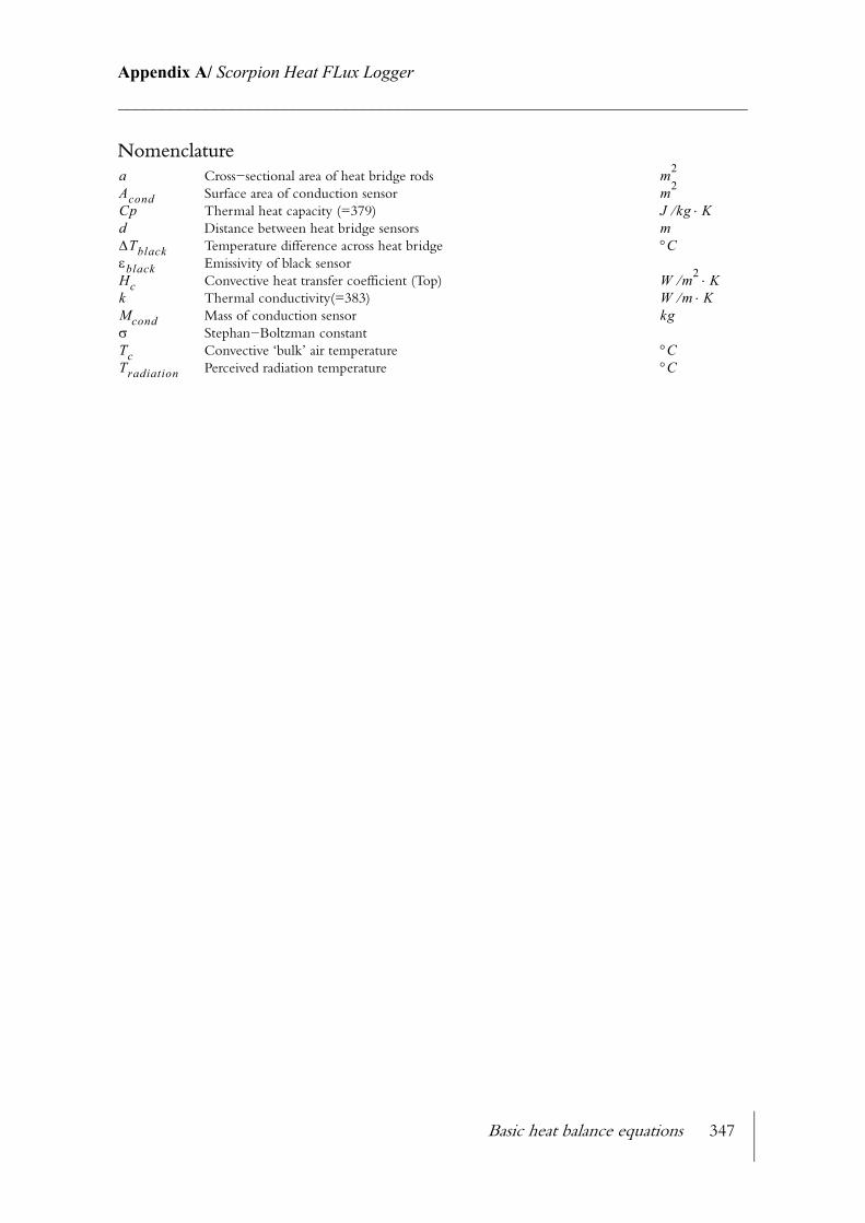
Basic heat balance equations 347
Appendix A/ Scorpion Heat FLux Logger________________________________________________________________________
NomenclatureCross−sectional area of heat bridge rodsSurface area of conduction sensorThermal heat capacity (=379)Distance between heat bridge sensorsTemperature difference across heat bridgeEmissivity of black sensorConvective heat transfer coefficient (Top)Thermal conductivity(=383)Mass of conduction sensor Stephan−Boltzman constantConvective ‘bulk’ air temperaturePerceived radiation temperature
a m2
Acond m2
Cp J kg K⋅⁄d m∆Tblack °CεblackHc W m2⁄ K⋅k W m⁄ K⋅Mcond kgσTc °CTradiation °C

348
Appendix B/ Thermal properties of dry air and correlations in use for the temperature range [200-800 K]________________________________________________________________________
APPENDIX B
THERMAL PROPERTIES OF DRY AIR AND CORRELATIONS IN USE FOR THE TEMPERATURE RANGE [200−800 K]
1. Thermal diffusivity correlation and results of ANOVA table
Results of the ANOVA table for thermal diffusivity correlation: Eqn y-1=a+b/x2 r2 Coef Det DF Adj r2 Fit Std Err F-value 0.9999800304 0.9999760365 0.1698624917 550825.77370 Parm Value Std Error t-value 99% Confidence Limits P>|t| a 0.002400319 2.09233e-05 114.7200198 0.002335335 0.002465303 0.00000 b 3810.652866 9.765226768 390.2267665 3780.323960 3840.981771 0.00000 Area Xmin-Xmax Area Precision 35646.562080 4.320676e-15 Function min X-Value Function max X-Value 10.238937359 200.00026817 119.69648631 800.00000000 1st Deriv min X-Value 1st Deriv max X-Value 0.0998728451 200.00026817 0.2147621377 727.45229681 2nd Deriv min X-Value 2nd Deriv max X-Value -3.97846e-05 800.00000000 0.0004502727 200.00026817 Soln Vector Covar Matrix Direct LUDecomp r2 Coef Det DF Adj r2 Fit Std Err Max Abs Err 0.9999800304 0.9999760365 0.1698624917 0.3035136869 Source Sum of Squares DF Mean Square F Statistic P>F Regr 15893.123 1 15893.123 550826 0.00000 Error 0.31738593 11 0.028853266 Total 15893.44 12
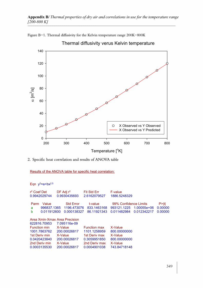
349
Appendix B/ Thermal properties of dry air and correlations in use for the temperature range [200-800 K]________________________________________________________________________
Figure B−1. Thermal diffusivity for the Kelvin temperature range 200K−800K
2. Specific heat correlation and results of ANOVA table
Thermal diffusivity verus Kelvin temperature
Temperature [oK]
200 300 400 500 600 700 800
α [m
2 /s]
0
20
40
60
80
100
120
140
X Observed vs Y Observed X Observed vs Y Predicted
Results of the ANOVA table for specific heat correlation: Eqn y2=a+bx2.5 r2 Coef Det DF Adj r2 Fit Std Err F-value 0.9942029744 0.9930435693 2.6162079527 1886.5248329 Parm Value Std Error t-value 99% Confidence Limits P>|t| a 996837.1365 1196.473076 833.1463168 993121.1225 1.00055e+06 0.00000 b 0.011912600 0.000138327 86.11921343 0.011482984 0.012342217 0.00000 Area Xmin-Xmax Area Precision 622816.70953 7.095116e-09 Function min X-Value Function max X-Value 1001.7863762 200.00026817 1101.1258959 800.00000000 1st Deriv min X-Value 1st Deriv max X-Value 0.0420423840 200.00026817 0.3059951850 800.00000000 2nd Deriv min X-Value 2nd Deriv max X-Value 0.0003135530 200.00026817 0.0004901038 743.84718148

350
Appendix B/ Thermal properties of dry air and correlations in use for the temperature range [200-800 K]________________________________________________________________________
Figure B−2. Specific heat for the Kelvin temperature range 200K−800K
3. Thermal conductivity correlation and results of ANOVA table
Soln Vector Covar Matrix Direct LUDecomp r2 Coef Det DF Adj r2 Fit Std Err Max Abs Err 0.9942029744 0.9930435693 2.6162079527 5.2136351016 Source Sum of Squares DF Mean Square F Statistic P>F Regr 12912.402 1 12912.402 1886.52 0.00000 Error 75.289985 11 6.8445441 Total 12987.692 12
Specific heat verus Kelvin temperature
Temperature [oK]
200 300 400 500 600 700 800
Cp
[j/kg
.K]
980
1000
1020
1040
1060
1080
1100
1120
X Observed vs Y Observed X Observed vs Y Predicted
Results of the ANOVA table for thermal conductivity correlation: Eqn y-1=a+b/x r2 Coef Det DF Adj r2 Fit Std Err F-value 0.9996801414 0.9996161697 0.0002384657 34379.194302 Parm Value Std Error t-value 99% Confidence Limits P>|t| a 5.047374400 0.124459315 40.55441245 4.660827839 5.433920961 0.00000 b 9834.099796 75.28223991 130.6297449 9600.287719 10067.91187 0.00000
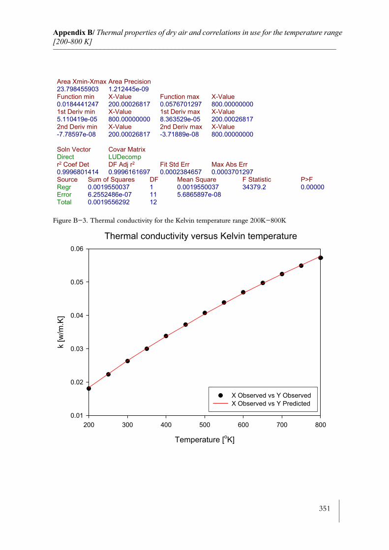
351
Appendix B/ Thermal properties of dry air and correlations in use for the temperature range [200-800 K]________________________________________________________________________
Figure B−3. Thermal conductivity for the Kelvin temperature range 200K−800K
Area Xmin-Xmax Area Precision 23.798455903 1.212445e-09 Function min X-Value Function max X-Value 0.0184441247 200.00026817 0.0576701297 800.00000000 1st Deriv min X-Value 1st Deriv max X-Value 5.110419e-05 800.00000000 8.363529e-05 200.00026817 2nd Deriv min X-Value 2nd Deriv max X-Value -7.78597e-08 200.00026817 -3.71889e-08 800.00000000 Soln Vector Covar Matrix Direct LUDecomp r2 Coef Det DF Adj r2 Fit Std Err Max Abs Err 0.9996801414 0.9996161697 0.0002384657 0.0003701297 Source Sum of Squares DF Mean Square F Statistic P>F Regr 0.0019550037 1 0.0019550037 34379.2 0.00000 Error 6.2552486e-07 11 5.6865897e-08 Total 0.0019556292 12
Thermal conductivity versus Kelvin temperature
Temperature [oK]
200 300 400 500 600 700 800
k [w
/m.K
]
0.01
0.02
0.03
0.04
0.05
0.06
X Observed vs Y Observed X Observed vs Y Predicted
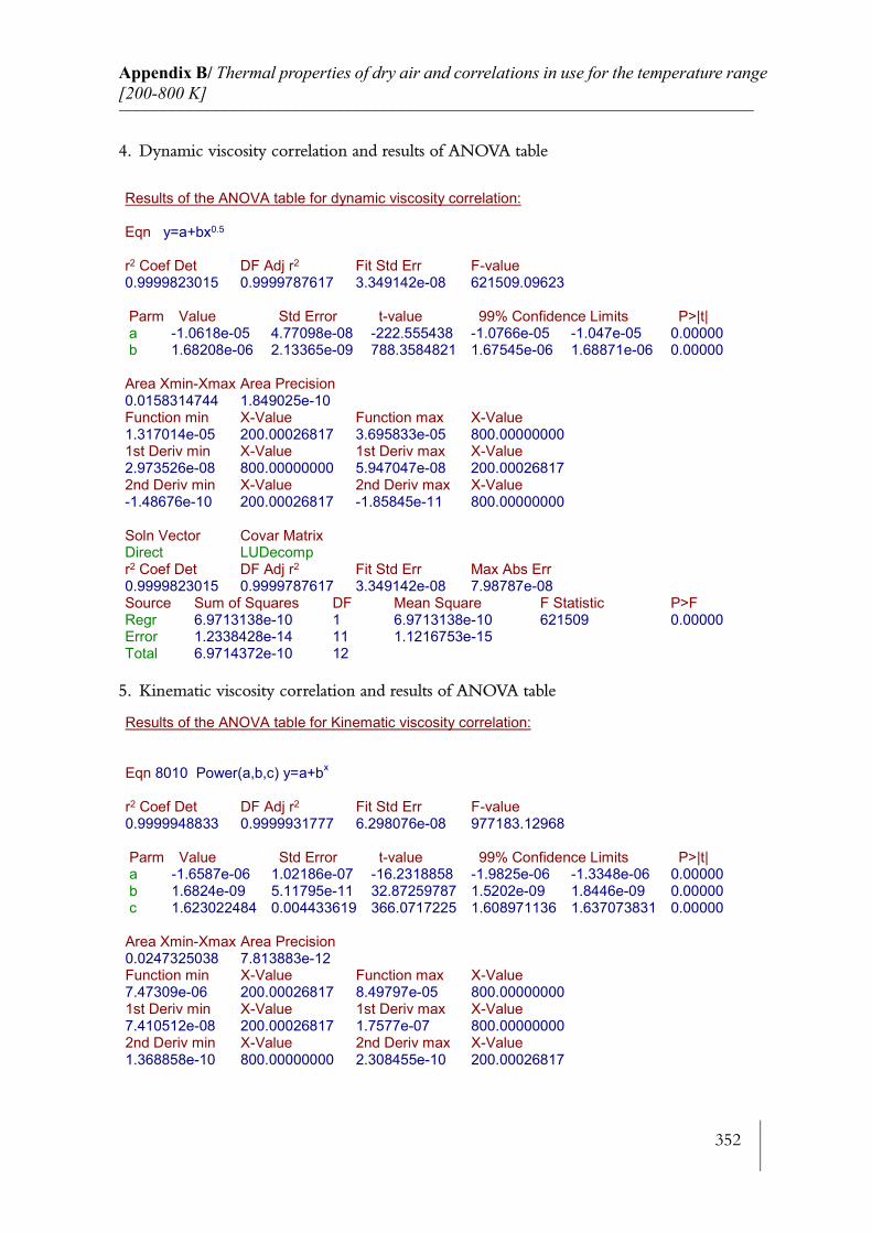
352
Appendix B/ Thermal properties of dry air and correlations in use for the temperature range [200-800 K]________________________________________________________________________
4. Dynamic viscosity correlation and results of ANOVA table
5. Kinematic viscosity correlation and results of ANOVA table
Results of the ANOVA table for dynamic viscosity correlation: Eqn y=a+bx0.5 r2 Coef Det DF Adj r2 Fit Std Err F-value 0.9999823015 0.9999787617 3.349142e-08 621509.09623 Parm Value Std Error t-value 99% Confidence Limits P>|t| a -1.0618e-05 4.77098e-08 -222.555438 -1.0766e-05 -1.047e-05 0.00000 b 1.68208e-06 2.13365e-09 788.3584821 1.67545e-06 1.68871e-06 0.00000 Area Xmin-Xmax Area Precision 0.0158314744 1.849025e-10 Function min X-Value Function max X-Value 1.317014e-05 200.00026817 3.695833e-05 800.00000000 1st Deriv min X-Value 1st Deriv max X-Value 2.973526e-08 800.00000000 5.947047e-08 200.00026817 2nd Deriv min X-Value 2nd Deriv max X-Value -1.48676e-10 200.00026817 -1.85845e-11 800.00000000 Soln Vector Covar Matrix Direct LUDecomp r2 Coef Det DF Adj r2 Fit Std Err Max Abs Err 0.9999823015 0.9999787617 3.349142e-08 7.98787e-08 Source Sum of Squares DF Mean Square F Statistic P>F Regr 6.9713138e-10 1 6.9713138e-10 621509 0.00000 Error 1.2338428e-14 11 1.1216753e-15 Total 6.9714372e-10 12
Results of the ANOVA table for Kinematic viscosity correlation: Eqn 8010 Power(a,b,c) y=a+bx r2 Coef Det DF Adj r2 Fit Std Err F-value 0.9999948833 0.9999931777 6.298076e-08 977183.12968 Parm Value Std Error t-value 99% Confidence Limits P>|t| a -1.6587e-06 1.02186e-07 -16.2318858 -1.9825e-06 -1.3348e-06 0.00000 b 1.6824e-09 5.11795e-11 32.87259787 1.5202e-09 1.8446e-09 0.00000 c 1.623022484 0.004433619 366.0717225 1.608971136 1.637073831 0.00000 Area Xmin-Xmax Area Precision 0.0247325038 7.813883e-12 Function min X-Value Function max X-Value 7.47309e-06 200.00026817 8.49797e-05 800.00000000 1st Deriv min X-Value 1st Deriv max X-Value 7.410512e-08 200.00026817 1.7577e-07 800.00000000 2nd Deriv min X-Value 2nd Deriv max X-Value 1.368858e-10 800.00000000 2.308455e-10 200.00026817
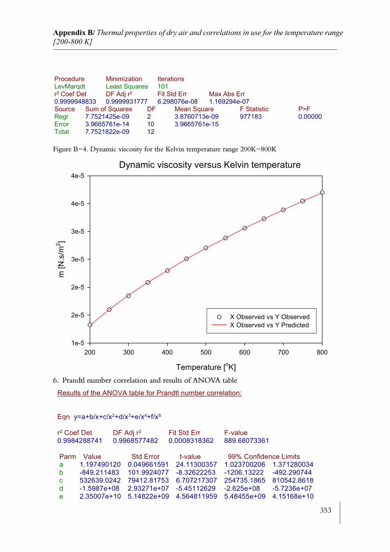
353
Appendix B/ Thermal properties of dry air and correlations in use for the temperature range [200-800 K]________________________________________________________________________
Figure B−4. Dynamic viscosity for the Kelvin temperature range 200K−800K
6. Prandtl number correlation and results of ANOVA table
Procedure Minimization Iterations LevMarqdt Least Squares 101 r2 Coef Det DF Adj r2 Fit Std Err Max Abs Err 0.9999948833 0.9999931777 6.298076e-08 1.169294e-07 Source Sum of Squares DF Mean Square F Statistic P>F Regr 7.7521425e-09 2 3.8760713e-09 977183 0.00000 Error 3.9665761e-14 10 3.9665761e-15 Total 7.7521822e-09 12
Dynamic viscosity versus Kelvin temperature
Temperature [oK]
200 300 400 500 600 700 800
m [N
.s/m
2 ]
1e-5
2e-5
2e-5
3e-5
3e-5
4e-5
4e-5
X Observed vs Y Observed X Observed vs Y Predicted
Results of the ANOVA table for Prandtl number correlation: Eqn y=a+b/x+c/x2+d/x3+e/x4+f/x5 r2 Coef Det DF Adj r2 Fit Std Err F-value 0.9984288741 0.9968577482 0.0008318362 889.68073361 Parm Value Std Error t-value 99% Confidence Limits a 1.197490120 0.049661591 24.11300357 1.023700206 1.371280034 b -849.211483 101.9924077 -8.32622253 -1206.13222 -492.290744 c 532639.0242 79412.81753 6.707217307 254735.1865 810542.8618 d -1.5987e+08 2.93271e+07 -5.45112629 -2.625e+08 -5.7236e+07 e 2.35007e+10 5.14822e+09 4.564811959 5.48455e+09 4.15168e+10
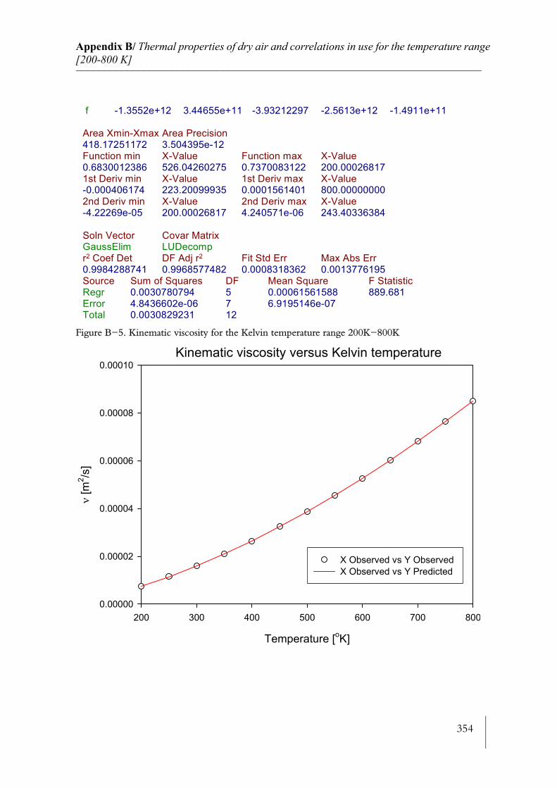
354
Appendix B/ Thermal properties of dry air and correlations in use for the temperature range [200-800 K]________________________________________________________________________
Figure B−5. Kinematic viscosity for the Kelvin temperature range 200K−800K
f -1.3552e+12 3.44655e+11 -3.93212297 -2.5613e+12 -1.4911e+11 Area Xmin-Xmax Area Precision 418.17251172 3.504395e-12 Function min X-Value Function max X-Value 0.6830012386 526.04260275 0.7370083122 200.00026817 1st Deriv min X-Value 1st Deriv max X-Value -0.000406174 223.20099935 0.0001561401 800.00000000 2nd Deriv min X-Value 2nd Deriv max X-Value -4.22269e-05 200.00026817 4.240571e-06 243.40336384 Soln Vector Covar Matrix GaussElim LUDecomp r2 Coef Det DF Adj r2 Fit Std Err Max Abs Err 0.9984288741 0.9968577482 0.0008318362 0.0013776195 Source Sum of Squares DF Mean Square F Statistic Regr 0.0030780794 5 0.00061561588 889.681 Error 4.8436602e-06 7 6.9195146e-07 Total 0.0030829231 12
Kinematic viscosity versus Kelvin temperature
Temperature [oK]
200 300 400 500 600 700 800
ν [m
2 /s]
0.00000
0.00002
0.00004
0.00006
0.00008
0.00010
X Observed vs Y Observed X Observed vs Y Predicted
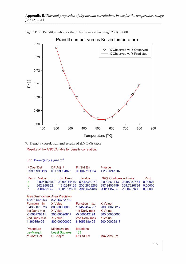
355
Appendix B/ Thermal properties of dry air and correlations in use for the temperature range [200-800 K]________________________________________________________________________
Figure B−6. Prandtl number for the Kelvin temperature range 200K−800K
7. Density correlation and results of ANOVA table
Prandtl number versus Kelvin temperature
Temperature [oK]
100 200 300 400 500 600 700 800 900
Pr [-
]
0.68
0.69
0.70
0.71
0.72
0.73
0.74
X Observed vs Y Observed X Observed vs Y Predicted
Results of the ANOVA table for density correlation: Eqn Power(a,b,c) y=a+bxc r2 Coef Det DF Adj r2 Fit Std Err F-value 0.9999996118 0.9999994825 0.0002719364 1.288124e+07 Parm Value Std Error t-value 99% Confidence Limits P>|t| a 0.005159457 0.000914410 5.642389742 0.002261443 0.008057471 0.00021 b 362.9888621 1.812345165 200.2868268 357.2450459 368.7326784 0.00000 c -1.00791695 0.001022600 -985.641486 -1.01115785 -1.00467606 0.00000 Area Xmin-Xmax Area Precision 482.99545053 8.201476e-16 Function min X-Value Function max X-Value 0.4355073526 800.00000000 1.7455454087 200.00026817 1st Deriv min X-Value 1st Deriv max X-Value -0.008770811 200.00026817 -0.000542194 800.00000000 2nd Deriv min X-Value 2nd Deriv max X-Value 1.36085e-06 800.00000000 8.805518e-05 200.00026817 Procedure Minimization Iterations LevMarqdt Least Squares 183 r2 Coef Det DF Adj r2 Fit Std Err Max Abs Err
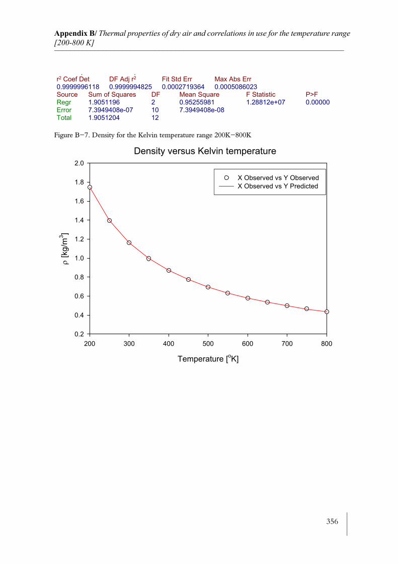
356
Appendix B/ Thermal properties of dry air and correlations in use for the temperature range [200-800 K]________________________________________________________________________
Figure B−7. Density for the Kelvin temperature range 200K−800K
q qr2 Coef Det DF Adj r2 Fit Std Err Max Abs Err 0.9999996118 0.9999994825 0.0002719364 0.0005086023 Source Sum of Squares DF Mean Square F Statistic P>F Regr 1.9051196 2 0.95255981 1.28812e+07 0.00000 Error 7.3949408e-07 10 7.3949408e-08 Total 1.9051204 12
Density versus Kelvin temperature
Temperature [oK]
200 300 400 500 600 700 800
ρ [k
g/m
3 ]
0.2
0.4
0.6
0.8
1.0
1.2
1.4
1.6
1.8
2.0
X Observed vs Y Observed X Observed vs Y Predicted

357
Appendix C/ Smoothing Factor and Decimal Precision of Selected Variables________________________________________________________________________
APPENDIX C
SMOOTHING FACTOR AND DECIMAL PRECISION OF SELECTED VARIABLES
Table C−1. Smoothing factor and decimal place of selected variables
Variable name Description ‘Smoothing factor’ based on x points
Decimal place (dp)
External wall surface temperature 120 1
Ambient air temperature 120 1
Internal wall surface temperature 60 1
Internal product temperature 20 1
Nozzle air temperature 5 1
Pressure measurement 40 1
Mean external wall surface heat transfer coefficient
120 2
Nozzle heat transfer coefficient 40 2
Rate of energy loss by leakages 180 1
Heater surface temperature 5 1
Mass flow, sum of mass flow and mass flow difference
0 3
Air velocity 0 2
Nozzle slot width, characteristic length
0 1
Wall surface area 0 2
External wall heat transfer con-vective and radiative heat loss
0 3
Ts w o( ),
T∞
Ts w i( ),
TCA
Tnozt
PTXx
hv h,
hnozt
∆Ql
TCh w,
Mx
Vx
W CL,
Aw
Qcv h, ,Qrw
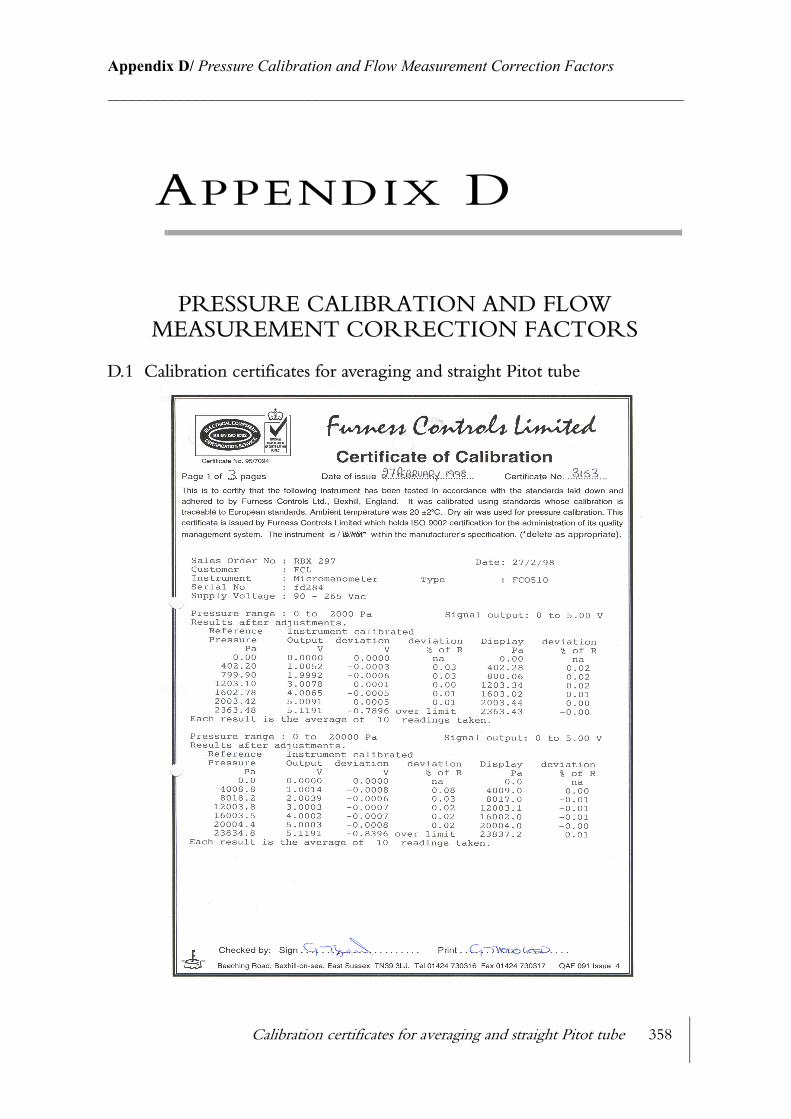
Calibration certificates for averaging and straight Pitot tube 358
Appendix D/ Pressure Calibration and Flow Measurement Correction Factors________________________________________________________________________
APPENDIX D
PRESSURE CALIBRATION AND FLOW MEASUREMENT CORRECTION FACTORS
D.1 Calibration certificates for averaging and straight Pitot tube

Calibration certificates for averaging and straight Pitot tube 359
Appendix D/ Pressure Calibration and Flow Measurement Correction Factors________________________________________________________________________
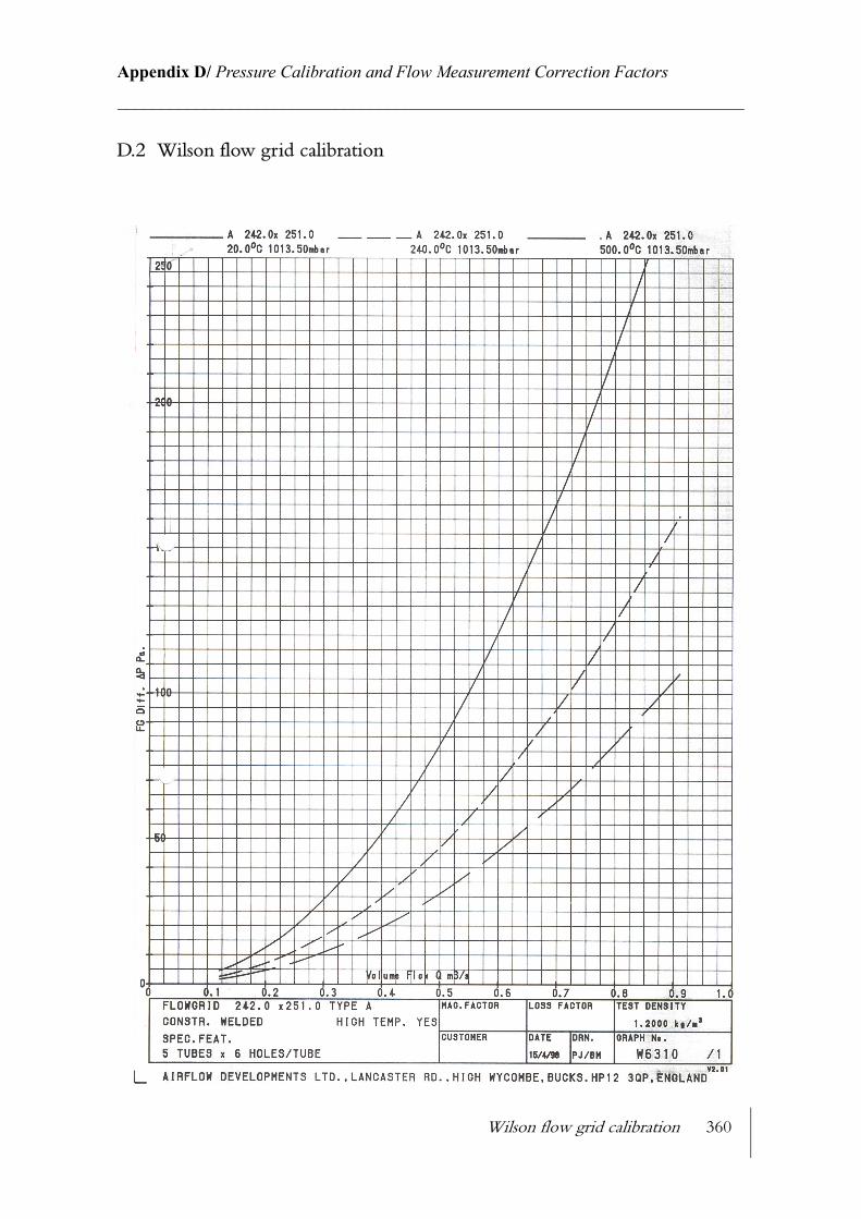
Wilson flow grid calibration 360
Appendix D/ Pressure Calibration and Flow Measurement Correction Factors________________________________________________________________________
D.2 Wilson flow grid calibration
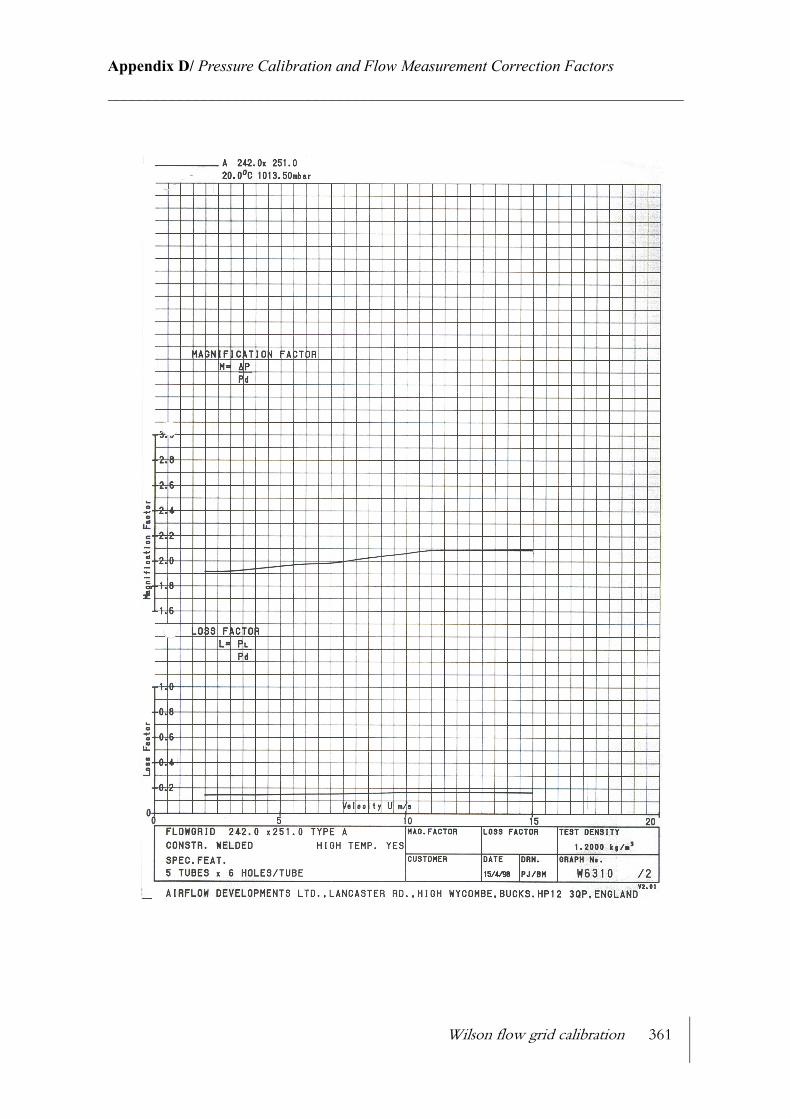
Wilson flow grid calibration 361
Appendix D/ Pressure Calibration and Flow Measurement Correction Factors________________________________________________________________________
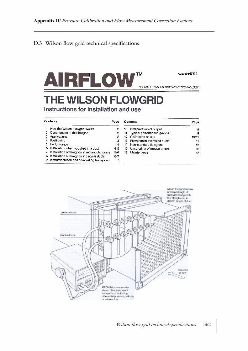
Wilson flow grid technical specifications 362
Appendix D/ Pressure Calibration and Flow Measurement Correction Factors________________________________________________________________________
D.3 Wilson flow grid technical specifications
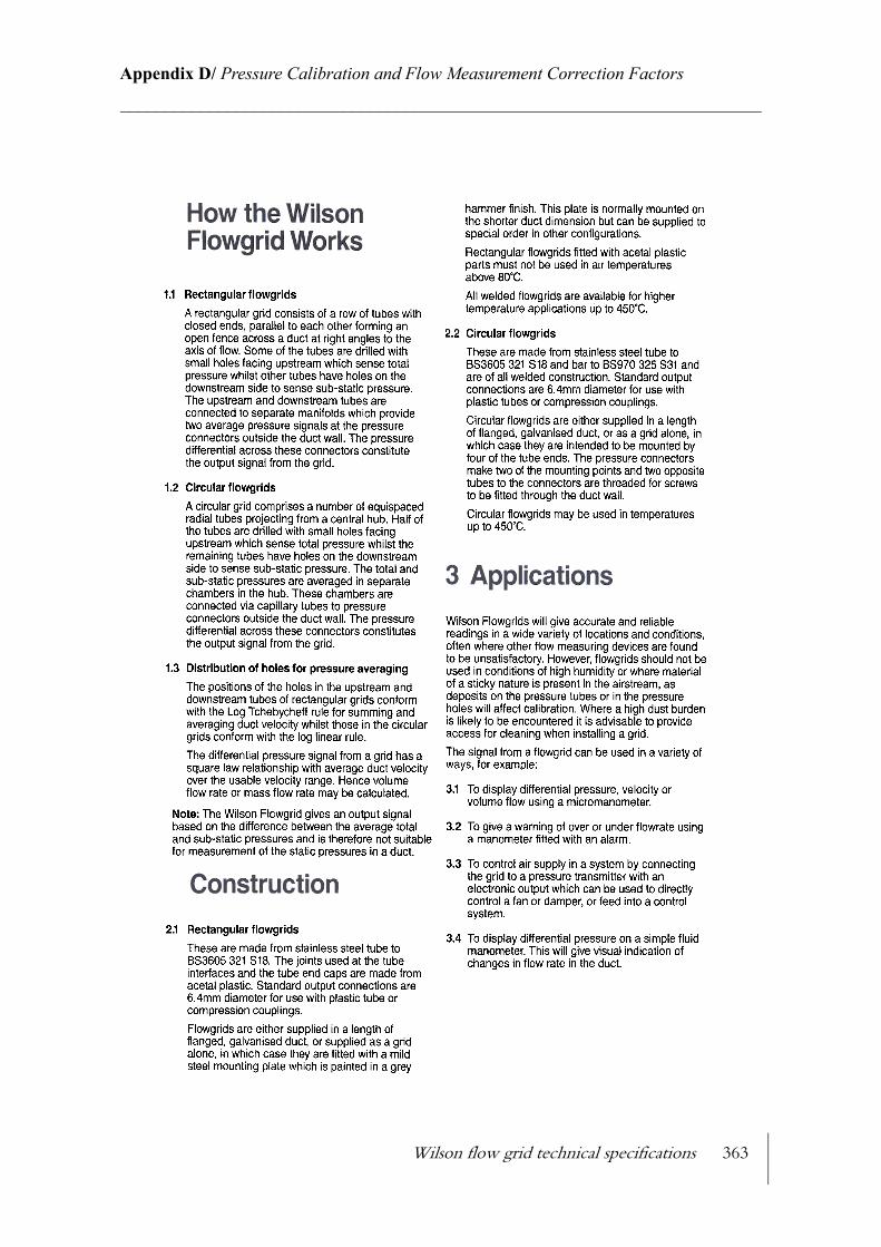
Wilson flow grid technical specifications 363
Appendix D/ Pressure Calibration and Flow Measurement Correction Factors________________________________________________________________________

Wilson flow grid technical specifications 364
Appendix D/ Pressure Calibration and Flow Measurement Correction Factors________________________________________________________________________
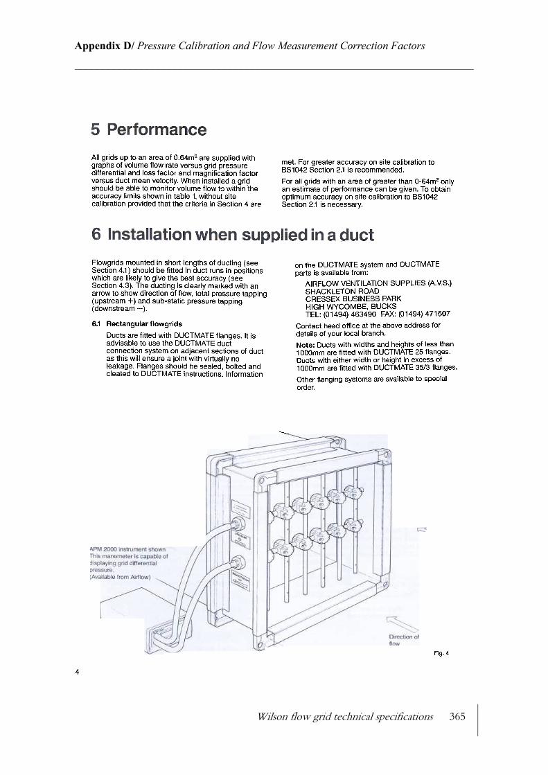
Wilson flow grid technical specifications 365
Appendix D/ Pressure Calibration and Flow Measurement Correction Factors________________________________________________________________________

Wilson flow grid technical specifications 366
Appendix D/ Pressure Calibration and Flow Measurement Correction Factors________________________________________________________________________

Wilson flow grid technical specifications 367
Appendix D/ Pressure Calibration and Flow Measurement Correction Factors________________________________________________________________________

Wilson flow grid technical specifications 368
Appendix D/ Pressure Calibration and Flow Measurement Correction Factors________________________________________________________________________
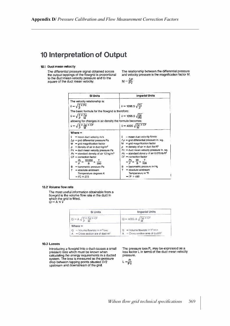
Wilson flow grid technical specifications 369
Appendix D/ Pressure Calibration and Flow Measurement Correction Factors________________________________________________________________________
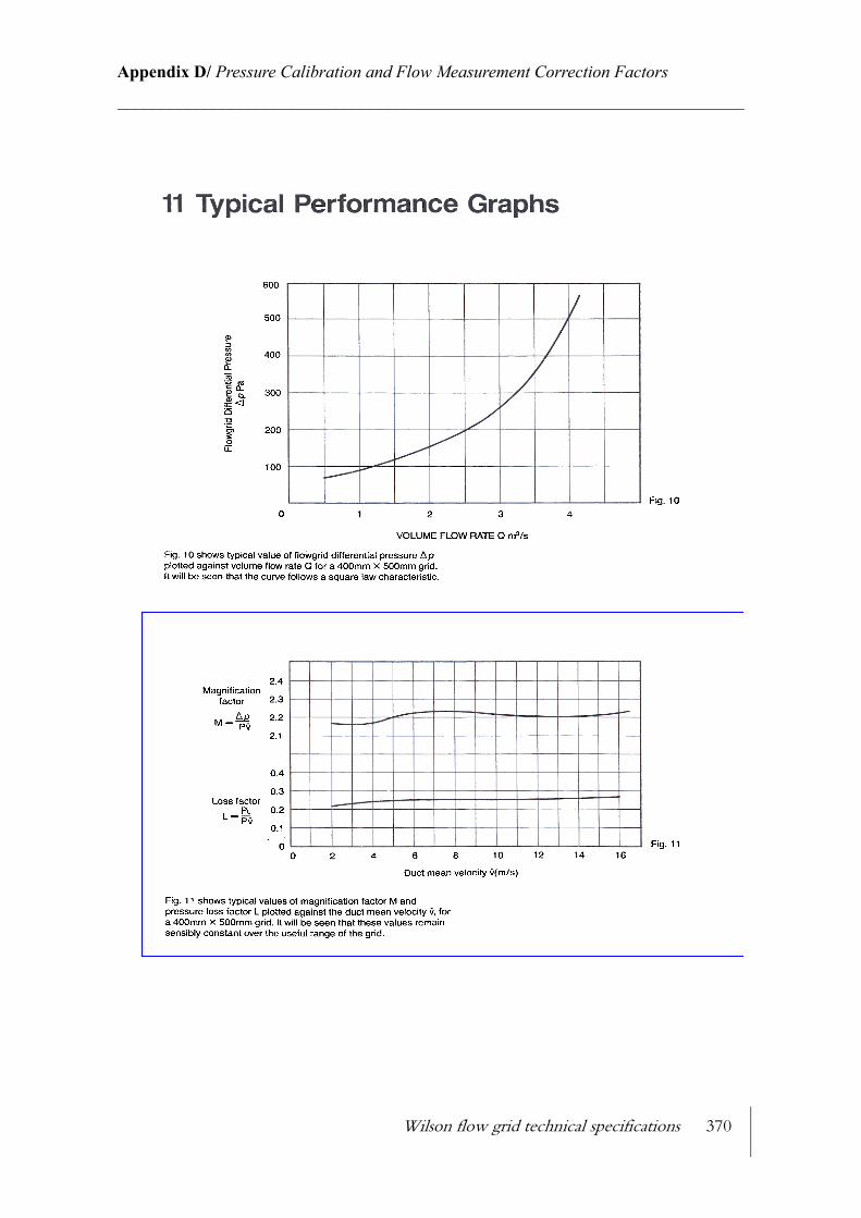
Wilson flow grid technical specifications 370
Appendix D/ Pressure Calibration and Flow Measurement Correction Factors________________________________________________________________________
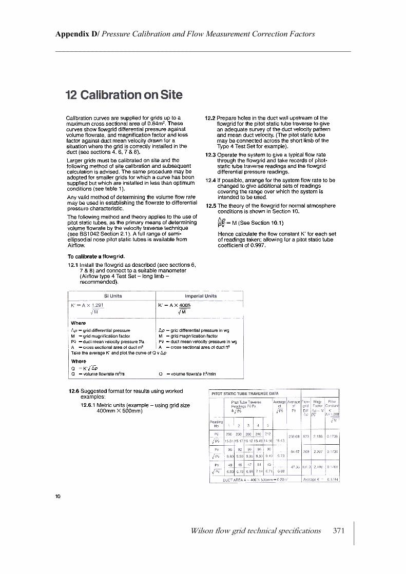
Wilson flow grid technical specifications 371
Appendix D/ Pressure Calibration and Flow Measurement Correction Factors________________________________________________________________________
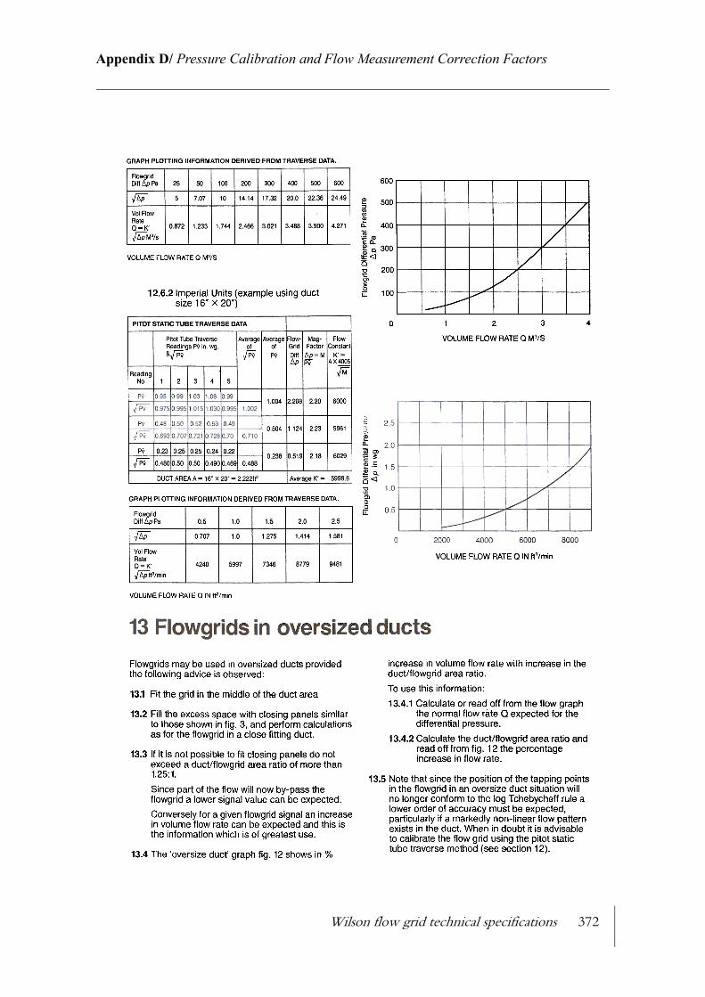
Wilson flow grid technical specifications 372
Appendix D/ Pressure Calibration and Flow Measurement Correction Factors________________________________________________________________________

Wilson flow grid technical specifications 373
Appendix D/ Pressure Calibration and Flow Measurement Correction Factors________________________________________________________________________
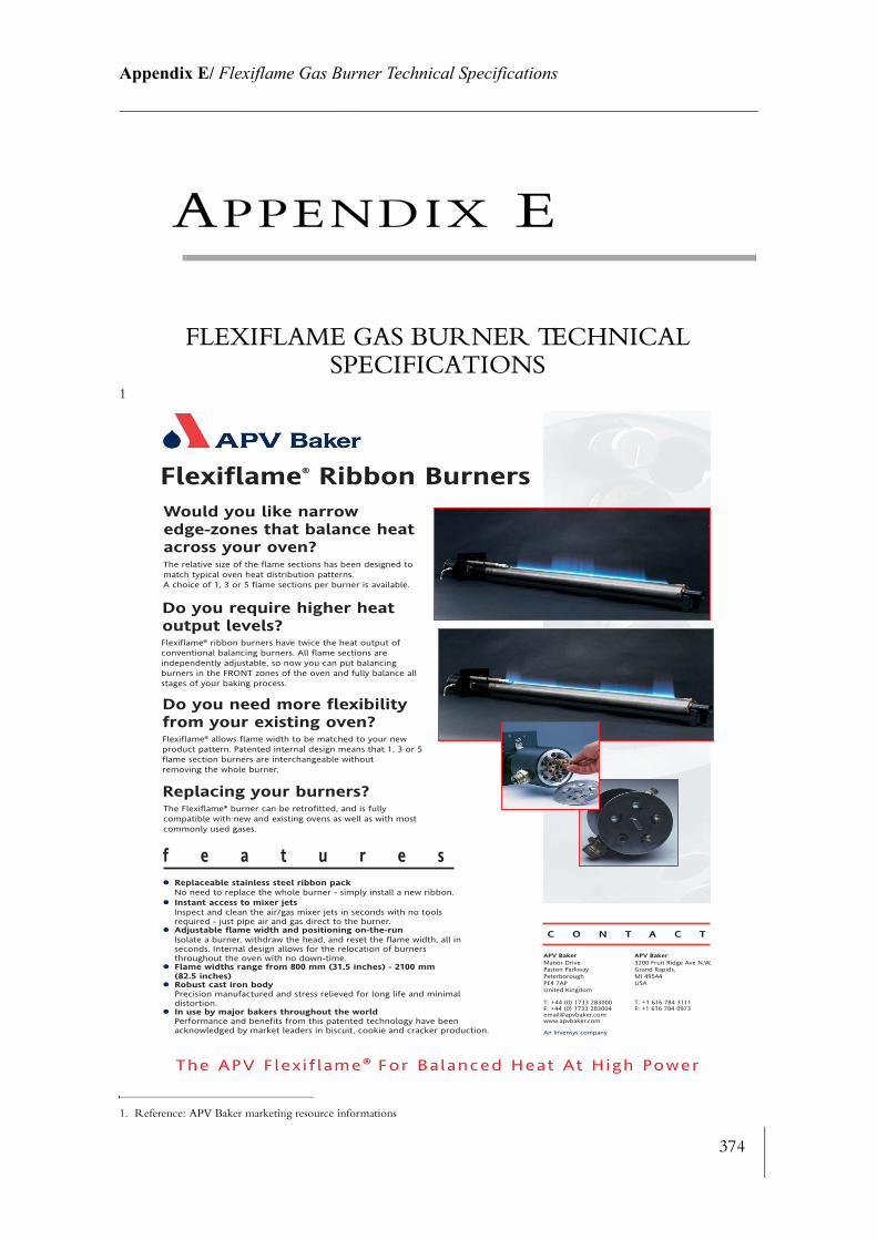
374
Appendix E/ Flexiflame Gas Burner Technical Specifications________________________________________________________________________
APPENDIX E
FLEXIFLAME GAS BURNER TECHNICAL SPECIFICATIONS
1
1. Reference: APV Baker marketing resource informations
The APV Flex i f lame® For Balanced Heat At High Power
The relative size of the flame sections has been designed tomatch typical oven heat distribution patterns. A choice of 1, 3 or 5 flame sections per burner is available.
Would you like narrow edge-zones that balance heatacross your oven?
Flexiflame® Ribbon Burners
Do you require higher heat output levels?
Do you need more flexibilityfrom your existing oven?Flexiflame® allows flame width to be matched to your newproduct pattern. Patented internal design means that 1, 3 or 5flame section burners are interchangeable without removing the whole burner.
Flexiflame® ribbon burners have twice the heat output ofconventional balancing burners. All flame sections are independently adjustable, so now you can put balancingburners in the FRONT zones of the oven and fully balance allstages of your baking process.
f e a t u r e s Replaceable stainless steel ribbon pack
No need to replace the whole burner - simply install a new ribbon. Instant access to mixer jets
Inspect and clean the air/gas mixer jets in seconds with no tools required - just pipe air and gas direct to the burner.
Adjustable flame width and positioning on-the-runIsolate a burner, withdraw the head, and reset the flame width, all in seconds. Internal design allows for the relocation of burners throughout the oven with no down-time.
Flame widths range from 800 mm (31.5 inches) - 2100 mm(82.5 inches)
Robust cast iron bodyPrecision manufactured and stress relieved for long life and minimal distortion.
In use by major bakers throughout the worldPerformance and benefits from this patented technology have been acknowledged by market leaders in biscuit, cookie and cracker production.
The Flexiflame® burner can be retrofitted, and is fully compatible with new and existing ovens as well as with mostcommonly used gases.
Replacing your burners?
C O N T A C T
APV Baker Manor DrivePaston ParkwayPeterboroughPE4 7APUnited Kingdom
T: +44 (0) 1733 283000 F: +44 (0) 1733 [email protected]
An Invensys company
APV Baker 3200 Fruit Ridge Ave N.W.Grand Rapids, MI 49544USA
T: +1 616 784 3111 F: +1 616 784 0973
Emissivity determination by experiment 375
Appendix F/ Emissivity Measurement________________________________________________________________________
APPENDIX F
EMISSIVITY MEASUREMENT
F.1 Emissivity determination by experiment
Experiments were undertaken to determine the emissivities of the various materials that were used during this project. The instrument in used was the emissometer (manufactured by Devices & Services Ltd., Texas Model AE). Other equipment had to be used for the pur−pose of this experiment (See Figure F−1):
• Digital multi−meter (standard 240 volt meter, with an accuracy of 1/100 of a millivolt)
• Heat sink made of an aluminium finned block painted black, which help to stabilise the temperature of the emissometer during the warm up and during the measurement.
• Two calibration pieces of known emissivities.
• Test sample which emissivity is unknown.
The assumptions taken into consideration were the following:
1. The surface of the test materials were smooth and free from contamination to enable sufficiently accurate results
2. The emissometer has a linear emissivity versus voltage characteristics3. The emissometer reaches a sufficiently close to steady state conditions before the cali−
bration starts4. The test material was left long enough for thermal equilibrium to be reached, before
experiment starts5. The materials tested have relatively flat temperature versus emissivity curve to allow the
values to be used over the temperature used during the experiment using the TPRO.6. Diffuse and grey body concepts are applicable to the materials surfaces under consider−
ation.
The material to be measured is placed between the emissometer and the heat sink (See Figure F−1). When the power is switched on, the emissometer warms up until a pre−set temperature. The two calibrating blocks were used to estimate a calibration curve. The cal−ibration blocks were placed in turn on the heat sink, waiting for the mutli−meter readings to stabilise and then noting the stabilised reading. The experiment was repeated 10 times to ensure consistency. The results were used to plot a graph outlining the emissometer charac−teristics.
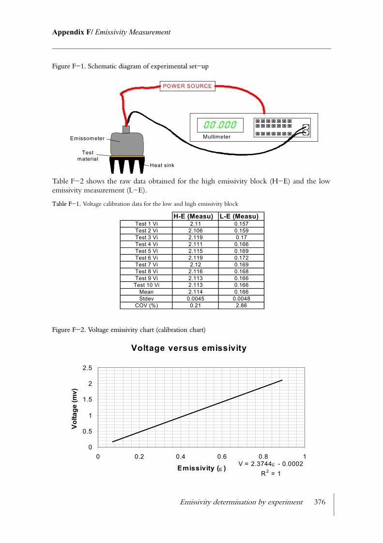
Emissivity determination by experiment 376
Appendix F/ Emissivity Measurement________________________________________________________________________
Figure F−1. Schematic diagram of experimental set−up
Table F−2 shows the raw data obtained for the high emissivity block (H−E) and the low emissivity measurement (L−E).
Table F−1. Voltage calibration data for the low and high emissivity block
Figure F−2. Voltage emissivity chart (calibration chart)
00.000Multimeter
POWER SOURCE
Heat sink
Testmaterial
Emissometer
H-E (Measu) L-E (Measu)Test 1 Vi 2.11 0.157Test 2 Vi 2.106 0.159Test 3 Vi 2.119 0.17Test 4 Vi 2.111 0.166Test 5 Vi 2.115 0.169Test 6 Vi 2.119 0.172Test 7 Vi 2.12 0.169Test 8 Vi 2.116 0.168Test 9 Vi 2.113 0.166
Test 10 Vi 2.113 0.166Mean 2.114 0.166Stdev 0.0045 0.0048
COV (%) 0.21 2.86
Voltage versus emissivity
V = 2.3744ε - 0.0002R2 = 1
0
0.5
1
1.5
2
2.5
0 0.2 0.4 0.6 0.8 1
Emissivity (ε )
Volta
ge (m
v)
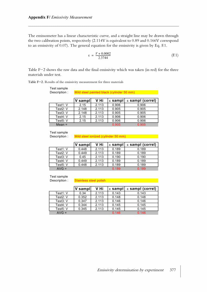
Emissivity determination by experiment 377
Appendix F/ Emissivity Measurement________________________________________________________________________
The emissometer has a linear characteristic curve, and a straight line may be drawn through the two calibration points, respectively (2.114V is equivalent to 0.89 and 0.166V correspond to an emissivity of 0.07). The general equation for the emissivity is given by Eq. F.1.
(F.1)
Table F−2 shows the raw data and the final emissivity which was taken (in red) for the three materials under test.
Table F−2. Results of the emissivity measurement for three materials
ε V 0.0002+2.3744
--------------------------=
Test sampleDescription : Mild steel painted black (cylinder 50 mm)
V sampl V Hi ε sampl ε sampl (correl)Test1: V 2.15 2.113 0.906 0.906Test2: V 2.148 2.113 0.905 0.905Test3: V 2.148 2.113 0.905 0.905Test4: V 2.15 2.113 0.906 0.906Test5: V 2.15 2.113 0.906 0.906Mean = 0.905 0.905
Test sampleDescription : Mild steel ionized (cylinder 50 mm)
V sampl V Hi ε sampl ε sampl (correl)Test1: V 0.448 2.113 0.189 0.189Test2: V 0.449 2.113 0.189 0.189Test3: V 0.45 2.113 0.190 0.190Test4: V 0.449 2.113 0.189 0.189Test5: V 0.448 2.113 0.189 0.189AVG = 0.189 0.189
Test sampleDescription : Stainless steel polish
V sampl V Hi ε sampl ε sampl (correl)Test1: V 0.34 2.113 0.143 0.143Test2: V 0.352 2.113 0.148 0.148Test3: V 0.347 2.113 0.146 0.146Test4: V 0.344 2.113 0.145 0.145Test5: V 0.345 2.113 0.145 0.145AVG = 0.146 0.146
Mean 378
Appendix G/ Statistical definitions________________________________________________________________________
APPENDIX G
STATISTICAL DEFINITIONS
G.1 Mean
A population is defined as a collection of data which can be finite or infinite. If not finite the population can be reduced to smaller sample. The mean value of a sample of size can be represented by Eq. G.1:
(G.1)
G.2 Standard deviation
The standard deviation of STDEV (in text) measures the spread of data and can be expressed as:
(G.2)
G.3 Coefficient of variance
The standard deviation can be expressed as a percent of the mean in which case it is known as the coefficient of variation ( ).
(G.3)
By dividing the standard deviation by the mean the distribution is linearised which allows an easier comparison between sets of data sample. A low (close to zero) means that data are close together, while a large spread of data is expressed by a close to 1.
x n
x
xii 1=
n
∑
n--------------
x1 x2 ... xn+ + +
n---------------------------------------= =
s
s
xi x–( )2
i 1=
n
∑
n 1–------------------------------=
COV
COV sx--=
COVCOV
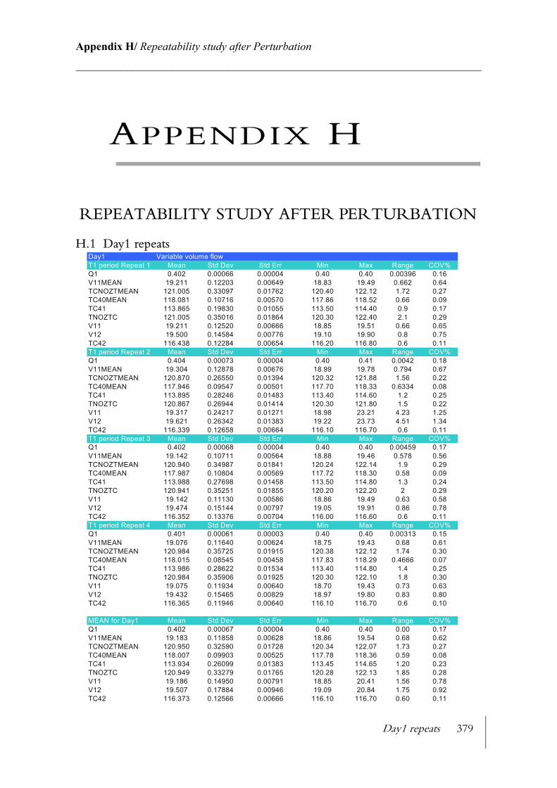
Day1 repeats 379
Appendix H/ Repeatability study after Perturbation________________________________________________________________________
APPENDIX H
REPEATABILITY STUDY AFTER PERTURBATION
H.1 Day1 repeatsDay1 Variable volume flowT1 period Repeat 1 Mean Std Dev Std Err Min Max Range COV%Q1 0.402 0.00066 0.00004 0.40 0.40 0.00396 0.16V11MEAN 19.211 0.12203 0.00649 18.83 19.49 0.662 0.64TCNOZTMEAN 121.005 0.33097 0.01762 120.40 122.12 1.72 0.27TC40MEAN 118.081 0.10716 0.00570 117.86 118.52 0.66 0.09TC41 113.865 0.19830 0.01055 113.50 114.40 0.9 0.17TNOZTC 121.005 0.35016 0.01864 120.30 122.40 2.1 0.29V11 19.211 0.12520 0.00666 18.85 19.51 0.66 0.65V12 19.500 0.14584 0.00776 19.10 19.90 0.8 0.75TC42 116.438 0.12284 0.00654 116.20 116.80 0.6 0.11T1 period Repeat 2 Mean Std Dev Std Err Min Max Range COV%Q1 0.404 0.00073 0.00004 0.40 0.41 0.0042 0.18V11MEAN 19.304 0.12878 0.00676 18.99 19.78 0.794 0.67TCNOZTMEAN 120.870 0.26550 0.01394 120.32 121.88 1.56 0.22TC40MEAN 117.946 0.09547 0.00501 117.70 118.33 0.6334 0.08TC41 113.895 0.28246 0.01483 113.40 114.60 1.2 0.25TNOZTC 120.867 0.26944 0.01414 120.30 121.80 1.5 0.22V11 19.317 0.24217 0.01271 18.98 23.21 4.23 1.25V12 19.621 0.26342 0.01383 19.22 23.73 4.51 1.34TC42 116.339 0.12658 0.00664 116.10 116.70 0.6 0.11T1 period Repeat 3 Mean Std Dev Std Err Min Max Range COV%Q1 0.402 0.00068 0.00004 0.40 0.40 0.00459 0.17V11MEAN 19.142 0.10711 0.00564 18.88 19.46 0.578 0.56TCNOZTMEAN 120.940 0.34987 0.01841 120.24 122.14 1.9 0.29TC40MEAN 117.987 0.10804 0.00569 117.72 118.30 0.58 0.09TC41 113.988 0.27698 0.01458 113.50 114.80 1.3 0.24TNOZTC 120.941 0.35251 0.01855 120.20 122.20 2 0.29V11 19.142 0.11130 0.00586 18.86 19.49 0.63 0.58V12 19.474 0.15144 0.00797 19.05 19.91 0.86 0.78TC42 116.352 0.13376 0.00704 116.00 116.60 0.6 0.11T1 period Repeat 4 Mean Std Dev Std Err Min Max Range COV%Q1 0.401 0.00061 0.00003 0.40 0.40 0.00313 0.15V11MEAN 19.076 0.11640 0.00624 18.75 19.43 0.68 0.61TCNOZTMEAN 120.984 0.35725 0.01915 120.38 122.12 1.74 0.30TC40MEAN 118.015 0.08545 0.00458 117.83 118.29 0.4666 0.07TC41 113.986 0.28622 0.01534 113.40 114.80 1.4 0.25TNOZTC 120.984 0.35906 0.01925 120.30 122.10 1.8 0.30V11 19.075 0.11934 0.00640 18.70 19.43 0.73 0.63V12 19.432 0.15465 0.00829 18.97 19.80 0.83 0.80TC42 116.365 0.11946 0.00640 116.10 116.70 0.6 0.10
MEAN for Day1 Mean Std Dev Std Err Min Max Range COV%Q1 0.402 0.00067 0.00004 0.40 0.40 0.00 0.17V11MEAN 19.183 0.11858 0.00628 18.86 19.54 0.68 0.62TCNOZTMEAN 120.950 0.32590 0.01728 120.34 122.07 1.73 0.27TC40MEAN 118.007 0.09903 0.00525 117.78 118.36 0.59 0.08TC41 113.934 0.26099 0.01383 113.45 114.65 1.20 0.23TNOZTC 120.949 0.33279 0.01765 120.28 122.13 1.85 0.28V11 19.186 0.14950 0.00791 18.85 20.41 1.56 0.78V12 19.507 0.17884 0.00946 19.09 20.84 1.75 0.92TC42 116.373 0.12566 0.00666 116.10 116.70 0.60 0.11
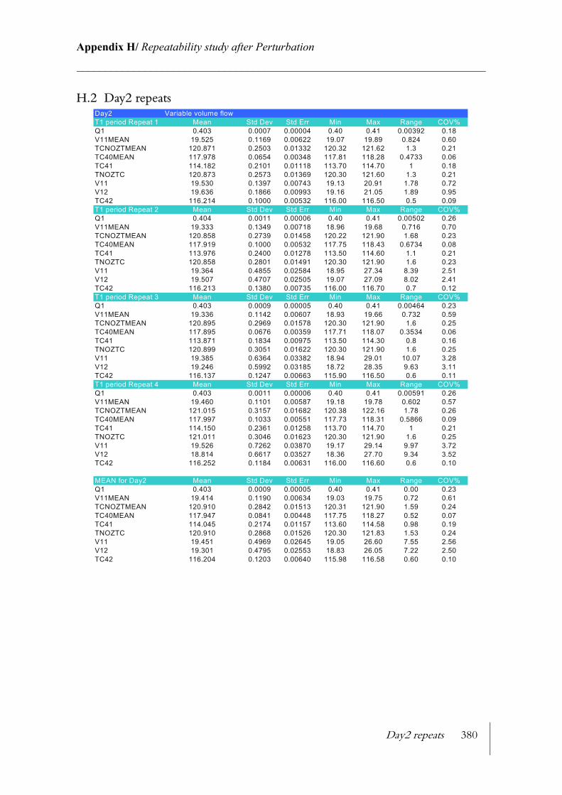
Day2 repeats 380
Appendix H/ Repeatability study after Perturbation________________________________________________________________________
H.2 Day2 repeatsDay2 Variable volume flowT1 period Repeat 1 Mean Std Dev Std Err Min Max Range COV%Q1 0.403 0.0007 0.00004 0.40 0.41 0.00392 0.18V11MEAN 19.525 0.1169 0.00622 19.07 19.89 0.824 0.60TCNOZTMEAN 120.871 0.2503 0.01332 120.32 121.62 1.3 0.21TC40MEAN 117.978 0.0654 0.00348 117.81 118.28 0.4733 0.06TC41 114.182 0.2101 0.01118 113.70 114.70 1 0.18TNOZTC 120.873 0.2573 0.01369 120.30 121.60 1.3 0.21V11 19.530 0.1397 0.00743 19.13 20.91 1.78 0.72V12 19.636 0.1866 0.00993 19.16 21.05 1.89 0.95TC42 116.214 0.1000 0.00532 116.00 116.50 0.5 0.09T1 period Repeat 2 Mean Std Dev Std Err Min Max Range COV%Q1 0.404 0.0011 0.00006 0.40 0.41 0.00502 0.26V11MEAN 19.333 0.1349 0.00718 18.96 19.68 0.716 0.70TCNOZTMEAN 120.858 0.2739 0.01458 120.22 121.90 1.68 0.23TC40MEAN 117.919 0.1000 0.00532 117.75 118.43 0.6734 0.08TC41 113.976 0.2400 0.01278 113.50 114.60 1.1 0.21TNOZTC 120.858 0.2801 0.01491 120.30 121.90 1.6 0.23V11 19.364 0.4855 0.02584 18.95 27.34 8.39 2.51V12 19.507 0.4707 0.02505 19.07 27.09 8.02 2.41TC42 116.213 0.1380 0.00735 116.00 116.70 0.7 0.12T1 period Repeat 3 Mean Std Dev Std Err Min Max Range COV%Q1 0.403 0.0009 0.00005 0.40 0.41 0.00464 0.23V11MEAN 19.336 0.1142 0.00607 18.93 19.66 0.732 0.59TCNOZTMEAN 120.895 0.2969 0.01578 120.30 121.90 1.6 0.25TC40MEAN 117.895 0.0676 0.00359 117.71 118.07 0.3534 0.06TC41 113.871 0.1834 0.00975 113.50 114.30 0.8 0.16TNOZTC 120.899 0.3051 0.01622 120.30 121.90 1.6 0.25V11 19.385 0.6364 0.03382 18.94 29.01 10.07 3.28V12 19.246 0.5992 0.03185 18.72 28.35 9.63 3.11TC42 116.137 0.1247 0.00663 115.90 116.50 0.6 0.11T1 period Repeat 4 Mean Std Dev Std Err Min Max Range COV%Q1 0.403 0.0011 0.00006 0.40 0.41 0.00591 0.26V11MEAN 19.460 0.1101 0.00587 19.18 19.78 0.602 0.57TCNOZTMEAN 121.015 0.3157 0.01682 120.38 122.16 1.78 0.26TC40MEAN 117.997 0.1033 0.00551 117.73 118.31 0.5866 0.09TC41 114.150 0.2361 0.01258 113.70 114.70 1 0.21TNOZTC 121.011 0.3046 0.01623 120.30 121.90 1.6 0.25V11 19.526 0.7262 0.03870 19.17 29.14 9.97 3.72V12 18.814 0.6617 0.03527 18.36 27.70 9.34 3.52TC42 116.252 0.1184 0.00631 116.00 116.60 0.6 0.10
MEAN for Day2 Mean Std Dev Std Err Min Max Range COV%Q1 0.403 0.0009 0.00005 0.40 0.41 0.00 0.23V11MEAN 19.414 0.1190 0.00634 19.03 19.75 0.72 0.61TCNOZTMEAN 120.910 0.2842 0.01513 120.31 121.90 1.59 0.24TC40MEAN 117.947 0.0841 0.00448 117.75 118.27 0.52 0.07TC41 114.045 0.2174 0.01157 113.60 114.58 0.98 0.19TNOZTC 120.910 0.2868 0.01526 120.30 121.83 1.53 0.24V11 19.451 0.4969 0.02645 19.05 26.60 7.55 2.56V12 19.301 0.4795 0.02553 18.83 26.05 7.22 2.50TC42 116.204 0.1203 0.00640 115.98 116.58 0.60 0.10

Day3 repeats 381
Appendix H/ Repeatability study after Perturbation________________________________________________________________________
H.3 Day3 repeats
H.4 Results summary
Day3 Variable volum e flowT1 period Repeat 1 M ean Std Dev Std Err M in M ax Range CO V%Q 1 0.40357 8.99E-04 4.78E-05 0.40159 0.40599 0.0044 0.22V11M EAN 19.19933 0.11702 0.00623 18.848 19.618 0.77 0.61TCNO ZTM EAN 120.8815 0.30246 0.0161 120.3 121.76 1.46 0.25TC40M EAN 117.9456 0.08011 0.00426 117.74 118.2066 0.4666 0.07TC41 114.1062 0.21164 0.01126 113.5 114.6 1.1 0.19TNO ZTC 120.8782 0.3097 0.01648 120.3 121.8 1.5 0.26V11 19.20017 0.11881 0.00632 18.83 19.63 0.8 0.62V12 19.69612 0.16484 0.00877 19.33 20.13 0.8 0.84TC42 116.3337 0.14271 0.0076 116 116.8 0.8 0.12T1 period Repeat 2 M ean Std Dev Std Err M in M ax Range CO V%Q 1 0.40361 6.22E-04 3.31E-05 0.40215 0.40555 0.0034 0.15V11M EAN 19.14467 0.12005 0.00639 18.76 19.45 0.69 0.63TCNO ZTM EAN 120.8977 0.28389 0.01511 120.24 121.98 1.74 0.23TC40M EAN 117.9631 0.0838 0.00446 117.76 118.1533 0.3933 0.07TC41 113.9997 0.27464 0.01462 113.4 114.6 1.2 0.24TNO ZTC 120.8972 0.29056 0.01546 120.2 121.9 1.7 0.24V11 19.14414 0.12462 0.00663 18.75 19.49 0.74 0.65V12 19.72909 0.1595 0.00849 19.22 20.36 1.14 0.81TC42 116.3346 0.12129 0.00646 115.9 116.6 0.7 0.10T1 period Repeat 3 M ean Std Dev Std Err M in M ax Range CO V%Q 1 0.40358 7.37E-04 3.93E-05 0.40175 0.40603 0.00428 0.18V11M EAN 19.08661 0.11282 0.00601 18.77 19.398 0.628 0.59TCNO ZTM EAN 120.9685 0.31996 0.01705 120.4 122.18 1.78 0.26TC40M EAN 118.0103 0.08989 0.00479 117.7867 118.28 0.4933 0.08TC41 113.9821 0.27754 0.01479 113.5 114.8 1.3 0.24TNO ZTC 120.9639 0.32393 0.01727 120.4 122.2 1.8 0.27V11 19.10284 0.28777 0.01534 18.76 23.99 5.23 1.51V12 19.64412 0.3393 0.01808 19.22 25.21 5.99 1.73TC42 116.3858 0.12664 0.00675 116.1 116.7 0.6 0.11T1 period Repeat 4 M ean Std Dev Std Err M in M ax Range CO V%Q 1 0.40386 6.14E-04 3.32E-05 0.40217 0.40571 0.00354 0.15V11M EAN 19.09082 0.11783 0.00636 18.73 19.402 0.672 0.62TCNO ZTM EAN 120.9441 0.31889 0.01722 120.34 122.02 1.68 0.26TC40M EAN 118.0088 0.08803 0.00475 117.7867 118.2867 0.5 0.07TC41 114.1344 0.21801 0.01177 113.5 114.6 1.1 0.19TNO ZTC 120.9362 0.31721 0.01713 120.3 122.1 1.8 0.26V11 19.08983 0.11868 0.00641 18.77 19.41 0.64 0.62V12 19.64522 0.14263 0.0077 19.27 20.05 0.78 0.73TC42 116.3729 0.12423 0.00671 116 116.7 0.7 0.11
M EAN for Day3 M ean Std Dev Std Err M in M ax Range CO V%Q 1 0.404 0.00072 0.00004 0.40 0.41 0.00 0.18V11M EAN 19.130 0.11693 0.00625 18.78 19.47 0.69 0.61TCNO ZTM EAN 120.923 0.30630 0.01637 120.32 121.99 1.67 0.25TC40M EAN 117.982 0.08546 0.00457 117.77 118.23 0.46 0.07TC41 114.056 0.24546 0.01311 113.48 114.65 1.18 0.22TNO ZTC 120.919 0.31035 0.01659 120.30 122.00 1.70 0.26V11 19.134 0.16247 0.00868 18.78 20.63 1.85 0.85V12 19.679 0.20157 0.01076 19.26 21.44 2.18 1.02TC42 116.357 0.12872 0.00688 116.00 116.70 0.70 0.11
Day to day variation
Q1 V11MEAN TCNOZTMEAN TC40MEAN TC41 TNOZTC V11 V12 TC42Mean-Day1 0.402 19.183 120.950 118.007 113.934 120.949 19.186 19.507 116.373Mean-Day2 0.403 19.414 120.910 117.947 114.045 120.910 19.451 19.301 116.204Mean-Day3 0.404 19.130 120.923 117.982 114.056 120.919 19.134 19.679 116.357
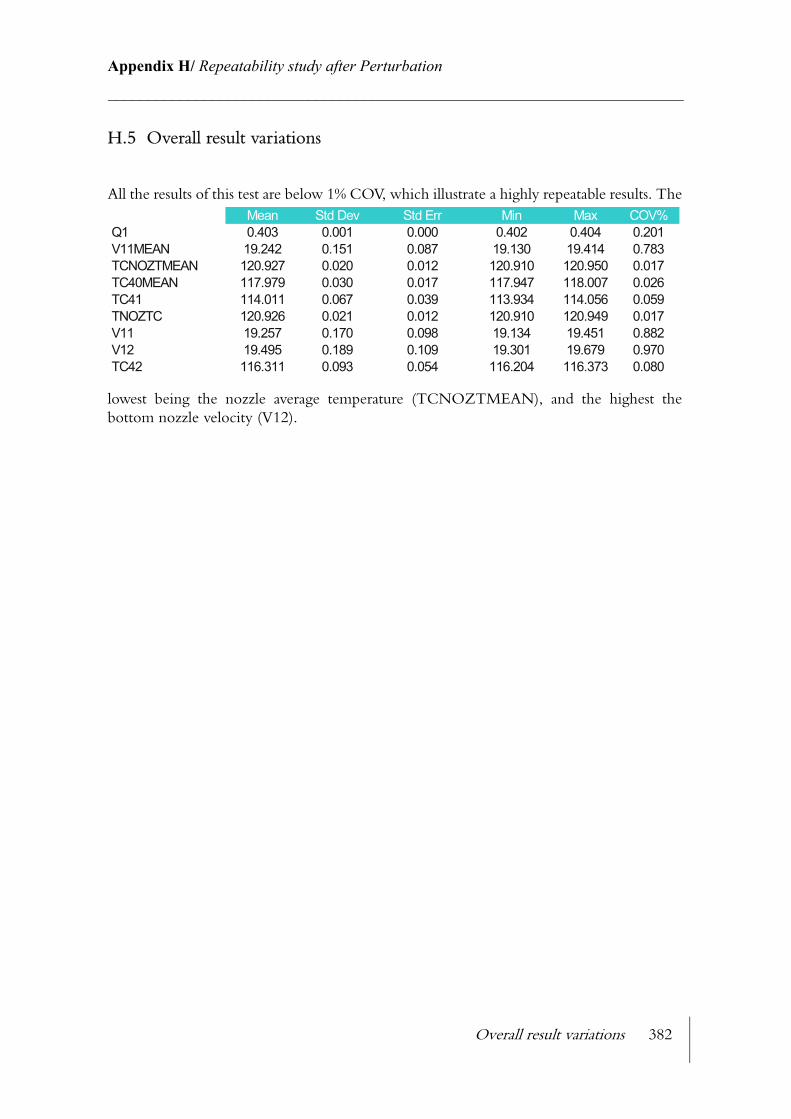
Overall result variations 382
Appendix H/ Repeatability study after Perturbation________________________________________________________________________
H.5 Overall result variations
All the results of this test are below 1% COV, which illustrate a highly repeatable results. The
lowest being the nozzle average temperature (TCNOZTMEAN), and the highest the bottom nozzle velocity (V12).
Mean Std Dev Std Err Min Max COV%Q1 0.403 0.001 0.000 0.402 0.404 0.201V11MEAN 19.242 0.151 0.087 19.130 19.414 0.783TCNOZTMEAN 120.927 0.020 0.012 120.910 120.950 0.017TC40MEAN 117.979 0.030 0.017 117.947 118.007 0.026TC41 114.011 0.067 0.039 113.934 114.056 0.059TNOZTC 120.926 0.021 0.012 120.910 120.949 0.017V11 19.257 0.170 0.098 19.134 19.451 0.882V12 19.495 0.189 0.109 19.301 19.679 0.970TC42 116.311 0.093 0.054 116.204 116.373 0.080
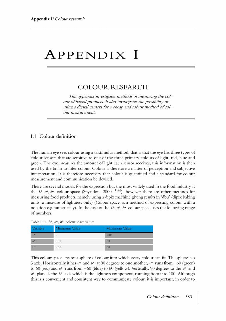
Colour definition 383
Appendix I/ Colour research________________________________________________________________________
APPENDIX I
COLOUR RESEARCHThis appendix investigates methods of measuring the col−
our of baked products. It also investigates the possibility of using a digital camera for a cheap and robust method of col−our measurement.
I.1 Colour definition
The human eye sees colour using a tristimulus method, that is that the eye has three types of colour sensors that are sensitive to one of the three primary colours of light, red, blue and green. The eye measures the amount of light each sensor receives, this information is then used by the brain to infer colour. Colour is therefore a matter of perception and subjective interpretation. It is therefore necessary that colour is quantified and a standard for colour measurement and communication be devised.
There are several models for the expression but the most widely used in the food industry is the colour space (Spyridon, 2000 [126]), however there are other methods for measuring food products, namely using a dipix machine giving results in ‘dbu’ (dipix baking units, a measure of lightness only) (Colour space, is a method of expressing colour with a notation e.g numerically). In the case of the colour space uses the following range of numbers.
This colour space creates a sphere of colour into which every colour can fit. The sphere has 3 axis. Horizontally it has and at 90 degrees to one another, runs from −60 (green) to 60 (red) and runs from −60 (blue) to 60 (yellow). Vertically, 90 degrees to the and
plane is the axis which is the lightness component, running from 0 to 100. Although this is a convenient and consistent way to communicate colour, it is important, in order to
Table I−1. colour space values
Variable Minimum Value Maximum Value
L* 0 100
a* -60 60
b* -60 60
L∗ a∗ b∗, ,
L∗ a∗ b∗, ,
L∗ a∗ b∗, ,
a∗ b∗ a∗b∗ a∗
b∗ L∗
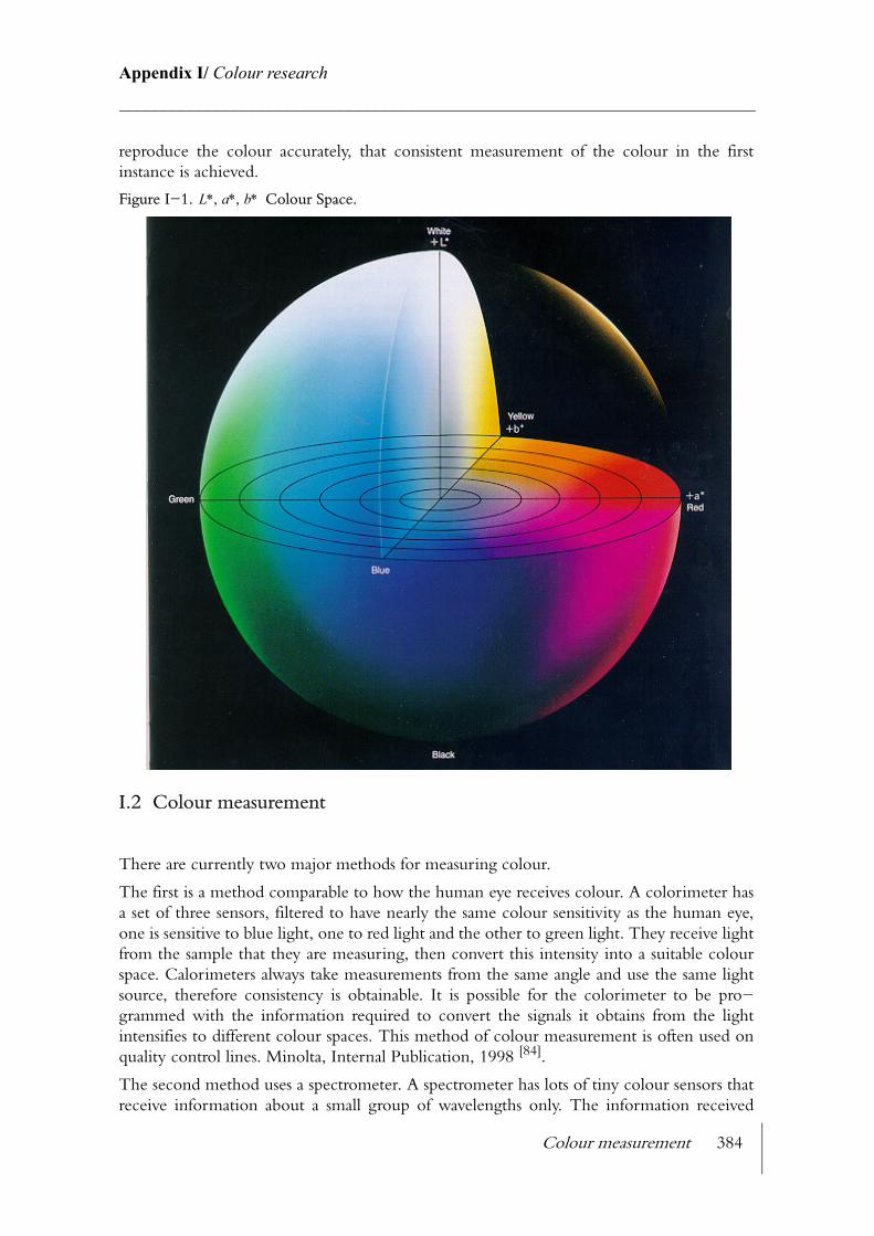
Colour measurement 384
Appendix I/ Colour research________________________________________________________________________
reproduce the colour accurately, that consistent measurement of the colour in the first instance is achieved.
Figure I−1. Colour Space.
I.2 Colour measurement
There are currently two major methods for measuring colour.
The first is a method comparable to how the human eye receives colour. A colorimeter has a set of three sensors, filtered to have nearly the same colour sensitivity as the human eye, one is sensitive to blue light, one to red light and the other to green light. They receive light from the sample that they are measuring, then convert this intensity into a suitable colour space. Calorimeters always take measurements from the same angle and use the same light source, therefore consistency is obtainable. It is possible for the colorimeter to be pro−grammed with the information required to convert the signals it obtains from the light intensifies to different colour spaces. This method of colour measurement is often used on quality control lines. Minolta, Internal Publication, 1998 [84].
The second method uses a spectrometer. A spectrometer has lots of tiny colour sensors that receive information about a small group of wavelengths only. The information received
L∗ a∗ b∗, ,
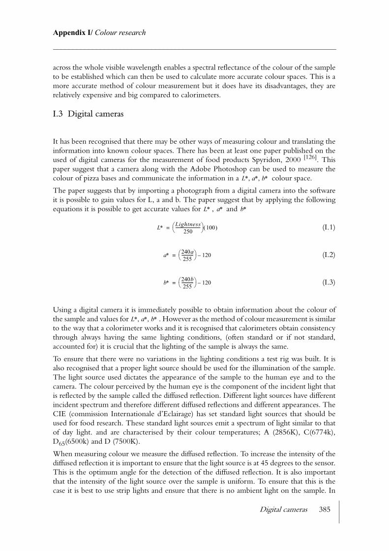
Digital cameras 385
Appendix I/ Colour research________________________________________________________________________
across the whole visible wavelength enables a spectral reflectance of the colour of the sample to be established which can then be used to calculate more accurate colour spaces. This is a more accurate method of colour measurement but it does have its disadvantages, they are relatively expensive and big compared to calorimeters.
I.3 Digital cameras
It has been recognised that there may be other ways of measuring colour and translating the information into known colour spaces. There has been at least one paper published on the used of digital cameras for the measurement of food products Spyridon, 2000 [126]. This paper suggest that a camera along with the Adobe Photoshop can be used to measure the colour of pizza bases and communicate the information in a colour space.
The paper suggests that by importing a photograph from a digital camera into the software it is possible to gain values for L, a and b. The paper suggest that by applying the following equations it is possible to get accurate values for , and
(I.1)
(I.2)
(I.3)
Using a digital camera it is immediately possible to obtain information about the colour of the sample and values for . However as the method of colour measurement is similar to the way that a colorimeter works and it is recognised that calorimeters obtain consistency through always having the same lighting conditions, (often standard or if not standard, accounted for) it is crucial that the lighting of the sample is always the same.
To ensure that there were no variations in the lighting conditions a test rig was built. It is also recognised that a proper light source should be used for the illumination of the sample. The light source used dictates the appearance of the sample to the human eye and to the camera. The colour perceived by the human eye is the component of the incident light that is reflected by the sample called the diffused reflection. Different light sources have different incident spectrum and therefore different diffused reflections and different appearances. The CIE (commission Internationale d’Eclairage) has set standard light sources that should be used for food research. These standard light sources emit a spectrum of light similar to that of day light. and are characterised by their colour temperatures; A (2856K), C(6774k), D65(6500k) and D (7500K).
When measuring colour we measure the diffused reflection. To increase the intensity of the diffused reflection it is important to ensure that the light source is at 45 degrees to the sensor. This is the optimum angle for the detection of the diffused reflection. It is also important that the intensity of the light source over the sample is uniform. To ensure that this is the case it is best to use strip lights and ensure that there is no ambient light on the sample. In
L∗ a∗ b∗, ,
L∗ a∗ b∗
L∗ Lightness250
------------------------- 100( )=
a∗ 240a255
------------ 120–=
b∗ 240b255
------------ 120–=
L∗ a∗ b∗, ,
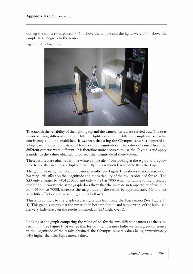
Digital cameras 386
Appendix I/ Colour research________________________________________________________________________
our rig the camera was placed 0.45m above the sample and the lights were 0.4m above the sample at 45 degrees to the sensor.
Figure I−2. Set up of rig.
To establish the reliability of the lighting rig and the camera, tests were carried out. The tests involved using different cameras, different light sources and different samples to see what consistency could be established. It was seen that using the Olympus camera as opposed to a Fuji gave the best consistency. However the magnitudes of the values obtained from the different cameras were different. It is therefore more accurate to use the Olympus and apply a model to the values obtained to correct the magnitude of these values.
These results were obtained from a white sample tile. From looking at these graphs it is pos−sible to see that in all cases displayed the Olympus is much less variable than the Fuji.
The graph showing the Olympus camera results (See Figure I−3) shows that the resolution has very little affect on the magnitude and the variability of the results obtained for . The S.D only changes by +0.4 at 3500 and only +0.24 at 7000 when switching to the increased resolution. However the same graph does show that the increase in temperature of the bulb from 3500k to 7000k increases the magnitude of the results by approximately 5% and has very little affect on the variability, all S.D bellow 1.
This is in contrast to the graph displaying results from only the Fuji camera (See Figure I−4). This graph suggests that the variation in both resolution and temperature of the bulb used has very little affect on the results obtained, all S.D high, over 2.
Looking at the graph comparing the value of for the two different cameras at the same resolution (See Figure I−5) we see that for both temperature bulbs we see a great difference in the magnitude of the results obtained, the Olympus camera values being approximately 14% higher than the Fuji camera values.
L∗
L∗
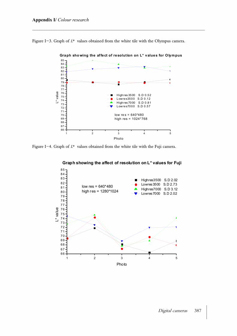
Digital cameras 387
Appendix I/ Colour research________________________________________________________________________
Figure I−3. Graph of values obtained from the white tile with the Olympus camera.
Figure I−4. Graph of values obtained from the white tile with the Fuji camera.
L∗
1 2 3 4 56667686970717273747576777879808182838485
low re s = 640*480high res = 1024*768
Graph sho wing the af fect of resolut ion on L* values for O lympusL*
val
ue
Photo
High res 3500 S .D 0 .52 Lowres3500 S .D 0 .12 High res 7000 S .D 0 .81 Lowres7000 S .D 0 .57
L∗
1 2 3 4 56667686970717273747576777879808182838485
low res = 640*480high res = 1280*1024
Graph showing the affect of resolution on L* values for Fuji
L* v
alue
Photo
Highres3500 S.D 2.02 Lowres3500 S.D 2.73 Highres7000 S.D 3.12 Lowres7000 S.D 2.02

Digital cameras 388
Appendix I/ Colour research________________________________________________________________________
Figure I−5. Graph comparing values of the white tile obtained with the Olympus and Fuji cameras.
In conclusion it is possible to see that he Olympus offers much more consistent results for values of (all S.D values are bellow 1) and at a higher magnitude than the Fuji. No direct comparison could be made between the two different cameras at there highest resolution as these resolutions differ.
A similar set of tests where carried out on the biscuit sample with similar results.
It is possible to see that as with the biscuit tile the Fuji has a larger S.D compared to the Olympus (See Figure I−6). It can also be seen that there is a difference in the magnitude of the values of for the same resolution with different cameras. The Olympus values being approximately 15% larger than the Fuji, this is similar to the results found with the white tile, Olympus values being 14% higher. Again no direct comparison could be made between the two different cameras at there highest resolution as these resolutions differ.
From looking at this graph (See Figure I−6) it is possible to see that the temperature of the bulb has very little affect on the value obtained. It is known that hue (in our case and
) can be measured independently of Lightness ( ) Minolta, Internal Publication, 1995[85]. It is possible to see from this graph that the values of for the biscuit tile do not seem to differ with different bulbs. Changing the bulb (as mention earlier) changes the incident ray spectrum and therefore the diffused reflection and appearance but does not however seem to affect the lightness.
L∗
1 2 3 4 56667686970717273747576777879808182838485
res = 640*480
Graph to showing the affect of each camera on the L* value at the same res L*
val
ue
Photo
Olympus3500 S.D 0.12 Olympus7000 S.D 0.57 Fuji3500 S.D 2.73 Fuji7000 S.D 2.02
L∗
L∗
L∗ a∗b∗ L∗
L∗
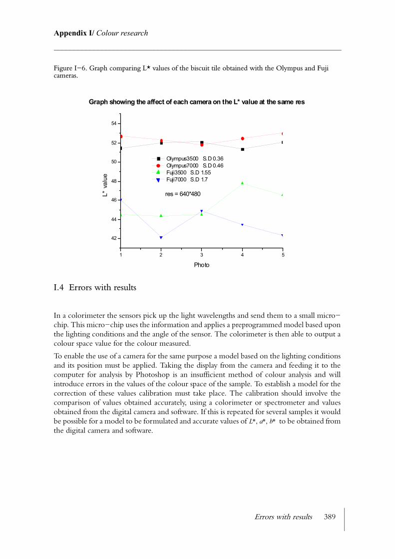
Errors with results 389
Appendix I/ Colour research________________________________________________________________________
Figure I−6. Graph comparing L* values of the biscuit tile obtained with the Olympus and Fuji cameras.
I.4 Errors with results
In a colorimeter the sensors pick up the light wavelengths and send them to a small micro−chip. This micro−chip uses the information and applies a preprogrammed model based upon the lighting conditions and the angle of the sensor. The colorimeter is then able to output a colour space value for the colour measured.
To enable the use of a camera for the same purpose a model based on the lighting conditions and its position must be applied. Taking the display from the camera and feeding it to the computer for analysis by Photoshop is an insufficient method of colour analysis and will introduce errors in the values of the colour space of the sample. To establish a model for the correction of these values calibration must take place. The calibration should involve the comparison of values obtained accurately, using a colorimeter or spectrometer and values obtained from the digital camera and software. If this is repeated for several samples it would be possible for a model to be formulated and accurate values of to be obtained from the digital camera and software.
1 2 3 4 5
42
44
46
48
50
52
54
res = 640*480
Graph showing the affect of each camera on the L* value at the same resL*
val
ue
Photo
Olympus3500 S.D 0.36 Olympus7000 S.D 0.46 Fuji3500 S.D 1.55 Fuji7000 S.D 1.7
L∗ a∗ b∗, ,

Additional screening design results 390
Appendix J/ DOE / Screening Design________________________________________________________________________
APPENDIX J
DOE / SCREENING DESIGN
I.1 Additional screening design results
TITLE OF EXPT. = TPRO Bake Tests - Screening 1DESIGN REF. NO. = D16/8
NUMBER OF REPLICATES = 4NUMBER OF BLOCKS = 4
VARIABLE -1 +1 UNITS-----------------------------------------------X1 Temp 130 230 CX2 fan speed 3 50 HzX3 T Damper -1 +1 m/sX4 B Damper -1 +1 m/sX5 T Radiation 130 520 CX6 B Radiation 130 520 CX7 Humidity 0 700 g/kgX8 Band Speed 0 15 X9 Bk1 X10 Bk2 -----------------------------------------------
RESPONSE = Top Colour L
ANOVA TABLE
POOLING METHOD USED = COEFFICIENTS WITH LESS THAN 5% CONTRIBUTION
SOURCE DF SUM OF SQUARES MEAN SQUARE F VALUE % SIGNIF. Regression 4 6493.43 1623.358 24.78603 100.00 *** Residuals 15 982.423 65.49487 Total 19 7475.854
R Squared = 0.8685872 Std error of estimate = 8.09289
REGRESSION COEFFICIENTS
SOURCE COEFFICIENT % CONTRIB. POOLED ERROR t VALUE % SIGNIF.E0 47.01E1 [Temp] -13.52 54.3 1.893 7.142 99.96 ***E2 [fan inverter settings] -4.176 5.2 1.893 2.207 95.63 *E12 [T Radiation] -8.291 20.4 1.893 4.381 99.91 ***E14 [Humidity] 4.114 5.0 1.893 2.174 95.35 *
95.0% Significance for 15 d.f.= 2.131 [*] 99.0% Significance for 15 d.f.= 2.947 [**] 99.9% Significance for 15 d.f.= 4.073 [***]
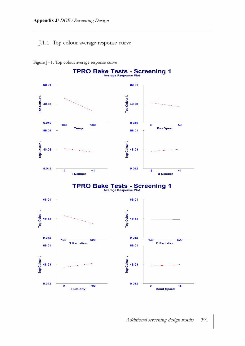
Additional screening design results 391
Appendix J/ DOE / Screening Design________________________________________________________________________
J.1.1 Top colour average response curve
Figure J−1. Top colour average response curve

Additional screening design results 392
Appendix J/ DOE / Screening Design________________________________________________________________________
J.1.2 Crumb springiness average response curve
Figure J−2. Srumb springiness average response curve

Additional screening design results 393
Appendix J/ DOE / Screening Design________________________________________________________________________
J.1.3 Density change average response curve
Figure J−3. Density change average response curve

394
Appendix K/ Input and Ouput List________________________________________________________________________
APPENDIX K
INPUT AND OUPUT LIST
InControl Project OVEN
Slot 0 Node2:1794-IB16 : 16 x 24VDC Inputs ADN0 (Node2)
Point DESCRIPTION InControl Tag
0 Emergency Stop Relay ESR_STS
1 Inverters fault Health Status INV_STS
2 Micro cirsuit breaker (MCB) Health Status MCB_STS
3 N2_S0_I3
4 OTC1 Duct High Temperature OCT1_DUCT
5 OTC2 Top Radiant High Temperature OTC2_TOPRAD
6 OTC3 Bottom Radiant High Temperature OTC3_BOTRAD
7 N2_S0_I7
8 N2_S0_I8
9 Band Position Proxy PX1 BAND_PX1
10 Band Position Proxy PX2 BAND_PX2
11 Band Position Proxy PX3 BAND_PX3
12 Band Position Proxy PX4 BAND_PX4
13 Door Solenoid Status DOOR_STS
14 OTC4 Duct2 High Temperature OTC4_DUCT2
15 OTC5 Duct3 High Temperature OTC5_DUCT3
Note: Bytes 0,1 are Input status
Slot 1 1794-OB16 : 16 x 24VDC Outputs ADN0 (Node2)
Point DESCRIPTION InControl Tag
0 Circulation Fan Enable Relay CFAN.RUN
1 Extraction Fan Enable Relay EFAN.RUN
2 Oven Band Motor Enable Relay BAND.RUN
3 Oven Band Motor FWD/REV Relay BAND.FWD
4 Top Radiant Heaters 1-3 Relay TOP_RAD_HEATER_13.CONTACT
5 Top Radiant Heaters 4-6 Relay TOP_RAD_HEATER_46.CONTACT
6 Bot Radiant Heaters 1-3 Relay BOT_RAD_HEATER_13.CONTACT
7 Bot Radiant Heaters 4-6 Relay BOT_RAD_HEATER_46.CONTACT
8 Duct Heater Contactor DUCT_HEATER.CONTACT
9 Duct Heater 2 Contactor DUCT_HEATER2.CONTACT
10 Duct Heater 3 Contactor DUCT_HEATER3.CONTACT
11 N2_S1_O11
12 N2_S1_O12
13 N2_S1_O13
14 N2_S1_O14
15 N2_S1_O15
Note:
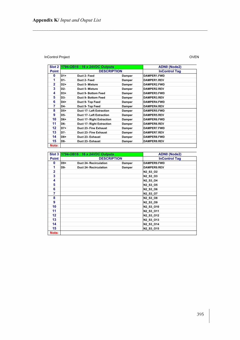
395
Appendix K/ Input and Ouput List________________________________________________________________________
InControl Project OVEN
Slot 2 1794-OB16 : 16 x 24VDC Outputs ADN0 (Node2)
Point DESCRIPTION InControl Tag
0 D1+ Duct 2- Feed Damper DAMPER1.FWD
1 D1- Duct 2- Feed Damper DAMPER1.REV
2 D2+ Duct 5- Mixture Damper DAMPER2.FWD
3 D2- Duct 5- Mixture Damper DAMPER2.REV
4 D3+ Duct 9- Bottom Feed Damper DAMPER3.FWD
5 D3- Duct 9- Bottom Feed Damper DAMPER3.REV
6 D4+ Duct 9- Top Feed Damper DAMPER4.FWD
7 D4- Duct 9- Top Feed Damper DAMPER4.REV
8 D5+ Duct 17- Left Extraction Damper DAMPER5.FWD
9 D5- Duct 17- Left Extraction Damper DAMPER5.REV
10 D6+ Duct 17- Right Extraction Damper DAMPER6.FWD
11 D6- Duct 17- Right Extraction Damper DAMPER6.REV
12 D7+ Duct 23- Fine Exhaust Damper DAMPER7.FWD
13 D7- Duct 23- Fine Exhaust Damper DAMPER7.REV
14 D8+ Duct 23- Exhaust Damper DAMPER8.FWD
15 D8- Duct 23- Exhaust Damper DAMPER8.REV
Note:
Slot 3 1794-OB16 : 16 x 24VDC Outputs ADN0 (Node2)
Point DESCRIPTION InControl Tag
0 D9+ Duct 24- Recirculation Damper DAMPER9.FWD
1 D9- Duct 24- Recirculation Damper DAMPER9.REV
2 N2_S3_O2
3 N2_S3_O3
4 N2_S3_O4
5 N2_S3_O5
6 N2_S3_O6
7 N2_S3_O7
8 N2_S3_O8
9 N2_S3_O9
10 N2_S3_O10
11 N2_S3_O11
12 N2_S3_O12
13 N2_S3_O13
14 N2_S3_O14
15 N2_S3_O15
Note:
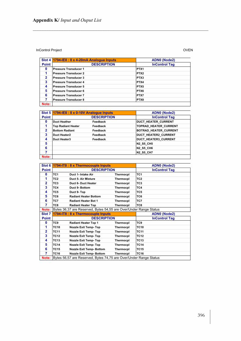
396
Appendix K/ Input and Ouput List________________________________________________________________________
InControl Project OVEN
Slot 4 1794-IE8 : 8 x 4-20mA Analogue Inputs ADN0 (Node2)
Point DESCRIPTION InControl Tag
0 Pressure Transducer 1 PTX1
1 Pressure Transducer 2 PTX2
2 Pressure Transducer 3 PTX3
3 Pressure Transducer 4 PTX4
4 Pressure Transducer 5 PTX5
5 Pressure Transducer 6 PTX6
6 Pressure Transducer 7 PTX7
7 Pressure Transducer 8 PTX8
Note:
Slot 5 1794-IE8 : 8 x 0-10V Analogue Inputs ADN0 (Node2)
Point DESCRIPTION InControl Tag
0 Duct Heather Feedback DUCT_HEATER_CURRENT
1 Top Radiant Heater Feedback TOPRAD_HEATER_CURRENT
2 Bottom Radiant Feedback BOTRAD_HEATER_CURRENT
3 Duct Heater2 Feedback DUCT_HEATER2_CURRENT
4 Duct Heater3 Feedback DUCT_HEATER3_CURRENT
5 N2_S5_CH5
6 N2_S5_CH6
7 N2_S5_CH7
Note:
Slot 6 1794-IT8 : 8 x Thermocouple Inputs ADN0 (Node2)
Point DESCRIPTION InControl Tag
0 TC1 Duct 1- Intake Air Thermocpl TC1
1 TC2 Duct 5- Air Mixture Thermocpl TC2
2 TC3 Duct 6- Duct Heater Thermocpl TC3
3 TC4 Duct 9- Bottom Thermocpl TC4
4 TC5 Duct 9- Top Thermocpl TC5
5 TC6 Radiant Heater Bottom Thermocpl TC6
6 TC7 Radiant Heater Bot 1 Thermocpl TC7
7 TC8 Radiant Heater Top Thermocpl TC8
Note: Bytes 36,37 are Reserved, Bytes 54,55 are Over/Under Range Status
Slot 7 1794-IT8 : 8 x Thermocouple Inputs ADN0 (Node2)
Point DESCRIPTION InControl Tag
0 TC9 Radiant Heater Top 1 Thermocpl TC9
1 TC10 Nozzle Exit Temp- Top Thermocpl TC10
2 TC11 Nozzle Exit Temp- Top Thermocpl TC11
3 TC12 Nozzle Exit Temp- Top Thermocpl TC12
4 TC13 Nozzle Exit Temp- Top Thermocpl TC13
5 TC14 Nozzle Exit Temp- Top Thermocpl TC14
6 TC15 Nozzle Exit Temp- Bottom Thermocpl TC15
7 TC16 Nozzle Exit Temp- Bottom Thermocpl TC16
Note: Bytes 56,57 are Reserved, Bytes 74,75 are Over/Under Range Status

397
Appendix K/ Input and Ouput List________________________________________________________________________
InControl Project OVEN
Slot 0 1794-IT8 : 8 x Thermocouple Inputs ADN1 (Node3)
Point DESCRIPTION InControl Tag
0 TC17 Nozzle Exit Temp- Bottom Thermocpl TC17
1 TC18 Nozzle Exit Temp- Bottom Thermocpl TC18
2 TC19 Nozzle Exit Temp- Bottom Thermocpl TC19
3 TC20 Duct 17- Extraction Left Thermocpl TC20
4 TC21 Duct 17- Extraction Right Thermocpl TC21
5 TC22 Duct 18- Extraction Left Thermocpl TC22
6 TC23 Duct 18- Extraction Right Thermocpl TC23
7 TC24 Duct 24- Recirculation Thermocpl TC24
Note: Bytes 0,1=Input status, Bytes 2,3 Reserved, Bytes 20,21 Over/Under Range
Slot 1 1794-IT8 : 8 x Thermocouple Inputs ADN1 (Node3)
Point DESCRIPTION InControl Tag
0 TC25 Plate Temperature Top Thermocpl TC25
1 TC26 Plate Temperature Top Thermocpl TC26
2 TC27 Plate Temperature Top Thermocpl TC27
3 TC28 Plate Temperature Bottom Thermocpl TC28
4 TC29 Plate Temperature Bottom Thermocpl TC29
5 TC30 Plate Temperature Bottom Thermocpl TC30
6 TC31 Duct 7- After Duct Heater Thermocpl TC31
7 TC32 OUTLET AIR Thermocpl TC32
Note: Bytes 22,23 Reserved, Bytes 40,41 Over/Under Range
Slot 2 1794-OE4 : 4 x 0-10V Analogue Outputs ADN1 (Node3)
Point DESCRIPTION InControl Tag
0 Circulation Fan Inverter Speed Reference CFAN.SPEED
1 Extraction Fan Inverter Speed Refernce EFAN.SPEED
2 Oven Band Inverter Speed Refernce BAND.SPEED
3 Steam Valve Steam Valve positionner out STEAM_VALVE
Note:
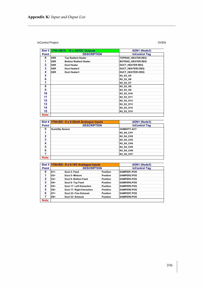
398
Appendix K/ Input and Ouput List________________________________________________________________________
InControl Project OVEN
Slot 3 1794-OB16 : 16 x 24VDC Outputs ADN1 (Node3)
Point DESCRIPTION InControl Tag
0 SSR Top Radiant Heater TOPRAD_HEATER.REQ
1 SSR Bottom Radiant Heater BOTRAD_HEATER.REQ
2 SSR Duct Heater DUCT_HEATER.REQ
3 SSR Duct Heater2 DUCT_HEATER2.REQ
4 SSR Duct Heater3 DUCT_HEATER3.REQ
5 N3_S3_O5
6 N3_S3_O6
7 N3_S3_O7
8 N3_S3_O8
9 N3_S3_O9
10 N3_S3_O10
11 N3_S3_O11
12 N3_S3_O12
13 N3_S3_O13
14 N3_S3_O14
15 N3_S3_O15
Note:
Slot 4 1794-IE8 : 8 x 4-20mA Analogue Inputs ADN1 (Node3)
Point DESCRIPTION InControl Tag
0 Humidity Sensor HUMIDITY.ACT
1 N3_S4_CH1
2 N3_S4_CH2
3 N3_S4_CH3
4 N3_S4_CH4
5 N3_S4_CH5
6 N3_S4_CH6
7 N3_S4_CH7
Note:
Slot 5 1794-IE8 : 8 x 0-10V Analogue Inputs ADN1 (Node3)
Point DESCRIPTION InControl Tag
0 D1+ Duct 2- Feed Position DAMPER1.POS
1 D2+ Duct 5- Mixture Position DAMPER2.POS
2 D3+ Duct 9- Bottom Feed Position DAMPER3.POS
3 D4+ Duct 9- Top Feed Position DAMPER4.POS
4 D5+ Duct 17- Left Extraction Position DAMPER5.POS
5 D6+ Duct 17- Right Extraction Position DAMPER6.POS
6 D7+ Duct 23- Fine Exhaust Position DAMPER7.POS
7 D8+ Duct 23- Exhaust Position DAMPER8.POS
Note:
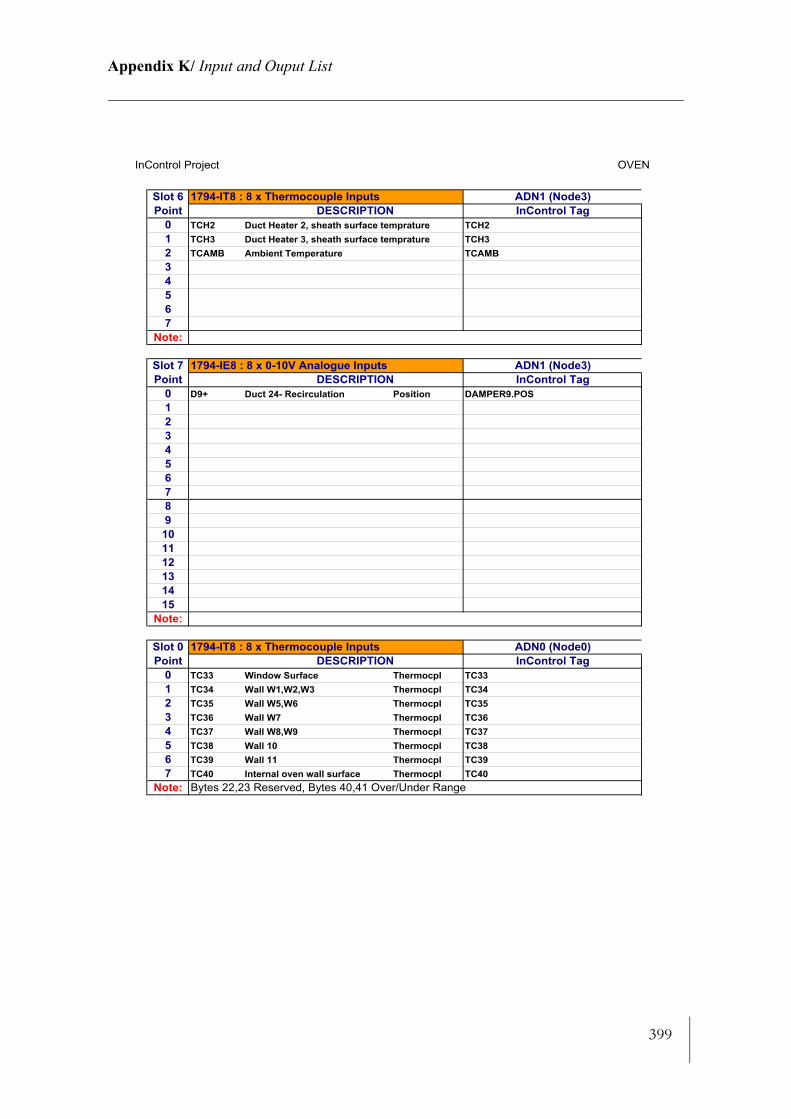
399
Appendix K/ Input and Ouput List________________________________________________________________________
InControl Project OVEN
Slot 6 1794-IT8 : 8 x Thermocouple Inputs ADN1 (Node3)
Point DESCRIPTION InControl Tag
0 TCH2 Duct Heater 2, sheath surface temprature TCH2
1 TCH3 Duct Heater 3, sheath surface temprature TCH3
2 TCAMB Ambient Temperature TCAMB
3
4
5
6
7
Note:
Slot 7 1794-IE8 : 8 x 0-10V Analogue Inputs ADN1 (Node3)
Point DESCRIPTION InControl Tag
0 D9+ Duct 24- Recirculation Position DAMPER9.POS
1
2
3
4
5
6
7
8
9
10
11
12
13
14
15
Note:
Slot 0 1794-IT8 : 8 x Thermocouple Inputs ADN0 (Node0)
Point DESCRIPTION InControl Tag
0 TC33 Window Surface Thermocpl TC33
1 TC34 Wall W1,W2,W3 Thermocpl TC34
2 TC35 Wall W5,W6 Thermocpl TC35
3 TC36 Wall W7 Thermocpl TC36
4 TC37 Wall W8,W9 Thermocpl TC37
5 TC38 Wall 10 Thermocpl TC38
6 TC39 Wall 11 Thermocpl TC39
7 TC40 Internal oven wall surface Thermocpl TC40
Note: Bytes 22,23 Reserved, Bytes 40,41 Over/Under Range
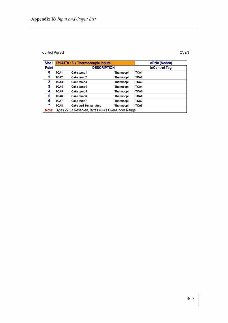
400
Appendix K/ Input and Ouput List________________________________________________________________________
InControl Project OVEN
Slot 1 1794-IT8 : 8 x Thermocouple Inputs ADN0 (Node0)
Point DESCRIPTION InControl Tag
0 TCA1 Cake temp1 Thermocpl TCA1
1 TCA2 Cake temp2 Thermocpl TCA2
2 TCA3 Cake temp3 Thermocpl TCA3
3 TCA4 Cake temp4 Thermocpl TCA4
4 TCA5 Cake temp5 Thermocpl TCA5
5 TCA6 Cake temp6 Thermocpl TCA6
6 TCA7 Cake temp7 Thermocpl TCA7
7 TCA8 Cake surf Temperature Thermocpl TCA8
Note: Bytes 22,23 Reserved, Bytes 40,41 Over/Under Range

401
Appendix L/ Velocity variation Investigation________________________________________________________________________
APPENDIX L
VELOCITY VARIATION INVESTIGATIONExperiment were performed to establish the velocity variation at the tray surface while the band is oscillating. The purpose of this experiment was to estimate where best to position the tin relative to the tray so even temperature and velocity can take place at the surface of the product. Tins were not positioned during this test. Velocity used for this trial was set to the maximum air velocity the velocity logger can measure (20 m/s). Logger velocity sensor from ScorpionTM was used to map the entire surface of the band as the product travel. See Figure L−1 shows the velocity variation along the tray during the test period. The band was oscillating forward and reverse. The tray surface (grey dash) represent the tray in which the product were positioned.
Figure L−1. Velocity variation over tray surface
1.0 1.2 1.4 1.6 1.8 2.0 2.2 2.4 2.6 2.8 3.0 3.2 3.4 3.61.0
1.5
2.0
2.5
3.0
3.5
4.0
4.5
5.0
5.5
6.0
6.5
7.0
Tray surfaceSensor position
Velocity variation along the nozzle arrangementversus time
1.500
2.250
3.000
3.750
4.500
5.250
6.000
6.750
7.500
Width of the tray [-]
Tim
e [m
in]
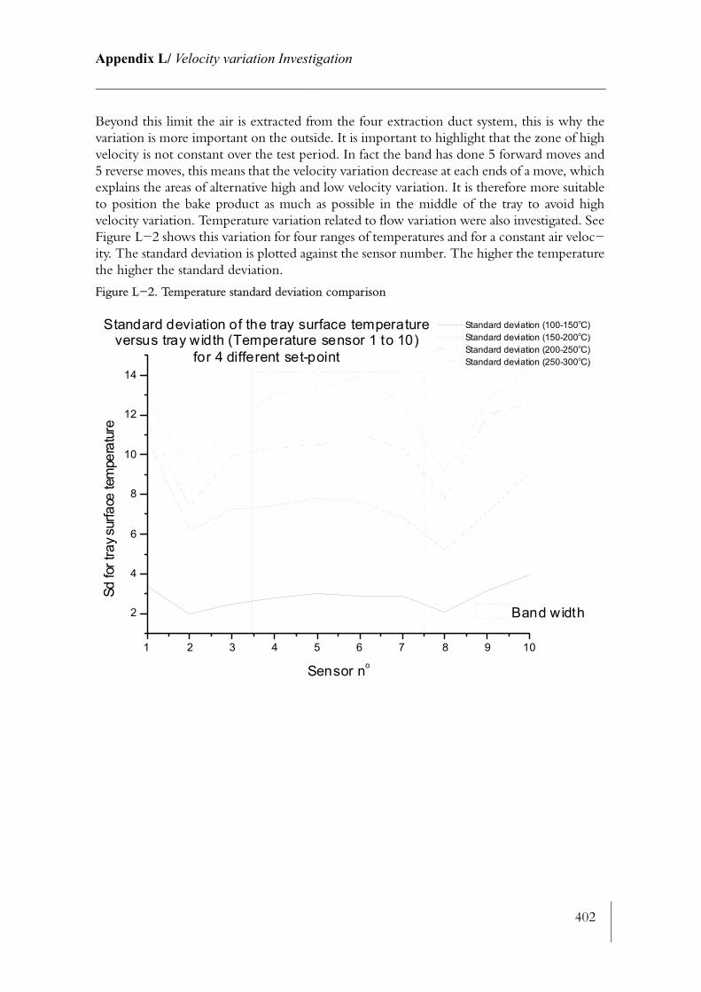
402
Appendix L/ Velocity variation Investigation________________________________________________________________________
Beyond this limit the air is extracted from the four extraction duct system, this is why the variation is more important on the outside. It is important to highlight that the zone of high velocity is not constant over the test period. In fact the band has done 5 forward moves and 5 reverse moves, this means that the velocity variation decrease at each ends of a move, which explains the areas of alternative high and low velocity variation. It is therefore more suitable to position the bake product as much as possible in the middle of the tray to avoid high velocity variation. Temperature variation related to flow variation were also investigated. See Figure L−2 shows this variation for four ranges of temperatures and for a constant air veloc−ity. The standard deviation is plotted against the sensor number. The higher the temperature the higher the standard deviation.
Figure L−2. Temperature standard deviation comparison
1 2 3 4 5 6 7 8 9 10
2
4
6
8
10
12
14
Standard deviation of the tray surface temperatureversus tray width (Temperature sensor 1 to 10)
for 4 different set-point
Band width
Sd fo
r tra
y sur
face
tem
pera
ture
Sensor no
Standard deviation (100-150oC) Standard deviation (150-200oC) Standard deviation (200-250oC) Standard deviation (250-300oC)
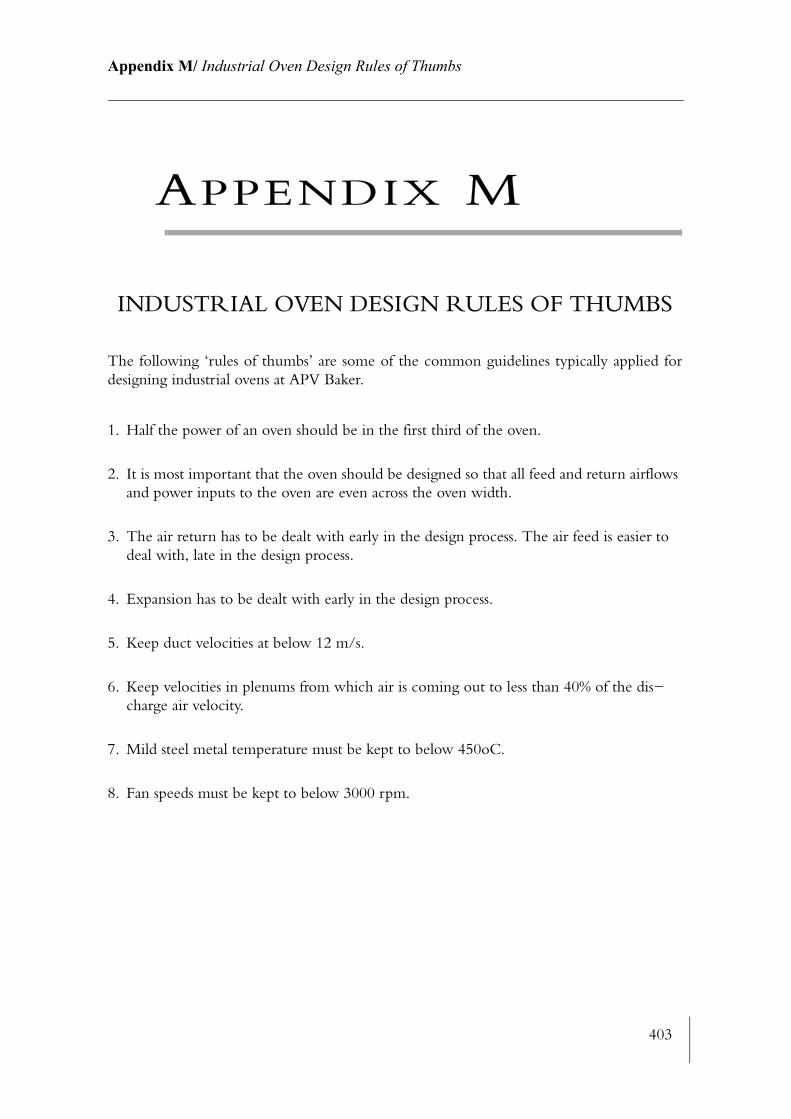
403
Appendix M/ Industrial Oven Design Rules of Thumbs________________________________________________________________________
APPENDIX M
INDUSTRIAL OVEN DESIGN RULES OF THUMBS
The following ‘rules of thumbs’ are some of the common guidelines typically applied for designing industrial ovens at APV Baker.
1. Half the power of an oven should be in the first third of the oven.
2. It is most important that the oven should be designed so that all feed and return airflows and power inputs to the oven are even across the oven width.
3. The air return has to be dealt with early in the design process. The air feed is easier to deal with, late in the design process.
4. Expansion has to be dealt with early in the design process.
5. Keep duct velocities at below 12 m/s.
6. Keep velocities in plenums from which air is coming out to less than 40% of the dis−charge air velocity.
7. Mild steel metal temperature must be kept to below 450oC.
8. Fan speeds must be kept to below 3000 rpm.
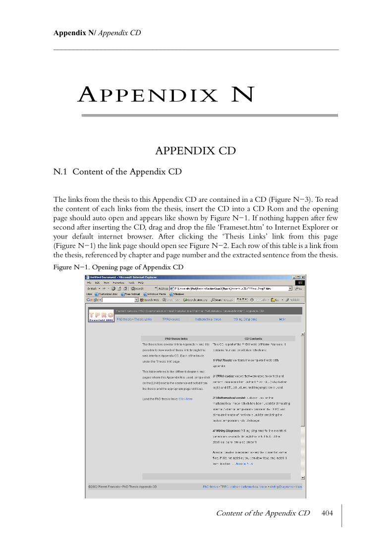
Content of the Appendix CD 404
Appendix N/ Appendix CD________________________________________________________________________
APPENDIX N
APPENDIX CD
N.1 Content of the Appendix CD
The links from the thesis to this Appendix CD are contained in a CD (Figure N−3). To read the content of each links from the thesis, insert the CD into a CD Rom and the opening page should auto open and appears like shown by Figure N−1. If nothing happen after few second after inserting the CD, drag and drop the file ‘Frameset.htm’ to Internet Explorer or your default internet browser. After clicking the ‘Thesis Links’ link from this page (Figure N−1) the link page should open see Figure N−2. Each row of this table is a link from the thesis, referenced by chapter and page number and the extracted sentence from the thesis.
Figure N−1. Opening page of Appendix CD

Content of the Appendix CD 405
Appendix N/ Appendix CD________________________________________________________________________
Figure N−2. Thesis link
Figure N−3. Appendix CD
406
References In Text
[1] AirflowTM
[2] Anderson and Kraber, 1999 [3] Andrews, 2001 [4] APV Baker, 2002 [5] APV Baker, 2002 [6] APV Baker, 2002 [7] APV Baker, 2002 [8] APV Baker, 2002 [9] APV Baker, 2002 [10] APV Baker, 2002 [11] APV Baker, 2002 [12] Ashworth and Armitage, 1980[13] Baik et al, 1999 [14] Bakers Federation, 1999[15] Bartlett, 2001[16] Boukadida and Ben Nasrallah, 2002 [17] Bourne et al, 1993 [18] Box et al, 1978 [19] Braud et al, 2001 [20] Bread and Bakery Products, 2001 [21] Brownell and Brown, 1941 [22] BTR, 1995[23] Calay et al, 1995[24] Campbell, 2002[25] Campbell and Shah, 1999 [26] Carlin, 1944[27] Cauvain et al, 1999[28] Charley, 1956 [29] Charley, 1950[30] Christensen et al, 1984 [31] Christensen and Singh, 1984 [32] Christenson et al, 1989 [33] Civille and Szczesniak, 1973 [34] Connan, 2000 [35] Cornford, 1969 [36] Cornforth J R, 1992 [37] Cortes, 1997 [38] Crompton, 2001 [39] Danesha, 2001 [40] Datta and Ni, 2001 [41] Datta and Zhang, 1999 [42] De Vries et al, 1988 [43] Denys and Hendrickx, 1999 [44] Dersh, 1989 [45] Elgidaily et al, 1969 [46] Elustondo et al, 2000
407
[47] Fanger, 1973 [48] Garrison and Peart, 1986[49] Ginzburg, 1969 [50] Gordon et al, 1979[51] Guibert, 1998 [52] Guy, 2000 [53] Guyer and Brownell, 1999 [54] Hall, 2001 [55] Hall et al, 1999 [56] Hallström et al, 1988 [57] Handleman et al, 1961[58] Hardman, 1988 [59] Herrington and Vernier, 1995 [60] Holger et al, 1977 [61] Holmes and Rahmel, 1978 [62] Holtz et al, 1984[63] Hood and Lowe, 1948[64] Hopkins, 2000 [65] Horace and Smith, 1960 [66] Howell, 2001 [67] Humphries and Griggs, 1977 [68] Incropera and De Witt, 1990 [69] Infrared Services Inc., 2000 [70] ISO 7730, 1995 [71] Kiemele et al, 1997 [72] Kreims and Möller, 1990 [73] Lane, 1983 [74] Lawson, 1994 [75] Luikov, 1966 [76] Marrs, 2001 [77] Mc Farlane, 1986 [78] Meffert, 1983 [79] Mellor, 1983 [80] Menjivar, 1990 [81] Microtherm, 1989[82] Milson and Kirk, 1980 [83] Milson and Kirk, 1980 [84] Minolta, Internal Publication, 1998 [85] Minolta, Internal Publication, 1995 [86] Mintel, 2001 [87] Mintel, 2001 [88] Mintel, 2001 [89] Mintel, 2001 [90] Mitchell et al, 1999[91] Montgomery, 2001 [92] Moreira, 2001 [93] Muir A, 1968 [94] Mälkki et al, 1984 [95] National Physical Laboratory, 2002

408
[96] Nelfood, 2002 [97] Obot, 1980 [98] Osborne and Turner, 1960[99] Ovadia and Walker, 1997[100] Park Cakes (Liverpool), 2001 [101] Pierrel, 1998 [102] Piller, 2001 [103] Pleass, 1986 [104] Profound, 2001[105] Pyler, 1988 [106] Rolston, 2001 [107] Rolston, 2001 [108] Rask and Hallström, 1989 [109] Richardson, 1986 [110] Rollin, 2000 [111] Sablani et al, 1998[112] Sakai and Hanzawa, 1994 [113] Saravacos, 1994[114] Sato et al, 1987 [115] Scarisbrick, 1994 [116] Setser, 1993 [117] Shah et al, 1999[118] Shariaty et al, 2000 [119] Shaughnessy, 1996 [120] Shaughnessy and Newborough, 1998 [121] Short et al, 1942 [122] Siegel and Howell, 1972[123] Singh, 2002[124] Skjöldebrand and Anderson, 1987 [125] Smith and Corripio, 1997[126] Spyridon, 2000 [127] Stear, 1990 [128] Sweat, 1994 [129] Szczesniak, 1963 [130] Tan et al, 2001 [131] Taylor and Kuyatt, 1994 [132] Tong and Lund, 1993 [133] Urrutia, 1997 [134] Vliet Van, 1999 [135] Wählby et al, 1999 [136] Walker, 1987 [137] Walker and Sparman, 1989 [138] Whaley and Ellis, 1986 [139] Wiggins, 1998 [140] Williamson M, 1996 [141] Wonderware, 2002 [142] Zanoni and Peri, 1993 [143] Zanoni et al, 1995 [144] Zanoni et al, 1994