countercyclical taxes in a monopolistically competitive environment

ARTICLE IN PRESS

Contents lists available at ScienceDirect

European Economic Review

European Economic Review 54 (2010) 692–717

0014-29

doi:10.1

� Tel.

E-m1 Se

Kim and

journal homepage: www.elsevier.com/locate/eer

Countercyclical taxes in a monopolistically competitive environment

Ioana R. Moldovan �

Department of Economics, University of Glasgow, Adam Smith Building, Glasgow G12 8RT, UK

a r t i c l e i n f o

Article history:

Received 19 November 2007

Accepted 8 December 2009Available online 4 January 2010

JEL classification:

E62

E32

H63

Keywords:

Tax policy

Countercyclical

Stabilization

Government debt

Welfare

21/$ - see front matter & 2009 Elsevier B.V. A

016/j.euroecorev.2009.12.006

: +44 141 330 8465.

ail address: [email protected]

e, for example, Auerbach and Feenberg (2000

Kim (2006).

a b s t r a c t

In the context of a neoclassical growth model with monopolistic competition, this paper

studies the stabilizing effects of countercyclical tax policy when the income tax rate has

an additional role of financing government budget deficits. Consistent with the

conventional wisdom, countercyclical taxes generally reduce aggregate volatility,

unless the fiscal response to debt accumulation is weak. The presence of monopoly

power enhances these effects. Even when automatic stabilizers successfully stabilize

business cycle fluctuations, countercyclical taxes are welfare inferior, due to reduced

precautionary saving motives. While, if the fiscal response to debt is weak and

countercyclical tax policy destabilizing, the increased precautionary saving motive is

not welfare enhancing as the asset accumulated is government debt rather than capital.

These results are generally robust. Nominal inertia may, however, dominate the

precautionary saving mechanism.

& 2009 Elsevier B.V. All rights reserved.

1. Introduction

The conventional wisdom states that countercyclical fiscal policies have stabilizing effects which help smooth outbusiness cycle fluctuations.1 Supporting evidence comes primarily in the form of empirical estimates of various fiscal rules,with a focus on the effects of such policies on output volatility. There is also a general consensus that countercyclical fiscalpolicy is most effective when it works via automatic stabilizers, which do not require active intervention from policymakers and therefore do not suffer from implementation lags. The focus of this paper is on the automatic stabilizerelement of tax policy, as captured by a progressive tax system. In a recession, the reduced income implies lower income taxrates, which attenuate the negative effects of the economic downturn. Furthermore, the relative effects of this automaticstabilizer on key macroeconomic variables will vary with the degree of monopoly distortion present in the economy. Thepresence of market power and profits in a monopolistically competitive environment affect the dynamics in the labormarket, especially by altering labor supply incentives, and can have significant implications for the stabilizing effects ofcountercyclical taxes.

Countercyclical taxes also impact on the government budget deficit. During economic downturns, tax revenues arelower, due to both lower income and lower countercyclical tax rates. Debt-financing any such changes creates a dynamiclink between current and future policies, as some aspects of future policy must adjust to balance the government budget in

ll rights reserved.

), Cohen and Follette (2000), Taylor (2000), Jones (2002), Auerbach (2003, 2005), Kletzer (2006) and

www.elsevier.com/locate/eer

dx.doi.org/10.1016/j.euroecorev.2009.12.006

mailto:[email protected]

ARTICLE IN PRESS

I.R. Moldovan / European Economic Review 54 (2010) 692–717 693

an intertemporal sense. This is important as expectations of future policies matter for the effectiveness of current policies.2

For example, higher expected future tax rates have adverse effects on current saving decisions. Focusing on thisintertemporal margin, Gordon and Leeper (2005) show that countercyclical policies can be counterproductive,exacerbating and prolonging the business cycle.

This paper brings together these aspects of policy. It investigates the stabilization role and welfare consequences ofcountercyclical tax policy in an environment distorted by monopolistic competition in the product market, and where thegovernment uses a single instrument, the income tax rate, to achieve its countercyclical objective and to satisfy theintertemporal government budget constraint. This dual role of fiscal policy is relevant, for example, in countries belongingto a monetary union where national governments have no control over monetary policy and must rely exclusively on fiscalpolicies to attain their goals. Also, governments generally have a wide range of objectives but a limited (and smaller) rangeof instruments, so a ‘‘one instrument—multiple objectives’’ policy is more likely to be the norm, rather than the exception.The government in the model economy adopts an endogenous simple rule where, in a manner which mimics theprogressivity of the tax system, the income tax rate responds positively to contemporaneous output fluctuations andpositively to lagged changes in government liabilities. The policy is evaluated for a range of empirically relevantparameters values.

Three main conclusions emerge. First, while it is generally true that countercyclical taxes reduce the volatility of someaggregate variables like output, investment, and consumption, others show an increase. In particular, employmentvariability is found to vary non-monotonically with the income elasticity of the tax rate, increasing under plausibleparameter configurations. Also, market imperfections matter for the stabilization effects of such policies.3 Themonopolistic competition distortion tends to enhance the stabilization effects of countercyclical taxes, relative to thecase of perfect competition. In the labor market, results depend on the degree of fiscal response to debt: a smaller responsemakes employment more volatile under monopolistic competition, while a stronger response reverses the results.

Second, considering the stabilization role of fiscal policy in isolation, there is a direct welfare benefit from the reducedvolatility. However, when people take direct account of the level of uncertainty when making decisions, then the reducedvolatility lowers the precautionary saving motive. Since the only asset available to households is physical capital, the lowerlevel of precautionary savings will reduce capital accumulation and, therefore, consumption in the long run. This secondeffect dominates in welfare calculations.

Third, when requiring taxes to adjust to ensure fiscal solvency, the strength of the tax rate adjustment to fulfil this rolecrucially impinges on the stabilization role of automatic stabilizers. A slow fiscal response to debt allows more medium-run debt accumulation and makes changes in aggregate variables highly persistent. Furthermore, countercyclical taxesbecome destabilizing. However, allowing for a stronger response restores the stabilizing properties of countercyclicaltaxes.4

In contrast to the results without government debt, the precautionary savings effects of increased volatility are notnecessarily welfare improving when there is a slow fiscal response to debt. This is because substitution between assetsleads to the accumulation of the riskless government bond and decumulation of capital, so that the long-run level ofconsumption is still lower under countercyclical taxes.

Along some dimensions, the results of this paper are broadly consistent with the conventional wisdom, ascountercyclical tax rates do tend to lower volatilities. In the same time, it is pointed out that some variables of interest,like employment, may become more volatile, especially in the presence of market distortions. The results also highlightthat precautionary saving motives, the nature of the assets into which such savings are channelled, and the associatedlong-run effects on consumption, are crucial in determining the welfare implications of government policies. In theabsence of precautionary savings, the stabilizing effects of countercyclical policy would unambiguously improve welfare,as Kletzer (2006) finds in an environment without capital.5 The precautionary savings mechanism may, however, bedominated by the costs of nominal inertia in a New Keynesian model with sticky prices. The welfare costs of nominalinertia in these types of models are, however, typically very high, such that their dominant effects may not be surprising.6

Finally, the paper shows the importance of a careful consideration of debt dynamics.The next section lays out the model, defines a symmetric equilibrium, and details the solution method and choice of

parameter values. The direct effects of countercyclical taxes are presented in Section 3. Section 4 analyzes the interactionbetween the stabilizing role of taxes and their fiscal financing role. Section 5 looks at the sensitivity of the results with

2 A selective list of articles which address this aspect includes: Bryant and Zhang (1996), Gordon and Leeper (2005), Leeper and Yang (2008) and Yang

(2007).3 The role of frictions and distortions for the effects of tax policy is also discussed by Andres and Domenech (2006). They find that constant

distortionary capital, labor, and consumption taxes help reduce output volatility (relative to lump-sum taxes), when rigidities due to price stickiness and

investment adjustment costs are sufficiently large.4 The notion that a more aggressive fiscal adjustment to debt dynamics is beneficial is also present in Leeper and Yang (2008). However, in the

context of a New Keynesian model with optimal monetary policy, it can be best to have a very small or mild fiscal feedback [Kollmann (2008), Schmitt-

Grohe and Uribe (2007), and Kirsanova and Wren-Lewis (2007)]. These results are discussed in Section 4.1.5 The link between volatility and capital accumulation is present in Kim and Kim (2006) and Kollmann (2008) who, for certain specifications of their

models, find that a countercyclical response of various distortionary taxes to exogenous technology shocks is optimal.6 This aspect is discussed further in Section 5.3.

ARTICLE IN PRESS

I.R. Moldovan / European Economic Review 54 (2010) 692–717694

respect to alternative specifications of preferences and of the government policy, and extends the model to allow fornominal rigidities. The last section concludes.

2. A model of monopolistic competition

The economy consists of a perfectly competitive final goods sector, a monopolistically competitive intermediate goodssector, households, and the government. There is one composite good used for consumption and investment, and acontinuum of differentiated goods used as inputs in the production of the final good.

2.1. The private sector

The final goods sector. Final goods are produced by an infinite number of firms in a perfectly competitive market. Theavailable technology is of the Dixit–Stiglitz type

Yt ¼

Z 1

0Y ðe�1Þ=e

it di

!e=ðe�1Þ

; ð1Þ

where Yit is the amount of each intermediate good i and e is the constant elasticity of substitution between them. Themarkup, denoted by m¼ e=ðe�1Þ, represents the degree of monopoly power of intermediate goods producers.

Firms take as given the prices of intermediate goods and, subject to the available technology, choose the amount of eachintermediate input, Yit , to maximize profits, Pt ¼ Yt�

R 10 PitYit di. The first order condition yields the demand for

intermediate goods

Yit ¼ Pm=ð1�mÞit Yt ; 8i: ð2Þ

The price elasticity of this demand is constant and depends negatively on the markup, m. The zero profit condition gives thefollowing price index:

1¼

Z 1

0P1=ð1�mÞ

it di

!1�m

: ð3Þ

The intermediate goods sector. The intermediate sector consists of a continuum of monopolistically competitive firmsindexed by i and of measure 1. Each firm i produces a unique good, using capital, Kit�1, and labor, Hit , as inputs in theproduction process

Yit ¼ ztKait�1H1�a

it �f; a 2 ð0;1Þ: ð4Þ

The production function exhibits increasing returns to scale due to the presence of positive fixed costs, f, but has adecreasing average cost and a marginal cost independent of scale. Total factor productivity, zt , affects all firmssymmetrically and follows an exogenous stationary process, lnzt ¼ rzlnzt�1þez

t , with persistence parameter rz 2 ð0;1Þ andrandom shocks ez

t � iid Nð0;s2z Þ.

The monopolistic producers take as given the capital rental rate, rt , and the real wage, wt , as well as the amount of finalgoods, Yt , and given the production technology (4) and the demand for their own good (2), they choose factor inputs andthe price level to maximize profits. Optimally, the price is set as a markup over marginal cost

Pit ¼ mMCit ¼ m Orat w1�at

1

zt

� �;

where O� ½a�að1�aÞa�1�. The choices of capital and labor inputs are such that their marginal products exceed rental prices

by the same constant markup m. (See Appendix A for more details.)Focusing on a symmetric equilibrium, the values of capital and labor are Kit�1 ¼ Kt�1 and Hit ¼Ht , and the aggregate final

goods production can be written as

Yt ¼ Ft�f;

where Ft � ztKat�1H1�a

t denotes aggregate output inclusive of fixed costs. Prices are the same across firms and equal to unity,by the zero-profit condition of final goods producers. The aggregate profits of the intermediate goods producers,Ft ¼ ð1�1=mÞFt�f, are rebated to households in lump-sum fashion. Monopoly power has a positive effect on profits butfixed costs a negative one.

Households. The representative household chooses consumption, Ct , capital, Kt , hours worked, Ht , and one-period risk-free government bonds, Bt , to maximize expected lifetime utility

E0

X1t ¼ 0

bt½logCtþwlogð1�HtÞ�

ARTICLE IN PRESS


subject to the budget constraint

CtþKtþBt r ð1�ttÞðrtKt�1þwtHtþFtÞþð1�dÞKt�1þRt�1Bt�1:

Et is the mathematical expectation conditional on information available at time t, b is the discount factor ð0obo1Þ, and wis the relative weight on leisure in the utility. At the beginning of every period, households rent capital and labor tointermediate goods producing firms. At the end of each period, they receive capital rental payments, rtKt�1, wages, wtHt ,and dividends, Ft , all of which are being taxed by the government at a single income tax rate, tt . Also included inhousehold income are the value of undepreciated capital and payments on government debt. d is the capital depreciationrate ð0rdr1Þ and Rt is the gross real interest rate on one-period government bonds.

The first order condition for labor and the Euler equations for consumption and bonds, together with the twotransversality conditions for capital and bonds, characterize the households’ optimal choices. (See Appendix A for thedetailed expressions.)

2.2. The government

The government consumes an exogenous amount of final goods. They are financed by distortionary taxation and byissuing government debt. The period government budget constraint is

Gt ¼ ttYtþBt�Rt�1Bt�1; ð5Þ

where Gt represents government consumption, ttYt distortionary tax revenues, Bt the amount of newly issued governmentdebt, and Rt�1Bt�1 the level of outstanding government liabilities. Government consumption follows a stationary AR(1)process, lnGt ¼ ð1�rGÞlnGþrGlnGt�1þeG

t , with persistence parameter rG 2 ð0;1Þ and random shocks eGt � iid Nð0;s2

GÞ.The income tax rate tt responds to contemporaneous output fluctuations and to lagged changes in the level of

government indebtedness as follows:

lntt ¼ dþylnYtþglnBt�1; yZ0; g40; ð6Þ

where d is a constant term.The dependence of the tax rate on output reflects the stabilization aspect of tax policy which occurs automatically,

without intervention from policy makers. A positive y indicates a countercyclical tax policy, an automatic response of thetax rate, which declines during recessions and increases during booms. In a broad way, this policy mimics the progressivityof the tax system. Fiscal financing is tax policy’s other component. When the government issues debt to balance thebudget, it must adjust future policies to service debt obligations and achieve intertemporal budget balance. The response oftaxes to the level of government indebtedness must be such that the policy is sustainable. Only a certain range of values ofg ensures that debt does not grow faster than the real interest rate, so that the transversality condition for debt holds. Aminimal response of future taxes to current debt levels is required for equilibrium.

An implicit, and plausible, assumption is that the government cannot implement subsidies to remove the distortionarising from imperfect competition.

2.3. Equilibrium

The dynamics of the economy are characterized by the first order conditions of households and firms, governmentpolicies, the government budget constraint, the aggregate resource constraint, and the exogenous processes. A symmetricequilibrium can be defined as:

Definition 1. A symmetric equilibrium is an allocation sequence fCt ;Ht ;Ktg1t ¼ 0, a price sequence fPt ;wt ; rt ;Rtg

1t ¼ 0, a

sequence of government policy variables fGt ; tt ;Btg1t ¼ 0, and initial conditions fK�1;B�1; z0g such that:

(i)
given prices, government policies, and initial conditions, the allocation sequence solves the households’ utilitymaximization problem and the final goods producers’ profit maximization problem,
(ii)
given factor prices, government policies, and initial conditions, the allocation sequence and the price sequence fPtg1t ¼ 0
solve the profit maximization problem of intermediate goods producing firms,
(iii) fiscal policy variables follow the specified processes and the government budget constraint is satisfied at all times, and (iv) all markets clear.
2.4. The solution

In the absence of a closed form solution, the equilibrium conditions are approximated around the deterministic steadystate. To compute welfare, a second order accurate solution of the model was employed, using the algorithm in Schmitt-Grohe and Uribe (2004).

ARTICLE IN PRESS

Table 1Parameter values used in simulations.

Parameter Value

b 0.99

w 3.0

a 0.36

j 0.193

d 0.015

B=Y 0:44� 4

G=Y 0.20

t 0.22

rG 0.925

sG 0.014

rz 0.95

sz 0:009 ðm¼ 1:0Þ

0:006 ðm¼ 1:4Þ

(

y [0,2]

m f1:0;1:4g


2.5. Model calibration

The model is calibrated to a quarterly frequency and follows the usual parameterization in the literature.7 Table 1 givessome of the assumed and implied parameter values. The relative weight on leisure, w, is such that the proportion of timespent working averages 20%. The capital depreciation rate d matches the average investment-output ratio of 0.17 in the U.S.data (1947:1–2005:4). The fixed costs f are set at the value needed to ensure profits in the deterministic steady state arezero. With a markup value m of 1.4, the degree of monopolistic competition is moderate, in the context of a range 1.1–2.4identified in the literature and, furthermore, consistent with values most commonly encountered in real models. Undermonopolistic competition, the standard deviation of the technology shock is re-scaled, to allow for accurate comparisonsacross economies with different degrees of market power.8

The elasticity of the tax rate with respect to output, y, is allowed to vary in the ½0;2� range. This parameter representsthe magnitude of the endogenous response of the income tax rate to output fluctuations, i.e. how countercyclical tax policyis. The specific range reflects available evidence: Blanchard and Perotti (2002) rely on institutional information to estimatethe quarterly elasticity of tax revenues with respect to output and obtain an average over the post-war period of 2.08, withspecific values ranging from 1.58 in 1947:Q1 to 1.63 in 1960:Q1 to 2.92 in 1997:Q4. This implies an average value of y, theelasticity of tax rates to output, of approximately 1 with plausible values of almost 2. Using the TAXSIM model of taxreturns, Auerbach and Feenberg (2000) provide annual evidence on the change in the income tax rate for a 1% change inincome. This implies an approximate value of y between 0.32 and 0.92. Cohen and Follette (2000) give similar estimates.

In the presence of government debt, the steady state debt-output ratio corresponds to an annual average ratio ofprivately held federal debt to GDP of 0.44 [1947–2005, Table 78, Economic Report of the President (2006)]. Consistent withthis value and a government spending-output ratio of 0.2 is an income tax rate t of 0.22.9 The parameter g, measuring theresponse of future taxes to the level of government debt, is set so as to ensure the sustainability of the fiscal policy. For allvalues considered, a unique equilibrium exists. With only one period adjustment lag, plausible values of g must be on thelower side of the identified range. For illustration purposes, g¼ 0:25 is chosen as a ‘‘low’’ value and 0.75 as ‘‘high’’ value.10

2.6. Monopolistic competition

Monopolistic competition differs from perfect competition because firms set prices above marginal costs and makeprofits on the margin.11 Any increase in output exceeds the corresponding increase in real labor costs. In comparison toperfect competition, this translates into larger percent changes in output for any given change in employment. Thepresence of monopoly power changes the relative weight of the income and substitution effects that arise from shocks tothe economy: changes in employment tend to be lower, while variations in output, consumption, and investment are

7 See, for example, Braun (1994), Jones (2002), Yang (2005), Leeper and Yang (2008), and Trabandt and Uhlig (2006).8 The presence of market power and increasing returns to scale leads to Solow residuals that tend to overestimate the true technology factor. See

Hornstein (1993), Rotemberg and Woodford (1995), and Devereux et al. (1993) for more detailed discussions.9 This value of the average marginal income tax rate lies in the range of estimates in the literature. Akhand and Liu (2002) give a rate of

approximately 0.2, while Braun (1994) and Auerbach and Feenberg (2000) report a value of 0.25.10 The simulations conducted below suggest that this parameter range is consistent with the differing speeds of fiscal adjustment found in the

empirical work of Chung and Leeper (2007). Note that too low a value of g will violate the transversality condition for debt and the intertemporal

government budget constraint. Under the described parameterization, the minimum value of g that ensures solvency is 0.22.11 See Blanchard and Kiyotaki (1987), Rotemberg and Woodford (1995), and Benassy (2002) for detailed expositions on monopolistic competition.

ARTICLE IN PRESS

0 2 4 6 8−0.08

−0.06

−0.04

−0.02Perfect Competition

Con

sum

ptio

n

0 2 4 6 80

0.1

0.2

Em

ploy

men

t

0 2 4 6 8−1

−0.5

0

0.5

Inve

stm

ent

0 2 4 6 80

0.05

0.1

years

Out

put

0 2 4 6 8−0.08

−0.06

−0.04

−0.02Monopolistic Competition

0 2 4 6 80

0.1

0.2

0 2 4 6 8−0.5

0

0.5

0 2 4 6 80

0.05

0.1

years

θ = 0.0θ = 1.0

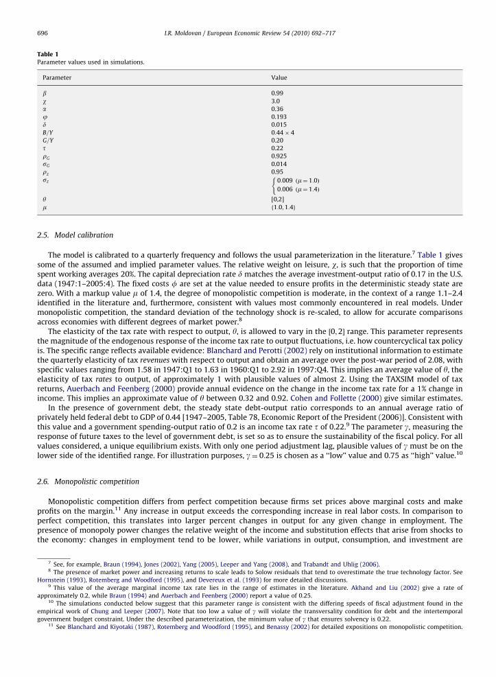
Fig. 1. Impulse responses to a 1% increase in government spending under perfect competition (left column) and monopolistic competition (right column):

acyclical tax rates (y¼ 0, solid lines) and countercyclical tax rates (y¼ 1:0, dash lines).


larger. In combination with the dynamics induced by the government’s tax policy, this aspect will prove important for thestabilization properties of countercyclical taxes.

3. The stabilizing role of countercyclical taxes

To better assess the direct effect of countercyclical taxes, it is assumed, initially, that bonds are in zero net supply andthat the government relies exclusively on lump-sum taxes to balance its budget every period and intertemporally.12 Lump-sum taxes replace government debt in the budget constraints of the government and households, and the tax policy rulebecomes

lntt ¼ dþylnYt ; yZ0: ð7Þ

3.1. An accounting of shocks

Two types of shocks hit the economy and their characteristics are important in assessing the stabilization role ofcountercyclical taxes.

A positive government spending shock. Exogenous and persistent increases in government spending reduce the presentvalue of privately available after-tax income. This leads to an increase in the labor supply and higher equilibriumemployment and output, but crowds out private consumption and investment. In the presence of market power, thenegative effects of an increase in government spending are, however, more modest: a consequence of the fact that the

12 In Section 4, the fiscal financing role of taxation is considered alongside its stabilization role.

ARTICLE IN PRESS

0 2 4 6 80.4

0.6

0.8

1Perfect Competition

Con

sum

ptio

n

0 2 4 6 8−0.5

0

0.5

1

Em

ploy

men

t

0 2 4 6 80

5

10

Inve

stm

ent

0 2 4 6 80

1

2

years

Out

put

0 2 4 6 80.4

0.6

0.8

1Monopolistic Competition

0 2 4 6 8−0.5

0

0.5

1

0 2 4 6 80

5

10

0 2 4 6 80

1

2

years

θ = 0.0

θ = 1.0

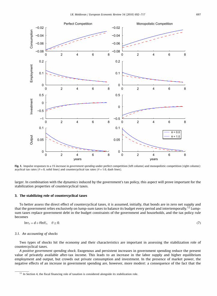
Fig. 2. Impulse responses to a 1% increase in the technological factor under perfect competition (left column) and monopolistic competition (right

column): acyclical tax rates (y¼ 0, solid lines) and countercyclical tax rates (y¼ 1:0, dash lines).


change in output derived from an increase in employment exceeds the change in labor costs. Fig. 1 presents the responsesof consumption, hours worked, investment, and output under the two environments.

When taxes are countercyclical, the increased output leads to a contemporaneous increase in the income tax rate,which has adverse effects on all aggregate variables. The positive response of employment is reduced and so is the increasein output. Persistence of the shock creates expectations of higher future tax rates and lower expected after-tax rates ofreturn on capital. Investment thus declines even further (relative to the case of acyclical tax rates) and capitalaccumulation is adversely affected. While in a perfectly competitive economy the change in taxes has virtually nocontemporaneous effect on consumption, this effect is more substantial under monopolistic competition. The difference ismainly because, given the exogenous shock, monopolistic competition gives rise to a larger percent change in output andtax rates than perfect competition.

Overall, when faced with government spending shocks, countercyclical taxes help reduce the magnitude of changes inhours worked and output, but amplify the responses of investment and consumption.

A positive technology shock. A persistent increase in technology raises the demand for capital and labor. Higher wagesmake households substitute current work for future leisure. This substitution effect dominates the incentive to work lessdue to the higher income and leads to overall higher equilibrium employment, output, investment, and consumption.

These effects are, however, altered when tax rates become countercyclical which means that they increase when outputis above its long run level (Fig. 2). Such a policy reduces the positive income effect via higher tax payments; it also lowersafter-tax real wages and capital rental rates. The substitution effect dominates and reduces the overall increase inemployment or it can even cause hours worked to decline. As before, the persistence of the tax rate induces expectations oflower after-tax rates of return on capital and deters investment. Output, consumption, and investment increase less than iftaxes were not countercyclical. Again, the effects on consumption are stronger in the presence of market power.

Employment and technology shocks. The response of employment to changes in technology deserves further attention. Inresponse to a positive technology shock, hours worked can decline when taxes are countercyclical. This can occur underboth perfect and monopolistic competition. The main factors influencing the results are the degree of monopoly power, theprogressivity of the tax system, and the persistence of the technology shock. All three contribute to a reduced employment

ARTICLE IN PRESS

0 1 2 3 4 5 6 7 8−0.4

−0.3

−0.2

−0.1

0

0.1

0.2

0.3

0.4Employment under monopolistic competition

years

%

θ = 0.0θ = 0.74θ = 1.0θ = 1.25

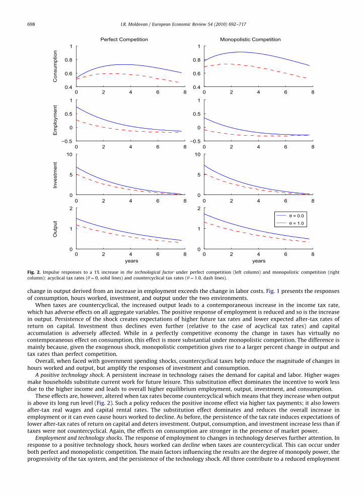
Fig. 3. Impulse responses of hours worked to a 1% increase in the technological factor under monopolistic competition (m¼ 1:4) for y equals to 0.0 (solid

line), 0.74 (diamonds), 1.0 (dash line), and 1.25 (dash-dot line).


response. Market power (larger value of the markup m) enhances the positive income effect, diminishing the supply oflabor. The progressivity of the tax system affects the magnitude of changes in the tax rate and the after-tax wage rate, thusaccentuating the substitution effect, which again reduces employment. Finally, the more persistent the shock, the lowerthe incentive of households to supply labor.

Conditional on the persistence of technology shocks and the amount of market power, one can find a value of thecountercyclical parameter, y, for which employment shows virtually no contemporaneous response to changes inproductivity. Under the current calibration, y is approximately 1.81 under perfect competition and 0.74 undermonopolistic competition—plausible values of y according to the range identified in the literature. Fig. 3 provides anillustration of the monopolistically competitive case. For values of y greater than y employment decreases when apersistent positive technology shock occurs. More important, the higher is y, for y4y, the larger the decline in hoursworked, which represents a destabilizing effect of countercyclical taxes. For less persistent technological changes, thevalues of y required to obtain such effects would be very large and would exceed the plausible range ½0;2�.

3.2. Stabilization effects

The conventional notion of stabilization policies is that they reduce the volatility of aggregate variables, and especiallythe volatility of output. But the focus on output volatility is not necessarily well grounded. As households are primarilyconcerned with the utility derived from the consumption of various quantities (including leisure), it is the volatility ofconsumption and hours worked that is relevant.

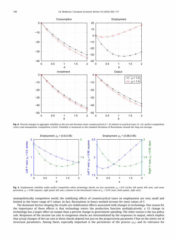
In the current model, countercyclical tax policies reduce output volatility measured as the standard deviation offluctuations around the long-run average. The result is consistent with the literature. Countercyclical taxes are also foundto decrease the volatility of investment and consumption. Fig. 4 shows the percent changes in aggregate volatility inducedby a countercyclical tax ðy40Þ relative to a non-countercyclical tax ðy¼ 0Þ. For y equal to 1, for example, the volatility ofthese variables is reduced by about 20–25%. Notice that, in the case of output, consumption, and investment, therelationship between volatility and the degree of progressivity of the tax system is almost linear. Also, countercyclical taxeshave a stronger effect under monopolistic competition than under perfect competition, but differences are small.

With respect to employment, however, results are a lot more sensitive to the values of the progressivity parameter yand the markup m. Employment volatility under perfect competition is a non-monotonic function of y, decreasing forsmaller responses of the tax rate to output fluctuations, and then increasing as these endogenous changes become larger.But, for all values of y considered, a countercyclical tax rate always reduces the variability of hours worked. In contrast, in a

ARTICLE IN PRESS

0 0.5 1 1.5 2−40

−30

−20

−10

0Consumption

θ0 0.5 1 1.5 2

−40

−30

−20

−10

0

10

20Employment

θ

0 0.5 1 1.5 2−50

−40

−30

−20

−10

0Investment

θ0 0.5 1 1.5 2

−50

−40

−30

−20

−10

0Output

θ

μ = 1.0μ = 1.4

Fig. 4. Percent changes in aggregate volatility as the tax rate becomes more countercyclical ðy40Þ relative to acyclical taxes ðy¼ 0Þ: perfect competition

(stars) and monopolistic competition (circle). Volatility is measured as the standard deviation of fluctuations around the long-run average.

0.5 1 1.50

1

2Employment: ρz = (0.8,0.95)

θ

Left

Y−a

xis:

ρz =

0.8

, circ

les

0 21

1.5

2

0.5 1 1.51.5

2

2.5Employment: ρz = (0.98,0.95)

θ

Left

Y−a

xis:

ρz =

0.9

8, s

quar

es

0 21

1.5

2

Rig

ht Y

−axi

s: ρ

z = 0

.95,

sta

rs

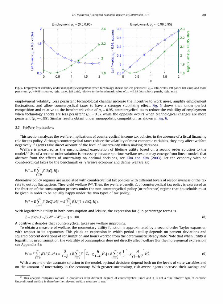
Fig. 5. Employment volatility under perfect competition when technology shocks are less persistent, rz ¼ 0:8 (circles, left panel, left axis), and more

persistent, rz ¼ 0:98 (squares, right panel, left axis), relative to the benchmark value of rz ¼ 0:95 (stars, both panels, right axis).


monopolistically competitive world, the stabilizing effects of countercyclical taxes on employment are very small andlimited to the lower range of y values. In fact, fluctuations in hours worked increase for most values of y.

The dominant factors shaping the results are stabilization effects associated with changes in technology. One reason forthe importance of these effects is that technology enters the production function multiplicatively: a 1% change intechnology has a larger effect on output than a percent change in government spending. The other reason is the tax policyrule. Responses of the income tax rate to exogenous shocks are intermediated by the responses in output, which impliesthat actual changes of the tax rate to these shocks depend not just on the progressivity parameter y but on the entire set ofstructural parameters. Among them, especially important is the persistence of the process ðrzÞ and its relevance for

ARTICLE IN PRESS

0.5 1 1.50.5

1

1.5

2Employment: ρz = (0.8,0.95)

θ

Left

Y−a

xis:

ρz

= 0.

8, c

ircle

s

0 21.8

2

2.2

2.4

0 0.5 1 1.5 22.8

3

3.2

3.4

3.6

3.8Employment: ρz = (0.98,0.95)

θ

Left

Y−a

xis:

ρz =

0.9

8, s

quar

es

1.8

1.9

2

2.1

2.2

2.3

Rig

ht Y

−axi

s: ρ

z = 0

.95,

sta

rs

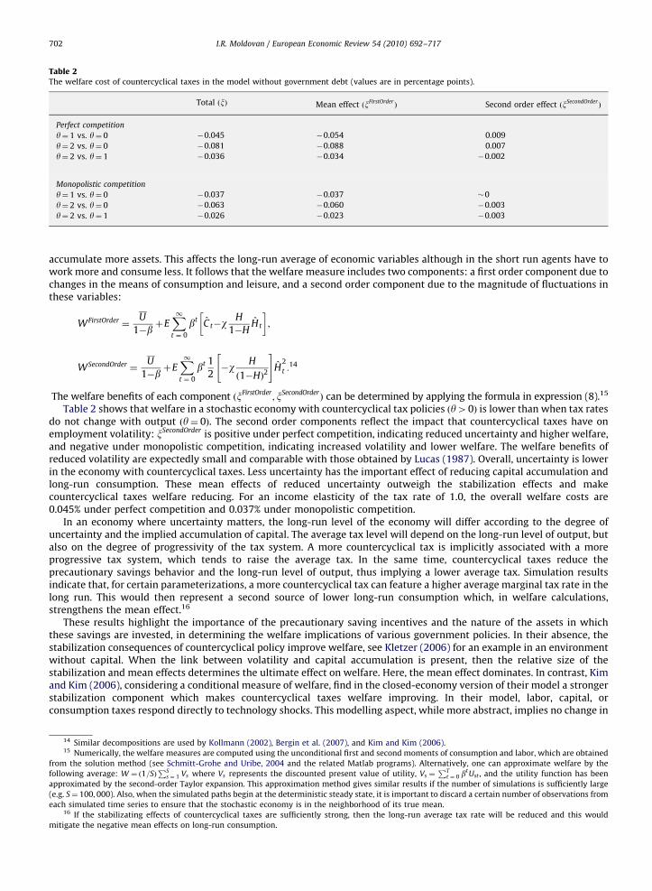
Fig. 6. Employment volatility under monopolistic competition when technology shocks are less persistent, rz ¼ 0:8 (circles, left panel, left axis), and more

persistent, rz ¼ 0:98 (squares, right panel, left axis), relative to the benchmark value of rz ¼ 0:95 (stars, both panels, right axis).


employment volatility. Less persistent technological changes increase the incentive to work more, amplify employmentfluctuations, and allow countercyclical taxes to have a stronger stabilizing effect. Fig. 5 shows that, under perfectcompetition and relative to the benchmark value of rz ¼ 0:95, countercyclical taxes reduce the volatility of employmentwhen technology shocks are less persistent ðrz ¼ 0:8Þ, while the opposite occurs when technological changes are morepersistent ðrz ¼ 0:98Þ. Similar results obtain under monopolistic competition, as shown in Fig. 6.

3.3. Welfare implications

This section analyzes the welfare implications of countercyclical income tax policies, in the absence of a fiscal financingrole for tax policy. Although countercyclical taxes reduce the volatility of most economic variables, they may affect welfarenegatively if agents take direct account of the level of uncertainty when making decisions.

Welfare is measured as the unconditional expectation of lifetime utility based on a second order solution to themodel.13 Use of a second-order solution is necessary because spurious welfare results may emerge from linear models thatabstract from the effects of uncertainty on optimal decisions, see Kim and Kim (2003). Let the economy with nocountercyclical taxes be the benchmark or reference economy and define welfare as:

Wr ¼ EX1t ¼ 0

btUðCrt ;H

rt Þ:

Alternative policy regimes are associated with countercyclical tax policies with different levels of responsiveness of the taxrate to output fluctuations. They yield welfare Wa. Then, the welfare benefit, x, of countercyclical tax policy is expressed asthe fraction of the consumption process under the non-countercyclical policy (or reference) regime that households mustbe given in order to be equally happy under the two types of tax policy:

Wa ¼ EX1t ¼ 0

btUðCat ;H

at Þ ¼ E

X1t ¼ 0

btUðð1þxÞCrt ;H

rt Þ:

With logarithmic utility in both consumption and leisure, the expression for x in percentage terms is

x¼ ½expðð1�bÞðWa�WrÞÞ�1� � 100: ð8Þ

A positive x denotes that countercyclical taxes are welfare improving.To obtain a measure of welfare, the momentary utility function is approximated by a second order Taylor expansion

with respect to its arguments. This yields an expression in which period-t utility depends on percent deviations andsquared percent deviations of consumption and hours worked from the deterministic steady state. Note that when utility islogarithmic in consumption, the volatility of consumption does not directly affect welfare (for the more general expression,see Appendix B):

W ¼ EX1t ¼ 0

btUðCt ;HtÞ ¼U

1�bþE

X1t ¼ 0

bt C t�wH

1�HHt�þE

X1t ¼ 0

bt 1

2�w H

ð1�HÞ2

" #H

2

t :

"ð9Þ

With a second order accurate solution to the model, optimal decisions depend both on the levels of state variables andon the amount of uncertainty in the economy. With greater uncertainty, risk-averse agents increase their savings and

13 This analysis compares welfare in economies with different degrees of countercyclical taxes and it is not a ‘‘tax reform’’ type of exercise.

Unconditional welfare is therefore the relevant welfare measure to use.

ARTICLE IN PRESS

Table 2The welfare cost of countercyclical taxes in the model without government debt (values are in percentage points).

Total ðxÞ Mean effect ðxFirstOrderÞ Second order effect ðxSecondOrder

Þ

Perfect competition

y¼ 1 vs. y¼ 0 �0.045 �0.054 0.009

y¼ 2 vs. y¼ 0 �0.081 �0.088 0.007

y¼ 2 vs. y¼ 1 �0.036 �0.034 �0.002

Monopolistic competition

y¼ 1 vs. y¼ 0 �0.037 �0.037 �0

y¼ 2 vs. y¼ 0 �0.063 �0.060 �0.003

y¼ 2 vs. y¼ 1 �0.026 �0.023 �0.003


accumulate more assets. This affects the long-run average of economic variables although in the short run agents have towork more and consume less. It follows that the welfare measure includes two components: a first order component due tochanges in the means of consumption and leisure, and a second order component due to the magnitude of fluctuations inthese variables:

WFirstOrder ¼U

1�bþE

X1t ¼ 0

bt C t�wH

1�HHt

� �;

WSecondOrder ¼U

1�bþE

X1t ¼ 0

bt 1

2�w H

ð1�HÞ2

" #H

2

t :14

The welfare benefits of each component ðxFirstOrder ; xSecondOrderÞ can be determined by applying the formula in expression (8).15

Table 2 shows that welfare in a stochastic economy with countercyclical tax policies ðy40Þ is lower than when tax ratesdo not change with output ðy¼ 0Þ. The second order components reflect the impact that countercyclical taxes have onemployment volatility: xSecondOrder is positive under perfect competition, indicating reduced uncertainty and higher welfare,and negative under monopolistic competition, indicating increased volatility and lower welfare. The welfare benefits ofreduced volatility are expectedly small and comparable with those obtained by Lucas (1987). Overall, uncertainty is lowerin the economy with countercyclical taxes. Less uncertainty has the important effect of reducing capital accumulation andlong-run consumption. These mean effects of reduced uncertainty outweigh the stabilization effects and makecountercyclical taxes welfare reducing. For an income elasticity of the tax rate of 1.0, the overall welfare costs are0.045% under perfect competition and 0.037% under monopolistic competition.

In an economy where uncertainty matters, the long-run level of the economy will differ according to the degree ofuncertainty and the implied accumulation of capital. The average tax level will depend on the long-run level of output, butalso on the degree of progressivity of the tax system. A more countercyclical tax is implicitly associated with a moreprogressive tax system, which tends to raise the average tax. In the same time, countercyclical taxes reduce theprecautionary savings behavior and the long-run level of output, thus implying a lower average tax. Simulation resultsindicate that, for certain parameterizations, a more countercyclical tax can feature a higher average marginal tax rate in thelong run. This would then represent a second source of lower long-run consumption which, in welfare calculations,strengthens the mean effect.16

These results highlight the importance of the precautionary saving incentives and the nature of the assets in whichthese savings are invested, in determining the welfare implications of various government policies. In their absence, thestabilization consequences of countercyclical policy improve welfare, see Kletzer (2006) for an example in an environmentwithout capital. When the link between volatility and capital accumulation is present, then the relative size of thestabilization and mean effects determines the ultimate effect on welfare. Here, the mean effect dominates. In contrast, Kimand Kim (2006), considering a conditional measure of welfare, find in the closed-economy version of their model a strongerstabilization component which makes countercyclical taxes welfare improving. In their model, labor, capital, orconsumption taxes respond directly to technology shocks. This modelling aspect, while more abstract, implies no change in

14 Similar decompositions are used by Kollmann (2002), Bergin et al. (2007), and Kim and Kim (2006).15 Numerically, the welfare measures are computed using the unconditional first and second moments of consumption and labor, which are obtained

from the solution method (see Schmitt-Grohe and Uribe, 2004 and the related Matlab programs). Alternatively, one can approximate welfare by the

following average: W ¼ ð1=SÞPS

s ¼ 1 Vs where Vs represents the discounted present value of utility, Vs ¼PT

t ¼ 0 btUst , and the utility function has been

approximated by the second-order Taylor expansion. This approximation method gives similar results if the number of simulations is sufficiently large

(e.g. S¼ 100;000). Also, when the simulated paths begin at the deterministic steady state, it is important to discard a certain number of observations from

each simulated time series to ensure that the stochastic economy is in the neighborhood of its true mean.16 If the stabilizating effects of countercyclical taxes are sufficiently strong, then the long-run average tax rate will be reduced and this would

mitigate the negative mean effects on long-run consumption.

ARTICLE IN PRESS

0 20 40 60−1.5

−1

−0.5

0Consumption

%

0 20 40 60−0.4

−0.2

0

0.2

0.4Employment

%

0 20 40 60−10

−5

0

5Investment

%

0 20 40 60−2

−1.5

−1

−0.5

0

Output

%

0 20 40 60−2

−1

0

1

Capital rental rate

%

0 20 40 60−0.04

−0.02

0

0.02

After−tax rate of return on capital

%

0 20 40 60−0.5

0

0.5

1

1.5

Tax Rate

years

%

0 20 40 60−2

−1

0

1

Tax Revenues

years

%

0 20 40 600

1

2

3

4

Government Debt

years

%

γ = 0.25γ = 0.5γ = 0.75

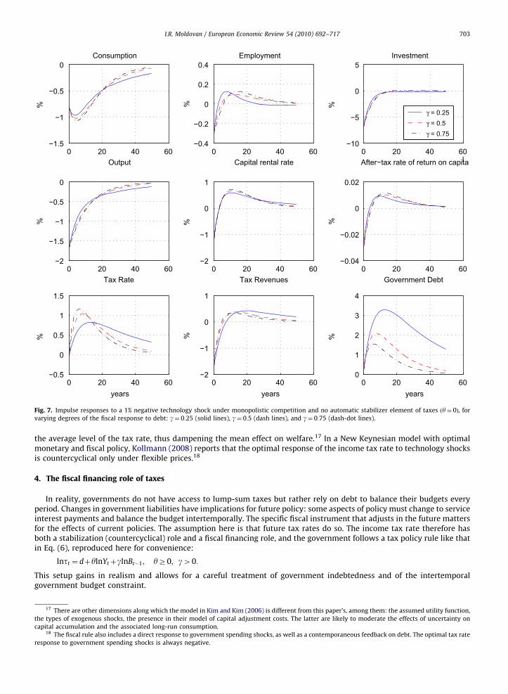
Fig. 7. Impulse responses to a 1% negative technology shock under monopolistic competition and no automatic stabilizer element of taxes ðy¼ 0Þ, for

varying degrees of the fiscal response to debt: g¼ 0:25 (solid lines), g¼ 0:5 (dash lines), and g¼ 0:75 (dash-dot lines).


the average level of the tax rate, thus dampening the mean effect on welfare.17 In a New Keynesian model with optimalmonetary and fiscal policy, Kollmann (2008) reports that the optimal response of the income tax rate to technology shocksis countercyclical only under flexible prices.18

4. The fiscal financing role of taxes

In reality, governments do not have access to lump-sum taxes but rather rely on debt to balance their budgets everyperiod. Changes in government liabilities have implications for future policy: some aspects of policy must change to serviceinterest payments and balance the budget intertemporally. The specific fiscal instrument that adjusts in the future mattersfor the effects of current policies. The assumption here is that future tax rates do so. The income tax rate therefore hasboth a stabilization (countercyclical) role and a fiscal financing role, and the government follows a tax policy rule like thatin Eq. (6), reproduced here for convenience:

lntt ¼ dþylnYtþglnBt�1; yZ0; g40:

This setup gains in realism and allows for a careful treatment of government indebtedness and of the intertemporalgovernment budget constraint.

17 There are other dimensions along which the model in Kim and Kim (2006) is different from this paper’s, among them: the assumed utility function,

the types of exogenous shocks, the presence in their model of capital adjustment costs. The latter are likely to moderate the effects of uncertainty on

capital accumulation and the associated long-run consumption.18 The fiscal rule also includes a direct response to government spending shocks, as well as a contemporaneous feedback on debt. The optimal tax rate

response to government spending shocks is always negative.

ARTICLE IN PRESS


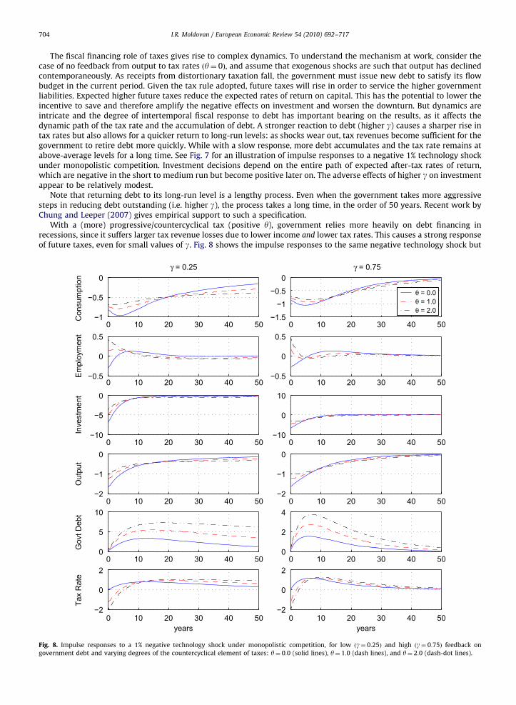
The fiscal financing role of taxes gives rise to complex dynamics. To understand the mechanism at work, consider thecase of no feedback from output to tax rates ðy¼ 0Þ, and assume that exogenous shocks are such that output has declinedcontemporaneously. As receipts from distortionary taxation fall, the government must issue new debt to satisfy its flowbudget in the current period. Given the tax rule adopted, future taxes will rise in order to service the higher governmentliabilities. Expected higher future taxes reduce the expected rates of return on capital. This has the potential to lower theincentive to save and therefore amplify the negative effects on investment and worsen the downturn. But dynamics areintricate and the degree of intertemporal fiscal response to debt has important bearing on the results, as it affects thedynamic path of the tax rate and the accumulation of debt. A stronger reaction to debt (higher g) causes a sharper rise intax rates but also allows for a quicker return to long-run levels: as shocks wear out, tax revenues become sufficient for thegovernment to retire debt more quickly. While with a slow response, more debt accumulates and the tax rate remains atabove-average levels for a long time. See Fig. 7 for an illustration of impulse responses to a negative 1% technology shockunder monopolistic competition. Investment decisions depend on the entire path of expected after-tax rates of return,which are negative in the short to medium run but become positive later on. The adverse effects of higher g on investmentappear to be relatively modest.

Note that returning debt to its long-run level is a lengthy process. Even when the government takes more aggressivesteps in reducing debt outstanding (i.e. higher g), the process takes a long time, in the order of 50 years. Recent work byChung and Leeper (2007) gives empirical support to such a specification.

With a (more) progressive/countercyclical tax (positive y), government relies more heavily on debt financing inrecessions, since it suffers larger tax revenue losses due to lower income and lower tax rates. This causes a strong responseof future taxes, even for small values of g. Fig. 8 shows the impulse responses to the same negative technology shock but

0 10 20 30 40 50−1

−0.5

0γ = 0.25

Con

sum

ptio

n

0 10 20 30 40 50−0.5

0

0.5

Em

ploy

men

t

0 10 20 30 40 50−10

−5

0

Inve

stm

ent

0 10 20 30 40 50−2

−1

0

Out

put

0 10 20 30 40 500

5

10

Gov

t Deb

t

0 10 20 30 40 50−2

0

2

years

Tax

Rat

e

0 10 20 30 40 50−1.5

−1

−0.5

0γ = 0.75

0 10 20 30 40 50−0.5

0

0.5

0 10 20 30 40 50−10

0

10

0 10 20 30 40 50−2

−1

0

0 10 20 30 40 500

2

4

0 10 20 30 40 50−2

0

2

years

θ = 0.0θ = 1.0θ = 2.0

Fig. 8. Impulse responses to a 1% negative technology shock under monopolistic competition, for low ðg¼ 0:25Þ and high ðg¼ 0:75Þ feedback on

government debt and varying degrees of the countercyclical element of taxes: y¼ 0:0 (solid lines), y¼ 1:0 (dash lines), and y¼ 2:0 (dash-dot lines).

ARTICLE IN PRESS

0 1 2

0

20

40γ = 0.25

θ

Con

sum

ptio

n

0 1 2−50

050

100

θ

Em

ploy

men

t

0 1 2−30−20−10

0

θ

Inve

stm

ent

0 1 2−20

0

20

θ

Out

put

0 1 2

0

20

40γ = 0.3

θ

0 1 2−50

050

100

θ

0 1 2−30−20−10

0

θ

0 1 2−20

0

20

θ

0 1 2

0

20

40γ = 0.5

θ

0 1 2−50

050

100

θ

0 1 2−30−20−10

0

θ

0 1 2−20

0

20

θ

0 1 2

0

20

40γ = 0.75

θ

0 1 2−50

050

100

θ

0 1 2−30−20−10

0

θ

0 1 2−20

0

20

θ

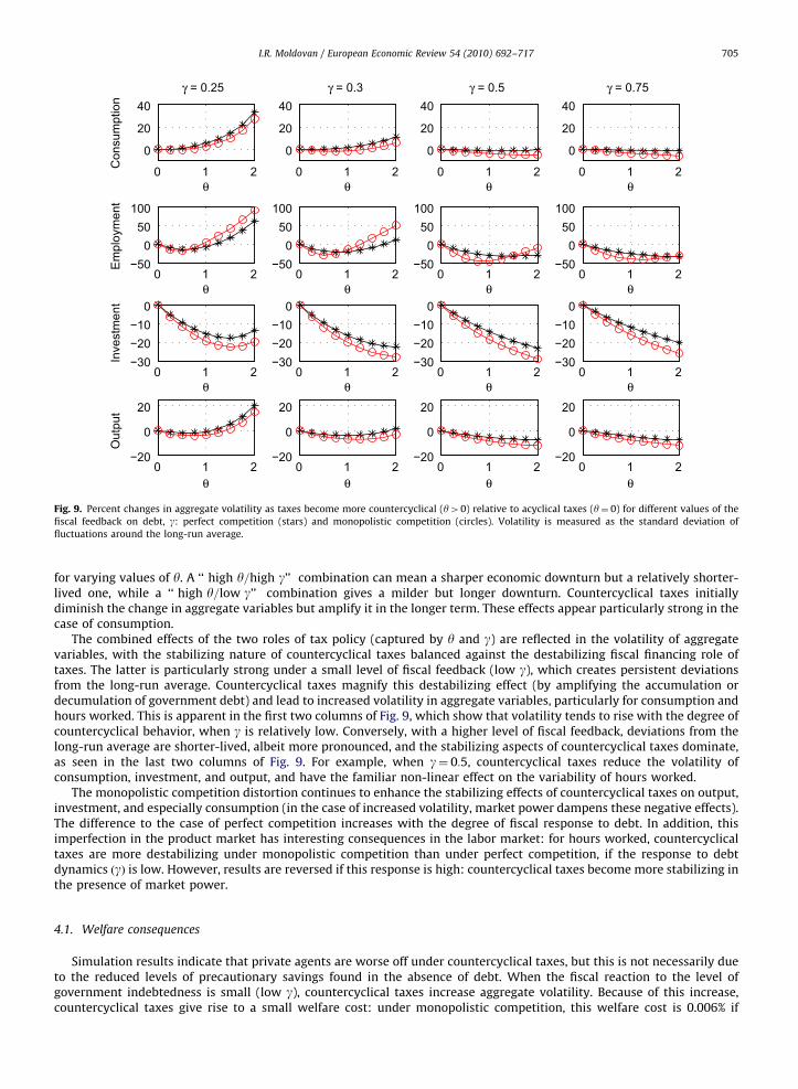
Fig. 9. Percent changes in aggregate volatility as taxes become more countercyclical (y40) relative to acyclical taxes (y¼ 0) for different values of the

fiscal feedback on debt, g: perfect competition (stars) and monopolistic competition (circles). Volatility is measured as the standard deviation of

fluctuations around the long-run average.


for varying values of y. A ‘‘ high y=high g’’ combination can mean a sharper economic downturn but a relatively shorter-lived one, while a ‘‘ high y=low g’’ combination gives a milder but longer downturn. Countercyclical taxes initiallydiminish the change in aggregate variables but amplify it in the longer term. These effects appear particularly strong in thecase of consumption.

The combined effects of the two roles of tax policy (captured by y and g) are reflected in the volatility of aggregatevariables, with the stabilizing nature of countercyclical taxes balanced against the destabilizing fiscal financing role oftaxes. The latter is particularly strong under a small level of fiscal feedback (low g), which creates persistent deviationsfrom the long-run average. Countercyclical taxes magnify this destabilizing effect (by amplifying the accumulation ordecumulation of government debt) and lead to increased volatility in aggregate variables, particularly for consumption andhours worked. This is apparent in the first two columns of Fig. 9, which show that volatility tends to rise with the degree ofcountercyclical behavior, when g is relatively low. Conversely, with a higher level of fiscal feedback, deviations from thelong-run average are shorter-lived, albeit more pronounced, and the stabilizing aspects of countercyclical taxes dominate,as seen in the last two columns of Fig. 9. For example, when g¼ 0:5, countercyclical taxes reduce the volatility ofconsumption, investment, and output, and have the familiar non-linear effect on the variability of hours worked.

The monopolistic competition distortion continues to enhance the stabilizing effects of countercyclical taxes on output,investment, and especially consumption (in the case of increased volatility, market power dampens these negative effects).The difference to the case of perfect competition increases with the degree of fiscal response to debt. In addition, thisimperfection in the product market has interesting consequences in the labor market: for hours worked, countercyclicaltaxes are more destabilizing under monopolistic competition than under perfect competition, if the response to debtdynamics ðgÞ is low. However, results are reversed if this response is high: countercyclical taxes become more stabilizing inthe presence of market power.

4.1. Welfare consequences

Simulation results indicate that private agents are worse off under countercyclical taxes, but this is not necessarily dueto the reduced levels of precautionary savings found in the absence of debt. When the fiscal reaction to the level ofgovernment indebtedness is small (low g), countercyclical taxes increase aggregate volatility. Because of this increase,countercyclical taxes give rise to a small welfare cost: under monopolistic competition, this welfare cost is 0.006% if

ARTICLE IN PRESS

Table 3The welfare cost of countercyclical taxes under both slow adjustment (gamma¼ 0:25) and rapid adjustment (gamma¼ 0:75) to debt dynamics, the case

of monopolistic competition (values are in percentage points).


Þ

Monopolistic competition: g¼ 0:25

y¼ 1 vs. y¼ 0 �1.361 �1.361 �0

y¼ 2 vs. y¼ 0 �11.092 �11.086 �0.006

y¼ 2 vs. y¼ 1 �9.864 �9.858 �0.006

Monopolistic competition: g¼ 0:75

y¼ 1 vs. y¼ 0 �0.058 �0.061 0.003

y¼ 2 vs. y¼ 0 �0.146 �0.148 0.002

y¼ 2 vs. y¼ 1 �0.088 �0.087 �0.001


y¼ 2:0. (See the top part of Table 3.) With more uncertainty in the economy, the precautionary saving motive is muchstronger. However, with a ‘‘ high y=low g’’ parameter combination, private holdings of government bonds are on averagehigher and so is the average tax rate. People save more but also substitute away from capital and into the riskless asset, thegovernment bond. Consequently, despite an increased precautionary saving motive, the economy experiencesaccumulation of government debt and decumulation of capital. Long-run output and consumption are therefore lower,which explains the large welfare losses associated with this policy. This illustrates the importance of identifying whichtype of asset households accumulate their precautionary savings in, before concluding that such savings are welfareimproving.

In contrast, under a strong adjustment of taxes to debt (high g), countercyclical taxes reduce aggregate volatility, and sohave a positive direct effect on welfare. This is illustrated for g¼ 0:75 in the bottom part of Table 3. As is the case withoutdebt, the reduced uncertainty lowers the precautionary saving motive, reducing capital accumulation and causing a lowerlong-run level of consumption and lower overall welfare.

In a normative sense, the results suggest that countercyclical taxes are better coupled with a more aggressive debtmanagement policy. Such a policy contributes to less volatility in aggregate variables and improves welfare relative toalternative policies where corrections to the level of government debt are slow. This is in line with findings by Leeper andYang (2008) who discuss the role of alternative financing options for the dynamic effects of permanent changes in capitaland labor income taxes. However, in a flexible price economy not dissimilar to the one described here, Kollmann (2008)finds that the optimal implied value of g is about �0:012 (negative but very small, even smaller than the ‘‘low’’ valuesconsidered here).19 In that environment, the monetary authority adopts a passive monetary policy rule, which effectivelystabilizes the debt stock when the fiscal authority does not attempt to do so. In contrast, this paper is concerned with thetrade-offs existent in a situation where only fiscal policy has the dual role described above.20

5. Extensions

This section considers three extensions: first, it undertakes robustness checks with respect to alternative specificationsof preferences; second, it assesses the implications for countercyclical tax policy of the government adjusting its spending(rather than taxes) in response to accumulated debt liabilities, and finally, it evaluates the significance of nominal inertiafor the effects of countercyclical taxes.

5.1. Sensitivity analysis

The aim of this subsection is to assess the sensitivity of the results obtained so far to alternative specifications regardingthe elasticity of intertemporal substitution in consumption and the labor supply elasticity. To that purpose, consider thefollowing, more general utility function:

UðC;1�HÞ ¼C1�s

1�s þwð1�HÞ1�u

1�u; ð10Þ

19 Other papers which find it desirable to stabilize debt slowly include Schmitt-Grohe and Uribe (2007) and Kirsanova and Wren-Lewis (2007), both

in the context of New Keynesian economies. However, the former paper specifies a rule in terms of tax revenues and ignores the progressivity of the tax

system emphasized in the current paper, while the latter uses a linearized model, government spending as the fiscal policy instrument and abstracts from

capital accumulation. As a result they will not trigger the precautionary savings effects stressed in this paper.20 Section 5.3 considers a New Keynesian model with sticky prices, with monetary policy described by a simple Taylor-type rule.

ARTICLE IN PRESS

0 0.5 1 1.5 2−60

−40

−20

0Consumption

θ0 0.5 1 1.5 2

−100

−50

0

50Employment

θ

0 0.5 1 1.5 2−60

−40

−20

0Investment

θ0 0.5 1 1.5 2

−60

−40

−20

0Output

θ

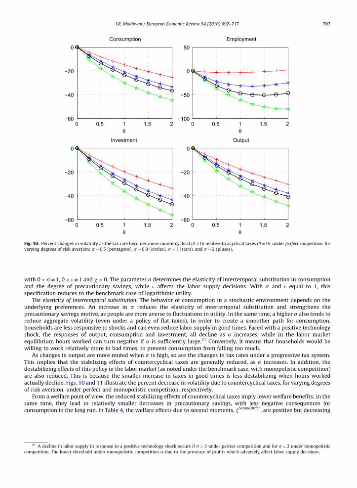
Fig. 10. Percent changes in volatility as the tax rate becomes more countercyclical ðy40Þ relative to acyclical taxes ðy¼ 0Þ, under perfect competition, for

varying degrees of risk aversion: s¼ 0:5 (pentagons), s¼ 0:8 (circles), s¼ 1 (stars), and s¼ 2 (pluses).


with 0osa1, 0oua1 and w40. The parameter s determines the elasticity of intertemporal substitution in consumptionand the degree of precautionary savings, while u affects the labor supply decisions. With s and u equal to 1, thisspecification reduces to the benchmark case of logarithmic utility.

The elasticity of intertemporal substitution. The behavior of consumption in a stochastic environment depends on theunderlying preferences. An increase in s reduces the elasticity of intertemporal substitution and strengthens theprecautionary savings motive, as people are more averse to fluctuations in utility. In the same time, a higher s also tends toreduce aggregate volatility (even under a policy of flat taxes). In order to create a smoother path for consumption,households are less responsive to shocks and can even reduce labor supply in good times. Faced with a positive technologyshock, the responses of output, consumption and investment, all decline as s increases, while in the labor marketequilibrium hours worked can turn negative if s is sufficiently large.21 Conversely, it means that households would bewilling to work relatively more in bad times, to prevent consumption from falling too much.

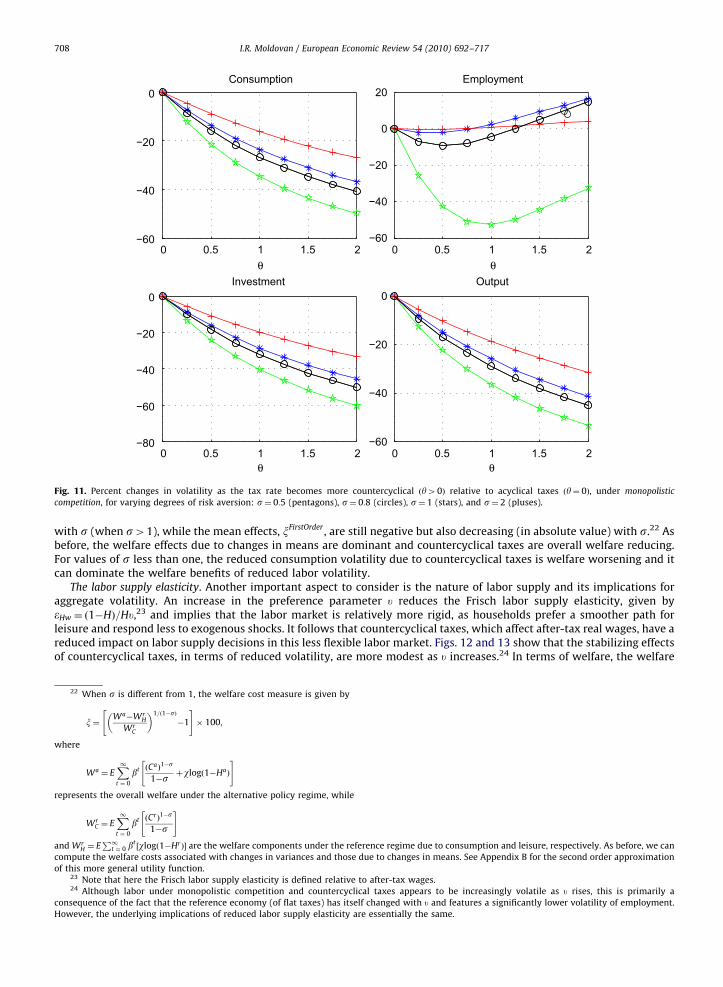
As changes in output are more muted when s is high, so are the changes in tax rates under a progressive tax system.This implies that the stabilizing effects of countercyclical taxes are generally reduced, as s increases. In addition, thedestabilizing effects of this policy in the labor market (as noted under the benchmark case, with monopolistic competition)are also reduced. This is because the smaller increase in taxes in good times is less destabilizing when hours workedactually decline. Figs. 10 and 11 illustrate the percent decrease in volatility due to countercyclical taxes, for varying degreesof risk aversion, under perfect and monopolistic competition, respectively.

From a welfare point of view, the reduced stabilizing effects of countercyclical taxes imply lower welfare benefits; in thesame time, they lead to relatively smaller decreases in precautionary savings, with less negative consequences forconsumption in the long run. In Table 4, the welfare effects due to second moments, xSecondOrder , are positive but decreasing

21 A decline in labor supply in response to a positive technology shock occurs if s45 under perfect competition and for s¼ 2 under monopolistic

competition. The lower threshold under monopolistic competition is due to the presence of profits which adversely affect labor supply decisions.

ARTICLE IN PRESS

0 0.5 1 1.5 2−60

−40

−20

0Consumption

θ0 0.5 1 1.5 2

−60

−40

−20

0

20Employment

θ

0 0.5 1 1.5 2−80

−60

−40

−20

0Investment

θ0 0.5 1 1.5 2

−60

−40

−20

0Output

θ

Fig. 11. Percent changes in volatility as the tax rate becomes more countercyclical ðy40Þ relative to acyclical taxes ðy¼ 0Þ, under monopolistic

competition, for varying degrees of risk aversion: s¼ 0:5 (pentagons), s¼ 0:8 (circles), s¼ 1 (stars), and s¼ 2 (pluses).


with s (when s41), while the mean effects, xFirstOrder , are still negative but also decreasing (in absolute value) with s.22 Asbefore, the welfare effects due to changes in means are dominant and countercyclical taxes are overall welfare reducing.For values of s less than one, the reduced consumption volatility due to countercyclical taxes is welfare worsening and itcan dominate the welfare benefits of reduced labor volatility.

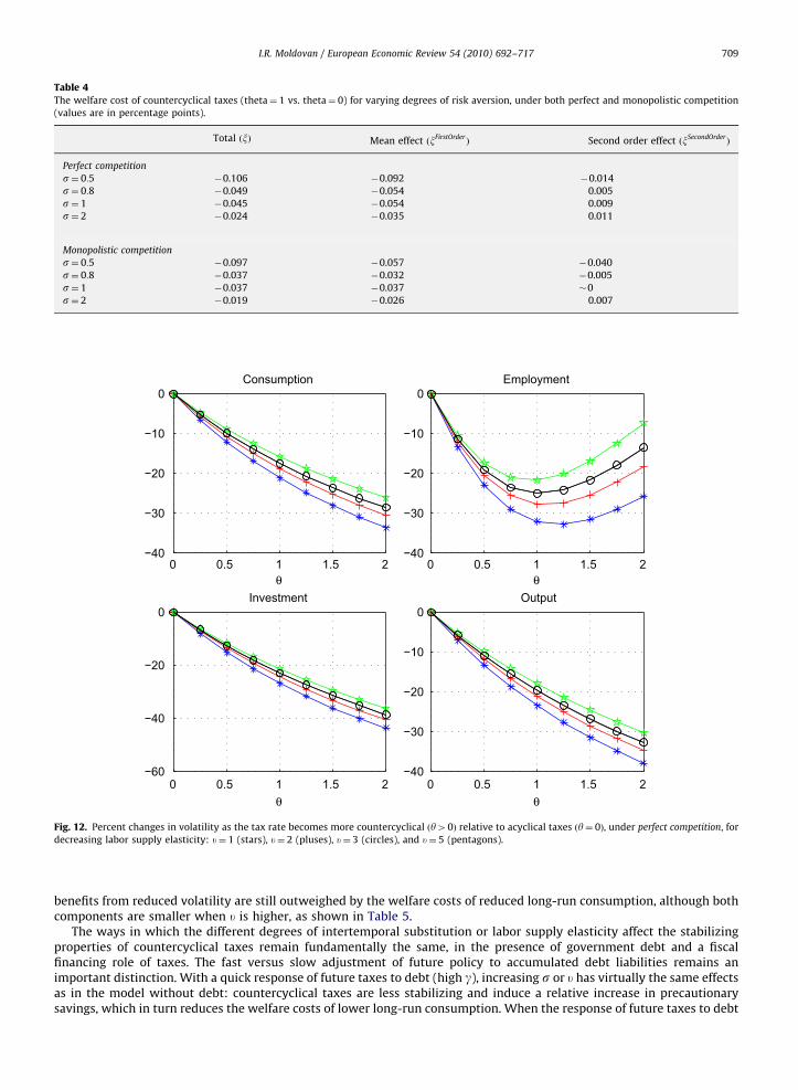
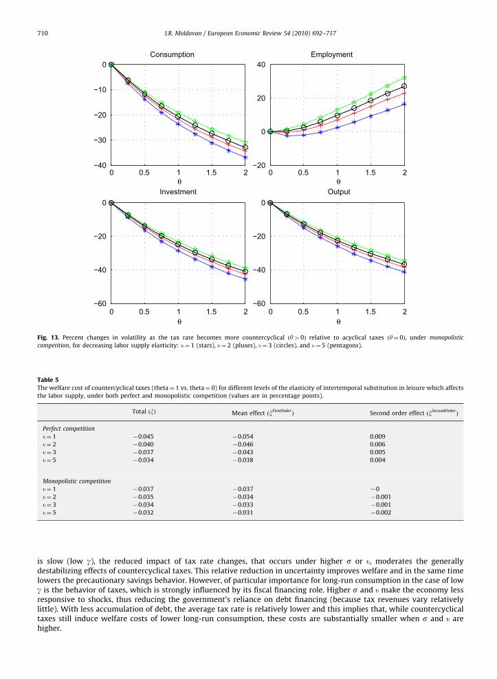
The labor supply elasticity. Another important aspect to consider is the nature of labor supply and its implications foraggregate volatility. An increase in the preference parameter u reduces the Frisch labor supply elasticity, given byeHw ¼ ð1�HÞ=Hu,23 and implies that the labor market is relatively more rigid, as households prefer a smoother path forleisure and respond less to exogenous shocks. It follows that countercyclical taxes, which affect after-tax real wages, have areduced impact on labor supply decisions in this less flexible labor market. Figs. 12 and 13 show that the stabilizing effectsof countercyclical taxes, in terms of reduced volatility, are more modest as u increases.24 In terms of welfare, the welfare

22 When s is different from 1, the welfare cost measure is given by

x¼Wa�Wr

H

WrC

� �1=ð1�sÞ�1

" #� 100;

where

Wa ¼ EX1t ¼ 0

bt ðCaÞ

1�s

1�sþwlogð1�HaÞ

" #

represents the overall welfare under the alternative policy regime, while

WrC ¼ E

X1t ¼ 0

bt ðCrÞ

1�s

1�s

" #

and WrH ¼ E

P1t ¼ 0 b

t½wlogð1�HrÞ� are the welfare components under the reference regime due to consumption and leisure, respectively. As before, we can

compute the welfare costs associated with changes in variances and those due to changes in means. See Appendix B for the second order approximation

of this more general utility function.23 Note that here the Frisch labor supply elasticity is defined relative to after-tax wages.24 Although labor under monopolistic competition and countercyclical taxes appears to be increasingly volatile as u rises, this is primarily a

consequence of the fact that the reference economy (of flat taxes) has itself changed with u and features a significantly lower volatility of employment.

However, the underlying implications of reduced labor supply elasticity are essentially the same.

ARTICLE IN PRESS

Table 4

The welfare cost of countercyclical taxes (theta¼ 1 vs. theta¼ 0) for varying degrees of risk aversion, under both perfect and monopolistic competition

(values are in percentage points).


Þ

Perfect competition

s¼ 0:5 �0.106 �0.092 �0.014

s¼ 0:8 �0.049 �0.054 0.005

s¼ 1 �0.045 �0.054 0.009

s¼ 2 �0.024 �0.035 0.011


s¼ 0:5 �0.097 �0.057 �0.040

s¼ 0:8 �0.037 �0.032 �0.005

s¼ 1 �0.037 �0.037 �0

s¼ 2 �0.019 �0.026 0.007

0 0.5 1 1.5 2−40

−30

−20

−10

0Consumption

θ0 0.5 1 1.5 2

−40

−30

−20

−10

0Employment

θ

0 0.5 1 1.5 2−60

−40

−20

0Investment

θ0 0.5 1 1.5 2

−40

−30

−20

−10

0Output

θ

Fig. 12. Percent changes in volatility as the tax rate becomes more countercyclical ðy40Þ relative to acyclical taxes ðy¼ 0Þ, under perfect competition, for

decreasing labor supply elasticity: u¼ 1 (stars), u¼ 2 (pluses), u¼ 3 (circles), and u¼ 5 (pentagons).


benefits from reduced volatility are still outweighed by the welfare costs of reduced long-run consumption, although bothcomponents are smaller when u is higher, as shown in Table 5.

The ways in which the different degrees of intertemporal substitution or labor supply elasticity affect the stabilizingproperties of countercyclical taxes remain fundamentally the same, in the presence of government debt and a fiscalfinancing role of taxes. The fast versus slow adjustment of future policy to accumulated debt liabilities remains animportant distinction. With a quick response of future taxes to debt (high g), increasing s or u has virtually the same effectsas in the model without debt: countercyclical taxes are less stabilizing and induce a relative increase in precautionarysavings, which in turn reduces the welfare costs of lower long-run consumption. When the response of future taxes to debt

ARTICLE IN PRESS

0 0.5 1 1.5 2−40

−30

−20

−10

0Consumption

θ0 0.5 1 1.5 2

−20

0

20

40Employment

θ

0 0.5 1 1.5 2−60

−40

−20

0Investment

θ0 0.5 1 1.5 2

−60

−40

−20

0Output

θ

Fig. 13. Percent changes in volatility as the tax rate becomes more countercyclical ðy40Þ relative to acyclical taxes ðy¼ 0Þ, under monopolistic

competition, for decreasing labor supply elasticity: u¼ 1 (stars), u¼ 2 (pluses), u¼ 3 (circles), and u¼ 5 (pentagons).

Table 5

The welfare cost of countercyclical taxes (theta¼ 1 vs. theta¼ 0) for different levels of the elasticity of intertemporal substitution in leisure which affects

the labor supply, under both perfect and monopolistic competition (values are in percentage points).


Þ

Perfect competition

u¼ 1 �0.045 �0.054 0.009

u¼ 2 �0.040 �0.046 0.006

u¼ 3 �0.037 �0.043 0.005

u¼ 5 �0.034 �0.038 0.004


u¼ 1 �0.037 �0.037 �0

u¼ 2 �0.035 �0.034 �0.001

u¼ 3 �0.034 �0.033 �0.001

u¼ 5 �0.032 �0.031 �0.002


is slow (low g), the reduced impact of tax rate changes, that occurs under higher s or u, moderates the generallydestabilizing effects of countercyclical taxes. This relative reduction in uncertainty improves welfare and in the same timelowers the precautionary savings behavior. However, of particular importance for long-run consumption in the case of lowg is the behavior of taxes, which is strongly influenced by its fiscal financing role. Higher s and u make the economy lessresponsive to shocks, thus reducing the government’s reliance on debt financing (because tax revenues vary relativelylittle). With less accumulation of debt, the average tax rate is relatively lower and this implies that, while countercyclicaltaxes still induce welfare costs of lower long-run consumption, these costs are substantially smaller when s and u arehigher.

ARTICLE IN PRESS

0 1 2

−50

0γ = −0.18

θ

Con

sum

ptio

n

0 1 2

−500

50100

θ

Em

ploy

men

t

0 1 2

−40

−20

0

θ

Inve

stm

ent

0 1 2−40

−20

0

θ

Out

put

0 1 2

−50

0

γ = −0.3

θ

0 1 2

−500

50100

θ

0 1 2

−40

−20

0

θ

0 1 2−40

−20

0

θ

0 1 2

−50

0

γ = −0.5

θ

0 1 2

−500

50100

θ

0 1 2

−40

−20

0

θ

0 1 2−40

−20

0

θ

0 1 2

−50

0

γ = −0.75

θ

0 1 2

−500

50100

θ

0 1 2

−40

−20

0

θ

0 1 2−40

−20

0

θ

Fig. 14. Percent changes in aggregate volatility as taxes become more countercyclical ðy40Þ relative to acyclical taxes ðy¼ 0Þ, for different values of the

fiscal feedback on debt, g, and when government spending has the fiscal financing role: perfect competition (stars) and monopolistic competition

(circles). Volatility is measured as the standard deviation of fluctuations around the long-run average.


5.2. The fiscal financing role of government spending

An alternative specification to the policy rule in Eq. (6) is to assume that the government adjusts its spending, Gt , ratherthan taxes, in response to accumulated debt. Fiscal policy can then be described as

lntt ¼ dþylnYt ; yZ0;

lnGt ¼~dþglnBt�1; go0;

where g is now negative, as higher debt must be met with decreases in future government spending.25 As before, theadjustment in future policy must be sufficiently large to ensure the intertemporal government budget constraint issatisfied (a value of �0:15 is needed under countercyclical taxes with y¼ 2).

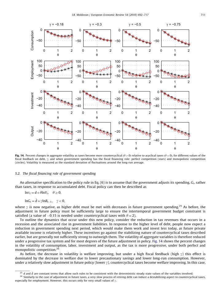
To outline the dynamics that occur under this new policy, consider the reduction in tax revenues that occurs in arecession and the associated rise in government liabilities. In response to the higher level of debt, people now expect areduction in government spending next period, which would make them work and invest less today, as future privateavailable income is relatively higher. These incentives go against the stabilizing nature of countercyclical taxes describedearlier, but are generally not sufficiently strong to outweigh them. The volatility of aggregate variables is therefore reducedunder a progressive tax system and for most degrees of the future adjustment in policy. Fig. 14 shows the percent changesin the volatility of consumption, labor, investment and output, as the tax is more progressive, under both perfect andmonopolistic competition.26

As before, the decrease in volatility is welfare improving, but under a high fiscal feedback (high g) this effect isdominated by the decrease in welfare due to lower precautionary savings and lower long-run consumption. However,under a relatively slow adjustment in future policy (lower g), countercyclical taxes become welfare improving. In this case,

25 d and ~d are constant terms that allow such rules to be consistent with the deterministic steady state values of the variables involved.26 Similarly to the case of adjustment in future taxes, a very slow process of retiring debt can induce a destabilizing aspect to countercyclical taxes,

especially for employment. However, this occurs only for very small values of g.

ARTICLE IN PRESS

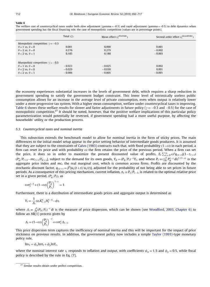
Table 6The welfare cost of countercyclical taxes under both slow adjustment (gamma¼ -0:3) and rapid adjustment (gamma¼ -0:5) to debt dynamics when

government spending has the fiscal financing role, the case of monopolistic competition (values are in percentage points).


Þ

Monopolistic competition: g¼�0:3

y¼ 1 vs. y¼ 0 0.091 0.090 0.001

y¼ 2 vs. y¼ 0 0.276 0.279 �0.002

y¼ 2 vs. y¼ 1 0.185 0.188 �0.003

Monopolistic competition: g¼�0:5

y¼ 1 vs. y¼ 0 �0.023 �0.025 0.002

y¼ 2 vs. y¼ 0 �0.029 �0.030 0.001

y¼ 2 vs. y¼ 1 �0.006 �0.005 �0.001


the economy experiences substantial increases in the levels of government debt, which requires a sharp reduction ingovernment spending to satisfy the government budget constraint. This lower level of intrinsically useless publicconsumption allows for an increase in the average level of private consumption, even when output is relatively lowerunder a more progressive tax system. With a higher mean consumption, welfare under countercyclical taxes is improving.Table 6 shows these welfare results for slower and faster adjustments in future policy (g¼�0:3 and �0:5) for the case ofmonopolistic competition.27 It should be noted, however, that the positive welfare implications of this particular policyparameterization would potentially be reversed, if government spending had a more useful purpose, by affecting thehouseholds’ utility or the production process.

5.3. Countercyclical taxes and nominal inertia

This subsection extends the benchmark model to allow for nominal inertia in the form of sticky prices. The maindifferences to the initial model setup appear in the price setting behavior of intermediate goods producers. It is assumedthat they are subject to the constraints of Calvo (1983)-contracts such that, with fixed probability ð1�oÞ in each period, afirm can reset its price and with probability o the firm retains the price of the previous period. When a firm can set

the price, it does so in order to maximize the present discounted value of profits, EtP1

s ¼ 0 osqt;tþ s½ð1�ttþ sÞ

ðP�it=Ptþ s�mctþ sÞYitþ s�, subject to the demand for its own goods, Yit ¼ ðPit=PtÞ�eYt , and where Pt � ð

R 10 P1�e

it diÞ1=ð1�eÞ is the

aggregate price index and mct the real marginal cost, which is common across firms. Profits are discounted by the

stochastic discount factor, qt;tþ s ¼ bs½uCðtþsÞ=uCðtÞ�, adjusted for the probability of not being able to set prices in future

periods. As a consequence of this pricing mechanism, current inflation, pt � Pt=Pt�1, is related to the optimal relative priceset in a given period, ðP�it=PtÞ, as

ope�1t þð1�oÞ

P�itPt

� �1�e¼ 1:

Furthermore, there is a distribution of intermediate goods prices and aggregate output is determined as

Yt ¼1

DtðztK

at�1H1�a

t �fÞ;

where Dt �R 1

0 ðPit=PtÞ�e di is the measure of price dispersion, which can be shown (see Woodford, 2003, Chapter 6) to

follow an AR(1) process given by

Dt ¼ ð1�oÞP�itPt

� ��eþopetDt�1:

This price dispersion term captures the inefficiency of nominal inertia and this will be important for the impact of pricestickiness on previous results. In addition, the government policy now includes a simple Taylor (1993)-type monetarypolicy rule,

lnit ¼fplnptþfylnYt ;

where the nominal interest rate it responds to inflation and output, with coefficients fp ¼ 1:5 and fy ¼ 0:5, while fiscal

policy is described by the rule in Eq. (7).

27 Similar results obtain under perfect competition.

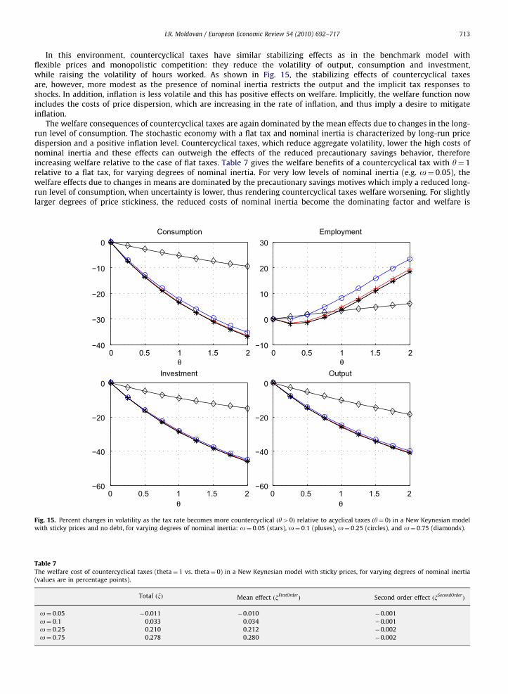
ARTICLE IN PRESS


In this environment, countercyclical taxes have similar stabilizing effects as in the benchmark model withflexible prices and monopolistic competition: they reduce the volatility of output, consumption and investment,while raising the volatility of hours worked. As shown in Fig. 15, the stabilizing effects of countercyclical taxesare, however, more modest as the presence of nominal inertia restricts the output and the implicit tax responses toshocks. In addition, inflation is less volatile and this has positive effects on welfare. Implicitly, the welfare function nowincludes the costs of price dispersion, which are increasing in the rate of inflation, and thus imply a desire to mitigateinflation.

The welfare consequences of countercyclical taxes are again dominated by the mean effects due to changes in the long-run level of consumption. The stochastic economy with a flat tax and nominal inertia is characterized by long-run pricedispersion and a positive inflation level. Countercyclical taxes, which reduce aggregate volatility, lower the high costs ofnominal inertia and these effects can outweigh the effects of the reduced precautionary savings behavior, thereforeincreasing welfare relative to the case of flat taxes. Table 7 gives the welfare benefits of a countercyclical tax with y¼ 1relative to a flat tax, for varying degrees of nominal inertia. For very low levels of nominal inertia (e.g. o¼ 0:05), thewelfare effects due to changes in means are dominated by the precautionary savings motives which imply a reduced long-run level of consumption, when uncertainty is lower, thus rendering countercyclical taxes welfare worsening. For slightlylarger degrees of price stickiness, the reduced costs of nominal inertia become the dominating factor and welfare is

Table 7

The welfare cost of countercyclical taxes (theta¼ 1 vs. theta¼ 0) in a New Keynesian model with sticky prices, for varying degrees of nominal inertia

(values are in percentage points).


Þ

o¼ 0:05 �0.011 �0.010 �0.001

o¼ 0:1 0.033 0.034 �0.001

o¼ 0:25 0.210 0.212 �0.002

o¼ 0:75 0.278 0.280 �0.002

0 0.5 1 1.5 2−40

−30

−20

−10

0Consumption

θ0 0.5 1 1.5 2

−10

0

10

20

30Employment

θ

0 0.5 1 1.5 2−60

−40

−20

0Investment

θ0 0.5 1 1.5 2

−60

−40

−20

0Output

θ

Fig. 15. Percent changes in volatility as the tax rate becomes more countercyclical ðy40Þ relative to acyclical taxes ðy¼ 0Þ in a New Keynesian model

with sticky prices and no debt, for varying degrees of nominal inertia: o¼ 0:05 (stars), o¼ 0:1 (pluses), o¼ 0:25 (circles), and o¼ 0:75 (diamonds).

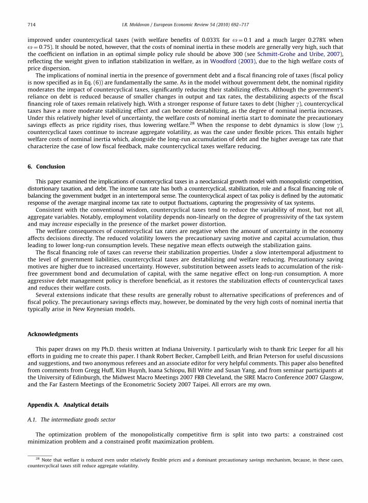
ARTICLE IN PRESS


improved under countercyclical taxes (with welfare benefits of 0.033% for o¼ 0:1 and a much larger 0.278% wheno¼ 0:75). It should be noted, however, that the costs of nominal inertia in these models are generally very high, such thatthe coefficient on inflation in an optimal simple policy rule should be above 300 (see Schmitt-Grohe and Uribe, 2007),reflecting the weight given to inflation stabilization in welfare, as in Woodford (2003), due to the high welfare costs ofprice dispersion.

The implications of nominal inertia in the presence of government debt and a fiscal financing role of taxes (fiscal policyis now specified as in Eq. (6)) are fundamentally the same. As in the model without government debt, the nominal rigiditymoderates the impact of countercyclical taxes, significantly reducing their stabilizing effects. Although the government’sreliance on debt is reduced because of smaller changes in output and tax rates, the destabilizing aspects of the fiscalfinancing role of taxes remain relatively high. With a stronger response of future taxes to debt (higher g), countercyclicaltaxes have a more moderate stabilizing effect and can become destabilizing, as the degree of nominal inertia increases.Under this relatively higher level of uncertainty, the welfare costs of nominal inertia start to dominate the precautionarysavings effects as price rigidity rises, thus lowering welfare.28 When the response to debt dynamics is slow (low g),countercyclical taxes continue to increase aggregate volatility, as was the case under flexible prices. This entails higherwelfare costs of nominal inertia which, alongside the long-run accumulation of debt and the higher average tax rate thatcharacterize the case of low fiscal feedback, make countercyclical taxes welfare reducing.

6. Conclusion

This paper examined the implications of countercyclical taxes in a neoclassical growth model with monopolistic competition,distortionary taxation, and debt. The income tax rate has both a countercyclical, stabilization, role and a fiscal financing role ofbalancing the government budget in an intertemporal sense. The countercyclical aspect of tax policy is defined by the automaticresponse of the average marginal income tax rate to output fluctuations, capturing the progressivity of tax systems.

Consistent with the conventional wisdom, countercyclical taxes tend to reduce the variability of most, but not all,aggregate variables. Notably, employment volatility depends non-linearly on the degree of progressivity of the tax systemand may increase especially in the presence of the market power distortion.

The welfare consequences of countercyclical tax rates are negative when the amount of uncertainty in the economyaffects decisions directly. The reduced volatility lowers the precautionary saving motive and capital accumulation, thusleading to lower long-run consumption levels. These negative mean effects outweigh the stabilization gains.

The fiscal financing role of taxes can reverse their stabilization properties. Under a slow intertemporal adjustment tothe level of government liabilities, countercyclical taxes are destabilizing and welfare reducing. Precautionary savingmotives are higher due to increased uncertainty. However, substitution between assets leads to accumulation of the risk-free government bond and decumulation of capital, with the same negative effect on long-run consumption. A moreaggressive debt management policy is therefore beneficial, as it restores the stabilization effects of countercyclical taxesand reduces their welfare costs.

Several extensions indicate that these results are generally robust to alternative specifications of preferences and offiscal policy. The precautionary savings effects may, however, be dominated by the very high costs of nominal inertia thattypically arise in New Keynesian models.

Acknowledgments

This paper draws on my Ph.D. thesis written at Indiana University. I particularly wish to thank Eric Leeper for all hisefforts in guiding me to create this paper. I thank Robert Becker, Campbell Leith, and Brian Peterson for useful discussionsand suggestions, and two anonymous referees and an associate editor for very helpful comments. This paper also benefitedfrom comments from Gregg Huff, Kim Huynh, Ioana Schiopu, Bill Witte and Susan Yang, and from seminar participants atthe University of Edinburgh, the Midwest Macro Meetings 2007 FRB Cleveland, the SIRE Macro Conference 2007 Glasgow,and the Far Eastern Meetings of the Econometric Society 2007 Taipei. All errors are my own.

Appendix A. Analytical details

A.1. The intermediate goods sector

The optimization problem of the monopolistically competitive firm is split into two parts: a constrained costminimization problem and a constrained profit maximization problem.

28 Note that welfare is reduced even under relatively flexible prices and a dominant precautionary savings mechanism, because, in these cases,

countercyclical taxes still reduce aggregate volatility.

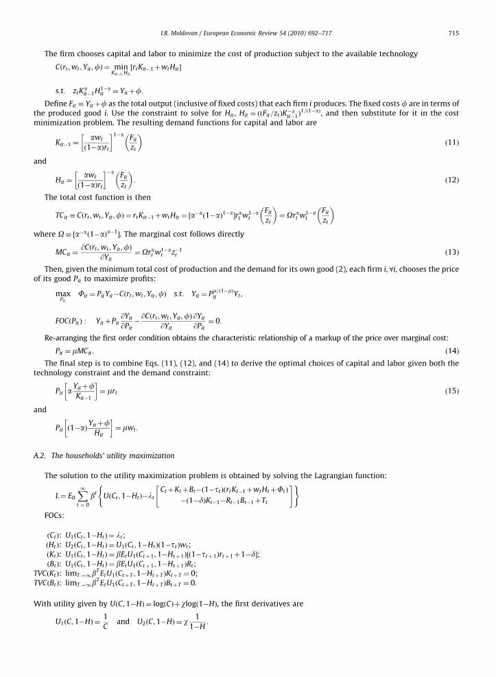
ARTICLE IN PRESS


The firm chooses capital and labor to minimize the cost of production subject to the available technology

Cðrt ;wt ;Yit ;fÞ ¼ minKit�1;Hit

½rtKit�1þwtHit �

s:t: ztKait�1H1�a

it ¼ Yitþf:

Define Fit � Yitþf as the total output (inclusive of fixed costs) that each firm i produces. The fixed costs f are in terms ofthe produced good i. Use the constraint to solve for Hit , Hit ¼ ððFit=ztÞK�ait�1Þ

1=ð1�aÞ, and then substitute for it in the costminimization problem. The resulting demand functions for capital and labor are

Kit�1 ¼awt

ð1�aÞrt

� �1�a Fit

zt

� �ð11Þ

and

Hit ¼awt

ð1�aÞrt

� ��a Fit

zt

� �: ð12Þ

The total cost function is then

TCit � Cðrt ;wt ;Yit ;fÞ ¼ rtKit�1þwtHit ¼ ½a�að1�aÞ1�a�rat w1�at

Fit

zt

� �¼Orat w1�a

t

Fit

zt

� �

where O� ½a�að1�aÞa�1�. The marginal cost follows directly

MCit ¼@Cðrt ;wt ;Yit ;fÞ

@Yit¼Orat w1�a

t z�1t ð13Þ

Then, given the minimum total cost of production and the demand for its own good (2), each firm i; 8i, chooses the priceof its good Pit to maximize profits:

maxPit

Fit ¼ PitYit�Cðrt ;wt ;Yit ;fÞ s:t: Yit ¼ Pm=ð1�mÞit Yt ;

FOCðPitÞ : YitþPit@Yit

@Pit�@Cðrt ;wt ;Yit ;fÞ

@Yit

@Yit

@Pit¼ 0:

Re-arranging the first order condition obtains the characteristic relationship of a markup of the price over marginal cost:

Pit ¼ mMCit : ð14Þ

The final step is to combine Eqs. (11), (12), and (14) to derive the optimal choices of capital and labor given both thetechnology constraint and the demand constraint:

Pit aYitþfKit�1

� �¼ mrt ð15Þ

and

Pit ð1�aÞYitþf

Hit

� �¼ mwt :

A.2. The households’ utility maximization

The solution to the utility maximization problem is obtained by solving the Lagrangian function:

L¼ E0

X1t ¼ 0

bt UðCt ;1�HtÞ�lt

CtþKtþBt�ð1�ttÞðrtKt�1þwtHtþFtÞ

�ð1�dÞKt�1�Rt�1Bt�1þTt

" #( )

FOCs:

ðCtÞ:
U1ðCt ;1�HtÞ ¼ lt; ðHtÞ: U2ðCt ;1�HtÞ ¼U1ðCt ;1�HtÞð1�ttÞwt; ðKtÞ: U1ðCt ;1�HtÞ ¼ bEtU1ðCtþ1;1�Htþ1Þ½ð1�ttþ1Þrtþ1þ1�d�; ðBtÞ: U1ðCt ;1�HtÞ ¼ bEtU1ðCtþ1;1�Htþ1ÞRt;
TVCðKtÞ:
limT-1bT EtU1ðCtþT ;1�HtþT ÞKtþT ¼ 0;
TVCðBtÞ:
limT-1bT EtU1ðCtþT ;1�HtþT ÞBtþT ¼ 0.
With utility given by UðC;1�HÞ ¼ logðCÞþwlogð1�HÞ, the first derivatives are

U1ðC;1�HÞ ¼1

Cand U2ðC;1�HÞ ¼ w 1

1�H:

ARTICLE IN PRESS


Appendix B. Approximation of the utility function

To calculate the welfare associated with a given fiscal policy rule, the momentary utility is approximated by a second-order Taylor expansion. First, take a second-order Taylor expansion of UðCt ;HtÞ with respect to ðCt ;HtÞ around thedeterministic steady state values C ;H and express it in algebraic percent deviations:

UðCt ;HtÞ �Uþ½UCðC ;HÞC �dCt

Cþ½UHðC ;HÞH�

dHt

Hþ

1

2½UCCðC ;HÞC

2�

dCt

C

� �2(

þ2½UCHðC ;HÞCH �dCt

C

� �dht

H

� �þ½UHHðC ;HÞH

2�

dHt

H

� �2):

Then, following Woodford (2002, 2003), approximate the algebraic percent change by a second-order expansion interms of logarithmic changes

xt�x

x¼

dxt

x� xtþ

1

2x

2t where xt � lnxt�lnx:

Finally, substitute the logarithmic changes for the algebraic percent changes and keep only the terms of order Oð1Þ andlower to get

UðCt ;HtÞ �Uþ½UCðC ;HÞC �C tþ½UHðC ;HÞH �Htþ1

2 ½UCC ðC ;HÞC2þUCðC ;HÞC � C

2

t þ2½UCHðC ;HÞCH�ðC tHtÞ

nþ½UHHðC ;HÞH

2þUHðC ;HÞH �H

2

t

o:

For a general CRRA utility function, separable in consumption and leisure, such as

UðC;1�HÞ ¼C1�s

1�sþw ð1�HÞ1�u

1�u;

the approximation reduces to

UðCt ;HtÞ �UþC1�sC t�wH

ð1�HÞuHtþ

1

2ð1�sÞC1�sC

2

t�wH

ð1�HÞu1þu

H

1�H

� �H

2

t �

�

which becomes Eq. (9) in the text, when s and u equal 1. Note that, when the momentary utility is logarithmic inconsumption ðs¼ 1Þ, the variability of consumption does not directly affect lifetime utility and that, when so1,consumption volatility becomes welfare improving.

References

Akhand, H., Liu, H., 2002. Marginal income tax rates in the United States: a non-parametric approach. Journal of Monetary Economics 49, 383–404.Andres, J., Domenech, R., 2006. Automatic stabilizers, fiscal rules and macroeconomic stability. European Economic Review 50 (6), 1487–1506.Auerbach, A., 2003. Fiscal policy past and present. Brookings Papers on Economic Activity 1, 75–138.Auerbach, A., 2005. The effectiveness of fiscal policy as stabilization policy. In: Korea, B.o. (Ed.), The Effectiveness of Stabilization Policies, pp. 100–130.Auerbach, A.J., Feenberg, D., 2000. The significance of federal taxes as automatic stabilizers. Journal of Economic Perspectives 14 (Summer), 37–56.Benassy, J.-P., 2002. The Macroeconomics of Imperfect Competition and Nonclearing Markets: A Dynamic General Equilibrium Approach. The MIT Press,

Cambridge, MA.Bergin, P.R., Shin, H.-C., Tchakarov, I., 2007. Does exchange rate variability matter for welfare? A quantitative investigation of stabilization policies.

European Economic Review 51 (May), 1041–1058.Blanchard, O.J., Kiyotaki, N., 1987. Monopolistic competition and the effects of aggregate demand. The American Economic Review 77 (September),

647–666.Blanchard, O.J., Perotti, R., 2002. An empirical characterization of the dynamic effects of changes in government spending and taxes on output. Quarterly

Journal of Economics 117 (4), 1329–1368.Braun, A.R., 1994. Tax disturbances and real economic activity in the postwar United States. Journal of Monetary Economics 33, 441–462.Bryant, R.C., Zhang, L., 1996. Alternative specifications of intertemporal fiscal policy in a small theoretical model. Manuscript.Calvo, G., 1983. Staggered prices in a utility maximising framework. Journal of Monetary Economics 12 (3), 383–398.Chung, H., Leeper, E.M., 2007. What has financed government debt? NBER Working Paper No. 13425.Cohen, D., Follette, G., 2000. The automatic fiscal stabilizers: quietly doing their thing. FRB New York Economic Policy Review (April), 35–68.Devereux, M.B., Head, A.C., Lapham, B.J., 1993. Monopolistic competition, technology shocks, and aggregate fluctuations. Economic Letters 41, 57–61.Gordon, D.B., Leeper, E.M., 2005. Are Countercyclical fiscal policies counterproductive. NBER Working Paper No. 11869.Hornstein, A., 1993. Monopolistic competition, increasing returns to scale, and the importance of productivity shocks. Journal of Monetary Economics 31,

299–316.Jones, J.B., 2002. Has fiscal policy helped stabilize the postwar U.S. economy? Journal of Monetary Economics 49, 709–746.Kim, J., Kim, S.H., 2003. Spurious welfare reversals in international business cycle models. Journal of International Economics 60, 471–500.Kim, J., Kim, S.H., 2006. Welfare effects of tax policy in open economies: stabilization and cooperation. Manuscript, Tufts University.Kirsanova, T., Wren-Lewis, S., 2007. Optimal fiscal feedback on debt in an economy with nominal rigidities. Manuscript.Kletzer, K., 2006. Taxes and stabilization in contemporary macroeconomic models. International Tax and Public Finance 13 (4), 351–371.Kollmann, R., 2002. Monetary policy rules in the open economy: effects on welfare and business cycles. Journal of Monetary Economics 49, 989–1015.Kollmann, R., 2008. Welfare maximizing operational monetary and tax policy rules. Macroeconomic Dynamics 12 (Supplement 1), 112–125.Leeper, E.M., Yang, S.-C.S., 2008. Dynamic scoring: alternative financing schemes. Journal of Public Economics 92 (February), 159–182.Lucas, R.E.J., 1987. Models of Business Cycles, Yrjo Jahnsson Lectures. Basil Blackwell Ltd, Cambridge, MA.Rotemberg, J.J., Woodford, M., 1995. Dynamic general equilibrium models with imperfectly competitive product markets. In: Cooley, T.F. (Ed.), Frontiers of

Business Cycle Research. Princeton University Press, Princeton, NJ.

ARTICLE IN PRESS


Schmitt-Grohe, S., Uribe, M., 2004. Solving dynamic general equilibrium models using a second-order approximation to the policy function. Journal ofEconomic Dynamics and Control 28, 755–775.

Schmitt-Grohe, S., Uribe, M., 2007. Optimal, simple, and implementable monetary and fiscal rules. Journal of Monetary Economics 54 (September),1702–1725.

Taylor, J., 1993. Discretion versus policy rules in practice. Carnegie-Rochester Conferences Series on Public Policy 39 (December), 195–214.Taylor, J.B., 2000. Reassessing discretionary fiscal policy. Journal of Economic Perspectives 14 (Summer), 21–36.Trabandt, M., Uhlig, H., 2006. How far are we from the slippery slope? The Laffer curve revisited. SFB 649 Discussion Paper 2006-023.Woodford, M., 2002. Inflation stabilization and welfare. Contributions to Macroeconomics 2 (1), 1–51.Woodford, M., 2003. Interest and Prices: Foundations of a Theory of Monetary Policy. Princeton University Press, Princeton, NJ.Yang, S.-C.S., 2005. Quantifying tax effects under policy foresight. Journal of Monetary Economics 58 (2), 1557–1568.Yang, S.-C.S., 2007. Do capital income tax cuts trickle down? National Tax Journal 60 (3), 551–567.

countercyclical taxes in a monopolistically competitive environment

Documents