cost-volume-profit analysis - pdf4pro

CHAPTER

3 Cost-Volume-Profit Analysis

Overview This chapter explains a planning tool called cost-volume-profit (CVP) analysis. CVP analysis examines the behavior of total revenues, total costs, and operating income (profit) as changes occur in the units sold, the selling price, the variable cost per unit, or the fixed costs of a product. The reliability of the results from CVP analysis depends on the reasonableness of the assumptions. The Appendix to the chapter gives additional insights about CVP analysis; it explains decision models and uncertainty. Highlights

1. Because managers want to avoid operating losses, they are interested in the breakeven point calculated using CVP analysis. The breakeven point is the quantity of output sold at which total revenues equal total costs. There is neither a profit nor a loss at the breakeven point. To illustrate, assume a company sells 2,000 units of its only product for $50 per unit, variable cost is $20 per unit, and fixed costs are $60,000 per month. Given these conditions, the company is operating at the breakeven point:

Revenues, 2,000 × $50 $100,000 Deduct:

Variable costs, 2,000 × $20 40,000 Fixed costs 60,000

Operating income $ -0- The breakeven point can be expressed two ways: 2,000 units and $100,000 of revenues.

2. Under CVP analysis, the income statement above is reformatted to show a key line item, contribution margin:

Revenues, 2,000 × $50 $100,000 Variable costs, 2,000 × $20 40,000Contribution margin 60,000 Fixed costs 60,000Operating income $ -0-

This format, called the contribution income statement, is used extensively in this chapter and throughout the textbook.

3. Contribution margin can be expressed three ways: in total, on a per unit basis, and as a percentage of revenues. In our example, total contribution margin is $60,000. Contribution margin per unit is the difference between selling price and variable cost per unit: $50 − $20 = $30. Contribution margin per unit is also equal to contribution margin divided by the number of units sold: $60,000 ÷ 2,000 = $30. Contribution margin percentage (also called contribution margin ratio) is contribution margin per unit divided by selling price: $30 ÷ $50 = 60%; it is also equal to contribution margin divided by revenues: $60,000 ÷ $100,000 = 60%. This contribution margin percentage means that 60 cents in contribution margin is gained for each $1 of revenues.

4. In our example, compute the breakeven point (BEP) in units and in revenues as follows:

000,100$60.0000,60$revenues BEP

e percentagmargin onContributicosts fixed Totalrevenues BEP

units000,230$000,60$ unitsBEP

unit permargin onContributicosts fixed Total unitsBEP

==

=

==

=

5. The CVP analysis above is based on the

following assumptions: a. Changes in the levels of revenues and costs

arise only because of changes in the number of product (or service) units sold (that is, the number of output units is the only driver of revenues and costs).

b. Total costs can be separated into a fixed component that does not vary with units sold and a component that is variable with respect to units sold.

c. When represented graphically, the behaviors of both total revenues and total costs are linear

COST-VOLUME-PROFIT ANALYSIS 23

(straight lines) in relation to the units sold within a relevant range (and time period).

d. Selling price, variable cost per unit, and total fixed costs (within a relevant range and time period) are known and constant.

6. While the breakeven point is often of

interest to managers, CVP analysis considers a broader question: What amount of sales in units or in revenues is needed to achieve a specified target operating income? The answer is easily obtained by adding target operating income to total fixed costs in the numerator of the formulas above. Assuming target operating income (TOI) is $15,000:

000,125$60.0

000,15$000,60$TOI achieve

to Revenues

units500,230$

000,15$000,60$TOI achieve

to sales Unit

=+

=

=+

=

7. Because for-profit organizations are

subject to income taxes, their CVP analyses must include this factor. For example, if a company earns $50,000 before income taxes and the tax rate is 40%, then:

Operating income $50,000Deduct income taxes (40%) 20,000Net income $30,000

To state a target net income figure in terms of operating income, divide target net income by 1 − tax rate: $30,000 ÷ (1 − .40) = $50,000. Note, the income-tax factor does not change the breakeven point because no income taxes arise if operating income is $0.

8. Managers use CVP analysis to guide their decisions, many of which are strategic decisions. For example, CVP analysis helps managers decide how much to spend on advertising, whether or not to reduce selling price, whether or not to expand into new markets, and which features to add to existing products. Of course, different choices can affect fixed costs, variable cost per unit, selling prices, units sold, and operating income.

9. Single-number “best estimates” of input data for CVP analysis are subject to varying degrees of uncertainty, the possibility that an actual amount will deviate from an expected amount. One approach to deal with uncertainty is to use sensitivity analysis (discussed in paragraphs 10 through 12). Another approach is to compute expected values using probability distributions (discussed in paragraph 19).

10. Sensitivity analysis is a “what if” technique that managers use to examine how a result will change if the original predicted data are not achieved or if an underlying assumption changes. In the context of CVP analysis, sensitivity analysis examines how operating income (or the breakeven point) changes if the predicted data for selling price, variable cost per unit, fixed costs, or units sold are not achieved. The sensitivity to various possible outcomes broadens managers’ perspectives as to what might actually occur before they make cost commitments. Electronic spreadsheets, such as Excel, enable managers to conduct CVP-based sensitivity analyses in a systematic and efficient way.

11. An aspect of sensitivity analysis is the margin of safety, the amount by which budgeted (or actual) revenues exceed the breakeven quantity. The margin of safety answers the “what-if” question: If budgeted revenues are above breakeven and drop, how far can they fall below budget before the breakeven point is reached?

12. CVP-based sensitivity analysis highlights the risks and returns that an existing cost structure holds for a company. This insight may lead managers to consider alternative cost structures. For example, compensating a salesperson on the basis of a sales commission (a variable cost) rather than a salary (a fixed cost) decreases the company’s downside risk if demand is low but decreases its return if demand is high. The risk-return tradeoff across alternative cost structures can be measured as operating leverage. Operating leverage describes the effects that fixed costs have on changes in operating income as changes occur in units sold and contribution margin. Companies with a high proportion of fixed costs in their cost

24 CHAPTER 3

structures have high operating leverage. Consequently, small changes in units sold cause large changes in operating income. At any given level of sales:

income Operatingmargin onContributi

=leverageoperating ofDegree

Knowing the degree of operating leverage at a given level of sales helps managers calculate the effect of changes in sales on operating income.

13. The time horizon being considered for a decision affects the classification of costs as variable or fixed. The shorter the time horizon, the greater the proportion of total costs that are fixed. For example, virtually all the costs of an airline flight are fixed one hour before takeoff. When the time horizon is lengthened to one year and then five years, more and more costs become variable. This example underscores the point that which costs are fixed in a specific decision situation depends on the length of the time horizon and the relevant range.

14. Sales mix is the quantities (or proportions) of various products (or services) that constitute total unit sales of a company. If the sales mix changes and the overall unit sales target is still achieved, however, the effect on the breakeven point and operating income depends on how the original proportions of lower or higher contribution margin products have shifted. Other things being equal, for any given total quantity of units sold, the breakeven point decreases and operating income increases if the sales mix shifts toward products with higher contribution margins.

15. In multiple product situations, CVP analysis assumes a given sales mix of products remains constant as the level of total units sold changes. The breakeven point is some number of units of each product, depending on the sales mix. To illustrate, assume a company sells two products, A and B. The sales mix is 4 units of A and 3 units of B. The contribution margins per unit are $80 for A and $40 for B. Fixed costs are $308,000 per month. To compute the breakeven point:

units100,27003even break to unitsB units800,27004even break to unitsA

units700440$

000,308$X units in BEP

)40($3)80($4000,308$X units in BEP

even break to B of unitsof No.3X Theneven break to A of unitsof No.4X Let

=×==×=

==

+=

==

Proof of breakeven point:

A: 2,800 × $80 $224,000B: 2,100 × $40 84,000Total contribution margin 308,000Fixed costs 308,000Operating income $ -0-

16. Recall from paragraph 5a that CVP

analysis assumes that the number of output units is the only revenue and cost driver. By relaxing this assumption, CVP analysis can be adapted to the more general case of multiple cost drivers but the simple formulas in paragraphs 4 and 6 can no longer be used. Moreover, there is no unique breakeven point. The example, text pp. 76-78, has two cost drivers—the number of software packages sold and the number of customers. One breakeven point is selling 26 packages to 8 customers. Another breakeven point is selling 27 packages to 16 customers.

17. CVP analysis can be applied to service organizations and nonprofit organizations. The key is measuring their output. Unlike manufacturing and merchandising companies that measure their output in units of product, the measure of output differs from one service industry (or nonprofit organization) to another. For example, airlines measure output in passenger-miles and hotels/motels use room-nights occupied. Government welfare agencies measure output in number of clients served and universities use student credit-hours.

18. Contribution margin, a key concept in this chapter, contrasts with gross margin discussed in Chapter 2. Gross margin is an important line item in the GAAP income statements of merchandising and manufacturing companies. Gross margin is total revenues minus cost of goods sold, whereas contribution margin is total revenues minus total variable costs (from the entire value chain). Gross


margin and contribution margin will be different amounts (except in the highly unlikely case that cost of goods sold and total variable costs are equal). For example, a manufacturing company deducts the fixed manufacturing costs that become period costs from revenues in computing gross margin (but not contribution margin); it deducts sales commissions from revenues in computing contribution margin (but not gross margin).

19. The Appendix to this chapter uses a probability distribution to incorporate uncertainty into a decision model. This approach provides additional insights about CVP analysis. A decision model, a formal method for making a choice, usually includes five steps: (a) identify a choice criterion such as maximize income, (b) identify the set of alternative actions (choices) to be

considered, (c) identify the set of events (possible occurrences) that can occur, (d) assign a probability to each event that can occur, and (e) identify the set of possible outcomes (the economic result of each action-event combination). Uncertainty is present in a decision model because for each alternative action there are two or more possible events, each with a probability of occurrence. The correct decision is to choose the action with the best expected value. Expected value is the weighted average of the outcomes, with the probability of each outcome serving as the weight. Although the expected value criterion helps managers make good decisions, it does not prevent bad outcomes from occurring.

Featured Exercise In its budget for next month, Welker Company has revenues of $500,000, variable costs of $350,000, and fixed costs of $135,000. a. Compute contribution margin percentage. b. Compute total revenues needed to break even. c. Compute total revenues needed to achieve a target operating income of $45,000. d. Compute total revenues needed to achieve a target net income of $48,000, assuming the income tax rate is

40%.

26 CHAPTER 3

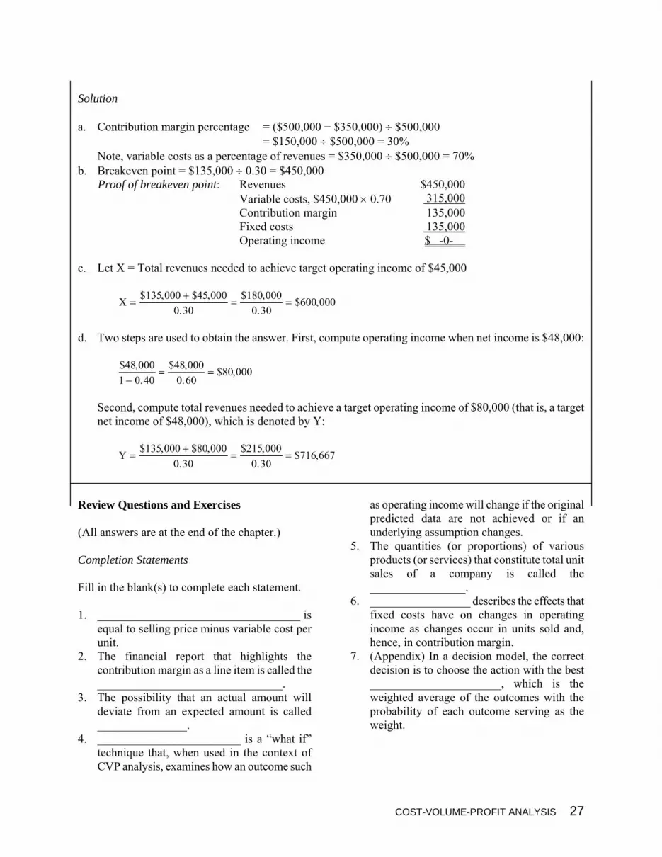
Solution a. Contribution margin percentage = ($500,000 − $350,000) ÷ $500,000 = $150,000 ÷ $500,000 = 30% Note, variable costs as a percentage of revenues = $350,000 ÷ $500,000 = 70% b. Breakeven point = $135,000 ÷ 0.30 = $450,000 Proof of breakeven point: Revenues $450,000 Variable costs, $450,000 × 0.70 315,000 Contribution margin 135,000 Fixed costs 135,000 Operating income $ -0- c. Let X = Total revenues needed to achieve target operating income of $45,000

000,600$30.0000,180$

30.0000,45$000,135$X ==

+=

d. Two steps are used to obtain the answer. First, compute operating income when net income is $48,000:

000,80$60.0000,48$

40.01000,48$

==−

Second, compute total revenues needed to achieve a target operating income of $80,000 (that is, a target

net income of $48,000), which is denoted by Y:

667,716$30.0000,215$

30.0000,80$000,135$Y ==

+=

Review Questions and Exercises (All answers are at the end of the chapter.) Completion Statements Fill in the blank(s) to complete each statement. 1. __________________________________ is

equal to selling price minus variable cost per unit.

2. The financial report that highlights the contribution margin as a line item is called the _______________________________.

3. The possibility that an actual amount will deviate from an expected amount is called _______________.

4. ________________________ is a “what if” technique that, when used in the context of CVP analysis, examines how an outcome such

as operating income will change if the original predicted data are not achieved or if an underlying assumption changes.

5. The quantities (or proportions) of various products (or services) that constitute total unit sales of a company is called the ________________.

6. _________________ describes the effects that fixed costs have on changes in operating income as changes occur in units sold and, hence, in contribution margin.

7. (Appendix) In a decision model, the correct decision is to choose the action with the best ______________________, which is the weighted average of the outcomes with the probability of each outcome serving as the weight.


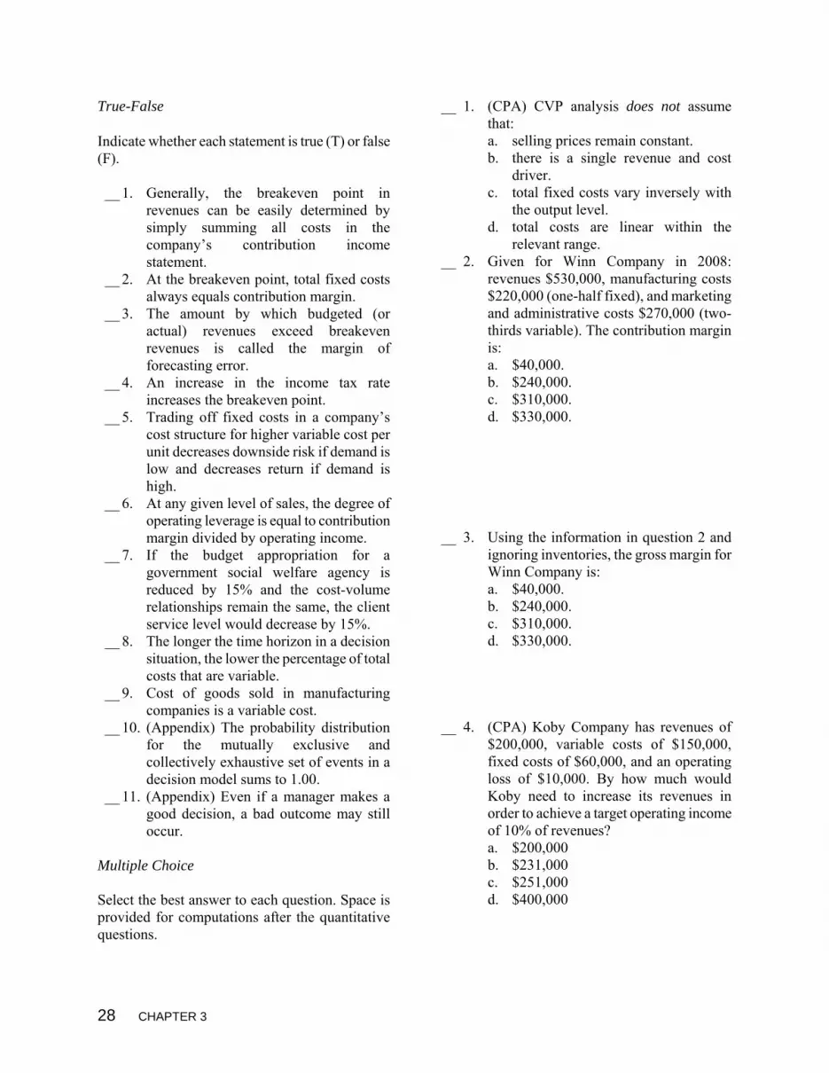
True-False Indicate whether each statement is true (T) or false (F). __ 1. Generally, the breakeven point in

revenues can be easily determined by simply summing all costs in the company’s contribution income statement.

__ 2. At the breakeven point, total fixed costs always equals contribution margin.

__ 3. The amount by which budgeted (or actual) revenues exceed breakeven revenues is called the margin of forecasting error.

__ 4. An increase in the income tax rate increases the breakeven point.

__ 5. Trading off fixed costs in a company’s cost structure for higher variable cost per unit decreases downside risk if demand is low and decreases return if demand is high.

__ 6. At any given level of sales, the degree of operating leverage is equal to contribution margin divided by operating income.

__ 7. If the budget appropriation for a government social welfare agency is reduced by 15% and the cost-volume relationships remain the same, the client service level would decrease by 15%.

__ 8. The longer the time horizon in a decision situation, the lower the percentage of total costs that are variable.

__ 9. Cost of goods sold in manufacturing companies is a variable cost.

__ 10. (Appendix) The probability distribution for the mutually exclusive and collectively exhaustive set of events in a decision model sums to 1.00.

__ 11. (Appendix) Even if a manager makes a good decision, a bad outcome may still occur.

Multiple Choice Select the best answer to each question. Space is provided for computations after the quantitative questions.

__ 1. (CPA) CVP analysis does not assume that: a. selling prices remain constant. b. there is a single revenue and cost

driver. c. total fixed costs vary inversely with

the output level. d. total costs are linear within the

relevant range. __ 2. Given for Winn Company in 2008:

revenues $530,000, manufacturing costs $220,000 (one-half fixed), and marketing and administrative costs $270,000 (two-thirds variable). The contribution margin is: a. $40,000. b. $240,000. c. $310,000. d. $330,000.

__ 3. Using the information in question 2 and

ignoring inventories, the gross margin for Winn Company is: a. $40,000. b. $240,000. c. $310,000. d. $330,000.

__ 4. (CPA) Koby Company has revenues of

$200,000, variable costs of $150,000, fixed costs of $60,000, and an operating loss of $10,000. By how much would Koby need to increase its revenues in order to achieve a target operating income of 10% of revenues? a. $200,000 b. $231,000 c. $251,000 d. $400,000

28 CHAPTER 3

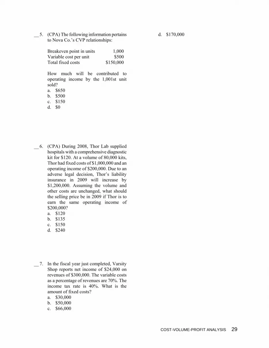
__ 5. (CPA) The following information pertains to Nova Co.’s CVP relationships:

Breakeven point in units 1,000Variable cost per unit $500Total fixed costs $150,000

How much will be contributed to operating income by the 1,001st unit sold? a. $650 b. $500 c. $150 d. $0

__ 6. (CPA) During 2008, Thor Lab supplied

hospitals with a comprehensive diagnostic kit for $120. At a volume of 80,000 kits, Thor had fixed costs of $1,000,000 and an operating income of $200,000. Due to an adverse legal decision, Thor’s liability insurance in 2009 will increase by $1,200,000. Assuming the volume and other costs are unchanged, what should the selling price be in 2009 if Thor is to earn the same operating income of $200,000? a. $120 b. $135 c. $150 d. $240

__ 7. In the fiscal year just completed, Varsity

Shop reports net income of $24,000 on revenues of $300,000. The variable costs as a percentage of revenues are 70%. The income tax rate is 40%. What is the amount of fixed costs? a. $30,000 b. $50,000 c. $66,000

d. $170,000


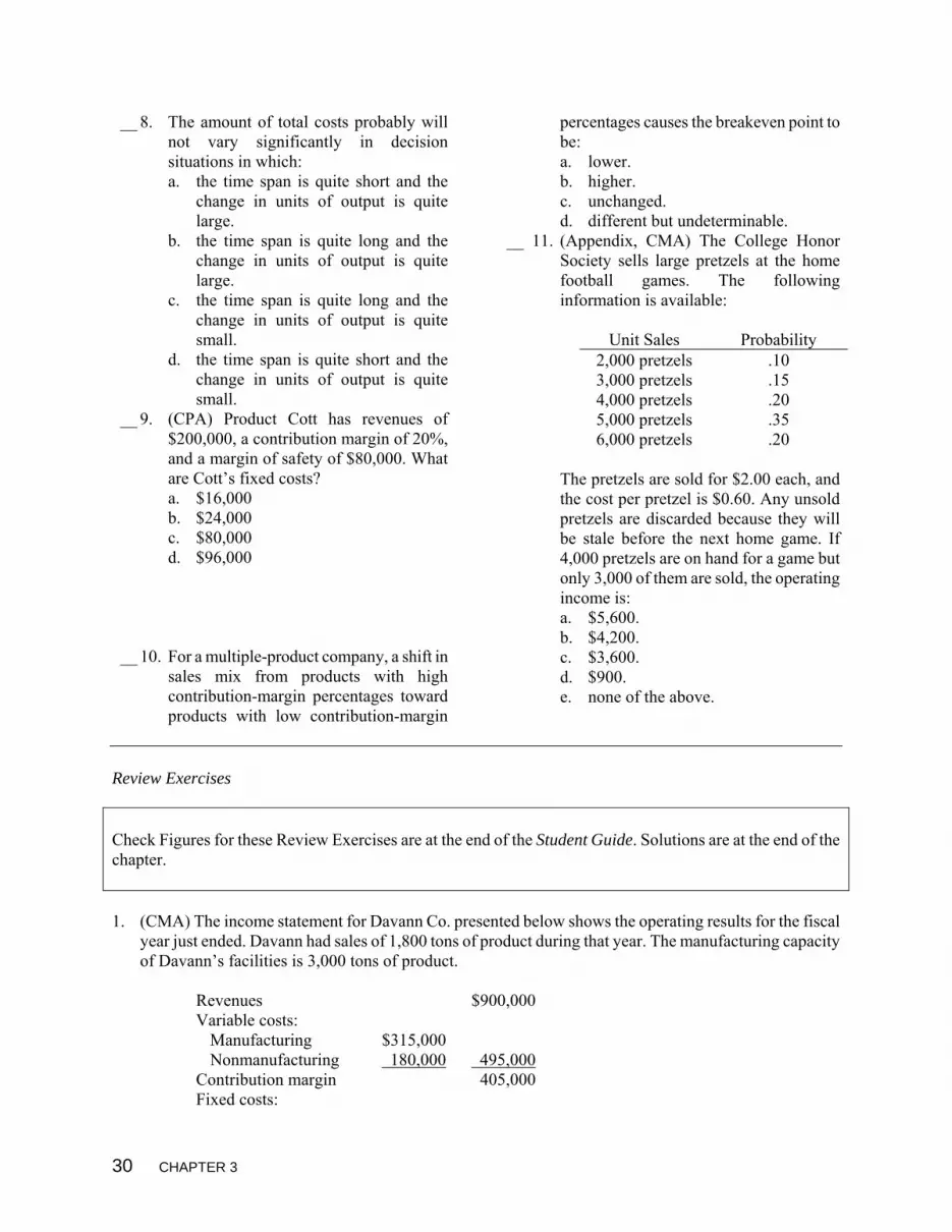
__ 8. The amount of total costs probably will not vary significantly in decision situations in which: a. the time span is quite short and the

change in units of output is quite large.

b. the time span is quite long and the change in units of output is quite large.

c. the time span is quite long and the change in units of output is quite small.

d. the time span is quite short and the change in units of output is quite small.

__ 9. (CPA) Product Cott has revenues of $200,000, a contribution margin of 20%, and a margin of safety of $80,000. What are Cott’s fixed costs? a. $16,000 b. $24,000 c. $80,000 d. $96,000

__ 10. For a multiple-product company, a shift in sales mix from products with high contribution-margin percentages toward products with low contribution-margin

percentages causes the breakeven point to be: a. lower. b. higher. c. unchanged. d. different but undeterminable.

__ 11. (Appendix, CMA) The College Honor Society sells large pretzels at the home football games. The following information is available:

Unit Sales Probability

2,000 pretzels .10 3,000 pretzels .15 4,000 pretzels .20 5,000 pretzels .35 6,000 pretzels .20

The pretzels are sold for $2.00 each, and the cost per pretzel is $0.60. Any unsold pretzels are discarded because they will be stale before the next home game. If 4,000 pretzels are on hand for a game but only 3,000 of them are sold, the operating income is:

a. $5,600. b. $4,200.

c. $3,600. d. $900. e. none of the above.

Review Exercises Check Figures for these Review Exercises are at the end of the Student Guide. Solutions are at the end of the chapter. 1. (CMA) The income statement for Davann Co. presented below shows the operating results for the fiscal

year just ended. Davann had sales of 1,800 tons of product during that year. The manufacturing capacity of Davann’s facilities is 3,000 tons of product.

Revenues $900,000Variable costs:

Manufacturing $315,000Nonmanufacturing 180,000 495,000

Contribution margin 405,000Fixed costs:

30 CHAPTER 3

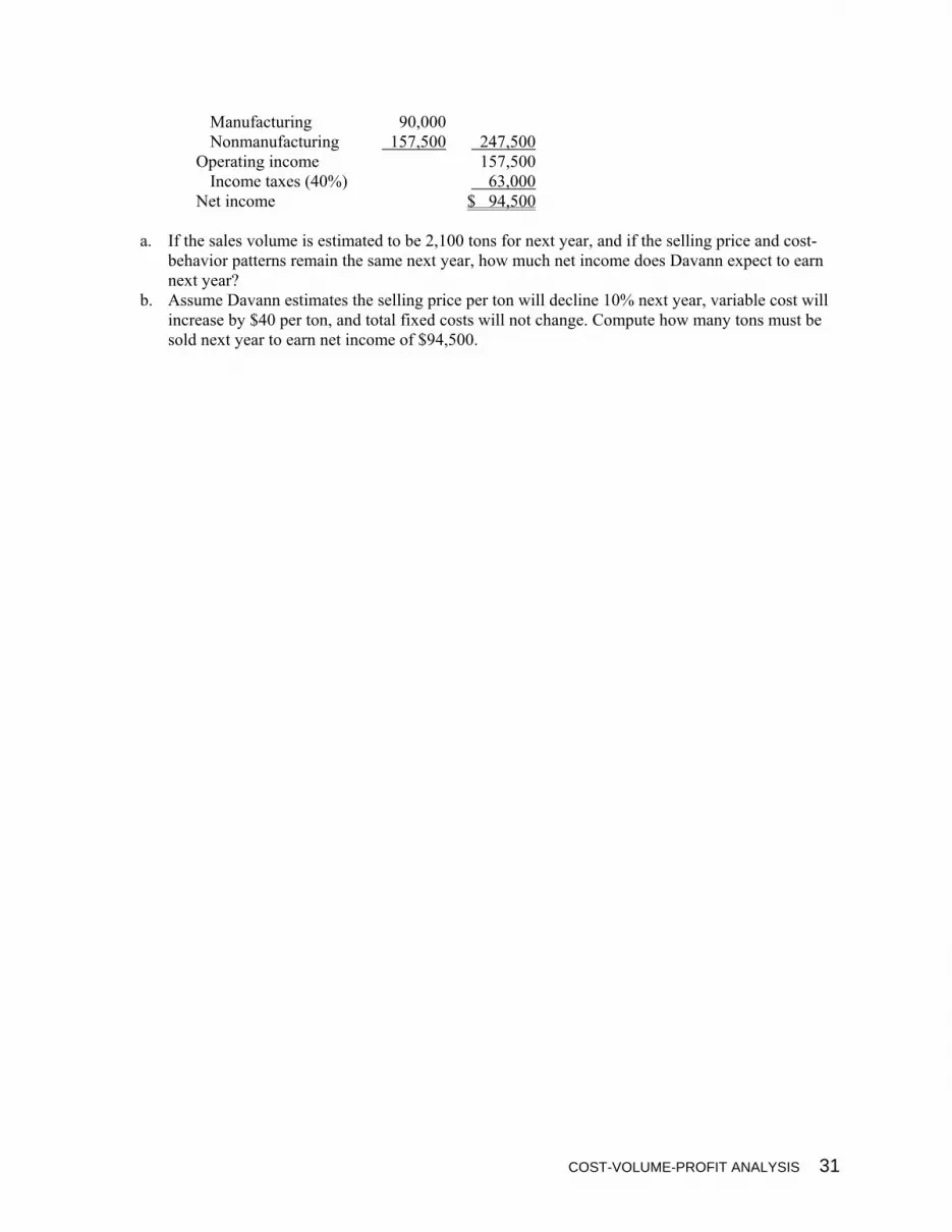
Manufacturing 90,000Nonmanufacturing 157,500 247,500

Operating income 157,500Income taxes (40%) 63,000

Net income $ 94,500

a. If the sales volume is estimated to be 2,100 tons for next year, and if the selling price and cost-behavior patterns remain the same next year, how much net income does Davann expect to earn next year?

b. Assume Davann estimates the selling price per ton will decline 10% next year, variable cost will increase by $40 per ton, and total fixed costs will not change. Compute how many tons must be sold next year to earn net income of $94,500.


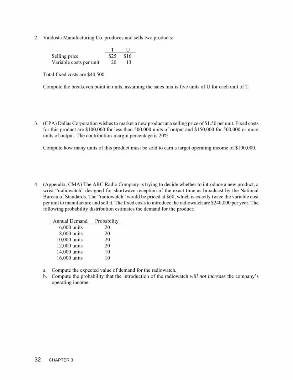
2. Valdosta Manufacturing Co. produces and sells two products:

T U Selling price $25 $16 Variable costs per unit 20 13

Total fixed costs are $40,500.

Compute the breakeven point in units, assuming the sales mix is five units of U for each unit of T.

3. (CPA) Dallas Corporation wishes to market a new product at a selling price of $1.50 per unit. Fixed costs

for this product are $100,000 for less than 500,000 units of output and $150,000 for 500,000 or more units of output. The contribution-margin percentage is 20%.

Compute how many units of this product must be sold to earn a target operating income of $100,000.

4. (Appendix, CMA) The ARC Radio Company is trying to decide whether to introduce a new product, a

wrist “radiowatch” designed for shortwave reception of the exact time as broadcast by the National Bureau of Standards. The “radiowatch” would be priced at $60, which is exactly twice the variable cost per unit to manufacture and sell it. The fixed costs to introduce the radiowatch are $240,000 per year. The following probability distribution estimates the demand for the product:

Annual Demand Probability

6,000 units .20 8,000 units .20

10,000 units .20 12,000 units .20 14,000 units .10 16,000 units .10

a. Compute the expected value of demand for the radiowatch. b. Compute the probability that the introduction of the radiowatch will not increase the company’s

operating income.

32 CHAPTER 3

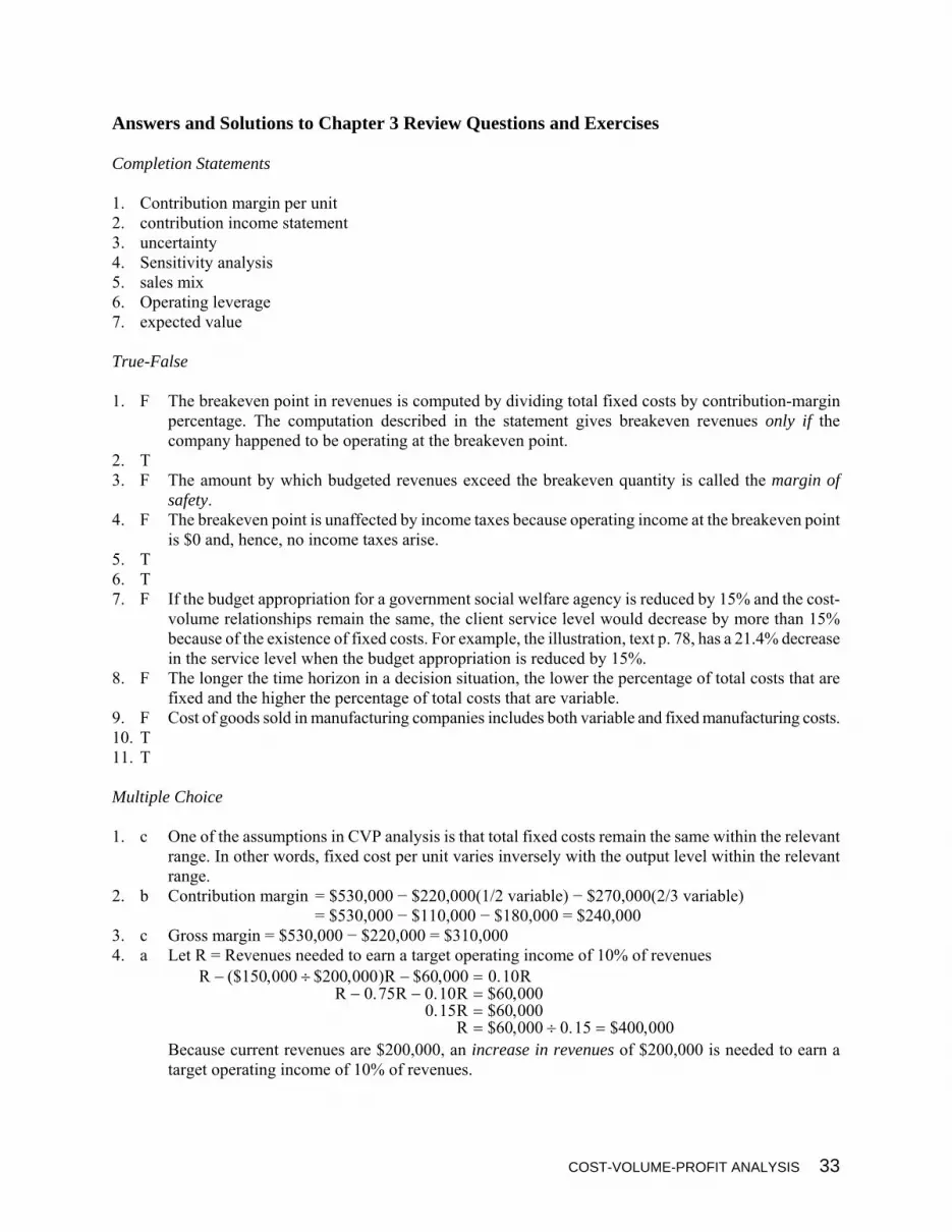
Answers and Solutions to Chapter 3 Review Questions and Exercises Completion Statements 1. Contribution margin per unit 2. contribution income statement 3. uncertainty 4. Sensitivity analysis 5. sales mix 6. Operating leverage 7. expected value True-False 1. F The breakeven point in revenues is computed by dividing total fixed costs by contribution-margin

percentage. The computation described in the statement gives breakeven revenues only if the company happened to be operating at the breakeven point.

2. T 3. F The amount by which budgeted revenues exceed the breakeven quantity is called the margin of

safety. 4. F The breakeven point is unaffected by income taxes because operating income at the breakeven point

is $0 and, hence, no income taxes arise. 5. T 6. T 7. F If the budget appropriation for a government social welfare agency is reduced by 15% and the cost-

volume relationships remain the same, the client service level would decrease by more than 15% because of the existence of fixed costs. For example, the illustration, text p. 78, has a 21.4% decrease in the service level when the budget appropriation is reduced by 15%.

8. F The longer the time horizon in a decision situation, the lower the percentage of total costs that are fixed and the higher the percentage of total costs that are variable.

9. F Cost of goods sold in manufacturing companies includes both variable and fixed manufacturing costs. 10. T 11. T Multiple Choice 1. c One of the assumptions in CVP analysis is that total fixed costs remain the same within the relevant

range. In other words, fixed cost per unit varies inversely with the output level within the relevant range.

2. b Contribution margin = $530,000 − $220,000(1/2 variable) − $270,000(2/3 variable) = $530,000 − $110,000 − $180,000 = $240,000 3. c Gross margin = $530,000 − $220,000 = $310,000 4. a Let R = Revenues needed to earn a target operating income of 10% of revenues

000,400$15.0000,60$R000,60$R15.0000,60$R10.0R75.0RR10.0000,60$R)000,200$000,150($R

=÷===−−=−÷−

Because current revenues are $200,000, an increase in revenues of $200,000 is needed to earn a target operating income of 10% of revenues.


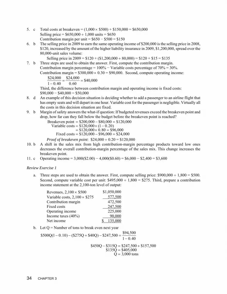
5. c Total costs at breakeven = (1,000 × $500) + $150,000 = $650,000 Selling price = $650,000 ÷ 1,000 units = $650 Contribution margin per unit = $650 − $500 = $150

6. b The selling price in 2009 to earn the same operating income of $200,000 is the selling price in 2008, $120, increased by the amount of the higher liability insurance in 2009, $1,200,000, spread over the 80,000-unit sales volume:

Selling price in 2009 = $120 + ($1,200,000 ÷ 80,000) = $120 + $15 = $135 7. b Three steps are used to obtain the answer. First, compute the contribution margin.

Contribution margin percentage = 100% − Variable costs percentage of 70% = 30%. Contribution margin = $300,000 × 0.30 = $90,000. Second, compute operating income:

000,40$60.0000,24$

40.01000,24$

==−

Third, the difference between contribution margin and operating income is fixed costs: $90,000 − $40,000 = $50,000

8. d An example of this decision situation is deciding whether to add a passenger to an airline flight that has empty seats and will depart in one hour. Variable cost for the passenger is negligible. Virtually all the costs in this decision situation are fixed.

9. b Margin of safety answers the what-if question: If budgeted revenues exceed the breakeven point and drop, how far can they fall below the budget before the breakeven point is reached?

000,24$000,96$000,120$costs Fixed000,96$80.0000,120$

)20.01(000,120$costs Variable000,120$000,80$000,200$ pointBreakeven

=−==×=

−×==−=

Proof of breakeven point: $24,000 ÷ 0.20 = $120,000 10. b A shift in the sales mix from high contribution-margin percentage products toward low ones

decreases the overall contribution-margin percentage of the sales mix. This change increases the breakeven point.

11. c Operating income = 3,000($2.00) − 4,000($0.60) = $6,000 − $2,400 = $3,600 R eview Exercise 1

a. Three steps are used to obtain the answer. First, compute selling price: $900,000 ÷ 1,800 = $500. Second, compute variable cost per unit: $495,000 ÷ 1,800 = $275. Third, prepare a contribution income statement at the 2,100-ton level of output:

Revenues, 2,100 × $500 $1,050,000Variable costs, 2,100 × $275 577,500Contribution margin 472,500Fixed costs 247,500Operating income 225,000Income taxes (40%) 90,000Net income $ 135,000

b. Let Q = Number of tons to break even next year

40.01500,94$500,247$)Q40$Q275($)10.01(Q500$

−=−+−−

tons 000,3Q000,405$Q135$

500,157$500,247$Q315$Q450$

==

+=−

34 CHAPTER 3

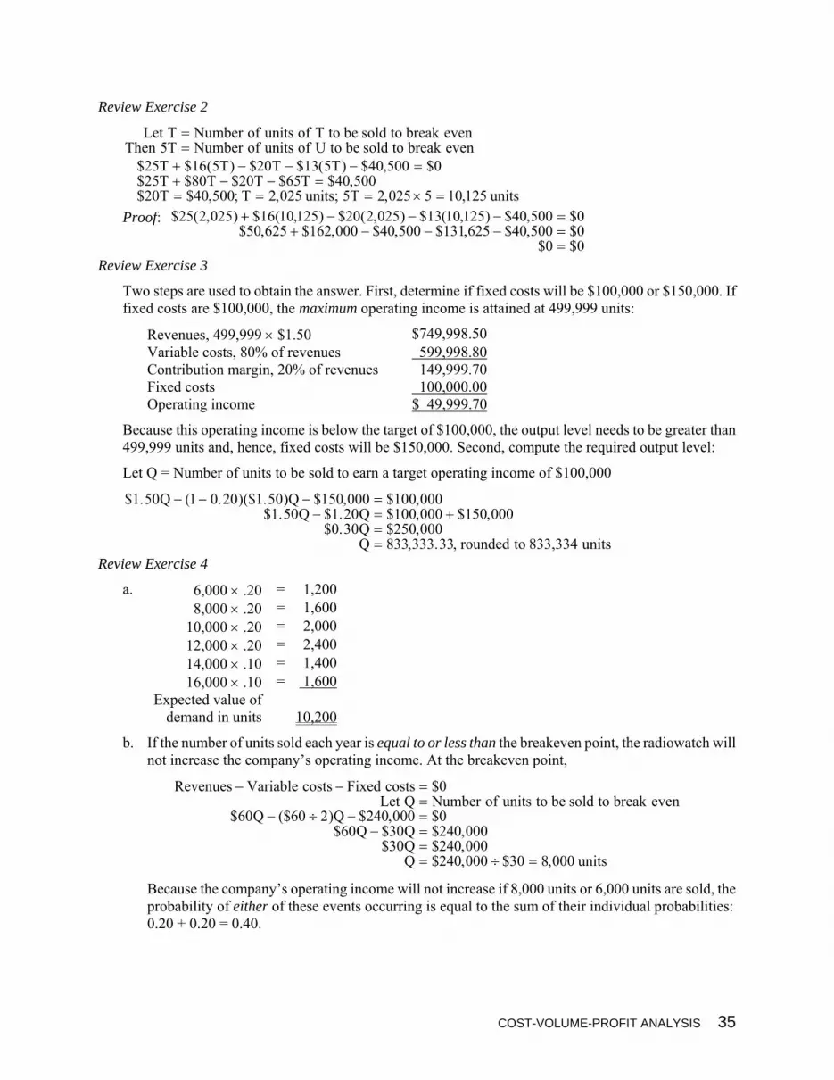
R eview Exercise 2

even break to sold be to U of unitsof Number5T Theneven break to sold be to T of unitsof NumberT Let

==

units125,105025,2T5 units;025,2T ;500,40$T20$500,40$T65$T20$T80$T25$

0$500,40$)T5(13$T20$)T5(16$T25$

=×====−−+

=−−−+

Proof:

0$0$0$500,40$625,131$500,40$000,162$625,50$0$500,40$)125,10(13$)025,2(20$)125,10(16$)025,2(25$

==−−−+=−−−+

R eview Exercise 3

Two steps are used to obtain the answer. First, determine if fixed costs will be $100,000 or $150,000. If fixed costs are $100,000, the maximum operating income is attained at 499,999 units:

Revenues, 499,999 × $1.50 $749,998.50Variable costs, 80% of revenues 599,998.80Contribution margin, 20% of revenues 149,999.70Fixed costs 100,000.00Operating income $ 49,999.70

Because this operating income is below the target of $100,000, the output level needs to be greater than 499,999 units and, hence, fixed costs will be $150,000. Second, compute the required output level:

Let Q = Number of units to be sold to earn a target operating income of $100,000

units833,334 to rounded ,33.333,833Q000,250$Q30.0$

000,150$000,100$Q20.1$Q50.1$000,100$000,150$Q)50.1)($20.01(Q50.1$

==

+=−=−−−

R eview Exercise 4

a. 6,000 × .20 = 1,200 8,000 × .20 = 1,600 10,000 × .20 = 2,000 12,000 × .20 = 2,400 14,000 × .10 = 1,400 16,000 × .10 = 1,600 Expected value of

demand in units

10,200

b. If the number of units sold each year is equal to or less than the breakeven point, the radiowatch will not increase the company’s operating income. At the breakeven point,

units000,830$000,240$Q000,240$Q30$000,240$Q30$Q60$

0$000,240$Q)260($Q60$even break to sold be to unitsof NumberQ Let

0$costs Fixedcosts VariableRevenues

=÷===−=−÷−==−−

Because the company’s operating income will not increase if 8,000 units or 6,000 units are sold, the probability of either of these events occurring is equal to the sum of their individual probabilities: 0.20 + 0.20 = 0.40.


cost-volume-profit analysis - pdf4pro

Documents