cost minimization for rule caching in software defined
TRANSCRIPT

1
Cost Minimization for Rule Caching in SoftwareDefined Networking
Huawei Huang, Student Member, IEEE, Song Guo, Senior Member, IEEE, Peng Li, Member, IEEE,Weifa Liang, Senior Member, IEEE, and Albert Y. Zomaya, Fellow, IEEE
Abstract—Software-Defined Networking (SDN) is an emerging network paradigm that simplifies network management by decouplingthe control plane and data plane, such that switches become simple data forwarding devices and network management is controlledby logically centralized servers. In SDN-enabled networks, network flow is managed by a set of associated rules that are maintained byswitches in their local Ternary Content Addressable Memories (TCAMs) which support high-speed parallel lookup on wildcard patterns.Since TCAM is an expensive hardware and extremely power-hungry, each switch has only limited TCAM space and it is inefficient andeven infeasible to maintain all rules at local switches. On the other hand, if we eliminate TCAM occupation by forwarding all packets tothe centralized controller for processing, it results in a long delay and heavy processing burden on the controller. In this paper, we strivefor the fine balance between rule caching and remote packet processing by formulating a minimum weighted flow provisioning (MWFP)problem with an objective of minimizing the total cost of TCAM occupation and remote packet processing. We show the problemis NP-hard, and propose an efficient offline algorithm if the network traffic is given, otherwise, we propose two online algorithmswith guaranteed competitive ratios. Finally, we conduct extensive experiments by simulations using real network traffic traces. Thesimulation results demonstrate that our proposed algorithms can significantly reduce the total cost of remote controller processing andTCAM occupation, and the solutions obtained are nearly optimal.
F
1 INTRODUCTION
Software Defined Networking (SDN) is regarded as onepromising next generation network architecture [1]–[3].By shifting the control plane to a logically centralizedcontroller, SDN offers programmable functions (e.g.,OpenFlow [1], [4] ) to dynamically control and managepackets forwarding and processing in switches, such thata wide range of network policies (e.g., traffic engineering[5]–[7], security [8], fault-tolerance [9] ) and new networktechnologies can be easily deployed.
In SDN, each network flow is associated with a set ofrules, such as packet forwarding, dropping and modi-fying, that should be installed at switches in terms offlow table entries along the flow path. SDN-enabledswitches maintain flow rules in their local TCAMs [10]–[12], which support high-speed parallel lookup on wild-card patterns. A typically flow setup process [2], [13]between a pair of users, say users A and B, in SDNcontains three steps. 1) User A sends out packets afterconnection initialization. Once a packet arrives a switchwithout matched flow table entries, this packet is for-warded to the controller. 2) Upon receiving the packet,the controller decides whether to allow or deny this flowaccording to network management policies. 3) If the flowis allowed, the controller installs corresponding rules toall switches along the path, such that consecutive packets
H. Huang, S. Guo and P. Li are with the School of Computer Scienceand Engineering, the University of Aizu, Japan. Email: {d8152101, sguo,pengli}@u-aizu.ac.jpW. Liang is with the Research School of Computer Science, the AustralianNational University, Australia. Email: [email protected]. Y. Zomaya is with the School of Information Technologies, the Universityof Sydney, Australia. Email: [email protected]
0 20 40 60 80 1000
1000
2000
0 10 20 30 40 500
1000
2000
0 5 10 15 20 250
1000
2000
Pac
ket
s (B
yte
s)
0 5 10 150
1000
2000
Time slot
Fig. 1. The sniffed TCP traffic flow [14].
can be processed by the installed rules locally at switch-es. Note that switches usually set an expiration timefor rules, which defines the maximum rule maintenancetime when no packet of associated flow arrives.
In practice, network flow shows various traffic pat-terns. For example, we show real-time traffic of fournetwork flows [14] in Fig. 1, where some are bursttransmission while the others have consecutive packettransmissions for a long time. For consecutive trans-mission, only the first packet experiences the delay ofremote processing at the controller, and the rest will beprocessed by local rules at switches. However, for bursttransmission, the corresponding rules cached in switcheswill be removed between two batches of packets if theirinterval is greater than the rule expiration time. As a
2
result, remote packet processing would be incurred bythe first packet of each batch, leading to a long delayand high processing burden on the controller. A simplemethod to reduce the overhead of remote processingis to cache rules at switches within the lifetime ofnetwork flow, ignoring the rule expiration time. Unfor-tunately, network devices are equipped with limited-space TCAMs because they are expensive hardware andextremely power-hungry. For instance, it is reported thatTCAMs are 400 times more expensive [12] and 100 timesmore power-consuming [15] per Mbit than RAM-basedstorage. Since TCAM space is shared by multiple flow innetworks, it is inefficient and even infeasible to maintainall rules at local switches. This dilemma motivates usto investigate efficient rule caching schemes for SDN tostrive for a fine balance between network performanceand TCAM usage.
The main contributions of our paper are summarizedas follows.
• To the best of our knowledge, we are the first tostudy the rule caching problem with the objectiveof minimizing the sum of remote processing costand TCAM occupation cost.
• We show the NP-hardness of the problem, andpropose an offline algorithm by adopting a greedystrategy if the network traffic is given in advance.We also devise two online algorithms with guaran-teed competitive ratios.
• Finally, we conduct extensive simulations using realnetwork traffic traces to evaluate the performance ofour proposals. The simulation results demonstratethat our proposed algorithms can significantly re-duce the total cost of remote controller processingand TCAM occupation, and the solutions obtainedare nearly optimal.
The reminder of the paper is structured as follows.Section 2 reviews some related work in table entriesscheduling in SDN. Section III introduces the systemmodel and problem formulation. An offline algorithm isproposed in Section IV. Two online algorithms are pro-posed and analysed in Section 5. Section 6 demonstratesthe performance evaluation results. Finally, section 7concludes this paper.
2 RELATED WORK
As one pioneering work of recouping control plane fromthe data plane, NOX [8] has been proposed to controldata forwarding based on OpenFlow.
Following this line of research, lots of efforts have beenmade on rule caching strategies in SDN, which can beclassified into two categories: reactive way [2], [8] andproactive way [3], [4], [16].
The reactive rule caching has been widely adopted byexisting work [2], [8] because of its efficient usage ofTCAM space. The first packet of each “microflow” isforwarded to the controller that reactively installs flowentries in switches. For instance, Ethane [2] controller
reactively installs flow table entries based on the firstpacket of each TCP/UDP flow. Recently, Bari et al. [13]use the on-demand approach to response flow setuprequests.
On the other hand, other studies [17], [18] argue thatreactive approach is time-consuming because of remoterule fetching, leading to heavy overhead in packet pro-cessing [5], [13], [16]. To reduce the response time forpackets at switches without matched rules, proactiveapproach has been proposed to install rules in switchesbefore corresponding packets arrive. For example, Ben-son, et al. [5] developed a system MicroTE that adapts totraffic fluctuations, with which rules can be dynamicallyupdated in switches to imposes minimal overhead onnetwork based on traffic prediction. Kang, et al. [3]have proposed to pre-compute backup rules for possiblefailures and cache them in switches in advance to reducenetwork recovery time.
In addition, other related literatures [7], [12], [19], [20]focus on the rules scheduling considering forwardingtable size utilization. For instance, Katta et al. [12] pro-posed a abstraction of an infinite switch based on anarchitecture that leverages both hardware and software,in which rules caching space can be infinite. In that case,rules can be cached in forwarding table as many aspossible. This abstraction saves TCAMs space, but thepacket processing speed in switch is a bottleneck. Toefficiently use TCAMs space, Kanizo et al. [7], Nguyenet al. [19] and Cohen et al. [20] propose their rulesplacement scheduling jointly consider the traffic routingin network. However, rules updating is ignored in theiroptimization. To the contrast, we study both the twoaspects in our optimization.
The work most related with our paper is DIFANE[16], a compromised architecture that leverages a setof authority switches serving as a middle layer be-tween the controller in control plane and switches indata plane. The endpoints rules are pre-computed andcached in authority switches. Once the first packet ofa new microflow arrives the switch, the desired rulesare reactively installed, from authority switches ratherthan the controller. In this way, the flow setup timecan be significantly reduced. Unfortunately, caching pre-computed rules all in authority switches consumes largeTCAM space. In our work, we still load the flow rulesinto switches in a reactive way. However, rule cachingperiod is controlled by our proposed algorithm by takingboth remote processing and TCAM occupation cost intoconsideration.
3 SYSTEM MODEL AND PROBLEM FORMULA-TION
We consider a discrete time model, where the timehorizon is divided into T time slots of equal lengthl. A network flow travels along a set of SDN-enabledswitches, each of which is assigned a set of rules toimplement routing or network management functions.

3
TABLE 1Notions and Variables
Notations DescriptionT maximum time-slot range of considerationl length of each time slot (seconds)ai a binary indicator that denotes the positive flow rate
in time slot i, i=1,2,..Tδ sum of time slots where ai > 0D amount of valid periods during [1, T ]Vi the ith valid period during [1, T ]Ei the ith empty period during [1, T ]α occupation cost of caching table entryβ remote processing costγ γ = α
β
xi a binary variable indicating whether cache actionhappens in time slot i, i=1,2,..T
yi a binary variable indicating whether fetch actionhappens in time slot i, i=1,2,..T
CC total cost of cache action during [1, T ]CF total cost of fetch action during [1, T ]
For simplicity, in this paper, we study rule caching at aswitch with a set of associated rules whose maintenancecost is α per second, and our results can be directlyextended to all switches along the flow path. Notethat the set of rules associated with the network flowwill be cached or removed as a whole at the switch.When no matched flow table entries are available at theswitch for arriving packets, these packets will be sentto the controller for processing. We model the remoteprocessing cost at controller as β. The ratio between thesetwo kinds of cost is denoted by γ, i.e., γ = α
β . We considerarbitrary traffic pattern of the network flow. The set oftime slots with (at > 0) and without (at = 0) packettransmission are referred to as valid period and emptyperiod, respectively. All symbols and variables used inthis paper are summarized in Table 1.
We define a binary variable xi to denote whether aflow entry is cached at the i-th time slot:
xi =
{1, if rules are cached at the i-th time slot,0, otherwise.
The occupation cost can be calculated as follows.
CC = αl ·T∑
i=1
xi. (1)
We also define a binary variable yi to indicate whetherremote packet processing is conducted.
yi =
{1, if rules are remotely fetched in the i-th time slot,0, otherwise.
and the corresponding cost can be calculated by:
CF = βl ·T∑
i=1
yi. (2)
With the global information of the given traffic flow,the minimum weighted flow provisioning (MWFP)
problem can be formulated as follows:
MWFP : minxi,yi
CTotal = CC + CF
s.t. xi − xi−1 ≤ yi, (3a)i∑
j=1
yj ≥ xi, (3b)
(xi + yi) ≥ ai, (3c)xi, yi ∈ {1, 0}, ∀i = 1, 2, .., T.
The trigger of remote processing is represented by con-straint (3a), where yi = 1 only when we decide to cacherules from the i-th time slot, which are not available atlocal switches in the (i− 1)-th time slot, i.e., xi = 1 andxi−1 = 0. Constraint (3b) indicates that the switch needsto fetch rules at least one time before caching. Constraint(3c) claims that arriving packets must be processed bylocal cached rules or remote controller. Note that theinput of this problem are ai, α, β or γ, and the outputare the scheduling solution xi, yi, i=1,2,..T .
Theorem 1. The MWFP problem is NP-hard.
Proof: We show MWFP problem is NP-hard byperforming a polynomial reduction from the weightedset cover problem, a classic combinatorial optimizationproblem that is proved NP-hard [21], [22]: Suppose wehave an instance of the weighted set cover problemA′=(U ′,S ′). Given a set U ′ = {1, 2, .., T}, a collectionS ′={S′
1, S′2, ..., S′
m}(m= 12 (T
2 + T )) of subsets of U ′, withweights w(S′
i), the goal is to find a collection C′ of thesesubsets whose union is U ′, such that
∑C′
i∈C′ w(C ′i) is
minimized.We construct an instance of the MWFP from this
instance, i.e., A= (U , S) with U = {1, 2, .., T}, S ={{1},{2},.., {T}, {1,2},{2,3},.., {T -1,T}, {1,2,3},{2,3,4},..,{T -2,T -1,T}, ..., {1,2,..,T -1}, {2,3,..,T}, {1,2,..,T}}, inwhich each element in each subset of S denotes the time-slot during [1,T ]. Every subset in S is a cost(Si), whichcan be calculated as
cost(Si) =
{βl + αl · |Si|, if |Si| > 1;
βl · ai, if |Si| = 1.(4)
The target is to find a collection of time slots C ⊆ Ssuch that
∪Ci∈C Ci = U , and ensuring the total cost of
C is minimum. It can be seen that such transformationcan be done in polynomial time. As the weighted setcover problem is NP-hard, the MWFP is NP-hard too asthe reduction can be done in polynomial time, and viceversa.
4 OFFLINE ALGORITHM
Due to the NP-hardness, solving MWFP problem is com-putationally infeasible for large-scale problem instances.In this section, we propose a heuristic algorithm to solvethe offline version of the problem. As shown in Algorith-m Offline Greedy, we first generate a collection of timeslot sets that represents possible rule cache periods as

4
shown in line 1. Each set is assigned a weight accordingto (4) in line 2. Then, we select time slot sets for rulecaching in an iterative manner from line 4 to 8. In eachiteration, we choose the set X that minimizes the valueof weight w(X) divided by number of elements not yetcovered.
Algorithm 1 Offline Greedy Algorithm to solve MWFPInput: flow indicator set F = {a(t), t∈[1,T ]}, and
T ={1,2,...,T}Output: The collection C of subsets of T
1: generate sample collection S with∪
S∈S S = T ,where its generating method has been described inthe proof of Theorem 1.
2: generate the weight function w: S → R+ by invoking(4)
3: C ← ∅, and R← T4: while R = ∅ do5: X ← argminX∈S
w(X)|X∩R|
6: C ← C ∪X7: R← R \X8: end while
Theorem 2. Alg.1 is (lnT+1)-approximation to the optimalsolution of MWFP, where T is the maximum time slot.
Proof: For each element (time slot) tj ∈ T , let Sj bethe first picked set that covers it while applying Alg.1,and θ(tj) denote the amortized cost of each element inSj ,
θ(tj) =w(Sj)
|Sj ∩R|.
Obviously, the cost of Alg.1 can be written as∑tj∈T θ(tj).Then, let T = {t1, t2, ..., tT } denote the ordered set
of elements in [1,T ] that each is covered. Note that,when tj is to be covered, apparently we have R ⊇{tj , tj+1, ..., tT }. We can see that R contains at least(T − j + 1) elements. Therefore, the amortized cost inSj is at most the average cost of the optimum solution(denoted by OPT), i.e.,
θ(tj) =w(Sj)
|Sj ∩R|≤ OPT
T − j + 1.
By summing the θ(tj) in all time slots, we get:∑tj∈T
θ(tj) ≤ OPT(1
T+
1
T − 1+ · · ·+ 1
2+ 1).
That is Greedy ≤ OPT ·H(T ) ≤ OPT · (1 + lnT ), whereH(T ) is called the harmonic number of T .
5 ONLINE ALGORITHMS
In this section, we consider the MWFP problem assum-ing that the packet traffic information is not given inadvance. We first present several important observations
i i
FNC i
i+1
i+2 i+2
CIE i+2
i+3
FNC i+1
FNC
j
j
j
j
i+4
SUF i+4 NF i+5
|Vi+5|=1
Fig. 2. Illustration of typical actions in optimum solution.
in the optimal solution, followed by two proposed on-line algorithms with low computational complexity toapproximate the optimal solution.
5.1 Typical actions in optimal solutionsBy carefully examining the optimal solutions of sever-al problem instances, we find that there exists severaltypical actions as follows.
• FNC (Fetch and Cache): for valid periods with atleast 2 time slots, flow rules are first fetched fromthe remote controller, and then they are cached atlocal switches.
• SUF (Successive Fetch): for a valid period with atleast 2 time slots, all packets are forwarded to theremote controller for processing.
• CIE (Cache in Empty period): rules are cached inswitches during the empty period between twovalid periods.
• NF (Only Forward): Packets are processed by thecontroller in the empty periods of one time slot.
Above typical actions are illustrated in Fig. 2. Theoptimal solutions can be categorized into following threecases.
• OPT-A: there are only SUF actions in the optimalsolution.
• OPT-B: there are only CIE actions in the optimalsolution.
• OPT-C: both SUF and CIE actions exist in the opti-mal solution.
5.2 Online Exactly Match the Flow AlgorithmOur first online algorithm, which is referred to as EMF(Exactly Match the Flow Algorithm), is shown in Alg. 2.In each time slot, each switch makes a decision, cachingor fetching, according to observed network traffic. Whenthere are packets arriving in the current time slot, i.e.,at = 1, if no matched rules are cached, i.e., xt−1 = 0,switch fetches rules from the controller. Otherwise, wekeep caching them in switches.
Lemma 1. Suppose there are D valid periods (denoted by Vi,i = 1,2,...,D) including δ valid time slots within [1, T ], thetotal cost of EMF is
CEMF = βlD + αlδ. (5)

5
Algorithm 2 online Exactly Match the Flow (EMF) Al-gorithm
1: for each time slot t ∈ [1, T ] do2: if at=1 and xt−1=0 then3: fetch flow rules from the controller4: yt ← 1, xt ← 15: else if at=1 and xt−1=1 then6: keep caching entries in switches7: else if at=0 and xt−1=1 then8: remove the corresponding flow table entries9: xt ← 0
10: end if11: end for
Proof: In Alg. 2, flow rules are maintained in switch-es only when there are network traffic passing through,such that TCAM occupation cost can be easily calcu-lated by αlδ. Since rule fetching action happens in thebeginning of each valid period, we have fetching cost ofβlD. By summing them up, the total cost of EMF can becalculated by (5).
Lemma 2. When the optimal solution belongs to OPT-A, SUF is adopted by any valid period Vi, we have γ >|Vi|−1|Vi| , ∀i = 1, 2, ..., D.
Proof: Since SUF is adopted in the optimal solution,its cost must be less than FNC, i.e.,
|Vi|βl < βl + |Vi|αl
⇒ β <|Vi|α|Vi| − 1
⇒ γ >|Vi| − 1
|Vi|, ∀i = 1, 2, ..., D.
Theorem 3. When the optimal solution belongs to OPT-A,the EMF algorithm is (γ + D
δ )-competitive.
Proof: Since the optimal solution belongs to OPT-A,i.e., all packets are sent to the controller for processing,it is easy to see that the total cost of optimal solution isβlδ. Thus, the competitive ratio λA is:
λA =CEMF
βlδ=
αδ + βD
βδ= γ +
D
δ.
Lemma 3. When the optimal solution belongs to OPT-B,rules are always maintained by switches once downloaded, i.e.,CIE is adopted by the period Ei between any two valid periodsVi and Vi+1, and we have γ < 1
|Ei| ,∀i = 1, 2, ..., D − 1.
Proof: If switches continue to cache rules once they’redownloaded, the TCAM occupation cost during Ei mustbe less than the fetching cost at the beginning of Vi+1,i.e.,
αl(|Ei|+ |Vi+1|) < βl + |Vi+1| · αl
⇒ β > α|Ei| ⇒ γ <1
|Ei|, ∀i = 1, 2, ..., D − 1.
i i
FNC i
i+1
i i
CIE i
i+1
FNC i+1
FNC i i i+1
j
j
j
j
Fig. 3. Rules are cached in Ei because of CIE action.
Theorem 4. When the optimal solution belongs to OPT-B,the EMF algorithm is
(D+γδ
1+γ(δ+D−1)
)-competitive.
Proof: As shown in Fig. 3, since rules are maintainedin switches once downloaded under OPT-B, its total costcan be easily calculated by βl+αl(δ+
∑D−1i=1 |Ei|), where
the first term is the cost of the only fetching that happensin the beginning of the first valid period, and the secondterm is TCAM occupation cost. Combined with Lemma1, the competitive ratio is:
λB =CEMF
βl + αl(δ +∑D−1
i=1 |Ei|)
≤ βD + αδ
β + α(δ +D − 1)=
D + γδ
1 + γ(δ +D − 1).
Lemma 4. When the optimal solution belongs to OPT-C,there exists at least one valid period Vi, i ∈ [1, D] and oneempty period Ej , j ∈ [1, D− 1], such that |Vi|−1
|Vi| < γ < 1|Ej | .
Proof: This lemma can be easily proved followingsimilar analysis in Lemmas 2 and 3.
Theorem 5. When the optimal solution belongs to OPT-C,the EMF algorithm is
(D+γδ
D+γ(δ−D+2)
)-competitive.
Proof: Without loss of generality, we suppose CIE isadopted in empty periods {E1, E2, ..., Ex}, and SUF isadopted in valid periods {V1, V2, ..., Vy}. There are z NFactions in the optimal solution. The total cost of optimalsolution belongs to OPT-C can be calculated by:
COPT−C = βl[D − x+
y∑i=1
(|Vi| − 1)] +
αl(δ +x∑
j=1
|Ej | −y∑
i=1
|Vi|)− αlz,
= βlD + αlδ + h(x, y, z),
where
h(x, y, z) = αlx∑
j=1
|Ej | − βlx+ [βl
y∑i=1
(|Vi| − 1)−
αl
y∑i=1
|Vi|]− αlz.

6
Referring to Lemma 4, γ < 1|Ej | ⇒ α − β < 0 and
|Vi|−1|Vi| < γ ⇒ βl
∑yi=1(|Vi| − 1) − αl
∑yi=1 |Vi| < 0.
Therefore, h(x, y, z) < 0 and the ratio λC >1.Obviously, we have x ≥ 1, y ≥ 1 and z ≥ 0. We then
consider two extreme cases. In the first case, there existsmultiple CIE actions but only one SUF action. Since theremust be one empty period between these two types ofpatterns, CIE actions cover at most D−2 empty periods,i.e., x ≤ D − 2. In the second case, there are only oneCIE action and multiple SUF actions. The only one CIEoccupies at least two valid periods. As a result, SUFactions use at most D − 2 valid periods, i.e., y ≤ D − 2.Furthermore, the constitution of y SUF actions occupyy valid periods, and the other D − y ones are left toCIE and NF actions, which cover x empty periods andz tiny valid periods, respectively. If there is only one CIEpattern, in which all the D− y valid periods are crossedwith x empty periods, we have xmax +1+ z=D− y, i.e.,x + y + z ≤ D − 1. Finally, we obtain a feasible regionof h(x, y, z), which is denoted by Λ = {(x, y, z)|1 ≤ x ≤D− 2, 1 ≤ y ≤ D− 2, z ≥ 0, x+ y+ z ≤ D− 1}, where x,y and z are all integers. The lower bound of h(x, y, z) isderived as follows.
h(x, y, z) = αlx∑
j=1
|Ej | − βlx+ (β − α)l
y∑i=1
|Vi|−
βly − αlz,
≥ (α− β)lx+ (β − α)l · 2y − βly − αlz,
= (α− β)lx+ (β − 2α)ly − αlz,
≥ (α− β)l + (β − 2α)l − αl(D − 3),
= αl(2−D).
Therefore, the competitive ratio can be expressed by:
λC ≤βD + αδ
βD + αδ + α(2−D)=
D + γδ
D + γ(δ −D + 2).
5.3 Online Extra η time-slot Caching Algorithm
Our proposed EMF algorithm attempts to minimizethe TCAM occupation cost by caching flow rules onlywhen there are network traffic passing through switches.However, it would incur frequent remote processingat the controller under burst packet transmissions. Inthis subsection, we study to further reduce total costby proposing the ECA (Extra Cache Algorithm (ECA)algorithm that specifies an expiration time for cachedrules. As shown in Alg. 3, we specify a parameter η asinput. In each time slot, if we decide to conduct fetchingaction, the expiration time of fetched rules, which isdenoted by idle_timeout, is set to ηl. We show how toset the value of η to achieve the closest performance withoptimal solution by empirical analysis in next section.
Algorithm 3 online Extra Cache Algorithm (ECA)Input: η
1: for each time slot t ∈ [1, T ] do2: if fetch action happens in slot t then3: idle_timeout ← ηl for all entries to be in-
stalled4: end if5: t++6: end for
Time slot
V1 V2
Extended FNC
V3 V4 VD
Cover fully. Cover fully.Cover partly. Cover partly.
Extended FNC
yj :
xj :
FNC
Fig. 4. An example of the ECA algorithm.
5.3.1 General cases of ECAWe let N0 denote the number of empty periods whoselength is less than η. By representing the total numberof empty time slots covered by η with L, we have thefollowing theorem.
Theorem 6. The competitive ratios of ECA over OPT-A, OPT-B and OPT-C are ζA = D−N0+γ(δ+L)
δ , ζB =D−N0+γ(δ+L)1+γ(δ+D−1) and ζC = D−N0+γ(δ+L)
D+γ(δ−D+2) , respectively.
Proof: As shown in Fig. 4, if the length of an emptyperiod is longer than η, cached rules will be removedafter the expiration time, and they will be refetched atthe beginning of next valid period. The total TCAMoccupation cost can be calculated by αl(δ+L). Otherwise,rules are cached at the switch during the empty period,leading to remote processing cost βl(D−N0). Therefore,the total cost of ECA with η is
CECA(η) = βl(D −N0) + αl(δ + L). (6)
Following the similar analysis in Theorems 3, 4, and5, we can easily obtain the competitive ratios of ζA =D−N0+γ(δ+L)
δ , ζB = D−N0+γ(δ+L)1+γ(δ+D−1) and ζC = D−N0+γ(δ+L)
D+γ(δ−D+2)
over OPT-A, OPT-B, and OPT-C, respectively.
5.3.2 Special case of ECASuppose the length (denoted by variable X) of all theempty periods Ej (j = 1, 2, ..., D − 1) are exponentiallydistribution with mean value µe, i.e., X ∼ exp( 1
µe), the
value of N0 can be calculated by:
N0 = (D − 1) · Pr(X ≤ ηl) = (D − 1)(1− e−ηlµe ). (7)
And the total length of the completely covered emptyperiods by η can be written as
L1 = (D − 1) · E(X ≤ ηl)
= (D − 1)
∫ ηl
0
(X(1
µee
X−µe ))dX
= µe(D − 1)[1− (ηl
µe+ 1)e
−ηlµe ].
(8)
7
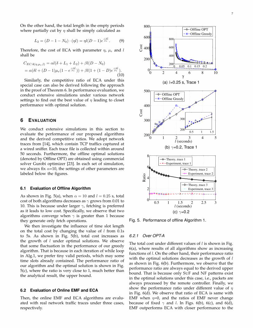
On the other hand, the total length in the empty periodswhere partially cut by η shall be simply calculated as
L2 = (D − 1−N0) · (ηl) = ηl(D − 1)e−ηlµe . (9)
Therefore, the cost of ECA with parameter η, µe and lshall be
CECA(η,µe,l) = αl(δ + L1 + L2) + βl(D −N0)
= α(δl + (D − 1)µe(1− e−ηlµe )) + βl(1 + (1−D)e
−ηlµe ).
(10)Similarly, the competitive ratio of ECA under this
special case can also be derived following the approachin the proof of Theorem 6. In performance evaluation, weconduct extensive simulations under various networksettings to find out the best value of η leading to closetperformance with optimal solution.
6 EVALUATION
We conduct extensive simulations in this section toevaluate the performance of our proposed algorithmsand the derived competitive ratios. We adopt networktraces from [14], which contain TCP traffics captured ata wired sniffer. Each trace file is collected within around50 seconds. Furthermore, the offline optimal solutions(denoted by Offline OPT) are obtained using commercialsolver Gurobi optimizer [23]. In each set of simulation,we always fix α=10, the settings of other parameters arelabeled below the figures.
6.1 Evaluation of Offline Algorithm
As shown in Fig. 5(a), when α = 10 and l = 0.25 s, totalcost of both algorithms decreases as γ grows from 0.01 to10. This is because under larger γ, fetching is preferredas it leads to low cost. Specifically, we observe that twoalgorithms converge when γ is greater than 1 becausethey generate only fetch operations.
We then investigate the influence of time slot lengthon the total cost by changing the value of l from 0.1sto 5s. As shown in Fig. 5(b), total cost increases asthe growth of l under optimal solutions. We observethat some fluctuation in the performance of our greedyalgorithm. That is because in each iteration of while loopin Alg.1, we prefer tiny valid periods, which may sometime slots already contained. The performance ratio ofour algorithm and the optimal solution is shown in Fig.5(c), where the ratio is very close to 1, much better thanthe analytical result, the upper bound.
6.2 Evaluation of Online EMF and ECA
Then, the online EMF and ECA algorithms are evalu-ated with real network traffic traces under three cases,respectively.
0 2 4 6 8 100
200
400
600
800
γ
Cost
Offline OPT
Offline Greedy
0 0.05 0.1 0.15 0.2200
400
600
800
(a) l=0.25 s, Trace 1
0 1 2 3 4 5200
300
400
500
l (seconds)C
ost
Offline OPT
Offline Greedy
0.5 1 1.5200
300
(b) γ=0.2, Trace 1
0.5 1 1.5 2 2.5 30
2
4
6
8
l (seconds)
Rat
io
Theory, trace 1
Experiment, trace 1
Theory, trace 2
Experiment, trace 2
Theory, trace 3
Experiment, trace 3
(c) γ=0.2
Fig. 5. Performance of offline Algorithm 1.
6.2.1 Over OPT-A
The total cost under different values of l is shown in Fig.6(a), where results of all algorithms show as increasingfunctions of l. On the other hand, their performance ratiowith the optimal solutions decreases as the growth of las shown in Fig. 6(b). Furthermore, we observe that theperformance ratio are always equal to the derived upperbound. That is because only SUF and NF patterns existin the optimal solutions under this case, i.e., packets arealways processed by the remote controller. Finally, weshow the performance ratio under different value of ηin Fig. 6(d). We observe that ratio of ECA is same withEMF when η=0, and the ratios of EMF never changebecause of fixed γ and l. In Figs. 6(b), 6(c), and 6(d),EMF outperforms ECA with closer performance to the

8
0 1 2 350
100
150
200
250
300
l (seconds)
Co
st
Offline OPT
ECA
EMF
(a) γ=2, η=5, trace 3
0 1 2 32
2.5
3
3.5
4
4.5
l (seconds)
Rat
io
Theory, ECA
Experiment, ECA
Theory, EMF
Experiment, EMF
(b) γ=2, η=5, trace 3
1 2 3 4 50
2
4
6
8
10
γ
Rat
io
Theory, ECA
Experiment, ECA
Theory, EMF
Experiment, EMF
(c) η=5, l = 0.5 s, trace 3
0 1 2 3 4 5 6 7 8 9 100
1
2
3
4
η
Rat
io
Theory, ECA
Experiment, ECA
Theory, EMF
Experiment, EMF
(d) γ=1, l = 0.2 s, trace 3
Fig. 6. Performance of EMF and ECA over OPT-A.
0 1 2 3250
300
350
400
450
500
l (seconds)
Cost
Offline OPT
ECA
EMF
(a) γ=0.2, η=2, trace 2
0.5 1 1.51
1.2
1.4
1.6
1.8
2
l (seconds)
Rat
io
Theory, ECA
Experiment, ECA
Theory, EMF
Experiment, EMF
(b) γ=0.2, η=2, trace 2
0.1 0.2 0.3 0.4 0.51
1.5
2
2.5
3
3.5
γ
Rat
io
Theory, ECA
Experiment, ECA
Theory, EMF
Experiment, EMF
(c) η=2, l = 0.2 s, trace 2
0 2 4 60.5
1
1.5
2
2.5
3
3.5
η
Rat
io
Theory, ECA
Experiment, ECA
Theory, EMF
Experiment, EMF
(d) γ=0.2, l = 0.2 s, trace 2
Fig. 7. Performance of EMF and ECA over OPT-B.
0.5 0.6 0.7 0.81.1
1.2
1.3
1.4
1.5
1.6
γ
Rat
io
Theory, ECA
Experiment, ECA
Theory, EMF
Experiment, EMF
(a) η=2,l=0.2 s,trace 2
0 5 10 15
1.2
1.3
1.4
1.5
1.6
η
Rat
io
Theory, ECA
Experiment, ECA
Theory, EMF
Experiment, EMF
(b) γ=0.625,l=0.2 s,trace 2
0.5 0.6 0.7 0.81
1.05
1.1
1.15
1.2
γ
Rat
io
Theory, ECA
Experiment, ECA
Theory, EMF
Experiment, EMF
(c) η=2,l=0.4 s,trace 2
0 5 10 151.05
1.1
1.15
1.2
1.25
η
Rat
io
Theory, ECA
Experiment, ECA
Theory, EMF
Experiment, EMF
(d) γ=0.625,l=0.4 s,trace 2
Fig. 8. Performance of EMF and ECA over OPT-C.
optimal solution under most of settings. We attribute thisphenomenon to the fact that rules are cached at switchesfor a longer time under ECA.
6.2.2 Over OPT-B
In this case, packets tend to be processed at local switch-es because γ becomes small. In Figs. 7(a) and 7(b),we have similar observations with the results underOPT-A case, except ECA outperforms EMF. This can beattributed to that there are mainly CIE patterns and fewNF patterns under OPT-B case, and the extra cachingdurations of ECA cover many empty periods. Accord-ingly, the cost of ECA is smaller than EMF, particularlywhen γ and η become large. Finally, both algorithmsconverge to the optimal solution under larger value of l.In respect of performance ratio, Fig. 7(c) shows ratio isdecreasing function of γ for both ECA and EMF. Becauselarger γ leads to more short FCN patterns in optimalsolution, which makes ECA and EMF close to optimalsolution. Therefore, their ratios decrease and approach to1 gradually. As we mentioned above, Fig. 7(d) shows thebenefit of a larger η in ECA, because more empty periodsare covered and much fetching cost can be saved underOPT-B case.
6.2.3 Over OPT-CThe performance of ECA and EMF is investigated inFigs. 8 and 9. We observe that ECA and EMF showdistinct performance under different settings. For exam-ple, in Fig. 9(a), the cost of ECA is larger than EMFwhen l=0.2, but it becomes opposite when l is greaterthan 0.3. We have similar observations in other figures.Interestingly, in Fig. 8(b), we observe that the curveof ECA first increases, and then decreases when η isgreater than 3, finally converging to 1.28 after η = 4.This is because when η is small, it only covers fewempty periods with short length, and the advantageof extra caching is not obvious. As η becomes larger,the number of covered empty periods grows, leading toreduced total cost. When all empty periods are coveredby large η, the performance of ECA becomes stable. InFig. 8(d), the ratios of ECA keep decreasing and thenconverging because short empty periods become fewerwhen l increases to 0.4.
6.3 Evaluation of Special Case of ECAFinally, we study the performance of ECA when lengthsof empty periods are exponential distribution. We con-sider randomly generated network traffic with µe=1.0and T=100.

9
0.2 0.3 0.4 0.5 0.6200
220
240
260
280
l (seconds)
Cost
Offline OPT
ECA
EMF
(a) γ=0.625, η=2, trace 2
0.2 0.3 0.4 0.5 0.60
0.5
1
1.5
2
l (seconds)
Rat
io
Theory, ECA
Experiment, ECA
Theory, EMF
Experiment, EMF
(b) γ=0.625, η=2, trace 2
Fig. 9. Performance of EMF and ECA over OPT-C whilevarying l.
0 2 4 6 8 101
1.2
1.4
1.6
1.8
η
Rat
io
Theory, ECA
Experiment, ECA
Theory, EMF
Experiment, EMF
Fig. 10. ECA over OPT-A under special case, γ=1,µe=1.0, l=0.25.
As shown in Fig. 10, ratio of ECA algorithm increasesas η grows from 0 to 10, which shows the same per-formance with Fig. 6(d). In Fig. 11, we have similarobservation with Fig. 8(b) because of the same reasons.In Fig. 12, we set l=0.5, and performance ratios arealways below the theoretical bound as γ and η changeswithin [0.5,0.8] and [0,10], respectively. The simulationresults also suggest that η shall be set to small values nomatter how γ changes.
0 2 4 6 8 101
1.5
2
2.5
η
Rat
io
Theory, ECA
Experiment, ECA
Theory, EMF
Experiment, EMF
Fig. 11. ECA over OPT-B under special case, γ=0.2,µe=1.0, l=0.25.
0
5
10
0.5
0.6
0.7
0.8
1.1
1.2
1.3
1.4
1.5
ηγ
Rati
o
Theory
Experiment
Fig. 12. Performance of ECA over OPT-C under specialcase, µe=1.0, l=0.5.
7 CONCLUSION
In this paper, we studied traffic flow provisioning prob-lem by formulating it as a minimum weighted flow pro-visioning problem with objective of minimizing the totalcost of TCAM occupation and remote packet processing.This problem is proved to be NP-hard, and an efficientheuristic algorithm is proposed to solve this problemwhen network traffic is given. We further propose twoonline algorithms to approximate the optimal solutionwhen network traffic information is unknown in ad-vance. Finally, extensive simulations were conducted tovalidate the performance of theoretical analysis of theproposed algorithms, using the real traffic traces.
REFERENCES[1] N. McKeown, T. Anderson, H. Balakrishnan, G. Parulkar, L. Pe-
terson, J. Rexford, S. Shenker, and J. Turner, “Openflow: enablinginnovation in campus networks,” ACM SIGCOMM ComputerCommunication Review, vol. 38, no. 2, pp. 69–74, 2008.
[2] M. Casado, M. Freedman, J. Pettit, J. Luo, N. Gude, N. McKe-own, and S. Shenker, “Rethinking enterprise network control,”IEEE/ACM Transactions on Networking, vol. 17, no. 4, pp. 1270–1283, Aug 2009.
[3] N. Kang, Z. Liu, J. Rexford, and D. Walker, “Optimizing the onebig switch abstraction in software-defined networks,” Proc. ACMCoNEXT, 2013.

10
[4] “Openflow switch specification,” https://www.opennetworking.org/sdn-resources/onf-specifications/openflow.
[5] T. Benson, A. Anand, A. Akella, and M. Zhang, “Microte: Finegrained traffic engineering for data centers,” in Proceedings ofthe Seventh COnference on Emerging Networking EXperiments andTechnologies (CONEXT), 2011, pp. 1–12.
[6] S. Agarwal, M. Kodialam, and T. Lakshman, “Traffic engineeringin software defined networks,” in IEEE International Conference onComputer Communications (INFOCOM), April 2013, pp. 2211–2219.
[7] Y. Kanizo, D. Hay, and I. Keslassy, “Palette: Distributing tablesin software-defined networks,” in IEEE International Conference onComputer Communications (INFOCOM), 2013, pp. 545–549.
[8] N. Gude, T. Koponen, J. Pettit, B. Pfaff, M. Casado, N. McKeown,and S. Shenker, “Nox: towards an operating system for networks,”ACM SIGCOMM Computer Communication Review, vol. 38, no. 3,pp. 105–110, 2008.
[9] U. C. Kozat, G. Liang, and K. Kokten, “On diagnosis of for-warding plane via static forwarding rules in software definednetworks,” in 2014 Proceedings of IEEE International Conference onComputer Communications (INFOCOM). IEEE, 2014.
[10] K. Pagiamtzis and A. Sheikholeslami, “Content-addressable mem-ory (cam) circuits and architectures: A tutorial and survey,” IEEEJournal of Solid-State Circuits, vol. 41, no. 3, pp. 712–727, 2006.
[11] Y. Sun and M. S. Kim, “Tree-based minimization of tcam entriesfor packet classification,” in 7th IEEE Consumer Communicationsand Networking Conference(CCNC),. IEEE, 2010, pp. 1–5.
[12] N. Katta, J. Rexford, and D. Walker, “Infinite cacheflow insoftware-defined networks,” Tech. Rep. TR-966-13, Departmentof Computer Science, Princeton University, Tech. Rep., 2013.
[13] M. F. Bari, A. R. Roy, S. R. Chowdhury, Q. Zhang, M. F. Zhani,R. Ahmed, and R. Boutaba, “Dynamic controller provisioning insoftware defined networks.” in CNSM, 2013, pp. 18–25.
[14] S. Yang, J. Kurose, and B. N. Levine, “Disambiguation of resi-dential wired and wireless access in a forensic setting,” in IEEEInternational Conference on Computer Communications (INFOCOM).IEEE, 2013, pp. 360–364.
[15] E. Spitznagel, D. Taylor, and J. Turner, “Packet classificationusing extended tcams,” in Proceedings of 11th IEEE InternationalConference on Network Protocols (ICNP). IEEE, 2003, pp. 120–131.
[16] M. Yu, J. Rexford, M. J. Freedman, and J. Wang, “Scalable flow-based networking with difane,” ACM SIGCOMM Computer Com-munication Review, vol. 40, no. 4, pp. 351–362, 2010.
[17] S. Sharma, D. Staessens, D. Colle, M. Pickavet, and P. Demeester,“Openflow: Meeting carrier-grade recovery requirements,” Com-puter Communications, vol. 36, no. 6, pp. 656–665, 2013.
[18] F. Durr, “Towards cloud-assisted software-defined networking,”Technical Report 2012/04, Institute of Parallel and DistributedSystems, Universitat Stuttgart, Tech. Rep., 2012.
[19] X. N. Nguyen, D. Saucez, C. Barakat, T. Thierry et al., “Optimizingrules placement in openflow networks: trading routing for betterefficiency,” in ACM SIGCOMM Workshop on Hot Topics in SoftwareDefined Networking (HotSDN 2014), 2014.
[20] R. Cohen, L. Lewin-Eytan, J. S. Naor, and D. Raz, “On the effect offorwarding table size on sdn network utilization,” in 2014 Proceed-ings of IEEE International Conference on Computer Communications(INFOCOM). IEEE, 2014, pp. 1734–1742.
[21] R. Bar-Yehuda and S. Even, “A linear-time approximation algo-rithm for the weighted vertex cover problem,” Journal of Algo-rithms, vol. 2, no. 2, pp. 198–203, 1981.
[22] B. Korte and J. Vygen, Combinatorial optimization: Theory andAlgorithms (5 ed.). Springer, 2012.
[23] G. Optimization, “Gurobi optimizer reference manual,” 2013.