Correcting apparent off-season CO2 uptake due to surface heating of an open path gas analyzer: progress report of an ongoing study

G.G. Burba, D. J. Anderson, Liukang Xu and D.K. McDermitt LI-COR Biosciences, Lincoln, NE, USA

____________________________________________________________________________________________________________________________

A bstract A number of Eddy Covariance flux sites with open path analyzers have observed small apparent CO2 uptake outside the growing season. In this study, we propose an additional correction due to instrument surface heating as a part of the Webb-Pearman-Leuning correction. Effects of the proposed correction were examined on hourly and seasonal time scales. Significant reduction in apparent CO2 uptake during off-season periods was observed, while fluxes during the growing season were not noticeably affected. The proposed correction may be useful for future CO2 flux research, and can also be applied to pre-existing data. ____________________________________________________________________________________________________________________________ 1. Introduction

Open-path infrared gas analyzers are low

maintenance high-quality sensors widely used in field research (Ameriflux, 2006). As more year-round carbon flux studies become available, there is growing concern about apparent off-season CO2 uptake being measured when it is physiologically unreasonable to expect it (Hirata et al., 2005). Solving this problem is an important step in improving CO2 measurements, annual NEE estimates, and subsequent global carbon exchange and climate modeling efforts.

One laboratory study and two field experiments are currently underway to examine the influence of the open-path infrared gas analyzer surface temperature on the measured CO2 flux using the Eddy Covariance technique. The original concept and some initial results were presented at the Ameriflux Annual Meeting in October, 2005 (Burba et al., 2005a,b), and has been developed further in subsequent months due to the interest and enthusiasm generated in the flux research community towards resolving this issue. Here we present the latest updates from these experiments: a theoretical correction due to the surface heating is introduced, the relationship of instrument surface temperature and ambient air temperature is investigated, and the effect of an additional term on the CO2 fluxes is examined. The following specific questions are addressed:

(1) Do the electronics inside the sensor head contribute substantially to instrument surface heating?

(2) Is the air in the optical path of the open-path analyzer significantly warmer then the ambient air due to the heated instrument surface?

(3) How do the electronics and ambient factors combine to affect the final surface temperature?

(4) What is the effect of the final surface temperature on the carbon dioxide flux data?

2. Concept of the correction due to instrument surface heating

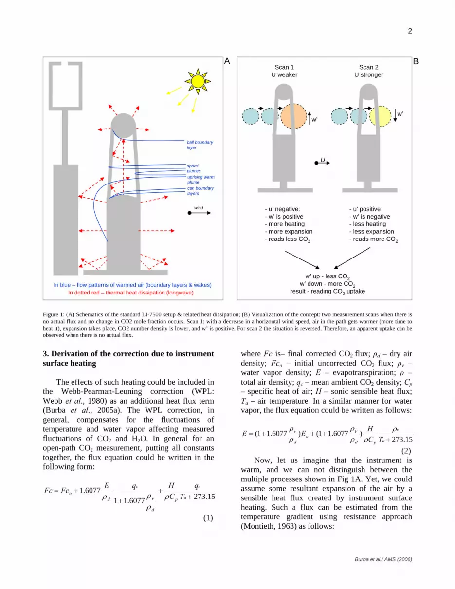
The surface of the open-path infrared gas analyzers (e.g., LI-7500, LI-COR Inc., Lincoln, NE) could be warmer than the ambient air due to heat generated by the electronics in and instrument’s sensor head (chopper motor, heating of the chopper housing, infrared source, thermoelectric coolers, etc.), and by solar radiation. The instrument may also be cooled by emission of long-wave radiation and by wind-induced convective exchange (Fig. 1A). The heat flux from an instrument surface is in addition to the ambient heat flux: colder air continuously enters the open optical path, and is warmed and expanded by the warm instrument surface in the same way that the atmosphere is warmed by the soil surface (Burba et al., 2005a).

Another way to look at this process is on the scale of two measurement scans (Fig. 1B) for a situation in which there is no actual flux and no change in actual CO2 mole fraction. With a decrease in horizontal wind speed (scan1), air in the path gets warmer than ambient because there is more time to heat it, and expansion takes place; so, CO2 number density is lower than ambient. At the same time, w’ is positive to assure momentum flux is always toward the surface. With an increase in horizontal wind speed (scan 2), the air is heated less, expansion is less, and CO2 number density is closer to ambient. At the same time w’ is negative (to keep momentum transfer toward the surface). Thus, from the covariance calculation ( ''Cw ), a false uptake would be observed when no actual flux is occurring.

2

In blue – flow patterns of warmed air (boundary layers & wakes)In dotted red – thermal heat dissipation (longwave)

wind

ball boundary layer

can boundary layers

uprising warm plume

spars’plumes

U

- u’ positive- w’ is negative- less heating- less expansion- reads more CO2

- u’ negative:- w’ is positive- more heating- more expansion- reads less CO2

w’ up - less CO2w’ down - more CO2

result - reading CO2 uptake

Scan 2U stronger

Scan 1U weaker

w’w’

A B

Figure 1: (A) Schematics of the standard LI-7500 setup & related heat dissipation; (B) Visualization of the concept: two measurement scans when there is no actual flux and no change in CO2 mole fraction occurs. Scan 1: with a decrease in a horizontal wind speed, air in the path gets warmer (more time to heat it), expansion takes place, CO2 number density is lower, and w’ is positive. For scan 2 the situation is reversed. Therefore, an apparent uptake can be observed when there is no actual flux.

3. Derivation of the correction due to instrument surface heating

The effects of such heating could be included in the Webb-Pearman-Leuning correction (WPL: Webb et al., 1980) as an additional heat flux term (Burba et al., 2005a). The WPL correction, in general, compensates for the fluctuations of temperature and water vapor affecting measured fluctuations of CO2 and H2O. In general for an open-path CO2 measurement, putting all constants together, the flux equation could be written in the following form:

15.2736077.116077.1

++

++=

a

c

p

d

v

c

do T

qCHqEFcFc

ρρρρ

(1)

where Fc is– final corrected CO2 flux; ρd – dry air density; Fco – initial uncorrected CO2 flux; ρv – water vapor density; E – evapotranspiration; ρ – total air density; qc – mean ambient CO2 density; Cp – specific heat of air; H – sonic sensible heat flux; Ta – air temperature. In a similar manner for water vapor, the flux equation could be written as follows:

15.273)6077.11()6077.11(

++++=

a

v

pd

Vo

d

v

TCHEE ρ

ρρρ

ρρ

(2) Now, let us imagine that the instrument is

warm, and we can not distinguish between the multiple processes shown in Fig 1A. Yet, we could assume some resultant expansion of the air by a sensible heat flux created by instrument surface heating. Such a flux can be estimated from the temperature gradient using resistance approach (Montieth, 1963) as follows:

Burba et al./ AMS (2006)

3

a

aspI

rTTC

H)( −

=ρ (3)

where HI – sensible heat flux from the warm instrument to the ambient air, Ts – instrument surface temperature, and ra – aerodynamic resistance. For an instrument oriented near vertically, only a fraction of HI would affect the measurement because the wind will remove much of the warmed air from the optical path, carrying away most of H without affecting the measurements. However, a portion of the warmed and expanded air will remain in the boundary layer, reducing the measured air density and influencing the measurement (Fig. 1A). The fraction fr of HI retained in the optical path is called HP and can be expressed as follows:

IP frHH = (4) So, combining Eqs. 1,3, and 4, the WPL would be transformed as follows:

++

+=

d

v

c

donew

qEFcFc

ρρρ 6077.11

6077.1

15.273

))/)(((+

−++

a

c

p

aasp

Tq

CrTTCfrH

ρρ (5)

The term E in Eq. 5 also needs an additional heat correction as well (Eq.2) , such that:

++= od

v EE )6077.11(ρρ

15.273))/)(((

)6077.11(+

−+++

a

v

p

aasp

d

V

TCrTTCfrH ρ

ρρ

ρρ

(6) If open-path flux data have already been corrected in the traditional way (frequency response and WPL), then the additional correction for E would be (from Eqs. 2 and 6):

)15.273()()6077.11(

+−

++=aa

vas

d

vnew

TrTTfrEE ρ

ρρ

(7)

and the correction to Fc for data already corrected in the traditional way, would be (from Eqs. 1,5 and 7):

)6077.11()15.273(

)(

d

v

aa

casnew

TrqTTfrFcFc

ρρ

++−

+= (8)

where

)15.273()(

+−

aa

cas

TrqTTfr represents the instrument

heating correction for Fc. The additional correction to E in Eq. 6 is represented by )6077.11(

d

v

ρρ

+ ,

which is typically very small, on the order of 0.5-2% for a majority of ambient temperature and humidity ranges.

For the particular case of the LI-7500, each of the two major structural elements of the instrument (can and ball, Fig. 1A) may contribute differently to the proposed additional term in WPL correction:

+++−

+= )6077.11()15.273(

)(

d

v

aa

cascannew

TrqTTfrFcFc

can

can

ρρ

)6077.11()15.273(

)(

d

v

aa

casball Tr

qTTfrball

ball

ρρ

++−

+ (9)

Resistances to heat transfer can be estimated assuming that forced convection prevails near the surfaces of the instrument (Campbell and Norman, 1998):

Ud

r cancana 4.7≈ (10)

Udr ball

balla 4.7≈ (11)

where d is the characteristic dimension of each element (0.042 m for the ball, and 0.133 m for the can); dcan=0.133 m was computed from the radius of the curve making the top surface of the can). Both structural elements are assumed here to be cylinders and spheres, so no additional multiplier for d is required. Assume that the fraction of the sensible heat flux affecting measurement fr (=HP/HI) could be approximated by the ratio of pathlengths containing air influenced by HP divided by the total mechanical pathlength of the instrument (lpath=0.128 m). The

Burba et al./ AMS (2006)

4

pathlengths affected by HP will be the sum of the thermal boundary layer thicknesses of the can and the ball. Thus:

path

cancan

l

lfr = (12)

path

ballball

l

lfr = (13)

and fr=frcan+frball. The layers’ thickness could be approximated, assuming laminar boundary layer and vertical instrument position, as follows:

wincan

can dtgdl *)(21

Re5.5 α+≈ (14)

Re5.5 ball

ball dl ≈ (15)

µρUd x

=Re (16)

where Re is Reynolds number (Gates, 1980); dcan=0.033 m (radius of the can); α=20o (angle between the bottom window and metal ‘shoulders’ around it); dwin= 0.012 m (radius of the flat portion of the window) ); dball =0.022 m (radius of the ball); dx

is dcan or dball; µ is dynamic viscosity of the air. The air heated inside the sensor between windows and transducers is CO2 free, and its temperature fluctuations do not contribute to the flux correction. 4. Results 4.1.Electronics contribution – environmental chamber experiment

To evaluate contribution of the electronics in the sensor head to the heating of the instrument surface, an experiment was conducted in an environmental chamber (Model F466PC-1, Blue M Electronic Company, Blue Island, Illinois) with a vertical-down recirculating conditioning stream to ensure uniform mixing of the air. Thermocouples were attached to various parts of the instrument (side of the cylinder, lower window area, upper window area, and spar) and covered with small

pieces of foam to minimize direct heating and cooling of the thermocouple by chamber air.

Figure 2 shows the instrument surface temperatures plotted versus ambient temperature for the range from -25 to +50 C. The bottom window area was consistently warmer than ambient chamber air with an average relationship as follows:

Ts=0.92 Ta+4.83, r2=1.00, n>900 (17) Equation 17 holds for the original version of the instrument electronic board, housed in the white control box (version 1). Eq. 17 demonstrates that differences between ambient temperature and the surface temperatures of the lower window area increase with a decrease in ambient temperature: the instrument was warmer than ambient by +0.8 C at +50 C ambient, and by +6.8 C at -25 C ambient. Other parts of the instrument did not display significant difference from the ambient temperature, though all relationships were very tight, with little or no hysteresis. These observations are corroborated by the location of the majority of the internal instrument electronics, and particularly the heater for the instrument source, near the bottom window of the instrument. A somewhat smaller influence of electronic heating was observed for the newer version of the instrument electronic board (version 2): Ts=0.93 Ta+3.53, r2=1.00, n>900 (18) The instrument was heated by the electronics to +0.03 C above ambient at +50 C, and by +5.3 C at -25 C due to higher efficiency and lower heat dissipation of the new board configuration. Relationships were linear in all cases, with total number of samplings n>900, grouped by ambient temperatures in 9 groups, and yielding r-square of 1.00. Both of these equations (Eqs. 17 and 18) demonstrate a significant influence of the sensor head electronics on the instrument surface heating, especially at low ambient temperatures. Also, both are likely to be specific only to the version of the electronic board, and should hold for all instrument configurations and for various experimental setups. In principle, these relationships could be used, with appropriate assumptions and caution, to evaluate the effect of the surface heating on the measured flux (Burba et al., 2005a,b).

Burba et al./ AMS (2006)

5

-25

0

25

50

-25 0 25 50

1:1

Ts, C

Ta, C

Environmental Chamber

slope offset r2

Lower window areaver. 1 0.92 4.83 1.00ver. 2 0.93 3.53 1.00

Upper window area 1.01 0.25 1.00

Figure 2. Instrument surface temperature (Ts) is plotted versus air temperature (Ta) in the climate controlled chamber for two versions of electronic boards. Each point on the plot is an average of 20-30 one-minute data points after temperature equilibrium between chamber air and instrument surface was achieved. Data gathered before equilibrium was achieved have been removed from the analysis.

4.2 Ambient air warming near the instrument surface – LI-COR facility experiment

Field conditions are different from those in the environmentally controlled chamber, primarily due to factors influencing the instrument surface directly (not via electronics heating): sunlight, wind and radiative cooling. A field experiment is being conducted at the LI-COR experimental facility (Lincoln, NE) starting in October, 2005 to evaluate the resulting surface-to-air temperature gradient in field conditions with and without the influence of the electronics. During the experiment instrument power was turned off for several weeks and on for several months. Fine-wire thermocouples were attached to LI-7500 analyzer at the center of the lower window area approximately 0.5 mm and 1.0 mm above the lower window, and in the center of the upper window area. Ambient fine-wire thermocouple was installed 20 cm away from the open-path sensor.

Figure 3A demonstrates that air coming into the instrument path is warmed up significantly by the heated instrument surface in the ambient environment. Temperature gradients are very steep in the first 1 mm above the lower window area: for cold air in calm atmospheric conditions, gradients

may exceed 2 C per 1 mm, while during windy conditions gradients seem to decrease (Fig. 3A). During warm days gradients are considerably smaller than in cold temperature, while some wind effect is still observed (Fig. 3B).

Figure 3 C demonstrates that even without electronics heating (with power off) the instrument surface can be several degrees warmer than the ambient air in the middle of the day (likely due to sunlight), and several degrees cooler at night (due to radiative cooling). This phenomenon has important implications for any open-path instrument measuring flux: unless the instrument surface temperature is controlled to be similar to the ambient, instrument surface heating/cooling may significantly affect the measured flux. 4.3 Combination of all factors affecting instrument surface temperature - experiment at Mead, NE

A field experiment to directly evaluate the influence of instrument heating on the measured CO2 flux during the off-season is being conducted (starting November, 2005) at the University of Nebraska Carbon Sequestration Program research site near Mead, Nebraska (in collaboration with S.B. Verma and A. Suyker). This site is equipped

Burba et al./ AMS (2006)

6

-18

-12

-6

0

343 344Time

T, C Lower window area

0.5 mm deg C1.0 mm deg CUpper window areaTair

Cold day: 12/9/05

calm

windy

A

0

6

12

18

26 27Time

T, C

Warm day: 01/26/06

calm

windy

B

-18

-12

-6

0

338 339Central Standard Time

T, C

Power off: 12/9/05

C

0:00 6:00 12:00 18:00 24:00

Figure 3. Daily patterns of surface temperature of the lower and upper window areas; air temperature was measured at approximately 0. 5 mm and 1 mm above the lower window, and in the open air away from the instrument on selected days: (A) cold day, 12/9/05; (B) warm day, 1/26/06; and (C) day with instrument power turned off, 12/9/05. LI-COR facility experiment.

with a comprehensive Eddy Covariance station, which has an open-path CO2/H2O gas analyzer (LI-7500), and a complete set of instruments for measuring weather and radiation (Suyker et al., 2005). Fine-wire thermocouples were attached to an LI-7500 open-path analyzer near the lower window, on the side of the cylinder, on a spar, and near the upper window. All thermocouples were painted with the same titanium oxide paint as the body of the instrument to assure a similar albedo. Relationships between the air and instrument surface temperatures near the lower and upper windows are shown in Fig. 4. Similar to the

environmental chamber experiment, the temperature of the upper window was not significantly different from the ambient, at least for the majority of the data (linear regression yielded slope of 0.99 and offset of 0.23 C). The lower window area, however, was warmer than ambient, but not as much as inside of the environmental chamber. Linear fits from all experiments to date are shown in Table I. Ambient experiments (LI-COR facility and Mead) produce consistently lower Ts for the same Ta, as compared to the environmental chamber. We attribute this to better thermal exchange in ambient conditions due to

Burba et al./ AMS (2006)

7

-30

-20

-10

0

10

20

30

40

-30 -20 -10 0 10 20 30 40

Ta, C

Ts, C

1:1

Mead experiment: November, 2005-March, 2006

equation r2

Lower window arealinear fit Ts=0.90Ta+2.21 0.99polynomial Ts=0.0025Ta2+0.90Ta+2.07 0.99

Upper window area Ts=0.99Ta+0.23 1.00x

Figure 4. Hourly values of instrument surface temperature (Ts) at the lower and upper window areas plotted versus air temperature (Ta) during the period from November, 2005 to March, 2006.

wind convection, and due to radiative cooling at night (as seen in Fig. 3C). This is somewhat corroborated by frequently observed condensation and dew formation near the top window in cold and humid field environments. Another important feature of the ambient relationship between Ts and Ta is that the best fit

may not actually be linear, because a linear fit would imply the occurrence of the cooling of the surface at ambient temperatures above +20 to +30 C. It is difficult to justify such a situation, in which the electronics would cool the instrument below the ambient temperature.

Experiment Ver. Influencing factors lower window area upper window area

slope offset r2 n slope offset r2 n

Climate control chamber 1 electronics 0.92 4.83 1.00 >900 - - - -

Climate control chamber 2 electronics 0.93 3.53 1.00 >900 1.01 0.25 1.00 >900

Li-Cor Facility* 2 electronics & ambient 0.89 2.23 0.99 >2000 1.00 -0.22 1.00 >2000

Mead experiment* 2 electronics & ambient 0.90 2.21 0.99 >1500 0.99 0.23 1.00 >1500

*non-linear may be better: regression fit will become more complete after warm-season data become available

Table I. Linear fit parameters of the relationship between ambient air temperature (Ta) and instrument surface temperature (Ts) for the lower and upper window areas: Ts = slope Ta+ offset. Influence of the heating by electronics (chamber experiment) is noticeably offset by atmospheric exchange for the outside experiments. Upper window Ts did not seem to be consistently affected by Ta. (*) Non-linear may be better: regression fit will become more complete after warm-season data become available. With only colder temperatures available in the Mead experiment to date, a polynomial fit can not be confidently extrapolated beyond +20C. However, a polynomial relationship for the ambient

temperature range from -25 to +20 C does seem to fit the data as well or better, than a linear fit (Fig. 4):

Burba et al./ AMS (2006)

8

Ts=0.0025Ta2+0.90Ta+2.07, r2=0.99, n>1500 (19)

Temperatures for the relationship presented in Eq. 19 were measured directly, and all factors influencing Ts (e.g., electronics, sunlight, radiative cooling, and wind exchange) have been incorporated into the actual measurement of Ts,

however, this relationship may also be less general than those presented in Eqs. 17 and 18, and may vary from site to site and from one setup to another (because of differences in shadowing of the instrument from sun and wind, temperature ranges, instrument orientation etc.), so it should be used with caution.

-0.5

0.0

0.5

0:00 12:00 0:00

Fc, m

g m

-2 s

-1

-0.5

0.0

0.5

0:00 12:00 0:00

62627500 old7500 new

-0.5

0.0

0.5

0:00 12:00 0:00

Fc, m

g m

-2 s

-1

-0.5

0.0

0.5

0:00 12:00 0:00

Maize: October 6, 2002 Maize: January 29, 2003

Central Standard Time

Soybean: October 9, 2002 Soybean: February 8, 2003

A B

C D

Figure 5. Daily patterns of hourly carbon dioxide flux (Fc) as obtained using closed-path LI-COR analyzer (6262), traditionally corrected LI-7500 (7500 old), and flux corrected with a proposed additional member of WPL correction (7500 new): (A) maize, warm day; (B) maize, cold day; (C) soybean, warm day; (D) soybean, cold day. Uptake of CO2 is positive and release is negative. 4.4. Applying corrections to pre-existing data

To take advantage of exactly the same instrument configuration and setup, we have used Ts relationship obtained from Mead experiment in 2005-06 (Eq. 19), and applied it via Eq. 9 to the traditionally corrected Fc flux data from 2002-03 from the same study site under maize, and from a similar neighboring site under soybean (data courtesy of S.B. Verma and A. Suyker: Suyker et al., 2005). Fc from the LI-7500 was compared to that from a closed-path instrument, the LI-6262, which was not affected by instrument surface heating, during off-season with no green canopy,

and during the entire year. Fc from the LI-7500 with the traditional form of WPL was compared to that from the LI-7500 with an additional correction due to instrument surface heating. Figs.5A-D compare daily patterns of hourly Fc from the LI-6262 and LI-7500 (corrected traditionally and with proposed additional correction) during warm and cold periods without a green canopy. Uptake of CO2 is positive and release is negative. An additional term in WPL (Eq. 9) helped to reduce the apparent off-season uptake and made the LI-7500 and LI-6262 match reasonably well for such a small overall flux (fluctuations are in the order of 0.05 mg CO2 m-2 s-1). The magnitude

Burba et al./ AMS (2006)

9

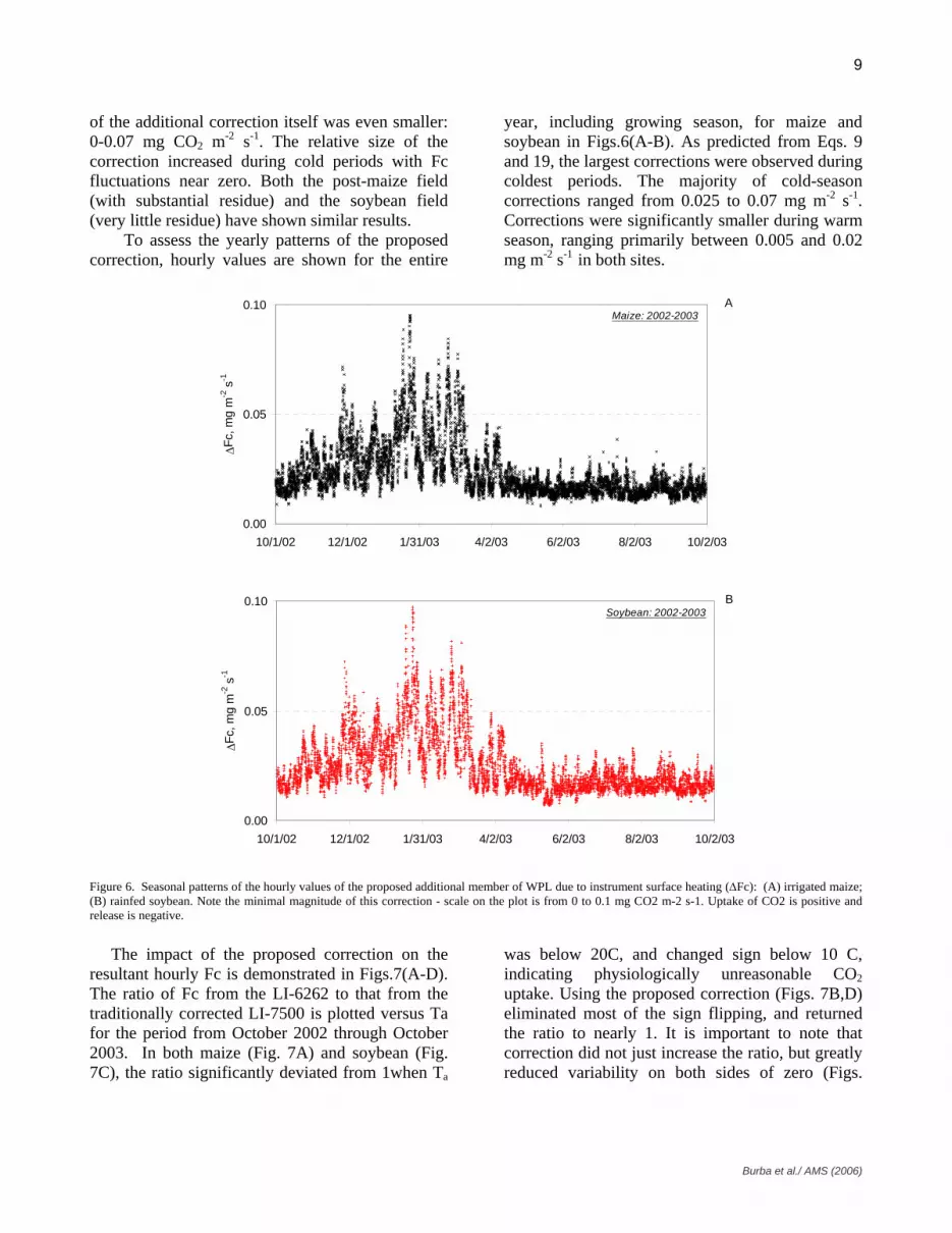
of the additional correction itself was even smaller: 0-0.07 mg CO2 m-2 s-1. The relative size of the correction increased during cold periods with Fc fluctuations near zero. Both the post-maize field (with substantial residue) and the soybean field (very little residue) have shown similar results. To assess the yearly patterns of the proposed correction, hourly values are shown for the entire

year, including growing season, for maize and soybean in Figs.6(A-B). As predicted from Eqs. 9 and 19, the largest corrections were observed during coldest periods. The majority of cold-season corrections ranged from 0.025 to 0.07 mg m-2 s-1. Corrections were significantly smaller during warm season, ranging primarily between 0.005 and 0.02 mg m-2 s-1 in both sites.

0.00

0.05

0.10

10/1/02 12/1/02 1/31/03 4/2/03 6/2/03 8/2/03 10/2/03

∆Fc,

mg

m-2

s-1

A

0.00

0.05

0.10

10/1/02 12/1/02 1/31/03 4/2/03 6/2/03 8/2/03 10/2/03

∆Fc,

mg

m-2

s-1

B

Maize: 2002-2003

Soybean: 2002-2003

Figure 6. Seasonal patterns of the hourly values of the proposed additional member of WPL due to instrument surface heating (∆Fc): (A) irrigated maize; (B) rainfed soybean. Note the minimal magnitude of this correction - scale on the plot is from 0 to 0.1 mg CO2 m-2 s-1. Uptake of CO2 is positive and release is negative.

The impact of the proposed correction on the resultant hourly Fc is demonstrated in Figs.7(A-D). The ratio of Fc from the LI-6262 to that from the traditionally corrected LI-7500 is plotted versus Ta for the period from October 2002 through October 2003. In both maize (Fig. 7A) and soybean (Fig. 7C), the ratio significantly deviated from 1when Ta

was below 20C, and changed sign below 10 C, indicating physiologically unreasonable CO2 uptake. Using the proposed correction (Figs. 7B,D) eliminated most of the sign flipping, and returned the ratio to nearly 1. It is important to note that correction did not just increase the ratio, but greatly reduced variability on both sides of zero (Figs.

Burba et al./ AMS (2006)

10

-10

0

10

-15 -5 5 15 25 35

-10

0

10

-15 -5 5 15 25 35

-10

0

10

-15 -5 5 15 25 35

Fc 6

262/

Fc 7

500

-10

0

10

-15 -5 5 15 25 35

Fc 6

262/

Fc 7

500

Ta, C

Maize: Fc 7500 old Maize: Fc 7500 new

Soybean: Fc 7500 old Soybean: Fc 7500 new

A B

C D

Figure 7. Hourly ratio of carbon dioxide flux measured with LI-6262 (Fc 6262) to that measured with LI-7500 (Fc 7500) corrected in a traditional way (old) and corrected with a proposed additional member of WPL correction (new): (A) maize, traditional WPL; (B) maize, WPL with additional term; (C) soybean, traditional WPL; (D) soybean, WPL with additional term. The period is from October 2002 to October, 2003. Additional correction improved both means and distribution of the data, and have not just shifted all data upward. 7B,D). It is also worth mentioning that very small quantities are divided in these ratios, and therefore some variability should be expected, especially at low temperatures.

The contrast between seemingly small hourly values of the proposed correction and its impact on the integrated fluxes can be demonstrated by comparing Figs. 8 (A, B) and Table II (A-B). Using the proposed correction reduced the slope from 3% to 2% and reduced the offset from 0.03 to 0.01 mg m-2 s-1 in maze (Fig. 8A), and from 0.03 to zero mg m-2 s-1 in soybean (slope was not affected; Fig. 8B). This shows that off-season fluxes are somewhat affected, while growing season fluxes did not significantly change. In contrast, the impact of the correction on off-season integrations of Fc was extremely important (Table II). The proposed correction dramatically reduced the number of uptake hours (Table IIA), from 716 to 252 hours in maize, and from 571 to 189 hours in soybean. As a

result, the underestimation of off-season losses of CO2 (and resulting overestimation of the yearly uptake of CO2) was reduced several fold (from -80 g CO2 to -304 g in maize and from -32 g CO2 to -186 g in soybean (Table IIB: uptake is positive and release is negative). After applying the proposed correction the LI-6262 and LI-7500 data matched to within few percent, which is well within the accuracy of the Eddy Covariance method.

5. Discussion 5.1 Note of caution

The method described above for correcting Fc

due to instrument surface heating was relying, on the assumption that the instrument was oriented nearly vertically. There are two variables in Eq. 9 that would be significantly affected by different instrument configurations: fr and Ts. The

Burba et al./ AMS (2006)

11

y = 1.02x + 0.03R2 = 0.99

y = 1.02x + 0.00R2 = 0.99

-1.0

0.0

1.0

2.0

3.0

-1.0 0.0 1.0 2.0 3.0

Fc 6262, mg m-2 s-1

Fc 7

500,

mg

m-2

s-1

B

y = 0.97x + 0.03R2 = 0.99

-1.0

0.0

1.0

2.0

3.0

-1.0 0.0 1.0 2.0 3.0

Fc 6262, mg m-2 s-1

Fc 7

500,

mg

m-2

s-1

AMaize:

black - Fc 7500 old

y = 0.98x + 0.01R2 = 0.99

red - Fc 7500 new

Soybean

black - Fc 7500 oldred - Fc 7500 new

Figure 8. Hourly carbon dioxide flux measured with LI-7500 (Fc 7500) plotted versus that measured with LI-6262 (Fc 6262) in: (A) maize, and (B) soybean during the period is from October 2002 to October, 2003. 'Fc 7500 old' was corrected in a traditional way, and 'Fc 7500 new' was corrected with a proposed additional member of WPL correction. Additional correction was so small as compared to the hourly fluxes during the growing season, that the latter were not noticeably affected. Uptake of CO2 is positive and release is negative.

A

Off-season uptake hours LI-6262 LI-7500 old LI-7500 new

Irrigated maize fallow 131 716

571

-80

-32

252

Rainfed soybean fallow 138 189B

Off-season CO2 release, when both 6262 and 7500 available, g C LI-6262 LI-7500 old LI-7500 new

Irrigated maize fallow -324 -304

Rainfed soybean fallow -175 -186

Table II. Comparison of the (A) off-season uptake hours and (B) integrated carbon dioxide release between a closed path analyzer (LI-6262), traditionally corrected open-path data (LI-7500 old) and data corrected using the proposed additional member of WPL correction (LI-7500 new). All tables and plots include only hours with complete data: when actual readings from the LI-6200, LI-7500, and other instruments used in the proposed corrections were available. Non-stationary conditions, rain, snow, instrument malfunctions and other filled-in periods were excluded to assure proper comparison between Fc7500 and Fc6262. Off-season periods are periods without green foliage area from October 1 to April 30.

Burba et al./ AMS (2006)

12

orientation of the instrument may impact the fr term, since the instrument would not be vertical, and the portion of the path affected by warm air may be higher than assumed for a nearly-vertical instrument. Also, in such a situation, Ts should include the influence of the can surface temperature that would now also affect the path, in addition to the window area temperature. Wind direction in a non-vertical configuration would be an important factor as well, since a configuration with a significantly inclined sensor would not be symmetrical for all wind directions. In addition to instrument orientation, the placement of other instruments and the tower might affect both fr and ra in Eq. 9, thus affecting the correction, especially when wind blows through the structures into the LI-7500 path. Therefore, the findings presented here should be treated with caution, as only an update on the ongoing investigation of the impact of instrument surface heating on measurements made by a nearly-vertical open-path CO2/H2O analyzer.

5.2 Alternative way to evaluate effect of various sensor configurations

In some cases there may be a way to evaluate the effects of a particular complex sensor configuration on fr and ra in Eq.9, and thus avoid some assumptions (e.g., near-vertical sensor position, prevalence of laminar boundary layer around sensor parts, absence of flow obstruction from other nearby sensors). If the correct value of flux is known from closed path instrument or could be confidently assumed for a range of wind speeds and wind directions, Eq.9 may be solved for fr/ra ratio. This would establish a site-specific fr/ra ratio for different wind speeds and directions, assuming these relationships would not change significantly with temperature, humidity or pressure. Such solution may include the short-term use of the closed-path sensor (e.g., LI-6262 or LI-7000) as standard, or establishing periods when flux value should be physiologically close to zero (e.g., extremely low temperatures below -25 or -30 C). The rest of the data could be corrected for various sensor configurations using these ratios in Eq.9 in place of the Eqs. 9-16. This approach should be treated with special care due to possible statistical errors involved in estimating the fr/ra ratio for various wind speeds and directions, and due to the number of data points required to construct confident empirical relationships; however, using such methods on pre-existing flux data from sites

with complicated sensor configurations is perhaps still more beneficial than rejecting large periods in the measurement year. 5.3 Future research

The data in the ongoing experiments were collected primarily during cold conditions with few regression points above 15C, and with predominantly low fluxes. This forced us to apply the empirical relationship between directly measured Ts and Ta developed in 2005-2006 to the Fc data from 2002-2003. With more data to be collected during the warm season of 2006, further tests will include comparison of fluxes between the closed path LI-6262 and open path LI-7500 for a wide range of directly measured surface temperatures.

There are several other steps that may help to further study and manage the effects of instrument heating. Having thermocouples on the surface near the lower and upper windows would help to specify the proposed correction without the difficulty of having to estimate Ts (e.g., Eqs. 16-18). Further experiments on the best sensor orientation might also be done to minimize the effects of instrument surface heating. Particularly, upside-down sensor positioning might reduce the effect of the heating on the flux in all directions. Further research is also needed to evaluate, test and fine-tune the proposed concept for various environments, and for different manufacturers of open-path CO2 analyzers. 6. Summary and conclusion

The influence of surface heating on the CO2 flux measured with the LI-7500 open path gas analyzer is being examined in one laboratory study and two field experiments. Experiment in a convective environmental chamber showed that the sensor head electronics substantially contributed to surface heating, and that the surface of the open-path analyzer could be 5-7°C warmer than the ambient air due to electrical energy dissipation in the instrument head. The difference was largest at low ambient temperatures and decreased linearly with an increase in the ambient temperature.

A field experiment at the LI-COR facility, which is still in progress, has shown that large temperature gradients (up to 2 C per 1mm) can exist just above the lower window of the instrument, implying strong sensible heat fluxes in the first few mm above the instrument surface. The thermal

Burba et al./ AMS (2006)

13

boundary layer was thicker during calm conditions, as expected. During the day, surface heating occurred due to solar radiation even when the electronics were not powered. Our measurements also suggest that emission of long-wave radiation can cause surface cooling at night to temperatures below ambient.

An experiment is in progress near Mead, NE also in which we are comparing Fc measured with an open-path LI-7500 to Fc measured by a closed path LI-6262, which is not affected by surface heating and is viewed as “standard”. To date, this experiment has demonstrated, that instrument surface temperature is directly and strongly related to air temperature (Eq. 19), but lack of data during warm season did not allow for confident extrapolation of the relationship beyond +20 C.

An additional term due to instrument surface heating was introduced as a part of the Webb-Pearman-Leuning correction. The temperature relationship developed in the Mead experiment in 2005-2006 (Eq. 18) was applied to LI-7500 data from 2002-03 in maize and soybean, and was compared against LI-6262 data from the same period. Even with partial results from the experiments available, a significant reduction in apparent CO2 uptake during off-season periods was observed as a result of applying the additional correction, while fluxes during the growing season have not been noticeably affected. The correction also resulted in elimination of most of the wrong signs from off-season open-path CO2 measurements, a significant reduction in variability of the data, elimination of the offset between measurements made with the LI-6262 and the LI-7500, and in a significant improvement in off-season integrations of CO2 exchange. A framework was created to develop a site-specific practical correction due to instrument heating. The proposed additional term in the Webb-Pearman-Leuning correction may prove useful for future year-round CO2 flux research. The technique to estimate the proposed correction for pre-existing data may help in better interpretation of previously collected information.

Acknowledgements

We would like to acknowledge a number of scientists who contributed to this study via valuable discussions, advice, data sets, and other personal communications. Particularly we want to thank Drs. Shashi Verma and Andrew Suyker for providing

data and facilities for the Mead experiment, and for numerous valuable help and advice. We also thank Drs. Brian Amiro, Robert Clement, David Cook, Marc-André Giasson, Ryuichi Hirata, Ray Leuning, Bill Massman, Walt Oechel, Howard Skinner, and Jon Welles for their interest in developing the topic. We acknowledge help provided by Jerry Ficke of LI-COR on LI-7500’s electronics and other properties, and for assistance with the environmental chamber experiment. We also thank Fluxnet, Ameriflux, Fluxnet-Canada, and Carbo-Europe networks for providing opportunity for the discussions and for access to flux data obtained with LI-7500 and LI-6262 instruments.

References: Ameriflux, 2006. “Ameriflux Sites Information."

<http://public.ornl.gov/ameriflux/site-select.cfm> Burba G. G., Anderson D. J., Xu L., and D. K. McDermitt.

2005a. Solving the off-season uptake problem: correcting fluxes measured with the LI-7500 for the effects of instrument surface heating. Progress report of the ongoing study. PART I: THEORY. Poster presentation. AmeriFlux 2005 Annual Meeting, Boulder, Colorado.

Burba G. G., Anderson D. J., Xu L., and D. K. McDermitt. 2005b. Solving the off-season uptake problem: correcting fluxes measured with the LI-7500 for the effects of instrument surface heating. Progress report of the ongoing study. PART II: RESULTS. Poster Presentation. AmeriFlux 2005 Annual Meeting, Boulder, Colorado.

Cambell, G. S., and J. M. Norman, 1998. Environmental Biophysics. Second Edition. Springer Science, New York: 286 pp.

Gates, D. M. 1980. Biophysical Ecology. Springer-Verlag, NY. Hirata R., Hirano T., Mogami J., Fujinuma Y., Inukai K.,

Saigusa N., and S. Yamamoto, 2005. CO2 flux measured by an open-path system over a larch forest during snow-covered season. Phyton, 45: 347-351

Monteith, J. L., 1963. Gas exchange in plant communities. Environmental Control of Plant Growth. L. T. Evans, ed. Academic Press, New York: 95-112

Suyker, A.E., S.B. Verma, G.G. Burba, and T.J. Arkebauer. 2005. Gross primary production and ecosystem respiration of irrigated maize and irrigated soybean during a growing season. Agricultural and Forest Meteorology, 131: 180-190

Verma, S. B., and A. E. Suyker. Personal Communications. September-December, 2005.

Webb, E. K., Pearman, G. I., and R. Leuning, 1980. Correction of flux measurements for density effects due to heat and water vapour transfer. Quart. J. R. Met. Soc., 106: 85-100

Burba et al./ AMS (2006)