copyright undertaking

Copyright Undertaking

This thesis is protected by copyright, with all rights reserved.

By reading and using the thesis, the reader understands and agrees to the following terms:

1. The reader will abide by the rules and legal ordinances governing copyright regarding the use of the thesis.

2. The reader will use the thesis for the purpose of research or private study only and not for distribution or further reproduction or any other purpose.

3. The reader agrees to indemnify and hold the University harmless from and against any loss, damage, cost, liability or expenses arising from copyright infringement or unauthorized usage.

IMPORTANT

If you have reasons to believe that any materials in this thesis are deemed not suitable to be distributed in this form, or a copyright owner having difficulty with the material being included in our database, please contact [email protected] providing details. The Library will look into your claim and consider taking remedial action upon receipt of the written requests.

Pao Yue-kong Library, The Hong Kong Polytechnic University, Hung Hom, Kowloon, Hong Kong

http://www.lib.polyu.edu.hk

1

2

STUDY AND DEVELOPMENT OF NOVEL 3

THERMAL FUNCTIONAL TEXTILE WITH 4

CONDUCTIVE MATERIALS 5

6

7

8

9

10

11

12

13

14

15

ZHAO YUANFANG 16

17

18

19

20

21

22

23

24

PHD 25

THE HONG KONG POLYTECHNIC UNIVERSITY 26

2019 27

2

1

The Hong Kong Polytechnic University 2

Institute of Textiles and Clothing 3

4

5

6

Study and Development of Novel Thermal Functional 7

Textile with Conductive Materials 8

9

10

11

12

13

14

15

16

ZHAO Yuanfang 17

18

19

20

21

22

23

24

A thesis submitted in partial fulfillment of the requirements for the 25

degree of Doctor of Philosophy 26

27

September 2018 28

3

1 2 3

Certificate of Originality 4 5 6 7 8

I hereby declare that this thesis is my own work and that, to the best of my knowledge 9 and belief, it reproduces no material previously published or written, nor material that 10 has been accepted for the award of any other degree or diploma, except where due 11 acknowledgement has been made in the text. 12

13

14

15

16

17

18

19

20

21

ZHAO Yuanfang 22

23

24

25

26

27

28

29

30

31

4

1

2

3

4

5

6

7

8

To 9

My Beloved Father, Prof. ZHAO Wei 10

My Beloved Mother, Ms. XU Jiaying 11

My Beloved Parents-in-law, Mr. XIE Hedan and Ms. ZHENG Lifang 12

My Beloved Husband, Mr. XIE Xin 13

My Beloved Daughter, Miss. XIE Yuqing 14

and 15

Me 16

17

For the Endless Love and Support 18

19

20

21

22

23

24

25

26

5

Abstract 1

The research focuses on study and development of novel thermal functional textile with 2

conductive materials, especially of thermal woven textile. The aim is to develop a new 3

generation of wearable thermal functional woven textile based on electronical heating 4

technology for providing temperature protection and healthcare treatment. First of all, 5

theoretical models are established to simulate the electrical resistance of the thermal 6

woven fabric. Furthermore, design-oriented temperature prediction model is 7

established to estimate the target temperature thus to guide the production with energy 8

and financial conservation. Subsequently, systematic fabrications are conducted to 9

create qualified experiment samples. After conducting performance analysis, the best 10

combinations of design can be selected to develop optimized thermal sample. In 11

addition, impact of different conductive path design and fabrication on temperature 12

variations is studied. Moreover, thermal functional garments are designed and 13

manufactured with the one step formation thermal lining. Finally, temperature indicator 14

thermochromic pigment is developed for efficiently obtaining the temperature of 15

thermal woven textile. 16

This project covers multidisciplinary knowledge and the relevant scientific areas 17

include thermal mechanism, electronic technology, weaving technology, garment 18

design technology, colour science knowledge. The results of the research are 19

satisfactory with significant outcomes. Simulation models of fabric electrical resistance 20

successfully imitated the actual electrical resistance. Temperature prediction model is 21

also effectively in estimating the target temperature. With the great help of these 22

theoretical models, it is possible to guide the production with less material, energy and 23

manpower waste. The thermal sample fabrics work well as proposed and have excellent 24

appearance, which is easy to use as a normal lining for the garment. After studying the 25

characteristics of thermal fabrics, the results and experience can assist to develop a 26

mature commercialized garment with customized design. = 27

6

Publications Arising from the Thesis 1

2

Refereed Journal Publications: 3

1 Y. F. Zhao and L. Li, “Colorimetric Properties and Application of Temperature

Indicator Thermochromic Pigment for Thermal Woven Textile,” Textile

Research Journal, Vol. 89, no.15, pp. 3098-3111, 2019.

2 Y. F. Zhao and L. Li, “A simulation model of electrical resistance applied in

designing conductive woven fabrics – Part II: fast estimated model,” Textile


3 Y. F. Zhao and L. Li, “3D Foot Model for Women Who Wear Smaller Size

Shoes,” Current Trends in Fashion Technology & Textile Engineering,

CTFTTE.MS.ID.555570. Vol.1, no. 4, pp. 1-5, 2017.

4 Y. F. Zhao, J. H. Tong, C. X. Yang, Y. F. Chan and L. Li, “A simulation model

of electrical resistance applied in designing conductive woven fabrics,” Textile


5 Y. F. Zhao and L. Li, “Study on Thermal Conductive Woven Fabric Applied in

An Integrated Thermal Functional Garment for Primary Dysmenorrhea Relief,”

Textile Research Journal, Accepted, 2019.

6 Y. F. Zhao and L. Li, “A Design-oriented Temperature Prediction Model for

Thermal Conductive Woven Fabric,” Textile Research Journal, Under review,

2018.

7 Y. F. Zhao and L. Li, “Impact of Different Conductive Path Design and

Fabrication on Temperature Variation of Thermal Stainless Steel Woven

Fabric,” Textile Research Journal, Under review, 2018.

7

8 J. H. Tong, Y. F. Zhao, C.X. Yang, L. Li, “Comparison of Airflow

Environmental Effects on Thermal Fabrics,” Textile Research Journal, Vol. 88,

no. 2, pp. 203-212, 2018.

9 S. Liu, C. X. Yang, Y. F. Zhao, X.M. Tao, J. H. Tong L. Li, “The Impact of

Float Stitches on the Resistance of Conductive Knitted Structures,” Textile

Research Journal, Vol. 86, no. 4, pp. 1455-1473, 2016.

10 Y.T. Chui, C.X. Yang, J.H. Tong, Y.F. Zhao, C.P. Ho, L. Li, “A Systematic

Method for Stability Assessment of Ag-coated Nylon Yarn,” Textile Research

Journal, Vol. 86, no. 8, pp. 787-802, 2016.

11 Y. F. Zhao, L. LI, “Development and Application of Intelligent Textiles,” China

Textiles Development Report 2015, pp. 133-138, 2015.

1

2

Refereed Conference Publications: 3

1 Y. F. Zhao, L. Li, “Stainless Steel Yarn Applied in Thermal Conductive Woven

Fabric,” Textile Summit 2018, P-31, 2018.

2 Y. F. Zhao, L. Li, “Weaving Method Design for Conductive Path of Smart

Conductive Thermal Woven Fabric,” The 7th Cross-straits Conference on

Textiles, FMP-P-06, P92, 2016.

3 Y. F. Zhao, Y. F. Chan, L. LI, “Design of Control System for Thermal

Functional Garments,” 2014 Cross-straits Conference on Textiles, P342-348,

2014.

4

5

8

Patent: 1

1 L. Li, Y. F. Zhao, C. X. Yang, S. Liu, “A Test Method and Application for

Thermal Silver-coated Yarn,” China Patent, CN105572326A, 2016.5.11

2 L. Li, Y. F. Zhao, C. X. Yang, “A Smart Thermal Method for Knitting Textile

of Flat Knitting Machine,” China Patent, CN106480590A, 2017.3.8

3 W. W. Wong, Y. F. Zhao, L. Li, C. X. Yang, “A Novel Weaving Method for

Knitted and Woven Combination Fabrics,” China Patent, P20494CN00,

2019.3.28

2

Awards: 3

1 W.H. Kok, Y.F. Zhao, M. Fei, C.X. Yang, “Hot Solution - Development of

Ceramic Thermal Management Material and Interposer Process Technology for

3D Integrated Circuit and Beyond,” Outstanding Project Award, From

Research to Business, October 2015.

2 L. Li, K. M. Wan, J. H. Tong, Y. F. Zhao, Y. F. Chan, Y. T. Chui, S. Liu,

“Textile themiques avec controle de la temperature,” Silver Medal, The 42nd

International Exhibition of Inventions of Geneva, April 2014.

3 Y. F. Zhao, Collection “Imprisoned”, Excellent Exhibition Work, “Shenghong

Cup” - China Fiber Creative Work Joint Exhibition, March 2013.

4 Y. F. Zhao, Collection “Control the Obsession”, Finalist, M.A. Graduation

Fashion Show, Hong Kong Fashion Week, June 2012.

5 Y. F. Zhao, Collection “Black chrysanthemum”, Enterprise Choice Award, B.

Eng. Graduation Fashion Show, Shanghai Fashion Week, April 2011

4

9

Exhibitions: 1

1 L. Li, Y. F. Zhao, C. X. Yang, Y. T. Chui, “Wearable Thermal Garments,”

PolyU Fund-raising Dinner cum Mini-Expo, Hong Kong Convention and

Exhibition Centre, Hong Kong, China, January 25, 2016.

2 L. Li, Y. F. Zhao, C. X. Yang, Y. T. Chui, “Wearable Thermal Garments,”

Hong Kong Fashion Week for Spring/Summer, Hong Kong Convention

and Exhibition Centre, Hong Kong, China, July 7-9, 2015.

3 L. Li, K. M. Wan, J. H. Tong, Y. F. Zhao, Y. F. Chan, Y. T. Chui, S. Liu,

“Textile themiques avec controle de la temperature,” The 42nd International

Exhibition of Inventions of Geneva, International Exhibition of Inventions

Geneva, Geneva, Switzerland, April 2-6, 2014.

4 Y. F. Zhao, M.A. Graduation Fashion Show, Hong Kong Fashion Week 2012,

Hong Kong Convention and Exhibition Centre, Hong Kong, China, June 4,

2012.

5 Y. F. Zhao, B. Eng. Graduation Fashion Show, Shanghai Fashion Week 2011,

Donghua University, Shanghai, China, April 7, 2011.

2

3

4

5

6

7

8

9

10

10

Acknowledgements 1

I would like to take this opportunity to express my sincere appreciation to the people 2

who assist and support me during this study period. Without these great people, I will 3

not persist until today. Thank you all so much for caring and loving. 4

First of all, I would like to express my deepest gratitude to my chief supervisor, Dr. Li 5

Li, Lilly, Associate Professor of Institute of Textile and Clothing, The Hong Kong 6

Polytechnic University. She is the one who gave me the opportunity to access the 7

academic world in the first place. She saw the possibility of me, trusted me and nurtured 8

me until today. She offered me abundance helpful advices, instructs and resources in 9

my research. She also gave me freedom to conduct my research based on my own 10

consideration. I am so grateful for this cultivation mode that allowed me to grow up on 11

my own strength, thus to obtain so much that cannot even tell. She is not only a great 12

supervisor in my study, but also a kind friend in my life. During the period in her group, 13

I lost my dearest father. Dr. Li is the one who constantly enlightened me, supported me 14

and helped me to put myself together and pick up my life back. During the period in 15

the study, I also gave birth to my baby girl. Dr. Li is the one who gave full understanding 16

and support like a superior women model. She is so kind and diligent, which will always 17

be my role model in the future. 18

Secondly, I would like to sincerely thank my co-supervisors, Dr. Au Sau Chuen, Joe, 19

Associate Professor of Institute of Textile and Clothing, The Hong Kong Polytechnic 20

University and Prof. Yan Feng, Professor of Department of Applied Physics, The Hong 21

Kong Polytechnic University. Without their fully support and guidance, I would not 22

accomplish my study until today. 23

In addition, I would like to appreciate the great help and instruct by Mr. Wong Wang 24

Wah, technical officer of MN008 weaving workshop. During my study period, Mr. 25

Wong has offered me important guidance and assistance for so many times. He is a 26

great teacher who has rich knowledge and experience in woven textile and taught me a 27

11

lot in his specialty. He is so generous to help me in designing and fabricating my 1

samples and garments. Without his kind support and assistance, I would not finish my 2

research in time. 3

Moreover, I would express my gratitude to all my team members. With their friendship 4

and precious support, I have managed to accomplish my study and really have a good 5

time. 6

Finally, I would like to express my special appreciation to my family. Without their 7

continuous support, encouragement and comprehension, I would not have abled to 8

complete this study and thesis. 9

My sincere appreciation to all of you. 10

11

12

13

14

15

16

17

18

19

20

21

22

12

Table of Contents 1

Abstract 5

Publication Arising from the Thesis 6-9

Acknowledgements 10-11

Table of Contents 12-17

List of Figures 18-23

List of Tables 24-25

Chapter 1 Introduction 25-32

1.1 Background 26-28

1.2 Aim and Objectives 28-29

1.3 Research Methodology 29

1.3.1 Literature Review 30

1.3.2 Theoretical Models of Thermal Functional Woven Fabrics 30

1.3.3 Weaving Experiments of Thermal Functional Woven fabrics 30

1.3.4 Performance Experiments of Thermal Functional Woven fabrics 31

1.3.5 Development of Thermal Functional Prototypes 31

1.3.6 Development of Temperature Indicator Thermochromic Pigment for

Fast Obtaining the Temperature of Thermal Woven Textile 31-32

1.4 Significance and Values 32

Chapter 2 Literature Review 33-44

2.1 Conductive Fiber 33-37

2.1.1 Metal Conductive Fiber 33-36

2.1.2 Carbon Fiber 36

2.1.3 Organic Conductive Fiber 36-37

2.2 Textile Application of Conductive Fiber 37-41

13

2.2.1 Antistatic Textile 39

2.2.2 Electromagnetic Shielding Textiles 39-40

2.2.3 Sensor Textiles 40

2.2.4 Military Textiles 40-41

2.3 Thermal Textile 41-44

Chapter 3 Methodology and Weaving Experiment 45-63

3.1 Methodology 45-47

3.1.1Introduction 45

3.1.2 Literature View 45

3.1.3 Theoretical Models of Thermal Functional Woven Fabrics 45-46




3.1.7 Development of Temperature Indicator Thermochromic Pigment for

Fast Obtaining the Temperature of Thermal Woven Textile 47

3.2 Weaving Trial by Manual Sampling Loom 47-50

3.2.1 Materials 47

3.2.2 Equipment 48

3.2.3 Trial Design 48-50

3.3 Weaving Trial by CCI Sampling Loom 50-58

3.3.1 Materials 50

3.3.2 Equipment 51

3.3.3 Experimental Design 51-54

3.3.4 Weaving Process 54-58

3.4 Weaving Trial by Staubli Jacquard Loom 58-64

3.4.1 Materials 58

3.4.2 Equipment 58-59

14

3.4.3 Experimental Design 59-60

3.4.4 Weaving Process 60-63

Chapter 4 Theoretical Models of Electrical Resistance 64-89

4.1 Simulation Model of Electrical Resistance Applied in Designing

Conductive Woven Fabrics 64-79

4.1.1 Introduction 64

4.1.2 Resistive Simulation Model of Conductive Woven Fabrics 64-65

4.1.3 Calculation of the Length of Weft Yarn in Different Woven

Structures 65-68

4.1.4 Simulative Resistance of Single Conductive Yarn 68-70

4.1.5 Experimental Setup 70-72

4.1.6 Result and Discussion 72-79

4.1.7 Conclusion 79

4.2 Fast Estimated Model of Electrical Resistance Applied in Designing


4.2.1 Introduction 79-80

4.2.2 Calculation of Cover Factor 80-81

4.2.3 Fast Estimated Model of Electrical Resistance 81-84

4.2.4 Experiment 84-85

4.2.5 Result and Discussion 85-89

4.2.6 Conclusion 89

Chapter 5 Design-oriented Temperature Prediction Model for Thermal


5.1 Introduction 90-91

5.2 Thermal Conductive Woven Fabric 91-95

15

5.2.1 Synopsis of Thermal Conductive Woven Fabric 91

5.2.2 Influence Factor 91-95

5.3 Temperature Prediction Model for TCWF 95-101

5.3.1 Prediction Model Establishment 95-97

5.3.2 Computation of Regression Coefficients 97-98

5.3.3 Significance Test for the Overall Regression Model 98-100

5.3.4 Significance Tests for Individual Coefficients of the Regression

Model 100-101

5.3.5 Computation of Confidence Interval of Regression Coefficient 101

5.4 Experiment 101-104

5.4.1 Material 101-102

5.4.2 Equipment 102

5.4.3 Design 102-103

5.4.4 Fabrication 103-104

5.4.5 Test and Calculation 104

5.5 Result and Discussion 104-114

5.5.1 Heating Temperature 104-106

5.5.2 Temperature Prediction Model 107-110

5.5.3 Model Validation 110-111

5.5.4 Design-Oriented Utilization 111-114

5.6 Conclusion 114-115

Chapter 6 Performance Study on Thermal Conductive Woven Fabrics 116-132

6.1 Thermal Conductive Woven Fabric (TCWF) Design 116-117


6.2.1 Material 117-118


6.2.3 Performance Test 120-121

16


6.3.1 Appearance 121-122

6.3.2 Mass and Thickness 122-123

6.3.3 Air Permeability 123-124

6.3.4 Thermal Conductivity and Qmax 124-125

6.3.5 Electrical Resistance 125-127

6.3.6 Temperature 127-129

6.3.7 Power 129-132

6.4 Conclusion 132

Chapter 7 Impact of Different Conductive Path Design and Fabrication on

Temperature Variation of Thermal Stainless Steel Woven Fabric 133-144



7.2.1 Design 135-136

7.2.2 Material 136-137

7.2.3 Test 137-138



7.3.2 Temperature Analysis 139-143

7.4 Conclusion 144

Chapter 8 Development of Garment Prototype Applied in Thermal


8.1 Introduction 145

8.2 Thermal Functional Dress for Primary Dysmenorrhea Relief 145-155

8.2.1 Introduction 145-148

8.2.2 Garment design 148-149

17

8.2.3 Thermal Functional Panel Development 149-152

8.2.4 Detachable Controller Development 152-153

8.2.5 Apparel Application Development 153-154

8.2.6 Wear Trial Evaluation 154

8.2.7 Conclusion 155

8.3 Other Thermal Functional Garment Prototypes 155-158

8.3.1 Thermal Functional Jacket 155-156

8.3.2 Thermal Functional Coat 157

8.3.3 Thermal Functional Shirt 158

Chapter 9 Development of Temperature Indicator Thermochromic

Pigment for Thermal Conductive Woven Textile 159-176




9.3.1 Data Processing 163-165

9.3.2 Colorimetric Properties 166-169

9.3.3 Error Analysis 169-173

9.4 Application Design 173-175

9.5 Conclusion 176

Chapter 10 Conclusion and Future Works 177-182

10.1 Conclusion 177-179

10.2 Limitations 180

10.3 Future Works 180-182

Appendix 183

References 184-194

18

List of Figures 1

Figure 1.1.3 Research methodology 29

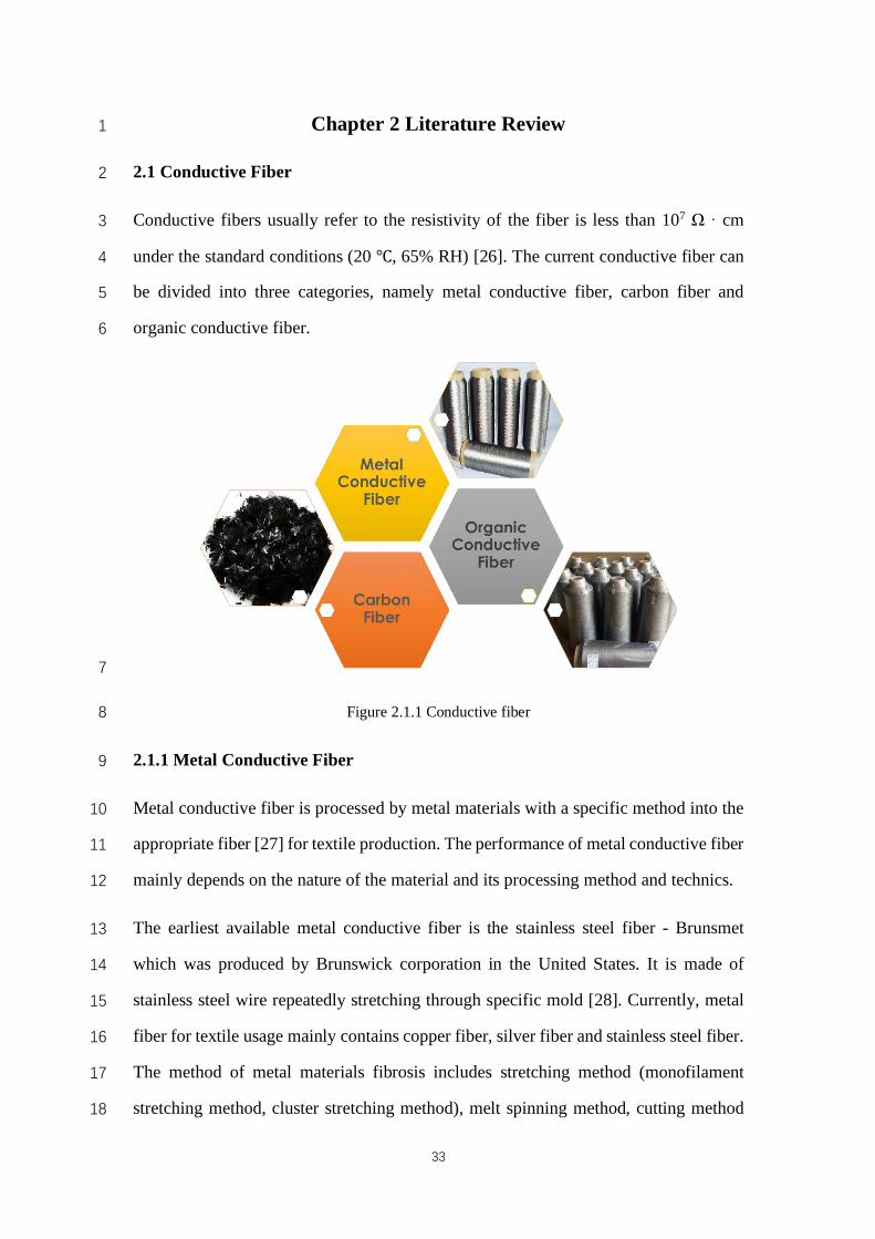
Figure 2.1.1 Conductive fiber 33

Figure 2.2.1 Common categories of textile application of conductive Fiber 37

Figure 3.1.1 Flowchart of study and development of thermal functional

woven textiles

45

Figure 3.2.1 Manual sampling loom 48

Figure 3.2.2 Concept of thermal woven sample 48

Figure 3.3.1 Microscope longitudinal view of cotton yarn (a), silver-

coated conductive yarn B (b), silver-coated conductive yarn A (c), silver-

coated conductive yarn A in natural state (d)

50

Figure 3.3.2 CCI tech automatic dobby sampling loom 51

Figure 3.3.3 3D images of the conductive yarn in different structures 51-52

Figure 3.3.4 Selected 3D images of the conductive yarn arrangement 53-54

Figure 3.3.5 Experiment samples on CCI sampling loom 54

Figure 3.3.6 Experiment samples with different yarn A arrangement (twill

weave; weft density: 30 picks/inch)

55-56

Figure 3.3.7 Experiment samples with different weave structure (weft

density: 30 picks/inch; yarn a in every 2 picks)

56

Figure 3.3.8 Experiment samples with different weft density (satin weave;

yarn a in every 6 picks)

57

Figure 3.3.9 Thermal image of selected woven samples in plain weave 58

Figure 3.4.1 Staubli jacquard loom and Doriner weaving loom 59

Figure 3.4.2 Sample design 60

Figure 3.4.3 Warp yarn replacement design 60

Figure 3.4.4 Warp yarn replacement 61

Figure 3.4.5 Weft arrangement design 61

Figure 3.4.6 Fabric layout design 62

19

Figure 3.4.7 Sample on jacquard loom 62

Figure 3.4.8 Experiment sample 63

Figure 4.1.1 Schematic diagram of unit model 65

Figure 4.1.2 Schematic diagram of single yarn model 65

Figure 4.1.3 Schematic diagram of lr, ls and θ 66

Figure 4.1.4 Schematic diagram and 3d image of plain weave (1/1) 67

Figure 4.1.5 Schematic diagram and 3d image of twill weave (1/3) 67-68

Figure 4.1.6 Schematic diagram and 3d image of satin weave (8 ends) 68

Figure 4.1.7 Schematic diagram of woven fabric (left) and woven fabric

model (right)

69

Figure 4.1.8 Equivalent resistive network of woven fabric model 69

Figure 4.1.9 Comparison between the measured and simulated electrical

resistance values in plain weave with 25/30/35 picks/inch weft density

73


resistance values in twill weave with 25/30/35 picks/inch weft density

73


resistance values in satin weave with 25/30/35 picks/inch weft density

73

Figure 4.1.12 Linear regression analyses of the measured and simulated

resistance

74

Figure 4.1.13 Comparisons between the measured and simulated electrical

resistance

75

Figure 4.1.14 Comparisons between the measured and simulated

resistance by weft density

76

Figure 4.1.15 Comparisons between the measured and simulated

resistance by structure

76


resistance of S1

77

20


resistance of s6 and S11

77

Figure 4.2.1 Structure diagram of 1/3 twill weave 80

Figure 4.2.2 Three basic structure of woven fabric 82

Figure 4.2.3 CTWF samples in weft density of 25 picks/inch (P for plain;

T for twill; S for satin)

83

Figure 4.2.4 Curve fitting for plain weave, twill weave and satin weave 84

Figure 4.2.5 Comparison on simulated value and measured value 85

Figure 4.2.6 Linear regression analyses of the simulated and measured

value

86

Figure 4.2.7 Comparison on previous model and fast estimated model 87

Figure 5.2.1 Synopsis of thermal conductive woven fabric 92

Figure 5.2.2 Schematic diagrams of weft conductive yarn (WECY)

arrangement and weft length calculation

94

Figure 5.2.3 Relations of influence factors 95

Figure 5.4.4 Selected fabrication sample images and microscope images 104

Figure 5.5.5 Fabric temperature and thermal images of selected TCWFs

after 20 mins heating

105

Figure 5.5.6 Fabric temperature and thermal images of selected TCWFs

under different influence factor change: a - WECY arrangement (A)

change; b - Weft density (Dwe) change; c - Voltage (U) change

106

Figure 5.5.7 Residual analysis: a - residual statistics; b - scatterplot of

regression standardized predicted value and regression standardized

residual; c - histogram of regression standardized residual; d - normal P-P

plot of regression standardized residual.

110

Figure 5.5.8 Design-oriented utilization 112

Figure 5.5.9 Example design 113

21

Figure 6.1.1 TCWF design description: (a) - size and function of TCWF

sample; (b) - plain weave and illustration of SCCY A and SCCY B; (c) -

twill weave; (d) - satin weave

116

Figure 6.2.2 Fabrication experiment: (a) - weft density weaving trial; (b) -

structure weaving trial; (c) - warp yarn replacement design; (d) - warp

yarn replacement effect; (f) - weft yarn weaving design

119

Figure 7.1.1 Parameter comparison between SSY and SCCY used in this

study

135

Figure 7.2.1 a - SSY used in experiment; b - microscope image of normal

SSY; c - untwisted and easy to be loose; d - entangled together after

friction

137

Figure 7.3.1 Fabrication images of thermal stainless steel woven fabric 139

Figure 7.3.2 Microscope images of conductive path 139

Figure 7.3.3 Electrical resistance network and equivalent electrical

resistance network of TSSWF: a - electrical resistance network of whole

TSSWF; b - equivalent electrical resistance network of TSSWF with 1cm

conductive path (Type A); c - equivalent electrical resistance network of

TSSWF with 2cm conductive path (Type B)

141

Figure 7.3.4 a- Results of electrical resistance and heating temperature of

all TSSWF samples; b - electrical resistance comparison between before

heating and after heating; c - temperature comparison between two types

in width change to length change; d - temperature comparison between

two types in length change to width change

143

Figure 8.1.1 Introduction of Dysmenorrhea 148

Figure 8.2.1 Design sheet of thermal functional garment 149

Figure 8.2.2 Design and fabrication specifications of TCWF sample for

apparel application

149-150

22

Figure 8.2.3 Design and fabrication specifications of optimized TCWF

lining for apparel application

151

Figure 8.2.4 Notations of weaving design for optimized TCWF 152

Figure 8.2.5 Detachable battery controller design and prototype 153

Figure 8.2.6 Apparel application and thermal effect under heating 153-154

Figure 8.2.7 Thermal image of wear trial 154

Figure 8.3.1 Thermal functional jacket 156

Figure 8.3.2 Thermal functional coat 157

Figure 8.3.3 Thermal functional shirt 158

Figure 9.2.1 Experimental images: a - Thermochromic pigment samples;

b - experiment process; c - thermal woven fabric; d - Yarn A; e - Yarn B;

f - fabrication design; g - 3D fabric concept design; h - 40℃; i - 50℃; j -

60℃; k - 70℃; l - light box; m - spectroradiometer; n - tripod; o - thermal

imaging camera; p - power supply

162

Figure 9.3.1 Raw data process: a - raw data diagram of red color; b - raw

data diagram of white board; c - raw data processed by XwYwZw

correction and Yw correction and their color differences

163-164

Figure 9.3.2 Decolorization color images: a - reflectance of red color

group; b - reflectance of yellow color group; b - reflectance of green color

group; b - reflectance of blue color group; e - decolorization colors in

CIELAB space; L*a*b* distribution of decolorization colors; g - L*, a*,

b* values and CMC 2:1 color difference value during color change.

166-167

Figure 9.3.3 Comparison diagrams of four color groups: a - CIELAB

values in a* and b* plane at heating; CIELAB lightness L* in dependence

on temperature at heating; c - measured color by spectroradiometer; d -

K/S in dependence on temperature at heating; e - CMC 2:1 color

difference in dependence on temperature at heating

169

Figure 9.3.4 Color difference between Rw correction and Yw correction 170

23

Figure 9.3.5 Color difference between Red pigment sample measured by

spectroradiometer (Red) and spectrophotometer (dRed): a - diagram of

ΔL*, Δa*, Δb*; b - spectrogram of Red color; c - spectrogram of dRed

color; d - diagram of measured wavelength comparison

171

Figure 9.3.6 Color difference between Yellow pigment sample measured

by spectroradiometer (Yellow) and spectrophotometer (dYellow): a -

diagram of ΔL*, Δa*, Δb*; b - spectrogram of Yellow color; c -

spectrogram of dYellow color; d - diagram of measured wavelength

comparison

172

Figure 9.3.7 Color difference between Green pigment sample measured

by spectroradiometer (Green) and spectrophotometer (dGreen): a -

diagram of ΔL*, Δa*, Δb*; b - spectrogram of Green color; c -

spectrogram of dGreen color; d - diagram of measured wavelength

comparison

172

Figure 9.3.8 Color difference between Blue pigment sample measured by

spectroradiometer (Blue) and spectrophotometer (dBlue): a - diagram of

ΔL*, Δa*, Δb*; b - spectrogram of Blue color; c - spectrogram of dBlue

color; d - diagram of measured wavelength comparison

173

Figure 9.4.1 Application design flow and prototype demonstration: a -

SLR camera; b - tripod; c - power supply; d - thermal imaging camera; e -

spectrophotometer; f - color printing machine; 1 - color matching by SLR

camera photos and MATLAB calculation; 2 - color matching by color

database; g - indicator prototype design; h - thermal woven garment; i -

indicator prototype before heating up the garment; j - thermal image of

thermal woven garment under heating up; k - indicator prototype after

heating up the garment

175

Figure 10.3.1 Design application implementation of thermal woven fabric 181

1

24

List of Tables 1

Table 2.2.1 Textile Application of Conductive Fiber 37-38

Table 3.2.1 Weaving Design of Trial A 49

Table 3.2.2 Weaving Design of Trial B 49

Table 3.2.3 Weaving Design of Trial C 50

Table 3.3.1 Weaving Samples for Different Weft Density and Conductive

Yarn Arrangement in the Experiment

53

Table 3.3.2 Sample Design Information 54

Table 3.4.1 Electrical Resistance of Yarn and Fabric 63


Table 4.1.2 Weaving Samples for Different Weft Densities and

Conductive Yarn Arrangements in the Experiment

72

Table 4.1.3 ANOVA Table of S1 74

Table 4.2.1 Weaving Samples for Different Weft Density and Conductive

Yarn Arrangement in the Experiment

82

Table 4.2.2 Weft Density of Yarn A of Selected Samples 82

Table 4.2.3 Cover Factor and Electrical Resistance of CTWF 83

Table 4.2.4 ANOVA Table of Curve Fitting 84


Table 4.2.6 Electrical Resistance Simulated Result 85

Table 4.2.7 ANOVA Table of Linear Regression 86

Table 4.2.8 Equivalent Samples with Weft Density in 25 picks/inch 87

Table 4.2.9 Cover Factor of Yarn A of All Samples 88

Table 5.4.1 Sample design 102-103

Table 5.5.1 Data results of selected influence factors 107

Table 5.5.2 Model summaryc 109

Table 5.5.3 ANOVAa 109

Table 5.5.4 Coefficientsa 109

25

Table 5.5.5 Residuals statisticsa 110

Table 5.5.6 Validation results of Model 1 and Model 2 111

Table 5.5.7 Cost of silver coated conductive yarn (SCCY) used in the

experiment

113

Table 5.5.8 SCCY cost example 114

Table 6.1.1 Specifications of TCWF sample design 117

Table 6.2.1 Microscope image and yarn specifications of material used:

(a) - cotton yarn, (b) - silver-coated conductive yarn A (SCCY A), (c) -

silver-coated conductive yarn B (SCCY B)

118

Table 6.3.1 TCWF samples and microscope images 121-122

Table 6.3.2 Test results of sample mass and thickness 123

Table 6.3.3 Test results of sample air resistance 124

Table 6.3.4 Test results of sample thermal conductivity (k) and Qmax 125

Table 6.3.5 Test results of sample original resistance (RO) and heating

resistance (RS) in steady state

127

Table 6.3.6 Test results of sample heating temperature and heating

resistance

128-129

Table 6.3.7 Results of sample power utilization efficiency 132

Table 7.2.1 Detailed sample design and size 136

Table 7.3.1 Thermal stainless steel samples and thermal images when

heating

140

Table 7.3.2 Experiment results of electrical resistance and heating

temperature

143

1

2

3

4

26

Chapter 1 Introduction 1

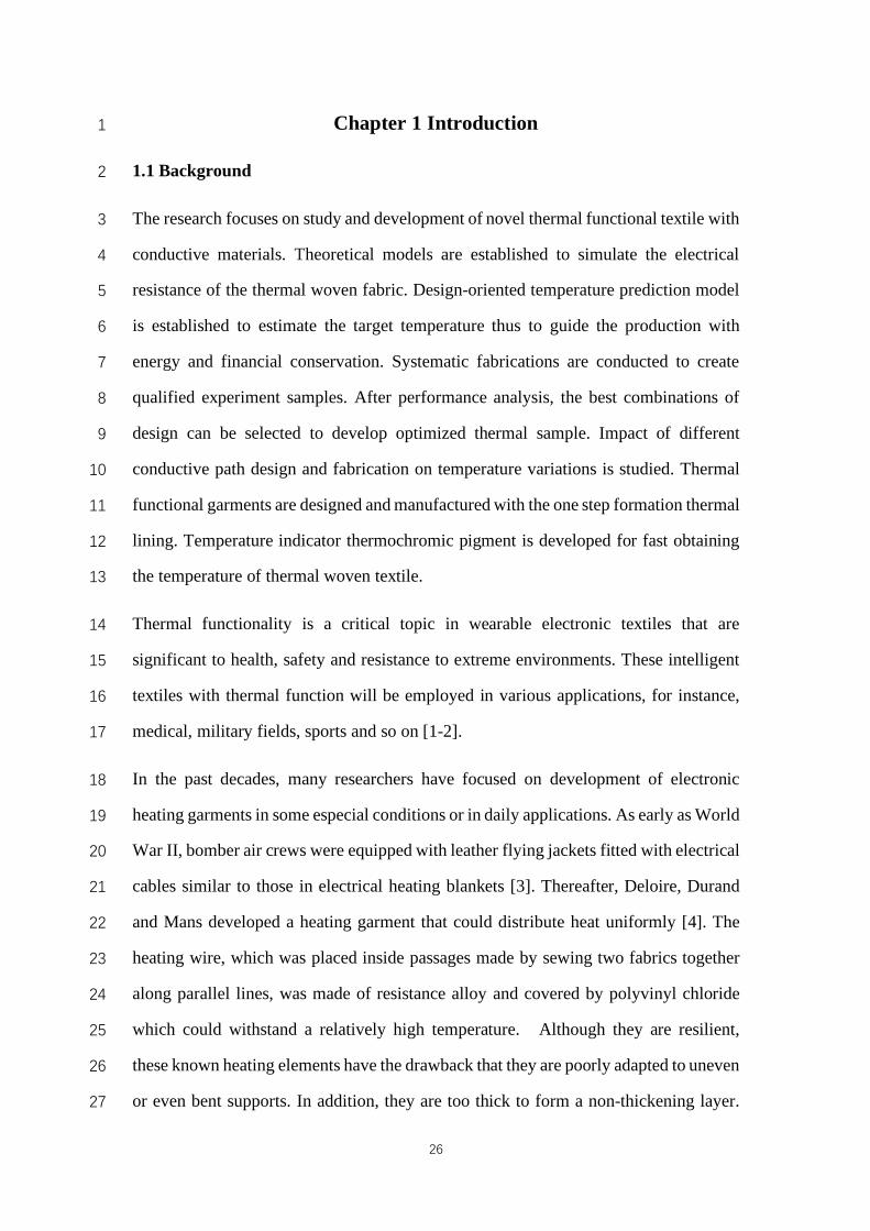
1.1 Background 2

The research focuses on study and development of novel thermal functional textile with 3

conductive materials. Theoretical models are established to simulate the electrical 4

resistance of the thermal woven fabric. Design-oriented temperature prediction model 5

is established to estimate the target temperature thus to guide the production with 6

energy and financial conservation. Systematic fabrications are conducted to create 7

qualified experiment samples. After performance analysis, the best combinations of 8

design can be selected to develop optimized thermal sample. Impact of different 9

conductive path design and fabrication on temperature variations is studied. Thermal 10

functional garments are designed and manufactured with the one step formation thermal 11

lining. Temperature indicator thermochromic pigment is developed for fast obtaining 12

the temperature of thermal woven textile. 13

Thermal functionality is a critical topic in wearable electronic textiles that are 14

significant to health, safety and resistance to extreme environments. These intelligent 15

textiles with thermal function will be employed in various applications, for instance, 16

medical, military fields, sports and so on [1-2]. 17

In the past decades, many researchers have focused on development of electronic 18

heating garments in some especial conditions or in daily applications. As early as World 19

War II, bomber air crews were equipped with leather flying jackets fitted with electrical 20

cables similar to those in electrical heating blankets [3]. Thereafter, Deloire, Durand 21

and Mans developed a heating garment that could distribute heat uniformly [4]. The 22

heating wire, which was placed inside passages made by sewing two fabrics together 23

along parallel lines, was made of resistance alloy and covered by polyvinyl chloride 24

which could withstand a relatively high temperature. Although they are resilient, 25

these known heating elements have the drawback that they are poorly adapted to uneven 26

or even bent supports. In addition, they are too thick to form a non-thickening layer. 27

27

Thus, new conductive materials and manufacturing methods of heating garments 1

emerged with the development of technology [5]. Much attention has been paid to 2

heated jackets that usually attach a carbon fiber material layer inside the jacket to 3

support heating energy [6]. Besides, the heating products presented by Gerbing are 4

constructed with an interior protective moisture barrier and breathable membrane to 5

generate heat [6]. Yet, sew processes and electronic control systems are necessary to 6

realize its thermal function. Many researchers tried to incorporate the electric resistance 7

heating wires into the fabric body during its formation by employing knitting or 8

weaving technology. Roell made an electrical heating element in the form of a knit 9

fabric by using mesh structure on flat knitting machines, which included current supply 10

and resistance wires provided with a corrosion-resistant conductive coating [7]. 11

Moreover, another method of forming a fabric article to generate heat was discussed. 12

A stitch yarn and a loop yarn which consist of a core of insulating material and at least 13

one conductive heating filament were used to form the fabric body by using a reverse 14

plaiting circular knitting process. Consequently, to avoid damaging the electronic 15

resistance heating elements, the technical face or technical back of the fabric body was 16

finished, and fleece surface regions were formed [8]. In addition, Hill et al invented a 17

plural layer woven electronic article which comprise a plurality of electrically 18

insulating yarn and electrically conductive yarn in the warp, a plurality of electrically 19

insulating yarn and electrically conductive yarn in the weft which defined at least one 20

cavity between them. A circuit carrier disposed in the cavity and has at least one 21

exposed electrical contact in electrical connection with at least one electrically 22

conductive yarn [9]. The lightweight and flexibility of wearable electrical heating 23

textile are popular. Rantanen et al. described an implementation of two electrical 24

heating prototypes with an electrical heating system that consisted of 12 conductive 25

woven carbon fabric panels, 9 temperature sensors, 3 humidity sensors, power control 26

electronics, measurement electronics, voltage regulation electronics and batteries. All 27

the electrical devices, excluding batteries, were connected into a polyester shirt [10]. 28

28

Recently, in order to solve the problem that the temperature cannot be changed smartly 1

according to the current necessity in different parts of the body, a new method of 2

forming an electric heating /warming fabric article was discussed, which included 3

interposing a barrier layer between the fabric body and conductive sheet-form layer 4

with adhesive. The conductive sheet-form layer comprising metalized textile, metalized 5

plastic sheeting and metal foils can be readily configured for various circuit patterns to 6

provide different heating to different areas of articles by varying the effective 7

electricity-conductive volume in selected regions [11]. Rapid development is activated 8

by the huge potential demand and thermal garment research is becoming a growing 9

sector in the textiles lab and industry [12]. Recently, a notable application of thermal 10

function in textile including WarmX, a German company which focuses on thermal 11

knitwear research to retain warmth during outdoor sport activities and work protections, 12

is made of conductive polyamide fiber by weaving technology and knitting technology. 13

However, most thermal garment operated by attaching a heating layer that may be a 14

piece of conductive fiber or metal material, and some products incorporated conductive 15

heat fabric with normal fabric sewn together by the patchwork method to format a 16

heating area and electronic routing. Few studies can provide a systemic method to 17

develop the thermal function garment incorporating a heating area and resistive 18

network together in one formation. 19

1.2 Aim and Objectives 20

The aim of this study is to develop a new generation of wearable thermal functional 21

woven textile based on electronical heating technology for providing temperature 22

protection and medical healthcare treatment. 23

This project proposes to achieve the following principal objectives: 24

1) To establish thermal theoretical models to simulate the electrical resistance of the 25

thermal woven fabric, which allows customized design to be produced in order to 26

meet the demand of a highly efficient prototype design and reducing cost. 27

29

2) To establish temperature prediction model to estimate the target temperature, 1

which can guide the production with energy and financial conservation. 2

3) To study the characteristic performance of the thermal woven fabrics, thus the best 3

combinations of design can be selected to develop optimized thermal fabric. 4

4) To study the impact of different conductive path design and fabrication on 5

temperature variations, which will guide the design and material use. 6

5) To design and develop prototypes of thermal functional clothing with formability 7

by the use of conductive yarns, optimized manufacturing technology, 8

microelectronics and garment design method. 9

6) To develop temperature indicator thermochromic pigment for fast obtaining the 10

temperature of thermal woven textile. 11

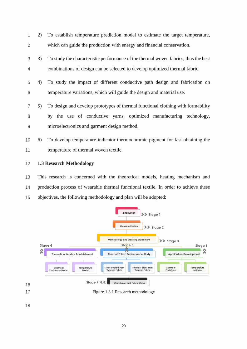
1.3 Research Methodology 12

This research is concerned with the theoretical models, heating mechanism and 13

production process of wearable thermal functional textile. In order to achieve these 14

objectives, the following methodology and plan will be adopted: 15

16

Figure 1.3.1 Research methodology 17

18

30


A literature review will be conducted in relevant areas with an aim to gain 2

comprehensive background knowledge, such as the development of current heated 3

products, thermal mechanism, new technologies applied in the thermal functional 4

textile, the application areas of intelligent wearable thermal textile. By this way, the 5

current problems of thermal functional textile and practical topic choice could be 6

achieved much more reasonably. 7


Woven fabric, which is interwoven between warp yarn and weft yarn, is an approach 9

to provide the desired resistance heating articles. Compared with electronic knitting 10

textile, the electronic woven textile achieves better uniform and consistent properties. 11

Therefore, the electronic heating woven fabrics with different weaving parameters will 12

be designed and woven in this study. It is notable that the configuration approach of 13

ordinary yarn and conductive yarn has extreme influence on the heated temperature of 14

thermal fabric. In relatively simple arrangement of conductive yarn, the characteristics 15

of conductive yarn determine the heating characteristics of the heated woven fabrics. 16

An effective and systematic approach will be explored to compute the equivalent 17

electrical resistance of conductive networks built based on the novel arrangement of 18

conductive yarn and woven technology. In addition, design-oriented temperature 19

prediction model will be established to estimate target temperature. 20


Two kinds of conductive yarns, silver coated conductive yarn and stainless steel yarn, 22

will be used to select the suitable material for thermal woven fabric. Three weaving 23

machines will be used to conduct the weaving experiment. There is manual sampling 24

loom, CCI sampling loom, Staubli jacquard loom and Doriner weaving loom. All the 25

samples are specially designed and well fabricated to match the testing requirement. 26

31


Several performance tests are conducted to evaluate the thermal woven fabrics, which 2

are Mass and Thickness Test, Air Permeability Test, Thermal Conductivity Test, Qmax 3

Test, Electrical Resistance Test and Heating Temperature Test. After tests and 4

evaluation, an optimized design combination can be developed to create integrated 5

commercialize-oriented garment with thermal functions. The design method of thermal 6

woven fabric development, apparel development and supporting accessory 7

development effectively reduce the material waste, energy consumption and financial 8

cost, which is likely to become the future inspiration and guidance of industrial design 9

and production. 10


On the basis of the thermal theoretical model, optimized manufacturing process, the 12

development of thermal garment design methods, four apparel prototypes including 13

electronic heating jacket, coat, shirt and dress will be made to achieve thermal 14

functionality by targeting different locations. 15

1.3.6 Development of Temperature Indicator Thermochromic Pigment for Fast 16

Obtaining the Temperature of Thermal Woven Textile 17

Thermal products are rapidly increasing in the e-textile industry. There are generally 18

three common ways to measure the heating temperature: thermometer, infrared thermal 19

imaging camera and temperature sensor. When selling the products, it is difficult to 20

measure the thermal pads by the three ways mentioned above due to the accuracy 21

requirement or the price budget. As for designers, these instruments may be hard to 22

operate and too technical, which may affect them to design related products. In this 23

case, thermochromic pigment like TIP can be a very useful method, by using which 24

customers can more intuitively feel the temperature change and range. In addition, the 25

colorimetric result of different thermochromic pigment can also help designers to create 26

various pattern design which can cleverly combined with the thermal products thus to 27

32

add additional value. After analyzing the colorimetric properties of four thermochromic 1

pigments, the best temperature indicator pigment for thermal woven textile can be 2

determined and developed. 3

1.4 Significance and Values 4

This study of nonconventional thermal functional textile, which has the following 5

advantages, represents a great challenge and significant contribution to the advance of 6

wearable thermal functional textile: 1) heat can be provided to the multi-target locations; 7

2) the conductive paths and the heating areas could be made into fabric without external 8

modification such as sewing; 3) power distribution. It is expected that this project will 9

lead to better understanding the manufacturing process of novel thermal functional 10

textile with formability. Moreover, the thermal theoretical model could be used as a 11

theoretical reference for researchers. The novel thermal functional textile will have 12

large application areas, such as outdoor apparel products, home thermal products, 13

healthcare and medical treatment. The project will promote the new development of 14

high added-value textile products to increase the competitive capacity of the Hong 15

Kong textile and apparel industry and business. 16

17

18

19

20

21

22

23

24

33

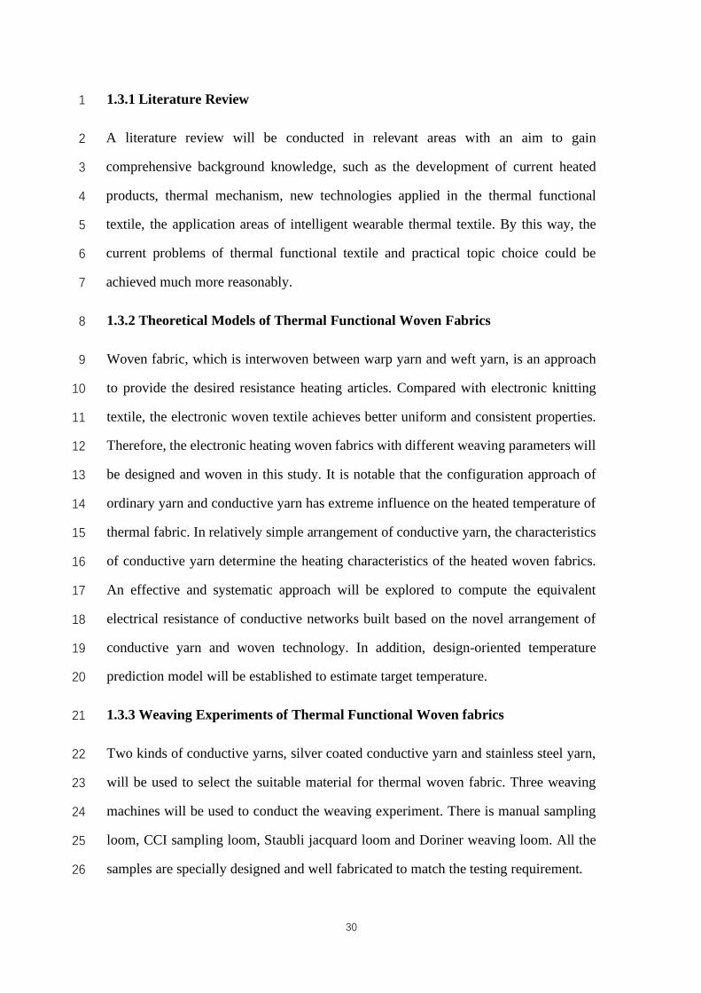
Chapter 2 Literature Review 1

2.1 Conductive Fiber 2

Conductive fibers usually refer to the resistivity of the fiber is less than 107 Ω · cm 3

under the standard conditions (20 ℃, 65% RH) [26]. The current conductive fiber can 4

be divided into three categories, namely metal conductive fiber, carbon fiber and 5

organic conductive fiber. 6

7

Figure 2.1.1 Conductive fiber 8

2.1.1 Metal Conductive Fiber 9

Metal conductive fiber is processed by metal materials with a specific method into the 10

appropriate fiber [27] for textile production. The performance of metal conductive fiber 11

mainly depends on the nature of the material and its processing method and technics. 12

The earliest available metal conductive fiber is the stainless steel fiber - Brunsmet 13

which was produced by Brunswick corporation in the United States. It is made of 14

stainless steel wire repeatedly stretching through specific mold [28]. Currently, metal 15

fiber for textile usage mainly contains copper fiber, silver fiber and stainless steel fiber. 16

The method of metal materials fibrosis includes stretching method (monofilament 17

stretching method, cluster stretching method), melt spinning method, cutting method 18

34

and crystallization precipitation method. Metal materials are usually processed into 1

short fibers, blended and fabricated with common textile fiber. 2

Metal conductive fiber has uniform conductive composition with excellent electrical 3

conductivity, heat resistance, chemical corrosion resistance and softness. However, it 4

has large specific gravity, weak cohesive force and relatively poor spinnability. 5

Conductive fiber with high linear density produced by these metal fibers is expensive 6

and the colors of which are limited. Besides, it is necessary to enwrap a shielding layer 7

of special electric magnetic outside the metal conductive fiber when using it, in order 8

to reduce the interference between the fibers. [29] 9

-Copper Fiber 10

Copper fiber possesses remarkable electrical conductivity and thermal conductivity 11

with small electrical resistivity and relatively high linear density. Currently, the linear 12

density of copper fiber used is approximately around 4000 dtex. Antistatic textile with 13

copper conductive fiber can be applied in uniforms, which reveals a certain 14

development value. [27] 15

-Silver Fiber 16

Silver has been used by human being since thousands of years ago. As early as BC, 17

ancestors used silver utensils. In the middle ages, ulcers were avoided by spreading 18

silver to the surface of the wound. During the first world war, silver thread was utilized 19

for suturing the wound in order to avoid cross infection. Modern medicine considered 20

silver as having the highly effective broad spectrum antimicrobial properties, which has 21

not been discovered any allergic report of human being. Silver has the greatest electrical 22

conductivity and thermal conductivity among all the metals, which was assumed to be 23

the most effective storage and reflective material. [28] 24

Silver fiber has excellent antibacterial properties. In warm and moist environment, 25

silver ions with high biological activity are easily combined with other substances, 26

35

which can coagulate the proteins inside and outside the bacterial cell membrane, thus 1

blocking the respiration and reproduction process in order to achieve sterilization. 2

Silver fiber can resist 99.9% bacteria that exposed to the surface in1 hour. In contrast, 3

most other antibacterial products still cannot achieve the same effect after 48 hours. 4

[26-28] 5

Silver fiber possesses remarkable antistatic and radiation protection performance. As 6

long as there is a small amount of silver fiber in clothing, static generated by friction 7

will be eliminated rapidly. Due to the high electrical conductivity, silver fiber can 8

protect human body from electromagnetic waves effectively. [[26-28] 9

Silver fiber owns great heat insulation performance. It will emit the heat from human 10

skin rapidly to reduce temperature with cool feeling. In cold weather, since silver is the 11

most effective storage and reflective material, radiant energy can be stored or reflected 12

back to the body, in order to preserve heat. [26-28] 13

Silver fiber can be obtained through two methods: one is to plate a layer of silver on 14

the surface of polymer; the other one is to add silver particles in the process of fiber 15

forming. [34] Currently, the first method was the main technology adopted of preparing 16

silver fiber. Due to the high cost of silver, it is rare to fabricate textile with pure silver. 17

In general, the effect of antibacterial, anti-radiation, antistatic, body temperature 18

regulation can be achieved with small amount of silver fiber blended with regular fibers. 19

-Stainless Steel Fiber 20

Stainless steel fiber is a bundle of stainless steel filaments, which is made by pulling 21

stainless steel wire into finer filament. Stainless steel fiber is widely adopted with fine 22

flexibility - 8 microns in diameter stainless steel fiber has the same flexibility with 13 23

microns in diameter hemp fiber. It also has descent mechanical properties and corrosion 24

resistance, which prevents corrosion from nitric acid, phosphorus acid, alkali and 25

organic solvent. It is a high temperature resistant material with terrific performance and 26

can be continuously used in oxidation atmosphere such as 600 ℃. The resistance of 27

36

fabric made by stainless steel fiber reduces as the temperature increased, which 1

indicates an excellent performance in textile applications. [26] 2

2.1.2 Carbon Fiber 3

Carbon fiber mainly refers to the polymer fiber which has carbon content higher than 4

90% mass fraction, while fiber with a carbon content higher than 99% mass fraction is 5

called graphite fiber. Carbon fiber has uniformity of conductive composition, the axial 6

strength and modulus of which is high. Specific heat and conductivity are between non-7

metal and metal. Thermal expansion coefficient is poor while drug resistance is perfect. 8

Due to the small fiber density, the X-ray permeability of carbon fiber is quite satisfying. 9

The disadvantages of carbon fiber are that it has poor impact resistance, is oxidized 10

easily in hot strong acid and lacks toughness. [28] 11

Carbon fiber and its fabric are conductors with a negative temperature coefficient of 12

resistance, which means the humidity has less effect on the properties of the 13

conductivity. Sensor sensitivity of the resistance of carbon fiber is higher than stainless 14

steel fiber, but the sensor sensitivity of the resistance of carbon fiber textile is lower 15

than textile made by stainless steel fiber. It is generally used with composite materials 16

due to the narrow application in textile field. [26-28] 17

2.1.3 Organic Conductive Fiber 18

Basic physical and mechanical properties of the organic conductive fiber are similar to 19

common textile fiber. It has fine textile processing performance, dyeing properties, 20

chemical resistance and electrical conductivity, which is not easily affected by 21

environmental temperature and humidity. 22

Organic conductive fiber can be divided by the processing method: directly 23

polymerizing from conductive material, coating with conductive material on common 24

synthetic fiber, compositing or spinning conductive material and polymer fibers. The 25

37

composite organic conductive fiber is widely adopted owing to its comprehensive and 1

beyond average performance [30]. 2

2.2 Textile Application of Conductive Fiber 3

Conductive fibers are extensively used in antistatic textile, electromagnetic shielding 4

textiles, sensor textiles and anti-reconnaissance camouflage materials. The application 5

performance of intelligent textiles made by the integration of information technology 6

and conductive fiber textile technology is improving. 7

8

Figure 2.2.1 Common categories of textile application of conductive fiber 9

Table 2.2.1 Textile Application of Conductive Fiber [36-44] 10

Highly conductive fabric with soft handle, called silk organza, was reported by Post. It contains two types of fibers, which were a plain silk yarn as the warp and a silk yarn wrapped with thin copper foil as the weft.

A research team developed transmission line using a woven fabric with conductive metal yarn in plain weave fabrics. Insulated metal filaments twisted with polyester yarn woven in conventional plain weave structure have been chosen for development. This construction is the most elementary and simple textile structure.

By the year of 1999, Philips Research Laboratories developed a wearable sensor jacket that uses advanced knitting techniques to form soft stretchable fabric sensors placed Polyester Yarn in the joint positions of jacket to measure upper limb and body movement.

38

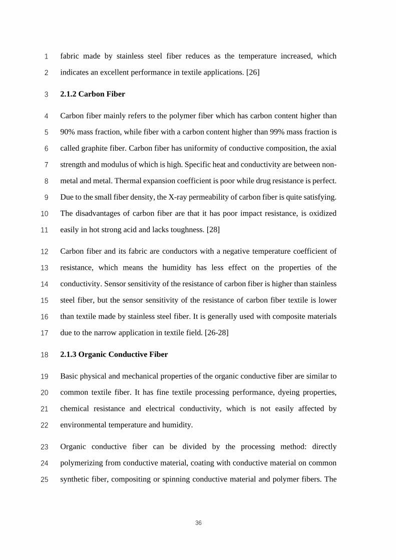
Woven and knitted stainless steel fabrics were used as electrodes, as shown as ‘Textrodes’ in Figure, for the development of smart suit. The suit was intended for the monitoring of electrocardiogram and respiration rate of children in a hospital environment.

A tracking tape knitted with conductive fiber was developed for the purpose of transmitting an electrical signal and connected with sensors. The requirements of high conductivity and good stability are very useful for a tracking cables development, the knitted tracking was 10mm wide with only 3 ohms resistance over 100mm.

The developed prototypes of respibelt for measuring respiration.

In 2000, a detailed article was published regarding the development of electronic embroidery which is the patterning of conductive textiles by numerically controlled sewing or weaving processes. Interactive electrical textiles embroidered with conductive threads have demonstrated their abilities to stitch multiple layers of fabric in one step and to precisely specify circuit layout with computer-aided design.

Baby suit for measuring heart rate and electrocardiogram respectively.

Smart shirt and intelligent biomedical clothes developed by European funded projects: WEALTHY and MY HEART. This system was designed for collecting risk factors to support citizens to fight against major cardio-vascular diseases and help avoid heart attack. Hence, it can provide the necessary motivation for the new life styles.

Smart shirt and intelligent biomedical clothes developed by European funded projects: WEALTHY and MY HEART. The fabric sensors implemented with the wearable systems can be used for medical monitoring of body parameters such as heart beat rate and breathing rate. The fabric sensors were made by commercial stainless steel threads twisted around a standard continuous viscose or cotton textile yarn.

Post built electronic circuits entirely out of textiles to distribute data and power and perform touch sensing. He applied stainless steel fibers into textiles in order to connect circuit boards for developing different types of textile electronics. Figure 5 shows the prototype of musical jacket. Those circuits use conventional electronic components by sewing with conductive yarns, such as musical keyboards and graphic input surfaces.

The sensor jacket includes knitted fabrics which have electrical properties suited for either sensing elongation or for use as non-sensing conductive tracking. A connection port on the jacket can be connected to other wearable devices for data collecting from the current limb movement and body position of the wearer.

1

2

39

2.2.1 Antistatic Textile 1

During industrial production, electrostatic hazard causes safety problem and destroys 2

electronic components as well. Electrostatic discharge spectrum interference is one of 3

the key causes that damage electronic equipment operation. 4

The fabric can obtain conductivity after inserting conductive fiber into common fabric, 5

so that the accumulated charge on the fabric can release as soon as possible, thus 6

effectively preventing the static electricity accumulation. The DuPont company 7

launched the product “Nomex” in the 1950s, which is a kind of fiber that can avoid 8

static under dry conditions. Until then, conductive fiber is playing an important role in 9

antistatic uniform. In last decade, W L Gore & Associates company in America 10

promoted an antistatic work uniform called “Gore-Tex”, which is mainly used in the 11

petrochemical industry. Differing from weaving the electric conductive fiber into 12

common fabric previously, this novel uniform is made from nano conductive carbon 13

particles of carbon fiber by covering the conductive substrate protective layer on the 14

surface of fabric. This technology improved antistatic effect and prevented the 15

conductive carbon particles from peeling off due to some reasons such as the friction 16

in washing [33]. 17

2.2.2 Electromagnetic Shielding Textiles 18

Fabric manufactured by spinning a certain proportion of conductive fibers into the 19

common fiber with a specific process can shield electromagnetic wave. When 20

electromagnetic wave radiates the fabric’s surface, conductive fiber in uniform 21

distribution as conductive medium can convert or transmit the electromagnetic wave to 22

achieve shielding effect. The nature of electromagnetic shielding can be utilized to 23

manufacture precise electronic components and high frequency welding machine, to 24

produce wall cloth with special requirements of building wall, ceiling to absorb radio 25

waves. In Japan, blended copper-coated conductive fiber textile or nonwoven textile is 26

40

extensively used for electromagnetic shielding and absorbing materials, such as the 1

cover of electromagnetic wave absorption for the ship. [35] 2

2.2.3 Sensor Textiles 3

Sensor textiles was produced by flexible conductive fiber applying the principle of 4

electronic sensors, which is easy to carry and has enormous application. Japanese 5

companies use carbon fiber to develop sensor that can detect maximum strain, which is 6

suitable for buildings, roads, factories, aircrafts and ropeways for safety diagnosis. 7

In 2005, the “Textronics” company developed an intelligent motion clothing which can 8

be woven into the fabric. By monitoring the sensor, wearer's heart rate and other health 9

status can be uploaded to the converter in the clothing for achieving the goal of real-10

time monitoring. In August 2008, the company has developed a new generation of 11

upgrade intelligence kit called Textronics Developer's Kit, a supporting element with 12

elastic conductive fabrics, which can carry on the system through a more comfortable 13

way of health monitoring [34]. Intelligent sensing textiles are the combination of 14

comfortableness and sensor technology. 15

2.2.4 Military Textiles 16

The future war will be the information war under high-tech conditions, which means 17

the traditional military equipment are outdated under the circumstances of fast fighting, 18

frequent attack and defense conversion, changeable battlefield situation. To improve 19

the comprehensive capabilities of modern battlefield soldiers must improve the ability 20

of processing and transferring information of soldiers, which makes the understanding 21

of the battlefield reached higher level. The informative garment made of conductive 22

fiber can meet the requirements. [35] 23

Most of conductive fiber is sensitive to electric and heat, thus a single soldier thermal 24

imaging protective garment can be produced due to the conductive textile perfectly 25

prevent the reconnaissance of thermal imaging equipment. Conductive fiber and low 26

41

dielectric substrate such as resin and rubber can composite to be electromagnetic wave 1

absorption materials which is able to absorb radar and avoid the radar tracking, thus to 2

realize the invisibility aim of weapons and equipment [10]. Color changing uniform 3

developed by American is inserting conductive fiber in to form the current circuit. By 4

controlling the temperature in uniform to change color ink on the fabric, the appearance 5

of the uniform will change to fit external environment color，which become a kind of 6

reactive environmental camouflage. [35] 7

2.3 Thermal Textiles 8

A variety of competitive thermal products in the commercial market can be divided into 9

three types. 1) Nuanshoubao, based on iron oxide to generate heat, which is unable to 10

control the temperature and, in some cases, may injure skin. 2) Thermal cap is the 11

second largest heating products. The major heating material, tourmaline, can release 12

the far-infrared rays. However, the relatively expensive price and complicated 13

production process impeded the development of these products. 3) Electric blanket，14

which is easily and rapidly keeping warm but with electromagnetic radiation and waste 15

of energy. Industry and laboratory have strengthened security with temperature 16

controller, however, heating element cannot be newly replaced. [45-46] 17

Rapid development is activated by the huge potential demand and thermal garment 18

research is becoming a growing sector in the textile lab and industry. Heat and energy 19

management is one theme among wearable electronic textiles and resistive heating by 20

using conductive material application is well developed, such as retail products 21

including WarmX, iTermx and so on as the latest kind of thermal product. a notable 22

application of thermal function in textile including WarmX, a German company which 23

focuses on thermal knitwear research to retain warmth during outdoor sport activities 24

and work protections, is made of conductive polyamide fiber by weaving technology 25

and knitting technology. In the last decade, much attention has been paid to the heated 26

42

jacket that usually attaches a carbon fiber material layer inside the jacket to support 1

heating energy. [47-51] 2

Another issue is the advanced control system; Solaris ski-gloves were produced by 3

Reush with a new microcontroller platform named iTermx. In addition, the heating 4

products presented by Gerbing are constructed with an interior protective moisture 5

barrier and breathable membrane to generate heat. Yet, sewing process and electronic 6

control system are necessary to realise their thermal functions. The thermal garments 7

are also designed for specific situation of sub-aqua heated by piped hot water. Aside 8

from retail clothing and the industrial sector, other research works have also been 9

conducted. However, most thermal garments operate by attaching a heating layer that 10

may be a piece of conductive fiber or metal materials, and some products incorporate 11

conductive heat fabric with normal fabric sewn together by the patchwork method to 12

format the heating area and electronic routing. Few studies can provide systemic 13

methods to develop the thermal function garment incorporating a heating area and 14

resistive network together in one formation. [52-56] 15

In the past few decades, many researchers have focused on the development of 16

electronic heating clothing in some special conditions or in daily applications. As early 17

as the second world war, the bomber air personnel equipped with flight jacket with 18

cables and electric heating blanket [57]. After that, Christopher Duran and mans 19

developed heated clothing, to distribute the heat evenly [58]. Heating wire, a paragraph 20

by sewing together two fabrics along parallel lines, by the resistance alloy and by 21

polyvinyl chloride (PVC) can withstand high temperature. Although these known 22

elements are flexible, they have a key shortcoming in that they do not adapt to the 23

uneven or crooked support. In addition, they are too thick non - thickening layer. 24

Therefore, a new type of conductive materials and manufacturing methods, heating 25

clothing emerged with the development of technology [59]. 26

43

Many researchers have tried to incorporate resistance heating wire into the structure of 1

its formation by weaving or knitting technology. Roell made an electrical heating 2

element in the form of a knit fabric by using mesh structure on flat knitting machines, 3

which included current supply and resistance wires provided with a corrosion-resistant 4

conductive coating [60]. In addition, another method of forming a fabric article to 5

generate heat was discussed [61]. Embroidery thread and loop yarn consist of a core of 6

insulating material and at least one conductive heating wire is used to form the fabric 7

of the body through a reverse folding knitting process. Therefore, in order to avoid 8

damage to the electrical resistance heating element, technical or technology of fabric 9

body complete and formation of wool surface area. In addition, lightweight and flexible 10

wearable electric heating textile is welcome. Rantanen et al. described the 11

implementation of the two electric heating prototype of electric heating system, the 12

system consists of 12 conductive carbon fiber fabric panel, nine temperature sensor, 13

humidity sensor, 3 power control electronics, electronic measurement, voltage 14

regulating electronics and batteries. All electrical equipment, not including battery, 15

connected into a dacron shirt [62]. 16

Recently, in order to solve this problem, the temperature does not change smartly 17

according to the necessity of the current in different parts of the body, forming an 18

electric/climate warming, a new method to discuss the fabric of the article, including 19

the plug in the fabric of the barrier layer between the body and conductive adhesive 20

sheet - the form layer. Conductive sheet - form layer of electrostatic spinning and 21

weaving, electrostatic plastic film and foil can be easily configured various circuit 22

model with different heating to different areas of the article by changing the effective 23

electricity conductive rolls [63] in selected areas. 24

Generally, the researchers focused on the following development of electrical heating 25

fabric. First of all, heating articles focused on structures which defined a series of 26

envelope or tubular channel electrical resistance heating wire or element is inserted. 27

Second, coating or printing method was used to design a circuit with plastic film 28

44

resistance heating element. Finally, the electrical resistance heating wire was 1

incorporated into the overall structure body in its formation by weaving or knitting 2

method. However, most of the electronic heating methods from the article were with 3

the aid of sewing or adhesive method which limited the development of commercial 4

market. 5

6

7

8

9

10

11

12

13

14

15

16

17

18

19

20

21

22

45

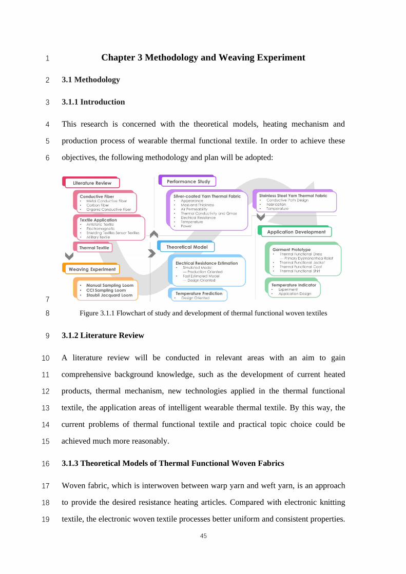
Chapter 3 Methodology and Weaving Experiment 1

3.1 Methodology 2


This research is concerned with the theoretical models, heating mechanism and 4

production process of wearable thermal functional textile. In order to achieve these 5

objectives, the following methodology and plan will be adopted: 6

7

Figure 3.1.1 Flowchart of study and development of thermal functional woven textiles 8


A literature review will be conducted in relevant areas with an aim to gain 10

comprehensive background knowledge, such as the development of current heated 11

products, thermal mechanism, new technologies applied in the thermal functional 12

textile, the application areas of intelligent wearable thermal textile. By this way, the 13

current problems of thermal functional textile and practical topic choice could be 14

achieved much more reasonably. 15


Woven fabric, which is interwoven between warp yarn and weft yarn, is an approach 17

to provide the desired resistance heating articles. Compared with electronic knitting 18

textile, the electronic woven textile processes better uniform and consistent properties. 19

46

Therefore, the electronic heating woven fabrics with different weaving parameters will 1

be designed and woven in this study. It is notable that the configuration approach of 2

ordinary yarn and conductive yarn has extreme influence on the heated temperature of 3

thermal fabric. In relatively simple arrangement of conductive yarn, the characteristics 4

of conductive yarn determine the heating characteristics of the heated woven fabrics. 5

An effective and systematic approach will be explored to compute the equivalent 6

electrical resistance of conductive networks built based on the novel arrangement of 7

conductive yarn and woven technology. In addition, design-oriented temperature 8

prediction model will be established to estimated target temperature. 9


Two kinds of conductive yarns, silver coated conductive yarn and stainless steel yarn, 11

will be used to select the suitable material for thermal woven fabric. Three weaving 12

machines will be used to conduct the weaving experiment. There is manual sampling 13

loom, CCI sampling loom, Staubli jacquard loom and Doriner weaving loom. All the 14

samples are specially designed and well fabricated to match the testing requirement. 15


Several performance tests are conducted to evaluate the thermal woven fabrics, which 17

are Mass and Thickness Test, Air Permeability Test, Thermal Conductivity Test, Qmax 18

Test, Electrical Resistance Test and Heating Temperature Test. After tests and 19

evaluation, an optimized design combination can be developed to create integrated 20

commercialize-oriented thermal functional garment. The design method of thermal 21

woven fabric development, apparel development and supporting accessory 22

development effectively reduce the material waste, energy consumption and financial 23

cost, which is likely to become the future inspiration and guidance of industrial design 24

and production. 25

26

47


On the basis of the thermal theoretical model, optimized manufacturing process, the 2

development of thermal garment design methods, four apparel prototypes including 3

electronic heating jacket, coat, shirt and dress will be made to achieve thermal 4

functionality by targeting different locations. 5

3.1.7 Development of Temperature Indicator Thermochromic Pigment for Fast 6

Obtaining the Temperature of Thermal Woven Textile 7

Thermal products are rapidly increasing in the e-textile industry. There are generally 8

three common ways to measure the heating temperature: thermometer, infrared thermal 9

imaging camera and temperature sensor. When selling the products, it is difficult to 10

measure the thermal pads by the three ways mentioned above due to the accuracy 11

requirement or the price budget. As for designers, these instruments may be hard to 12

operate and too technical, which may affect them to design related products. In this 13

case, thermochromic pigment like TIP can be a very useful method, by using which 14

customers can more intuitively feel the temperature change and range. In addition, the 15

colorimetric result of different thermochromic pigment can also help designers to create 16

various pattern design which can cleverly combined with the thermal products thus to 17

add additional value. After analyzing the colorimetric properties of four thermochromic 18

pigments, the best temperature indicator pigment for thermal woven textile can be 19

determined and developed. 20

3.2 Weaving Trial by Manual Sampling Loom 21

3.2.1 Materials 22

In this trial, 100% black acrylic 369/3 dtex (yarn A), 100% white acrylic 369/3 dtex 23

(yarn B) and 100% cotton 58/10 dtex (yarn C) were used as the basic materials. 100% 24

white acrylic 210/2 dtex (yarn D) 235/34 dtex 2-ply silver-coated yarn (yarn E) and 25

235/34 dtex 24-ply silver-coated yarn (yarn F) were used as conductive materials. 26

27

48

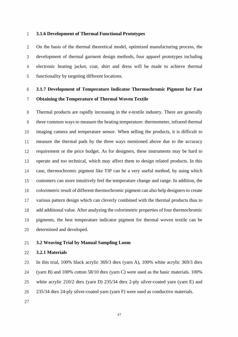
3.2.2 Equipment 1

The woven samples designed in this trial were woven by a manual sampling loom 2

shown in Figure 3.2.1. 3

4

Figure 3.2.1 Manual Sampling Loom 5

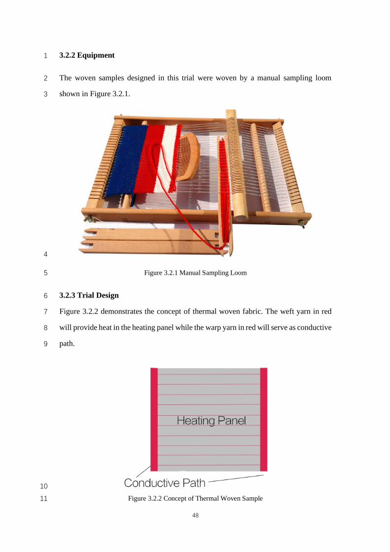
3.2.3 Trial Design 6

Figure 3.2.2 demonstrates the concept of thermal woven fabric. The weft yarn in red 7

will provide heat in the heating panel while the warp yarn in red will serve as conductive 8

path. 9

10

Figure 3.2.2 Concept of Thermal Woven Sample 11

49

Trial A was conduct as designed in Table 3.2.1. Yarn B imitated conductive path while 1

yarn D imitated heating material. After analysis and consideration, the design in trial 2

A-1 was abandoned due to the complex electrical resistance. In the beginning of this 3

research, trial A-2 is more realistic and promising. 4

Table 3.2.1 Weaving Design of Trial A 5 Basic Material: yarn A, yarn B Heating Material: yarn D

Trial A-1 To insert Yarn D in both warp and weft direction

Trial A-2 To insert Yarn D every

other pick in weft direction

6

Trial B was conduct as designed in Table 3.2.2. Yarn F imitated conductive path while 7

yarn E imitated heating material. The concept of trial B is able to accomplish the 8

thermal fabric after further design. 9

Table 3.2.2 Weaving Design of Trial B 10 Basic Material: yarn C, yarn F Heating Material: yarn E

Trial B-1 To insert Yarn E every pick in weft direction

Trial B-2 To insert Yarn E every 3 picks in weft direction

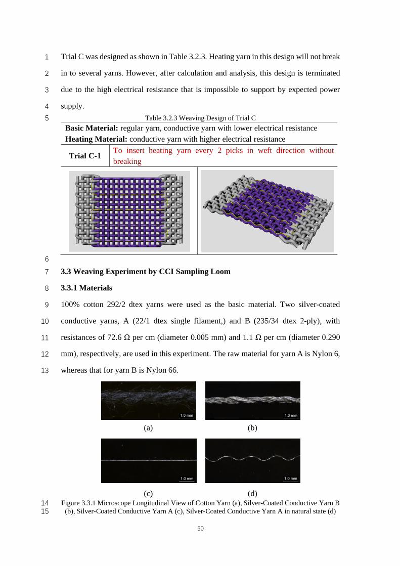
50

Trial C was designed as shown in Table 3.2.3. Heating yarn in this design will not break 1

in to several yarns. However, after calculation and analysis, this design is terminated 2

due to the high electrical resistance that is impossible to support by expected power 3

supply. 4

Table 3.2.3 Weaving Design of Trial C 5 Basic Material: regular yarn, conductive yarn with lower electrical resistance Heating Material: conductive yarn with higher electrical resistance

Trial C-1 To insert heating yarn every 2 picks in weft direction without breaking

6

3.3 Weaving Experiment by CCI Sampling Loom 7

3.3.1 Materials 8

100% cotton 292/2 dtex yarns were used as the basic material. Two silver-coated 9

conductive yarns, A (22/1 dtex single filament,) and B (235/34 dtex 2-ply), with 10

resistances of 72.6 Ω per cm (diameter 0.005 mm) and 1.1 Ω per cm (diameter 0.290 11

mm), respectively, are used in this experiment. The raw material for yarn A is Nylon 6, 12

whereas that for yarn B is Nylon 66. 13

(a) (b)

(c) (d) Figure 3.3.1 Microscope Longitudinal View of Cotton Yarn (a), Silver-Coated Conductive Yarn B 14

(b), Silver-Coated Conductive Yarn A (c), Silver-Coated Conductive Yarn A in natural state (d) 15

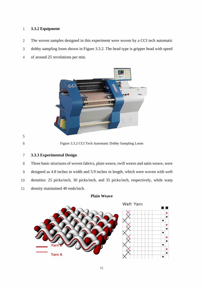
51

3.3.2 Equipment 1

The woven samples designed in this experiment were woven by a CCI tech automatic 2

dobby sampling loom shown in Figure 3.3.2. The head type is gripper head with speed 3

of around 25 revolutions per min. 4

5

Figure 3.3.2 CCI Tech Automatic Dobby Sampling Loom 6

3.3.3 Experimental Design 7

Three basic structures of woven fabrics, plain weave, twill weave and satin weave, were 8

designed as 4.8 inches in width and 5.9 inches in length, which were woven with weft 9

densities: 25 picks/inch, 30 picks/inch, and 35 picks/inch, respectively, while warp 10

density maintained 40 ends/inch. 11

Plain Weave

Yarn B

Yarn A

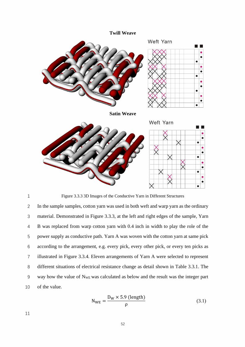
52

Twill Weave

Satin Weave

Figure 3.3.3 3D Images of the Conductive Yarn in Different Structures 1

In the sample samples, cotton yarn was used in both weft and warp yarn as the ordinary 2

material. Demonstrated in Figure 3.3.3, at the left and right edges of the sample, Yarn 3

B was replaced from warp cotton yarn with 0.4 inch in width to play the role of the 4

power supply as conductive path. Yarn A was woven with the cotton yarn at same pick 5

according to the arrangement, e.g. every pick, every other pick, or every ten picks as 6

illustrated in Figure 3.3.4. Eleven arrangements of Yarn A were selected to represent 7

different situations of electrical resistance change as detail shown in Table 3.3.1. The 8

way how the value of NWE was calculated as below and the result was the integer part 9

of the value. 10

11

N#$ =D# × 5.9(length)

ρ (3.1)

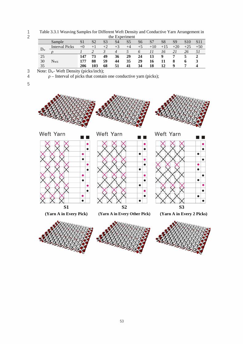
53

Table 3.3.1 Weaving Samples for Different Weft Density and Conductive Yarn Arrangement in 1 the Experiment 2

Sample S1 S2 S3 S4 S5 S6 S7 S8 S9 S10 S11

Dw Interval Picks +0 +1 +2 +3 +4 +5 +10 +15 +20 +25 +50 ρ 1 2 3 4 5 6 11 16 21 26 51

25 NWE

147 73 49 36 29 24 13 9 7 5 2 30 177 88 59 44 35 29 16 11 8 6 3 35 206 103 68 51 41 34 18 12 9 7 4

Note: Dw- Weft Density (picks/inch); 3 ρ – Interval of picks that contain one conductive yarn (picks); 4

5

S1

(Yarn A in Every Pick) S2

(Yarn A in Every Other Pick) S3

(Yarn A in Every 2 Picks)

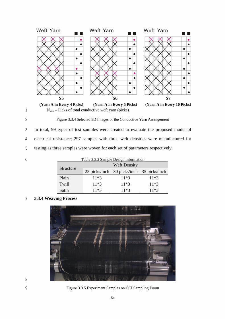
54

NWE – Picks of total conductive weft yarn (picks). 1

Figure 3.3.4 Selected 3D Images of the Conductive Yarn Arrangement 2

In total, 99 types of test samples were created to evaluate the proposed model of 3

electrical resistance; 297 samples with three weft densities were manufactured for 4

testing as three samples were woven for each set of parameters respectively. 5


Structure Weft Density

25 picks/inch 30 picks/inch 35 picks/inch Plain 11*3 11*3 11*3 Twill 11*3 11*3 11*3 Satin 11*3 11*3 11*3

3.3.4 Weaving Process 7

8

Figure 3.3.5 Experiment Samples on CCI Sampling Loom 9

S5

(Yarn A in Every 4 Picks) S6

(Yarn A in Every 5 Picks) S7

(Yarn A in Every 10 Picks)

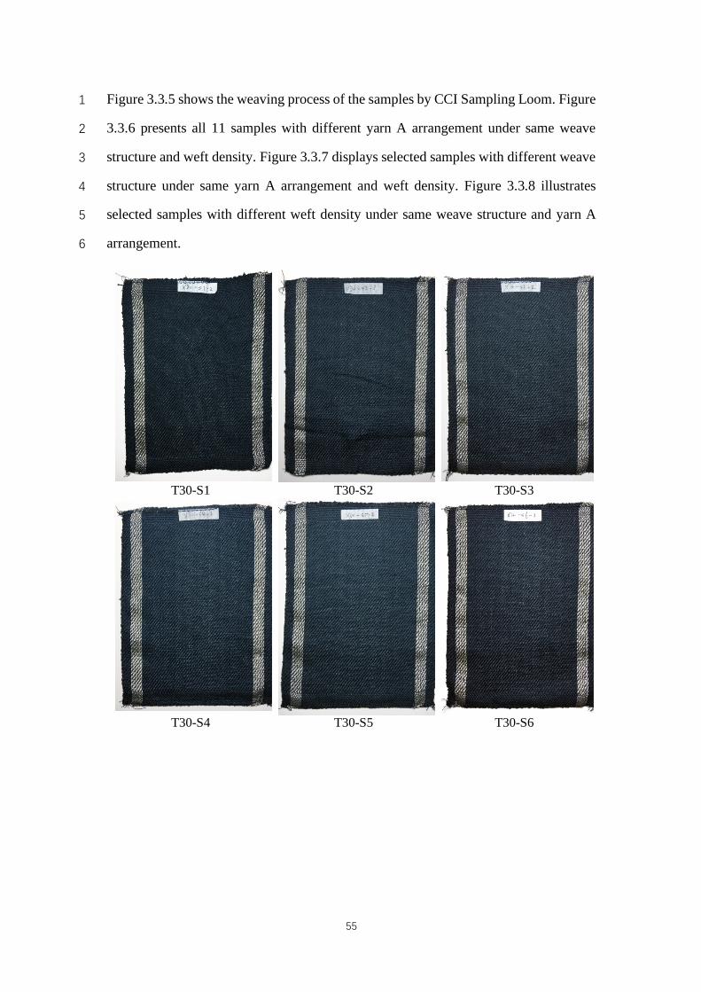
55

Figure 3.3.5 shows the weaving process of the samples by CCI Sampling Loom. Figure 1

3.3.6 presents all 11 samples with different yarn A arrangement under same weave 2

structure and weft density. Figure 3.3.7 displays selected samples with different weave 3

structure under same yarn A arrangement and weft density. Figure 3.3.8 illustrates 4

selected samples with different weft density under same weave structure and yarn A 5

arrangement. 6

T30-S1 T30-S2 T30-S3

T30-S4 T30-S5 T30-S6

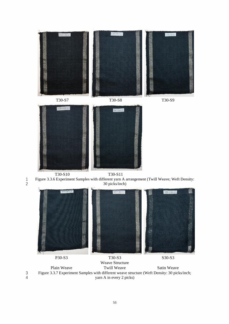
56

T30-S7 T30-S8 T30-S9

T30-S10 T30-S11 Figure 3.3.6 Experiment Samples with different yarn A arrangement (Twill Weave; Weft Density: 1

30 picks/inch) 2

P30-S3 T30-S3 S30-S3

Weave Structure Plain Weave Twill Weave Satin Weave

Figure 3.3.7 Experiment Samples with different weave structure (Weft Density: 30 picks/inch; 3 yarn A in every 2 picks) 4

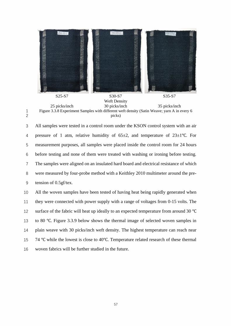
57

S25-S7 S30-S7 S35-S7

Weft Density 25 picks/inch 30 picks/inch 35 picks/inch

Figure 3.3.8 Experiment Samples with different weft density (Satin Weave; yarn A in every 6 1 picks) 2

All samples were tested in a control room under the KSON control system with an air 3

pressure of 1 atm, relative humidity of 65±2, and temperature of 23±1℃. For 4

measurement purposes, all samples were placed inside the control room for 24 hours 5

before testing and none of them were treated with washing or ironing before testing. 6

The samples were aligned on an insulated hard board and electrical resistance of which 7

were measured by four-probe method with a Keithley 2010 multimeter around the pre-8

tension of 0.5gf/tex. 9

All the woven samples have been tested of having heat being rapidly generated when 10

they were connected with power supply with a range of voltages from 0-15 volts. The 11

surface of the fabric will heat up ideally to an expected temperature from around 30 ℃ 12

to 80 ℃. Figure 3.3.9 below shows the thermal image of selected woven samples in 13

plain weave with 30 picks/inch weft density. The highest temperature can reach near 14

74 ℃ while the lowest is close to 40℃. Temperature related research of these thermal 15

woven fabrics will be further studied in the future. 16

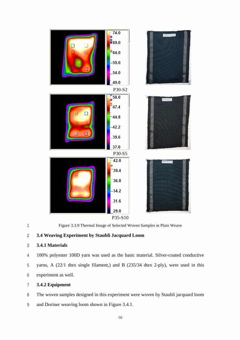
58

P30-S2

P30-S5

P35-S10

Figure 3.3.9 Thermal Image of Selected Woven Samples in Plain Weave 1

3.4 Weaving Experiment by Staubli Jacquard Loom 2

3.4.1 Materials 3

100% polyester 100D yarn was used as the basic material. Silver-coated conductive 4

yarns, A (22/1 dtex single filament,) and B (235/34 dtex 2-ply), were used in this 5

experiment as well. 6

3.4.2 Equipment 7

The woven samples designed in this experiment were woven by Staubli jacquard loom 8

and Doriner weaving loom shown in Figure 3.4.1. 9

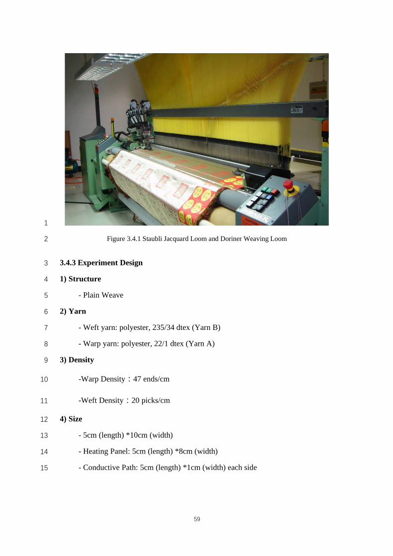
59

1

Figure 3.4.1 Staubli Jacquard Loom and Doriner Weaving Loom 2

3.4.3 Experiment Design 3

1) Structure 4

- Plain Weave 5

2) Yarn 6

- Weft yarn: polyester, 235/34 dtex (Yarn B) 7

- Warp yarn: polyester, 22/1 dtex (Yarn A) 8

3) Density 9

-Warp Density：47 ends/cm 10

-Weft Density：20 picks/cm 11

4) Size 12

- 5cm (length) *10cm (width) 13

- Heating Panel: 5cm (length) *8cm (width) 14

- Conductive Path: 5cm (length) *1cm (width) each side 15

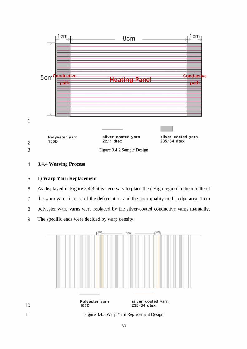
60

1

2

Figure 3.4.2 Sample Design 3

3.4.4 Weaving Process 4

1) Warp Yarn Replacement 5

As displayed in Figure 3.4.3, it is necessary to place the design region in the middle of 6

the warp yarns in case of the deformation and the poor quality in the edge area. 1 cm 7

polyester warp yarns were replaced by the silver-coated conductive yarns manually. 8

The specific ends were decided by warp density. 9

10

Figure 3.4.3 Warp Yarn Replacement Design 11

Heating Panel Conductive

path Conductive

path

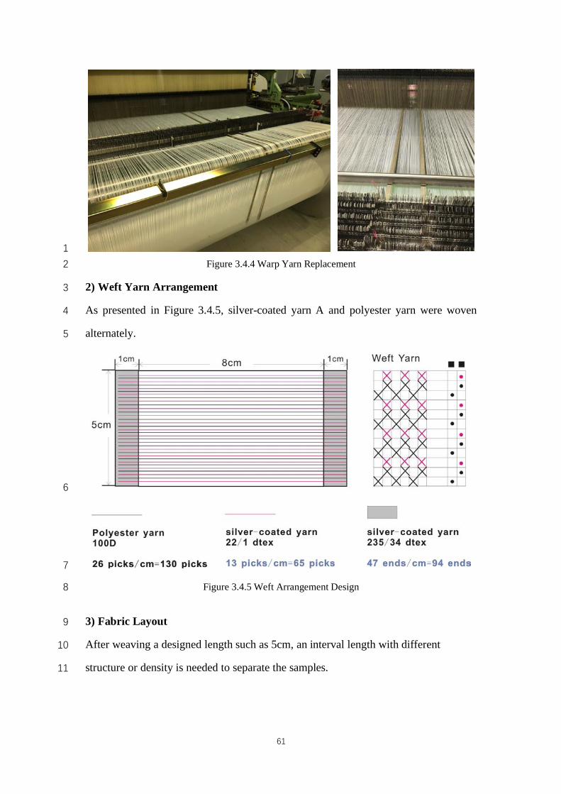
61

1

Figure 3.4.4 Warp Yarn Replacement 2

2) Weft Yarn Arrangement 3

As presented in Figure 3.4.5, silver-coated yarn A and polyester yarn were woven 4

alternately. 5

6

7

Figure 3.4.5 Weft Arrangement Design 8

3) Fabric Layout 9

After weaving a designed length such as 5cm, an interval length with different 10

structure or density is needed to separate the samples. 11

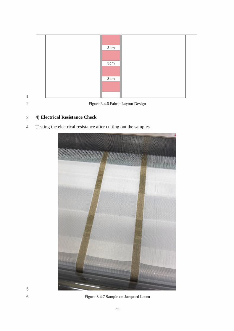
62

1

Figure 3.4.6 Fabric Layout Design 2

4) Electrical Resistance Check 3

Testing the electrical resistance after cutting out the samples. 4

5

Figure 3.4.7 Sample on Jacquard Loom 6

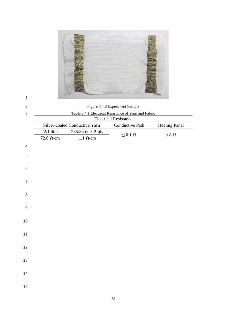
63

1

Figure 3.4.8 Experiment Sample 2

Table 3.4.1 Electrical Resistance of Yarn and Fabric 3 Electrical Resistance

Silver-coated Conductive Yarn Conductive Path Heating Panel 22/1 dtex 235/34 dtex 2-ply

≤ 0.1 Ω ≈ 8 Ω 72.6 Ω/cm 1.1 Ω/cm

4

5

6

7

8

9

10

11

12

13

14

15

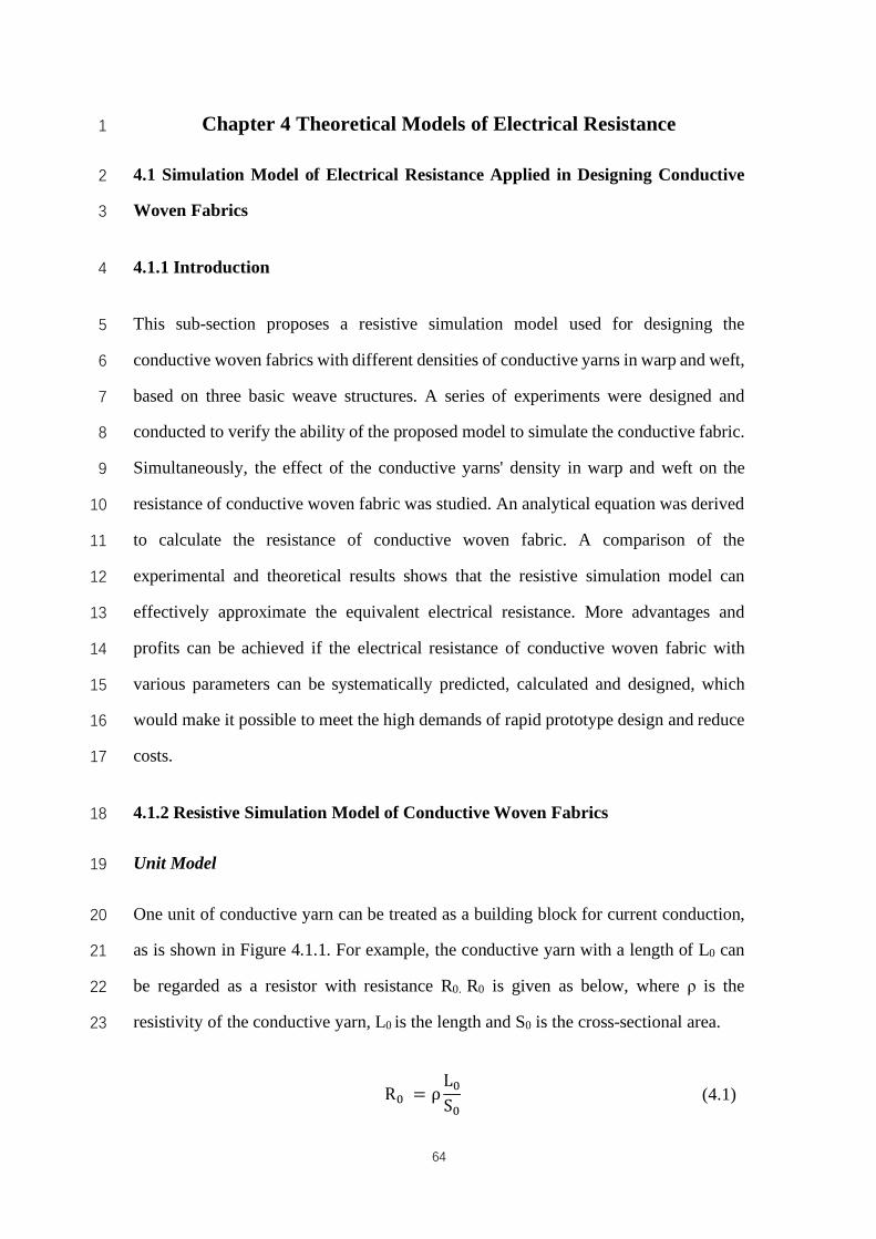
64

Chapter 4 Theoretical Models of Electrical Resistance 1

4.1 Simulation Model of Electrical Resistance Applied in Designing Conductive 2

Woven Fabrics 3


This sub-section proposes a resistive simulation model used for designing the 5

conductive woven fabrics with different densities of conductive yarns in warp and weft, 6

based on three basic weave structures. A series of experiments were designed and 7

conducted to verify the ability of the proposed model to simulate the conductive fabric. 8

Simultaneously, the effect of the conductive yarns' density in warp and weft on the 9

resistance of conductive woven fabric was studied. An analytical equation was derived 10

to calculate the resistance of conductive woven fabric. A comparison of the 11

experimental and theoretical results shows that the resistive simulation model can 12

effectively approximate the equivalent electrical resistance. More advantages and 13

profits can be achieved if the electrical resistance of conductive woven fabric with 14

various parameters can be systematically predicted, calculated and designed, which 15

would make it possible to meet the high demands of rapid prototype design and reduce 16

costs. 17

4.1.2 Resistive Simulation Model of Conductive Woven Fabrics 18

Unit Model 19

One unit of conductive yarn can be treated as a building block for current conduction, 20

as is shown in Figure 4.1.1. For example, the conductive yarn with a length of L0 can 21

be regarded as a resistor with resistance R0. R0 is given as below, where ρ is the 22

resistivity of the conductive yarn, L0 is the length and S0 is the cross-sectional area. 23

R6 = ρ

L6S6

(4.1)

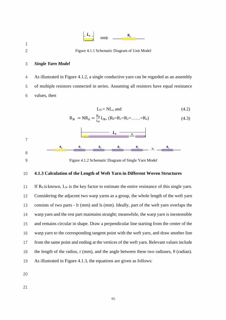
65

1

Figure 4.1.1 Schematic Diagram of Unit Model 2

Single Yarn Model 3

As illustrated in Figure 4.1.2, a single conductive yarn can be regarded as an assembly 4

of multiple resistors connected in series. Assuming all resistors have equal resistance 5

values, then 6

7

8

Figure 4.1.2 Schematic Diagram of Single Yarn Model 9

4.1.3 Calculation of the Length of Weft Yarn in Different Woven Structures 10

If R0 is known, LN is the key factor to estimate the entire resistance of this single yarn. 11

Considering the adjacent two warp yarns as a group, the whole length of the weft yarn 12

consists of two parts - lr (mm) and ls (mm). Ideally, part of the weft yarn overlaps the 13

warp yarn and the rest part maintains straight; meanwhile, the warp yarn is inextensible 14

and remains circular in shape. Draw a perpendicular line starting from the center of the 15

warp yarn to the corresponding tangent point with the weft yarn, and draw another line 16

from the same point and ending at the vertices of the weft yarn. Relevant values include 17

the length of the radius, r (mm), and the angle between these two radiuses, θ (radian). 18

As illustrated in Figure 4.1.3, the equations are given as follows: 19

20

21

LN = NLo and (4.2)

R9 = NR6 =:;<;L9, (R0=R1=R2=……=Rn) (4.3)

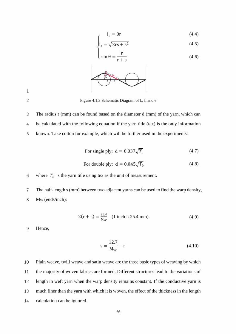
66

1

Figure 4.1.3 Schematic Diagram of lr, ls and θ 2

The radius r (mm) can be found based on the diameter d (mm) of the yarn, which can 3

be calculated with the following equation if the yarn title (tex) is the only information 4

known. Take cotton for example, which will be further used in the experiments: 5

where 𝑇> is the yarn title using tex as the unit of measurement. 6

The half-length s (mm) between two adjacent yarns can be used to find the warp density, 7

MW (ends/inch): 8

Hence, 9

Plain weave, twill weave and satin weave are the three basic types of weaving by which 10

the majority of woven fabrics are formed. Different structures lead to the variations of 11

length in weft yarn when the warp density remains constant. If the conductive yarn is 12

much finer than the yarn with which it is woven, the effect of the thickness in the length 13

calculation can be ignored. 14

I@ = θr (4.4)

IC = D2rs + sH (4.5)

sin θ =r

r + s (4.6)

For single ply: d = 0.037D𝑇> (4.7)

For double ply: d = 0.045D𝑇>, (4.8)

2(r + s) = 25.4OP

(1 inch ≈ 25.4 mm). (4.9)

s =

12.7M#

− r (4.10)

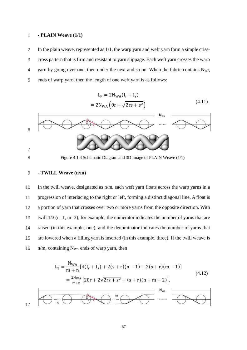
67

- PLAIN Weave (1/1) 1

In the plain weave, represented as 1/1, the warp yarn and weft yarn form a simple criss-2

cross pattern that is firm and resistant to yarn slippage. Each weft yarn crosses the warp 3

yarn by going over one, then under the next and so on. When the fabric contains NWA 4

ends of warp yarn, then the length of one weft yarn is as follows: 5

6

7

Figure 4.1.4 Schematic Diagram and 3D Image of PLAIN Weave (1/1) 8

- TWILL Weave (n/m) 9

In the twill weave, designated as n/m, each weft yarn floats across the warp yarns in a 10

progression of interlacing to the right or left, forming a distinct diagonal line. A float is 11

a portion of yarn that crosses over two or more yarns from the opposite direction. With 12

twill 1/3 (n=1, m=3), for example, the numerator indicates the number of yarns that are 13

raised (in this example, one), and the denominator indicates the number of yarns that 14

are lowered when a filling yarn is inserted (in this example, three). If the twill weave is 15

n/m, containing NWA ends of warp yarn, then 16

17

LT = 2N#U(I@ + IC)

= 2N#U Vθr + D2rs + sHW (4.11)

LX =

N#U

m + n[4(I@ + IC) + 2(s + r)(n − 1) + 2(s + r)(m − 1)]

= H9P\]^_

`2θr + 2√2rs + sH + (s + r)(n +m − 2)b. (4.12)

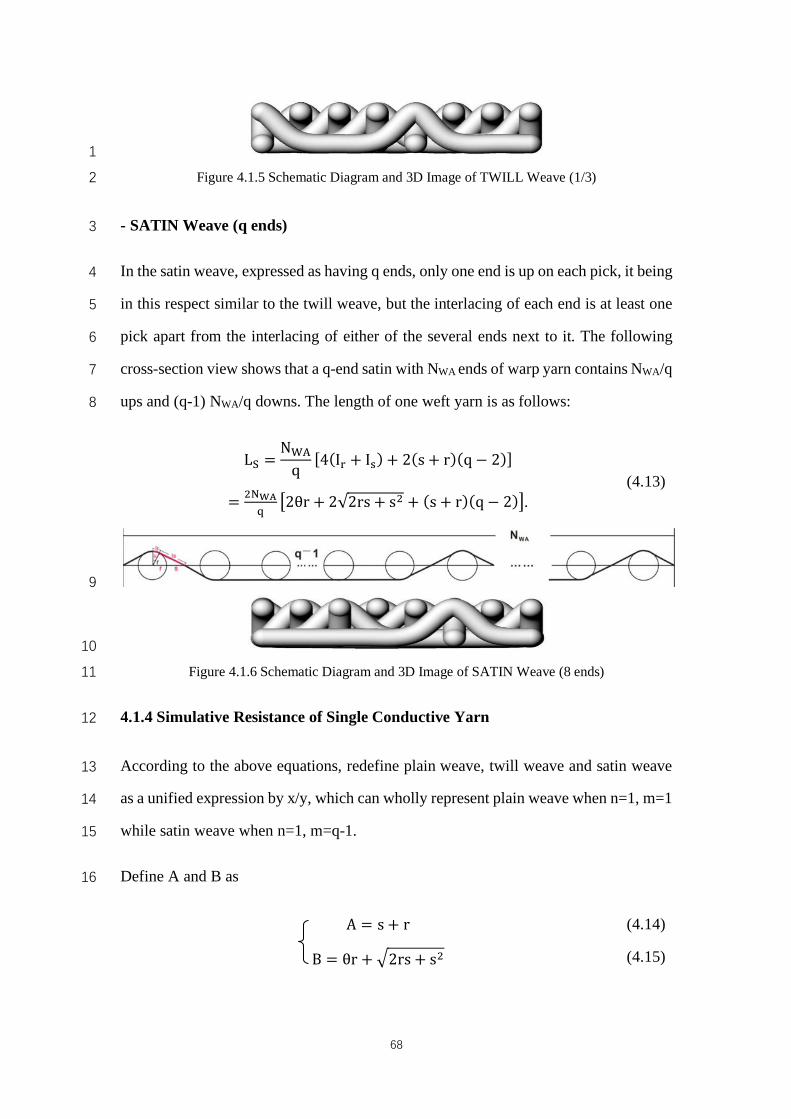
68

1

Figure 4.1.5 Schematic Diagram and 3D Image of TWILL Weave (1/3) 2

- SATIN Weave (q ends) 3

In the satin weave, expressed as having q ends, only one end is up on each pick, it being 4

in this respect similar to the twill weave, but the interlacing of each end is at least one 5

pick apart from the interlacing of either of the several ends next to it. The following 6

cross-section view shows that a q-end satin with NWA ends of warp yarn contains NWA/q 7

ups and (q-1) NWA/q downs. The length of one weft yarn is as follows: 8

9

10

Figure 4.1.6 Schematic Diagram and 3D Image of SATIN Weave (8 ends) 11

4.1.4 Simulative Resistance of Single Conductive Yarn 12

According to the above equations, redefine plain weave, twill weave and satin weave 13

as a unified expression by x/y, which can wholly represent plain weave when n=1, m=1 14

while satin weave when n=1, m=q-1. 15

Define A and B as 16

Lc =N#U

q[4(I@ + IC) + 2(s + r)(q − 2)]

= H9P\e

`2θr + 2√2rs + sH + (s + r)(q − 2)b. (4.13)

A = s + r (4.14)

B = θr + D2rs + sH (4.15)

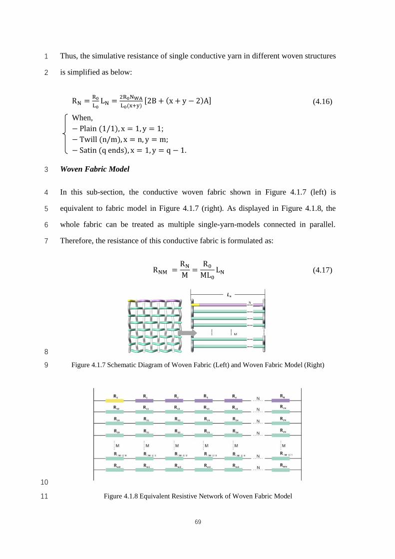
69

Thus, the simulative resistance of single conductive yarn in different woven structures 1

is simplified as below: 2

Woven Fabric Model 3

In this sub-section, the conductive woven fabric shown in Figure 4.1.7 (left) is 4

equivalent to fabric model in Figure 4.1.7 (right). As displayed in Figure 4.1.8, the 5

whole fabric can be treated as multiple single-yarn-models connected in parallel. 6

Therefore, the resistance of this conductive fabric is formulated as: 7

8

Figure 4.1.7 Schematic Diagram of Woven Fabric (Left) and Woven Fabric Model (Right) 9

10

Figure 4.1.8 Equivalent Resistive Network of Woven Fabric Model 11

R9 =:;<;L9 =

H:;9P\<;(h^i)

[2B + (x + y − 2)A] (4.16)

When, −Plain(1/1), x = 1, y = 1; −Twill(n/m), x = n, y = m; −Satin(qends), x = 1, y = q − 1.

R9O =R9M =

R6ML6

L9 (4.17)

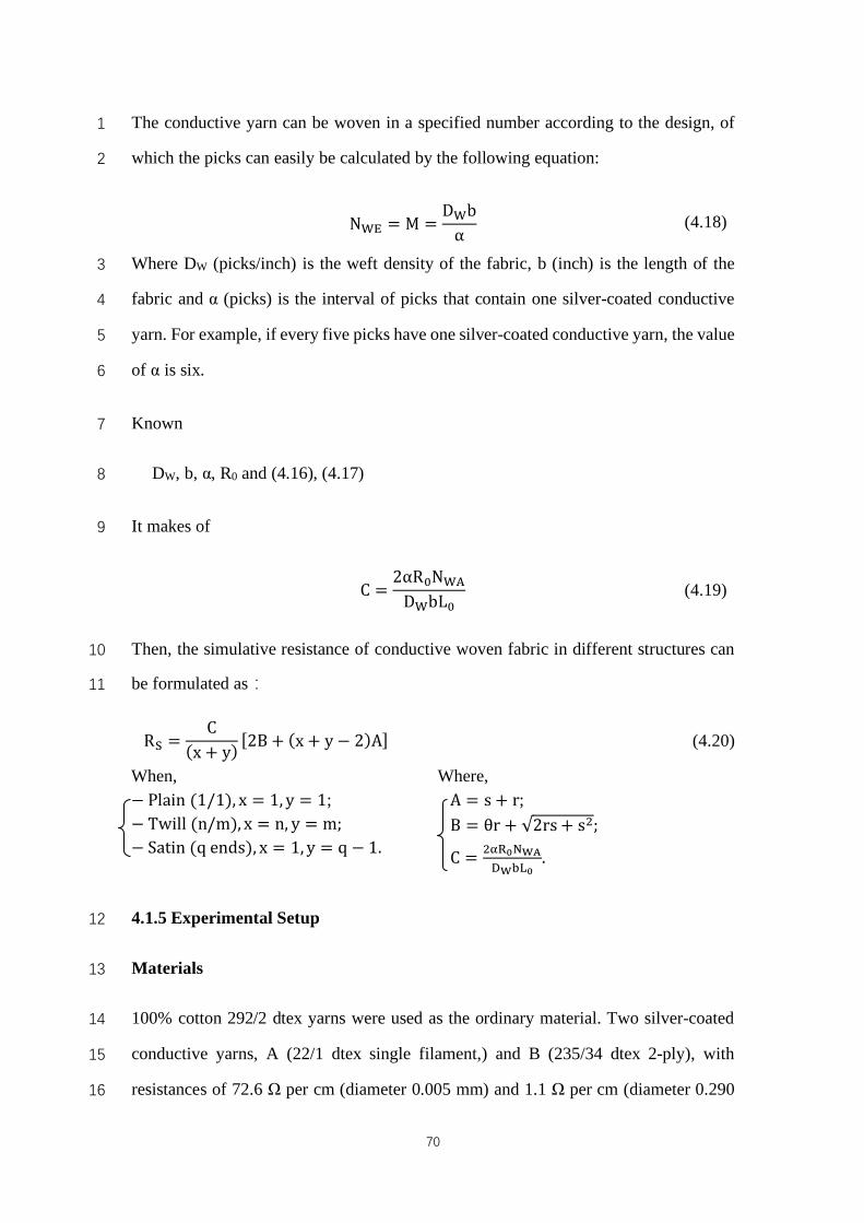
70

The conductive yarn can be woven in a specified number according to the design, of 1

which the picks can easily be calculated by the following equation: 2

Where DW (picks/inch) is the weft density of the fabric, b (inch) is the length of the 3

fabric and α (picks) is the interval of picks that contain one silver-coated conductive 4

yarn. For example, if every five picks have one silver-coated conductive yarn, the value 5

of α is six. 6

Known 7

DW, b, α, R0 and (4.16), (4.17) 8

It makes of 9

Then, the simulative resistance of conductive woven fabric in different structures can 10

be formulated as： 11

Rc =C

(x + y)[2B + (x + y − 2)A] (4.20)

When, −Plain(1/1), x = 1, y = 1; −Twill(n/m), x = n, y = m; −Satin(qends), x = 1, y = q − 1.

Where, A = s + r; B = θr + √2rs + sH;

C = Ht:;9P\uPv<;

.

4.1.5 Experimental Setup 12

Materials 13

100% cotton 292/2 dtex yarns were used as the ordinary material. Two silver-coated 14

conductive yarns, A (22/1 dtex single filament,) and B (235/34 dtex 2-ply), with 15

resistances of 72.6 Ω per cm (diameter 0.005 mm) and 1.1 Ω per cm (diameter 0.290 16

N#$ = M =

D#bα (4.18)

C =

2αR6N#U

D#bL6 (4.19)

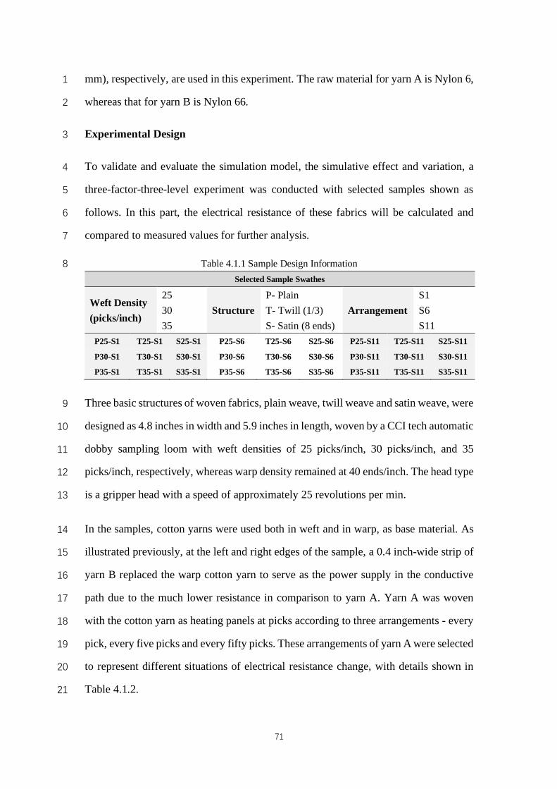
71

mm), respectively, are used in this experiment. The raw material for yarn A is Nylon 6, 1

whereas that for yarn B is Nylon 66. 2

Experimental Design 3

To validate and evaluate the simulation model, the simulative effect and variation, a 4

three-factor-three-level experiment was conducted with selected samples shown as 5

follows. In this part, the electrical resistance of these fabrics will be calculated and 6

compared to measured values for further analysis. 7

Table 4.1.1 Sample Design Information 8 Selected Sample Swathes

Weft Density (picks/inch)

25 Structure

P- Plain Arrangement

S1 30 T- Twill (1/3) S6 35 S- Satin (8 ends) S11

P25-S1 T25-S1 S25-S1 P25-S6 T25-S6 S25-S6 P25-S11 T25-S11 S25-S11



Three basic structures of woven fabrics, plain weave, twill weave and satin weave, were 9

designed as 4.8 inches in width and 5.9 inches in length, woven by a CCI tech automatic 10

dobby sampling loom with weft densities of 25 picks/inch, 30 picks/inch, and 35 11

picks/inch, respectively, whereas warp density remained at 40 ends/inch. The head type 12

is a gripper head with a speed of approximately 25 revolutions per min. 13

In the samples, cotton yarns were used both in weft and in warp, as base material. As 14

illustrated previously, at the left and right edges of the sample, a 0.4 inch-wide strip of 15

yarn B replaced the warp cotton yarn to serve as the power supply in the conductive 16

path due to the much lower resistance in comparison to yarn A. Yarn A was woven 17

with the cotton yarn as heating panels at picks according to three arrangements - every 18

pick, every five picks and every fifty picks. These arrangements of yarn A were selected 19

to represent different situations of electrical resistance change, with details shown in 20

Table 4.1.2. 21

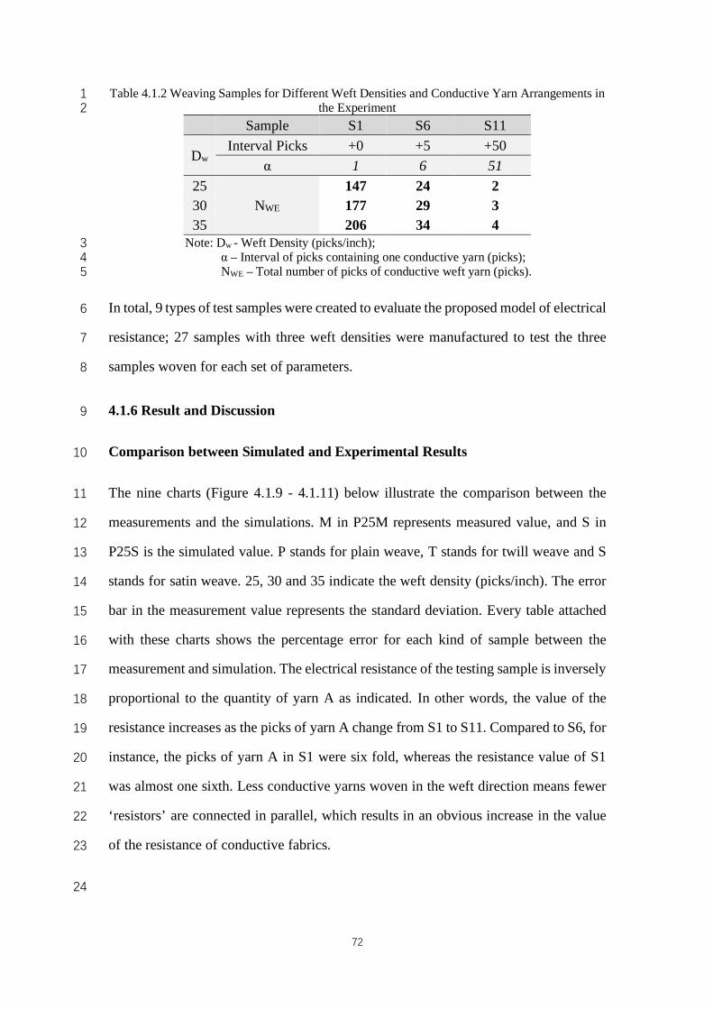
72

Table 4.1.2 Weaving Samples for Different Weft Densities and Conductive Yarn Arrangements in 1 the Experiment 2

Sample S1 S6 S11

Dw Interval Picks +0 +5 +50

α 1 6 51 25

NWE 147 24 2

30 177 29 3 35 206 34 4

Note: Dw - Weft Density (picks/inch); 3 α – Interval of picks containing one conductive yarn (picks); 4 NWE – Total number of picks of conductive weft yarn (picks). 5

In total, 9 types of test samples were created to evaluate the proposed model of electrical 6

resistance; 27 samples with three weft densities were manufactured to test the three 7

samples woven for each set of parameters. 8

4.1.6 Result and Discussion 9

Comparison between Simulated and Experimental Results 10

The nine charts (Figure 4.1.9 - 4.1.11) below illustrate the comparison between the 11

measurements and the simulations. M in P25M represents measured value, and S in 12

P25S is the simulated value. P stands for plain weave, T stands for twill weave and S 13

stands for satin weave. 25, 30 and 35 indicate the weft density (picks/inch). The error 14

bar in the measurement value represents the standard deviation. Every table attached 15

with these charts shows the percentage error for each kind of sample between the 16

measurement and simulation. The electrical resistance of the testing sample is inversely 17

proportional to the quantity of yarn A as indicated. In other words, the value of the 18

resistance increases as the picks of yarn A change from S1 to S11. Compared to S6, for 19

instance, the picks of yarn A in S1 were six fold, whereas the resistance value of S1 20

was almost one sixth. Less conductive yarns woven in the weft direction means fewer 21

‘resistors’ are connected in parallel, which results in an obvious increase in the value 22

of the resistance of conductive fabrics. 23

24

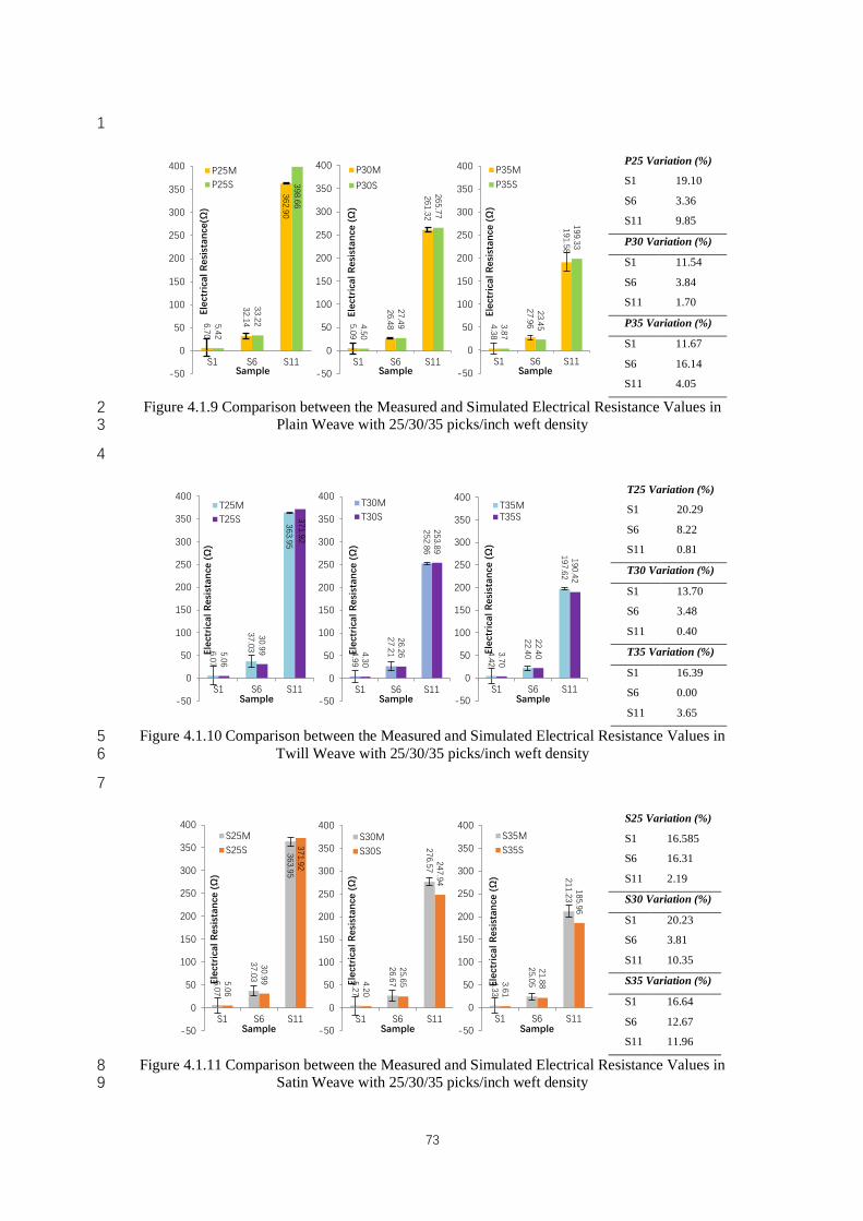
73

1

P25 Variation (%)

S1 19.10

S6 3.36

S11 9.85

P30 Variation (%)

S1 11.54

S6 3.84

S11 1.70

P35 Variation (%)

S1 11.67

S6 16.14

S11 4.05

Figure 4.1.9 Comparison between the Measured and Simulated Electrical Resistance Values in 2 Plain Weave with 25/30/35 picks/inch weft density 3

4

T25 Variation (%)

S1 20.29

S6 8.22

S11 0.81

T30 Variation (%)

S1 13.70

S6 3.48

S11 0.40

T35 Variation (%)

S1 16.39

S6 0.00

S11 3.65

Figure 4.1.10 Comparison between the Measured and Simulated Electrical Resistance Values in 5 Twill Weave with 25/30/35 picks/inch weft density 6

7

S25 Variation (%)

S1 16.585

S6 16.31

S11 2.19

S30 Variation (%)

S1 20.23

S6 3.81

S11 10.35

S35 Variation (%)

S1 16.64

S6 12.67

S11 11.96

Figure 4.1.11 Comparison between the Measured and Simulated Electrical Resistance Values in 8 Satin Weave with 25/30/35 picks/inch weft density 9

6.70

32.14

362.90

5.42

33.22

398.66

-50

0

50

100

150

200

250

300

350

400

S1 S6 S11

Elec

tric

al R

esis

tanc

e(Ω

)

Sample

P25MP25S

5.09

26.48

261.32

4.50

27.49

265.77

-50

0

50

100

150

200

250

300

350

400

S1 S6 S11El

ectr

ical

Res

ista

nce

(Ω)

Sample

P30M

P30S

4.38

27.96

191.58

3.87

23.45

199.33

-50

0

50

100

150

200

250

300

350

400

S1 S6 S11

Elec

tric

al R

esis

tanc

e (Ω

)

Sample

P35MP35S

6.07

37.03

363.95

5.06

30.99

371.92

-50

0

50

100

150

200

250

300

350

400

S1 S6 S11

Elec

tric

al R

esis

tanc

e (Ω

)

Sample

T25MT25S

4.99

27.21

252.86

4.30

26.26

253.89

-50

0

50

100

150

200

250

300

350

400

S1 S6 S11

Elec

tric

al R

esis

tanc

e (Ω

)

Sample

T30MT30S

4.42

22.40

197.62

3.70

22.40

190.42

-50

0

50

100

150

200

250

300

350

400

S1 S6 S11

Elec

tric

al R

esis

tanc

e (Ω

)

Sample

T35MT35S

6.07

37.03

363.95

5.06

30.99

371.92

-50

0

50

100

150

200

250

300

350

400

S1 S6 S11

Elec

tric

al R

esis

tanc

e (Ω

)

Sample

S25MS25S

5.27

26.67

276.57

4.20

25.65

247.94

-50

0

50

100

150

200

250

300

350

400

S1 S6 S11

Elec

tric

al R

esis

tanc

e (Ω

)

Sample

S30MS30S

4.33

25.05

211.23

3.61

21.88

185.96

-50

0

50

100

150

200

250

300

350

400

S1 S6 S11

Elec

tric

al R

esis

tanc

e (Ω

)

Sample

S35MS35S

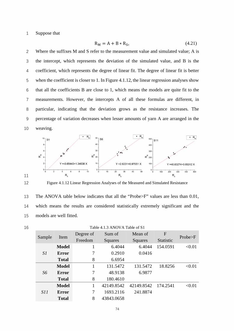
74

Suppose that 1

Where the suffixes M and S refer to the measurement value and simulated value; A is 2

the intercept, which represents the deviation of the simulated value, and B is the 3

coefficient, which represents the degree of linear fit. The degree of linear fit is better 4

when the coefficient is closer to 1. In Figure 4.1.12, the linear regression analyses show 5

that all the coefficients B are close to 1, which means the models are quite fit to the 6

measurements. However, the intercepts A of all these formulas are different, in 7

particular, indicating that the deviation grows as the resistance increases. The 8

percentage of variation decreases when lesser amounts of yarn A are arranged in the 9

weaving. 10

11

Figure 4.1.12 Linear Regression Analyses of the Measured and Simulated Resistance 12

The ANOVA table below indicates that all the “Probe>F” values are less than 0.01, 13

which means the results are considered statistically extremely significant and the 14

models are well fitted. 15

Table 4.1.3 ANOVA Table of S1 16

Sample Item Degree of Freedom

Sum of Squares

Mean of Squares

F Statistic

Probe>F

S1 Model 1 6.4044 6.4044 154.0591 <0.01 Error 7 0.2910 0.0416 Total 8 6.6954



RO = A + B ∗ Rc, (4.21)

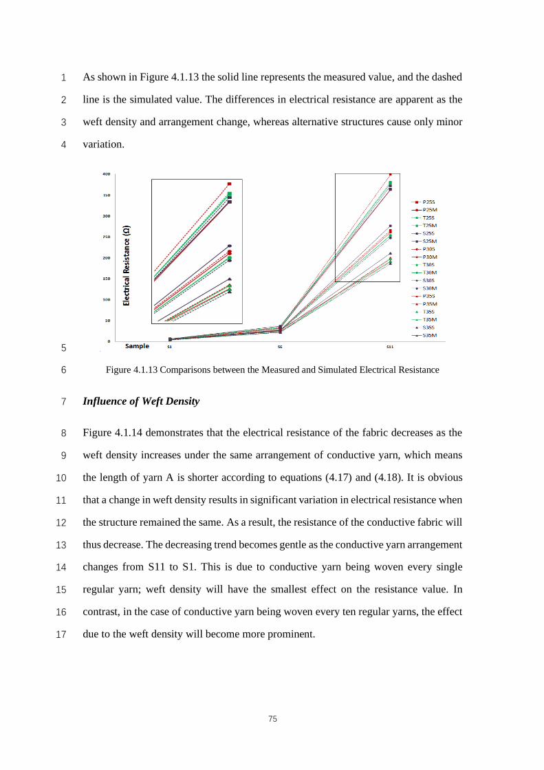
75

As shown in Figure 4.1.13 the solid line represents the measured value, and the dashed 1

line is the simulated value. The differences in electrical resistance are apparent as the 2

weft density and arrangement change, whereas alternative structures cause only minor 3

variation. 4

5

Figure 4.1.13 Comparisons between the Measured and Simulated Electrical Resistance 6

Influence of Weft Density 7

Figure 4.1.14 demonstrates that the electrical resistance of the fabric decreases as the 8

weft density increases under the same arrangement of conductive yarn, which means 9

the length of yarn A is shorter according to equations (4.17) and (4.18). It is obvious 10

that a change in weft density results in significant variation in electrical resistance when 11

the structure remained the same. As a result, the resistance of the conductive fabric will 12

thus decrease. The decreasing trend becomes gentle as the conductive yarn arrangement 13

changes from S11 to S1. This is due to conductive yarn being woven every single 14

regular yarn; weft density will have the smallest effect on the resistance value. In 15

contrast, in the case of conductive yarn being woven every ten regular yarns, the effect 16

due to the weft density will become more prominent. 17

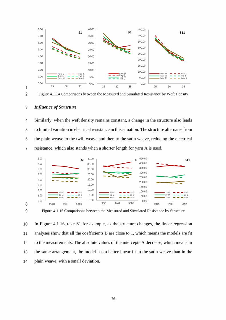
76

1

Figure 4.1.14 Comparisons between the Measured and Simulated Resistance by Weft Density 2

Influence of Structure 3

Similarly, when the weft density remains constant, a change in the structure also leads 4

to limited variation in electrical resistance in this situation. The structure alternates from 5

the plain weave to the twill weave and then to the satin weave, reducing the electrical 6

resistance, which also stands when a shorter length for yarn A is used. 7

8

Figure 4.1.15 Comparisons between the Measured and Simulated Resistance by Structure 9

In Figure 4.1.16, take S1 for example, as the structure changes, the linear regression 10

analyses show that all the coefficients B are close to 1, which means the models are fit 11

to the measurements. The absolute values of the intercepts A decrease, which means in 12

the same arrangement, the model has a better linear fit in the satin weave than in the 13

plain weave, with a small deviation. 14

0.00

1.00

2.00

3.00

4.00

5.00

6.00

7.00

8.00

25 30 35

S1

Plain-M Plain-STwill-M Twill-SSatin-M Satin-S

0.00

5.00

10.00

15.00

20.00

25.00

30.00

35.00

40.00

25 30 35

S6

Plain-MPlain-STwill-MTwill-S

0.00

50.00

100.00

150.00

200.00

250.00

300.00

350.00

400.00

450.00

25 30 35

S11

Plain-M Plain-STwill-M Twill-SSatin-M Satin-S

0.00

1.00

2.00

3.00

4.00

5.00

6.00

7.00

8.00

Plain Twill Satin

S1

25-M 25-S30-M 30-S35-M 35-S

0.00

5.00

10.00

15.00

20.00

25.00

30.00

35.00

40.00

Plain Twill Satin

S6

25-M 25-S30-M 30-S35-M 35-S

0.00

50.00

100.00

150.00

200.00

250.00

300.00

350.00

400.00

450.00

Plain Twill Satin

S11

25-M 25-S30-M 30-S35-M 35-S

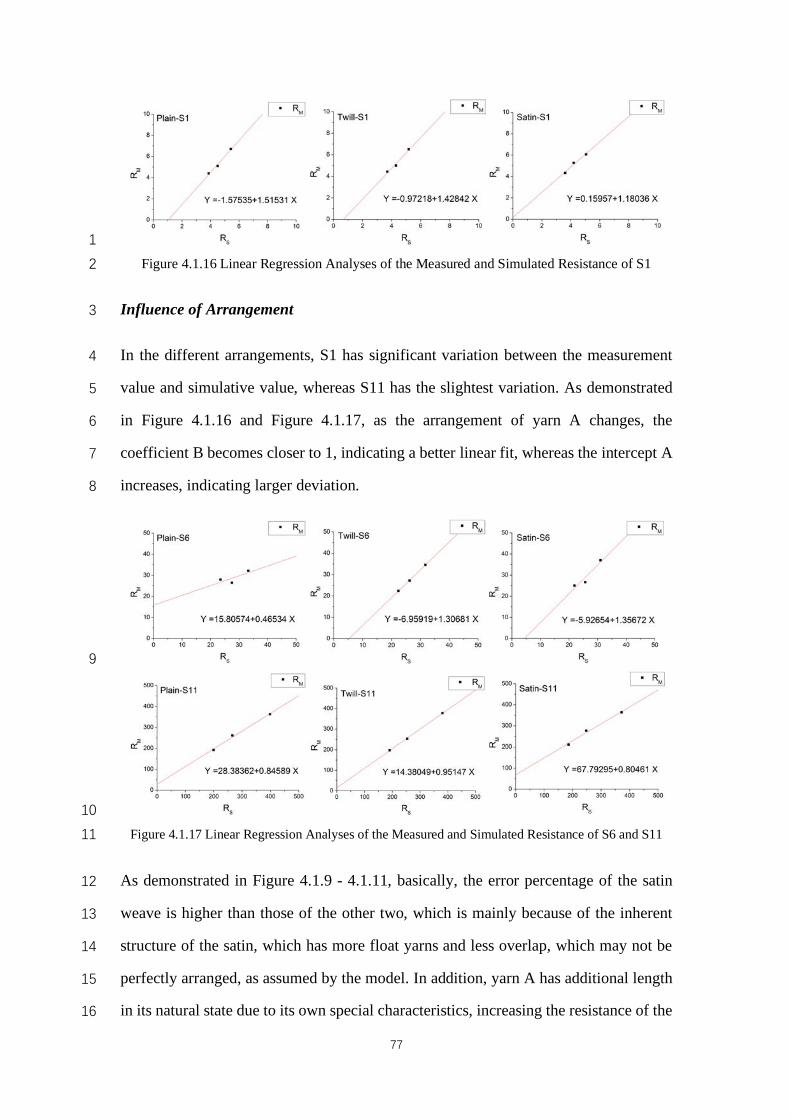
77

1

Figure 4.1.16 Linear Regression Analyses of the Measured and Simulated Resistance of S1 2

Influence of Arrangement 3

In the different arrangements, S1 has significant variation between the measurement 4

value and simulative value, whereas S11 has the slightest variation. As demonstrated 5

in Figure 4.1.16 and Figure 4.1.17, as the arrangement of yarn A changes, the 6

coefficient B becomes closer to 1, indicating a better linear fit, whereas the intercept A 7

increases, indicating larger deviation. 8

9

10

Figure 4.1.17 Linear Regression Analyses of the Measured and Simulated Resistance of S6 and S11 11

As demonstrated in Figure 4.1.9 - 4.1.11, basically, the error percentage of the satin 12

weave is higher than those of the other two, which is mainly because of the inherent 13

structure of the satin, which has more float yarns and less overlap, which may not be 14

perfectly arranged, as assumed by the model. In addition, yarn A has additional length 15

in its natural state due to its own special characteristics, increasing the resistance of the 16

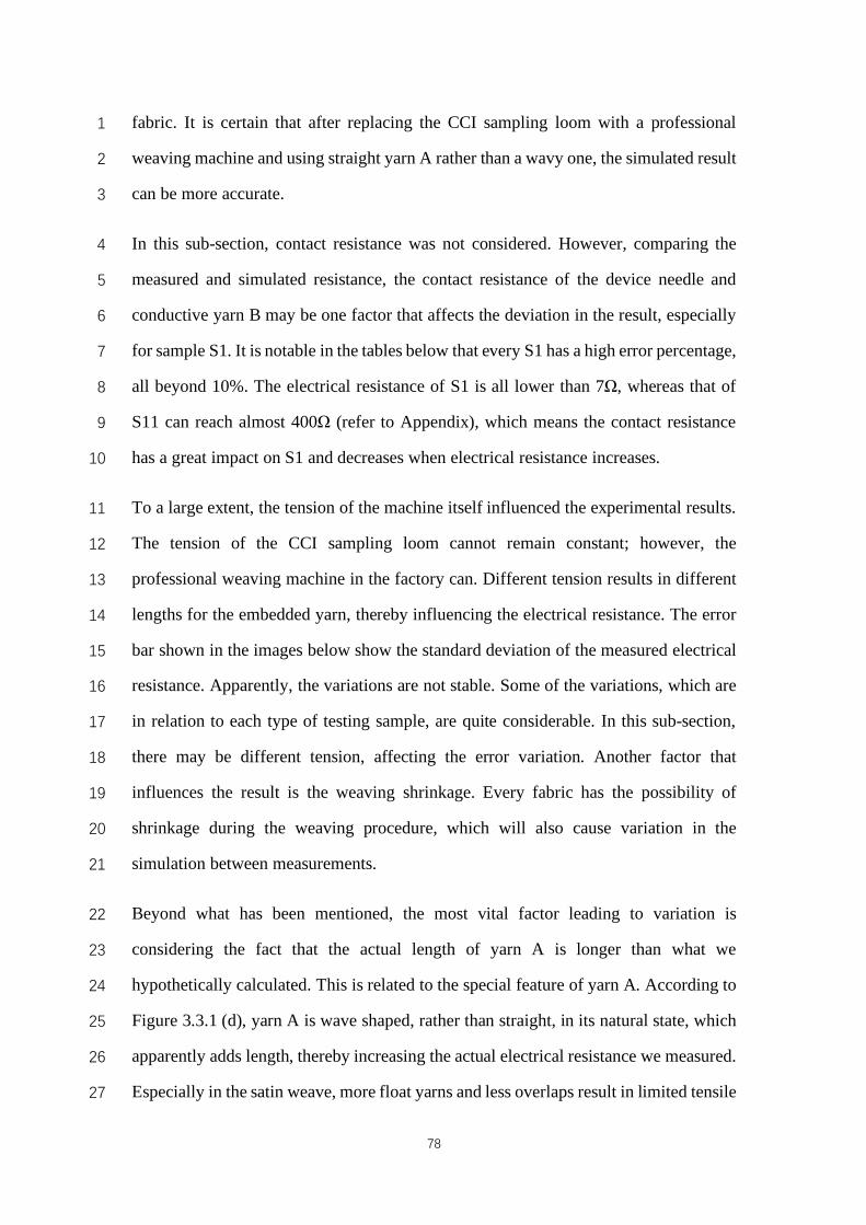
78

fabric. It is certain that after replacing the CCI sampling loom with a professional 1

weaving machine and using straight yarn A rather than a wavy one, the simulated result 2

can be more accurate. 3

In this sub-section, contact resistance was not considered. However, comparing the 4

measured and simulated resistance, the contact resistance of the device needle and 5

conductive yarn B may be one factor that affects the deviation in the result, especially 6

for sample S1. It is notable in the tables below that every S1 has a high error percentage, 7

all beyond 10%. The electrical resistance of S1 is all lower than 7Ω, whereas that of 8

S11 can reach almost 400Ω (refer to Appendix), which means the contact resistance 9

has a great impact on S1 and decreases when electrical resistance increases. 10

To a large extent, the tension of the machine itself influenced the experimental results. 11

The tension of the CCI sampling loom cannot remain constant; however, the 12

professional weaving machine in the factory can. Different tension results in different 13

lengths for the embedded yarn, thereby influencing the electrical resistance. The error 14

bar shown in the images below show the standard deviation of the measured electrical 15

resistance. Apparently, the variations are not stable. Some of the variations, which are 16

in relation to each type of testing sample, are quite considerable. In this sub-section, 17

there may be different tension, affecting the error variation. Another factor that 18

influences the result is the weaving shrinkage. Every fabric has the possibility of 19

shrinkage during the weaving procedure, which will also cause variation in the 20

simulation between measurements. 21

Beyond what has been mentioned, the most vital factor leading to variation is 22

considering the fact that the actual length of yarn A is longer than what we 23

hypothetically calculated. This is related to the special feature of yarn A. According to 24

Figure 3.3.1 (d), yarn A is wave shaped, rather than straight, in its natural state, which 25

apparently adds length, thereby increasing the actual electrical resistance we measured. 26

Especially in the satin weave, more float yarns and less overlaps result in limited tensile 27

79

force for yarn A, thereby causing higher electrical resistance than we had simulated, in 1

which the model had regarded the yarn as straight. 2

4.1.7 Conclusion 3

A theoretical model was proposed to simulate electrical resistance for conductive 4

woven fabrics. An analytic equation was derived based on an equivalent length of 5

conductive yarn woven in three basic woven structures with three different weft 6

densities. Once the radius of the warp yarn and the resistance of one unit of conductive 7

yarn are known, the electrical resistance of woven conductive fabric can be readily 8

computed. The results show that the simulative equation can predict the resistance of 9

woven fabrics, which allows designers to estimate the fabric parameters to meet the 10

required resistance. The differences in electrical resistance become apparent as the weft 11

yarn density and arrangement change, whereas alternative structures cause only minor 12

variation. Moreover, electrical resistance can be controlled by different structures and 13

arrangements under the same size fabric. Because the contact resistance, so far, has not 14

been considered in our research, further research will be conducted for to more 15

accurately model and compute resistance and therefore achieve an improved version of 16

the proposed resistive model. 17

4.2 Fast Estimated Model of Electrical Resistance Applied in Designing 18

Conductive Woven Fabrics 19


This sub-section proposes a fast estimated model of electrical resistance used in 21

designing conductive thermal woven fabrics (CTWF) with three basic weaving 22

structures – plain weave, twill weave, and satin weave. Weft density of weft silver-23

coated yarn was changed according to different arrangement. Combining with the result 24

of previous simulation model, the new model will be experience model using only cover 25

factor as variable. Experiments were designed and conducted to verify the availability 26

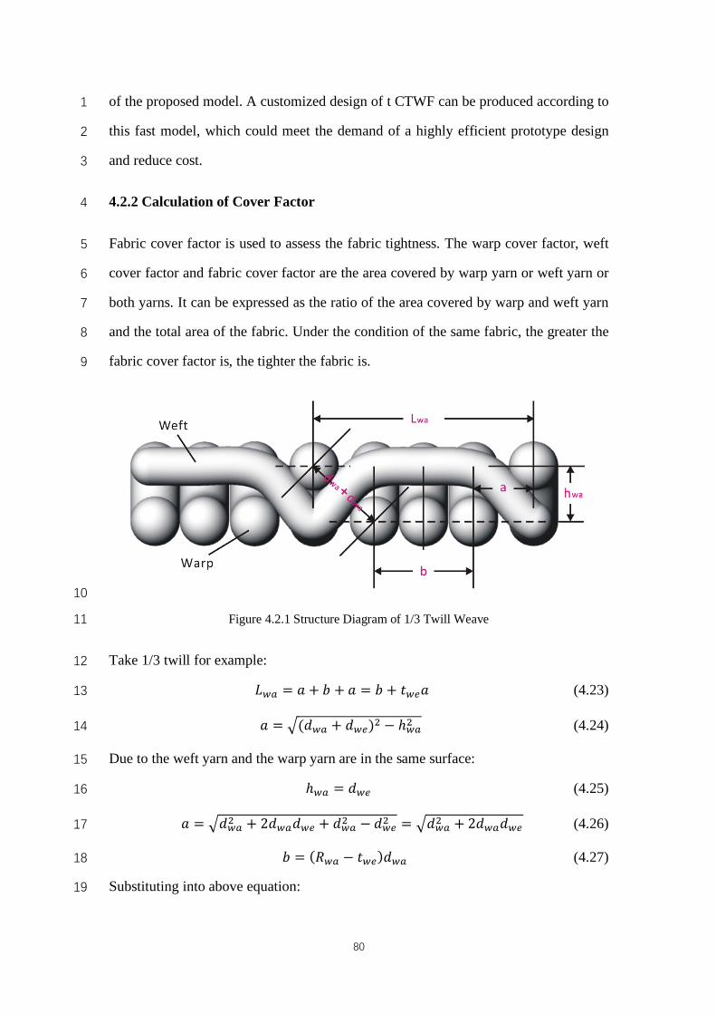
80

of the proposed model. A customized design of t CTWF can be produced according to 1

this fast model, which could meet the demand of a highly efficient prototype design 2

and reduce cost. 3

4.2.2 Calculation of Cover Factor 4

Fabric cover factor is used to assess the fabric tightness. The warp cover factor, weft 5

cover factor and fabric cover factor are the area covered by warp yarn or weft yarn or 6

both yarns. It can be expressed as the ratio of the area covered by warp and weft yarn 7

and the total area of the fabric. Under the condition of the same fabric, the greater the 8

fabric cover factor is, the tighter the fabric is. 9

10

Figure 4.2.1 Structure Diagram of 1/3 Twill Weave 11

Take 1/3 twill for example: 12

𝐿{| = 𝑎 + 𝑏 + 𝑎 = 𝑏 + 𝑡{�𝑎 (4.23) 13

𝑎 = D(𝑑{| + 𝑑{�)H − ℎ{|H (4.24) 14

Due to the weft yarn and the warp yarn are in the same surface: 15

ℎ{| = 𝑑{� (4.25) 16

𝑎 = D𝑑{|H + 2𝑑{|𝑑{� + 𝑑{|H − 𝑑{�H = D𝑑{|H + 2𝑑{|𝑑{� (4.26) 17

𝑏 = (𝑅{| − 𝑡{�)𝑑{| (4.27) 18

Substituting into above equation: 19

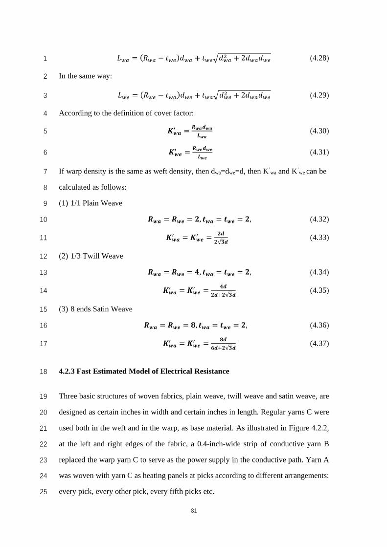
81

𝐿{| = (𝑅{| − 𝑡{�)𝑑{| + 𝑡{�D𝑑{|H + 2𝑑{|𝑑{� (4.28) 1

In the same way: 2

𝐿{� = (𝑅{� − 𝑡{|)𝑑{� + 𝑡{|D𝑑{�H + 2𝑑{|𝑑{� (4.29) 3

According to the definition of cover factor: 4

𝑲𝒘𝒂� = 𝑹𝒘𝒂𝒅𝒘𝒂

𝑳𝒘𝒂 (4.30) 5

𝑲𝒘𝒆� = 𝑹𝒘𝒆𝒅𝒘𝒆

𝑳𝒘𝒆 (4.31) 6

If warp density is the same as weft density, then dwa=dwe=d, then K’wa and K’we can be 7

calculated as follows: 8

(1) 1/1 Plain Weave 9

𝑹𝒘𝒂 = 𝑹𝒘𝒆 = 𝟐, 𝒕𝒘𝒂 = 𝒕𝒘𝒆 = 𝟐, (4.32) 10

𝑲𝒘𝒂� = 𝑲𝒘𝒆

� = 𝟐𝒅𝟐√𝟑𝒅

(4.33) 11

(2) 1/3 Twill Weave 12

𝑹𝒘𝒂 = 𝑹𝒘𝒆 = 𝟒, 𝒕𝒘𝒂 = 𝒕𝒘𝒆 = 𝟐, (4.34) 13


� = 𝟒𝒅𝟐𝒅^𝟐√𝟑𝒅

(4.35) 14

(3) 8 ends Satin Weave 15

𝑹𝒘𝒂 = 𝑹𝒘𝒆 = 𝟖, 𝒕𝒘𝒂 = 𝒕𝒘𝒆 = 𝟐, (4.36) 16


� = 𝟖𝒅𝟔𝒅^𝟐√𝟑𝒅

(4.37) 17

4.2.3 Fast Estimated Model of Electrical Resistance 18

Three basic structures of woven fabrics, plain weave, twill weave and satin weave, are 19

designed as certain inches in width and certain inches in length. Regular yarns C were 20

used both in the weft and in the warp, as base material. As illustrated in Figure 4.2.2, 21

at the left and right edges of the fabric, a 0.4-inch-wide strip of conductive yarn B 22

replaced the warp yarn C to serve as the power supply in the conductive path. Yarn A 23

was woven with yarn C as heating panels at picks according to different arrangements: 24

every pick, every other pick, every fifth picks etc. 25

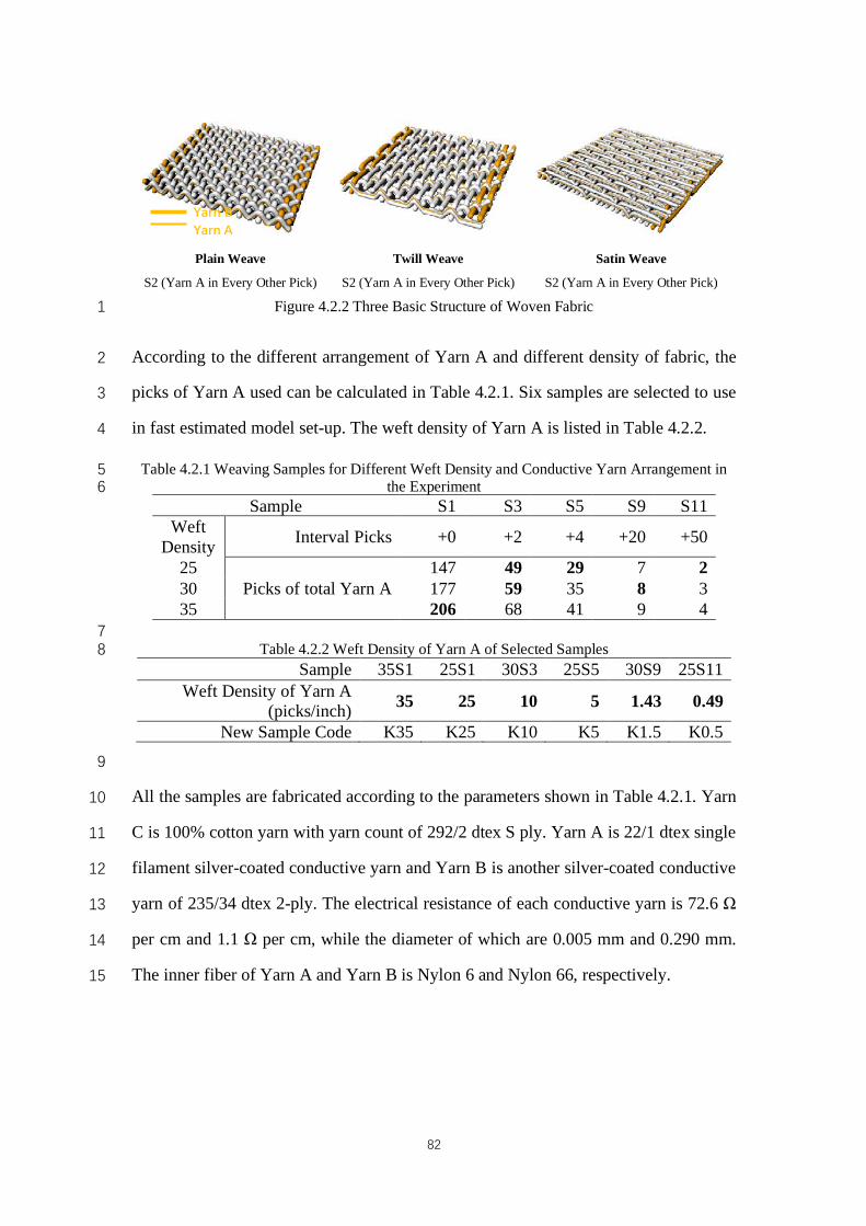
82

Plain Weave

S2 (Yarn A in Every Other Pick)

Twill Weave


Satin Weave


Figure 4.2.2 Three Basic Structure of Woven Fabric 1

According to the different arrangement of Yarn A and different density of fabric, the 2

picks of Yarn A used can be calculated in Table 4.2.1. Six samples are selected to use 3

in fast estimated model set-up. The weft density of Yarn A is listed in Table 4.2.2. 4

Table 4.2.1 Weaving Samples for Different Weft Density and Conductive Yarn Arrangement in 5 the Experiment 6

Sample S1 S3 S5 S9 S11 Weft

Density Interval Picks +0 +2 +4 +20 +50

25 Picks of total Yarn A

147 49 29 7 2 30 177 59 35 8 3 35 206 68 41 9 4

7 Table 4.2.2 Weft Density of Yarn A of Selected Samples 8

Sample 35S1 25S1 30S3 25S5 30S9 25S11 Weft Density of Yarn A

(picks/inch) 35 25 10 5 1.43 0.49

New Sample Code K35 K25 K10 K5 K1.5 K0.5 9

All the samples are fabricated according to the parameters shown in Table 4.2.1. Yarn 10

C is 100% cotton yarn with yarn count of 292/2 dtex S ply. Yarn A is 22/1 dtex single 11

filament silver-coated conductive yarn and Yarn B is another silver-coated conductive 12

yarn of 235/34 dtex 2-ply. The electrical resistance of each conductive yarn is 72.6 Ω 13

per cm and 1.1 Ω per cm, while the diameter of which are 0.005 mm and 0.290 mm. 14

The inner fiber of Yarn A and Yarn B is Nylon 6 and Nylon 66, respectively. 15

Yarn B Yarn A

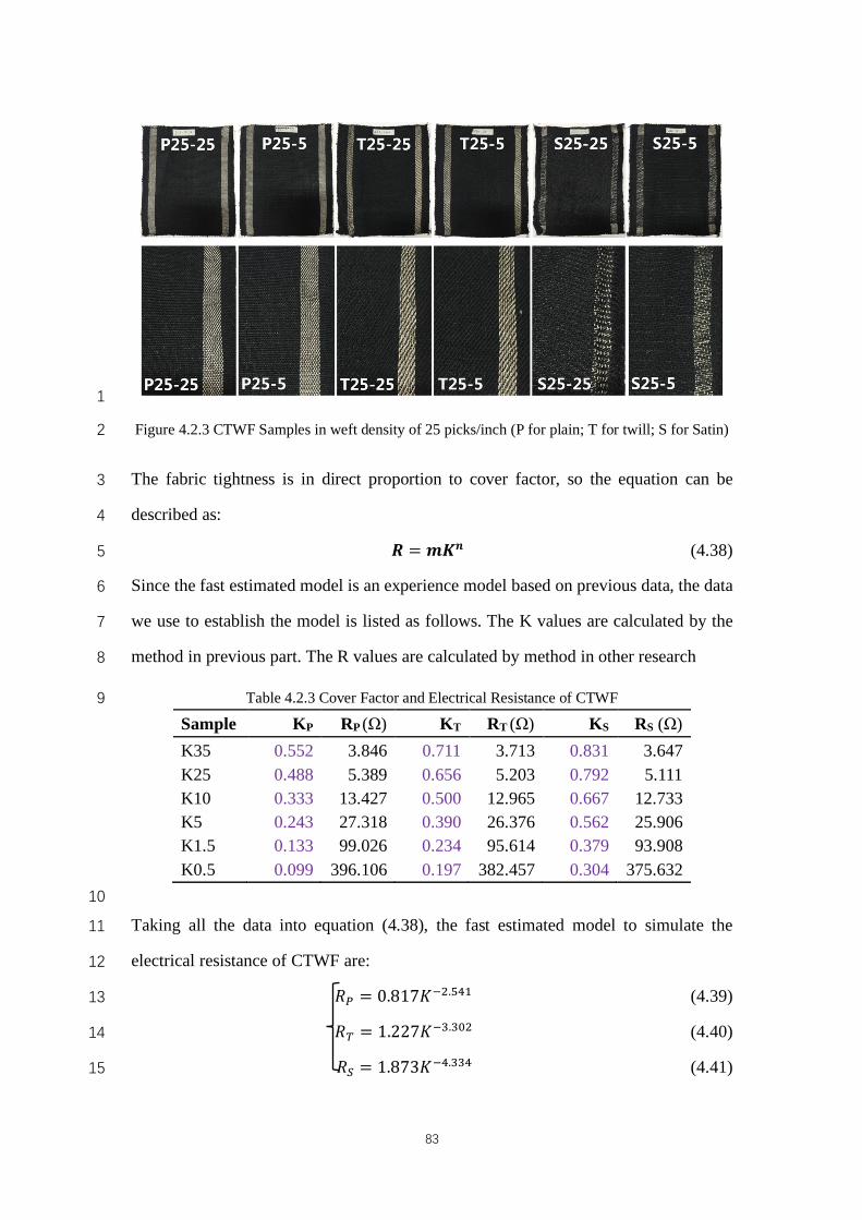
83

1

Figure 4.2.3 CTWF Samples in weft density of 25 picks/inch (P for plain; T for twill; S for Satin) 2

The fabric tightness is in direct proportion to cover factor, so the equation can be 3

described as: 4

𝑹 = 𝒎𝑲𝒏 (4.38) 5

Since the fast estimated model is an experience model based on previous data, the data 6

we use to establish the model is listed as follows. The K values are calculated by the 7

method in previous part. The R values are calculated by method in other research 8

Table 4.2.3 Cover Factor and Electrical Resistance of CTWF 9

Sample KP RP (Ω) KT RT (Ω) KS RS (Ω) K35 0.552 3.846 0.711 3.713 0.831 3.647 K25 0.488 5.389 0.656 5.203 0.792 5.111 K10 0.333 13.427 0.500 12.965 0.667 12.733 K5 0.243 27.318 0.390 26.376 0.562 25.906 K1.5 0.133 99.026 0.234 95.614 0.379 93.908 K0.5 0.099 396.106 0.197 382.457 0.304 375.632

10

Taking all the data into equation (4.38), the fast estimated model to simulate the 11

electrical resistance of CTWF are: 12

𝑅� = 0.817𝐾�H.�� (4.39) 13

𝑅� = 1.227𝐾��.�6H (4.40) 14

𝑅� = 1.873𝐾��.�� (4.41) 15

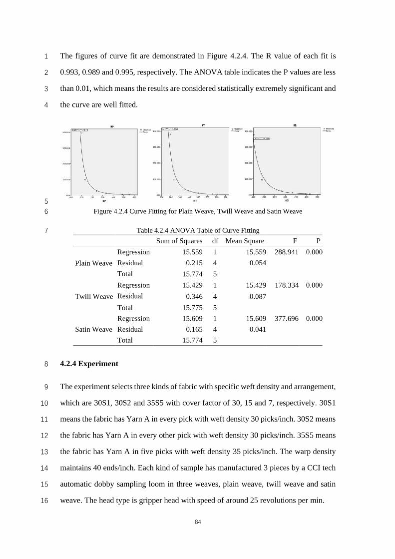
84

The figures of curve fit are demonstrated in Figure 4.2.4. The R value of each fit is 1

0.993, 0.989 and 0.995, respectively. The ANOVA table indicates the P values are less 2

than 0.01, which means the results are considered statistically extremely significant and 3

the curve are well fitted. 4

5 Figure 4.2.4 Curve Fitting for Plain Weave, Twill Weave and Satin Weave 6

Table 4.2.4 ANOVA Table of Curve Fitting 7

4.2.4 Experiment 8

The experiment selects three kinds of fabric with specific weft density and arrangement, 9

which are 30S1, 30S2 and 35S5 with cover factor of 30, 15 and 7, respectively. 30S1 10

means the fabric has Yarn A in every pick with weft density 30 picks/inch. 30S2 means 11

the fabric has Yarn A in every other pick with weft density 30 picks/inch. 35S5 means 12

the fabric has Yarn A in five picks with weft density 35 picks/inch. The warp density 13

maintains 40 ends/inch. Each kind of sample has manufactured 3 pieces by a CCI tech 14

automatic dobby sampling loom in three weaves, plain weave, twill weave and satin 15

weave. The head type is gripper head with speed of around 25 revolutions per min. 16

Sum of Squares df Mean Square F P

Plain Weave Regression 15.559 1 15.559 288.941 0.000 Residual 0.215 4 0.054 Total 15.774 5

Twill Weave Regression 15.429 1 15.429 178.334 0.000 Residual 0.346 4 0.087 Total 15.775 5

Satin Weave Regression 15.609 1 15.609 377.696 0.000 Residual 0.165 4 0.041 Total 15.774 5

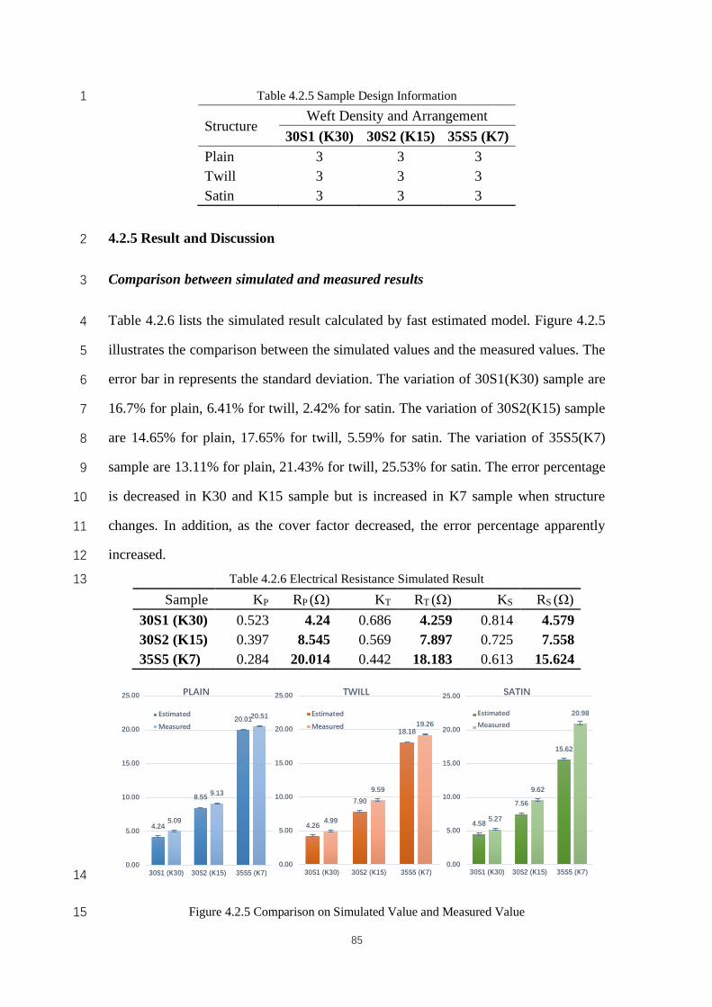
85


Structure Weft Density and Arrangement

30S1 (K30) 30S2 (K15) 35S5 (K7) Plain 3 3 3 Twill 3 3 3 Satin 3 3 3

4.2.5 Result and Discussion 2

Comparison between simulated and measured results 3

Table 4.2.6 lists the simulated result calculated by fast estimated model. Figure 4.2.5 4

illustrates the comparison between the simulated values and the measured values. The 5

error bar in represents the standard deviation. The variation of 30S1(K30) sample are 6

16.7% for plain, 6.41% for twill, 2.42% for satin. The variation of 30S2(K15) sample 7

are 14.65% for plain, 17.65% for twill, 5.59% for satin. The variation of 35S5(K7) 8

sample are 13.11% for plain, 21.43% for twill, 25.53% for satin. The error percentage 9

is decreased in K30 and K15 sample but is increased in K7 sample when structure 10

changes. In addition, as the cover factor decreased, the error percentage apparently 11

increased. 12

Table 4.2.6 Electrical Resistance Simulated Result 13

Sample KP RP (Ω) KT RT (Ω) KS RS (Ω) 30S1 (K30) 0.523 4.24 0.686 4.259 0.814 4.579 30S2 (K15) 0.397 8.545 0.569 7.897 0.725 7.558 35S5 (K7) 0.284 20.014 0.442 18.183 0.613 15.624

14

Figure 4.2.5 Comparison on Simulated Value and Measured Value 15

4.24

8.55

20.01

5.09

9.13

20.51

0.00

5.00

10.00

15.00

20.00

25.00

30S1 (K30) 30S2 (K15) 35S5 (K7)

PLAIN

Estimated

Measured

4.26

7.90

18.18

4.99

9.59

19.26

0.00

5.00

10.00

15.00

20.00

25.00

30S1 (K30) 30S2 (K15) 35S5 (K7)

TWILL

Estimated

Measured

4.58

7.56

15.62

5.27

9.62

20.98

0.00

5.00

10.00

15.00

20.00

25.00

30S1 (K30) 30S2 (K15) 35S5 (K7)

SATIN

Estimated

Measured

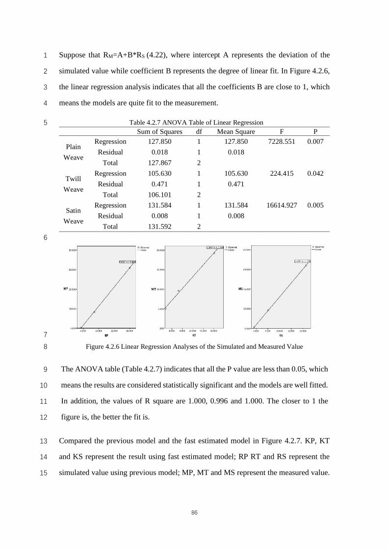
86

Suppose that RM=A+B*RS (4.22), where intercept A represents the deviation of the 1

simulated value while coefficient B represents the degree of linear fit. In Figure 4.2.6, 2

the linear regression analysis indicates that all the coefficients B are close to 1, which 3

means the models are quite fit to the measurement. 4

Table 4.2.7 ANOVA Table of Linear Regression 5

6

7

Figure 4.2.6 Linear Regression Analyses of the Simulated and Measured Value 8

The ANOVA table (Table 4.2.7) indicates that all the P value are less than 0.05, which 9

means the results are considered statistically significant and the models are well fitted. 10

In addition, the values of R square are 1.000, 0.996 and 1.000. The closer to 1 the 11

figure is, the better the fit is. 12

Compared the previous model and the fast estimated model in Figure 4.2.7. KP, KT 13

and KS represent the result using fast estimated model; RP RT and RS represent the 14

simulated value using previous model; MP, MT and MS represent the measured value. 15

Sum of Squares df Mean Square F P

Plain Weave

Regression 127.850 1 127.850 7228.551 0.007 Residual 0.018 1 0.018

Total 127.867 2

Twill Weave


Total 106.101 2

Satin Weave


Total 131.592 2

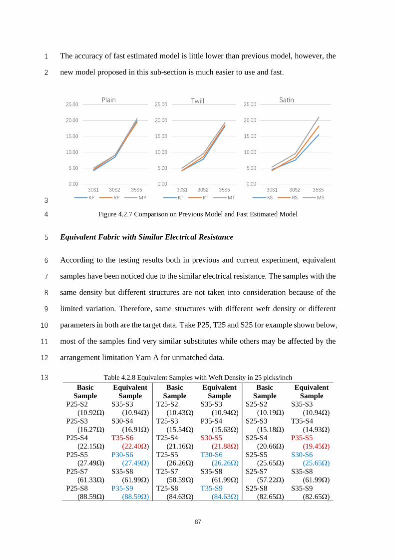
87

The accuracy of fast estimated model is little lower than previous model, however, the 1

new model proposed in this sub-section is much easier to use and fast. 2

3

Figure 4.2.7 Comparison on Previous Model and Fast Estimated Model 4

Equivalent Fabric with Similar Electrical Resistance 5

According to the testing results both in previous and current experiment, equivalent 6

samples have been noticed due to the similar electrical resistance. The samples with the 7

same density but different structures are not taken into consideration because of the 8

limited variation. Therefore, same structures with different weft density or different 9

parameters in both are the target data. Take P25, T25 and S25 for example shown below, 10

most of the samples find very similar substitutes while others may be affected by the 11

arrangement limitation Yarn A for unmatched data. 12

Table 4.2.8 Equivalent Samples with Weft Density in 25 picks/inch 13 Basic

Sample Equivalent

Sample Basic

Sample Equivalent

Sample Basic

Sample Equivalent

Sample P25-S2

(10.92Ω) S35-S3

(10.94Ω) T25-S2

(10.43Ω) S35-S3

(10.94Ω) S25-S2

(10.19Ω) S35-S3

(10.94Ω) P25-S3

(16.27Ω) S30-S4

(16.91Ω) T25-S3

(15.54Ω) P35-S4

(15.63Ω) S25-S3

(15.18Ω) T35-S4

(14.93Ω) P25-S4

(22.15Ω) T35-S6

(22.40Ω) T25-S4

(21.16Ω) S30-S5

(21.88Ω) S25-S4

(20.66Ω) P35-S5

(19.45Ω) P25-S5

(27.49Ω) P30-S6

(27.49Ω) T25-S5

(26.26Ω) T30-S6

(26.26Ω) S25-S5

(25.65Ω) S30-S6

(25.65Ω) P25-S7

(61.33Ω) S35-S8

(61.99Ω) T25-S7

(58.59Ω) S35-S8

(61.99Ω) S25-S7

(57.22Ω) S35-S8

(61.99Ω) P25-S8

(88.59Ω) P35-S9

(88.59Ω) T25-S8

(84.63Ω) T35-S9

(84.63Ω) S25-S8

(82.65Ω) S35-S9

(82.65Ω)

0.00

5.00

10.00

15.00

20.00

25.00

30S1 30S2 35S5

Plain

KP RP MP

0.00

5.00

10.00

15.00

20.00

25.00

30S1 30S2 35S5

Twill

KT RT MT

0.00

5.00

10.00

15.00

20.00

25.00

30S1 30S2 35S5

Satin

KS RS MS

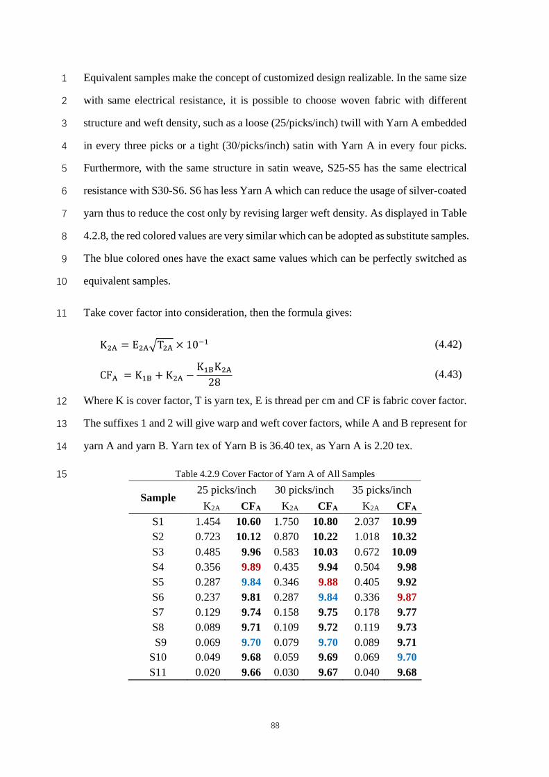
88

Equivalent samples make the concept of customized design realizable. In the same size 1

with same electrical resistance, it is possible to choose woven fabric with different 2

structure and weft density, such as a loose (25/picks/inch) twill with Yarn A embedded 3

in every three picks or a tight (30/picks/inch) satin with Yarn A in every four picks. 4

Furthermore, with the same structure in satin weave, S25-S5 has the same electrical 5

resistance with S30-S6. S6 has less Yarn A which can reduce the usage of silver-coated 6

yarn thus to reduce the cost only by revising larger weft density. As displayed in Table 7

4.2.8, the red colored values are very similar which can be adopted as substitute samples. 8

The blue colored ones have the exact same values which can be perfectly switched as 9

equivalent samples. 10

Take cover factor into consideration, then the formula gives: 11

Where K is cover factor, T is yarn tex, E is thread per cm and CF is fabric cover factor. 12

The suffixes 1 and 2 will give warp and weft cover factors, while A and B represent for 13

yarn A and yarn B. Yarn tex of Yarn B is 36.40 tex, as Yarn A is 2.20 tex. 14

Table 4.2.9 Cover Factor of Yarn A of All Samples 15

Sample 25 picks/inch 30 picks/inch 35 picks/inch

K2A CFA K2A CFA K2A CFA S1 1.454 10.60 1.750 10.80 2.037 10.99 S2 0.723 10.12 0.870 10.22 1.018 10.32 S3 0.485 9.96 0.583 10.03 0.672 10.09 S4 0.356 9.89 0.435 9.94 0.504 9.98 S5 0.287 9.84 0.346 9.88 0.405 9.92 S6 0.237 9.81 0.287 9.84 0.336 9.87 S7 0.129 9.74 0.158 9.75 0.178 9.77 S8 0.089 9.71 0.109 9.72 0.119 9.73

S9 0.069 9.70 0.079 9.70 0.089 9.71 S10 0.049 9.68 0.059 9.69 0.069 9.70 S11 0.020 9.66 0.030 9.67 0.040 9.68

KHU = EHUDTHU × 10�� (4.42)

CFU = K�¡ + KHU −K�¡KHU28 (4.43)

89

After calculating all the cover factors of Yarn A, some interesting phenomena occurred. 1

As highlighted in red color, Table 4.2.9 shows the cover factor of 25 picks/inch is the 2

same as those with 30 picks/inch. Referred to Table 4.2.8, all the samples S5 with weft 3

density of 25 picks/inch have similar electrical resistance of those in S6 of 30 picks/inch, 4

despite of structures. In addition, as colored in blue in Table 4.2.9, the values of cover 5

factor are exact the same which means the electrical resistance of those samples can be 6

switch to equivalent samples with some adjustment in structure. In sum, samples with 7

lower density in certain numbers of Yarn A can be replaced by samples with higher 8

density in less numbers of Yarn A combining with structure adjustment, which makes 9

it controllable to the electrical resistance of the thermal woven fabric within the same 10

size can be obtained, thus to reduce the usage of silver-coated yarn thus to reduce the 11

cost. 12

4.2.6 Conclusion 13

This sub-section proposed another fast estimated method to obtain electrical resistance 14

of conductive thermal woven fabrics (CTWF) based on the previous model. Cover 15

factor was a major factor in this model. The results revealed that the proposed fast 16

estimated model was well fitted and could well simulate the electrical resistance of 17

CTWF within certain error variation. Compared to previous model, this new model has 18

slightly lower accuracy but within acceptable deviation. Based on this model, 19

conductive woven fabric and equivalent fabric as substitute for different applications at 20

optimum conditions. Designers can easily estimate the electrical resistance, thus 21

customized design of CTWF can be produced effectively without extra waste of testing 22

weaving. 23

24

25

26

90

Chapter 5 Design-Oriented Temperature Prediction Model for 1

Thermal Conductive Woven Fabrics 2

5.1 Introduction 3

Thermal functionality is a critical topic in wearable electronic textiles which is 4

significant to health, safety and resistance to extreme environments. The intelligent 5

textiles with thermal function are employed in various applications, such as medical 6

products, military products, sports products, home products and et cetera [1-2]. The 7

huge potential demand leads to rapid development of this area. Therefore, the related 8

thermal garment research is becoming a growing sector in the textile lab and industry. 9

In the past decades, numerous researchers have focused on the development of 10

electronic heating garments in particular conditions or in daily applications by various 11

design, methods and functions [3-12]. Currently, most studies and products focus on 12

thermal knitwear research to retain warmth during outdoor sport activities and work 13

protection. Generally, the heating part of these thermal garments are made of 14

conductive polyamide fiber by knitting technology or manufactured by attaching non-15

woven carbon sheet. Some products even incorporate conductive heat fabric with 16

normal fabric sewn together by the patchwork method to format a heating area and 17

electronic routing. Few studies can provide a systemic method to develop the thermal 18

function garment incorporating a heating area and resistive network together in one 19

formation. Li et al. have developed systematic methods in designing and fabricating 20

knitted thermal fabric and garment [14,16,17,19,64-68]. However, the temperature 21

prediction research is still lacking. Additionally, limited research can be found on 22

woven thermal fabrics, not to mention the lack of theoretical model in predicting the 23

heating temperature. Previous studies have managed to establish two kinds of 24

simulation models of electrical resistance for thermal woven fabric [69-70]. Base on 25

the outcome so far, this study focuses on a design-oriented temperature prediction 26

model establishment. Different influence factors are taking in to consideration to 27

91

determine the final model. Since the thermal woven fabric is the core area of the novel 1

thermal functional garment. It is critical to obtain the target temperature in advance to 2

conserve energy and cost. 3

5.2 Thermal conductive woven fabric 4

5.2.1 Synopsis of thermal conductive woven fabric 5

Thermal conductive woven fabric (TCWF) is designed as a one-step formation heating 6

textile that provides warmth. The TCWF can design and fabricate in many different 7

styles as needed, such as different structure, density, size, pattern and et cetera. 8

Different design combination results in different oriented functional products, which 9

provide customers and producers plenty of options. In current market, most thermal 10

textiles are either knitted with conductive yarn or use non-woven carbon sheet as 11

heating part. Unlike the existing product, the product adopted TCWF technique has 12

better performance in appearance design, manufacture, financial cost and user 13

experience. The concept of TCWF is demonstrated in Figure 5.2.1-a, the weft yarn in 14

blue will provide heat in the heating panel while the warp yarn in blue will serve as 15

conductive path. The size of heating panel and conductive path are designable. 16

Normally, three basic woven structure, plain weave, twill weave and satin weave, will 17

be used in designing as shown in Figure 5.2.1-b, 5.2.1-c and 5.2.1-d. Since for one 18

particular warp beam of the weaving machine, the warp density is always set remain, 19

only weft density can alternate as required. Besides, weft conductive yarn (WECY) has 20

much higher electrical resistance can also be arranged as different set, such as weaving 21

in every weft pick, every five weft picks, every ten weft picks and et cetera. Warp 22

conductive yarn (WACY) is placed in warp direction using as conductive path which 23

has the lower electrical resistance. The area between two conductive paths is the heating 24

area that provide thermal treatment. The size, structure and pattern of this area are all 25

manageable. 26

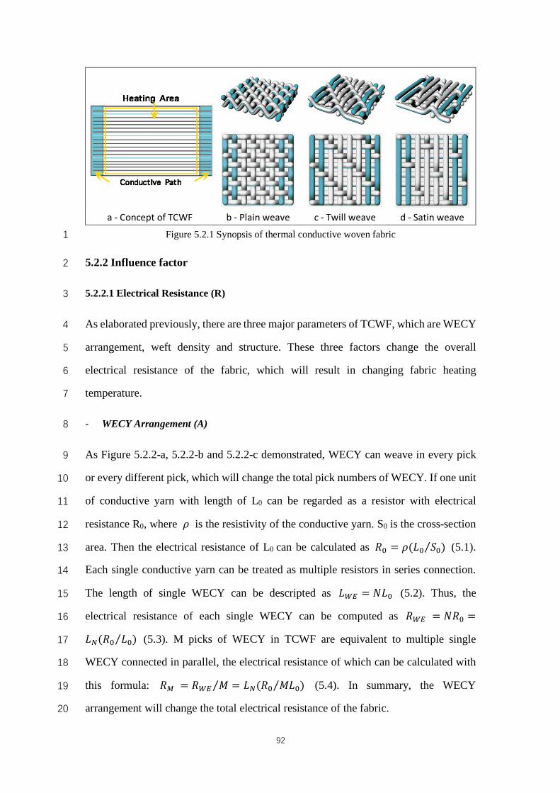
92

a - Concept of TCWF b - Plain weave c - Twill weave d - Satin weave

Figure 5.2.1 Synopsis of thermal conductive woven fabric 1

5.2.2 Influence factor 2

5.2.2.1 Electrical Resistance (R) 3

As elaborated previously, there are three major parameters of TCWF, which are WECY 4

arrangement, weft density and structure. These three factors change the overall 5

electrical resistance of the fabric, which will result in changing fabric heating 6

temperature. 7

- WECY Arrangement (A) 8

As Figure 5.2.2-a, 5.2.2-b and 5.2.2-c demonstrated, WECY can weave in every pick 9

or every different pick, which will change the total pick numbers of WECY. If one unit 10

of conductive yarn with length of L0 can be regarded as a resistor with electrical 11

resistance R0, where 𝜌 is the resistivity of the conductive yarn. S0 is the cross-section 12

area. Then the electrical resistance of L0 can be calculated as 𝑅6 = 𝜌(𝐿6 𝑆6)⁄ (5.1). 13

Each single conductive yarn can be treated as multiple resistors in series connection. 14

The length of single WECY can be descripted as 𝐿¥¦ = 𝑁𝐿6 (5.2). Thus, the 15

electrical resistance of each single WECY can be computed as 𝑅¥¦ = 𝑁𝑅6 =16

𝐿¨(𝑅6 𝐿6)⁄ (5.3). M picks of WECY in TCWF are equivalent to multiple single 17

WECY connected in parallel, the electrical resistance of which can be calculated with 18

this formula: 𝑅© = 𝑅¥¦ 𝑀⁄ = 𝐿¨(𝑅6 𝑀𝐿6)⁄ (5.4). In summary, the WECY 19

arrangement will change the total electrical resistance of the fabric. 20

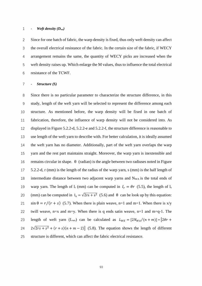
93

- Weft density (Dwe) 1

Since for one batch of fabric, the warp density is fixed, thus only weft density can affect 2

the overall electrical resistance of the fabric. In the certain size of the fabric, if WECY 3

arrangement remains the same, the quantity of WECY picks are increased when the 4

weft density raises up. Which enlarge the M values, thus to influence the total electrical 5

resistance of the TCWF. 6

- Structure (S) 7

Since there is no particular parameter to characterize the structure difference, in this 8

study, length of the weft yarn will be selected to represent the difference among each 9

structure. As mentioned before, the warp density will be fixed in one batch of 10

fabrication, therefore, the influence of warp density will not be considered into. As 11

displayed in Figure 5.2.2-d, 5.2.2-e and 5.2.2-f, the structure difference is reasonable to 12

use length of the weft yarn to describe with. For better calculation, it is ideally assumed 13

the weft yarn has no diameter. Additionally, part of the weft yarn overlaps the warp 14

yarn and the rest part maintains straight. Moreover, the warp yarn is inextensible and 15

remains circular in shape. θ (radian) is the angle between two radiuses noted in Figure 16

5.2.2-d, r (mm) is the length of the radius of the warp yarn, s (mm) is the half length of 17

intermediate distance between two adjacent warp yarns and NWA is the total ends of 18

warp yarn. The length of lr (mm) can be computed in 𝐼¬ = 𝜃𝑟 (5.5), the length of ls 19

(mm) can be computed in IC = √2rs + sH (5.6) and θ can be look up by this equation: 20

sin θ = 𝑟 (𝑟 + 𝑠)⁄ (5.7). When there is plain weave, n=1 and m=1. When there is x/y 21

twill weave, n=x and m=y. When there is q ends satin weave, n=1 and m=q-1. The 22

length of weft yarn (Lwe) can be calculated as 𝐿¥¦ = [2𝑁¥° (𝑛 +𝑚)⁄ ] ∗ `2𝜃𝑟 +23

2√2𝑟𝑠 + 𝑠H + (𝑟 + 𝑠)(𝑛 + 𝑚 − 2)b (5.8). The equation shows the length of different 24

structure is different, which can affect the fabric electrical resistance. 25

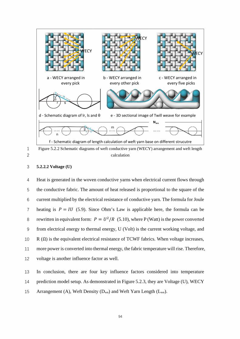
94

a - WECY arranged in

every pick b - WECY arranged in

every other pick c - WECY arranged in

every five picks

d - Schematic diagram of lr, ls and θ e - 3D sectional image of Twill weave for example

f - Schematic diagram of length calculation of weft yarn base on different strucutre

Figure 5.2.2 Schematic diagrams of weft conductive yarn (WECY) arrangement and weft length 1 calculation 2

5.2.2.2 Voltage (U) 3

Heat is generated in the woven conductive yarns when electrical current flows through 4

the conductive fabric. The amount of heat released is proportional to the square of the 5

current multiplied by the electrical resistance of conductive yarn. The formula for Joule 6

heating is 𝑃 = 𝐼𝑈 (5.9). Since Ohm’s Law is applicable here, the formula can be 7

rewritten in equivalent form: 𝑃 = 𝑈H/𝑅 (5.10), where P (Watt) is the power converted 8

from electrical energy to thermal energy, U (Volt) is the current working voltage, and 9

R (Ω) is the equivalent electrical resistance of TCWF fabrics. When voltage increases, 10

more power is converted into thermal energy, the fabric temperature will rise. Therefore, 11

voltage is another influence factor as well. 12

In conclusion, there are four key influence factors considered into temperature 13

prediction model setup. As demonstrated in Figure 5.2.3, they are Voltage (U), WECY 14

Arrangement (A), Weft Density (Dwe) and Weft Yarn Length (Lwe). 15

WECY

WECY

WECY

95

Figure 5.2.3 Relations of influence factors 1

5.3 Temperature prediction model for TCWF 2

5.3.1 Prediction model establishment 3

In the objective world, complex phenomena often have multiple connections, involving 4

quantitative relationships between multiple variables. In many practical problems, a 5

dependent variable often changes with the multiple independent variables. When 6

dealing such problems, multiple regression analysis must be adopted. Multiple 7

regression analysis is a statistical method for studying the relationship between a 8

dependent variable and multiple independent variables. It considers the influence of 9

multiple independent variables on the dependent variable and can more realistically 10

reflect the correlation and interaction between phenomena. This study aims to obtain a 11

reasonable temperature prediction model by multiple regression analysis to explore the 12

influence and relationship of Voltage (U), WECY Arrangement (A), Weft Density (Dwe) 13

and Weft Yarn Length (Lwe) on the Temperature (T) of the thermal conductive woven 14

fabric. 15

96

The establishment of the prediction model follows the several steps: 1) qualitatively 1

analyzing the objective phenomena and judging the correlation between phenomena; 2) 2

graphing related diagrams and tables; 3) calculating the correlation coefficients; 4) 3

conducting regression analysis to obtain the regression equation; 5) calculating the 4

estimated standard error; 6) conducting regression model significance test; 7) 5

conducting regression coefficient significance test; 8) computing confidence interval of 6

regression coefficient; 9) adopting regression prediction model. 7

Assuming that the dependent variable Y is a linear function of multiple independent 8

variables 𝑋�,⋯ ,𝑋¸(𝑘 ≥ 2) and random error terms, it can be expressed as 9

𝑌 = 𝛽6 + 𝛽�𝑋� +⋯+ 𝛽¸𝑋¸ + 𝜇 (5.11) 10

Equation (5.11) is called a multiple linear regression model, where Y is a random 11

dependent variable; 𝑋�, 𝑋H ⋯ , 𝑋¸ are determined independent variables; 𝜇 is a 12

random error term; 𝛽6, 𝛽�,⋯ , 𝛽¸ are unknown regression coefficient. 13

Let (𝑋�¾, 𝑋H¾ ⋯ ,𝑋¸¾ ; 𝑌¾), 𝑖 = 1, 2,⋯ , 𝑛 , n is an observation value of n times 14

independent observations of the population (𝑋�, 𝑋H⋯ ,𝑋¸; 𝑌), substituting them into 15

equation (5.11), then 16

𝑌¾ = 𝛽6 + 𝛽�𝑋�¾ + 𝛽H𝑋H¾ ⋯+ 𝛽¸𝑋¸¾ + 𝜇¾, 𝑖 = 1, 2,⋯ , 𝑛 (5.12) 17

which is 18

À

𝑌� = 𝛽6 + 𝛽�𝑋�� + ⋯+ 𝛽¸𝑋¸� + 𝜇�𝑌H = 𝛽6 + 𝛽�𝑋�H + ⋯+ 𝛽¸𝑋¸H + 𝜇H⋯⋯𝑌Á = 𝛽6 + 𝛽�𝑋�Á + ⋯+ 𝛽¸𝑋¸Á + 𝜇Á

(5.13) 19

Let 20

𝑌 = Â

𝑌�𝑌H⋮𝑌Á

Ä

ÁÅ�

, 𝑋 = Â

1 𝑋�� 𝑋H� ⋯ 𝑋¸�1 𝑋�� 𝑋HH ⋯ 𝑋¸H⋮ ⋮ ⋮ ⋯ ⋮1 𝑋�Á 𝑋HÁ ⋯ 𝑋¸Á

Ä

ÁÅ¸^�)

21

97

𝛽 =

⎣⎢⎢⎢⎡𝛽6𝛽�𝛽H⋮𝛽¸⎦⎥⎥⎥⎤

(¸^�)Å�

,𝜇 = Â

𝜇�𝜇H⋮𝜇Á

Ä

ÁÅ�

1

Then the equations set (5.13) can be expressed in matrix form 2

𝑌 = 𝑋𝛽 + 𝜇 (5.14) 3

In the model (5.11), assuming 4

(1) 𝜇�, 𝜇H ⋯ , 𝜇Á are independent of each other, and are distributed in the normal 5

distribution 𝑁(0, 𝜎H), which means 𝜇, 𝑖𝑖𝑑~𝑁(0, 𝜎H) or 𝜇~𝑁(0, 𝜎H𝐼Á), where In is 6

an n-order unit matrix. 7

(2) There is no complete linear correlation between the independent variables 8

𝑋�, 𝑋H ⋯ , 𝑋¸, that is the matrix X is the full rank of the row 9

𝑟𝑎𝑛𝑘(𝑋) = 𝑘 + 1 < 𝑛 (5.15) 10

According to the above assumptions, 𝑌¾(𝑖 = 1, 2,⋯ , 𝑛) are also normal random 11

variables, and 12

𝑌~𝑁(𝛽6 + 𝛽�𝑋�¾ + ⋯+ 𝛽¸𝑋¸¾ , 𝜎H) (5.16) 13

5.3.2 Computation of regression coefficients 14

For the estimation of the regression coefficient 𝛽6, 𝛽�,⋯ , 𝛽¸ , the least squares 15

estimation method is used in this study. According to the principle of least squares, the 16

estimation 𝛽6, 𝛽�, ⋯ , ��¸ of 𝛽6, 𝛽�,⋯ , 𝛽¸ is required to minimize the following 17

quadratic forms: 18

𝑄(𝛽6, 𝛽�,⋯ , 𝛽¸) = ∑ [𝑌¾~(𝛽6 + 𝛽�𝑋�¾ + ⋯+ 𝛽¸𝑋¸¾)]HÁ¾Ò� (5.17) 19

which is 20

𝑄Ó𝛽6, 𝛽�,⋯ , 𝛽¸Ô = minÕ;,ÕÖ,⋯,Õ×

𝑄(𝛽6, 𝛽�,⋯ , 𝛽¸) (5.18) 21

98

According to the extreme value theory of multivariate function, 𝛽6, 𝛽�, ⋯ , ��¸ satisfies 1

𝜕𝑄 𝜕𝛽¾⁄ = 0, 𝑖 = 0, 1,⋯ , 𝑘C, which is 2

⎩⎪⎨

⎪⎧ÝÞÝÕ;

= −2∑ (𝑌¾ − 𝛽6 − 𝛽�𝑋�¾ −Á¾Ò� ⋯− 𝛽¸𝑋¸¾) = 0

ÝÞÝÕÖ

= −2∑ (𝑌¾ − 𝛽6 − ��𝑋�¾ −Á¾Ò� ⋯− 𝛽¸𝑋¸¾)𝑋�¾ = 0

⋯⋯ÝÞÝÕ×

= −2∑ (𝑌¾ − 𝛽6 − 𝛽�𝑋�¾ −Á¾Ò� ⋯− 𝛽¸𝑋¸¾)𝑋¸¾ = 0

(5.19) 3

Equations set can be obtained after finishing 4

⎩⎪⎨

⎪⎧𝑛𝛽6 + 𝛽� ∑ 𝑋�¾Á

¾Ò� + ⋯+ 𝛽¸ ∑ 𝑋¸¾ÁÁÒ� = ∑ 𝑌¾Á

¾Ò� 𝛽6 ∑ 𝑋�¾Á

¾Ò� + 𝛽� ∑ 𝑋�¾HÁ¾Ò� + 𝛽H ∑ 𝑋H¾𝑋�¾Á

¾Ò� + ⋯+ 𝛽¸ ∑ 𝑋¸¾𝑋�¾ÁÁÒ� = ∑ 𝑌¾𝑋�¾Á

¾Ò�⋯⋯𝛽6 ∑ 𝑋¸¾Á

¾Ò� + 𝛽� ∑ 𝑋�¾𝑋¸¾Á¾Ò� + 𝛽H ∑ 𝑋H¾𝑋¸¾Á

¾Ò� +⋯+ 𝛽¸ ∑ 𝑋¸¾HÁÁÒ� = ∑ 𝑌¾𝑋¸¾Á

¾Ò�

(5.20) 5

The matrix form of (5.19) is 6

𝑋�𝑋�� = 𝑋�𝑌 (5.21) 7

Among them 8

�� =

⎣⎢⎢⎡��6��⋮��¸⎦⎥⎥⎤

(¸^�)Å�

9

According to the assumption (5.2) and equation (5.15), 𝑋�𝑋 is a non-singular square 10

matrix of 𝑘 + 1 order, which has an inverse matrix. Therefore, 11

�� = (𝑋�𝑋)��𝑋�𝑌 (5.22) 12

�� is the least squares estimate of 𝛽. 13

5.3.3 Significance test for the overall regression model 14

In order to test the overall significance of the linear correlation between the independent 15

variable and the dependent variables in the regression model (5.11), let null hypothesis 16

of the test be 17

𝐻6: 𝛽� = 𝛽H = ⋯ = 𝛽¸ = 0 (5.23) 18

99

and the alternative hypothesis be 1

𝐻�: 𝛽�, 𝛽H,⋯ , 𝛽¸𝑎𝑟𝑒𝑛𝑜𝑡𝑎𝑙𝑙0 (5.24) 2

The total sum of squared deviation is 3

𝑆� = ∑ (𝑌¾�𝑌ä)H = 𝑌�𝑌 − 𝑛𝑌äHÁ¾Ò� (5.25) 4

The regression sum of squares is 5

𝑆å = ∑ (��¾�𝑌ä)H = 𝛽� 𝑋�𝑌 − 𝑛𝑌äHÁ¾Ò� (5.26) 6

The residual sum of squares is 7

𝑆� = ∑ (𝑌¾��)H = 𝑌�𝑌 − 𝛽� 𝑋�𝑌Á¾Ò� (5.27) 8

Then, the total sum of squared deviation can be expressed as 9

𝑆� = ∑ (𝑌¾�𝑌ä)H = ∑ (��¾�𝑌ä)H + ∑ (𝑌¾��)H = 𝑆å + 𝑆�Á¾Ò�

Á¾Ò�

Á¾Ò� (5.28) 10

In the meantime, following conclusions can be obtained: 11

(1) 𝐸(𝑆å) = 𝐸Ó𝛽� 𝑋�𝑌 − 𝑛𝑌äHÔ = 𝑘𝜎H + ∑ [∑ 𝛽çÓ𝑋¾ç − 𝑋äçÔÁçÒ� ]HÁ

¾Ò� ≥ 𝑘𝜎H (5.29) 12

(2) 𝐸(𝑆�) = (𝑛 − 𝑘 − 1)𝜎H, 𝑆�H 𝜎H~𝜒H⁄ (𝑛 − 𝑘 − 1) (5.30) 13

(3) when null hypothesis (5.23) is true, 14

�éêë~𝜒H(𝑘) (5.31) 15

Therefore, the F ratio that tests the null hypothesis can be calculated as 16

𝐹 = �é ¸⁄�í (Á�¸��)⁄ (5.32) 17

When null hypothesis (5.23) is true, 𝐹~𝐹(𝑘, 𝑛 − 𝑘 − 1). 18

At a given level of significance 𝛼(0 < 𝛼1), checking the critical value 𝐹ï(𝑘, 𝑛 − 𝑘 −19

1): 20

100

(1) when 𝐹 > 𝐹ï, rejecting the null hypothesis 𝐻6, and the linear correlation between 1

Y and 𝑋�, 𝑋H ⋯ ,𝑋¸ is significant; 2

(2) when 𝐹 ≤ 𝐹ï, accepting the null hypothesis 𝐻6, and the linear correlation between 3

Y and 𝑋�, 𝑋H ⋯ ,𝑋¸ is not obvious. 4

5.3.4 Significance tests for individual coefficients of the regression model 5

In the overall significance test of the regression equation, if the null hypothesis (5.23) 6

is rejected, the linear correlation between Y and 𝑋�, 𝑋H ⋯ ,𝑋¸ is significant, which 7

indicating that 𝛽6, 𝛽�,⋯ , 𝛽¸ cannot be zero at the same time. However, it cannot 8

assure if there are some coefficients 𝛽ç do equal to zero. Therefore, it is necessary to 9

test whether the regression coefficient 𝛽ç(𝑗 = 1,⋯ , 𝑘) has a significant influence on 10

Y, which means to test whether 𝛽ç is zero or not. 11

Set the null hypothesis be 12

𝐻6: 𝛽ç = 0(𝑗 = 1,⋯ , 𝑘) (5.33) 13

and the alternative hypothesis be 14

𝐻�: 𝛽ç ≠ 0(𝑗 = 1,⋯ , 𝑘) (5.34) 15

Available in 16

β~𝑁(𝛽, ((𝑋�𝑋)��)𝜎H) (5.35) 17

and equation (5.30), it can achieve 18

𝑡¸ =Õõ�Õö

÷(øùø)úûÖê~𝑡(𝑛 − 𝑘 − 1) (5.36) 19

Among them, 20

𝜎 = ü 𝑆�𝑛 − 𝑘 − 1 21

when 𝛽ç = 0 is true, there is 22

101

𝑡¸ =𝛽ý

D(𝑋�𝑋)Á��𝜎~𝑡(𝑛 − 𝑘 − 1) 1

Therefore, at a given level of significance 𝛼, checking the critical value 𝑡ï H⁄ (𝑛 − 𝑘 −2

1): 3

(1) When |𝑡| ≤ 𝑡ï H⁄ (𝑛 − 𝑘 − 1), accepting the null hypothesis 𝐻6 , and the linear 4

correlation between 𝑋ç and Y is not significant, which needs to eliminate it from the 5

regression model; 6

(2) When |𝑡| > 𝑡ï H⁄ (𝑛 − 𝑘 − 1), rejecting the null hypothesis 𝐻6 , and the linear 7

correlation between 𝑋ç and Y is significant, which means to keep it in the regression 8

model. 9

5.3.5 Computation of confidence interval of regression coefficient 10

For a given level of significance, checking the critical value 𝑡ï H⁄ (𝑛 − 𝑘 − 1) of the 11

(𝑛 − 𝑘 − 1) degrees of freedom, then 12

𝑃 V|𝑡| ≤ 𝑡ï H⁄ (𝑛 − 𝑘 − 1)W = 1 − 𝛼 13

which is 14

𝑃(ÿ𝛽ý − 𝛽çÿ ≤ 𝑡ï H⁄ (𝑛 − 𝑘 − 1)D(𝑋�𝑋)Á��𝜎 = 1 − 𝛼 15

The confidence interval of regression coefficient 𝛽ç is 16

[𝛽ý − 𝑡ï H⁄ D(𝑋�𝑋)Á��𝜎, 𝛽ý + 𝑡ï H⁄ D(𝑋�𝑋)Á��𝜎] (5.37) 17

5.4 Experiment 18

5.4.1 Material 19

Two different silver-coated conductive yarns (SCCYs) were used in this experiment. 20

SCCY A was wove in weft direction as heating material. The yarn count is 22/1 dtex 21

single filament and the diameter is 0.005mm with electrical resistance of 72.6 Ω per 22

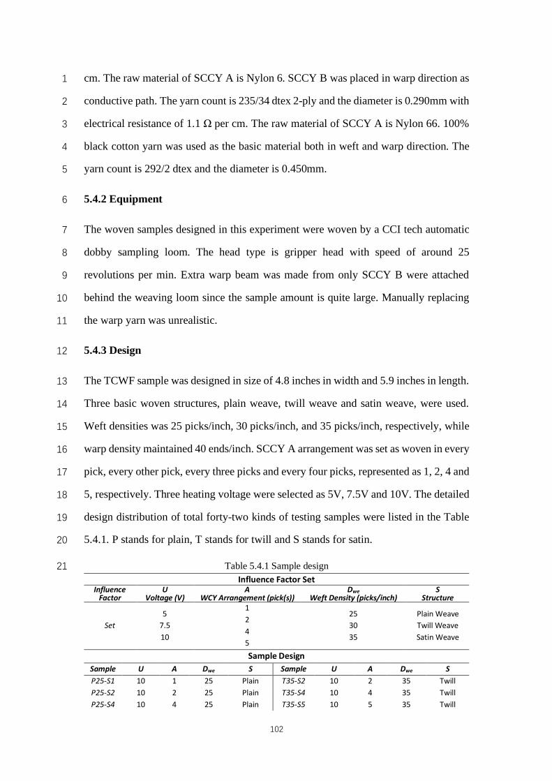
102

cm. The raw material of SCCY A is Nylon 6. SCCY B was placed in warp direction as 1

conductive path. The yarn count is 235/34 dtex 2-ply and the diameter is 0.290mm with 2

electrical resistance of 1.1 Ω per cm. The raw material of SCCY A is Nylon 66. 100% 3

black cotton yarn was used as the basic material both in weft and warp direction. The 4

yarn count is 292/2 dtex and the diameter is 0.450mm. 5

5.4.2 Equipment 6

The woven samples designed in this experiment were woven by a CCI tech automatic 7

dobby sampling loom. The head type is gripper head with speed of around 25 8

revolutions per min. Extra warp beam was made from only SCCY B were attached 9

behind the weaving loom since the sample amount is quite large. Manually replacing 10

the warp yarn was unrealistic. 11

5.4.3 Design 12

The TCWF sample was designed in size of 4.8 inches in width and 5.9 inches in length. 13

Three basic woven structures, plain weave, twill weave and satin weave, were used. 14

Weft densities was 25 picks/inch, 30 picks/inch, and 35 picks/inch, respectively, while 15

warp density maintained 40 ends/inch. SCCY A arrangement was set as woven in every 16

pick, every other pick, every three picks and every four picks, represented as 1, 2, 4 and 17

5, respectively. Three heating voltage were selected as 5V, 7.5V and 10V. The detailed 18

design distribution of total forty-two kinds of testing samples were listed in the Table 19

5.4.1. P stands for plain, T stands for twill and S stands for satin. 20

Table 5.4.1 Sample design 21 Influence Factor Set

Influence Factor

U Voltage (V)

A WCY Arrangement (pick(s))

Dwe Weft Density (picks/inch)

S Structure

Set 5

7.5 10

1 2 4 5

25 30 35

Plain Weave Twill Weave Satin Weave

Sample Design Sample U A Dwe S Sample U A Dwe S P25-S1 10 1 25 Plain T35-S2 10 2 35 Twill P25-S2 10 2 25 Plain T35-S4 10 4 35 Twill P25-S4 10 4 25 Plain T35-S5 10 5 35 Twill

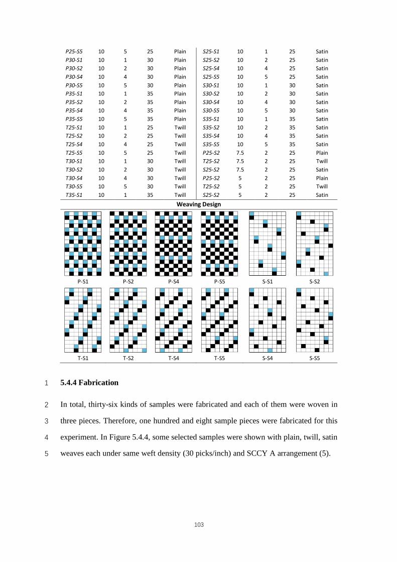
103

P25-S5 10 5 25 Plain S25-S1 10 1 25 Satin P30-S1 10 1 30 Plain S25-S2 10 2 25 Satin P30-S2 10 2 30 Plain S25-S4 10 4 25 Satin P30-S4 10 4 30 Plain S25-S5 10 5 25 Satin P30-S5 10 5 30 Plain S30-S1 10 1 30 Satin P35-S1 10 1 35 Plain S30-S2 10 2 30 Satin P35-S2 10 2 35 Plain S30-S4 10 4 30 Satin P35-S4 10 4 35 Plain S30-S5 10 5 30 Satin P35-S5 10 5 35 Plain S35-S1 10 1 35 Satin T25-S1 10 1 25 Twill S35-S2 10 2 35 Satin T25-S2 10 2 25 Twill S35-S4 10 4 35 Satin T25-S4 10 4 25 Twill S35-S5 10 5 35 Satin T25-S5 10 5 25 Twill P25-S2 7.5 2 25 Plain T30-S1 10 1 30 Twill T25-S2 7.5 2 25 Twill T30-S2 10 2 30 Twill S25-S2 7.5 2 25 Satin T30-S4 10 4 30 Twill P25-S2 5 2 25 Plain T30-S5 10 5 30 Twill T25-S2 5 2 25 Twill T35-S1 10 1 35 Twill S25-S2 5 2 25 Satin

Weaving Design

P-S1 P-S2 P-S4 P-S5 S-S1 S-S2

T-S1 T-S2 T-S4 T-S5 S-S4 S-S5

5.4.4 Fabrication 1

In total, thirty-six kinds of samples were fabricated and each of them were woven in 2

three pieces. Therefore, one hundred and eight sample pieces were fabricated for this 3

experiment. In Figure 5.4.4, some selected samples were shown with plain, twill, satin 4

weaves each under same weft density (30 picks/inch) and SCCY A arrangement (5). 5

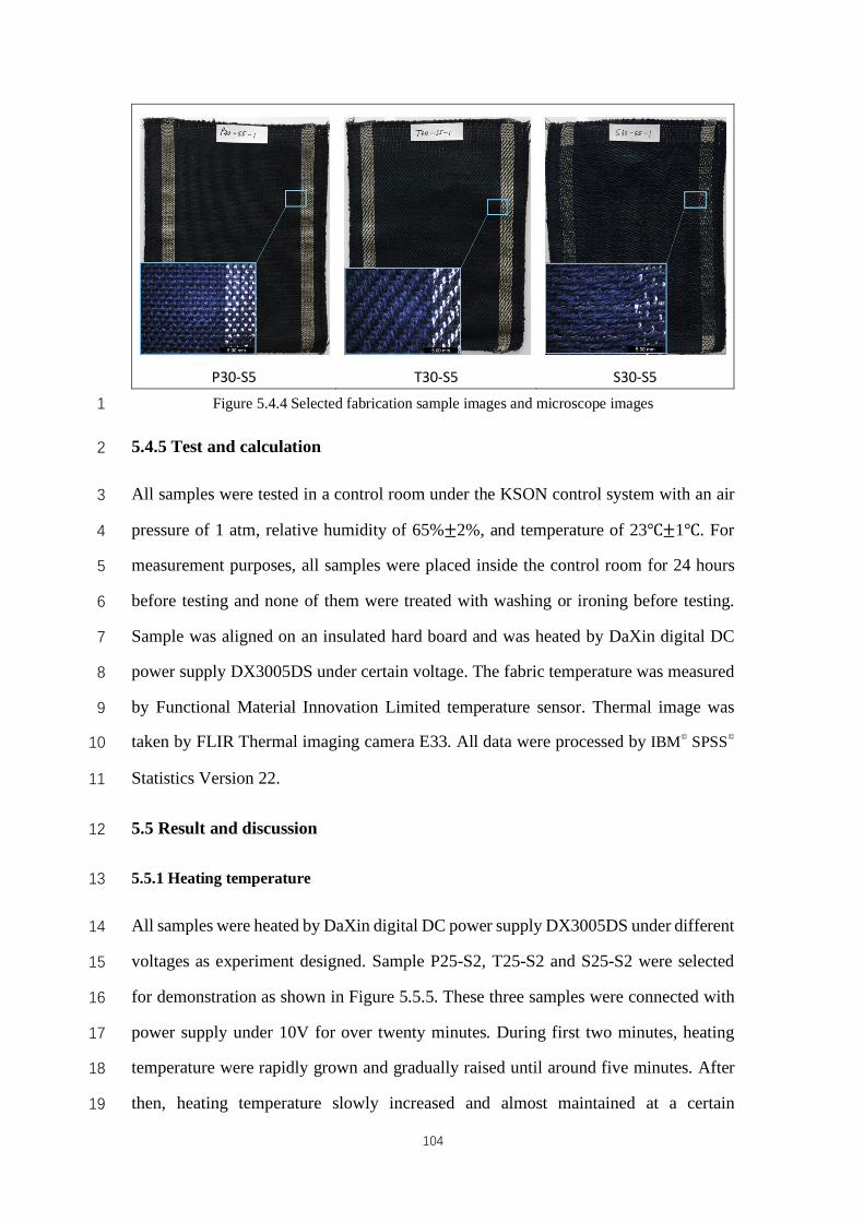
104

P30-S5 T30-S5 S30-S5

Figure 5.4.4 Selected fabrication sample images and microscope images 1

5.4.5 Test and calculation 2


pressure of 1 atm, relative humidity of 65%±2%, and temperature of 23℃±1℃. For 4



Sample was aligned on an insulated hard board and was heated by DaXin digital DC 7

power supply DX3005DS under certain voltage. The fabric temperature was measured 8

by Functional Material Innovation Limited temperature sensor. Thermal image was 9

taken by FLIR Thermal imaging camera E33. All data were processed by IBM© SPSS© 10

Statistics Version 22. 11

5.5 Result and discussion 12

5.5.1 Heating temperature 13

All samples were heated by DaXin digital DC power supply DX3005DS under different 14

voltages as experiment designed. Sample P25-S2, T25-S2 and S25-S2 were selected 15

for demonstration as shown in Figure 5.5.5. These three samples were connected with 16

power supply under 10V for over twenty minutes. During first two minutes, heating 17

temperature were rapidly grown and gradually raised until around five minutes. After 18

then, heating temperature slowly increased and almost maintained at a certain 19

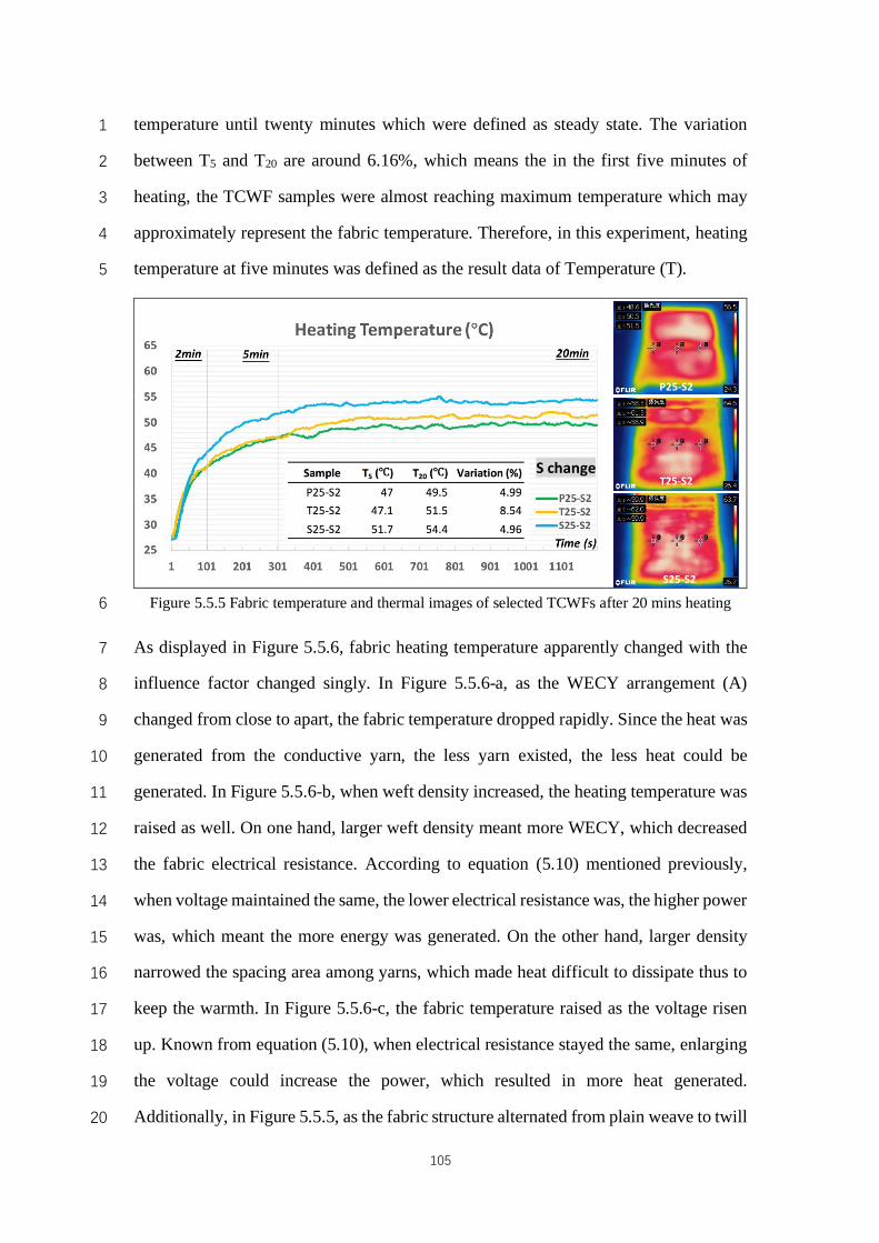
105

temperature until twenty minutes which were defined as steady state. The variation 1

between T5 and T20 are around 6.16%, which means the in the first five minutes of 2

heating, the TCWF samples were almost reaching maximum temperature which may 3

approximately represent the fabric temperature. Therefore, in this experiment, heating 4

temperature at five minutes was defined as the result data of Temperature (T). 5

Figure 5.5.5 Fabric temperature and thermal images of selected TCWFs after 20 mins heating 6

As displayed in Figure 5.5.6, fabric heating temperature apparently changed with the 7

influence factor changed singly. In Figure 5.5.6-a, as the WECY arrangement (A) 8

changed from close to apart, the fabric temperature dropped rapidly. Since the heat was 9

generated from the conductive yarn, the less yarn existed, the less heat could be 10

generated. In Figure 5.5.6-b, when weft density increased, the heating temperature was 11

raised as well. On one hand, larger weft density meant more WECY, which decreased 12

the fabric electrical resistance. According to equation (5.10) mentioned previously, 13

when voltage maintained the same, the lower electrical resistance was, the higher power 14

was, which meant the more energy was generated. On the other hand, larger density 15

narrowed the spacing area among yarns, which made heat difficult to dissipate thus to 16

keep the warmth. In Figure 5.5.6-c, the fabric temperature raised as the voltage risen 17

up. Known from equation (5.10), when electrical resistance stayed the same, enlarging 18

the voltage could increase the power, which resulted in more heat generated. 19

Additionally, in Figure 5.5.5, as the fabric structure alternated from plain weave to twill 20

P25-S2

T25-S2

S25-S2

S change

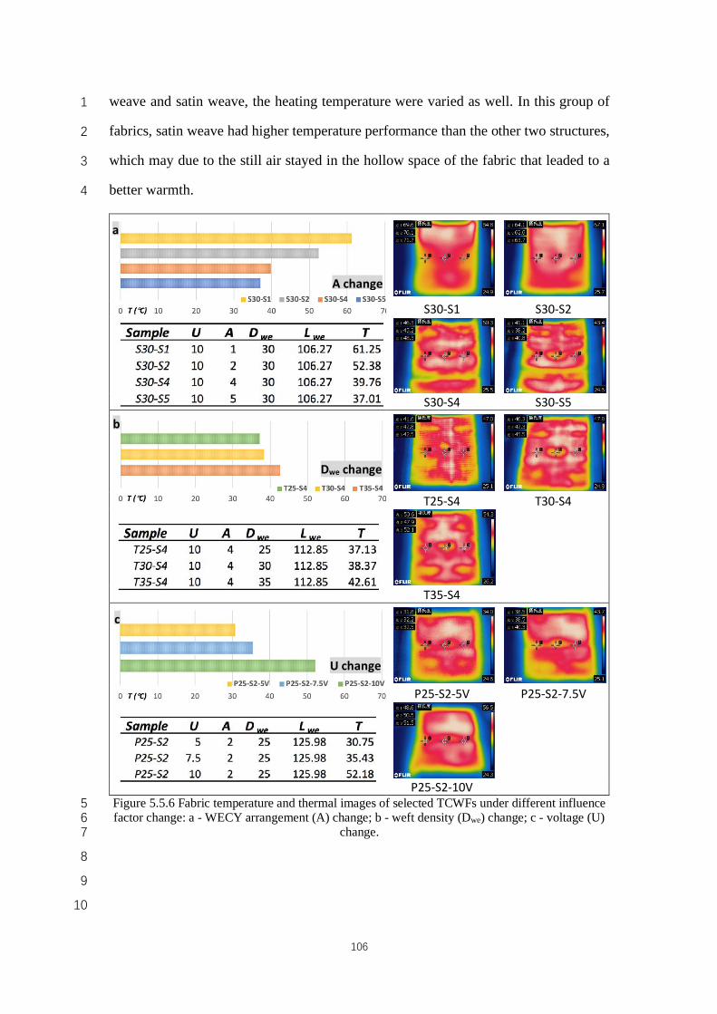
106

weave and satin weave, the heating temperature were varied as well. In this group of 1

fabrics, satin weave had higher temperature performance than the other two structures, 2

which may due to the still air stayed in the hollow space of the fabric that leaded to a 3

better warmth. 4

S30-S1 S30-S2

S30-S4 S30-S5

T25-S4 T30-S4

T35-S4

P25-S2-5V P25-S2-7.5V

P25-S2-10V Figure 5.5.6 Fabric temperature and thermal images of selected TCWFs under different influence 5 factor change: a - WECY arrangement (A) change; b - weft density (Dwe) change; c - voltage (U) 6

change. 7

8

9

10

A change

Dwe change

U change

a

b

c

107

5.5.2 Temperature prediction model 1

All result data of experiment are listed in Table 5.5.1. Temperature results are the 2

average values of three times measurement of each sample. Since there are four 3

independent variables, software SPSS Statistics were used for data processing. 4

Backward method was chosen to conduct the multiple linear regression, which 5

processed the data based on a predetermined probability of F. All the independent 6

variables were taken into the regression and then to eliminate the insignificant variables 7

to finalize the regression equation. The variable stays in the equation if the probability 8

is lower than 0.05 and removes from it if equal to or greater than 0.1. 9

Table 5.5.1 Data results of selected influence factors 10 Sample U A Dwe Lwe T Sample U A Dwe Lwe T

P25-S1 10 1 25 125.98 54.01 T35-S2 10 2 35 112.85 54.01 P25-S2 10 2 25 125.98 52.18 T35-S4 10 4 35 112.85 42.61 P25-S4 10 4 25 125.98 34.99 T35-S5 10 5 35 112.85 37.69 P25-S5 10 5 25 125.98 34.24 S25-S1 10 1 25 106.27 56.75 P30-S1 10 1 30 125.98 60.53 S25-S2 10 2 25 106.27 51.96 P30-S2 10 2 30 125.98 47.53 S25-S4 10 4 25 106.27 36.38 P30-S4 10 4 30 125.98 41.01 S25-S5 10 5 25 106.27 35.19 P30-S5 10 5 30 125.98 34.17 S30-S1 10 1 30 106.27 61.25 P35-S1 10 1 35 125.98 63.54 S30-S2 10 2 30 106.27 52.38 P35-S2 10 2 35 125.98 49.43 S30-S4 10 4 30 106.27 39.76 P35-S4 10 4 35 125.98 42.74 S30-S5 10 5 30 106.27 37.01 P35-S5 10 5 35 125.98 36.60 S35-S1 10 1 35 106.27 69.26 T25-S1 10 1 25 112.85 53.83 S35-S2 10 2 35 106.27 55.11 T25-S2 10 2 25 112.85 50.02 S35-S4 10 4 35 106.27 36.69 T25-S4 10 4 25 112.85 37.13 S35-S5 10 5 35 106.27 38.10 T25-S5 10 5 25 112.85 34.18 P25-S2 7.5 2 25 125.98 35.43 T30-S1 10 1 30 112.85 59.93 T25-S2 7.5 2 25 112.85 34.59 T30-S2 10 2 30 112.85 51.53 S25-S2 7.5 2 25 106.27 35.96 T30-S4 10 4 30 112.85 38.37 P25-S2 5 2 25 125.98 30.75 T30-S5 10 5 30 112.85 38.36 T25-S2 5 2 25 112.85 29.16 T35-S1 10 1 35 112.85 68.22 S25-S2 5 2 25 106.27 28.86

There were two regression models established according to Table 5.5.2. The first 11

regression model contains all four independent variables, while the second one has 12

removed the variable “Lwe”. Shown in Table 5.5.2 and Table 5.5.3, both models have 13

significant values of 0.000 and F values of 124.291 and 164.342 respectively, which 14

means both models are statistically significant. Therefore, it is reasonable to use voltage, 15

WECY arrangement, weft density and length of weft yarn to predict fabric heating 16

108

temperature. Both R values are around 0.96 which denotes the linear correlations 1

between dependent variable and independent variables are quite obvious. Both R square 2

values are around 0.93, which stands for that these two models can predict the heating 3

temperature of 93% of TCWFs. According to the calculation results of regression 4

coefficients listed in Table 5.5.4, the first regression model can be expressed as: 5

𝑇� = −6.141𝐴 + 4.437𝑈 + 0.571𝐷{� − 0.064𝐿{� + 11.007 (5.38) 6

The absolute values of standardized coefficients Beta of each variable implies the 7

importance of each variable impacts on the heating temperature. In Model 1 (5.38), 8

WECY arrangement has the most significant influence and followed by voltage, weft 9

density and length of weft yarn. In addition, significant values of three coefficients, A, 10

U and Dwe, are close to 0.000, which are much smaller than 0.05. This denotes that these 11

three variables are statistically significant and should stay in the model. However, the 12

significant value of Lwe is 0.276 that is higher than 0.1, which has lower impact on 13

heating temperature compared to the other three variables. 14

The second regression model is the finalized regression model conducted by 15

backward method. The model equation is: 16

𝑇H = −6.141𝐴 + 4.437𝑈 + 0.571𝐷{� + 3.634 (5.39) 17

In Model 2 (5.39), variable Lwe has been eliminated, although the R value and R square 18

value of the model is slightly lower than Model 1, the adjust R square is the same. This 19

Model can predict 92.8% of TCWFs' heating temperature. According to Table 5.5.4, 20

all three coefficients are statistically significant thus remain in the model. The 95% 21

confidence interval are listed in Table 5.5.4 as well. Moreover, from collinearity 22

statistics part in Table 5.5.4, all the tolerance values are much greater than 0.1 and 23

almost close to 1, which indicates that the predictors have no multicollinearity and can 24

be entered into the multiple linear regression model. 25

26

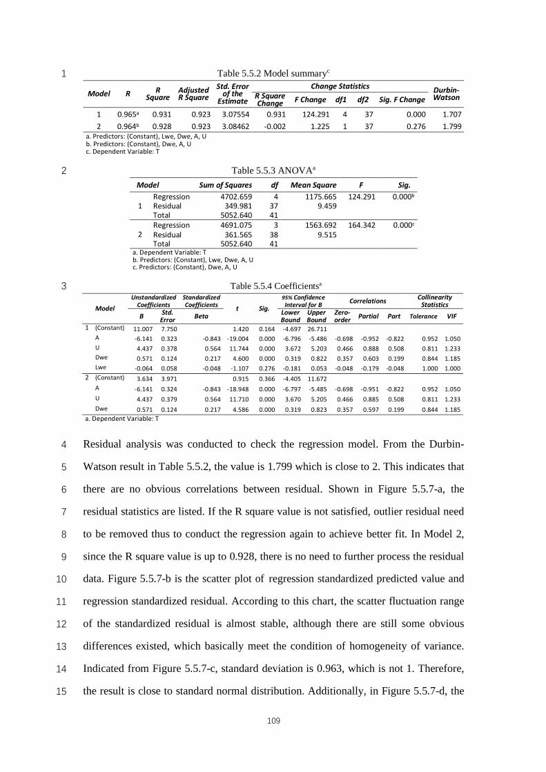
109

Table 5.5.2 Model summaryc 1

Model R R Square

Adjusted R Square

Std. Error of the

Estimate

Change Statistics Durbin-Watson R Square

Change F Change df1 df2 Sig. F Change

1 0.965a 0.931 0.923 3.07554 0.931 124.291 4 37 0.000 1.707 2 0.964b 0.928 0.923 3.08462 -0.002 1.225 1 37 0.276 1.799

a. Predictors: (Constant), Lwe, Dwe, A, U b. Predictors: (Constant), Dwe, A, U c. Dependent Variable: T

Table 5.5.3 ANOVAa 2 Model Sum of Squares df Mean Square F Sig.

1 Regression 4702.659 4 1175.665 124.291 0.000b Residual 349.981 37 9.459 Total 5052.640 41

2 Regression 4691.075 3 1563.692 164.342 0.000c Residual 361.565 38 9.515 Total 5052.640 41

a. Dependent Variable: T b. Predictors: (Constant), Lwe, Dwe, A, U c. Predictors: (Constant), Dwe, A, U

Table 5.5.4 Coefficientsa 3

Model Unstandardized

Coefficients Standardized Coefficients t Sig.

95% Confidence Interval for B Correlations Collinearity

Statistics B Std.

Error Beta Lower Bound

Upper Bound

Zero-order Partial Part Tolerance VIF

1 (Constant) 11.007 7.750 1.420 0.164 -4.697 26.711 A -6.141 0.323 -0.843 -19.004 0.000 -6.796 -5.486 -0.698 -0.952 -0.822 0.952 1.050 U 4.437 0.378 0.564 11.744 0.000 3.672 5.203 0.466 0.888 0.508 0.811 1.233 Dwe 0.571 0.124 0.217 4.600 0.000 0.319 0.822 0.357 0.603 0.199 0.844 1.185 Lwe -0.064 0.058 -0.048 -1.107 0.276 -0.181 0.053 -0.048 -0.179 -0.048 1.000 1.000

2 (Constant) 3.634 3.971 0.915 0.366 -4.405 11.672 A -6.141 0.324 -0.843 -18.948 0.000 -6.797 -5.485 -0.698 -0.951 -0.822 0.952 1.050 U 4.437 0.379 0.564 11.710 0.000 3.670 5.205 0.466 0.885 0.508 0.811 1.233 Dwe 0.571 0.124 0.217 4.586 0.000 0.319 0.823 0.357 0.597 0.199 0.844 1.185

a. Dependent Variable: T

Residual analysis was conducted to check the regression model. From the Durbin-4

Watson result in Table 5.5.2, the value is 1.799 which is close to 2. This indicates that 5

there are no obvious correlations between residual. Shown in Figure 5.5.7-a, the 6

residual statistics are listed. If the R square value is not satisfied, outlier residual need 7

to be removed thus to conduct the regression again to achieve better fit. In Model 2, 8

since the R square value is up to 0.928, there is no need to further process the residual 9

data. Figure 5.5.7-b is the scatter plot of regression standardized predicted value and 10

regression standardized residual. According to this chart, the scatter fluctuation range 11

of the standardized residual is almost stable, although there are still some obvious 12

differences existed, which basically meet the condition of homogeneity of variance. 13

Indicated from Figure 5.5.7-c, standard deviation is 0.963, which is not 1. Therefore, 14

the result is close to standard normal distribution. Additionally, in Figure 5.5.7-d, the 15

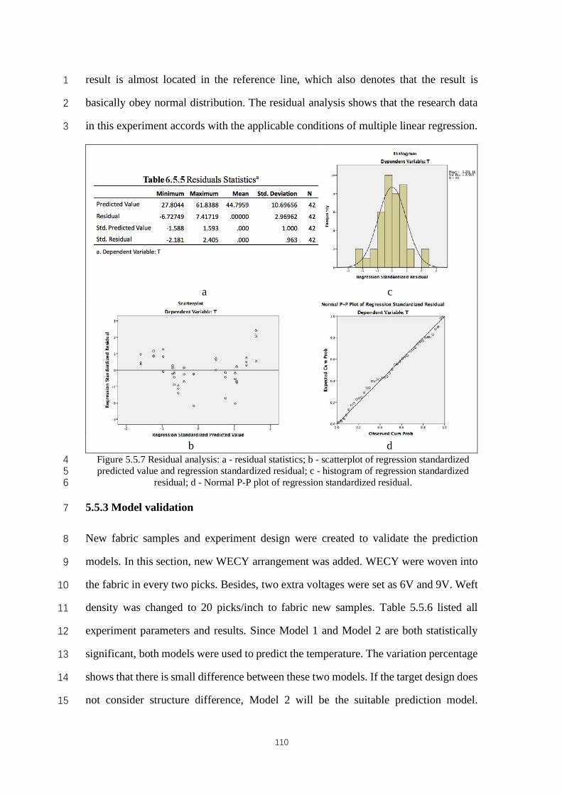
110

result is almost located in the reference line, which also denotes that the result is 1

basically obey normal distribution. The residual analysis shows that the research data 2

in this experiment accords with the applicable conditions of multiple linear regression. 3

a c

b d

Figure 5.5.7 Residual analysis: a - residual statistics; b - scatterplot of regression standardized 4 predicted value and regression standardized residual; c - histogram of regression standardized 5

residual; d - Normal P-P plot of regression standardized residual. 6

5.5.3 Model validation 7

New fabric samples and experiment design were created to validate the prediction 8

models. In this section, new WECY arrangement was added. WECY were woven into 9

the fabric in every two picks. Besides, two extra voltages were set as 6V and 9V. Weft 10

density was changed to 20 picks/inch to fabric new samples. Table 5.5.6 listed all 11

experiment parameters and results. Since Model 1 and Model 2 are both statistically 12

significant, both models were used to predict the temperature. The variation percentage 13

shows that there is small difference between these two models. If the target design does 14

not consider structure difference, Model 2 will be the suitable prediction model. 15

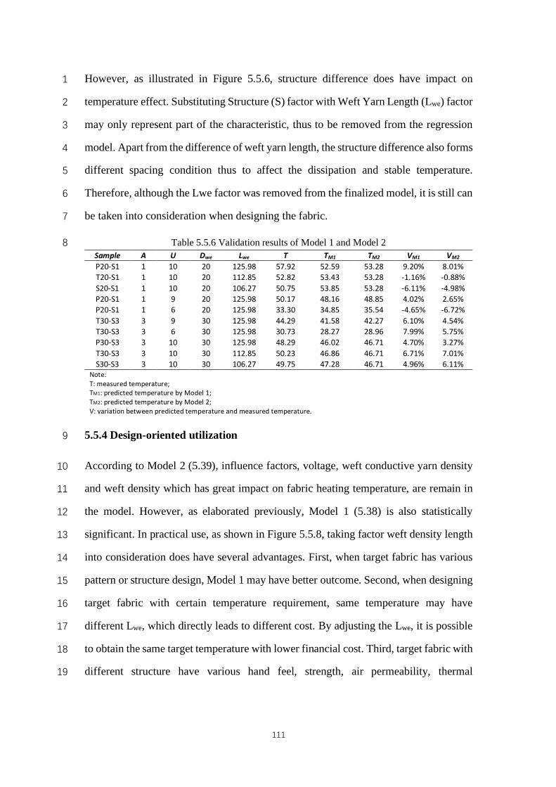
111

However, as illustrated in Figure 5.5.6, structure difference does have impact on 1

temperature effect. Substituting Structure (S) factor with Weft Yarn Length (Lwe) factor 2

may only represent part of the characteristic, thus to be removed from the regression 3

model. Apart from the difference of weft yarn length, the structure difference also forms 4

different spacing condition thus to affect the dissipation and stable temperature. 5

Therefore, although the Lwe factor was removed from the finalized model, it is still can 6

be taken into consideration when designing the fabric. 7

Table 5.5.6 Validation results of Model 1 and Model 2 8 Sample A U Dwe Lwe T TM1 TM2 VM1 VM2 P20-S1 1 10 20 125.98 57.92 52.59 53.28 9.20% 8.01% T20-S1 1 10 20 112.85 52.82 53.43 53.28 -1.16% -0.88% S20-S1 1 10 20 106.27 50.75 53.85 53.28 -6.11% -4.98% P20-S1 1 9 20 125.98 50.17 48.16 48.85 4.02% 2.65% P20-S1 1 6 20 125.98 33.30 34.85 35.54 -4.65% -6.72% T30-S3 3 9 30 125.98 44.29 41.58 42.27 6.10% 4.54% T30-S3 3 6 30 125.98 30.73 28.27 28.96 7.99% 5.75% P30-S3 3 10 30 125.98 48.29 46.02 46.71 4.70% 3.27% T30-S3 3 10 30 112.85 50.23 46.86 46.71 6.71% 7.01% S30-S3 3 10 30 106.27 49.75 47.28 46.71 4.96% 6.11%

Note: T: measured temperature; TM1: predicted temperature by Model 1; TM2: predicted temperature by Model 2; V: variation between predicted temperature and measured temperature.

5.5.4 Design-oriented utilization 9

According to Model 2 (5.39), influence factors, voltage, weft conductive yarn density 10

and weft density which has great impact on fabric heating temperature, are remain in 11

the model. However, as elaborated previously, Model 1 (5.38) is also statistically 12

significant. In practical use, as shown in Figure 5.5.8, taking factor weft density length 13

into consideration does have several advantages. First, when target fabric has various 14

pattern or structure design, Model 1 may have better outcome. Second, when designing 15

target fabric with certain temperature requirement, same temperature may have 16

different Lwe, which directly leads to different cost. By adjusting the Lwe, it is possible 17

to obtain the same target temperature with lower financial cost. Third, target fabric with 18

different structure have various hand feel, strength, air permeability, thermal 19

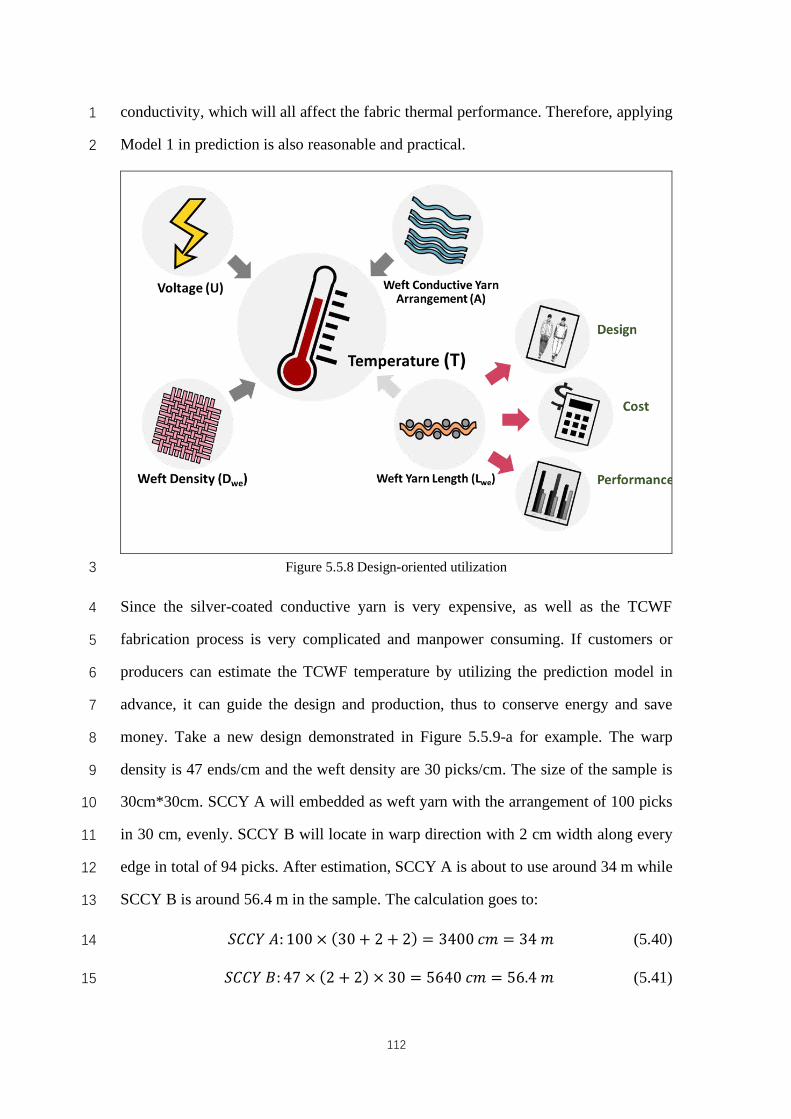
112

conductivity, which will all affect the fabric thermal performance. Therefore, applying 1

Model 1 in prediction is also reasonable and practical. 2

Figure 5.5.8 Design-oriented utilization 3

Since the silver-coated conductive yarn is very expensive, as well as the TCWF 4

fabrication process is very complicated and manpower consuming. If customers or 5

producers can estimate the TCWF temperature by utilizing the prediction model in 6

advance, it can guide the design and production, thus to conserve energy and save 7

money. Take a new design demonstrated in Figure 5.5.9-a for example. The warp 8

density is 47 ends/cm and the weft density are 30 picks/cm. The size of the sample is 9

30cm*30cm. SCCY A will embedded as weft yarn with the arrangement of 100 picks 10

in 30 cm, evenly. SCCY B will locate in warp direction with 2 cm width along every 11

edge in total of 94 picks. After estimation, SCCY A is about to use around 34 m while 12

SCCY B is around 56.4 m in the sample. The calculation goes to: 13

𝑆𝐶𝐶𝑌𝐴: 100 × (30 + 2 + 2) = 3400𝑐𝑚 = 34𝑚 (5.40) 14

𝑆𝐶𝐶𝑌𝐵: 47 × (2 + 2) × 30 = 5640𝑐𝑚 = 56.4𝑚 (5.41) 15

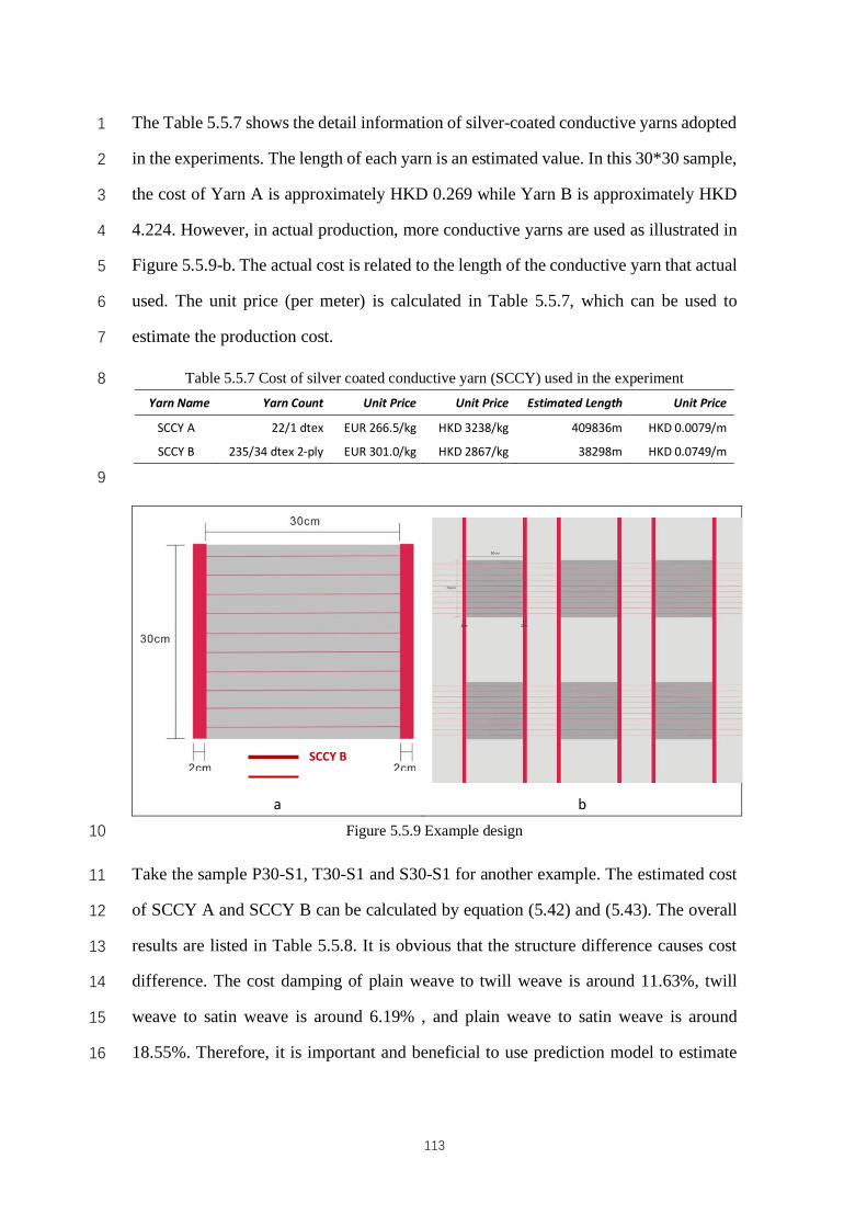
113

The Table 5.5.7 shows the detail information of silver-coated conductive yarns adopted 1

in the experiments. The length of each yarn is an estimated value. In this 30*30 sample, 2

the cost of Yarn A is approximately HKD 0.269 while Yarn B is approximately HKD 3

4.224. However, in actual production, more conductive yarns are used as illustrated in 4

Figure 5.5.9-b. The actual cost is related to the length of the conductive yarn that actual 5

used. The unit price (per meter) is calculated in Table 5.5.7, which can be used to 6

estimate the production cost. 7

Table 5.5.7 Cost of silver coated conductive yarn (SCCY) used in the experiment 8 Yarn Name Yarn Count Unit Price Unit Price Estimated Length Unit Price

SCCY A 22/1 dtex EUR 266.5/kg HKD 3238/kg 409836m HKD 0.0079/m

SCCY B 235/34 dtex 2-ply EUR 301.0/kg HKD 2867/kg 38298m HKD 0.0749/m

9

a b

Figure 5.5.9 Example design 10

Take the sample P30-S1, T30-S1 and S30-S1 for another example. The estimated cost 11

of SCCY A and SCCY B can be calculated by equation (5.42) and (5.43). The overall 12

results are listed in Table 5.5.8. It is obvious that the structure difference causes cost 13

difference. The cost damping of plain weave to twill weave is around 11.63%, twill 14

weave to satin weave is around 6.19% , and plain weave to satin weave is around 15

18.55%. Therefore, it is important and beneficial to use prediction model to estimate 16

SCCY B

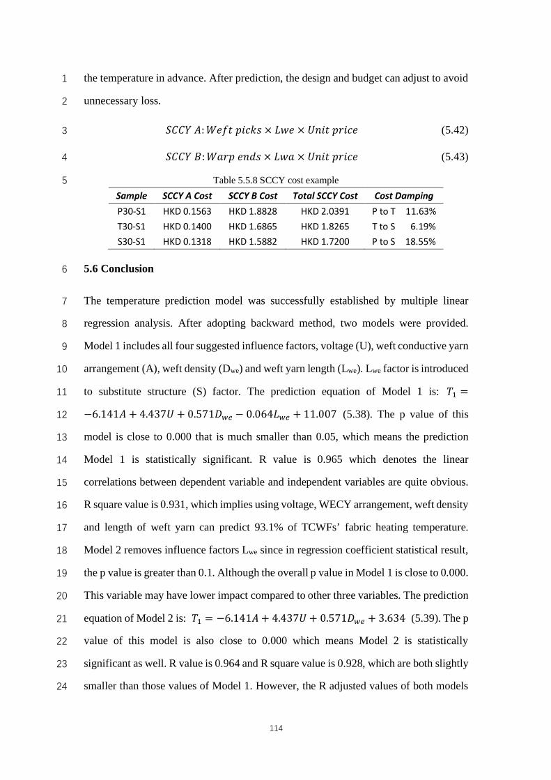
114

the temperature in advance. After prediction, the design and budget can adjust to avoid 1

unnecessary loss. 2

𝑆𝐶𝐶𝑌𝐴:𝑊𝑒𝑓𝑡𝑝𝑖𝑐𝑘𝑠 × 𝐿𝑤𝑒 × 𝑈𝑛𝑖𝑡𝑝𝑟𝑖𝑐𝑒 (5.42) 3

𝑆𝐶𝐶𝑌𝐵:𝑊𝑎𝑟𝑝𝑒𝑛𝑑𝑠 × 𝐿𝑤𝑎 × 𝑈𝑛𝑖𝑡𝑝𝑟𝑖𝑐𝑒 (5.43) 4

Table 5.5.8 SCCY cost example 5

Sample SCCY A Cost SCCY B Cost Total SCCY Cost Cost Damping P30-S1 HKD 0.1563 HKD 1.8828 HKD 2.0391 P to T 11.63% T30-S1 HKD 0.1400 HKD 1.6865 HKD 1.8265 T to S 06.19% S30-S1 HKD 0.1318 HKD 1.5882 HKD 1.7200 P to S 18.55%

5.6 Conclusion 6

The temperature prediction model was successfully established by multiple linear 7

regression analysis. After adopting backward method, two models were provided. 8

Model 1 includes all four suggested influence factors, voltage (U), weft conductive yarn 9

arrangement (A), weft density (Dwe) and weft yarn length (Lwe). Lwe factor is introduced 10

to substitute structure (S) factor. The prediction equation of Model 1 is: 𝑇� =11

−6.141𝐴 + 4.437𝑈 + 0.571𝐷{� − 0.064𝐿{� + 11.007 (5.38). The p value of this 12

model is close to 0.000 that is much smaller than 0.05, which means the prediction 13

Model 1 is statistically significant. R value is 0.965 which denotes the linear 14

correlations between dependent variable and independent variables are quite obvious. 15

R square value is 0.931, which implies using voltage, WECY arrangement, weft density 16

and length of weft yarn can predict 93.1% of TCWFs’ fabric heating temperature. 17

Model 2 removes influence factors Lwe since in regression coefficient statistical result, 18

the p value is greater than 0.1. Although the overall p value in Model 1 is close to 0.000. 19

This variable may have lower impact compared to other three variables. The prediction 20

equation of Model 2 is: 𝑇� = −6.141𝐴+ 4.437𝑈 + 0.571𝐷{� + 3.634 (5.39). The p 21

value of this model is also close to 0.000 which means Model 2 is statistically 22

significant as well. R value is 0.964 and R square value is 0.928, which are both slightly 23

smaller than those values of Model 1. However, the R adjusted values of both models 24

115

are the same. Model 2 can predict 92.8% of TCWFs' heating temperature. According 1

to the performance results and utilization influence, the structure factor actually affects 2

the integrity design, target temperature and financial cost. In conclusion, applying 3

Model 1 in temperature prediction maybe a reasonable and practical option. 4

5

6

7

8

9

10

11

12

13

14

15

16

17

18

19

20

21

22

116

Chapter 6 Performance Study on Thermal Conductive Woven 1

Fabrics 2

6.1 Thermal conductive woven fabric (TCWF) design 3

The TCWF sample is designed in size of 12 cm (4.8 inches) in width and 15 cm (5.9 4

inches) in length (Figure 6.1.1-a). Plain weave, twill weave (1/3) and satin weave (8 5

ends) are used for structural changes (Figure 6.1.1-b, 6.1.1-c, 6.1.1-d). Weft densities 6

are 25 picks/inch, 30 picks/inch, and 35 picks/inch, respectively, while warp density 7

maintains 40 ends/inch. As demonstrated in Figure 6.1.1, SCCY A is arranged as in 8

every weft pick, every other weft pick and every five weft picks. SCCY B is placed in 9

warp direction using as conductive path. The area between two conductive paths is the 10

heating area that provide thermal treatment. Table 6.1.1 lists the specifications of all 11

seven TCWF samples, P25-S1, P25-S2, P25-S6, P30-S6, S35-S6, T25-S2 and S25-S2, 12

which designed for the experiment respectively. Alphabet P, T and S stand for structure 13

plain weave, twill weave and satin weave. Numeral 25, 30 and 35 represent for weft 14

densities. Label S1, S2 and S6 denote the SCCY A arrangement. 15

c

a b d

Figure 6.1.1 TCWF design description: (a) - size and function of TCWF sample; (b) - plain weave 16 and illustration of SCCY A and SCCY B; (c) - twill weave; (d) - satin weave 17

18 19 20 21 22

SCCY A

SCCY

B

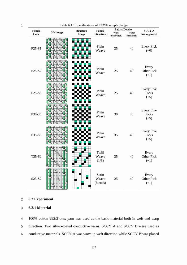
117

Table 6.1.1 Specifications of TCWF sample design 1

Fabric Code 3D Image Structure

Image Fabric

Structure Fabric Density SCCY A

Arrangement Weft (picks/inch)

Warp (ends/inch)

P25-S1

Plain Weave 25 40 Every Pick

(+0)

P25-S2

Plain Weave 25 40

Every Other Pick

(+1)

P25-S6

Plain Weave 25 40

Every Five Picks (+5)

P30-S6

Plain Weave 30 40


P35-S6

Plain Weave 35 40


T25-S2

Twill Weave (1/3)

25 40 Every

Other Pick (+1)

S25-S2

Satin Weave (8 ends)

25 40 Every

Other Pick (+1)

6.2 Experiment 2

6.2.1 Material 3

100% cotton 292/2 dtex yarn was used as the basic material both in weft and warp 4

direction. Two silver-coated conductive yarns, SCCY A and SCCY B were used as 5

conductive materials. SCCY A was wove in weft direction while SCCY B was placed 6

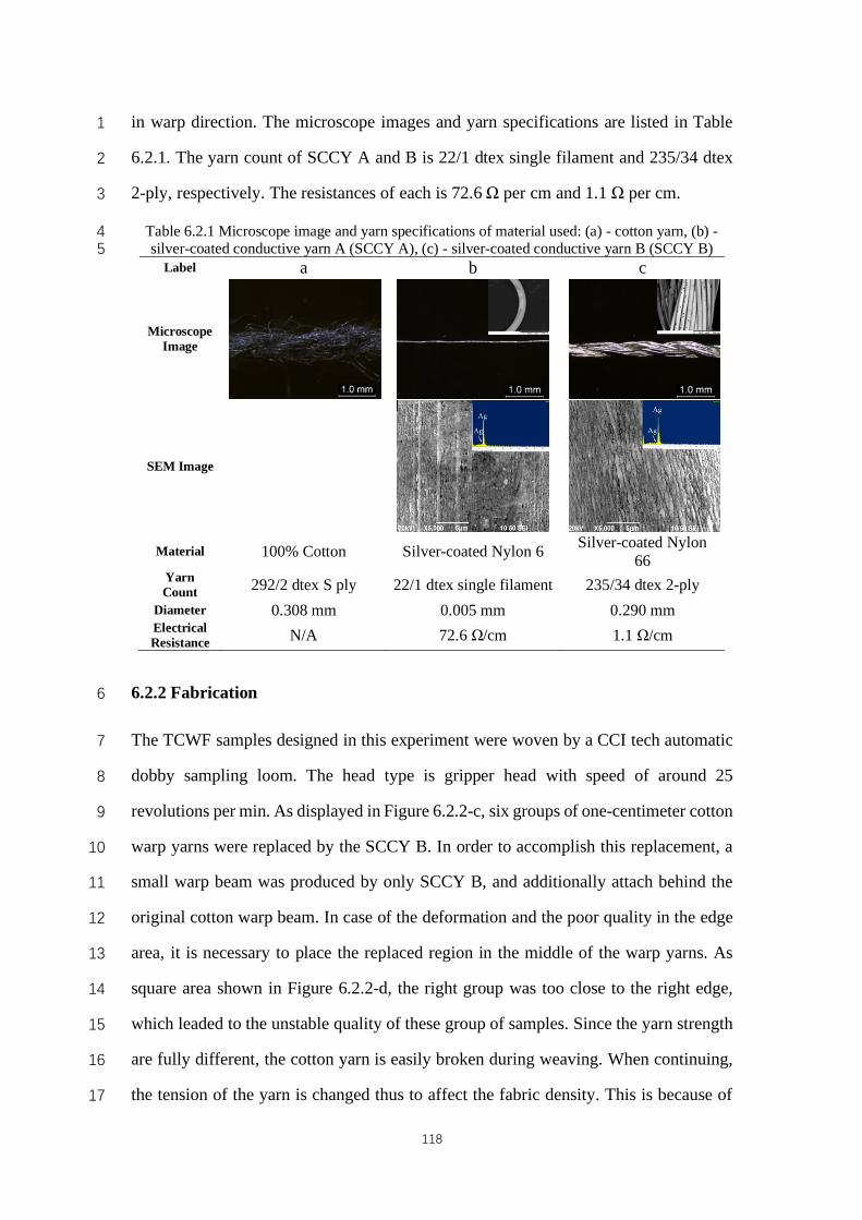
118

in warp direction. The microscope images and yarn specifications are listed in Table 1

6.2.1. The yarn count of SCCY A and B is 22/1 dtex single filament and 235/34 dtex 2

2-ply, respectively. The resistances of each is 72.6 Ω per cm and 1.1 Ω per cm. 3

Table 6.2.1 Microscope image and yarn specifications of material used: (a) - cotton yarn, (b) - 4 silver-coated conductive yarn A (SCCY A), (c) - silver-coated conductive yarn B (SCCY B) 5

Label a b c

Microscope Image

SEM Image

Material 100% Cotton Silver-coated Nylon 6 Silver-coated Nylon

66 Yarn Count 292/2 dtex S ply 22/1 dtex single filament 235/34 dtex 2-ply

Diameter 0.308 mm 0.005 mm 0.290 mm Electrical Resistance N/A 72.6 Ω/cm 1.1 Ω/cm

6.2.2 Fabrication 6

The TCWF samples designed in this experiment were woven by a CCI tech automatic 7

dobby sampling loom. The head type is gripper head with speed of around 25 8

revolutions per min. As displayed in Figure 6.2.2-c, six groups of one-centimeter cotton 9

warp yarns were replaced by the SCCY B. In order to accomplish this replacement, a 10

small warp beam was produced by only SCCY B, and additionally attach behind the 11

original cotton warp beam. In case of the deformation and the poor quality in the edge 12

area, it is necessary to place the replaced region in the middle of the warp yarns. As 13

square area shown in Figure 6.2.2-d, the right group was too close to the right edge, 14

which leaded to the unstable quality of these group of samples. Since the yarn strength 15

are fully different, the cotton yarn is easily broken during weaving. When continuing, 16

the tension of the yarn is changed thus to affect the fabric density. This is because of 17

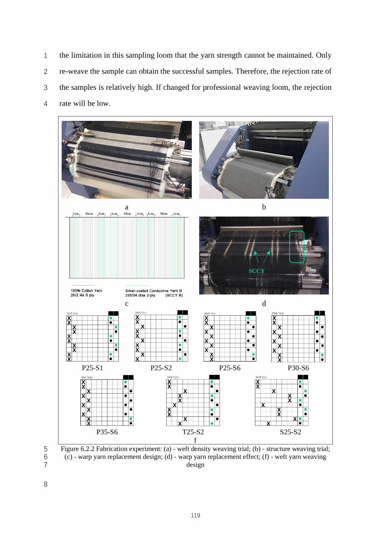
119

the limitation in this sampling loom that the yarn strength cannot be maintained. Only 1

re-weave the sample can obtain the successful samples. Therefore, the rejection rate of 2

the samples is relatively high. If changed for professional weaving loom, the rejection 3

rate will be low. 4

a b

c d

P25-S1 P25-S2 P25-S6 P30-S6

P35-S6 T25-S2 S25-S2

f Figure 6.2.2 Fabrication experiment: (a) - weft density weaving trial; (b) - structure weaving trial; 5

(c) - warp yarn replacement design; (d) - warp yarn replacement effect; (f) - weft yarn weaving 6 design 7

8

SCCY

B

120

6.2.3 Performance test 1


pressure of 1 atm, relative humidity of 65%±2%, and temperature of 23℃±1℃. For 3



Mass and Thickness Test 6

The mass of the samples was tested by electronic balance AY210 equipment with a 7

readability of 0.1 mg, and the thickness of the fabrics were tested under the pressure 4 8

gf/cm2 by RMES equipment. Each sample was measured five times and calculated the 9

average value. 10

Air Permeability Test 11

The air permeability was evaluated on a KES-F8-AP1 type air permeability tester 12

according to standard ASTM D 737. Sample was placed on the circular testing head. 13

This test was carried out under an air velocity of 0.02m/s. Air resistance of each sample 14

measured ten random points and calculated the average value. 15

Thermal Conductivity and Qmax Test 16

A KES-F7 Precise and Fast Thermal Property - Measuring Instrument Thermo Labo II 17

was used to test the thermal conductivity. Sample was placed onto the testing area of 18

the instrument, and the heat loss W values and Qmax values were measured, 19

respectively. The test for each type of sample was repeated for five times. The thermal 20

conductivity k value was calculated according to Equation:𝑘 = 𝑊 ∙ 𝑑 𝑎 ∙ ∆𝑇⁄ (6.1), 21

where W is heat loss (watt), d is thickness (mm), a is tested area (25cm2) and ∆T is 22

temperature difference (10℃). 23

Electrical Resistance Test 24

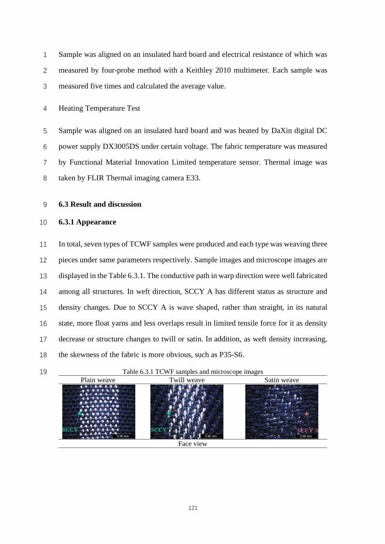
121

Sample was aligned on an insulated hard board and electrical resistance of which was 1

measured by four-probe method with a Keithley 2010 multimeter. Each sample was 2

measured five times and calculated the average value. 3

Heating Temperature Test 4

Sample was aligned on an insulated hard board and was heated by DaXin digital DC 5

power supply DX3005DS under certain voltage. The fabric temperature was measured 6

by Functional Material Innovation Limited temperature sensor. Thermal image was 7

taken by FLIR Thermal imaging camera E33. 8


6.3.1 Appearance 10

In total, seven types of TCWF samples were produced and each type was weaving three 11

pieces under same parameters respectively. Sample images and microscope images are 12

displayed in the Table 6.3.1. The conductive path in warp direction were well fabricated 13

among all structures. In weft direction, SCCY A has different status as structure and 14

density changes. Due to SCCY A is wave shaped, rather than straight, in its natural 15

state, more float yarns and less overlaps result in limited tensile force for it as density 16

decrease or structure changes to twill or satin. In addition, as weft density increasing, 17

the skewness of the fabric is more obvious, such as P35-S6. 18

Table 6.3.1 TCWF samples and microscope images 19 Plain weave Twill weave Satin weave

Face view

SCCY A SCCY

B

SCCY

B

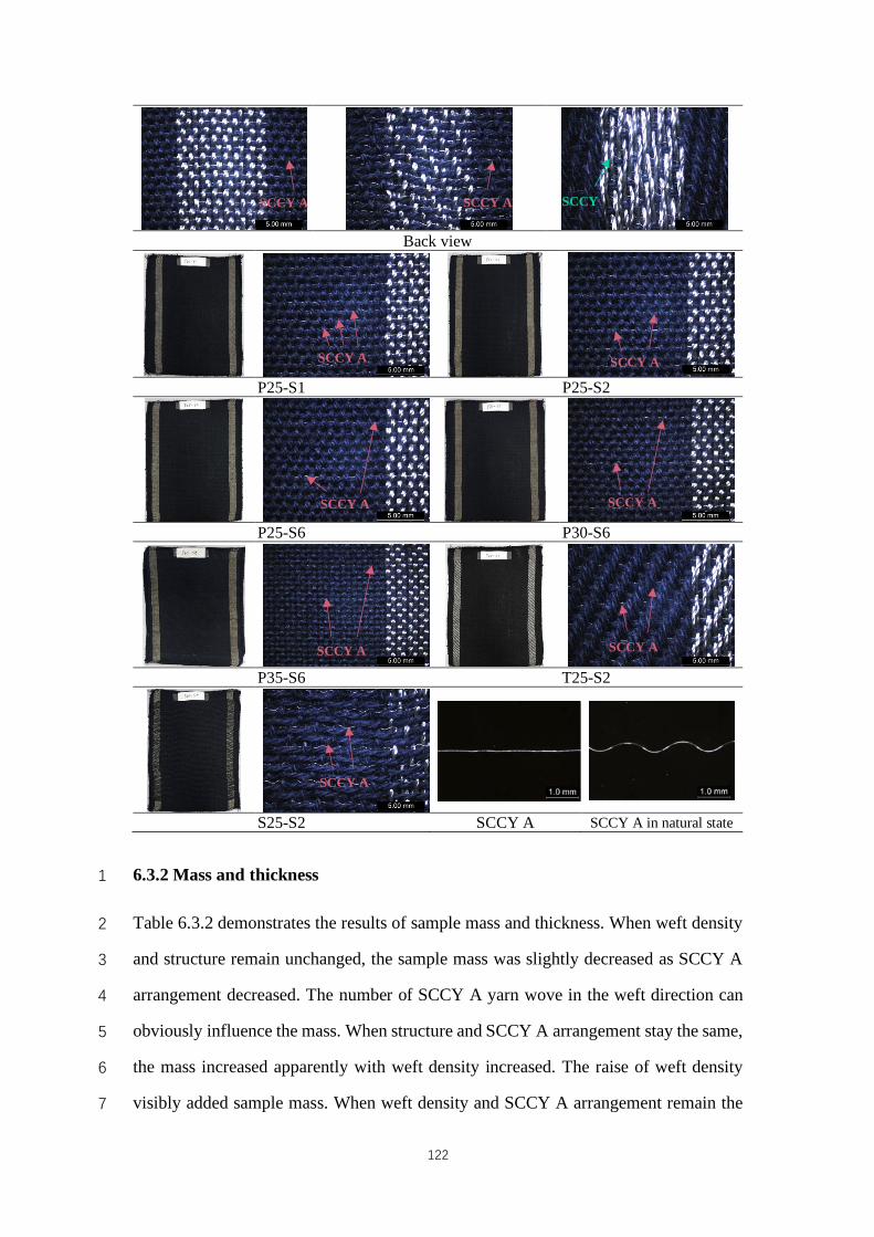
122

Back view

P25-S1 P25-S2

P25-S6 P30-S6

P35-S6 T25-S2

S25-S2 SCCY A SCCY A in natural state

6.3.2 Mass and thickness 1

Table 6.3.2 demonstrates the results of sample mass and thickness. When weft density 2

and structure remain unchanged, the sample mass was slightly decreased as SCCY A 3

arrangement decreased. The number of SCCY A yarn wove in the weft direction can 4

obviously influence the mass. When structure and SCCY A arrangement stay the same, 5

the mass increased apparently with weft density increased. The raise of weft density 6

visibly added sample mass. When weft density and SCCY A arrangement remain the 7

SCCY A

SCCY A SCCY A

SCCY A SCCY A

SCCY A SCCY A

SCCY A SCCY A SCCY

B

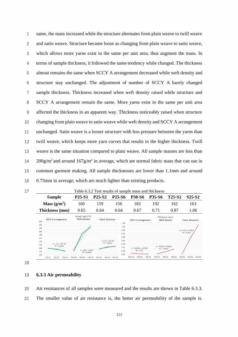
123

same, the mass increased while the structure alternates from plain weave to twill weave 1

and satin weave. Structure became loose as changing from plain weave to satin weave, 2

which allows more yarns exist in the same per unit area, thus augment the mass. In 3

terms of sample thickness, it followed the same tendency while changed. The thickness 4

almost remains the same when SCCY A arrangement decreased while weft density and 5

structure stay unchanged. The adjustment of number of SCCY A barely changed 6

sample thickness. Thickness increased when weft density raised while structure and 7

SCCY A arrangement remain the same. More yarns exist in the same per unit area 8

affected the thickness in an apparent way. Thickness noticeably raised when structure 9

changing from plain weave to satin weave while weft density and SCCY A arrangement 10

unchanged. Satin weave is a looser structure with less pressure between the yarns than 11

twill weave, which keeps more yarn curves that results in the higher thickness. Twill 12

weave is the same situation compared to plain weave. All sample masses are less than 13

200g/m2 and around 167g/m2 in average, which are normal fabric mass that can use in 14

common garment making. All sample thicknesses are lower than 1.1mm and around 15

0.75mm in average, which are much lighter than existing products. 16

Table 6.3.2 Test results of sample mass and thickness 17 Sample P25-S1 P25-S2 P25-S6 P30-S6 P35-S6 T25-S2 S25-S2

Mass (g/m2) 160 159 156 182 192 162 163 Thickness (mm) 0.65 0.64 0.64 0.67 0.71 0.87 1.06

18

6.3.3 Air permeability 19

Air resistances of all samples were measured and the results are shown in Table 6.3.3. 20

The smaller value of air resistance is, the better air permeability of the sample is. 21

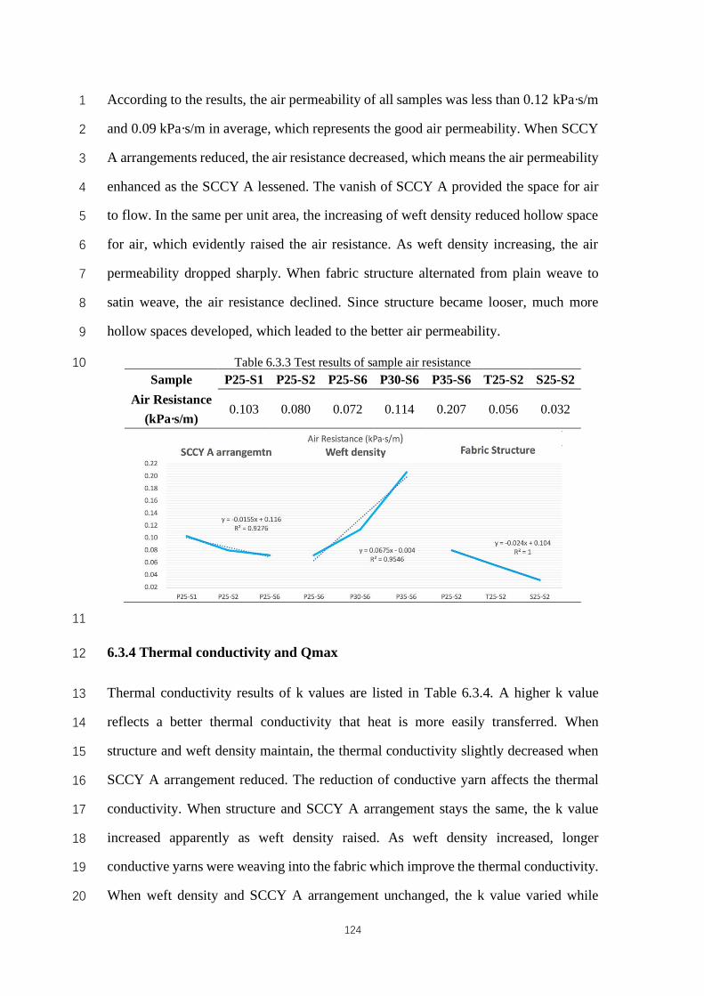
124

According to the results, the air permeability of all samples was less than 0.12 kPa·s/m 1

and 0.09 kPa·s/m in average, which represents the good air permeability. When SCCY 2

A arrangements reduced, the air resistance decreased, which means the air permeability 3

enhanced as the SCCY A lessened. The vanish of SCCY A provided the space for air 4

to flow. In the same per unit area, the increasing of weft density reduced hollow space 5

for air, which evidently raised the air resistance. As weft density increasing, the air 6

permeability dropped sharply. When fabric structure alternated from plain weave to 7

satin weave, the air resistance declined. Since structure became looser, much more 8

hollow spaces developed, which leaded to the better air permeability. 9

Table 6.3.3 Test results of sample air resistance 10 Sample P25-S1 P25-S2 P25-S6 P30-S6 P35-S6 T25-S2 S25-S2

Air Resistance (kPa·s/m)

0.103 0.080 0.072 0.114 0.207 0.056 0.032

11

6.3.4 Thermal conductivity and Qmax 12

Thermal conductivity results of k values are listed in Table 6.3.4. A higher k value 13

reflects a better thermal conductivity that heat is more easily transferred. When 14

structure and weft density maintain, the thermal conductivity slightly decreased when 15

SCCY A arrangement reduced. The reduction of conductive yarn affects the thermal 16

conductivity. When structure and SCCY A arrangement stays the same, the k value 17

increased apparently as weft density raised. As weft density increased, longer 18

conductive yarns were weaving into the fabric which improve the thermal conductivity. 19

When weft density and SCCY A arrangement unchanged, the k value varied while 20

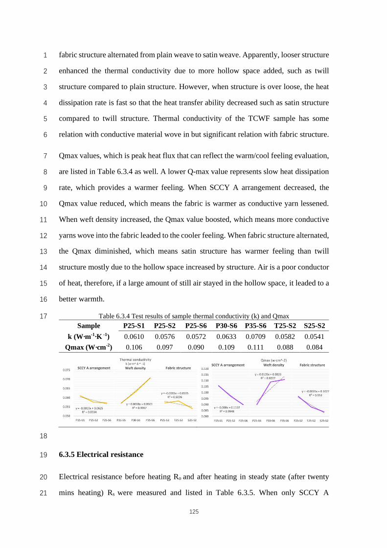
125

fabric structure alternated from plain weave to satin weave. Apparently, looser structure 1

enhanced the thermal conductivity due to more hollow space added, such as twill 2

structure compared to plain structure. However, when structure is over loose, the heat 3

dissipation rate is fast so that the heat transfer ability decreased such as satin structure 4

compared to twill structure. Thermal conductivity of the TCWF sample has some 5

relation with conductive material wove in but significant relation with fabric structure. 6

Qmax values, which is peak heat flux that can reflect the warm/cool feeling evaluation, 7

are listed in Table 6.3.4 as well. A lower Q-max value represents slow heat dissipation 8

rate, which provides a warmer feeling. When SCCY A arrangement decreased, the 9

Qmax value reduced, which means the fabric is warmer as conductive yarn lessened. 10

When weft density increased, the Qmax value boosted, which means more conductive 11

yarns wove into the fabric leaded to the cooler feeling. When fabric structure alternated, 12

the Qmax diminished, which means satin structure has warmer feeling than twill 13

structure mostly due to the hollow space increased by structure. Air is a poor conductor 14

of heat, therefore, if a large amount of still air stayed in the hollow space, it leaded to a 15

better warmth. 16

Table 6.3.4 Test results of sample thermal conductivity (k) and Qmax 17 Sample P25-S1 P25-S2 P25-S6 P30-S6 P35-S6 T25-S2 S25-S2

k (W·m-1·K -1) 0.0610 0.0576 0.0572 0.0633 0.0709 0.0582 0.0541 Qmax (W·cm-2) 0.106 0.097 0.090 0.109 0.111 0.088 0.084

18

6.3.5 Electrical resistance 19

Electrical resistance before heating Ro and after heating in steady state (after twenty 20

mins heating) Rs were measured and listed in Table 6.3.5. When only SCCY A 21

126

arrangement parameter reduced, fabric resistance enormously enlarged. Since weft 1

conductive yarns were wove into the fabric in parallel, the less the quantity is, the higher 2

the electrical resistance is. When only weft density parameter increased, the fabric 3

resistance decreased. The raise of weft density added the length of SCCY A, which 4

increased the single yarn resistance but decreased the fabric resistance due to the 5

parallel connection. When only parameter fabric structure changed, the electrical 6

resistance has minor difference. Theoretically, the different structure may cause 7

different resistance since the tightness will matter the length of conductive yarn wove 8

into, which will affect the whole fabric resistance. However, in this experiment, under 9

weft density 25 picks/inch and SCCY A arranged every other pick may not obviously 10

reflect the difference caused by structure. Further expended experiments will be 11

conducted to investigate this issue. According to Joule’s law: 𝑄 = 𝐼H𝑅𝑡 (6.2), where 12

Q (Watt) is the amount of heat generated, I (Ampere) is the electric current flowing 13

through a conductor (heating area of TCWF sample), R is the electrical resistance of 14

TCWF sample, t is the time when electrical current flowing through. The electrical 15

resistance is the major determining parameter for thermal performance when the power 16

supply settled. The smaller R is, the more heat Q will be generated. Therefore, TCWF 17

sample with smaller R value has more heat thus has higher thermal temperature effect 18

than those with larger R value. 19

However, when temperature is not constant during heating, the resistance value of 20

conductive yarn varies as shown in Table 6.3.6. The heating temperature increased 21

gradually as heating and tended to be stable after twenty min. However, this heating 22

temperature would influence R in return. Normally, a linear approximation of electrical 23

resistivity of metals is used for evaluating the percentage change in resistance value: 24

𝜌(𝑇) = 𝜌6[1 + 𝛼 ∙ (𝑇 − 𝑇6)] (6.3), where 𝜌 is the electrical resistivity of the 25

conductor material (silver), 𝜌6 is the electrical resistivity of silver at 𝑇6 , and 𝛼 26

indicates the temperature coefficient of resistivity of silver at 𝑇6 , 𝑇6 is a fixed 27

reference temperature usually room temperature. As demonstrated in the images of 28

127

Table 6.3.6, the electrical resistance sharply increased in the first two minutes and 1

slightly decreased until five minutes and almost remained the same until heating to 2

twenty minutes. This may because in the first two minutes, fabric temperature rapidly 3

raised and the electrons absorb more energy and move faster, which leads to more 4

scattering, thus increasing the amount of resistance. When after two minutes, the 5

temperature started slowly increasing while the conductive yarn expanded the length, 6

surface and volume, which may all lead to a reduction of fabric resistance. From five 7

minutes to twenty minutes, the temperature tented to be steady and the conductive yarns 8

were expended to its maximum, thus the fabric resistance has slight change during this 9

period. When SCCY A changed, the expansion of R value is marginally added. When 10

weft density increased, as well as fabric structure alternated, the expansion of R value 11

was both reduced. The discrepancy between RS and RO were around 3.04%. 12

Table 6.3.5 Test results of sample original resistance (RO) and heating resistance (RS) in steady 13 state 14

Sample P25-S1 P25-S2 P25-S6 P30-S6 P35-S6 T25-S2 S25-S2 RO (Ω) 6.70 11.60 32.14 27.48 23.96 12.10 11.41 RS (Ω) 9.24 14.62 39.22 28.82 24.51 13.95 12.85

Discrepancy 5.04% 1.31% 2.34% 1.72% 3.54% 2.91% 4.81%

15

6.3.6 Temperature 16

All samples were heated by power supply under 10V and the results were shown in 17

Table 6.3.6. During first two minutes, heating temperature were rapidly grown and 18

gradually raised until five minutes. After then, heating temperature slowly increased 19

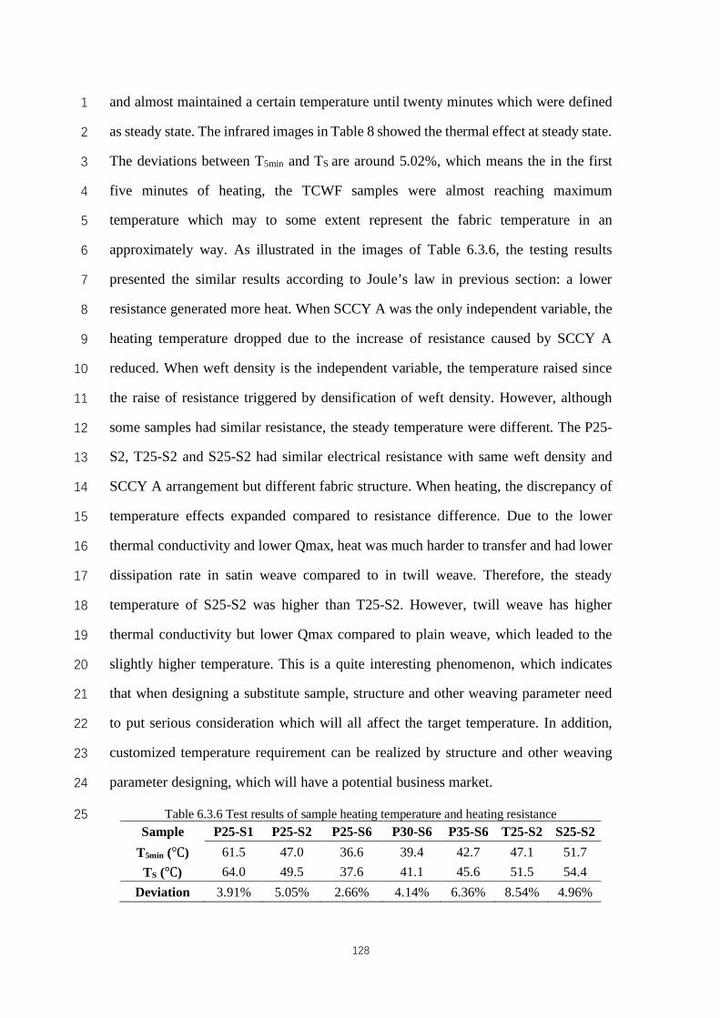
128

and almost maintained a certain temperature until twenty minutes which were defined 1

as steady state. The infrared images in Table 8 showed the thermal effect at steady state. 2

The deviations between T5min and TS are around 5.02%, which means the in the first 3

five minutes of heating, the TCWF samples were almost reaching maximum 4

temperature which may to some extent represent the fabric temperature in an 5

approximately way. As illustrated in the images of Table 6.3.6, the testing results 6

presented the similar results according to Joule’s law in previous section: a lower 7

resistance generated more heat. When SCCY A was the only independent variable, the 8

heating temperature dropped due to the increase of resistance caused by SCCY A 9

reduced. When weft density is the independent variable, the temperature raised since 10

the raise of resistance triggered by densification of weft density. However, although 11

some samples had similar resistance, the steady temperature were different. The P25-12

S2, T25-S2 and S25-S2 had similar electrical resistance with same weft density and 13

SCCY A arrangement but different fabric structure. When heating, the discrepancy of 14

temperature effects expanded compared to resistance difference. Due to the lower 15

thermal conductivity and lower Qmax, heat was much harder to transfer and had lower 16

dissipation rate in satin weave compared to in twill weave. Therefore, the steady 17

temperature of S25-S2 was higher than T25-S2. However, twill weave has higher 18

thermal conductivity but lower Qmax compared to plain weave, which leaded to the 19

slightly higher temperature. This is a quite interesting phenomenon, which indicates 20

that when designing a substitute sample, structure and other weaving parameter need 21

to put serious consideration which will all affect the target temperature. In addition, 22

customized temperature requirement can be realized by structure and other weaving 23

parameter designing, which will have a potential business market. 24

Table 6.3.6 Test results of sample heating temperature and heating resistance 25 Sample P25-S1 P25-S2 P25-S6 P30-S6 P35-S6 T25-S2 S25-S2

T5min (℃) 61.5 47.0 36.6 39.4 42.7 47.1 51.7 TS (℃) 64.0 49.5 37.6 41.1 45.6 51.5 54.4

Deviation 3.91% 5.05% 2.66% 4.14% 6.36% 8.54% 4.96%

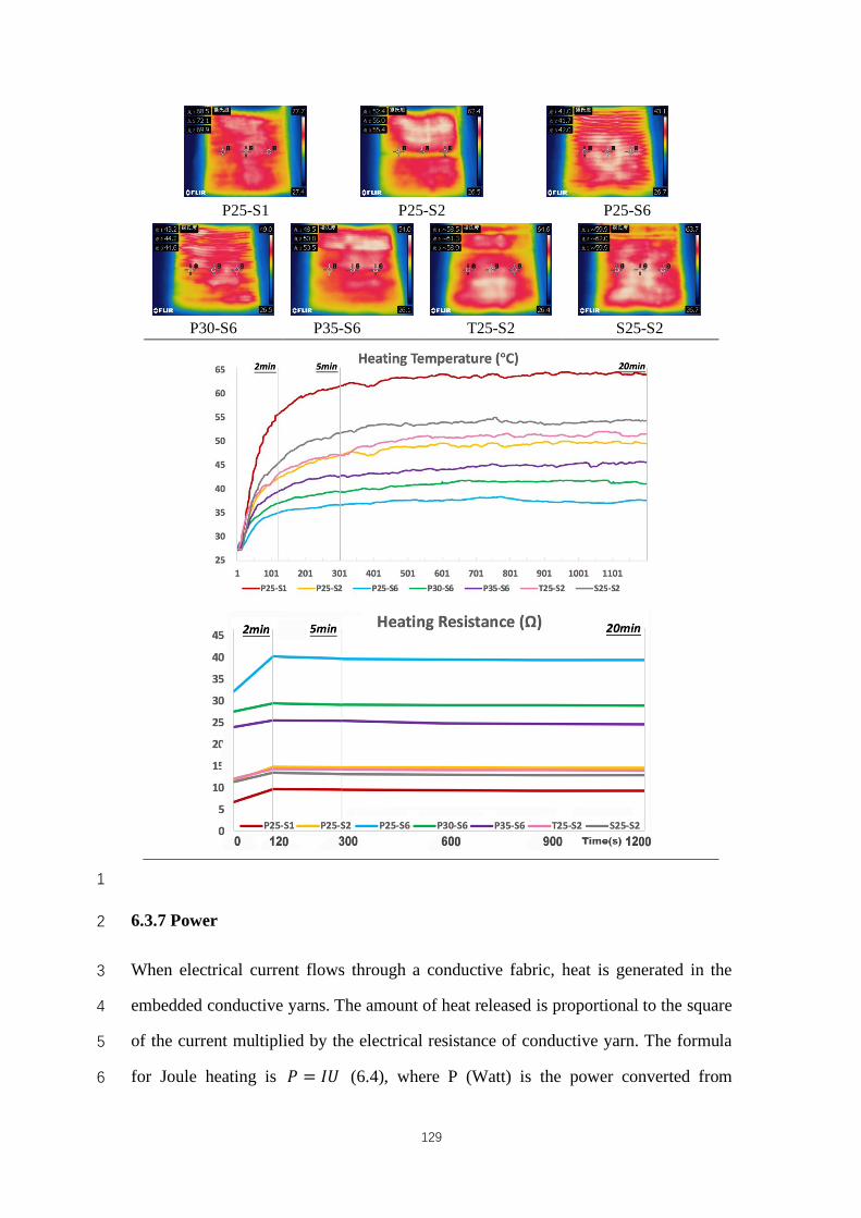
129

P25-S1 P25-S2 P25-S6

P30-S6 P35-S6 T25-S2 S25-S2

1

6.3.7 Power 2

When electrical current flows through a conductive fabric, heat is generated in the 3

embedded conductive yarns. The amount of heat released is proportional to the square 4

of the current multiplied by the electrical resistance of conductive yarn. The formula 5

for Joule heating is 𝑃 = 𝐼𝑈 (6.4), where P (Watt) is the power converted from 6

130

electrical energy to thermal energy, I (Ampere) is the current flowing through 1

conductive yarns, and U (Volt) is the current working voltage. Since Ohm’s Law is 2

applicable here, the formula can be rewritten in equivalent form: 𝑃 = 𝐼H𝑅 = 𝑈H/𝑅 3

(6.5), where R (Ω) is the equivalent resistance of TCWF samples. In this experiment, 4

direct current is the only consideration. The temperature of the surface of the TCWF 5

sample rises when a power supply is connected. Heat capacity is the measurable 6

physical quantity that specifies the amount of thermal energy required to change the 7

temperature of an object by a given amount. It is defined as the ratio of the amount of 8

thermal energy Q (Joule) transferred to an object and the resulting increase in 9

temperature T (Kelvin) of the object: 𝐶 = 𝑄 Δ𝑇⁄ (6.6). Normally, the term specific 10

heat capacity c (J/kg∙K) which is defined as heat capacity per unit mass is more 11

commonly used for experimental and theoretical purposes. Ideally, all the thermal 12

energy transferred from electrically energy will be absorbed by the fabric in each time 13

duration t (s). Therefore, it can deduce 𝑃𝑡 = 𝑄 = 𝑐𝑚Δ𝑇 (6.7), where m (kg) is the 14

mass of the TCWF sample. However, in practice, there will be certain amount of heat 15

loss to the surrounding environment. A quantity 𝜂(%) is thus introduced which refers 16

to the percentage of thermal energy contributed to the increase in temperature of 17

conductive fabric. Thus, the equation will be Pt𝜂 = 𝑐𝑚Δ𝑇 (6.8), or (𝑈H 𝑅⁄ )t𝜂 =18

𝑐𝑚Δ𝑇 (6.9). Thus, the amount of increase in temperature is approximately proportional 19

to the square of the voltage applied to the TCWF sample. 20

In this experiment, the electric power P is not constant since resistance value R is 21

temperature dependent. Therefore, transient analysis must be conducted to study the 22

detailed heating process. The model of heat transfer can be described as 𝑄 =𝑊 + 𝑆 23

(6.10), where Q is the electrical energy provided to the fabric, W is the actual energy 24

absorbed by the fabric contributed to the temperature rising, and S is the energy 25

dissipated to surrounding environment. Assuming very short time interval, it has 𝑑𝑄 =26

𝑑𝑊 + 𝑑𝑆 (6.11), known that 𝑑𝑄 = 𝑃 ∙ 𝑑𝑡 (6.12), 𝑑𝑊 = 𝑐𝑚 ∙ 𝑑𝑇 (6.13), and 𝑑𝑆 =27

𝛼(𝑇 − 𝑇6) ∙ 𝑑𝑡 (6.14), where 𝛼 is the heat dissipation coefficient (W/K) calculated in 28

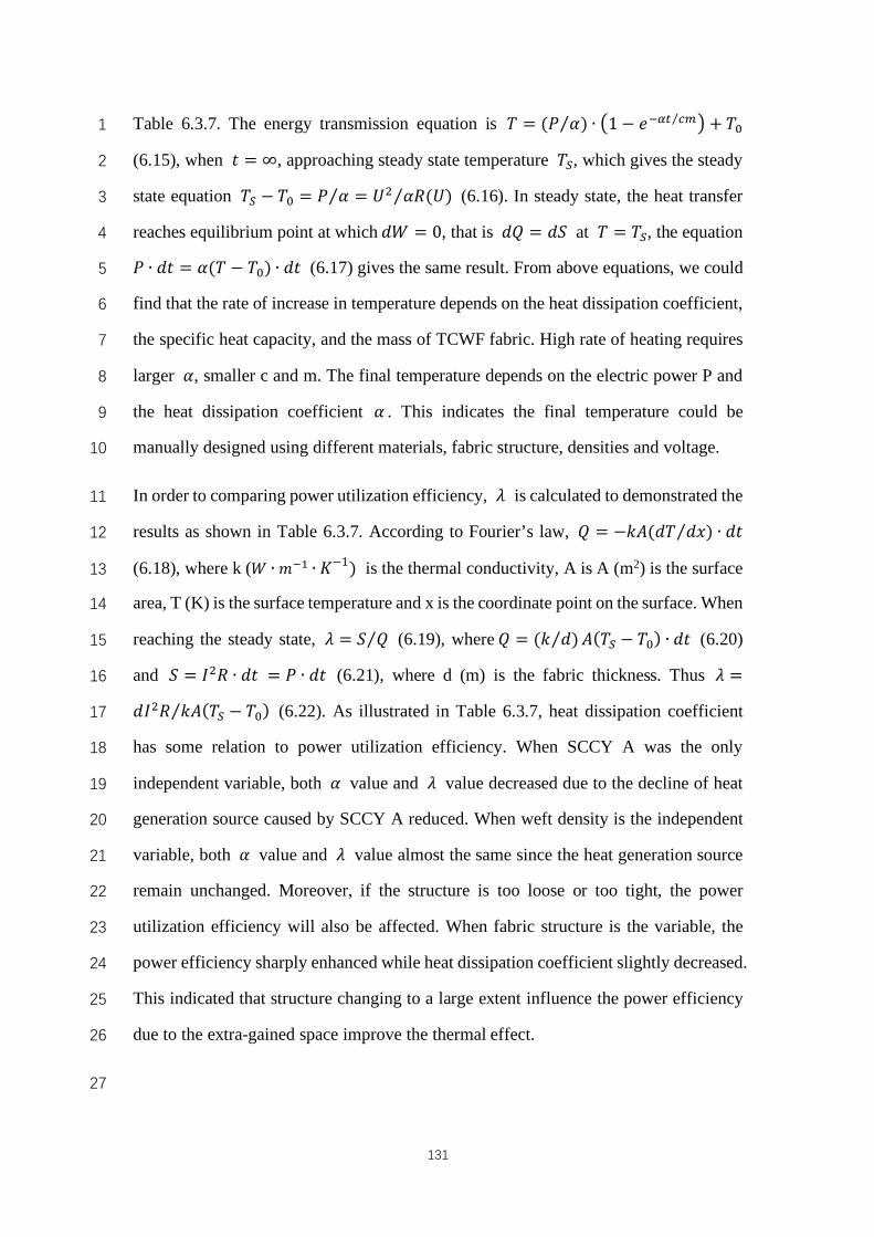
131

Table 6.3.7. The energy transmission equation is 𝑇 = (𝑃 𝛼⁄ ) ∙ Ó1 − 𝑒�ï> 01⁄ Ô + 𝑇6 1

(6.15), when 𝑡 = ∞, approaching steady state temperature 𝑇�, which gives the steady 2

state equation 𝑇� − 𝑇6 = 𝑃 𝛼⁄ = 𝑈H 𝛼𝑅(𝑈)⁄ (6.16). In steady state, the heat transfer 3

reaches equilibrium point at which𝑑𝑊 = 0, that is 𝑑𝑄 = 𝑑𝑆 at 𝑇 = 𝑇�, the equation 4

𝑃 ∙ 𝑑𝑡 = 𝛼(𝑇 − 𝑇6) ∙ 𝑑𝑡 (6.17) gives the same result. From above equations, we could 5

find that the rate of increase in temperature depends on the heat dissipation coefficient, 6

the specific heat capacity, and the mass of TCWF fabric. High rate of heating requires 7

larger 𝛼, smaller c and m. The final temperature depends on the electric power P and 8

the heat dissipation coefficient 𝛼 . This indicates the final temperature could be 9

manually designed using different materials, fabric structure, densities and voltage. 10

In order to comparing power utilization efficiency, 𝜆 is calculated to demonstrated the 11

results as shown in Table 6.3.7. According to Fourier’s law, 𝑄 = −𝑘𝐴(𝑑𝑇 𝑑𝑥) ∙ 𝑑𝑡⁄ 12

(6.18), where k (𝑊 ∙𝑚�� ∙ 𝐾−1) is the thermal conductivity, A is A (m2) is the surface 13

area, T (K) is the surface temperature and x is the coordinate point on the surface. When 14

reaching the steady state, 𝜆 = 𝑆 𝑄⁄ (6.19), where𝑄 = (𝑘 𝑑)⁄ 𝐴(𝑇� − 𝑇6) ∙ 𝑑𝑡 (6.20) 15

and 𝑆 = 𝐼H𝑅 ∙ 𝑑𝑡 = 𝑃 ∙ 𝑑𝑡 (6.21), where d (m) is the fabric thickness. Thus 𝜆 =16

𝑑𝐼H𝑅 𝑘𝐴(𝑇� − 𝑇6)⁄ (6.22). As illustrated in Table 6.3.7, heat dissipation coefficient 17

has some relation to power utilization efficiency. When SCCY A was the only 18

independent variable, both 𝛼 value and 𝜆 value decreased due to the decline of heat 19

generation source caused by SCCY A reduced. When weft density is the independent 20

variable, both 𝛼 value and 𝜆 value almost the same since the heat generation source 21

remain unchanged. Moreover, if the structure is too loose or too tight, the power 22

utilization efficiency will also be affected. When fabric structure is the variable, the 23

power efficiency sharply enhanced while heat dissipation coefficient slightly decreased. 24

This indicated that structure changing to a large extent influence the power efficiency 25

due to the extra-gained space improve the thermal effect. 26

27

132

1

Table 6.3.7 Results of sample power utilization efficiency 2 Sample P25-S1 P25-S2 P25-S6 P30-S6 P35-S6 T25-S2 S25-S2 α (W/K) 0.264 0.258 0.175 0.192 0.181 0.252 0.248 λ (%) 6.8% 7.0% 10.3% 9.4% 10.0% 7.2% 7.3%

6.4 Conclusion 3

Seven types of thermal conductive woven fabrics, with three structures, three weft 4

densities and three weft conductive yarn arrangements, wove with two different kinds 5

of silver-coated conductive yarns were designed, fabricated and tested. The results of 6

appearance, mass, thickness, air permeability, thermal conductivity, Qmax, electrical 7

resistance, heating temperature and power efficiency can guide the development of 8

application. Structure majorly influenced the fabric thickness, air permeability, thermal 9

effect and power efficiency except electrical resistance. Weft density has minor effect 10

on thickness and power efficiency while has considerable influence on air permeability, 11

thermal effect and resistance. SCCY A arrangement significantly changed thermal 12

effect, resistance and power efficiency. 13

14

15

16

133

Chapter 7 Impact of Different Conductive Path Design and 1

Fabrication on Temperature Variation of Thermal Stainless Steel 2

Woven Fabric 3

7.1 Introduction 4

Currently, the development of materials science and engineering has brought 5

tremendous changes in work and lifestyle. Products manufactured by stainless steel 6

yarn, a new type of metal material, have penetrated every corner of society and life. 7

Stainless steel yarn generally refers to a soft industrial material with a diameter of 10 8

µm or less, which is made of stainless steel of 304, 304L, 316, 316L et cetera. Stainless 9

steel yarn is a pure metal yarn which has obvious superiority in spinnability, usability 10

and financial cost compared with other metal fibers such as nickel, copper and 11

aluminum. Stainless steel yarn has good electrical conductivity, corrosion resistance 12

and heat resistance. Stainless steel yarn also meets the requirements of spinning in terms 13

of length and linear density. With a certain strength, the single yarn strength of 8 µm 14

can reach 2.94-5.88 cN, which is similar to the strength of single cotton yarn. However, 15

the rigidity of the stainless steel yarn is large and has no curl and poor elasticity. As 16

well as the toughness is inferior to that of ordinary textile fibers. [71-74] 17

Stainless steel yarn can be applied in both processed filament and staple fibers 18

depending on the application. The preparation of stainless steel filaments mainly adopts 19

the methods of wire drawing, melting and cutting, and the stainless steel staple fibers 20

are mainly formed by cutting the stainless steel filaments. Fabric made of pure stainless 21

steel filament can be made into pillow-type sealed bag or dust bag to be used for dust 22

removal system; or be made into conveyor belt, heat insulation curtain and heat-23

resistant cushion to be used in the production of car windshields, TV screens, kitchen 24

supplies. Stainless steel staple fiber is mainly blended with other fibers into 25

cotton/stainless steel, wool/stainless steel and polyester/stainless steel blended yarns. It 26

is used to produce antistatic fabric and electromagnetic wave shielding fabric. 27

134

Numerous researchers have studied in this field to develop better products. The fabric 1

used blended stainless steel yarn can be made into antistatic garments with reliable anti-2

combustion and explosion-proof effects, which can prevent the damage by self-control 3

failure caused by electromagnetic wave interference. In addition, anti-electromagnetic 4

wave radiation fabric can be developed to make electromagnetic wave shielding 5

garment, maternity garment, hospital special work garment et cetera. Moreover, metal 6

elements such as silver and copper have a permanent inhibitory effect on 7

microorganisms like viruses, bacteria, and fungi. Since stainless steel yarn contain these 8

elements, the blended yarn can be used to develop medical and health products. Not 9

only is the antibacterial effect permanent, but it has no toxic side effects on the human 10

body and meets the requirements of healthy yarn. Besides, the physical wrinkling and 11

scintillation effects of the fabric with blended yarn can be used to make fashion casual 12

garment as well. Apart from the civil products, stainless steel yarn is also widely used 13

in the military products, for instance, camouflage nets, radar target cloth, military multi-14

purpose tarpaulin et cetera. [75-80] 15

When it comes to thermal products, apart from carbon fiber sheet, the metal yarn is the 16

major material to applied in the products. Most researchers selected silver-coated yarn 17

to study and develop thermal fabric or garments. [7-12,14,16,17,19,64-70] In the 18

commercial market, most heated products are made with carbon fiber sheet, only few 19

of them are made with silver-coated yarn. [81-84] Only limited research and product 20

can be found about thermal function applied in stainless steel yarn. In this study, 21

thermal stainless steel woven fabric is designed and fabricated. After tests and 22

evaluation, temperature performance is analyzed to guide the design and potential 23

production. 24

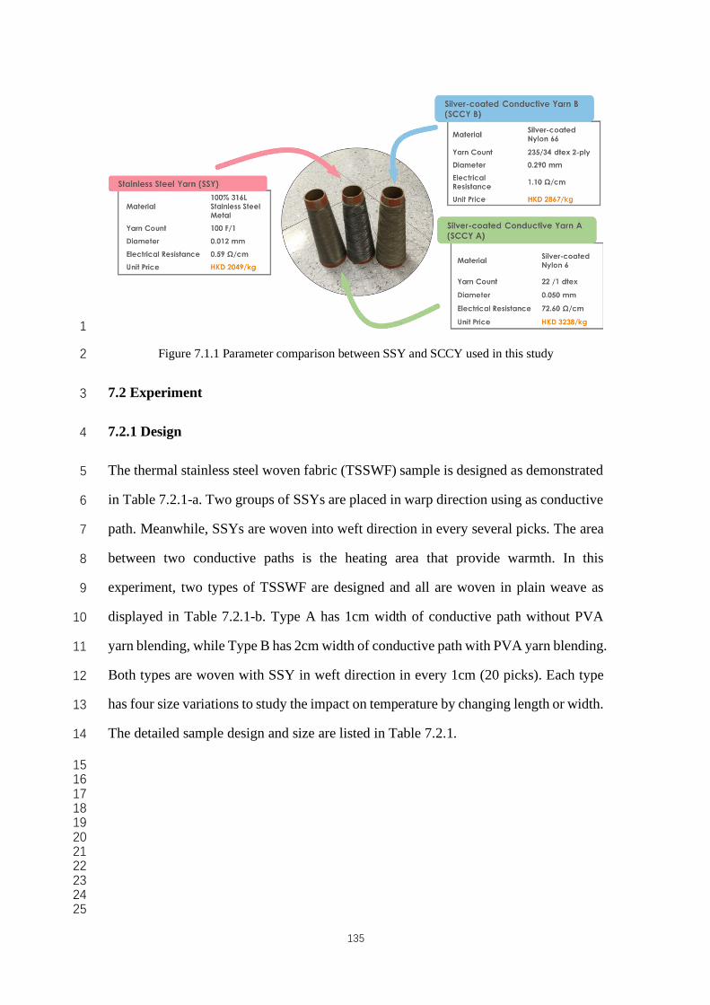
135

1

Figure 7.1.1 Parameter comparison between SSY and SCCY used in this study 2

7.2 Experiment 3

7.2.1 Design 4

The thermal stainless steel woven fabric (TSSWF) sample is designed as demonstrated 5

in Table 7.2.1-a. Two groups of SSYs are placed in warp direction using as conductive 6

path. Meanwhile, SSYs are woven into weft direction in every several picks. The area 7

between two conductive paths is the heating area that provide warmth. In this 8

experiment, two types of TSSWF are designed and all are woven in plain weave as 9

displayed in Table 7.2.1-b. Type A has 1cm width of conductive path without PVA 10

yarn blending, while Type B has 2cm width of conductive path with PVA yarn blending. 11

Both types are woven with SSY in weft direction in every 1cm (20 picks). Each type 12

has four size variations to study the impact on temperature by changing length or width. 13

The detailed sample design and size are listed in Table 7.2.1. 14

15 16 17 18 19 20 21 22 23 24 25

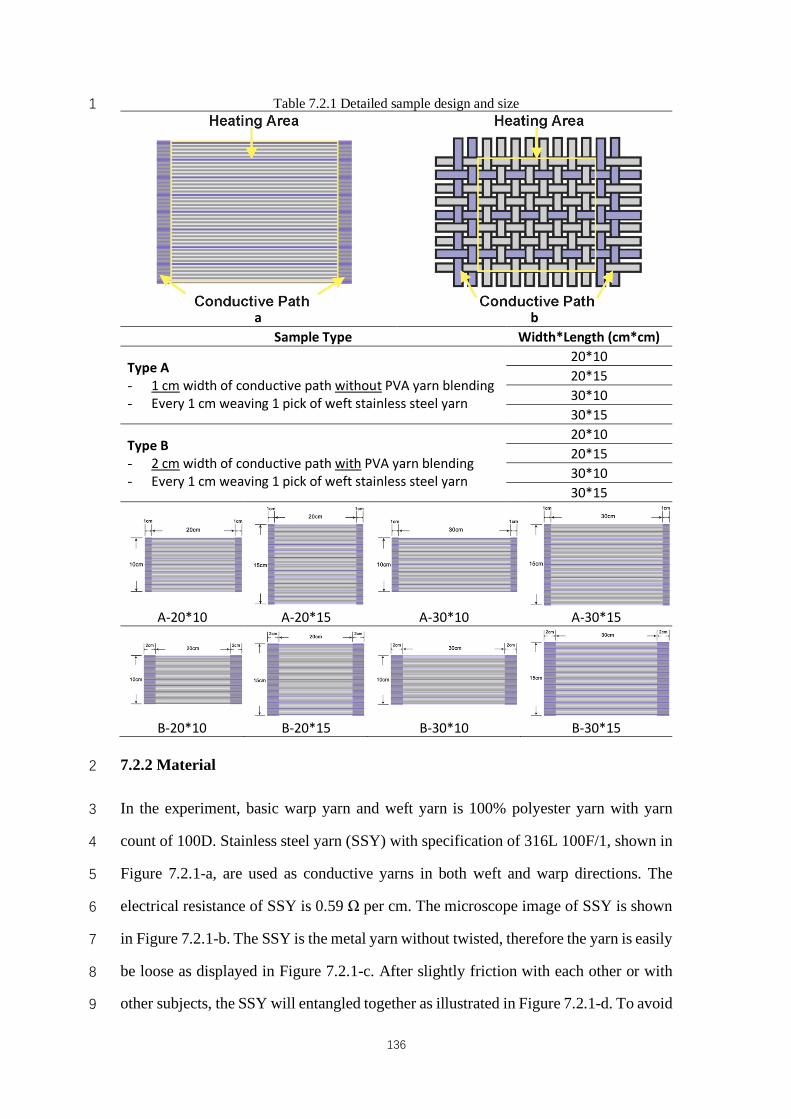
136

Table 7.2.1 Detailed sample design and size 1

a b

Sample Type Width*Length (cm*cm)

Type A - 1 cm width of conductive path without PVA yarn blending - Every 1 cm weaving 1 pick of weft stainless steel yarn

20*10 20*15 30*10 30*15

Type B - 2 cm width of conductive path with PVA yarn blending - Every 1 cm weaving 1 pick of weft stainless steel yarn

20*10 20*15 30*10 30*15

A-20*10 A-20*15 A-30*10 A-30*15

B-20*10 B-20*15 B-30*10 B-30*15

7.2.2 Material 2

In the experiment, basic warp yarn and weft yarn is 100% polyester yarn with yarn 3

count of 100D. Stainless steel yarn (SSY) with specification of 316L 100F/1, shown in 4

Figure 7.2.1-a, are used as conductive yarns in both weft and warp directions. The 5

electrical resistance of SSY is 0.59 Ω per cm. The microscope image of SSY is shown 6

in Figure 7.2.1-b. The SSY is the metal yarn without twisted, therefore the yarn is easily 7

be loose as displayed in Figure 7.2.1-c. After slightly friction with each other or with 8

other subjects, the SSY will entangled together as illustrated in Figure 7.2.1-d. To avoid 9

137

this situation, water soluble yarn is used to blend with SSY before weaving. The water 1

soluble yarn used is 100% PVA yarn with yarn count of 40S and will dissolve in water 2

at 20°C. Each kind of sample has manufactured 3 pieces by Staubli jacquard loom and 3

Doriner weaving loom in plain weave. The weft density is 20 picks per cm and the warp 4

density is 47 ends per cm. 5

a b

c d

Figure 7.2.1 a - SSY used in experiment; b - microscope image of normal SSY; c - untwisted and 6 easy to be loose; d - entangled together after friction 7

7.2.3 Test 8

All fabric samples are tested in a control room under the KSON control system with an 9

air pressure of 1 atm, relative humidity of 65±2, and temperature of 23±1℃. For 10

measurement purposes, all samples are placed inside the control room for 24 hours 11

before testing and none of them were treated with ironing before testing. Type A 12

samples are washed before testing for removing the PVA yarn while Type B are not. 13

The samples are aligned on an insulated hard board and electrical resistance of which 14

are measured by four-probe method with a Keithley 2010 multimeter. Samples are 15

heating under 5V by DaXin digital DC power supply DX3005DS and measured by 16

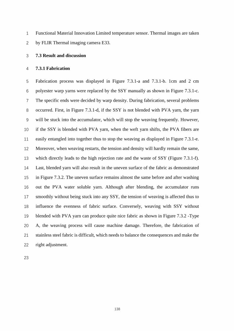
138

Functional Material Innovation Limited temperature sensor. Thermal images are taken 1

by FLIR Thermal imaging camera E33. 2


7.3.1 Fabrication 4

Fabrication process was displayed in Figure 7.3.1-a and 7.3.1-b. 1cm and 2 cm 5

polyester warp yarns were replaced by the SSY manually as shown in Figure 7.3.1-c. 6

The specific ends were decided by warp density. During fabrication, several problems 7

occurred. First, in Figure 7.3.1-d, if the SSY is not blended with PVA yarn, the yarn 8

will be stuck into the accumulator, which will stop the weaving frequently. However, 9

if the SSY is blended with PVA yarn, when the weft yarn shifts, the PVA fibers are 10

easily entangled into together thus to stop the weaving as displayed in Figure 7.3.1-e. 11

Moreover, when weaving restarts, the tension and density will hardly remain the same, 12

which directly leads to the high rejection rate and the waste of SSY (Figure 7.3.1-f). 13

Last, blended yarn will also result in the uneven surface of the fabric as demonstrated 14

in Figure 7.3.2. The uneven surface remains almost the same before and after washing 15

out the PVA water soluble yarn. Although after blending, the accumulator runs 16

smoothly without being stuck into any SSY, the tension of weaving is affected thus to 17

influence the evenness of fabric surface. Conversely, weaving with SSY without 18

blended with PVA yarn can produce quite nice fabric as shown in Figure 7.3.2 -Type 19

A, the weaving process will cause machine damage. Therefore, the fabrication of 20

stainless steel fabric is difficult, which needs to balance the consequences and make the 21

right adjustment. 22

23

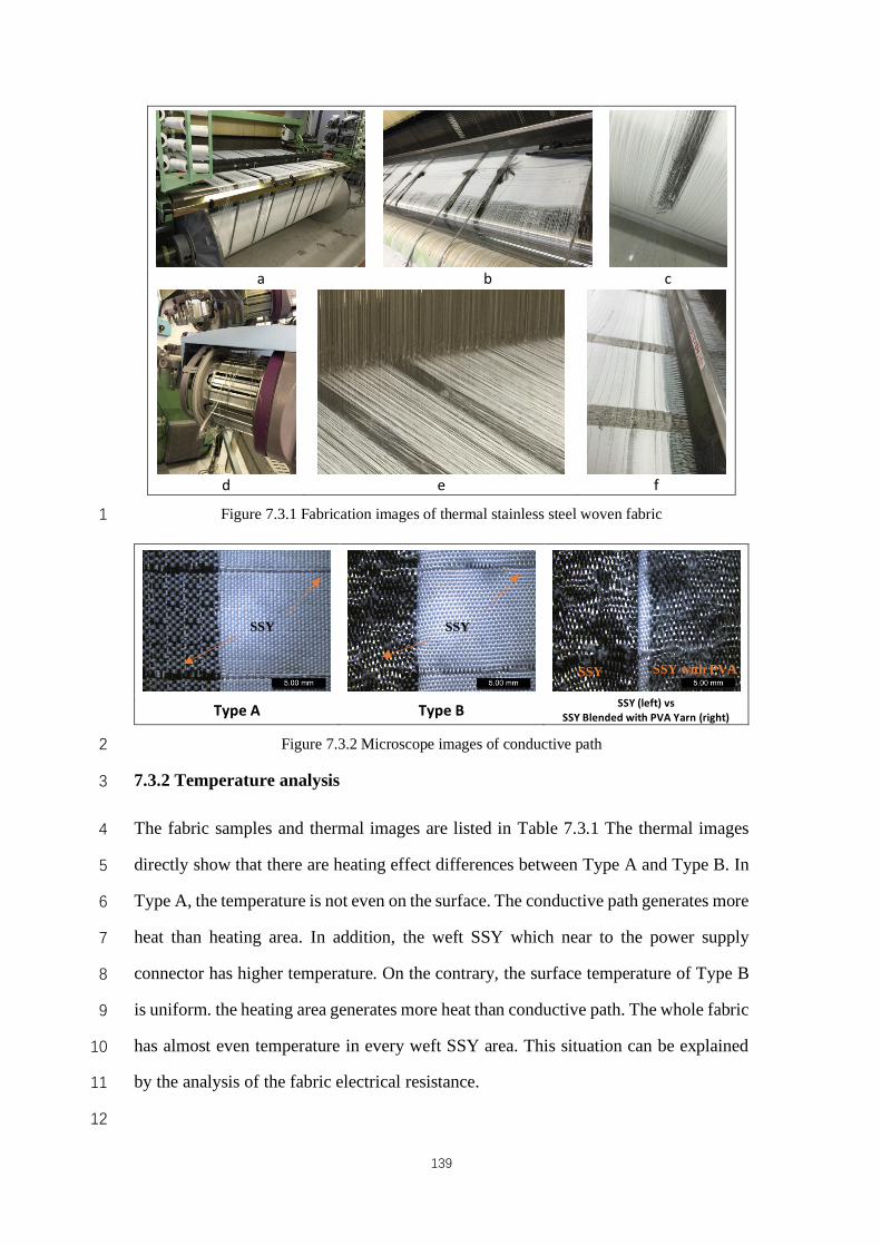
139

a b c

d e f

Figure 7.3.1 Fabrication images of thermal stainless steel woven fabric 1

Type A Type B SSY (left) vs

SSY Blended with PVA Yarn (right)

Figure 7.3.2 Microscope images of conductive path 2

7.3.2 Temperature analysis 3

The fabric samples and thermal images are listed in Table 7.3.1 The thermal images 4

directly show that there are heating effect differences between Type A and Type B. In 5

Type A, the temperature is not even on the surface. The conductive path generates more 6

heat than heating area. In addition, the weft SSY which near to the power supply 7

connector has higher temperature. On the contrary, the surface temperature of Type B 8

is uniform. the heating area generates more heat than conductive path. The whole fabric 9

has almost even temperature in every weft SSY area. This situation can be explained 10

by the analysis of the fabric electrical resistance. 11

12

SSY SSY with PVA

SSY SSY

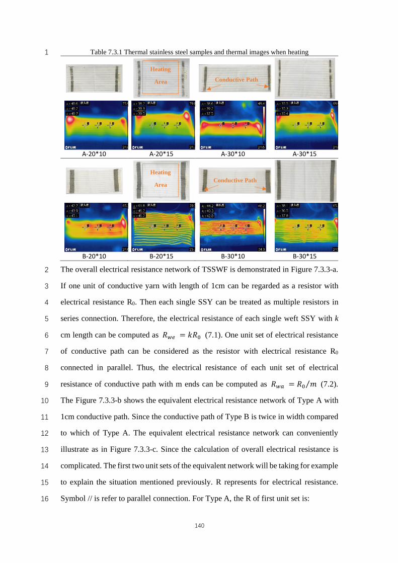
140

Table 7.3.1 Thermal stainless steel samples and thermal images when heating 1

A-20*10 A-20*15 A-30*10 A-30*15

B-20*10 B-20*15 B-30*10 B-30*15

The overall electrical resistance network of TSSWF is demonstrated in Figure 7.3.3-a. 2

If one unit of conductive yarn with length of 1cm can be regarded as a resistor with 3

electrical resistance R0. Then each single SSY can be treated as multiple resistors in 4

series connection. Therefore, the electrical resistance of each single weft SSY with k 5

cm length can be computed as 𝑅{� = 𝑘𝑅6 (7.1). One unit set of electrical resistance 6

of conductive path can be considered as the resistor with electrical resistance R0 7

connected in parallel. Thus, the electrical resistance of each unit set of electrical 8

resistance of conductive path with m ends can be computed as 𝑅{| = 𝑅6 𝑚⁄ (7.2). 9

The Figure 7.3.3-b shows the equivalent electrical resistance network of Type A with 10

1cm conductive path. Since the conductive path of Type B is twice in width compared 11

to which of Type A. The equivalent electrical resistance network can conveniently 12

illustrate as in Figure 7.3.3-c. Since the calculation of overall electrical resistance is 13

complicated. The first two unit sets of the equivalent network will be taking for example 14

to explain the situation mentioned previously. R represents for electrical resistance. 15

Symbol // is refer to parallel connection. For Type A, the R of first unit set is: 16

Heating

Area

Heating

Area

Conductive Path

Conductive Path

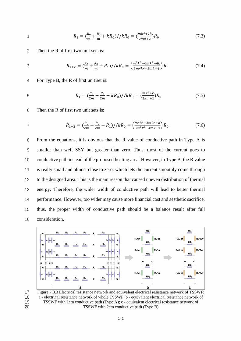
141

𝑅� = (å;1+ å;

1+ 𝑘𝑅6)//𝑘𝑅6 = (1¸

ë^H¸H¸1^H

)𝑅6 (7.3) 1

Then the R of first two unit sets is: 2

𝑅�^H = (å;1+ å;

1+ 𝑅�)//𝑘𝑅6 = V1

ë¸5^61¸ë^�¸�1ë¸ë^71¸^�

W𝑅6 (7.4) 3

For Type B, the R of first unit set is: 4

�� = (å;H1+ å;

H1+ 𝑘𝑅6)//𝑘𝑅6 = (1¸

ë^¸H¸1^�

)𝑅6 (7.5) 5

Then the R of first two unit sets is: 6

��^H = (å;H1+ å;

H1+ ��)//𝑘𝑅6 = V1

ë¸5^H1¸ë^¸�1ë¸ë^�1¸^�

W𝑅6 (7.6) 7

From the equations, it is obvious that the R value of conductive path in Type A is 8

smaller than weft SSY but greater than zero. Thus, most of the current goes to 9

conductive path instead of the proposed heating area. However, in Type B, the R value 10

is really small and almost close to zero, which lets the current smoothly come through 11

to the designed area. This is the main reason that caused uneven distribution of thermal 12

energy. Therefore, the wider width of conductive path will lead to better thermal 13

performance. However, too wider may cause more financial cost and aesthetic sacrifice, 14

thus, the proper width of conductive path should be a balance result after full 15

consideration. 16

Figure 7.3.3 Electrical resistance network and equivalent electrical resistance network of TSSWF: 17 a - electrical resistance network of whole TSSWF; b - equivalent electrical resistance network of 18

TSSWF with 1cm conductive path (Type A); c - equivalent electrical resistance network of 19 TSSWF with 2cm conductive path (Type B) 20

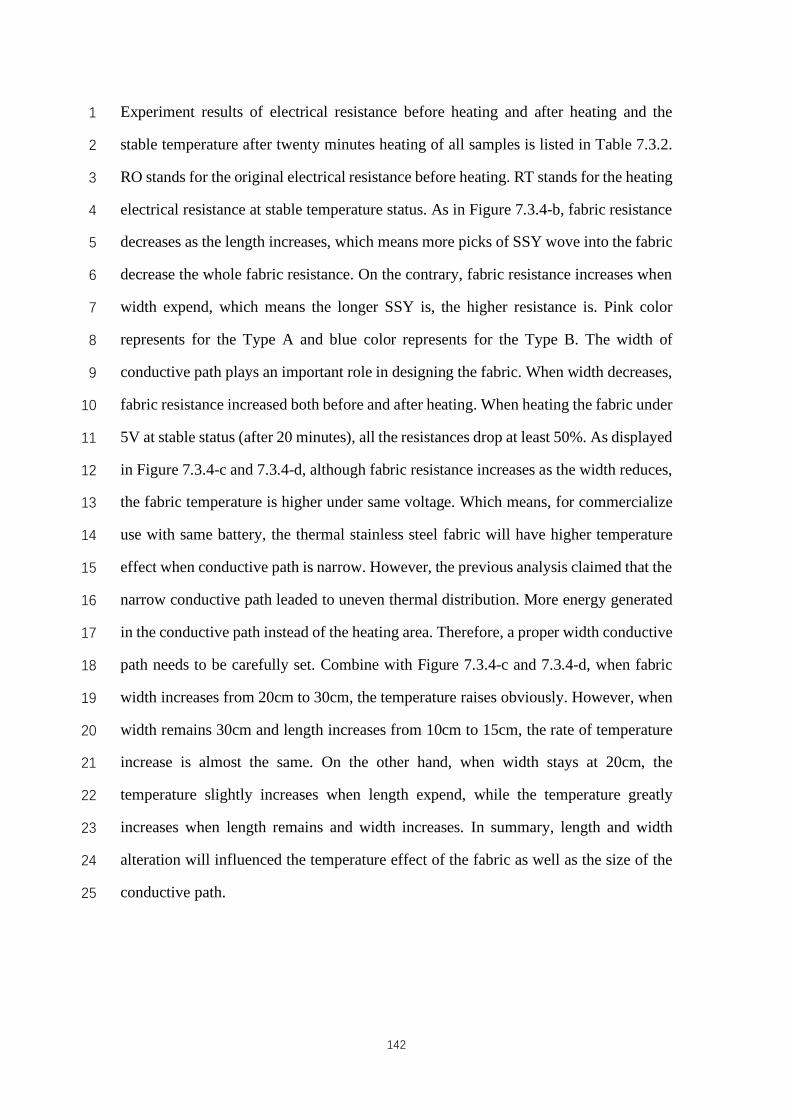
142

Experiment results of electrical resistance before heating and after heating and the 1

stable temperature after twenty minutes heating of all samples is listed in Table 7.3.2. 2

RO stands for the original electrical resistance before heating. RT stands for the heating 3

electrical resistance at stable temperature status. As in Figure 7.3.4-b, fabric resistance 4

decreases as the length increases, which means more picks of SSY wove into the fabric 5

decrease the whole fabric resistance. On the contrary, fabric resistance increases when 6

width expend, which means the longer SSY is, the higher resistance is. Pink color 7

represents for the Type A and blue color represents for the Type B. The width of 8

conductive path plays an important role in designing the fabric. When width decreases, 9

fabric resistance increased both before and after heating. When heating the fabric under 10

5V at stable status (after 20 minutes), all the resistances drop at least 50%. As displayed 11

in Figure 7.3.4-c and 7.3.4-d, although fabric resistance increases as the width reduces, 12

the fabric temperature is higher under same voltage. Which means, for commercialize 13

use with same battery, the thermal stainless steel fabric will have higher temperature 14

effect when conductive path is narrow. However, the previous analysis claimed that the 15

narrow conductive path leaded to uneven thermal distribution. More energy generated 16

in the conductive path instead of the heating area. Therefore, a proper width conductive 17

path needs to be carefully set. Combine with Figure 7.3.4-c and 7.3.4-d, when fabric 18

width increases from 20cm to 30cm, the temperature raises obviously. However, when 19

width remains 30cm and length increases from 10cm to 15cm, the rate of temperature 20

increase is almost the same. On the other hand, when width stays at 20cm, the 21

temperature slightly increases when length expend, while the temperature greatly 22

increases when length remains and width increases. In summary, length and width 23

alteration will influenced the temperature effect of the fabric as well as the size of the 24

conductive path. 25

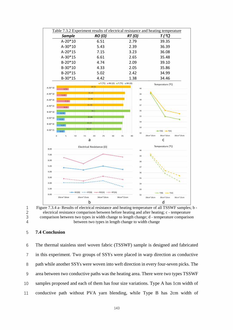
143

Table 7.3.2 Experiment results of electrical resistance and heating temperature Sample RO (Ω) RT (Ω) T (℃) A-20*10 6.51 2.79 39.35 A-30*10 5.43 2.39 36.39 A-20*15 7.15 3.23 36.08 A-30*15 6.61 2.65 35.48 B-20*10 4.74 2.09 39.10 B-30*10 4.33 2.05 35.86 B-20*15 5.02 2.42 34.99 B-30*15 4.42 1.38 34.46

a c

b d

Figure 7.3.4 a- Results of electrical resistance and heating temperature of all TSSWF samples; b - 1 electrical resistance comparison between before heating and after heating; c - temperature 2

comparison between two types in width change to length change; d - temperature comparison 3 between two types in length change to width change 4

7.4 Conclusion 5

The thermal stainless steel woven fabric (TSSWF) sample is designed and fabricated 6

in this experiment. Two groups of SSYs were placed in warp direction as conductive 7

path while another SSYs were woven into weft direction in every four-seven picks. The 8

area between two conductive paths was the heating area. There were two types TSSWF 9

samples proposed and each of them has four size variations. Type A has 1cm width of 10

conductive path without PVA yarn blending, while Type B has 2cm width of 11

144

conductive path with PVA yarn blending. PVA yarn was adopted into the fabrication 1

to reduce the damage during weaving. However, the outcome using PVA yarn was not 2

satisfied as planned. The fabric surface was affected by PVA yarn blending and 3

weaving process was also be affected by the PVA fiber tangling together. Results 4

showed that fabric length reduction can raise the temperature more effectively 5

compared to fabric width reduction. In addition, conductive path in wider width had 6

better thermal performance. However, the narrow width can save energy but caused 7

uneven thermal distribution. The wider width caused more energy to reach the same 8

temperature but had uniform temperature distribution. Although the financial cost was 9

higher. Therefore, a balanced design was required during commercial production. 10

11

12

13

14

15

16

17

18

19

20

21

22

23

145

Chapter 8 Development of Garment Prototype Applied in Thermal 1

Conductive Woven Fabrics 2

8.1 Introduction 3

In this chapter, one step formation technology is adopted to develop the thermal 4

functional fabric for garment prototype. Silver-coated conductive yarn is selected to be 5

the conductive material. Four different garments, dress, coat, jacket and shirt were 6

designed and manufactured. The thermal dress is selected to be one example for 7

detailed elaboration. 8

8.2 Thermal Functional Dress for Primary Dysmenorrhea Relief 9


Dysmenorrhea refers to the occurrence of painful cramps during women’s menstruation 11

[104]. It is a common disease in obstetrics and gynecology and has a great impact on 12

the physical and mental health of female compatriots, which has attracted extensive 13

attention from scholars worldwide. Primary dysmenorrhea (PD) refers to those with no 14

organic disease or specific abnormality in the reproductive organs, among which the 15

incidence rate of adolescent females is the highest. Secondary dysmenorrhea is usually 16

caused by pelvic organic lesions such as adenomyosis, endometriosis, pelvic 17

inflammatory disease or cervical stenosis, which is more common in women of 18

childbearing age [104-106]. PD occurs when prostaglandins, a hormone-like substance 19

produced by uterine tissue, cause intense muscle contraction in the uterus during 20

menstruation. The pain is convulsive and strongest on the lower abdomen, but they can 21

also radiate to the back and interior of the thigh. Cramps are usually accompanied by 22

one or more systemic symptoms including nausea and vomiting (89%), fatigue (85%), 23

diarrhea (60%), back pain (60%) and headache (45%). For hours to one day, the 24

symptoms seldom last more than two to three days [105]. 25

146

Studies indicate that the PD rate is highest among adolescents and young adults and 1

declines with age [104]. Related survey results claim that, for instance, in United States, 2

67% of teenagers and 27% of women in their 30s suffered from PD (Mai, Odle, & Frey, 3

2011). In Sweden, as high as 90% adolescent stated PD [104]. In Turkey, the incidence 4

of PD in young women is around 72% [107], while in China, the rate is around 68% 5

[108]. Although there is no organic abnormality in PD, the incident rate is very high 6

among young unmarried women. The clinical symptoms are obvious, which brings 7

many physical and psychological pains to them, thus greatly reducing their live 8

qualities. In addition, PD becomes the main reason for short-term absenteeism and also 9

cause economic loss. Such as among adolescent American girls, PD is the leading cause 10

that responsible for absence. In the workplace, dysmenorrhea causes 600 million 11

missing work hours in the United States with an economic loss of $2 billion each year 12

[104]. 13

However, there is currently no specific cure for PD. The methods of treatment and pain 14

relief include nonsteroidal anti-inflammatory drugs (NSAIDs), oral contraceptives, 15

surgery, herbal therapy, acupuncture therapy, thermal compress therapy, 16

transcutaneous electrical nerve stimulation (TENS) and physical exercise 17

[104,105,109-113]. Warming the abdomen or waist area is a well-known non-18

pharmacological treatment for dysmenorrhea. According to the survey, 75% of young 19

people and more than 50% of teenagers use non-pharmacological methods such as hot 20

water baths and heating pads to relieve menstruation [114-115]. For instance, in China, 21

64% of female college students choose hot compresses, while only 18% of whom 22

choose NSAIDs to reduce the painful symptoms [116]. Study has shown that attaching 23

a piece of heat-and steam-generating (HSG) sheet around 38.5 °C to the skin of the 24

lower abdomen for 8 hours, 57% and 63% of the subjects felt relief of abdominal pain, 25

and 54% and 61% of the subjects felt relief of low back pain on the first and second 26

day of menstruation, respectively. The results prove that the application of heating pad 27

can be used as a non-pharmacological method to alleviate the symptoms of PD [113]. 28

147

Current commercial market provides hot-water bag or hot patch for women to use in 1

dysmenorrhea. Thermal garment is one kind of heating clothes that provide warmth. 2

However, the existing thermal jacket are only targeted at chest, back, waist, leg and 3

foot. The thermal pad of which is either knitted with conductive yarn or use non-woven 4

carbon sheet. When searching on the internet, there are plenty of brands of heated 5

garment displayed in the Amazon, eBay and AliExpress [81,102,103]. Even the famous 6

brand such as warmX, Ravean and AVADE only have the same kinds of products [82-7

84]. Limited commercial thermal garment especially targeted for dysmenorrhea has 8

been developed, not to mention products applying thermal conductive woven fabrics 9

(TCWF). There are abundant researches of thermal conductive knitted fabrics and 10

apparels in studying the resistance models, fabric performance and functional garment 11

development [14,16,17,19,64]. There are several researches about resistance models of 12

TCWF [69,70], however limited research has been generated in fabric performance and 13

functional garment development of TCWF. In this study, novel TCWFs are designed 14

and fabricated. After tests and evaluation, an integrated commercialize-oriented 15

thermal functional garment is developed by adopting the optimized design combination. 16

The design method of TCWF development, apparel development and supporting 17

accessory development effectively reduce the material waste, energy consumption and 18

financial cost, which is likely to become the future inspiration and guidance of 19

industrial design and production. 20

21

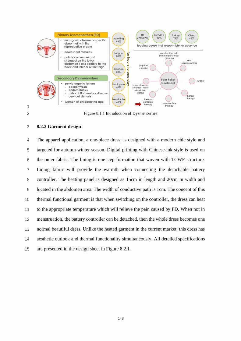
148

1

Figure 8.1.1 Introduction of Dysmenorrhea 2

8.2.2 Garment design 3

The apparel application, a one-piece dress, is designed with a modern chic style and 4

targeted for autumn-winter season. Digital printing with Chinese-ink style is used on 5

the outer fabric. The lining is one-step formation that woven with TCWF structure. 6

Lining fabric will provide the warmth when connecting the detachable battery 7

controller. The heating panel is designed as 15cm in length and 20cm in width and 8

located in the abdomen area. The width of conductive path is 1cm. The concept of this 9

thermal functional garment is that when switching on the controller, the dress can heat 10

to the appropriate temperature which will relieve the pain caused by PD. When not in 11

menstruation, the battery controller can be detached, then the whole dress becomes one 12

normal beautiful dress. Unlike the heated garment in the current market, this dress has 13

aesthetic outlook and thermal functionality simultaneously. All detailed specifications 14

are presented in the design sheet in Figure 8.2.1. 15

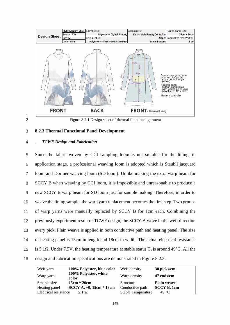
149

1 Figure 8.2.1 Design sheet of thermal functional garment 2

8.2.3 Thermal Functional Panel Development 3

- TCWF Design and Fabrication 4

Since the fabric woven by CCI sampling loom is not suitable for the lining, in 5

application stage, a professional weaving loom is adopted which is Staubli jacquard 6

loom and Doriner weaving loom (SD loom). Unlike making the extra warp beam for 7

SCCY B when weaving by CCI loom, it is impossible and unreasonable to produce a 8

new SCCY B warp beam for SD loom just for sample making. Therefore, in order to 9

weave the lining sample, the warp yarn replacement becomes the first step. Two groups 10

of warp yarns were manually replaced by SCCY B for 1cm each. Combining the 11

previously experiment result of TCWF design, the SCCY A wove in the weft direction 12

every pick. Plain weave is applied in both conductive path and heating panel. The size 13

of heating panel is 15cm in length and 18cm in width. The actual electrical resistance 14

is 5.1Ω. Under 7.5V, the heating temperature at stable status Ts is around 49°C. All the 15

design and fabrication specifications are demonstrated in Figure 8.2.2. 16

Weft yarn 100% Polyester, blue color Weft density 30 picks/cm

Warp yarn 100% Polyester, white color Warp density 47 ends/cm

Smaple size 15cm * 20cm Structure Plain weave Heating panel SCCY A, +0, 15cm * 18cm Conductive path SCCY B, 1cm Electrical resistance 5.1 Ω Stable Temperature 49 °C

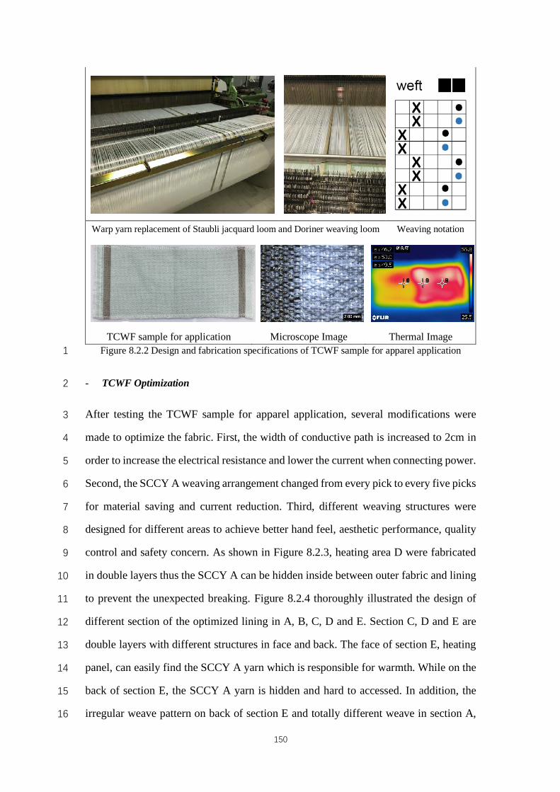
150

Warp yarn replacement of Staubli jacquard loom and Doriner weaving loom Weaving notation

TCWF sample for application Microscope Image Thermal Image Figure 8.2.2 Design and fabrication specifications of TCWF sample for apparel application 1

- TCWF Optimization 2

After testing the TCWF sample for apparel application, several modifications were 3

made to optimize the fabric. First, the width of conductive path is increased to 2cm in 4

order to increase the electrical resistance and lower the current when connecting power. 5

Second, the SCCY A weaving arrangement changed from every pick to every five picks 6

for material saving and current reduction. Third, different weaving structures were 7

designed for different areas to achieve better hand feel, aesthetic performance, quality 8

control and safety concern. As shown in Figure 8.2.3, heating area D were fabricated 9

in double layers thus the SCCY A can be hidden inside between outer fabric and lining 10

to prevent the unexpected breaking. Figure 8.2.4 thoroughly illustrated the design of 11

different section of the optimized lining in A, B, C, D and E. Section C, D and E are 12

double layers with different structures in face and back. The face of section E, heating 13

panel, can easily find the SCCY A yarn which is responsible for warmth. While on the 14

back of section E, the SCCY A yarn is hidden and hard to accessed. In addition, the 15

irregular weave pattern on back of section E and totally different weave in section A, 16

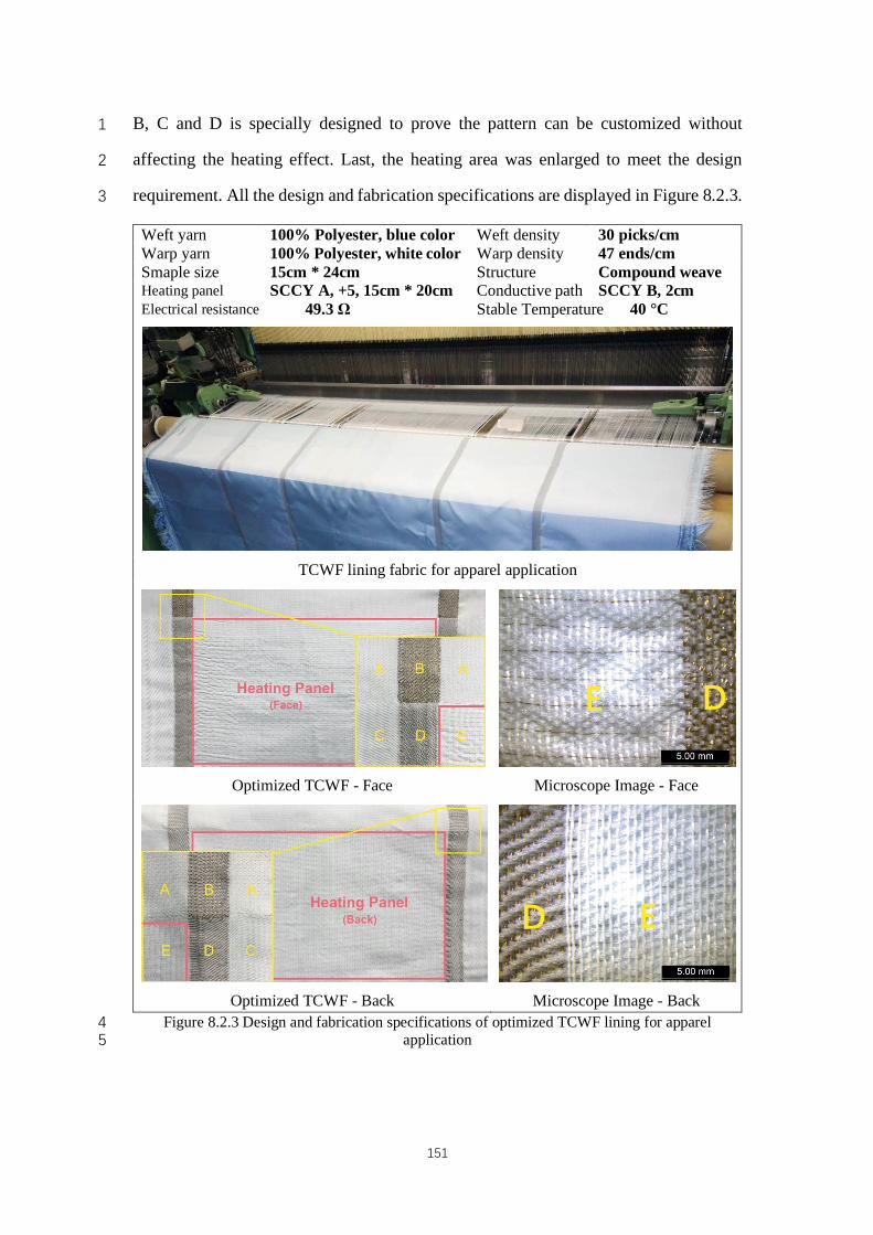
151

B, C and D is specially designed to prove the pattern can be customized without 1

affecting the heating effect. Last, the heating area was enlarged to meet the design 2

requirement. All the design and fabrication specifications are displayed in Figure 8.2.3. 3

Weft yarn 100% Polyester, blue color Weft density 30 picks/cm Warp yarn 100% Polyester, white color Warp density 47 ends/cm Smaple size 15cm * 24cm Structure Compound weave Heating panel SCCY A, +5, 15cm * 20cm Conductive path SCCY B, 2cm Electrical resistance 49.3 Ω Stable Temperature 40 °C

TCWF lining fabric for apparel application

Optimized TCWF - Face Microscope Image - Face

Optimized TCWF - Back Microscope Image - Back

Figure 8.2.3 Design and fabrication specifications of optimized TCWF lining for apparel 4 application 5

E D

D E

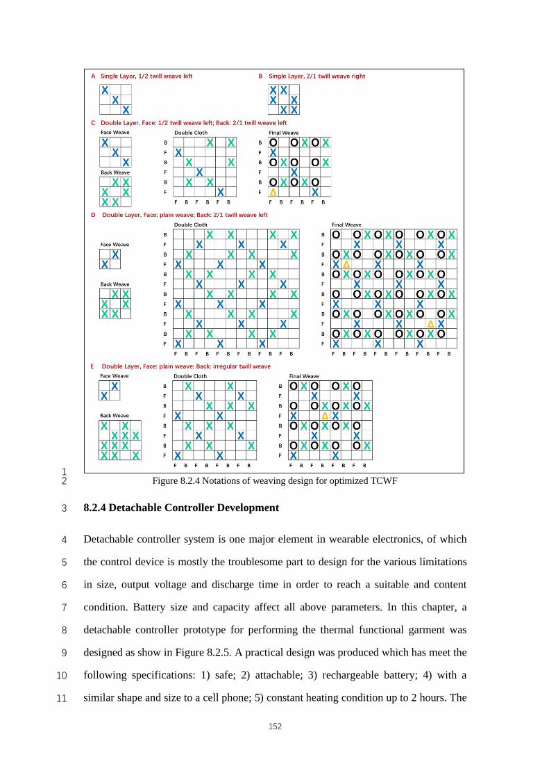
152

1 Figure 8.2.4 Notations of weaving design for optimized TCWF 2

8.2.4 Detachable Controller Development 3

Detachable controller system is one major element in wearable electronics, of which 4

the control device is mostly the troublesome part to design for the various limitations 5

in size, output voltage and discharge time in order to reach a suitable and content 6

condition. Battery size and capacity affect all above parameters. In this chapter, a 7

detachable controller prototype for performing the thermal functional garment was 8

designed as show in Figure 8.2.5. A practical design was produced which has meet the 9

following specifications: 1) safe; 2) attachable; 3) rechargeable battery; 4) with a 10

similar shape and size to a cell phone; 5) constant heating condition up to 2 hours. The 11

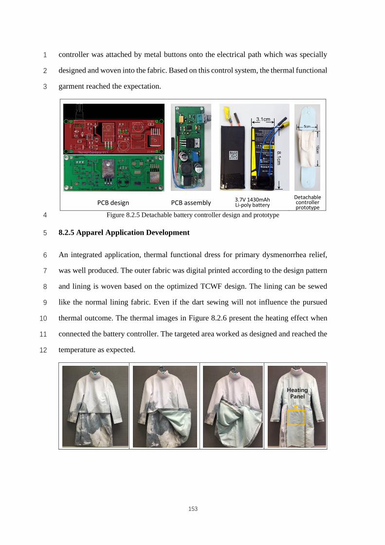
153

controller was attached by metal buttons onto the electrical path which was specially 1

designed and woven into the fabric. Based on this control system, the thermal functional 2

garment reached the expectation. 3

PCB design PCB assembly 3.7V 1430mAh

Li-poly battery Detachable controller prototype

Figure 8.2.5 Detachable battery controller design and prototype 4

8.2.5 Apparel Application Development 5

An integrated application, thermal functional dress for primary dysmenorrhea relief, 6

was well produced. The outer fabric was digital printed according to the design pattern 7

and lining is woven based on the optimized TCWF design. The lining can be sewed 8

like the normal lining fabric. Even if the dart sewing will not influence the pursued 9

thermal outcome. The thermal images in Figure 8.2.6 present the heating effect when 10

connected the battery controller. The targeted area worked as designed and reached the 11

temperature as expected. 12

Heating Panel

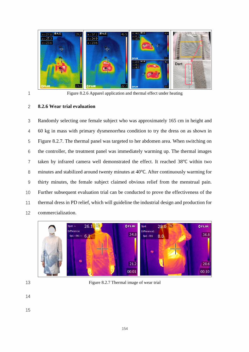
154

Figure 8.2.6 Apparel application and thermal effect under heating 1

8.2.6 Wear trial evaluation 2

Randomly selecting one female subject who was approximately 165 cm in height and 3

60 kg in mass with primary dysmenorrhea condition to try the dress on as shown in 4

Figure 8.2.7. The thermal panel was targeted to her abdomen area. When switching on 5

the controller, the treatment panel was immediately warming up. The thermal images 6

taken by infrared camera well demonstrated the effect. It reached 38℃ within two 7

minutes and stabilized around twenty minutes at 40℃. After continuously warming for 8

thirty minutes, the female subject claimed obvious relief from the menstrual pain. 9

Further subsequent evaluation trial can be conducted to prove the effectiveness of the 10

thermal dress in PD relief, which will guideline the industrial design and production for 11

commercialization. 12

Figure 8.2.7 Thermal image of wear trial 13

14

15

Dart

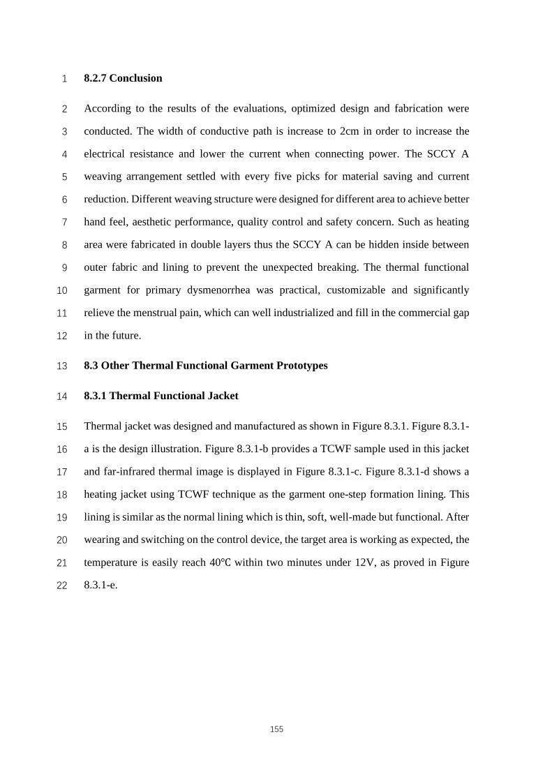
155

8.2.7 Conclusion 1

According to the results of the evaluations, optimized design and fabrication were 2

conducted. The width of conductive path is increase to 2cm in order to increase the 3

electrical resistance and lower the current when connecting power. The SCCY A 4

weaving arrangement settled with every five picks for material saving and current 5

reduction. Different weaving structure were designed for different area to achieve better 6

hand feel, aesthetic performance, quality control and safety concern. Such as heating 7

area were fabricated in double layers thus the SCCY A can be hidden inside between 8

outer fabric and lining to prevent the unexpected breaking. The thermal functional 9

garment for primary dysmenorrhea was practical, customizable and significantly 10

relieve the menstrual pain, which can well industrialized and fill in the commercial gap 11

in the future. 12

8.3 Other Thermal Functional Garment Prototypes 13

8.3.1 Thermal Functional Jacket 14

Thermal jacket was designed and manufactured as shown in Figure 8.3.1. Figure 8.3.1-15

a is the design illustration. Figure 8.3.1-b provides a TCWF sample used in this jacket 16

and far-infrared thermal image is displayed in Figure 8.3.1-c. Figure 8.3.1-d shows a 17

heating jacket using TCWF technique as the garment one-step formation lining. This 18

lining is similar as the normal lining which is thin, soft, well-made but functional. After 19

wearing and switching on the control device, the target area is working as expected, the 20

temperature is easily reach 40℃ within two minutes under 12V, as proved in Figure 21

8.3.1-e. 22

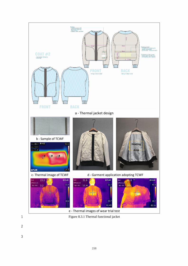
156

a - Thermal jacket design

b - Sample of TCWF

c- Thermal image of TCWF d - Garment application adopting TCWF

e - Thermal images of wear trial test Figure 8.3.1 Thermal functional jacket 1

2

3

Heating

Area

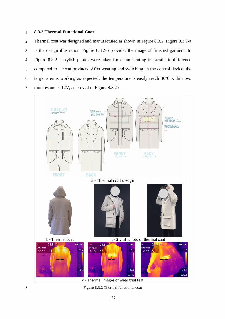
157

8.3.2 Thermal Functional Coat 1

Thermal coat was designed and manufactured as shown in Figure 8.3.2. Figure 8.3.2-a 2

is the design illustration. Figure 8.3.2-b provides the image of finished garment. In 3

Figure 8.3.2-c, stylish photos were taken for demonstrating the aesthetic difference 4

compared to current products. After wearing and switching on the control device, the 5

target area is working as expected, the temperature is easily reach 36℃ within two 6

minutes under 12V, as proved in Figure 8.3.2-d. 7

a - Thermal coat design

b - Thermal coat c - Stylish photo of thermal coat

d - Thermal images of wear trial test

Figure 8.3.2 Thermal functional coat 8

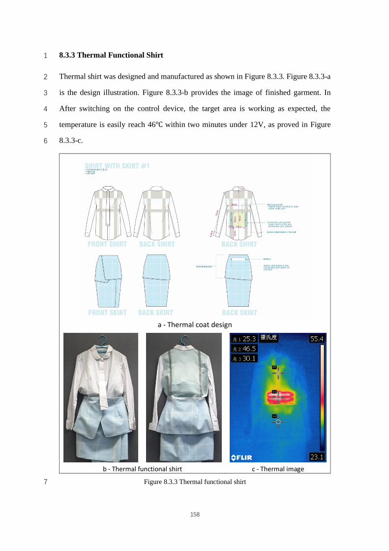
158

8.3.3 Thermal Functional Shirt 1

Thermal shirt was designed and manufactured as shown in Figure 8.3.3. Figure 8.3.3-a 2

is the design illustration. Figure 8.3.3-b provides the image of finished garment. In 3

After switching on the control device, the target area is working as expected, the 4

temperature is easily reach 46℃ within two minutes under 12V, as proved in Figure 5

8.3.3-c. 6

a - Thermal coat design

b - Thermal functional shirt c - Thermal image

Figure 8.3.3 Thermal functional shirt 7

159

Chapter 9 Development of Temperature Indicator Thermochromic 1

Pigment for Thermal Conductive Woven Textile 2

9.1 Introduction 3

There are a variety of different classes of color-changing materials. The energy sources 4

change leads to the alteration of their optical properties. Thermochromic materials 5

change colors with temperature changing. Most of them are reversible while some of 6

them are not. Thermochromic pigments are produced and commercialized by many 7

chemical companies in various fields of application. These pigments are used to 8

produce paints and inks for surface treatment or mixed with other materials such as 9

polymers for batch coloring. [85-86] Reversible thermochromic organic materials 10

generally consist of at least three components, a color former, color developer and 11

solvent. Color formers are electron donors, which are colorless dyes. When the pH 12

changes, these compounds are halochromic thus to change color. Their reaction with 13

the electron-accepting developer determines the position of the longest wavelength 14

absorption that results in coloration/decoloration. [87-91] At lower temperatures where 15

the solvent is solid and produces a colored dye developer complex; then at higher 16

temperature, solvent developer interaction dominates when solvent melts. As a result, 17

the dye developer complex is destroyed, turning the system into a colorless state. [92-18

94] To date, leuco dye-developer-solvent composites are the most important systems 19

for achieving thermochromic properties using organic materials. [95] 20

Temperature indicating paint (TIP) is one of the thermochromic pigments that coated 21

onto the subject surface to indicate the temperature change and distribution. When the 22

TIP coating is heated to the trigger temperature, the pigment color changes. [96] A 23

Germany compony invented the earliest TIP in 1938. In the 1940s and 1970s, there is 24

a great development of the research and application of TIP. In this period, easy-to-use 25

and sensitive TIP sheet and reversible TIP had been produced. After then, the research 26

focus gradually shifted to the area of low trigger temperature and reversible TIP.[96] 27

160

Currently, researchers have conducted a lot of work and have made many encouraging 1

progress.[97] In general, TIP technology is becoming a mature and widely recognized 2

reliable test technology of temperature measurement.[98] The application area of TIP 3

is various, such as mercury thermometers, millivoltmeters, temperature measurement 4

where high-radiation meters are not suitable for, and temperature distribution 5

measurement of continuous operation components and large-area surface.[96-101] For 6

instance, it can be used for over-temperature alarm of chemical, refining and reactor 7

wall. As well as temperature measurement and temperature distribution measurement 8

of aircraft engine, internal instrument and skin structure. The advantage of TIP is that 9

it can be adopted in occasions where the traditional temperature measurement 10

instrument cannot reach. It can measure surface temperature distribution, which is 11

convenient and equipment free. The disadvantage is that it is limited by the conditions 12

of use and have poor accuracy. [96-101] 13

Thermal products are rapidly increasing in the e-textile industry. Take thermal pad for 14

example, there are generally three common ways to measure the heating temperature: 15

thermometer, infrared thermal imaging camera and temperature sensor. When selling 16

the products, it is difficult to measure the thermal pads by the three ways mentioned 17

above due to the accuracy requirement or the price budget. As for designers, these 18

instruments may be hard to operate and too technical, thus refraining them from 19

designing related products. Therefore, an easier, cheaper, more rapid and convenient 20

method need to be approached. In this case, thermochromic pigment like TIP can be a 21

very useful method, by using which customers can more intuitively feel the temperature 22

change and range. In addition, the colorimetric result of different thermochromic 23

pigment can also help designers to create various pattern design which can cleverly 24

combined with the thermal products thus to add additional value. This study aims to 25

analyze the colorimetric properties of four thermochromic pigments and determine the 26

best temperature indicator pigment for thermal woven textile. 27

28

161

9.2 Experiment 1

Four thermochromic pigments, produced by Zhongshan JIAHUA printing material 2

company, China, in red, yellow, green and blue were used (Figure 9.2.1-a). According 3

to the manufacture’s specification, the activation temperature is 31 ℃. Each color was 4

brushed onto a 3 cm * 5.5 cm thin grey fabric around 2 cm * 2 cm. The pigment samples 5

were placed in thermostatic room at 20℃ in 3 hours in advance. They were heated 6

respectively by a 5.9 inches * 4.8 inches thermal woven fabric (Figure 9.2.1-c) which 7

was woven by a CCI tech automatic dobby sampling loom with plain structure, weft 8

densities of 30 picks/inch and warp density of 40 ends/inch. The conductive path was 9

woven by silver-coated conductive Yarn A (Figure 9.2.1-d), while the heating area was 10

woven by silver-coated conductive Yarn B (Figure 9.2.1-e) and was designed as shown 11

in Figure 9.2.1-f and Figure 1-g, which Yarn B was woven in every other pick. The 12

samples were measured at 40℃ (Figure 9.2.1-h), 50℃ (Figure 9.2.1-i), 60℃ (Figure 13

9.2.1-j) and 70℃ (Figure 9.2.1-k) under illuminant D65 light box as shown in Figure 14

9.2.1-b. The thermal woven fabric was given electricity at 8.5V, 11V, 13V and 14.8V 15

by DaXin digital DC power supply DX3005DS (Figure 9.2.1-p) and was measured 16

temperature by FLIR Thermal imaging camera E33 demonstrated in Figure 1-o. Color 17

assessment cabinet VeriVide CAC 120 (Figure 9.2.1-l) provided the light source. The 18

colors were measured by Konica Minolta CS-2000 spectroradiometer (Figure 9.2.1-m) 19

in real time when temperature raising up. GIT20 tripod (Figure 9.2.1-n) held the 20

spectroradiometer to keep the focal distance fixed. 21

22

23

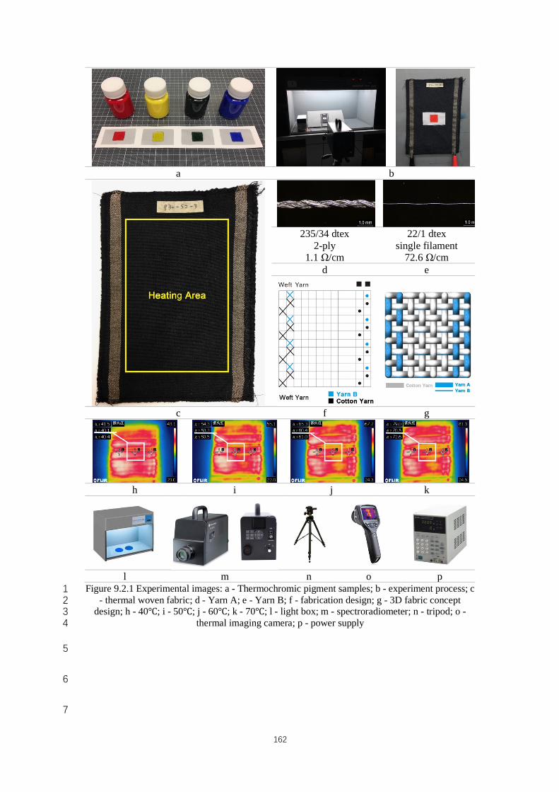
162

a b

235/34 dtex

2-ply 1.1 Ω/cm

22/1 dtex single filament

72.6 Ω/cm d e

c f g

h i j k

l m n o p Figure 9.2.1 Experimental images: a - Thermochromic pigment samples; b - experiment process; c 1

- thermal woven fabric; d - Yarn A; e - Yarn B; f - fabrication design; g - 3D fabric concept 2 design; h - 40℃; i - 50℃; j - 60℃; k - 70℃; l - light box; m - spectroradiometer; n - tripod; o - 3

thermal imaging camera; p - power supply 4

5

6

7

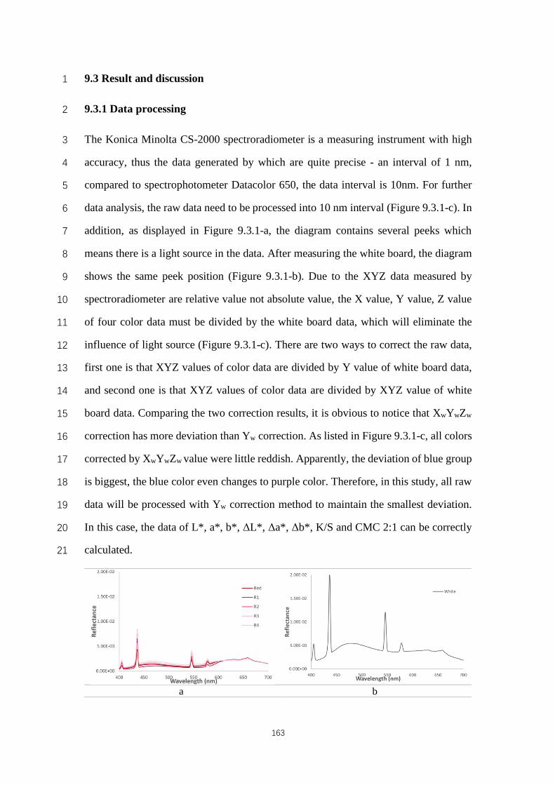
163


9.3.1 Data processing 2

The Konica Minolta CS-2000 spectroradiometer is a measuring instrument with high 3

accuracy, thus the data generated by which are quite precise - an interval of 1 nm, 4

compared to spectrophotometer Datacolor 650, the data interval is 10nm. For further 5

data analysis, the raw data need to be processed into 10 nm interval (Figure 9.3.1-c). In 6

addition, as displayed in Figure 9.3.1-a, the diagram contains several peeks which 7

means there is a light source in the data. After measuring the white board, the diagram 8

shows the same peek position (Figure 9.3.1-b). Due to the XYZ data measured by 9

spectroradiometer are relative value not absolute value, the X value, Y value, Z value 10

of four color data must be divided by the white board data, which will eliminate the 11

influence of light source (Figure 9.3.1-c). There are two ways to correct the raw data, 12

first one is that XYZ values of color data are divided by Y value of white board data, 13

and second one is that XYZ values of color data are divided by XYZ value of white 14

board data. Comparing the two correction results, it is obvious to notice that XwYwZw 15

correction has more deviation than Yw correction. As listed in Figure 9.3.1-c, all colors 16

corrected by XwYwZw value were little reddish. Apparently, the deviation of blue group 17

is biggest, the blue color even changes to purple color. Therefore, in this study, all raw 18

data will be processed with Yw correction method to maintain the smallest deviation. 19

In this case, the data of L*, a*, b*, ΔL*, Δa*, Δb*, K/S and CMC 2:1 can be correctly 20

calculated. 21

a b

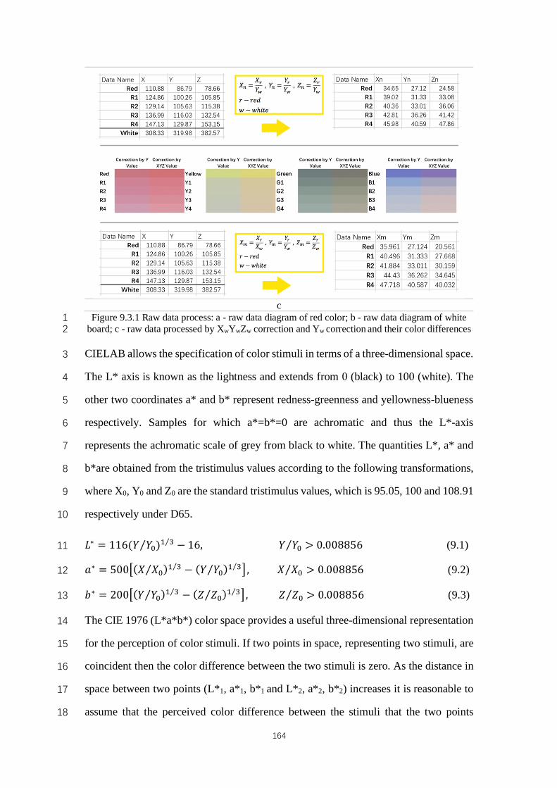
164

c

Figure 9.3.1 Raw data process: a - raw data diagram of red color; b - raw data diagram of white 1 board; c - raw data processed by XwYwZw correction and Yw correction and their color differences 2

CIELAB allows the specification of color stimuli in terms of a three-dimensional space. 3

The L* axis is known as the lightness and extends from 0 (black) to 100 (white). The 4

other two coordinates a* and b* represent redness-greenness and yellowness-blueness 5

respectively. Samples for which a*=b*=0 are achromatic and thus the L*-axis 6

represents the achromatic scale of grey from black to white. The quantities L*, a* and 7

b*are obtained from the tristimulus values according to the following transformations, 8

where X0, Y0 and Z0 are the standard tristimulus values, which is 95.05, 100 and 108.91 9

respectively under D65. 10

𝐿∗ = 116(𝑌 𝑌6⁄ )� �⁄ − 16, 𝑌 𝑌6⁄ > 0.008856 (9.1) 11

𝑎∗ = 500`(𝑋 𝑋6⁄ )� �⁄ − (𝑌 𝑌6⁄ )� �⁄ b,𝑋 𝑋6⁄ > 0.008856 (9.2) 12

𝑏∗ = 200`(𝑌 𝑌6⁄ )� �⁄ − (𝑍 𝑍6⁄ )� �⁄ b,𝑍 𝑍6⁄ > 0.008856 (9.3) 13

The CIE 1976 (L*a*b*) color space provides a useful three-dimensional representation 14

for the perception of color stimuli. If two points in space, representing two stimuli, are 15

coincident then the color difference between the two stimuli is zero. As the distance in 16

space between two points (L*1, a*1, b*1 and L*2, a*2, b*2) increases it is reasonable to 17

assume that the perceived color difference between the stimuli that the two points 18

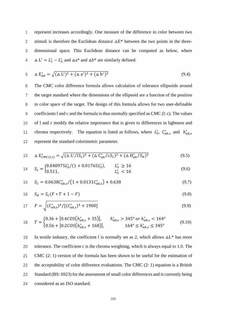
165

represent increases accordingly. One measure of the difference in color between two 1

stimuli is therefore the Euclidean distance △E* between the two points in the three-2

dimensional space. This Euclidean distance can be computed as below, where 3

△ L∗ = 𝐿�∗ − 𝐿H∗ and △a* and △b* are similarly defined. 4

△ E|:∗ = D(△ L∗)H + (△ a∗)H + (△ b∗)H (9.4) 5

The CMC color difference formula allows calculation of tolerance ellipsoids around 6

the target standard where the dimensions of the ellipsoid are a function of the position 7

in color space of the target. The design of this formula allows for two user-definable 8

coefficients l and c and the formula is thus normally specified as CMC (l: c). The values 9

of l and c modify the relative importance that is given to differences in lightness and 10

chroma respectively. The equation is listed as follows, where 𝐿�∗ , 𝐶|:,;∗ and ℎ|:,;∗ 11

represent the standard colorimetric parameter. 12

△ E<©<(=:0)∗ = D(△ L∗ 𝑙𝑆>⁄ )H + (△ C|:∗ 𝑐𝑆<⁄ )H + (△ H|:∗ 𝑆@⁄ )H (9.5) 13

𝑆> = A0.040975𝐿�∗ (1 + 0.01765𝐿�∗ ),⁄ 𝐿�∗ ≥ 16

0.511,𝐿�∗ < 16 (9.6) 14

𝑆< = 0.0638𝐶|:,;∗ Ó1 + 0.0131𝐶|:,;∗ Ô + 0.638⁄ (9.7) 15

𝑆@ = 𝑆<(𝐹 ∗ 𝑇 + 1 − 𝐹) (9.8) 16

𝐹 = ÷(𝐶|:,;∗ )� [(𝐶|:,;∗ )� + 1900]⁄ (9.9) 17

𝑇 = B0.36+ ÿ0.4𝐶𝑂𝑆Óℎ|:,;∗ + 35Ôÿ,ℎ|:,;∗ > 345°𝑜𝑟ℎ|:,;∗ < 164°0.56+ ÿ0.2𝐶𝑂𝑆Óℎ|:,;∗ + 168Ôÿ,164° ≤ ℎ|:,;∗ ≤ 345°

(9.10) 18

In textile industry, the coefficient l is normally set as 2, which allows △L* has more 19

tolerance. The coefficient c is the chroma weighting, which is always equal to 1.0. The 20

CMC (2: 1) version of the formula has been shown to be useful for the estimation of 21

the acceptability of color difference evaluations. The CMC (2: 1) equation is a British 22

Standard (BS: 6923) for the assessment of small color differences and is currently being 23

considered as an ISO standard. 24

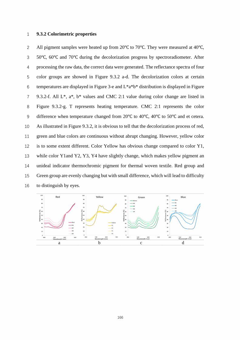
166

9.3.2 Colorimetric properties 1

All pigment samples were heated up from 20℃ to 70℃. They were measured at 40℃, 2

50℃, 60℃ and 70℃ during the decolorization progress by spectroradiometer. After 3

processing the raw data, the correct data were generated. The reflectance spectra of four 4

color groups are showed in Figure 9.3.2 a-d. The decolorization colors at certain 5

temperatures are displayed in Figure 3-e and L*a*b* distribution is displayed in Figure 6

9.3.2-f. All L*, a*, b* values and CMC 2:1 value during color change are listed in 7

Figure 9.3.2-g. T represents heating temperature. CMC 2:1 represents the color 8

difference when temperature changed from 20℃ to 40℃, 40℃ to 50℃ and et cetera. 9

As illustrated in Figure 9.3.2, it is obvious to tell that the decolorization process of red, 10

green and blue colors are continuous without abrupt changing. However, yellow color 11

is to some extent different. Color Yellow has obvious change compared to color Y1, 12

while color Y1and Y2, Y3, Y4 have slightly change, which makes yellow pigment an 13

unideal indicator thermochromic pigment for thermal woven textile. Red group and 14

Green group are evenly changing but with small difference, which will lead to difficulty 15

to distinguish by eyes. 16

a b c d

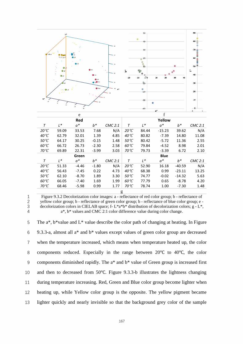
167

e f Red Yellow

T L* a* b* CMC 2:1 T L* a* b* CMC 2:1 20℃ 59.09 33.53 7.68 N/A 20℃ 84.44 -15.23 39.62 N/A 40℃ 62.79 32.01 1.39 4.85 40℃ 80.82 -7.39 14.80 11.08 50℃ 64.17 30.25 -0.15 1.48 50℃ 80.42 -5.72 11.36 2.55 60℃ 66.72 26.73 -2.30 2.58 60℃ 79.84 -4.52 8.98 2.01 70℃ 69.89 22.31 -3.99 3.03 70℃ 79.73 -3.39 6.72 2.10

Green Blue T L* a* b* CMC 2:1 T L* a* b* CMC 2:1

20℃ 51.33 -4.46 -1.80 N/A 20℃ 52.90 16.18 -40.59 N/A 40℃ 56.43 -7.45 0.22 4.73 40℃ 68.38 0.99 -23.11 13.25 50℃ 62.10 -8.70 1.89 3.30 50℃ 74.77 -0.02 -14.32 5.63 60℃ 66.05 -7.40 1.69 1.99 60℃ 77.79 0.65 -8.78 4.20 70℃ 68.46 -5.98 0.99 1.77 70℃ 78.74 1.00 -7.30 1.48

g Figure 9.3.2 Decolorization color images: a - reflectance of red color group; b - reflectance of 1

yellow color group; b - reflectance of green color group; b - reflectance of blue color group; e - 2 decolorization colors in CIELAB space; f- L*a*b* distribution of decolorization colors; g - L*, 3

a*, b* values and CMC 2:1 color difference value during color change. 4

The a*, b*value and L* value describe the color path of changing at heating. In Figure 5

9.3.3-a, almost all a* and b* values except values of green color group are decreased 6

when the temperature increased, which means when temperature heated up, the color 7

components reduced. Especially in the range between 20℃ to 40℃, the color 8

components diminished rapidly. The a* and b* value of Green group is increased first 9

and then to decreased from 50℃. Figure 9.3.3-b illustrates the lightness changing 10

during temperature increasing. Red, Green and Blue color group become lighter when 11

heating up, while Yellow color group is the opposite. The yellow pigment became 12

lighter quickly and nearly invisible so that the background grey color of the sample 13

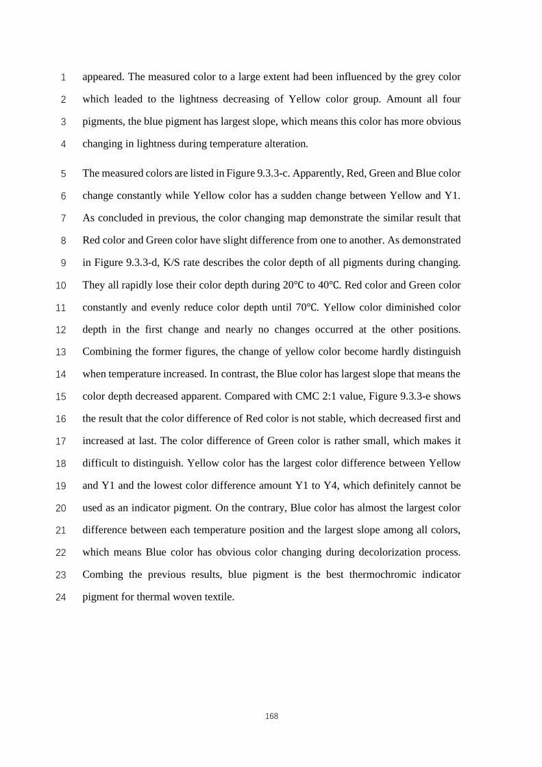
168

appeared. The measured color to a large extent had been influenced by the grey color 1

which leaded to the lightness decreasing of Yellow color group. Amount all four 2

pigments, the blue pigment has largest slope, which means this color has more obvious 3

changing in lightness during temperature alteration. 4

The measured colors are listed in Figure 9.3.3-c. Apparently, Red, Green and Blue color 5

change constantly while Yellow color has a sudden change between Yellow and Y1. 6

As concluded in previous, the color changing map demonstrate the similar result that 7

Red color and Green color have slight difference from one to another. As demonstrated 8

in Figure 9.3.3-d, K/S rate describes the color depth of all pigments during changing. 9

They all rapidly lose their color depth during 20℃ to 40℃. Red color and Green color 10

constantly and evenly reduce color depth until 70℃. Yellow color diminished color 11

depth in the first change and nearly no changes occurred at the other positions. 12

Combining the former figures, the change of yellow color become hardly distinguish 13

when temperature increased. In contrast, the Blue color has largest slope that means the 14

color depth decreased apparent. Compared with CMC 2:1 value, Figure 9.3.3-e shows 15

the result that the color difference of Red color is not stable, which decreased first and 16

increased at last. The color difference of Green color is rather small, which makes it 17

difficult to distinguish. Yellow color has the largest color difference between Yellow 18

and Y1 and the lowest color difference amount Y1 to Y4, which definitely cannot be 19

used as an indicator pigment. On the contrary, Blue color has almost the largest color 20

difference between each temperature position and the largest slope among all colors, 21

which means Blue color has obvious color changing during decolorization process. 22

Combing the previous results, blue pigment is the best thermochromic indicator 23

pigment for thermal woven textile. 24

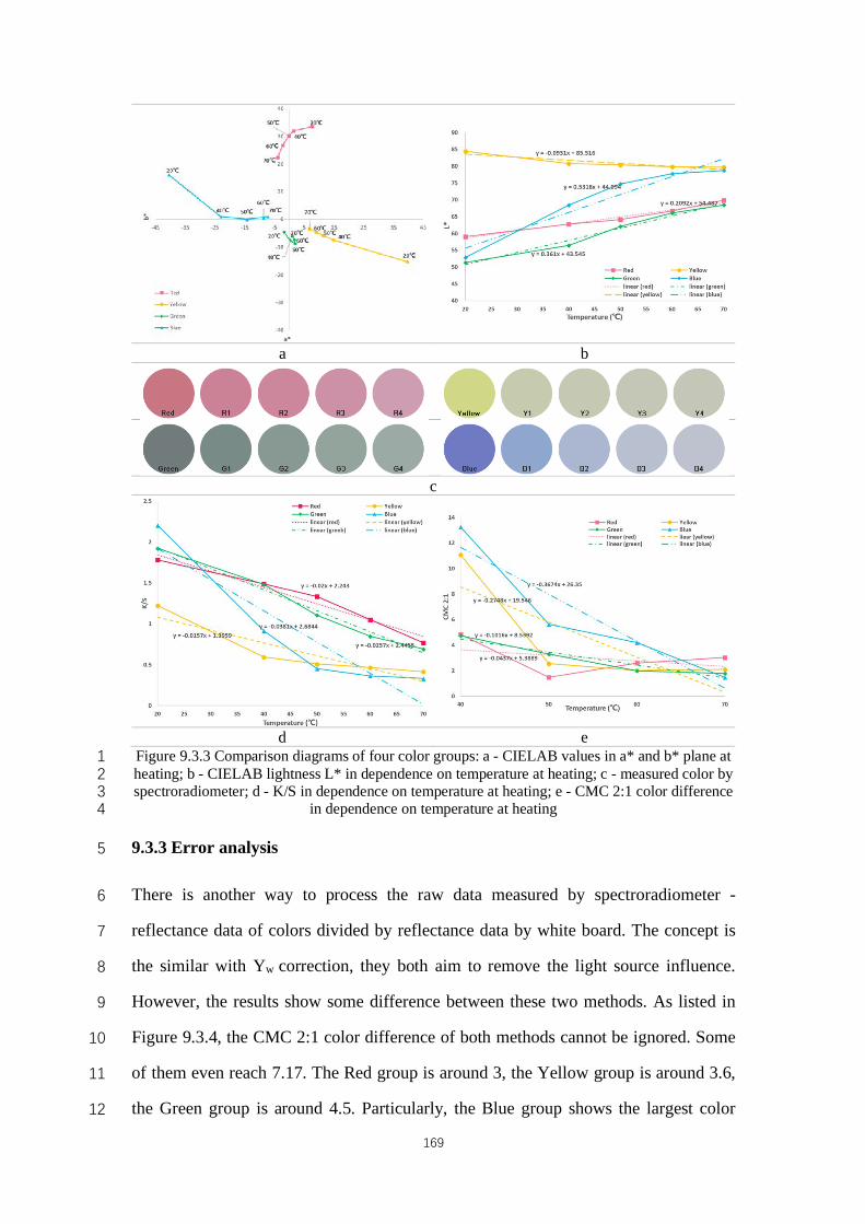
169

a b

c

d e Figure 9.3.3 Comparison diagrams of four color groups: a - CIELAB values in a* and b* plane at 1 heating; b - CIELAB lightness L* in dependence on temperature at heating; c - measured color by 2 spectroradiometer; d - K/S in dependence on temperature at heating; e - CMC 2:1 color difference 3

in dependence on temperature at heating 4

9.3.3 Error analysis 5

There is another way to process the raw data measured by spectroradiometer - 6

reflectance data of colors divided by reflectance data by white board. The concept is 7

the similar with Yw correction, they both aim to remove the light source influence. 8

However, the results show some difference between these two methods. As listed in 9

Figure 9.3.4, the CMC 2:1 color difference of both methods cannot be ignored. Some 10

of them even reach 7.17. The Red group is around 3, the Yellow group is around 3.6, 11

the Green group is around 4.5. Particularly, the Blue group shows the largest color 12

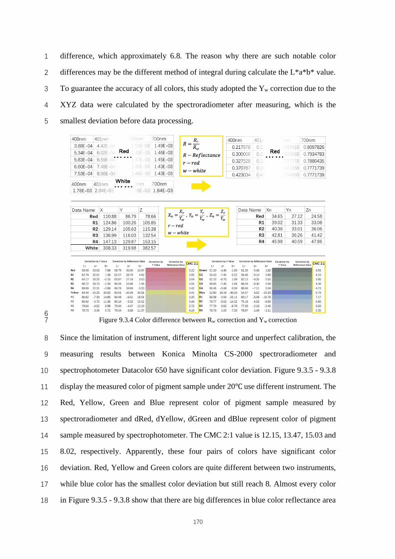
170

difference, which approximately 6.8. The reason why there are such notable color 1

differences may be the different method of integral during calculate the L*a*b* value. 2

To guarantee the accuracy of all colors, this study adopted the Yw correction due to the 3

XYZ data were calculated by the spectroradiometer after measuring, which is the 4

smallest deviation before data processing. 5

6 Figure 9.3.4 Color difference between Rw correction and Yw correction 7

Since the limitation of instrument, different light source and unperfect calibration, the 8

measuring results between Konica Minolta CS-2000 spectroradiometer and 9

spectrophotometer Datacolor 650 have significant color deviation. Figure 9.3.5 - 9.3.8 10

display the measured color of pigment sample under 20℃ use different instrument. The 11

Red, Yellow, Green and Blue represent color of pigment sample measured by 12

spectroradiometer and dRed, dYellow, dGreen and dBlue represent color of pigment 13

sample measured by spectrophotometer. The CMC 2:1 value is 12.15, 13.47, 15.03 and 14

8.02, respectively. Apparently, these four pairs of colors have significant color 15

deviation. Red, Yellow and Green colors are quite different between two instruments, 16

while blue color has the smallest color deviation but still reach 8. Almost every color 17

in Figure 9.3.5 - 9.3.8 show that there are big differences in blue color reflectance area 18

171

and gradually diminish. In the red color reflectance area, the graphs are almost 1

overlapping. All four colors have over 10 values biases in lightness which explains why 2

the color measured by spectroradiometer appear dark and greyish. 3

The most possibly reason may be the different light source influence. The 4

spectroradiometer was measured samples under real light source - illuminant D65 from 5

light box, while the spectrophotometer used theoretical illuminant D65 to be the light 6

source. These two light sources are supposed to be the same, however, they result in 7

different measurement. Moreover, these two instruments have different measuring 8

method. Spectroradiometer measures the relative value, it needs to be divided by white 9

board value. During the calculation process, deviation may be introduced into. On the 10

contrary, spectrophotometer provides the absolute value, which do not need further 11

process. Lastly, the calibration of spectroradiometer is much hard then 12

spectrophotometer which may probably cause the deviation in calibration phase. 13

b c

a d

Figure 9.3.5 Color difference between Red pigment sample measured by spectroradiometer (Red) 14 and spectrophotometer (dRed): a - diagram of ΔL*, Δa*, Δb*; b - spectrogram of Red color; c - 15

spectrogram of dRed color; d - diagram of measured wavelength comparison 16

17

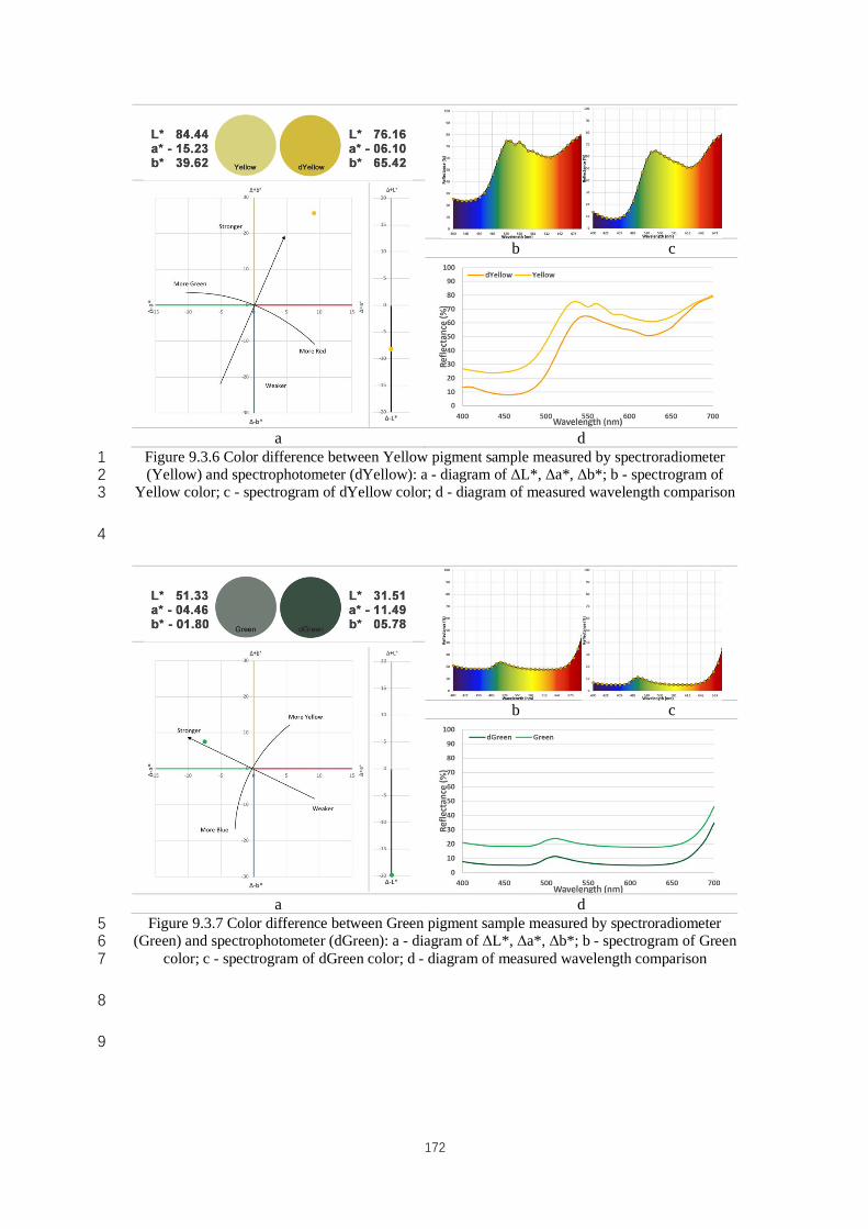
172

b c

a d

Figure 9.3.6 Color difference between Yellow pigment sample measured by spectroradiometer 1 (Yellow) and spectrophotometer (dYellow): a - diagram of ΔL*, Δa*, Δb*; b - spectrogram of 2

Yellow color; c - spectrogram of dYellow color; d - diagram of measured wavelength comparison 3

4

b c

a d

Figure 9.3.7 Color difference between Green pigment sample measured by spectroradiometer 5 (Green) and spectrophotometer (dGreen): a - diagram of ΔL*, Δa*, Δb*; b - spectrogram of Green 6

color; c - spectrogram of dGreen color; d - diagram of measured wavelength comparison 7

8

9

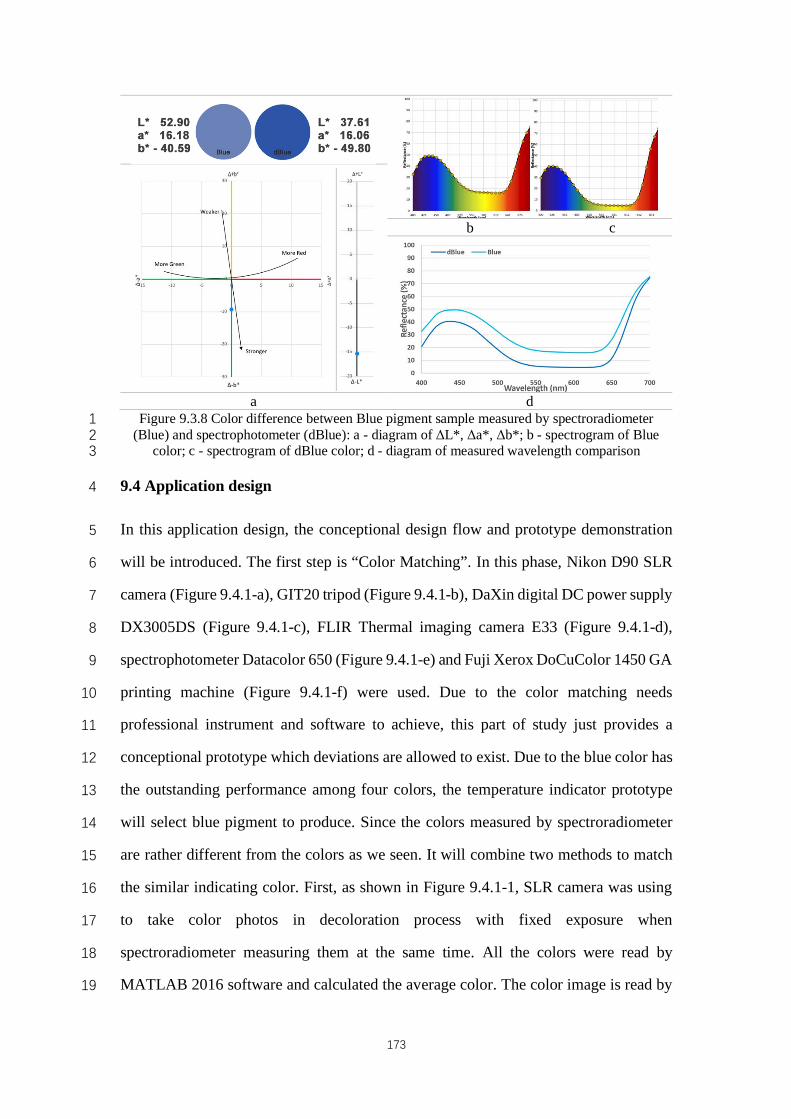
173

b c

a d

Figure 9.3.8 Color difference between Blue pigment sample measured by spectroradiometer 1 (Blue) and spectrophotometer (dBlue): a - diagram of ΔL*, Δa*, Δb*; b - spectrogram of Blue 2

color; c - spectrogram of dBlue color; d - diagram of measured wavelength comparison 3

9.4 Application design 4

In this application design, the conceptional design flow and prototype demonstration 5

will be introduced. The first step is “Color Matching”. In this phase, Nikon D90 SLR 6

camera (Figure 9.4.1-a), GIT20 tripod (Figure 9.4.1-b), DaXin digital DC power supply 7

DX3005DS (Figure 9.4.1-c), FLIR Thermal imaging camera E33 (Figure 9.4.1-d), 8

spectrophotometer Datacolor 650 (Figure 9.4.1-e) and Fuji Xerox DoCuColor 1450 GA 9

printing machine (Figure 9.4.1-f) were used. Due to the color matching needs 10

professional instrument and software to achieve, this part of study just provides a 11

conceptional prototype which deviations are allowed to exist. Due to the blue color has 12

the outstanding performance among four colors, the temperature indicator prototype 13

will select blue pigment to produce. Since the colors measured by spectroradiometer 14

are rather different from the colors as we seen. It will combine two methods to match 15

the similar indicating color. First, as shown in Figure 9.4.1-1, SLR camera was using 16

to take color photos in decoloration process with fixed exposure when 17

spectroradiometer measuring them at the same time. All the colors were read by 18

MATLAB 2016 software and calculated the average color. The color image is read by 19

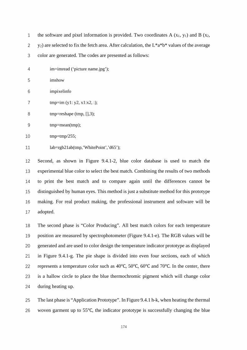
174

the software and pixel information is provided. Two coordinates A (x1, y1) and B (x2, 1

y2) are selected to fix the fetch area. After calculation, the L*a*b* values of the average 2

color are generated. The codes are presented as follows: 3

im=imread (‘picture name.jpg’); 4

imshow 5

impixelinfo 6

tmp=im (y1: y2, x1:x2, :); 7

tmp=reshape (tmp, [],3); 8

tmp=mean(tmp); 9

tmp=tmp/255; 10

lab=rgb21ab(tmp,’WhitePoint’,’d65’); 11

Second, as shown in Figure 9.4.1-2, blue color database is used to match the 12

experimental blue color to select the best match. Combining the results of two methods 13

to print the best match and to compare again until the differences cannot be 14

distinguished by human eyes. This method is just a substitute method for this prototype 15

making. For real product making, the professional instrument and software will be 16

adopted. 17

The second phase is “Color Producing”. All best match colors for each temperature 18

position are measured by spectrophotometer (Figure 9.4.1-e). The RGB values will be 19

generated and are used to color design the temperature indicator prototype as displayed 20

in Figure 9.4.1-g. The pie shape is divided into even four sections, each of which 21

represents a temperature color such as 40℃, 50℃, 60℃ and 70℃. In the center, there 22

is a hallow circle to place the blue thermochromic pigment which will change color 23

during heating up. 24

The last phase is “Application Prototype”. In Figure 9.4.1 h-k, when heating the thermal 25

woven garment up to 55℃, the indicator prototype is successfully changing the blue 26

175

color to indicating color between 50℃ to 60℃, which means the user will know the 1

thermal fabric now is heating up to around 50℃ to 60℃. After modifying the 2

instruments and producing the indicator under industrial assistance, more accurate 3

product can be produced thus to indicate the temperature within small range. 4

5 Figure 9.4.1 Application design flow and prototype demonstration: a - SLR camera; b - tripod; c - 6 power supply; d - thermal imaging camera; e - spectrophotometer; f - color printing machine; 1 - 7 color matching by SLR camera photos and MATLAB calculation; 2 - color matching by color 8

database; g - indicator prototype design; h - thermal woven garment; i - indicator prototype before 9 heating up the garment; j - thermal image of thermal woven garment under heating up; k - 10

indicator prototype after heating up the garment 11

176

9.5 Conclusion 1

This chapter aims to propose a possible method to select thermochromic pigment 2

indicator for thermal textile to show the temperature in a fast and convenient way for 3

potential customers. Four thermochromic pigment samples were heated respectively 4

and measured the decolorization color by spectroradiometer at 40℃, 50℃, 60℃ and 5

70℃ under illuminant D65 light source. When temperature increased, color component 6

decreased while lightness increased. Color depth reduced when heated up, especially 7

between 20℃ to 40℃. Color difference of Yellow, Red and Green color are unstable. 8

Combining all analysis result, in this experiment, Blue color is the ideal indicator for 9

thermal woven textile which can instruct the temperature range in a rapid and 10

convenient way. Color deviation was analyzed, and the major reasons caused may be 11

instrument limitation, light source difference and calibration variation. A successful 12

temperature indicator prototype using thermochromic pigment was produced and the 13

working effect was demonstrated. In the future work, modification can be adopted to 14

accurate the indicating temperature range within industrial assistance when producing 15

profession product. In addition, pigments from different companies will be used to 16

conduct contrast test to verify if the method can be used in any scenario. 17

18

19

20

21

22

23

24

25

177

Chapter 10 Conclusion and Future Works 1

10.1 Conclusion 2

Systematic research has been done about the thermal functional textiles with conductive 3

materials. Two theoretical models were proposed to simulate electrical resistance for 4

conductive woven fabrics. In the first model, an analytic equation was derived based 5

on an equivalent length of conductive yarn woven in three basic woven structures with 6

three different weft densities. Once the radius of the warp yarn and the resistance of 7

one unit of conductive yarn are known, the electrical resistance of woven conductive 8

fabric can be readily computed. The results show that the simulative equation can 9

predict the resistance of woven fabrics, which allows designers to estimate the fabric 10

parameters to meet the required resistance. The other model proposed a fast estimated 11

method to obtain electrical resistance of conductive thermal woven fabrics based on the 12

previous model. Cover factor was a major factor in this model. The results revealed that 13

the proposed fast estimated model was well fitted and could well simulate the electrical 14

resistance of conductive thermal woven fabrics within certain error variation. 15

Compared to first model, this model has slightly lower accuracy but within acceptable 16

deviation. Based on this model, conductive woven fabric and equivalent fabric as 17

substitute for different applications at optimum conditions. Designers can easily 18

estimate the electrical resistance; thus, customized design of conductive thermal woven 19

fabrics can be produced effectively without extra waste of testing weaving. 20

Apart from the electrical resistance simulation model, temperature prediction model 21

was also successfully established by multiple linear regression analysis. After adopting 22

backward method, two models were provided. Model 1 includes all four suggested 23

influence factors, voltage (U), weft conductive yarn arrangement (A), weft density (Dwe) 24

and weft yarn length (Lwe). Lwe factor is introduced to substitute structure (S) factor. 25

The p value of this model is close to 0.000 that is much smaller than 0.05, which means 26

the prediction Model 1 is statistically significant. R square value is 0.931, which implies 27

178

using voltage, WECY arrangement, weft density and length of weft yarn can predict 1

93.1% of TCWFs’ fabric heating temperature. Model 2 removes influence factors Lwe 2

since in regression coefficient statistical result, the p value is greater than 0.1. Although 3

the overall p value in Model 1 is close to 0.000. This variable may have lower impact 4

compared to other three variables. The p value of this model is also close to 0.000 which 5

means Model 2 is statistically significant as well. R square value is 0.928 which is 6

slightly smaller than the value of Model 1. According to the performance results and 7

utilization influence, the structure factor actually affects the integrity design, target 8

temperature and financial cost. In conclusion, applying Model 1 in temperature 9

prediction maybe a reasonable and practical option. 10

Different types of thermal conductive woven fabrics, with three structures, three weft 11

densities and three weft conductive yarn arrangements, wove with two different kinds 12

of silver-coated conductive yarns were designed, fabricated and tested. The results of 13

appearance, mass, thickness, air permeability, thermal conductivity, Qmax, electrical 14

resistance, heating temperature and power efficiency can guide the development of 15

application. Structure majorly influenced the fabric thickness, air permeability, thermal 16

effect and power efficiency except electrical resistance. Weft density has minor effect 17

on thickness and power efficiency while has considerable influence on air permeability, 18

thermal effect and resistance. SCCY A arrangement significantly changed thermal 19

effect, resistance and power efficiency. 20

In addition, the thermal stainless steel woven fabric sample is designed and fabricated 21

in this experiment. Two groups of SSYs were placed in warp direction as conductive 22

path while another SSYs were woven into weft direction in every four-seven picks. The 23

area between two conductive paths was the heating area. There were two types thermal 24

stainless steel woven fabric samples proposed and each of them has four size variations. 25

Type A has 1cm width of conductive path without PVA yarn blending, while Type B 26

has 2cm width of conductive path with PVA yarn blending. PVA yarn was adopted into 27

the fabrication to reduce the damage during weaving. However, the outcome using PVA 28

179

yarn was not satisfied as planned. The fabric surface was affected by PVA yarn 1

blending and weaving process was also be affected by the PVA fiber tangling together. 2

Results showed that fabric length reduction can raise the temperature more effectively 3

compared to fabric width reduction. In addition, conductive path in wider width had 4

better thermal performance. However, the narrow width can save energy but caused 5

uneven thermal distribution. The wider width caused more energy to reach the same 6

temperature but had uniform temperature distribution. Although the financial cost was 7

higher. Therefore, a balanced design was required during commercial production. 8

After establishing the theoretical models and evaluating the thermal woven fabrics, one 9

step formation technology was adopted to develop the thermal functional fabric for 10

garment prototype. Silver-coated conductive yarn was selected to be the conductive 11

material. Four different garments, dress, coat, jacket and shirt were designed and 12

manufactured. 13

A relevant product, thermochromic pigment indicator for thermal textile to show the 14

temperature in a fast and convenient way for potential customers, was also developed. 15

Four thermochromic pigment samples were heated respectively and measured the 16

decolorization color by spectroradiometer at 40℃, 50℃, 60℃ and 70℃ under 17

illuminant D65 light source. When temperature increased, color component decreased 18

while lightness increased. Color depth reduced when heated up, especially between 20℃ 19

to 40℃. Color difference of Yellow, Red and Green color are unstable. Combining all 20

analysis result, in this experiment, Blue color is the ideal indicator for thermal woven 21

textile which can instruct the temperature range in a rapid and convenient way. 22

Moreover, a successful temperature indicator prototype using thermochromic pigment 23

was produced and the working effect was demonstrated. Modification can be adopted 24

to accurate the indicating temperature range within industrial assistance when 25

producing profession product. 26

27

180

10.2 Limitations 1

Although this study made significant contributions to study and development of the 2

woven thermal functional textiles with conductive materials, there are still limitations. 3

First, all the theoretical models are based on ideal geometrical models instead of 4

realistic dynamic models. The deviations exist. Second, the sample population may be 5

not big enough to obtain the better simulation model. Much more sample populations 6

are needed to accurate the simulation models. Third, demonstrated control device is not 7

well-finished as a commercial product. Improvement needs to be made to produce a 8

small, nice and functional control device. Fourth, the battery issue may be the key 9

obstacle for the thermal garment. As long as there is no major progress made in battery, 10

the size and mass of battery will not be optimized. 11

10.3 Future Works 12

The present study focused on thermal woven textile with conductive material. Based 13

on the planned methodology and outcomes worked so far, the future works mainly are 14

about: 15

1. Further evaluation and development for commercialization 16

In order to accomplish this goal, firstly, abundant samples and experiments need 17

to produced and conducted to accurate the temperature prediction model for 18

industrial use. This is an important method to save cost, energy and manpower, as 19

well as a vital guidance for designer to follow. Secondly, all the woven thermal 20

fabrics will be evaluated by conducting mechanical test, thermal comfort test, 21

laundry test, drying test, corrosion test, electrical safety test and thorough wear trial, 22

as well as market survey for better commercialization in the future. Thirdly, more 23

efficient and commercialized control device need to be developed. The control 24

device proposed in this study is a simple prototype for concept demonstration. The 25

appearance and the function are not as satisfied as planned. There is a huge 26

improvement space to work on this topic. 27

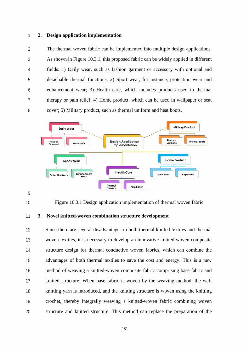
181

2. Design application implementation 1

The thermal woven fabric can be implemented into multiple design applications. 2

As shown in Figure 10.3.1, this proposed fabric can be widely applied in different 3

fields: 1) Daily wear, such as fashion garment or accessory with optional and 4

detachable thermal functions; 2) Sport wear, for instance, protection wear and 5

enhancement wear; 3) Health care, which includes products used in thermal 6

therapy or pain relief; 4) Home product, which can be used in wallpaper or seat 7

cover; 5) Military product, such as thermal uniform and heat boots. 8

9

Figure 10.3.1 Design application implementation of thermal woven fabric 10

3. Novel knitted-woven combination structure development 11

Since there are several disadvantages in both thermal knitted textiles and thermal 12

woven textiles, it is necessary to develop an innovative knitted-woven composite 13

structure design for thermal conductive woven fabrics, which can combine the 14

advantages of both thermal textiles to save the cost and energy. This is a new 15

method of weaving a knitted-woven composite fabric comprising base fabric and 16

knitted structure. When base fabric is woven by the weaving method, the weft 17

knitting yarn is introduced, and the knitting structure is woven using the knitting 18

crochet, thereby integrally weaving a knitted-woven fabric combining woven 19

structure and knitted structure. This method can replace the preparation of the 20

182

additional warp beam with the structure of the knitted ferrule while ensuring the 1

stability of the base fabric, and can realize the precise and specific weaving of 2

various functional yarns and complex design fabrics. 3

4

5

6

7

8

9

10

11

12

13

14

15

16

17

18

19

20

21

22

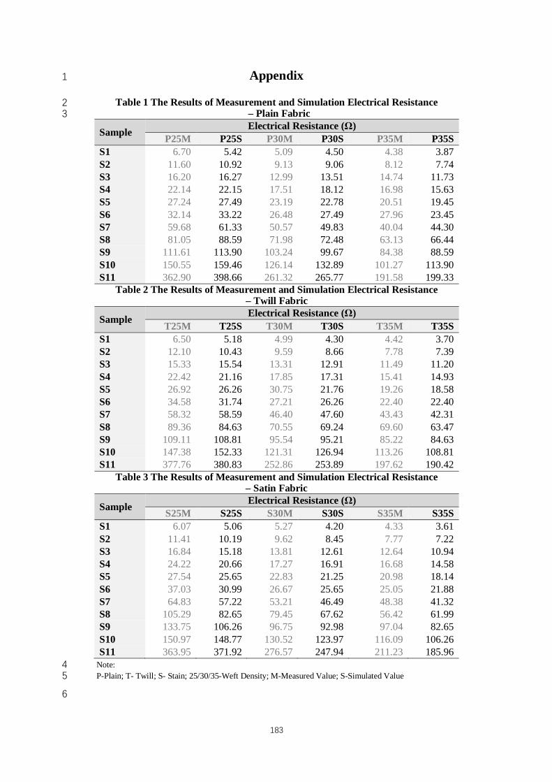
183

Appendix 1

Table 1 The Results of Measurement and Simulation Electrical Resistance 2 – Plain Fabric 3

Sample Electrical Resistance (Ω) P25M P25S P30M P30S P35M P35S

S1 6.70 5.42 5.09 4.50 4.38 3.87 S2 11.60 10.92 9.13 9.06 8.12 7.74 S3 16.20 16.27 12.99 13.51 14.74 11.73 S4 22.14 22.15 17.51 18.12 16.98 15.63 S5 27.24 27.49 23.19 22.78 20.51 19.45 S6 32.14 33.22 26.48 27.49 27.96 23.45 S7 59.68 61.33 50.57 49.83 40.04 44.30 S8 81.05 88.59 71.98 72.48 63.13 66.44 S9 111.61 113.90 103.24 99.67 84.38 88.59 S10 150.55 159.46 126.14 132.89 101.27 113.90 S11 362.90 398.66 261.32 265.77 191.58 199.33

Table 2 The Results of Measurement and Simulation Electrical Resistance – Twill Fabric

Sample Electrical Resistance (Ω) T25M T25S T30M T30S T35M T35S

S1 6.50 5.18 4.99 4.30 4.42 3.70 S2 12.10 10.43 9.59 8.66 7.78 7.39 S3 15.33 15.54 13.31 12.91 11.49 11.20 S4 22.42 21.16 17.85 17.31 15.41 14.93 S5 26.92 26.26 30.75 21.76 19.26 18.58 S6 34.58 31.74 27.21 26.26 22.40 22.40 S7 58.32 58.59 46.40 47.60 43.43 42.31 S8 89.36 84.63 70.55 69.24 69.60 63.47 S9 109.11 108.81 95.54 95.21 85.22 84.63 S10 147.38 152.33 121.31 126.94 113.26 108.81 S11 377.76 380.83 252.86 253.89 197.62 190.42

Table 3 The Results of Measurement and Simulation Electrical Resistance – Satin Fabric

Sample Electrical Resistance (Ω) S25M S25S S30M S30S S35M S35S

S1 6.07 5.06 5.27 4.20 4.33 3.61 S2 11.41 10.19 9.62 8.45 7.77 7.22 S3 16.84 15.18 13.81 12.61 12.64 10.94 S4 24.22 20.66 17.27 16.91 16.68 14.58 S5 27.54 25.65 22.83 21.25 20.98 18.14 S6 37.03 30.99 26.67 25.65 25.05 21.88 S7 64.83 57.22 53.21 46.49 48.38 41.32 S8 105.29 82.65 79.45 67.62 56.42 61.99 S9 133.75 106.26 96.75 92.98 97.04 82.65 S10 150.97 148.77 130.52 123.97 116.09 106.26 S11 363.95 371.92 276.57 247.94 211.23 185.96

Note: 4 P-Plain; T- Twill; S- Stain; 25/30/35-Weft Density; M-Measured Value; S-Simulated Value 5

6

184

References 1

[1] Sahin O, Kayacan O, and Bulgun E, Smart textiles for soldier of the future, 2

Defence Sci. J., 2005;55:195-205. 3

[2] Wiezlak W, and Zielinski J, Clothing heated and textile heating elements, Int. J. 4

Cloth. Sci. Technol. 1993; 5: 9-23. 5

[3] Scott R A, The technology of electrically Heated Clothing, Ergonomics 19588; 6

31:1065–1081. 7

[4] Deloire R, Durand J and Mans L. Heating garment. U.S. Patent No. 3 729 613; 8

1973. 9

[5] Narendra VB, Devender TS, and Mandar MN, Development of conductive cotton 10

fabrics for heating devices. Journal of Applied Polymer Science 2006; 102: 4690-11

4695. 12

[6] Moshe R. Electronic heating/warming fabric articles. U.S. Patent No. 6501055B2; 13

2002. 14

[7] Roell F. Electric heating element in knitted fabric. U.S. Patent No.5 484 983; 15

1996. 16

[8] Hill et al. Plural layer woven electronic textile, article and method. U.S. Patent 17

No. 7144830 B2; 2006. 18

[9] Rantanen J, Vuorela T, Kukkonen K, Ryynanen O, Siili A, Vanhala J. Improving 19

human thermal comfort with smart clothing. In: Proceedings of 2001 IEEE 20

International Conference on System, Man and Cybernetics. New York, NY, USA: 21

IEEE Publishing; 2001. p.795–800 (DOI: 10.1109/ICSMC.2001.973012). 22

[10] MoShe R. Electric heating/warming fabric articles. U.S. Patent No. 23

20050127057A1. 24

[11] Kochman, E. Textile heating with continuous temperature sensing and hot spot 25

detection. U.S. Patent No. 6713733 B2. 26

[12] Van P. Electronic textile. U. S. Patent No. 2011/0036448 A1. 27

185

[13] Tao XM, Smart Fibers. Fabrics and Clothing. Cambridge, UK: Woodhead 1

Publishing, 2001 2

[14] Li L, Au WM, Wan KM, et al. A Resistive Network Model for Conductive 3

Knitting Stitches. Textile Research Journal 2010; 80: 935–947. 4

[15] Hao L, Yi Z, Li C, Li XJ, Wang YX, Yan G. Development and characterization 5

of flexible heating fabric based on conductive filaments. Measurement 2012; 45: 6

1855-1865. 7

[16] Li L, Au WM, Hua T, Wong KS. Design of a conductive fabric network by the 8

sheet resistance method. Textile Research Journal 2011; 81: 1568-1577. 9

[17] Li L, Au WM, Ding F, Hua T, Wong KS. Wearable electronic design: 10

electrothermal properties of conductive knitted fabrics. Textile Research Journal 11

2013; 0(00): 1–11. 12

[18] Tong JH, Ding F, Tao XM, Au WM, Li L. Temperature effect on the conductivity 13

of knitted fabrics embedded with conducting yarns Textile Research Journal 2014; 14

0(00): 1–9. 15

[19] Li L, Au WM, Li Y, Wan KM, Chung WY, Wong KS. A Novel Design Method 16

for an Intelligent Clothing Based on Garment Design and Knitting. Textile 17

Research Journal 2009 79(18): 1670–1679. 18

[20] Li L, Au WM, Yi Li, Wan KM, Wan SH, Wong KS. Design of Intelligent 19

Garment with Transcutaneous Electrical Nerve Stimulation Function Based on 20

the Intarsia Knitting Technique. Textile Research Journal 2010; 80(3): 279–286. 21

[21] Hamdani STA, Potluri P, Fernando A. Thermo-Mechanical Behavior of Textile 22

Heating Fabric Based on Silver Coated Polymeric Yarn. Materials 2013; 6: 1072-23

1089. 24

[22] Cotton Handbook, China Textile & Apparel Press, 2004. 25

[23] Wang GH. Plain Weave, Fabric for Fashion Design, China Textile & Apparel 26

Press, 2007. 27

186

[24] Wang GH. Twill Weave, Fabric for Fashion Design, China Textile & Apparel 1

Press, 2007. 2

[25] Wang GH. Satin Weave, Fabric for Fashion Design, China Textile & Apparel 3

Press, 2007. 4

[26] Lan F. Conductive Fiber: novel Functional Textile Material. China Fiber Test. 5

2007, 3(3):55. 6

[27] Yang SB. Wang Y. Conductive Fiber and its Application. Sichuan Textile and 7

Technology. 2001, 2(2)13-16. 8

[28] Li W. Zhuang QL. Conductive Fiber and its Smart Textile. Industrial Textiles. 9

2003, 8(8)1-3. 10

[29] Liu HY, Liu HF, Wang WX. Development of Metal Fiber. Technology 11

Innovation. 2005(12). 12

[30] Shi MW. Nan Y. The Study of Structure and Performance of Organic Conductive 13

Fiber. Wool Textiles. 2001, 1(1)5-8. 14

[31] Gao GY. An SL. Characteristic and Development of Organic Conductive Fiber. 15

Tianjing Textile and Technology. 2005, 2(2)29-32. 16

[32] Ni HY. Meng JH. Study of Organic Conductive Fiber. Development of Textile 17

and Technology. 2004, 5(5)16-17. 18

[33] Anti-static technology in performance apparel. Technical Textile Markets. 2005, 19

4(4)11-31. 20

[34] New uses for wearable textile- based health monitoring technology. Textile 21

Outlook International, 2008, 5(5)87-93. 22

[35] Li MC. Gong RZ. Feng ZK. Study of Absorption Material particularly in Radar 23

Absorption. Electrical Engineering of Ships. 2004, 24(8) 232-236. 24

[36] Dhawan, A., Seyam, A.M., Ghosh, T. K., Muth, J.F. Woven Fabric-Based 25

Electrical Circuits: Part I: Evaluating Interconnect Methods. Textile Res J. 74: 26

913-919(2004). 27

187

[37] Sezgin, H., Bahadir, S.K., Boke, E., Kalaoglu, F. Effect of Different Conductive 1

Yarns on Heating Behaviour of Fabrics. RMUTP International Conference: 2

Textiles & Fashion 2012. July 3-4(2012). 3

[38] Li, L. Innovative Functional Knitwear Design with Conductive Yarns. (2010). 4

[39] Toshihiro, I., Shinji, Y. Patent: Conductive Conjugate Fiber. US20120237766A1. 5

(2011). 6

[40] Tsang, H.Y. Design and Development Electrically Conducting Sensors for Smart 7

Textile and Apparel. (2006). 8

[41] Rheaume, W. A. Patent: Heat Conductive Fabric. US4312913. (1980). 9

[42] DeAngelis, A. R., Wolynes E. Patent: Thermal Textile. US007151062B2. (2003). 10

[43] Li, L., Au, W.M., Wong, K.S., Chung, W.Y., Wan, S.H. Patent: Smart Thermal 11

Textile for Acupuncture Therapy. US20100004720A1. (2008). 12

[44] WarmX. (2012). Retrieved 2012 from: 13

http://www.wellness.warmx.de/index.php/mehr-informationen.html 14

[45] Nakad Z, Jones M, Martin T, etc. Networking in E-textiles. Computer 15

Communications2010; 33: 655-666. 16

[46] Edmison J, Jones M, Nakad Z, etc. Using piezoelectric material for wearable 17

electronic textiles. Proceeding of the 6th international symposium on wearable 18

computers (ISWC’02) 2002; 41-48. 19

[47] Cherenck KH, Kinkeldei T, Zysset C, etc. Woven thin-film metal interconnects. 20

IEEE Electron Device Letters2010, 31: 740-742. 21

[48] Locher L and Troster G. Enable technologies for electrical circuits on a woven 22

monofilament hybrid fabric. Textile Res J 2008, 78:583-594. 23

[49] Bashir T, Fast L, Skrifvars M, etc. Electrical resistance measurement methods 24

and electrical characterization of poly(3,4-ethylenedioxythiophene) coated 25

conductive fibers. Journal of Applied Polymer Science 2012, 124: 2954-2961. 26

188

[50] Zhang H, Tao XM, Wang SY, etc. Electromechanical properties of knitted fabric 1

made from conductive multi-filament yarn under unidirectional extension. Textile 2

Res J 2006, 126: 598-606. 3

[51] Xue P, Tao XM, Kwok WY, Leung MY and Yu TX. Electromechanical behavior 4

of fibers coated with an electrically conductive polymer. Textile Res J 2004; 74: 5

924-937. 6

[52] He JW. Allometric scaling law in conductive polymer. Polymer 2004; 45: 9067-7

9070. 8

[53] Li L, Au WM, Li Y, Wan KM, etc. Electromechanical analysis of conductive 9

yarn knitted in plain knitting stitch under unidirectional extension. Proc TBIS 10

2008; 1:793-797. 11

[54] Haykin SS. Active network theory. L.D: Addison-Wesley, 1970. 12

[55] Li L, Au WM, Wan KM, etc. A resistive network model for conductive knitting 13

stitches. Textile Res J 2009; 80: 935-947. 14

[56] Jaeger RC. International to microelectronic fabrication. Upper Saddle River, NJ: 15

Prentice Hall, 2001. 16

[57] Scott R A, The Technology of Electrically Heated Clothing, Ergonomics 31 17

(1988) 1065–1081. 18

[58] Deloire R, Durand J, Mans L. Heating garment. U.S. Patent No. 3 729 613; 1973. 19

[59] Narendra VB, Devender TS, Mandar MN, etc. Development of conductive cotton 20


4695. 22

[60] Roell F. Electric heating element in knitted fabric. U.S. Patent No.5 484 983; 23

1996. 24

[61] Moshe R. Electronic heating/warming fabric articles. U.S. Patent No. 6501055B2 25

[62] Rantanen J, Vuorela T, Kukkonen K, Ryynanen O, Siili A, Vanhala J. Improving 26

human thermal comfort with smart clothing. In: Proceedings of 2001 IEEE 27

189

International Conference on System, Man and Cybernetics. New York, NY, USA: 1

IEEE Publishing; 2001. p. 795–800 (DOI: 10.1109/ICSMC.2001.973012). 2

[63] MoShe R. Electric heating/warming fabric articles. U.S. Patent No. 3

20050127057A1. 4

[64] Tong JH, Ding F, Li L, et al. Temperature effect on the conductivity of knitted 5

fabrics embedded with conducting yarns. Textile Research Journal 2014; 84 (17): 6

1849–1857. 7

[65] Tong JH, Liu S, Li L, et al. Modeling of package-free flexible conductive fabric 8

with thermal regulation where temperature can be customized. Textile Research 9

Journal 2015; 85 (6): 590–600. 10

[66] Tong JH, Zhao YF, Li L, et al. Comparison of air flow environmental effects on 11

thermal fabrics. Textile Research Journal 2018; 88 (2): 203–212. 12

[67] Liu S, Yang CX, Li L, et al. The impact of float stitches on the resistance of 13

conductive knitted structures. Textile Research Journal 2016; 86 (14): 1455–1473. 14

[68] Liu S, Tong JH, Li L, et al. Smart E-textile: Resistance properties of conductive 15

knitted fabric – Single pique. Textile Research Journal 2017; 87 (14): 1669–1684. 16

[69] Zhao YF, Tong JH, Li L, et al. A simulation model of electrical resistance applied 17

in designing conductive woven fabrics. Textile Research Journal 2016; 86 (16): 18

1688-1700. 19

[70] Zhao YF and Li L. A simulation model of electrical resistance applied in designing 20

conductive woven fabrics - Part II: fast estimated model. Textile Research Journal 21

2018; 88 (11): 308-1318. 22

[71] Scott RA. The technology of electrically Heated Clothing. Ergonomics 1988; 31: 23

1065–1081. 24

[72] Deloire R, Durand J, and Mans L. Heating garment. U.S. Patent No. 3729613; 25

1973. 26

190

[73] Narendra VB, Devender TS, and Mandar MN. Development of conductive cotton 1


4695. 3

[74] Roell F. Electric heating element in knitted fabric. U.S. Patent No.5484983; 1996. 4

[75] Jagatheesan K, Ramasamy A and et al. Electromagnetic shielding effectiveness of 5

carbon/stainless steel/polypropylene hybrid yarn-based knitted fabrics and their 6

composites. The Journal of the Textile Institute 2018; 1-14. 7

[76] Jagatheesan K, Ramasamy A and et al. Investigation on Shielding and Mechanical 8

Behavior of Carbon/Stainless Steel Hybrid Yarn Woven Fabrics and Their 9

Composites. Journal of Electronic Materials 2017; 46(6): 5073-5088. 10

[77] Lin JH, Jhang JC and et al. Manufacturing Techniques, Mechanical Properties, Far 11

Infrared Emissivity, and Electromagnetic Shielding Effectiveness of Stainless 12

Steel/Polyester/Bamboo Charcoal Knits. Fibers and Polymers 2017; 18(3): 597-13

604. 14

[78] Lou CW and Lin JH. Evaluation of Bamboo Charcoal/Stainless Steel/TPU 15

Composite Woven Fabrics. Fibers and Polymers 2011; 12(4): 514-520. 16

[79] Palanisamy S, Tunakova V and et al. Study on textile comfort properties of 17

polypropylene blended stainless steel woven fabric for the application of 18

electromagnetic shielding effectiveness. 17th World Textile Conference AUTEX 19

2017- Textiles - Shaping the Future 2017; 1-8. 20

[80] Gupta KK, Abbas Sm and Abhyankar AC. Ultra-lightweight hybrid woven fabric 21

containing stainless steel/polyester composite yarn for total EMI shielding in 22

frequency range 8–18 GHz. Journal of Electromagnetic Waves and Applications 23

2015; 29(11): 1454-1472. 24

[81] Heated Jacket, (Online). Available: 25

https://www.aliexpress.com/wholesale?catId=0&initiative_id=SB_2018070520226

523&SearchText=heated+jacket. Accessed: July 6, 2018. 27

191

[82] Warming Clothes for Women, (Online). Available: 1

https://www.warmx.de/shop/index.php?main_page=index&cPath=1&sort=20a&2

language=en. Accessed: July 6, 2018. 3

[83] Heated Jackets, (Online). Available: https://ravean.com/pages/heated-jackets. 4

Accessed: July 6, 2018. 5

[84] Heated Garments, (Online). Available: http://www.avade.com.au/products.html. 6

Accessed: July 6, 2018. 7

[85] Ferrara M, Bengisu M. Materials that change color - smart materials, intelligent 8

design. Springer. Cham Heidelberg New York Dordrecht London. 2014 9

[86] Kulcar R, Friskovec M, et al. Colorimetric properties of reversible thermochromic 10

printing inks. Dyes and Pigments 2010; 86: 271-277 11

[87] MacLaren DC, White MA. Design rules for reversible thermochromic mixtures. 12

Journal of Materials Chemistry 2005; 40: 669-76. 13

[88] Seeboth A, Klukowska A, Ruhmann R, Lötzch D. Thermochromic polymer 14

materials. Chinese Journal of Polymer Science 2007; 25: 123-135. 15

[89] White MA. Thermochromism in commercial products. Journal of Chemical 16

Education 1999; 76(9): 1201-1205. 17

[90] Aitken D, Burkinshaw SM, Griffiths J, Towns AD. Textile applications of 18

thermochromic systems. Review of Progress on Coloration 1996; 26: 1-8. 19

[91] Burkinshaw SM, Griffiths J, Towns AD. Reversibly thermochromic systems 20

based on pH-sensitive spirolactone-derived functional ink. Journal of Materials 21

Chemistry 1998; 8: 267-283. 22

[92] Maclaren DC, White MA. Dye-developer interactions in the crystal violet lactone-23

lauryl gallate binary system: implications for thermochromism. Journal of 24

Materials Chemistry 2003; 13: 1695-1700. 25

192

[93] MacLaren DC, White MA. Competition between dye-developer and solvent-1

developer interactions in a reversible thermochromic system. Journal of Materials 2

Chemistry 2003; 13: 1701- 3

[94] Zhu CF, Wu AB. Studies on the synthesis and thermochromic properties of crystal 4

violet lactone and its reversible thermochromic complexes. Thermochimica Acta 5

2005; 425: 7-12. 6

[95] Seeboth A, Lötzsch D. Thermochromic phenomena in polymers. Shawbury: 7

Smithers Rapra Technology Limited; 2008. 8

[96] Zhang X, Xue XS, Chen B and et al. Research and application of thermal 9

indicating paint in aeroengine. Measurement and control technology 2008; 27(1): 10

21-23, 41. 11

[97] Chandrasekhar U, Anbazhagans R. Full temperature mapping and heat transfer 12

analysis of aero gas turbine engine components through thermal painting. ISABE 13

2009; 1358. 14

[98] Li Y, Li ZM. The Research of Temperature Indicating Paints and Its Application 15

in Aero-engine Temperature Measurement. Procedia Engineering 2015; 99: 1152-16

1157. 17

[99] Lempereur C, Andral R and Prudhomme JY. Surface temperature measurement 18

on engine components by means of irreversible thermal coatings. Measurement 19

Science and Technology 2008; 19:1-11. 20

[100] Rabhiou A, Feist J and et al. Phosphorescent thermal history sensors. Sensors and 21

Actuators A: Physical 2011; 169:18-26. 22

[101] Song HF, Chen KC, Tian H. Alkali induced chromics and stable single crystal of 23

opened-ring form of a new spirooxazine. Dyes and Pigments 2005; 67:1-7. 24

193

[102] Heated Jacket, [Online]. Available: 1

https://www.amazon.com/s/ref=nb_sb_noss_1?url=search-alias%3Daps&field-2

keywords=heated+jacket&rh=i%3Aaps%2Ck%3Aheated+jacket. [Acessed: July 3

6, 2018]. 4

[103] Heated Jacket, [Online]. Available: 5

https://www.ebay.com/sch/i.html?_from=R40&_trksid=m570.l1313&_nkw=He6

ated+Jacket&_sacat=0. [Acessed: July 6, 2018]. 7

[104] Mai T, Odle TG and Frey RJ. Dysmenorrhea. Cengage Learning 2011;1429-1433. 8

[105] Dawood YM. Dysmenorrhea. The Global Library of Women's Medicine 2008 9

Jun. 10

[106] Lee LC, Tu CH and et. al. Association of Brain-Derived Neutophic Factor Gene 11

Val66Met Polymorphism with Primary Dysmenorrhea. PLOS One 2014; 9(11): 12

1-10. 13

[107] Nivashini G. Prevalence of Primary Dysmenorrhea along with irregular Periods. 14

Research Journal of Pharmacy and Technology 2015; 8(8): 1099-1106. 15

[108] Sun YM, Wang L and Li G. Investigation on Influencing Factors of Primary 16

Dysmenorrhea in 1800 Female College Students. Tianjin Journal of Traditional 17

Chinese Medicine 2009; 5(5): 367-369. 18

[109] Chen YT, Cao Y and et. al. Traditional Chinese Medicine for the Treatment of 19

Primary Dysmenorrhea: How Do Yuanhu Painkillers Effectively Treat 20

Dysmenorrhea. Phytomedicine 2013; 20: 1095-1104. 21

[110] Ji B, Ren XX and et. al. Comments on Study of Pathogenesy, Prevention and 22

Treatment of Primary Dysmenorrhea. China Journal of Modern Medicine 2008; 23

18(13): 1856-1862. 24

194

[111] Davis AR and Westhoff CL. Primary Dysmenorrhea in Adolescent Girls and 1

Treatment with Oral Contraceptives. Journal of Pediatric and Adolescent 2

Gynecology 2001; 14: 3-8. 3

[112] Wang ZJ, Li KF and Xu JJ. Study on the Biological Mechanism of Exercise 4

Training for Dysmenorrhea. Sport 2015; 8: 153-154. 5

[113] Hosono T, Takashima Y and et. al. Effects of A Heat- and Steam-Generating 6

Sheet on Relieving Symptoms of Primary Dysmenorrhea in Young Women. The 7

Journal of Obstetrics and Gynaecology Research, 2010; 36(4): 818-824. 8

[114] O'Connell K, Davis AR and Westhoff C. Self-treatment Patterns Among 9

Adolescent Girls with Dysmenorrhea. Journal of Pediatric and Adolescent 10

Gynecology 2006; 19: 285-289. 11

[115] Campbell MA and Mcgrath PJ. Non-pharmacologic Strategies Used by 12

Adolescents for the Management of Menstrual Discomfort. The Clinical Journal 13

of Pain 1999; 15(4): 313-320. 14

[116] Zhang QM. Analysis of Influence Factors to Primary Dysmenorrhea of Coedna. 15

Journal of Hanjiang University 2012; 40(6): 68-71. 16

copyright undertaking

Documents