NBER WORKING PAPER SERIES

COORDINATION VS. DIFFERENTIATION IN A STANDARDS WAR:56K MODEMS

Angelique AugereauShane Greenstein

Marc Rysman

Working Paper 10334http://www.nber.org/papers/w10334

NATIONAL BUREAU OF ECONOMIC RESEARCH1050 Massachusetts Avenue

Cambridge, MA 02138March 2004

The views expressed herein are those of the authors and not necessarily those of the National Bureau ofEconomic Research.

©2004 by Angelique Augereau, Shane Greenstein, and Marc Rysman. All rights reserved. Short sections oftext, not to exceed two paragraphs, may be quoted without explicit permission provided that full credit,including © notice, is given to the source.

Coordination vs. Differentiation in a Standards War: 56K ModemsAngelique Augereau, Shane Greenstein, and Marc RysmanNBER Working Paper No. 10334March 2004JEL No. L15, L63, L86

ABSTRACT

56K modems were introduced under two competing incompatible standards. We show the

importance of competition between Internet Service Providers in the adoption process. We show that

ISPs were less likely to adopt the technology that more competitors adopted. This result is

particularly striking given that industry participants expected coordination on one standard or the

other. We speculate about the role of ISP differentiation in preventing the market form achieving

standardization until a government organization intervened.

Angelique AugereauMcKinsey and Co.

Shane GreensteinJ.L. Kellogg School of ManagementLeverone Hall2001 Sheridan RoadEvanston, IL 60208-2013and NBERgreenstein@kellogg.northwestern.edu

Marc RysmanDepartment of EconomicsBoston University270 Bay State Rd.Boston, MA 02215mrysman@bu.edu

Coordination vs. Differentiation in a StandardsWar: 56K Modems∗

Angelique AugereauMcKinsey and Co.

Shane GreensteinKellogg School of Management

Marc RysmanBoston University

February 13, 2004

Abstract

56K modems were introduced under two competing incompatible stan-dards. We show the importance of competition between Internet ServiceProviders in the adoption process. We show that ISP’s were less likelyto adopt the technology that more competitors adopted. This result isparticularly striking given that industry participants expected coordina-tion on one standard or the other. We speculate about the role of ISPdifferentiation in preventing the market from achieving standardizationuntil a government organization intervened. JEL: L15, L63, L86

1 Introduction

This paper studies the role of Internet Service Providers in the 56K standards

war. Introduced in 1997, 56K modems allowed for data transfer at up to twice

the speed of the previous technology at a time when the demand for large files

(such as graphics) over the Internet became increasingly important. Originally,

there were two competing standards. The standards were functionally identical

in the sense that they had the same performance characteristics. However,

∗We thank seminar audiences at the SED 2002 meetings, Brown University, the Departmentof Justice, the University of Illinois and Pennsylvania State University, the AEA 2003 meetings,the Federal Reserve Bank of Chicago, Northwestern University, Syracuse University and theGraduate School of Business at Stanford University. We also thank Tim Bresnahan, DavidDranove, Mike Mazzeo, Ariel Pakes, Greg Rosston and Katja Seim for helpful comments.Martino De Stefano provided excellent research assistance. This research was supported byNSF Grant SES-0112527 and a grant from NET Institute.

1

these standards were incompatible. If a consumer used one standard and the

consumer’s Internet Service Provider (ISP) used the other standard, then data

transfer speed diminished to that of the previous technology, only 33K or 28K.

In this setting we study the role of competition in technology adoption by

ISPs. Despite much theoretical interest in adoption of new technologies and

the competition between alternatives standards, very little empirical research

examines demand for technology and how demand shapes competitive behavior.

Data needs are the primary impediment. We rarely observe competition between

two comparable technologies played out in more than one market. Even when

that occurs, it is often difficult to disentangle the effects of competition from

other important effects.

This study’s setting is uniquely well suited to meet these requirements. An

important feature of the ISP market is that consumers almost always connect to

ISPs within their local telephone calling plan. This creates numerous geograph-

ically distinct or partially overlapping markets, which leads to geographically

dispersed decision making and a variety of competitive interactions. We will

study over 2200 ISPs in 2300 calling areas. Thus, we are able to compare de-

cisions across markets, where a variety of factors shape decision making, such

as the competitive and demographic environment and ISP size and previous

technology.

We focus on understanding the role of competition in adoption by an ISP.

We highlight findings about our central hypothesis, that competition between

ISPs shaped decision making over modem choice. We show that competition

consistently pushed behavior in a specific direction. ISP’s were less likely to

adopt a standard as more of their competitors adopted that standard. We also

show that the magnitude of change could be the most important to outcomes,

though we caution that this latter finding does not hold for every model.

We employ three modeling approaches: simple statistics about agglomera-

tion, a bivariate probit model of technology adoption, and a bivariate probit

2

model with controls for endogeneity. Specifically, simple statistics illustrate a

prevalence towards “even splits” in local markets. That is, adopting ISP’s were

more likely to be evenly split between the two standards than would be predicted

by independent random choice. Estimates from bivariate probit models show

the same prevalence. We estimate each ISP’s choice over adoption of the two

technologies as a function of the competitive environment, local demographics,

ISP characteristics and ISP decision-making across multiple markets. The same

prevalence also arises, though more weakly, when the model accounts for pos-

sible endogeneity between the choices of competing ISP’s. The estimates that

control for endogeneity push our data as far as they will go. It contains novel

features which we describe in detail in the text.

Theories about standardization discuss the role of competitive choice be-

tween standards, but few prominent cases ever permit researchers to garner

a close look at behavior during deployment, as we get here. The 56K mo-

dem fight had a well-publicized “standards war’ for early adopters in Internet

markets. Many contemporary press reports discuss how modem makers com-

peted fiercely for adoption by the earliest choosers. Related, Shapiro and Varian

(1999), pp 267-270, feature it prominently in their discussion of strategic behav-

ior during standardization fights. Contemporary press accounts tend to cover

announcements from firms, not the deployment in each local areas. No research

has closely examined the deployment decision of service providers, as we do.

The competitive experience is also interesting because it motivated interven-

tion from a government agency. At the time this experience appeared to be an

example of “coordination failure.” That is, there was a benefit to coordinating

ISP’s and consumers on a single standard as quickly as possible, but market

actors failed to quickly standardize. Market participants expected that stan-

dardization would arise because it was in user interest. The popular standard

would have more ISP’s servicing it, which ensured consumers of high-quality,

low hassle, low price service into the future. However, coordination did not arise

3

in the first year of competition. Not only did the two technologies maintain rel-

atively similar market shares, but overall sales to consumers and ISP’s were well

below what the two sides had hoped. Sales increased only after a government

standard setting organization introduced a third incompatible standard as a new

focal point for designs. The new standard quickly gained market acceptance and

unified all designs. High industry sales followed.

Did competitive rivalry among ISPs contribute to the market’s inability to

coordinate on a standard unaided? In a final more speculative section of the

paper, we argue that the standards war was prolonged by the market’s struc-

ture, i.e., geographically dispersed decision making combined with the incentive

to differentiate locally. This discussion directs further attention at issues not

highlighted in the applied literature on standardization.

2 Related Literature

Our research goals are empirical. Yet, we lack prototypes for how to measure

buyer and supplier behavior during a standards war. While user choice between

alternatives plays a prominent role in many models of standardization, there are

few empirical studies for characterizing its effect. Related, previous empirical

work has focused on either the decision of whether to adopt a standard or not,

or the decision of which standard to adopt, but has not dealt with decisions

linking choice between two standards and non-adoption.

A few prior studies of competition in technology adoption provide us with

general approaches for measuring competitive incentives. For instance, Klepper

(2002) uses firm exit patterns, comparing very competitive and oligopolistic

markets, to suggest a strong role for competition in cost-reducing technology

adoption in a number of manufacturing industries. Genesove (1999) provides a

study of the adoption of offset printing by newspapers and argues that firms in

more competitive markets adopted earlier. Mulligan and Llinares (2003) show

4

that ski-lifts were less likely to adopt quality-enhancing technology when local

competitors had done so.

Though standards wars and the adoption of standards have received con-

siderable attention in theoretical discussion, little empirical research examines

decision making for standards. We borrow broadly from the general approach

of empirical studies of technology adoption in network industries, though none

explicitly provides us with a model for how to measure competitive behavior in

a standards war.1 For example, Saloner and Shepard (1995) show the existence

of network effects in bank service by showing that banks with more consumers

adopt ATM networks earlier. Like our paper, they infer consumer behavior from

observing decisions by firms in different locations. Gowrisankaran and Stavins

(2002) and Ackerberg and Gowrisankaran (2003) look at the adoption of au-

tomated clearinghouse technology by banks. As with our paper, they exploit

overlapping local geographic markets for important variation. However, they

use a very different structural model of adoption incentives.

There are a few papers that consider the decision between two standards

in horizontal competition. The approaches are quite different from ours, so we

borrow broad motivation, but not a specific model. For example, Dranove and

Gandal (2003) argue that the introduction of the DIVX standard slowed down

the acceptance of DVD technology. Park (2000) and Ohashi (2000) study the

standards war between VHS and Beta in the VCR market. Using market level

data on quantities and prices, they focus on the role of installed base. Gandal,

Kende and Rob (2000) study network effects between producers of compact

disks and producers of CD players. They too find evidence of the interaction

between software and hardware.

There also is a small literature on the behavior of ISPs. Closest to the present

study is Augereau and Greenstein (2001), who examine the upgrade behavior by

1Shy (2001) provides an introduction and overview of both theoretical and empirical work

on network effects.

5

ISPs into higher speed technologies. The statistical model does not focus directly

on the role of competitive incentives because the data are too coarse, allowing

only for a comparison of ISPs located in “urban’ and “rural’ locations. They find

faster upgrade behavior by ISPs in urban settings. Greenstein (2000) looks at

whether ISPs differentiate from each other by offering services other than dial-up

basic access, such as web design, network maintenance, hosting, or broadband

to business. There is more differentiation among firms in urban settings, but,

again, because the data are coarse so too is the inference. These papers can

only speculate about why firms in different settings behave differently. The

competitive setting might cause such differences across locations, but so could

other factors.

In comparison to the previous literature this paper offers advances in several

respects. First, we have access to very granular data about who competes with

whom in ISP markets. This permits a direct measurement between the adoption

decision of one competitor and all rivals. Second, we provide an empirical model

of technology adoption in a standards war. We develop a non-cumbersome

model that links decisions about whether to adopt with decisions about what to

adopt. This provides insight about factors that shape decision making, such as

competition and other local factors. Third, we provide an empirical method of

a discrete decision while controlling for econometric issues of endogeneity, using

the insights from the model of Seim (2002) to aggregate over the decisions of

many other rivals. As such, the method generalizes to other types of decisions

over discrete choices in rivalrous settings.

Finally, on a broad level we also build on a literature of cases studies of other

industries that experienced events that looked like coordination failure to con-

temporaries. For example, Postrel (1990) associates the failure to adopt quadra-

phonic stereo with the presence of multiple, competing standards, which created

confusion and delay downstream in distribution. Saloner (1989) attributes the

failure to unify on a single standard of UNIX in the 1980s to proprietary in-

6

terests in pursuing strategies that raise switching costs to work station users.

Besen and Johnson (1986) and Rohlfs (2001) also relate a number of stories of

delayed or failed adoption. For example, Besen and Johnson report that AM

stereo required broadcasters and radio owners to be on the same standard, and

broadcasts were delayed by the presence of multiple standards. As in our case,

these are examples in which increasing the number of new choices plays a role.

We differ in that we highlight the role of differentiation in prolonging a

standards war and leading to coordination failure. Existing theory would lead

one to expect local “tipping” in a market with network effects. That, in turn,

might give rise to either quick national unification or geographic balkanization,

each market tipping in its own direction. Instead, neither of those theoretical

possibilities occurred. There was no coordination between markets or within

markets. Local competitive rivalry pushed in the opposite direction, towards

local “splitting”, when adoption occurred at all. We argue that this splitting

fostered confusion about which technology would emerge as a standard — i.e.,

widespread splitting interfered with emergence of a technical focal point for mar-

ket participants — which further deterred adoption decisions. In this sense our

discussion, based on the theory in Rysman (2003a), is also a contribution be-

cause it differs from the common explanation. Rather, we observe behavior that

appears consistent with inefficient incentives to differentiate across standards.

3 Industry2

A modem allows a computer to send and receive data over a telephone line.

Up until early 1997, 33.6K was the fastest modem available for use with analog

telephone lines. A 33.6K modem can send and receive 33.6 kilobits of data

every second. Most modems connect to the Internet through a local telephone

call to an Internet Service Provider. In 1997, about 93% of the U.S. population

2A more in-depth discussion of these issues can be found in Rickard (1997a, 1997b, 1998).

7

had access to a commercial ISP (Downes and Greenstein, 2002). As ISP’s

and telephone companies upgraded their connections to each other, it became

technologically possible to raise modem speeds to 56K. ˙With the concurrent

development of the World Wide Web and the use of more graphics, demand for

the Internet access and the importance of speed increased, providing demand

for 56K technology.

Players in the modem industry fell into two camps, either with US Robot-

ics which developed the “X2” modem3 or with Rockwell Semiconductor which

called their product “K56Flex.” Both brought their product to market at es-

sentially the same time, February 1997. Independent comparisons showed that

the two standards worked equally well, although there was significant variabil-

ity across and between standards depending on local connection characteristics.

The two standards were incompatible in the sense that a consumer with one

standard that connected to an ISP with the other standard would receive data

at only 28 or 33K (at most).

The ISP market was young in 1997, undergoing growth in new users and

new entry in service providers. There were thousands of small firms with very

small geographic focus, a few hundred firms with service beyond one city, and

a few dozen with national or near-national footprints (Downes and Greenstein,

2002). Only the large firms had recognizable brands, such as AT&TWorldnet or

America On Line. Small and medium ISPs often offered other Internet services

in addition to their dial-up service. Many took strategic positions as early

movers into new technology and new services as a way to develop local customers

bases and differentiate from their branded national ISP rivals (Greenstein, 2002).

The cost of the new modems depended on the purchaser. Modems for con-

sumers were initially priced at around $200, as compared to 33K modems around

3“X2” referred to the fact that 56=28X2. Although modems were up to 33K, much of the

market was at 28K, and 33K used the same basic technology at 28K.

8

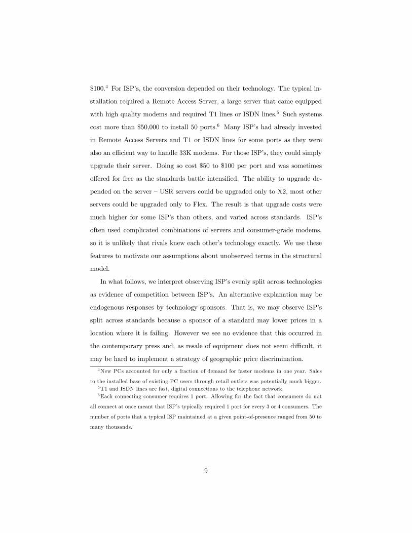
$100.4 For ISP’s, the conversion depended on their technology. The typical in-

stallation required a Remote Access Server, a large server that came equipped

with high quality modems and required T1 lines or ISDN lines.5 Such systems

cost more than $50,000 to install 50 ports.6 Many ISP’s had already invested

in Remote Access Servers and T1 or ISDN lines for some ports as they were

also an efficient way to handle 33K modems. For those ISP’s, they could simply

upgrade their server. Doing so cost $50 to $100 per port and was sometimes

offered for free as the standards battle intensified. The ability to upgrade de-

pended on the server — USR servers could be upgraded only to X2, most other

servers could be upgraded only to Flex. The result is that upgrade costs were

much higher for some ISP’s than others, and varied across standards. ISP’s

often used complicated combinations of servers and consumer-grade modems,

so it is unlikely that rivals knew each other’s technology exactly. We use these

features to motivate our assumptions about unobserved terms in the structural

model.

In what follows, we interpret observing ISP’s evenly split across technologies

as evidence of competition between ISP’s. An alternative explanation may be

endogenous responses by technology sponsors. That is, we may observe ISP’s

split across standards because a sponsor of a standard may lower prices in a

location where it is failing. However we see no evidence that this occurred in

the contemporary press and, as resale of equipment does not seem difficult, it

may be hard to implement a strategy of geographic price discrimination.

4New PCs accounted for only a fraction of demand for faster modems in one year. Sales

to the installed base of existing PC users through retail outlets was potentially much bigger.5T1 and ISDN lines are fast, digital connections to the telephone network.6Each connecting consumer requires 1 port. Allowing for the fact that consumers do not

all connect at once meant that ISP’s typically required 1 port for every 3 or 4 consumers. The

number of ports that a typical ISP maintained at a given point-of-presence ranged from 50 to

many thousands.

9

4 Data

The data set used in this paper draws on a number of sources. The unit of

analysis is the ISP and we use two directories of ISP’s to create our data set.

The first is from theDirectory. The list from theDirectory is meant to be compre-

hensive, including even the smallest ISP’s. Importantly, theDirectory provides

each phone number that each ISP can be contacted through, so we are able to

determine each ISP’s points of presence (POPs). However, theDirectory does

not provide any other data on ISP’s. In contrast, the Boardwatch directory gives

information about the technologies that ISP’s were using — in particular, which

type of 56k an ISP adopted in October 1997 and July 1997 (before many large

ISP’s adopted and before the ITU was turned to in earnest). Also, Boardwatch

lists whether an ISP had a T1 line and whether an ISP offered ISDN service to

consumers. However, Boardwatch does not provide information on individual

POPs. We merge the two data sets so we have both ISP technologies and their

geographic locations.

This merge has a number of implications. First, we lose many observations

from theDirectory because Boardwatch is less comprehensive. However, we be-

lieve that this loss is not a serious problem as Boardwatch contains data on the

“most important” ISP’s, and ISP’s that are not in Boardwatch were unlikely to

adopt 56k. We assume the 56k adopters face a “competitive fringe” of 28/33K

firms to which these “lost firms” belong.

A second implication of the construction of our data set is that we observe

only one adoption decision for each firm. We do not see if an ISP adopted

one type of 56k in one market, the other in a second market, and chose not

to adopt in a third market. Again, we believe this issue is not problematic

as it appears that ISP’s themselves treated the adoption decision as a single

firm-wide decision. There are a few reasons for this to be the case. ISP’s had

an incentive to deliver uniform service throughout their market area, especially

10

for clients who traveled. The choice of standard even seemed to become part

of the image of the ISP. Also, competition among Rockwell and US Robotics

led to the offering of exclusive contracts to ISP’s. For instance, it is clear from

press releases that national ISP’s such as AT&T and AOL, when they finally did

adopt in November 1997, adopted only a signal standard and did so throughout

their service areas.

Matching the October releases for each data set gives us 2233 ISP’s.7 Next

we determine markets for ISP’s. Consumers almost always work with an ISP

that is within the consumer’s local telephone calling range. From CCMI, we

obtain the Qtel data base which allows us to link telephone numbers to tele-

phone switches, and switches to local calling plans. We assign each switch to

the primary consumer local calling plan available from the incumbent telephone

company. From this information, we can determine the switches that are served

by each ISP, and the competitors that a consumer at each switch could poten-

tially call. Also, we observe the zip code associated with each switch, which we

use to add demographic data. We match switches to zip codes and counties and

use zip code level demographics from the 2000 Decennial Census or (when zip

code level data was unavailable) county level demographic data from the 1995

USA Counties CD-ROM. ISP’s are spread over 9,076 switches, which creates

216,583 separate ISP-switch combinations.8

Using switches as a measure of size shows that the market is served by many

small ISP’s and a few very large ones. The mean number of switches served by

an ISP is 96.8 but the distribution around the mean is very skewed. The median

7The original Boardwatch data set had 2653 observations, whereas theoriginal list from

theDirectory contained 5363 ISPs.8Note the difference with Augereau and Greenstein (2001), who also examines ISDN and

56k modem adoption. That paper uses county boundaries as the definition for a geographic

market, which identifies urban and rural locations, but not direct competitiors. In contrast

here, the emphasis on the rivalrous behavior between potential adopters requires a definition

of markets with greater granularity.

11

ISP serves 16 switches, the 75th percentile is 32, and the largest 5 firms serve

more than 4000 switches each.9 Note that there are more than 9,000 switches

in the data set so no ISP covers the entire market.10

Table 1 shows adoption rates in July and October. Note that we construct

the data using the October samples and simply append the October ISP’s choices

from July. That is, we ignore entry and exit over this 3 month period. Adoption

by July was very low. While there was significant adoption by October, still only

about half of ISP’s had adopted. Moreover, the vast majority of non-adopting

ISPs were large, so the percentage of customers served by 56k was much lower

than a half. The slight lead enjoyed by X2 in July had turned into a slight

lag by October. While very few firms adopt both technologies in July, they

represent more than 15% of adopters in October. Note that having a T1 line

is highly correlated with adoption. Among ISP’s with T1 lines, 56% adopted

X2 or Flex, whereas the adoption rate is 38% for those without a T1 line. We

also observe whether firms offer ISDN lines to their consumers.11 Firms offering

ISDN service adopted 56K 66% of the time, whereas the adoption rate was only

29% among firms that did not offer ISDN service.

A simple way to look at the data is to take local calling areas as distinct

markets. In fact, local calling areas do not create a partition of the United

States — there are areas where switch A can make a local call to switch B and

switch B can make a local call to C but A and C are not in the same local

calling area. Hence, we create local calling areas by making some arbitrary

9Sixteen switches would be one or two local calling areas.10There is no such thing as a truly national ISP as there are more then 19,000 switches in

the United States. Most of these switches are served by ISP’s, but by ISP’s that we classify

as being unlikely to adopt 56k.̇ Downes and Greenstein (2002) show that the largest ISP’s are

present mostly in urban areas.11Our dummy variable indicates if a firm offered ISDN service to consumers, not if a firm has

an ISDN connection to the Internet. Firms that offer ISDN service to consumers require an

ISDN connection to the Internet themselves. But many ISP’s had ISDN connections without

offering ISDN service to consumers.

12

July 1997 October 1997

None 1909 85.5% 1136 50.9%

X2 185 8.3 389 17.4

Flex 112 5.0 523 23.4

Both 27 1.2 185 8.3

Table 1: Number and Percent of ISP’s Adopting

assignments of switches to calling areas when a question arises. We find that

this arbitrariness is not very problematic for looking at some simple summary

statistics.12 Moreover, our final estimation procedure properly accounts for the

overlap patterns.

Our method creates 2,298 local calling areas. Local calling areas have rela-

tively few firms in each one. The average number of ISP’s in a calling area is

15 with a standard deviation of 20.8. However, there are 738 calling areas with

only 1 ISP and the median number is only 3. Table 2 gives average adoption

rates by local calling area. Again, there are only a few adopters in each calling

area. The average number of adopters in October 1997 is about 6. Interestingly,

although Flex leads X2 when tallied by ISP (as in Table 1), X2 leads Flex when

tallied by locale (as in Table 2).13

5 Simple Measures of Differentiation

Our goal is to show that ISP’s differentiated across standards instead of coordi-

nated on one standard or the other. In this section, we present simple statistics

that capture the spread of ISP’s across the two standards within local calling

12Most of the issues arise in dense urban markets with many competitors. Medium to low

density locations make up the bulk of the dataset and these are not problematic.13Although this finding suggests that larger firms were more likely to adopt X2, we find the

parameter on size (POPs) to be very similar across the two standards in our final estimation

procedure.

13

7/97 10/97

ISP’s 15.06 15.06

Adopters 0.99 5.98

X2 0.59 2.58

Flex 0.22 1.99

Both 0.18 1.40

Table 2: Averages by Local Calling Area

areas. This “first cut” of the data shows that ISP adoption is characterized by

differentiation. This prediction is borne out in the more comprehensive empiri-

cal model presented in Section 6.

Our approach in this section is to compare the national adoption rate with

the adoption rate in each local calling area. If the rates are close to the same,

it suggests that ISP’s were differentiating from each other. If local markets

are characterized by agglomeration on one standard or the other, it suggests

network effects were important.

Let {n0i , nAi , nBi , nABi } be the number of ISP’s in market i (a local callingarea) that do not adopt, that adopt Flex, that adopt X2 and that adopt both.

We start with a graphical presentation of our data. We calculate the number

of adopters of only X2 as a percentage of the number of ISP’s that adopt only

one standard, ignoring markets with only one such firm. That is, we compute

nBi /(nAi + nBi ) in each market where n

Ai + nBi > 1. For now, we ignore firms

that adopt both or neither standard (n0i and nABi ). The national adoption rate

computed in this way is 58%.

Figure 1 presents a histogram of adoption by calling area and captures much

of what we try to show in this paper. The black bars represent the observed

data. Figure 1 shows that most of the calling areas have between 50% and

80% adoption rates of X2, and there are very few calling areas with adoption

14

0

50

100

150

200

250

300

350

400

450

0.1 0.3 0.5 0.7 0.9

# of

loca

l cal

ling

area

sTRUESimulated

Figure 1: Percentage of ISP’s adopting X2.

close to 0 or 100%. As a point of comparison, we also calculate what would

have happened if ISP’s made independent random choices — that is, if nAi + nBi

firms in each market chose between A and B independently with probability

58%. These results are represented by the gray bars. Figure 1 shows that

independent random choice puts less weight in the center of the distribution

and more weight on the tails. The black bars are higher than grey bars for

the middle three bins and are lower than the grey bars for the outer seven.

Figure 1 suggests that differentiation (even splits between each standard within

each locale) characterizes this data, relative to independent random choice or

coordination.

In order to statistically test whether the hypothesis of independent ran-

dom choice can be rejected, we use the dartboard index of Ellison and Glaeser

15

(1997).14 We compute the index for each calling area separately and take an

unweighted national average. The dartboard index is positive if ISP’s are more

coordinated on a single standard than we would expect from independent ran-

dom choice and is negative if they are more differentiated. The dartboard index

accounts for the fact that we have small sample sizes within locales15. Under

the null hypothesis of independent random choice, the dartboard index is 0 and

we use Monte Carlo techniques to generate a standard deviation.

Results appear in Table 3. In Row 1, we consider ISP’s that adopt only one

standard and markets with at least two such ISP’s. In the terminology of Ellison

and Glaeser, firms can be in one of two states A and B and we check if nAi and

nBi show evidence of agglomeration, dispersion or independent allocation. The

average dartboard index across 1595 markets is -0.085. Under the null, it would

be 0 with a standard error of 0.012, so the null hypothesis can be rejected in

favor of differentiation. Row 2 includes firms that adopt both standards as if

they adopted X2. That is, the two states are {A} and {B,AB} and we computethe dartboard index on nAi and (nBi + nABi ). The results do not change. We

may also be interested in the distinction between adopting and not adopting,

ignoring the choice of standard. We consider the case where firms can be in

one of the two states {A,B,AB} or {0} and compare (nAi + nBi + nABi ) to n0i .

Row 3 shows that for this case, the data appears coordinated (in each case,

we include only markets with at least 2 ISP’s satisfying the relevant criteria).

That is, most markets are characterized by very high adoption or very little

14Ellison and Glaeser’s approach has the advantage over more standard tests such as the

Pearson Goodness of Fit test that it not only rejects independent random choice but also tells

the researcher whether the rejection is due to disperse or agglomerated data. See Rysman

and Greenstein (2003) for further discussion and an alternative approach.15The dartboard index is essentially a Gini coefficient for the distribution of ISPs over each

standard. If there are a small number of ISP’s in a locale, we expect the Gini to be greater

then zero regardless of how they make decisions, so the dartboard index modifies the Gini

coefficient by the Herfindahl of the decision making agents to get a value that has an expected

value of zero under the null of independent random choice.

16

Table 3: Dartboard Test for Differentiation

Description index std dev t-statistic Markets

Adopt only X2 vs. Adopt only Flex -0.085 0.012 -6.78 1595

Adopt X2 or Both vs. Adopt only Flex -0.038 0.012 -3.12 1698

Adopt vs. Not Adopt 0.034 0.010 3.32 2200

adoption, and there are few markets in between. This result may be explained

by local rivalry or local market demand (i.e., local demographic information),

and suggests the importance of controlling for local conditions in more stringent

tests.

Another way to look at the issue of differentiation across standards is to

exploit the dynamic aspect of the data. We can compare choices made up to

July 1997 to choices made afterwards. The results appear in Table 4. This

table shows that there were 1029 local calling areas where there was at least one

adopter by July. The columns refer to whether or not X2 was leading in that

calling area by July 1997. On the row is the number of calling areas where more

ISP’s adopted X2 than Flex in the July-October window. For instance, the table

shows that of the 686 calling areas where X2 led in July, Flex tied or led X2

from over the next 3 months in more than half the calling areas. The numbers

are more striking for calling areas where Flex led in July. Of these 152 calling

areas, there are 3 times as many locales where X2 led for July - October as there

are those where Flex led. These numbers suggest that ISP’s that observed one

standard obtain a lead did not continue to adopt that standard.

These statistics characterized the data by differentiation, not coordination.

They are strongly suggestive of the results we find in the full empirical model

in Section 6.

17

Table 4: Adoption in July 1997 versus adoption over the next 3 months

Adoption by 7/97

X2>Flex Tied Flex>X2 Total

Adoption X2 Leads for 7-10 325 79 67 471

Betw. 7/97 Tie 178 54 65 297

and 10/97 Flex Leads 183 58 20 261

Total Calling Areas 686 191 152 1029

6 Estimation

While the results in Section 5 are suggestive of an industry characterized by

differentiation, the methodology ignores important features of the industry. In

particular, ISP’s make a single adoption choice at all of their points-of-presence

so local calling areas are not independent markets. Even defining local callings

areas involves some arbitrariness. Furthermore, the methodology above does

not exploit demographic data and is difficult to interpret when we recognize

that some firms adopt both standards. The main econometric model addresses

all of these features.

6.1 Model

In our econometric model, ISP’s that offer 33K service at a POP decide whether

or not to offer 56k service on X2, Flex, both or neither. In this sense, the model is

like an entry game into two markets, X2 and Flex, in which we observe potential

entrants, as in Berry (1992). Following the theoretical model in Rysman (2003a),

we model the entry game as one of imperfect information, where we allow for

firms to observe their own unobservable draws but not those of their competitors.

In this regard, we follow the estimation methodology of Seim (2002).16

16 Several recent papers have exploited this assumption to develop two-stage estimators of

discrete (and dynamic) games. See Pakes, Ostrovsky and Berry (2003), Agguiregabiria and

18

Our estimation model is as follows. There are n firms and I locations.

Locations in the model are equivalent to switches in the data.17 The set of

locations in which firm j appears is ϑj . We compute ϑj to be the set of all

switches from which ISP j can be contacted by a local telephone call. A firm

may adopt either standard s, adopt both or not adopt, but the firm makes

the same adoption decision in every location. The number of firms that have

adopted technology s at location i besides j is nsi , where s can be equal to

{0, A,B,AB} (none, Flex, X2, and both). The potential adopters at a switchare identified by finding all ISP’s that can be contacted by a local telephone

call.

Firms draw a cost shock εsj for each standard. Firms observe their own draws

of εsj but not those of their competitors. The shocks represent the adoption cost

for the firm. One source of these costs may be the combination of servers,

consumer grade modems and digital connections a firm has which, as argued

earlier, affected the adoption cost of 56K and were arguably not well known

to their competitors. Because of this incomplete information, we search for a

Perfect Bayesian Equilibrium.18 The expected profit from adopting A or B in

location i for firm j is:

E[πsij ] = xliβ1 + xfj β2 +E[ψ1(nsi + 1) + ψ2n

ABi |X, θ] s = A,B (1)

The “+1” in the parenthesis accounts for the effect of firm j on profitability in

Mira (2002) and Pesendorfer and Schmidt-Dengler (2003).17 In this section, location i refers to a switch whereas in Section 5, location i referred to a

local calling area.18Our solution concept is equivalent to a Quantal Response Equilibrium. See McKelvey

and Palfrey (1995), and Haile, Hortascu and Kosenock (2003) for a discussion of its empirical

content.

19

location i. Average profit for firm j from adopting standard s is:19

E[Πsj ] =1

I

Xi∈ϑj

E[πsij] + εsj , s = A,B

We assume the 33K market is competitive everywhere and normalize profits

from non-adoption to zero. The profits from adopting both standards is simply

the sum of adopting each standard. Therefore:

E[Π0j ] = 0 E[ΠABj ] = E[ΠAj ] +E[ΠBj ]

The firm chooses the option with the highest expected payoff.20 The vectors

xli and xfj capture location specific and firm specific variables. The parame-

ters ψi capture the effect of competition on profits. The matrix X contains all

exogenous variables, including all values of xli, xfj and adoption decisions by

firms in previous periods. The variable εsj is a random fixed cost for standard s

unobserved by the researcher or other firms. We assume that [εAj εBj ] is distrib-

uted iid according the standard bivariate normal distribution with correlation

parameter ρ.21 The parameters θ = {β1, β2, ψ1, ψ2, ρ} are to be estimated. Inpractice, we allow them to differ for each standard. Our goal is to check whether

ψ1 < 0, which implies that firms prefer differentiation to agglomeration.

A widely recognized problem in the empirical literature on entry games is

the potentially endogenous determination of the number of competitors. A high

19Using average profit is equivalent to using total profit and imposing a particular form of

heteroskedasticity.20Note that in describing profits, we have left off any terms representing value in the future.

We do not try to solve the full dynamic game and in this sense, the parameters we estimate

capture both the flow profit from their associated variable and the expected future profit.

In addition, they may capture the fact that waiting has different values to different firms,

depending on future expectations.21An alternative approach would be to have firms that adopt both standards recieve a

(possibly negative) award due to economies of scope. It is difficult to distinguish between

economies of scope and a correlation in errors, which Manski (1998) terms the reflection

problem. We take ρ to capture both correlation in errors and economies of scope.

20

draw of εsj might be due to the fact the location is desirable. In that case, nsi will

also be high. Conversely, a high draw of εsj might suggest that nsi is small because

firm j will almost surely enter. However, as shown in Seim (2002), modelling

the entry game as one of imperfect information addresses this problem. In this

case, firms make their decision based not on nsi but on E[nsi |X,θ],which depends

only on exogenous variables. We discuss computation of E[nsi |X,θ] below.

Integrating over εAj and εBj , the implied adoption probabilities for firms that

did not adopt in July are:

PjN = Prob(dj = N) = Φ(−ΠAj ,−ΠBj , ρ) (2)

Pjs = Prob(dj = s) = Φ(Πsj ,−Π−sj ,−ρ) s = A,B

PjAB = Prob(dj = AB) = Φ(ΠAj ,ΠBj , ρ)

Here, dj is the decision of firm j and Φ() is the bivariate normal CDF with

correlation parameter ρ. For a firm that adopted one technology in July, the

probability of adopting the other in October is:

Pjs = Prob(E[Πsj ] > −εsj |E[Π−sj ] > −ε−sj )

We compute this integral by Gaussian quadrature. The likelihood function for

observing the n decisions d1, ..., dn is:

L(d1, ..., dn,X,θ) =nYj=1

Pjdj (3)

In order to compute E[nsi |X,θ], we use the following relation: The expectednumber of firms making choice s at location i can be divided into the the number

that chose s previously (by July 1997) ns,pri and the number choosing currently

ns,cui , the expectation of which depends on the adoption probabilities. Let Υ(i)

be the set of firms present in location i:

E[nsi |X,θ] =ns,pri +E[ns,cui |X, θ] = ns,pri +X

k∈Υ(i)Pks (4)

21

In order to calculate the term E[ψ1nsi +ψ2n

ABi |X, θ], we follow Seim (2002)

and exploit the fact that the system of equations 1, 2 and 4 form a fixed point

equation, solved by the n× 4 matrix of adoption probabilities P, with elementPjs. For any given set of parameters θ, the first step in solving for E[ψ1n

si +

ψ2nABi |X, θ] is to compute E[Πsj ]0, the value of E[Πsj ] assuming no firms adopt.

Doing so gives probabilities of adoption P0 that we use to create an initial guess,

E[ψ1nsi+ψ2n

ABi ]0. Using this value, we calculate E[Πsj ]

1, which generates a new

set of adoption probabilities P1 and a new value E[ψ1nsi+ψ2n

ABi ]1.We continue

iterating in this way as described by Seim (2002) until there is convergence,

thereby finding a fixed point in adoption probabilities for the system of best-

response functions.22 The appendix discusses the computation of the fixed point

in greater detail.

A weakness of our approach is that it does not guarantee that there is a

unique equilibrium. There may be multiple matrices P that solve the system

of equations above. In this model, this can occur for two reasons. The first

is associated with entry models and can occur if ψi < 0. Intuitively, there

could be an equilibrium where ISP 1 is expected to enter with high probability

and ISP 2 with low, and another equilibrium where the opposite is true. The

second is associated with network effects and can occur if ψi > 0. In this case,

there can be an equilibrium where most firms adopt and one where few firms

adopt. Our methodology requires either a unique equilibrium or an equilibrium

selection mechanism. The methodology relies on asymmetry in the data to

find uniqueness. For instance, while one might expect that there are multiple

equilibria between two symmetric firms, it would be less likely between a very

large firm and a very small firm.23 We further discuss this issue with the results.

22The adoption probabilities PjN , PjA, PjB, and Pj2 can be defined by only 2 cut-offs, so

in fact, the solution to our fixed point system is an n× 2 matrix.23 It is possible for there to be multiple equilibria in expectations that are so similar that

their difference is not important empirically.

22

6.2 Identification

This methodology creates a variable E[ψ1nsi +ψ2n

ABi |X, θ] that nicely captures

our intuition for identification. As with standard instrumenting techniques, it is

important that there are variables that affect the expected number of adopters

that j faces but that do not otherwise affect the decision of firm j. In this sense

the overlapping calling areas of different ISPs acts as a virtue. The relationship

between firms that provides the best identifying power would be a firm that

is completely overlapped by another firm, where the overlapping firm is also

present in many other locations. Then, the variable E[ψ1nsi + ψ2n

ABi |X, θ] for

the small firm depends on a large amount of demographic data that do not

otherwise appear in the decision of the firm. Cases where two firms completely

overlap but do not appear in many other locations should not provide strong

identification as the same demographic data that affect E[ψ1nsi + ψ2n

ABi |X, θ]

also appear directly in the firms’ decisions. Similarly, firms that appear in many

different locations but barely overlap with each other should not provide much

identification as these firms barely affect E[ψ1nsi + ψ2n

ABi |X, θ] for each other.

Other papers, such as Gowrisankaran and Stavins (2002), have used the

intuition that the decisions of geographically large firms can be thought of as

exogenous to the decisions of small firms. Our intuition is similar, although

we capture exogeneity in a more continuous way — the decision of a large firm

may be exogenous to a medium-sized firm and the decision of large and medium

firms may be exogenous to that of a small firm. With our methodology, we

do not have to make an a priori decision about which firms are exogenous to

which. A drawback is that we do not use the actual decision of large firms as an

exogenous variable, only the prediction of those decisions based on explanatory

variables.

Further important exogenous variation comes from the characteristics of

firms, such as their size and the presence of a digital connection. A final but

23

potentially important form of exogenous variation comes from decisions made

by firms in July 1997. The above mentioned forms of exogenous variation differ

across firms but not across standards. Without an exogenous variable that

varied by standard, we would not be able to predict that firms are more likely

to choose one standard or another. Adoption choices made three months earlier

provide this form of variation.24

7 Results

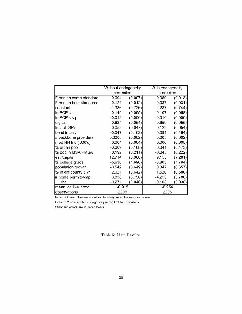
Table 5 presents the main results. The first two columns present coefficient

estimates and standard errors from estimating Equation 1 using the observed

values of nsi instead of expected values. It is equivalent to a bivariate probit

model predicting adoption of Flex and X2. Relative to the histogram in Figure

1, this model controls for ISP decision-making across multiple markets, for de-

mographics and ISP characteristics and for the exact competitive environment

resulting from the pattern of local calling areas. This model does not explicitly

correct for endogeneity of choices by competing firms.25 We present these re-

sults as an interim step towards our true model and to evaluate the role of the

instruments in the true model.

However, we begin our discussion with the second column, which presents

results correcting for endogeneity according to the model of imperfect infor-

mation described above. The result of primary interest is the first row, which

measures the effect of the number of competitors on standard s on the proba-

24A common criticism of the entry literature is that it models dynamic processes as simul-

taneous games. While we are subject to this criticism as well, the effects are mitigated by the

fact that we model only a 3 month process as a simultaneous game.25Note that under the assymetric information assumptions made in the model, the realized

number of entrants nsi is exogenous. Furthermore, under the assumption that nsi −E[nsi |X, θ]

is normal, this difference is absorbed by the probit error and the model using the observed nsi

in place of E[nsi |X, θ] is actually a consistent estimator for the true model.

24

bility of adopting standard s. In the first row of column 2, the effect is negative

and significant, implying the incentive to differentiate outweighed the incentive

to coordinate. The effect is reasonable and important. Doubling the number of

competitors adopting Flex reduces the probability of adopting Flex for a given

firm by 4.3 percentage points, a 13.9% change. These numbers are evaluated

at means in the data, where the average number of competitors on Flex is 5.78

and the average number of competitors on X2 is 7.02.

The coefficient on the number of firms adopting both standards is positive

but insignificant. We provide an interpretation for this result below. We see that

ISP characteristics are important predictors of adoption. Firms that have digital

connections to the Internet are much more likely to adopt 56K.26 Larger firms,

as measured by the number of switches a firms serves, are also more likely to

adopt both standards. This effect is estimated to be quadratic, probably driven

by the fact that the very largest firms in this data set do not adopt.

Under the assumption that the 33K market is competitive in all markets, the

number of ISP’s in a market should not matter directly. However, we include

the log of the number of ISP’s at a switch as a proxy for both the consumer

population at a switch (which we do not otherwise observe) and that popula-

tions’ preference for technology. This parameter is positive and significant. We

also include a dummy for whether that standard had a lead at this switch in

July, 1997. This parameter is not significant. It may be that there was simply

very little variation in this variable, as suggested by the Table 2. We also in-

clude the number Internet backbone providers at a switch. These firms often

leased modem banks to ISP’s indicating it was particularly easy to adopt in

these locations. As expected, this coefficient is positive and significant.

Demographic characteristics do not appear to be very important as only a

few are estimated to be significant. Surprisingly, the percentage of the pop-

26As above, digital indicates the firm has a T1 line or offers ISDN service to customers, but

could be 0 if a firm has ISDN lines but does not offer ISDN service to consumers.

25

Firms on same standard -0.094 (0.007) -0.050 (0.013)Firms on both standards 0.121 (0.012) 0.037 (0.031)constant -1.386 (0.726) -2.287 (0.744)ln POP's 0.149 (0.055) 0.107 (0.058)ln POP's sq -0.012 (0.006) -0.010 (0.006)digital 0.624 (0.054) 0.659 (0.055)ln # of ISP's 0.059 (0.047) 0.122 (0.054)Lead in July -0.047 (0.162) 0.091 (0.164)# backbone providers 0.0008 (0.002) 0.005 (0.002)med HH Inc ('000's) 0.004 (0.004) 0.006 (0.005)% urban pop -0.009 (0.168) 0.041 (0.173)% pop in MSA/PMSA 0.192 (0.211) -0.045 (0.222)est./capita 12.714 (6.960) 9.155 (7.281)% college grads -5.630 (1.690) -3.803 (1.794)population growth -0.542 (0.649) 0.347 (0.657)% in diff county 5 yr 2.021 (0.642) 1.520 (0.680)# home permits/cap. 3.838 (3.790) -4.253 (3.786) rho -0.271 (0.046) -0.103 (0.038)mean log likelihoodobservationsNotes: Column 1 assumes all explanatory variables are exogenous.Column 2 corrects for endogeneity in the first two variables.Standard errors are in parenthesis.

22062206-0.915 -0.954

With endogeneity correction

Without endogeneitycorrection

Table 5: Main Results

26

ulation that graduated from college is negative. As expected, the percentage

of the population living in a different county five years previous (a proxy for

county growth) is positive and significant. A test of joint insignificance for the

demographic variables can be rejected, suggesting that the demographics still

play a role in identifying the parameters on endogenous variables despite their

individually imprecise estimates.

The parameter ρ is estimated to be negative, implying that firms that adopt

one technology are less likely to adopt the other. This may reflect a number

of issues, such as diseconomies of scope or a negative correlation in unobserved

shocks.

Returning to the first column in Table 5 (which does not control for endo-

geneity), we see that the number of firms on the same standard has a negative

and significant impact on adopting of that standard. Most of the results are

similar across the two models, although the number of ISP’s in a market is in-

significant in column 1. The parameter on the number of firms adopting both

standards is positive and significant in column 1. We interpret this result as

reflecting consumer adoption patterns. If some areas have a strong preference

for new technology, we might expect many firms to adopt both technologies

in those markets. If we do not otherwise control for these consumer actions,

we will estimate a positive coefficient on the effect of firms that adopt both.

This “endogeneity” interpretation is supported by column 2, as the effect turns

insignificant when we estimate the structural parameter.

Overall, we conclude that the incentive to differentiate outweighed the incen-

tive to coordinate in this market. This result is surprising in these tests because

of the size of the markets. Finding differentiation in favor of independent ran-

dom choice is more difficult in large markets as the two hypothesis have similar

predictions as the number of agents gets large. In the histogram in Figure 1,

the level of observation is a market and the average number of adopters in a

market is 5.98. However, the level of observation in these regressions is the ISP

27

and ISP’s face on average 17.1 adopters. One need only a few large markets to

achieve this dichotomy. Even so, the results reject independent random choice

by ISP’s in favor of differentiation by ISP’s.

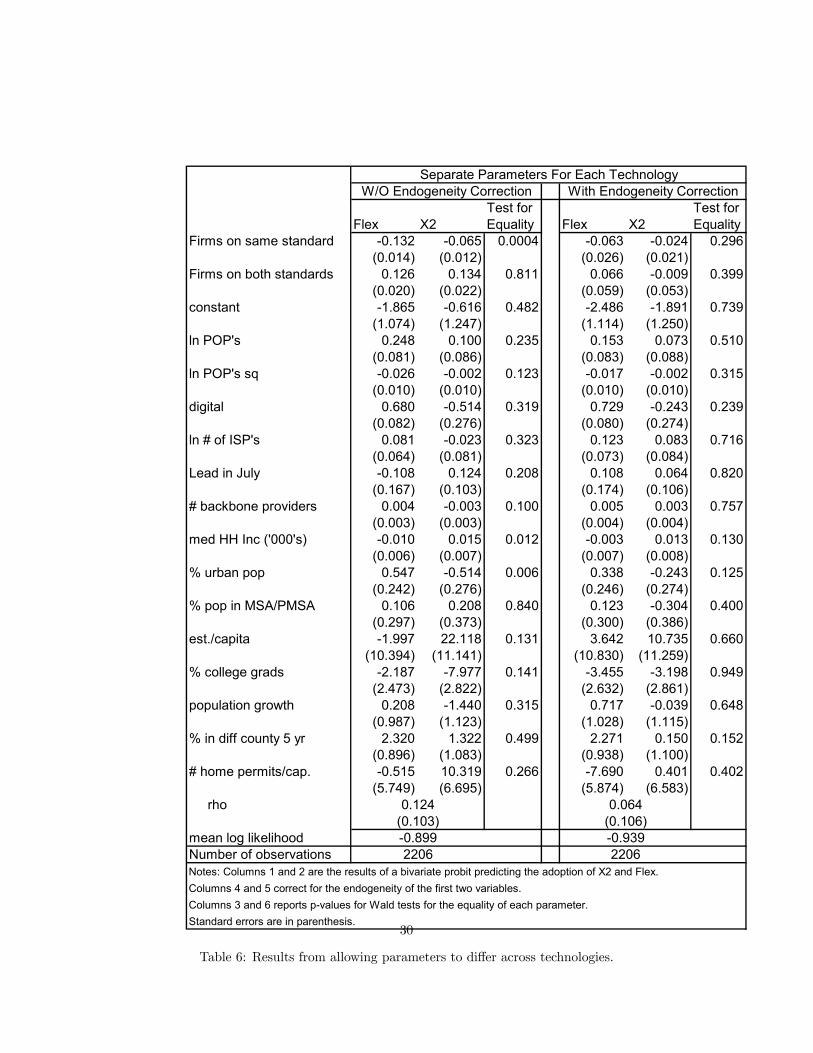
We perform a number of robustness tests. An important component for our

story is that the two technologies are functionally identical. We test for that by

testing the hypothesis that the parameters are equal across the two standards.

Table 6 presents results in which parameters are allowed to differ across the

two technologies. The first set of results assume that nsi is exogenous and the

second correct for endogeneity. Both the likelihood ratio test and the Wald test

reject the hypothesis of joint equality of each parameter row in both models.

However, we present p-values for variable-by-variable Wald tests and these are

more supportive. For these independent tests, we see that the hypothesis of

equality cannot be rejected at a 95% or even 90% level of confidence for any

variable for the model controlling for endogeneity. Even when not controlling

for endogeneity, the hypothesis of individual equality can be rejected at a 95%

level of confidence for only three variables. Furthermore, variables look broadly

similar across the equations. Given these results and the strong institutional

support for the symmetry of the two technologies, we conclude that restricting

the parameters to be the same across technologies is reasonable.

Also, note that the variable measuring the effect of the number of firms on

the same standard is negative for both technologies in both models. However, it

is insignificant in one of the cases: X2 in the model correcting for endogeneity.

Why is this result insignificant here but significant when we restrict parameters

to be the same across technologies? One reason is that allowing the parameters

on endogenous variables to differ across standards means we need an instrument

that varies across standards. The fact that we get inconclusive results in this

circumstance suggests that our instrument, adoption in July, does not provide

the necessary variation to identify all of these parameters. Indeed, note that

the dummy for the standard having a lead in July turns out to be insignificant

28

throughout the results.

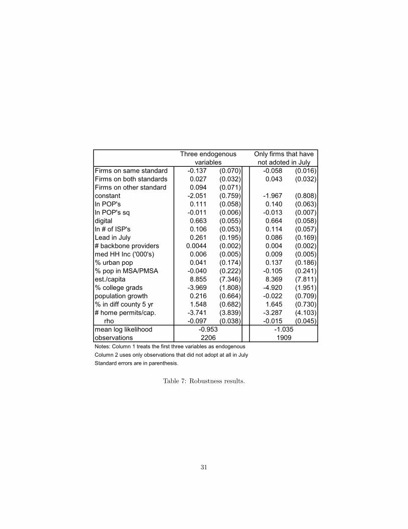
We present another set of robustness results in Table 7. In the first column,

we include the number of firms on the other standard as a third endogenous

variable. If consumer adoption were adequately controlled for, the number of

firms on the other standard might be reasonably expected to have no impact.

However, in our circumstance, it may reflect consumer adoption. In fact, we

find the new variable is statistically insignificant. Otherwise, we find similar

results to those reported in Table 5. Note that the variable of primary interest,

the parameter on the number of firms in the same standard, is again negative

but less precisely estimated: the t-statistic is 1.957.

As a final robustness test, we check if our results are driven by the firms that

adopt one standard in July. We re-estimate the model in column 2 of Table 5

but construct the likelihood value from only the 1909 observations that did not

adopt at all in July.27 The results appear in column 2 of Table 7. The results are

very similar to those estimated using all of the observations. The most striking

difference is the change in the estimate of ρ. Here, ρ is estimated to be much

closer to zero and insignificant. This result suggests that ISP’s that adopted

one technology in July were less likely to adopt both in October than ISP’s that

did not adopt at all in July. As the results of primary interest do not change in

this model, we do not further explore this issue here.

As discussed above, it is necessary that there be a unique equilibria or we

specify an equilibrium selection mechanism. For models that control for endo-

geneity, we search for multiple equilibria at the estimated parameters. We do

this by using different starting values in our fixed point algorithm that finds

equilibrium adoption probabilities. For instance, we start the algorithm at zero

adoption for all firms, certain adoption of A for all firms, certain adoption uni-

27The model of imperfect information requires us to make predictions about the adoption of

the remaining technology for firms that adopt one standard in July. The estimated parameters

are applied to those firms in this sense.

29

Test for Test forFlex X2 Equality Flex X2 Equality

Firms on same standard -0.132 -0.065 0.0004 -0.063 -0.024 0.296(0.014) (0.012) (0.026) (0.021)

Firms on both standards 0.126 0.134 0.811 0.066 -0.009 0.399(0.020) (0.022) (0.059) (0.053)

constant -1.865 -0.616 0.482 -2.486 -1.891 0.739(1.074) (1.247) (1.114) (1.250)

ln POP's 0.248 0.100 0.235 0.153 0.073 0.510(0.081) (0.086) (0.083) (0.088)

ln POP's sq -0.026 -0.002 0.123 -0.017 -0.002 0.315(0.010) (0.010) (0.010) (0.010)

digital 0.680 -0.514 0.319 0.729 -0.243 0.239(0.082) (0.276) (0.080) (0.274)

ln # of ISP's 0.081 -0.023 0.323 0.123 0.083 0.716(0.064) (0.081) (0.073) (0.084)

Lead in July -0.108 0.124 0.208 0.108 0.064 0.820(0.167) (0.103) (0.174) (0.106)

# backbone providers 0.004 -0.003 0.100 0.005 0.003 0.757(0.003) (0.003) (0.004) (0.004)

med HH Inc ('000's) -0.010 0.015 0.012 -0.003 0.013 0.130(0.006) (0.007) (0.007) (0.008)

% urban pop 0.547 -0.514 0.006 0.338 -0.243 0.125(0.242) (0.276) (0.246) (0.274)

% pop in MSA/PMSA 0.106 0.208 0.840 0.123 -0.304 0.400(0.297) (0.373) (0.300) (0.386)

est./capita -1.997 22.118 0.131 3.642 10.735 0.660(10.394) (11.141) (10.830) (11.259)

% college grads -2.187 -7.977 0.141 -3.455 -3.198 0.949(2.473) (2.822) (2.632) (2.861)

population growth 0.208 -1.440 0.315 0.717 -0.039 0.648(0.987) (1.123) (1.028) (1.115)

% in diff county 5 yr 2.320 1.322 0.499 2.271 0.150 0.152(0.896) (1.083) (0.938) (1.100)

# home permits/cap. -0.515 10.319 0.266 -7.690 0.401 0.402(5.749) (6.695) (5.874) (6.583)

rho

mean log likelihoodNumber of observationsNotes: Columns 1 and 2 are the results of a bivariate probit predicting the adoption of X2 and Flex.Columns 4 and 5 correct for the endogeneity of the first two variables.Columns 3 and 6 reports p-values for Wald tests for the equality of each parameter.Standard errors are in parenthesis.

2206 2206

Separate Parameters For Each TechnologyW/O Endogeneity Correction With Endogeneity Correction

0.124(0.103)-0.899

0.064(0.106)-0.939

Table 6: Results from allowing parameters to differ across technologies.

30

Firms on same standard -0.137 (0.070) -0.058 (0.016)Firms on both standards 0.027 (0.032) 0.043 (0.032)Firms on other standard 0.094 (0.071)constant -2.051 (0.759) -1.967 (0.808)ln POP's 0.111 (0.058) 0.140 (0.063)ln POP's sq -0.011 (0.006) -0.013 (0.007)digital 0.663 (0.055) 0.664 (0.058)ln # of ISP's 0.106 (0.053) 0.114 (0.057)Lead in July 0.261 (0.195) 0.086 (0.169)# backbone providers 0.0044 (0.002) 0.004 (0.002)med HH Inc ('000's) 0.006 (0.005) 0.009 (0.005)% urban pop 0.041 (0.174) 0.137 (0.186)% pop in MSA/PMSA -0.040 (0.222) -0.105 (0.241)est./capita 8.855 (7.346) 8.369 (7.811)% college grads -3.969 (1.808) -4.920 (1.951)population growth 0.216 (0.664) -0.022 (0.709)% in diff county 5 yr 1.548 (0.682) 1.645 (0.730)# home permits/cap. -3.741 (3.839) -3.287 (4.103) rho -0.097 (0.038) -0.015 (0.045)mean log likelihoodobservationsNotes: Column 1 treats the first three variables as endogenousColumn 2 uses only observations that did not adopt at all in JulyStandard errors are in parenthesis.

-0.953 -1.0352206 1909

Three endogenous Only firms that havevariables not adoted in July

Table 7: Robustness results.

31

formly distributed across A, B and both for all firms, and several other values.

In all cases, the algorithm finds one and only set of probabilities that satisfy

the equilibrium conditions. We conclude that each of the models estimated here

contain only one equilibrium. As suggested above, there is enough asymmetry

between firms to rule out multiple equilibria.

To summarize, we find evidence consistent with our central hypothesis, that

competition shaped ISP decision making over modem choice. We show that

competition consistently pushed behavior towards differentiation. ISP’s were

less likely to adopt a standard as more of their competitors adopted that stan-

dard.

8 Sources of Adoption Delay

As it turned out, 56K modem sales to ISP’s went very slowly relative to the

hopes of the modem producers. As we discussed, barely 50% of ISP’s adopted

56K by October 1997. Furthermore, none of the large ISP’s (AOL, AT&T,

UUNET, MSN, GTE, Bell-South, EarthLink) adopted. Due to the large skew

in market share (e.g. twenty firms serve more than three quarters of the users),

the vast majority of customers could not use 56K unless they switched from their

existing large ISP to one of these smaller ISPs. Most consumers did not make

this switch, even though most geographic regions had at least one or more ISP

carrying 56K. Accordingly, sales to consumers were much less than the modem

manufacturers expected.

Beyond expecting greater sales, industry participants expected the market to

coordinate on a single standard. The sponsors of the two technologies engaged in

a “standards war,” with deep discounts as well as marketing promotions arguing

that their technology would be the widely adopted standard.

Rockwell and USR both felt that the source of the slow sales was the stan-

dards battle and turned to the International Telecommunications Union, associ-

32

ated with the United Nations, to set a standard. The ITU announced the V.90

standard, an amalgam of X2 and Flex (but incompatible with both), in Febru-

ary 1998. At the time, this was regarded as the shortest period of time the ITU

had ever required to reach a decision. (Press Release ITU/98-4). Although the

ITU had no jurisdiction in this market, it created a focal point for the industry.

Sales were very strong thereafter and we interpret this widespread adoption by

both ISP’s and consumers as evidence of the value of coordinating on a single

standard.

Given the importance of standardization, why were consumers and ISP’s

unable to coordinate without the ITU? What role did the differentiation by

ISP’s identified above play in that process? In this section, we argue that

differentiation may have prolonged adoption delay.

Intuitively, network effects provide a force in favor of “tipping” towards one

technology or the other. Even with many geographically dispersed markets and

dispersed decision making, theory would lead one to expect local “tipping.”

That, in turn, might give rise to quick national unification of all local markets

on the same standard or geographic balkanization, with Chicago and Atlanta

tipping one way, Cleveland and Denver another, and so on. Instead, our tests

show that there was no coordination at any level.

Can such splitting result in adoption delay if competition is strong enough?

If consumers prefer a coordinated market and observe a split market, they may

delay adoption until one of the two technologies emerges as a standard. Our

model of how this might work is formalized in Rysman (2003a). In Rysman

(2003a), consumers and firms play a dynamic adoption game choosing between

two standards. Adopting a standard allows the adopter to trade with other

adopters. Firms draw random fixed costs of adoption for each standard in each

period. For particular parameter values, the model exhibits an equilibrium

with adoption delay. A small group of technology-loving consumers adopt each

standard in the first period. The remaining consumers delay their adoption

33

until a critical number of firms adopts one standard or the other. Knowing this,

firms avoid the standard with more firms on it in order to take advantage of the

higher margins available on the other standard. This differentiation by firms

justifies the consumers’ decision to delay adoption as they cannot guess which

standard will gain widespread acceptance. This equilibrium is more likely to

exist if competition is very fierce as it causes firms to avoid competition. This

models sets up the association between differentiation and delay that we claim

took place in the 56K market.28 The results of this model differ from most

previous work on network effects, which would predict coordination in a case

with homogenous technologies like the 56K modems.

However, if a delay in standardization happened for some reason other than

ISP differentiation, we might still expect to see ISP’s differentiating in response

to consumer behavior. Here we discuss explanations for adoption delay alter-

native to ISP differentiation. One possible explanation for the high sales of

modems in 1998 could be that there was a substantial increase in demand for

modems and Internet in early 1998 unrelated to standardization. We are skep-

tical of this explanation since the fastest period of growth in Internet adoption

was already under way in 1997. For instance, there were already thousands of

ISPs in the US, providing service to all but a small part of the US population

(Downes and Greenstein, 2002). Second, the ITU’s design for the V.90 did not

differ functionally from either the X2 or Flex standards, and yet the introduc-

tion of the V.90 generated enormous growth in demand. Another alternative

is that consumers were waiting for a new technology in 1997 (such as ISDN or

28Chou and Shy (1990) and Church and Gandal (1992) also consider models where multiple

networks exist when efficiency calls for a single network. They rely on consumer heterogeneity

but Church and Gandal specifically note the inefficient incentives of software providers to

differentiate across standards. Ellison and Fudenberg (2002) indentify a similar issue in a

more general setting and with homogenous standards. All three of these papers study static

games where all consumers adopt. Rysman (2003a) shows in a dynamic game that the choice

between standards can lead consumers to delay adoption, a particularly inefficient result.

34

cable modems) that they gave up on in 1998 in favor of 56K modems. We find

these hypotheses implausible.

We believe that most compelling alternative explanation is that market par-

ticipants were waiting for the ITU decision. Indeed, deliberations over 56K

modems at the ITU took place as early as November 1996 and the ITU claimed

that it would announce a standard about two years after the introduction of

the modem. However, there are a number of reasons to believe that the market

could have progressed before the ITU decision. First, it is not clear how credible

the ITU’s scheduling claims were. Two years would be very quick relative to

previous ITU decisions. Farrell (1996) reports that similar organizations deliver

standards in 5 years, on average. Also, the ITU had no enforcement power in

this case, it served only to create a focal point. If one technology could emerge

as the market standard, it might not matter what the ITU’s decision was. Even

two years was considered a long time in this industry, enough time to establish

a private standard. Furthermore, the ITU might pick one standard unmodified.

In the ITU’s previous interaction with the modem industry, it chose Rockwell’s

model for the 33.6K standard almost unmodified. Again, success in the pri-

vate market could influence the ITU along these lines. As evidence that the

market was not waiting for the ITU, note that the sponsors of the two tech-

nologies competed very aggressively on the market to become the 56K modem

standard.29

Another possibility for why there was adoption delay is that consumers were

simply confused. It was a new product and consumers had little information as

to which standard to pick so they waited. We believe that this explanation is

consistent with our story. Indeed, we would expect consumers that adopt before

a standard is set to choose randomly. Our point is that one source of consumer

29Also, note that it would have been difficult for the ITU to act without industry support.

There is evidence that Motorola prevented the advent of a new standard at an earlier ITU

meeting by demanding high licensing fees for a patented technology. (Greene, 1997)

35

confusion is that ISP’s split evenly between the two standards. Similar to con-

fused consumers, we could lay the blame at PC makers because they did not

pick a default 56K modem technology to bundle with computers. But, as with

consumer adoption, the explanation for this behavior must be that PC mak-

ers could not predict which standard would gain acceptance, which presumably

is at least partly because PC makers observed ISP’s evenly separating across

standards.

Note that Shapiro and Varian (1999) discuss the tactics by sponsors of com-

peting standards, both in general and in the particular case of 56K (on pages

267-270). Their general discussion focuses on characterizing a standards battle

and deducing whether tactics are aligned with market incentives. Their discus-

sion of the 56K modem case is broadly consistent with ours. However, they

do not offer a detailed explanation of why there was adoption failure previous

to the ITU decision and do not consider incentives to differentiate across the

standards by ISPs.30

9 Conclusion

This paper studies the importance of competition in technology adoption. We

exploit a unique data set on the standardization process for 56K modems in

numerous geographically independent markets. We show that Internet Service

Providers split evenly across the two available standards in local markets, con-

firming the importance of competition. We show that ISP’s split much more

evenly than independent random choice would predict with the dartboard index

of Ellison and Glaeser (1997). We confirm this result in a bivariate probit frame-

30Shapiro and Varian suggest a faster diffusion process then we do prior to the ITU decision,

relying mostly on announced adoption decisions for source material. Most of these announce-

ments come from the medium to large firms. As they point out, many of these announcements

were not followed by deployment. We follow our data source about deployments and report

non-deployment for the largest firms. See Rickard (1997a,1997b, 1998).

36

work that controls for ISP characteristics, demographics and decision-making

by ISP’s in multiple markets. Finally, we verify the result in a model based

on an entry game of imperfect information that controls for the endogeneity

of entry between rival ISP’s. The fact that competitive forces are so strong is

particularly surprising given the presence of an indirect network effect between

ISP and consumer adoption of a 56K standard.

We use this result to consider a new hypothesis about adoption delay in

a standards war. Previous theoretical work typically predicts that when net-

work effects are present, competition between two undifferentiated technologies

should lead to relatively quick standardization. However, this market failed to

standardize without the intervention of a standard-setting organization. The re-

sult that ISP’s differentiated across markets is consistent with our theory (for-

malized in Rysman, 2003a) that competitive differentiation across standards

caused consumers to delay their adoption, and ultimately necessitated the in-

tervention of the standard-setting organization. More broadly, the competitive

environment of service providers may be an important determinant in the suc-

cess or failure of a standards war, a previously overlooked issue by researchers,

policy makers and private-sector managers.

10 Appendix

Details on computing the fixed point algorithm: We can write E[Πsj ] as:

E[Πsj ] = xfj β2 +1

I

Xi∈ϑj

xliβ1 + ψ11

I

Xi∈ϑj

E[nsi |X, θ] + ψ1 + ψ21

I

Xi∈ϑj

E[nABi |X, θ]

Let Λ(j) be the set of firms that overlap with j and let λjk be the number of

switches at which j overlaps with k. Then we have that:

Xi∈ϑj

E[nsi |X, θ] =Xi∈ϑj

Xk∈Υ(i)

Pks =X

k∈Λ(j)λjkPks

37

Therefore, the average expected number of entrants faced by firm j depends only

on the number of locations at which j faces entrants and their entry probabilities,

not on where j faces them. That is, facing 3 markets with one potential entrant

in each has the same competitive implications as facing 2 markets with no

potential entrants and 1 market with 3, assuming entry probabilities are the

same. This feature allows us to solve the fixed point algorithm in an economical

manner. Let Λ be an n×n matrix with λjk in position j, k with λjk = 0 if j = k.

Let ψ be the 4× 1 matrix with elements 1,2,3 and 4 measuring the competitiveimpact of firms adopting none, the same standard, the other standard and both.

In our implementation, ψ = [0, ψ1, 0, ψ2] for Flex and ψ = [0, 0, ψ1, ψ2] for X2.

Then:

E[Πsj ] = xfj β2 +1

I

Xi∈ϑj

xliβ1 +ΛPψ + ψ1 (5)

Solving the fixed point algorithm consists of picking a starting matrix P0, plug-

ging into Equation 5 and plugging the result into Equation 2 to obtain a new

matrix of adoption probabilities P1. We can iterate this way until convergence.

The termP

i∈ϑj xli/I can be computed once at the beginning of the estimation

algorithm, further reducing the computational burden.

Note how restricting the competitive impact to be linear reduces the com-

putational burden: we need only know the number of locations at which any

firm overlaps with any other firm. If we were to add square terms, we would

need to know the number of locations at which a firm overlaps with any pair

of competitors and cubic terms require us to know the how many locations a

firm overlaps with any triplet. Putting in a more complicated term, such as

the ratio of adopters of one standard to the other, would likely requires us to

loop through every firm-location combination in the data (more than 200,000

items) and would be infeasible to our knowledge. It is straightforward to add

these terms to the analysis that assumes exogeneity and we found that it did not

change the analysis. For instance, adding squares of the number of competitors

38

adopting one of the choices does not change any of the results in a substantial

way.

References[1] Ackerberg, D and G. Gowrisankaran (2003) “Quantifying Equilibrium Net-

work Externalities in the ACH Banking Industry," mimeo, UCLA.

[2] Amemiya, T (1985) Advanced Econometrics, Harvard University Press,Cambridge.

[3] Armstrong, M. (2002) “Competition in Two-Sided Markets," mimeo, Ox-ford University.

[4] Aguirregabiria, V and P. Mira (2002) “Identification and Estimation ofDynamic Discrete Games,” mimeo, Boston University.

[5] Augereau, A, and S. Greenstein (2001)," The Need for Speed in EmergingCommunications Markets: Upgrades to Advanced Technology at InternetService Providers." International Journal of Industrial Organization, v 19,pp 1085-1102.

[6] Besen S.M. and L. Johnson (1986), Compatibility Standards, Competition,and Innovation in Broadcasting Industry, Rand Report, R-3453/1-Nsf.

[7] Berry, S.T. (1992) “Estimation of a Model of Entry in the Airline Industry,”Econometrica, 60(4), 889-917.

[8] Berry, S. and A. Pakes (2002) “Two Estimators for the Parameters of Dy-namic Discrete Games,” mimeo, Harvard University.

[9] Church, J. and N. Gandal (1992) “Network Effects, Software Provision andStandardization," Journal of Industrial Economics, 40(1) 85-103.

[10] Chou, C. and O. Shy (1990) “Network Effects without Network Externali-ties" International Journal of Industrial Organization, 8 259-270.

[11] Dranove, D and N. Gandal (2003) “The DVD vs. DIVX StandardWar: Em-pirical Evidence of Network Effects and Preannouncement Effects,"Journalof Economics and Management Science., 12 (3), pp. 363-386.

[12] Downes, T. and S. Greenstein (1999), “Universal Access and Local Com-mercial Internet Markets "Research Policy, 31, 1035-1052.

[13] Ellison, G. (1997) “Geographic Concentration in U.S. Manufacturing In-dustries: A Dartboard Approach,” Journal of Political Economy, 105(5)889-927.

39

[14] Ellison, G. and D. Fudenberg (2003) “Knife Edge or Plateau: When DoMarket Models Tip?” MIT Department of Economics Working Paper No.03-07.

[15] Farrell, J. (1996) “Choosing Rules for Formal Standardization,” mimeo,University of California, Berkeley.

[16] Gandal, N., M. Kende and R. Rob (2000), “The Dynamics of Technolog-ical Adoption in Hardware/Software Systems: The Case of Compact DiscPlayers", Rand Journal of Economics, 31, 43-61.

[17] Genesove D, (1999) “The Adoption of Offset Presses in the Daily Newspa-per Industry in the United States,” NBER Working Paper 7076.

[18] Gourieroux, C and A. Monfort (1995) Statistics and Econometric Models:Volume 1. Cambridge University Press, Cambridge.

[19] Gowrisankaran, G. and J. Stavins (2002) “Network Externalities and Tech-nology Adoption: Lessons from Electronic Payments,” RAND Journal ofEconomics, forthcoming.

[20] Greene, T (1997) “More Bumps in the Road for 56K modems,” NetworkWorld, September 22, 1997, p12.

[21] Greenstein, Shane (2000) “Building and Delieverying the Virtual World:The Commercial Internet Access Market", Journal of Industrial Economics

[22] Haile, P.A., A. Hortascu and G. Kosenock (2003) “On the Empirical Con-tent of Quantal Response Equilibrium,” mimeo, Yale University.

[23] Klepper, S. (2002) “Firm Survival and the Evolution of Oligopoly,” RandJournal of Economics, 33(1) 37-61.

[24] Manski, C. (1993) “Identification of Endogenous Social Effects: The Re-flection Problem,” Review of Economic Studies, 60, 531-542.

[25] McKelvey, R.D. and T.R. Palfrey (1995) “Quantal Response Equilibriumfor Normal Form Games,” Games and Economic Behavior, 10(1), 6-38.

[26] Mulligan, J.G. and E. Llinares (2003) “Market Segmentation and the Dif-fusion of Quality-Enhancing Innovations: The Case of Downhill Skiing,”Review of Economics and Statisitcs, 85(3), 493-502.

[27] National Telecommunications Information Administration (2002),. “A Na-tion Online: How Americans Are Expanding Their Use Of The Internet.’http://www.ntia.doc.gov/reports.html.

[28] Ohashi, H (2000) “Network Externalities and Consumer Welfare: HomeVideo Cassette Recorders in the U.S., 1978-1986" mimeo, University ofBritish Columbia.

40

[29] Park, S (2000) “Quantitative Analysis of Network Externalities in Com-peting Technologies: The VCR Case," mimeo, SUNY-Stony Brook.

[30] Pesendorfer, M and P. Schmidt-Dengler (2003) “Identification and Estima-tion of Dynamic Games,” mimeo, London School of Economics.

[31] Postrel, S (1990) “Competing Networks and Proprietary Standards: TheCase of Quadraphonic Sound," Journal of Industrial Economics, 39(2),169-185.

[32] Rickard, J (1998) “The 56K Modem Battle,” Boardwatch, March 1998.

[33] Rickard, J (1997a) “56K Modems: The Battle Continues,” Boardwatch,March 1997.

[34] Rickard, J (1997b) “U.S. Robotics Launches the New Battle - 56KbpsModems” Boardwatch, January 1997.

[35] Rochet, J.-C. and J. Tirole (2002) “Platform Competition in Two-SidedMarkets" mimeo, University of Toulouse.

[36] Rohlfs, J (2001) Bandwagon Effects in High Technology Industries, MITPress, Cambridge.

[37] Rysman, M. (2003a), “A Standards War Under Indirect Network Effects,”mimeo, Boston University.

[38] Rysman, M. (2003b), “Competition Between Networks: A Study of theMarket for Yellow Pages,” Review of Economic Studies, forthcoming.

[39] Rysman, M. and S. Greenstein (2003), “Testing for Agglomeration andDispersion,” mimeo, Boston University.

[40] Saloner, G. and S. Shepard (1995) “Adoption of Technologies with NetworkEffects: An Empirical Examination of the Adoption of Automated TellerMachines” Rand Journal of Economics, 26, 479-501.

[41] Shapiro, C., and H. Varian (1999), Information Rules: A Strategic Guideto the Network Economy, Harvard Business School Press, Cambridge.

[42] Shy, O. (2001) The Economics of Network Industries, Cambridge UniversityPress, Cambridge.

[43] Seim, K. (2002) “An Empirical Model of Firm Entry with EndogenousProduct-Type Choices,” mimeo, Stanford University GSB.

41