arX

iv:1

004.

5037

v1 [

q-fi

n.C

P] 2

8 A

pr 2

010

Convenient Multiple Directions of Stratification∗

Benjamin Jourdain, Bernard Lapeyre†, Piergiacomo Sabino‡

Abstract

This paper investigates the use of multiple directions of stratification as a variance reductiontechnique for Monte Carlo simulations of path-dependent options driven by Gaussian vectors.The precision of the method depends on the choice of the directions of stratification and theallocation rule within each strata. Several choices have been proposed but, even if they providevariance reduction, their implementation is computationally intensive and not applicable to re-alistic payoffs, in particular not to Asian options with barrier. Moreover, all these previouslypublished methods employ orthogonal directions for multiple stratification. In this work weinvestigate the use of algorithms producing convenient directions, generally non-orthogonal,combining a lower computational cost with a comparable variance reduction. In addition, westudy the accuracy of optimal allocation in terms of variance reduction compared to the LatinHypercube Sampling. We consider the directions obtained by the Linear Transformation andthe Principal Component Analysis. We introduce a new procedure based on the Linear Approx-imation of the explained variance of the payoff using the law of total variance. In addition, weexhibit a novel algorithm that permits to correctly generate normal vectors stratified along non-orthogonal directions. Finally, we illustrate the efficiency of these algorithms in the computationof the price of different path-dependent options with and without barriers in the Black-Scholesand in the Cox-Ingersoll-Ross markets.

Keywords. Monte Carlo methods, variance reduction, stratification methods.

1 Introduction

The main purpose of Monte Carlo (MC) simulations is to compute integrals numerically. It is fre-quently the only alternative for solving problems in applied sciences and notably for financial ap-plications. The pricing of derivative contracts and value-at-risk calculations for risk-managementpurposes typically require numerical simulations. However, the MC method for high-dimensionalproblems is a demanding computational task and a considerable number of studies have been de-voted to increase its efficiency via variance reduction techniques. This paper investigates theuse of multiple directions of stratification as a variance reduction technique for MC simulationsof path-dependent options driven by high-dimensional Gaussian vectors. The precision of themethod depends on the choice of the partitions of the space and the allocation of the number ofsamples within each strata. Usually, the strata are polyhedrons delimited by hyperplanes orthog-onal to a few direction vectors. Several choices have been proposed: Glasserman et al. [8] selectthe directions for the stratification of linear projections based on the quadratic approximationof the integrand or payoff function. In contrast, Etoré et al. [4] find the directions by adaptivetechniques. These two approaches provide a high variance reduction but their implementationcan be computationally intensive and the former one cannot be applied to more realistic payofffunctions such as Asian options with barrier at each time step. Moreover, these two methodssuppose orthogonal directions for multiple stratification. In this work, we investigate the use ofalgorithms producing convenient directions, generally non-orthogonal, combining a lower com-putational cost with a variance reduction that is comparable to the above mentioned methods.In addition, we study the accuracy of optimal allocation, combined with the above stratification

∗This research benefited from the support of the chair "Risques Financiers", Fondation du Risque.†Université Paris-Est, CERMICS, Projet MathFi, ENPC-INRIA-UMLV, 6 et 8 avenue Blaise Pascal, 77455 Marne La

Vallée, Cedex 2, France, E-mails: jourdain@cermics.enpc.fr, bl@cermics.enpc.fr‡Université Paris 7 Diderot, LPMA, 175 rue du Chavaleret, 75013 Paris, France, Email: sabino@math.jussieu.fr

1

techniques, in terms of variance reduction, compared to “fixed” allocation procedures such asLatin Hypercube Sampling (LHS). We consider the directions produced by the Linear Transfor-mation (LT) decomposition introduced by Imai and Tan [9] and the Principal Component Analysis(PCA). Moreover, we propose a new procedure based on the Linear Approximation (LA) of the“explained” variance of the payoff function by the use of the law of total variance. Notably, wedesign a novel algorithm that permits to correctly generate multivariate normal random vectorsstratified along non-orthogonal directions. We illustrate the efficiency of the proposed algorithmsand their combination for the computation of the price of different path-dependent options withand without barriers in the Black-Scholes (BS) and in the Cox-Ingersoll-Ross (CIR) models. In theformer dynamics, it turns out that the LA and the LT approaches return the same first order direc-tion while this vector is almost parallel to the one obtained by the GHS technique even in the caseof Asian options with a barrier at expiry. This justifies the application and the good performanceof the LA (and LT) if the barrier is at each monitoring time. Consequently, the approaches returnthe same variance reduction and the LA (LT) is easier to implement and has a lower computationalcost. We repeat our numerical investigation in the CIR framework where we find explicit solutionsfor the LT and LA directions. In order to find a further direction, we compute the first principalcomponent of the sampled covariance matrix of the price process obtained by a MC estimationvia a pilot run. In both BS and CIR dynamics, LT and LA return remarkable variance reductionwith a low computational cost. We also show that in some setting the stratification along multipledirections can be more efficient than stratifying along a single one. In particular, the combinationof the LA (LT) direction and a non-orthogonal direction, notably the first principal component,can even outperform the variance reduction of two orthogonal directions in the case of barrieroptions. Finally, as far as the allocation of the samples is concerned, in any case the LHS displaysa considerable higher computational time and has always a lower variance reduction as comparedto the use of a convenient direction of stratification with optimal allocation.

The paper is organized as follows. Section 2 reviews the main ideas of stratification andthe motivations of this study. Section 3 presents the new algorithm that permits the stratificationalong non-orthogonal directions. Section 4 discusses the use of convenient stratification directionsand in particular, contains the presentation of the LT decomposition and the introduction of theLA procedure. In Section 5 we explain the financial applications and find the explicit solutionsfor the LA and the LT methods both for the BS and the CIR dynamics. In Section 6 the variancereductions and the computational costs of the proposed technique are illustrated by numericalexperiments. Finally, Section 7 concludes the paper by summarizing the most important findings.

2 Stratified Sampling and Linear Projections

Stratified Sampling is a general variance reduction technique that consists of drawing the observa-tions from specific partitions of the sample space. More specifically, suppose we want to computeby MC simulations an expectation of the form E[g(Y)] where g : R

d → R is a Borel function andY is a R

d-valued random vector with the assumption that E[g(Y)2] < ∞. Consider a stratification

variable X and let A1, . . . , AK be disjoint subsets of the real line for which P

(⋃K

k=1{X ∈ Ak})

= 1.Then

E[g(Y)] =K

∑k=1

E[g(Y)|X ∈ Ak]P(X ∈ Ak) =K

∑k=1

E[g(Y)|X ∈ Ak]pk (1)

where pk = P(X ∈ Ak), k = 1, . . . , K. The stratified estimator with NS draws is defined as:

K

∑k=1

pk1nk

nk

∑j=1

g(Ykj) =1

NS

K

∑k=1

pk

qk

nk

∑j=1

g(Ykj), (2)

where nk are the number allocations in the k-th stratum and qk = nk/NS is their fraction in thek-th stratum and Ykj are independent draws from the conditional distribution of Y given X ∈ Ak.

Its variance is given by ∑Kk=1 p2

k

σ2k

nkwhere σk is the conditional variance of g(Y) given X ∈ Ak.

This estimator may be more efficient than the usual MC sample mean estimator of a randomsample of size NS. The potential higher efficiency of the former estimator critically depends on

2

the allocation rule and the choice of the partition of the sample space. The optimal allocation ruleis the one that minimizes the variance of the stratified sampling estimator given the partition ofthe state space and the constraint ∑

Kk=1 qk = 1. It is given by:

qk =pkσk

∑Kk=1 pkσk

. (3)

The probabilities pk are known whereas generally the conditional variances are not known. Theycan be estimated in a pilot run and then used in a second stage to determine the stratified estima-tor. This is not the optimal procedure and more sophisticated techniques can be employed, seefor example Etoré and Jourdain [5].

We focus our attention on MC simulation driven by high-dimensional Gaussian vectors thatare of particular interest in financial applications. As such, we consider in the following onlynormal random variables.

2.1 Stratifying Linear Projections: 1-dimensional Setting

We begin with a general description of stratifying a linear projection of a Gaussian random vector.Suppose Z is a d dimensional centered Gaussian random vector, Z ∼ N (0, ΣZ) and then considerthe stratification variable X as the linear projection of Z over a fixed direction v ∈ R

d, X = v · Z.X is also Gaussian with variance v · ΣZv. This choice permits to partition the sample space R

d

into strata defined by

Sk,v ={

x ∈ Rd, x · v ∈ Ak

}

. (4)

Due to the Gaussian structure of the random variables we can generate Z stratified along thedirection v in the following way. Consider a general Gaussian random vector Y = (Y1, Y2):

Y = (Y1, Y2) ∼ N( (

µ1µ2

)

,(

Σ11 Σ12Σ21 Σ22

) )

(5)

and denote L (Y1|Y2 = x) the law of Y1 given Y2 = x, it is possible to prove (see for instanceGlasserman [7]) that

L(Y1 | Y2 = x) = N(

µ1 + Σ12Σ−122 (x − µ2) , Σ11 − Σ12Σ−1

22 Σ21

)

. (6)

where we assume that Σ22 is invertible. Adapting the above result for Z given X = v · Z andVar[X] = v · ΣZv = 1 we have

L (Z |X = x ) = N(

ΣZv

v · ΣZvx, ΣZ − ΣZvvTΣZ

v · ΣZv

)

= N(

ΣZvx, ΣZ − ΣZvvTΣZ

)

. (7)

If we consider ΣZ = Id the above equation becomes:

L (Z |X = x ) = N(

vx, Id − vTv)

. (8)

The conditional covariance matrix D = Id − vTv does not depend on x and since D is an orthog-onal projection matrix, we have DDT = D. Due to this result, we do not need to compute theCholesky (or a general square-root) matrix of D to sample from the conditional distribution ofZ given X. These observations give an easy and simple algorithm to generate K samples of Zstratified along the direction v.

Suppose now that Ak is the interval between the quantiles of order k−1K and of order k

K of thestandard normal distribution. We can sample from Z given Z · v ∈ Ak in the following steps:

1. generate U ∼ U ([0, 1]).

2. Set V = k−UK and X = Φ−1(V), with Φ the inverse of the cumulative normal distribution.

3. Generate Z′ ∼ N (0, Id) independent on U.

4. Set vX +(

I − vvT)

Z′.

We suggest to implement the last term in the last step as Z′ − v(v · Z′) which requires O(d)operation rather than O(d2).

3

2.2 Stratifying Linear Projections: Multidimensional Setting

We start with the case of orthogonal directions and consider a matrix V ∈ Rd×d′ , d′ ≤ d, whose

columns are the direction vectors, such that VTV = Id′ . Following the notation introduced abovewe have:

X = VTZ (9)

where now X is d′ dimensional. Moreover,(

ZX

)

∼ N( (

00

)

,(

ΣZ ΣZVVTΣZ VTΣZV

) )

(10)

Consequently

L (Z |X = x ) = N(

ΣZV(

VTΣZV)−1

x, ΣZ − ΣZV(

VTΣZV)−1

VTΣZ

)

(11)

where we assume that VTΣZV is invertible. In the case ΣZ = Id we have

L (Z |X = x ) = N(

V(

VTV)−1

x, Id − V(

VTV)−1

VT

)

. (12)

Hence, if we adopt orthogonal directions VTV = Id′ the algorithm to stratify Z given X = VTZ is asimple multidimensional version of the algorithm illustrated before where now we should stratifythe d′ dimensional hypercube [0, 1]d

′. Suppose, for example, that we stratify the j-th coordinate

of the hypercube, j = 1, . . . , d′, into Kj intervals of equal length so that we have a total number ofK1 × · · · × Kd′ equiprobable strata. In this multidimensional setting we can sample from Z given

X = VTZ ∈ Ak, where Ak = ∏d′j=1 Φ

([k j−1

Kj,

k j

Kj

])

, in the following steps:

1. generate U = (U1 . . . , Ud′) with independent components each of law U ([0, 1]).

2. Set Vj =k j−Uj

Kjwith j ∈ {1, . . . , d′} and kj ∈ {1, . . . , Kj}.

3. Set X = (X1 . . . , Xd′), Xj = Φ−1(Vj).

4. Generate Z′ ∼ N (0, Id) independent of U.

5. Set VX +(

Id − VVT)

Z′.

We now investigate the possibility to stratify over different directions that can be non-orthogonaleither. When the directions are not orthogonal the components of X are not independent sinceVar[X] = VVT 6= Id′ and the previous multidimensional algorithm cannot be adopted anymore.

A first way yo approach this problem may be to assume XL= CXǫ with ǫ ∼ N (0, Id′) independent

on Z and CX ∈ Rd′×d′ such that Var[X] = CXCT

X, and use the following slight modification of theabove algorithm.

1. generate U = (U1 . . . , Ud′) with independent components each of law U ([0, 1]).

2. Set Vj =k j−Uj

Kjwith j = {1, . . . , d′} and kj = {1, . . . , Kj}.

3. Set ǫ = (ǫ1 . . . , ǫd′), ǫj = Φ−1(Vj).

4. Generate Z′ ∼ N (0, Id) independent of U.

5. Set V(CXX )

−1ǫ + (Id − V(VTV

)−1VT)Z′.

However, although mathematically correct, this algorithm stratifies the marginals of the randomvector ǫ that has independent components. This construction does not consider the fact that themarginals of X are not independent and the introduction of the dependence can affect this partialstratification in complicated ways (see Glasserman [7]).

4

3 Stratification along non-orthogonal directions

In this section we show how to generate multivariate normal random vectors, Z ∼ N (0, Id),stratified along non-orthogonal directions. We prove the following proposition:

Proposition 1. Let B1 = {e1 . . . , ed′} be a set of linearly independent vectors in Rd′ , d′ ≤ d, such that

‖ei‖ = 1, i = 1, . . . , d′, let B′ = {f′1 . . . , f′d′} be the set of orthogonal vectors produced the Gram-Schmidt

procedure: f′i = ei − ∑i−1m=1(ei·f′m)f′m

‖f′m‖2 . Finally consider B2 = {fi =f′i

‖f′i‖, i = 1, . . . , d′} the orthonormal

version of B′ and let F be the d × d′ matrix whose i-th column is fi.

Suppose g : Rd → R such that E[g2(Z)] < +∞ and consider two vectors in R

d′ , a± = {a±1 , . . . , a′±d },

such that a−i < a+i , ∀i = 1, . . . , d′. We have

E[g(Z)

∣∣a−i ≤ Z · ei ≤ a+i , i = 1, . . . , d′

]

= E

[

g

((

I − FFT)

Z

+d′

∑m=1

fmΦ−1(

Φ(

a−m(

U(m−1)))

+ Um

(

Φ(

a+m

(

U(m−1)))

− Φ(

a−m(

U(m−1)))))

)

×∏

d′m=1

(

Φ(

a+m

(

U(m−1)))

− Φ(

a−m(

U(m−1))))

P(a−i ≤ Z · ei ≤ a+i , i = 1, . . . , d′

)

(13)

where

a±i(

U(i−1))

=a±i − ∑

i−1j=1 ei · fjΦ

−1(

Φ(

a−j(

U(j−1)))

+ Uj

(

Φ(

a+j

(

U(j−1))

− Φ(

a−j(

U(j−1))))))

‖ f ′i ‖(14)

with the notation, U(j) =(U1, . . . , Uj

), j = 1 . . . , n and U1, . . . , Ud′ i.i.d. uniformly distributed random

variables, all independent on Z; we assume U0 = 0 and a±1 = a±1 .

Remark 1. The above result requires the computation of the joint probability P(a−i ≤ Z · ei ≤ a+i , i = 1, . . . , d′

)

where the random variables Z · ei, i = 1, . . . , d′ are not independent; in contrast, this term is not necessaryfor the estimation of E [g(Z)]. Indeed, suppose K strata, by conditioning we have:

E [g(Z)] =K

∑k=1

E [g(Z) |Z ∈ k-th stratum ] P (Z ∈ k-th stratum) , (15)

then plugging in the conditional expectation the result of equation (13) the probabilities at the numeratorand at the denominator simplify out.

Proof. For simplicity we suppose d′ = 2, the Gram-Schmidt procedure returns f′1 = f1 = e1,

f′2 = e2 − (e1 · e2)e1 and f2 =f′2

‖f′2‖. It follows that

E

[

g(Z)

∣∣∣∣

a−1 ≤ Z · e1 ≤ a+1a−2 ≤ Z · e2 ≤ a+2

]

= E

[

g(Z)

∣∣∣∣∣

a−1 ≤ Z · f1 ≤ a+1a−2 −(e1·e2)e1·Z

‖ f ′2‖≤ Z · f2 ≤ a+2 −(e1·e2)e1·Z

‖ f ′2‖

]

.

Based on the results of the Section 2 and the properties of the conditional expectation, the previousexpression equals:

CE

[

g(

Z + f1

(

Φ−1 (Φ(a−1 ) + U1(Φ(a+1 )− Φ(a−1 )

))− f1 · Z

))

11a−2 (U1)≤f2·Z≤a+2 (U1)

]

(16)

where

C =Φ(a+1 )− Φ(a−1 )

P

(a−1 ≤ Z · e1 ≤ a+1a−2 ≤ Z · e2 ≤ a+2

) .

5

The expected value is then:∫ 1

0E

[

g(

Z + f1

(

Φ−1 (Φ(a−1 ) + u1(Φ(a+1 )− Φ(a−1 )

))− f1 · Z))

11a−2 (u1)≤f2·Z≤a+2 (u1)

]

du1

=∫ 1

0E

[

g

(

Z + f1

(

Φ−1 (Φ(a−1 ) + u1(Φ(a+1 )− Φ(a−1 )

))− f1 · Z

)

+ f2

(

Φ−1 (Φ(a−2 (u1)) + U2(Φ(a+2 (u1))− Φ(a−2 (u1))

))− f2 · Z

))

× (Φ(a+2 (u1))− Φ(a−2 (u1))

)]du1

= E

[

g

(

Z + f1

(

Φ−1 (Φ(a−1 ) + U1(Φ(a+1 )− Φ(a−1 )

))− f1 · Z)

+ f2

(

Φ−1 (Φ(a−2 (U1)) + U2(Φ(a+2 (U1))− Φ(a−2 (U1))

))− f2 · Z))

× (Φ(a+2 (U1))− Φ(a−2 (u1))

)].

Rearranging the terms in Z we get equation (13) for d′ = 2. The result for d′ direction is obtainediterating the steps above.

4 Convenient Directions

Given an allocation rule, the crucial point in the stratification of linear projections is the choiceof the directions of stratification. Indeed, stratified sampling eliminates the sampling variabilityacross strata without affecting the sampling variability within strata. Good directions are charac-terized by their higher capacity to dissect the state space into strata where the integrand functionis nearly constant. In the following we describe the approaches that we adopt in order to find thedirections of stratification.

4.1 Principal Component Directions

Suppose we want to find the singled-factor approximation of a d-dimensional Gaussian randomvector X ∼ N (0, Σ) that maximizes the variance of v · X. This is equivalent to the followingoptimization problem:

arg max‖v‖=1

v · Σv (17)

Suppose λ1 ≥ · · · ≥ λd represent the eigenvalues of Σ in increasing order, and e1, . . . , ed their as-sociated eigenvectors, then the optimization above is solved by v∗ = e1 an eigenvector associatedto the largest eigenvalue λ1.

As e1 produces the linear combination e1 · X that best captures the variability of the compo-nents of X. We may choose this vector as the first direction of stratification. In the case we wouldconsider multiple stratification, we can iterate the optimization above. This means that we wouldconsider ej, j = 1, . . . , d, associated to the j-th eigenvalue, as the j-th direction of stratification. In-deed, in the statistical literature, the linear combinations ej · X, j = 1, . . . , d, are called the principalcomponents of X. The variance explained by the first k ≤ d principal components is the ratio:

∑ki=1 λi

∑di=1 λi

Finally, we note that this procedure based on the PCA only produces orthogonal directions.

4.2 Law of Total Variance and GHS Directions

In this section we illustrate the law of total variance and we briefly describe the strategy to selectoptimal directions illustrated in Glasserman et al. [8]. Given two random vectors X1 and X2 of

6

dimension d1 and d2, respectively, and a function g : Rd1 → R, if E[g(X)2] < ∞, the law of total

variance reads as:

Var [g(X1)] = E [Var[g(X1)|X2]] + Var[E[g(X1)|X2]]. (18)

Usually, in the context of linear model, the two terms are known as the “unexplained” and the“explained” components of the variance, respectively. In our case, X1 is a standard normal ran-dom vector Z and X2 = v · Z where v ∈ R

d. It is well known that stratification eliminates the“explained” component of the variance up to terms with order o(1/NS), where NS is the totalnumber of draws (see for instance Lemma 4.1 in Glasserman et al. [8]). Hence, a good directioncandidate is the one that maximizes the “explained” component of the variance or minimizes the“unexplained” part.

Such an optimal direction is then the solution of the following optimization problem:

v∗ = arg minv∈Rd,‖v‖=1

∫

RdVar

[

g(Z)∣∣∣v · Z = x

]

pX(x)dx, (19)

where pX is the density of X = v · Z.The approach proposed in Glasserman et al. [8] is to adopt directions that are optimal for the

quadratic approximation of the logarithm of the integrand function. Glasserman et al. [8] consid-ered g(z) = exp

(12 z · Bz

)

with B non-singular symmetric matrix whose eigenvalues λ1, . . . , λd

are all less than 1/2. Now number the eigenvalues and eigenvectors of the matrix B so that

(λ1

1 − λ1

)2≥(

λ2

1 − λ2

)2≥(

λd

1 − λd

)2. (20)

Glasserman et al. [8] proved that the optimal direction v∗ is the eigenvector e1 of the matrix Bassociated with the eigenvalue λ1. When one considers multiple stratification, the j-th optimaldirection is the eigenvector ej associated with the eigenvalue λj. Since the directions are theeigenvectors of the matrix B, the GHS approach only produces orthogonal directions.

When the logarithm of the integrand function is not quadratic, one could evaluate its Hessianat the certain point. Glasserman et al. [8] proposed to calculate the Hessian at a point used for animportance sampling procedure. This last operation might be really computationally expansive,in particular if d is large. It depends on a non-convex optimization procedure and cannot alwaysbe easily applied to realistic situations arising in finance. In addition, in financial applications,payoff functions (integrand functions) are far to be quadratic. In contrast, Etoré et al. [4] found thedirections by adaptive techniques that in some cases outperform the above approach. However,the numerical procedure still remains computationally intensive. These drawbacks motivate ourstudy where our main purpose is to investigate convenient multiple stratification directions thatprovide comparable variance reductions with a notable advantage from the computational pointof view.

4.3 Linear Approximations

In this section we describe a different approach, that we name Linear Approximation (LA), inorder to find convenient directions for the stratification of linear projections.

Suppose g ∈ C1, this approach is based on a linear approximation of the function g that leadsto an approximation of the “unexplained” component of the variance. Then, we can approximatethe optimization problem (19) as:

∫

Rn∇g(0) · Var

[

Z∣∣∣Z · v = x

]

∇g(0)pX(x)dx, (21)

where we also use the approximation ∇g(E[Z∣∣∣Z · v = x]) ≈ ∇g(E[Z]), that is we evaluate the

gradient at the expected value of Z (zero for each component) instead of its conditional one. Thesolution of the optimization problem (21) is given by the following proposition:

7

Proposition 2. The optimal direction v∗ of the optimization problem (21) is:

v∗ = ± ∇g(0)

‖∇g(0)‖ (22)

Proof. Developing equation (21) we get:∫

Rd∇g(0) · Var

[

Z∣∣∣X = x

]

∇g(0)pX(x)dx =∫

Rd∇g(0) · (I − vTv)∇g(0)pX(x)dx =

‖∇g(0)‖2 −∇g(0) · vTv∇g(0). (23)

The minimization problem is equivalent to maximize the second term that can be written as(∇g(0) · v)2. The maximum of this dot product is attained when the two vectors are parallel. Theoptimal direction is then obtained by normalization.

Multiple directions in the LA procedure can be produced calculating the gradient at differentpoints. For example, we might iteratively consider Z2 = ∇g (∇g(0)) , . . . , Zd′ = ∇g (∇g(Zd′−1))in order to capture higher order components. We remark that the LA approach does providenon-orthogonal directions.

4.4 Linear Transformations

The LT procedure, proposed by Imai and Tan [9], is originally conceived to enhance the accuracyof simulation techniques that employ low-discrepancy sequences also known as Quasi-MonteCarlo (QMC) methods. Indeed, given Z ∼ N (0, Id), the variance of the MC estimation of theexpected value E[g(Z)] does not change if we replace Z by Aǫ where ǫ ∼ N (0, Id) and A isa d × d orthogonal matrix, AAT = Id, while the choice of A can deeply affect the accuracy ofQMC simulations (see for instance Papageorgiou [14]). The Imai and Tan’s choice is such thatA minimizes the effective dimension in the truncation sense defined in Caflisch et al. [3] of theintegrand function. In our context, the columns of A will be chosen as the orthogonal directionsof stratification.

We briefly describe the LT algorithm. Consider a d dimensional normal random vector T ∼N (µ; Σ), a vector w = (w1, . . . , wd) ∈ R

d and let f (T) = ∑di=1 wiTi be a linear combination of T.

Let C be such that Σ = CCT and assume ǫ ∼ N (0, Id) with TL= Cǫ. The LT approach considers

C as C = CLT = CCH A, with CCH the Cholesky decomposition of Σ. Then, in the linear case, wecan define:

gA(ǫ) := f (CCHAǫ) =d

∑k=1

αkǫk + µ · w, (24)

where αk = CLT·k · w = A·k · B, k = 1 . . . , d and B = (CCH)Tw while C·k and A·k are the k-th

columns of the matrix C and A, respectively. In the linear case, setting

A∗·1 = ± B

‖B‖ , (25)

with arbitrary remaining columns with the only constrain that AAT = Id, leads to the followingexpression:

gA(ǫ) = µ · w ± ‖B‖ǫ1. (26)

This is equivalent to reduce the effective dimension in the truncation sense to 1 and this means tomaximize the variance of the first component ǫ1.

In a non-linear framework, we can use the LT construction, which relies on the first orderTaylor expansion of gA:

gA(ǫ) ≈ gA(ǫ) +d

∑l=1

∂gA(ǫ)

∂ǫl∆ǫl . (27)

8

The approximated function is linear in the standard normal random vector ∆ǫ ∼ N (0, Id) and wecan rely on the considerations above. The first column of the matrix A∗ is then:

A·1∗ = arg maxA·1∈Rd

(∂gA(ǫ)

∂ǫ1

)2

(28)

Since we have already maximized the variance contribution for(

∂gA(ǫ)∂ǫ1

)2, in order to improve

the method using adequate columns we might consider the expansion of g about d − 1 differentpoints. More precisely Imai and Tan [9] propose to maximize:

A·k∗ = arg max

A·k∈Rd

(∂gA(ǫk)

∂ǫk

)2

(29)

subject to ‖A·k∗‖ = 1 and A·j∗ · A·k∗ = 0, j = 1, . . . , k − 1, k ≤ d.Although equation (25) provides an easy solution at each step, the correct procedure requires

that the column vector A·k∗ is orthogonal to all the previous (and future) columns. Imai andTan [9] propose to choose ǫ = ǫ1 = E[ǫ] = 0, ǫ2 = (1, 0, . . . , 0), . . . ǫk = (1, 1, 1, . . . , 0, . . . , 0),where the k-th point has k − 1 leading ones. Sabino [16] illustrated an economic and convenientimplementation of the LT algorithm by an iterative QR decomposition that we will use to find thedirections of stratification. This method is computationally more expensive than the LA and it isnot clear if it admits a solution when the sequence of expansion points is different from the onedescribed above.

5 Financial Applications

In this section we illustrate how to calculate the convenient directions introduced above in thecontext of option pricing. We consider two price-dynamics:

• BS dynamics for M risky assets with constant volatilities:

dSi (t) = rSi (t) dt + σiSi (t) dWi (t) , Si(0) = Si0, i = 1, . . . , M, (30)

Si (t) denotes the i-th asset price at time t, σi represents the volatility of the i-th asset return, ris the risk-free rate, and W (t) = (W1 (t) , . . . , WM (t)) is a M-dimensional Brownian motionsuch that dWi(t)dWk(t) = ρikdt, i, k = 1, . . . , M. When M = 1 we simply denote S(t) = S1(t).

• CIR dynamics:

dS(t) = α (µ − S(t)) dt + σ√

S(t)dW(t), S(0) = S0, (31)

with S0, α, µ, σ positive constants. We impose the condition 2αµ > σ2 in order to ensure thatS(t) remains positive.

Applying the risk-neutral pricing formula (see Lamberton and Lapeyre [12]), the calculation ofthe price at time t of any European derivative contract with maturity date T boils down to theevaluation of an (discounted) expectation:

a(t) = exp (−r(T − t))E [ψ| Ft], (32)

the expectation is under the risk-neutral probability measure and ψ is a generic FT-measurablevariable that determines the payoff of the contract.

We show how to derive the convenient directions of stratification for the following derivativecontracts:

1. discretely monitored Asian basket options:

a (t) = exp (−r(T − t))E

(M

∑i=1

N

∑j=1

wij Si

(tj

)− KS

)+ ∣∣∣∣Ft

Option on a Basket (33)

9

where x+ = max(x, 0), t1 < t2 · · · < tN = T is a time grid, the coefficients wij satisfy∑i,j wij = 1 and KS is the strike price. When N = 1 and M > 0 the option is known asbasket option while if M = 1 and N > 0 it is simply known as Asian option.

2. Asian option with knock-out barrier at expiry T:

a (t) = exp (−r(T − t))E

(

1N

N

∑j=1

S(tj

)− KS

)+

11S(T)<B

∣∣∣∣Ft

(34)

where B represents the value of the barrier.

3. Asian option with knock-out barrier at each monitoring time:

a (t) = exp (−r(T − t))E

(

1N

N

∑j=1

S(tj

)− KS

)+

11S(tj)<B ,∀j=1,...,N

∣∣∣∣Ft

(35)

where B represents the value of the barrier.

5.1 Linear Transformation in the Black-Scholes Market

Suppose the BS dynamics with constant volatilities and a time grid t1 < t2 · · · < tN = T, theelements of the autocorrelation matrix ΣB of the Brownian motion are (ΣB)jn = min(tj, tn), j, n =1, . . . , N. Moreover, denote ΣA the a covariance matrix whose elements are (ΣA)im = σiρimσm,i, m = 1, . . . , M, and consider ΣMN = ΣB ⊗ ΣA where ⊗ denotes the Kronecker product. Givenǫ ∼ N(0, IMN) and CLT = CCHA such that CCH(CCH)T = ΣMN and AAT = IMN, the payoff of anAsian basket option can written as:

ψ = (g(ǫ)− KS)+ where g(ǫ) =

MN

∑k=1

exp

{

µk +MN

∑l=1

CLTkl ǫl

}

(36)

and

µk = ln(wk1k2Sk1(0)) +(

r −σ2

k1

2

)

tk2 (37)

where the indexes k1 and k2 are k1 = (k − 1)moduloM + 1, k2 = ⌊(k − 1)/M⌋+ 1, respectivelyand ⌊x⌋ denotes the greatest integer less than or equal to x.

Since the Asian payoff function is not everywhere differentiable, the LT procedure is appliedto its differentiable part g (or g − KS). This is done also for the other barrier-style Asian options,hence we obtain the same directions of stratification for the three types of derivative contracts.Hereafter we detail the adopted procedure:

1. Expand g up to the first order:

g(ǫ) ∼= g(ǫ) +NM

∑l=1

(NM

∑i=1

exp

(

µi +NM

∑k=1

CLTik ǫk

)

CLTil

)

∆ǫl (38)

2. For ǫ = 0 find the first column of the optimal matrix A:

g(ǫ) ∼= g(0) +NM

∑l=1

(NM

∑i=1

exp (µi)CLTil

)

∆ǫl (39)

Set αl =(

∑NMi=1 exp (µi) CLT

il

)

= ∑NMm=1

(

∑NMi=1 exp (µi) CCH

im

)

Aml and set u(1) = (eµ1 , . . . , eµMN )T

and B(1) = (CCH)Tu(1) then the first column is

A∗·1 = ± B(1)

‖B(1)‖ . (40)

10

3. The p-th optimal column is found considering the p-th expansion point of the strategy. Thisresults in:

g(ǫ) ∼= g(ǫp) +NM

∑l=1

(NM

∑i=1

exp

(

µi +p−1

∑k=1

C∗ik

)

CLTil

)

∆ǫl (41)

where C∗ik = (CCHA∗

k)i, k < p have been already found at the p − 1 previous steps and A·p∗

must be orthogonal to all the other columns.

Also define u(p) =(

exp(

µ1 + ∑p−1k=1 C∗

1k

)

, . . . , exp(

µMN + ∑p−1k=1 C∗

MNk

))Tand B(p) = (CCH)Tu(p),

then the solution is

A∗·p = ± B(p)

‖B(p)‖ . (42)

We remark that at each time step all the columns must be orthogonalized (see Sabino [15, 16])

5.2 Linear Transformation in the CIR Market

We extend the procedure described in the previous section with the assumption of a CIR dynam-ics. Consider an equally spaced time-grid whose time step is denoted by ∆t, the Euler scheme ofthe CIR dynamic is:

Sj = Sj−1 + α(µ − Sj−1

)∆t + σ

√

Sj−1∆t Zj, j = 1, . . . N, (43)

where Z is a Gaussian vector of N independent standard random variables. The Asian payoff is:

ψ = (h(Z)− KS)+ with h(Z) =

1N

N

∑j=1

Sj(Z). (44)

As done in the BS setting, we find the LT-based convenient directions of stratification applyingthe LT technique to the differentiable part of the payoff function of an Asian option (in thisdynamics we only consider options on a single asset). This is done also for the other barrier-styleAsian options, so that we have the same directions of stratification for the three types derivativecontracts. Applying the LT decomposition the Euler scheme becomes

Sj = Sj−1 + α(µ − Sj−1

)∆t + σ

√

Sj−1∆tN

∑m=1

Ajmǫm, j = 1, . . . N, (45)

the computation of the first direction of LT decomposition consists in the following steps:

1. Compute the partial derivatives∂Sj

∂ǫ1, j = 1, . . . , N:

∂Sj(0)

∂ǫ1=

{[

1 − α∆t +σ

2

√

∆t

Sj−1

N

∑m=1

Ajmǫm

]

∂Sj−1

∂ǫ1+ σ

√

∆tSj−1Aj1

}∣∣∣ǫ=0

. (46)

Now denote p(1)j =

∂Sj(0)

∂ǫ1, α

(1)j−1 =

(

1 − α∆t + σ2

√∆t

Sj−1∑

Nm=1 Ajmǫm

) ∣∣∣ǫ=0

and β(1)j−1 = σ

√

∆tSj−1(0),

we havep(1)j = p

(1)j−1α

(1)j−1 + β

(1)j−1Aj1. (47)

Remark 2. The third term in α(1) is zero, nevertheless we show its expression because the results

below still hold when we compute the vector α(l) of parameters in the l-th step, where we considerǫl = (1, 1, . . . , 1

︸ ︷︷ ︸

l−1 times

, 0, . . . , 0), l = 1, . . . , N.

Proposition 3. The solution of the recurrence equation (47) is a linear combination of the rows of A:

p(1)j =

j

∑m=1

w(1)m (j)Am1 , j = 1, . . . , N, (48)

11

where the components of vector w(1)(j), that depends on j, are:

w(1)m (j) = β

(1)m−1

j−1

∏i=m

α(1)i . (49)

The superscripts indicate the number of the direction under consideration and the proof canbe obtained by iteration.

Remark 3. Note that w(1)j (j) = β

(1)j−1 with the assumption that ∏i∈∅ α

(1)i = 1 and w

(1)m (j + 1) =

α(1)j w

(1)m (j), ∀j, m.

2. Denote h(ǫ) = h(Z) = h(Aǫ) then

∂h(0)

∂ǫ1=

1N

N

∑j=1

p(1)j . (50)

Corollary 1. ∂h∂ǫl

∣∣∣ǫ1=0

in equation (50) is a linear combination of the rows of A:

N

∑j=1

p(1)j =

N

∑j=1

t(1)j Aj1, ∀N ∈ N, (51)

where

t(1)j = β

(1)j−1

(

1 +N−1

∑l=j

l

∏i=j

α(1)i

)

. (52)

As for Proposition 3, the proof can be obtained by iteration.

Remark 4. t(1)N = β

(1)N−1 = w

(1)N (N).

3. The first optimal direction is established by the following theorem.

Theorem 1. The first column of the matrix A, solution of the LT optimization problem, in the caseof Asian options assuming the Euler discretization of the CIR model is:

A·l∗ =

t(1)

‖t(1)‖ , (53)

with t being the vector defined in Corollary 1.

Proof. Knowing that the scalar product t(1) · A·1 attains the maximum when the two vectorsare parallel, we can conclude that the optimal A∗

·1 is proportional to t(1). After normalizationthe optimum solution is given by equation (53).

Remark 5. We observe that, if Z = 0, after some algebra, the Euler discretization is simply

Sj − µ = (1 − α∆t)(Sj−1 − µ

)(54)

thenSj = (1 − α∆t)j (S0 − µ) + µ (55)

We use the results of this remark to simplify the computational cost to find the first direction ofstratification.

4. In order to compute the remaining optimal columns we need to repeat the procedure illus-trated in steps 1 to step 3. As far as the calculation of the l-th column is concerned, one

needs to evaluate∂Sj(ǫl)

∂ǫland accordingly the quantities p

(l)j , α

(l)j , β

(l)j , ∀j, and the compo-

nents of the vectors w(l) and t(l). All the results in Proposition 3, Corollary 1 and Theorem1 remain valid while now considering the quantities with superscripts l. The orthogonaldirections LT are then obtained by orthogonalization.

12

5.3 Linear Approximation in the Black-Scholes Market

Hereafter we describe how to find the directions of the LA technique in the case of a BS dynam-ics. Since the payoff function is not differentiable, as for the LT method we consider only thedifferentiable part g − KS. The gradient has components:

∂g(ǫ)

∂ǫm=

MN

∑k=1

Ckm exp

{

µk +MN

∑l=1

Cklǫl

}

,

then,

∇g(0) =

∑MNk=1 Ck1eµ1

...∑

MNk=1 CkMNeµMN

and in general ∇g(ffl) =

∑MNk=1 Ck1eµ1+ǫ1

...∑

MNk=1 CkMNeµMN+ǫMN

. (56)

In the above derivation we assume that C = CCH since we do not need to introduce any orthog-onal matrix and the Cholesky decomposition of the autocorrelation matrix of a Brownian motionis explicitly known. It turns out that the LT and the LA methods return the same first orderdirection. Nevertheless, the latter approach can produce different directions changing the valueat which the gradient is calculated. In contrast, the LT procedure admits solution only assumingthe starting points strategy described above. Hence, the LA is more flexible and in particularthe new algorithm does not require an incremental QR decomposition to find the new directions.Indeed, if we would look for orthogonal directions a unique orthogonalization would be required;consequently, the LA computational cost is much lower. Moreover, the mathematical derivationis simpler.

5.4 Linear Approximation in the CIR Market

We now illustrate how to apply the new LT approach for the derivative contracts above in CIRdynamics. Consider the Euler discretization scheme in equation (43) and compute the followingpartial derivatives for j, l = 1, . . . , N:

∂Sj

∂Zl=

[

1 − α∆t +σ

2

√

∆t

Sj−1Zj

]

∂Sj−1

∂Zl+ σ

√

∆tSj−1δjl,

then∂Sj(0)

∂Zl= (1 − α∆t)

∂Sj−1(0)

∂Zl+ σ

√

∆tSj−1(0)δjl , (57)

and the gradient is

∇Sj(0) =

(1 − α∆t)j−1 σ√

∆tS0

(1 − α∆t)j−2 σ√

∆tS1(0)...

(1 − α∆t) σ√

∆tSj−2(0)

σ√

∆tSj−1(0)

0...0

. (58)

Due to Proposition 2, the LA first optimal direction is given by the normalized sum of ∇Sj(0), j =1, . . . , N. Further directions are obtained by iterating this procedure with a starting points rule.Alternatively, we can choose the evaluation points as in the LT strategy or the components of thel-th direction for the starting point of the gradient for the l + 1-direction.

13

6 Numerical Illustrations

We now illustrate the results developed in the previous sections through examples and numericalexperiments. As mentioned before, we consider the BS and the CIR dynamics and different exoticpath-dependent options. All the numerical procedures have been implemented in MATLAB on acomputer with Intel Pentium M, 1.60 GHz, 1 GB RAM. In the numerical illustrations we considerK = 1000 strata and NS = 2 × 106 total number of scenarios so that for orthogonal directionswe have a constant allocation rule (which, in this case, coincides the proportional rule as thestrata are equiprobable) with 2000 random draws in each stratum (const in the tables). When weconsider non-orthogonal directions the constant allocation rule is not proportional anymore sincethe strata are not equiprobable. For the optimal allocation rule (opt), the standard deviations havebeen computed by a first pilot run and then they have been used in a second stage to determinethe stratified estimator.

We report the estimated variances and the total computational times with constant and opti-mal allocation. We compare the variances employing the directions of stratification returned byGHS (see Glasserman et al. [8]), LT, LA, the PCA and their combination. Note that the GHSprocedure requires the calculation of an importance sampling direction that is a computation-ally demanding task. In our experiments we report the variances due to the stratification onlyin order to compare the relative efficiency of the pure stratification methods. As far as the PCAdirections are concerned, they consist of the eigenvectors associated to the highest eigenvalues ofthe autocorrelation matrix of the multi-dimensional Brownian motion that drives the BS dynam-ics. In contrast, since the CIR dynamics is not Gaussian, in a first pilot run with a 2000-samplewe compute the MC estimation of the autocorrelation matrix of the price dynamics and thencalculate its eigenvectors and values. We employ a Euler scheme that always takes the positivevalue of the square-root term because it was shown that this exhibits the smallest discretizationbias among Euler CIR-discretizations (see Andersen [2]). Even if this dynamics is not normal,the i-th step price, given the i − 1-th one, is normal and this can justify the use of the PCA inthe CIR dynamics. We consider the multiple combination of two directions of stratification. Ouralgorithm and considerations are also applicable to additional directions but, due to the so calledcurse of dimensionality, this would require a higher number of strata and hence a higher numberof total samples that would considerably increase the computational burden. Finally, we comparethese stratified estimators to LHS-based estimators (see Owen [13] or Stein [17] for more on thistopic). Stein [17] proved that LHS eliminates the variance of the additive part of the integrand(payoff) function and hence produces an important variance reduction when coupled with LAor LT. Unfortunately, it is difficult to numerically compute the asymptotic variance in the centrallimit theorem for the LHS estimator. LHS is characterized by a fixed multiple allocation rule thathas a high computational cost. Our purpose is to compare this very high-dimensional allocationrule to one with a lower dimension where we can adopt optimal allocation. In addition, the ex-pectation of interest E[ψ(Z)] is equal to E[ψ(OZ)] where O is a general orthogonal matrix. In astandard MC simulation the variance of the two estimators does not depend on O but in contrast,the accuracy of LHS-based estimators critically depend on the choice of O. Our simulations adoptthe orthogonal matrix produced by the LT decomposition that has been shown to be an efficientchoice (see Sabino [16]).

6.1 Asian Options in the Black-Scholes Market

Our first example is the pricing of arithmetic Asian options on a single risky security defined byequation (33) with M = 1. For simplicity we assume that the time grid is regular with time stepsti = i∆t, i = 1, . . . , N. This permits a simple derivation of the PCA and the Cholesky decomposi-tion of the autocorrelation matrix of the Brownian motion (see Åkesson and Lehoczky [1]). Table1(a) reports the input parameters used in the simulation with different moneyness of the options.We remind that in this setting LT and LA provide the same first order direction. Tables 5-7 reportthe numerical results obtained and the total computational times: all the procedures return unbi-ased estimates of the option prices while giving remarkably different variances. All the stratifiedtechniques give a variance reduction that is particularly remarkable with the GHS and the LA (LT)methods. The PCA orthogonal directions (one dimensional and two dimensional) give a modesteffect also taking into account the computational times. The main observation is that GHS and LA

14

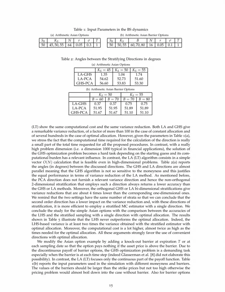
Table 1: Input Parameters in the BS dynamics(a) Arithmetic Asian Options

S0 KS N r σ T50 45, 50, 55 64 0.05 0.3 1

(b) Arithmetic Asian Barrier Options

S0 KS B N r σ T50 50, 55 60, 70, 80 16 0.05 0.1 1

Table 2: Angles between the Stratifying Directions in degrees(a) Arithmetic Asian Options

KS = 45 KS = 50 KS = 55LA-GHS 1.35 1.04 1.74LA-PCA 54.62 52.73 51.60

GHS-PCA 56.60 53.83 53.30

(b) Arithmetic Asian Barrier Options

KS = 50 KS = 55B = 60 B = 70 B = 70 B = 80

LA-GHS 0.37 0.37 0.75 0.75LA-PCA 51.95 51.95 51.89 51.89

GHS-PCA 51.67 51.67 51.10 51.10

(LT) show the same computational cost and the same variance reduction. Both LA and GHS givea remarkable variance reduction, of a factor of more than 100 in the case of constant allocation andof several hundreds in the case of optimal allocation. However, given the parameters in Table 1(a),we stress the fact that the computational time required for the calculation of the direction is reallya small part of the total time requested for all the proposed procedures. In contrast, with a reallyhigh problem dimension (i.e. a dimension 1000 typical in financial applications), the solution ofthe GHS optimization problem becomes a hard task depending on the starting guess and its com-putational burden has a relevant influence. In contrast, the LA (LT) algorithm consists in a simplevector O(N) calculation that is feasible even in high-dimensional problems. Table 2(a) reportsthe angles (in degrees) between the discussed directions. The GHS and LA directions are almostparallel meaning that the GHS algorithm is not so sensitive to the moneyness and this justifiesthe equal performance in terms of variance reduction of the LA method. As mentioned before,the PCA direction does not furnish a relevant variance direction and hence the non-orthogonal2-dimensional stratification that employs such a direction always returns a lower accuracy thanthe GHS or LA methods. Moreover, the orthogonal GHS or LA bi-dimensional stratifications givevariance reductions that are about 4 times lower than the corresponding one-dimensional ones.We remind that the two settings have the same number of strata so that we can conclude that thesecond order direction has a lower impact on the variance reduction and, with these directions ofstratification, it is more efficient to employ a stratified MC estimator with a single direction. Weconclude the study for the simple Asian options with the comparison between the accuracies ofthe LHS and the stratified sampling with a single direction with optimal allocation. The resultsshown in Table 5 illustrate that the LHS never outperforms the optimal allocation. Indeed, theLHS-based variance is at least two times the variance obtained with the stratified estimator withoptimal allocation. Moreover, the computational cost is a lot higher, almost twice as high as thetimes needed for the optimal allocation. All these arguments strongly favor the use of convenientdirections with optimal allocation.

We modify the Asian option example by adding a knock-out barrier at expiration T or ateach sampling date so that the option pays nothing if the asset price is above the barrier. Due tothe discontinuous payoff of barrier options, the GHS optimization problem is a demanding taskespecially when the barrier is at each time step (indeed Glasserman et al. [8] did not elaborate thispossibility). In contrast, the LA (LT) focuses only the continuous part of the payoff function. Table1(b) reports the input parameters used in the simulation with different moneyness and barriers.The values of the barriers should be larger than the strike prices but not too high otherwise thepricing problem would almost boil down into the case without barrier. Also for barrier options

15

Table 3: Input Parameters and Angles between Directions of Stratification for Basket Options.(a) Input Parameters.

M S0 ρ r σ T40 Linear 20-60 0.5 0.05 Linear 0.1 − 0.4 1

(b) Angles in degrees

KS = 30 KS = 40 KS = 50LA-GHS 2.76 3.11 2.52LA-PCA 64.74 65.04 65.19

GHS-PCA 62.29 62.02 62.47

(barrier at expiry), we notice that GHS and LA give directions of stratification that are almostparallel as illustrated in Table 2(b). This justifies the approximation of the LA method and its usefor stratified MC to price the two types of barrier options. In addition, the GHS algorithm is notapplicable to Asian options with a complete barrier. Different approaches should be employedin order to improve the stratification efficiency for barrier-style options, as suggested in Etoré etal. [4], but these are nevertheless computationally expensive and use orthogonal directions. Thestratified MC does not return variances as low as for plain Asian options, especially when thebarrier is close to the strike price. For example, the case of Asian options with barrier B = 80(both at expiry and at each sampling date) and with strike KS = 55 displays a variance reductionof several hundreds with a computational time that ranges between 22% and 55% higher than thestandard MC. However, when the barrier and the strike price are KS = 50 and B = 60, respectively,the variance reduction is lower with an extra effort ranging from 22% and 50% with respect to thestandard MC.

The numerical simulation of the prices of Asian basket options with a barrier close to thestrike price, both at expiry and at all the monitoring times, shows that stratifying along multipledirections can be worthwhile. Indeed, if KS = 50 and B = 60, the multiple stratification enhancesthe accuracy of the estimation compared to the use of a single direction. In particular, the highestvariance reduction is achieved with the choice of non-orthogonal directions (LA-PCA) with opti-mal allocation. In this setting the variance reduction is of an order 100, with barrier at expiry, or40, with barrier at each monitoring time, and is several times higher compared to the other settingof stratification.

Finally, even for Asian barrier options the LHS never outperforms the technique that displaysthe smallest variance with optimal allocation. These considerations suggest that the use of mul-tiple non-orthogonal directions can be worthwhile. However, finding many different multipledirections is not a simple task.

6.2 Basket Options in the Black-Scholes Market

In this example the stratification estimator once more improves the accuracy of the standard MCmethod. Indeed, in the BS market, the financial features of basket options are almost the same asthose of arithmetic Asian options. The main difference between the two is that for Asian optionsthe Gaussian variables are correlated by the autocovariance matrix of a single Brownian motionwhile for basket options the dependence is measured by the covariance matrix among the assetreturns. In addition, both payoffs contain a (weighted) average of the exponential of a Gaussianrandom vector. Table 8 shows that for all the considered exercise prices, the stratification using theLA (LT) with and without optimal allocation has a remarkable variance reduction comparable tothe one given by the GHS algorithm with the same computational considerations as in the Asianoption example. Indeed, these two directions are almost parallel (see Table 3(b)). The PCA-baseddirection has again a modest effect in terms of variance reduction and the stratification over a sin-gle linear projection produces a better accuracy than the one that exploits two directions. Finally,the LHS estimator neither achieves a higher variance reduction than the stratified estimator witha single LA direction with optimal allocation nor does it require a lower computational effort.

6.3 Asian Options in the CIR Market

As a last example we consider arithmetic Asian options on a single asset in a CIR dynamics whosedepicted parameters (in Table 4(a)) are chosen in order to ensure positive prices (2αµ > σ2). In this

16

Table 4: Input Parameters and Angles between Directions of Stratification in the CIR dynamics.(a) Input Parameters

S0 N r α µ σ T100 64 0.05 1.5 1 0.8 1

(b) Angles in degrees for Asian Options

KS = 90 KS = 100 KS = 110LA-LT 1.00 1.00 1.00

LA-PCA 43.72 43.72 43.72LT-PCA 44.24 41.52 41.53

setting the LA method and the LT decomposition do not provide the same stratification directionand the GHS algorithm is really difficult to apply. However, as illustrated in Table 4 the directionsreturned by the LT and LA are almost parallel. In any case the derivation of the LA solution andits implementation are much easier. Since the CIR model is neither a Gaussian nor a lognormalprocess, the PCA decomposition is not applicable. However, in order to obtain a further directionwe estimate a PCA-like direction as explained at the beginning of this section. Tables 9-11 showthat both the LA and LT algorithms give remarkable variance reductions. The best accuraciesare obtained with the stratification along a single direction which attains a reduction of an orderof several hundreds, both with a constant and optimal allocation rule. The extra cost for thecomputational time is only 20%. As in the BS setting, the PCA approach is less efficient andrequires a higher computational cost due to calculation of the sampled autocovariance matrix ofthe price process. Also in this situation the solution employing two orthogonal or non-orthogonaldirections provides a variance reduction. Unfortunately, this choice never provides an accuracy asprecise as the one obtained by a single direction. Moreover, the use of the fixed LHS-allocation rulenever enhances the accuracy of the simulation more than the best low-dimensional stratificationmethod with optimal allocation.

As in the BS example, we add a knock-out barrier at expiry or at each monitoring time. Forthis latter option we must chose a barrier level that is much higher than the strike price. Indeed,due to the high variability of the CIR dynamics, with a low barrier value the option would easilyknock-out producing a zero-valued price.

As already mentioned, in the example of barrier options we adopt the same convenient direc-tions of stratification that we would consider without the barrier since the LA and LT approachesdo not take into account the non-differentiable part of the payoff. Tables 6 and 7 illustrate theresults of this numerical investigation. The variance reduction is not as efficient as the casewithout barrier but in contrast, the use of multiple directions improves the efficiency of thesimulation without highly influencing the computational cost. In addition, the combination ofnon-orthogonal directions can achieve a better variance reduction. Indeed, the combination ofLA-PCA directions (LT and LA are almost parallel) returns a variance that ranges from 10 to 30times lower than that with standard Monte Carlo. Moreover, this estimated variance is always atleast equal, for KS = 100, B = 170 with barrier at each monitoring time, or lower than the varianceobtained with different combinations of stratifying directions and barrier levels.

Finally, as in all examples, the LHS sampling coupled with LT does not provide a convenientalternative to stratification over few directions with optimal allocation.

7 Concluding Remarks and Future Perspectives

In this paper we have investigated the use of convenient multidimensional directions of stratifica-tion in order to enhance the accuracy of Monte Carlo methods. We have discussed directions ofstratification that are easy to derive and display variance reductions that are comparable to thoseintroduced by Glasserman et al. [8]. These solutions do not require a complex calculation andcan be applied in really high-dimensional problems without an extra cost. In contrast, the use ofthe Glasserman et al. [8] or Etoré et al. [4] methods risk to be computationally unfeasible and arebased only on orthogonal directions. Indeed, the LT and the LA directions are computed underconvenient approximations that lead to simple matrix operations and vector norms. Moreover,we have proved an algorithm that allows to correctly generate Gaussian vectors stratified alongnon-orthogonal directions. Our numerical experiments demonstrate that the proposed convenient

17

directions return remarkable variance reductions both in BS, where the proposed techniques dis-play the same variance reduction as those given by GHS, and in the CIR dynamics. In particular,the use of multiple non-orthogonal directions can be worthwhile for barrier style options. More-over, in this work we show that the use of a few convenient directions of stratification withoptimal allocation always outperform LHS (even in its LT-enhanced form) especially in terms ofcomputational burden. A natural extension would be the combination with importance samplingprocedures like the Robust Adaptive Technique recently proposed by Jourdain and Lelong [10] forGaussian random vectors. In addition, due to its simple derivation and its affinity with the Fox’sgreedy rule (see Fox [6]), it would be interesting to investigate how to apply the LA procedure toderive a Quasi-Monte Carlo version of discretization schemes for stochastic volatility models likethose proposed by Andersen [2] and Jourdain and Sbai [11].

18

Table 5: Results for Arithmetic Asian Options in the BS dynamics.Price 1 Dir 2 dirs

MC GHS LA PCA GHS LA PCA GHS-PCA LA-PCA LHSconst opt const opt const opt const opt const opt const opt const opt const opt

KS = 45 7.02 var 55.89 0.32 0.06 0.31 0.06 15.46 11.4 1.74 0.61 0.94 0.16 10.08 8.66 8.12 0.21 8.32 0.19 0.06time 1 ×1.41 ×1.51 ×1.41 ×1.51 ×1.41 ×1.51 ×1.41 ×1.51 ×1.41 ×1.51 ×1.41 ×1.51 ×1.58 ×1.68 ×1.58 ×1.68 ×3.6

KS = 50 4.02 var 36.966 0.28 0.04 0.31 0.05 20.94 16.18 0.95 0.2 0.94 0.12 7.77 6.18 9.47 0.21 9.21 0.2 0.06time 1 ×1.41 ×1.51 ×1.41 ×1.51 ×1.41 ×1.51 ×1.41 ×1.51 ×1.41 ×1.51 ×1.41 ×1.51 ×1.58 ×1.68 ×1.58 ×1.68 ×3.24

KS = 55 2.06 var 20.357 0.3 0.02 0.31 0.03 10.52 7.75 1.06 0.28 0.93 0.09 7.54 3.8641 7.4 0.13 7.49 0.13 0.06time 1 ×1.41 ×1.51 ×1.41 ×1.51 ×1.41 ×1.51 ×1.41 ×1.51 ×1.41 ×1.51 ×1.41 ×1.51 ×1.58 ×1.68 ×1.58 ×1.68 ×3.77

Table 6: Results for Arithmetic Asian Options with a Barrier at Expiry in the BS dynamics.Price 1 Dir 2 dirs

MC GHS LA PCA GHS LA PCA GHS-PCA LA-PCA LHSconst opt const opt const opt const opt const opt const opt const opt const opt

KS = 50B = 60 1.38 var 2.99 1.13 0.3 1.13 0.31 2.99 2.99 0.54 0.23 0.83 0.19 1.24 0.93 0.33 0.02 0.32 0.02 1.02

time 1 ×1.41 ×1.41 ×1.41 ×1.35 ×1.41 ×1.35 ×1.47 ×1.47 ×1.47 ×1.40 ×1.47 ×1.40 ×1.50 ×1.50 ×1.55 ×1.50 ×3.91KS = 50B = 70 1.9 var 4.8 0.13 0.01 0.13 0.01 4.77 4.77 0.3 0.16 0.15 0.02 1.28 0.99 0.41 0.02 0.68 0.02 0.13

time 1 ×1.41 ×1.41 ×1.41 ×1.35 ×1.41 ×1.35 ×1.47 ×1.47 ×1.47 ×1.40 ×1.47 ×1.40 ×1.55 ×1.50 ×1.55 ×1.50 ×3.90KS = 55B = 70 0.19 var 0.49 0.04 0.00074 0.04 0.00082 0.48 0.48 0.04 0.0035 0.06 0.0039 0.22 0.06 0.17 0.0038 0.16 0.0037 0.04

time 1 ×1.41 ×1.41 ×1.41 ×1.35 ×1.41 ×1.35 ×1.47 ×1.47 ×1.47 ×1.40 ×1.47 ×1.40 ×1.55 ×1.50 ×1.55 ×1.50 ×3.89KS = 55B = 80 0.2 var 0.55 0.0016 0.00026 0.0018 0.00058 0.55 0.54 0.05 0.0037 0.06 0.0038 0.22 0.06 0.18 0.0048 017 0.0048 0.0018

time 1 ×1.41 ×1.41 ×1.41 ×1.35 ×1.41 ×1.35 ×1.47 ×1.47 ×1.47 ×1.40 ×1.47 ×1.40 ×1.50 ×1.55 ×1.50 ×1.55 ×3.91

Table 7: Results for Arithmetic Asian Options with a Complete Barrier in the BS dynamics.Price 1 Dir 2 dirs

MC LA PCA LA PCA LA-PCA LHSconst opt const opt const opt const opt const opt

KS = 50B = 60 1.22 var 2.42 0.85 0.23 2.42 2.39 0.54 0.12 1.23 0.92 0.53 0.07 0.77

time 1 ×1.54 ×1.14 ×1.54 ×1.14 ×1.54 ×1.14 ×1.54 ×1.14 ×1.56 ×1.22 ×3.80KS = 50B = 70 1.89 var 4.76 0.14 0.0047 4.75 4.75 0.16 0.02 1.29 1 1.52 0.02 0.15

time 11.17 ×1.54 ×1.14 ×1.54 ×1.14 ×1.54 ×1.14 ×1.54 ×1.14 ×1.56 ×1.22 ×3.81KS = 55B = 70 0.19 var 0.47 0.041 0.00087 0.47 0.46 0.06 0.0038 0.22 0.06 0.14 0.0036 0.04

time 1 ×1.54 ×1.14 ×1.54 ×1.14 ×1.54 ×1.14 ×1.54 ×1.14 ×1.56 ×1.22 ×3.85KS = 55B = 80 0.2 var 0.55 0.0015 0.000059 0.55 0.53 0.05 0.0038 0.22 0.06 0.056 0.0048 0.002

time 1 ×1.54 ×1.14 ×1.54 ×1.14 ×1.54 ×1.14 ×1.54 ×1.14 ×1.56 ×1.22 ×3.83

Table 8: Results for Basket Options in the BS dynamics.Price 1 Dir 2 dirs

MC GHS LA PCA GHS LA PCA GHS-PCA LA-PCA LHSconst opt const opt const opt const opt const opt const opt const opt const opt

KS = 30 11.58 var 61.77 0.09 0.06 0.1 0.06 31.54 21.63 0.93 0.29 0.91 0.25427 21.17 18.34 6.33 0.24 5.27 0.25406 0.06time 1 ×1.48 ×1.60 ×1.48 ×1.60 ×1.48 ×1.60 ×1.48 ×1.60 ×1.48 ×1.60 ×1.48 ×1.60 ×1.75 ×1.79 ×1.75 ×1.79 2.87

KS = 40 4.15 var 34.88 0.07 0.03 0.08 0.04 24.91 17.74 0.84 0.15 0.86 0.15 19.1 16.71 3.9 0.12 3.69 0.13214 0.1time 1 ×1.48 ×1.60 ×1.48 ×1.60 ×1.48 ×1.60 ×1.48 ×1.60 ×1.48 ×1.60 ×1.48 ×1.60 ×1.75 ×1.79 ×1.75 ×1.79 2.81

KS = 50 0.93 var 8.92 0.04 0.004 0.05 0.005 3.92 3.88 0.8 0.06 0.81287 0.06 3.05 2.18 2.87 0.04 2.55 0.05 0.08time 1 ×1.48 ×1.60 ×1.48 ×1.60 ×1.48 ×1.60 ×1.48 ×1.60 ×1.48 ×1.60 ×1.48 ×1.60 ×1.75 ×1.79 ×1.75 ×1.79 2.89

19

Table 9: Results for Asian Options in the CIR dynamics.Price 1 Dir 2 dirs

MC LT LA PCA LT PCA LA-PCA LHSconst opt const opt const opt const opt const opt const opt

KS = 90 15.63 var 427.73 1.85 1.09 1.54 0.9 115.73 106.85 9.3 2.28 51.21 40.61 9.13 4.62 1.08time 1 ×1.2 ×1.22 ×1.2 ×1.22 ×1.5 ×1.6 ×1.2 ×1.22 ×1.5 ×1.6 ×1.55 ×1.55 ×2.76

KS = 100 10.6 var 310.11 1.49 0.67 1.22 0.54 97.22 69.7 8.75 1.73 53.03 25.73 8.92 1.66 1.02time 1 ×1.2 ×1.22 ×1.2 ×1.22 ×1.5 ×1.6 ×1.2 ×1.22 ×1.5 ×1.6 ×1.55 ×1.554 ×2.75

KS = 110 6.95 var 212.19 1.18 0.37 0.29 82.25 54.28 8.72 1.26 40.34 20.69 8.29 2.22 0.9time 1 ×1.2 ×1.22 ×1.2 ×1.22 ×1.5 ×1.6 ×1.2 ×1.22 ×1.5 ×1.6 ×1.55 ×1.55 ×2.76

Table 10: Results for Arithmetic Asian Options with a Barrier at Expiry in the CIR dynamics.Price 1 Dir 2 dirs

MC LT LA PCA LT PCA LA-PCA LHSconst opt const opt const opt const opt const opt const opt

KS = 100B = 110 2.63 var 60.43 45.76 17.77 45.78 17.22 55.81 38.69 26.19 9.17 40.61 12.49 20.23 3.08 39.46

time 1 ×1.2 ×1.22 ×1.2 ×1.22 ×1.5 ×1.6 ×1.2 ×1.22 ×1.5 ×1.6 ×1.55 ×1.55 ×2.91KS = 110B = 120 1.82 var 41.64 32.64 8.1 32.55 7.85 38.69 26.43 20.76 5.77 26.4 6.27 11.95 1.26 28.52

time 1 ×1.2 ×1.22 ×1.2 ×1.22 ×1.5 ×1.6 ×1.2 ×1.22 ×1.5 ×1.6 ×1.55 ×1.55 ×2.87KS = 100B = 120 3.46 var 81.21 34.54 20.77 31.61 20.3 53.62 33.82 37.05 15.01 50.05 15.57 21.19 4.5 48.97

time 1 ×1.2 ×1.22 ×1.2 ×1.22 ×1.5 ×1.6 ×1.2 ×1.22 ×1.5 ×1.6 ×1.55 ×1.55 ×2.87

Table 11: Results for Arithmetic Asian Options with a Complete Barrier in the CIR dynamics.Price 1 Dir 2 dirs

MC LT LA PCA LT PCA LA-PCA LHSconst opt const opt const opt const opt const opt const opt

KS = 100B = 180 2.84 var 42.98 25.39 7.44 25.38 7.32 37.52 27.98 22.4 6.25 30.14 16.5 21.37 5.57 22.58

time 1 ×1.21 ×1.1 ×1.21 ×1.1 ×1.33 ×1.23 ×1.21 ×1.1 ×1.33 ×1.23 ×1.33 ×1.23 ×2.82KS = 110B = 180 1.1 var 14.03 9.51 2.05 9.59 2.05 12.68 8.37 8.63 1.73 11.33 4.76 8.35 1.58 8.79

time 1 ×1.21 ×1.1 ×1.21 ×1.1 ×1.33 ×1.23 ×1.21 ×1.1 ×1.33 ×1.23 ×1.33 ×1.23 ×2.85KS = 100B = 170 1.79 var 23.7 15.86 4.65 15.96 4.58 21.59 15.21 10.75 3.44 15.97 8.75 13.73 3.47 15.08

time 1 ×1.21 ×1.1 ×1.21 ×1.1 ×1.33 ×1.23 ×1.21 ×1.1 ×1.33 ×1.23 ×1.33 ×1.23 ×2.79

20

References

[1] F. Åkesson and J.P. Lehoczky. Discrete Eigenfuction Expansion of Multi-Dimensional Brow-nian Motion and the Ornstein-Uhlenbeck Process. Technical Report, 1998.

[2] L. Andersen. Efficient Simulation of the Heston Stochastic Volatility Model. Available inwww.ssrn.com, 2007.

[3] R. Caflisch, W. Morokoff, and A. Owen. Valuation of Mortgage-backed Securities UsingBrownian Bridges to Reduce Effective Dimension. Journal of Computational Finance, pages27–46, 1997.

[4] P. Etoré, G. Fort, B. Jourdain, and E. Moulines. On Adaptive Stratification. Forthcoming inAnnals of Operations Research.

[5] P. Etoré and B. Jourdain. Adaptive Optimal Allocation in Stratified Sampling Methods. Forth-coming in Methodology and Computing in Applied Probability.

[6] B.L. Fox. Strategies for Quasi-Monte Carlo. Kluwer Academic Publishers, 1999.

[7] P. Glasserman. Monte Carlo Methods in Financial Engineering. Springer-Verlag New York, 2004.

[8] P. Glasserman, P. Heidelberger, and P. Shahabuddin. Asymptotically Optimal ImportanceSampling and Stratification for Pricing Path-dependent Options. Mathematical Finance, pages117–152, 1999.

[9] J. Imai and K.S. Tan. A General Dimension Reduction Technique for Derivative Pricing.Journal of Computational Finance, pages 129–155, 2006.

[10] B. Jourdain and J. Lelong. Robust Adaptive Importance Sampling for Normal Random Vec-tors. Annals of Applied Probability, pages 1687–1718, 2009.

[11] B. Jourdain and M. Sbai. High Order Discretization Schemes for Stochastic Volatility Models.Preprint arXiv 0908-1926, 2009.

[12] D. Lamberton and B. Lapeyre. Introduction to Stochastic Calculus Applied to Finance. Chapman& Hall, 1996.

[13] A. Owen. A Central Limit Theorem for Latin Hypercube Sampling. Journal of the RoyalStatistical Society, pages 541–551, 1992. Series B (Methodological).

[14] A. Papageorgiou. The Brownian Bridge Does Not Offer a Consistent Avantage in Quasi-Monte Carlo Integration. Journal of Complexity, 18:171–186, 2002.

[15] P. Sabino. Efficient Quasi-Monte Simulations for Pricing High-dimensional Path-dependentOptions. Decision in Economics and Finance, 32(1):48–65, 2009.

[16] P. Sabino. Implementing Quasi-Monte Carlo Simulations with Linear Transformations. Com-putational Management Science, in press., 2009.

[17] M. Stein. Large Sample Properties of Simulations Using Latin Hypercube Sampling. Techno-metrics, pages 143–51, 1987.

21