Contingent Preferences and the Sure-Thing Principle:

Revisiting Classic Anomalies in the Laboratory∗

Ignacio Esponda Emanuel Vespa

(WUSTL) (UC Santa Barbara)

April 11, 2017

Abstract

We formalize an aspect of hypothetical thinking first pointed out by Sav-

age–who referred to it informally as the Sure-Thing Principle (STP)–and show

that it underlies many of the classic anomalies in decision and game theory. We

perform an experimental test of STP and find that indeed some of the most

common anomalies found in the laboratory, including overbidding in auctions,

naive voting in elections, and both Ellsberg and Allais types of paradoxes can

in large part be attributed to the failure of the type of hypothetical thinking

underlying STP.

∗We thank Eduardo Azevedo, Gary Charness, Larry Epstein, Daniel Gottlieb, Paul J. Healy,Shengwu Li, Bart Lipman, Mark Machina, Paulo Natenzon, Ryan Oprea, Pietro Ortoleva, MarcianoSiniscalchi, Joel Sobel, Charlie Sprenger, Georg Weizsäcker, and Sevgi Yuksel for helpful comments.Esponda: Olin Business School, Campus Box 1133, Washington University, 1 Brookings Drive, SaintLouis, MO 63130, iesponda@wustl.edu; Vespa: Department of Economics, University of California atSanta Barbara, 2127 North Hall, University of California Santa Barbara, CA 93106, vespa@ucsb.edu.

1 Introduction

motivation and main finding. Hypothetical or contingent thinking is a form of

“what–if” thinking that entails reasoning about events without knowing whether or

not these events are true or will occur. A large literature in psychology finds that

people have difficulty with various forms of hypothetical thinking.1 Given the role

of hypothetical reasoning in explaining anomalies in psychology, it seems plausible

that it has a role in producing anomalies in economics, where hypothetical thinking

remains relatively unexplored. The economics literature has focused on several other

interesting mechanisms to explain anomalies. Some of these mechanisms include

mistakes with Bayesian updating, failure to understand that other people’s actions

convey useful information, violations of axioms with normative appeal (such as the

independence axiom), and preference-based explanations including risk, regret, and

ambiguity aversion.

In this paper, we show that subjects in the laboratory have trouble with a very

particular form of hypothetical thinking. More importantly, we find that difficulty

with this particular form of hypothetical thinking underlies a large part of the mistakes

and anomalies uncovered in several classic economic environments. In particular, we

provide a unifying explanation for behavior documented in two very different strands

of the literature. One strand shows that people make systematic mistakes, particularly

in strategic settings. Examples include the winner’s curse in common value auctions,

overbidding in second-price private-value auctions, and non-pivotal voting in elections.

The second strand of the literature documents violations of expected utility axioms,

such as the Ellsberg and Allais paradoxes.

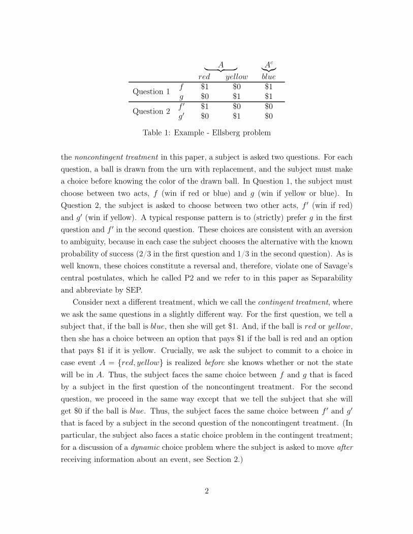
illustrative example. For clarity, we will use Ellsberg’s (1961) one-urn ex-

ample to illustrate the type of hypothetical thinking that fails in all of the classic

problems that we study. There is an urn with 90 balls, 30 of which are red and 60

of which are yellow or blue. The problem is depicted in Table 1, where there are 3

states of the world, red, yellow, and blue. A decision maker faces choices between

four acts, f , g, f ′, and g′, where each act maps the states of the world into monetary

rewards.

In the standard experiment in the literature, which corresponds to what we call

1The early evidence dates back to Wason selection tasks (Wason 1966, 1968). See Evans (2007)and Nickerson (2015) for recent textbook treatments.

1

A︸ ︷︷ ︸

Ac

︸︷︷︸

red yellow blue

Question 1f $1 $0 $1g $0 $1 $1

Question 2f ′ $1 $0 $0g′ $0 $1 $0

Table 1: Example - Ellsberg problem

the noncontingent treatment in this paper, a subject is asked two questions. For each

question, a ball is drawn from the urn with replacement, and the subject must make

a choice before knowing the color of the drawn ball. In Question 1, the subject must

choose between two acts, f (win if red or blue) and g (win if yellow or blue). In

Question 2, the subject is asked to choose between two other acts, f ′ (win if red)

and g′ (win if yellow). A typical response pattern is to (strictly) prefer g in the first

question and f ′ in the second question. These choices are consistent with an aversion

to ambiguity, because in each case the subject chooses the alternative with the known

probability of success (2/3 in the first question and 1/3 in the second question). As is

well known, these choices constitute a reversal and, therefore, violate one of Savage’s

central postulates, which he called P2 and we refer to in this paper as Separability

and abbreviate by SEP.

Consider next a different treatment, which we call the contingent treatment, where

we ask the same questions in a slightly different way. For the first question, we tell a

subject that, if the ball is blue, then she will get $1. And, if the ball is red or yellow,

then she has a choice between an option that pays $1 if the ball is red and an option

that pays $1 if it is yellow. Crucially, we ask the subject to commit to a choice in

case event A = {red, yellow} is realized before she knows whether or not the state

will be in A. Thus, the subject faces the same choice between f and g that is faced

by a subject in the first question of the noncontingent treatment. For the second

question, we proceed in the same way except that we tell the subject that she will

get $0 if the ball is blue. Thus, the subject faces the same choice between f ′ and g′

that is faced by a subject in the second question of the noncontingent treatment. (In

particular, the subject also faces a static choice problem in the contingent treatment;

for a discussion of a dynamic choice problem where the subject is asked to move after

receiving information about an event, see Section 2.)

2

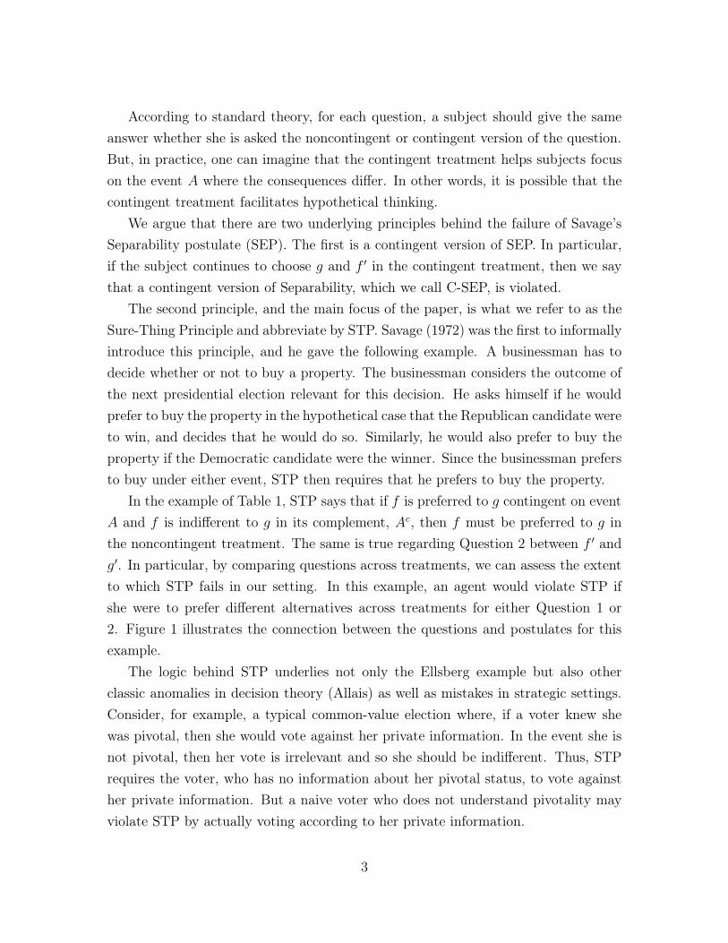
According to standard theory, for each question, a subject should give the same

answer whether she is asked the noncontingent or contingent version of the question.

But, in practice, one can imagine that the contingent treatment helps subjects focus

on the event A where the consequences differ. In other words, it is possible that the

contingent treatment facilitates hypothetical thinking.

We argue that there are two underlying principles behind the failure of Savage’s

Separability postulate (SEP). The first is a contingent version of SEP. In particular,

if the subject continues to choose g and f ′ in the contingent treatment, then we say

that a contingent version of Separability, which we call C-SEP, is violated.

The second principle, and the main focus of the paper, is what we refer to as the

Sure-Thing Principle and abbreviate by STP. Savage (1972) was the first to informally

introduce this principle, and he gave the following example. A businessman has to

decide whether or not to buy a property. The businessman considers the outcome of

the next presidential election relevant for this decision. He asks himself if he would

prefer to buy the property in the hypothetical case that the Republican candidate were

to win, and decides that he would do so. Similarly, he would also prefer to buy the

property if the Democratic candidate were the winner. Since the businessman prefers

to buy under either event, STP then requires that he prefers to buy the property.

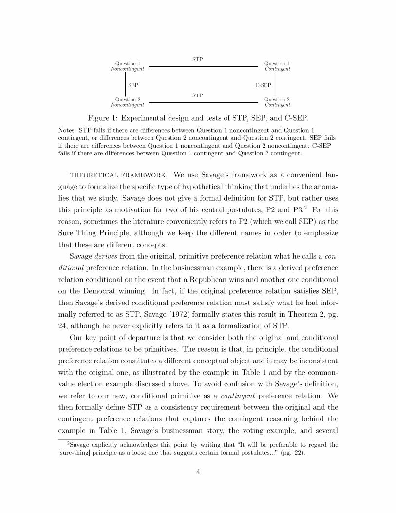
In the example of Table 1, STP says that if f is preferred to g contingent on event

A and f is indifferent to g in its complement, Ac, then f must be preferred to g in

the noncontingent treatment. The same is true regarding Question 2 between f ′ and

g′. In particular, by comparing questions across treatments, we can assess the extent

to which STP fails in our setting. In this example, an agent would violate STP if

she were to prefer different alternatives across treatments for either Question 1 or

2. Figure 1 illustrates the connection between the questions and postulates for this

example.

The logic behind STP underlies not only the Ellsberg example but also other

classic anomalies in decision theory (Allais) as well as mistakes in strategic settings.

Consider, for example, a typical common-value election where, if a voter knew she

was pivotal, then she would vote against her private information. In the event she is

not pivotal, then her vote is irrelevant and so she should be indifferent. Thus, STP

requires the voter, who has no information about her pivotal status, to vote against

her private information. But a naive voter who does not understand pivotality may

violate STP by actually voting according to her private information.

3

STPQuestion 1Contingent

Question 1Noncontingent

Question 2Noncontingent

Question 2Contingent

STP

SEP C-SEP

Figure 1: Experimental design and tests of STP, SEP, and C-SEP.

Notes: STP fails if there are differences between Question 1 noncontingent and Question 1contingent, or differences between Question 2 noncontingent and Question 2 contingent. SEP failsif there are differences between Question 1 noncontingent and Question 2 noncontingent. C-SEPfails if there are differences between Question 1 contingent and Question 2 contingent.

theoretical framework. We use Savage’s framework as a convenient lan-

guage to formalize the specific type of hypothetical thinking that underlies the anoma-

lies that we study. Savage does not give a formal definition for STP, but rather uses

this principle as motivation for two of his central postulates, P2 and P3.2 For this

reason, sometimes the literature conveniently refers to P2 (which we call SEP) as the

Sure Thing Principle, although we keep the different names in order to emphasize

that these are different concepts.

Savage derives from the original, primitive preference relation what he calls a con-

ditional preference relation. In the businessman example, there is a derived preference

relation conditional on the event that a Republican wins and another one conditional

on the Democrat winning. In fact, if the original preference relation satisfies SEP,

then Savage’s derived conditional preference relation must satisfy what he had infor-

mally referred to as STP. Savage (1972) formally states this result in Theorem 2, pg.

24, although he never explicitly refers to it as a formalization of STP.

Our key point of departure is that we consider both the original and conditional

preference relations to be primitives. The reason is that, in principle, the conditional

preference relation constitutes a different conceptual object and it may be inconsistent

with the original one, as illustrated by the example in Table 1 and by the common-

value election example discussed above. To avoid confusion with Savage’s definition,

we refer to our new, conditional primitive as a contingent preference relation. We

then formally define STP as a consistency requirement between the original and the

contingent preference relations that captures the contingent reasoning behind the

example in Table 1, Savage’s businessman story, the voting example, and several

2Savage explicitly acknowledges this point by writing that “It will be preferable to regard the[sure-thing] principle as a loose one that suggests certain formal postulates...” (pg. 22).

4

other contexts, as we illustrate in the paper.

It is well known that postulates P2 and P3 are central to Savage’s theory of

subjective expected utility; in addition, early examples by Allais (1953) and Ellsberg

(1961) illustrate violations of P2 (recall that we refer to P2 as SEP in this paper). A

bit less obvious, it is also the case that a common-ratio version of the Allais paradox,

the voting paradox described above, and overbidding in a second-price auction, all

violate a postulate that is implied by both P2 and P3 and that we refer to in this

paper as Dominance (DOM).

findings. Our main finding is that what we formally define as STP underlies

classic anomalies from both decision and game theory experiments. To be more

precise, we define corresponding versions of SEP and DOM, which hold on Savage’s

original preference relation, on our contingent preference relation. We call these

postulates C-SEP and C-DOM. We then formally show that, if STP and C-SEP

(or C-DOM) hold, then SEP (or DOM) must also hold for the original preference

relation, provided that a simple indifference postulate is satisfied, which we call C-

REF, for reflexivity. This result formalizes the claim that a very particular form

of hypothetical thinking, modeled via our definition of STP, underlies behavior in

classical environments from both decision and game theory.

We next turn to testing to what extent STP fails in the classic problems, compared

to C-DOM or C-SEP.3 Our research strategy is to run subjects through standard ver-

sions of each of these canonical problems (we call these noncontingent versions of these

problems). We then run subjects through slight alterations of each problem, remov-

ing the need for subjects to employ the type of hypothetical sophistication captured

by STP (we call these variations contingent versions of the problems). We study five

problems: Ellsberg, common-consequence and common-ratio Allais, a common-value

election, and a second-price private-values auction.

We find relatively large rates of failure of STP in all problems that we study. In

particular, we report a rate of violations of STP that ranges from 20% to 70% across

problems. Consistent with the literature, we find violations of SEP in the Ellsberg

and common-consequence Allais problems and violations of DOM in the second-price

private-values auction, in the common-value election, and in the common-ratio Allais

3We focus on the more interesting postulates by designing the experiment in a manner that C-REF holds by design. In particular, in the contingent treatment of the example in Table 1, we donot elicit if subjects are indifferent in event Ac, where both acts yield the same payoff, but ratherdirectly tell them that their choice in event Ac will be inconsequential.

5

problem. But we find that violations of versions of separability and dominance in the

contingent treatment (i.e., C-SEP and C-DOM) drop by half, except for the common-

consequence Allais problem. The rates of violations of C-SEP or C-DOM ranges from

15% to 45%, with magnitudes that are comparable to the lower bound of violations

of STP. Thus, a large part of the anomalies are driven by the failure of the particular

form of hypothetical thinking formalized via STP.

implications. We conclude by discussing implications of our results. The first is

that, despite the fact that strategic and decision problems are usually studied from

different perspectives, there is actually common ground between them in the form

of a particular form of hypothetical thinking. The second is that our subjects are

not good at thinking through the state space in the way modelers often assume, and

there is indeed a very specific way in which this phenomenon can be formalized and

tested. A third implication speaks to welfare analysis. As the literature points out,

it is reasonable that, for example, overbidding in auctions can be attributed to a

preference for winning and that the Ellsberg paradox can be attributed to ambiguity

aversion. From a welfare perspective, however, the question is the extent to which

such behavior constitutes preferences or mistakes. While this is a difficult question

to answer, the finding that overbidding and Ellsberg-type anomalies decrease by one-

half in the contingent treatment suggests that difficulty with hypothetical thinking

also plays an important role. Fourth, the finding that anomalies decrease in the

contingent treatment suggests that there is room for interventions that help people

think hypothetically and be more consistent with postulates with normative appeal,

such as dominance.

Finally, the literature has previously acknowledged that we often make the implicit

assumption that the agent can construct the state space in the same way as the

modeler, while in fact incomplete preferences or anomalies may precisely stem from

the fact that states are not naturally given and may be hard to construct (e.g., Gilboa

et al., 2009). Our finding that subjects have trouble with hypothetical thinking

suggests that we should pay more attention to theories of decision-making that do

not rely on hypothetical thinking, such as case-based decision theory (Gilboa and

Schmeidler, 1995) or the notion of obviously dominant strategies in games (Li, 2016).

We discuss the related literature in the next section, present the theoretical frame-

work in Section 3, describe the experimental design in Section 4, and present the

experimental results in Section 5. We conclude in Section 6.

6

2 Related literature

anomalies. There is a large experimental literature for each of the anomalies that

we focus on. See, for example, Bazerman and Samuelson (1983), the survey by Kagel

and Levin (2002), Charness and Levin (2009), Ivanov et al. (2010), Esponda and

Vespa (2014), and Levin et al. (2016) for mistakes in common value settings, such as

auctions or elections;4 Kagel et al. (1987), Kagel and Levin (1993), and Harstad (2000)

for overbidding in second-price private value auctions; and MacCrimmon and Larsson

(1979), the survey by Camerer (1995), Wakker (2001), Halevy (2007), Andreoni et

al. (2014), Dean and Ortoleva (2015), and Kovářík et al. (2016) for a limited sample

of the very large literature on the Ellsberg (1961) and Allais (1953) paradoxes. This

experimental literature has also motivated a large theoretical literature for modeling

the behavior of agents who make mistakes or have richer types of preferences.5

It is important to emphasize that our main finding that failure of STP underlies

all of these anomalies does not take any merit away from the interesting mechanisms

uncovered by previous work. In fact, the mechanisms examined in the literature (e.g.,

overbidding, ambiguity aversion, etc.) can be thought of as some of the factors that

cause STP to fail in these problems. The reason why these problems have not been

connected before is likely to be that the mechanisms are all very different. What we

find in this paper is that there is indeed large common ground between these seemingly

dissimilar settings, in the form of failure of a particular form of hypothetical thinking,

as embodied by STP.

dynamic choice. Another aspect that distinguishes our paper from previous

work is that we focus on static contexts, in the sense that the subject does not

receive any information about the realized state. There is a literature that instead

studies decision making in dynamic contexts. This literature defines a conditional

preference relation as the preference relation that applies after the agent observes

the realization of an event. Two of the main postulates studied in dynamic choice

settings include dynamic consistency and consequentialism (e.g., Hammond (1988),

4See also the experimental literature on correlation neglect, e.g., Eyster and Weizsacker (2010)and Enke and Zimmermann (2013).

5For theoretical responses to mistakes, see Eyster and Rabin (2005), Crawford and Iriberri (2007),Jehiel and Koessler (2008), and Esponda (2008). For theoretical responses to the paradoxes, see thesurveys by Machina (2008), Gilboa and Marinacci (2011) and Machina and Siniscalchi (2013). Fora critical assessment of the ambiguity aversion literature, see Al-Najjar and Weinstein (2009) andSiniscalchi (2009).

7

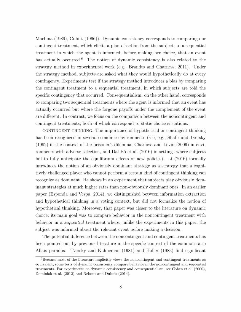
Machina (1989), Cubitt (1996)). Dynamic consistency corresponds to comparing our

contingent treatment, which elicits a plan of action from the subject, to a sequential

treatment in which the agent is informed, before making her choice, that an event

has actually occurred.6 The notion of dynamic consistency is also related to the

strategy method in experimental work (e.g., Brandts and Charness, 2011). Under

the strategy method, subjects are asked what they would hypothetically do at every

contingency. Experiments test if the strategy method introduces a bias by comparing

the contingent treatment to a sequential treatment, in which subjects are told the

specific contingency that occurred. Consequentialism, on the other hand, corresponds

to comparing two sequential treatments where the agent is informed that an event has

actually occurred but where the forgone payoffs under the complement of the event

are different. In contrast, we focus on the comparison between the noncontingent and

contingent treatments, both of which correspond to static choice situations.

contingent thinking. The importance of hypothetical or contingent thinking

has been recognized in several economic environments (see, e.g., Shafir and Tversky

(1992) in the context of the prisoner’s dilemma, Charness and Levin (2009) in envi-

ronments with adverse selection, and Dal Bó et al. (2016) in settings where subjects

fail to fully anticipate the equilibrium effects of new policies). Li (2016) formally

introduces the notion of an obviously dominant strategy as a strategy that a cogni-

tively challenged player who cannot perform a certain kind of contingent thinking can

recognize as dominant. He shows in an experiment that subjects play obviously dom-

inant strategies at much higher rates than non-obviously dominant ones. In an earlier

paper (Esponda and Vespa, 2014), we distinguished between information extraction

and hypothetical thinking in a voting context, but did not formalize the notion of

hypothetical thinking. Moreover, that paper was closer to the literature on dynamic

choice; its main goal was to compare behavior in the noncontingent treatment with

behavior in a sequential treatment where, unlike the experiments in this paper, the

subject was informed about the relevant event before making a decision.

The potential difference between the noncontingent and contingent treatments has

been pointed out by previous literature in the specific context of the common-ratio

Allais paradox. Tversky and Kahneman (1981) and Holler (1983) find significant

6Because most of the literature implicitly views the noncontingent and contingent treatments asequivalent, some tests of dynamic consistency compare behavior in the noncontingent and sequentialtreatments. For experiments on dynamic consistency and consequentialism, see Cohen et al. (2000),Dominiak et al. (2012) and Nebout and Dubois (2014).

8

differences between treatments. In a detailed analysis of the common-ratio Allais

paradox, Cubitt et al. (1998) decompose the paradox into four principles of dynamic

choice and then test these principles in the lab. One of these tests is a compari-

son between the noncontingent and contingent treatments. They find no significant

differences in the marginal responses across treatments, like we do for this specific

problem. Their focus, however, is different than ours and so they do not test if there

is a reduction of reversals when both questions of the Allais paradox are asked using

the standard (i.e., noncontingent) treatment (we find there is). To our knowledge,

however, there has been no formalization of the form of hypothetical thinking that

underlies this phenomenon nor any experimental work finding a common source link-

ing mistakes in strategic environments such as auctions and elections with the classic

anomalies in decision problems.7

3 Theoretical framework

Hypothetical thinking is relevant in many settings but is nevertheless an elusive con-

cept in the sense that it can be challenging to formalize. We will use the framework

introduced by Savage as a convenient language to formalize the specific type of hy-

pothetical thinking that underlies the anomalies that we study. One advantage of

this approach is that it allows us to link several seemingly unrelated anomalies with a

common concept, and it prescribes a very natural experimental test of that concept.

We begin by describing Savage’s approach; in particular, we focus on two of his

central postulates on the agent’s preference relation and we explicitly state the prop-

erties that these postulates imply on the conditional preference relation that Savage

derives from the original one. We then introduce our approach, where the contingent

preference relation constitutes a primitive of its own and the Sure-Thing Principle

is defined as a consistency restriction over the original and contingent preferences.

Finally, we establish the main results connecting the postulates defined over our

primitives to Savage’s central postulates.

7In a theory paper, Eliaz et al. (2006) make a connection between anomalies in decision andgame theory environments by establishing a formal equivalence between violations of expected utilitytheory and choice shifts in groups.

9

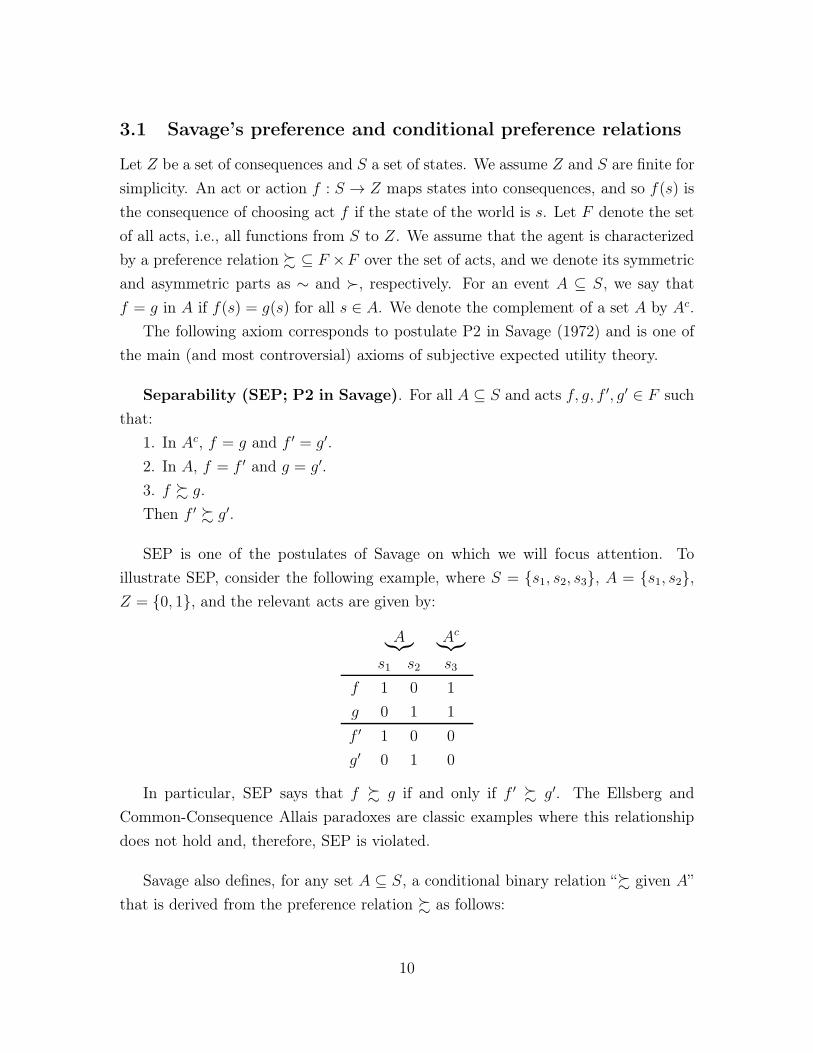
3.1 Savage’s preference and conditional preference relations

Let Z be a set of consequences and S a set of states. We assume Z and S are finite for

simplicity. An act or action f : S → Z maps states into consequences, and so f(s) is

the consequence of choosing act f if the state of the world is s. Let F denote the set

of all acts, i.e., all functions from S to Z. We assume that the agent is characterized

by a preference relation % ⊆ F ×F over the set of acts, and we denote its symmetric

and asymmetric parts as ∼ and ≻, respectively. For an event A ⊆ S, we say that

f = g in A if f(s) = g(s) for all s ∈ A. We denote the complement of a set A by Ac.

The following axiom corresponds to postulate P2 in Savage (1972) and is one of

the main (and most controversial) axioms of subjective expected utility theory.

Separability (SEP; P2 in Savage). For all A ⊆ S and acts f, g, f ′, g′ ∈ F such

that:

1. In Ac, f = g and f ′ = g′.

2. In A, f = f ′ and g = g′.

3. f % g.

Then f ′ % g′.

SEP is one of the postulates of Savage on which we will focus attention. To

illustrate SEP, consider the following example, where S = {s1, s2, s3}, A = {s1, s2},

Z = {0, 1}, and the relevant acts are given by:

A︸︷︷︸

Ac

︸︷︷︸

s1 s2 s3

f 1 0 1

g 0 1 1

f ′ 1 0 0

g′ 0 1 0

In particular, SEP says that f % g if and only if f ′ % g′. The Ellsberg and

Common-Consequence Allais paradoxes are classic examples where this relationship

does not hold and, therefore, SEP is violated.

Savage also defines, for any set A ⊆ S, a conditional binary relation “% given A”

that is derived from the preference relation % as follows:

10

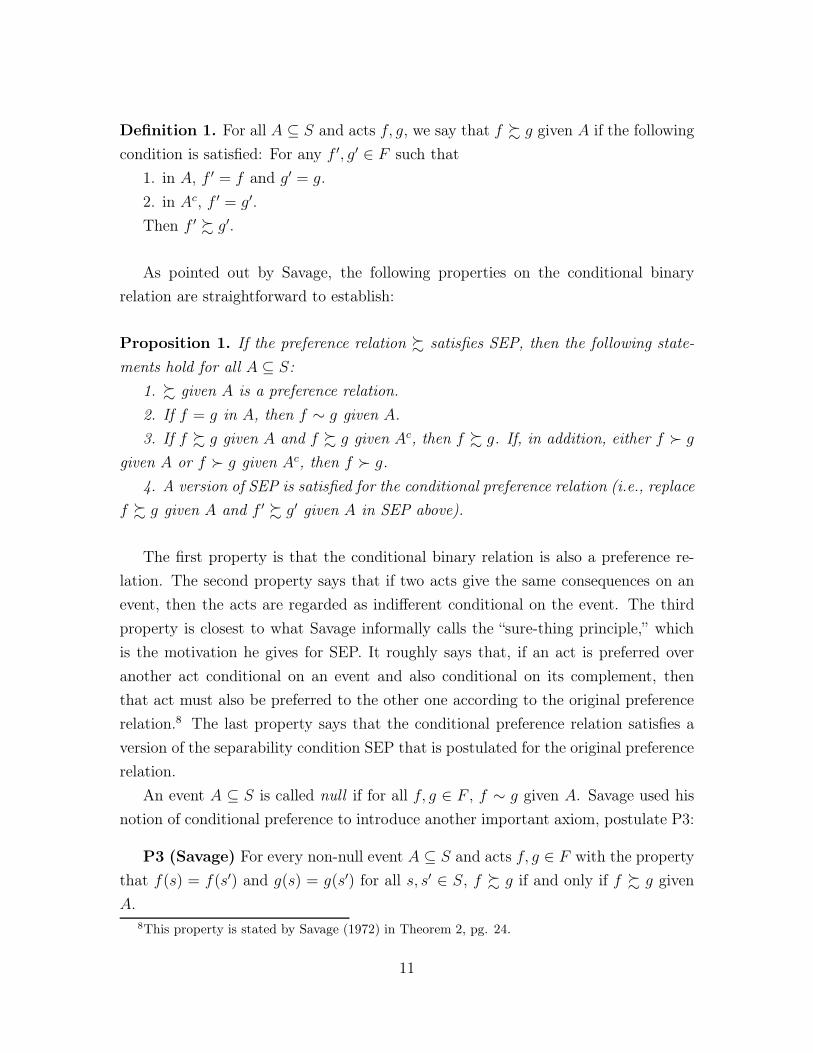
Definition 1. For all A ⊆ S and acts f, g, we say that f % g given A if the following

condition is satisfied: For any f ′, g′ ∈ F such that

1. in A, f ′ = f and g′ = g.

2. in Ac, f ′ = g′.

Then f ′ % g′.

As pointed out by Savage, the following properties on the conditional binary

relation are straightforward to establish:

Proposition 1. If the preference relation % satisfies SEP, then the following state-

ments hold for all A ⊆ S:

1. % given A is a preference relation.

2. If f = g in A, then f ∼ g given A.

3. If f % g given A and f % g given Ac, then f % g. If, in addition, either f ≻ g

given A or f ≻ g given Ac, then f ≻ g.

4. A version of SEP is satisfied for the conditional preference relation (i.e., replace

f % g given A and f ′ % g′ given A in SEP above).

The first property is that the conditional binary relation is also a preference re-

lation. The second property says that if two acts give the same consequences on an

event, then the acts are regarded as indifferent conditional on the event. The third

property is closest to what Savage informally calls the “sure-thing principle,” which

is the motivation he gives for SEP. It roughly says that, if an act is preferred over

another act conditional on an event and also conditional on its complement, then

that act must also be preferred to the other one according to the original preference

relation.8 The last property says that the conditional preference relation satisfies a

version of the separability condition SEP that is postulated for the original preference

relation.

An event A ⊆ S is called null if for all f, g ∈ F , f ∼ g given A. Savage used his

notion of conditional preference to introduce another important axiom, postulate P3:

P3 (Savage) For every non-null event A ⊆ S and acts f, g ∈ F with the property

that f(s) = f(s′) and g(s) = g(s′) for all s, s′ ∈ S, f % g if and only if f % g given

A.8This property is stated by Savage (1972) in Theorem 2, pg. 24.

11

For our purposes, it will be convenient to work with the following postulate.

Dominance (DOM) For all A ⊆ S and acts f, g, f ′, g′ ∈ F such that:

1. f(s) = f(s′) and g(s) = g(s′) for all s, s′ ∈ S.

2. In Ac, f ′ = g′.

3. In A, f ′ = f and g′ = g.

4. f % g

Then f ′ % g′.

DOM is neither weaker nor stronger than P3. It is easy to see that P3 is equivalent

to a version of DOM where: (i) DOM is weakened by restricting A to be non-null,

and (ii) DOM is strengthened to require that f % g if and only if f ′ % g′. The reason

we use DOM and not P3 in our experimental application is that P3 would require us

to assume or test that the relevant event A is non-null.

The next result shows that DOM is actually implied by SEP and P3.

Proposition 2. If the preference relation % satisfies SEP and P3, then it also satisfies

DOM.

Proof. Fix A ⊆ S and acts f, g, f ′, g′ ∈ F such that: (1) f(s) = f(s′) and g(s) = g(s′)

for all s, s′ ∈ S, (2) In Ac, f ′ = g′, (3) In A, f ′ = f and g′ = g, and (4) f % g. If

A is non-null, then it follows trivially from P3 alone that f ′ % g′. So suppose that

A is null. We will use the following result from Savage (Theorem 1(4), pg. 24): If

A is null, then f ′ % g′ if and only if f ′ % g′ given Ac. Suppose, in order to obtain

a contradiction, that is it not true that f ′ % g′. Then, by Savage’s Theorem 1(4),

it is also not true that f ′ % g′ given Ac. In particular, there exist f ′′, g′′ ∈ F such

that (1) in Ac, f ′′ = f ′ and g′′ = g′, (2) in A, f ′′ = g′′, and (3) it is not true

that f ′′ % g′′. But this must be a contradiction because, by construction, f ′′ = g′′.

Therefore, f ′ % g′.

DOM is the second postulate implied by Savage’s framework on which we will focus

attention. To illustrate DOM, consider the following example, where S = {s1, s2},

A = {s1}, Z = {x, y, z} are monetary payoffs, and the relevant acts are given by:

12

s1 s2

f x x

g y y

f ′ x z

g′ y z

Suppose that x ≥ y. If the agent prefers more money to less, it is then reasonable

that f % g. DOM then requires that f ′ % g′. We will show that this is the kind of

“dominance” relationship that fails in strategic environments, such as auctions and

elections. Finally, by taking the space of consequences Z to be a specific set of

lotteries, we will show that the common-ratio Allais paradox constitutes a violation

of DOM.9

Finally, if SEP holds, the following version of DOM, linking both the original and

conditional preference relations, is satisfied.

Proposition 3. If the preference relation % satisfies SEP and DOM, the following

statement holds: For all A ⊆ S and acts f, g, f ′, g′ ∈ F such that:

1. f(s) = f(s′) and g(s) = g(s′) for all s, s′ ∈ S.

2. In Ac, f ′ = g′.

3. In A, f ′ = f and g′ = g.

4. f % g.

Then f ′ % g′ given A.

Proof. Fix A ⊆ S and f, g, f ′, g′ ∈ F satisfying conditions 1-4 in the statement of the

proposition. By DOM, it follows that f ′ % g′. To establish that f ′ % g′ given A, let

f ′′, g′′ ∈ F such that (1) in A, f ′′ = f ′ and g′′ = g′, (2) in Ac, f ′′ = g′′. We must show

that f ′′ % g′′. Note that f ′, g′, f ′′, g′′ are such that (1) In Ac, f ′ = g′ and f ′′ = g′′, (2)

In A, f ′ = f ′′ and g′ = g′′, and (3) f ′ % g′. It then follows by SEP that f ′′ % g′′.

The importance of Proposition 3 for our purposes is that it indicates yet another

property that is satisfied by the conditional preference relation introduced by Sav-

age.10

9When consequences are not monetary payoffs, DOM can be interpreted as requiring utility tobe state independent; see, e.g., Gilboa (2009).

10If condition 4 in Proposition 3 were replaced by f % g given A, then the result would also hold(it is simply implied by SEP). But this other property is not the right one for the purpose of ourexperiments.

13

3.2 Contingent preferences

Savage defines the primitive preference relation to be % and then uses it to derive a

conditional preference relation % given A. In contrast, we adopt an approach where

both the original and the conditional preference relations are primitives. The reason is

that, in principle, the conditional preference relation constitutes a different conceptual

object and it may not be derived from the original one as defined by Savage.

We continue to assume that % is a preference relation and to interpret it as a

preference relation over acts before any uncertainty about the state is realized. For

clarity, we will often refer to % as the noncontingent preference relation. But, in

contrast to Savage, we also introduce as a new primitive, for all A ⊆ S, a preference

relation %A, with corresponding symmetric and asymmetric parts ∼A and ≻A. We

refer to the collection (%A)A⊆S as the contingent preference relation, to distinguish it

from Savage’s conditional preference relation, (% given A)A⊆S.11

The interpretation is that %A reflects the preferences of the agent over acts when

she is asked to commit to an act, conditional on an event A, before any uncertainty

about the state is realized. (We focus on static choice but, if we were interested in

dynamic choice, there would be yet another preference relation to define that reflects

preferences after the agent finds out that event A is realized; see the references in

Section 2.)

The properties which Savage derived for “% given A” that are listed in Proposi-

tion 1 seem very natural. We now state the analog of these properties as potential

postulates that our contingent preference relation may satisfy.

Contingent reflexivity (C-REF) For all A ⊆ S and acts f, g ∈ F : If f = g in

A, then f ∼A g.

Sure-thing principle (STP) For all A ⊆ S and acts f, g ∈ F : If f %A g and

f %Ac g, then f % g. If, in addition, either f ≻A g or f ≻Ac g, then f ≻ g.

Contingent separability (C-SEP) For all A ⊆ S and acts f, g, f ′, g′ ∈ F such

that:

1. In Ac, f = g and f ′ = g′.

2. In A, f = f ′ and g = g′.

3. f %A g.

11For our purposes, it does not matter whether or not we assume that %S=%.

14

Then f ′ %A g′.

While we naturally view C-SEP as corresponding to a particular version of SEP

in the domain of contingent preferences, it is important to highlight the following

difference: The definition of SEP fixes the noncontingent preference relation % and

restricts it to satisfy certain conditions for all subsets A ⊆ S. In contrast, in the

definition of C-SEP, the preference relation %A changes as a function of the set A.12

Our first main result is as follows:

Theorem 1. If the preference relations (%A)A⊆S and % satisfy C-REF, STP, and

C-SEP, then % satisfies SEP.

Proof. Fix A ⊆ S and f, g, f ′, g′ ∈ F such that (1) In Ac, f = g and f ′ = g′, (2) In

A, f = f ′ and g = g′, and f % g. We must establish that f ′ % g′. By C-REF and

the fact that f = g in Ac, f ∼Ac g. Thus, by STP, f %A g (otherwise, we would

have g ≻ f , a contradiction). Then, by C-SEP, f ′ %A g′. In addition, C-REF and

the fact that f ′ = g′ in Ac implies that f ′ ∼Ac g′. Finally, the facts that f ′ %A g′ and

f ′ ∼Ac g′ imply, by STP, that f ′ % g′, as desired.

Theorem 1 shows that violations of SEP in Savage’s setting can be attributed to

violations of three different postulates defined over the noncontingent and contingent

preference relations.

We now state a fourth postulate on the noncontingent and contingent preference

relations, which is the analog of the property stated in Proposition 3 for Savage’s

original and conditional preference relations.

Contingent Dominance (C-DOM) For all A ⊆ S and acts f, g, f ′, g′ ∈ F such

that:

1. f(s) = f(s′) and g(s) = g(s′) for all s, s′ ∈ S.

2. In Ac, f ′ = g′.

3. In A, f ′ = f and g′ = g.

4. f % g.

Then f ′ %A g′.

Our second main result is as follows:

12In particular, it is not true that C-SEP by itself implies SEP.

15

Theorem 2. If the preference relations (%A)A⊆S and % satisfy C-REF, STP, and

C-DOM, then % satisfies DOM.

Proof. Let A ⊆ S and let f, g, f ′, g′ ∈ F be such that: (1) f(s) = f(s′) and g(s) =

g(s′) for all s, s′ ∈ S, (2) In Ac, f ′ = g′, (3) In A, f ′ = f and g′ = g, and (4) f % g.

We want to establish that f ′ % g′. By C-DOM, f ′ %A g′. By C-REF, f ′ ∼Ac g′. It

follows from these two previous statements and STP that f ′ % g′.

Theorem 2 shows that violations of DOM in Savage’s setting can be attributed to

violations of three different postulates defined over the noncontingent and contingent

preference relations.

Theorems 1 and 2 are the main theoretical results of the paper. As mentioned

in the introduction, Savage informally introduced a notion he called “the sure-thing

principle” and used it as motivation for postulates SEP and DOM. By conceptually

distinguishing between noncontingent and contingent preferences, we are able to for-

mally define the sure-thing principle, STP. Theorems 1 and 2 describe precisely how

this principle underlies both postulates SEP and DOM in Savage’s framework.

These results motivate our subsequent experimental design. In particular, we will

look at seemingly unrelated problems where standard postulates in Savage’s frame-

work (SEP and DOM) are shown to fail. We will then document to what extent

such failures are related to violations of STP, and whether we also observe failures in

either C-SEP or C-DOM. To focus on these questions, we will design the experiment

in a way that C-REF will be satisfied by construction. We will find that indeed STP

fails in all of these problems, and that there are fewer violations of separability and

dominance in contingent versions of these problems.

4 Experimental Design

We study five classic problems in the laboratory: Ellsberg (ells), common-consequence

Allais (cc allais), a private-values second-price auction (auct), a common-value

election (elect), and common-ratio Allais (cr allais). For each of these five prob-

lems, we conduct two treatments. In the noncontingent treatment, we elicit what

we called in Section 2 the noncontingent preferences. This is the benchmark treat-

ment and it is intended to replicate existing results in the literature. ells and

16

cc allais constitute examples of violation of separability (SEP), while auct, elect

and cr allais constitute examples of violation of dominance (DOM).

We also run a second treatment, the contingent treatment, where we elicit what we

called in Section 2 the contingent preferences. We design this treatment in a manner

that C-REF is satisfied by construction and we evaluate the extent to which the sure-

thing principle (STP) and either C-SEP (for ells and cc allais) or C-DOM (for

auct, elect, and cr allais) are satisfied.

We conducted both a between-subjects design, where each subject participated in

one of the problems and in one of the treatments only, and a within-subjects design,

where each subject participated in both treatments for all of the problems. There are

well-know trade-offs between these designs (e.g., Camerer (1995), pg. 633). In par-

ticular, the between-subjects design minimizes confounding effects, while the within-

subjects design allows us to identify additional primitives such as the correlation

between problems. The experiment was conducted at the University of California,

Santa Barbara and subjects were recruited using ORSEE (Greiner, 2015). There were

a total of 624 participants in the between-subjects design (120, 125, 129, 124, and

126 participants for each of the five problems, respectively) and a total of 131 par-

ticipants in the within-subjects design. The experiment was conducted using zTree

(Fischbacher, 2007).13 At the end of the experiment, each subject was asked addi-

tional questions to assess her level of risk or ambiguity aversion and cognitive ability.

We describe these questions in further detail in the Appendix.

We now describe the two treatments for each of the five problems.

4.1 Five experimental problems

We begin by discussing the ells problem in detail. The other four problems follow

a design similar to the ells problem, and so we describe them more succinctly.

4.1.1 Ellsberg problem

There is a jar with 90 balls. Of the 90 balls, 30 are red (R) and 60 are yellow (Y) or

blue (B). A subject must answer two questions, Q1 and Q2, in sequential order and

she does not know the second question when answering the first. For each of the two

13A session in the between-subjects (within-subjects) design lasted approximately 30 (90) minutesand on average subjects received $9.50 ($19.1) in compensation.

17

R Y B

Question 1f $10 $0 $10g $0 $10 $10

Question 2f ′ $10 $0 $0g′ $0 $10 $0

Table 2: Ellsberg problem

questions, a ball is randomly drawn (with replacement).

Noncontingent treatment. In Q1, the subject must choose between f , which gives

$10 if the drawn ball is red or blue, and g, which gives $10 if it is yellow or blue. In

Q2, the subject must choose between f ′, which gives $10 if the drawn ball is red, and

g′, which gives $10 if it is yellow. For this treatment and for all other treatments and

problems, subjects did not receive feedback until the end of the experiment.

Table 2 depicts the choices in each question (note that the written instructions

did not include Table 2). The typical paradox is that a significant number of subjects

choose g in the first question (where the probability of receiving $10 is known to be

2/3) and f ′ in the second question (where the probability of receiving $10 is known

to be 1/3). This is a violation of SEP.14

Contingent treatment. In Q1, we tell the subject that if the drawn ball is blue, the

problem ends there and the decision-maker gets $10. But, if the drawn ball is red or

yellow, the decision maker has to make a choice between two options: (1) get $10 if

the ball is red and (2) get $10 if it is yellow. We then ask the subject to make a choice

contingent on the event in which the ball is red or yellow, without yet knowing if this

is the event that will happen. Note that a choice between (1) and (2) corresponds

to a choice between f and g in Table 2. Q2 is identical to the first question except

that the decision maker gets $0 if the drawn ball is blue. Thus, the subject is in fact

choosing between f ′ and g′ in Table 2.

Testable hypotheses. According to standard theory, there is no difference between

the noncontingent and contingent treatments because the subject is essentially facing

the same choices over acts in both treatments. In practice, however, one may see

a difference. The theoretical framework in Section 3 allows for a difference between

14In accordance with the literature, we take these choices to reflect strict preferences. The un-derlying assumption is that a subject who is in fact indifferent in both questions chooses the firstof the two options with the same probability in each question. The same point holds for all otherproblems.

18

the noncontingent preference %, elicited in the noncontingent treatment, and the

contingent preference %{R,Y }, elicited in the contingent treatment. Intuitively, the

reason why one may expect different choices in the two treatments is that, in the

second treatment, the subject is helped to focus on the event that is payoff relevant

for her decision, {R, Y }.

Another important feature of the contingent treatment is that we do not ask for

a choice conditional on the event {B}. Rather, we simply tell the subject that her

choice does not matter in that event. By doing so, we are essentially guaranteeing

that C-REF is satisfied by design in our experiment, so that we can focus attention

on the more interesting postulates, STP and C-SEP. We follow the same idea in

the contingent treatments for all other problems: cc allais, auct, elect and

cr allais.

Figure 1 (reported earlier in pg. 4) illustrates the testable hypotheses in the

context of this problem. As mentioned above, a comparison between Q1 and Q2 in

the noncontingent treatment is the standard way of testing for SEP in the literature.

A comparison between Q1 and Q2 in the contingent treatment provides a test of

C-SEP. A comparison between Q1 in the noncontingent treatment and Q1 in the

contingent treatment provides a test of STP; the same is true for the comparison

between Q2 in both treatments.

4.1.2 Common-consequence Allais problem

There is a jar with 100 balls. Of the 100 balls, 1 is red (R), 10 are yellow (Y), and

89 are blue (B). For each of the two questions, Q1 and Q2, a ball is randomly drawn

(with replacement).

Noncontingent treatment. In Q1, the subject must choose between f , which gives

$100 million for sure, and g, which gives $500 million if the ball is yellow and $100

million if it is blue.15 In Q2, the subject must choose between f ′, which gives $100

million if the ball is red or yellow, and g′, which gives $500 million if the ball is yellow.

15This is the only decision problem for which we use hypothetical payoffs. Huck and Müller (2012)study three alternative ways of implementing the common-consequence Allais problem. They findfew violations of SEP with small payoffs, but that violations become more prevalent with hypotheticalpayoffs expressed in millions of euros.

19

R (1) Y (10) B (89)

Question 1f $100m $100m $100mg $0 $500m $100m

Question 2f ′ $100m $100m $0g′ $0 $500m $0

Table 3: Common-consequence Allais problem

Table 3 depicts the choices in each question. The paradox is that a significant

number of subjects choose f (safe option) in Q1 and g′ (risky option) in Q2. This is

a violation of SEP.

Contingent treatment. In Q1, we tell the subject that if the drawn ball is blue, the

problem ends there and the decision maker gets $100 million. But, if the drawn ball

is red or yellow, the decision maker has to make a choice: (1) get $100 million if the

ball is red or yellow and (2) get $500 million if the ball is yellow. We then ask them to

make a choice contingent on the event in which the ball is red or yellow, without yet

knowing if this is the event that will happen. Note that a choice between (1) and (2)

corresponds to a choice between f and g in Table 3. Q2 is identical except that the

decision maker gets $0 if the drawn ball is blue. Thus, the subject is in fact choosing

between f ′ and g′ in Table 3.

Testable hypotheses. This problem has the same structure of ells, and so it is

straightforward to see that the previous discussion applies here. In particular, Figure

1 (reported earlier in pg. 4) also describes the hypotheses for cc allais.

4.1.3 Auction problem

There are three cards, numbered 4.5, 0.5, and 8.5, and one card is randomly drawn.

There is only one question in each treatment.16

16While it is typical in experiments of strategic behavior to repeat the same or similar questionsmany times to test for experience effects, here we decided to only ask each question once, in orderto make the results comparable to the standard decision experiments (Ellsberg and Allais). Theliterature documents that the strategic biases that we replicate here are actually robust to experience(see, for example, Kagel and Levin (1993) for the Auction problem and Esponda and Vespa (2014)for the Election problem).

20

4.5 0.5 8.5

Question*f $3 $3 $3g $1 $1 $1

Question 1f ′ $3 $5 $3g′ $1 $5 $3

Table 4: Auction problem

Noncontingent treatment. Without knowing the drawn card, the subject must

choose an integer between 1 and 8. If the number she chooses is higher than the

number on the drawn card, her payoff is $5.5 minus the number on the card (in

dollars). If the number she chooses is lower than the number on the card, her payoff

is $3. In this problem, one’s choice is only relevant if the card is 4.5, and, in that

case, it is optimal to choose 1, 2, 3, or 4.

Table 4 depicts the problem faced by the agent. To simplify the exposition of the

results, we codify an optimal choice of 1, 2, 3, or 4 as act f ′ and a suboptimal choice

of 5, 6, 7, or 8 (overbidding) as act g′. We also define the constant acts f (payoff

of $3 in all states) and g (payoff of $1 in all states). The paradox in this problem

is that a significant fraction of subjects choose g′ over f ′. This choice violates DOM

under the reasonable assumption that subjects prefer more money to less, i.e., f is

preferred to g.

Contingent treatment. We tell the subject that she will get $5 if the drawn card is

0.5, $3 if it is 8.5, and we ask her to make a contingent choice for the event in which

the card is 4.5, without her knowing if this is the event that will happen. Thus,

the contingent treatment elicits the preference between f ′ and g′ according to the

contingent preference %{4.5}.

Testable hypotheses. Figure 2 describes the hypotheses for auct. In the figure,

Question 1 corresponds to the question we asked and Question* corresponds to the

choice between acts f and g in Table 4. Therefore, a comparison between Q1 and

Q* in the noncontingent treatment tests DOM. Because Q* seems trivial, we did not

ask it; instead, we simply assume that, if Q* were asked, a subject would prefer more

to less money, i.e, f over g. Therefore, DOM is violated in this example provided

that a subject prefers g′ to f ′ in the noncontingent treatment. Similarly, C-DOM is

violated if a subject prefers g′ to f ′ in the contingent treatment. Finally, a comparison

between Q1 in the noncontingent treatment and Q1 in the contingent treatment tests

STP.

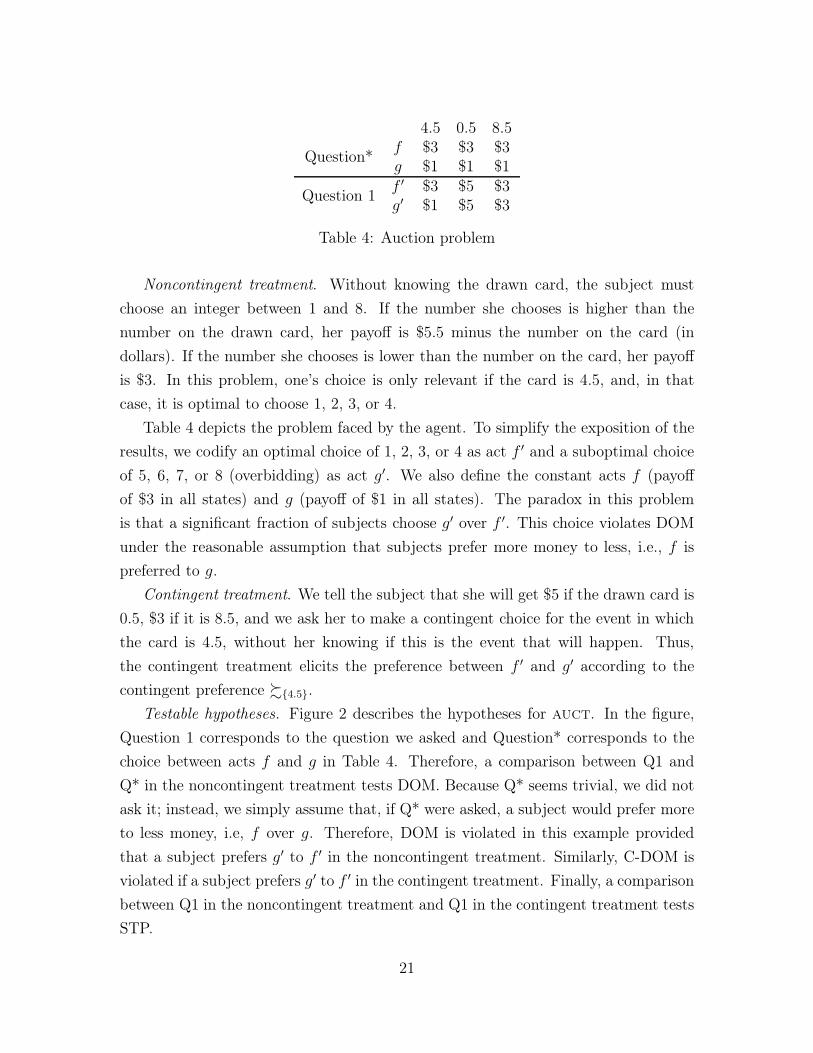
21

STPQuestion 1Contingent

Question 1Noncontingent

Question* Question*

DOM C-DOM

Figure 2: Experimental design and tests of STP, DOM, and C-DOM.

Notes: In auct and elect, Question* was not presented to subjects and it corresponds to assuming that subjectsprefer more money to less. In cr allais, Question* corresponds to Question 2 in Table 6.

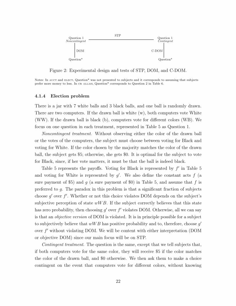
4.1.4 Election problem

There is a jar with 7 white balls and 3 black balls, and one ball is randomly drawn.

There are two computers. If the drawn ball is white (w), both computers vote White

(WW). If the drawn ball is black (b), computers vote for different colors (WB). We

focus on one question in each treatment, represented in Table 5 as Question 1.

Noncontingent treatment. Without observing either the color of the drawn ball

or the votes of the computers, the subject must choose between voting for Black and

voting for White. If the color chosen by the majority matches the color of the drawn

ball, the subject gets $5; otherwise, she gets $0. It is optimal for the subject to vote

for Black, since, if her vote matters, it must be that the ball is indeed black.

Table 5 represents the payoffs. Voting for Black is represented by f ′ in Table 5

and voting for White is represented by g′. We also define the constant acts f (a

sure payment of $5) and g (a sure payment of $0) in Table 5, and assume that f is

preferred to g. The paradox in this problem is that a significant fraction of subjects

choose g′ over f ′. Whether or not this choice violates DOM depends on the subject’s

subjective perception of state wWB. If the subject correctly believes that this state

has zero probability, then choosing g′ over f ′ violates DOM. Otherwise, all we can say

is that an objective version of DOM is violated. It is in principle possible for a subject

to subjectively believe that wWB has positive probability and to, therefore, choose g′

over f ′ without violating DOM. We will be content with either interpretation (DOM

or objective DOM) since our main focus will be on STP.

Contingent treatment. The question is the same, except that we tell subjects that,

if both computers vote for the same color, they will receive $5 if the color matches

the color of the drawn ball, and $0 otherwise. We then ask them to make a choice

contingent on the event that computers vote for different colors, without knowing

22

pivotal︸ ︷︷ ︸

not pivotal︸ ︷︷ ︸

bWB wWB⊘ bWW⊘ wBB⊘ bBB⊘ wWW

Question*f $5 $5 $5 $5 $5 $5g $0 $0 $0 $0 $0 $0

Question 1f ′ $5 $0 $0 $0 $5 $5g′ $0 $5 $0 $0 $5 $5

Table 5: Election problem. States marked by ⊘ have zero probability.

if this is the event that will happen. This question elicits the subjects’ preference

contingent on the pivotal event, i.e., %{bWB,wWB}.

Testable hypotheses. Figure 2 can also be used to describe the hypotheses for

elect. In the figure, Question 1 corresponds to the question we asked and Question*

corresponds to the choice between acts f and g in Table 5. Therefore, a comparison

between Q1 and Q* in the noncontingent treatment tests either DOM or an objective

version of DOM, as explained earlier. Because Q* seems trivial, we did not ask it;

instead, we simply assume that, if Q* were asked, a subject would prefer more to

less money, i.e, f over g. Therefore, DOM (or its objective version) is violated in

this example provided that a subject prefers g′ to f ′ in the noncontingent treatment.

Similarly, C-DOM (or its objective version) is violated if a subject prefers g′ to f ′

in the contingent treatment. Finally, a comparison between Q1 in the noncontingent

treatment and Q1 in the contingent treatment tests STP. Note that STP is tested

irrespective of whether or not the subject understands that state wWB has zero

probability. For example, a subject may choose g′ over f ′ because she thinks that

state wWB is very likely. But the same subject who then prefers f ′ over g′ in the

contingent treatment would be violating STP.

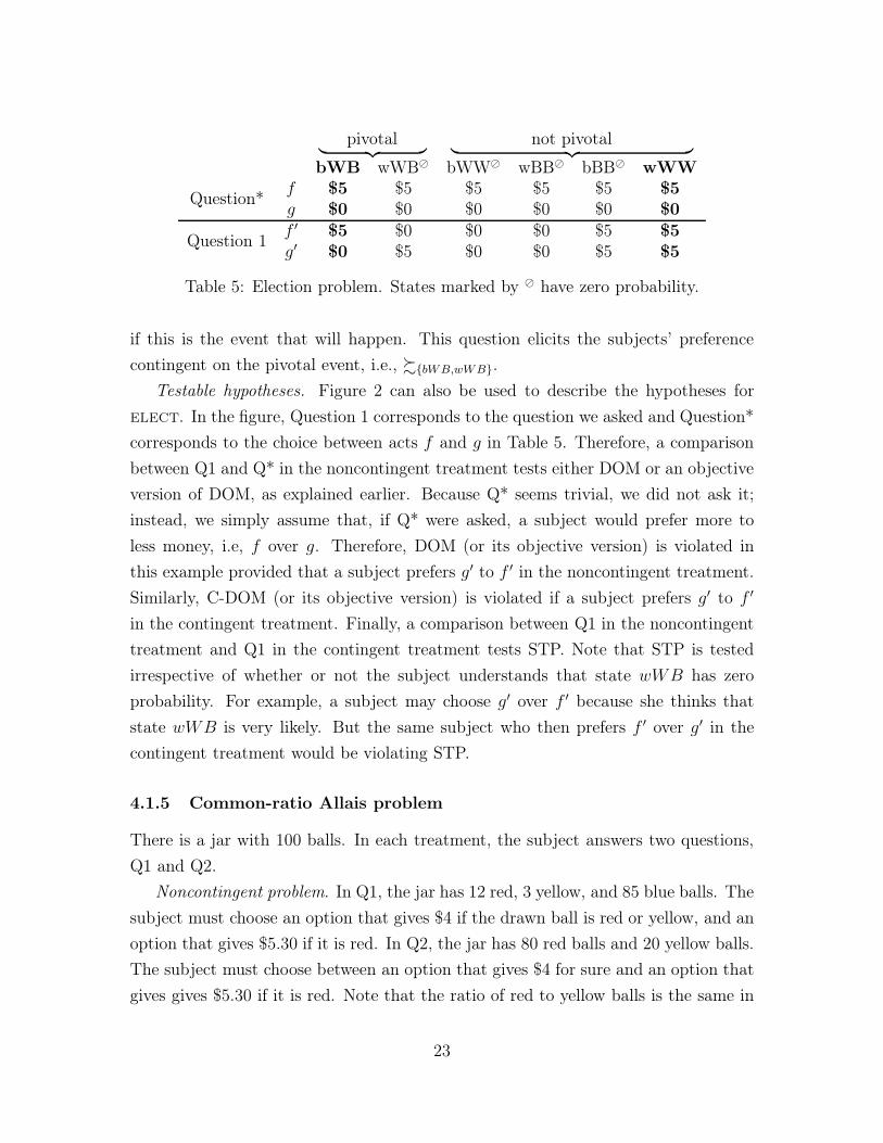
4.1.5 Common-ratio Allais problem

There is a jar with 100 balls. In each treatment, the subject answers two questions,

Q1 and Q2.

Noncontingent problem. In Q1, the jar has 12 red, 3 yellow, and 85 blue balls. The

subject must choose an option that gives $4 if the drawn ball is red or yellow, and an

option that gives $5.30 if it is red. In Q2, the jar has 80 red balls and 20 yellow balls.

The subject must choose between an option that gives $4 for sure and an option that

gives gives $5.30 if it is red. Note that the ratio of red to yellow balls is the same in

23

RY B

Question 2f x x

g y y

Question 1f ′ x $0g′ y $0

Table 6: Common-ratio Allais problem

both jars, which explains the typical term “common-ratio” in this experiment.

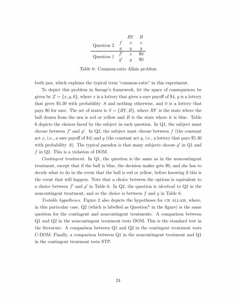
To depict this problem in Savage’s framework, let the space of consequences be

given by Z = {x, y, 0}, where x is a lottery that gives a sure payoff of $4, y is a lottery

that gives $5.30 with probability .8 and nothing otherwise, and 0 is a lottery that

pays $0 for sure. The set of states is S = {RY,B}, where RY is the state where the

ball drawn from the urn is red or yellow and B is the state where it is blue. Table

6 depicts the choices faced by the subject in each question. In Q1, the subject must

choose between f ′ and g′. In Q2, the subject must choose between f (the constant

act x, i.e., a sure payoff of $4) and g (the constant act y, i.e., a lottery that pays $5.30

with probability .8). The typical paradox is that many subjects choose g′ in Q1 and

f in Q2. This is a violation of DOM.

Contingent treatment. In Q1, the question is the same as in the noncontingent

treatment, except that if the ball is blue, the decision maker gets $0, and she has to

decide what to do in the event that the ball is red or yellow, before knowing if this is

the event that will happen. Note that a choice between the options is equivalent to

a choice between f ′ and g′ in Table 6. In Q2, the question is identical to Q2 in the

noncontingent treatment, and so the choice is between f and g in Table 6.

Testable hypotheses. Figure 2 also depicts the hypotheses for cr allais, where,

in this particular case, Q2 (which is labelled as Question* in the figure) is the same

question for the contingent and noncontingent treatments. A comparison between

Q1 and Q2 in the noncontingent treatment tests DOM. This is the standard test in

the literature. A comparison between Q1 and Q2 in the contingent treatment tests

C-DOM. Finally, a comparison between Q1 in the noncontingent treatment and Q1

in the contingent treatment tests STP.

24

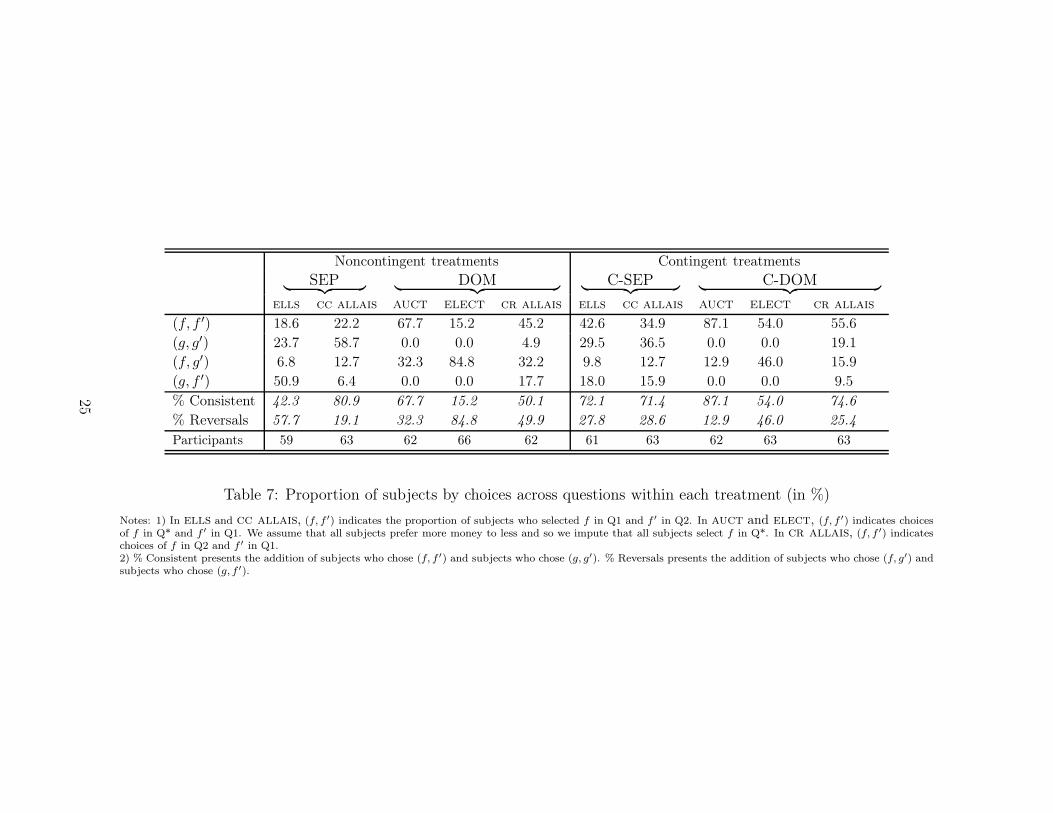
Noncontingent treatments Contingent treatments

SEP︸ ︷︷ ︸

DOM︸ ︷︷ ︸

C-SEP︸ ︷︷ ︸

C-DOM︸ ︷︷ ︸

ells cc allais auct elect cr allais ells cc allais auct elect cr allais

(f, f ′) 18.6 22.2 67.7 15.2 45.2 42.6 34.9 87.1 54.0 55.6

(g, g′) 23.7 58.7 0.0 0.0 4.9 29.5 36.5 0.0 0.0 19.1

(f, g′) 6.8 12.7 32.3 84.8 32.2 9.8 12.7 12.9 46.0 15.9

(g, f ′) 50.9 6.4 0.0 0.0 17.7 18.0 15.9 0.0 0.0 9.5

% Consistent 42.3 80.9 67.7 15.2 50.1 72.1 71.4 87.1 54.0 74.6

% Reversals 57.7 19.1 32.3 84.8 49.9 27.8 28.6 12.9 46.0 25.4

Participants 59 63 62 66 62 61 63 62 63 63

Table 7: Proportion of subjects by choices across questions within each treatment (in %)

Notes: 1) In ells and cc allais, (f, f ′) indicates the proportion of subjects who selected f in Q1 and f ′ in Q2. In auct and elect, (f, f ′) indicates choicesof f in Q* and f ′ in Q1. We assume that all subjects prefer more money to less and so we impute that all subjects select f in Q*. In cr allais, (f, f ′) indicateschoices of f in Q2 and f ′ in Q1.2) % Consistent presents the addition of subjects who chose (f, f ′) and subjects who chose (g, g′). % Reversals presents the addition of subjects who chose (f, g′) andsubjects who chose (g, f ′).

25

5 Results

We divide our results into five main findings. We mainly focus on the results from the

treatments in the between-subjects design. We then show that the results are robust

to using data from the within-subjects design. Finally, we use the within-subjects

design to assess the correlation between decision and game-theoretic problems.

We begin by examining violations of separability and dominance in the noncon-

tingent and contingent treatments.

Finding #1: We replicate the anomalies pointed out in the literature for all

noncontingent versions of the problems. In ells and cc allais, the choices of 57.7

and 19.1 percent of subjects, respectively, are inconsistent with SEP. In auct, elect

and cr allais the choices of 32.3, 84.8 and 49.9 percent of subjects, respectively,

are inconsistent with DOM.

Evidence for Finding #1 is presented in columns under the ‘Noncontingent treat-

ments’ heading of Table 7. Consider first the case of ells. The table shows that

most subjects (50.9%) select g in Q1 and f ′ in Q2. These choices are consistent with

the heuristic of ambiguity aversion (Ellsberg, 1961): subjects in this group prefer g

in the first question (where the probability of receiving $10 is known to be 2/3) and

f ′ in the second question (where the probability of receiving $10 is known to be 1/3).

There is also a 6.8% of subjects who fail SEP by selecting f in Q1, but g′ in Q2.

Overall, the proportion of subjects with choices that are inconsistent with SEP is

57.7%. In the case of cc allais, in line with the literature, we find that the most

common violation of SEP occurs when subjects select f in Q1 and g′ in Q2. These

choices are consistent, for example, with the heuristic of regret aversion (Loomes and

Sugden, 1982). Overall, the proportion of subjects with choices that are inconsistent

with SEP is 19.1%.17

Choices of g′ in Q1 of auct and elect are inconsistent with DOM (or objective

DOM, in the case of elect) under the assumption that subjects prefer more money to

less. In Table 7, we force this assumption by imposing that all subjects would select

17Of all the anomalies we replicated, the one that is hardest to find is the paradox in cc allais

(see, Huck and Müller, 2012 and Blavatskyy et al., 2015). In our experiment, only 19.1% of subjectswere inconsistent in the noncontingent treatment, a figure that may seem low but which is consistentwith the literature. The proportion of reversals that we find is lower than the average value reportedby Huck and Müller (2012) for large hypothetical payoffs, but in line with their findings for highlyeducated and high income people.

26

f in Q*. We find that 32.3% and 84.8% of subjects select g′ in auct and elect,

respectively. In auct, the observed overbidding is consistent with the illusion that it

increases the chance of winning with little cost because the winner pays the second

highest bid (Kagel et al., 1987). In elect, the mistake is consistent with the heuristic

that subjects choose the color that is more prevalent in the jar.18

Finally, in cr allais, DOM is violated if subjects’ choices are (f, g′) or (g, f ′).

Table 7 shows that approximately half of our subjects make choices inconsistent with

DOM. As in ells and cc allais, the most prevalent anomaly in cr allais coincides

with the one found in the literature, which corresponds to choosing (f, g′). These

choices are consistent with the certainty effect heuristic (Tversky and Kahneman,

1986).

Finding #2: There are fewer anomalies in all contingent versions of the problems

relative to the noncontingent versions, except for cc allais. In ells and cc allais,

the choices of 27.8 and 28.6 percent of subjects, respectively, are inconsistent with

C-SEP. In auct, elect and cr allais, the choices of 12.9, 46.0 and 25.4 percent of

subjects, respectively, are inconsistent with C-DOM. Violations of C-SEP or C-DOM

correspond to approximately half of the documented violations of SEP and DOM in

all problems except in cc allais, where the difference is not statistically significant.

The evidence supporting Finding #2 is presented in the second set of columns

of Table 7, under the ‘Contingent treatments’ heading. In all problems we still find

some subjects who violate C-SEP or C-DOM, with the proportion of inconsistencies

by problem listed in the ‘% of reversals’ row.

We can also contrast violations of DOM and SEP in contingent treatments against

violations of C-DOM and C-SEP in noncontingent treatments. Whenever differences

across treatments are significant, we find more violations in noncontingent treatments.

Inconsistent choices decrease from 32.3% to 12.9% in auct and from 84.8% to 46.0%

in elect, with both differences being statistically significant at the 1% level.19 We

18The elect problem has received the least amount of attention in the experimentalliterature, and so to make sure that the conjectured heuristic is correct and to confirmthat the labels white or black are not influencing the results, we asked each subject in bothtreatments a second question. In this other question, the composition of the jar was changedto a majority of black balls (7 black, 3 white). We indeed find that most people vote for Blackin this case: 75.8 percent in the noncontingent and 84.1 percent in the contingent treatment(p-value of .24), compared to 15.2 and 54 percent for the first question, respectively.

19We conduct a regression where the right-hand side is a dummy that takes value 1 if f ′ is selected

27

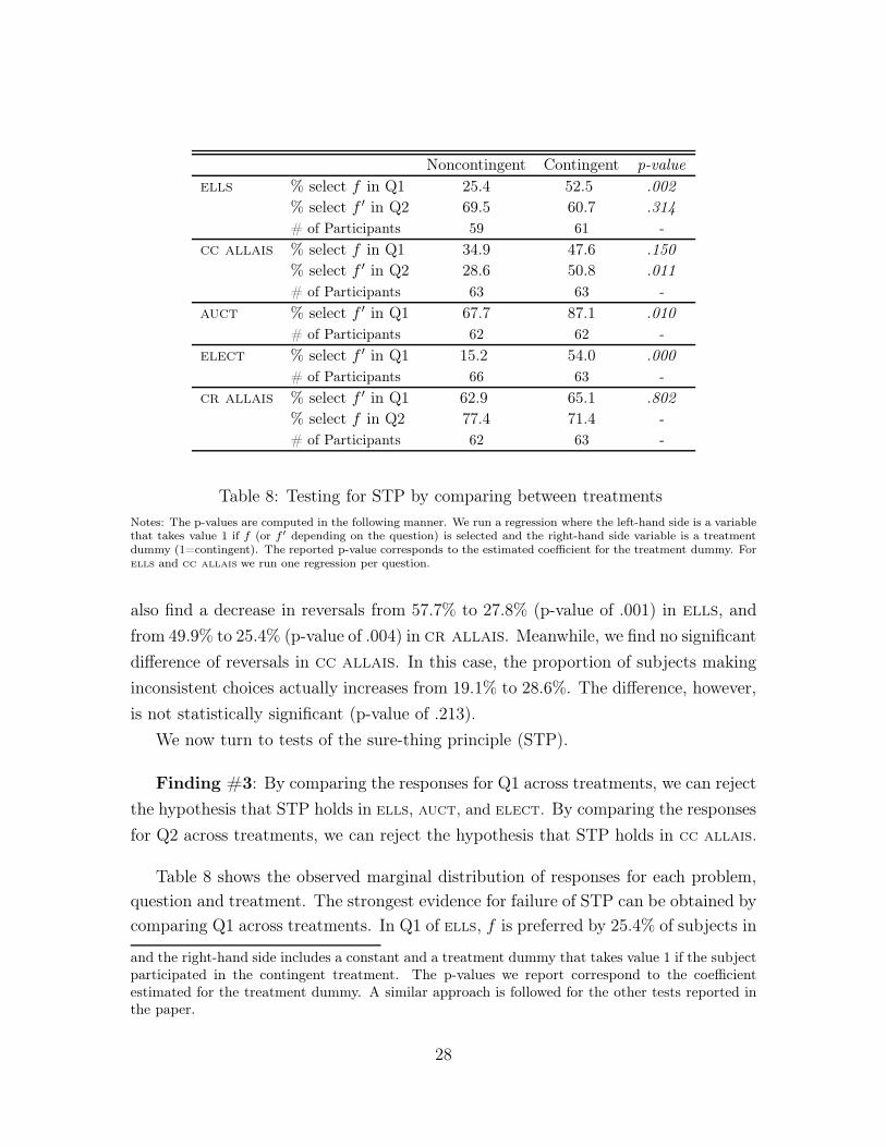
Noncontingent Contingent p-value

ells % select f in Q1 25.4 52.5 .002

% select f ′ in Q2 69.5 60.7 .314

# of Participants 59 61 -

cc allais % select f in Q1 34.9 47.6 .150

% select f ′ in Q2 28.6 50.8 .011

# of Participants 63 63 -

auct % select f ′ in Q1 67.7 87.1 .010

# of Participants 62 62 -

elect % select f ′ in Q1 15.2 54.0 .000

# of Participants 66 63 -

cr allais % select f ′ in Q1 62.9 65.1 .802

% select f in Q2 77.4 71.4 -

# of Participants 62 63 -

Table 8: Testing for STP by comparing between treatments

Notes: The p-values are computed in the following manner. We run a regression where the left-hand side is a variablethat takes value 1 if f (or f ′ depending on the question) is selected and the right-hand side variable is a treatmentdummy (1=contingent). The reported p-value corresponds to the estimated coefficient for the treatment dummy. Forells and cc allais we run one regression per question.

also find a decrease in reversals from 57.7% to 27.8% (p-value of .001) in ells, and

from 49.9% to 25.4% (p-value of .004) in cr allais. Meanwhile, we find no significant

difference of reversals in cc allais. In this case, the proportion of subjects making

inconsistent choices actually increases from 19.1% to 28.6%. The difference, however,

is not statistically significant (p-value of .213).

We now turn to tests of the sure-thing principle (STP).

Finding #3: By comparing the responses for Q1 across treatments, we can reject

the hypothesis that STP holds in ells, auct, and elect. By comparing the responses

for Q2 across treatments, we can reject the hypothesis that STP holds in cc allais.

Table 8 shows the observed marginal distribution of responses for each problem,

question and treatment. The strongest evidence for failure of STP can be obtained by

comparing Q1 across treatments. In Q1 of ells, f is preferred by 25.4% of subjects in

and the right-hand side includes a constant and a treatment dummy that takes value 1 if the subjectparticipated in the contingent treatment. The p-values we report correspond to the coefficientestimated for the treatment dummy. A similar approach is followed for the other tests reported inthe paper.

28

the noncontingent treatment and by 52.5% of subjects in the contingent treatment;

the difference is statistically significant (p-value of .002). We also find significant

differences for Q1 of elect (15.2% vs. 54%; p-value of .000) and Q1 of auct (67.7%

vs. 87.1%; p-value of .010).20 For Q1 of cc allais, there is a difference but it

is marginally not significant (34.9% vs 47.6%; p-value of .15). We do not find a

significant difference for Q1 of cr allais. Moreover, there is a significant difference

for Q2 of cc allais (28.6% vs. 50.8%; p-value of .011).

A statistically significant difference between the marginal responses to Q1 or Q2

implies that STP must be violated. This test for STP may not be too informative,

however, because the failure to reject differences in Q1 and/or Q2 across treatments

does not imply that STP is satisfied. To illustrate, consider the following extreme ex-

ample: If half of the subjects would hypothetically choose (f, g′) in the first treatment

and (g, f ′) in the second treatment and half would choose (g, f ′) in the first treatment

and (f ′, g) in the second treatment, then we would observe a 50-50 marginal choice in

both questions and treatments, when there is in fact 100 percent of subjects violating

STP.

A more informative test compares the joint distribution of responses across treat-

ments. If STP holds, then it must be the case that the joint distribution over responses

in the noncontingent treatment must equal the joint distribution in the contingent

treatment. Of course, the additional informativeness obtained from this test comes

at the expense of making the assumption that being faced with Question 1 does not

alter responses for Question 2, which is a typical assumption when testing for sepa-

rability and dominance. While we cannot test this assumption directly in our data,

there are two findings that are consistent with this assumption. The first is that our

experiment reversed the typical order in which the questions are asked in the ells

and cr allais paradoxes, yet it still finds the same patterns of violations documented

in the literature. The second piece of evidence comes from the fact that there are no

significant differences for Q2 across treatments of cr allais (p-value .45), suggesting

that whether a subject faces Q1 in the noncontingent or contingent version does not

affect her response for Q2 (recall that Q2 is identical across treatments for cr allais).

Finding #4: By comparing the joint distribution of responses across treatments,

we can reject the hypothesis that STP holds in all of the five problems that we study.

Finding #4 is directly implied by Finding #3 for ells, cc allais, auct and

20Note that for elect and auct, the test for STP is numerically the same as the testpresented in finding #2 to assess the difference between DOM and C-DOM.

29

elect.21 For cr allais, to establish that the joint distributions are different across

treatments, it suffices to show that the proportion of reversals (i.e., choices inconsis-

tent with DOM and C-DOM) are different. We can indeed see from Table 7 that, for

cr allais, the percent of reversals is 49.9 in the noncontingent treatment and 25.4

in the contingent treatment; the difference is statistically significant with a p-value

of .004.

Table 9 summarizes our findings from the between-subjects design and also reports

new findings from the within-subjects design.22 The main message that arises is that

findings #1 through #4 also hold for the within-subjects design. We now discuss

each column of Table 9 in detail.

The first column of Table 9 reports the percent of subjects who fail one of Savage’s

postulates under both designs. The only noteworthy difference with the between-

subjects design is that a larger percentage of subjects violate SEP in cc allais

(35.1 vs. 19.1), a figure that is in line with the range of findings in the literature.

The second column reports the percent who fail the corresponding contingent version

of the postulate. Under both designs, violations of C-SEP or C-DOM correspond to

approximately half of the documented violations of SEP and DOM in all problems ex-

cept in cc allais, where the difference goes in the opposite direction in the between

vs. within subjects design, although in both cases the difference is not statistically

significant.

The last two columns of Table 9 report figures on the percent of subjects who

violate STP. In the between-subjects design, subjects only participate in the noncon-

tingent or contingent treatment (but not both), and, therefore, we cannot assess the

exact level of violations of STP. Nevertheless, we can compute a tight lower bound

for the percent of subjects who violate STP, which we report in the third column.23

21For auct and elect there is a single question, and so the joint distribution is simply themarginal distribution over the single question. Thus, Finding #4 for auct and elect simply followsfrom Finding #3. For ells and cc allais, Finding #3 already establishes statistically significantdifferences in the marginal distributions, which implies that there must be significant differences inthe joint distribution.

22The Online Appendix reports additional results from the within-subjects treatment.23For problems with only one question (auct and elect), the tight lower bound is |r1 − r2|,

where rj is the proportion that choose the first option in treatment j. For the remaining problems, letpNC = (pNC

ff ′ , pNCfg′ , pNC

gf ′ , pNCgg′ ) denote the proportion of each of the four possible responses, (f, f ′),

(f, g′), (g, f ′), and (g, g′) in the noncontingent treatment, and similarly for pC in the contingent

30

Percent of observed violations of SEP or DOM, C-SEP or C-DOM, and STP

STPBetween-subjects Within-subjects

SEP or DOM C-SEP or C-DOM Lower bound[95% Confidence Interval]

Exact

ells

between 57.7 27.8 32.872.5

within 53.4 29.8 [19.4, 50.0]

cc allais

between 19.1 28.6 22.243.5

within 35.1 25.9 [9.5, 39.7]

auct between 32.3 12.9 19.419.9

within 22.9 6.1 [4.8, 33.9]

elect between 84.8 46.0 38.845.8

within 78.5 40.5 [23.3, 54.4%]

cr allais between 49.9 25.4 24.525.2

within 35.1 16.8 [10.8, 40.7]

Table 9: Failures of STP, SEP or DOM, and C-SEP or C-DOM, by problem.

Notes: Violations of SEP, DOM, C-SEP and C-DOM are computed by contrasting the answers of subjects within the corresponding noncontingent or contingenttreatment. In all cases, we consider STP to be violated if it is violated for one of the questions across the noncontingent and contingent treatments. The lower boundon violations of STP in the between-subjects design can be subject to sampling error. For this reason we provide a 95% confidence interval on the lower bound foreach problem. We compute the confidence interval via bootstrap: in each of 1000 repetitions we randomly draw a sample with replacement and compute the tightlower bound corresponding to the sample; the confidence interval reports the 2.5th and 97.5th percentiles of the obtained distribution of lower bounds.

31

The advantage of the within-subjects design is that, because subjects participates

in both the noncontingent and contingent version of each problem, we can compute

the exact percentage of subjects who fail STP. Of course, this figure relies on the

assumption that there is no contamination from the fact that a subject participated

in both treatments, but the findings reported in the first two columns suggest that

this is a reasonable assumption in this context.

Table 9 shows that a large part of the violations in the standard postulates of

Savage’s subjective expected utility framework can be attributed to violations in STP

in all of the problems that we study. In ells and auct, the observed lower bound rate

of violations of STP reported in the table is higher than the rate of violations of the

our version of Savage’s postulates for the contingent preferences (C-SEP or C-DOM).

In cc allais, the observed lower bound of STP violations is higher than the rate

of violations of SEP. Finally, the observed lower bound of STP violations in elect

and cr allais and the rate of C-DOM violations are of comparable magnitude. The

figures on the exact percentage of violation of STP coming from the within-subjects

design confirms that STP fails significantly across all problems.

The previous findings indicate that failure of STP is an important force behind vio-

lations of the standard postulates, and it provides a unifying explanation of anomalies

in a wide range of environments. In contrast, the literature has viewed these prob-

lems in isolation and has focused on different heuristics to explain behavior, such as

the thrill of winning for overbidding in auctions and ambiguity aversion in the Ells-

berg example. A further question that we now study is whether or not the heuristics

responsible for failure of STP are related to each other.

There are two natural hypotheses here. The first is that heuristics are independent

in the sense that, for example, some subjects are susceptible to the thrill of winning

but not to ambiguity aversion, and vice versa. In this case, we would see failure of

STP in both types of problems but these failures would not be correlated. The second

hypothesis is that the failures are correlated, so that a subject who is susceptible to

one heuristic is more likely to be susceptible to another one.

We are able to investigate this question using data from the within-subjects de-

sign, since we observe subjects participate in both the noncontingent and contingent

treatments in all problems. A natural instinct is to start by correlating failures of

treatment. The tight lower bound is 1 − (min{pNCff ′ , pCff ′} + min{pNC

fg′ , pCfg′} + min{pNCgf ′ , pCgf ′} +

min{pNCgg′ , pCgg′}).

32

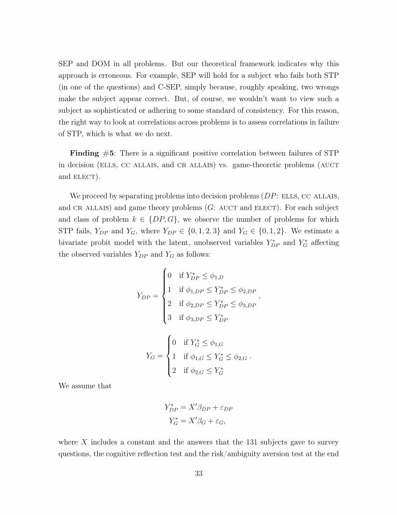
SEP and DOM in all problems. But our theoretical framework indicates why this

approach is erroneous. For example, SEP will hold for a subject who fails both STP

(in one of the questions) and C-SEP, simply because, roughly speaking, two wrongs

make the subject appear correct. But, of course, we wouldn’t want to view such a

subject as sophisticated or adhering to some standard of consistency. For this reason,

the right way to look at correlations across problems is to assess correlations in failure

of STP, which is what we do next.

Finding #5: There is a significant positive correlation between failures of STP

in decision (ells, cc allais, and cr allais) vs. game-theoretic problems (auct

and elect).

We proceed by separating problems into decision problems (DP : ells, cc allais,

and cr allais) and game theory problems (G: auct and elect). For each subject

and class of problem k ∈ {DP,G}, we observe the number of problems for which

STP fails, YDP and YG, where YDP ∈ {0, 1, 2, 3} and YG ∈ {0, 1, 2}. We estimate a

bivariate probit model with the latent, unobserved variables Y ∗DP and Y ∗

G affecting

the observed variables YDP and YG as follows:

YDP =

0 if Y ∗DP ≤ φ1,D

1 if φ1,DP ≤ Y ∗DP ≤ φ2,DP

2 if φ2,DP ≤ Y ∗DP ≤ φ3,DP

3 if φ3,DP ≤ Y ∗DP

,

YG =

0 if Y ∗G ≤ φ1,G

1 if φ1,G ≤ Y ∗G ≤ φ2,G

2 if φ2,G ≤ Y ∗G

.

We assume that

Y ∗DP = X ′βDP + εDP

Y ∗G = X ′βG + εG,

where X includes a constant and the answers that the 131 subjects gave to survey

questions, the cognitive reflection test and the risk/ambiguity aversion test at the end

33

of the experiment (see the Appendix for additional details on these observables). We

also assume that (εDP , εG) are normally distributed with zero mean, unit variance,

and correlation coefficient ρ. One interpretation of this model is that a subject has a

latent level of cognitive ability for decision problems, Y ∗DP , and another one for game

theory problems, Y ∗G, that determine her ability or desire to overcome heuristics and

satisfy STP. A higher value of the latent variable is associated with a higher number

of problems for which the subject satisfies STP. The main parameter of interest,

ρ, measures the correlation between failures of STP in decision and game-theoretic

problems.

We assume that each subject’s observation is drawn from the same distribution and

use maximum likelihood to estimate the parameters βDP , βG, φDP = (φ1,DP , φ2,DP , φ3,DP ),

φG = (φ1,G, φ2,G), and ρ.24 We present the full results of the estimation in the Online

Appendix. Here, we focus on the correlation coefficient. We estimate a correlation

coefficient of ρ̂ = 0.34, with a p-value of 0.001 and a 95% confidence interval of

[0.1345, 0.5363].

6 Conclusion

We find that failure of a particular type of hypothetical thinking underlies classic

anomalies from both decision and game theory experiments, thus providing common

ground for literatures that have evolved along different paths. The particular type

of hypothetical thinking underlying these anomalies is what Savage informally called

the Sure-Thing Principle (STP) and used as motivation for two of the central postu-

lates in his theory of subjective expected utility. Our approach to formalizing STP

is to assume that both the original preference relation and the contingent preference

relations are primitives, and we define STP as a particular type of consistency require-

ment between these primitives. We then establish that violations of some of Savage’s

central postulates can be attributed to violations of STP and to violations of contin-

gent versions of these postulates. We find that some of the most common anomalies

uncovered in laboratory experiments, including overbidding in auctions, naive voting

in elections, and Ellsberg and Allais types of paradoxes, spring (at least in large part)

from the failure of the type of hypothetical thinking embodied by STP. In particular,

many subjects do not reason about hypothetical events the way economic theories

24For further details see Greene and Hensher (2010).

34

typically assume.

Our strategy is to run subjects through standard versions of each of these canonical

problems, which require sophisticated hypothetical thinking on the part of subjects.

We then run subjects through slight alterations of each problem, removing the need

for them to employ this type of hypothetical sophistication (we call these variations

contingent versions of the problem). We find that subjects behave differently in

these two versions of the problem, and that this difference explains about half of the

anomalies in many classic problems.

The finding that errors in a set of seemingly dissimilar settings originate from a

common source suggests that finding other root phenomena underlying failures of clas-

sical assumptions may be an important and fruitful avenue for future research. More

narrowly, our results suggest that exploring, both theoretically and empirically, how

the models that people construct of their environments might differ from the models

built in standard theories may yield critical insight into the source of deviations from

these theories.

References

Al-Najjar, Nabil I and Jonathan Weinstein, “The ambiguity aversion literature:

a critical assessment,” Economics and Philosophy, 2009, 25 (03), 249–284.

Allais, Maurice, “Le comportement de l’homme rationnel devant le risque: cri-

tique des postulats et axiomes de l’école américaine,” Econometrica: Journal of the

Econometric Society, 1953, pp. 503–546.

Andreoni, James, Tobias Schmidt, and Charles Sprenger, “Measuring Ambi-

guity Aversion: Experimental Tests of Subjective Expected Utility,” mimeo, 2014.

Bazerman, Max H and William F Samuelson, “I won the auction but don’t

want the prize,” Journal of Conflict Resolution, 1983, 27 (4), 618–634.

Blavatskyy, Pavlo R, Andreas Ortmann, and Valentyn Panchenko, “Now

you see it, now you don’t: How to make the Allais Paradox appear, disappear, or

reverse,” UNSW Business School Research Paper, 2015, (2015-14).

Bó, Ernesto Dal, Pedro Dal Bó, and Erik Eyster, “The Demand for Bad Policy

When Voters Underappreciate Equilibrium Effects,” 2016.

35

Brandts, Jordi and Gary Charness, “The strategy versus the direct-response

method: a first survey of experimental comparisons,” Experimental Economics,

2011, 14 (3), 375–398.

Camerer, C, “Individual Decision Making. Chapter 8 in John Kagel and Al Roth

(eds.), The Handbook of Experimental Economics,” 1995.

Charness, G. and D. Levin, “The origin of the winner’s curse: a laboratory study,”

American Economic Journal: Microeconomics, 2009, 1 (1), 207–236.

Cohen, Michele, Itzhak Gilboa, Jean-Yves Jaffray, David Schmeidler et al.,

“An experimental study of updating ambiguous beliefs,” Risk Decision and Policy,

2000, 5 (2), 123–133.

Crawford, V.P. and N. Iriberri, “Level-k Auctions: Can a Nonequilibrium Model

of Strategic Thinking Explain the Winner’s Curse and Overbidding in Private-Value

Auctions?,” Econometrica, 2007, 75 (6), 1721–1770.

Crosetto, Paolo and Antonio Filippin, “The ‘bomb’ risk elicitation task,” Journal

of Risk and Uncertainty, 2013, 47 (1), 31–65.

Cubitt, Robin, Chris Starmer, and Robert Sugden, “Dynamic choice and the

common ratio effect: An experimental investigation,” The Economic Journal, 1998,

108 (450), 1362–1380.

Cubitt, Robin P, “Rational dynamic choice and expected utility theory,” Oxford

Economic Papers, 1996, 48 (1), 1–19.

Dean, Mark and Pietro Ortoleva, “Is it all connected? a testing ground for

unified theories of behavioral economics phenomena,” mimeo, 2015.

Dominiak, Adam, Peter Dürsch, and Jean-Philippe Lefort, “A dynamic Ells-

berg urn experiment,” Games and Economic Behavior, 2012, 75 (2), 625–638.

Eliaz, K., D. Ray, and R. Razin, “Choice shifts in groups: A decision-theoretic

basis,” The American economic review, 2006, 96 (4), 1321–1332.

Ellsberg, Daniel, “Risk, ambiguity, and the Savage axioms,” The quarterly journal

of economics, 1961, pp. 643–669.

36

Enke, Benjamin and Florian Zimmermann, “Correlation neglect in belief for-

mation,” 2013.

Esponda, I., “Behavioral equilibrium in economies with adverse selection,” The

American Economic Review, 2008, 98 (4), 1269–1291.

and E. Vespa, “Hypothetical Thinking and Information Extraction in the Labo-

ratory,” American Economic Journal: Microeconomics, 2014, 6 (4), 180–202.

Evans, Jonathan St BT, Hypothetical thinking: Dual processes in reasoning and

judgement, Vol. 3, Psychology Press, 2007.

Eyster, E. and M. Rabin, “Cursed equilibrium,” Econometrica, 2005, 73 (5), 1623–

1672.

Eyster, Erik and Georg Weizsacker, “Correlation neglect in financial decision-

making,” 2010.

Fischbacher, U., “z-Tree: Zurich toolbox for ready-made economic experiments,”

Experimental Economics, 2007, 10 (2), 171–178.

Frederick, Shane, “Cognitive reflection and decision making,” The Journal of Eco-

nomic Perspectives, 2005, 19 (4), 25–42.

Gilboa, Itzhak, Theory of decision under uncertainty, Vol. 1, Cambridge university

press, 2009.

and David Schmeidler, “Case-based decision theory,” The Quarterly Journal of

Economics, 1995, pp. 605–639.

and Massimo Marinacci, “Ambiguity and the Bayesian paradigm,” Chapter,

2011, 7, 179–242.

, Andrew Postlewaite, and David Schmeidler, “Is it always rational to satisfy

Savage’s axioms?,” Economics and Philosophy, 2009, 25 (03), 285–296.

Greene, William H and David A Hensher, Modeling Ordered Choices, Cam-

bridge University, 2010.

Greiner, Ben, “Subject pool recruitment procedures: organizing experiments with

ORSEE,” Journal of the Economic Science Association, 2015, 1 (1), 114–125.

37

Halevy, Yoram, “Ellsberg revisited: An experimental study,” Econometrica, 2007,

75 (2), 503–536.

Hammond, Peter J, “Consequentialist foundations for expected utility,” Theory

and decision, 1988, 25 (1), 25–78.

Harstad, Ronald M, “Dominant strategy adoption and bidders’ experience with

pricing rules,” Experimental economics, 2000, 3 (3), 261–280.

Holler, Manfred J, “Do economics students choose rationally? A research note.,”

Social Science Information/sur les sciences sociales, 1983.

Huck, Steffen and Wieland Müller, “Allais for all: Revisiting the paradox in a

large representative sample,” Journal of Risk and Uncertainty, 2012, 44 (3), 261–

293.

Ivanov, A., D. Levin, and M. Niederle, “Can relaxation of beliefs rationalize the

winner’s curse?: an experimental study,” Econometrica, 2010, 78 (4), 1435–1452.

Jehiel, P. and F. Koessler, “Revisiting games of incomplete information with

analogy-based expectations,” Games and Economic Behavior, 2008, 62 (2), 533–

557.

Kagel, J.H. and D. Levin, Common value auctions and the winner’s curse, Prince-

ton Univ Pr, 2002.

, R.M. Harstad, and D. Levin, “Information impact and allocation rules in

auctions with affiliated private values: A laboratory study,” Econometrica, 1987,

pp. 1275–1304.

Kagel, John H and Dan Levin, “Independent private value auctions: Bidder be-

haviour in first-, second-and third-price auctions with varying numbers of bidders,”

The Economic Journal, 1993, 103 (419), 868–879.

Kovářík, Jaromír, Dan Levin, and Tao Wang, “Ellsberg paradox: Ambiguity

and complexity aversions compared,” Journal of Risk and Uncertainty, 2016, 52

(1), 47–64.

38

Levin, Dan, James Peck, and Asen Ivanov, “Separating bayesian updating from

non-probabilistic reasoning: An experimental investigation,” American Economic

Journal: Microeconomics, 2016, 8 (2), 39–60.

Li, Shengwu, “Obviously strategy-proof mechanisms,” mimeo, 2016.

Loomes, Graham and Robert Sugden, “Regret theory: An alternative theory of

rational choice under uncertainty,” The economic journal, 1982, 92 (368), 805–824.

MacCrimmon, Kenneth R and Stig Larsson, “Utility theory: Axioms versus

paradoxes,” in “Expected utility hypotheses and the Allais paradox,” Springer, 1979,

pp. 333–409.

Machina, M, “Non-Expected Utility Theory. In Steven Durlauf and Lawrence Blume

(eds.), The New Palgrave Dictionary of Economics,” 2008.

Machina, Mark J, “Dynamic consistency and non-expected utility models of choice

under uncertainty,” Journal of Economic Literature, 1989, 27 (4), 1622–1668.

and Marciano Siniscalchi, “Ambiguity and ambiguity aversion,” Economics of

Risk and Uncertainty, Handbook in Economics, North Hollad, Machina and Viscusi

eds, 2013.

Nebout, Antoine and Dimitri Dubois, “When Allais meets Ulysses: Dynamic

axioms and the common ratio effect,” Journal of Risk and Uncertainty, 2014, 48

(1), 19–49.

Nickerson, Raymond, Conditional Reasoning: The Unruly Syntactics, Semantics,

Thematics, and Pragmatics of “If”, Oxford University Press, 2015.

Savage, Leonard J, The foundations of statistics, Courier Corporation, 1972.

Shafir, Eldar and Amos Tversky, “Thinking through uncertainty: Nonconsequen-

tial reasoning and choice,” Cognitive psychology, 1992, 24 (4), 449–474.

Siniscalchi, Marciano, “Two out of three ain’t bad: A comment on ‘the ambiguity

aversion literature: A critical assessment’,” Economics and Philosophy, 2009, 25

(03), 335–356.

39

Tversky, Amos and Daniel Kahneman, “The framing of decisions and the psy-

chology of choice,” Science, 1981, 211 (4481), 453–458.

and , “Rational choice and the framing of decisions,” Journal of business, 1986,

pp. S251–S278.

Wakker, Peter P, “Testing and characterizing properties of nonadditive measures

through violations of the sure-thing principle,” Econometrica, 2001, 69 (4), 1039–

1059.

Wason, Peter C, “Reasoning,” New horizons in psychology, Vol. 1, BM Foss ed,

1966.

, “Reasoning about a rule,” The Quarterly journal of experimental psychology, 1968,

20 (3), 273–281.

40

Appendix

Controlling for observables

In this appendix, we show that our treatment effects remain unchanged when we

control for observables that we collected at the end of the experiment. We incentivized

subjects to provide answers to the Cognitive Reflection Test (CRT, see Frederick,

2005). This test involves three questions (see the Online Appendix) and is intended

to measure the extent to which the respondent gives spontaneous (System 1) vs.

reasoned (System 2) answers. We also control for other factors that might affect

behavior by eliciting additional information for each subject, including a measure

of risk aversion (or ambiguity aversion for the Ellsberg problem) and demographic

information, including gender, major (economics related or not), and their year of

study (freshman, sophomore, junior, senior, or graduate student). The measure of

risk or ambiguity aversion is obtained using the bomb risk elicitation test (BRET, see

Crosetto and Filippin, 2013).25 Table 10 shows descriptive statistics. The measures

of risk aversion and cognitive ability are in line with previous literature.26

Variable Mean Median Std. dev. ObservationsTotal CRT 1.45 1.00 1.11 624

BRET (Ambiguity) 40.45 40.00 15.50 120BRET (Risk) 38.64 39.50 14.97 504Econ Major 0.204 - - 624

Female 0.579 - - 624Junior or older 0.564 - - 624

Table 10: Observables: Summary statistics

Table 11 shows the results of regressions, where the rand-hand side is a dummy

variable that takes value 1 if the subject chooses f (or f ′ depending on the question).

The regression controls for the treatment and the observables described above. As

shown by the table, the treatment effect highlighted in Finding #3 continues to hold,

25For ambiguity aversion, we modify the experiment by creating ambiguity about the location ofthe bomb; see the Online Appendix for details.

26Frederick (2005) finds a mean of 1.24 for Total CRT and Crosetto and Filippin (2013) find amean of 46.5 for BRET (Risk). There is no comparable exercise for ambiguity aversion.

41

but the observables are mostly statistically not significant (although the measure or

risk or ambiguity aversion tends to have the expected sign, i.e., a lower aversion

measure -higher value for the BRET variable- is associated with less risky choice in

both of the Allais problems and in Question 2 of the Ellsberg problem.27) Table

12 shows the results of regressions of whether or not behavior across Q1 and Q2

is inconsistent for each problem, controlling for the treatment and the observables

described above. Once again, the treatment effects reported in Finding #2 continue

to hold.

27Note that in auct and elect, there is an optimal choice and there is no reason why risk aversionshould explain who is sophisticated and makes the right choice.

42

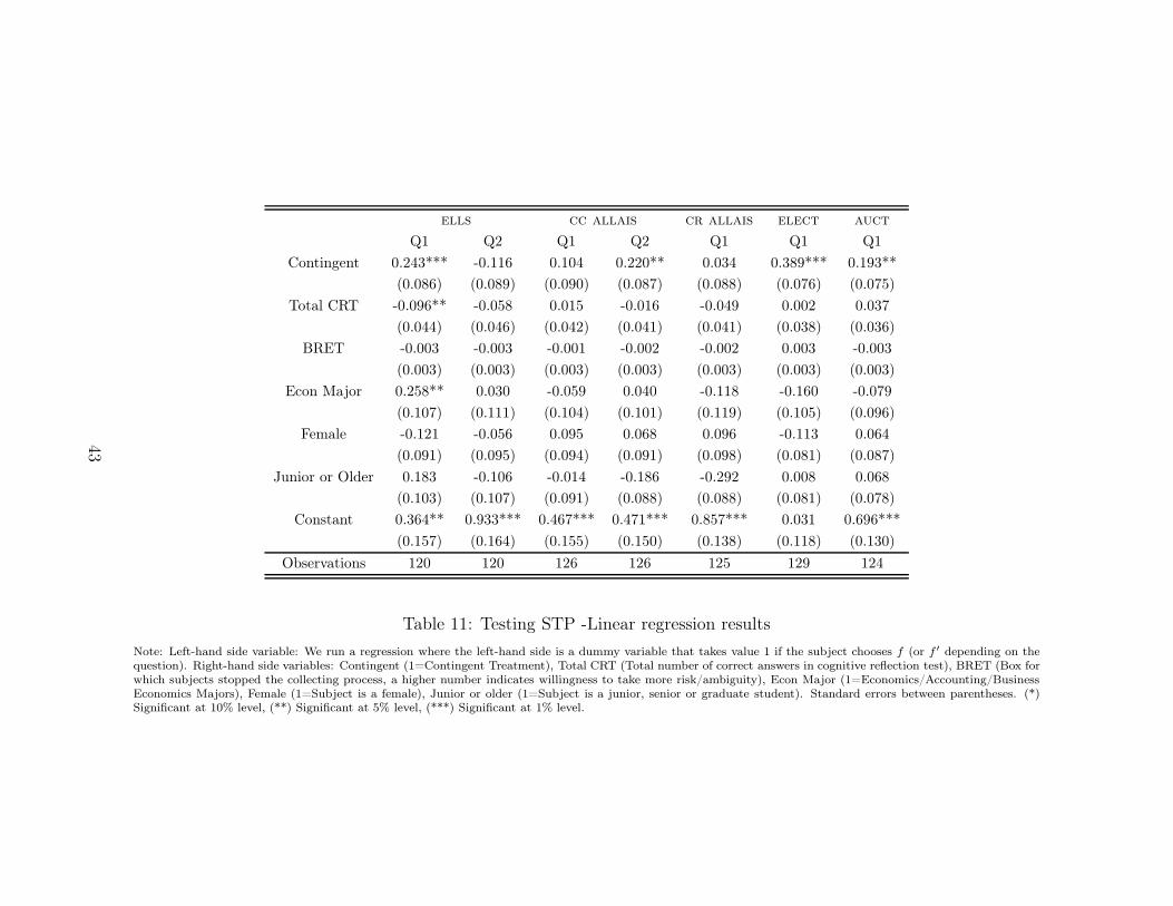
ells cc allais cr allais elect auct

Q1 Q2 Q1 Q2 Q1 Q1 Q1

Contingent 0.243*** -0.116 0.104 0.220** 0.034 0.389*** 0.193**

(0.086) (0.089) (0.090) (0.087) (0.088) (0.076) (0.075)

Total CRT -0.096** -0.058 0.015 -0.016 -0.049 0.002 0.037

(0.044) (0.046) (0.042) (0.041) (0.041) (0.038) (0.036)

BRET -0.003 -0.003 -0.001 -0.002 -0.002 0.003 -0.003

(0.003) (0.003) (0.003) (0.003) (0.003) (0.003) (0.003)

Econ Major 0.258** 0.030 -0.059 0.040 -0.118 -0.160 -0.079

(0.107) (0.111) (0.104) (0.101) (0.119) (0.105) (0.096)

Female -0.121 -0.056 0.095 0.068 0.096 -0.113 0.064

(0.091) (0.095) (0.094) (0.091) (0.098) (0.081) (0.087)

Junior or Older 0.183 -0.106 -0.014 -0.186 -0.292 0.008 0.068

(0.103) (0.107) (0.091) (0.088) (0.088) (0.081) (0.078)

Constant 0.364** 0.933*** 0.467*** 0.471*** 0.857*** 0.031 0.696***

(0.157) (0.164) (0.155) (0.150) (0.138) (0.118) (0.130)

Observations 120 120 126 126 125 129 124

Table 11: Testing STP -Linear regression results

Note: Left-hand side variable: We run a regression where the left-hand side is a dummy variable that takes value 1 if the subject chooses f (or f ′ depending on thequestion). Right-hand side variables: Contingent (1=Contingent Treatment), Total CRT (Total number of correct answers in cognitive reflection test), BRET (Box forwhich subjects stopped the collecting process, a higher number indicates willingness to take more risk/ambiguity), Econ Major (1=Economics/Accounting/BusinessEconomics Majors), Female (1=Subject is a female), Junior or older (1=Subject is a junior, senior or graduate student). Standard errors between parentheses. (*)Significant at 10% level, (**) Significant at 5% level, (***) Significant at 1% level.

43

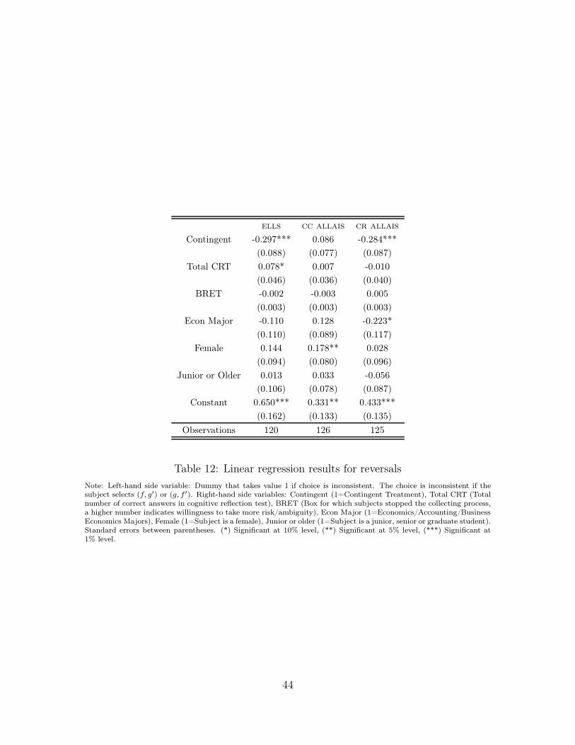
ells cc allais cr allais

Contingent -0.297*** 0.086 -0.284***

(0.088) (0.077) (0.087)

Total CRT 0.078* 0.007 -0.010

(0.046) (0.036) (0.040)

BRET -0.002 -0.003 0.005

(0.003) (0.003) (0.003)

Econ Major -0.110 0.128 -0.223*

(0.110) (0.089) (0.117)

Female 0.144 0.178** 0.028

(0.094) (0.080) (0.096)

Junior or Older 0.013 0.033 -0.056

(0.106) (0.078) (0.087)

Constant 0.650*** 0.331** 0.433***

(0.162) (0.133) (0.135)

Observations 120 126 125

Table 12: Linear regression results for reversals

Note: Left-hand side variable: Dummy that takes value 1 if choice is inconsistent. The choice is inconsistent if thesubject selects (f, g′) or (g, f ′). Right-hand side variables: Contingent (1=Contingent Treatment), Total CRT (Totalnumber of correct answers in cognitive reflection test), BRET (Box for which subjects stopped the collecting process,a higher number indicates willingness to take more risk/ambiguity), Econ Major (1=Economics/Accounting/BusinessEconomics Majors), Female (1=Subject is a female), Junior or older (1=Subject is a junior, senior or graduate student).Standard errors between parentheses. (*) Significant at 10% level, (**) Significant at 5% level, (***) Significant at1% level.

44