conformally parallel g2 structures on a class of solvmanifolds
TRANSCRIPT
arX
iv:m
ath/
0409
137v
1 [
mat
h.D
G]
8 S
ep 2
004 CONFORMALLY PARALLEL G2 STRUCTURES
ON A CLASS OF SOLVMANIFOLDS
SIMON G. CHIOSSI AND ANNA FINO
Abstract. Starting from a 6-dimensional nilpotent Lie group N endowed with an in-variant SU(3) structure, we construct a homogeneous conformally parallel G2-metric onan associated solvmanifold. We classify all half-flat SU(3) structures that endow therank-one solvable extension of N with a conformally parallel G2 structure. By suitablydeforming the SU(3) structures obtained, we are able to describe the corresponding non-homogeneous Ricci-flat metrics with holonomy contained in G2. In the process we alsofind a new metric with exceptional holonomy.
1. Introduction
A seven-dimensional Riemannian manifold (Y, g) is called a G2-manifold if it admits a re-duction of the structure group of the tangent bundle to the exceptional Lie group G2. Thepresence of a G2 structure is equivalent to the existence of a certain type of three-form ϕ onthe manifold. Whenever this 3-form is covariantly constant with respect to the Levi–Civitaconnection then the holonomy group is contained in G2, and the corresponding manifold iscalled parallel. The development of the theory of explicit metrics with holonomy G2 followsthe by-now-classical line of Bonan [5], Fernandez and Gray [15], Bryant [7] and Salamon [9].We shall review a few relevant facts in section 2.
Interesting non-compact examples are provided by Gibbons, Lu, Pope, Stelle in [17],where incomplete Ricci-flat metrics of holonomy G2 with a 2-step nilpotent isometry groupN acting on orbits of codimension one are presented. It turns out that these metrics havescaling symmetries generated by a homothetic Killing vector field, and are locally isometric(modulo a conformal change) to homogeneous metrics on solvable Lie groups. The solvableLie group in question is obtained by extending the isometry group of the original manifold,and can be seen as the universal cover of the product of R with the 2-step nilmanifoldcorresponding to N , which is a compact quotient Γ\N by a discrete uniform subgroup.Solvmanifolds — that is solvable Lie groups endowed with a left-invariant metric — andin particular solvable extensions of nilpotent Lie groups provide instances of homogeneousEinstein manifolds. The fact that any nilpotent Lie algebra of dimension 6 admits a solvableextension carrying Einstein metrics [31] will be of the foremost importance.
We shall concentrate on conformally parallel G2 structures, characterised by the fact thatthe Riemannian metric g can be modified to metric with holonomy a subgroup of G2 by atransformation
g 7→ e2fg,
for some function f .
1991 Mathematics Subject Classification. Primary 53C10 – Secondary 53C25, 53C29, 22E25.
1
2 SIMON G. CHIOSSI AND ANNA FINO
In the light of [31], it is natural to study such G2 structures on a rank-one solvableextension of a metric 6-dimensional nilpotent Lie algebra n endowed with an SU(3) structure(ω, ψ+) and a non-singular self-adjoint derivation D which is diagonalisable by a unitarybasis. This last condition is equivalent to (DJ)2 = (JD)2 and we show that this is thecompatibility that one has to impose between D and the SU(3) structure in order to obtainthe non-compact examples found in [17].
As shown in section 3, such an extension is given by a metric Lie algebra s = n ⊕ RHwith bracket
[H,U ] = DU, [U, V ] = [U, V ]n×n,
where U, V ∈ n and H ⊥ n, ‖H‖ = 1. The subscript denotes the Lie bracket on n, and theinner product extends that of n. There is a natural G2 structure on the manifold Y = N ×R
corresponding to the 3-form
ϕ = ω ∧H + ψ+ ∈ Λ3T ∗Y,
where is the isomorphism of T onto T ∗ induced by the metric. The Lie algebra s isisomorphic to each fibre of the principal fibration T ∗Y −→ Y , and we prove the
Main result. (Y, ϕ) is conformally parallel if and only if n is either R6, or 2-step nilpotent
but not isomorphic to the Lie algebra h3 ⊕ h3,
where h3 denotes the real 3-dimensional Heinsenberg algebra (cf. §4). The operator D hasthe same eigenvalue type of the derivation considered by Will to construct Einstein metricson 7-dimensional solvmanifolds [31].
In section 5 we describe explicitly the corresponding metrics g with holonomy a non-trivial subgroup of G2. Half of such metrics have Hol(g) = G2 and stem from the threeirreducible 2-step nilpotent Lie algebras. The remaining metrics have holonomy either SU(2)or SU(3) and correspond to Lie algebras with abelian summands. Using this we show thatsome metrics have also been considered by [17] in the study of special domain walls in stringtheory. We are able to produce a new metric with holonomy equal to G2, that arises fromthe 6-dimensional Lie algebra spanned by e1, . . . , e6 with
e2 = [e5, e4], e3 = [e6, e4] = [e1, e5]
as the only non-trivial brackets.The conformally parallel G2 structure forces the initial SU(3) structure to be of a special
kind, known in the literature as half-flat [11]. This turns out to be a useful notion, whichallows one to find explicit metrics with holonomy G2 by investigating the correspondingHitchin flow [21]. Section 6 is especially devoted to such a description. We determine asolution of the evolutions equations and compare the resulting G2 holonomy metrics withthe ones previously described. These rank-one solvmanifolds S admit then a pair of distin-guished metrics. The first is the homogeneous Einstein metric with negative scalar curvatureconstructed in [31]. The other arises by conformally changing a homogeneous metric andpossesses a homothetic Killing field, i.e. a vector field with respect to which the Lie deriva-tive of g is a multiple of the identity; our investigation proves that it is also obtainable byevolving the original SU(3) structure.
Acknowledgements. The authors are indebted to S. Salamon and A. Swann for the invaluablesuggestions, and thank I. Agricola and T. Friedrich for hospitality during the initial stage

CONFORMALLY PARALLEL G2 STRUCTURES ON A CLASS OF SOLVMANIFOLDS 3
of this project. They are both members of the Edge Research Training Network hprn-
ct--, supported by the European Human Potential Programme. The research ispartially supported by Miur, Gnsaga–Indam in Italy.
2. G structures in 6 and 7 dimensions
Suppose that X indicates a six-dimensional nilmanifold with an invariant almost Hermit-ian structure. Thus, X is endowed with an orthogonal almost complex structure J and anon-degenerate 2-form ω which induce a Riemannian metric h. An SU(3)-reduction of thestructure group is determined by fixing a real 3-form ψ+ lying in the S1-bundle of unitelements inside the canonical bundle
[[
Λ3,0]]
at each point. We adopt the parenthetical nota-
tion of [30] to indicate real modules of p, q-forms underlying the complex space Λp+qC
. LetΨ = ψ++iψ− be the associated holomorphic section (so that Jψ− = −ψ+). The descriptionis always intended to be local, so one can define the forms
(2.1)ω = e14 − e23 + e56,
ψ+ + iψ− = (e1 + ie4) ∧ (e2 − ie3) ∧ (e5 + ie6),
of type (1, 1) and (3, 0) relative to J . It has become customary to suppress wedge signswhen writing differential forms, so eij... indicates ei ∧ ej ∧ . . . from now on. Following [11]and [6] we tackle six-dimensional geometry by means of the enhanced Gray and Hervelladecomposition of the intrinsic torsion space into five representations W1, . . . ,W5. These arethe SU(3)-modules appearing in Λ1⊗
([[
Λ2,0]]
⊕R)
that identify the kind of almost Hermitianstructure. Complex SU(3)-manifolds are for instance characterised by the vanishing of theintrinsic torsion components belonging to W1
∼= R ⊕ R,W2∼= su(3) ⊕ su(3). Tagging the
irreducible ‘halves’ by ±, one can correspondingly split the Nijenhius tensor NJ = N+J +N−
J .
The modules W±1 ,W±
2 can be defined explicitly by prescribing the various types of the realforms
dψ+ = −2W5 ∧ ψ+ +W+2 ∧ ω +W+
1 ω2
dψ− = 2W5 ∧ ψ− +W−2 ∧ ω +W−
1 ω2
corresponding to Λ4T ∗X ∼=[[
Λ0,1]]
⊕[
Λ1,10
]
⊕ R. The nought in the middle term denotes(1, 1)-forms α satisfying α ∧ ω = 0, called primitive.
Moving up one dimension, we consider a product Y of X with R, endowed with metricg. Indicating by e7 the unit 1-form on the real line one obtains a basis for the cotangentspaces T ∗
y Y . The manifold Y inherits a non-degenerate three-form ϕ = ω∧ e7 +ψ+ which isstable, a la Hitchin [21], and defines a reduction to the exceptional group. The fundamentalmaterial for the G2 story can be found in standard references [30, 23]. Let us only recallthat the Riemannian geometry of Y is completely determined by the tensor
ϕ = e125 − e345 + e567 + e136 + e246 − e237 + e147.
The seminal results of Fernandez and Gray [15] permit one to describe G2 geometry exclu-sively in algebraic terms, by looking at the various components of dϕ, d∗ϕ in the irreduciblesummands X1,X2,X3 and X4 of the space T ∗Y ⊗ g⊥2 . Many authors have studied specialclasses of G2 structures, see for instance [10, 16, 12]. Before concentrating on a particularsituation, recall that in general the exterior derivatives can be expressed as
d∗ϕ = 4τ4 ∧ ∗ϕ+ τ2 ∧ ϕdϕ = τ1 ∧ ∗ϕ+ 3τ4 ∧ ϕ+ ∗τ3 ,
4 SIMON G. CHIOSSI AND ANNA FINO
where the various τi’s represent the differential forms corresponding to the representationsXi, as in [8]. For example τ4 is the 1-form encoding the ‘conformal’ data of the structure.With the convention of dropping all unnecessary wedge signs, the torsion three-form of theunique G2-connection [16] is given by
Φ = 7
6τ1ϕ− ∗dϕ+ ∗(4τ4 ϕ)
in terms of τ1 = 1
7g(dϕ, ∗ϕ) and τ4 = − 3
4∗(∗dϕ ∧ ϕ), the latter being the Lee form of the
7-manifold, essentially.
Our aim is to study conformally parallelG2 structures on Riemannian products, otherwisesaid manifolds X ×R whose intrinsic torsion belongs to the class X4 only. If this is the case,the above pair of equations simplifies to
d∗ϕ = 4τ4 ∧ ∗ϕ, dϕ = 3τ4 ∧ ϕ
and the obstruction to the reduction of the holonomy can be written as Φ = ∗(τ4 ϕ), pro-portional to the Hodge dual of dϕ. Now τ4 is a closed 1-form in the more general settingof G2T-structures, so as soon as one has dimH1(Y,R) = 1 (see (3.3)), it will be natural toassume it is proportional to e7. So let us rewrite those relations as
(2.2)
d∗ϕ = 4me7 ∧ ∗ϕdϕ = 3me7 ∧ ϕ ,
which also serve as a definition for the real constant m. To prevent the holonomy of themetric g from reducing to G2, we implicitly assume that m does not vanish.
We shall next fit the geometric picture into the theory of Lie algebras, and suppose X isa nilpotent Lie group. This is indeed no real restriction since [32] any Riemannian manifoldX admitting a transitive nilpotent Lie group of isometries is essentially a nilpotent Liegroup N with an invariant metric. We shall determine which six-dimensional (1-connected)nilpotent Lie groups N generate conformally parallel structures on manifolds of a specialkind, described hereby.
3. Solvable extensions of nilpotent Lie algebras
Let (N, h) denote a six-dimensional connected and simply-connected nilpotent Lie group witha left-invariant Riemannian metric, and n its Lie algebra. The orthonormal basis e1, . . . , e6of the cotangent bundle T ∗N is intended to be nilpotent, i.e. such that dei ∈ Λ2Vi−1, wherethe spaces Vj = spanRe1, . . . , ej−1 filtrate the dual Lie algebra: 0 ⊂ V1 ⊂ . . . ⊂ V5 ⊂ V6 =n∗. The step-length of n is defined as the number p of non-zero subspaces appearing in thelower central series
n ⊇ [n, n] ⊇[
[n, n], n]
⊇ . . . ⊇ 0.Given this, the terms Abelian and 1-step are synonymous. We shall need later the fact [29]that a nilmanifold Γ\N and the Lie algebra of its universal cover have isomorphic cohomol-ogy theories, H∗(n) ∼= H∗
dR(Γ\N).
CONFORMALLY PARALLEL G2 STRUCTURES ON A CLASS OF SOLVMANIFOLDS 5
Fix now a unit element H /∈ n and suppose there exists a non-singular self-adjoint derivationD of n endowing
(3.1) s = n ⊕ RH
with the structure of a solvable Lie algebra. In other words think of s as an extension of thefollowing kind
3.1. Definition. A metric solvable Lie algebra(
s, 〈 , 〉)
is said of Iwasawa type if
(1) s = a ⊕ n, with n = [s, s] and a = n⊥ Abelian;(2) adH is self-adjoint with respect to the scalar product 〈 , 〉 and non-zero, for all H ∈
a, H 6= 0;(3) for some (canonical) element H ∈ a, the restriction of adH to n is positive-definite.
The terminology is clearly reminiscent of the Iwasawa decomposition of a semisimple Liegroup. This is indeed no coincidence, for any irreducible symmetric space of non-compacttype Y = G/K can be isometrically identified with the solvmanifold S = AN relative tothe decomposition G = KAN of the connected component of the isometry group of Y .Iwasawa-type extensions are instances of standard solvmanifolds in the sense of Heber, andin a way represent the basic model of standard Einstein manifolds [20]. Now the nilpotentLie groups of concern (actually all, up to dimension six) always admit Einstein solvableextensions [26], yet we wish to stress that all known examples of non-compact homogeneousspaces with Einstein metrics are of this kind, modulo isometries. What is more, they arecompletely solvable, i.e. the eigenvalues of any inner derivation are real. The curvature ofthese spaces must be non-positive, because Ricci-flat homogeneous manifolds are flat [2],and Alekseevskiı has conjectured that a non-compact homogeneous Einstein manifold has atransitive solvable isometry group. The latter cannot be unimodular, as the space is assumedto be non-flat [14]. This is in contrast to the nilpotent picture, where a cocompact discretesubgroup always exists [28], under the hypothesis of rationality of the structure constants.
The whole point of reducing to rank one is that in the Einstein case, this is no bigspecialisation, for [20] classifying standard Einstein solvmanifolds is essentially the same asdetermining those with codim [s, s] = 1.
Since N has an invariant SU(3) structure one can suppose there exists a diagonalisableoperator D ∈ Der(n) with respect to a Hermitian basis, that determines the rank-one exten-sion as in (3.1). That entails that there is indeed a unitary basis consisting of eigenvectors —let us still call it ei, i = 1 . . . 6 — for which the matrix associated to D = adH is diagonal.Hence,
(3.2) adH(ei) = ciei
for some real constants ci, which must be positive in order to satisfy Definition 3.1. Thederivation D is chosen to be precisely ade7 , and since the Cartan subalgebra a is now one-
dimensional the only inner automorphism acting on n is the bracket with the vector H = e7,which is self-adjoint for the inner product, and non-degenerate because cj 6= 0, for all j’s.Therefore, the Maurer-Cartan equations of the rank-one solvable extension s = n ⊕ Re7assume the form
(3.3)
dej = dej + cjej7, 1 6 j 6 6
de7 = 0,
6 SIMON G. CHIOSSI AND ANNA FINO
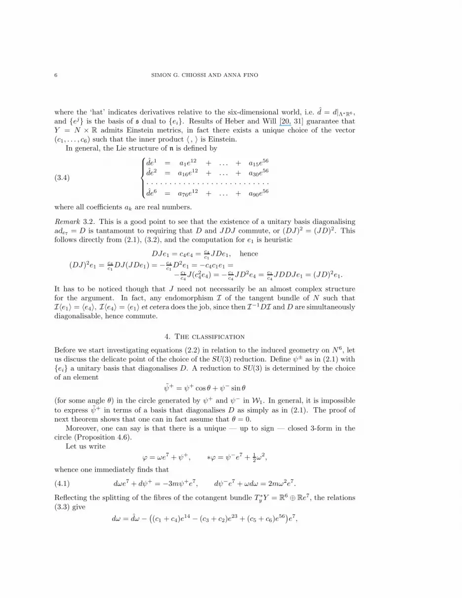
where the ‘hat’ indicates derivatives relative to the six-dimensional world, i.e. d = d|Λ∗R6 ,and ej is the basis of s dual to ei. Results of Heber and Will [20, 31] guarantee thatY = N × R admits Einstein metrics, in fact there exists a unique choice of the vector(c1, . . . , c6) such that the inner product 〈 , 〉 is Einstein.
In general, the Lie structure of n is defined by
(3.4)
de1 = a1e12 + . . . + a15e
56
de2 = a16e12 + . . . + a30e
56
. . . . . . . . . . . . . . . . . . . . . . . . . . .
de6 = a76e12 + . . . + a90e
56
where all coefficients ak are real numbers.
Remark 3.2. This is a good point to see that the existence of a unitary basis diagonalisingade7 = D is tantamount to requiring that D and JDJ commute, or (DJ)2 = (JD)2. Thisfollows directly from (2.1), (3.2), and the computation for e1 is heuristic
DJe1 = c4e4 = c4c1JDe1, hence
(DJ)2e1 = c4c1DJ(JDe1) = − c4
c1D2e1 = −c4c1e1 =
− c1c4J(c24e4) = − c1
c4JD2e4 = c1
c4JDDJe1 = (JD)2e1.
It has to be noticed though that J need not necessarily be an almost complex structurefor the argument. In fact, any endomorphism I of the tangent bundle of N such thatI〈e1〉 = 〈e4〉, I〈e4〉 = 〈e1〉 et cetera does the job, since then I−1DI andD are simultaneouslydiagonalisable, hence commute.
4. The classification
Before we start investigating equations (2.2) in relation to the induced geometry on N6, letus discuss the delicate point of the choice of the SU(3) reduction. Define ψ± as in (2.1) withei a unitary basis that diagonalises D. A reduction to SU(3) is determined by the choiceof an element
ψ+ = ψ+ cos θ + ψ− sin θ
(for some angle θ) in the circle generated by ψ+ and ψ− in W1. In general, it is impossible
to express ψ+ in terms of a basis that diagonalises D as simply as in (2.1). The proof ofnext theorem shows that one can in fact assume that θ = 0.
Moreover, one can say is that there is a unique — up to sign — closed 3-form in thecircle (Proposition 4.6).
Let us write
ϕ = ωe7 + ψ+, ∗ϕ = ψ−e7 + 1
2ω2,
whence one immediately finds that
(4.1) dωe7 + dψ+ = −3mψ+e7, dψ−e7 + ωdω = 2mω2e7.
Reflecting the splitting of the fibres of the cotangent bundle T ∗y Y = R
6 ⊕ Re7, the relations(3.3) give
dω = dω −(
(c1 + c4)e14 − (c3 + c2)e
23 + (c5 + c6)e56
)
e7,
CONFORMALLY PARALLEL G2 STRUCTURES ON A CLASS OF SOLVMANIFOLDS 7
so
dω2 = dω2 + 2(
(c1 + c4 + c3 + c2)e1423 + (c3 + c2 + c5 + c6)e
2356
− (c1 + c4 + c5 + c6)e1456
)
e7.
Similarly one computes the exterior derivatives of the real 3-forms:
dψ+ = dψ+ + (c1 + c2 + c5)e1257 + (c1 + c3 + c6)e
1367
− (c3 + c4 + c5)e3457 + (c2 + c4 + c6)e
2467,
dψ− = dψ− + (c1 + c2 + c6)e1267 − (c1 + c3 + c5)e
1357
− (c2 + c4 + c5)e2457 − (c3 + c4 + c6)e
3467.
When, in general, G2-manifolds Y are constructed starting from six dimensions, many oftheir features are determined by the underlying SU(3) structure, and the following definitionbecomes natural
4.1. Definition. [11] An almost Hermitian manifold is half-flat, or half-integrable, if the
reduction is such that both ψ+ and ω2 are closed (with respect to d).
This is the same as asking that the intrinsic torsion components W+1 ,W
+2 ,W4 and W5 vanish
simultaneously. This sort of structure appears, in various disguises, on any hypersurface inR
7 (or Joyce manifold, for that matter), and its possible role in M-theory has been recentlyexamined [19, 4].
Plugging the previous equations into system (2.2) allows us to discover a geometricalconstraint, for
4.2. Lemma. When (Y, ϕ) is conformal to a G2-holonomy manifold, N has a half-flat SU(3)structure.
Proof. This is clear if one considers the terms in (4.1) that belong to (e7)⊥.
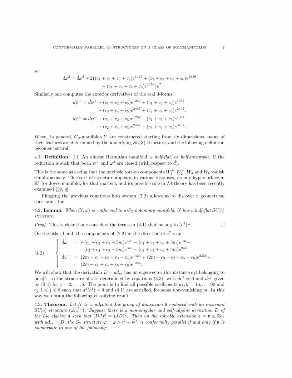
On the other hand, the components of (2.2) in the direction of e7 read
(4.2)
dω = −(c1 + c2 + c5 + 3m)e125 − (c1 + c3 + c6 + 3m)e136−(c3 + c4 + c5 + 3m)e345 − (c2 + c4 + c6 + 3m)e246
dψ− = (2m− c1 − c2 − c3 − c4)e1423 + (2m− c3 − c2 − c5 − c6)e
2356+
(2m+ c1 + c4 + c5 + c6)e1456.
We will show that the derivation D = ade7 has an eigenvector (for instance e1) belonging to
[n, n]⊥, so the structure of s is determined by equations (3.3), with de1 = 0 and dej givenby (3.4) for j = 2, . . . , 6. The point is to find all possible coefficients ak, k = 16, . . . , 90 andcj , 1 6 j 6 6 such that d2(ej) = 0 and (4.1) are satisfied, for some non-vanishing m. In thisway we obtain the following classifying result
4.3. Theorem. Let N be a nilpotent Lie group of dimension 6 endowed with an invariant
SU(3) structure (ω, ψ+). Suppose there is a non-singular and self-adjoint derivation D of
the Lie algebra n such that (DJ)2 = (JD)2. Then on the solvable extension s = n ⊕ Re7with ade7 = D, the G2 structure ϕ = ω ∧ e7 + ψ+ is conformally parallel if and only if n is
isomorphic to one of the following:
8 SIMON G. CHIOSSI AND ANNA FINO
(0, 0, 0, e12, e13, e23), (0, 0, 0, 0, e12, e13),
(0, 0, 0, 0, e12, e14 + e23), (0, 0, 0, 0, 0, e12 + e34),
(0, 0, 0, 0, e13 + e42, e12 + e34), (0, 0, 0, 0, 0, e12),
(0, 0, 0, 0, 0, 0).
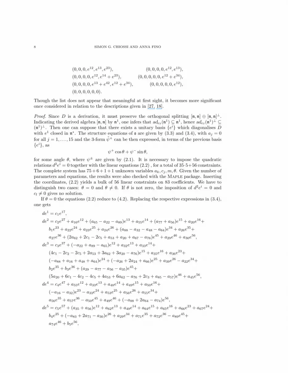
Though the list does not appear that meaningful at first sight, it becomes more significantonce considered in relation to the descriptions given in [27, 18].
Proof. Since D is a derivation, it must preserve the orthogonal splitting [n, n] ⊕ [n, n]⊥.Indicating the derived algebra [n, n] by n1, one infers that ade7(n
1) ⊆ n1, hence ade7(n1)⊥ ⊆
(n1)⊥. Then one can suppose that there exists a unitary basis ei which diagonalises Dwith e1 closed in n∗. The structure equations of s are given by (3.3) and (3.4), with aj = 0
for all j = 1, . . . , 15 and the 3-form ψ+ can be then expressed, in terms of the previous basisei, as
ψ+ cos θ + ψ− sin θ,
for some angle θ, where ψ± are given by (2.1). It is necessary to impose the quadraticrelations d2ei = 0 together with the linear equations (2.2) , for a total of 35·5+56 constraints.The complete system has 75+6+1+1 unknown variables ak, cj ,m, θ. Given the number ofparameters and equations, the results were also checked with the Maple package. Insertingthe coordinates, (2.2) yields a bulk of 56 linear constraints on 83 coefficients. We have todistinguish two cases: θ = 0 and θ 6= 0. If θ is not zero, the imposition of d2ei = 0 andcl 6= 0 gives no solution.
If θ = 0 the equations (2.2) reduce to (4.2). Replacing the respective expressions in (3.4),one gets
de1 = c1e17,
de2 = c2e27 + a16e
12 + (a65 − a22 − a89)e13 + a55e
14 + (a77 + a56)e15 + a20e
16+
b1e23 + a22e
24 + a23e25 + a24e
26 + (a88 − a32 − a48 − a64)e34 + a26e
35+
a27e36 + (2a62 + 2c1 − 2c5 + a53 + a20 + a67 − a76)e
45 + a29e46 + a30e
56,
de3 = c3e37 + (−a22 + a89 − a65)e
12 + a32e13 + a33e
14+
(4c1 − 2c2 − 2c5 + 2a53 + 3a62 + 3a20 − a76)e15 + a35e
16 + a36e23+
(−a88 + a16 + a48 + a64)e24 + (−a26 + 2a24 + a66)e
25 + a39e26 − a22e
34+
b2e35 + b3e
36 + (a29 − a77 − a56 − a35)e45+
(5a20 + 6c1 − 4c2 − 4c5 + 4a53 + 6a62 − a76 + 2c3 + a85 − a57)e46 + a45e
56,
de4 = c4e47 + a55e
12 + a33e13 + a48e
14 + a49e15 + a50e
16+
(−a16 − a32)e23 − a33e
24 + a53e25 + a56e
26 + a55e34+
a56e35 + a57e
36 − a50e45 + a49e
46 + (−a88 + 2a64 − a74)e56,
de5 = c5e57 + (a35 + a56)e
12 + a62e13 + a49e
14 + a64e15 + a65e
16 + a66e23 + a67e
24+
b4e25 + (−a83 + 2a71 − a30)e
26 + a29e34 + a71e
35 + a72e36 − a89e
45+
a74e46 + b5e
56,

CONFORMALLY PARALLEL G2 STRUCTURES ON A CLASS OF SOLVMANIFOLDS 9
de6 = c6e67 + a76e
12 + a77e13 + a50e
14 + (2a89 − a65)e15 + b6e
16+
(2a23 + a27 + a39)e23 + (a29 − a77 − a56 − a35)e
24 + a83e25 + b7e
26+
a85e34 + (2a33 − 2a36 + a72 + a45)e
35 + b8e36 + a88e
45 + a89e46 + b9e
56,
de7 = 0,
in terms of a certain number of parameters. We have put
b1 = −a83 + a55 + a71, b2 = a27 + a39 + a23, b3 = −a24 − a66,
b4 = −a33 − a72 + a36 − a45, b5 = −a49 + a24 − a26 + a66, b6 = −a88 + a64 − a74,
b7 = a33 + a72 − a36, b8 = −a71 + a30, b9 = a39 + a23 − a50
for convenience. Besides, the following relations must hold:
c4 = −5c1 + 3c2 + 4c5 − 4a53 − 5a62 − 4a20 − c3 − a67 + a76 − a85,
c6 = 3c2 − c3 + 3c5 + a57 − 3a53 − 4c1 − 4a62 − 4a20,
m = c1 − c2 − c5 + a53 + a62 + a20.
Only at this point it seems realistic to annihilate the quadratic relations coming from theJacobi identity, hence set to zero the coefficients of the terms eij7 appearing in the variousd2ei = 0. Since cj 6= 0 for all j = 1, . . . , 6, the closure of dei kills all bl’s above, andfurthermorea16 = a22 = a24 = a23 = a32 = a33 = a36 = a48 = a49 = a50 = a55 = a64 = a71 = a89 = 0.
Thus, the structure equations eventually reduce to a simpler form
de1 = c1e17
de2 = c2e27 + a65e
13 + (a77 + a56)e15 + a20e
16 − a74e34+
(2a62 + 2c1 − 2c5 + a53 + a20 + a67 − a76)e45 + a29e
46
de3 = c3e37 − a65e
12 + (4c1 − 2c2 − 2c5 + 2a53 + 3a62 + 3a20 − a76)e15+
a35e16 + a74e
24 + (a29 − a77 − a56 − a35)e45+
(5a20 + 6c1 − 4c2 − 4c5 + 4a53 + 6a62 − a76 + 2c3 + a85 − a57)e46
de4 = c4e47 + a53e
25 + a56e26 + a56e
35 + a57e36
de5 = c5e57 + (a35 + a56)e
12 + a62e13 + a65e
16 + a67e24 + a29e
34 + a74e46
de6 = c6e67 + a76e
12 + a77e13 − a65e
15 + (a29 − a77 − a56 − a35)e24+
a85e34 − a74e
45
de7 = 0.
In particular, the vanishing of the coefficients of e137, e347 in d2(e2) and of e127, e247 in d2(e3)yields
a65(c1 − c2 + c3) = 0, a74(−c2 − c3 + c4) = 0,a65(−c1 − c2 + c3) = 0, a74(c2 − c3 + c4) = 0,
thus a65 = a74 = 0. The terms e357, e267 in d2(e4) similarly give
a56(−c3 + c4 − c5) = 0, a56(−c2 + c4 − c6) = 0, a53(−c2 + c4 − c5) = 0,a57(−c2 + a57 + a53 + c1 + a62 + c3 + a67 − a76 + a85) = 0.
Altogether, the following cases crop up. We shall examine them one by one trying to makefurther coefficients disappear.

10 SIMON G. CHIOSSI AND ANNA FINO
Case a) a53 = a56 = a57 = 0 (corresponding to de4 = 0). The relation d2 = 0 yieldsa29 = a35 = a77 = 0, and six non-isomorphic algebra types come out:
(4.3) (−me17,−me27,−me37,−me47,−me57,−me67, 0)
has an underlying Abelian Lie algebra, if one disregards the D-action. Next,
(4.4) (− 2
3me17,−me27,− 4
3me37 + 2
3me15,−me47,− 2
3me57,−me67, 0)
extends n ∼= (0, 0, 0, 0, 0, e12);
(4.5)(
− 3
4me17,−me27,− 3
2me37 + 1
2m(e15 − e46),− 3
4me47,− 3
4me57,− 3
4me67, 0
)
is clearly given by n ∼= (0, 0, 0, 0, 0, e12 + e34);
(4.6)(
− 4
5me17,− 6
5me27 − 2
5me45,− 7
5me37 + 2
5m(e15 − e46),− 3
5me47,− 3
5me57,− 4
5me67, 0
)
attached to n ∼= (0, 0, 0, 0, e12, e14 + e23);
(4.7) (−me17,− 5
4me27 − 1
2me45,− 5
4me37 − 1
2me46,− 1
2me47,− 3
4me57,− 3
4me67, 0),
whose n is essentially (0, 0, 0, 0, e12, e13);(4.8)(
− 2
3me17,− 4
3me27 − 1
3m(e16 + e45),− 4
3me37 + 1
3m(e15 − e46),− 2
3me47,− 2
3me57,− 2
3me67, 0
)
is an extension of the Iwasawa Lie algebra, isomorphic to (0, 0, 0, 0, e13 + e42, e12 + e34).
b) a53 = a56 = 0, a57 = c5 − c1 − a62 − c3 − a67 + a76 − a85. Up to isomorphism, one getsthe two Lie algebras with structure (4.4) and (4.7).
c) a56 = a57 = 0, c2 = 5
2c1 − 3
2c5 + 5
2a62 + 2a20 + 1
2c3 + 1
2a67 + 2a53 − 1
2a76 + 1
2a85. This time
around one finds the algebras of b) plus
(4.9) (− 3
5me17,− 3
5me27,− 6
5me37+ 2
5me15,− 6
5me47+ 2
5me25,− 3
5me57,− 6
5me67+ 2
5me12, 0),
which arises from n ∼= (0, 0, 0, e12, e13, e23).
d) a56 = 0, c2 = 5
2c1 − 3
2c5 + 5
2a62 + 2a20 + 1
2c3 + 1
2a67 + 2a53 − 1
2a76 + 1
2a85, a57 =
c5 − a53 − c1 − a62 − c3 − a67 + a76 − a85, by which one regains (4.5).
e) a53 = a57 = 0, a20 = −c1 + c2 + 1
2c5 − a62 − 1
2c3, a76 = c1 + c2 − c5 + a62 + a67 + a85 yield
no solutions.
f) a76 = c1 + c2 − c5 + a53 + a57 + a62 + a67 + a85, c3 = c2, a20 = −c1 + 1
2c2 + 1
2c5 − 3
4a53 −
a62 + 1
4a57. The last case produces (4.5) one more time, and basically concludes the proof
of the Theorem.
The fact that so few Lie algebras are gotten may depend on the requirements made bothon the G2 structure and on the seven-dimensional construction. One easily recognizes thatthe groups associated to (4.3) and (4.4) are the torus T 6 and the product T 3 × H3 of atorus with the real 3-dimensional Heisenberg group respectively, while (4.8) is attached tothe complexified 3-dimensional Heisenberg group HC
3 .In the case of an Einstein solvmanifold, the eigenvalues of the derivation D are positive
integers k1 < . . . < kr without common divisors [20]. Indicating the respective multiplici-ties by d1, . . . , dr, Heber defines the string (k1, . . . , kr; d1, . . . , dr) the eigenvalue type of thesolvmanifold. In our situation we have the following

CONFORMALLY PARALLEL G2 STRUCTURES ON A CLASS OF SOLVMANIFOLDS 11
4.4. Corollary. With the above hypotheses, the eigenvalues of the derivation D have all the
same sign. More precisely, the eigenvalue data of the algebras of Theorem 4.3 are given by
the following scheme
Nilpotent Lie algebra Eigenvalues Multiplicities
(0, 0, e15, 0, 0, 0) − 2
3m,−m,− 4
3m 2, 3, 1
(0, 0, e15 + e64, 0, 0, 0) − 3
4m,−m,− 3
2m 4, 1, 1
(0, e45, e64 + e51, 0, 0, 0) − 3
5m,− 4
5m,− 6
5m,− 7
5m 2, 2, 1, 1
(0, e45, e46, 0, 0, 0) − 1
2m,− 3
4m,−m,− 5
4m 1, 2, 1, 2
(0, e16 + e45, e15 + e64, 0, 0, 0) − 2
3m,− 4
3m 4, 2
(0, 0, e15, e25, 0, e12) − 3
5m,− 6
5m 3, 3
The real number m has to be a negative, in order for s to be of Iwasawa type. Noticethat the result holds just assuming non-degeneracy (thus dropping (3) in Definition 3.1).
In the present set-up, the Corollary matches to the result of [31] for appropriate choicesof m. Moreover, the eigenvalue type is unique to each example, in contrast to the Einsteincase where the solvmanifolds associated h3 ⊕ h3 and hC
3 have the same eigenvalue type.
As a by-product of the classification, the following necessary condition crops up:
4.5. Corollary. With the above hypotheses, if Y has a G2 structure of type X4, then N is
either a 2-step nilpotent Lie group or a torus.
This is reflected in the fact that the metrics supported by these solvmanifolds arise ontorus bundles over tori of various dimensions and rank, cf. §5. Notice that the only 2-stepnilmanifold missing, so to speak, is that corresponding to (0, 0, 0, 0, e12, e34) ∼= h3 ⊕ h3. It isknown to the authors that this Lie algebra admits a large family of half-flat SU(3)-structures.The product of the corresponding nilmanifold with some real interval can be endowed witha metric with holonomy contained in G2 [21], but by the Theorem such metric will not beconformally equivalent to a homogeneous one on a solvable extension of H3 ×H3.
4.1. Some consequences. A slight change of approach allows to detect properties in asimpler way. Let
α1 = e1 + ie4, α2 = e2 − ie3, α3 = e5 + ie6
be the basis of complex (1, 0)-forms determined by (2.1), so one may write
Ψ = α1 ∧ α2 ∧ α3 = α123.
Translate all SU(3) forms into this language
ω = − 1
2i (α11 + α22 + α33) and ψ+ = 1
2(α123 + α123) etc.,
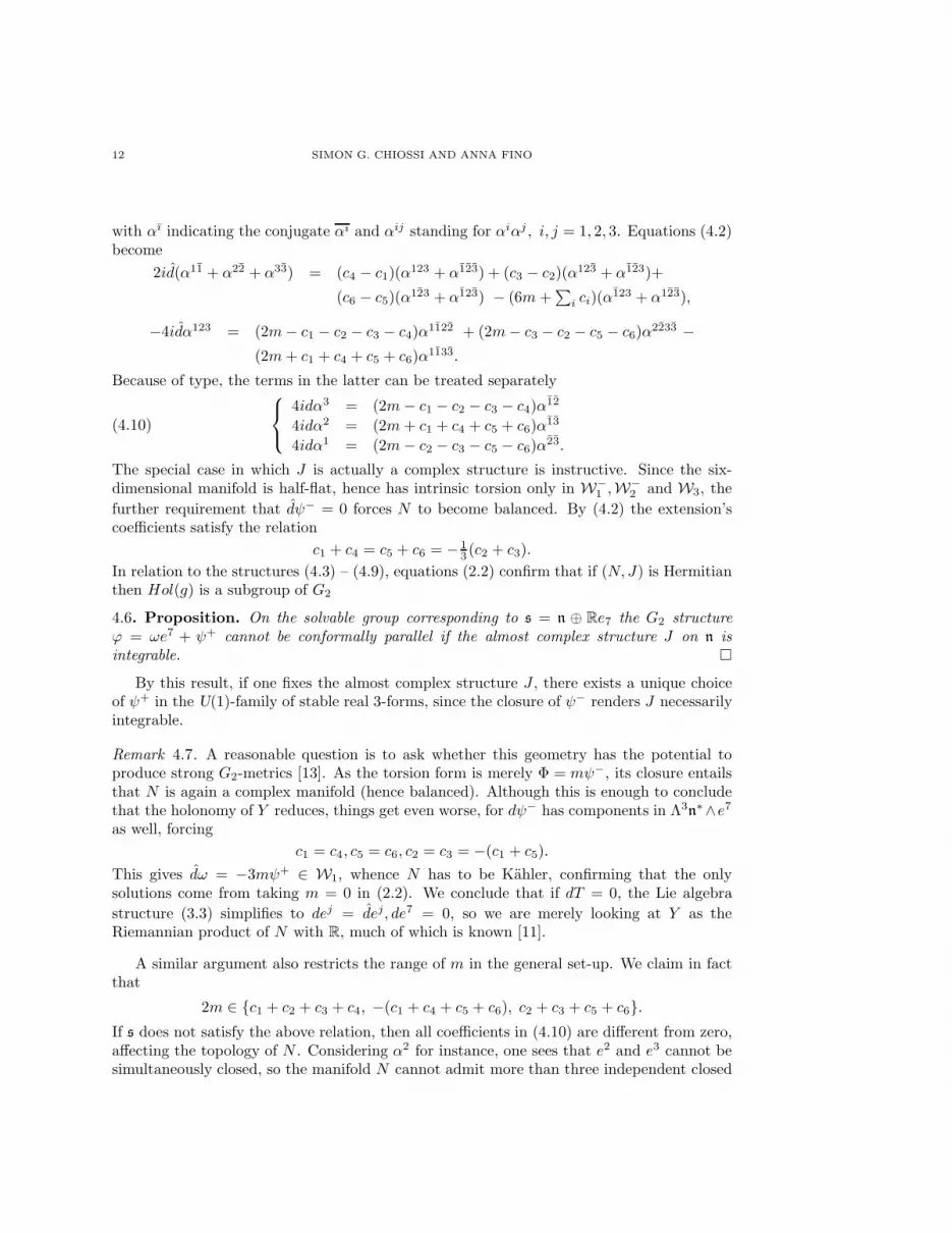
12 SIMON G. CHIOSSI AND ANNA FINO
with αı indicating the conjugate αı and αij standing for αiαj , i, j = 1, 2, 3. Equations (4.2)become
2id(α11 + α22 + α33) = (c4 − c1)(α123 + α123) + (c3 − c2)(α
123 + α123)+
(c6 − c5)(α123 + α123) − (6m+
∑
i ci)(α123 + α123),
−4idα123 = (2m− c1 − c2 − c3 − c4)α1122 + (2m− c3 − c2 − c5 − c6)α
2233 −(2m+ c1 + c4 + c5 + c6)α
1133.
Because of type, the terms in the latter can be treated separately
(4.10)
4idα3 = (2m− c1 − c2 − c3 − c4)α12
4idα2 = (2m+ c1 + c4 + c5 + c6)α13
4idα1 = (2m− c2 − c3 − c5 − c6)α23.
The special case in which J is actually a complex structure is instructive. Since the six-dimensional manifold is half-flat, hence has intrinsic torsion only in W−
1 ,W−2 and W3, the
further requirement that dψ− = 0 forces N to become balanced. By (4.2) the extension’scoefficients satisfy the relation
c1 + c4 = c5 + c6 = − 1
3(c2 + c3).
In relation to the structures (4.3) – (4.9), equations (2.2) confirm that if (N, J) is Hermitianthen Hol(g) is a subgroup of G2
4.6. Proposition. On the solvable group corresponding to s = n ⊕ Re7 the G2 structure
ϕ = ωe7 + ψ+ cannot be conformally parallel if the almost complex structure J on n is
integrable.
By this result, if one fixes the almost complex structure J , there exists a unique choiceof ψ+ in the U(1)-family of stable real 3-forms, since the closure of ψ− renders J necessarilyintegrable.
Remark 4.7. A reasonable question is to ask whether this geometry has the potential toproduce strong G2-metrics [13]. As the torsion form is merely Φ = mψ−, its closure entailsthat N is again a complex manifold (hence balanced). Although this is enough to concludethat the holonomy of Y reduces, things get even worse, for dψ− has components in Λ3n∗∧e7as well, forcing
c1 = c4, c5 = c6, c2 = c3 = −(c1 + c5).
This gives dω = −3mψ+ ∈ W1, whence N has to be Kahler, confirming that the onlysolutions come from taking m = 0 in (2.2). We conclude that if dT = 0, the Lie algebra
structure (3.3) simplifies to dej = dej, de7 = 0, so we are merely looking at Y as theRiemannian product of N with R, much of which is known [11].
A similar argument also restricts the range of m in the general set-up. We claim in factthat
2m ∈ c1 + c2 + c3 + c4, −(c1 + c4 + c5 + c6), c2 + c3 + c5 + c6.If s does not satisfy the above relation, then all coefficients in (4.10) are different from zero,affecting the topology of N . Considering α2 for instance, one sees that e2 and e3 cannot besimultaneously closed, so the manifold N cannot admit more than three independent closed
CONFORMALLY PARALLEL G2 STRUCTURES ON A CLASS OF SOLVMANIFOLDS 13
1-forms. But Theorem 4.3 tells that only Lie algebras with first Betti number b1 > 3 cropup, and the unique 2-step algebra attaining the minimum is (4.9), which fails to satisfy theassumption.
The conditions to have a compatible almost Kahler structure are found in a similar fash-ion. It is non-obvious, and certainly unusual, that the symplectic condition also annihilatesthe component of the intrinsic torsion in W−
2 , a module not directly depending upon dω:
4.8. Proposition. Under the above assumptions, the nilpotent Lie group (N, J, ω) is sym-
plectic only when it is a torus, in other words
dω = 0 ⇐⇒ n is Abelian.
Proof. If ω is closed, its expression in complex form easily gives c1 = c4, c3 = c2, c5 = c6,which corresponds precisely to Jade7 = ade7J ; concerning Remark 3.2, it is definitely worthnoticing that the almost complex structure and the derivation D = ade7 commute just fortwo nilpotent Lie algebras, that is the Abelian one and the Iwasawa Lie algebra. The latterthough does not satisfy the requirement that m = −∑
ci = −tr ade7 , whence only the torusT 6 has symplectic structures generating a G2-manifold of type X4.
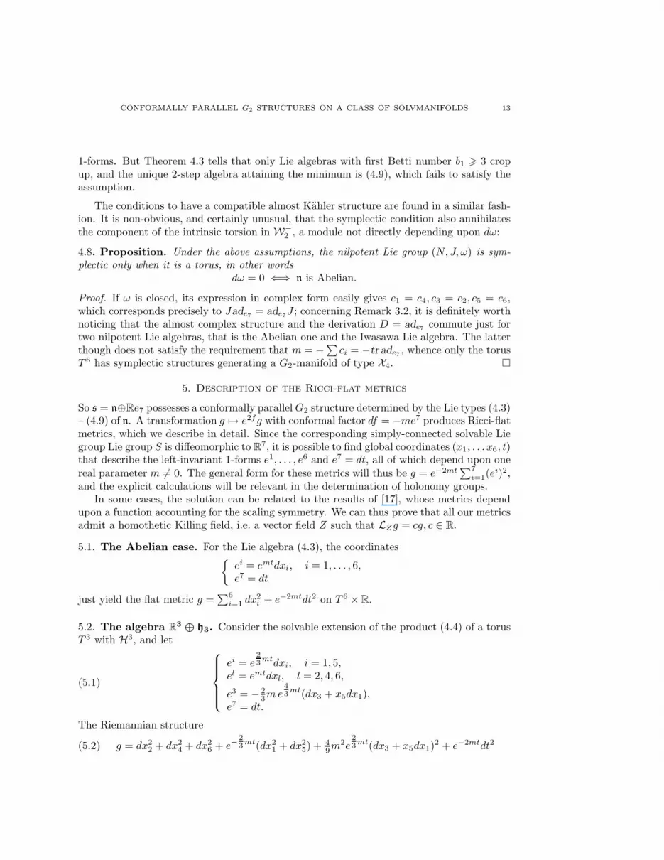
5. Description of the Ricci-flat metrics
So s = n⊕Re7 possesses a conformally parallelG2 structure determined by the Lie types (4.3)– (4.9) of n. A transformation g 7→ e2fg with conformal factor df = −me7 produces Ricci-flatmetrics, which we describe in detail. Since the corresponding simply-connected solvable Liegroup Lie group S is diffeomorphic to R
7, it is possible to find global coordinates (x1, . . . x6, t)that describe the left-invariant 1-forms e1, . . . , e6 and e7 = dt, all of which depend upon one
real parameter m 6= 0. The general form for these metrics will thus be g = e−2mt∑7
i=1(ei)2,
and the explicit calculations will be relevant in the determination of holonomy groups.In some cases, the solution can be related to the results of [17], whose metrics depend
upon a function accounting for the scaling symmetry. We can thus prove that all our metricsadmit a homothetic Killing field, i.e. a vector field Z such that LZg = cg, c ∈ R.
5.1. The Abelian case. For the Lie algebra (4.3), the coordinates
ei = emtdxi, i = 1, . . . , 6,e7 = dt
just yield the flat metric g =∑6
i=1 dx2i + e−2mtdt2 on T 6 × R.
5.2. The algebra R3 ⊕ h3. Consider the solvable extension of the product (4.4) of a torus
T 3 with H3, and let
(5.1)
ei = e2
3mtdxi, i = 1, 5,
el = emtdxl, l = 2, 4, 6,
e3 = − 2
3me
4
3mt(dx3 + x5dx1),
e7 = dt.
The Riemannian structure
(5.2) g = dx22 + dx2
4 + dx26 + e−
2
3mt(dx2
1 + dx25) + 4
9m2e
2
3mt(dx3 + x5dx1)
2 + e−2mtdt2

14 SIMON G. CHIOSSI AND ANNA FINO
restricts to a special holonomy metric ds on spanx1, x3, x5, t viewed as Q×R, Q being thetotal space of a circle bundle over T 2. In fact the subgroup of G2 preserving ds is orthogonal,hence Hol(g) = G2 ∩ SO(4) = SU(2).
5.3. The algebra (0, 0, e15 + e64, 0, 0, 0). When S corresponds to (4.5), we set
ei = e3
4mtdxi, i = 1, 4, 5, 6,
e2 = emtdx2,
e3 = − 1
2me
3
2mt(3
2dx3 + x5dx1 + x4dx6),
e7 = dt,
whence
(5.3) g = dx22 + e−
1
2mt(dx2
1 + dx24 + dx2
5 + dx26)+
9
16m2emt(dx3 + 2
3x5dx1 + 2
3x4dx6)
2 + e−2mtdt2
has holonomy SU(3) ⊂ G2. Restricting ourselves to 〈x2〉⊥, we obtain a metric on the productof a principal T 1-bundle over T 4 with R.
5.4. The algebra (0, e45, e64 + e51, 0, 0, 0). Let us look at (4.6) now:
ei = e4
5mtdxi, i = 1, 6,
e2 = − 3
5me
6
5mt(dx2 + 2
3x4dx5),
e3 = − 3
5me
7
5mt(dx3 − 2
3x1dx5 + 2
3x4dx6),
el = e3
5mtdxl, l = 4, 5,
e7 = dt
allow to write down a previously unknown exceptional metric
5.1. Proposition. Let n be the nilpotent Lie algebra defined by
e2 = [e5, e4], e3 = [e6, e4] = [e1, e5].
Then with the above conventions, the solvmanifold S relative to s = n ⊕ Re7 carries a
Riemannian metric
(5.4) g = e−2mtdt2 + e−2
5mt(dx2
1 + dx26) + e−
4
5mt(dx2
4 + dx25)+
9
25m2e
4
5mt(dx3 − 2
3x1dx5 + 2
3x4dx6)
2 + 9
25m2e
2
5mt(dx2 + 2
3x4dx5)
2
whose holonomy group is precisely G2.
In sufficiently small neighbourhoods, this metric is clearly isometric to
ds2 = V 3dy2 + V (dz21 + dz2
6) + V 2(dz24 + dz2
5)+
V −2(
dz3 + k(−z1dz5 + z4dz6))2
+ V 2(dz2 + kz4dz5)2,

CONFORMALLY PARALLEL G2 STRUCTURES ON A CLASS OF SOLVMANIFOLDS 15
with V = ky, on the product of R with a T 2-bundle over a T 4. The fibre coordinates arez2, z3, whilst y accounts for the R factor. The metric (5.4) has a symmetry generated by thehomothetic Killing field
Z = − 5
m∂∂t + 4x1
∂∂x1
+ 4x6∂∂x6
+ 3x4∂∂x4
+ 3x5∂∂x5
+ 21
5mx3
∂∂x3
+ 18
5mx2
∂∂x2
,
found by imposing invariance under a suitable scaling factor. For appropriate Killing vectorfields, this feature is common to all other metrics in this section [17]. Note that Z does notcorrespond to e7, for
(dZ)( ∂∂t ,∂∂x1
) = ∂∂tZ
( ∂∂x1
) − ∂∂x1
Z( ∂∂t ) − Z([ ∂∂t ,∂∂x1
]) 6= 0.
5.5. The algebra (0, e45, e46, 0, 0, 0). The coordinates
e1 = emtdx1, e4 = e1
2mtdx4,
e2 = 1
2me
5
4mt(− 3
2dx2 + x5dx4), ei = e
3
4mtdxi, i = 5, 6,
e3 = 1
2me
5
4mt(− 3
2dx3 + x6dx4), e7 = dt,
relative to (4.7) produce the metric
(5.5) g = dx21 + 9
16m2e
1
2mt(dx2 − 2
3x5dx4)
2 + 9
16m2e
1
2mt(dx3 − 2
3x6dx4)
2
+ e−mtdx24 + e−
1
2mt(dx2
5 + dx26) + e−2mtdt2.
It has holonomy SU(3), too. This can be recovered by looking at 〈x1〉⊥ = R6, and the
induced metric on the product of R with a principal T 2-bundle over T 3.
5.6. The Iwasawa algebra. The algebra (4.8) comes equipped with 1-forms
(5.6)
ei = e2
3mtdxi, i = 1, 4, 5, 6,
e2 = m3e
4
3mt(2dx2 + x6dx1 − x4dx5),
e3 = −m3e
4
3mt(2dx3 + x5dx1 + x4dx6),
e7 = dt.
Then
(5.7)g = 4
9m2e
2
3mt(dx3 + 1
2x5dx1 + 1
2x4dx6)
2 + 4
9m2e
2
3mt(dx2 + 1
2x6dx1 − 1
2x4dx5)
2+
e−2
3mt(dx2
1 + dx24 + dx2
5 + dx26) + e−2mtdt2
has holonomy G2.
16 SIMON G. CHIOSSI AND ANNA FINO
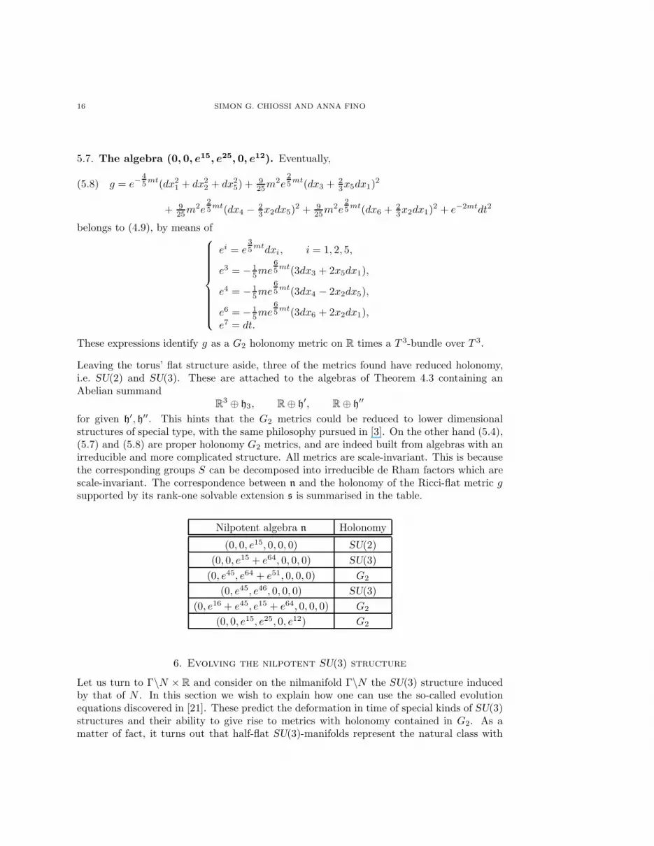
5.7. The algebra (0, 0, e15, e25, 0, e12). Eventually,
(5.8) g = e−4
5mt(dx2
1 + dx22 + dx2
5) + 9
25m2e
2
5mt(dx3 + 2
3x5dx1)
2
+ 9
25m2e
2
5mt(dx4 − 2
3x2dx5)
2 + 9
25m2e
2
5mt(dx6 + 2
3x2dx1)
2 + e−2mtdt2
belongs to (4.9), by means of
ei = e3
5mtdxi, i = 1, 2, 5,
e3 = − 1
5me
6
5mt(3dx3 + 2x5dx1),
e4 = − 1
5me
6
5mt(3dx4 − 2x2dx5),
e6 = − 1
5me
6
5mt(3dx6 + 2x2dx1),
e7 = dt.
These expressions identify g as a G2 holonomy metric on R times a T 3-bundle over T 3.
Leaving the torus’ flat structure aside, three of the metrics found have reduced holonomy,i.e. SU(2) and SU(3). These are attached to the algebras of Theorem 4.3 containing anAbelian summand
R3 ⊕ h3, R ⊕ h′, R ⊕ h′′
for given h′, h′′. This hints that the G2 metrics could be reduced to lower dimensionalstructures of special type, with the same philosophy pursued in [3]. On the other hand (5.4),(5.7) and (5.8) are proper holonomy G2 metrics, and are indeed built from algebras with anirreducible and more complicated structure. All metrics are scale-invariant. This is becausethe corresponding groups S can be decomposed into irreducible de Rham factors which arescale-invariant. The correspondence between n and the holonomy of the Ricci-flat metric gsupported by its rank-one solvable extension s is summarised in the table.
Nilpotent algebra n Holonomy
(0, 0, e15, 0, 0, 0) SU(2)
(0, 0, e15 + e64, 0, 0, 0) SU(3)
(0, e45, e64 + e51, 0, 0, 0) G2
(0, e45, e46, 0, 0, 0) SU(3)
(0, e16 + e45, e15 + e64, 0, 0, 0) G2
(0, 0, e15, e25, 0, e12) G2
6. Evolving the nilpotent SU(3) structure
Let us turn to Γ\N × R and consider on the nilmanifold Γ\N the SU(3) structure inducedby that of N . In this section we wish to explain how one can use the so-called evolutionequations discovered in [21]. These predict the deformation in time of special kinds of SU(3)structures and their ability to give rise to metrics with holonomy contained in G2. As amatter of fact, it turns out that half-flat SU(3)-manifolds represent the natural class with
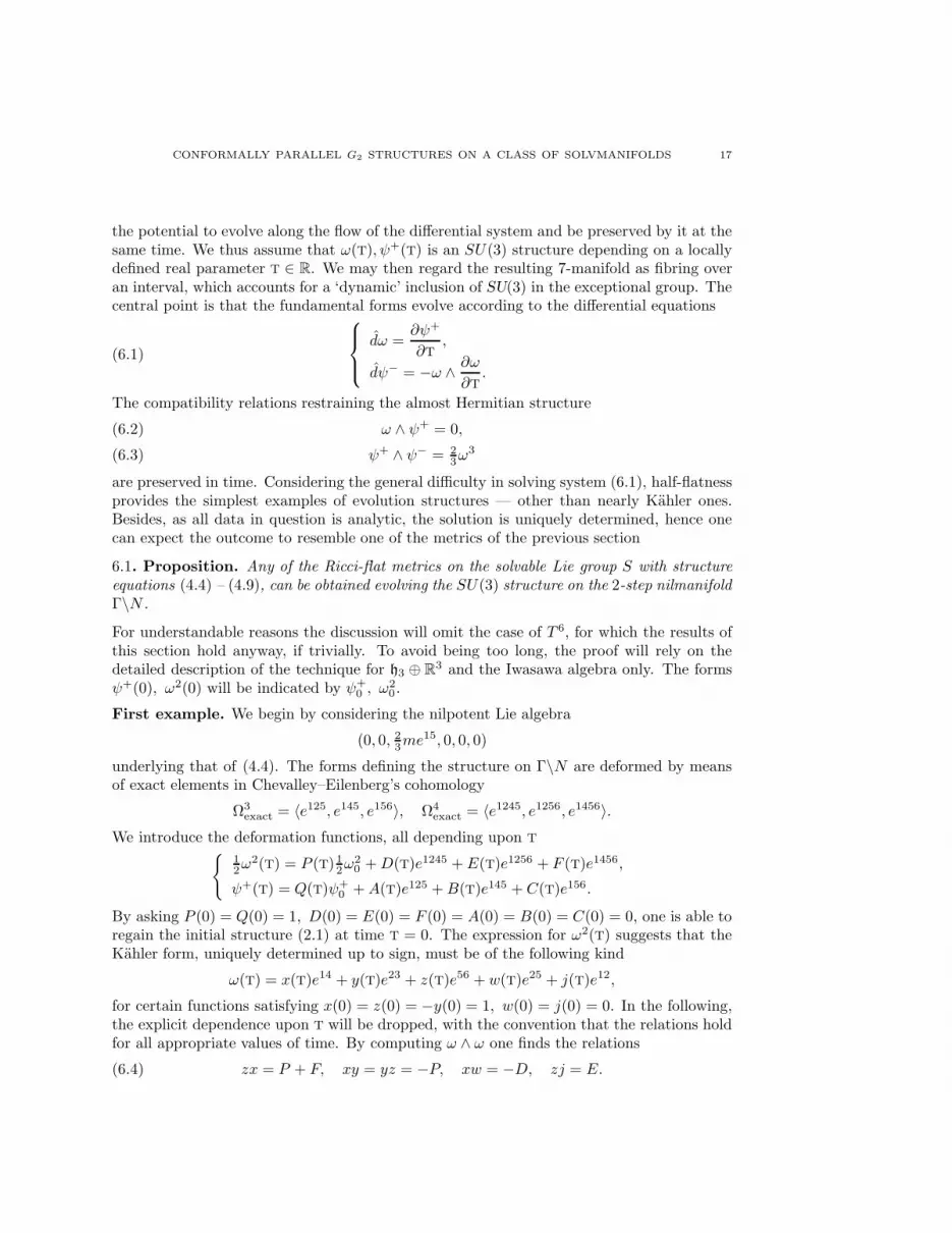
CONFORMALLY PARALLEL G2 STRUCTURES ON A CLASS OF SOLVMANIFOLDS 17
the potential to evolve along the flow of the differential system and be preserved by it at thesame time. We thus assume that ω(T), ψ+(T) is an SU(3) structure depending on a locallydefined real parameter T ∈ R. We may then regard the resulting 7-manifold as fibring overan interval, which accounts for a ‘dynamic’ inclusion of SU(3) in the exceptional group. Thecentral point is that the fundamental forms evolve according to the differential equations
(6.1)
dω =∂ψ+
∂T,
dψ− = −ω ∧ ∂ω
∂T.
The compatibility relations restraining the almost Hermitian structure
ω ∧ ψ+ = 0,(6.2)
ψ+ ∧ ψ− = 2
3ω3(6.3)
are preserved in time. Considering the general difficulty in solving system (6.1), half-flatnessprovides the simplest examples of evolution structures — other than nearly Kahler ones.Besides, as all data in question is analytic, the solution is uniquely determined, hence onecan expect the outcome to resemble one of the metrics of the previous section
6.1. Proposition. Any of the Ricci-flat metrics on the solvable Lie group S with structure
equations (4.4) – (4.9), can be obtained evolving the SU(3) structure on the 2-step nilmanifold
Γ\N .
For understandable reasons the discussion will omit the case of T 6, for which the results ofthis section hold anyway, if trivially. To avoid being too long, the proof will rely on thedetailed description of the technique for h3 ⊕ R
3 and the Iwasawa algebra only. The formsψ+(0), ω2(0) will be indicated by ψ+
0 , ω20 .
First example. We begin by considering the nilpotent Lie algebra
(0, 0, 2
3me15, 0, 0, 0)
underlying that of (4.4). The forms defining the structure on Γ\N are deformed by meansof exact elements in Chevalley–Eilenberg’s cohomology
Ω3exact = 〈e125, e145, e156〉, Ω4
exact = 〈e1245, e1256, e1456〉.We introduce the deformation functions, all depending upon T
1
2ω2(T) = P (T)1
2ω2
0 +D(T)e1245 + E(T)e1256 + F (T)e1456,
ψ+(T) = Q(T)ψ+0 +A(T)e125 +B(T)e145 + C(T)e156.
By asking P (0) = Q(0) = 1, D(0) = E(0) = F (0) = A(0) = B(0) = C(0) = 0, one is able toregain the initial structure (2.1) at time T = 0. The expression for ω2(T) suggests that theKahler form, uniquely determined up to sign, must be of the following kind
ω(T) = x(T)e14 + y(T)e23 + z(T)e56 + w(T)e25 + j(T)e12,
for certain functions satisfying x(0) = z(0) = −y(0) = 1, w(0) = j(0) = 0. In the following,the explicit dependence upon T will be dropped, with the convention that the relations holdfor all appropriate values of time. By computing ω ∧ ω one finds the relations
(6.4) zx = P + F, xy = yz = −P, xw = −D, zj = E.

18 SIMON G. CHIOSSI AND ANNA FINO
In addition, the primitivity of ψ± underlying equation (6.2) implies yB = jQ, yC = wQ.The first differential equation of (6.1) compares
∂ψ+
∂T = (Q′ +A′)e125 +Q′(−e345 + e136 + e246) +B′e145 + C′e156
with
dω = 2
3mye125,
dashed letters denoting derivatives with respect to T. This gives Q(T) = 1, B(T) = C(T) = 0for all T’s, and A′(T) = 2
3my(T). Therefore
ψ+ = (A+ 1)e125 − e345 + e136 + e246.
From (6.4) one has j(T) = w(T) = 0, hence D(T) = E(T) = 0. The determination of anorthonormal basis of 1-forms enables one to get ψ−(T). Inspired by equations (5.1), onedefines
λae1, λbe2, λce3, λbe4, λae5, λbe6,
for some non-zero function λ = λ(T) with λ(0) = 1. For ψ+ = λ2a+be125 + λa+b+c(−e345 +e136) + λ3be246 to resemble the previous expression one takes a + b + c = 0 = 3b. One ofmany possible choices is a = 1
2= −c, so that now ψ± assume the form
ψ+ = λe125 − e345 + e136 + e246, ψ− = λ1/2(e126 − e245 − e135) − λ−1/2e346
and thus λ(T) = A(T) + 1. The second evolution equation
−(P ′ + F ′)e1456 + P ′(e1423 + e2356) = −ωω′ = dψ− = 2m3√λe1456
implies P (T) = 1 and F ′ = − 2m3√A+1
. Eventually, volume normalisation (6.3) says that
√A+ 1 = − 2
3m(A′)−1
A(0) = 0.
The solution to this initial value problem reads
A(t) = (1 −mT)2/3 − 1,
so the geometric structure is evolving according to
ψ+(T) = 3√
(1 −mT)2 e125 − e345 + e136 + e246,
ω(T) = 3√
1 −mT (e14 + e56) − 13√
1 −mTe23.
The associated metric
g = (1 −mT)2/3(
(e1)2 + (e5)2)
+∑
i=2,4,6
(ei)2 + (1 −mT)−2/3(e3)2 + dT2
mirrors precisely (5.2): the appropriate coordinate system xi on R6 is given by
ei = dxi, i 6= 3, e3 = − 2
3m(dx3 + x5dx1),
and the correspondence follows once one identifies 1 −mT with the conformal factor e−mt.

CONFORMALLY PARALLEL G2 STRUCTURES ON A CLASS OF SOLVMANIFOLDS 19
Second example. Let us look at the Iwasawa Lie algebra(
0,− 1
3m(e16 + e45), 1
3m(e15 − e46), 0, 0, 0
)
,
whose evolution also deserves a detailed description. To start with, the deformation is givenby
ψ+ = Qψ+0 +Ae145 +Be146 + Ce156 +D456,
1
2ω2 = 1
2Pω2
0 + Fe1456 +G(e1435 − e1426) +H(−e1436 − e1425)+
L(e1356 + e2456) +M(e3456 − e1256),
the latter telling that the Kahler form is
ω = xe14 + ye23 + ze56 + u(e35 − e26) + v(−e36 − e25) + ρ(e13 + e24) + σ(e34 − e12).
This first relations obtained by comparison are
(6.5)−P = xy = yz, P + F = xz,
G = xu, H = xv, L = zρ, M = zσ,uρ+ vσ = 0, −uσ + vρ = 0.
Then the evolution of ψ+ immediately annihilates A,B,C,D and yields
Q′ = 1
3my,
as ψ+0 is exact. On the other hand 0 = 1
Qωψ+ = −2e23(ue456 + ve156 + ρe146 − σe145) forces
the vanishing of most of the remaining coefficients
ψ+ = Qψ+0 ,
1
2ω2 = 1
2Pω2
0 + Fe1456.
The orthonormal basis λaei, i = 1, 4, 5, 6, λbej , j = 2, 3 is chosen in order to mimic equations(5.6). The actual values of a, b ∈ R are irrelevant at present, one could for example takea = −1, b = 1. In any case
ψ+ = λ2a+bψ+0 , ψ− = λ2a+bψ−
0 , with λ2a+b = Q.
From dψ− = −ωω′ one obtains P = 1 and F ′ = 4
3mQ, so that each of ω2, ψ+ evolves in one
direction only. This could have been predicted by counting dimensions, see [24]. The firstline in (6.5) tells that x = z = −1/y =
√F + 1, and (6.3) gives the quartic curve
Q2 =√F + 1,
so the evolution equations are equivalent to the first order system
Q′(T) = −m3Q−2
F ′(T) = − 4
3m(F + 1)1/4
Q(0) = 1, F (0) = 0.
The first equation is solved by Q(T) = (1−mT)1/3, hence F (T) = (1−mT)4/3−1. Eventually,the SU(3) structure results in
ψ+(T) = (1 −mT)1/3 (e125 − e345 + e136 + e246),
ω(T) = (1 −mT)2/3 (e14 + e56) − 1
(1 −mT)2/3e23.
These data identify the non-integrable complex structure −J3 studied in a broader contextby [1] and the flow corresponds to the one given in [3, ex. 2 (iii)]. A glance at the level
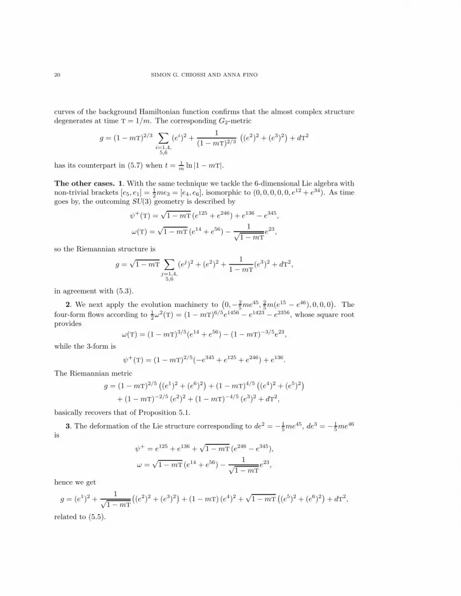
20 SIMON G. CHIOSSI AND ANNA FINO
curves of the background Hamiltonian function confirms that the almost complex structuredegenerates at time T = 1/m. The corresponding G2-metric
g = (1 −mT)2/3∑
i=1,4,5,6
(ei)2 +1
(1 −mT)2/3(
(e2)2 + (e3)2)
+ dT2
has its counterpart in (5.7) when t = 1
m ln |1 −mT|.
The other cases. 1. With the same technique we tackle the 6-dimensional Lie algebra withnon-trivial brackets [e5, e1] = 1
2me3 = [e4, e6], isomorphic to (0, 0, 0, 0, 0, e12 + e34). As time
goes by, the outcoming SU(3) geometry is described by
ψ+(T) =√
1 −mT (e125 + e246) + e136 − e345,
ω(T) =√
1 −mT (e14 + e56) − 1√1 −mT
e23,
so the Riemannian structure is
g =√
1 −mT∑
j=1,4,5,6
(ej)2 + (e2)2 +1
1 −mT(e3)2 + dT
2,
in agreement with (5.3).
2. We next apply the evolution machinery to(
0,− 2
5me45, 2
5m(e15 − e46), 0, 0, 0
)
. The
four-form flows according to 1
2ω2(T) = (1 −mT)6/5e1456 − e1423 − e2356, whose square root
provides
ω(T) = (1 −mT)3/5(e14 + e56) − (1 −mT)−3/5e23,
while the 3-form is
ψ+(T) = (1 −mT)2/5(−e345 + e125 + e246) + e136.
The Riemannian metric
g = (1 −mT)2/5(
(e1)2 + (e6)2)
+ (1 −mT)4/5(
(e4)2 + (e5)2)
+ (1 −mT)−2/5 (e2)2 + (1 −mT)−4/5 (e3)2 + dT2,
basically recovers that of Proposition 5.1.
3. The deformation of the Lie structure corresponding to de2 = − 1
5me45, de3 = − 1
5me46
is
ψ+ = e125 + e136 +√
1 −mT (e246 − e345),
ω =√
1 −mT (e14 + e56) − 1√1 −mT
e23,
hence we get
g = (e1)2 +1√
1 −mT
(
(e2)2 + (e3)2)
+ (1 −mT) (e4)2 +√
1 −mT(
(e5)2 + (e6)2)
+ dT2,
related to (5.5).
CONFORMALLY PARALLEL G2 STRUCTURES ON A CLASS OF SOLVMANIFOLDS 21
4. At last, let us write what happens to (0, 0, 2
5me15, 2
5me25, 0, 2
5me12). After some com-
putations one finds that
ψ+ = (1 −mT)6/5 e125 + e136 + e246 − e345,
ω = (1 −mT)1/5 (e14 − e23 + e56)
are compatible with the metric
g = (1 −mT)4/5∑
i=1,2,5
(ei)2 + (1 −mT)−2/5∑
j=3,4,6
(ej)2 + dT2,
see (5.8).
It is no coincidence that in all cases the identification between the ‘evolved’ holonomymetrics and the ones found in §5 is attained by uniformly putting T = 1/m(1 − e−mt)and using global coordinates x1, . . . , x6 on the nilpotent Lie group N to represent the left-invariant forms ei. Which brings to the completeness’ properties of the metrics. We arealways in presence of a unique singularity, determined by f(t) = exp(−mt) or, if one prefers,
by the linear function f(T) = 1 − mT. This means that away from the degeneration, allmetrics are complete in one direction of time, i.e. the tensors g, ψ+, ω describe a smoothstructure for T ∈ (−∞,T0], T0 < 1/m, see related discussion in [3].
References
1. E. Abbena, S. Garbiero, and S. Salamon, Almost Hermitian geometry on six dimensional nilmanifolds,Ann. Scuola Norm. Sup. Pisa Cl. Sci. (4) 30 (2001), no. 1, 147–170.
2. D. V. Alekseevskiı and B. N. Kimel’fel’d, Structure of homogeneous Riemannian spaces with zero Ricci
curvature, Funkcional. Anal. i PriloZen. 9 (1975), no. 2, 5–11.3. V. Apostolov and S. Salamon, Kahler reduction of metrics with holonomy G2, Comm. Math. Phys. 246
(2004), no. 1, 43–61.4. M. Becker, K. Dasgupta, A. Knauf, and R. Tatar, Geometric transitions, flops and non-Kahler manifolds:
I, March 2004, eprint arXiv:hep-th/0403288 .5. E. Bonan, Sur des varietes riemanniennes a groupe d’holonmie G2 ou Spin(7), C. R. Acad. Sci. Paris,
262 (1966), 127–129.6. G. Bor and L. Hernandez Lamoneda, Bochner formulae for orthogonal G-structures on compact mani-
folds, Differential Geom. Appl. 15 (2001), no. 3, 265–286.7. R. L. Bryant, Metrics with exceptional holonomy, Ann. of Math. 126 (1987), 525–576.8. , Some remarks on G2-structures, May 2003, eprint arXiv:math.DG/0305124 .9. R. L. Bryant and S. M. Salamon, On the construction of some complete metrics with exceptional holo-
nomy, Duke Math. J. 58 (1989), 829–850.10. F. M. Cabrera, M. D. Monar, and A. F. Swann, Classification of G2-structures, J. London Math. Soc.
53 (1996), 407–416.11. S. G. Chiossi and S. Salamon, The intrinsic torsion of SU(3) and G2 structures, Differential geometry,
Valencia, 2001, World Sci. Publishing, River Edge, NJ, 2002, pp. 115–133.12. R. Cleyton and S. Ivanov, On the geometry of closed G2-structures, June 2003, eprint
arXiv:math.DG/0306362 .13. R. Cleyton and A. Swann, Strong G2 manifolds with cohomogeneity-one actions of simple Lie groups,
in preparation.14. I. Dotti, Ricci curvature of left invariant metrics on solvable unimodular Lie groups, Math. Z. 180
(1982), no. 2, 257–263.15. M. Fernandez and A. Gray, Riemannian manifolds with structure group G2, Ann. Mat. Pura Appl. (4)
132 (1982), 19–45 (1983).16. T. Friedrich and S. Ivanov, Parallel spinors and connections with skew-symmetric torsion in string
theory, Asian J. Math. 6 (2002), no. 2, 303–335.

22 SIMON G. CHIOSSI AND ANNA FINO
17. G. W. Gibbons, H. Lu, C. N. Pope, and K. S. Stelle, Supersymmetric domain walls from metrics of
special holonomy, Nuclear Phys. B 623 (2002), no. 1-2, 3–46.18. M. Goze and Y. Khakimdjanov, Nilpotent Lie algebras, Mathematics and its Applications, vol. 361,
Kluwer Academic Publishers Group, Dordrecht, 1996.19. S. Gurrieri, J. Louis, A. Micu, and D. Waldram, Mirror symmetry in generalized Calabi-Yau compacti-
fications, Nuclear Phys. B 654 (2003), no. 1-2, 61–113.20. J. Heber, Noncompact homogeneous Einstein spaces, Invent. Math. 133 (1998), no. 2, 279–352.21. N. J. Hitchin, Stable forms and special metrics, Global differential geometry: the mathematical legacy
of Alfred Gray (Bilbao, 2000), Contemp. Math., vol. 288, Amer. Math. Soc., Providence, RI, 2001,pp. 70–89.
22. D. Joyce, Compact Riemannian 7-manifolds with holonomy G2: I, II, J. Differential Geom. 43 (1996),291–328, 329–375.
23. D. D. Joyce, Compact manifolds with special holonomy, Oxford University Press, Oxford, 2000.24. G. Ketsetzis and S. Salamon, Complex structures on the Iwasawa manifold, Adv. in Geometry 4 (2004),
165–179.25. A. Kovalev, Twisted connected sums and special Riemannian holonomy, J. Reine Angew. Math. 565
(2003), 125–160.26. J. Lauret, Standard Einstein solvmanifolds as critical points, Q. J. Math. 52 (2001), no. 4, 463–470.27. L. Magnin, Sur les algebres de Lie nilpotentes de dimension 6 7, J. Geom. Phys. 3 (1986), no. 1, 119–144.28. A. I. Mal’cev, On a class of homogeneous spaces, Amer. Math. Soc. Translation 1951 (1951), no. 39,
33, originally appearing in Izv. Akad. Nauk. SSSR. Ser. Mat. 13 (1949), 9–32.29. K. Nomizu, On the cohomology of compact homogeneous spaces of nilpotent Lie groups, Ann. of Math.
(2) 59 (1954), 531–538.30. S. M. Salamon, Riemannian geometry and holonomy groups, Pitman Research Notes in Mathematics,
vol. 201, Longman, Harlow, 1989.
31. C. Will, Rank-one Einstein solvmanifolds of dimension 7, Differential Geom. Appl. 19 (2003), no. 3,307–318.
32. E. N. Wilson, Isometry groups on homogeneous nilmanifolds, Geom. Dedicata 12 (1982), no. 3, 337–346.
(S.G.Chiossi) Institut for Matematik og Datalogi, Syddansk Universitet, Campusvej 55, 5230
Odense M, Denmark
E-mail address: [email protected]
(A.Fino) Dipartimento di Matematica, Universita di Torino, via Carlo Alberto 10, 10123
Torino, Italy
E-mail address: [email protected]