cone penetrometer comparison testing - wisconsin
TRANSCRIPT
Wis
co
ns
in H
igh
way
Re
sea
rch
Pro
gra
m
Cone Penetrometer Comparison Testing
James A. Schneider & Jonathan N. Hotstream University of Wisconsin – Madison
Department of Civil and Environmental Engineering
WHRP 0092-10-10
i
DISCLAIMER
This research was funded through the Wisconsin Highway Research Program by the Wisconsin
Department of Transportation and the Federal Highway Administration under Project 0092-10-
10. The contents of this report reflect the views of the authors who are responsible for the facts
and accuracy of the data presented herein. The contents do not necessarily reflect the official
views of the Wisconsin Department of Transportation or the Federal Highway Administration at
the time of publication.
This document is disseminated under the sponsorship of the Department of Transportation in the
interest of information exchange. The United States Government assumes no liability for its
contents or use thereof. This report does not constitute a standard, specification or regulation.
The United States Government does not endorse products or manufacturers. Trade and
manufacturers’ names appear in this report only because they are considered essential to the
object of the document.
ii
EXECUTIVE SUMMARY
A total of 61 cone penetration tests were performed at 14 sites in the state of Wisconsin. Data
reinforced conclusions from practice in Minnesota and previously performed test programs
related to the Marquette Interchange and Mitchell interchange project that use of the CPT can be
successful in glacial geologies. Within in this study CPTs were performed to depths in excess of
75 feet in alluvial deposits, outwash, and lacustrine soils. Difficulties were encountered in clay
tills and fill placed for highway structures. However, previous experience in Milwaukee by
commercial CPT operators had success in clayey tills of eastern Wisconsin.
CPT data are discussed in relation to:
soil classification
assessment of water flow characteristics of soils
assessment of compressibility of clayey soils
assessment of shear stiffness of clays and sands
assessment of undrained strength of clay soils
assessment of drained strength of sandy soils
design applications for shallow foundations, axially loaded piles, and embankments
It is recommended to continue to perform CPTs on transportation projects in Wisconsin as a
complement to drilling operations. Boreholes should be performed adjacent to a number of CPTs
for each project and targeted sampling of critical and representative layers should be performed.
Sampling and laboratory testing procedures for WisDOT projects needs to be improved such that
consistency is observed between in-situ and laboratory test results.
iii
TABLE OF CONTENTS
Disclaimer ........................................................................................................................................ i
Executive Summary ........................................................................................................................ ii
Table of Contents ........................................................................................................................... iii
List of Figures ................................................................................................................................. v
List of Tables ............................................................................................................................... viii
Acknowledgements ......................................................................................................................... x
1 Project Overview .............................................................................................................. 1
1.1 Introduction ...................................................................................................................... 1
1.2 Problem Statement ........................................................................................................... 3
1.3 Objectives ......................................................................................................................... 3
2 Additional Background and Previous Regional Experience ............................................ 5
2.1 Additional Background .................................................................................................... 6
2.1.1 Wisconsin geology and soils ..................................................................................... 6
2.1.2 Fundamentals of soil behavior ................................................................................ 13
2.1.3 CPT Parameters and Normalization ........................................................................ 23
2.2 Minnesota DOT (after Dasenbrock, Schneider & Mergen 2010) .................................. 28
2.2.1 Procedures and cone performance .......................................................................... 28
2.2.2 Geology and typical soil profiles ............................................................................ 29
2.2.3 Performance at additional sites ............................................................................... 34
2.2.4 Summary and conclusions related to Mn/DOT data ............................................... 38
2.3 Wisconsin DOT .............................................................................................................. 39
3 Equipment and testing procedures ................................................................................. 45
3.1 Field Equipment ............................................................................................................. 45
3.2 Site Setup........................................................................................................................ 49
3.3 Pressure Transducer Saturation ...................................................................................... 51
3.4 Test Naming Convention ............................................................................................... 52
3.5 Supplemental Testing ..................................................................................................... 53
3.5.1 Drilling Operations ................................................................................................. 53
3.5.2 Laboratory Testing .................................................................................................. 53
3.6 CPT Study Areas ............................................................................................................ 54
iv
4 Data presentation and results .......................................................................................... 55
4.1 Data presentation ............................................................................................................ 55
4.1.1 Graphs and Figures ................................................................................................. 55
4.1.2 Contractor Documents ............................................................................................ 61
4.1.3 Geographic Information System ............................................................................. 63
4.2 Results ............................................................................................................................ 66
4.3 Equivalent Commercial Costs ........................................................................................ 72
5 Evaluation of soil behavior and properties ..................................................................... 74
5.1 CPT and SPT correlations .............................................................................................. 74
5.2 Assessment of Geotechnical Parameters ........................................................................ 76
5.2.1 Water Flow Characteristics ..................................................................................... 77
5.2.2 Compressibility ....................................................................................................... 82
5.2.3 Shear Stiffness ........................................................................................................ 84
5.2.4 Resilient Modulus ................................................................................................... 86
5.2.5 Strength ................................................................................................................... 87
5.3 Soil Classification .......................................................................................................... 92
6 Applications ................................................................................................................. 109
6.1 Shallow Foundations .................................................................................................... 109
6.2 Axial loading of Driven Piled Foundations .................................................................. 112
6.3 Embankments on Soft Soils ......................................................................................... 120
7 Specialized Equipment and Non Standard Procedures ................................................ 122
7.1 Seismic Piezocone Penetration Test ............................................................................. 122
7.2 Hard Ground Conditions .............................................................................................. 124
8 Conclusions and Recommendations ............................................................................. 130
9 References .................................................................................................................... 134
Appendix 1 – Location of cone penetration tests reviewed from previous investigations Appendix 2 – Cone penetration tests completed during this study Appendix 3 – Cone penetration test site summaries Appendix 4 – Supplemental soil boring and laboratory data performed for this study Appendix 5 – CPT Calibration and pre/post test zero readings
v
LIST OF FIGURES
Figure 1.1. Equipment, setup and procedures for piezocone testing ...........................................2
Figure 2.1. Extent of the glaciated areas in Wisconsin during the last glacial maximum ...........7
Figure 2.2. Thickness of soil overlying bedrock in Wisconsin ....................................................9
Figure 2.3. Depositional units of the surficial unconsolidated material ......................................10
Figure 2.4. Influence of loading rate on changes in effective stress and volume during loading 14
Figure 2.5. Relationship between soil type and water flow characteristics .................................15
Figure 2.6. Compression/recompression indices and constrained modulus in two clays ............17
Figure 2.7. Comparison of compression, distortion, and dilation for an element of soil ............18
Figure 2.8. Influence of strain level on soil stiffness ...................................................................19
Figure 2.9. Drained and undrained strength parameters ..............................................................21
Figure 2.10. Influence of mean stress at failure on the peak friction angle due to dilation .........23
Figure 2.11. Normalized cone tip resistance in normally consolidated and overconsolidated clays......................................................................................................................................................27
Figure 2.12. Normalized cone tip resistance in loose and very dense sands ...............................27
Figure 2.13. Location of initial Mn/DOT CPT sites on a map of Minnesota Quaternary geology......................................................................................................................................................30
Figure 2.14. Profiles of qcnet and F for selected sites in Minnesota ...........................................32
Figure 2.15. Profiles of qcnet and �u2 for selected sites in Minnesota ......................................33
Figure 2.16. Location of Mn/DOT CPT sites with detailed analysis ...........................................35
Figure 2.17. Comparison between penetration depth and CPT parameters .................................37
Figure 2.18. Location of WisDOT CPT sites from previous projects. ........................................40
Figure 2.19. Location of WisDOT CPT tests for Marquette Interchange ...................................41
Figure 2.20. Location of WisDOT CPT tests and adjacent borings for Mitchell Interchange ....42
Figure 2.21. Comparison of penetration depth and CPT parameters for soundings in Milwaukee......................................................................................................................................................43
Figure 3.1. University of Wisconsin-Madison's 24-ton CPT truck .............................................46
Figure 3.2. Hydraulic ram that advances the cone .......................................................................47
vi
Figure 3.3. Purdue University’s CPT truck .................................................................................48
Figure 3.4. Setup for seismic shear wave testing .........................................................................49
Figure 3.5. Site setup with traffic control devices .......................................................................50
Figure 3.6. Exploration trench .....................................................................................................51
Figure 4.1. Vertical profile of CPT parameters at the sandy Wakota Bridge site, MN ...............56
Figure 4.2. Vertical profile of CPT parameters at the clayey St. Vincent site, MN ....................56
Figure 4.3. Combined boring log and CPT from DOT-3R ..........................................................57
Figure 4.4. Single vertical axis plotting for cross section development ......................................58
Figure 4.5. Partial cross section for Mitchell Interchange ...........................................................58
Figure 4.6. Single vertical axis plotting for cross section ............................................................59
Figure 4.7. West-East partial cross section at the Marquette Interchange ...................................59
Figure 4.8. Site summary for lake clays at Mn/DOT site 17 .......................................................60
Figure 4.9. Mn/DOT plans including CPT information ..............................................................62
Figure 4.10. Screenshot of GIS database with site locations .......................................................63
Figure 4.11. Screenshot of GIS database with site locations overlaying simplified surface geology .........................................................................................................................................64
Figure 4.12. Screenshot of GIS database showing link to Excel spreadsheet summary of data .64
Figure 4.13. Screenshot of GIS database showing link to boring log..........................................65
Figure 4.14. Screenshot of GIS database showing link to pdf of combined CPT/boring log ......65
Figure 4.15. CPT test locations shown against surficial geology map ........................................67
Figure 4.16. The dummy rod .......................................................................................................68
Figure 4.17. Comparison between penetration depth and CPT parameters for geologic conditions tested in Wisconsin ......................................................................................................................70
Figure 5.1. Comparison of SPT and CPT penetration resistance ................................................75
Figure 5.2. Drainage conditions associated with cone penetration testing as compared to soil type......................................................................................................................................................77
Figure 5.3. Comparison between a monotonic and dilatory dissipation curves ..........................80
Figure 5.4. Evaluation of dilatory dissipation using square root of time method ........................80
vii
Figure 5.5. Comparison of dissipation data to laboratory oedometer tests ..................................81
Figure 5.6. Comparison of cone tip resistance to constrained modulus ......................................83
Figure 5.7. Comparison of pressuremeter unload-reload stiffness to cone tip resistance ............85
Figure 5.8. Comparison of CPT results to strength data at Wisconsin sites from this study .......90
Figure 5.9. Comparison of friction angle measured in triaxial compression tests to normalized cone tip resistance ........................................................................................................................91
Figure 5.10. USCS plasticity based classification chart for fine grained soils ............................94
Figure 5.11. SBTn chart in Q-u2/’v0 space (Schneider et al. 2008) and Q-F space. ...............95
Figure 5.12. Q-F chart with Wisconsin data with dissipation t50 times between 300-3000 s ......98
Figure 5.13. Data points in Q-F space for dissipations with t50 times of 100 s to 300 s .............98
Figure 5.14. Data points in Q-F space for dissipations with t50 times of 30 s to 100 s ................99
Figure 5.15. Data points in Q-F space for dissipations with t50 times of 15 s to 30 s ..................99
Figure 5.16. Data points in Q-F space for dissipations with t50 times of 0 s to 15 s ....................100
Figure 5.17. Sand layers plotted in Q-F and Q-u2/'v0 space. ...................................................104
Figure 5.18. Layers of sand mixtures plotted in Q-F and Q-u2/'v0 space. ...............................104
Figure 5.19. Silt layers plotted in Q-F and Q-u2/'v0 space. ......................................................105
Figure 5.20. Clayey till layers plotted in Q-F and Q-u2/'v0 space ............................................105
Figure 5.21. Lake deposits plotted in Q-F and Q-u2/'v0 space .................................................106
Figure 5.22. Organic layer plotted in Q-F and Q-u2/'v0 space. ................................................106
Figure 6.1. Comparison of database of footing tests to empirical correlations between shear modulus and cone tip resistance ..................................................................................................110
Figure 6.2. Comparison between CPT and pile ...........................................................................112
Figure 6.3. Comparison of pile qb to CPT qt ................................................................................113
Figure 6.4. Pile end bearing in siliceous sands ............................................................................114
Figure 6.5. CPT averaging based on the Dutch method ..............................................................115
Figure 6.6. Comparison of CPT fs,avg and pile f,avg .....................................................................118
Figure 6.7. CPT sleeve friction setup in soft sensitive lake clay at DOT-1 site in Green Bay ....119
Figure 7.1. Recorded shear wave velocity data for SCPTU2-01 at site UW-1 ...........................123
viii
Figure 7.2. Processed results for seismic cone at site UW-1 .......................................................124
Figure 7.3. Schematic of Fugro’s wireline CPT and sampling system ........................................125
Figure 7.4. Combined drilling and cone penetration testing in very dense sand and cemented clay at Ras Tanajib site, Saudi Arabia .................................................................................................126
Figure 7.5. CPT rig with drilling capabilities ..............................................................................126
Figure 7.6 CPTWD wireline cone penetration system ................................................................128
Figure 7.7 EAPS wireline cone penetration system .....................................................................129
LIST OF TABLES
Table 2.1. Comparison of normally consolidated undrained shear strength ratio .......................22
Table 2.2. Description of initial Mn/DOT CPT sites ...................................................................31
Table 2.3. Summary of regional geology for Mn/DOT sites analyzed ........................................36
Table 2.4. Summary of CPT performance for Mn/DOT sites analyzed ......................................36
Table 2.5. Summary of regional geology for previous WisDOT sites analyzed .........................39
Table 2.6. Summary of CPT performance for previous WisDOT sites analyzed ........................39
Table 3.1: Summary of soil borings conducted ...........................................................................53
Table 4.1. Summary of regional geology for WisDOT sites tested .............................................69
Table 4.2. Summary of CPT performance for WisDOT sites tested ...........................................69
Table 4.3. Summary of CPT performance for WisDOT sites tested by geology ........................69
Table 4.4. Estimated equivalent commercial costs for testing program undertaken ...................72
Table 5.1. Comparison of CPT and SPT penetration resistance in organic and clayey soils ......76
Table 5.2. Comparison of CPT and SPT penetration resistance in sands, sand mixtures, and fill......................................................................................................................................................76
Table 5.3. Modified time factors for CPTU dissipations .............................................................79
Table 5.4. Summary of laboratory and field coefficient of consolidation data for Wisconsin sites......................................................................................................................................................81
Table 5.5. Summary of laboratory and field constrained modulus data for Wisconsin sites ......83
ix
Table 5.6. Factors influencing apparent cone factor (Nk,app) .......................................................88
Table 5.7. Soil behavior type number zones and descriptions .....................................................96
Table 5.8. Estimates of cv and V based on different t50 times .....................................................97
Table 5.9. Legend and range of t50 presented in Figures 5.12 to 5.16 .........................................97
Table 5.10. Percentages of points that plot within each soil zone of the revised Q-F SBTn charts in Figures 5.12 to 5.16 .................................................................................................................100
Table 5.11. Summary of selected representative soil layers from Wisconsin test locations .......102
Table 5.12. Percentage of point plotting in revised Q-F soil classification charts for representative layers .....................................................................................................................103
Table 7.1. Special techniques for increased success of cone penetration in hard geomaterials ..127
x
ACKNOWLEDGEMENTS
The authors would like to acknowledge The U.S. Bureau of Reclamation for donating a 24 ton
CPT rig and accessories to the University of Wisconsin. This project could not have been
performed without that generous gift. Additionally, support from Vertek when updating the CPT
equipment and rig controls is gratefully acknowledged. Professor Rodrigo Salgado of Purdue
University is thanked for allowing use of the Purdue CPT rig, and Seth Scheilz is thanked for
donating his time during testing in Summer 2011.
Jeff Horsfall and Bob Arndorfer of WisDOT are thanked for assistance in site selection and
liaising with local maintenance crews in testing areas. Derrick Dasenbrock at Mn/DOT is
thanked for sharing their CPT experiences as well as vast quantities of electronic CPT data and
boring logs. Elliott Mergen is thanked for assistance with field work and initial review of
Mn/DOT CPT data. Professor Dave Bohnoff and Andy Holstein from the Agricultural
Engineering Department are thanked for donated time and a skid steer to perform soil borings in
Middleton and Sheboygan Falls. Tom Wright of the West Madison Agricultural Research Station
is thanked for providing a site for rig storage and initial testing.
Rory Holland and staff at the UW-Madison Physical Sciences Lab (PSL) are acknowledged for
developing creative and cost effective solutions to repair a 1982 vintage CPT rig.
Professor Paul Mayne of Georgia Tech is thanked for providing electronic copies of CPT
correlation databases.
Additional funding for this project was provided through CFIRE (National Center for Freight
and Infrastructure Research and Education), as well as the UW-Madison College of Engineering
and Wisconsin Alumni Research Foundation (WARF). This support is gratefully acknowledged.
1
1 Project Overview
1.1 Introduction
The cone penetration test (CPT) has a long history of use in geotechnical engineering. The
mechanical version of the tool was developed in the Netherlands over 75 years ago primarily for
efficient evaluation of the length needed for driven piles bearing in deep sand layers underlying
thick compressible clays (Delft 1936). Due to the similarity in geometry and full displacement
method of installation it is logical to estimate the end bearing of closed ended piles with the
device (when accounting for differences in diameter). Further extension of the CPT to estimate
pile shaft friction in sands was proposed by Meyerhof (1956), and shaft friction of piles in clay
was, and is, often related to CPT cone tip resistance indirectly through undrained shear strength
(e.g., Schmertmann 1975, Almeida et al. 1996). Major advances in speed of use, repeatability,
and reliability in CPT measurement came with the development of the Fugro electric friction
cone penetrometer which was in use by 1966 (Fugro 2002). The flexibility and applicability of
cone penetration testing for geotechnical engineering has been aided by the incorporation of
additional sensors into the device, such as pore pressure measurements during penetration
(piezocone, CPTU, e.g., Wissa et al. 1975, Torstensson 1975), and downhole seismic
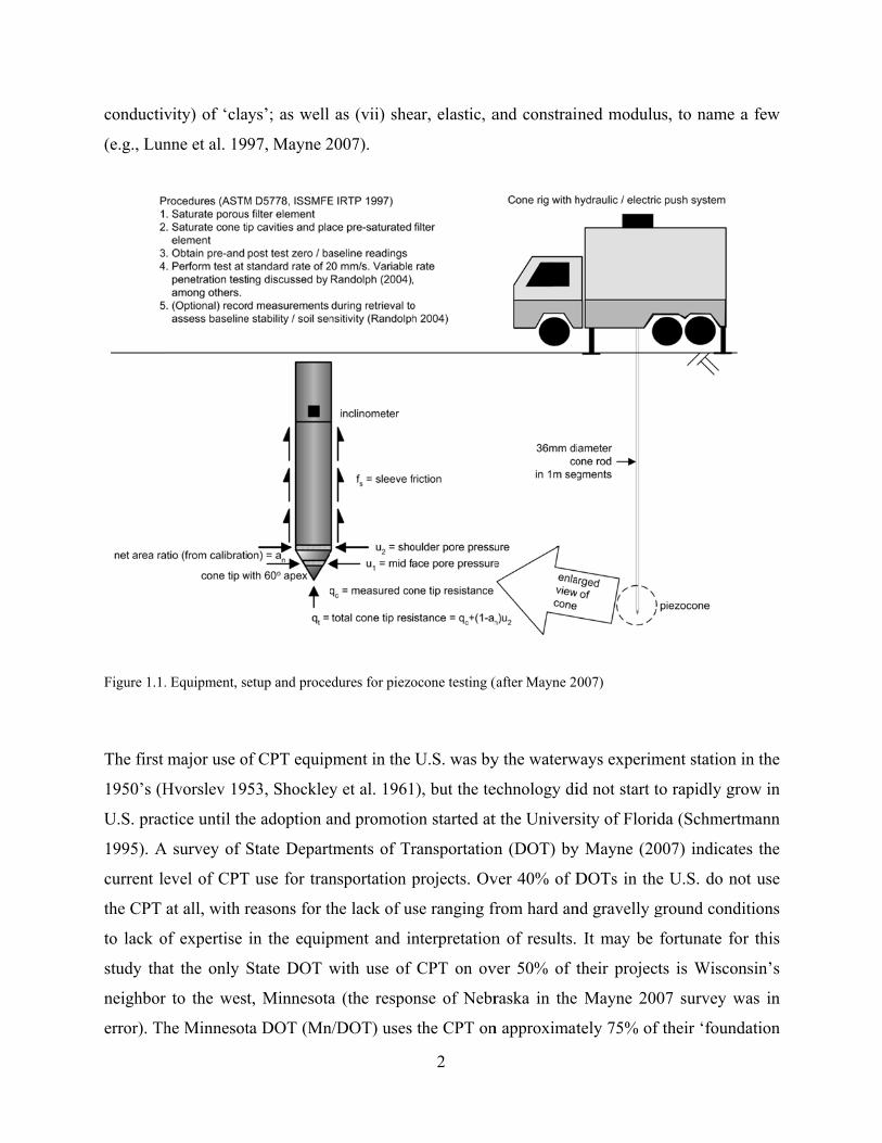
measurements (seismic piezocone, SCPTU, e.g., Campanella et al. 1986). Figure 1.1 illustrates
equipment, setup and procedures for piezocone penetration testing.
In current geotechnical engineering practice, results of the electric cone and piezocone
penetration tests are applied in a variety of applications, including (i) bridges; (ii) embankments;
(iii) deep foundations; (iv) slopes; (v) retaining wall design (including foundations); (vi) soft soil
delineation; (vii) earthquake site amplification and soil liquefaction; (viii) degree of soil
improvement; (ix) excavations; and (x) subgrades (e.g., Mayne 2007). Additionally, results of
the cone penetration test can be used to estimate a number of different soil characteristics and
properties, including: (i) soil type and stratigraphy; (ii) effective stress friction angle of ‘sands’;
(iii) relative density of ‘sands’; (iv) undrained shear strength of ‘clays’; (v) preconsolidation
stress of ‘clays’; (vi) water flow characteristics (coefficient of consolidation and hydraulic
conductiv
(e.g., Lun
Figure 1.1.
The first
1950’s (H
U.S. prac
1995). A
current le
the CPT
to lack o
study tha
neighbor
error). Th
vity) of ‘cla
nne et al. 19
. Equipment, se
major use o
Hvorslev 19
ctice until th
A survey of S
evel of CPT
at all, with r
of expertise
at the only S
r to the west
he Minnesot
ays’; as well
97, Mayne 2
etup and proce
f CPT equip
53, Shockley
he adoption a
State Depart
T use for tran
reasons for t
in the equip
State DOT w
t, Minnesota
ta DOT (Mn
as (vii) she
2007).
edures for piezo
pment in the
y et al. 1961
and promotio
tments of Tr
nsportation p
the lack of u
pment and in
with use of
a (the respo
n/DOT) uses
2
ear, elastic, a
ocone testing (
U.S. was by
1), but the te
on started at
ransportation
projects. Ov
se ranging fr
nterpretation
CPT on ov
nse of Nebr
the CPT on
and constrain
(after Mayne 20
y the waterw
echnology di
t the Univers
n (DOT) by
ver 40% of D
from hard an
n of results.
ver 50% of t
raska in the
n approximat
ned modulu
007)
ways experim
id not start to
sity of Florid
y Mayne (20
DOTs in the
nd gravelly g
It may be f
their project
Mayne 200
tely 75% of
us, to name a
ment station i
o rapidly gro
da (Schmertm
007) indicate
e U.S. do no
ground condi
fortunate fo
ts is Wiscon
07 survey w
their ‘found
a few
in the
ow in
mann
es the
ot use
itions
r this
nsin’s
was in
dation
3
engineering’ projects, and has performed over 7500 cone tests since 2001 (personal
communication Glenn Engstrom and Derrick Dasenbrock, Mn/DOT).
The glacial geological conditions of Minnesota are similar to those of the northern and eastern
half to ⅔ of Wisconsin, suggesting that the use of CPT may be viable for a majority of areas in
the state. However, the underlying bedrock conditions in the two states are different in that much
of Minnesota is underlain by shale, while Wisconsin is primarily underlain by dolomite /
limestone. This would cause a different type of sediment / clast entrained in the till and could
lead to differences in potential for CPT refusal if the cone encountered these clasts during
penetration. The study proposed in this research will first work with Mn/DOT and other regional
DOTs to build upon their experiences in implementation of cone penetration testing for
transportation projects, and address additional issues specific to the needs of the Wisconsin
Department of Transportation. Data collected in Wisconsin will be analyzed and discussed using
conventional soil parameters so that practitioners are familiar with factors controlling the
behavior of the measurements of the device, minimizing the reliance on ‘black box’ data
processing and interpretation programs.
1.2 Problem Statement
WisDOT is considering the use of CPT investigations on transportation projects. The
Department needs to learn more about the technology, its advantages and limitations, and feel
comfortable that CPT data correlates with Wisconsin soil boring methods/information/geology
and leads to design assumptions that are comparable to WisDOT’s current methods.
1.3 Objectives
It is the objective of this research project to evaluate the potential use of CPT technology for
Wisconsin DOT projects through performance of tests around the state and comparing CPT
results to available data. Specific objectives include:

4
Departmental subsurface investigative methods (generally soil borings) and cone
penetrometer findings will be compared at a number of sites with differing soils and
geology.
Evaluation of design parameters will be compared.
Discuss advantages and limitations of CPT equipment, operations and interpretation.
Detailed suggestions for the application of this technology on WisDOT projects will be
presented.
5
2 Additional Background and Previous Regional Experience
The cone penetration test (CPT) and variants [piezocone penetration test (CPTU), seismic
piezocone penetration test (SCPTU), resistivity cone penetration test (RCPT), etc.] have had
successful application in geotechnical engineering for over 75 years. At present there is still a
relatively limited application of CPT data by DOTs to design and construction of transportation
projects in the United States. Some of the reasons / perceptions for this lack of use include (e.g.,
Mayne 2007):
ground conditions are too hard;
soil contains gravel and stones;
CPTs are more expensive than borings;
data analysis requires too much expertise;
practice is acceptable using SPT;
equipment too expensive / not available in the area.
Many of these same obstacles exist for the glacial soil conditions of Wisconsin and need to be
assessed. However, similar geological conditions exist in the neighboring state of Minnesota and
their continued experience with CPTs since 2001 allows for use of CPT on more than 75% of
Minnesota DOT (Mn/DOT) “foundations” projects. These projects include (i) bridge and culvert
foundations; (ii) large embankment fills; (iii) buildings, towers, and other structures; (iv) slopes;
(v) retaining wall foundations; (vi) roadway alignment and soft soil delineation; (vii)
excavations; and (viii) sinkholes. A review of previous use of the CPT for Minnesota DOT and
Wisconsin DOT projects is presented in this chapter. Preliminary discussion of assessed profiles
is contained herein, with data included for supplemental analysis in later chapters. Attempts to
obtain data from other Midwestern state DOTs (i.e., Ohio) was unsuccessful. Discussion of
Minnesota data is largely taken from the conference paper Dasenbrock, Schneider & Mergen
(2010).
6
2.1 Additional Background
2.1.1 Wisconsin geology and soils
The CPT is a method used to determine the layering and engineering properties of
unconsolidated sediment overlying the local bedrock. This report addresses CPT testing at
various locations across the state of Wisconsin. A brief discussion of Wisconsin geologic history
is provided for a more thorough understanding of the regional soil conditions.
In the Quaternary period, or the past 2.6 million years (International Commission on Stratigraphy
2010), the planet has experienced fluctuations in the continental ice sheets. The amount of ice on
the surface of the earth has varied with climatic conditions throughout time as observed in the
oxygen isotope records in the skeletons of sea organisms and the variation in sea-level (Lambeck
& Chappell 2001, Lisiecki & Raymo 2005). Currently, the planet is in an interglacial period
where large continental ice sheets have regressed to Greenland and Antarctica. The last glacial
maximum occurred during the late Wisconsinan period from approximately 23,000 to 15,000
radiocarbon years before present (Clark et al. 2009). The extent of glacial ice coverage in
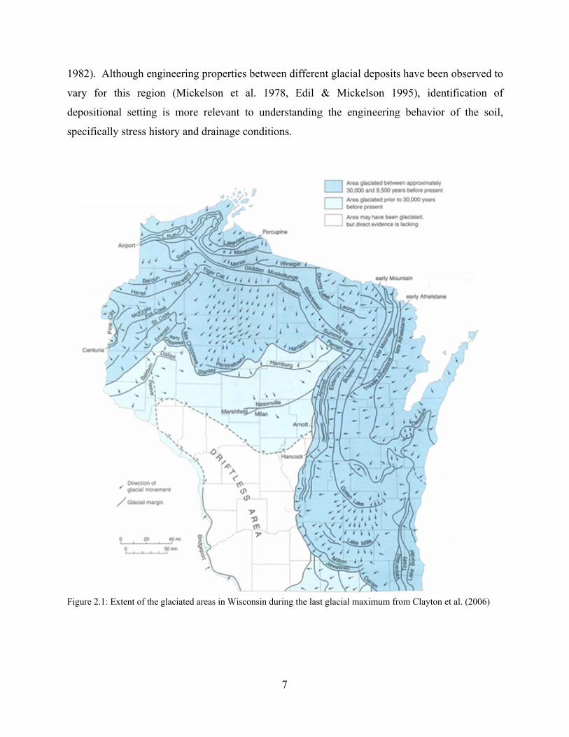
Wisconsin is provided in Figure 2.1 (Clayton et al. 2006). Approximately 60% of Wisconsin’s
land surface was covered by ice at some time in the past, either during the last glacial maximum
or during a previous glacial episode. The south west corner of the state is known as the driftless
area, Figure 2.1. This name is derived from the lack of glacial deposits historically grouped into
the all-encompassing term “drift”. Figure 2.2 illustrates the expected thickness of soil over
bedrock. Soil thickness is also thinner in the driftless area.
The areas covered by glaciers in the past bear distinct landforms associated with the prior
glaciations including till plains, drumlins, moraines, eskers, outwash plains, kettle and kame
landscapes, glacial lake plains, and ice-walled lake plains. Areas not directly glaciated do have
some glacially derived sediment typically in the form of loess, wind-blown silt, deposits.
Geologists have described the different drift deposits and divided them into different groups to
determine the chronology and extent of the fluctuations concerning the advance and retreat of
continental glaciers in the region (Clayton and Moran 1982, Attig et al. 1985, Acomb et al.
1982). A
vary for
depositio
specifica
Figure 2.1:
Although eng
r this regio
onal setting
ally stress his
: Extent of the
gineering pro
n (Mickelso
is more rel
story and dra
glaciated areas
operties betw
on et al. 1
levant to un
ainage condi
s in Wisconsin
7
ween differen
1978, Edil
nderstanding
itions.
n during the las
nt glacial de
& Mickels
g the engine
st glacial maxim
eposits have
son 1995),
eering beha
mum from Clay
been observ
identificatio
avior of the
yton et al. (200
ved to
on of
soil,
06)
8
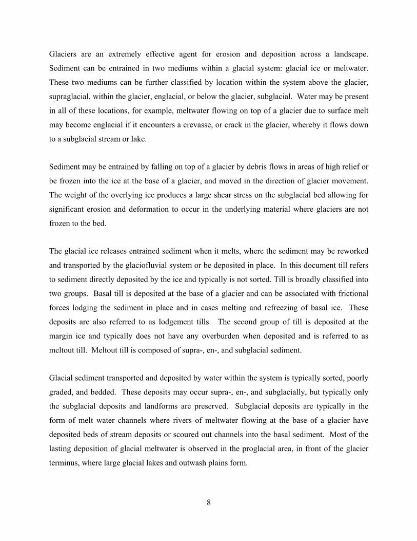
Glaciers are an extremely effective agent for erosion and deposition across a landscape.
Sediment can be entrained in two mediums within a glacial system: glacial ice or meltwater.
These two mediums can be further classified by location within the system above the glacier,
supraglacial, within the glacier, englacial, or below the glacier, subglacial. Water may be present
in all of these locations, for example, meltwater flowing on top of a glacier due to surface melt
may become englacial if it encounters a crevasse, or crack in the glacier, whereby it flows down
to a subglacial stream or lake.
Sediment may be entrained by falling on top of a glacier by debris flows in areas of high relief or
be frozen into the ice at the base of a glacier, and moved in the direction of glacier movement.
The weight of the overlying ice produces a large shear stress on the subglacial bed allowing for
significant erosion and deformation to occur in the underlying material where glaciers are not
frozen to the bed.
The glacial ice releases entrained sediment when it melts, where the sediment may be reworked
and transported by the glaciofluvial system or be deposited in place. In this document till refers
to sediment directly deposited by the ice and typically is not sorted. Till is broadly classified into
two groups. Basal till is deposited at the base of a glacier and can be associated with frictional
forces lodging the sediment in place and in cases melting and refreezing of basal ice. These
deposits are also referred to as lodgement tills. The second group of till is deposited at the
margin ice and typically does not have any overburden when deposited and is referred to as
meltout till. Meltout till is composed of supra-, en-, and subglacial sediment.
Glacial sediment transported and deposited by water within the system is typically sorted, poorly
graded, and bedded. These deposits may occur supra-, en-, and subglacially, but typically only
the subglacial deposits and landforms are preserved. Subglacial deposits are typically in the
form of melt water channels where rivers of meltwater flowing at the base of a glacier have
deposited beds of stream deposits or scoured out channels into the basal sediment. Most of the
lasting deposition of glacial meltwater is observed in the proglacial area, in front of the glacier
terminus, where large glacial lakes and outwash plains form.
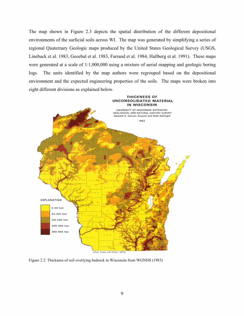
The map
environm
regional
Lineback
were gen
logs. T
environm
eight diff
Figure 2.2:
p shown in
ments of the
Quaternary
k et al. 1983,
nerated at a s
The units id
ment and the
ferent divisio
: Thickness of
Figure 2.3
surficial soi
Geologic m
, Geoebal et
scale of 1:1,
dentified by
e expected e
ons as expla
soil overlying
depicts th
ls across WI
maps produce
al. 1983, Fa
,000,000 usi
the map a
engineering p
ined below.
bedrock in Wi
9
e spatial di
I. The map
ed by the U
arrand et al.
ing a mixtur
authors were
properties o
isconsin from W
istribution o
was generat
United States
1984, Hallb
re of aerial m
e regrouped
f the soils.
WGNHS (1983
of the differ
ted by simpl
s Geological
berg et al. 19
mapping and
d based on
The maps w
3)
rent deposit
lifying a seri
l Survey (U
991). These
d geologic b
the deposit
were broken
tional
ies of
USGS,
maps
boring
tional
n into
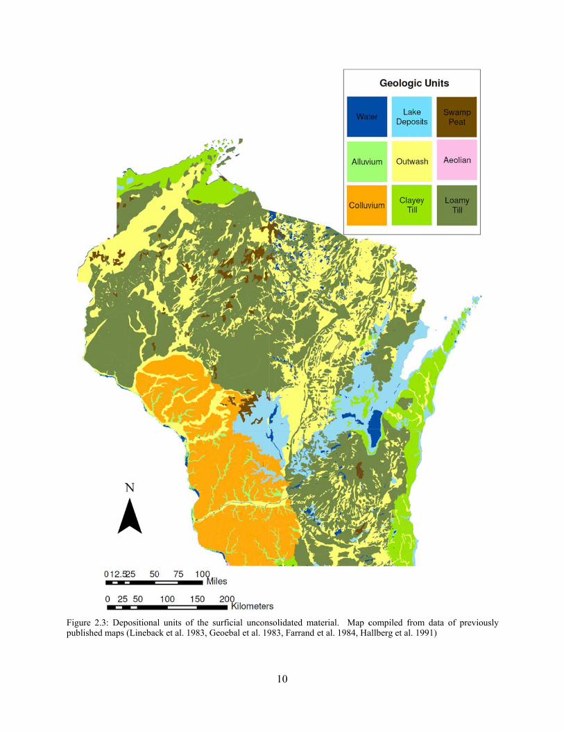
Figure 2.3published m
: Depositionalmaps (Linebac
l units of the ck et al. 1983, G
surficial uncoGeoebal et al. 1
10
onsolidated ma1983, Farrand
aterial. Map cet al. 1984, Ha
compiled fromallberg et al. 19
m data of prev991)
viously
11
The first division is non-glacial residual soils or colluvium. The colluvium group represents
residual soils that developed in place by weathering of the underlying bedrock. This unit occurs
primarily in the driftless area. These soils typically overly a shallow bedrock and are composed
of clay to boulder sized material. The landscape of the driftless area is characterized by hill and
steep valleys where streams have incised into the bedrock surface. Many of the soil deposits are
the result of debris flows and rock falls from the slopes.
Included in the non glacial soils are the alluvial deposits which represent recent stream deposits
placed after glaciers retreated from the region. These deposits are mostly found along the major
streams and rivers in the driftless area. The soils in the alluvial deposits are composed of clays
to gravel deposits representing overbank deposits, point bars, and abandoned channels.
Typically the soils in this category are primarily classified as sands from an engineering
standpoint.
Outwash deposits form proglacially where meltwater streams transport and deposit glacial
sediment. These deposits occur well dispersed throughout the state as a result of deposition in
front of the retreating glacial front. The soils in outwash deposits are silt to gravel sized particles
typically deposited in sorted, bedded, braided stream networks. Also included in this group are
the ice contact sands and gravels which are a form of meltout till. Although the original map
classification indicates transport solely by ice, the engineering behavior should be similar and
therefore was grouped with the outwash deposits.
Aeolian deposits representing loess and sand dunes that formed from wind re-working glacial
deposits. Local aeolian deposits occur throughout the mapped area in thin coverings, but they
were not separated out when the regional maps were created. Thick sequences, >5m thick, were
not mapped within the state and therefore this unit is not observed in Figure 2.3.
Till was mapped in the USGS sources as basal till, moraines, or undifferentiated and was
typically grouped as loamy, sandy, or clayey. From an engineering standpoint, interest in the
behavior of the till matrix will govern the behavior of the soil. The maps generated in this study
divided the tills into two groups: loamy and clayey. Sandy tills were incorporated with the
12
loamy tills. These till descriptions are very generalized and it must be understood that the grain
size distributions and descriptions are generated using the United States Department of
Agriculture (USDA) soil classification system percent silt, clay, and sand are compared. It is
also important to note that the tills were typically described with two grain sizes identified, for
example a loamy clayey till. It was assumed that there are no single modal grain size tills. This
assumption was taken further as an indication of water flow characteristics. Specifically, that
any clayey till would for the most part have a low hydraulic conductivity and display undrained
behavior and loamy-sandy tills would possess medium to high hydraulic conductivities and
behave partially drained to drained.
The distributions of the two till units indicate that the loamy tills cover much more area of the
state than clayey tills. The low occurrence of clayey tills relates back to the concept that a
glacier cannot produce clay because no significant chemical weathering occurs when particles
are entrained in ice. These clayey tills also occur above previously deposited tills, and therefore
reflect further transport and reworking of entrained sediment from the pre-existing tills. The
clayey tills occur mainly along the eastern shore of Lake Michigan and correlate with an
interstadial period where the glaciers receded northward out of the Great Lake basins prior to re-
advancing. When the glaciers receded northward, clayey sediment was deposited in Lake
Michigan. During the re-advance, this clay was entrained in the glacial ice and deposited in the
till associated with that advance.
The lake deposits represent depositional facies related to glacial lakes. These deposits are well
distributed in the central and eastern-central portions of the state where glacial lakes Wisconsin
(Attig and Knox 2008) and Oshkosh (Hooyer 2007) have been identified. The large extent of
these lakes is indicative of how large the impact of ice sheet loading is on crustal deformation.
Note that these deposits show the extents over time and are not meant to suggest that both lakes
were that size concurrently. Typical soils associated with the lake deposits are clays, silts and
sands representing subaqueous stream fans and deltas, and fine grained deposits related to release
of suspended sediment load in low energy environments. Occasional drop stones of gravel to
boulder size can be found which represent deposition of sediment from melting ice blocks that
calved and floated from the ice margin. These deposits are primarily composed of silts and clays
13
The swamp and peat deposits are closely associated with the lake deposits from a formation
standpoint. The deposits can be associated with the glacial lake deposits or occur as standalone
features where either large stagnant ice blocks formed a low area for water to collect or
meltwater collected in a natural topographic low. These deposits are composed of fine grained
silts and clays with high organic contents with anticipated low strengths and high
compressibilities. These soils make up a small portion of the mapped areas; however, this may
be a function of the scale of the mapping.
2.1.2 Fundamentals of soil behavior
Soil behavior is typically analyzed as a continuum, and interpretation and application revolves
around 5 primary characteristics:
Water flow characteristics – rate at which water moves through a soil matrix as a function
of a hydraulic gradient and/or change in volume
Compressibility – change in volume due to a change in effective stress (i.e., change in
size of a soil element)
Shear Stiffness – resistance to shear distortions that result from shear stresses (i.e.,
change is shape of a soil element)
Strength – ultimate resistance to shear stresses
Dilation – change in volume due to shear deformations (i.e., change in size due to change
in shape)
Interpretation of soil behavior is largely influenced by the rate of loading as compared to the rate
of water flow through the soil. If a soil is loaded slowly as compared to how fast water flows
through the soil (e.g., loading of saturated sand), no excess water pressure builds up and changes
in total stress are equal to changes in effective stress. This is referred to as drained loading.
Increases in effective stress lead to increases in strength of the soil, and dilation of soil particles
affect the geometry of a failure surface and changes in effective stress during loading. If a soil is
loaded rapidly compared to how fast water can flow through the pores (e.g., loading of saturated
clays), strength is generally controlled by short term loading prior to increases in effective stress,
while a majority of deformations are time dependent, provided that a shear failure does not
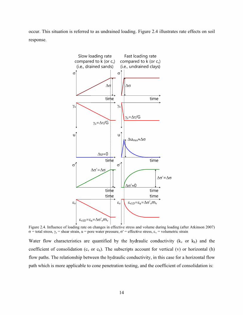
occur. Th
response
Figure 2.4. = total st Water fl
coefficien
flow path
path whic
his situation
.
. Influence of ltress, s = shear
low characte
nt of consol
hs. The relat
ch is more a
is referred t
loading rate onr strain, u = po
eristics are
lidation (cv
ionship betw
applicable to
to as undrain
n changes in efore water pressu
quantified
or ch). The
ween the hyd
cone penetr
14
ned loading.
ffective stress aure, ' = effect
by the hyd
subscripts a
draulic condu
ration testing
. Figure 2.4
and volume dutive stress, v =
draulic cond
account for v
uctivity, in t
g, and the co
illustrates ra
uring loading (a= volumetric st
ductivity (kv
vertical (v)
this case for
oefficient of
ate effects on
after Atkinson train
v or kh) and
or horizonta
a horizontal
consolidatio
n soil
2007)
d the
al (h)
l flow
on is:
w
hh
kc
Where D
coefficien
respectiv
is the ini
shown in
Figure 2.5.
Compres
strains ar
laborator
previousl
h
h
w m
kD
D is the con
nt of volum
vely, 'h,avg is
tial in-situ v
n Figure 2.5.
. Relationship b
ssion of soils
re equal to z
ry compress
ly compresse
h
w
k
435.0
1
strained mo
me change, C
s the average
void ratio. A
between soil ty
s is typically
zero and ax
sion curves
ed, the 1D so
RC
avh
CC
e
' ,0
odulus, w is
Cc and Cr a
e horizontal
A relationship
ype and water f
y defined ba
ial strain eq
for two un
oil compress
15
w
vg
s the unit w
are the 1D c
effective str
p between w
flow characteri
ased on the o
quals volume
nstructured
sibility is de
weight of wa
compression
ress during t
water flow ch
istics (after Sa
one dimensi
etric strain.
clays. For
efined using t
ater, mh is th
n and recom
the loading i
haracteristic
algado 2008)
ional (1D) c
Figure 2.6 i
soils which
the compres
(2
he horizonta
mpression ind
increment, a
cs and soil ty
case where la
illustrates ty
h have not
ssion index (
.1)
al 1D
dices,
and e0
ype is
ateral
ypical
been
(Cc):
16
iv
fvc
eC
,
,
'
'log
(2.2)
Where 'v,f is the final vertical effective stress and 'v,i is the initial vertical effective stress, and
e is the change in void ratio for that change in effective stress. Likewise, below the maximum
previous effective stress that a soil has been loaded to, or a vertical effective yield stress that has
resulted from ageing or cementation, the recompression index (Cr) is defined as:
iv
fvr
eC
,
,
'
'log
(2.3)
Use of Cc and Cr indicate that as effective stress increases, compressibility decreases. The 1D
coefficient of volume change, mv = a/'v, is the inverse of the 1D constrained modulus, D =
1/mv = 'v/a. The relationship between constrain modulus and coefficient of compression for
normally consolidated soil is:
c
avgv
v C
e
mD
435.0
'11 ,0
(2.4)
Constrained modulus, the inverse of compressibility, tends to increase with effective stress. For
overconsolidated soils, constrained modulus is related to the recompression index.
r
avgv
v C
e
mD
435.0
'11 ,0
(2.5)
This equation would also result in the constrained modulus in the overconsolidated region
increasing (essentially linearly) with increasing effective stress. However, it is common to
assume that constrained modulus is constant within the overconsolidated region (e.g., Janbu
1985). T
disturban
stress in t
modulus
Figure 2.6.
This assump
nce, but is a
the overcons
may apply (
. Compression/
ption is part
reasonable
solidated reg
(for a relativ
/recompression
tially influen
assumption
gion (small C
vely low p'c o
n indices and c
17
nced by lab
due to the s
Cr) as well a
or ' during
constrained mo
boratory test
small chang
as the limited
g loading).
odulus in two u
ting procedu
ges in modul
d stress rang
unstructured cla
ures and sa
lus with effe
e over which
ays
ample
ective
h that
While co
shear stif
shear stif
2.7.
Figure 2.7.
When us
1
1
D
Where E
shear mo
relationsh
refGG
ompressibilit
ffness is the
ffness and co
. Comparison o
ing elastic th
21
1
E
E (=y/y,
odulus (xz/
hips for shea
n
reff p
s
'
ty is the ‘cha
e resistance t
ompressibili
of (a) compress
heory, stiffne
21
21
G
for plane s
/xy). Shea
ar modulus f
ange in size’
to distortion
ty (and its re
sion, (b) distor
ess is related
tress conditi
ar stiffness o
for soils can
18
of a soil ele
n from a res
elationship t
rtion, and (c) di
d to compres
ions) is the
of soil is cha
be expresse
ement due to
sulting shear
to dilation an
ilation for an e
ssibility thro
elastic (You
aracterized b
d as (e.g., af
o increases in
r stress. Diff
ngle) are illu
element of soil
ough the Pois
ung’s) modu
by shear mo
fter Santama
n effective s
ferences bet
ustrated in F
sson ratio (
(2
ulus and G i
dulus, G. Si
arina et al. 20
(2
stress,
tween
Figure
):
.6)
is the
imple
001):
.7)
where Gr
the mean
(for ceme
clays at l
stiffness
and tend
Addition
stiffness
in void ra
A main d
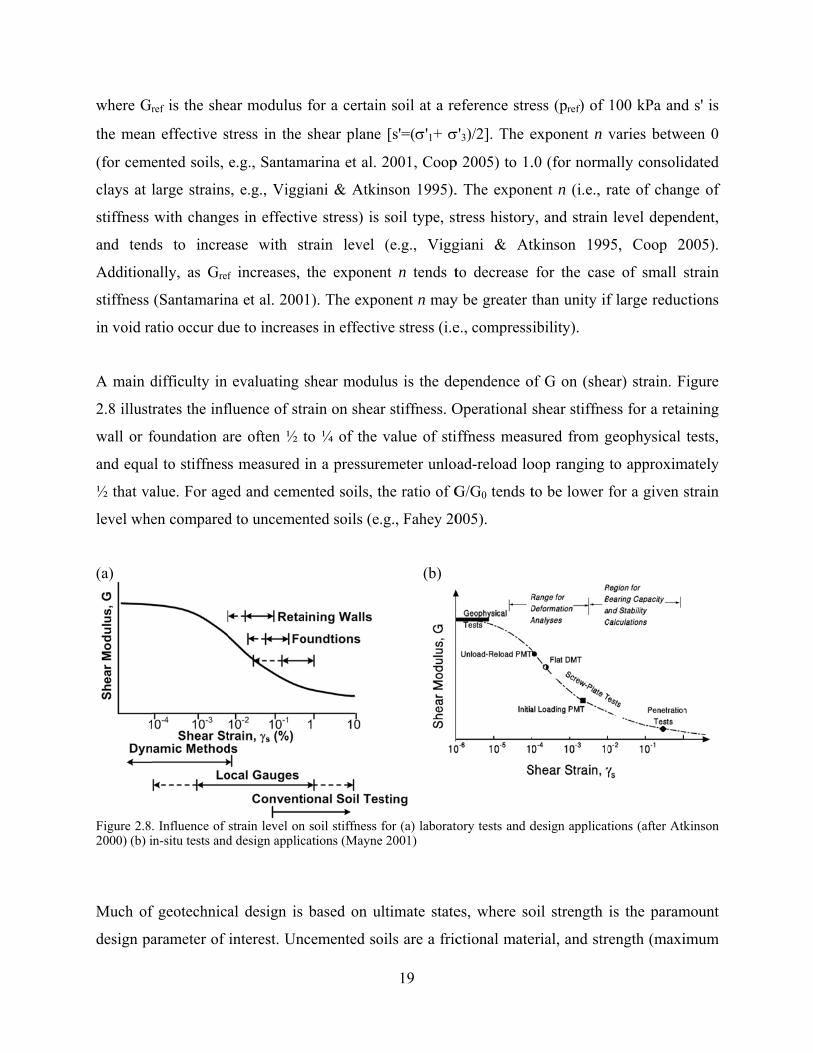
2.8 illust
wall or f
and equa
½ that va
level whe
(a)
Figure 2.82000) (b) i
Much of
design pa
ref is the she
n effective s
ented soils,
large strains
with change
ds to incre
nally, as Gref
(Santamarin
atio occur du
difficulty in
rates the inf
foundation a
al to stiffnes
alue. For age
en compared
. Influence of in-situ tests and
f geotechnica
arameter of
ear modulus
stress in the
e.g., Santam
s, e.g., Vigg
es in effectiv
ase with st
f increases,
na et al. 200
ue to increas
evaluating
fluence of str
are often ½ t
s measured
ed and ceme
d to uncemen
strain level ond design applic
al design is
interest. Un
for a certain
shear plane
marina et al.
iani & Atki
ve stress) is
train level
the exponen
1). The expo
ses in effectiv
shear modul
rain on shea
to ¼ of the
in a pressur
ented soils, t
nted soils (e
n soil stiffness cations (Mayne
based on u
cemented so
19
n soil at a re
e [s'=('1+
2001, Coop
nson 1995).
soil type, st
(e.g., Vigg
nt n tends t
onent n may
ve stress (i.e
lus is the de
r stiffness. O
value of sti
emeter unlo
the ratio of G
.g., Fahey 20
(b)
for (a) laborate 2001)
ultimate state
oils are a fric
eference stre
'3)/2]. The e
p 2005) to 1.
. The expon
tress history
giani & At
to decrease
y be greater t
e., compress
ependence o
Operational s
iffness meas
oad-reload lo
G/G0 tends t
005).
tory tests and d
es, where so
ctional mate
ess (pref) of
exponent n v
.0 (for norm
nent n (i.e., r
y, and strain
tkinson 199
for the cas
than unity if
ibility).
of G on (she
shear stiffne
sured from g
oop ranging
to be lower
design applicat
oil strength
erial, and str
100 kPa and
varies betwe
mally consoli
rate of chan
level depen
95, Coop 2
e of small s
f large reduc
ear) strain. F
ess for a reta
geophysical
to approxim
for a given s
tions (after Atk
is the param
rength (maxi
d s' is
een 0
dated
nge of
ndent,
2005).
strain
ctions
Figure
aining
tests,
mately
strain
kinson
mount
imum
20
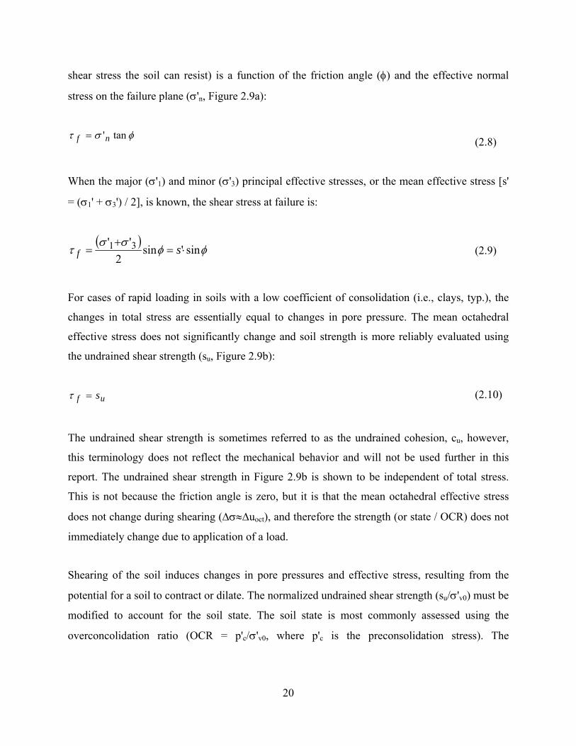
shear stress the soil can resist) is a function of the friction angle () and the effective normal
stress on the failure plane ('n, Figure 2.9a):
tan'nf (2.8)
When the major ('1) and minor ('3) principal effective stresses, or the mean effective stress [s'
= (1' + 3') / 2], is known, the shear stress at failure is:
sin'sin
2
'' 31
sf (2.9)
For cases of rapid loading in soils with a low coefficient of consolidation (i.e., clays, typ.), the
changes in total stress are essentially equal to changes in pore pressure. The mean octahedral
effective stress does not significantly change and soil strength is more reliably evaluated using
the undrained shear strength (su, Figure 2.9b):
uf s (2.10)
The undrained shear strength is sometimes referred to as the undrained cohesion, cu, however,
this terminology does not reflect the mechanical behavior and will not be used further in this
report. The undrained shear strength in Figure 2.9b is shown to be independent of total stress.
This is not because the friction angle is zero, but it is that the mean octahedral effective stress
does not change during shearing (uoct), and therefore the strength (or state / OCR) does not
immediately change due to application of a load.
Shearing of the soil induces changes in pore pressures and effective stress, resulting from the
potential for a soil to contract or dilate. The normalized undrained shear strength (su/'v0) must be
modified to account for the soil state. The soil state is most commonly assessed using the
overconcolidation ratio (OCR = p'c/'v0, where p'c is the preconsolidation stress). The
relationsh
Mayne 1
0
s
'
s
v
u
The para
consolida
Figure 2.9.
Undraine
This stren
normaliz
triaxial
anisotrop
test (VS
strength r
hip between
980, Wroth
12
sinOCR
ameter sin
ated undrain
. Drained and u
ed strength r
ngth anisotro
zed undraine
undrained c
pically conso
T), among
ratios for cla
n su/'v0 and
& Houlsby
.0cr CC
/2 (assume
ned strength r
undrained stren
ratios, such a
opy can be o
ed strength
compression
olidated triax
others. Tab
ays and varv
d OCR can b
1985, Ladd
8.023 OCR
ed to be ap
ratio [(su/'v
ngth parameter
as that descr
observed in l
ratios being
n tests (CK
xial undrain
ble 2.1 sum
ved clays.
21
be approxim
1991):
pproximately
v0)NC].
rs
ribed by Equ
laboratory te
g observed
K0UC); (ii)
ed extension
mmarizes ty
mated as (e.g
y 0.23) is
uation 2.11,
ests, with dif
for (i) K0
direct sim
n tests (CK0
ypical norma
g., Schofield
often terme
vary by dire
fferent norm
anisotropica
mple shear
0UE); and (iv
ally consoli
d & Wroth
(2
ed the norm
ection of loa
mally consoli
ally consoli
(DSS); (iii
v) the vane
idated undr
1968,
.11)
mally
ading.
dated
dated
i) K0
shear
ained
22
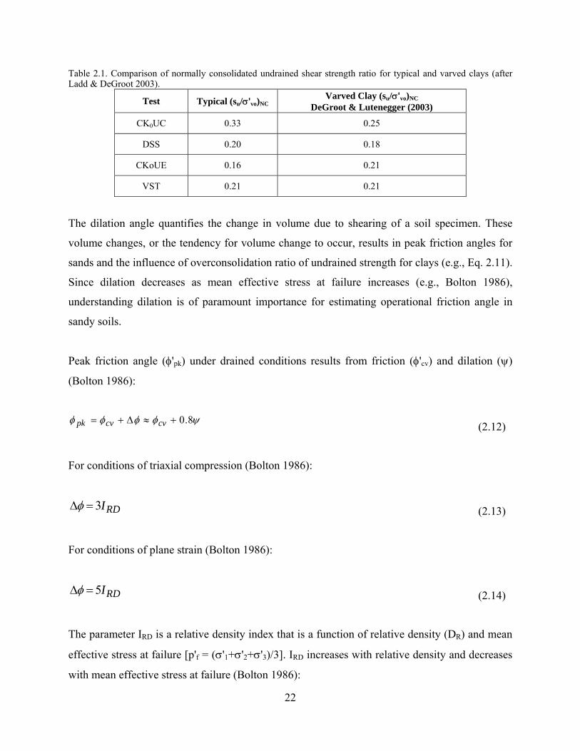
Table 2.1. Comparison of normally consolidated undrained shear strength ratio for typical and varved clays (after Ladd & DeGroot 2003).
Test Typical (su/'vo)NC Varved Clay (su/'vo)NC
DeGroot & Lutenegger (2003)
CK0UC 0.33 0.25
DSS 0.20 0.18
CKoUE 0.16 0.21
VST 0.21 0.21
The dilation angle quantifies the change in volume due to shearing of a soil specimen. These
volume changes, or the tendency for volume change to occur, results in peak friction angles for
sands and the influence of overconsolidation ratio of undrained strength for clays (e.g., Eq. 2.11).
Since dilation decreases as mean effective stress at failure increases (e.g., Bolton 1986),
understanding dilation is of paramount importance for estimating operational friction angle in
sandy soils.
Peak friction angle ('pk) under drained conditions results from friction ('cv) and dilation ()
(Bolton 1986):
8.0 cvcvpk (2.12)
For conditions of triaxial compression (Bolton 1986):
RDI3 (2.13)
For conditions of plane strain (Bolton 1986):
RDI5 (2.14)
The parameter IRD is a relative density index that is a function of relative density (DR) and mean
effective stress at failure [p'f = ('1+'2+'3)/3]. IRD increases with relative density and decreases
with mean effective stress at failure (Bolton 1986):
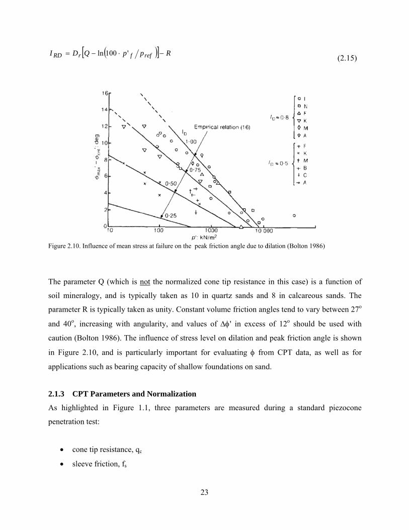
DI RD
Figure 2.10
The para
soil mine
paramete
and 40o,
caution (
in Figure
applicatio
2.1.3 C
As highl
penetrati
co
sl
QDr 100ln
0. Influence of
ameter Q (w
eralogy, and
er R is typica
increasing
(Bolton 1986
e 2.10, and
ons such as b
CPT Parame
lighted in F
on test:
one tip resist
leeve friction
pp reff '0
f mean stress at
which is not t
d is typically
ally taken as
with angula
6). The influ
is particula
bearing capa
eters and No
Figure 1.1,
tance, qc
n, fs
R
t failure on the
the normaliz
y taken as
s unity. Cons
arity, and va
uence of stre
arly importan
acity of shall
ormalizatio
three param
23
peak friction
zed cone tip
10 in quartz
stant volume
alues of
ess level on d
nt for evalu
low foundati
on
meters are m
angle due to d
p resistance
z sands and
e friction ang
' in excess
dilation and
uating from
ions on sand
measured d
dilation (Bolton
in this case)
d 8 in calcar
gles tend to v
of 12o shou
peak frictio
m CPT data
d.
during a sta
(2
n 1986)
) is a functi
reous sands.
vary betwee
uld be used
on angle is sh
a, as well a
andard piezo
.15)
on of
. The
en 27o
with
hown
as for
ocone
24
penetration pore pressure measured at the cone shoulder, u2
Cone tip resistance is influenced by the geometry of a specific cone penetrometer. The corrected
cone tip resistance needs to be used for all analyses such that uncertainty in comparison to
previous studies and theoretical analysis is minimized. The corrected cone tip resistance is
expressed as:
cone tip resistance corrected for pore pressure effects, qt = qc + (1-an)u2
where an is the net area ratio of the penetrometer that typically varies between 0.5 and 0.95
(Lunne et al. 1986, Lunne et al. 1997). To account for initial in-situ conditions on CPT
measurements, the following derived parameters are often used:
net cone tip resistance, qcnet = qt – v0
excess penetration pore pressure, u2 = u2 – u0
effective cone tip resistance, qE = qt – u2
For the above derived parameters v0 is the total stress at a given depth prior to penetration, and
u0 is the in-situ pore pressure at a given depth prior to penetration.
Since soil mechanical properties are controlled by initial effective stress and changes in effective
stress during loading, rational interpretation of CPT measurements requires normalization by
some measure of effective stress (e.g., Wroth 1984, 1988). For soil classification based on
normalized piezocone parameters, a combination of two of the seven following parameters is
typically used (e.g., Douglas & Olsen 1981,Wroth 1984, Wroth 1988, Robertson 1990, Olsen &
Mitchell 1995, Robertson & Wride 1998, Jefferies & Been 2006, Schneider et al. 2008,
Robertson 2010):
normalized cone tip resistance, Q = qcnet/'v0
modified normalized cone tip resistance, Qtn = (qcnet/pref)/('v0/pref)n
normalized effective cone tip resistance, QE = (qt-u2)/'v0
25
friction ratio, F (%) = fs/qcnet·100
normalized sleeve friction, fs/'v0
pore pressure parameter, Bq = u2/qcnet
normalized excess penetration pore pressure, u2/'v0
While the initial horizontal effective stress or preconsolidation stress may be more appropriate
for normalization (e.g., Mayne 1986, Houlsby 1988, Houlsby & Hitchman 1988, Been &
Jefferies 2006), the in-situ vertical effective stress is used for the above mentioned normalized
parameters as it can be calculated without significant additional analyses. For initial
classification purposes, it is preferred to use Q rather than Qtn. Q is equal to Qtn for a stress
exponent (n) equal to unity, and therefore does not require iteration in its interpretation (i.e., is
easier to use). Additionally, no significant advantages have been observed when using Qtn over Q
for classification purposes (e.g., Schneider et al. 2008), and use of Q allows for plotting data in a
variety of different frameworks to highlight different responses. Plotting Q vs. Bq or Q vs.
u2/'v0 are analogous since Q·Bq = u2/'v0 . Likewise, plotting Q vs. F or Q vs. fs/'v0 are
analogous since Q·F = fs/'v0. Each plotting format has advantages and disadvantages for
highlighting aspects of soil behavior.
As mentioned in the previous section, soil strength and stiffness generally increase with effective
stress, but this relationship is also influenced by the effective stress loading history of a soil
element and/or crushable nature of the soil grains, herein discusses as ‘state.’ Undrained
behavior in clay soils is used as an example to illustrate the influence of state on normalized
response. If we assume that soil undrained strength (su) is the primary factor controlling cone tip
resistance, qt, a direct relationship between the two properties would exist (through a ‘bearing
capacity’, or cone, factor, Nkt):
ktucnet Nsq (2.16)
For a constant Nkt, the normalized cone tip resistance would therefore be equal to:
26
ktv
u Ns
Q 0' (2.17)
For normally consolidated clays that have not been previously loaded (or aged), su/'v0 is
typically taken as a constant [i.e., (su/'v0)NC], and therefore Q is a constant value (generally
around 3 to 5). Q is essentially constant in normally consolidated clays and as the
overconsolidation ratio (OCR) increases Q will also increase:
ktNCv
u NOCRs
Q
0' (2.18)
Figure 2.11 shows normalized cone tip resistance in normally consolidated and an
overconsolidated clay.
When evaluating specific engineering behavior, such as friction angle, relative density,
liquefaction resistance, Q may not be the most appropriate normalizing parameter, and Qtn is
often used. Observations of stress exponents less than unity are largely influenced by stress
dependency on dilation angle and crushability of sands at high stresses (e.g., Bolton 1986,
Salgado et al. 1997, Olsen & Mitchell 1995, Moss et al. 2006). Figure 2.12 illustrates normalized
cone tip resistance in loose and dense sands. At shallow depths Q in both drained sands and
undrained clays may exceed 20 and approach 1000.
Figure 2.1Amundsen
Figure 2.12
11. Normalizedn et al. 1985, Li
2. Normalized
d cone tip reiao et al. 2010)
cone tip resista
sistance in no)
ance in loose a
27
ormally conso
and very dense
olidated and o
sands (after S
overconsolidate
chneider et al.
ed clays (data
2008)
a from
28
2.2 Minnesota DOT (after Dasenbrock, Schneider & Mergen 2010)
Since 2001 the Minnesota DOT (Mn/DOT) has performed over 7500 CPTs in glacial geological
conditions. Despite these conditions often being considered as difficult ground for this technique,
Mn/DOT uses the CPT on more than 75% of their “foundations” projects. Over 400 of those
CPTs from 21 sites are assessed herein.
Boring logs and electronic CPT data have been made available through Mn/DOT are included as
electronic files on the ArcGIS database complied for this project. Additional site information can
be found through the Mn/DOT Geotechnical Investigation Information Interchange Internet
Interface (GI5) (e.g., Dasenbrock 2008):
http://www.mrr.dot.state.mn.us/geotechnical/foundations/Gis/gi5_splash.html
2.2.1 Procedures and cone performance
To minimize the potential for cone damage and ensure collection of high quality data, Mn/DOT
has adopted standard procedures for test preparation, performance, and data recording (e.g.,
Lunne et al. 1997). Mn/DOT has 3 CPT rigs in year round operation; a 11 ton tracked rig, a 13
ton 4x4 truck, and a 30 ton 6x6 truck. Many projects require only shallow exploration, and
investigations are performed to depths of 30 ft to 50 ft. For bridges, explorations in excess of 100
ft are often required. Hole sealing procedures for depths in excess of 50 ft require grouting from
the bottom of the hole during cone extraction. For these projects Mn/DOT utilizes a standard
setup for grouting during cone extraction, which is semi-automated on the 30 ton truck.
Both 10 cm2 (1.44 inch diameter) and 15 cm2 (1.72 inch diameter) cones are used; the two truck
rigs typically use the larger diameter cones. Mn/DOT keeps approximately 15 ‘service ready
cones’ on hand (distributed among the 3 rigs and the lab) at any given time. Calibrations are
performed by the penetrometer manufacturer and occur annually or at the time of a cone repair.
The net area ratio (an) used for correction of the tip resistance for pore pressure effects is 0.8, as
provided by the cone manufacturer. Due to hard ground conditions or obstructions,
approximately one cone is broken per year. Additionally, approximately every 1.5 months, an in-
29
service cone will need to be repaired. These repairs are usually for a bad channel (e.g. pore
pressure), bending or crushing of the sleeve or probe housing, or water damage due to an issue
with one of the seals. To minimize cone damage, methods suggested by Lunne et al. (1997) have
been adopted, namely, (i) keeping the inclination less than 10o, particularly for shallow holes; (ii)
minimizing total force applied to dense soils underlying thick zones of very soft material, such as
peat; and (iii) having a presence of mind to realize that there may be boulders or cobbles in
certain geological conditions, and that sharp spikes in tip resistance associated with rapid
changes in inclination (> 1o/m push) should result in termination of a sounding.
On projects where clay soils are present and consolidation characteristics are of interest, or
where materials are not well defined, pore pressure dissipation test data have proved valuable on
many Mn/DOT projects. An effort is made to ensure reliable pore pressure data; Mn/DOT
purchases filter element from the CPT manufacturer that are pre-saturated with silicone oil.
While the oil viscosity may result in sluggish response, it also helps reduce the likelihood that
the system will become unsaturated. In some cases it is difficult to maintain proper saturation
and record high quality pore pressure data through an entire layer, particularly in deposits above
the water table, very stiff soils, or layered clays and silty sands. More detailed review of data
quality is required when evaluating design parameters from qt and or u2 data in these situations.
2.2.2 Geology and typical soil profiles
The geology of Minnesota has primarily been shaped by glacial action. As a result, the state has
highly variable deposits consisting of (i) alluvium; (ii) colluvium; (iii) glacial lake deposits; (iv)
outwash; (v) peat; (vi) weathered bedrock; and (vii) glacial till. Initial review of single CPTs
from 6 sites was performed for this section. The six locations include geologic conditions
consisting of (i) till soils; (ii) lake deposits; (iii) peat; (iv) outwash; and (v) alluvium. Details on
the project types and soil conditions are included in Figure 2.13 and Table 2.2.
Figure 2.13data on preSwinehart
3. Location of eviously publiset al. 1994, Fu
f initial Mn/DOshed maps (Go
ullerton et al. 19
OT CPT sites ooebal et al. 198995, Sado et al
30
on a map of M83, Farrand et l. 1995, Fullert
Minnesota Quateal. 1984, Hall
ton et al. 2000)
ernary geologylberg et al. 199)
y. Map adapted91, Sado et al.
d from 1994,
31
Table 2.2. Description of initial Mn/DOT CPT sites UW Site No.
Depth Range
Analyzed (ft)
Site Project ID: Design Issues Regional Geology Number of CPTs
- 10-36 1003-28: Roadway / settlement Loamy Till 40 8 5-50 3609-25: Roadway / bridge / geofoam Lake Clays 60 - 5-80 1480-149: Landslide Lake Clays 13
13 6-25 3413-22: Roadway failure / Retaining Wall Peat 149 - 0-35 2903-10: Roadway Alignment Outwash (Sand) 20 - 0-33 8823-01: Groundwater monitoring Alluvium (Silty Sand) 3
Upon completion of a site investigation, CPT (and boring) data are processed, entered into
project databases, and exported for use in a web enabled Geographic Information System (GIS)
(Dasenbrock 2008). Individual vertical profiles are analyzed, and cross sections are developed
for larger projects. Profiles of net tip resistance and friction ratio from the 6 sites are shown in
Figure 2.14, and profiles of net tip resistance (qcnet=qt-v0) and excess pore pressure (u2=u2-u0)
are shown in Figure 2.15. Normalized soil behavior type is used by Mn/DOT for preliminary
evaluation of layering. Both the Robertson (1990, 1991) Q-F and Q-Bq charts have been used by
Mn/DOT, depending upon soil layering. In sandy soils, Q-F charts are typically used, while in
clayey soils, Q-Bq charts are typically used. Use of these charts requires selection of appropriate
normalized parameters and requires judgment that is dependent upon data quality and design
application.
Since soil behavior is controlled by ‘soil state’ as well as rate of drainage (particle size), among
other factors, Figures 2.14 and 2.15 include a trend line reflecting inferred soil state. In glacial
deposits where the soil can often be considered preconsolidated by a vertical load (i.e., a glacier),
the preconsolidation difference (p'c) allows for assessment of reduction in OCR (state) with
depth in clayey soils. Assuming a constant Nk value of 15 and a normally consolidated undrained
strength ratio [(su/'v0)NC] of 0.27 for preliminary analyses, the net cone tip resistance (qcnet = qt-
v0) can be estimated as a function p'c and 'v0.
75.0
000
0 '
'1'4'
'
v
cvv
NCv
ukcnet
pOCR
sNq
(2.19)
Figure 2.144. Profiles of qqcnet and F for selected sites in
32
n Minnesota
Figure 2.155. Profiles of qqcnet and u2 forr selected sites
33
in Minnesota
34
Estimated values of p'c vary from 75kPa to 200 kPa for the lake deposits, and 550kPa for the
loamy till soil shown. The peat soils have very low tip resistance, and are modeled fairly well as
a normally consolidated deposit (p'c=0), particularly at depth. While use of p'c does not
satisfactorily match the entire depth of each profile, it does provide an indication of soil state
such that design issues can be addressed in a more rational framework.
Relative density (Dr) is a useful parameter for evaluation of the anticipated behavior of sandy
soils, and is related to soil state when combined with effective stress at failure (e.g., Figure 2.10).
Profiles of net cone tip resistance are estimated from an inferred relative density in Figures 2.14
and 2.15 using the following equation (e.g. updated based on Jamiolkowski et al. 2003):
5.0
086.2 '20
ref
vDrefcnet p
epq r
(2.20)
Two extremes of sand density can be seen, with these outwash soils having a relative density on
the order of 0.35 and these alluvial soils have a relative density near 1.0.
2.2.3 Performance at additional sites
Detailed evaluation of 21 sites and over 400 CPTUs was performed (Figure 2.16), as
summarized in Tables 2.3 and 2.4, and Appendix 1 and 3. The main purpose of this exercise was
to assess the typical geological conditions, penetration depths, and soil types in which Mn/DOT
has had successful use of the CPT. Lateral spatial variability of cone tip resistance and friction
ratio were quantified to see if variability had an influence of likelihood of meeting premature
refusal when testing in a given soil environment. Borings were compared to a given CPT at
20/21 sites. Table 2.2 summarizes typical geological environments where CPTs were performed:
Alluvium – 8 sites
Clay Till – 2 sites
Lake deposits – 5 sites
Loamy Till – 5 sites
Figure 2.16adapted froet al. 1994
6. Location of om data on pre, Swinehart et
Mn/DOT CPTeviously publisal. 1994, Fulle
T sites with detashed maps (Goerton et al. 1995
35
ailed analysis oebal et al. 1985, Sado et al. 1
on a map of M3, Farrand et a
1995, Fullerton
Minnesota Quateal. 1984, Hallbn et al. 2000)
ernary geologyerg et al. 1991
y. Map , Sado
36
Table 2.3. Summary of regional geology for Mn/DOT sites analyzed UW
Site No. Mn/DOT Proj. No.
County Regional Geology
1 MAC Hennepin Alluvial valley of Minnesota river within outwash deposits 2 6918-69 St. Louis Clayey till 3 8285-80 Washington Alluvial valley of Mississippi river within outwash deposits 4 0916-16 Carlton Alluvial valley of St. Louis river between Lake and Loamy till deposits 5 2713-75 Hennepin Loamy till 6 3609-30 Koochiching Alluvial valley of Little Fork river adjacent to Loamy till, Lake clays,
and Peat 7 8103-47 Waseca Loamy till 8 3609-25 Koochiching Lake clay & silt adjacent to Sandy till, crossing Little Fork river 9 1009-16 Carver Clayey till
10 2207-32 Faribault Loamy till adjacent to Lake clays / silt (no borings) 11 3507-12 Kittson Lake deposits adjacent to Alluvial valley of Red river 12 7602-16 Swift Alluvial valley of the Chippewa river adjacent to Clayey and Loamy till 13 3413-22 Kandiyohi Lake deposits within Outwash (Peat) 14 4913-21 Morrison Alluvial valley of the Mississippi river within Outwash deposits adjacent
to Sandy till 15 4013-43 LeSueur Loamy till 16 0208-123 Anoka Lake deposits within Outwash 17 0901-74 Carlton Lake clay & silt within Outwash adjacent to Clayey till 18 1002-79 Carver Loamy till 19 1601-48 Cook Alluvium over Sandy / Clayey Till, Onion river at Lake Superior 20 8580-149 Winona Alluvial valley of Mississippi river w/in Outwash adjacent to Colluvium 21 5509-63 Olmsted Sandy Loamy till
Table 2.4. Summary of CPT performance for Mn/DOT sites analyzed UW Site No.
Mn/DOT Proj. No.
County # CPTs
Depth (ft) Median CPTU values lateral variability1 min median max qt
(tsf) F
(%) u2
(tsf) 1 MAC Hennepin 14 5.6 20.5 30 155 1.0 0.2 moderate 2 6918-69 St. Louis 14 4.4 37 48 18.3 3.4 0.1 high 3 8285-80 Washington 14 48 77 119 52.1 0.6 1.2 moderate 4 0916-16 Carlton 2 32.6 34.5 36.4 13.5 3.9 0.2 moderate 5 2713-75 Hennepin 7 24.8 41.3 41.2 12.2 2.0 2.3 low-mod 6 3609-30 Koochiching 7 19.5 93.2 103.5 11.2 4.2 6.0 low 7 8103-47 Waseca 41 11 24 44 13.7 2.6 0.4 mod-high 8 3609-25 Koochiching 60 40 50 98 13.4 3.3 4.6 low-mod 9 1009-16 Carver 9 9 49 50 24.1 2.6 2.3 low-mod
10 2207-32 Faribault 33 27 48.4 49 10 4.1 1.3 high 11 3507-12 Kittson 24 40 115 163 11.5 3.3 4.4 low 12 7602-16 Swift 3 43 44 46 7.5 4.6 1.4 moderate 13 3413-22 Kandiyohi 25 18 33 50 16.1 2.3 0.7 high 14 4913-21 Morrison 6 13 23 29 91.4 0.9 0.1 low-mod 15 4013-43 LeSueur 54 44 71.5 80 13.6 3.7 0.6 high 16 0208-123 Anoka 13 40 49.5 50 85.0 0.7 0.3 low 17 0901-74 Carlton 12 49 53.5 54 11.8 2.1 4.5 low 18 1002-79 Carver 11 14 37 49 14.2 2.5 0.3 moderate 19 1601-48 Cook 34 1.5 12 32 14.2 1.7 0 high 20 8580-149 Winona 4 4 5 6.5 45.9 1.2 0.1 moderate 21 5509-63 Olmsted 30 5 20 42 30.4 1.6 0.1 mod-high
1 for lateral variability, high = a majority of depths with qt COV > 1, low = a majority of depths with qt COV ≤ 0.3, moderate = a majority of depths with 0.3 ≤ qt COV ≤ 1, dual symbols used for profiles with mixed variability
Figure 2.17
7. Comparisonn between peneetration depth a
37
and CPT parammeters for a rannge of geologicc conditions in
MN
38
A majority of sites (16/21) had low median cone tip resistance less than 40 tsf, and moderate to
high median friction ratios greater than 2%. This indicates predominantly clayey soils. Of the 5
sites with sands and silty sands, 4 of them were from alluvial environments and 1 was lacustrine.
There was little correlation between formation environment or CPT parameters and depth of
penetration, as illustrated in Figure 2.17. This tends to occur because of the layered nature of
soils, refusal for onshore projects is typically met when a hard layer is reached rather than an
accumulation of frictional resistance along the cone rods. Additionally, the median depth of
soundings for many sites was on the order of 50 ft. This is often the depth required for
investigation, so soundings were terminated because project objectives were met rather than soil
response. Shallower soundings with a maximum depth of 30ft were observed in some high tip
resistance low friction ratio sandy sites, however it is possible that the soundings were also
terminated due to project requirements rather than soil response.
2.2.4 Summary and conclusions related to Mn/DOT data
Mn/DOT has enjoyed successful use of CPT for projects in glacial soil conditions. Cone damage
occurs, but breakage and complete loss of cones is relatively infrequent. Depth ranges of interest
are typically less than 50 ft for most projects (100 ft for bridges). Within these depth ranges,
normalized Q-F and Q-Bq soil classification charts can be used, provided engineering judgment
is applied.
Significantly, use of CPT on Mn/DOT projects provides the ability to collect much larger
amounts of high quality data to develop detailed profiles of soil strength and stiffness, and
detailed cross sections highlighting thin continuous layers, which ultimately impact design
decisions. When designing based on limited SPT data, the stratigraphic detail (particularly the
horizontal variation across a site) was comparatively crude and imprecise. While site
investigations, performed now with the addition of CPT techniques, typically cost about the
same as SPT-only based investigations, they are faster, provide significantly more data for
assessment of variability, and the data quality is higher such that correlations to lab data can be
relied upon with greater certainty. Two compelling observations are that (i) critical time sensitive
investigations would have been otherwise impossible to perform without use of the CPT; and (ii)
39
on many occasions the justification for very expensive or time consuming soil improvement
procedures, or use of additional structural systems, was made more compelling by the large
amount of high quality soil strength data and stratigraphy inferred from the CPT.
2.3 Wisconsin DOT
CPT data from 2 major projects in the Milwaukee area have been evaluated:
Marquette Interchange
Mitchell Interchange
The Marquette Interchange project included a number of CPTs in Lake clays and silts, as well as
Clayey Tills. The soils for the Mitchell Interchange were predominantly Clayey Tills. This
section will focus on typical characteristics of CPTs at each project, and analyses related to
engineering parameters will be included in Chapter 5. Figure 2.18 shows locations of soundings
for both sites on a geological map of Milwaukee county. Locations at each site are enlarged in
Figures 2.19 and 2.20.
Table 2.5. Summary of regional geology for previous WisDOT sites analyzed UW
Site No. WisDOT Project
County Regional Geology
W1a Marquette Milwaukee Clayey Till and Fill W1b Marquette Milwaukee Lake Clays and Silts W2 Mitchell Milwaukee Clayey Till
Table 2.6. Summary of CPT performance for previous WisDOT sites analyzed UW Site No.
WisDOT Project
County # CPTs
Depth (ft) Median CPTU values lateral variability1 min median max qt
(tsf) F
(%) u2
(tsf) W1a Marquette Milwaukee 23 13 41 92 38.6 2.9 0.2 high W1b Marquette Milwaukee 4 43 65 70 12.2 3.6 1.8 low-mod W2 Mitchell Milwaukee 8 18 55 61 40.2 2.8 0.1 moderate
1 for lateral variability, high = a majority of depths with qt COV > 1, low = a majority of depths with qt COV ≤ 0.3, moderate = a majority of depths with 0.3 ≤ qt COV ≤ 1, dual symbols used for profiles with mixed variability
Figure 2.1data on pre
8. Location ofeviously publis
f WisDOT CPTshed maps (Lin
T sites from pnebeck et al. 19
40
revious projec983) Aerial pho
cts. Wisconsin oto from ESRI
Quaternary geI ArcGIS Onlin
eology adaptedne, World Imag
d from gery.
Figure 2.19Borings wiadapted froWorld Ima
9. Location of ith pressuremeom data on pragery.
WisDOT CPTeter testing (PMreviously publi
T tests for MarqMT) and static lished maps (L
41
quette Interchaload tests (SLTinebeck et al.
ange. Borings wT) shown on m
1983) Aerial
were located admap. Wisconsin
photo from ES
djacent to eachn Quaternary geSRI ArcGIS O
h CPT. eology
Online,
Figure 2.2available f(Linebeck
20. Location ofor Boring 178 et al. 1983) Ae
f WisDOT CPand 210A. Wi
erial photo from
PT tests and aisconsin Quatem ESRI ArcGI
42
adjacent boringrnary geologyIS Online, Wor
gs for Mitcheladapted from
rld Imagery.
ll Interchange.data on previo
. Pressuremeteously published
er data d maps
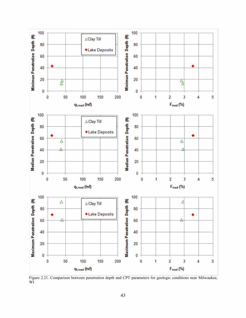
Figure 2.2WI
1. Comparisonn between peneetration depth
43
and CPT paraameters for geoologic conditioons near Milw
aukee,
44
Cone penetration testing for the Marquette Interchange and Mitchell Interchange can be
considered moderately successful. Median values of penetration depth were 40 to 65 ft, with
penetrations in general being deeper in the Lake Deposits. The deepest penetration of 92 feet was
achieved in a clayey till. Dense sands underlying the Lake Deposits resulted in a maximum
penetration of 70 ft. Early refusal in the dense layers underlying the Lake deposits may be
somewhat problematic from a foundation design standpoint. Cone tip resistance must be
averaged over 8 diameters above a proposed pile tip depth and to up to 4 diameters below a
proposed pile tip depth to account for differences in response of small diameter cones and large
diameter piles (see section 6.2).
It is noted that 4/27 CPTs for the Marquette interchange were identified as soft Lake deposits
based on the results of CPT tests. Geologic maps indicated 18/27 CPTs may contain significant
thicknesses of near surface soft Lake sediment.
CPTs in Clayey Tills at the Marquette Interchange and Mitchell Interchange produced similar
results, with median tip resistance values on the order of 40 tsf and median friction ratios just
under 3. Only one CPTU collected high quality measurements of pore pressure for the Mitchell
Interchange project (CPTU-03), and the combination of testing above the water table as well as
interlayer sands and clays resulted in low mean pore pressures observed in the Marquette data.
45
3 Equipment and testing procedures
3.1 Field Equipment
CPTs were primarily performed using the University of Wisconsin-Madison’s 24 ton CPT truck,
Figure 3.1. The truck is a 1982 Mack RM series Hogentogler modified truck that transports the
equipment and powers the hydraulic system. The hydraulic system in turn powers the jacks
mounted at the front, center, and rear of the truck. These jacks elevate the truck to maximize the
reaction force and to provide a level surface to advance the cone. The two exterior jacks at the
center of the truck, closest to the cone, are connected by a beam that provides additional stability
where the cone is pushed into the ground. The hydraulic system also operates the ram system
used to advance the CPT probe, Figure 3.2. The hydraulic ram is capable of 25 ton capacity and
is setup with a rate control allowing advance rates from 0.004 in/sec to 4 in/sec. The hydraulic
pump, rams, and control equipment are located within the box compartment aft of the truck cab.
Due to a hydraulic pump failure, an additional CPT truck was used for a portion of this study.
The Purdue University’s CPT truck is a lighter 7-ton Hogentogler open bed truck, Figure 3.3.
This is a smaller truck had a similar hydraulic system and control panel. Because the dead
weight of the vehicle is much lighter, the truck is equipped with a helical anchoring system to
develop additional reaction force to advance the cone.
The CPT data acquisition equipment was obtained through Vertek in the spring of 2010. The
data acquisition equipment is hard-wired to the CPT probe during sounding and converts the
voltage output from the cone sensors to a digital signal which is transmitted to a conversion box
in the cone truck. The conversion box transforms the digital signal to engineering units based on
a calibration factor that the field laptop can record and display real-time measurements during
the push. The proprietary Vertek software package displays real-time plots of cone measured
data and records measurements for later analysis.
The cone penetrometer probe used for testing is a Hogentogler subtraction type digital seismic
piezocone with a 1.44 in diameter, a 1.55 in2 (10 cm2) projected tip end area, and a friction
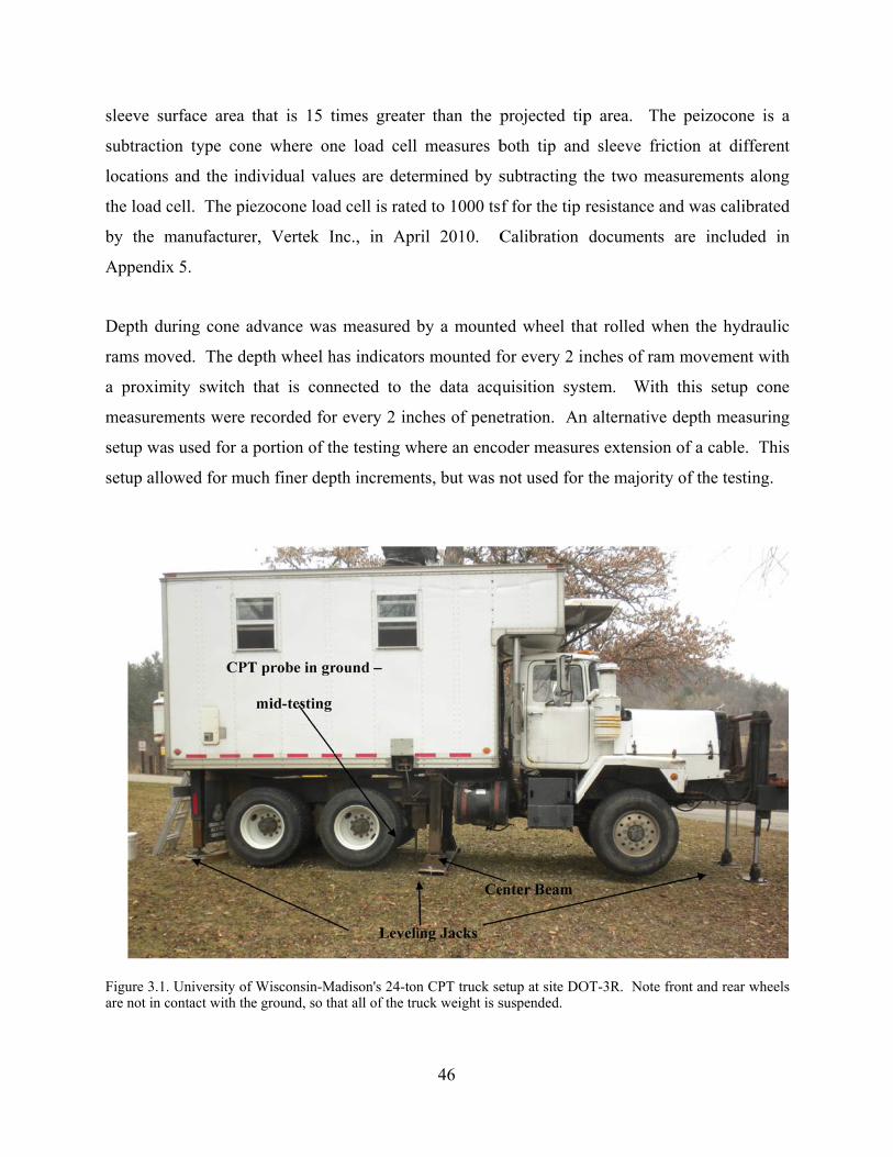
sleeve su
subtractio
locations
the load c
by the m
Appendix
Depth du
rams mov
a proxim
measurem
setup wa
setup allo
Figure 3.1.are not in c
urface area
on type con
s and the ind
cell. The pie
manufacture
x 5.
uring cone a
ved. The de
mity switch
ments were r
as used for a
owed for mu
. University ofcontact with th
that is 15 t
ne where on
dividual valu
ezocone load
er, Vertek I
advance was
epth wheel h
that is conn
recorded for
portion of th
uch finer dep
f Wisconsin-Mhe ground, so th
times greate
ne load cell
ues are dete
d cell is rate
Inc., in Apr
s measured b
has indicator
nected to th
r every 2 inc
he testing wh
pth incremen
Madison's 24-tonhat all of the tru
46
er than the p
measures b
ermined by s
d to 1000 tsf
ril 2010. C
by a mounte
rs mounted f
he data acq
ches of pene
here an enco
nts, but was n
n CPT truck seuck weight is s
projected tip
both tip and
subtracting t
f for the tip
Calibration
ed wheel th
for every 2 in
quisition sys
etration. An
oder measur
not used for
etup at site DOsuspended.
p area. Th
d sleeve fric
the two mea
resistance an
documents
hat rolled wh
nches of ram
stem. With
n alternative
res extension
the majority
OT-3R. Note f
e peizocone
ction at diff
asurements a
nd was calib
are include
hen the hydr
m movement
h this setup
depth meas
n of a cable.
y of the testi
front and rear w
e is a
ferent
along
brated
ed in
raulic
t with
cone
suring
This
ng.
wheels
Figure 3.2frame, and
. Hydraulic rad a new rod wit
am that advancth push cap in p
ces the cone. place.
47
Picture is takeen mid test wiith the rams fuully extended,
top of
Figure 3.3called out.
The con
continuou
the porou
testing w
time afte
conducte
abandone
812.
The prob
arrival tim
shear wa
hammer,
surface w
wired int
measurin
. Purdue Unive
ne is capabl
usly during
us filter loc
was conducte
er cone arre
ed following
ed according
be also has a
mes to be m
ave was gene
Figure 3.4
which allow
to a circuit w
ng time and p
ersity’s CPT tr
le of measu
penetration
ated just ab
ed where the
est. Times
g the proced
g to Wiscons
a geophone i
measured dur
erated at the
. When the
s the shear
with the cent
particle velo
ruck setup on s
uring tip re
. Pore-wate
bove the con
e change in
s allowed fo
dures outlin
sin Departm
installed 6 in
ring pauses i
e surface by
e truck is ja
wave to pro
ter beam suc
city from th
48
site at Long-10
esistance, sl
er pressure m
ne tip at the
pore water
or dissipatio
ned in ASTM
ment of Natur
nches above
in penetratio
y striking the
acked, the c
opagate into
ch that when
e geophone.
0. Jacks for li
leeve frictio
measuremen
e u2 position
pressures w
on tests var
M D 5778.
ral Resource
the friction
on. To measu
e center beam
center beam
the subsurf
n contact is m
.
ifting truck and
on, and por
nts were typ
n. At rod b
was measure
ried. CPT
. CPT soun
es guidelines
n sleeve, allo
ure the shear
m of the tru
is coupled
face. The s
made the com
d helical ancho
re-water pre
ically made
breaks dissip
d with respe
soundings
nding holes
s NR 141 an
owing shear
r wave veloc
uck with a s
with the gr
sledge hamm
mputer can b
ors are
essure
with
pation
ect to
were
were
d NR
wave
city a
ledge
round
mer is
begin
Figure 3.4.
3.2 Sit
When arr
equipmen
signage w
Research
working
workers
to increa
were sele
. Setup for seis
te Setup
riving at the
nt and staff
was set up t
h Center (19
at night. Us
to drivers. S
se visibility.
ected.
smic shear wav
e site and pri
f. All testin
to alert mot
999), Figure
se of emerge
Safety vests
. When ava
ve testing for S
ior to CPT w
ng occurred
torists of wo
e 3.5. Lighti
ency flashers
were worn
ailable, locati
49
CPTU2-01 at D
work proper
on or near
orkers in the
ing was also
s and exterio
at all times
ions with ba
DOT-1.
safety preca
roadways s
e area as ou
o a key saf
or flood light
while work
arriers betwe
autions were
so temporary
utlined by th
fety feature
ting indicate
king outside
een the road
e taken to pr
y, reflective
he Transport
especially w
ed the presen
of the cone
and test loc
rotect
road
tation
while
nce of
truck
cation
Figure 3.5.
Because
performe
site. Th
determin
this explo
would b
procedur
refusal.
initially a
. Site setup at D
the test site
ed prior to so
ese pits wer
ne the nature
oration trenc
e advanced
re was perfor
Secondly, i
advancing th
DOT-10c with
es are locate
ounding. Ty
re small 0.3
of the near
ch or pilot h
through th
rmed for tw
it reduced t
he cone into
traffic control
ed on previo
ypically, som
m by 0.3 m
surface fill,
hole. For sub
he fill with
wo reasons. F
the amount
the ground.
50
devices in the
usly develop
me form of a
m and 0.5m
Figure 3.5.
bsequent sou
gravel prio
First it prote
of near sur
e form of signag
ped land ad
an explorato
m deep and e
A sounding
undings at th
or to advan
ected the con
rface inclina
ge and cones.
dditional site
ory pit was p
excavated w
g would then
he same site
cing the CP
ne from dam
ation change
e preparation
performed at
with hand too
n be perform
e, the dummy
PT probe.
mage and sha
e associated
n was
t each
ols to
med in
y rod
This
allow
with
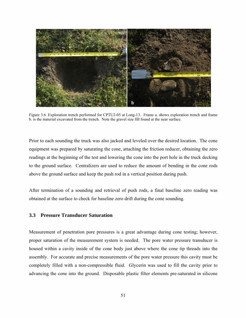
Figure 3.6b. is the ma
Prior to e
equipmen
readings
to the gr
above the
After ter
obtained
3.3 Pr
Measurem
proper sa
housed w
assembly
complete
advancin
. Exploration taterial excavat
each soundin
nt was prepa
at the begin
ound surfac
e ground sur
rmination of
at the surfac
essure Tra
ment of pen
aturation of
within a cav
y. For accur
ely filled wi
ng the cone i
trench performted from the tre
ng the truck
ared by satur
nning of the t
e. Centraliz
rface and kee
f a sounding
ce to check f
ansducer Sa
netration por
the measure
vity inside of
rate and prec
th a non-co
into the grou
med for CPTU2ench. Note the
was also jac
rating the co
test and low
zers are used
ep the push r
g and retriev
for baseline
aturation
re pressures
ement system
f the cone b
cise measure
mpressible
und. Dispos
51
2-05 at Long-13e gravel size fil
cked and lev
one, attachin
ering the con
d to reduce
rod in a vert
val of push
zero drift du
is a great a
m is needed
body just ab
ements of the
fluid. Glyc
sable plastic
3. Frame a. shll found at the n
veled over th
ng the frictio
ne into the p
the amount
tical position
rods, a fina
uring the con
advantage du
d. The pore
bove where t
e pore water
cerin was us
c filter eleme
hows exploratinear surface.
he desired lo
on reducer, o
port hole in t
of bending
n during push
al baseline z
ne sounding.
uring cone t
water press
the cone tip
r pressure th
sed to fill th
ents pre-satu
ion trench and
cation. The
obtaining the
the truck dec
in the cone
h.
zero reading
testing; how
sure transduc
p threads int
his cavity mu
he cavity pri
urated in sil
frame
cone
e zero
cking
e rods
g was
wever,
cer is
to the
ust be
ior to
icone
52
oil were used during the testing program. To saturate the pressure transducer the following
procedure was performed:
Unthread cone tip and invert cone clamping to vise so that pressure transducer cavity is
facing upward
Fill entire cavity with glycerin such that meniscus forms above cone body
Inspect cavity for small air bubbles. If bubbles are present gently tap cone body to agitate
bubbles to the surface
Using syringe fill the channel in the cone tip with glycerin allowing a bead of glycerin to
form around the seat for the pore water pressure filter
Remove saturated filter from the silicone oil container and fit onto tip
Make sure that there is a meniscus above the cone tip and cone body prior to placing the tip
onto the cone
Quickly invert the tip onto the cone to minimize the chance of air bubbles entering the tip
and thread the tip into place. Threading of the tip will displace the excess glycerin out of
the cone body cavity.
Place a thin latex membrane filled with additional glycerin around the saturated cone
pressure transducer and filter to reduce chance of losing saturation prior to initializing the
sounding.
3.4 Test Naming Convention
Tip, friction sleeve, and pore water pressures were measured continuously for all soundings. The
test naming system provides insight into the configuration and data collected for each cone test.
Most soundings are designated CPTU#-##. The U indicates that a piezocone test was performed
and the number directly following, for instance U2, identifies the position of the pore water filter
element. With the CPT probe used for this study u1 and u2 positions are possible, although u2 is
the primary configuration used Figure 1.2. In addition seismic piezocone tests are identified as
SCPTU2-##. The numbers following the cone configuration represent the test number
performed for that study area. In some cases a letter is designated after the cone number
indicating that the sounding was stopped, CPT probe removed from the ground, and a new
53
sounding was started in the same location. This process was typically performed if initial
readings indicated poor saturation of the pore water pressure transducer or some equipment error
was indicated.
3.5 Supplemental Testing
3.5.1 Drilling Operations
Four independent borings were conducted to obtain samples for laboratory testing. These
borings are outlined in Table 3.1. Nominally undisturbed tube samples were obtained at sites
UW-1, DOT-7 and DOT-10c. Disturbed auger samples were obtained at all locations. Samples
were field identified according to the procedures outlined by ASTM D 2488 by an engineer in
the field and preserved for review and subsequent laboratory testing. Logs for borings are
included with site descriptions in Appendix 4.
Table 3.1: Summary of soil borings conducted Site Drill Rig Depth of Sampling Sample Type
UW-1 CME- D 120 98 ft Tube and Split Spoon Long-10 Hand Auger 13 ft Auger (Disturbed) DOT-7 Gehl Skid Steer 10 ft Tube and Auger
DOT-10c Gehl Skid Steer 10 ft Tube and Auger
3.5.2 Laboratory Testing
At multiple study areas laboratory data was available for CPT comparison. These data included
DOT-1 with data provided by WisDOT, UW-1, DOT-7, and DOT-10c with laboratory testing
conducted in the University of Wisconsin-Madison’s geotechnical laboratory. Laboratory tests
conducted include moisture content determination (ASTM D 2216 ), Atterberg limits (ASTM D
4318), fall cone testing, grain size analysis using mechanical sieves and hydrometer (ASTM D
422 and D 6913), oedometer tests (ASTM D 2435), unconsolidated undrained triaxial tests
(ASTM D 2850) and consolidated undrained triaxial tests with pore water pressure
measurements (ASTM D 4767). Available lab data is provided in Appendix 4.
54
3.6 CPT Study Areas
CPT testing was performed at multiple locations across the state of Wisconsin in order to
investigate the different soil types that are typically encountered in engineering design. Specific
locations were coordinated with WisDOT engineers to focus on locations with specific interest.
Coordination with WisDOT was key because use of previous soil boring data was considered for
subsurface interpretation. These locations were typically close to large population centers in the
state and are therefore representative of soil conditions for many foundation design projects.
Site selection was chiefly determined by accessibility for the CPT truck, location proximal to
existing boring data, and site geology. Accessibility was a top priority because most testing
occurred on the side of the road near highway structures. Soundings typically took at least one
day for advance and closure operations. When conducting dissipation testing, individual
soundings required up to 3 days to conduct. For these reasons finding a safe location was a
paramount concern. In addition to safety, slopes and ground hazards were also considered in
evaluating accessibility. Most testing occurred near existing highway structures so that the
subsurface explorations for the highway structure could be used for comparison to CPT results.
Finally, the site geology and depth to bedrock played a role in the site selection.
The cone was advanced until one of multiple refusal criterion were met. The term refusal is used
to indicate a point during a sounding where it is not possible or impractical to continue
advancing the cone deeper. The most apparent case of refusal occurs when the resistance to
pushing is larger than the reaction load of the vehicle. In this case the CPT truck is lifted off of
the ground when attempting to advance deeper and the sounding is stopped for safety reasons.
More commonly, soundings are determined to be at refusal when large changes in inclination
occur over short depth intervals. A high degree of inclination over a short distance stresses the
cone and push rods that may potentially cause damage. This condition was achieved for an
increase of inclination over 1 degree over a depth of 1 m.
55
4 Data presentation and results
4.1 Data presentation
4.1.1 Graphs and Figures
It is most common to show plots of cone tip resistance (qt), friction ratio (F=fs/qcnet %), and
penetration pore pressure (u2) with depth for a CPT sounding (Figure 4.1, Figure 4.2). The
estimated in-situ pore pressure, u0, is plotted on the pore pressure figure, and is typically equal to
u2 in drained sandy soils. Scales are adjusted to encompass the most important aspects of the
data; the sandy soils at the Mn/DOT Wakota Bridge site have a maximum tip resistance scale of
450 tsf, while the soft lake clays at the Mn/DOT St. Vincent’s site have a maximum tip
resistance scale that is an order of magnitude lower, at 40 tsf.
Typical layering can be selected based on major changes in tip resistance, friction ratio, and/or
pore pressure response. These layers can be subgrouped based on estimated formation
environment and/or anticipated engineering response. Five major layers with up to three
occurrences (at different vertical locations) are identified (on the pore pressure plot) in Figure
4.1. It is evident that Layer I generally has a higher tip resistance and lower friction ratio than
Layer II. From bearing capacity theory it is conceptually known that drained sandy soils have
higher bearing capacity factors (Nq) than undrained clayey soils (Nc) [additionally noting that
undrained strength is on the order of 0.25 to 1.0 times 'v0, after Ladd 1991] which is reflected in
Figure 4.1 by higher qt values for the Layer I ‘drained’ sands than the Layer II ‘undrained’
clayey soils. Layer II is split into two sub layers due to variation in friction ratio as well as tip
resistance (which is difficult to see on this linear scale). Layer III is broadly similar to Layer I in
that it has a high cone tip resistance. Additionally, for Layer III the measured penetration pore
pressure (u2) is increasing along the (dashed) hydrostatic (u0) line. Hydrostatic penetration pore
pressures below the water table are also indicative of drained penetration in sandy soils. Sharp
drops in qt are observed in Layer IV at about 55ft and 72ft, which are clear indications of
changes in material behavior. The low tip resistance is coupled with high u2 values, indicating
undrained behavior in a clayey soil. Two thin silty layers are observed in Layer V between 80
and 90 ft, which are characterized by tip resistance that is slightly higher than the undrained case
and pene
from cla
drained t
Figure 4.1.
Figure 4.2.
etration pore
ays to silts t
o drained, an
. Vertical profi
. Vertical profi
e pressures w
to sands, the
nd tip resista
ile of CPT para
ile of CPT para
which are low
e cone pene
ance increase
ameters at the s
ameters at the c
56
wer than the
etration beha
es while pen
sandy Wakota
clayey St. Vinc
e undrained
avior shifts
netration por
Bridge site, M
cent site, MN
case. As ma
from undra
re pressures
MN
aterials trans
ained to par
decrease.
sition
rtially
Figure 4.3.
To aid in
boring lo
equal to a
adjacent
indicate
layer at d
slightly o
. Combined bo
n understand
ogs (Append
a typical val
to the Wis
a predomina
depth, indic
offset in the
oring log and C
ding CPT m
dix 2). SPT N
lue for sandy
sconsin Rive
antly sand p
ated in the
CPT as com
CPT from DOT
easurements
N-value is pl
y soils of 4.
er in Spring
profile, with
CPT profile
mpared to the
57
T-3R
s, data collec
lotted on the
Figure 4.3 s
g Green. In
high tip res
e by increase
e boring due
cted in this
e CPT qt pro
hows an exa
n agreement
sistance and
es in frictio
to spatial va
study are pl
file, with a r
ample from t
with the b
low friction
n ratio and
ariability.
lotted adjace
ratio of (qt/p
the DOT-3R
boring, CPT
n ratios. The
pore pressu
ent to
pref)/N
R site,
data
e clay
ure, is
When ge
resistanc
pressure
Figure 4.4.
Figure 4.5.
enerating cr
e data are ty
data are inve
. Single vertica
. Partial cross s
oss sections
ypically plott
erted with th
al axis plotting
section for Mit
s, a single v
ted with the
he positive a
for cross secti
tchell Interchan
58
vertical axis
positive x-a
axis to the lef
ion developmen
nge project bas
s at a test l
axis to the rig
ft.
nt based on qt
sed on qt and F
location is n
ght, and fric
and F (Mn/DO
F
needed. Con
ction ratio or
OT 8823-01)
ne tip
r pore
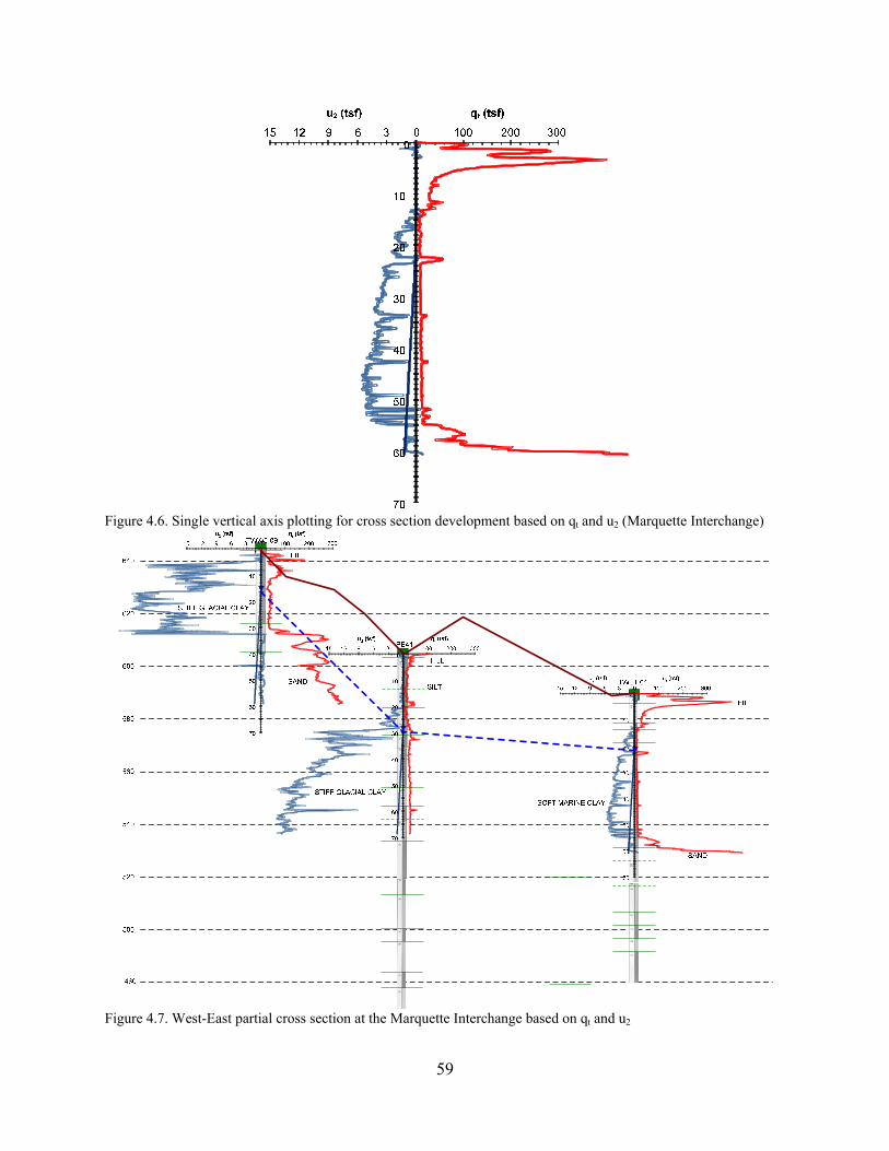
59
Figure 4.6. Single vertical axis plotting for cross section development based on qt and u2 (Marquette Interchange)
Figure 4.7. West-East partial cross section at the Marquette Interchange based on qt and u2
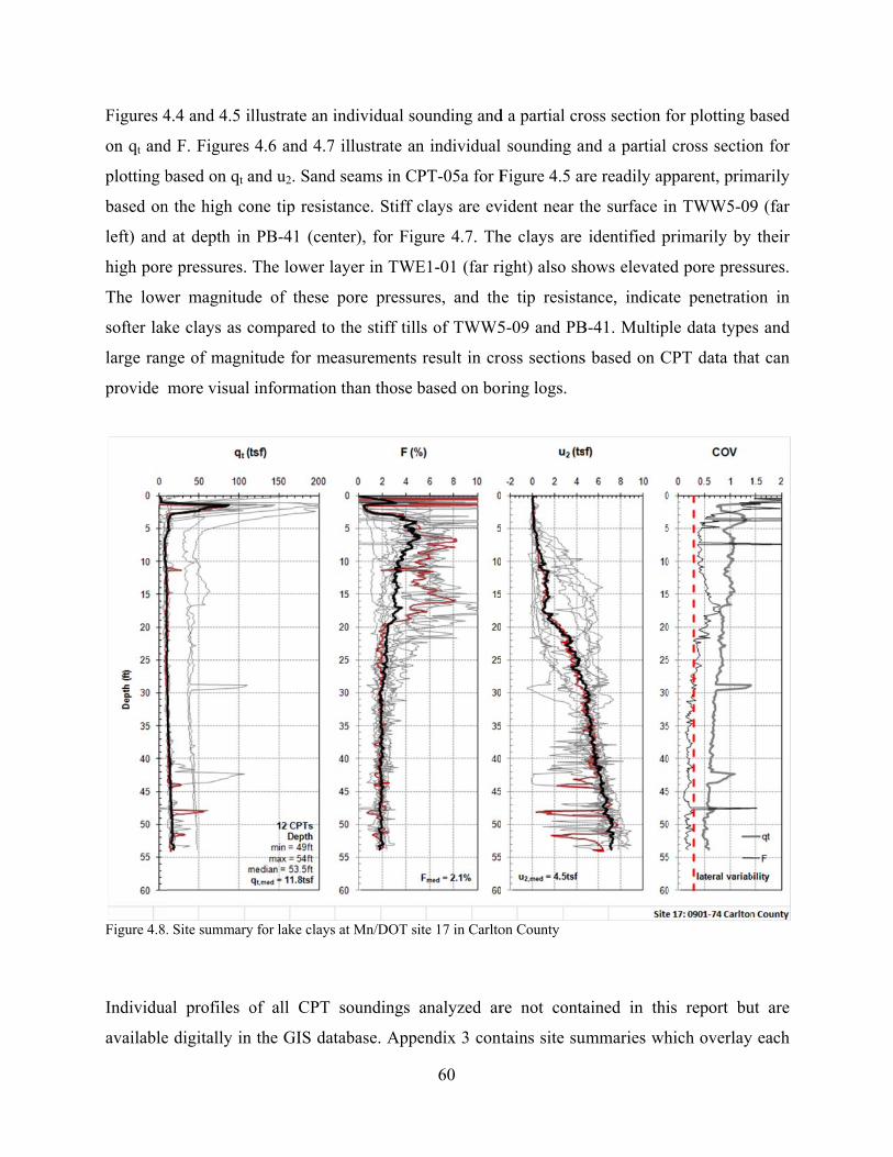
Figures 4
on qt and
plotting b
based on
left) and
high pore
The low
softer lak
large ran
provide
Figure 4.8.
Individua
available
4.4 and 4.5 i
d F. Figures
based on qt a
n the high co
at depth in
e pressures.
er magnitud
ke clays as c
nge of magni
more visual
. Site summary
al profiles o
e digitally in
llustrate an i
4.6 and 4.7
and u2. Sand
one tip resist
PB-41 (cen
The lower l
de of these
compared to
itude for me
information
y for lake clays
of all CPT
n the GIS dat
individual so
7 illustrate an
d seams in CP
tance. Stiff c
nter), for Fig
ayer in TWE
pore pressu
o the stiff till
easurements
n than those b
s at Mn/DOT si
soundings
tabase. App
60
ounding and
n individual
PT-05a for F
clays are ev
gure 4.7. Th
E1-01 (far ri
ures, and th
ls of TWW5
result in cro
based on bor
ite 17 in Carlto
analyzed ar
endix 3 cont
d a partial cro
sounding a
Figure 4.5 ar
vident near th
he clays are
ight) also sh
e tip resista
5-09 and PB
oss sections
ring logs.
on County
re not conta
ntains site su
oss section f
and a partial
re readily ap
he surface in
identified p
hows elevate
ance, indica
B-41. Multip
s based on C
ained in thi
ummaries wh
for plotting b
cross sectio
pparent, prim
n TWW5-09
primarily by
ed pore press
ate penetratio
le data type
CPT data tha
is report bu
hich overlay
based
on for
marily
9 (far
their
sures.
on in
s and
at can
ut are
y each
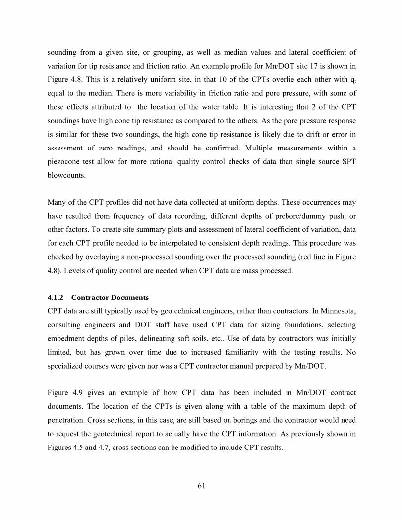
61
sounding from a given site, or grouping, as well as median values and lateral coefficient of
variation for tip resistance and friction ratio. An example profile for Mn/DOT site 17 is shown in
Figure 4.8. This is a relatively uniform site, in that 10 of the CPTs overlie each other with qt
equal to the median. There is more variability in friction ratio and pore pressure, with some of
these effects attributed to the location of the water table. It is interesting that 2 of the CPT
soundings have high cone tip resistance as compared to the others. As the pore pressure response
is similar for these two soundings, the high cone tip resistance is likely due to drift or error in
assessment of zero readings, and should be confirmed. Multiple measurements within a
piezocone test allow for more rational quality control checks of data than single source SPT
blowcounts.
Many of the CPT profiles did not have data collected at uniform depths. These occurrences may
have resulted from frequency of data recording, different depths of prebore/dummy push, or
other factors. To create site summary plots and assessment of lateral coefficient of variation, data
for each CPT profile needed to be interpolated to consistent depth readings. This procedure was
checked by overlaying a non-processed sounding over the processed sounding (red line in Figure
4.8). Levels of quality control are needed when CPT data are mass processed.
4.1.2 Contractor Documents
CPT data are still typically used by geotechnical engineers, rather than contractors. In Minnesota,
consulting engineers and DOT staff have used CPT data for sizing foundations, selecting
embedment depths of piles, delineating soft soils, etc.. Use of data by contractors was initially
limited, but has grown over time due to increased familiarity with the testing results. No
specialized courses were given nor was a CPT contractor manual prepared by Mn/DOT.
Figure 4.9 gives an example of how CPT data has been included in Mn/DOT contract
documents. The location of the CPTs is given along with a table of the maximum depth of
penetration. Cross sections, in this case, are still based on borings and the contractor would need
to request the geotechnical report to actually have the CPT information. As previously shown in
Figures 4.5 and 4.7, cross sections can be modified to include CPT results.
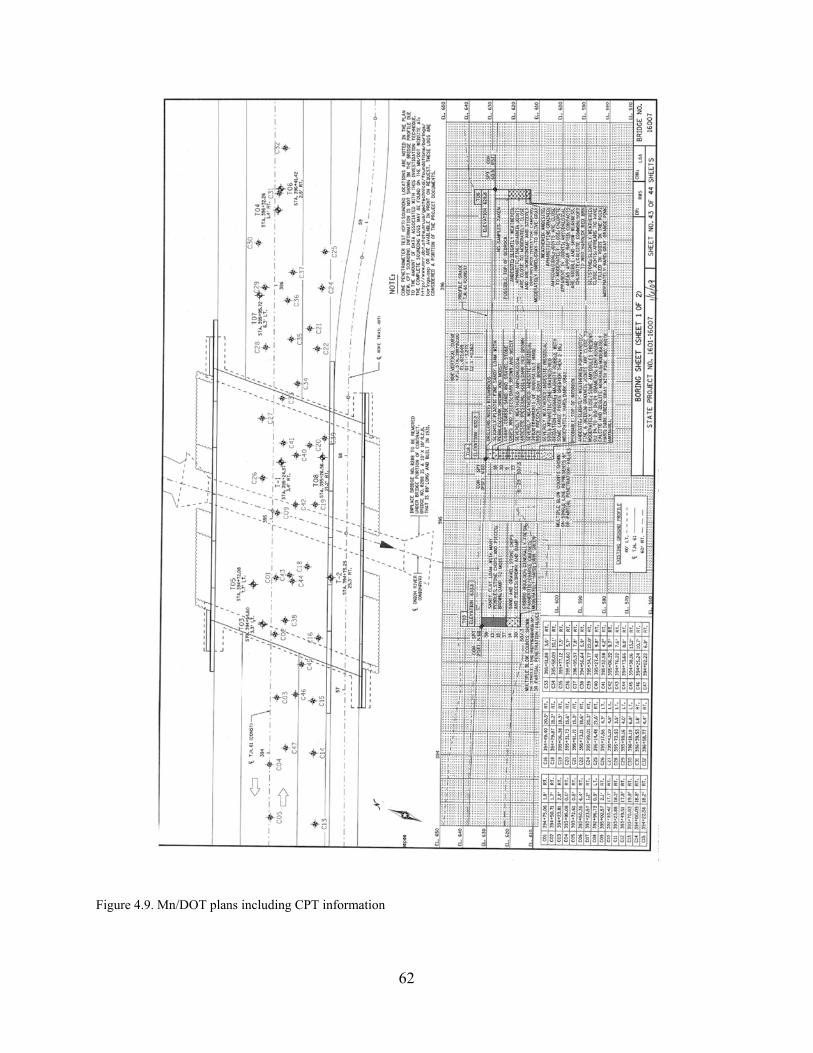
Figure 4.9.. Mn/DOT planns including CPPT information
62
n
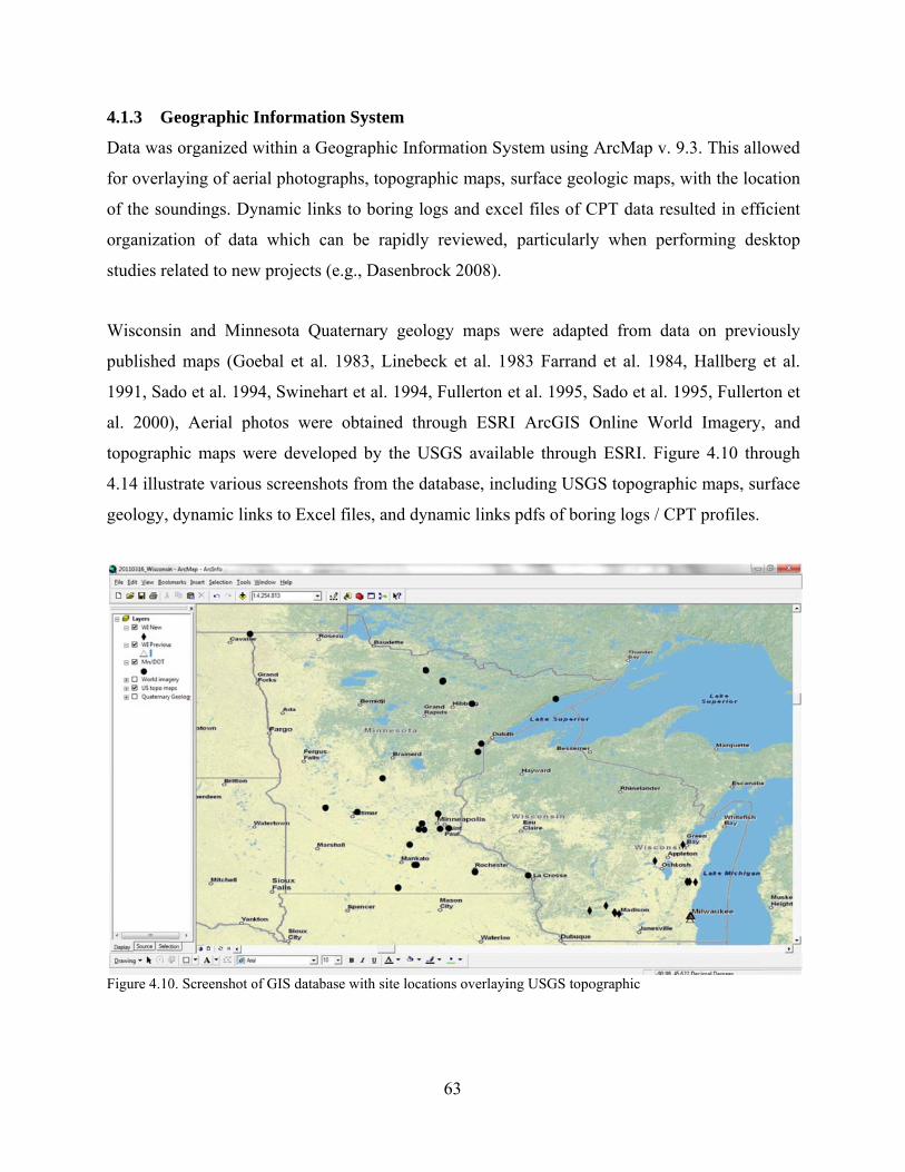
4.1.3 G
Data was
for overl
of the so
organizat
studies re
Wisconsi
published
1991, Sa
al. 2000)
topograp
4.14 illus
geology,
Figure 4.10
Geographic I
s organized w
aying of aer
oundings. Dy
tion of data
elated to new
in and Min
d maps (Go
do et al. 199
), Aerial ph
hic maps w
strate variou
dynamic lin
0. Screenshot o
Information
within a Geo
rial photogra
ynamic links
a which can
w projects (e
nnesota Quat
ebal et al. 1
94, Swinehar
hotos were
were develop
us screenshot
nks to Excel
of GIS databas
n System
ographic Inf
aphs, topogra
s to boring l
n be rapidly
e.g., Dasenbr
ternary geol
1983, Lineb
rt et al. 1994
obtained th
ped by the U
ts from the d
files, and dy
e with site loca
63
formation Sy
aphic maps,
logs and exc
y reviewed,
rock 2008).
logy maps
eck et al. 19
4, Fullerton e
hrough ESR
USGS availa
database, inc
ynamic links
ations overlayi
ystem using
surface geo
cel files of C
particularly
were adapte
983 Farrand
et al. 1995,
RI ArcGIS O
able through
cluding USG
s pdfs of bor
ing USGS topo
ArcMap v. 9
logic maps,
CPT data res
y when per
ed from dat
d et al. 1984
Sado et al. 1
Online Wor
h ESRI. Figu
GS topograph
ring logs / CP
ographic
9.3. This all
with the loc
sulted in effi
rforming de
ta on previ
4, Hallberg
1995, Fullert
rld Imagery,
ure 4.10 thr
hic maps, su
PT profiles.
owed
cation
ficient
sktop
ously
et al.
ton et
, and
rough
urface
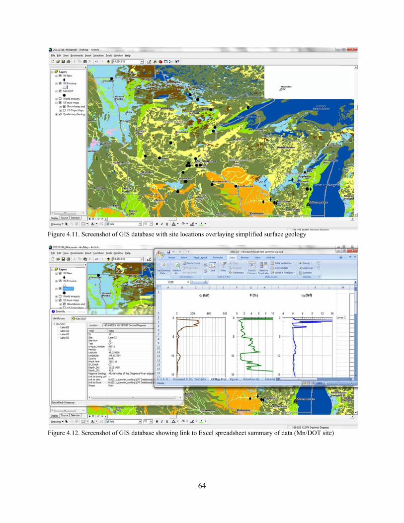
Figure 4.1
Figure 4.12
1. Screenshot o
2. Screenshot o
of GIS databas
of GIS databas
e with site loca
e showing link
64
ations overlayi
k to Excel sprea
ing simplified s
adsheet summa
surface geolog
ary of data (Mn
gy
n/DOT site)
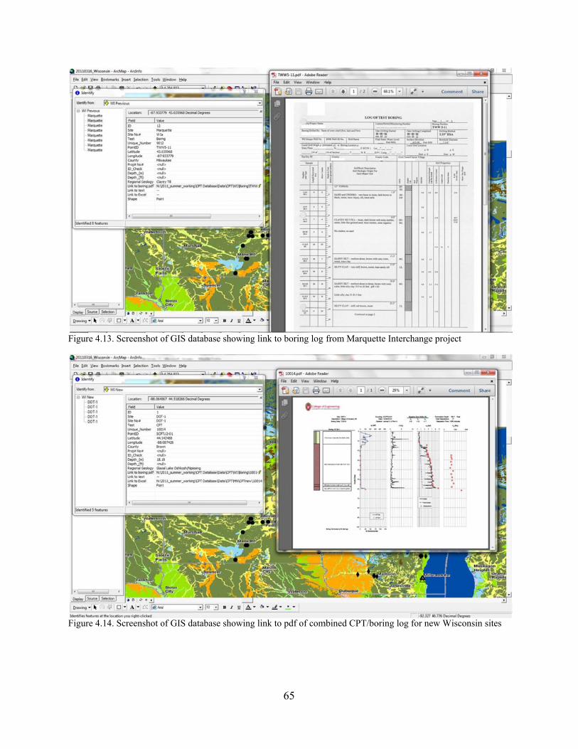
Figure 4.13
Figure 4.14
3. Screenshot o
4. Screenshot o
of GIS databas
of GIS databas
e showing link
e showing link
65
k to boring log
k to pdf of com
from Marquet
mbined CPT/bo
tte Interchange
oring log for ne
project
ew Wisconsin s
sites
66
4.2 Results
A total of 61 soundings at 14 sites were performed for this study, as summarized in Figure 4.15,
Table 4.11, Table 4.12, and Appendix 2. Eight of these soundings were probes using the dummy
push rod, Figure 4.16, and did not result in tip, sleeve or pore-water pressure measurements. Out
of the 53 soundings using the CPT probe, only two did not have saturated pressure transducers,
and 15 of the soundings included seismic shear wave velocity measurements. The depths for all
soundings combined to a total length of 1848 ft. Appendix 2 provides cone profiles of measured
parameters with comparison to WisDOT borings and individual sitemaps.
Dissipation testing was conducted during most soundings. A total of 320 dissipation tests were
performed for a cumulative duration of 212 hours. Many of these tests were short duration, less
than 5 minutes, tests performed during rod breaks to develop a better indication of drainage
conditions.
Figure 4.155: CPT test loccations shown aagainst surficia
67
al geology mapp.
Figure 4.1dummy pupulverized
CPTs we
of 0.8 in/
rate effec
Site char
CPT pro
character
6. The dummy
ush rod was usematerial.
ere performe
/s +/- 0.2 in/
cts at sites U
racteristics a
operties sorte
rizes minimu
y rod consists ed to check for
ed following
/sec. Variab
UW-1, DOT-
and average
ed by estim
um, median,
of a conical tr near surface r
the guidelin
ble rate CPT
10c, and DO
CPT prope
mated surface
and maximu
68
tip welded to refusal and pre
nes of ASTM
testing was
OT-7. Result
erties are co
e geology ar
um penetrati
a push rod wiesence of grave
M D 5778 th
conducted t
ts are discuss
ontained in T
re presented
ion achieved
ith a 1.75 in oel fill. Note w
hat requires a
to assess CP
sed by Hotst
Tables 4.1 a
d in Tables
d at each site
outer diameterwhite dust on tip
a penetration
PT probe adv
tream (2011)
and 4.2. Av
4.3. Figure
e.
r. The p from
n rate
vance
).
erage
4.17
69
Table 4.1. Summary of regional geology for WisDOT sites tested UW
Site No. UW
Site ID County Regional Geology
T01 UW-1 Dane Lake T02 Long-10 Dane Outwash T03 Long-12 Dane Outwash T04 Long-13 Dane Outwash T05 DOT-7 Dane Outwash T06 Long-11 Dane Outwash T07 DOT-1 Brown Lake / Fill T08 DOT-16 Winnebago Clayey Till T09 DOT-10 Sheboygan Fill T10 DOT-10a Sheboygan Clayey Till T11 DOT-10b Sheboygan Clayey Till T12 DOT-10c Sheboygan Clayey Till T13 DOT-3R Sauk Alluvium T14 Long-8 Dane Alluvium
Table 4.2. Summary of CPT performance for WisDOT sites tested UW Site No.
UW Site ID
County # CPTs1
Depth (ft) Median CPTU values lateral variability2 min median max qt
(tsf) F
(%) u2
(tsf) T01 UW-1 Dane 4 (5) 13 65 99.6 130 1.0 0.9 low T02 Long-10 Dane 7 26 26 89 87 1.3 0.3 low-mod T03 Long-12 Dane 1 - 62.8 - 128 1.4 1.0 - T04 Long-13 Dane 1 - 56 - 144 1.2 0.5 - T05 DOT-7 Dane 8 12.5 14.8 42.7 67 0.8 0.4 low T06 Long-11 Dane 2 23.9 53.2 38.6 177 1.0 0.1 low T07 DOT-1 Brown 2(5) 3.3 3.3 70 9.7 0.7 5.1 low T08 DOT-16 Winnebago 4 15 25 35.4 33.8 2.4 2.5 low T09 DOT-10 Sheboygan 0 (4) 2.5 3.2 3.9 - - - - T10 DOT-10a Sheboygan 2 (3) 7.6 7.7 7.9 167 0.7 0.1 mod-high T11 DOT-10b Sheboygan 5 5.7 12.8 24 34.4 3.4 0.6 moderate T12 DOT-10c Sheboygan 6 19.7 21.9 26.3 29 3.4 1.3 moderate T13 DOT-3R Sauk 5 73.4 73.6 78.1 142 0.7 1.1 low T14 Long-8 Dane 5 2 5.7 9.2 40.7 1.7 0.3 moderate
1 number in parentheses indicates total number of cones pushed, includes dummy probes that met shallow refusal and erroneous CPTU1 qc and fs data from UW-1
2 for lateral variability, high = a majority of depths with qt COV > 1, low = a majority of depths with qt COV ≤ 0.3, moderate = a majority of depths with 0.3 ≤ qt COV ≤ 1, dual symbols used for profiles with mixed variability Table 4.3. Summary of CPT performance for WisDOT sites tested by geology Regional Geology #
CPTs1 Depth (ft) Median CPTU values lateral
variability2 min median max qt (tsf)
F (%)
u2 (tsf)
Fill 0 (7) 2.5 3.3 3.9 - - - - Lake 6 (7) 13.1 65.3 99.6 60.1 1.0 1.6 high Alluvium 10 2 41.3 78.1 141 0.7 1.0 high Outwash 19 12.5 26.3 88.8 102.6 1.2 0.4 moderate Clayey Till 17 (18) 5.7 19.4 35.4 32.3 2.9 1.1 low-mod 1 number in parentheses indicates total number of cones pushed, includes dummy probes that met shallow refusal and erroneous CPTU1 qc and fs data from UW-1
2 for lateral variability, high = a majority of depths with qt COV > 1, low = a majority of depths with qt COV ≤ 0.3, moderate = a majority of depths with 0.3 ≤ qt COV ≤ 1, dual symbols used for profiles with mixed variability
Figure 4.1Wisconsin
17. Comparisoon between penetration dep
70
pth and CPT parameters ffor geologic cconditions test
ted in
71
Good success was achieved in Lake, Alluvium, and Outwash conditions, with maximum
penetration depths exceeding 75 feet in each geological condition. Data from Long-8 near the
Wisconsin river are grouped with the Alluvial deposits from site DOT-3R. Good performance
was achieved at site DOT-3R, with a median penetration of 74 feet, but the maximum
penetration at site Long-8 was less than 10 feet. The Long-8 site may have had geological
conditions more similar to a loamy till than alluvium. The clayey tills of Sheboygan county also
resulted in difficult testing conditions, with numerous near surface refusals from cobbles and
gravel. Continuing eastward from Plymouth resulted in deeper penetrations, with relatively
successful testing at site DOT-10c. The inability to penetrate greater than 4 ft at site DOT-10 is
attributed the fill soils that also contain gravel, rather than the natural material. Difficulties were
also encountered for the fill soils at site DOT-1 in Green Bay.
On average, penetration depths were lower in this study as compared to data reviewed from
Mn/DOT and tests performed by commercial firms in the Milwaukee area. It is noted that
median tip resistance values recorded at sites in this study were higher from previous sites in
glacial geology reviewed. Both sites in Milwaukee had median tip resistance values less than 50
tsf, and 18/21 Mn/DOT sites had median tip resistance values less than 55 tsf. Only 5/14 sites
tested in this study had median tip resistance values less than 55 tsf, and 6/14 had median tip
resistance values greater than 125 tsf. This being said, it is not the median tip resistance that
results in refusal, it is the local maximum tip resistance or potential to cause sharp changes in
inclination. These difficulties arose due to the presence of gravel and cobbles, mostly
encountered in the relatively low tip resistance clayey tills.
Commercial testing in the Milwaukee area had greater success when retesting adjacent to a
sounding which had met refusal than retesting in this study. If testing in this program met refusal,
retesting was performed at an offset of 6 ft. Additional offsets at 30 to 60 feet from a given
location were attempted for repeat refusals. Excavation of near surface material aided in some
situations, such as DOT-7, but was generally only successful if gravel and cobbles were limited
to the upper 1 to 2 feet.
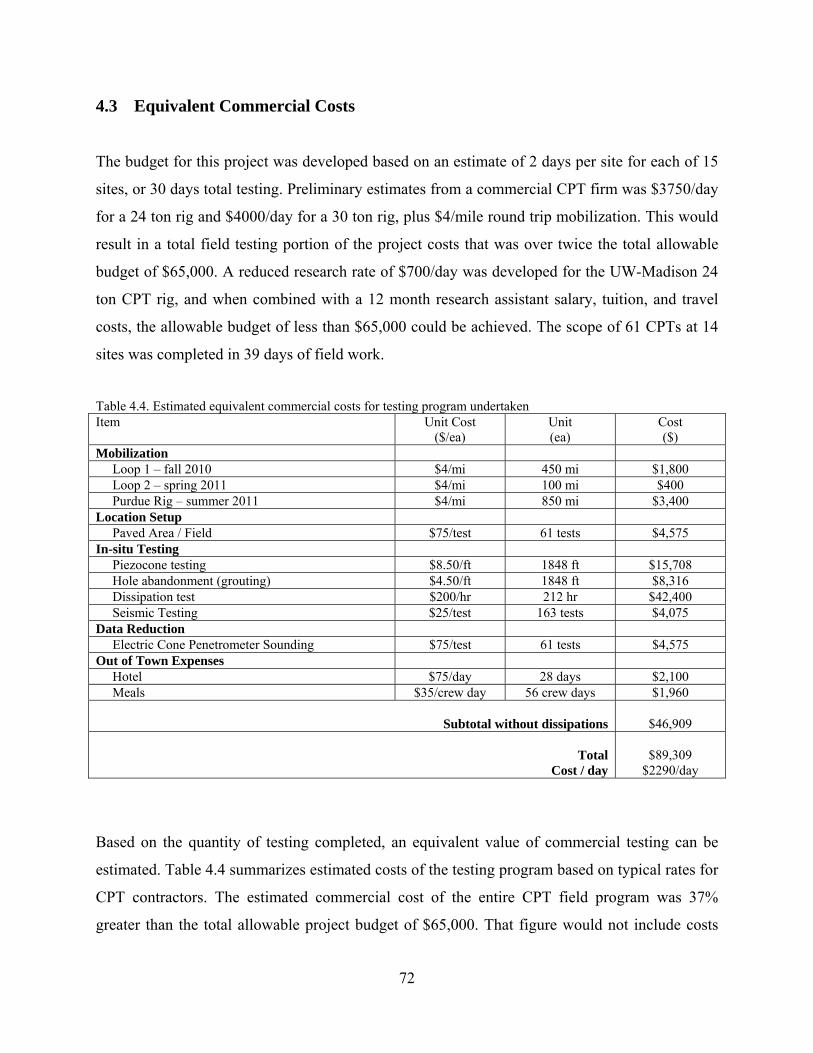
72
4.3 Equivalent Commercial Costs
The budget for this project was developed based on an estimate of 2 days per site for each of 15
sites, or 30 days total testing. Preliminary estimates from a commercial CPT firm was $3750/day
for a 24 ton rig and $4000/day for a 30 ton rig, plus $4/mile round trip mobilization. This would
result in a total field testing portion of the project costs that was over twice the total allowable
budget of $65,000. A reduced research rate of $700/day was developed for the UW-Madison 24
ton CPT rig, and when combined with a 12 month research assistant salary, tuition, and travel
costs, the allowable budget of less than $65,000 could be achieved. The scope of 61 CPTs at 14
sites was completed in 39 days of field work.
Table 4.4. Estimated equivalent commercial costs for testing program undertaken Item Unit Cost
($/ea) Unit (ea)
Cost ($)
Mobilization Loop 1 – fall 2010 $4/mi 450 mi $1,800 Loop 2 – spring 2011 $4/mi 100 mi $400 Purdue Rig – summer 2011 $4/mi 850 mi $3,400 Location Setup Paved Area / Field $75/test 61 tests $4,575 In-situ Testing Piezocone testing $8.50/ft 1848 ft $15,708 Hole abandonment (grouting) $4.50/ft 1848 ft $8,316 Dissipation test $200/hr 212 hr $42,400 Seismic Testing $25/test 163 tests $4,075 Data Reduction Electric Cone Penetrometer Sounding $75/test 61 tests $4,575 Out of Town Expenses Hotel $75/day 28 days $2,100 Meals $35/crew day 56 crew days $1,960
Subtotal without dissipations
$46,909
Total
Cost / day
$89,309
$2290/day
Based on the quantity of testing completed, an equivalent value of commercial testing can be
estimated. Table 4.4 summarizes estimated costs of the testing program based on typical rates for
CPT contractors. The estimated commercial cost of the entire CPT field program was 37%
greater than the total allowable project budget of $65,000. That figure would not include costs
73
associated with compilation of this report, evaluation of CPT data from previous sites, or
supplemental borings and laboratory testing performed. The average day rate based on
commercial production rates would be on the order of $2,300, however, due to the research
nature of this study, productivity in terms of footage was lower than that of a commercial firm.
Dissipation testing accounted for 47% of the total estimated commercial budget. Collection and
interpretation of dissipation test results was paramount to this study and the understanding of
CPT data in Wisconsin, but may not be needed for routine project testing once experience is
organized.
74
5 Evaluation of soil behavior and properties
5.1 CPT and SPT correlations
In areas where use of the CPT is not prevalent, many engineers have developed their experience
evaluating soil resistance based on SPT N-value. A first stage in starting to adopt the CPT often
involves creating equivalent SPT blowcount profiles from CPT data (e.g., Robertson et al. 1983,
Jeffereies & Davies 1993) and then applying SPT based correlation that the engineer is more
comfortable with. Now that CPT based correlations to material properties have sufficiently large
databases (e.g., Lunne et al. 1997, Mayne 2007), the intermediate step of generating correlations
between cone tip resistance and SPT blowcount is unnecessary. However, the large amount of qt
and SPT N-value data that are available in this study makes a review of qt and N correlations
appropriate. Data from Minnesota is presented as energy corrected N60 values, while the
correction of data from Wisconsin is uncertain and uncorrected N value are used.
Figure 5.1 illustrates correlations between (qt/pref) and SPT N-value in relation to CPT
normalized cone tip resistance and CPT friction ratio. Detail on the breakdown of the database
and specific correlations for different soil types is contained in Tables 5.1 and 5.2. A reference
stress (pref) equal to 1 atmosphere (1.058 tsf) is used to make the correlation nondimensional.
Similar observations are made for each study, which are in general agreement with (qt/pref)/N60
ratios presented by Robertson et al. (1983); (i) (qt/pref)/N60 increases from approximately unity in
fine grained soil to approximately 4 in coarse grained soils; (ii) the coefficient of variation is
between 50 and 100%. For the new Wisconsin sites (this study), 18 tests in soft clays and organic
material had blowcounts of zero, negating the applicability of the N-value or assessment of
(qt/pref)/N. The ability to accurately measure resistance in very soft soils is an advantage of the
CPT.

Figure 5.1.. Comparison oof SPT and CPT penetration r
75
resistance
76
Table 5.1. Comparison of CPT and SPT penetration resistance in organic and clayey soils Dataset Organic Low Plasticity Clay High Plasticity Clay Median COV n Median COV n Median COV n Minnesota
1.0 0.45 9 1.3 0.53 44 1.9 0.41 28
Wisconsin Marquette / Mitchell
1.2 0.56 13 2.4 0.72 63 - - -
Wisconsin UW Study
0.6 - 1a 2.3 0.71 26b - - -
a 2 tests with SPT N-value of 0 (weight of rods or weight of hammer) b 16 tests with SPT N-value of 0 (weight of rods or weight of hammer) Table 5.2. Comparison of CPT and SPT penetration resistance in sands, sand mixtures, and fill Dataset Sand Loam Fill Median COV n Median COV n Median COV n Minnesota 3.8 0.31 36 2.5 0.88 24 - - - Wisconsin Marquette / Mitchell 3.5 0.83 8 2.2 0.96 5 4.3 0.82 29 Wisconsin UW Study 5.6 0.46 35 2.5 0.49 20 - - -
It is interesting to note, that on average (qt/pref)/N ratios for Wisconsin sites were 50 to 80%
higher than those from Minnesota and the coefficient of variations for the correlations are higher.
It is inferred that these differences and higher uncertainties are associated with SPT hammer
energy and other correction factors. The higher (qt/pref)/N ratios for Wisconsin sites indicate
lower N-values, which indicate transferred energies greater than 60%. It is recommended that if
SPT data is collected at a site, a calibrated hammer is used and data are presented as N60 rather
than N. This will reduce uncertainty in application, and may lead to less conservative assessment
of engineering parameters.
5.2 Assessment of Geotechnical Parameters
This section focuses on correlations between CPT measurements and mechanical parameters.
Definitions and a summary of engineering parameters discussed in this section are presented in
Section 2.1.2.
5.2.1 W
Within t
importan
concern,
undraine
between
water flo
penetrati
or hydrau
on assess
Figure 5.2.
Water fl
Pumping
were ava
penetrati
provided
Water Flow
transportatio
nt to time r
particularly
d or partial
engineering
ow characte
on testing. S
ulic conduct
sment of the
. Drainage con
ow characte
g tests would
ailable for t
on test to la
d by WisDOT
Characteris
on engineeri
rate settleme
y in glacial d
lly drained
g properties
eristics and
Slightly diffe
tivity (kh) ba
coefficient o
ditions associa
eristics cann
d need to b
this study. C
aboratory da
T and perfor
stics
ing, water
ent and stre
deposits, is
conditions.
and CPT res
soil type in
erent bounda
ased assessm
of consolida
ated with cone
not be teste
be performed
Comparison
ata was per
rmed in the U
77
flow charac
ength gain f
whether an
These drain
sponse. Figu
n relation to
aries are asse
ment of drai
ation and hyd
penetration tes
d in the fie
d after bore
of water fl
formed usin
UW-Madison
cteristics ar
for soft gro
in-situ test
nage condit
ure 5.2 illus
o drainage
essed for coe
inage condit
draulic cond
sting as compa
eld using th
ehole comple
flow charact
ng results of
n geotechnic
re commonl
ound constru
is performe
ions will af
trates a rela
conditions
efficient of c
tions. This s
ductivity from
ared to soil type
he standard
etion. No pu
teristics mea
f laboratory
cal laborator
ly seen as
uction. Of
ed under dra
ffect correla
ationship bet
during and
consolidation
section will
m in-situ test
e
penetration
umping test
asured in a
y oedometer
ry.
most
equal
ained,
ations
tween
cone
n (ch)
focus
ts.
n test.
t data
cone
tests
78
Dissipation testing measures the change in pore-water pressure with time during a halt in
penetration. This test is analogous to an oedometer test where a load is applied to the soil and
reduction in pore pressure (or settlement related to increases in effective stress) is measured with
time. Results of CPTU dissipation tests can be used to directly assess the coefficient of
consolidation and indirectly assess the hydraulic conductivity.
Results are analyzed in terms of the dimensionless normalized excess pore-water pressure, U:
i
t
i
t
u
u
uu
uuU
0
0 (5.1)
ut is the measured pore pressure at time t, u0 is the in-situ hydrostatic pore water pressure, and ui
is the measured pore water pressure at the beginning of the dissipation. t100 is the time to 100%
dissipation of excess pore-water pressures where the measured pore-water pressure is equivalent
to the hydrostatic value (um = u0). Conventional dissipation curves decrease continually with
time. Normalized modified time factors (T*) can be used to analyze the coefficient of
consolidation from dissipation tests.
t
IrTc r
h
2* (5.2)
where r is the cone radius, T* is a modified time factor (Table 5.3) and t is the time to reach that
percentage of dissipation or consolidation, for example t50 for T*50. Equation 5.2 is typically
applied by determining the initial pore pressure at the beginning of the test, calculating U at each
time measurement, and determining the time at 50% dissipation, t50, when U = 0.5. The ch
calculation is typically performed using t50, but may be taken from any point on the dissipation
curve. Schnaid et al. (1997) compared the variability of results depending on what percent of
consolidation is selected and found that estimates taken at 50% and greater displayed less
variability. This is an important point because conducting a dissipation test to hydrostatic values
in soils with low hydraulic conductivities may require several days.
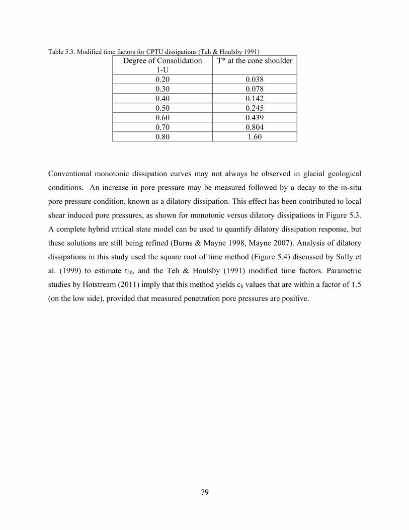
79
Table 5.3. Modified time factors for CPTU dissipations (Teh & Houlsby 1991) Degree of Consolidation
1-U T* at the cone shoulder
0.20 0.038 0.30 0.078 0.40 0.142 0.50 0.245 0.60 0.439 0.70 0.804 0.80 1.60
Conventional monotonic dissipation curves may not always be observed in glacial geological
conditions. An increase in pore pressure may be measured followed by a decay to the in-situ
pore pressure condition, known as a dilatory dissipation. This effect has been contributed to local
shear induced pore pressures, as shown for monotonic versus dilatory dissipations in Figure 5.3.
A complete hybrid critical state model can be used to quantify dilatory dissipation response, but
these solutions are still being refined (Burns & Mayne 1998, Mayne 2007). Analysis of dilatory
dissipations in this study used the square root of time method (Figure 5.4) discussed by Sully et
al. (1999) to estimate t50, and the Teh & Houlsby (1991) modified time factors. Parametric
studies by Hotstream (2011) imply that this method yields ch values that are within a factor of 1.5
(on the low side), provided that measured penetration pore pressures are positive.
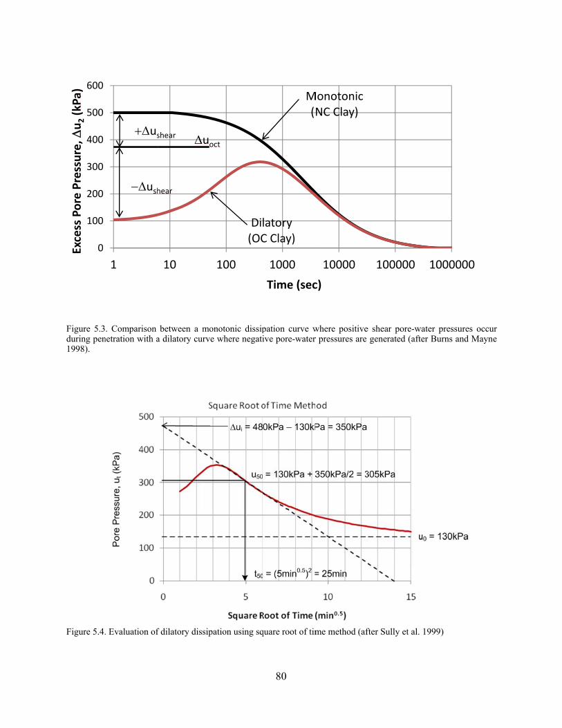
Figure 5.3during pen1998).
Figure 5.4.
0
100
200
300
400
500
600Excess Pore Pressure,
u2(kPa)
. Comparison netration with a
. Evaluation of
1
ush
us
between a moa dilatory curv
f dilatory dissip
10
hear
shear uo
onotonic dissipe where negati
pation using sq
100
Dil(OC
oct
80
pation curve wive pore-water
quare root of tim
1000
Time (sec
latoryC Clay)
M(
where positiver pressures are
me method (af
10000
c)
MonotonicNC Clay)
e shear pore-wgenerated (aft
fter Sully et al.
100000
water pressures ter Burns and M
1999)
1000000
occur Mayne
0
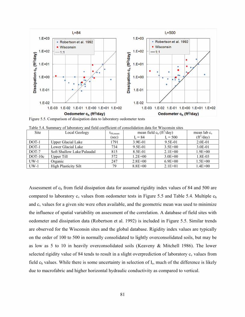
Figure 5.5. Table 5.4.
Site
DOT-1 DOT-1 DOT-7 DOT-10c UW-1 UW-1
Assessm
compared
and cv va
the influe
oedomete
are obser
on the or
as low a
selected r
field ch v
due to m
. Comparison o
Summary of laLo
Upper GlacLower GlacSoft ShalloUpper Till Organic High Plasti
ent of ch fro
d to laborato
alues for a gi
ence of spati
er and dissip
rved for the
rder of 100 t
as 5 to 10 i
rigidity valu
values. While
acrofabric an
of dissipation d
aboratory and focal Geology
cial Lake cial Lake w Lake/Palaud
city Silt
om field diss
ory cv value
iven site wer
ial variabilit
pation data (
Wisconsin s
to 500 in nor
in heavily o
ue of 84 tend
e there is som
nd higher ho
data to laborato
field coefficient50,m
(se1773
dal 8157247
ipation data
s from oedo
re often avai
y on assessm
(Robertson e
sites and the
rmally conso
overconsolid
ds to result in
me uncertain
orizontal hyd
81
ory oedometer
nt of consolidatmean ec)
mIr =
91 3.934 9.515 8.572 1.2E47 2.8E9 8.8E
for assumed
ometer tests
ilable, and th
ment of the c
et al. 1992)
e global data
olidated to li
dated soils (
n a slight ov
nty in select
draulic condu
tests
tion data for Wmean field ch (= 84
9E-01 5E-01 5E-01 E+00 E+00 E+00
d rigidity ind
in Figure 5.
he geometric
correlation. A
is included
abase. Rigidi
ightly overco
(Keaveny &
verprediction
tion of Ir, mu
ductivity as c
Wisconsin sites (ft2/day)
Ir = 500 9.5E-01 3.5E+00 2.1E+00 3.0E+00 6.9E+00 2.1E+01
dex values o
.5 and Table
c mean was
A database o
in Figure 5.
ity index va
onsolidated
& Mitchell 1
n of laborato
uch of the di
compared to
mean lab(ft2/da2.0E-03.0E-01.9E+01.8E-01.5E+01.4E+0
of 84 and 50
e 5.4. Multip
used to mini
of field sites
.5. Similar tr
lues are typi
soils, but m
986). The l
ry cv values
ifference is l
vertical.
b cv ay) 01 01 00 03 00 00
00 are
ple ch
imize
s with
rends
ically
ay be
lower
from
likely
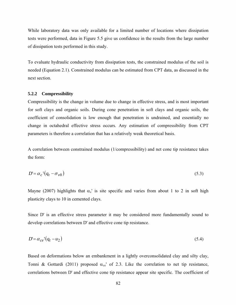
82
While laboratory data was only available for a limited number of locations where dissipation
tests were performed, data in Figure 5.5 give us confidence in the results from the large number
of dissipation tests performed in this study.
To evaluate hydraulic conductivity from dissipation tests, the constrained modulus of the soil is
needed (Equation 2.1). Constrained modulus can be estimated from CPT data, as discussed in the
next section.
5.2.2 Compressibility
Compressibility is the change in volume due to change in effective stress, and is most important
for soft clays and organic soils. During cone penetration in soft clays and organic soils, the
coefficient of consolidation is low enough that penetration is undrained, and essentially no
change in octahedral effective stress occurs. Any estimation of compressibility from CPT
parameters is therefore a correlation that has a relatively weak theoretical basis.
A correlation between constrained modulus (1/compressibility) and net cone tip resistance takes
the form:
0'' vtc qD (5.3)
Mayne (2007) highlights that c' is site specific and varies from about 1 to 2 in soft high
plasticity clays to 10 in cemented clays.
Since D' is an effective stress parameter it may be considered more fundamentally sound to
develop correlations between D' and effective cone tip resistance.
2'' uqD tce (5.4)
Based on deformations below an embankment in a lightly overconsolidated clay and silty clay,
Tonni & Gottardi (2011) proposed ce' of 2.3. Like the correlation to net tip resistance,
correlations between D' and effective cone tip resistance appear site specific. The coefficient of
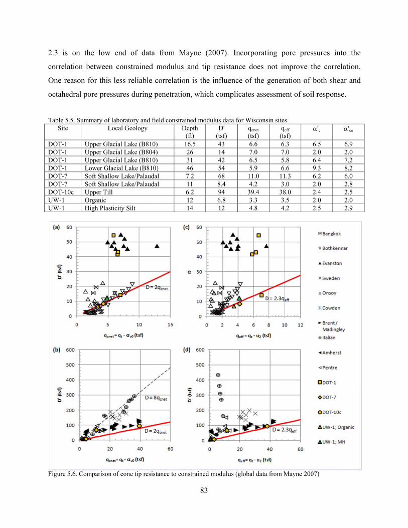
2.3 is on
correlatio
One reas
octahedra
Table 5.5. Site
DOT-1 DOT-1 DOT-1 DOT-1 DOT-7 DOT-7 DOT-10c UW-1 UW-1
Figure 5.6.
n the low
on between
son for this l
al pore press
Summary of laLo
Upper GlacUpper GlacUpper GlacLower GlacSoft ShalloSoft ShalloUpper Till Organic High Plasti
. Comparison o
end of data
constrained
less reliable
sures during
aboratory and focal Geology
cial Lake (B810cial Lake (B804cial Lake (B810cial Lake (B81w Lake/Palaudw Lake/Palaud
city Silt
of cone tip resi
a from May
d modulus a
correlation
penetration,
field constraineDep
(ft0) 164) 260) 310) 46
dal 7.dal 11
6.1214
istance to const
83
yne (2007).
nd tip resist
is the influe
, which com
ed modulus dapth t)
D' (tsf)
.5 43 6 14 1 42 6 54 2 68 1 8.42 94 2 6.84 12
trained modulu
Incorporati
tance does n
ence of the g
mplicates asse
ata for Wisconsqcnet (tsf) 6.6 7.0 6.5 5.9
11.0 4.2
39.4 3.3 4.8
us (global data
ing pore pr
not improve
generation o
essment of s
sin sites qeff (tsf) 6.3 7.0 5.8 6.6
11.3 3.0
38.0 3.5 4.2
a from Mayne 2
ressures into
e the correla
of both shea
soil response
'c
6.5 2.0 6.4 9.3 6.2 2.0 2.4 2.0 2.5
2007)
o the
ation.
ar and
e.
'ce
6.9 2.0 7.2 8.2 6.0 2.8 2.5 2.0 2.9
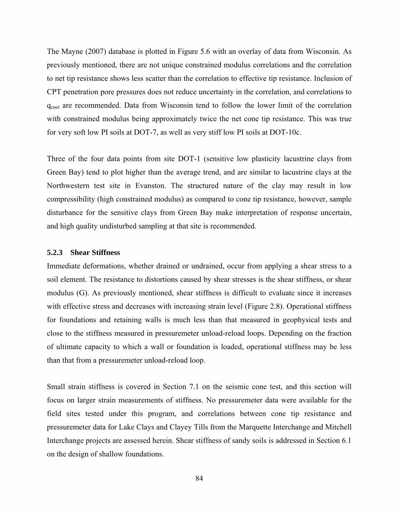
84
The Mayne (2007) database is plotted in Figure 5.6 with an overlay of data from Wisconsin. As
previously mentioned, there are not unique constrained modulus correlations and the correlation
to net tip resistance shows less scatter than the correlation to effective tip resistance. Inclusion of
CPT penetration pore pressures does not reduce uncertainty in the correlation, and correlations to
qcnet are recommended. Data from Wisconsin tend to follow the lower limit of the correlation
with constrained modulus being approximately twice the net cone tip resistance. This was true
for very soft low PI soils at DOT-7, as well as very stiff low PI soils at DOT-10c.
Three of the four data points from site DOT-1 (sensitive low plasticity lacustrine clays from
Green Bay) tend to plot higher than the average trend, and are similar to lacustrine clays at the
Northwestern test site in Evanston. The structured nature of the clay may result in low
compressibility (high constrained modulus) as compared to cone tip resistance, however, sample
disturbance for the sensitive clays from Green Bay make interpretation of response uncertain,
and high quality undisturbed sampling at that site is recommended.
5.2.3 Shear Stiffness
Immediate deformations, whether drained or undrained, occur from applying a shear stress to a
soil element. The resistance to distortions caused by shear stresses is the shear stiffness, or shear
modulus (G). As previously mentioned, shear stiffness is difficult to evaluate since it increases
with effective stress and decreases with increasing strain level (Figure 2.8). Operational stiffness
for foundations and retaining walls is much less than that measured in geophysical tests and
close to the stiffness measured in pressuremeter unload-reload loops. Depending on the fraction
of ultimate capacity to which a wall or foundation is loaded, operational stiffness may be less
than that from a pressuremeter unload-reload loop.
Small strain stiffness is covered in Section 7.1 on the seismic cone test, and this section will
focus on larger strain measurements of stiffness. No pressuremeter data were available for the
field sites tested under this program, and correlations between cone tip resistance and
pressuremeter data for Lake Clays and Clayey Tills from the Marquette Interchange and Mitchell
Interchange projects are assessed herein. Shear stiffness of sandy soils is addressed in Section 6.1
on the design of shallow foundations.
Figure 5.7normalized
Figure 5
resistanc
Marquett
correlatio
since net
next sect
increases
5.7, Gu-r/
correlate
roughly s
clay.
Data from
from the
resistanc
penetrati
pressurem
7. Comparisond cone tip resis
5.7 compare
e. No CPT
te Interchan
ons in Table
t cone tip res
tion). Ir has
s (e.g., Keav
/qcnet is plotte
well with O
shows Ir red
m the Mitch
Marquette I
e. This is n
on resistanc
meter test m
n of pressuremstance
es the unloa
Ts were per
nge project,
e 5.1. The ra
sistance duri
been shown
veny & Mitc
ed against no
OCR (e.g., M
ducing from
hell Intercha
Interchange
not believed
ce or differe
ethods.
meter unload-r
ad-reload st
rformed adja
and qt was
atio of Gu-r t
ng undraine
n to increase
chell 1986).
ormalized co
Mayne 1986
150 to 50 a
ange generall
show lower
to be due
ences in soil
85
reload stiffness
tiffness from
acent to bo
s estimated
to qcnet is an
d penetratio
e as plasticit
To account
one tip resist
6, Mayne 20
as OCR incr
ly follow th
values of st
to the use o
l characteris
s to cone tip
m pressurem
orings with
from SPT
nalogous to
n is analogo
ty index dec
for the influ
tance, Q. Th
007). The tre
reases, whic
he trend in F
tiffness for t
of a correla
stics, but mo
resistance fo
meter tests
pressureme
N-value us
the rigidity
ous to undrai
creases and d
uence of OC
he value Q h
end line in F
ch is approp
Figure 5.7, h
the same nor
ation betwee
ore due to t
or various valu
to net con
eter data fo
sing site spe
index, Ir =
ined strength
decrease as
CR on Ir in F
has been show
Figures 5.7a
riate for a P
however, the
rmalized con
en SPT and
the variabili
ues of
ne tip
or the
ecific
G/su,
h (see
OCR
Figure
wn to
a & b
PI=20
e data
ne tip
CPT
ity in
86
As pressuremeter unload-reload loop depth increases (change in total stress, p), the average
strain over the loop increases and Gu-r/G0 decreases (i.e., Figure 2.8). When the loop depth (p)
exceeds twice the undrained strength, the soil is yielding plastically, resulting in lower stiffness
values. Average p/su values for pressuremeter tests performed at the Mitchell interchange were
1.5, but were 2.0 for the Marquette Interchange. This greater loop depth during unload-reload
loops, as well borehole disturbance and other differences in testing procedures, likely resulted in
the differences in correlations between CPT parameters and shear stiffness.
Data generally support the following correlation between intermediate strain level shear stiffness
for low plasticity clays from the Milwaukee area:
1
10114
Q
q
G
cnet
ru
(5.5)
Correlations of this format require additional site specific validation with high quality
pressuremeter testing. Additional comparison to results from seismic cone tests may reduce
uncertainty in assessment of low-high strain values of shear stiffness.
5.2.4 Resilient Modulus
For design of flexible pavement systems, estimations of the resilient modulus (MR) are a key
design parameter. Resilient modulus is conceptually similar to the unload-reload shear modulus
discussed in the previous section, and therefore, it is logical that a state dependent correlation to
cone tip resistance could be developed. It is noted that correlations in the previous section were
only applicable for low plasticity clays tested at an intermediate strain level, and the empirical
coefficients need validation in other soil and loading conditions.
Additional complexities in resilient modulus occur since the resilient modulus is defined at a
particular bulk stress level, which will generally differ from the in situ mean effective stress.
Schuettpelz et al. (2010) discuss the need to account for void ratio, stress level and strain level in
the evaluation of resilient modulus.
87
While no assessment of resilient modulus from CPT parameters was performed in this study,
existing correlations have been discussed by Puppala (2008). The following equation has been
used as an estimate of resilient modulus for overburden and traffic conditions based on CPT
measurements (Puppala 2008):
w
dsc
R
w
fq
M
7.14.17047
1
155.0
3
(5.6)
Where MR is the resilient modulus in MPa, qc is the cone tip resistance in MPa, fs is the sleeve
friction in MPa, 1 and 3 are the major and minor principal stresses in kPa, w is the water
content expressed as a decimal, d is the dry unit weight, and w is the unit weight of water.
While it is not recommended to use this dimensionally specific (and inconsistent) empirical
correlation that has no link to physical mechanisms, the format highlights that the correlation
between strength and stiffness is soil type dependent (i.e., depends on qc and fs), varies with void
ratio (use of w and d in correlation), as well as mean stress (3). It is recommended to extend the
correlation formats discussed by Schuettpelz et al. (2010) in light of sand and clay G/qcnet
correlations presented in sections 5.2.3 and 6.1 of this report if attempting to assess resilient
modulus from CPT parameters.
5.2.5 Strength
Undrained
A primary application of the cone penetration test is to evaluate undrained strength of clayey
soils. The results would be applicable to assess embankment stability, deep foundation axial and
lateral resistance, bearing capacity of shallow foundations, among other design issues. The net
cone tip resistance is reduced by a cone factor (Nk) to estimate the undrained strength at the time
of testing.
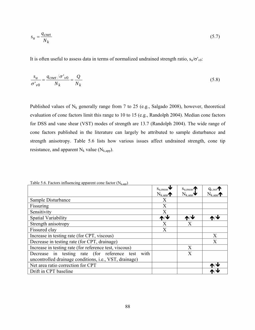
88
k
cnetu N
qs (5.7)
It is often useful to assess data in terms of normalized undrained strength ratio, su/'v0:
kk
vcnet
v
u
N
Q
N
qs 0
0
'
'
(5.8)
Published values of Nk generally range from 7 to 25 (e.g., Salgado 2008), however, theoretical
evaluation of cone factors limit this range to 10 to 15 (e.g., Randolph 2004). Median cone factors
for DSS and vane shear (VST) modes of strength are 13.7 (Randolph 2004). The wide range of
cone factors published in the literature can largely be attributed to sample disturbance and
strength anisotropy. Table 5.6 lists how various issues affect undrained strength, cone tip
resistance, and apparent Nk value (Nk,app).
Table 5.6. Factors influencing apparent cone factor (Nk,app) su,meas
Nk,app su,meas Nk,app
qc,net Nk,app
Sample Disturbance X Fissuring X Sensitivity X Spatial Variability / / / Strength anisotropy X X Fissured clay X Increase in testing rate (for CPT, viscous) X Decrease in testing rate (for CPT, drainage) X Increase in testing rate (for reference test, viscous) X Decrease in testing rate (for reference test with uncontrolled drainage conditions, i.e., VST, drainage)
X
Net area ratio correction for CPT / Drift in CPT baseline /
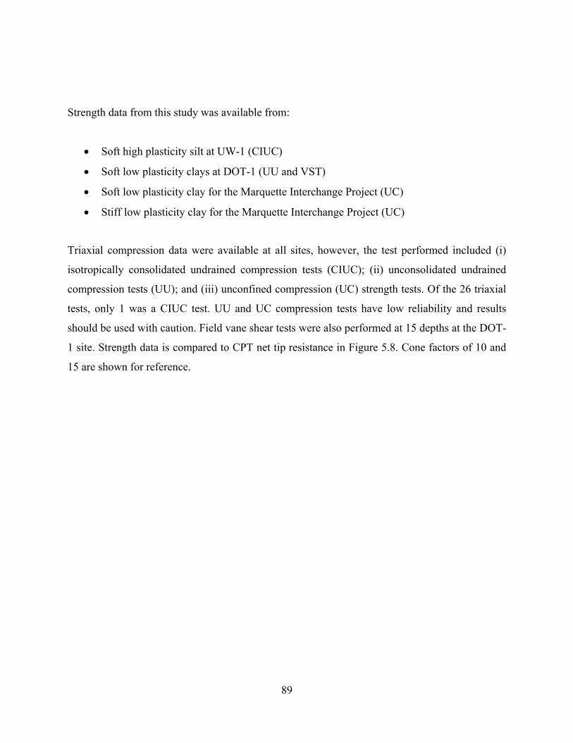
89
Strength data from this study was available from:
Soft high plasticity silt at UW-1 (CIUC)
Soft low plasticity clays at DOT-1 (UU and VST)
Soft low plasticity clay for the Marquette Interchange Project (UC)
Stiff low plasticity clay for the Marquette Interchange Project (UC)
Triaxial compression data were available at all sites, however, the test performed included (i)
isotropically consolidated undrained compression tests (CIUC); (ii) unconsolidated undrained
compression tests (UU); and (iii) unconfined compression (UC) strength tests. Of the 26 triaxial
tests, only 1 was a CIUC test. UU and UC compression tests have low reliability and results
should be used with caution. Field vane shear tests were also performed at 15 depths at the DOT-
1 site. Strength data is compared to CPT net tip resistance in Figure 5.8. Cone factors of 10 and
15 are shown for reference.
Figure 5.8.
Poor corr
This is co
procedur
the 25 U
normally
correlatio
by the VS
. Comparison o
relations are
onsidered to
res than vari
UU or UC tes
y consolidate
ons were ob
ST indicate
of CPT results
e observed be
o be predomi
ability in the
sts had undr
ed undrained
served betw
some disturb
to strength dat
etween labor
inantly a fun
e correlation
rained streng
d strength ra
ween cone an
bance during
90
ta at Wisconsin
ratory measu
nction of the
n between C
gth ratios les
atio, and typ
nd vane tests
g installation
n sites from thi
urements of
sampling an
CPT measure
ss than 0.23
pical of high
s, however,
n and testing
is study
f strength and
nd laborator
ements and s
3. This is be
hly disturbed
the low sen
g, particularly
d CPT resist
ry strength te
strength. Eig
low the exp
d samples. B
sitivity mea
y at depth.
tance.
esting
ght of
pected
Better
sured
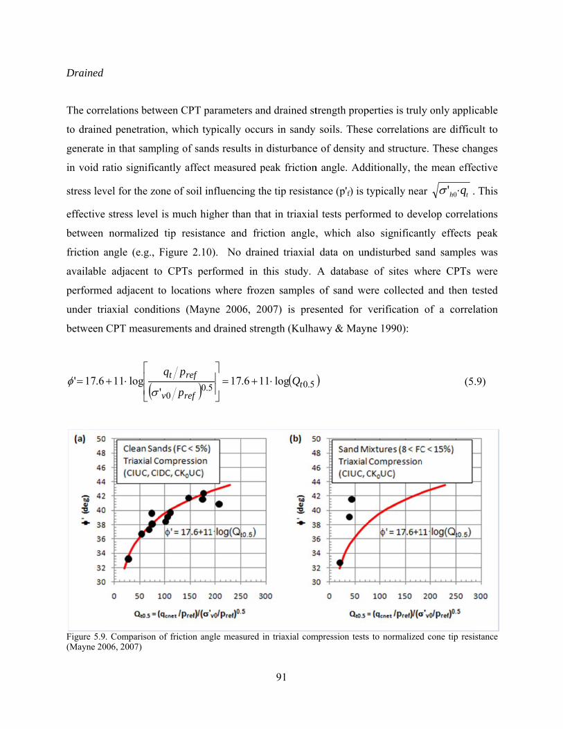
Drained
The corre
to draine
generate
in void r
stress lev
effective
between
friction a
available
performe
under tri
between
6.17'
Figure 5.9(Mayne 20
elations betw
ed penetratio
in that samp
ratio signific
vel for the zo
stress level
normalized
angle (e.g.,
e adjacent to
ed adjacent
iaxial condi
CPT measur
log11
. Comparison 006, 2007)
ween CPT pa
on, which ty
pling of sand
cantly affect
one of soil in
is much hig
d tip resistan
Figure 2.10
o CPTs per
to locations
itions (Mayn
rements and
5.00' refv
reft
p
pq
of friction ang
arameters an
ypically occu
ds results in
measured p
nfluencing th
gher than th
nce and fri
0). No drain
rformed in t
where froz
ne 2006, 20
d drained stre
516.17
gle measured i
91
nd drained st
urs in sandy
disturbance
peak friction
he tip resista
at in triaxial
ction angle,
ned triaxial
this study.
zen samples
007) is pres
ength (Kulha
5.0log1 tQ
in triaxial com
trength prop
soils. These
e of density
n angle. Add
ance (p'f) is t
l tests perfor
, which als
data on un
A database
of sand we
sented for v
awy & Mayn
mpression tests
perties is trul
e correlation
and structur
ditionally, th
typically nea
rmed to dev
so significan
ndisturbed sa
of sites w
ere collected
verification
ne 1990):
s to normalized
ly only appli
ns are difficu
re. These cha
he mean effe
ar th q0' .
velop correla
ntly effects
and samples
where CPTs
d and then t
of a correl
(5
d cone tip resi
icable
ult to
anges
ective
. This
ations
peak
s was
were
tested
lation
.9)
istance
92
The recommended correlation of Kulhawy & Mayne (1990) matches triaxial test results from
frozen specimens of clean sands well in Figure 5.9a. Application of the correlation in Figure 5.9b
to undrained triaxial tests on clayey tailings with 5 to 15% fines appears slightly conservative. It
should be noted that the friction angle for relatively low stress triaxial tests summarized in Figure
5.9 will be too high for application to bearing capacity of shallow foundations in sands. These
friction angles should be reduced to account for mean stress at failure (e.g., Equation 2.15).
5.3 Soil Classification
Conventional soil classification for geotechnical engineering is typically performed to the
specifications of the USCS (Casagrande 1948, ASTM D 2487 and D 2488) a primarily textural
system. The USCS breaks soils into two major divisions: coarse and fine grained soils based on
the percentage of fined grained soil particles, nominal diameter < 0.075 mm, passing through the
number 200 sieve (#200). Coarse grained soils are sands and gravels defined as having over
50% of the particles with a nominal diameter greater than or retained on the #200. Fine grained
soils, silts and clays, have over 50% passing the #200. Further, divisions within these two main
groupings are made based on additional factors such as percent fines and plasticity.
Sands and gravels are further grouped based on gradation, or the distribution of particle sizes. A
well graded soil exhibits a gradual transition in grain size from coarser gravels and sands to fine
sands. A poorly graded soil has a poor distribution of grain sizes and is therefore likely to
exhibit a larger void space than a well graded sand or gravel. Fines content, the percentage of
particles by mass passing the # 200 sieve, is also considered in the classification of sands and
gravels where the fines content greater than 5% changes the classification to indicate the
presence of fines. This classification system groups coarse grained soils by void space because
the strength and water flow behavior is dependent upon inter-particle interactions and void space.
Silts and clays are classified by consistency limits or the Atterberg limits. These limits represent
the water contents at which fine grained soils change behavior. The plastic limit (PL) represents
the change in soil behavior from a brittle solid to a plastic material defined as a shear strength of
170 kPa (Wroth & Wood 1978). The liquid limit (LL) represents the threshold between plastic
93
and viscous liquid behavior and is defined as the shear strength of 1.7 kPa (Wroth & Wood
1978). The difference of these parameters is the Plasticity Index (PI=LL-PL), and is plotted
against liquid limit, allowing for classification of fine grained soils in Figure 5.10.
This classification based on Atterberg Limits does not accurately account for grain size
differences between silt and clay particles, but rather indexes potential compressibility. Studies
have found “silts” classified as clays and “clays” classified as silts (USBR 1998), however; PI is
a useful indicator of anticipated soil behavior. The plasticity index has been correlated to the
compression index, Cc, (Wroth & Wood 1978, Atkinson 2007):
5.3100
PIGC s
c (5.10)
Estimates of remolded undrained shear strength (su) can be estimated using the liquidity index
(LI) which is defined as:
PI
PLwLI
(5.11)

Figure 5.10relationship
Assumin
an estim
Liquidity
1983).
The USC
predomin
compress
soils wil
assumpti
fine grai
observed
observati
sand (SM
condition
0. USCS plastips.
ng a power la
mate of the
y Index valu
CS uses a b
nantly by w
sibility. Inh
ll behave in
on works w
ned particle
d on both si
ion in their c
M) and anoth
ns of the two
icity based clas
aw relationsh
remolded u
ues greater th
bimodal syst
water flow
herent assum
n an undrai
ell for end m
es and borde
ides of the
comparison o
her as poorly
o will be sim
ssification char
hip between
undrained sh
han unity in
tem of class
characterist
mptions are m
ined manner
members of t
erline soils
classificatio
of uniformly
y graded san
milar.
94
rt for fine grain
strength and
hear strengt
dicate sensit
sifying soils
tics, and c
made that, un
r and coars
the classifica
the system
on boundary
y graded san
nd (SP) but t
ned soils. Note
d water cont
th may be
tive clays (B
s where san
clays and s
nder typical
se grained s
ation, but fo
fails in tha
y. Douglas a
nds where a s
the expected
e arrows indica
tent between
determined
Bjerrum 195
nds and grav
silts are gro
rates of load
soils behave
or soil mixtu
at similar be
and Olsen (
sample may
d behavior fo
ating compress
n the plastic
for a given
54, Leroueil
vels are gro
ouped base
ding, fine gr
e drained.
ures of coars
ehavior in-s
(1981) make
classify as a
or typical loa
sibility
limit,
n LI.
et al.
ouped
d on
ained
This
e and
itu is
e this
a silty
ading
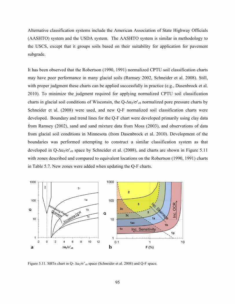
Alternati
(AASHT
the USC
subgrade
It has bee
may hav
with prop
2010). T
charts in
Schneide
develope
from Ram
from gla
boundari
develope
with zon
in Table
Figure 5.1
a.
ive classifica
TO) system a
CS, except th
e.
en observed
e poor perfo
per judgmen
To minimize
glacial soil
er et al. (20
ed. Boundar
msey (2002)
acial soil con
ies was per
ed in Q-u2/
es described
5.7. New zo
1. SBTn chart
ation system
and the USD
hat it group
that the Rob
ormance in
nt these chart
the judgme
conditions o
008) were u
ry and trend
), sand and
nditions in M
rformed atte
/'v0 space b
d and compa
ones were ad
in Q-u2/’v0
ms include th
DA system.
ps soils base
bertson (199
many glacia
ts can be app
ent required
of Wisconsin
used, and ne
lines for the
sand mixtur
Minnesota (
empting to
by Schneider
ared to equiv
dded when up
space (Schneid
b
95
he American
The AASH
ed on their
90, 1991) no
al soils (Ram
plied succes
d for applyin
n, the Q-u2
ew Q-F nor
e Q-F chart w
re data from
(from Dasen
construct a
r et al. (200
valent locatio
pdating the Q
der et al. 2008)
b.
n Association
HTO system
suitability f
ormalized CP
msey 2002,
ssfully in pra
ng normaliz
2/'v0 norma
rmalized so
were develop
m Moss (200
nbrock et al.
a similar cl
08), and char
ons on the R
Q-F charts.
) and Q-F spac
n of State H
is similar in
for applicati
PTU soil cla
Schneider e
actice (e.g., D
zed CPTU s
alized pore p
oil classifica
ped primaril
03), and obs
. 2010). Dev
lassification
rts are show
Robertson (19
ce.
Highway Off
n methodolo
on for pave
assification c
et al. 2008).
Dasenbrock
soil classific
pressure char
ation charts
ly using clay
ervations of
velopment o
n system as
wn in Figure
990, 1991) c
ficials
ogy to
ement
charts
Still,
et al.
cation
rts by
were
y data
f data
of the
s that
e 5.11
charts
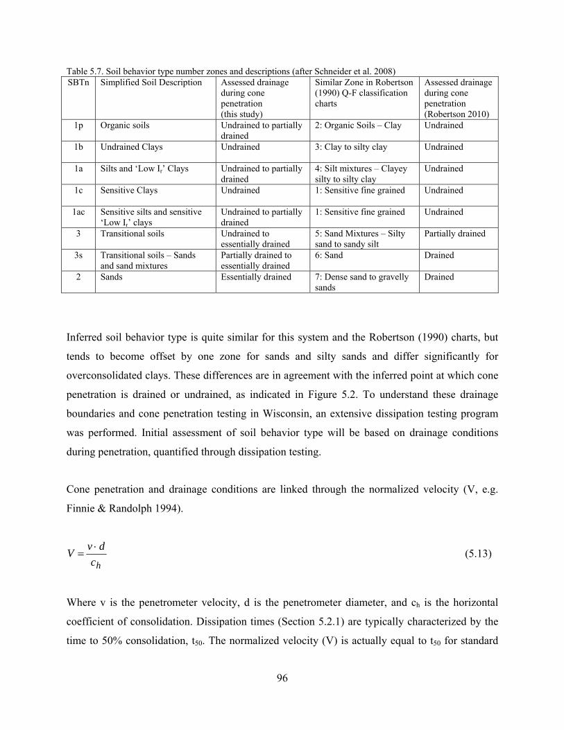
96
Table 5.7. Soil behavior type number zones and descriptions (after Schneider et al. 2008) SBTn Simplified Soil Description Assessed drainage
during cone penetration (this study)
Similar Zone in Robertson (1990) Q-F classification charts
Assessed drainage during cone penetration (Robertson 2010)
1p Organic soils Undrained to partially drained
2: Organic Soils – Clay
Undrained
1b Undrained Clays Undrained 3: Clay to silty clay
Undrained
1a Silts and ‘Low Ir’ Clays Undrained to partially drained
4: Silt mixtures – Clayey silty to silty clay
Undrained
1c Sensitive Clays Undrained 1: Sensitive fine grained
Undrained
1ac Sensitive silts and sensitive ‘Low Ir’ clays
Undrained to partially drained
1: Sensitive fine grained Undrained
3 Transitional soils Undrained to essentially drained
5: Sand Mixtures – Silty sand to sandy silt
Partially drained
3s Transitional soils – Sands and sand mixtures
Partially drained to essentially drained
6: Sand Drained
2 Sands Essentially drained
7: Dense sand to gravelly sands
Drained
Inferred soil behavior type is quite similar for this system and the Robertson (1990) charts, but
tends to become offset by one zone for sands and silty sands and differ significantly for
overconsolidated clays. These differences are in agreement with the inferred point at which cone
penetration is drained or undrained, as indicated in Figure 5.2. To understand these drainage
boundaries and cone penetration testing in Wisconsin, an extensive dissipation testing program
was performed. Initial assessment of soil behavior type will be based on drainage conditions
during penetration, quantified through dissipation testing.
Cone penetration and drainage conditions are linked through the normalized velocity (V, e.g.
Finnie & Randolph 1994).
hc
dvV
(5.13)
Where v is the penetrometer velocity, d is the penetrometer diameter, and ch is the horizontal
coefficient of consolidation. Dissipation times (Section 5.2.1) are typically characterized by the
time to 50% consolidation, t50. The normalized velocity (V) is actually equal to t50 for standard
97
cone dimensions (d=1.44 inches) and penetration rates (0.78 in/sec) and an assumed rigidity
index of 84 (Figure 5.5a). This relationship is only applicable if penetration is undrained. If
penetration is partially drained, normalized time factors tend to increase as compared to the
undrained case (Silva et al. 2006, Schneider et al. 2007) and the V-t50 relationship needs to be
modified. Table 5.8 presents several t50 times with anticipated water flow characteristics. The
calculated values of V in Table 5.8 agrees well with the suggested ranges for drained penetration
with V< 0.1 and undrained penetration occurring at V>30-100 (Randolph 2004).
The location of data in Q-F soil classification charts is shown in Figures 5.12 to 5.16. The
sensitivity boundary has been removed such that CPTU soil classification charts should be in
better agreement with non state assessment of soil types (i.e., USCS, AASHTO). Table 5.9
provides drainage estimates of several t50 values. Hydraulic conductivity was estimated using
Equation 2.1 with an assumed D of 100 tsf. This table allows for rough estimation of the water
flow properties of the soil.
Table 5.8. Estimates of cv and V based on different t50 times calculated using Teh and Houlsby (1991) solution. Values were corrected based on results by Silva et al. (2006). Calculations based on a cone diameter of 35.6 mm and soil with Ir = 84.
v (mm/s)
t50 (s)
T50
Apparent ch
(ft2/day)
Apparent V
T50,pc/T50
T50,pc
ch (ft2/day)
V
Drainage Condition
20 5 0.245 132 5 16 3.9 2119 0.3 Essentially Drained
20 15 0.245 43.7 15 5.6 1.37 247 2.7 Partially Drained
20 30 0.245 18.6 30 2 0.49 44.6 15 Partially Drained
20 100 0.245 6.5 100 1 0.245 6.5 100 Undrained
20 300 0.245 1.9 300 1 0.245 2.2 300 Undrained
20 3000 0.245 0.2 3000 1 0.245 0.2 3000 Undrained
Table 5.9. Legend and range of t50 presented in Figures 5.12 to 5.16. Estimated water flow characteristics based on calculations in Table 5.8. Values presented in this table are applicable to a 10 cm2 cone advanced at the standard steady rate of 20 mm/s.
t50 (s)
Symbol V ch
(ft2/day) kh
(ft/day) Drainage Condition
0 – 15 <2.7 >247 >0.07 Essentially Drained 15-30 2.7 – 15 45-247 0.003-0.03 Partially Drained 30-100 15 - 100 6.5-45 0.0003-0.003 Essentially Undrained 100-300 100 – 300 2-6.5 0.0003 Undrained 300-3000 300 - 3000 0.2-2 3x10⁻⁵-3x10⁻⁴ Undrained
Figure 5.12Colors are times and l
Figure 5.13
2. Q-F chart wbased on dissi
location on the
3. Data points
with Wisconsin ipation t50 time
e revised Q-F S
in Q-F space f
data presentedes within a laySBTn chart.
for dissipations
98
d and grouped yer, Table 4.1.
s with t50 times
by dissipation This is one of
s of 100 s to 30
n t50 times betwf 5 figures rep
00 s.
ween 300 s to 3resenting dissi
3000 s. ipation
Figure 5.14
Figure 5.15
4. Data points
5. Data points
in Q-F space fo
in Q-F space fo
for dissipations
for dissipations
99
with t50 times
with t50 times
of 30 s to 100
of 15 s to 30 s
s.
s.

Figure 5.16
Table 5.105.16.
D
Table 5.1
5.12 to 5
3s and 2
of 1p, 1b
addition
6. Data points
0. Percentages
Dissipation t5
Times (s)
0 - 15 15 - 30
30 - 100 100 - 300
300 - 3000
10 provides t
5.16. The tre
containing t
b, and 1a con
to displayin
in Q-F space fo
of points that p
0 % Datain 1p
0 0
0.6 9.1 3
the distribut
ends of drain
the majority
ntain the ma
g trends in d
for dissipations
plot within eac
a % Data in 1b
0 0
18.9 10.3 29.5
ion of points
ned layers p
of data poin
ajority of po
drainage in Q
100
with t50 times
ch soil zone of
% Data in 1a
%
0.1 6.1
55.2 63
65.1
s that plot w
plotting in zo
nts for dissip
oints with di
Q-F space, th
of 0 s to 15 s.
f the revised Q
% Data in 3
%i
4.2 74.1 4
16.6 16.4 1.9
within each c
ones 3, 3s an
pation times o
issipation t50
his series of
Q-F SBTn char
% Datain 3s
% Din
72.6 2345.7 448.1 01.3 0.4
lassification
nd 2 are obs
of 0 to 30s.
0 times great
f figures is in
rt for Figures 5
Data n 2
TotaPoin
3.1 6934.1 245
0.6 3440 3970 789
n zone for Fi
served with z
The SBTn z
ter than 100
n agreement
5.12 to
al nts
3 5 4 7 9
gures
zones
zones
s. In
t with
101
the shape of the boundaries suggested by the revised Q-F chart of constant F at larger values of Q
and variable F values at low Q conditions for soils with similar water flow characteristics.
The next step in evaluating soil classification from CPT data is to provide a link from water flow
characteristics to soil type. This was achieved by simplifying data from study CPTU soundings
conducted across WI in varying geologic deposits to a number of representative layers. The
results of the field work have been summarized in Table 5.11 in 23 representative layers based
on visual classification. Many of these layers (13/23) also include laboratory classification.
Initial review of the median of the CPTU normalized parameters provides an indication of the
relative differences expected between different soil types. Large differences in Q and F are
observed between the sand and clay soils as expected. The distribution of these data in soil
classification charts is provided in Table 5.12. Layers analyzed in this study are presented in the
revised Q-F and Q-u2/'v0 space in Figures 5.17 to 5.22.
This large dataset allows a check of the relationships determined for data placement in the
revised Q-F classification chart, as well as consistency between Q-F and Q-u2/'v0 charts.
Firstly, the sand soils, Figure 5.17 and 5.18, typically fall within zones 2 and 3 s as indicated by
the dissipation testing performed in this study. The differences in drainage conditions are readily
apparent in the pore pressure based charts, where the sand mixtures are showing elevated pore
pressures.
Table 5.11. Summary of selected repressentative soil la
102
ayers from Wissconsin test loccations
Table 5.12
2. Percentage off point plottingg in revised Q-F
103
F soil classificcation charts foor selected reprresentative laye
ers
Figure 5.17
Figure 5.1these soils
7. Sand layers
8. Layers of sabehave partial
plotted in Q-F
and mixtures plly drained to d
and Q-u2/'v
plotted in Q-F drained during
104
v0 space.
and Q-u2/'vpenetration
v0 space. Trendds in Q-u2/'vv0 space indica
ate that
Figure 5.19penetration
Figure 5.20with increa
9. Silt layers pn
0. Clayey till lasing OCR can
plotted in Q-F
layers plotted in be observed in
and Q-u2/'v
in Q-F and Q-n Q-F space
105
0 space. All d
u2/'v0 space
data suggests v
. The trend of
variable drainag
f data of increa
ge conditions d
asing Q at cons
during
stant F
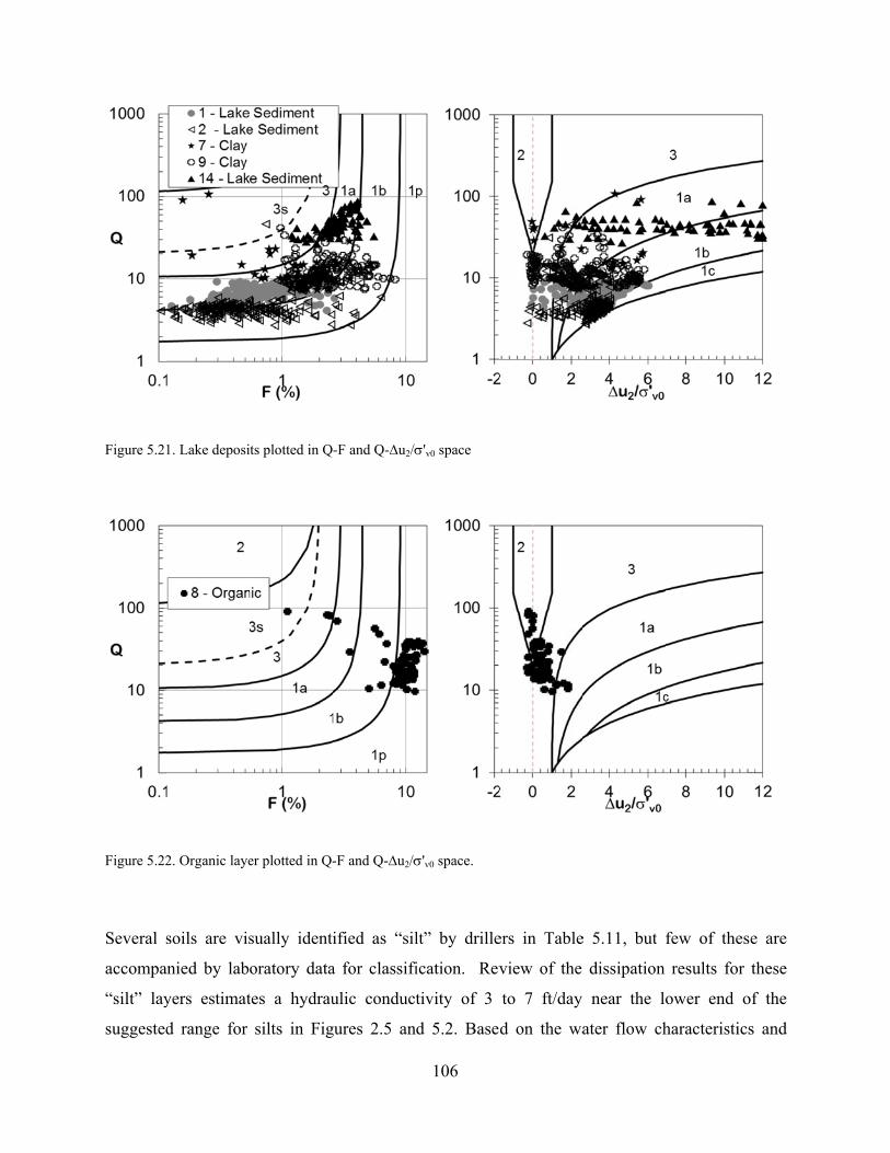
Figure 5.2
Figure 5.22
Several s
accompa
“silt” lay
suggested
1. Lake deposi
2. Organic laye
soils are vis
anied by lab
yers estimat
d range for
ts plotted in Q
er plotted in Q-
sually identi
oratory data
tes a hydrau
silts in Fig
-F and Q-u2/
-F and Q-u2/
ified as “sil
a for classifi
ulic conduct
gures 2.5 an
106
'v0 space
'v0 space.
lt” by drille
ication. Rev
tivity of 3
d 5.2. Base
ers in Table
view of the
to 7 ft/day
d on the wa
e 5.11, but f
dissipation
near the lo
ater flow ch
few of thes
results for
ower end o
haracteristics
e are
these
of the
s and
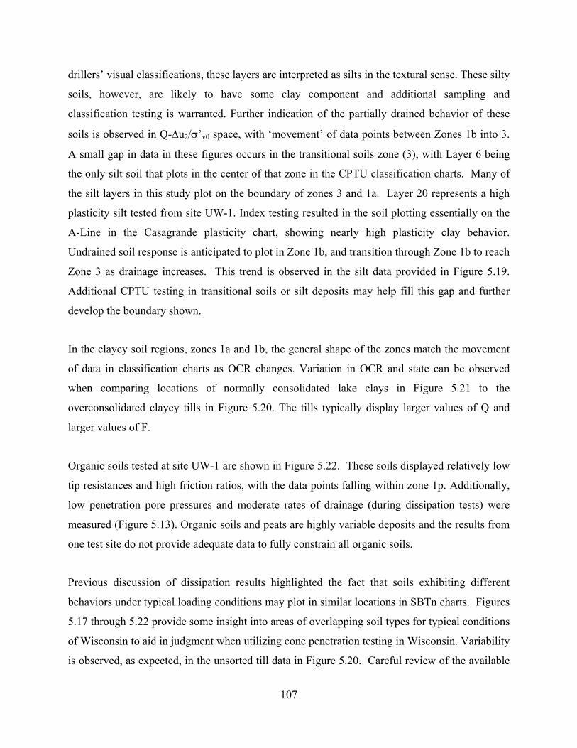
107
drillers’ visual classifications, these layers are interpreted as silts in the textural sense. These silty
soils, however, are likely to have some clay component and additional sampling and
classification testing is warranted. Further indication of the partially drained behavior of these
soils is observed in Q-u2/’v0 space, with ‘movement’ of data points between Zones 1b into 3.
A small gap in data in these figures occurs in the transitional soils zone (3), with Layer 6 being
the only silt soil that plots in the center of that zone in the CPTU classification charts. Many of
the silt layers in this study plot on the boundary of zones 3 and 1a. Layer 20 represents a high
plasticity silt tested from site UW-1. Index testing resulted in the soil plotting essentially on the
A-Line in the Casagrande plasticity chart, showing nearly high plasticity clay behavior.
Undrained soil response is anticipated to plot in Zone 1b, and transition through Zone 1b to reach
Zone 3 as drainage increases. This trend is observed in the silt data provided in Figure 5.19.
Additional CPTU testing in transitional soils or silt deposits may help fill this gap and further
develop the boundary shown.
In the clayey soil regions, zones 1a and 1b, the general shape of the zones match the movement
of data in classification charts as OCR changes. Variation in OCR and state can be observed
when comparing locations of normally consolidated lake clays in Figure 5.21 to the
overconsolidated clayey tills in Figure 5.20. The tills typically display larger values of Q and
larger values of F.
Organic soils tested at site UW-1 are shown in Figure 5.22. These soils displayed relatively low
tip resistances and high friction ratios, with the data points falling within zone 1p. Additionally,
low penetration pore pressures and moderate rates of drainage (during dissipation tests) were
measured (Figure 5.13). Organic soils and peats are highly variable deposits and the results from
one test site do not provide adequate data to fully constrain all organic soils.
Previous discussion of dissipation results highlighted the fact that soils exhibiting different
behaviors under typical loading conditions may plot in similar locations in SBTn charts. Figures
5.17 through 5.22 provide some insight into areas of overlapping soil types for typical conditions
of Wisconsin to aid in judgment when utilizing cone penetration testing in Wisconsin. Variability
is observed, as expected, in the unsorted till data in Figure 5.20. Careful review of the available
108
data is critical to a correct interpretation of soil type from SBTn charts. Assigning a rigid
classification to all data within a certain zone is not recommended; however, incorporating
knowledge of the surrounding geology, landscape features, and previous investigations (i.e., soil
survey maps and geologic maps) an engineer/geologist may anticipate soils and sequences that
will be encountered during an investigation.
A summary of the zones of the soil classification chart in which data plot is provided in Table
5.12. A majority of data plot is zones 1b and 3s, ‘Low Ir’ clays and silts and sand mixtures. Since
the clays tested in this study were predominantly low plasticity index clays, this zone could be
considered as low PI clays in Wisconsin. Only one high plasticity inorganic fine grained soil was
tested, layer 20. This bias may be due to the relative low occurrence of high plasticity clays and
silts in WI or the sites tested.
In relation to soil classification, it is summarized that even when testing in an area with little to
no background knowledge, the CPTU is an applicable tool even though it does not provide a soil
sample. Sands below the water table are readily identified as plotting in zones 3s and 2 of the
revised Q-F SBTn space with no excess pore pressures generated during penetration. Normally
to overconsolidated, insensitive clay soils will provide friction ratios greater than 3 and typically
positive excess pore pressures. Negative pore pressures are typically associated with highly
overconsolidated soils and will therefore coincide with large Q values. Soft layers of concern are
readily identified by CPTU testing based on tip resistance, and the extents of these layers can be
quickly determined by performing multiple soundings. Pore-water pressures are key in
determining drainage characteristics of soils that plot in or near the transition zone. If pore
pressures are unavailable (i.e., a low water table) use of Q-F SBTn chart may be done assuming
the worst case scenario for a low risk project; for example if a soil plots in zone 3s assume that it
is a transitional soil with a significant fines content as suggested by Ramsey (2002). Gradually,
as more testing is performed a reliable interpretation of the soils at a site/region can be developed
using CPTU.
109
6 Applications
No field data of foundation or embankment performance was available at the WisDOT CPT test
sites, and this section will provide an overview of mechanisms that influence the use of CPT data
for design of shallow foundations, axial loading of driven piles, and embankments.
6.1 Shallow Foundations
For shallow foundations to be applicable to transportation structures, the underlying soils
typically need to have a high stiffness to minimize deformations. For the most part, if settlements
are minimized then a sufficient factor of safety against bearing capacity is achieved (e.g., Mayne
& Illingsworth 2010). Bearing capacity calculations still need to be performed, but design
decisions related to application of bearing capacity equations are primarily driven by selection of
strength parameters, discussed in Section 5.2.4. This section will focus on shear deformations of
sands and stiff clays. Consolidation settlements of clay soils would additionally need to be
considered for shallow foundation design, but is not specifically addressed herein.
The analysis of settlements caused by shear distortions of the soil beneath shallow foundations
can simply be thought of as a stress-strain curve, the stress is the footing load divided by the area
(q) and the strain is indicated by the settlement (s) normalized by the footing width (B) or
equivalent diameter (Deq).
12
12
11
2 I
q
G
q
qI
G
qI
E
q
D
s
tteq (6.1)
where I is an influence factor that is typically defined in terms of elastic modulus. For a rigid
footing on an infinitely thick homogeneous elastic half space, I is equal to /4. Values of
influence factors are affected by a number of issues including:
Change in shear stiffness with depth
Footing shape (circle / square, rectangular, strip)
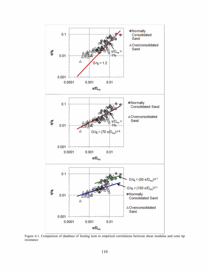
Figure 6.1resistance
. Comparison of database off footing tests
110
to empirical ccorrelations bettween shear m
modulus and coone tip
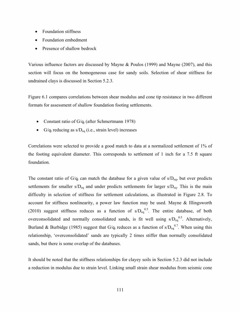
111
Foundation stiffness
Foundation embedment
Presence of shallow bedrock
Various influence factors are discussed by Mayne & Poulos (1999) and Mayne (2007), and this
section will focus on the homogeneous case for sandy soils. Selection of shear stiffness for
undrained clays is discussed in Section 5.2.3.
Figure 6.1 compares correlations between shear modulus and cone tip resistance in two different
formats for assessment of shallow foundation footing settlements.
Constant ratio of G/qt (after Schmertmann 1978)
G/qt reducing as s/Deq (i.e., strain level) increases
Correlations were selected to provide a good match to data at a normalized settlement of 1% of
the footing equivalent diameter. This corresponds to settlement of 1 inch for a 7.5 ft square
foundation.
The constant ratio of G/qt can match the database for a given value of s/Deq, but over predicts
settlements for smaller s/Deq and under predicts settlements for larger s/Deq. This is the main
difficulty in selection of stiffness for settlement calculations, as illustrated in Figure 2.8. To
account for stiffness nonlinearity, a power law function may be used. Mayne & Illingsworth
(2010) suggest stiffness reduces as a function of s/Deq0.5. The entire database, of both
overconsolidated and normally consolidated sands, is fit well using s/Deq0.5. Alternatively,
Burland & Burbidge (1985) suggest that G/qt reduces as a function of s/Deq0.7. When using this
relationship, ‘overconsolidated’ sands are typically 2 times stiffer than normally consolidated
sands, but there is some overlap of the databases.
It should be noted that the stiffness relationships for clayey soils in Section 5.2.3 did not include
a reduction in modulus due to strain level. Linking small strain shear modulus from seismic cone
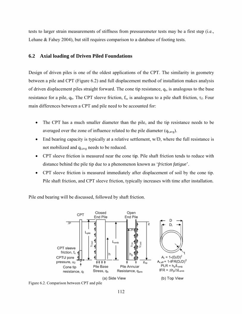
tests to la
Lehane &
6.2 Ax
Design o
between
of driven
resistanc
main diff
T
av
E
n
C
d
C
P
Pile end b
Figure 6.2.
arger strain
& Fahey 200
xial loading
of driven pil
a pile and C
n displaceme
e for a pile,
ferences betw
The CPT has
veraged ove
End bearing c
ot mobilized
CPT sleeve fr
istance behin
CPT sleeve f
ile shaft fric
bearing will
. Comparison b
measuremen
04), but still r
g of Driven
es is one of
CPT (Figure
ent piles strai
qb. The CPT
ween a CPT
s a much sm
r the zone of
capacity is ty
d and qt,avg n
friction is me
nd the pile ti
friction is m
ction, and CP
be discusse
between CPT a
nts of stiffne
requires com
n Piled Fou
f the oldest a
6.2) and full
ight forward
T sleeve fric
and pile nee
maller diame
f influence r
ypically at a
eeds to be re
easured near
ip due to a p
measured imm
PT sleeve fri
d, followed
and pile
112
ess from pre
mparison to a
undations
applications
l displaceme
d. The cone t
ction, fs, is a
ed to be acco
eter than the
related to the
a relative sett
educed.
r the cone tip
phenomenon
mediately aft
iction, typica
by shaft fric
essuremeter t
a database o
of the CPT
ent method o
tip resistanc
analogous to
ounted for:
e pile, and th
e pile diamet
tlement, w/D
p. Pile shaft
n known as ‘f
fter displacem
ally increase
ction.
tests may be
f footing tes
T. The simila
of installatio
e, qt, is analo
a pile shaft
he tip resist
ter (qt,avg).
D, where the
friction tend
friction fatig
ment of soil
es with time
e a first step
sts.
arity in geom
on makes ana
ogous to the
t friction, f.
ance needs
e full resistan
ds to reduce
gue’.
l by the con
after installa
p (i.e.,
metry
alysis
e base
Four
to be
nce is
e with
ne tip.
ation.
Figure 6.3.
Figure 6.
base stre
bbq
For close
typically
Smaller f
Davisson
Lower va
driven op
displacem
steel. Thi
, A effr
Where IF
an increm
. Comparison o
.3 compares
ss, qb is typi
avgtq ,
ed ended pil
associated
fractions of
n offset defin
alues of bas
pen ended a
ment of soil
is degree of
1
D
DIFR i
FR is the inc
ment of pile
of pile qb to CP
CPT qt to p
cally less tha
les, b is on
with partial
cone tip res
nition of failu
e resistance
and does not
during pile i
displacemen
2
cremental fil
driving (IFR
PT qt (data from
ile qb in san
an CPT qt, a
the order of
mobilizatio
sistance wou
ure.
are mobiliz
t plug. The b
installation t
nt can be qua
lling ratio de
R = hp/Le
113
m Xu et al. 200
nds and clays
and is quanti
f 0.6 in both
on of base r
uld be availa
ed at a tip d
base resistan
that is a func
antified usin
efined as the
emb, Figure 6
08, Chow 1997
s for a tip di
fied as:
h sands and
resistance at
able for pile
displacement
nce becomes
ction of pile
ng the effecti
e incrementa
6.2). For the
7)
splacement
clays. This
a tip displa
e base resist
t of 0.1D in
s a function
plugging an
ive area ratio
al change in
e case of a fu
of 0.1D. The
(6
reduction in
acement of 0
tance if usin
sands if a p
n of the degr
nd relative ar
o:
(6
plug height
fully plugged
e pile
.2)
n qt is
0.1D.
ng the
pile is
ree of
rea of
.3)
t over
d pile
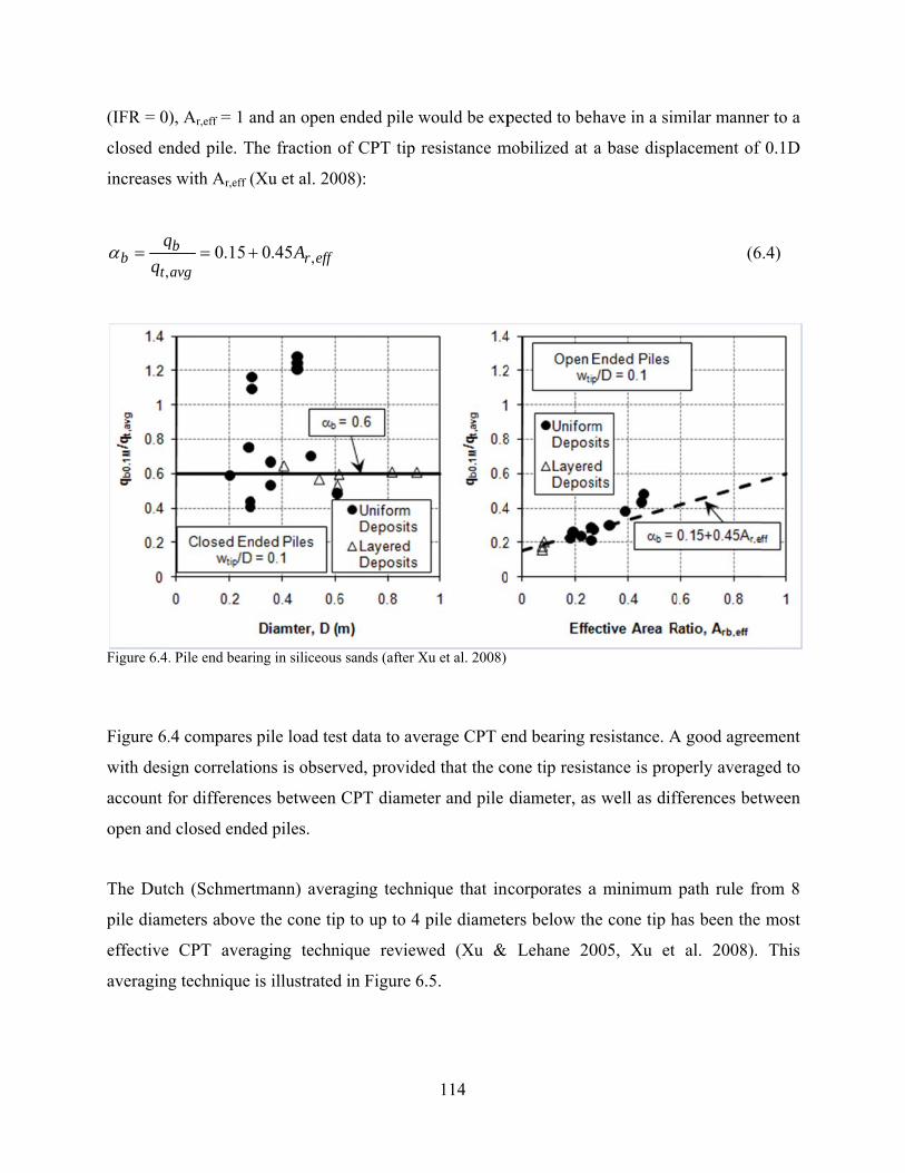
(IFR = 0)
closed en
increases
tb q
q
,
Figure 6.4.
Figure 6.
with desi
account f
open and
The Dutc
pile diam
effective
averaging
), Ar,eff = 1 a
nded pile. T
s with Ar,eff (
avg
bq15.0
. Pile end beari
.4 compares
ign correlatio
for differenc
d closed ende
ch (Schmert
meters above
CPT avera
g technique
and an open
he fraction o
(Xu et al. 20
effrA ,45.0
ing in siliceous
pile load tes
ons is observ
ces between
ed piles.
tmann) aver
e the cone tip
aging techn
is illustrated
ended pile w
of CPT tip r
08):
s sands (after X
st data to ave
ved, provide
CPT diamet
aging techn
p to up to 4
nique review
d in Figure 6
114
would be exp
resistance m
Xu et al. 2008)
erage CPT e
ed that the co
ter and pile
ique that inc
pile diamete
wed (Xu &
6.5.
pected to beh
mobilized at
end bearing r
one tip resis
diameter, as
corporates a
ers below th
Lehane 20
have in a sim
a base displ
resistance. A
stance is prop
s well as diff
a minimum
he cone tip h
005, Xu et
milar manne
lacement of
(6
A good agree
perly averag
fferences bet
path rule fr
has been the
al. 2008).
er to a
0.1D
.4)
ement
ged to
tween
rom 8
most
This
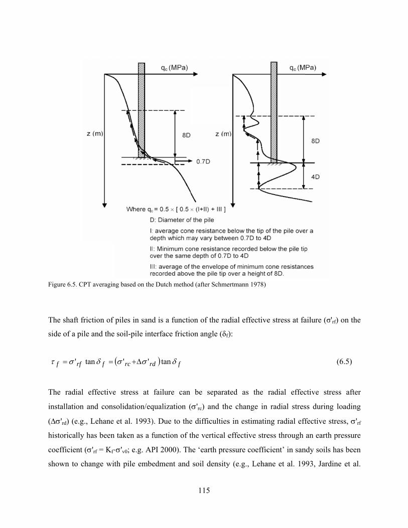
Figure 6.5.
The shaft
side of a
f '
The radi
installatio
('rd) (e
historical
coefficien
shown to
. CPT averagin
ft friction of
pile and the
frf tan
ial effective
on and cons
e.g., Lehane
lly has been
nt ('rf = Kf·
o change wit
ng based on the
piles in sand
soil-pile int
rdrc ''
e stress at
solidation/eq
et al. 1993)
taken as a f
·'v0; e.g. AP
th pile embe
e Dutch method
d is a functio
terface frictio
fd tan
failure can
qualization (
). Due to the
function of t
PI 2000). Th
edment and
115
d (after Schme
on of the rad
on angle (δf)
be separat
('rc) and the
e difficulties
the vertical e
he ‘earth pre
soil density
ertmann 1978)
dial effective
):
ted as the
e change in
s in estimatin
effective stre
ssure coeffic
y (e.g., Leha
e stress at fa
radial effec
n radial stres
ng radial eff
ess through
cient’ in san
ane et al. 19
ailure (σ'rf) o
(6
ctive stress
ss during loa
fective stres
an earth pre
ndy soils has
93, Jardine
on the
.5)
after
ading
s, 'rf
essure
been
et al.
116
2005), and also be influenced by the relative level of soil displacement during pile installation
(e.g., Gavin & Lehane 2003). Pile shaft friction correlations between f based on CPT qt are still
considered more reliable than correlations to CPT fs.
A multi variable expression relating f to qt has been developed based on mechanisms
influencing pile shaft friction and the assumed (relative density independent) correlation between
radial effective stress after installation and equalization and qt (Lehane & Jardine 1994, Gavin &
Lehane 2003, Lehane et al. 2005):
frd
ceffrst
c
tf D
h
a
Aq
f
f tan',max
,
(6.6)
Terms within Equation 6.6 are illustrated in Figure 6.2, where ft/fc is the ratio of friction in
tension to that in compression (taken as unity in compression), Ars,eff is the effective area ratio of
the pile toe during installation and ‘h’ is the height above the pile tip. Ars,eff is affected by
plugging at various stages during installation, which is best assessed using the IFR that may vary
with depth during driving. With the above expression, fitting parameters are related to various
mechanisms that affect the correlation between qt and f:
a = parameter to account for the reduction in radial stress behind the pile tip
b = parameter to account for differences between open and closed ended piles
c = exponent to account for ‘friction fatigue’
= parameter to account for and upper limit on (h/D)-c near the pile tip
It is noted that friction fatigue is the reduction in local friction, which occurs as a pile tip is
driven deeper into the soil (e.g., White & Lehane, 2004). Within the UWA-05 method for
siliceous sands, the parameters a, b, c, and have been calibrated for piles in compression to
equal 33, 0.3, 0.5, and 2 (Lehane et al. 2005, 2008). For clays, ‘a’ is dependent on OCR and
sensitivity, while ‘b’, ‘c’, and ‘’ have been preliminarily estimated as 0.1, 0.2, and 2,
respectively (Schneider et al. 2010).
117
If the effects of friction fatigue, area ratio, ratio of tension to compression shaft capacity, change
in radial effective stress during loading, and interface friction angle are ignored, the parameters
c, b, 'rd, tanf and ft/fc in Equation 6.6 become equal to 0, 0, 0, 1, and 1, respectively. Equation
6.6 therefore simplifies to:
s
tf
q
(6.7)
Equation 6.7 is commonly referred to as a CPT ‘alpha’ method. Eslami & Fellenius (1997)
recommend using s equal to 250 for clean siliceous sands, and it is common to take s as 40 in
clays. An intermediate value of s equal to 100 is often used in sandy silts and clayey silts. It is
recommended to use s of 40 in heavily over consolidated clayey and loamy tills, if cone
penetration is undrained. The parameter s is related to the parameter ‘a’ from Equation 5, but
has a higher value since the effects of friction fatigue, area ratio, ratio of tension to compression
shaft capacity, change in radial effective stress during loading, and interface friction angle are
ignored. Use of simplified s values calibrated to empirical databases clearly induces bias when
applied to conditions outside of the database used to calibrate the method.
It is logical, and tempting, to try to use CPT fs to estimate pile shaft friction (e.g., Begemann
1965). A comparison between average CPT fs and average pile f for databases of pile load tests
in clays is shown in Figure 6.6. Two regimes of dominant behavior are identified from Figure
6.6; (i) setup, where f,avg/fs,avg is greater than unity; and (ii) friction fatigue, where f,avg/fs,avg is
less than unity.
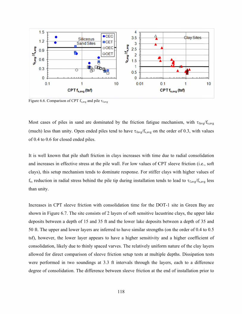
Figure 6.6.
Most cas
(much) le
of 0.4 to
It is well
and incre
clays), th
fs, reduct
than unit
Increases
shown in
deposits
50 ft. Th
tsf), how
consolida
allowed
were per
degree of
. Comparison o
ses of piles
ess than uni
0.6 for close
l known tha
eases in effe
his setup me
tion in radia
y.
s in CPT sle
n Figure 6.7.
between a d
e upper and
wever, the lo
ation, likely
for direct co
rformed in t
f consolidati
of CPT fs,avg an
in sand are
ty. Open end
ed ended pile
t pile shaft
ective stress
echanism ten
al stress behi
eeve friction
The site con
depth of 15 a
lower layers
ower layer a
due to thinly
omparison o
two soundin
ion. The diff
nd pile f,avg
e dominated
ded piles ten
es.
friction in c
at the pile w
nds to domin
ind the pile t
n with conso
nsists of 2 la
and 35 ft and
s are inferred
appears to h
y spaced var
f sleeve fric
ngs at 3.3 ft
ference betw
118
d by the fric
nd to have
clays increas
wall. For low
nate respons
tip during in
olidation tim
ayers of soft
d the lower
d to have sim
ave a highe
rves. The rel
ction setup t
ft intervals t
ween sleeve
ction fatigue
favg/fs,avg on
ses with time
w values of C
e. For stiffe
nstallation te
me for the D
sensitive la
lake deposit
milar strengt
er sensitivity
latively unif
tests at multi
through the
friction at th
e mechanism
the order of
e due to rad
CPT sleeve
r clays with
ends to lead
DOT-1 site i
custrine clay
ts between a
ths (on the o
y and a high
form nature
iple depths.
layers, each
he end of ins
m, with favg
f 0.3, with v
dial consolid
friction (i.e.
h higher valu
to f,avg/fs,av
in Green Ba
ys, the upper
a depth of 35
order of 0.4 t
her coefficie
of the clay l
Dissipation
h to a differ
stallation pri
g/fs,avg
values
dation
., soft
ues of
vg less
ay are
r lake
5 and
to 0.5
ent of
layers
n tests
rence
ior to
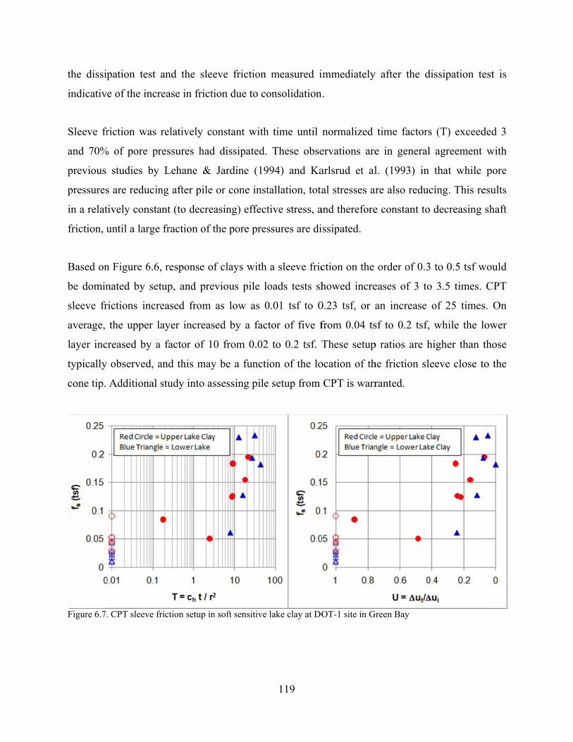
the dissip
indicativ
Sleeve fr
and 70%
previous
pressures
in a relat
friction, u
Based on
be domin
sleeve fr
average,
layer inc
typically
cone tip.
Figure 6.7.
pation test a
e of the incr
riction was r
% of pore pr
studies by
s are reducin
tively consta
until a large
n Figure 6.6,
nated by set
rictions incre
the upper la
creased by a
observed, a
Additional s
. CPT sleeve fr
and the slee
rease in fricti
relatively co
ressures had
Lehane &
ng after pile
ant (to decrea
fraction of t
, response of
tup, and pre
eased from
ayer increas
factor of 10
and this may
study into as
riction setup in
eve friction
ion due to co
onstant with
d dissipated.
Jardine (19
or cone inst
asing) effect
the pore pres
f clays with
vious pile lo
as low as 0
sed by a fact
0 from 0.02
y be a functi
ssessing pile
n soft sensitive
119
measured i
onsolidation
h time until
These obse
994) and Ka
tallation, tota
tive stress, a
ssures are di
a sleeve fric
oads tests sh
0.01 tsf to 0
tor of five f
to 0.2 tsf. T
ion of the lo
e setup from
lake clay at DO
immediately
n.
normalized
ervations are
arlsrud et al
al stresses ar
and therefore
issipated.
ction on the
howed incre
0.23 tsf, or a
from 0.04 ts
These setup
ocation of th
CPT is warr
OT-1 site in G
y after the d
time factors
e in general
l. (1993) in
are also redu
e constant to
order of 0.3
eases of 3 to
an increase
sf to 0.2 tsf,
p ratios are h
he friction sl
ranted.
Green Bay
dissipation te
s (T) exceed
l agreement
n that while
cing. This re
o decreasing
3 to 0.5 tsf w
o 3.5 times.
of 25 times
, while the l
higher than
leeve close t
est is
ded 3
with
pore
esults
shaft
would
CPT
s. On
lower
those
to the
120
6.3 Embankments on Soft Soils
Embankments on soft soils involve three major design issues:
Stability, evaluated through the undrained strength
Magnitude of settlements
Time for settlements and strength increase to occur
The cone penetration test is ideal to assess undrained strength and time dependent properties, and
has some application to assessment of the magnitude of settlements.
Cone penetration testing can reliably be used to evaluate soil strength at the time of testing
through the cone factor Nk, as discussed in Section 5.2.4. To assess changes in strength with time
under an embankment, both the change in in-situ effective stress and change in state (OCR) need
to be quantified (i.e., Ladd 1991). Increases in effective stress due to consolidation under an
embankment increase strength, but increases in effective stress reduce OCR that reduces the
undrained strength ratio:
8.08.01
0023.0
2
sin
''OCROCROCR
sscr
NC
CC
v
u
v
u
(6.8)
To be able to understand changes in strength with time, the OCR and normalized undrained
strength ratio need to be quantified. Mayne (2007) provides a thorough discussion of estimating
OCR and/or preconsolidation stress from CPTU data. OCR correlations were not assessed in this
study as no high quality preconsolidation stress data were available.
Magnitude of settlements can be quantified by constrained modulus estimated from CPT
(Section 5.2.2). The constrained modulus is relatively constant prior to the preconsolidation
stress, but drops significantly for normally consolidated soils. In normally consolidated soils,
constrained modulus will increase with increasing effective stress, and appropriate stress ranges
must be used for assessment of compressibility.
121
Dissipation data can be very useful for evaluating time dependent behavior. For application to
embankments, the dissipation results are directly applicable to radial drainage when using
prefabricated vertical drains. Due to anisotropy in hydraulic conductivity and coefficient of
consolidation, ch from dissipation tests may overestimate cv by up to an order of magnitude in
varved clays.
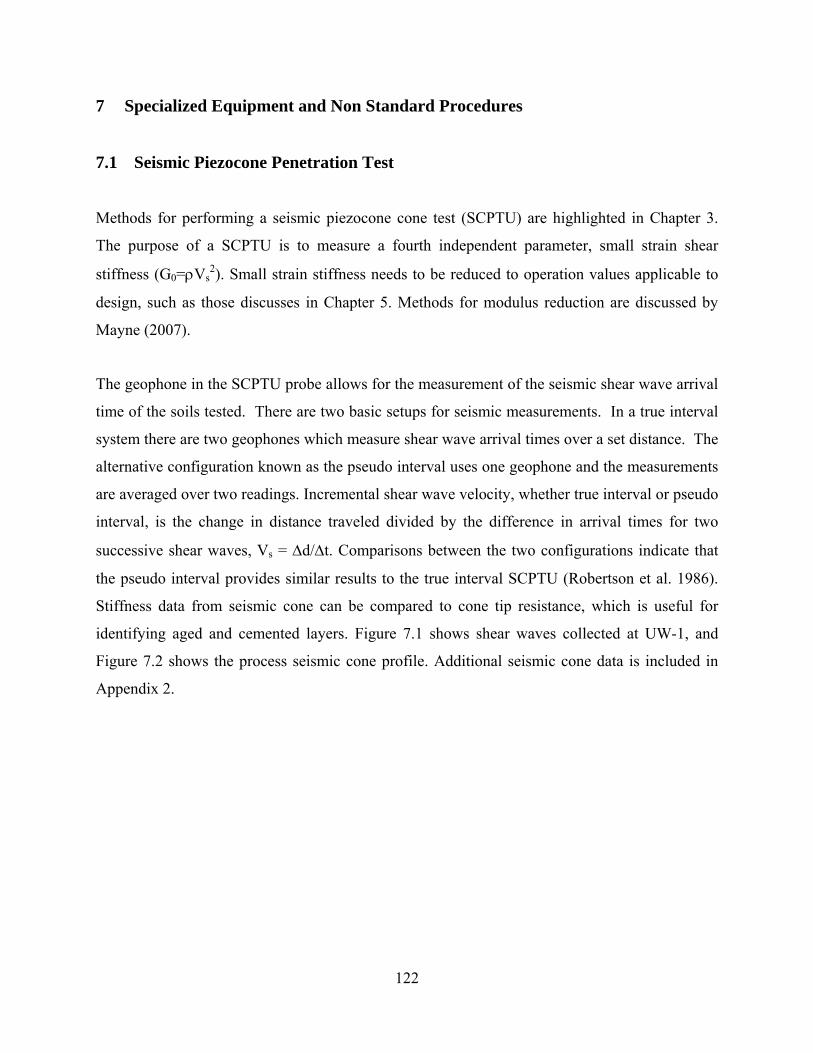
122
7 Specialized Equipment and Non Standard Procedures
7.1 Seismic Piezocone Penetration Test
Methods for performing a seismic piezocone cone test (SCPTU) are highlighted in Chapter 3.
The purpose of a SCPTU is to measure a fourth independent parameter, small strain shear
stiffness (G0=Vs2). Small strain stiffness needs to be reduced to operation values applicable to
design, such as those discusses in Chapter 5. Methods for modulus reduction are discussed by
Mayne (2007).
The geophone in the SCPTU probe allows for the measurement of the seismic shear wave arrival
time of the soils tested. There are two basic setups for seismic measurements. In a true interval
system there are two geophones which measure shear wave arrival times over a set distance. The
alternative configuration known as the pseudo interval uses one geophone and the measurements
are averaged over two readings. Incremental shear wave velocity, whether true interval or pseudo
interval, is the change in distance traveled divided by the difference in arrival times for two
successive shear waves, Vs = d/t. Comparisons between the two configurations indicate that
the pseudo interval provides similar results to the true interval SCPTU (Robertson et al. 1986).
Stiffness data from seismic cone can be compared to cone tip resistance, which is useful for
identifying aged and cemented layers. Figure 7.1 shows shear waves collected at UW-1, and
Figure 7.2 shows the process seismic cone profile. Additional seismic cone data is included in
Appendix 2.
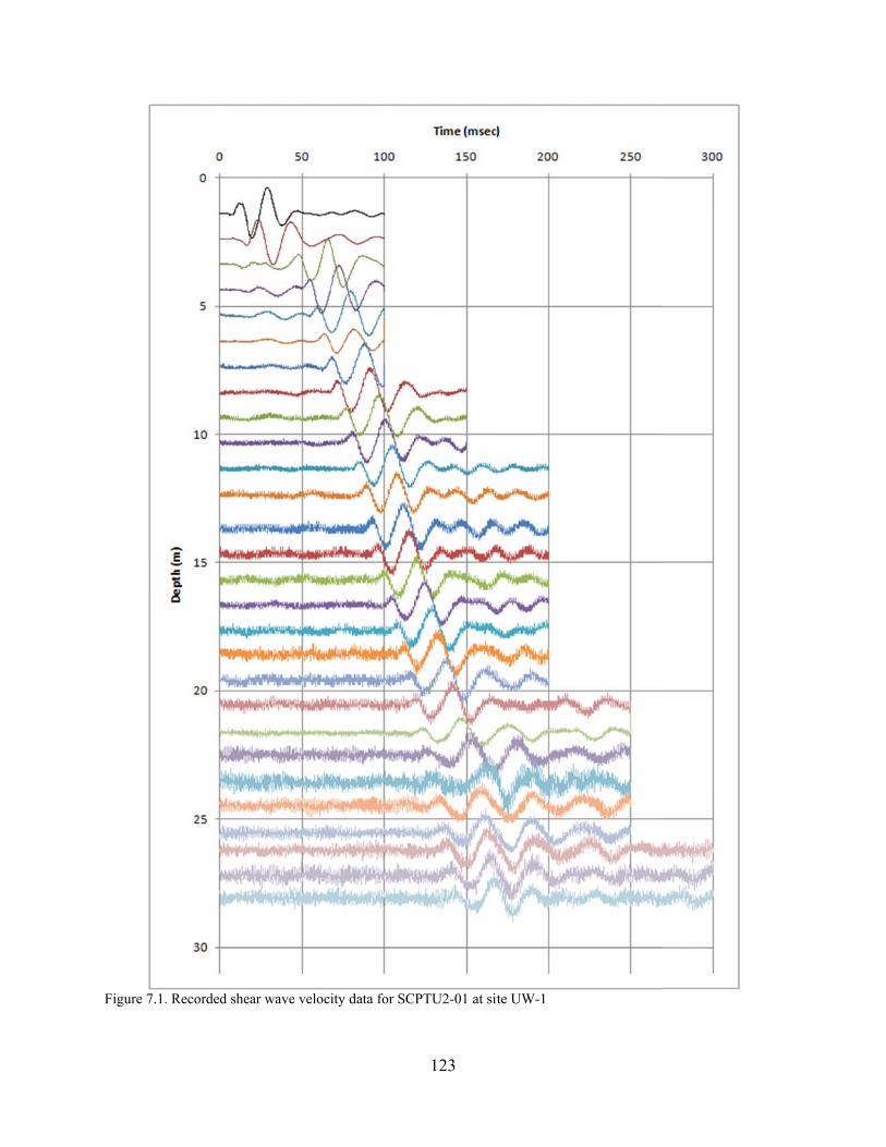
Figure 7.1.
. Recorded sheear wave velociity data for SC
123
CPTU2-01 at sitte UW-1
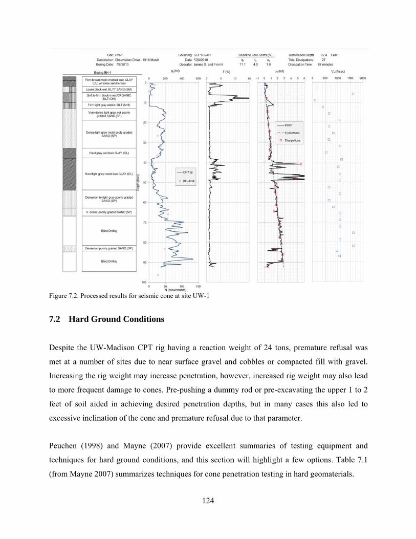
Figure 7.2.
7.2 Ha
Despite t
met at a
Increasin
to more f
feet of s
excessive
Peuchen
technique
(from Ma
. Processed res
ard Ground
the UW-Ma
number of
ng the rig we
frequent dam
oil aided in
e inclination
(1998) and
es for hard
ayne 2007) s
sults for seismi
d Conditio
adison CPT
sites due to
eight may in
mage to cone
n achieving
n of the cone
d Mayne (2
ground cond
summarizes
c cone at site U
ons
rig having a
near surfac
ncrease penet
es. Pre-push
desired pen
and prematu
2007) provid
ditions, and
techniques f
124
UW-1
a reaction w
ce gravel and
tration, how
hing a dumm
netration dep
ure refusal d
de excellent
this section
for cone pen
weight of 24
d cobbles or
wever, increa
my rod or pre
pths, but in
due to that pa
t summarie
n will highlig
netration test
tons, prema
r compacted
ased rig weig
e-excavating
many cases
arameter.
s of testing
ght a few op
ting in hard g
ature refusal
d fill with gr
ght may also
g the upper 1
s this also l
g equipment
ptions. Tabl
geomaterials
l was
ravel.
o lead
1 to 2
ed to
t and
le 7.1
s.
Offshore
drilling a
but, use o
past 20 y
were com
required
Figure 7.3.
cone penet
and in-situ t
of these sam
years. Figure
mbined. Pen
reducing the
. Schematic of
tration testin
testing since
me technolog
e 7.4 illustrat
netration wa
e cone size to
Fugro’s wireli
ng has relied
e the early 7
gies have on
tes results fr
s successful
o 5 cm2 (1 in
ine CPT and sa
125
d on the use
70s (Figure 7
nly been adv
rom an onsho
l to tip resis
nch diameter
ampling system
e of wirelin
7.3, Zuidber
vancing for o
ore investiga
stance value
r) (Kolk et a
m (Wison) (Fug
ne technique
rg 1974, Fu
onshore appl
ation where
es of 1200 t
al. 2005).
gro 2001)
s and altern
ugro 2001, 2
lications ove
CPT and dr
tsf, however
nating
2002),
er the
rilling
r, this
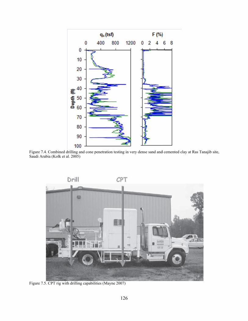
Figure 7.4.Saudi Arab
Figure 7.5.
. Combined dribia (Kolk et al.
. CPT rig with
illing and cone 2005)
drilling capabi
e penetration te
ilities (Mayne
126
esting in very d
2007)
dense sand and
d cemented clayy at Ras Tanaji
ib site,
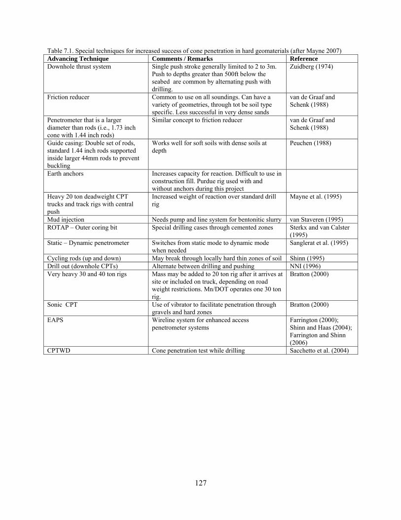
127
Table 7.1. Special techniques for increased success of cone penetration in hard geomaterials (after Mayne 2007) Advancing Technique Comments / Remarks Reference Downhole thrust system Single push stroke generally limited to 2 to 3m.
Push to depths greater than 500ft below the seabed are common by alternating push with drilling.
Zuidberg (1974)
Friction reducer Common to use on all soundings. Can have a variety of geometries, through tot be soil type specific. Less successful in very dense sands
van de Graaf and Schenk (1988)
Penetrometer that is a larger diameter than rods (i.e., 1.73 inch cone with 1.44 inch rods)
Similar concept to friction reducer van de Graaf and Schenk (1988)
Guide casing: Double set of rods, standard 1.44 inch rods supported inside larger 44mm rods to prevent buckling
Works well for soft soils with dense soils at depth
Peuchen (1988)
Earth anchors Increases capacity for reaction. Difficult to use in construction fill. Purdue rig used with and without anchors during this project
Heavy 20 ton deadweight CPT trucks and track rigs with central push
Increased weight of reaction over standard drill rig
Mayne et al. (1995)
Mud injection Needs pump and line system for bentonitic slurry van Staveren (1995) ROTAP – Outer coring bit Special drilling cases through cemented zones Sterkx and van Calster
(1995) Static – Dynamic penetrometer Switches from static mode to dynamic mode
when needed Sanglerat et al. (1995)
Cycling rods (up and down) May break through locally hard thin zones of soil Shinn (1995) Drill out (downhole CPTs) Alternate between drilling and pushing NNI (1996) Very heavy 30 and 40 ton rigs Mass may be added to 20 ton rig after it arrives at
site or included on truck, depending on road weight restrictions. Mn/DOT operates one 30 ton rig.
Bratton (2000)
Sonic CPT Use of vibrator to facilitate penetration through gravels and hard zones
Bratton (2000)
EAPS Wireline system for enhanced access penetrometer systems
Farrington (2000); Shinn and Haas (2004); Farrington and Shinn (2006)
CPTWD Cone penetration test while drilling Sacchetto et al. (2004)
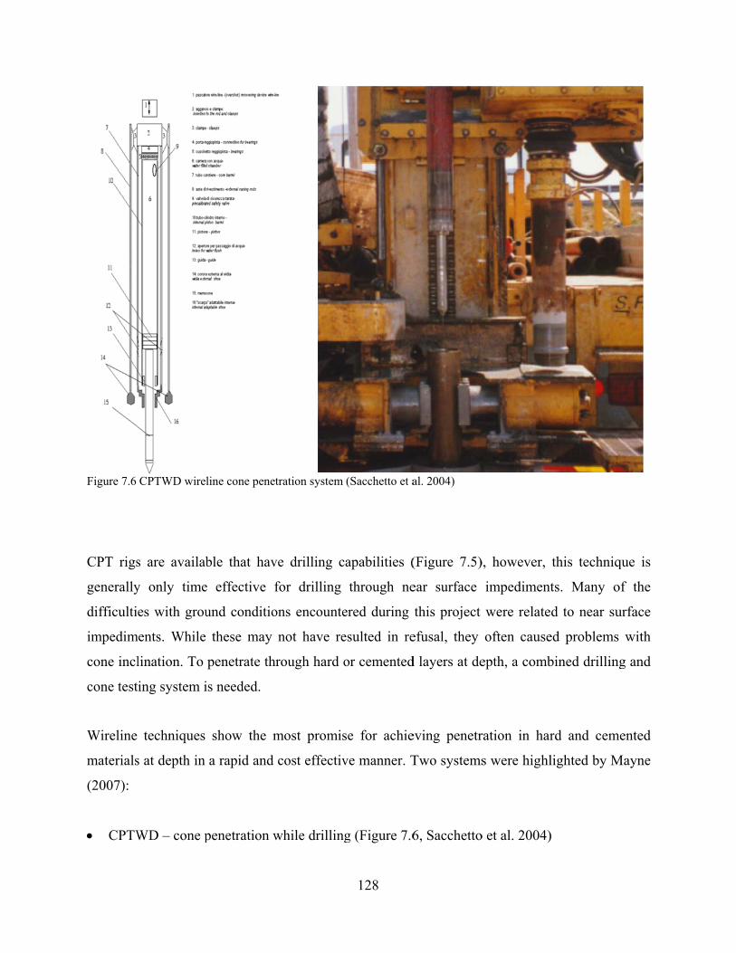
Figure 7.6
CPT rigs
generally
difficulti
impedim
cone incl
cone test
Wireline
materials
(2007):
CPTW
CPTWD wirel
s are availab
y only time
es with grou
ments. While
lination. To
ing system i
techniques
s at depth in
WD – cone p
line cone penet
ble that hav
e effective f
und conditio
these may
penetrate th
is needed.
show the m
a rapid and
penetration w
tration system
ve drilling c
for drilling
ons encounte
not have re
hrough hard o
most promis
cost effectiv
while drilling
128
(Sacchetto et a
capabilities (
through ne
ered during
esulted in re
or cemented
se for achie
ve manner. T
g (Figure 7.6
al. 2004)
(Figure 7.5)
ear surface
this project
efusal, they
d layers at de
eving penetr
Two systems
6, Sacchetto
), however,
impediment
were relate
often cause
epth, a comb
ration in har
s were highl
o et al. 2004)
this techniq
ts. Many o
d to near su
ed problems
bined drilling
rd and cem
lighted by M
)
que is
of the
urface
with
g and
ented
Mayne
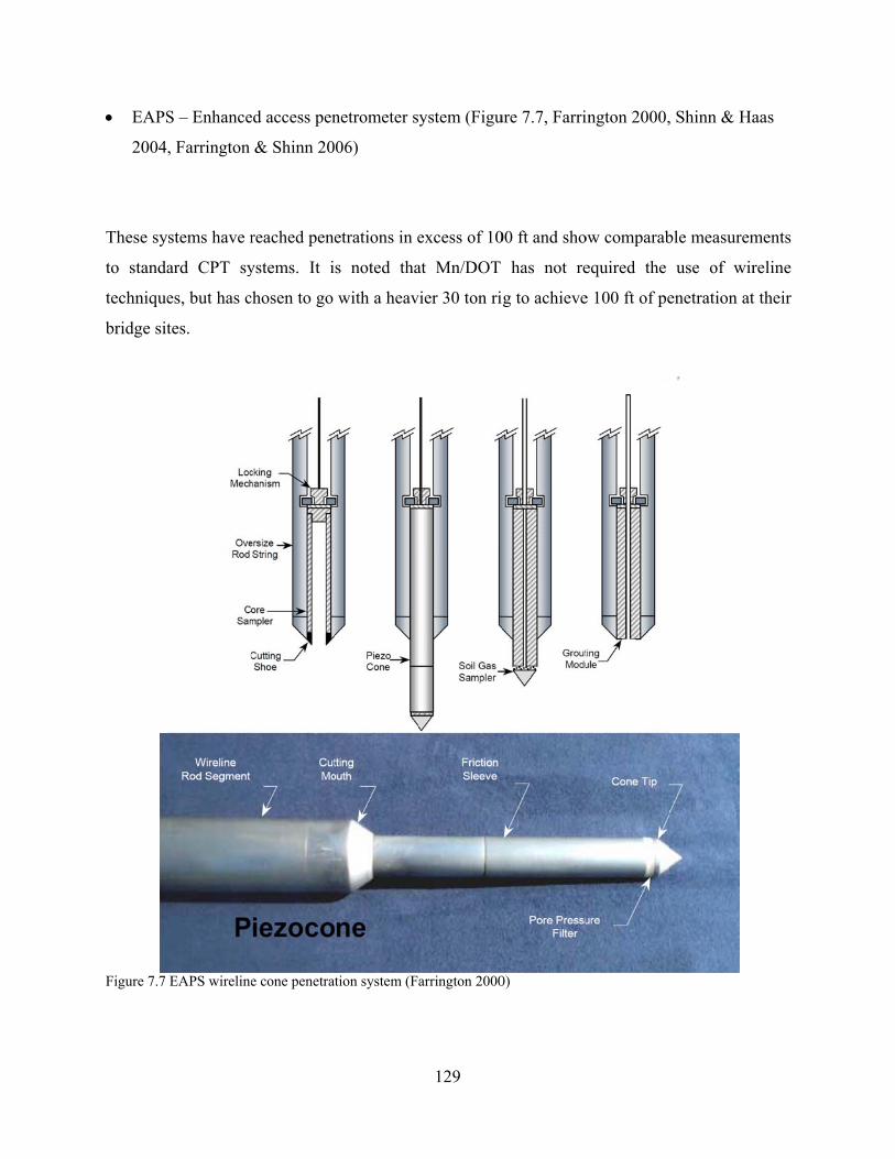
EAPS
2004
These sy
to standa
technique
bridge sit
Figure 7.7
S – Enhance
, Farrington
stems have r
ard CPT sy
es, but has c
tes.
EAPS wireline
ed access pen
& Shinn 20
reached pene
ystems. It i
chosen to go
e cone penetrat
netrometer s
06)
etrations in e
s noted tha
with a heav
tion system (F
129
ystem (Figu
excess of 10
at Mn/DOT
vier 30 ton ri
arrington 2000
ure 7.7, Farri
00 ft and sho
has not re
g to achieve
0)
ington 2000,
ow comparab
equired the
e 100 ft of pe
, Shinn & Ha
ble measurem
use of wir
enetration at
aas
ments
reline
t their
130
8 Conclusions and Recommendations
The objectives of this research were to evaluate the potential use of CPT technology for
Wisconsin DOT projects. Tests were performed at sites in different geological conditions around
the state and CPT results were compared to available data. This report was written to aid in
understanding CPT data and how it relates to geologic history and engineering parameters.
Analysis of the data compiled in the GIS will give the user more experience and familiarity with
CPT results.
Conclusions and recommendations will address the specific objectives of the project.
Departmental subsurface investigative methods (generally soil borings) and cone penetrometer
findings will be compared at a number of sites with differing soils and geology.
Cone penetration in excess of 75 feet was achieved at sites in alluvium, outwash, and lake
deposits. Difficulties were encountered in clay tills that had a significant amount of gravel and
cobbles, as well as fill soils with gravel and cobbles. Commercial firms that performed testing
for the Marquette Interchange and Mitchell Interchange project had slightly better success in
Clay tills, reaching a maximum penetration depth of 92 feet for the Marquette interchange.
While the databases for evaluating soil engineering parameters from CPT data does not need the
intermediate step of CPT-SPT correlations, some interesting observations occurred from
comparing those parameters. The correlations between SPT N-value and CPT tip resistance at
WisDOT sites indicated higher ratios and more scatter compared to data from Mn/DOT.
Mn/DOT uses corrected blowcounts with calibrated hammer energies. Correction of SPT
blowcount for energy and other factors would be expected to result in more reliable site
investigation than current practice.
Evaluation of design parameters will be compared.
Comparison between CPT data and engineering parameters was available for:
131
Coefficient of consolidation
Constrained modulus
Shear stiffness of undrained clays
Undrained strength, and
Soil type
Good correlation was achieved for coefficient of consolidation and soil type (using soil behavior
type charts updated for this project). The small amount of data and questionable quality for
constrained modulus, preconsolidation stress (not discussed), shear stiffness, and undrained
strength did not allow for conclusions to be drawn.
Although no data from Wisconsin were available, global databases were used to provide
discussion of:
drained friction angle in sands
shear stiffness of sands (shallow foundation settlements in sands)
axial pile capacity; and
embankment performance
Discuss advantages and limitations of CPT equipment, operations and interpretation will be
presented.
Testing in Wisconsin and comparison to existing data reinforced existing experience related to
the CPT:
Advantages
CPT data are of higher quality than SPT or laboratory samples collected using current
practice
CPT results are available quicker than drilling, sampling, and lab testing
132
The high volume of CPT data gives confidence in the ability to assess uncertainties and
variability in soil conditions at a given site.
Disadvantages
CPT may meet refusal due to changes in inclination if gravel or cobbles are present
CPTs in excess of 100 ft were not achieved in this study
These disadvantages have been overcome by Mn/DOT and local CPT contractors in that area.
Commercial CPT contractors are expected to have more success in achieving deep penetration
than achieved in this research project, mainly due to the available capital to handle damage to
CPT equipment.
Detailed suggestions for the application of this technology on WisDOT projects will be
presented.
It has taken some time for Mn/DOT to use the CPT on a wide range of projects. WisDOT should
not expect immediate success and cost savings from use of the CPT. They will need to constantly
evaluate and update their site investigation experience. The electronic GIS provided with this
project provides a framework where experience can be collected and rapidly reviewed. However,
for the use of the CPT to be successful on a high percentage of Wisconsin DOT projects, an in
house champion is needed to promote use of the technology and guide its application.
For future projects, it is recommended to perform more CPTs than borings, and to start the CPT
program a week or two before the drilling program. This will still require mobilization of two
rigs, but if the CPT is not successful, the scope of the drillers can be expanded. Perform targeted
sampling of critical and representative layers, not sampling on standard intervals. Borings should
be performed adjacent to CPTs and the drillers need to take high quality samples. The sample
quality and results of strength testing (i.e., UU and UC) observed in this study does not produce
reliable results, making it difficult to assess uncertainty, reliability, and levels of conservatism in

133
design. High quality sampling proposed for the DOT-1 site should be a good first step to
improving practice and understanding the inherent assumptions behind successful designs.
Ideally, each of the 23 representative layers evaluated in detail in this report would have high
quality sampling and laboratory testing performed at some time in the future. Only with
consistent evaluations from laboratory and in-situ test data can practice move forward and cost
savings be realized.
134
9 References
Acomb, L. J., Mickelson, D. M., & Evenson, E. B. (1982). “Till Stratigraphy and Late Glacial Events in the Lake Michigan Lobe of Eastern Wisconsin.” Geological Society of America Bulletin , 93, 289-296.
Almeida, M., Danziger, F., and Lunne, T. (1996). “The use of the piezocone test to predict the axial capacity of driven and jacked piles.” Canadian Geotechnical Journal, 33(1), 23-41.
Amundsen, T., Lunne, T., and Christophersen, H.P. (1985). “Advanced deep-water soil investigation at the Troll East field.” Advances in Underwater Technology, Offshore Site Investigation, 3, Grahan & Trotman, London, 165 – 186.
API (2000). “Recommended Practice for Planning, Designing, and Constructing Fixed Offshore Platforms – Working Stress Design,” API RP2A, 21st Edition, American Petroleum Institute, Washington, D.C.
ASTM (American Society for Testing and Materials) (2000). “Standard test method for performing electronic friction cone and piezocone penetration testing of soils.” D5778-95, ASTM Book of Standards, Vol. 04-09.
ASTM (2004) “Standard Test Method for Consolidated Undrained Triaxial Compression Test for Cohesive Soils” D4767, ASTM Book of Standards.
ASTM (2004) “Standard Test Methods for One-Dimensional Consolidation Properties of Soils Using Incremental Loading” D2435, ASTM Book of Standards.
ASTM (2005) “Standard Test Methods for Laboratory Determnation of Water (Moisture) Content of Soil and Rock by Mass” D2216, ASTM Book of Standards.
ASTM (2007) “Standard Test Method for Particle-Size Analysis of Soils” D422, ASTM Book of Standards.
ASTM (2007) “Standard Test Method for Unconsolidated-Undrained Triaxial Compression Test on Cohesive Soils” D2850, ASTM Book of Standards.
ASTM (2009) “Standard Practice for Description and Identification of Soils (Visual-Manual Procedure)” D2488, ASTM Book of Standards.
ASTM (2009) “Standard Test Methods for Particle-Size Distribution (Gradation) of Soils Using Sieve Analysis” D6913, ASTM Book of Standards.
ASTM (2010) “Standard Test Methods for Liquid Limit, Plastic Limit, and Plasticity Index of Soils” D4318, ASTM Book of Standards.
ASTM (2010) “Standard Practice for Classification of Soils for Engineering Purposes (Unified Soil Classification System)” D2487, ASTM Book of Standards.
Atkinson, J. (2007). The Mechanics of Soils and Foundations. New York: Taylor & Francis.
Attig, J. A., & Knox, J. C. (2008). “Catastrophic Flooding from Glacial Lake Wisconsin.” Geomorphology, 93, 384-397.
135
Attig, J. W., Clayton, L., & Mickelson, D. M. (1985). “Correlation of Late Wisconsin Glacial Phases in Western Great Lakes Area.” Geological Society of America Bulletin , 96, 1585-1593.
Begemann, H. K. (1965). “The Friction Jacket Cone as an Aid in Determining the Soil Profile.” Proceedings of the 6th International Conference on Soil Mechanics and Foundation Engineering, 1, pp. 17-20. Montreal.
Bjerrum, L. (1954). “Geotechnical Properties of Norwegian Marine Clays.” Géotechnique, 4 (2), 49-69.
Bolton, M.D. (1986). “The Strength and Dilatancy of Sands.” Géotechnique, 36(1), 65-78.
Burland, J. B., & Burbidge, M. C. (1985). “Settlement of Foundations on Sand and Gravel.” In Proceedings fo the Institution of Civil Engineering, Part I, 78 (6), pp. 1325-1381.
Burns, S. E., & Mayne, P. W. (1998a). “Monotonic and Dilatory Pore-Pressure Decay During Piezocone Test in Clay.” Canadian Geotechnical Journal, 35, 1063-1073.
Campanella, R.G., Robertson, P.K. & Gillespie, D. (1986). “Seismic cone penetration test.” Use of In Situ tests in Geotechnical Engineering, GSP 6, Blacksburg, VA, ASCE, 116-130.
Casagrande, A. (1948). “Classification and Identification of Soils.” Transactions. 113, pp. 901-930. ASCE.
Chow, F. C. (1997). “Investigations into the behaviour of displacement piles for offshore foundations.” PhD Thesis, Imperial College, London.
Clark, P. U., Dyke, A. S., Shakun, J. D., Carlson, A. E., Clark, J., Wohlfarth, B., et al. (2009). “The Last Glacial Maximum.” Science , 325, 710-714.
Clayton, J. A., & Knox, J. C. (2008). “Catastrophic Flooding from Glacial Lake Wisconsin.” Geomorphology, 93, 384-397.
Clayton, L., & Moran, S. R. (1982). “Chronology of Late Wisconsinan Glaciation in Middle North America.” Quaternary Science Reviews, 1, 55-82.
Clayton, L., Attig, J. W., Mickelson, D. M., Johnson, M. D., & Syverson, K. M. (2006). “Glaciation of Wisconsin.” Madison, WI: Wisconsin Geologic and Natural History Survey.
Coop, M.R. (2005). “On the Mechanics of Reconstituted and Natural Sands.” Deformation Characteristics of Geomaterials, Lyon, Taylor & Francis, 29-58.
Dasenbrock, D.D. 2008.” Geotechnical Data Sharing and Electronic Data Exchange at Minnesota DOT.” GeoCongress 2008: Characterization, Monitoring, and Modeling of GeoSystems (GSP 179), ASCE, Reston, VA.
Dasenbrock, D. D., Schneider, J. A., & Mergen, E. M. (2010). “CPT Experience in Glacial Geological Conditions of Minnesota, USA.” Proceedings of CPT 2010. Huntington Beach, CA.
Delft Laboratory of Soil Mechanics (Delft) (1936). “The predetermination of the required length and the prediction of the toe resistance of piles.” Proc. 1st Int. Conf. on Soil Mech. and Foundation Eng., Cambridge, 181-184.
136
De Groot, D. J., & Lutenegger, A. J. (2003). “Geology and Engineering Properties of the Conneticut Valley Varved Clay.” Characterization and Engineering Properties of Natural Soils (pp. 695-724). Lisse, The Netherlands: Swets and Zeitlinger.
Douglas, B.J., and Olsen, R.S. (1981). “Soil classification using the electric cone penetrometer test.” Cone Penetration Testing and Experience, ASCE, 209-227.
Edil, T. B., & Mickelson, D. M. (1995). “Overconsolidated Glacial Tills in Eastern Wisconsin.” Transportation Research Record, 1479, 99-106.
Eslami, A., and Fellenius, B. (1997). “Pile capacity by direct CPT and CPTu methods applied to 102 case histories.” Canadian Geotech. J., 34, 886-904.
ESRI ArcGIS Online, World Imagery [Aerial Photographs]. Visual Scale. http://www.arcgis.com/home/group.html?owner=esri&title=ESRI%20Maps%20and%20Data.
ESRI ArcGIS Online, US Topo Maps [Topographic Maps]. Visual Scale. http://www.arcgis.com/home/group.html?owner=esri&title=ESRI%20Maps%20and%20Data.
Farrand, W. R., Mickelson, D. M., Cowan, R. W., & Geobel, J. E. (1984). “Quaternary Geologic Map of the Lake Superior 4° x 6° Quadrangle, United States.” Map I-1420 (NL-16) . United States Geological Survey.
Farrington, S. P. (2000). “Development of a Wirline CPT System for Multiple Tool Usage.” Proceedings, Industry Partnerships for Environmental Science and Technology, (p. 40).
Farrington, S. P., & Shinn, J. D. (2006). “Hybrid Penetration for Geotechnical Site Investigation.” Proceedings, Geo-Congress 2006, (p. 5 pp). Atlanta, GA.
Finnie, I. M., & Randolph, M. F. (1994). “Punch-through and Liquefaction Induced Failure of Shallow Foundations on Calcareous Sediments.” Proceedings of the International Conference on Behavior of Offshore Structures, (pp. 217-230). Boston.
Fugro (2001). “Geophysical and Geotechncial Techniques for the Investigation of Near-Seabed Soils and Rocks,” Fugro NV, Leidschendam, NL, 51 p.
Fugro (2002). “Down to Earth and Up-to-Date,” Fugro NV, Leidschendam, NL, 304 p.
Fullerton, D. S., Ringrose, S. M., Clayton, L., Schreiner, B. T., & Goebel, J. E. (2000). Quaternary Geologic Map of the Winnepeg 4°x6° Quadrangle, United States and Canada. I-1420 (NM-14) . USGS.
Gavin, K., and Lehane, B.M. (2007). “Base load-displacement response of piles in sand.” Canadian Geotechnical Journal, 44(9), 1053-1063.
Goebel, J. E., Mickelson, D. M., Farrand, W. R., Clayton, L., Knox, J. C., Cahow, A., et al. (1983). “Quaternary Geologic Map of the Minneapolis 4° x 6° Quadrangle, United States.” Map I-1420 (NL-15). United States Geologic Survey.
Hallberg, G. R., Lineback, J. A., Mickelson, D. M., Knox, J. C., Geobel, J. F., Hobbs, H. C., et al. (1991). “Quaternary Geologic Map of the Des Moines 4° x 6° Quadrangle, United States.” Map I-1420 (NK-15). United States Geological Survey.
137
Hooyer, T. S. (2007). “Late-Glacial History of East-Central Wisconsin.” Madison, WI: Wisconsin Geological and Natural History Survey.
Hotstream, J. N. (2011).” Classification of Wisconsin glacial soils using the cone penetration test.” M.S. Thesis, University of Wisconsin – Madison.
Houlsby, G.T., and Hitchman, R. (1988). “Calibration chamber tests of a cone penetrometer in sand.” Géotechnique, 38(1), 39-44.
Hvorslev, M.J. (1953). “Cone penetrometer operated by rotary drilling rig.” Proc. 3rd Int. Conf. on Soil Mech. and Foundation Engineering, Vol. 1, 236.
International Commission on Stratigraphy. (2010). International Stratigraphic Chart. http://www.stratigraphy.org/ics%20chart/09_2010/StratChart2010.jpg.
Jamiolkowski, M. B., Lo Presti, D. F. C., and Manassero, M. 2003. “Evaluation of Relative Density and Shear Strength of Sands from Cone Penetration Test.” Soil Behaviour and Soft Ground Construction, (GSP 119), ASCE, Reston, VA, 201-238.
Janbu, N., 1985. “Soil Models in Offshore Engineering (25th Rankine Lecture).” Géotechnique, 35:243-281.
Jardine, R. J., Chow, F. C., Overy, R. F., Standing, J. R. (2005). ICP design methods for driven piles in sands and clays. Thomas Telford, London, 97.
Jefferies, M. G., & Been, K. (2006). Soil Liquefaction: A Critical State Approach. London and New York: Taylor and Francis.
Jefferies, M. G., & Davies, M. P. (1993). “Use of CPTu to Estimate Equivalent SPT N60.” Geotechnical Testing Journal, 16 (4), 458-468.
Karlsrud, K., Hansen, S.B., Dyvic, R., and Kalsnes, B. (1993). “NGI’s pile tests at Tilbrook and Pentre – review of testing procedures and results.” Large-scale pile tests in clay, Thomas Telford, London, 405-429.
Keaveny, J. M., & Mitchell, J. K. (1986). “Strength of Fine-Grained Soils Using the Piezocone.” Use of In-Situ Tests in Geotechnical Engineering (pp. 668-699). Reston: ASCE.
Kolk, H. J., Baaijens, A. E., & Senders, M. (2005). “Design Criteria for Pipe Piles in Silica Sands.” Frontiers in Offshore Geotechnics (Proc. ISFOG, Perth, Australia) (pp. 711-716). London, United Kingdom: Taylor and Francis Group.
Kulhawy, F. H., & Mayne, P. W. (1990). “Manual on Estimating Soil Properties for Foundation Design.” Palo Alto, CA: Electric Power Research Institute.
Ladd, C.C. (1991). “Stability Evaluation During Staged Construction.” ASCE Journal of Geotechnical Engineering, 117(4), 540-615.
Ladd, C.C., and DeGroot, D.J. 2003. Recommended Practice for Soft Ground Site Characterization. Arthur Casagrande Lecture. In Soil and Rock America 2003: Proceedings of the 12th Panamerican Conference on Soil Mechanics and Geotechnical Engineering, Cambridge, Mass., 22–26 June 2003. VGE Verlag Glückauf, 2003. Vol. 1, pp. 3–57.
Lambeck, K., & Chappell, J. (2001). “Sea Level Change Through the Last Glacial Cycle.” Nature , 292, 679-686.
138
Lehane, B.M. and Fahey, M. (2004). “Using SCPT and DMT Data for Settlement Prediction in Sand.” Proc. 2nd International Conf. on Site Characterisation, Porto, Portugal, Vol. 2, 1673–1680, Millpress, Rotterdam.
Lehane, B.M. and Jardine R.J. (1994). :Displacement-Pile Behavior in a Soft Marine Clay.” Canadian Geotechnical Journal. 31, 181-191.
Lehane, B.M., Jardine, R.J., Bond, A.J., and Frank, R. (1993). “Mechanisms of Shaft Friction in Sand from Instrumented Pile Tests.” J. Geotech. Eng., 119 (1), 19-35.
Lehane, B.M., Schneider, J.A., and Xu, X. (2005). “CPT based design of driven piles in sand for offshore structures.” Report GEO 05345, The University of Western Australia.
Lehane, B.M., Schneider, J.A., and Xu, X. 2008. “Design of Displacement Piles in Siliceous Sands Using the CPT.” Australian Geomechanics, 43(2), 21-40.
Leroueil, S., Tavenas, F., Samson, L., & Morin, P. (1983). “Preconsolidation Pressure of Champlain Clays. Part 2 Laboratory Determination.” Canadian Geotechnical Journal, 20, 803-816.
Liao, T., Bell, K. R., & Senapathy, H. (2010). “CPT in Glacial Soils After Deep Excavation.” Proceedings of CPT 2010, (p. 8). Huntington Beach, CA.
Lineback, J. A., Bleuer, N. K., Mickelson, D. M., Farrand, W. R., & Goldthwait, R. P. (1983). “Quaternary Geologic Map of the Chicago 4° x 6° Quadrangle, United States.” Map I-420 (NK-16). United States Geological Survey.
Lisiecki, L. E., & Raymo, M. E. (2005). “A Plio-Pleistocene Stack of 57 Globally Distributed Benthic d18O Records.” Paleoceanography , 20, 1003.
Lunne, T., Eidsmoen, T., Gillespie, D., and Howland, J.D. (1986). “Laboratory and field evaluation of cone penetrometers.” Use of In Situ Tests in Geotechnical Engineering, GSP 6, ASCE, 714-729.
Lunne, T. M., Robertson, P. K., & Powell, J. M. (1997). Cone Penetration Testing in Geotechnical Practice. New York, NY: Blackie Academic, EF Spon/Routledge Publishers.
Mayne, P.W. (1980). "Cam-Clay Predictions of Undrained Shear Strength", Journal of the Geotechnical Engineering Division, ASCE, Vol. 106 (GT11), 1219-1242.
Mayne, P.W. (1986). "CPT Indexing of In-Situ OCR in Clays", Use of In-Situ Tests in Geotechnical Engineering (GSP 6), ASCE, New York, NY, pp. 780-793.
Mayne, P. W. (2001). “Stress-Strain-Strength-Flow Parameters from Enhanced In-Situ Tests.” Proceedings, International Conference on In-Situ Measurement of Soil Properties and Case Histories, (pp. 27-48). Bali, Indonesia.
Mayne, P. W. (2006). “The 2nd James K. Mitchell Lecture: Undisturbed Sand Strength from Seismic Cone Tests.” Geomechanics and Geoengineering , 1 (4), 239-247.
Mayne, P. W. (2007). “Cone Penetration Testing: A Synthesis of Highway Practice.” Washington, D. C.: Transportation Research Board.
Mayne, P. W., & Illingworth, F. (2010). “Direct CPT Method for Footing Response in Sands Using a Database Approach.” Proceedings of CPT 2010, (p. 8). Huntington Beach, CA.
139
Mayne, P. W., & Poulos, H. G. (1999). “Approximate Displacement Influence Factors for Elastic Shallow Foundations.” Jounal of Geotechnical and Geoenvironmental Engineering , 125 (6), 453-460.
Meyerhof, G.G. (1956). “Penetration tests and bearing capacity of cohesionless soils.” J. Soil Mech. and Foundation Div., 82(SM1), Paper 886, 19.
Mickelson, D. M., Acomb, L. J., & Edil, T. B. (1978). “The Origin of Preconsolidated and Normally Consolidated Tills in Eastern Wisconsin, USA.” Moraines and Varves: Origin, Genesis and Classification (pp. 179-187). Zurich: Balkema.
Moss, R. E. (2003). “CPT-Based Probalistic Assessment of Seismic Soil Liquefaction Initiation.” PhD. Dissertation University of California, Berkeley.
Moss, R. E., Seed, R. B., & Olsen, R. S. (2006). “Normalizing the CPT for Overburden Stress.” Journal of Geotechnical and Geoenvironmental Engineering, 132 (3), 378-387.
Olsen, R.S., Mitchell, J.K. (1995). “CPT stress normalization and prediction of soil classification.” Proc., Int. Symp. on Cone Penetration Testing, CPT'95, Linköping, 2, Geotechnical Society. SGF Report 3:95, 257 – 262.
Peuchen, J. (1998). Commercial CPT Profiling in Soft Rocks and Hard Soils. Geotechnical Site Characterization. 2, pp. 1131-1137. Rotterdam, The Netherlands: Balkema.
Puppula, A. J. (2008). “Estimating Stiffness of Subgrade and Unbound Materials for Pavement Design: A Synthesis of Highway Practice.” Washington, D. C.: Transportation Research Board.
Ramsey, N. (2002). “A Calibrated Model for the Interpretation of Cone Penetration Tests in North Sea Quaternary Soils.” Offshore Site Investigation and Geotechnics: Diversity and Sustainability, (pp. 341-356). London.
Randolph, M. F. (2004). “Characterization of Soft Sediments for Offshore Applications.” 2nd Int. Conf. on Site Characterization (Proc. ISC'2, Porto). I, pp. 209-232. Rotterdam, the Netherlands: Millpress.
Robertson, P. K. (1990). “Soil Classification Using the Cone Penetration Test.” Canadian Geotechnical Journal, 27, 151-158.
Robertson, P. K. (1991). “Soil Classification Using the Cone Penetration Test: Reply.” Canadian Geotechnical Journal, 28, 176-178.
Robertson, P. K. (2010). Estimating in-situ soil permeability from CPT & CPTu. 2nd International Symposium on Cone Penetration Testing, II. Huntington Beach, CA.
Robertson, P. K., & Wride, C. E. (1998). “Evaluating cyclic liquefaction potential using the cone penetration test.” Canadian Geotechnical Journal, 35, 442-459.
Robertson, P. K., Campanella, R. G., & Wightman, A. (1983). “SPT-CPT Correlations.” Journal of the Geotechnical Engineering Division , 108 (No. GT 11), 1449-1459.
Robertson, P. K., Campanella, R. G., Gillespie, D., & Rice, A. (1986). “Seismic CPT to Measure In Situ Shear Wave Velocity.” Journal of Geotechnical Engineering, 112 (8), 791-803.
140
Robertson, P. K., Sully, J. P., Woeller, D. J., Lunne, T., Powell, J. J., & Gillespie, D. G. (1992). “Estimating Coefficient of Consolidation from Piezocone Tests.” Canadian Geotechnical Journal, 29, 539-550.
Sacchetto, M. A., Trevisan, A., Elmgren, K., & Melander, K. (2004). “Cone Penetration Test While Drilling.” Geotechnical and Geophysical Site Characterization. 1, pp. 787-794. Rotterdam, The Netherlands: Millpress.
Sado, E. V., Fullerton, D. S., & Farrand, W. R. (1994). Quaternary Geologic Map of the Lake Nipigon 4°x6° Quadrangle, United States and Canada. I-1420 (NM-16) . USGS.
Sado, E. V., Fullerton, D. S., Goebal, J. E., & Ringrose, S. M. (1995). Quaternary Geologic Map of the Lake of the Woods 4°x6° Quadrangle, United States and Canada. I-1420 (NM-15) . USGS.
Salgado, R. (2008) The Engineering of Foundations, McGraw Hill.
Salgado, R., Mitchell, J. K., & Jamiolkowski, M. (1997). “Cavity Expansion and Penetration Resistance in Sands.” Journal of Geotechnical and Geoenvironmental Engineering. 123, 334-354.
Santamarina, J.C., Klein, K.A., and Fam, M.A. 2001. Soils and Waves. John Wiley & Sons, New York.
Schmertmann, J. H. (1975). Measurement of In Situ Shear Strength. Proceedings of the Conference on In Situ Measurement of Soil Properties (pp. 57-138). Raleigh, NC: ASCE.
Schmertmann, J. H. (1978). Guidelines for Cone Test, Performance, and Design (No. FHWATS-78209): U.S. Federal Highway Administration.
Schmertmann, J.H. (1995). “CPT’63(+) – A history in the USA from a University of Florida viewpoint.” Proc. Int. Symp. On Cone Penetration Testing, Vol. 3, 269-275.
Schneider, J. A., Lehane, B. A., & Schnaid, F. (2007). “Velocity Effects on Piezocone Measurements in Normally and Overconsolidated Clays.” International Journal of Physical Modeling in Geotechnics, 2, 23-34.
Schneider, J. A., Randolph, M. F., Mayne, P. W., & Ramsey, N. R. (2008). “Analysis of Factors Influencing Soil Classification Using Normalized Piezocone Tip Resistance and Pore Pressure Parameters.” Journal of Geotechnical and Geoenvironmental Engineering, 134 (11), 1569-1586.
Schneider, J. A., Xu, X., & Lehane, B. M. (2010). End Bearing Formulation for CPT Based Driven Pile Design Methods in Siliceous Sands. Proceedings of CPT 2010, (p.7). Huntington Beach, CA.
Schofield, A., & Wroth, P. (1968). Critical State Soil Mechanics.
Schuettpelz, C.C., Fratta, D., and Edil, T. (2010). “Mechanistic corrections for determining the resilient modulus of base course materials based on elastic wave measurements.” Journal of Geotechnical and Geoenvironmental Engineering, 136(8), 1086-1094.
Shinn, J. K., & Haas, J. W. (2004). “Enhanced Access Penetration System: A Direct Push System for Difficult Site Conditions.” Geotechnical and Geophysical Site Characterization. 1, pp. 795-800. Rotterdam, The Netherlands: Millpress.

141
Shockley, W.G., Cunny, R.W., and Strohm, W.E., Jr. (1961). “Investigations with rotary cone penetrometer,” Proc. 5th Int. Conf. on Soil Mech. and Foundation Eng., Vol. 1, 523.
Silva, M. F., White, D. J., & Bolton, M. D. (2006). “An Analytical Study of the Effect of Penetration Rate on Piezocone Tests in Clay.” International Journal of Numerical Analytical Methods in Geomechanics, 30, 501-527.
Stratigraphics (2003a). “Piezometric cone penetration testing with soil electrical conductivity measurements: Marquette Interchange West Leg Core, Milwaukee, Wisconsin.” Prepared for Soils and Engineering Services, Inc., Report 03-110-190, December.
Stratigraphics (2003b). “Piezometric cone penetration testing with soil electrical conductivity measurements: Marquette Interchange, Milwaukee, Wisconsin.” Prepared for Maxim Technologies, Report 03-120-050, April.
Sully, J. P., Robertson, P. K., Campanella, R. G., & Woeller, D. J. (1999). “An approach to evaluation of field CPTU dissipation data in overconsolidated fine-grained soils.” Canadian Geotechnical Journal, 36, 369-381.
Teh, C. I., & Houlsby, G. T. (1991). An analytical study of the cone penetration test in clay. Géotechnique, 41 (1), 17-34.
Tonni, L., & Gottardi, G. (2011). “Analysis and Interpretation of Peizocone Data on the Silty Soil of the Venetian Lagoon (Treporti Test Site).” Canadian Geotechnical Journal , 48 (4), 616-633.
Torstensson, B. A. (1975). “Pore Pressure Sounding Instrument.” Proceedings of the Conference on In Situ Measurement of Soil Properties. 2, pp. 48-55. Raleigh, NC: ASCE.
Transporation Research Center-LTAP. (1999). Work Zone Safety. Madison, WI: University of Wisconsin-Madison.
U.S. Bureau of Reclamation - U.S. Department of the Interior. (1998). Earth Manual - Part 1. Denver: US Government Printing Office.
Viggiani, G., & Atkinson, J. H. (1995). Stiffness of Fine-Grained Soil at Small Strains. Géotechnique , 45 (2), 249-265.
White, D. J., & Lehane, B. M. (2004). Friction Fatigue on Displacement Piles in Sand. Géotechnique , 54 (10), 645-658.
Wisconsin Geological and Natural History Survey (WGNHS). (1983). Thickness of Unconsolidated Material in Wisconsin. Madison, Wisconsin: University of Wisconsin-Extension.
Wissa, A.E.Z., Martin, R.T., and Garlanger, J.E. (1975). “The piezometer probe.” Proc. ASCE Specialty Conference on In Situ Measurement of Soil Properties, Vol. 1, Raleigh, NC,536-545.
Wroth, C. P. (1984). Interpretation of In Situ Soil Tests. Géotechnique , 34 (4), 449-489.
Wroth, C. P. (1988). Penetration Testing - A More Rigorous Approach to Interpretation. In J. De Ruiter (Ed.), Penetration Testing 1988 (pp. 303-311). Orlando: Balkema.
142
Wroth, C.P., and Houlsby, G.T. (1985). “Soil mechanics: property characterization & analysis procedures.” Proc., 11th Int. Conf. on Soil Mech. and Foundation Eng., ICSMFE, Vol. 1, San Francisco, 1-56.
Wroth, C. P., & Wood, D. M. (1978). The Correlation of Index Properties with Some Basic Engineering Properties of Soil. Canadian Geotechnical Journal, 137-145.
Xu, X., and Lehane, B. M. (2005). “Evaluation of end-bearing capacity of closed-ended pile in sand from cone penetration data.” Proceedings of the First International Symposium on Frontiers in Offshore Geotechnics, Perth, 733-739.
Xu, X., Schneider, J. A., & Lehane, B. M. (2008). Cone Penetration Test Methods for End-Bearing Assessment of Open-and Close-Ended Driven Piles in Siliceous Sand. Canadian Geotechnical Journal, 45, 1130-1141.
Zuidberg, H. (1974). Use of Static Cone Penetrometer Testing in the North Sea. Porceedings of the European Symposium on Penetration Testing (ESOPT), 2.2, pp. 433-436. Stockholm, Sweden.