www.elsevier.com/locate/commatsci

Computational Materials Science 36 (2006) 319–328

Computer simulations of true stress development andviscoelastic behavior in amorphous polymeric materials

Ricardo Simoes a,b,*, Antonio M. Cunha a, Witold Brostow b

a Institute for Polymers and Composites (IPC), Department of Polymer Engineering, University of Minho, 4800-058 Guimaraes, Portugalb Laboratory of Advanced Polymers and Optimized Materials (LAPOM), Department of Materials Science and Engineering,

University of North Texas, Denton, TX 76203-5310, USA

Received 7 March 2005; received in revised form 4 April 2005; accepted 12 April 2005

Abstract

Molecular dynamics simulations were employed to study the mechanical properties and true stress development in amorphouspolymeric materials. As expected, the true stress levels are much higher than those indicated by the engineering stress. However, thetrue stress behavior was found to be not only quantitatively but also qualitatively different from that of the engineering stress. Highlylocalized deformation results in abrupt increases of the true stress in certain regions, favoring crack formation and propagation. Thecomputer-generated materials exhibit viscoelastic recovery curves similar to those seen in experiments. The recovery process is non-homogeneous and affected by the spatial arrangement of the amorphous chains. The loading conditions determine the preferentialdeformation mechanisms and influence the extent of recovery. Some deformation mechanisms are not recovered and contribute topermanent deformation.� 2005 Elsevier B.V. All rights reserved.

PACS: 07.05.T; 36.20.E; 36.20.F; 62.20.F

Keywords: Computer simulations; Molecular dynamics; Polymer viscoelasticity; True stress; Mechanical properties; Structure–properties relation-ships

1. Introduction

As argued before, service performance and reliabilityof polymeric materials are of interest to all, not only toscientists and engineers [1,2]. As polymers become morewidely used and in many demanding applications arereplacing metals and ceramics, understanding their

0927-0256/$ - see front matter � 2005 Elsevier B.V. All rights reserved.doi:10.1016/j.commatsci.2005.04.007

* Corresponding author. Address: Institute for Polymers and Com-posites (IPC), Department of Polymer Engineering, University ofMinho, 4800-058 Guimaraes, Portugal. Tel.: +351 253510320; fax:+351 253510339.

E-mail addresses: rsimoes@dep.uminho.pt (R. Simoes), amcun-ha@dep.uminho.pt (A.M. Cunha), brostow@unt.edu (W. Brostow).

behavior becomes a critical issue. However, the proper-ties of polymers are often difficult to characterize andeven more difficult to predict, due to their complexstructure and to the variety of factors involved, namelythe time-dependent behavior, the processing history andtheir anisotropic character.

Computer simulations have an enormous potential toprovide better understanding of the behavior and prop-erties of polymeric materials. As eloquently argued byFossey [3], simulations provide information not readilyaccessible experimentally; this either due to the prohibi-tively difficult nature of the tests, the inadequacy ofexisting equipment and techniques to study a particularphenomena, or other impediments. A significant advan-tage of computer simulations is the ability to create

320 R. Simoes et al. / Computational Materials Science 36 (2006) 319–328

conditions that cannot be replicated in a controlledexperimental environment. Even more importantly, theycan be used to determine the effects of one system vari-able at a time.

As pointed out by Gilman [4], not all computer sim-ulations are of interest, particularly those which onlyconfirm what is already known from experiments. Thispaper meets this challenge, introducing a method forthe determination of true stress response of computer-generated materials (CGMs). Results on viscoelasticbehavior of simulated amorphous polymers are alsoreported.

It is important to point out that the simulations pre-sented and discussed in this paper were not performedwith the intent of replacing experiments but rather tocomplement them. The concomitant use of computersimulations and experiments should produce a synergis-tic effect, enabling a more complete understanding of theproperties and behavior of polymeric materials.

2. Applications of computer simulations to polymerbehavior and properties

At least three simulation approaches have beenwidely used by the scientific community: the MonteCarlo (MC), the Brownian dynamics (BD), and themolecular dynamics (MD) methods [5,6]. MD is themethod preferred by our research group for the presentpurpose of studying the time-dependent deformation ofpolymeric materials. This method was originally devel-oped by Alder and Wainwright, with the intent of deter-mination of phase diagrams of systems of hard spheres[7]. At a later stage, continuous potentials allowed amore realistic response of the system. Rahman was thefirst to introduce Mie potentials (often called Lennard-Jones potentials) in the MD simulations [8], which cre-ated the basis for most of the work done in this areasince then.

Atomistic simulations have been extensively used tostudy molecular-level phenomena in polymers [9–12].Termonia and Smith have used the kinetic model offracture to simulate the mechanical behavior of poly-mers [13–15] and spider silk fibers [16]. Fossey and Tri-pathy [17] have also dealt with this topic, havingcombined the method of Theorodou and Suter [10] toform a polypeptide glass with Termonia�s spider silkelasticity three-phase system model.

A different approach to the mechanics of polymersconsists in the use of linear and non-linear fracturemechanics [18–20], including the essential work of frac-ture (EWF) method. An extensive review on fracturemechanics approaches used to describe the behavior ofpolymers has been provided by Nishioka [21]. Biniendaand co-workers have also employed such methods in theanalysis of crack development [22,23].

Bicerano has employed numerical simulations andthe Monte Carlo method to simulated stress–straincurves of rubbery amorphous and semi-crystalline poly-mers [24], where the amorphous rubbery phase exhibitsboth chemical crosslinks and physical entanglements.He had previously proposed a model for studying dy-namic relaxations in amorphous polymers [25].

A review paper on both continuum mechanics andmolecular models for describing yield in amorphouspolymers has been provided by Stachurski [26], includ-ing a discussion on computer modeling results from dif-ferent authors in view of molecular deformation andyield theories. In more recent work the same authoremploys micro-mechanics theories to model deforma-tion mechanisms in amorphous polymers, obtainingsimulated stress vs strain curves in qualitative agreementwith experimental data [27].

The MD method is widely used for simulations ofmaterial systems, and can be applied from the atomisticlevel to the mesoscale. One of its major advantages overalternative methods is the use of time as an explicitvariable, allowing for simulation of both equilibriumproperties and time-dependent ones—an essential fea-ture for simulation of viscoelastic materials. The MDmethod considers a system of N particles (statisticalchain segments in this case), each described by threeCartesian coordinates and three momentumcomponents along the main axes. In order to obtainthe time-dependent behavior of the system, these sixvariables are calculated at every time step of thesimulation. Typically, the status of the system isanalyzed every several thousand time steps (every 2000time steps in the simulations reported here).

MD methods have been used to study a wide varietyof phenomena, in many different fields of work. Smithet al. [28] used MD to simulate the X-ray scattering pat-tern. Gerde and Marder [29] investigated friction and itsconnection to the mechanism of self-healing cracks.Theodorou et al. have investigated the phenomena ofdiffusion [30], permeation [31], elongational flow [32],and stress relaxation [33]. However, they have per-formed their simulations mostly at the atomistic level,following a different approach from the one employedin the present study. Other relevant MD simulations ap-plied to materials science include the thermodynamicproperties of simple fluids and polymer melts [34,35],the melting phenomena including that of thin layerson a substrate [36,37], and transport of fluids throughpolymer membranes [38].

Simulations of stress relaxation in metals and poly-mers have been previously reported [39,40]. The pres-ence of defects was found to greatly affect theresponse, increasing by several orders of magnitudethe time span for relaxation. These simulations haveshown also that stress relaxation is mainly achieved byplastic deformation in the vicinity of defects. A higher

R. Simoes et al. / Computational Materials Science 36 (2006) 319–328 321

force is required to initiate a crack in an ideal lattice, butthen the force is sufficient to cause quick propagation.The simulated stress–relaxation curves mimic all theessential features of experimental curves and also arein accordance with the Kubat cooperative theory ofstress relaxation in materials [41].

More recently, computer simulations were employedin the study of mechanical properties [5] and the crackformation and propagation phenomena in polymerliquid crystals (PLCs) [42]. This works goes in parallelwith our predictions of long term behavior of PLCsfrom short term tests [2] and also using statisticalmechanics to determine PLC behavior [43,44]. One ofthe key questions is where cracks form in the materialand how they propagate through it. The cracks can beequally expected to form in the flexible matrix becauseof its relative weakness or inside the reinforcing phasebecause of its relative rigidity. The simulations resultshave indicated that cracks appear preferentially betweensecond phase agglomerates in close proximity, growingnext to the interface between the two phases. Crackscan then propagate through the flexible phase, includingconnecting to other cracks.

A similar approach was also developed to performthe first simulations of scratching in amorphous materi-als [45]. The results show how local structure affectsscratch resistance and recovery; preferential migrationof a rigid second phase to the surface of a two-phasematerial can improve its tribological performance.

State-of-the-art in computer simulations of polymericmaterials includes the work by Grest on poly(dim-ethylsiloxane) [46,47], which exhibits excellent agree-ment with X-ray scattering measurements. Grest andPlimpton have also investigated several methods forthe equilibration of long chain polymer melts [48].Rottler and Robbins have studied shear yielding inglassy polymers under triaxial loading [49], as well asthe growth and failure of crazes in amorphous glassypolymers [50,51].

3. Simulation method

The model used for simulation considers a polymericchain as a set of statistical segments (or ‘‘beads’’), whereeach statistical segment represents several repeatingunits of the material. This model, advocated by Flory[52], allows for simulations at larger scale than thoseusing the united-atom model or those performed at theatomistic level. The statistical segment model is alsooften named coarse grain model. Section 4 covers theprocedure for creating the materials on the computer.

Each of the segments interacts with its neighborsthrough pair-wise interactions. These are described bya set of interaction potentials that differ for primary(intra-chain) and secondary (inter-chain) bonds. A

spliced double well potential characterizes the strongprimary bonds, allowing for conformation transitionsas in real polymer chains. A much weaker Morse-likepotential is used for the secondary interactions. A de-tailed description of the interaction potentials has beenpreviously provided [5].

The molecular dynamics (MD) method was used tosimulate the time-dependent behavior of the system,with the time evolution calculated through a leap-frogalgorithm [53]. The advantages over other simulationmethods have been discussed before [5,42].

The employed MD simulation method assumes thatthe forces on particles are nearly constant over veryshort time periods—what defines the time step for thesimulation. The value of the time step was previouslydiscussed [40], together with a detailed description ofthe time integration method. It can be shown that inthe limit of short time steps, this procedure samplesstates accessible in the micro-canonical ensemble. How-ever, additional features can be added to the algorithmthat allow one to specify the configurational tempera-ture, or allow the simulation to access a range ofenergies and/or pressures that correspond to either thecanonical or isothermal-isobaric ensembles.

When using the micro-canonical ensemble, one main-tains the number of particles, volume and energy (NVE)constant throughout the simulation. However, the simu-lations reported in this paper were performed atconstant temperature (room temperature) to avoid aneffect of stochastic thermal forces; this because the pur-pose is to study non-thermal sources of polymer fracture[40]. Also, the material is allowed to deform freely alongall three axes. This implies that upon sufficient deforma-tion, there is formation and propagation of cracks,resulting in an increase of the internal free volume.Thus, this procedure is closer to the isothermal ensem-ble. When performing constant-temperature MD [53],one has to rescale the velocities at each time step, basedon the kinetic energy of the system. Further details con-cerning the simulation model were previously provided[5,40].

4. Material generation procedures

In order to perform the simulations, one must firstcreate a polymeric material on the computer. Althoughprevious work reported results pertaining to two-phasepolymer liquid crystals, the present paper deals withsingle-phase amorphous polymers.

The approach used to create the chains was initiallydeveloped by Mom [54] and later modified [55]. Themethod results in a system of self-avoiding chains on athree-dimensional lattice. In previous 2D simulations,the triangular lattice had been chosen for several reasonsstated before [39,55]. Particularly, this lattice results in a

322 R. Simoes et al. / Computational Materials Science 36 (2006) 319–328

more realistic coordination number than, for example,the square lattice. Likewise, for the present 3D simula-tions the hexagonal close packed lattice was chosen overthe cubic lattice. The methodology is effective both forcompletely filled lattices and those containing vacancies.

Initially, all segments in the material are positioned atequidistant lattice locations, each segment representingat this stage one chain of length 1. The system is thensearched for neighboring end-of-chain segments. Atthe first stage, all segments fulfill this condition andtherefore a statistical function determines which seg-ments bond together forming chains of length 2. Thechains continue to grow by bonding of adjacentend-of-chain segments until no more segments can bebonded in this way. When a segment can equally bondto several others, the choice of which two segments toconnect is made at random.

While the procedure appears simple, the resultingmaterials exhibit realistic features, such as a molecularweight distribution and physical entanglements betweenchains [55].

Two optimization algorithms can also be used inorder to increase the average molecular weight of thechains and simultaneously introduce vacancies in thematerial. These algorithms are based on the removalof specific end-of-chain segments in order to allow newbonds to be created.

A detailed description of the entire one- and two-phase material generation procedure, including a briefreview of alternative methods to generate polymericmaterials on a computer, has been provided elsewhere[55].

5. Simulation details

As noted in Section 1, obtaining true stress values isan important objective. As discussed in textbooks ofMaterials Science and Engineering (MSE), uniaxialextension constitutes the most widely used mechanicaltest [56]. During that extension the minimal cross-sectional Am area of the specimen decreases. However,one uses the initial cross-sectional area A0 determinedbefore application of the tensile force F. Thus, insteadof the true stress rt = F/Am one works with the engineer-

ing stress rn = F/A0. The failure of the specimen occursearlier than the engineering stress values would suggest.As the present simulations have the capability to evalu-ate both kinds of stress, the dependence of both param-eters on time is presented below and the differencesbetween them discussed.

A specific procedure for the evaluation of changes ofAm with time during the simulations was developed. Thecomputer-generated tensile specimen is divided into anumber of sections; 10 is a convenient number—although it could easily be changed to accommodate

materials of larger sizes or of complicated shapes. Thegeometry of each section is monitored with time andthus the true stress calculated and updated for eachsection. By definition, the highest value of rt found inany section is the true stress in the specimen. In experi-ments, deformation is non-homogeneous, with alocalized necking and crack formation taking place.Similar behavior is expected from the simulations, withsignificant changes in the true stress with time.

During the simulation, a uniaxial external tensileforce is applied to the edges of the material along thex-axis. Simulations can be performed with the value ofthe external force increasing continuously until fractureof the material is observed. Another option consists inthe force removal after a stipulated number of stepsand monitoring of the subsequent viscoelastic recovery.Recovery, well known in polymer mechanics, has beenfound also in tribology: significant shallowing of thescratch depth with time, this both in experiments[57,58] and in simulations [45].

Before the simulation begins, the segments are per-turbed from their initial lattice positions by a randomsmall fraction (between 1/100 and 1/1000) of the averageintersegmental distance. This perturbation from theideal lattice positions is sufficient to originate a startingconfiguration appropriate for the off-lattice simulation,but without inducing exaggerated attractive or repulsiveforces during the first simulation steps.

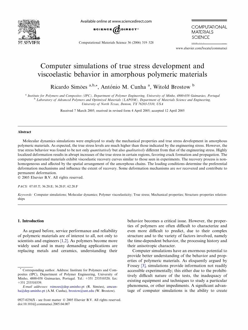
At the first stage of the simulation the material isallowed to equilibrate for 2000 time steps without anyexternal forces applied. The 2000 equilibration timesteps were found sufficient for the simulated materialsto recover from the induced perturbation mentionedbefore, after which every segment is merely oscillatingaround the equilibrium distance. After this quasi-equi-librium state has been reached, an external force is im-posed and the state of the system is monitored andperiodically recorded [5]. The external tensile force isapplied to all segments on both edges of the materialalong the x-axis (see Fig. 1a).

Since the force is always applied along the x-axis, thecross-section is defined in the y–z plane. All sections areinitially parallelepipeds of equal size, except for the sec-tion number 10 (the last one) which will be created basedon the exact number of columns in the material. Eachsection is defined by the positions of the segments attheir eight corners. These segments are assigned to eachsection in the beginning of the simulation; their changesin position along time determine the geometry of the sec-tions. The initial division of the material in sections andthe definition of a section are shown in Fig. 1.

Each section can be characterized by two cross-sectional areas, one defined by the leftmost segmentsand the other defined by the rightmost segments alongthe x-axis. These two areas are labeled Al and Ar inFig. 1b, and are simply called the left area and right area

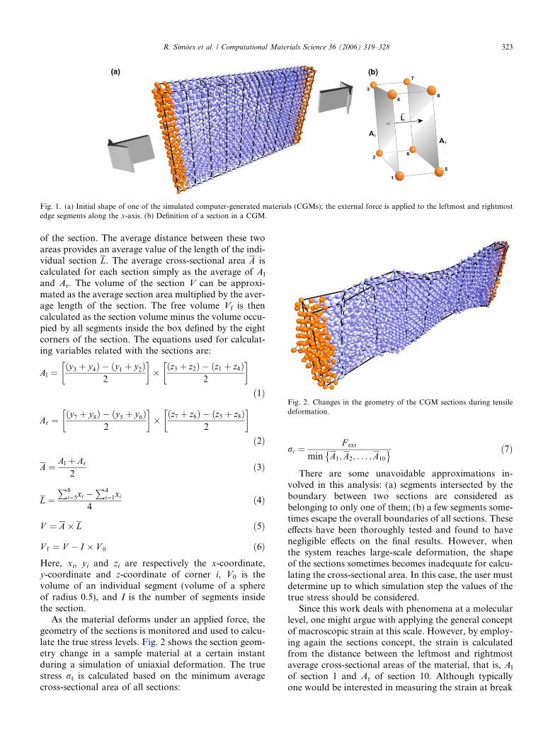
Fig. 1. (a) Initial shape of one of the simulated computer-generated materials (CGMs); the external force is applied to the leftmost and rightmostedge segments along the x-axis. (b) Definition of a section in a CGM.

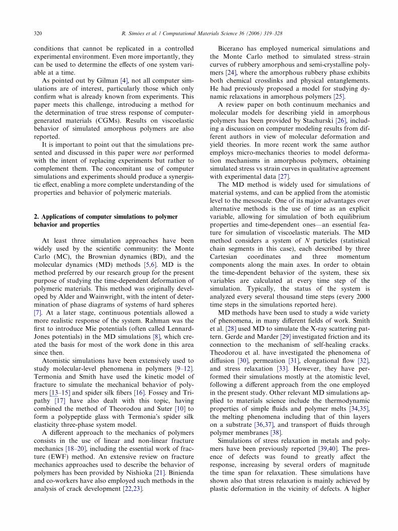
Fig. 2. Changes in the geometry of the CGM sections during tensiledeformation.

R. Simoes et al. / Computational Materials Science 36 (2006) 319–328 323

of the section. The average distance between these twoareas provides an average value of the length of the indi-vidual section L. The average cross-sectional area A iscalculated for each section simply as the average of Al

and Ar. The volume of the section V can be approxi-mated as the average section area multiplied by the aver-age length of the section. The free volume Vf is thencalculated as the section volume minus the volume occu-pied by all segments inside the box defined by the eightcorners of the section. The equations used for calculat-ing variables related with the sections are:

Al ¼y3 þ y4ð Þ � y1 þ y2ð Þ

2

� �� z3 þ z2ð Þ � z1 þ z4ð Þ

2

� �

ð1Þ

Ar ¼y7 þ y8ð Þ � y5 þ y6ð Þ

2

� �� z7 þ z6ð Þ � z5 þ z8ð Þ

2

� �

ð2Þ

A ¼ Al þ Ar

2ð3Þ

L ¼P8

i¼5xi �P4

i¼1xi

4ð4Þ

V ¼ A� L ð5Þ

V f ¼ V � I � V 0 ð6ÞHere, xi, yi and zi are respectively the x-coordinate,y-coordinate and z-coordinate of corner i, V0 is thevolume of an individual segment (volume of a sphereof radius 0.5), and I is the number of segments insidethe section.

As the material deforms under an applied force, thegeometry of the sections is monitored and used to calcu-late the true stress levels. Fig. 2 shows the section geom-etry change in a sample material at a certain instantduring a simulation of uniaxial deformation. The truestress rt is calculated based on the minimum averagecross-sectional area of all sections:

rt ¼F ext

min A1;A2; . . . ;A10

� � ð7Þ

There are some unavoidable approximations in-volved in this analysis: (a) segments intersected by theboundary between two sections are considered asbelonging to only one of them; (b) a few segments some-times escape the overall boundaries of all sections. Theseeffects have been thoroughly tested and found to havenegligible effects on the final results. However, whenthe system reaches large-scale deformation, the shapeof the sections sometimes becomes inadequate for calcu-lating the cross-sectional area. In this case, the user mustdetermine up to which simulation step the values of thetrue stress should be considered.

Since this work deals with phenomena at a molecularlevel, one might argue with applying the general conceptof macroscopic strain at this scale. However, by employ-ing again the sections concept, the strain is calculatedfrom the distance between the leftmost and rightmostaverage cross-sectional areas of the material, that is, Al

of section 1 and Ar of section 10. Although typicallyone would be interested in measuring the strain at break

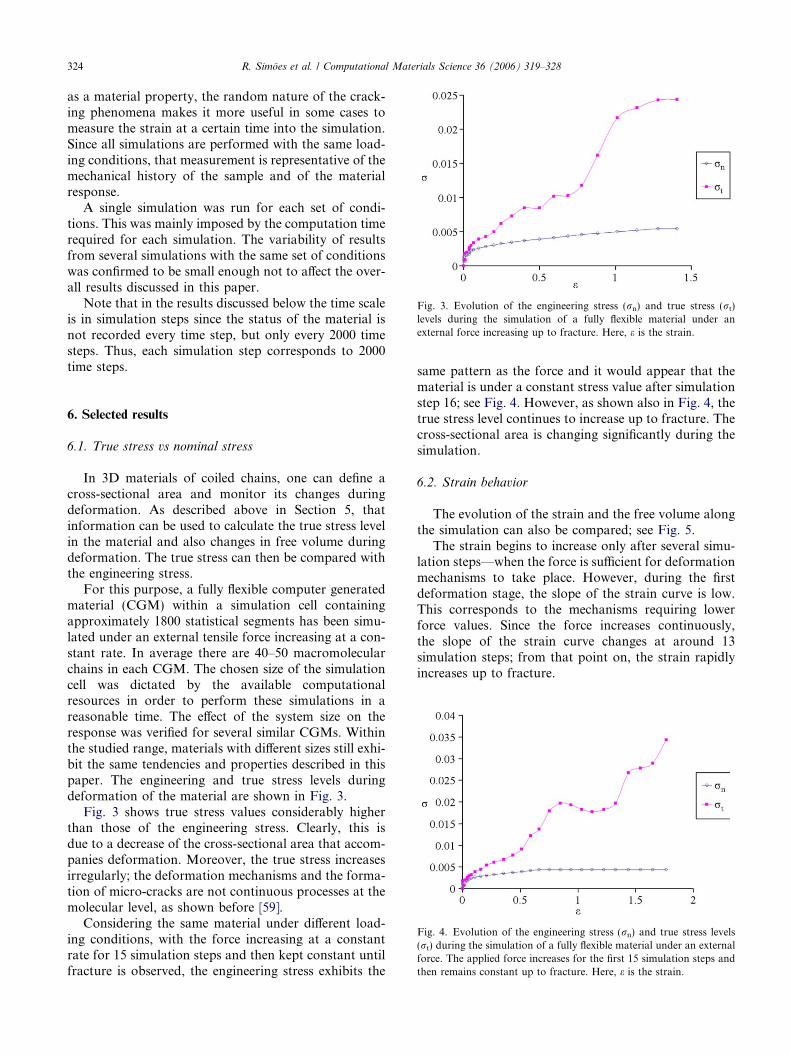
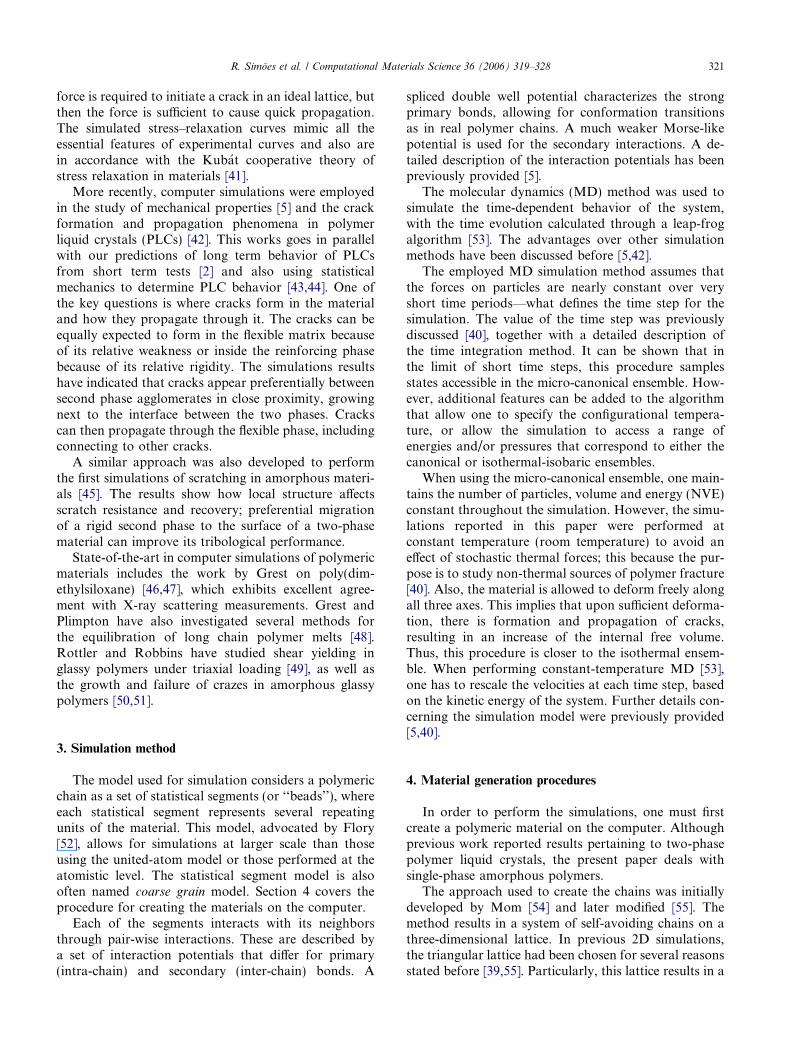
Fig. 3. Evolution of the engineering stress (rn) and true stress (rt)levels during the simulation of a fully flexible material under anexternal force increasing up to fracture. Here, e is the strain.

324 R. Simoes et al. / Computational Materials Science 36 (2006) 319–328

as a material property, the random nature of the crack-ing phenomena makes it more useful in some cases tomeasure the strain at a certain time into the simulation.Since all simulations are performed with the same load-ing conditions, that measurement is representative of themechanical history of the sample and of the materialresponse.

A single simulation was run for each set of condi-tions. This was mainly imposed by the computation timerequired for each simulation. The variability of resultsfrom several simulations with the same set of conditionswas confirmed to be small enough not to affect the over-all results discussed in this paper.

Note that in the results discussed below the time scaleis in simulation steps since the status of the material isnot recorded every time step, but only every 2000 timesteps. Thus, each simulation step corresponds to 2000time steps.

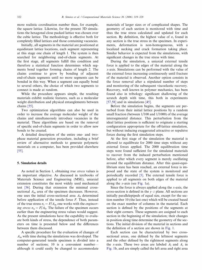
Fig. 4. Evolution of the engineering stress (rn) and true stress levels(rt) during the simulation of a fully flexible material under an externalforce. The applied force increases for the first 15 simulation steps andthen remains constant up to fracture. Here, e is the strain.

6. Selected results

6.1. True stress vs nominal stress

In 3D materials of coiled chains, one can define across-sectional area and monitor its changes duringdeformation. As described above in Section 5, thatinformation can be used to calculate the true stress levelin the material and also changes in free volume duringdeformation. The true stress can then be compared withthe engineering stress.

For this purpose, a fully flexible computer generatedmaterial (CGM) within a simulation cell containingapproximately 1800 statistical segments has been simu-lated under an external tensile force increasing at a con-stant rate. In average there are 40–50 macromolecularchains in each CGM. The chosen size of the simulationcell was dictated by the available computationalresources in order to perform these simulations in areasonable time. The effect of the system size on theresponse was verified for several similar CGMs. Withinthe studied range, materials with different sizes still exhi-bit the same tendencies and properties described in thispaper. The engineering and true stress levels duringdeformation of the material are shown in Fig. 3.

Fig. 3 shows true stress values considerably higherthan those of the engineering stress. Clearly, this isdue to a decrease of the cross-sectional area that accom-panies deformation. Moreover, the true stress increasesirregularly; the deformation mechanisms and the forma-tion of micro-cracks are not continuous processes at themolecular level, as shown before [59].

Considering the same material under different load-ing conditions, with the force increasing at a constantrate for 15 simulation steps and then kept constant untilfracture is observed, the engineering stress exhibits the

same pattern as the force and it would appear that thematerial is under a constant stress value after simulationstep 16; see Fig. 4. However, as shown also in Fig. 4, thetrue stress level continues to increase up to fracture. Thecross-sectional area is changing significantly during thesimulation.

6.2. Strain behavior

The evolution of the strain and the free volume alongthe simulation can also be compared; see Fig. 5.

The strain begins to increase only after several simu-lation steps—when the force is sufficient for deformationmechanisms to take place. However, during the firstdeformation stage, the slope of the strain curve is low.This corresponds to the mechanisms requiring lowerforce values. Since the force increases continuously,the slope of the strain curve changes at around 13simulation steps; from that point on, the strain rapidlyincreases up to fracture.

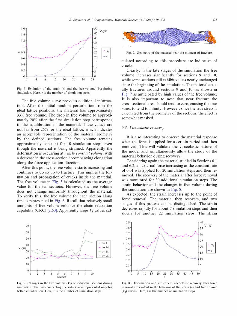
Fig. 7. Geometry of the material near the moment of fracture.

Fig. 5. Evolution of the strain (e) and the free volume (Vf) duringsimulation. Here, t is the number of simulation steps.

R. Simoes et al. / Computational Materials Science 36 (2006) 319–328 325

The free volume curve provides additional informa-tion. After the initial random perturbation from theideal lattice positions, the material has approximately33% free volume. The drop in free volume to approxi-mately 20% after the first simulation step correspondsto the equilibration of the material. These values arenot far from 26% for the ideal lattice, which indicatesan acceptable representation of the material geometryby the defined sections. The free volume remainsapproximately constant for 10 simulation steps, eventhough the material is being strained. Apparently thedeformation is occurring at nearly constant volume, witha decrease in the cross-section accompanying elongationalong the force application direction.

After this point, the free volume starts increasing andcontinues to do so up to fracture. This implies the for-mation and propagation of cracks inside the material.The free volume in Fig. 5 is calculated as the averagevalue for the ten sections. However, the free volumedoes not change uniformly throughout the material.To verify this, the free volume for each section alongtime is represented in Fig. 6. Recall that relatively smallamounts of free volume enhance the chain relaxationcapability (CRC) [2,60]. Apparently large Vf values cal-

Fig. 6. Changes in the free volume (Vf) of individual sections duringsimulation. The lines connecting the values were represented only forbetter visualization. Here, t is the number of simulation steps.

culated according to this procedure are indicative ofcracks.

Clearly, in the late stages of the simulation the freevolume increases significantly for sections 9 and 10,while some sections still exhibit values nearly unchangedsince the beginning of the simulation. The material actu-ally fractures around sections 9 and 10, as shown inFig. 7 as anticipated by high values of the free volume.It is also important to note that near fracture thecross-sectional area should tend to zero, causing the truestress to tend to infinity. However, since the true stress iscalculated from the geometry of the sections, the effect issomewhat masked.

6.3. Viscoelastic recovery

It is also interesting to observe the material responsewhen the force is applied for a certain period and thenremoved. This will validate the viscoelastic nature ofthe model and simultaneously allow the study of thematerial behavior during recovery.

Considering again the material studied in Sections 6.1and 6.2, an external force increasing at the constant rateof 0.01 was applied for 20 simulation steps and then re-moved. The recovery of the material after force removalwas monitored for 30 additional simulation steps. Thestrain behavior and the changes in free volume duringthe simulation are shown in Fig. 8.

As expected, the strain increases up to the point offorce removal. The material then recovers, and twostages of this process can be distinguished. The straindecreases rapidly for about 7 simulation steps and thenslowly for another 22 simulation steps. The strain

Fig. 8. Deformation and subsequent viscoelastic recovery after forceremoval are evident in the behavior of the strain (e) and free volume(Vf) curves. Here, t is the number of simulation steps.

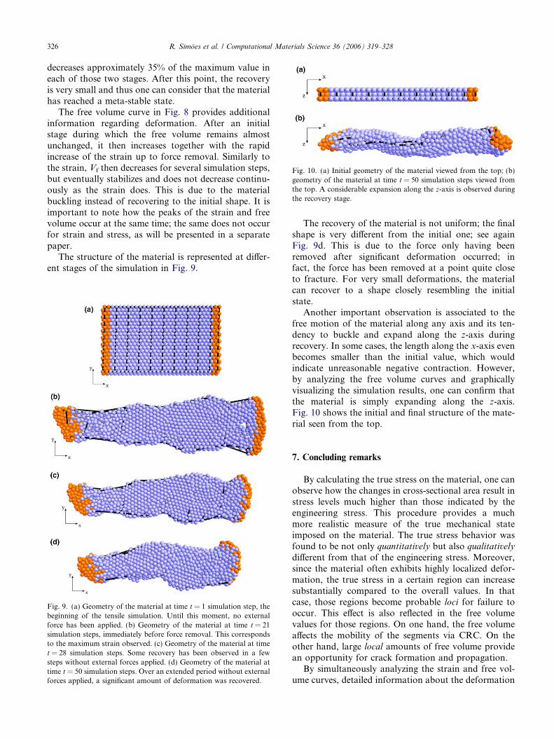
Fig. 10. (a) Initial geometry of the material viewed from the top; (b)geometry of the material at time t = 50 simulation steps viewed fromthe top. A considerable expansion along the z-axis is observed duringthe recovery stage.

326 R. Simoes et al. / Computational Materials Science 36 (2006) 319–328

decreases approximately 35% of the maximum value ineach of those two stages. After this point, the recoveryis very small and thus one can consider that the materialhas reached a meta-stable state.

The free volume curve in Fig. 8 provides additionalinformation regarding deformation. After an initialstage during which the free volume remains almostunchanged, it then increases together with the rapidincrease of the strain up to force removal. Similarly tothe strain, Vf then decreases for several simulation steps,but eventually stabilizes and does not decrease continu-ously as the strain does. This is due to the materialbuckling instead of recovering to the initial shape. It isimportant to note how the peaks of the strain and freevolume occur at the same time; the same does not occurfor strain and stress, as will be presented in a separatepaper.

The structure of the material is represented at differ-ent stages of the simulation in Fig. 9.

Fig. 9. (a) Geometry of the material at time t = 1 simulation step, thebeginning of the tensile simulation. Until this moment, no externalforce has been applied. (b) Geometry of the material at time t = 21simulation steps, immediately before force removal. This correspondsto the maximum strain observed. (c) Geometry of the material at timet = 28 simulation steps. Some recovery has been observed in a fewsteps without external forces applied. (d) Geometry of the material attime t = 50 simulation steps. Over an extended period without externalforces applied, a significant amount of deformation was recovered.

The recovery of the material is not uniform; the finalshape is very different from the initial one; see againFig. 9d. This is due to the force only having beenremoved after significant deformation occurred; infact, the force has been removed at a point quite closeto fracture. For very small deformations, the materialcan recover to a shape closely resembling the initialstate.

Another important observation is associated to thefree motion of the material along any axis and its ten-dency to buckle and expand along the z-axis duringrecovery. In some cases, the length along the x-axis evenbecomes smaller than the initial value, which wouldindicate unreasonable negative contraction. However,by analyzing the free volume curves and graphicallyvisualizing the simulation results, one can confirm thatthe material is simply expanding along the z-axis.Fig. 10 shows the initial and final structure of the mate-rial seen from the top.

7. Concluding remarks

By calculating the true stress on the material, one canobserve how the changes in cross-sectional area result instress levels much higher than those indicated by theengineering stress. This procedure provides a muchmore realistic measure of the true mechanical stateimposed on the material. The true stress behavior wasfound to be not only quantitatively but also qualitatively

different from that of the engineering stress. Moreover,since the material often exhibits highly localized defor-mation, the true stress in a certain region can increasesubstantially compared to the overall values. In thatcase, those regions become probable loci for failure tooccur. This effect is also reflected in the free volumevalues for those regions. On one hand, the free volumeaffects the mobility of the segments via CRC. On theother hand, large local amounts of free volume providean opportunity for crack formation and propagation.

By simultaneously analyzing the strain and free vol-ume curves, detailed information about the deformation

R. Simoes et al. / Computational Materials Science 36 (2006) 319–328 327

mechanisms is obtained. First, short-scale deformationwas found to be achieved at near-constant free volume;as the material elongates in the direction of force appli-cation, the average cross-section is decreasing. Whensignificant increases in Vf occur under larger deforma-tions, they reflect the fact that cracks begin to appearand grow. These results corroborate what had beenstated before about deformation mechanisms takingplace at the mesoscale in polymeric materials [59]. Thisprevious publication includes several animations of thetensile deformation of these materials.

When a force is applied and then removed after large-scale deformation has occurred, the CGMs exhibitviscoelastic recovery. A significant part of the imposeddeformation is recovered, but after some time the recov-ery reaches a plateau. The recovery process is non-homogeneous and depends on the chain structure ofthe material. Deformation mechanisms such as chainslippage and bond rupture are not recovered andcontribute to permanent deformation. The CGMs havea tendency to buckle during recovery; this phenomenonwill be further investigated in future work.

A better understanding of the molecular phenomenathat take place during deformation of polymers emergesfrom these simulations. The possibility of predicting themechanical properties from simulation results is encour-aging. However, further work is warranted, particularlyso on connections between the nano- and mesoscopiclevels and macroscopic properties and behavior.

Acknowledgements

Support for this research has been provided bythe Fundacao para a Ciencia e a Tecnologia, Lisbon,through the 3� Quadro Comunitario de Apoio, andthrough the POCTI and FEDER programmes, and alsoby the Robert A. Welch Foundation, Houston (Grant #B-1203). The authors also acknowledge discussions withProf. J. Karger-Kocsis, University of Kaiserslautern.

References

[1] W. Brostow, R.D. Corneliussen (Eds.), Failure of Plastics,Hanser, Munich–Vienna–New York, 1992.

[2] W. Brostow, N.A. D�Souza, J. Kubat, R.D. Maksimov, J. Chem.Phys. 110 (1999) 9706.

[3] S. Fossey, in: W. Brostow (Ed.), Performance of Plastics, Hanser,Munich–Cincinnati, 2000, p. 63.

[4] J.J. Gilman, Mater. Res. Innovat. 4 (2001) 209.[5] W. Brostow, M. Donahue III, C.E. Karashin, R. Simoes, Mater.

Res. Innovat. 4 (2001) 75.[6] W. Brostow, M. Drewniak, J. Chem. Phys. 105 (1996) 7135.[7] B.J. Alder, T.E. Wainwright, J. Chem. Phys. 27 (1957) 1208.[8] A. Rahman, Phys. Rev. A 136 (1964) 405.[9] G.C. Rutledge, U.W. Suter, Macromolecules 24 (1991) 1921.

[10] D.N. Theodorou, U.W. Suter, Macromolecules 19 (1986)139.

[11] M. Parrinello, A. Rahman, J. Chem. Phys. 76 (1982) 2662.[12] D.R. Rottach, P.A. Tillman, J.D. McCoy, S.J. Plimpton, J.G.

Curro, J. Chem. Phys. 111 (1999) 9822.[13] Y. Termonia, in: Encyclopedia of Polymer Science and Technol-

ogy, third ed., Wiley-Interscience, New York, 2002.[14] Y. Termonia, P. Smith, Macromolecules 20 (1987) 835.[15] Y. Termonia, P. Smith, Macromolecules 21 (1988) 2184.[16] Y. Termonia, Macromolecules 27 (1994) 7378.[17] S. Fossey, S. Tripathy, Int. J. Biol. Macromol. 24 (1999)

119.[18] J. Karger-Kocsis, in: A.M. Cunha, S. Fakirov (Eds.), Structure

Development During Polymer Processing, Kluwer, Dordrecht,2000, p. 163.

[19] J. Karger-Kocsis, in: J.G. Williams, A. Pavan (Eds.), Fracture ofPolymers, Composites and Adhesives, ESIS vol. 27, ElsevierScience, Oxford, 2000, p. 213.

[20] O.O. Santana, M.L. Maspoch, A.B. Martinez, Polym. Bull. 39(1999) 511.

[21] T. Nishioka, Int. J. Fract. 86 (1997) 127.[22] Y. Li, H. Ann, W.K. Binienda, Int. J. Solids Struct. 11 (1998)

981.[23] N. Shbeeb, W.K. Binienda, K. Kreider, Int. J. Fract. 104 (2000)

23.[24] J. Bicerano, N.K. Grant, J.T. Seitz, K. Pant, J. Appl. Polym. Sci.

Part B: Polym. Phys. 35 (1997) 2715.[25] J. Bicerano, J. Appl. Polym. Sci. Part B: Polym. Phys. 29 (1991)

1329.[26] Z.H. Stachurski, Prog. Polym. Sci. 22 (1997) 407.[27] Z.H. Stachurski, Polymer 44 (2003) 6067.[28] C. Ayyagari, D. Bedrov, G.D. Smith, Macromolecules 33 (2000)

6194.[29] E. Gerde, M. Marder, Nature 413 (2001) 285.[30] N.C. Karayiannis, V.G. Mavrantzas, D.N. Theodorou, Chem.

Eng. Sci. 56 (2001) 2789.[31] K. Makrodimitris, G.K. Papadopoulos, D.N. Theodorou, J. Phys.

Chem. B 105 (2001) 777.[32] V.G. Mavrantzas, D.N. Theodorou, Macromol. Theory Simul. 9

(2000) 500.[33] V.A. Harmandaris, V.G. Mavrantzas, D.N. Theodorou, Macro-

molecules 33 (2000) 8062.[34] H.C. Andersen, J. Chem. Phys. 72 (1980) 2384.[35] M. Banaszak, TASK Quart. 5 (2001) 17.[36] F.F. Abraham, Phys. Rev. Lett. 44 (1980) 463.[37] F.F. Abraham, W.E. Rudge, D.J. Auerbach, S.W. Koch, Phys.

Rev. Lett. 52 (1984) 445.[38] L. Fritz, D. Hofmann, Polymer 38 (1997) 1035.[39] W. Brostow, J. Kubat, Phys. Rev. B 47 (1993) 7659.[40] S. Blonski, W. Brostow, J. Kubat, Phys. Rev. B 49 (1994)

6494.[41] J. Kubat, M. Rigdahl, Chapter 5 in Ref. [1].[42] W. Brostow, A.M. Cunha, J. Quintanilla, R. Simoes, Macromol.

Theory Simul. 11 (2002) 308.[43] W. Brostow, K. Hibner, J. Walasek, J. Chem. Phys. 108 (1998)

6484.[44] W. Brostow, J. Walasek, J. Chem. Phys. 121 (2004) 3272.[45] W. Brostow, J.A. Hinze, R. Simoes, J. Mater. Res. 19 (2004)

851.[46] M. Tsige, T. Soddemann, S.B. Rempe, G.S. Grest, J.D. Kress,

M.O. Robbins, S.W. Sides, M.J. Stevens, E. Webb III, J. Chem.Phys. 118 (2002) 5132.

[47] S.W. Sides, J. Curro, G.S. Grest, M.J. Stevens, T. Soddemann, A.Habenschuss, J.D. Londono, Macromolecules 35 (2002)6455.

[48] R. Auhl, R. Everaers, G.S. Grest, K. Kremer, S.J. Plimpton, J.Chem. Phys. 119 (2003) 12718.

328 R. Simoes et al. / Computational Materials Science 36 (2006) 319–328

[49] J. Rottler, M.O. Robbins, Phys. Rev. E 64 (2001) 051801.[50] J. Rottler, S. Barsky, M.O. Robbins, Phys. Rev. Lett. 89 (2002)

148304.[51] J. Rottler, M.O. Robbins, Phys. Rev. E 68 (2003) 011801.[52] P.J. Flory, Statistical Mechanics of Chain Molecules, Wiley

Interscience, New York, 1969.[53] W.F. van Gunsteren, in: D.G. Truhlar (Ed.), Mathematical

Frontiers in Computational Chemical Physics, Springer, NewYork, 1988.

[54] V. Mom, J. Comput. Chem. 2 (1981) 446.

[55] W. Brostow, A.M. Cunha, R. Simoes, Mater. Res. Innovat. 7(2003) 19.

[56] W. Brostow, R.P. Singh, in: J. Kroschwitz (Ed.), Encyclopedia ofPolymer Science and Technology, Wiley, New York, 2004.

[57] W. Brostow, B. Bujard, P.E. Cassidy, H.E. Hagg, P.E. Monte-martini, Mater. Res. Innovat. 6 (2002) 7.

[58] W. Brostow, G. Damarla, J. Howe, D. Pietkiewicz, e-Polymers no.025, 2004.

[59] R. Simoes, A.M. Cunha, W. Brostow, e-Polymers no. 067, 2004.[60] W. Brostow, Chapter 10 in Ref. [1].