Computer simulations for the optimization of technological processes

Alessandro Baldi Antognini1, Alessandra Giovagnoli1, Daniele Romano2 and Maroussa Zagoraiou1

1 Department of Statistical Sciences, University of Bologna

2 Department of Mechanical Engineering, University of Cagliari

a.baldi@unibo.it, alessandra.giovagnoli@unibo.it, romano@dimeca.unica.it

maroussa.zagoraiou@unibo.it

Abstract

This chapter is about experiments for quality improvement and innovation of products and processes performed by computer simulation. It describes familiar methods for creating surrogate models of simulators (emulators), with particular reference to Kriging, and some new ways of fitting the models to the simulated data.

It also deals with the advantages of computer experiments performed sequen-tially, and with computer experiments in which some of the random noise factors that affect the output of a process is simulated stochastically.

As an example, an application to the integrated parameter and tolerance design of a high precision space measuring instrument is illustrated, and other possible applications are also mentioned.

1 Introduction

1.1 Importance of computer simulation

The importance of experimenting for quality improvement and innovation of products and processes is only too well known by now: experimenting means to

2

implement significative and intentional changes with the aim of obtaining useful information. In particular, the majority of industrial experiments have a double goal:

• to quantify the dependence of one or more observable response variables on a group of input factors in the design or the manufacturing of a product, in order to forecast the behaviour of the system in a reliable way.

• to identify the ideal setting of the levels of the inputs (design parameters), ca-pable of optimizing the response.

The set of rules that govern experiments for technological improvement in a physical set-up are now comprehensively labelled as “DoE”. In recent years, the use of experimentation in engineering design has received a renewed momentum by the practice of computer experiments (Sacks et al. 1989, Santner et al. 2003), which has been steadily growing in the last two decades. These experiments are run on a computer code implementing a simulation model of a physical system of interest. This enables us to explore the complex relationships between input and output variables. The main advantage is that the system becomes more “observ-able” since computer runs are generally easier and cheaper than measurements taken in a physical set-up, and the exploration may be carried out more thor-oughly. This is particularly attractive in industrial design applications where the goal is system optimization.

1.2 Simulators and Emulators

The request that the simulator be accurate in describing the physical system means that the simulator itself may be rather complex. In general it will consist in the si-multaneous solution of a large number of linear or non-linear, ordinary and/or dif-ferential equations, and it may not be possible to express it analytically. Further-more, the number of input factors may be large, so that runs may be expensive and/or time-consuming. This has led to the use of surrogate models (emulators), i.e. simpler models which represent a valid approximation of the original simula-tor. These emulators are statistical interpolators built from the simulated input-output data. Prediction at untried points, most useful in the case of expensive simulation, is made by the surrogate models.

Familiar methods for creating surrogate models are the Response Surface Methodology and Kriging. The latter is a technique where the deterministic re-sponse of the computer is regarded as a realization of a random process whose correlation function can be shaped in such a way to reflect the characteristic of the response surface. For details see Santner et al. (2003). This and other types of emulators are reviewed in Section 2.

3

The existing methods for fitting a Kriging model generally start with a space-filling design e.g. a Latin Hypercube Sampling scheme. A novel method based on the theory of optimal designs has been introduced by Zagoraiou and Baldi An-tognini (2008) and will be explained in Section 2.

1.3 Sequential computer experiments

Originally introduced by Box and Wilson (1951) in the context of statistical qual-ity control and optimization of engineering processes/products, sequential experi-mentation includes a vast class of statistical procedures which employ the data previously collected in order to modify the trial as it goes along. Because of their greater flexibility and efficiency with respect to the classical fixed-sample proce-dures (see for instance Siegmund (1985) and Ghosh and Sen (1991)), sequential procedures are now widely used in the great majority of applied contexts, such as biomedical practice, physical research, industrial experimentation. In this field in particular where economic demands (time and costs saving) may be crucial, the ability to exploit the newly acquired data during the trial may help detect potential defects, inefficient settings, dangerous or ineffective treatments, and enable de-signers to pursue continuous quality improvement.

There is a fair amount of recent literature on this topic (see Romano, 2006): the existing sequential methods generally start with a space-filling design (a Latin Hypercube Sampling design or a maximin design); then, once the sequential pro-cedure is activated, the estimates of the parameters of the unknown quantities process are recursively updated at each step or, to reduce the computational bur-den, after a few steps. Adaptive designs for optimization in the Response Surface Methodology framework are available, that iteratively reduce the design space. Wang et al. (2001) discard regions with large values of the objective function at each modelling-optimization iteration, while Farhang-Mehr and Azarm (2003) and Lin et al. (2004) use maximum entropy as the criterion. Other criteria for succes-sively reducing the design space include move limits (Wujek and Renaud 1998) and trust region (Alexandrov et al. 1998). Van Beers and Kleijnen (2005) use bootstrap to estimate the prediction variance at untried sites and then choose as next input the point with the maximum prediction variance.

In Section 3 the principles of sequential experimentation are illustrated, fol-lowed by some recent proposals of sequential procedures. A new virtual experi-ment for a Kriging model by Baldi Antognini and Pedone is introduced which, be-ing randomized, makes it possible to overcome a typical problem, namely that algorithms tend to linger for a long time around local maxima/minima. The new method extends the one by Kleijnen and Van Beers (2004) and has turned out to be very efficient for small samples too, reaching the same degree of precision with 40% fewer observations.

4

1.4 Stochastic Simulators

A major problem of most simulators is that they use a deterministic code. This choice is too restrictive. First, in many instances some important input variables are random in the real process. Typical examples are the design of robust engi-neering systems, where parameters which are not controllable by the designer (like external temperature and manufacturing errors) act randomly, and the manage-ment and control of queuing systems (for instance production and telecommunica-tion facilities) where arrival and service times (of parts, phone calls) are random. In such cases the simulation code e.g. a Finite Element code for a new product (Romano et al., 2004) or a discrete event simulator for inventory systems (Bashyam and Fu, 1998) may be random too: this appears to be the natural tool for transmitting the distribution of noise input to the output. Secondly, the construc-tion of a computer simulator of a complex system has often some degree of uncer-tainty. It involves several decisions about different modelling options, numerical algorithms, the assignment of a value to physical and numerical parameters. Since often there are no clear-cut best decisions, a huge number of computer codes are compatible with the same physical system. Here again random simulation seems preferable (Romano and Vicario, 2002a, 2002b). One practical consequence is that the rationale for using standard statistical tools is restored. Thus regression analy-sis can be safely used for prediction.

In Section 4 a modified protocol for conducting robust design studies on the computer is described, which extends the dual response surface approach (Gio-vagnoli and Romano, 2008). The suggested protocol utilizes stochastic simulation, which is now largely employed in several technological and scientific areas. It is characterized by a different treatment of the noise factors, some of which are con-sidered random, as they are in the real process. The proposed model includes both the crossed array and the combined array as special cases. When the design scope is extended to the specification of allowable deviations of parameters from nomi-nal setting (tolerances), an integrated parameter and tolerance design problem arises. Here the additional objective of minimizing the production costs needed to fulfil tolerance specs will compete with the minimum variance objective. This method can be beneficial to the solution of an integrated parameter and tolerance design problem, by adding standard deviations of internal noise factors as controls in the experiment and simulating the internal noise accordingly.

The method appears to be particularly suited for designing complex measure-ment systems. The main quality requirements of a measure, namely lack of bias and repeatability, are strictly linked to the mean and variance of the measurement. In Giovagnoli and Romano (2008) the method was applied to the design of a high precision measuring instrument, an optical profilometer. In Section 4 we describe this case study briefly and show that the same method can be applied in a wide range of other possible contexts.

5

2 Construction of the Emulators

A common approach to deal with the problem of complex input-output relation-ships exhibited by the simulation model is by constructing an emulator, also called surrogate. Since emulators are models of the original simulator which is itself a model of reality, they are often called metamodels. The goal of using a surrogate model is to provide a smooth relationship of possible high fidelity to the true func-tion with the advantage of quick computational speed instead of the time-consuming runs related to the computer code. This section provides a guideline for the construction of an emulator and a brief overview of many different emulators not with the aim of explaining each type in detail but in order to underline the wide variety of approximating models available in the literature. The Kriging methodology is discussed in a thorough way due to its importance as a tool for ac-curate predictions.

2.1 A protocol for creating emulators

Kleijnen and Sargent (2000) have suggested a procedure for developing an emula-tor which can be briefly described as follows:

1. Determine the aim of the emulator: any model should be developed for a spe-cific goal. Usually we can identify four different goals: understanding the prob-lem, predicting values of the response variable, performing optimization and aiding the validation of the simulator.

2. Identify the output variable: the simulator usually has multiple response vari-ables. However, current practice suggests to develop a separate metamodel for each output (single-response models).

3. Identify the inputs and their characteristics: determination of the independent variables and specification of the domain of applicability or experimental re-gion X.

4. Specify the required accuracy of the metamodel: the range of accuracy de-pends on the goal of the metamodel. For example, if the main interest lies in the optimization of a system, we cannot require a high level of complexity since the optimization algorithms need simple models.

5. Specify the metamodel: in this step we should select a particular type of model among those proposed in the literature, e.g. polynomial regression models, Fourier metamodels, splines, neural networks, Kriging....

6. Specify the type of experiment: the experimental design problem is the selec-tion of inputs at which to run the computer code. The following main ap-proaches are used for selecting designs (for more details see section 2.4):

6

– if we believe that interesting features of the simulator can be found in sev-eral parts of the experimental region, i.e. no privileged areas exist, it seems natural to use designs that spread the points “evenly” to cover the full range of the input space. This allows the researcher to gather information about the relationship between the inputs and outputs for all regions of the domain of applicability. Furthermore, by covering the full range of the in-put domain, space-filling designs could lead to good prediction over the entire input space, which is typically a fundamental goal in computer ex-periments. There are a number of ways to define what it means to spread points and these lead to a variety of designs, usually called space-filling designs;

– if we choose a particular type of metamodel it is possible to formulate spe-cific criteria for choosing a design and adopt an optimal design approach. Several criteria have been proposed in the literature. A recent class of de-sign procedures which use a criterion based on the Fisher Information ma-trix can be found in Zagoraiou and Baldi Antognini (2008).

7. Fit the metamodel: we run the simulation to obtain the output data from the in-puts specified in step 6 for fitting the metamodel. From these data we estimate the parameters of the metamodel.

8. Validation of the fitted model: starting from a test set of inputs we run simula-tions for validating the emulator verifying the accuracy of the prediction (see section 2.3). In the case of time-consuming and/or computationally intensive experiments the researcher can apply “cheap” methods such as cross-validation.

2.2 A special type of emulator: the Kriging technique

A big variety of different modelling techniques is available in the literature. In this section we mention some of them and we focus our attention on the Kriging meth-odology, originally developed for geological applications and nowadays a very important tool for producing accurate predictions of the output of a deterministic computer code.

The selection of a metamodel to approximate the true model as accurately as possible is a crucial problem. Generally, most of the metamodels in the literature are linear combinations of basis functions defined on an experimental region and the unknown coefficients of the combination have to be estimated. Thus, when the simulator is deterministic, the construction of a surrogate can be viewed as an in-terpolation problem. Following this point of view, most metamodels have the form:

7

jjj

Bg β)()( xx ∑=

where Bj is a set of basis functions, βj are unknown coefficients and x is the input variable. If the basis function is polynomial we obtain the polynomial surrogates, widely used for modelling computer experiments. Often, the behaviour of the data cannot be explained by the polynomials models. A solution to this problem consist in using the so-called splines, where the polynomials are defined in a piecewise way, i.e. several low order polynomials are fit to the data, each in a separate range defined by the knots. Splines and polynomial models make the assumption that the data can be locally or globally fit by a polynomial. An alternative method which lets the data be fitted in a less constrained form is known as neural network tech-nique. For more details see Fang et al. (2006). Other bases for the construction of a metamodel have also appeared in the literature. For example the Fourier basis can be used to approximate periodic functions.

Metamodels set up on a polynomial basis, spline basis or Fourier basis are competitive if the number of input variables is small but their extension to a high dimensional multivariate input could be difficult. Therefore other techniques have been proposed. One of the most popular is the Kriging methodology. This kind of approach was originally proposed by a South African geologist, D. G. Krige (1951) for the analysis of geostatistical data. Later his work was developed by Matheron (1962) and has become very popular in several applied contexts of the spatial statistics literature (see Ripley, 1981 and Cressie, 1993). Recently, this modelling approach has been widely used for the design and analysis of computer experiments (see for instance Sacks et al., 1989, Welch et al., 1992 and Bursztyn and Steinberg, 2006).

Following Sacks et al. (1989) the Kriging approach consists in treating the de-terministic response y(x), i.e. the output of the simulator, as a realization of a sto-chastic process (random field) Y(x) such that

),()()( xxx ZY += µ

where µ(x) denotes the global trend and Z(x) represents the departure of the re-sponse variable Y(x) from the trend. More precisely, Z(x) is usually assumed to be a Gaussian stationary process with E(Z(x))=0, constant variance σZ

2 and non-negative correlation function between two inputs x and w ∈ X.

,),()](),([ wxwx RZZCorr =

depending only on the displacement vector between any pair of points in X and tending to 1 as the displacement vector goes to 0.

The correlation function should reflect the characteristics of the output. For a smooth response a correlation function with some derivatives would be preferred,

8

while an irregular response might call for a function with no derivatives. It is cus-tomary for the correlation to have the following property:

|),(|),( jjjj

wxRR −= ∏wx

i.e. products of one-dimensional correlations. Of special interest are those within the power exponential family:

)||exp(),( pjjj

j

wxR −−= ∏ θwx (1)

where 0 < p ≤ 2. We can also permit p to vary with j. The case p=1 is the product of Ornstein-Uhlenbeck processes; they are continuous but not very smooth. A spe-cial type is the one-parameter exponential correlation function given by:

|).|exp(),( wxwxR −−= θ (2)

When p = 2 we have the so-called Gaussian correlation function which is suitable for smooth and infinitely differentiable responses. An alternative choice for R(x,w) is the linear correlation function:

.||),( wxwxR −−= θ (3)

Two different types of Kriging metamodels have been proposed in the literature depending on the functional form of the trend component: • Ordinary Kriging: the trend is constant µ(x) = µ but unknown; • Universal Kriging: the trend component depends on x and is modelled in a

regressive way

( ) βxfxx )()(1

tj

p

jjf =β=µ ∑

=

where f1(·),…,fp(·) are known functions and β = (β1,…,βp)t is the vector of the un-

known parameters. Kriging modelling lends itself to a sound theoretical methodology for the pre-

diction of the output. Let

( ) )()()()(1

xβxfxxx ZZfY tj

p

jj +⋅=+β⋅=∑

=

9

be the model under study, x1,…,xn the inputs,

tn

tn

n yyYY ))(),...,((),...,( 11 xxY ==

the set of outputs variables and y(x0) = Y0 the output to predict. Furthermore, let

0̂Y denote a generic predictor of Y0. Then the model is denoted

σ

Rr

rβ

F

fY 0

0200 1,~

t

Z

t

nY

where f0 = f(x0) is the (p×1) vector of regression functions for Y0,

==)()(

)()(

))((

1

11

npn

pp

ijf

xfxf

xfxf

xF

K

MM

K

is the (n×p) matrix of regression functions for the observed data, r0 = (R(x0-x1),…,R(x0-xn))

t is the (n×1) vector of correlations of Yn and Y0,

( )),(, jiji R xxRR ==

is the (n×n) matrix of correlations among the entries of Yn, and β and σZ2 are the

unknown parameters. If the correlation function is known, which is hardly ever the case in practical

situations, the BLUP (Best Linear Unbiased Predictor) of Y0 is given by

( )βFYRrβf ˆˆˆ 1000 −+≡ − nttY

where

( ) ntt YRFFRFβ 111ˆ −−−=

is the generalized least squares estimator of β. Note that 0̂Y interpolates the data

(xi , y(xi)) for 1 ≤ i ≤ n and 0̂Y is a Linear Unbiased Predictor of Y(x0).

On the other hand, if the correlation function is unknown R(·) can be written as

10

( ) ( )ψ⋅=⋅ RR

where ψ is an unknown parameter vector. Then it can be estimated by maximum likelihood, restricted maximum likelihood, cross-validation or the posterior mode.

In this case the predictor 0̂Y is named as Empirical Best Linear Unbiased Predic-

tor, given by:

( )βFYRrβf ˆˆˆˆˆ 1000 −+≡ − nttY

However, predictions are no longer linear. For a thorough reading see Santner et al. (2003).

2.3 Accuracy of the predictor

To validate an emulator, we must know the accuracy required of it and this de-pends on its purpose. However, as is well known, in many cases there will be a trade-off between accuracy and complexity. Ideally, we want the departure of the emulator from the true model as small as possible over the experimental region, i.e.

,0))(),(ˆ( Xyy L ∈→ xxx all for

where L is some measure of distance. Usually, the mean square error (MSE) of prediction at an untried point x is used to provide a measure for the overall model accuracy:

( ) .)()(ˆ))(ˆ( 2xxx yyEyMSE −= (4)

Thus, one would need to know the values of the true model over the whole X. Therefore, the key element is to compare the predictions with the known true val-ues in a test set. Possible ways for the choice of this kind of set are:

• in the case of “cheap” experiments, we may collect a large number of points, say N points xi

*, i = 1, …, N and calculate the Empirical Integrated Mean Squared Error (EIMSE):

( )2

1

** )()(ˆ1∑

=

−=N

iii yy

NEIMSE xx (5)

11

or the Empirical Maximum Mean Squared Error (EMMSE)

( )2** )()(ˆ max * ii yyEMMSEi

xxx

−= (6)

to check if the metamodel satisfies the required accuracy;

• in general, since computer experiments are time-consuming and computation-ally intensive, the accuracy of the prediction will be assessed using adequate methods such as cross validation. This method is based on iteratively partition-ing the full set of available data into training and test subsets. For each parti-tion, the researcher can estimate the model via the training subset and evaluate its accuracy using the test subset (see Fang et al., 2006).

2.4 Experiments for a Kriging model

The experimental design problem regarding the topic of the computer experiments is the selection of inputs at which to run a computer code. The following main ap-proaches are used in the literature for selecting designs: space-filling designs and designs based on some optimality criterion.

Space-Filling Designs

As is recognized by many researchers, when no details on the functional behav-iour of the response variable are available, it is important to be able to obtain in-formation from the entire design space. Therefore, design points should fill up the entire region in a “uniform fashion”.

There are several statistical strategies that one might adopt to fill a given ex-perimental region. One possibility is to select a simple random sample of points from the experimental region. However, other sampling schemes such as the stratified random sampling are preferable since the simple random sampling is not completely satisfactory, e.g. with small samples and in high-dimensional experi-mental regions, it may present some clustering and fail to provide points in several portions of the domain.

Another method to generate designs that spread observations over the range of each input variable is the so-called Latin Hypercube Sampling (LHS). Introduced by McKay et al. (1979), LHS design is one of the most commonly used space-filling designs. An LHS design yielding n design points involves stratifying the experimental space into n equal probability intervals for each dimension, ran-domly selecting a value in each stratum and combining them in order to obtain a design point.

12

The “space filling” property has inspired many statisticians to develop related designs. One class of designs maximizes the minimum Euclidean distance be-tween any two points in the multi-dimensional experimental area. Other designs minimize the maximum distance or are based on the principle of comparing the distribution of the points with the uniform distribution. See Johnson et al. (1990), Koehler and Owen (1996) and also Santner et al. (2003).

Optimal Designs

An alternative way of choosing a design is based on some statistical criterion. Af-ter the selection of the type of metamodel, the researcher can choose the design according to one of the many criteria proposed in the literature. The search for op-timum designs for random field models is a rich but difficult research area. A good design for a computer experiment should facilitate accurate prediction and in this area most progress has been made with respect to criteria based on functionals of the MSE, i.e.

• the Integrated Mean Squared Error (IMSE) criterion:

[ ] xxx dyyEIMSEX

2)()(ˆ∫ −= (7)

where the expectation is taken with respect to the random field;

• the Maximum Mean Squared Error (MMSE) criterion:

[ ] .)()(ˆmax 2xxx yyEMMSE X −= ∈ (8)

Then, a design is said to be IMSE-optimal or MMSE-optimal if it minimizes (7) or (8), respectively. Observe that the IMSE and MMSE criteria can be considered as generalizations of the A- and G-optimality (see Silvey, 1980), respectively. Both criteria can be calculated if the correlation function is known, which is impossible in practical situations. One possible way to overcome this problem consists in starting with a space-filling design, e.g. a Latin Hypercube Sampling scheme, in order to estimate the unknown correlation parameters, and then determine the IMSE-optimal or MMSE-optimal design treating the obtained estimates as the true parameter values.

Lindley (1956) proposed the use of the change in entropy before and after col-lecting data as a measure of the information provided by an experiment. The en-tropy criterion for random fields is thus:

))(( YHE ∆

13

where ∆H(Y) is the reduction in entropy after observing Y. A good design should maximize the expected reduction in entropy (see Shewry and Wynn, 1987, and Bates et al., 1996).

An alternative criterion proposed in the literature is the maximum prediction variance. In this case we choose to take observations where Kriging predictions are most uncertain, i.e. we select the design point which maximizes ( ))(ˆ xyVar .

A novel method based on the theory of optimal designs has been proposed by Zagoraiou and Baldi Antognini (2008). The main purpose of the authors is to de-rive optimal designs for maximum likelihood estimation for Ordinary Kriging with exponential correlation structure (2) using a criterion based on the Fisher in-formation matrix. When the interest lies in the estimation of the trend parameter, they prove that the equispaced design is optimal for any sample size, while an op-timal design for the estimation of the correlation parameter does not exist. Fur-thermore, the optimal strategy for the trend conflicts with the one for θ, since the equispaced design is the worst solution for estimating the correlation parameter. Hence, when the inferential purpose concerns the estimation of both the unknown parameters the authors propose the Geometric Progression Design, namely a flexible class of procedures that allow the experimenter to choose a suitable com-promise regarding the estimation precision of the two unknown parameters guar-anteeing, at the same time, high efficiency for both.

3 Sequential experiments for Kriging

3.1 Design and analysis of sequential experiments

When experiments are carried out sequentially by the observer, at each step all the information gathered up to that point is available to decide whether to observe any further and if so how to perform the next observations. Thus, the experimental de-cisions concerning the data collection process can evolve in an adaptive way on the basis of the experiment itself. Sequential Designs are a type of experimental plans which consist of

1. a rule specifying at each stage the set of experimental conditions under which the next statistical unit(s) must be observed, and

2. a stopping rule, usually governed by economy constrains.

These rules are defined a-priori in terms of the information gathered up to each given step, namely the data observed and the way in which the experiment itself has evolved.

14

In point of fact, there are many potential reasons to conduct the trial sequen-tially, in particular crucial economic demands (time-cost saving); the ability to ex-ploit the newly acquired data during the very trial may allow one to pursue con-tinuous quality improvement, providing also a significant cost reduction.

There is another important factor in experiments in various fields of applica-tion, namely randomization. This is a rather loose term that has been brought into general use by R.A. Fisher; it means assigning some features of the experiment by “controlled chance”: it may refer to the way in which experimental units are cho-sen, the order in which treatments are allocated to the units and so on. It is nowa-days commonly believed that a component of randomization in the design of the experiment is always required in order to protect against various types of bias (for instance accidental bias, selection bias, chronological bias etc...) and is also a fun-damental tool for correct inferential procedures. However, there may be other rea-sons for introducing a probabilistic component in the experimental design that have not been sufficiently stressed in the literature, resulting in an improvement of the convergence properties of the experiment itself, like in (Baldi Antognini and Giovagnoli, 2005).

In general, the choice of the design depends on several aspects, which reflect the experimental aims: accurate inference about unknown parameters, accurate predictions at untried sites, cost saving, etc... Often these objectives can be defined as an optimization problem but the solutions, the so-called optimal design or tar-get, may depend on the unknown parameters (local optimality). This is typically so in non-linear problems, namely when the statistical model is non-linear in the parameters of interest or the inferential aim consists in estimating a non-linear function of the unknown parameters. In this context, sequential designs are essen-tial, since they may represent a natural solution to the local optimality problem. In fact, by adopting a suitable response-adaptive procedure the available outcomes can be used at each stage for estimating the unknown parameters, and so the opti-mal design too; thus the allocations can be redirected in order to converge to the unknown target (asymptotic optimality). An example is the Maximum Likelihood design, which is a sequential randomized procedure based on the step-by-step up-dating of the optimal target by ML estimates (see for instance Baldi Antognini and Giovagnoli, 2005).

However, the adoption of a particular sequential procedure may pose problems as regards the correct inferential paradigm (see Silvey, 1980; Ford et al., 1985; Rosenberger et al., 1997; Giovagnoli, 1999; Hu and Rosenberger, 2003; Baldi An-tognini and Giovagnoli, 2006). If the design does not depend on the observed data, then it can be regarded as an ancillary statistics and we may infer conditionally on the observed sequence of design points. In contrast, for all response-adaptive pro-cedures, the design variability must be accounted for and we should argue uncon-ditionally (Rosenberger and Lachin, 2002). Thus, sequential experiments may be difficult to analyze, because the inferential methodology depends on the adopted design (see Ford et al., 1985; Chaudhuri and Mykland, 1993; Thompson and Se-

15

ber, 1996; Melfi and Page, 2000; Aickin, 2001). Recently, Baldi Antognini and Giovagnoli (2005) have shown that, under suitable conditions related to the statis-tical model and the allocation rule, conditional and unconditional inference tend to be the same asymptotically. This result can be applied when it is possible to simu-late extensively from the computer code, but may be inappropriate for small sam-ples, e.g. when the simulation runs are very time/cost expensive.

3.2 Recent developments of sequential computer experiments for Kriging with applications

A vast literature on sequential designs for computer experiments based on the Kriging methodology is available (see Williams et al., 2000; Van Beers and Klei-jnen, 2003; Kleijnen and Van Beers, 2004; Gupta et al., 2006; Romano, 2006). In general, these methods start with a pilot study, where a small number n0 of obser-vations from a space-filling design will be gathered in order to get an initial esti-mation of the unknown parameters of the model; then, the sequential procedure is activated through the adoption of a suitable allocation rule, which specifies at each step the choice of the next design point; popular criteria are based on IMSE, MMSE, entropy, variance of prediction, etc... (See Section 2 of this Chapter for details). Finally, these procedure are stopped according to the specification of the stopping rule, usually related to cost-time constrains or to required inferential ac-curacy (i.e. when the improvement in precision is negligible).

For instance, the Sequential Kriging design (SK) is one of the first proposals in this area (see the Chapter by Romano et al.). This is a deterministic response-adaptive procedure which selects at each step the design point where the estimated variance of prediction is maximal. The SK procedure is very simple to implement and at each step is sequential over the entire design region; however, it tends to get locked in the so-called interesting areas, namely in certain subset of the experi-mental domain where the function assumes a critical behaviour (i.e. local or global maxima/minima).

3.3 The “Application-Driven Sequential Designs”

This is the name of a sequential procedure recently introduced by Kleijnen and Van Beers (2004) for fitting the Ordinary Kriging metamodel with one-parameter exponential correlation (2) or linear correlation function in (3).

The Application-Driven Sequential Designs (ADSD) can be briefly described as follows:

16

• the procedure starts with a pilot experiment generated by a LHS or a maximin design, which includes the extremes of the design space (since extrapolations via the Kriging methodology is not recommended); based on the simulations on these points, the correlation parameter is estimated by the cross-validation method;

• using a space-filling approach, a given set of candidate points is selected (the authors suggest to take the specific candidates halfway between the design points of the pilot study), and at each candidate the variance of the predicted output is estimated by a cross-validation combined with jackknife technique;

• at each stage the next design point, i.e. the winner among the candidate points for the actual simulation, is the one with maximum jackknife variance;

• the sequential procedure is stopped when no substantial improvement in terms of jackknife variance is observed.

The authors test the properties of the ADSD through two applications, namely hy-perbolic and polynomial Input-Output functions, for small samples (i.e. n0 = 4 and total sample size N up to 36). Assuming that the prediction errors induced by the procedure can be measured by EIMSE (4) and EMMSE (5), the authors show that ADSD gives better results than LHS with a prefixed sample of the same size.

3.4 A modified version via randomization

Alessandro Baldi Antognini together with Paola Pedone have generalized the ADSD of Kleijnen and Van Beers (2004) by introducing the Randomized Sequen-tial Kriging (RSK) design. This is a randomized response-adaptive procedure for fitting the Universal Kriging metamodel with power exponential correlation (1), which can be described as follows:

• the experiment starts with a space-filled design (LHS), which includes the ex-tremes of the design space and, based on the simulations on these points, the unknown parameters are estimated by the maximum likelihood method;

• again, a given set of candidate points is selected using a space-filling approach, and at each candidate the variance of the predicted output is estimated;

• the choice of the next design point is made through a random assignment where the probability of selecting each candidate is proportional to the estimated pre-diction variance at this site obtained at the previous step;

• this sequential procedure is stopped when no substantial improvement in terms of EIMSE or EMMSE is observed.

With respect to ADSD, the peculiar feature of RSK are: a) the assumed model is more general than the Ordinary Kriging with one-parameter exponential correla-tion (4) and is also more suitable in the case of smooth functions; b) at each stage

17

the unknown parameters will be estimated by the maximum likelihood method; c) the choice of the design points is randomized: this random mechanism in the as-signments is suggested for exploring all the design region without being trapped by local maxima/minima.

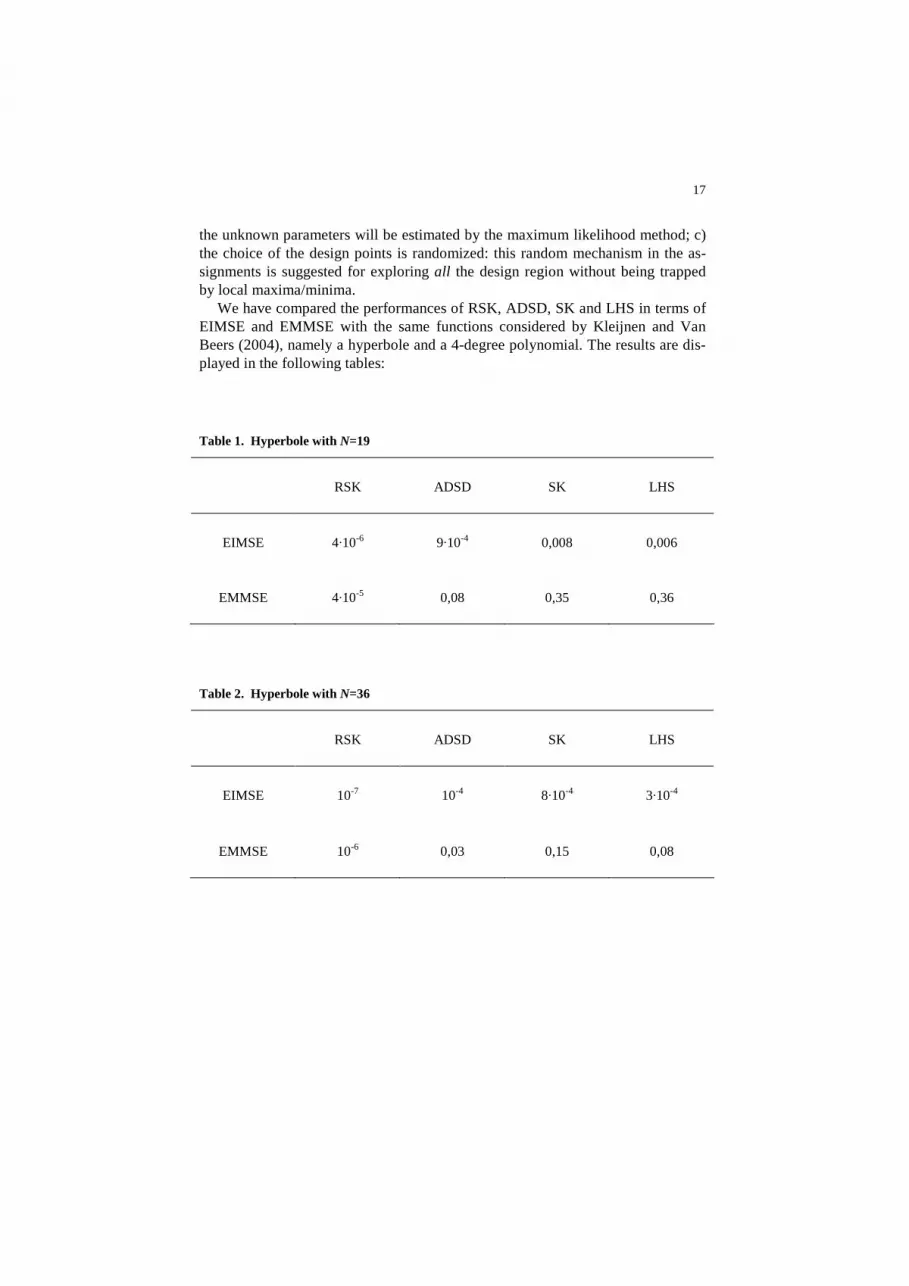
We have compared the performances of RSK, ADSD, SK and LHS in terms of EIMSE and EMMSE with the same functions considered by Kleijnen and Van Beers (2004), namely a hyperbole and a 4-degree polynomial. The results are dis-played in the following tables:

Table 1. Hyperbole with N=19

RSK ADSD SK LHS

EIMSE 4·10-6 9·10-4 0,008 0,006

EMMSE 4·10-5 0,08 0,35 0,36

Table 2. Hyperbole with N=36

RSK ADSD SK LHS

EIMSE 10-7 10-4 8·10-4 3·10-4

EMMSE 10-6 0,03 0,15 0,08

18

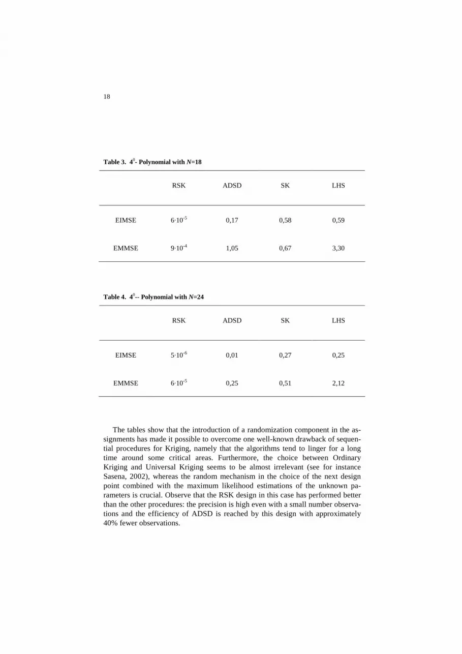
Table 3. 40- Polynomial with N=18

RSK ADSD SK LHS

EIMSE 6·10-5 0,17 0,58 0,59

EMMSE 9·10-4 1,05 0,67 3,30

Table 4. 40-- Polynomial with N=24

RSK ADSD SK LHS

EIMSE 5·10-6 0,01 0,27 0,25

EMMSE 6·10-5 0,25 0,51 2,12

The tables show that the introduction of a randomization component in the as-signments has made it possible to overcome one well-known drawback of sequen-tial procedures for Kriging, namely that the algorithms tend to linger for a long time around some critical areas. Furthermore, the choice between Ordinary Kriging and Universal Kriging seems to be almost irrelevant (see for instance Sasena, 2002), whereas the random mechanism in the choice of the next design point combined with the maximum likelihood estimations of the unknown pa-rameters is crucial. Observe that the RSK design in this case has performed better than the other procedures: the precision is high even with a small number observa-tions and the efficiency of ADSD is reached by this design with approximately 40% fewer observations.

19

4 Robust parameter and tolerance design via computer experiments

4.1 Robust parameter and tolerance design: crossed arrays and combined arrays

Robust parameter design, introduced in the eighties by the Japanese engineer G. Taguchi (see Taguchi and Wu 1980), is an experiment-based statistical methodol-ogy that aims at finding the nominal setting of design variables (parameters) which achieves a desired compromise between two objectives: optimizing the per-formance of a system by keeping the mean system performance around an ideal quality target and the variation around the mean to a minimum. This variation is caused by random variables (noise) related either to the external conditions (tem-perature, humidity, electromagnetic field, mechanical vibrations, way of use) un-der which the product/process is operating or to random variation of parameters due to manufacturing errors. Thus random noise plays a major role in robust de-sign.

When the design scope is extended to the specification of allowable deviations of parameters from nominal setting (tolerances), an integrated parameter and tol-erance design problem arises. Here the additional objective of minimizing the production costs needed to fulfil tolerance specs will compete with the minimum variance objective.

The statistical methodology underlying robust design that has by now become most widely accepted is the Dual Response Surface Methodology which estimates two surfaces, one for the mean and one for the variance (or the log-variance) of the process: see for instance Myers et al. (1992) and Myers and Montgomery (2002).

Let the system performance be described by a variable which depends on a set of controllable factors and a set of random noise factors: we write Y(x,Z) where the vector x stands for the levels of the controls and the vector Z for those of the noise. To explore the dependence of Y on x and Z one option is to run a crossed-array (Taguchi-type) experiment: some level combinations of the control factors (inner array) are chosen and tested across some level combinations of the random factors (outer array), which in the experimental setting are selected by the ex-perimenters and are therefore regarded as fixed (non-random).

An alternative is a combined array experiment (Vining and Myers 1990; Welch, Yu, Kang and Sacks 1990), with fixed levels of both the control and the noise variables. In such experiments the in-process response is described by the model:

20

Y(x, Z) = β0 + ββββTx + xTBx + γγγγTΖΖΖΖ + xT∆Z + ε , (8)

where Z is the random noise vector, ε’s are i.i.d. Ν(0,σ2) random errors, and ε and Z are independent. The constant β0, the vectors β β β β, γγγγ and the matrices B and ∆ con-sist of unknown parameters, and σ2 is also usually unknown. It is also assumed that E(Z) = 0 and that Cov(Z) is known. After model (8) is fitted to the data, two response surfaces, one for the mean of Y as a function of the control factors x, and one for the variance of Y, also in terms of the control factors, are obtained analyti-cally from (8), by taking expectations.

Both approaches (crossed array and combined array) have some drawbacks: we describe briefly the method suggested in (Giovagnoli and Romano, 2008) which generalizes both approaches making use of a stochastic simulator.

4.2 The proposed simulation protocol and its application to the integrated design of parameters and tolerances

Let us divide the random factors into two independent vectors, Z1 and Z2. The random vector Z1 will include the variables that we are going to simulate stochas-tically, while the remaining set of noise factors Z2 will be given fixed levels z2 for some different choices of z2. At the same time different levels x of the control fac-tors are also chosen for the experimentation. The computer experiment is per-formed by stochastically simulating the noise Z1 for chosen pairs (x,z2), and the sample mean and variance of the observed responses are calculated. The hypothe-sis underlying the proposed approach is that a simulation code of the physical sys-tem is available and noise factors are explicitly modelled in the code. Often nor-mality of Z1 can be reasonably assumed. Clearly this method requires to modify existing models to take into account the additional variability introduced by simu-lating the randomness of Z1 .

In the case Z1 = ∅ (or, equivalently, Z2 = Z), the simulation becomes non-stochastic and the model reduces to Model (8) for the combined array approach, but without the experimental error. In the case Z1 = Z (or, equivalently, Z2 = ∅), with independent and normally distributed noises one gets the crossed array ap-proach.

This method can be extended to a several-stage procedure if noise factors are simulated by adding them sequentially one after another to Z1. This allows se-quential assessment of the way in which each single noise factor affects the total variability.

Other proposals for conducting robust design studies (Lehman et al. 2004); Bates, Kennett, Steinberg and Wynn 2006) have been recently made in the context of Computer Experiments but they do not envisage any stochastic simulation.

Sometimes Robust Design aims at setting both design parameters and tolerance specifications. External noise variables are totally out of the designer's control, but

21

internal noise variables, which represent random deviation in design parameters due to part-to-part variation induced by uncontrollable manufacturing errors, are partially controllable. In this case the size of the common variability can be de-cided upon by the designer choosing components of suitable quality. It seems natural, at the experimental stage, to take this variability as a control factor and simulate the internal noise accordingly at each level of this factor. Hence internal noise variables, under the common assumption of independence and normal dis-tribution with zero mean, are natural candidates for inclusion in the Z1 vector of the proposed method.

After the modified dual response approach is applied, in-process mean and variance of the response are obtained as functions of the control factors. These functions, coupled with cost functions which specify how individual tolerances af-fect production cost (the tighter the tolerances, the more expensive the manufac-turing processes), are the ingredients for posing the integrated parameter and tol-erance design problem (Li and Wu 1999; Romano et al. 2004) as an optimization problem under constraints.

4.3 An application to complex measurement systems

The new method was applied to the design of a high precision optical profilome-ter. This is a measuring device that inspects the surface of mechanical parts and then reconstructs the relevant profile. Its peculiar features are that the surface is inspected without contact and measurement uncertainty is very low.

Insert Giovagnoli-Romano Figure1 about here

An innovative prototype, based on the technique of white-light interferometry, has been recently realized at the Department of Mechanical Engineering of Cagliari University, Italy (see Baldi et al. 2002; Baldi and Pedone 2005). The measurement process combines the analogue treatment of optical signals with the numerical processing of digitized images.

An experiment was performed at the Department of Mechanical Engineering of Cagliari University, Italy, with the objective of improving the measurement qual-ity of the profilometer, i.e. minimizing bias and uncertainty in the profile recon-struction. As there are several sources of noise in the system, robust design was called for. Since experimenting on the prototype would have been exceedingly ex-pensive, the whole measurement process was reproduced by a suitable simulator. The simulator incorporated both theoretical and experimental knowledge on the physical mechanisms involved. Measurement variance predicted by the simulator was also validated by comparison with that obtained by replicated measurements on the prototype (Baldi et al. 2006).

22

4.4 Other potential applications

It is useful to clarify what are the most suitable conditions for utilizing the pro-posed method and thus identify applications which could benefit most from it. Some of the most congenial set-ups are described hereafter.

• The simulator should not be exceedingly expensive in terms of completion time of the single runs. This is generally true for stochastic simulators, but not just for them. Think for instance of Finite Element codes to solve engineering de-sign problems in the most diverse areas (mechanical components, buildings, electrical and electro-magnetic apparatus, fluid-dynamic systems, etc.). In the not too infrequent case in which the problem can be modelled through a system of linear differential equations, the computing code is very reliable and the run-ning time relatively short.

• There are circumstances in which simulating noise variables may be convenient not only for a better quality of the solution of a robust design problem but also, although this may seem paradoxical, for cost saving. This may be due to the presence of a very large number of noise variables which all share the same probability distribution because of their common physical source. Think for in-stance of a simulator of microeconomic systems in which a large number of in-dividual - independent and identically distributed - choices come into play. Simulation from a common distribution is evidently more appropriate as well as more convenient. This is true for external noise factors and even more so for internal ones, like manufacturing errors induced on a number of similar part features, such as flat faces, bores, cylindrical surfaces, machined by the same physical process (milling, drilling, turning). This way of simulating internal noise was applied in the case study mentioned above, the optical profilometer. Here the same piezoelectric transducer repeatedly moves a mirror by a nomi-nally constant distance. Random errors of successive displacements, though in-dependent, come from the same distribution. Under these circumstances, all the independent identically distributed internal noise variables can be cumulatively accounted for by just one tolerance factor. This may yield a considerable saving of runs. Suppose there are 2 control factors and 10 internal noise variables of this kind. If we take 2 levels per control, 3 levels per noise variable and cross them fully, as is done in a Taguchi type experiment, an outer array of 22x310 = 236156 runs will result. This number is by far larger than a reasonable sam-pling size (800) obtained running 100 simulations of 10-tuples drawn from the common underlying distribution, for each combination of levels of the toler-ance and control factors, say 23.

• Another interesting application field concerns a class of systems, sometimes re-ferred as hybrid systems, incorporating both a hardware and a software compo-nent. The hardware part collects or generates analogical information which, in turn, after being converted into a digital format, is further processed by some software module. Such systems are already a common factor in our daily life

23

and the trend is upward. Familiar examples are cellular phones and household appliances like dishwashers, food processors etc. Sophisticated software proc-esses electric signals to allow for an acceptable quality of mobile communica-tion even in hostile external conditions. Household machines are provided with carefully designed digital controllers which can modify in real time the operat-ing conditions of the machine to get optimised performance (effective opera-tions, energy saving, noise reduction, vibration control and safety control). The design of hybrid systems is particularly challenging. Although the design tech-niques for the hardware and software components are highly heterogeneous, they must be perfectly coupled for effective design. The option here is to re-place, at the design stage, the physical part of the system by a simulation model. In this circumstance the whole system can be represented by a computer code, very easy to handle for design purposes. It is sensible to forecast that the software part of the hybrid systems will become dominant and more and more complex. This will make these systems easier to be simulated (numerical treatment is a computer code) and even more adapt to be designed (numerical treatment can deal with a huge number of design variables). This opens the way to intelligent and innovative products. The optical profilometer mentioned be-fore is a hybrid system. Reconstruction of the microgeometry requires a mas-sive numerical treatment of several images collected by a digital videocamera after a number of costly optical components have processed the white light. Measurement and diagnosis systems are in fact one of the most interesting sec-tors where designing via simulators is applicable. Let us mention three more cases: the process for dimensional and geometric control of manufactured parts by Coordinate Measuring Machines (CMM) (Romano and Vicario 2002a); the supervising systems for fault diagnosis in industrial processes (Romano and Kinnaert 2006); and the fixed-bed gassifier in a clean plant for obtaining en-ergy from coal (Cocco et al. 2008). In all these applications a robust design ap-proach has been applied to ad-hoc developed stochastic simulators of the in-volved processes.

References AICKIN, M.: Randomization, balance, and the validity and efficiency of design-adaptive alloca-

tion methods. J. Stat Plan Infer 94, 97-119 (2001) ALEXANDROV, N., DENNIS, J.E. Jr., LEWIS, R.M., TORCZON, V.: A Trust Region Frame-

work for Managing the Use of Approximation Models in Optimization. Struct Optimiz 15(1), 16-23 (1998)

BALDI ANTOGNINI, A., GIOVAGNOLI, A.: On the large sample optimality of sequential de-signs for comparing two or more treatments. Sequential Anal 24, 205-217 (2005)

BALDI ANTOGNINI, A., GIOVAGNOLI, A.: On the asymptotic inference for response-adaptive experiments. Metron 64, 29-45 (2006)

BALDI ANTOGNINI, A., GIOVAGNOLI, A., ROMANO, D.: Implementing Asymptotically Optimal Experiments for Treatment Comparison. Presented at the 5th ENBIS Conference, Newcastle, UK, September 2005, available on CDrom (2005)

BALDI, A., PEDONE, P.: Caratterizzazione numerico sperimentale dei rotatori geometrici nell’interferometria in luce bianca. Proc. of XXXIV AIAS Conference, Milan, Italy, September 14-17, 2005, 203-204 (extended version on CD-rom) (2005)

24

BALDI, A., GIOVAGNOLI, A., ROMANO, D.: Robust Design of a High-Precision Optical Pro-filometer by Computer Experiments.. CCommunication at the 2nd ENBIS Conference, Rimini, Italy, September 23-24, (2002)

BALDI, A.; GINESU, F.; PEDONE, P.; ROMANO, D.: “Performance Comparison of White Light - Optical Profilometers”, Proc. of 2006 SEM (Society for Experimental Mechanics) Annual Conference, St. Louis, (Missouri, USA), paper n. 378 on CD-rom, ISBN 0-912053-93-X. (2006)

BASHYAM, S., FU, M.C.: Optimization of (s, S) inventory systems with random lead times and a service level constraint, Managt Sci 44(12), 243-256 (1998)

BATES, R.A., BUCK, R.J., RICCOMAGNO, E., WYNN, H.P.: Experimental design and obser-vation for large systems. J. Roy Statl Soc B 58, 77-94 (1996)

BATES, R.A., KENETT, R.S., STEINBERG, D.M., WYNN, H.P.: Achieving Robust Design from Computer Simulation. Qual Technol Quantit Manag 3(2), 161-177 (2006)

BURSZTYN, D., STEINBERG, D.M.: Comparisons of designs for computer experiments. J. Statl Plan Infer 136, 1103-1119 (2006)

BOX G.E.P., WILSON K.B.: On the Experimental Attainment of Optimum Conditions. J. Roy Stat Soc B 13, 1-45 (1951)

CHAUDHURI, P., MYKLAND, P.A.: Nonlinear experiments: optimal design and inference based on likelihood. J. Am Stat Assoc 88, 538-546 (1993)

CRESSIE, N.A.C.: Statistics for Spatial Data. Wiley, New York (1993) COCCO, D., ROMANO, D., SERRA, F.: Caratterizzazione di un gassificatore a letto fisso me-

diante la metodologia della pianificazione degli esperimenti. accepted for publication on Proc. of 63° Congresso ATI (Associazione Termotecnica Italiana). Palermo (Italy), 2008, September 23-26, (2008)

FANG, K.-T., LI, R., SUDJIANTO, A.: Design and Modeling for Computer Experiments. Chapman and Hall / CRC, London, UK (2006)

FARHANG-MEHR, A., AZARM, S.: An Information-Theoretic Performance Metric for Quality Assessment of Multi-Objective Optimization Solution Sets. J. Mech D-T ASME 125(4), 655-663 (2003)

FORD, I., TITTERINGTON, D.M., WU, C.F.J.: Inference and sequential design. Biometrika, 72, 545-551 (1985)

GHOSH, B.K., SEN, P.K. (Eds.): Handbook of sequential analysis. Marcel Dekker, New York (1991)

GIOVAGNOLI, A.: Sul ruolo della probabilità e della verosimiglianza nella programmazione degli esperimenti. Statistica 59, 559-580 (1999)

GIOVAGNOLI, A., ROMANO, D.: Robust Design via Experiments on a Stochastic Simulator: A Modified Dual Response Surface Approach. Qual Reliab Eng Inter, to appear (2008)

GUPTA, A., DING, Y., XU, L.: Optimal Parameter Selection for Electronic Packaging Using Sequential Computer Simulations. J. Manuf Sci Eng-T ASME 128, 705-715 (2006)

HU, F., ROSENBERGER, W.F.: Optimality, variability, power: evaluating response-adaptive randomization procedures for treatment comparisons. J. Am Stat Assoc 98, 671-678 (2003)

JOHNSON, M.E., MOORE, L.M., YLVISAKER, D.: Minimax and maxmin distance design. J. Stat Plan Infer 26, 131-148 (1990)

KLEIJNEN, J.P.C., SARGENT, R.G.: A methodology for fitting and validating metamodels in simulation. Eur J. Oper Res 120, 14-29 (2000)

KLEIJNEN, J.P.C., VAN BEERS, W.C.M.: Application-driven sequential designs for simulation experiments: Kriging metamodeling. J. Oper Res Soc 55, 876-883 (2004)

KOEHLER, J.R., OWEN, A.B.: Computer Experiments. In: Handbook of Statistics, Vol.13 (S.Ghosh, C.R. Rao (eds)), Elsevier Science B.V. pp. 261-308 (1996)

LEHMAN, J.S., SANTNER, T.J., NOTZ, W.I.: Designing computer experiments to determine robust control variables. Stat Sinica 14, 571-590 (2004)

LI, W., WU, C.F.J.: An Integrated Method of Parameter Design and Tolerance Design. Qual Eng 11, 417-425 (1999)

25

LIN, Y., MISTREE, F., ALLEN, J.K.: A Sequential Exploratory Experimental Design Method: Development of Appropriate Empirical Models in Design, in: ASME 30th Conference of De-sign Automation, Chen W. (Ed.), Salt Lake City, UT, USA, ASME Paper no. DETC2004/DAC-57527. (2004)

LINDLEY, D.V.: On a measure of information provided by an experiment. Ann Math Stat 27, 986-1005 (1956)

MATHERON, G.: Traité de Géostatistique appliquée,Vol. 1, Memoires du Bureau de Recher-ches Geologiques et Miniéres. Editions Bureau de Recherches Geologiques et Minieres, vol. 24. Paris (1962)

MCKAY, M.D., BECKMAN, R.J., CONOVER, W.J.: A comparison of three methods for select-ing values of input variables in the analysis of output from a computer code. Technometrics 21, 239-245 (1979)

MELFI, V., PAGE, C.: Estimation after adaptive allocation. J. Stat Plan Infer 87, 353-363 (2000)

MONTGOMERY, D.C.: Design and analysis of experiments. 5th edition. John Wiley & Sons, New York, NY (2005)

MYERS, R.H., MONTGOMERY D.C.: Response Surface Methodology, 2nd edition. John Wiley & Sons, New York, NY. (2002)

MYERS, R.H., KHURI, A.I., VINING, G.G.: Response Surface Alternatives to the Taguchi Ro-bust Parameter Design Approach. Am Stat 46(2), 131-139 (1992)

PEDONE, P., VICARIO, G., ROMANO, D.: Kriging-Based Sequential Inspection Plans for Co-ordinate Measuring Machines. ENBIS-DEINDE Conference, Turin, 11-13 April 2007, avail-able on CDrom (2007)

RIPLEY, B.: Spatial Statistics. Wiley (1981) ROMANO, D.: Sequential Experiments for Technological Applications: Some Examples. Pro-

ceedings of XLIII Scientific Meeting of the Italian Statistical Society - Invited Session: Adap-tive Experiments, Turin, 14-16 June 2006, pp. 391-402 (2006)

ROMANO, D., KINNAERT, M.: Robust Design of Fault Detection and Isolation Systems. Qual Reliab Eng Int 22(5), 527-538 (2006)

ROMANO, D., VARETTO, M., VICARIO, G.: A General Framework for Multiresponse Robust Design based on Combined Array. J. Qual Technol 36(1), 27-37 (2004)

ROMANO, D., VICARIO, G.: Inspecting Geometric Tolerances: Uncertainty In Position Toler-ances Control On Coordinate Measuring Machines. Stat Method Appl 11(1), 83-94 (2002a)

ROMANO, D., VICARIO, G.: Reliable Estimation in Computer Experiments on Finite Element Codes. Qual Eng 14(2), 195-204 (2002b)

ROSENBERGER, W.F., FLOURNOY, N., DURHAM S.D.: Asymptotic normality of maximum likelihood estimators from multiparameter response-driven designs. J. Statist. Plan Infer 60, 69-76 (1997)

ROSENBERGER, W.F., LACHIN, J.M.: Randomization in Clinical Trials. Wiley, New York (2002)

SACKS, J., WELCH, W., MITCHELL, T.J., ,WYNN, H.P.: Design and Analysis of Computer Experiments. Stat Sci 4, 409-435 (1989)

SANTNER, J.T., WILLIAMS, B.J., NOTZ, W.J. The Design and Analysis of Computer Ex-periments. Springer, New York, NY (2003)

SASENA, M.J.: Flexibility and Efficiency Enhancements for Constrained Global Design Opti-mization with Kriging Approximations. PhD thesis, University of Michigan (2002)

SHEWRY, M.C., WYNN, H.P.: Maximum entropy sampling. J. Appl Stat 14, 165-170 (1987) SILVEY, S.D.: Optimal Designs. Chapman & Hall, London (1980) TAGUCHI, G., WU, Y.: Introduction to Off-Line Quality Control. Nagoya, Japan: Central Japan

Quality Control Association, [available from American Supplier Institute, Romulus, MI] (1980)

THOMPSON, S.K., SEBER, G.A.F.: Adaptive Sampling. Wiley, New York (1996)

26

VAN BEERS, W.C.M., KLEIJNEN, J.P.C.: Kriging for interpolation in random simulation. J. Oper Research Society 54, 255-262 (2003)

VAN BEERS, W.C.M., KLEIJNEN, J.P.C. Customized Sequential Designs for Random Simula-tion Experiments: Kriging Metamodeling and Bootstrapping, Discussion paper n. 55, Tilburg University, Holland (2005)

VINING, G.G., MYERS, R.H.: Experimental Design for Estimating both Mean and Variance Functions. J. Qual Technol 28, 135-147 (1990)

WANG, G.G., DONG, Z., AITCHISON, P.: Adaptive Response Surface Method — A Global Optimization Scheme for Computation-intensive Design Problems, J. Eng Optimiz 33(6), 707-734 (2001)

WELCH, W.J., BUCK, R.J., SACKS, J., WYNN, H.P., MITCHELL, T.J., MORRIS, M.D.: Screening, predicting, and computer experiments. Technometrics 34, 15-25 (1992)

WELCH, W.J., YU, T.-K., KANG, S.M., SACKS, J.: Computer experiments for quality control by parameter design. J. Qual Technol 22, 15-22 (1990) WILLIAMS, B.J., SANTNER, T.J., NOTZ, W.I.: Sequential design of computer experiments to

minimize integrated response functions. Stat Sinica 10, 1133-1152 (2000) WUJEK, B.A., RENAUD, J.E.: New Adaptive Move-Limit Management Strategy for Approxi-

mate Optimization, Part 1 and 2, AIAA J 36(10), 1911-1934 (1998) ZAGORAIOU, M., BALDI ANTOGNINI, A.: On the Optimal Designs for Gaussian Ordinary

Kriging with exponential correlation structure. Manuscript, submitted for publication (2008)

27