C O M P U T E R S C I E N C E R E V I E W ( ) –

available at www.sciencedirect.com

journal homepage: www.elsevier.com/locate/cosrev

Survey

Computational models for networks of tiny artifacts: Asurvey

Carme Àlvareza, Ioannis Chatzigiannakisb, Amalia Ducha, Joaquim Gabarróa,Othon Michailb,∗, Maria Sernaa, Paul G. Spirakisb

aUniversitat Politècnica de Catalunya (UPC), ALBCOM Research Group, Dept. de Llenguatges i Sistemes Informàtics, Barcelona, Spainb Research Academic Computer Technology Institute (RACTI) & Computer Engineering and Informatics Department (CEID),University of Patras, Patras, Greece

A R T I C L E I N F O

Article history:

Received 11 June 2010

Received in revised form

25 July 2010

Accepted 9 August 2010

Keywords:

Population protocols

Mediated population protocols

Sensor field

Graph languages

Sensing problems

Sensor networks

A B S T R A C T

We survey here some recent computational models for networks of tiny artifacts. In

particular, we focus on networks consisting of artifacts with sensing capabilities. We first

imagine the artifacts moving passively, that is, being mobile but unable to control their

own movement. This leads us to the population protocol model of Angluin et al. (2004)

[16]. We survey this model and some of its recent enhancements. In particular, we also

present the mediated population protocol model in which the interaction links are capable

of storing states and the passively mobile machines model in which the finite state nature

of the agents is relaxed and the agents become multitape Turing machines that use a

restricted space. We next survey the sensor field model, a general model capturing some

identifying characteristics of many sensor network’s settings. A sensor field is composed

of kinds of devices that can communicate one to the other and also to the environment

through input/output data streams. We, finally, present simulation results between sensor

fields and population protocols and analyze the capability of their variants to decide graph

properties.c⃝ 2010 Elsevier Inc. All rights reserved.

1. Introduction

The use of networks of tiny artifacts is becoming a key

ingredient in the technological development of XXI cen-

tury societies. An example of these networks is a network

with sensors, where some of the artifacts have the ability of

This work has been partially supported by the ICT Programme of the European Union under contract number ICT-2008-215270(FRONTS). The first, third, fourth, and sixth authors were partially supported by SGR2009-2013 (ALBCOM). The first, fourth, and sixthauthors were partially supported by MEC TIN-2007-66523 (FORMALISM).

∗ Corresponding author.E-mail addresses: alvarez@lsi.upc.edu (C. Àlvarez), ichatz@cti.gr (I. Chatzigiannakis), duch@lsi.upc.edu (A. Duch),

gabarro@lsi.upc.edu (J. Gabarró), michailo@cti.gr (O. Michail), mjserna@lsi.upc.edu (M. Serna), spirakis@cti.gr (P.G. Spirakis).

sensing the environment and communicate among them-selves. It is quite usual nowadays to hear about sensor net-work applications. For instance, the use of sensor networksto study the roaming of herds of endangered species or tocontrol flooding threats or to coordinate mobile communica-tion networks or even to monitor vital signs in human pa-tients and perform highway traffic control.

1574-0137/$ - see front matter c⃝ 2010 Elsevier Inc. All rights reserved.doi:10.1016/j.cosrev.2010.09.001

2 C O M P U T E R S C I E N C E R E V I E W ( ) –

All these applications and many more are possible dueto a wide range of artifacts that become smaller, low-cost,available, extended and wireless interconnected to existingnetworks which are pervasive (they are embedded in theenvironment and almost form part of it) and ubiquitous (theyare everywhere, anytime).

Such networks require several capabilities. Namely, sense,communicate, move, evolve, interact, adapt, act, amongothers. Therefore, the study of such systems involves severaland very different areas of computing: hybrid and distributedsystems, communication systems and protocols, circuitdesign, multi-agent systems, ad-hoc networks, algorithmicdesign, complexity theory or pervasive and ubiquitouscomputing. Consequently, one can assume that these kindsof systems are intrinsically complex. In fact, there is no easyway to design a universal sensor network that acts properlyin all possible situations.

However, it is important to understand the computationalprocess and behavior of the different types of artifact’snetworks, which will help in taking the maximum profitof those networks. In the particular case of networks withsensors several proposals (taxonomies and surveys) thatelucidate their distinguishing features and their applicationshave been published [1–7]. These proposals state clearly theneed of formal models that capture the clue characteristicsof networks with sensors that consist of massive amounts oftiny devices with limited resources.

The general sensing setting can be described by twoelements: the observers or end users and the phenomenon,the entity of interest to the observers that is monitoredand analyzed by a network with sensors. The correspondinginformation is discretized in two ways: first the environmentis sampled on a discrete set of locations (sensor positions),and second the measures taken by the sensors are digitalizedto the corresponding precision. To analyze the correctnessand performance of the system we are faced with a doubletask; on one side there is a computational problem to besolved by a particular network; on the other hand, it isnecessary to assess whether a computed solution is a validobservation of the phenomenon. Both tasks will requiredifferent analysis tools and we concentrate here on the firstone. The distinctive peculiarities of the computational systemdefine new parameters to be evaluated in order to measurethe performance or the stability of the system. Metrics areneeded to allow us to estimate the suitability of a specificor generic network topology or the possibility of emergentbehavior with pre-specified requirements.

The computational system can be perceived and analyzedin two complementary ways. The first one has as goal to showthe emergency of some designed behavior. In this scenarioit is usual to assume that the system models some kindof interaction among the participating devices and the finalgoal is to achieve a configuration with the pre-specified goals.The task has to be carried out by the network based onthe subjacent communication model and the exchange ofinformation among the devices.

For the first, we focus on models coming from thearea of population protocols [8–10]. They represent sensornetworks, supposing that the corresponding sensing devicesare extremely limited mobile agents, unable to control their

own movement, that interact only in pairs by means of aninteraction graph. These models bear a strong resemblanceto models of interacting molecules in theoretical chemistry[11,12]. According to [13], the population protocol model wasinspired in part by work by Diamadi and Fischer [14] on trustpropagation in a social network. The urn automata of [15]can be seen as a first draft of the model that retained investigial form several features of classical automata: insteadof interacting with each other, agents could interact onlywith a finite-state controller, complete with input tape. Themotivation given for the population protocol model proposedin [16] was the study of sensor networks in which passiveagents were carried along by other entities; the canonicalexample was sensors attached to a flock of birds. The name ofthe model was chosen by analogy to population processes [17]in probability theory.

The computational system arising from the ad-hoc com-putation network point of view can be modeled by combiningthe notion of graph automata [18] together with distributeddata streams [19], a combination inspired in similar ideasdeveloped in the context of concurrent programming [20].Existing models coming from distributed systems [21], hy-brid systems and ad-hoc networks [22,23] capture some ofsuch networks. This approach has been used also in manypapers in which the communication network is assumed tobe formed by a random geometric graph [24–28] and followsclassic distributed approaches to solve problems on particu-lar topologies [29]. Based on those ideas the Sensor Fieldmodelwas proposed in [30]. A sensor field captures some character-istic differences of sensor networks, it is composed of a kindof actuator devices that can communicate one to the otherand also can measure and signal the environment. The ini-tial study has been concentrated on the case in which thedevices and the communication links do not appear and dis-appear during the computation. The model assumes thatthose devices synchronize at barriers marking rounds, in away similar to the BSP model [31]. During a computationround, a device access the received messages and data pro-vided by the environment, performs some computation, andfinally sends messages to its neighbors and to the environ-ment. Those are the fundamental features of the Static andSynchronous Sensor Field (SSSF) model. The SSSF model can beseen as a non-uniform computational model in the sense thatit is easy to introduce constraints to all or some of the devicesof the sensor field and relate it to classic complexity classes.

In the remainder of this paper we survey recent resultson computational models for networks of tiny artifacts. Thesurvey is organized as follows: In Section 2 we highlightthe fundamental problems to be solved in such networks.Section 3 is devoted to the population protocol model andits variants. The sensor field model is reviewed in Section 4.In Section 5 we provide the main ideas used to simulatepopulation protocols by a sensor field. Section 6 is devotedto analyze the graph languages that are decidable by anenhancement of population protocols and some subfamiliesof sensor fields with constant memory per device. Thelast section provides some conclusions and open lines ofresearch.

C O M P U T E R S C I E N C E R E V I E W ( ) – 3

2. Problems of interest

Before introducing in detail the models and the results wewant to highlight first some classes of problems that arerelevant in sensor networks application.

Sensor networks usually consist of massive amountsof cheap, bulk-produced sensor nodes (also called agents)and the resources available to each node are most of thetime severely limited. Such limitations can be surpassed ifthe system designer has fine control over the interactionsbetween the agents. In this case, even finite-state agents canbe regimented into cellular automata [32] with computationalpower equivalent to linear space Turingmachines. As Angluinet al. noticed in [8], if the system designer cannot controlthese interactions, it is not clear what the computationallimits are.

Consider a wireless sensor network in which the sensornodes move according to some mobility pattern over whichthey have totally no control. This kind of mobility is known aspassive mobility [8]. For example, imagine that millions of suchnodes are thrown into a hurricane in order to cooperativelystudy its various characteristics. Some metrics of interestcould be the average or maximum barometric pressure, thehighest temperature, or some collective data concerningthe wind speed near the eye of the hurricane. In thisscenario, the movement of the sensor nodes follows somecollection of interchanging probability distributions which, asa result of some natural phenomenon, are in general totallyunpredictable (any other phenomenon offering an abundanceof kinetic energy could be representative). The nodes have tosense their environment according to the underlying queryand then interact with the remaining population in order tomake some cooperative decision or cooperatively computea required function on the sensed inputs. An interaction isestablished when two nodes come sufficiently close to eachother so that communication becomes feasible (one withinthe range of the other). Communication is usually assumedto be two-way though various modes of communication havebeen studied in the relevant literature [33,13]. Additionally,the nodes are assumed to communicate in ordered pairs(u, υ), where u plays the role of the initiator and v thatof the responder. The distinct roles of the two participantsconstitutes a fundamental symmetry breaking assumption.

The critical constraints of these systems are clearly mem-ory and the inability of protocols to control interactions.These constraints render most classical distributed algo-rithms useless under this setting. Even electing a leader andexploiting it to execute a protocol that assumes its existenceis clearly non-trivial. The reason is that we may easily elect aleader but, under no probabilistic termination estimates, wewill never be able to detect termination of the leader elec-tion process. Recent developments [34,10] relax the memoryconstraint to allow the existence of unique identifiers (com-monly abbreviated as ids or uids) but no previously existingalgorithm can perform the id assignment under this totallyasynchronous and pairwise communication setting.

Another set of computational problems of interest consid-ers the sensors as a source of data to be treated by the sys-tem. These sensing problems have been stated in a generic way

in terms of input/output data streams and a relation that out-put data streams have to satisfy given the input data streams,i.e. the property that defines the problem [30]. Let us first in-troduce the notion of data stream.

A data stream w is a sequence of data items w = w1w2 . . .

wi . . . that can be infinite. For any i ≥ 1, w[i] denotes the i-thelement of w, i.e. w[i] = wi. For any i, j, 1 ≤ i ≤ j, w[i, j] denotesthe subsequence of w composed by all data items between thei-th and j-th positions, i.e. w[i, j] = wi . . . wj. For any n ≥ 1, an n-data stream w is an n-tuple of data streams, w = (w1, . . . , wn).For any i ≥ 1,w[i] denotes the n-tuple composed by all the i-thelements of each data stream, w[i] = (w1[i], . . . , wn[i]). For anyi, j such that 1 ≤ i ≤ j, w[i, j] denotes the n-tuple composed bythe subsequences between the i-th and j-th positions of eachdata stream, w[i, j] = (w1[i, j], . . . , wn[i, j]).

Now we can define formally in an abstract way what asensing problem is.

Sensing problem Π : Given an n-tuple of data streams u =

(uk)1≤k≤n for some n ≥ 1, compute an m-tuple of data streamsv = (vk)1≤k≤m for some m ≤ n such that RΠ (u[1, t],v[1, t]) issatisfied for every t ≥ 1. RΠ is the relation that output datastreams have to satisfy given the input data streams, i.e. theproperty that defines the problem.

Sensing problems capture many classes of problems thatarise in a natural way in a distributed system. Concerning theapplications of sensor networks we consider some sensingproblem subfamilies. These families are obtained by posingadditional requirements on the part of the input data streamthat is required for computing the t-th element of the outputdata stream.

• Cumulative monitoring

v[t] depends on all the data measured by the network upto time t.

• Monitoring

v[t] depends only on the data measured at time t.

• One step measure

v[t] depends only on the data measured at a particulartime step, usually the first.

When the computational model per node is a finite statemachine, the output data stream can contain the internalstate. Thus conditions on the internal state can be transferredto conditions on the output data stream.

Let us post some examples of sensing problems of thethree types. First we consider a problem in which it is neededto monitor continuously a wide area. This implies “sensinglocally” and “informing locally” about a global environmentalphenomena.

Average Monitoring: Given n data streams (uk)1≤k≤n for somen ≥ 1, compute n data streams (vk)1≤k≤n such that vk[t] =

(u1[t] + · · · + uk[t])/n.The second example we consider is related to “fire

detection alarm”. In this case it is desired to detect thesituation in which there is a high risk of fire. One elementto be measured is the level of smoke in the air of such areaand if this level is higher than a certain value then the alerthas to be activated. A specific device (number 1 for instance)acts as a master and outputs the result.

4 C O M P U T E R S C I E N C E R E V I E W ( ) –

Alerting: Given n data streams (uk)1≤k≤n for some n ≥ 1, andthreshold value A, device 1 has to compute a data stream v1such that

v1[t] =

1 if ∃k : 1 ≤ k ≤ n : uk[t] ≥ A⊥ otherwise.

This is a continuous monitoring type of problem as thet-th output data stream is computed from all the previoussegment of input data streams. The third example uses theinput data stream artificially. The final goal is to analyze afirst step property, therefore only the initial measurement isof relevance.

Initially even?: Given n data streams (uk)1≤k≤n for some n ≥ 1,such that for uk[t] ∈ 0,1, for any 1 ≤ k ≤ n and any t > 0,compute n data streams (vk)1≤k≤n such that vk[t] = [(u1[1] +

· · · + un[1]) mod 2 = 0]. Usually for this class of problems wespeak rather of an input to the network than of an input datastream for the network.

Observe that in the definition of the problems we havestated properties in which, in general, the t-th output datais related up to the t-th input data. Of course when solvingthe problem we have to allow some delay in the computationof the system. As we will see this will be one of the relevantparameters when solving the problem with time restrictions(as in the sensor field model). In other models we do not careabout the time as the interest is in showing that eventuallythe required output data stream will be attained (as in thepopulation protocol models). Note that sensing problems aredefined in terms of input and output data streams and theirdefinition is independent of the topology of the network.

The second family of problems, the graph decisionproblems, are related to the network’s topology. In thiscase we face the problem of deciding whether the actualsubjacent topology (interaction or communication) satisfiessome required property. This notion has been formalizedas graph languages which will be formally described inSection 6.

The goal of deciding graph languages is to determine prop-erties of the subjacent unknown, interaction or communica-tion, graph. Observe, that in this case the general definitionof the problem must consider also the subjacent (interac-tion/communication) graph that is used to solve the problem.As an example let us consider the following problem.

2-cycle?: Compute n data streams (vk)1≤k≤n such that, for antt > 0, vk[t] = 1 iff the subjacent graph contains a two cycle.

In this case, the output data streams have to agree ona repeated symbol that depends on whether the networkproperty is or is not verified by the network. Besidessolving information problem about the subjacent topologydecidability of graph languages can be used to compare thecomputational power of different computational models fornetworks formed by constant memory devices.

So, there was a clear need for some new theoreticalframework in order to study the computational power ofthe population protocol model and its enhancements and todevise protocols for practical problems that need to be solved.

3. Population protocols & enhancements

Let us start by defining formally a population protocol (PP)[16,8].

Population protocol A (PP A): Formally, we define a populationprotocol A by a 6-tuple A = (X, Y, Q, I, O, δ), where X, Y, and Qare all finite sets and

1. X is the input alphabet,2. Y is the output alphabet,3. Q is the set of states,4. I : X → Q is the input function,5. O : Q → Y is the output function, and6. δ : Q × Q → Q × Q is the transition function.

If δ(a, b) = (a′, b′) then (a, b) → (a′, b′) is called a transition andδ1(a, b) = a′ and δ2(a, b) = b′ are defined.

A simplification is that all agents concurrently sense theirenvironment, as a response to a global start signal, and eachone of them receives some input symbol from X. For example,X could contain all possible barometric pressures that theagent’s sensors can detect. Then all agents concurrently applythe input function I to their input symbols to obtain theirinitial state. In this manner, the initial configuration of thesystem is formed. A configuration in general, given a populationof n agents, is any string from Qn, in which the i-th symbol isthe state of agent i, 1 ≤ i ≤ n (by assuming an ordering on theagents).

Now the crucial part is that any interaction between theagents is possible and this is interpreted as some inherentnondeterminism of the system. Formally, the agents areorganized in an interaction graph G = (V, E), which is adirected graph without self-loops and multiple edges, andwhere V is a population of |V| = n agents and E describesthe permissible interactions. Angluin et al. in [16,8] modeledmobility via an adversary scheduler that is a black-box tothe protocol and simply selects members of E to interactaccording to δ (all agents apply the same global transitionfunction). The only, but necessary, restriction imposed on thescheduler is that it has to be fair so that it does not foreverpartition the network into non-communicating clusters and,as Aspnes and Ruppert cleverly observe in [13], to prevent thepossibility of having agents interacting only at “inconvenient”times. An execution (which is any sequence of configurations)is said to be fair if there exists no configuration in theexecution that appears infinitely often while some successorof it does not. A computation is an infinite fair execution.

Computations by definition do not halt. In fact, thedefinition itself captures the inherent inability of suchsystems to detect termination, which is mainly due to theuniformity and anonymity properties of population protocols.Uniformity requires protocol descriptions to be independentof n and anonymity that the set of agent states is smallenough so that there is no room in it for unique identifiers.Instead, computations are required to stabilize to a correctcommon or distributed value. Angluin et al. used functionson input assignments in order to formalize the specifications ofprotocols. For example, a natural question in our examplecould be whether at least one agent detects barometricpressure over some constant pressure c (which possiblypartitions the pressures in low and increased). What we do

C O M P U T E R S C I E N C E R E V I E W ( ) – 5

expect from a protocol that solves this problem is to alwaysstabilize (converge) in a finite number of steps to the correctanswer. Since such a query has a binary range, making it apredicate, we want all agents to output 1 when the predicate ismade true and 0 otherwise, which is a convention that wemake for gathering the protocol’ s output. Since our mainaim here is to survey the computational power of the modelsunder consideration, we can w.l.o.g. focus on predicates [13],although [16,8] provided general definitions for functions andalso proposed many other natural output conventions.

Formally, the input (also called an input assignment) to a PPA may be any x ∈ X∗, where X∗ denotes the set of all stringsthat can be made by concatenating zero or more symbolsfrom X. In fact, any such x = σ1σ2 . . . σn can be the input toA when it runs on a population of size n. This is done byassuming an arbitrary ordering on the set of agents, whichis hidden from the agents themselves. Then we can simplymake the convention that agent i, 1 ≤ i ≤ n, senses the inputsymbol σi. A specification for A is any predicate p : X∗

→ 0,1

which can also be thought as its corresponding languageLp = x ∈ X∗

| p(x) = 1.The transition graph T(A, G) of a protocol A that is executed

on an interaction graph G [8] is a directed graph whosenodes are all possible configurations and whose edges are allpossible one-step transitions between those configurations.

Not all interaction graphs are allowed in most practicalscenarios. For example, if no obstacles are present we canassume that the interaction graph is always complete, whichis the most commonly studied case. On the other extreme,we could also consider only line graphs or even morecomplicated collections of restricted graphs. This networkselection is captured by graph universes (also called families)which are sets of graphs. The set of all complete directedinteraction graphs, that has been extensively studied, is suchan example of graph universe. One simple way to think ofgraph universes is that they capture the interaction graphson which our protocols are about to be executed.

A predicate p over X∗ is said to be stably computable by thePP model in the graph universe U, if there exists a PP A suchthat for any input assignment x ∈ X∗, any computation of A,on any interaction graph from the set G ∈ U | |V(G)| = |x|,beginning from the initial configuration corresponding to xreaches an output stable configuration in which all agentsoutput p(x).

Research first focused on complete interaction graphs.Note that the completeness of the graph implies that stablycomputable predicates have to be symmetric. A predicate pis called symmetric if for every x ∈ X∗ and any x′ which isa permutation of x’s symbols, it holds that p(x) = p(x′) (inwords, permuting the input symbols does not affectthe predicate’s outcome). In [16,8] the authors, amongother results, established that any semilinear predicate or,equivalently [35], any predicate definable by first-order logicalformulas in Presburger arithmetic [36], is stably computableby the PP model. Moreover, in [37,33] it was proven thatthis inclusion is tight, thus, arriving to the following exactcharacterization for the computable predicates in completegraphs: A predicate is stably computable iff it is semilinear. This isa fairly small class, not including multiplication of variables,exponentiations, and many other important operations on

input variables. In particular (according to [16]), each termin these predicates is a constant (nonnegative integer), avariable, or the sum of two terms, or the product of aconstant and a term, or the integer quotient of a term anda nonzero constant, or the remainder of a term modulo anonzero constant. Atomic expressions are formed from twoterms and one of the predicates: =, ≤, <, ≥, >. For example,the predicate ((17N1 ≥ 3N0) ∧ (4N1 ≤ N0)) expresses thatthe input assignments to be accepted are those in whichthe number of 1s is between 15% and 20% of the totalpopulation. Moreover, Delporte-Gallet et al. [38] showed thatPPs can tolerate only O(1) crash failures and not even asingle Byzantine agent.1 These weaknesses were inevitablegiven that the PP model was on purpose designed to beminimalistic. We do not attempt a complete survey of theresults concerning population protocols since there is alreadyan excellent one [13]. Finally, for a step by step (less technicalthan the current article) introduction to population protocolsand related models, including examples and exercises, theinterested reader is referred to [40].

Another possibility is to allow the inputs to the populationto oscillate and only require that this oscillation ceasesafter some finite time. This is the stabilizing inputs variantof population protocols [41]. Here all agents are assumedto be initially in some initial state q0 (i.e. no input functionis defined) and the transition function is now of the formδ : (Q × X) × (Q × X) → Q × Q. Each agent is like havingtwo components in its state, where the first one is its actualstate from Q and the second one plays the role of an inputport whose symbol may change arbitrarily between any twointeractions but will eventually stabilize. The output functionis applied to the state components of the agents. In [41] itwas shown that all semilinear predicates can be computedwith stabilizing inputs, which, together with the above exactcharacterization for population protocols, implies that anypopulation protocol for fixed inputs can be adapted to work withstabilizing inputs. Moreover, [37] also established that nothingmore than semilinear predicates can be computed by thestabilizing inputs variant.

For some other relevant previous work, [16,8] alsoproposed the probabilistic population protocol model, in whichthe scheduler selects randomly and uniformly the next pair tointeract. Some recent work has concentrated on performance,supported by this random scheduling assumption (seee.g. [42]). [43,44] considered a huge population hypothesis(population going to infinity), and studied the dynamics,stability and computational power of probabilistic populationprotocols by exploiting the tools of continuous nonlineardynamics. Moreover, several extensions of the basic modelhave been proposed in order to more accurately reflect therequirements of practical systems. In [41], Angluin et al. alsostudied what properties of restricted interaction graphs arestably computable by the population protocol model and gaveprotocols for some of them. Recently, Bournez et al. [45]investigated the possibility of studying population protocolsvia game-theoretic approaches.

1 A Byzantine agent is an agent that has a Byzantine failure,that is, during any interaction it may pretend to be in any state(see e.g. [39] for a lot more on Byzantine failures and how they arehandled in classical distributed systems).

6 C O M P U T E R S C I E N C E R E V I E W ( ) –

3.1. Mediated population protocols

In [9] (see also [46] for an extensive presentation of theresults discussed in this section) the authors consideredthe following enhancement. They made the assumptionthat each interaction link is also a finite-state agent thatonly communicates with the agents it joins. In particular,whenever any two agents u and v interact via the edge e =

(u, v), u and v read the state of e and their own states andupdate all of them according, again, to some global transitionfunction. Now, it is like the agents are capable of leavingsmall pieces of pairwise information that will be availableduring their subsequent interactions. The authors namedtheir model the Mediated Population Protocol (MPP) model.

Mediated population protocol A (MPP A): A mediated populationprotocol A is a 7-tuple A = (X, Y, Q, S, I, O, δ), where X, Y, Q(it is now called set of agent states), I, and O are as in thePP model, S is a finite set of edge states, and the transitionfunction is now of the form δ : Q × Q × S → Q × Q × S.

As you may have noticed, there is no input to theedges (although such an input function was defined in [9]).We follow here the simplified definition given in [47] andconsequently make the assumption that there exists someedge initialization function ι : E → S, that specifies the initialstate of each edge. Note that ι is not part of the protocol butgenerally models some preprocessing on the network thathas taken place before the protocol’s execution. We focus oncomplete communication graphs and initially identical edges,that is, ι(e) = s0 for all e ∈ E. MPS is the class of all predicatesthat are stably computable by the so called “Symmetric” MPPmodel (SMPP).

Theorem 1 ([9]). The class of semilinear predicates is a propersubset of MPS.

Proof Idea. The PP model is a special case of the MPP modeland, thus, any semilinear predicate is stably computable bythe SMPP model. Consider now the non-semilinear predicate(Nc = Na · Nb) which is true iff the number of cs in theinput is the product of the number of as and the numberof bs. By exploiting the fact that in complete graphs thenumber of edges leading from a-agents to b-agents is equalto the product, it is easy to devise a SMPP protocol A withstabilizing states (i.e. whose states eventually stop changing)that provides the following semilinear guarantee: If Nc = Na ·

Nb then at least one agent remains in some state from someQ′

⊂ Q, otherwise no such state remains. Finally, compose Awith a SMPP B that stably computes with stabilizing inputsthe above guarantee to obtain a SMPP that stably computesthe non-semilinear predicate (Nc = Na · Nb).

The above result of [9] was a first indication that MPP pro-tocols in general can exploit the extra information stored onthe edges in order to compute more complicated predicates.The following theorem shows that this information increasesthe computational power to the maximum possible degree,which was hardly expected at the beginning. Generally, byNSPACE(f(n)) we denote the class of all languages decided bysome O(n2) space nondeterministic Turing machine (a deter-ministic Turing machine is abbreviated TM, while a nondeter-ministic one is abbreviated NTM, according e.g. to Sipser [48]),where n here denotes the size of the input to the machine.

Theorem 2 ([9,47]). A predicate is in MPS iff it is symmetric and isin NSPACE(n2).

Proof Idea. The “only if” part is easy. Any predicate in MPSis obviously symmetric and additionally we can performin O(n2) space a nondeterministic search on the transitiongraph of the SMPP that stably computes the predicate.

The sufficiency of the conditions is somewhat morecomplicated. We have to show that for all symmetriclanguages L ∈ NSPACE(n2) there exists a SMPP that stablycomputes pL, defined as pL(x) = 1 iff x ∈ L. It is easy to seethat pL is symmetric iff L is symmetric. The idea is to organizethe agents into a spanning line subgraph of the interactiongraph. To do that, the agents begin to form small line graphsthat in the sequel are merged together and are expandedto isolated nodes. When this process ends, the edges ofthe spanning line graph will be active and all other O(n2)

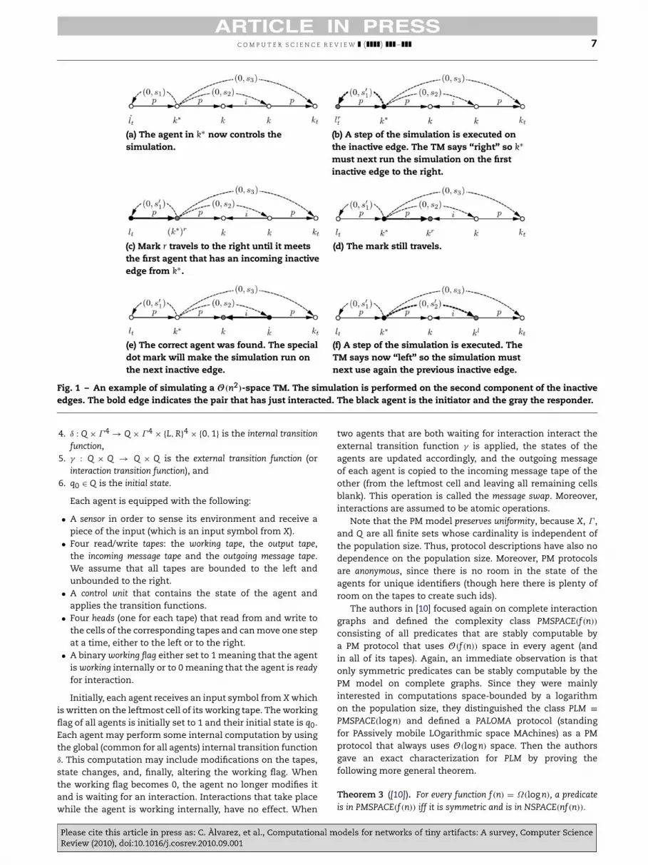
edges will be inactive. Now the network can operate as aTuring machine of O(n2) space by using the agents as thecontrol units and the inactive edges as the cells (see Fig. 1).Whenever the inactive edges of some agent are exhausted itpasses control (via some active edge) to its neighbor on thespanning line graph. By also exploiting the nondeterminisminherent in the interaction pattern the agents can simulatethe nondeterministic TM that decides L. Note that, since theagents cannot detect termination of the spanning line graphconstruction process, any time that the structure changesthey reinitialize their computation in a systematic manner,so that reinitialized agents do not communicate with non-reinitialized ones, and by exploiting a backup of their inputthat is maintained throughout the computation. The finalreinitialization happens when the spanning line graph isformed an then the simulation is executed correctly.

3.2. Communicating machines

Another natural enhancement of the population protocolmodel is to equip the agents withmorememory and to enablethem operate as Turing machines instead of being automata.For example, a natural question could be: “What can such amodel compute when each agent’s memory is logarithmic inthe population size?”. First of all, the communicating machinesassumption is perfectly consistent with current technology(cellphones, iPods, PDAs, and so on). Moreover, logarithmic is,in fact, extremely small. For a convincing example, it sufficesto mention that for a population consisting of 2266 agents,which is a number greater than the number of atoms in theobservable universe, it is only required for each agent to have266 cells of memory (while small-sized flash memory cardsnowadays exceed 16 GB of storage capacity)! This kind ofquestion engaged the author’s attention in [10] who provideda general model independent of space bounds, called the PMmodel (standing for Passively mobile Machines).

Passively mobile machines protocol A (PM A): Formally, a PMprotocol A is a 6-tuple A = (X,Γ , Q, δ, γ, q0) where X, Γ and Qare all finite sets and

1. X is the input alphabet, where ⊔ ∈ X (⊔ is the blank symbol),2. Γ is the tape alphabet, where ⊔ ∈ Γ and X ⊂ Γ ,3. Q is the set of states,

C O M P U T E R S C I E N C E R E V I E W ( ) – 7

(a) The agent in k∗ now controls thesimulation.

(b) A step of the simulation is executed onthe inactive edge. The TM says “right” so k∗

must next run the simulation on the firstinactive edge to the right.

(c) Mark r travels to the right until it meetsthe first agent that has an incoming inactiveedge from k∗.

(d) The mark still travels.

(e) The correct agent was found. The specialdot mark will make the simulation run onthe next inactive edge.

(f) A step of the simulation is executed. TheTM says now “left” so the simulation mustnext use again the previous inactive edge.

Fig. 1 – An example of simulating a O(n2)-space TM. The simulation is performed on the second component of the inactiveedges. The bold edge indicates the pair that has just interacted. The black agent is the initiator and the gray the responder.

4. δ : Q × Γ4→ Q × Γ4

× L, R4

× 0,1 is the internal transitionfunction,

5. γ : Q × Q → Q × Q is the external transition function (orinteraction transition function), and

6. q0 ∈ Q is the initial state.

Each agent is equipped with the following:

• A sensor in order to sense its environment and receive apiece of the input (which is an input symbol from X).

• Four read/write tapes: the working tape, the output tape,the incoming message tape and the outgoing message tape.We assume that all tapes are bounded to the left andunbounded to the right.

• A control unit that contains the state of the agent andapplies the transition functions.

• Four heads (one for each tape) that read from and write tothe cells of the corresponding tapes and canmove one stepat a time, either to the left or to the right.

• A binaryworking flag either set to 1 meaning that the agentisworking internally or to 0 meaning that the agent is readyfor interaction.

Initially, each agent receives an input symbol from X whichis written on the leftmost cell of its working tape. The workingflag of all agents is initially set to 1 and their initial state is q0.Each agent may perform some internal computation by usingthe global (common for all agents) internal transition functionδ. This computation may include modifications on the tapes,state changes, and, finally, altering the working flag. Whenthe working flag becomes 0, the agent no longer modifies itand is waiting for an interaction. Interactions that take placewhile the agent is working internally, have no effect. When

two agents that are both waiting for interaction interact theexternal transition function γ is applied, the states of theagents are updated accordingly, and the outgoing messageof each agent is copied to the incoming message tape of theother (from the leftmost cell and leaving all remaining cellsblank). This operation is called the message swap. Moreover,interactions are assumed to be atomic operations.

Note that the PM model preserves uniformity, because X, Γ ,and Q are all finite sets whose cardinality is independent ofthe population size. Thus, protocol descriptions have also nodependence on the population size. Moreover, PM protocolsare anonymous, since there is no room in the state of theagents for unique identifiers (though here there is plenty ofroom on the tapes to create such ids).

The authors in [10] focused again on complete interactiongraphs and defined the complexity class PMSPACE(f(n))

consisting of all predicates that are stably computable bya PM protocol that uses O(f(n)) space in every agent (andin all of its tapes). Again, an immediate observation is thatonly symmetric predicates can be stably computable by thePM model on complete graphs. Since they were mainlyinterested in computations space-bounded by a logarithmon the population size, they distinguished the class PLM ≡

PMSPACE(logn) and defined a PALOMA protocol (standingfor PAssively mobile LOgarithmic space MAchines) as a PMprotocol that always uses O(logn) space. Then the authorsgave an exact characterization for PLM by proving thefollowing more general theorem.

Theorem 3 ([10]). For every function f(n) = Ω(logn), a predicateis in PMSPACE(f(n)) iff it is symmetric and is in NSPACE(nf(n)).

8 C O M P U T E R S C I E N C E R E V I E W ( ) –

Proof Idea. Again the “only if” part is not hard. In fact, thispart holds for any function and not only those that are at leastlogn. p ∈ PMSPACE(f(n)) means that there exists a PM protocolA using O(f(n)) space in every agent that stably computes p.Thus, each agent configuration can be represented in O(f(n))

space and each population configuration (consisting of theagent configurations of all agents) in O(nf(n)) space. Then theNTM simply performs, as in Theorem 2, a nondeterministicsearch on the transition graph of protocol A by alwaysstoring at most one population configuration and decides thelanguage Lp = x ∈ X∗

| p(x) = 1.For the other part, take any symmetric language L ∈

NSPACE(nf(n)). The predicate pL defined as pL(x) = 1 iff x ∈

L is also symmetric. Obviously, wemust present a PM protocolthat stably computes pL by using O(f(n)) space in everyagent. Assume that the PM model was equipped with theunique consecutive ids 0,1, . . . , n − 1. In this case, we couldline up all agents and make them simulate the NTM Nthat decides L. In order to ensure that no agent exceedsthe desired space bound, we could run the simulation ina modular way, that is, the first n cells of N correspondto the first cells of the n agents, and generally, the cellskn + 1, . . . , (k + 1)n of N , k ≥ 0, correspond to the (k + 1)thcells of all agents. In this manner, the O(nf(n)) space of Nis evenly divided between n agents and this ensures thateach agent uses O(f(n)) space. Moreover, note that the uniqueids consume O(logn) space and since f(n) = Ω(logn) therewill always be enough space to store them. To simulate thenondeterminism of N the idea is to make a nondeterministicsearch on N ’s computation tree. The nondeterminism ofthe search stems from the inherent nondeterminism of theinteraction pattern. Whenever the simulation must take anondeterministic transition, the corresponding agent takesan ineffective interaction only to read the id of the other agentand this id is used to determine the nondeterministic choiceto be made. Whenever the search reaches a rejecting nodeit is being restarted, beginning another nondeterministicsearch from the root. Obviously, the fairness of the executionguarantees that if there exists an accepting node it will beeventually found, otherwise the simulation will forever rejectit. Call the described protocol B.

One important point remains: PM protocols do not haveunique ids. However, at the space cost ofO(logn) PM protocolscan create these ids. Initially, all agents have the same id 0.Whenever two of them meet, one of them increases its id byone. It is not so hard to see that this process eventually endswith a correct assignment of the unique ids 0,1, . . . , n − 1.A difficulty is that the agents cannot detect the terminationof this process, because, otherwise, it is easy to show thattermination could have been erroneously detected in a subsetof the population. So, we actually do not know when tostart executing the protocol B that makes use of these ids.Only one option remains: whenever some id is modified allagents get informed of this event and start simulating B fromthe beginning. This iterative reinitiation technique (used alsoin [34]) guarantees that when the last id-modification takesplace, when the agents have just obtained the correct ids, allagents will restart B’s execution for the last time and B willbe executed without further interruptions and as if the idswere provided to it from the beginning. Thus, it will correctlysimulate N and will stably compute pL.

As PLM is by definition PMSPACE(logn), we can concludethat:

Corollary 1 ([10]). PLM is equal to the class of all symmetricpredicates in NSPACE(n logn).

4. The sensor field model

In [30] the authors propose a general model capturing somecharacteristic differences of sensor networks. A sensor fieldis composed of a kind of devices that can communicate oneto the other and also to the environment. In this study theauthors assume that the devices and the communicationlinks do not appear and disappear during the computation.Furthermore, those devices synchronize at barriers markingrounds, in a way similar to the BSP model [31]. During acomputation round, a device accesses the received messagesand data provided by the environment, performs somecomputation, and finally sends messages to its neighborsand to the environment. Those are the fundamental featuresof the Static and Synchronous Sensor Field (SSSF) model. Themodel allows the definition of complexity measures likelatency, round duration, message number or message lengthamong others. In this setting it is possible to formulate ageneral and natural definition of sensing problems by meansof input/output data streams. The model can be seen as anon-uniform computational model in the sense that it is easyto introduce constraints to all or some of the devices of thesensor field and relate it to classic complexity classes.

As described before, the general sensing setting consid-ered in this model is described by the following elements:the observers and the the phenomenon. The phenomenon is theentity of interest to the observers that is being sensed and po-tentially analyzed by the sensor network. Multiple phenom-ena may be concurrently under consideration in the samenetwork.

Depending on the information required by the observersfrom the environment, different kinds of problems of interestcan be formulated as sensing problems. Those problemshave to be solved on a decentralized network composed ofsensing units and other elements. We have to re-examinenot only the meaning of successful computation but alsoto examine different performance metrics to measure theefficiency of the computational solutions given in this newmodel. The vision of the cycle of problem solving bynetworked sensors correspond to the schema given in Fig. 2.This schema discretizes information in two ways. First theenvironment is sampled only on a discrete set of locationsand second the measures taken by the sensor are digitalizedto the corresponding precision. We face a dual problem inanalyzing correctness and performance. On one side we havea computational problem to be solved on a particular network(or a family of networks). On the other hand we have to assesswhether the observation of the phenomenon is valid. It isclear that both tasks will require different analysis tools. Thecomputational models focus on the first problem. Now wedescribe the main components of a sensor field.

A communication graph is a directed graph G = (N, E) whereN is the set of nodes and E is the set of edges, E ⊆ N × N.

C O M P U T E R S C I E N C E R E V I E W ( ) – 9

Region Sensor Field

Phenomena

Output data streamsObservation

PROBLEM

SOLUTION

Fig. 2 – Problem solving with sensor fields.

Unless explicitly stated we assume that N has n nodes thatare enumerated from 1 to n and m edges. Each node k isassociated to a device, let us say to device k, that has access tothe k-th data stream. Each edge (i, j) ∈ E specifies that devicei can send messages to device j or what is the same, devicej can receive messages from device i. Given a device k let usdenote by I(k) = i | (i, k) ∈ E the set of neighbors from whichdevice k can receive data items and by O(k) = j | (k, j) ∈ E

the set of neighbors to which device k can send data. Letink = |I(k)| and outk = |O(k)| be the in and out degrees of nodek. Set inG = maxk∈N ink and outG = maxk∈N outk. We use dG todenote the diameter of the graph G.

A Static Synchronous Sensor Field consists of a set of devicesand a communication graph. The communication graph speci-fies how the devices communicate one to the other. For themoment and without loss of generality, we assume that alldevices are sensing devices that can receive information fromthe environment and send information to the environment.Since the model we consider is static we assume that theedges are the same during all the computation time. More-over each device executes its own process, communicateswith their neighbors (devices associated to adjacent nodes)and also with the environment. All the devices work in a syn-chronous way, at the beginning of each round they receivedata from their neighbors and from the environment, thenthey apply their own transition function changing in this waytheir actual configuration and finish the round sending datato their neighbors and to the environment. Let us describe indetail themain components of the Static Synchronous SensorField.

Static Synchronous Sensor Field F (SSSF F ): Formally wedefine a Static Synchronous Sensor Field F by a tuple F =

(N, E, U, V, X, (Qk, δk)k∈N) where

– GF = (N, E) is the communication graph.– U is the alphabet of data items used to represent the input

data streams that can be received from the environment.– V is the alphabet of items used to represent the output

data streams that can be send to the environment.– X is the alphabet of items used to communicate each

device to the other devices. Each m ∈ X∗ is called messageor packet. U, V ⊆ X. We denote by data items the elementsof alphabets U and V and by communication items (oritems) the elements of X.

– (Qk, δk) defines for each device associated to a node k ∈ N(device k) its set of local states and its transition function,respectively.

The local computation of each device k in F is defined by(Qk, δk) and depends on the communication with its neigh-bors and with the environment. Qk is a (potentially infinite)set of local states and δk is a transition function. A state codi-fies the values of some local set of variables (ordinary programvariables, message buffers, program counters...) and all whatis needed to describe completely the instantaneous config-uration of the local computation. The transition function δkthat depends on its local state qk ∈ Qk as well as on:

– the communication items received by device k fromdevices i ∈ I(k),

– the data item that device k receives as input from theenvironment,

– the communication items sent by device k to devices j ∈

O(k),– and the data item that device k sends to the environment.

The transition function is defined as

δk : Qk × (X∗)ink × U −→ Qk × (X∗)outk × V.

The meaning of

δk(qk, (xik)i∈I(k), uk) = (q′

k, (ykj)j∈O(k), vk)

is that if device k of F is in its local state qk ∈ Qk, receivesxik ∈ X∗ from each of its neighbors i ∈ I(k), and receives theinput data item uk ∈ U from the environment, then in onecomputation step device k changes its local state to q′

k ∈ Qk,sends ykj ∈ X∗ to each of its neighbors j ∈ O(k) and outputsvk ∈ V to the environment. In the case that device k does notsend any value, we denote this ‘no value’ or ‘does not care’by the special symbol ⊥. For any device k, let q0k be the initiallocal state. For any t ≥ 1, the t-th computation round of devicek is described as follows: If the local state of device k is qt−1

k ,and it receives (xt

ik)i∈I(k) from its input neighbors, utk from the

environment and δk(qt−1k , (xt

ik)i∈I(k), utk) = (qt

k, (ytkj)j∈O(k), vt

k)

then device k changes its local state from qt−1k to qt

k, sends(yt

kj)j∈O(k) to its output neighbors and vtk to the environment.

A computation of F is a sequence

c0,d1, c1,d2, . . . , ct−1,dt, ct, . . . ,

eventually infinite, where c0 = (q0k)k∈N is the n-tuple of theinitial local states of the n devices, and for each t ≥ 1, ct

=

(qtk)k∈N is the n-tuple of the local states after t computation

rounds. The tuple dt= (dt

k)k∈N represents the input/outputdata of the t-th computation round (i.e. the transitionfrom round t − 1 to round t). In particular, for device kthe input/output data of the t-th round is represented bydt

k = ((xtik)i∈I(k), ut

k, (ytkj)j∈O(k), vt

k). Note that device k receives

(xtik)i∈I(k) from its neighbors, xt

ik = yt−1ki receives ut

k from

the environment, changes its state from qt−1k to qt

k, sends(yt

kj)j∈O(k) to its neighbors and sends vtk to the environment.

The stream behavior of a computation

c0,d1, c1,d2, . . . , ct−1,dt, ct, . . .

of F is defined as (u,v) where u = (uk)k∈N is the tuplecomposed by the input data streams of each device k, uk =

10 C O M P U T E R S C I E N C E R E V I E W ( ) –

u1ku2k . . . utk . . . and v = (vk)k∈N is the tuple composed by the

output data stream of each device vk = v1kv2k . . . vtk . . . . Notice

that this information can be extracted from the computationc0,d1, . . . , ct−1,dt, ct, . . .. Thus the sensor field F outputs thetuple of output data streams v = (vk)k∈N given the tuple ofinput data streams u = (uk)k∈N or what is the same, v[1, t]given u[1, t] for each t ≥ 1.

We define the function fF associated to the streambehavior of F as follows: Given any pair of tuples of datastreams u and v and any t ≥ 1, fF (u[1, t]) = v[1, t] if and onlyif the sensor field F computes v[1, t] given u[1, t].

Function computed by F : A function f (defined on data streams)is computed by a sensor field F with latency d if for all(appropriate) tuple of data streams u, and for all t ≥ 1, fF(u[1, t+d])[t+d] = f(u[1, t])[t]. That is the SSSF outputs at timet + d the t-th element of f . We say that f is computed by a sensorfield F if there exists d for which f is computed by F withlatency at most d.

Note that u and v have in general infinite length. In orderto express formally the behavior of a SSSF we consider all thefinite prefixes of the input stream (u[1, t]) and those of theoutput stream (v[1, t]). However, take into account that eachsensor will output only one data item (v[t]) per round.

The computational resources used by a sensor to computea function of this kind are the following. For each device andcomputation round we can measure

– Time. The number of operations performed in the givenround of the device. This is a rough estimation of the“physical time” needed to input data, receive informationfrom other sensor, compute, send information and outputdata.

– Space. The space used by the device in such computationround.

– Message Length. The maximum number of data items of amessage sent by the device in such computation round.

– Number of messages. The maximum number of messagessent by the device in such round.

We consider the following worst case complexity mea-sures taken over any device and computation round of a sen-sor field F :

• Size: The number of nodes or devices of the communica-tion graph G.

• Time (T ): The maximum time used by any device in any ofits rounds.

• Space (S): The maximum space used by any device of inany of its rounds.

• MessageLength (L): The maximum message length of anydevice of in any of its rounds.

• MessageNumber (M): The maximum number of messagessent by any device in any of its rounds.

In general we analyze these complexity measures withrespect to the Size of the communication graph which usuallywill coincide with the number n of data streams, we denoteby T (n) the Time, by S(n) the Space, by L(n) the MessageLengthand by M(n) the MessageNumber.

Computational problems that are susceptible of beingsolved by a sensor field are any of the family of problems

defined in Section 2. Recall that all these problems can bestated as a sensing problem.

Sensing problem Π : Given an n-tuple of data streams u =

(uk)1≤k≤n for some n ≥ 1, compute an m-tuple of data streamsv = (vk)1≤k≤m for some m ≤ n such that RΠ (u[1, t],v[1, t]) issatisfied for every t ≥ 1.

Therefore it remains to formalize the notion of solvedproblem.

Problem solved by F : A sensor field F solves problem Π withlatency d if for every pair of data streams u and v, and everyt ≥ 1, if fF (u[1, t]) = v[1, t] then RΠ (u[1, t],v[1 + d, t + d]). Asensor field F solves the problem Π if there is a d such that Fsolves problem Π with latency d.

This definition introduces an additional parameter thelatency. This latency specifies the number of time steps thatwe have to wait before the output data stream coincides withthe problem’s output data stream.

To compare formally the computational power of sensorfields with some classical language classes we need to definethe decisional version of fF .

Language associated to F : Let F be a SSSF and let fF bethe function associated to the behavior of F . We define thelanguage associated to the behavior of F , denoted by L(F ), tobe the set

⟨u[1],v[1], . . . ,u[t],v[t]⟩ | t ≥ 1 and fF (u[1, t]) = v[1, t].

Solving sensing problems

We report here some results on the Average Monitoringproblem and the Alerting problem introduced in Section 2together with some additional results reported in [30].

4.1. Average Monitoring

The study of the requirements of a SSSF for solving theAverage Monitoring problem can be divided in two parts. Thefirst one provides lower bounds on some parameters andthe second providing sensor fields giving upper bounds.These algorithms provide matching upper bounds for someparticular topologies.

4.1.1. Lower boundsIn order to be able to state lower bounds, we make anadditional assumption: all the sent messages are formed onlyby tuples of input data items (without compression). An easyargument shows the following lower bound.

Lemma 1 ([30]). A SSSF F with communication graph G solvingthe Average Monitoring problem requires at least latency dG.

In the following results we assume, in addition, that alongthe whole computation the flow of packets from node i tonode j, for any i, j ∈ N, follows a fixed path pi,j. Thus thealgorithm uses a fixed communication pattern P = (pi,j)i,j∈N.Let βP(k) be the out-degree of node k in the subgraph G′ ofG formed by the paths in P that start at k and have length dG.Set β(G, P) = maxk∈N βP(k). Observe that those subgraphs arecritical in terms of the delivery of packets in dG rounds. It iseasy to show the following lower bound on MessageNumber.

C O M P U T E R S C I E N C E R E V I E W ( ) – 11

Lemma 2 ([30]). Let F be a SSSF, with communication graphG and communication pattern P, solving the Average Monitoringproblem with latency dG. It holds that for any round t > dG, there isa device sending at least β(G) packets simultaneously.

Taking into account that the different communicationflows must be pipelined along paths with critical length thefollowing lower bound on MessageLength can be established.

Lemma 3 ([30]). Let F be a SSSF, with communication graphG and communication pattern P, solving the Average Monitoringproblem with latency dG. Then, if k1, . . . , kdG+1 is the fixedcommunication path used by devices k1, . . . , kdG

to send their datato kdG+1 in P, there is a round t0 > dG such that for any roundt > t0, there is a device receiving a message composed of at least dGdata items.

4.1.2. AlgorithmsWe first sketch a generic SSSF with optimal latency providedthat the communication graph is strongly connected. Ingeneral, this algorithm is not optimal in Space, MessageLengthand MessageNumber, however when the topology of thecommunication graph is known in advance, it is possibleto obtain SSSF s with specific topologies that optimize suchparameters. In what follows, we assume that every device inthe SSSF is aware of the total number of devices n and thediameter d of the communication graph.

The algorithm is based on simple flooding. Each devicekeeps a table M of size d × n of data items. That is forwardedat each time step to the neighbors. At each time stepthe information is updated, taking into account the actualmeasurement at the node and the data received from theneighbors. This simple algorithm provides the followingupper bounds.

Lemma 4 ([30]). Let G be a strongly connected communicationgraph with n nodes. There is a SSSF F with communication graphG solving the Average Monitoring problem with latency dG, T (n) =

O(n dG(inG + outG)), L(n) = O(n dG logn), S(n) = O(n dG logn)

and M(n) = outG.

4.1.3. Algorithms with optimal latencyWhen the topology of the communication graph is known itis possible to improve the generic algorithm to obtain optimalalgorithms provided latency is kept at its minimum. Thelower bounds follow from Lemmas 1–3 taking into accountthe considered topologies.

Theorem 4 ([30]). The Average Monitoring problem can be solvedwith latency dG and optimal MessageNumber and MessageLengthby SSSFs whose communication graph are bidirectional cliques,oriented rings or balanced binary trees, respectively.

4.1.4. Improving the message lengthBy data aggregation and allowing a larger latency, it has beenpossible to improve the MessageLength. In this case, messagesare no longer tuples of data items but sums of data items. Thesynchronization needed to compute the right sums forces anincrement on the latency.

Theorem 5 ([30]). The Average Monitoring problem can be solvedwith latency 2n − 1, T (n) = Θ(n), S(n) = Θ(n logn), L(n) =

Θ(logn) and M(n) = Θ(1) by a SSSF in which the communicationnetwork is an oriented ring.

4.2. Alerting

The Alerting problem can be solved in constant memory SSSFby the following algorithm. Initially all the nodes are in a non-alert state. At any round, if an unalerted device receives analert message or reads data that provokes an alert changeit starts to alert and sends an alert message. An alerteddevice, different from device 1 does nothing. Device one uponachieving the alert state outputs 1 at each round. This givesthe following bounds.

Lemma 5 ([30]). Let G be a communication graph in which thereis a path from any node to node 1. There is a SSSF F withcommunication graph G solving the Alerting problem with latencybounded by dG, T (n) = Θ(1), S(n) = Θ(1), L(n) = Θ(1) andM(n) = O(outG).

4.3. Trading space/time for size

In general, we can say that by restricting thememory capacityof each device to be a constant w.r.t. the total number ofdevices then the kinds of problems solved by these SSSFs arenot more difficult than the ones in DSPACE(O(n + m)).

Theorem 6 ([30]). Let F be a constant space SSSF. Then, thelanguage L(F ) ∈ DSPACE(O(n + m)).

It is natural to ask whether an additional amount of nodesin the communication graph in which the attached devicesparticipate in the computation but do not play any activerole in sensing. In such a network we have a communicationgraph with S nodes and we want to solve a problem thatinvolves only n < S input data streams.

On particular topologies the additional nodes togetherwith pipeline allows to obtain constant time sensor fieldsfor solving the Average Monitoring. The particular topology isa balanced communication tree in which it is assumed thatthere are n sensing devices placed on the leaves of the tree,edges to leaves are replaced by paths in such a way that allthe leaves are at the same distance to the root. Thus, thetree has depth O(logn) and n leaves. In such a network analgorithm with two flows can be considered. In the bottom-up flow each node receives from its children the average ofthe data at the subtree leaves, together with the number ofleaves, and computes its corresponding values to be sent toits parent. The top-down computation is initiated by the rootthat computes the average value which flows to the leaves.The analysis is summarized as follows.

Theorem 7 ([30]). Let G be a balanced communication tree whosen leaves are sensing devices with constant space and whose internalnodes are non-sensing devices with space O(logn). There is a SSSFF with communication graph G solving the Average Monitoringproblem with latency dG, S(n) = L(n) = O(logn) and T (n) =

M(n) = O(1).

In the algorithm described above the nodes in thecommunication tree require different levels of internalmemory, ranging from constant at the leaves to logn in theupper levels. The following result shows that by increasingthe number of auxiliary nodes we can solve sensing problemswith constant memory components in an adequate topologywithin constant time.

12 C O M P U T E R S C I E N C E R E V I E W ( ) –

Let P be a property defined on Un. We consider thefollowing sensing problem:

Monitoring Problem for property P : Given an n-tuple of datastreams u = (uk)1≤k≤n for some n ≥ 1, compute an n-tuple ofdata streams v = (vk)1≤k≤m such that v[t] = P (u[t]) for everyt ≥ 1.

Any polynomially computable property can be decide by auniform family of circuits with polynomial size. Furthermorethose circuits can be assumed to be layered and to havebounded fan in and fan out by adding propagator gates.The communication network is formed by the circuit withsensors attached to the corresponding inputs together witha communication tree that flows the result to the inputs. Asthe circuit is layered we can guarantee the pipelined flow ofpartial computations with constant time and memory withinlatency equal to the circuit’s depth plus the tree depth. Thus,we have a polynomial in n.

Theorem 8 ([30]). Let P be a property defined on Un computablein polynomial time. There is a constant space SSSF that solves theassociated sensing problem in polynomial size and latency (withrespect to n) with S(n) = T (n) = L(n) = M(n) = O(1).

5. Sensor fields with constant memory perdevice

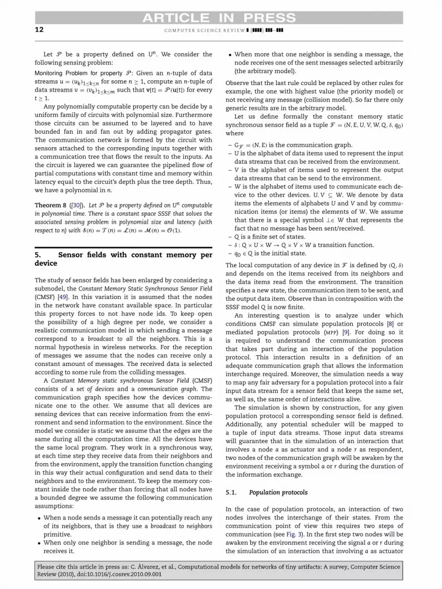
The study of sensor fields has been enlarged by considering asubmodel, the Constant Memory Static Synchronous Sensor Field(CMSF) [49]. In this variation it is assumed that the nodesin the network have constant available space. In particularthis property forces to not have node ids. To keep openthe possibility of a high degree per node, we consider arealistic communication model in which sending a messagecorrespond to a broadcast to all the neighbors. This is anormal hypothesis in wireless networks. For the receptionof messages we assume that the nodes can receive only aconstant amount of messages. The received data is selectedaccording to some rule from the colliding messages.

A Constant Memory static synchronous Sensor Field (CMSF)consists of a set of devices and a communication graph. Thecommunication graph specifies how the devices commu-nicate one to the other. We assume that all devices aresensing devices that can receive information from the envi-ronment and send information to the environment. Since themodel we consider is static we assume that the edges are thesame during all the computation time. All the devices havethe same local program. They work in a synchronous way,at each time step they receive data from their neighbors andfrom the environment, apply the transition function changingin this way their actual configuration and send data to theirneighbors and to the environment. To keep the memory con-stant inside the node rather than forcing that all nodes havea bounded degree we assume the following communicationassumptions:

• When a node sends a message it can potentially reach anyof its neighbors, that is they use a broadcast to neighborsprimitive.

• When only one neighbor is sending a message, the nodereceives it.

• When more that one neighbor is sending a message, thenode receives one of the sent messages selected arbitrarily(the arbitrary model).

Observe that the last rule could be replaced by other rules forexample, the one with highest value (the priority model) ornot receiving any message (collision model). So far there onlygeneric results are in the arbitrary model.

Let us define formally the constant memory staticsynchronous sensor field as a tuple F = (N, E, U, V, W, Q, δ, q0)

where

– GF = (N, E) is the communication graph.– U is the alphabet of data items used to represent the input

data streams that can be received from the environment.– V is the alphabet of items used to represent the output

data streams that can be send to the environment.– W is the alphabet of items used to communicate each de-

vice to the other devices. U, V ⊆ W. We denote by dataitems the elements of alphabets U and V and by commu-nication items (or items) the elements of W. We assumethat there is a special symbol ⊥∈ W that represents thefact that no message has been sent/received.

– Q is a finite set of states.– δ : Q × U × W → Q × V × W a transition function.– q0 ∈ Q is the initial state.

The local computation of any device in F is defined by (Q, δ)

and depends on the items received from its neighbors andthe data items read from the environment. The transitionspecifies a new state, the communication item to be sent, andthe output data item. Observe than in contraposition with theSSSF model Q is now finite.

An interesting question is to analyze under whichconditions CMSF can simulate population protocols [8] ormediated population protocols (MPP) [9]. For doing so itis required to understand the communication processthat takes part during an interaction of the populationprotocol. This interaction results in a definition of anadequate communication graph that allows the informationinterchange required. Moreover, the simulation needs a wayto map any fair adversary for a population protocol into a fairinput data stream for a sensor field that keeps the same set,as well as, the same order of interactions alive.

The simulation is shown by construction, for any givenpopulation protocol a corresponding sensor field is defined.Additionally, any potential scheduler will be mapped toa tuple of input data streams. Those input data streamswill guarantee that in the simulation of an interaction thatinvolves a node a as actuator and a node r as respondent,two nodes of the communication graph will be awaken by theenvironment receiving a symbol a or r during the duration ofthe information exchange.

5.1. Population protocols

In the case of population protocols, an interaction of twonodes involves the interchange of their states. From thecommunication point of view this requires two steps ofcommunication (see Fig. 3). In the first step two nodes will beawaken by the environment receiving the signal a or r duringthe simulation of an interaction that involving a as actuator

C O M P U T E R S C I E N C E R E V I E W ( ) – 13

Fig. 3 – The two communication steps involved in a PPinteraction.

and r as respondent. The remaining nodes do not receive anysignal. In the second these two nodes interchange their state.

Observe that the interchange of information requiresbidirectional communication even if the interaction isdirected. The formal definition of the sensor field is thefollowing.

Given a PP P = (X, Y, Q, I, O, δ) that runs on interactiongraph G = (N, E), we define the SSSF F = F (P , G) = (N, E ∪

E′, U, V, W, Q′, δ′, q0) as follows:

• E′= (u, v) | (v, u) ∈ E.

• U = X ∪ a, r, ⊥, V = Y, and W = Q ∪ ⊥.• Q′

= Q ∪ Q × a, r.• The transition function δ′ is defined as follows:

– δ′(q0, x, ⊥) = (I(x), ⊥, ⊥), for any x.– δ′(q, ⊥, z) = (q, O(q), ⊥), for any q ∈ Q, z ∈ U.– δ′(q, a, ⊥) = ((q, a), O(q), q, ), for any q ∈ Q.– δ′(q, r, ⊥) = ((q, r), O(q), q), for any q ∈ Q.– δ′((q, a), a, q′) = (δ1(q, q′), O(q), ⊥), for q ∈ Q.– δ′((q, r), r, q′) = (δ2(q′, q), O(q), ⊥), for q ∈ Q.

Where we use the projections of the transition function ofthe PP, that is δ(q, q′) = (δ1(q, q′), δ2(q, q′)). Observe that thetransition function δ′ implements the two communicationrounds required by the interaction. The output is set to bethe output corresponding to the last state in the populationprotocol to keep compatibility between the output datastream in the sensor field and the output of the populationprotocol.

The second step is to define a way to transform an input xand a scheduler S for P to a set of input data streams u(x, S)

to be used as input data stream by the sensor field. In thiscase the transformation is uniform to be able to expand oneinteraction two two time steps.

The input data stream u = u(x, S) is the following:

• For any node k, uk[1] = xk.• If the t-th interaction of the scheduler is (i, j) then

– ui[2t,2t + 1] = aa– uj[2t,2t + 1] = rr– uℓ[2t,2t + 1] = ⊥⊥, for ℓ = i, j.

Observe that a symbol a on the input data stream codes thefact that the node participates in an interaction as actuator,r as a respondent, and ⊥ indicates that the node doesnot participate in any interaction at step t. The repetitioncorresponds to the fact that an interaction requires twocommunication steps.

Theorem 9 ([49]). Given a graph G and a population protocol Pconsider the CMSF f(P , G) defined above. For any scheduler S and

Fig. 4 – The two communication steps involved in a MPPinteraction.

input x consider the data stream u(x, S) defined above. The t-thconfiguration of P on input x and scheduler S is identical to the2t − 1-configuration of f(P ) on input data stream u(x, S).

5.2. Mediated population protocols

The simulation of a mediated population protocol by a sensorfield can be done in two different ways. In the first one thenetwork has no additional devices. The state of the edgeparticipating in the interaction is assumed to be kept bythe environment, and it is revealed to the agents duringthe interaction. As before the simulations consists of aconstruction of a sensor field and of a transformation of inputand mediated scheduler to a tuple of input data streams.

Given a MPP P = (X, Y, Q, S, I, O, δ) that runs on interactiongraph G = (N, E), define the following SSSF f(P, G) =

(N, E′, U, V, W, Q′, δ′, q0) as follows:

• E′= E ∪ (u, v) | (v, u) ∈ E.

• U = X ∪ Y ∪ a, r, ⊥.• V = Y and W = Q ∪ ⊥.• Q′

= q0 ∪ Q ∪ (Q × a, r).

The transition function δ′ is defined as in the caseof population protocols to keep the communication stepsrequired by the interaction as depicted in figure (see Fig. 4).For mediated population protocols an interaction requirestwo communication steps. Observe that in the first step theenvironment provides the role of the nodes in the interactionand in the second step the state of the edge participating inthe interaction to the interested nodes. As before, the outputdata item is set to the output of the population protocolcorresponding to the last seen state, and in the second stepto the new state of the edge.

Next step is to define a way to transform a scheduler forthe population protocol to a set of input data streams for thesensor field.

The input data stream u = u(x, S) is the following:

• For any node k, uk[1] = xk.• If the t-th interaction of the scheduler is (i, j) and the actual

state of the link (i, j) is s ∈ S then– ui[2t,2t + 1] = as– uj[2t,2t + 1] = rs– uk[2t,2t + 1] =⊥⊥, for any k = i, j.

Observe that in this simulation, we are assuming thatthe consistency of the edge states is preserved by the

14 C O M P U T E R S C I E N C E R E V I E W ( ) –

environment and that the edge state do not use networkresources.

Theorem 10 ([49]). Given a communication graph G and a me-diated population protocol P consider the CMSF f(P , G) definedabove. For any input x and mediated scheduler S, the t-th config-uration of P on communication graph G, input x, and scheduler S isidentical to the 2t −1-configuration of f(P , G) on input data streamu(G, x, S).

There is another way to perform the simulation byincluding additional nodes that simulate edges and keep theedge state. This simulation seems more realistic as it allowsto consider, as part of the complexity of the protocols, theincrease in space due to maintaining information on everyedge. Although nodes are not allowed to keep it as partof their internal state, which might require a non-constantspace per node. In the following we define a simulation ofa population protocol by a sensor field with additional nodes,these nodes represent the edges (links) in the communicationgraph. Observe that although in the communication graphdirected arcs are possible, the way in which the transitionfunction of the mediated population protocols is defined,makes that information is updated in both directions,independently on whether the edge is directed or undirected.To keep this property we add an additional node per link, thisnew node is connected through bidirectional links to both ofits endpoints. As before, we define define the states and thetransition function of the sensor field, then the mapping ofinput and scheduler to a tuple of input data streams. Observethat in mediated population protocols the nodes and the edgehave distinguished roles. In our simulation we will assumethat the first input on a data stream indicates the role ofthe node during the computation, and that the assignmentis correct. Alternatively, we can assume that all the nodes areinitially in state qv and all the edges are initially in state qe.

Given a MPP P = (X, Y, Q, S, I, O, δ) running on interactiongraph G = (N, E), we define a CMSF f(P, G) = (N′, E′, U, V, W, Q′,

δ′, q0, qv, qe) as follows:

• The communication graph is the graph (N′, E′) where N′=

N ∪ E. The edge set is defined as follows

E′= (u, v) | u, v ∈ Nand(u, v) ∈ E

∪((u, v), u)((u, v), v) | (u, v) ∈ E.

• U = X ∪ Y ∪ a, r, e, ⊥.• V = Y and W = Q ∪ S ∪ ⊥.• Q′

= q0, qv, qe ∪ Q ∪ S ∪ (Q × a, r) ∪ (Q × S × a, r, e, w) ∪

(Q × Q × S ∪ S × w, e).

The transition function δ′ is again designed to keep trackof the different communication rounds required in aninteraction. In this case a total of 5 communications stepsare required. The sending phases are depicted in Fig. 5 andinvolve the three nodes participating in an interaction.

The input data stream u(x, S) is the following:

• For any node k ∈ Vuk[1] = a, for any node edge (i, j) ∈

Eu(i,j)[1] = e.• For any node k, uk[2] = xk. For any edge u(i,j)[2] = s0, where

s0 is the initial state.• If the t-th interaction of the scheduler is (i, j), then

– ui[5t − 2,5t + 2] = aaaaa– uj[5t − 2,5t + 2] = rrrrr

Fig. 5 – The four sending phases involved in a MPPinteraction when edge nodes are added.

– u(i,j)[5t − 2,5t + 2] = eeeee– uk[5t − 2,5t + 2] =⊥⊥⊥⊥⊥, for any k = i, j, (i, j).

Theorem 11 ([49]). Given a mediated population protocol Pconsider the CMSF f(P ) defined above. For any interaction graphG, mediated scheduler S, and input x consider the data streamu(G, S, x) defined above. The t-th configuration of P on input x andscheduler S is identical to the 5t−2-th configuration of f(P ) on inputdata stream u(G, x, S).

6. Deciding graph languages

In [50] and in its more recent full version [51], the authorswent one step further and studied what graph propertiesare stably computable by the MPP model. To understandthe properties of the interaction or communication graphis an important step in almost any distributed system. Inparticular, they temporarily disregarded the input notion andmade the assumption that all agents simply start from acommon initial state q0. Also, as in the SMPPmodel, theymadea similar assumption for the edges, that is, ι(e) = s0 for alle ∈ E (recall that ι denotes the edge initialization function).Here the interest is in protocols that when executed on anycommunication graph G of a given graph universe, after afinite number of steps stabilize to configurations where allagents give 1 as output if G belongs to a graph languageL, and 0 otherwise. This is motivated by the idea of havingprotocols that eventually accept all communication graphs(on which they run) that satisfy a specific property, and rejectall remaining graphs.

A graph universe (family) U is closed under disjoint unionif for any pair of graphs G1, G2 ∈ U, the graph G obtained asthe disjoint union of G1 and G2 belongs to U.We consider thefollowing graph families:

• W formed by all weakly connected digraphs without loops,and multiple edges.

• S formed by all strongly connected digraphs without loops,and multiple edges.

• H formed by all the directed graphs without isolatedvertices, loops, and multiple edges.

• G formed by all possible directed graphs of any finitenumber of nodes greater or equal to 2.

C O M P U T E R S C I E N C E R E V I E W ( ) – 15

To be able to perform some computation/communication, wehave made the natural assumption, for the general case, thatthere are no isolated vertices on the communication graphs.All the following definitions hold w.r.t. some fixed graphuniverse U. A graph language L is a subset of U containingcommunication graphs that possibly share some commonproperty. Some examples of graph languages are:

• The graph language consisting of all strongly connectedmembers of U.

• L = G ∈ U|G contains a directed Hamiltonian path.• L = G ∈ U|G has an even number of edges.• L = G ∈ U||V(G)| = |E(G)|.

A graph language is said to be trivial if L = ∅ or L = U.A protocol A in model M is said to stably decide a graph

language L ⊆ U (or equivalently a predicate pL : U → 0,1

defined as pL(G) = 1 iff G ∈ L) if for any G ∈ U and any compu-tation of A on G, all agents eventually output 1 if G ∈ L and allagents eventually output 0 if G ∈ L. A graph language is saidto be stably decidable by model M (also called M-decidable) ifsome protocol A of M stably decides it.

A protocol A in model M is said to stably recognize a graphlanguage L ⊆ U (or equivalently a predicate pL : U → 0,1

defined as pL(G) = 1 iff G ∈ L) if for any G ∈ U and anycomputation of A on G, all agents eventually output 1 if G ∈ Land at least one agent outputs 0 if G ∈ L. A graph languageis said to be stably recognizable by model M (also called M-recognizable) if some protocol A of M stably recognizes it.

6.1. Deciding graph languages in the MPP model

To formally summarize, here the output alphabet is alwaysbinary, that is, Y = 0,1, ι(e) = s0 for all e ∈ E, and I(σ) = q0,for all σ ∈ X (due to this, an input alphabet is not specifiedneither is an input function and the assumption is that theinitial configuration is C0(u) = q0 for all u ∈ V). This specialcase is called the Graph Decision Mediated Population Protocol(GDMPP) model.

Theorem 12 ([51]). The class of stably decidable graph languagesby the GDMPP model is closed under complement, union, andintersection operations.

Node and edge parity, bounded out-degree by a constant,existence of a node with more incoming than outgoingneighbors, and existence of some directed path of length atleast k = O(1) are some examples of stably decidable graphlanguages by the GDMPP model, in the case where the graphuniverse is W . Also, given the same graph universe, thefollowing impossibility result holds.

Theorem 13 ([51]). There exists no GDMPP with stabilizing statesto stably decide the graph language

2C = G ∈ W | ∃u, υ ∈ V(G) | (u, υ), (υ, u) ∈ E(G)

(in words, G has at least one 2-cycle).

Proof Idea. We give the main idea of the proof with the helpof Fig. 6. Note that graph G Fig. 6(a) has a 2-cycle, thus, belongsto 2C, while G′ Fig. 6(b) does not. Assume that a GDMPP withstabilizing states stably decides 2C and take any computationof the protocol on G. Eventually, in such a computation, both

(a) Graph G. (b) Graph G′.

Fig. 6 – G ∈ 2C and G′ ∈ 2C.

agents output 1. Now, apply the same computation on G′ inthe followingmanner. Whenever e1 is chosen in G choose firstt1 and then t3 in G′, and whenever e2 is chosen in G choose t2and then t4 in G′. It is not so hard to see that, due to symmetry,when the protocol state-stabilizes on G it also state-stabilizeswith precisely the same states on G′ (thus, also with the sameoutput). Consequently, the protocol also accepts G′ which isa contradiction and we reach the conclusion that no suchprotocol can exist.

In the case where the graph universe is G, containingall possible directed communication graphs (i.e. also thedisconnected ones), it is possible to obtain a very strongimpossibility result.

Lemma 6 ([51]). For any non-trivial graph language L (L is non-trivial if L = ∅ and L = G), there exists some disconnected graph Gin L where at least one component of G does not belong to L or thereexists some disconnected graph G′ in L where at least one componentof G′ does not belong to L (or both).

Theorem 14 ([51]). Any non-trivial graph language L ⊂ G is notstably decidable by the GDMPP model.

Proof Idea. The proof of the result is based on the verysimple observation that in disconnected graphs, the variouscomponents cannot communicate with each other. ThenLemma 6 can be used to argue that a language (or itscomplement) must contain at least one disconnected graphwith a component not in the language, so any protocolmaking some decision on the whole graph would make theopposite decision on the component (since this componentdoes not belong to the language and is isolated from the othercomponents), which is contradictory.

Now, since the connectivity property is a non-trivialproperty, the following corollary comes as an immediateapplication of Theorem 14.

Corollary 2 ([51]). The graph language

C = G ∈ G | G is (weakly) connected

is not stably decidable by the GDMPP model.

6.2. Graph languages decided by constant memory sensorfields

Following the proposal in [51] the decidability of graphlanguages in the CMSF model has been analyzed in [49].When the sensor field does not have access to any input datastream the set of decidable languages is too small. To have

16 C O M P U T E R S C I E N C E R E V I E W ( ) –

more significative results we allow only access to a particularinput data stream. The input data stream will contain theinformation required to break the node’s symmetry, thisinformation can be used to drive the computation in differentways. In this section we survey the results on graph languagedecidability for three variations of the CMSF model. The aimof the submodels is to explore different ways in which theinput data stream can be used to guide the computation ofa sensor field and compare the computational power of theresulting models by ways of the sets of graph languages thatare decidable in the model.

6.2.1. The simplistic CMSFThis basic submodel assumes that we have a CMSF in whichall the nodes have the same initial state and no input datastream is accessible. We call this model the simplistic CMSF.

In the case that we consider digraphs in a class that isclosed under disjoint union, we have the same undecidabilityas in [51] concerning non-trivial properties. Observe thatin this case, as communication between disconnectedcomponents cannot be established, a communication graphformed by several connected components in which there arecomponents with positive answer and components with anegative answer cannot agree on a common answer.

Theorem 15 ([49]). Let U be a graph family closed under disjointunion, then any non-trivial graph language in U is undecidable bysimplistic CMSF.

When the universe is the set of all strongly connectedgraphs non-trivial graph languages are undecidable. Theproof is based on the fact that all the devices receive andsend messages, because the graph is strongly connected. Insuch a case as all of them have the same initial state thecomputation is equivalent to a local computation in whichthe sent messages are the input messages for the followingsteps. Thus any decidable property must be independent ofthe communication graph.

Theorem 16 ([49]). Any non-trivial graph language in S isundecidable by simplistic CMSF with topology in S.

When the graph universe is restricted to be W it is easyto find constructions in which information can be computedbut not forwarded to all the nodes. Using this arguments ithas been shown the following generic result.

Theorem 17 ([49]). Any non-trivial graph property in S isundecidable by simplistic CMSF on W .

However in the simplistic CMSF model there are non-trivial decidable and undecidable properties when thecommunication graph belongs to W . In decidable languagesnode symmetry is broken by some property that can bechecked locally. Furthermore, the distinguished nodes mustbe able to broadcast this information to the rest of thenetwork. The undecidable property obeys properties thatcannot be checked locally.

Theorem 18 ([49]). In the simplistic CMSF, the graph language

G ∈ W | G has a node with no ingoing edges

is decidable but the graph language

G ∈ W | G has a node with no outgoing edges

is undecidable.

6.2.2. Node driven CMSF computationThe computational power of the simplistic CMSF has been en-hanced by adding an input data stream that at any time stepselects a node that can act as a leader for a local computation.This is equivalent to the scheduler in population protocols,but now the environment is selecting a node rather than anedge. On a valid computation it is required in addition fair-ness for the input data stream.

For most of the results a extension of the notion of fairnessis required. A node scheduler S is an infinite sequence ofnodes v1, v2, . . .. For a constant k we say that a node scheduleris k-fair if the subsequence (vi)i mod k=1 is fair. Therefore,we require that all the nodes appear infinitely often at thebeginning of some periods of fixed length. All the definitionsof decidability for this model will require stabilization onk-fair scheduler, for some constant k, that depends on theprotocol. Observe that any fair scheduler can be padded todevise a k-fair scheduler, but that a fair scheduler might notbe k-fair.

Theorem 19 ([49]). Let U be a graph family closed under disjointunion, then any non-trivial graph language in U is undecidable bynode driven CMSF.

When the graph universe is restricted to be W we have thefollowing generic results.

Theorem 20 ([49]). Any non-trivial graph property in S isundecidable by node driven CMSF on W .

But not taking into account the input data stream we havethe following result.

Theorem 21 ([49]). Any graph property decidable by simplisticCMSF on W is decidable by node driven CMSF on W .

However when restricted to strongly connected graphssome non-trivial graph languages become decidable in thenode driven model. The main idea is to use a controlledbroadcast, consisting of a fixed number of steps, that allowsone to check the property on the local neighborhood of theactivated node. This results in a scheduler that stabilizeson any k-fair scheduler for some adequate constant k thatdepends on the designed protocol.

Theorem 22 ([49]). The following properties are decidable by nodedriven CMSF with communication topology in S.

• kC = G ∈ S | G contains a k-cycle, for any constant k.• Directed simple path of constant length.

Observe that kC is a non-trivial graph property (even onstrongly and weakly connected graphs) and therefore thelanguage is not decidable in the simplistic CMSF neither inthe node driven CMSF on W .

6.2.3. Edge driven CMSF computationAnother extension is to consider the CMSF that has beenused to simulate the computation of a mediated populationprotocol. Here the communication graph has additionalnodes that keep the state of the edge. In addition it isassumed that all the nodes corresponding to vertices in thecommunication graph have the same initial state and all thenodes corresponding to edges also have the same initial state.However, the initial state of edges can be different to theinitial state of vertices. The data stream will select one edgeper time step, thus activating the three participants on the

C O M P U T E R S C I E N C E R E V I E W ( ) – 17

interaction, the actuator, the respondent, and the edge. On avalid computation we assume in addition k-fairness, for somefixed constant k.

This computational model has more computational powerthan the GDMPP model. The result follows from using avariation of the simulation MPP in which the repetition ofthe values on the data stream is replaced by local states inorder to guarantee that the protocol stabilizes on 5-fair edgeschedulers.

Theorem 23 ([49]). Any graph property that is decidable byGDMPP is decidable by edge driven CMSF.

Furthermore, the edge driven CMSF has also more compu-tational power than the node driven CMSF model. Here in anyactivation of an edge (u, v), the simulation simulates first thesteps taken by a node scheduler that activates u and contin-ues simulating the activation of v. This leads to the construc-tion of a k-fair node scheduler from a 2k-fair edge scheduler.

Theorem 24 ([49]). Any graph property that is decidable by nodedriven CMSF is decidable by edge driven CMSF.

7. Conclusions — open problems

We surveyed some very recently proposed computationalmodels for networks of tiny artifacts. For the case of interac-tion based models we focused on the area of population pro-tocols. We discussed some recent enhancements, namely, theMPP model and the PM model. Both models are the result ofadding some extra feature to the population protocol model.The former assumes that the communication links can storelimited information and the latter that each agent is a mul-titape TM. We discussed some very recent research provingthat both models are extremely powerful in terms of theircomputational power. In complete graphs, theMPPmodel andthe PM model for every f(n) = Ω(logn) space bound are equiv-alent to nondeterministic TMs ofO(n2) andO(nf(n)) space, re-spectively, that compute symmetric predicates. In particular,we presented the Static Synchronous Sensor Field (SSSF) whichconsists of a set of devices and a communication graph. The com-putation of a SSSF depends on the communication betweenthe devices and the environment. We reviewed the computa-tional problems that are susceptible of being solved by sensorfields and we analyzed the computational resources used tosolve them. We discussed several memory restrictions of thetiny devices involved in a SSSF allowing only devices with con-stant or bounded memory capacity. We analyzed the compu-tational power of sensor fields in the particular case in whichthe memory per device is constant, the CMSF model, in rela-tion with the Population Protocol models, showing adequatesimulations of population protocols by sensor fields. We alsoanalyzed the decidability of properties of the communicationor interaction graph under different variants of PP and CMSF.

Many interesting problems remain open in the area ofpopulation protocols:

• Are the MPP and PM models fault-tolerant? What pre-conditions are needed in order to achieve satisfactoryfault-tolerance?

• In order to apply our protocols in real and criticalapplication scenarios some sort of code verification seemsnecessary. A first attempt for the basic population protocol

model can be found in [52]. Verification methods for MPPs,Community Protocols, and PM protocols are still totallyunknown, although the ideas of [52] may also be applicableto these models.

• [53] revealed the need for population protocols to haveadaptation capabilities in order to keep working correctlyand/or fast when natural modifications of the mobilitypattern occur. However, we do not know yet how to achieveadaptivity.

• Is there an exact characterization of the class of stablydecidable graph languages by GDMPP in the weakly-connected case?

• O(logn) memory per agent seems to behave as a threshold.Is there some sort of impossibility result showing that withO(f(n)) memory, where f(n) is asymptotically smaller thanlogn, the class of stably computable predicates is strictlysmaller than SNSPACE(nf(n))? At first glance, it seems thatthe agents are unable to store uids and get informed of thepopulation size.

• Study the stable decidability of graph languages by thePM model for various space bounds (the most prominentbeing the logarithmic bound).

In the area of sensor fields, among many others, we canpost the following open directions:

• Is there a characterization of the sensing problems thatcan be solved in logarithmic or constant space?

• Allow the incorporation of a dynamic communication graph.This requires a slight modification of the definition ofthe sensor field, just allowing that the sets of neighborschange dynamically at any time step. The dynamicityin the communication graph can come from faults(either nodes or links) or from mobility, or both. Findingthe paradigmatic family of problems for such networksand the adequate complexity measures will require anadditional modeling effort.

• Consider and incorporate energy models to the commu-nication graph. For analyzing the energy consumption theperformance measures proposed so far proportionate thebasic ingredients for the case that sending/receiving amessage has uniform cost for all the nodes. Further ba-sic complexitymeasures can be required formore complexenergy models. The aim should be in the design of optimal(efficient) algorithms under different energy models.

• In the CMSF model all the results are obtained for thearbitrarymodel of communication. To some extentmost ofthe results can be extended to the priority model. A goodunderstanding of the collision model will be of interestas losing information due to collisions is a problem thatnaturally arises in wireless networks.

R E F E R E N C E S

[1] D. Estrin, R. Govindan, J. Heidemann, S. Kumar, Next centurychallenges: scalable coordination in sensor networks, in:ACM/IEEE Int. Conf. on Mobile Computing and Networking,Seattle, pp. 263–270.

[2] B. Warneke, M. Last, B. Liebowitz, K. Pister, Smart dust:communicating with a cubic-millimeter computer, Computer34 (2001) 44–51.

[3] J.M. Kahn, R.H. Katz, K.S.J. Pister, Emerging challenges: mo-bile networking for smart dust, Journal of Communicationsand Networks 2 (2000) 188–196.

18 C O M P U T E R S C I E N C E R E V I E W ( ) –

[4] I. Akyildiz, W. Su, Y. Sankarasubramaniam, E. Cayirci, Asurvey on sensor networks, IEEE Communications Magazine40 (2002) 102–114.

[5] D. Estrin, D. Culler, K. Pister, G. Sukatme, Connecting thephysical world with pervasive networks, IEEE PervasiveComputing 6 (2002) 59–69.

[6] S. Tilak, N. Abu-Ghazaleh, W. Heinzelman, A taxonomy ofwireless micro-sensor network models, Mobile Computingand Communications Review 6 (2003) 28–36.

[7] M. Vinyals, J. Rodriguez-Aguilar, J. Cerquides, A survey onsensor networks from a multi-agent perspective, in: Proc. ofAAMAS, 2008.

[8] D. Angluin, J. Aspnes, Z. Diamadi, M.J. Fischer, R. Peralta,Computation in networks of passively mobile finite-statesensors, Distributed Computing (2006) 235–253.

[9] I. Chatzigiannakis, O. Michail, P.G. Spirakis, Mediatedpopulation protocols, in: 36th International Colloquium onAutomata, Languages and Programming, ICALP 2009. Part 2,in: LNCS, vol. 5556, pp. 363–374.

[10] I. Chatzigiannakis, O. Michail, S. Nikolaou, A. Pavlogiannis,P.G. Spirakis, Passively mobile communicating logarithmicspace machines, Technical Report FRONTS-TR-2010-16,RACTI, Patras, Greece, 2010.

[11] D.T. Gillespie, Exact stochastic simulation of coupledchemical reactions, The Journal of Physical Chemistry 81(1977) 2340–2361.

[12] D.T. Gillespie, A rigorous derivation of the chemical masterequation, Physica A 188 (1992) 404–425.

[13] J. Aspnes, E. Ruppert, An introduction to population pro-tocols, Bulletin of the European Association for TheoreticalComputer Science 93 (2007) 98–117.

[14] Z. Diamadi, M.J. Fischer, A simple game for the study of trustin distributed systems, Wuhan University Journal of NaturalSciences 6 (2001) 72–82. Also appears as Yale Technical ReportTR1207, Jan. 2001.

[15] D. Angluin, J. Aspnes, Z. Diamadi, M.J. Fischer, R. Peralta,Urn automata, Technical Report YALEU/DCS/TR-1280, YaleUniversity, Department of Computer Science, 2003.

[16] D. Angluin, J. Aspnes, Z. Diamadi, M.J. Fischer, R. Peralta,Computation in networks of passively mobile finite-statesensors, in: PODC’04: Proceedings of the Twenty-ThirdAnnual ACM Symposium on Principles of DistributedComputing, ACM, New York, NY, USA, 2004, pp. 290–299.

[17] T.G. Kurtz, Approximation of population processes, in: CBMS-NSF Regional Conference Series in Applied Mathematics, vol.36, 1981.

[18] J. Berstel, Quelques applications des reseaux d’automates,Thèse de 3ème Cycle, 1967.

[19] P. Gibbons, S. Tirthapura, Estimating simple functions on theunion of data streams, in: SPAA, pp. 281–291.

[20] C. Hoare, A calculus of total correctness for communicatingprocesses, Science of Computer Programming 1 (1981) 49–72.

[21] D. Peleg, Distributed Computing. A Locality-Sensitive Ap-proach, in: SIAM Monographs on Discrete Mathematics andApplications.

[22] T. Henzinger, The Theory of Hybrid Automata, in: Proceed-ings of the 11th Annual IEEE Symposium, LICS 96, pp.278–292.

[23] N. Lynch, R. Segala, F. Vaandrager, Hybrid I/O AutomataRevisited, in: Hybrid Systems: Computation and Control:4th International Workshop, HSCC’01, in: LNCS, vol. 2034,pp. 403–417.

[24] I. Chatzigiannakis, S. Nikoletseas, P. Spirakis, Smart dust localdetection and propagation protocols, in: Proceedings of thesecond ACM International Workshop on Principles of MobileComputing, pp. 9–16.

[25] J. Díaz, J. Petit, M. Serna, A random graph model foroptical smart dust networks, IEEE Transactions on MobileComputing 2 (2003) 186–196.

[26] G. Arzhantseva, J. Díaz, J. Petit, J. Rolim, M. Serna, Broad-casting on networks of sensors communicating through di-rectional antennas, in: P. Spirakis, A. Kameas, S. Nikoletseas(Eds.), International Workshop on Ambient Intelligence Com-puting, Ellinika Grammata, CTI Press, 2003, pp. 1–12.

[27] M. Penrose, Random Geometric Graphs, in: Oxford Studies inProbability, Oxford U.P., 2003.

[28] F. Xue, P. Kumar, The number of neighbors needed forconnectivity of wireless networks, Wireless Networks 10(2004) 169–181.

[29] F.T. Leighton, Introduction to Parallel Algorithms andArchitectures: Arrays, Trees, Hypercubes, Morgan Kaufmann,San Mateo, CA, 1993.

[30] C. Àlvarez, A. Duch, J. Gabarro, M. Serna, Sensor field: a com-putational model, in: Algorithmic Aspects of Wireless SensorNetworks: 5th International Workshop, ALGOSENSORS 2009,Rhodes, Greece, July 10–11, 2009. Revised Selected Papers,Springer-Verlag, Berlin, Heidelberg, 2009, pp. 3–14.

[31] L. Valiant, A bridging model for parallel computation,Communications of the ACM 33 (1990) 103–111.

[32] J. von Neumann, Theory and organization of complicatedautomata, in: A. Burks (Ed.), Theory of Self-ReproducingAutomata [by] John von Neumann, University of IllinoisPress, Urbana, 1949, pp. 29–87 (Part One). Based on transcriptsof lectures delivered at the University of Illinois, in December1949. Edited for publication by A.W. Burks.

[33] D. Angluin, J. Aspnes, D. Eisenstat, E. Ruppert, Thecomputational power of population protocols, DistributedComputing 20 (2007) 279–304.

[34] R. Guerraoui, E. Ruppert, Names trump malice: tiny mobileagents can tolerate byzantine failures, in: ICALP, 2, pp.484–495.

[35] S. Ginsburg, E.H. Spanier, Semigroups, presburger formulas,and languages, Pacific Journal of Mathematics 16 (1966)285–296.

[36] M. Presburger, Über die vollständigkeit eines gewissensystems der arithmetik ganzer zahlen, in welchem dieaddition als einzige operation hervortritt, in: Comptes-Rendus du I Congrès de Mathématiciens des Pays Slaves,pp. 92–101.

[37] D. Angluin, J. Aspnes, D. Eisenstat, Stably computablepredicates are semilinear, in: PODC’06: Proceedings of the25th Annual ACM Symposium on Principles of DistributedComputing, ACM Press, New York, NY, USA, 2006, pp. 292–299.

[38] C. Delporte-Gallet, H. Fauconnier, R. Guerraoui, E. Ruppert,When birds die: making population protocols fault-tolerant,in: DCOSS, pp. 51–66.

[39] N.A. Lynch, Distributed Algorithms, 1st edition, MorganKaufmann, 1996.

[40] P.G. Spirakis, Population protocols and related models,S. Nikoletseas, J. Rolim (Eds.), Theoretical Aspects ofDistributed Computing in Sensor Networks, Springer-Verlag,2010 (in press).

[41] D. Angluin, J. Aspnes, M. Chan, M.J. Fischer, H. Jiang, R.Peralta, Stably computable properties of network graphs,in: V.K. Prasanna, S. Iyengar, P. Spirakis, M. Welsh (Eds.),Distributed Computing in Sensor Systems: First IEEEInternational Conference, DCOSS 2005, Marina del Rey,CA, USE, June/July, 2005, Proceedings, in: Lecture Notes inComputer Science, vol. 3560, Springer-Verlag, 2005, pp. 63–74.

[42] D. Angluin, J. Aspnes, D. Eisenstat, Fast computation bypopulation protocols with a leader, Distributed Computing 21(2008) 183–199.

[43] O. Bournez, P. Chassaing, J. Cohen, L. Gerin, X. Koegler, On theconvergence of population protocols when population goesto infinity, Applied Mathematics and Computation (2009)(in press).

C O M P U T E R S C I E N C E R E V I E W ( ) – 19

[44] I. Chatzigiannakis, P.G. Spirakis, The dynamics of proba-bilistic population protocols, in: DISC’08: Proceedings of the22nd International Symposium on Distributed Computing,Springer-Verlag, Berlin, Heidelberg, 2008, pp. 498–499.

[45] O. Bournez, J. Chalopin, J. Cohen, X. Koegler, Playing withpopulation protocols, in: CSP, pp. 3–15.

[46] I. Chatzigiannakis, O. Michail, P.G. Spirakis, Recent advancesin population protocols, in: MFCS’09: Proceedings of the 34thInternational Symposium on Mathematical Foundations ofComputer Science 2009, Springer-Verlag, Berlin, Heidelberg,2009, pp. 56–76.

[47] I. Chatzigiannakis, O. Michail, S. Nikolaou, A. Pavlogiannis,P.G. Spirakis, All symmetric predicates in NSPACE(n2) arestably computable by the mediated population protocolmodel, in: MFCS’10: Proceedings of the 35th InternationalSymposium on Mathematical Foundations of ComputerScience 2010, in: LNCS, vol. 6281, 2010, pp. 270–281.doi:10.1007/978-3-642-15155-2_25.

[48] M. Sipser, Introduction to the Theory of Computation,second edition, International edition, 2006, Thomson CourseTechnology.

[49] C. Àlvarez, M. Serna, P.G. Spirakis, On the computationalpower of constant memory sensor fields, Technical ReportFRONTS-TR-2010-10, 2010.

[50] I. Chatzigiannakis, O. Michail, P.G. Spirakis, Brief announce-ment: decidable graph languages by mediated populationprotocols, in: DISC, pp. 239–240.

[51] I. Chatzigiannakis, O. Michail, P.G. Spirakis, Stably decidablegraph languages by mediated population protocols, in: 12thInternational Symposium on Stabilization, Safety, andSecurity of Distributed Systems, SSS 2010, in: LNCS, vol. 6366,2010, pp. 252–266. doi:10.1007/978-3-642-16023-3_21.

[52] I. Chatzigiannakis, O. Michail, P.G. Spirakis, Algorithmic ver-ification of population protocols, in: 12th International Sym-posium on Stabilization, Safety, and Security of DistributedSystems, SSS 2010, in: LNCS, vol. 6366, 2010, pp. 221–235.doi:10.1007/978-3-642-16023-3_19.

[53] I. Chatzigiannakis, S. Dolev, S.P. Fekete, O. Michail, P.G.Spirakis, Not all fair probabilistic schedulers are equivalent,in: OPODIS’09: Proceedings of the 13th InternationalConference on Principles of Distributed Systems, Springer-Verlag, Berlin, Heidelberg, 2009, pp. 33–47.

Carme Àlvarez obtained her Ph.D. fromTechnical University of Catalonia (UPC),in 1994. She is currently Professor in theUPC, Barcelona. Her research interestsare Computational Complexity, Modelsof Computation, and Algorithmic GameTheory. Carme Àlvarez has published inimportant Computer Science journals andsignificant refereed conferences.

Ioannis Chatzigiannakis obtained hisPh.D. from the Department of ComputerEngineering & Informatics of the Univer-sity of Patras in 2003. He is currentlyAdjunct Faculty at the Computer Engi-neering & Informatics Department of theUniversity of Patras (since October 2005).He is the Director of the Research Unit 1of RACTI (since July 2007). He has coau-

thored over 70 scientific publications. His main researchinterests include distributed and mobile computing, wirelesssensor networks, algorithm engineering and software sys-tems. He has served as a consultant to major Greek comput-ing industries. He is the Secretary of the European Associationfor Theoretical Computer Science since July 2008.

Amalia Duch obtained her Ph.D. fromthe Department of Languages and Infor-matics Systems of the Technical Univer-sity of Catalonia in 2004. She is currentlyan Associate Professor of the Departmentof Languages and Informatics Systemsof the Technical University of Catalonia(since September 2005). Her research in-terests include Average-case Analysis of

Algorithms, Multidimensional Data Structures and, recently,Algorithmic Game Theory.

Joaquim Gabarro, was born in Barcelona(Spain) in 1953 and studied Physics andComputer Science, obtained his Ph.D.from Universitat Politècnica de Calatunyain 1983. From 1985 is Associate Professor(Profesor Titular) in Universitat Politèc-nica de Calatunya. Currently representsSpain in the TC1 (Foundations of Com-puter Sciences) of IFIP. Main research top-

ics are Concurrency, Algorithms and Complexity.

Othon Michail, born in 1984, obtained hisDiploma and his M.Sc. in Computer Sci-ence & Technology from the Departmentof Computer Engineering & Informaticsof the University of Patras in 2007 and2009, respectively. He recently (September2010) obtained his Ph.D. from the samedepartment under the supervision of Prof.Dr. Paul Spirakis. The title of his thesis

is “New Models for Population Protocols”. He is currently amember of the Research Unit 1 of the RACTI (since April 2009).His research interests include Theory of Computation in newmodels of computation (like wireless sensor networks and, inparticular, population protocols), Computational Complexity,and Algorithms.

Maria Serna obtained her Ph.D. fromTechnical University of Catalonia (UPC) in1990. She is currently Full Professor inthe Department of Languages and Infor-matics Systems (LSI) of UPC. She is thecoordinator of the Computing Postgrad-uate program at LSI. She has co-autoredover 90 scientific publications. Her mainresearch interest are algorithms and com-

plexity, parallel and distributed computing, problems ongraphs and networks, and algorithmic game theory. She is theeditor of the Bulletin of the EATCS.

Paul Spirakis, born in 1955, obtainedhis Ph.D. from Harvard University, in1982. He is currently the Director of theRACTI and a Full Professor in the PatrasUniversity, Greece. He was acknowledgedbetween the top 50 scientists worldwidein Computer Science with respect toThe best Nurturers in Computer ScienceResearch, published by B. Kumar and

Y.N. Srikant, ACM Data Mining, 2005. His research interestsare Algorithms and Complexity and interaction of Complexityand Game Theory. Paul Spirakis has extensively published inmost of the important Computer Science journals andmost ofthe significant refereed conferences contributing to over 200scientific publications. He was elected unanimously as one ofthe two Vice Presidents of the Council of the EATCS.